reverse logistics, process innovation, operational

REVERSE LOGISTICS, PROCESS INNOVATION, OPERATIONAL

PERFORMANCE AND COMPETITIVE ADVANTAGE OF

MANUFACTURING FIRMS IN KENYA

BY:

MWANYOTA, JOB LEWELA

A RESEARCH THESIS SUBMITTED IN PARTIAL FULFILMENT

OF THE REQUIREMENTS FOR THE AWARD OF THE DEGREE

OF DOCTOR OF PHILOSOPHY IN BUSINESS ADMINISTRATION,

FACULTY OF BUSINESS AND MANAGEMENT SCIENCE,

UNIVERSITY OF NAIROBI

2021

ii

DECLARATION

I, the undersigned, do declare that this research thesis is my original work and has not been

submitted for any award to any other university, institution or college for examination other

than the University of Nairobi.

Signed: ____ ____ Date: _27th August 2021____

Mwanyota Job Lewela

D80/60629/2010

This research thesis has been submitted with our approval as the university supervisors.

Signed: ___________________________ Date: ___30-8-2021_________

Prof. Muranga Njihia

Associate Professor,

Department of Management Science and Project Planning,

Faculty of Business and Management Sciences,

University of Nairobi.

Signed: ___ _____ Date: 30th August 2021_____

Prof. Jackson Maalu


Department of Business Administration,



Signed: ___________________________ Date: ______________________

Prof. X.N. Iraki


Department of Management Science and Project Planning,



31st August 2021

iii

COPYRIGHT ©

All rights reserved. No part of this thesis may be reproduced or used in any form without

prior written permission from the author or the University of Nairobi except for brief

quotations embodied in review articles and research papers. Making copies of any part of

this thesis for any purpose other than personal use is a violation of the Kenyan and

international copyrights laws.

For further information, kindly contact:

Mwanyota Job Lewela

P. O. Box 93578 – 80102

Email: [email protected]

Phone: 0736-501202

mailto:[email protected]

iv

ACKNOWLEDGEMENTS

This doctoral thesis has been realized through the inspiration, support and various inputs

from a number of people to whom I am considerably grateful.

First and foremost, I am beholden to the Almighty God for his guidance and protection

during the entire duration of this study. He renewed my strength each and every day

throughout the entire process of completing this study. I also wish to extend my solemn

gratitude to my supervisors, Prof. Muranga Njihia, Prof. Jackson Maalu and Prof. X. N.

Iraki for their constant encouragement and instruction as a result of which you made it

possible for me to complete this study successfully. Your contributions I gratefully

acknowledge.

This study would not have been successful without the suggestions and contributions of a

number of my friends and more so my colleagues, members of the academic and

administrative staff in the Faculty of Business and Management Sciences. In particular

many thanks go to Dr. Stephen Odock, the Late Dr. Joseph Aranga, Dr. Onesmus Mutunga

and Dr. Zipporah Onsomu for your insightful critiques and advice. I am also deeply

appreciative to the University of Nairobi for the financial support all through this study.

I proffer my appreciation for the support and encouragement of my wife, Mrs. Dinais Dali

Mwakio, my parents, Mr. Lomas Mwanyota and Mrs. Mariam Shighadi Mwanyota and my

siblings Mr. Wycliffe Mwachola, Mr. Eric Ngali, Mrs. Alice Maghuwa Bett and Mr. Moris

Mlamba for the constant concern they had on my progress towards completing this

program. I would also like to appreciate the support given to me by the Kenya Association

of Manufacturers for their assistance in data collection. I extend my gratitude to the

v

management and employees of the manufacturing companies in Kenya for their

cooperation during the data gathering phase.

To all of you, I say God bless you.

vi

DEDICATION

This doctoral thesis is dedicated to the Late Prof. Isaac Albert Wamola for his inspiration

and for being a pillar of strength in my academic life; and to my children Andrew

Mwanyota Lewela and Adrian Mwakio Lewela.

vii

TABLE OF CONTENTS

DECLARATION................................................................................................................... ii

COPYRIGHT © ................................................................................................................... iii

ACKNOWLEDGEMENTS ................................................................................................ iv

DEDICATION...................................................................................................................... vi

LIST OF FIGURES ........................................................................................................... xiv

LIST OF TABLES ............................................................................................................ xvii

ABBREVIATIONS AND ACRONYMS ......................................................................... xxii

ABSTRACT ...................................................................................................................... xxiii

CHAPTER ONE: INTRODUCTION ................................................................................. 1

1.1 Background of the Study ............................................................................................... 1

1.1.1 Reverse Logistics .................................................................................................. 2

1.1.2 Process Innovation ................................................................................................ 3

1.1.3 Operational Performance ...................................................................................... 4

1.1.4 Competitive Advantage ........................................................................................ 5

1.1.5 Manufacturing Sector in Kenya ............................................................................ 6

1.2 Research Problem .......................................................................................................... 7

1.3 Research Objectives ..................................................................................................... 10

1.4 Value of the Study ....................................................................................................... 11

CHAPTER TWO: LITERATURE REVIEW .................................................................. 13

2.1 Introduction .................................................................................................................. 13

2.2 Theoretical Foundations of the Study .......................................................................... 13

2.2.1 Transaction Cost Theory ..................................................................................... 13

2.2.2 Resource Advantage Theory of Competition ..................................................... 14

2.2.3 Diffusion of Innovation Theory .......................................................................... 15

2.2.4 Institutional Theory ............................................................................................. 17

viii

2.3 Reverse Logistics and Competitive Advantage ........................................................... 18

2.4 Reverse Logistics, Operational Performance and Competitive Advantage ................. 19

2.5 Reverse Logistics, Process Innovation and Operational Performance ........................ 20

2.6 Reverse Logistics, Process Innovation, Operational Performance and Competitive

Advantage .......................................................................................................................... 21

2.7 Recapitulation of Knowledge Gaps ............................................................................. 22

2.8 Conceptual Structure and Hypotheses ......................................................................... 23

CHAPTER THREE: RESEARCH METHODOLOGY ................................................. 26

3.1 Introduction .................................................................................................................. 26

3.2 Research Philosophy .................................................................................................... 26

3.3 Research Design........................................................................................................... 27

3.4 Population of the Study ................................................................................................ 27

3.5 Sample and Sampling Technique................................................................................. 28

3.6 Data Collection ............................................................................................................ 29

3.7 Research Variable Operationalization ......................................................................... 29

3.8 Reliability and Validity Tests ...................................................................................... 32

3.9 Data Diagnostics .......................................................................................................... 33

3.10 Data Processing and Inquiry ...................................................................................... 36

CHAPTER FOUR: DESCRIPTIVE STATISTICS AND DATA DIAGNOSTICS ..... 45

4.1 Introduction .................................................................................................................. 45

4.2 Background of Research .............................................................................................. 45

4.2.1 Response Rate ..................................................................................................... 46

4.2.2 Missing Data ....................................................................................................... 47

4.2.3 Non-Response Sample Bias ................................................................................ 48

4.2.4 Duration of Operation in Kenya ......................................................................... 49

4.2.5: Sampling Adequacy and Sphericity ................................................................... 51

4.2.5.1 Sampling Adequacy and Sphericity Tests for the Association of Reverse

Logistics with Competitive Advantage ........................................................................ 51

ix

4.2.5.2 Sampling Adequacy and Sphericity Tests for the Association linking Reverse

Logistics, Operational Performance and Competitive Advantage ............................... 52

4.2.5.3 Sampling Adequacy and Sphericity Test for the Association linking Reverse

Logistics, Process Innovation and Operational Performance ...................................... 53


Logistics, Process Innovation, Operational Performance and Competitive Advantage

...................................................................................................................................... 54

4.3 Reliability Tests ........................................................................................................... 55

4.4 Validity Tests ............................................................................................................... 60

4.4.1 Content Validity Tests ........................................................................................ 60

4.4.2 Convergent and Discriminant Validity ............................................................... 61

4.4.2.1 Convergent and Discriminant Validity Tests Associating Reverse Logistics with

Competitive Advantage ............................................................................................... 61

4.4.2.2 Convergent and Discriminant Validity among Reverse Logistics, Operational

Performance and Competitive Advantage ................................................................... 64

4.4.2.3 Convergent and Discriminant Validity Tests for the Association among Reverse

Logistics, Process Innovation and Operational Performance ...................................... 67

4.4.2.4 Convergent and Discriminant Validity Tests for the Association among Reverse


...................................................................................................................................... 71


Advantage Descriptive Statistics ....................................................................................... 78

4.5.1 Reverse Logistics ................................................................................................ 78

4.5.1.1 Outsourcing ...................................................................................................... 78

4.5.1.2 Collaborative Enterprising ............................................................................... 80

4.5.1.3 Green Strategies ............................................................................................... 82

x

4.5.1.4 Product Life Cycle Approach .......................................................................... 83

4.5.1.5 Summary of Reverse Logistics ........................................................................ 85

4.5.2 Process Innovation .............................................................................................. 87

4.5.2.1 Information Systems ........................................................................................ 88

4.5.2.2 Product Redesign ............................................................................................. 89

4.5.2.3 Process Reengineering ..................................................................................... 91

4.5.2.4 Business Value Chain ...................................................................................... 92

4.5.2.5 Summary of Process Innovation ...................................................................... 93

4.5.3 Operational Performance .................................................................................... 95

4.5.4 Competitive Advantage ...................................................................................... 96

4.6 Data Diagnostics .......................................................................................................... 97

4.6.1 Outlier Tests ........................................................................................................ 98

4.6.2 Normality Tests ................................................................................................... 99

4.6.3 Tests for Autocorrelation .................................................................................. 100

4.6.4 Linearity Test .................................................................................................... 102

4.6.5 Multicollinearity Test........................................................................................ 104

4.6.6 Heteroscedasticity Test ..................................................................................... 104

4.6.7 Confirmatory Factor Analysis........................................................................... 106

4.6.7.1 Confirmatory Factor Analysis for the Measured Model for the Latent constructs

.................................................................................................................................... 106

4.6.7.2 Confirmatory Factor Analysis for the Association linking Reverse Logistics

with Competitive Advantage ..................................................................................... 108

4.6.7.3 Confirmatory Factor Analysis for the Association linking Reverse Logistics,

Operational Performance and Competitive Advantage ............................................. 112

xi

4.6.7.4 Confirmatory Factor Analysis for the association Linking Reverse Logistics,

Process Innovation and Operational Performance ..................................................... 118

4.6.7.5 Confirmatory Factor Analysis for the Moderated – Mediation Relationship 123

4.6.7.6 Confirmatory Factor Analysis for the Joint association linking Reverse


.................................................................................................................................... 129

4.7 Common Method Variance ........................................................................................ 134

4.7.1 Common Method Variance Test on the Reverse Logistics link with Competitive

Advantage. ................................................................................................................. 135

4.7.2 Common Method Variance Test on the Association linking Reverse Logistics,

Operational Performance and Competitive Advantage ............................................. 136


Process Innovation and Operational Performance ..................................................... 138


Process Innovation, Operational Performance and Competitive Advantage ............. 140

4.8 Summary of Chapter Results ..................................................................................... 143

CHAPTER FIVE: TEST OF HYPOTHESES, INTERPRETATIONS AND

DISCUSSIONS .................................................................................................................. 147

5.1 Introduction ................................................................................................................ 147

5.2 Tests of Hypotheses ................................................................................................... 147

5.2.1 The Influence of Reverse Logistics on Competitive Advantage of Manufacturing

Firms in Kenya ........................................................................................................... 147

5.2.2 The Mediation Effect of Operational Performance on Reverse Logistics

Association with Competitive Advantage in Manufacturing Firms in Kenya ........... 148

xii

5.2.3 The Moderation Effect of Process Innovation on the Association linking Reverse

Logistics and Operational Performance of Manufacturing Firms in Kenya .............. 150

5.2.4 The Moderated - Mediation Effect of Process Innovation and Operational

Performance ............................................................................................................... 151

5.2.5 The Joint Effect of Reverse Logistics, Process Innovation and Operational

Performance on Competitive Advantage of Manufacturing Firms in Kenya ............ 153

5.2.6 Summary Table of Hypotheses Tests ............................................................... 154

5.3 Discussion of the Results ........................................................................................... 156

5.3.1 Reverse Logistics and Competitive Advantage ................................................ 156

5.3.2 Reverse Logistics, Operational Performance and Competitive Advantage ...... 158

5.3.3 Reverse Logistics, Operational Performance and Competitive Advantage ...... 159

5.3.4 Moderated – Mediation effect of Process Innovation and Operational Performance

on Reverse Logistics and Competitive Advantage .................................................... 161

5.3.5 Joint Effect of Reverse Logistics, Process Innovation and Operational

Performance on Competitive Advantage ................................................................... 162

CHAPTER SIX: SUMMARY, CONCLUSIONS, IMPLICATIONS AND

RECOMMENDATIONS .................................................................................................. 163

6.1 Introduction ................................................................................................................ 163

6.2 Summary of Findings ................................................................................................. 163

6.3 Conclusions ................................................................................................................ 166

6.4 Implications of the Study ........................................................................................... 167

6.4.1 Contribution to Knowledge............................................................................... 168

6.4.2 Contribution to Theory ..................................................................................... 169

6.4.3 Contribution to Policy and Practice .................................................................. 170

6.5 Recommendations ...................................................................................................... 171

6.6 Limitations of the Study............................................................................................. 173

xiii

6.7 Suggestions for Future Research ............................................................................... 174

REFERENCES .................................................................................................................. 176

APPENDICES: .................................................................................................................. 185

Appendix 1: Data Collection Instrument (Questionnaire): .............................................. 185

Appendix 2: Quantum Index of Manufacturing Production (2012 – 2016) .................... 194

Appendix 3: Manufacturing Firms Per Sub Sector .......................................................... 195

Appendix 4: Sampled Firms Per Manufacturing Sub-Sectors ......................................... 196

Appendix 5: Inter-Item Correlation Matrix between Latent Constructs of Reverse Logistics

and Process Innovation .................................................................................................... 201


and Operational Performance .......................................................................................... 202


and Competitive Advantage ............................................................................................. 203

Appendix 8: Inter-Item Correlation Matrix between Latent Constructs of Process

Innovation and Operational Performance ........................................................................ 204

Appendix 9: Inter-Item Correlation Matrix between Latent Constructs of Process

Innovation and Competitive Advantage .......................................................................... 205

Appendix 10: Inter-Item Correlation Matrix between Latent Constructs of Operational

Performance and Competitive Advantage ....................................................................... 206

Appendix 11: Letter for Data Collection ......................................................................... 207

xiv

LIST OF FIGURES

Figure 2.1. Conceptual Model ........................................................................................... 24

Figure 3.1. Overall Model Path Diagram ........................................................................... 37

Figure 3.2. Path Diagram showing the Association linking Reverse Logistics with

Competitive Advantage ..................................................................................................... 38

Figure 3.3. Path Diagram for the Association linking Reverse Logistics, Operational

Performance and Competitive Advantage ......................................................................... 40

Figure 3.4. Path Diagram for the Association among Reverse Logistics, Process Innovation

and Operational Performance ............................................................................................ 41

Figure 3.5. Path Diagram for the Moderated-Mediation Relationship among Reverse

Logistics, Process Innovation, Operational Performance and Competitive Advantage .... 42

Figure 3.6. Path Diagram for the Combined Effect of Reverse Logistics, Process Innovation

and Operational Performance on Competitive Advantage. ............................................... 43

Figure 4.1. Histogram of the Duration of Operation in Years among Manufacturing Firms

............................................................................................................................................ 49

Figure 4.2. Convergent Validity Test for the Association linking Reverse Logistics with


Figure 4.3. Convergent Validity Test for the Association among Reverse Logistics,

Operational Performance and Competitive Advantage ..................................................... 64

Figure 4.4. Convergent Validity Test for the Association among Reverse Logistics, Process

Innovation and Operational Performance .......................................................................... 68

Figure 4.5. Convergent Validity Test for the Association among Reverse Logistics, Process

Innovation, Operational Performance and Competitive Advantage .................................. 72

Figure 4.6. Unstandardized Structural Equation Model for the Reverse Logistics Interaction

with Competitive Advantage. .......................................................................................... 109

xv

Figure 4.7. Standardized Factor Loadings for the Measured and Structured Association

linking Reverse Logistics with Competitive Advantage. ................................................ 112

Figure 4.8. Unstandardized Structural Equation Model for the Association linking Reverse

Logistics, Operational Performance and Competitive Advantage. .................................. 114

Figure 4.9. Standardized Factor Loadings for the Measured and Structured Model

Associating Reverse Logistics, Operational Performance and Competitive Advantage. 117

Figure 4.10. Unstandardized Structural Equation Model for the Association linking Reverse

Logistics, Process Innovation and Operational Performance. ......................................... 119


Associating Reverse Logistics, Process Innovation and Operational Performance. ....... 122

Figure 4.12. Confirmatory Factor Analysis Model for the Moderated-Mediation

Relationship ..................................................................................................................... 124

Figure 4.13. Standardized Factor Loadings for the Measured and Structured relationships

for the Moderated – Mediation Model ............................................................................. 128

Figure 4.14. Structural Model for the Joint Relationship among Reverse Logistics, Process

Innovation, Operational Performance and Competitive Advantage ................................ 130

Figure 4.15. Standardized Factor Loadings for the Measured and Structured relationships

for the Joint Model ........................................................................................................... 134

Figure 4.16. Common Latent Factor Analysis Model for Reverse Logistics interaction with

Competitive Advantage. .................................................................................................. 135

Figure 4.17. Common Latent Factor Analysis Model for the Association linking Reverse

Logistics, Operational Performance and Competitive Advantage. .................................. 137


Logistics Process Innovation and Operational Performance. .......................................... 139

xvi


Logistics, Process Innovation, Operational Performance and Competitive Advantage .. 141

Figure 5.1. Revised Conceptual Model ............................................................................ 155

xvii

LIST OF TABLES

Table 2.1 Recapitulation of Knowledge Gaps ................................................................... 22

Table 3.1 Operationalization of Study Variables ............................................................... 31

Table 3.2 Summary Table of Data Analysis Techniques per Objective ............................ 44

Table 4.1 Response Rate per Manufacturing Sub-sector ................................................... 47

Table 4.2 Test for Homogeneity of Variance .................................................................... 48

Table 4.3 Descriptive Summary for the Duration of Operation among Manufacturing Firms

in Kenya ............................................................................................................................. 50

Table 4.4 ISO 14001 Certification Status of Manufacturing Firms ................................... 50

Table 4.5 Sampling Adequacy and Sphericity Tests for Reverse Logistics Association with


Table 4.6 Sampling Adequacy and Sphericity Tests for the Association linking Reverse

Logistics, Operational Performance and Competitive Advantage ..................................... 52

Table 4.7 Sampling Adequacy and Sphericity Tests the association linking Reverse

Logistics, Process Innovation and Operational Performance ............................................ 53

Table 4.8 Sampling Adequacy and Sphericity Test for the Association linking Reverse


Table 4.9 Cronbach Alpha Test Results Measuring Internal Reliability of Questionnaire

Items for Reverse Logistics and Process Innovation ......................................................... 55

Table 4.10 Communality Coefficient Results for the Questionnaire Items Measuring

Reverse Logistics Latent Constructs .................................................................................. 57

Table 4.11 Communality Co-efficient Results for the Questionnaire Items Measuring

Process Innovation Latent Constructs ................................................................................ 58

Table 4.12 Cronbach Alpha Test Results Measuring Internal Consistency of Latent

Construct on the Latent Variable ....................................................................................... 59

xviii

Table 4.13 Communality Coefficient Results for the Latent Constructs Measuring Latent

Variables ............................................................................................................................ 59

Table 4.14 Average Variance Extraction results for Reverse Logistics Interaction with


Table 4.15 Maximum Shared Variance results for Reverse Logistics Interaction with


Table 4.16 Average Variance Extraction results for the Association among Reverse


Table 4.17 Maximum Shared Variance results for the Association among Reverse










Table 4.22 Respondent Scores on Outsourcing ................................................................. 79

Table 4.23 Respondents Scores on Collaborative Enterprise ............................................ 81

Table 4.24 Respondent Scores on Green Strategies .......................................................... 82

Table 4.25 Respondent Scores on Product Life Cycle Approach ...................................... 84

Table 4.26 Descriptive Summary of Reverse Logistics Latent Constructs ....................... 85

Table 4.27 Descriptive Summary of Reverse Logistics Questionnaire Items ................... 86

Table 4.28 Respondents Scores on Information Systems .................................................. 88

xix

Table 4.29 Respondent Scores on Product Redesign ......................................................... 90

Table 4.30 Respondent Scores on Process Reengineering ................................................ 91

Table 4.31 Respondent Scores on Business Value Chain .................................................. 92

Table 4.32 Descriptive Summary for Process Innovation Latent Constructs .................... 93

Table 4.33 Descriptive Summary for Process Innovation Questionnaire Items ................ 94

Table 4.34 Descriptive Statistics for Operational Performance ......................................... 95

Table 4.35 Descriptive Statistics for Competitive Advantage ........................................... 97

Table 4.36 Test for Outliers ............................................................................................... 98

Table 4.37 Kolmogorov-Smirnov and Shapiro-Wilk Test Results .................................... 99

Table 4.38 Durbin-Watson Test Statistic ......................................................................... 101

Table 4.39 Multicollinearity Test Statistic ....................................................................... 104

Table 4.40 Koenker Test Results ..................................................................................... 105

Table 4.41 Overall Model Fit Results for the Latent Constructs of Reverse Logistics

Process Innovation, Operational Performance and Competitive Advantage ................... 107

Table 4.42 Overall Model Fit results for the Association linking Reverse Logistics with

Competitive Advantage ................................................................................................... 108

Table 4.43 Unstandardized Factor Loadings for the Measured Model of Reverse Logistics

Interaction with Competitive Advantage ......................................................................... 110

Table 4.44 Standardized Factor Loadings for the Measured Model of Reverse Logistics


Table 4.45 Unstandardized Factor Loadings for the Structured Model of Reverse Logistics


Table 4.46 Overall Model Fit Results for the Association linking Reverse Logistics,

Operational Performance and Competitive Advantage ................................................... 113

xx

Table 4.47 Unstandardized Factor Loadings for the Measured Model on the Association

linking Reverse Logistics, Operational Performance and Competitive Advantage ........ 115

Table 4.48 Standardized Factor Loadings for the Measured Model on the Association


Table 4.49 Unstandardized Factor Loadings for the Structured Model on the Association


Table 4.50 Overall Model Fit Results for the association linking Reverse Logistics, Process

Innovation and Operational Performance ........................................................................ 118


linking Reverse Logistics, Process Innovation and Operational Performance ................ 120

Table 4.52 Standardized Factor Loadings for the Measured Model Associating Reverse

Logistics, Process Innovation and Operational Performance .......................................... 120

Table 4.53 Unstandardized Factor Loadings for the Structured Model Associating Reverse

Logistics, Operational Performance and Competitive Advantage ................................... 121

Table 4.54 Overall Model Fit Results for the Moderated – Mediation Relationship ...... 123

Table 4.55 Unstandardized Factor Loadings for the Measured Model on the Moderated -

Mediation Relationship .................................................................................................... 125

Table 4.56 Standardized Factor Loadings for the Measured Model on the Moderated –

Mediation Model .............................................................................................................. 126

Table 4.57 Unstandardized Factor Loadings for the Structured Model on the Moderated –

Mediation Model .............................................................................................................. 127

Table 4.58 Overall Model Fit Results for the Joint Relationship between Reverse Logistics,

Process Innovation, Operational Performance and Competitive Advantage ................... 129

Table 4.59 Unstandardized Factor Loadings for the Measured Model of the Joint

Relationship ..................................................................................................................... 131

xxi

Table 4.60 Standardized Factor Loadings for the Measured Model for the Joint Relationship

.......................................................................................................................................... 132

Table 4.61 Unstandardized Factor Loadings for the Structured Model for the Joint

Relationship ..................................................................................................................... 133

Table 4.62 Common Latent Factor Difference Analysis Model for Reverse Logistics

interaction with Competitive Advantage ......................................................................... 136

Table 4.63 Common Latent Factor Difference Analysis Model for the Association linking

Reverse Logistics, Operational Performance and Competitive Advantage ..................... 138


Reverse Logistics, Process Innovation and Operational Performance ............................ 140


Reverse Logistics, Process Innovation, Operational Performance and Competitive

Advantage ........................................................................................................................ 142

Table 5.1 Hypotheses Tests, Results and Conclusions .................................................... 154

xxii

ABBREVIATIONS AND ACRONYMS

AGFI - Adjusted Goodness of Fit Index

AMOS - Analysis of Moment Structures

AVE - Average Variance Extraction

CV - Coefficient of Variation

CFA - Confirmatory Factor Analysis

CFI - Comparative Fit Index

CLF - Common Latent Factor

CMIN/DF - Chi-Square/Degrees of Freedom

EMA - Energy Management Award

EMCA - Environmental Management and Co-ordination Act

GDP - Gross Domestic Product

GFI - Goodness of Fit Index

K-GESIP - Kenya Green Economy Strategy and Implementation Plan

KAM - Kenya Association of Manufacturers

KMO - Kaiser-Meyer-Olkin

KNBS - Kenya National Bureau of Statistics

MNCs - Multi National Corporations

MSV - Maximum Shared Variance

NEMA - National Environmental Management Authority

NFI - Normed Fit Index

PCA - Principal Component Analysis

RMSEA - Root Mean Square Error of Approximation

SD - Standard Deviation

SEM - Structural Equation Modeling

TLI - Turker Lewis Index

UN - United Nations

UNEP - United Nations Environment Programme

USA - United States of America

VIF - Variance Inflation Factor

xxiii

ABSTRACT

Today globally, countries and manufacturing entities alike are concerned with

environmental sustainability. Execution of reverse logistics strategies has been

contemplated as a feasible alternative to mitigate the negative environmental effects of

manufacturing. However the question has been whether implementing reverse logistics

creates competitive advantage for manufacturing entities. Literature has also suggested that

process innovations result in improved operational performance in the achievement of

competitiveness. Specifically, the study objectives were to establish the influence of reverse

logistics on competitive advantage; determine the influence of operational performance on

the relationship between reverse logistics and a firm’s competitive advantage; determine

the influence of process innovation on the relationship linking reverse logistics and gaining

internal operational proficiency; examine the conditional indirect effect on the relationship

among reverse logistics, process innovation and operational performance on a firm’s

competitive advantage; and examine the joint effect of reverse logistics, process innovation

and operational performance on a firm’s competitive advantage. Appropriate hypotheses

were developed from the specific objectives respectively. Using a positivist philosophy and

correlation cross-sectional survey design, primary data were collected among 340 KAM

registered manufacturing firms in Kenya using a structured questionnaire. A response rate

of 44.4 percent was attained. In data analysis, Covariance-based, SEM was used. Results

from the hypotheses tests revealed a statistically significant influence of reverse logistics

on a firm’s competitive advantage. Secondly, operational performance significantly

mediated the association linking reverse logistics and a firm’s competitive advantage.

Third, the relationship linking reverse logistics and gaining internal operational

competency was not significantly moderated by process innovation. Fourth, process

innovation and the operational performance had a partial moderated-mediation influence

on the association linking reverse logistics and competitive advantage. Finally only

operational performance had a significant and positive influence in the joint model. The

study thus confirmed that implementation of reverse logistics strategies will lead firms to

experience increased customer loyalty, increased market share, improved brand recognition

and an increase in revenues. It further confirmed that when resources are mobilized

uniquely, they create comparative advantage consequently leading to competitive

advantage. The study recommended that manufacturing firms should implement reverse

logistics as an integrated intervention consisting of outsourcing, collaborative enterprising,

green strategies and closed-loop supply chain approaches to achieve organizational and

environmental benefits. The study further recommended that implementation of reverse

logistics should be guided by a process that requires identifying the uniqueness of resources

the organization has and strategically placing these resources in a manner that builds

comparative advantage. Policymakers within the manufacturing sector in Kenya should

improve the regulatory framework to upscale application of reverse logistics strategies. The

research identified replication of the study using direct measures for all the study variables

and in other contexts as possible future research streams. Further making intra-industry or

intra-sectoral comparisons would also be useful in generating knowledge on the

implementation of reverse logistics.

1

CHAPTER ONE: INTRODUCTION

1.1 Background of the Study

Environmental concerns presently have led manufacturing firms to redesign their processes

in order to have environmentally friendly manufacturing (Govindan, Soleimani & Kannan,

2015; Prakash, Barua & Pandya, 2015). As a way of addressing the repercussions of climate

change, the emphasis of the United Nations (UN) has been for countries and businesses

alike to reexamine their value chains in order to devise new and sustainable business

models that create sustainable supply chains (United Nations Environment Programme

(UNEP), 2016). As a result, manufacturers and consumers alike are required to dismantle

used products into their constituent parts for reuse, recycling, or safe disposal (Sheth, Sethia

& Srinivas, 2011). Reverse logistics is concerned with moving “end of useful life” goods

from consumers to manufacturers so as to recapture value or ensure environmentally

friendly disposal (Stock, 1992). In the process of strategically managing the product returns

process, firms also aim at gaining operational efficiency (Stock, Speh & Shear, 2006).

Similarly, the introduction of process innovation in managing reverse logistics helps firms

to generate and implement strategies that result in efficient and effective business models

(Barney, 1991). Gaining operational efficiency by strategically managing product returns

can lead to improving a firm’s competitory position.

In this study, the theories that were used to explain why organizations implement reverse

logistics programs and how these relate to process innovation, operational performance and

competitive advantage include transaction cost theory, the resource advantage theory of

competition, diffusion of innovation theory and institutional theory. Transaction cost theory

establishes a framework for explaining the development of optimal organization structure

and relationships among operational systems (Williamson, 1991). Resource advantage

http://amj.aom.org/content/49/3/519.full#ref-238

2

theory of competition recognizes that unique resources found in a firm can lead to

innovative internal capabilities and hence competitive advantage (Hunt & Morgan, 2005).

The diffusion of innovation theory creates a platform for explaining factors hindering or

enabling the diffusion of innovations (Rogers, 2003). Finally, institutional theory which

was the primary theory in the study was relevant in explaining the effects of institutional

pressures on various study variables (North, 1991).

The manufacturing sector accounted for 10.3 percent of Kenya’s Gross Domestic Product

(GDP) in 2017 (Kenya National Bureau of Statistics (KNBS), 2017). As a consequence of

environmental concerns and climate change effects, legislation requiring manufacturers to

be environmentally conscious have been developed. Through the Environmental

Management and Co-ordination Act (EMCA) No.8 of 1999, Kenya established the National

Environmental Management Authority (NEMA) to be the government’s arm mandated to

implement policies concerning the environment. Similarly through the Kenya Green

Economy Strategy and Implementation Plan (K-GESIP), Kenya is adopting various green

economy approaches and policies (KNBS, 2017). Despite these, uptake of strategies to

mitigate environmental effects among manufacturing firms has been slow with firms being

more profit-oriented (World Bank, 2016).

1.1.1 Reverse Logistics

According to Stock (1992) reverse logistics entails logistics activities relating to recycling

and disposal of waste and hazardous materials management. Reverse logistics as a process

systematically involves the cost-effective planning, implementation, and control of the

efficient movement of raw materials, partly completed and finished products, and the

associated information from their usage locale back to their origin either to reclaim value

3

or for apt disposal (Rogers & Tibben-Lembke, 1999). Environmental concerns, effects of

climate change, scarcity of manufacturing raw materials and technological advancements

have increased attention and focus on reverse logistics (Blumberg, 1999; Dias & Braga Jr.,

2016). Factors leading to increased volumes of reverse product flow include; lowering of

product quality; liberal returns polices; buyer’s changing preferences; increased internet

product purchases; and shortened product life cycles (Bernon & Cullen, 2007; Ravi &

Shankar, 2015).

The strategies proposed to implement reverse logistics programs include outsourcing,

collaborations, adopting green strategies or implementing reverse logistics from a product-

life cycle approach using closed-loop supply strategy. Outsourcing enables a firm to

concentrate on its core capabilities, achieve higher flexibility and transfer risk to a third

party (He & Wang, 2005; Moghaddam, 2015; Hsu, Tan & Mohamad-Zailani, 2016).

Collaborations led by industry associations or governments can integrate reverse logistics

operations for firms in an industry (Hung-Lau & Wang, 2009). Adopting green strategies

such as reuse, recycle and remanufacture help in “greening” the supply chain (Rogers &

Tibben‐Lembke, 2001; Rao & Holt, 2005). Finally, implementing reverse logistics using

the product-life cycle approach allows for the recreation of value through the closed-loop

supply chain (Closs, Speier & Meacham, 2011; Govindan et al., 2015; Sangwan, 2017).

1.1.2 Process Innovation

Davenport (2013) notes that process innovation involves the radical development of new

services, products and production systems in a creative manner. This improves equipment,

production techniques or software. Keeley, Walters, Pikkel and Quinn (2013) classified

innovations into an offering, configuration and experience linked innovations. Schumpeter

http://www.emeraldinsight.com/doi/full/10.1108/09574091111181372


4

(1934) identified innovations as of two types. The first is process innovation which consists

of new production approaches and new sources of manufacturing inputs, semi-finished

products or components. The second being product innovation which includes a new

product, a new product quality, a new market, or a reconstitution of a new industry

structure.

Adopting process innovation in a multidimensional manner through process reengineering,

value chain restructuring, resource deployment, product redesign, and implementing

information systems should guide organization strategy (Jayaraman & Luo, 2007). Process

reengineering involves an examination and redesign of business processes to significantly

improve on critical performance indicators (Armbruster, Bikfalvi, Kinkel & Lay, 2008);

Value chain restructuring involves an analysis of internal organizational activities to

develop and upgrade the value of products or processes (Porter, 2008). Resource

deployment is the way in which the organization methodologically introduces programs,

processes, and activities (Jayaraman & Luo, 2007). Product redesign involves generating

and developing ideas to improve the existing product(s) (Porter, 2008). Information

systems involve the use of computer and telecommunication systems to monitor supply

network activities, achieve visibility, and improve collaboration among supply chain

partners (Morgan, Richey Jr. & Autry, 2016). Further, interaction with suppliers, customers

and competitors together with the establishing of innovation systems are characteristic of

innovative organizations (Inauen & Schenker-Wicki, 2012).

1.1.3 Operational Performance

Operational performance is the degree to which predetermined goals and targets are being

accomplished using a process-oriented approach that measures’ productivity of resources

5

and the quality of outputs and outcomes of products and services (Shaw, 2003). Operational

performance identifies and measures attributes that relate outcomes of firm processes to

performance such as defect rates, production cycle time, and inventory turnover.

Operational performance measurement is an on-going process of establishing, monitoring

and pro-actively taking corrective action towards achieving organizational goals,

efficiently and effectively (Carter, Kale & Grimm, 2000).

Various indices exist for measuring operational performance. Operational performance can

be measured in terms of defect rate per item, the extent of customer complaints, degree of

waste, mean- time failure rate, client query time, requisition lead time, throughput rate, and

efficiency level (Slack, Chambers & Johnston, 2010). Studies have shown that the major

operational performance dimensions include; cost, time/speed, operations flexibility,

dependability and quality (Carter et al., 2000; Brah & Ying-Lim, 2006; De Souza & Brito,

2011; Chavez, Gimenez, Fynes, Wiengarten & Yu, 2013).

1.1.4 Competitive Advantage

Competitive advantage refers to the unique ability in a firm that enables it to have higher

returns than its competitors (Kim & Hoskisson, 2015). To have competitive advantage

firms need to offer distinct value propositions using customized value chains with unique

trade-offs from those of its competitors (Porter, 2008). Building the product returns process

to generate new market opportunities creates competitive advantage by attracting new

clients and retaining existing ones (Jayaraman & Luo, 2007). Reverse logistics has

facilitated the generation of competitive advantage through influencing the purchasing

behavior of customers based on how the product returns are handled (Stock, Speh & Shear,

2006). Barney (1991) identified properties that permit the sustainable realization of


6

competitive advantage to include resource value, the rarity of the resource, an imperfectly

imitable resource, an imperfectly mobile resource and a non-substitutable resource.

Markley and Davis (2007) suggested customer loyalty, waste reduction, revenue increase,

market share, and brand recognition as indices for measuring competitive advantage.

Jayaraman and Luo (2007) similarly suggested customer relations, brand image and

reputation as ways of assessing a firm’s competitive advantage.

1.1.5 Manufacturing Sector in Kenya

The manufacturing field is a collection of firms all engaged in intermediate operations that

transform substances, components or materials into new products using physical, chemical

or mechanical processes. In spite of Kenya’s position in East Africa as the most industrially

developed country, the manufacturing field in Kenya is not dominant compared to the

service and agricultural sectors (Kenya Association of Manufacturers (KAM), 2018).

Growth in the manufacturing sector stood at 3.5 percent in 2016. The growth was

occasioned by reduced energy costs. Overall, investments in the manufacturing sector stood

at Kshs. 277.4 billion in 2016 with 300,900 persons in formal employment representing

11.8 percent of the formal jobs in the country (KNBS, 2017). Further the manufacturing

sector contributed 11.8, 11.0, 10.7, 10.0 and 10.3 percent to GDP in the years 2012, 2013,

2014, 2015 and 2016 respectively. Appendix 2 shows the quantum index for manufacturing

production from 2012 until 2016 with the year 2009 as the base year.

Although manufacturing firms globally are increasingly recognizing the importance of

conserving the environment, implementation of strategies such as reverse logistics aimed

at reducing environmental effect has been slow (KAM, 2018). This is because

manufacturing firms in Kenya have information systems tailored to optimize forward

7

logistics but similar systems for implementing reverse logistics have persisted at the

planning stage. Similarly the development of asset value recovery systems is also at its

infancy (Dekker, Fleischmann, Inderfurth & van Wassenhove, 2013). Reverse logistics

requires additional infrastructure such as warehousing space, additional materials handling

equipment and transportation vehicles, a factor which not many firms in Kenya are willing

to invest in (Rogers, Banasiak, Brokman, Johnson & Tibben-Lembke, 2002). Further

developing accurate demand forecasts for reverse logistics is more intricate compared to

forecasting for forward logistics as a consequence of complexities of tracking defectives.

Currently most manufacturing firms in Kenya tend to control product return processes at

the individual business unit level and not as a supply chain. Finally the increasing volume

of returns greatly exceeds the capacity of business units to manage reverse logistics

effectively (Genchev, Glenn-Richey & Gabler, 2011).

1.2 Research Problem

A key assumption has been that reverse logistics strategies facilitate sustenance of future

generations to fulfill their needs by holding present generations environmentally

accountable to all shareholders including the number one shareholder, planet earth (Sheth

et al, 2011; Dias & Braga Jr., 2016; Sangwan, 2017). Such strategies are opined to create

innovative processes that ensure effective and efficient utilization of a firm’s resources

thereby legitimizing environmental effects on planet earth at a macro level and providing

operational performance gains for firms at a micro-level (Closs et al., 2011; Ravi & Shankar

2015). Although reverse logistics has been argued to potentially create sustainable

competitive capabilities research in supply chain has not given it considerable attention

until recently (Zhikang, 2017). Similarly the uptake of reverse logistics programs by firms

8

has been slow due to the challenges associated with implementation (Huscroft, Skipper,

Hazen, Hanna & Hall, 2013).

Studies done in reverse logistics have been exploratory using case study research design

(Jim & Cheng, 2006; Jayaraman & Luo, 2007; Hung-Lau & Wang, 2009; Genchev et al.,

2011). More recently studies are using survey designs with regression modeling but with

disparate results (Ho, Choy, Lam & Wong, 2012; Somuyiwa & Adebayo, 2014; Ravi &

Shankar, 2015). These studies have also used varied sampling procedures with varying

response rates (Ravi & Shankar, 2015; Hsu et al., 2016; Morgan et al., 2016). Further, there

is a lack of the usage of more robust techniques to analyze the effect other extraneous

variables have on the association between reverse logistics and performance (Huang &

Yang, 2014; Govindan et al., 2015).

Manufacturing firms in Kenya in their quest to gain competitive advantage have not

harnessed the potential of implementing reverse logistics programs. The main reason is that

developing and implementing such a program has been considered to be a tedious process

because of the complexities in developing demand forecasts for reverse logistics and capital

requirements for additional infrastructure (Rogers et al., 2002). Similarly, a lack of

information systems and asset recovery systems to support informed decision making while

developing reverse logistics programs further complicates implementation (Dekker et al.,

2013). The Kenyan manufacturing sector has also witnessed the exploitation of the weak

institutional mechanisms for enforcing environmental legislation despite initiatives such as

K-GESIP (World Bank, 2016). Only until recently have we seen research on reverse

logistics in the African context (Somuyiwa & Adebayo, 2014; Kwateng, Debrah, Parker,

Owusu & Prempeh, 2014; Meyer, Niemann, Mackenzie & Lombaard, 2017). To account

9

for differences across contexts and due to the prominence of developing economies in

global business more research on reverse logistics needs to be done in Africa.

Scholars have explored relationships among reverse logistics, process innovation,

operational performance and competitive advantage and given disparate results. For

instance, reverse logistics has the potential in achieving competitive advantage (Markley

& Davis, 2007; Ravi & Shankar, 2015). However, studies in reverse logistics have mainly

focused on adoption levels, implementation barriers or factors influencing adoption

(Abdullah, Halim, Yaakub & Abdullah, 2011; Abdulrahman, Gunasekaran &

Subramanian, 2014; Hosseini, Chileshe, Rameezdeen & Lehmann, 2014; Bouzon,

Govindan & Rodriguez, 2018). These studies have not demonstrated how reverse logistics

strategies impact a firm’s competitive advantage. Hung-Lau and Wang (2009) opined that

the independent effect of reverse logistics on competitive advantage has been hypothesized

and tested with varied results.

Research linking reverse logistics, process innovation and operational performance has

been exploratory (Hart, 2005: Armbruster et al., 2008; Jack, Powers & Skinner, 2010;

Huang & Yang, 2014). According to Christmann (2000) process innovation is essential for

reverse logistics since reverse logistical flows are distinct from forward logistics. Reverse

logistics also requires additional resources because of the uniqueness of handling systems

(Zhikang, 2017). Glenn-Richey, Genchev and Daugherty (2005) suggested that the strategy

guiding resource utilization in the firm should be based on building innovative

competencies to handling product returns. Despite the relative importance of how process

innovation influences reverse logistics and achieving internal operational proficiency, few

studies have sought to examine the nature of this relationship.

10

Studies have argued for an association linking reverse logistics and the generation of

competitiveness advantageously without considering the effect of extraneous variables to

this relationship (Stock, 2001; Jack et al., 2010; Huang & Yang, 2014). Further, although

scholars have argued for a relationship between operational performance and competitive

advantage Oral and Yolalan (1990), Voss, Åhlström and Blackmon (1997) and Carter et al.

(2000) this was not from a reverse logistics perspective. Yet, reverse logistics practices

have capacity to reduce clients' risk when purchasing products and add value to the

customer (Russo & Cardinali, 2012). Rogers and Tibben-Lembke (2001) opined that

reverse logistics programmes can assist a firm to minimize product returns by identifying

problem areas and defect patterns through its value system. De Brito, Flapper and Dekker

(2005) argued that such a value system has either direct (financial) or indirect (non-

financial) benefits resulting in improved competitiveness of the firm. The above studies

suggest reverse logistics and gaining competitiveness have a relationship contingent on

process innovation and achieving operational competence. However the nature and strength

of these relationships are unexplored. Similarly, the net effect of reverse logistics, process

innovation and operational performance on competitive advantage is worthy of further

investigation. This study sought to answer the following: What is the relationship among

reverse logistics, process innovation, operational performance and competitive advantage

of manufacturing firms in Kenya?

1.3 Research Objectives

The main objective of this study was to examine the relationships among reverse logistics,

process innovation, operational performance and competitive advantage of manufacturing

firms in Kenya. The specific objectives were:

i. To establish the influence of reverse logistics on competitive advantage.

11

ii. To determine the influence of operational performance on the relationship between

reverse logistics and a firm’s competitive advantage.

iii. To determine the influence of process innovation on the relationship between reverse

logistics and operational performance.

iv. To examine the conditional indirect effect of process innovation and operational

performance on the relationship between reverse logistics and a firm’s competitive

advantage.

v. To examine the joint effect of reverse logistics, process innovation and operational

performance on a firm’s competitive advantage.

1.4 Value of the Study

The proposed study is envisaged to make a contribution to knowledge, theory, policy-

making and practice of reverse logistics. Theoretically the research findings will help

academicians and firms to apprehend the significance of having a reverse logistics plan in

manufacturing and the relative contributions of process innovation and operational

performance on gaining competitive advantage. This will be achieved by providing an

evidence-based framework that suggests the relationships underlying the research

variables. Transaction cost theory, diffusion of innovations theory, institutional theory and

the resource advantage theory of competition will be used to offer rational explanations to

the relationship between reverse logistics, process innovation, operational performance and

competitive advantage. This is useful to academicians as it helps in substantiating the

theories.

Policymakers will gain an apprehension of issues in the application of reverse logistics

approaches. Such understanding will influence the government and its departments to enact

12

laws, develop policy guidelines or establish frameworks within which firms can implement

reverse logistics. These will inform manufacturers of the strategic significance reverse

logistics has to the economy of Kenya.

The study serves to apprise the application of reverse logistics approaches for

manufacturing entities by providing a diagnostic tool for establishing weaknesses within

current reverse logistics approaches. Study results could also be useful in prioritizing

reverse logistics strategies application. The study further provides owners and managers of

manufacturing firms with an opportunity to apprehend the position of reverse logistics as a

key process for gaining competitiveness advantageously.

13

CHAPTER TWO: LITERATURE REVIEW

2.1 Introduction

This chapter discussed the theoretical and empirical evidence in understanding the

relationships among reverse logistics, process innovation, operational performance and

competitive advantage. A summary of the literature gap, proposed conceptual framework

and hypotheses are provided.

2.2 Theoretical Foundations of the Study

This section introduced transaction cost theory, diffusion of innovation theory, resource

advantage theory of competition and the institutional theory. Emphasis was in

understanding conceptual, theoretical and methodological implications of these theories

within the framework of this study.

2.2.1 Transaction Cost Theory

Transaction cost theory is guided by certain key premises. First, the basic unit of analysis

for firms is a transaction and transaction cost optimizing behaviour is useful in studying

firms (Williamson, 1991). Second, in optimizing transaction costs, the key is in balancing

between transactions that have different attributes and governance structures with different

costs and competences (Clemons & Row, 1992). Third, transaction costs are classified into

coordination costs which are costs of decision making while integrating economic

processes and transaction risk costs referring to the exposure of exploitation in the

economic relationship (Geyskens, Steenkamp & Kumar, 2006). Fourth, the risk of

opportunism exists in transactions. Opportunism refers to the disclosure of distorted or

incomplete information with an aim to mislead, confuse or obscure others (Williamson,

14

1991). Fifth, the theory provides a framework for explaining why some operations are

executed in-house whereas others are outsourced (Coase, 1937).

Transaction cost theory has limitations. First, although this theory has wide applicability,

its functionality is not optimal because the theory is an evolutionary theory. Secondly, lack

of integration across disciplines where the theory has been applied such as economics, law

and operations has hindered its maturity and use (Geyskens et al., 2006).

Irrespective of this, transaction cost theory has relevance to this study. At the strategic level

the theory provides a framework of how firm structure and operational systems can be

established from a reverse logistics perspective. At a tactical level the theory guides in

determining activities to be performed in-house and those to be outsourced and why. At the

operational level, the theory provides guidance in the organization of the human asset such

that internal governance structures, match team attributes (Williamson, 1991).

2.2.2 Resource Advantage Theory of Competition

The resource advantage theory of competition posits that organizations gain competitive

advantage through marshaling comparative advantage internally (Hunt & Morgan, 2005).

Accumulation of resources internal to the organization rather than the external environment

should influence competitive strategy (Amit & Shoemaker, 1993). From the theory, the

resource selection process determines how competition for comparative advantage is

gained such that the organization is viewed as the transmissible unit of selection (Conner,

1991). Each organization has unique resources that become a comparative advantage

source leading to advantageous opportunities in the market. Such resources provide long-

term competitive advantage (Barney, 1991). The theory also recognizes innovation as

15

endogenous to the organizational processes within a firm’s competitive environment (Hunt

& Madhavaram, 2012).

The limitations of this theory are first, the theory is only applicable to those economies that

are not monopolistic but embrace competition (Hunt & Morgan, 2005). Secondly, resources

of a firm are not always at a state of comparative advantage, therefore competitive

advantage is not always assured (Barney, 1991). Finally, firms can determine their level of

comparative advantage after competing in the market place not before.

Despite these, the theory becomes relevant in understanding how operational performance

affects reverse logistics and competitive advantage by explaining resource relationships

within organizations as they seek to gain comparative advantage. The theory further

establishes a framework for interrogating how reverse logistics associated capabilities and

outcomes impact a firm (Hunt & Morgan, 2005).

2.2.3 Diffusion of Innovation Theory

Diffusion of innovation theory recognizes that in a societal system, innovations are spread

widely within a certain time interval to members using varying avenues at several levels of

influence (Rogers, 2003). The theory is guided by certain key tenets. First, innovations are

spread using information streams founded on communication network attributes

established by the interconnectedness of individuals. Second, innovation disseminators in

their position as opinion leaders or seekers dictate how innovations will disseminate in the

network. Third, innovation characteristics namely compatibility, relative advantage,

simplicity, observability and trialability together with the innovation’s perceived attributes,

influence diffusion rate (Shoham & Ruvio, 2008). Relative advantage examines the extent

16

to which current process innovations are perceived to be better than those used previously

or those used by our competitors (M’Chirgui & Chanel, 2008). Compatibility examines the

extent to which current process innovations are deduced to be accordant with prevailing

values and the requirements of possible adopters. Simplicity determines the extent to which

current processes are discerned as easy to learn, apprehend and use (Shoham & Ruvio,

2008). Trialability looks at the extent to which current processes can be explored or tested

on a restricted basis. Finally, observability looks at how current processes are visible to

potential adopters (Rogers, 2003).

The weaknesses of the theory are lack of causality, pro-innovation bias and heterophily

(Rogers, 1976). Lack of causality means diffusion of innovation research lacks the ability

to track variable changes over time. Pro-innovation bias assumes all innovations yield

positive results and should wholesomely be adopted by everyone. Heterophily means

separating the effect individual characteristics have on a system and the effect the system

structure has on diffusion is complex (Rogers, 2003). This makes explaining the impact of

environmental dynamics and power play among various business partners on the diffusion

rate difficult.

Despite these limitations, diffusion of innovation theory will be useful in testing the extent

to which adoption variations in process interventions affect innovation spread. Adoption

variations will be established by measuring the degree to which innovation attributes

influence diffusion rate. Therefore, the theory advances a basis to illustrate and forecast

factors that accelerate or hinder innovations spread in understanding how process

innovation influences reverse logistics and operational performance.

17

2.2.4 Institutional Theory

As the over-arching theory in this study, institutional theory views the structure of the

formal organization as based on technology, resource dependencies and institutional forces

(Scott, 2008). Institutions define how interactions among people take place using an

informal process established by codes of conduct, behavior norms and conventions and

their enforcement characteristics (North, 1991). Institutional structures and technologies

determine transformational and transaction costs impacting production costs. For firms to

compete, increased organizational legitimacy should be as a result of organizational

isomorphism (Kostova, Roth & Dacin, 2008). Mechanisms for isomorphism have been

categorized as coercive, mimetic and normative (DiMaggio & Powell, 2004).

The theory’s full potential remains untapped when examining the tenacity and homogeneity

of phenomena while ignoring dynamics of the external environment that bring institutional

change (Dacin, Goodstein & Scott, 2002). Further, a lack of consensus on concepts and

measurement systems poses the challenge of not having a standard research methodology

based on the theory (Tolbert & Zucker, 1999). Similarly, a process approach to

institutionalization is yet to be conceptualized and specified in most organizational analysis

(DiMaggio & Powell, 2004).

Institutional theory is useful in explaining similarities in practice among firms brought

about by isomorphic pressures; understanding obstacles on the spread and establishment of

firm practices; conceptualization of business environments with respect to regulatory,

cognitive and normative pillars; identifying relationships between the host environment and

the firm; and understanding of business process using the ideas of legitimacy, institutional

transition, upheaval and imperfection (Kostova, Roth & Dacin, 2008).

http://onlinelibrary.wiley.com/doi/10.1111/j.1540-6210.2007.00832_2.x/full#b38

18

2.3 Reverse Logistics and Competitive Advantage

Research in reverse logistics has focused on adoption levels, factors influencing adoption

or implementation barriers. Empirical research has indicated adoption at lower than average

level (Abdullah et al., 2011; Bouzon et al., 2018; Prakash & Barua, 2015). According to

Ho et al. (2012) key internal factors determining reverse logistics implementation were

financial and human resources while external factors included cooperation with other firms.

Abdulrahman et al. (2014) categorized reverse logistics implementation obstacles as

management, financial, policy and infrastructure related. Studies have also identified

inadequate apprehension of reverse logistics and percipience that capital requirements for

reverse logistics actualization as high to be the major implementation barriers (Huang &

Yang, 2014; Prakash et al., 2015). Genchev et al. (2011) and Meyer et al. (2017) indicated

firm’s ignore reverse logistics processes because they impose costs, hinder growth in

productivity and impede competitiveness. Yet, according to Ravi and Shankar (2015) firms

adopt reverse logistics practices to benefit from economic advantages associated with them.

Markley and Davis (2007) opined reverse logistics could lead to gaining competitive

advantage, but implementation is complex due to process challenges and uncertainties.

Hung-Lau and Wang (2009) while investigating the applicability of reverse logistics

models and theories, revealed lack of economic support and absence of a preferential tax

policy as impediments to the reduction of investment costs of reverse logistics. Jim and

Cheng (2006) concluded that the loss on material costs due to discarding returned goods is

less than the resources spent on reverse logistics. These studies suggest reverse logistics

has an association with advantageously creating competitiveness but with contrasting

results. Similarly, previous studies discussed reverse logistics as a singular approach to the

implementation of reverse flow systems (He & Wang, 2005; Hung-Lau & Wang, 2009;

19

Rao & Holt, 2005; Govindan et al., 2015). In this study it was found to be worth studying

reverse logistics as an intervention consisting of several approaches. Further studies prior

have also considered studying reverse logistics as a sub-variable of an overall latent

variable (Zhu, Sarkis & Lai, 2008; Ninlawan, Seksan, Tossapol & Pilada, 2010; Ochieng,

Awino, Njihia & Iraki, 2016). In contrast Markley and Davis, (2007); Kumar and Putnam,

(2008); Kwateng et al., (2014) posited that reverse logistics can be considered as an

independent construct resulting in the creation of competitiveness. In view of the foregoing

discussion the researcher posits the following:

Proposition 1: Reverse logistics has no significant influence on a firm’s competitive

advantage.

2.4 Reverse Logistics, Operational Performance and Competitive Advantage

Stock et al. (2006) established that reverse logistics programme achievement was

influenced by how resources are committed by management. The resource advantage

theory of competition posits that, harnessing unique resources assists firms to gain internal

comparative advantage, and after build competitive advantage at the marketplace. Firms’

gain comparative advantage when resources in their control help to generate and implement

strategies resulting in highly efficient and effective operations (Barney, 1991).

Stock et al. (2006) also posited that a business unit’s customer satisfaction levels, cost

reduction efforts, revenues and profits are directly and positively affected by how product

returns are managed. Cannella, Bruccoleri and Framinan (2016) posited that reverse

logistics results in creating order and stock stability and therefore firms need to invest in

returns management. Similarly, reverse logistics practices have potential to increase

20

customer value and reduce customer’s risk when purchasing products (Dias & Braga Jr.,

2016). Thus, the need to initiate sustainability creating capabilities in reverse logistics such

that competitive advantage is created is essential for firms (Russo & Cardinali, 2012;

Prakash & Barua, 2015). Reverse logistics and a firm’s competitory position therefore have

a relationship contingent on achieving internal operational proficiency but the strength of

the relationship is not known to have been investigated before. Thus the researcher posits

the following:

Proposition 2: Operational performance has no significant influence on the association

between reverse logistics and a firm’s competitive advantage.

2.5 Reverse Logistics, Process Innovation and Operational Performance

Hart (2005) observed that firms need to reposition current assets to gain innovative

capabilities in order to have higher operational performance and generate sustainability

creating processes in the short and long-run. According to Porter (2008) innovations should

be considered at a strategic and operational level. He differentiated operational efficiency

and strategy and argued both are critical components for competitive advantage.

Armbruster et al. (2008) opined that innovations affect operational performance with regard

to flexibility, dependability, productivity and quality.

Process innovation is useful in reverse logistical flows because they are distinct from

forward logistics operations (Christmann, 2000; Sangwan, 2017). Huang and Yang (2014)

observed that reverse logistics innovation positively influences firm performance. Glenn-

Richey et al. (2005) and Hsu et al. (2016) argued that developing innovative reverse

logistics capabilities using resources is important for improving operational performance

21

and competitiveness. Yet, until recently, research linking reverse logistics, process

innovation and competitive advantage has been scarce (Jack et al., 2010). Morgan et al.

(2016) posited that innovations in information technology moderate the relationship

between collaboration and level of reverse logistics capabilities. These studies have shown

process innovation is a necessary driver for the improved performance of a firm. However,

the nature of the relationship among reverses logistics, process innovation and operational

performance remains unexplored. Based on these the researcher posits the following:

Proposition 3: Process innovation has no significant influence on the association linking

reverse logistics and operational performance.


Advantage

Huang and Yang (2014) argued that a firm’s reaction to the presence of institutional

pressures influences how reverse logistics and external organizational performance

associate. Rogers and Tibben-Lembke (2001) observed that reverse logistics can assist a

firm’s value system in identifying problem areas and defect patterns, hence minimizing

returned products. Value chains organized innovatively can create higher value than

competitors (Porter, 2008). Such a value system has direct and indirect benefits (De Brito

et al., 2005). Direct benefits comprise income from re-sold products, spare parts savings

or savings realized from de-manufactured parts or recycled materials. The indirect benefits

come from improved corporate image due to recycling of waste.

Empirical literature has suggested reverse logistics contributes to generating

competitiveness for firms but with disparate results (Hung-Lau & Wang, 2009; Jim &

Cheng, 2006; Prakash & Barua, 2015). Similarly, empirical evidence suggests a

22

relationship among reverse logistics, process innovation and operational performance

(Christmann, 2000; Huang & Yang, 2014; Morgan et al. 2016). Literature has also linked

reverse logistics, operational performance and competitive advantage (Jack et al., 2010;

Russo & Cardinali, 2012; Cannella et al., 2016). These studies have shown reverse

logistics, process innovation and achieving operational proficiency have an influence on a

firm’s competitory position. On this basis the researcher proposes the following:

Proposition 4: Process innovation and operational performance have no significant

moderated-mediation effect on the association linking reverse logistics and a firm’s

competitive advantage.

Proposition 5: Reverse logistics, process innovation and operational performance have no

significant effect on a firm’s competitive advantage.

2.7 Recapitulation of Knowledge Gaps

Table 2.1 shows a recapitulation of studies done in reverse logistics, process innovation,

operational performance and competitive advantage from various theoretical perspectives

and gaps in knowledge addressed in this research.

Table 2.1 Recapitulation of Knowledge Gaps

Researcher (s) Focus Methodology Findings Knowledge Gap

Abdulrahman,

Gunasekaran,

&

Subramanian,

(2014)

Reverse

Logistics

Adoption

Based on a survey on

reverse logistics

implementation barriers

among Chinese

manufacturers using

cross-sectional designs

Reverse logistics implementation

barriers include insufficient

knowledge and awareness of

reverse logistics and a perception

that reverse logistics require large

capital commitment to implement

Lack of

acknowledgement on the

critical role of reverse

logistics and that reverse

logistics require

considerable initial costs

23

with regression

modeling

of adoption and it is

demanding and time-

consuming.

Huang &

Yang, (2014)

Environmental

Performance,

Sustainable

Development,

Economic

Performance,

Hierarchical regression

analysis is used to

explain how

institutional pressures

moderate innovation in

reverse logistics and

performance.

Innovation in reverse logistics

positively impacts environmental

and economic performance.

Further institutional pressures

moderate innovation in reverse

logistics and environmental

performance.

Inadequate understanding

of how reverse logistics

determines future

performance of the

organization

Hunt &

Mudhavaram,

(2012).

Competitive

Advantage

Review of literature on

institutional theory

The paper identifies five

conceptual frameworks that are

posited to have positive theoretical

foundations using the resource

advantage theory of competition

Competitive advantage

has continued to raise

philosophical and

theoretical considerations

among scholars including

those in reverse logistics

Jack, Powers,

& Skinner,

(2010)

Reverse

logistics

scheduling &

Cost saving

Based on a survey of

295 retailers

investigating how

customer and retailer

associated antecedence

of reverse logistics

capabilities affect cost

savings.

Creating reverse logistics

capabilities to gain competitive

advantage is self evident for firms

as it leads to cost savings.

Opportunism has negative effect

on reverse logistics capabilities.

Lack of explanatory

research linking reverse

logistics, process

innovation and

competitive advantage

Armbruster,

Bikfalvi,

Kinkel & Lay,

(2008)

Process and

Organizational

Innovation,

A survey of 1450

German manufacturing

f i r m s .

Within one and the same sample,

different methods of measuring

innovation in organizations have

yielded varied results.

Lack of research on

approaches to be used in

measuring innovation in

organizations on a large

scale.

Scott, (2008) Institutional

Theory

Review of literature on

institutional theory

There is a group of scholars

developing and testing

institutional arguments from intra-

organization and inter-

organization perspective,

The non-existent of

research examining the

effects of institutional

pressures on reverse

logistics

Source: Research Data, 2020

2.8 Conceptual Structure and Hypotheses

Figure 2.1 shows that reverse logistics strategies include outsourcing, collaborative

enterprise, green strategies and product-life cycle approach. Operational performance

measured using cost, time/speed, operations flexibility, dependability and quality

intervenes the association relating reverse logistics and the firm’s competitory position.

Process innovation is measured using process reengineering, value chain restructuring,

resource deployment, product redesign, and implementing information systems and has a

moderating outcome on the association linking reverse logistics and gaining operational

proficiency. Competitive advantage is measured using customer loyalty, waste reduction,

revenue increase, brand recognition and market share.

REVERSE

LOGISTICS

• Outsourcing

• Collaborative

Enterprising

• Green

COMPETITIVE

ADVANTAGE

• Customer

loyalty

• Waste

reduction

24

H1

H3 H2

H3

H4

H5

Figure 2.1. Conceptual Model

Based on figure 2.1 the hypotheses to establish how reverse logistics generates competitive

advantage and how process innovation and operational performance, moderate and mediate

respectively the interactions among the variables are summarized as follows.

H1: Reverse logistics has no significant influence on a firm’s competitive advantage.

H2: Operational performance has no significant mediating influence on the relationship


H3: Process innovation has no significant moderating influence on the relationship between

reverse logistics and operational performance.

H4: Process innovation and operational performance have no significant moderated-

mediation influence on the relationship between reverse logistics and a firm’s competitive

advantage.

PROCESS

INNOVATION

• Information Systems

• Resource Deployment

• Product Redesign

• Process

Reengineering

• Business Value Chain

(Moderating Variable)

OPERATIONAL

PERFORMANCE

• Cost

• Time/Speed

• Operations

Flexibility

• Dependability

• Quality

(Intervening

Variable)

25

H5: Reverse logistics, process innovation and operational performance have no significant

joint influence on a firm’s competitive advantage.

26

CHAPTER THREE: RESEARCH METHODOLOGY

3.1 Introduction

This chapter described the philosophical grounding of the research, research design,

population of the study, sample and sampling design, research instruments, data collection

and analysis procedures. The chapter also discussed how the operationalization of the study

variables was undertaken and the validity and reliability tests used. The chapter concluded

by discussing data diagnostic tests used and analysis.

3.2 Research Philosophy

Common approaches used in research philosophy are interpretivism, realism and

positivism. Interpretivism portends that the actual state of existence and the researchers

notional idea are inseparable. Interpretivism aims at grasping individual and shared

meanings, where understanding is a never ending hermeneutical process (Clarke, 2009).

Qualitative interpretations are based on the researcher’s experience such that reality

becomes a social construct (Weber, 2004).

Realism is built upon an opinion that a “real” world exists independent of any one person

and the world is imperfectly and probabilistically apprehensible as founded on abstractions

of people’s intelligence (Healy & Perry, 2000). In realism a perception is studied as a

window for understanding a reality by developing a picture of reality through triangulation

with perceptions beyond that perception. Realism is more on theory-construction rather

than testing how applicable a theory is to a population.

Positivists seek the goal of explanation through universal law, hypotheses testing and

prediction. In positivism beyond the human mind there exists objective reality such that

27

independent of the researcher are inherent qualities in the research object and reality can

be measured using quantitative data (Weber, 2004). This study was grounded on the

positivism as it required explanation and understanding of hypothesized systematic

association of variables (Clarke, 2009).

3.3 Research Design

This study sought to deploy a correlation cross-sectional survey. The study was correlation

as it was concerned with determining if two or more variables covary. In correlation

research no attempt to manipulate or control the variables is made. Correlation research

aims at indicating the direction, extent and nature of observed relationships (Zikmund,

Babin, Carr & Griffin, 2013).

The study was cross-sectional because data was collected over a single duration. Secondly,

cross-sectional research also permitted the creation of heterogeneous population clusters in

understanding the underlying group characteristics. Thirdly, these studies also allow for

comparison among many variables in a study (O'Cass & Viet, 2007). Finally, cross-

sectional designs are appropriate where the study requires the collection of data pertaining

to specific variables in a study.

3.4 Population of the Study

The population of this study consisted of all manufacturing firms in Kenya. The researcher

established that KAM has the most comprehensive listing of manufacturing firms in Kenya.

As at 30th June 2018 there were 903 firms registered as KAM members in the manufacturing

sector. The unit of analysis was the manufacturing firm. Appendix 3 shows the distribution

of these firms per manufacturing sector.

28

KAM membership is considered appropriate for this study because the association

encourages members to have a reuse, reduce and recycling policy. The association also

encourages partner organizations to work closely with NEMA in implementing

environmental management activities. KAM has an annual Energy Management Award

(EMA) that recognizes firms’ efforts towards energy conservation. These efforts reflect on

efforts towards implementation of reverse logistics practices.

3.5 Sample and Sampling Technique

Based on the degree of precision, the confidence level and the degree of variability required

for this study, sample size was established as follows:

n = N

1 + N(e)2

Where: n = sample size required

N= population

e = precision level assuming 5 percent significance level.

Source: Yamane, (1967)

The sample size was 340 manufacturing firms in Kenya after taking into account a non-

response factor of 0.8 based on similar studies (Mellat-Parast & Spillan, 2014; O'Cass &

Viet, 2007). Ho et al. (2012) used a sample of 300 in Hong Kong. The study sought to use

proportionate stratified random sampling based on the manufacturing sub-sectors in the

KAM directory and the number of firms in each sub-sector. Proportionate stratified random

sampling minimizes sampling bias where the researcher can mutually exclusively classify

members of the population. Appendix 3 provides details of the sample stratification and

appendix 4 provides a listing of sampled firms per manufacturing sub-sectors.

29

3.6 Data Collection

Using a structured questionnaire, primary data was gathered. The questionnaire had five

sections namely; organization profile; reverse logistics; process innovation; operational

performance; and competitive advantage. Reverse logistics and process innovation were

measured using a 5 point Likert-type scale while operational performance and competitive

advantage were measured using direct measures. Self administered questionnaires were

dropped and picked by the researcher and data collection assistants. Targeted respondents

were the managing director/owner, the operations/supply chain director/manager or their

equivalent in the targeted firms because of their orientation towards strategic returns

management responsibilities.

Academia and industry experts participated in the development of the data collection

instrument to ensure validity. Pre-testing of the questionnaire was done using thirty (30)

members of the sample. The study used single respondent in each firm as reliability and

validity of single informant research is as good as multiple informant research (O'Cass & Viet,

2007).

3.7 Research Variable Operationalization

The researcher operationalized reverse logistics and process innovation, using multi-item

indicators. Operational performance and competitive advantage were measured using direct

measures. Table 3.1 provides further details of how the variables were operationalized.

For reverse logistics and process innovation, the likert-type scale was used in determining

these measures. Presence of an underlying continuous variable characterizing the

respondents’ value on a belief, opinion or attitude is presumed in likert-type scaling where

30

data cannot be gathered definitely, precisely or categorically (Clason & Dormody, 1994).

Likert-type scaling is therefore used as an alternative in generating relevant data for

understanding such variables (Boone & Boone, 2012).

31

Table 3.1 Operationalization of Study Variables

Latent

Variable

Operational Definition Constructs Indicators Source /

Authority

Measurement Scale Questionnaire

Item

Reverse

Logistics

Reverse logistics is operationally

defined as the average rating of a

multi-item score on the five point

Likert type scaling for the pre-

defined sub-constructs.

Outsourcing to third party Multi-item

indicators as shown

in questionnaire –

Section B

He and Wang,

(2005); Rao and

Holt, (2005); De

Brito et al.,

(2005).

Five Point

Likert-type

Scale

Interval Section B –

Question 2.1,

2.2 and 2.3 Collaborative enterprise

Green strategies

Product – Life Cycle

Approach

Process

Innovation

Process innovation is

operationally defined as the

average rating of a multi-item

score on the five point Likert type

scaling for the pre-defined sub-

constructs.

Information systems Multi item

indicators as shown

in questionnaire -

Section C

Jayaraman and

Luo, (2007);

Armbruster et

al., (2008);

Porter (2008)

Five Point

Likert -type

Scale

Interval Section C –

Questions 3.1 Resource deployment

Product redesign

Process reengineering

Business value chain

Operational

Performance

Operational performance is a

multi-item assessment of direct

measures of the per unit cost of

production, order fill rate,

number of customer complaints,

number of product lines, down-

time and average lead-time

Cost Per unit variable

cost of production

Brah and Ying-

Lim, (2006); De

Souza and

Brito, (2011);

Chavez et al.,

(2013)

Direct

measures of

operational

performance

using

numbers,

percentages or

ratios

Ratio Section D –

Questions 4.1

Quality Order fill rate

No. of customer

complaints

Delivery speed Average lead-time

Flexibility No. of product lines

Dependability Down-time

Competitive

Advantage

Competitive advantage is a multi-

item assessment of direct

measures of customer retention

rate, defect rate, percentage

increase in revenue, percentage

increase in market share and

profit margins.

Customer loyalty Customer retention

rate

Markley and

Davis, (2007);

Hunt and

Madhavaram,

(2012)

Direct

measures of

competitive

advantage

using numbers,

percentages or

ratios

Ratio Section E –

Questions 5.1

Waste reduction Defect rate

Revenue increase Percentage revenue

increase/decrease

Market share Percentage market

share

increase/decrease

Brand recognition Profit margins


32

3.8 Reliability and Validity Tests

Cronbach’s alpha coefficients were computed for all variables in the model in examining

reliability. In the opinion of Hair, Money, Samouel and Page (2007) a Cronbach alpha

coefficient ≥ 0.7 represents good association among data instruments. Communalities were

then assessed using Principal Component Analysis (PCA) to determine the magnitude with

which the variance in each of the latent constructs and variables were explicated by the

questionnaire items (Field, 2009). Pallant (2007) suggested that communalities values

should be > 0.3 for them to have sufficient explanatory power.

Content validity evaluates the level of similarity between the questionnaire items picked to

comprise a totalized scale and its conceptual interpretation. The aim is to make sure that

the choice of scale items goes beyond considering only empirical issues, to include practical

and theoretical circumstances. Content validity was checked using a panel of expert’s

opinion in the field of reverse logistics (Hair, Black, Babin & Anderson, 2014).

Convergent validity which establishes how indicators of a particular construct merge or

share a larger percentage of variance was measured using the standardized factor loading

for each of the five objectives of the study. For these the factor loadings were expected to

be > 0.5 for acceptable convergent validity. Convergent validity was measured using

Average Variance Extraction (AVE) method. For these the AVE for each of the latent

constructs was expected to be > 0.5. Discriminant validity examines how constructs

perceived not to be theoretically associated are indeed not associated. The AVE was

expected to be > Maximum Shared Variance (MSV) for each of the latent variables to be

considered not to be theoretically associated.

33

3.9 Data Diagnostics

Credible results can be obtained if the data set has high level of accuracy in data entry;

issues of missing data are addressed; level of fit between data set and assumptions of

normality, collinearity, heteroscedasticity and autocorrelation are checked; and variable

transformations for outliers and perfect or near perfect correlations are performed

(Tabachnick & Fidell, 2013). To achieve accuracy in data entry, an examination of

descriptive statistics and graphic representation of variables was done (Hair et al., 2014).

T-test between missing and non-missing data sets was done to determine significant

differences between data sets. Where significant differences were observed, mean

substitution method was used for non-missing data items.

Outliers were examined using a univariate identification method where the distribution

formed by the observations for each variable in the analysis is first converted to a standard

normal distribution. Each observation is then tested to see the extent to which its Standard

Deviation (SD) is significantly different from the mean. In the opinion of Hair et al. (2014)

those observations with standard scores > 2.5 or < -2.5 are considered outliers.

Preceding the factor analysis was the Kaiser-Meyer-Olkin (KMO) test for sampling

adequacy and Bartlett‟s test of sphericity. The KMO statistic varies between 0 and 1.

According to Kaiser, Rice, Little & Mark (1974) the indices of factorial simplicity using

KMO test may be evaluated as follows. Values < 0.50 are unacceptable; 0.50s range are

considered miserable; 0.60s range are mediocre; 0.70s range are middling; 0.80s range are

meritorious and 0.90s range are considered marvelous. Based on this acceptable KMO

values should be above 0.70. Values close to 1 indicate that the patterns of correlations are

generally succinct therefore factor analysis would realize unambiguous and reliable factors.

34

Sphericity requires the p-value to be < 0.05. If the value is < 0.05 indicates that data

reduction techniques can truncate the data in a statistically meaningful way.

Kolmogorov-Smirnov test and Shapiro-Wilk test were used for testing normality. The tests

require the p-value to be > 0.05 to have ample evidence to suggest normality in the

distribution (Field, 2013). Variance Inflation Factor (VIF) was used to diagnose collinearity

where the VIF for the independent variables were expected to be < 5 if the variable is not

collinearly related to the other regressor variables (Tabachnick & Fidell, 2013). The VIF

was calculated using the formula

VIF = 1

(1 – R2)

Where:

VIF = Variance Inflation Factor

R2= The resultant co-efficient of determination

Heteroscedasticity was tested using the Koenker’s test, where the hypothesis that no

significant differences exist among group variances was tested. For the test, if the p-value

was > 0.05 homoscedasticity was assumed.

Durbin-Watson test was used to test for autocorrelation. Generally, if the test statistic (D)

= 2 it means no autocorrelation exists in the sample. If test statistic is < 2 this indicates

positive autocorrelation and if it is > 2 then we have negative autocorrelation (Tabachnick

& Fidel, 2013). Durbin-Watson statistic is calculated using the formula below.

35

Where:

d = Durbin-Watson statistic

ȗt = residual of the nth observation

ȗt-1 = residual of the nth – 1 observation

In the event the statistic lies in the indecision range, a modified Durbin-Watson statistic to

assess the extent of negative or positive serial autocorrelation is calculated by use of the

formulae below.

Where:

n = number of observations

d= first order Durbin-Watson statistic

This modified statistic standardizes the initial Durbin-Watson statistic to conform to the

properties of the standard normal distribution.

Before conducting the hypothesis tests for each hypothesis, Confirmatory Factor Analysis

(CFA) was performed to ascertain the overall model fit. Checking for the overall model

fitness requires investigating three parameters. First was the absolute model fitness which

was evaluated using the chi-square value, the p-value, Root Mean Square Error of

Approximation (RMSEA) and Goodness of Fit Index (GFI). For a good absolute fit model

36

the chi-square value is expected to be small, probability level < 0.05, RMSEA < 0.08 and

GFI > 0.90. Second was the incremental model fitness which was evaluated using Adjusted

Goodness of Fit Index (AGFI), Comparative Fit Index (CFI), Normed Fit Index (NFI) and

the Turker Lewis Index (TLI). For a good incremental fit, AGFI > 0.90, CFI > 0.90, 0.8 <

NFI < 1.00 and TLI > 0.9. Third was the parsimonious model fitness which was calculated

by finding the ratio between chi-square value and the degrees of freedom. This ratio refers

to the minimum discrepancy and is commonly denoted as CMIN/DF. For a good

parsimonious fit CMIN/DF < 5 (Hooper, Coughlan & Mullen, 2008).

Common Method Variance (CMV) determines the spurious correlation resulting from

ascertaining the degree to which every variable was assessed using the same technique

especially when a single respondent evaluates all the variables in the research using

Common Latent Factor (CLF) method. CLF is a covariant of the measure of assumed

source of the method variance (Lindell & Whitney, 2001). The common variance determined

by squaring the common factor of each path before standardization. This value should be

< 0.50. A more efficient way of performing CLF method is by getting the difference

between the standardized regression weights with the common methods variables in the

model and comparing them with standardized regression weights when the common

methods variables is not in the model. The difference between the two weights should be <

0.20. If the differences are < 0.20 it means therefore that it will not be necessary to include

the common method latent variable while performing the hypothesis test.

3.10 Data Processing and Inquiry

This study proposed to use covariance-based SEM in the processing of the data (Allen &

Seaman, 2007). Hair et al., (2014) posits that Analysis of Moment Structures (AMOS) uses

SEM to validate and give explanatory power to conceptual models that involve perceptual

37

data. SEM is more robust than standard approaches because within the same model one or

more variables measured using multiple indicators are analyzed to determine model

interaction, correlations and measurement errors (Tabachnick & Fidel, 2013). In order to

achieve this, path analysis was used to link study variables. Figure 3.1 below illustrates the

overall model.

Figure 3.1. Overall Model Path Diagram

Where:

RevLog = Reverse logistics

ProInno = Process innovation

OprPerf = Operational performance

CompAdv = Competitive advantage

Eis = Residuals on latent constructs

Ɛis = Residual on variables

bis = Coefficients of the model

38

Based on figure 3.1 SEM was used to diagrammatically represent the proposed measured

and structured relationship among the variables where reverse logistics was the independent

variable and operational performance mediated the interaction linking reverse logistics and

the firm’s competitory position. From the figure process innovation moderated the

association linking reverse logistics and operational performance. Similarly the moderated-

mediation effect of process innovation and operational performance on the association

linking reverse logistics and the firm’s competitory position were tested using the model.

To further understand these relationships an examination of the effect of reverse logistics,

process innovation and operational performance as independent variables on competitive

advantage was conducted using the path diagram. Figure 3.2, 3.3, 3.4, 3.5 and 3.6 provided

the specific path diagrams for each of the relationships as seen in the overall model in figure

3.1.

Figure 3.2. Path Diagram showing the Association linking Reverse Logistics with

Competitive Advantage

39

Figure 3.2 above demonstrated the hypothesized relationship between the latent variable

reverse logistics and competitive advantage represented by the oval nodes Revlog and

CompAdv respectively in the diagram. Reverse logistics had outsourcing, collaborative

enterprising, green strategies and the product life cycle each of these represented by the

rectangular nodes RLOS1, RLCE1, RLGS1 and RLPLCA1 respectively in the diagram.

Competitive advantage was measured using customer loyalty, market share, brand

recognition, waste reduction and revenue increase. These were diagrammatically

represented using the rectangular nodes CACL1, CAMS1, CABR1, CAWR1 and CARI1

respectively. Figure 3.3 below reveals the path diagram demonstrating the hypothesized

association linking reverse logistics, operational performance and a firm’s competitive

advantage.

40

Figure 3.3. Path Diagram for the Association linking Reverse Logistics, Operational

Performance and Competitive Advantage

Figure 3.3 suggested that operational performance mediated the association of reverse

logistics with competitive advantage. Operational performance represented in the diagram

as an oval node labeled OprPerf was operationalized using per unit variable cost, order fill

rate, number of product lines, machine availability and leadtime represented as rectangular

nodes labeled, OPUVC1, OPOFR1, OPPL1, OPDMA1 and OPLTA1 respectively. Reverse

logistics and competitive advantage and their latent constructs were labeled the same way

as in figure 3.2. Figure 3.4 below shows the path diagram demonstrating the hypothesized

association linking reverse logistics, process innovation and operational performance.

41

Figure 3.4. Path Diagram for the Association among Reverse Logistics, Process

Innovation and Operational Performance

According to figure 3.4 above, process innovation was hypothesized to moderate the

association linking reverse logistics and operational performance. Process innovation was

diagrammatically represented as an oval node labeled ProInno and measured using the

latent constructs information systems, resource deployment, product redesign, process

reengineering and business value chain. These were represented in the diagram using

rectangular nodes labeled PIIS1, PIRD1, PIPRD1, PIPRE1 and PIBVA1 respectively.

Figure 3.2 and 3.3 discussed how the latent variables and constructs for reverse logistics,

operational performance and competitive advantage were labeled. Figure 3.5 shows the

path diagram demonstrating the hypothesized moderated-mediation relationship among

reverse logistics, process innovation, operational performance and competitive advantage.

42

Figure 3.5. Path Diagram for the Moderated-Mediation Relationship among Reverse


According to figure 3.5 above, process innovation was hypothesized to moderate the

association linking reverse logistics and operational performance and at the same time

operational performance mediated the interaction linking reverse logistics and

improvement of a firm’s competitory position resulting in the moderated-mediation effect.

Latent variables and constructs labels used followed the convention used in figure 3.2, 3.3

and 3.4. Finally figure 3.6 shows the path diagram demonstrating the hypothesized

combined-effect relationship among reverse logistics, process innovation, operational

performance and competitive advantage.

43

Figure 3.6. Path Diagram for the Combined Effect of Reverse Logistics, Process

Innovation and Operational Performance on Competitive Advantage.

Figure 3.6 above, shows the interaction of reverse logistics, process innovation and

operational performance as predictor variables and competitive advantage as the outcome

variable in understanding the combined effect. Latent variables and constructs labels used

followed the convention used in figure 3.2, 3.3 and 3.4. Table 3.2 summarizes the analysis

technique used for each objective.

44

Table 3.2 Summary Table of Data Analysis Techniques per Objective

Objective Hypothesis Data Analysis Technique Decision Criteria

Objective 1: To establish

the influence of reverse

logistics on competitive

advantage.

H1: Reverse logistics has no

significant influence on a

firm’s competitive

advantage.

Structural Equation

Modeling. (SEM).

Significance of

Standardized Root Mean

Square (SRMR) residual

and path coefficient.

Hypothesis is rejected

if p-value of path

coefficients is less than

0.05

Objective 2: To

determine the influence of

operational performance

on the relationship

between reverse logistics

and a firm’s competitive

advantage.

H2: Operational

performance has no

significant mediating

influence on the relationship



advantage.

Structural Equation

Modeling. (SEM).

Significance of





if p-value of path


0.05

Objective 3: To

determine the influence of

process innovation on the

relationship between

reverse logistics and

operational performance.

H3: Process innovation has

no significant moderating



and operational

performance.

Structural Equation

Modeling. (SEM).

Significance of



and path coefficient


if p-value of path


0.05

Objective 4: To examine

the conditional indirect

effect on the relationship

among reverse logistics,

process innovation and


on a firm’s competitive

advantage.

H4: Process innovation and


have no significant

moderated-mediation




advantage.

Structural Equation

Modeling. (SEM).

Significance of



and path coefficient


if p-value of path


0.05

Objective 5: To examine

the joint effect of reverse

logistics, process

innovation and operational

performance on a firm’s


H5: Reverse logistics,

process innovation and


have no significant joint

influence on a firm’s


Structural Equation

Modeling. (SEM).

Significance of





if p-value of path


0.05

Source: Researcher, (2020)

45

CHAPTER FOUR: DESCRIPTIVE STATISTICS AND DATA

DIAGNOSTICS

4.1 Introduction

This chapter analyzed the descriptive statistics and data diagnostics performed before

examining the interaction among reverse logistics, process innovation, operational

performance and competitive advantage. The chapter began by evaluating the response rate,

non-response bias and the homogeneity of variance. The chapter then examined the

reliability and validity of the instrument used in gathering data. The chapter proceeded by

giving descriptive statistics that summarize descriptive coefficients of the data set. Further

the chapter discussed the results of outlier, normality, autocorrelation, multicollinearity and

heteroscedasticity tests. The chapter then presented the results of CFA in assessing model

fitness. The chapter concluded by conducting CMV in order to check for spurious

correlation between variables as a result of using similar methods to measure each variable

particularly where a single respondent evaluated all the research variables.

4.2 Background of Research

The research aimed to examine the relationships among reverse logistics, process

innovation, operational performance and competitive advantage among Kenyan

manufacturing firms. Specifically, the study sought to establish the influence of reverse

logistics on competitive advantage among the manufacturing firms. The second specific

objective sought to determine the extent to which operational performance mediates the

association linking reverse logistics and a firm’s competitive advantage.

Thirdly, the study aimed at determining the moderating effect of process innovation on the

association linking reverse logistics and operational performance. Fourth, the study

46

examined the moderation-mediating effect of process innovation and operational

performance on the association linking reverse logistics, on a firm’s competitive advantage.

Lastly, the study examined the joint effect of reverse logistics, process innovation and

operational performance on competitive advantage of firms. The study context was Kenyan

manufacturing firms that are members of KAM. Given the research background above the

response rate, non-response bias and homogeneity of variance are examined in the ensuing

sub-sections.

4.2.1 Response Rate

A total of 340 questionnaires were circulated to respondents out of which 175 were filled

and returned. This represented a response rate of 51.5 percent. Although high response rates

( > 70 percent) are preferable Mugenda and Mugenda (1999) other studies have shown that

results from studies with response rates as low as 20 percent have no statistically significant

difference with those of high response rates (Keeter, Kennedy, Dimock, Best & Craighill,

2006: Curtin, Presser & Singer, 2000).

A detailed scrutiny of the questionnaires revealed that 24 had more than 15 percent of data

missing on key variables of the study. Therefore of the 175 questionnaires, 151 were found

to be useful for further statistical analysis. This represents an adjusted response rate of 44.4

percent. Table 4.1 below recapitulates the response rate per manufacturing sub-sector.

47

Table 4.1 Response Rate per Manufacturing Sub-sector

Manufacturing Sub-sector Sample

Size

Responses Response

Rate (%)

Usable Adjusted

Response

Rate (%)

Building, Mining and

Construction

15 13 86.7% 11 73.3%

Food & Beverage Sector 88 42 47.7% 33 37.5%

Fresh Produce 5 5 100.0% 5 100.0%

Chemical and Allied Sector 34 15 44.1% 12 35.3%

Energy, Electrical and

Electronics

22 9 40.9% 8 36.4%

Leather and Footwear 3 3 100.0% 3 100.0%

Metal and Allied Sector 36 24 66.7% 22 61.1%

Motor Vehicle and

Accessories

22 10 45.5% 9 40.9%

Paper and Board Sector 31 15 48.4% 13 41.9%

Pharmaceutical and

Medical Equipment

11 6 45.5% 5 45.5%

Plastics and Rubber 34 15 44.1% 14 41.2%

Textiles and Apparels 28 13 46.4% 12 42.9%

Timber, Wood and

Furniture

11 5 45.5% 4 36.4%

Total 340 175 51.5% 151 44.4%


4.2.2 Missing Data

A closer examination of the 175 questionnaires revealed that 24 had more than 15 percent

of data missing on key variables of the study. For these T-test were done between missing

and non-missing data sets and significant differences were established. In the opinion of

Tabachnick and Fidell (2013) one alternative of dealing with missing data is the deletion

of the item as long as they are random subsamples of the whole sample. These were

therefore deleted from the data set.

Of the remaining 151 questionnaires, 18 had less than 15 percent of data missing on key

variables. For these t-tests were also conducted between missing and non-missing data sets

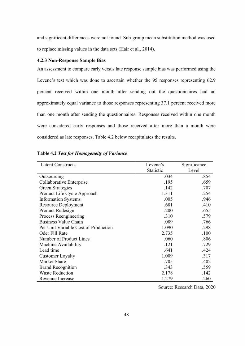
48

and significant differences were not found. Sub-group mean substitution method was used

to replace missing values in the data sets (Hair et al., 2014).

4.2.3 Non-Response Sample Bias

An assessment to compare early versus late response sample bias was performed using the

Levene’s test which was done to ascertain whether the 95 responses representing 62.9

percent received within one month after sending out the questionnaires had an

approximately equal variance to those responses representing 37.1 percent received more

than one month after sending the questionnaires. Responses received within one month

were considered early responses and those received after more than a month were

considered as late responses. Table 4.2 below recapitulates the results.

Table 4.2 Test for Homogeneity of Variance

Latent Constructs Levene’s

Statistic

Significance

Level

Outsourcing .034 .854

Collaborative Enterprise .195 .659

Green Strategies .142 .707

Product Life Cycle Approach 1.311 .254

Information Systems .005 .946

Resource Deployment .681 .410

Product Redesign .200 .655

Process Reengineering .310 .579

Business Value Chain .089 .766

Per Unit Variable Cost of Production 1.090 .298

Oder Fill Rate 2.735 .100

Number of Product Lines .060 .806

Machine Availability .121 .729

Lead time .641 .424

Customer Loyalty 1.009 .317

Market Share .705 .402

Brand Recognition .343 .559

Waste Reduction 2.178 .142

Revenue Increase 1.279 .260


49

The null hypothesis in the Levine’s test is that there is no difference in the variance of the

early responses and the variances of the late responses. If the significance value is > 0.05,

Levene’s test is non-significant and the assumption of equal variance holds. Table 4.2

shows the significance values to be > 0.05. Although the F-values for the latent construct,

product life cycle approach, per unit variable cost of production, customer loyalty, waste

reduction and revenue increase are > 1 these remain statistically insignificant. Therefore

the Levene’s test is non-significant and therefore there is equal variance. This therefore

means early and late responses were insignificant statistically.

4.2.4 Duration of Operation in Kenya

Respondents were to inform the study on how long they have been in operation in Kenya.

Figure 4.5 below provides a graphical representation of the duration.

Figure 4.1. Histogram of the Duration of Operation in Years among Manufacturing

Firms

The distribution in figure 4.1 suggests the greater number of the firms were < 30 years old

with the mode standing between 5 and 10 years. These were followed by firms in the age

50

bracket between 30 and 60 years. There were firms older than 60 years with two firms over

100 years old. The table below shows the distribution of the duration of operation in Kenya.

Table 4.3 Descriptive Summary for the Duration of Operation among Manufacturing

Firms in Kenya

Description Statistic Value

Mean 31.27

Standard Deviation (SD) 21.18

Skewness 1.13

Std. Error of Skewness 0.20

Kurtosis 1.71

Std. Error of Kurtosis 0.39

Minimum 2

Maximum 113


Based on table 4.3, the mean age was 31.27 years meaning on average manufacturing firms

have been in operation for 31.27 years. The SD was 21.18 years indicating high Coefficient

of Variation (CV) of 67.7 percent (21.18/31.27*100 percent). The high co-efficient of

variation can be explained by range of ages from 2 years to 113 years. The Z-skewness of

5.65 (1.13/0.20) is > 1.96 meaning that the distribution is positively skewed. Finally the Z-

kurtosis value of 4.38 (1.71/0.39) is also > 1.96 showing that the distribution is leptokurtic.

The respondents were also asked whether they are ISO 14001 certified or not. ISO 14001

certification indicates the organizations environmental consciousness. Having ISO 14001

was considered a proxy indicator of whether a firm implements reverse logistics. Table 4.4

below recapitulates the responses on ISO 14001 certification.

Table 4.4 ISO 14001 Certification Status of Manufacturing Firms

Class Frequency Percent Cumulative Percent

No 124 82.1 82.1

Yes 27 17.9 100.0

51

Total 151 100.0


Table 4.4 above reveals that the greater number of manufacturing firms were not ISO 14001

certified. This indicates that the firms need to incorporate more environmental management

practices in their processes. The next sub- sections summarizes descriptive statistics for

reverse logistics latent variable.

4.2.5: Sampling Adequacy and Sphericity

Sampling adequacy was established using KMO test. According to Kaiser.et.al., (1974)

acceptable KMO values should be > 0.70. Bartlett’s test of sphericity evaluated whether

there is a possibility of dimension reduction. This requires the p-value to be < 0.05. The

ensuing sub-sections summarize the results of sampling adequacy and sphericity test for

each of the five objectives of the study.

4.2.5.1 Sampling Adequacy and Sphericity Tests for the Association of Reverse

Logistics with Competitive Advantage

The first objective of this study was to establish the influence of reverse logistics on

competitive advantage. KMO and Bartlett tests were conducted using the latent constructs

of reverse logistics and competitive advantage latent variables. Table 4.11 below

recapitulates the results of these tests.

Table 4.5 Sampling Adequacy and Sphericity Tests for Reverse Logistics Association

with Competitive Advantage

Tests Co-efficient

Sampling Adequacy Test 0.872

Chi-Square Approximation 2938.359

Degrees of Freedom 36

Significance Level 0.000

52


Table 4.5 above reveals the KMO test value as 0.872 which is > 0.7. Bartlett’s test gave a

p-value of 0.000 which is < 0.05. Component matrix values ranged between 0.564 and

0.934. This means that conducting confirmatory factor analysis will produce statistically

reliable factors and results. It also means that it is possible to conduct dimension reduction

for both the measured and structured model with reverse logistics and competitive

advantage as latent variables.

4.2.5.2 Sampling Adequacy and Sphericity Tests for the Association linking Reverse

Logistics, Operational Performance and Competitive Advantage

Determining the influence of operational performance on the association linking reverse

logistics with competitive advantage was the second objective of the study. KMO and

Bartlett tests were applied on the constructs of reverse logistics, operational performance

and competitive advantage. Table 4.6 below recapitulates these test results.

Table 4.6 Sampling Adequacy and Sphericity Tests for the Association linking Reverse


Test Co-efficient






Based on table 4.6 the KMO test yielded a value of 0.919 which is > 0.7. Sphericity test

gave a p-value of 0.000 which is < 0.05. This means that conducting confirmatory factor

analysis will produce statistically reliable factors and results. It also means that it is possible

to conduct dimension reduction for both the measured and structured model with reverse

53

logistics operational performance and competitive advantage as latent variables.

Component matrix values ranged between -0.09 and 0.937. However the latent construct

with a low component matrix co-efficient was per unit variable cost of production. The

other latent constructs had component matrix coefficient < 0.5. This indicates that the

latent construct per unit variable cost of production is a potential latent construct to be

considered for deletion.


Logistics, Process Innovation and Operational Performance

The third objective sought to determine the influence of process innovation on the

association linking reverse logistics and operational performance. KMO and Bartlett tests

were applied on the constructs of reverse logistics, process innovation and operational

performance. Table 4.7 below recapitulates these tests.

Table 4.7 Sampling Adequacy and Sphericity Tests the association linking Reverse


Tests Co-efficients

Sampling Adequacy Test. 0.950





Table 4.7 shows KMO test value of 0.950 which is > 0.7. Sphericity test p-value was 0.000

which is < 0.05. This means that conducting confirmatory factor analysis will produce

statistically reliable factors and results. It also means that it is possible to conduct dimension

reduction for both the measured and structured model where reverse logistics, operational

performance and competitive advantage are latent variables. The latent construct with low

54

component matrix co-efficient were resource deployment and per unit variable cost of

production with co-efficients of - 0.049 and 0.002 respectively indicating they were

potential latent constructs to be removed from the model.



The fourth objective sought to examine the conditional indirect effect on the interaction

among reverse logistics, process innovation and operational performance on a firm’s

competitive advantage. Further the fifth objective sought to examine the joint effect of

reverse logistics, process innovation and operational performance on a firm’s competitive

advantage. KMO and Bartlett tests were applied using the constructs of reverse logistics,

process innovation, operational performance and competitive advantage. Table 4.8 below

recapitulates these test results.

Table 4.8 Sampling Adequacy and Sphericity Test for the Association linking Reverse


Tests Co-efficients






Based on table 4.8, KMO test results were 0.942 which is > 0.7. Sphericity p-value was

0.000 which is < 0.05. This means that conducting confirmatory factor analysis will

produce statistically reliable factors and results. It also means that it is possible to conduct

dimension reduction for both the measured and structured model with reverse logistics

operational performance and competitive advantage as latent variables. The latent construct

55

with low component matrix co-efficient were resource deployment and per unit variable

cost of production with co-efficients of - 0.045 and - 0.008 respectively, indicating they

were potential latent constructs to be removed from the model.

4.3 Reliability Tests

Reliability was examined by working out the Cronbach’s alpha coefficient at two levels.

At the first level coefficients were examined to measure how well the questionnaire items

for reverse logistics and process innovation were actually measuring the latent constructs.

In the process, questionnaire items that were reducing the internal consistency of the latent

construct were deleted. At the second level coefficients were examined to measure how

well the latent constructs were actually measuring the latent variable. In both cases a

Cronbach alpha coefficient of ≥ 0.7 represented sufficient association among data

instruments (Hair et al., 2007). Table 4.9 below provides details of the Cronbach’s alpha

measuring the internal reliability of the questionnaire items for reverse logistics and process

innovation.

Table 4.9 Cronbach Alpha Test Results Measuring Internal Reliability of Questionnaire

Items for Reverse Logistics and Process Innovation

Variables Cronbach Alpha Items Deleted

1 Outsourcing 0.708 RLO8

2 Collaborative Enterprise 0.716 CE5, CE6, CE9, CE10

3 Green Strategies 0.729 GS1, GS2, GS3,GS4, GS5,

GS14 & GS15

4 Product Life Cycle

Approach

0.707

5 Information Systems 0.704

6 Resource Deployment 0.744 RD4

7 Product Redesign 0.732 PRD1

8 Process Reengineering 0.723 PRE1, PRE2, PRE3, PRE8,

PRE9, PRE12 & PRE13

9 Business Value Chain 0.709 BVA1, BVA2


56

Based on table 4.9 above the Cronbach alpha coefficient to check whether the questionnaire

items were actually measuring the latent constructs for reverse logistics and process

innovation ranged between 0.704 and 0.744. This indicates sufficient internal consistency

between the questionnaire items and the latent constructs they were measuring.

Communalities were then assessed using PCA in order to determine how much of the

variance in each of the latent constructs for reverse logistics and process innovation were

explained by the undeleted questionnaire items (Field, 2013). Pallant (2007) posited that

communalities values of less than 0.3 should be dropped because they have low explanatory

power. Table 4.10 and 4.11 below summarize the communality coefficient for the

questionnaire items measuring the latent constructs for reverse logistics and process

innovation respectively.

57

Table 4.10 Communality Coefficient Results for the Questionnaire Items Measuring

Reverse Logistics Latent Constructs

Item

Code

Questionnaire Item Extraction

Factor

OS1 Outsourcing reverse logistics increases return on investment .634

OS2 Outsourcing reverse logistics provides better operational flexibility .611

OS3 Outsourcing reverse logistics results to improved customer service quality .440

OS4 Outsourcing reverse logistics results to improved speed to market. .410

OS5 Reverse logistics outsourcing provides access to functional and industry expertise .307

OS6 Reverse logistics outsourcing provides access to best technology .525

OS7 Reverse logistics outsourcing results to benefitting from best practices .600

CE1 There is high volume data exchange among partners in reverse logistics. .545

CE2 Partners implementing reverse logistics have standardized information exchange

platforms

.432

CE3 The focus in implementing reverse logistics is on building data integrity among

supply chain partners

.539

CE4 The emphasis in implementing reverse logistics is on managing transactions using

IT tools.

.707

CE7 Supply chain partners have fully integrated reverse logistics processes among

themselves

.460

CE8 Supply chain partners have set joint business goals in planning and implementing

reverse logistics

.429

GS6 Products are designed to facilitate re-use .753

GS7 Products are designed to facilitate recycling .787

GS8 Products are designed to facilitate remanufacture .612

GS9 Organizational processes optimization leads to a reduction in emissions and solid

waste

.723

GS10 Savings in energy and water are an outcome of using technologically cleaner

processes

.647

GS11 Recycling of materials internally is practiced during production .431

GS12 Supply chain partners practice environmental management principles like worker

empowerment.

.767

GS13 Environmentally affable packaging such as eco-labeling is used .889

PLA1 Control and reduction of returns rate does not undermine customer service .831

PLA2 Supply chain partners segregate returned products into categories for processing,

selling or disposal

.779

PLA3 The firm undertakes repair, remanufacture or refurbishing activities to make

product reusable

.792

PLA4 The firm recycles returned product parts to be used in manufacture of other

products or components

.499

PLA5 The firm undertakes disposal activities for returned products that have no more

economic or ecological value

.690

PLA6 The firm facilitates transportation of returned products in the process of recovering

value

.663


Based on table 4.10, the communality coefficient for the questionnaire items measuring the

latent constructs for reverse logistics range from 0.307 to 0.889. Since these values were >

0.3 it indicates that questionnaire items have sufficient explanatory power on the latent

constructs.

58

Table 4.11 Communality Co-efficient Results for the Questionnaire Items Measuring

Process Innovation Latent Constructs

Item

Code

Questionnaire Item Extraction

Factor

IS1 Information systems in use are perceived to be better than our competitors. .826

IS2 Information systems in use are perceived to be better than previous systems. .765

IS3 Information systems in use are perceived as easy to learn, understand and use. .771

IS4 Information systems in use are perceived as being compatible to the needs of

potential users.

.538

IS5 Users consider information systems as easy to explore and experiment with. .699

IS6 The results of using the information systems in the organization are visible. .676

RD1 Firm budgets have a component for reverse logistics activities .703

RD2 Staff have relevant skills to implement reverse logistics activities .639

RD3 Supply chain partners have acquired the relevant technology and equipment to

implement reverse logistics

.482

RD5 Suppliers are integrated in our current reverse logistics programming .360

RD6 Resource deployment processes in the firm are perceived to be superior to our

competitors

.598

RD7 Over time resource deployment processes in the organization have improved .541

PRD2 The firm maintains superiority in manufacturing technology .659

PRD3 Change in customer requirements have influenced our product design strategy .621

PRD4 Clients consider our current products as more convenient to use .504

PRD5 Over time manufacturing processes have been standardized and simplified .754

PRD6 Manufacturing processes are much easier as a result of redesigning our products .577

PRD7 The benefits of product redesign processes can be quantified within the

organization.

.650

PRD8 The quality of our products has improved as a result of product redesign .686

PRE4 Management constructively use ideas from other staff members .485

PRE5 Affable interactions among staff exist .490

PRE6 A teamwork approach is used in problem solving .530

PRE7 Members of staff work together collegially .675

PRE10 Employees have a degree of autonomy to make decisions .449

PRE11 Employee skills updates training programs exist .385

BVA3 Suppliers have capacity to meet demand variability .638

BVA4 Suppliers have a fairly constant lead-time variability .630

BVA5 Suppliers voluntarily share information .501

BVA6 Suppliers have adequate information and communication sharing infrastructure .735

BVA7 Clients avail information on demand well in advance .627

BVA8 Organizational systems have capacity to meet our customers demand variability .707

BVA9 Customers voluntarily share information .671


Based on table 4.11, the communality coefficient for the questionnaire items measuring the

latent constructs for process innovation range from 0.360 to 0.826, indicating that

questionnaire items have sufficient explanatory power on the latent constructs. Table 4.12

below details how well the latent constructs were measuring the latent variables.

59

Table 4.12 Cronbach Alpha Test Results Measuring Internal Consistency of Latent

Construct on the Latent Variable

Latent variables Cronbach Alpha Number of items

1 Reverse Logistics 0.943 4

2 Process Innovation 0.972 4

3 Operational Performance 0.908 4

4 Competitive Advantage 0.897 4


Table 4.12 above the Cronbach alpha coefficient to check whether the latent constructs

were actually measuring the latent variables ranged between 0.897 and 0.972. This

indicates sufficient internal consistency between the latent constructs and variables they

were measuring. Communality assessments using PCA were conducted in order to

determine the extent to which the variances in each of the latent variables were explained

by the latent constructs. Table 4.13 below details the communality assessment of the latent

constructs.

Table 4.13 Communality Coefficient Results for the Latent Constructs Measuring Latent

Variables

Latent Variable Initial Extraction

Outsourcing 1.000 .938

Collaborative Enterprise 1.000 .914

60

Green Strategies 1.000 .909

Product Life Cycle Approach 1.000 .898

Information Systems 1.000 .924

Resource Deployment 1.000 .937

Product Redesign 1.000 .937

Process Reengineering 1.000 .855

Business Value Chain 1.000 .968

Per Unit Variable Cost of Production 1.000 .810

Oder Fill Rate 1.000 .832

Number of Product Lines 1.000 .925

Machine Availability 1.000 .894

Lead time Analysis 1.000 .860

Customer Loyalty 1.000 .938

Market Share Analysis 1.000 .915

Brand Recognition Analysis 1.000 .873

Waste Reduction Analysis 1.000 .930

Revenue Increase Analysis 1.000 .941


Based on table 4.13 the communality coefficient for the latent constructs measuring the

latent variables for range from 0.810 to 0.968. This means that the latent constructs

explained between 81.0 and 96.8 percent of the variance of the respective latent variable.

Since these values are > 0.3 it indicates that latent constructs have sufficient explanatory

power on the latent variables. The next section discusses tests conducted to establish

construct validity of the latent constructs and latent variables.

4.4 Validity Tests

The ensuing sub-sections discuss how content, convergent and discriminant validity tests

were conducted and the results thereof.

4.4.1 Content Validity Tests

Content validity evaluated the extent to which conformity existed between the

questionnaire items chosen to form a totalized scale and the conceptual interpretation of the

latent variable. The objective was to ensure that the selection of questionnaire items

61

explained the latent construct both theoretically and practically. Content validity was

checked using a team of resource persons in the field of reverse logistics (Hair et al., 2014).

4.4.2 Convergent and Discriminant Validity

Convergent validity was measured using the standardized factor loading for each of the five

objectives of the study. For these the factor loadings were expected to be > 0.5 for

acceptable convergent validity. Convergent validity was confirmed through the use of AVE

method. For these the AVE for each of the latent constructs is expected to be > 0.5.

Discriminant validity which examines how constructs perceived not to be theoretically

associated are indeed not associated was measured by comparing the AVE with the MSV.

The AVE is expected to be > MSV for the latent variables to be considered not to be

theoretically associated. The ensuing sub-sections summarize the results of the convergent

and discriminant test per objective.

4.4.2.1 Convergent and Discriminant Validity Tests Associating Reverse Logistics


Establishing the influence of reverse logistics on competitive advantage was the first study

objective. Before further statistical analysis convergent and discriminant validity tests were

conducted on the latent constructs model depicting the association linking reverse logistics

with competitive advantage. Figure 4.2 below shows the standardized factor loadings to

check convergent validity on the model depicting the latent constructs and the latent

variables of reverse logistics and competitive advantage.

62

Figure 4.2. Convergent Validity Test for the Association linking Reverse Logistics


Based on figure 4.2 above the standardized factor loadings for all the latent constructs of

reverse logistics were > 0.5. The standardized factor loadings for each of the latent

constructs of competitive advantage were > 0.5 except for the construct CAWR1 with a

factor loading of 0.49. This was therefore deleted from the model. These standardized

factor loadings suggest that we have acceptable levels of convergent validity. Convergent

validity was also checked using AVE. For these the AVE for each of the latent constructs

is expected to be > 0.5. Table 4.14 below reveals the AVE for the latent constructs showing

the association linking reverse logistics with competitive advantage.

63

Table 4.14 Average Variance Extraction results for Reverse Logistics Interaction with


Factor <--- Component Loadings Squared Loadings AVE

RLPLCA1 <--- RevLog 0.967 0.935 0.569

RLGS1 <--- RevLog 0.681 0.464

RLCE1 <--- RevLog 0.658 0.433

RLOS1 <--- RevLog 0.667 0.445

CABR1 <--- CompAdv 0.837 0.701 0.875

CAMS1 <--- CompAdv 0.901 0.812

CACL1 <--- CompAdv 0.992 0.984

CARI1 <--- CompAdv 1.002 1.004


Since the AVE values for the association of reverse logistics with competitive advantage

are > 0.5, indicating good convergent validity. Discriminant validity which examines how

constructs perceived not to be theoretically associated are indeed not associated was

measured by comparing the AVE with the MSV. Table 4.15 below summarizes the MSV

squared loadings for the reverse logistics association with competitive advantage latent

variable.

Table 4.15 Maximum Shared Variance results for Reverse Logistics Interaction with


Component <--> Component Loadings Squared Loadings

RevLog <--> CompAdv 0.657 0.431


Based on table 4.15 above the square correlation for the interaction of reverse logistics with

competitive advantage latent variables was 0.431. From table 4.14 the AVE for reverse

logistics was 0.569. The AVE for competitive advantage latent variable was 0.748. This

shows that the square correlation is < the AVE of reverse logistics and competitive

advantage latent variables. This suggests discriminant validity among the latent constructs.

64

4.4.2.2 Convergent and Discriminant Validity among Reverse Logistics, Operational

Performance and Competitive Advantage

This study sought to determine the influence of operational performance on the association

linking reverse logistics and a firm’s competitive advantage as its second objective.

Convergent and discriminant validity tests were conducted on the latent constructs model

depicting the association among reverse logistics, operational performance and competitive

advantage as revealed in figure 4.3 below.


Operational Performance and Competitive Advantage

From figure 4.3, the standardized factor loadings for all the latent constructs of reverse

logistics and operational performance were > 0.5 except for the latent construct OPUVC1

65

which had a standardized factor loading significantly < 0.5. For this reason it was expunged

from the model. The standardized factor loadings for all the latent constructs of competitive

advantage were > 0.5. The standardized factor loadings establish there was convergent

validity. To confirm convergent validity AVE method was used. Table 4.14 below reveals

AVE computations.




RLPLCA1 <--- RevLog 0.622 0.387 0.841

RLGS1 <--- RevLog 0.997 0.994

RLCE1 <--- RevLog 0.994 0.988

RLOS1 <--- RevLog 0.997 0.994

OPLTA1 <--- OprPerf 0.928 0.861 0.836

OPDMA1 <--- OprPerf 0.903 0.815

OPPL1 <--- OprPerf 0.888 0.789

OPOFR1 <--- OprPerf 0.938 0.880

CARI1 <--- CompAdv 0.998 0.996 0.883

CABR1 <--- CompAdv 0.848 0.719

CAMS1 <--- CompAdv 0.91 0.828

CACL1 <--- CompAdv 0.995 0.990


Since the AVE values for reverse logistics, operational performance and competitive

advantage are > 0.5, this indicated good convergent validity. Table 4.17 below summarizes

the MSV squared loadings for reverse logistics, operational performance and competitive

advantage latent variables to examine discriminant validity.




RevLog <--> OprPerf 0.691 0.477

66


OprPerf <--> CompAdv 0.657 0.432


Based on table 4.17 above the square correlation between reverse logistics and operational

performance latent variable was 0.477. This value was < the AVE of reverse logistics latent

variable with a coefficient of 0.841 (Table 4.16). The square correlation linking reverse

logistics with competitive advantage latent variables was 0.874. This value was not

significantly > the AVE of reverse logistics latent variable (Table 4.16). This suggests the

latent constructs of reverse logistics were significantly distinct. This means that there was

evidence to suggest discriminant validity.

The square correlation between operational performance and reverse logistics latent

variables was 0.477. The square correlation between operational performance and

competitive advantage latent variables was 0.432. These values were < the AVE of

operational performance latent variable with a coefficient of 0.836 (Table 4.16). This means

that there was evidence to suggest the constructs of operational performance were unique

to the constructs of reverse logistic and those of competitive advantage.

The square correlation between competitive advantage and reverse logistics latent variables

was 0.874. This value was not significantly > the AVE of operational performance latent

variable with a coefficient of 0.836 (Table 4.16). The square correlation between

competitive advantage and operational performance latent variables was 0.432. The value

is < the AVE of operational performance latent variable. This means that there was

evidence to suggest discriminant validity.

67

4.4.2.3 Convergent and Discriminant Validity Tests for the Association among

Reverse Logistics, Process Innovation and Operational Performance

Determining the influence of process innovation on the association linking reverse logistics

and operational performance was the third study objective. Figure 4.4 reveals the

standardized factor loadings to check convergent validity on the model depicting the latent

constructs and the latent variables of reverse logistics, process innovation and operational

performance.

From figure 4.4 below the standardized factor loadings for all the latent constructs for

reverse logistics and process innovation were > 0.5 except for PIPRE1 and PIRD1 with a

loading of 0.46 an - 0.07 respectively. The latent construct PIRD1 had a loading that was

significantly < 0.5. It was therefore expunged from the model. The loadings for each of the

latent constructs of operational performance were > 0.5.

68


Process Innovation and Operational Performance

To confirm convergent validity AVE method was applied. Table 4.18 below reveals the

AVE for the latent constructs for the association among reverse logistics, process

innovation and operational performance.

69




RLPLCA1 <--- RevLog 0.631 0.398 0.844

RLGS1 <--- RevLog 0.997 0.994

RLCE1 <--- RevLog 0.995 0.990

RLOS1 <--- RevLog 0.996 0.992

PIBVA1 <--- ProInno 0.969 0.939 0.782

PIPRE1 <--- ProInno 0.457 0.209

PIPRD1 <--- ProInno 0.996 0.992

PIIS1 <--- ProInno 0.994 0.988

OPLTA1 <--- OprPerf 0.918 0.843 0.852

OPDMA1 <--- OprPerf 0.933 0.870

OPPL1 <--- OprPerf 0.925 0.856

OPOFR1 <--- OprPerf 0.916 0.839


Since the AVE values for reverse logistics, process innovation and operational performance

were > 0.5, this demonstrated good convergent validity among the latent constructs. Table

4.19 below summarizes the MSV squared loadings for reverse logistics, process innovation

and operational performance latent variables in measuring discriminant validity.




RevLog <--> ProInno 0.999 0.998


ProInno <--> OprPerf 0.690 0.476


Based on table 4.19 above the square correlation between reverse logistics and process

innovation latent variables was 0.998. This value was > the AVE of reverse logistics latent

variable with a coefficient of 0.844 (Table 4.18). The square correlation between reverse

70

logistics and operational performance latent variables was 0.465. This value was < the AVE

of reverse logistics latent variable. This suggests the latent constructs of reverse logistics

were not significantly distinct from those of process innovation but they were significantly

distinct from those of operational performance. This means that there was evidence to

suggest the constructs of reverse logistics were unique from those of operational

performance and capture some phenomena that operational performance does not.

The square correlation between process innovation and reverse logistics latent variables

was 0.998. This value was > the AVE of process innovation latent variable with a

coefficient of 0.782 (Table 4.18). The square correlation between process innovation and

operational performance latent variables was 0.476. This value was < the AVE of reverse

logistics latent variable. This suggests the latent constructs of process innovation were not

significantly distinct from those of reverse logistics but they were significantly distinct

from those of operational performance. This means that there was evidence to suggest the

constructs of process innovation were unique from those of operational performance.


variables was 0.465. The square correlation between operational performance and process

innovation latent variables was 0.476. These values were < the AVE of operational

performance latent variable with a coefficient of 0.845 (Table 4.18). Therefore there was

sufficient evidence to suggest the constructs of operational performance were unique and

capture some phenomena that reverse logistics and process innovation do not.

71

4.4.2.4 Convergent and Discriminant Validity Tests for the Association among


Advantage

The fourth objective examined the conditional indirect effect on the association linking

reverse logistics, process innovation and operational performance on a firm’s competitive

advantage. The fifth objective examined the joint effect of reverse logistics, process

innovation and operational performance on a firm’s competitive advantage. Convergent

and discriminant validity tests were conducted on the latent constructs model. Figure 4.5

reveals the standardized factor loadings to check convergent validity on the model

depicting the latent constructs and the latent variables of reverse logistics, process

innovation, operational performance and competitive advantage.

From figure 4.5 below the standardized factor loadings all of the latent constructs for

reverse logistics and process innovation were > 0.5 except for the latent construct PIPRE1

with a standardized factor loading of 0.46. Since this was > 0.3 it was not expunged from

the model. The loadings for each of the latent constructs of operational performance and

competitive advantage were > 0.5.

72


Process Innovation, Operational Performance and Competitive Advantage

Table 4.20 below reveals the AVE for the latent constructs for the association among

reverse logistics, process innovation and operational performance to confirm convergent

validity.

73




RLPLCA1 <--- RevLog 0.631 0.398 0.844

RLGS1 <--- RevLog 0.997 0.994

RLCE1 <--- RevLog 0.995 0.990

RLOS1 <--- RevLog 0.996 0.992

PIBVA1 <--- ProInno 0.969 0.939 0.782

PIPRE1 <--- ProInno 0.457 0.209

PIPRD1 <--- ProInno 0.996 0.992

PIIS1 <--- ProInno 0.994 0.988

OPLTA1 <--- OprPerf 0.928 0.861 0.850

OPDMA1 <--- OprPerf 0.921 0.848

OPPL1 <--- OprPerf 0.907 0.823

OPOFR1 <--- OprPerf 0.931 0.867

CARI1 <--- CompAdv 0.999 0.998 0.883

CABR1 <--- CompAdv 0.848 0.719

CAMS1 <--- CompAdv 0.909 0.826

CACL1 <--- CompAdv 0.995 0.990


Since the AVE values for reverse logistics, process innovation, operational performance

and competitive advantage were > 0.5, this demonstrated good convergent validity. Table

4.21 below summarizes the MSV squared loadings for the latent variables to check for

discriminant validity.




RevLog <--> ProInno 0.999 0.998



ProInno <--> OprPerf 0.684 0.468

ProInno <--> CompAdv 0.659 0.434

OprPerf <--> CompAdv 0.924 0.854


74

Based on table 4.21 above the square correlation between reverse logistics and process

innovation latent variables was 0.998. This value was > the AVE of reverse logistics latent

variable with a coefficient of 0.844 (Table 4.20). The square correlation between reverse

logistics and operational performance latent variables was 0.479. The square correlation

between reverse logistics and competitive advantage latent variables was 0.440. These

values were < the AVE of reverse logistics latent variable. This suggests the latent

constructs of reverse logistics were not significantly distinct from latent constructs of

process innovation. Further the results suggest the latent constructs of reverse logistics were

significantly distinct from the latent constructs of operational performance and competitive

advantage. This means that there was evidence to suggest the constructs of reverse logistics

were unique from those of operational performance and competitive advantage.

The square correlation between process innovation and reverse logistics latent variables

was 0.998. This value was > the AVE of process innovation latent variable with a

coefficient of 0.782 (Table 4.20). The square correlation between process innovation and

operational performance latent variables is 0.468. This value was < the AVE of process

innovation latent variable. The square correlation between process innovation and

competitive advantage latent variables is 0.434. This value was < the AVE of reverse

logistics latent variable. This suggests the latent constructs of process innovation were not

significantly distinct from latent constructs of reverse logistics. Further the results suggest

the latent constructs of process innovation were significantly distinct from the latent

constructs of operational performance and competitive advantage.

75


variables was 0.479. This value was < the AVE of operational performance latent variable

with a coefficient of 0.850 (Table 4.20). The square correlation between operational

performance and process innovation latent variables was 0.468. This value was < the AVE

of operational performance latent variable. The square correlation between operational

performance and competitive advantage latent variables was 0.854. This value was > the

AVE of operational performance latent variable, although this was not significantly larger.

This suggests the latent constructs of operational performance were significantly distinct

from latent constructs of reverse logistics and process innovation. Further the results

suggest the latent constructs of operational performance were not significantly distinct from

the latent constructs of competitive advantage. This means that there was empirical

evidence to suggest the constructs of operational performance were unique from those of

reverse logistics and process innovation demonstrating discriminant validity.

Finally the square correlation between competitive advantage and reverse logistics latent

variables was 0.440. This value was < the AVE of competitive advantage latent variable

with a coefficient of 0.883 (Table 4.20). The square correlation between competitive

advantage and process innovation latent variables was 0.434. This value was < the AVE of

competitive advantage latent variable. The square correlation between competitive

advantage and operational performance latent variables was 0.854. This value was > the

AVE of competitive advantage latent variable. This suggests the latent constructs of

competitive advantage were not significantly distinct from latent constructs of operational

performance. Further the results suggest the latent constructs of competitive advantage

were significantly distinct from the latent constructs of reverse logistics and process

76

innovation. This means that there was empirical evidence to suggest the constructs of

competitive advantage were unique from those of reverse logistics and process innovation.

To further explain the nature of association among the latent constructs of reverse logistics,

process innovation, operational performance and competitive advantage, appendix 5, 6, 7,

8, 9 and 10 reveal patterns of correlation among these latent constructs. Appendix 5

indicates the latent constructs of reverse logistics have equal patterns of correlation among

themselves in comparison to the correlations between the latent constructs of reverse

logistics and process innovation. Similarly, the latent constructs of process innovation have

equal patterns of correlation among themselves in comparison to the correlations between

the latent constructs of process innovation and reverse logistics. This indicates the

interaction among the latent constructs of reverse logistics and process innovation have

high association.

Appendix 6 reveals the latent constructs of reverse logistics have higher patterns of

correlation among each other compared to patterns of correlation between the latent

constructs of reverse logistics and operational performance. Similarly, from appendix 6 and

8 the latent constructs of operational performance have higher patterns of correlation

among themselves in comparison to the correlations between the latent constructs of

operational performance and reverse logistics and between the latent constructs of

operational performance and process innovation. According to appendix 8 the latent

constructs of process innovation have higher patterns of correlation among each other

compared to patterns of correlation between the latent constructs of process innovation and

operational performance. These indicate discriminant validity between the latent constructs

77

of reverse logistics and operational performance and between the latent constructs of

process innovation and operational performance.

Appendix 7 reveals the latent constructs of reverse logistics have higher patterns of

correlation among each other compared to patterns of correlation between the latent

constructs of reverse logistics and competitive advantage. Similarly, from appendix 7 and

9 the latent constructs of competitive advantage have higher patterns of correlation among

themselves in comparison to the correlations between the latent constructs of competitive

advantage and reverse logistics and between the latent constructs of competitive advantage

and process innovation. According to appendix 9 the latent constructs of process innovation

have higher patterns of correlation among each other compared to patterns of correlation

between the latent constructs of process innovation and competitive advantage. These

indicated discriminant validity between the latent constructs of reverse logistics and

competitive advantage and between the latent constructs of process innovation and


Appendix 10 indicated the latent constructs of operational performance have equal patterns

of correlation among themselves in comparison to the correlations between the latent

constructs of operational performance and competitive advantage. In addition, the latent

constructs of competitive advantage have equal patterns of correlation among themselves

in comparison to the correlations between the latent constructs of competitive advantage

and operational performance. This indicates the interaction between the latent constructs of

operational performance and competitive advantage have good discriminant validity.

78

These validity tests suggest the study had good content and convergent validity. Good

discriminant validity especially on the models linking all the latent variables of reverse

logistics, process innovation operational performance and competitive advantage was

observed. Arguably the models demonstrate good construct validity. The next section

discussed the descriptive statistics for all the questionnaire items included in the analysis.


Advantage Descriptive Statistics

Descriptive statistics were then analyzed to understand the nature of the distributions

generated from the questionnaire items. The analysis involved examining the mean, SD,

CV, skewness and kurtosis. SD was used to understand variability among items with the

same unit of measure while the CV was used to compare levels of variability among items

that were not measured on the same measurement scale. The ensuing sub-sections

recapitulate the descriptive statistics for reverse logistics, process innovation, operational

performance and competitive advantage.

4.5.1 Reverse Logistics

In measuring reverse logistics, four latent constructs namely; outsourcing, collaborative

enterprise, green strategies and product life cycle were used. Each of the latent constructs

had a number of questionnaire items for which reliability tests were used to check the extent

to which they have explanatory power over the construct they were purported to measure.

The results are outlined in the ensuing sub-sections.

4.5.1.1 Outsourcing

Outsourcing was measured using seven questionnaire items using a five point Likert scale

with 1 being “not at all” and 5 being “to a very large degree”. The results are recapitulated

in table 4.22. From the table, it can be observed that the mean score for the seven

79

questionnaire items ranged from 3.24 to 3.85 indicating that outsourcing reverse logistics

was practiced from a moderate to a large extent. Questionnaire item OS2 had the highest

mean score (3.85). This demonstrates that manufacturing firms in Kenya put high emphasis

in improving operational flexibility. Questionnaire item OS7 had the lowest mean score

(3.24).

Table 4.22 Respondent Scores on Outsourcing

Code Questionnaire Item N Mean SD Z-

Skewness

Z-

Kurtosis

OS1 Outsourcing reverse logistics

increases return on investment.

151 3.79 0.64 -3.78 3.04

OS2 Outsourcing reverse logistics

provides better operational

flexibility.

151 3.85 0.81 -2.48 0.09

OS3 Outsourcing reverse logistics results

to improved customer service

quality.

151 3.82 0.95 -1.94 -1.97

OS4 Outsourcing reverse logistics results

to improved speed to market.

151 3.80 0.93 -1.24 -2.21

OS5 Reverse logistics outsourcing

provides access to functional and

industry expertise.

151 3.61 0.88 -0.31 -1.77

OS6 Reverse logistics outsourcing

provides access to best technology.

151 3.30 0.98 1.97 -2.07

OS7 Reverse logistics outsourcing results

to benefitting from best practices.

151 3.24 1.00 1.21 -2.65


The levels of variability in the data set ranged from 0.64 to 1.00 SDs. The questionnaire

item OS7 had the highest degree of variability with 1.00 SDs. This means that observations

within the item were more scattered away from the mean. The high variability suggests

that the respondents were more indifferent in their responses to this item as compared to

the other items of measuring reverse logistics outsourcing. The questionnaire item OS1 had

the lowest variability in the data set with 0.64 SDs.

80

The z-skewness statistic ranged from -3.78 to 1.97. Z-skewness scores ranging between ±

1.96 suggest that the distributions were fairly symmetrical. This reveals that observations

in the items were fairly equally distributed on either side of the mean. While z-skewness

scores that were less than -1.96 suggest that more observations were found on the left side

of the mean. Questionnaire item OS1 was most skewed to the left with a z-skewness score

of -3.78.

The z-kurtosis statistic ranged from -2.65 to 3.04. Distributions with z-kurtosis scores

above 1.96 are considered to be leptokurtic. Z-kurtosis scores ranging between ± 1.96

suggest that the distribution were fairly mesokurtic while those with scores less than -1.96

are considered to be platykurtic. Questionnaire item OS1 had the highest z-kurtosis score

of 3.04 meaning that it was leptokurtic. Platykurtic distributions were exhibited by

questionnaire items OS7, OS4 and OS6 with z-kurtosis scores of -2.65, -2.21 and -2.07

respectively.

4.5.1.2 Collaborative Enterprising

The respondents indicated the extent to which they engaged in collaborative enterprise in

reverse logistics. This was measured using six questionnaire items. Table 4.23 below

recapitulates the results for collaborative enterprise latent construct.

Table 4.23 revealed that the mean scores ranged between 3.31 and 3.68 indicating the

respondents concurred with the questionnaire items to a moderate extent but tending

towards a large extent. The questionnaire item CE1 and CE7 had the highest and lowest

mean scores. The degree of variability ranged from 0.82 to 1.13 SDs. The questionnaire

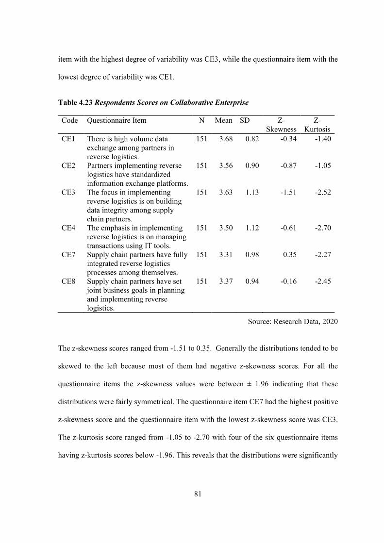
81

item with the highest degree of variability was CE3, while the questionnaire item with the

lowest degree of variability was CE1.

Table 4.23 Respondents Scores on Collaborative Enterprise


Skewness

Z-

Kurtosis

CE1 There is high volume data

exchange among partners in

reverse logistics.

151 3.68 0.82 -0.34 -1.40

CE2 Partners implementing reverse

logistics have standardized

information exchange platforms.

151 3.56 0.90 -0.87 -1.05

CE3 The focus in implementing

reverse logistics is on building

data integrity among supply

chain partners.

151 3.63 1.13 -1.51 -2.52

CE4 The emphasis in implementing

reverse logistics is on managing

transactions using IT tools.

151 3.50 1.12 -0.61 -2.70

CE7 Supply chain partners have fully

integrated reverse logistics

processes among themselves.

151 3.31 0.98 0.35 -2.27

CE8 Supply chain partners have set

joint business goals in planning

and implementing reverse

logistics.

151 3.37 0.94 -0.16 -2.45


The z-skewness scores ranged from -1.51 to 0.35. Generally the distributions tended to be

skewed to the left because most of them had negative z-skewness scores. For all the

questionnaire items the z-skewness values were between ± 1.96 indicating that these

distributions were fairly symmetrical. The questionnaire item CE7 had the highest positive

z-skewness score and the questionnaire item with the lowest z-skewness score was CE3.

The z-kurtosis score ranged from -1.05 to -2.70 with four of the six questionnaire items

having z-kurtosis scores below -1.96. This reveals that the distributions were significantly

82

platykurtic. The questionnaire item CE2 had the highest z-kurtosis score and questionnaire

item with the lowest z-kurtosis score was CE4.

4.5.1.3 Green Strategies

A set of eight questionnaire items were used to assess green strategies in reverse logistics

as recapitulated in table 4.24.

Table 4.24 Respondent Scores on Green Strategies


Skewness

Z-

Kurtosis

GS6 Products are designed to

facilitate re-use.

151 3.87 0.83 -1.32 -1.45


facilitate recycling.

151 3.57 0.98 -0.68 -2.45


facilitate remanufacture.

151 3.48 0.92 0.09 -2.14

GS9 Organizational processes

optimization leads to a

reduction in emissions and

solid waste.

151 3.64 0.84 -1.18 -1.23

GS10 Savings in energy and

water are an outcome of

using technologically

cleaner processes.

151 3.52 0.97 -0.13 -2.41

GS11 Recycling of materials

internally is practiced

during production.

151 3.48 0.90 -0.18 -1.91

GS12 Supply chain partners

practice environmental

management principles like

worker empowerment.

151 3.53 0.90 -0.94 -1.91

GS13 Environmentally affable

packaging such as eco-

labeling is used.

151 3.45 0.97 -0.17 -2.38


The results show the mean scores ranged between 3.45 (questionnaire item GS13) and 3.87

(questionnaire item GS6) indicating that the respondents concurred with the questionnaire

items moderately but tending towards a large extent. The degree of variability ranged from

83

0.83 to 0.98 SDs. Questionnaire item GS7 had the highest degree of variability followed

by questionnaire item GS10 and GS13. Questionnaire item GS6 had the lowest degree of

variability.

The z-skewness scores ranged from -1.32 to 0.09. This generally reflects that all the

questionnaire items had fairly symmetrical distributions. The z-kurtosis scores ranged from

-2.45 to -1.23. Four of the questionnaire items had z-kurtosis scores below -1.96 suggesting

they were platykurtic. The other four questionnaire items had z-kurtosis scores ranging

between ±1.96 suggesting they were mesokurtic.

4.5.1.4 Product Life Cycle Approach

Six questionnaire items were used to measure the extent to which firms utilize the product

life cycle approach in reverse logistics activities as per table 4.25 below. Based on the table,

the mean scores ranged between 3.14 (PLA6) and 3.68 (PLA1). This reveals that

respondents concurred with the questionnaire items moderately but tending towards a large

extent.

From the ensuing table, variability levels were between 0.87 and 1.04 SDs. Respondents

were most inconsistent in their responses to questionnaire item PLA3 and PLA5

respectively. Questionnaire item PLA1 had the lowest degree of variability. The z-

skewness scores were between -0.80 and 2.89. Generally reflect that the distributions

tended to be symmetrical. The only questionnaire item with a z-skewness score that did not

fall in the range ± 1.96 was PLA2. This had a z-skewness value of 2.89 indicating that the

distribution was skewed to the right.

84

Table 4.25 Respondent Scores on Product Life Cycle Approach


Skewness

Z-

Kurtosis

PLA1 Control and reduction of returns

rate does not undermine

customer service.

151 3.68 0.87 -0.29 -1.89

PLA2 Supply chain partners segregate

returned products into

categories for processing,

selling or disposal.

151 3.53 0.89 0.62 -1.85

PLA3 The firm undertakes repair,

remanufacture or refurbishing

activities to make product

reusable.

151 3.63 1.04 -0.14 -2.73

PLA4 The firm recycles returned

product parts to be used in

manufacture of other products

or components.

151 3.65 1.01 -0.80 -2.69

PLA5 The firm undertakes disposal

activities for returned products

that have no more economic or

ecological value.

151 3.43 1.02 1.16 -2.72

PLA6 The firm facilitates

transportation of returned

products in the process of

recovering value.

151 3.14 0.89 2.89 -0.76


The z-kurtosis scores (table 4.25) were between -3.47 to -0.35. Four of the questionnaire

items namely; PLA1, PLA2, PLA3 and PLA5 had z-kurtosis scores of less than -1.96

suggesting these distributions formed from the responses of these questionnaire items

tended to be platykurtic. The remaining two questionnaire items namely; PLA4 and PLA6

had z-kurtosis values of -1.88 and -0.75. These suggest mesokurtic distributions but tending

towards being platykurtic.

85

4.5.1.5 Summary of Reverse Logistics

Each of the latent constructs forming the reverse logistics variable were aggregated and

coefficients that summarize the aggregated data set were calculated. Table 4.26 below

provides summarized coefficients of the latent constructs.

Table 4.26 Descriptive Summary of Reverse Logistics Latent Constructs

Latent Construct N Mean Std.

Dev

Z-

Skewness

Z-

Kurtosis

Outsourcing 151 3.63 0.51 0.04 -1.28

Collaborative Enterprise 151 3.51 0.60 0.05 -0.82

Green Strategies 151 3.56 0.44 -0.06 -1.56

Product Life Cycle Approach 151 3.51 0.58 0.11 -0.78


Outsourcing was rated as the most common reverse logistics approach among Kenyan

manufacturing firms with a mean of 3.63 (SD = 0.51). The second most common reverse

logistics approach was green strategies with a mean of 3.56 (SD = 0.41). The least rated

were product life cycle approach and collaborative enterprise both with means of 3.51 (SD

= 0.58 and 0.60 respectively). These generally indicate that the respondents generally

concurred with the statements moderately but tending towards a large degree.

The z-skewness scores were between -0.06 and 0.11. This generally reflects that the

distributions generated from these latent constructs tended to be symmetrical. The z-

kurtosis scores were between -1.56 and -0.78. Although this suggests the distributions

formed by these latent constructs were mesokurtic but they were tending towards being

platykurtic.

86

The respondents were also asked to provide information regarding reverse logistics cost,

level of energy consumption on reverse logistics and the extent to which they undertake

refurbishing, remanufacturing, recycling and disposal activities. The ensuing table 4.27

summarizes the responses.

Table 4.27 Descriptive Summary of Reverse Logistics Questionnaire Items


Based on table 4.27 above, asked to estimate the percentage of cost of running reverse

logistics operations in the manufacturing firm in relation to sales, on average 34.52 percent

of cost was spent on running reverse logistics operations among manufacturing firms in

Kenya (CV = 43.9 percent). On the questionnaire item requiring firms to estimate costs

recovered from reverse logistics activities; on average these firms recovered 34.55 percent

of cost from reverse logistics activities (CV = 44.2 percent). Generally this indicates the

Code Questionnaire Item N Mean CV

(%)

Z-

Skewness

Z-

Kurtosis

RL1 Estimated cost of running

reverse logistics operations

in relation to sales.

151 34.52 43.9% 0.34 -1.15

RL2 Estimated cost recovered

from reverse logistics

activities.

151 34.55 44.2% 0.16 -1.17

RL3 Energy used in handling

returns in relation to total

energy consumption.

151 29.58 41.8% -0.01 -0.76

RL4 Rate of product

refurbishment in relation to

total production.

151 21.06 43.5% 0.34 -0.57

RL5 Rate of product

remanufacture in relation to

total production.

151 21.01 40.6% 0.40 -0.27

RL6 Raw materials recycled. 151 21.00 41.2% 0.48 -0.07

RL7 Raw materials moved to

landfills, incinerated or

disposed as waste.

151 20.96 41.7% 0.34 -0.16

87

costs linked to reverse logistics are somewhat equal to the costs recovered from the same.

The respondents also indicated that the average amount of energy used in handling returns

in relation to total energy consumption was 29.58 percent (CV = 41.8 percent).

The average rate of product refurbishment in relation to total production among the

manufacturing firms was 21.06 percent (CV = 43.5 percent). The mean rate of product

remanufacture in relation to total production was 21.01 percent (CV = 40.6 percent). The

average amount of raw materials recycled was 21.00 percent (CV = 41.2 percent). This

indicates that refurbishing, remanufacturing and recycling were undertaken by

manufacturing firms with equal measure. The mean amount of raw materials moved to

landfills, incinerated or disposed as waste among the manufacturing firms was 20.96

percent (CV = 41.7 percent).

The z-skewness scores ranged between -1.01 and 0.48. These generally reflect that the

distributions tended to be symmetrical with a tendency to be skewed to be skewed to the

left. The z-kurtosis scores ranged between -1.17 to -0.07. Because these scores were in the

range between than ±1.96, it suggests that these distributions formed from the responses of

these questionnaire items tended to be mesokurtic but tending towards being platykurtic.

4.5.2 Process Innovation

The latent variable, process innovation was measured using four latent constructs. These

were information systems, product redesign, process reengineering and business value

chain. The ensuing sub-sections provide descriptive summaries for each of the latent

constructs.

88

4.5.2.1 Information Systems

To measure the extent to which firm utilize information systems to improve process

innovativeness, six questionnaire items were used as shown in the ensuing table 4.28. From

the table the mean scores ranged between 3.25 (IS6) and 3.99 (IS1, IS2) indicating agreed

with the statements moderately and tending towards a large extent.

Table 4.28 Respondents Scores on Information Systems

Code Questionnaire Item N Mean Std.

Dev

Z-

Skewness

Z-Kurtosis

IS1 Information systems in use

are perceived to be better

than our competitors.

151 3.99 0.76 -0.83 -1.92


are perceived to be better

than previous systems in use.

151 3.99 0.83 -0.58 -3.11


are perceived as easy to

learn, understand and use.

151 3.62 0.92 0.34 -2.30


are perceived as being

compatible to the needs of

potential users.

151 3.67 0.90 -0.37 -2.03

IS5 Users consider the

information systems as easy

to explore and experiment

with.

151 3.52 0.95 0.83 -2.34

IS6 The results of using the

information systems in the

organization are visible.

151 3.25 0.93 2.16 -1.57


Variability levels ranged from 0.76 to 0.95 SDs. Respondents were most invariable to

questionnaire item IS1. The second most invariable response was questionnaire item IS2.

The least invariable response was questionnaire item IS5. The z-skewness scores for the

six questionnaire items ranged between -0.83 and 2.16. These generally reflect that the

distributions tended to be symmetrical. Questionnaire item IS6 was the only item among

89

the six questionnaire items that the z-skewness score was not within the range ± 1.96. This

had a z-skewness value of 2.16 indicating that the distribution was skewed to the right.

The z-kurtosis scores ranged between -3.11 to -1.57. Questionnaire items IS2, IS3, IS4 and

IS5 had z-kurtosis scores of less than -1.96 suggesting these distributions formed from the

responses of these questionnaire items tended to be platykurtic. Questionnaire items IS1

and IS6 had z-kurtosis values of -1.92 and -1.57 respectively. Although this suggests

mesokurtic distributions but they were tending towards being platykurtic.

4.5.2.2 Product Redesign

Product redesign latent construct had a total of seven questionnaire items as indicated in

table 4.29. The mean scores ranged between 3.11 and 3.81 showing respondents agreed

with the questionnaire items moderately but approaching a large extent. The questionnaire

item with the highest score was PRD3 with a mean of 3.81 (SD = 0.82). They also agreed

to a large extent with questionnaire item PRD2 with a mean of 3.74 (SD = 0.67).

Respondents agreed moderately with questionnaire items PRD7 and PRD8 (Mean = 3.22

and 3.11, SD = 0.93 and 0.94 respectively). Questionnaire item with the highest degree of

variability was PRD4 with a mean of 3.72 (SD = 0.97).

The z-skewness scores for the seven questionnaire items ranged between -3.59 and 2.32.

Questionnaire items with z-skewness scores of < -1.96 and in ascending order were PRD2

and PRD3 suggesting they are skewed to the left. Questionnaire item with z-skewness

scores of > 1.96 was PRD7 suggesting it was skewed to the right. The remaining four

questionnaire items had z-skewness scores within the range ± 1.96, indicating they were

fairly symmetrical.

90

Table 4.29 Respondent Scores on Product Redesign


Dev

Z-

Skewness

Z-

Kurtosis

PRD2 The firm maintains

superiority in manufacturing

technology.

151 3.74 0.67 -3.59 1.95

PRD3 Change in customer

requirements have

influenced our product

design strategy.

151 3.81 0.82 -2.19 -0.49

PRD4 Clients consider our current

products as more convenient

to use.

151 3.72 0.97 -1.48 -2.25

PRD5 Over time manufacturing

processes have been

standardized and simplified.

151 3.68 0.96 -0.86 -2.37

PRD6 Manufacturing processes

are much easier as a result

of redesigning our products.

151 3.52 0.92 0.05 -2.09

PRD7 The benefits of product

redesign processes can be

quantified within the

organization.

151 3.22 0.93 2.32 -1.42

PRD8 The quality of our products

has improved as a result of

product redesign.

151 3.11 0.94 1.55 -2.42


The z-kurtosis scores ranged between -2.42 to 1.95. Questionnaire items PRD8, PRD5,

PRD4 and PRD6 had z-kurtosis scores < -1.96 and in ascending order. This suggests that

these distributions formed from the responses of these questionnaire items tended to be

platykurtic. For the other remaining three questionnaire items z-kurtosis scores ranged

between ± 1.96, suggesting mesokurtic distributions, although questionnaire item PRD2

was tending towards being leptokurtic.

91

4.5.2.3 Process Reengineering

Process reengineering latent construct had a total of six questionnaire items. Table 4.30

below indicated that the mean scores ranged between 3.46 and 3.87. The questionnaire item

with the highest score was PRE6 with a mean of 3.87 (Std. Dev = 1.02). The questionnaire

item with the lowest mean score was PRE11 (Mean = 3.46, SD = 0.90). Questionnaire item

PRE7 had the highest SD (Mean = 3.85, SD = 1.07)

Table 4.30 Respondent Scores on Process Reengineering

Code Process Reengineering N Mean Std.

Dev

Z-

Skewness

Z-

Kurtosis

PRE4 Management constructively

use ideas from other staff

members.

151 3.71 0.80 -0.22 -1.42

PRE5 Affable interactions among

staff exist.

151 3.70 0.80 -0.94 -0.97

PRE6 A teamwork approach is used

in problem solving.

151 3.87 1.02 -2.46 -2.30

PRE7 Members of staff work

together collegially.

151 3.85 1.07 -2.66 -2.50

PRE10 Employees have a degree of

autonomy to make decisions.

151 3.50 0.97 -0.18 -2.47

PRE11 Employee skills updates

training programs exist.

151 3.46 0.95 -0.44 -2.36


Based on table 4.30, the six questionnaire items had z-skewness scores ranging between -

2.66 and -0.18. Two questionnaire items, PRE7 and PRE6 had z-skewness scores of < -

1.96 while the remaining four questionnaire items had ranged between ± 1.96. This

suggested that questionnaire item in the process reengineering latent construct were either

skewed to the left or fairly symmetrical.

The z-kurtosis scores for the six questionnaire items ranged between -2.50 and -0.97. Four

of the questionnaire items PRE7, PRE10, PRE11 and PRE6 had z-kurtosis scores of less

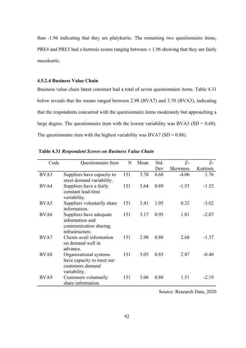
92

than -1.96 indicating that they are platykurtic. The remaining two questionnaire items,

PRE4 and PRE5 had z-kurtosis scores ranging between ± 1.96 showing that they are fairly

mesokurtic.

4.5.2.4 Business Value Chain

Business value chain latent construct had a total of seven questionnaire items. Table 4.31

below reveals that the means ranged between 2.98 (BVA7) and 3.70 (BVA3), indicating

that the respondents concurred with the questionnaire items moderately but approaching a

large degree. The questionnaire item with the lowest variability was BVA3 (SD = 0.68).

The questionnaire item with the highest variability was BVA7 (SD = 0.88).

Table 4.31 Respondent Scores on Business Value Chain


Dev

Z-

Skewness

Z-

Kurtosis

BVA3 Suppliers have capacity to

meet demand variability.

151 3.70 0.68 -4.06 1.76

BVA4 Suppliers have a fairly

constant lead-time

variability.

151 3.64 0.89 -1.53 -1.52

BVA5 Suppliers voluntarily share

information.

151 3.41 1.05 0.32 -3.02

BVA6 Suppliers have adequate

information and

communication sharing

infrastructure.

151 3.17 0.95 1.81 -2.07

BVA7 Clients avail information

on demand well in

advance.

151 2.98 0.88 2.68 -1.37

BVA8 Organizational systems

have capacity to meet our

customers demand

variability.

151 3.05 0.85 2.87 -0.40

BVA9 Customers voluntarily

share information.

151 3.06 0.88 1.51 -2.19


93

Based on table 4.31, the seven questionnaire items had z-skewness scores ranging between

-4.06 and 2.87. Questionnaire items BVA4, BVA5, BVA9 and BVA6 had z-skewness

scores ranging between ± 1.96 indicating they were fairly symmetrical. Questionnaire item

BVA3 had z-skewness scores of < -1.96 showing that it was skewed to the left.

Questionnaire item BVA7 and BVA8 had z-skewness scores of > 1.96 showing that they

were skewed to the right or were positively skewed.

The seven questionnaire items used to measure the business value chain latent construct

had z-kurtosis scores ranging from -3.02 to 1.76. Questionnaire items BVA4, BVA7, BVA8

and BVA3 had z-kurtosis scores ranging between ± 1.96 indicating they were fairly

mesokurtic. Questionnaire items BVA5, BVA9 and BVA6 had z-kurtosis scores of < -1.96

indicating that they were platykurtic.

4.5.2.5 Summary of Process Innovation

The latent constructs forming the process innovation variable were each aggregated and

coefficients that summarize the aggregated data set were then calculated. Table 4.32 below

provides a summary of coefficients summarizing latent constructs for process innovation.

Table 4.32 Descriptive Summary for Process Innovation Latent Constructs

Latent Construct N Mean Std.

Dev

Z-

Skewness

Z-

Kurtosis

Information Systems 151 3.67 0.43 -0.03 -0.91

Product Redesign 151 3.54 0.51 -0.06 -1.00

Process Reengineering 151 3.68 0.43 0.32 -0.85

Business Value Chain 151 3.26 0.37 -0.01 -0.96


94

Based on table 4.32 above, process reengineering and information systems were rated as

the most common process innovation approaches with a mean of 3.68 and 3.67 (SD = 0.43

and 0.43 respectively). The least rated was business value chain with an average score of

3.26 (SD = 0.37). These generally indicate that the respondents agreed with the statements

from a moderate degree but tending towards a large degree.

The z-skewness scores were between -0.06 and 0.32. This generally reflects that the

distributions generated from these latent constructs of process innovation tended to be

symmetrical. The z-kurtosis scores were between -1.00 and -0.85. This suggests that the

distributions formed by the latent constructs of process innovation were mesokurtic

although tending towards being platykurtic.

The respondents were required to share information on the percentage of sales from new

products, percentage of budget devoted to research and development, amount of time spent

on research and ideation and the percentage of employees trained on innovation. Table

4.33 below provides a summary of the responses.

Table 4.33 Descriptive Summary for Process Innovation Questionnaire Items

Code Questionnaire Item N Mean CV

(%)

Z-

Skewness

Z-

Kurtosis

PI1 Percentage of sales from new

products introduced in the last

two years.

151 23.71 45.3% -0.18 -1.04

PI2 Percentage of budget devoted

to research and development.

151 23.41 46.2% 0.22 -1.32

PI3 Percentage of employee hours

spent on research and ideation.

151 39.06 45.3% 0.28 -1.10

PI4 Percentage of employees who

have received training and

tools for innovation.

151 49.55 35.7% -0.01 -1.01


95

Based on table 4.33, the percentage of sales from new products introduced in the last two

years, was estimated to be 23.71 percent (CV = 45.3 percent). On average 23.41 percent

(CV = 46.2 percent) of the budget is devoted to research and development. The amount of

employee hours spent on research and ideation averaged 39.06 percent (CV = 45.3 percent).

The percentage of employees who had received training and tools for innovation averaged

49.55 percent (CV = 35.7 percent).

The z-skewness scores ranged between -0.18 and 0.28. These reflect symmetry in the

distributions. The z-kurtosis scores ranged between -1.32 to -1.01. Because these scores

were in the range between than ±1.96, it suggests that these distributions formed from the

responses of these questionnaire items tended to be mesokurtic but tending towards being

platykurtic.

4.5.3 Operational Performance

Operational performance was measured using four constructs namely; quality, flexibility,

dependability and delivery speed. In order to measure quality, order fill rate was used.

Flexibility was measured using the number of product lines. Dependability was measured

using capacity utilization rate of machine and equipment as a proxy indicator. Delivery

speed was measured using lead-time. Table 4.34 below provides recapitulated descriptive

statistics for the four constructs.

Table 4.34 Descriptive Statistics for Operational Performance

Operational Performance N Mean CV (%) Z-

Skewness

Z-

Kurtosis

Oder Fill Rate 151 95.20 2.0% 0.26 -1.32

Number of Product Lines 151 9.47 36.6% 0.06 -0.74

Machine Availability 151 91.26 1.3% 0.33 -1.33

Lead time Analysis 151 10.50 33.7% 0.01 -1.00

96


Based on the table 4.34 above, using the order fill rate, on average the number of items

actually delivered to customers in the course of the year stated as a percentage of the total

orders stood at 95.20 percent (CV = 2.0 percent). The average number of product-lines

among manufacturing firms was 9.47 (CV = 36.6 percent). Using the capacity utilization

rate, on average the number of hours of equipment/machines that were actually available

for manufacturing operations in the year stated as a percentage of the hours these

equipment/machines are supposed to be available for manufacturing operations was 91.26

percent (CV = 1.3 percent). An analysis of the lead-time revealed the mean number of days

between order receipt and shipment to the customer was 10.50 days (CV = 33.7 percent).

The four constructs used to measure operational performance had z-skewness scores

ranging between 0.01 and 0.33. These scores ranged between ± 1.96 indicating they were

fairly symmetrical. Z-kurtosis scores ranged from - 1.33 to - 0.74. These z-kurtosis scores

range between ± 1.96 indicating that the distributions were mesokurtic.

4.5.4 Competitive Advantage

Competitive advantage was measured using five constructs namely; customer loyalty,

market share, brand recognition, waste reduction and revenue increase. Customer loyalty

was measured using the customer retention rate. Market share was measured using the

market share index for each firm in each industry. Brand recognition was measured using

the profit margin as a proxy indicator. Waste reduction was measured using the non-

defective rate. Revenue increase was measured by subtracting the revenue for last from

those of the previous year and dividing this with the revenue for the previous year to

97

determine the percentage increase. Table 4.35 below provides recapitulates descriptive

statistics for the five constructs.

Table 4.35 Descriptive Statistics for Competitive Advantage

Competitive Advantage N Mean CV (%) Z-

Skewness

Z-

Kurtosis

Customer Loyalty 151 91.66 3.2% 0.01 -1.58

Market Share 151 17.52 20.6% -0.07 -1.40

Brand Recognition 151 26.97 25.7% -0.19 -1.89

Revenue Increase 151 6.43 31.6% -0.23 -1.32


Based on table 4.35 above, on average the customer retention rate was 91.66 percent (CV

= 3.2 percent). The mean market share for the manufacturing firms was 17.52 percent (CV

= 20.6 percent). On average the profit margin for the manufacturing firms was 26.97

percent (CV = 25.7 percent) and the average revenue increase for the manufacturing firms

was 6.43 percent (CV = 31.6 percent).

The four constructs used to measure competitive advantage had z-skewness scores ranging

between -0.23 and 0.01 indicating symmetrical distributions. Z-kurtosis scores ranged from

-1.89 to -1.32. These z-kurtosis scores range between ± 1.96 indicating that the distributions

are mesokurtic but tended towards being platykurtic.

4.6 Data Diagnostics

The diagnostic tests were essential in checking the integrity of the data before conducting

further statistical analysis. This section focused on conducting outlier, normality,

autocorrelation, linearity, multicolinearity and heteroscedasticity test. CFA to check on the

98

overall model fitness was conducted per objective and the results presented in this section.

The sub-sections below discuss each of these tests in detail.

4.6.1 Outlier Tests

Outliers were examined using a univariate identification method. Each observation was

then tested to see the extent to which its SD was significantly different from the mean. In

the opinion of Hair et al. (2014) outliers are identified as those observations with standard

scores > 2.5 or < -2.5. Table 4.36 below summarizes the ranges for each variable by

checking the minimum and maximum standard scores.

Table 4.36 Test for Outliers

Latent Constructs Outlier Test Ranges

Minimum Maximum

1 Outsourcing -2.120 2.104

2 Collaborative Enterprise -2.153 2.058

3 Green Strategies -2.194 2.157

4 Product Life Cycle Approach -2.108 2.145

5 Information Systems -2.096 2.124

6 Product Redesign -2.221 2.195

7 Process Reengineering -2.421 2.301

8 Business Value Chain -2.105 2.107

9 Oder Fill Rate -1.989 2.112

10 Number of Product Lines -2.153 2.170

11 Machine Availability -2.059 2.277

12 Lead time Analysis -2.121 2.123

13 Customer Loyalty -2.005 2.019

14 Market Share Analysis -2.085 2.072

15 Brand Recognition Analysis -2.056 1.947

16 Revenue Increase Analysis -2.145 2.132


Based on table 4.36 the lowest minimum standard score for all variables was -2.421 while

the highest maximum standard score was 2.301. This indicates that for all observations

within every variable value were within the ± 2.5 standard score criteria. This reveals that

the data set did not have outliers.

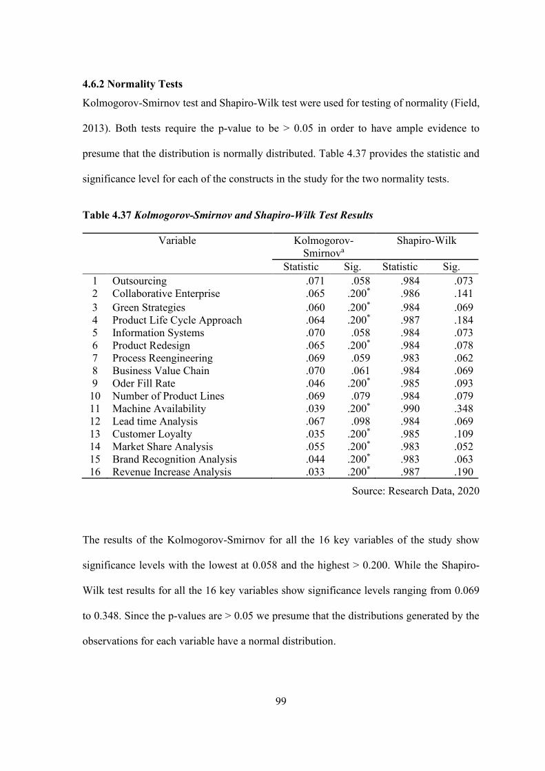
99

4.6.2 Normality Tests

Kolmogorov-Smirnov test and Shapiro-Wilk test were used for testing of normality (Field,

2013). Both tests require the p-value to be > 0.05 in order to have ample evidence to

presume that the distribution is normally distributed. Table 4.37 provides the statistic and

significance level for each of the constructs in the study for the two normality tests.

Table 4.37 Kolmogorov-Smirnov and Shapiro-Wilk Test Results

Variable Kolmogorov-

Smirnova

Shapiro-Wilk

Statistic Sig. Statistic Sig.

1 Outsourcing .071 .058 .984 .073

2 Collaborative Enterprise .065 .200* .986 .141

3 Green Strategies .060 .200* .984 .069

4 Product Life Cycle Approach .064 .200* .987 .184

5 Information Systems .070 .058 .984 .073

6 Product Redesign .065 .200* .984 .078

7 Process Reengineering .069 .059 .983 .062

8 Business Value Chain .070 .061 .984 .069

9 Oder Fill Rate .046 .200* .985 .093

10 Number of Product Lines .069 .079 .984 .079

11 Machine Availability .039 .200* .990 .348

12 Lead time Analysis .067 .098 .984 .069

13 Customer Loyalty .035 .200* .985 .109

14 Market Share Analysis .055 .200* .983 .052

15 Brand Recognition Analysis .044 .200* .983 .063

16 Revenue Increase Analysis .033 .200* .987 .190


The results of the Kolmogorov-Smirnov for all the 16 key variables of the study show

significance levels with the lowest at 0.058 and the highest > 0.200. While the Shapiro-

Wilk test results for all the 16 key variables show significance levels ranging from 0.069

to 0.348. Since the p-values are > 0.05 we presume that the distributions generated by the

observations for each variable have a normal distribution.

100

4.6.3 Tests for Autocorrelation

Durbin-Watson test statistic (D) was used to test for autocorrelation of the first order.

According to Gujarati (2003) Durbin-Watson test statistic criteria is dependent on the

number of observations of the predictor variables entered and the number of predictor

variables. For this study the number of observations was 151 while the number of

independent variables entered was 4. From the Durbin-Watson test statistic table for 151

observations at 4 degrees of freedom the acceptance region was the range between 1.788

and 2.212. The regions of indecision are between 1.679 and 1.788 and between 2.212 and

2.321. Durbin-Watson statistics that fall in the indecision range were going to be further

tested using the modified Durbin-Watson statistic. Table 4.38 reveals the calculated

Durbin-Watson statistic value for each dependent variable among the study variables with

the associated independent variables entered.

Results in table 4.38 reveal that where reverse logistics latent constructs were entered as

independent variables against the respective operational performance and competitive

advantage latent constructs as dependent variables the Durbin-Watson calculated statistics

values ranged from 1.848 to 2.148. These were all within the acceptance region of 1.788 to

2.212 meaning that serial autocorrelation does not exist at the first order level.

101

Table 4.38 Durbin-Watson Test Statistic

Independent Variables Entered Dependent Variable Durbin – Watson

Statistic

Outsourcing

Collaborative Enterprise

Green Strategies

Product Life Cycle Approach

Customer Loyalty 1.848

Market Share 1.878

Brand Recognition 1.949

Revenue Increase 1.880

Order Fill Rate 2.002

Number of Product Lines 2.110

Machine Availability 1.923

Lead-time 2.148

Information Systems

Product Redesign

Process Reengineering

Business Value Chain


Market Share 2.088






Lead-time 2.138

Oder Fill Rate

Number of Product Lines

Machine Availability

Lead-time


Market Share 2.000




Further the results reveal that where process innovation latent constructs were entered as

independent variables against the respective operational performance and competitive

advantage latent constructs as dependent variables the Durbin-Watson calculated statistics

values ranged from 1.808 to 2.138. These latent constructs had Durbin-Watson statistics

within the acceptance region meaning that serial autocorrelation does not exist at the first

order level.

Finally the results reveal that where the operational performance latent constructs were

entered as independent variables against the respective competitive advantage latent

constructs as dependent variables the Durbin-Watson calculated statistics values ranged

102

from 1.989 to 2.033. These latent constructs had Durbin-Watson statistics within the

acceptance region meaning that serial autocorrelation does not exist at the first order level.

4.6.4 Linearity Test

Linearity tests were conducted by obtaining bivariate correlations among the latent

constructs of the latent variables of reverse logistics, process innovation operational

performance and competitive advantage were calculated and the p-values examined at 0.05

significance level. The p-values were expected to be < 0.05. Appendix 5, 6, 7, 8, 9 and 10

reveal the results of these bivariate correlations.

Appendix 5 reveals the bivariate correlations between the latent constructs of reverse

logistics and process innovation and their significance levels. From appendix 6 all the

bivariate correlations were significant at ά = 0.01. This indicates linearity among the latent

constructs of reverse logistics and process innovation. Correlation co-efficients ranged

from 0.440 to 0.994 indicating moderate to very strong positive correlation among the latent

constructs

Appendix 6 reveals the bivariate correlations between the latent constructs of reverse

logistics and operational performance and their significance levels. From appendix 6 the

bivariate correlations were significant at ά = 0.01. This indicates linearity among the latent

constructs of reverse logistics and operational performance. Correlation co-efficients

ranged between 0.564 and 0.994 indicating moderate to very strong positive correlation

among the latent constructs

103

Appendix 7 reveals the bivariate correlations among the latent constructs of reverse

logisitics and competitive advantage were significant at ά = 0.01. This indicates linearity

among the latent constructs of reverse logistics and competitive advantage. Correlation co-

efficients ranged between 0.613 to 0.994 indicating weak to very strong positive

correlation.

Appendix 8 and 9 reveals that the bivariate correlations between the latent constructs of

process innovation and operational performance and between process innovation and

competitive advantage were significant at ά = 0.01. This indicates linearity among the latent

constructs of process innovation and operational performance and among latent constructs

of process innovation and competitive advantage. Correlation co-efficients of the latent

constructs of process innovation and operational performance ranged between 0.448 and

0.989 indicating moderate to very strong positive correlation. Correlation co-efficients of

the latent constructs of process innovation and competitive advantage ranged between

0.448 and 0.989 indicating weak to very strong positive correlation.

Appendix 10 reveals that the bivariate correlations between the latent constructs of

operational performance and competitive advantage were significant at ά = 0.01. This

indicates linearity among the latent constructs of operational performance and competitive

advantage. Correlation co-efficients ranged between 0.793 to 0.927 indicating moderate to

very strong positive correlation. Arguably there was linearity among the latent constructs

of reverse logistics, process innovation, operational performance and competitive

advantage. The next sub-section tests the latent constructs for multicollinearity.

104

4.6.5 Multicollinearity Test

VIF was used to diagnose collinearity where the VIF for the independent latent constructs

were expected to be < 10 if the variable is not collinearly related to the other regressor

variables (Tabachnick & Fidell, 2013). Multicollenearity tests are recapitulated in table

4.39.

Table 4.39 Multicollinearity Test Statistic

Independent Latent Constructs

Entered

Multicollinearity Test

Tolerance Variable Inflation

Factor (VIF)

1 Outsourcing 0.894 1.119

2 Collaborative Enterprise 0.924 1.082

3 Green Strategies 0.954 1.048

4 Product Life Cycle Approach 0.194 5.148

5 Information Systems 0.179 5.597

6 Product Redesign 0.197 5.075

7 Process Reengineering 0.351 2.849

8 Business Value Chain 0.596 1.679

9 Oder Fill Rate 0.160 6.267

10 Number of Product Lines 0.164 6.114

11 Machine Availability 0.139 7.178

12 Lead time Analysis 0.177 5.659


In table 4.39 above, the VIF values for the latent constructs of reverse logistics and

operational performance were between 1.082 and 7.178. The corresponding tolerance

values ranged between 0.139 to 0.954. Since all the VIF co-efficients were < 10, they

indicated the latent constructs were not multicollinearly associated.

4.6.6 Heteroscedasticity Test

Heteroscedasticity was tested using the Koenker test. For this tests if the p-value is > 0.05

then heteroscedasticity is not present and homoscedasticity is assumed (Hair et al., 2014).

105

Table 4.40 Koenker Test Results

Independent Variables Entered Dependent Variable Koenker Test p-

values

Outsourcing

Collaborative Enterprise

Green Strategies



Market Share 0.062






Leadtime Analysis 0.101

Information Systems

Product Redesign




Market Share 0.867






Leadtime Analysis 0.702

Oder Fill Rate

Number of Product Lines

Machine Availability

Lead time Analysis


Market Share 0.216




From table 4.40 above, reverse logistics latent constructs were tested for heteroscedasticity

as independent variables against the respective competitive advantage and operational

performance latent constructs as dependent variables. The Koenker calculated test statistics

value ranged from 0.062 to 0.494. Because these p-values are > 0.05 then the variance of

the outcome variable given predictor variables is presumed to be constant and therefore

homoscedasticity is assumed.

Further the process innovation latent constructs were tested for heteroscedasticity as

independent variables against the respective competitive advantage and operational

performance latent constructs as dependent variables. The Koenker test calculated statistics

value ranged from 0.055 to 0.702. Since these p-values are > 0.05 then the variance of the

106

dependent variables given the independent variables is presumed to be constant and

therefore there is no heteroscedasticity.

Finally the operational performance latent constructs were tested for heteroscedasticity as

independent variables against the respective competitive advantage latent constructs as

dependent variables. The Koenker test calculated statistics value ranged from 0.073 to

0.316. Since these p-values are > 0.05 then the variance of the dependent variables given

the independent variables is presumed to be constant and therefore there is no

heteroscedasticity.

4.6.7 Confirmatory Factor Analysis

To assess both the overall fitness of the SEM model and the statistical significance of

measured model and the structured model an evaluation of the standardized factor loadings

was done. This was done for each of the five objectives of the study. The ensuing sub-

sections summarize the results of the CFA for the measured model and of the structured

models for the five objectives.

4.6.7.1 Confirmatory Factor Analysis for the Measured Model for the Latent

constructs

The overall model fit of the measured models was assessed through the absolute,

incremental and parsimonious model fitness tests. Absolute fitness was assessed using chi-

square value, p-value, RMSEA and GFI where the chi-square value was expected to be

small, p-value > 0.05, RMSEA < 0.80 and GFI > 0.90. Incremental model fitness was

assessed using AGFI, CFI, NFI and TLI. For a good incremental fit, AGFI > 0.90, CFI >

107

0.90, 0.8 < NFI < 1.00 and TLI > 0.9. Parsimonious model fitness was assessed using

CMIN/DF. For a good parsimonious fit the minimum discrepancy ratio is expected to be <

5. Table 4.41 below summarizes the results of the CFA for the measured model for the

latent constructs of reverse logistics, process innovation, operational performance and


Table 4.41 Overall Model Fit Results for the Latent Constructs of Reverse Logistics


Test Decision

Criteria

Model Result

RevLog ProInno OprPerf CompAdv

Chi-Square 0.319 0.253 5.050 0.122

Degrees of Freedom 1 2 2 1

p-value > 0.05 0.572 0.881 0.080 0.727

GFI > 0.90 0.999 0.999 0.983 1.000

CFI > 0.90 1.000 1.000 0.995 1.000

AGFI > 0.90 0.989 0.996 0.916 0.996

NFI 0.8 < NFI <

1.00

1.000 1.000 0.993 1.000

TLI > 0.90 1.003 1.005 0.986 1.005

RMSEA < 0.08 0.000 0.000 0.101 0.000

CMIN/DF < 5 0.319 0.126 2.525 0.122


From the results absolute fitness was assessed using chi-square value, p-value, RMSEA

and GFI where the chi-square value ranged between 5.050 and 0.122 indicating they were

small. P-value ranged between 0.08 and 0.881 showing that they were > 0.05. RMSEA <

values for the latent constructs of reverse logistics, process innovation and competitive

advatange were > 0.08. The RMSEA value for the latent constructs of operational

performance was 0.101 which was not significantly > 0.08. GFI values ranged between

0.983 and 1.000 indicating they were > 0.90. These suggest that the measured models had

good absolute fit.

108

Incremental model fitness was assessed using AGFI, CFI, NFI and TLI. AGFI values

ranged between 0.916 and 0.996. These were all > 0.90. CFI values were between 0.995

and 1.000 indicating they were all > 0.90. The NFI values ranged between 0.993 and 1.000

showing they were between the threshold values, 0.8 < NFI < 1.00. TLI values were ranging

between 0.986 and 1.005 showing they were > 0.9. These values indicate that all the

measured models for the latent constructs had good incremental fit. CMIN/DF values

ranged between 0.122 and 2.525. The minimum discrepancy ratio was expected to be < 5.

These indicated that measured models for the latent constructs had good parsimonious fit.

4.6.7.2 Confirmatory Factor Analysis for the Association linking Reverse Logistics


Establishing the influence of reverse logistics on competitive advantage was the first

objective of the study. CFA was using chi-square value, RMSEA, GFI, AGFI, CFI, NFI,

TLI and CMIN/DF. Table 4.49 below summarizes the results of the CFA for the interaction

of reverse logistics with competitive advantage.

Table 4.42 Overall Model Fit results for the Association linking Reverse Logistics with


Test Decision Criteria Model Result

Chi-Square 49.099


GFI > 0.90 0.929

CFI > 0.90 0.989

AGFI > 0.90 0.841

NFI 0.8 < NFI < 1.00 0.983

TLI > 0.90 0.980

RMSEA < 0.80 0.117

CMIN/DF < 5 3.069


109

Table 4.42 above reveals chi-square value as 49.099 which was considered to be fairly

small given that the number of degrees of freedom is 16. RMSEA was 0.117 which is >

0.08 but not significantly larger. The GFI of 0.929 was > 0.90. These suggest that the model

had a fairly good absolute fit.

From table 4.42 above, AGFI, CFI, NFI and TLI had coefficients of 0.841, 0.989, 0.983

and 0.980. NFI was within the range between 0.80 and 1.00. CFI and TLI were > 0.9.

Although the AGFI was low (0.841) it was tending towards the threshold of 0.9. These

indicate the model had a fairly good incremental fit. Table 4.42 indicated a CMIN/DF of

3.069 which was < 5 suggesting a good parsimonious fit. Generally the model had good

overall fit. Figure 4.6 below reveals the unstandardized structural equation model for the

reverse logistics interaction with competitive advantage.

Figure 4.6. Unstandardized Structural Equation Model for the Reverse Logistics

Interaction with Competitive Advantage.

110

An assessment of whether the unstandardized factor loadings were statistically significant

was then performed by calculating the standard error of the estimates, the critical ration and

p-values as revealed in table 4.43 below.

Table 4.43 Unstandardized Factor Loadings for the Measured Model of Reverse

Logistics Interaction with Competitive Advantage

Factor <--- Component Estimate Standard

Error

Critical

Ratio

p-value

RLCE1 <--- RevLog 1.000

RLGS1 <--- RevLog 0.739 0.008 87.719 <0.001

RLPLCA1 <--- RevLog 0.610 0.688 9.927 <0.001

RLOS1 <--- RevLog 0.841 0.009 90.224 <0.001

CABR1 <--- CompAdv 1.000

CAMS1 <--- CompAdv 0.561 0.026 21.267 <0.001

CACL1 <--- CompAdv 0.501 0.027 18.259 <0.001

CARI1 <--- CompAdv 0.352 0.019 18.743 <0.001


Based on table 4.43, the critical ratios were all > 1.96 with p-values < 0.05, indicating that

the factor loadings are statistically significant. This means that the latent constructs of the

measured models have a statistically significant relationship. To further establish the extent

to which the factors load on the components the unstandardized factor loadings were

standardized. Table 4.44 below reveals the standardized factor loadings.

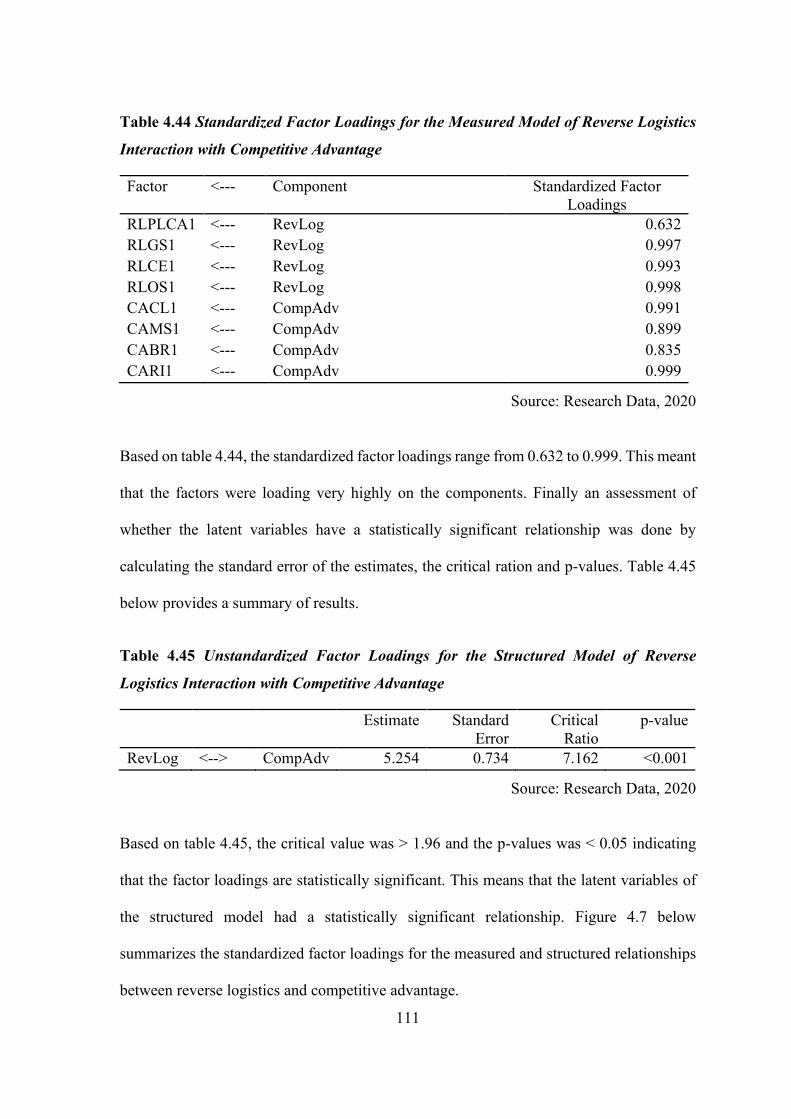
111

Table 4.44 Standardized Factor Loadings for the Measured Model of Reverse Logistics

Interaction with Competitive Advantage

Factor <--- Component Standardized Factor

Loadings

RLPLCA1 <--- RevLog 0.632

RLGS1 <--- RevLog 0.997


RLOS1 <--- RevLog 0.998

CACL1 <--- CompAdv 0.991

CAMS1 <--- CompAdv 0.899


CARI1 <--- CompAdv 0.999


Based on table 4.44, the standardized factor loadings range from 0.632 to 0.999. This meant

that the factors were loading very highly on the components. Finally an assessment of

whether the latent variables have a statistically significant relationship was done by

calculating the standard error of the estimates, the critical ration and p-values. Table 4.45

below provides a summary of results.

Table 4.45 Unstandardized Factor Loadings for the Structured Model of Reverse

Logistics Interaction with Competitive Advantage

Estimate Standard

Error

Critical

Ratio

p-value

RevLog <--> CompAdv 5.254 0.734 7.162 <0.001


Based on table 4.45, the critical value was > 1.96 and the p-values was < 0.05 indicating

that the factor loadings are statistically significant. This means that the latent variables of

the structured model had a statistically significant relationship. Figure 4.7 below

summarizes the standardized factor loadings for the measured and structured relationships

between reverse logistics and competitive advantage.

112

Figure 4.7. Standardized Factor Loadings for the Measured and Structured

Association linking Reverse Logistics with Competitive Advantage.

Figure 4.7 also indicated the standardized factor loading for the latent variables reverse

logistics and competitive advantage was 0.66. Since this is > 0.5 it indicated a strong

association linking the latent variables

4.6.7.3 Confirmatory Factor Analysis for the Association linking Reverse Logistics,



logistics with competitive advantage was the second study objective. CFA was conducted

using chi-square value, RMSEA, GFI, AGFI, CFI, NFI, TLI and CMIN/DF. Table 4.49

below summarizes the results of the CFA for the association linking reverse logistics,

operational performance and competitive advantage.

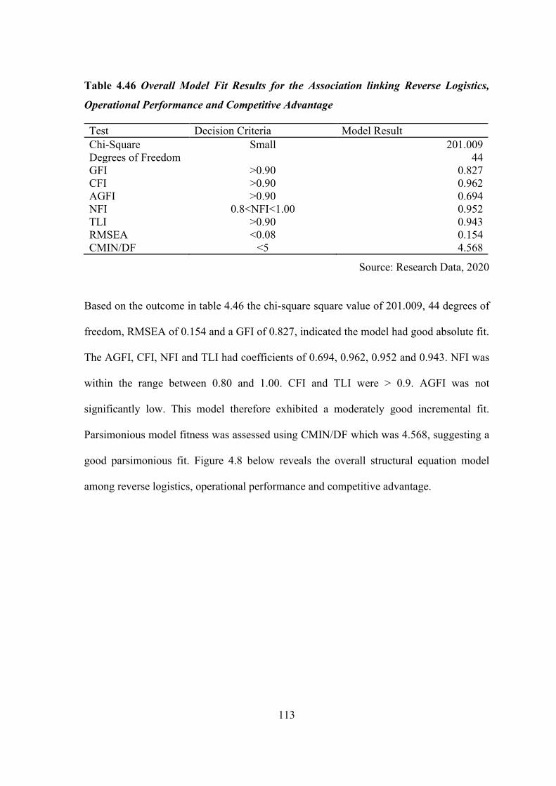
113

Table 4.46 Overall Model Fit Results for the Association linking Reverse Logistics,



Chi-Square Small 201.009


GFI >0.90 0.827

CFI >0.90 0.962

AGFI >0.90 0.694

NFI 0.8<NFI<1.00 0.952

TLI >0.90 0.943

RMSEA <0.08 0.154

CMIN/DF <5 4.568


Based on the outcome in table 4.46 the chi-square square value of 201.009, 44 degrees of

freedom, RMSEA of 0.154 and a GFI of 0.827, indicated the model had good absolute fit.

The AGFI, CFI, NFI and TLI had coefficients of 0.694, 0.962, 0.952 and 0.943. NFI was

within the range between 0.80 and 1.00. CFI and TLI were > 0.9. AGFI was not

significantly low. This model therefore exhibited a moderately good incremental fit.

Parsimonious model fitness was assessed using CMIN/DF which was 4.568, suggesting a

good parsimonious fit. Figure 4.8 below reveals the overall structural equation model

among reverse logistics, operational performance and competitive advantage.

114

Figure 4.8. Unstandardized Structural Equation Model for the Association linking

Reverse Logistics, Operational Performance and Competitive Advantage.

To assess the extent to which the unstandardized factor loadings are statistically significant,

the standard error of the estimates, the critical ration and p-values were calculated. Table

4.47 below provides a summary of these.

115


linking Reverse Logistics, Operational Performance and Competitive Advantage


Error

Critical

Ratio

p-value


RLGS1 <--- RevLog 0.739 0.008 88.291 <0.001

RLPLCA1 <--- RevLog 0.607 0.063 9.680 <0.001

RLOS1 <--- RevLog 0.841 0.009 90.590 <0.001

OPLTA1 <--- OprPerf 1.000

OPDMA1 <--- OprPerf 0.329 0.017 19.054 <0.001

OPPL1 <--- OprPerf 0.939 0.052 18.100 <0.001

OPOFR1 <--- OprPerf 0.552 0.026 21.646 <0.001


CACL1 <--- CompAdv 0.495 0.026 19.338 <0.001

CAMS1 <--- CompAdv 0.559 0.026 21.450 <0.001

CARI1 <--- CompAdv 0.345 0.018 19.481 <0.001


Based on table 4.47 above the critical values were all > 1.96 with p-values < 0.05 suggesting

that the factor loadings are statistically significant. This meant that the latent constructs of

the measured models had a statistically significant relationship. The unstandardized factor

loadings were standardized to determine the degree to which the factors load on the

components. Table 4.48 reveals the standardized factor loadings.

116

Table 4.48 Standardized Factor Loadings for the Measured Model on the Association



Loadings






OPDMA1 <--- OprPerf 0.903

OPPL1 <--- OprPerf 0.888

OPOFR1 <--- OprPerf 0.938






Based on table 4.48, the standardized factor loadings ranged between 0.622 and 0.998. This

indicated a high loading of the factors on the components. This therefore meant that the

factors explain the components to a large extent. Finally an analysis of whether the latent

variables had a statistically significant relationship of the structured model was done by

calculating the standard error of the estimates, the critical ration and p-values. Table 4.49

below reveals the results.

Table 4.49 Unstandardized Factor Loadings for the Structured Model on the Association


Component <--> Component Estimate Standard

Error

Critical

Ratio

p-value

RevLog <--> OprPerf 3.776 0.357 10.589 <0.001

OprPerf <--> CompAdv 1.650 0.131 12.556 <0.001

RevLog <--> CompAdv 0.202 0.475 0.426 0.670


117

Based on table 4.49, the critical values were > 1.96 except for the structured relationship

between the latent variables reverse logistics and competitive advantage. This indicates that

the factor loadings for the structured relationships between reverse logistics and operational

performance and between operational performance and competitive advantage were

statistically significant as revealed in figure 4.9 below.


Associating Reverse Logistics, Operational Performance and Competitive Advantage.

Factor loadings for the association linking the latent constructs reverse logistics and

competitive advantage was 0.02 indicating a weak association. Factor loadings for the

association linking the latent construct reverse logistics and operational performance and

between operational performance and competitive advantage were 0.69 and 0.92

respectively indicating relatively high association.

118

4.6.7.4 Confirmatory Factor Analysis for the association Linking Reverse Logistics,


Determining the influence of process innovation on the relationship between reverse

logistics and operational performance was the third study objective. CFA was assessed

using chi-square value, probability level, RMSEA, GFI, AGFI, CFI, NFI, TLI and

CMIN/DF. Table 4.50 below summarizes the results of the CFA.

Table 4.50 Overall Model Fit Results for the association linking Reverse Logistics,



Chi-Square 183.970


GFI >0.90 0.848

CFI >0.90 0.970

AGFI >0.90 0.761

NFI 0.8<NFI<1.00 0.957

TLI >0.90 0.960

RMSEA <0.08 0.120

CMIN/DF <5 3.172


Table 4.50 above, absolute fitness was assessed using chi-square, probability level,

RMSEA and GFI. The chi-square value was 183.970, RMSEA was 0.120 which is > 0.08

but sufficiently low to consider the model for analysis. The GFI of 0.848 was not

significantly < 0.90. This reveals that the model does have a fairly good absolute fit.

According to table 4.50, AGFI, CFI, NFI and TLI had coefficients of 0.761, 0.970, 0.957

and 0.960. NFI was within the range between 0.80 and 1.00. CFI and TLI were > 0.9.

Despite the low AGFI (0.761) this model exhibited a fairly good incremental fit.

Parsimonious model fitness was assessed using CMIN/DF which was 3.172. For a good

119

parsimonious fit the minimum discrepancy ratio is expected to be < 5. This suggests a good

parsimonious fit. In conclusion the model had a fairly good overall fit. Figure 4.10 below

reveals the overall structure of the CFA model.

Figure 4.10. Unstandardized Structural Equation Model for the Association linking

Reverse Logistics, Process Innovation and Operational Performance.

The standard error of the estimates of the unstandardized factor loading, the critical ration

and p-values were calculated to assess whether the factor loadings are statistically

significant. Table 4.51 summarizes the unstandardized factor loadings.

120


linking Reverse Logistics, Process Innovation and Operational Performance


Error

Critical

Ratio

p-value


RLGS1 <--- RevLog 0.737 0.008 95.526 <0.001

RLPLCA1 <--- RevLog 0.614 0.062 9.931 <0.001

RLOS1 <--- RevLog 0.839 0.009 92.476 <0.001

PIPRD1 <--- ProInno 1.000

PIIS1 <--- ProInno 0.833 0.010 84.351 <0.001

PIPRE1 <--- ProInno 0.383 0.061 6.271 <0.001

PIBVA1 <--- ProInno 0.699 0.016 45.071 <0.001


OPPL1 <--- OprPerf 0.990 0.050 19.804 <0.001

OPDMA1 <--- OprPerf 0.344 0.017 20.376 <0.001

OPOFR1 <--- OprPerf 0.544 0.029 19.073 <0.001


Based on table 4.51 the critical values are > 1.96 with p-values < 0.05 indicating statistical

significance of factor loadings. In order to determine the degree to which the factors load

on the components, the unstandardized factor loadings were standardized as revealed in

table 4.52 below.

Table 4.52 Standardized Factor Loadings for the Measured Model Associating Reverse


Factor <--- Component Estimate

121





PIBVA1 <--- ProInno 0.969

PIIS1 <--- ProInno 0.994

PIPRE1 <--- ProInno 0.657







Based on table 4.52 above, the least standardized factor loading was 0.631 and highest was

0.997. This therefore meant that the factors explain the components to a large extent. To

check whether a statistically significant association among the latent variables of the

structured model was present, calculations of the standard error of the estimates, the critical

ration and p-values were performed as revealed in table 4.53 below.

Table 4.53 Unstandardized Factor Loadings for the Structured Model Associating

Reverse Logistics, Operational Performance and Competitive Advantage


Error

Critical

Ratio

p-value

RevLog <--> ProInno 0.303 0.035 8.618 <0.001

RevLog <--> IntVar 0.155 0.055 2.793 0.005

ProInno <--> IntVar 0.129 0.047 0.929 0.006


Based on table 4.53, the critical values were in the region > 1.96 with p-values < 0.05

indicating that the factor loadings were statistically significant. This meant that the latent

variables of the structured equation model had statistically significant relationship. Figure

122

4.11 also indicates the standardized factor loading for the latent variables reverse logistics,

process innovation and operational performance.


Associating Reverse Logistics, Process Innovation and Operational Performance.

Factor loadings in figure 4.11 for the association linking the latent variables reverse

logistics, process innovation, the interaction variable and operational performance were

6.45, -5.78 and 0.07 respectively.

123

4.6.7.5 Confirmatory Factor Analysis for the Moderated – Mediation Relationship

Examining the conditional indirect effect on the association among reverse logistics,

process innovation and operational performance on a firm’s competitive advantage was the

fourth study objective. CFA was performed using chi-square value, RMSEA, GFI, AGFI,

CFI, NFI, TLI and CMIN/DF. Table 4.54 below summarizes the results thereof.

Table 4.54 Overall Model Fit Results for the Moderated – Mediation Relationship




GFI >0.90 0.743

CFI >0.90 0.907

AGFI >0.90 0.629

NFI 0.8<NFI<1.00 0.892

TLI >0.90 0.881

RMSEA <0.08 0.188

CMIN/DF <5 6.274


Table 4.54 above reveals a chi-square value of 665.019 which is considered to be fairly

small because the number of degrees of freedom is 106. RMSEA was 0.188 which is > 0.08

and GFI was 0.743. This reveals a fairly good absolute fit. Based on the table 4.54, AGFI,

CFI, NFI and TLI had coefficients of 0.629, 0.907, 0.892 and 0.881. NFI was within the

range between 0.80 and 1.00. CFI was > 0.9 and TLI was approaching the threshold of 0.9.

Despite having a low AGFI of 0.629 the model exhibited a fairly good incremental fit.

Parsimonious model fitness was assessed using CMIN/DF which was 6.274. A good

parsimonious fit requires the minimum discrepancy ratio to be < 5. This suggests a fairly

good parsimonious fit. In general the model had a fairly good overall fit. Figure 4.12 below

reveals the structured model showing the moderated- mediation relationship among reverse

logistics, process innovation, operational performance and competitive advantage. The

124

figure reveals the covariance between the exogenous variables and the unstandardized

factor loadings.

Figure 4.12. Confirmatory Factor Analysis Model for the Moderated-Mediation

Relationship


and p-values were calculated to assess the statistical significance of the factor loadings as

revealed in table 4.55 below.

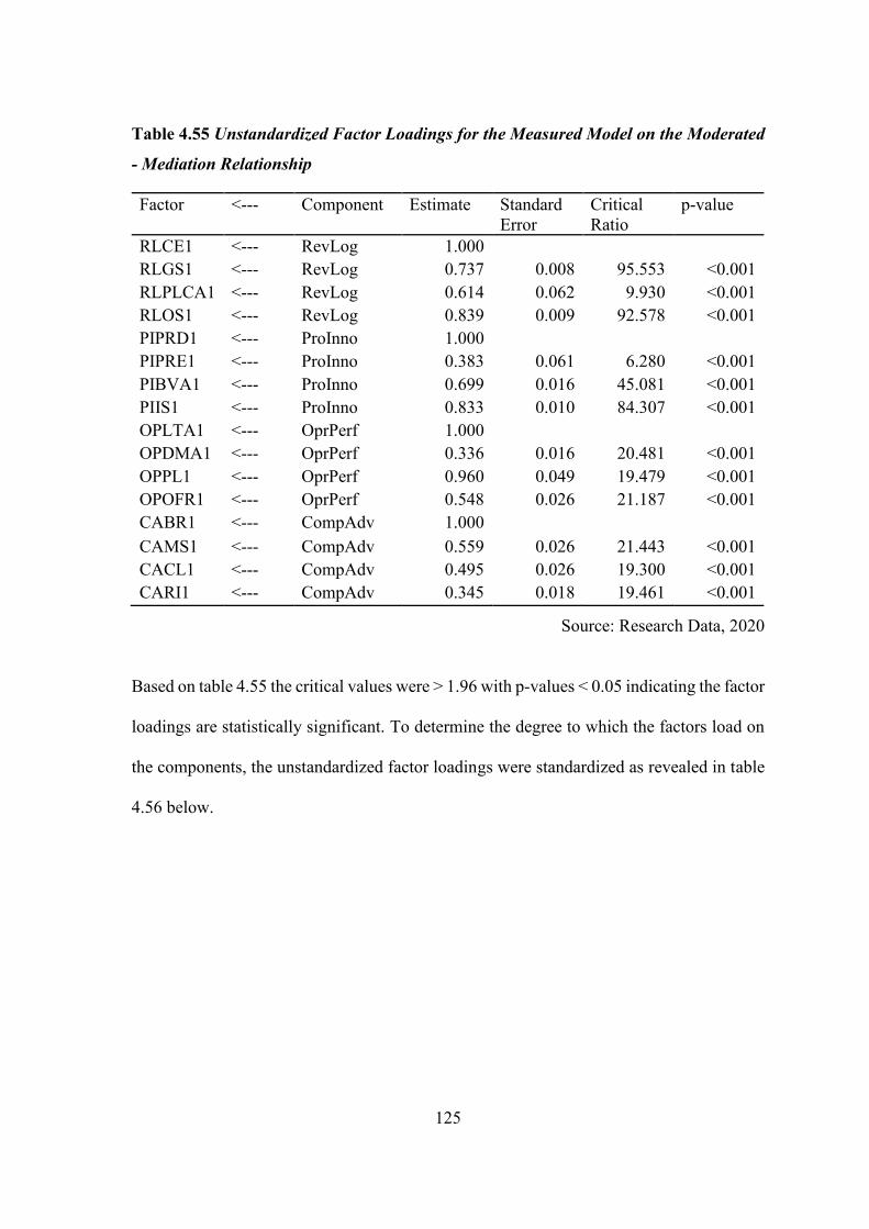
125

Table 4.55 Unstandardized Factor Loadings for the Measured Model on the Moderated

- Mediation Relationship


Error

Critical

Ratio

p-value


RLGS1 <--- RevLog 0.737 0.008 95.553 <0.001

RLPLCA1 <--- RevLog 0.614 0.062 9.930 <0.001

RLOS1 <--- RevLog 0.839 0.009 92.578 <0.001


PIPRE1 <--- ProInno 0.383 0.061 6.280 <0.001

PIBVA1 <--- ProInno 0.699 0.016 45.081 <0.001

PIIS1 <--- ProInno 0.833 0.010 84.307 <0.001


OPDMA1 <--- OprPerf 0.336 0.016 20.481 <0.001

OPPL1 <--- OprPerf 0.960 0.049 19.479 <0.001

OPOFR1 <--- OprPerf 0.548 0.026 21.187 <0.001


CAMS1 <--- CompAdv 0.559 0.026 21.443 <0.001

CACL1 <--- CompAdv 0.495 0.026 19.300 <0.001

CARI1 <--- CompAdv 0.345 0.018 19.461 <0.001


Based on table 4.55 the critical values were > 1.96 with p-values < 0.05 indicating the factor

loadings are statistically significant. To determine the degree to which the factors load on

the components, the unstandardized factor loadings were standardized as revealed in table

4.56 below.

126

Table 4.56 Standardized Factor Loadings for the Measured Model on the Moderated –

Mediation Model


Loadings


















Based on table 4.56, the least standardized factor loading was 0.631 and the highest as

0.999. This therefore meant that the factors explain the components to a large extent. To

check the statistical significance among the latent variables of the structured model,

calculations of the standard error of the estimates, the critical ration and p-values were

performed as revealed in table 4.57 below.

127

Table 4.57 Unstandardized Factor Loadings for the Structured Model on the Moderated

– Mediation Model


Error

Critical

Ratio

p-value

RevLog <--> ProInno 0.303 0.035 8.618 <0.001

RevLog <--> IntVar 0.129 0.047 2.757 0.006

ProInno <--> IntVar 0.155 0.055 2.793 0.005

RevLog <--> CompAdv 0.469 0.485 0.966 0.334

RevLog <--> OprPerf -32.137 39.830 -0.807 0.420

OprPerf <--> CompAdv 1.595 0.131 12.214 <0.001


Based on table 4.57, the critical ratio for the covariance relationships between reverse

logistics, process innovation and the interaction variable were > 1.96 with p-values < 0.05

showing that moderation was statistically significant. The critical ratio between the latent

variable reverse logistics and competitive advantage and between reverse logistics and

operational performance were < 1.96 with p-values > 0.05 however the critical ratio

between operational performance and competitive advantage was > 1.96 with a p-value <

0.05 showing a statistically significant mediation relationship. Therefore the moderated-

mediation relationship was statistically significant.

128


relationships for the Moderated – Mediation Model

Figure 4.13 indicates standardized factor loadings for the relationship between the latent

constructs reverse logistics and competitive advantage was 0.05 indicating a weak

association. Factor loadings for the association linking the interaction variable and

operational performance was 0.05 indicating a weak moderation effect in the moderated –

mediation relationship. Factor loadings for the association linking the latent construct

operational performance and competitive advantage was 0.89 indicating strong mediation

effect when considering the moderated – mediation relationship.

129

4.6.7.6 Confirmatory Factor Analysis for the Joint association linking Reverse


Examining the joint effect of reverse logistics, process innovation and operational

performance on a firm’s competitive advantage was the last study objective. Table 4.58

below summarizes the results of the CFA for the relationship among the latent variables.

Table 4.58 Overall Model Fit Results for the Joint Relationship between Reverse





GFI >0.90 0.747

CFI >0.90 0.904

AGFI >0.90 0.583

NFI 0.8<NFI<1.00 0.890

TLI >0.90 0.877

RMSEA <0.08 0.202

CMIN/DF <5 5.824


Table 4.58 above reveals chi-square value of 547.531, RMSEA of 0.202 which is > 0.08

and the GFI of 0.747 indicating fairly good absolute fit. Based on table 4.58, AGFI, CFI,

NFI and TLI had coefficients of 0.583, 0.904, 0.890 and 0.877. NFI was within the range

between 0.80 and 1.00. CFI was > 0.90 and TLI was approaching the threshold of 0.9.

Despite having a low AGFI of 0.583 the model exhibited a fairly good incremental fit.

Parsimonious model fitness was assessed using CMIN/DF which was 5.824. A good

parsimonious fit requires the minimum discrepancy ratio to be < 5. However 5.824 was

approaching the threshold. This suggests a fairly good parsimonious fit. In general the

model had a fairly good overall fit. Figure 4.14 below reveals the overall structure of the

structural model for the joint effect among the latent variables.

130

Figure 4.14. Structural Model for the Joint Relationship among Reverse Logistics,



and p-values were calculated to assess whether the factor loadings are statistically

significant. Table 4.59 below provides a summary of results for the unstandardized factor

loadings.

131

Table 4.59 Unstandardized Factor Loadings for the Measured Model of the Joint

Relationship


Error

Critical

Ratio

p-value


RLGS1 <--- RevLog 0.737 0.008 95.607 <0.001

RLPLCA1 <--- RevLog 0.614 0.062 9.914 <0.001

RLOS1 <--- RevLog 0.839 0.009 92.467 <0.001


PIPRE1 <--- ProInno 0.383 0.061 6.286 <0.001

PIBVA1 <--- ProInno 0.699 0.016 45.071 <0.001

PIIS1 <--- ProInno 0.833 0.010 84.313 <0.001


OPDMA1 <--- OprPerf 0.329 0.017 19.174 <0.001

OPPL1 <--- OprPerf 0.938 0.052 18.165 <0.001

OPOFR1 <--- OprPerf 0.551 0.025 21.645 <0.001


CACL1 <--- CompAdv 0.494 0.025 19.521 <0.001

CAMS1 <--- CompAdv 0.558 0.035 15.937 <0.001

CARI1 <--- CompAdv 0.344 0.018 19.632 <0.001


Based on table 4.59, the critical values were >1.96 with p-values < 0.05 indicating that the

factor loadings are statistically significant. To determine the degree to which the factors

load on the components, the unstandardized factor loadings were standardized as revealed

in table 4.60 below.

132

Table 4.60 Standardized Factor Loadings for the Measured Model for the Joint

Relationship


Loadings


















Based on table 4.60, the least standardized factor loading was 0.631 and highest 0.998. This

therefore meant that the factors explain the components to a large extent. To check if a

statistically significant association among the latent variables of the structured model was

present, calculations of the standard error of the estimates, the critical ration and p-values

were performed as revealed in table 4.61 below.

133

Table 4.61 Unstandardized Factor Loadings for the Structured Model for the Joint

Relationship


Error

Critical

Ratio

p-value

RevLog <--> ProInno 0.303 0.035 8.618 <0.001

RevLog <--> OprPerf 1.362 0.202 6.738 <0.001

ProInno <--> OprPerf 1.140 0.170 6.692 <0.001

CompAdv <--> RevLog -24.023 33.072 -0.726 0.468

CompAdv <--> ProInno 28.478 38.749 0.735 0.462

CompAdv <--> OprPerf 1.704 0.163 10.453 < 0.001


Based on table 4.61, the covariance relationship among reverse logistics, process

innovation and operational performance had critical values >1.96 with a p-value < 0.05

pointing out that the factor loadings were statistically significant. The relationship between

the latent variables operational performance and competitive advantage was also >1.96

with a p-value < 0.05. Figure 4.15 below, indicates the standardized factor loading for the

latent variables. Factor loadings for the relationship between the latent variables reverse

logistics, process innovation and operational performance on competitive advantage were

-2.45, 2.46 and 0.95 respectively.

134


relationships for the Joint Model

4.7 Common Method Variance

In the CLF method for each latent variable, the CMV is the square of the common factor

of each path before standardization. It can also be obtained by getting the difference

between the standardized regression weights with CLF and without the CLF. The difference

between the two weights should be < 0.20. The ensuing sub-sections discuss the CMV tests

performed for each of the five objectives of the study.

135

4.7.1 Common Method Variance Test on the Reverse Logistics link with Competitive

Advantage.

Establishing the influence of reverse logistics on competitive advantage was the first study

objective. CMV was assessed to determine whether it was necessary to include the common

method latent variable while performing hypothesis test. Figure 4.16 reveals the results of

the CLF method performed on the association linking reverse logistics with competitive

advantage.

Figure 4.16. Common Latent Factor Analysis Model for Reverse Logistics interaction

with Competitive Advantage.

Based on figure 4.16 above, the CLF for each of the variables was - 0.03. This therefore

gives a common method variance of 0.0009 which is < 0.5 for each of the variables. This

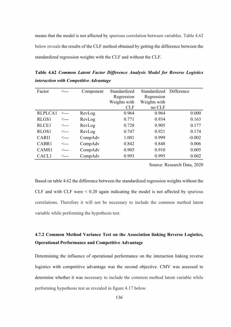
136

means that the model is not affected by spurious correlation between variables. Table 4.62

below reveals the results of the CLF method obtained by getting the difference between the

standardized regression weights with the CLF and without the CLF.

Table 4.62 Common Latent Factor Difference Analysis Model for Reverse Logistics

interaction with Competitive Advantage

Factor <--- Component Standardized

Regression

Weights with

CLF

Standardized

Regression

Weights with

no CLF

Difference

RLPLCA1 <--- RevLog 0.964 0.964 0.000

RLGS1 <--- RevLog 0.771 0.934 0.163

RLCE1 <--- RevLog 0.728 0.905 0.177

RLOS1 <--- RevLog 0.747 0.921 0.174

CARI1 <--- CompAdv 1.001 0.999 -0.002

CABR1 <--- CompAdv 0.842 0.848 0.006

CAMS1 <--- CompAdv 0.905 0.910 0.005

CACL1 <--- CompAdv 0.993 0.995 0.002


Based on table 4.62 the difference between the standardized regression weights without the

CLF and with CLF were < 0.20 again indicating the model is not affected by spurious

correlations. Therefore it will not be necessary to include the common method latent

variable while performing the hypothesis test.



Determining the influence of operational performance on the interaction linking reverse

logistics with competitive advantage was the second objective. CMV was assessed to

determine whether it was necessary to include the common method latent variable while

performing hypothesis test as revealed in figure 4.17 below.

137

Figure 4.17. Common Latent Factor Analysis Model for the Association linking

Reverse Logistics, Operational Performance and Competitive Advantage.

Based on figure 4.17 above the common latent factor for each of the variables was 0.00.

This therefore gives a common method variance of 0.0000 which is < 0.5 for each of the

variables. This means that the model is not affected by spurious correlations. Table 4.63

below reveals the results of the common latent factor method.

138

Table 4.63 Common Latent Factor Difference Analysis Model for the Association



Regression

Weights with

CLF

Standardized

Regression

Weights with

no CLF

Difference

RLPLCA1 <--- F1 0.630 0.630 0.000

RLGS1 <--- F1 0.997 0.997 0.000

RLCE1 <--- F1 0.993 0.993 0.000

RLOS1 <--- F1 0.997 0.997 0.000

OPLTA1 <--- F3 0.928 0.928 0.000

OPDMA1 <--- F3 0.920 0.920 0.000

OPPL1 <--- F3 0.907 0.907 0.000

OPOFR1 <--- F3 0.932 0.932 0.000

CARI1 <--- F4 0.998 0.998 0.000

CABR1 <--- F4 0.850 0.850 0.000

CAMS1 <--- F4 0.911 0.911 0.000

CACL1 <--- F4 0.996 0.996 0.000



CLF and with CLF < 0.20 therefore it confirmed that it will not be necessary to include the

common method latent variable while performing the hypothesis test.




and operational performance was the third objective of the study. Figure 4.18 reveals the

results of the common latent factor method performed on the relationship among the latent

variables.

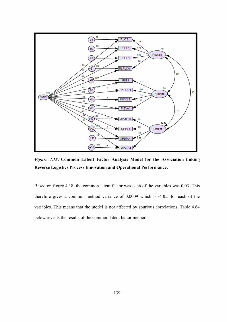
139


Reverse Logistics Process Innovation and Operational Performance.

Based on figure 4.18, the common latent factor was each of the variables was 0.03. This

therefore gives a common method variance of 0.0009 which is < 0.5 for each of the

variables. This means that the model is not affected by spurious correlations. Table 4.64

below reveals the results of the common latent factor method.

140


linking Reverse Logistics, Process Innovation and Operational Performance


Regression

Weights with

CLF

Standardized

Regression

Weights with

no CLF

Difference

RLPLCA1 <--- F1 0.629 0.631 -0.002

RLGS1 <--- F1 0.995 0.997 -0.002

RLCE1 <--- F1 0.994 0.995 -0.001

RLOS1 <--- F1 0.995 0.996 -0.001

PIBVA1 <--- F2 0.967 0.969 -0.002

PIPRE1 <--- F2 0.454 0.457 -0.003

PIPRD1 <--- F2 0.995 0.996 -0.001

PIIS1 <--- F2 0.992 0.994 -0.002

OPLTA1 <--- F3 0.917 0.918 -0.001

OPDMA1 <--- F3 0.933 0.933 0.000

OPPL1 <--- F3 0.925 0.925 0.000

OPOFR1 <--- F3 0.915 0.916 -0.001

OPUVC1 <--- F3 0.629 0.631 -0.002




common method latent variable while performing the hypothesis test.



Examining the conditional indirect effect on the relationship among reverse logistics,

process innovation and operational performance on a firm’s competitive advantage was the

fourth study objective. Further examining the joint effect of the latent variables was the last

study objective. For both of these objectives common method variance was assessed to

141

determine whether it was necessary to include the common method latent variable while

performing hypotheses tests as revealed in figure 4.19 below.



Advantage

142

Based on figure 4.19 below, the common latent factor for each of the variables was 0.04.

This therefore gives a common method variance of 0.0016 which is < 0.5 for each of the

variables. This meant that the models were not affected by spurious correlations. Table 4.65

reveals the results of the common latent factor method.


linking Reverse Logistics, Process Innovation, Operational Performance and



Regression

Weights with

CLF

Standardized

Regression

Weights with

no CLF

Difference

RLPLCA1 <--- F1 0.628 0.631 -0.003

RLGS1 <--- F1 0.995 0.997 -0.002

RLCE1 <--- F1 0.994 0.995 -0.001

RLOS1 <--- F1 0.995 0.996 -0.001

PIBVA1 <--- F2 0.965 0.982 -0.017

PIPRE1 <--- F2 0.455 0.457 -0.002

PIPRD1 <--- F2 0.990 0.944 0.046

PIIS1 <--- F2 0.992 0.982 0.010

OPLTA1 <--- F3 0.924 0.942 -0.018

OPDMA1 <--- F3 0.923 0.941 -0.018

OPPL1 <--- F3 0.909 0.902 0.007

OPOFR1 <--- F3 0.932 0.913 0.019

CARI1 <--- F4 0.999 0.996 0.003

CABR1 <--- F4 0.842 0.854 -0.012

CAMS1 <--- F4 0.906 0.910 -0.004

CACL1 <--- F4 0.993 0.997 -0.004




common method latent variable while performing the hypotheses tests.

143

4.8 Summary of Chapter Results

The main objective of this study was to examine the relationships among reverse logistics,

process innovation, operational performance and competitive advantage of manufacturing

firms in Kenya.

Prior to hypotheses testing, it was important to check whether patterns of correlations are

relatively compact and whether there is a possibility of dimension reduction. KMO tests

yielded values of 0.872, 0.919, 0.950 and 0.942 (Table 4.5, 4.6, 4.7 and 4.8) which were >

0.7. Sphericity tests produced p-values < 0.05. This meant that conducting CFA will

produce statistically reliable factors and results. Component matrix values were > 0.5

except for the latent constructs, OPUVC1 and PIRD1. These two latent constructs were

considered as potential for deletion in the models prior to hypotheses tests.

Cronbach’s alpha coefficient measuring how well the questionnaire items for reverse

logistics and process innovation were actually measuring the latent constructs yielded co-

efficient values ranging between 0.704 and 0.744 (Table 4.9). Since they were > 0.7, these

indicated sufficient internal consistency between the questionnaire items and the latent

constructs. To further assess whether the questionnaire items had sufficient explanatory

power on the latent constructs for reverse logistics and process innovation communality

co-efficients were calculated and they were all > 0.3. In order to determine how well the

latent constructs were actually measuring the latent variable cronbach’s alpha yielded co-

efficient values ranging between 0.897 and 0.972 (Table 4.12). These were > 0.7 showing

sufficient internal consistency between the constructs and variables. Communality co-

efficients ranged between 0.810 and 0.968.

144

Content, convergent and discriminant validity tests were performed to check for construct

validity. A team of resource persons from the field of reverse logistics was used to ascertain

content validity. Convergent validity was tested using SFL and AVE. SFL for the latent

constructs are as shown in figure 4.2, 4.3, 4.4 and 4.5. From the figures the latent constructs

CAWR1, OPUVC1 and PIRD1 had factor loadings < 0.5 for which they were deleted from

the model. From table 4.14, 4.16, 4.18 and 4.20, the AVE values were > 0.5 showing good

convergent validity among the constructs.

To check for discriminant validity, AVEs were compared to MSVs. The AVEs (Table 4.16)

were 0.841 and 0.836 showing they were > MSV at 0.479 (Table 4.21) for reverse logistics

and operational performance showing good discriminant validity among the variables.

Similarly, the AVEs (Table 4.14) were 0.569 and 0.875 which shows they were > MSV at

0.440 (Table 4.21) for reverse logistics and competitive advantage. The AVEs (Table 4.18)

were 0.782 and 0.852 showing they were > MSV at 0.468 (Table 4.21) for process

innovation and operational performance showing good discriminant validity among the

variables. Similarly, the AVEs (Table 4.20) were 0.782 and 0.883 which shows they were

> MSV at 0.443 (Table 4.21) for process innovation and competitive advantage. The AVEs

(Table 4.20) were 0.850 and 0.883 which shows they were almost equal to the MSV at

0.854 (Table 4.21) for operational performance and competitive advantage. All these

suggested good discriminant validity among the variables.

Summary descriptive statistics for the latent variable reverse logistics, process innovation,

operational performance and competitive advantage generally showed the distributions

formed from the data were normally distributed. Z-skewness and z-kurtosis scores ranging

145

between ± 1.96 (Table 4.26, 4.32, 4.34 and 4.35). Outlier test results for reverse logistics,

process innovation, operational performance and competitive advantage latent constructs

forming the respective latent variables ranged between -2.421 and 2.301 (Table 4.36).

These were within ± 2.5 range meaning that there were no outliers.

Kolmogorov-Smirnov tests for the latent constructs indicated significance levels with the

lowest at 0.058 and the highest > 0.200 (Table 4.37). From the same table, the Shapiro-

Wilk test results for the latent constructs indicated significance levels ranging from 0.052

to 0.48. Since the p-values were > 0.05 we presumed that the distributions generated by the

observations for each latent construct had a normal distribution.

Durbin-Watson statistic were use to test for autocorrelation. From table 4.38 the Durbin-

Watson statistics ranged from 1.808 and 2.148. These were all within the acceptable region

(1.788 – 2.212) meaning serial autocorrelation did not exist. Linearity tests from appendices

5, 6, 7, 8, 9 and 10 showed the p-values were significant at ά = 0.01. Correlation co-

efficients ranged between 0.448 and 0.994 showing there was sufficient evidence to support

linearity. Multicollinearity tests (table 4.39) revealed that the latent constructs are not

significantly affected by multicollinearity. To test for heteroscedasticity, Koenker test was

used with calculated statisitics values ranging from 0.055 to 0.867. Because these p-values

were > 0.05, homoscedasticity was assumed.

The RMSEA for the measured model ranged between 0.000 and 0.101, while the GFI

values were between 0.983 and 1.000 suggesting good absolute fit. AGFI, CFI, NFI and

TLI had coefficients ranging between 0.916 and 0.996; 0.995 and 1.000; 0.993 and 1.000;

146

and 0.986 and 1.005 respectively suggesting good incremental fit in the models. CMIN/DF

ranged between 0.122 and 2.525 suggesting good parsimonious fit (Table 4.41). In general

the measured models had good overall fit.

For the structured models, the RMSEA ranged between 0.117 and 0.202, while the GFI

values were between 0.743 and 0.929 suggesting fairly good absolute fit. AGFI, CFI, NFI

and TLI had coefficients ranging between 0.583 and 0.841; 0.904 and 0.989; 0.890 and

0.983; and 0.877 and 0.980 respectively suggesting a fairly good incremental fit in the

models. CMIN/DF ranged between 3.069 and 6.274 suggesting fairly good parsimonious

fit. In general the all the models had a fairly good overall fit (Table 4.42, 4.46, 4.50, 4.54

and 4.58). The unstandardized factor loadings for all the measured models had p-values of

< 0.001, showing the latent constructs of the measured models were statistically significant

(Table 4.43, 4.47, 4.51, 4.55 and 4.59). All these indicate that the results thereof will have

significant explanatory power on the models.

CMV and CLFD were used to check for spurious correlations between variables as a result

of using similar measurement methods for the variables. CMV yielded results of 0.0009,

0.0000, 0.0009 and 0.0016 (Figure 4.16 – 4.19) which were < 0.5. CLFD showed the

difference in standardized weights with and without common latent factor. These figures

varied between -0.018 and 0.177 (Table 4.62 – 4.65) indicating they were < 0.2. The results

of the CMV and CLFD confirm that the models were not affected by spurious correlations.

147

CHAPTER FIVE: TEST OF HYPOTHESES, INTERPRETATIONS

AND DISCUSSIONS

5.1 Introduction

This study sought to examine the relationships among reverse logistics, process innovation,

operational performance and competitive advantage of manufacturing firms in Kenya. Five

hypotheses were tested and section 5.2 provides the discussion of findings from the test of

hypothesis. Section 5.3 provides comparative analysis between the expected relationships and

the actual findings.

5.2 Tests of Hypotheses

To achieve the objectives of the study, hypotheses were tested and the results and

discussions of findings for each of the five hypotheses are provided in the ensuing sub-

sections.

5.2.1 The Influence of Reverse Logistics on Competitive Advantage of Manufacturing

Firms in Kenya

The first objective of this study was to establish the influence of reverse logistics on

competitive advantage of manufacturing firms in Kenya. A review of literature suggested

that reverse logistics can be implemented using four strategies. For this objective, the study

hypothesized that;

H1: Reverse logistics has no significant influence on a firm’s competitive advantage.

Indices advanced by Hair et al., (2014) such as chi-square, RMSEA, GFI, AGFI, CFI, NFI,

TLI and CMIN/DF were used in examining model fitness. These had values of 49.099,

148

0.117, 0.929, 0.841, 0.989, 0.983, 0.980 and 3.069 respectively indicating a good model fit

(Table 4.42).

Figure 4.7 revealed the standardized structural equation model for the reverse logistics

interaction with competitive advantage as predictor and outcome variables respectively.

From the figure the path co-efficient between reverse logistics and competitive advantage

was positive (0.66) showing that the reverse logistics association with competitive

advantage was positive. Figure 4.6 reveals the unstandardized structural equation model

for reverse logistics interaction with competitive advantage with a path co-efficient of 5.25

meaning that for every unit increase in reverse logistics initiatives competitive advantage

improves by a factor of 5.25. The p-value for reverse logistics interaction with competitive

advantage was < 0.001 (table 4.45). Since this p-value was < 0.05, the null hypothesis was

rejected therefore reverse logistics has a significant and positive influence on a firm’s


5.2.2 The Mediation Effect of Operational Performance on Reverse Logistics

Association with Competitive Advantage in Manufacturing Firms in Kenya

The second objective of this study was to determine the influence of operational

performance on the association linking reverse logistics with competitive advantage of

manufacturing firms in Kenya. For this objective, the study hypothesized that;

H2: Operational performance had no significant mediating influence on the relationship


149

For one to identify the mediating effect, it was important to establish whether significant

interaction exists between the predictor and outcome variable. Once the nature of the

association was identified the mediator was introduced in the diagram to assess the indirect

effect on the association between the predictor and outcome variables. Before testing for

mediation, model fit was assessed using chi-square, RMSEA, GFI, AGFI, CFI, NFI, TLI

and CMIN/DF. These had values of 201.009, 0.154, 0.827, 0.694, 0.962, 0.952, 0.943 and

4.568 respectively indicating a fairly good model fit (Table 4.46).

The direct interaction of reverse logistics on competitive advantage was found to be

significant as discussed in section 5.2.1 above. For the indirect relationship, Figure 4.9

revealed the standardized structural equation model for the association linking reverse

logistics, competitive advantage and operational performance as independent, dependent

and mediating variables respectively. From the figure the path co-efficient between reverse

logistics and competitive advantage was positive (0.02) having significantly decreased as

compared to the direct relationship (0.66). The figure also revealed that the path co-efficient

between reverse logistics and operational performance and between operational

performance and competitive advantage were 0.69 and 0.92 respectively.

Figure 4.8 revealed the unstandardized structural equation model for reverse logistics

association with competitive advantage with a path co-efficient of 0.17 a decrease of 5.08

as compared to the direct relationship. The p-value for the reverse logistics association

with competitive advantage was < 0.001 for the direct relationship but changed to 0.670 in

the mediating relationship, while the p-value between reverse logistics and operational

performance and between operational performance and competitive advantage were both <

150

0.001 (table 4.49). Since these p-value were both < 0.05, the null hypothesis was rejected

therefore operational performance had significant mediating influence on the relationship


5.2.3 The Moderation Effect of Process Innovation on the Association linking Reverse

Logistics and Operational Performance of Manufacturing Firms in Kenya

The third objective of this study was to determine the influence of process innovation on

the relationship between reverse logistics and operational performance of manufacturing

firms in Kenya. For this objective, the study hypothesized that;

H3: Process Innovation has no significant moderating influence on the relationship

between reverse logistics and operational performance.

According to Sharma, Durand and Gur-Arie (1981) in order to identify the moderating

effect requires the creation of an interaction variable. The interaction variable was found

by computing the product of reverse logistics and process innovation for each data point in

the respective data sets. This resulted in the unstandardized path diagram shown in figure

4.10. The model fit was assessed using chi-square, RMSEA, GFI, AGFI, CFI, NFI, TLI

and CMIN/DF (Hair et al., 2014). These had values of 183.970, 0.120, 0.848, 0.761, 0.970,

0.957, 0.960 and 3.172 respectively indicating a good model fit (Table 4.50).

Based on figure 4.11 the path co-efficient for the interaction variable was positive (0.07)

indicating the process innovation had a positive moderating effect on the association

linking reverse logistics and operational performance. The p-values between reverse

151

logistics, process innovation and the interaction variable were <0.001, 0.005 and 0.006

(table 4.53). Since the p-value between the interaction variable, process innovation and

reverse logistics were < 0.05, this indicated the moderating effect is statistically significant.

The null hypothesis was rejected and a conclusion that process innovation has significant

moderating effect on the relationship between reverse logistics and operational

performance reached.

5.2.4 The Moderated - Mediation Effect of Process Innovation and Operational

Performance

The fourth objective of this study was to determine the conditional indirect effect of process

innovation and operational performance on the reverse logistics association with

competitive advantage of manufacturing firms in Kenya. For this objective, the study

hypothesized that;

H4: Process Innovation and operational performance have no significant moderated-

mediation influence on the relationship between reverse logistics and competitive

advantage.

Model fit was assessed using chi-square, RMSEA, GFI, AGFI, CFI, NFI, TLI and

CMIN/DF. These had values of 665.019, 0.188, 0.743, 0.629, 0.907, 0.892, 0.881 and 6.274

respectively indicating a fairly good model fit (Table 4.54).

For the moderated-mediation relationship figure 4.13 revealed the standardized structural

equation model with reverse logistics, process innovation, operational performance and

competitive advantage as predictor, moderating, mediating and outcome variables

152

respectively. From the figure the path co-efficient between reverse logistics and

competitive advantage was positive (0.05) having significantly decreased as compared to

the direct relationship (0.66) in figure 4.7. The figure also reveals that the path co-efficient

between reverse logistics and the interaction variable and between operational performance

and competitive advantage were 0.05 and 0.89 respectively.

Figure 4.13 revealed the path co-efficient for the interaction variable was positive (0.05)

indicating the process innovation had a positive moderating relationship between reverse

logistics and operational performance. The p-values between the reverse logistics, process

innovation and the interaction variable were < 0.006 (table 4.57) therefore the relationship

was statistically significant.

Figure 4.12 reveals the unstandardized structural equation model for reverse logistics

interaction with competitive advantage with a path co-efficient of 0.38 a decrease of 4.87

as compared to the direct relationship in figure 4.6. While the p-value between the latent

variables of reverse logistics and competitive advantage was < 0.001 in the direct

relationship (table 4.45), the p-value for the reverse logistics interaction with competitive

advantage was 0.334 in the moderated-mediation relationship. The p-value between reverse

logistics and operational performance was 0.420 and between operational performance and

competitive advantage was < 0.001. The p-values between reverse logistics and the

interaction variable was 0.006 and between process innovation and the interaction variable

was 0.005 (table 4.57).

153

Since the p-value for the reverse logistics interaction with competitive advantage was >

0.05, the p-value between reverse logistics and operational performance > 0.05, the p-value

between reverse logistics and the interaction variable < 0.05, the p-value between process

innovation and the interaction variable < 0.05 and between operational performance and

competitive advantage was < 0.05 the null hypothesis was rejected and process innovation

and operational performance were found to have a significant partial moderated-mediation

influence on the reverse logistics association with competitive advantage.

5.2.5 The Joint Effect of Reverse Logistics, Process Innovation and Operational

Performance on Competitive Advantage of Manufacturing Firms in Kenya

The fifth objective of this study was to examine the joint effect of reverse logistics, process

innovation and operational performance on competitive advantage of manufacturing firms

in Kenya. For this objective, the study hypothesized that;

H5: Reverse logistics, process innovation and operational performance had no significant

joint influence on a firm’s competitive advantage.

Model fit was assessed using chi-square, RMSEA, GFI, AGFI, CFI, NFI, TLI and

CMIN/DF. These had values of 547.531, 0.202, 0.747, 0.583, 0.904, 0.890, 0.877 and 5.824

respectively indicating a fairly good model fit (Table 4.58).

For the joint relationship, Figure 4.15 reveals the standardized structural equation model

for the relationship between reverse logistics, process innovation, operational performance

as predictor variables and competitive advantage as the outcome variable. From the figure

154

the path co-efficient between reverse logistics and competitive advantage was – 2.45. The

figure also shows that the path co-efficient between process innovation and competitive

advantage as 2.46 and between operational performance and competitive advantage were

0.95. The p-values between the reverse logistics, process innovation and operational

performance on competitive advantage were 0.468, 0.462 and < 0.001 respectively (table

4.61) suggesting that only the relationship between operational performance and

competitive advantage was statistically significant in the joint model. It is important to note

the p-value between the latent variables of reverse logistics and competitive advantage was

< 0.001 in the direct relationship (table 4.45).

Figure 4.14 reveals the unstandardized structural equation model for the reverse logistics

interaction with competitive advantage with a path co-efficient of -19.34, that between

process innovation and competitive advantage with a co-efficient of 20.12 and between

operational performance and competitive advantage with a co-efficient of 0.84. Since only

the p-value for the relationship between operational performance and competitive

advantage was < 0.05, the null hypothesis is not rejected and conclude reverse logistics,

process innovation and operational performance had no significant joint influence on a

firm’s competitive advantage.

5.2.6 Summary Table of Hypotheses Tests

Table 5.1 below provides a summary of the results from the hypothesis tests conducted in

this study and the conclusions made thereof.

Table 5.1 Hypotheses Tests, Results and Conclusions

Objective Hypothesis Results Conclusion

155

Objective 1: To establish the influence of

reverse logistics on competitive

advantage.

H1: Reverse logistics has no significant

influence on a firm’s competitive

advantage.

Reject Significant

Objective 2: To determine the influence

of operational performance on the

relationship between reverse logistics

and a firm’s competitive advantage.

H2: Operational performance has no

significant mediating influence on the



Reject Significant

Objective 3: To determine the influence

of process innovation on the relationship

between reverse logistics and operational

performance.

H3: Process innovation has no significant

moderating influence on the relationship

between reverse logistics and operational

performance.

Reject Significant

Objective 4: To examine the conditional

indirect effect on the relationship among

reverse logistics, process innovation and

operational performance on a firm’s


H4: Process innovation and operational

performance have no significant

moderated-mediation influence on the



Reject Significant

Objective 5: To examine the joint effect

of reverse logistics, process innovation

and operational performance on a firm’s


H5: Reverse logistics, process innovation

and operational performance have no

significant joint influence on a firm’s


Fail to

reject

Not significant

Based on the above findings, the revised conceptual framework from the results is

presented in the following figure 5.1.

Figure 5.1. Revised Conceptual Model

156

From figure 5.1 above the fifth hypothesis where reverse logistics, process innovation and

operational performance were hypothesized to have a joint effect on competitive advantage

was deleted from the model. This is because the results demonstrated an insignificant

relationship among the variables. Similarly, waste reduction was deleted as a construct to

measure competitive advantage because of its low standardized factor loading according to

figure 4.2. In addition, per unit cost was deleted as a construct to measure operational

performance because of its low standardized factor loading according to figure 4.3. Finally,

resource deployment was deleted as a construct to measure process innovation because of

its low standardized factor loading according to figure 4.4.

5.3 Discussion of the Results

This section provided a discussion of the results of the study based on the five hypotheses.

The discussion was as a result of a comparison of the results with the results of other similar

studies.

5.3.1 Reverse Logistics and Competitive Advantage

From the results in the first hypothesis, reverse logistics had a significant and positive

influence on a firm’s competitive advantage. While observing that implementation of

reverse logistics is intricate as a result of process challenges and unpredictability, Markley

and Davis (2007) opined that reverse logistics can lead to gaining competitive advantage.

Other studies have had similar conclusions to this empirical investigation (Glenn-Richey

et al., 2005; Jim & Cheng, 2006; Jayaraman & Luo, 2007). In this regard the study has

supported in reducing the uncertainty associated with past studies that have suggested

contradicting findings on whether pursuing reverse logistics is beneficial or not to a firm

157

(Jim & Cheng, 2006; Abdulrahman et al., 2014). This has resulted to the expansion of

literature supporting positive links between reverse logistics and competitive advantage.

Similarly, previous studies discussed reverse logistics as a unitary approach to the

implementation of reverse flow systems (Ochieng et al., 2016). In this study reverse

logistics was considered as an intervention consisting of several approaches. The strategies

for the implementation of reverse logistics programmes included; Outsourcing which

facilitated firms to concentrate on their core competences also enabled organizations to

achieve higher degrees of flexibility and they were able to transfer risk to third party (He

& Wang, 2005; Moghaddam, 2015; Hsu et al., 2016). Collaborations among supply chain

partners facilitated the integration of reverse logistics operations for firms in an industry

(Hung-Lau & Wang, 2009). Adopting green strategies such as reuse, recycle and

remanufacture helped in “greening” the supply chain (Rogers & Tibben‐Lembke, 2001;

Rao & Holt, 2005). Finally, implementing reverse logistics using the product-life cycle

approach allowed for recreation of value through the closed-loop supply chain (Closs et al.,

2011; Govindan et al., 2015; Sangwan, 2017).

This study also made additional contribution to the knowledge base of reverse logistics by

considering the variable as an independent latent variable. Previous studies discussed

reverse logistics as a sub-variable of Green Supply Chain Management (GSCM) practices

(Zhu et al., 2008; Ninlawan et al., 2010; Ochieng et al., 2016). In the production of goods

and services, organizations today are faced with increasing need to conserve the

environment through reverse logistics programmes while creating competitiveness

(Markley & Davis, 2007; Kumar & Putnam, 2008; Kwateng et al., 2014). This study


158

considered reverse logistics independently from other latent variables as a means to address

key concerns of reverse logistics namely; lowered product quality; increased need for

liberal returns policies; increased change in buyer’s tests and preferences; increased internet

product purchase and shortened product life cycles (Bernon & Cullen, 2007; Ravi &

Shankar, 2015).

Reverse logistics association with competitive advantage was anchored on the transaction

cost theory and resource advantage theory of competition which suggest that competitive

advantage is gained by firms that offer distinct value proposition using customized value

chains with unique trade-offs from those of their competitors. In so doing this study took a

holistic view of competitive advantage by lending traction to Markley & Davis (2007) who

suggested that competitive advantage can be measured through customer loyalty, revenue

increase, market share and brand recognition.

5.3.2 Reverse Logistics, Operational Performance and Competitive Advantage

Theoretical underpinning from the resource advantage theory of competition and literature

review led to the opinion that operational performance mediates the association linking

reverse logistics implementation and firms gaining competitive advantage. The result in the

second hypothesis indicated there was complete mediation of operational performance on

reverse logistics association with competitive advantage.

This result is in congruence with the results from other studies (Prakash & Barua, 2015;

Cannella et al., 2016; Dias & Braga Jr., 2016). These studies generally assumed that

mobilizing resources in a unique way led to the creation of comparative advantage which

159

in turn resulted in the creation of competitive advantage but with minimal empirical

confirmation. This study therefore made a positive contribution to the link between reverse

logistics programme achievement, gaining operational competence and the achievement of


The theoretical basis behind the mediation relationship between reverse logistics,

operational performance and competitive advantage was founded on the resource

advantage theory of competition. The theory posited that, harnessing unique resources

assists firms to gain unique internal competencies, which enable firms’ to build competitive

advantage at the marketplace (Barney, 1991). The study revealed that there exists a positive

and significant association linking reverse logistics implementation and operational

performance in creating competitive advantage. This supported the proposition that the

resource selection process determines how competition for comparative advantage is

gained (Conner, 1991; Hunt & Morgan, 2005).

5.3.3 Reverse Logistics, Operational Performance and Competitive Advantage

From the results in the third hypothesis, process innovation had significant moderating

influence on the relationship between reverse logistics and operational performance.

According to Hart (2005) firms should reposition current assets to gain innovative

potentials in order to have higher operational performance and generate sustainability

creating processes. According to Armbruster et al. (2008), innovations influence

operational performance dimensions such as flexibility, dependability, productivity and

quality. This study, revealed that developing innovative reverse logistics capabilities using

160

resources was going to improve operational performance and competitiveness (Huang and

Yang, 2014; Glenn-Richey et al., 2005; Hsu et al., 2016).

These findings suggested that the manner in which process innovations were shared is

affected by communication network characteristics such as compatibility, relative

advantage, simplicity, observability and trialability and the innovation’s perceived

attributes formed by the interconnection of individuals (Shoham & Ruvio, 2008). This

could either imply current process innovations are deduced to be in harmony with

prevailing values and the requirements of possible adopters or current process innovations

could be perceived to be better than those used previously or those used by competitors

(M’Chirgui & Chanel, 2008). It further could imply current processes are perceived as easy

to learn, understand and use (Shoham & Ruvio, 2008). It could also be interpreted to mean

current processes could be explored or tested or they had visibility to potential adopters

(Rogers, 2003).

The findings however agree with those of Rogers (1976) that not all innovations yield

positive results and should not be wholesomely adopted. They further concur that

explaining the diffusion rate is arduous because of environmental dynamics and power play

among various business partners. These are brought about by the complexity of

understanding the difference between the effect individual characteristics have on a system

and the effect the system structure has on diffusion (Rogers, 2003). Therefore, the diffusion

of innovation theory provided the basis to describe and predict factors that accelerated or

hindered innovation spread.

161

5.3.4 Moderated – Mediation effect of Process Innovation and Operational

Performance on Reverse Logistics and Competitive Advantage

The results in the fourth hypothesis indicate there was significant partial moderated-

mediation effect of process innovation and operational performance on the relationship


The partial moderated- mediation effect has been supported by empirical literature. Studies

suggested a reverse logistics interaction with competitive advantage (Hung-Lau & Wang,

2009; Jim & Cheng, 2006; Prakash & Barua, 2015). Further empirical literature showed a

relationship among reverse logistics, process innovation and operational performance

(Christmann, 2000; Huang & Yang, 2014; Morgan et al. 2016). Literature also linked

reverse logistics, operational performance and competitive advantage (Jack et al., 2010;

Russo & Cardinali, 2012; Cannella et al., 2016). This study therefore made a positive

contribution to the nature of the relationship among reverse logistics programme

achievement, process innovation, gaining operational capabilities and gaining competitive

advantage.

The over-arching theory in this study was the institutional theory which viewed the

structure of the firm as built on technology, resource dependencies and institutional forces

(Scott, 2008). Huang and Yang (2014) argued that a firm’s response to institutional

pressures affected how reverse logistics and external organizational performance related.

Institutions determine interactions among people using an informal process governed by

codes of conduct, behavior norms and conventions and their enforcement characteristics

(North, 1991). This study revealed that there was a significant association among reverse

http://onlinelibrary.wiley.com/doi/10.1111/j.1540-6210.2007.00832_2.x/full#b38

162

logistics implementation, process innovation and operational performance in creating

competitive advantage. The study supported the proposition that for firms to compete

increased organizational legitimacy should be as a result of coercive, mimetic and

normative forces (Kostova, Roth & Dacin, 2008).

5.3.5 Joint Effect of Reverse Logistics, Process Innovation and Operational

Performance on Competitive Advantage

From the fifth hypothesis, reverse logistics, process innovation and operational

performance had no significant joint influence on a firm’s competitive advantage. Only the

association linking operational performance and competitive advantage was statistically

significant in the joint model, despite the fact that the reverse logistics association with

competitive advantage was statistically significant in the direct relationship (table 4.45).

This can be attributed to the complete mediation effect of operational performance on the

reverse logistics interaction with competitive advantage and the significant moderating

influence of process innovation on the association linking reverse logistics and operational

performance. Studies conducted by Stock et al. (2006); Russo and Cardinali (2012);

Prakash and Barua, (2015); Cannella et al. (2016) all do support that operational

performance contributed to creating competitive advantage capabilities for firms’. The

study demonstrated that, order fill rate, number of product lines, machine availability and

lead-time influence competitive advantage.

163

CHAPTER SIX: SUMMARY, CONCLUSIONS, IMPLICATIONS

AND RECOMMENDATIONS

6.1 Introduction

This chapter summarizes the findings and draws conclusions from the study. The chapter

then proceeds to discuss how the findings and conclusions contribute to the study. The

discussion on the contributions is done at the knowledge, theory, policy and practice level.

Finally, the limitations of the study are discussed and probable future research streams

arising from the study made.

6.2 Summary of Findings

This study hypothesized to establish how reverse logistics association with competitive

advantage as inveigled by process innovation and operational performance among

manufacturing firms in Kenya. Specifically, reverse logistics was the predictor variable and

competitive advantage was the outcome variable. Operational performance mediated the

association linking reverse logistics and creating competitiveness advantageously. Process

innovation moderated the association linking reverse logistics and operational

performance. Similarly the moderated-mediation effect of process innovation and

operational performance on how reverse logistics generated competitive advantage were

tested. Finally to understand these relationships further an analysis of the effect of reverse

logistics, process innovation and operational performance as independent variables on

competitive advantage was conducted.

The first objective was to establish the influence of reverse logistics on competitive

advantage of manufacturing firms in Kenya. Model fit as summarized in table 4.42

164

suggested good model fit with chi-square, RMSEA, GFI, AGFI, CFI, NFI, TLI and

CMIN/DF values of 49.099, 0.117, 0.929, 0.841, 0.989, 0.983, 0.980 and 3.069

respectively. From figure 4.7 the path co-efficient between reverse logistics and

competitive advantage was positive (0.66) showing that reverse logistics association with

competitive advantage was positive and moderately strong. The p-value for reverse

logistics interaction with competitive advantage was < 0.001 (table 4.45) indicating a

statistically significant relationship.


logistics with competitive advantage in manufacturing firms in Kenya formed the second

objective. Before testing for mediation, model fit was assessed using chi-square, RMSEA,

GFI, AGFI, CFI, NFI, TLI and CMIN/DF. These had values of 201.009, 0.154, 0.827,

0.694, 0.962, 0.952, 0.943 and 4.568 respectively indicating a fairly good model fit (Table

4.46). From figure 4.9 the path co-efficient between reverse logistics and competitive

advantage was positive (0.02) having significantly decreased as compared to the direct

relationship (0.66). The figure also revealed that the path co-efficient between reverse

logistics and operational performance and between operational performance and

competitive advantage were 0.69 and 0.92 respectively. From table 4.49 the p-value

between reverse logistics and operational performance and between operational

performance and competitive advantage were both < 0.05 and the p-value for reverse

logistics interaction with competitive advantage was > 0.05, this indicated there was

complete mediation of operational performance on reverse logistics interaction with


165


and operational performance of manufacturing firms in Kenya formed the third objective.

Model fit results indicated chi-square, RMSEA, GFI, AGFI, CFI, NFI, TLI and CMIN/DF

having values of 183.970, 0.120, 0.848, 0.761, 0.970, 0.957, 0.960 and 3.172 respectively

indicating a good model fit (Table 4.50). From table 4.53, because the p-value between the

interaction variable, process innovation and reverse logistics and were < 0.05, this

indicated the moderating effect of process innovation on reverse logistics and operational

performance was statistically significant.

Examining the conditional indirect effect of process innovation and operational

performance on the association linking reverse logistics with competitive advantage among

manufacturing firms in Kenya, was the fourth specific objective. Model fit indicated values

of 665.019, 0.188, 0.743, 0.629, 0.907, 0.892, 0.881 and 6.274 for chi-square, RMSEA,

GFI, AGFI, CFI, NFI, TLI and CMIN/DF respectively indicating a fairly good model fit

(Table 4.54). Since the p-value (Table 4.57) for the reverse logistics association with

competitive advantage was > 0.05, the p-value between reverse logistics and operational

performance > 0.05 and between operational performance and competitive advantage was

< 0.05 this indicated there was partial moderated-mediation of process innovation and

operational performance on the association linking reverse logistics with competitive

advantage.

The final objective examined the joint effect of reverse logistics, process innovation and

operational performance on competitive advantage of manufacturing firms in Kenya.

Model fit was assessed using chi-square, probability level, RMSEA, GFI, AGFI, CFI, NFI,

166

TLI and CMIN/DF. These had values of 547.531, 0.202, 0.747, 0.583, 0.904, 0.890, 0.877

and 5.824 respectively indicating a fairly good model fit (Table 4.58). The p-values (Table

4.61) between the reverse logistics, process innovation and operational performance on

competitive advantage were 0.468, 0.462 and < 0.001 respectively suggesting that only the

association linking operational performance and competitive advantage was statistically

significant in the joint model.

6.3 Conclusions

One key conclusion of this research is that implementation of reverse logistics holistically

leads to competitive benefits in the form of increased customer loyalty, increased market

share, improved brand recognition and an increase in revenues (Glenn-Richey et al., 2005;

Jim & Cheng, 2006; Jayaraman & Luo, 2007). The positive association of reverse logistics

and advantageously gaining competitiveness as demonstrated in the results of this study

propounded that manufacturing firms in Kenya are cognizant of the importance of reverse

logistics strategies in creating competitiveness. Further, reverse logistics programmes

while creating competitiveness also need to preserve and conserve the environment in

today’s competitive markets (Markley & Davis, 2007; Kumar & Putnam, 2008; Kwateng

et al., 2014).

A second conclusion is that operational performance strongly dominates the significant

reverse logistics interaction with competitive advantage. This meant that when resources

are mobilized in a unique way, they create comparative advantage which then has the

outcome of creating competitive advantage (Prakash & Barua, 2015; Cannella et al., 2016;

Dias & Braga Jr., 2016). This means that for manufacturing firms in Kenya the better the

resource selection process the higher the chances of gaining competitiveness through the

167

gains of comparative advantage (Conner, 1991; Hunt & Morgan, 2005). This reveals that

gaining operational competence is linked to the achievement of competitive advantage.

The third conclusion is that the effect of reverse logistics on operational performance is

dependent on process innovation. Developing innovative reverse logistics capabilities

using resources improved operational performance and competitiveness (Hart, 2005;

Ambruster et al., 2008; Huang and Yang, 2014; Glenn-Richey et al., 2005; Hsu et al., 2016).

This could either imply current process innovations may be consistent with prevailing

objectives and requirements of manufacturers in Kenya in so far as implementation of

reverse logistics is concerned. It could also imply that current process innovations could be

perceived to be better than those used previously or those used by competitors of

manufacturing firms. Manufacturers in Kenya could also be perceiving current process

innovations as easy to implement within and among supply chain partners.

Considering there was complete mediation of operational performance on the association

linking reverse logistics with operational performance, the moderation of process

innovation had negative consequence to this relationship. This could be attributed to the

strong dominance of operational performance on the reverse logistics association with

competitive advantage and the fact that process innovation had significant influence on the

relationship between reverse logistics and operational performance. This is further

supported by the joint model where, only the association linking operational performance

and competitive advantage was statistically significant among manufacturers in Kenya.

6.4 Implications of the Study

Although it is relevant to compare the results of this study with previous studies, an

evaluation of the implications builds the basis for making improvements theoretically,

168

empirically and practically. Therefore the findings contribute to knowledge, theory, policy

and practice in the following ways as discussed in the subsections below.

6.4.1 Contribution to Knowledge

The findings propounded that reverse logistics influences competitive advantage in the

direct-relationship. This is supported by general reverse logistics literature (Glenn-Richey

et al., 2005; Jim & Cheng, 2006; Jayaraman & Luo, 2007). These results bridge the gap in

knowledge by showing effective implementation of reverse logistics positively influences


The study also observed that mobilization of resources in a distinctive way creates

operations efficiency and this leads to achieving competitive advantage. This is propounded

in literature (Prakash & Barua, 2015; Cannella et al., 2016; Dias & Braga Jr., 2016).

Therefore the study contributes to knowledge by suggesting that the comparative advantage

is improved by having a better resource selection process. This in turn improves

competitiveness (Conner, 1991; Hunt & Morgan, 2005). This reveals that achievement of

competitive advantage is dependent on gaining operational competence.

In this study, establishing innovative reverse logistics capabilities would result to improved

operational performance (Ambruster et al., 2008; Huang and Yang, 2014; Hsu et al., 2016).

The results build on the understanding that not all innovations yield positive results. This

contributes to knowledge by emphasizing that adoption of innovation does not

automatically result to improved internal performance for a firm. Secondly it also

emphasizes that the extent to which an innovation will result to improved performance is

169

as a result of the difference between how personal characteristics affect a system and how

the system affects diffusion (Rogers, 2003). The research therefore confirms the limitations

of causality and heterophily in the diffusion of innovation theory.

6.4.2 Contribution to Theory

This study was based on the transaction cost theory, resource advantage theory of

competition, diffusion of innovations theory and institutional theory. The reverse logistics

interaction with competitive advantage was anchored on the transaction cost theory and

resource advantage theory of competition. These theories propound that competitive

advantage is achieved by firms that offer distinguishable value proposition using custom-

made value chains with unique trade-offs from those of their competitors. The research

contributed to theory by supporting Markley & Davis (2007) who suggested that

competitive advantage can be measured through customer loyalty, revenue increase, market

share and brand recognition.

Theoretical foundation from the resource advantage theory of competition led to the

assertion that operational performance mediates the reverse logistics association with

competitive advantage. The theory posited that, mobilizing distinct resources enables firms

to gain distinct internal competencies, which enable organizations to build competitive

advantage at the marketplace (Barney, 1991). Similarly the study contributed to theory by

supporting the assertion that the resource selection process determines how competition for

comparative advantage is gained (Conner, 1991; Hunt & Morgan, 2005).

170

From a diffusion of innovations theory this research contributed to the findings of Rogers

(1976) that not all innovations generate positive results and should not be adopted in

totality. Further it contributed to the proposition that explaining the diffusion rate is

challenging as a result of the complexity of understanding the difference between the effect

individual characteristics have on a system and the effect the system structure has on

diffusion (Rogers, 2003).

This study contributed to the institutional theory by supporting the assertion that for firms

to compete increased organizational legitimacy should be as a result of coercive, mimetic

and normative forces (Kostova, Roth & Dacin, 2008). The study further demonstrated the

significance of the institutional theory in comprehending the influence of technology,

resource dependencies and institutional forces in the implementation of reverse logistics.

6.4.3 Contribution to Policy and Practice

These research findings directly impact policy and practice. The study provided a

framework for regulating policy in the implementation of reverse logistics in achieving

competitive advantage. The study suggested that by implementing reverse logistics as an

integrated intervention this would lead to firms’ increasing customer satisfaction levels,

market share, brand recognition and also result to revenue increase. Policy makers and

practitioners through this study can understand the strategic significance reverse logistics

has both at a micro and macro-economic level to the economy of Kenya. The study also

demonstrated that while striving to gain economic benefits, through reverse logistics also

contribute to social and environmental benefits creating a triple bottom line effect.

171

The results of the study also showed that only 17.9 percent of manufacturing firms in Kenya

have sought ISO 14001 certification. This could be the fact that attributed to the fact that

developing and implementing reverse logistics programmes is complex and requires

additional capital and infrastructure (Rogers et al., 2002). Manufacturing firms in Kenya

could also be lacking information systems and asset recovery systems to support informed

decision making in implementing reverse logistics programmes (Dekker et al., 2013). The

Kenyan manufacturing sector has also witnessed exploitation of the weak institutional

mechanisms for enforcing environmental legislation (World Bank, 2016). These

observations indicate that government laws and policies on the environment are important

for reverse logistics implementation and environmental sustainability.

6.5 Recommendations

This study recognized that competitive advantage can be gained by implementing reverse

logistics holistically. Therefore manufacturing firms should implement reverse logistics as

an integrated intervention consisting of outsourcing, collaborative enterprising, green

strategies and closed-loop supply chain approaches. By doing so, they will contribute to

environmental conservation apart from gaining market share, customer satisfaction, brand

recognition and an increase in revenues.

The study established that operational performance strongly influenced the reverse logistics

link with competitive advantage. Manufacturing firms in Kenya should implement resource

selection processes that increase the chances of gaining comparative advantage and hence

competitiveness. This implementation should be guided by a process that requires

identifying the uniqueness of resources the organization has and strategically placing these

resources in a manner that builds comparative advantage.

172

The study observed that the effect of reverse logistics on operational performance was

dependent on process innovation. Previous studies have shown that developing process

innovations while implementing reverse logistics was likely to improve operational

performance and competitiveness (Hart, 2005; Ambruster et al., 2008; Huang and Yang,

2014; Glenn-Richey et al., 2005; Hsu et al., 2016). This is attributed to the fact that process

innovations remove the requirement for disposal and associated costs thereof thereby

improving the organization’s image and its profitability. It also encourages reuse and

remanufacture. These practices reduce negative environmental impact apart from

improving competitiveness and profitability for the firm. Policy makers within the

manufacturing sector in Kenya should therefore improve the regulatory framework to

enable firms to implement reverse logistics strategies using innovative processes. Such a

framework should encourage awareness creation on the significance of reverse logistics

both at the micro and macro-economic level. This would increase the use of

remanufactured/refurbished products. The end result is that it will have a triple bottom line

effect that is it will have social, environmental and organizational benefits.

The study investigated the conditional indirect effect on the relationship among reverse

logistics, process innovation and operational performance on a firm’s competitive

advantage. Process innovation was found to have negative consequence on the mediation

relationship among reverse logistics, operational performance and a firm’s

competitiveness. This research recommends that future researchers should use the

evidence-based framework that suggests the relationships underlying the research variables

as a basis of building other relationships with reverse logistics. Therefore future reverse

173

logistics studies could rely on this study in building upon the body of knowledge of reverse

logistics.

6.6 Limitations of the Study

This study had limitations that could potentially provide key research themes for

consideration by future researchers. First, although reverse logistics was considered as an

integrated intervention consisting of a number of strategies (outsourcing, collaborative

enterprising, green strategies and closed-loop supply chain) these strategies were not

collectively exhaustive. Other strategies or approaches to the implementation of reverse

logistics can provide additional explanation on how reverse logistics can be implemented

more holistically. Additional strategies or approaches could also provide more explanations

on the nature of causation of the independent variable on the other study variables.

Secondly, the study employed perceptual measures using Likert type scale in generating

responses for reverse logistics and process innovation. Perceptual measures tend to vary

with time and across different manufacturing sectors as was the case in this study. Objective

data would have provided more robust results for the hypothesized relationships among the

study variables. Future researchers should consider operationalizing variables in

hypothesized relationships using direct measures of performance.

The third limitation was that this study used survey research design. The study did not

therefore endavour to control for other factors affecting operational performance or

competitive advantage in the hypothesized relationships in the context of manufacturing

firms in Kenya. In order to fully account for the effect of reverse logistics, process

innovation and operational performance on competitive advantage future researchers

174

should consider experimental research design. Experimental research design focuses on

designing research that has high internal validity.

The fourth limitation was that the response rate was rather low. Although covariance-based

SEM was used in the data analysis, a higher number of responses would have provided

more robust results. In using covariance-based SEM, future researchers should consider

having more data points compared to this study.

6.7 Suggestions for Future Research

The factors used to measure reverse logistics namely; outsourcing, collaborative

enterprising, green strategies and closed-loop supply chain were not exhaustive. A more

in-depth review of reverse logistics literature would uncover additional strategies or

approaches to the implementation of reverse logistics. These additional approaches or

strategies could augment generalizability and validity of the results of the study models and

variables.

Reverse logistics and process innovation were measured using perceptual data. Objective

data does not change over time and sectoral variations are easier to control within the

models. Objective data therefore tends to have better explanatory power among the

variables in the model. Future researchers should consider operationalizing variables in

hypothesized relationships using direct measures of performance especially where

covariance-based SEM is the method to be used for data analysis.

Increased attention of research in the service sector requires future research to aim at

generalizing the results beyond the context of manufacturing. This research could also be

175

replicated in other industries or countries with different cultural backgrounds. Similarly

intra-industry or intra-sectoral comparison of results could also be undertaken as a research

stream. These would require larger samples per industry or sector.

Previously studies have indicated that developing process innovations when implementing

reverse logistics, increased operational performance efficiency and competitiveness (Hart,

2005; Ambruster et al., 2008; Huang and Yang, 2014; Glenn-Richey et al., 2005; Hsu et

al., 2016). The negative moderating consequence on the mediating relationship could be

attributed to the long-term effect of process innovation on the association linking reverse

logistics and operational performance. Further research is therefore relevant to ascertain

the differences in the results.

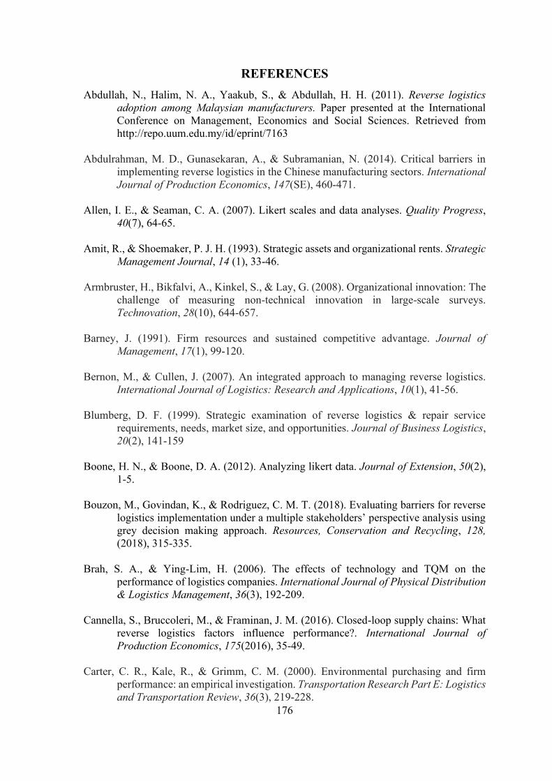
176

REFERENCES

Abdullah, N., Halim, N. A., Yaakub, S., & Abdullah, H. H. (2011). Reverse logistics

adoption among Malaysian manufacturers. Paper presented at the International

Conference on Management, Economics and Social Sciences. Retrieved from

http://repo.uum.edu.my/id/eprint/7163

Abdulrahman, M. D., Gunasekaran, A., & Subramanian, N. (2014). Critical barriers in

implementing reverse logistics in the Chinese manufacturing sectors. International

Journal of Production Economics, 147(SE), 460-471.

Allen, I. E., & Seaman, C. A. (2007). Likert scales and data analyses. Quality Progress,

40(7), 64-65.

Amit, R., & Shoemaker, P. J. H. (1993). Strategic assets and organizational rents. Strategic

Management Journal, 14 (1), 33-46.

Armbruster, H., Bikfalvi, A., Kinkel, S., & Lay, G. (2008). Organizational innovation: The

challenge of measuring non-technical innovation in large-scale surveys.

Technovation, 28(10), 644-657.

Barney, J. (1991). Firm resources and sustained competitive advantage. Journal of

Management, 17(1), 99-120.

Bernon, M., & Cullen, J. (2007). An integrated approach to managing reverse logistics.

International Journal of Logistics: Research and Applications, 10(1), 41-56.

Blumberg, D. F. (1999). Strategic examination of reverse logistics & repair service

requirements, needs, market size, and opportunities. Journal of Business Logistics,

20(2), 141-159

Boone, H. N., & Boone, D. A. (2012). Analyzing likert data. Journal of Extension, 50(2),

1-5.

Bouzon, M., Govindan, K., & Rodriguez, C. M. T. (2018). Evaluating barriers for reverse

logistics implementation under a multiple stakeholders’ perspective analysis using

grey decision making approach. Resources, Conservation and Recycling, 128,

(2018), 315-335.

Brah, S. A., & Ying-Lim, H. (2006). The effects of technology and TQM on the

performance of logistics companies. International Journal of Physical Distribution

& Logistics Management, 36(3), 192-209.

Cannella, S., Bruccoleri, M., & Framinan, J. M. (2016). Closed-loop supply chains: What

reverse logistics factors influence performance?. International Journal of

Production Economics, 175(2016), 35-49.

Carter, C. R., Kale, R., & Grimm, C. M. (2000). Environmental purchasing and firm

performance: an empirical investigation. Transportation Research Part E: Logistics

and Transportation Review, 36(3), 219-228.

http://repo.uum.edu.my/id/eprint/7163

177

Chavez, R., Gimenez, C., Fynes, B., Wiengarten, F., & Yu, W. (2013). Internal lean

practices and operational performance: The contingency perspective of industry

clockspeed. International Journal of Operations & Production Management, 33(5),

562-588.

Christmann, P. (2000). Effects of “best practices” of environmental management on cost

advantage: The role of complementary assets. Academy of Management Journal,

43(4), 663-680.

Clarke, C. (2009). Paths between positivism and interpretivism: An appraisal of Hay's via

media. Politics, 29(1), 28-36.

Clason, D. L., & Dormody, T. J. (1994). Analyzing data measured by individual Likert-

type items. Journal of Agricultural Education, 35(4), 31-35.

Clemons, E. K., & Row, M. C. (1992). Information technology and industrial cooperation:

the changing economics of coordination and ownership. Journal of Management

Information Systems, 9(2), 9-28.

Closs, D. J., Speier, C., & Meacham, N. (2011). Sustainability to support end-to-end value

chains: the role of supply chain management. Journal of the Academy of Marketing

Science, 39(1), 101-116.

Coase, R. H. (1937). The nature of the firm. Economica, 4(16), 386-405.

Conner, K. R. (1991). A historical comparison of resource-based theory and five schools

of thought within industrial organization economics: do we have a new theory of

the firm?. Journal of Management, 17(1), 121-154.

Curtin, R., Presser, S., & Singer, E. (2000). The effects of response rate changes on the

index of consumer sentiment. Public opinion quarterly, 64(4), 413-428.

Dacin, M. T., Goodstein, J., & Scott, W. R. (2002). Institutional theory and institutional

change: Introduction to the special research forum. Academy of Management

Journal, 45(1), 45-56.

Davenport, T. H. (2013). Process innovation: Reengineering work through information

technology. Cambridge, Massachusetts, United States of America (USA): Harvard

Business Press.

Davis, L. L. (1992). Instrument review: Getting the most from a panel of experts. Applied

nursing research, 5(4), 194-197.

De Brito M.P., Dekker R., Flapper S.D.P. (2005) Reverse logistics: A review of case

studies. In B. Fleischmann & A. Klose (Eds.), Distribution logistics. Lecture notes

in economics and mathematical systems, 544, (pp. 243-281). Berlin, Germany:

Springer Science & Business Media. doi:10.1007/978-3-642-17020-1_13

178

De Souza M. P. L., & Brito, L. A. L. (2011). Supply chain management measurement and

its influence on operational performance. Journal of Operations and Supply Chain

Management, 4(2), 56-70.

Dekker, R., Fleischmann, M., Inderfurth, K., & van Wassenhove, L. N. (Eds.). (2013).

Reverse logistics: Quantitative models for closed-loop supply chains. Berlin,

Germany: Springer Science & Business Media.

Dias, K. T., & Braga Jr., S. S. (2016). The use of reverse logistics for waste management

in a Brazilian grocery retailer. Waste Management & Research, 34(1), 22-29.

DiMaggio, P. J., & Powell, W. W. (2004). The iron cage revisited: institutional

isomorphism and collective rationality in organizational fields. In F. Dobbin (Ed.),

The new economic sociology, (pp. 111-134). Princeton, New Jersey, USA:

Princeton University Press.

Field, A. (2013). Discovering statistics using IBM SPSS statistics. Thousand Oaks,

Carlifonia, USA: Sage.

Genchev, S. E., Glenn-Richey, R., & Gabler, C. B. (2011). Evaluating reverse logistics

programs: A suggested process formalization. The International Journal of

Logistics Management, 22(2), 242-263.

Geyskens, I., Steenkamp, J. B. E., & Kumar, N. (2006). Make, buy, or ally: A transaction

cost theory meta-analysis. Academy of Management Journal, 49(3), 519-543.

Glenn-Richey, R., Genchev, S. E., & Daugherty, P. J. (2005). The role of resource

commitment and innovation in reverse logistics performance. International Journal

of Physical Distribution & Logistics Management, 35(4), 233-257.

Govindan, K., Soleimani, H., & Kannan, D. (2015). Reverse logistics and closed-loop

supply chain: A comprehensive review to explore the future. European Journal of

Operational Research, 240(3), 603-626.

Gujarati, D. N. (2003). Basic Econometrics 4th edition McGraw Hill United states Military

Academy. West Point.

Hair, J. F., Money, A. H., Samouel, P., & Page, M. (2007). Research methods for business.

West Sussex, England: John Wiley & Sons.

Hair, J. F., Black, W. C., Babin, B. J., & Anderson, R. E. (2014). Multivariate data analysis

(7th ed.). Essex, England: Pearson Education.

Hart, S. L. (2005). Capitalism at the crossroads: The unlimited business opportunities in

solving the world's most difficult problems. Essex, England: Pearson.

He, X., & Wang, J. X. (2005). An overview of reverse logistics. International Journal of

Plant Engineering and Management, 10(2), 120-124.

179

Healy, M., & Perry, C. (2000). Comprehensive criteria to judge validity and reliability of

qualitative research within the realism paradigm. Qualitative Market Research: An

International Journal, 3(3), 118-126.

Ho, G. T. S., Choy, K. L., Lam, C. H. Y., & Wong, D. W. (2012). Factors influencing

implementation of reverse logistics: A survey among Hong Kong businesses.

Measuring Business Excellence, 16(3), 29-46.

Hooper, D., Coughlan, J., & Mullen, M. (2008). Structural equation modelling:

Guidelines for determining model fit. Articles, 2.

Hosseini, M. R., Chileshe, N., Rameezdeen, R., & Lehmann, S. (2014). Reverse logistics

for the construction industry: Lessons from the manufacturing context.

International Journal of Construction Engineering and Management, 3(3), 75-90.

Hsu, C. C., Tan, K. C., & Mohamad-Zailani, S. H. (2016). Strategic orientations,

sustainable supply chain initiatives, and reverse logistics: Empirical evidence from

an emerging market. International Journal of Operations & Production

Management, 36(1), 86-110.

Huang, Y. C., & Yang, M. L. (2014). Reverse logistics innovation, institutional pressures

and performance. Management Research Review, 37(7), 615-641.

Hung-Lau, K., & Wang, Y. (2009). Reverse logistics in the electronic industry of China: a

case study. Supply Chain Management: An International Journal, 14(6), 447-465.

Hunt, S. D., & Morgan, R. M. (2005). The resource-advantage theory of competition.

Review of Marketing Research, 1(4), 153-206

Hunt, S. D., & Madhavaram, S. (2012). Managerial action and resource-advantage theory:

Conceptual frameworks emanating from a positive theory of competition. Journal

of Business & Industrial Marketing, 27(7), 582-591.

Huscroft, R. J., Skipper, B. J., Hazen, T. B., Hanna, B.J., & Hall, J. D. (2013). Reverse

logistics: past research, current management issues, and future directions. The

International Journal of Logistics Management, 24(3), 304-327.

Inauen, M., & Schenker-Wicki, A. (2012). Fostering radical innovations with open

innovation. European Journal of Innovation Management, 15(2), 212-231.

Jack, E. P., Powers, T. L., & Skinner, L. (2010). Reverse logistics capabilities: antecedents

and cost savings. International Journal of Physical Distribution & Logistics

Management, 40(3), 228-246.

Jayaraman, V., & Luo, Y. (2007). Creating competitive advantages through new value

creation: a reverse logistics perspective. The Academy of Management

Perspectives, 21(2), 56-73.

180

Jim, W. Y. C., & Cheng, W. P. (2006). Reverse logistics in the publishing industry: China,

Hong Kong, and Taiwan. International Journal of Physical Distribution &


Kaiser, H. F., Rice, J., Little, J., & Mark, I. (1974). Educational and psychological

measurement. American Psychological Association, 34, 111-7.

Keeley, L., Walters, H., Pikkel, R., & Quinn, B. (2013). Ten types of innovation: The

discipline of building breakthroughs. West Sussex, England: John Wiley & Sons.

Keeter, S., Kennedy, C., Dimock, M., Best, J., & Craighill, P. (2006). Gauging the impact

of growing nonresponse on estimates from a national RDD telephone survey.

International Journal of Public Opinion Quarterly, 70(5), 759-779.

Kenya Manufacturers and Exporters Directory. (2018). Annual Report. Retrieved from

http:// www.manufacturersandexportersdirectory.co.ke.

Kenya National Bureau of Statistics. (2017). Economic Survey. Retrieved from

http://www.knbs.or.ke.

Kim, H., & Hoskinsson, R.E. (2015). A resource environment view of competitive

advantage. Emerging Economies and Multinational Enterprises, 28, 95-140.

Kostova, T., Roth, K., & Dacin, M. T. (2008). Institutional theory in the study of

multinational corporations: A critique and new directions. Academy of Management

Review, 33(4), 994-1006.

Kumar, S., & Putnam, V. (2008). Cradle to cradle: Reverse logistics strategies and

opportunities across three industry sectors. International Journal of Production

Economics, 115(2), 305-315.

Kwateng, K. O., Debrah, B., Parker, D. V., Owusu, R. N., & Prempeh, H. (2014). Reverse

logistics practices in pharmaceutical manufacturing industry: experiences from

Ghana. Global Journal of Business Research, 8(5), 17-26.

Markley, M. J., & Davis, L. (2007). Exploring future competitive advantage through

sustainable supply chains. International Journal of Physical Distribution &


M’Chirgui, Z., & Chanel, O. (2008). The adoption and use of smart card technology in

banking: An empirical evidence from the Moneo electronic purse in France. In

Advances in Banking Technology and Management: Impacts of ICT and CRM (pp.

70-87). IGI Global.

Mellat-Parast, M., & Spillan,E. J. (2014). Logistics and supply chain process integration as

a source of competitive advantage: An empirical analysis. The International

Journal of Logistics Management, 25(2), 289-314.

http://www.manufacturers/

181

Meyer, A., Niemann, W., Mackenzie, J., & Lombaard, J. (2017). Drivers and barriers of

reverse logistics practices: A study of large grocery retailers in South Africa.

Journal of Transport and Supply Chain Management, 11(1), 1-16.

Moghaddam, K. S. (2015). Fuzzy multi-objective model for supplier selection and order

allocation in reverse logistics systems under supply and demand uncertainty. Expert

Systems with Applications, 42(15-16), 6237-6254.

Morgan, T. R., Richey Jr, R. G., & Autry, C. W. (2016). Developing a reverse logistics

competency: The influence of collaboration and information technology.

International Journal of Physical Distribution & Logistics Management, 46(3),

293-315.

Mugenda, O. M., & Mugenda, A. G. (1999). Research methods: Quantitative and

qualitative approaches. Acts press.

Ninlawan, C., Seksan, P., Tossapol, K., & Pilada, W. (2010, March). The implementation

of green supply chain management practices in electronics industry. In World

Congress on Engineering 2012. July 4-6, 2012. London, UK. (Vol. 2182, pp. 1563-

1568). International Association of Engineers.

North, D. C. (1991). Institutions. Journal of Economic Perspectives, 5(1), 97-112.

O'Cass, A., & Viet, N. L. (2007). Market orientation versus innovative culture: two routes

to superior brand performance. European Journal of Marketing, 41(7/8), 868-887.

Ochieng, O. S., Awino, Z. B., Njihia, M. J., & Iraki, W. N. (2016). Green supply chain

management practices and performance of ISO 14001 certified manufacturing firms

in East Africa. DBA Africa Management Review, 6(3).

Oral, M., & Yolalan, R. (1990). An empirical study on measuring operating efficiency and

profitability of bank branches. European Journal of Operational Research, 46(3),

282-294.

Porter, M. E. (2008). On competition. Cambridge, Massachusetts, USA: Harvard Business

Press.

Prakash, C., & Barua, M. K. (2015). Integration of AHP-TOPSIS method for prioritizing

the solutions of reverse logistics adoption to overcome its barriers under fuzzy

environment. Journal of Manufacturing Systems, 37(2015), 599-615.

Prakash, C., Barua, M. K., & Pandya, K. V. (2015). Barriers analysis for reverse logistics

implementation in Indian electronics industry using fuzzy analytic hierarchy

process. Procedia-Social and Behavioral Sciences, 189(2015), 91-102.

Rao, P., & Holt, D. (2005). Do green supply chains lead to competitiveness and economic

performance?. International Journal of Operations & Production Management,

25(9), 898-916.

182

Ravi, V., & Shankar, R. (2015). Survey of reverse logistics practices in manufacturing

industries: an Indian context. Benchmarking: An International Journal, 22(5), 874-

899.

Rogers, D. S., Banasiak, K., Brokman, K., Johnson, T., & Tibben-Lembke, R. (2002,

January). Reverse logistics challenges. Paper presented at the 2001 Annual

Conference Proceedings.

Rogers, D. S., & Tibben-Lembke, R. S. (1999). Going backwards: reverse logistics trends

and practices (Vol. 2). Pittsburgh, Pennsylvania, USA: Reverse Logistics

Executive Council.

Rogers, D. S., & Tibben-Lembke, R. S. (2001). An examination of reverse logistics

practices, Journal of Business Logistics, 22(2), 129-149.

Rogers, E. M. (1976). New product adoption and diffusion. Journal of Consumer Research,

2(4), 290-301.

Rogers, E. M. (2003). Diffusion of innovations, (5th ed.). New York, New York, USA: Free

Press.

Russo I., & Cardinali S. (2012). Product returns and customer value: A footware industry

case. In H. Jodlbauer, J. Olhager & R. Schonberger (Eds.), Modelling value.

Contributions to management science. (pp 79-97). Physica-Verlag HD doi:10.1007/978-3-7908-2747-7_5

Sangwan, K. S. (2017). Key activities, decision variables and performance indicators of

reverse logistics. Procedia CIRP, 61(2017), 257-262.

Schumpeter, J. A. (1934). Theorie der Wirtschaftlichen Entwicklung: the theory of

economic development: An inquiry into profits, capital, credit, interest and the

business cycle. Cambridge, Massachusetts, USA: Harvard Business Press.

Translated by …Redvers Opie.

Scott, W. R. (2008). Approaching adulthood: The maturing of institutional theory. Theory

and Society, 37(5), 427-442.

Sharma, S., Durand, R. M., & Gur-Arie, O. (1981). Identification and analysis of moderator

variables. Journal of marketing research, 18(3), 291-300.

Shaw, T. (2003). Performance measures of operational effectiveness for highway segments

and systems (Vol. 311). Transportation Research Board.

Sheth, J. N., Sethia, N. K., & Srinivas, S. (2011). Mindful consumption: A customer centric

approach to sustainability. Journal of the Academy of Marketing Science, 39(1), 21-

39.

Shoham, A., & Ruvio, A. (2008). Opinion leaders and followers: A replication and

extension. Psychology & Marketing, 25(3), 280-297.

183

Slack, N., Chambers, S., & Johnston, R. (2010). Operations management. (6th ed.). Essex,

England: Pearson Education.

Somuyiwa, A. O., & Adebayo, I. T. (2014). Empirical study of the effect of reverse logistics

objectives on economic performance of food and beverages companies in Nigeria.

International Review of Management and Business Research, 3(3), 1484-1493.

Stock, J. R. (1992). Reverse logistics: White paper. Council of Logistics Management.

Stock, J. R. (2001). The 7 deadly sins of reverse logistics. Material Handling Management,

56(3), 5-11.

Stock, J., Speh, T., & Shear, H. (2006). Managing product returns for competitive

advantage. MIT Sloan Management Review, 48(1), 57-62.

Tabachnick, B. G., & Fidell, L. S. (2013). Using Multivariate Statistics, (6th ed.). Essex,

England: Pearson Education.

Tolbert, P. S., & Zucker, L. G. (1999). The institutionalization of institutional theory. In S.

R. Clegg & C. Hardy (Eds.), Studying organization: Theory & method (pp 169 –

184). Thousand Oaks, Carlifonia, USA: Author.

UNEP Report. (2016). Engaging people to protect the planet. Retrieved from

http://www.unep.org/annualreport/2016/index.php.

Voss, C. A., Åhlström, P., & Blackmon, K. (1997). Benchmarking and operational

performance: Some empirical results. International Journal of Operations &

Production Management, 17(10), 1046-1058.

Weber, R. (2004). Editor's Comments: The rhetoric of positivism versus interpretivism: A

personal view. MIS Quarterly, 28(1), 3-12. doi:10.2307/25148621

Williamson, O. (1991). Economic Institutions: Spontaneous and Intentional Governance.

Journal of Law, Economics, & Organization, 7(SE), 159-187. Retrieved from

http://www.jstor.org/stable/764962

World Bank. (2016). Economic Update: Kenya’s Ecconomy Strong in a Challenging

Global Environment. Retrieved from http://www.worldbank.org/en/country/

kenya/ publication

Yamane, T. (1967). Statistics: An introductory analysis (2nd ed.). New York, New York:

Harper & Row.

Zhikang, L. (2017). Research on Development Strategy of Automobile Reverse Logistics

Based on SWOT Analysis. Procedia engineering, 174, 324-330.

Zikmund, W. G., Babin, B. J., Carr, J. C., & Griffin, M. (2013). Business research methods

(9th ed.). Boston, Massachusetts, USA: Cengage Learning.

http://www.unep.org/annualreport/2016/index.php

http://www.jstor.org/stable/764962

http://www.worldbank.org/en/country/

184

Zhu, Q., Sarkis, J., & Lai, K. H. (2008). Confirmation of a measurement model for green

supply chain management practices implementation. International journal of

production economics, 111(2), 261-273.

185

APPENDICES:

Appendix 1: Data Collection Instrument (Questionnaire):

Introduction:

Dear respondent,

This is a questionnaire designed to collect data on Reverse Logistics, Process Innovation,

Operational Performance and Competitive Advantage of Large Manufacturing Firms in Kenya. The

questionnaire has five main parts. Kindly respond to each of the items in the questionnaire. There

are no wrong or right answers and the results are strictly confidential and purely for academic use.

Your accurate participation will be crucial in attaining the objectives of the study.

PART A: ORGANIZATION PROFILE

Please answer all of the following questions. Where there is a choice indicate your answer with a

tick (√) in the brackets ( ) or space provided.

1.1 Name of the organization

________________________________________________________________________

________________________________________________________________________

1.2 Designation of the respondent

________________________________________________________________________

1.3 The year the organization was established ___________________________________

1.4 Is your organization ISO 14001 certified? Yes [ ] No [ ]

1.5 Which manufacturing sub-sector does your firm belong to?

Building, Mining and Construction

Food & Beverage Sector

Fresh Produce

Chemical and Allied Sector

Energy, Electrical and Electronics

Leather and Footwear

Metal and Allied Sector

Motor Vehicle and Accessories

Paper and Board Sector

Pharmaceutical and Medical Equipment

Plastics and Rubber

Textiles and Apparels

Timber, Wood and Furniture

186

PART B: REVERSE LOGISTICS

2.1 Please record the degree to which your organization concurs with the statements

regarding reverse logistics. Please read each statement carefully and tick (√) the appropriate

box (Key: 1 = Not at all; 2= To a small degree; 3= To a moderate degree; 4= To a large

degree; and 5 = To a very large degree).

Label Reverse Logistics 1 2 3 4 5

Outsourcing Reverse Logistics

OS1 Outsourcing reverse logistics increases return on

investment

OS2 Outsourcing reverse logistics provides better

operational flexibility

OS3 Outsourcing reverse logistics results to improved

customer service quality

OS4 Outsourcing reverse logistics results to improved

speed to market.

OS5 Reverse logistics outsourcing provides access to

functional and industry expertise

OS6 Reverse logistics outsourcing provides access to

best technology

OS7 Reverse logistics outsourcing results to

benefitting from best practices

OS8 In-housing reverse logistics is more costly than

outsourcing

Collaborative Enterprising in Reverse

Logistics

CE1 There is high volume data exchange among

partners in reverse logistics.

CE2 Partners implementing reverse logistics have

standardized information exchange platforms

CE3 The focus in implementing reverse logistics is on

building data integrity among supply chain

partners

CE4 The emphasis in implementing reverse logistics

is on managing transactions using IT tools.

CE5 Partners implementing reverse logistics

participate in short-term planning and decision

making among

CE6 In implementing reverse logistics more

interpersonal interactions and less transactional

data is used

CE7 Supply chain partners have fully integrated

reverse logistics processes among themselves

CE8 Partners have set joint business goals in planning

and implementing reverse logistics

187

CE9 Supply chain partners have designed inter-

enterprise reverse logistics processes

CE10 Supply chain partners have fully integrated

reverse logistics processes among them.

Green Strategies in Reverse Logistics

GS1 Awareness seminars for suppliers and

contractors are conducted on green strategies

GS2 Suppliers are guided in setting-up their own

green programs.

GS3 Suppliers are chosen based on the extent of

implementation of green programs

GS4 There is a structure for suppliers to share

knowledge and issues in green implementation

GS5 Suppliers are informed about the benefits of

green programs

GS6 Products are designed to facilitate re-use

GS7 Products are designed to facilitate recycling

GS8 Products are designed to facilitate remanufacture

GS9 Organizational processes optimization leads to a

reduction in emissions and solid waste

GS10 Savings in energy and water are an outcome of

using technologically cleaner processes

GS11 Recycling of materials internally is practiced

during production

GS12 Supply chain partners practice environmental

management principles like worker

empowerment.

GS13 Environmentally affable packaging such as eco-

labeling is used

GS14 Environmentally affable transportation is used

GS15 Information on environmentally affable products

is shared to consumers.


PLA1 Control and reduction of returns rate does not

undermine customer service

PLA2 Supply chain partners segregate returned

products into categories for processing, selling

or disposal

PLA3 The firm undertakes repair, remanufacture or

refurbishing activities to make product reusable

PLA4 The firm recycles returned product parts to be

used in manufacture of other products or

components

PLA5 The firm undertakes disposal activities for

returned products that have no more economic or

ecological value

188

PLA6 The firm facilitates transportation of returned

products in the process of recovering value

2.2 Using the scale below, please indicate the percentage to which you agree with the

following statements regarding reverse logistics.

Label Reverse Logistics 0 -

10%

11 -

20%

21 -

30%

31 -

40%

Over

40%

Estimated cost of running

reverse logistics operations in

relation to sales

Estimated cost recovered

from reverse logistics

activities

Energy used in handling

returns in relation to total

energy consumption

Rate of product refurbishment

in relation to total production

Rate of product

remanufacture in relation to

total production

Raw materials recycled

Raw materials moved to

landfills, incinerated or

disposed as waste

PART C: PROCESS INNOVATION

3.1 Please record the degree to which your organization concurs with the statements

regarding process innovation. Please read each statement carefully and tick (√) the

appropriate box (Key: 1 = Not at all; 2= To a small degree; 3= To a moderate degree; 4=

To a large degree; and 5 = To a very large degree).

Label Process Innovation 1 2 3 4 5

Information Systems (IS)

IS1 Information systems in use are perceived to

be better than our competitors.

IS2 Information systems in use are perceived to

be better than previous systems in use.

IS3 Information systems in use are perceived as

easy to learn, understand and use.

189

IS4 Information systems in use are perceived as

being compatible to the needs of potential

users.

IS5 Users consider the information systems as

easy to explore and experiment with.

IS6 The results of using the information systems

in the organization are visible.

Resource Deployment

RD1 Firm budgets have a component for reverse

logistics activities

RD2 Staff have relevant skills to implement

reverse logistics activities

RD3 Supply chain partners have acquired the

relevant technology and equipment to

implement reverse logistics

RD4 Customers are integrated in our current

reverse logistics programming

RD5 Suppliers are integrated in our current

reverse logistics programming

RD6 Resource deployment processes in the firm

are perceived to be superior to our

competitors

RD7 Over time resource deployment processes in

the organization have improved

Product Redesign

PRD1 New markets and market segments can be

attributed to product redesign

PRD2 The firm maintains superiority in

manufacturing technology

PRD3 Change in customer requirements have

influenced our product design strategy

PRD4 Clients consider our current products as

more convenient to use

PRD5 Over time manufacturing processes have

been standardized and simplified

PRD6 Manufacturing processes are much easier as

a result of redesigning our products

PRD7 The benefits of product redesign processes

can be quantified within the organization.

PRD8 The quality of our products has improved as

a result of product redesign


PRE1 The vision of the organization is shared to

all members of staff

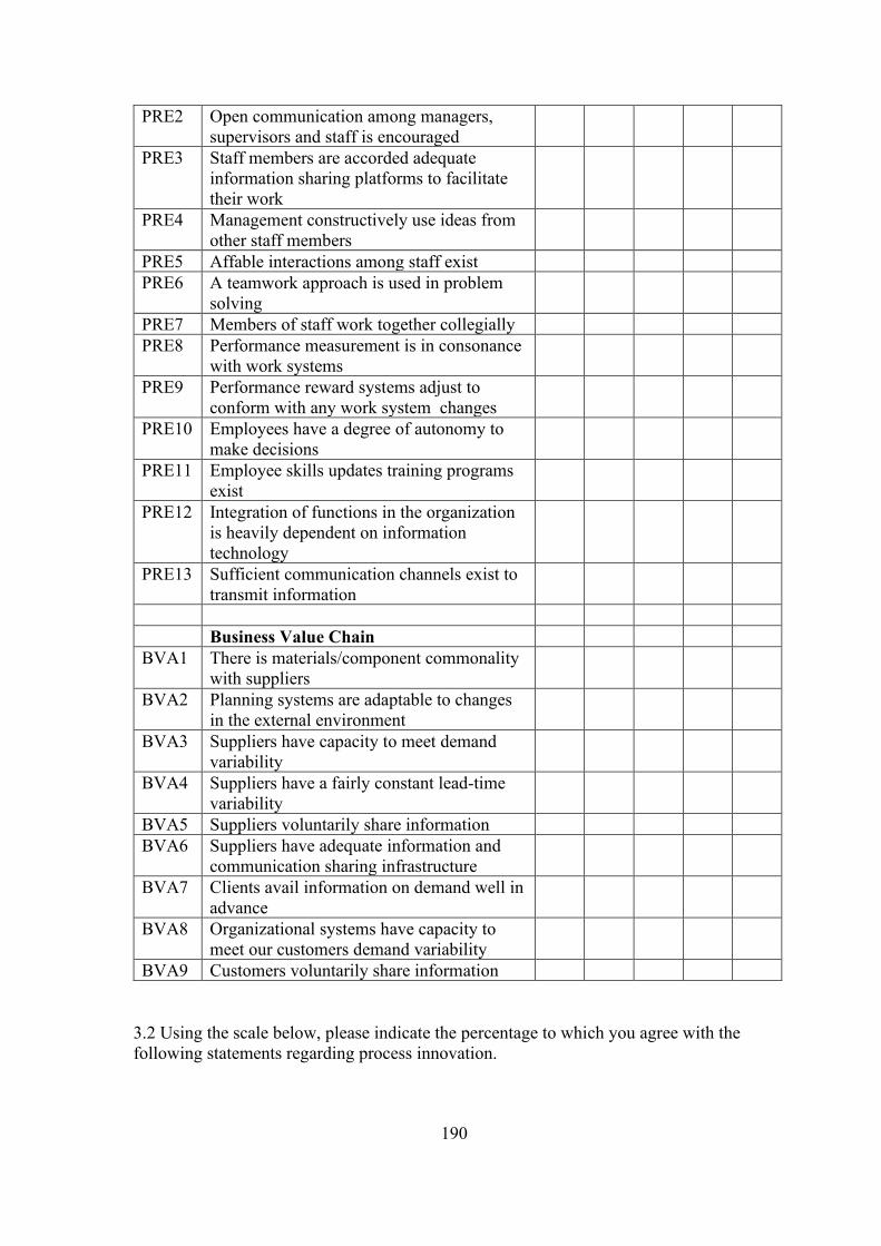
190

PRE2 Open communication among managers,

supervisors and staff is encouraged

PRE3 Staff members are accorded adequate

information sharing platforms to facilitate

their work

PRE4 Management constructively use ideas from

other staff members

PRE5 Affable interactions among staff exist

PRE6 A teamwork approach is used in problem

solving

PRE7 Members of staff work together collegially

PRE8 Performance measurement is in consonance

with work systems

PRE9 Performance reward systems adjust to

conform with any work system changes

PRE10 Employees have a degree of autonomy to

make decisions

PRE11 Employee skills updates training programs

exist

PRE12 Integration of functions in the organization

is heavily dependent on information

technology

PRE13 Sufficient communication channels exist to

transmit information


BVA1 There is materials/component commonality

with suppliers

BVA2 Planning systems are adaptable to changes

in the external environment

BVA3 Suppliers have capacity to meet demand

variability

BVA4 Suppliers have a fairly constant lead-time

variability

BVA5 Suppliers voluntarily share information

BVA6 Suppliers have adequate information and

communication sharing infrastructure

BVA7 Clients avail information on demand well in

advance

BVA8 Organizational systems have capacity to

meet our customers demand variability

BVA9 Customers voluntarily share information

3.2 Using the scale below, please indicate the percentage to which you agree with the

following statements regarding process innovation.

191

Label Process Innovation 0-10% 11-

20%

21-

30%

31-

40%

Over

40%

Percentage of sales from new

products introduced in the last

two years

Percentage of budget devoted to

research and development

Percentage of employee hours

spent on research and ideation

Percentage of employees who

have received training and tools

for innovation.

PART D: OPERATIONAL PERFORMANCE

4.1 Please record the number for the indicators of operational performance in your firm

for the year 2015, 2016 and 2017.

Label Operational

Performance

Indicator

Unit of Measure

2015

2016

2017

Cost Annual total

variable cost of

production

Total number of

items produced in

the year

Quality Number of items

ordered by

customers in the

year

Number of items

actually delivered

to customers in the

year

Number of

customer

complaints in the

year

Flexibility Number of product

lines in the year

Dependability Number of hours

equipment /

machines are

supposed to be

192

available for

manufacturing

operations in the

year.

Number of hours

equipment /

machines were

available for

manufacturing

operations in the

year.

Delivery

speed

Average number of

days between when

an order is received

and when it is

shipped to the

customer in the

year.

PART E: COMPETITIVE ADVANTAGE

5.1 Please record the number for the indicators of competitive advantage in your firm for

the year 2015, 2016 and 2017.

Label Competitive

Advantage

Indicator

Unit of Measure

2015

2016

2017

Customer

loyalty

Number of

customers at the

beginning of the

year

Number of

customers acquired

during year

Number of

customers at the end

of the year

Market share Market share at the

beginning of the

year

Market share at the

end of the year

193

Brand

recognition

Cost of goods sold

in the year

Total sales for the

year

Waste

reduction

No. of units tested

for defects in the

year

No. of units actually

found to be

defective in the year

Revenue

increase

Percentage revenue

increase for the year

THANK YOU VERY MUCH FOR TAKING PART IN THIS PROCESS

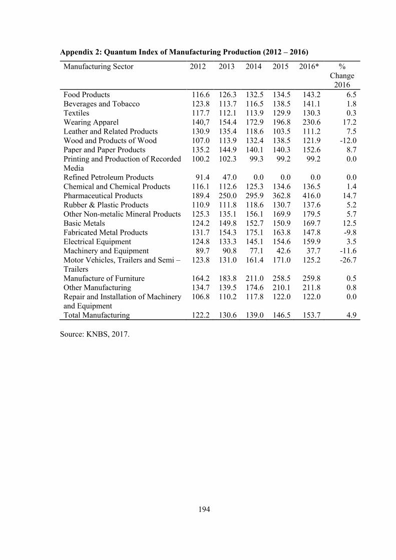
194

Appendix 2: Quantum Index of Manufacturing Production (2012 – 2016)

Manufacturing Sector 2012 2013 2014 2015 2016* %

Change

2016

Food Products 116.6 126.3 132.5 134.5 143.2 6.5

Beverages and Tobacco 123.8 113.7 116.5 138.5 141.1 1.8

Textiles 117.7 112.1 113.9 129.9 130.3 0.3

Wearing Apparel 140,7 154.4 172.9 196.8 230.6 17.2

Leather and Related Products 130.9 135.4 118.6 103.5 111.2 7.5

Wood and Products of Wood 107.0 113.9 132.4 138.5 121.9 -12.0

Paper and Paper Products 135.2 144.9 140.1 140.3 152.6 8.7

Printing and Production of Recorded

Media

100.2 102.3 99.3 99.2 99.2 0.0

Refined Petroleum Products 91.4 47.0 0.0 0.0 0.0 0.0

Chemical and Chemical Products 116.1 112.6 125.3 134.6 136.5 1.4

Pharmaceutical Products 189.4 250.0 295.9 362.8 416.0 14.7

Rubber & Plastic Products 110.9 111.8 118.6 130.7 137.6 5.2

Other Non-metalic Mineral Products 125.3 135.1 156.1 169.9 179.5 5.7

Basic Metals 124.2 149.8 152.7 150.9 169.7 12.5

Fabricated Metal Products 131.7 154.3 175.1 163.8 147.8 -9.8

Electrical Equipment 124.8 133.3 145.1 154.6 159.9 3.5

Machinery and Equipment 89.7 90.8 77.1 42.6 37.7 -11.6

Motor Vehicles, Trailers and Semi –

Trailers

123.8 131.0 161.4 171.0 125.2 -26.7

Manufacture of Furniture 164.2 183.8 211.0 258.5 259.8 0.5

Other Manufacturing 134.7 139.5 174.6 210.1 211.8 0.8

Repair and Installation of Machinery

and Equipment

106.8 110.2 117.8 122.0 122.0 0.0

Total Manufacturing 122.2 130.6 139.0 146.5 153.7 4.9

Source: KNBS, 2017.

195

Appendix 3: Manufacturing Firms Per Sub Sector

Sector Number of

Members

Proportionate

Stratified

Sample Size

Percentage

Membership

Building, Mining and Construction 39 15 4.32%

Food & Beverage Sector 234 88 25.91%

Fresh Produce 13 5 1.44%

Chemical and Allied Sector 90 34 9.97%

Energy, Electrical and Electronics 58 22 6.43%

Leather and Footwear 9 3 1.00%

Metal and Allied Sector 96 36 10.63%

Motor Vehicle and Accessories 59 22 6.53%

Paper and Board Sector 82 31 9.08%

Pharmaceutical and Medical Equipment 30 11 3.32%

Plastics and Rubber 90 34 9.97%

Textiles and Apparels 73 28 8.08%

Timber, Wood and Furniture 30 11 3.32%

903 340 100.00%

Source: KAM, 2018

196

Appendix 4: Sampled Firms Per Manufacturing Sub-Sectors

Building Mining and Construction: 1. Bamburi Cement Ltd

2. Building Construction Concepts

3. Flamingo Tiles (Kenya) Ltd

4. International Energy Technik Ltd

5. Kemu Salt Packers Production Ltd

6. Kurawa Industries Ltd

7. Malindi Salt Works

8. Mombasa Cement Ltd

9. Orbit Enterprises Ltd

10. Reliable Concrete Works Ltd

11. Saj Ceramics Ltd

12. Savannah Cement Ltd

13. Skylark Construction Ltd

14. Tile & Carpet Centre Ltd

15. Vallem Construction Ltd

Food and Beverage Sector: 1. Africa Spirits Ltd

2. Agriner Agricultural Development

3. Alliance One Tobacco Kenya Ltd

4. Alpha Fine Foods Ltd

5. Alpine Coolers Ltd

6. Aquamist Ltd

7. Aviano East Africa Ltd

8. Belat Enterprises

9. Beverage Services (K) Ltd

10. Bdelo Ltd

11. Broadway Bakery Ltd

12. Brown Biashara Ltd

13. Burton and Mamber Company Ltd

14. Czarnikow Sugar East Africa ltd

15. Caffe Del Duca Ltd

16. Capwell Industries Ltd

17. Chemelil Sugar Company Ltd

18. Coast Silos (K) Ltd

19. Coastal Bottlers Ltd

20. CoffTea Agencies Ltd

21. Del Monte Kenya Ltd

22. Diamond Industries Ltd

23. Doinyo Lessos Creameries Ltd

24. East African Breweries Ltd

25. East African Seed Co. Ltd

26. Eldoret Grains Ltd

27. Equator Bottlers Ltd

28. Excel Chemicals Ltd

29. Fresh Produce Exporters

Association of Kenya

30. General Mills East Africa Ltd

31. Glacier Products (Amor Mia,

Dairyland, Mio)

32. Global Tea and Commodities (K)

Ltd

33. Gold Crown Foods (EPZ) Ltd

34. Golden Africa Kenya Ltd

35. Grain Industries Ltd

36. Heritage Foods Kenya Ltd

37. Highlands Mineral Water Company

Ltd

38. Italian Gelati and Food Produce Ltd

39. Jjasm Mini-Distillery

40. Kabianga Dairy Ltd

41. Kambu Distillers Ltd

42. Karirana Estate Ltd

43. Kenafric Bakery

44. Kenchic Ltd

45. Kentaste Products Ltd

46. Kibos Sugar Refinery Ltd

47. Kenya Seed Company Ltd

48. Kenya Highland Seed Company Ltd

49. Kenya Horticultural Exporters

(1977)

50. Kenya Sweets Ltd

51. Kenya Tea Growers Association

52. Kinangop Dairy Ltd

53. Koba Waters Ltd/Bromhill Springs

Water

54. Kuguru Food Complex Ltd

55. Kwale International Company Ltd

56. Meru Water and Sewerage Services

57. Miritini Kenya Ltd

58. Mombasa Maize Millers

59. Mount Kenya Bottlers Ltd

60. Mzuri Sweets Ltd

61. Nairobi Flour Mills Ltd

62. NesFoods Industries Ltd

63. Norda Industries Ltd

64. Olivado EPZ

65. Pearly LLP

66. Pembe Flour Mills Ltd

67. Premier Flour Mills Ltd

68. Pride Industries Ltd

69. Pristine International Ltd

70. Promasidor Kenya Ltd

71. Propack Kenya Ltd

72. Pwani Oil Product Ltd

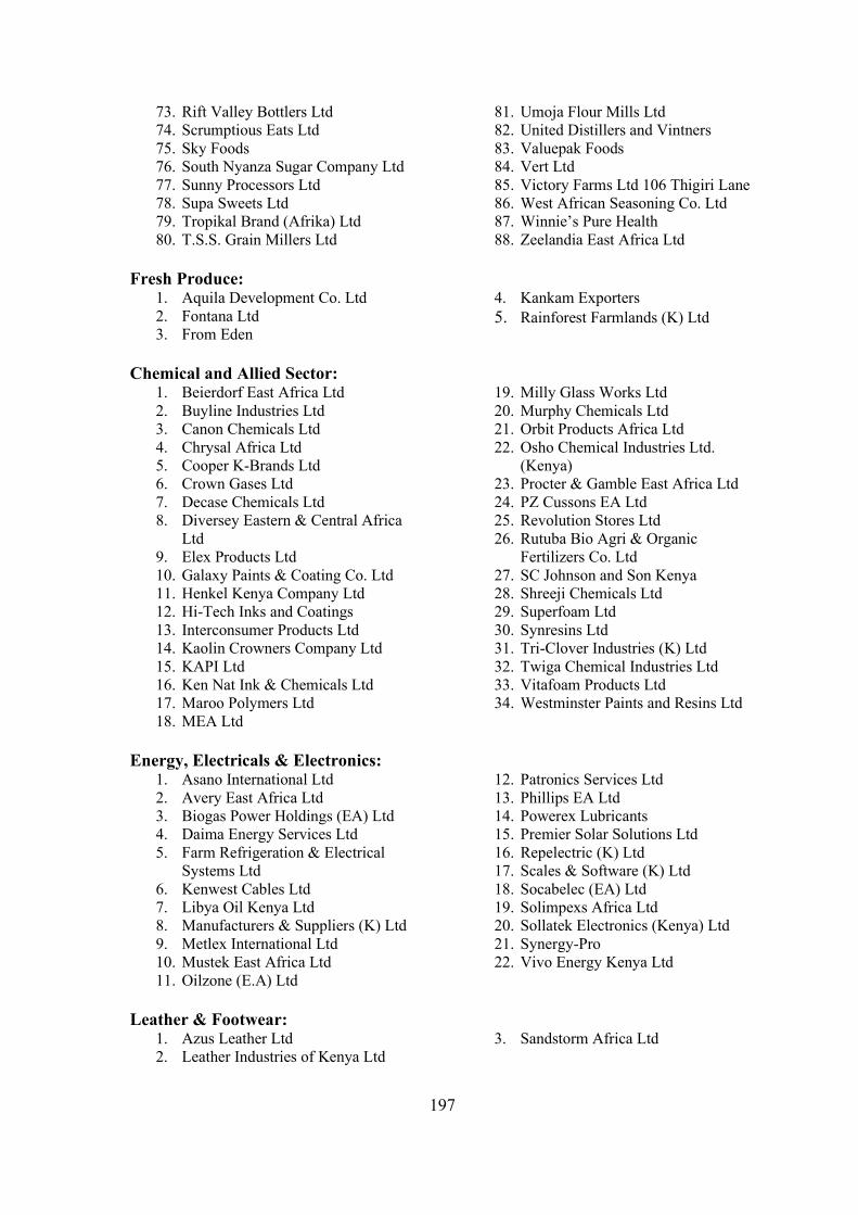
197

73. Rift Valley Bottlers Ltd

74. Scrumptious Eats Ltd

75. Sky Foods

76. South Nyanza Sugar Company Ltd

77. Sunny Processors Ltd

78. Supa Sweets Ltd

79. Tropikal Brand (Afrika) Ltd

80. T.S.S. Grain Millers Ltd

81. Umoja Flour Mills Ltd

82. United Distillers and Vintners

83. Valuepak Foods

84. Vert Ltd

85. Victory Farms Ltd 106 Thigiri Lane

86. West African Seasoning Co. Ltd

87. Winnie’s Pure Health

88. Zeelandia East Africa Ltd

Fresh Produce: 1. Aquila Development Co. Ltd

2. Fontana Ltd

3. From Eden

4. Kankam Exporters

5. Rainforest Farmlands (K) Ltd

Chemical and Allied Sector: 1. Beierdorf East Africa Ltd

2. Buyline Industries Ltd

3. Canon Chemicals Ltd

4. Chrysal Africa Ltd

5. Cooper K-Brands Ltd

6. Crown Gases Ltd

7. Decase Chemicals Ltd

8. Diversey Eastern & Central Africa

Ltd

9. Elex Products Ltd

10. Galaxy Paints & Coating Co. Ltd

11. Henkel Kenya Company Ltd

12. Hi-Tech Inks and Coatings

13. Interconsumer Products Ltd

14. Kaolin Crowners Company Ltd

15. KAPI Ltd

16. Ken Nat Ink & Chemicals Ltd

17. Maroo Polymers Ltd

18. MEA Ltd

19. Milly Glass Works Ltd

20. Murphy Chemicals Ltd

21. Orbit Products Africa Ltd

22. Osho Chemical Industries Ltd.

(Kenya)

23. Procter & Gamble East Africa Ltd

24. PZ Cussons EA Ltd

25. Revolution Stores Ltd

26. Rutuba Bio Agri & Organic

Fertilizers Co. Ltd

27. SC Johnson and Son Kenya

28. Shreeji Chemicals Ltd

29. Superfoam Ltd

30. Synresins Ltd

31. Tri-Clover Industries (K) Ltd

32. Twiga Chemical Industries Ltd

33. Vitafoam Products Ltd

34. Westminster Paints and Resins Ltd

Energy, Electricals & Electronics: 1. Asano International Ltd

2. Avery East Africa Ltd

3. Biogas Power Holdings (EA) Ltd

4. Daima Energy Services Ltd

5. Farm Refrigeration & Electrical

Systems Ltd

6. Kenwest Cables Ltd

7. Libya Oil Kenya Ltd

8. Manufacturers & Suppliers (K) Ltd

9. Metlex International Ltd

10. Mustek East Africa Ltd

11. Oilzone (E.A) Ltd

12. Patronics Services Ltd

13. Phillips EA Ltd

14. Powerex Lubricants

15. Premier Solar Solutions Ltd

16. Repelectric (K) Ltd

17. Scales & Software (K) Ltd

18. Socabelec (EA) Ltd

19. Solimpexs Africa Ltd

20. Sollatek Electronics (Kenya) Ltd

21. Synergy-Pro

22. Vivo Energy Kenya Ltd

Leather & Footwear: 1. Azus Leather Ltd

2. Leather Industries of Kenya Ltd

3. Sandstorm Africa Ltd

198

Metal & Allied Sector: 1. African Marine & General

Engineering Co. Ltd

2. Alloy Steel Casting Ltd

3. Arvind Engineering Ltd

4. Arshut Engineers Ltd

5. Blue Nile Wire Products Ltd

6. Brollo Kenya Ltd

7. Cook ‘N Lite Ltd

8. Corugated Sheets Ltd

9. Davis & Shirtliff Ltd

10. Doshi & Company Hardware Ltd

11. East Africa Glassware Mart Ltd

12. Fine Engineering Works Ltd

13. Friendship Container Manufacturers

Ltd

14. Greif Kenya Ltd

15. Heavy Engineering Ltd

16. Iron Art Ltd

17. Kenya General Industries Ltd

18. Kenya United Steel Company

(2006) Ltd

19. Laminate Tube Industries Ltd

20. Marine Crafts & Boat Repairs

21. Mecol Ltd

22. Mitsubishi Corporation Nairobi

Liaison Office

23. Naline Steel Works

24. Napro Industries Ltd

25. Orbit Engineering Ltd

26. Rolmil Kenya Ltd

27. Southern Engineering Co. Ltd

28. Standard Rolling Mills Ltd

29. Steelwool (Africa) Ltd

30. Tarmal Wire Products Ltd

31. Technoconstruct Kenya Ltd

32. Tononoka Rolling Mills Ltd

33. Towertech Africa Ltd

34. Viking Industries Ltd

35. Welding Alloys Ltd

36. Zenith Steel Fabricators Ltd

Motor Vehicles & Accessories: 1. Ace Motors Ltd

2. Associated Vehicle Assemblers Ltd

3. Autofine Filters & Seals Ltd

4. Bhachu Industries Ltd

5. Chui Auto Spring Industries Ltd

6. CMC Motors Group Ltd

7. Dodi Autotech (K) Ltd

8. General Motors East Africa Ltd

9. Igo Holdings Ltd

10. Kenya Vehicle Manufacturers Ltd

11. King-Bird (K) Ltd

12. Labh Singh Harnam Singh Ltd

13. Mash East Africa Ltd

14. Megh Cushion Industries Ltd

15. Pipe Manufacturers Ltd

16. Rockey Africa Ltd

17. Scania East Africa Ltd

18. Sohansons Ltd

19. Soroya Motors Spares

20. Toyota Tshusho East Africa Ltd

21. Transtrailers Ltd

22. Uni-Truck World Ltd

Paper and Board Sector:1. Adpak International Ltd

2. ASL Packaging Ltd

3. Autolitho Ltd

4. Brand Printers LtdCempack

Solutions Ltd

5. Colour Labels Ltd

6. De La Rue Currency and Security

Print Ltd

7. Dodhia Packaging Ltd

8. East Africa Packaging Industries Ltd

9. Elegant Printing Works Ltd

10. English Press Ltd

11. Euro Packaging Ltd

12. Green Pencils Ltd

13. Guaca Stationers Ltd

14. Juja Pulp & Paper Ltd

15. Kenafric Diaries Manufacturers Ltd

16. Kenya Stationers Ltd

17. Kul Graphics Ltd

18. Manipal International Printing Press

Ltd

19. Modern Lithographic (K) Ltd

20. Nation Media Group Ltd – Printing

Plant

21. Ndalex Digital Technology

22. Paper House of Kenya Ltd

23. Prime Cartons Ltd

24. Printpak Multi Packaging Ltd

25. Ramco Printing Works Ltd

26. Shri Krishana Overseas Ltd

27. Sintel Security Print Solutions Ltd

28. Statpack Industries Ltd

29. The Print Exchange

30. Tissue Kenya Ltd

199

31. Uneeco Paper Products Ltd

Pharmaceuticals & Medical Equipment: 1. African Cotton Industries Ltd

2. Benmed Pharmaceuticals Ltd

3. Biodeal Laboratories Ltd

4. Cosmos Ltd

5. Dawa Ltd

6. Glaxo Smithkline Kenya Ltd

7. Laboratory & Allied Ltd

8. Osschemie (K) Ltd

9. Questa Care Ltd

10. Revital Healthcare (EPZ) Ltd

11. Universal Corporation Ltd

Plastic and Rubber: 1. ACME Containers Ltd

2. Afro Plastics (K) Ltd

3. Bobmil industries Ltd

4. Cocorico Investments Ltd

5. Dune Packaging Ltd

6. Elgitread (Kenya) Ltd

7. Five Star Industries Ltd

8. General Plastics Ltd

9. Jamlam Industries Ltd

10. Jumbo Chem Kenya Ltd

11. Kamba Manufacturing (1986) Ltd

12. Kentainers Ltd

13. Kinpash Enterprises Ltd

14. Lakhir Plastics Ltd

15. Mega (EA) Plastics

16. Mombasa Polythene Bags Ltd

17. Ombi Rubber Rollers Ltd

Textiles and Apparels: 18. Plast Packaging Industries Ltd

19. Plastic and Rubber Industries Ltd

20. Polyflex Industries Ltd

21. Polly Propelin Bags Ltd

22. Prosel Ltd

23. Raffia Bags (K) Ltd

24. Rushabh Industries Ltd

25. Sanpac Africa Ltd

26. Shiv Enterprises (E) Ltd

27. Silpack Industries Ltd

28. Sols Inclination Ltd

29. Smartpack Limited

30. Super Manufacturers Ltd

31. Thermopak Ltd

32. Treadsetters Tyres Ltd

33. Vectus Kenya Ltd 34. Zaverchand Punja Ltd

1. Adpack Ltd

2. Alpha Knits Ltd

3. Bedi Investments Ltd

4. Brilliant Garments EPZ Ltd

5. Ethical Fashion Artisons EPZ Ltd

6. Gone Fishing Ltd

7. Insight Kenya

8. Kavirondo Filments Ltd

9. Kenya Shirts Manufacturing

Company Ltd

10. Kenya Trading (EPZ) Ltd

11. Kikoy Mall EPZ Ltd

12. Leeways Control Systems and

Suppliers

13. Long-Yun Ltd

14. Manchester Outfitters

15. New Wide Garments (K) Ltd

16. Panah Ltd

17. Penny Galore Ltd

18. Rivatex (East Africa) Ltd

19. Shin-Ace Garments Kenya (EPZ)

Ltd

20. Soko EPZ Ltd

21. Spin Knit Ltd

22. Spinners & Spinners Ltd

23. Squaredeal Uniforms Centre Ltd

24. Summit Fibres Ltd

25. Tarpo Industries Ltd

26. TSS Spinning and Weaving Ltd

27. United Aryan (EPZ) Ltd

28. World of Kikoys

Timber, Wood & Furniture: 1. Biashara Master Sawmills

2. Contrive Industries Ltd

3. Fine Wood Works Ltd

4. Furniture International Ltd

5. Little Cribs Ltd

6. Major Furniture

200

7. Panesar’s Kenya Ltd

8. Rai Plywoods (Kenya) Ltd

9. Shamco Industries Ltd

10. Timsales Ltd

11. Wood Makers (K) Ltd

Source: KAM, 2018

201

Appendix 5: Inter-Item Correlation Matrix between Latent Constructs of Reverse Logistics and Process Innovation

RLOS1 RLCE1 RLGS1 RLPLCA1 PIIS1 PIPRD1 PIPRE1 PIBVA1

RLOS1 1.000

RLCE1 .991** 1.000

RLGS1 .994** .990** 1.000

RLPLCA1 .620** .613** .639** 1.000

PIIS1 .988** .990** .989** .620** 1.000

PIPRD1 .991** .992** .992** .627** .989** 1.000

PIPRE1 .462** .440** .468** .694** .453** .454** 1.000

PIBVA1 .962** .966** .964** .620** .968** .963** .448** 1.000

**. Correlation is significant at the 0.01 level (2-tailed).

202

Appendix 6: Inter-Item Correlation Matrix between Latent Constructs of Reverse Logistics and Operational Performance

RLOS1 RLCE1 RLGS1 RLPLCA1 OPOFR1 OPPL1 OPDMA1 OPLTA1

RLOS1 1.000

RLCE1 .991** 1.000

RLGS1 .994** .990** 1.000

RLPLCA1 .620** .613** .639** 1.000

OPOFR1 .662** .649** .676** .864** 1.000

OPPL1 .676** .657** .683** .801** .837** 1.000

OPDMA1 .583** .564** .596** .833** .846** .878** 1.000

OPLTA1 .620** .602** .633** .823** .855** .832** .861** 1.000


203

Appendix 7: Inter-Item Correlation Matrix between Latent Constructs of Reverse Logistics and Competitive Advantage

RLOS1 RLCE1 RLGS1 RLPLCA1 CACL1 CAMS1 CABR1 CARI1

RLOS1 1.000

RLCE1 .991** 1.000

RLGS1 .994** .990** 1.000

RLPLCA1 .620** .613** .639** 1.000

CACL1 .654** .641** .666** .933** 1.000

CAMS1 .669** .655** .683** .865** .903** 1.000

CABR1 .648** .624** .655** .820** .842** .877** 1.000

CARI1 .654** .644** .667** .951** .994** .907** .845** 1.000


204

Appendix 8: Inter-Item Correlation Matrix between Latent Constructs of Process Innovation and Operational Performance

PIIS1 PIPRD1 PIPRE1 PIBVA1 OPOFR1 OPPL1 OPDMA1 OPLTA1

PIIS1 1.000

PIPRD1 .989** 1.000

PIPRE1 .453** .454** 1.000

PIBVA1 .968** .963** .448** 1.000

OPOFR1 .659** .662** .694** .654** 1.000

OPPL1 .658** .668** .744** .662** .837** 1.000

OPDMA1 .569** .573** .782** .564** .846** .878** 1.000

OPLTA1 .611** .611** .752** .608** .855** .832** .861** 1.000


205

Appendix 9: Inter-Item Correlation Matrix between Latent Constructs of Process Innovation and Competitive Advantage

PIIS1 PIPRD1 PIPRE1 PIBVA1 CACL1 CAMS1 CABR1 CARI1

PIIS1 1.000

PIPRD1 .989** 1.000

PIPRE1 .453** .454** 1.000

PIBVA1 .968** .963** .448** 1.000

CACL1 .647** .654** .715** .643** 1.000

CAMS1 .668** .663** .692** .662** .903** 1.000

CABR1 .638** .637** .779** .636** .842** .877** 1.000

CARI1 .649** .654** .723** .644** .994** .907** .845** 1.000


206

Appendix 10: Inter-Item Correlation Matrix between Latent Constructs of Operational Performance and Competitive

Advantage

OPOFR1 OPPL1 OPDMA1 OPLTA1 CACL1 CAMS1 CABR1 CARI1

OPOFR1 1.000

OPPL1 .837** 1.000

OPDMA1 .846** .878** 1.000

OPLTA1 .855** .832** .861** 1.000

CACL1 .881** .793** .818** .867** 1.000

CAMS1 .903** .832** .827** .922** .903** 1.000

CABR1 .840** .871** .899** .927** .842** .877** 1.000

CARI1 .886** .807** .830** .869** .994** .907** .845** 1.000


207

Appendix 11: Letter for Data Collection

reverse logistics, process innovation, operational

Documents

Transcript of reverse logistics, process innovation, operational