Tuck School ofBusiness at Dartmouth

Working Paper No.01-05

June 2002

Retained Equity, Investment Decisions andPrivate Information

DIEGO GARCIATuck School of Business at Dartmouth

This paper can be downloaded from theSocial Science Research Network Electronic Paper Collection:

http://papers.ssrn.com/abstract_id=289801

Retained equity, investment decisions and private information∗

Diego Garcıa†

First draft: February 2001

June 26, 2002

Abstract

This paper considers an optimal contracting problem between an informed risk-averse

agent and a set of risk averse principals. An informed entrepreneur approaches a group of

outside investors to sell them an equity share in the firm motivated by risk-sharing gains.

In contrast to the Leland and Pyle (1977) model I give the bargaining power to the outside

investors and I assume that, on top of the risk-allocation decision, the investors and the

entrepreneur also negotiate over a real investment decision in the firm. It is shown that the

introduction of this investment decision may destroy the main qualitative implication of the

Leland and Pyle model: the quantity retained by the entrepreneur may not be increasing

in his private information. The model’s results point to potential specification problems

in empirical studies trying to confirm the Leland-Pyle hypothesis, and more generally

endogeneity problems that may arise when testing adverse-selection hypotheses based on

one-dimensional problems when the parties can use multi-dimensional mechanisms. A new

set of empirical predictions on the relation between retained equity and investment and

firm characteristics is also discussed.

JEL classification: D82, G32.

Keywords: retained equity, mechanism design, multi-dimensional screening.

∗The latest version of this paper can be downloaded from http://diego-garcia.dartmouth.edu.†Correspondence information: Diego Garcıa, Tuck School of Business Administration, Hanover NH 03755-

9000, tel: (603) 646-3615, fax: (603) 646-1308, email: Diego.Garcia@Dartmouth.edu.

1

1 Introduction

The idea that retained equity signals the underlying quality of a firm dates back to Leland and

Pyle (1977). In their seminal paper, Leland and Pyle describe a setting in which an informed

entrepreneur approaches a group of outside investors to sell them an equity share in the firm.

The cash flows are not affected by this decision, and the motivation for the trade is based on

risk-sharing benefits: outside investors are risk-neutral, whereas the entrepreneur is risk-averse.

They showed that by retaining some equity of the firm, the high-valuation types can separate

themselves from lower-valuation types in a signalling equilibrium.

The theme of costly signalling by retaining a larger equity share has sprung up a signifi-

cant literature in corporate finance. There have been several extensions to the Leland and Pyle

(1977) model, e.g. by considering several stages in the capital raising process (see Welch (1989),

Grinblatt and Hwang (1989)), by allowing for the possibility of non-linear contracts (DeMarzo

and Duffie (1997), Chemmanur and Fulghieri (1997), Stein (1992)), by seeking “robust” con-

tracts (Ravid and Spiegel (1997), Admati and Pfleiderer (1984)), by focusing on particular

aspects of the IPO process (Mauer and Senbet (1992), Spatt and Srivastava (1991)). For an

excellent survey of this signalling literature see Daniel and Titman (1995). In all these models

the retention rate of the informed party acts as a signal of the quality of the underlying as-

sets: these theories predict that there should be an unambiguous positive relation between the

quantity retained by the entrepreneur and the value of the firm. This property of the optimal

mechanism is shared by many other models based in asymmetric information considerations

outside the going-public literature (e.g. venture capital financing, standard principal-agent

models).

In this paper I model jointly the risk allocation and investment decisions that the en-

trepreneur and the investors negotiate over. It is surprising that the investment decision is

usually analyzed as an exogenous decision:1 the entrepreneur is assumed to need a fixed amount

to fund a project, and he pockets any extra money put up by investors (see for example the

original Leland and Pyle (1977) paper). In contrast to models with a one-dimensional screen-

ing variable, I allow the investors and the entrepreneur to negotiate over both the allocation1Krasker (1986) considers the investment decision of a firm in a Myers and Majluf (1984) framework, but

does not study the retained equity decision facing the entrepreneur (or current equityholders). Bajaj, Chan, andDasgupta (1998) also study investment and retained equity decisions, although in their model only the retainedequity acts as a signal. Other recent papers in which the investment decision is explicitly modelled, but whichfocus on a different set of issues, are Bachmann (2001) and Povel and Raith (2001).

2

of risk (how much equity the entrepreneur retains) and a real investment decision in the firm.

It is shown that the introduction of this investment decision may destroy the main qualitative

implication of the Leland and Pyle model: the quantity held by the entrepreneur may not be

increasing in the quality or information possessed by the firm. In Leland and Pyle (1977),

and models with a fixed investment decision, incentive compatibility requires the quantity

held by the entrepreneur to be monotonic, which generates the usual empirical hypothesis.

In contrast, once the agents bargain on both the investment and the retained equity deci-

sions, the incentive compatibility constraint only requires the product of the equity retained

and an increasing function of the investment decision to be monotonic. The intuition for the

non-monotonicity result is that if the investment function is steep enough, then the quantity

retained by the entrepreneur can be decreasing in his type without violating incentive com-

patibility. For example, if risk-sharing gains are important, then pushing the retained equity

closer to its first-best value by introducing this non-monotonicity may be optimal (see Figure

1 for an illustration). Moreover, both retained equity and the investment decision increase the

informational rents earned by the agent. This creates a direct informational effect for retained

equity, just as in the one-dimensional case, but also an indirect effect by affecting the marginal

informational cost of the investment decision. This effect in itself is sufficient to generate a

non-monotone retained equity function.

I assume that the investors make the first move and have the bargaining power in the

negotiations. The non-competitive behavior of the investors distinguishes this model from the

standard signalling paradigm (e.g. Leland and Pyle (1977)). It should be noted that the change

in bargaining power does not destroy the main implications of the standard signalling models:

in section 3.1 I show that if the investment decision is fixed then the standard increasing

retained equity function is the optimal mechanism. There are several ways to motivate the

non-competitive assumption. On one hand, the underwriting industry is often argued to be

closer to a monopoly than to a competitive market.2 Therefore, if we interpret the underwriter

and the actual outside investors as a single player, this would favor a model in which it is the

entrepreneurs who face a “take-it-or-leave-it” offer: competition does not make the outsiders

make zero profits. One possible justification for this is given by the long-term agency literature,

and by the literature on reputation. The extent to which investors and investment bankers

interact during several periods, whereas entrepreneurs only occasionally tap the market for2The seemingly collusive behavior of investment bankers in setting underwriting spreads (Chen and Ritter

(2000)) supports this view.

3

funds (in many cases just once), and the fact that underwriters have an incentive to keep a

good reputation to attract new clientele, should mitigate possible agency problems between

the investors and the underwriters. Moreover, several papers report favorable treatment to

institutional investors by underwriters (see Ljungqvist and Wilhelm (2000) and the references

cited in Biais, Bossaerts, and Rochet (1998)). Therefore, it seems like an interesting alternative,

if not a more natural assumption, to let the investors make the first move about the mechanism

to be played and the securities to be traded. A similar view is taken in Biais, Bossaerts, and

Rochet (1998), who also study a non-competitive IPO allocation model from a mechanism

design perspective.3 Finally, given the results in the common agency literature (Stole (1995),

Martimort (1996), Stole (1997b), Biais, Martimort, and Rochet (2000)), the results should be

robust and carry over to other types of market power assumptions.

The paper’s main results are casted in a simple setting where the main motivation for trade

is risk-sharing gains, and the investor’s investment is a crucial input in the production process.

Venture capital financing agreements are probably closer to the setting in the main body of

the paper, whereas a sale of a well-established firm may have a different flavor in terms of the

outside opportunities for the entrepreneur. In order to differentiate between these two cases I

study a variant of the model where there is a type-dependent reservation utility constraint. The

optimal solution may be distorted in a different direction than in the case where the outside

opportunity was type-independent, 4 but the main qualitative features discussed above carry

over with few caveats. Lastly, the model is also generalized to include an effort choice by the

agent after the contract has been signed.5 In a static version of the Holmstrom and Milgrom

(1987) model with private information I show that the previous results apply, giving a richer

set of implications.

The non-monotonicity result outlined above is a warning to studies in which adverse-

selection theories are rejected because the data do not support a positive relationship between3The informational structure and the agents’ preferences in that paper are significantly different from those

to be presented here. The focus of Biais, Bossaerts, and Rochet (1998) is on the role of institutional (informed)investors in the IPO process. The entrepreneur is assumed to maximize the proceeds from the sale of securities,so the investment decision is a black-box in their model. Benveniste and Spindt (1989) and Benveniste andWilhelm (1990) also take a mechanism design perspective when analyzing the IPO process, but assume thatthe underwriter acts in the best interest of the entrepreneur.

4To be precise the incentive-compatibility constraints in the main body of the paper always bind down-wards. If the outside opportunities of the agent are type-dependent it is possible for the incentive compatibilityconstraint to bind upwards.

5This can also be interpreted as the agent having some discretion over the investment decision after signingthe contract.

4

the quantity held by the informed party and the value of the firm. The model in this paper,

based on asymmetric information, would explain this empirical finding by simply noting that

with multiple screening variables (in this case the investment decision and the quantity retained

by the entrepreneur), we should not expect these quantities to be related in a monotonic fashion

with the signal, even though in the same model with a single screening instrument this would

be the case. Probably more important is to realize that the investment decision and the

quantity retained by the entrepreneur are both endogenous quantities. It is customary to run

multi-variate regressions on a particular variable of interest.6 Once we include the size of the

investment and/or the quantity retained by the entrepreneur in the right-hand side of our

regression equation biases are likely to appear due to the endogeneity of these two variables.

This line of reasoning suggests that more work needs to be done in establishing what variables

entrepreneurs and investors bargain about,7 and on estimating these models empirically taking

into account the endogeneity of these variables. The model’s optimal contracts offer a rich set

of “structural” empirical predictions.

The paper shares many aspects of standard moral hazard models with private information

(Sappington (1983), Besanko and Sibley (1991), Reichelstein (1992)). Also closely related is the

capital budgeting literature, where elements of adverse selection and moral hazard are usually

present (Harris, Kriebel, and Raviv (1982), Antle and Eppen (1985)). Bernardo, Cai, and Luo

(2001) present a model that shares many of the same features as the one described in this

paper, since it includes a flexible investment decision on top of a sharing-rule that motivates

effort.8 The parametric restrictions in the solutions they present rule out the possibility of

non-monotonic allocations that are shown to be optimal here.9 Section 5.1 extends the model

in the main body of the paper to deal with effort considerations, and further discusses how it

complements the results in Bernardo, Cai, and Luo (2001).

The paper is also related to the literature on multi-dimensional mechanism design problems

(see Rochet and Stole (2000) for a survey). Matthews and Moore (1987) extend the monopolist6This variable is usually total firm value (e.g. Downes and Heinkel (1982)) or underpricing at the IPO stage

(e.g. Michaely and Shaw (1994)).7This paper uses the equity retained and the investment decision as the two critical elements of the problem.

In Chemmanur and Fulghieri (1997) on the other hand we have equity retained and warrants issued as the twovehicles for signalling information.

8Sung (2001) studies a similar setting to the one in Bernardo, Cai, and Luo (2001), but focusing on differentaspects of the optimal contracts.

9Bernardo, Cai, and Luo (2001) depart from the model in this paper by assuming risk-neutrality for theagent and including a “private benefits” (perk consumption) element in the agent’s utility function. In all otherrespects the models are formally equivalent.

5

pricing problem of Mussa and Rosen (1978) to allow the monopolist to discriminate through

both price and the use of warranties. In the same fashion, investors in this model can use

both the retained equity and the amount investment as different instruments to screen agents.

Matthews and Moore (1987) show, by means of an example, that non-monotonic allocations

may be optimal. Garcıa (2001) analyzes a general mechanism design model with quasi-linear

preferences showing that models with multi-dimensional allocation rules may have very dif-

ferent properties than those in which the principal can only use one single element of the

allocation vector.

In section 2 the basic model is introduced, and the solution under symmetric information is

discussed. Section 3 discusses the optimal contracts when either investment or retained equity

are fixed. In section 4 the optimal mechanism under asymmetric information is presented. It is

then shown that this mechanism may entail a non-monotonic relationship between the equity

retained by the entrepreneur and firm quality. In section 5, I consider different extensions to

the basic model, and analyze a set of new empirical implications.

2 The model and first-best solution

2.1 The economic setting

An entrepreneur owns an idea that, after an initial investment I, generates a cash flow at some

future date given by

V = v(I, s) + ε; (1)

where I is the amount invested at date 0, s is a random variable that measures the private

information of the entrepreneur, and ε is an independent mean zero (non-degenerate) random

variable with variance σ2. The private information, which I will also allude to as the signal

or type of the agent, is distributed on an interval10 [s, s], and has density and distribution

functions g(s) and G(s), with associated hazard rate H(s) = g(s)/(1 − G(s)). It will be

assumed that g(s) > 0 for all s ∈ [s, s]. The inverse of the hazard rate will be denoted by µ(s).

The entrepreneur needs to get the necessary funds, I, from outside investors to finance10The assumption of s having a continuous support is simply made in order to get closed-form solutions:

assuming a discrete state space for the signal would not alter the results of the paper.

6

the project.11 I will assume, without loss of generality, that the discount rate for the project

cash flows is zero. In exchange for investing in the firm, the investors get a fraction (1− q) of

the final cash flows. With this notation q denotes the fraction of the project’s final cash flows

retained by the entrepreneur. On top of this contingent compensation the entrepreneur gets a

fixed wage t. It should be noted that the investors’ total cash outflow is given by t+ I, i.e. the

model explicitly accounts for investment into the firm and cash paid out to the entrepreneur.12

Both the entrepreneur and the outside investors have mean-variance preferences, with risk-

aversion parameters RE and RI respectively. The utility (conditional on the signal) for the

agent, the entrepreneur, is given by13

UA(q, t, I, s) = qv(I, s)− RE2q2σ2 + t. (2)

and for the principal, the investors,

UP (q, t, I, s) = (1− q)v(I, s)− RI2

(1− q)2σ2 − t− I.

Note that the function UP (·) incorporates the benefits of holding (1 − q) of the final cash

flows, as well as the cost of the investment decision at date 0, I, and the wage paid to the

entrepreneur t.

The following assumptions will be made throughout the main body of the paper:14

• The cash flows from the firm can be ordered through the signal s according to first-order

stochastic dominance, vs ≥ 0.

• The function v(I, ·) : R→ R is increasing and concave, vI ≥ 0, vII < 0.

• The “single-crossing property” with respect to investment holds, vsI ≥ 0.

• The hazard rate of the distribution of s is monotonically increasing, H ′(s) ≥ 0.11This seems appropriate as long as the agent has no capital of his own. All the results in the model will go

through as stated if the agent had some funds K, and the investors finance the rest of the venture I −K.12As discussed in the introduction, this generalizes the usual assumption, made when the investment decision

is fixed, that the informed party keeps the proceeds of the asset sale above those needed for investing.13It is straightforward to check that a model with CARA preferences and Gaussian returns would yield this

preference representation.14I will use subscripts to denote derivatives, and omit the arguments of the functions when there is no room

for ambiguity.

7

• The following derivatives exist and have the given signs: vss ≤ 0, vsII ≥ 0, vssI ≤ 0.

• Non-negativity conditions: σ2RI−µ(s)vs(I(s), s) > 0, limI↓0 vI(I, s) =∞, and limI↑∞ vI(I, s) =

0,

• Quasi-concavity of the principal’s objective function: µ(s)2v2sI ≤ −σ2(RE + RI)(vII −

qvsIIµ(s)).

The first four assumptions seem uncontroversial. The single-crossing property is typically

made in models of asymmetric information. This assumption, higher signals being associated

with higher marginal value of the investment decision, is a necessary and sufficient condition for

the investment decision in the firm to be non-decreasing in the signal in a first-best world. The

monotone-hazard rate assumption is also commonly made in the mechanism design literature.

Moreover, it is well-known that many commonly used distributions satisfy this property (see

Bagnoli and Bergstrom (1989)).

The non-negativity conditions guarantee that the solution to the principal’s problem is

interior, i.e. the non-negativity constraints will not bind. The conditions on the non-negativity

of q and I state that the benefits from risk-sharing and investment outweigh the costs generated

through the informational rents earned by the informed entrepreneur. A upper bound on µ(s)

can easily be obtained from these conditions that would make the constraints not bind. In

a similar fashion, lower bounds on the parameter values for RE , RI , σ2 and on the function

v(·) could be found so that the constraints do not bind for large enough values of any of these

parameters. Similarly, I ignore the possibility that the principal may not want to offer financing

to a subset of the types, so the solution will always be interior. In section 5.2 I generalize both

these assumptions.

The rest of the assumptions are of technical type. The condition vss ≤ 0 guarantees that if

the amount of investment I is fixed, then the quantity retained by the entrepreneur under the

optimal contract will be monotonic in his type (see Proposition 2). The last condition simply

guarantees that there exists a solution to the principal’s problem when there are multiple

screening variables.15

15It is literally a necessary and sufficient condition for the second-order conditions to the principal’s optimiza-tion problem to hold, see Proposition 5.

8

2.2 The investor’s problem

In contrast to Leland and Pyle (1977), it is assumed that the investors make the first move and

approach the entrepreneur. Using the revelation principle (e.g. Myerson (1979)) the investors

can restrict attention to truthful mechanisms in which the message space is restricted to be

the private information possessed by the agent.

The principal’s problem is then given by

maxq(·),t(·),I(·)

∫ s

sUP (q(s), t(s), I(s), s)g(s)ds (3)

such that

UA(q(s), t(s), I(s), s) ≥ u ∀s ∈ [s, s]; (4)

and

UA(q(s), t(s), I(s), s) ≥ UA(q(s), t(s), I(s), s) ∀s, s ∈ [s, s]; (5)

with the non-negativity constraints q(s) ≥ 0 and I(s) ≥ 0.

Constraint (4) bounds from below the expected utility for the entrepreneur. The quantity

u can be interpreted as the best alternative for the agent outside his relationship with the

investors, and is assumed to be small enough so that the principal’s participation constraint

does not bind.16 Equation (5) captures the truth-telling constraint in the direct revelation

mechanism: for any pair of signals s and s, an entrepreneur who received a signal s must

be at least as well off by announcing s than by announcing any other valuation s. The non-

negativity constraint on q(s) can be motivated on the grounds of the entrepreneur having a

free-disposal technology (i.e. being able to destroy output). This is a standard assumption

in the agency and security design literature (see DeMarzo and Duffie (1997) for a discussion).

The main qualitative features of the model’s solution will not be affected by the non-negativity

constraints, as discussed in section 5.2.16See section 5.2 for more general specifications of the reservation utility profile of the agent and for an analysis

of the case where the principal’s participation constraint may bind.

9

2.3 First-best solution

The first-best problem is the solution to (3) subject to (4), ignoring the incentive compatibility

constraint (5). This would be the optimal financing arrangement between the entrepreneur

and the investors if the private information were common knowledge to all parties. The next

proposition characterizes the optimal mechanism in this case.

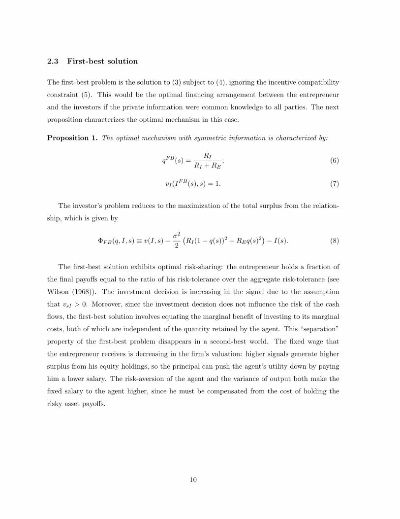
Proposition 1. The optimal mechanism with symmetric information is characterized by:

qFB(s) =RI

RI +RE; (6)

vI(IFB(s), s) = 1. (7)

The investor’s problem reduces to the maximization of the total surplus from the relation-

ship, which is given by

ΦFB(q, I, s) ≡ v(I, s)− σ2

2(RI(1− q(s))2 +REq(s)2

)− I(s). (8)

The first-best solution exhibits optimal risk-sharing: the entrepreneur holds a fraction of

the final payoffs equal to the ratio of his risk-tolerance over the aggregate risk-tolerance (see

Wilson (1968)). The investment decision is increasing in the signal due to the assumption

that vsI > 0. Moreover, since the investment decision does not influence the risk of the cash

flows, the first-best solution involves equating the marginal benefit of investing to its marginal

costs, both of which are independent of the quantity retained by the agent. This “separation”

property of the first-best problem disappears in a second-best world. The fixed wage that

the entrepreneur receives is decreasing in the firm’s valuation: higher signals generate higher

surplus from his equity holdings, so the principal can push the agent’s utility down by paying

him a lower salary. The risk-aversion of the agent and the variance of output both make the

fixed salary to the agent higher, since he must be compensated from the cost of holding the

risky asset payoffs.

10

3 Optimal one-dimensional mechanisms

3.1 Screening with retained equity

This section considers the problem in which the principal can design a mechanism {q(s), t(s)},

where the investment decision I is fixed. This corresponds most closely to the models in the

signalling literature (i.e. Leland and Pyle (1977)), in which only retained equity is considered

as a possible signal of quality.

The principal’s problem is then given by the program (3)-(5) with I(s) = I ∈ R+ fixed, plus

the non-negativity constraints q(s) ≥ 0. The following proposition characterizes the optimal

quantity retained by the entrepreneur in this case.

Proposition 2. The optimal mechanism, when it involves an interior solution, is given by the

following retained equity function

q(s) =bPσ

2 − µ(s)vs(I, s)(RI +RE)σ2

= qFB − µ(s)vs(I, s)(RI +RE)σ2

. (9)

The tradeoff is familiar: on one hand there are the risk-sharing benefits; on the other, the

informational rents that the agent gets in equilibrium. Retained equity is distorted downwards

from its first-best level to economize on the informational rents earned by the entrepreneur.

Just as in the Leland and Pyle (1977) model, here the quantity retained by the entrepreneur is

an increasing function of the quality of the firm, which guarantees the incentive compatibility

of the mechanism. Therefore, giving the bargaining power to the investors does not change

the main qualitative features of their model. The main difference lies in the split of the total

surplus from the relationship, which introduces possibility that the non-negativity constraint

will bind. This will occur for either large uncertainty about the agent’s type (large µ(s)), small

asset uncertainty (small σ2). Intuitively, the non-negativity constraint will not bind as long

as there are sufficient gains from risk-sharing as compared to the costs associated with private

information.

3.2 Screening with a real investment decision

This section considers the problem in which the principal can design a mechanism {I(s), t(s)},

where the amount retained by the entrepreneur q is fixed. The principal’s problem is given by

11

the program (3)-(5) with q(s) = q ∈ (0, 1) fixed, plus the non-negativity constraint I(s) ≥ 0.

The following proposition identifies the optimal mechanism.

Proposition 3. The optimal investment function, when it involves an interior solution, is

characterized by

vI(I(s), s) = 1 + µ(s)qvsI(I(s), s). (10)

As in the previous section, the investment decision is distorted downwards because of the

informational rents earned by the entrepreneur. Moreover, agents with higher signals get a

higher allocation of capital - a necessary condition for incentive compatibility to hold. The last

term in equation (10) captures the marginal informational costs of the investment decision.

Proposition 3 further implies that

dI

ds= −vsI(1− µ

′q)− qµvssI(vII − µqvsII)

;

so that the investment decision is always increasing in s under the assumptions of the paper,

e.g. as long as the single-crossing property, vsI ≥ 0, holds, and vssI ≤ 0.

4 Optimal mechanisms with asymmetric information

In this section the problem of screening agents using both the quantity retained by the agent

and the investment decision in the firm is studied. First I analyze the set of allocations that

can be implemented by the principal. Then I proceed to characterize the optimal mechanisms

and discuss its properties.

4.1 Characterization of implementable mechanisms

The existence of private information conditions the set of allocations that can be implemented

by the principal. In this subsection I characterize the set of feasible retained equity and

investments functions. Let U(s, s) ≡ UA(q(s), t(s), I(s), s) denote the utility for the agent

when he announces signal s and his true private information is s. Define the expected utility

of an agent under a truthful mechanism as

u(s) ≡ U(s, s)|s=s = q(s)v(I(s), s)− RE2q(s)2σ2 + t(s).

12

The next proposition characterizes the set of implementable mechanisms in this model in

terms of this indirect utility function.

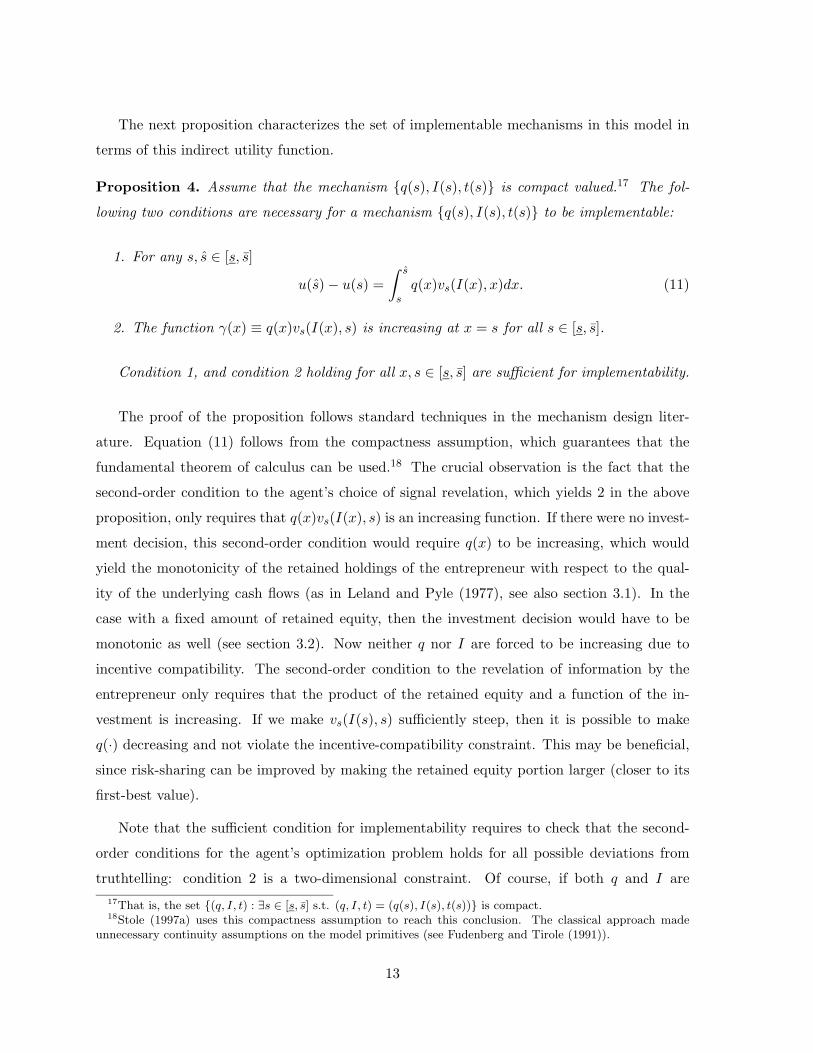
Proposition 4. Assume that the mechanism {q(s), I(s), t(s)} is compact valued.17 The fol-

lowing two conditions are necessary for a mechanism {q(s), I(s), t(s)} to be implementable:

1. For any s, s ∈ [s, s]

u(s)− u(s) =∫ s

sq(x)vs(I(x), x)dx. (11)

2. The function γ(x) ≡ q(x)vs(I(x), s) is increasing at x = s for all s ∈ [s, s].

Condition 1, and condition 2 holding for all x, s ∈ [s, s] are sufficient for implementability.

The proof of the proposition follows standard techniques in the mechanism design liter-

ature. Equation (11) follows from the compactness assumption, which guarantees that the

fundamental theorem of calculus can be used.18 The crucial observation is the fact that the

second-order condition to the agent’s choice of signal revelation, which yields 2 in the above

proposition, only requires that q(x)vs(I(x), s) is an increasing function. If there were no invest-

ment decision, this second-order condition would require q(x) to be increasing, which would

yield the monotonicity of the retained holdings of the entrepreneur with respect to the qual-

ity of the underlying cash flows (as in Leland and Pyle (1977), see also section 3.1). In the

case with a fixed amount of retained equity, then the investment decision would have to be

monotonic as well (see section 3.2). Now neither q nor I are forced to be increasing due to

incentive compatibility. The second-order condition to the revelation of information by the

entrepreneur only requires that the product of the retained equity and a function of the in-

vestment is increasing. If we make vs(I(s), s) sufficiently steep, then it is possible to make

q(·) decreasing and not violate the incentive-compatibility constraint. This may be beneficial,

since risk-sharing can be improved by making the retained equity portion larger (closer to its

first-best value).

Note that the sufficient condition for implementability requires to check that the second-

order conditions for the agent’s optimization problem holds for all possible deviations from

truthtelling: condition 2 is a two-dimensional constraint. Of course, if both q and I are17That is, the set {(q, I, t) : ∃s ∈ [s, s] s.t. (q, I, t) = (q(s), I(s), t(s))} is compact.18Stole (1997a) uses this compactness assumption to reach this conclusion. The classical approach made

unnecessary continuity assumptions on the model primitives (see Fudenberg and Tirole (1991)).

13

increasing then the mechanism is incentive compatible. Even though this monotonicity restric-

tion on the retained equity and investment functions avoids the technical difficulties of dealing

with a two-dimensional incentive compatibility constraint, it also restricts the analysis of the

problem in a non-trivial way.

If the mechanism is differentiable,19 then condition 2 in Proposition 4 becomes

q′(s)vs(I(s), s) + q(s)vsI(I(s), s)I ′(s) ≥ 0; ∀s, s ∈ [s, s]. (12)

The fact that only the product of the quantity held by the entrepreneur and the slope of the

value function enter the previous expression will be the key ingredient to show that q(s) may

not be monotonic: if I(s) increases sufficiently fast it may be possible for q(s) to be decreasing

without violating the second-order conditions to the agent’s problem.

Example 1. I will use the following specification for the production function in a set of

examples throughout the paper

v(I, s) = a1I + a2s+ a3Is− a4I2

2.

The parameter a2 measures the pure impact of information on valuation, whereas a3 cap-

tures the marginal value of the investment decision with respect to information. Equation (12)

restricts the set of implementable mechanisms to those satisfying

q′(s) ≥ −(a3q(s)I ′(s)a2 + a3I(s)

)∀s ∈ [s, s].

It is important to note that the two-dimensional contraint in 2 in Proposition 4 becomes

a one-dimensional constraint in this particular example, since the left-hand side of (12) is

independent of s.20 The above equation specifies a lower bound for the derivative of q, but it

does allow the retained equity function to be decreasing, since this lower bound will generically

be a negative number. �19The differentiability of the optimal mechanism follows from Proposition 5.20This simplification is due to the linearity of the value function in this example: see Garcıa (2001) for a

discussion of this property.

14

4.2 Characterization of the optimal mechanisms

The next proposition characterizes the optimal mechanism ignoring the non-negativity con-

straints q(s) ≥ 0 and I(s) ≥ 0, and the monotonicity constraint (12).

Proposition 5. The optimal mechanism, when it involves an interior solution, is characterized

by the following equations:

q(s) =σ2RI − µ(s)vs(I(s), s)

σ2(RI +RE); (13)

vI(I(s), s) = 1 + µ(s)vsI(I(s), s)q(s). (14)

Following the standard terminology in the mechanism design literature we can define the

“virtual surplus” (see Myerson (1981)) as

Φ(q, I, s) = v(I, s)− I − σ2

2(REq

2 +RI(1− q)2)− qµ(s)vs(I, s). (15)

Comparing (15) with (8) we see that the virtual surplus is simply equal to the total surplus

from the relationship minus the term q(s)µ(s)vs(I(s), s), which measures the marginal cost to

the investors in terms of the informational rents earned by the entrepreneur under the optimal

mechanism. This term distorts the solution from the first-best case: on top of maximizing

risk-sharing benefits and the expected value of the investment decision, the investor takes into

account in her optimization problem the informational rents that the entrepreneur earns due

to his informational advantage. It is also immediate from the above expressions that both

the quantity retained and the investment decision will be smaller in a second-best world as

compared to the solution without asymmetric information (see Proposition 1).

Now we are in a position to give some further intuition for the optimality of a non-monotonic

retained equity function. Equation (27), the first-order condition with respect to q, has the

standard risk-sharing term plus a second one due to informational considerations: just as in

the one-dimensional case a higher q(s) increases the rents earned by all types above s. But now

there is also an indirect effect: the informational rents term in (26) is also dependent on the

retained equity decision. This interdependency between retained equity and the investment

decision due to informational rents considerations drives the potential optimality of a non-

monotone retained equity function.

Before proceeding with the analysis of these optimality conditions, I rule out the possibility

15

of having corner solutions. The above proposition ignores the monotonicity constraint on γ(s)

(see Proposition 4). This is the typical approach to solve this type of mechanism design problem

(see Fudenberg and Tirole (1991) or Stole (1997a)): after having solved the problem ignoring

this constraint, it is customary to put sufficient structure into the model that guarantees that

the constraint will not bind. It seems feasible to solve the full problem using the “ironing”

procedure of Mussa and Rosen (1978), but since these technicalities are not crucial for the

main results of the paper,21 I will simply assume that the parameters of the model allow us to

ignore the monotonicity constraint (12). One possible justification for this is presented in the

next proposition.

Proposition 6. As either σ2, RE or RI become large, the monotonicity constraint (12) does

not bind.

As long as the risk-sharing gains are sufficiently large, we can then safely ignore the mono-

tonicity constraint (12). This is a robust sufficient condition: similar ones could be given

involving the relative magnitudes of µ and v and their derivatives.

I conclude this section by solving the model in Example 1.

Example 2. It is straightforward to compute the optimal allocation of risk and investment

under the specification of the model in Example 1 using the results from Proposition 5:22

q(s) =σ2RI − µ(s)(a2 + a3I)

σ2(RE +RI);

I(s) =(a1 + a3s− 1)σ2(RE +RI)− a3µ(s)(σ2RI − µ(s)a2)

a4σ2(RE +RI)− µ(s)2a23

.

4.3 General properties of the optimal mechanism

This section presents a set of comparative statics of the previous model, and relates it to

empirical predictions. The next proposition shows that the mechanism approaches the first-

best outcome as we move up the quality scale.

Proposition 7. Under the optimal mechanism, as s ↑ s:21Just note that if the monotonicity constraint (12) binds, then the optimal mechanism immediately implies

non-monotonic allocations.22The second-order conditions to the problem restrict the parameters under consideration to µ(s)2a2

3 ≤σ2(RI + RE)a4. The non-negativity constraints further require that σ2RI ≥ µ(s)(a2 + a3I(s)), and that(a1 + a3s− 1)σ2(RE +RI) ≥ a3µ(s)(σ2RI − µa2).

16

1. The optimal investment and allocation of risk tend to the first-best outcome.

2. Both q(s) and I(s) are increasing functions.

The intuition for these results is based on the fact that the incentive-compatibility con-

straints bind “downwards”: the allocation to the highest type s will not change other agents’

informational rents so investment and risk-sharing are not distorted from their first-best levels.

It is worth noticing that the derivatives of the functions q and I do not converge to those in the

first-best world, although they do have the same (positive) sign at the top of the type space.

This result implies that in the cross-section of firms we should see the Leland-Pyle signalling

hypothesis holding at least for the highest valued cohort. This seems to be a prediction novel

to this paper. Carrying out its correspondent empirical test would be a natural experiment to

confirm the appropriateness of the model.

The main result of the paper is given in the next proposition.

Proposition 8. If the monotonicity constraint (12) does not bind, then the following condition

is necessary and sufficient for q(s) to be non-monotonic:

(vII − µqvsII)(−µ′vs − µvss) + µv2sI(1− µ′q)− qµ2vsIvsII ≥ 0. (16)

The quantity allocated to the entrepreneur q(s) is non-monotonic in a (weakly) generic

sense.23

The derivation of (16) is straightforward given the solution from Proposition 5. The proof

goes through by showing that: (i) condition (16) holds for an open set of the model’s parame-

ters; (ii) these parameter values can be chosen so the second-order conditions are satisfied and

the monotonicity constraint (12) does not bind. This yields the (weakly) generic statement

that q(s) will be non-monotonic under the optimal mechanism.

The intuition for this result is based again in the form of the informational rents. Decreasing

q does have a direct negative impact in the informational rents gained by the agent, as in the

one-dimensional case. But once investment can also be used to screen agents, there is an

additional indirect effect in lowering q through its effect in I. From the first-order conditions it

is easy to check that dI/dq = µ(s)vsI/(vII − qµ(s)vsII) < 0, i.e. the indirect effect of lowering23By weak genericity of a property I mean that it holds for an open set of the model’s parameters.

17

q is to raise I, which increases the rents earned by the agent. This effect in itself is sufficient

to generate a non-monotonic retained equity function, as the following examples illustrate.

Example 3. In the specification of Example 1, retained equity will be non-monotonic if and

only if (s− s)a23(1 + q(s)) ≥ a4(a2 + a3I(s)). The investment decision function will always be

monotonically increasing in this particular variant of the model (see Proposition 9 below).24

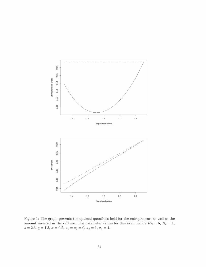
Figure 1 presents the optimal quantities held for the entrepreneur, as well as the amount

invested in the venture, for the following parameter values: RE = 5, RI = 1, a1 = a2 = 0,

a3 = 1, a4 = 4, σ2 = 0.5. The first-best levels for these variables is also plotted (as a dotted

line). It is straightforward to check that for these parameter values the second-order conditions

are satisfied, so that the interior solution is indeed the optimal one (i.e. the monotonicity

constraint does not bind). Note how the deviation of the investment from first-best levels

increases as we move down the quality scale: the slope of the investment decision is highest

for the lower range of the signals. This increased slope makes the incentive compatibility hold

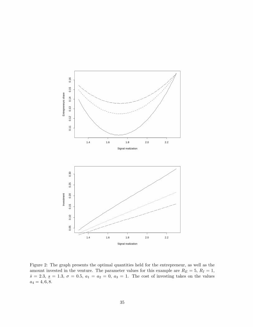
even though the quantity allocated to the entrepreneur is decreasing on that range. Figure 2

plots the optimal mechanism for the parameter values in the previous example, changing the

cost of investing from a4 = 4 to a4 = 8. As the investment cost is raised the function q(s)

becomes flatter. This is due to the fact that distorting the allocation of risk is more expensive,

relative to distorting the investment decision, as we increase a4 (similar comparative static

results apply to increasing σ). �

Few other general statements can be made. As a matter of fact, it would be possible to

have a model where the amount invested in the venture is decreasing in the private information

in a (weakly) generic sense.25 Note that this can only happen when the quantity retained is an

increasing function of the signal, i.e. for cases ruled out by Proposition 8. The next proposition

gives a set of sufficient conditions for the investment decision to be increasing in the agent’s

type.

Proposition 9. The invesment function is monotonically increasing for all s if either:

(i) σ2, or RE, or RI are sufficiently large.

(ii) |µ′(s)| ≤ 1 and |vss| < ε for ε sufficiently close to zero.24In order to see this note that a necessary condition for I(s) to be non-monotonic is that σ2(RE+RI)(1+q) ≤

µ(a2 + a3I). Since µ(a2 + a3I) ≤ σ2RI (from the non-negativity conditions), it is immediate that I ′(s) ≥ 0.25See Garcıa (2001) for a discussion of monotonicity properties in an abstract mechanism design problem with

quasi-linear preferences, which formally subsumes the model in this paper.

18

Under fairly natural conditions the investment decision is monotonic in the agent’s type,

where this is not the case for the retained equity function. Intuitively, as long as the risk sharing

gains are sufficiently important, the investment function will be the main vehicle for screening.

Moreover, this is still the case under condition (ii), which only involves the distribution of the

private information, namely the slope of its hazard rate, and a mild technical assumption on

the concavity of the function v.

I conclude this section giving a set of simple conditions under which the retained equity

function is non-monotone.

Proposition 10.

(a) The retained equity function becomes monotonically increasing as the pure marginal value

of information, vs, becomes large.

(b) As the marginal value of information with respect to the investment decision becomes

large, vsI ↑ ∞, the retained equity decision becomes non-monotone.

(c) Under the conditions of Proposition 9, as µ(s) ↑ ∞, the retained equity decision becomes

non-monotone.

The proposition gives two conditions on the nature of the informational asymmetry, whether

it affects vs or vsI , which have very different implications in terms of the monotonicity prop-

erties of the retained equity decision. These predictions seem to be novel to this paper. It is

intuitive that as the pure marginal value of information goes up most of the screening should

be done through the retained equity decision. Under condition (a), it is easy to check that

the investment decision may actually become non-monotone. Condition (b) has the effect of

increasing the sensitivity of the investment decision with respect to the private information.

Since the sign of q is given by the sign of −µ′vs − µvss − µvsII′, parameters that tend to

increase I ′ will immediately give a non-monotone retained equity function. Similarly, as long

as I ′(s) ≥ 0, increasing the importance of informational rents considerations (raising µ(s))

brings the optimality of bring q back closer to its first-best level: the screening is done solely

by the investment decision.

Example 4. Continuing with the example introduced previously, Figure 3 plots the optimal

mechanism changing the pure value of information from a2 = 0 to a2 = 0.16. As this value is

raised the optimal retained equity is shifted down, and eventually loses its non-monotonicity

19

properties. Figure 4 changes the interaction parameter a3. The retained equity function is also

shifted down in this case, but note how this function is still non-monotone for large values of

a3, as established by the previous proposition. Figure 5 changes the risk-aversion parameter

for the agent from RE = 5 to RE = 15. Again, this change has an important effect in the

level (and shape) of the retained equity function, but it does not eliminate the presence of

non-monotonic allocation rules.

5 Extensions

In the model discussed in previous sections the agent did not play an active role after the

contract was signed. This is an important simplification that is relaxed in the next section,

where it is assumed the agent participates on the properties of final output by exerting effort, in

a standard moral hazard model. I show that the problem can be mapped into a similar model

to the one discussed this far. I then examine the case where the non-negativity constraints

and/or the principal’s participation constraint may bind.

5.1 Effort considerations

The purpose of this section is to show that the non-monotonicity result is not specific to the risk-

sharing problem with private information discusseed in the previous sections. Namely, I will

consider a standard moral hazard problem, where the quantity allocated to the entrepreneur

is motivated by effort eliciting considerations, and show that, in a weakly generic sense, the

optimal mechanism will involve a non-monotone retained equity function.

The value of the assets now depends not only on the investment decision and the private

information possessed by the entrepreneur, but also on an effort decision, that I will denote by

e. I assume that the final value of the firm is given by

V = v(I, e, s) + ε.

The agent incurs a personal cost of c(e), so his utility, conditional on a signal realization

s, is given by

UA(q, t, I, s, e) = qv(I, e, s) + t− 12REq

2σ2 − c(e).

20

I will assume in this section that the risk-aversion of the principal is zero,26 so his objective

function becomes

UP (q, t, I, s, e) = (1− q)v(I, e, s)− t− I.

The problem that the principal faces is given by equations (3)-(5) with the additional

constraint:

e(I, q, s) ∈ arg maxeUA(q, t, I, s, e) (17)

As long as the function e(·) is uniquely determined by (17) we can substituted back into

the value and cost functions and set v(I, q, s) ≡ v(I, e(I, q, s), s) and c(I, q, s) ≡ c(e(I, q, s)).

The model reduces to one in which the final payoff is given by

V = v(I, q, s) + ε;

with the agent’s preferences given by

UA(q, t, I, s) = qv(I, q, s) + t− 12REq

2σ2 − c(I, q, s).

The total surplus from the relationship is given by ΦFB(I, q, s) ≡ v(I, q, s) − c(I, q, s) −12REq

2σ2. Therefore the only difference with the model in the main body of the paper is

that the retained equity decision q also has an effect on the mean value of the assets under

management, due to the incentives that it creates for effort.

The following proposition characterizes the optimal solution in this version of the model.27

Proposition 11. The principal’s problem reduces to the pointwise maximization of the follow-

ing function

maxq,I

Φ(q, I, s) = v(q, I, s)− RE2q2σ2 − c(q, I, s)− µ(s) (qvs(q, I, s)− cs(q, I, s)) ; (18)

26This assumption is for simplicity, and to show that the model does not require a risk-averse investor to havean interior solution once we introduce costly effort. The results for the case where the investor is risk-aversecan be easily derived adapting the proof of the next proposition.

27The proof is omitted, since it follows along the same lines as the previous propositions.

21

such that the following monotonicity constraint holds for all s, s ∈ [s, s]:28

(vs(q, I, s) + qvqs(q, I, s)− cqs(q, I, s)) q′ + (qvIs(q, I, s)− cIs(q, I, s)) I ′ ≥ 0. (19)

The effort level is given by (17), where q and I solve (18).

As before, the function Φ(q, I, s) can be interpreted as the “virtual surplus” from the

relationship between the entrepreneur and the investors. The first three terms in (18) are the

total surplus from the relationship, whereas the last term captures the informational rents

earned by the entrepreneur. It is worth comparing equation (19) with (12): now the effects

of information on the marginal values of v(·) and c(·) also play a part of the monotonicity

constraint, due to the effort considerations.

Rather than developing a new set of results for the most general model with costly effort,

I settle on illustrating that the non-monotonicity property of previous sections holds in this

version of the model by means of an example.

Example 5. Consider the case where v(I, s, e) = sI − 12I

2 + e, and that c(e) = 12ce

2. Using

the results from Proposition 11, the optimal mechanism, at an interior solution, is given by

q(s) =1− c(s− 1)µ(s)

1 + cREσ2 − cµ(s)2; (20)

I(s) = s− q(s)µ(s)− 1. (21)

In order to see that q(s) may be non-monotonic, first note that the sign of q′(s) is given by

the sign of

(−cµ(s)− c(s− 1)µ′(s)

) (1 + cREσ

2 − cµ(s)2)

+ 2cµ(s)µ′(s) (1− c(s− 1)µ(s)) . (22)

For s close to s the above expression is positive, since the last term goes to zero and the

first-term becomes positive. To see that it is possible to have this expression negative, just

note that the second term is always negative (at an interior solution), and that the first term

is negative when −cµ(s)− c(s− 1)µ′(s) < 0 (which happens in a weakly generic sense). Since

e(s) = q(s)/c in this example, it is immediate that the effort incurred by the agent is also a28In equation (19) I omit the argument s from the functions q and I and their derivatives for notational

simplicity: the constraint is generally, as in condition 2 of Proposition 4, a two-dimensional constraint.

22

non-monotone function of his type.

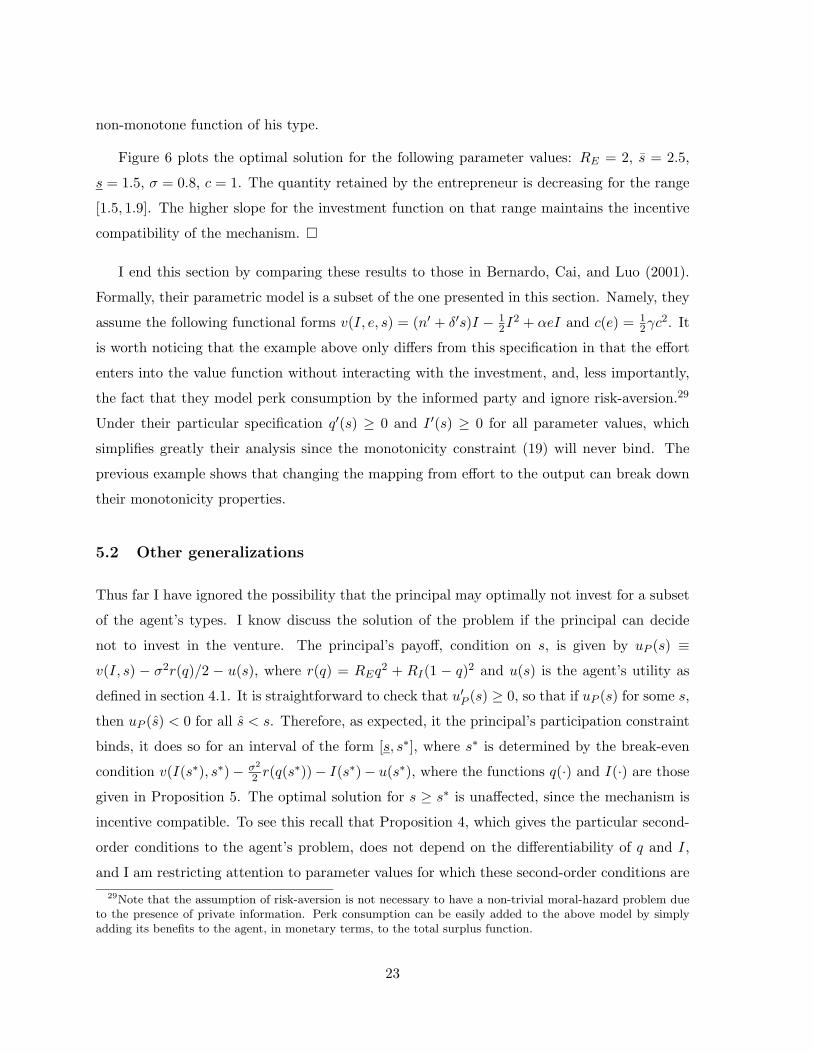
Figure 6 plots the optimal solution for the following parameter values: RE = 2, s = 2.5,

s = 1.5, σ = 0.8, c = 1. The quantity retained by the entrepreneur is decreasing for the range

[1.5, 1.9]. The higher slope for the investment function on that range maintains the incentive

compatibility of the mechanism. �

I end this section by comparing these results to those in Bernardo, Cai, and Luo (2001).

Formally, their parametric model is a subset of the one presented in this section. Namely, they

assume the following functional forms v(I, e, s) = (n′ + δ′s)I − 12I

2 + αeI and c(e) = 12γc

2. It

is worth noticing that the example above only differs from this specification in that the effort

enters into the value function without interacting with the investment, and, less importantly,

the fact that they model perk consumption by the informed party and ignore risk-aversion.29

Under their particular specification q′(s) ≥ 0 and I ′(s) ≥ 0 for all parameter values, which

simplifies greatly their analysis since the monotonicity constraint (19) will never bind. The

previous example shows that changing the mapping from effort to the output can break down

their monotonicity properties.

5.2 Other generalizations

Thus far I have ignored the possibility that the principal may optimally not invest for a subset

of the agent’s types. I know discuss the solution of the problem if the principal can decide

not to invest in the venture. The principal’s payoff, condition on s, is given by uP (s) ≡

v(I, s) − σ2r(q)/2 − u(s), where r(q) = REq2 + RI(1 − q)2 and u(s) is the agent’s utility as

defined in section 4.1. It is straightforward to check that u′P (s) ≥ 0, so that if uP (s) for some s,

then uP (s) < 0 for all s < s. Therefore, as expected, it the principal’s participation constraint

binds, it does so for an interval of the form [s, s∗], where s∗ is determined by the break-even

condition v(I(s∗), s∗)− σ2

2 r(q(s∗))− I(s∗)− u(s∗), where the functions q(·) and I(·) are those

given in Proposition 5. The optimal solution for s ≥ s∗ is unaffected, since the mechanism is

incentive compatible. To see this recall that Proposition 4, which gives the particular second-

order conditions to the agent’s problem, does not depend on the differentiability of q and I,

and I am restricting attention to parameter values for which these second-order conditions are29Note that the assumption of risk-aversion is not necessary to have a non-trivial moral-hazard problem due

to the presence of private information. Perk consumption can be easily added to the above model by simplyadding its benefits to the agent, in monetary terms, to the total surplus function.

23

satisfied (see Proposition 6).

The paper has also been silent on the reservation utility that the mechanism must satisfy.

In general, one may expect that the agent’s outside opportunities will depend on the private

information that he possesses. A particularly natural specification of this reservation utility

profile is to set u(s) = max(v(0, s)− σ2RE/2, 0), i.e. the payoff that the agent would receive if

he were to retain all the firm’s cash flows without any further investment. Of course, if v(0, s)

is small then all the previous results apply. Actually, the following condition is sufficient for the

previous results to go through as stated: q(s)vs(I(s), s)− vs(0, s) ≥ 0. Note that the previous

equation is simply the derivative of u(s) − u(s). Intuitively, as long as the agetn’s utility

increases faster under the optimal mechanism than without investment, then the participation

constraint will only bind for the lowest type. The only role played by v(0, s) is in setting the

reservation wage for the lowest type, i.e. u = v(0, s)− σ2RE/2.

The problem with an arbitrary function v(0, s) is significantly more complicated. In princi-

ple the participation constraint oculd bind at different subsets of [s, s] (see Jullien (2000)). It is

possible that this constraint only binds for the highest type. This would occur, for example, if

v is independent of I. If this were the case, then the principal’s problem can be shown to reduce

to the pointwise maximization of ΦFB(I, q, s) + H(s)qvs(I, s), where H(s) ≡ F (s)f(s) . The distor-

tion due to informational rents now encourages “over production,” as the principal makes it

harder for low-types to mimic high-types. One can check that q′(s) = H ′(s)vs+ Hvss+HvsII′

for the optimal mechanism. Now a positively sloped investment function makes the optimal

retained equity function more likely to be increasing, in contrast to the case where the incentive

compatibility constraints bind downwards. It is worth noticing that if vss < 0, as assumed

throughout, it is still possible for q to be non-monotone, and this would now occur for high

realizations of s.30

To summarize, a general type-dependent reservation utility for the agent can change sig-

nificantly the optimal mechanisms. The paper’s results apply directly to firms for which the

investment decision has a strong informational component, i.e. there is a significant gap be-

tween vs(I, s) and vs(0, s). Firms for which investment, or more generally some type of input

from the investors (e.g. expertise from a venture capitalist), is a crucial part to the success of

the enterprise fall within this category. In contrast, firms that already have a strong source of

revenues (without further investment) are more likely to face distortions along the lines of the30Note that the lowest-type s consumes efficiently in this case.

24

discussion in the previous paragraphs.

The case of the non-negativity constraints on q and I can be dealt similarly to the problem

with a participation constraint for the principal, by introducing state-dependent constraints.

Consider first the case where both q and I given by Proposition 5 are monotonically increas-

ing. When one of the non-negativity constraints binds, then the optimal q or I is given by

the expressions from section 3, otherwise they are characterized by Proposition 5. A more

interesting question is which of the two non-negativity constraints will bind first. Bernardo,

Cai, and Luo (2001) showed that under their model specification the non-negativity constraint

on q will always bind before that on I. As the following example shows, this will not be the

case in the model in this paper: the agent could get some contingent compensation before any

investment.

Example 6. In the context of Example 1 the retained equity function is non-negative if and

only if σ2RI − µ(s)a2 ≥ 0; whereas the investment function is non-negative if and only if

(a1 + a3s− 1)− a3κµ(s)(σ2RI − µ(s)a2) ≥ 0. It is immediate that either of these constraints

could bind first. The optimal solution can be described as follows. Let sq ≡ max{s : q(s) = 0},

sI ≡ max{s : I(s) = 0}. If we let s = max{sI , sq}, then the optimal solution will be given

by Proposition 5 for s ≥ s. If s = sq, then for all s < s we have q(s) = 0 and I(s) =

(a1 +a3s− 1)/a4 (the first-best level of investment). If s = sI , then for s < s we have I(s) = 0

and q(s) = RIRI+RE

− µ(s)a2

σ2(RE+RI). �

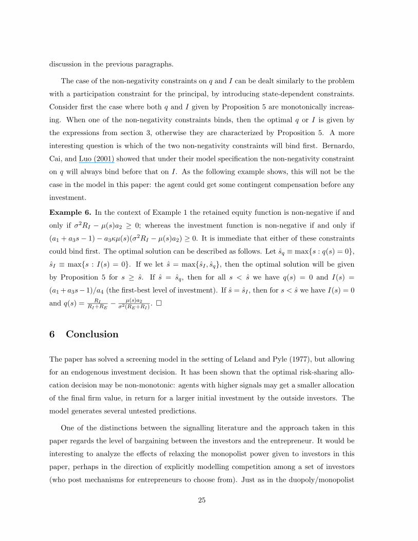
6 Conclusion

The paper has solved a screening model in the setting of Leland and Pyle (1977), but allowing

for an endogenous investment decision. It has been shown that the optimal risk-sharing allo-

cation decision may be non-monotonic: agents with higher signals may get a smaller allocation

of the final firm value, in return for a larger initial investment by the outside investors. The

model generates several untested predictions.

One of the distinctions between the signalling literature and the approach taken in this

paper regards the level of bargaining between the investors and the entrepreneur. It would be

interesting to analyze the effects of relaxing the monopolist power given to investors in this

paper, perhaps in the direction of explicitly modelling competition among a set of investors

(who post mechanisms for entrepreneurs to choose from). Just as in the duopoly/monopolist

25

case, we would expect decreases in the distortion generated from the informational rents earned

by the entrepreneur (from the first-best case scenario). It seems plausible to pursue this line

of research using similar techniques to those in common agency literature (see Stole (1995),

Martimort (1996), Stole (1997b), Biais, Martimort, and Rochet (2000)).

Another interesting extension would be to analyze a model where the private information

is multi-dimensional (for a model of the IPO process where this type of problem arises see

Chemmanur and Fulghieri (1997)). The techniques in the literature (Rochet and Chone (1998),

Rochet and Stole (2000), Wilson (1993)) seem to suggest that the optimal mechanisms would

involve bunching of middle types (a positive-measure subset getting the same mix of financial

securities) and complete separation of high-types. The precise direction of the distortions

caused by multi-dimensional asymmetric information in an entrepreneurial setting seems to

deserve further attention.

26

Appendix

Proof of proposition 1. Since the participation constraint will bind, it is immediate that

t(s) = u+RE2q(s)2σ2 − q(s)

(I(s)s− cI

2

2

).

This allows us to eliminate t(s) from the principal’s objective function. Her problem then

becomes maxI(s),q(s) ΦFB(q, I, s), where ΦFB is given by (8). The equations in the proposition

follow immediately from the first-order conditions to the above optimization problem.

Proof of proposition 4. First, I’ll show necessity. Equation (5), that constrains type s from

mimicking type s, can be rearranged to yield

u(s) ≥ u(s) + q(s) [v(I(s), s)− v(I(s), s)]

Using this constraint together with the incentive compatibility constraint that restricts type s

from picking the mechanism for type s, we obtain

q(s) [v(I(s), s)− v(I(s), s)] ≥ u(s)− u(s) ≥ q(s) [v(I(s), s)− v(I(s), s)] (23)

From (23) it is immediate that q(s)vs(I(s), s) must be increasing. Moreover, taking the limit

as s → s, we get that u′(s) = q(s)vs(I(s), s) at all points where q(s)vs(I(s), s) is continuous

(which is everywhere except possibly a countable set of points since the function is monotonic).

From the compactness of the mechanism (which makes u(s) uniformly continuous), we can

apply the fundamental theorem of calculus to get (11).

In order to proof sufficiency simply note that if q(x)vs(I(x), s) is increasing for all x, s ∈ [s, s]

then the mechanism is incentive compatible by the argument above.

Proof of proposition 5. From Proposition 4, the incentive compatibility constraint boils

down to

u(s) = u+∫ s

sq(x)vs(I(x), x)dx = q(s)v(I(s), s)− RE

2q(s)2σ2 + t(s). (24)

27

Using (24) to solve for t(s), the principal’s problem becomes

maxq(s),I(s)

∫ s

s

(ΦFB(q(s), I(s), s)−

∫ s

sq(x)vs(I(x), x)dx

)g(s)ds. (25)

As usual, the participation constraint, given by (4), will bind for the lowest valuation s.

Integrating by parts the term inside the integral in (25), it is immediate that the principal’s

problem reduces to the pointwise maximization of (15).

The characterization of an interior solution is given by the following two first-order condi-

tions:

vI(I(s), s) = 1 + q(s)vsI(I(s), s)µ(s); (26)

−σ2(REq(s)−RI(1− q(s)))− vs(I(s), s)µ(s) = 0. (27)

The equations in the proposition follow from these first-order conditions.

Proof of proposition 6. The monotonicity constraint is I ′qvsI ≥ −q′vs, which after some

algebra becomes

−[σ2(RE +RI)(vsI − µ′qvsI − µqvssI) + µvsI(µ′vs + µvss)

]qvsI

≤ vs[(vII − µqvsII)(−µ′vs − µvss) + µv2

sI(1− µ′q)− qµ2vsIvsII]

(28)

Since vsI(I(s), s) − µ′(s)q(s)vsI(I(s), s) − µ(s)q(s)vssI(I(s), s) > 0 for all s, s ∈ [s, s], we

see that the above constraint holds as σ2(RE + RI) ↑ ∞, since all other terms are bounded

when taking this limit. Moreover, all other conditions for an interior solution will also be met

as σ2 →∞.

Proof of proposition 7. The convergence to the first-best outcome is immediate from the

expressions in Propositions 1 and 5 (see also equations (8) and (15)).

From (13) and (14) we have

q′(s) =1

σ2(RE +RI)(−µ′vs − µvss − µvsII ′

)(29)

28

I ′(s) = −vIs (1− qµ′ + µq′)− vssIqµvII − vsIIqµ

(30)

From the above two expressions it is immediate that as µ(s) ↓ 0 both q and I are increasing

functions.

Proof of proposition 8. Note that since Proposition 7 established that q′(s) > 0 for s

sufficiently large, it is sufficient to show that there exists an open set of parameters for which

q′(s) < 0 for some s. Using the expressions in the proof of proposition 7 to solve for q′(s), we

see that q′(s) ≤ 0 if and only if condition (16) holds. We need to show that there exists an open

set of parameter values for which (16) holds without violating the conditions that guarantee

an interior solution in Proposition 5 (the non-negativity constraints) and the monotonicity

constraint on q(x)vs(I(x), s). From Proposition 6 we know that the monotonicity constraint

will not be binding as σ2 →∞. Moreover, taking this limit does not violate any of the second-

order conditions to the principal’s problem. Therefore, as long as (16) holds, the optimal

retained equity function will be non-monotonic under the conditions of Proposition 6.

Proof of proposition 9. From (29) and (30) we get that

I ′(s) = −vsI(1− qµ′ + µ(µ′vs + µvss)κ)− qµvssI

vII − qµvsII + v2sIµ

2κ(31)

where κ ≡ 1/(σ2(RE + RI)). Since vssI ≥ 0, it follows that I ′(s) ≥ 0 for all s if 1 − qµ′ +

κµ(µ′vs + µvss) > 0. Since the first two terms in this expression are positive, (i) is immediate.

To see that (ii) is also sufficient, note that RI/(RE + RI) − κµvs ≥ 0 (since q ≥ 0), i.e.

κµvs is bounded by 1. Therefore, under the conditions in (ii) I ′(s) ≥ 0 as claimed.

Proof of proposition 10.

Immediate by inspection of equation (29).

29

References

Admati, A. R., and P. Pfleiderer, 1984, “Robust Financial Contracting and the Role of Venture

Capitalists,” Journal of Finance, 49(2), 371–402.

Antle, R., and G. D. Eppen, 1985, “Capital Rationing and Organizational Slack in Capital

Budgeting,” Management Science, 31(2), 163–174.

Bachmann, R., 2001, “The Pricing of Initial Public Offerings when IPO Size and Investment

Choice are Endogenous,” working paper, University of Amsterdam.

Bagnoli, M., and T. Bergstrom, 1989, “Log-Concave Probability and its Applications,” working

paper, University of Michigan.

Bajaj, M., Y.-S. Chan, and S. Dasgupta, 1998, “The relationship between ownership, financing

decisions and firm performance: A signaling model,” International Economic Review, 39(3),

723–744.

Benveniste, L., and P. Spindt, 1989, “How investment bankers determine the offer price and

allocation of new issues,” Journal of Financial Economics, 24, 343–361.

Benveniste, L., and W. Wilhelm, 1990, “A comparative analysis of IPO proceeds under alter-

native regulatory environments,” Journal of Financial Economics, 28, 173–207.

Bernardo, A. E., H. Cai, and J. Luo, 2001, “Capital Budgeting and Compensation with Asym-

metric Information and Moral Hazard,” Journal of Financial Economics, 61(3), 311–344.

Besanko, D., and D. S. Sibley, 1991, “Compensation and Transfer Pricing in a Principal-Agent

Model,” International Economic Review, 32(1), 55–68.

Biais, B., P. Bossaerts, and J.-C. Rochet, 1998, “An Optimal IPO Mechanism,” working paper,

CalTech.

Biais, B., D. Martimort, and J.-C. Rochet, 2000, “Competing Mechanisms in a Common Value

Environment,” Econometrica, 68(4), 799–837.

Chemmanur, T. J., and P. Fulghieri, 1997, “Why Include Warrants in New Equity Issues? A

Theory of Unit IPOs,” Journal of Financial and Quantitative Analysis, 32(1), 1–24.

30

Chen, H.-C., and J. R. Ritter, 2000, “The Seven Percent Solution,” Journal of Finance, 55(3),

1105–1131.

Daniel, K., and S. Titman, 1995, “Financing Investment Under Asymmetric Information,”

in Handbooks in Operations Research and Management Science, volume 9, Finance, ed. by

R. Jarrow, V. Maksimovic, and W. Ziemba. North-Holland, Amsterdam.

DeMarzo, P. M., and D. Duffie, 1997, “A Liquidity-Based Model of Security Design,” working

paper, Stanford University.

Downes, D., and R. Heinkel, 1982, “Signaling and the Valuation of Unseasoned New Issues,”

Journal of Finance, 37, 1–10.

Fudenberg, D., and J. Tirole, 1991, Game Theory. MIT Press, Cambridge, Mass.

Garcıa, D., 2001, “Monotonicity in direct revelation mechanisms,” working paper, Amos Tuck

School of Business, Dartmouth College.

Grinblatt, M., and C. Y. Hwang, 1989, “Signalling and the Pricing of New Issues,” Journal of

Finance, 44(2), 393–420.

Harris, M., C. Kriebel, and A. Raviv, 1982, “Asymmetric Information, Incentives and Intrafirm

Resource Allocation,” Management Science, 28(6), 604–620.

Holmstrom, B., and P. Milgrom, 1987, “Aggregation and Linearity in the Provision of In-

tertemporal Incentives,” Econometrica, 55, 303—328.

Jullien, B., 2000, “Participation constraints in adverse selection models,” Journal of Economic

Theory, 93(1), 1–47.

Krasker, W. S., 1986, “Stock Price Movements in Response to Stock Issues under Asymmetric

Information,” Journal of Finance, 41(1), 93–105.

Leland, H. E., and D. H. Pyle, 1977, “Informational Asymmetries, Financial Structure, and

Financial Intermediation,” Journal of Finance, 32(2), 371–387.

Ljungqvist, A. P., and W. J. Wilhelm, 2000, “IPO allocations: discriminatory or discre-

tionary?,” working paper, New York University.

31

Martimort, D., 1996, “Exclusive dealing, common agency, and multiprincipals incentive the-

ory,” Rand Journal of Economics, 27(1), 1–31.

Matthews, S., and J. Moore, 1987, “Monopoly Provision of Quality and Warranties: An Ex-

ploration in the Theory of Multidimensional Screening,” Econometrica, 55(2), 441–467.

Mauer, D. C., and L. W. Senbet, 1992, “The Effect of the Secondary Market on the Pricing

of Initial Public Offerings: Theory and Evidence,” Journal of Financial and Quantitative

Analysis, 27(1), 55–79.

Michaely, R., and W. H. Shaw, 1994, “The Pricing of Initial Public Offerings: Tests of Adverse-

Selection and Signalling Theories,” Review of Financial Studies, 7(2), 279–319.

Mussa, M., and S. Rosen, 1978, “Monopoly and Product Quality,” Journal of Economic The-

ory, 18, 301–317.

Myers, S. C., and N. S. Majluf, 1984, “Corporate financing and investment decisions when

firms have information that investors do not have,” Journal of Financial Economics, 13,

187–221.

Myerson, R., 1981, “Optimal Auction Design,” Mathematics of Operations Research, 6(1),

58–73.

Myerson, R. B., 1979, “Incentive Compatibility and the Bargaining Problem,” Econometrica,

47(1), 61–73.

Povel, P., and M. Raith, 2001, “Optimal investment under financial constraints: the roles of

internal funds and asymmetric information,” working paper, University of Chicago.

Ravid, S. A., and M. Spiegel, 1997, “Optimal Financial Contracts for a Start-Up with Unlimited

Operating Discretion,” Journal of Financial and Quantitative Analysis, 32(3), 269–286.

Reichelstein, S., 1992, “Incentives in government contracts: an application of agency theory,”

Accounting Review, 67(4), 712–731.

Rochet, J.-C., and P. Chone, 1998, “Ironing, Sweeping, and Multidimensional Screening,”

Econometrica, 66(4), 783–826.

Rochet, J.-C., and L. A. Stole, 2000, “The Economics of Multidimensional Screening,” working

paper, University of Chicago.

32

Sappington, D., 1983, “Limited-liability contracts between principal and agent,” Journal of

Economic Theory, 29(1), 1–21.

Spatt, C., and S. Srivastava, 1991, “Preplay Communication, Participation Restrictions, and

Efficiency in Initial Public Offerings,” Review of Financial Studies, 4(4), 709–726.

Stein, J. C., 1992, “Convertible bonds as backdoor equity financing,” Journal of Financial

Economics, 32, 3–21.

Stole, L. A., 1995, “Nonlinear Pricing and Oligopoly,” Journal of Economics & Management

Strategy, 4(4), 529–562.

, 1997a, “Lectures on the Theory of Contracts and Organizations,” working paper,

University of Chicago.

, 1997b, “Mechanism Design under Common Agency: Theory and Applications,” work-

ing paper, University of Chicago, unpublished draft.

Sung, J., 2001, “Optimal Contracts under Moral Hazard and Adverse Selection: a Continuous-

Time Approach,” working paper, University of Illinois at Chicago.

Welch, I., 1989, “Seasoned Offerings, Imitation Costs, and the Underpricing of Initial Public

Offerings,” Journal of Finance, XLIV(2), 421–449.

Wilson, R. B., 1968, “On the theory of syndicates,” Econometrica, 36, 119—132.

Wilson, R. B., 1993, Nonlinear Pricing. Oxford University Press, New York.

33

Signal realization

Ent

repr

eneu

rs s

hare

1.4 1.6 1.8 2.0 2.2

0.11

0.12

0.13

0.14

0.15

0.16

Signal realization

Inve

stm

ent

1.4 1.6 1.8 2.0 2.2

0.05

0.10

0.15

0.20

0.25

0.30

Figure 1: The graph presents the optimal quantities held for the entrepreneur, as well as theamount invested in the venture. The parameter values for this example are RE = 5, RI = 1,s = 2.3, s = 1.3, σ = 0.5, a1 = a2 = 0, a3 = 1, a4 = 4.

34

Signal realization

Ent

repr

eneu

rs s

hare

1.4 1.6 1.8 2.0 2.2

0.11

0.12

0.13

0.14

0.15

0.16

Signal realization

Inve

stm

ent

1.4 1.6 1.8 2.0 2.2

0.05

0.10

0.15

0.20

0.25

0.30

Figure 2: The graph presents the optimal quantities held for the entrepreneur, as well as theamount invested in the venture. The parameter values for this example are RE = 5, RI = 1,s = 2.3, s = 1.3, σ = 0.5, a1 = a2 = 0, a3 = 1. The cost of investing takes on the valuesa4 = 4, 6, 8.

35

Signal realization

Ent

repr

eneu

rs s

hare

1.4 1.6 1.8 2.0 2.2

0.0

0.05

0.10

0.15

0.20

Signal realization

Inve

stm

ent

1.4 1.6 1.8 2.0 2.2

0.05

0.15

0.25

Figure 3: The graph presents the optimal quantities held for the entrepreneur, as well as theamount invested in the venture. The parameter values for this example are RE = 5, RI = 1,s = 2.3, s = 1.3, σ = 0.5, a1 = 0, a3 = 1, a4 = 4. The parameter a2 takes on the valuesa2 = 0, 0.08, 0.16.

36

Signal realization

Ent

repr

eneu

rs s

hare

1.4 1.6 1.8 2.0 2.2

0.0

0.05

0.10

0.15

0.20

Signal realization

Inve

stm

ent

1.4 1.6 1.8 2.0 2.2

0.0

0.1

0.2

0.3

0.4

0.5

Figure 4: The graph presents the optimal quantities held for the entrepreneur, as well as theamount invested in the venture. The parameter values for this example are RE = 5, RI = 1,s = 2.3, s = 1.3, σ = 0.5, a1 = 0.2, a2 = 0, a4 = 4. The parameter a3 takes on the valuesa3 = 0.8, 1, 1.2.

37

Signal realization

Ent

repr

eneu

rs s

hare

1.4 1.6 1.8 2.0 2.2

0.0

0.05

0.10

0.15

Signal realization

Inve

stm

ent

1.4 1.6 1.8 2.0 2.2

0.10

0.20

0.30

0.40

Figure 5: The graph presents the optimal quantities held for the entrepreneur, as well as theamount invested in the venture. The parameter values for this example are RI = 1, s = 2.3,s = 1.3, σ = 0.5, a1 = 0.2, a2 = 0, a3 = 1, a4 = 4. The risk-aversion parameter takes on thevalues RE = 5, 10, 15.

38

Signal realization

Ent

repr

eneu

rs s

hare

1.6 1.8 2.0 2.2 2.4

0.25

0.30

0.35

0.40

Signal realization

Inve

stm

ent

1.6 1.8 2.0 2.2 2.4

0.2

0.4

0.6

0.8

1.0

1.2

1.4

Figure 6: The graph presents the optimal quantities held for the entrepreneur, as well as theamount invested in the venture in the variant of the model with moral hazard. The parametervalues for this example are RE = 2, RI = 0, s = 2.5, s = 1.5, σ = 0.8, c = 1.

39