Electronic copy available at: http://ssrn.com/abstract=1285057

Resurrecting the Weak Credibility Hypothesis inModels of Exchange-Rate-Based Stabilization

Edward F. Buffie and Manoj Atolia

August 2007

1

Electronic copy available at: http://ssrn.com/abstract=1285057

ABSTRACT

We analyze how weak credibility affects the volatility of consumption spending in a model

of exchange-rate-based stabilization that allows for both durable and nondurable goods.

The inclusion of durables greatly improves the explanatory power of the weak credibility

hypothesis. The hypothesis can account for the main qualitative properties of the boom-bust

cycle provided the elasticity of durables expenditure with respect to Tobin’s q is greater than

the intertemporal elasticity of substitution. Moreover, the quantitative effects are very large.

In numerical simulations based on conservative assumptions about the expenditure share of

durables (20%) and wealth effects (none), aggregate consumption increases 12-28% during

the low-crawl phase and the real exchange rate appreciates 24-26%. In variants of the model

that incorporate supply effects, the consumption boom is equally strong but appreciation of

the real exchange rate rises to 30-40%.

JEL Codes: E31, E63, F41.

Keywords: credibility, exchange-rate-based stabilization, durables.

• Edward F. BuffieDepartment of EconomicsWylie Hall 105Indiana UniversityBloomington, IN 47405United States

Email: ebuffie@indiana.edu

• Manoj Atolia288 Bellamy BuildingDepartment of EconomicsFlorida State UniversityTallahassee, FL 32306

2

The announcement of an exchange-rate-based stabilization (ERBS) program is usually

followed by a pronounced surge in consumption spending. This stylized fact is the key to

understanding many of the other stylized facts associated with ERBS. It is a small step

from a consumption boom to a large current account deficit, large capital inflows, and

persistent, strong appreciation of the real exchange rate. If prices are sticky and firms in

the nontradables sector produce to demand, the consumption boom also fuels a temporary

output boom.

In a pair of seminal papers, Calvo and Vegh (1993, 1994a) focused on weak credibility as

the underlying source of the consumption boom. The link between credibility and spending

arises when holdings of real money balances affect the cost of consumption. Following Calvo

and Vegh, suppose money demand is governed by a cash-in-advance constraint and that the

country operates in a perfect world capital market. In this setup, a temporary (i.e., non-

credible) reduction in the rate of crawl lowers the price of consumption today relative to the

price of consumption in the future. Intertemporal substitution then leads to a consumption

boom and a current account deficit financed by private capital inflows. The bill for high

spending during the boom phase is paid in perpetuity in the post-ERBS period: when the

policy collapses, consumption drops below its previous level and the country runs a trade

surplus year in and year out to cover higher interest payments on the external debt.1

While the weak credibility (WC) hypothesis exercises a strong intuitive appeal, its ex-

planatory power is thought to be limited by the fact that the intertemporal elasticity of

substitution is low in LDCs. Consider the solution for the peak increase in real consumption

(Cp) in the Calvo-Vegh model. This is2

Cp −CoCo

=µ

1 + µ(r + πo)τe−rT (πo − π1),

where Co is initial consumption; r is the world market real interest rate; µ is the ratio of

money balances to aggregate consumption (the parameter in the CIA constraint); πo is the

initial rate of crawl and π1 the rate during ERBS; T is the length of the ERBS program;

and τ is the intertemporal elasticity of substitution. For T = 3, r = .08, µ = .10, πo = 1

and π1 = .10, we have (Cp − Co)/Co = .064τ . The empirical evidence places τ between

.20 and .50 in LDCs (Agenor and Montiel, 1996, Table 10.1). But with τ = .20 − .50,

1

the peak increase in consumption is only 1-3%. Consistent with this, Reinhart and Vegh

(1995a) and Mendoza and Uribe (1996) found that the WC hypothesis predicts increases in

consumption only 10-20% as large as the increases observed in the southern cone tablitas

and other ERBS episodes.3 Thus both theory and empirical tests seem to argue that the WC

hypothesis cannot deliver strong quantitative effects (Agenor and Montiel, 1996, p.353).

Since the Calvo-Vegh papers first appeared, theoretical research has moved on to inves-

tigate the properties of models with assorted wealth and supply-side effects in the hope of

achieving a better fit with the stylized facts. This hope has not been borne out. After

surveying the literature and conducting additional independent analysis, Rebelo and Vegh

(1995) conclude that, even when combined for maximum impact, the proposed effects can-

not account for the quantitative magnitude of the consumption boom and real exchange

rate appreciation seen in ERBS programs. The bottom line in Uribe (2002, p.563), the

most recent attempt to secure strong wealth/supply effects, is equally discouraging: “ . . .

existing models produce consumption booms and real exchange rate appreciations that are

too small compared to the actual data. The quantitative analysis conducted in Section 6 .

. . does not help resolve this problem.”

Repeated failure has taken a toll. New research on ERBS now has to battle uphill against

the perception that “everything has been tried and nothing works.” This is unfortunate be-

cause the WC hypothesis was never given a fair hearing. Rebelo and Vegh (1995) and

Reinhart and Vegh (1995) were careful to note that the spending boom might be much

stronger in models that incorporate durable consumer goods. Certainly there is abundant

casual evidence to support this conjecture. According to case studies and Calvo and Vegh’s

(1999) stabilization time profiles, the boom-bust cycle is driven by the tremendous expansion

and subsequent collapse in durables purchases. But despite the “hints” in the data, durables

have not figured in most ERBS models. The sole exception is De Gregorio, Guidotti, and

Vegh’s (1998) elegant analysis of the “bunching” pattern in durables spending when pur-

chases follow a S-s rule. Their model, however, abstracts from nondurables consumption,

treats wealth effects as largely exogenous, and assumes ERBS is permanent and fully credi-

ble. It is too stylized therefore to confront with the data or with the competing hypothesis

that the consumption boom stems from weak credibility. The second limitation is partic-

2

ularly important, for the underlying theory does not establish a presumption that credible

ERBS will trigger a boom-bust cycle in durables spending of exceptional amplitude and

duration. In fact, there are good reasons to believe that, despite bunching, the assumption

of perfect credibility is incompatible with large quantitative effects.4

This paper reevaluates the WC hypothesis in a variety of models that accomodate both

durable and nondurable consumer goods. We start with a simple one-sector model that

permits the derivation of sharp analytical results. Many of the qualitative properties of

the consumption path in the one-sector model depend on whether the elasticity of durables

spending with respect to Tobin’s q (Ω) is larger or smaller than the intertemporal elasticity of

substitution (τ). In the benchmark case of a separable utility function, we demonstrate that

Ω > τ is sufficient for: (i) durables spending to increase more than nondurables expenditure

on impact; (ii) aggregate consumption to rise more than in the counterfactual scenario where

all consumption is nondurable; (iii) durables spending to decrease more than nondurables

consumption at the time of the policy reversal and (iv) durables spending to overshoot its

lower steady-state level during the ERBS period. These results – especially overshooting –

are consistent with durables being the most volatile component of aggregate consumption

and with the stylized fact that durables spending leads in both the boom and the bust

phases of the ERBS cycle.

The theoretical results are developed in the first two sections of the paper. In Section

3 we calibrate the model and present solutions for the global nonlinear saddle path. The

numerical results confirm that weak credibility triggers a huge, double-digit spending boom.

Aggregate consumption increases 9-18% in the first year, rising to 12-28% by the end of

ERBS. Throughout, most of the heavy lifting is done by the smallest component of expen-

diture: durables comprise only 20% of consumption but account for 70-90% of the increase

in total spending.

A satisfactory theory should explain not only the magnitude of the consumption boom but

also the slope of the consumption path. The latter requirement has proven difficult (Uribe,

2002). Most ERBS models predict that, after an initial jump, the path of consumption

is flat or declining during the low-crawl period. In reality, consumption either increases

continuously or follows a hump-shaped path, with the downturn coming in the last 6-12

3

months of the program.

Our model predicts that the post-jump path of consumption is flat for the first half of

the ERBS program and positively sloped in the second half. This improves on the existing

literature but is still unsatisfactory. Accordingly, in Section 4 we investigate whether habit

formation eliminates the problematic flat stretch in the consumption path. It does, albeit

not for familiar, off-the-shelf specifications. The improvement in the results is minimal when

habit enters the utility function in the normal way. But if habit affects durables spending (as

opposed to the utility flow from consumption), the path of aggregate consumption is hump-

shaped and the turning point comes at the right time, 6-9 months before ERBS collapses.

Moreover, in contrast to the results in Uribe (2002), there is no marked tradeoff between

the slope of the consumption path and its height. Depending on the specification, the peak

increase in aggregate consumption is either about the same or twice as high as in the model

without habit formation.

While the one-sector model is a useful device for thinking about the elements needed to

explain the boom-bust cycle in consumption, it precludes analysis of other important stylized

facts, most notably the impact of ERBS on the path of the real exchange rate. To remedy

this, we add a nontradables sector in Sections 5-6 and compare outcomes in flexprice models

with and without supply effects and for temporary/noncredible vs. permanent/credible pro-

grams. The results further strengthen the case for resurrecting the WC hypothesis. When

there are no supply effects, the consumption boom peaks at 17-22% and the real exchange

rate appreciates 24-26%. Augmenting the model with supply effects produces even better

numbers. In our preferred specification, the consumption boom is equally strong but ap-

preciation of the real exchange rate rises to 30-40%. In other runs, the consumption boom

increases to 25-35% without diminishing appreciation of the real exchange rate (which stays

in the 20-25% range). Supply effects are limited, however, to a secondary role. When

stabilization is credible, their quantitative kick is bigger but insufficient to compensate for

intertemporal substitution in durables spending. The consumption boom peaks at a mod-

est 5% and the real exchange rate appreciates only 3-8%. Future research may overturn

this conclusion, but, for now, the WC hypothesis stands alone as the only hypothesis that

explains the stylized facts associated with ERBS.

4

1. A Simple One-Sector Model

The economy is small and completely open. Domestic output is fixed at Q and the inflation

rate equals the rate of crawl of the currency π. The private sector divides its wealth between

money m and a tradable bond b that pays the world market interest rate r. C, S, and D

denote, respectively, nondurables consumption, gross new durables purchases, and the stock

of durables.

We lay out the model in stages, starting with the specification of financial markets and

the transactions technology.

Financial Markets and the Transactions Technology

Bonds are bought and sold in a perfect world capital market. The nominal interest rate

i is tied down therefore by the interest parity condition:

i = r + π. (1)

Money is held to reduce transactions costs. These costs enter the budget constraint [see

equation (4) below] via the term (C + S)L[m/(C + S)], where L is decreasing and strictly

convex in the ratio of money balances to total spending (L < 0, L > 0).

The Private Agent’s Optimization Problem

All economic decisions in the private sector are controlled by a representative agent who

possesses an instantaneous utility function of the form U (C,D) − R(D/D)D, where a dotsignifies a time derivative and U(·) is increasing and strictly concave in C and D. The R(·)Dcomponent of the utility function is taken from Bernanke (1985). It introduces a friction

that prevents durables purchases from being absurdly volatile.5 As Bernanke emphasizes,

new durables purchases are not easy or automatic: in contrast to spending on nondurables,

the decision to buy a durable often involves time-consuming search and careful deliberation.

The utility cost of worrying and lost leisure time is assumed to be increasing, symmetric,

and convex in net purchases of durable goods: R(0) = 0, R ≷ 0 as D ≷ 0, and R > 0.

After imposing interest parity and defining A ≡ m + b to be total wealth, the private

5

agent’s optimization problem may be written as

Max(C,S,m,b)

∞

0

[U(C,D)−R(S/D − δ)D]e−ρtdt, (2)

subject to

A = m+ b, (3)

A = Q+ g + rb− (C + S) 1 + L m

C + S− πm, (4)

D = S − δD, (5)

where ρ is the time preference rate; g = g + (C + S)L is lump-sum transfers; and δ is the

depreciation rate of of the durable good. Transfer payments are split into two components:

government transfers, g, and rebated profits of firms that supply transactions services, (C+

S)L. The artificial component, (C + S)L, ensures that transactions costs wash out in the

budget constraint. This eliminates a potentially dubious income effect. With the income

effect removed, variations in the cost of liquidity influence spending only insofar as they

alter the price of current vs. future consumption.

The Maximum Principle furnishes the necessary conditions for an optimum. These consist

of

UC(C,D) = ω1(1 + L− L m/X), (6)

−L = r + π, (7)

ω2 = ω1(1 + L− L m/X) +R (S/D − δ), (8)

ω1 = ω1(ρ− r) = 0 for ρ = r, (9)

ω2 = ω2(ρ+ δ) +R −R S/D − UD, (10)

where X ≡ C+S and ω1 and ω2 are the multipliers attached to the constraints (4) and (5).

Equation (6) says that the marginal utility of nondurables consumption equals the shadow

price of wealth multiplied by the effective price of consumption (1 +L−L m/X), while (7)requires money to earn the same return at the margin as bonds. In equation (9) we have

assumed ρ = r in order to abstract from trends in saving. Finally, equations (8) and (10)

define a Tobin’s q model of durables purchases in which ω2/ω1(1+L−L m/X) = ω2/UC is

6

the ratio of the demand price (or shadow price) of a durable to its supply price (unity) and

R captures additional adjustment costs incurred by increasing S a small amount.

Path of the Crawl

The path for the crawl is

π =

⎧⎨⎩ π1 < πo for 0 < t < T

πo for t > T(11)

ERBS commences with an announcement that the rate of crawl will be reduced from πo to

π1 and maintained at the lower level forever more. This proves false. Forever more lasts

only until year T , at which time the government aborts the program and raises the crawl to

its original level.

The Public Sector Budget Constraint

Money is injected into the economy whenever the central bank accumulates foreign ex-

change reserves k or runs the printing press to finance the fiscal deficit. Assuming reserves

are invested in the tradable bond, the consolidated public sector budget constraint reads

k = rk + πm+ m− g. (12)

Fiscal policy is passive. Crucially, the reduction in the crawl is not supported by a cut

in real transfer payments.6 When the program fails and π returns to its original level, g

adjusts only enough to offset any changes in the sum of interest income and revenue from

the inflation tax (rk + πm).7

Net Foreign Asset Accumulation and the Current Account Balance

Summing the public and private budget constraints produces the accounting identity that

net foreign asset accumulation equals the current account surplus, viz.:

Z = Q+ rZ − C − S, (13)

where Z ≡ k + b.

7

Functional Forms

To obtain concrete analytical results and prepare the model for calibration, we assume

U (C,D) =[a1C

(σ−1)/σ + a2D(σ−1)/σ]σ/(σ−1)1−1/τ

1− 1/τ ,

R(S/D − δ) = x(S/D − δ)2

2, x > 0,

Lm

C + S= h

m

C + S

1−1/β, h > 0, 0 < β < 1,

where a1 and a2 are distribution parameters, σ is the elasticity of substitution between

durable and nondurable consumer goods, and τ is the intertemporal elasticity of substitution.

These are familiar functional forms. Nondurable consumption and the service flow from

durables combine in a CES-CRRA function, while deliberation costs are a quadratic function

of new durables purchases. The specification of transactions costs is the same as in Reinhart

and Vegh (1995) and Uribe (2002).

The CES-CRRA utility function is flexible but a bit ungainly. In what follows, it will

prove helpful to have some elasticity formulas at hand:

− UCUCCC

=στ

τθd + σθc,

UCDD

UC=

τ − σ

τσθd,

− UDUDDD

=στ

τθc + σθd,

UDCC

UD=

τ − σ

τσθc.

θc and θd are the respective shares of nondurables and durables in total consumption. It is

easy to show from the first-order conditions that

θc =a1C(σ−1)/σ

a1C(σ−1)/σ + a2D(σ−1)/σ =UCC

UCC + UDD=

C

C + (r + δ)D,

θd =a2D(σ−1)/σ

a1C(σ−1)/σ + a2D(σ−1)/σ = 1− θc,

evaluated at a steady state.

8

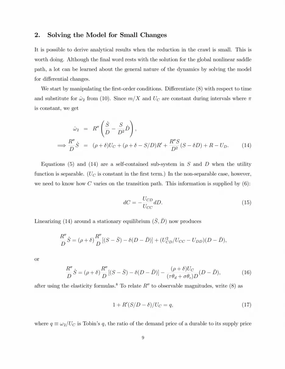
2. Solving the Model for Small Changes

It is possible to derive analytical results when the reduction in the crawl is small. This is

worth doing. Although the final word rests with the solution for the global nonlinear saddle

path, a lot can be learned about the general nature of the dynamics by solving the model

for differential changes.

We start by manipulating the first-order conditions. Differentiate (8) with respect to time

and substitute for ω2 from (10). Since m/X and UC are constant during intervals where π

is constant, we get

ω2 = RS

D− S

D2D ,

=⇒ R

DS = (ρ+ δ)UC + (ρ+ δ − S/D)R +

R S

D2(S − δD) +R − UD. (14)

Equations (5) and (14) are a self-contained sub-system in S and D when the utility

function is separable. (UC is constant in the first term.) In the non-separable case, however,

we need to know how C varies on the transition path. This information is supplied by (6):

dC = −UCDUCC

dD. (15)

Linearizing (14) around a stationary equilibrium (S, D) now produces

R

DS = (ρ+ δ)

R

D[(S − S)− δ(D − D)] + (U2CD/UCC − UDD)(D − D),

or

R

DS = (ρ+ δ)

R

D[(S − S)− δ(D − D)]− (ρ + δ)UC

(τθd + σθc)D(D − D), (16)

after using the elasticity formulas.8 To relate R to observable magnitudes, write (8) as

1 +R (S/D − δ)/UC = q, (17)

where q ≡ ω2/UC is Tobin’s q, the ratio of the demand price of a durable to its supply price

9

(unity). Differentiating with respect to S and q yields

R S

UCD

dS

S= q

dq

q.

Define Ω ≡ (dS/dq)q/S to be the elasticity of durables spending with respect to Tobin’s q.Evaluated at a steady state where S/D = δ and q = 1,

R =UCΩδ.

The linearized system is thus⎡⎣ S

D

⎤⎦ =⎡⎣ ρ + δ −(ρ+ δ)δ − c

1 −δ

⎤⎦⎡⎣ S − S

D − D

⎤⎦ , (18)

where

c ≡ −(ρ+ δ)δΩ

τθd + σθc< 0.

The steady state is a saddle point with eigenvalues

λ1,2 =ρ± ρ2 − 4c

2, λ1 > 0, λ2 < 0.

During the ERBS phase, the dynamics are governed by a nonconvergent path of the

system associated with the low rate of crawl π1. For this phase, (18) gives

S(t)− S1 = (λ1 + δ)h1eλ1t + (λ2 + δ)h2e

λ2t, t < T, (19)

D(t)−D1 = h1eλ1t + h2e

λ2t, t < T, (20)

where h1 and h2 are constants and (S1, D1) is the stationary equilibrium paired with π1.

After the policy reversal at time T , the economy follows the saddle path that leads to the

new long-run equilibrium (S2, D2). On the convergent path, the term involving the positive

eigenvalue drops out:

S(t)− S2 = (λ2 + δ)h3eλ2t, t ≥ T, (21)

D(t)−D2 = h3eλ2t, t ≥ T. (22)

10

h3 is another constant. Also, we have exploited the fact that for small changes the negative

eigenvalue is the same as in (19) and (20).

Turning back to (15), interpret the differentials as deviations from the stationary equi-

librium and write the path of C as

C(t) = Ci − UCDUCC

[D(t)−Di],

=⇒ C(t) = Ci + f [D(t)−Di], (23)

where9

f ≡ (τ − σ)θc(ρ+ δ)

τθd + σθc.

Across steady states, UD/UC = ρ+ δ. This and homothetic preferences imply

Ci − Co = CoDo(Di −Do), i = 1, 2. (24)

There are two more steps in the solution procedure: (1) derive the five boundary con-

ditions that pin down D1, D2, and h1- h3 (Si = δDi takes care of durables spending); (2)

plug the solutions into (19)-(23) and extract conditions that delineate the path of spending.

Both steps involve a good deal of tedious algebra. In a supplementary appendix (available

upon request), we show that

D1 > Do > D2,

S(0), C(0) > 0, with S(0) > C(0) if (25)

Ω > τρθc(τ − σ) + δτ

δ(τθd + σθc), (25a)

Ω > σ 1 +δ(σ − τ )θd

(ρ+ δ)(τθd + σθc), (25b)

S(T ), C(T ) < 0 with |S(T )| > |C(T )| iff Ω >στ

τθd + σθc, (25)

S(t) < S2 iff λ2 + δ < 0

=⇒ S(t) < S2 iff Ω > τθd + σθc. (27)

11

The conditions in (25)-(27) have the same general structure: in each, Ω stands alone on

the left side and a term involving σ and τ occupies the right. These parameters claim the

spotlight because they play pivotal roles in conditioning the intertemporal responses of S

and C. The scope for intertermporal substitution in nondurables consumption is tied to

concavity of the utility function in C, which depends on both σ and τ . Concavity of the

utility function also affects durables spending but is much less important as very little of

the durable good is consumed at the time of purchase. Intertemporal substitution is limited

instead by rising marginal deliberation costs. This friction is subsumed in the elasticity of

S with respect to Tobin’s q. Consequently, when Ω is large relative to σ and τ , the response

of durables to intertemporal variations in the effective price of consumption is stronger than

the response of nondurables. In the subsections that follow, we will be precise about what

“large relative to σ and τ” means.

2.1 The Benchmark Case of a Separable Utility Function (σ = τ)

Econometricians have yet to estimate the value of σ for even one LDC. Nevertheless, there is

some basis for the view that a separable utility function deserves the status of the benchmark

case. Estimates of demand systems with 5-10 goods find that compensated own-price elastic-

ities in both developed and less developed countries are on the order of .15-.65 (Lluch et al.,

1977; Deaton and Muellbauer, 1980; Blundell et al., 1993), implying a slightly higher range

of .20-.75 for the intratemporal elasticity of substitution. Some of the product categories

in the demand systems refer mainly to semi-durables (e.g., clothing and textiles); others

mix durable, non-durable, and semi-durable goods. At present, therefore, the best educated

guess is that σ also lies in the .20-.75 range. Since this closely overlaps the estimated range

for τ in LDCs, we center the analysis around the dynamics for σ = τ .

The results in the benchmark case are exceptionally clean. When the utility function is

separable, the conditions in (25a),(25b),(26) and (27) all reduce to Ω > τ . This gives

Proposition 1 When the utility function is separable between durables and nondurables, Ω >τ is necessary and sufficient for durables spending to (i) increase more than nondurablesspending at the start of ERBS [S(0) > C(0)], (ii) decrease more than nondurables spendingat the time of the policy reversal, and (iii) overshoot and remain below its steady-state levelthroughout the post-ERBS period [S(t) < S2, t > T ].

12

Figure 1 shows the complete transition path. The S = 0 and D = 0 schedules determine

which way the north-south and east-west directional arrows point during the ERBS phase,

whileAiAi is the saddle path associated with (Si, Di). In the lower quadrant, we use equation

(23) to track the path of nondurables consumption.

When ERBS is announced, C jumps to C1 and S jumps to a point above A1A1 (see

the appendix). After the initial jumps, C stays at C1 until ERBS collapses while S either

rises continously or follows a shallow U-shaped path. In the latter case, the transition path

includes a period of decreasing expenditure. This phase is strictly transitory. Before the

program fails, the path crosses the S = 0 schedule. In the numerical simulations, the crossing

point is typically around the middle of the second year (when T = 3).

The consumption spree and ERBS end at the same moment. When the crawl abruptly

increases at T , spending plummets across-the-board. The diagram suggests and the numer-

ical simulations will shortly confirm that the collapse is concentrated in durables purchases:

C jumps to C2 and is constant thereafter, but S overshoots S2.10 Durables lead in the sud-

den crash just as they lead in the boom. Over the whole cycle, the gyrations in aggregate

consumption mirror the volatile dynamics of durables expenditure.

2.2 Edgeworth Substitutes (σ > τ)

In the case where durables and nondurables are Edgeworth substitutes, Ω ≥ σ guarantees

the conditions in (25a), (26), and (27), but not the condition in (25b). This can be handled

by pushing Ω a little above σ. Write (25b) as

Ω > σ 1 +(σ − τ )(1− γ)

τ (1 + ρ/δ)(1− γ) + σγ, (25b)

where γ ≡ C/(C + δD) is the share of nondurables in total consumption spending. Since

the term in square brackets is less than 1/γ, we have

Proposition 2 When durables and nondurables are Edgeworth substitutes, Ω > σ/γ is suf-ficient for durables spending to (i) increase more than nondurables spending at the startof ERBS [S(0) > C(0)], (ii) decrease more than nondurables spending at the time of thepolicy reversal, and (iii) overshoot and remain below its steady-state level throughout thepost-ERBS period [S(t) < S2, t > T ].

Remark 1 The data place γ around .80 in LDCs; hence Ω does not have to be very muchabove σ to meet the sufficient condition.

13

Figure 2 portrays the path to the new steady state. The main difference compared to the

benchmark case is that both components of consumption overshoot at time T .

2.3 Edgeworth Complements (τ > σ)

The conditions in (25a) and (25b) are jointly sufficient for S(0) > C(0). To derive the

strongest result for the case of Edgeworth complements, we also need to consult the necessary

and sufficient condition

S(0) > C(0) iff Ωx2(1− e−λ2T ) > στ

τθd + σθc−Ω x2

r(1− γ)

δ+ e−λ2T , (28)

where

x2 = 1 +λ2τ

δΩsign Ω− τ

ρθc(τ − σ) + δτ

δ(τθd + σθc)

Positive when (25a) holds

.

The term in square brackets is always positive (see the appendix). Thus the above condition

holds for x2 < 0 and Ω > στ/(τθd + σθc). On the other hand, if x2 is positive, then (25a)

must hold. We need only appeal to (25b) therefore to ensure S(0) > C(0). But since τ > σ

in the case under consideration, any value of Ω that satisfies (25a) also satisfies the weaker

condition (25b). The upshot of all this is

Proposition 3 When durables and nondurables are Edgeworth complements,

Ω > Maxστ/(τθd + σθc), τθd + σθc

is sufficient for durables spending to (i) increase more than nondurables spending at thestart of ERBS [S(0) > C(0)], (ii) decrease more than nondurables spending at the time ofthe policy reversal, and (iii) overshoot and remain below its steady-state level throughout thepost-ERBS period [S(t) < S2, t > T ].

Remark 2 The borderline value of Ω that satisfies the sufficient condition is smaller thanτ . (τ > σ and the arguments of Max· are the weighted harmonic mean and the weightedarithmetic mean.)

Edgeworth complementarity changes the look of the adjustment process in two ways (Fig-

ure 3). First, nondurables consumption rises throughout the ERBS phase and undershoots

its steady-state level in the post-ERBS period. Second, S does not necessarily jump to a

14

point above the A1A1 schedule (see the appendix). Consequently, durables spending may

decrease steadily after its initial jump.

2.4 The Grand Corollary

Absent information about the sign of σ− τ , it is useful to have a general result that applies

irrespective of whether durables and nondurables are Edgeworth substitutes, Edgeworth

complements, or independent. The union of Propositions 1-3 fills the bill:

Corollary 1 Ω > Maxσ/γ, τ is sufficient for durables spending to (i) increase morethan nondurables spending at the start of ERBS [S(0) > C(0)], (ii) decrease more thannondurables spending at the time of the policy reversal, and (iii) overshoot and remain belowits steady-state level throughout the post-ERBS period [S(t) < S2, t > t1].

Taking stock, after three propositions and one corollary, where do we stand? Certainly

the weak credibility hypothesis has regained some of its swagger. Given the weight of

the evidence that σ and τ are well below unity and the tremendous volatility of durables

spending in ERBS programs, there is not much doubt that Ω is considerably larger than

both σ/γ and τ and that the boom-bust cycle in durables expenditure drives the boom-bust

cycle in aggregate consumption. On its own, however, this is not enough to rehabilitate the

hypothesis. The analytical results were derived for small changes. As such, they are only

suggestive of strong quantitative effects. Confirmation is needed from numerical simulations

that the predicted paths for durables expenditure and aggregate consumption lie within

shouting distance of the big numbers seen in the data.

3. Calibration of the Model and Numerical Results

To calibrate the model, we set

γo = .80, µo = .10, β = .50, πo = 1, π1 = 0, δ = .10, T = 3, r = .05,

and let σ, Ω and τ assume multiple values:

σ = .25, .50, .75, τ = .25, .50, Ω = 5, 10.

The ratio of money balances to aggregate spending (µ) is 10%. This is a conservative choice

15

closer to the ratio of money to GDP than to the ratio of money to private consumption. It is

intended to counteract any bias toward a strong consumption boom caused by the absence

of a nontradables sector. With respect to the other choices:

• Elasticity of money demand with respect to the interest rate (β). Reinhart and Vegh(1995a), Rossi (1989), and Arrau et al. (1995) have estimated money demand functionsof the type employed in our model. The value assigned to β is almost the same as theaverage of their estimates for Argentina, Brazil, Mexico, Chile and Uruguay.11

• Consumption share of durables ( 1− γ). The share of durables in aggregate spending isS/(C + S). A figure close to this can be computed from the United Nations NationalIncome Accounts. For a broad definition that includes semi-durables, the share lies in the.18-.22 range: .223 for Mexico (2000), .179 for Colombia (1998), .180 for Bolivia (1992),.203 for the Philippines, and .217 for S. Africa (2001) and S. Korea (2002). The value inthe model (.20) is the average of the values for Mexico and Colombia.

• Depreciation rate for durables ( δ). The Central Statistical Office of Great Britain andthe U.S. Department of Commerce estimate the service life to be ten years for majorappliances, cars, and other vehicles (Williams, 1998). We used this figure to fix δ. (Thereare no data for LDCs.)

• Length of the ERBS program (T). The low-crawl period lasts three years. Three is apopular choice in the literature and close to the average value in Calvo and Vegh’s (1999)dataset for major ERBS episodes.

• Rate of crawl before vs. during ERBS (πo,π1). The numerical simulations cut the rateof crawl from an initial value of 100% to zero during ERBS. This is larger than thereductions in the Chilean and Uruguayan tablitas but far smaller than the reductions inthe Argentine tablita, Mexico’s Solidarity Pact, or Argentina’s Convertibility Plan.

• Real interest rate (r). Reinhart and Vegh (1995a) peg the world market real interest rateat 3%. Burstein et al. (2001) and Rebelo and Vegh (1995) opt for 4.1%, while Uribe(2002) prefers 6.5%. We compromise on 5%, a value inbetween the long-run real returnspaid by U.S. stocks and treasury bonds.

• Intertemporal elasticity of substitution (τ). The low and high values for the intertemporalelasiticity of substitution are in line with estimates for LDCs, most of which place τsomewhere between .20 and .50 (Agenor and Montiel, 1996, Table 10.1).

• Elasticity of substitution between durable and nondurable consumer goods (σ). Althoughthere are no estimates of σ for LDCs, a range of .25-.75 is at least consistent with theempirical evidence that compensated elasticities of demand tend to be small at highlevels of aggregation. This range is also wide enough to encompass cases of Edgeworthcomplementarity and Edgeworth substitutability.

• Elasticity of durables spending with respect to Tobin’s q (Ω). Baxter (1996) sets Ω at 200.(Note: 200 is not a typo.) Baxter and Crucini (1993) and Rebelo and Vegh (1995) choose

16

15 in models where the durable good is physical capital. 200 and 15 appear to be a pureguesses. (Our own literature search for information about Ω proved fruitless.) We restrictΩ to much lower values but still get tremendous variation in durables expenditure overthe ERBS cycle.

3.1 Solution Technique

The numerical solutions report the results for the global nonlinear saddle path. This required

a technical innovation to deal with the unit root problem generic to models that postulate

an exogenous world market interest rate. (In continuous time, the unit root shows up as

a zero eigenvalue.) Due to the unit root, it is not possible to solve for the steady state

independent of the transition path. But without prior knowledge of the steady state, a

conventional shooting program does not know what to shoot for. The existing literature has

relied therefore on linear approximations to the true solution.

We solved the unit root problem by employing a different search strategy. Instead of

shooting for the path that takes the economy to the unknown steady state, our program

shoots for the path that eventually satisfies the conditions for a stationary equilibrium.

Guided by this strategy, the program solves for the transition path and the steady state

simultaneously. See Atolia and Buffie (2007) for a more detailed discussion of the algorithm.

3.2 Numerical Results

Figures 4-7 show the percentage deviations of nondurables consumption, durables spending,

and aggregate consumption (C + S) from their initial values. There are four runs with a

separable utility function and two each for the cases of Edgeworth complementarity and

Edgeworth substitutability. In the figure for aggregate consumption, the dashed line is the

path when all consumption is nondurable. The vertical distance between this line and the

actual path reflects the impact of durables expenditure at each point in the cycle.

What stands out in a quick pass through the figures are the big numbers for aggregate

consumption and durables spending. The peak increase ranges from 12% to 27% for ag-

gregate consumption and from 46% to 117% for durables. Furthermore, the “fit” between

the numerical results and the stylized facts pertaining to the composition of consumption

growth and the volatility of durables expenditure is remarkably good. In the panel regres-

sions reported by DeGregorio et al. (1998), annual growth of durables spending averages

17

21% for the first three years, with the 95% confidence interval bracketing 8.5%-33.7%.12 The

point estimate of 21% is 3.5 times larger than the estimate for total consumption growth.

By comparison, in the eight cases covered by Figures 4-7, the peak increase in durables

spending is 3-5 times larger than the peak increase in aggregate consumption and the av-

erage growth rate for durables ranges from 13% to 29%. The numbers are also close for

the bust phase of the cycle. DeGregorio et al.’s alternative point estimates have durables

expenditure plunging 21-72% (relative to the pre-ERBS trend line) in the year after ERBS

collapses. The range in our simulations is -31% to -75%.

4. Habit Formation

While the model delivers good results for the magnitude and the composition of the con-

sumption boom, it does less well in accounting for the slope of the consumption path. The

time profiles of aggregate consumption and durables spending are essentially the same in

each case: a sharp jump at t = 0, a succeeding flat stretch for the next 1.5 years, and then

rapid, accelerating growth until the end of year three. This is at variance with the facts.

Consumption rose continuously in some ERBS episodes (e.g., Argentina, 1967-1970; Brazil,

1964-1968; Mexico, 1988-1994; Peru, 1985-1987; Paraguay, 1991-1997);13 in others, a flat

stretch or a downturn materialized, but only in the last year of the program.

The results in Uribe (2002) suggest that a model with habit formation might generate a

more realistic path for consumption. Following Carroll et al. (2000) and Fuhrer (2000), let

the stock of habit H grow at the rate

H = v(N −H), (29)

where v > 0 and

N ≡ [a1C(σ−1)/σ + a2D(σ−1)/σ]σ/(σ−1).

Habit enters the utility function with the persistence parameter α. Two formulations dom-

inate the literature:

U(N,H) =(N − αH)1−1/τ

1− 1/τ , 0 < α < 1 (30a)

18

and

U(N,H) =(N/Hα)1−1/τ

1− 1/τ , 0 < α < 1. (30b)

In the additive specification, utility is a function of the difference between current con-

sumption and the stock of habit (also called the “subsistence level of consumption”). The

multiplicative specification assumes that felicity depends instead on consumption relative to

the stock of habit. Both specifications capture the basic idea of habit formation – that the

private agent desires to smooth the change as well as the level of consumption.

There is general agreement in the literature that the persistence parameter α is on the

order of .70. Unfortunately, no similar consensus exists about the likely value of v. Numerous

papers postulate very rapid habit formation, citing Fuhrer (2000) for support. It is common

practice, for example, to set the stock of habit equal to last quarter’s consumption. At the

opposite extreme, the evidence marshalled in Constantinides (1991), Heaton (1995), and

Boldrin et al. (1997) suggests that it takes years for habits to fully adjust. Carroll et al.

(2000) and Mansoorian and Michelis (2005) subscribe to this view, calibrating their models

with v = .20.

In the next two sections we present results for the multiplicative specification when τ =

σ = .25, Ω = 10, α = .70, and v = .5, 3 or 6.5. In the runs with v = 6.5, the stock of habit

covers 80% of the distance to its new long-run level within one quarter.14 For v = .5, the

80% point is not reached until 3.25 years elapse.

4.1 Numerical Results

Habit formation moderates consumption growth most in the early and late stages of ERBS

as the private agent tries to smooth the large jumps in C and S at t = 0 and t = T . Beyond

this, not much can be said. It is not clear a priori how the peak and the slope of the spending

path will change compared to the benchmark model. A closer look at the utility function in

(30b) shows why. In the extreme short run (where H is fixed), the intertemporal elasticity

equals τ and the utility function is separable in durables and nondurables consumption

(UCD = 0). Over time, however, intertemporal substitution becomes easier (Carroll et

al., 2000) and accumulation of durables exerts a positive effect on the marginal utility of

19

nondurables consumption. After habits have fully adjusted,

− UNUNNN dH=dN

≡ τ =τ

τα+ 1− α> τ for τ < 1

and

UCDD

UC dH=dN

≡ η =θdα(1− τ )

τ> 0 for τ < 1.

Since τ > τ , the consumption boom may be stronger than in the model without habit

formation. This is most likely when v = 6.5 and the intertemporal elasticity of substitution

rises quickly to τ .

The relationship between habit formation and the trajectory of nondurables consump-

tion is more complex. As usual, higher consumption today raises the marginal utility of

consumption tomorrow by increasing the stock of habit. Growth in the stock of habit also

increases the degree of complementarity between durables and nondurables (η rises with H).

If the story ended here, we could be sure that habit formation would impart an upward tilt

to the path of nondurables consumption. But it doesn’t. There is a complicating factor:

the desire to smooth the fall in consumption at T tends to ratchet the consumption path

southward immediately after the jump at t = 0.

Figure 8 confirms these analytic-based conjectures. The results for v = .50 in Panel A

are disappointing. Raising v to 6.5, however, gives rise to a nice hump-shaped path for

nondurables consumption and a generally better fit with the stylized facts. Absent habit

formation, nondurables consumption jumps 3.4% at t = 0 and then stays flat for the rest

of the ERBS period. In Panel B, C surges 6% in the first six months, rising to a peak of

8% at t = 2.25. Since durables spending also rises more at the outset, total consumption

growth at t = 1 and t = 2 is 5-6 percentage points higher than in the model without habit

formation. The gap narrows in the third year but does not disappear. Thus the time profiles

for aggregate consumption and its principal components are uniformly superior to the time

profiles in the model without habit formation. Unlike in Uribe (2002), there is no tradeoff

of lower heigth for better slope – the path of aggregate consumption is continuously above

the no habit formation path.

Two additional points merit comment. First, regardless of whether one favors the multi-

20

plicative or the additive specification, the case for habit formation requires very fast adjust-

ment in the stock of habit. There is not much to choose from between a model with slow

or moderately fast habit formation and a model with no habit formation. Second, while

the introduction of rapid habit formation produces better results, it is not a complete fix.

The paths for durables spending and aggregate consumption still have the wrong shape –

growth should be greater in the second year than in the third, not the other way around.

This motivates us to investigate a less conventional specification of habit formation.

4.2 Habit Formation in Durables Spending

So far we have followed Bernanke (1985) in assuming that deliberation costs depend on how

fast the stock of durables changes. This is not the only sensible specification. It is equally

plausible that the private agent experiences psychological unease when durables spending S

varies from its customary level. Suppose therefore

R(S,H) = x(S/H − 1)2

2H, (31)

where

H = v(S −H), v > 0. (32)

Naturally, we hope that habit formation will now generate a smooth hump-shaped path for

S and, by extension, for aggregate consumption. The idea is not entirely new. Burnside et

al. (2004) have employed a similar strategy to dampen the volatility of investment in a real

business cycle model.

Panel A in Figure 9 shows the outcome when τ = σ = .25, Ω = 5, v = 3, and habit

formation appears only in the deliberation cost function. We would like to include habit

formation in the utility function as well, but, at present, our computer program cannot solve

for the nonlinear saddle path in systems that have more than three jump variables.15 The

new specification is perforce less than ideal.

Even so, the run in Panel A gives us almost everything we want. The paths for durables

spending and aggregate consumption are hump-shaped, with expenditure contracting rapidly

in the last six months of the program. Equally important, the pace of consumption growth

does not slow until the start of the third year. Durables spending increases 46% in year

21

one, 42% in year two, and 11% in the first half of year three. The corresponding numbers

for aggregate consumption are 12%, 12% and 5%. Perhaps the most surprising result is

that the peak increases in durables spending and aggregate consumption are 2-2.5 times

as large as in the model without habit formation. This is a natural consequence, however,

of substituting H for D in the deliberation cost function. Increases in H reduce marginal

deliberation costs in (47) in the same way that increases in D do when R = x(S/D− δ)2D.

But habit formation is extremely fast relative to durables formation (v is large and H is

only a tenth the size of D). Hence, after about six months, the higher level of S becomes

routine and marginal deliberation costs decrease sharply. This paves the way for a boom

that is both smoother and much more powerful than in the model without habit formation.

Sensitivity Analysis

The numerical simulations in Panel A assume that all durables spending enters the scale

variable in the liquidity cost function. If some durables are pure credit goods, this exagger-

ates the incentive to shift purchases from the future to the present when the reduction in the

crawl is temporary. Our own view is that most durables spending belongs in the liquidity

cost function.16 Given the paucity of empirical evidence, however, the right specification of

the scale variable is a judgment call.

We have undertaken additional runs to test the sensitivity of the results to the coefficient

on S in the liquidity cost function. In Panels B and C of Figure 9, we write the scale variable

as C + ξS and reduce ξ from unity to .50 or .25.

The results hold up surprisingly well. Because smaller values of ξ lessen the impact of

S on liquidity costs, the percentage decrease in durables spending is much smaller than the

decrease in ξ. The peak increase in aggregate consumption drops from 29% when ξ = 1

(Panel A) to 22% when ξ = .50 and to 18% when ξ = .25. These are nontrivial decreases,

but 18% and 22% are still big numbers. Clearly, ξ close to unity is not essential to a

durables-driven explanation of the consumption boom.

22

5. Adding a Nontradables Sector

In this section we add a nontradables sector to the model. This allows us to demonstrate

that the powerful consumption boom is not an artifact of the one-good model and that the

WC hypothesis can explain strong, sustained appreciation of the real exchange rate.

The traded good, now called the export good, serves as the numeraire in the expanded

model. Thus, unless otherwise indicated, prices and monetary aggregates are divided by the

nominal exchange rate. Other notational conventions are as follows: Pn, w, Qi, Li, Ki, and

Ci refer to the price of the nontraded good, the wage, production, employment and capital

in sector i (i = n,x), and nondurables consumption of good i.

Technology and Labor Demand

Competitive firms operate CES production functions

Qx = F (Kx, Lx) = [a3L(σ−1)/σx + a4K

(σ−1)/σx ]σ/(σ−1), (33a)

Qn = G(Kn, Ln) = [a5L(σ−1)/σn + a6K

(σ−1)/σn ]σ/(σ−1), (33b)

and hire labor up to the point where its marginal value product equals the wage:

FL = w, (34)

PnGL = w. (35)

Labor is intersectorally mobile, but the capital stocks are fixed. The latter assumption will

be relaxed when we introduce supply effects in Section 8.

Consumption of multiple durable goods greatly complicates the model. To avoid this,

we assume that one unit of the imported durable always combines with a7 units of the

nontraded durable. The price of the composite durable is thus

Pd = 1 + a7Pn. (36)

The Private Agent’s Optimization Problem

The private agent solves his optimization problem in two stages. In the first stage, Cn

and Cx are chosen to maximize C(Cn, Cx), subject to PnCn + Cx = E, where E is total

23

nondurables expenditure and C(Cn, Cx) is a linearly homogenous CES aggregator function.

The optimal choices Cn and Cx are subsumed in the indirect utility function

V (Pn,E) = C[Cn(Pn, E), Cx(Pn, E)] = E/c(Pn),

where

c(Pn) = kβo + kβ1P

1−βn

1/(1−β),

ko and k1 are distribution parameters, and β is the elasticity of substitution between the

two consumer goods.

In the second stage of optimization, the agent chooses m, b, E, and S to maximize

U =∞

0

(N/Hα1 )1−1/τ

1− 1/τ − x(S/H2 − 1)2

2H2 e−ρtdt, (37)

subject to

A = m+ b, (38)

A = PnQn +Qx + g + rb− (E + PdS) 1 + L m

E + PdS− χm, (39)

D = S − δD, (40)

H1 = v(N −H1), (41)

H2 = v(N −H2), (42)

where

N ≡ a1[E/c(Pn)](σ−1)/σ + a2D(σ−1)/σσ/(σ−1).

We allow habit formation to operate in the utility function as well as the deliberation costs

function. This maximizes the probability of getting realistic, hump-shaped paths for both

durables spending and nondurables consumption.

Net Foreign Asset Accumulation and the Current Account Balance

Summing the budget constraints of the private agent and the government now yields

Z = PnQn +Qx + rZ − E − PdS. (43)

24

Market-Clearing Conditions

The model is closed by the conditions that demand equal supply in the labor and non-

tradables markets:

Lx + Ln = L (44)

Cn + a7S = Qn. (45)

The supply of labor is fixed at L. In (44), Cn is retrieved from the indirect utility function

via Roy’s Identity:

Cn = −∂V/∂Pn∂V/∂E

= Ek1P

−βn

kβo + kβ1P

1−βn

. (46)

Solution Technique

The core dynamic system in the model has four jump variables [E, S, and the multipliers

associated with (41) and (42)] and four state variables (D, Z, H1, and H2). Our algorithms

cannot solve these higher-order systems for the global nonlinear saddle path. Consequently,

the zero eigenvalue/unit root reappears as an insoluble problem (see the discussion in Section

4.1).

To circumvent this difficulty, we adopt Schmitt-Grohe and Uribe’s (2003) suggestion to

let the real interest rate depend very weakly on the country’s debt-GDP ratio:

r = ρ + κb

PnQn +Qx− boPn,oQn,o +Qx,o

, κ < 0. (47)

f is assigned a small value to close to zero so that the loan supply curve is almost perfectly

flat. This converts the zero eigenvalue in the perfect capital markets model into a tiny

negative eigenvalue in the approximating model. It also makes the stationary equilibrium

independent of the transition path. In the long run, r = ρ requires the foreign debt to

change by the same percentage amount as the dollar value of real GDP. This and the other

equilibrium conditions in the model tie down the steady state.

5.1 Calibration of the Model and Numerical Solutions

“At a quantitative level the results for our baseline parameterization fall short of ex-plaining the orders of magnitude involved in stabilization episodes, suggesting that the

25

large consumption booms and the sizable real appreciations are puzzling.” (Rebelo andVegh, 1995, p.168)

Table 1 lists the parameter values used to calibrate the expanded model. None of the

values are terribly exotic. Durables are more import intensive than nondurables, habit

formation is rapid (v = 6.5), and ordinary numbers are assigned to the cost share of labor,

the elasticity of substitution between traded and nontraded nondurables, and the elasticity

of substitution between capital and labor (all equal .50). The ratio of money balances to

consumption is .15 vs. .10 in the one-sector model.17 The higher value is in line with the ratio

of M1 to consumption for many ERBS episodes in Latin America. It is too low, however,

for most episodes in Africa.18 Finally, the value of κ, which fixes the slope of the loan supply

curve in (47) is .0001. An increase in the debt-GDP ratio from 25% to 125% thus raises the

borrowing rate by only one basis point.

Figure 10 shows the paths of aggregate consumption, durables spending, and the relative

price of the nontraded good in the base run where τ = .25 and σ = .75. The peak increases in

these variables for all runs are collected in Table 2. This is done to save space and facilitate

comparisons across models and parameter values. The graphs always have the same general

shape; what differs is the scale on the vertical axis.

Despite its simplicity, the no-frills flexprice model performs quite well. The real exchange

rate appreciates 24-26%, while the peak level of aggregate consumption ranges from 17% to

22%. As usual, the consumption boom is driven by a tremendous surge in durables spending.

Observe also that adjustment is difficult in the post-ERBS period. In the first year after

the policy reversal, the slump deepens and the real exchange rate depreciates continuously.

This is followed by slow recovery to the pre-ERBS equilibrium. Even at year five, aggregate

consumption and the real exchange rate are 8-10% below their initial levels.

6. Supply Effects and Temporary vs. Permanent ERBS

The stylized facts for successful ERBS programs look much like those for failed programs.19

This a problem for the preceding models. When ERBS is credible, the relative price of cur-

rent consumption does not decrease and the private sector does not shift spending from the

future to the present. Consequently, adjustment is instantaneous. There are no transitory

26

changes in consumption, the real exchange rate, or the current account deficit. The economy

jumps immediately to the new low-inflation steady state.

In the case of a credible program, wealth effects have to propel the consumption boom.

Most of the literature has focused on models where increases in wealth stem from supply-

side expansion. As noted in the introduction, these models have not been successful in

explaining the stylized facts. But this might change in more elaborate models that distin-

guish between nondurable and durables consumption. Durables spending responds strongly

to wealth shocks. Even a modest increase in wealth has the potential therefore to trigger

a multi-year consumption boom. The sticking point is that the normal definition of boom

does not apply. When the context is ERBS, we need really big numbers.

6.1 One Last Model

“ . . . further work on the structure of the supply-side and on the differential responseof the tradable and non-tradable goods sector – which would allow us to build morerefined quantitative models – would be particularly useful.” (Calvo and Vegh, 1999,p.1581)

We add a labor-leisure choice and sector-specific capital accumulation to the model of

Section 6. The complete model is laid out in Table 3.20 The key equation in the model is

(B14), the first-order condition for the optimal supply of labor. It is evident from inspection

of this condition that a lower rate of crawl raises the return to work by reducing the nominal

interest rate and the effective price of consumption. The jump in employment, in turn,

increases the marginal product of capital (FKL, GKL > 0), spurring firms to invest more.

Across steady states, output, employment, and the capital stock in each sector increase by

the same percentage amount as the supply of labor. The real exchange rate appreciates in

the short and medium run, but returns to its original level in the long run.21

Before proceeding further, we call attention to two aspects of the model. First, invest-

ment rises only in response to the increase in employment. It follows from this and the

separable form of the utility function that the limiting case s→∞ (perfectly inelastic labor

supply) retrieves the model without supply effects. The strength of the supply effects can

be measured therefore by comparing the results with corresponding run in Section 7.

The other noteworthy feature of the model is that firms accumulate capital in both

27

sectors. By contrast, the rest of the ERBS literature restricts investment to the tradables

sector. This bothers us. Symmetry is not only more natural, it is also important to the

credibility of the results (no pun intended). Keeping capital out of the nontradables sector

puts a thumb on the scale, creating a bias toward the desired outcome of strong appreciation

of the real exchange rate. The story line is simple. On impact, Pn jumps upward as higher

investment in the tradables sector increases demand for nontraded capital inputs.22 Beyond

the short run, expansion in the tradables sector raises real income and either decreases

or slows employment growth in the nontradables sector. Higher real income pushes the

demand curve in the nontradables sector further to the right, while the transfer of labor to

the tradables sector shifts the supply curve to the left. Both factors pull in the direction of

more appreciation of the real exchange rate.

Under symmetry, things play out very differently. Since the terms of trade move in favor

of the nontradables sector, the supply boom is concentrated there. Thus the pure supply

effects serve to moderate appreciation of the real exchange rate. In fact, at the end of the

day, they prevent any change in Pn. This does not imply, however, that real appreciation

is continuously less than in the model without supply effects. Supply-side expansion takes

time to develop, whereas the impact of higher wealth on durables spending is immediate and

large. For a while, demand grows more rapidly (ex ante) than supply in the nontradables

sector.

6.2 Temporary ERBS

To calibrate the model we set s so that labor supply increases 5.5-6.5% when ERBS is

permanent and f so that the elasticity of investment with respect to Tobin’s q equals .25,

1 or 2. (All other parameters take the same values as in Section 6.) The response of

labor supply is in line with response assumed in Rebelo and Vegh (1995) and with the

responses reported in Roldos (1995) for Mexico’s 1987 Solidarity Pact and Argentina’s 1991

Convertibility Plan.23 The alternative values for the q-elasticity correspond to low, middle

and high-end estimates in the literature on empirical investment functions.24

Figure 11 and Panel B of Table 2 contain the latest results. The fit with the stylized facts

is excellent, including the temporal and sectoral distribution of supply effects. Investment

decreases slightly in both sectors, while employment and output rise sharply in the nontrad-

28

ables sector and fall in the export sector. Real GDP is 2.5-3% higher at the peak of the

boom, and recessionary pressures appear 6-9 months before ERBS collapses. On the demand

side, although the supply response is temporary and the associated wealth effect small, the

consumption boom is significantly stronger than before. The peak increases in durables

spending and aggregate consumption are 79-142% and 23-35%; without supply effects, the

ranges are 57-97% and 17-22%. Finally, despite rapid supply expansion in the nontradables

sector, ERBS is still compatible with pronounced appreciation of the real exchange rate;

because the consumption boom is so strong, Pn increases 17-25%.

A. Remarks

Below we comment on (i) the interdependence of the consumption and investment dy-

namics and (ii) how the results for investment compare to the empirical evidence.

• Since the increase in labor supply raises the marginal product of capital, it might seemodd that investment falls. The decrease in the nominal interest rate, however, lowers theeffective price of consumption relative to the price of capital. This creates an incentiveto substitute away from fixed investment toward current consumption during the ERBSphase. Substitution between the two assets is easier and the consumption boom strongerwhen the q-elasticity of investment equals two (see Table 2). Total spending increasesless, however, making it more difficult to explain strong appreciation of the real exchangerate.

• At the trough of the cycle, investment is lower by 15-20% in the runs where the q-elasticity equals two and by 2-4% in the runs where the q-elasticity equals .25. Neitherresult contradicts the stylized facts. The raw numbers for fixed investment are all over themap in ERBS programs (Kiguel and Liviatan,1992; Reinhart and Vegh, 1995b; Calvo andVegh, 1999), and the estimated impact is weak and statistically insignificant in Hamaan’s(2001) large panel dataset.

• The stabilization time profile for fixed investment in Calvo and Vegh (1999) shows aninitial decline of 7-10% followed by recovery to a temporarily higher level in the post-ERBS period. Our model generates the same investment cycle, with similar numbers,when the q-elasticity of investment spending equals unity (see Figure 11).

• The model suggests two explanations for the mix of positive and negative outcomes in thedata.25 First, as will be seen in Section 6.3, investment increases sharply when ERBS ispermanent (or perceived as credible). Thus variations in the response of investment mightreflect variations in the credibility of different ERBS programs. Second, it can be arguedthat part of investment spending should enter the scale variable in the liquidity costfunction. This would introduce another pro-investment effect (alongside higher laborsupply) that competes against the substitution-toward-durables effect. We conjecturethat the sign and the magnitude of the impact on investment in non-credible programs

29

would then be sensitive to small variations in the coefficient on I in the liquidity costfunction.

B. An Important Refinement

Twenty-five percent appreciation of the real exchange rate is very good by the standards

of the literature, but not good enough. While there is always a problem in controlling

for other effects, it appears that in some episodes ERBS caused the real exchange rate to

appreciate 40-50% (Calvo and Vegh, 1994b, Table 1).

A refinement of the model helps a great deal here. Suppose firms incur adjustment costs

when changing the workforce. This converts Ln and Lx into state variables, producing a

smoother, more realistic supply response (there is no jump in nontradables output at t = 0).

In Panel C of Table 2 we assume adjustment costs are the same for labor and capital.

Overall, the results now match up better with the data. The consumption boom is no less

powerful than in the model without supply effects, but appreciation of the real exchange

rate rises to 26-38%.

6.3 Permanent ERBS

“It should be pointed out, however, that for the purposes of our model the wealth effectneed not be necessarily large since there is a ‘multiplicative’ effect brought about by thebunching in the purchase of durable goods. Hence, it is conceivable that a relativelysmall wealth effect may have a large impact on durable goods purchases.” (De Gregorioet al., 1998, pp.126-127)

Endowing ERBS with credibility makes the wealth effect stronger but eliminates the

incentive to substitute from future to current consumption. The tradeoff is obviously unfa-

vorable. Without intertemporal substitution, the paths for aggregate consumption, durables

spending, and the real exchange rate peak much too early and far too low (Figure 12 and

Panels D and E of Table 2). This conclusion is extremely robust. Fishing for better num-

bers, we experimented with alternative values for every parameter in the model. The results

always came back looking like Figure 12. Our search did not turn up a single case in which

the peak increases for both aggregate consumption and the real exchange rate exceeded 10%.

These results cast doubt on the thesis of De Gregorio et al. (1998) that the wealth

effects associated with credible ERBS can account for the boom phase of the consumption

30

cycle via their impact on durables spending. Our model of durables expenditure postulates

deliberation costs instead of an S-s rule, but this difference is superficial. We get the bunching

pattern predicted by their analytical results: the surge in durables expenditure is packed

into the first six months of the transition path. The numerical simulations also incorporate

large wealth effects – the increase in real income from supply-side expansion is 5.5-6.5%.

Nevertheless, the consumption boom lacks heigth and length. The thesis in De Gregorio et

al. isn’t exactly wrong. After all, a consumption boom of 5% is pretty good. But, to repeat,

ERBS is special: the stylized facts demand much bigger numbers.

7. Concluding Remarks

Many supporters of the weak credibility (WC) hypothesis probably sympathize with the

theorist who complained that “facts are inconvenient things.” In empirical tests, models

reliant on the hypothesis have not come close to explaining the dramatic consumption boom

seen in ERBS programs. But maybe the problem is with the models as opposed to the hy-

pothesis. The tests were conducted on models that assume all consumption is nondurable.

Since the response of nondurables consumption is limited by the low value of the intertem-

poral elasticity of substitution, it was almost a foregone conclusion that the models would

fare poorly when confronted with the data.

In this paper we have used a mix of theory and numerical methods to investigate the

explanatory power of the WC hypothesis in a more general model that allows for both

durable and nondurable consumer goods. Inclusion of durables is essential for a fair test.

Because refrigerators, TVs, etc. provide a service flow for many years, large-scale purchases

of durables do not unbalance the consumption path in the same way as a spike in nondurables

expenditure. Consequently, low values of the intertemporal elasticity of substitution do

not preclude a durables-driven consumption boom. Our results go further and argue that

the WC hypothesis is a very promising hypothesis. In numerical simulations based on

conservative assumptions about the expenditure share of durables (20%) and wealth effects

(none), aggregate consumption increases 17-22% and the real exchange rate appreciates

24-26% during the low-crawl phase. In every case, the boom is powered by spectacular,

eye-catching growth in durables spending; when durables are removed from the model, the

31

peak increase in consumption is only 4-8%.

The model with a standard time-separable utility function suffers from the shortcoming

that the path to the peak of the consumption boom has the wrong shape. Consumption

grows too fast at the beginning and the end of ERBS and too slow in the middle. This can

be fixed by adding habit formation to the model, but only if habit affects deliberation costs

involved in purchasing durable goods. For conventional specifications of habit formation,

the trajectory of nondurables consumption is hump-shaped but the improvement in the

paths of durables spending and aggregate consumption is comparatively modest. Shifting

habit formation from the utility function to the deliberation cost function solves the latter

problem by strengthening the incentive to smooth the path of durables spending. In the

runs with this specification, the paths of durables expenditure and aggregate consumption

are steeply sloped and hump-shaped: spending rises apace for two years, then slows and

contracts sharply in the last year.

In their influential survey paper, Rebelo and Vegh (1995) assert that supply-side effects

are “an essential component in accounting for the stylized facts of exchange-rate-based

stabilizations.” We disagree. A pedestrian flexprice model that appeals to weak credibility

does an excellent job of explaining the stylized facts provided durables are part of the

consumption basket and habit formation is modeled in the right way. But supply effects are

helpful if not essential. Variants of the model that allow for endogenous labor supply and

sector-specific capital accumulation add another 7-13 percentage points to the consumption

boom or another 4-12 percentage points to appreciation of the real exchange rate. Fully

armed, the WC hypothesis can account for ERBS episodes where aggregate consumption

rose 35% (e.g., Argentina, 1991-1994) and the real exchange rate appreciated 40%.

Supply and wealth effects operate at maximum strength when ERBS is perceived to be

credible. Even in a model with durables, however, they are not potent enough to explain

the quantitative aspects of the ERBS syndrome. In our model, increases in labor supply

and the capital stock buy, at most, a 5% consumption boom and 3-8% appreciation of the

real exchange rate. Something else besides standard supply effects must be fueling a large

part of the consumption boom in successful ERBS program. Finding this last piece of the

puzzle is the main priority for future research.

32

NOTES

1. Tradables consumption drops below its pre-stabilization level in a single jump at the timeof the policy reversal. Nontradables consumption may fall below its pre-stabilization levelbefore ERBS is abandoned.

2. The peak increase in consumption occurs at t = 0. The solution stated in the text isobtained by solving the Calvo-Vegh model for small changes. It is approximately correctfor large changes.

3. The Reinhart-Vegh model delivers much larger increases in consumption when the nom-inal interest rate falls several hundred percentage points (according to their calculations,1,270 points in the case of Argentina’s Austral Plan). But then doubts arise about howthe change in the nominal interest rate is computed and about the story told by thecash-in-advance (liquidity costs) constraint: Are Reinhart and Vegh correct in assumingthat the difference between the initial interest rate and the lowest rate observed duringERBS is close to the average change in the rate? And is it believable that temporaryhuge variations in the nominal interest rate generate equally huge variations in the priceof current vs. future consumption?

4. See the discussion of the results for permanent ERBS in Section 6.3.

5. The data for the U.S. and other developed countries indicate that durables spending isfar smoother than predicted by a frictionless Permanent Income/Life Cycle model.

6. This description of fiscal policy is included only to motivate the failure of ERBS. Noneof our results depend on the assumption that fiscal policy is completely passive. Thesolutions for the paths of consumption and net foreign debt are independent of the pathpostulated for g. (The only restriction on g is that eventually it must adjust to align thefiscal deficit with seigniorage.)

7. Although π returns to its original level, k and m do not. The central bank suffers aloss in foreign exchange reserves and the increase in net foreign debt reduces aggregateconsumption and holdings of real money balances.

8. Write the term multiplying (D − D) as

U2CDUCC

− UDD =UDD

UCDD

UC

UDCC

UD

UCUCCC

− UDDDUD

= −UDD

τθc + σθdστ

− (τ − σ)2θdθc(τθd + σθc)στ

= − UD(τθd + σθc)D

(τθd + σθc)(τθc + σθd)

στ− (τ − σ)2θdθc

στ.

Mercifully, the term in square brackets simplifies to unity. Moreover, UD = UC(ρ+ δ) at

33

a steady state. Hence

U2CDUCC

− UDD = − (ρ+ δ)UC(τθd + σθc)D

.

9. The expression for f is derived from the elasticity formulas for UCDD/UC and−UC/UCCC.10. S and C decrease proportionately in the long run. This and overshooting imply that the

contraction in durables spending is greater than the contraction in nondurables expendi-ture throughout the post-ERBS adjustment process [(S(t)−So)/So < (C2−Co)/Co, t >T ].

11. We ignore Arrau et al.’s estimate for Brazil (3.26 is implausibly high) and use the averageof Arrau et al. and Reinhart and Veghs’ estimates for Argentina and Chile (.27 and.30, respectively). The simple average of the estimated interest elasticities for Chile,Argentina, Mexico, Brazil and Uruguay then works out to .51.

12. The numbers cited here are for failed, noncredible ERBS programs. The 95% confidenceinterval in the full sample is 14.1-44%.

13. In the Brazilian episode, the path has an early flat stretch much as in Figures 4-7. Con-sumption rose sharply in year 1, decreased slightly in year 2, and accelerated rapidly inyears 3 and 4. See DeGregorio, Guidotti and Vegh (1998, Table 1) and Calvo and Vegh(1994b) for data on the episodes in Mexico, Argentina and Brazil. For data on consump-tion growth in the Paraguayan and Peruvian programs, see Economic Survey of LatinAmerica and the Caribbean.

14. Following a permanent increase in N from No to N1, the solution to (45) reads [H(t) −H1]/(H1 − Ho) = e−vt (where H1 = N1). For v = 6.5 and t = .25, this gives [H(t) −H1]/(H1 −Ho) = e

−1.625t = .197.

15. In the model without habit formation, the dynamic system has two jump variables, ω1and ω2 (or C and S), the multipliers associated with the constraints in equations (4) and(5). (Even though ω1 = 0, the computer has to solve for the initial jump in ω1.) Whenhabit formation enters both the utility function and the deliberation cost function, themultipliers associated with the equations governing habit accumulation become part ofthe dynamic system. This adds two more jump variables to the system.

16. A broad definition of durables includes semi-durables like clothing and footwear. Theinclusion of semi-durables and the likelihood that the poorest half of the population paysfor most of its durables purchases with cash (even those who are better off may haveto make a downpayment to get acceptable credit terms) argues that ξ is closer to unitythan zero. It should also be noted that money may facilitate durables purchases throughother changels similar in spirit to the liquidity cost function. De Gregorio et al. (1998)emphasize that the purchase of durable goods is time intensive; if money reduces timespent in transactions related to nondurables consumption, it increases the supply of trueleisure time and lowers the total time + money cost of buying a durable good.

17. Recall that we chose the low value .10 in the one-sector model to offset any bias toward

34

a strong consumption boom caused by the absence of a nontradables sector.

18. Prior to the adoption of ERBS programs in Chile (1978), Uruguay (1978), Argentina(1978), Ecuador (1993), Brazil (1994), and Venezuela (1990, 1997), the ratio of M1 toprivate consumption ranged from 12% to 17%. At the start of ERBS episodes in SierreLeone (1988), Zambia (1990), Egypt (1991), Zimbabwe (1993), Nigeria (1990, 1995), andMozambique (1996), the range was 13% to 23%.

19. There are not many successful ERBS programs. Informed observers contend, however,that many programs enjoyed a high degree of credibility until shortly before they col-lapsed. See, for example, Dornbusch andWerner (1994), Nazmi (1997), Blejer and Castillo(1998), and Cinquetti (2000).

20. Lahiri (2001) works out analytical (not quantitative) results in a model with a similarspecification for the supply-side of the economy. Our model differs in allowing for durableconsumer goods, nontraded capital inputs, habit formation, and capital accumulation inthe nontradables sector.

21. Across steady states, PnGK(Kn/Ln) = (ρ + c)Pk(Pn), FK(Kx/Lx) = (ρ + c)Pk(Pn), andPnGL(Kn/Ln) = FL(Kx/Lx). These three equations can be solved for Kn/Ln, Kx/Lx,and Pn. None of the variables change in the long run. Under constant returns to scale,they depend only on technology and the rate of time preference.

22. Typically investment is included in the cash-in-advance constraint or the liquidity costfunction. This virtually guarantees that investment will increase after the rate of crawldeclines.

23. s equals three. The increase in labor supply is 5.5% when τ = .25 and 6.5% whenτ = .50. Rebelo and Vegh also set s equal to three but employ a utility function whereconsumption and leisure are Edgeworth substitutes. Roldos (1995) reports that laborforce participation increased 5.2% in Argentina from 1990-1993 and 6.8% in Mexico from1988-1993.

24. The estimates for developed countries range from .2 to 2.3, with the majority being lessthan unity (Engel and Foley, 1975; Malkiel et al., 1986; Summers, 1981; Hayashi, 1982;Abel and Blanchard, 1986; Galeoti and Schiantarelli, 1991; Alonso-Borrego and Bertolila,1994). There are also a few estimates for LDCs, but it is doubtful that the small, thin stockmarkets in the studies – the source for data on the demand price of capital – accuratelyreflect information about the fundamentals that drive private investment decisions. Avalue of two is consistent with Shafik’s (1990) estimate of the elasticity of investment withrespect to the supply price of capital in Egypt, and with recent theoretical and empiricalwork which suggests that previous studies may have substantially underestimated theq-elasticity in developed countries (Barnett and Sakellaris, 1998).

25. Although the empirical evidence is highly mixed, there are well documented cases whereERBS was accompanied by a surge in private investment (e.g., Israel 1985, Mexico 1988,Argentina 1999, and Turkey 2000).

35

References

• Abel, A. and O. Blanchard, 1986, “The Present Value of Profits and Cyclical Movementsin Investment.” Econometrica 54, 249-276.

Agneor, R. and P. Montiel, 1996, Development Macroeconomics, 1st edition (Princeton,N.J.; Princeton University Press).

Alonso-Borrego, C. and S. Bertolila, 1994, “Investment and Q in Spanish Manufacturing.”Oxford Bulletin of Economics and Statistics 56, 49-66.

Arrau, P. et al., 1995, “The Demand for Money in Developing Countries: Assessing theRole of Financial Innovation.” Journal of Development Economics 46, 317-340

Atolia, M. and E. Buffie, 2007, “Solving the Unit Root Problem in Models with anExogenous World Market Interest Rate.” Mimeo.

Baxter, M., 1996, “Are Consumer Durables Important for Business Cycles.” Review ofEconomics and Statistics 78, 147-155.

Baxter, M. and M. Crucini, 1993, “Explaining Saving/Investment Correlations.” Ameri-can Economic Review 83, 416-436.

Blejer, M. and G. del Castillo, 1998, “Deja Vu All Over Again?: The Mexican Crisis andthe Stabilization of Uruguay in the 1970s.” World Development 26, 449-464.

Blundell, R., Pashardes, P. and G. Weber, 1993, “What do we Learn about ConsumerDemand Patterns from Micro Data?” American Economic Review 83, 570-597.

Boldrin, M. et al., 1997, “Habit Persistence and Asset Returns in an Exchange Economy.”Macroeconomic Dynamics 1, 312-332.

Burnside, C. et al., 2004, “Fiscal Shocks and Their Consequences.” Journal of EconomicTheory 115, 89-117.

Burstein, A., Neves, J. and S. Rebelo, 2001, “Distribution Costs and Real Exchange RateDynamics During Exchange-Rate-Based Stabilizations.” Mimeo.

Calvo, G. and C. Vegh, 1993, “Exchange-Rate-Based Stabilization under Imperfect Credi-bility.” In, H. Frisch and A. Worgotter, eds., Open Economy Macroeconomics (New York,St. Martin’s Press).

Calvo, G. and C. Vegh, 1994a, “Credibility and the Dynamics of Stabilisation Policy: ABasic Framework,” in C. Sims, ed., Advances in Econometrics: Sixth World Congress,Volume II (London, Cambridge University Press).

Calvo, G. and C. Vegh, 1994b, “Inflation Stabilization and Nominal Anchors.” Contem-porary Economic Policy 12, 35-45.

Calvo, G. and C. Vegh, 1999, “Inflation Stabilization and BOP Crises in DevelopingCountries.” In, J. Taylor and M. Woodford, eds., Handbook of Macroeconomics, Volume1c (New York, North-Holland).

36

Carroll, C. et al., 2000, “Saving and Growth with Habit Formation.” American EconomicReview 90, 341-355.

Cinquetti, C., 2000, “The Real Plan: Stabilization and Destabilization.” World Develop-ment 28, 155-171.

Constantinides, G., 1990, “Habit Formation: A Resolution of the Equity Premium Puz-zle.” Journal of Political Economy 98, 519-543.

Corbo, V., 1985, “Reforms and Macroeconomic Adjustment in Chile during 1974-1984.”World Development 13, 893-916.

Corbo, V., de Melo, J. and J. Tybout, 1986, “What Went Wrong with the Recent Reformsin the Southern Cone.” Economic Development and Cultural Change 34, 607-640.

Deaton, A., and D. Muellbauer, 1980, Economics and Consumer Behavior (New York,Cambridge University Press).

De Gregorio, J., Guidotti, P. and C. Vegh, 1998, “Inflation Stabilisation and the Con-sumption of Durable Goods.” Economic Journal 108, 105-131.

Dornbusch, R. and A. Werner, 1994, “Mexico: Stabilization, Reform, and No Growth.”Brookings Papers on Economic Activity, No.1, 253-315.

Engel, R. and D. Foley, 1975, “An Asset Price Model of Aggregate Investment.” Inter-national Economic Review 16, 625-647.

Fuhrer, J., 2000, “Habit-Formation in Consumption and Its Implications for Monetary-Policy Models.” American Economic Review 90, 367-390.

Galeoti, M. and F. Schiantarelli, 1991, “Generalized Q Models for Investment.” Reviewof Economics and Statistics 73, 383-392.

Hayashi, F., 1982, “Tobin’s Marginal q and Average q: A Neoclassical Interpretation.”Econometrica 50: 213-224.

Heaton, J., 1995, “An Empirical Investigation of Asset Pricing with Temporally Depen-dent Preference Specifications.” Econometrica 63, 681-717.

Lahiri, A., 2001, “Exchange Rate Based Stabilizations Under Real Frictions: The Role ofEndogenous Labor Supply.” Journal of Economic Dynamics and Control 25, 1157-1177.

Lluch, C. et al., 1977, Patterns in Household Demand and Saving (London, Oxford Uni-versity Press).

Mansoorian, A. and L. Michelis, 2005, “Money, Capital and Real Liquidity Effects withHabit Formation.” Canadian Journal of Economics 38, 430-453.

Mendoza, E. and M. Uribe, 1996, “The Syndrome of Exchange-Rate-Based Stabilizationsand the Uncertain Durtion of Currency Pegs.” International Finance Discussion Papers,No. 548 (Washington, D.C.; Board of Governors of the Federal Reserve System).

Malkiel, B. et al., 1979, “Expectations, Tobin’s q and Industry Investment.” Journal ofFinance 34: 549-561.

37

Nazmi, N., 1997, “Exchange-Rate-Based Stabilization in Latin America.” World Devel-opment 25, 519-535.

Rebelo, S. and C. Vegh, 1995, Real Effects of Exchange-Rate-Based Stabilization: AnAnalysis of Competing Theories.” NBER Macroeconomics Annual 1995, 125-174.

Reinhart, C. and C. Vegh, 1995a, “Nominal Interest Rates, Consumption Booms, andLack of Credibility: A Quantitative Examination.” Journal of Development Economics46, 357-378.

Reinhart, C. and C. Vegh, 1995b, “Do Exchange Rate-Based Stabilizations Carry theSeeds of Their Own Destruction?” Mimeo.

Roldos, J., 1995, “Supply-Side Effects of Disinflation Programs.” IMF Staff Papers 42,158-183.

Rossi, J., 1989, “The Demand for Money in Brazil: What Happened in the 1980s.”Journal of Development Economics 31, 357-367.

Schmitt-Grohe, S. and M. Uribe, 2003, “Closing Small Open Economy Models.” Journalof International Economics 61, 163-186.

Shafik, N., 1990, “Modeling Investment Behavior in Developing Countries.” PRE Work-ing Paper 452 (World Bank; Washington, D.C.).

Summers, L., 1981, “Taxation and Corporate Investment: A q-theory Approach.” Brook-ings Papers on Economic Activity 1, 67-127.

Uribe, M., 2002, “The Price-Consumption Puzzle of Currency Pegs.” Journal of MonetaryEconomics 49, 533-569.

Williams, G., 1998, “The Stock of Consumer Durables in the United Kingdom: NewEstimates 1948-1995.” Review of Income and Wealth 44, 417-438.

38

Table 1: Calibration of the model with a nontradables sector

Value

Intertemporal elasticity of substitution .25, .50

Elasticity of substitution between durables and nondurables .25, .75

Elasticity of substitution between traded and nontraded nondurables .50

Share of nontradables in nondurables consumption .70

Share of nontradables in durables consumption .30

Share of durables in total consumption spending .20

Cost share of labor (same in both sectors) .50

Elasticity of substitution in the CES production functions (same in both sectors)

.50

Speed-of-habit-formation parameter (v) 6.5

q-elasticity of durables spending 5

Habit persistence parameter .70

Length of ERBS program 3 years

Slope of the loan supply schedule (κ) .0001

Table 2: Peak increases in durables spending, aggregate consumption, and the real exchange rate in different variants of the model with a nontradables sector.1

Panel A: No Supply Effects Variant Durables Spending Total Consumption Real Exchange Rate

Base Run2 92.7 20.8 23.9 σ = .25 56.7 16.5 23.9 τ = .50 96.8 22.3 26.4

Panel B: Temporary ERBS with Supply Effects3

Variant Durables Spending Total Consumption Real Exchange Rate Ψ = .25

Base Run 120.3 29.1 21.8 σ = .25 79.0 23.2 20.2 τ = .50 127.9 31.8 24.8

Ψ = 1 Base Run 127.3 30.5 20.7 σ = .25 83.2 24.2 18.9 τ = .50 134.9 33.4 23.7

Ψ = 2

Base Run 134.8 32.1 19.3 σ = .25 87.8 25.1 17.3 τ = .50 142.3 35.1 22.2

Panel C: Temporary ERBS with Supply Effects and

Adjustment Costs to Changing Employment Variant Durables Spending Total Consumption Real Exchange Rate

Ψ = .25 Base Run 86.8 22.7 35.0 σ = .25 52.7 18.6 35.0 τ = .50 93.6 24.5 37.9

Ψ = 1

Base Run 99.9 25.4 31.5 σ = .25 62.8 20.6 30.3 τ = .50 106.5 27.6 34.2

Ψ = 2

Base Run 113.2 28.1 28.0 σ = .25 72.1 22.5 26.2 τ = .50 119.5 30.5 30.8

Table 2 (continued)

Panel D: Permanent ERBS with Supply Effects Variant Durables Spending Total Consumption4 Real Exchange Rate

Ψ = 1 Base Run 13.7 5.3 2.9 σ = .25 16.6 5.5 2.8 τ = .50 14.4 5.4 2.7

Ψ = 2

Base Run 13.3 5.3 3.5 σ = .25 16.0 5.5 3.4 τ = .50 13.7 5.2 3.3

Ψ = 10

Base Run 12.0 5.1 4.4 σ = .25 14.8 5.3 4.3

Panel E: Permanent ERBS with Supply Effects and

Adjustment Costs to Changing Employment Variant Durables Spending Total Consumption4 Real Exchange Rate

Ψ = 1 Base Run 6.8 3.6 7.7 σ = .25 7.7 3.6 7.7 τ = .50 7.2 3.7 7.0

Ψ = 2, σ = .25 8.7 3.9 8.0 Ψ = 10, σ = .25 11.4 4.6 7.0

1 Percentage increases relative to pre-ERBS steady state. 2 In all of the panels, τ = .25 and σ = .75 in the Base Run. 3 Ψ is the elasticity of investment with respect to Tobin’s q. 4 Figures are for the peak increase in total consumption in the first five years. In the very long run, total consumption increases by the same amount as real output (5.5% when τ = .25 and 6.5% when τ = .50).

Table 3: The Model with Supply Effects

Qx = F (Kx, Lx) = [a3L(σ−1)/σx + a4K

(σ−1)/σx ]σ/(σ−1) (B1)

Qn = G(Kn, Ln) = [a5L(σ−1)/σn + a6K

(σ−1)/σn ]σ/(σ−1) (B2)

FL = w (B3)PnGL = w (B4)Pd = 1 + a7Pn (B5)

Private Agent’s Optimization Problem

Max∞

0

(N/Hα1 )1−1/τ

1− 1/τ − a8Ls − x(S/H2 − 1)2

2H2 e−ρtdt, s > 1, (B6)

subject to

A = PnG(Kn, Ln) + F (Kx, L− Ln) + g + r(A−m)− (E + PdS) 1 + L( m

E + PdS)

−Pk In + f(In/Kn − c)2

2Kn − Pk Ix + f

(Ix/Kx − c)22

Kx − χm, (B7)

D = S − δD, (B8)

H1 = v(B −H1), (B9)

H2 = v(S −H2), (B10)

Kn = In − cKn, (B11)

Kx = Ix − cKx, (B12)

where

N ≡ a1[E/c(Pn)](σ−1)/σ + a2D(σ−1)/σσ/(σ−1).

First-order conditions and co-state equations:

N

Hα1

−1/τ NEHα1

+ φ3vNE = φ1(1 + L− L m/X), (B13)

a8sLs−1 = φ1FL, (B14)

44

PnGL = FL, (B15)

−L = r + χ, (B16)

φ2 + φ4v = φ1Pd(1 + L− L m/X) + x(S/H2 − δ), (B17)

φ5 = φ1Pk[1 + f (In/Kn − c)], (B18)

φ6 = φ1Pk[1 + f (Ix/Kx − c)], (B19)

φ1 = φ1(ρ− r), (B20)

φ2 = (ρ + δ)φ2 − φ3vND −N

Hα1

−1/τ NDHα1

, (B21)

φ3 = (ρ + v)φ3 +N

Hα1

−1/τ N

Hα1

αN

Hα+11

, (B22)

φ4 = (ρ + v)φ4 + x(S/H2 − 1)2

2− x(S/H2 − 1) S

H2

, (B23)

φ5 = (ρ + c)φ5 − φ1 FK + Pkf(Ix/Kx − c) IxKx

− Ix/Kx − c2

, (B24)

φ6 = (ρ + c)φ6 − φ1 PnGK + Pkf(In/Kn − c) InKn

− In/Kn − c2

. (B25)

where φ1- φ6 are the multipliers attached to the constraints in (B7)-(B12).

Z = PnQn +Qx + rZ − E − PdS − Pk In + Ix + f(In/Kn − c)2Kn

2+ f

(Ix/Kx − c)2Kx

2(B26)

Cn + a7S = Qn (B27)

Cn = Ek1P−βn

kβo + kβ1P

1−βn

(B28)

r = ρ+ κb

PnQn +Qx− boPn,oQn,o +Qx,o

, κ < 0 (B29)

45

0 1 2 3 4 5 6t

-5

5

10

Total Consumption

0 1 2 3 4 5 6t

1

2

3

Non−durables Consumption

0 1 2 3 4 5 6t

-40

-20

20

40

Durables Spending

Panel A: W = 5.

0 1 2 3 4 5 6t

-10

10

20

Total Consumption

0 1 2 3 4 5 6t

-1

1

2

3

Non−durables Consumption

0 1 2 3 4 5 6t

-75

-50

-25

25

50

75

Durables Spending

Panel B: W = 10.

Figure 4: Transition path when s = t = .25.

ERBSnew, Figures 4-8.nb 1

0 1 2 3 4 5 6t

-5

5

10

15

Total Consumption

0 1 2 3 4 5 6t

2

4

6

Non−durables Consumption

0 1 2 3 4 5 6t

-20

20

40

Durables Spending

Panel A: W = 5.

0 1 2 3 4 5 6t

-20

-10

10

20

Total Consumption

0 1 2 3 4 5 6t

2

4

6

Non−durables Consumption

0 1 2 3 4 5 6t

-50

50

100

Durables Spending

Panel B: W = 10.

Figure 5: Transition path when s = t = .50.

ERBSnew, Figures 4-8.nb 2

0 1 2 3 4 5 6t

-5

5

10

15

Total Consumption

0 1 2 3 4 5 6t

2

4

6

8Non−durables Consumption

0 1 2 3 4 5 6t

-40

-20

20

40

Durables Spending

Panel A: W = 5.

0 1 2 3 4 5 6t

-10

10

20

Total Consumption

0 1 2 3 4 5 6t

2

4

6

8

Non−durables Consumption

0 1 2 3 4 5 6t

-100

-75

-50

-25

25

50

75

Durables Spending

Panel B: W = 10.

Figure 6: Transition path when durables and nondurables are Edgeworth Complements (t = .50 and s =.25).

ERBSnew, Figures 4-8.nb 3

0 1 2 3 4 5 6t

-5

5

10

Total Consumption

0 1 2 3 4 5 6t

-2

2

4

Non−durables Consumption

0 1 2 3 4 5 6t

-20

20

40

60

Durables Spending

Panel A: W = 5.

0 1 2 3 4 5 6t

-20

-10

10

20

Total Consumption

0 1 2 3 4 5 6t

-4

-2

2

4

Non−durables Consumption

0 1 2 3 4 5 6t

-50

50

100

Durables Spending

Panel B: W = 10.

Figure 7: Transition path when durables and nondurables are Edgeworth Substitutes (s = .75, t = .25).

ERBSnew, Figures 4-8.nb 4

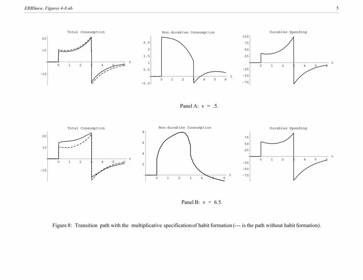
0 1 2 3 4 5 6t

-10

10

20

Total Consumption

0 1 2 3 4 5 6t

-0.5

0.5

1

1.5

2

2.5

Non−durables Consumption

0 1 2 3 4 5 6t

-75

-50

-25

25

50

75

100Durables Spending

Panel A: v = .5.

0 1 2 3 4 5 6t

-10

10

20

Total Consumption

0 1 2 3 4 5 6t

2

4

6

8Non−durables Consumption

0 1 2 3 4 5 6t

-75

-50

-25

25

50

75

Durables Spending

Panel B: v = 6.5.

Figure 8: Transition path with the multiplicative specification of habit formation (--- is the path without habit formation).

ERBSnew, Figures 4-8.nb 5

0 1 2 3 4 5 6t

-10

10

20

Total Consumption

0 1 2 3 4 5 6t

-1

1

2

3

Non−durables Consumption

0 1 2 3 4 5 6t

-50

50

100

Durables Spending

Panel A: All durables spending enters the liquidity cost function (---is the path without habit formation).

0 1 2 3 4 5 6t

-10-5

510

1520

Total Consumption

0 1 2 3 4 5 6t

-1

1

2

3

Non−durables Consumption

0 1 2 3 4 5 6t

-50

-25

25

50

75

Durables Spending

Panel B: Transition path when x = .50.

0 1 2 3 4 5 6t

-10

-5

5

10

15

Total Consumption

0 1 2 3 4 5 6t

-1

1

2

3

Non−durables Consumption

0 1 2 3 4 5 6t

-40

-20

20

40

60

Durables Spending

Panel C: Transition path when x = .25.

Figure 9: Transition Path when habit formation affects deliberation costs.

ERBSnew, Figures 9, 11, 12.nb 1

0 1 2 3 4 5 6t

-10

-5

5

10

15

20

Total Consumption

0 1 2 3 4 5 6t

-50

-25

25

50

75

Durables Spending

0 1 2 3 4 5 6t

-10

10

20

Relative Price of NT Good

Figure 10: Base Run for the model with a nontradables sector.

ERBSnew, Figure 10.nb 1

0 1 2 3 4 5 6t

-20

-10

10

20

30Total Consumption

0 1 2 3 4 5 6t

-50

50

100

Durables Spending

0 1 2 3 4 5 6t

-10

-5

5

10

15

20Relative Price of NT Good

0 1 2 3 4 5 6t

-4

-2

2

4

6

Traded Sector Employment

0 1 2 3 4 5 6t

-5

5

10

Nontraded Sector Employment

0 1 2 3 4 5 6t

123456

Total Employment

0 1 2 3 4 5 6t

-7.5-5

-2.5

2.55

7.5Traded Sector Investment

0 1 2 3 4 5 6t

-12-10-8-6-4-2

2Nontraded Sector Investment

0 1 2 3 4 5 6t

-10-8-6-4-2

24

Total Investment

0 1 2 3 4 5 6t

-3

-2

-1

1

2

3Traded Sector Output

0 1 2 3 4 5 6t

-2

2

4

6

Nontraded Sector Output

0 1 2 3 4 5 6t

-0.5

0.51

1.52

2.5Total Real Output

Figure 11: Base Run for Temporary ERBS with supply effects ( q-elasticity of investment equals unity).

ERBSnew, Figures 9, 11, 12.nb 2

0 1 2 3 4 5t

1

2

3

4

5

Total Consumption

0 1 2 3 4 5t

2468

101214

Durables Spending

0 1 2 3 4 5t

0.5

1

1.5

2

2.5

Relative Price of NT Good

0 1 2 3 4 5t

1

2

3

4

Traded Sector Employment

0 1 2 3 4 5t

1234567

Nontraded Sector Employment

0 1 2 3 4 5t

1

2

3

4

5

Total Employment

0 1 2 3 4 5t

1

2

3

4

5Traded Sector Investment

0 1 2 3 4 5t

123456

Nontraded Sector Investment

0 1 2 3 4 5t

1

2

3

4

5

Total Investment

0 1 2 3 4 5t

0.5

1

1.5

2

2.5

Traded Sector Output

0 1 2 3 4 5t

0.51

1.52

2.53

3.5Nontraded Sector Output

0 1 2 3 4 5t

0.5

1

1.5

2

2.5

3

Total Output

Figure 12: Base Run for Permanent ERBS with supply effects ( q-elasticity of investment equals unity).

ERBSnew, Figures 9, 11, 12.nb 3