Restricted ROC curves are useful tools to evaluate the performance of tumour markers

Article

Restricted ROC curves are usefultools to evaluate theperformance of tumour markers

S Parodi,1 M Muselli,2 B Carlini,3 V Fontana,4

R Haupt,5 V Pistoia3 and MV Corrias3

Abstract

In Clinical Epidemiology, receiver operating characteristic (ROC) analysis is a standard approach for the

evaluation of the performance of diagnostic tests for binary classification based on a tumour marker

distribution. The area under a ROC curve is a popular indicator of test accuracy, but its use has been

questioned when the curve is asymmetric. This situation often happens when the marker concentrations

overlap in the two groups under study in the range of low specificity, corresponding to a subset of values

useless for classification purposes (non-informative values). The partial area under the curve at a high

specificity threshold has been proposed as an alternative, but a method to identify an optimal cut-off that

separates informative from non-informative values is not yet available. In this study, a new statistical

approach is proposed to perform this task. Furthermore, a statistical test associated with the area

under a ROC curve corresponding to informative values only (restricted ROC curve) is provided and

its properties are explored by extensive simulations. Finally, the proposed method is applied to a real data

set containing peripheral blood levels of six tumour markers proposed for the diagnosis of neuroblastoma.

A new approach to combine couples of markers for classification purposes is also illustrated.

Keywords

Tumour markers, receiver operating characteristic analysis, diagnostic tests, restricted receiver operating

characteristic curve

1Clinical Epidemiology Unit, Department of Epidemiology and Prevention, IRCCS AOU San Martino-IST, Genoa, Italy2Institute of Electronics, Computer and Telecommunication Engineering, Genoa, Italy3Laboratory of Oncology, G. Gaslini Children’s Hospital, Genoa, Italy4Unit of Epidemiology, Biostatistics and Clinical Trials, Department of Epidemiology and Prevention, IRCCS AOU San Martino-IST,

Genoa, Italy5Epidemiology and Biostatistics Section, G. Gaslini Children’s Hospital, Genoa, Italy

Corresponding author:

S Parodi, Clinical Epidemiology Unit, Department of Epidemiology and Prevention, IRCCS AOU San Martino-IST, Largo R. Benzi 10,

16132 Genoa, Italy

Email: [email protected]

Statistical Methods in Medical Research

0(0) 1–21

! The Author(s) 2012

Reprints and permissions:

sagepub.co.uk/journalsPermissions.nav

DOI: 10.1177/0962280212452199

smm.sagepub.com

by guest on February 12, 2016smm.sagepub.comDownloaded from

http://smm.sagepub.com/

1 Introduction

Receiver operating characteristic (ROC) curves are statistical tools largely applied in ClinicalEpidemiology to evaluate the performance of tumour markers (TMs) in the context of binaryclassification problems.1–3 Because the early steps for a marker validation, in general, require acase-control approach,2,4 in this article the class of diseased subjects will be referred to as the‘cases’ and the referent group, which typically includes healthy individuals or subjects affected byless severe diseases, as the ‘controls’. In general, to be useful for diagnostic purposes a TM shouldpresent, on average, higher values in the class of the cases than in that of the controls. A binary testmay be obtained by selecting a specific value of a continuous TM and by defining as positive any testwith value exceeding such a threshold, and as negative the remaining other tests. The proportion ofpositive cases provides an estimate of the test sensitivity and the proportion of negative controls anestimate of its specificity. A ROC curve is obtained by plotting the true positive fraction (sensitivity)vs the false positive fraction (1-specificity) using all the available values of a TM concentration.Figure 1(a) shows a theoretical ROC curve obtained from infinite values of a hypothetical TM andan empirical ROC curve obtained from a finite sample of 200 units (100 cases and 100 controls)randomly selected from the same binormal distribution (displayed in panel (b)).

The area under a ROC curve (AUC) is a popular measure of diagnostic accuracy. It is equivalentto the Mann-Whitney U statistic, thus representing the probability that a subject, randomly selectedamong the case class, shows a marker value higher than a subject randomly extracted from thecontrols.5,6 For completely non-informative TMs the ROC curve will approach the rising diagonal(called ‘chance diagonal’ or ‘chance line’, Figure 1(a)) and AUC will tend to 0.5, i.e. the expectedprobability for a classification due to chance alone. On the contrary, in the case of a perfectclassification the ROC curve will reach the point of the highest theoretical accuracy (sensitivityand specificity both 100%) and AUC will tend to one, i.e. the highest probability value.

Figure 1. Theoretical and empirical ROC curves (panel (a)) and a corresponding density probability distribution

(panel (b)) (binormal model with the same variance). The empirical curves was obtained from 200 random samples

(100 cases and 100 controls).

FPF: false positive fraction; TPF: true positive fraction.

2 Statistical Methods in Medical Research 0(0)



A statistical test to verify that AUC is different from its expected value under the null hypothesis iseasily performed exploiting the normal asymptotic distribution of the U statistic7–9

zAUC ¼dAUC� 0:5ffiffiffiffiffiffiffiffiffiffiffiffiffiffiffiffiffiffiffiffiffiffiffiffidVar dAUC

� �r ð1Þ

where Var(AUC) represents the variance of AUC that may be estimated by some differentformulas.5,8,9 In this study, the following equation was adopted, which was derived from thevariance of the U statistic under the null hypothesis10

dVar dAUC� �

¼n0 þ n1 þ 1

12n0n1ð2Þ

An optimal cut-off for a binary classification test may be identified on a ROC curve as the valuecorresponding to the highest vertical distance J from the chance line (Figure 1, panel (a)). J alsocorresponds to the highest value of the Youden’s index, a popular measure of pure accuracy.2,11,12

Proper ROC curves are concave and symmetric and never cross each other, thus allowing an easyand reliable comparison between the corresponding markers. In fact, for proper ROC curves, thehighest AUC ever corresponds to the highest sensitivity at any specificity value. Furthermore, theselection of an optimal cut-off on proper curves is easily performed, because they include a uniquepoint that corresponds to the optimal threshold based on the Youden’s index.2,11,12 However, in theanalysis of TM, asymmetric (not proper) ROC curves are often encountered, due to the presence inthe two classes under study of overlapping marker values at an extreme of their distributions. Inmany situations, a lack of sensitivity is observed in the correspondence of the lowest range ofspecificity values,13 causing the corresponding ROC curve to be unimodal and right asymmetricwith respect to the chance line. In this article, curves of this kind will be called ‘positive skewedROC’. Four examples of such curves are illustrated in Figure 2(a) to (d), while Figure 3(a) to (d)shows four corresponding density distributions of four hypothetical TM concentrations. In moredetails, the ROC curve in Figure 2(a) is positive skewed and concave, and may correspond to aunimodal distribution of marker values among the controls and a bimodal ones among the cases(‘Normal–Binormal model’, Figure 3(a)). In the real world, this situation may occur when asubgroup of cases does not differ from the controls for the expression of the TM under study.13

Another situation is that illustrated in Figure 3(b), corresponding to the ROC curve in Figure 2(b),in which cases and controls have a similar distribution density (both normal), but among the casesthe marker have both higher mean and variance values (‘Binormal model’ with different variances).This behaviour may be considered as a variant of the previous one, when the two subgroups of casesare less distinguishable. In that case, the corresponding ROC tends to lose its concavity at the lowestscale of specificity and it may even cross the chance line2,3,13,14 (Figure 2(b)). Moreover, Figure 3(c)shows a bimodal distribution both in the cases and in the controls, with a subgroup within any classshowing a similar TM distribution in the range of low marker values (‘Binormal–Binormal model’).This behaviour may be attributable to a detection threshold of the device used to measure the TMconcentrations, which automatically replaces null values with a white noise. The correspondingROC curve will be similar to that in Figure 2(c), when the curve approaches the chance line atlow specificity values. Finally, a quite common variant of this situation is that of a TM with mass atzero, illustrated in Figure 3(d), in which the range of non-informative values is made by some zero

Parodi et al. 3



values (‘Zero-inflated Binormal’ model). The corresponding ROC curve will be still positive skewedand it will also show a jump discontinuity of the derivative,15 like the curve in Figure 2(d).

In the case of not proper ROC curves, some Authors have proposed the use of the partial areaunder the curve (pAUC) at an a priori selected cut-off of high specificity, or based on some utilityfunction.13,16,17 All these approaches, however, do not provide a method to identify the range ofnon-informative values, if any, within the TM distribution. In general, subjects whose values fall insuch a range are defined as ‘test negative’, albeit this range may include different proportions of casesand controls.

In this article, a new simple method of ROC analysis is illustrated, which allows to identify anoptimal threshold to separate the range of non-informative values of a TM from those potentiallyuseful for classification purposes. A statistical test associated with the ROC curve corresponding tothe informative range only (restricted ROC, rROC) is also provided. Finally, a method to combinerestricted and standard ROC analysis is illustrated and applied to a real data set of six TMs for thediagnosis of localized neuroblastoma.

Figure 2. Example of four positive skewed ROC curves.





This article is organized as follows: in Section 2 a new statistical test for rROC is provided, basedon the standard normal distribution; in Section 3 its statistical power is investigated by extensivesimulations and compared with that of the standard test on AUC; in Section 4 a simple rule for thechoice between standard and rROC curves is illustrated; in Section 5 a method to combineinformation from standard and rROC curves is analysed; in Section 6 the new proposed methodis applied to a real data set of concentrations of six putative TMs proposed for the diagnosis ofneuroblastoma; in Section 7 a discussion of the method and the obtained results is provided.

2 Definition of a new statistical test for rROC

Let X be a TM whose concentrations are expressed on a continuous scale in two classes (controlsand cases). Let Y be a random sample of X-values sorted in an ascending order in an array {yi}(i¼ 1, . . . ,N) and let n0 be the sample size of the controls and n1 that of the cases, with n0þ n1¼N. Aleft rROC curve (simply called rROC, because right restriction will not be considered in this article)is defined as the ROC curve obtained after the elimination from Y of the first j ordered values. Forany value of j ( j¼ 0, . . . ,N), a rROCj may be identified and the corresponding area under the curve(rAUCj) estimated. Similarly to equation (1) a test statistic may be associated to rAUCj as follows

rzAUCj ¼drAUCj � 0:5ffiffiffiffiffiffiffiffiffiffiffiffiffiffiffiffiffiffiffiffiffiffiffiffiffiffiffidVar drAUCj

� �r ð3Þ

Figure 3. Example of four density distributions corresponding to the positive skewed ROC curves in Figure 2.

(a) Normal–binormal model; (b) binormal model with different variances; (c) binormal–binormal model; and

(d) zero-inflated binormal model.

Parodi et al. 5



where, similarly to equation (2)

dVar drAUCj

� �¼

rn0 þ rn1 þ 1

12rn0rn1ð4Þ

and rn0 and rn1 represent the sample size of the two classes (controls and cases, respectively) after therestriction to N – j samples.

The new statistic test proposed in this article is defined as follows

rzAUC ¼Max rzAUCj

� �ð5Þ

Accordingly to equations (3) and (5), rzAUC represents the highest ‘standardized’ AUC, i.e. thevalue that identifies the rROC with the highest accuracy, estimated taking into account both theprobability of a correct classification (i.e. rAUC) and a measure of its variability. Accordingly, thecorresponding j allows the identification of a cut-off Cj (if any) which separates informative TMvalues from non-informative ones. jmay be zero in the case of non-restriction, i.e. when the standardAUC has a higher performance than any other rAUCj. Finally, to allow rzAUC to be unique for anyROC curve, in the case of more than one value from equation (5), only that corresponding to thelowest j is retained, corresponding to the rROC based on the largest sample size.

The probability density of the rzAUC statistic under the null hypothesis H0 of an equaldistribution of TM values among the two classes was investigated by extensive randomsimulations. N samples from a standard normal distribution were generated by letting N varyfrom 10 to 500 in each class. Each simulation was repeated 105 times in order to obtain stableestimates of the expected value and of the variance of rzAUC. The analysis was performed by asoftware ad hoc developed by the freely available package Microsoft Visual Basic Express 2010.Random values from an uniform probability density were obtained by the RAN1 algorithm,18 whilenormal distributions were obtained by the GASDEV algorithm.18 Furthermore, most routines forboth standard and rROC analysis were implemented in an open source statistical program (called‘rROC’) freely available at: http://www.ge.ieiit.cnr.it/�muselli/supplement/smmr-2012.html.Finally, histograms and the quantile–quantile inverse normal plots (qqplots), for the evaluationof the normality of rzAUC distribution, were obtained by STATA for Windows statisticalpackage (release 11.0, Stata Corporation, College Station, TX, USA).

Figure 1S(a) to (f) in Supplemental Material shows six histograms of the simulated probabilitydensity of rzAUC under H0 in the comparison of two balanced classes. The density of rzAUCdistribution seems to approach a normal probability function when the sample size is increased.However, in the presence of a high number of samples the distribution tends to be slightlyleptokurtic and negative skewed (Figure 1S, panel (f)).

The following statistical test based on a standard normal distribution applied to rzAUC isproposed to test the null hypothesis of a non-informative rROC

z �

drzAUC� bE drzAUC� �

ffiffiffiffiffiffiffiffiffiffiffiffiffiffiffiffiffiffiffiffiffiffiffiffiffiffiffiffidVar drzAUC� �r ð6Þ

where the estimates of the expected value bEð drzAUCÞ and variance dVarð drzAUCÞ of rzAUC areobtained from the mean values and the variances of the simulated distributions, which are listedin Table 1 and in Table 2, respectively. To assess the degree of agreement of the proposed test to a




Table 1. Expected value of rzAUC as a function of the sample size under the null hypothesis

n0

n1

10 15 20 25 30 35 40 45 50 60 70 80 90 100 150 200 250 300 400 500

10 1.15 1.28 1.36 1.42 1.46 1.50 1.53 1.55 1.58 1.61 1.64 1.67 1.69 1.71 1.76 1.80 1.83 1.85 1.87 1.89

15 1.15 1.28 1.36 1.42 1.46 1.50 1.53 1.55 1.57 1.62 1.64 1.67 1.69 1.70 1.77 1.81 1.83 1.85 1.88 1.90

20 1.15 1.29 1.36 1.42 1.47 1.50 1.53 1.56 1.58 1.62 1.65 1.67 1.69 1.71 1.77 1.81 1.84 1.86 1.89 1.91

25 1.15 1.28 1.36 1.42 1.47 1.51 1.53 1.56 1.58 1.62 1.65 1.67 1.69 1.71 1.77 1.81 1.84 1.86 1.89 1.92

30 1.15 1.28 1.37 1.42 1.47 1.51 1.54 1.57 1.58 1.62 1.65 1.67 1.69 1.72 1.77 1.82 1.84 1.87 1.90 1.92

35 1.14 1.28 1.37 1.42 1.47 1.51 1.53 1.56 1.59 1.62 1.65 1.67 1.70 1.72 1.77 1.81 1.85 1.86 1.90 1.92

40 1.15 1.28 1.36 1.43 1.47 1.51 1.54 1.56 1.59 1.62 1.65 1.68 1.70 1.71 1.78 1.82 1.85 1.87 1.91 1.93

45 1.15 1.28 1.37 1.42 1.47 1.51 1.54 1.57 1.59 1.63 1.65 1.67 1.70 1.72 1.78 1.82 1.85 1.87 1.90 1.93

50 1.14 1.28 1.37 1.43 1.47 1.51 1.54 1.56 1.59 1.62 1.66 1.68 1.70 1.71 1.78 1.82 1.85 1.88 1.91 1.93

60 1.14 1.28 1.37 1.43 1.47 1.51 1.54 1.56 1.58 1.63 1.66 1.68 1.70 1.71 1.79 1.82 1.85 1.87 1.91 1.93

70 1.15 1.28 1.37 1.43 1.48 1.51 1.54 1.57 1.59 1.62 1.66 1.68 1.70 1.72 1.78 1.83 1.86 1.88 1.92 1.94

80 1.15 1.28 1.37 1.43 1.47 1.51 1.54 1.57 1.59 1.62 1.66 1.68 1.71 1.72 1.78 1.83 1.86 1.88 1.91 1.94

90 1.15 1.28 1.37 1.43 1.47 1.51 1.54 1.57 1.59 1.63 1.66 1.68 1.71 1.72 1.79 1.83 1.86 1.88 1.91 1.94

100 1.15 1.28 1.36 1.43 1.47 1.51 1.54 1.57 1.59 1.63 1.66 1.68 1.71 1.72 1.79 1.83 1.86 1.89 1.92 1.94

150 1.15 1.28 1.36 1.43 1.47 1.51 1.54 1.57 1.59 1.63 1.66 1.69 1.71 1.72 1.79 1.83 1.87 1.89 1.92 1.95

200 1.14 1.28 1.36 1.43 1.47 1.51 1.54 1.57 1.59 1.63 1.66 1.68 1.71 1.73 1.79 1.84 1.86 1.89 1.92 1.95

250 1.14 1.28 1.37 1.43 1.47 1.51 1.54 1.57 1.59 1.63 1.66 1.68 1.71 1.73 1.79 1.83 1.87 1.90 1.93 1.95

300 1.15 1.28 1.37 1.43 1.47 1.51 1.54 1.57 1.59 1.63 1.66 1.69 1.71 1.72 1.80 1.84 1.87 1.89 1.93 1.95

400 1.15 1.28 1.36 1.43 1.47 1.51 1.54 1.57 1.59 1.63 1.66 1.69 1.71 1.73 1.80 1.84 1.87 1.90 1.94 1.96

500 1.15 1.28 1.37 1.43 1.48 1.51 1.55 1.57 1.59 1.63 1.66 1.68 1.70 1.73 1.79 1.84 1.88 1.90 1.94 1.96

n0¼ number of controls; n1¼ number of cases.

Estimates obtained by 105 random samples.

Table 2. Variance of rzAUC as a function of the sample size under the null hypothesis

n0

n1

10 15 20 25 30 35 40 45 50 60 70 80 90 100 150 200 250 300 400 500

10 0.59 0.52 0.49 0.46 0.45 0.43 0.41 0.40 0.39 0.37 0.36 0.34 0.33 0.32 0.28 0.26 0.24 0.23 0.21 0.20

15 0.60 0.55 0.51 0.49 0.47 0.45 0.44 0.43 0.41 0.40 0.39 0.38 0.37 0.35 0.32 0.30 0.28 0.26 0.24 0.23

20 0.60 0.55 0.52 0.50 0.48 0.46 0.45 0.44 0.43 0.41 0.40 0.39 0.38 0.38 0.35 0.31 0.30 0.29 0.27 0.26

25 0.60 0.55 0.52 0.50 0.48 0.47 0.45 0.45 0.44 0.42 0.41 0.41 0.39 0.39 0.36 0.34 0.32 0.31 0.29 0.28

30 0.61 0.56 0.53 0.50 0.49 0.48 0.47 0.45 0.45 0.43 0.42 0.41 0.40 0.40 0.37 0.35 0.34 0.32 0.30 0.29

35 0.60 0.56 0.53 0.51 0.49 0.48 0.47 0.46 0.45 0.44 0.43 0.42 0.41 0.40 0.37 0.35 0.34 0.33 0.31 0.30

40 0.61 0.56 0.53 0.51 0.49 0.48 0.47 0.46 0.45 0.44 0.43 0.42 0.41 0.40 0.39 0.36 0.35 0.34 0.32 0.31

45 0.61 0.56 0.53 0.51 0.49 0.48 0.47 0.46 0.45 0.44 0.43 0.43 0.41 0.42 0.39 0.37 0.36 0.35 0.33 0.32

50 0.61 0.56 0.53 0.51 0.50 0.48 0.47 0.47 0.46 0.44 0.44 0.42 0.42 0.41 0.39 0.37 0.36 0.35 0.34 0.32

60 0.60 0.56 0.53 0.51 0.50 0.49 0.48 0.47 0.46 0.45 0.44 0.43 0.42 0.42 0.40 0.38 0.37 0.36 0.35 0.33

70 0.61 0.56 0.53 0.52 0.50 0.49 0.47 0.47 0.46 0.45 0.44 0.44 0.43 0.42 0.40 0.38 0.37 0.36 0.35 0.34

80 0.61 0.56 0.54 0.52 0.50 0.49 0.48 0.47 0.47 0.45 0.44 0.44 0.43 0.42 0.40 0.39 0.38 0.37 0.36 0.35

90 0.61 0.56 0.53 0.52 0.50 0.49 0.48 0.47 0.46 0.46 0.44 0.44 0.43 0.43 0.41 0.39 0.38 0.37 0.36 0.35

100 0.61 0.56 0.54 0.52 0.50 0.49 0.48 0.48 0.47 0.45 0.45 0.44 0.43 0.43 0.41 0.40 0.38 0.38 0.36 0.35

150 0.61 0.56 0.54 0.52 0.50 0.49 0.49 0.48 0.47 0.46 0.45 0.45 0.44 0.44 0.41 0.40 0.39 0.38 0.37 0.37

200 0.61 0.56 0.54 0.52 0.50 0.49 0.49 0.48 0.47 0.46 0.46 0.44 0.45 0.44 0.42 0.41 0.40 0.39 0.38 0.37

250 0.61 0.57 0.53 0.52 0.51 0.49 0.48 0.48 0.48 0.46 0.46 0.45 0.45 0.44 0.42 0.41 0.40 0.39 0.38 0.37

300 0.61 0.56 0.53 0.52 0.51 0.49 0.49 0.48 0.48 0.46 0.46 0.45 0.44 0.44 0.42 0.41 0.40 0.40 0.39 0.38

400 0.61 0.56 0.54 0.52 0.51 0.49 0.49 0.48 0.47 0.46 0.46 0.45 0.44 0.44 0.43 0.41 0.41 0.40 0.39 0.38

500 0.61 0.56 0.53 0.52 0.50 0.49 0.48 0.48 0.47 0.46 0.45 0.45 0.45 0.44 0.43 0.41 0.41 0.40 0.39 0.38

n0¼ number of controls; n1¼ number of cases.

Estimates obtained by 105 random samples.

Parodi et al. 7



standard normal distribution, simulated data were standardized using equation (6) and theircumulative distribution plotted vs the corresponding expected values from an inverse normalfunction (qqplot). Results are shown in Figure 2S(a) to (f) in the Supplemental Material, where thevertical lines correspond to the critical values for one and two sided tests at the conventional 0.05threshold for the type I (�) error. rzAUC shows a quite good agreement with a Gaussian distribution,but it does not asymptotically converge to it. However, in each plot rzAUC strictly approaches thenormal distribution in the correspondence of critical �-values, indicating that a small bias is expectedto occur in the application of the test in equation (6) using conventional thresholds for statisticalsignificance (Figure 2S). The same analysis was carried out for unbalanced groups (Figures 3S to 12S).Strong departures for normality was observed for very unbalanced groups when the smaller samplesize referred to controls (see for example, Figure 3S, panel (f), which included 10 controls and 500cases). Conversely, rzAUC showed a quite good approximation to the Gaussian distribution in thepresence of a small number of samples among cases, even for very unbalanced classes (see for exampleFigure 11S, panel (a), which included 500 controls and 10 cases). The cumulative distribution of thestandardized rzAUC showed a quite satisfactory agreement with the corresponding value of theinverse normal in the range of �¼ 0.05 also in the presence of a strong departure from normality ofthe corresponding density (see for example the qqplot in Figure 4S, panel (f)).

3 Estimates of statistical power of rzAUC

Statistical power of the approximately normal test for rzAUC, shown in equation (6), was estimatedunder some simulated distributions and compared with the standard asymptotic normal test forAUC in equation (1). The selected distributions corresponded both to the binormal model with equalvariances (Figure 1(b)) and to the distributions illustrated in Figure 3(a) to (d), namely: (a) normal–binormal, (b) binormal with different variances, (c) binormal–binormal and (d) zero-inflatedbinormal. In each analysis, statistical power was estimated as the proportion of positive results(i.e. tests called statistically significant) on a total of 1000 simulated distributions. Moreover, anytest was also repeated using 2000 random permutations of the samples in the two classes in order toassess the impact of the non-perfect fit of rzAUC to the normal distribution. Results are resumed inTable 3.

3.1 Binormal model with equal variances

In the case of binormal model with equal variances, when the means in the two groups were equal(difference between the two means, ��¼ 0) the proportion of positive results represented anestimate of the test bias under H0, whereas in the presence of a positive �� value, such aproportion provided an estimate of the corresponding statistical power. Both asymptotic andpermutation tests on rzAUC showed a rather good agreement with the expected �-value (0.05)under H0 and with the corresponding results from the standard analysis on AUC, even if theasymptotic test on rzAUC was slightly biased in the presence of small sample size (Table 3).Under H1 (�� from 0.5 to 2.0) a good agreement between the asymptotic and the permutationanalysis was observed for both statistics at any sample size, except for a small loss of power for theasymptotic test for rzAUC, which tended to decrease when increasing ��. The test for AUC showedthe highest statistical power, but the difference between the two tests tended to disappear withincreasing both the sample size and ��.




Tab

le3.

Pro

port

ion

of

posi

tive

resu

lts

(%)

for

test

on

rzAU

Can

dAU

Cunder

diff

ere

nt

TM

sdis

trib

ution

assu

mption

TM

dis

trib

ution

��¼

0.0

��¼

0.5

��¼

1.0

��¼

1.5

��¼

2.0

AU

Crz

AU

CAU

Crz

AU

CAU

Crz

AU

CAU

Crz

AU

CAU

Crz

AU

C

Asy

Asy

Per

Asy

Asy

Per

Asy

Asy

Per

Asy

Asy

Per

Asy

Asy

Per

n 0¼

10,n

1¼

10

Bin

orm

al–

equal

vari

ance

5.0

*3.8

*5.2

*25.9

13.2

17.1

67.1

41.4

48.8

94.0

76.6

80.5

99.4

93.6

95.3

Bin

orm

al–

unequal

vari

ance

5.4

*8.7

12.3

23.3

21.0

27.5

50.9

41.9

50.3

79.9

67.1

74.1

95.4

89.0

91.6

Norm

al–bin

orm

al5.1

*3.7

*5.8

*14.5

7.5

11.7

25.7

15.5

21.7

39.2

26.1

33.2

51.8

45.8

56.5

Bin

orm

al–bin

orm

al4.2

*2.6

*3.6

*8.1

6.6

11.1

13.8

13.5

21.5

21.6

29.0

38.6

25.4

43.4

57.0

Zero

-infla

ted

bin

orm

al0.0

*0.4

*3.0

*0.1

2.0

10.1

0.0

5.4

22.8

0.2

14.0

36.4

0.2

29.4

59.1

n 0¼

15,n

1¼

15

Bin

orm

al–

equal

vari

ance

5.0

*4.0

*5.7

*39.3

20.8

24.5

81.8

59.8

63.5

98.8

92.2

93.5

100

99.8

100

Bin

orm

al–

unequal

vari

ance

5.4

*16.0

19.2

27.6

31.8

38.9

65.0

61.0

66.4

93.7

88.4

90.8

99.2

98.1

98.7

Norm

al–bin

orm

al3.5

*2.9

4.4

12.0

8.4

10.7

27.0

19.1

23.3

46.8

36.4

41.5

60.2

61.0

67.1

Bin

orm

al–bin

orm

al3.1

*3.9

*5.4

*7.2

9.7

13.1

15.8

22.1

29.7

27.3

43.1

49.9

36.6

65.7

73.7

Zero

-infla

ted

bin

orm

al0.0

*0.8

*3.7

*0.1

3.8

11.8

0.2

14.0

30.4

0.4

31.8

54.7

0.6

57.8

79.9

n 0¼

20,n

1¼

20

Bin

orm

al–

equal

vari

ance

4.3

*3.4

*4.5

*44.0

23.7

26.8

92.5

75.0

78.2

99.9

98.1

98.4

100

100

100

Bin

orm

al–

unequal

vari

ance

5.7

*16.2

19.5

34.1

39.8

45.0

78.9

75.4

77.6

97.3

94.8

96.3

100

99.6

99.6

Norm

al–bin

orm

al2.7

*4.3

*4.1

*20.0

12.8

15.0

41.3

31.1

34.7

65.8

55.9

60.5

80.7

80.7

84.2

Bin

orm

al–bin

orm

al3.4

*3.4

*4.3

*13.3

11.6

13.2

25.2

33.5

38.4

42.1

65.0

69.0

54.1

86.1

88.2

Zero

-infla

ted

bin

orm

al0.1

*1.6

*4.7

*0.0

7.4

15.9

2.4

25.5

41.3

6.1

54.4

71.3

10.3

82.5

92.2

n 0¼

30,n

1¼

30

Bin

orm

al–

equal

vari

ance

5.3

*4.6

*4.6

*58.9

38.6

38.4

97.8

91.4

90.8

100

99.9

99.8

100

100

100

Bin

orm

al–

unequal

vari

ance

4.7

*26.8

26.6

47.1

63.4

63.0

90.8

91.7

91.8

99.8

99.5

99.5

100

100

100

Norm

al–bin

orm

al2.7

*4.3

*4.1

*25.4

19.1

18.6

51.9

45.4

44.7

80.7

77.9

77.2

94.0

95.6

95.2

Bin

orm

al–bin

orm

al2.8

*4.9

*4.5

*15.8

19.2

18.6

34.6

51.9

51.6

64.3

86.2

86.0

77.3

99.1

98.9

Zero

-infla

ted

bin

orm

al0.0

*2.7

4.6

*0.7

12.4

18.9

6.3

42.5

53.2

26.0

80.4

86.3

52.9

95.9

97.5

n 0¼

50,n

1¼

50

Bin

orm

al–

equal

vari

ance

4.8

*4.7

*4.9

*77.2

49.7

50.4

100

98.8

98.8

100

100

100

100

100

100

Bin

orm

al–

unequal

vari

ance

6.9

*40.9

40.9

63.9

78.6

79.5

98.6

98.8

98.8

100

100

100

100

100

100

Norm

al–bin

orm

al5.4

*4.3

*4.9

*35.2

23.1

24.2

76.7

61.6

62.7

95.1

92.0

92.5

99.4

99.7

99.7

Bin

orm

al–bin

orm

al2.8

*3.9

*3.9

*23.9

27.8

28.9

61.0

73.6

74.4

84.0

97.4

97.6

96.8

100

100

Zero

-infla

ted

bin

orm

al0.3

*2.1

*5.8

*3.1

18.7

26.2

27.8

62.6

72.2

75.9

96.8

98.6

97.1

100

100

TM

s:tu

mour

mar

kers

.

Asy¼

asym

pto

tic

norm

alte

st;Per¼

perm

uta

tion

test

(bas

ed

on

2000

random

perm

uta

tions)

;n 0¼

num

ber

of

contr

ols

;n 1¼

num

ber

of

case

s;an

d*H

0is

true.

��

:expect

ed

diff

ere

nce

inT

Mm

ean

sbetw

een

case

san

dco

ntr

ols

.

Parodi et al. 9



3.2 Binormal model with different variances

The estimate of statistical power of the two tests under a binormal model with differentvariances was obtained setting to 1.0 the variance among controls and to 2.0 that among thecases. Results from permutation and asymptotic methods were in a rather good agreement forboth tests in any analysis, except for a small loss of statistical power in the permutation test forrzAUC either at sample size �20 or when the difference between means (��) was lower than 1.5(Table 3). The test for rzAUC showed a higher statistical power than that for AUC at ��¼ 0.5,while for larger �� values the two tests had a comparable performance. At ��¼ 0, theproportion of positive results was higher for the test for rzAUC (both from permutation thanasymptotic analysis) than that for AUC. However, it should be noted that in this situationresults for the new proposed test do not estimate the test bias under H0, because thecorresponding ROC curve crosses the chance line.

3.3 Normal-binormal model

Simulations for the normal–binormal model (corresponding to ROC curves like that in Figure 3(c))were carried out setting to 1.0 the variance for any distribution (i.e. two normal distributions amongthe cases and one normal among the controls). Mean values were set to zero for both the firstsubgroup of cases and the class of controls, while it ranged from 0.0 to 2.0 for the second subgroupof cases. A sampling ratio of 2:1 was adopted for the two subgroups of cases (the largest one wasthat with the same distribution of the controls). In this analysis, �� represents the differencebetween the means between the two groups of cases or (equivalently) between the second groupof cases and the controls.

Permutation test showed a higher statistical power than the asymptotic test, but this differencetended to disappear with increasing the sample size (Table 3).

3.4 Binormal–binormal model

Under the binormal–binormal model, in the two subgroup of cases and controls with the samemean, variance was 1.0, the mean value was 0.0 and the sample size was the same. In the remainingtwo subgroups of controls and cases, mean values were 1.0 for the controls and were left to varyfrom 1.0 to 3.0 in the subgroup of cases (in Table 3 such differences were expressed as distances ��between such subgroups, which accordingly varied from 0.0 to 2.0). Variance and sample size wereequal to those of the former two subgroups.

In the presence of small sample size, the normal test for rzAUC showed a loss of statistical powercompared with the permutation approach. Tests for rzAUC outperformed that for AUC, withdifferences becoming more pronounced when increasing �� values.

3.5 Zero-inflated binormal model

For the zero-inflated binormal model the same sample size was adopted for the two subgroups ofcases and controls with mass at zero and for the remaining two subgroups. For these latter, abinormal model with equal variances (�2¼ 1.0) was used, with a mean value of 1.0 in thesubgroup of controls and a mean value varying from 1.0 to 3.0 in the subgroup of cases(corresponding to �� from 0.0 to 2.0 in Table 3). Negative values extracted from the normaldistributions were replaced with zero. At ��¼ 0.0, the test for AUC showed a proportion offalse positive tests close to 0. The asymptotic test for rzAUC was also biased, especially for low




sample size, while for the permutation test the false positive proportion was quite similar to theselected �-value (0.05).

The permutation approach outperformed the asymptotic test for rzAUC in any analysis. Bothtests for rzAUC showed a higher statistical power than that for AUC.

In summary, results of power analysis reported in Table 3 suggest that, in most cases theasymptotic test for rzAUC seems to be appropriated when at least 20 samples are present in eachclass, whereas for smaller sample sizes the permutation test should be preferred.

4 Choosing between complete and rROC curves

In order to find a convenient rule to choose between restricted and standard ROC analysis weanalysed the following three situations: (a) only a rROC analysis was performed and the testassociated with the rAUC (equation (3)) was statistically significant (first column in Table 4); (b)the p-value associated to a rROC (equation (3)) was statistically significant and also lower thanthe corresponding p-value associated to the entire curve (equation (1), second column in Table 4);(c) the previous rule was respected and the mean difference percent (MDP) between rAUCand AUC was higher of some selected thresholds (third column in Table 4), where MDP wasdefined as

dMDP ¼drAUC� dAUCdAUC

� 100 ð7Þ

Simulations included only proper ROC curves, because the standard ROC analysis approachshould be preferred in the case of a proper ROC curve, due to the highest statistical power of the testfor AUC. Moreover, the case of non-informative ROC curve was also considered. The distributionof j-values was obtained from 1000 simulated TMs. The corresponding statistical significance ofrzAUC was estimated by the test based on the normal approximation (equation (6)), except when thesample size was lower than 20 to prevent the loss of statistical power. In that case, a test based on2000 random permutations was employed.

Table 4 reports the percentages of rROC curves that would have been selected using the abovecited three criteria and some corresponding percentiles of the j statistic, which corresponds to thenumber of samples excluded from the curve. The first column corresponds to the results of rROCanalysis only (case a). The number of excluded samples was about 5% under H0 and tended toincrease with increasing ��, while the corresponding median value of j tended to decrease. Inparticular, for �� 1.0 the median value of j was 0 in any comparison and for �� 1.5 also the75� percentile equals 0 in all comparisons except one, indicating that the rROC analysis tends toprovide results very similar to those from the standard ROC approach when the underline TMdistributions are well separated.

The second column in Table 4 (case b) shows the results of the combination of restricted andstandard ROC analysis based on the comparison between the corresponding p-values. Theproportion of selected rROC was slightly lower than those observed by the rROC only (firstcolumn) at ��¼ 0.0, while the median value of j was slightly higher. Proportion of errors tendedto increase with increasing �� up to ��¼ 1.0 and to decrease subsequently. Finally, when onlyrROC curves corresponding to DMP >20% were selected (case c, third column in Table 4) theproportion of errors clearly decreased ranging between 4% and 7% for �� 1.0 and dropping to 0–2% for ��> 1.5, while the corresponding j-values decreased accordingly.

Parodi et al. 11



Tab

le4.

Dis

trib

ution

ofth

enum

ber

ofsa

mple

sje

xcl

uded

by

rRO

Can

alys

isat

the

conve

ntional

0.0

5�

leve

lfo

rnot

info

rmat

ive

(��¼

0)

and

for

pro

per

RO

Ccu

rves

(��>

0)

Sam

ple

s

(a)

rRO

Can

alys

isonly

(b)

Stan

dar

dan

drR

OC

anal

ysis

(any

MD

P)

(c)

Stan

dar

dan

drR

OC

anal

ysis

(MD

P>

20%

)

Perc

entile

s

%

Perc

entile

s

%

Perc

entile

s

%n 0

n 110

25

50

75

90

10

25

50

75

90

10

25

50

75

90

��¼

0.0

10

10

02

58

11

5.2

34

69

11

3.3

23

58

92.8

15

15

15

12

15

20

5.7

49

13

17

20

4.7

711

14

18

20

4.2

20

20

59

18

23

27

3.4

716

20

25

28

2.6

13

16

20

25

28

2.5

30

30

311

25

38

43

4.6

918

29

39

44

3.6

17

23

31

40

44

3.1

50

50

726

55

71

85

4.7

26

45

63

73

87

3.8

32

52

64

75

87

3.5

��¼

0.5

10

10

00

26

917.1

12

57

10

9.3

34

79

10

6.4

15

15

00

310

16

24.5

24

10

15

18

10.1

911

14

17

19

6.2

20

20

00

312

20

23.7

59

14

19

25

6.3

912

17

23

25

4.7

30

30

00

621

35

38.6

511

20

34

41

12.0

16

22

29

39

43

7.2

50

50

00

522

55

49.7

613

31

55

73

10.2

41

48

57

73

79

4.7

��¼

1.0

10

10

00

03

848.8

12

48

10

12.8

56

89

11

5.8

15

15

00

03

863.5

13

59

16

11.7

68

11

16

17

4.5

20

20

00

03

11

75.0

15

11

17

21

6.7

912

18

20

25

3.2

30

30

00

03

13

91.4

13

815

31

10.1

13

22

33

37

47

1.7

50

50

00

01

698.8

12

49

21

14.0

43

50

54

63

70

0.5

��¼

1.5

10

10

00

00

380.5

12

35

79.1

36

77

91.8

15

15

00

00

493.5

12

47

11

9.2

11

11

13

13

14

1.1

20

20

00

03

598.1

11

46

96.0

23

23

23

23

23

0.1

30

30

00

00

299.9

12

46

11

6.8

n.e

.n.e

.n.e

.n.e

.n.e

.0.0

50

50

00

00

1100

12

34

79.9

n.e

.n.e

.n.e

.n.e

.n.e

.0.0

��¼

2.0

10

10

00

00

095.3

12

34

55.5

34

89

11

0.6

15

15

00

00

0100

12

34

75.7

n.e

.n.e

.n.e

.n.e

.n.e

.0.0

20

20

00

00

0100

22

45

82.5

n.e

.n.e

.n.e

.n.e

.n.e

.0.0

30

30

00

00

0100

22

44

73.1

n.e

.n.e

.n.e

.n.e

.n.e

.0.0

50

50

00

00

0100

33

45

72.4

n.e

.n.e

.n.e

.n.e

.n.e

.0.0

rRO

C:re

stri

cted

rece

iver

opera

ting

char

acte

rist

ic.

n 0¼

num

ber

of

contr

ols

;n 1¼

num

ber

of

case

s;%¼

perc

enta

ges

of

rRO

Ccu

rves

sele

cted;M

DP¼

mean

diff

ere

nce

perc

ent

betw

een

rAU

Can

dAU

C;an

dn.e

.¼not

eval

uab

le.

��¼

expect

ed

diff

ere

nce

inT

Mm

ean

sbetw

een

case

san

dco

ntr

ols

.




Taken together, these results suggest that in the presence of a statistically significant test for therROC curve and a MDP> 20% standard ROC analysis may be replaced by rROC ones with anacceptable proportion of errors (about 5% or less).

5 Combining information from restricted and standard ROC curves

The main limit of the rROC analysis is the exclusion from the ROC curve of the j subjects whose TMvalues are lower than Cj, the cut-off that separates informative from non-informative values (asillustrated in Section 2). To recover this drawback, information from two or more TMs can becombined. A new approach will be illustrated, which extends the traditional method of applying alogistic regression model to two or more marker values in order to obtain a risk score (RS) forclassification purposes.19 RS is usually employed as a new TM in a standard ROC analysis and abinary test is identified from a corresponding suitable cut-off.

In a standard approach, a logistic regression model with main effects can be employed, and RSestimated as a weighted sum of the TMs value (TMi), by adopting as weights the correspondingregression coefficients �k

cRSi ¼Xpk¼1

b�kTMki ð8Þ

where i represents the statistical units (i.e. the individuals) and p the number of predictors(i.e. the TMs).

In the presence of rROC curves, the corresponding markers can be introduced in the regressionmodel using a nested approach

cRSi ¼Xpk¼1

b�1,kDki þ b�2,kNki ð9Þ

where Dki is a dummy variable, which takes the value 0 when TMi<Cj and the value 1 otherwise,while Nki is the TM nested variable, obtained by multiplying the TMi values by Dki. Using thisapproach each non-informative value will do not contribute to RSi, because both Dki and Nki willtake the value 0. Conversely, in the presence of a proper ROC curve all TM values will be consideredas potentially informative. In this case, equation (9) will reduce to equation (8). As a consequence,adopting the above described nested modelling approach, information from TMs corresponding toboth proper and rROC curves can be easily combined.

In the further section an application of the proposed method will be illustrated using a real dataset (Section 6.3).

6 Application of the new method to a real data set

6.1 Description of the data set

The new method of ROC curve analysis based on rROC was applied to a real data set that collecteddata of peripheral blood concentrations of seven putative TMs from 15 patients affected byneuroblastoma and from 20 healthy controls, namely: tyrosine hydroxylase (TH), beta-1,4-N-acetyl-galactosaminyl transferase 1 (GD2), dopamine-decarboxylase (DDC), doublecortin (DCX),embryonic lethal, abnormal vision-4 (ELAV-4), sialyltranferase ST8SiaII (STX) and paired-likehomeobox 2b (Phox2b).20 Neuroblastoma is the most frequent extra cranial solid tumour of

Parodi et al. 13



childhood, presenting in localized (stages 1, 2 and 3) and metastatic (stages 4 and 4S) forms.21 Sinceneuroblastoma originates from neuronal cell precursors, the presence of neuronal specific RNAs inperipheral blood samples have been proposed as a measure of tumour cell contamination. However,low expression of neuronal RNAs from peripheral blood cells have been documented also in samplesfrom healthy subjects.22 Patients with localized neuroblastoma are supposed to have little, if any,tumour cells in blood, but their presence may have important prognostic value.21 Therefore, it is ofthe outmost importance to identify the TMs able to discriminate patients with tumour infiltration inthe blood from those without.

The TM concentration values were obtained by means of RT–qPCR analysis of total RNAextracted from 2mL of peripheral blood samples using the same procedure for both cases andcontrols.20 Samples were considered negative if the three quantification cycle (Cq) values (i.e. thecycle at which amplification overcomes the limit of detection) were equal to 40. Samples wereconsidered positive if the three Cq values were lower than 40, and positive results were expressedas relative values (��Ct method23), using �2-microglobulin as endogenous reference RNA, and aneuroblastoma cell line as the exogenous reference sample. Table 5 reports the concentration valuesmeasured in the study subjects together with patient and control characteristics. Phox2B data wereexcluded due to the presence of eight missing values (four in the class of controls and four among thecases).

6.2 Comparison between standard ROC and rROC analysis

Figure 4 (panels (a) to (f)) shows the ROC curves corresponding to the TM values in Table 5. Ineach panel, results of both standard ROC analysis (AUC, zAUC) and rROC analysis (rAUC andrzAUC) are reported with the corresponding p-values obtained by the normal tests (pNorm) and by2000 random permutations (pPermut). Moreover, in each plot the cut-off of highest accuracy J andthe cut-off C, which identifies the rROC according to equation (5), are also reported with thecorresponding 95% confidence intervals (in brackets) estimated by the percentiles of thebootstrapped distribution obtained from 5000 bootstrapped samples.24

All the considered markers corresponded to a non-proper positive skewed ROC curve. Inparticular, TH, DDC, STX and DCX (Figure 4, panels (a), (c), (d) and (e)) showed a behavioursimilar to that of the theoretical ROC curve in Figure 2(d), due to the presence of numerous nullvalues in the TM distribution (Table 5). The shape of the curve corresponding to Elav (panel (f)) isdue to the presence of a range of small positive values of marker concentration, similarly distributedamong the two classes under study and it is consistent with a behaviour like those described by theROC curves in Figure 2, panels (b) and (c). Finally, the ROC curve for GD2 (panel (b)) showed anintermediate behaviour, due to the presence of a range of small non-informative TM concentrationsthat also included some zero values. Results from permutation tests were consistent with those fromnormal tests for both standard ROC and rROC analysis. Using a conventional 0.05 level ofstatistical significance (one sided test), STX and DCX would have been rejected as TM by thestandard ROC analysis (AUC¼ 0.64, pNorm¼ 0.086 for STX and AUC¼ 0.63, pNorm¼ 0.103for DCX, respectively), whereas the test for rROC was statistically significant in both cases(pNorm¼ 0.045 and pNorm< 0.001, respectively). For the remaining curves both approachesprovided evidence of a possible application of the corresponding TM for the diagnosis oflocalized neuroblastoma. Interestingly, the two approaches provided the same result(AUC¼ rAUC) for DDC, whose ROC curve (Figure 11S, panel (c)) was rather similar to aproper ROC curve (Figure 1, panel (a)). All TMs, except DDC, showed a MDP> 20%,suggesting that the application of the rROC analysis may be appropriated (Section 4).




Figure 4. ROC curves corresponding to the TM values in Table 3.

In each panel results of both standard ROC analysis and rROC analysis are reported with the corresponding p-values

obtained both by the normal tests (pNorm) and by 2000 random permutations (pPermut).

rROC: restricted receiver operating characteristic; TM: tumour marker.


Parodi et al. 15



Tab

le5.

Conce

ntr

atio

nva

luesa

of

six

puta

tive

neuro

bla

stom

aT

Ms

meas

ure

din

the

study

subje

cts

IDSe

xSt

age

TH

GD

2D

DC

STX

DC

XEla

v

Neu

robl

asto

ma

pat

ient

s(c

ases

)

T01

F3

3.3

10�

63.6

10�

62.5

10�

51.7

10�

74.6

10�

78.6

10�

6

T02

F1

3.7

10�

51.7

10�

55.0

10�

60

3.7

10�

62.3

10�

6

T03

F1

4.3

10�

51.6

10�

42.4

10�

61.4

10�

70

1.6

10�

6

T04

F1

02.0

10�

65.2

10�

60

3.7

10�

72.9

10�

6

T05

F3

1.3

10�

20

2.9

10�

49.7

10�

72.9

10�

62.2

10�

5

T06

M1

02.9

10�

60

00

1.0

10�

5

T07

M3

3.0

10�

23.9

10�

71.9

10�

60

06.6

10�

6

T08

M3

5.2

10�

56.5

10�

60.4

51.3

10�

50.4

11.7

10�

2

T09

F1

4.4

10�

41.5

10�

50

5.1

10�

70

2.4

10�

5

T10

M1

06.4

10�

43.8

10�

50

7.5

10�

63.0

10�

5

T11

F3

08.2

10�

20

3.1

10�

70

8.4

10�

7

T12

M1

01.6

10�

50.1

40

03.5

10�

4

T13

F3

1.6

10�

43.9

10�

72.7

10�

51.9

10�

63.2

10�

79.0

10�

6

T14

M1

3.1

10�

53.2

10�

31.7

10�

62.1

10�

70

1.2

10�

5

T15

F3

4.3

10�

41.1

10�

46.5

10�

38.3

10�

54.4

10�

41.3

10�

4

Hea

lthy

indi

vidu

als

(con

trol

s)

C01

Fn.a

.1.4

10�

63.7

10�

60

02.2

10�

73.6

10�

6

C02

Mn.a

.0

2.2

10�

61.8

10�

61.1

10�

70

4.2

10�

6

C03

Mn.a

.3.7

10�

64.9

10�

60

7.0

10�

81.3

10�

74.7

10�

6

C04

Mn.a

.4.0

10�

72.3

10�

60

01.9

10�

74.8

10�

6

C05

Mn.a

.1.3

10�

50

01.0

10�

71.7

10�

75.8

10�

6

C06

Mn.a

.2.8

10�

51.5

10�

61.6

10�

60

01.5

10�

6

C07

Mn.a

.4.5

10�

71.9

10�

60

00

7.4

10�

6

C08

Fn.a

.4.0

10�

72.3

10�

60

02.0

10�

73.1

10�

6

C09

Mn.a

.0

6.5

10�

61.4

10�

61.4

10�

61.5

10�

74.7

10�

6

C10

Mn.a

.3.9

10�

67.6

10�

76.8

10�

61.3

10�

71.6

10�

74.1

10�

6

C11

Fn.a

.9.4

10�

710.8

10�

61.5

10�

64.0

10�

81.5

10�

74.3

10�

6

C12

Mn.a

.4.0

10�

73.1

10�

60

8.0

10�

81.6

10�

74.3

10�

6

C13

Mn.a

.1.0

10�

62.1

10�

60

00

8.4

10�

6

C14

Fn.a

.4.7

10�

61.1

10�

62.2

10�

60

2.6

10�

72.4

10�

6

C15

Mn.a

.6.3

10�

73.0

10�

70

6.0

4

10�

80

4.5

10�

6

C16

Fn.a

.0

1.8

10�

60

8.2

4

10�

70

3.4

10�

6

C17

Fn.a

.0

1.8

10�

60

9.0

4

10�

81.3

10�

77.1

10�

6

C18

Mn.a

.5.3

10�

76.9

10�

60

00

3.3

10�

6

C19

Mn.a

.2.8

10�

71.4

10�

64.2

10�

67.5

4

10�

70

7.5

10�

6

C20

Fn.a

.5.0

10�

76.0

10�

71.6

10�

60

1.8

10�

73.1

10�

6

TH

:ty

rosi

ne

hydro

xyl

ase;G

D2:

beta

-1,4

-N-a

cety

l-ga

lact

osa

min

yltr

ansf

era

se1;D

DC

:dopam

ine-d

eca

rboxyl

ase;

STX

:si

alyl

tran

fera

seST

8Si

aII;

DC

X:double

cort

in;

and

Ela

v:

em

bry

onic

leth

al,ab

norm

alvi

sion.

aVal

ues

were

obta

ined

by

apply

ing

the

��

Cq

form

ula

toth

ere

adout

of

real

-tim

ePC

Requip

ment

(see

text

for

deta

ils).

n.a

.¼non-a

pplic

able

.




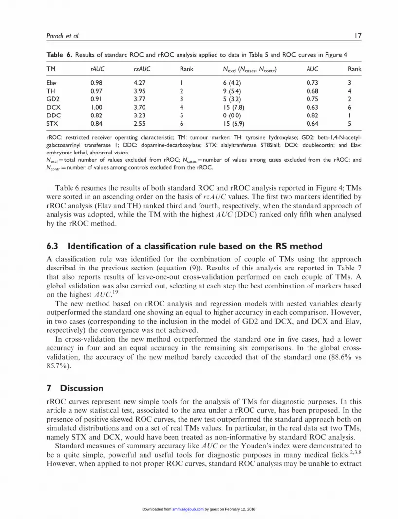
Table 6 resumes the results of both standard ROC and rROC analysis reported in Figure 4; TMswere sorted in an ascending order on the basis of rzAUC values. The first two markers identified byrROC analysis (Elav and TH) ranked third and fourth, respectively, when the standard approach ofanalysis was adopted, while the TM with the highest AUC (DDC) ranked only fifth when analysedby the rROC method.

6.3 Identification of a classification rule based on the RS method

A classification rule was identified for the combination of couple of TMs using the approachdescribed in the previous section (equation (9)). Results of this analysis are reported in Table 7that also reports results of leave-one-out cross-validation performed on each couple of TMs. Aglobal validation was also carried out, selecting at each step the best combination of markers basedon the highest AUC.19

The new method based on rROC analysis and regression models with nested variables clearlyoutperformed the standard one showing an equal to higher accuracy in each comparison. However,in two cases (corresponding to the inclusion in the model of GD2 and DCX, and DCX and Elav,respectively) the convergence was not achieved.

In cross-validation the new method outperformed the standard one in five cases, had a loweraccuracy in four and an equal accuracy in the remaining six comparisons. In the global cross-validation, the accuracy of the new method barely exceeded that of the standard one (88.6% vs85.7%).

7 Discussion

rROC curves represent new simple tools for the analysis of TMs for diagnostic purposes. In thisarticle a new statistical test, associated to the area under a rROC curve, has been proposed. In thepresence of positive skewed ROC curves, the new test outperformed the standard approach both onsimulated distributions and on a set of real TMs values. In particular, in the real data set two TMs,namely STX and DCX, would have been treated as non-informative by standard ROC analysis.

Standard measures of summary accuracy like AUC or the Youden’s index were demonstrated tobe a quite simple, powerful and useful tools for diagnostic purposes in many medical fields.2,3,8

However, when applied to not proper ROC curves, standard ROC analysis may be unable to extract

Table 6. Results of standard ROC and rROC analysis applied to data in Table 5 and ROC curves in Figure 4

TM rAUC rzAUC Rank Nexcl (Ncases, Ncontr) AUC Rank

Elav 0.98 4.27 1 6 (4,2) 0.73 3

TH 0.97 3.95 2 9 (5,4) 0.68 4

GD2 0.91 3.77 3 5 (3,2) 0.75 2

DCX 1.00 3.70 4 15 (7,8) 0.63 6

DDC 0.82 3.23 5 0 (0,0) 0.82 1

STX 0.84 2.55 6 15 (6,9) 0.64 5

rROC: restricted receiver operating characteristic; TM: tumour marker; TH: tyrosine hydroxylase; GD2: beta-1,4-N-acetyl-

galactosaminyl transferase 1; DDC: dopamine-decarboxylase; STX: sialyltranferase ST8SiaII; DCX: doublecortin; and Elav:

embryonic lethal, abnormal vision.

Nexcl¼ total number of values excluded from rROC; Ncases¼ number of values among cases excluded from the rROC; and

Ncontr¼ number of values among controls excluded from the rROC.

Parodi et al. 17



most of the relevant information or it may even provide unreliable results.25 In ClinicalEpidemiology not proper ROC curves are often encountered, especially in the analysis of putativeTMs. In particular, positive skewed ROCs may results from the presence of similar values at lowTM concentrations in the two classes under study. Many reasons may be advocated for this

Table 7. Results of the classification using a RS obtained by the combination of couple of the tumour markers in

Table 3 by either a standard approach or a nested model based on the rROC analysis

TMs

Standard approach (main effect model) rROC approach (nested model)

Se% Sp% Acc% Se% Sp% Acc%

Whole data set

TH, GD2 80.0 100 91.4 93.3 90.0 91.4

TH, DDC 80.0 100 91.4 86.7 100 94.3

TH, STX 60.0 100 83.9 86.7 95.0 91.4

TH, DCX 73.3 95.0 85.7 86.7 95.0 91.4

TH, Elav 86.7 90.0 88.6 100 100 100

GD2, DDC 86.7 95.0 91.4 93.3 95.0 94.3

GD2, STX 66.7 95.0 82.9 80.0 100 91.4

GD2, DCX 80.0 100 91.4 100 90 94.3*

GD2, Elav 86.7 95.0 91.4 100 100 100

DDC, STX 73.3 85.0 80.0 73.3 85.0 80.0

DDC, DCX 60.0 95.0 80.0 80.0 90.0 85.7

DDC, Elav 86.7 90.0 88.6 86.7 100 94.3

STX, DCX 53.3 90.0 74.3 100 70.0 82.9

STX, Elav 66.7 100 85.7 93.3 90.0 91.4

DCX, Elav 73.3 100 88.6 93.3 95.0 94.3*

Verification set in leave-one-out cross-validation

TH, GD2 80.0 100 91.4 80.0 85.0 82.9

TH, DDC 73.3 90.0 82.9 73.3 95.0 85.7

TH, STX 46.7 95.0 74.3 46.7 80.0 65.7

TH, DCX 66.7 85.0 77.1 66.7 85.0 77.1

TH, Elav 73.3 85.0 80.0 86.7 90.0 88.6

GD2, DDC 80.0 90.0 85.7 80.0 90.0 85.7

GD2, STX 60.0 95.0 80.0 60.0 90.0 77.1

GD2, DCX 40.0 95.0 71.4 40.0 95.0 71.4

GD2, Elav 73.3 95.0 85.7 73.3 95.0 85.7

DDC, STX 60.0 80.0 71.4 60.0 75.0 68.6

DDC, DCX 46.7 85.0 68.6 60.0 85.0 74.3

DDC, Elav 53.3 95.0 77.1 73.3 80.0 77.1

STX, DCX 33.3 85.0 62.9 66.7 70.0 68.6

STX, Elav 53.3 85.0 71.4 73.3 80.0 77.1

DCX, Elav 66.7 100 85.7 86.7 90.0 88.6

Global validation 73.3 95.0 85.7 86.7 90.0 88.6

RS: risk score; rROC: restricted receiver operating characteristic; TMs: tumour markers; TH: tyrosine hydroxylase; GD2: beta-1,4-

N-acetyl-galactosaminyl transferase 1; DDC: dopamine-decarboxylase; STX: sialyltranferase ST8SiaII; DCX: doublecortin; and Elav:

embryonic lethal, abnormal vision.

Legend: Se¼ sensitivity; Sp¼ specificity; Acc¼ diagnostic accuracy; Global validation: the best couple of markers (based on the

highest AUC for the RS) selected at each step from the whole data set.

*Convergence was not achieved.




behaviour, including the presence of a detection threshold in the measure device, the presence of asubgroup of cases with a TM expression similar to that of controls, and the presence among controlsof individuals with a rather high expression of TM in the absence of neoplastic cells, as brieflyillustrated in the Introduction and shown by some examples in Figures 2 and 3. With respect to thereal data set analysed in this article,20 the shape of the corresponding ROC curves reported inFigure 4 indicates that a mix of these different situations have occurred. In particular, zero-inflated distributions may have arisen from the detection threshold of the RT-qPCR method thatis unable to perform more than 40 amplification cycles, while bimodal distributions among casesmay be related to the fact that all the considered TMs can be expressed in some proportion also bynormal cells as a consequence of the so called illegitimate transcription.23 Furthermore, somepatients with localized neuroblastoma, which have little tendency to spread to distant tissues,including blood, may have TMs concentration values similar to those of healthy individuals.

Information from the shape of a ROC curve seems to be at least as important as informationfrom summary indices of accuracy like AUC. In recent years, modern ROC analysis has tried todevelop new approaches to extract and combine all available information from a TM, exploring theROC regions with informative values.26 Probably the most important and reliable method is basedon pAUC, which was demonstrated to be a useful tool for diagnostic purposes in the presence ofasymmetric ROC plots.13,17,26 The method based on rROC, described in this article, may beconsidered as an extension of the methods based on pAUC. In fact, the area under a rROC curve(rAUC) is equivalent to the pAUC identified by the cut-off C, divided by the corresponding 1-specificity value. However, there are two major differences with the pAUC based approaches,namely: (a) the cut-off that identifies rROC is selected by a recursive procedure coupled with anindex of accuracy (rzAUCj, equation (3)) and (b) samples corresponding to the non-informative TMconcentrations are considered as missing values and not as negative test. For this reason at leastanother diagnostic marker, if available, is needed in order to complete the classification analysis,thus allowing those subjects, whose TM levels lie in the range of ‘not informative values’ (TMconcentrations <C), to be allocated in either one class under study. Using the real data set ofneuroblastoma markers,20 a combination of information from both standard and rROC analysisvia a logistic regression model provided a classification rule based on the corresponding RS whoseaccuracy was higher than that of any other combination of couples of TMs. However, a morereliable estimate should have been obtained from an external validation set, which unfortunatelywas not available. The small sample size of the data set (20 controls and 15 cases) just allowed theapplication of the leave-one out cross-validation. Most results from this analysis indicated a betterperformance of the new proposed method, but accuracy of the global validation was only marginallyhigher than that of the standard analysis. Furthermore, the use of regression models with nestedvariables in some instances provided unstable estimates due to a lack of convergence even in theanalysis of the whole data set, probably as a consequence of the small sample size. Finally, nestedmodels may be more prone to overfitting than the corresponding main effect models due to theinclusion of a higher number of predictors. Further analyses, based on both extensive simulationsand real databases of TMs with different sample sizes, are needed to estimate the accuracy and theprecision of the new proposed method and to assess the advantage of using rROC analysis inclassification based on RS from a regression model.

Another limitation of the proposed method is that the statistical properties of the new proposedtest were explored only via extensive simulations, whereas an analytical formula for rzAUCdistribution under H0 is not available. This limit might make difficult its application to very largedata sets, such as multicentre follow up study, where the analysis by random permutations is rathertime-consuming. Furthermore, only left restriction has been considered in this article in the presence

Parodi et al. 19



of positive skewed ROC curves, whereas in clinical setting many other types of not proper curvesmay be encountered. In particular, applying a right restriction, the proposed method should beextended to negative skewed ROC, that may originate by a ceiling detection threshold in adiagnostic device or by the presence of some spiked values among the controls. However, theextension of the rROC method to include either type of restriction will require a very largenumber of simulations and the use of new databases of real data, and is behind the scope of thisinvestigation. Finally, the method should also be extended to allow the inclusion of an utilityfunction16 in the evaluation of optimal cut-offs, since false positive and false negative errors mayhave different costs in different situations. Nonetheless, results from this investigation indicate thatrROC curves may be a new simple and useful tool to explore the diagnostic utility of putative TMs.In the coming future, new statistical tests should be developed to extract information from differentkinds of TM distributions, possibly exploiting the properties of the corresponding rROC plots. Thedevelopment of a comprehensive approach to combine any relevant information from both standardand modern ROC analysis will provide an optimal framework for the evaluation of the diagnosticpotential of new TMs.

Acknowledgements

The authors thank Dr Paolo Bruzzi (National Cancer Research Institute of Genoa) for providing precious

advice.

Funding

This study was partly supported by the Ligurian Region and by the Italian Neuroblastoma Foundation

(Fondazione Italiana per la Lotta al Neuroblastoma). B.C. is a recipient of a grant from the Italian

Neuroblastoma Foundation.

Declaration of conflicting interest

None declared.

References

1. Erdreich LS. Use of relative operating characteristicanalysis in epidemiology. Am J Epidemiol 1981; 114:649–662.

2. Pepe MS. The statistical evaluation of medical tests forclassification and prediction. Oxford, UK: OxfordUniversity Press, 2003.

3. Krzanowski WJ and Hand DJ. ROC curves for continuousdata. Boca Raton, FL: CRC Press, 2009.

4. Baker SG. Improving the biomarker pipeline to develop andevaluate cancer screening tests. J Natl Cancer Inst 2009; 101:1–4.

5. Bamber D. The area above the ordinal dominance graphand the area below the receiver operating characteristicgraph. J Math Psychology 1975; 12: 387–415.

6. Mann HB and Whitney DR. On a test whether one of tworandom variables is stochastically larger than another. AnnMath Stat 1947; 18: 50–60.

7. Hoeffding W. A class of statistics withasymptotically normal distribution. Ann Math Stat 1948;19: 293–325.

8. Hanley JA and McNeil BJ. A method of comparing the areaunder receiver operating characteristic curves derived fromthe same cases. Radiology 1983; 148: 839–843.

9. DeLong ER, DeLong DM and Clarke-Pearson DL.Comparing the areas under two or more correlatedreceiver operating characteristic curves: a nonparametricapproach. Biometrics 1988; 44: 837–845.

10. Rosner B and Glynn RJ. Power and sample size estimationfor the Wilcoxon rank sum test with application tocomparisons of c statistics from alternative predictionmodels. Biometrics 2009; 65: 188–197.

11. Baker SG and Kramer BS. Peirce, Youden, and receiveroperating characteristic curves. Am Statistician 2007; 61:343–346.

12. Perkins NJ and Schisterman EF. The inconsistency of‘‘oprimal’’ cutpoints obtained using two criteria based onthe receiver operating characteristic curve. Am J Epidemiol2006; 163: 670–675.

13. Pepe MS, Longton G, Anderson GL, et al. Selectingdifferentially expressed genes from microarrayexperiments. Biometrics 2003; 59: 133–142.




14. Hanley JA. The use of the ‘binormal’ model for parametricROC analysis of quantitative diagnostic tests. Stat Med1996; 15: 1575–1585.

15. Schisterman EF, Reiser B and Faraggi D. ROC analysisfor markers with mass at zero. Stat Med 2006; 25: 623–638.

16. Baker SG. Identifying combinations of cancer markers forfurther study as triggers of early intervention. Biometrics2000; 56: 1082–1087.

17. Dodd LE and Pepe MS. Partial AUC estimation andregression. Biometrics 2003; 59: 614–623.

18. Sprott JC. Numerical recipes software: numerical recipes:routine and examples in BASIC. New York, NY, USA:Cambridge University Press, 1998.

19. McIntosh MW and Pepe MS. Combining several screeningtests: optimality of the risk score. Biometrics 2002; 58:657–664.

20. Corrias MV, Haupt R, Carlini B, et al. Multiple targetmolecular monitoring of bone marrow and peripheralblood samples from patients with localized neuroblastomaand healthy donors. Pediatr Blood Cancer 2012; 58(1):43–49.

21. Maris JM. Recent advances in neuroblastoma. N Engl JMed 2010; 362: 2202–2211.

22. Beiske K, Burchill SA, Cheung IY, et al. Consensuscriteria for sensitive detection of minimal neuroblastomacells in bone marrow, blood and stem cell preparations byimmunocytology and RT-QPCR: recommendations by theInternational Neuroblastoma Risk Group Task Force. BrJ Cancer 2009; 100: 1627–1637.

23. Livak KJ and Schmittgen TD. Analysis of relative geneexpression data using real-time quantitative PCR and the2(-Delta Delta C(T)) Method. Methods 2001; 25: 402–408.

24. Davison AC and Hinkley DV. The basic bootstrap.In: Davison AC and Hinkley DV (eds) Bootstrap methodsand their application. New York: Cambridge UniversityPress, 2006, pp.11–69.

25. Lee WC and Hsiao CK. Alternative summary indices forthe receiver operating characteristic curve. Epidemiology1996; 7: 605–611.

26. Kagaris D and Yiannoutsos CT. A multi-index ROC-based methodology for high throughput experiments ingene discovery. Int J Data Min Bioinform 2011; in press.

Parodi et al. 21



Restricted ROC curves are useful tools to evaluate the performance of tumour markers

Documents

Transcript of Restricted ROC curves are useful tools to evaluate the performance of tumour markers