IEEE TRANSACTIONS ON COMPUTER-AIDED DESIGN OF INTEGRATED CIRCUITS AND SYSTEMS, VOL. 15, NO. 9, SEPTEMBER 1996 1151

circuits

TABLE VI1 ALGORITHM COMPLEXITY COMPARISONS

Approach 1 Approach 2 Approach 3 bd.back 1 retry bd.back I retry bd.back I retry

primitive

4-to-I MUX 0 1 0 0 1 0 0 1 0

MP2

Am2910 1 Incrementer /I 0 I 0 1 0 1 0 1 0 I 0 RegCnt-CL2 1597 36 1072 25 42 24 16-bitALU 99664 2022 0 0 0 0 %hit XOR n n n n n n

MPl . . .. . . -. . I - 1 1 - 1 - 1 - 2-to-1Mux I[ 6739 1 181 I 6578 I 173 I 171 I 171

PCONR PUR8

for different modules. For bus constraints, we first propose a top- down approach based on a simulation-based constraint abstraction technique. For circuits with very complex data path module config- urations, it is usually computationally prohibitive to derive accurate constraint estimations. A bottom-up approach based on the test cube justification technique is therefore developed to efficiently avoid the bus constraints. These proposed algorithms have been implemented in our hierarchical test generation package, ARTEST, and several high level circuits with different constraint characteristics have been tried in the experiments. The experimental results show the effectiveness of combining the control cover abstraction technique and the test cube justification technique as a complete solution to the architectural level functional constraint problem.

Adder 2540 51 906 19 10 10 8-bit Adder 67974 2487 31428 1250 950 785 8-bit Adder 34334 1035 6016 207 210 162

REFERENCES

H.-K. T. Ma, S. Devadas, A. R. Newton, and A. Sangiovanni- Vincentelli, “Test generation for sequential circuits,” IEEE Trans. Computer-Aided Design, vol. 7, pp. 1081-1093, Oct. 1988. W. T. Cheng, “The back algorithm for sequential test generation,” Proc. IEEE Int. Con$ Comput. Design, Oct. 1988, pp. 66-69. V. D. Agrawal, K. T. Cheng, and P. Agrawal, “CONTEST: A concurrent test generator for sequential circuits,” in Proc. 25th IEEE/ACM Design Automation Con$, June 1988, pp. 88-89. T. Niermann and J. H. Patel, “HITEC: A test generation package for sequential circuits,” in Proc. Euro. Design Automution Con$, Feb. 1991, pp. 214-218. S. J. Chandra and J. H. Patel, “A hierarchical approach to test vector generation,” in Proc. 24th IEEE/ACM Design Automation CO$, June 1987, pp. 495-501. B. Krishnamurthy, “Hierarchical test generation: can AI help?,:’ in Proc. Int. Test Con$, Aug. 1987, pp. 694-700. J . D. Calhoun and F. Brglez, “A framework and method for hierarchical test generation,” in Pruc. Int. Test Con$. Sept. 1989, pp. 480490. D. Bhattacharya and J. P. Hayes, “A hierarchical test generation method- ology for digital circuits,” J. Elect. Testing: Theory Appl., vol. 1, pp. 103-123, 1990. J. P. Roth, “Diagnosis of automata failures: A calculus and a method,” IBM J. Res. Develop., vol. 10, pp. 278-281, 1966. P. Goel, “An implicit enumeration algorithm to generate tests for combinational circuits,’’ IEEE Trans. Comput., vol. C-30, pp. 215-222, Mar. 1981. M. H. Schulz, E. Trischler, and T. M. Sarfert, “SOCRATES: A highly efficient automatic test pattern generation system,” in Proc. Int. Test Con$. Sept. 1987, pp. 1016-1026. T. M. Sarfert, P. Markgraf, E. Trischler, and M. H. Schulz, “Hierarchical test pattern generation based on high-level primitives,” in Proc. Int. Test Con$, Sept. 1989, pp. 470-479. R. P. Kunda, P. Narain, J. A. Abraham, and B. D. Rathi, ‘Speedup of test generation using high-level primitive,” in Proc. 27th ACM/IEEE Design Automution Con$, June 1990, pp. 594-599.

[14] B. T. Murray and J. P. Hayes, “Hierarchical test generation using precomputed tests for modules,” in Proc. Int. Test Con$, 1988, pp. 221-229.

[I51 K. Roy and J. A. Abraham, “High level test generation using data flow descriptions,” in Proc. IEEE Euro. Design Automation Con$, 1990, pp. 480-484.

[16] P. N. Anirudhan and P. R. Menon, “Symbolic test generation for hierarchically modeled digital systems,” in Proc. Int. Test Con$, Sept. 1989, pp. 461469.

[17] J. Lee and J. H. Patel, “An architectural level test generator based on nonlinear equation solving,” J. Elect. Testing: Theory Appl., vol. 4, no. 2, pp. 137-150, 1993.

[18] -, “An architectural level test generator for a hierarchical design environment,” in Proc. 21th Symp. Fault-Tolerant Computing, June 1991, pp. 44-51.

[19] J. Lee, V. Chickermane, and J. H. Patel, “Impact of high level functional constraints on testability,” in Proc. IEEE VLSI Test Symp., Apr. 1993, pp. 309-312.

[20] J. Lee and J. H. Patel, “An instruction sequence assembling methodology for testing microprocessors,” in Proc. Inc. Test Con$, Sept. 1992, pp.

[21] Advanced Micro Devices, “The Am2910, a complete 12-bit micropro- gram sequence controller,” in AMD Data Book. Sunnyvale, CA: AMD, 1978.

[22] T. Niermann, W. T. Cheng, and J. H. Patel, “PROOFS: A fast, memory- efficient sequential circuit fault simulator,” IEEE Trans. Compufer-Aided Design, vol. 11 , pp. 198-207, Feb. 1992.

49-58.

Efficient Net Extraction for Restricted Orientation Designs

Mario A. Lopez, Ravi Janardan, and Sartaj Sahni

Abstract-Net extraction is crucial in VLSI design verification. Current algorithms for net extraction do not exploit the fact that the number, c, of different orientations of the line segments or polygons in a practical VLSI mask design is small relative to the number, n, of segments or polygon edges. Instead they rely on computing all intersections in the input and hence take time that is at least proportional to the number of intersections. In this paper we develop and implement a practical algorithm for net extraction that runs in O(cn1ogn) time and o(n) space, which is optimal for fixed c. The algorithm uses only integer operations and is, as a result, numerically stable. Experiments indicate that the algorithm will outperform existing algorithms on practical VLSI designs, We expect that the techniques presented will he useful in other VLSYCAD problems that operate with restricted orientation geometries.

I. INTRODUCTION VLSI masks are usually described by a collection of geometric ob-

jects, such as, for instance, line segments and polygons. A crucial step in the VLSI layout verification process is net extraction. Informally, net extraction is the process of determining the elements of the mask

Manuscript received January 26, 1992; revised August 13, 1993, August 7, 1995, and May 5 , 1996. This work was supported in part by the National Science Foundation by Grant MIP9103379. This paper was recommended by past Editor M. Marek-Sadowska.

M. A. Lopez is with the Department of Mathematics and Computer Science, University of Denver, Denver, CO 80208 USA.

R. Janardan is with the Department of Computer Science, University of Minnesota, Minneapolis, MN 55455 USA.

S . Sahni is with the Department of Computer and Infomation Sciences, University of Florida, Gainesville, FL 3261 1 USA.

Publisher Item Identifier S 0278-0070(96)06730-9.

0278-0070/96$05.00 0 1996 IEEE

1152 IEEE TRANSACTIONS ON COMPUTER-AIDED DESIGN OF INTEGRATED CIRCUITS AND SYSTEMS, VOL. 15, NO. 9, SEPTEMBER 1996

Fig. 1. nents, labeled A and B.

Connected components of a set of polygons. There are two compo-

that are electrically connected. These connected elements are called nets. Once a proposed design is complete, the nets are extracted and compared to a known correct set of nets. If an error is found, the mask is corrected and net extraction done again. Since in practice a mask can very well contain on the order of one million polygons, doing net extraction efficiently is of the utmost importance.

We now formalize the notion of a net. Let S be the set of objects comprising the mask. Two objects in S intersect if they have at least one point in common; there need not be a boundary intersection. Two objects a and b are connected if and only if there are objects a = C O , c l , . . . , ct = b in S, such that c, intersects c,+1: 0 5 i < t . The maximal subsets of connected objects are the connected components of S. Net extraction is the process of obtaining these connected components. Fig. 1 illustrates the connected components of a set of polygons.

Efficient net extraction algorithms have been designed for the cases where S consists of orthogonal segments or rectangles [7] , [9]. These algorithms run in O(n) space and O ( n log 7 1 ) time, where n is the input size. For nonorthogonal objects, which are common in today's technology, practical net extraction algorithms are based on computing all intersections among input objects [4], [12]. Every time an intersection is detected, the nets of the objects involved are merged. Because the number of intersections can be large, it is not hard to construct instances where this approach performs poorly. Specifically, we can expect performance to drop as the number of intersections increases. The efficiency of the algorithms for the orthogonal case stems from the fact that they cleverly avoid computing all intersections.

In this paper we consider the problem of extracting the connected components from sets of line segments and polygons whose sides are oriented in at most a small number, c, of different directions. This is often the case in practical VLSI designs where c << n. For instance c = 2 for orthogonal designs and c = 4 in 45" VLSI artwork. Traditional net extraction algorithms do not take advantage of this fact which, as we show, can lead to substantial algorithmic improvements.

Formally, we say that a set of line segments is e-oriented if every segment in the set is oriented in one of at most c different directions. Similarly, a set of polygons is e-oriented if the set of edges making up the polygons is e-oriented. For example, the polygons in Fig. 1 are 4-oriented.

We derive efficient algorithms for reporting the connected compo- nents of a set of e-oriented line segments or polygons. Our algorithms run in O(c72 log n) time and require only O ( n ) space, where n is the number of input segments or polygon edges. They require only simple data structures and are practical for small values of e. If c is a constant, independent of n, our results are optimal, both in time and space.'

'An optimal solution to this problem clearly requires n(n) space. By reducing the Element Uniqueness problem to a restricted version of this problem, Edelsbrunner et al. [7] show that n(n log 71) time is required.

We do not require that the directions in the input be fixed or known beforehand. Moreover, for integer input, as normally used in VLSI design, our algorithms require only integer arithmetic. Contrast this with traditional intersection-computing algorithms. Even with integer- only input data, intersections can fall on arbitrary rational valued positions making basic operations such as event ordering during sweepline processing an activity prone to round-off errors. As pointed out by Ottmann et al. [13], a single error in order determination for a computed intersection point can have a disastrous global effect on correctness.

Both our algorithms and a solution based on computing all object intersections were implemented and evaluated experimentally. This evaluation showed that our algorithms outperform traditional methods when c < 2 k / n , where k is the number of object intersections. This is often the case in practical VLSI designs, as corroborated from two large chip descriptions provided by AT&T Bell Labs. We found that for four (respectively, eight) orientations, 2 k / n = I I .2 (respectively, 14.9) making our algorithms the preferred choice.

We expect that the techniques presented here will find applications in other VLSYCAD problems with restricted orientation geometries. For example, we decompose input polygons into simpler polygons of prescribed shapes. We show how to store these simpler polygons in a dynamic data structure and show how to query it efficiently to determine information about the nesting of polygons. Similar techniques could be useful in interactive VLSI editing systems where inexpensive incremental updates and fast performance are important (see for example [14], which runs efficiently only with rectangular objects).

In the next section we develop an algorithm for e-oriented line seg- ments which is then extended to e-oriented polygons in Section 111. The last section compares the performance of the algorithms of Sections I1 and 111 with that of the common approach based on computing all object intersections.

11. e-ORIENTED LINE SEGMENTS We develop an O( cn log n ) time and O ( n ) space algorithm for

computing the connected components of a e-oriented set of line segments. We first review the algorithm of [9], which works only for orthogonal segments, and then develop a solution for arbitrarily oriented sets of segments.

A. Review of an Algorithm for Orthogonal Segments

The algorithm of [9] operates in two phases. The first phase computes in o(n log 7 1 ) time the O ( n ) edges of a graph G ( S ) whose nodes corcespond to the input segments of S. Each edge of G ( S ) joins two segments (which may or may not intersect) that belong to the same connected component. The second phase computes the connected components of G ( S ) , which are precisely the connected components of S. This can be done in O(n) time using the algorithm in [ll, p. 3511. The first phase is implemented by sweeping S from left to right. The sweepline schedule is obtained by sorting the endpoints of the horizontal segments and the vertical segments by x-coordinate. Two data structures are used while sweeping S: the active tree and the illuminator tree. The former is a balanced search tree that stores the horizontal segments that are currently cut by the sweepline (segment gh in Fig. 2). To better understand the latter, imagine each segment as being opaque on the left and luminous on the right. For convenience, assume there is an infinite vertical segment that intersects no input segment and is located to the left of S (segment ab in Fig. 2). Each point on the sweepline is illuminated by a unique input segment which is either active or to the left of the sweepline. The sweepline is thus partitioned into

IEEE TRANSACTIONS ON COMPUTER-AIDED DESIGN OF INTEGRATED CIRCUITS AND SYSTEMS, VOL. 15, NO. 9, SEPTEMBER 1996

t- Fig. 2. A set of segments partitions the sweepline (shown bold) into a setof illuminated intervals. The active tree contains segment yh.The illuminator tree contains six intervals: a‘c‘, c’e’, c‘g‘. g’ (a degenerate case), y’f’ and f’b’.

a set of disjoint intervals. Note that some intervals are projections of horizontal segments (for example g h ) , and hence, degenerate to a single point (9‘ in this case). All points of an interval are illuminated by the same input segment. The illuminator tree is a balanced search tree that stores these intervals. With each such interval I we also store the id of the illiminator input segment whose luminous projection on the sweepline is I . When the sweepline encounters a vertical segment or the left endpoint of a horizontal segment, this segment s becomes the illuminator of the interval I , that s “carves out” from the sweepline. I , is then inserted into the illuminator tree by locating in that tree the two (one if s is horizontal or short enough) intervals that contain the endpoints of I,. These intervals are split at the endpoints of I,., and all intervals in between are merged into the single interval L . For every such interval r7 with illuminator s I , if J intersects any segment in the active tree, we output (s J , .s) as a new edge of G( S). Additionally, if s is horizontal, we also insert it into the active tree. When reaching the right endpoint of a horizontal segment, we delete that segment from the active tree. For further details as well as for a proof of correctness see [91.

B. The Algorithm for c-Oriented Line Segments

Essentially the same approach as above still works for c = 2 even if the two orientations d l and rla are not orthogonal. We use a slanted sweepline parallel to d2 that scans the segments while moving in direction dl. Conceptually, the sweepline schedule is defined by projecting along d2, onto a line L parallel to d l , the endpoints of the segments of orientation dl and also the segments of orientation d . ~ , and then sorting these projections along L. Notice that it is possible for an endpoint p to the left of another endpoint q to be placed later in the sweep schedule. Both dz as well as the ,r and y coordinates of a point determine its position in the schedule. After these modifications, the rest of the algorithm proceeds similarly to [9]. We omit the details.

Lemma 1: The connected components of a 2-oriented set of 11 line segments in the plane can be computed in O(71 log 7 1 ) time and O( t i )

space. Consider now the case e > 2. We solve this problem by reducing it

to c(c - 1 ) / 2 instances of the 2-oriented case, coupled with a global union-find structure [ 111 to keep track of the components. We show that even though the number of instances is quadratic in c, we can obtain an algorithm which is linear in c.

We begin by sorting the set S of segments by slope and partitioning it into c subsets. Let S, denote the set of segments of orientation d,, and / i t , its size. Initially, each segment of S is in a connected component by itself. Call these components partial components.

1153

The algorithm repeatedly merges certain partial components using information from various runs of the modified 2-oriented algorithm. At termination, the partial . components that exist are the desired connected components. For each pair of integers i and j , where i = 1:. . . , c - 1 and j = i + 1,. . . , c do the following. Use the modified 2-oriented algorithm to compute the connected components of S, U S,,. Let C,,7 be the set of these components. For each, component C in C,, do the following. Let SI. . . . , s1- be the segments in c. For 11 = 2 , . . . , r , merge the partial components of sI and sh

(if different). After all components C in Czi have been processed in this way, delete the storage required by Cz,.

We represent the partial components using the union-find data structure given in [ll], where each find takes O(1) time and a sequence of 11 - 1 union operations on an initial total of tz singleton sets takes O( 11 log n ) time in worst case. The partial component containing an arbitrary segment is found by doing a find operation and two partial components are merged by doing a union operation.

Theorem 1: The set of connected components of a e-oriented set of line segments in the plane, where c > 2, can be computed in O(cn logn) time and O ( n ) space.

Pro08 Apply the above algorithm (for e > 2). We prove correctness by showing that two segments p and q will be put in the same partial component (at some time) if and only if they are connected. Since partial components are never split, this implies the desired result. Let p E S , and q E S, , where possibly i = j. Suppose that p and Q are connected. If p intersects q, then by the correctness of the modified 2-oriented algorithm for S, U S, p and q are both in the same component in C,, , so their partial components are merged. Otherwise, there exist segments p = ro. . . . . r S = q , s > 1, such that rrz intersects rlZ+lr 0 5 h < s. Thus, rh and ~ h + l will be placed in the same partial component, since the algorithm runs the 2-oriented algorithm for all possible pairs of orientations. It follows that p and q will be end up in the same component.

For the converse, suppose that p and q are put in the same partial component. We claim that throughout the execution of the algorithm, any two segments in the same partial components are connected, and therefore, p and q must be connected. The claim is true at the beginning when each partial component is a seg- ment by itself. Assume it is true just before partial components P and P‘ are about to be merged. From the correctness of the 2-oriented algorithm, there exist connected segments s E P and s‘ E P‘. By the induction hypothesis, each segment of P (re- spectively, p’) is connected to s (respectively, s‘). Therefore, every segment of P is connected to every segment of P‘ and the claim follows.

The run time analysis is as follows. We can partition S into the various 5;’s in O ( n l ogn) time. Computing the connected components of S, US, takes O ( ( n , +iiJ)log(it , + n J ) ) time. Thus all such component computations take time O(c:z; cs=L+l ( T I ; + 1) log n xi=, n h ) = o ( c n log’r~). Additionally, there are a total of

C5,L+l(~lt + r i J ) = ( c - 1 ) r r find operations and at most n - 1 union operations, which take O(crc + 7rlog~) time. Thus the total run time is O(~n1ogu) .

The space used is O ( n ) because the 2-oriented algorithm uses O ( n ) space, the union-find structure takes O(71) space [I l l , and each

0

/1.,)109(?lz + I ? , , ) ) = O(log/t c;z; x;Tz+L(/L; + n j ) ) = O ( ( c -

C,, is deleted after its components have been processed.

C. An Implementation Issue

Computing the projections requires the use of divisions. Further- more, depending on the relative values of d1 and d2, the projection of a point might produce coordinates with extremely large (or small)

1154 IEEE TRANSACTIONS ON COMPUTER-AIDED DESIGN OF INTEGRATED CIRCUITS AND SYSTEMS. VOL 15, NO. 9, SEPTEMBER 1996

floating point values. Consequently, in order to avoid round-off errors, in practice we do not compute the projections explicitly. Instead, we define a total order 4 as induced by the slanted sweepline. Precompute Cl (respectively, 2 2 ) as any vector oriented rightward (upward if d, is vertical) in direction dl (respectively, (12). Given any two endpoints p and 4 : p 4 p iff p is on the left (on the top if dZ is horizontal) halfplane defined by a line of slope d2 passing through q. In other words, p 4 q iff & is clockwise from $I. It is not hard two show that for any two vectors 51 = (SI, ~ 1 ) and 5’ = (m,y2), 51 is clockwise from sC2 iff z l y 2 - x2y1 > 0 (see [6, p. 8871 for example). We use this definition of “less-than” when sorting the events. Other operations needed by the algorithm, such as intersection detection, can be implemented similarly.

111. e-ORIENTED POLYGONS

Consider now a e-oriented set R of simple polygons. Let I L

denote the total number of polygon edges in R. We develop both a O(c’n1ogn) time algorithm, which is simple to implement, as well as a more efficient O(cn log n) time solution. Both algorithms require O(n) space.

Initially, we form a set S of the polygon edges from R, re- membering for each edge the polygon it came from. We run the algorithm of the previous section to find the connected components induced by intersections in S , except that, initially, all edges of the same polygon are placed in the same component. This yields a set of connected components of polygons. However, these components are not necessarily maximal subsets of connected polygons from R. Components that nest without boundary intersections belong to the same connected component, and nesting is not accounted for in the above procedure. For instance, in Fig. 1, the components induced by intersections in S are c1 = {u,d},c~ = {brc),e3 = {e,h},c4 = { f , g } . c5 = { i , j } , c6 = { k } , whereas the desired components are c1 U c2 U e3 U e4 and c j U cg.

Call the components induced by intersections in S partial compo- nents. We will repeatedly merge partial components that nest into larger ones. When this phase terminates, the partial components that exist are the desired connected components. For each partial component we identify an extreme point, e.g., a vertex of highest y-coordinate. The set E of all such extreme points has size O ( n ) and can be computed in O ( n ) time. For each point p in E , we then determine any polygon T in €2 such that p lies in the interior of T . If such a polygon exists, we merge the partial components containing p and T. Note that p and r cannot already be in the same partial component, as otherwise, p would not be an extreme point.

We call the above problem of determining for each extreme point p a polygon of R (if any) that contains p the batched c- oriented polygonal point enclosure (BCPPE) problem. This problem can be solved by using Giiting’s solution to the polygonal point enclosure searching problem [lo]. His algorithm preprocesses a c- oriented set R of polygons so that given a query point p , all polygons of R containing p can be reported efficiently. The algorithm can be modified so that only one enclosing polygon is reported. This method is, unfortunately, too expensive for our puvoses, requiring O(.n log 7%) space and O(cn log’ n) time. Instead, we take advantage of the batched nature of the problem to obtain a more efficient solution. We decompose the polygons of R into “simpler” polygons and group these into a small number of classes, remembering the partial component that each polygon came from. We then solve the BCPPE problem with respect to E on each class. The decomposition of polygons is done in two stages, referred to as the first and second stage of partitioning, respectively. Solving the BCPPE problem on the polygons produced by the first stage

dt = da

Partitioning of a trapezoid into at most

dt > da

Fig. 3.

dt < db

c - 1 trapezoids

results in a O( c’7~ log n) time algorithm. Using those produced by the second stage results in the more efficient O(cn1ogn) time algorithm.

A. Decomposing Polygons: The First Stage During the first stage, the polygons of R are decomposed into

trapezoids and triangles. This can be done in O ( n ) space and O ( n log 7%) time using, for example, the algorithm in [8]. For each trapezoid, the top side and the bottom side are each oriented in one of the c directions, while the other two sides are vertical. Each triangle will have one vertical side. For simplicity, we treat triangles as degenerate trapezoids with a vertical side of length zero. Let R‘ be the resulting set of O ( n ) trapezoids. Since our method requires that the top (respectively, bottom) edges of any two trapezoids in the same class have the same slope, we partition R’ accordingly, into at most c2 classes (one class for each combination of top and bottom slopes). We then solve the BCPPE problem with respect to E on each of the O( e2 ) classes. As shown later, a BCPPE instance with m trapezoids and 1%

points can be solved in O(m+n) space and O ( ( m + n ) logm) time, yielding a total space of O ( n ) and worst case time of O ( c 2 n l o g n ) . (A worst case scenario occurs when no trapezoid of R‘ contains a point of E and each of the @(e’) classes has approximately the same size). However, we can do better. As shown below, we can reduce the number of classes to at most 3c - 2 with O(n) trapezoids per class. Although there are now O( en) trapezoids in all, the space bound can still be kept at O ( n ) by carefully processing each class.

B. Decomposing Polygons: The Second Stage During the second partitioning stage, we further divide each

trapezoid (and triangle) in RI into at most c - 1 trapezoids by drawing at most c - 2 lines through one of its vertices. Let d l , . . . , d, be the list of directions sorted in ascending order by slope, and let p be an arbitrary trapezoid of R‘. Let 2 (respectively, T ) denote the left (respectively, right) vertical side of q , and dt (respectively, dh), the slope of its top (respectively, bottom) side. If It - b 1 5 1, then q needs no further partitioning. Otherwise, we partition q into It - bl pieces by drawing It - b / - 1 lines through one of its vertices, as follows. If f > b, we draw lines of slopes &,+I,. . . , d t - l through the top vertex of 1. Otherwise, t < b, and we draw lines of slopes &+I, . . . , d b - 1

through the top vertex of r . This is illustrated in Figs. 3 and 4. After we are done, each resulting trapezoid has top and bottom with slopes at most one position apart in the sorted slope list. The number of classes (i.e., possible combinations of top and bottom slopes) is no more than 3c- 2: at most three for each of da, . . . , and at most two for each of d~ and d,. We now group the trapezoids by class, and solve the BCPPE problem with respect to E on each of the classes.

The second partitioning stage may produce @(en) trapezoids with 0 ( 1 1 ) trapezoids per class. In order to maintain the space at 0 (n) , we generate and process the trapezoids one class at a time. After a

1155 IEEE TRANSACTIONS ON COMPUTER-AIDED DESIGN OF INTEGRATED CIRCUITS AND SYSTEMS, VOL. 15, NO. 9, SEPTEMBER 1996

Fig. 4. Decomposition of a polygon into trapezoids. Dashed lines show the initial decomposition into ? or fewer classes. Dotted lines show the further decomposition into 3c - 2 or fewer classes. Trapezoids in the same class are labeled with the same letter.

class has been processed, its associated storage is deleted. Let Wit ; . ,

(respectively, ZtJ) denote the class of trapezoids with top slopes d; and bottom slopes d, , that result after the first (respectively, second) stage of partitioning. Note that for each Z;j. li - j l 5 1. Since after the first stage, each Z,, , 1 2 i 5 c, is already available as W,,, we process and delete these classes, one at a time, using O ( n ) space. We now show how to generate Z12, . . . , Zc-l,c, in that order, without exceeding O(7c) space. The Zi j , i > j, can be handled similarly. A trapezoid p of R‘ will not be decomposed into its O( e ) pieces all at once. Instead, we gradually produce the ensuing pieces, from top to bottom, only as required by the Z,, currently being generated. As a result, each trapezoid in R‘ requires O(1) storage throughout the process. We proceed as follows. Sort the remaining trapezoids of R’ (i.e., excluding the trapezoids in the TVcc ’s), lexicographically, on the indices of their top and bottom slopes, into a linked list L. In other words, if p , q E R’, and t , . b,, f,, b, denote their top and bottom slopes respectively, then p comes before q if t , < f , or t , = t , and b, < b,. All trapezoids that generate a piece for the current Z;, are said to be active. L has the useful property that all the required active trapezoids occur at the front (Lemma 2 below). Therefore, to generate the next Z,,, we simply traverse L chopping off a member of Z,, from the next active trapezoid until we reach a trapezoid that is not active. After a trapezoid has been fully decomposed, it is deleted from L. The desired O ( n ) space bound follows from the fact that each Z,, has size O(71) and is deleted after it has been processed.

Lemma 2: After Zz-1,2 has been processed, all active trapezoids of Z,,,+l occur at the front of L.

Proof: The lemma is obvious once we outline the way in which L changes. Initially, L = T.T-12 . . . . . The active trapezoids of Z12 are I+-, U . . . U TVlC, and they occur at the front of L. After Z12 has been processed, T’b-12 is deleted from L and the remaining portion of each trapezoid in W;3, . . . WI has a top with slope ( I 2 , Additionally, M h . . . . , lV2c become active, so the active trapezoids of 2 2 3 also occur at the front of L.

cessing Z%-I ,~ , L = L1 . Ls , where LP = Wc-l,,, and L1 is the concatenation of i - 1

sublists of the form Vi/:,i+l - 9 . . . W:=. 1 5 j < i. The trapezoids in La are still intact, and those of L1 have tops with slope d,. At this point TVt,,+l U ’ . .ul.t;, become active, and Z;,;+1 can be processed.

0

. WSS

The required active trapezoids occur at the front.

C. Solving the BCFFE Problem We consider now the solution of the BCPPE problem for an arbi-

trary class C. The top (respectively, bottom) sides of the trapezoids in C can be totally ordered according to the intersections of their

supporting lines with a vertical line.* We sort by r-coordinate the set consisting of E and the vertical sides of the trapezoids in C. We then sweep this set with a vertical line. We maintain a data structure T (described below) to store the top and bottom sides of the trapezoids currently cut by the sweepline. When the left (respectively, right) vertical side of a trapezoid is encountered, we insert (respectively, delete) its top and bottom sides in T. When a point p from E is encountered we query T as follows: among those trapezoids in C (if any) with top side strictly above p , report the one with the lowest bottom side. (The querying strategy is described below). If p is inside the trapezoid (if any) that is reported, then we return the polygon ‘r of R that the trapezoid came from as the answer to the BCPPE problem for 11, and then remove p from E.

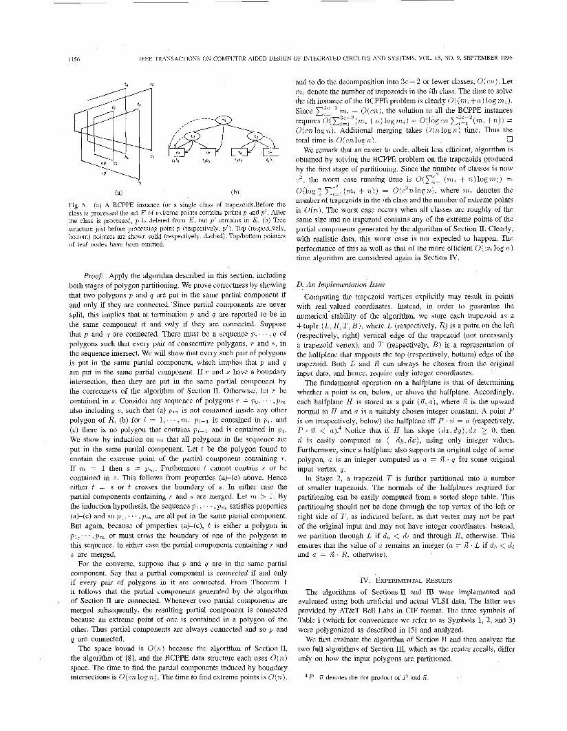
T can be implemented as a balanced binary search tree where each pair of top-bottom sides currently cut by the sweepline is stored at a leaf and the leaves are organized left to right in nondecreasing order by top side. For each top-bottom pair, we also keep track of the corresponding trapezoid. Each internal node 11 stores two pointers: a top pointer which points to the rightmost leaf in 21’s left subtree and a bottom pointer which points to the leaf in U’S subtree storing the lowest bottom side (ties broken arbitrarily). For convenience assume that each leaf has top and bottom pointers that point to the leaf itself. To answer a query for point p we search down T from the root and at each nonleaf node v visited do the following: If the top side stored at the leaf pointed to by U ’ S top pointer is strictly above p , then all trapezoids in U ’ S right subtree have top sides strictly above p . Thus, we use the bottom pointer of U’S right child to extract the lowest bottom side in ‘ti’s right subtree and then visit v’s left child.3 Otherwise (i.e., the top side is on or below p ) we visit 7)’s right child. If LI is a leaf and its top side is strictly above p , then we extract ‘tj’s bottom side. When the search ends, we return the trapezoid corresponding to the lowest of the bottom sides (if any) extracted in the search. An example of this procedure is given in Fig. 5. When using point p , the nodes visited are ’ ~ 1 , ,112, and u4. At 2 ~ 1 , h4 is extracted from the subtree rooted at 1:3. At ~ ‘ 2 . b2 is extracted from P J ~ . Finally, at v4. bl is extracted (from tiq). The search returns the lowest extracted bottom, i.e., b l . Since bl is below p , we conclude that p is contained by the trapezoid t I bl . If, instead, we use point p‘, the search path is the same as above, but no trapezoid of the given class is found to contain p‘.

To insert a top-bottom pair we search down T using the top side and insert a leaf ui for the pair. We then walk up the search path and at each node Y reset the top and bottom pointers as follows: If LJ is the lowest node on the path such that ‘U! is in U ’ S left subtree, then we set ‘(J’S top pointer to W . We set the bottom pointer of ti equal to the bottom pointer of that child of II whose bottom pointer points to the lower bottom side. We then walk up the path again and rebalance T , if necessary, by means of single and double rotations [6], [l 11 in the usual way. The reader can verify that rotations do not affect any top pointers and at most two bottom pointers per rotation need to be reset (those of the nodes whose children change). These bottom pointers can be computed in constant time from the bottom pointers stored at the children of the affected nodes. Deletion is analogous. It follows from the above discussion that a queryhpdate is handled correctly and takes O(log7n) time, where n~ is the number of leaves in T .

Theorem 2: The connected components of a e-oriented set of simple polygons with a total of 71 edges can be computed in O ( I Z ) space and O( c7i log 7 ~ ) time.

*The supporting line of a segment is the unique line containing that segment.

3Actually, since all we need is any polygon containing p , if the bottom side pointed to by U ’ S right child is below p we can return the corresponding polygon and stop the search.

1156 IEEE TRANSACTIONS ON COMPUTER-AIDED DESIGN OF INTEGRATED CIRCUITS AND SYSTEMS, VOL. 15, NO. 9, SEPTEMBER 1996

ta t 3

(a) (b)

Fig. 5. (a) A BCPPE instance for a single class of trapezoids.Before the class is processed the set E of extreme points contains points p and p ' . After the class is processed, p is deleted from E, but p' remains in E. (b) Tree structure just before processing point p (respectively, p ' ) . Top (respectively, bottom) pointers are shown solid (respectively, dashed). Topibottom pointers of leaf nodes have been omitted.

Proof: Apply the algorithm described in this section, including both stages of polygon partitioning. We prove correctness by showing that two polygons p and q are put in the same partial component if and only if they are connected. Since partial components are never split, this implies that at termination p and q are reported to be in the same component if and only if they are connected. Suppose that p and q are connected. There must be a sequence p , . . . . q of polygons such that every pair of consecutive polygons, r and s, in the sequence intersect. We will show that every such pair of polygons is put in the same partial component, which implies that p and q are put in the same partial component. If r and s have a boundary intersection, then they are put in the same partial component by the correctness of the algorithm of Section 11. Otherwise, let r be contained in s. Consider any sequence of polygons r = PO, ' ' . , p,,,, also including s , such that (a) p m is not contained inside any other polygon of R, (b) for i = 1,. . . , m, pz-l is contained in p t , and (c) there is no polygon that contains p,-1 and is contained in p i . We show by induction on In that all polygons in the sequence are put in the same partial component. Let t be the polygon found to contain the extreme point of the partial component containing r . If m = 1 then s = pl,z. Furthermore t cannot contain s or be contained in s. This follows from properties (a)-(c) above. Hence either t = s or t crosses the boundary of s. In either case the partial components containing r and s are merged. Let m > 1. By the induction hypothesis, the sequence p l , . . . p m satisfies properties (a)-(c) and so p l . . . , pVn are all put in the same partial component. But again, because of properties (a)-(c), t is either a polygon in p l , . . . , pm or must cross the boundary of one of the polygons in this sequence. In either case the partial components containing T and s are merged.

For the converse, suppose that p and q are in the same partial component. Say that a partial component is connected if and only if every pair of polygons in it are connected. From Theorem 1 it follows that the partial components generated by the algorithm of Section I1 are connected. Whenever two partial components are merged subsequently, the resulting partial component is connected because an extreme point of one is contained in a polygon of the other. Thus partial components are always connected and so p and q are connected.

The space bound is O ( n ) because the algorithm of Section 11, the algorithm of [8], and the BCPPE data structure each uses O ( n ) space. The time to find the partial components induced by boundary intersections is O(cn log n) . The time to find extreme points is O ( n ) ,

and to do the decomposition into 3c - 2 or fewer classes, O( c n ) . Let m, denote the number of trapezoids in the ith class. The time to solve the ith instance of the BCPPE problem is clearly O((m;+n) log m,). Since C ~ ~ ~ T " m, = O(cn), the solution to all the BCPPE instances requires o(c:~T~ (m, +n) log 7n2) = log cn ~ P ~ ~ ' ( m , +n)) = O(cn log n). Additional merging takes O(n log n ) time. Thus the total time is O(cn log n). 0

We remark that an easier to code, albeit less efficient, algorithm is obtained by solving the BCPPE problem on the trapezoids produced by the first stage of partitioning. Since the number of classes is now c2, the worst case running time is O ( ~ ~ ~ , ( m , + 12)logm,) = O(log; ~ ~ ~ , ( m ; + n,)) = O(c?nlogn), where m, denotes the number of trapezoids in the ith class and the number of extreme points is O(n) . The worst case occurs when all classes are roughly of the same size and no trapezoid contains any of the extreme points of the partial components generated by the algorithm of Section 11. Clearly, with realistic data, this worst case is not expected to happen. The performance of this as well as that of the more efficient O(cn. log n,) time algorithm are considered again in Section IV.

D. An Implementation Issue Computing the trapezoid vertices explicitly may result in points

with real-valued coordinates. Instead, in order to guarantee the numerical^ stability of the algorithm, we store each trapezoid as a 4-tuple ( L , R, T ; B ) , where L (respectively, R) is a point on the left (respectively, right) vertical edge of the trapezoid (not necessarily a trapezoid vertex), and T (respectively, B ) is a representation of the halfplane that supports the top (respectively, bottom) edge of the trapezoid. Both L and R can always be chosen from the original input data, and hence, require only integer coordinates.

The fundamental operation on a halfplane is that of determining whether a point is on, below, or above the halfplane. Accordingly, each halfplane H is stored as a pair (.',a), where n' is the upward normal to H and a is a suitably chosen integer constant. A point P is on (respectively, below) the halfplane iff P . ii = a (respectively, P . ii < Notice that if H has slope ( d z ; dy) , dz 2 0, then ,i: is easily computed as ( - d y , d ~ ) , using only integer values. Furthermore, since a halfplane also supports an original edge of some polygon, a is an integer computed as n = n' . q for some original input vertex q.

In Stage 2, a trapezoid T is further partitioned into a number of smaller trapezoids. The normals of the halfplanes required for partitioning can be easily computed from a sorted slope table. This partitioning should not be done through the top vertex of the left or right side of T , as indicated before, as that vertex may not be part of the original input and may not have integer coordinates. Instead, we partition through L if d b < d t and through R, otherwise. This ensures that the value of a remains an integer (a = n' . L if d b < d l

and a = 6. R, otherwise).

IV. EXPERIMENTAL RESULTS

The algorithms of Sections I1 and 111 were implemented and evaluated using both artificial and actual VLSI data. The latter was provided by AT&T Bell Labs in CIF format. The three symbols of Table I (which for convenience we refer to as Symbols 1, 2, and 3) were polygonized as described in [SI and analyzed.

We first evaluate the algorithm of Section I1 and then analyze the two full algorithms of Section 111, which as the reader recalls, differ only on how the input polygons are partitioned.

4 P . ii denotes the dot product of P and 6.

IEEE TRANSACTIONS ON COMPUTER-AIDED DESIGN OF INTEGRATED CIRCUITS AND SYSTEMS, VOL. 15, NO. 9, SEPTEMBER 1996 1157

Symbol 1

TABLE I GEOMETRIC PROPERTIES OF THE AT&T BELL LABS DATA

Symbol 2 Symbol 3

TABLE I1 MINUMUM NUMBER OF INTERSECTIONS PER SEGMENT

REQUIRED FOR ALGORITHM A TO OUTPERFORM ALGORITHM B

We point out that, as shown later, with realistic VLSI data the full algorithm spends at least 87% of the time computing components due to polygon edge intersections. Thus, the performance of the algorithm of Section I1 is the most important factor in the evaluation the full algorithm.

A. e-Oriented Segments

The algorithm of Section I1 was compared to the common approach based on computing all intersections among the segments in S . For brevity, we refer to the former as Algorithm A, and to the other, as Algorithm B. Both algorithms were written in C and run on a Sun Sparc workstation.

A union-find structure is used to keep track of the connected components. Initially, each segment is stored in a separate component. Algorithm B first generates the pairs of intersecting segments as suggested in [l J, and for each reported pair, merges the corresponding components (if different). This is done by sweeping the plane and keeping track of the active segments, sorted by y-coordinate, in a balanced tree. Since at the point of intersection two segments must be neighbors in the sorted list, the algorithm identifies intersecting pairs by checking the neighbors of a segment every time that segment changes its position in the tree. This requires O(n) space (with a modification by Brown [ 3 ] ) and O ( ( n + 5 ) l o g n ) time, where k is the number of intersecting pairs. Using a union-find structure described in [Ill, each find operation takes 0(1) time, and a sequence of n - 1 union operations takes O(n logn) time. Thus, the connected components can be computed in O(71) space and O( ( n + k ) log a ) time, independently of the number of different slopes in S. Solutions similar to this, are common in practice (see for example [4], [12]).

350

250

150

5 0 1 ’ 4 . I ’ I . I ’ I 100 200 300 400 500 600

Number of Intersections (~1000)

Effect of lc on the performance of Algorithms A and B. All data Fig. 6. sets were generated with n = 12000 and c = 50.

Consider the conditions under which each solution performs poorly. The run time of Algorithm B depends on k , the number of intersections in S. Since k can be as high as O ( n 2 ) , we can expect its performance to degrade as the number of intersections increases. Similarly, since the run time of Algorithm A is O(cn log n) , we can expect its performance to degrade as the number of slopes increases. Experimental evaluation showed that Algorithm A outperforms Algorithm B provided the number of intersections is high enough. Also, as expected, we found that Algorithm B is insensitive to c.

In actual VLSI designs, the number of intersections is much less than quadratic and the relative performance of Algorithms A and B depends on the relative values of k and c. This is illustrated in Fig. 6, where all data sets were generated with the same number of segments (ri = 12000) and slopes (e = 50), but with different numbers of intersections. Note that Algorithm B degrades linearly as 5 increases. Algorithm 4 , on the other hand, is fairly insensitive to k . Similar behavior was observed with other values of n and e.

In the example of Fig. 6, Algorithm A runs faster than B when the number of intersections is greater than approximately 275 000. Of course, this “threshold” value depends on n and e. We conducted another set of experiments whose objective was to characterize the relationship between n, c, and the threshold value of k above which Algorithm A outperforms B. We considered values of n between 100 and 20000 and several values of c between 2 and 4000. For each combination of n and e, a large number of data sets was generated, each with a different value of k . Within each data set, the 71 segments were distributed about equally among the e slopes. This provides a worst-case scenario for Algorithm A. When the run times of the two algorithms were “close enough,” linear interpolation was used to estimate the threshold value, above which, Algorithm A runs faster. For example, for n = 20000 and c = 3000, our experiments indicated that with more than approximately 3 0 . 5 ~ lo6 intersections Algorithm A is the preferred choice. The results are summarized in Fig. 7. Note that as c or n increase, so does the threshold value. Note also that, for fixed 71, a linear function of e, is a good predictor of that value. This function was estimated by fitting a simple regression line to the data. Thus, for n = 20 000, the threshold value IS given by y = 289.43 + 10 .24~ . Thus, when 11 = 20000 and k 2 289430 S10240c we can expect Algorithm A to outperform Algorithm B.

A useful interpretation of these results is obtained by expressing 0

the threshold as minimum number of intersections per segment. The results of this transformation are shown in Table 11. Consider, for example, the row corresponding to c = 50. The threshold for the

1158

prop siope (1,-2)

(2,-1)

(1,-1)

IEEE TRANSACTIONS ON COMPUTER-AIDED DESIGN OF INTEGRATED CIRCUITS AND SYSTEMS, VOL. 15, NO 9, SEPTEMBER 1996

(I,-z) (1,-1) (2 -1) (LO) (-21) ( I , ] ) ('>2)

12 (0) 208 (3) 93 (0) 3 (0) - 101 (0) -

1(0) - 172 (0) 374 (0) 208 (2) 209 (0) 1 (0)

597 (11) 223 ( 0 ) 2 (0) 1857 (4) 2 (0) 3457(109) -

40000

30000 X v VI

,- ti 2 20000 E 5 4.

$ 10000

i

0

(1 ,O)

(2% 1)

(I, 1)

y = 289.43 + 10.24c A n=20m

y = 25.18 + 2 . 0 7 ~ * n=4W y = - 1.85 + 0 . 5 3 ~ 0 n=1W

y = 228.19 + 6.12~ 0 n=12om

I For n=20000 and c=3000, A 1

108 (I) 3485 (126) 504 (5) 422579 (18692) 262 (0) 3386 (17) 45 (0)

404 (0) 264 (0) - -

208 (21) 530 (20) 104 (0) 3322 (38) - 1810 (0) l ( 0 )

- 104 (0) 208 (24)

I outperforms B if k > 30 5e+6 I

0 1000 2000 3000 4000 Number of Slopes (c)

Fig. 7. Threshold values as a function of ? L and c.

h

U

U 5 200

g 100

w 5

i:

U

n W \f m m m

W 10 P - F

N

CO m m .-

m N

d

t.

m

m m

rn

0 LD N CO - LD

rf VI

N 0 W

- W W W

m W

(D

t. 0 m r.

m * VI m m m

.- 0 LD m 7 .-. 0

Number of Polygon Edges

Fig. 8. Performance of the Algorithms of Section I11 using Symbol 1

given input sizes varies little, between 45.4 and 47.8. Similar behavior can be observed for the other rows. In other words, our algorithm outperforms Algorithm B when the average number of intersections per segment is, approximately, greater than c, irrespective of input size. Thus, Algorithm A can be expected to run faster, provided k > c n / 2 (the average number of intersections per segment i s 2 k / n ) . The results for small values of c are even more favorable to Algorithm A as the threshold is even smaller. For large enough e , Algorithm B still performs better, unless the number of intersections is very large.

We note that this analysis is based on worst case behavior of Algorithm A. In actual VLSI data the slope distribution is not uniform and the performance of Algorithm A is better than that predicted above. Furthermore, in practical designs the number of slopes is small, i.e., c < 2 k / ? i . This was verified experimentally with the large symbols (2 and 3) of Table I, for which the value of 2 k / n is 14.9 and 11.2, respectively, making Algorithm A more than 1.8 times faster than B.

B. c-Oriented Polygons The two full algorithms of Section I11 were implemented in C and

run on a DEC Alpha computer which provided the additional memory and extended integer precision (64 b) required by the amount of data and large coordinate values5 present in Symbols 2 and 3. Henceforth

With the available VLSI data coordinate values required up to 6 digits. The computation of dot products can result in values with 12 digits which require a minimum of 40 b.

300

/-. 2 200 0

w

E 100

C %. 0

E-

0

ml Time for Polygon Component

Q Time for Edge Component

Number of Polygon Edges

Fig. 9. Time required by edge and polygon components oi C2 using Symbol 1

TABLE I11 TRAPEZOID DISTRIBUTION FOR SYMBOL 2. THE NUMBER OF SUCCESSFUL UNION OPERATIONS PERFORMED DURING

BCPPE PROCESSING ARE INDICATED IN PARENTHESES

Bottom Slone

we refer to the O(cn log77) algorithm as C1 and to the O(c2n logn) algorithm as C2.

In order to measure performance as a function of the number of segments while using realistic data the two algorithms were run on an increasing number of nonoverlapping copies of Symbol 1. In each run the copies were organized in a perfect grid arrangement, i.e., same number of rows as columns, so as to keep the number of edges cut by the sweepline at O( fi), a value often quoted in the literature (see for example [4]). The number of copies used was selected so as to provide increments of approximately 100 000 edges for each subsequent run. The results of this experiment are illustrated in Figs. 8 and 9.

The two algorithms ran in roughly the same amount of time (differing by about 1%). Furthermore, the polygon component of both required only around 12% of the total running time for all values of n , as illustrated for Algorithm C2 in Fig. 9. The relative time spent by each component was roughly the same for Algorithm C1.

Sample runs were also conducted with artificial data so as to elicit the worst case behavior of Algorithm C2, i.e., all trapezoid classes of roughly the same size and few successful component unions during BCPPE processing (as described in Section 111). For example, with 8 slopes, the polygon component required at least 33% of the total running time for both algorithms and this component ran roughly 15% faster in C1 than in C2. These percentages increase as the number of slopes increases.

The discrepancy between artificial and realistic data is due to the fact that with actual VLSI data most trapezoid classes are empty or very small. Consider Symbol 2, for example. Since a trapezoid cannot have a vertical top or bottom edge, the 8 input slopes result in a total of 49 trapezoid classes. For Symbol 2 the trapezoids are

IEEE TRANSACTIONS ON COMPUTER-AIDED DESIGN OF INTEGRATED CIRCUITS AND SYSTEMS, VOL. 15, NO. 9, SEPTEMBER 1996 1159

Edge Component

TABLE IV RUNNING TIMES (IN S) FOR TWO LARGE DESIGNS

___ ~- 743.47 (92.1%) 756.24 (92.3%) 250.33 (86.9%) 251.79 (87.1%)

II Symbol 2 I Symbol 3

Time /I Algorithm C1 1 Algorithm C2 I Algorithm C1 1 Algorithm C2

Total 11 807.68 1 819.75 1288.06 1 289.21

distributed as shown in Table 111. Notice that the class of trapezoids with horizontal top and bottom edges contains 94.9% of the total number of trapezoids. Furthermore, 98% of union operations, i.e., merging of two connected components, performed during BCPPE processing are executed while processing this class. Consequently, after processing these rectangular trapezoids (which should be done first) only very small BCPPE instances remain. These instances can be processed very quickly and require less than 1% of total processing time. For all practical purposes, with actual VLSI data, the algorithm behaves as if only two slopes were present.

Running times for the larger Symbols 2 and 3 are summarized in Table IV. The results are similar to those obtained with Symbol 1, namely:

1) With actual VLSI data the additional effort of coding the more complicated Algorithm C1 does not result in significant performance improvements over Algorithm C2.

2) The polygon component of both algorithms requires a very small fraction of the total running time. Since c < 2 k / n as well, both C1 and C2 are expected to outperform algorithms based on explicitly computing all intersections.

We conclude by briefly considering the important issue of ro- bustness and numerical stability. VLSI geometric data is usually expressed using exclusively integer coordinates. With this type of data our algorithms are very robust as all operations can be easily coded using integer arithmetic only. Algorithms based on computing intersections, on the other hand, are often prone to round-off errors, as intersection positions can fall on arbitrary rational values. In a typical implementation, these calculated intersection points are inserted in the event queue along with the original input points. Correctness of the algorithm is seriously impaired if proper event order cannot be determined accurately. One single error in order testing can cause several true intersections to remain undetected [ 131. This problem may easily arise if a generated event (i.e., an intersection) is too close to another event, According to Beretta, if the input data have integer coordinates in the range 0 . * . M - 1, a correct implementation of the sweepline algorithm for computing intersections requires a minimum of 5 l o g M + 4 b for storing the fractional part of floating-point numbers [2]. For the data of Symbols 2 and 3, where coordinate values occur within the interval [-707300, 557 7251, respectively, a minimum of 105 b per value would be required. Most current machines do not provide efficient arithmetic operations on values with this amount of precision.

V. CONCLUSION We have developed efficient net extraction algorithms for line

segments and polygons whose sides are oriented in at most a small number of different directions. The algorithms use only integer opera- tions and are, as a result, numerically stable. Experimental evaluation with actual VLSI data indicates that our algorithms are practical and will generally outperform existing algorithms based on computing all object intersections. Furthermore, we have presented interesting algorithmic and data structuring techniques, including polygon de-

composition and dynamic polygon nesting reporting, which may be useful in other VLSVCAD problems that involve restricted orientation geometry.

ACKNOWLEDGMENT

The authors wish to thank H. Arnold, M. Elges, and Y. Garcia for help with the implementation of this software.

REFERENCES

J. L. Bentley and T. A. Ottmann, “Algorithms for reporting and counting geometric intersections,” IEEE Trans. Compur., vol. 28, pp. 643-647, Sept. 1979. G. B. Beretta, “An implementation of a plane-sweep algorithm on a personal computer,” Ph.D. dissertation, Swiss Federal Institute of Technology, Zurich, Switzerland, 1984. K. Q. Brown, Comments on “Algorithms for reporting and counting geometric intersections,” IEEE Trans. Coinput., vol. 30, pp. 147-148, Feb. 1981. K. Chiang, S. Nahar, and C. Lo, “Time-efficient VLSI artwork analysis algorithms in GOALIE2,” IEEE Trans. Computer-Aided Design, vol. 8, pp. 640-647, June 1989. C. Mead and L. Conway, Introduction to VLSI Systems. Reading, MA: Addison-Wesley, 1980. T. H. Cormen, C. E. Leiserson, and R. L. Rivest, Introduction to Algorithms. H. Edelshrunner, J. van Leeuwen, T. Ottmann, and D. Wood, “Comput- ing the connected components of simple rectilinear geometrical objects in d-space,” RAIRO Theoretical Informatics, vol. 18, no. 2, pp. 171-183, 1984. A. Foumier and D. Montuno, “Triangulating simple polygons and equivalent problems,” ACM Trans. Graphics, vol. 3, no. 153-174, Apr. 1984. L. Guibas and J. Saxe, Problem 80-15, J. Algorithms, vol. 4, pp. 176-181, June 1983. R. Guting, “Dynamic c-oriented polygonal intersection searching,” Inform. Contr., vol. 63, pp. 143-163, Dec. 1984. E. Horowitz and S. Sahni, Fundamentals of Data Structures in PASCAL. New York Computer Science Press, 1990, 3rd ed. S . Nahar and S . Sahni, “Time and space efficient net extractor,” Computer Aided Design, vol. 20, pp. 17-26, Jan. 1988. T. Ottmann, G. Thiemt, and Christian Ullrich, “Numerical stability of geometric algorithms,” in Proce.3rd Annual ACM Symp. Computational Geometry, June 1987, pp. 119-125. J . K. Ousterhout, “Corner stitching: A data structuring technique for VLSI layout tools,” IEEE Trans. Computer-Aided Design, vol. 3, pp. 87-100, Jan. 1984.

Cambridge, MA: The MIT Press, 1990.