Responsiveness and Efficiency of Pull-Based and Push-Based Planning Systems in the High-Tech Electronics Industry

Dennis Minnich1

McKinsey & Company, Inc. Königsallee 60C

40027 Düsseldorf, Germany e-mail dennis.minnich@i-u.de

Frank H. Maier2

International University in Germany Campus 1

76646 Bruchsal, Germany Phone +49 7251 700-320 Fax +49 7251 700-350

e-mail frank.maier@i-u.de Abstract Planning systems for supply chain management can be designed in different ways in order to achieve the multiple objectives of supply chain management. Two of these ob-jectives are responsiveness and efficiency of the system. In this paper, a System Dynam-ics simulation model is used to assess the performance of planning approaches for sup-ply chains in the high-tech electronics industry on the dimensions of responsiveness and efficiency. Supply chains in this industry are subject to a number of challenges that complicate the achievement of these two objectives. The findings suggest that pull-based planning approaches can be used to achieve high efficiency and responsiveness, at the expense of higher fluctuations in capacity utilization upstream in the supply chain. Keywords: Supply Chain Management, High-Tech Electronics Industry, Planning Approaches, System Dynamics

1. Achieving Efficiency and Responsiveness in Complex Supply Chains

Efficiency and responsiveness are two objectives of supply chain management. Whether or not high performance can be achieved on both dimensions at the same time, however, is questionable. Responsiveness can be defined as the “the ability of the sup-ply chain to respond purposefully and within an appropriate time-scale to customer re-

1 Dennis Minnich, MSc, is a consultant at McKinsey & Company, Inc. Previously, he was a Research

and Teaching Associate at the Department of Operations Management at the International Univer-sity in Germany, Bruchsal, and PhD student at the Industrieseminar of the University of Mannheim.

2 Prof. Dr. Frank Maier is Professor of Operations Management and Dean of the School of Business Administration at the International University in Germany, Bruchsal.

Dennis Minnich 2

quests or changes in the marketplace”.3 In contrast, a supply chain would be considered to be efficient if the focus is on cost reduction and no resources are wasted on non-value added activities.4 Decision makers in supply chains face conflicting priorities and need to weigh and balance various performance objectives, such as delivery performance or supply chain costs, and need to find appropriate ways to improve performance on one or both of these dimensions. Supply chains can be designed in different ways for different types of products in order to address this potential trade-off between responsiveness to customer requirements and efficiency, but they are also subject to external factors and challenges.

Supply chains face a number of challenges that can reduce the responsiveness of the system. Examples include long component lead times, erroneous components, capacity constraints, complex technologies and missing information about actual end customer demand. There are also internal challenges for supply chains, such as mismanagement of the planning process. In particular the high-tech electronics industry is – compared to other industries – confronted with a large number of challenges to supply chain man-agement; the most important ones are summarized in Table 1. The combination of these challenges leads to delays in both the flow of information and the flow of materials and requires long-term planning.5

Table 1: Challenges in the High-Tech Industry6

Challenges Other industries facing these challenges (examples)

Short product life cycle and rapid price erosion

Pharma, Retail (fashion apparel)

Volatile and unpredictable demand, especially for new products

Retail (fashion apparel)

Stock keeping unit (SKU) proliferation caused by customization requirements

Consumer packaged goods

Long lead time for key components Retail (fashion apparel)

3 This definition is based on Reichhart, Andreas and Matthias Holweg: Creating the Customer-

responsive Supply Chain: A Reconciliation of Concepts, 2006, forthcoming in: International Journal of Operations & Production Management, http://www-innovation.jbs.cam.ac.uk/publications/reichhart_creating.pdf, retrieved on: 10 September 2006, p. 10 and Holweg, Matthias: The three dimensions of responsiveness, in: International Journal of Operations & Production Management, Vol. 25 (2005), No. 7, p. 605 and p. 608. Holweg’s defini-tions are based on and extend Kritchanchai, Duangpun and Bart L. MacCarthy: Responsiveness of the order fulfilment process, in: International Journal of Operations & Production Management, Vol. 19 (1999), No. 8, p. 812–817.

4 Cf. Naylor, J. Ben, Mohamed M. Naim and Danny Berry: Leagility: Integrating the lean and agile manufacturing paradigms in the total supply chain, in: International Journal of Production Econom-ics, Vol. 62 (1999), p. 108.

5 Cf. Kaipia, Riikka, Hille Korhonen and Helena Hartiala: Planning nervousness in a demand supply network: an empirical study, in: The International Journal of Logistics Management, Vol. 17 (2006), No. 1, p. 95.

6 Adapted from Jayaram, Kartik et al.: Segmented Approach to Supply Chain Management System Design in High Tech, McKinsey & Company, Inc., 2006, p. 4 and extended based on Burruss, Jim and Dorothea Kuettner: Forecasting for Short-Lived Products: Hewlett-Packard's Journey, in: Jour-nal of Business Forecasting Methods & Systems, Vol. 21 (2002), No. 4, p. 9.

Dennis Minnich 3

Challenges Other industries facing these challenges (examples)

Demanding customer requirements on lead time and volume flexibility

Automotive

Global low cost country (LCC) based supply chain leading to higher end-to-end complexity

Automotive, Retail (fashion apparel)

Complicated product design involving thousands of components

Automotive

High inventory cost and risk of obsolescence

Automotive

Some of these challenges are not unique and experienced in other industries as well,

such as the fashion industry. For example, Christopher et al. as well as Hochmann find that short life cycles, high volatility, seasonality and low predictability, high SKU com-plexity, long materials lead times and capacity constraints are among the characteristics of the fashion industry.7 Other challenges are present in the consumer packaged goods industry, such as SKU proliferation. Similarly, automotive companies, such as General Motors, faced an environment with national markets and trade barriers until the 1990s. Today, the environment they operate in is perceived to be more global, with fewer trade barriers and higher customer expectations. New entrants to the industry caused and con-tinue to cause a proliferation of model offerings and brands.8 This is similar to the de-velopment observed in the high-tech electronics industry. The combination of all of these challenges makes supply chains in the high-tech electronics industry a good ex-ample for a complex system, providing a large variety of issues to be analysed.9

In the following, a System Dynamics simulation model is used to identify appropri-ate ways to design supply chains such that they can cope with these challenges. As Lee notes, “the best supply chains aren’t just fast and cost-effective. They are also agile and adaptable, and they ensure that all their companies’ interests stay aligned”.10 Decision makers in supply chains face conflicting priorities and need to weigh and balance vari-ous performance objectives, such as delivery performance or supply chain costs, and need to find appropriate ways to improve performance on one or both of these dimen-sions. There may be planning approaches that achieve both, increased efficiency and increased responsiveness, at the same time and optimise the balance between the two for

7 Cf. Christopher, Martin G., Robert Lowson and Helen Peck: Creating agile supply chains in the

fashion industry, in: International Journal of Retail & Distribution Management, Vol. 32 (2004), No. 8, p. 367; Christopher, Martin G. and Denis R. Towill: Developing market specific supply chain strategies, in: International Journal of Logistics Management, Vol. 13 (2002), No. 1, p. 2–7; and Hochmann, Stephen: Flexibility – Finding the Right Fit, in: Supply Chain Management Review, Vol. 9 (2005), No. 5, p. 10.

8 This was pointed out by by G. Richard Wagoner, Chairman and CEO of General Motors, Detroit, during a talk on “Leadership in the Automotive Industry” on 11 October 2006 at the Sloan School of Management. A video recording of the talk is available at http://mitsloan.mit.edu/corporate/dils.php.

9 See also Beckman, Sara and Kingshuk K. Sinha: Conducting Academic Research with an Industry Focus: Production and Operations Management in the High Tech Industry, in: Production and Op-erations Management, Vol. 14 (2005), No. 2, p. 117.

10 Lee, Hau L.: The Triple-A Supply Chain, in: Harvard Business Review, Vol. 82 (2004), No. 10, p. 102.

Dennis Minnich 4

different types of products. By developing a System Dynamics simulation model of a multi-tier supply chain system in the high-tech electronics industry, this paper investi-gates the impact of altering key aspects of the planning activities in the supply chain with the objective of determining the scope for potential improvements in both respon-siveness and efficiency of supply chains in this industry. The model developed by the author allows simulation of the dynamics in supply chains as complex as those in the high-tech industry and supports the identification of appropriate supply chain planning approaches for products with different characteristics. While the model serves primarily as a basis for research, research findings are of high practical relevance. The System Dynamics model can support decision makers in managing supply chains according to the goals of responsiveness and efficiency.

2. Planning Approaches in the High-Tech Electronics Industry

2.1. Production Processes and Supply Chain Structure in the High-Tech Electronics Industry

Supply chains for products in the high-tech electronics sector typically stretch from raw materials, such as silicon for wafer manufacturing and crude oil for the plastic used for injection molded cases, through several different component manufacturers who supply the final assembly plant with components.11 From the final assembly plant, the products pass through companies such as network operators, distributors and/or elec-tronic goods retailers to reach the end customer and ultimate user of the product.12 There are three main production steps for most high-tech electronics products, such as network routers, mobile phones or MP3 players. These are (1) board printing, also known as printed circuit board assembly (PCBA), (2) final assembly and (3) software flashing, packaging and shipment. The final step of software flashing and packing is typically done in house by OEMs such as Nokia, Ericsson, Apple or SonyEricsson, and a large percentage of the rest of the supply chain is often outsourced to contract manu-facturers, such as Solectron. These companies often have a role that exceeds that of pro-viding production capacity according to customer specifications and can encompass raw material purchases as well as product design and planning.13 Apple, for example, has an own facility for final assembly in Ireland. However, the company also relies on external vendors for final assembly, e.g. final assembly of all of Apple’s portable products (PowerBooks, iBooks, iPods) is performed by third-party vendors in Japan, Taiwan and China.14

11 See, for example, Catalan, Michael and Herbert Kotzab: Assessing the responsiveness in the Danish

Mobile phone supply chain, in: International Journal of Physical Distribution & Logistics Manage-ment, Vol. 33 (2003), No. 8, p. 671.

12 Cf. Olhager, Jan et al.: Supply chain impacts at Ericsson – from production units to demand-driven supply units, in: International Journal of Technology Management, Vol. 23 (2002), No. 1/2/3, p. 47.

13 Cf. Kaipia, Korhonen and Hartiala: Planning nervousness in a demand supply network, p. 97; Mason, Scott J. et al.: Improving electronics manufacturing supply chain agility through outsourc-ing, in: International Journal of Physical Distribution & Logistics Management, Vol. 32 (2002), No. 7, p. 613 and Wendin, Christine: Electronics Manufacturing: EMS at a Crossroads, PriceWater-houseCoopers, 2004, p. 3–8.

14 Cf. Apple Computer, Inc.: Form 10-Q: Quarterly Report Pursuant to Section 13 or 15(d) of the Se-curities Exchange Act of 1934, United States Securities and Exchange Commission, 2006, p. 36.

Dennis Minnich 5

Supply chains in this industry consist of multiple fabrication, assembly, testing and packaging sites that are often located in different countries.15 The simplified supply chain depicted in Figure 1, for example, has two inbound chains, even though in reality there would be multiple.16 The upper one represents circuit boards, which are electronic components that are needed for final assembly. The chipset suppliers need to use sub-suppliers to obtain, for example, wafers. These wafer suppliers need other raw materi-als, such as silicon. These relationships are not represented in the figure. The lower in-bound chain to final assembly (FAT) deals with other components, for example flips for mobile phones. The Other FAT supplier making those flips will need its own suppliers that deliver, for example, plastics (the 2nd tier supplier). Those plastics suppliers again need raw materials, such as plastic granules, which are made from oil or through reverse logistics processes from recycled plastics parts.17 Those upstream suppliers are not in the focus of the discussion in this paper, which is why they are not represented explic-itly in the graph. In this work, the focus is on policy structures at the first tier suppliers, final assembly and testing and software flashing and packing stages.

Chipset supplier

Board printing

Final assembly and testing

Software flashing and packing

Other Tier 1 supplier

Other Tier 2 supplier

Upstream Downstream

Tier 2 Suppliers Tier 1 Suppliers OEM or Contract Manufacturer

OEM or Service Provider

Customer

Customer

Figure 1: Supply Chain with Two Sample Inbound Chains

Board Printing. The board printing (BP) stage is a fully automated process that is highly capital- and technology intensive.18 The process requires standard components, such as silicon wafers, as well as more complex components, such as integrated circuits and chipsets. These components are typically imported from other countries, which cre-

15 Cf. Lee, Young Hoon et al.: Supply chain model for the semiconductor industry in consideration of

manufacturing characteristics, in: Production Planning & Control, Vol. 17 (2006), No. 5, p. 518. 16 This simplified approach to visualizing a supply chain in the high-tech industry is also taken by

Olhager et al.: Supply chain impacts at Ericsson, p. 47. See also Catalan and Kotzab: Assessing the responsiveness in the Danish Mobile phone supply chain, p. 672, for a more complex representation of the relationships. The definition of first tier suppliers, second tier suppliers etc. depends on the position of the supply chain node considered as the focal company. In this work, while the OEMs are focal companies, software flashing and packing and final assembly and testing are considered as the central part of the manufacturing process, even though both of these may be outsourced to other companies. The suppliers to final assembly are called the first tier suppliers in line with other repre-sentations of similar supply chains.

17 Cf. Catalan and Kotzab: Assessing the responsiveness in the Danish Mobile phone supply chain, p. 671.

18 Cf. Chang, Shih-Chia, Neng-Pai Lin and Chwen Sheu: Aligning manufacturing flexibility with envi-ronmental uncertainty: evidence from high-technology component manufacturers in Taiwan, in: In-ternational Journal of Production Research, Vol. 40 (2002), No. 18, p. 4769.

Dennis Minnich 6

ates uncertain supply lead times.19 The board printing production step is typically a bot-tleneck process, since excess capacity is costly. While the equipment is capable of mak-ing a high variety of board designs, it is an economic necessity to operate the equipment at board printing at a high utilization rate.20

Final Assembly and Testing. The second stage of manufacturing is the final assembly and testing (FAT) process. This process is usually very manual, which is why it typi-cally happens in China or other low cost countries, leading to relatively long delivery lead times. For example, in mobile phone production, this production step involves as-sembling the display and keypad into the product, as well as testing the device. Final assembly plants typically keep small stocks of component inventories whose size de-pends on the type of product and the material used.

Software Flashing and Packing. Before the final software flashing and packing pro-duction step (SWF) there is a sizable inventory of semi-finished products, which is critical for short-term flexibility. The size of this stock is specified by the OEM and depends on the type of product. For example, stocks of standard mobile phones are typically larger than those of specialized mobile phones, such as phones co-branded with an operator, which are expensive to stock. At software flashing, after receipt of a customer order the software is flashed on the device, the manual, charger and other de-sired accessories are put into the box, and the package is then shipped to the customers, which are companies such as network operators or distributors.21 The reason that this step can only begin after receipt of a customer order is that the customers, for example mobile phone operators, often require customized products, with unique software and features that they expect to be installed by the OEM.22 This production step can happen in the same plant as final assembly and testing and is typically controlled by the OEM; for example, Nokia customizes the products at the final factors of distribution centre with a serial number (IMEI), software, and special features, such as logoed faceplates or special keypad buttons.23

2.2. Difference between Push- and Pull-based Planning Approaches Differences in the characteristics of products and their markets create different re-

quirements for supply chain management. In volatile markets, for example, supply chain capabilities may be required that are less important for products where demand is highly predictable. Also, these requirements may change over the product life cycle. Supply chain design therefore needs to consider the requirements of the products to be

19 Cf. Chang, Lin and Sheu: Aligning manufacturing flexibility with environmental uncertainty,

p. 4769. 20 Cf. Chang, Lin and Sheu: Aligning manufacturing flexibility with environmental uncertainty,

p. 4769; Kok, Ton G. de et al.: Philips Electronics Synchronizes Its Supply Chain to End the Bull-whip Effect, in: Interfaces, Vol. 35 (2005), No. 1, p. 40 and Aertsen, Freek and Edward Versteijnen: Responsive Forecasting and Planning Process in the High-Tech Industry, in: The Journal of Busi-ness Forecasting, Vol. 25 (2006), No. 2, p. 33.

21 Cf. Olhager et al.: Supply chain impacts at Ericsson, p. 47 and 49. 22 Cf. Reinhardt, Andy: Nokia's Magnificent Mobile-Phone Manufacturing Machine, in: Business

Week online, 3 August 2006, 2006, http://www.businessweek.com/globalbiz/content/aug2006/gb20060803_618811.htm, retrieved on 9 March 2007, p. 1.

23 Cf. Reinhardt: Nokia's Magnificent Mobile-Phone Manufacturing Machine, p. 1.

Dennis Minnich 7

supplied via that chain. Different planning approaches may provide a means to tailor supply chains to different products.

The objective of supply chain planning is to match supply chain capabilities, such as available material and production capacity availability, with the demand characteristics faced by the supply chain. Planning is therefore concerned with developing plans and schedules that allow to capture sales opportunities and to satisfy customer needs in terms of speed, location and product variability.24 The decision rules in different plan-ning approaches that relate to the activities necessary in supply chain planning, such as demand forecasting, inventory planning or materials management, have significant dif-ferences. In this context, pull systems, push systems and hybrid systems can be distin-guished.

In a push-based supply chain, material processing is started when (1) material is available and (2) processing capacity of the next step is available. In other words, a push-based system is driven by a forecast as production and distribution decisions are based on long-term estimates of demand.25 In a push-based supply chain, assumptions are made about the system and its losses in order to attempt to match the final output with the customer requirements. Typical assumptions in push-based MRP systems in-clude fixed demand and fixed lead times – if these conditions are not fulfilled, the origi-nal plan needs to be overridden. This can cause accumulations of inventory, for example at the suppliers with capacity limits.

In a pull-based supply chain, material processing is started when (1) material is available, (2) processing capacity of the next step is available and (3) an external trigger arrives. The external trigger would be the order from the immediate customer of the process, which can be both an internal or an external customer. In other words, the pro-duction and distribution processes in a pull-based system are driven by actual down-stream demand and not forecasted demand.26 According to Ohno, who, among other things, devised a pull-based system for Toyota:

“Manufacturers and workplaces can no longer base production on desktop planning alone and then distribute, or push, them onto the market. It has be-come a matter of course for customers, or users, each with a different value system, to stand in the front line of the marketplace and, so to speak, pull the goods they need, in the amount and at the time they need them.”27

24 Two parts of supply chain planning can be distinguished. Strategic planning is concerned with the

identification and evaluation of resource acquisition options with the objective of sustaining and en-hancing a company’s competitive position over the long term. This work is more concerned with tactical planning, focusing on resource adjustment and allocation decisions over shorter planning ho-rizons, e.g. for one product generation in the high-tech electronics industry. Cf. Shapiro, Jeremy F.: Modeling the Supply Chain, Duxbury 2007, p. 307–308, Kaipia, Riikka and Jan Holmström: Select-ing the right planning approach for a product, in: Supply Chain Management: An International Jour-nal, Vol. 12 (2007), No. 1, p. 3 and Kaipia, Riikka: The impact of improved supply chain planning on upstream operations, 17th Annual NOFOMA Conference, Copenhagen 2005, p. 2.

25 See, for example, Simchi-Levi, David, Philip Kaminsky and Edith Simchi-Levi: Designing and managing the supply chain: Concepts, strategies, and case studies, 2nd ed., New York 2003, p. 121.

26 See, for example, Simchi-Levi, Kaminsky and Simchi-Levi: Designing and managing the supply chain, p. 121.

27 Ohno, Taiichi: Toyota Production System: Beyond Large Scale Production, Cambridge, MA 1988, p. xiv. Cited in Hopp, Wallace J. and Mark L. Spearman: To Pull or Not to Pull: What Is the Ques-tion?, in: Manufacturing & Service Operations Management, Vol. 6 (2004), No. 3, p. 140.

Dennis Minnich 8

A pull-based system is simpler to implement than a push-based system and requires fewer interventions as the system reacts very quickly to small variations in demand. However, larger variations do require intervention by the planners as backlog situations are likely to occur. Another advantage of pull-based systems is the prevention of over-production and excessive inventory levels, which are core objectives of the lean phi-losophy, through an explicit limit of the amount of orders that can be in the system.28 Other advantages are that pull-based systems are simple and easy to understand and that all processes in the supply chain are synchronised with the customer.29

A hybrid supply chain, also known as a push-pull system, combines the characteris-tics of pure push-based supply chains and pure pull-based supply chains. The initial stages of the supply chain, such as component suppliers, operate based on long-term forecasts, while the rest of the supply chain, for example the assembly and shipment processes, is driven by realized demand.30 In the high-tech electronics industry, most supply chains are hybrid supply chains, as the last steps of software flashing and testing are mostly performed after receipt of an actual customer order. However, the planning approach used for the rest of the supply chain may vary and could be either be push-based or pull-based. This is represented in the two different planning approaches that are analysed in this work.

The different planning approaches may be more or less suitable for different types of products and at different phases of their life cycles. For example, Simchi-Levi, Kamin-sky and Simchi-Levi argue that push systems are more suitable if demand uncertainty is low, while pull systems are more suitable if demand uncertainty is high.31 However, it remains to be analysed whether pull-based or push-based supply chains are suitable even for products with extremely high demand volatility. The impact of long component lead times on the appropriateness of the planning approach is a further issue of concern.

Some components needed for manufacturing high-tech products have long and vari-able manufacturing lead times. In the case of Cisco, components for networking prod-ucts have lead times ranging between two and 24 weeks.32 Expensive application-specific integrated circuits (ASICs), for example, are unique to the respective product.33 In mobile phone production, for instance, each mobile phone model uses boards with different integrated circuits. Producing the wafers required to make the integrated cir-cuits is a complex process characterised by long lead times, yield variations and capac-ity limitations.34 Equipment can also fail as machines break down. Also, the lead times in the supply chain and the output of the processes may vary and prices change.35 These

28 Cf. Hopp and Spearman: To Pull or Not to Pull: What Is the Question?, p. 142f. 29 See Simchi-Levi, Kaminsky and Simchi-Levi: Designing and managing the supply chain, p. 122 and

Hopp and Spearman: To Pull or Not to Pull: What Is the Question?, p. 137f. 30 Cf. Simchi-Levi, Kaminsky and Simchi-Levi: Designing and managing the supply chain, p. 122 and

Gonçalves, Paulo M.: Demand Bubbles and Phantom Orders in Supply Chains, 2003, Doctoral The-sis, Massachusetts Institute of Technology, p. 69.

31 Cf. Simchi-Levi, Kaminsky and Simchi-Levi: Designing and managing the supply chain, p. 123–125.

32 Cf. Parmar, Varun: Supply Chain Architecture in a High Demand Variability Environment, 2005, Master's Thesis, Massachusetts Institute of Technology, p. 20.

33 Cf. Kok et al.: Philips Electronics Synchronizes Its Supply Chain to End the Bullwhip Effect, p. 39. 34 Cf. Gonçalves: Demand Bubbles and Phantom Orders in Supply Chains, p. 72–81. 35 Cf. Kaipia: The impact of improved supply chain planning on upstream operations, p. 1. For an

example of how the interplay of limited capacity, short product life cycles, technological innova-tions and complex technology can create major price changes, see Helo, Petri: Managing agility and

Dennis Minnich 9

long supplier lead times in the high-tech electronics industry are an important consid-eration for the selection of appropriate supply chain planning processes. Therefore, Christopher, Peck and Towill suggest a taxonomy based on lead times and demand pre-dictability. For products with long replenishment lead times, they suggest lean supply chain design if demand is predictable, which would mean to “make or source ahead of demand in the most efficient way”.36 While this is necessary to some extent in the high-tech electronics industry due to the long component lead times, such an approach entails problems for supply chain management that need to be addressed with appropriate planning mechanisms. If demand is unpredictable – as typical is in the high-tech elec-tronics industry – Christopher et al. suggest leagile production and logistics postpone-ment, where the final assembly steps are performed only after customer demand has been encountered.37 To some extent, the hybrid supply chains in the high-tech electron-ics industry already follow such a hybrid, “leagile” strategy, as the software flashing and packing steps are only performed as actual demand is observed. The product speci-ficity of some of the components, however, makes supply chain planning a challenge even if postponement strategies are implemented. This requires different approaches to design the supply chain efficiently and avoid costly inventory build-ups or stockouts.

The challenge for planners in the high-tech industry today, where companies sell a wide portfolio of products in volatile markets, is to design the planning approaches in the supply chain appropriately and implement them successfully. This is one possibility for achieving both increased efficiency and responsiveness in such supply chains as good planning approaches reduce the need for management attention. The scarce re-sources of management can then be dedicated to extraordinary situations, such as supply chain disruptions.38

2.3. Overview of the System Dynamics Model The System Dynamics model represents different planning systems that are con-

ceived to be potential yet realistic approaches for supply chains in the high-tech elec-tronics industry. Even though it may be theoretically possible to devise a system that incorporates all of the suggestions made by researchers on successful supply chain strategies, many of these are difficult to implement in practice. Typically, supply chains for high-tech electronics products, such as mobile phones or routers, are set up as hybrid push–pull production systems, with a varying extent of the use of each planning ap-proach in the supply chain.39 The key distinction between different planning approaches in this supply chain model is achieved through differences in the decision-making poli-cies by the supply chain members. Those locally rational decisions affect material or-

productivity in the electronics industry, in: Industrial Management + Data Systems, Vol. 104 (2004), No. 7, p. 571.

36 Cf. Christopher, Martin G., Helen Peck and Denis R. Towill: A taxonomy for selecting global sup-ply chain strategies, in: The International Journal of Logistics Management, Vol. 17 (2006), No. 2, p. 284.

37 Cf. Christopher, Peck and Towill: A taxonomy for selecting global supply chain strategies, p. 283f. and Childerhouse, Paul and Denis R. Towill: Engineering supply chains to match customer require-ments, in: Logistics Information Management, Vol. 13 (2000), No. 6, p. 343f.

38 Cf. Kaipia and Holmström: Selecting the right planning approach for a product, p. 11. 39 See also Gonçalves, Paulo M., Jim Hines and John D. Sterman: The impact of endogenous demand

on push-pull production systems, in: System Dynamics Review, Vol. 21 (2005), No. 3, p. 191, who describe the production process for semiconductors at Intel.

Dennis Minnich 10

ders, production levels and shipment rates in each period, and are based both on infor-mation known to the different players in the supply chain, e.g. a forecast provided to them, as well as on own beliefs about future developments. Due to aspects of bounded rationality, such policies can lead to unexpected dynamic behaviour in the system.40

The first supply chain planning approach that is modelled is a push-based supply chain planning approach, in which a central planning department prepares the forecasts for components. This push approach, based on long-term demand forecasts, is used by the supply chain members upstream of software flashing, up to a major buffer stock of semi-finished products. This buffer stock is located at the software flashing and packing production step. From there, the customer pulls the product and the final customization steps and shipment are performed within a very short lead time and driven by customer orders. In the mobile phone industry, for example, operators, such as T-Mobile or Voda-fone, place their orders directly with the country representatives of the mobile phone OEMs, such as Nokia. Cisco calls such an approach “build to stock and ship to order”.41 The second planning approach is a pull-based system from the customer until the board printing stage. Suppliers to board printing, e.g. semiconductor chip manufacturers, still use a push approach, since the lead time for these components is very long, i.e. several weeks up to months. Each of these modelled planning approaches can receive several different demand patterns as an input; in this paper, a typical demand pattern for a high-tech electronics product is analysed. The flexibility of the model allows identification of the most appropriate approaches for the supply chain planning and ordering mecha-nisms for each of several demand scenarios with different demand uncertainty.

The underlying supply chain set-up is based on the structure of a typical high-tech supply chain and currently represents decision policies for four stages plus the cus-tomer. The structure represented in the System Dynamics model consists of a customer, software flashing and packing, final assembly and testing, and first tier suppliers. In addition to board printing, a further supplier to the final assembly stage is also explicitly included in the model. The model considers the information and material flows through the supply chain, beginning with the initial customer order for a single product and end-ing with its delivery. This is done with the objective of obtaining a fundamental under-standing of the underlying structure of the decision-making processes at the different supply chain nodes. Considering fewer supply chain tiers would have been a serious limitation of the research. Figure 2 provides an overview of the model structure. At each step in the supply chain materials are converted to finished goods (FG), while the fin-ished goods at the supplier and board printing level then become inputs for the produc-tion process at the final assembly stage, and the finished goods at final assembly be-come inputs for the customization process at software flashing. At each of these echelons, there are thus materials, work in process and finished goods inventory levels.

The supply chain is adaptable to different conditions through various parameters. These include delays in information processing, production and shipment delays and resulting lead times, capacity limitations and external shocks to the supply chain that can happen at board printing and at the supplier. Most of these parameters do not differ

40 Cf. Sterman, John D.: Business Dynamics – Systems Thinking and Modeling for a Complex World,

Boston 2000, pp. 597–629, Morecroft, John D.W.: System Dynamics: Portraying Bounded Rational-ity, in: Omega, Vol. 11 (1983), No. 2, and Größler, Andreas, Peter M. Milling and Graham Winch: Perspectives on rationality in system dynamics – a workshop report and open research questions, in: Omega, Vol. 20 (2004), No. 1.

41 Parmar: Supply Chain Architecture in a High Demand Variability Environment, p. 12.

Dennis Minnich 11

for comparing different planning approaches, which enables a comparison of perform-ance measures purely based on changes in decision-making policies. From this general-ized structure, insights can be gained into the dynamic performance of the system and opportunities for improvement.

Mat. WIP FG

Inventory

Board printing

Mat. WIP FG

Inventory

Final assembly & testing

Inventory

Software flashing& packing Customer

...

Material Flow Order Flow

Order and Forecasting Policies

Demand

Mat. WIP FG

Mat. WIP FG

Inventory

Supplier

...Production and Shipping Policies

Figure 2: Overview of the Structure of the System Dynamics Model

2.4. Decision Rules in the Two Planning Approaches Represented in the Model

2.4.1. Push-Based Planning Approach with Central Planning In an approach that is primarily based on push principles with central planning up to

the software flashing production step, there is one global plan. This plan drives produc-tion at the upstream suppliers. Long supplier lead times for chipsets needed for board printing (e.g., 46 days) require that second tier suppliers base their production and shipments on a forecast. Such a forecast is initially prepared by the Original Equipment Manufacturers (OEMs), which typically run the software flashing part of the supply chain. This initial forecast is based on information from the sales people, who talk di-rectly to customers and then aggregate the forecasts to product groups. The planners at software flashing adjust this forecast to accommodate deviations of demand expecta-tions and actual demand and to keep their raw materials inventory at the desired level. Then they communicate this adjusted forecast to the final assembly and testing stage. Once the product is released to the market, this forecast prepared by software flashing is also adjusted based on the difference between the original forecast and actual customer demand to account for forecast errors. The planners at the software flashing stage can additionally place emergency orders with the chipset suppliers. The chipset suppliers may be able to supply a limited amount of chipsets faster than usually – and typically at a higher cost. Anything that is produced by the suppliers based on the global plan is then pushed through the other production steps, board printing and final assembly, until the products reach the buffer stock at the software flashing stage. This approach is visu-alized in Figure 3.

Dennis Minnich 12

Central Planning

1st tier supplier forecast & orders based on:

• Central plan• Emergency orders

by central planner

Central plan based on:

• Original forecast• Difference forecast and

customer demand• Raw materials

inventory level• Emergency orders

based on backlog at software flashing

Chipset suppliers

Board printing

Final assembly and testing

Software flashing and packing

Other FAT supplier

2nd tier supplier

Major buffer stock

OrdersForecast

Material

PushDriven by forecast

PullDriven by actual demand

C

Figure 3: Push Approach with Central Planning until Software Flashing Stage

Software Flashing and Packing (SWF). The processes at the software flashing and packing stage are driven entirely by customer demand. Software flashing begins per-forming the final software flashing and packing steps nine days before the customer request date (CRD), which corresponds to the time it takes to perform these steps and ship the product to the customer. To trigger this process, customer demand for any given day is received by software flashing nine days ahead of that day.

Figure 4 visualizes the order fulfilment process at software flashing. Orders are re-ceived nine days ahead of time as incoming production requests SWF and flow into a stock of Backlog SWF, which represents the amount of orders waiting to be produced and is depleted by production starts. The number of products whose production begins in a given period is determined by (1) the desired orders in production SWF, which are the desired amount of orders that should begin processing at software flashing, and (2) the availability of sufficient raw materials inventory (Inventory RM SWF). The value of desired orders in production is calculated by taking the new incoming production re-quests, i.e. the orders that are supposed to begin processing at software flashing because of incoming orders in this period, plus any orders that may have accumulated in the Backlog SWF. The equation is:

desired orders in production SWF = MAX (0, (Backlog SWF/minimum time to start production SWF) + incoming production requests SWF)

The Feasible production SWF is then defined as the amount of desired orders in production SWF or possible production given the amount of raw materials available42, whichever is smaller:

42 The variable materials used per FG unit SWF is included to allow possible future modifications of

the model with more than one unit of raw materials used per finished good unit, and is set to 1. The minimum time to start production SWF is also set to 1.

Dennis Minnich 13

Feasible production SWF = MIN ( desired orders in production SWF, Inventory RM SWF/materials used per FG unit SWF /minimum time to start production SWF)

Once production at software flashing is started, the stock of Backlog SWF is reduced by the amount just calculated.

shipment delayFAT

InventoryRM SWFreceiving

rate RMSWF

outgoing rateRM SWF

-

Feasibleproduction SWF

desired orders inproduction SWF

+

+

+

Backlog SWF

incoming productionrequests SWF

production startsSWF

+

+

initial inventoryRM SWF

+

materials used perFG unit SWF

++

minimum time to startproduction SWF

-

-

-

<shipment rateFAT>

+

<demand adj Cust9 days ahead>

+

Figure 4: Push: Order Fulfilment SWF

The production process at software flashing, depicted in Figure 5, is represented by a third-order exponential delay of the Feasible production SWF that converts materials into finished goods, flowing into the stock of Inventory FG SWF, which is the stock of finished good as software flashing that is immediately shipped to the customers. The pipeline stock of work in process inventory is also computed to allow inventory cost calculations. As soon as the production process is finished and products reach the fin-ished goods inventory they are shipped to the customer. The customer then receives them after a third-order exponential shipment delay of four days.

Dennis Minnich 14

InventoryFG SWF shipment rate

SWFproduct

completionsSWF

initial inventoryFG SWF

+

shipment delaySWF

Total productsshipped to Cust

receivingrate Cust

-

+

production timeSWF

-

<Feasibleproduction SWF>

+

<minimum time tostart shipping SWF>

-

Figure 5: Push: Production SWF

In the planning approach with central planning, a single central plan is prepared and communicated to the first tier suppliers. This plan is prepared by the central planners that are based at the software flashing and planning stage, which corresponds to the OEMs. Before the product is introduced to the market these forecasts are intended to determine initial staging of components at second tier suppliers, i.e. (1) the supplier to the board printing stage and (2) the supplier to the first tier component supplier. Due to the supplier lead times, the forecast for board printing needs to have a horizon of 76 days, while that for the other supplier has a forecast horizon of 36 days. The original base forecasts for customer demand are read as input data from an Excel spreadsheet. This is necessary because before the product is introduced to the market the forecast needs to be based on information that is exogenous to the model. After the product in-troduction this forecast is adjusted by software flashing based on two factors, (1) an adjustment to account for the difference between the base forecast and actual demand once the product has been released to the market and (2) an adjustment to the forecast aimed at achieving a specified goal for the desired level of raw materials inventory at software flashing. These adjustments can be switched on and off such that their impact on the system can be analysed. The overall structure of the forecast adjustment process at software flashing is represented in Figure 6.

Dennis Minnich 15

forecast for boardprinting SWF

<forecast 76days out>

forecast forsupplier SWF

<forecast 36days out>

adjusted forecastfor supplier by SWF

adjusted forecastfor BP by SWF

++

switch adjustmentto forecast

++

<adjustment toInventory RM SWF>

+

<adjustment todemand for BP SWF>

+

<adjustment todemand for Sup

SWF>

++

Figure 6: Push: Overview of Forecast Adjustments at Software Flashing

Finally, software flashing can place emergency orders with alternative chipset sup-pliers that have shorter delivery delays. These emergency orders are based on the size of the backlog observed by software flashing. Similarly to the adjustment for inventory, the amount of emergency orders is calculated as a goal-adjustment process, with the goal being a backlog at software flashing of zero units.

Final Assembly and Testing (FAT). In the push-based planning approach with central planning the production process at the final assembly and testing stage is driven by the amount of production that is feasible based on the raw materials that are available, i.e. there is no forecast that drives production and production continues as long as enough raw materials, i.e. both boards and other supplies, are available. This is visualised in Figure 7 and corresponds to pushing the parts through the supply chain, following the central plan that drives production at the suppliers.

Dennis Minnich 16

InventoryFG FAT

shipmentrate FAT

InventoryRM FAT

receivingrate RM FAT initial inventory

RM FAT

productiontime FAT

outgoing rateRM FAT

productcompletions

FAT

shipmentdelay Sup

InventoryBoards FAT

receiving rateBoards FAT

outgoing rateBoards FAT

shipmentdelay BP

capacity limit FAT

feasible productionbased on inventory

FAT

waiting forproduction

FATinflow waiting forproduction FAT

productionstarts FAT

capacity FAT

<shipment rateSup>

<shipment rateBP>

Figure 7: Push: Production FAT

First Tier Suppliers (BP/Sup). In the push-based planning approach with central planning, the first tier suppliers, i.e. board printing and the other supplier to final as-sembly, receive the central plan and order the materials from their raw materials suppli-ers based on exactly this plan. Board printing orders the forecast through the standard channel and considers emergency orders separately, while the supplier orders the fore-cast as well as the emergency orders from the same second tier supplier. Production at the first tier suppliers is then, similarly to that at final assembly, driven by the amount of materials they receive from their suppliers.

2.4.2. Pull-Based Planning Approach In a pull-based planning approach, material orders are based on actual demand and

on changes to safety stock levels. Specifically, in each period a supply chain member orders materials to fulfil demand of a period, as well as a potential additional adjustment to achieve the desired safety stock level.43 This approach is visualized in Figure 8. For the different supply chain tiers modelled, i.e. software flashing and packing, final as-sembly and testing, and the first tier suppliers, some details of these decision rules are explained in the following.

43 Cf. Reiner, Gerald: Customer-oriented improvement and evaluation of supply chain processes sup-

ported by simulation models, in: International Journal of Production Economics, Vol. 96 (2005), No. 3, p. 407.

Dennis Minnich 17

1st tier supplier orders based on:

• Central plan• Emergency

orders by central planner

• Difference central plan and own demand

• Raw materials inventory level

Final assembly orders from suppliers based on:

• Pull replenishment logic

Software flashing orders from final assembly based on:

• Pull replenishment logic

Central plan based on:

• Original forecast• Difference

forecast and customer demand

• Emergency orders based on backlog at software flashing

Central Planning

Chipset suppliers

Board printing

Final assembly and testing

Software flashing and packing

Other FAT supplier

2nd tier supplier

Major buffer stock

OrdersForecast

Material

PushDriven by forecast

PullDriven by actual demand

C

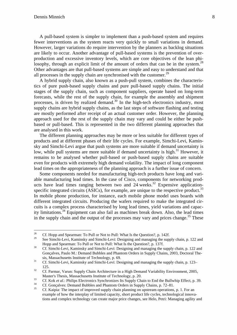
Figure 8: Pull Loops

Software Flashing and Packing (SWF). The production and shipment processes at software flashing as well as the preparation of the central plan are identical to those in the push-based planning approach with central planning. A central plan is necessary even in a pull-based planning approach since the first tier suppliers need to place orders with their suppliers according to a long-term forecast. The difference of the pull-based approach lies in the policies regulating the receipt of materials from final assembly. In contrast to the push approach, the pull approach triggers a shipment from final assembly to software flashing only when an order by software flashing has been placed. This or-dering logic is based on a pull replenishment logic that is explained in the following.

First, the number of orders to be placed with a specified order size is calculated. This number is then multiplied with the order size resulting in the amount of materials to be ordered each day. This value is accumulated in the stock Materials on order SWF that itself is reduced by the material arrival rate at software flashing. There is also a possibil-ity to limit the amount of orders placed per day to a maximum value. In the base case, however, this limit is not used.

The number of orders to be placed is calculated as follows. The material orders itself consist of several factors that are summed up. First, the incoming production requests SWF, which represents customer demand in the current period, are part of material or-ders. Considering new incoming orders is, however, not sufficient for driving the order-ing process. Therefore the forecasted demand during the lead time until any orders are received from FAT also becomes part of the calculation, since this period needs to be covered with materials on order. This forecast for demand during the expected lead time fluctuates if demand is different from the original forecast, as the forecasts used for the calculation are the adjusted forecasts. Then, the safety stock size is added to the material orders. Also, the backlog at SWF is considered since orders need to be placed to con-sider any orders that could not yet be fulfilled. From this, the inventory position, i.e. the amount of materials on order plus the current inventory level at SWF, is deducted. The inventory position represents the amount of materials already ordered or received, and

Dennis Minnich 18

creates a limit to the amount of orders that are in the system.44 The INTEGER function is finally used to identify the number of orders to be placed in each period when divid-ing the desired orders through the order size.

no of orders SWF = INTEGER ( ( (incoming production requests SWF * materials used per FG unit SWF * time to place an order SWF) + forecast demand in materials LT SWF + safety stock size SWF + initial stock SWF + (Backlog SWF * materials used per FG unit SWF) - Materials on order SWF - Inventory RM SWF ) /order size SWF ) /time to place an order SWF

The safety stock size at software flashing is calculated as the standard deviation of demand over the material lead time, which is 10 days, multiplied with a safety factor z, representing the number of standard deviations of demand to be covered. In the base scenario this safety factor is set to 1.65, which corresponds to a service level of 95 percent. The standard deviation of demand is calculated every 10 days using an algo-rithm developed by John D. Sterman45.

In addition to the safety stock size SWF variable there is also the possibility to in-clude an additional initial stock SWF. This initial stock can incorporate planned product introductions in the model even when currently no demand is observed, i.e. before the product introduction. Except where otherwise indicated, to simulate a pure pull-based system based solely on realized demand this initial stock is zero.

44 See Hopp and Spearman: To Pull or Not to Pull: What Is the Question?, pp. 142–143. 45 Cf. Sterman, John D.: Appropriate Summary Statistics for Evaluating the Historical Fit of System

Dynamics Models, in: Dynamica, Vol. 10 (1984), Winter, pp. 51–66 and Sterman: Business Dynam-ics, p. 874–880.

Dennis Minnich 19

Materials onorder SWF material arrival

rate SWF

order size SWF

no of orders SWF-

material ordersfrom FAT SWF

<receiving rateRM SWF>

+

<Inventory RM SWF>

-<Backlog SWF>

+

-

<incoming productionrequests SWF>

+

<Emergency orders toaccount for Backlog

SWF>

+

safety stocksize SWF

forecast demand inmaterials LT SWF

+

+

standard deviationof last 10 days SWF

safety factor zSWF

+ +

time to place anorder SWF

-

initial stock SWF

+max order size

SWF

orders SWF

+ - +

+

Figure 9: Pull: Material Orders at SWF

Final Assembly and Testing (FAT). Production and shipment processes at final as-sembly in the pull planning approach begin only after orders from software flashing have been received. Material orders are placed following the same policies as at soft-ware flashing. The incoming orders, i.e. current period demand, are the incoming order rate FAT, which is the sum of normal material orders placed by software flashing at final assembly and emergency orders.

First Tier Suppliers (BP/Sup). Production and shipment processes at board printing in the pull planning approach begin only after orders from final assembly have been received. Standard material orders, however, are placed according to a forecast prepared by central planning. The orders are adjusted to account for the difference between that forecast and actually experienced demand, i.e. orders placed by final assembly, and for a desired inventory level at board printing. This desired stock level is determined by a desired number of days of stock based on average demand observed from final assem-bly. Emergency orders by software flashing are placed separately as in the other two planning approaches.

Similarly to board printing, production and shipment processes at the other first tier supplier in the pull planning approach begin only after orders from final assembly have been received. Material orders, including emergency orders, are placed according to a forecast prepared by central planning. This forecast is adjusted to account for the differ-ence between that forecast and actually experienced demand, i.e. orders placed by final assembly, and for a desired inventory level at the first tier supplier. The desired inven-tory level is is determined by a desired number of days of stock as determined by aver-age demand from final assembly.

Dennis Minnich 20

3. Evaluation of Planning Policies to Achieve Responsiveness and Efficiency for a Product with a Typical Product Life Cycle

Product life cycles in the high-tech industry are characterised by a strong increase in demand during the introduction phase, followed by a gradual downward trend during maturity and finally an end-of-life demand drop, often caused by a new product genera-tion being introduced.46 The demand pattern for the simulations is the product life cycle shown in Figure 10, with an initial sales peak of close to 17,000 units on day 130 fol-lowed by a gradual downward trend in demand and a steep drop at the end of the prod-uct life cycle. The initial forecasts predict exactly this product life cycle.

y20,000

15,000

10,000

5,000

0 0 50 100 150 200 250 300 350 400 450 500

Time (Day)

demand for the current day Widget/Day

Figure 10: Demand Pattern

In reality, demand is subject to variation over time. Such demand volatility is intro-duced in the model in order to analyse its impact on the performance of the different planning approaches. Three demand scenarios are analysed – one scenario without ran-dom demand variations, one scenario with a low amount of variation, and one scenario with a high amount of variation. The forecast in each of these scenarios is the product life cycle shown above, without noise, and mean demand is also corresponding to this product life cycle. Noise is added to the previously stable product life cycle through a pink noise process, which is first-order autocorrelated noise where the next random variation depends in part on the previous variations. This is necessary to represent that one period’s demand is not independent of the last but depends to some degree on his-tory, i.e. there is some inertia.47 In the simulations with random noise, the supply chain performance measures discussed refer to the mean values obtained from a sensitivity analysis with 200 different random demand patterns. The values indicated for inventory turns and delivery performance to customer request are the mean values over 200 simu-lations with different noise seeds, i.e. 200 demand patterns with different noise patterns, each with mean demand following the product life cycle shown above. The standard

46 Cf. Burruss and Kuettner: Forecasting for Short-Lived Products, p. 10. 47 Cf. Sterman: Business Dynamics, p. 917.

Dennis Minnich 21

deviation of the pink noise remains constant over these 200 simulations and is 0.1 in the low noise scenario and 0.8 in the high noise scenario.

Driven by the variation in demand the planners in all planning approaches are con-fronted with the same problem – how to satisfy customer demand on time considering that the raw material receipts are unlikely to constantly coincide with the requirements during a particular period. If demand is below the forecast for a few days, inventory will build up, and if demand is higher than the forecast, the inventory levels will decline until eventually a backlog situation arises as demand can no longer be fulfilled.

3.1. Effect of Random Demand Deviations

The push approach achieves the highest level of delivery performance in each of the three demand scenarios with different demand volatility. This approach achieves 86 percent in the demand scenario without noise, 74 percent in the low noise scenario, and 41 percent in the high noise scenario. While the pull-based planning approach out-performs the push-based planning approach on efficiency in the scenarios with low noise and no noise, its delivery performance is consistently lower than that achieved by the alternative planning approach. Delivery performance in the pull-based planning ap-proach is 60 percent in the no noise scenario, 56 percent in the low noise scenario, and 24 percent in the high noise scenario. Depending on the objectives of the organisation, the lack of planning for the initial demand spike and consequential high initial backlog makes the pure pull-based planning approach unattractive.

Responsiveness vs. Efficiency

High25

Low0

Low20%

High100%

Resp

onsi

vene

ss(d

eliv

ery

perfo

rman

ce)

Efficiency(inventory turns)

Pull

PLC no noisePLC low noisePLC high noise

Push

Pull

Push

Push

Pull

Figure 11: Sensitivity to Randomness in the Demand Pattern

Dennis Minnich 22

Table 2: Sensitivity to Randomness in the Demand Pattern

Product Life Cycle Base Case Low Noise48 High Noise49

Delivery Perf.

Inventory Turns

Delivery Perf.

Inventory Turns

Delivery Perf.

Inventory Turns

Push 86% 14.0 74% 14.3 41% 9.6

Pull 60% 16.2 56% 16.1 24% 8.4

3.2. Planning the Product Introduction in the Pull-Based Planning Approach A major problem of the pull-based approach is the low delivery performance in the

initial phase of the product life cycle. In order to accommodate this difficulty, the prod-uct introduction is planned for by initialising production before customer demand is observed. Software flashing and final assembly and testing therefore order materials with the objective to have an initial stock of 100,000 units of components available when the product is introduced to the market.50 This intention is also known to the sup-pliers at the beginning of the forecasting process. In period 120, i.e. 20 days after the product introduction, this desired amount of materials in stock to cover for the product introduction phase is reset to zero.

For the demand scenario with high demand uncertainty the initial staging of the sup-ply chain through pre-production of components and stocking these at software flashing and final assembly increases average delivery performance to 40 percent (from 24 percent) and increases inventory turns to 9.0 (from 8.4). Delivery performance is equal to that in the push-based planning approach and efficiency as measured by inven-tory turns is slightly lower.

48 Mean values over a 200 simulations with different noise seeds; standard deviation of white noise

used for pink noise process is 0.1; this noise is added to the constant demand. Pink noise is first-order autocorrelated noise where the next random shock depends in part on the previous shocks.

49 Mean values over a 200 simulations with different noise seeds; standard deviation of white noise used for pink noise process is 0.8.

50 In the model, each final product at software flashing is composed of one finished good unit received from final assembly. Similarly, each finished good at final assembly is composed of one finished good unit from each first tier supplier and each finished component at the first tier suppliers is com-posed of one unit of components received from the respective second tier supplier.

Dennis Minnich 23

Responsiveness vs. Efficiency

High25

Low0

Low20%

High100%

Resp

onsi

vene

ss(d

eliv

ery

perfo

rman

ce)

Efficiency(inventory turns)

Pull

PLC high noise

PushPull with Initialization Stock

Figure 12: Improvement through Initial Staging of Components in Pull Approach51

The stability of the forecasts provided to the component suppliers in this approach is also high, which is beneficial for the supply chain. This can be seen when comparing the forecasts sent to board printing in the pull-based and push-based planning approach in Figure 13 to the initial forecast corresponding to the expected product life cycle.

g30,000

20,000

10,000

0 0 50 100 150 200 250 300 350 400 450 500

Time (Day)

forecast for board printing SWF : push plc2 high Widget/Day forecast for board printing SWF : pull plc2 high noise initial Widget/Day forecast 76 days out Widget/Day

Figure 13: Forecast for Board Printing (example, not averaged)

51 This figure shows the performance of incorporating the base safety stock level into the initial fore-

cast, which leads to a delivery performance of 75 percent and inventory turns of also 7.2 for the pull-based planning approach with a base safety stock level.

Dennis Minnich 24

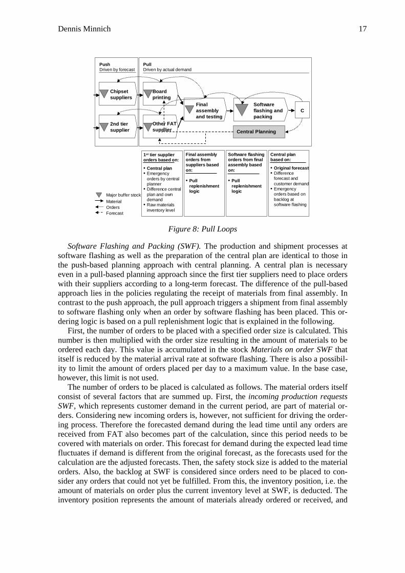
A major drawback of the pull-based planning approach is the large degree of varia-tion in the production rate at the suppliers, which is caused by the large variability in material orders by final assembly. As can be seen in Figure 14 for a sample simulation run, production of components in the push-based planning approach with central plan-ning follows the actual product life cycle relatively closely, even though production may be ramped up to the full capacity at board printing. This eliminates a large degree of the variation of end customer demand, which is beneficial to the efficiency of the supply chain as high and relatively stable capacity utilization is a success factor for effi-cient processes at board printing. In contrast, the production rate at board printing in the pull-based planning approach experiences large fluctuations with subsequent periods of both production at the capacity limit as well as production at zero. This is caused by the direct transmission of demand data through the supply chains, where relatively large deviations in demand cause relatively large deviations in material orders, even if these are only issued in large batches. Such large variations can pose a major challenge to the production planners at the suppliers, as it may be difficult to ramp up and ramp down capacity within these relatively short time intervals.

25,000

20,000

15,000

10,000

5,000

0 0 50 100 150 200 250 300 350 400 450 500

Time (Day)

production rate BP : push plc2 high Boards/Day production rate BP : pull plc2 high noise initial Boards/Day

Figure 14: Production at Board Printing (example, not averaged)

4. Achieving Responsiveness and Efficiency over the Product Life Cycle

The decisions taken to achieve an appropriate level of both dimensions of supply chain performance, efficiency and responsiveness, need to take into consideration as-pects related to the product life cycle. Sales in the initial phase of the product life cycle are particularly important, as higher prices can be charged and product life cycles are often very short. Therefore, high delivery performance is particularly desirable during the initial phase of the product life cycle. For the typical product life cycle of a high-tech product as modelled in the simulations the time behaviour of delivery performance over time varies significantly between the different planning approaches. As an example Figure 15 shows the demand scenario with high noise and the resulting delivery per-

Dennis Minnich 25

formance for the different planning approaches. The push-based planning approach with central planning achieves relatively high delivery performance at the beginning of the product life cycle, ranging in the example between 100 percent and around 50 percent. The pull-based planning approach in its pure form, however, is unable to deliver on time from the beginning of the product life cycle – the first unit is delivered on time around day 250 – and therefore a large amount of sales are potentially lost as customers move to competitors.

1

0.8

0.6

0.4

0.2

0 0 50 100 150 200 250 300 350 400 450 500

Time (Day)

delivery performance: push plc high noise Dmnl delivery performance: pull plc high noise Dmnl delivery performance: pull plc high noise initial stock Dmnl

Figure 15: Delivery Performance (example, not averaged)

It has been shown that planning for the product introduction by producing a certain amount of products before customer demand is first observed can increase delivery per-formance with only a small reduction in efficiency. As illustrated in Figure 15 for the product life cycle demand scenario with high demand volatility, such a an initial stock level allows a delivery performance that exceeds that of the push planning approach with central planning. The range of delivery performance in the example is between 75 percent and 100 percent in the first weeks after the product introduction. At the same time a value of inventory turns of 9.0 on average is achieved, which is only slightly worse than in the push planning approach, achieving 9.6 on average.52 In addition, both the push-based and the pull-based planning approach with initial staging of the supply chain are also able to react to supply chain disruptions in a meaningful way, such that delivery performance only experiences a small reduction. On average, delivery per-formance is only reduced by one percentage point if production at board printing is dis-rupted for 10 days in both planning approaches.

A major concern with regard short product life cycles is inventory of products and components that is unsold at the end of the product life cycle. Due to the characteristics of the two push-based planning approaches, both are subject to major inventory build-ups at all stages of the supply chain both during and at the end of the product life cycle.

52 As in the preceding discussion, an initial stock of 100,000 units is introduced for the raw materials

inventory levels at software flashing and final assembly. In addition, the initial forecast is adjusted to consider these planned stock levels for the product introduction phase by a one-time peak of 200,000 units plus the original forecast in the first forecast period.

Dennis Minnich 26

Inventory build-ups are particularly detrimental downstream in the supply chain due to the higher value of the products as they near completion. Such downstream inventory build-ups, as well as inventory build-ups at final assembly, are avoided in the pull-based planning approach. Due to the different decision making policies in the pull-based plan-ning approach, with no adjustments for desired inventory levels, inventory of semi-finished products at software flashing at the end of the product life cycles is signifi-cantly lower than in the other planning approaches, independent of the demand pattern. However, inventory build-ups in the pull-based planning approach may still occur at the upstream suppliers, which are driven by a forecast.

There, however, the cost of inventory is significantly lower, which also reduces the damage if obsolete inventory needs to be discarded. In the demand scenario with the second product life cycle, perfect forecasts and high noise, for example, the raw materi-als inventory levels at software flashing at the end of the simulation in the push-based planning approach with central planning correspond to 420,000 Euros, and in the pure pull planning approach they are only 45,000 Euros. In the pull approach with initial staging of components for the first phase of the product life cycle, the end raw materials inventory level at software flashing in this demand scenario is worth 50,000 Euros on average.53 At the first tier suppliers, mean inventory levels at the end of the simulations are 5,000 Euros (Push), 270,000 Euros (Pull) and 180,000 Euros (Pull with initial stock). To put these values into perspective, consider that total sales over the product life cycle are 3,000,000 units, with each unit valued at 1 Euro. Inventory levels at the end of the product life cycle can therefore, on average, reach up to almost 20 percent of total sales. The pull approach that plans for the product introduction can therefore achieve a higher level of delivery performance in the initial phase of the product life cycle with lower average inventory levels in the supply chain at the end of the simula-tion. Overall inventory turnover over the course of the product life cycle, however, is slightly lower than in the push-based planning approach. The results in all of the other simulations with different levels of demand volatility are comparable.

270

100

5

180

100

110

45

50

420

PullInitialisation

Stock

Pure Pull

Push

Average Inventory Levels at the End of the PLCThousand Euros

SuppliersFinal Assembly

Software Flashing

Figure 16: Average Inventory Levels at the End of the Product Life Cycle

53 All values are averages over 200 simulations with different noise seeds and rounded to full 5,000.

Dennis Minnich 27

It has been shown that it is possible to design the planning policies in the high-tech electronics industry in such a way that the performance of the supply chain is improved on both dimensions, responsiveness and efficiency. A combination of a simple pull-based planning system with a plan for the initial phase of the product introduction can perform as well as or even better than a push-based planning approach with central planning, independent of the demand characteristics of the product. This finding has a number of implications. First, it shows that both objectives, responsiveness and effi-ciency, can be achieved in a supply chain with one planning approach. Segmenting the product portfolio may not be necessary.

The finding that pull-based planning approaches can be used even in environments with high demand uncertainty and long component lead times is valuable if one consid-ers issues of implementation. Push-based planning approaches are more difficult to im-plement than pull-based planning approaches, in particular if the supply chain crosses multiple organizational boundaries. Planners in push-based planning systems depend on information about capacities, inventory levels, and generally the structure of the supply chain. For example, if information about supply chain disruptions at the supplier side is not communicated to the supply chain planners, as in this model, then their observations of such disruptions will only occur after a significant time delay.

In contrast, a pull-based system needs much less information and depends entirely on local decision rules at each supply chain echelon, which would immediately adjust to supply chain disruptions, for example, through local decision heuristics. The only act of planning that is needed is the long-term forecast that is communicated to the suppliers. As has been shown, these forecasts can be more stable in a pull-based planning system, which is advantageous for the supply chain.

However, there are also notable drawbacks to implementing the pull-based planning approach in the high-tech electronics industry. A complication when implementing pull-based planning systems in such an environment with a high potential for demand vari-ability is that the production rate at suppliers may be subject to large fluctuations if these are integrated in the pull-based planning system. These fluctuations may require higher average inventory levels at the suppliers. If there were several product variants, however, which use some of the same base components and could be produced on the same line at board printing, then this would smooth the overall production rate. How-ever, producing different variants on the same line would also add additional complex-ity as the production of the different variants needs to be scheduled to coincide with the demand. Correlations between different variants also need to be considered. The feasi-bility of such a system therefore depends on the product characteristics in terms of mix variability as well as the flexibility of changing production volumes at board printing. Also, the suppliers may need to be financially compensated for larger variations in de-mand and resulting increases and fluctuations of their raw materials inventory levels.

Dennis Minnich 28

References

Aertsen, Freek and Edward Versteijnen: Responsive Forecasting and Planning Process in the High-Tech Industry, in: The Journal of Business Forecasting, Vol. 25 (2006), No. 2, pp. 33–35.

Apple Computer, Inc.: Form 10-Q: Quarterly Report Pursuant to Section 13 or 15(d) of the Securities Exchange Act of 1934, United States Securities and Exchange Commission, 2006.

Beckman, Sara and Kingshuk K. Sinha: Conducting Academic Research with an Indus-try Focus: Production and Operations Management in the High Tech Industry, in: Production and Operations Management, Vol. 14 (2005), No. 2, pp. 115–124.

Burruss, Jim and Dorothea Kuettner: Forecasting for Short-Lived Products: Hewlett-Packard's Journey, in: Journal of Business Forecasting Methods & Systems, Vol. 21 (2002), No. 4, pp. 9–14.

Catalan, Michael and Herbert Kotzab: Assessing the responsiveness in the Danish Mo-bile phone supply chain, in: International Journal of Physical Distribution & Lo-gistics Management, Vol. 33 (2003), No. 8, pp. 668–685.

Chang, Shih-Chia, Neng-Pai Lin and Chwen Sheu: Aligning manufacturing flexibility with environmental uncertainty: evidence from high-technology component manufacturers in Taiwan, in: International Journal of Production Research, Vol. 40 (2002), No. 18, pp. 4765–4780.

Childerhouse, Paul and Denis R. Towill: Engineering supply chains to match customer requirements, in: Logistics Information Management, Vol. 13 (2000), No. 6, pp. 337–345.

Christopher, Martin G. and Denis R. Towill: Developing market specific supply chain strategies, in: International Journal of Logistics Management, Vol. 13 (2002), No. 1, pp. 1–14.

Christopher, Martin G., Robert Lowson and Helen Peck: Creating agile supply chains in the fashion industry, in: International Journal of Retail & Distribution Manage-ment, Vol. 32 (2004), No. 8, pp. 367–376.

Christopher, Martin G., Helen Peck and Denis R. Towill: A taxonomy for selecting global supply chain strategies, in: The International Journal of Logistics Man-agement, Vol. 17 (2006), No. 2, pp. 277–287.

Gonçalves, Paulo M.: Demand Bubbles and Phantom Orders in Supply Chains, 2003, Doctoral Thesis, Massachusetts Institute of Technology.

Gonçalves, Paulo M., Jim Hines and John D. Sterman: The impact of endogenous de-mand on push-pull production systems, in: System Dynamics Review, Vol. 21 (2005), No. 3, pp. 187–216.

Größler, Andreas, Peter M. Milling and Graham Winch: Perspectives on rationality in system dynamics – a workshop report and open research questions, in: Omega, Vol. 20 (2004), No. 1, pp. 75–87.

Helo, Petri: Managing agility and productivity in the electronics industry, in: Industrial Management + Data Systems, Vol. 104 (2004), No. 7, pp. 567–577.

Hochmann, Stephen: Flexibility – Finding the Right Fit, in: Supply Chain Management Review, Vol. 9 (2005), No. 5, pp. 10–11.

Dennis Minnich 29

Holweg, Matthias: The three dimensions of responsiveness, in: International Journal of Operations & Production Management, Vol. 25 (2005), No. 7, pp. 603–622.

Hopp, Wallace J. and Mark L. Spearman: To Pull or Not to Pull: What Is the Question?, in: Manufacturing & Service Operations Management, Vol. 6 (2004), No. 3, pp. 133–148.

Jayaram, Kartik, Axel Karlsson, Mayank Bansal, Andrei Kokoev, John Haller, Yanfeng Lim, Claire Fang, Dennis Minnich, Jay Bar, Ramesh Raman and Uwe Schmid: Segmented Approach to Supply Chain Management System Design in High Tech, McKinsey & Company, Inc., 2006.

Kaipia, Riikka: The impact of improved supply chain planning on upstream operations, 17th Annual NOFOMA Conference, Copenhagen 2005, pp. 1–15.

Kaipia, Riikka and Jan Holmström: Selecting the right planning approach for a product, in: Supply Chain Management: An International Journal, Vol. 12 (2007), No. 1, pp. 3–13.

Kaipia, Riikka, Hille Korhonen and Helena Hartiala: Planning nervousness in a demand supply network: an empirical study, in: The International Journal of Logistics Management, Vol. 17 (2006), No. 1, pp. 95–113.

Kok, Ton G. de, Fred Janssen, Jan van Doremalen, Erik van Wachem, Mathieu Clerkx and Winfried Peeters: Philips Electronics Synchronizes Its Supply Chain to End the Bullwhip Effect, in: Interfaces, Vol. 35 (2005), No. 1, pp. 37–48.

Kritchanchai, Duangpun and Bart L. MacCarthy: Responsiveness of the order fulfilment process, in: International Journal of Operations & Production Management, Vol. 19 (1999), No. 8, pp. 812–833.

Lee, Hau L.: The Triple-A Supply Chain, in: Harvard Business Review, Vol. 82 (2004), No. 10, pp. 102–112.

Lee, Young Hoon, Sunguk Chung, Byungjin Lee and Kyung Hwan Kang: Supply chain model for the semiconductor industry in consideration of manufacturing charac-teristics, in: Production Planning & Control, Vol. 17 (2006), No. 5, pp. 518–533.

Mason, Scott J., Michael H. Cole, Brian T. Ulrey and Li Yan: Improving electronics manufacturing supply chain agility through outsourcing, in: International Journal of Physical Distribution & Logistics Management, Vol. 32 (2002), No. 7, pp. 610–620.

Morecroft, John D.W.: System Dynamics: Portraying Bounded Rationality, in: Omega, Vol. 11 (1983), No. 2, pp. 131–142.

Naylor, J. Ben, Mohamed M. Naim and Danny Berry: Leagility: Integrating the lean and agile manufacturing paradigms in the total supply chain, in: International Journal of Production Economics, Vol. 62 (1999), pp. 107–118.

Ohno, Taiichi: Toyota Production System: Beyond Large Scale Production, Cambridge, MA 1988.

Olhager, Jan, Fredrik Persson, Berne Parborg and Sonny Rosén: Supply chain impacts at Ericsson – from production units to demand-driven supply units, in: Interna-tional Journal of Technology Management, Vol. 23 (2002), No. 1/2/3, pp. 40–59.

Parmar, Varun: Supply Chain Architecture in a High Demand Variability Environment, 2005, Master's Thesis, Massachusetts Institute of Technology.

Dennis Minnich 30

Reichhart, Andreas and Matthias Holweg: Creating the Customer-responsive Supply Chain: A Reconciliation of Concepts, 2006, forthcoming in: International Jour-nal of Operations & Production Management, http://www-innovation.jbs.cam.ac.uk/publications/reichhart_creating.pdf, retrieved on: 10 September 2006.

Reiner, Gerald: Customer-oriented improvement and evaluation of supply chain proc-esses supported by simulation models, in: International Journal of Production Economics, Vol. 96 (2005), No. 3, pp. 381–395.

Reinhardt, Andy: Nokia's Magnificent Mobile-Phone Manufacturing Machine, in: Busi-ness Week online, 3 August 2006, 2006, http://www.businessweek.com/globalbiz/content/aug2006/gb20060803_618811.htm, retrieved on 9 March 2007.

Shapiro, Jeremy F.: Modeling the Supply Chain, Duxbury 2007. Simchi-Levi, David, Philip Kaminsky and Edith Simchi-Levi: Designing and managing

the supply chain: Concepts, strategies, and case studies, 2nd ed., New York 2003.

Sterman, John D.: Appropriate Summary Statistics for Evaluating the Historical Fit of System Dynamics Models, in: Dynamica, Vol. 10 (1984), Winter, pp. 51–66.

Sterman, John D.: Business Dynamics – Systems Thinking and Modeling for a Com-plex World, Boston 2000.

Wendin, Christine: Electronics Manufacturing: EMS at a Crossroads, PriceWater-houseCoopers, 2004.