Resource abundance vs. resource dependence in cross-country growth regressions

Resource abundance vs. resourcedependence in cross-countrygrowth regressionsopec_ 107..130

Annika Kropf

less-developed economiesDepartment of Political Science, University of Vienna Department of Political Science, Universitätsstrasse7/2, floor 1010 Vienna, Austria. Email: [email protected]

Abstract

Having analysed the macroeconomic performance of large oil exporters, I found that, in many cases,rents from natural resources have been successfully used to enhance economic growth. Neverthe-less, adherents of the ‘resource curse’ seem to have found ample evidence suggesting that resource-abundant countries grow slower than resource-poor countries. A review of empirical research on the‘resource curse’ reveals that the variables used were usually proxies for resource dependence. Thesevariables introduce a bias, making less developed economies per se more resource ‘abundant’ thandeveloped economies. As a consequence, a new variable, not containing any information on a coun-try’s stage of development, was introduced. Comparing the variables on resource dependence andresource abundance in a model by Sachs and Warner, resource abundance was not significant. In anew model, resource abundance was even positively correlated with growth.

1. Introduction

Since the beginning of cross-country growth regressions, variables on the natural resourceendowments have become widely used. Numerous researchers have not only added vari-ables on natural resources to their regressions, but have focused on related issues such asthe resource curse, Dutch disease or the conflictual potential of resource wealth.

Sala-i-Martin (1997) and Doppelhofer et al. (2004) deem natural resource abun-dance one of the most robust variables in cross-country growth regressions, displaying asignificantly negative correlation with growth. This statement has been confirmedseveral times by Sachs and Warner, who had tried to find potential omitted variables,and also by Eric Neumayer (2004). Neumayer took over a model by Sachs and Warner(1995/1997), but calculated growth rates based on ‘genuine income’. This ‘genuineincome’ basically consists of the ‘normal’ gross domestic product (GDP) minus rentsfrom resource production. In 2001, Sachs and Warner, for example, conclude a paper asfollows:

107

© 2010 The Author. Journal compilation © 2010 Organization of the Petroleum Exporting Countries. Published by

Blackwell Publishing Ltd, 9600 Garsington Road, Oxford OX4 2DQ, UK and 350 Main Street, Malden, MA 02148, USA.

Empirical studies have shown that this [resource] curse is a reasonably solid fact.It is not easily explained by other variables, or by alternative ways to measureresource abundance. This paper shows that there is little direct evidence thatomitted geographical or climate variables explain the curse, or that there is a biasresulting from some other unobserved growth deterrent. (Sachs and Warner, 2001:837)

Correspondingly, Neumayer states in his concluding remarks that

[. . .] natural resource-intensive countries really do suffer from a ‘resource curse.’Existing studies have failed to take into account natural capital depreciation and haveanalysed growth of the wrong term, namely GDP, instead of genuine income. In fact,looking at genuine income instead reinforces the ‘resource curse.’Resource-intensive economies grow slower than their less resource-intensive peers interms of genuine income as well. (Neumayer, 2004: 1636)

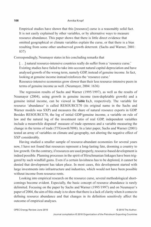
The regression results of Sachs and Warner (1995/1997), as well as the results ofNeumayer (2004), using growth in genuine income (non-depletable growth) and agenuine initial income, can be viewed in Table 1a,b, respectively. The variable forresource ‘abundance’ is called RESOURCE70 (its original name in the Sachs andWarner models was SXP) and measures the share of natural resource exports in GDP.Besides RESOURCE70, the log of initial GDP/genuine income, a variable on rule oflaw and the natural log of the investment ratio of real GDP, independent variablesinclude a meanwhile disputed1 measure of trade openness and a variable measuring thechange in the terms of trade (TTGrowth7098). In a later paper, Sachs and Warner (2001)tested an array of variables on climate and geography, not altering the negative effect ofSXP considerably.

Having studied a smaller sample of resource-abundant economies for several yearsnow, I have not found that resources represent a long-lasting fate, dooming a country tolow growth. On the contrary, if resources are used properly, resource-based development isindeed possible. Planning processes in the spirit of Hirschmanian linkages have been trig-gered by such windfall gains. Even if a certain lavishness has to be deplored, it cannot bedenied that development has taken place. In most cases, this development started withlarge investments into infrastructure and industries, which would not have been possiblewithout income from resource rents.

Looking into empirical research on the resource curse, several methodological short-comings become evident. Especially, the basic concept of resource abundance is rarelydelimited. Focusing on the paper by Sachs and Warner (1995/1997) and on Neumayer’spaper of 2004, the aim of this study is to show that there is a lack of clarity when it comes todefining resource abundance and that changes in its definition sensitively affect theoutcome of empirical analyses.

Annika Kropf108

OPEC Energy Review June 2010 © 2010 The Author.

Journal compilation © 2010 Organization of the Petroleum Exporting Countries

Table 1 Results by Sachs and Warner (1995/1997), as compiled by Neumayer (2004) (a) and resultsby Neumayer, using the model by Sachs and Warner with genuine income (2004) (b)

a

Dependent variable (1a) (2a) (3a) (4a) (5a)

Growth7098 Growth7098 Growth7098 Growth7098 Growth7098

LGDP70 0.078 -0.542 -0.813 -0.855 -0.843

(0.46) (2.94)** (3.92)** (3.75)** (3.66)**

LGENINC70

SXP (RESOURCE70) -5.576 -4.107 -3.502 -5.262 -5.383

(3.15)** (2.67)** (2.33)* (3.10)** (3.14)**

OPEN7090 2.206 1.979 1.596 1.594

(5.62)** (5.07)** (3.28)** (3.27)**

LINV7098 0.773 0.726 0.755

(2.55)* (2.31)* (2.37)*

RULE8295 0.063 0.051

(0.46) (0.37)

TTGROWTH7098 -0.051

(0.62)

Constant 1.457 5.624 5.904 6.511 6.371

(0.97) (3.78)** (4.09)** (4.18)** (4.03)**

Observations 86 86 86 79 79

R2 0.12 0.37 0.41 0.42 0.43

b

Dependent variable (1b) (2b) (3b) (4b) (5b)

GEN-GROWTH GEN-GROWTH GEN-GROWTH GEN-GROWTH GEN-GROWTH

7098 7098 7098 7098 7098

LGDP70

LGENINC70 -0.001 -0.614 -0.879 -0.912 -0.896

(0.01) (3.26)** (4.14)** (3.92)** (3.83)**

RESOURCE70 -5.048 -3.630 -3.061 -5.060 -5.206

(2.84)** (2.34)* (2.01)* (2.96)** (3.02)**

OPEN7090 2.159 1.931 1.551 1.549

(5.49)** (4.91)** (3.17)** (3.16)**

LINV7098 0.750 0.706 0.741

(2.46)* (2.24)* (2.31)*

RULE8295 0.052 0.037

(0.38) (0.27)

TTGROWTH7098 -0.061

(0.74)

Constant 2.022 6.115 6.394 6.972 6.801

(1.32) (4.04)** (4.34)** (4.40)** (4.23)**

Observations 86 86 79 79 79

R2 0.09 0.34 0.38 0.40 0.41

Absolute t-values in parentheses.* Significant at a 0.05 level.** Significant at a 0.01 level.Source: Neumayer (2004), Table 3, p. 1633.

Resource abundance versus resource dependence in cross-country growth regressions 109

OPEC Energy Review June 2010© 2010 The Author.


1.1. Resource abundance versus resource dependenceResource abundance and resource wealth are notions of a country’s natural resourceendowment that can reasonably be measured by the annual rent of resource production percapita. To make the annual resource rent per capita better comparable to SXP, which isbasically a number between 0 and 1, it was divided by 1000.2

Resource dependence, in contrast, can be found in economies where the current con-sumption level relies mainly on natural resource production and export. Measures such asthe share of resource exports in GDP (SXP/RESOURCE70) or the share of naturalresources in total exports fall into this category.

In Neumayer’s paper, ‘resource intensity’ is a frequently used notion, but it is notdefined: Neumayer deliberately avoids the discussion, choosing a notion in between andstating that he will not look into different definitions of resource intensity. When referringto earlier studies, he uses resource abundant, resource rich and resource intensive inter-changeably (Neumayer 2004: 1627). Sachs and Warner intermingle the three notions ofresource rich, resource abundant and resource intense, but never use resource dependence.

However, neither Neumayer nor Sachs and Warner are exceptions when using an out-right measure of resource dependence, while claiming to test concepts relying on resourceabundance. It is difficult to identify a reason for this. Sachs and Warner may have preferredSXP because SXP displays the highest significance, as can be seen in Table 2, but dataavailability may also have played a role.

Out of the four variables, the first three are clearly proxies for resource dependence,while LAND (the log of arable land divided by population) displays the smallest coeffi-cient and is not a measure of dependence. However, the inclusion of agrarian products inthe theory of the resource curse is disputed and its sole use as a proxy for resource abun-dance, excluding mineral, metals, etc., may be at best called insufficient.

The variable SXP suffers from three problems: Firstly, the year of 1970 is an unfortu-nate choice, because fossil fuels (oil, natural gas) experienced a significant price increasein the mid-1970s. The famous ‘natural resource booms’, important in Dutch diseasetheory, took place later. The second shortcoming is data availability: Many importantresource exporters are not covered by SXP. Most importantly, SXP contains additionalinformation on the quantity of exports and GDP, blurring the information on the realresource wealth of a country.

A short example can explain that SXP contains a lot more information about a countrythan only resource abundance and creates a heavy bias.

Norway and Oman are similarly resource-rich countries: from 1973 to 2005, Omanhad an average annual resource rent of US$2291 per capita, while Norway had an averageresource rent per capita of US$2891. Norway, thus, depletes even more resources thanOman. SXP, however, assigns Norway a 0.14, while Oman receives a 0.89, which means

Annika Kropf110



that in 1970, Oman exported resources worth 89 per cent of its GDP, while Norwayexported resources worth 14 per cent of its GDP. The reasons are obvious: while Norwaystarted with a non-depletable GDP of US$15,511 in 1973 (per capita in constant US$),Oman had a non-depletable GDP of US$3747 in 1973. Additionally, Norway, being anindustrialised and developed country, used a considerable part of its produced resourcesherself, adding value before export. Oman had scarcely any manufacturing at that time andexported the lion’s share of its resources without added value. This highlights the impor-tance of distinguishing between resource wealth/abundance on the one hand and resourcedependence on the other.A correlation test of the variable SXP and of the average resourcerent from 1973 to 2005 (RENT) shows that there is not even a significant correlation ofboth measures (Table 3).

Table 2 The use of different proxies for resource ‘abundance’

(3.1) (3.2) (3.3) (3.4)

SXP -8.28 — — —(-6.67)

SNR — -6.45 — —(-3.95)

PXI70 — — -2.50 —(-3.89)

LAND — — — -0.39(-3.78)

Adjusted R2 0.73 0.63 0.63 0.64Sample size 74 74 73 74Standard error 0.97 1.12 1.14 1.12

Dependent variable: GEA7089.The numbers in parentheses are t-statistics.The natural resource intensity variables are first, the SXPvariable [. . .], which measures natural resource exports divided by GDP in 1970; second, SNR(mineral production divided by GNP in 1970); third, PXI70 (natural resource exports divided bytotal exports in 1970), and LAND (the log of arable land area divided by population). The otherexplanatory variables in the regressions are LGDPEA70 (LGDP70 in Table 1a), SOPEN (OPEN709in Table 1a), RL (RULE8295 in Table 1a), DTT7090 (TTGrowth7098 in Table 1a) and LINV7089(LINV7098 in Table 1a).Source: Sachs and Warner (1995/1997), Table 3, p. 39.

Table 3 Testing the correlation of RENT and SXP

| rent sxp+

rent | 1.0000sxp | 0.5792 1.0000




In a first step of this paper, SXP in Sachs’ and Warner’s model will be replaced byRENT.

Since this model has a focus on trade, it seems advisable to construct, secondly, amodel testing a series of widely used significant growth variables, using non-depletablegrowth (growth in genuine income) as a dependent variable. Contrary to Sachs andWarner, all countries covered by SXP will be included. In a next step, the SXP variable willbe added and replaced by RENT in the following regression.This is to test, firstly, if SXP isas significant in my model as it is in the model by Sachs and Warner. In second place, thepaper investigates if the resource curse, or rather its part which is not explained by othervariables, still holds true if resource wealth instead of resource dependence is measured intwo different models.

A third aim is to enlarge the sample size of Sachs and Warner considerably and to testRENT for its correlation with non-depletable growth. This is possible today, because dataon resource rents have been made available for almost all countries in the world by theWorld Bank’s Green Accounting program.3

2. Theoretical background

Before explaining my model, a short summary of the theoretical background of theresource curse is necessary.

The background of including a variable on resources in growth regressions is anapparent observation that resource-abundant countries seldom manage to develop a viableeconomy and tend to grow more slowly than less resource-rich countries. This observationis widely called ‘resource curse’ or ‘paradox of plenty’, the latter notion indicating thateconomists are puzzled by this finding: while natural resources were regarded to be asource of growth a century or more ago (as in the United States), they came to be regardedas a curse. Several explanations have been pushed forward. The most prominent is an eco-nomic explanation called ‘Dutch disease’. Dutch disease, as explained in the seminalpaper by Cordon and Neary (1982), suggests two effects of resource booms, both leadingto a neglect of the manufacturing sector.The resource windfalls can lead to an appreciationof the local currency, which leads to higher wages. Since, however, manufactured goodsare bound to world market prices, wages cannot rise accordingly, because this wouldincrease the prices of tradeable goods. On the contrary, prices and wages in the non-tradeable goods and service sector can rise. The allocation of labour and investment mayshift from the tradeable, manufacturing sector to the non-tradeable sectors.A similar effectis created by the higher profits that can be gained in the resource sector, the latter becomingprobably more emphasised than the manufacturing sector.

The notion of Dutch disease stems from the effects of natural gas production in theNetherlands in the 1950s and 1960s. A gas export boom was followed by a decline in

Annika Kropf112



exports of manufactured goods. However, this decline only lasted during a very shortperiod of time. In Norway, on the contrary, a similar process seems to be of long-lastingeffect. Dutch disease has been commented as ‘Neither Dutch nor a Disease’ because ofthese facts (Gylfason, 2001: 3). Furthermore, it should be noted that Dutch disease theoryrelies on several assumptions, which are far from given in many resource-rich economies.

Another reason for the apparently bad growth performance of resource-abundantcountries is seen in the conflict potential of resources, which can become the object of civilwars. Profits from resource production, in turn, can be used to purchase further weaponsand lead to protracted civil strife. In another more recent paper, Neumayer and de Soysa(2005) found a correlation of resource ‘abundance’ and political instability.

Recent approaches towards the resource curse blame low institutional quality becauseof a lack of incentives. (Robinson et al., 2006) New institutional economists considerinstitutions as crucial for economic growth because well-functioning institutions reduceuncertainty and transaction costs. In resource-rich countries, incentives to allocate eco-nomic resources efficiently are lower, partly because there is no need of taxation andbecause rulers benefit from natural resources even if there is no economic development. Inaddition, revenues from resources help to stay in power for a very long time. For Robinson,Torvik and Verdier, it is institutional quality, which decides if natural resource endow-ments enhance or impede growth. It seems that incentives are at the core of most of therecent approaches: Gylfason’s work (2000) and Gylfason and Zoega (2006), for example,highlights a lack of incentives to invest and to enhance education.

In about the same vein, a political science approach characterises ‘rentier economies’,where the state is rather a distribution state than a production state. Large-scale distribu-tion from above, in turn, may lead to non-productive rent-seeking activities and, thus, toeconomic inefficiencies. (Beblawi and Luciani, 1987)

This is only a short overview on resource abundance and growth and mostly, the termi-nology in this literature is quite lax. Looking at the theories, however, the resource curseand Dutch disease consider windfall gains from resource exports and a large naturalresource production to cause the negative effect on growth (by other intervening factors),while empirics mostly use resource dependence measures. It is thus not sure if the conclu-sions by Sachs and Warner or Neumayer are valid, because theory and empirics have beenlinked by a false proxy.

3. Model and analysis

My model is a multivariate regression (OLS) with six independent variablesand the average non-depletable growth rate from 1973 to 2004 as the dependent vari-able. Using SXP, the sample is restricted to 111 countries (109 countries, if democracyis included).




First of all, note that several variables will be used in their ‘non-depletable’ or‘genuine’ form, which means that they have been corrected for resource rents. This is dueto the reasoning that the depletion of natural resources is not a form of added value, butrather a form of capital depreciation. (Stauffer and Lennox, 1984)

Recently, the World Bank has attracted attention to this fact in the context of sustain-able development. In order to calculate ‘net adjusted savings’(not to be used in this paper),data on resource rents for several decades and most countries of the world have been com-piled. The natural resource rents have been calculated using a method not based onresource stocks, but on annual resource production and current world marked prices. Thesimple formula is

P AC R−( )⋅ (1)

where P is the world market price, AC the average production cost and R the quantityproduced.4

Resource rents were subtracted from GDP and the resulting ‘genuine’ GDP was thebasis for the calculation of non-depletable growth rates (NDGROWTH735) and also forthe non-depletable initial GDP as of 1973. This correction of the GDP for resource rentshas already been used by Eric Neumayer, who named it ‘genuine income’.5 The ideabehind this is to measure if the non-resource sectors have grown or if growth has only beengenerated by more resource production or higher prices.As for initial non-depletable GDP(NDINITIAL), large revenues from natural resource exports overstate the size of theeconomies. Non-depletable GDP should fit better into convergence theory and Solow’sidea of the steady state.

It is important to note that reducing the GDP by the amounts of rents included doesnot necessarily mean that growth rates become smaller. When, as in the case of the year1973, oil prices rocket and revenue from oil exports quadruples, normal growth ratesdisplay this increase and tend to be very high. After subtracting the rents from thenatural resource, the growth rate becomes usually smaller. In contrast, if income fromnatural resources plummets, normal growth rates become very small or even negative.In this case, less resource rents are subtracted than the year before and non-depletablegrowth rates are higher.6

It is more difficult to decide whether, theoretically, investments as a share of GDP orinvestments as a share of non-depletable GDP are preferable. On the one hand, investmentcompared to the size of the non-resource economy should be responsible for the non-depletable growth. On the other hand, investment data will also include investments intothe resource production—which can be very capital intensive, but usually, these invest-ments are very costly once, and stay in place for a very long time. Therefore, the invest-ment share of non-depletable GDP (NDINVEST) was preferred to the investment share ofGDP (INVEST).

Annika Kropf114



Graphically, both, NDINVEST and NDINITIAL seem to display a logarithmic rela-tionship to NDGROWTH. They entered the regression as the natural log: LOGNDIN-VEST and LOGNDINITIAL.

Measuring human capital is a complicated issue and different measures can lead toentirely different outcomes, as Wößmann (2004) has demonstrated. Within the scope ofwhat is feasible, possible proxies are the school enrolment rates (especially secondaryschool enrolment), literacy rates or the average years of schooling of the labour force. Inmy study, the mean average years of schooling for the labour force over 15 from 1970 to2000, as contained in the Barro Lee dataset7 on educational attainment (AVSCHOOL),was used. I also tested a quality-adjusted measure of human capital (QUALSCO), takenfrom Wößmann (2004) and based on the work of Hanushek and Kimko (2000) as well as avariable based on public spending on education (EDUSPEND).

The crucial variable, as mentioned in the introduction, is the proxy for resourceabundance. As an alternative to SXP, I propose to use the annual per capita rent fromresource production as a proxy for resource wealth and not for resource dependence.Other possibilities would be measures based on the stock of natural resources, but thesemeasures are rejected for two reasons. Firstly, as long as resource stocks stay in soil,they should have only limited effects on the economy, at least within Dutch diseasetheory. Rentier theory, of course, may point to the psychological effect of long lastingresources, reducing incentives to develop a viable economy. Secondly and moreimportantly, measures of resource stocks are very imprecise and are permanentlycorrected, because new sources are found, or new technologies make resourcesrecoverable, while higher price make it economic to recover even less readily recover-able resources.

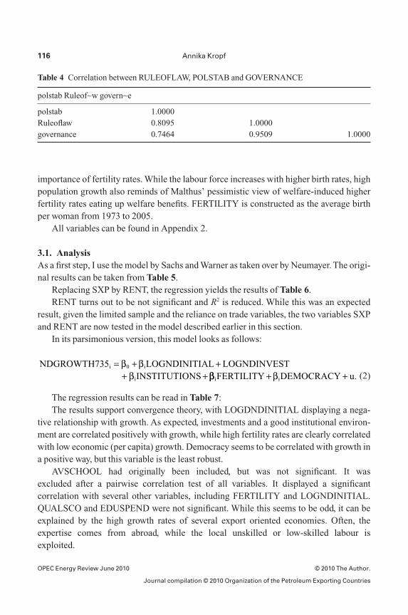
Very important are measures of institutional quality. The World Bank governanceindicators8 offer several related indices, starting in the year of 1996, which were used toconstruct three different variables. The average of the annual political stability index wastaken as a proxy for political stability (POLSTAB). As a measure of governance, the meanof governance and regulatory quality was taken and averaged from 1996 to 2006 (GOV-ERNANCE). Rule of Law and Control of Corruption were averaged to construct a moregeneral measure of rule of law (RULEOFLAW). As expected, these variables are highlycorrelated (Table 4) and therefore, a variable INSTITUTIONS using the mean values ofthe three indices, was constructed.

Even if often criticised as biased, the Freedom House index9 is probably the mostwidely used assessment of democracy. In my analysis, the averaged scores of civil libertiesand political rights from 1973 to 2005 were calculated. The result is the variableDEMOCRACY.

As mentioned above, the dependent variable consists of per capita growth rates. Thisfact and also several theoretical reflections on the size of the labour force point to the




importance of fertility rates. While the labour force increases with higher birth rates, highpopulation growth also reminds of Malthus’ pessimistic view of welfare-induced higherfertility rates eating up welfare benefits. FERTILITY is constructed as the average birthper woman from 1973 to 2005.

All variables can be found in Appendix 2.

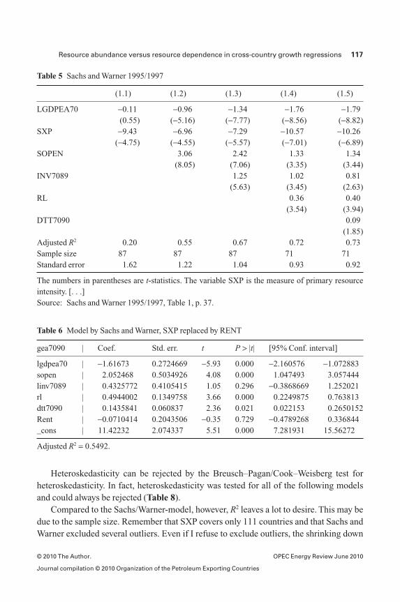
3.1. AnalysisAs a first step, I use the model by Sachs and Warner as taken over by Neumayer. The origi-nal results can be taken from Table 5.

Replacing SXP by RENT, the regression yields the results of Table 6.RENT turns out to be not significant and R2 is reduced. While this was an expected

result, given the limited sample and the reliance on trade variables, the two variables SXPand RENT are now tested in the model described earlier in this section.

In its parsimonious version, this model looks as follows:

NDGROWTH735 LOGNDINITIAL LOGNDINVESTINSTITUTIONS

i 0 i

i

= + ++ +β β

β ββ βi iFERTILITY DEMOCRACY u+ + . (2)

The regression results can be read in Table 7:The results support convergence theory, with LOGDNDINITIAL displaying a nega-

tive relationship with growth. As expected, investments and a good institutional environ-ment are correlated positively with growth, while high fertility rates are clearly correlatedwith low economic (per capita) growth. Democracy seems to be correlated with growth ina positive way, but this variable is the least robust.

AVSCHOOL had originally been included, but was not significant. It wasexcluded after a pairwise correlation test of all variables. It displayed a significantcorrelation with several other variables, including FERTILITY and LOGNDINITIAL.QUALSCO and EDUSPEND were not significant. While this seems to be odd, it can beexplained by the high growth rates of several export oriented economies. Often, theexpertise comes from abroad, while the local unskilled or low-skilled labour isexploited.

Table 4 Correlation between RULEOFLAW, POLSTAB and GOVERNANCE

polstab Ruleof~w govern~e

polstab 1.0000Ruleoflaw 0.8095 1.0000governance 0.7464 0.9509 1.0000

Annika Kropf116



Heteroskedasticity can be rejected by the Breusch–Pagan/Cook–Weisberg test forheteroskedasticity. In fact, heteroskedasticity was tested for all of the following modelsand could always be rejected (Table 8).

Compared to the Sachs/Warner-model, however, R2 leaves a lot to desire. This may bedue to the sample size. Remember that SXP covers only 111 countries and that Sachs andWarner excluded several outliers. Even if I refuse to exclude outliers, the shrinking down

Table 5 Sachs and Warner 1995/1997

(1.1) (1.2) (1.3) (1.4) (1.5)

LGDPEA70 -0.11 -0.96 -1.34 -1.76 -1.79(0.55) (-5.16) (-7.77) (-8.56) (-8.82)

SXP -9.43 -6.96 -7.29 -10.57 -10.26(-4.75) (-4.55) (-5.57) (-7.01) (-6.89)

SOPEN 3.06 2.42 1.33 1.34(8.05) (7.06) (3.35) (3.44)

INV7089 1.25 1.02 0.81(5.63) (3.45) (2.63)

RL 0.36 0.40(3.54) (3.94)

DTT7090 0.09(1.85)

Adjusted R2 0.20 0.55 0.67 0.72 0.73Sample size 87 87 87 71 71Standard error 1.62 1.22 1.04 0.93 0.92

The numbers in parentheses are t-statistics. The variable SXP is the measure of primary resourceintensity. [. . .]Source: Sachs and Warner 1995/1997, Table 1, p. 37.

Table 6 Model by Sachs and Warner, SXP replaced by RENT

gea7090 | Coef. Std. err. t P > |t| [95% Conf. interval]

lgdpea70 | -1.61673 0.2724669 -5.93 0.000 -2.160576 -1.072883sopen | 2.052468 0.5034926 4.08 0.000 1.047493 3.057444linv7089 | 0.4325772 0.4105415 1.05 0.296 -0.3868669 1.252021rl | 0.4944002 0.1349758 3.66 0.000 0.2249875 0.763813dtt7090 | 0.1435841 0.060837 2.36 0.021 0.022153 0.2650152Rent | -0.0710414 0.2043506 -0.35 0.729 -0.4789268 0.336844_cons | 11.42232 2.074337 5.51 0.000 7.281931 15.56272

Adjusted R2 = 0.5492.




of the sample to the 109/111 cases covered by SXP boosts R2. This step is also necessary inorder to make RENT and SXP comparable (Table 9).

Interestingly, DEMOCRACY is not significant on a 95 per cent confidence level anymore. This is not astonishing, democracy being anyway a highly disputed factor.10 Thelarger sample included many new democracies, especially in Eastern Europe, which hadgood economic performances. These cases of positive correlation between economicgrowth and democracy are absent in the smaller sample of 109 observations. Democracyis, however, significant on a 90 per cent confidence level. Testing the same model withoutDEMOCRACY did not result in any significant difference.

Table 7 New model, without SXP or RENT, 176 obs

ndgrowth735 | Coef. Std. err. t P > |t| [95% Conf. interval]

logndinitial | -1.705172 0.2052334 -8.31 0.000 -2.110306 -1.300038logndinvest | 1.03102 0.2687961 3.84 0.000 0.5004122 1.561628institutions | 1.166808 0.2575463 4.53 0.000 0.6584069 1.675208democracy | 0.2455723 0.117496 2.09 0.038 0.0136333 0.4775113fertility | -0.7413088 0.1154902 -6.42 0.000 -0.9692885 -0.5133292_cons | 14.76172 2.06112 7.16 0.000 10.69303 18.8304


Table 8 Heteroskedasticity test

Breusch–Pagan/Cook–Weisberg test for heteroskedasticityHo: Constant varianceVariables: fitted values of ndgrowth735chi2(1) = 0.88Prob > chi2 = 0.3483

Table 9 New model without SXP and RENT, sample covered by SXP (109 obs.)

ndgrowth735 Coef. Std. err. t P > t [95% Conf. interval]

logndinitial -2.110156 0.2448296 -8.62 0.000 -2.595718 -1.624595logndinvest 0.9267582 0.3162465 2.93 0.004 0.2995578 1.553959institutions 1.303593 0.2474762 5.27 0.000 0.8127824 1.794404fertility -0.9342151 0.1560047 -5.99 0.000 -1.243614 -0.6248166democracy 0.278675 0.1444064 1.93 0.056 -0.0077211 0.5650711_cons 18.9145 2.351879 8.04 0.000 14.25011 23.5789

Adjusted R2 = 0.5802, not heteroskedastic.

Annika Kropf118



In a next step, SXP is added to the model (Table 10).Astonishingly, SXP is not significant anymore. How can this be explained? Most prob-

ably, the strong institutional variable has taken some of the explanatory power of SXP.Alsoour larger sample (109 instead of 87) and the refusal to exclude cases deliberately can playa role. In contrast to Neumayer’s findings, my observation that several negative growthrates of resource-abundant and dependent countries have turned positive, should also havechanged the strong relationship between SXP and negative growth. Also, the enlargementof the time frame is important: Several resource-rich economies learned to avoid negativeeffects of Dutch disease or they learned from low resource prices in the 1980s and 1990s toinvest revenue from natural resources wisely. The result suggests that there are differentexplanations for resource-dependent countries growing slower and that even this lowergrowth performance cannot be taken for granted.

Adding, instead of SXP, RENT to the regression, RENT shows a significant positivecorrelation to non-depletable growth (Table 11).

This is true whether democracy is included or not. Testing the resource curse on thebasis of resource abundance instead of resource dependence would thus probably result inthe rejection of any kind of ‘curse’.

Table 10 New model with SXP (109 obs.)


logndinitial -2.125941 0.25537 -8.32 0.000 -2.632466 -1.619415logndinvest 0.9139203 0.3225831 2.83 0.006 0.2740783 1.553762institutions 1.294695 0.251618 5.15 0.000 0.7956122 1.793778fertility -0.9473515 0.1668229 -5.68 0.000 -1.278244 -0.6164591democracy 0.2713477 0.1485364 1.83 0.071 -0.0232736 0.565969sxp 0.2217248 0.9646789 0.23 0.819 -1.691711 2.135161_cons 19.12279 2.530586 7.56 0.000 14.10338 24.14219


Table 11 New model, using RENT, sample covered by SXP (109 obs.)


logndinitial -2.340607 0.2376897 -9.85 0.000 -2.811902 -1.869312logndinvest 0.7853476 0.3113711 2.52 0.013 0.1679562 1.402739institutions 1.090243 0.2233703 4.88 0.000 0.6473409 1.533145fertility -0.9443793 0.1448241 -6.52 0.000 -1.231539 -0.6572198rent 0.3034981 0.1140374 2.66 0.009 0.0773831 0.5296131_cons 22.15656 2.47817 8.94 0.000 17.2428 27.07031





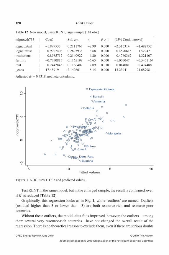
Test RENT in the same model, but in the enlarged sample, the result is confirmed, evenif R2 is reduced (Table 12).

Graphically, this regression looks as in Fig. 1, while ‘outliers’ are named. Outliers(residual higher than 3 or lower than -3) are both resource-rich and resource-poorcountries.

Without these outliers, the model-data fit is improved, however, the outliers—amongthem several very resource-rich countries—have not changed the overall result of theregression. There is no theoretical reason to exclude them, even if there are serious doubts

Table 12 New model, using RENT, large sample (181 obs.)


logndinitial | -1.899533 0.2111767 -8.99 0.000 -2.316314 -1.482752logndinvest | 0.9907406 0.2693938 3.68 0.000 0.4590615 1.52242institutions | 0.8985717 0.2140922 4.20 0.000 0.4760367 1.321107fertility | -0.7750815 0.1165199 -6.65 0.000 -1.005047 -0.5451164rent | 0.2442845 0.1166407 2.09 0.038 0.014081 0.474488_cons | 17.45919 2.142661 8.15 0.000 13.23041 21.68798


Armenia

Bahrain

Belarus

Bulgaria

Congo, Dem. Rep.

Equatorial Guinea

Eritrea

Iraq

Kuwait

Mongolia

Swaziland

-50

510

ndgro

wth

735

-5 0 5 10Fitted values

Figure 1 NDGROWTH735 and predicted values.

Annika Kropf120



about data quality. Table 13, which is the same regression as in Table 12, but withoutoutliers, should only demonstrate that the differences in measure of fit between the Sachsand Warner regression and my regression probably stem from the sample size.

4. Discussion and conclusion

The following table (Table 14) sums up the behaviour of the variables SXP and RENT inthe different models and sample sizes.

SXP is not as robust as expected and it is still unclear how it would behave in a largersample. As mentioned above, several reasons can be adduced in order to explain why SXPis not significant in our model.

First of all, the institutional variable, including corruption, rule of law and politicalstability has absorbed some of its explanatory power. This suggests that the institutionalenvironment is indeed of vital importance for the efficient use of resource rents. Further-more, high FERTILITY is usually a characteristic of less developed countries—and thecountries with high SXP values are usually non-developed countries, living basically ontheir natural resources. It is, thus, not astonishing that FERTILITY reduces the explana-tory power of SXP.

Table 13 Model as in Table 12, but without eleven outliers (->170 obs.)


logndinvest | 0.7572531 0.1914926 3.95 0.000 0.3791445 1.135362logndinitial | -1.874608 0.1486544 -12.61 0.000 -2.168132 -1.581085fertility | -0.7401515 0.0825575 -8.97 0.000 -0.9031641 -0.5771389institutions | 1.013184 0.1519927 6.67 0.000 0.7130694 1.313299rent | 0.3017897 0.091633 3.29 0.001 0.1208572 0.4827222_cons | 17.68911 1.509153 11.72 0.000 14.70924 20.66899


Table 14 Behaviour of SXP and RENT, overview

Model/ sample size

SXP RENT

Coeff. t-stats P-value Coeff. t-stats P-value

Sachs/Warner model (79/74) -10.26 -6.89 n.a. -0.0710414 -0.35 0.729New model (109/111) 0.9646789 0.23 0.819 0.3034981 2.66 0.009New model (181) — — — 0.2442845 2.09 0.038




Secondly, it is possible to argue that the non-depletable growth rates of several large oilproducers have turned positive and that these were countries with high SXP values, whichhave been excluded by Sachs and Warner as well as by Neumayer. The following plot andtable confirm a negative correlation of ‘normal growth’ and SXP on a 90 per cent confi-dence level in a bivariate regression (Fig. 2, Table 15).

This relationship, however, is almost the same in a regression of non-depletablegrowth and SXP, as Table 16 and Fig. 3 show.

Nevertheless, in the larger sample and with several other variables, the differencebetween non-depletable growth and ‘normal’ growth may still be crucial. This is to beexpected, because NDGROWTH735 and the ‘normal’ growth GRO735 display a correla-tion of 0.3167 only.

-10

010

20

30

gro

73

5

0 .2 .4 .6 .8 1sxp

Figure 2 ‘Normal’ growth and SXP.

Table 15 ‘Normal’ growth and SXP (113 obs.)

gro735 | Coef. Std. err. t P > |t| [95% Conf. interval]

sxp | -3.154178 1.733957 -1.82 0.072 -6.59013 0.2817729_cons | 2.098059 0.3964413 5.29 0.000 1.312484 2.883634


Annika Kropf122



Excluded cases have certainly played a big role in changing the robustness of SXP.Moreover, the enlarged time frame up to 2005 may also be responsible for the bettergrowth performance of some resource-dependent countries.

Nevertheless, SXP was significant in other models, analysing earlier time frames andsmaller samples. SXP has basically three ‘ingredients’: resources, exports and GNP in1970.The use of averaged per capita rents only increased the amount of resources, becausein most cases, real prices increased: Nevertheless, the negative correlation could not bereproduced. It is thus likely that the point of SXP really lies in the small size of the non-resource sector. And this is actually what dependence means. Dependence, in turn, canlead to traps, which are hard to overcome.

As for the role of large amount of natural resources for ‘common’ growth, it probablymakes a difference if revenue from natural resources ‘affect’ a poor, non-developed

Table 16 Non-depletable growth and SXP (113 obs.)


sxp | -2.262117 1.246706 -1.81 0.072 -4.732547 0.2083143_cons | 1.847663 0.274989 6.72 0.000 1.302754 2.392572


-50

51

0

nd

gro

wth

73

5

0 .2 .4 .6 .8 1sxp

Figure 3 Non-depletable growth and SXP.




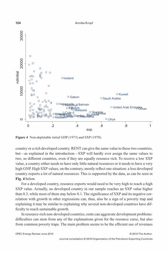
country or a rich developed country. RENT can give the same value to these two countries,but—as explained in the introduction—SXP will hardly ever assign the same values totwo, so different countries, even if they are equally resource rich. To receive a low SXPvalue, a country either needs to have only little natural resources or it needs to have a veryhigh GNP. High SXP values, on the contrary, mostly reflect one situation: a less developedcountry exports a lot of natural resources. This is supported by the data, as can be seen inFig. 4 below.

For a developed country, resource exports would need to be very high to reach a highSXP value. Actually, no developed country in our sample reaches an SXP value higherthan 0.3, while most of them stay below 0.1. The significance of SXP and its negative cor-relation with growth in other regressions can, thus, also be a sign of a poverty trap andexplaining it may be similar to explaining why several non-developed countries have dif-ficulty to reach sustainable growth.

In resource-rich non-developed countries, rents can aggravate development problems:difficulties can stem from any of the explanations given for the resource curse, but alsofrom common poverty traps. The main problem seems to be the efficient use of revenues

BahrainBelize

Cote d

Fiji

Gabon

Gambia, TheGhanaGuyana

Honduras

Iceland

Iraq

Kuwait

Liberia

LibyaMalawi

Malaysia

Mauritania

MauritiusOman

Saudi Arabia

Uganda

United Arab EmiratesVenezuela

Zambia

01

00

00

20

00

03

00

00

nd

initia

l

0 .2 .4 .6 .8 1sxp

Figure 4 Non-depletable initial GDP (1973) and SXP (1970).

Annika Kropf124



from natural resources to develop the local economy. Given that these rents accrue to thestate, the ability of governments and institutions to plan and to implement decisions arecrucial in the first place.

However, while many reasons for development problems of resource-dependent coun-tries can be found in the local economies, I cannot exclude that dependency theories play arole here. Revenues from resource exports increase purchasing power and make resource-rich, non-developed economies good markets for produced goods and oil is a strategicresource. Large oil exporters, for example, can be bound to a package deal of providing acountry with oil, thus, being obliged to maintain a high level of production, while in return,they receive military equipment and protection. Nevertheless, also these problems ofinternational dependance can be tackled by wise decisions or regional cooperation.

With regard to resource abundance, the mere size of gains from natural resources,however, does not seem to create any kind of ‘curse’ if this is measured without any infor-mation about the stage of development of the economy. It seems that a lot depends on howthese revenues are handled. In several countries, they have been used to improve infra-structure and institutions and to build a vast welfare system, increasing, in turn, politicalstability. Of course, the efficient use of resource windfalls is easier if good institutions arealready in place, but there are also many success stories of countries having managed tobuild viable institutions after their resource windfalls.

Again, it should be noted that there are still several shortcomings in my analysis. Themain leakage is the fact that SXP does only cover 111 countries and only for 1 year. Itwould also be interesting to use resource exports in GNP of other years. Moreover,resource stocks (possibly per capita) could be interesting, when testing for the effects ofincentives. This is where further research can hook in. In the end, using revenue fromnatural resources and making efficient production decisions depend a lot on facts noteasily covered by macroeconomic data. In many cases, only the focus on details shows,why the non-resource sector develops or not. And probably, variables such as RENT andSXP will continue to change sign and significance depending on the model.

Notes

1. Rodríguez and Rodrik (2000) found that several components of SOPEN, meant to measuretrade openness, are actually not meaningful at all, such as the ‘black market premium’.

2. Natural log was avoided because of the fact that many countries were assigned a resource rentof zero.

3. The dataset can be downloaded from the permanent URL:http://go.worldbank.org/EPMTVTZOM0 (February 2010). Apart from oil and gas, it covershard and soft coal, numerous metals and forests.

4. Following the concept of the Hotelling rent, marginal costs would have been preferable, butdata on marginal cost is hard to obtain. Please note that agrarian products are not considered




natural resources. Given high production costs and low prices, only small rents (if at all) canbe expected from agrarian products.

5. It is noteworthy that non-depletable GDP or genuine income is not resource independent.Even if rents from natural resources are subtracted, they have a multiplier effect: they accrueto the government and the government, for instance, uses these rents to pay salaries. Civilservants, in turn, use their salaries for consumption. (Stauffer and Lennox, 1984)

6. To illustrate this, the calculation of the non-depletable GDP of Canada can be found inAppendix 2. Please note that Canada is not a very striking example because the ratio ofnatural resource rents in GDP is not as high as in other big oil exporting countries. Canadahas been chosen because of her better data quality. Nonetheless, even Canada displays theabove-mentioned phenomena in the years of 1973 or 1985/1986 very clearly.

7. The Barro-Lee dataset can be downloaded fromhttp://www.cid.harvard.edu/ciddata/ciddata.html (15 June 2009).

8. Data can be retrieved from http://www.worldbank.org/wbi/governance/data (15 June 2009).Unfortunately, this index only goes back to 1996.

9. Download from http://www.freedomhouse.org/template.cfm?page=1 (15 June 2009).Democracies are assigned lower values (1), while the value rises with the degree of autocracyto 7. I have reversed this variable by multiplying the Freedom House figures with -1 andadding 8. The index measures two concepts: civil liberties and political rights, which areusually similar. The average of both was used for this paper.

10. The theoretical approaches towards democracy and growth are controversial. Someresearchers claim that democracy has a positive effect on growth because people indemocracies enjoy economic freedom and live in a sound institutional environment. Othersclaim that democracy leads to economic inefficiency, because governments in power areeager to be reelected. They are likely to distribute funds and privileges for potential votersand shy away from implementing necessary, but unpopular reforms. This ambiguity isreflected in controversial empirical results. (Quinn and Woolley, 2001)

References

Beblawi, H. and Luciani, G. (eds), 1987. The Rentier State (Nation, State and Integration in theArab World Vol. II). Sydney Croom Helm, London; NewYork, pp. 49–62.

Cordon, W.M. and Neary, P., 1982. Booming sector and de-industrialisation in a small openeconomy. The Economic Journal 92, 368, 825–848.

Doppelhofer, G., Miller, R.I. and Sala-i-Martin, X., 2004. Determiniants of long-term growth: aBayesian averaging of classical estimates (BACE) approach. American Economic Review 94,4, 813–835.

Gylfason, T., 2000. Natural resources, education, and economic development. European EconomicReview 45, 4–6, 847–859.

Gylfason, T., 2001. Lessons from the Dutch disease: causes, treatment, and cures. Institute ofEconomic Studies (Reykjavik, Iceland) Working Paper Series.

Annika Kropf126



Gylfason, T. and Zoega, G., 2006. Natural resources and economic growth: the role of investment.World Economy 29, 1091–1115.

Hanushek, E.A. and Kimko, D.D., 2000. Schooling, labor-force quality and the growth of nations.The American Economic Review 90, 5, 1184–1208.

Heston, A., Summers, R. and Aten, B., 2006. Penn WorldTableVersion 6.2, Center for InternationalComparisons of Production, Income and Prices at the University of Pennsylvania.

Neumayer, E., 2004. Does the ‘resource curse’ hold for growth in genuine income as well? WorldDevelopment 32, 10, 1627–1640.

Quinn, D.P. and Woolley, J.T., 2001. Democracy and national economic performance: thepreference for stability. American Journal of Political Science 45, 3, 634–657.

Robinson, J.A., Torvik, R. and Verdier, T., 2006. Political foundations of the resource curse.Journal of Development Economics 79, 447–468.

Rodríguez, F. and Rodrik, D., 2000. Trade policy and economic growth: a skeptic’s guide to thecross-national evidence. NBER Macroeconomics Annual 15, 261–325.

Sachs, J.D. and Warner, A.M., 1995/1997. Natural resource abundance and economic growth.Working Paper 5398, Cambridge, MA: National Bureau of Economic Research and HarvardUniversity.

Sachs, J.D. and Warner, A.M., 2001. Natural resources and economic development: the curse ofnatural resources. European Economic Review 45, 827–838.

Sala-i-Martin, X., 1997. I just ran two million regressions. American Economic Review Papers andProceedings, 87, 2, 178–183.

Soysa, I. and Neumayer, E., 2005. Resource Wealth and the Risk of Civil War Onset: Results froma New Data Set of Natural Resource Rents, 1970–1999, International Peace Research Institute,Oslo.

Stauffer, T.R. and Lennox, F.H., 1984. Accounting for ‘wasting assets’. Income measurement foroil and mineral-exporting rentier states. OFID Pamphlet Series no. 25.

Wößmann, L., 2004. Specifying human capital. In George, D., Oxley, L. and Carlaw, K. (eds)Surveys in Economic Growth. Theory and Empirics, Blackwell Publishing, Malden, MA;Oxford; Victoria, pp. 13–44.

Appendix 1: ‘Normal’ and non-depletable growth rates: Canada

YearNominalGDP Real GDP Growth

Nom.GDP

Nom.Rent

Nom. NdGDP

Real ndGDP

Ndgrowth

1973 5143.6 16,149.45 5143.6 295.1 4848.5 15,222.931974 5914.89 17,035.97 5.49 5914.89 598.88 5316.01 15,311.09 0.581975 6484.03 17,058.75 0.13 6484.03 524.54 5959.49 15,678.74 2.41976 7172.95 17,843.16 4.6 7172.95 541.52 6631.43 16,496.1 5.211977 7791.08 18,220.49 2.11 7791.08 572.81 7218.27 16,880.9 2.331978 8466.5 18,501.97 1.54 8466.5 515.8 7950.7 17,374.77 2.93




Appendix 1 Continued

YearNominalGDP Real GDP Growth

Nom.GDP

Nom.Rent

Nom. NdGDP

Real ndGDP

Ndgrowth

1979 9581.78 19,337.6 4.52 9581.78 1118.32 8463.46 17,080.66 -1.691980 10,687.25 19,769.24 2.23 10,687.25 1303.43 9383.82 17,358.16 1.621981 11,737.74 19,850.74 0.41 11,737.74 1161.33 10,576.41 17,886.7 3.041982 11,794.67 18,799.28 -5.3 11,794.67 1037.38 10,757.29 17,145.82 -4.141983 12,500.78 19,170.04 1.97 12,500.78 888.08 11,612.7 17,808.16 3.861984 13,500.8 19,953.89 4.09 13,500.8 889.49 12,611.31 18,639.24 4.671985 14,327.46 20,550 2.99 14,327.46 786.72 13,540.74 19,421.6 4.21986 14,754.82 20,702.71 0.74 14,754.82 372.23 14,382.59 20,180.43 3.911987 15,853.83 21,658.24 4.62 15,853.83 452.26 15,401.57 21,040.39 4.261988 17,010.45 22,467.9 3.74 17,010.45 483.34 16,527.11 21,829.49 3.751989 17,998.11 22,907.1 1.95 17,998.11 488.94 17,509.17 22,284.8 2.091990 18,331.4 22,462.2 -1.94 18,331.4 641.59 17,689.81 21,676.04 -2.731991 18,048.25 21,368.99 -4.87 18,048.25 602.06 17,446.19 20,656.16 -4.711992 18,326.75 21,211.52 -0.74 18,326.75 488.11 17,838.64 20,646.57 -0.051993 18,843.62 21,318.72 0.51 18,843.62 484.76 18,358.86 20,770.29 0.61994 19,950.71 22,101.15 3.67 19,950.71 460.62 19,490.09 21,590.88 3.951995 20,971.83 22,765.77 3.01 20,971.83 595.54 20,376.29 22,119.29 2.451996 21,555.95 22,966.07 0.88 21,555.95 704.12 20,851.83 22,215.89 0.441997 22,635 23,721.44 3.29 22,635 673 21,962 23,016.14 3.61998 23,039.34 23,879.91 0.67 23,039.34 357.19 22,682.15 23,509.69 2.141999 24,615.57 25,151.29 5.32 24,615.57 341.12 24,274.45 24,802.75 5.52000 26,820.73 26,820.73 6.64 26,820.73 1087.89 25,732.84 25,732.84 3.752001 27,414.49 26,771.96 -0.18 27,414.49 950.16 26,464.33 25,844.08 0.432002 28,187.84 27,054.27 1.05 28,187.84 733.77 27,454.07 26,350 1.962003 29,775.9 27,982.24 3.43 29,775.9 1055.28 28,720.62 26,990.53 2.432004 31,600.21 28,869.19 3.17 31,600.21 1470.01 30,130.2 27,526.22 1.98

Mean:1.93

Mean:1.96

Sources: PENN World Table 6.2, World Bank.The table shows normal growth rates (Growth) and the growth rates (Nd growth) calculated from anon-depletable real GDP (Real nd GDP). Recurring to nominal GDP numbers was necessary,because natural resource rents were nominal. To calculate real GDPs, the GDP deflator was used (inUS$ as of 2000). As a general observation, non-depletable growth rates are lower than ‘normal’growth rates when prices for resources rise (see 1974, 1979, 1980, 2003–2006). The contrary is thecase when prices fall (see 1985–1987, 1998).

Annika Kropf128



Appendix 2: List of variables

Growth in genuine income/non-depletable GDP (NDGROWTH735)Mean of non-resource per capita growth rates from 1973 to 2004. Calculation: current percapita GDP from PENN 6.2 minus the sum of resource rents in current prices (from WorldBank Net adjusted Savings Data) divided by the population (also from PENN 6.2).

The resulting non-natural-resource current GDP is chained into constant US$ (2000)by the GDP deflator. This is the basis of non-resource growth.

World Bank resource rents cover oil, natural liquid gas, hard and soft coal, eight differ-ent metals and ores as well as a measure of deforestation. Rents have been calculated asP - AC · Q, where P is the resource price on the international market, AC the average costof production and Q the quantity produced.

Gross fixed capital investment (INVEST)Is the mean investment into fixed capital (per cent of GDP) taken from the World BankDevelopment Indicators CD from 1973 to 2005.

Investment share of non-depletable GDP (NDINVEST)Investment share, taken from Penn 6.2 (ci), calculated from current GDP and calculatedanew as a share of non-depletable GDP as computed for non-depletable growth. Averagedfrom 1972 to 2005.

Initial genuine income/non-depletable GDP (NDINITIAL)Genuine income/non-depletable GDP as calculated for NDGROWTH735, as of 1973 inUS$ (2000 prices), if available. For some countries, later years were taken, but in thosecases also the average calculation of growth rates started in this later year. This isespecially the case for countries which came into being after 1989.

Averages years of schooling (AVSCHOOL)Average years of schooling of the labour force over 15, averaged from 1970 to the mostrecent available year (usually 2000), taken from the Barro-Lee dataset on educationalattainment.

Fertility rate (FERTILITY)The mean of the fertility rate (births per woman) from 1973 to 2005, taken from the WorldBank Data CD 2007.




Democracy (DEMOCRACY)is the mean value of civil liberties and political rights from 1973 to 2005 taken from theFreedom House index. While Freedom House gives the highest value (7) not free and thelowest value (1) to free countries, I have reversed this relationship by multiplying thevalues with -1 and adding 8.

Institutional quality (INSTITUTIONS)This is the mean value of the three above-mentioned and highly intercorrelated variablesRULEOFLAW, GOVERNANCE and POLSTAB. All three are taken from the WorldBank’s Governance Indicators and start in 1996. While RULEOFLAW combines rule oflaw and control of corruption, GOVERNANCE combines regulatory quality and govern-ment effectiveness. POLSTAB reflects the index of political stability only.

Exports share (SHEXP735)The mean of the annual data on the share of exports in GDP, taken from the World Bankdata CD 2007.

Women’s share in total labour force (WOMEN)The average of the percentage of women participating in the labour force, taken from theWorld Bank data CD 2007.

Resource exports as a percentage of GNP (SXP), also called RESOURCE70 inNeumayer’s paperIs the share of resource exports of the GDP in 1970. This variable has been taken from theSachs and Warner dataset.

Resource rents per capita (RENT)Is the mean annual, per capita resource rent of a country from 1973 to 2006, in thousanddollars.

Quality of schooling (QUALSCO)Is the average years of schooling of the labor force, adjusted for a measure of schoolingquality. Taken from Ludger Wößmann (2004).

Educational spending (EDUSPEND)Is an average of the percentage of GDP spent on education, taken from the World BankDevelopment Indicators Data CD 2007.

Annika Kropf130



Resource abundance vs. resource dependence in cross-country growth regressions

Documents

Transcript of Resource abundance vs. resource dependence in cross-country growth regressions