Requirements of a global near-surface soil moisture satellite mission: accuracy, repeat time, and...

Advances in Water Resources 27 (2004) 785–801

www.elsevier.com/locate/advwatres

Requirements of a global near-surface soil moisture satellitemission: accuracy, repeat time, and spatial resolution

Jeffrey P. Walker a,b,*, Paul R. Houser a

a Hydrological Sciences Branch, Laboratory for Hydrospheric Processes, NASA Goddard Space Flight Center, Greenbelt, MD 20771, USAb Department of Civil and Environmental Engineering, The University of Melbourne, Parkville, Vic. 3010, Australia

Received 11 September 2003; received in revised form 29 March 2004; accepted 4 May 2004

Available online 8 July 2004

Abstract

Soil moisture satellite mission accuracy, repeat time and spatial resolution requirements are addressed through a numerical twin

data assimilation study. Simulated soil moisture profile retrievals were made by assimilating near-surface soil moisture observations

with various accuracy (0, 1, 2, 3, 4, 5 and 10%v/v standard deviation) repeat time (1, 2, 3, 5, 10, 15, 20 and 30 days), and spatial

resolution (0.5, 6, 12 18, 30, 60 and 120 arc-min). This study found that near-surface soil moisture observation error must be less

than the model forecast error required for a specific application when used as data assimilation input, else slight model forecast

degradation may result. It also found that near-surface soil moisture observations must have an accuracy better than 5%v/v to

positively impact soil moisture forecasts, and that daily near-surface soil moisture observations achieved the best soil moisture and

evapotranspiration forecasts for the repeat times assessed, with 1–5 day repeat times having the greatest impact. Near-surface soil

moisture observations with a spatial resolution finer than the land surface model resolution (�30 arc-min) produced the best results,

with spatial resolutions coarser than the model resolution yielding only a slight degradation. Observations at half the land surface

model spatial resolution were found to be appropriate for our application. Moreover, it was found that satisfying the spatial res-

olution and accuracy requirements was much more important than repeat time.

Published by Elsevier Ltd.

Keywords: Soil moisture; Remote sensing; Mission requirements; Data assimilation; Modelling

1. Introduction

Data on land surface moisture is vital to under-standing the earth system water, energy, and carbon

cycles. Fluxes of these quantities over land are strongly

influenced by a surface resistance that is largely soil

moisture dependent. Soil moisture knowledge is critical

in weather and climate prediction, where model initial-

ization with hydrospheric state measurements has been

shown to bring significant improvements in forecast

accuracy and reliability [2,13,14]. Soil moisture obser-vations will also benefit climate-sensitive socioeconomic

activities, such as water management, agriculture, flood

and drought monitoring, and policy planning, by

extending the capability to predict regional water

*Corresponding author. Address: Department of Civil and Envi-

ronmental Engineering, The University of Melbourne, Parkville, Vic.

3010, Australia. Tel.: +61-3-8344-5590; fax: +61-3-8344-6215.

E-mail address: [email protected] (J.P. Walker).

0309-1708/$ - see front matter Published by Elsevier Ltd.

doi:10.1016/j.advwatres.2004.05.006

availability and seasonal climate. However, accurate

land surface soil moisture observations are lacking, due

to an inability to economically monitor spatial variationin soil moisture from traditional point measurement

techniques. As a result, land surface models have been

relied upon to provide an estimate of the spatial and

temporal variation in land surface soil moisture. How-

ever, due to uncertainties in atmospheric forcing, land

surface model parameters and land surface model

physics, there is often a wide range of variation between

different land surface model forecasts of soil moisture[16].

Over the past two-decades there have been numerous

ground-based, air-borne and space-borne near-surface

soil moisture (top 1–5 cm) remote sensing studies, using

both thermal infrared and microwave (passive and ac-

tive) electromagnetic radiation. Of these, passive

microwave soil moisture measurement has been the

most promising technique, due to its all weather capa-bility, its direct relationship with soil moisture through

mail to: [email protected]

786 J.P. Walker, P.R. Houser / Advances in Water Resources 27 (2004) 785–801

the soil dielectric constant, and a reduced sensitivity to

land surface roughness and vegetation cover [11].

However, to date there has been no dedicated space

mission for the measurement of near-surface soil mois-

ture. This is mainly due to the large antenna size (10’s ofmeters) required for obtaining radiometric L-band

observations at the desired spatial resolution (10’s of

km). As a result, scientists have resorted to making the

best use of soil moisture information from non-optimal

(i.e. C-band) sensors (e.g. [25]) and models [e.g. [20]).

Although current remote sensing technology can only

provide a soil moisture measurement of the thin near-

surface layer rather than the entire profile, there is asizeable body of literature that has demonstrated an

ability to retrieve the soil moisture content at much

greater depths when this near-surface information is

assimilated into a land surface model (e.g. [12,17,26–

28,32–35]). Moreover, there is a great scientific demand

for the soil moisture data that would be provided by

such a mission [21].

While there is no current space-borne mission dedi-cated to soil moisture measurement, there are two mis-

sions in development stages. These are the European

Space Agency passive L-band Soil Moisture and Ocean

Salinity (SMOS) mission (2007 launch) and the U.S.

National Aeronautics and Space Administration active/

passive L-band HYDROSpheric states (HYDROS)

mission (2009 launch).

Defensible global near-surface soil moisture mea-surement science and application requirements are vi-

tally important for mission planning. In particular,

mission planners need: (i) sensor polarization, wave-

length and look angle requirements; and (ii) measure-

ment accuracy, temporal resolution and spatial

resolution requirements. (While satellite mission design

must also consider the satellite overpass time, the main

impact of this will be accuracy of the inferred near-surface soil moisture content, which will be a function of

the specific remote sensing technique. Thus, we consider

this as part of measurement accuracy.) The (i) require-

ments have been fairly well defined, with horizontally

polarized <50� look angle [18,25] L-band [24] radiome-

ter measurements, and horizontally polarized send and

receive [31] C-band [8] 15� look angle radar measure-

ments [30] yielding the greatest soil moisture sensitivi-ties. However, the (ii) requirements have been less well

defined. Apart from some ‘‘best guess’’ estimates by

Engman [10] for spatial resolution (1–100 km), repeat

time (1–10 days), measurement depth (top 5–10 cm) and

accuracy levels (4–10%v/v) according to application,

there are only the studies of Milly [22] and Hoeben and

Troch [15], which recommend a daily repeat time, and

Calvet and Noilhan [6], which recommends a 3 day re-peat time. Finally, Jackson et al. [19] recommend with-

out justification an accuracy of 4%v/v with a 10 km

spatial resolution and 2–3 day repeat time.

Whilst L-band measurements are sensitive to a deeper

layer of soil moisture near the earth’s surface (�1/10 to

1/4 of the wavelength, depending on soil moisture, wave

polarization, look angle, etc) than say C-band, the

requirement for passive L-band measurements is thereduced sensitivity due to soil moisture signal masking

by vegetation, rather than sensing depth. Moreover,

Walker et al. [33] have shown that in the context of data

assimilation, the near-surface soil moisture observation

depth is relatively unimportant, providing the actual

measurement depth is known and this matches closely

the model near-surface layer thickness.

This paper seeks to defensibly address the yet unre-solved global near-surface soil moisture measurement

accuracy, repeat time and spatial resolution require-

ments. Although the scientific community is calling for a

2–3 day repeat time and 10 km spatial resolution with

better than 4%v/v accuracy in low vegetation areas [19],

this may have little scientific basis. Rather than limit this

paper’s scope to a specific soil moisture remote sensing

technique (such as the passive microwave brightnesstemperature), we consider the inferred space-borne near-

surface soil moisture content measurement accuracy,

repeat time and spatial resolution requirements, inde-

pendent of the measurement technique.

It should be recognized that there may be complex

interdependencies between the accuracy, repeat time,

and spatial resolution soil moisture mission require-

ments, and that there may be other important criteriathat are not examined here (i.e. observation depth,

model structure,, model objective, spatial scale of the

model, simulation error and its representation, etc.).

Hence, this study examines the sensitivity of each

observation requirement for a given objective, rather

than finding the optimum requirement combination. In

light of the near impossibility of completely defining the

interdependency between all possible observationrequirements and application objectives, this paper

makes some important first steps towards quantifying

some defensible targets. The authors hope that this pa-

per will lead to a plethora of studies on this topic with

different model structures, resolutions and objectives,

using both synthetic and real data, so that firm recom-

mendations on mission requirements can be made.

2. Methods

This paper addresses the near-surface soil moisture

measurement mission requirements through a numerical‘‘twin’’ (i.e. where a ‘‘control’’ model simulation is

compared with a ‘‘treatment’’ model simulation) data

assimilation study. First, a land surface model was used

to generate a ‘‘truth’’ data set that provides the near-

surface soil moisture ‘‘observations’’ to be assimilated,

and the evaluation data against which the assimilation

J.P. Walker, P.R. Houser / Advances in Water Resources 27 (2004) 785–801 787

results are compared. The land surface forcing data and

initial conditions were then degraded to simulate mod-

eling uncertainties, and a second ‘‘open-loop’’ simula-

tion (our best estimate of the truth from modeling

without assimilation) performed. Finally, simulationswere made where the observations with various accu-

racy, repeat time and spatial resolution are assimilated

(using the extended Kalman filter) into the open-loop

simulation.

There exists a continuum of possible twin synthetic

data assimilation studies that are not only bounded by

the choice of model physics (where the identical twin

uses the same truth and open-loop model physics, andthe fraternal twin uses different truth and open-loop

model physics) but also by the choice of forcing, initial

condition, observation, and error perturbations. While

we can classify this study as an identical twin because it

uses the same model physics for the truth and open-loop

cases, our perturbation of open-loop simulation forcing

fields prevent the open-loop simulation from identically

replicating the truth, as in a true identical twin study. Itis not possible or necessary for a single study to address

the entire continuum of possible twin studies, so we

present a logical first step in this research area.

2.1. Land surface model

This study used the catchment-based land surface

model of Koster et al. [20]. It imposes a non-traditional

land surface modeling framework that includes an ex-

plicit sub-grid soil moisture variability treatment that

impacts both runoff and evaporation. A key catchment-

based land surface model innovation is that the land

surface element shape is defined by a hydrologic wa-tershed, rather than an arbitrary grid.

This land surface model uses TOPMODEL [1] con-

cepts to relate the water table distribution to the

topography. Both water table distribution and non-

equilibrium root zone conditions are considered, leading

to the definition of three bulk moisture prognostic

variables (catchment deficit, root zone excess and sur-

face excess) and a special moisture transfer treatmentbetween them. Using these three prognostic variables,

the catchment may be divided into stressed, unstressed

and saturated soil moisture regions. This land surface

model framework provides a method for calculating the

catchment fraction in each of these three regimes and

their respective soil moisture content. Alternatively, the

catchment average soil moisture content may be evalu-

ated. As this model does not forecast near-surface soilmoisture directly, as required for the assimilation, it

must be diagnosed from the three moisture prognostic

variables as outlined in Walker and Houser [32]. A

complete model description is given by Koster et al. [20]

and Ducharne et al. [9], and is summarized further by

Walker and Houser [32]. The model has been evaluated

against field data used by the PILPS-2c model inter-

comparison study in the Red-Arkansas Basin [9],

PILPS-2e model intercomparison study in an arctic

watershed [4], and the very large Rhone-AGG mid lat-

itude watershed [3], with reasonable results.

2.2. Extended Kalman filter

The Kalman filter data assimilation algorithm tracks

the statistically optimal conditional mean of a statevector and its covariance matrix, through a series of

forecasting and update steps [5]. We have used a one-

dimensional Kalman filter for updating the land surface

model’s soil moisture prognostic variables. A one-

dimensional Kalman filter was used because of its

computational efficiency and the fact that at the scale of

catchments used (average catchment area of 4400 km2),

correlation between adjacent catchment soil moistureprognostic variables is only through the large-scale

correlation of atmospheric forcing, soil properties and

topographic attributes. Moreover, all land model soil

moisture forecast calculations are independent of the

adjacent catchment soil moisture content. The reader is

referred to Walker and Houser [32] for a more detailed

discussion of the Kalman filter, the Kalman filter

equations and their catchment-based land surface modelapplication.

For the initial covariance matrix, diagonal terms were

specified to have a standard deviation of the maximum

difference between the initial prognostic state value and

the upper and lower limits. This represents a large initial

soil moisture prognostic state uncertainty. Off-diagonal

terms were specified as zero initially, suggesting no ini-

tial error correlation between the three soil moistureprognostic state variables. The forecast model error

covariance matrix diagonal terms were taken to be the

predefined values of 0.0025, 0.025 and 0.25 mm/min for

surface excess, root zone excess and catchment deficit

respectively, with the off-diagonal terms taken to be zero

[32]. The assumption of error independence between the

three soil moisture model prognostic variables is valid,

as the physics used for forecasting these state variablesare independent (i.e. different equations are used to

represent the time evolution of surface excess, root zone

excess and catchment deficit). This is unlike typical land

surface models that vertically discretize the soil and

apply the same soil moisture physics (i.e. Richards

equation) for each of the soil layers.

3. Numerical experiments

To assess the global near-surface soil moisture mea-

surement mission accuracy, repeat time and spatial

resolution requirements, a set of numerical twin data

assimilation experiments have been undertaken for the


entire North American continent. While these most

closely resemble identical twin experiments because they

use identical model physics, we impose model error by

perturbing the open-loop atmospheric forcing. We

investigate the potential evapotranspiration and soilmoisture forecast accuracy increase, when periodic near-

surface soil moisture observations are assimilated into

the land surface model, given typical atmospheric forc-

ing and initial condition errors. By assimilating near-

surface observations with different levels of error

imposed, at different repeat times and from different

spatial resolutions, the question of mission requirements

is addressed. While there will be interaction betweenthese three requirements, we deal with these individually

so as to clearly demonstrate the individual impact that

each of these will have on the assimilation of near-surface

soil moisture observations. That is, we assimilate obser-

vations that are (i) perfect in spatial resolution at 3 day

repeat (the proposed repeat time for SMOS and HYD-

ROS) but with a range of accuracies––addresses the

accuracy requirement, (ii) perfect in spatial resolutionand accuracy at a range of temporal resolutions––ad-

dresses the temporal resolution requirement, and (iii)

perfect accuracy at 3 day repeat with a range of spatial

resolutions––addresses the spatial resolution require-

ment.

3.1. Model input data

This study uses atmospheric forcing data and soil and

vegetation properties from the first International Sa-

tellite Land Surface Climatology Project (ISLSCP) ini-

tiative [29]. Such data include 2 m air temperature and

humidity, 10 m wind speed, atmospheric pressure, pre-

cipitation, downward solar and longwave radiation,

greenness, leaf area index, surface roughness length,surface snow-free albedo, zero plane displacement

height, vegetation class, soil porosity, soil depth and

texture. The land surface model was implemented with a

20 min time step, using 6 h atmospheric forcing data and

monthly vegetation data. Soil properties in areas not

defined by ISLSCP were assumed uniform with the

values given by Walker and Houser [32]. The initial

model states for 1 January 1987 were determined by‘‘spin-up’’ through repeated simulation of 1987 until the

model states reached equilibrium (i.e. the values at the

end of the simulation period were the same for two

successive simulations).

3.2. Truth simulation: observation and evaluation data

Using the Koster et al. [20] catchment-based land

surface model, the initial spin-up conditions, and the

model input data described above, the ‘‘true’’ soil

moisture temporal and spatial variation across the

North American continent was forecast for 1987. The

near-surface (top 2 cm) soil moisture content forecasts

were output once per day for each catchment to repre-

sent the soil moisture measurements that could be made

by a space-borne remote sensing instrument. As such,

these are error-free ‘‘observations’’, independent ofspatial resolution, with a daily repeat time, and form

the basis of the observation data to be assimilated. The

evaluation data from this truth run also includes the

root zone and profile soil moisture content, as well as

evapotranspiration data.

To investigate soil moisture mission accuracy

requirements, zero mean normally distributed pertur-

bations were added to the error-free near-surface soilmoisture observation data set described above. Standard

deviations used for generating perturbations were 1, 2,

3, 4, 5 and 10%v/v. The repeat time requirement was

investigated by sub-sampling the perfect observations to

1, 2, 3, 5, 10, 20 and 30 day repeat times.

In addressing the spatial resolution requirement, near

surface soil moisture observations were derived at a

range of spatial resolutions 0.5, 6, 12, 18, 30, 60 and 120arc-min (�1–200 km). These were derived from the

near-surface soil moisture catchment-based land surface

model forecasts within the three soil moisture regimes

(stressed, unstressed and saturated) and their respective

fractions, rather than the catchment average used above.

The three soil moisture spatial distribution regimes were

mapped onto a grid with 30 arc-s resolution, using the

compound topographic index [23] data from HY-DRO1K. Using this approach, the saturated regime

catchment fraction was assigned to that fraction of grid

cells lying within the catchment boundary having the

highest compound topographic index values, the stres-

sed regime catchment fraction was assigned to the grid

cell fraction having the lowest compound topographic

index values, and the unstressed regime catchment

fraction was assigned to the remaining grid cell fractionhaving intermediate compound topographic index val-

ues (Plate 1). This provided an error-free near-surface

soil moisture observation data set at a resolution of 30

arc-s (�1 km), whose mean soil moisture content was

the same as the original catchment average near-surface

soil moisture output. This data set was then aggregated

up to resolutions of 0.5, 6, 12, 18, 30, 60 and 120 arc-

min, to represent near-surface soil moisture obser-vations at different spatial resolutions by taking the

average of the 0.5 arc-min soil moisture data for areas

representing the appropriate resolution. These data sets

were then transformed back to individual catchment

average soil moisture observations (using an area

weighting scheme) for assimilation.

3.3. Open-loop simulation

To represent the errors associated with any simula-

tion due to initial condition and atmospheric forcing

Table 1

Standard deviations used for applying normally distributed random

perturbations to the initial conditions and atmospheric forcing data

Surface excess 1 mm

Root zone excess 10 mm

Catchment deficit 100 mm

Convective precipitation 50% or 0.1–8 mmh�1

Total precipitation 50% or 0.1–8 mmh�1

2 m air temperature 5 �C2 m dewpoint temperature 5 �CDownward longwave radiation 25 Wm2

Downward shortwave radiation 50 Wm2

Surface pressure 1 kPa

10 m wind speed 1 m s�1

Plate 1. (a) Compound topographic index, (b) catchment average

near-surface soil moisture for the entire profile (v/v) and (c) spatial

variation of near-surface soil moisture within the catchments based on

the compound topographic index (v/v).


error, the initial conditions and forcing data that were

used in the truth run were degraded before input to the

open-loop simulation. However, this does not account

for model physics errors, as would be possible in a truefraternal twin experiment. Because this study assumed a

perfect model, significant error in the open-loop simu-

lation was ensured by initial condition and atmospheric

forcing perturbations, namely precipitation.

The initial conditions were degraded by applying zero

mean normally distributed random perturbations with

the standard deviations given in Table 1 to the original

three spun-up soil moisture prognostic variables. The

forcing data were similarly degraded, using the Table 1standard deviations to represent the uncertainty associ-

ated with atmospheric forcing measurement and inter-

polation error.

Applying precipitation perturbations was more diffi-

cult than other forcing parameters, as precipitation is an

intermittent process. To account for the fact that pre-

cipitation could have occurred even when the data

suggested there was none, a perturbation to precipita-tion was added whenever a normally distributed zero

mean random number greater than three times its

standard deviation was generated. To account for spa-

tial variability, the precipitation record for each indi-

vidual catchment was perturbed by a normally

distributed zero mean random number with a standard

deviation that is proportional to the average annual

precipitation for that catchment. In this way, the per-turbation standard deviation was taken as 1 mmh�1

multiplied by the ratio of catchment mean annual pre-

cipitation (55–4595 mm) to average North American

catchment annual precipitation (595 mm).

As wind speed, downward radiation and precipitation

cannot be negative, negative values after perturbation

were truncated to zero; there was no attempt to main-

tain long-term averages. Fig. 1a shows a time seriesprecipitation error histogram and Fig. 2a shows the

resulting profile soil moisture forecast error. (The his-

togram plots show how the percentage number of

catchments (indicated by variation in intensity) with a

certain level of error (horizontal axis) varies through

time (vertical axis) for a particular field (in this case

precipitation).) It can be seen here that there is a wet

open-loop simulation soil moisture bias due to a per-turbed precipitation forcing wet bias. The open-loop

precipitation forcing bias arises from truncation of

random error perturbations that fall below zero. While

this is undesirable from an assimilation perspective, such

Fig. 2. Time series histogram of errors in soil moisture for the entire soil profile (%v/v) given the original experimental design: (a) no assimilation, (b)

assimilation of perfect near-surface soil moisture observations and (c) assimilation of near-surface observations with 4%v/v standard error. Near-

surface soil moisture observations are independent of spatial resolution with a 3-day repeat time.

Fig. 1. Temporal precipitation error variation plotted as a time series (vertical axis––day of year) histogram (% of catchments) of errors in pre-

cipitation (horizontal axis––mm/day): (a) the original experimental design, (b) dry bias experiment and (c) wet bias experiment.


biases are typical in atmospheric re-analysis data, so we

decided to study the impact of this bias, rather than

recreating an unbiased precipitation forcing perturba-tion.

It must be recognized that the perturbations applied

to the open-loop simulation, and its subsequent forecast

skill, is a critical assumption made in this study. Great

care was taken to apply realistic atmospheric forcing

errors to the open-loop simulation. While it would have

been relatively easy to create an open-loop simulation

with virtually no forecast skill by applying ridiculous

forcing perturbations, that would result in unrealisti-

cally large skill increases when assimilation is per-

formed.

3.4. Accuracy requirement

To investigate global near-surface soil moisture

measurement mission accuracy requirements, individual

simulations were made where the observation data, with

various errors imposed, were assimilated into the open-

loop simulation described above. The resulting soil


moisture profile forecast error time series histogram

with assimilation is given in Fig. 2b for error-free

observations, and Fig. 2c for observations with 4%v/v

error. The soil moisture forecast bias from the initial

open-loop simulation (Fig. 2a) has been improved inboth simulations, but the forecast error increased for the

latter. Moreover, it should be noted that there is now a

dry bias for the simulation with assimilation of perfect

observations, most notably during the summer months.

This is in direct contrast to the wet precipitation bias in

the simulation without assimilation. This phenomenon

is discussed in greater detail in the following section on

bias considerations.Fig. 3 shows the observation error effect on soil

moisture profile forecasts when near-surface soil mois-

ture measurements are assimilated. Here, both the spa-

tially and temporally averaged root mean square (rms)

error and mean error (or bias) in soil moisture and

evapotranspiration forecasts from assimilation into the

open-loop simulation are compared with that from the

open-loop simulation without assimilation. This figure

0

1

2

3

4

5

0 2 4 6 8 10

Moi

stur

eR

MS

Err

or(%

v/v)

Observation Error (% v/v)

0

0.2

0.4

0.6

0.8

1

0 2 4

Eva

potr

ansp

iratio

nE

rror

(mm

/day

)

Observation E

(c)

(a)

Fig. 3. Near-surface soil moisture observation error effects on: (a) surface (cir

surface (circle), root zone (square) and profile (triangle) soil moisture mean

Simulations with assimilation (solid symbols) are compared with the simula

observations are independent of spatial resolution with a 3-day repeat time.

shows that both soil moisture and evapotranspiration

forecast rms errors from simulations with the assimila-

tion increased with observation error. Less than 3%v/v

observation error was required for soil moisture fore-

casts to have less error than the original open-loopsimulation. Provided the observation error was less than

5.5%v/v there was a mean error improvement.

A disconcerting result from these simulations was

that, in some cases, the soil moisture forecast error with

assimilation exceeded the soil moisture forecast error

without assimilation; the basis for doing assimilation is

to improve the soil moisture forecast error derived from

imperfect initial conditions and atmospheric forcing, notexacerbate it. In the situation where one has ‘perfect’

forecast error covariance knowledge, this situation

should not occur.

While this study had ‘perfect’ model physics, there

were still errors in the model forecasts due to errors in

the initial conditions and atmospheric forcing data.

Moreover, the extended Kalman filter model covariance

forecasts are at best a crude approximation of the true

-2

-1

0

1

2

0 2 4 6 8 10

Moi

stur

eM

ean

Err

or(%

v/v)

Observation Error (% v/v)

6 8 10

rror (% v/v)

(b)

cle), root zone (square) and profile (triangle) soil moisture rms error; (b)

error; and (c) evapotranspiration rms (square) and mean (circle) error.

tion without assimilation (open symbols). Near-surface soil moisture

Plate 2. Temporally averaged evapotranspiration (mm/day) rms error (top row) and bias (bottom row) for (a) no assimilation, (b) assimilation of perfect near-surface soil moisture observations and

(c) assimilation of near-surface soil moisture observation with 4%v/v standard error. Near-surface soil moisture observations are independent of spatial resolution with a 3-day repeat time.

792

J.P.Walker,

P.R.Houser

/Advances

inWater

Reso

urces

27(2004)785–801

Plate 3. Temporally averaged soil moisture profile (v/v) rms error (top row) and bias (bottom row) for (a) no assimilation, (b) assimilation of perfect near-surface soil moisture observations and

(c) assimilation of near-surface soil moisture observation with 4%v/v standard error. Near-surface soil moisture observations are independent of spatial resolution with a 3-day repeat time.

J.P.Walker,

P.R.Houser

/Advances

inWater

Reso

urces

27(2004)785–801

793

Plate 4. (a) Spatial variation in soil depth (mm), (b) temporally aver-

aged spatial variation in precipitation bias (mm/day) and (c) yearly

average soil moisture in the entire soil profile (v/v).


covariances (due to model linearization, assumptions

about the model noise covariances, etc.). Using the

ensemble Kalman filter in place of the extended Kalman

filter [28] may overcome linearity assumptions, but it

does not resolve the issue of model noise covariancespecification. Correct knowledge of this model error

covariance is essential if the correct weighting between

model forecasts and observations is to be obtained. In

this case it would seem that the estimated model

uncertainty was too great in comparison to the obser-

vations, and hence the assimilation ‘corrupted’ the

simulated soil moisture with the low quality observa-

tions. While the correct model error may have beencalibrated in this application, that is not possible in the

real world, and these problems are typical of what can

be expected in the real world where we have even more

limited forecast error covariance knowledge (see also

[15]). Having said that, one still needs to be careful how

the results from Fig. 3 are interpreted, as a great deal of

information (5018 catchments by 365 days) is summa-

rized into a single number, and it is likely that thesevalues are being skewed by a few small catchments with

large errors (see Plates 2 and 3).

Fig. 3 also shows that without assimilation, evapo-

transpiration forecasts from the open-loop simulation

are positive biased. That is, open-loop simulation

evapotranspiration forecasts are greater than truth sim-

ulation forecasts. This results from the wet open-loop

soil moisture bias, which follows from the wet precipi-tation bias. However, provided the observation error was

less than 3%v/v there was an evapotranspiration mean

error improvement when near-surface soil moisture

observations were assimilated, but the rms evapotrans-

piration forecast error was always greater than for the

original open-loop simulation. Particularly interesting is

the fact that the rms evapotranspiration error obtained

for the assimilation run was always greater than for theopen-loop simulation (only slightly for perfect observa-

tions). Plate 2 shows that for perfect observations, there

are only few catchments (<5%) that have rms and mean

errors significantly greater than for no assimilation. On

the whole, there is a general rms and mean error

improvement, with the bias switching from positive to

negative for approximately 50% of the continent. How-

ever, for observations with 4%v/v accuracy, there is amuch greater proportion with larger rms errors (20%)

than for no assimilation, with distinct positive and neg-

ative bias zones. Moreover, there are some regions (most

notable is Alaska) that show distinct rms and mean error

similarities, both with and without the assimilation. This

results from evapotranspiration being primarily con-

trolled by factors other than soil moisture in that region.

Also note that the rms error estimates have not beencorrected for bias, and therefore reflect the mean error.

Plate 3 shows that apart from Alaska, there is a high

correlation between both evapotranspiration and soil

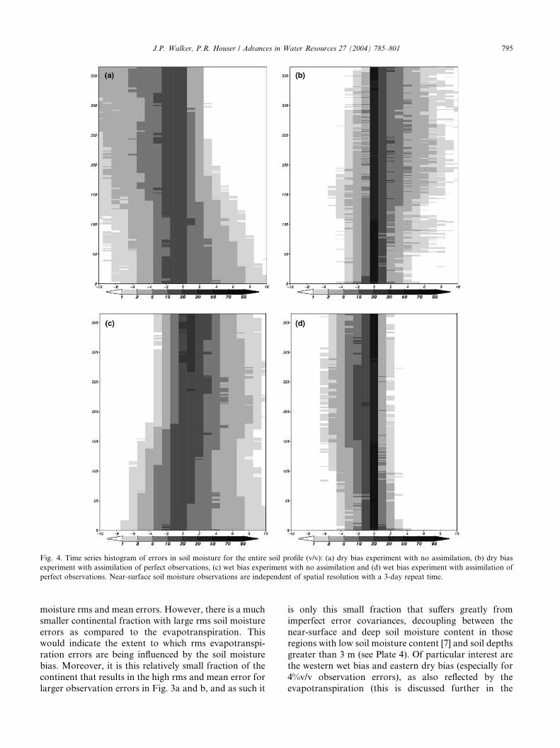
Fig. 4. Time series histogram of errors in soil moisture for the entire soil profile (v/v): (a) dry bias experiment with no assimilation, (b) dry bias

experiment with assimilation of perfect observations, (c) wet bias experiment with no assimilation and (d) wet bias experiment with assimilation of

perfect observations. Near-surface soil moisture observations are independent of spatial resolution with a 3-day repeat time.


moisture rms and mean errors. However, there is a much

smaller continental fraction with large rms soil moisture

errors as compared to the evapotranspiration. Thiswould indicate the extent to which rms evapotranspi-

ration errors are being influenced by the soil moisture

bias. Moreover, it is this relatively small fraction of the

continent that results in the high rms and mean error for

larger observation errors in Fig. 3a and b, and as such it

is only this small fraction that suffers greatly from

imperfect error covariances, decoupling between the

near-surface and deep soil moisture content in thoseregions with low soil moisture content [7] and soil depths

greater than 3 m (see Plate 4). Of particular interest are

the western wet bias and eastern dry bias (especially for

4%v/v observation errors), as also reflected by the

evapotranspiration (this is discussed further in the

0

1

2

3

4

5

6

-2 -1 0 t

Moi

stur

eR

MS

Err

or(%

v/v)

Precipitation Bias (mm/day)

-3

-2

-1

0

1

2

3

-2 -1 0 1

Moi

stur

eM

ean

Err

or(%

v/v)


-2

-1

0

1

2

-2 -1 0 1

Eva

potr

ansp

iratio

nE

rror

(mm

/day

)


(a) (b)

(c)

Fig. 5. Precipitation bias effect on: (a) surface (circle), root zone (square) and profile (triangle) soil moisture rms error; (b) surface (circle), root zone

(square) and profile (triangle) soil moisture mean error; and (c) evapotranspiration rms (square) and mean (circle) error. Simulations with assimi-

lation (solid symbols) are compared with the simulation without assimilation (open symbols). Near-surface soil moisture observations are free from

error with a 3-day repeat time.


following section on bias considerations). It is this wet

soil moisture forecast bias in a high evaporative demand

area that leads to such a large positive evapotranspira-

tion forecast bias.

The results from these simulations would suggest that

to have a positive impact, assimilated near-surface soilmoisture measurements should be no worse than 5%v/v

accurate, but preferably better than 3%v/v. A degraded

soil moisture simulation may result from assimilation of

less accurate soil moisture observations (i.e. observa-

tions from areas with dense vegetation or other external

influences), due to imperfect error covariance knowl-

edge.

3.5. Bias considerations

Fig. 2 shows that a wet soil moisture bias, caused by a

wet precipitation bias, results in a dry soil moisture bias

when near-surface soil moisture observations are

assimilated. Likewise, Plate 3 shows an eastern North

America dry bias and a western North America wet bias

when near-surface soil moisture observations are

assimilated, with this wet bias being more pronounced

as the near-surface soil moisture observation error in-

creases.

The soil moisture profile forecast bias when near-

surface soil moisture observations are assimilated resultsfrom violating a key Kalman filter assumption; that the

continuous time error process is a zero mean Gaussian

white noise stochastic process. Since the precipitation

field was wet biased, the near-surface soil moisture

forecast was always wet biased. The Kalman filter rec-

ognized (through the forecast covariance matrix) that

the near-surface soil moisture had a strong correlation

with the soil moisture profile, resulting in a soil moistureprofile dry bias when the profile was corrected to

counteract the near-surface wet bias (note that this

model does not use traditional model layers but rather

soil moisture storages from which soil moisture contents

for various depths can be diagnosed). As the observa-

tion error was increased, the weight given to observa-

tions relative to model forecasts was decreased,

0

1

2

3

4

5

0 5 10 15 20 25 30

Moi

stur

eR

MS

Err

or(%

v/v)

Temporal Resolution (days)

-2

-1

0

1

2

0 5 10 15 20 25 30

Moi

stur

eM

ean

Err

or(%

v/v)


0

0.2

0.4

0.6

0.8

1

0 5 10 15 20 25 30

Eva

potr

ansp

iratio

nE

rror

(mm

/day

)


(a) (b)

(c)

Fig. 6. Near-surface soil moisture observation repeat time effect on: (a) surface (circle), root zone (square) and profile (triangle) soil moisture rms

error; (b) surface (circle), root zone (square) and profile (triangle) soil moisture mean error; and (c) evapotranspiration rms (square) and mean (circle)

error. Simulations with assimilation (solid symbols) are compared with the simulation without assimilation (open symbols). Near-surface soil

moisture observations are free from error.


producing less impact on the profile soil moisture con-

tent.

While this explains the dry soil moisture bias, it does

not account for the wet bias. Plate 4b shows the spatial

precipitation bias distribution, which is concentrated in

the east, and hence explains why the dry soil moisture

bias is most significant in the east (though there is ageneral wet precipitation bias for the entire continent).

Moreover, Plate 4c alludes to the reason for the wet soil

moisture bias in the west; the regions that display a wet

bias in Plate 3 correspond with the regions that have the

driest soil moisture content in Plate 4c. The reader

should also note that this wet soil moisture bias only

persists for the simulations with non-perfect near-sur-

face soil moisture observations (see Plate 3). Thus, thereason for a wet soil moisture forecast bias is an effective

wet near-surface soil moisture observation bias. When a

perturbation makes the near-surface soil moisture

observation wetter than the wilting point, there is the

potential to make the total soil moisture wetter, but

when the perturbation makes the near-surface soil

moisture observation drier than the wilting point, the

assimilation is unable to decrease the total soil moisture

content below the wilting point due to model physical

constraints. As such, this is equivalent to truncating the

near-surface soil moisture observation to the wilting

point, resulting in a wet biased surface soil moistureobservation, which is more significant as the perturba-

tion size (or amount of error) increases. This demon-

strates that either model forcing or observation bias not

accounted for in the assimilation scheme may cause

adverse effects when near-surface soil moisture obser-

vations are assimilated.

To further demonstrate the forcing bias effect on soil

moisture and evapotranspiration forecasts when near-surface soil moisture observations are assimilated, two

additional simulations were made. The first assumed

there was no precipitation (Fig. 1b), while the second

assumed greater precipitation error, with a 100% stan-

dard deviation perturbation (Fig. 1c). Fig. 4 shows the

0

1

2

3

4

5

0 20 40 60 80 100 120

Moi

stur

eR

MS

Err

or(%

v/v)

Spatial Resolution (minutes of arc)

-2

-1

0

1

2

0 20 40 60 80 100 120

Moi

stur

eM

ean

Err

or(%

v/v)


0

0.2

0.4

0.6

0.8

1

0 20 40 60 80 100 120

Eva

potr

ansp

iratio

nE

rror

(mm

/day

)


-1

0

1

2

3

0 20 40 60 80 100 120

Soi

lMoi

stur

eE

rror

(%v/

v)


(a) (b)

(c) (d)

Fig. 7. Near-surface soil moisture observation spatial resolution effect on: (a) surface (circle), root zone (square) and profile (triangle) soil moisture

rms error; (b) surface (circle), root zone (square) and profile (triangle) soil moisture mean error; and (c) evapotranspiration rms (square) and mean

(circle) error. Simulations with assimilation (solid symbols) are compared with the simulation without assimilation (open symbols). Near-surface soil

moisture observations, with a 3-day repeat time, are free from error apart from that introduced from spatial resolution; (d) rms (square) and mean

(circle) error in observations.


profile soil moisture error time series histograms, with

and without assimilation, where the assimilation both

improves the soil moisture forecast and switches the

direction of the bias. However, the soil moisture forecast

bias for the simulation with no precipitation is worse

than the simulation with precipitation, with the biaspersisting for all months and not just during the summer.

The precipitation bias effect on soil moisture profile

simulation with and without the near-surface soil

moisture assimilation is shown in Fig. 5. Again, both the

spatially and temporally averaged rms error and mean

error in retrieved soil moisture and forecast evapo-

transpiration are compared with that from the open-

loop simulation. This figure shows that modeled soilmoisture and evapotranspiration rms errors are im-

proved despite precipitation bias when perfect observa-

tions are assimilated. However, the best results were

obtained when the precipitation bias was minimized.

The resulting near-surface soil moisture and evapo-

transpiration forecast bias with assimilation was largely

unaffected by the precipitation bias, but the root zone

and profile soil moisture forecasts were heavily im-

pacted. Moreover, these results would indicate that it is

better to use poor precipitation information than to

assume no precipitation occurred.

3.6. Repeat time requirement

To investigate the global near-surface soil moisture

measurement mission repeat time requirement, individ-

ual simulations were made where the observation data,

with various repeat times (1–30 days) and no error im-posed, were assimilated into the open-loop simulation

described above. The effect of repeat time on both soil

moisture profile and evapotranspiration forecasts is

shown in Fig. 6, where the spatially and temporally

averaged rms and mean error from forecasts with near-

surface soil moisture assimilation are compared with


those without assimilation. This figure shows that the

rms and mean soil moisture error is significantly im-

proved when near-surface soil moisture observations are

assimilated into the land surface model for all repeat

times up to 30 days. However, a daily repeat time hasthe lowest rms soil moisture error, especially in the near-

surface layer. This is to be expected, as this layer has the

greatest interaction with the atmosphere; precipitation is

the most dominant factor for near-surface soil moisture

variations. We also note that decreasing the repeat time

from one to two days has a significant near-surface soil

moisture rms forecast error impact, with less impact for

greater repeat times. However, the root zone and soilprofile moisture contents are not similarly affected, as

they have a much slower response to atmospheric forc-

ing. Other reasons for the apparent lack of sensitivity to

repeat time are: (i) the particular model used in this

study has a very strong correlation between surface soil

moisture and profile soil moisture content (i.e. catch-

ment deficit), meaning that profile soil moisture retrieval

occurs very quickly, as described by Walker and Houser[32]; and (ii) the analysis presented here is for the aver-

age across a continent and a year, meaning that the

small time and space scale variations may be smoothed

out. If the study were to be repeated for a different land

surface model and/or a different analysis, then the re-

sults may well be different.

Fig. 6 also shows a significant mean evapotranspira-

tion error decrease when near-surface soil moistureobservations are assimilated, with little rms error im-

pact. The mean error shows repeat time dependence

similar to that for the near-surface soil moisture rms

error.

This study suggests that the global near-surface soil

moisture repeat time requirement for use in constraining

land surface model states by assimilation is less than 5

days, with at least daily repeat time as the preferredinterval. However, greater than 5 day repeat times (up to

30 days) have shown very little forecast degradation

beyond those from a 5 day repeat time. Moreover, apart

from near-surface soil moisture and evapotranspiration

forecasts, repeat time has very little forecast perfor-

mance impact.

3.7. Spatial resolution requirement

To investigate the global near-surface soil moisture

spatial resolution requirement, individual simulations

were made where the 3 day repeat time (no error im-

posed) soil moisture observations with various spatialresolutions (0.5–120 arc-min) were assimilated into the

open-loop simulation. Fig. 7 shows the spatial resolu-

tion effect on both the soil moisture profile and evapo-

transpiration forecasts, where the spatially and

temporally averaged rms and mean error from forecasts

with near-surface soil moisture assimilation are com-

pared with those without assimilation. This figure also

shows the near-surface soil moisture observation error

introduced due to interpolation from coarser resolution

data. Here it can be seen that near-surface soil moisture

observation rms error rose quickly from zero at thefinest resolution to approximately 1.5%v/v at 30 arc-min

(the average land surface model spatial resolution), and

then increased only marginally for coarser resolutions

(1.7%v/v).

These results suggest that the assimilated observation

spatial resolution should be less than the land surface

model resolution (the average catchment size in our

application). This is because the interpolation ofobservations from a grid to an irregularly shaped

catchment becomes more accurate as the spatial reso-

lution of the observation data is decreased beyond the

size of the catchment. As the observation spatial reso-

lution becomes finer it more accurately maps the outline

of the catchment, giving a more accurate average for the

catchment. We suggest that while the highest spatial

resolution data is desirable, a resolution of half themodel resolution would be an appropriate trade-off be-

tween technical constraints and model requirements.

Fig. 7 shows consistent trends between the soil

moisture forecast rms and mean error with assimilation,

and the near-surface soil moisture observation rms

error. This suggests that the near-surface soil moisture

observation ability to accurately represent the near-

surface soil moisture content at the appropriate scale isan important spatial resolution requirement consider-

ation. As such, the accuracy requirement discussion

would also apply here. This is most apparent when Fig.

7 is compared with Fig. 3c. Since the observation data

error due to spatial resolution degradation was smaller

than for accuracy degradation, the soil moisture errors

decrease with the assimilation of observations from any

spatial resolution. A comparison with Fig. 6 suggeststhat spatial (and hence accuracy) requirements are more

important than repeat time requirements.

The results from this spatial resolution study do not

take into account the additional information, such as

stressed, unstressed and saturated soil moisture catch-

ment fractions, which might be obtained from higher

spatial resolution observations. This additional infor-

mation may further constrain the assimilation by takingadvantage of the unique catchment-based land surface

model physics. Moreover, these results are applicable to

a land surface model with approximately 30 arc-min

spatial resolution; finer resolution land surface models

may show stronger spatial resolution dependence.

These results suggest that the global near-surface soil

moisture spatial resolution requirement is application

specific; the flood forecasting and precision agriculturerequirements will likely have different requirements than

climate modeling and policy planning, as they operate at

different spatial resolutions. We found that near-surface


soil moisture measurements with a spatial resolution of

approximately half the land surface model resolution

were appropriate. However, this finding is dependent on

the near-surface soil moisture measurement at a given

resolution being an accurate near-surface soil moisturerepresentation at the application resolution. Hence, 30

arc-min (50 km) near-surface soil moisture observations

would be appropriate for climate modeling and policy

planning applications.

4. Conclusions

This study has shown that the near-surface soil

moisture observation error must be less than the re-

quired soil moisture forecast error, or slight model

forecast degradation may result when used as data

assimilation input. Typically, near-surface soil moistureobservations must have an accuracy better than 5%v/v,

but preferably better than 3%v/v. This study has also

shown that assumptions in the assimilation framework

lead to degraded forecasts when biased forcing and

observations are used.

It was also found that for the temporal resolutions

tested, daily near-surface soil moisture observations

were required (further slight improvement would beexpected from more frequent observations) to achieve

the best soil moisture and evapotranspiration forecasts

using a land surface model with 30 arc-min spatial res-

olution, particularly for near-surface (2 cm) soil mois-

ture content and evapotranspiration. Longer repeat

times between observations had only a minor root zone

and total profile soil moisture forecast impact. The

greatest repeat time impact was from 1 to 5 days, withlonger times between observations having only a mar-

ginal degradation. These results conflict with Hoeben

and Troch [15], who suggests that a repeat time greater

than a day would be of little to no use in data assimi-

lation. However, it must be noted that these two studies

were undertaken for vastly different spatial scales.

Near-surface soil moisture observations with a spatial

resolution finer than the model resolution were found toproduce the best forecasts of soil moisture content and

evapotranspiration. Observations with a spatial resolu-

tion coarser than the model resolution produced only

slightly poorer results than observations at the model

resolution. However, assimilating near-surface soil

moisture observations at half the land surface model

spatial resolution was a good compromise between

model demands and technical constraints on makingvery high resolution measurements. Moreover, the re-

sults have shown that spatial resolution and accuracy

are more important than observation repeat time.

While the above guidelines are a useful first step to-

wards identifying some defensible targets for a global

satellite soil moisture mission, it is not until a number of

similar studies from a range of research groups are

undertaken that firm recommendations can be made.

Specifically, these studies should consider a range of

model structures, spatial resolutions (from hillslope to

global), and objectives (from climate modelling andweather prediction to flood forecasting), and should

make use of both synthetic and real data (such as that

from the SGP and SMEX experiments).

Acknowledgements

This work was supported by funding from the NASASeasonal-to-Interannual Prediction Project (NSIPP)

NRA 98-OES-07. Projection of the HYDRO1K com-

pound topographic index to a geographical coordinate

system by Matthew Rodell is acknowledged and useful

discussions with Dara Entekhabi, Randal Koster and

Rolf Reichle are appreciated.

References

[1] Beven KJ, Kirkby MJ. A physically based, variable contributing

area model of basin hydrology. Hydrologic Sci––Bull 1979;24(1):

43–69.

[2] Betts AK, Ball JH, Viterbo P. Basin-scale surface water and

energy budgets for the Mississippi from the ECMWF reanalysis. J

Geophys Res 1999;104:19293–306.

[3] Boone A, Habets F, Noilhan J, Clark D, Dirmeyer P, Fox S,

Gusev Y, Haddeland I, Koster R, Lohmann D, Mahanama S,

Mitchell K, Nasonova O, Niu GY, Pitman A, Polcher J, Shmakin

AB, Tanaka K, van den Hurk B, Verant S, Verseghy D, Viterbo P,

Yang ZL. The Rhone-aggregation land surface scheme intercom-

parison project: an overview. J Climate 2003;17(1):187–208.

[4] Bowling LC, Lettenmaier DP, Nijssen B, Graham LP, Clark DB,

El Maayar M, Essery R, Goers S, Gusev YM, Habets F, van den

Hurk B, Jin JM, Kahan D, Lohmann D, Ma XY, Mahanama S,

Mocko D, Nasonova O, Niu GY, Samuelsson P, Shmakin AB,

Takata K, Verseghy D, Viterbo P, Xia YL, Xue YK, Yang ZL.

Simulation of high latitude hydrological processes in the Torne-

Kalix basin: PILPS Phase 2(e) 1: Experiment description and

summary intercomparisons. J Global Planetary Change 2003;

38(1–2):1–30.

[5] Bras RL, Rodriguez-Iturbe I. Random functions and hydrology.

Reading, MA: Addison Wesley; 1985. p. 559.

[6] Calvet JC, Noilhan J. From near-surface to root-zone soil

moisture using year-round data. J Hydrometeorol 2000;1(5):

393–411.

[7] Capehart WJ, Carlson TN. Estimating near-surface soil moisture

availability using a meteorologically driven soil-water profile

model. J Hydrol 1994;160:1–20.

[8] Dobson MC, Ulaby FT. Active microwave soil moisture research.

IEEE Trans Geosci Remote Sensing 1986;GE-24(1):23–36.

[9] Ducharne A, Koster RD, Suarez MJ, Stieglitz M, Kumar P. A

catchment-based approach to modeling land surface processes in a

GCM. Part 2: Parameter estimation and model demonstration. J

Geophys Res 2000;105(D20):24823–38.

[10] Engman ET. Soil moisture needs in earth sciences. In: Proceedings

of International Geoscience and Remoe Sensing Symposium

(IGARSS). 1992. p. 477–9.

[11] Engman ET, Chauhan N. Status of microwave soil moisture

measurements with remote sensing. Remote Sensing Environ

1995;51(1):189–98.


[12] Entekhabi D, Nakamura H, Njoku EG. Solving the inverse

problem for soil moisture and temperature profiles by sequential

assimilation of multifrequency remotely sensed observations.

IEEE Trans Geosci Remote Sensing 1994;32(2):438–48.

[13] Fennessey MJ, Shukla J. Impact of initial soil wetness on seasonal

atmospheric prediction. J Climate 1999;12:3167–80.

[14] Gallus Jr WA, Segal M. Sensitivity of forecasted rainfall in a

Texas convective system to soil moisture and convective param-

eterization. Weather Forecast 2000;15:509–25.

[15] Hoeben R, Troch PA. Assimilation of active microwave obser-

vation data for soil moisture profile estimation. Water Resour Res

2000;36(10):2805–19.

[16] Henderson-Sellers A, Pitman AJ, Love PK, Irannejad P, Chen T.

The project for intercomparison of land-surface parameterisation

schemes (PILPS) phases 2 and 3. Bull Am Meteorol Soc

1995;76:489–503.

[17] Houser PR, Shuttleworth WJ, Famiglietti JS, Gupta HV, Syed

KH, Goodrich DC. Integration of soil moisture remote sensing

and hydrologic modeling using data assimilation. Water Resour

Res 1998;34(12):3405–20.

[18] Jackson TJ, Schmugge TJ. Vegetation effects on the microwave

emission of soils. Remote Sensing Environ 1991;36:203–12.

[19] Jackson TJ, Bras R, England A, Engman ET, Entekhabi D,

Famiglietti J, et al. Soil moisture mission (EX-4) report, NASA

land surface hydrology program post-2002 land surface hydrology

planning workshop. Irvine, CA: April 12–14, 1999.

[20] Koster RD, Suarez MJ, Ducharne A, Stieglitz M, Kumar P. A

catchment-based approach to modeling land surface processes in a

GCM. Part 1: Model structure. J Geophys Res 2000;105(D20):

24809–22.

[21] Leese J, Jackson T, Pitman A, Dirmeyer P. Meeting summary:

GEWEX/BAHC international workshop on soil moisture mon-

itoring, analysis, and prediction for hydrometeorological and

hydroclimatological applications. Bulletin of the American Mete-

orological Society. 2001. p. 1423–30.

[22] Milly PCD. Integrated remote sensing modeling of soil moisture:

sampling frequency, response time and accuracy of estimates. In:

Integrated design of hydrological networks (Proceedings of the

Budapest Symposium), IAHS Publication No. 158. 1986. p. 201-

11.

[23] Moore ID, Grayson RB, Ladson AR. Digital terrain modelling: a

review of hydrological geomorphological and biological applica-

tions. Hydrol Process 1991:3–30.

[24] Njoku EG, Entekhabi D. Passive microwave remote sensing of

soil moisture. J Hydrol 1996;184:101–29.

[25] Owe M, de Jeu R, Walker JP. A methodology for surface soil

moisture and vegetation optical depth retrieval using the micro-

wave polarization difference index. IEEE Trans Geosci Remote

Sensing 2001;39(8):1643–54.

[26] Reichle RH, McLaughlin DB, Entekhabi D. Variational data

assimilation of microwave radiobrightness observations for land

surface hydrologic applications. IEEE Trans Geosci Remote

Sensing 2001;39(8):1708–18.

[27] Reichle RH, McLaughlin DB, Entekhabi D. Hydrologic data

assimilation with the ensemble Kalman filter. Monthly Weather

Rev 2002;130(1):103–14.

[28] Reichle RH, Walker JP, Koster RD, Houser PR. Extended vs.

ensemble Kalman filtering for land data assimilation. J Hydro-

meteorol 2002;3(6):728–40.

[29] Sellers P, Meeson BW, Closs J, Collatz J, Corprew F, Dazlich D,

et al. The ISLSCP initiative i global data sets: surface boundary

conditions and atmospheric forcings for land-atmosphere studies.

Bull Am Meteorol Soc 1996;77:1987–2005.

[30] Ulaby FT, Batliva PP. Optimum radar parameters for mapping

soil moisture. IEEE Trans Geosci Electron 1976;GE-14(2):81–93.

[31] Ulaby FT, Batliva PP, Dobson MC. Microwave backscatter

dependence on surface roughness, soil moisture and soil texture.

Part 1–– Bare soil. IEEE Trans Geosci Electron 1978;GE-

16(4):286–95.

[32] Walker JP, Houser PR. A methodology for initialising soil

moisture in a global climate model: Assimilation of near-surface

soil moisture observations. J Geophys Res––Atmospheres

2001;106(D11):11761–74.

[33] Walker JP, Willgoose GR, Kalma JD. One-dimensional soil

moisture profile retrieval by assimilation of near-surface observa-

tions: a comparison of retrieval algorithms. Adv Water Resour

2001;24(6):631–50.

[34] Walker JP, Willgoose GR, Kalma JD. One-dimensional soil

moisture profile retrieval by assimilation of near-surface mea-

surements: a simplified soil moisture model and field application. J

Hydrometeorol 2001;2(4):356–73.

[35] Walker JP, Willgoose GR, Kalma JD. Three-dimensional soil

moisture profile retrieval by assimilation of near-surface mea-

surements: simplified Kalman filter covariance forecasting and

field application. Water Resour Res 2002;38(12):1301,

doi:10.11029/2002/WRR001545.

Requirements of a global near-surface soil moisture satellite mission: accuracy, repeat time, and...

Documents

Transcript of Requirements of a global near-surface soil moisture satellite mission: accuracy, repeat time, and...