
republic of kenya learning guide for common units for plant ...
792
REPUBLIC OF KENYA LEARNING GUIDE FOR COMMON UNITS FOR PLANT AND SERVICES ENGINEERING SECTOR LEVEL 6 TVET CDACC P.O BOX 15745-00100 NAIROBI
-
Upload
khangminh22 -
Category
Documents
-
view
1 -
download
0
Transcript of republic of kenya learning guide for common units for plant ...
REPUBLIC OF KENYA
LEARNING GUIDE
FOR
COMMON UNITS
FOR
PLANT AND SERVICES ENGINEERING SECTOR
LEVEL 6
TVET CDACC
P.O BOX 15745-00100
NAIROBI

i
First published 2019
Copyright TVET CDACC
All rights reserved. No part of this plant and service engineering learning guide may
be reproduced, distributed, or transmitted in any form or by any means, including
photocopying, recording, or other electronic or mechanical methods without the
prior written permission of the TVET CDACC, except in the case of brief quotations
embodied in critical reviews and certain other non-commercial uses permitted by
copyright law. For permission requests, write to the Council Secretary/CEO, at the
address below:
Council Secretary/CEO
TVET Curriculum Development, Assessment and Certification Council
P.O. Box, 15745–00100,
Nairobi, Kenya.
Email: [email protected]
ii
FOREWORD
The provision of quality education and training is fundamental to the Government’s
overall strategy for social-economic development. Quality education and training will
contribute to achievement of Kenya’s development blueprint and sustainable
development goals (SDGs). This can only be addressed if the current skill gap in the
world of work is critically taken into consideration.
Reforms in the education sector are necessary for the achievement of Kenya Vision
2030 and meeting the provisions of the Constitution of Kenya 2010. The education
sector has to be aligned to the Constitution and this has triggered the formulation of the
Policy Framework for Reforming Education and Training (Sessional Paper No. 4 of
2016). A key provision of this policy is the radical change in the design and delivery of
the TVET training which is the key to unlocking the country’s potential in
industrialization. This policy document requires that training in TVET be Competency-
Based, Curriculum development be industry led, Certification be based on
demonstration and mastery of competence and mode of delivery that allows for multiple
entries and exit in TVET programs.
These reforms demand that industry takes a leading role in TVET curriculum
development to ensure that the curriculum addresses and responds to its competence
needs. The learning guide in plant and service engineering common units enhances a
harmonized delivery of the common units for plant and service engineering and
construction plant engineering Level 6. It is my conviction that this learning guide will
play a critical role towards supporting the development of competent human resource
for the plant and service engineering sector’s growth and sustainable development.
PRINCIPAL SECRETARY, VOCATIONAL AND TECHNICAL TRAINING
MINISTRY OF EDUCATION
iii
PREFACE
Kenya Vision 2030 is anticipated to transform the country into a newly industrializing;
“middle-income country providing a high-quality life to all its citizens by the year
2030”. The Sustainable Development Goals (SDGs) further affirm that the
manufacturing sector is an important driver to economic development. The SDGs
number 9, which focuses on Building resilient infrastructures, promoting sustainable
industrialization and innovation can only be attained if the curriculum focuses on skill
acquisition and mastery. Kenya intends to create a globally competitive and adaptive
human resource base to meet the requirements of a rapidly industrializing economy
through life-long education and training.
TVET has a responsibility of facilitating the process of inculcating knowledge, skills
and attitudes necessary for catapulting the nation to a globally competitive country,
hence the paradigm shift to embrace Competency Based Education and Training
(CBET). The Technical and Vocational Education and Training Act No. 29 of 2013 and
the Sessional Paper No. 4 of 2016 on Reforming Education and Training in Kenya,
emphasized the need to reform curriculum development, assessment and certification
to respond to the unique needs of the industry. This called for shift to CBET to address
the mismatch between skills acquired through training and skills needed by the industry
as well as to increase the global competitiveness of Kenyan labor force.
The TVET Curriculum Development, Assessment and Certification Council (TVET
CDACC), in conjunction with industry/sector developed the occupational standards for
the common units which was the basis of developing competency-based curriculum and
assessment of an individual for competence certification for plant service engineering
and construction plant engineering levels 6. The learning guide is geared towards
promoting efficiency in delivery of the common units.
The learning guide is designed and organized with clear and interactive learning
activities for each learning outcome of a unit of competency. The guide further provides
information sheet, self-assessment tools, equipment, supplies, materials and references.
I am grateful to the Council Members, Council Secretariat, plant service engineering
experts and all those who participated in the development of this learning guide.
Prof. CHARLES M. M. ONDIEKI, PhD, FIET (K), Con. Eng Tech.
CHAIRMAN, TVET CDACC
iv
ACKNOWLEDGEMENT
This learning guide has been designed to support and enhance uniformity,
standardization and coherence in implementing TVET Competency Based Education
and training in Kenya. In developing the learning guide, significant involvement and
support was received from various organizations.
I recognize with appreciation the critical role of the participants drawn from technical
training institutes, universities, private sector and consultants in ensuring that this
learning guide is in-line with the competencies required by the industry as stipulated in
the occupational standards and curriculum. I also thank all stakeholders in the plant and
service engineering sector for their valuable input and all those who participated in the
process of developing this learning guide.
I am convinced that this learning guide will go a long way in ensuring that workers in
plant and service engineering sectors acquire competencies that will enable them to
perform their work more efficiently and make them enjoy competitive advantage in the
world of work.
DR. LAWRENCE GUANTAI M’ITONGA, PhD
COUNCIL SECRETARY/CEO
TVET CDACC
v
TABLE OF CONTENTS
FOREWORD ............................................................................................................. II
PREFACE ................................................................................................................ III
ACKNOWLEDGEMENT .......................................................................................IV
TABLE OF CONTENTS .......................................................................................... V
LIST OF FIGURES ................................................................................................... X
LIST OF TABLES ............................................................................................... XVII
ACRONYMS ......................................................................................................XVIII
CHAPTER 1: INTRODUCTION ........................................................................... 19
1.1. Background Information .................................................................................. 19
1.2. The Purpose of Developing the Learning Guide ............................................. 19
1.3. Layout of the Trainee Guide ............................................................................ 19
Learning Activities ..................................................................................................... 20
Information Sheet ....................................................................................................... 20
Self-Assessment ......................................................................................................... 20
Common Units of Learning ........................................................................................ 21
CHAPTER 2: ENGINEERING MATHEMATICS/ APPLY ENGINEERING
MATHEMATICS .......................................................................................... 22
2.1 Introduction .......................................................................................................... 22
2.2 Performance Standard .......................................................................................... 22
2.3 Learning Outcomes .............................................................................................. 22
2.3.1 List of learning outcomes .................................................................................. 22
2.3.2 Learning Outcome No1: Apply Algebra ........................................................... 23
2.3.3 Learning Outcome No 2: Apply trigonometry and hyperbolic functions ......... 29
2.3.4 Learning Outcome No 3: Apply complex numbers .......................................... 33
2.3.5 Learning Outcome No 4: Apply coordinate geometry ...................................... 38
2.3.6 Learning Outcome No 5: Carry out binomial expansion .................................. 41
2.3.7 Learning Outcome No 6: Apply calculus .......................................................... 44
2.3.8 Learning Outcome No7: Solve ordinary differential equations ........................ 50
2.3.9 Learning Outcome No 8: Carry out mensuration .............................................. 54
2.3.10 Learning Outcome No 9: Apply power series ................................................. 65
2.3.11 Learning Outcome No10: Apply statistics ...................................................... 68
2.3.12 Learning Outcome No 11: Apply numerical methods .................................... 73
2.3.13 Learning Outcome No12: Apply vector theory ............................................... 76
2.3.14 Learning Outcome No13: Apply matrix ......................................................... 82
vi
CHAPTER 3: WORKSHOP TECHNOLOGY PRACTICES/APPLY
WORKSHOP TECHNOLOGY PRINCIPLES .......................................... 87
3.1 Introduction .......................................................................................................... 87
3.2 Performance Standard .......................................................................................... 87
3.3 Learning Outcomes .............................................................................................. 88
3.3.1 List of Learning Outcomes ................................................................................ 88
3.3.2 Learning Outcome No 1: Use technical drawing to plan work operations ....... 89
3.3.3 Learning Outcome No 2: Choose appropriate tools and materials ................... 96
3.3.4 Learning Outcome No 3: Measure and mark out dimensions on work pieces 109
3.3.5 Learning Outcome No 4: Use hand tools to cut and file parts ........................ 123
3.3.6 Learning Outcome No 5: Use drills to make holes ......................................... 135
3.3.7 Learning Outcome No 6: Thread using taps and dies ..................................... 144
3.3.8 Learning Outcome No 7: Produce components using a lathe machine ........... 152
3.3.9 Learning Outcome No 8: Assemble metal parts and sub-assemblies ............. 162
3.3.10 Learning Outcome No 9: Polish finished work ............................................. 174
3.3.11 Learning Outcome No. 10: Perform housekeeping ....................................... 182
3.3.12 Learning Outcome No 11: Inspect finished work for accuracy and quality . 189
3.3.13 Learning Outcome No 12: Maintenance of tools and equipment ................. 197
CHAPTER 4: PRINCIPLES OF MECHANICAL SCIENCE/APPLY
MECHANICAL SCIENCE PRINCIPLES ............................................... 204
4.1 Introduction ........................................................................................................ 204
4.2 Performance Standard ........................................................................................ 204
4.3 Learning Outcomes ............................................................................................ 204
4.3.1 List of learning outcomes ................................................................................ 204
4.3.2 Learning Outcome No 1: Determine forces in a system ................................. 206
4.3.3 Learning Outcome No 2: Demonstrate knowledge of moments ..................... 218
4.3.4 Learning Outcome No 3: Understand friction principles .............................. 227
4.3.5 Learning Outcome No 4: Understand motions in engineering ........................ 236
4.3.6 Learning Outcome No 5: Describe work, energy and power .......................... 246
4.3.7 Learning Outcome No 6: Perform machine calculation .................................. 259
4.3.8 Learning Outcome No7: Demonstrate gas principles ..................................... 270
4.3.9 Learning Outcome No 8: Apply heat knowledge ............................................ 278
4.3.10 Learning Outcome No 9: Apply density knowledge ..................................... 288
4.3.11 Learning Outcome No 10: Apply pressure principles ................................... 297
CHAPTER 5: FLUID MECHANICS/ APPLY FLUID MECHANICS
PRINCIPLES ............................................................................................... 305
vii
5.1 Introduction ........................................................................................................ 305
5.2 Performance Standard ........................................................................................ 305
5.3 Learning Outcomes ............................................................................................ 305
5.3.1 List of Learning Outcomes .............................................................................. 305
5.3.2 Learning Outcome No1: Understand flow of fluids ........................................ 306
5.3.3 Learning Outcome No 2: Demonstrate knowledge in viscous flow ............... 328
5.3.4 Learning Outcome No3: Perform dimensional analysis ................................. 337
5.3.5 Learning Outcome No 4: Operate fluid pumps ............................................... 345
CHAPTER 6: THERMODYNAMICS / APPLY FLUID MECHANICS
PRINCIPLES ............................................................................................... 355
6.1 Introduction ........................................................................................................ 355
6.2 Performance Standard ........................................................................................ 355
6.3 Learning Outcomes. ........................................................................................... 355
6.3.1 List of Learning Outcomes .............................................................................. 355
6.3.2 Learning Outcome No 1: Understand fundamentals of thermodynamics ....... 357
6.3.3 Learning Outcome No. 2: Perform steady flow processes .............................. 371
6.3.4 Learning Outcome No. 3: perform non steady flow processes ....................... 385
6.3.5 Learning Outcome No.4: Understand perfect gases ........................................ 392
6.3.6 Learning Outcome No 5: Generate steam ....................................................... 404
6.3.7 Learning Outcome No.6: Perform thermodynamics reversibility and
entropy ........................................................................................................... 411
6.3.8 Learning Outcome No. 7: Understand ideal gas cycle .................................... 427
6.3.9 Learning Outcome No 8: Demonstrate Fuel and Combustion....................... 437
6.3.10 Learning Outcome No9: Perform heat transfer ............................................. 447
6.3.11 Learning Outcome No10: Understand heat exchangers ................................ 469
6.3.12 Learning Outcome No 11: understand air compressors ................................ 485
6.3.13 Learning Outcome No 12: Understand gas turbine ....................................... 502
6.3.14 Learning Outcome No 13: Understand impulse steam turbines .................... 519
CHAPTER 7: MATERIAL SCIENCE AND METALLURGICAL PROCESSES/
APPLY MATERIAL SCIENCE AND PERFORM METALLURGICAL
PROCESSES ................................................................................................ 530
7.1 Introduction ........................................................................................................ 530
7.2 Performance Standard ........................................................................................ 530
7.3 Learning Outcomes ............................................................................................ 530
7.3.1 List of Learning Outcomes .............................................................................. 530
7.3.2 Learning Outcome No 1: Analyze properties of engineering materials .......... 532
viii
7.3.3 Learning Outcome No. 2: Perform ore extraction processes .......................... 540
7.3.4 Learning Outcome No 3: Produce iron materials ............................................ 548
7.3.5 Learning Outcome No 4: Produce alloy materials .......................................... 555
7.3.6 Learning Outcome No 5: Produce non-ferrous materials ............................... 562
7.3.7 Learning Outcome No 6: Produce ceramics materials .................................... 572
7.3.8 Learning Outcome No 7: Produce composite materials .................................. 579
7.3.9 Learning Outcome No 8: Utilize other engineering materials ........................ 586
7.3.10 Learning Outcome No 9: Perform heat treatment ......................................... 594
7.3.11 Learning Outcome No 10: Perform material testing ..................................... 601
7.3.12 Learning Outcome No 11: Prevent material corrosion ................................. 613
CHAPTER 8: ELECTRICAL PRINCIPLES/ APPLY ELECTRICAL SCIENCE
PRINCIPLES ............................................................................................... 617
8.1 Introduction ........................................................................................................ 617
8.2 Performance Standard ........................................................................................ 618
8.3 Learning Outcomes ............................................................................................ 618
8.3.1 List of Learning Outcomes .............................................................................. 618
8.3.2 Learning Outcome No 1: Use the concept of basic Electrical quantities ........ 620
8.3.3 Learning Outcome No 2: Use the concepts of D.C and A.C circuits in electrical
installation ...................................................................................................... 629
8.3.4 Learning Outcome No 3: Use of basic electrical machine .............................. 639
8.3.5 Learning Outcome No 4: Use of power factor in electrical installation ......... 655
8.3.6 Learning Outcome No 5: Use of earthling in Electrical installations ............. 663
8.3.7 Learning Outcome No 6: Apply lightning protection measures ..................... 677
8.3.8 Learning Outcome No 7: Apply Electromagnetic field theory ....................... 684
8.3.9 Learning Outcome No 8: Apply Electrodynamics .......................................... 691
8.3.10 Learning Outcome No 9: Apply Energy and momentum in Electromagnetic
field ................................................................................................................ 698
8.3.11 Learning Outcome No10: Apply Transient in Electrical circuit analysis ..... 707
8.3.12 Learning Outcome No 11: Use two port networks ........................................ 713
CHAPTER 9: TECHNICAL DRAWING/PREPARE AND INTERPRET
TECHNICAL DRAWINGS ........................................................................ 720
9.1 Introduction ........................................................................................................ 720
9.2 Performance Standard ........................................................................................ 720
9.3 Learning Outcomes ............................................................................................ 720
9.3.1 List of learning outcomes ................................................................................ 720
9.3.2 Learning Outcome No 1: Use and maintain drawing equipment and
materials ......................................................................................................... 722

ix
9.3.3 Learning Outcome No 2: Produce plain geometry drawings .......................... 736
9.3.4 Learning outcome No.3: Produce solid geometry ........................................... 746
9.3.5 Learning Outcome No 4: Produce pictorial and orthographic drawings of
components .................................................................................................... 753
9.3.6 Learning Outcome No 5: Produce mechanical drawings ................................ 764
9.3.7 Learning Outcome No 6: Apply CAD packages in drawings ......................... 775
x
LIST OF FIGURES
Figure 1: Sketched Argand diagram. ........................................................................... 35
Figure 2: A density Plot of Y ....................................................................................... 70
Figure 3. Vectors .......................................................................................................... 77
Figure 4. Types of lines used in Engineering Drawing ............................................... 91
Figure 5: Tool mount ................................................................................................... 92
Figure 6. Metals ........................................................................................................... 97
Figure 7. Scriber......................................................................................................... 101
Figure 8. Dot punch ................................................................................................... 101
Figure 9. Centre punch ............................................................................................... 101
Figure 10. Hermaphrodite caliper .............................................................................. 101
Figure 11. Dividers .................................................................................................... 102
Figure 12. Try square ................................................................................................. 102
Figure 13. Steel rule ................................................................................................... 102
Figure 14. Scribing block ........................................................................................... 102
Figure 15. V-blocks ................................................................................................... 102
Figure 16. File ............................................................................................................ 103
Figure 17. Hacksaw ................................................................................................... 103
Figure 18: Proper tools storage. ................................................................................. 104
Figure 19. Steel rule ................................................................................................... 111
Figure 20. Vernier caliper .......................................................................................... 111
Figure 21: Vernier Caliper ......................................................................................... 112
Figure 22. Micrometer ............................................................................................... 112
Figure 23: Reading Micrometer ................................................................................. 112
Figure 24. Depth gauge. ............................................................................................. 113
Figure 25: Vernier height gauge. ............................................................................... 113
Figure 26. Combination set ........................................................................................ 114
Figure 27. Micrometer calibration set ........................................................................ 116
Figure 28. Marking .................................................................................................... 117
Figure 29: Preaparation of Workpiece surface .......................................................... 118
Figure 30. Datum lines ............................................................................................... 119
Figure 31. File ............................................................................................................ 124
Figure 32: Hacksaw. .................................................................................................. 124
Figure 33. Chisels ...................................................................................................... 125
Figure 34. Combination cutting pliers ....................................................................... 125
Figure 35: Parts of a twist drill ................................................................................. 125
Figure 36: Types of cut files ...................................................................................... 127
Figure 37: Common shapes of Files .......................................................................... 128
Figure 38. Cross filing ............................................................................................... 129
Figure 39. Draw filing................................................................................................ 129
Figure 40: Clearance fit ............................................................................................. 130
Figure 41: Transition Fit ............................................................................................ 130
Figure 42: Interference Fit ......................................................................................... 131
Figure 43. Sensitive drilling machine ........................................................................ 136
Figure 44: Drilling Operation .................................................................................... 137
Figure 45: Reaming.................................................................................................... 137
xi
Figure 46: Boring ....................................................................................................... 137
Figure 47: Counter boring .......................................................................................... 138
Figure 48:( a), (b) Countersinking. ............................................................................ 138
Figure 49: Spoil facing............................................................................................... 138
Figure 50: Trapping ................................................................................................... 139
Figure 51: Holes inspected to specification. .............................................................. 140
Figure 52: Adjustment split die ................................................................................. 145
Figure 53: Diestock .................................................................................................... 145
Figure 54: Thread Nomenclature. .............................................................................. 145
Figure 55. Tie and Die ............................................................................................... 148
Figure 56: Lathe machine .......................................................................................... 152
Figure 57: Parts of a lathe machine............................................................................ 153
Figure 58: Centering operation. ................................................................................. 154
Figure 59: Facing operation. ...................................................................................... 155
Figure 60: Straight turning Operation. ....................................................................... 155
Figure 61: Straight turning. ........................................................................................ 156
Figure 62: Shoulder Turning ...................................................................................... 156
Figure 63: Rough and Finish Turning ........................................................................ 157
Figure 64: Tape turning ............................................................................................. 157
Figure 65: Bolt and Nuts. ........................................................................................... 163
Figure 66: Bolt and Nut. ............................................................................................ 163
Figure 67. Application of nuts and bolts .................................................................... 164
Figure 68: Studs ......................................................................................................... 164
Figure 69. Application of studs .................................................................................. 164
Figure 70: Tubular rivets ........................................................................................... 165
Figure 71 : Round head rivets .................................................................................... 165
Figure 72: Expanded rivets ........................................................................................ 165
Figure 73: Blind rivets ............................................................................................... 166
Figure 74: Specification of blind rivet. ...................................................................... 166
Figure 75: Butt Weld and Fillet weld. ....................................................................... 167
Figure 76: Joint preparation for welding ................................................................... 167
Figure 77: Welding positions ..................................................................................... 168
Figure 78. Basic principle of arc welding .................................................................. 168
Figure 79. Buffing compounds. ................................................................................. 175
Figure 80: Cutter grinding machine. .......................................................................... 199
Figure 81. Lathe tool .................................................................................................. 200
Figure 82: Tools ......................................................................................................... 201
Figure 83: Forces ....................................................................................................... 207
Figure 84. Parallelogram law of forces ...................................................................... 208
Figure 85. Triangle law of forces ............................................................................... 209
Figure 86. Polygon law of forces ............................................................................... 210
Figure 87. General coplanar force system ................................................................. 211
Figure 88. Concurrent coplanar force system ............................................................ 211
Figure 89: Space diagram .......................................................................................... 213
Figure 90: Force diagram ........................................................................................... 213
Figure 91. A beam resting on a fulcrum .................................................................... 219
xii
Figure 92: Calculation of moments............................................................................ 220
Figure 93: Applied force is a measure of static force ................................................ 228
Figure 94: Frictional Force ........................................................................................ 229
Figure 95. Relationship between linear and angular motion ..................................... 239
Figure 96: Displacement against Time ...................................................................... 243
Figure 97. Screw jack. ............................................................................................... 262
Figure 98. Mercury thermometer. .............................................................................. 280
Figure 99: Latent heat ................................................................................................ 282
Figure 100. Hydrometer. ............................................................................................ 291
Figure 101. Manometer .............................................................................................. 299
Figure 102. Continuity equation ................................................................................ 308
Figure 103. Continuity equation in three dimensions ................................................ 311
Figure 104. Darcy Weibach formulae ........................................................................ 313
Figure 105. Fluid flowing through a pipe .................................................................. 319
Figure 106:Reynold’s Experiment ............................................................................. 327
Figure 107: Viscous Flow .......................................................................................... 329
Figure 108: Viscous flow between parallel surfaces ................................................. 330
Figure 109: Thermodynamic system illustrated ........................................................ 358
Figure 110: System, Surroundings and Boundary ..................................................... 358
Figure 111: ISobaric Process ..................................................................................... 361
Figure 112: A cyclic process...................................................................................... 362
Figure 113: Equation of a flowing fluid .................................................................... 373
Figure 114: A condenser ............................................................................................ 380
Figure 115:A centrifugal compressor ........................................................................ 381
Figure 116: A reciprocating compressor.................................................................... 381
Figure 117: Filling a tank illustration ........................................................................ 386
Figure 118: The pressure law ..................................................................................... 393
Figure 119: Figure 120: The Boyle’s law .................................................................. 394
Figure 121: An illustration of the Charles law ........................................................... 396
Figure 122: A typical data from an experiment ......................................................... 396
Figure 123:The relationship between pressure and boiling points ............................ 405
Figure 124:Reversible adiabatic process. .................................................................. 406
Figure 125: Entropy in reversible adiabatic process. ................................................. 406
Figure 126: Relationship between temperature and pressure .................................... 407
Figure 127: Relationship between temperature and pressure at extended temperatures
.................................................................................................................................... 407
Figure 128: The steam formation process .................................................................. 408
Figure 129: Linear interpolation ................................................................................ 409
Figure 130: Thermodynamics reversibility ................................................................ 413
Figure 131: Graphical illustration of heat engine ...................................................... 415
Figure 132: The standard thermal efficiency ............................................................. 416
Figure 133: Illustration on Second law of thermodynamics ...................................... 419
Figure 134: The Carnot cycles ................................................................................... 420
Figure 135.Carnot cycle ............................................................................................. 427
Figure 136:The Otto cycle ......................................................................................... 428
Figure 137: A T-S diagram of the Diesel cycle ......................................................... 430
xiii
Figure 138: A T-S diagram of the Diesel cycle ......................................................... 430
Figure 139. Conduction through composite wall ....................................................... 449
Figure 140. The variation of temperature in the direction of heat transfer ................ 451
Figure 141. Furnace wall ........................................................................................... 455
Figure 142. Parallel-flow heat exchanger .................................................................. 471
Figure 143. Counter-flow heat exchanger. ................................................................ 471
Figure 144. The equations of the reciprocating compressor ...................................... 486
Figure 145: A reciprocated compressor with clearance ............................................. 489
Figure 146. A reciprocated compressor. .................................................................... 490
Figure 147: Volumetric efficiency. ............................................................................ 492
Figure 148:Multi-stage compression. ........................................................................ 494
Figure 149: Gas cooling in multistage compression. ................................................. 495
Figure 150. The impulse steam turbines .................................................................... 519
Figure 151. AL-CU phase diagram. ........................................................................... 566
Figure 152. Grain boundary diagram. ........................................................................ 567
Figure 153. Wrought aluminium alloys. .................................................................... 567
Figure 154. Fatigue tests ............................................................................................ 568
Figure 155: Heat treatment principles........................................................................ 597
Figure 156: Strain Diagram ....................................................................................... 604
Figure 157: Brinell test .............................................................................................. 605
Figure 158: Vicker hardness test................................................................................ 606
Figure 159:Charpy impact test ................................................................................... 607
Figure 160: Izod impact test ...................................................................................... 608
Figure 161: Ultra Sonic test ....................................................................................... 608
Figure 162. Resistance. .............................................................................................. 631
Figure 163. Voltage. .................................................................................................. 632
Figure 164: Illustration on Kirchhoff’s (1st law) law ................................................ 634
Figure 165:Kirchhoff’s voltage law (2nd law) .......................................................... 634
Figure 166:The superposition theorem ...................................................................... 635
Figure 167: Thevenin’s Theorem: ............................................................................. 635
Figure 168:Double-wound transformer ..................................................................... 640
Figure 169: An Auto transformer. ............................................................................. 640
Figure 170: An Induction Motor ................................................................................ 641
Figure 171: Synchronous motor................................................................................. 641
Figure 172: Switched reluctance motor ..................................................................... 642
Figure 173:Shunt wound motor ................................................................................. 643
Figure 174: Series wound motor ................................................................................ 643
Figure 175: Long shunt –compound motor ............................................................... 644
Figure 176: Separately excited generator ............................................................... 644
Figure 177: Shunt wound generator. .......................................................................... 645
Figure 178: Series wound generator ........................................................................ 645
Figure 179: Compound wound generator .................................................................. 646
Figure 180: The use of power factor .......................................................................... 657
Figure 181: KVAR generators ................................................................................... 659
Figure 182: TN-S system earthing ............................................................................. 664
Figure 183: TN-S earthing system ............................................................................. 665

xiv
Figure 184: TN-C-S earthing system ......................................................................... 665
Figure 185: TT- earthing system................................................................................ 666
Figure 186: Earthing of single motor from two place ................................................ 667
Figure 187: TT-earthing system................................................................................. 668
Figure 188: Test earth electrode resistance ................................................................ 671
Figure 189: An electrical tester .................................................................................. 673
Figure 190: Base earth fault loop impedance ............................................................ 674
Figure 191: Direct stroke ........................................................................................... 678
Figure 192: Electrostatic Induction strok ................................................................... 678
Figure 193: Measuring resistance earth electrode ..................................................... 680
Figure 194: Tagg method ........................................................................................... 681
Figure 195:The conservation energy theorem ........................................................... 699
Figure 196: The Poynting’s theorem ......................................................................... 701
Figure 197: Sourcewww.electrical.com ..................................................................... 708
Figure 198: R-C series circuit Source www.dumies.com .......................................... 708
Figure 199: Pysicscatalsyst.com ................................................................................ 709
Figure 200: A two port network................................................................................. 713
Figure 201:A two port network in series ................................................................... 714
Figure 202: The pi & T networks .............................................................................. 715
Figure 203: ABCD Constants Source: www.electrical4u.com .................................. 716
Figure 204. Drafting tables ........................................................................................ 724
Figure 205.Drawing templates. .................................................................................. 725
Figure 206. Caliper and vernier scale ........................................................................ 725
Figure 207. Drawing compass. .................................................................................. 726
Figure 208. Loose leg divider .................................................................................... 726
Figure 209. Pencil grades ........................................................................................... 728
Figure 210. Rulers and squares .................................................................................. 729
Figure 211. Protractor ................................................................................................ 729
Figure 212. Protractor and a ruler .............................................................................. 730
Figure 213. Mini drafter ............................................................................................. 730
Figure 214. T-square .................................................................................................. 730
Figure 215. Set square................................................................................................ 731
Figure 216. French curve ........................................................................................... 731
Figure 217. Eraser ...................................................................................................... 732
Figure 218. Paper holder ............................................................................................ 732
Figure 219. Lines ...................................................................................................... 737
Figure 220: Drawn line .............................................................................................. 737
Figure 221: Open Compass ........................................................................................ 738
Figure 222: Compass Position ................................................................................... 738
Figure 223: An arc ..................................................................................................... 738
Figure 224: End point Position .................................................................................. 739
Figure 225: Arcs above and below line segment ....................................................... 739
Figure 226: Connected arc intersections .................................................................... 739
Figure 227: Perpendicular line ................................................................................... 740
Figure 228: Completed Drawing ............................................................................... 740
Figure 229: Plane Geometry ...................................................................................... 740

xv
Figure 230: Plane Geometry example1 ...................................................................... 741
Figure 231: Shapes, Cone and Pentagonal pyramid with flat tops ............................ 747
Figure 232: Cone and 4 sided pyramid ...................................................................... 747
Figure 233: Cube and rectangular Box ...................................................................... 747
Figure 234: Tetrahedron and Pyramid ....................................................................... 747
Figure 235: Pyramid with flat top and octahedron .................................................... 748
Figure 236: pentagonal Cone and Irregular polyhedron ............................................ 748
Figure 237: Icosahedron and decahedron .................................................................. 748
Figure 238: Half Sphere ............................................................................................. 748
Figure 239: Plan and elevation of a sphere ................................................................ 749
Figure 240: Plan and elevation of another sphere ...................................................... 749
Figure 241: Diametric Projection............................................................................... 754
Figure 242: Isometric Projection ............................................................................... 755
Figure 243. Naming of views..................................................................................... 756
Figure 244: First Angle projection ............................................................................. 756
Figure 245: The Third Angle Projection .................................................................... 757
Figure 246: Assembly drawing .................................................................................. 758
Figure 247: Assembly drawing without detail Specifications ................................... 759
Figure 248: Stainless steel plates ............................................................................... 760
Figure 249. Sheet size dimensions ............................................................................. 765
Figure 250. Line types and application ...................................................................... 766
Figure 251. Mechanical terms and features ............................................................... 768
Figure 252. Sectioning ............................................................................................... 768
Figure 253. Sectioning ............................................................................................... 769
Figure 254. Cutting plane symbol .............................................................................. 769
Figure 255. Sectional views ....................................................................................... 769
Figure 256. Application of sectioning to web ............................................................ 770
Figure 257. Full section view..................................................................................... 770
Figure 258. Half section views .................................................................................. 771
Figure 259. Revolved and Removed Section Views ................................................. 771
Figure 260. Local section ........................................................................................... 772
Figure 261. Working of a CAD system ..................................................................... 776
Figure 262. Types of CAD software .......................................................................... 776
Figure 263. Nano CAD .............................................................................................. 778
Figure 264. 2D user interface ..................................................................................... 779
Figure 265. Setting CAD parameters ......................................................................... 779
Figure 266. 2D CAD illustration ............................................................................... 780
Figure 267. 3D CAD illustration ............................................................................... 780
Figure 268. Electrical drawing ................................................................................... 781
Figure 269. Electrical engineer design....................................................................... 781
Figure 270. Lights symbol ......................................................................................... 782
Figure 271. Switch symbol ........................................................................................ 782
Figure 272. Fuse symbol ............................................................................................ 782
Figure 273. Ground symbol ....................................................................................... 783
Figure 274. Wires symbol .......................................................................................... 783
Figure 275. Resistor symbols ..................................................................................... 784

xvi
Figure 276. Capacitor................................................................................................. 784
Figure 277. Power sources symbols........................................................................... 784
Figure 278. CAD mechanical design ......................................................................... 785
xvii
LIST OF TABLES
Table 1: Summary of Core Units of Competencies ..................................................... 21
Table 2. The backward difference table of the data ..................................................... 74
Table 3. Operation plan template ................................................................................. 90
Table 4. Differences between destructive testing and nondestructive testing ........... 100
Table 5. Inspection and calibration. ........................................................................... 115
Table 6: Tools ............................................................................................................ 118
Table 7: British standard pipe .................................................................................... 146
Table 8: BWS ............................................................................................................. 146
Table 9: Coarse Thread size ....................................................................................... 147
Table 10: Fine thread sizes ........................................................................................ 147
Table 11. Bolt specification with respective torque sample ..................................... 169
Table 12. Figure 69: Buff polish. ............................................................................... 175
Table 13. Calculation table ........................................................................................ 214
Table 14: Displacement Against time ........................................................................ 245
Table 15: Heat required to raise temperature ............................................................. 280
Table 16: principles of the bourdon gauge ................................................................ 300
Table 17. Classification of fuels ................................................................................ 438
Table 18. Symbols and molecule weights.................................................................. 440
Table 19: Gas and Volume ........................................................................................ 444
Table 20 Basic SI units .............................................................................................. 621
Table 21: Units of measurements .............................................................................. 630
Table 22:Typical un-improved power factor by industry .......................................... 655
Table 23: Classification of pencils ............................................................................. 727
Table 24. Uses of engineering pencil grades ............................................................. 728
Table 25. Abbreviation and symbols ......................................................................... 766

xviii
ACRONYMS
ANSI American National Standards Institute
BC Basic Competency
BS British Standards
CBET Competency Based Education Training
CDACC Curriculum Development, Assessment And
Certification Council
CTS/ RTS Request To Send/ Clear To Send
CU Curriculum
CV Control Version
DACUM Developing A Curriculum
EHS Environment , Health And Safety
EHS Environment Health And Safety
EHSRS European Union Machinery Directive
ENG Engineering
IBMS Integrated Building Management System
ISO International Organization For Standardization
KEBS Kenya Bureau Of Standards
LOD Limit Of Deviations
NCA National Construction Authority
NPSH Positive Suction Head Required
OS Occupational Standard
OSHA Occupational Safety And Health Act
PPE Personal Protection Equipment
PS Plant Service
PVC Polyvinyl Chloride
TAPPI Technical Association Of The Pulp And Paper
Industry
TVET Technical And Vocational Education And
Training
WIBA Work Injury Benefits Act
19
CHAPTER 1: INTRODUCTION
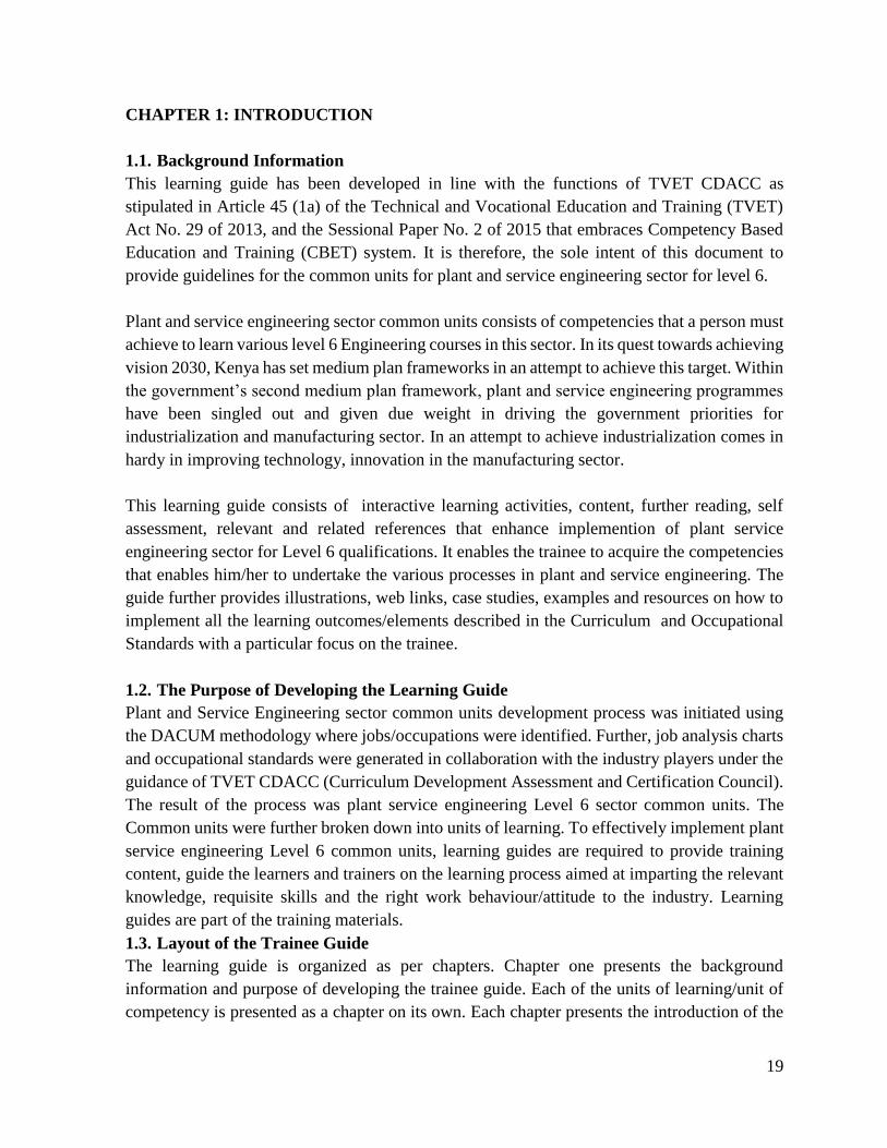
1.1. Background Information
This learning guide has been developed in line with the functions of TVET CDACC as
stipulated in Article 45 (1a) of the Technical and Vocational Education and Training (TVET)
Act No. 29 of 2013, and the Sessional Paper No. 2 of 2015 that embraces Competency Based
Education and Training (CBET) system. It is therefore, the sole intent of this document to
provide guidelines for the common units for plant and service engineering sector for level 6.
Plant and service engineering sector common units consists of competencies that a person must
achieve to learn various level 6 Engineering courses in this sector. In its quest towards achieving
vision 2030, Kenya has set medium plan frameworks in an attempt to achieve this target. Within
the government’s second medium plan framework, plant and service engineering programmes
have been singled out and given due weight in driving the government priorities for
industrialization and manufacturing sector. In an attempt to achieve industrialization comes in
hardy in improving technology, innovation in the manufacturing sector.
This learning guide consists of interactive learning activities, content, further reading, self
assessment, relevant and related references that enhance implemention of plant service
engineering sector for Level 6 qualifications. It enables the trainee to acquire the competencies
that enables him/her to undertake the various processes in plant and service engineering. The
guide further provides illustrations, web links, case studies, examples and resources on how to
implement all the learning outcomes/elements described in the Curriculum and Occupational
Standards with a particular focus on the trainee.
1.2. The Purpose of Developing the Learning Guide
Plant and Service Engineering sector common units development process was initiated using
the DACUM methodology where jobs/occupations were identified. Further, job analysis charts
and occupational standards were generated in collaboration with the industry players under the
guidance of TVET CDACC (Curriculum Development Assessment and Certification Council).
The result of the process was plant service engineering Level 6 sector common units. The
Common units were further broken down into units of learning. To effectively implement plant
service engineering Level 6 common units, learning guides are required to provide training
content, guide the learners and trainers on the learning process aimed at imparting the relevant
knowledge, requisite skills and the right work behaviour/attitude to the industry. Learning
guides are part of the training materials.
1.3. Layout of the Trainee Guide
The learning guide is organized as per chapters. Chapter one presents the background
information and purpose of developing the trainee guide. Each of the units of learning/unit of
competency is presented as a chapter on its own. Each chapter presents the introduction of the
20
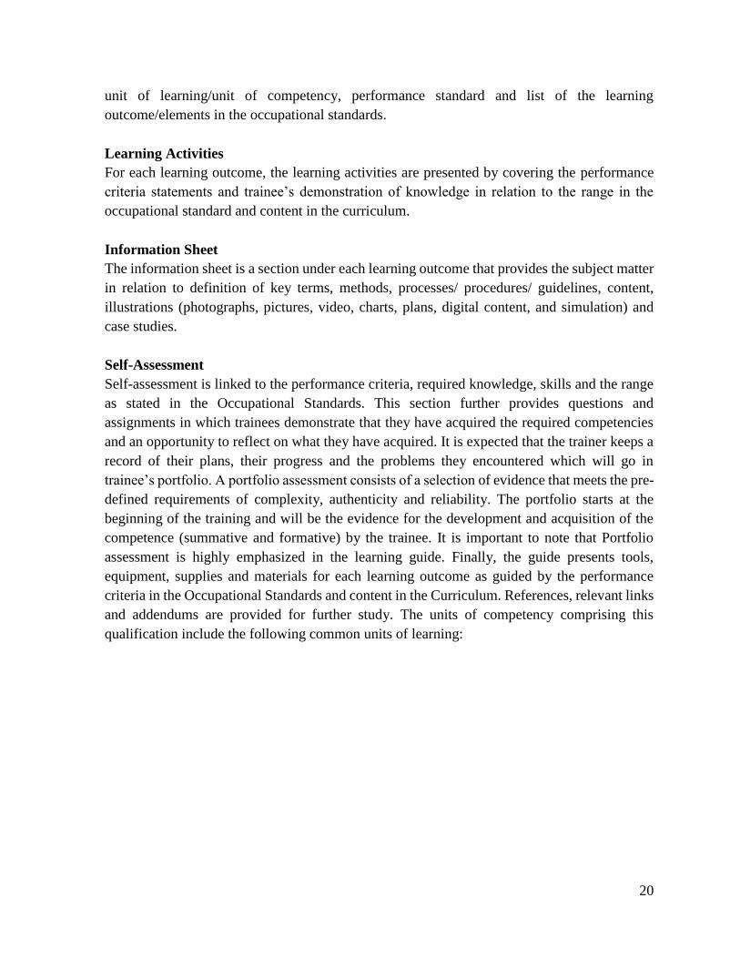
unit of learning/unit of competency, performance standard and list of the learning
outcome/elements in the occupational standards.
Learning Activities
For each learning outcome, the learning activities are presented by covering the performance
criteria statements and trainee’s demonstration of knowledge in relation to the range in the
occupational standard and content in the curriculum.
Information Sheet
The information sheet is a section under each learning outcome that provides the subject matter
in relation to definition of key terms, methods, processes/ procedures/ guidelines, content,
illustrations (photographs, pictures, video, charts, plans, digital content, and simulation) and
case studies.
Self-Assessment
Self-assessment is linked to the performance criteria, required knowledge, skills and the range
as stated in the Occupational Standards. This section further provides questions and
assignments in which trainees demonstrate that they have acquired the required competencies
and an opportunity to reflect on what they have acquired. It is expected that the trainer keeps a
record of their plans, their progress and the problems they encountered which will go in
trainee’s portfolio. A portfolio assessment consists of a selection of evidence that meets the pre-
defined requirements of complexity, authenticity and reliability. The portfolio starts at the
beginning of the training and will be the evidence for the development and acquisition of the
competence (summative and formative) by the trainee. It is important to note that Portfolio
assessment is highly emphasized in the learning guide. Finally, the guide presents tools,
equipment, supplies and materials for each learning outcome as guided by the performance
criteria in the Occupational Standards and content in the Curriculum. References, relevant links
and addendums are provided for further study. The units of competency comprising this
qualification include the following common units of learning:

21
Common Units of Learning
Summary of Common Units of Competencies
Table 1: Summary of Common Units of Competencies
Core Units of Learning
Unit Code
Unit Title Duration in
Hours
Credit
Factors
ENG/CU/PS/CC/01/6 Engineering mathematics 120 12
ENG/CU/PS/CC/02/6 Workshop technology practices 80 8
ENG/CU/PS/CC/03/6 Principles of mechanic science 90 9
ENG/CU/PS/CC/04/6 Fluids mechanics principles 100 10
ENG/CU/PS/CC/05/6 Thermodynamics principles 100 10
ENG/CU/PS/CC/06/6 Material science and metallurgical
processes
90 9
ENG/CU/PS/CC/07/6 Electrical science principles 90 9
ENG/CU/PS/CC/08/6 Technical Drawing 90 9
Total 760 76
22
CHAPTER 2: ENGINEERING MATHEMATICS/ APPLY ENGINEERING
MATHEMATICS
2.1 Introduction
This unit describes the competencies required by a technician in order to apply algebra, apply
trigonometry and hyperbolic functions, apply complex numbers, apply coordinate geometry, carry
out binomial expansion, apply calculus, solve ordinary differential equations, solve Laplace
transforms, apply power series, apply statistics, apply numerical methods, apply vector theory
apply matrix, apply Fourier series and numerical methods.
2.2 Performance Standard
The trainee will apply algebra, trigonometry and hyperbolic functions, complex numbers,
coordinate geometry, carryout binomial expansion, calculus ordinary differential equations,
Laplace transforms, power series, statistics Fourier series, vector theory, matrix and numerical
methods in solving engineering problems.
2.3 Learning Outcomes
2.3.1 List of learning outcomes
a) Apply Algebra
b) Apply Trigonometry and hyperbolic functions
c) Apply complex numbers
d) Apply Coordinate Geometry
e) Carry out Binomial Expansion
f) Apply Calculus
g) Solve Ordinary differential equations
h) Carry out Mensuration
i) Apply Power Series
j) Apply Statistics
k) Apply Numerical methods
l) Apply Vector theory
m) Apply Matrix
23
2.3.2 Learning Outcome No1: Apply Algebra
2.3.2.1 Learning Activities
Learning Outcome No 1:Apply Algebra
Learning Activities Special Instructions
1.1 Perform calculations involving Indices as per the concept
1.2 Perform calculations involving Logarithms as per the concept
1.3 Use scientific calculator is used mathematical problems in line with
manufacturer’s manual
1.4 Perform simultaneous equations as per the rules
1.5 Calculate quadratic equations as per the concept
Give group
assignments.
2.3.2.2 Information Sheet No2/LO 1: Apply Algebra
Introduction
This learning outcome covers algebra and the learner should be able to: perform calculations
involving Indices as per the concept; perform calculations involving Logarithms as per the
concept; use scientific calculator is used mathematical problems in line with manufacturer’s
manual; perform simultaneous equations as per the rules. Algebra is used throughout engineering,
but it is most commonly used in mechanical, electrical, and civil branches due to the variety of
obstacles they face. Engineers need to find dimensions, slopes, and ways to efficiently create any
structure or object.
Definition of key terms
Algebra is the study of mathematical symbols and the rules for manipulating these symbols; it is
a unifying thread of almost all of mathematics. It includes everything from elementary equation
solving to the study of abstractions such as groups, rings, and fields.
Content/Procedures/Methods/Illustrations
1.1 Calculations involving Indices are performed as per the concept
Indices
An index number is a number which is raised to a power. The power, also known as the index,
tells you how many times you have to multiply the number by itself. For example, 25 means that
you have to multiply 2 by itself five times = 2 × 2 × 2 × 2 × 2 = 32
24
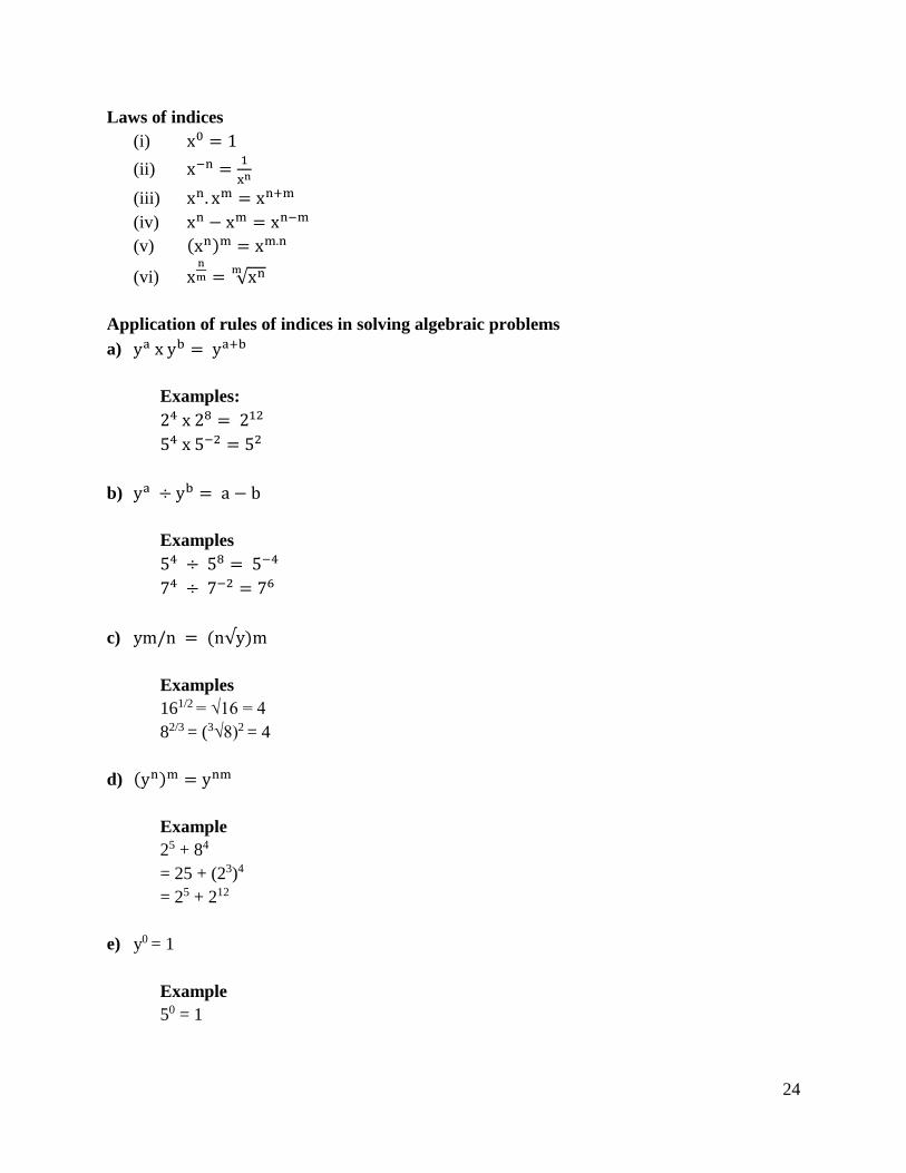
Laws of indices
(i) x0 = 1
(ii) x−n =1
xn
(iii) xn. xm = xn+m
(iv) xn − xm = xn−m
(v) (xn)m = xm.n
(vi) xn
m = √xnm
Application of rules of indices in solving algebraic problems
a) ya x yb = ya+b
Examples:
24 x 28 = 212
54 x 5−2 = 52
b) ya ÷ yb = a − b
Examples
54 ÷ 58 = 5−4
74 ÷ 7−2 = 76
c) ym/n = (n√y)m
Examples
161/2 = √16 = 4
82/3 = (3√8)2 = 4
d) (yn)m = ynm
Example
25 + 84
= 25 + (23)4
= 25 + 212
e) y0 = 1
Example
50 = 1
25
1.2 Calculations involving Logarithms are performed as per the concept
If a is a positive real number other than 1, then the logarithm of x with base a is defined
By:
y = loga x or x = ay
Laws of logarithms
(i) loga(xy) = logax + logay
(ii) loga (x
y) = logax − logay
(iii) loga(xn) = nlogax for every real number
1.3 Scientific calculator is used in solving mathematical problems
Use the scientific calculator manufacturer’s manual on the steps to be followed in doing so.
1.4 Simultaneous equations are performed as per the rules
Simultaneous equations are equations which have to be solved concurrently to find the unique
values of the unknown quantities which are time for each of the equations. Two common methods
of solving simultaneous equations analytically are:
(i) By substitution
(ii) By elimination
Simultaneous equations with three unknowns
Examples
Solve the following simultaneous equation by substitution methods
3x − 2y+ = 1……… . . (i)
x − 3y + 2z = 13 …… . (ii)
4x − 2y + 3z = 17………(iii)
From equation (ii) x = 13 + 3y − 2z
Substituting these expression (13 + 3y − 2z for x gives)
3(13 + 3y − 2z) + 2y + z = 1
39 + 9y − 6z + 2y + x = 1
11y − 5z = −38 …………… . . (iv)
4(13 + 3y − 2z) + 3z − 2y = 17
52 + 12y − 8z + 3z − 2y = 17
10y − 5z = −35… . . (v)
Solve equation (iv) and (v) in the usual way,
From equations (iv) 5z = 11y + 38; z =11y+38
5
26
Substituting this in equation (v) gives:
10y − 5 (11y+38
5) = −35
10y − 11y − 38 = −35
−y = −35 + 38 = 3
y = −3
z =11y + 38
5=
−33 + 38
5=
5
5= 1
But x = 13 + 3y − 2z
x = 13 + 3(−3) − 2(1)
=13 − 9 − 2
=2
Therefore, x = 2, y = −3 and z = 1 is the required solution
For more worked examples on substitution and elimination method refer to Engineering
Mathematics by A.K Stroud.
1.5 Quadratic equations are calculated as per the concept
Quadratic Equations
Quadratic equation is one in which the highest power of the unknown quantity is 2. For example
2x2 − 3x − 5 = 0 is a quadratic equation.
The general form of a quadratic equation is ax2 + bx + c = 0,where a, b and c are constants and
a ≠ 0 of solving quadratic equations.
1) By factorization (where possible)
2) By completing the square
3) By using quadratic formula
4) Graphically
Example
Solve the quadratic equation x2 − 4x + 4 = 0 by factorization method
Solution
x2 − 4x + 4 = 0
x2 − 2x − 2x + 4 = 0
x(x − 2) − 2(x − 2) = 0
(x − 2)(x − 2) = 0
i.e. x − 2 = 0 or x − 2 = 0
x = 2 or x = 2
I.e. the solution is x = 2 (twice)
27
For more worked examples on how to solve quadratic equations using, factorization, completing
the square, quadratic formula refer to basic engineering mathematics by J.O Bird, Engineering
mathematical by K.A strand, etc.
Conclusion
The learning outcome covered or equipped the learner with knowledge, skills and attitude to
perform calculations involving Indices as per the concept; perform calculations involving
Logarithms as per the concept; use scientific calculator in mathematical problems in line with
manufacturer’s manual; perform simultaneous equations as per the rules.
Further Reading
1. Stroud, A.K. (year). Engineering Mathematics
2.3.2.3 Self-Assessment
Written Assessment
1) Solve the following by factorization
a) x2 + 8x + 7 = 0
b) x2 − 2x + 1 = 0
2) Solve by completing the square the following quadratic equations
a) 2x2 + 3x − 6
b) 3x2 − x − 6 = 0
3) Simplify as far as possible
(i) log(x2 + 4x − 3) − log(x + 1)
(ii) 2log(x − 1) − log(x2 − 1)
4) Solve the following simultaneous equations by the method of substitution
x + 3y − z = 2
2x − 2y + 2z = 2
4x − 3y + 5z = 5
5) Simplify the following

28
F = (2x
12y
14)4 ÷ √
1
9x2y6 x (4 √x2y4)−1/2
Oral Assessment
1. What is your understanding of algebra
2.3.2.4 Tools, Equipment, Supplies and Materials
Scientific Calculators
Rulers, pencils, erasers
Charts with presentations of data
Graph books
Dice
Computers with internet connection
2.3.2.5 References
Khuri, A. I. (2003). Advanced calculus with applications in statistics (No. 04; QA303. 2, K4
2003.). Hoboken, NJ: Wiley-Interscience.
Stoer, J., &Bulirsch, R. (2013). Introduction to numerical analysis (Vol. 12). Springer Science &
Business Media.
Zill, D., Wright, W. S., & Cullen, M. R. (2011). Advanced engineering mathematics. Jones &
Bartlett Learning.
29
2.3.3 Learning Outcome No 2: Apply trigonometry and hyperbolic functions
2.3.3.1 Learning Activities
Learning Outcome No 2: Apply trigonometry and hyperbolic functions
Learning Activities Special Instructions
2.1 Perform calculations using trigonometric rules
2.2 Perform calculations using hyperbolic functions
2.3.3.2 Information Sheet No2/LO2: Apply trigonometry and hyperbolic functions
Introduction
This learning outcome equips the learner with knowledge and skills to perform calculations using
trigonometric rules and hyperbolic functions.
Definition of key terms
Trigonometry: This is a branch of mathematics which deals with the measurement of sides and
angles of triangles and their relationship with each other. Two common units used for measuring
angles are degrees and radians.
Content/Procedures/Methods/Illustrations
2.1 Calculations are performed using trigonometric rules
Trigonometric ratios
The three trigonometric ratios derived from a right-angled triangle are the sine, cosine and tangent
functions. Refer to basic engineering mathematics by J.0 Bird to read move about trigonometry
ratios.
Solution for right angled triangles
To solve a triangle means to find the unknown sides and angles; this is achieved by using the
theorem of Pythagoras and or using trigonometric ratios.
Example
Express 3 Sin θ + 4 Cosθ in the general form R Sin(θ + α)
Let 3 Sin θ + 4 Cos θ = R Sin (θ + α)
Expanding the right hand side using the compound angle formulae gives
3 Sin θ + 4 Cos θ = R [Sinθ Cosα + Cos θ Sinα ]
30
= R cosα Sin θ + R Sin α Cos θ
Equating the coefficient of:
Cosθ: = R Sin α i. e Sin α = 4
R
Sin θ ∶ 3 = R Cos α i. e Cos α =3
R
These values of R and α can be evaluated.
R = √42 + 32 = 5
α = tan−14
3= 53.130or 233.130
Since both Sin α and Cos α are positive, r lies in the first quadrant where all are positive, Hence
233.130 is neglected.
Hence
3 Sinθ + 4 Cos θ = 5 Sin (θ + 53.130)
Example
Solve the equation 3 Sin θ + 4 Cos θ = 2 for values of θ between 00 and 3600 inclusive
Solution
From the example above
3 Sinθ + 4 Cos θ = 5 Sin (θ + 53.130)
Thus
5 Sin(α + 53.130) = 2
Sin(θ + 53.130) = 2
5
θ + 53.130 = Sin−1 2/5
θ + 53.130 = 23.580or 156.420
θ = 23.580 − 53.130= −29.550
=330.450
OR θ = 156.420 − 53.130
=103.290
Therefore the roots of the above equation are 103.290 or 330.450
For more worked examples refer to Technician mathematics book 3 by J.) Bird.
31
Double/multiple angles
For double and multiple angles refer to Technician mathematics by J.O Bird
Factor Formulae
For worked exampled refer to Technic mathematics book 3 by J. O Bird, Pure mathematics by
backhouse and Engineering mathematics by KA Stroud.
Half-angle formulae
Refer to pure mathematics by backhouse and Engineering mathematics by K.A STROUD
2.2 Calculations are performed using hyperbolic functions
Hyperbolic functions
Definition of hyperbolic functions, Sinhx cosh x and tanh x
Evaluation of hyperbolic functions
|Hyperbolic identifies
Osborne’s Rule
Solve hyperbolic equations of the form a coshx + bSinhx = C
For all the above refer, to engineering mathematics by KA strand.
Conclusion
The learning outcome covered or equipped the learner with knowledge, skills and attitude to
perform calculations using trigonometric rules and perform calculations using hyperbolic
functions.
Further Reading
1. Stoer, J., &Bulirsch, R. (2013). Introduction to numerical analysis (Vol. 12). Springer
Science & Business Media.
2.3.3.3 Self-Assessment
Written Assessment
1. A surveyor measures the angle of elevation of the top of a perpendicular building as190.
He moves 120m nearer the building and measures the angle of elevation as470. Calculate
the height of the building to the nearest meter.
2. Solve the equation 5 cos θ + 4 Sinθ = 3 for values of θ between 00 and 3600
Inclusive.

32
3. Prove their identifies
(i)Cash 2x = cash2x + Sinh2x
(ii)Sinh(x + y)SinhCoshy + coshySinhx
4. Solve the equation
5. 3 Sinhx + 4 Coshx = 5
2.3.3.4 Tools, Equipment, Supplies and Materials
Scientific Calculators
Rulers, pencils, erasers
Charts with presentations of data
Graph books
Dice
Computers with internet connection
2.3.3.5 References
Khuri, A. I. (2003). Advanced calculus with applications in statistics (No. 04; QA303. 2, K4
2003.). Hoboken, NJ: Wiley-Interscience.
O’Neil, P. V. (2011). Advanced engineering mathematics. Cengage learning.
Stoer, J., &Bulirsch, R. (2013). Introduction to numerical analysis (Vol. 12). Springer Science &
Business Media.
33
2.3.4 Learning Outcome No 3: Apply complex numbers
2.3.4.1 Learning Activities
Learning Outcome No3: Apply complex numbers
Learning Activities Special
Instructions
3.1 Represent complex numbers are represented using Argand
diagrams
3.2 Perform operations involving complex numbers are performed
3.3 Perform calculations involving complex numbers using De
Moivre’s theorem
2.3.4.2 Information Sheet No2/LO3: Apply complex numbers
Introduction
This learning outcome covers an introduction to complex numbers, their representation in argand
diagrams and calculations involving complex numbers using De Moivre’s theorem
Definition of key terms
Argand diagram: A diagram on which complex numbers are represented geometrically using
Cartesian axes; the horizontal coordinate representing the real part of the number and the vertical
coordinate representing the imaginary part of the number, as depicted below
Content/Procedures/Methods/Illustration
A number of the form a + ib is called complex number where a and b are real numbers and i =
√−1 we call ′a′ the real part and ‘b’ the imaginary part of the complex a + ib if a = o then
ib is said to be purely imaginary, if b = 0 the number is real.
Pair of complex number a + ib are said to be conjugate of each other.
Addition and subtraction of complex numbers
Addition and subtraction of complex numbers is achieved by adding or subtracting the real parts
and the imaginary parts.
Example 1
(4 + j5) + (3 − j2)
(4 + j5) + (3 − j2)=4 + j5 + 3 − j2
=(4 + 3) + j(5 − 2)
=7 + j3
34
Example 2
(4 + j7) − (2 − js) = 4 + j7 − 2 + js = (4 − 2) + j(7 + 5)
= 2 + j12
Multiplication of complex numbers
Example 1
(3 + j4)(2 + j5)
6 + j8 + j15 + j220
6 + j23 − 20 (sincej2 = −1)
=−14 + j23
Examples 2
(5 + j8)(5 − j8)
(5 + j8)(5 − j8) = 25 + j40 − j40 − j264
= 25 + 64 =89
A pair of complex numbers are called conjugate complex numbers and the product of two
conjugate. Complex numbers is always entirely real.
cosθ + jsinθ
Argand diagram
Although we cannot evaluate a complex number as a real number, we can represent
diagrammatically in an argand diagram. Refer to Engineering Mathematics by K.A Stroud to learn
more on how to represent complex numbers on an argand diagram. Use the same back learn three
forms of expressing a complex number.
Demoivre’s Theorem
Demoivre’s theorem states that [r(cosθ + jsinθ)]n = rn(cosnθ + jsinnθ)
It is used in finding powers and roots of complex numbers in polar
Example
Find the three cube roots of z = 5(cos2250 + jsin2250)
Z1 = Z13 (Cos
2250
3+ jsin
2250
3)
1.71 (cos750 + jsin750
z1 = 1.71 (cos750 + jSin750)
Cube roots are the same size (modules) i.e. 1.71 and separated at intervals of 3600
3 , i.e 1200
z1=1.71 / 750
z2=1.71 cos (1950+jSin1950
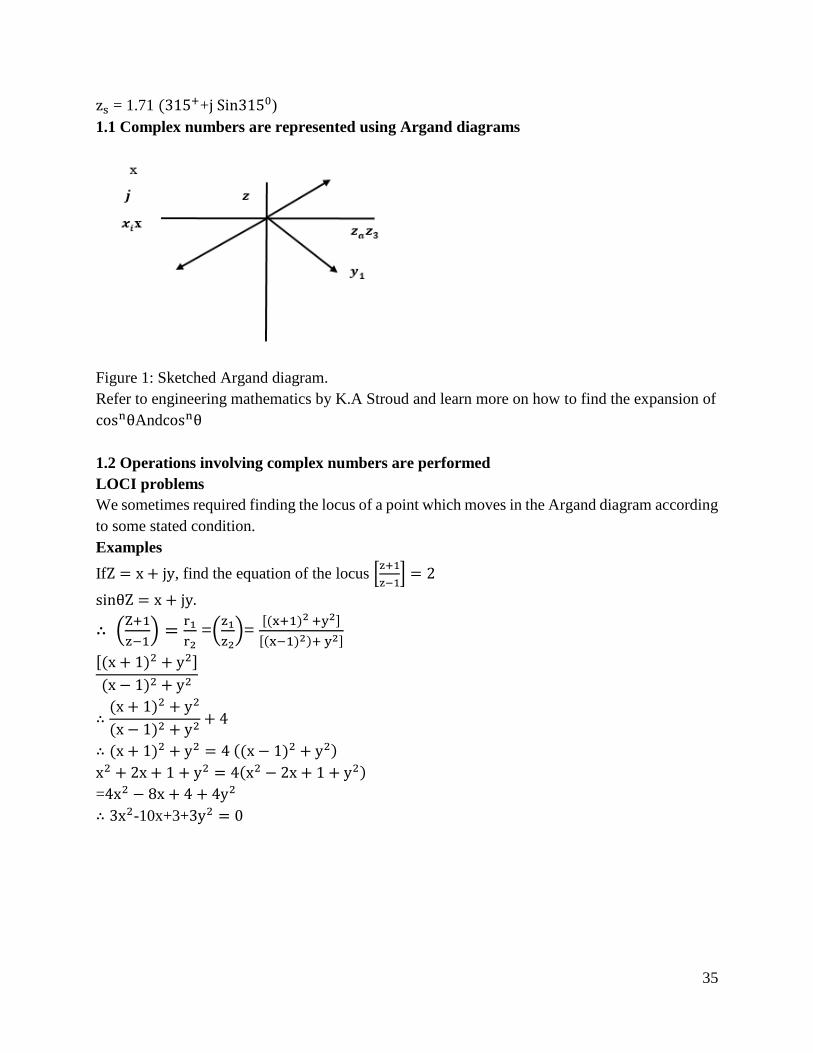
35
zs = 1.71 (315++j Sin3150)
1.1 Complex numbers are represented using Argand diagrams
Figure 1: Sketched Argand diagram.
Refer to engineering mathematics by K.A Stroud and learn more on how to find the expansion of
cosnθAndcosnθ
1.2 Operations involving complex numbers are performed
LOCI problems
We sometimes required finding the locus of a point which moves in the Argand diagram according
to some stated condition.
Examples
IfZ = x + jy, find the equation of the locus [z+1
z−1] = 2
sinθZ = x + jy.
∴ (Z+1
z−1) =
r1
r2 =(
z1
z2)=
[(x+1)2 +y2]
[(x−1)2)+ y2]
[(x + 1)2 + y2]
(x − 1)2 + y2
∴(x + 1)2 + y2
(x − 1)2 + y2+ 4
∴ (x + 1)2 + y2 = 4 ((x − 1)2 + y2)
x2 + 2x + 1 + y2 = 4(x2 − 2x + 1 + y2)
=4x2 − 8x + 4 + 4y2
∴ 3x2-10x+3+3y2 = 0
36
Conclusion
The learning outcome covered or equipped the learner with knowledge, skills and attitude to
represent complex numbers using Argand diagrams, perform operations involving complex
numbers and Perform calculations involving complex numbers using De Moivre’s theorem.
Further Reading
1. Atkinson, K. E. (2008). An introduction to numerical analysis. John Wiley & Sons.
2.3.4.3 Self-Assessment
Written Assessment
1. Find the fifth roots of −3 + j3 in polar form and in exponential form
2. Determine the three cube roots of 2−j
2+j giving the results in a modulus/ argument form.
3. Express the principal root in the form a + jb
4. If z = x + jy, where x and y are real, show that the locus (Z−2
z+2) = 2 is a circle and
5. Determine its center and radius.
Oral Assessment
1. Describe an Argand diagram according to your understanding.
2. What is a complex number?
Practical Assessment
1. Give an example of a complex number. Represent it in an Argand diagram
2. Find the root loci of the complex number above. Use De-Moivre’s theorem
2.3.4.4 Tools, Equipment, Supplies and Materials
Scientific Calculators
Rulers, pencils, erasers
Charts with presentations of data
Graph books
Dice
Computers with internet connection
2.3.4.5 References

37
Atkinson, K. E. (2008). An introduction to numerical analysis. John Wiley & Sons.
Greenberg, M.D. (1998), Advanced Engineering Mathematics, 2nd ed., Prentice Hall (Upper
Saddle River, N.J).
Stoer, J., & Bulirsch, R. (2013). Introduction to numerical analysis (Vol. 12). Springer Science &
Business Media.
38
2.3.5 Learning Outcome No 4: Apply coordinate geometry
2.3.5.1 Learning Activities
Learning Outcome No 4:apply coordinate geometry
Learning Activities Special Instructions
4.1 Calculate polar equations using coordinate geometry
4.2 Draw graphs of given polar equations using the Cartesian plane
4.3 Determine normal and tangents using coordinate geometry
2.3.5.2 Information Sheet No2/LO4: apply coordinate geometry
Introduction
This learning outcome covers calculation of polar equations using coordinate geometry, drawing
graphs of given polar equations using the Cartesian plane, determining normal and tangents using
coordinate geometry.
Content/Procedures/Methods/Illustrations
The position of a point in a plane can be represented in two forms
i) Cartesian co-ordinate (x, y)
ii) Polar co-ordinate (r, θ)
The position of a point in the corresponding axis can therefore generate Cartesian and polar
equations which can easily change into required form to fit the required result.
4.1 Polar equations are calculated using coordinate geometry
Example
Convert r2 = sinθ into Cartesian form.
cosθ =x
y sinθ =
y
x
Form Pythagoras theorem r2 = x2 + y2
r2 = sinθ
(x2 + y2) =y
x
(x2 + y2)x = y
(x2 + y2)(x2 + y2)1
2 = y
(x2 + y2)3
2 = y
39
Example 2
Find the Cartesian equation of
(i) r = a(1 + 2cos) (ii) rcos(θ − α) = p
[The Cosθ suggest the relationX = COSθ, so multiplying through by r
∴ r2 = a(r + 2rcosθ)
∴ x2 + y2 = a(√(x2 + y2) + 2x)
∴ x2 + y2 + 2x = a√(x2 + y2)
Therefore the Cartesian equation of r = a(1 + 2cos) is (x2 + y2 − 2ax)2 = a2(x2 + y2)
(ii) rcos(θ − α) = p
cos(θ − α) May be expanded
∴ rcosθcosα + rsinθsinα = p
(iii) Therefore the Cartesian equation of rcos(θ − α) = p is xcosα + ysinα = p
Example 3
Find the polar equation of the circle whose Cartesian equation is x2 + y2 = 4x
x2 + y2 = 4x
Put x = rcosθ, y = rsinθ, then
r2cos2θ + r2sin2θ = 4rcosθ
∴ r2 = 4rcosθ
Therefore the polar equation of the circle isr2 = 4rcosθ.
For more information on the conversion of Cartesian equation to polar equation and vice versa
refer to pure mathematics by J.K Backhouse.
Conclusion
The learning outcome covered or equipped the learner with knowledge, skills and attitude to
calculate polar equations using coordinate geometry, draw graphs of given polar equations using
the Cartesian plane, determine normal and tangents using coordinate geometry.
Further Reading
1. Kreyszig, E. (1999), Advanced Engineering Mathematics, 8th ed., John Wiley (New York).
2. O'Neil, P.V. (1995), Advanced Engineering Mathematics, 4th ed., PWS-Kent Pub.
(Boston).
40
2.3.5.3 Self-Assessment
Written Assessment
1. Obtain the polar equation of the following loci
a) x2 + y2 = a2
b) x2 − y2 = a2
c) y = 0
d) y2 = 4a(a − x)
e) x2 + y2 − 2y = 0
f) xy = c2
2. Obtain the Cartesian equation of the following loci
a) r = 2
b) a(1+cosθ)
c) r = acosθ
d) r = atanθ
e) r = 2a(1 + sin2θ)
f) 2r2sin2θ = c2
g) l
r= 1 + 8cosθ
h) r = 4acotθcosecθ
2.3.5.4 Tools, Equipment, Supplies and Materials
Scientific Calculators
Rulers, pencils, erasers
Charts with presentations of data
Graph books
Dice
Computers with internet connection
2.3.5.5 References
Greenberg, M.D. (1998), Advanced Engineering Mathematics, 2nd ed., Prentice Hall (Upper
Saddle River, N.J).
Hildebrand, F.B. (1974), Introduction to Numerical Analysis, 2nd ed., McGraw-Hill (New York).
Hildebrand, F.B. (1976), Advanced Calculus for Applications, 2nd ed., Prentice-Hall (Englewood
Cliffs, NJ).
41
2.3.6 Learning Outcome No 5: Carry out binomial expansion
2.3.6.1 Learning Activities
Learning Outcome No 5:carry out binomial expansion
Learning Activities Special Instructions
5.1 Determine roots of numbers using binomial theorem
5.2 Determine errors of small changes using binomial theorem
2.3.6.2 Information Sheet No2/LO5: Carry Out Binomial Expansion
Introduction
This learning outcome seeks to equip the learner with knowledge and skills to determine the roots
of numbers using binomial theorem and to determine errors of small changes using binomial
theorem.
Content/Procedures/Methods/Illustrations
5.1 Carry out Binomial expansion
Binomial is a formula for raising a binomial expansion to any power without lengthy
multiplication. It states that the general expansion of (a + b)n is given as
(a + b)n = anb0 + nan−1n1 +n(n−1)an−2b2
2!+
n(n−1)(n−2)an−3b3
3!+…
Where n can be a fraction, a decimal fraction, positive or negative integer.
Example 1
Use binomial theorem to expand (2 + x)3
Solution
(a + b)n = anb0 + nan−1n1 +n(n−1)an−2b2
2!+
n(n−1)(n−2)an−3b3
3!+…
A = 2, b = x and n = 3
(2 + x)3 = 23x0 + 3X22x1 +3(3−1)21x2
2!+
3(3−1)(3−2)20x3
3!+…
= 8 + 12x + 6x2 + x3
For more examples on positive power refer to Technician Mathematic Book by J.O Bird.
Binomial theorem for any index
It has been shown that:
(1 + x)n = 1 + nx +n(n−1)
2!x2 +….
The series may be continued indefinitely for any value of n provided −1 < x < 1
42
Example
Use the binomial theorem to expand 1
1−x in ascending power of x as far as the term in x3.
Solution
Since 1
1−x may be written(a − x + x)−1, the binomial theorem may be used. Thus
(1 − x)−1 = 1 + −1(−x) +−1(−2)
2!x2 +
−1(−2)(−3)
3!+….
1
1−x= 1 + x + x2 + x3 + ⋯
Provided −1 < x < 1
5.2 Practical application of binomial theorem
Example1
The radius of a cylinder is reduced by 4% and its height increased by 2%. Determine the
appropriate percentage change in its volume neglecting products of small quantities.
Solution
Volume, V = πr2h
Let original values be, radius = r
Height = h
New values radius = (1 − 0.04)r
Height = (1 + 0.02)h
New volume = π(1 − 0.004)2r2(1 + 0.02)h
Using binomial theorem, (1 − 0.04)2 = 1 − 2(0.04) + (0.04)2 = 1 − 0.08
=πr2h(1 − 0.08)(1.02) = πr2h(0.94)
Percentage change =(0.94−1)100%
1= −6%
The new volume decreased by 6%
Conclusion
The learning outcome covered or equipped the learner with knowledge, skills and attitude to
determine the roots of numbers using binomial theorem and to determine errors of small changes
using binomial theorem.
Further Reading
1. Hoyland, A., Rausand, and M. (1994), System Reliability Theory: Models and Statistical
Methods, John Wiley (New York).
2. Kaplan, W. (1984), Advanced Calculus, 3rd ed., Addison-Wesley (Cambridge, MA).
3. Kreyszig, E. (1999), Advanced Engineering Mathematics, 8th ed., John Wiley (New York).
43
2.3.6.3 Self-Assessment
Written Assessment
1. Expand as far as the third term and state the limits to which the expansions are valid.
i. 1
(1+2x)3
ii. √4 + x
2. Show that if higher powers of x are neglected,
√1 + x
1 − x= 1 + x +
x2
2
3. The second moment of area of a rectangular section through its centroid is given by bl3
12.
Determine the appropriate change in the second moment of area if b is increased by 3.5% and
l is reduced by 2.5%.
2.3.6.4 Tools, Equipment, Supplies and Materials
Scientific Calculators
Rulers, pencils, erasers
Charts with presentations of data
Graph books
Dice
Computers with internet connection
2.3.6.5 References
Greenberg, M.D. (1998), Advanced Engineering Mathematics, 2nd ed., Prentice Hall (Upper
Saddle River, N.J).
Hildebrand, F.B. (1974), Introduction to Numerical Analysis, 2nd ed., McGraw-Hill (New York).
Hildebrand, F.B. (1976), Advanced Calculus for Applications, 2nd ed., Prentice-Hall (Englewood
Cliffs, NJ).
44
2.3.7 Learning Outcome No 6: Apply calculus
2.3.7.1 Learning Activities
Learning Outcome No 6:Apply calculus
Learning Activities Special Instructions
6.1 Determine derivatives of functions using differentiation
6.2 Determine derivatives of hyperbolic functions using differentiation
6.3 Determine derivatives of inverse trigonometric functions using
differentiation
6.4 Determine rate of change and small change using differentiation
6.5 Perform calculation involving stationery points of functions of two
variables using differentiation
6.6 Determine integrals of algebraic functions using integration
6.7 Determine integrals of trigonometric functions using integration
6.8 Determine integrals of logarithmic functions using integration
6.9 Determine integrals of hyperbolic and inverse functions using
integration
2.3.7.2 Information Sheet No2/LO6: Apply calculus
Introduction
This learning outcome equips the learner with relevant knowledge, skills and attitude so that they
are able to: determine the derivatives of functions using differentiation; determine derivatives of
hyperbolic functions using differentiation; determine derivatives of inverse trigonometric
functions using differentiation; determine rate of change and small change using differentiation;
perform calculation involving stationery points of functions of two variables using differentiation;
determine integrals of algebraic functions using integration; determine integrals of trigonometric
functions using integration; determine integrals of logarithmic functions using integration;
determine integrals of hyperbolic and inverse functions using integration.
45
Definition of key terms
Calculus: It is a branch of mathematics involving calculations dealing with continuously varying
functions. The subject falls into two parts namely differential calculus (differentiation) and integral
calculus (integration).
Differentiation: The central problem of the differential calculus is the investigation of the rate of
change of a function with respect to changes in the variables on which it depends.
Content/Procedures/Methods/Illustrations
6.1 Differentiation from first principles
To differentiate from first principles means to find f ′(x) using the expression.
f ′(x) = limδx→0
f(x+δx)
δx
δx → 0, f(x+8x)−f(x)
δx
f(x) = x2
f(x + δx) = (x + δx)2 = x2 + 2xδx + (δx)2
f(x + δx) − f(x) = x2 + 2 xδx + (δx)2 − x2
=2xδx + (δx)2
f(x+δx)−f(x)
δx=
2xδx +(δx)2
δx
=2x + δx
As δx → 0,f(x+δx)−f(x)
δx→ 2x + 0
∴ f ′(x) = limδx→0
f(x+δx)−f(x)
δx= 2x
At x = 3, the gradient of the curve i.e f ′(x) = 2(3) = 6
Hence if f(x) = x2, f ′(x) = 2x. The gradient at x = 3 is 6
6.2 Methods of differentiation
There are several methods used to differentiate different functions which include:
(i) Product Rule
(ii) Quotient Rule
(iii)Chain Rule
(iv) Implicit Rule
Example
Determine dy
dx⁄ given that
a) y = x2Sinx
46
Solution
From product rule: uv(x) = udv
dx +v
du
dx
u = x2and v = Sinx du
dx =2x
dv
dx= Cosx
∴dy
dx= x2(Cosx) + Sinx (2x)
=x2Cos x + 2x Sin x
b) y =x2+1
x−3
Solution. Using Quotient rule:
u(x)
v(x)=
vdudx
− udvdx
v2
u = x2+1 v = x − 3 du
dx= 2x
dv
dx=1
∴dy⁄dx= (x−3)(2x)−(x2+1)(1)
(x−3)2
= 2x2 − 6x − x2 − 1
(x − 3)2
= x2 − 6x − 1
(x − 3)2
= x2 − 6x − 1
x2 − 6x + 9
For more examples on the cases of application of the other highlighted rates refer to Engineering
Mathematics by K Stroud.
6.3 Applications of differentiation
Differentiation can be used to determine velocity and acceleration of a moving body. It can also
be applied to determine maximum and minimum values.
Example: A rectangular area is formed using a piece of wire 36cm long. Find the length and
breadth of the rectangle if it is to enclose the maximum possible area.
Solution.
Let the dimension a rectangle be x and y
Perimeter of rectangle = 2x + 2y = 36
i.e.x + y = 18……………… (i)
47
Since it is the maximum area that is required, a formula for the area A must be obtained in terms
of one variable only.
Area = A = xy
From equation (i), y = 18 − x
Hence A = x(18 − x) = 18x − x2
Now that an expression for the area has been obtained in terms of one variable it can be
differentiated with respect to that variable dA
dx= 18 − 2x for maximum or minimum value i.e. x = 9
d2A
dx2= −2,which is negative giving a maximum value
y = 18 − x = 18 − 9 = 9
Hence the length and breadth of the rectangle for maximum area are both 9 cm i.e. a square gives
the maximum possible area for a given perimeter length When perimeter is 36cm, maximum area
possible is 81cm2.
6.6 Integrals of algebraic functions are determined using integration
Integration
Process of integration reverses the process of differentiation. In differentiation if f(x) =
x2, then f ′(x) = 2x.
Since integration reverse the process of moving from f(x) to f ′(x), it follows that the integral of
2x is x2 i. e it is the process of moving from f ′(x) tof(x). Similarly if y = x3 then dy
dx= 3x2.
Reversing this process shows that the integral of 3x2is x3.
Integration is also the process of summation or adding parts together and an elongated ′s′ shown
as ⨜ is used to replace the words ‘integrated of’. Thus ⨜2x=x2 and ⨜3x2 = x3
Refer to Engineering Mathematics by K.A Strand and learn those on definite and indefinite
integrals.
6.7 Methods of integration and application of integration
The methods available are:
a) By using algebraic substitution
b) Using trigonometric identities and substitutions
c) Using partial fraction
d) Using t = tanθ
2 substitution
e) Using integration by parts
Refer to Engineering Mathematics by K. A. Strand and learn more about methods of integration,
Also use the above stated book to learn more on application of integration to find areas, volumes
of revolutions, etc.
48
Conclusion
The learning outcome covered or equipped the learner with knowledge, skills and attitude to
determine the derivatives of functions using differentiation, determine derivatives of hyperbolic
functions using differentiation, determine derivatives of inverse trigonometric functions using
differentiation, determine the rate of change and small change using differentiation; perform
calculation involving stationery points of functions of two variables using differentiation;
determine integrals of algebraic functions using integration; determine integrals of trigonometric
functions using integration; determine integrals of logarithmic functions using integration;
determine integrals of hyperbolic and inverse functions using integration.
Further Reading
2.3.7.3 Self-Assessment
Written Assessment
1. Find the co-coordinator, of the points on the curve
y =1/3(5−6x)
3x2+2
where the gradient is zero
2. If y =4
3x3 −2
x2 +1
3x− √x . Find
d2y
dx and
d3y
dx
3. Find ⨜cos6x Sin 2x dx
4. Evaluate ∫x3−x2−5x
x2−2x+2
4
3dx
Oral Assessment
1. What do you understand by differentiation and integration as applied in calculus?
2. How are they intertwined?
3. What are some of their practical applications?
2.3.7.4 Tools, Equipment, Supplies and Materials
Scientific calculators
Rulers, pencils, erasers

49
Charts with presentations of data
Graph books
Computers with internet connection
2.3.7.5 References
Greenberg, M.D. (1998), Advanced Engineering Mathematics, 2nd ed., Prentice Hall (Upper
Saddle River, N.J).
Hildebrand, F.B. (1974), Introduction to Numerical Analysis, 2nd ed., McGraw-Hill (New York).
Hildebrand, F.B. (1976), Advanced Calculus for Applications, 2nd ed., Prentice-Hall (Englewood
Cliffs, NJ).
50
2.3.8 Learning Outcome No7: Solve ordinary differential equations
2.3.8.1 Learning Activities
Learning Outcome No 7: Solve ordinary differential equations
Learning Activities Special Instructions
7.1. Solve first order and second order differential equations using
the method of undetermined coefficients
7.2. Solve first order and second order differential equations from
given boundary conditions
2.3.8.2 Information Sheet No2/LO7: Solve ordinary differential equations
Introduction
7.1. Solve first order and second order differential equations using the method of
undetermined coefficients
This learning outcome equips the learner with knowledge and skills to solve first order differential
equations using the method of undetermined coefficients and also when given boundary
conditions.
Content/Procedures/Methods/Illustrations
An equation involves differential co-efficient is called a differential equation examples.
Examples
(i) dy
dx=
1+ x2
1−y2
(ii) d2y
dx2 + 2
dy
dx – 8y =0
The order of a differential equation is the order of the highest differential coefficient present in the
equation. Differential equations represent dynamic relationships i.e. quantities that change, and are
thus frequently occurring in scientific and engineering problems.
Formation of a differential equation
Differential equations may be formed in practice from a consideration of the physical problem to
which they refer. Mathematically, they can occur when arbitrary constants are eliminated from a
given function.
51
Example
Consider y = Asinx + Bcosx, where A and B are two arbitrary constants. If we differentiate, we
get
dy
dx= ACosx − BSinx and
d2y
dx2= −ASinx − BCosx = −(ASinx + BCosx)
i.e. d2y
dx2= −y
∴ d2y
dx2− y = 0
This is a differential equation of the second order.
Types of first order differential equations
a) By separating the variables
b) Homogeneous first order differential equations
c) Linear differential equations
d) Exact differential equations
7.2 Application of first order differential equations
Differential equations of the first order have many applications in Engineering and Science.
Example
The rate at which a body cools is given by the equations dθ
dt= −kθ where θ is the temperature of
the body above the surroundings and k is a constant. Solve the equation for θ given that t = 0 ,
θ = θ0
Solution
dθ
dt= −kθ
Rearranging gives: dt =−1
kθ
Integrating both sides gives: ∫ dt =−1
k∫
dθ
θ
i.e.t =−1
klnθ + c………………….. (i)
Substituting the boundary conditions t = 0 , θ = θ0 to find c gives
0 =−1
klnθ0 + c
i.e. c =1
klnθ0
Substituting c =−1
klnθ0 in equation (i) gives
t =−1
klnθ +
1
klnθ0
t =1
k(lnθ0 + lnθ) =
1
kln (
θ0
θ)
kt = ln (θ0
θ)
52
ekt =θ0
θ
e−kt =θ
θ0
Hence, θ = θ0e−kt
7.1 First order and second order differential equations are solved using the method of
undetermined coefficients
Formation of the second order differential equation
For formation of second order differential equations refer to Engineering Mathematics by K.A
Strand, Technician 4 and 5 by J.O Bird.
Application of second order differential equations
Many applications in engineering give rise to the second order differential equations of the form
ad2y
dx2 + bdy
dx+ cy = f(x)
Where a, b, c are constant coefficients and f(x) is a given function of x.
Examples include:
(1) Bending of beams
(2) Vertical oscillations and displacements
(3) Damped forced vibrations
Conclusion
The learning outcome covered or equipped the learner with knowledge, skills and attitude to solve
first order differential equations using the method of undetermined coefficients; and also when
given boundary conditions.
2.3.8.3 Self-Assessment
Written Assessment
1. Solve the following equations:
a) x(y − 3)dy
dx4y
b) (xy + y2) + (x2 − xy)dy
dx= 0
c) dy
dx+ ytanx = sinx
2. Show that the change, q, on a capacitor in an LCR circuit satisfies the second order
differential equation
53
Ld2q
dt2+ b
dq
dt+
1
cq = E
3. Show that if 2L = cR2 the general solution of this equation is
q = e−t
cR (Acos1
cRt + Bsin
1
cRt) + cE
4. If i =dq
dt= 0 and q = 0 when t = 0, show that the current in the circuit is
i =2E
Re
−t
cRsin1
cR
Oral Assessment
1. Consider the following differential equation
x(y − 3)dy
dx= 4y. Is it of the first order or the second order?
2. Justify your answer above
2.3.8.4 Tools, Equipment, Supplies and Materials
Scientific Calculators
Rulers, pencils, erasers
Charts with presentations of data
Graph books
Dice
Computers with internet connection
2.3.8.5 References
Greenberg, M.D. (1998), Advanced Engineering Mathematics, 2nd ed., Prentice Hall (Upper
Saddle River, N.J).
Hildebrand, F.B. (1974), Introduction to Numerical Analysis, 2nd ed., McGraw-Hill (New York).
Hildebrand, F.B. (1976), Advanced Calculus for Applications, 2nd ed., Prentice-Hall (Englewood
Cliffs, NJ).
54
2.3.9 Learning Outcome No 8: Carry out mensuration
2.3.9.1 Learning Activities
Learning Outcome No 8:Carry out mensuration
Learning Activities Special Instructions
8.1. Obtain perimeter and areas of figures
8.2. Obtain volume and surface area of solids
8.3. Obtain area of irregular figures
8.4. Obtain areas and volumes using Pappus theorem
2.3.2.9.2 Information Sheet No2/LO8: Carry out mensuration
Introduction
This learning outcome covers perimeter and areas of figures, volume and surface area of solids,
area of irregular figures and areas and volumes using Pappus theorem.
Definition of key terms
Area: Extent of part of a surface enclosed within a boundary.
Circumference: Distance around a circle.
Dimension: Measurable extent such as length, thickness and width.
Fraction: Number expressed as a quotient of two other numbers.
Mensuration: Act or art of measuring.
Perimeter: Bounding line or curve of a plain area.
Standard: Serves as a measure of reference.
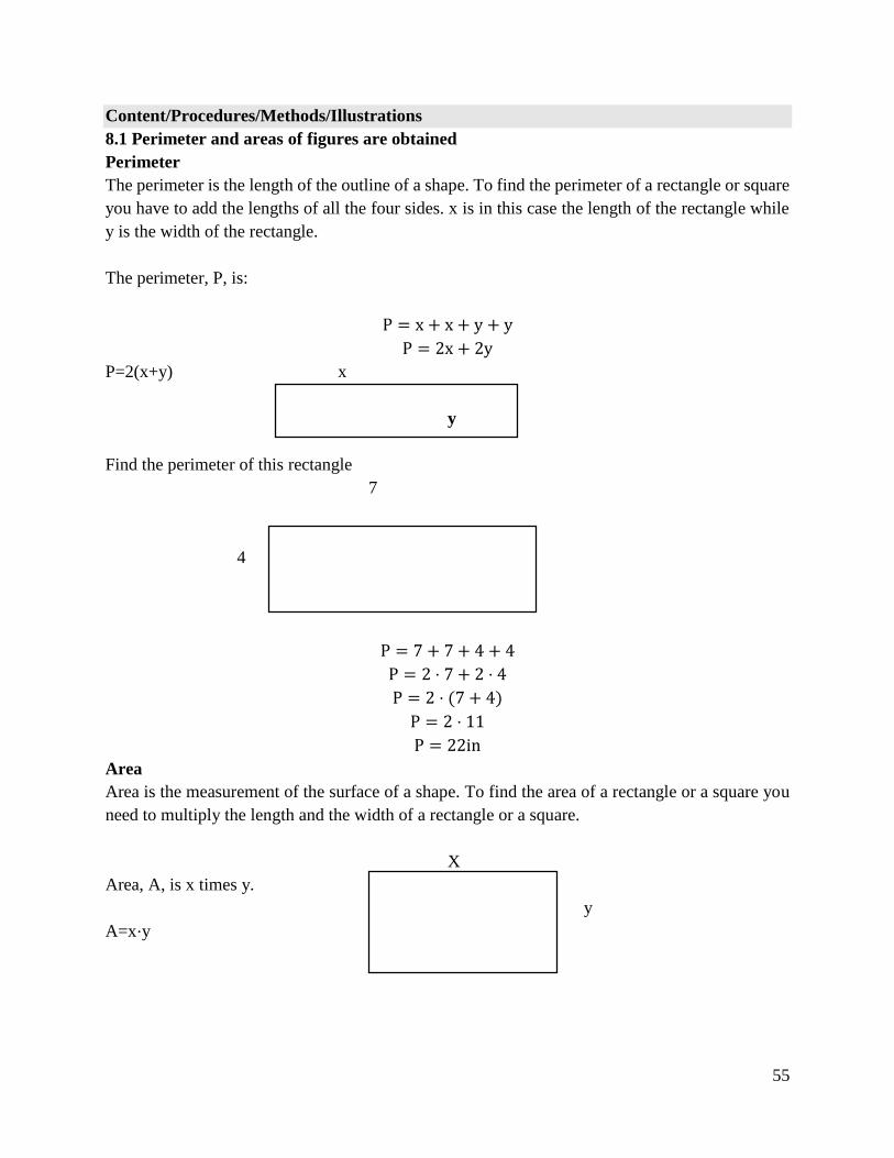
55
Content/Procedures/Methods/Illustrations
8.1 Perimeter and areas of figures are obtained
Perimeter
The perimeter is the length of the outline of a shape. To find the perimeter of a rectangle or square
you have to add the lengths of all the four sides. x is in this case the length of the rectangle while
y is the width of the rectangle.
The perimeter, P, is:
P = x + x + y + y
P = 2x + 2y
P=2(x+y) x
y
Find the perimeter of this rectangle
7
4
P = 7 + 7 + 4 + 4
P = 2 ⋅ 7 + 2 ⋅ 4
P = 2 ⋅ (7 + 4)
P = 2 ⋅ 11
P = 22in
Area
Area is the measurement of the surface of a shape. To find the area of a rectangle or a square you
need to multiply the length and the width of a rectangle or a square.
X
Area, A, is x times y.
y
A=x⋅y
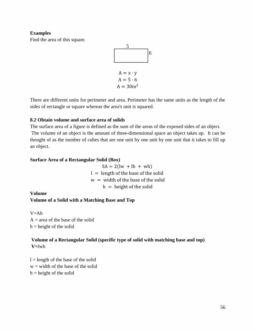
56
Examples
Find the area of this square.
5
6
A = x ⋅ y
A = 5 ⋅ 6
A = 30in2
There are different units for perimeter and area. Perimeter has the same units as the length of the
sides of rectangle or square whereas the area's unit is squared.
8.2 Obtain volume and surface area of solids
The surface area of a figure is defined as the sum of the areas of the exposed sides of an object.
The volume of an object is the amount of three-dimensional space an object takes up. It can be
thought of as the number of cubes that are one unit by one unit by one unit that it takes to fill up
an object.
Surface Area of a Rectangular Solid (Box)
SA = 2(lw + lh + wh)
l = length of the base of the solid
w = width of the base of the solid
h = height of the solid
Volume
Volume of a Solid with a Matching Base and Top
V=Ah
A = area of the base of the solid
h = height of the solid
Volume of a Rectangular Solid (specific type of solid with matching base and top)
V=lwh
l = length of the base of the solid
w = width of the base of the solid
h = height of the solid
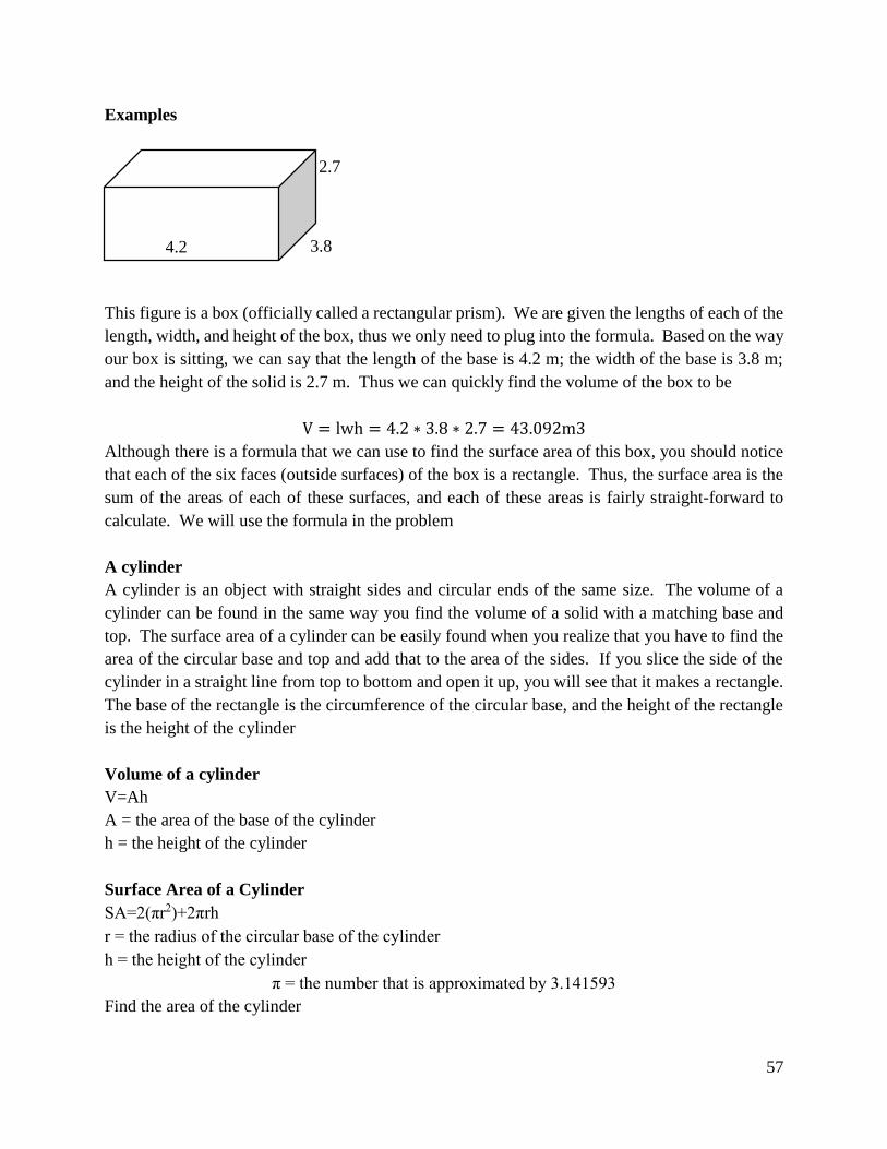
57
Examples
This figure is a box (officially called a rectangular prism). We are given the lengths of each of the
length, width, and height of the box, thus we only need to plug into the formula. Based on the way
our box is sitting, we can say that the length of the base is 4.2 m; the width of the base is 3.8 m;
and the height of the solid is 2.7 m. Thus we can quickly find the volume of the box to be
V = lwh = 4.2 ∗ 3.8 ∗ 2.7 = 43.092m3
Although there is a formula that we can use to find the surface area of this box, you should notice
that each of the six faces (outside surfaces) of the box is a rectangle. Thus, the surface area is the
sum of the areas of each of these surfaces, and each of these areas is fairly straight-forward to
calculate. We will use the formula in the problem
A cylinder
A cylinder is an object with straight sides and circular ends of the same size. The volume of a
cylinder can be found in the same way you find the volume of a solid with a matching base and
top. The surface area of a cylinder can be easily found when you realize that you have to find the
area of the circular base and top and add that to the area of the sides. If you slice the side of the
cylinder in a straight line from top to bottom and open it up, you will see that it makes a rectangle.
The base of the rectangle is the circumference of the circular base, and the height of the rectangle
is the height of the cylinder
Volume of a cylinder
V=Ah
A = the area of the base of the cylinder
h = the height of the cylinder
Surface Area of a Cylinder
SA=2(πr2)+2πrh
r = the radius of the circular base of the cylinder
h = the height of the cylinder
π = the number that is approximated by 3.141593
Find the area of the cylinder
4.2 3.8
2.7
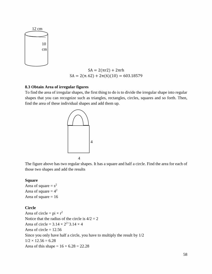
58
SA = 2(πr2) + 2πrh
SA = 2(π. 62) + 2π(6)(10) = 603.18579
8.3 Obtain Area of irregular figures
To find the area of irregular shapes, the first thing to do is to divide the irregular shape into regular
shapes that you can recognize such as triangles, rectangles, circles, squares and so forth. Then,
find the area of these individual shapes and add them up.
4
4
The figure above has two regular shapes. It has a square and half a circle. Find the area for each of
those two shapes and add the results
Square
Area of square = s2
Area of square = 42
Area of square = 16
Circle
Area of circle = pi × r2
Notice that the radius of the circle is 4/2 = 2
Area of circle = 3.14 × 22=3.14 × 4
Area of circle = 12.56
Since you only have half a circle, you have to multiply the result by 1/2
1/2 × 12.56 = 6.28
Area of this shape = 16 + 6.28 = 22.28
10
cm
12 cm
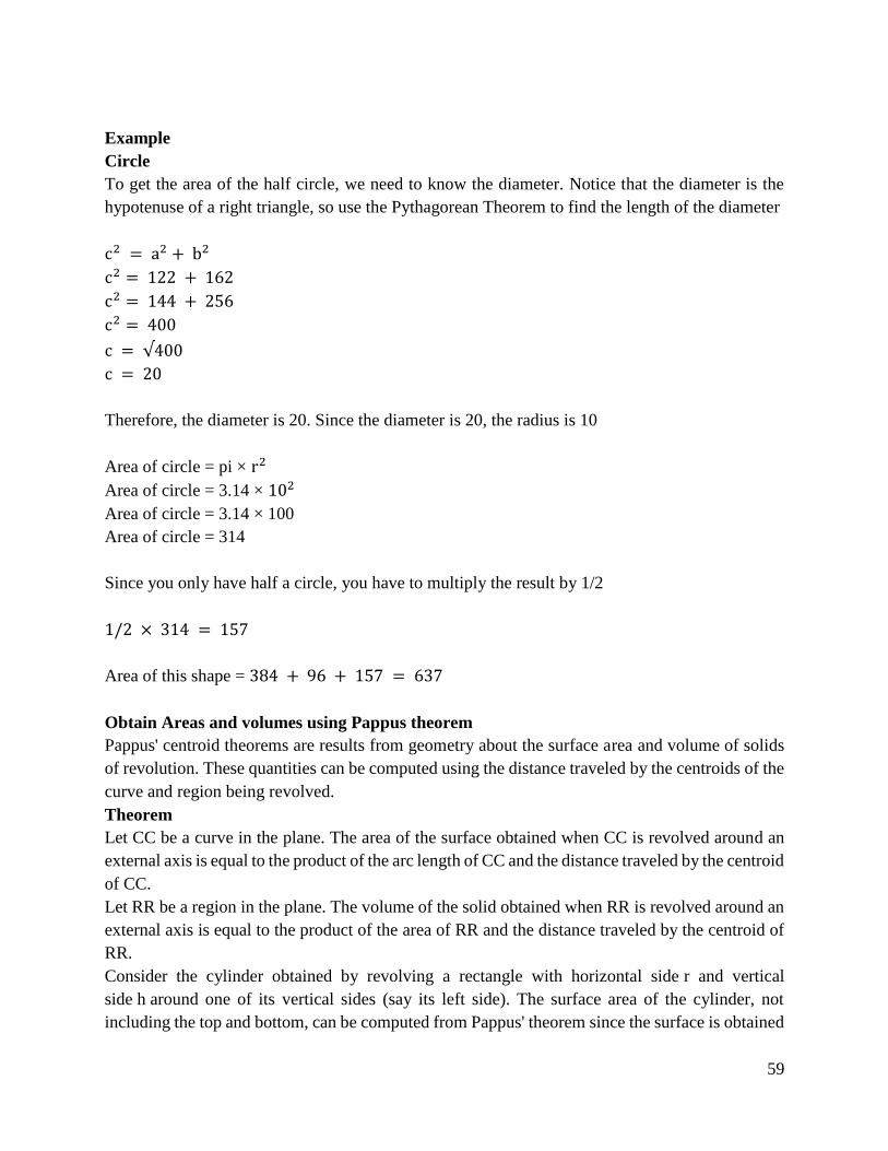
59
Example
Circle
To get the area of the half circle, we need to know the diameter. Notice that the diameter is the
hypotenuse of a right triangle, so use the Pythagorean Theorem to find the length of the diameter
c2 = a2 + b2
c2 = 122 + 162
c2 = 144 + 256
c2 = 400
c = √400
c = 20
Therefore, the diameter is 20. Since the diameter is 20, the radius is 10
Area of circle = pi × r2
Area of circle = 3.14 × 10²
Area of circle = 3.14 × 100
Area of circle = 314
Since you only have half a circle, you have to multiply the result by 1/2
1/2 × 314 = 157
Area of this shape = 384 + 96 + 157 = 637
Obtain Areas and volumes using Pappus theorem
Pappus' centroid theorems are results from geometry about the surface area and volume of solids
of revolution. These quantities can be computed using the distance traveled by the centroids of the
curve and region being revolved.
Theorem
Let CC be a curve in the plane. The area of the surface obtained when CC is revolved around an
external axis is equal to the product of the arc length of CC and the distance traveled by the centroid
of CC.
Let RR be a region in the plane. The volume of the solid obtained when RR is revolved around an
external axis is equal to the product of the area of RR and the distance traveled by the centroid of
RR.
Consider the cylinder obtained by revolving a rectangle with horizontal side r and vertical
side h around one of its vertical sides (say its left side). The surface area of the cylinder, not
including the top and bottom, can be computed from Pappus' theorem since the surface is obtained
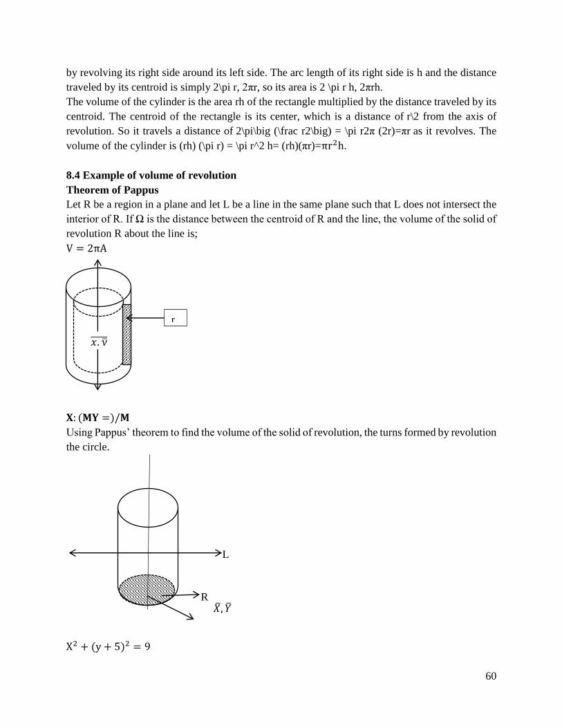
60
by revolving its right side around its left side. The arc length of its right side is h and the distance
traveled by its centroid is simply 2\pi r, 2πr, so its area is 2 \pi r h, 2πrh.
The volume of the cylinder is the area rh of the rectangle multiplied by the distance traveled by its
centroid. The centroid of the rectangle is its center, which is a distance of r\2 from the axis of
revolution. So it travels a distance of 2\pi\big (\frac r2\big) = \pi r2π (2r)=πr as it revolves. The
volume of the cylinder is (rh) (\pi r) = \pi r^2 h= (rh)(πr)=πr2h.
8.4 Example of volume of revolution
Theorem of Pappus
Let R be a region in a plane and let L be a line in the same plane such that L does not intersect the
interior of R. If Ω is the distance between the centroid of R and the line, the volume of the solid of
revolution R about the line is;
V = 2πA
𝐗: (𝐌𝐘 =)/𝐌
Using Pappus’ theorem to find the volume of the solid of revolution, the turns formed by revolution
the circle.
X2 + (y + 5)2 = 9
r
𝑥, 𝑦തതതതതത
R
L
𝑋ത, 𝑌ത
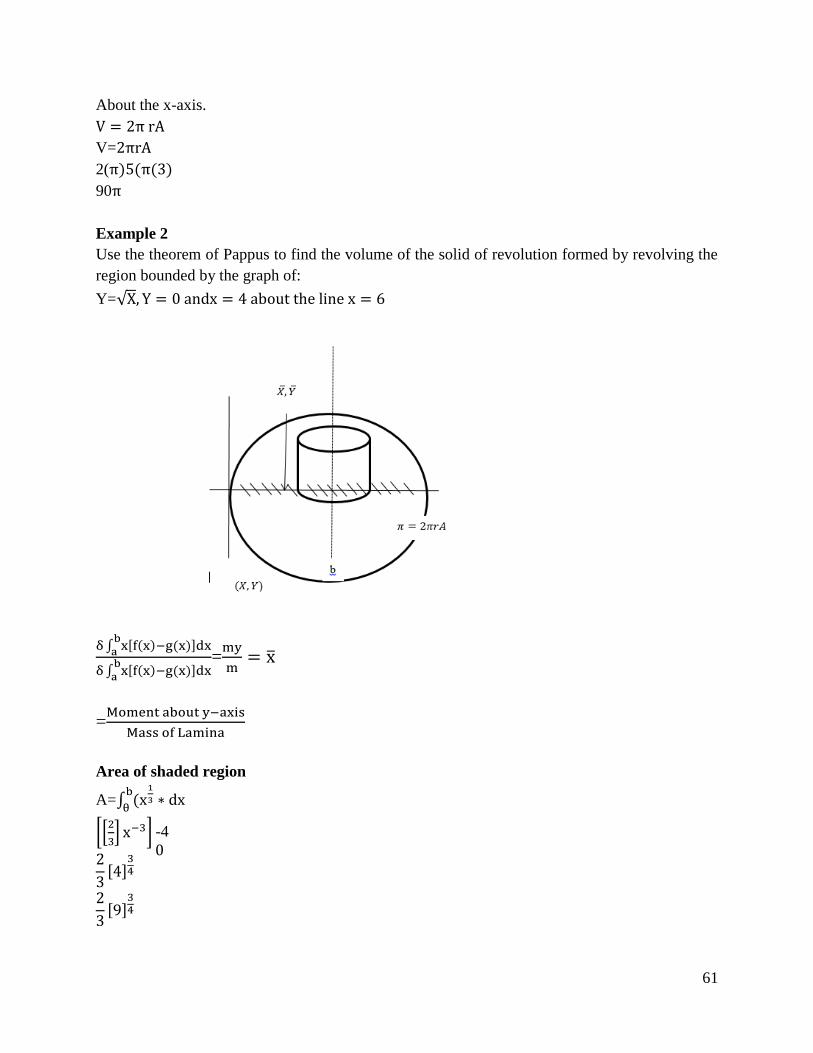
61
About the x-axis.
V = 2π rA
V=2πrA
2(π)5(π(3)
90π
Example 2
Use the theorem of Pappus to find the volume of the solid of revolution formed by revolving the
region bounded by the graph of:
Y=√X, Y = 0 andx = 4 about the line x = 6
δ∫ xb
a[f(x)−g(x)]dx
δ∫ xb
a[f(x)−g(x)]dx
=my
m= xത
=Moment about y−axis
Mass of Lamina
Area of shaded region
A=∫ (x1
3 ∗ dxb
θ
[[2
3] x−3]
2
3[4]
34
2
3[9]
34
-4
0
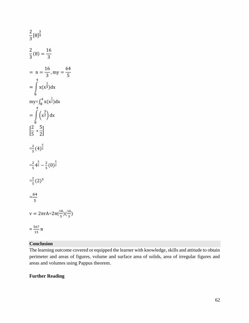
62
2
3[8]
34
2
3(8) =
16
3
= n =16
3,my =
64
5
= ∫x(x13)dx
4
θ
my=∫ x(x1
2)dx4
θ
= ∫(x32) dx
4
θ
[2
5 ∗
5
2]
=2
5(4)
5
2
=2
54
5
2 −2
5(0)
5
2
=2
5(2)5
=64
5
v = 2πrA=2π(18
5)(
16
3)
= 567
15π
Conclusion
The learning outcome covered or equipped the learner with knowledge, skills and attitude to obtain
perimeter and areas of figures, volume and surface area of solids, area of irregular figures and
areas and volumes using Pappus theorem.
Further Reading
63
1. Hoyland, A., Rausand, and M. (1994), System Reliability Theory: Models and Statistical
Methods, John Wiley (New York).
2.3.9.3 Self-Assessment
Written Assessment
1. An equilateral triangle of side length rr in the first quadrant, one of whose sides lies on
the xx-axis, is revolved around the line y= -r.y=−r. The volume of the resulting solid is c\pi
r^3cπr3 for some real number c.c. What is c.c?
2. Consider the single rectangle in R2 that passes through the points A = (1,2), B = (2,1),
C = (4,3), D = (3,4) A rotating around x-axis in R3. The volume of the surface of revolution
obtained can be written as A3 Aπ unit3. Submit A
3. Revolving a right triangle with legs of length r and h around the leg of length h produces a
cone. The surface of the cone (not including the circular base) is obtained by revolving the
hypotenuse around that leg. The centroid of the hypotenuse is just the midpoint, located
halfway up the side of the cone, which travels a distance 2π/2 as it rotates. So the surface
area is 2πr√R2 + H2
4. Consider the cylinder obtained by revolving a rectangle with horizontal side r and vertical
side h around one of its vertical sides (say its left side). The surface area of the cylinder,
not including the top and bottom, can be computed from Pappus's theorem since the surface
is obtained by revolving its right side around its left side. The arc length of its right side is
h and the distance traveled by its centroid is simply2π, 2πr, so its area is 2πr h. 2πrh.
2.3.9.4 Tools, Equipment, Supplies and Materials
Scientific Calculators
Rulers, pencils, erasers
Charts with presentations of data
Graph books
Dice
Computers with internet connection
2.3.9.5 References

64
Hoyland, A., Rausand, and M. (1994), System Reliability Theory: Models and Statistical Methods,
John Wiley (New York).
Kaplan, W. (1984), Advanced Calculus, 3rd ed., Addison-Wesley (Cambridge, MA).
Kreyszig, E. (1999), Advanced Engineering Mathematics, 8th ed., John Wiley (New York).
O'Neil, P.V. (1995), Advanced Engineering Mathematics, 4th ed., PWS-Kent Pub. (Boston).
65
2.3.10 Learning Outcome No 9: Apply power series
2.3.10.1 Learning Activities
Learning Outcome No 9 : Apply power series
Learning Activities Special Instructions
9.1 Obtain power series using Taylor’s Theorem
9.2 Obtain power series using McLaurin’s theorem
2.3.10.2 Information Sheet No2/LO9: Apply power series
Introduction
This learning outcome covers; derivation of power series using Taylor’s Theorem and derivation
of power series using McLaurin’s theorem.
Content/Procedures/Methods/Illustrations
9.1 Obtain power series using Taylor’s Theorem
The power series of McLaurin’s theorem is different functions can be carried out using two
theorems.
(i) Taylor’s Theorem
(ii) Maclaurin’s theorem
Taylor’s series states that;
f(x + h) = f(x) + hf ′(x) +h2
2!f ′′(x) +
h3
3!f ′′′(x) + …
Examples
Express Sin(x + h) as a series of powers of h and hence evaluates Sin 440 correct to four decimal
places.
Solution
f(x + h) = f(x) + hf ′(x) +h2
2!f ′′(x) +
h3
3!f ′′′(x) + ⋯
f(x) = Sinx
f′(x) = cos x
f′′(x) = −sinx
f ′′′(x) =-cosx
f iv(x) = sin x
66
∴ Sin(x + h) = sin x + hcos x −h2
2sin x -
h3
6 cos x….
Sin440 = sin(450 − 10)
=Sin(π 4⁄ ) − 0.01745
=sin π4⁄ + 0.01745 cos
π
4 -
0.017452
2sin π
4⁄ − 0.0174s3
6 cos π
4⁄
But sin45 = cos 45 = 0.707
= 0.707 (1 − 0.01745 − 0.0001523 + 0.0000009)
= 0.707(0.982395)
= 0.69466
0.6947(4dp)
For the use McLaurin’s theorem refer to Engineering Mathematics by Strand.
Conclusion
The learning outcome covered or equipped the learner with knowledge, skills and attitude to derive
power series using Taylor’s Theorem and power series using McLaurin’s theorem.
Further Reading
1. Greenberg, M.D. (1998), Advanced Engineering Mathematics, 2nd ed., Prentice Hall
(Upper Saddle River, N.J).
2. Hildebrand, F.B. (1974), Introduction to Numerical Analysis, 2nd ed., McGraw-Hill (New
York).
3. Hildebrand, F.B. (1976), Advanced Calculus for Applications, 2nd ed., Prentice-Hall
(Englewood Cliffs, NJ).
2.3.10.3 Self-Assessment
Written Assessment
1. Use McLaurin’s theorem to expand ln(3x + 1). Hence use the expansion to evaluate
∫ln(3x+1)
x2 dx 1
0 to four decimal places.
2. Use Taylor’s series to expand cos (π
3+ h) in terms of h as far as h3. Hence evaluate cos680
correct to four decimal places.

67
2.3.10.4 Tools, Equipment, Supplies and Materials
Scientific Calculators
Rulers, pencils, erasers
Charts with presentations of data
Graph books
Dice
Computers with internet connection
2.3.10.5 References
Hoyland, A., Rausand, and M. (1994), System Reliability Theory: Models and Statistical Methods,
John Wiley (New York).
Kaplan, W. (1984), Advanced Calculus, 3rd ed., Addison-Wesley (Cambridge, MA).
Kreyszig, E. (1999), Advanced Engineering Mathematics, 8th ed., John Wiley (New York).
68
2.3.11 Learning Outcome No10: Apply statistics
2.3.11.1 Learning Activities
Learning Outcome No10: Apply statistics
Learning Activities Special
Instructions
10.1. Obtain mean, median, mode and standard deviation from given data
10.2. Perform calculations based on laws of probability
10.3. Perform calculation involving probability distributions (binomial,
Poisson, normal) mathematical expectation sampling distributions
10.4. Apply sampling distribution methods in data analysis
10.5. Work out calculations involving use of standard normal table, sampling
distribution, T-distribution and estimation
10.6. Determine confidence intervals
Give real life
application
examples
2.3.11.2 Information Sheet No2/LO10: Apply statistics
Introduction
This learning outcome covers mean, mode and median and standard deviation from given data,
perform calculations based on Laws of probability, calculation involving probability distributions
(binomial, Poisson, normal) mathematical expectation sampling distributions, and calculations
involving use of standard normal table, sampling distribution, T-distribution and Estimation.
Definition of key terms
Statistics: It is discipline which deals with collection, organization, presentation and analysis of
data.
Data: It consists of a set of records and observations that carry information on a particular setting
with the availability of data.
Content/Procedures/Methods/Illustrations
A statistical exercise normally consists of four stages i.e.
Collection of data
Organization and presentation of data in convenient form
Analysis of data to make their meaning clear
Interpretation of 1b results and the conclusion
69
In statistics, we consider quantities that are varied. These quantities are referred to as variables.
Variables are denoted by letters
Examples
Heights
Ages
Weighs
Times
Types of data
1. Quantitative data
2. Qualitative data
Presentation of data
The aim of presenting data is to communicate information. The type of presentation chosen
depends on the requirement and the interest of people receiving that particular information.
Frequently the first stage in presenting is preparing a table.
Tabulation of data
Given a set of raw data we usually arrange into frequency distribution where we collect like
quantities and display them by writing down their frequencies.
For those on data presentation refer to Engineering Mathematics by K.A Stroud.
Measurers of Dispersion
They include:
Range
Standard deviation
Quartiles
This is a continuous distribution. It is derived as the limit of the Binomial distribution for large
values of n and p and q are not very small.
The normal distribution is given by the equation:
fx) =1
σ√2πe−
1
2σ2(x−μ)2
Where μ is the mean and σ is the standard deviation, π = 3.14159 and e = 2.71828P(x1 < x <
x2) = ∫1
σ√2πe−
1
2σ2(x−μ)2dx…………………… . (1)
x2
x1
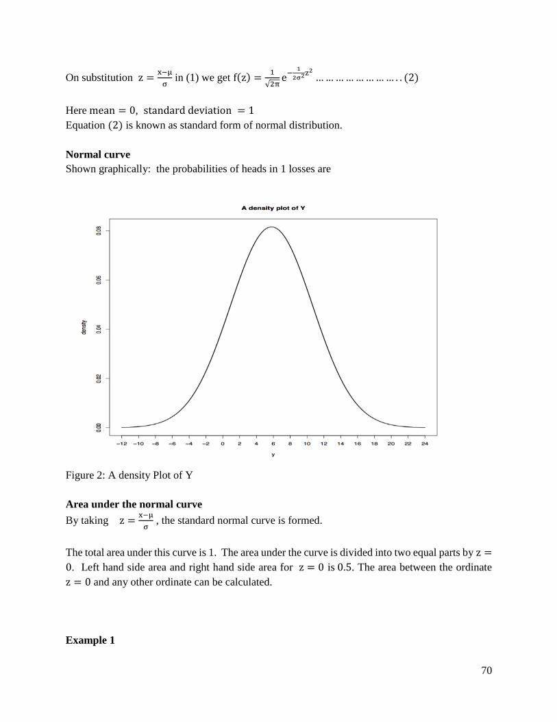
70
On substitution z =x−μ
σ in (1) we get f(z) =
1
√2πe−
1
2σ2z2
…………………… . . (2)
Here mean = 0, standard deviation = 1
Equation (2) is known as standard form of normal distribution.
Normal curve
Shown graphically: the probabilities of heads in 1 losses are
Figure 2: A density Plot of Y
Area under the normal curve
By taking z =x−μ
σ , the standard normal curve is formed.
The total area under this curve is 1. The area under the curve is divided into two equal parts by z =
0. Left hand side area and right hand side area for z = 0 is 0.5. The area between the ordinate
z = 0 and any other ordinate can be calculated.
Example 1
71
On the final examination in Mathematics the mean was 72 and the standard deviation was 15.
Determine the standard scores of students receiving grades
a) 60 b) 93 c) 72
Solution
a) z =x−μ
σ=
60−72
15= −0.8
b) z =93−72
15= 1.4
c) z =72−72
15= 0
Conclusion
The learning outcome covered mean, mode and median and standard deviation from given data,
perform calculations based on Laws of probability, calculation involving probability distributions
(binomial, Poisson, normal) mathematical expectation sampling distributions, and calculations
involving use of standard normal table, sampling distribution, T-distribution and Estimation.
Further Reading
1. For more refer to Mathematics for Engineers by H.K Dass.
2. Read on Poisson and standard deviation of Binomial distribution
2.3.11.3 Self-Assessment
Written Assessment
3. A machine produced components whose masses are normally distributed with mean μ and
standard deviation σ if 89.8 % of the components have a mass of at least 88g and 3% have
a mass less than 84.5g, find the mean and the standard deviation of the distribution (6mks).
4. The diameters of bolts produced by a certain machine are distributed by a probability
density function
f(x) = kx(3 − x), 0 ≤ x ≤ 3
0 Otherwise
Find:
a) The Constant k.
b) Probability that the diameter of a bolt-selected at a random will fall in the interval
1 < x < 2.5
c) Mean and the variance of the distribution (14mks)
72
5. Tumaini Ltd, is supplied with petrol once a week. The weekly demand, x hundreds of
liters, has the probability density function
f(x) = k(1 − x), 0 ≤ x ≤ 1
0 Otherwise
Where c is a constant
Determine the:
a) Value of c
b) Mean of x
6. Minimum capacity of the petrol tank if the probability that it will be exhausted in a given
week is not to exceed 0.02.
7. Metal bars produced in a factory have masses that are normally distributed with mean μand
standard deviationσ. Given that 9.4% have a mass less than 45kg and 7% have a mass
above 75kg. Evaluate the values of μ and σ.
8. Find the probability that a mass of a metal bar selected at random will be less than 40kg.
2.3.11.4 Tools, Equipment, Supplies and Materials
Scientific Calculators
Rulers, pencils, erasers
Charts with presentations of data
Graph books
Dice
Computers with internet connection
2.3.11.5 References
Greenberg, M.D. (1998), Advanced Engineering Mathematics, 2nd ed., Prentice Hall (Upper
Saddle River, N.J).
Hoyland, A., Rausand, and M. (1994), System Reliability Theory: Models and Statistical Methods,
John Wiley (New York).
Kaplan, W. (1984), Advanced Calculus, 3rd ed., Addison-Wesley (Cambridge, MA).
Kreyszig, E. (1999), Advanced Engineering Mathematics, 8th ed., John Wiley (New York).
O'Neil, P.V. (1995), Advanced Engineering Mathematics, 4th ed., PWS-Kent Pub. (Boston).
73
2.3.12 Learning Outcome No 11: Apply numerical methods
2.3.12.1 Learning Activities
Learning Outcome No 11: Apply numerical methods
Learning Activities Special Instructions
11.1. Obtain roots of polynomials using iterative numerical methods
(Newton Raphson and Gregory Newton)
11.2. Perform interpolation and extrapolation using numerical methods
2.3.12.2 Information Sheet No2/LO11: Apply numerical methods
Introduction
This learning outcome covers Application of numerical methods, roots of polynomials, and
performing interpolation and extrapolation using numerical methods.
Definition of key terms
Numerical methods: Are algorithms used for computing numeric data.
Content/Procedures/Methods/Illustrations
11.1 Obtain roots of polynomials using iterative numerical methods (Newton Raphson and
Gregory Newton)
Numerical method is a complete and definite set of procedures for the solution of a problem,
together with computable error estimates. The study and implementation of such methods is the
province of numerical analysis.
Types of numerical methods
a) Bisection method
b) Newton Raphson method (Newton’s Iteration method)
c) Iteration method
d) Newton’s forward interpolation formula
e) Newton’s backward interpolation formula
f) Gauss Seided method
g) Curve fitting
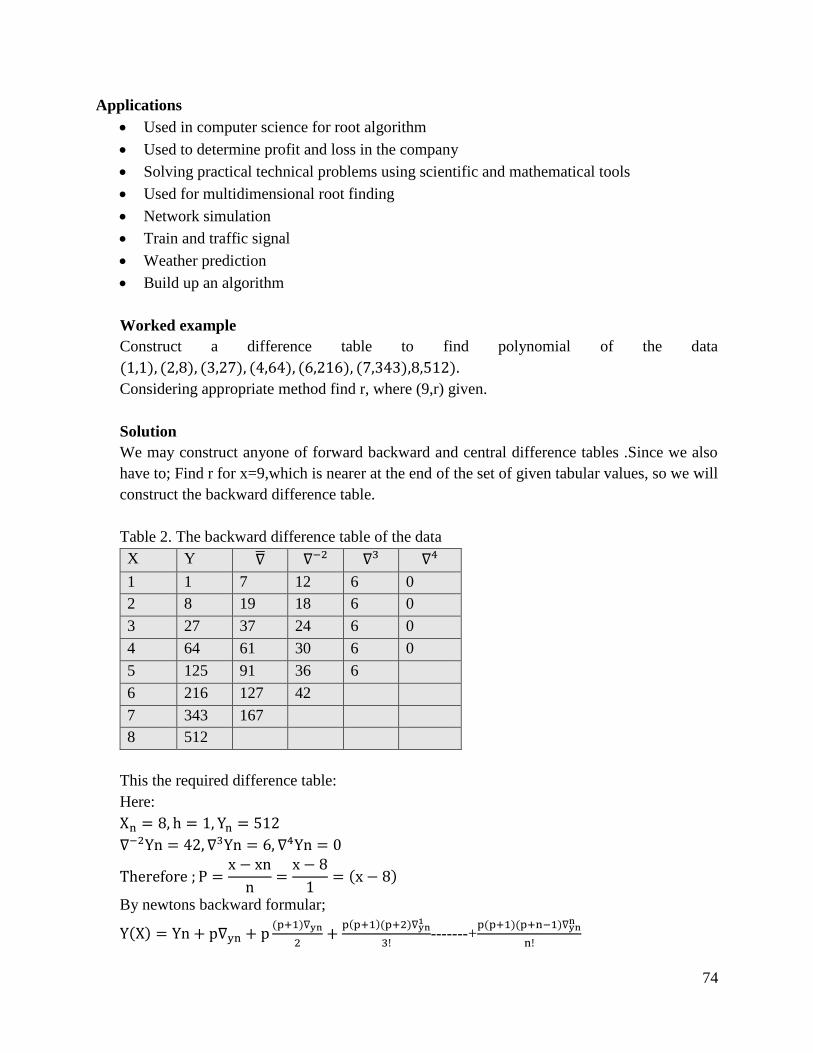
74
Applications
Used in computer science for root algorithm
Used to determine profit and loss in the company
Solving practical technical problems using scientific and mathematical tools
Used for multidimensional root finding
Network simulation
Train and traffic signal
Weather prediction
Build up an algorithm
Worked example
Construct a difference table to find polynomial of the data
(1,1), (2,8), (3,27), (4,64), (6,216), (7,343),8,512).
Considering appropriate method find r, where (9,r) given.
Solution
We may construct anyone of forward backward and central difference tables .Since we also
have to; Find r for x=9,which is nearer at the end of the set of given tabular values, so we will
construct the backward difference table.
Table 2. The backward difference table of the data
X Y ∇ ∇−2 ∇3 ∇4
1 1 7 12 6 0
2 8 19 18 6 0
3 27 37 24 6 0
4 64 61 30 6 0
5 125 91 36 6
6 216 127 42
7 343 167
8 512
This the required difference table:
Here:
Xn = 8, h = 1, Yn = 512
∇−2Yn = 42, ∇3Yn = 6, ∇4Yn = 0
Therefore ; P =x − xn
n=
x − 8
1= (x − 8)
By newtons backward formular;
Y(X) = Yn + p∇yn + p(p+1)∇yn
2+
p(p+1)(p+2)∇yn1
3!-------+
p(p+1)(p+n−1)∇ynn
n!

75
= 512 = 169(x − 8) + (x − 8)(x − 8 + 1) ∗ 42
2!
Conclusion
The learning outcome covered apply numerical methods, roots of polynomials, and perform
interpolation and extrapolation using numerical methods.
Further Reading
2.3.12.4 Tools, Equipment, Supplies and Materials
Scientific Calculators
Rulers, pencils, erasers
Charts with presentations of data
Graph books
Dice
Computers with internet connection
2.3.12.5 References
Greenberg, M.D. (1998), Advanced Engineering Mathematics, 2nd ed., Prentice Hall (Upper
Saddle River, N.J).
Hildebrand, F.B. (1974), Introduction to Numerical Analysis, 2nd ed., McGraw-Hill (New York).
Hildebrand, F.B. (1976), Advanced Calculus for Applications, 2nd ed., Prentice-Hall (Englewood
Cliffs, NJ).
Hoyland, A., Rausand, and M. (1994), System Reliability Theory: Models and Statistical Methods,
John Wiley (New York).
76
2.3.13 Learning Outcome No12: Apply vector theory
2.3.13.1 Learning Activities
Learning Outcome No 12:apply vector theory
Learning Activities Special Instructions
12.1 Obtain vectors and scalar quantities in two and three dimensions
12.2 Perform Operations (addition and subtraction)on vectors
12.3 Obtain position of vectors
12.4 Work out resolution of vectors
Encourage students
to practice
2.3.13.2 Information Sheet No2/LO12: Apply vector theory
Introduction
This learning outcome covers vectors and scalar quantities in two and three dimensions, operations
on vectors, and position and resolution of vectors.
Definition of key terms
Vectors: A quantity having direction as well as magnitude, especially as determining the position
of one point in space relative to another. A vector has both magnitude and direction, and both these
properties must be given in order to specify it. A quantity with magnitude but no direction is called
a scalar.
Content/Procedures/Methods/Illustrations
12.1 Apply Vector theory
Physical quantities can be divided into two main groups, scalar quantities and vector quantities. A
Scalar quantity is one that is defined completely by a single number with appropriate units e.g.
Lengths, area, volume, mass, time etc. A Vector quantity is defined completely when we know not
only its magnitude but also the direction in which it operates, e.g. force, velocity, acceleration etc.
Vector quantities are extremely useful in physics. The important characteristic of a vector quantity
is that it has both a magnitude (and size) and a direction. Both of these properties must be given in
order to specify a vector completely. An example of a vector quantity is a displacement. This tell
us how far away we are from a fixed point, and it also tells us our direction relative to that point.
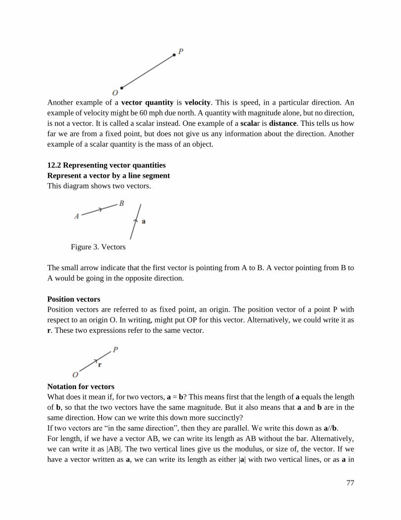
77
Another example of a vector quantity is velocity. This is speed, in a particular direction. An
example of velocity might be 60 mph due north. A quantity with magnitude alone, but no direction,
is not a vector. It is called a scalar instead. One example of a scalar is distance. This tells us how
far we are from a fixed point, but does not give us any information about the direction. Another
example of a scalar quantity is the mass of an object.
12.2 Representing vector quantities
Represent a vector by a line segment
This diagram shows two vectors.
Figure 3. Vectors
The small arrow indicate that the first vector is pointing from A to B. A vector pointing from B to
A would be going in the opposite direction.
Position vectors
Position vectors are referred to as fixed point, an origin. The position vector of a point P with
respect to an origin O. In writing, might put OP for this vector. Alternatively, we could write it as
r. These two expressions refer to the same vector.
Notation for vectors
What does it mean if, for two vectors, a = b? This means first that the length of a equals the length
of b, so that the two vectors have the same magnitude. But it also means that a and b are in the
same direction. How can we write this down more succinctly?
If two vectors are “in the same direction”, then they are parallel. We write this down as a//b.
For length, if we have a vector AB, we can write its length as AB without the bar. Alternatively,
we can write it as |AB|. The two vertical lines give us the modulus, or size of, the vector. If we
have a vector written as a, we can write its length as either |a| with two vertical lines, or as a in
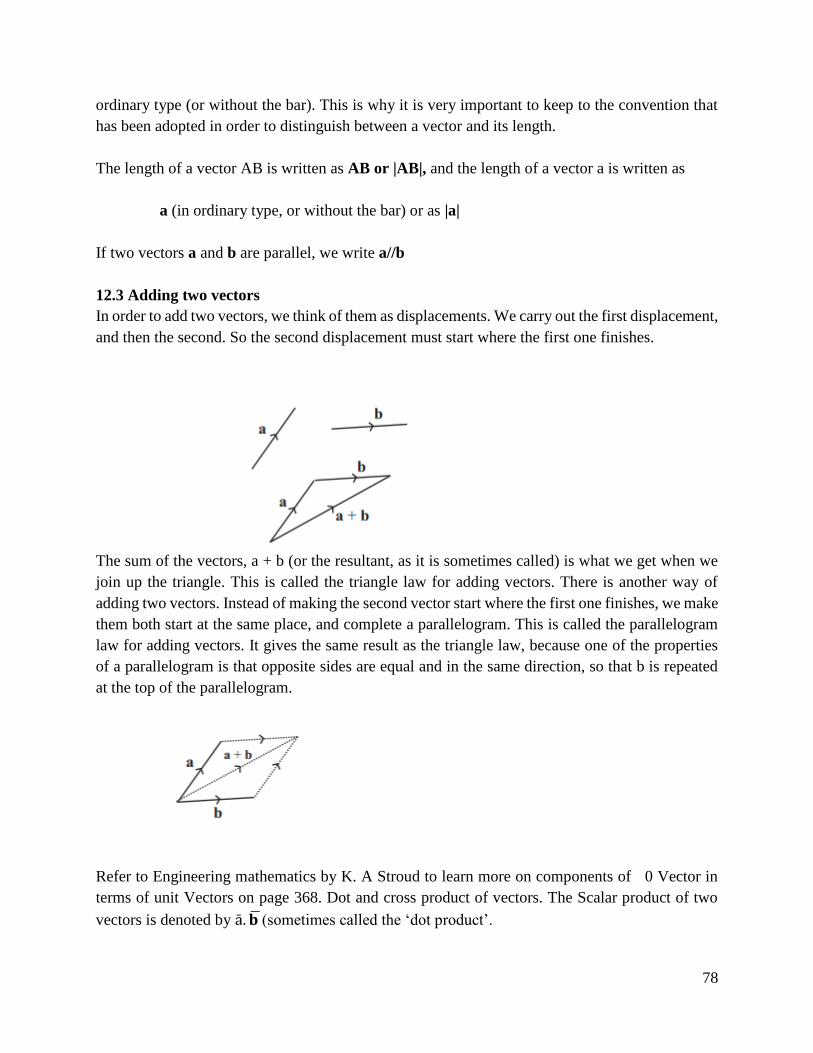
78
ordinary type (or without the bar). This is why it is very important to keep to the convention that
has been adopted in order to distinguish between a vector and its length.
The length of a vector AB is written as AB or |AB|, and the length of a vector a is written as
a (in ordinary type, or without the bar) or as |a|
If two vectors a and b are parallel, we write a//b
12.3 Adding two vectors
In order to add two vectors, we think of them as displacements. We carry out the first displacement,
and then the second. So the second displacement must start where the first one finishes.
The sum of the vectors, a + b (or the resultant, as it is sometimes called) is what we get when we
join up the triangle. This is called the triangle law for adding vectors. There is another way of
adding two vectors. Instead of making the second vector start where the first one finishes, we make
them both start at the same place, and complete a parallelogram. This is called the parallelogram
law for adding vectors. It gives the same result as the triangle law, because one of the properties
of a parallelogram is that opposite sides are equal and in the same direction, so that b is repeated
at the top of the parallelogram.
Refer to Engineering mathematics by K. A Stroud to learn more on components of 0 Vector in
terms of unit Vectors on page 368. Dot and cross product of vectors. The Scalar product of two
vectors is denoted by ā. 𝐛 (sometimes called the ‘dot product’.
79
The dot product of two vectors is defined as 𝐚. 𝐛 = |𝐚||𝐛|𝐜𝐨𝐬𝛉 where θ is the angle between a and
b.
Refer to Technician mathematics 3 by J.O. Bird on page 297.
Examples
Solution
𝐚ത = 𝟐𝐢 + 𝟑𝐣 + 𝟓𝐤 And = 𝟒𝐢 + 𝐣 + 𝟔𝐤, 𝐚ത.
aത . bത = 2.4 + 3.1 + 5.6
= 8 + 3+ 30
=41
A typical application of scalar products is that of determining the work done by a force when
moving a body. The amount of work done is the product of the applied force and the distance
moved in the direction of the applied force.
Example
Find the work done by a force F newtons acting at point A on a body, when A is displaced to point
B, the coordinates of A and B being (3, 1, -2) and (4, -1, 0) metres respectively and when
F = − i − 2j − k Newton’s.
Solution
If a vector displacement from A to B is d, then the work done is F. d Newton Meters or joules.
The position vector OA is 3i + j − 2k and OB is 4i − j
AB = d = OB − OA
= (4i – j) – (3i + j − 2k )
i – 2j + 2k.
Work done = F. d = (−1)/1) + (−2)(−2) + (−1)(2)
= −1 + 4 − 2
=1 Nm or joule
For more worked examples refer to Technician mathematics 3 by J. O. Bird.
Cross Product
The vector or Cross product of two vectors ā and bത is C where the magnitude of C is
|ā||b|Sinθ where θ is the angle between aത and b.
For more information refer to Technician mathematics 3 by J.O Bird and Engineering mathematics
by K. A Stroud.
80
Examples
pത = 2i + 4j + 3k and Q = i + 5j − 2k find P x Q = |i j k2 4 31 5 −2
|
=i |4 35 −2
| − j |2 31 −2
| + k |2 41 5
|
=−23i + 7j + 6k
Typical applications of vector products are to moments and to angular velocity.
Refer to Technician mathematics. 3 by J.O Bird on page 308.
12.4 Vector field Theory
Refer to further Engineering mathematics by K.A Stroud to learn and also go through the worked
examples and exercises on:
(i) Gradient
(ii) Divergence
(iii) Curl
Greens theorem
Learn how to perform vector calculations using Green’s theorem by referring to further Engineer
mathematics by KA. Stroud.
Stoke’s Theorem
Refer to further Engineer Mathematics by K.A Stroud to learn how to perform vector calculations
using Stroke’s theorem.
Gauss’s Theorem
Refer to the some book to learn how to determine line and surface integrals using Gauss’s theorem.
Conclusion
This learning outcome covered vectors and scalar quantities in two and three dimensions,
operations on vectors, and position and resolution of vectors.
Further Reading
1. Greenberg, M.D. (1998), Advanced Engineering Mathematics, 2nd ed., Prentice Hall
(Upper Saddle River, N.J).
2.3.13.3 Self-Assessment
81
Written Assessment
If aത =2i - 3j + 4k and bത = i + 2j + 5k determine
(2) aത . bത
(22) aത x bത
1. Find the work done by a force F Newtons acting at a point A on a body, when A is
displaced to point B ,the coordinates of A and B being (5, 2, -4) and (3,-1,1) meters
respectively , and when F = −2i − 3j − 2k Newton’s.
2.3.13.4 Tools, Equipment, Supplies and Materials
Scientific Calculators
Rulers, pencils, erasers
Charts with presentations of data
Graph books
Dice
Computers with internet connection
2.3.13.5 References
Duffy, D. G. (2016). Advanced engineering mathematics with MATLAB. Chapman and
Hall/CRC.
Jeffrey, A. (2001). Advanced engineering mathematics. Elsevier.
Zill, D., Wright, W. S., & Cullen, M. R. (2011). Advanced engineering mathematics. Jones &
Bartlett Learning.
82
2.3.14 Learning Outcome No13: Apply matrix
2.3.14.1 Learning Activities
Learning Outcome No13: Apply matrix
Learning Activities Special Instructions
13.1 Obtain determinant and inverse of 3x3 matrix
13.2 Obtain solutions of simultaneous equations
13.3 Perform calculation involving Eigen values and Eigen vectors
2.3.14.2 Information Sheet No2/LO13: Apply matrix
Introduction
This learning outcome enables the learner to obtain determinant of a 3x3 matrix; obtain solutions
of simultaneous equations; perform calculation involving Eigen values and Eigen vectors
Definition of key terms
Matrix: It is a set of real or complex numbers (or elements) arranged in rows and columns to form
a rectangular array.
Content/Procedures/Methods/Illustrations
A matrix having M rows and N columns is called a M × N(i. e M by N) matrix and is referred to
as having orderM × N.
A matrix is indicated by writing the array with large square brackets e.g.
[5 7 26 3 8
]is a 2 × 3 matrix i.e 2 by 3 matrix where 5,7,2,6,3 and 8 are the elements of the matrix.
Operation on matrices
1. Addition and subtraction
Matrices can be added or subtracted if they are of the same order.
Example
Given matrix A = [−1 2 53 0 41 −3 2
] and B = [3 2 −1
−2 1 61 −4 5
]
83
A + B = [−1 2 53 0 41 −3 2
] + [3 2 −1
−2 1 61 −4 5
] = [
(−1 + 3) (2 + 2) (3 ± −1)(3 ± 2) (0 + 1) (4 + 6)(1 + 1) (−3 ± 4) (2 + 5)
]
= [2 4 41 1 102 −7 7
]
2. Multiplication of Matrices
Example
Given matrix A = [−1 2 53 0 41 −3 2
] and B = [3 2 −1
−2 1 61 −4 5
]
A × B = [−1 2 53 0 41 −3 2
] [3 2 −1
−2 1 61 −4 5
]
= [1 × 3 + 2 × −2 + 5 ÷ 1 −1 × 2 + 2 × 1 + 6 × −4 −1 × 1 + 2 × 6 + 5 × 53 × 3 + 0 × −2 + 4 × 1 3 × 2 − 0 × 1 + 4 × −4 3 × −1 + 0 × 6 + 4 × 5
1 × 3 + −3 × −2 + 2 × 1 1 × 2 − 3 × 1 + 2 × −4 1 × −1 + 6 × −3 + 2 × 5]
= [−3 − 4 + 5 −2 + 2 − 20 −1 + 12 + 259 + 0 + 4 6 + 0 − 16 −3 + 0 + 2 03 + 6 + 2 1 − 3 − 8 −1 − 1 + 10
]
= [2 −20 3613 ∗ 10 1711 −10 −9
]
Note that in matrices AB ≠ BA
For more examples on matrices operations refer to Pure Mathematics I.
13.1 Determinant and inverse of 3x3 matrix are obtained
Determinant of a 𝟑 × 𝟑 matrix
Refer to engineering mathematics by K.A Strond and learn more on how to find the determinant
of a 3 × 3 (“3 by 3”) matrix.
Inverse of a 𝟑 × 𝟑 matrix
Example
To find the inverse of A = [1 2 34 1 56 0 2
]
84
Evaluate the determinant of A i.e |A|
a) For A = [1 2 34 1 56 0 2
], |A| = 1(2 − 0) − 2(8 − 30) + 3(0 − 6) = 28
b) Now from the matrix of the cofactors
C = [2 22 −6
−4 −16 127 7 −7
]
c) Next we have to write down the transpose of “C” to find the adjoint of “A”
Adj A = CT = [2 −4 722 −16 7−6 12 −7
]
d) Finally we divide the elements of adj A by the value of |A| i.e 28 to get A−1 the inverse
ofA.
A−1 =
[
2
28
−4
28
7
2822
28
−16
28
12
28−6
28
7
28
−7
28]
=1
28[
2 −4 722 −16 7−6 12 −7
]
13.2 Solutions of simultaneous equations are obtained
Solution of linear equation in three unknowns
Solve the set of equations
x1 + 2x2 + x3 = 4
3x1 − 4x2 − 2x3 = 2
5x1 + 3x2 + 5x2 = −1
First write the set of equations in matrix form
[1 2 13 −4 −26 3 5
] [
x1
x2
x3
] = [421]
Next step is to find the inverse of A where A is the square matrix on the left hand side.
|A| = |1 2 13 −4 −25 3 5
| = −14 − 50 + 29 = 29 − 64 = −35
Therefore |A| = −35
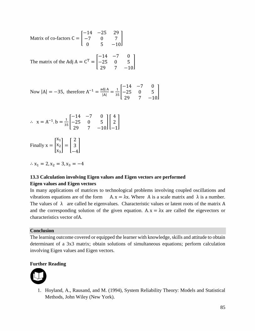
85
Matrix of co-factors C = [−14 −25 29−7 0 70 5 −10
]
The matrix of the Adj A = CT = [−14 −7 0−25 0 529 7 −10
]
Now |A| = −35, therefore A−1 =adj A
|A|=
1
35[−14 −7 0−25 0 529 7 −10
]
∴ x = A−1. b =1
35[−14 −7 0−25 0 529 7 −10
] [42
−1]
Finally x = [
x1
x2
x3
] = [23
−4]
∴ x1 = 2, x2 = 3, x3 = −4
13.3 Calculation involving Eigen values and Eigen vectors are performed
Eigen values and Eigen vectors
In many applications of matrices to technological problems involving coupled oscillations and
vibrations equations are of the form A. x = λx. Where A is a scale matrix and λ is a number.
The values of λ are called he eigenvalues. Characteristic values or latent roots of the matrix A
and the corresponding solution of the given equation. A. x = λx are called the eigevectors or
characteristics vector ofA.
Conclusion
The learning outcome covered or equipped the learner with knowledge, skills and attitude to obtain
determinant of a 3x3 matrix; obtain solutions of simultaneous equations; perform calculation
involving Eigen values and Eigen vectors.
Further Reading
1. Hoyland, A., Rausand, and M. (1994), System Reliability Theory: Models and Statistical
Methods, John Wiley (New York).
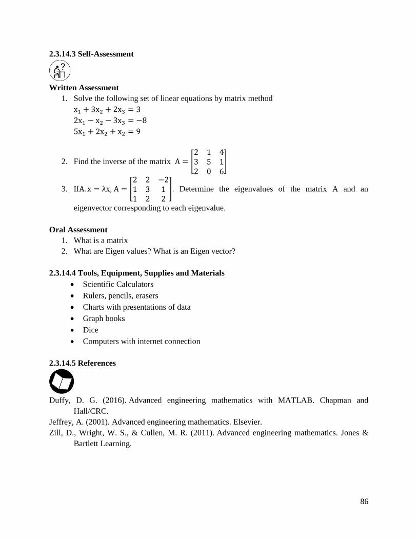
86
2.3.14.3 Self-Assessment
Written Assessment
1. Solve the following set of linear equations by matrix method
x1 + 3x2 + 2x3 = 3
2x1 − x2 − 3x3 = −8
5x1 + 2x2 + x2 = 9
2. Find the inverse of the matrix A = [2 1 43 5 12 0 6
]
3. IfA. x = λx, A = [2 2 −21 3 11 2 2
]. Determine the eigenvalues of the matrix A and an
eigenvector corresponding to each eigenvalue.
Oral Assessment
1. What is a matrix
2. What are Eigen values? What is an Eigen vector?
2.3.14.4 Tools, Equipment, Supplies and Materials
Scientific Calculators
Rulers, pencils, erasers
Charts with presentations of data
Graph books
Dice
Computers with internet connection
2.3.14.5 References
Duffy, D. G. (2016). Advanced engineering mathematics with MATLAB. Chapman and
Hall/CRC.
Jeffrey, A. (2001). Advanced engineering mathematics. Elsevier.
Zill, D., Wright, W. S., & Cullen, M. R. (2011). Advanced engineering mathematics. Jones &
Bartlett Learning.
87
CHAPTER 3: WORKSHOP TECHNOLOGY PRACTICES/APPLY WORKSHOP
TECHNOLOGY PRINCIPLES
3.1 Introduction
Workshop Technology Practices is among the common units of competencies offered in TVET
level 6 engineering courses qualification. This unit describes the competencies required by an
automotive technician in order to apply a wide range of workshop technology skills in their work.
It involves use of different methods to produce work pieces using basic tools while observing
occupational safety and health legislations, regulations and safe working practices, interpret
working drawings, select appropriate techniques for a given task to achieve specified results as
well as perform housekeeping. The significance of Workshop Technology Practices to TVET level
6 engineering curriculum is to enable learners acquire knowledge and skills to demonstrate logical
thinking, problem solving, Technical drawing, using measuring and inspection tools, using hand
tools, using portable and bench drilling machines, Soldering and brazing, riveting and fastening,
basic use of the lathe machine, using grinding machine to get along well in the workplace and task.
The critical aspect of competency to be covered includes identified observed rules and procedures
in the workshop, interpreted technical drawing, produced operation plan, produced holes on a work
piece, threaded using taps and dies, assembled metal parts, polished finished work, maintained
tools and equipment, did housekeeping before, during and after operations. The basic resources
required includes Hand measuring tools, Hand marking tools, Hand tools, Inspection tools and
equipment, Hand drilling machine, Bench Drilling machine, Lathe machine, Grinding machine,
Work benches, Bench vices, ISO, BS and ANSI standards, Rules and procedures, Resource
materials, manuals for bench, tools and equipment, Materials, Cutting tools among others. The
unit of competency covers twelve learning outcomes. Each of the learning outcome presents;
learning activity that covers performance criteria statements, thus creating trainee’ an opportunity
to demonstrate knowledge and skills in the occupational standards and content in curriculum.
Information sheet provides; definition of key terms, content and illustration to guide in training.
The competency may be assessed through observing the behavior of the learner, oral presentations,
inspection of written operation procedures, inspection of finished product, observing housekeeping
of the work area and/or machine tool. Self-assessment is provided at the end of each learning
outcomes. Holistic assessment with other units relevant to the industry sector workplace and job
role is recommended.
3.2 Performance Standard
Use technical drawing to plan work operations, choose appropriate tools and materials, Measure
and mark out dimensions on work pieces, Use hand tools to cut and file parts, Use drills to make
holes, Thread using taps and dies, produce components using a lathe machine, assemble metal
parts and sub-assemblies, Polish finished work, perform housekeeping, inspect finished work for
accuracy and quality, Maintenance of tools and equipment in accordance with the set standards.

88
3.3 Learning Outcomes
3.3.1 List of Learning Outcomes
a) Use technical drawing to plan work operations
b) Choose appropriate tools and materials
c) Measure and mark out dimensions on work pieces
d) Use hand tools to cut and file parts
e) Use drills to make holes
f) Thread using taps and dies
g) Produce components using a lathe machine
h) Assemble metal parts and sub-assemblies
i) Polish finished work
j) Perform housekeeping
k) Inspect finished work for accuracy and quality
l) Maintenance of tools and equipment
89
3.3.2 Learning Outcome No 1: Use technical drawing to plan work operations
3.3.2.1 Learning Activities
Learning Outcome No 1: Use technical drawing to plan work operations
Learning Activities Special Instructions
1.1 Read and interpret technical drawings and geometric
symbols as per drawing standards (ISO, BS, and ANSI).
1.2 Produce operation plan (sequence, measuring tools, hand
tools, cutting tools, inspection tools) as per the technical
drawings.
1.3 Produce technical drawings as per drawing Standards.
Use PPE(S) in workshop.
Work operation to be done in
workshop.
3.3.2.2 Information Sheet No3/LO1: Use technical drawing to plan work operations
Introduction
This learning outcome covers the knowledge, skills and altitudes required for a leaner to interpret
work drawings and prepare work plan.
Definition of key terms
BS: (British standards): the specification recommended procedures of quality input, terminology
and other details in a particular field drawn by British standard institution.
ISO (International Organization for Standardization): It is an international standard setting
body comprised of representatives from various nations’ standard organization.
ANSI (American National Standards Institute): is a private non-profit organization that
oversees the development of voluntary consensus standards for products, services, processes,
systems and personnel in United States.
Content/Procedures/Methods/Illustrations
1.1 Technical drawings and geometric symbols are read and interpreted as per drawing
standards.
Drawings are used in all fields of Engineering (Mechanical, Civil, Architectural, Electrical,
Aerospace, etc.). For this case more concern is put on Mechanical, but the concepts are all
transferable to the other Engineering fields. The main purpose of engineering drawings is
to communicate to other engineers, machinists, etc. Drawings do the communication best merely
because a picture is worth a thousand words.
90
Giving all of the information needed to make the product and being accurate in that information is
the main goal. Engineers are very picky about their drawings and must pay attention to detail.
How to Read a Technical Drawing
Start by looking at the Title Block on each drawing.
Drawings generally include the front, side and top of the object being designed.
Parallel projections include orthographic drawings: flat, multi-view drawings of the
subject.
The drawing of the front of the object shows dimensions of width and height.
Purpose of engineering drawings
Common standards allow interchangeability, compatibility and interoperability, which indirectly
help in developing new products faster. The uniformity in drafting standards allows better
communication between inter-departmental levels and improves manufacturing processes to
international quality.
1.2 Operation plan is produced as per the technical drawings
Table 3. Operation plan template
S/NO Operation
and
standards
Machines, Tools and
equipment.
Time Product
(check
against
standards)
Remarks.
1
2
3
4
5
6
7
8
9
10
1.3 Technical drawings are produced as per drawing Standards
The instruments used in engineering drawing are:
Drawing sheet
Drawing board
T square
Compass
Divider
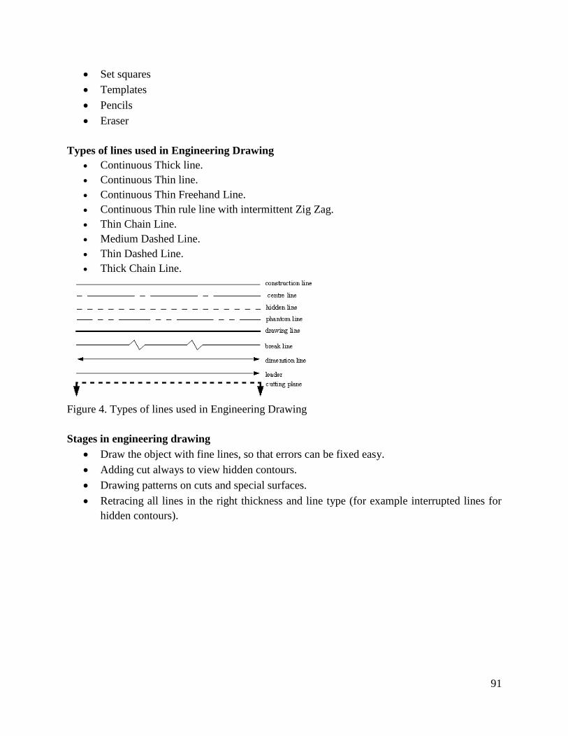
91
Set squares
Templates
Pencils
Eraser
Types of lines used in Engineering Drawing
Continuous Thick line.
Continuous Thin line.
Continuous Thin Freehand Line.
Continuous Thin rule line with intermittent Zig Zag.
Thin Chain Line.
Medium Dashed Line.
Thin Dashed Line.
Thick Chain Line.
Figure 4. Types of lines used in Engineering Drawing
Stages in engineering drawing
Draw the object with fine lines, so that errors can be fixed easy.
Adding cut always to view hidden contours.
Drawing patterns on cuts and special surfaces.
Retracing all lines in the right thickness and line type (for example interrupted lines for
hidden contours).
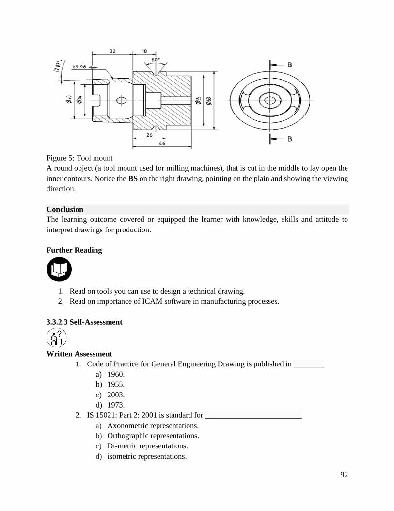
92
Figure 5: Tool mount
A round object (a tool mount used for milling machines), that is cut in the middle to lay open the
inner contours. Notice the BS on the right drawing, pointing on the plain and showing the viewing
direction.
Conclusion
The learning outcome covered or equipped the learner with knowledge, skills and attitude to
interpret drawings for production.
Further Reading
1. Read on tools you can use to design a technical drawing.
2. Read on importance of ICAM software in manufacturing processes.
3.3.2.3 Self-Assessment
Written Assessment
1. Code of Practice for General Engineering Drawing is published in ________
a) 1960.
b) 1955.
c) 2003.
d) 1973.
2. IS 15021: Part 2: 2001 is standard for _________________________
a) Axonometric representations.
b) Orthographic representations.
c) Di-metric representations.
d) isometric representations.
93
3. _________ is used to draw curves which are not circular.
a) Compass.
b) Protractor.
c) French curves.
d) Pro circle
4. The following is not included in title block of drawing sheet.
a) Sheet No.
b) Scale.
c) Method of Projection.
d) Size of sheet.
5. Which of the following represent reducing scale?
a) 1:1
b) 1:2
c) 2:1
d) 10:1
6. In first angle projection method, object is assumed to be placed in
a) First quadrant
b) Second quadrant
c) Third Quadrant
d) Fourth quadrant
7. Metric thread of 10mm diameter is represented by
a) 10M
b) M10
c) M^10
d) None of the above
8. What are the main equipment used in engineering drawing?
9. Why do engineers use scales in their drawings presentations.
10. What is the importance of engineering drawing?
11. Engineering can be considered as a language. What do we mean by this?
12. How do you apply continuous lines in engineering drawings?
Oral Assessment
1. What are the types of lines used in engineering drawing?
2. What is interchangeability in ISO?
Practical Assessment
1. Produce basic drawings for various parts.
2. Produce sketches from a machine drawing for machining and production of parts purpose.

94
Project
Prepare a work plan for the part in the figure below.
3.3.2.4 Tools, Equipment, Supplies and Materials
Drilling machines
Vices
Burnishing machine
Cutting tools
Combination square
Centre punch
Centre lathe
scribers
calipers
Dies and taps
Surface plate
V-blocks
Dial gauge
Die stock
Engineer’s square
File card
Assorted Files
Clamps
Assorted hand tools

95
3.3.2.5 References
Gare, S. K. (2005). Workshop Technology (manufacturing process) New Delhi. Larmi
Publications.
Greese, R. (2017). Introduction to Manufacturing process and material. CRC press.
Signh, R. (2006). Introduction To Basic manufacturing process &Workshop Technology. New
Age International.
96
3.3.3 Learning Outcome No 2: Choose appropriate tools and materials
3.3.3.1 Learning Activities
Learning Outcome No 2: Choose appropriate tools and materials
Learning Activities Special Instructions
2.1 Select working tools, equipment and materials for the
task.
2.2 Tidy up the work areas as per organization policy.
Tool selection to be done in the
workshop.
Use PPE in the workshop.
3.3.3.2 Information Sheet No3/LO2 Choose appropriate tools and materials
Introduction
This learning outcome covers materials, tools and equipment used in engineering processes and
application to produce various items.
Definition of key terms
Tools: A tool can be any item that is used to achieve a goal.
Equipment: Equipment usually denotes a set of tools that are used to achieve a specific objective.
Engineering materials: These are substances which are subjected to various operations and
processes so as to produce finished products.
Content/procedures/methods/illustrations
2.1 Working tools, equipment and materials are selected for the task.
Classification of engineering materials
a) Metals
They are polycrystalline bodies which are having number of differentially oriented fine crystals.
Normally major metals are in solid states at normal temperature. However, some metals such as
mercury are also in liquid state at normal temperature. All metals are having high thermal and
electrical conductivity. All metals are having positive temperature coefficient of resistance.
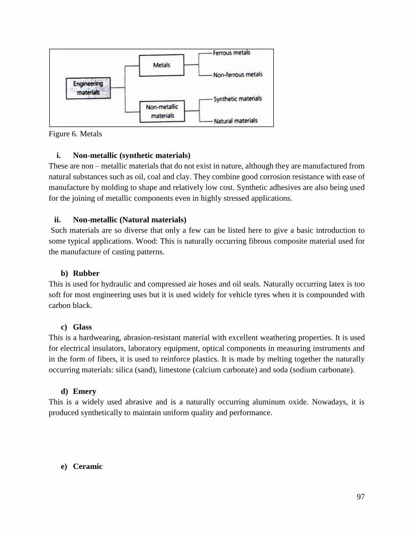
97
Figure 6. Metals
i. Non-metallic (synthetic materials)
These are non – metallic materials that do not exist in nature, although they are manufactured from
natural substances such as oil, coal and clay. They combine good corrosion resistance with ease of
manufacture by molding to shape and relatively low cost. Synthetic adhesives are also being used
for the joining of metallic components even in highly stressed applications.
ii. Non-metallic (Natural materials)
Such materials are so diverse that only a few can be listed here to give a basic introduction to
some typical applications. Wood: This is naturally occurring fibrous composite material used for
the manufacture of casting patterns.
b) Rubber
This is used for hydraulic and compressed air hoses and oil seals. Naturally occurring latex is too
soft for most engineering uses but it is used widely for vehicle tyres when it is compounded with
carbon black.
c) Glass
This is a hardwearing, abrasion-resistant material with excellent weathering properties. It is used
for electrical insulators, laboratory equipment, optical components in measuring instruments and
in the form of fibers, it is used to reinforce plastics. It is made by melting together the naturally
occurring materials: silica (sand), limestone (calcium carbonate) and soda (sodium carbonate).
d) Emery
This is a widely used abrasive and is a naturally occurring aluminum oxide. Nowadays, it is
produced synthetically to maintain uniform quality and performance.
e) Ceramic
98
These are produced by baking naturally occurring clays at high temperatures after molding to
shape. They are used for high voltage insulators and high-temperature-resistant cutting tool tips.
Classification of engineering materials properties
Mechanical properties
Physical properties
Chemical properties
Thermal properties
Mechanical properties
Hardness
Hardness is defined as the ability of a metal to cut another metal or scratch another material.
Malleability
Malleability is the ability of the material to be hammered into thin sheets under applications of
heavy compressive forces without cracking by hot or cold working means. The malleable materials
commonly used in engineering include lead, soft steel, wrought iron, Aluminum, copper, tin, lead,
steel, etc.
Brittleness
Brittleness is the property of a material to break easily with no appreciable deformation. The
materials having less than 5% elongation under loading behavior are said to be brittle materials.
Brittle materials when subjected to tensile loads, snap off without giving any sensible elongation.
These materials include Glass, cast iron, brass and ceramics.
Elasticity
It is defined as the property of a material to regain its original shape after deformation when the
external forces are removed.
Plasticity
Plasticity is defined the mechanical property of a material which retains the deformation produced
under load permanently. It is the ability or tendency of material to undergo some degree of
permanent deformation without its rupture or its failure.
Strength
Strength is defined as the ability of a material to resist the externally applied forces without
breakdown or yielding. The internal resistance offered by a material to an externally applied force
is called stress.
Stiffness
99
It is defined as the ability of a material to resist deformation under stress. The resistance of a
material to elastic deformation or deflection is called stiffness or rigidity. A material that suffers
slight or very less deformation under load has a high degree of stiffness or rigidity.
Ductility
Ductility is termed as the property of a material enabling it to be drawn into wire with the
application of tensile load. A ductile material must be strong and plastic.
Physical Properties
The important physical properties of the metals include:
Density
Color
Size and shape
Specific gravity
Porosity
Luster
Chemical Properties
The study of chemical properties of materials is necessary because most of the engineering
materials, when they come in contact with other substances with which they can react, suffer from
chemical deterioration of the surface of the metal. Some of the chemical properties of the metals
include:
Corrosion resistance
Chemical composition
Acidity or alkalinity
Thermal properties
The study of thermal properties is essential in order to know the response of metal to thermal
changes i.e. lowering or raising of temperature. Thermal properties include:
Thermal conductivity
Thermal expansion
Specific heat
Melting point
Thermal diffusivity
Material testing
There are types of material testing methods which include:
Destructive testing
Non- destructive testing
Non-Destructive Testing (NDT) commonly applied are:
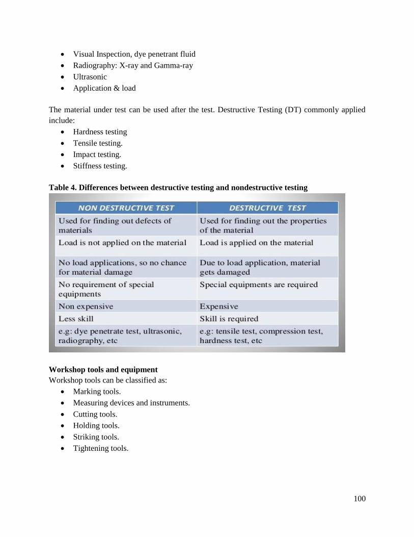
100
Visual Inspection, dye penetrant fluid
Radiography: X-ray and Gamma-ray
Ultrasonic
Application & load
The material under test can be used after the test. Destructive Testing (DT) commonly applied
include:
Hardness testing
Tensile testing.
Impact testing.
Stiffness testing.
Table 4. Differences between destructive testing and nondestructive testing
Workshop tools and equipment
Workshop tools can be classified as:
Marking tools.
Measuring devices and instruments.
Cutting tools.
Holding tools.
Striking tools.
Tightening tools.
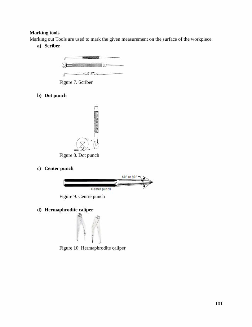
101
Marking tools
Marking out Tools are used to mark the given measurement on the surface of the workpiece.
a) Scriber
Figure 7. Scriber
b) Dot punch
Figure 8. Dot punch
c) Center punch
Figure 9. Centre punch
d) Hermaphrodite caliper
Figure 10. Hermaphrodite caliper
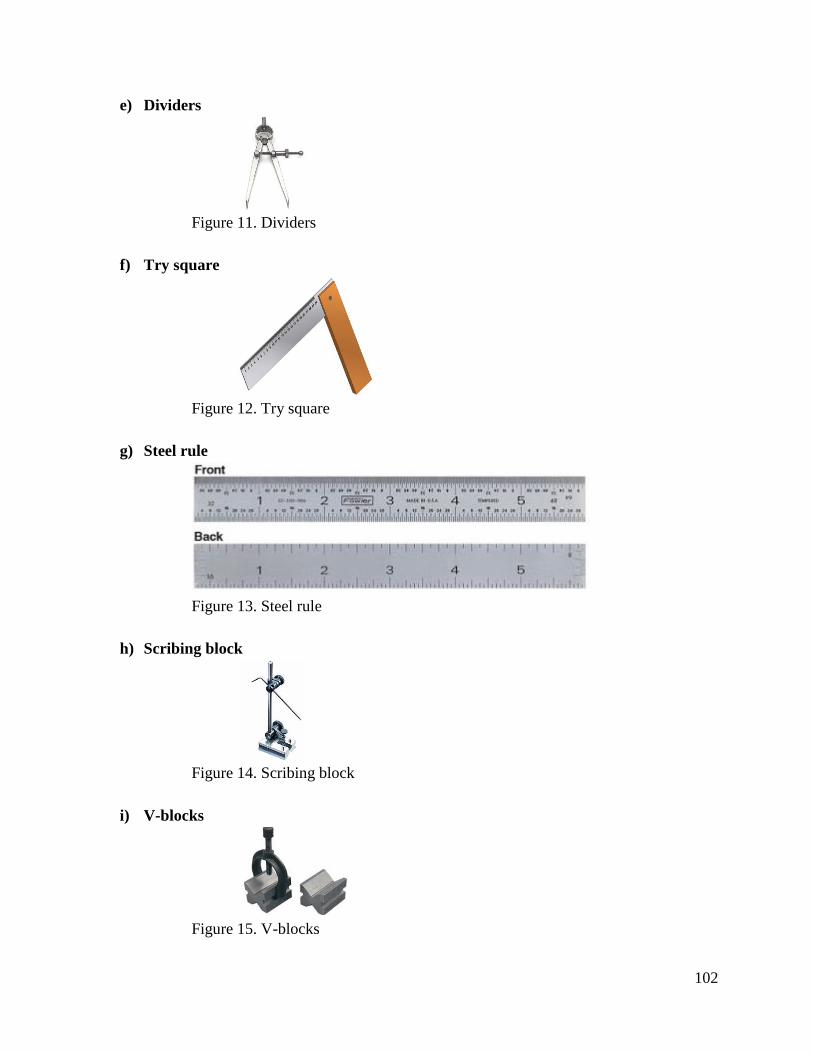
102
e) Dividers
Figure 11. Dividers
f) Try square
Figure 12. Try square
g) Steel rule
Figure 13. Steel rule
h) Scribing block
Figure 14. Scribing block
i) V-blocks
Figure 15. V-blocks
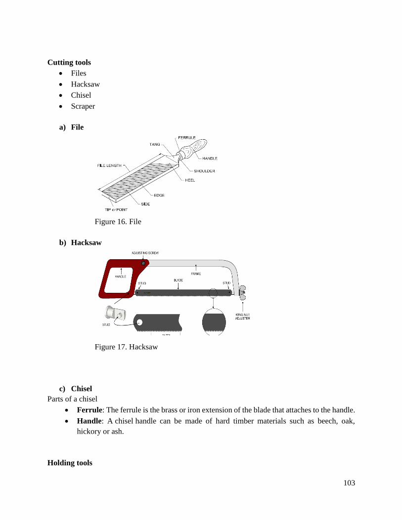
103
Cutting tools
Files
Hacksaw
Chisel
Scraper
a) File
Figure 16. File
b) Hacksaw
Figure 17. Hacksaw
c) Chisel
Parts of a chisel
Ferrule: The ferrule is the brass or iron extension of the blade that attaches to the handle.
Handle: A chisel handle can be made of hard timber materials such as beech, oak,
hickory or ash.
Holding tools
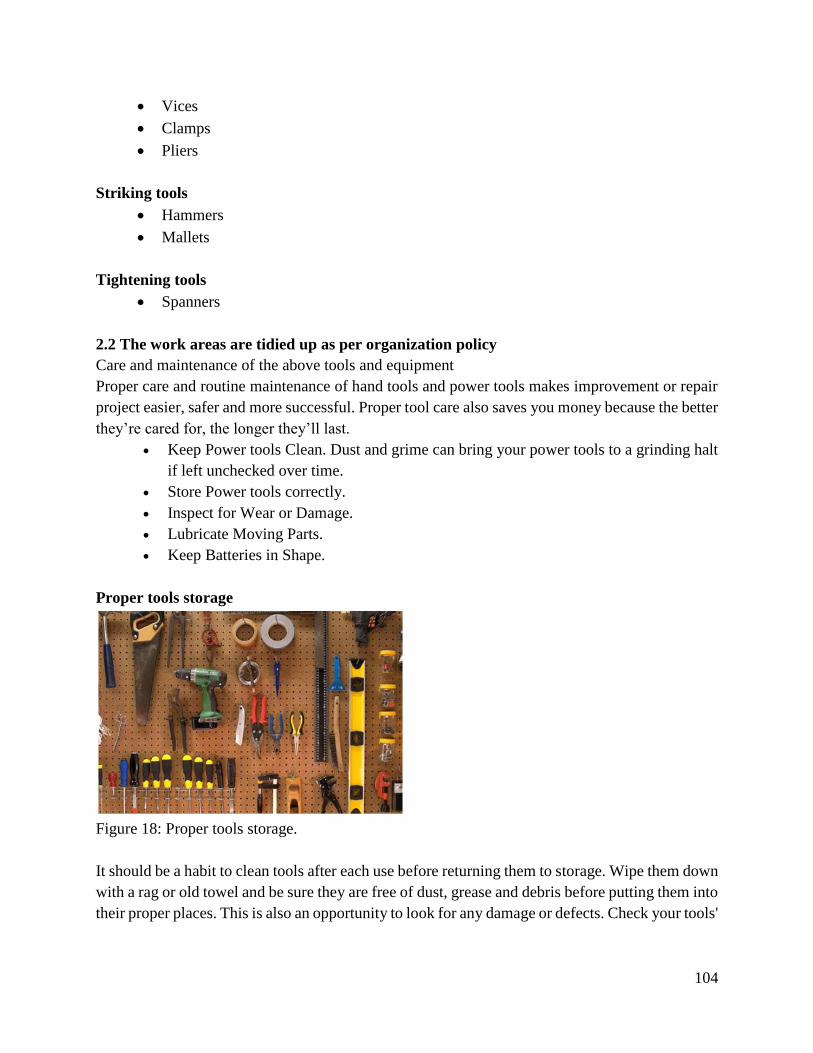
104
Vices
Clamps
Pliers
Striking tools
Hammers
Mallets
Tightening tools
Spanners
2.2 The work areas are tidied up as per organization policy
Care and maintenance of the above tools and equipment
Proper care and routine maintenance of hand tools and power tools makes improvement or repair
project easier, safer and more successful. Proper tool care also saves you money because the better
they’re cared for, the longer they’ll last.
Keep Power tools Clean. Dust and grime can bring your power tools to a grinding halt
if left unchecked over time.
Store Power tools correctly.
Inspect for Wear or Damage.
Lubricate Moving Parts.
Keep Batteries in Shape.
Proper tools storage
Figure 18: Proper tools storage.
It should be a habit to clean tools after each use before returning them to storage. Wipe them down
with a rag or old towel and be sure they are free of dust, grease and debris before putting them into
their proper places. This is also an opportunity to look for any damage or defects. Check your tools'
105
handles for splinters, breaks and cracks. Also, make sure that metal parts show no signs of
corrosion or rust. Repair or replace any tools that show signs of damage.
Cold chisels, log-splitting wedges and other striking tools can be very dangerous if they are not
maintained properly. Because these types of tools are used for repeated striking, the surface of the
metal head eventually mushrooms out and spreads to form a lip or ridge around the edge. With
continued use, there is more spreading and the metal lip may continue to thin, split or curl until it
finally breaks. If the metal head separates from the handle while in use, this could result in a
dangerous projectile. To prevent this hazard, just grind off the metal edges with a powered grinder
on a regular basis.
Care of measuring tools.
Always wipe not only the measuring faces of your tools, but of the work piece being measured
as well. This will help prevent dust or dirt from marring your tools. Generally speaking, it is
best not to use such tools as vernier calipers or micrometers on rough, abrasive surfaces if you
can possibly avoid it.
Always keep your tools used for measuring separate from your hand tools to save them being
knocked about and damaged. Never lay your tools on something like a lathe, either, because
the vibrations could compromise the accuracy of the tool.
Always use your tools used for measuring for that alone---measuring. This means don't use
your micrometers for little hammers or a vernier caliper as a line marker, for instance. This
will certainly damage them.
Always keep your tools used for measuring at or around room temperature. Never lay them on
a heat source or in direct sunlight as doing so could really mess them up so that their accuracy
is affected.
Always be wary of laying or using your tools too close to a magnet or magnetized surface.
Magnets can wreak havoc with many of these precision tools.
Always clean your tools after use. Unless they're made of stainless steel, each tool should have
some anti-rust oil dabbed on it and then stored by itself in a dry place.
Conclusion
The learning outcome covered or equipped the learner with knowledge, skills and attitude to:
Identify materials through performing various tests, select hand tools and equipment, apply hand
tools and equipment, properly clean the tools and work area and properly store tools and
equipment.
106
Further Reading
1. Shawhney , G.(2009).Mechanical Experiments and workshop practice .IK International
PVT Ltd.
3.3.3.3 Self-Assessment
Written Assessment
1. What is strain?
a) Determined by dividing the load by the smallest actual cross-sectional area of the test
specimen.
b) The ratio between the original length and the change in length when an external force
is applied.
c) The amount of stress that a material can absorb without exceeding its breaking stress.
d) Measurement of the deformation produced by the application of an external force.
2. Mineral oils
a) Are used where the load, speed and temperature is low.
b) Provide increased heating capacity in some applications.
c) Range from milky to transparent in appearance.
d) Are composed of oil droplets.
3. Which one of the following is steel hand tool with small sharp teeth used for sharpening or
shaping?
a) Metal vise
b) Steel file
c) Chalk line
d) Speed square
4. A combination tool with rubber and plastic heads designed to protect the surface being
struck. Which one is correct?
a) Ball peen hammer
b) Rubber hammer
c) Claw hammer
d) Rubber/plastic hammer
5. Which saw is used for cutting metal?
a) Nail set
b) Back saw
c) Rip saw
d) Hack saw
6. Which test can be performed without skilled labour?
107
a) Probe test
b) Bend liquid test
c) Dye penetrant test
d) Torsion test
7. During radiography test, which region absorbs less radiation and transmits more?
a) Low and high density regions absorb and transmit same amount of radiation
b) High density region
c) Low density region
d) Low and high density regions adsorb
8. A track driver notices that his vehicle loses power. The mechanic will have to conduct a
compression test according to certain procedures. Give the reason for carrying out each of
the following procedures?
a) Removing the high-tension leads
b) Unplugging the fuel injectors
c) Fully opening the throttle valve
d) Recording the readings
9. The wheel rims on some vehicles are manufactured from mild steel. Others are cast in
aluminum alloys. Answer the questions that follow.
a) Give THREE reasons for choosing to manufacture vehicle wheel rims out of
aluminum alloy.
b) Give TWO reasons why the wheel rims of heavy-duty vehicles (trucks) are
manufactured from steel.
10. Explain why alloys are produced? Give FOUR reasons.
Specify FIVE general safety rules to be considered when using equipment like the lathe
and drill press.
11. What is the difference between a destructive test and a non-destructive test on materials?
Oral Assessment
1. Classify the various properties of engineering materials.
2. Explain the following material testing methods.
a) Hardness testing.
b) Dye penetrant method
Practical Assessment
1. Inspect the workshop tools and equipment for damages and undertake proper repaires.
Project
1. Visit an engineering workshop within the locality and write a report on the method of tools
care storage and workshop cleaning.

108
3.3.3.4 Tools, Equipment, Supplies and Materials
Welding
Drilling machines
Vices
Burnishing machine
Cutting tools
Combination square
Centre punch
Centre lathe
Scribers
Calipers
Dies and taps
Surface plate
V-blocks
Dial gauge
Die stock
Engineer’s square
File card
Assorted Files
Clamps
Assorted hand tools
3.3.3.5 References
Sharma, s., Bajracharya,R.& Sitaula , B.(2009)Indigenous Technology Knowledge in Nepal. A
review.
Shawhney , G.(2009).Mechanical Experiments and workshop practice .IK International PVT Ltd.
Singh,R.(2006).Introduction to basic manufacturing processes and workshop technology/
Rajender Singh .New age . Ltd -2006-483p.
109
3.3.4 Learning Outcome No 3: Measure and mark out dimensions on work pieces
3.3.4.1 Learning Activities
Learning Outcome No3: Measure and mark out dimensions on work pieces
Learning Activities Special Instructions
3.1 Select measuring tools suitable for the work.
3.2 Inspect and calibrate measuring tools if
required.
3.3 Mark on the work piece dimensions as per the
working drawing.
Use the correct measuring tools and
equipment.
Make sure to use the correct
measurement.
Use correct dimensions on drawing.
3.3.4.2 Information Sheet No 3/LO3: Measure and mark out dimensions on work pieces
Introduction
This learning outcome covers the skills required for the leaner to perform measuring and marking
out.
Definition of key terms
Measuring: A measurement is a collection of quantitative or numerical data that describes a
property of an object or event. A measurement is made by comparing a quantity with a standard
unit. It is the aspect of taking the dimensions of a given object.
Marking out: Marking out or layout means the process of transferring a design or pattern to a
work piece, as the first step in the manufacturing process.
Calibration: Calibration is a process used to compare the inspection, measuring, and test
instruments to a recognized reference standard of known certified accuracy and precision, noting
the difference and adjusting the instrument, where possible, to agree with the standard.
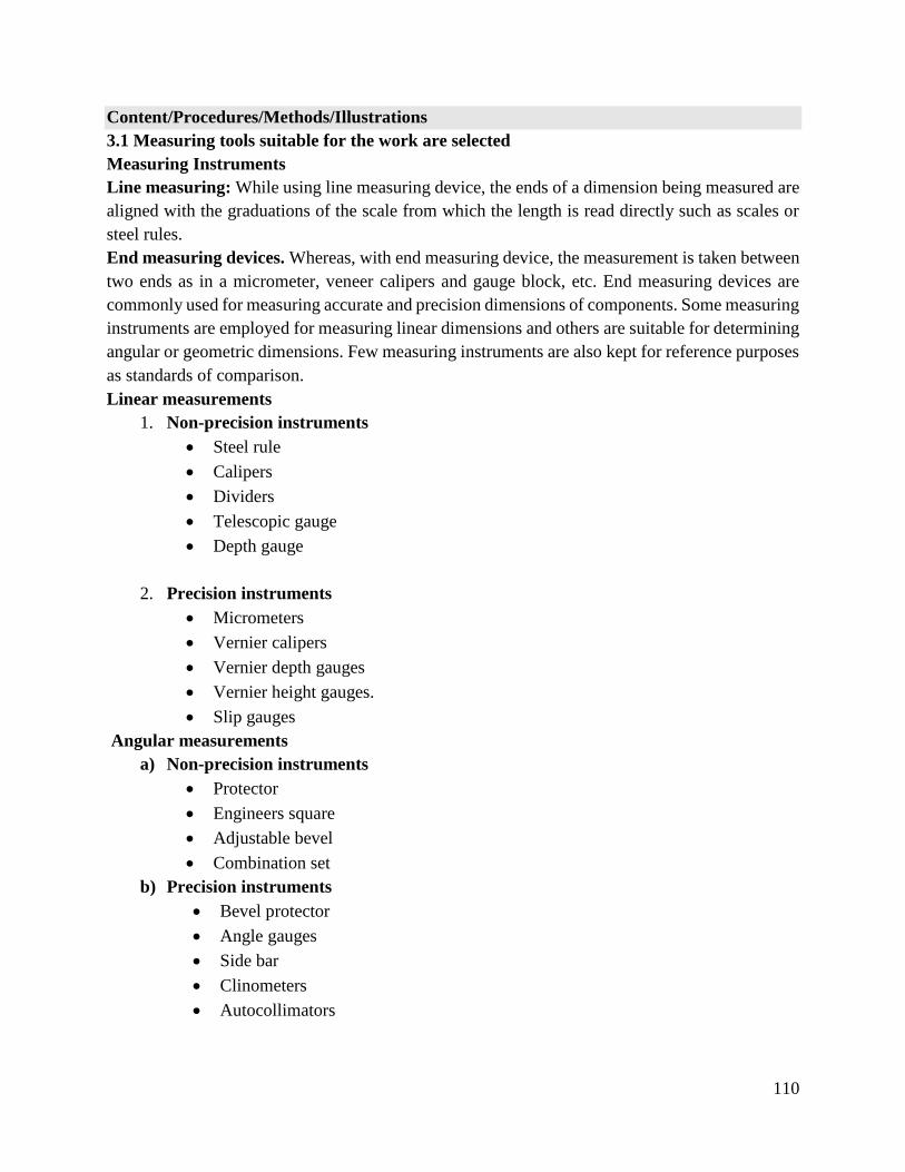
110
Content/Procedures/Methods/Illustrations
3.1 Measuring tools suitable for the work are selected
Measuring Instruments
Line measuring: While using line measuring device, the ends of a dimension being measured are
aligned with the graduations of the scale from which the length is read directly such as scales or
steel rules.
End measuring devices. Whereas, with end measuring device, the measurement is taken between
two ends as in a micrometer, veneer calipers and gauge block, etc. End measuring devices are
commonly used for measuring accurate and precision dimensions of components. Some measuring
instruments are employed for measuring linear dimensions and others are suitable for determining
angular or geometric dimensions. Few measuring instruments are also kept for reference purposes
as standards of comparison.
Linear measurements
1. Non-precision instruments
Steel rule
Calipers
Dividers
Telescopic gauge
Depth gauge
2. Precision instruments
Micrometers
Vernier calipers
Vernier depth gauges
Vernier height gauges.
Slip gauges
Angular measurements
a) Non-precision instruments
Protector
Engineers square
Adjustable bevel
Combination set
b) Precision instruments
Bevel protector
Angle gauges
Side bar
Clinometers
Autocollimators
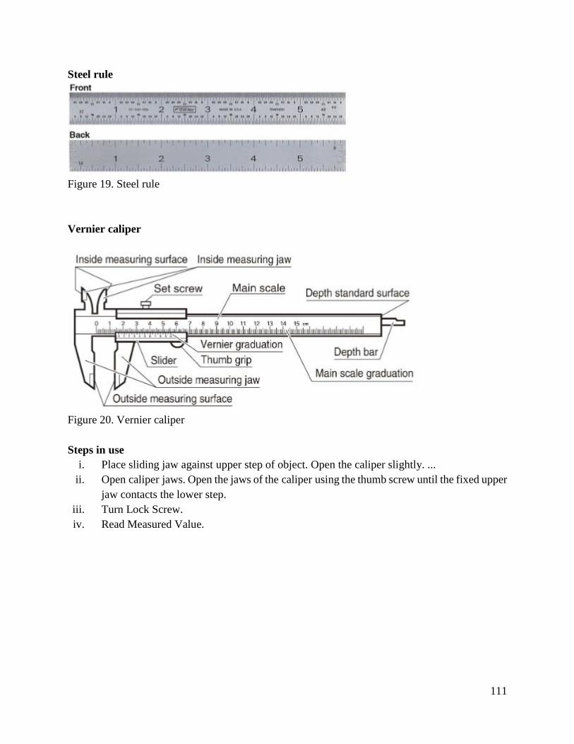
111
Steel rule
Figure 19. Steel rule
Vernier caliper
Figure 20. Vernier caliper
Steps in use
i. Place sliding jaw against upper step of object. Open the caliper slightly. ...
ii. Open caliper jaws. Open the jaws of the caliper using the thumb screw until the fixed upper
jaw contacts the lower step.
iii. Turn Lock Screw.
iv. Read Measured Value.
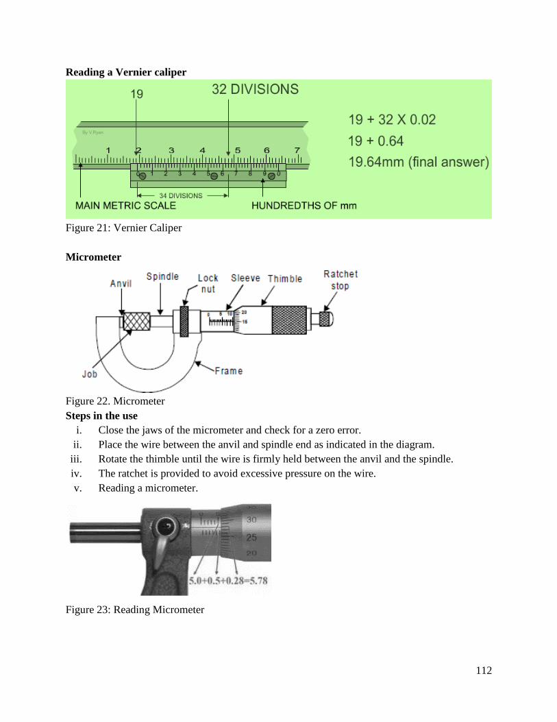
112
Reading a Vernier caliper
Figure 21: Vernier Caliper
Micrometer
Figure 22. Micrometer
Steps in the use
i. Close the jaws of the micrometer and check for a zero error.
ii. Place the wire between the anvil and spindle end as indicated in the diagram.
iii. Rotate the thimble until the wire is firmly held between the anvil and the spindle.
iv. The ratchet is provided to avoid excessive pressure on the wire.
v. Reading a micrometer.
Figure 23: Reading Micrometer
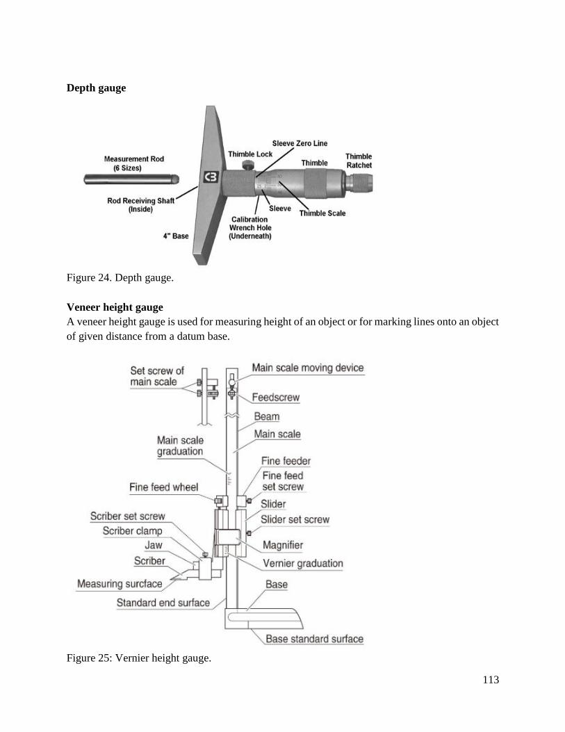
113
Depth gauge
Figure 24. Depth gauge.
Veneer height gauge
A veneer height gauge is used for measuring height of an object or for marking lines onto an object
of given distance from a datum base.
Figure 25: Vernier height gauge.
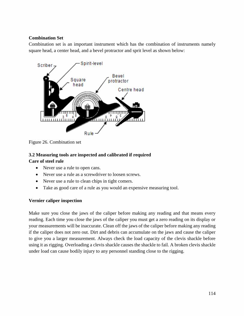
114
Combination Set
Combination set is an important instrument which has the combination of instruments namely
square head, a center head, and a bevel protractor and sprit level as shown below:
Figure 26. Combination set
3.2 Measuring tools are inspected and calibrated if required
Care of steel rule
Never use a rule to open cans.
Never use a rule as a screwdriver to loosen screws.
Never use a rule to clean chips in tight comers.
Take as good care of a rule as you would an expensive measuring tool.
Vernier caliper inspection
Make sure you close the jaws of the caliper before making any reading and that means every
reading. Each time you close the jaws of the caliper you must get a zero reading on its display or
your measurements will be inaccurate. Clean off the jaws of the caliper before making any reading
if the caliper does not zero out. Dirt and debris can accumulate on the jaws and cause the caliper
to give you a larger measurement. Always check the load capacity of the clevis shackle before
using it as rigging. Overloading a clevis shackle causes the shackle to fail. A broken clevis shackle
under load can cause bodily injury to any personnel standing close to the rigging.
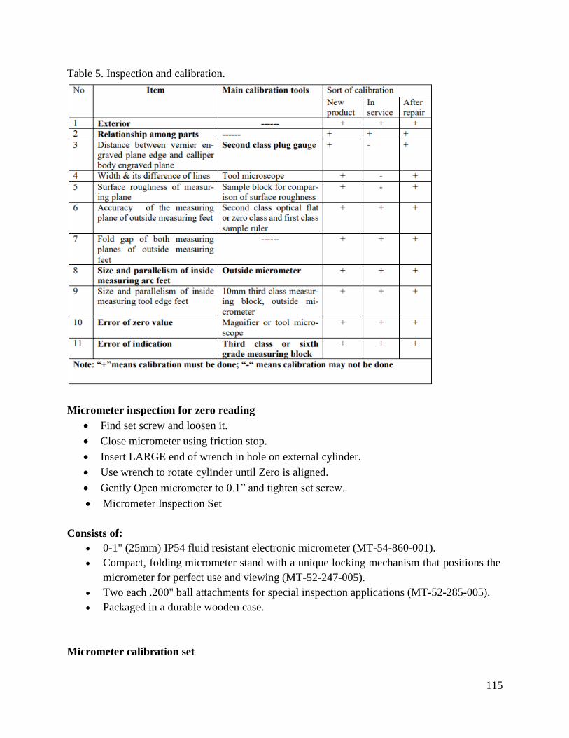
115
Table 5. Inspection and calibration.
Micrometer inspection for zero reading
Find set screw and loosen it.
Close micrometer using friction stop.
Insert LARGE end of wrench in hole on external cylinder.
Use wrench to rotate cylinder until Zero is aligned.
Gently Open micrometer to 0.1” and tighten set screw.
Micrometer Inspection Set
Consists of:
0-1" (25mm) IP54 fluid resistant electronic micrometer (MT-54-860-001).
Compact, folding micrometer stand with a unique locking mechanism that positions the
micrometer for perfect use and viewing (MT-52-247-005).
Two each .200" ball attachments for special inspection applications (MT-52-285-005).
Packaged in a durable wooden case.
Micrometer calibration set
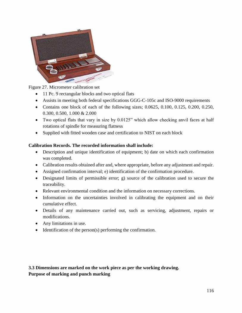
116
Figure 27. Micrometer calibration set
11 Pc. 9 rectangular blocks and two optical flats
Assists in meeting both federal specifications GGG-C-105c and ISO-9000 requirements
Contains one block of each of the following sizes; 0.0625, 0.100, 0.125, 0.200, 0.250,
0.300, 0.500, 1.000 & 2.000
Two optical flats that vary in size by 0.0125” which allow checking anvil faces at half
rotations of spindle for measuring flatness
Supplied with fitted wooden case and certification to NIST on each block
Calibration Records. The recorded information shall include:
Description and unique identification of equipment; b) date on which each confirmation
was completed.
Calibration results obtained after and, where appropriate, before any adjustment and repair.
Assigned confirmation interval; e) identification of the confirmation procedure.
Designated limits of permissible error; g) source of the calibration used to secure the
traceability.
Relevant environmental condition and the information on necessary corrections.
Information on the uncertainties involved in calibrating the equipment and on their
cumulative effect.
Details of any maintenance carried out, such as servicing, adjustment, repairs or
modifications.
Any limitations in use.
Identification of the person(s) performing the confirmation.
3.3 Dimensions are marked on the work piece as per the working drawing.
Purpose of marking and punch marking
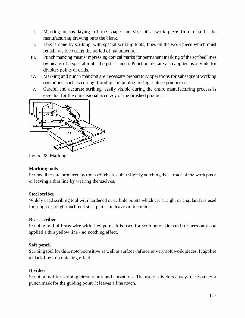
117
i. Marking means laying off the shape and size of a work piece from data in the
manufacturing drawing onto the blank.
ii. This is done by scribing, with special scribing tools, lines on the work piece which must
remain visible during the period of manufacture.
iii. Punch marking means impressing conical marks for permanent marking of the scribed lines
by means of a special tool - the prick punch. Punch marks are also applied as a guide for
dividers points or drills.
iv. Marking and punch marking are necessary preparatory operations for subsequent working
operations, such as cutting, forming and joining in single-piece production.
v. Careful and accurate scribing, easily visible during the entire manufacturing process is
essential for the dimensional accuracy of the finished product.
Figure 28. Marking
Marking tools
Scribed lines are produced by tools which are either slightly notching the surface of the work piece
or leaving a thin line by wearing themselves.
Steel scriber
Widely used scribing tool with hardened or carbide points which are straight or angular. It is used
for rough or rough-machined steel parts and leaves a fine notch.
Brass scriber
Scribing tool of brass wire with filed point. It is used for scribing on finished surfaces only and
applied a thin yellow line - no notching effect.
Soft pencil
Scribing tool for thin, notch-sensitive as well as surface-refined or very soft work pieces. It applies
a black line - no notching effect.
Dividers
Scribing tool for scribing circular arcs and curvatures. The use of dividers always necessitates a
punch mark for the guiding point. It leaves a fine notch.
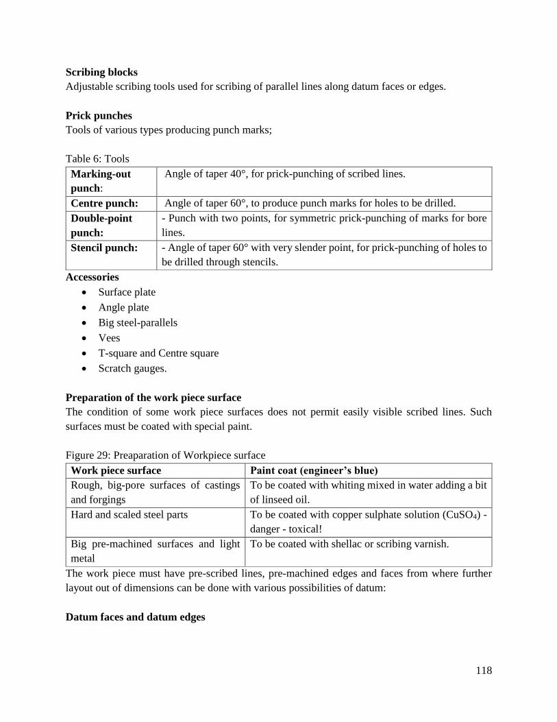
118
Scribing blocks
Adjustable scribing tools used for scribing of parallel lines along datum faces or edges.
Prick punches
Tools of various types producing punch marks;
Table 6: Tools
Marking-out
punch:
Angle of taper 40°, for prick-punching of scribed lines.
Centre punch: Angle of taper 60°, to produce punch marks for holes to be drilled.
Double-point
punch:
- Punch with two points, for symmetric prick-punching of marks for bore
lines.
Stencil punch: - Angle of taper 60° with very slender point, for prick-punching of holes to
be drilled through stencils.
Accessories
Surface plate
Angle plate
Big steel-parallels
Vees
T-square and Centre square
Scratch gauges.
Preparation of the work piece surface
The condition of some work piece surfaces does not permit easily visible scribed lines. Such
surfaces must be coated with special paint.
Figure 29: Preaparation of Workpiece surface
Work piece surface Paint coat (engineer’s blue)
Rough, big-pore surfaces of castings
and forgings
To be coated with whiting mixed in water adding a bit
of linseed oil.
Hard and scaled steel parts To be coated with copper sulphate solution (CuSO4) -
danger - toxical!
Big pre-machined surfaces and light
metal
To be coated with shellac or scribing varnish.
The work piece must have pre-scribed lines, pre-machined edges and faces from where further
layout out of dimensions can be done with various possibilities of datum:
Datum faces and datum edges
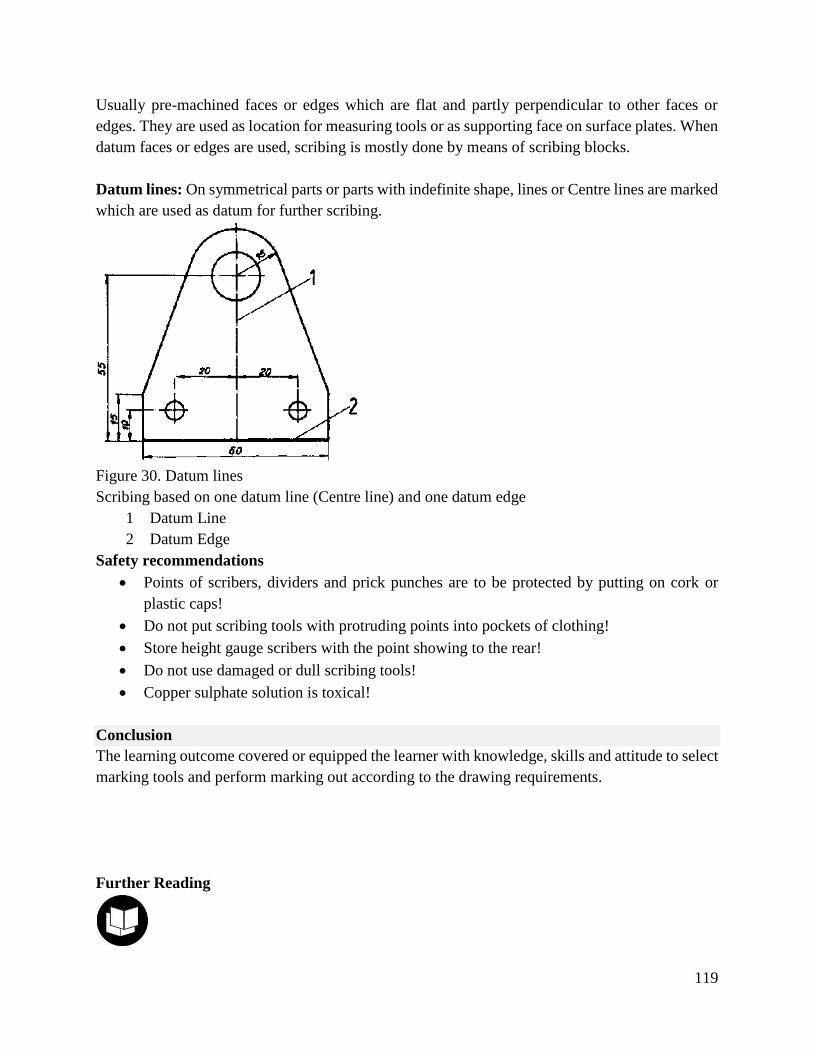
119
Usually pre-machined faces or edges which are flat and partly perpendicular to other faces or
edges. They are used as location for measuring tools or as supporting face on surface plates. When
datum faces or edges are used, scribing is mostly done by means of scribing blocks.
Datum lines: On symmetrical parts or parts with indefinite shape, lines or Centre lines are marked
which are used as datum for further scribing.
Figure 30. Datum lines
Scribing based on one datum line (Centre line) and one datum edge
1 Datum Line
2 Datum Edge
Safety recommendations
Points of scribers, dividers and prick punches are to be protected by putting on cork or
plastic caps!
Do not put scribing tools with protruding points into pockets of clothing!
Store height gauge scribers with the point showing to the rear!
Do not use damaged or dull scribing tools!
Copper sulphate solution is toxical!
Conclusion
The learning outcome covered or equipped the learner with knowledge, skills and attitude to select
marking tools and perform marking out according to the drawing requirements.
Further Reading
120
1. Mechanical experiment and workshop practice by GS Schwhney geometric and
engineering drawing by Kenneth martin.
3.3.4.3 Self-Assessment
Written Assessment
1. Laying large circles which tool do you use?
a) Trammel
b) Divider
c) Jenny caliper
d) Scriber
2. Scriber is made of which material?
a) Cast iron
b) Mild steel
c) High carbon steel
d) Copper
3. Which is not a part of combination set?
a) Stock
b) Protractor head
c) Square head
d) Centre head
4. Which one of the following parts of a universal surface gauge helps to draw parallel lines
along a datum edge?
a) Fine adjusting screw.
b) Guide pins.
c) Base.
d) Rocker arm
5. During marking, the reference surface is provided by
a) Sketch of the job.
b) Workpiece.
c) Marking off table surface.
d) Surface gauge.
6. Which type of rule is used for marking and measuring patterns and hot jobs handled by
blacksmith?
a) Narrow rule.
b) Shrink rule.
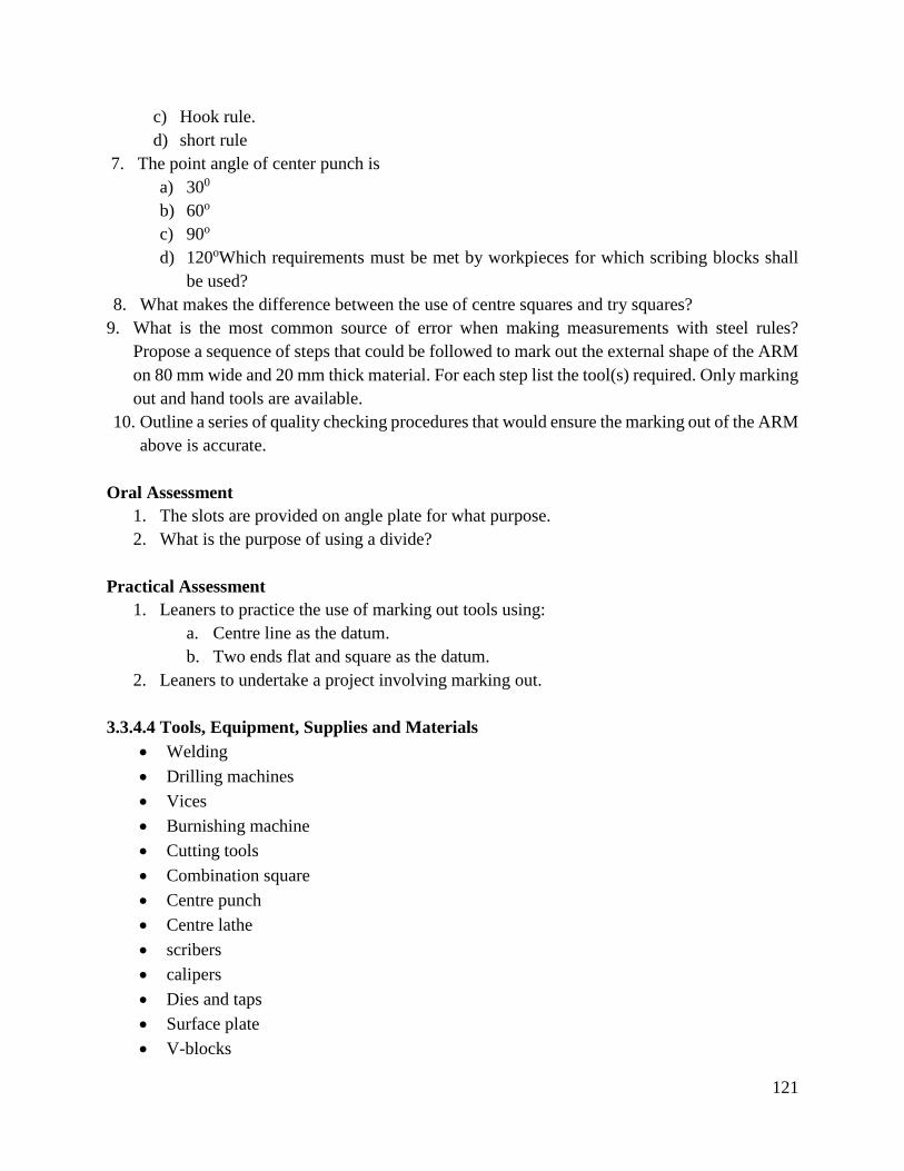
121
c) Hook rule.
d) short rule
7. The point angle of center punch is
a) 300
b) 60o
c) 90o
d) 120oWhich requirements must be met by workpieces for which scribing blocks shall
be used?
8. What makes the difference between the use of centre squares and try squares?
9. What is the most common source of error when making measurements with steel rules?
Propose a sequence of steps that could be followed to mark out the external shape of the ARM
on 80 mm wide and 20 mm thick material. For each step list the tool(s) required. Only marking
out and hand tools are available.
10. Outline a series of quality checking procedures that would ensure the marking out of the ARM
above is accurate.
Oral Assessment
1. The slots are provided on angle plate for what purpose.
2. What is the purpose of using a divide?
Practical Assessment
1. Leaners to practice the use of marking out tools using:
a. Centre line as the datum.
b. Two ends flat and square as the datum.
2. Leaners to undertake a project involving marking out.
3.3.4.4 Tools, Equipment, Supplies and Materials
Welding
Drilling machines
Vices
Burnishing machine
Cutting tools
Combination square
Centre punch
Centre lathe
scribers
calipers
Dies and taps
Surface plate
V-blocks

122
Dial gauge
Die stock
Engineer’s square
File card
Assorted Files
Clamps
Assorted hand tools
3.3.4.5 References
Morling, K. (2010). Geometric and engineering drawing. Routledge.
Sawhney, G. S. (2009). Mechanical experiments and workshop practice. IK International Pvt Ltd.
Singh, R. Introduction to basic manufacturing processes and workshop technology/Rajender
Singh. New age int. Ltd.–2006.–483 p.
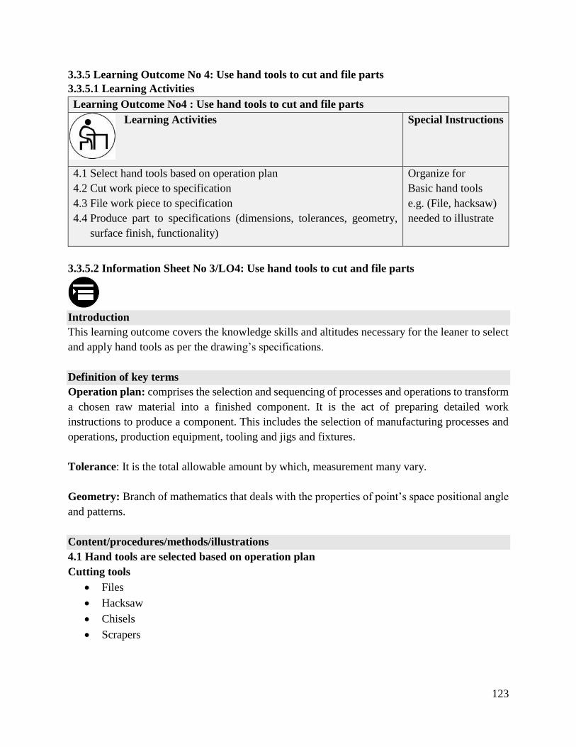
123
3.3.5 Learning Outcome No 4: Use hand tools to cut and file parts
3.3.5.1 Learning Activities
Learning Outcome No4 : Use hand tools to cut and file parts
Learning Activities Special Instructions
4.1 Select hand tools based on operation plan
4.2 Cut work piece to specification
4.3 File work piece to specification
4.4 Produce part to specifications (dimensions, tolerances, geometry,
surface finish, functionality)
Organize for
Basic hand tools
e.g. (File, hacksaw)
needed to illustrate
3.3.5.2 Information Sheet No 3/LO4: Use hand tools to cut and file parts
Introduction
This learning outcome covers the knowledge skills and altitudes necessary for the leaner to select
and apply hand tools as per the drawing’s specifications.
Definition of key terms
Operation plan: comprises the selection and sequencing of processes and operations to transform
a chosen raw material into a finished component. It is the act of preparing detailed work
instructions to produce a component. This includes the selection of manufacturing processes and
operations, production equipment, tooling and jigs and fixtures.
Tolerance: It is the total allowable amount by which, measurement many vary.
Geometry: Branch of mathematics that deals with the properties of point’s space positional angle
and patterns.
Content/procedures/methods/illustrations
4.1 Hand tools are selected based on operation plan
Cutting tools
Files
Hacksaw
Chisels
Scrapers
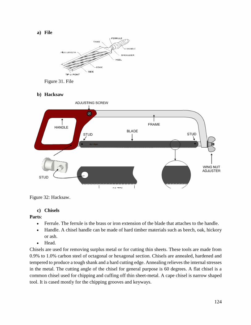
124
a) File
Figure 31. File
b) Hacksaw
Figure 32: Hacksaw.
c) Chisels
Parts:
Ferrule. The ferrule is the brass or iron extension of the blade that attaches to the handle.
Handle. A chisel handle can be made of hard timber materials such as beech, oak, hickory
or ash.
Head.
Chisels are used for removing surplus metal or for cutting thin sheets. These tools are made from
0.9% to 1.0% carbon steel of octagonal or hexagonal section. Chisels are annealed, hardened and
tempered to produce a tough shank and a hard cutting edge. Annealing relieves the internal stresses
in the metal. The cutting angle of the chisel for general purpose is 60 degrees. A flat chisel is a
common chisel used for chipping and cuffing off thin sheet-metal. A cape chisel is narrow shaped
tool. It is cased mostly for the chipping grooves and keyways.
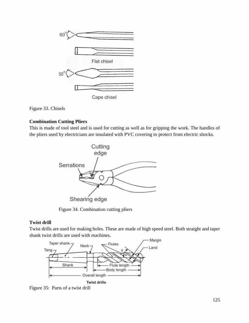
125
Figure 33. Chisels
Combination Cutting Pliers
This is made of tool steel and is used for cutting as well as for gripping the work. The handles of
the pliers used by electricians are insulated with PVC covering to protect from electric shocks.
Figure 34. Combination cutting pliers
Twist drill
Twist drills are used for making holes. These are made of high speed steel. Both straight and taper
shank twist drills are used with machines.
Figure 35: Parts of a twist drill
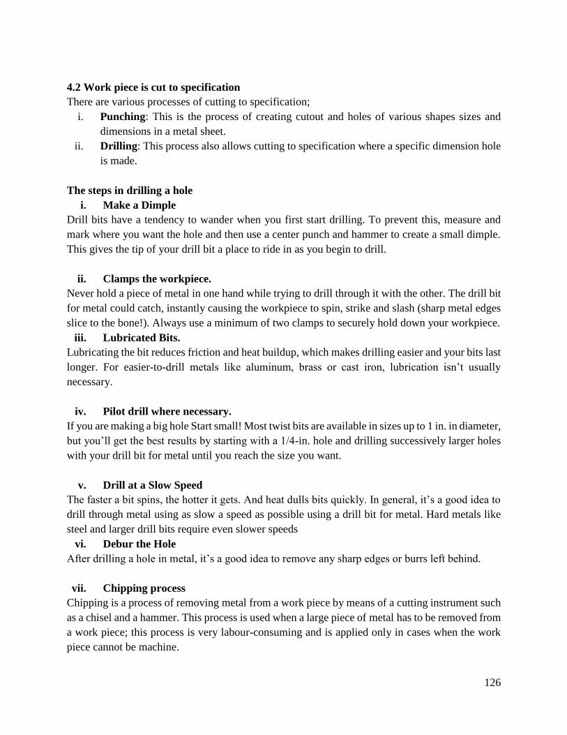
126
4.2 Work piece is cut to specification
There are various processes of cutting to specification;
i. Punching: This is the process of creating cutout and holes of various shapes sizes and
dimensions in a metal sheet.
ii. Drilling: This process also allows cutting to specification where a specific dimension hole
is made.
The steps in drilling a hole
i. Make a Dimple
Drill bits have a tendency to wander when you first start drilling. To prevent this, measure and
mark where you want the hole and then use a center punch and hammer to create a small dimple.
This gives the tip of your drill bit a place to ride in as you begin to drill.
ii. Clamps the workpiece.
Never hold a piece of metal in one hand while trying to drill through it with the other. The drill bit
for metal could catch, instantly causing the workpiece to spin, strike and slash (sharp metal edges
slice to the bone!). Always use a minimum of two clamps to securely hold down your workpiece.
iii. Lubricated Bits.
Lubricating the bit reduces friction and heat buildup, which makes drilling easier and your bits last
longer. For easier-to-drill metals like aluminum, brass or cast iron, lubrication isn’t usually
necessary.
iv. Pilot drill where necessary.
If you are making a big hole Start small! Most twist bits are available in sizes up to 1 in. in diameter,
but you’ll get the best results by starting with a 1/4-in. hole and drilling successively larger holes
with your drill bit for metal until you reach the size you want.
v. Drill at a Slow Speed
The faster a bit spins, the hotter it gets. And heat dulls bits quickly. In general, it’s a good idea to
drill through metal using as slow a speed as possible using a drill bit for metal. Hard metals like
steel and larger drill bits require even slower speeds
vi. Debur the Hole
After drilling a hole in metal, it’s a good idea to remove any sharp edges or burrs left behind.
vii. Chipping process
Chipping is a process of removing metal from a work piece by means of a cutting instrument such
as a chisel and a hammer. This process is used when a large piece of metal has to be removed from
a work piece; this process is very labour-consuming and is applied only in cases when the work
piece cannot be machine.
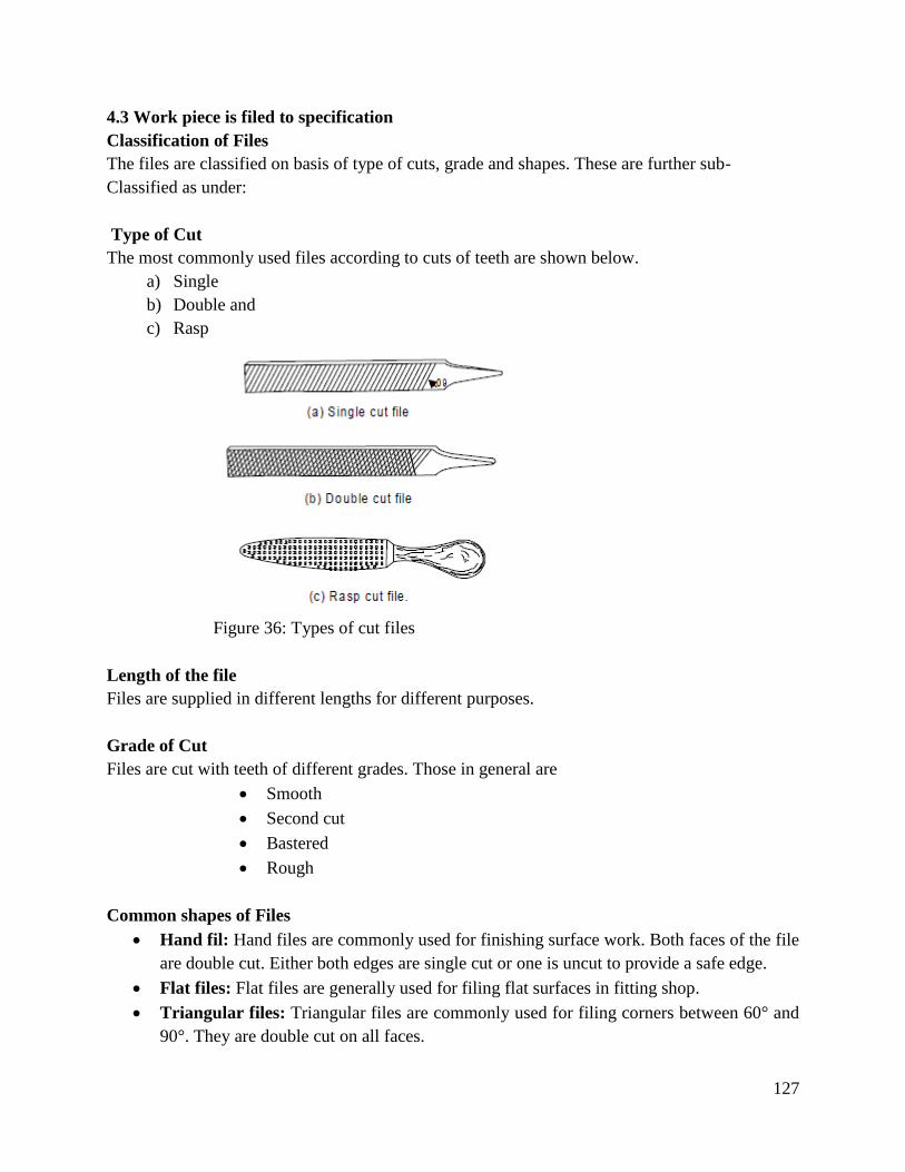
127
4.3 Work piece is filed to specification
Classification of Files
The files are classified on basis of type of cuts, grade and shapes. These are further sub-
Classified as under:
Type of Cut
The most commonly used files according to cuts of teeth are shown below.
a) Single
b) Double and
c) Rasp
Figure 36: Types of cut files
Length of the file
Files are supplied in different lengths for different purposes.
Grade of Cut
Files are cut with teeth of different grades. Those in general are
Smooth
Second cut
Bastered
Rough
Common shapes of Files
Hand fil: Hand files are commonly used for finishing surface work. Both faces of the file
are double cut. Either both edges are single cut or one is uncut to provide a safe edge.
Flat files: Flat files are generally used for filing flat surfaces in fitting shop.
Triangular files: Triangular files are commonly used for filing corners between 60° and
90°. They are double cut on all faces.
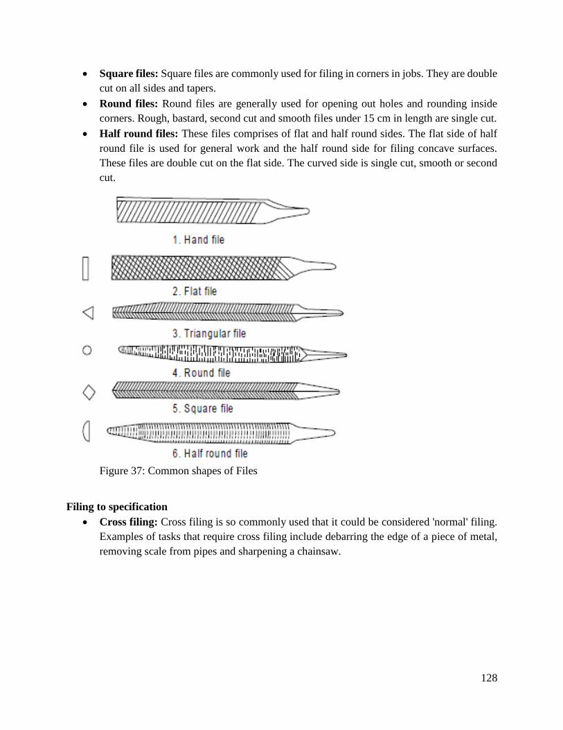
128
Square files: Square files are commonly used for filing in corners in jobs. They are double
cut on all sides and tapers.
Round files: Round files are generally used for opening out holes and rounding inside
corners. Rough, bastard, second cut and smooth files under 15 cm in length are single cut.
Half round files: These files comprises of flat and half round sides. The flat side of half
round file is used for general work and the half round side for filing concave surfaces.
These files are double cut on the flat side. The curved side is single cut, smooth or second
cut.
Figure 37: Common shapes of Files
Filing to specification
Cross filing: Cross filing is so commonly used that it could be considered 'normal' filing.
Examples of tasks that require cross filing include debarring the edge of a piece of metal,
removing scale from pipes and sharpening a chainsaw.
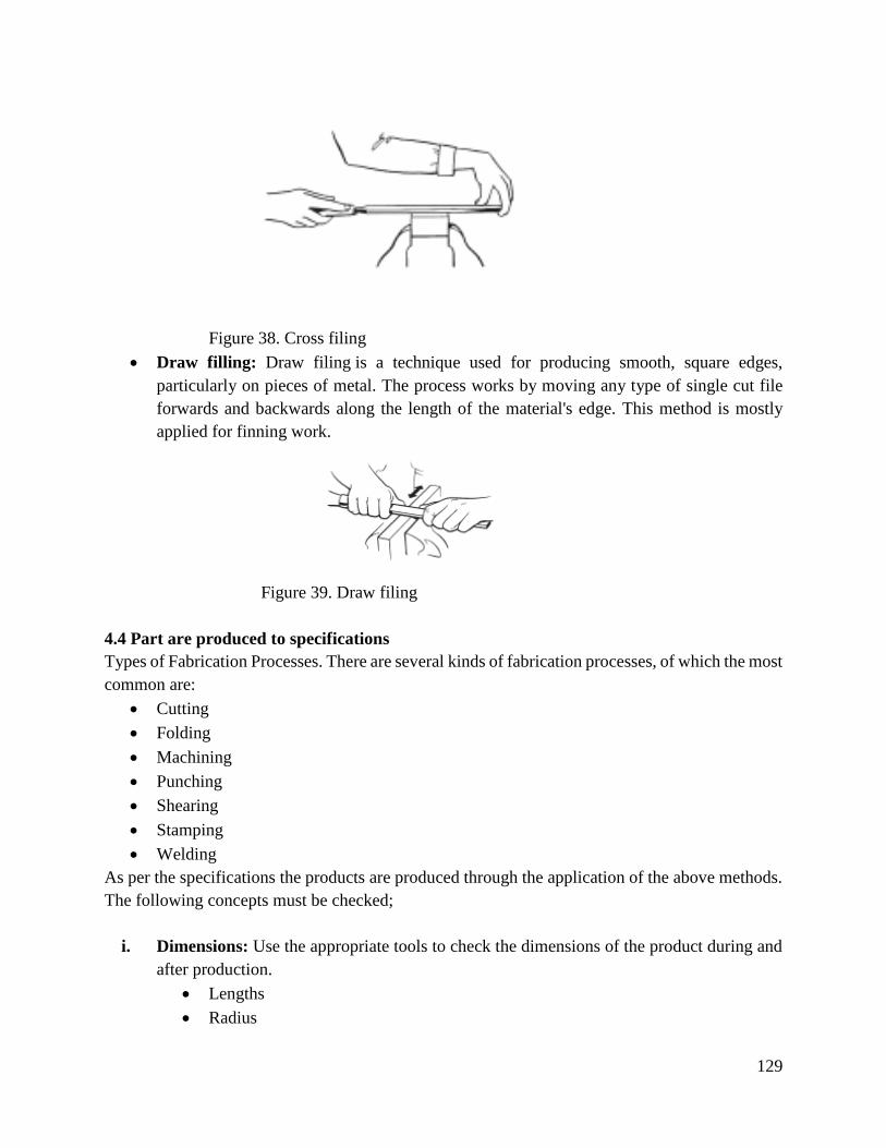
129
Figure 38. Cross filing
Draw filling: Draw filing is a technique used for producing smooth, square edges,
particularly on pieces of metal. The process works by moving any type of single cut file
forwards and backwards along the length of the material's edge. This method is mostly
applied for finning work.
Figure 39. Draw filing
4.4 Part are produced to specifications
Types of Fabrication Processes. There are several kinds of fabrication processes, of which the most
common are:
Cutting
Folding
Machining
Punching
Shearing
Stamping
Welding
As per the specifications the products are produced through the application of the above methods.
The following concepts must be checked;
i. Dimensions: Use the appropriate tools to check the dimensions of the product during and
after production.
Lengths
Radius
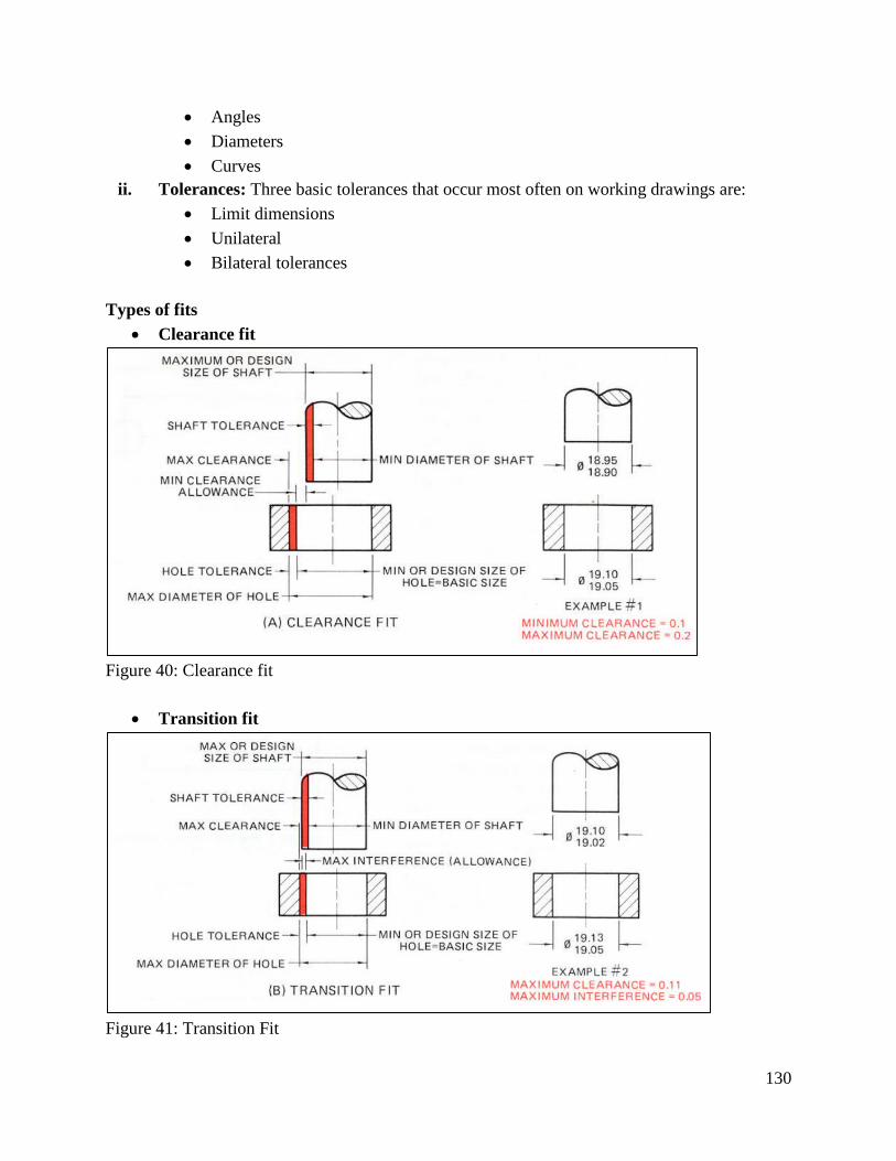
130
Angles
Diameters
Curves
ii. Tolerances: Three basic tolerances that occur most often on working drawings are:
Limit dimensions
Unilateral
Bilateral tolerances
Types of fits
Clearance fit
Figure 40: Clearance fit
Transition fit
Figure 41: Transition Fit
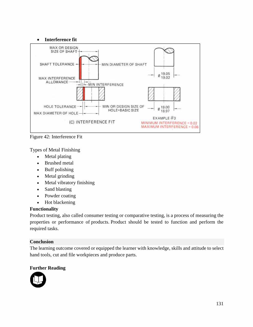
131
Interference fit
Figure 42: Interference Fit
Types of Metal Finishing
Metal plating
Brushed metal
Buff polishing
Metal grinding
Metal vibratory finishing
Sand blasting
Powder coating
Hot blackening
Functionality
Product testing, also called consumer testing or comparative testing, is a process of measuring the
properties or performance of products. Product should be tested to function and perform the
required tasks.
Conclusion
The learning outcome covered or equipped the learner with knowledge, skills and attitude to select
hand tools, cut and file workpieces and produce parts.
Further Reading

132
1. Lewis w.G.&Narayan ,C,V(11993)Design and sizing of economic handles for hand tools.
Applied ergonomics 24(5),35-356.
2. Mccormick,W(1973),U.S.Potent No.3,749,233 Washington DC;US.Patent and Trademark
office.
3.3.5.3 Self-Assessment
Written Assessment
1. The jaws in this type of wrench open parallel with the help of a screw thus providing
suitable for all sizes of nuts. These are ____________
a) Pipe wrenches
b) Monkey wrenches
c) Socket wrenches
d) Allen wrenches
2. What will happen if the job is loosely fitted between centres in cylindrical grinding?
a) The job will be out of round
b) The job will be oversized
c) The job will be thrown out
d) The job will not rotate
3. Which one among the following is NOT the cause for a broken tap while tapping?
a) The tap has coarse threads
b) Too much downward pressure is applied
c) Cutting oil is not used
d) Smaller tap drill size is used
4. The teeth of hacksaw blade are set to ___________
a) Prevent jamming and breakage of blade
b) Make the kerf wider than the blade
c) All of the above
5. Which one of the following bonds is most commonly used, on grinding wheels?
a) Vitrified
b) Rubber
c) Shellac
d) Silicate
6. What are the functional dimensions?
a) Have to be machined and fit with other mating components
b) Which have no effect on the performance of quality
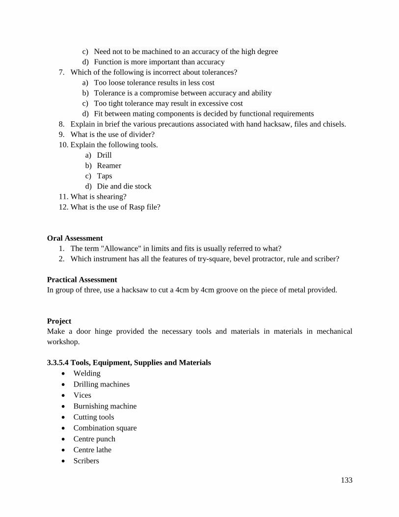
133
c) Need not to be machined to an accuracy of the high degree
d) Function is more important than accuracy
7. Which of the following is incorrect about tolerances?
a) Too loose tolerance results in less cost
b) Tolerance is a compromise between accuracy and ability
c) Too tight tolerance may result in excessive cost
d) Fit between mating components is decided by functional requirements
8. Explain in brief the various precautions associated with hand hacksaw, files and chisels.
9. What is the use of divider?
10. Explain the following tools.
a) Drill
b) Reamer
c) Taps
d) Die and die stock
11. What is shearing?
12. What is the use of Rasp file?
Oral Assessment
1. The term "Allowance" in limits and fits is usually referred to what?
2. Which instrument has all the features of try-square, bevel protractor, rule and scriber?
Practical Assessment
In group of three, use a hacksaw to cut a 4cm by 4cm groove on the piece of metal provided.
Project
Make a door hinge provided the necessary tools and materials in materials in mechanical
workshop.
3.3.5.4 Tools, Equipment, Supplies and Materials
Welding
Drilling machines
Vices
Burnishing machine
Cutting tools
Combination square
Centre punch
Centre lathe
Scribers

134
Calipers
Dies and taps
Surface plate
V-blocks
Dial gauge
Die stock
Engineer’s square
File card
Assorted Files
Clamps
Assorted hand tools
3.3.5.5 References
Morling, K. (2010). Geometric and engineering drawing. Routledge.
Sawhney, G. S. (2009). Mechanical experiments and workshop practice. IK International Pvt Ltd.
Singh, R. Introduction to basic manufacturing processes and workshop technology/Rajender
Singh. New age int. Ltd.–2006.–483 p.
135
3.3.6 Learning Outcome No 5: Use drills to make holes
3.3.6.1 Learning Activities
Learning Outcome No5 : Use drills to make holes
Learning Activities Special Instructions
5.1 Mark and center punch hole centers as per operation
plan
5.2 Select and mount drill bits
5.3 Mount and clamp work piece
5.4 Drill Hole (location, counter sinking, counter boring,
reaming, and boring) to specification
5.5 Inspect holes to specification (dimensions, tolerances,
geometry, surface finish, functionality)
Observation
3.3.6.2 Information Sheet No 3/LO5: Use drills to make holes
Introduction
This learning outcome covers the knowledge, skills and altitudes required for the leaner to perform
drilling operations as per the drawings specifications.
Definition of key terms
Drilling: It is the cutting process of a material using a specially designed rotating cutting tool
called a drill bit so as produce a hole.
Boring: Is the process of enlarging a hole that is already in the material.
Content/Procedures/Methods/Illustrations
5.1 Whole centers are marked and center-punched as per operation plan.
Laying out work for drilling consists of locating and marking the exact centers of the holes to be
drilled. The accuracy of the finished work piece depends, in most part, on the accuracy of the
layout. If the work does not require extreme accuracy, then laying out may be a simple punching
at the center only. The position of the center of the hole to be drilled is marked by scribing two or
more lines which intersect at the hole center. This intersecting point is then marked lightly with a
prick punch and hammer. Check to see that the punch mark is exactly at the center of the
intersection; use a magnifying glass if necessary. Use a pair of dividers, set to the radius of the
hole to be drilled, to scribe a circle on the work piece. When all scribing is finished, enlarge the
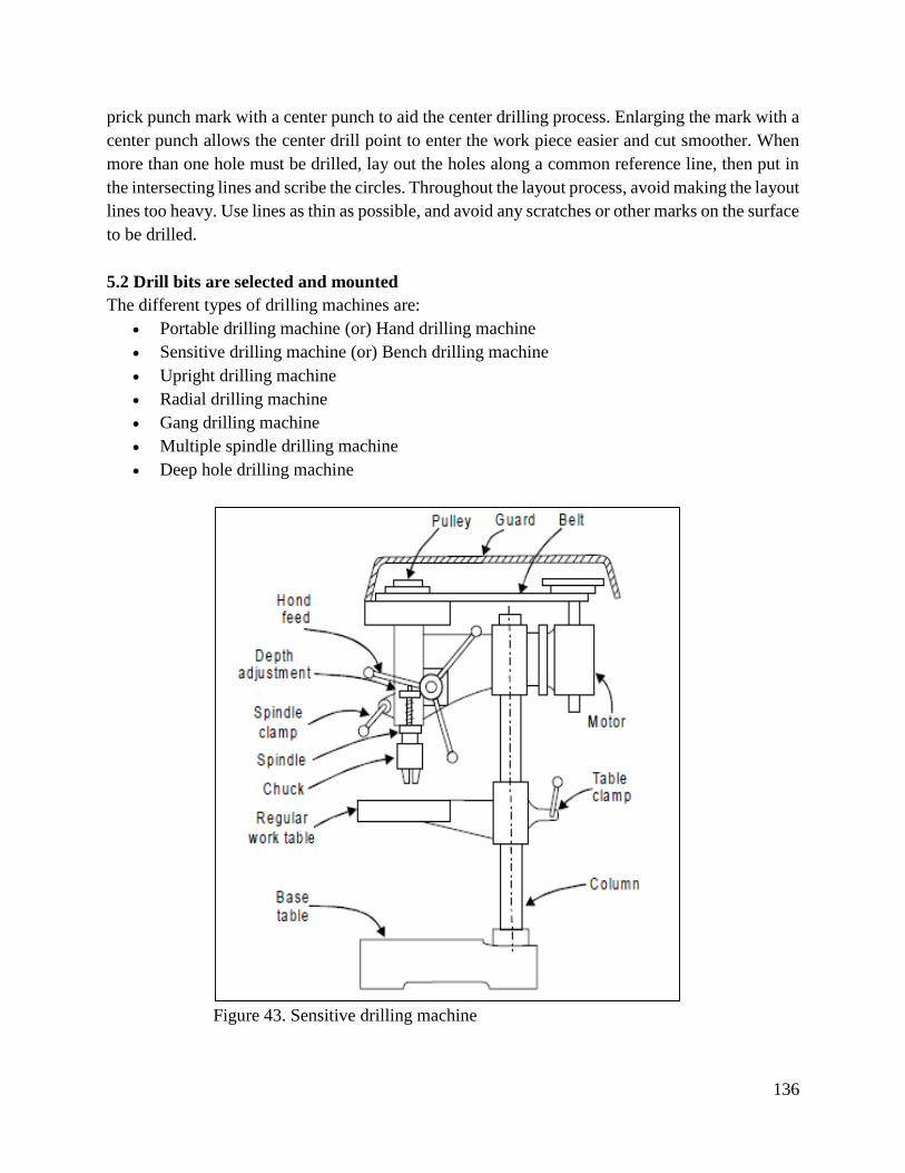
136
prick punch mark with a center punch to aid the center drilling process. Enlarging the mark with a
center punch allows the center drill point to enter the work piece easier and cut smoother. When
more than one hole must be drilled, lay out the holes along a common reference line, then put in
the intersecting lines and scribe the circles. Throughout the layout process, avoid making the layout
lines too heavy. Use lines as thin as possible, and avoid any scratches or other marks on the surface
to be drilled.
5.2 Drill bits are selected and mounted
The different types of drilling machines are:
Portable drilling machine (or) Hand drilling machine
Sensitive drilling machine (or) Bench drilling machine
Upright drilling machine
Radial drilling machine
Gang drilling machine
Multiple spindle drilling machine
Deep hole drilling machine
Figure 43. Sensitive drilling machine
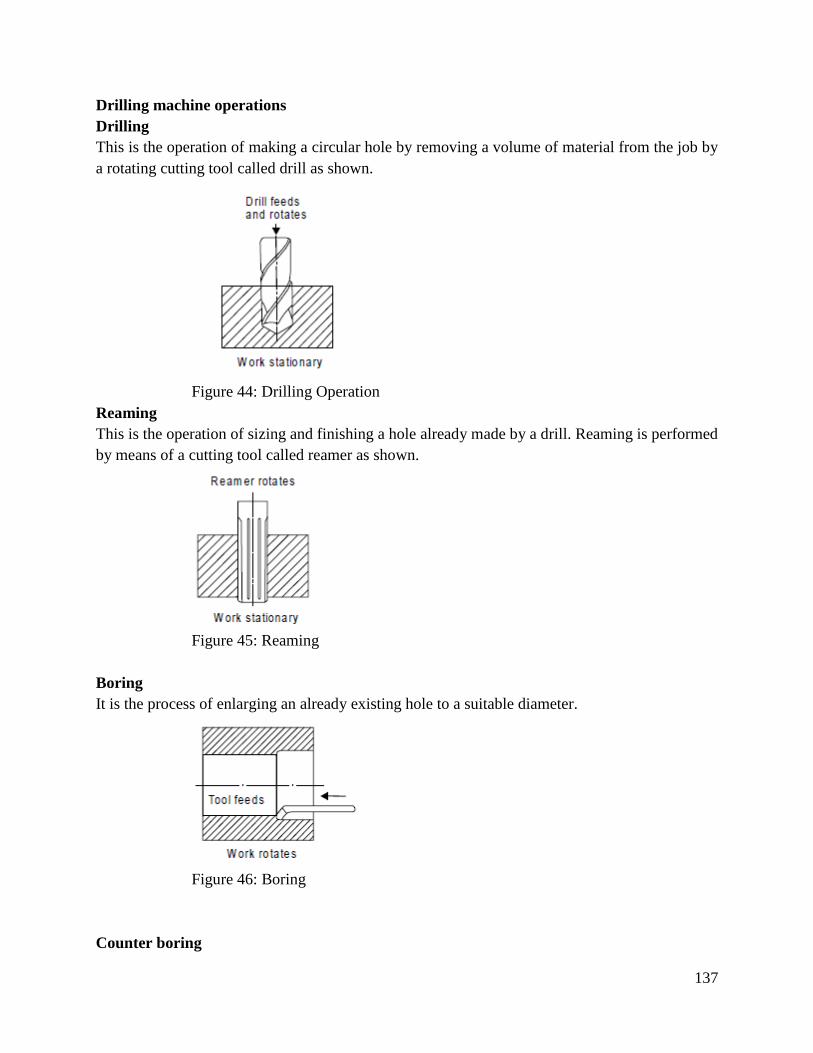
137
Drilling machine operations
Drilling
This is the operation of making a circular hole by removing a volume of material from the job by
a rotating cutting tool called drill as shown.
Figure 44: Drilling Operation
Reaming
This is the operation of sizing and finishing a hole already made by a drill. Reaming is performed
by means of a cutting tool called reamer as shown.
Figure 45: Reaming
Boring
It is the process of enlarging an already existing hole to a suitable diameter.
Figure 46: Boring
Counter boring
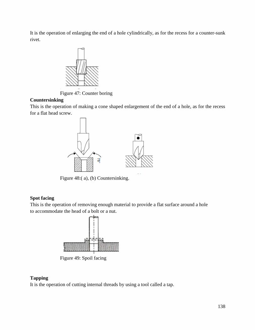
138
It is the operation of enlarging the end of a hole cylindrically, as for the recess for a counter-sunk
rivet.
Figure 47: Counter boring
Countersinking
This is the operation of making a cone shaped enlargement of the end of a hole, as for the recess
for a flat head screw.
Figure 48:( a), (b) Countersinking.
Spot facing
This is the operation of removing enough material to provide a flat surface around a hole
to accommodate the head of a bolt or a nut.
Figure 49: Spoil facing
Tapping
It is the operation of cutting internal threads by using a tool called a tap.

139
Figure 50: Trapping
5.3 Work piece is mounted and clamped
Before attempting to use a drilling machine, some provision must be made for holding the work
piece rigidly and securely in place. The work piece should always be firmly fastened to the table
or base to produce holes that are located accurately.
Methods of Mounting a Work piece
a. Mounting on vice
Most hand-feed drilling machines have no means of clamping or bolting workplaces to the table
or base. The work piece must be secured tightly in a machine table vise and swung around so that
the tail of the vise contacts and column of the drill press. The hole must be centered by hand so
that the center drill point is directly over the center punched mark. Other larger drilling machines
have slotted tables and bases so that the work and work holding devices can be bolted or clamped
firmly. All work should be securely clamped or set against a stop for all drilling to avoid letting
the drill grab and damage the work piece or injure the machine operator.
b. Table or base mounting
When a work piece is table or base mounted, the strap clamps must be as parallel to the table or
base as possible. All bolts and strap clamps should be as short as possible for rigidity and to provide
for drilling clearance.
Parallel bars should be set close together to keep from bending the work. Washers and nuts should
be in excellent condition. The slots and ways of the table, base, or vise must be free of all dirt and
chips. All work holding devices should be free of burrs and wiped clean of oil and grease. Work
holding devices should be the right size for the job. Devices that are too big or too small for the
job are dangerous and must be avoided.
5.4 Hole is drilled to specification
Drill bits selection .Drill bits are selected depending on the desired outcome .e.g. if large units of
production per unit time is required, it will be suitable to use bits with roller bearings.
NOTE:
Shale has a better drilling response to drill speed.
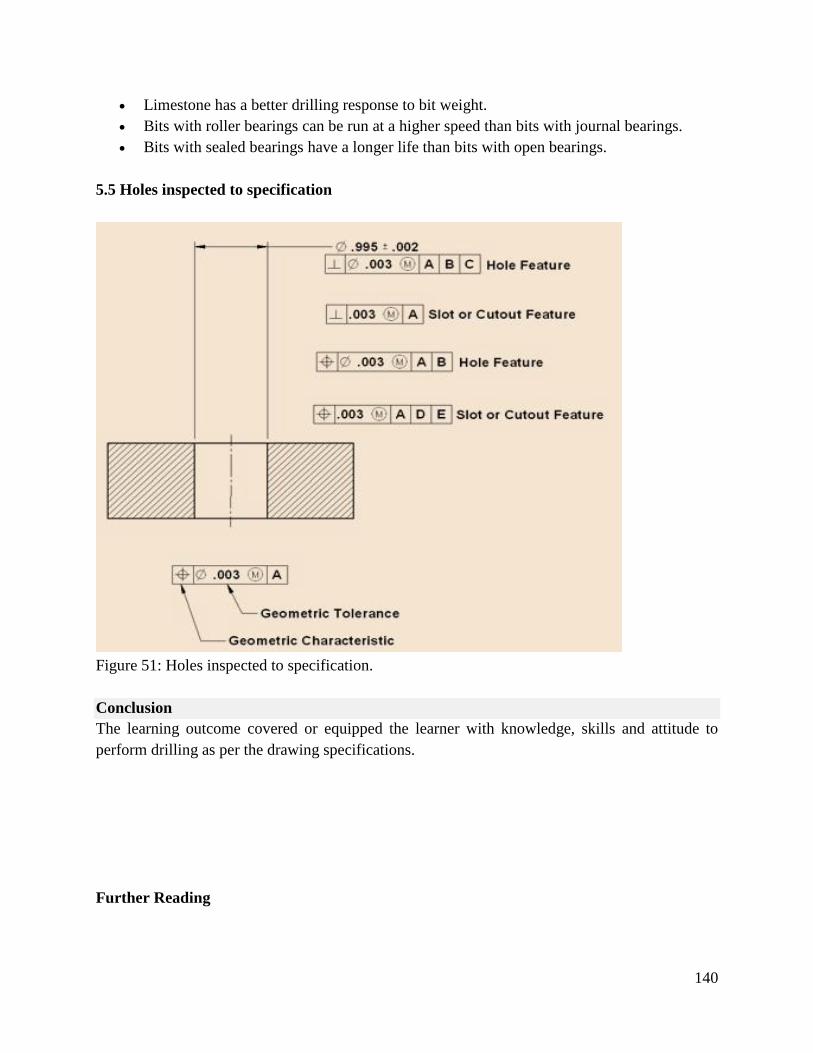
140
Limestone has a better drilling response to bit weight.
Bits with roller bearings can be run at a higher speed than bits with journal bearings.
Bits with sealed bearings have a longer life than bits with open bearings.
5.5 Holes inspected to specification
Figure 51: Holes inspected to specification.
Conclusion
The learning outcome covered or equipped the learner with knowledge, skills and attitude to
perform drilling as per the drawing specifications.
Further Reading
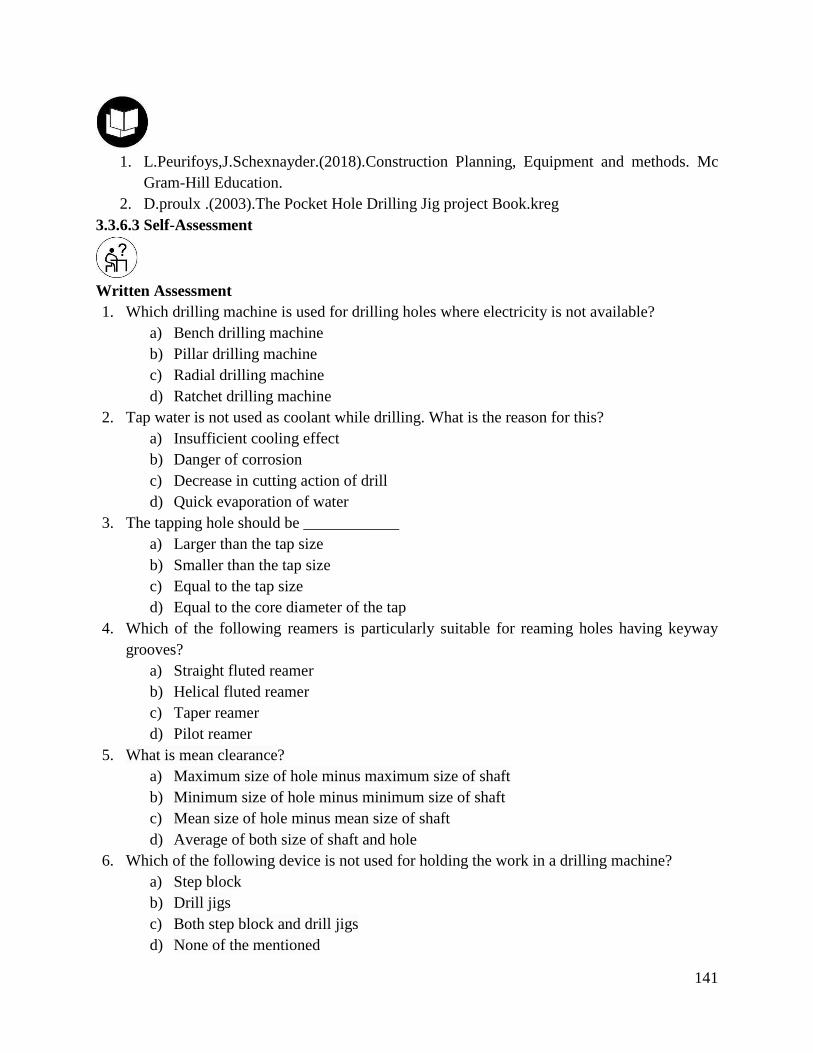
141
1. L.Peurifoys,J.Schexnayder.(2018).Construction Planning, Equipment and methods. Mc
Gram-Hill Education.
2. D.proulx .(2003).The Pocket Hole Drilling Jig project Book.kreg
3.3.6.3 Self-Assessment
Written Assessment
1. Which drilling machine is used for drilling holes where electricity is not available?
a) Bench drilling machine
b) Pillar drilling machine
c) Radial drilling machine
d) Ratchet drilling machine
2. Tap water is not used as coolant while drilling. What is the reason for this?
a) Insufficient cooling effect
b) Danger of corrosion
c) Decrease in cutting action of drill
d) Quick evaporation of water
3. The tapping hole should be ____________
a) Larger than the tap size
b) Smaller than the tap size
c) Equal to the tap size
d) Equal to the core diameter of the tap
4. Which of the following reamers is particularly suitable for reaming holes having keyway
grooves?
a) Straight fluted reamer
b) Helical fluted reamer
c) Taper reamer
d) Pilot reamer
5. What is mean clearance?
a) Maximum size of hole minus maximum size of shaft
b) Minimum size of hole minus minimum size of shaft
c) Mean size of hole minus mean size of shaft
d) Average of both size of shaft and hole
6. Which of the following device is not used for holding the work in a drilling machine?
a) Step block
b) Drill jigs
c) Both step block and drill jigs
d) None of the mentioned
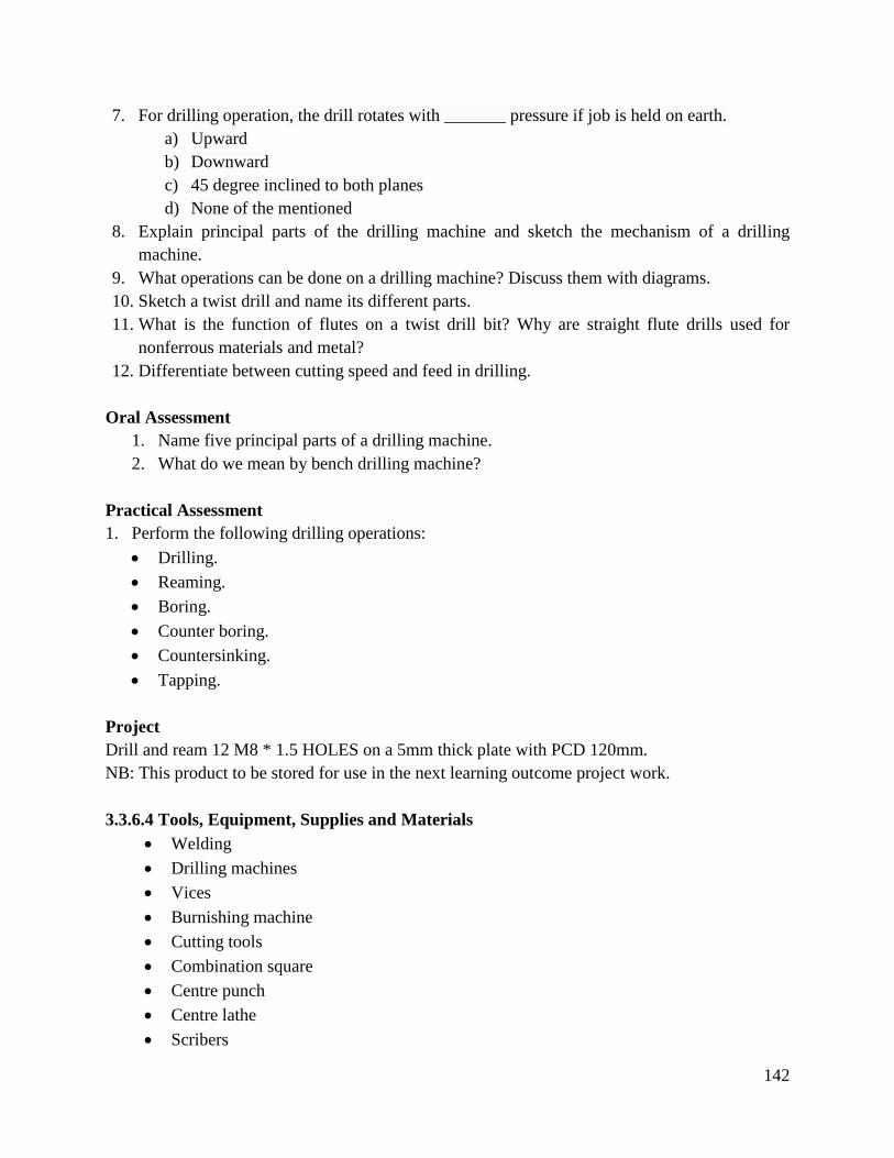
142
7. For drilling operation, the drill rotates with _______ pressure if job is held on earth.
a) Upward
b) Downward
c) 45 degree inclined to both planes
d) None of the mentioned
8. Explain principal parts of the drilling machine and sketch the mechanism of a drilling
machine.
9. What operations can be done on a drilling machine? Discuss them with diagrams.
10. Sketch a twist drill and name its different parts.
11. What is the function of flutes on a twist drill bit? Why are straight flute drills used for
nonferrous materials and metal?
12. Differentiate between cutting speed and feed in drilling.
Oral Assessment
1. Name five principal parts of a drilling machine.
2. What do we mean by bench drilling machine?
Practical Assessment
1. Perform the following drilling operations:
Drilling.
Reaming.
Boring.
Counter boring.
Countersinking.
Tapping.
Project
Drill and ream 12 M8 * 1.5 HOLES on a 5mm thick plate with PCD 120mm.
NB: This product to be stored for use in the next learning outcome project work.
3.3.6.4 Tools, Equipment, Supplies and Materials
Welding
Drilling machines
Vices
Burnishing machine
Cutting tools
Combination square
Centre punch
Centre lathe
Scribers

143
Salipers
Dies and taps
Surface plate
V-blocks
Dial gauge
Die stock
Engineer’s square
File card
Assorted Files
Clamps
Assorted hand tools
3.3.6.5 References
Morling, K. (1974). Geometric and Engineering drawing (3rded). Butterworth-Heine Amann.
Sawhney, G.S. (2009). Mechanical Experiments and workshop. IK International Publishing
House.
Sharma. (2001). Workshop technology and practice.
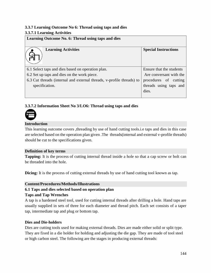
144
3.3.7 Learning Outcome No 6: Thread using taps and dies
3.3.7.1 Learning Activities
Learning Outcome No. 6: Thread using taps and dies
Learning Activities Special Instructions
6.1 Select taps and dies based on operation plan.
6.2 Set up taps and dies on the work piece.
6.3 Cut threads (internal and external threads, v-profile threads) to
specification.
Ensure that the students
Are conversant with the
procedures of cutting
threads using taps and
dies.
3.3.7.2 Information Sheet No 3/LO6: Thread using taps and dies
Introduction
This learning outcome covers ,threading by use of hand cutting tools.i.e taps and dies in this case
are selected based on the operation plan given .The threads(internal and external v-profile threads)
should be cut to the specifications given.
Definition of key terms
Tapping: It is the process of cutting internal thread inside a hole so that a cap screw or bolt can
be threaded into the hole.
Dicing: It is the process of cutting external threads by use of hand cutting tool known as tap.
Content/Procedures/Methods/Illustrations
6.1 Taps and dies selected based on operation plan
Taps and Tap Wrenches
A tap is a hardened steel tool, used for cutting internal threads after drilling a hole. Hand taps are
usually supplied in sets of three for each diameter and thread pitch. Each set consists of a taper
tap, intermediate tap and plug or bottom tap.
Dies and Die-holders
Dies are cutting tools used for making external threads. Dies are made either solid or split type.
They are fixed in a die holder for holding and adjusting the die gap. They are made of tool steel
or high carbon steel. The following are the stages in producing external threads:
145
Figure 52: Adjustment split die
Figure 53: Diestock
Figure 54: Thread Nomenclature.
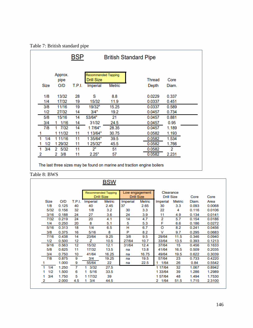
146
Table 7: British standard pipe
Table 8: BWS
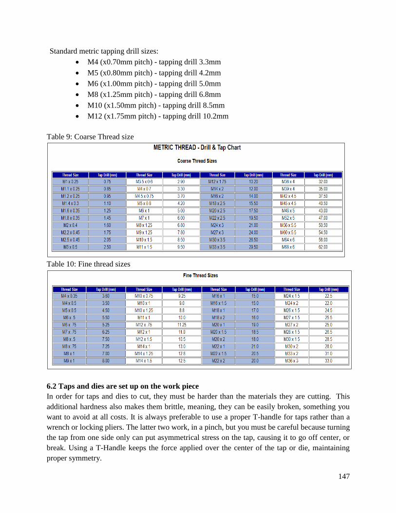
147
Standard metric tapping drill sizes:
M4 (x0.70mm pitch) - tapping drill 3.3mm
M5 (x0.80mm pitch) - tapping drill 4.2mm
M6 (x1.00mm pitch) - tapping drill 5.0mm
M8 (x1.25mm pitch) - tapping drill 6.8mm
M10 (x1.50mm pitch) - tapping drill 8.5mm
M12 (x1.75mm pitch) - tapping drill 10.2mm
Table 9: Coarse Thread size
Table 10: Fine thread sizes
6.2 Taps and dies are set up on the work piece
In order for taps and dies to cut, they must be harder than the materials they are cutting. This
additional hardness also makes them brittle, meaning, they can be easily broken, something you
want to avoid at all costs. It is always preferable to use a proper T-handle for taps rather than a
wrench or locking pliers. The latter two work, in a pinch, but you must be careful because turning
the tap from one side only can put asymmetrical stress on the tap, causing it to go off center, or
break. Using a T-Handle keeps the force applied over the center of the tap or die, maintaining
proper symmetry.
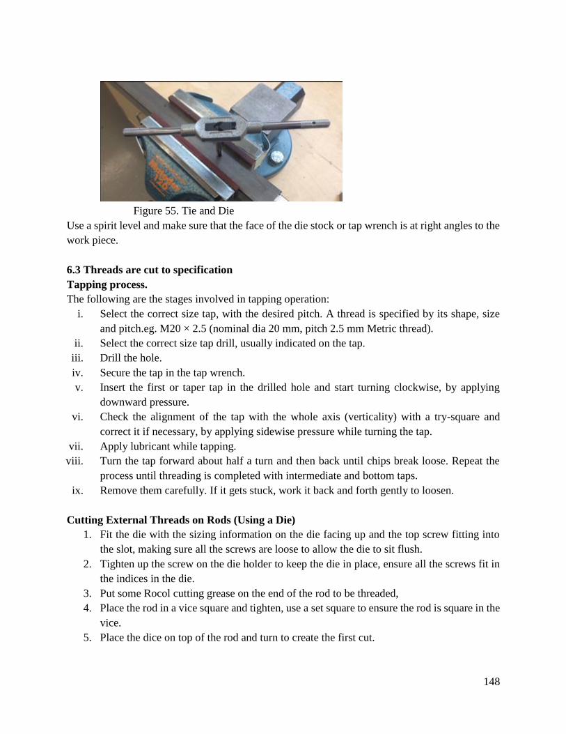
148
Figure 55. Tie and Die
Use a spirit level and make sure that the face of the die stock or tap wrench is at right angles to the
work piece.
6.3 Threads are cut to specification
Tapping process.
The following are the stages involved in tapping operation:
i. Select the correct size tap, with the desired pitch. A thread is specified by its shape, size
and pitch.eg. M20 × 2.5 (nominal dia 20 mm, pitch 2.5 mm Metric thread).
ii. Select the correct size tap drill, usually indicated on the tap.
iii. Drill the hole.
iv. Secure the tap in the tap wrench.
v. Insert the first or taper tap in the drilled hole and start turning clockwise, by applying
downward pressure.
vi. Check the alignment of the tap with the whole axis (verticality) with a try-square and
correct it if necessary, by applying sidewise pressure while turning the tap.
vii. Apply lubricant while tapping.
viii. Turn the tap forward about half a turn and then back until chips break loose. Repeat the
process until threading is completed with intermediate and bottom taps.
ix. Remove them carefully. If it gets stuck, work it back and forth gently to loosen.
Cutting External Threads on Rods (Using a Die)
1. Fit the die with the sizing information on the die facing up and the top screw fitting into
the slot, making sure all the screws are loose to allow the die to sit flush.
2. Tighten up the screw on the die holder to keep the die in place, ensure all the screws fit in
the indices in the die.
3. Put some Rocol cutting grease on the end of the rod to be threaded,
4. Place the rod in a vice square and tighten, use a set square to ensure the rod is square in the
vice.
5. Place the dice on top of the rod and turn to create the first cut.
149
6. Once a grip on the material has been made turn half a turn into the material and then a
quarter turn back this will ensure that the die doesn’t get clogged with the offcuts of
material and a better thread is created.
7. Keep turning until the depth of thread is achieved, there should be no resistance once the
cut has been made level and square to the rod.
8. Check the threading using the appropriate sized nut.
Conclusion
The learning outcome covered or equipped the learner with knowledge, skills and attitude to cut
internal and external threads as per the threads standards by use of hand cutting tools. The main
hand clothing tools used include taps dies. All the process involving thread have also been
highlighted in this learning outcome.
Further Reading
1. How to set the cutting speed of various threading operations using the formula
v =πdn
1000 mmin−1
2. Hex Rethreading dies and T .handle Tap wrenches.
3.3.7.3 Self-Assessment
Written Assessment
1. A cutting tool used to cut outside threads is called?
a) Drill
b) Reamer
c) Die
d) Tap
2. What is used for removing a broken tap?
a) Tap disposer
b) Tap wrench
c) Tap extractor
d) Tap nut
3. A hole, which is not made through full depth of the component is known as ______
a) Core hole
150
b) Blind hole
c) Pinhole
d) Bore hole
4. Jigs are not used in __________
a) Drilling
b) Reaming
c) Tapping
d) Milling
5. What is the name of screw thread which is formed on a cone?
a) Parallel screw thread
b) Straight screw thread
c) Tapered screw thread
d) Cylindrical screw thread
6. What is dedendum for external threads?
a) Radial distance between pitch and minor cylinder
b) Radial distance between major and pitch cylinder
c) Radial distance between major and minor cylinder
d) Axial distance between major and pitch cylinder
7. Which of the following is true for the multiple start screw threads?
a) It is produced by a single helical groove
b) Grooves should be different in spacing
c) It gives a quick transverse
d) It is formed in a transverse section on a cylinder
8. If a clearance fit is present between shaft and hole, what is the tolerance on shaft or hole for a
complete interchangeable approach?
9. Which tools are used for cutting internal and external threads by hand?
10. Why must we always move taps or, resp., dies or die-stocks backwards?
11. What does the designation "M 6 x 0.5" mean?
12. Which operations are involved in manufacturing an internal thread?
Oral Assessment
1. How can we calculate the minor diameter of an internal thread?
2. Which testing tools are used to test a completely tapped hole?
Practical Assessment
Cut internal and external threads using taps and dies. Identify all the approaches you followed in
cutting the threads basing on the metric standards used.
Project

151
Thread the above project for previous learning outcome (Drill and ream 12 M8 * 1.5 HOLES on
a 5mm thick plate with PCD 120mm) and produce bolts for the same.
3.3.7.4 Tools, Equipment, Supplies and Materials
Welding
Drilling machines
Vices
Burnishing machine
Cutting tools
Combination square
Centre punch
Centre lathe
scribers
calipers
Dies and taps
Surface plate
V-blocks
Dial gauge
Die stock
Engineer’s square
File card
Assorted Files
Clamps
Assorted hand tools
3.3.7.5 References
Brooks ,R.C(1988).Standard screw threads for scientific instruments .Part: Production techniques
and filiere Suisse.
Ducharme ,R.(2006).Greenfield Tap and Die .Economic and Historical journal of Massachusetts.
Juneja,B. L(2000). Fundamentals of metal cutting and machine tools. New age International.
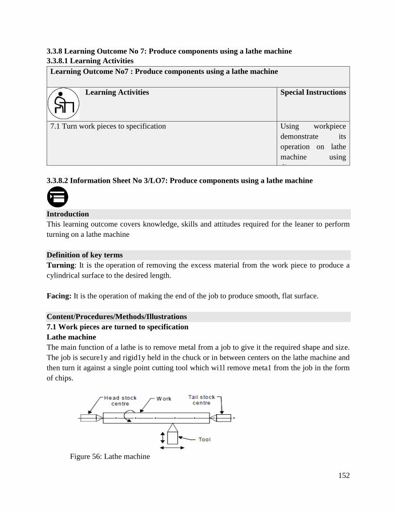
152
3.3.8 Learning Outcome No 7: Produce components using a lathe machine
3.3.8.1 Learning Activities
Learning Outcome No7 : Produce components using a lathe machine
Learning Activities Special Instructions
7.1 Turn work pieces to specification
Using workpiece
demonstrate its
operation on lathe
machine using
diagram.
3.3.8.2 Information Sheet No 3/LO7: Produce components using a lathe machine
Introduction
This learning outcome covers knowledge, skills and attitudes required for the leaner to perform
turning on a lathe machine
Definition of key terms
Turning: It is the operation of removing the excess material from the work piece to produce a
cylindrical surface to the desired length.
Facing: It is the operation of making the end of the job to produce smooth, flat surface.
Content/Procedures/Methods/Illustrations
7.1 Work pieces are turned to specification
Lathe machine
The main function of a lathe is to remove metal from a job to give it the required shape and size.
The job is secure1y and rigid1y held in the chuck or in between centers on the lathe machine and
then turn it against a single point cutting tool which wi1l remove meta1 from the job in the form
of chips.
Figure 56: Lathe machine
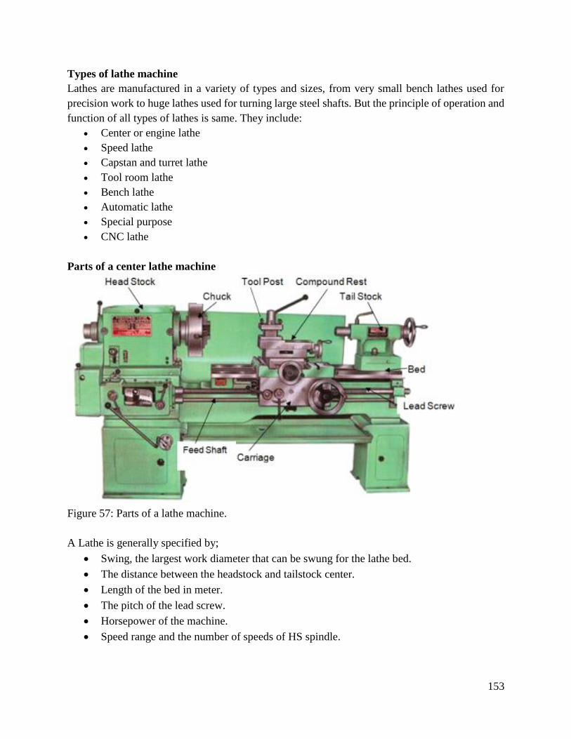
153
Types of lathe machine
Lathes are manufactured in a variety of types and sizes, from very small bench lathes used for
precision work to huge lathes used for turning large steel shafts. But the principle of operation and
function of all types of lathes is same. They include:
Center or engine lathe
Speed lathe
Capstan and turret lathe
Tool room lathe
Bench lathe
Automatic lathe
Special purpose
CNC lathe
Parts of a center lathe machine
Figure 57: Parts of a lathe machine.
A Lathe is generally specified by;
Swing, the largest work diameter that can be swung for the lathe bed.
The distance between the headstock and tailstock center.
Length of the bed in meter.
The pitch of the lead screw.
Horsepower of the machine.
Speed range and the number of speeds of HS spindle.
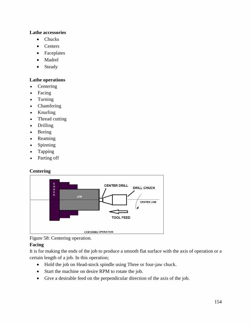
154
Lathe accessories
Chucks
Centers
Faceplates
Madrel
Steady
Lathe operations
Centering
Facing
Turning
Chamfering
Knurling
Thread cutting
Drilling
Boring
Reaming
Spinning
Tapping
Parting off
Centering
Figure 58: Centering operation.
Facing
It is for making the ends of the job to produce a smooth flat surface with the axis of operation or a
certain length of a job. In this operation;
Hold the job on Head-stock spindle using Three or four-jaw chuck.
Start the machine on desire RPM to rotate the job.
Give a desirable feed on the perpendicular direction of the axis of the job.
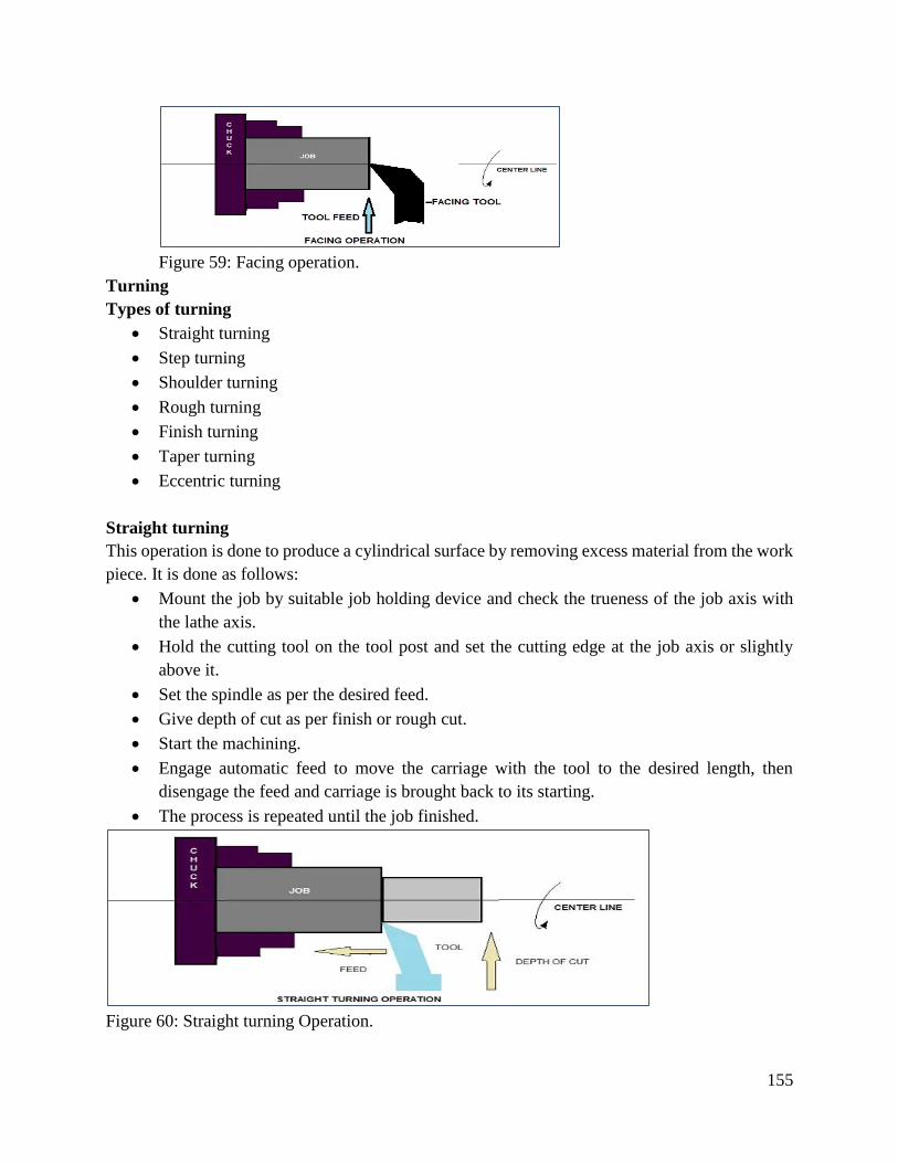
155
Figure 59: Facing operation.
Turning
Types of turning
Straight turning
Step turning
Shoulder turning
Rough turning
Finish turning
Taper turning
Eccentric turning
Straight turning
This operation is done to produce a cylindrical surface by removing excess material from the work
piece. It is done as follows:
Mount the job by suitable job holding device and check the trueness of the job axis with
the lathe axis.
Hold the cutting tool on the tool post and set the cutting edge at the job axis or slightly
above it.
Set the spindle as per the desired feed.
Give depth of cut as per finish or rough cut.
Start the machining.
Engage automatic feed to move the carriage with the tool to the desired length, then
disengage the feed and carriage is brought back to its starting.
The process is repeated until the job finished.
Figure 60: Straight turning Operation.
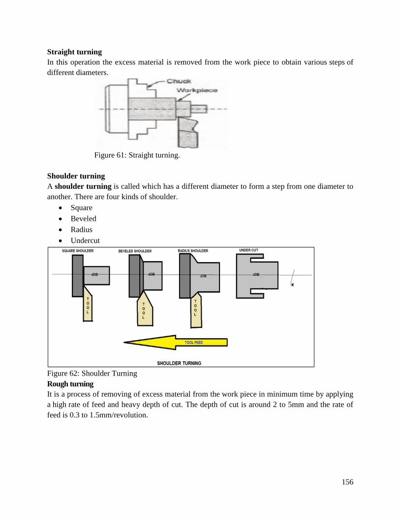
156
Straight turning
In this operation the excess material is removed from the work piece to obtain various steps of
different diameters.
Figure 61: Straight turning.
Shoulder turning
A shoulder turning is called which has a different diameter to form a step from one diameter to
another. There are four kinds of shoulder.
Square
Beveled
Radius
Undercut
Figure 62: Shoulder Turning
Rough turning
It is a process of removing of excess material from the work piece in minimum time by applying
a high rate of feed and heavy depth of cut. The depth of cut is around 2 to 5mm and the rate of
feed is 0.3 to 1.5mm/revolution.
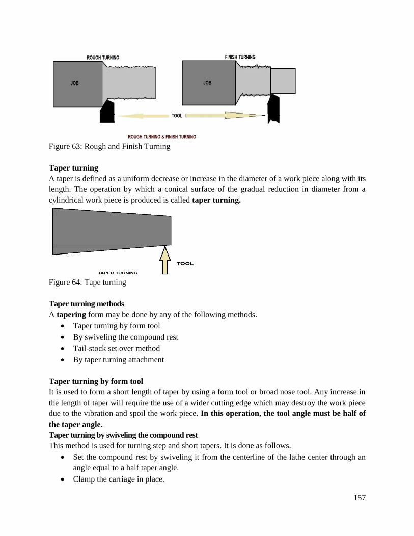
157
Figure 63: Rough and Finish Turning
Taper turning
A taper is defined as a uniform decrease or increase in the diameter of a work piece along with its
length. The operation by which a conical surface of the gradual reduction in diameter from a
cylindrical work piece is produced is called taper turning.
Figure 64: Tape turning
Taper turning methods
A tapering form may be done by any of the following methods.
Taper turning by form tool
By swiveling the compound rest
Tail-stock set over method
By taper turning attachment
Taper turning by form tool
It is used to form a short length of taper by using a form tool or broad nose tool. Any increase in
the length of taper will require the use of a wider cutting edge which may destroy the work piece
due to the vibration and spoil the work piece. In this operation, the tool angle must be half of
the taper angle.
Taper turning by swiveling the compound rest
This method is used for turning step and short tapers. It is done as follows.
Set the compound rest by swiveling it from the centerline of the lathe center through an
angle equal to a half taper angle.
Clamp the carriage in place.
158
After adjusting and setting the tool, feed is applied by the compound rest’s feed handle to
complete the taper.
Tail-stock set over method
Set over of tail-stock from its center-line is done equal to half taper. Job is held between the centers.
The length of the work piece will be long enough. An only a small taper on a long job is done by
this process. It is used for external taper only. By taper turning attachment: It is done in the following
ways:
The cross slide is first made free from lead screw by hinder screw.
The rear end of the cross slide is then tightened with a guide block by a belt.
Set the guide bar at an angle to the lathe axis. (Half taper angle)
The required depth of cut is given by the compound slide is at a right angle to the lathe
axis.
Chamfering operation:
Chamfering is used for beveling the end of a job to remove burrs, to look better, to make a passage
of the nut into the bolt. This operation is done after thread cutting, knurling, rough turning. Safety
in lathe work.
Correct dress is important, remove rings and watches, roll sleeves above elbows.
Always stop the lathe before making adjustments.
Do not change spindle speeds until the lathe comes to a complete stop.
Always wear protective eye protection.
Never lay tools directly on the lathe ways. If a separate table is not available, use a wide
board with a cleat on each side to lay on the ways.
Use two hands when sanding the work piece. Do not wrap sand paper or emery cloth around
the work piece.
Conclusion
The learning outcome covered or equipped the learner with knowledge, skills and attitude to
produce parts by lathe work.
Further Reading
1. Bray, stan (2004) poole. Special insert model book.
2. Holtzapihel, Charles (1843-1897).Turning and mechanical manipulation volume
159
3.3.8.3 Self-Assessment
Written Assessment
1. Lathe is primarily used for producing ____surfaces.
a) Flat
b) Curve
c) Taper
d) None of the mentioned
2. What is the necessary condition for turning?
a) Material of work piece should be harder than the cutting tool
b) Cutting tool should be harder than the material of work piece
c) Hardness of the cutting tool and material of of piece should be same
d) None of the mentioned
3. Traversing of tool parallel to the axis of job is termed as_____
a) Cross feed
b) Longitudinal feed
c) Both cross feed and traversing feed
d) None of the mentioned
4. Lathe spindle has got ___________
a) Internal threads
b) External threads
c) Taper threads
d) No threads
e) None of the above
5. Lathe centers are provided with the following standard taper _________
a) Morse
b) British
c) Metric
d) Sharpe
e) Any taper
6. Which of the following lathe operations requires that the cutting edge of a tool bit be placed
exactly on the work center line __________
a) Boring
b) Drilling
c) Facing
d) Turning
e) Chamfering
160
7. Lathe bed is usually made of _____________
a) Structural steel
b) Stainless steel
c) Cast iron
d) Mild steel
e) All of the above
8. Which type of feed is needed in facing?
9. Describe any two work holding devices used on the lathe.
10. With help of neat diagram, describe the following as done on a lathe machine.
a) Finish turning
b) Rough turning
c) Turning
d) Drilling
11. Name different methods of taper turning? Describe these methods using neat sketches.
12. What is the meaning of the following terms used in lathe operation.
a) Cutting speed
b) Feed
c) Depth of cut
Oral Assessment
1. What is the purpose of the Lathe carriage of the tool?
2. Which other name is given to tool rest?
Practical Assessment
1. Perform the following operations on a lathe machine.
a) Centering
b) Facing
c) Step turning
d) Tapper turning
e) Slotting
Project
1. Prepare an operation plan, grid the necessary tools and perform machining.
3.3.8.4 Tools, Equipment, Supplies and Materials
Welding
Drilling machines
Vices
Burnishing machine
Cutting tools

161
Combination square
Centre punch
Centre lathe
Scribers
Calipers
Dies and taps
Surface plate
V-blocks
Dial gauge
Die stock
Engineer’s square
File card
Assorted Files
Clamps
Assorted hand tools
3.3.8.5 References
Lee, S. S., & Chen, J. C. (2003). On-line surface roughness recognition system using artificial
neural networks system in turning operations. The International Journal of Advanced
Manufacturing Technology, 22(7-8), 498-509.
McCullough, E. M. (1962). Economics of multi-Tool lathe operations. ASME.
Youssef, H. A., & El-Hofy, H. (2008). Machining technology: machine tools and operations. CRC
Press.
162
3.3.9 Learning Outcome No 8: Assemble metal parts and sub-assemblies
3.3.9.1 Learning Activities
Learning Outcome No 8: Assemble metal parts and sub-assemblies
Learning Activities Special Instructions
8.1 Fit and assemble parts joined (riveting, fastening,
soldering, brazing, and welding).
8.2 Inspect final assembly as per specification.
Learning to describe the
welding process
And state various types of
welding process.
3.3.9.2 Information Sheet No 3/LO8: Assemble metal parts and sub-assemblies
Introduction
This learning outcome covers the knowledge, skills and attitudes required for the leaner to
assemble metal parts and sub- assemblies.
Definition of key terms
Major diameter: The major diameter is the largest diameter of the thread. It determines the
nominal size.
Minor diameter: It is the smallest diameter of the thread. In external thread, it is also called as
root diameter.
Pitch: Is the axial distance between any point of one thread and the corresponding point of an
adjacent thread.
Lead: The distance a bolt advances into a nut in one revolution is called lead.
Content/Procedures/Methods/Illustrations
8.1 Parts joined, fitted and assembled
There are two methods of metal joining;
Mechanical joining
Fusion joining
Mechanical joining
They include:
Folding
Riveting
Bolts and nuts
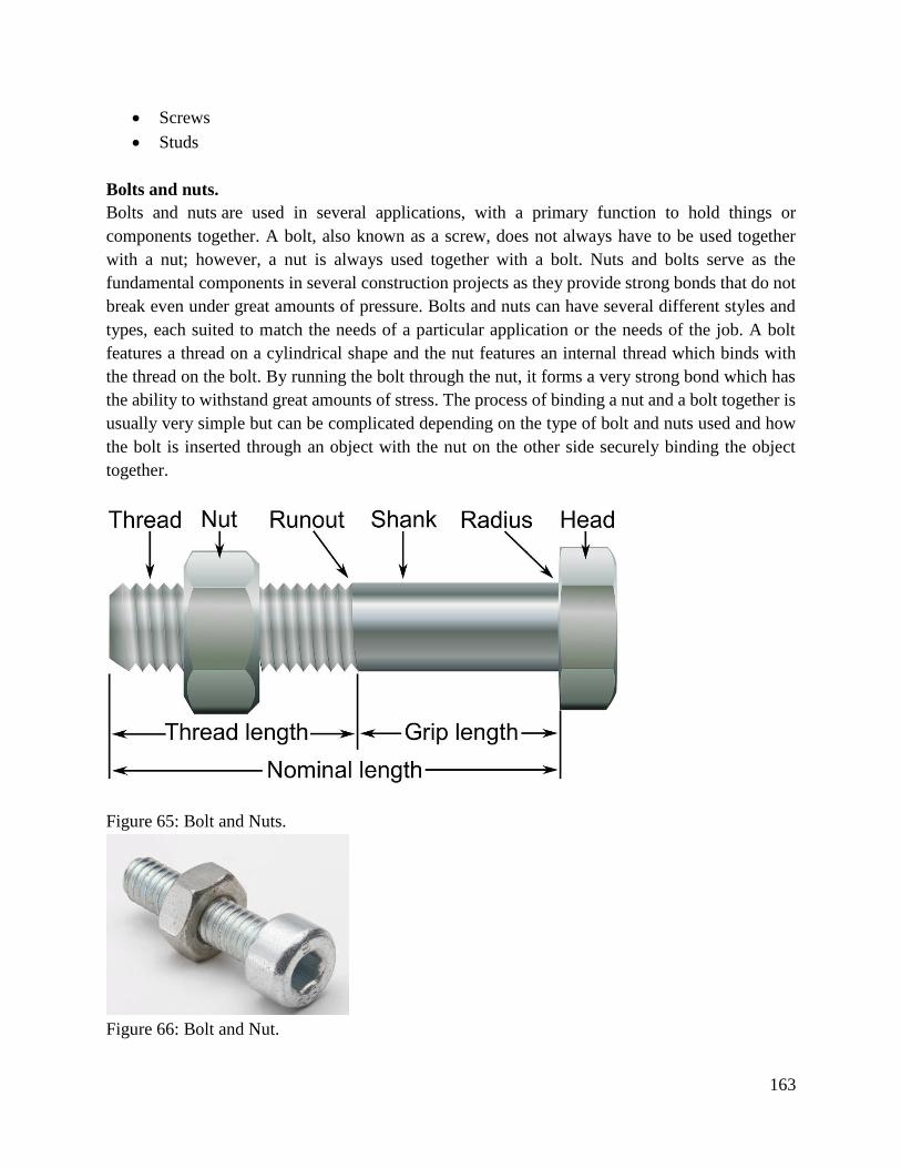
163
Screws
Studs
Bolts and nuts.
Bolts and nuts are used in several applications, with a primary function to hold things or
components together. A bolt, also known as a screw, does not always have to be used together
with a nut; however, a nut is always used together with a bolt. Nuts and bolts serve as the
fundamental components in several construction projects as they provide strong bonds that do not
break even under great amounts of pressure. Bolts and nuts can have several different styles and
types, each suited to match the needs of a particular application or the needs of the job. A bolt
features a thread on a cylindrical shape and the nut features an internal thread which binds with
the thread on the bolt. By running the bolt through the nut, it forms a very strong bond which has
the ability to withstand great amounts of stress. The process of binding a nut and a bolt together is
usually very simple but can be complicated depending on the type of bolt and nuts used and how
the bolt is inserted through an object with the nut on the other side securely binding the object
together.
Figure 65: Bolt and Nuts.
Figure 66: Bolt and Nut.
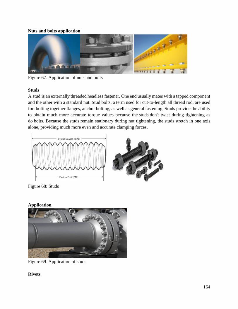
164
Nuts and bolts application
Figure 67. Application of nuts and bolts
Studs
A stud is an externally threaded headless fastener. One end usually mates with a tapped component
and the other with a standard nut. Stud bolts, a term used for cut-to-length all thread rod, are used
for: bolting together flanges, anchor bolting, as well as general fastening. Studs provide the ability
to obtain much more accurate torque values because the studs don't twist during tightening as
do bolts. Because the studs remain stationary during nut tightening, the studs stretch in one axis
alone, providing much more even and accurate clamping forces.
Figure 68: Studs
Application
Figure 69. Application of studs
Rivets
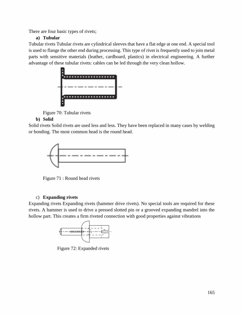
165
There are four basic types of rivets;
a) Tubular
Tubular rivets Tubular rivets are cylindrical sleeves that have a flat edge at one end. A special tool
is used to flange the other end during processing. This type of rivet is frequently used to join metal
parts with sensitive materials (leather, cardboard, plastics) in electrical engineering. A further
advantage of these tubular rivets: cables can be led through the very clean hollow.
Figure 70: Tubular rivets
b) Solid
Solid rivets Solid rivets are used less and less. They have been replaced in many cases by welding
or bonding. The most common head is the round head.
Figure 71 : Round head rivets
c) Expanding rivets
Expanding rivets Expanding rivets (hammer drive rivets). No special tools are required for these
rivets. A hammer is used to drive a pressed slotted pin or a grooved expanding mandrel into the
hollow part. This creates a firm riveted connection with good properties against vibrations
Figure 72: Expanded rivets
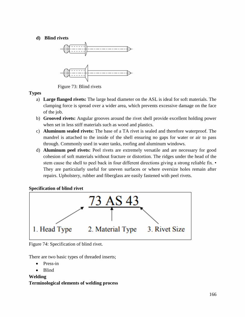
166
d) Blind rivets
Figure 73: Blind rivets
Types
a) Large flanged rivets: The large head diameter on the ASL is ideal for soft materials. The
clamping force is spread over a wider area, which prevents excessive damage on the face
of the job.
b) Grooved rivets: Angular grooves around the rivet shell provide excellent holding power
when set in less stiff materials such as wood and plastics.
c) Aluminum sealed rivets: The base of a TA rivet is sealed and therefore waterproof. The
mandrel is attached to the inside of the shell ensuring no gaps for water or air to pass
through. Commonly used in water tanks, roofing and aluminum windows.
d) Aluminum peel rivets: Peel rivets are extremely versatile and are necessary for good
cohesion of soft materials without fracture or distortion. The ridges under the head of the
stem cause the shell to peel back in four different directions giving a strong reliable fix. •
They are particularly useful for uneven surfaces or where oversize holes remain after
repairs. Upholstery, rubber and fiberglass are easily fastened with peel rivets.
Specification of blind rivet
Figure 74: Specification of blind rivet.
There are two basic types of threaded inserts;
Press-in
Blind
Welding
Terminological elements of welding process
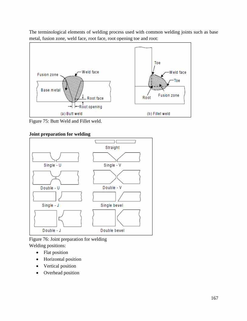
167
The terminological elements of welding process used with common welding joints such as base
metal, fusion zone, weld face, root face, root opening toe and root:
Figure 75: Butt Weld and Fillet weld.
Joint preparation for welding
Figure 76: Joint preparation for welding
Welding positions:
Flat position
Horizontal position
Vertical position
Overhead position
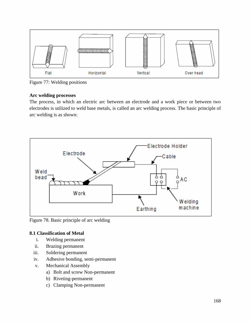
168
Figure 77: Welding positions
Arc welding processes
The process, in which an electric arc between an electrode and a work piece or between two
electrodes is utilized to weld base metals, is called an arc welding process. The basic principle of
arc welding is as shown:
Figure 78. Basic principle of arc welding
8.1 Classification of Metal
i. Welding permanent
ii. Brazing permanent
iii. Soldering permanent
iv. Adhesive bonding, semi-permanent
v. Mechanical Assembly
a) Bolt and screw Non-permanent
b) Riveting-permanent
c) Clamping Non-permanent
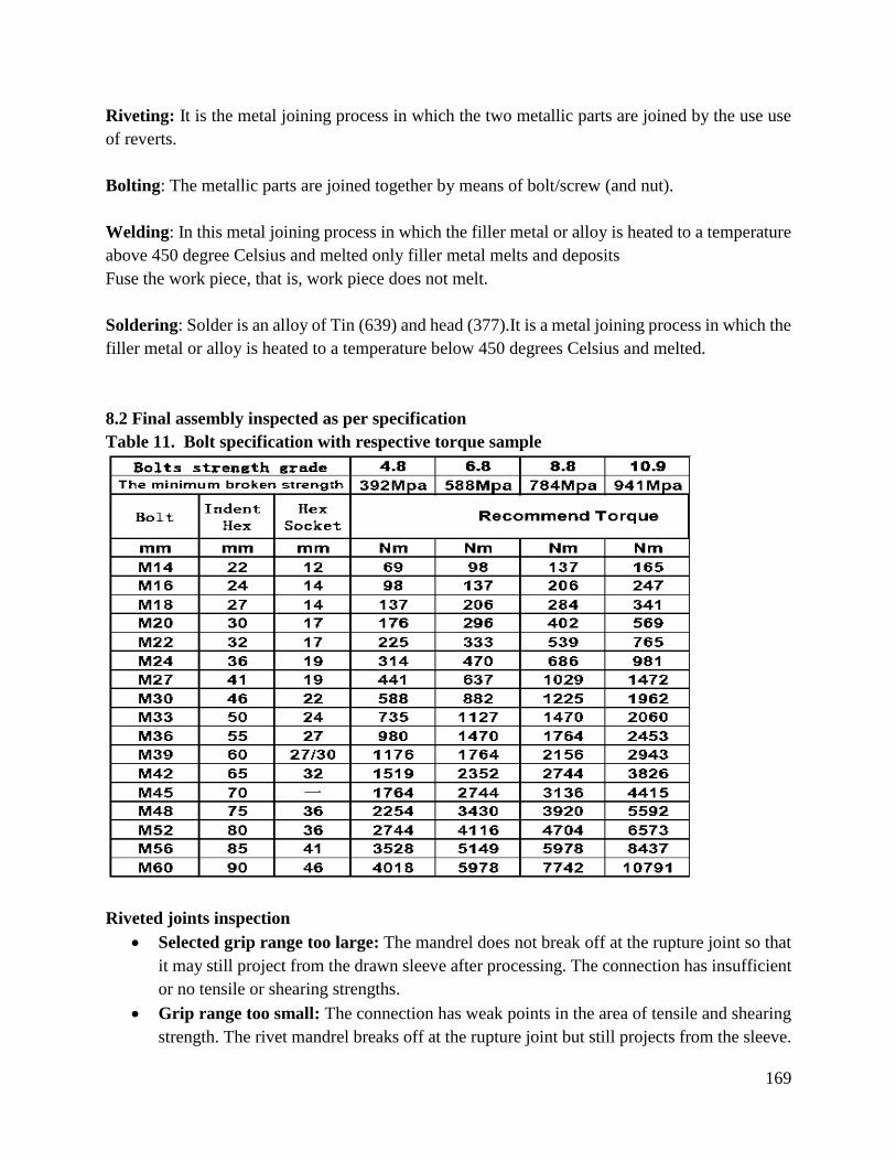
169
Riveting: It is the metal joining process in which the two metallic parts are joined by the use use
of reverts.
Bolting: The metallic parts are joined together by means of bolt/screw (and nut).
Welding: In this metal joining process in which the filler metal or alloy is heated to a temperature
above 450 degree Celsius and melted only filler metal melts and deposits
Fuse the work piece, that is, work piece does not melt.
Soldering: Solder is an alloy of Tin (639) and head (377).It is a metal joining process in which the
filler metal or alloy is heated to a temperature below 450 degrees Celsius and melted.
8.2 Final assembly inspected as per specification
Table 11. Bolt specification with respective torque sample
Riveted joints inspection
Selected grip range too large: The mandrel does not break off at the rupture joint so that
it may still project from the drawn sleeve after processing. The connection has insufficient
or no tensile or shearing strengths.
Grip range too small: The connection has weak points in the area of tensile and shearing
strength. The rivet mandrel breaks off at the rupture joint but still projects from the sleeve.
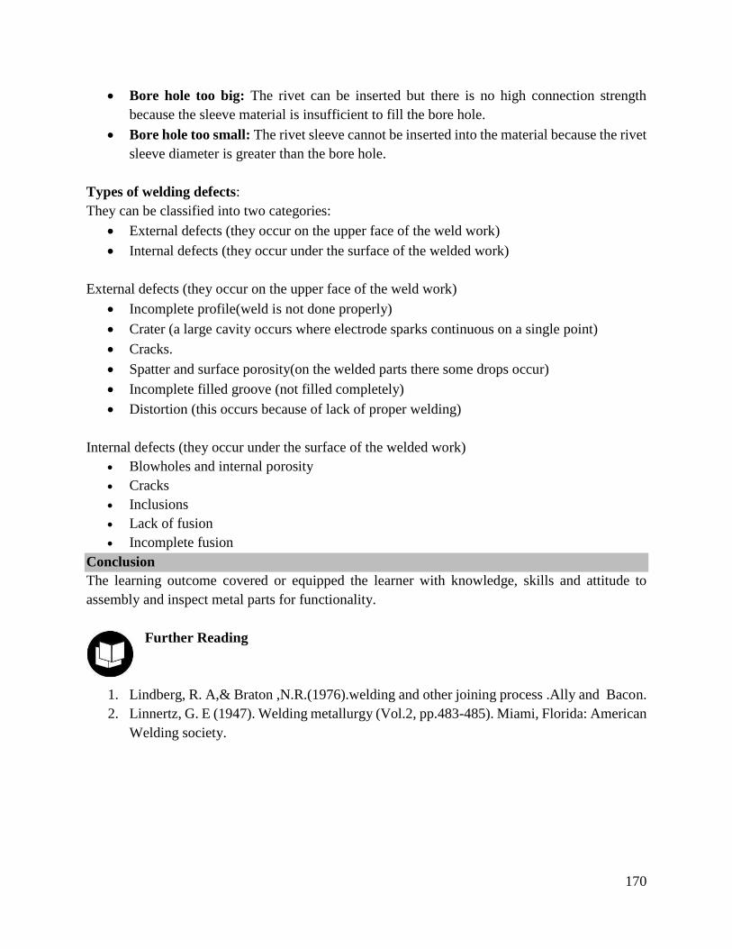
170
Bore hole too big: The rivet can be inserted but there is no high connection strength
because the sleeve material is insufficient to fill the bore hole.
Bore hole too small: The rivet sleeve cannot be inserted into the material because the rivet
sleeve diameter is greater than the bore hole.
Types of welding defects:
They can be classified into two categories:
External defects (they occur on the upper face of the weld work)
Internal defects (they occur under the surface of the welded work)
External defects (they occur on the upper face of the weld work)
Incomplete profile(weld is not done properly)
Crater (a large cavity occurs where electrode sparks continuous on a single point)
Cracks.
Spatter and surface porosity(on the welded parts there some drops occur)
Incomplete filled groove (not filled completely)
Distortion (this occurs because of lack of proper welding)
Internal defects (they occur under the surface of the welded work)
Blowholes and internal porosity
Cracks
Inclusions
Lack of fusion
Incomplete fusion
Conclusion
The learning outcome covered or equipped the learner with knowledge, skills and attitude to
assembly and inspect metal parts for functionality.
Further Reading
1. Lindberg, R. A,& Braton ,N.R.(1976).welding and other joining process .Ally and Bacon.
2. Linnertz, G. E (1947). Welding metallurgy (Vol.2, pp.483-485). Miami, Florida: American
Welding society.
171
9.3.2.3 Self-Assessment
Written Assessment
1. This is the smallest diameter of a screw thread:
a) Internal thread diameter
b) Minor diameter
c) Major diameter
d) External thread diameter
2. Amount of current required to generate the arc under no load condition is called?
a) Open circuit current
b) Closed circuit current
c) Short circuit current
d) Arc current
3. Amount of time during which the transformer will be used for welding under normal loading
condition is known as?
a) Hold time
b) Off time
c) Weld time
d) Duty cycle
4. Weaving in arc welding refers to __________
a) Side to side motion of electrode at right angles to the direction of the welding.
b) Side to side motion of electrode along the direction of the welding.
c) Spiral motion given to electrode.
d) A technique of striking the arc.
5. In arc welding operations the current value is decided by.
a) The thickness of plate
b) Length of welded portion
c) Voltage across the arc
d) Size of the electrode
6. For a good weld ____________
a) Cross-section of the added metal should be small and oxidation should be minimum.
b) Cross-section of the added metal should be small and oxidation should be maximum.
c) Cross-section of the added metal should be large and oxidation should be minimum.
d) Cross-section of the added metal should be large and oxidation should be maximum.
7. Give a list of equipment required in general for electric arc welding.
8. Explain the principle of arc-welding.
9. Compare the merits and demerits of using A.C and D.C for arc welding.
10. What is the advantage of having different polarities?

172
11. What do you understand by the term polarity?
Oral Assessment
1. What are the major safety concerns in arc welding?
2. When would you consider use if fasteners instead of welding.
Practical Assessment
1. Apply the various assembly methods in the mechanical workshop with the help of
technicians.
Project
Design and implement a project on joining of pipes and inspect for air passage.
9.3.2.4 Tools, Equipment, Supplies and Materials
Welding
Drilling machines
Vices
Burnishing machine
Cutting tools
Combination square
Centre punch
Centre lathe
Scribers
Calipers
Dies and taps
Surface plate
V-blocks
Dial gauge
Die stock
Engineer’s square
File card
Assorted Files
Clamps
Assorted hand tools

173
9.3.2.5 References
Greese, R. (2017). Introduction to Manufacturing process and material.CRCpress.
Gare, S. K. (2005). Workshop Technology (manufacturing process)New Delhi.Larmi
Publications.
Signh, R. (2006). Introduction to Basic manufacturing process &Workshop Technology.New Age
International.
174
3.3.10 Learning Outcome No 9: Polish finished work
3.3.10.1 Learning Activities
Learning Outcome No 9: Polish finished work
Learning Activities Special Instructions
9.1 Select polishing (emery cloth, polishing and burnishing machine,
filing) material.
9.2 Clean finished work.
9.3 Polish finished work to specification.
The student should
be well conversant
with metal choosing
Process
3.3.10.2 Information Sheet No 3/LO9: Polish finished work
Introduction.
This learning outcome covers the knowledge, skills and attitudes required for the leaner to perform
finishing on products.
Definition of key terms
Polishing: Technically polishing refers to processes that use an abrasive that is glued to the work
wheel, while buffing uses a loose abrasive applied to the work wheel. Polishing is a more
aggressive process while buffing is less harsh, which leads to a smoother, brighter finish.
Content/Procedures/Methods/Illustrations
9.1 Polishing material are selected
Choosing a Metal Finishing Process
There are a few considerations that can help you narrow your choices in selecting a metal finishing
technique suitable for your project. Some helpful things to keep in mind are:
Production speed: How quickly does the technique apply finish to the product?
Cost-effectiveness: Certain finishing machines (such as vibratory tumblers) can be
expensive, but may compensate for their price by delivering faster cycle rates
Metal hardness: harder metals usually require more intense finishing techniques, like
grinding, or may need tougher abrasives than those used on softer materials
Potential for vulcanization.
Types of finishing
Brushed Metal: Unlike plating, brushed metal finishing is an effective method for removing
surface imperfections. These finishing machines create a uniform, parallel grain surface texture to
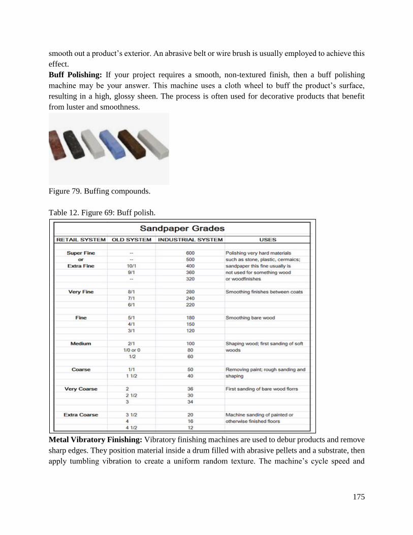
175
smooth out a product’s exterior. An abrasive belt or wire brush is usually employed to achieve this
effect.
Buff Polishing: If your project requires a smooth, non-textured finish, then a buff polishing
machine may be your answer. This machine uses a cloth wheel to buff the product’s surface,
resulting in a high, glossy sheen. The process is often used for decorative products that benefit
from luster and smoothness.
Figure 79. Buffing compounds.
Table 12. Figure 69: Buff polish.
Metal Vibratory Finishing: Vibratory finishing machines are used to debur products and remove
sharp edges. They position material inside a drum filled with abrasive pellets and a substrate, then
apply tumbling vibration to create a uniform random texture. The machine’s cycle speed and

176
magnitude of vibration are usually variable, allowing effective treatment for a range of small- to
large-sized parts.
Metal Grinding: Grinding machines use friction, attrition and/or compression to smooth out a
metal product’s surface. There are several types of grinding machines designed to deliver different
levels of finite smoothness.
Sand Blasting: Sand-blasting machines are typically employed in projects requiring a uniform
matte texture. The process (also known as bead blasting) forces sand, steel shots, metal pellets or
other abrasives into a substrate at high speed. This results in a smooth, clean product texture,
particularly in soft metals.
Powder Coating: Powder coating applies a decorative finish that is similar to paint, but with
greater durability. The process involves melting dry plastic powder onto the metal to produce a
textured, matte, or glossy coating. A textured powder-coating machine is also highly effective in
removing surface defects.
9.2 Finished work is cleaned
In cleaning spray the chloride free glass cleaner, or a plain substitute of rubbing alcohol, on a soft
non-abrasive cloth or sponge. Rub the cleanser dampened cloth on the stainless steel surface,
switching to a clean area of the cloth and using additional cleanser as necessary.
Methods of cleaning:
Dish Soap & Baby or Mineral Oil
First, you need to understand the direction of the grain. Just like wood and some fabrics, steel has
a grain. These are the faint striations that you can see on the surfaces of your appliances. In fact,
an entire sheet of steel will have the same directional grain. If you wipe vertical to the grain, more
cleaning residue may get deeper into the tiny crevices of the grain. For optimum shine, it is best to
clean with the grain. Use two non-abrasive cleaning rags, preferably those that are 100 percent
cotton because they leave almost no residual lint. You can use paper towels, but there will be some
lint left behind. Also, pick up some plain dish soap and baby or mineral oil. Dish soap cleans off
excess oils and simplifies the polishing process. Put just a little bit on your rag and moisten with a
modest amount of water (just enough to dampen your cloth).
Wipe along the grain of your appliance. For extra stubborn fingerprints, you might have to go over
the area a few times. When you finish cleaning an area, dry any water streaks with a clean towel.
Dab a small amount of mineral or baby oil onto your second rag. A couple of tiny drops will
suffice. Comparable to the cleaning process, follow the grain of your steel, moving in either
direction. Polishing the steel this way will produce optimal results.
White Vinegar & Olive Oil
177
Apply white vinegar directly to a microfiber cloth, or spray directly onto your surface. Let sit for
just a moment, and then wipe clean in the direction of the grain. Apply the vinegar as many times
as necessary to remove any grime. Then dab a clean towel into some olive oil and polish the
freshly-cleaned surface in the direction of the grain. If any extra olive oil residue remains, wipe
away with a clean cloth. This method works well because the vinegar gets rid of all the grime,
while the olive oil gives it a fresh, shiny polish.
9.3 Finished work is polished to specification
Polishing process
Before polishing your work piece, it's important to first clean it thoroughly.
Sanding.
Select Polishing Compound and Buffing Wheel.
Apply Polishing Compound.
Repeat.
Finish with Fine Compound.
Clean Before Polishing
Before polishing your work piece, it's important to first clean it thoroughly. Metals appear dull
when there are scratches or dirt preventing the light from reflecting directly off the surface. Dull
material may just be dirty. Clean thoroughly, and if your work piece is still dull then proceed to
polishing.
Polishing and Sanding
Polishing is similar to sanding. In order to make the material more reflective and smoother, when
polishing you are simply removing the surface of the material down to the depth of the deepest
scratch. Always work from coarse to fine when polishing (the same as if you were sanding a piece
of wood). The following steps can be followed for most reflective surfaces including metals,
plastics, rubber and even wood. Every material has different properties and will buff differently.
i. Detailed Buffing & Polishing Instructions
Metal polishing is part art and part science. These polishing instructions will take you from start
to finish through the process to help you understand the science and begin mastering the art of
metal polishing. Please note these instructions are for use with the polishing compounds, jewelers
rouge, and buffing wheels found on PJTool.com. Polishing compound grades and colors are not
consistent between manufactures.
178
ii. Clean Before Polishing
Before polishing your work piece, it's important to first clean it thoroughly. Metals appear dull
when there are scratches or dirt preventing the light from reflecting directly off the surface. Dull
material may just be dirty. Clean thoroughly, and if your work piece is still dull then proceed to
polishing.
iii. Polishing and Sanding
Polishing is similar to sanding. In order to make the material more reflective and smoother, when
polishing you are simply removing the surface of the material down to the depth of the deepest
scratch. Always work from coarse to fine when polishing (the same as if you were sanding a piece
of wood). The following steps can be followed for most reflective surfaces including metals,
plastics, rubber and even wood. Every material has different properties and will buff differently.
We recommend before polishing a new surface to practice on a piece of scrap to familiarize
yourself with the material and how it responds to polishing.
iv. Safety
Always wear protective gear when polishing including safety goggles or face shield, dust mask,
shop apron and gloves. You may also want to protect surfaces and tools with tape or padding to
prevent accidental gouging. Step by Step Polishing Instructions.
v. Sanding
Determine if the material you wish to polish needs to be sanded first. A good rule of thumb is if
your fingernail can catch the edge of a scratch then it will need to be sanded before it can be
polished. Select Polishing Compound and Buffing Wheel. To begin polishing start with a stiffer
buff such as a felt bob or felt cone, sisal buffing wheel, specialty buff, or spiral sewn buffing wheel.
(note: loose single stitched buffing wheels are primarily for finishing and working with fine
compounds).
Apply Polishing Compound
Coat the buffing wheel or felt bob by lightly spinning the buff against the polishing compound.
Use the compounds sparingly as you only need a small amount for them to work properly. Next,
spin the coated buff or felt bob onto the surface to be polished. Best results are obtained at 3,000
RPM or less. Continue polishing as needed, reapplying more compound if necessary. For best
results use a different buff for each polishing compound.
Repeat
Repeat the process with the next finer polishing compound as shown on the chart. Continue
polishing until visible scratches are removed and the desired luster is achieved.
Finish with Fine Compound
179
To finish your project and achieve a mirror like finish, use the finest applicable compound with
the loose single stitched buff. Again use very light pressure and let the buff do the work for you.
Wash and Coat
Once work is completed, wash the material with warm soapy water to remove any excess buffing
compound or residue. Dry your work piece with a soft cloth or chamois. Depending on the material
you may want to protect your restored finish with a clear coat.
Safety
Always wear protective gear when polishing including safety goggles or face shield, dust mask,
shop apron and gloves. You may also want to protect surfaces and tools with tape or padding to
prevent accidental gouging.
Conclusion
The learning outcome covered or equipped the learner with knowledge, skills and attitude required
for the learner to perform finishing products.
Further Reading
1. Mechanical Experiments and workshop practice, G.S Sawhney.
2. Workshop technology and practice by Sharma.
3.3.10.3 Self-Assessment
Written Assessment
1. When the primary requirement is only the high degree of surface finish, and a very close
dimensional accuracy is the primary requirement, we can use the following operation.
a) Buffing
b) Lapping
c) Honing
d) All of the above
2. Following abrasive is used for lapping hardened steel parts.
a) Silicon Carbide
b) Powdered garnet
c) Diamond
d) Aluminum Oxide
3. The operation of running two mating parts or shapes together with an abrasive between.
a) Equalizing Lapping
b) Form Lapping
180
c) Hand Lapping
4. The abrasive used in Super finishing is a __________
a) Bonded abrasive
b) Coated abrasive
c) Both (A) and (B)
d) None of the above
5. In Super finishing operation _________
a) The work rotates, the abrasive block reciprocates
b) The abrasive block rotates, the work reciprocates
c) Both abrasive block and work rotates
d) Both abrasive block and work reciprocates
6. Super finishing is largely used for ___________
a) Internal surfaces
b) External surfaces
c) Both (A) and (B)
7. Largest amount of material is used in _______________
a) Buffing
b) Lapping
c) Honing
d) Superfinishing
8. What is the difference between finishing and polishing?
9. Briefly describe three method of polished metal cleaning.
10. What are the most commonly applied polishing methods and why?
11. How would you conduct stainless steel cleaning after polishing?
12. Why should you not mix cleaning agents?
Oral Assessment
1. Name four grades of emery cloth.
2. Briefly explain the importance of metal polishing.
Practical Assessment
2. Describe the procedure for cleaning finished work.
Project
1. Illustrate two methods of cleaning.
2. With the aid of a diagram, describe Butt polishing.
3.3.10.4 Tools, Equipment, Supplies and Materials
Welding
Drilling machines

181
Vices
Burnishing machine
Cutting tools
Combination square
Centre punch
Centre lathe
scribers
calipers
Dies and taps
Surface plate
V-blocks
Dial gauge
Die stock
Engineer’s square
File card
Assorted Files
Clamps
Assorted hand tools
3.3.10.5 References
Greese , R .(2017).Introduction to Manufacturing process and material. CRC press.
S.K Gare (2005) Workshop Technology ( manufacturing process)New Delhi.Larmi Publications.
Signh, R. (2006) Introduction To Basic manufacturing process &Workshop Technology. New Age
International.
182
3.3.11 Learning Outcome No. 10: Perform housekeeping
3.3.11.1 Learning Activities
Learning Outcome No.10: Perform housekeeping
Learning Activities Special Instructions
10.1 segregate and dispose waste as per disposal guidelines.
10.2 carry out housekeeping as per workplace requirement
The proper methods for
housekeeping are used
Rules and safety are observed
Identify the correct tools and
equipment
3.3.11.2 Information Sheet No3/LO10: Perform housekeeping
Introduction
This learning outcome covers the knowledge, skills and attitudes required for the leaner to perform
housekeeping as per the working procedure.
Definition of key terms
Waste: Waste (or wastes) are unwanted or unusable materials. Waste is any substance which is
discarded after primary use, or is worthless, defective and of no use
.
Segregate: This is the dividing of waste into dry and wet waste.
Content/Procedures/Methods/Illustrations
10.1 Waste is segregated and disposed as per disposal guidelines
There are eight major groups of waste management methods, each of them divided into numerous
categories. Those groups include:
Source reduction and reuse.
Animal feeding.
Recycling.
Composting.
Fermentation.
Landfills.
Incineration.
Land application.
Waste Management
183
Workshop users should make an effort to keep waste to a minimum. The best way to do so is by
reducing the scale of operation, which minimizes the quantity of waste generated. Whenever
possible, chemicals used should be substituted with less hazardous chemicals. Chemical quantities
should be kept to a minimum. Store only what will be used in the near term. Besides preventing
or minimizing waste generation, chemicals should be recycled or recovered for reuse. When waste
is generated, it must be disposed of properly. Sink disposal may not always be appropriate and
may end contaminating drinking water. Alternative methods of disposal should be considered
including incineration, treatment, and land disposal. The institute's EHS office should be consulted
to determine the proper disposal method for different waste types.
Waste Collection and Storage
When generating or managing any chemical waste, appropriate personal protective
equipment (PPE) must be worn, and engineering controls should be implemented as
necessary.
Collect and store chemical waste at or near the point of generation in a designated satellite
accumulation area. This accumulation area should be well marked for easy identification.
Chemical waste must be stored in compatible containers with closed and properly fitted
caps.
Waste containers must be labeled mentioning chemical compositions, the accumulation
start date, and hazard warnings as appropriate. The institute's EHS office typically provides
these required labels.
Incompatible waste types should not be mixed and should be kept separate in order to avoid
any reaction, heat generation, and/or gas evolution.
Waste containers should be stored in secondary containers in a ventilated, cool, and dry
area.
In the central accumulation area, waste containers should be grounded to avoid fire and
explosion hazards.
10.2 Housekeeping is carried out as per workplace requirement
Effective housekeeping can help control or eliminate workplace hazards. Poor housekeeping
practices frequently contribute to hazardous incidents. If the sight of paper, debris, clutter and
spills is accepted as normal, then other more serious hazards may be taken for granted.
Housekeeping is not just cleanliness. It includes keeping work areas neat and orderly, maintaining
halls and floors free of slip and trip hazards, and removing of waste materials (e.g., paper,
cardboard) and other fire hazards from work areas. It also requires paying attention to important
details such as the layout of the whole workplace, aisle marking, the adequacy of storage facilities,
and maintenance. Good housekeeping is also a basic part of incident and fire prevention. Effective
housekeeping is an ongoing operation: It is not a one-time or hit-and-miss cleanup done
occasionally. Periodic "panic" cleanups are costly and ineffective in reducing incidents.

184
Poor housekeeping can be a cause of incidents such as;
Tripping over loose objects on floors, stairs and platforms.
Being hit by falling objects.
Slipping on greasy, wet or dirty surfaces.
Tricking against projecting, poorly stacked items or misplaced material.
Cutting, puncturing, or tearing the skin of hands or other parts of the body on projecting
nails, wire or steel strapping.
Effective housekeeping results in;
Reduced handling to ease the flow of materials
Fewer tripping and slipping incidents in clutter-free and spill-free work areas
Decreased fire hazards
Lower worker exposures to hazardous products (e.g. dusts, vapors)
Better control of tools and materials, including inventory and supplies
More efficient equipment cleanup and maintenance
Better hygienic conditions leading to improved health
More effective use of space
Reduced property damage by improving preventive maintenance
Less janitorial work
Improved morale
Improved productivity (tools and materials will be easy to find)
Elements of proper housekeeping
Maintenance
The maintenance of buildings and equipment may be the most important element of good
housekeeping. Maintenance involves keeping buildings, equipment and machinery in safe,
efficient working order and in good repair.
Dust and Dirt Removal
Enclosures and exhaust ventilation systems may fail to collect dust, dirt and chips adequately.
Vacuum cleaners are suitable for removing light dust and dirt that is not otherwise hazardous.
Industrial models have special fittings for cleaning walls, ceilings, ledges, machinery, and other
hard-to-reach places where dust and dirt may accumulate.
Employee Facilities
Employee facilities need to be adequate, clean and well maintained. Lockers may be necessary for
storing employees' personal belongings. Washroom facilities require cleaning once or more each
shift. They also need to have a good supply of soap, towels plus disinfectants, if needed.
Surfaces.

185
Floors
Poor floor conditions are a leading cause of accidents so cleaning up spilled oil and other liquids
at once is important. Allowing chips, shavings and dust to accumulate can also cause accidents.
Trapping chips, shavings and dust before they reach the floor or cleaning them up regularly can
prevent their accumulation.
Maintain Light Fixtures
Dirty light fixtures reduce essential light levels. Clean light fixtures can improve lighting
efficiency significantly.
Aisles and Stairways
Aisles should be wide enough to accommodate people and vehicles comfortably and safely. Aisle
space allows for the movement of people, products and materials. Warning signs and mirrors can
improve sight-lines in blind corners. Arranging aisles properly encourages people to use them so
that they do not take shortcuts through hazardous areas.
Spill Control
The best way to control spills is to stop them before they happen. Regularly cleaning and
maintaining machines and equipment is one way. Another is to use drip pans and guards where
possible spills might occur. When spills do occur, it is important to clean them up immediately.
Absorbent materials are useful for wiping up greasy, oily or other liquid spills. Used absorbents
must be disposed of properly and safely.
Tools and Equipment
Tool housekeeping is very important, whether in the tool room, on the rack, in the yard, or on the
bench. Tools require suitable fixtures with marked locations to provide an orderly arrangement.
Returning tools promptly after use reduces the chance of it being misplaced or lost. Workers should
regularly inspect, clean and repair all tools and take any damaged or worn tools out of service.
Waste Disposal
The regular collection, grading and sorting of scrap contribute to good housekeeping practices. It
also makes it possible to separate materials that can be recycled from those going to waste disposal
facilities. Allowing material to build up on the floor wastes time and energy since additional time
is required for cleaning it up. Placing scrap containers near where the waste is produced encourages
orderly waste disposal and makes collection easier. All waste receptacles should be clearly labelled
(e.g., recyclable glass, plastic, scrap metal, etc.).
Storage
Good organization of stored materials is essential for overcoming material storage problems
whether on a temporary or permanent basis. There will also be fewer strain injuries if the amount
186
of handling is reduced, especially if less manual material handling is required. The location of the
stockpiles should not interfere with work but they should still be readily available when required.
Conclusion
The learning outcome covered or equipped the learner with knowledge, skills and attitude to
perform housekeeping and conduct waste disposal as per the workshop procedures.
Further Reading
1. Mechanical experiment and workshop practice by C.S Sawhney
3.3.11.3 Self-Assessment
Written Assessment
1. Why burning waste is not an acceptable practice of solid waste management?
a) Because it is very costly
b) Because it requires modern technologies
c) Because it cause several environmental issues
d) Because it requires lot of space
2. What plan should we make to the disposal of solid waste?
a) Integrated waste management plan
b) Recycling of waste management plan
c) Reducing of waste management plan
d) Use of waste management plan
3. Which of the integrated waste management is reduced on an individual level?
a) Source reduction
b) Recycling
c) Disposal
d) Burning
4. Which of the following can be recycled many times?
a) Plastic
b) Wood
c) Organic materials
d) Aluminum
5. Why plastics are difficult to recycle?
a) Because it is very hard material

187
b) Because it is very adhesive in its nature
c) Because of different types of polymer resins
d) Because of different sizes of plastic
6. Why the recycled paper is banned for use in food containers?
a) Because it creates contamination
b) Because it creates a lot of spaces
c) Because paper can be used only one time
d) Because paper is very thick and can’t cover the food containers
7. Which waste disposal methods are applicable in workshop wastes?
8. What the main elements of a proper waste management program.
9. How can one best handle spillage in a workshop?
10. Why is it important for an organization to invest in proper waste management program?
11. Why is it important to maintain proper housekeeping?
Oral Assessment
1. What are the responsibilities of a machinist in waste disposal?
2. What is the act that guides industrial waste disposal?
Practical Assessment
1. Prepare bins for use in the institute workshops and compound for waste disposal.
Project
1. Plan a program for the institute waste disposal and present a report.
3.3.11.4 Tools, Equipment, Supplies and Materials
Welding
Drilling machines
Vices
Burnishing machine
Cutting tools
Combination square
Centre punch
Centre lathe
Scribers
Calipers
Dies and taps
Surface plate
V-blocks
Dial gauge
Die stock

188
Engineer’s square
File card
Assorted Files
Clamps
Assorted hand tools
3.3.11.5 References
Greese , R .(2017).Introduction to Manufacturing process and material.CRCpress.
S.K Gare (2005) Workshop Technology (manufacturing process)New Delhi.Larmi Publications.
Signh, R.(2006).Introduction To Basic manufacturing process &Workshop Technology.New Age
International.
189
3.3.12 Learning Outcome No 11: Inspect finished work for accuracy and quality
3.3.12.1 Learning Activities
Learning Outcome No. 11: Inspect finished work for accuracy and quality
Learning Activities Special Instructions
11.1 Select inspection tools and methods as per
operation plan
11.2 Inspect finished work as per specification
11.3 Make adjustments based on inspections
results
Outline the inspection tools required
Illustrate the inspection procedures
followed
Explain the adjustment required to be
done on the inspection results
3.3.12.2 Information Sheet No3/LO11: Inspect finished work for accuracy and quality
Introduction
This learning outcome covers the inspection tools and methods in accordance to the operation plan,
the inspection carried on as per the specifications and the adjustments made based on the inspection
results. The learning outcome equips the learner with knowledge, skills as the product
requirements.
Definition of key terms
Inspection: It involves examination of products through involves the measurements, tests, and
gauges applied to certain characteristics in regard to an object or activity.
Content/Procedures/Methods/Illustrations
11.1 Inspection tools and methods selected as per operation plan
Various operations are carried out and thus though inspection is required to be carried out. Various
methods are being deployed and also different tools. This is done in considerations to the types of
operations being carried out. The method of inspection also takes into consideration the purpose
and the use of the results being obtained. Therefore, below are methods and tools used inspections
of the various operations.
Methods of products inspection
Some common methods
Visual
Industrial computed tomography scanning
Microscopy
190
Dye penetrant inspection
Magnetic-particle inspection
X-ray or radiographic testing
Ultrasonic testing
Eddy-current testing
Acoustic emission testing
Thermographic inspection
Inspection tools in a workshop
Measuring tape for measuring product dimensions
Dial calipers for measuring finer dimensions
Camera for documentation
Defect stickers for marking product defects
Pantone swatch for color comparison
Barcode scanner
11.2 Finished work is inspected as per specification
Inspection is an important tool to achieve quality concept. It is necessary to assure confidence to
manufacturer and aims satisfaction to customer. Inspection is an indispensable tool of modern
manufacturing process. It helps to control quality, reduces manufacturing costs, eliminate scrap
losses and assignable causes of defective work.
Objectives of Inspection
To detect and remove the faulty raw materials before it undergoes production.
To detect the faulty products in production whenever it is detected.
To bring facts to the notice of managers before they become serious to enable them
discover weaknesses and cover the problem.
To prevent the substandard reaching the customers and reducing complaints.
To promote reputation for quality and reliability of product.
Purpose of Inspection
To distinguish good lots from bad lots
To distinguish good pieces from bad pieces
To determine if the process is changing
To determine if the process is approaching the specification limits
To rate quality of product
To rate accuracy of inspectors
To measure the precision of the measuring instrument
To secure products-design information
To measure process capability
191
Types of Inspection in Production
Floor inspection
Centralized inspection
Combined inspection
Functional inspection
First piece inspection
Pilot piece inspection
Final inspection
Floor Inspection
In this system, the inspection is performed at the place of production. It suggests the checking of
materials in process at the machine or in the production time by patrolling inspectors. These
inspectors move from machine to machine and from one to the other work centers.
Advantages
Detection of errors of the source reduces scrap and rework.
Correction is done before it affects further production, resulting in saving cost of
unnecessary work on defective parts.
Material handling time is reduced.
Job satisfaction to worker as he can’t be held responsible for bad work at a later date.
Greater number of pieces can be checked than a sample size.
Does not delay in production.
Disadvantages
Delicate instruments can be employed.
Measuring or inspection equipment have to be recalibrated often as they are subjected
to wear or dust.
High cost of inspection because of numerous sets of inspections and skilled inspectors.
Supervision of inspectors is difficult due to vibration.
Pressure on inspector.
Possibility of biased inspection because of worker.
Suitability
Heavy products are produced.
Different work centers are integrated in continuous line layout.
Centralized inspection
192
Inspection is carried in a central place with all testing equipment; sensitive equipment is housed
in air-conditioned area. Samples are brought to the inspection floor for checking. Centralized
inspection may locate in one or more places in the manufacturing industry.
Advantages
Greater degree of inspection due to sensitive equipment.
Less number of inspectors and tools.
Equipment needs less frequency of recalibration.
Cost of inspection is reduced.
Unbiased inspection.
Supervision of inspectors made possible.
No distraction to the inspector.
Disadvantages
Defects of job are not revealed quickly for prevention.
Greater material handling.
High cost as products are subjected to production before they are prevented.
Greater delay in production.
Inspection of heavy work not possible.
Production control work is more complicated.
Greater scrap.
Combined inspection
Combination of two methods whatever may be the method of inspection, whether floor or central.
The main objective is to locate and prevent defect which may not repeat itself in subsequent
operation to see whether any corrective measure is required and finally to maintain quality
economically.
Functional inspection
This system only checks for the main function; the product is expected to perform. Thus an
electrical motor can be checked for the specified speed and load characteristics. It does not reveal
the variation of individual parts but can assure combined satisfactory performance of all parts
put together. Both manufacturers and purchasers can do this, if large number of articles is needed
at regular intervals. This is also called assembly inspection.
11.3 Adjustments are made based on inspections results
Stages of inspection
i. First piece or first-off inspections: First piece of the shift or lot is inspected. This is
particularly used where automatic machines are employed. Any discrepancy from the
operator as machine tool can be checked to see that the product is within in control limits.
193
Excepting for need for precautions for tool we are check and disturbance in machine set
up, this yields good result if the operator is careful.
ii. Pilot piece inspection: This is done immediately after new design or product is
developed. Manufacturer of product is done either on regular shop floor if production is
not disturbed. If production is affected to a large extent, the product is manufactured in a
pilot plant. This is suitable for mass production and products involving large number of
components such as automobiles aero planes etc., and modification are design or
manufacturing process is done until satisfactory performance is assured or established.
iii. Final inspection: This is also similar to functional or assembly inspection. This
inspection is done only after completion of work. This is widely employed in process
industries where there are not possible such as, electroplating or anodizing products. This
is done in conjunction with incoming material inspection.
Methods of Inspection
There are two methods of inspection. They are: 100% inspection and sampling inspection.
Disadvantages of inspection
Inspection adds to the cost of the product but not for its value.
It is partially subjective, often the inspector has to judge whether a products passes or not.
Fatigue and Monotony may affect any inspection judgment.
Inspection merely separates good and bad items. It is no way to prevent the production
of bad items.
Conclusion
The learning outcome covered or equipped the learner with knowledge, skills and attitude to
inspect products.
Further Reading
1. Workshop technology and practice by Sharma
2. Mechanical experiment and workshop practice by G. S. Sawney. Introduction to basic
manufacturing processes and workshops technologies.
3.3.11.3 Self-Assessment
Written Assessment
1. Which of the following are three basic elements of a quality system?
194
a) Quality management, purchasing and document control
b) Quality management, quality control and quality assurance
c) SPC, inspection and quality assurance
d) Quality control, quality costs and control charts
2. Statistical quality control is best described as _____________
a) Keeping product characteristics within certain bounds
b) Calculating the mean and standard deviation
c) The study of the characteristics of a product or process, with the help of numbers
to make them behave the way we want them to behave.
d) The implementation of ISO 9000
3. Which of the following is the most important element in Statistical Quality Control?
a) The Feedback Loop
b) Make Operation
c) Inspection
d) Quality of Incoming Material
4. A quality audit program should begin with _________________
a) A study of the quality documentation system
b) An evaluation of the work being performed
c) A report listing findings, the action taken and recommendations
d) A charter of policy, objectives and procedures
5. Auditors should report to someone who is independent from ____________
a) The company being audited
b) Management
c) The function being audited
d) None of the above
6. Analysis of data on all product returns is important because ___________
a) Failure rates change with length of product usage
b) Changes in design and in customer use are often well reflected
c) Immediate feedback and analysis of product performance becomes available
d) All of the above
7. What are the two basic categories of quality?
a) Design and Conformance Quality
b) Good and Bad Quality
c) Defective and Non-Defective Quality
d) Attribute and Variable Quality
8. What are the objectives of inspection?
9. Why do we perform inspection?
195
10. What are the main inspection instruments in a machining shop?
11. What are the challenges of inspection program in machining shop?
12. What qualities are inspected in a machine shop?
Oral Assessment
1. What are the three types of inspection?
2. What would you consider to be visual inspection in a machine shop?
Practical Assessment
For all the products produced in the previous learning outcomes conduct respective inspection.
Project
Prepare a report for the practical above and give the necessary recommendations.
3.3.12.4 Tools, Equipment, Supplies and Materials
Welding
Drilling machines
Vices
Burnishing machine
Cutting tools
Combination square
Centre punch
Centre lathe
Scribers
Calipers
Dies and taps
Surface plate
V-blocks
Dial gauge
Die stock
Engineer’s square
File card
Assorted Files
Clamps
Assorted hand tools
3.3.12.5 References
Barbarosoglu, G., & Yazgac, T. (1997). An application of the analytic hierarchy process to the
supplier selection problem. Production and inventory management journal, 38(1), 14.

196
Dorris, A. L., & Foote, B. L. (1978). Inspection errors and statistical quality control: A
survey. AIIE Transactions, 10(2), 184-192.
Yao, Q., Chen, J., Guan, Z., Sun, C., & Zhu, Z. (2009, May). Inspection of rice appearance quality
using machine vision. In 2009 WRI Global Congress on Intelligent Systems (Vol. 4, pp.
274-279). IEEE.

197
3.3.13 Learning Outcome No 12: Maintenance of tools and equipment
3.3.13.1 Learning Activities
Learning Outcome No 12: Maintenance of tools and equipment
Learning Activities Special Instructions
12.1 Inspect machines and tools
12.2 Lubricate machines and tools
12.3 Ground tools to specification
12.4 Identify and report faults on machines and tools
12.5 Store tools and equipment
Group discussion
Illustration
3.3.13.2 Information Sheet No 9/LO12: Maintenance of tools and equipment
Introduction
This learning outcome covers knowledge, skills and attitudes required for the leaner to maintain
tools and equipment.
Definition of key terms
Lathe tool: It is a machine tool that rotates a workplace about an axis of rotation to perform various
operations such as cutting, sanding, drilling, facing and turning with tools that are applied to the
workpiece to create an object with symmetry about that axis.
Lubricate: Applying a substance such as oil or grease as to minimize friction.
Content/Procedures/Methods/Illustrations
12.1 Machines and tools are inspected
Workplace inspections help prevent incidents, injuries and illnesses. Through a critical
examination of the workplace, inspections help to identify and record hazards for corrective action.
Health and safety committees can help plan, conduct, report and monitor inspections.
Benefits of Inspections for the Maintenance Department
Equipment problems being detected and receiving maintenance attention before they
escalate into costlier issues.
Recurring equipment problems being identified so that their causes can be corrected.
Personnel taking better care of equipment because regular inspections hold them
accountable.
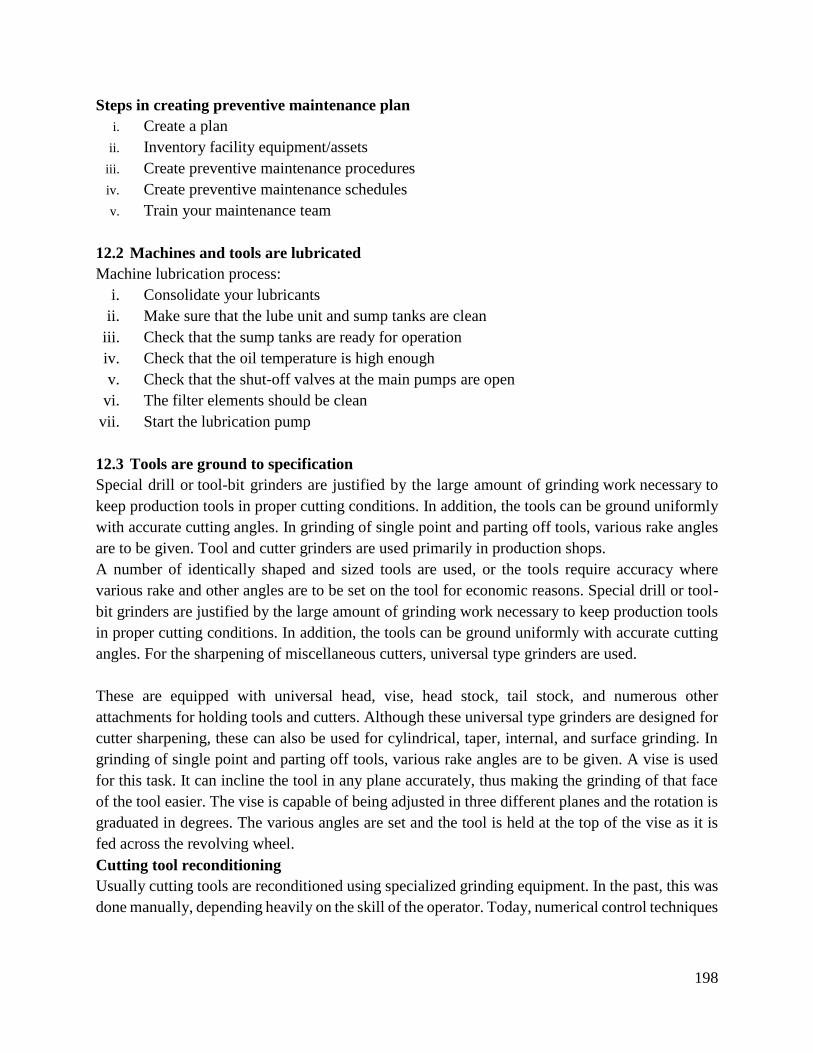
198
Steps in creating preventive maintenance plan
i. Create a plan
ii. Inventory facility equipment/assets
iii. Create preventive maintenance procedures
iv. Create preventive maintenance schedules
v. Train your maintenance team
12.2 Machines and tools are lubricated
Machine lubrication process:
i. Consolidate your lubricants
ii. Make sure that the lube unit and sump tanks are clean
iii. Check that the sump tanks are ready for operation
iv. Check that the oil temperature is high enough
v. Check that the shut-off valves at the main pumps are open
vi. The filter elements should be clean
vii. Start the lubrication pump
12.3 Tools are ground to specification
Special drill or tool-bit grinders are justified by the large amount of grinding work necessary to
keep production tools in proper cutting conditions. In addition, the tools can be ground uniformly
with accurate cutting angles. In grinding of single point and parting off tools, various rake angles
are to be given. Tool and cutter grinders are used primarily in production shops.
A number of identically shaped and sized tools are used, or the tools require accuracy where
various rake and other angles are to be set on the tool for economic reasons. Special drill or tool-
bit grinders are justified by the large amount of grinding work necessary to keep production tools
in proper cutting conditions. In addition, the tools can be ground uniformly with accurate cutting
angles. For the sharpening of miscellaneous cutters, universal type grinders are used.
These are equipped with universal head, vise, head stock, tail stock, and numerous other
attachments for holding tools and cutters. Although these universal type grinders are designed for
cutter sharpening, these can also be used for cylindrical, taper, internal, and surface grinding. In
grinding of single point and parting off tools, various rake angles are to be given. A vise is used
for this task. It can incline the tool in any plane accurately, thus making the grinding of that face
of the tool easier. The vise is capable of being adjusted in three different planes and the rotation is
graduated in degrees. The various angles are set and the tool is held at the top of the vise as it is
fed across the revolving wheel.
Cutting tool reconditioning
Usually cutting tools are reconditioned using specialized grinding equipment. In the past, this was
done manually, depending heavily on the skill of the operator. Today, numerical control techniques

199
can be applied to tool and cutter grinders, producing high quality tools with greater consistency at
lower costs.
New industries like fiber optics demand precise cutting tool tolerances that cannot be provided by
traditional tool room equipment. The present day requirements call for tolerances in microns, and
tighter specifications on concentricity, finish quality of radii bends, and complex geometries. CNC
tool grinders to produce consistent, high-quality tools are required for such applications.
Cutter grinding machine
Figure 80: Cutter grinding machine.
Lathe tool
200
Figure 81. Lathe tool
12.4 Faults on machines and tools are identified and reported
Types of electrical related faults in machines
Open Circuit Faults. These faults occur due to the failure of one or more conductors.
Short Circuit Faults.
Symmetrical and Unsymmetrical Faults.
Fuse.
Circuit Breaker.
Protective Relays.
Lighting Arrestor.
Types of mechanical faults in machines
The stator or armature faults.
The broken bar and end ring faults of induction machines.
Bearing faults.
The eccentricity related faults are the most prevalent ones and thus demand special
attention in our research.
12.5 Store tools and equipment
201
When not in use, sharp or cutting tools should be stored in a sturdy tool box or on a tool rack with
the sharp edges suitably covered. Otherwise, they should be placed near the back of work benches
to keep handles or blades from extending over the edge.
Figure 82: Tools
Conclusion
The learning outcome covered or equipped the learner with knowledge, skills and attitude to
maintain tools and equipment.
Further Reading
1. Signh, R. (2006). Introduction To Basic manufacturing process &Workshop Technology. New
Age International.
3.3.13.3 Self-Assessment
Written Assessment
1. Which of the following tools is most suitable for very hard and brittle material?
a) HSS
b) Cast-cobalt alloy
c) Carbides
d) None of the mentioned
2. Thermal conductivity of cutting tool must be ____________
a) High

202
b) Low
c) Very low
d) None of the mentioned
3. Wearing resistance of cutting tool must be ____________
a) High
b) Low
c) Very low
d) None of the mentioned
4. In cylindrical grinding, the abrasive wheel and the workpiece are ___________
a) Rotated by separate motors and at different speeds
b) Rotated by separate motors and at same speed
c) Rotated by single motor and at same speed
d) Any of the above
5. The time elapsed from the point the machine fails to perform its function to the point it is
repaired and brought into operating condition is known as ___________
a) Down time
b) Break Down time
c) Both (A) and (B)
d) Idle time
6. When belt of an electric motor is broken, it needs one of the following maintenances.
Which one is it?
a) Corrective maintenance
b) Scheduled maintenance
c) Preventive maintenance
d) Timely maintenance
7. Equipment history cards are meant to record __________
a) The way equipment behaves
b) Total down time of the equipment
c) The rate at which different components wear off
d) All of the above
8. What are the three main types of maintenance?
9. What is the importance of maintenance in an engineering workshop?
10. What is the importance of various tool angle of lathe cutting tool?
11. What are the benefits of preventive maintenance?
12. How would you handle sharp tools in a workshop?
Oral Assessment
1. What is the responsibility of a worker in machines maintenance?
2. What are the most common mechanical faults in a machine?
Practical Assessment

203
1. Conduct machines checks and lubrication in college machines.
Project
1. Prepare maintenance program for the college machines and the storage methods and write
a report.
3.3.13.4 Tools, Equipment, Supplies and Materials
Welding
Drilling machines
Vices
Burnishing machine
Cutting tools
Combination square
Centre punch
Centre lathe
Scribers
Calipers
Dies and taps
Surface plate
V-blocks
Dial gauge
Die stock
Engineer’s square
File card
Assorted Files
Clamps
Assorted hand tools
3.3.13.5 References
Greese, R. (2017). Introduction to Manufacturing process and material.CRCpress.
S. K Gare (2005). Workshop Technology (manufacturing process) New Delhi.Larmi Publications.
Signh, R. (2006). Introduction To Basic manufacturing process &Workshop Technology. New
Age International.
204
CHAPTER 4: PRINCIPLES OF MECHANICAL SCIENCE/APPLY MECHANICAL
SCIENCE PRINCIPLES
4.1 Introduction
Mechanical Science is among the common units of competencies offered in all the TVET level 6
engineering courses qualification. This unit describes the competencies required by a technician
in order to apply a wide range of mechanical science principles in their work. It includes using
concepts of mechanical science, determining effects of loading on static and dynamic engineering
systems, analyze properties of materials, determine parameters of a fluid system and use of basic
systems in power transfer. The significance of Engineering mathematics to TVET level 6
engineering curriculum is to enable learners acquire knowledge and skills to demonstrate, apply
basic mechanical formulas, use of basic mechanical machines, perform various unit conversions
of mechanical quantities, basic mechanical systems design mechanical machine operation, logical
thinking problem solving, applying statistics drawing graphs and using different measuring tools
to get along well in the workplaces.
The critical aspect of competency to be covered includes determining forces in a system,
demonstrating knowledge of moments, understanding friction principles, understanding motions
in engineering, describing work, energy and power, performing machine calculations,
demonstrating gas principles, applying heat knowledge, density knowledge, and pressure
principles. The basic resources required includes access to relevant workplace or appropriately
simulated environment where assessment can take place, measuring tools and equipment, sample
materials to be tested among others. The unit of competency covers ten learning outcomes. Each
of the learning outcome presents; learning activity that covers performance criteria statements,
thus creating trainee’s an opportunity to demonstrate knowledge and skills in the occupational
standards and content in curriculum. Information sheet provides; definition of key terms, content
and illustration to guide in training. The competency may be assessed through direct observation,
demonstration with oral questioning, case studies and written tests. Self-assessment is provided at
the end of each learning outcomes. Holistic assessment with other units relevant to the industry
sector workplace and job role is recommended.
4.2 Performance Standard
Determine forces in a system, demonstrate knowledge of moments, understand friction principles
and identify advantages and disadvantages, motions in engineering, describe work, energy and
power, perform machine calculations, demonstrate gas principles, apply heat knowledge, density
knowledge and pressure principles in accordance with workplace.
4.3 Learning Outcomes
4.3.1 List of learning outcomes
a) Determine forces in a system
b) Demonstrate knowledge of moments

205
c) Understand friction principles
d) Understand motions in engineering
e) Describe work, energy, and power
f) Perform machine calculations
g) Demonstrate gas principles
h) Apply heat knowledge
i) Apply density knowledge
j) Apply pressure principles
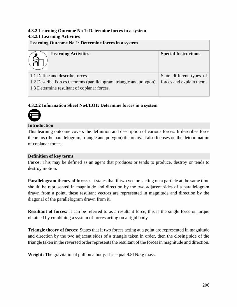
206
4.3.2 Learning Outcome No 1: Determine forces in a system
4.3.2.1 Learning Activities
Learning Outcome No 1: Determine forces in a system
Learning Activities Special Instructions
1.1 Define and describe forces.
1.2 Describe Forces theorems (parallelogram, triangle and polygon).
1.3 Determine resultant of coplanar forces.
State different types of
forces and explain them.
4.3.2.2 Information Sheet No4/LO1: Determine forces in a system
Introduction
This learning outcome covers the definition and description of various forces. It describes force
theorems (the parallelogram, triangle and polygon) theorems. It also focuses on the determination
of coplanar forces.
Definition of key terms
Force: This may be defined as an agent that produces or tends to produce, destroy or tends to
destroy motion.
Parallelogram theory of forces: It states that if two vectors acting on a particle at the same time
should be represented in magnitude and direction by the two adjacent sides of a parallelogram
drawn from a point, these resultant vectors are represented in magnitude and direction by the
diagonal of the parallelogram drawn from it.
Resultant of forces: It can be referred to as a resultant force, this is the single force or torque
obtained by combining a system of forces acting on a rigid body.
Triangle theory of forces: States that if two forces acting at a point are represented in magnitude
and direction by the two adjacent sides of a triangle taken in order, then the closing side of the
triangle taken in the reversed order represents the resultant of the forces in magnitude and direction.
Weight: The gravitational pull on a body. It is equal 9.81N/kg mass.
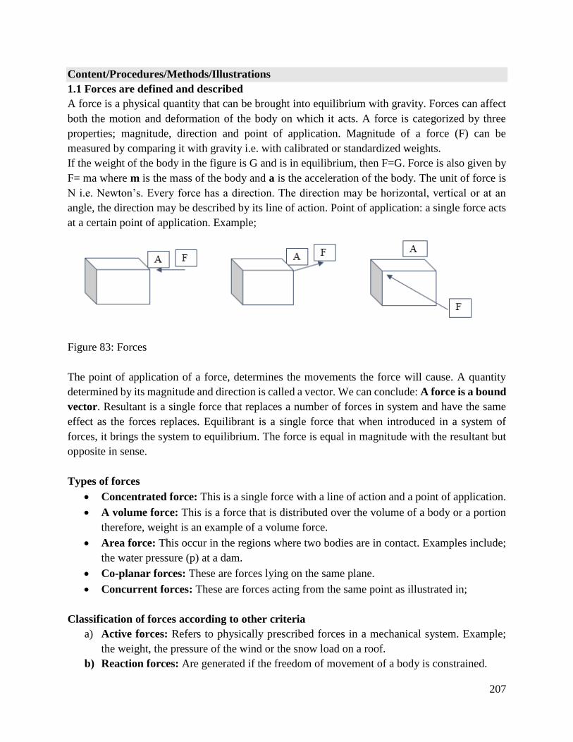
207
Content/Procedures/Methods/Illustrations
1.1 Forces are defined and described
A force is a physical quantity that can be brought into equilibrium with gravity. Forces can affect
both the motion and deformation of the body on which it acts. A force is categorized by three
properties; magnitude, direction and point of application. Magnitude of a force (F) can be
measured by comparing it with gravity i.e. with calibrated or standardized weights.
If the weight of the body in the figure is G and is in equilibrium, then F=G. Force is also given by
F= ma where m is the mass of the body and a is the acceleration of the body. The unit of force is
N i.e. Newton’s. Every force has a direction. The direction may be horizontal, vertical or at an
angle, the direction may be described by its line of action. Point of application: a single force acts
at a certain point of application. Example;
Figure 83: Forces
The point of application of a force, determines the movements the force will cause. A quantity
determined by its magnitude and direction is called a vector. We can conclude: A force is a bound
vector. Resultant is a single force that replaces a number of forces in system and have the same
effect as the forces replaces. Equilibrant is a single force that when introduced in a system of
forces, it brings the system to equilibrium. The force is equal in magnitude with the resultant but
opposite in sense.
Types of forces
Concentrated force: This is a single force with a line of action and a point of application.
A volume force: This is a force that is distributed over the volume of a body or a portion
therefore, weight is an example of a volume force.
Area force: This occur in the regions where two bodies are in contact. Examples include;
the water pressure (p) at a dam.
Co-planar forces: These are forces lying on the same plane.
Concurrent forces: These are forces acting from the same point as illustrated in;
Classification of forces according to other criteria
a) Active forces: Refers to physically prescribed forces in a mechanical system. Example;
the weight, the pressure of the wind or the snow load on a roof.
b) Reaction forces: Are generated if the freedom of movement of a body is constrained.
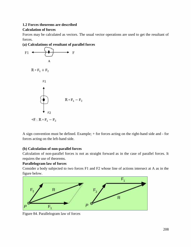
208
1.2 Forces theorems are described
Calculation of forces
Forces may be calculated as vectors. The usual vector operations are used to get the resultant of
forces.
(a) Calculations of resultant of parallel forces
A sign convention must be defined. Example; + for forces acting on the right-hand side and - for
forces acting on the left-hand side.
(b) Calculation of non-parallel forces
Calculation of non-parallel forces is not as straight forward as in the case of parallel forces. It
requires the use of theorems.
Parallelogram law of forces
Consider a body subjected to two forces F1 and F2 whose line of actions intersect at A as in the
figure below.
Figure 84. Parallelogram law of forces
F
1
F1
A
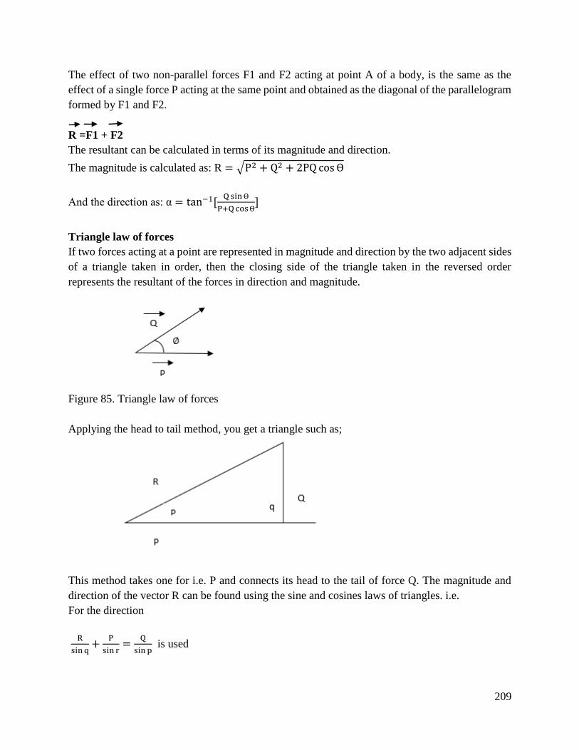
209
The effect of two non-parallel forces F1 and F2 acting at point A of a body, is the same as the
effect of a single force P acting at the same point and obtained as the diagonal of the parallelogram
formed by F1 and F2.
R =F1 + F2
The resultant can be calculated in terms of its magnitude and direction.
The magnitude is calculated as: R = √P2 + Q2 + 2PQ cosӨ
And the direction as: α = tan−1[QsinӨ
P+QcosӨ]
Triangle law of forces
If two forces acting at a point are represented in magnitude and direction by the two adjacent sides
of a triangle taken in order, then the closing side of the triangle taken in the reversed order
represents the resultant of the forces in direction and magnitude.
Figure 85. Triangle law of forces
Applying the head to tail method, you get a triangle such as;
This method takes one for i.e. P and connects its head to the tail of force Q. The magnitude and
direction of the vector R can be found using the sine and cosines laws of triangles. i.e.
For the direction
R
sinq+
P
sin r=
Q
sinp is used
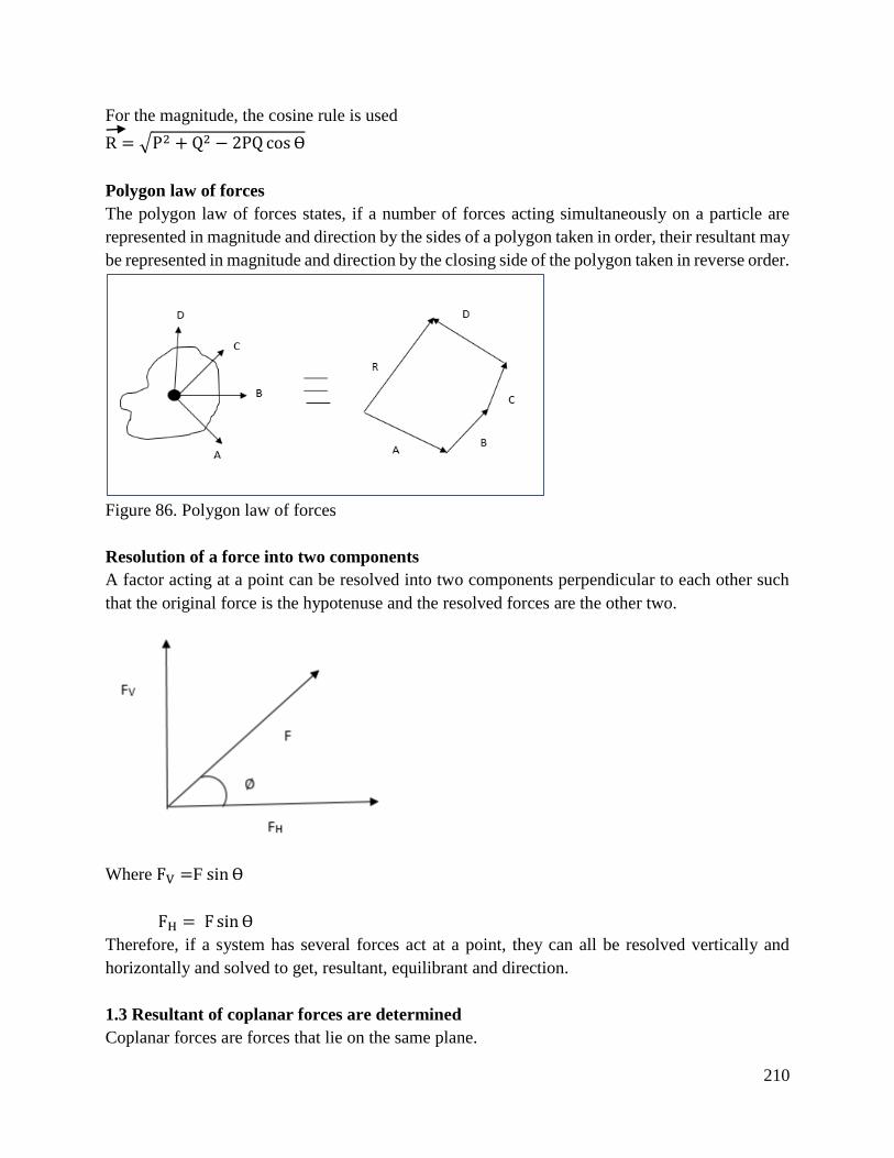
210
For the magnitude, the cosine rule is used
R = √P2 + Q2 − 2PQ cos Ө
Polygon law of forces
The polygon law of forces states, if a number of forces acting simultaneously on a particle are
represented in magnitude and direction by the sides of a polygon taken in order, their resultant may
be represented in magnitude and direction by the closing side of the polygon taken in reverse order.
Figure 86. Polygon law of forces
Resolution of a force into two components
A factor acting at a point can be resolved into two components perpendicular to each other such
that the original force is the hypotenuse and the resolved forces are the other two.
Where FV =F sin Ө
FH = F sinӨ
Therefore, if a system has several forces act at a point, they can all be resolved vertically and
horizontally and solved to get, resultant, equilibrant and direction.
1.3 Resultant of coplanar forces are determined
Coplanar forces are forces that lie on the same plane.
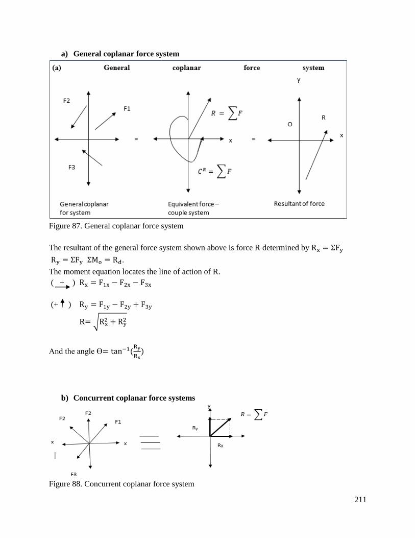
211
a) General coplanar force system
Figure 87. General coplanar force system
The resultant of the general force system shown above is force R determined by Rx = ΣFy
Ry = ΣFy ΣMo = Rd.
The moment equation locates the line of action of R.
( + ) Rx = F1x − F2x − F3x
(+ ) Ry = F1y − F2y + F3y
R= √Rx2 + Ry
2
And the angle Ө= tan−1(Ry
Rx)
b) Concurrent coplanar force systems
Figure 88. Concurrent coplanar force system
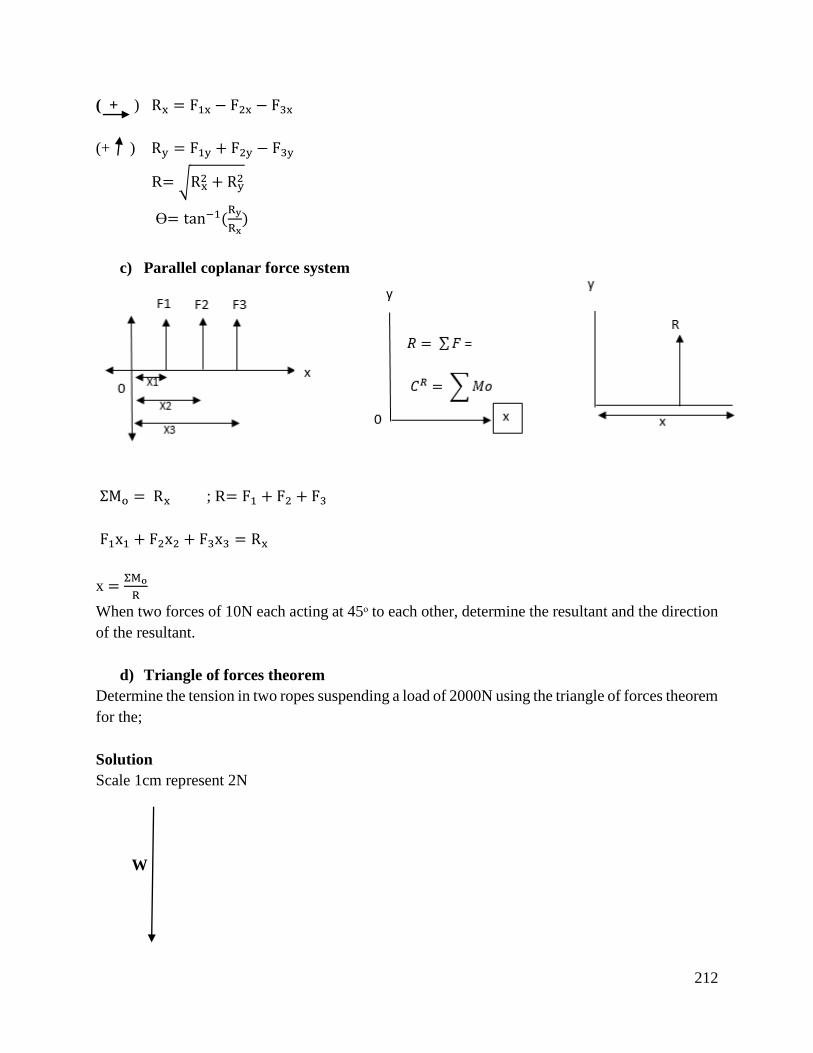
212
( + ) Rx = F1x − F2x − F3x
(+ ) Ry = F1y + F2y − F3y
R= √Rx2 + Ry
2
Ө= tan−1(Ry
Rx)
c) Parallel coplanar force system
ΣMo = Rx ; R= F1 + F2 + F3
F1x1 + F2x2 + F3x3 = Rx
x =ΣMo
R
When two forces of 10N each acting at 45ᵒ to each other, determine the resultant and the direction
of the resultant.
d) Triangle of forces theorem
Determine the tension in two ropes suspending a load of 2000N using the triangle of forces theorem
for the;
Solution
Scale 1cm represent 2N
W
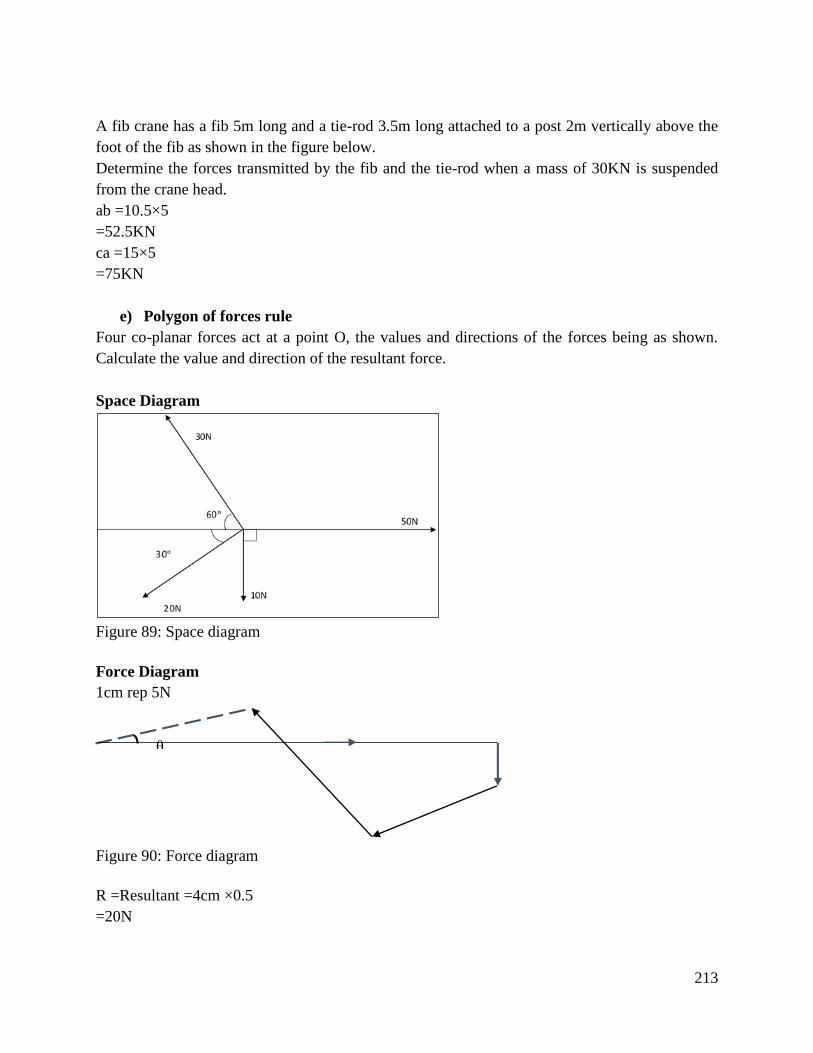
213
A fib crane has a fib 5m long and a tie-rod 3.5m long attached to a post 2m vertically above the
foot of the fib as shown in the figure below.
Determine the forces transmitted by the fib and the tie-rod when a mass of 30KN is suspended
from the crane head.
ab =10.5×5
=52.5KN
ca =15×5
=75KN
e) Polygon of forces rule
Four co-planar forces act at a point O, the values and directions of the forces being as shown.
Calculate the value and direction of the resultant force.
Space Diagram
Figure 89: Space diagram
Force Diagram
1cm rep 5N
Figure 90: Force diagram
R =Resultant =4cm ×0.5
=20N
θ R
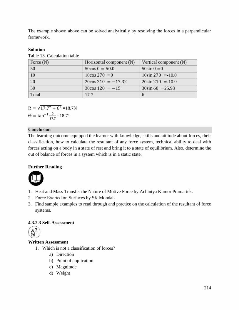
214
The example shown above can be solved analytically by resolving the forces in a perpendicular
framework.
Solution
Table 13. Calculation table
Force (N) Horizontal component (N) Vertical component (N)
50 50cos 0 = 50.0 50sin 0 =0
10 10cos 270 =0 10sin 270 =-10.0
20 20cos 210 = −17.32 20sin 210 =-10.0
30 30cos 120 = −15 30sin 60 =25.98
Total 17.7 6
R = √17.72 + 62 =18.7N
Ө = tan−1 6
17.7 =18.7ᵒ
Conclusion
The learning outcome equipped the learner with knowledge, skills and attitude about forces, their
classification, how to calculate the resultant of any force system, technical ability to deal with
forces acting on a body in a state of rest and bring it to a state of equilibrium. Also, determine the
out of balance of forces in a system which is in a static state.
Further Reading
1. Heat and Mass Transfer the Nature of Motive Force by Achintya Kumor Pramarick.
2. Force Exerted on Surfaces by SK Mondals.
3. Find sample examples to read through and practice on the calculation of the resultant of force
systems.
4.3.2.3 Self-Assessment
Written Assessment
1. Which is not a classification of forces?
a) Direction
b) Point of application
c) Magnitude
d) Weight
215
2. How many forces does the parallelogram of forces theorem deal with?
a) 4
b) 2
c) 3
d) More than 4
3. Between the following, which one of them is not a characteristic of a force?
a) It is a vector quantity
b) Has a point of action
c) Direction
d) None of the above
4. If a force of 8N inclined at an angle of 30 to the horizontal act at a point, what will be the
vertical component of the force?
a) 4.62N
b) 6.93N
c) 4N
d) 8N
5. The resultant of two forces is found to be 130N. Determine the other force if one of the
forces is 120N.
a) 45N
b) 250N
c) 10N
d) 50N
6. In the question (11) above, determine the angle of inclination of the resultant to the
horizontal if the 120N force is vertical.
a) 300
b) 57.40
c) 67.40
d) 790
7. In the definition of weight, what among the following was a component of weight?
a) Mass
b) Length
c) Time
d) All the above
8. If a body has a mass of 100kg, what is the weight of the body? Take g=9.81N/kg.
a) 9.81N
b) 98.1N
c) 981N
d) 100N
9. What is a force?
216
10. Name the types of forces.
11. Name the theorems of forces.
12. Describe the sine and cosine rule.
13. What is a coplanar force?
14. Describe the polygon law of forces.
15. Describe the triangle law of forces.
16. Differentiate between an equilibrant and a resultant of a system of forces.
17. State three theorem of forces.
18. For a body being pulled up a friction and surface inclined surface, state the most appropriate
theorem to apply in resolving the forces acting on the body.
19. Distinguish between force and weight.
Oral Assessment
1. Outline how the polygon law of forces, triangle law of forces and parallelogram law of
forces are used to calculate the resultant of a force.
2. Outline how forces are classified.
3. What are the forces acting on a body being dragged in a flat surface?
4. Gravity is a component of _______
Practical Assessment
1. In a lab, conduct an experiment to verify the triangle law and parallelogram law of forces.
2. Two forces of 7N and 11N acting at a point are right angle to each other. Determine the
magnitude and direction of the resultant of the system.
Project
A roller of mass 3tonnes is held on an inclined plane of 300 to the horizontal by a pull P parallel to
the plane;
a) Draw the forces triangle
b) Determine the magnitude of pull P
c) Determine the reaction of force on the surface due to the mass
4.3.2.4 Tools, Equipment, Supplies and Materials
Scientific Calculators
Relevant reference materials
Stationeries
Electrical workshop
Relevant practical materials
Dice
Computers with internet connection

217
4.3.2.5 References
Engineering Mechanics 1: Statics. Berlin, Germany: Springer Science and Business Media.
Gross, D, Hauger, W., Schroder, J., Wall, W.A., and Rajapaksa, N. (2012).
Hibbeler, R.C. (2011). Engineering Mechanics: Combined Statics and Dynamics. Pearson
Higher Ed.
Hughes E. and Hughes. C., Revised by Bolton W. (1994). Engineering Science Fourth Edition,
Long Man.
Pytel, A., and Kiusalaas, J. (2009). Engineering Mechanics: Statics. Boston, MA: Cengage
Learning.
Zammit S.J. (Peng,). (1987). Motor Vehicle Engineering Science for Technicians.
218
4.3.3 Learning Outcome No 2: Demonstrate knowledge of moments
4.3.3.1 Learning Activities
Learning Outcome No 2: Demonstrate knowledge of moments
Learning Activities Special Instructions
2.1 Define moments
2.2 Calculate moments
2.3 Describe principles of moments
2.4 Identify couples and applied in
engineering systems
Derive moment’s equations
Identify various moments’ application
in engineering
4.3.3.2 Information Sheet No4/LO2: Demonstrate knowledge of moments
Introduction
This learning outcome covers the moments of a force acting on a member. The moments can be
calculated as a component applied at a point in relation to the perpendicular distance from a fixed
point. Any member in engineering is under moments even when not loaded as long as it has weight.
Definition of key terms
Moment: It is a measure of the turning effect of a force from a fixed point. (Nm) units of moment.
I.e. moment = force x perpendicular distance.
Principle of moment: When a study member is in equilibrium under the action of a number of
forces, the algebraic sum of all the moments about a fixed point is zero. I.e. the clockwise moments
from a point is equal to the anti-clockwise moments from that point.
Couple: These are a parallel force, equal in magnitude but separate lines of action. E.g. the forces
applied in turning a steering wheel.
Torque: It is a turning moment acting perpendicular to the cross-section of a member and the axis
of rotation of the member.
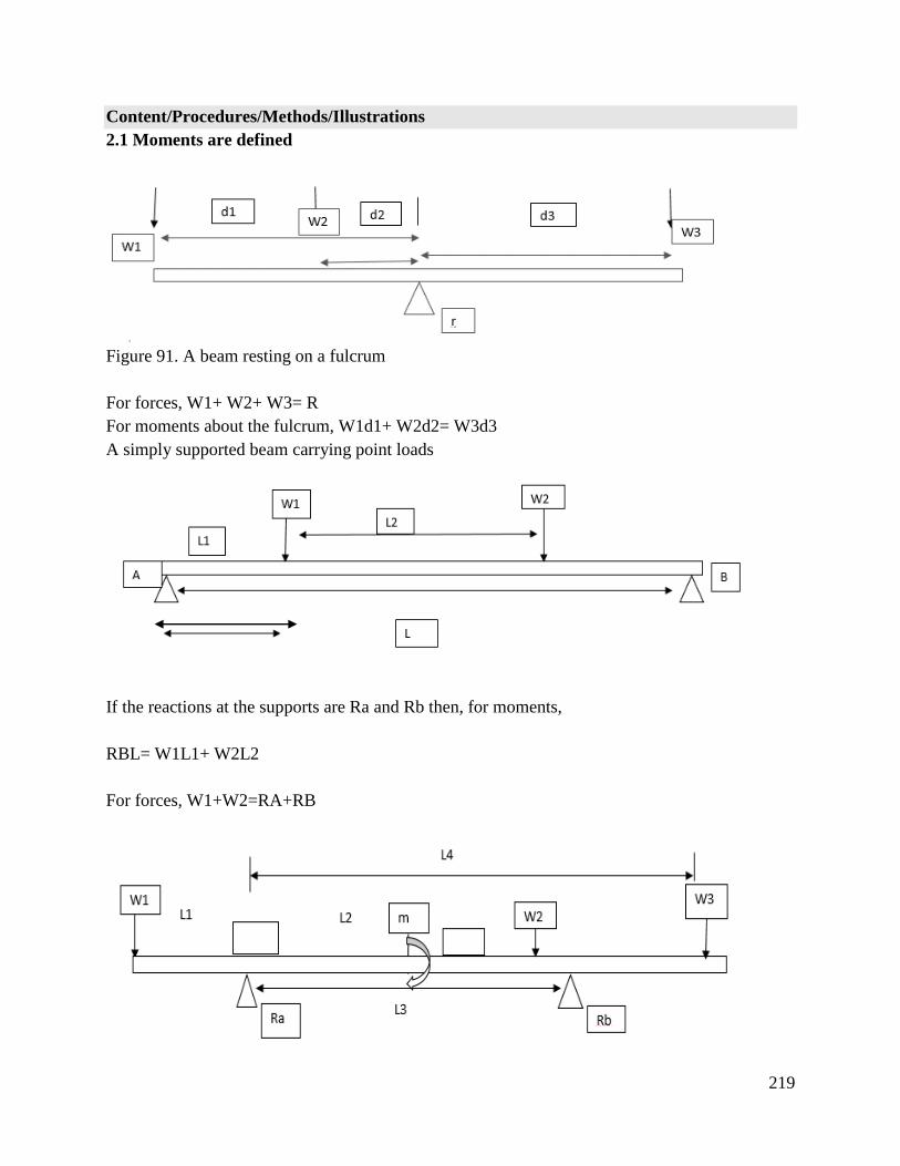
219
Content/Procedures/Methods/Illustrations
2.1 Moments are defined
Figure 91. A beam resting on a fulcrum
For forces, W1+ W2+ W3= R
For moments about the fulcrum, W1d1+ W2d2= W3d3
A simply supported beam carrying point loads
If the reactions at the supports are Ra and Rb then, for moments,
RBL= W1L1+ W2L2
For forces, W1+W2=RA+RB
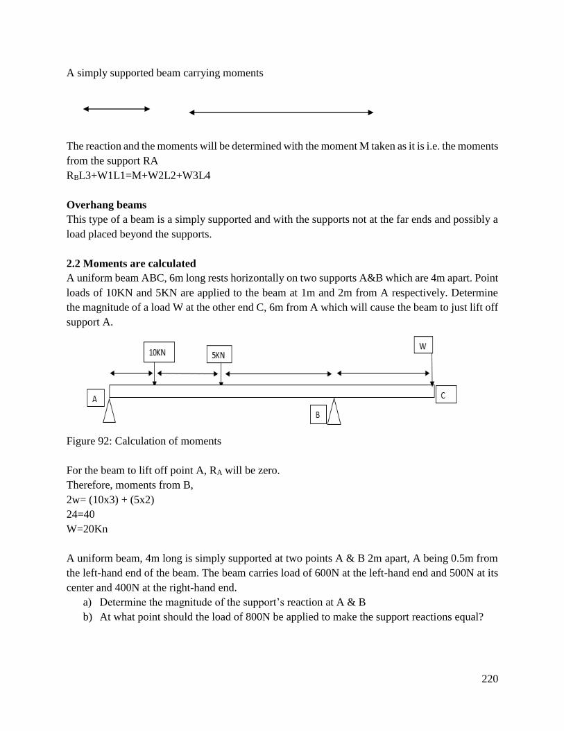
220
A simply supported beam carrying moments
The reaction and the moments will be determined with the moment M taken as it is i.e. the moments
from the support RA
RBL3+W1L1=M+W2L2+W3L4
Overhang beams
This type of a beam is a simply supported and with the supports not at the far ends and possibly a
load placed beyond the supports.
2.2 Moments are calculated
A uniform beam ABC, 6m long rests horizontally on two supports A&B which are 4m apart. Point
loads of 10KN and 5KN are applied to the beam at 1m and 2m from A respectively. Determine
the magnitude of a load W at the other end C, 6m from A which will cause the beam to just lift off
support A.
Figure 92: Calculation of moments
For the beam to lift off point A, RA will be zero.
Therefore, moments from B,
2w= (10x3) + (5x2)
24=40
W=20Kn
A uniform beam, 4m long is simply supported at two points A & B 2m apart, A being 0.5m from
the left-hand end of the beam. The beam carries load of 600N at the left-hand end and 500N at its
center and 400N at the right-hand end.
a) Determine the magnitude of the support’s reaction at A & B
b) At what point should the load of 800N be applied to make the support reactions equal?
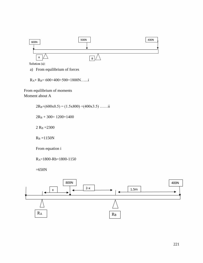
221
a) From equilibrium of forces
RA+ RB= 600+400+500=1800N…...i
From equilibrium of moments
Moment about A
2RB+(600x0.5) = (1.5x800) +(400x3.5) ……ii
2RB + 300= 1200+1400
2 RB =2300
RB =1150N
From equation i
RA=1800-Rb=1800-1150
=650N
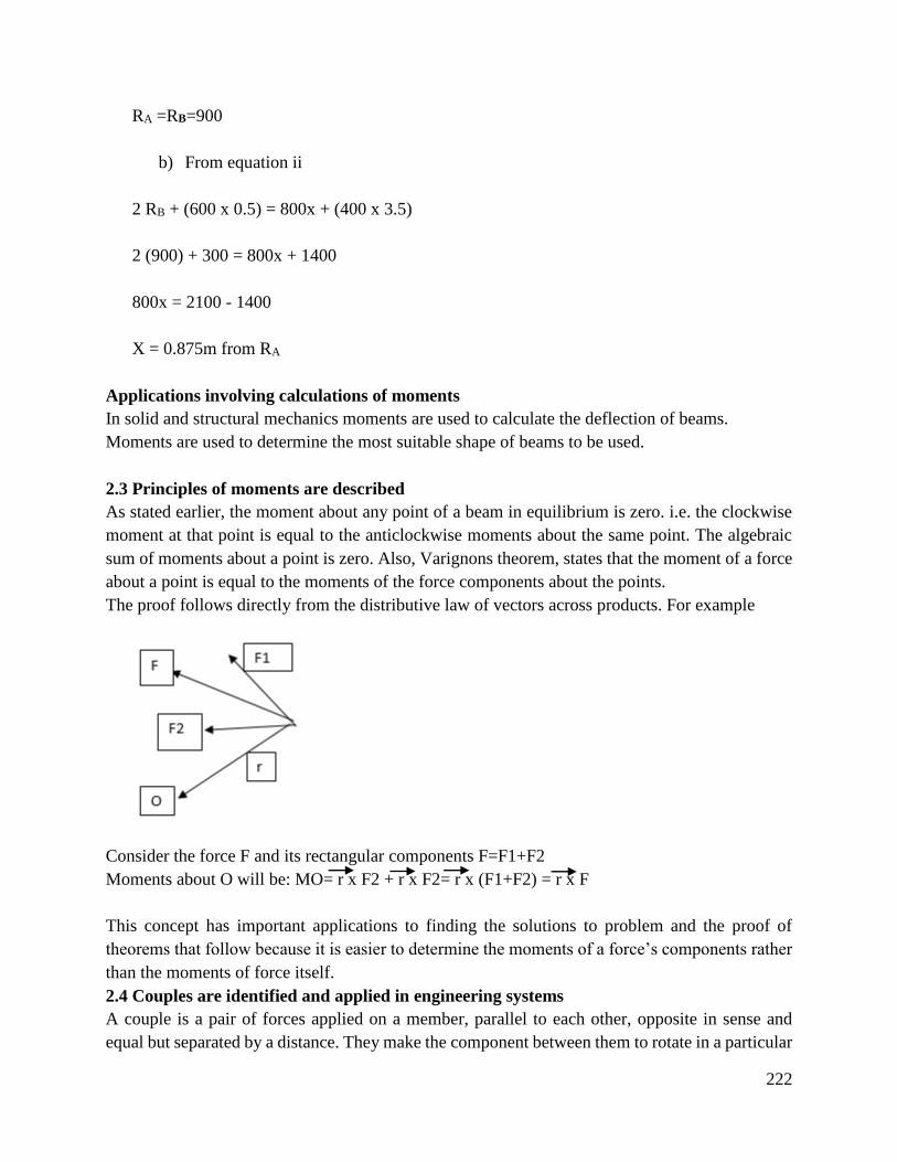
222
RA =RB=900
b) From equation ii
2 RB + (600 x 0.5) = 800x + (400 x 3.5)
2 (900) + 300 = 800x + 1400
800x = 2100 - 1400
X = 0.875m from RA
Applications involving calculations of moments
In solid and structural mechanics moments are used to calculate the deflection of beams.
Moments are used to determine the most suitable shape of beams to be used.
2.3 Principles of moments are described
As stated earlier, the moment about any point of a beam in equilibrium is zero. i.e. the clockwise
moment at that point is equal to the anticlockwise moments about the same point. The algebraic
sum of moments about a point is zero. Also, Varignons theorem, states that the moment of a force
about a point is equal to the moments of the force components about the points.
The proof follows directly from the distributive law of vectors across products. For example
Consider the force F and its rectangular components F=F1+F2
Moments about O will be: MO= r x F2 + r x F2= r x (F1+F2) = r x F
This concept has important applications to finding the solutions to problem and the proof of
theorems that follow because it is easier to determine the moments of a force’s components rather
than the moments of force itself.
2.4 Couples are identified and applied in engineering systems
A couple is a pair of forces applied on a member, parallel to each other, opposite in sense and
equal but separated by a distance. They make the component between them to rotate in a particular
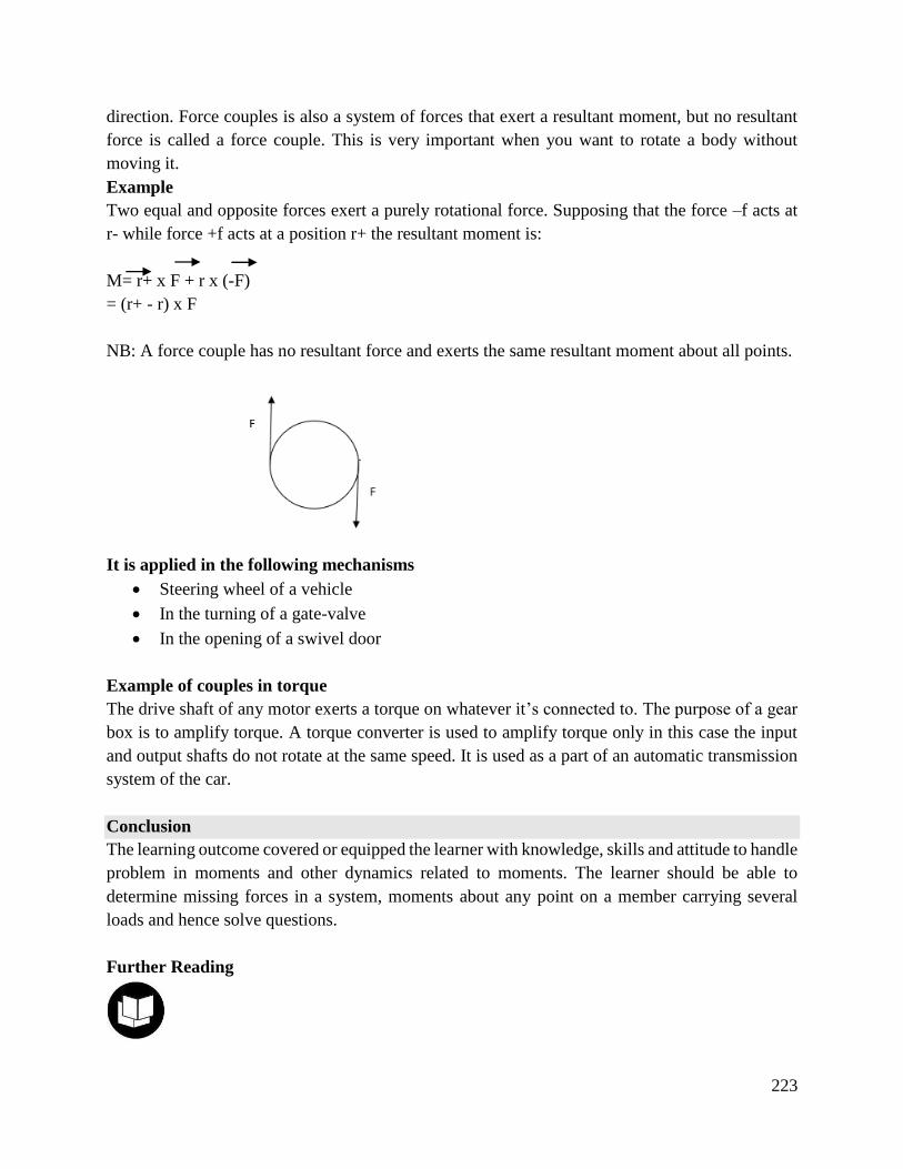
223
direction. Force couples is also a system of forces that exert a resultant moment, but no resultant
force is called a force couple. This is very important when you want to rotate a body without
moving it.
Example
Two equal and opposite forces exert a purely rotational force. Supposing that the force –f acts at
r- while force +f acts at a position r+ the resultant moment is:
M= r+ x F + r x (-F)
= (r+ - r) x F
NB: A force couple has no resultant force and exerts the same resultant moment about all points.
It is applied in the following mechanisms
Steering wheel of a vehicle
In the turning of a gate-valve
In the opening of a swivel door
Example of couples in torque
The drive shaft of any motor exerts a torque on whatever it’s connected to. The purpose of a gear
box is to amplify torque. A torque converter is used to amplify torque only in this case the input
and output shafts do not rotate at the same speed. It is used as a part of an automatic transmission
system of the car.
Conclusion
The learning outcome covered or equipped the learner with knowledge, skills and attitude to handle
problem in moments and other dynamics related to moments. The learner should be able to
determine missing forces in a system, moments about any point on a member carrying several
loads and hence solve questions.
Further Reading

224
1. Conle, C. (1999) “Moments of Interpleration in the perception and Evaluation of Teaching”.
Teaching and Teacher Education 15, (7) 801-814.
2. Winter, D.A. (1983) Moments of Force and Mechanical Power in Jogging. Journal of
biomechanics 16(1), 91-97.
4.3.3.3 Self-Assessment
Written Assessment
1. State the elements of moment.
a) Force and mass
b) Mass and area
c) Mass and distance
d) Force and perpendicular distance
2. The moment of a force of 4N acting from a distance of 2m is?
a) 4Nm
b) 2Nm
c) 8Nm
d) 14Nm
3. The moment acting between points is found to be 46Nm. What is the force if the point
of action is 2.3m away?
a) 20N
b) 105.8N
c) 0.05N
d) 10.58N
4. Describe a simply supported beam
a) Has multiple supports
b) Has a single support
c) Rests on 2 supports
d) Built in into a wall
5. State the principle of moment
a) Clockwise moment equals to anticlockwise moment
b) Anticlockwise is never equal to clockwise moment
c) At the end of a beam there are no moments
d) Moment is a product of force and distance
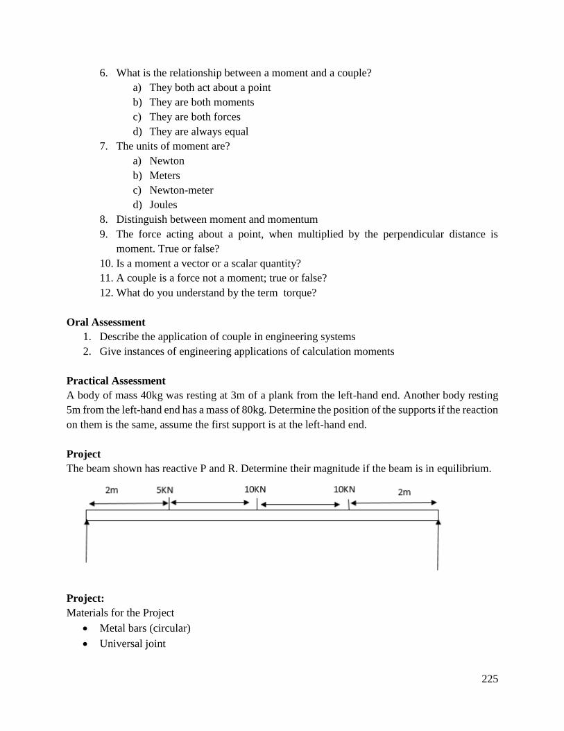
225
6. What is the relationship between a moment and a couple?
a) They both act about a point
b) They are both moments
c) They are both forces
d) They are always equal
7. The units of moment are?
a) Newton
b) Meters
c) Newton-meter
d) Joules
8. Distinguish between moment and momentum
9. The force acting about a point, when multiplied by the perpendicular distance is
moment. True or false?
10. Is a moment a vector or a scalar quantity?
11. A couple is a force not a moment; true or false?
12. What do you understand by the term torque?
Oral Assessment
1. Describe the application of couple in engineering systems
2. Give instances of engineering applications of calculation moments
Practical Assessment
A body of mass 40kg was resting at 3m of a plank from the left-hand end. Another body resting
5m from the left-hand end has a mass of 80kg. Determine the position of the supports if the reaction
on them is the same, assume the first support is at the left-hand end.
Project
The beam shown has reactive P and R. Determine their magnitude if the beam is in equilibrium.
Project:
Materials for the Project
Metal bars (circular)
Universal joint

226
Metal shaft
4 wheels
Equipment
Welding machine
Use the materials above to create a model of the wheels and axle of a vehicle to demonstrate the
turning of the wheels by exertion of a moment.
4.3.3.4 Tools, Equipment, Supplies and Materials
Scientific Calculators
Relevant reference materials
Stationeries
Electrical workshop
Relevant practical materials
Dice
Computers with internet connection
4.3.3.5 References
Bird, J.K., Ross C, 2002, Mechanical Engineering Principles, Nounes
Hibbeler R.C. (2011) Engineering Mechanics: Combined Statics and Dynamics. Pearson Higher
Ed.
Khurmi, R. et al;(2005) Theory of Machines, 14 edtion; New Delhi; S.Chand.
Pytel, A. Kiosabas, J. (2009) Engineering Mechanics and Statics. Boston, MA: Cengage
Walice, J.D. Applied Mechanics, London Melborne Aracland
Zammit, S.J., 1987, Motor Vehicle Engineering Science for Technicians
227
4.3.4 Learning Outcome No 3: Understand friction principles
4.3.4.1 Learning Activities
Learning Outcome No 3: Understand friction principles
Learning Activities Special Instructions
3.1 Identify laws of friction
3.2 Calculate limiting friction
3.3 Calculate forces applied at an angle to a
horizontal plane
3.4 Calculate coefficient of friction
3.5 Identify advantages and disadvantages of
friction
Determine the roughness and smoothness
of a surface.
Illustrate the difference between sliding
friction and static friction.
4.3.4.2 Information Sheet No4/LO3: Understand friction principles
Introduction
When an object such as wood is placed on a flat surface and sufficient force is applied to the object,
the force being parallel to the flat surface, the wood slides across the flat surface. When the force
is removed, motion of the block stops, thus there is a force which resists sliding. This force is
called dynamic friction. A force may be applied to the block, which is insufficient to move. In this
case the force resisting motion is called static friction.
Definition of key terms
Dynamic of sliding friction: It is the force which occurs when motion is taking place.
Static friction force: It is the force which occurs before motion takes place.
Coefficient of friction µ: It is a measure of the amount of friction exist between two surfaces.
Content/Procedures/Methods/Illustrations
3.1 Laws of friction are identified
The sliding frictional force opposing a motion, when one motion has started, is directly
proportional to the normal force between the surfaces. The sliding frictional force is dependent
upon the nature of the surface in contact. Relative motion is more difficult with rough surfaces
than with smooth surfaces. The sliding frictional force is dependent upon the physical properties
of the materials involved. For the same force pressing the sliding surfaces together, steel slides
more easily over nylon that it does over rubber. The sliding frictional force is independent of the
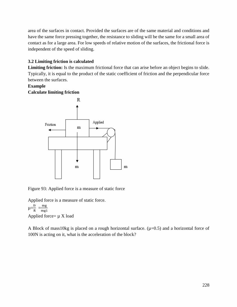
228
area of the surfaces in contact. Provided the surfaces are of the same material and conditions and
have the same force pressing together, the resistance to sliding will be the same for a small area of
contact as for a large area. For low speeds of relative motion of the surfaces, the frictional force is
independent of the speed of sliding.
3.2 Limiting friction is calculated
Limiting friction: Is the maximum frictional force that can arise before an object begins to slide.
Typically, it is equal to the product of the static coefficient of friction and the perpendicular force
between the surfaces.
Example
Calculate limiting friction
Figure 93: Applied force is a measure of static force
Applied force is a measure of static force.
µ=fr
R =
mg
mg1
Applied force= µ X load
A Block of mass10kg is placed on a rough horizontal surface. (µ=0.5) and a horizontal force of
100N is acting on it, what is the acceleration of the block?
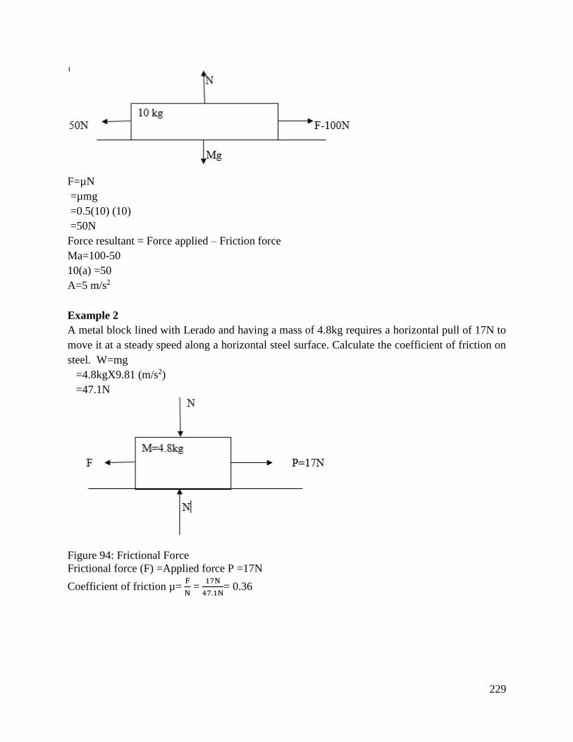
229
F=µN
=µmg
=0.5(10) (10)
=50N
Force resultant = Force applied – Friction force
Ma=100-50
10(a) =50
A=5 m/s2
Example 2
A metal block lined with Lerado and having a mass of 4.8kg requires a horizontal pull of 17N to
move it at a steady speed along a horizontal steel surface. Calculate the coefficient of friction on
steel. W=mg
=4.8kgX9.81 (m/s2)
=47.1N
Figure 94: Frictional Force
Frictional force (F) =Applied force P =17N
Coefficient of friction µ= F
N =
17N
47.1N= 0.36
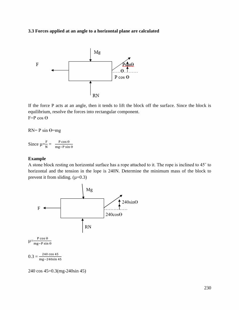
230
3.3 Forces applied at an angle to a horizontal plane are calculated
If the force P acts at an angle, then it tends to lift the block off the surface. Since the block is
equilibrium, resolve the forces into rectangular component.
F=P cos Ɵ
RN= P sin Ɵ=mg
Since µ=F
N =
P cos Ɵ
mg−P sin Ɵ
Example
A stone block resting on horizontal surface has a rope attached to it. The rope is inclined to 45˚ to
horizontal and the tension in the lope is 240N. Determine the minimum mass of the block to
prevent it from sliding. (µ=0.3)
Mg
240sinӨ
F ……………
240cosӨ
RN
µ=P cos Ɵ
mg−P sin Ɵ
0.3 = 240 cos 45
mg−240sin 45
240 cos 45=0.3(mg-240sin 45)
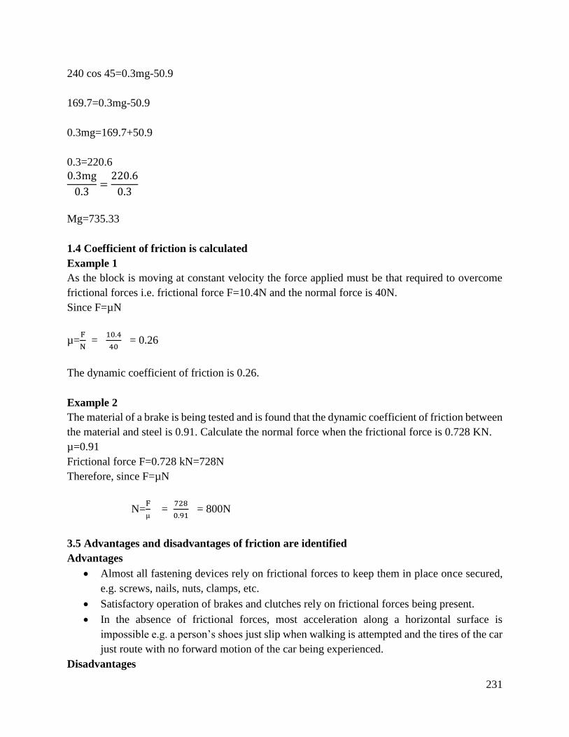
231
240 cos 45=0.3mg-50.9
169.7=0.3mg-50.9
0.3mg=169.7+50.9
0.3=220.6
0.3mg
0.3=
220.6
0.3
Mg=735.33
1.4 Coefficient of friction is calculated
Example 1
As the block is moving at constant velocity the force applied must be that required to overcome
frictional forces i.e. frictional force F=10.4N and the normal force is 40N.
Since F=µN
µ=F
N =
10.4
40 = 0.26
The dynamic coefficient of friction is 0.26.
Example 2
The material of a brake is being tested and is found that the dynamic coefficient of friction between
the material and steel is 0.91. Calculate the normal force when the frictional force is 0.728 KN.
µ=0.91
Frictional force F=0.728 kN=728N
Therefore, since F=µN
N=F
µ =
728
0.91 = 800N
3.5 Advantages and disadvantages of friction are identified
Advantages
Almost all fastening devices rely on frictional forces to keep them in place once secured,
e.g. screws, nails, nuts, clamps, etc.
Satisfactory operation of brakes and clutches rely on frictional forces being present.
In the absence of frictional forces, most acceleration along a horizontal surface is
impossible e.g. a person’s shoes just slip when walking is attempted and the tires of the car
just route with no forward motion of the car being experienced.
Disadvantages
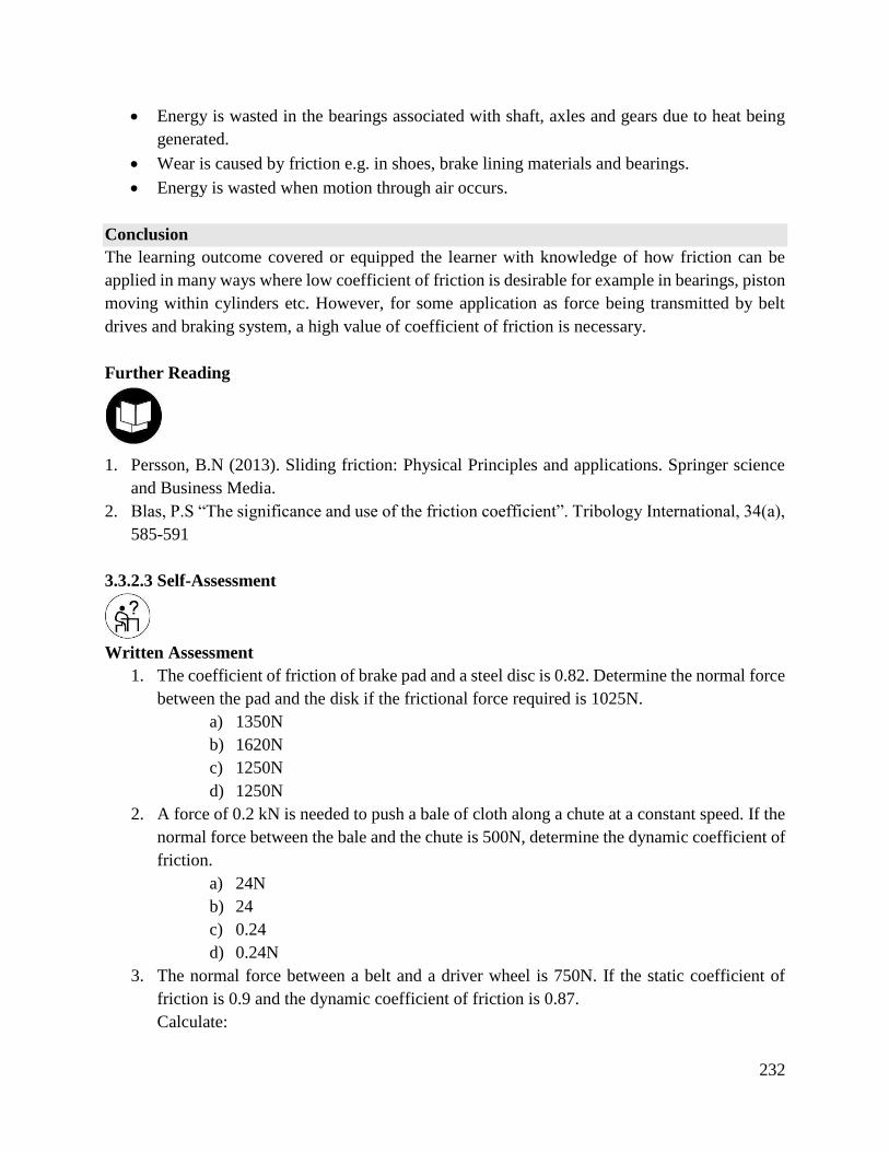
232
Energy is wasted in the bearings associated with shaft, axles and gears due to heat being
generated.
Wear is caused by friction e.g. in shoes, brake lining materials and bearings.
Energy is wasted when motion through air occurs.
Conclusion
The learning outcome covered or equipped the learner with knowledge of how friction can be
applied in many ways where low coefficient of friction is desirable for example in bearings, piston
moving within cylinders etc. However, for some application as force being transmitted by belt
drives and braking system, a high value of coefficient of friction is necessary.
Further Reading
1. Persson, B.N (2013). Sliding friction: Physical Principles and applications. Springer science
and Business Media.
2. Blas, P.S “The significance and use of the friction coefficient”. Tribology International, 34(a),
585-591
3.3.2.3 Self-Assessment
Written Assessment
1. The coefficient of friction of brake pad and a steel disc is 0.82. Determine the normal force
between the pad and the disk if the frictional force required is 1025N.
a) 1350N
b) 1620N
c) 1250N
d) 1250N
2. A force of 0.2 kN is needed to push a bale of cloth along a chute at a constant speed. If the
normal force between the bale and the chute is 500N, determine the dynamic coefficient of
friction.
a) 24N
b) 24
c) 0.24
d) 0.24N
3. The normal force between a belt and a driver wheel is 750N. If the static coefficient of
friction is 0.9 and the dynamic coefficient of friction is 0.87.
Calculate:
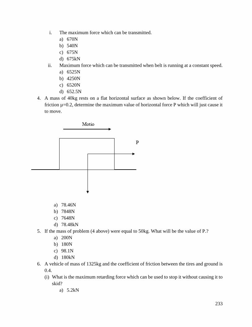
233
i. The maximum force which can be transmitted.
a) 670N
b) 540N
c) 675N
d) 675kN
ii. Maximum force which can be transmitted when belt is running at a constant speed.
a) 6525N
b) 4250N
c) 6520N
d) 652.5N
4. A mass of 40kg rests on a flat horizontal surface as shown below. If the coefficient of
friction µ=0.2, determine the maximum value of horizontal force P which will just cause it
to move.
a) 78.46N
b) 7848N
c) 7648N
d) 78.48kN
5. If the mass of problem (4 above) were equal to 50kg. What will be the value of P.?
a) 200N
b) 180N
c) 98.1N
d) 180kN
6. A vehicle of mass of 1325kg and the coefficient of friction between the tires and ground is
0.4.
(i) What is the maximum retarding force which can be used to stop it without causing it to
skid?
a) 5.2kN
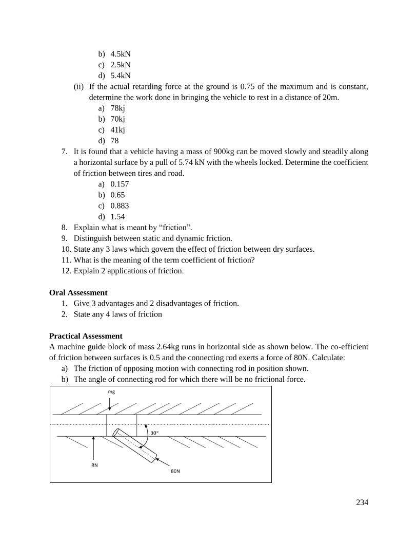
234
b) 4.5kN
c) 2.5kN
d) 5.4kN
(ii) If the actual retarding force at the ground is 0.75 of the maximum and is constant,
determine the work done in bringing the vehicle to rest in a distance of 20m.
a) 78kj
b) 70kj
c) 41kj
d) 78
7. It is found that a vehicle having a mass of 900kg can be moved slowly and steadily along
a horizontal surface by a pull of 5.74 kN with the wheels locked. Determine the coefficient
of friction between tires and road.
a) 0.157
b) 0.65
c) 0.883
d) 1.54
8. Explain what is meant by “friction”.
9. Distinguish between static and dynamic friction.
10. State any 3 laws which govern the effect of friction between dry surfaces.
11. What is the meaning of the term coefficient of friction?
12. Explain 2 applications of friction.
Oral Assessment
1. Give 3 advantages and 2 disadvantages of friction.
2. State any 4 laws of friction
Practical Assessment
A machine guide block of mass 2.64kg runs in horizontal side as shown below. The co-efficient
of friction between surfaces is 0.5 and the connecting rod exerts a force of 80N. Calculate:
a) The friction of opposing motion with connecting rod in position shown.
b) The angle of connecting rod for which there will be no frictional force.
235
Project
Discuss briefly two design implications that arise due to frictional forces and how lubrication may
or may not help.
4.3.4.4 Tools, Equipment, Supplies and Materials
Scientific calculators
Relevant reference materials
Stationeries
Electrical workshop
Relevant practical materials
Dice
Computers with internet connection
4.3.4.5 References
Bird, J., & Ross, C. (2014). Mechanical engineering principles. Routledge.
Blau, P. J. (2001). The significance and use of the friction coefficient. Tribology
International, 34(9), 585-591.
Zammit, S. J. (1987). Motor Vehicle Engineering Science for Technicians, Level 2. Longman
Scientific & Technical.
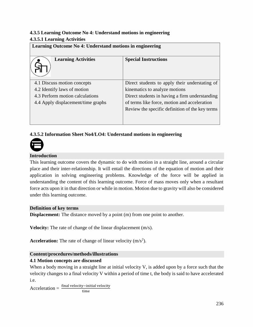
236
4.3.5 Learning Outcome No 4: Understand motions in engineering
4.3.5.1 Learning Activities
Learning Outcome No 4: Understand motions in engineering
Learning Activities Special Instructions
4.1 Discuss motion concepts
4.2 Identify laws of motion
4.3 Perform motion calculations
4.4 Apply displacement/time graphs
Direct students to apply their understating of
kinematics to analyze motions
Direct students in having a firm understanding
of terms like force, motion and acceleration
Review the specific definition of the key terms
4.3.5.2 Information Sheet No4/LO4: Understand motions in engineering
Introduction
This learning outcome covers the dynamic to do with motion in a straight line, around a circular
place and their inter-relationship. It will entail the directions of the equation of motion and their
application in solving engineering problems. Knowledge of the force will be applied in
understanding the content of this learning outcome. Force of mass moves only when a resultant
force acts upon it in that direction or while in motion. Motion due to gravity will also be considered
under this learning outcome.
Definition of key terms
Displacement: The distance moved by a point (m) from one point to another.
Velocity: The rate of change of the linear displacement (m/s).
Acceleration: The rate of change of linear velocity (m/s2).
Content/procedures/methods/illustrations
4.1 Motion concepts are discussed
When a body moving in a straight line at initial velocity V, is added upon by a force such that the
velocity changes to a final velocity V within a period of time t, the body is said to have accelerated
i.e.
Acceleration = final velocity−initial velocity
time
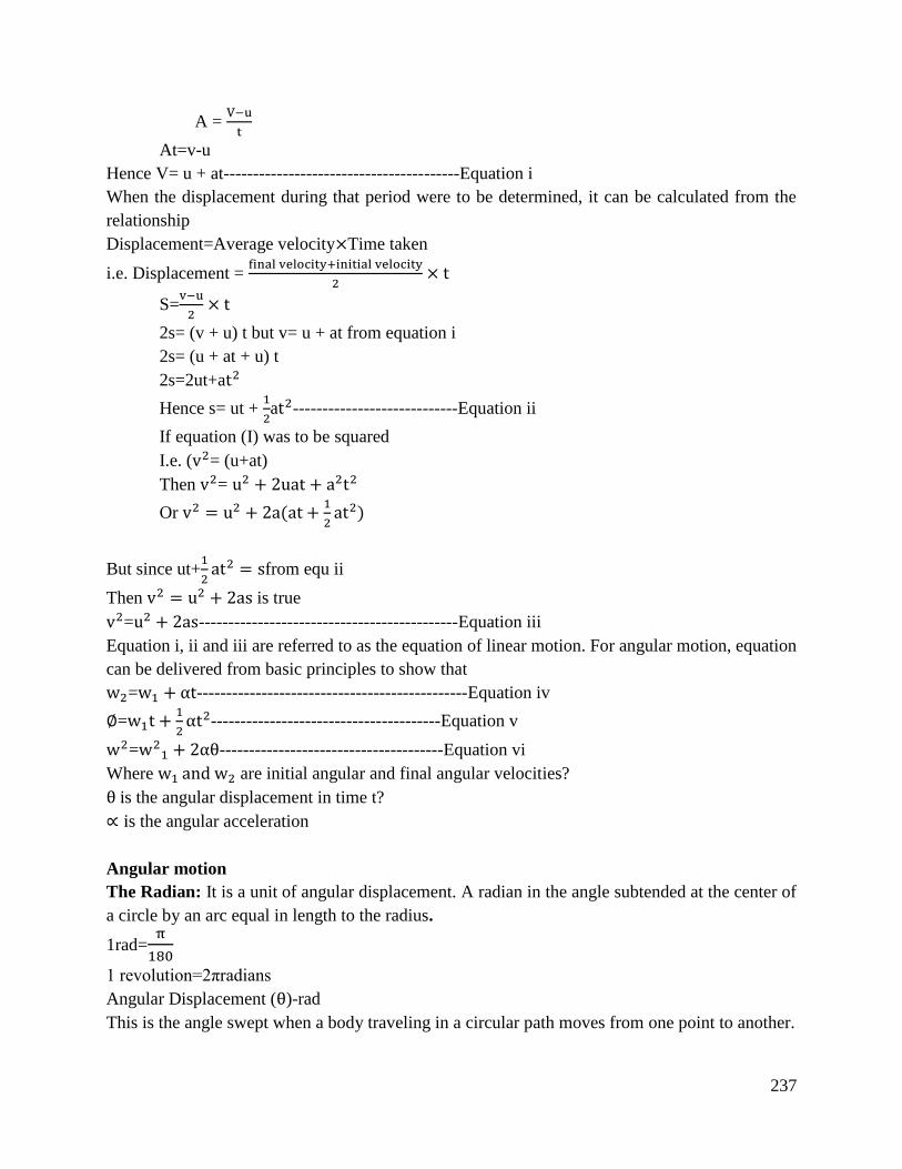
237
A = V−u
t
At=v-u
Hence V= u + at----------------------------------------Equation i
When the displacement during that period were to be determined, it can be calculated from the
relationship
Displacement=Average velocity×Time taken
i.e. Displacement = final velocity+initial velocity
2× t
S=v−u
2× t
2s= (v + u) t but v= u + at from equation i
2s= (u + at + u) t
2s=2ut+at2
Hence s= ut + 1
2at2----------------------------Equation ii
If equation (I) was to be squared
I.e. (v2= (u+at)
Then v2= u2 + 2uat + a2t2
Or v2 = u2 + 2a(at +1
2at2)
But since ut+1
2at2 = sfrom equ ii
Then v2 = u2 + 2as is true
v2=u2 + 2as--------------------------------------------Equation iii
Equation i, ii and iii are referred to as the equation of linear motion. For angular motion, equation
can be delivered from basic principles to show that
w2=w1 + αt----------------------------------------------Equation iv
∅=w1t +1
2αt2---------------------------------------Equation v
w2=w21 + 2αθ--------------------------------------Equation vi
Where w1 and w2 are initial angular and final angular velocities?
θ is the angular displacement in time t?
∝ is the angular acceleration
Angular motion
The Radian: It is a unit of angular displacement. A radian in the angle subtended at the center of
a circle by an arc equal in length to the radius.
1rad=π
180
1 revolution=2πradians
Angular Displacement (θ)-rad
This is the angle swept when a body traveling in a circular path moves from one point to another.
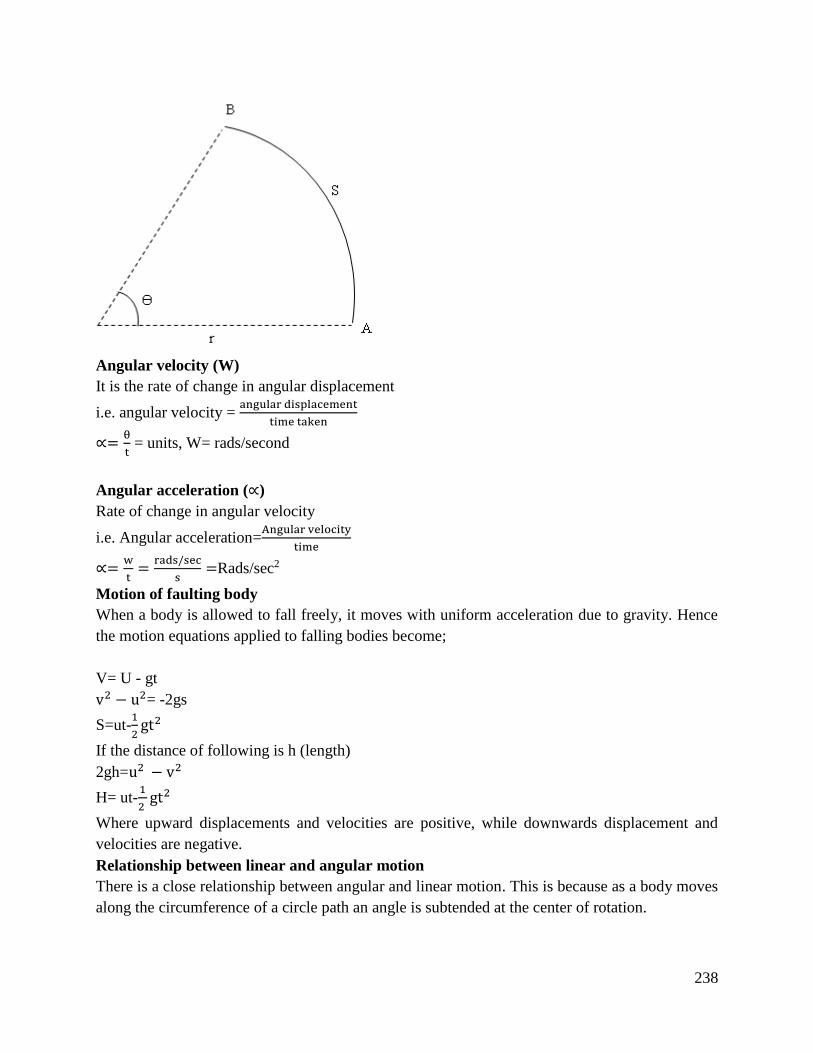
238
Angular velocity (W)
It is the rate of change in angular displacement
i.e. angular velocity = angular displacement
time taken
∝=θ
t = units, W= rads/second
Angular acceleration (∝)
Rate of change in angular velocity
i.e. Angular acceleration=Angular velocity
time
∝=w
t=
rads/sec
s=Rads/sec2
Motion of faulting body
When a body is allowed to fall freely, it moves with uniform acceleration due to gravity. Hence
the motion equations applied to falling bodies become;
V= U - gt
v2 − u2= -2gs
S=ut-1
2gt2
If the distance of following is h (length)
2gh=u2 − v2
H= ut-1
2 gt2
Where upward displacements and velocities are positive, while downwards displacement and
velocities are negative.
Relationship between linear and angular motion
There is a close relationship between angular and linear motion. This is because as a body moves
along the circumference of a circle path an angle is subtended at the center of rotation.
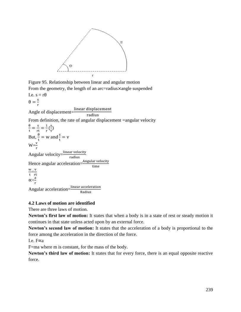
239
Figure 95. Relationship between linear and angular motion
From the geometry, the length of an arc=radius×angle suspended
I.e. s = rθ
θ =s
r
Angle of displacement=linear displacement
radius
From definition, the rate of angular displacement =angular velocity θ
t=
s
rt=
1
r(s
t)
But, θ
t= w and
s
t= v
W=v
r
Angular velocity=linear velocity
radius
Hence angular acceleration=Angular velocity
time
w
t=
v
rt
∝=a
r
Angular acceleration=linear acceleration
Radius
4.2 Laws of motion are identified
There are three laws of motion.
Newton’s first law of motion: It states that when a body is in a state of rest or steady motion it
continues in that state unless acted upon by an external force.
Newton’s second law of motion: It states that the acceleration of a body is proportional to the
force among the acceleration in the direction of the force.
I.e. F∝a
F=ma where m is constant, for the mass of the body.
Newton’s third law of motion: It states that for every force, there is an equal opposite reactive
force.
240
4.3 Motion calculations are performed
Problem one
A vehicle accelerates uniformly at 15m/s from a speed of 27km/h calculate
1. The time required to attain a speed of 81m/s.
2. The distance travelled in this time.
Solution
U= initial velocity=27km/h
= 27×1000
3000m/s
= 7.5m/s
Final velocity V=81×1000
3600=22.5m/s
a= 1.5m/s
i. Applying the first equation of motion
V=U + at
T=v−u
a=
22.5−7.5
1.5
=10 seconds
ii. Applying the third law of motion
v2 − y2 = 2as
S = v2−u2
2a=
7.52
2×1.5 = 150
Alternatively: from the second equation of motion
S = ut +1/2at2
= (7.5 x 10) + ½ x1.5x102
= 75+75
=150m
Problem two
A vehicle traveling at 81km/h is brought to rest uniformly though a distance of 225m find
a) The uniform velocity
b) Time taken
U=81km/h=22.5m/s
V=0m/s
a =?
t =?
S=225m
a) Applying the 3rd equation of motion
v2 = u2 + 2as
2as=u2
241
a= u2
25=
22.5
2×225
=1.125m/s
b) Applying the 1st equation of motion
V= u + at
0= 22.5-1.125t
T=22.5
1.125 = 20 seconds
iii. Problem three
A wheel rotating 5 rads accelerating uniformly at 0.5rad/s for 30 seconds. Find
a) The angular velocity after 30 seconds
b) The angle formed through by the wheel during this time
Solution
W1= 5rads w1=? ∝= 0.5rads
θ =? T=30s
Applying the 1st equation of motion
w2 = w1+∝ t
= 5+0.5(30)
= 20 rads
Applying the 2nd equation
∝=w1t +1
2∝ t2
(5× 30) +1
2× 0.5 × 52
=180+225
= 375rad
Alternatively: From the 3rd equation of motion
W22
= W1252 + 2 ∝ ∅
202 = 52 + (2 X 0.5) ∅
400 − 25 + ∅
∅ = 375
Problem 4
A wheel of diameter 200mm, rotate at 2100rads. What is the circumference of speed of the wheel
in m/s?
Solution
The angle speed needs to be expressed in rads
Since 1 rad= 2πrad
N=2100
242
Then 2100rad= 2π× 2100 = 4200πrad
=4200π
60 70πrads
I.e. w=2π N
60
Where N= speed in velocity. min
For v= wr then v= 70π× 0.1 =7πm
s
=22m/s
Problem 5
A wheel is rotated at 2000rads/min and a force is applied and brings it to rest with uniform
acceleration in reactions. Find
a) The time taken to bring the wheel to rest
b) The angular redaction in rads/d
Solution
N= 2000rads/min
θ =4000× 2π = 800πrads
w1 =2πN
60=
2π×2000
300=
200π
3= W2 = 0
From the 1st equation of motion
θ = (w2+w1
2) t
800π=200π
3= 2 ∝ (800π)
∝=200π2
9×2×800π
=200π2
18×800π× π2
=8.727rads
4.4 Displacement/time graphs are applied
This graph is plotted with the y- axis having the displacement and the x-axis having the time taken.
When properly drawn, the graph can be used to determine the velocity of an object at a particular
point, obtained from determining the gradient of the curve drawn at the point. It can be used to
plot liner and angular motion.
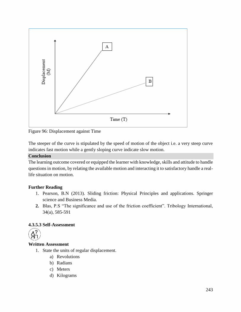
243
Figure 96: Displacement against Time
The steeper of the curve is stipulated by the speed of motion of the object i.e. a very steep curve
indicates fast motion while a gently sloping curve indicate slow motion.
Conclusion
The learning outcome covered or equipped the learner with knowledge, skills and attitude to handle
questions in motion, by relating the available motion and interacting it to satisfactory handle a real-
life situation on motion.
Further Reading
1. Pearson, B.N (2013). Sliding friction: Physical Principles and applications. Springer
science and Business Media.
2. Blas, P.S “The significance and use of the friction coefficient”. Tribology International,
34(a), 585-591
4.3.5.3 Self-Assessment
Written Assessment
1. State the units of regular displacement.
a) Revolutions
b) Radians
c) Meters
d) Kilograms
244
2. One revolution is equivalent to __________ radians.
a) 360
b) Meters
c) π
d) 2π
3. Acceleration is the rate change in __________
a) Displacement
b) Time
c) Velocity
d) None of the above
4. One of the following is not an equation of linear motion.
a) F=ma
b) V=u+at
c) y2 = u2 + 2as
d) S=ut+1
2at2
5. Angular and linear motion are related.
a) True
b) False
c) Not sure
d) Not entire
6. The unit of speed and velocity are the same.
a) Rads/s
b) M/s
c) Seconds
d) m/s2
7. If a wheel is rotated at a constant speed of N/min its angular velocity wards is given by the
expression.
a) πn
b) 2πn
c) 2πN
60
d) 60
2πN
8. State the 2nd law of motion.
9. Force is directly proportional to?
10. What do you understand by the term acceleration as used in motion?
11. The perimeter of the circular path is given by?
12. The velocity of a body can continually be obtained from a displacement fine graph by?
Oral Assessment
245
1. State the parameter obtained in linear motion.
2. State the units of the parameters stated above.
Practical Assessment
Using a displacement time graph draw the curve whose motion is as follows, determine the velocity
of mass.
Table 14: Displacement Against time
Displacement(m) 0 4 8 12 16 20
Time(s) 0 1 2 3 4 5
Project
1. From basic principle derive the equation of angular motion
4.3.5.4 Tools, Equipment, Supplies and Materials
Scientific Calculators
Relevant reference materials
Stationeries
Electrical workshop
Relevant practical materials
Dice
Computers with internet connection
4.3.5.5 References
Gibson, I. (2013). Micro prototyping and fabrication in manufacturing. Handbook of
Manufacturing Engineering and Technology, 1-14.
Kwan, F. Y., Cheung, K. C., & Gibson, I. (2000, September). Automatic extraction of bone
boundaries from CT scans using an intelligence-based approach. In Proceedings 15th
International Conference on Pattern Recognition. ICPR-2000 (Vol. 3, pp. 437-440). IEEE.
Zammit, S. J. (1987). Motor Vehicle Engineering Science for Technicians, Level 2. Longman
Scientific & Technical.

246
4.3.6 Learning Outcome No 5: Describe work, energy and power
4.3.6.1 Learning Activities
Learning Outcome No 5: Describe work, energy and power
Learning Activities Special Instructions
5.1 Calculate work
5.2 Calculate energy
5.3 Perform power calculations
Illustrate the concepts of work using examples
Illustrate concept of energy and power using examples
Derive the various equations in work, power and energy
4.3.6.2 Information Sheet No4/LO5: Describe work, energy and power
Introduction
This learning outcome covers work, energy and power and their calculation. In physics, we say
the work is done on an object when you transfer energy to that object. Work is the application of
force over a distance. Energy is also covered in this learning outcome and the various concepts of
energy. This learning outcome also covers thoroughly the concept of power and the applications
in various real-life situations. The learning outcomes equips the students with a variety of
knowledge in various fields in real life situation.
Definition of key terms
Work: Work is said to be done when a force is applied to a body and causes it to move in the
direction of the force. If one object transfers energy to a second object, then the first object does
work on the second object. Work = force x distance.
Energy: Energy is capacity for doing work and is measured in Joule (J).
Power: Power is defined as the rate of transfer of energy or rate of doing work or work done per
unit time. Unit of power is Watt = 1 Joule/second.
Content/Procedures/Methods/Illustrations
5.1 Work is calculated
When a constant force is applied on a body, the amount or work-done is measured by the product
of that force and the distance covered by that body i.e.
Work done = Force × distance moved
=F×S where S =distance
= F×S (NM) (Joules)
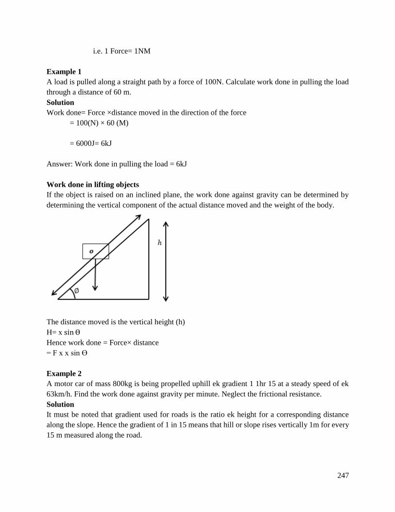
247
i.e. 1 Force= 1NM
Example 1
A load is pulled along a straight path by a force of 100N. Calculate work done in pulling the load
through a distance of 60 m.
Solution
Work done= Force ×distance moved in the direction of the force
= 100(N) × 60 (M)
= 6000J= 6kJ
Answer: Work done in pulling the load = 6kJ
Work done in lifting objects
If the object is raised on an inclined plane, the work done against gravity can be determined by
determining the vertical component of the actual distance moved and the weight of the body.
The distance moved is the vertical height (h)
H= x sin Ө
Hence work done = Force× distance
= F x x sin Ө
Example 2
A motor car of mass 800kg is being propelled uphill ek gradient 1 1hr 15 at a steady speed of ek
63km/h. Find the work done against gravity per minute. Neglect the frictional resistance.
Solution
It must be noted that gradient used for roads is the ratio ek height for a corresponding distance
along the slope. Hence the gradient of 1 in 15 means that hill or slope rises vertically 1m for every
15 m measured along the road.
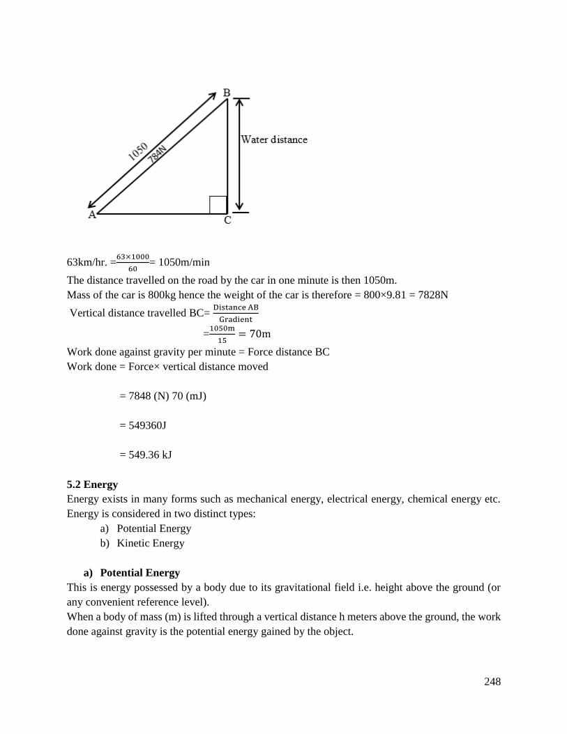
248
63km/hr. =63×1000
60= 1050m/min
The distance travelled on the road by the car in one minute is then 1050m.
Mass of the car is 800kg hence the weight of the car is therefore = 800×9.81 = 7828N
Vertical distance travelled BC= Distance AB
Gradient
=1050m
15= 70m
Work done against gravity per minute = Force distance BC
Work done = Force× vertical distance moved
= 7848 (N) 70 (mJ)
= 549360J
= 549.36 kJ
5.2 Energy
Energy exists in many forms such as mechanical energy, electrical energy, chemical energy etc.
Energy is considered in two distinct types:
a) Potential Energy
b) Kinetic Energy
a) Potential Energy
This is energy possessed by a body due to its gravitational field i.e. height above the ground (or
any convenient reference level).
When a body of mass (m) is lifted through a vertical distance h meters above the ground, the work
done against gravity is the potential energy gained by the object.

249
Work done = Force ×vertical distance
= mg× h
=mgh joules
Potential energy (PE) = mgh Joules
b) Kinetic Energy (KE)
This is the energy possessed by a body due to its velocity.
If a force F acts on a body of mass m kg initially at rest and eventually displaced at a distance S
then the work done = F×S
But F= Mass× acceleration
= ma
Work done = Force × distance
Therefore, work done = ma x d
From the third law of linear motion
v2 = u2 − 2as
s = (v2 − a2) ÷ 2a
Since u=0
S=v2/2a
Substituting for S in work done = ma × s
Work done= ma ×v2
2a
=mv2/2
=½mv2
Units of work done is NM or Joules (J)
Hence kinetic energy = ½mv2 joules
250
Example 3
A body of mass 5kg is supported above the ground. Determine the potential energy possessed by
the body due to its position with respect to the ground.
Solution
PE possessed by body =mgh
m= 5kg g= 9.81m/s2 h= 12m
PE= 5 ×9.81× 12
= 588.6 J
PE possessed by body= 588.6 J
Example 4
A motor vehicle of mass 2 tonnes is travelling at 50.4km/h. Determine the kinetic energy of the
vehicle at this speed.
Solution
KE of the vehicle= ½mv2
m= 2 tonnes= 2000kg
V= 50.4km/h =50.4×1000
60×60= 14m/s
KE= ½×2000×142 = 196000J
KE= 196kJ
Example 5
A vehicle of mass 1600kg increases its speed uniformly from 36km/h to 72km/h by the action of
a resistance force of 2.4 kN. Determine the increase in the kinetic energy of the vehicle during the
acceleration period show that this kinetic energy is equal to the work done by the accelerating
force.
Solution
Increase in KE=½ m (v2 − u2)
Where m= 1600kg u= 36km/h=10m/s v= 72km/h= 20m/s
Increase in KE= ½× 1600 (202 − 102
= 240,000 J= 240 kJ
Hence increase in KE is equal to the work done by the accelerating force.
Acceleration =F/m
m= 1600kg F= 2.4kN = 2400N

251
a= 2400kgm/s2
1600kg= 1.5m/s2
Distance covered S=(v2 −u2) ÷ 2a
=202-102 ( m2/s2) ÷ 2 × 1.5 (m/s2)= 100m
Work done = F × s
= 2400 (N) × 1OO (M) = 24000J
= Increase in KE
Increase in KE= 240kJ
Principle of conservation of energy
It states that energy can neither be created nor destroyed but can only be transformed from one
form to another. It is found that loss of energy in any form is always accompanied by an equivalent
increase in another form, in all such conversions, the total amount of energy remains constant. In
most cases, potential energy is converted to kinetic energy. In practical situations, friction is always
present and work has to be done in overcoming the friction resistance (thus amount of work done
is dissipated as heat) in such cases.
Final energy= Initial energy – work done against friction.
Consider a body of mass m kg raised to a height h meters above the ground. The potential energy
possessed by the body due to its position with respect to the ground is mgh Joules. If the body is
allowed to roll freely from that height until it is just about to strike the ground all its available
potential energy will be given up. Assuming no external work is done during the time of the roll
then, by the principle of conservation of energy, the body will gain kinetic energy equal in amount
to the initial potential energy.
KE on reaching the ground= Initial PE
½mv2=mgh
V=√2mgh
Example
An engine has a mass of 150kg and is suspended from a crane by a string 4m above ground level.
a) Determine the potential energy of the engine due to its position above the ground.
b) Due to a fault in the string, the engine falls freely to the ground from the height. Calculate
the velocity and the kinetic energy of the engine at the point of impact with the ground.
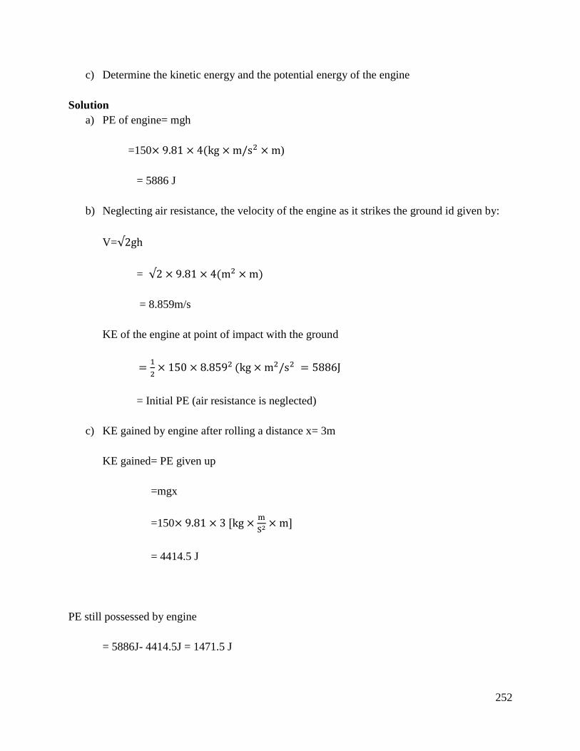
252
c) Determine the kinetic energy and the potential energy of the engine
Solution
a) PE of engine= mgh
=150× 9.81 × 4(kg × m/s2 × m)
= 5886 J
b) Neglecting air resistance, the velocity of the engine as it strikes the ground id given by:
V=√2gh
= √2 × 9.81 × 4(m2 × m)
= 8.859m/s
KE of the engine at point of impact with the ground
=1
2× 150 × 8.8592 (kg × m2/s2 = 5886J
= Initial PE (air resistance is neglected)
c) KE gained by engine after rolling a distance x= 3m
KE gained= PE given up
=mgx
=150× 9.81 × 3 [kg ×m
S2× m]
= 4414.5 J
PE still possessed by engine
= 5886J- 4414.5J = 1471.5 J
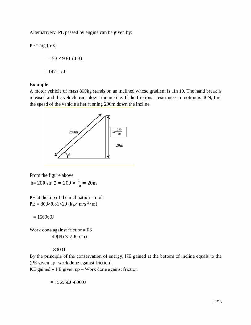
253
Alternatively, PE passed by engine can be given by:
PE= mg (h-x)
= 150 × 9.81 (4-3)
= 1471.5 J
Example
A motor vehicle of mass 800kg stands on an inclined whose gradient is 1in 10. The hand break is
released and the vehicle runs down the incline. If the frictional resistance to motion is 40N, find
the speed of the vehicle after running 200m down the incline.
From the figure above
h= 200 sin ∅ = 200 ×1
10= 20m
PE at the top of the inclination = mgh
PE = 800×9.81×20 (kg× m/s 2×m)
= 156960J
Work done against friction= FS
=40(N) × 200 (m)
= 8000J
By the principle of the conservation of energy, KE gained at the bottom of incline equals to the
(PE given up- work done against friction).
KE gained = PE given up – Work done against friction
= 156960J -8000J

254
=148960J
But KE=½mv2
148960= ½×800×v2
V=√148960×2
800= 19.3m/s
V= 19.3m/s
5.3 Power calculations are performed
Power is the rate of transfer of energy. If the energy transfer is in the form of mechanical work,
then;
Power = Workdone
Time taken
= Force×distance moved
Time taken
But Ditance moved
Time taken is velocity of the body
Power= Force ×Velocity
Power = FV
Power is given in watt (W) or J/s
Example
If an engine drives a car against a total resistance of 1.2kN over a distance of 250 m in 30 sec,
what power is being developed by the crank shaft?
Solution
If the vehicle is to overcome a resistance of 1.2kN, the engine must provide a force 1.2kN at the
crank shaft.
Power developed at crank shaft
= Force × Ditance moved
Time taken

255
= 1200×250(NM)
30(S)= 10,000W = 10kw
Power developed by the crank shaft = 10Kw
Example
A vehicle hauls a trailer at 72km/hr when exerting a steady pull of 800N at the tow- rope.
Calculate the power required.
Power required= Force × velocity
= F × V
F= 800 N and V=72km/h= 20m/s
Power required = 800 (N) × 20(m/s) = 16000W
= 16kW
Conclusion
The learning outcome covered or equipped the learner with knowledge and skills on the concept
of work, energy and power. A student having gone through this outcome will be able to solve
various calculations involved in power, work and energy. The learning outcome also covers the
various applications of work, power and energy through thorough examples. A student will thus
be able to solve real life problems which deal with work, energy and power.
Further Reading
1. Engineering science for Technicians
2. Mechanical Engineering Principles by John Bird and Earl Ross.
4.3.6.3 Self-Assessment
Written Assessment
1. A load is moved 15m along a workshop pathway by a force of 6.5 kN. Calculate the work
done.
256
a) 97.5kJ
b) 70.5kJ
c) 100kJ
d) 71.5kJ
2. A force of 250N is applied to a body, if the work done is 16 kJ, determine the distance
through which the body is moved in the direction of the force.
a) 2.4 m
b) 21.5m
c) 0.24m
d) 24m
3. A piston moved at a uniform velocity of 7m/s against a resistance of 250N. Find power
developed.
a) 7.5kW
b) 1.75kW
c) 5.7kW
d) 17.5kW
4. A vehicle of mass 4 tones is raised by a hydraulic heist through a distance of 2.25m in 36
seconds. Calculate the power required to perform this task.
a) 4.5 kW
b) 2.45 kW
c) 2 kW
d) 8 kW
5. Determine the power of a pump used to raise 75 litres of water to a height of 16m in 24
seconds. What is the potential energy of the water in the final position? (I litre of water has
a mass of 1kg).
a) 460W
b) 49W
c) 470W
d) 490.5W
6. A body of mass 1kg falls from rest through a vertical distance of 6m when its velocity is
decreased to 6m/s by imparting energy to a machine. Calculate the amount of energy given
to the machine.
a) 400J
b) 408.6J
c) 360J
d) 41kJ
7. The velocity of a body of mass 16kg is increased from 5m/s to 20m/s in 12 sec.
Calculate the power required to produce the change in Kinetic energy of the body.
a) 0.25W
b) 250W
257
c) 2400W
d) 3000W
8. Exaplain the term work and state the SI unit
9. List four forms of energy
10. State the difference between PE and KE
11. State the principle of conservation of energy
12. State down the formula for calculating
a) Kinetic energy
b) Potential energy
Oral Assessment
1. Discuss the principle of conservation of energy
2. Discuss power as a rate of transfer of energy using examples.
Practical Assessment
1. Using the following tools, explain the principle of conservation of energy from
mechanical to heat energy.
Tools
i. Load of mass 5kg
ii. A rough table top
i.e. use friction as the main objective
Project
Elaborate how PE of a body is the energy it possesses due to its position regardless of
gravitational field.
4.3.6.4 Tools, Equipment, Supplies and Materials
Scientific Calculators
Relevant reference materials
Stationeries
Electrical workshop
Relevant practical materials
Dice
Computers with internet connection
4.3.6.5 References
Duit. Reinders “Learning the Energy Concept in School Empirical Results from the Philippines
and West Germany. Physics education.19 (2), 59.

258
Goldring H. O. Osborne. J. (1994). Student’s difficulties with Energy and Related Concepts.
Physics education. 29(1), 26.
Perkovic, L., Silva P., Ban. M, Kranjecevic. O. Duic.N (2013). Harvesting high altitude wind
energy for Power Production. The concept based on Magnus. Effect. Applied Energy.
101,151-160.

259
4.3.7 Learning Outcome No 6: Perform machine calculation
4.3.7.1 Learning Activities
Learning Outcome No 6: Perform machine calculation
Learning Activities Special Instructions
6.1 Solve problems on simple machines (machine
advantages, velocity ratio and efficiency)
6.2 Solve problems on levers
6.3 Identify laws of machines
Illustrate the uses of lever and
problems experienced in lever use.
In groups, identify the laws of simple
machines and how they are applied in
mechanics.
4.3.7.2 Information Sheet No4/LO6: Perform machine calculation
Introduction
This learning outcome covers problems on simple machines. It highlights mechanical advantages,
velocity ration and efficiency. A machine is a device that can change the magnitude or line of
action or both magnitude and line of action of a force. A simple machine usually amplifies an input
force called effort to give a larger output force called load. Some typical examples of simple
machines include pulley system, screw jack, gear systems and lever system. It also covers lever
problems. It then highlights the laws of machines and how they are applied in mechanics.
Definition of key terms
Force ratio: Also known as mechanical advantage. It is the ratio of load to the effort.
Movement ratio/velocity ratio: It is the ratio of the distance moved by effort to distance moved
by load in the same time.
Efficiency of the machine: It’s the ratio of the ratio of the work output to work input into the
machine.
Limiting efficiency of machine: The ratio of the limiting force ratio to the movement ratio.
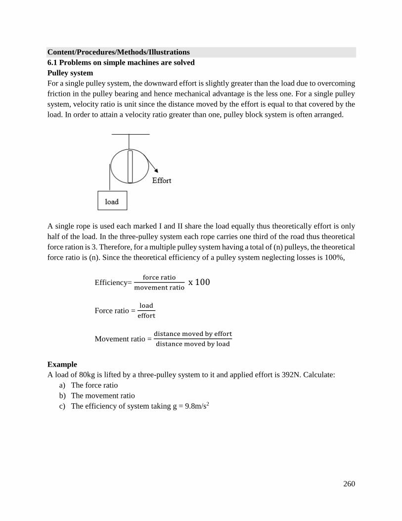
260
Content/Procedures/Methods/Illustrations
6.1 Problems on simple machines are solved
Pulley system
For a single pulley system, the downward effort is slightly greater than the load due to overcoming
friction in the pulley bearing and hence mechanical advantage is the less one. For a single pulley
system, velocity ratio is unit since the distance moved by the effort is equal to that covered by the
load. In order to attain a velocity ratio greater than one, pulley block system is often arranged.
A single rope is used each marked I and II share the load equally thus theoretically effort is only
half of the load. In the three-pulley system each rope carries one third of the road thus theoretical
force ration is 3. Therefore, for a multiple pulley system having a total of (n) pulleys, the theoretical
force ratio is (n). Since the theoretical efficiency of a pulley system neglecting losses is 100%,
Efficiency= force ratio
movement ratio x 100
Force ratio = load
effort
Movement ratio = distance moved by effort
distance moved by load
Example
A load of 80kg is lifted by a three-pulley system to it and applied effort is 392N. Calculate:
a) The force ratio
b) The movement ratio
c) The efficiency of system taking g = 9.8m/s2
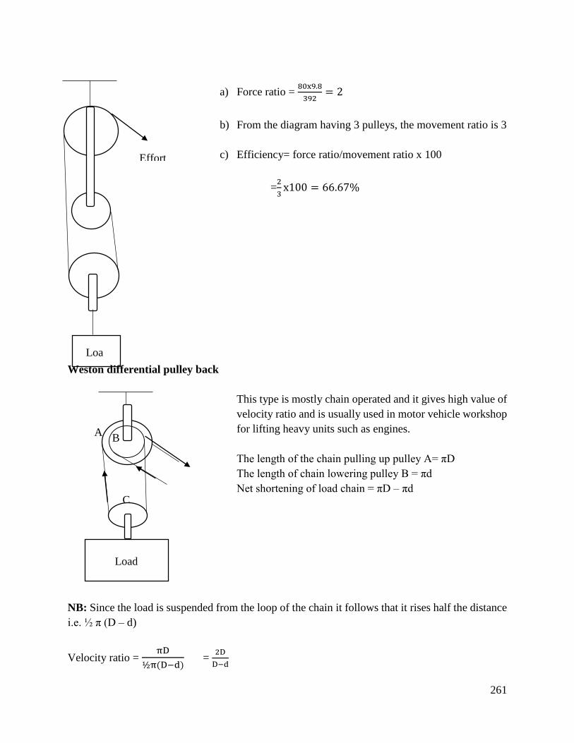
261
a) Force ratio = 80x9.8
392= 2
b) From the diagram having 3 pulleys, the movement ratio is 3
c) Efficiency= force ratio/movement ratio x 100
=2
3x100 = 66.67%
Weston differential pulley back
This type is mostly chain operated and it gives high value of
velocity ratio and is usually used in motor vehicle workshop
for lifting heavy units such as engines.
The length of the chain pulling up pulley A= πD
The length of chain lowering pulley B = πd
Net shortening of load chain = πD – πd
NB: Since the load is suspended from the loop of the chain it follows that it rises half the distance
i.e. ½ π (D – d)
Velocity ratio = πD
½π(D−d) =
2D
D−d
Loa
d
Effort
A
C
B
Load
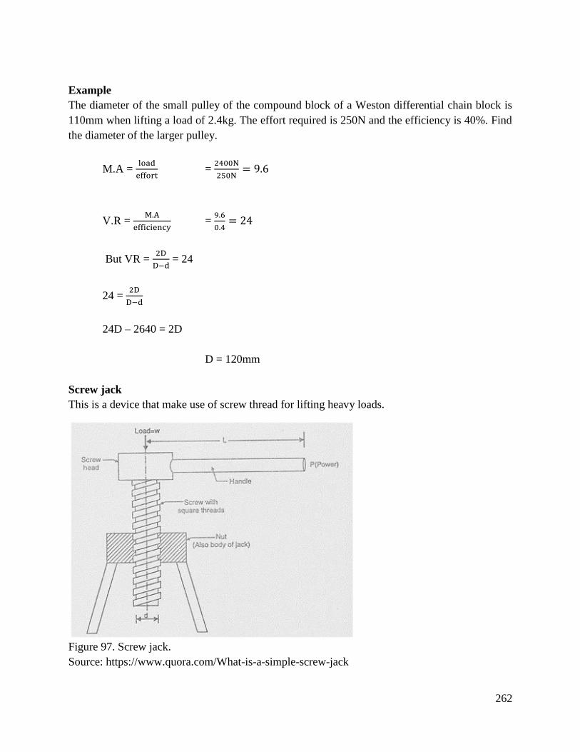
262
Example
The diameter of the small pulley of the compound block of a Weston differential chain block is
110mm when lifting a load of 2.4kg. The effort required is 250N and the efficiency is 40%. Find
the diameter of the larger pulley.
M.A = load
effort =
2400N
250N= 9.6
V.R = M.A
efficiency =
9.6
0.4= 24
But VR = 2D
D−d = 24
24 = 2D
D−d
24D – 2640 = 2D
D = 120mm
Screw jack
This is a device that make use of screw thread for lifting heavy loads.
Figure 97. Screw jack.
Source: https://www.quora.com/What-is-a-simple-screw-jack
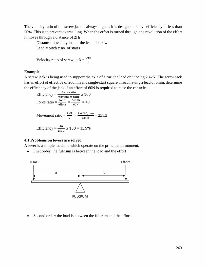
263
The velocity ratio of the screw jack is always high as it is designed to have efficiency of less than
50%. This is to prevent overhauling. When the effort is turned through one revolution of the effort
it moves through a distance of 2Πr
Distance moved by load = the lead of screw
Lead = pitch x no. of starts
Velocity ratio of screw jack = 2πR
L
Example
A screw jack is being used to support the axle of a car, the load on it being 2.4kN. The screw jack
has an effort of effective of 200mm and single-start square thread having a lead of 5mm. determine
the efficiency of the jack if an effort of 60N is required to raise the car axle.
Efficiency = force ratio
movement ratio x 100
Force ratio = load
effort =
2400N
60N = 40
Movement ratio = 2πR
L =
2π(200)mm
5mm = 251.3
Efficiency = 40
251.3 x 100 = 15.9%
4.1 Problems on levers are solved
A lever is a simple machine which operate on the principal of moment.
First order: the fulcrum is between the load and the effort
Second order: the load is between the fulcrum and the effort
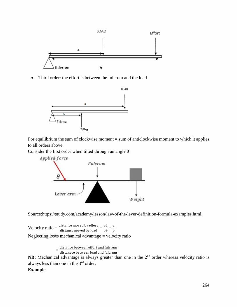
264
Third order: the effort is between the fulcrum and the load
For equilibrium the sum of clockwise moment = sum of anticlockwise moment to which it applies
to all orders above.
Consider the first order when tilted through an angle θ
Source:https://study.com/academy/lesson/law-of-the-lever-definition-formula-examples.html.
Velocity ratio = distance moved by effort
distance moved by load =
aθ
bθ =
a
b
Neglecting loses mechanical advantage = velocity ratio
= distance between effort and fulcrum
distancce between load and fulcrum
NB: Mechanical advantage is always greater than one in the 2nd order whereas velocity ratio is
always less than one in the 3rd order.
Example
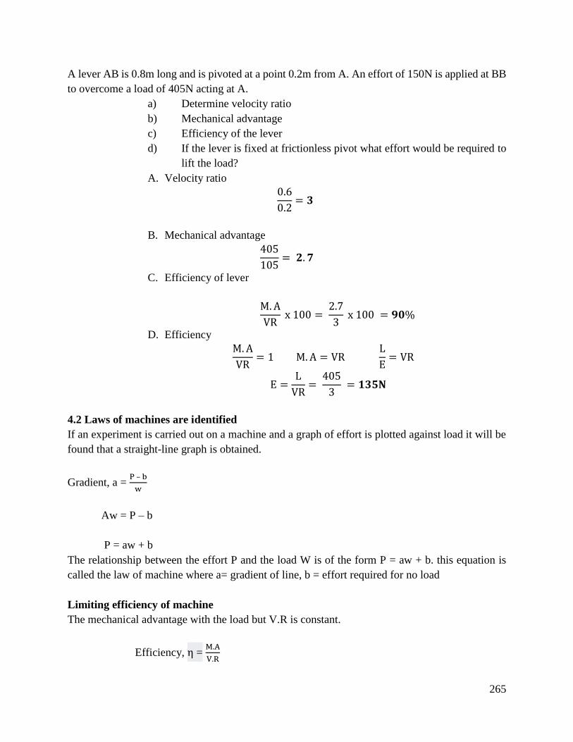
265
A lever AB is 0.8m long and is pivoted at a point 0.2m from A. An effort of 150N is applied at BB
to overcome a load of 405N acting at A.
a) Determine velocity ratio
b) Mechanical advantage
c) Efficiency of the lever
d) If the lever is fixed at frictionless pivot what effort would be required to
lift the load?
A. Velocity ratio
0.6
0.2= 𝟑
B. Mechanical advantage
405
105= 𝟐. 𝟕
C. Efficiency of lever
M.A
VR x 100 =
2.7
3 x 100 = 𝟗𝟎%
D. Efficiency
M.A
VR= 1 M. A = VR
L
E= VR
E =L
VR=
405
3 = 𝟏𝟑𝟓𝐍
4.2 Laws of machines are identified
If an experiment is carried out on a machine and a graph of effort is plotted against load it will be
found that a straight-line graph is obtained.
Gradient, a = P – b
w
Aw = P – b
P = aw + b
The relationship between the effort P and the load W is of the form P = aw + b. this equation is
called the law of machine where a= gradient of line, b = effort required for no load
Limiting efficiency of machine
The mechanical advantage with the load but V.R is constant.
Efficiency, η = M.A
V.R
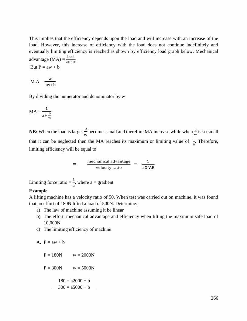
266
This implies that the efficiency depends upon the load and will increase with an increase of the
load. However, this increase of efficiency with the load does not continue indefinitely and
eventually limiting efficiency is reached as shown by efficiency load graph below. Mechanical
advantage (MA) = load
effort
But P = aw + b
M.A = w
aw+b
By dividing the numerator and denominator by w
MA = 1
a+ b
w
NB: When the load is large, b
w becomes small and therefore MA increase while when
b
w is so small
that it can be neglected then the MA reaches its maximum or limiting value of 1
a. Therefore,
limiting efficiency will be equal to
= mechanical advantage
velocity ratio =
1
a X V.R
Limiting force ratio = 1
a, where a = gradient
Example
A lifting machine has a velocity ratio of 50. When test was carried out on machine, it was found
that an effort of 180N lifted a load of 500N. Determine:
a) The law of machine assuming it be linear
b) The effort, mechanical advantage and efficiency when lifting the maximum safe load of
10,000N
c) The limiting efficiency of machine
A. P = aw + b
P = 180N w = 2000N
P = 300N w = 5000N
180 = a2000 + b
300 = a5000 + b
267
-120 = -a3000 a = 0.04
-3000 -3000
180 = 2000 x 0.04 + b
b = 100
The law of machine P = 0.04w + 100
B.
a. Effort, velocity ratio = distance of effort
distance of load
P = aw + b
P = 0.04 (10,000) + 100
P = 500N
b. Mechanical advantage
10000
500= 𝟐𝟎
c. Efficiency = MA
VR x 100 =
20
50 x 100 = 𝟒𝟎
C. Limiting efficiency
1
a x VR=
1
0.04 x 50 x 100 =
1
2 x 100 = 𝟓𝟎%
Conclusion
In conclusion, simple machine were applied where heavy objects or machineries such as engine
blocks were required to be lifted without causing any accidents. Simple machine problems were
solved.
Further Reading
1. Simple Machines. Jenniffer Lawson (2001). Portage and Main Press.
2. Simple Machines. Deborah Hodge, Adreinne Mason, Ontario Science Centre (1998).
268
4.3.7.3 Self-Assessment
Written Assessment
1. Which of the following statement is false?
a) In first order lever, the fulcrum is between the load and effort
b) In the second order lever, the effort is applied between the load and fulcrum
c) In 3rd order lever, the effort is applied between the load and fulcrum
d) The force ratio for a 1st order lever is given by:
i. distance of load from fulcrum
distance of effort from fulcrum
2. Which of the following statement concerning screw jack is false?
a. A screw jack changes both the line of action and magnitude of force
b. For a single start thread, the distance moved in 5 revolutions of the table is 5L where
L is lead of the screw.
c. The distance moved by effort is 2πr where r is effective radius of effort
d. The movement ratio is given by 2πr
5L
3. In second order lever system, the load is 200nm, from the fulcrum and the effort is 500mm
from fulcrum. If losses are neglected, an effort of 100N will rise a load of?
a. 100N
b. 250N
c. 400N
d. 40N
4. A hand operated lifting machine in a repair shop raises an engine of mass 260kg by means
of an effort of 210N at the handle. If the effort moves through a distance of 13.5m in raising
the engine 450mm:
i. The force ratio
a) 12.15
b) 10.2
c) 12.5
d) 13.10
ii. The movement ratio
a) 300
b) 200
c) 30
d) 40
iii. The efficiency of the machine
a) 4.5%
b) 40.5%
269
c) 20%
d) 25%
5. A load of 1.26kN is lifted by means of pulley block system consisting of 3pulleys in the
upper block and 2 pulleys in the lower block. If the efficiency of the system is 84%
determine:
i. The velocity ratio
a) 2
b) 3
c) 5
d) 7
ii. Mechanical advantage
a) 4.2
b) 4
c) 3.6
d) 7.6
iii. Effort required to lift the load
a) 300N
b) 200N
c) 400N
d) 800N
6. The diameter of small pulleys of a compound block of a Weston differential chain block is
110mm. When lifting a load of 2.4kN the effort required is 250N and the efficiency is 40%.
Find the diameter of the large pulley
a) 60mm
b) 120mm
c) 40mm
d) 100mm
7. A screw jack has two start of pitch 5mm. An effort of 40N is applied tangentially to the
tommy bar, at a radius of 350mm to lift a load of 2200N, calculate:
i. Efficiency of screw jack
a) 20%
b) 25%
c) 30%
d) 35%
ii. Work done in overcoming friction when the load is raised a distance of
75mm
a) 500J
b) 495J
c) 500kJ
d) 200J
270
8. State the formulae of the force ratio of simple machine
9. State the formulae of movement ratio of simple machine
10. Explain what is meant by the efficiency of machine
11. Give the reasons why efficiency of machine can never be 100%
12. What is the relationship between mechanical advantage and velocity ratio and efficiency?
Oral Assessment
1. State the first order of lever.
2. State what is meant by simple machine.
Practical Assessment
1. A screw jack has a thread of 6mm pitch. An effort of 80N applied at a radius of 420mm is
just sufficient to move a load of 8.8kN. Calculate:
a) The efficiency of the screw jack
b) The work done on the load to raise it by 50mm
c) The work done in overcoming friction when raising the load by 50mm
2. A pulley system consists of two blocks, each containing three pulleys and connected as
shown below. An effort of 400N is required to raise a load of 1500N, determine:
a) The force ratio
b) The movement ratio
c) The efficiency of the pulley
4.3.7.4 Tools, Equipment, Supplies and Materials
Scientific Calculators
Relevant reference materials
Stationeries
Electrical workshop
Relevant practical materials
Dice
Computers with internet connection
4.3.7.5 References
Design of Machine Elements. V.B. Bhandari. (2010). Tata.
Levers. Anne Welsbacher (2002). Capstone.
McGraw-Hill Education.
Mechanical engineering principles by John Bird and Carl Ross (2002)
4.3.8 Learning Outcome No7: Demonstrate gas principles
4.3.8.1 Learning Activities
271
Learning Outcome No7: Demonstrate gas principles
Learning Activities Special Instructions
7.1 Identify gas laws (Boyles law, Charles law and gas
equation)
7.2 Apply gas laws in solving engineering problems
7.3 Identify uses of gases in engineering systems
State different gas laws and
derive the equations
Apply these gas laws in different
mathematical problems using
their gas equations
4.3.8.2 Information Sheet No4/LO7: Demonstrate gas principles
Introduction
This learning outcome covers the relationship that exists between pressure, volume and
temperature in a gas are given in a set of law called gas law.
Definition of key terms
Boyle’s law: It states that the volume of a fixed mass of a gas is inversely proportional to its
absolute pressure (P) at constant temperature.
Charles’ law: It states that for a given mass of gas at constant pressure, the volume (V) is the
thermodynamic temperature (T).
The pressure law: It states that the pressure (P) of a fixed mass of a gas is directly proportional
to its thermodynamic temperature (T) at constant volume.
Dalton’s law of partial pressure: It states that the total pressure of a mixture of gases occupying
a given volume is equal to the sum of the pressure of each gas considered separately at constant
temperature.
Content/Procedures/Methods/Illustrations
7.1 Gas laws are identified
Generally, gases have properties substantially different than solids or liquids. Gases do not have
fixed volumes; instead their volume depend directly upon pressure and temperature. Gases don’t
have a fixed shape but are said to “take the shape of the container”. Gases have a fixed mass
although measuring the mass may be difficult sometimes.
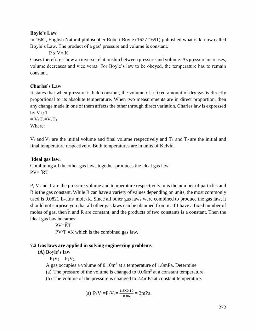
272
Boyle’s Law
In 1662, English Natural philosopher Robert Boyle (1627-1691) published what is k=now called
Boyle’s Law. The product of a gas’ pressure and volume is constant.
P x V= K
Gases therefore, show an inverse relationship between pressure and volume. As pressure increases,
volume decreases and vice versa. For Boyle’s law to be obeyed, the temperature has to remain
constant.
Charles’s Law
It states that when pressure is held constant, the volume of a fixed amount of dry gas is directly
proportional to its absolute temperature. When two measurements are in direct proportion, then
any change made in one of them affects the other through direct variation. Charles law is expressed
by V α T
= V1T2=V2T1
Where:
V1 and V2 are the initial volume and final volume respectively and T1 and T2 are the initial and
final temperature respectively. Both temperatures are in units of Kelvin.
Ideal gas law.
Combining all the other gas laws together produces the ideal gas law:
PV= RT
P, V and T are the pressure volume and temperature respectively. n is the number of particles and
R is the gas constant. While R can have a variety of values depending on units, the most commonly
used is 0.0821 L-atm/ mole-K. Since all other gas laws were combined to produce the gas law, it
should not surprise you that all other gas laws can be obtained from it. If I have a fixed number of
moles of gas, then n and R are constant, and the products of two constants is a constant. Then the
ideal gas law becomes:
PV=KT
PV/T =K which is the combined gas law.
7.2 Gas laws are applied in solving engineering problems
(A) Boyle’s law
P1V1 = P2V2
A gas occupies a volume of 0.10m3 at a temperature of 1.8mPa. Determine
(a) The pressure of the volume is changed to 0.06m3 at a constant temperature.
(b) The volume of the pressure is changed to 2.4mPa at constant temperature.
(a) P1V1=P2V2= 1.8X0.10
0.06 = 3mPa.
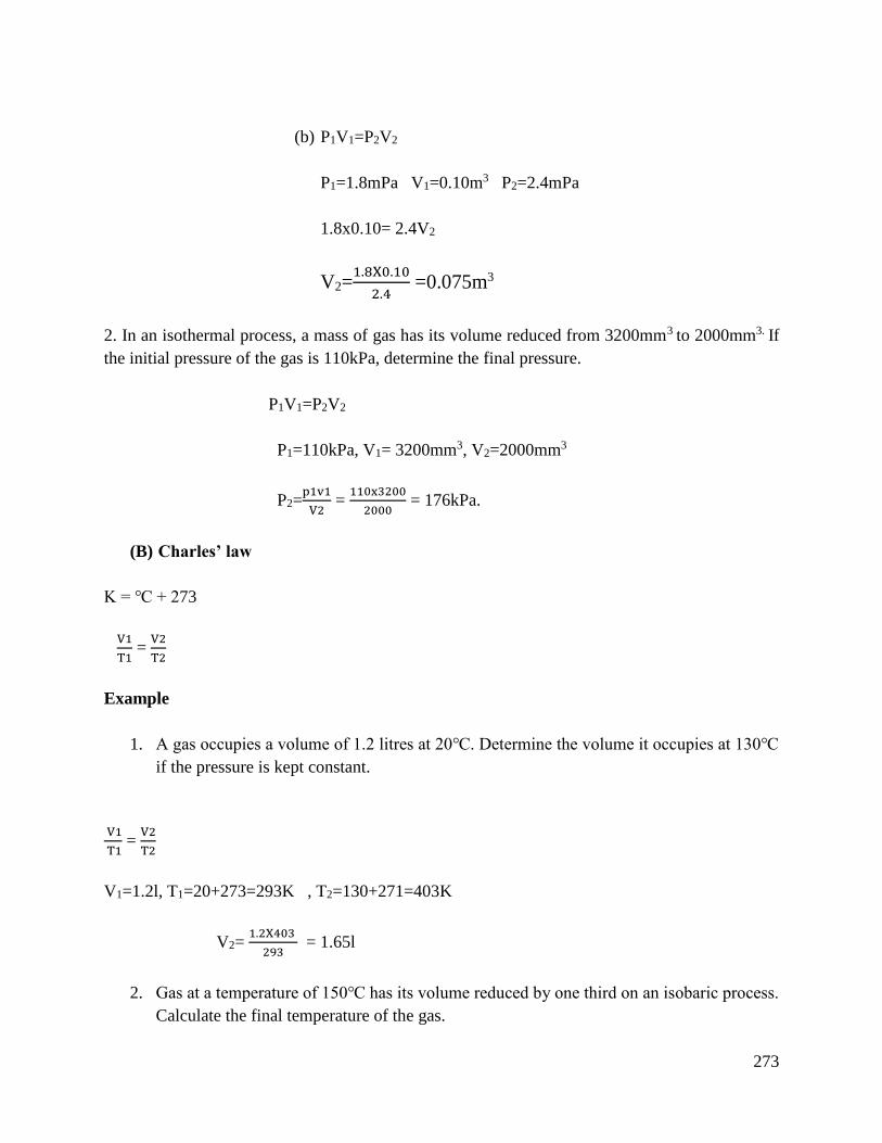
273
(b) P1V1=P2V2
P1=1.8mPa V1=0.10m3 P2=2.4mPa
1.8x0.10= 2.4V2
V2=1.8X0.10
2.4 =0.075m3
2. In an isothermal process, a mass of gas has its volume reduced from 3200mm3 to 2000mm3. If
the initial pressure of the gas is 110kPa, determine the final pressure.
P1V1=P2V2
P1=110kPa, V1= 3200mm3, V2=2000mm3
P2=p1v1
V2 =
110x3200
2000 = 176kPa.
(B) Charles’ law
K = + 273
V1
T1 =
V2
T2
Example
1. A gas occupies a volume of 1.2 litres at 20. Determine the volume it occupies at 130
if the pressure is kept constant.
V1
T1 =
V2
T2
V1=1.2l, T1=20+273=293K , T2=130+271=403K
V2= 1.2X403
293 = 1.65l
2. Gas at a temperature of 150 has its volume reduced by one third on an isobaric process.
Calculate the final temperature of the gas.
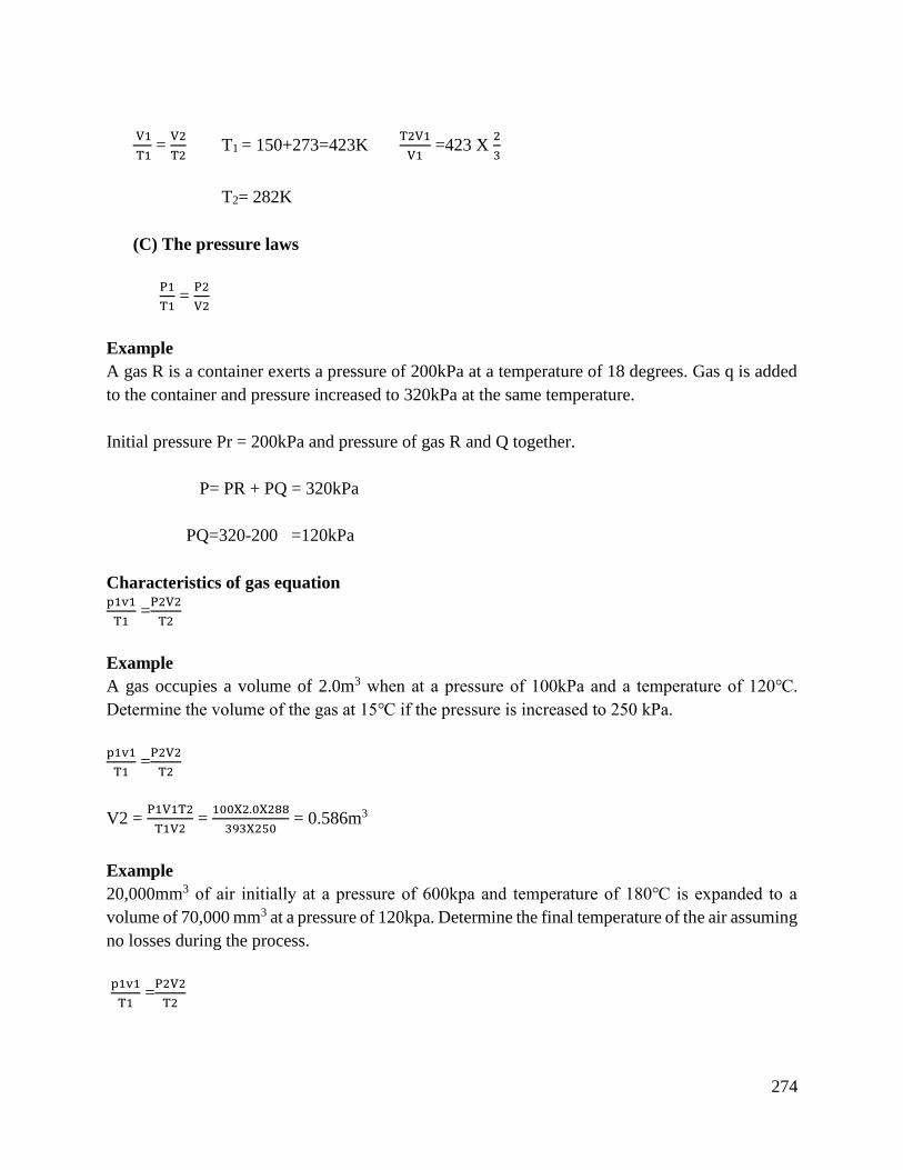
274
V1
T1 =
V2
T2 T1 = 150+273=423K
T2V1
V1 =423 X
2
3
T2= 282K
(C) The pressure laws
P1
T1 =
P2
V2
Example
A gas R is a container exerts a pressure of 200kPa at a temperature of 18 degrees. Gas q is added
to the container and pressure increased to 320kPa at the same temperature.
Initial pressure Pr = 200kPa and pressure of gas R and Q together.
P= PR + PQ = 320kPa
PQ=320-200 =120kPa
Characteristics of gas equation p1v1
T1 =
P2V2
T2
Example
A gas occupies a volume of 2.0m3 when at a pressure of 100kPa and a temperature of 120.
Determine the volume of the gas at 15 if the pressure is increased to 250 kPa.
p1v1
T1 =
P2V2
T2
V2 = P1V1T2
T1V2 =
100X2.0X288
393X250 = 0.586m3
Example
20,000mm3 of air initially at a pressure of 600kpa and temperature of 180 is expanded to a
volume of 70,000 mm3 at a pressure of 120kpa. Determine the final temperature of the air assuming
no losses during the process.
p1v1
T1 =
P2V2
T2
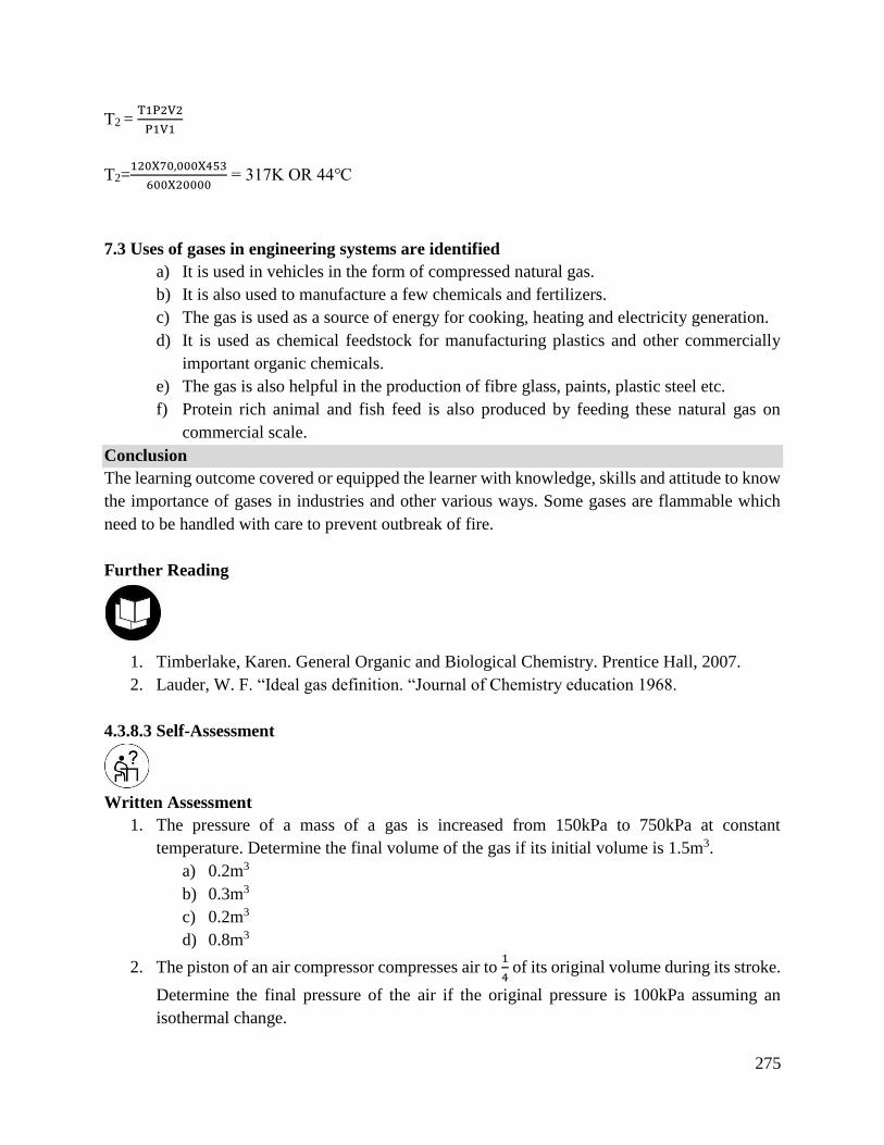
275
T2 = T1P2V2
P1V1
T2=120X70,000X453
600X20000 = 317K OR 44
7.3 Uses of gases in engineering systems are identified
a) It is used in vehicles in the form of compressed natural gas.
b) It is also used to manufacture a few chemicals and fertilizers.
c) The gas is used as a source of energy for cooking, heating and electricity generation.
d) It is used as chemical feedstock for manufacturing plastics and other commercially
important organic chemicals.
e) The gas is also helpful in the production of fibre glass, paints, plastic steel etc.
f) Protein rich animal and fish feed is also produced by feeding these natural gas on
commercial scale.
Conclusion
The learning outcome covered or equipped the learner with knowledge, skills and attitude to know
the importance of gases in industries and other various ways. Some gases are flammable which
need to be handled with care to prevent outbreak of fire.
Further Reading
1. Timberlake, Karen. General Organic and Biological Chemistry. Prentice Hall, 2007.
2. Lauder, W. F. “Ideal gas definition. “Journal of Chemistry education 1968.
4.3.8.3 Self-Assessment
Written Assessment
1. The pressure of a mass of a gas is increased from 150kPa to 750kPa at constant
temperature. Determine the final volume of the gas if its initial volume is 1.5m3.
a) 0.2m3
b) 0.3m3
c) 0.2m3
d) 0.8m3
2. The piston of an air compressor compresses air to 1
4 of its original volume during its stroke.
Determine the final pressure of the air if the original pressure is 100kPa assuming an
isothermal change.
276
a) 400kpa
b) 200kpa
c) 2.01m3
d) 4.04m3
3. Some gas initially at 16 is heated to 9 at constant pressure. If the initial volume of gas
is 0.8m3, determine the final volume of the gas.
a) 102m3
b) 1.02m3
c) 2.01m3
d) 4.04m3
4. In an isobaric process gas at a temperature of 120 has its volume reduced by a sixth.
Determine the final temperature of the gas?
a) 50
b) 300K
c) 54.5
d) 60
5. A gas initially at a temperature of 27 and pressure 100kPa is heated at constant volume
until its temperature is 150. Assuming no loss of gas, determine the final pressure of the
gas.
a) 141kPa
b) 200kPa
c) 300kPa
d) 1.62kPa
6. A gas A in a container exerts a pressure of 120kpa at a temperature of 20. Gas B is added
to the container and the pressure increases to 300kPa at the same temperature.
a) 120kPa
b) 160kPa
c) 180kPa
d) 200kPa.
7. Given a mass of air occupies a volume of 0.5m3 at a pressure of 50kpa and a temperature
of 20. Find the volume of air at STP.
a) 2.24m3
b) 2.30m3
c) 4.20m3
d) 3.4m3
8. State the pressure law, Charles’ law and Boyle’s law.
9. Derive the equation for Charles law.
10. Distinguish the difference between Boyle’s law and Charles’ law.
11. State Dalton’s law of partial pressure.
12. What is the meaning of an ideal gas?
277
Oral Assessment
1. State four uses of gas.
2. State the characteristics of gas equation.
Practical Assessment
1. A mass of gas occupies a volume of 0.02m3 when the pressure is 150kPa and its
temperature is 17. If the gas is compressed until its pressure is 500kPa and its
temperature is 57, determine;
a) The volume it will occupy.
b) Its mass if the characteristic gas constant for the gas is 205 J/kgW
2. Discuss how piston air type compressor compresses gas.
3. A vessel with an internal volume of 10.0l contains 2.80g of nitrogen gas, 0.404g if
hydrogen gas and 79.9g of argon gas. At 25, what is the pressure (in atm) inside the
vessel?
Project
1. Discuss how piston air type compressor compresses gas
4.3.8.4 Tools, Equipment, Supplies and Materials
Scientific Calculators
Computers with internet connection
4.3.8.5 References
Bird, J., & Ross, C. (2014). Mechanical engineering principles. Routledge.
Levine, S. (1985). Derivation of the ideal gas law. Journal of Chemical Education, 62(5), 399.
Luder, W. F. (1968). Ideal gas definition. Journal of Chemical Education, 45(5), 351.
Zammit, S. J. (1987). Motor Vehicle Engineering Science for Technicians, Level 2. Longman
Scientific & Technical.
278
4.3.9 Learning Outcome No 8: Apply heat knowledge
4.3.9.1 Learning Activities
Learning Outcome No 8: Apply heat knowledge
Learning Activities Special Instructions
8.1 Discuss heat concepts
8.2 Define working principle of heat
8.3 Discuss heat capacity
8.4 Solve heat problems
In groups discuss the heat concepts.
Make presentations on the working
principles of heat.
4.3.9.2 Information Sheet No4/LO 8: Apply heat knowledge
Introduction
This learning outcome covers heat transfer, quantity of heat, specific heat capacity and latent heat.
Definition of key terms
Heat: This is the transfer of energy from a hot body to a cooler body in the following ways:
i. Conduction
ii. Convection
iii. Radiation
Quantity of heat: This is the amount of heat required to raise the temperature of a given mass of
water by 10C.
Specific heat capacity: The quantity of heat required to raise the temperature of 1kg of the
substance by 1OC.
Content/Procedures/Methods/Illustrations
8.1 Heat concepts are discussed
Experiments have shown that work done in overcoming friction is converted into heat.
There are actions that have the same principle e.g. applying the brake on a motor vehicle, striking
a match etc. In this case, mechanical energy is converted into thermal energy and this produces an
increase on temperature. To appreciate thermal energy, we must consider the molecular structure
of matter. All substances are made of molecules e.g. hydrogen has molecule of element. Water has
molecule of compound. In a solid, molecules are arranged in an orderly manner. Their mean
position to one another is fixed, but they oscillate about their mean position at a speed that increases
with increase in temperature. Hence molecules of solid possess kinetic energy owing to vibrate
about their mean positions. In a liquid, the molecules are able to move about a random. In a gas,
279
the number of molecules in a given space is far less than in liquid. The higher the temperature of
a liquid or gas the faster the speed of movements of molecule.
For a substance to gain heat, the following aspects must be accompanied:
a) Temperature increase on the material
b) An increase in the volume of the material
Heat may change the state of the material, example
i. Ice may be melted
ii. Liquid may be vaporized
8.2 Working principle of heat is defined
Principle of heat may be elaborated as heat transfer from one substance to another.
Transfer of heat
Heat is a transfer of energy from a low temperature substance to a higher temperature substance
Heat is transferred in the following ways;
i. By conduction
ii. By convection
iii. By radiation
Conduction: This is the thermal conductivity that takes place on bodies that are actually in contact
and if they are at different temperatures.
Convection: This is the conveyance of heat by the actual movement of hot fluid which must be
liquid or gas.
Radiation: This is the transmission of heat by wave or by vibrating motion in the space between
the source and the body on which the wave impinges. The nature of heat wave is similar to that of
light wave and of radio waves but the only difference is the frequency of the wave. Thermal
radiation is transmitted through a vacuum i.e. transfer of heat energy by radiation is not dependent
upon a material medium. Example, in the case of thermal radiation. Thermal energy from the sun
reaches earth atmosphere by radiation through a vacuum. Heat transfer is due to change in
temperature.
Temperature
Temperature of a body relates to its degree of hotness or coldness and is independent of the size
and physical nature of the body. An instrument used to measure temperature is called a
thermometer. There are various thermometers but mercury thermometer is the most commonly
used for measuring temperature ranging between freezing and boiling point of water.
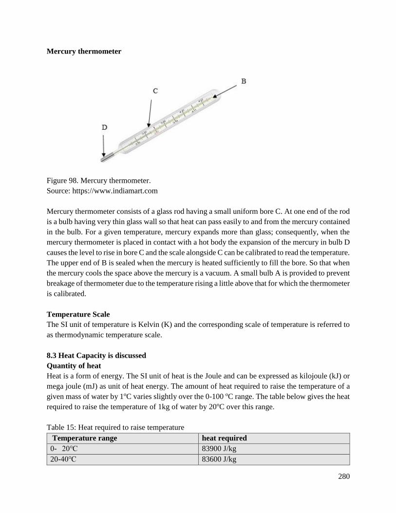
280
Mercury thermometer
Figure 98. Mercury thermometer.
Source: https://www.indiamart.com
Mercury thermometer consists of a glass rod having a small uniform bore C. At one end of the rod
is a bulb having very thin glass wall so that heat can pass easily to and from the mercury contained
in the bulb. For a given temperature, mercury expands more than glass; consequently, when the
mercury thermometer is placed in contact with a hot body the expansion of the mercury in bulb D
causes the level to rise in bore C and the scale alongside C can be calibrated to read the temperature.
The upper end of B is sealed when the mercury is heated sufficiently to fill the bore. So that when
the mercury cools the space above the mercury is a vacuum. A small bulb A is provided to prevent
breakage of thermometer due to the temperature rising a little above that for which the thermometer
is calibrated.
Temperature Scale
The SI unit of temperature is Kelvin (K) and the corresponding scale of temperature is referred to
as thermodynamic temperature scale.
8.3 Heat Capacity is discussed
Quantity of heat
Heat is a form of energy. The SI unit of heat is the Joule and can be expressed as kilojoule (kJ) or
mega joule (mJ) as unit of heat energy. The amount of heat required to raise the temperature of a
given mass of water by 1oC varies slightly over the 0-100 oC range. The table below gives the heat
required to raise the temperature of 1kg of water by 20oC over this range.
Table 15: Heat required to raise temperature
Temperature range heat required
0- 20 83900 J/kg
20-40 83600 J/kg
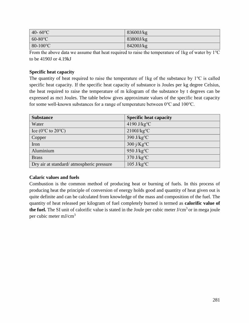
281
40- 60 83600J/kg
60-80 83800J/kg
80-100 84200J/kg
From the above data we assume that heat required to raise the temperature of 1kg of water by 1
to be 4190J or 4.19kJ
Specific heat capacity
The quantity of heat required to raise the temperature of 1kg of the substance by 1 is called
specific heat capacity. If the specific heat capacity of substance is Joules per kg degree Celsius,
the heat required to raise the temperature of m kilogram of the substance by t degrees can be
expressed as mct Joules. The table below gives approximate values of the specific heat capacity
for some well-known substances for a range of temperature between 0 and 100.
Substance Specific heat capacity
Water 4190 J/kg
Ice (0 to 20) 2100J/kg
Copper 390 J/kg
Iron 300 j/Kg
Aluminium 950 J/kg
Brass 370 J/kg
Dry air at standard/ atmospheric pressure 105 J/kg
Calaric values and fuels
Combustion is the common method of producing heat or burning of fuels. In this process of
producing heat the principle of conversion of energy holds good and quantity of heat given out is
quite definite and can be calculated from knowledge of the mass and composition of the fuel. The
quantity of heat released per kilogram of fuel completely burned is termed as calorific value of
the fuel. The SI unit of calorific value is stated in the Joule per cubic meter J/cm3 or in mega joule
per cubic meter mJ/cm3
282
Change of state; latent heat
Latent heat is the heat supplied at a constant rate.
Figure 99: Latent heat
From the above graph let’s say initial temperature of -20 when there is no heat loss by
conduction, convection or radiation the temperature will vary as shown in the graph above. The
temperature first increases at a uniform rate from -20 to 0 as shown for the line abled (ice). It
then remains constant at 0 for the time (ice + water) required for the time to melt ice into water,
further supply of heat to raise the temperature to 100 as shown in line labelled (water).When
pressure on the surface is kept constant the water begins to boil and temperature remain constant
at 100 until water is all evaporated. If the heat absorbed in affecting the change from ice to water
and from water to steam is not apparent as indications on thermometer is concerned and this
thermal energy is therefore said to be latent.
Specific latent heat of fusion: This is the heat required to change unit mass of substance from the
solid state to liquid state at the same temperature.
Example, when 1kg of ice at 00C is melted into water at 00C the heat absorbed is 335kJ i.e. specific
latent of fusion of ice is 335kJ/kg.
Evaporation Saturation Temperature
When heat is continuously applied to the liquid the temperatures continues to rise until a value is
reached at which the liquid vaporizes with no further rise in temperature. The liquid then boils and
the temperature attained is termed the boiling point of the liquid. The boiling point of water at any
particular pressure is known as saturation temperature of steam at that pressure. The term
saturation in this case implies that immediately the steam is subjected to a cooling influence, such
as contact with a cooler material, it begins to condense steam at saturation temperature is termed
as saturated steam.
Specific Latent Heat of Vaporization
283
This is the heat required to change 1kg of a substance from the liquid state to vapor at the same
temperature termed as specific latent heat of vaporization of that substance. For example, when
1kg of water at 1000 C is converted into steam at 1000C the heat absorbed is 2257KJ i.e. the specific
latent heat of vaporization of water at standard atmospheric pressure is 2257kg or 2.257MJ/Kg
8.4 Heat problems are solved
1. Problems on specific heat capacity
Problem 1
Calculate the quantity of heat required to raise the temperature of 6kg of water from 10
to 25
Solution
Temperature increase = 25-10=15
Heat required =MCDT
= 4190(j/kg) X6 (kg) x 15 ()
=377000J
=377kJ
2. Problems on fuels and calorific values
Problem 2
It is required to raise the temperature of 130 litres of water from 15 to 45 .How much
coal would provide the necessary amount of heat if calorific value is 32 mJ/kg. How much
gas at 18.6 mJ/m3 would provide the same amount of heat. Neglect any losses.
Solution
Mass of 1 litre of water = 1kg
Mass of 130 litres of water =130kg
Increase in temperature = 45-15=30
Hence heat required = 4190 (3kg) x 130(kg) x 30()
=16.34 x 1c = 16.34 MJ
For coal having a calorific value of 32 mJ/kg
284
Mass of coal required = 16.34(mg) ÷ 32(MJ/kg)
= 0.511 kg
For gas having a calorific value of 18.6 MJ/m³
Volume of gas required = 16.34 (MJ) ÷ 18.6 (MJ/m³)
= 0.878m³
Problems of specific latent of fusion and latent heat of vaporization
Calculate the amount of heat energy required to convert 0.5 kg of ice at - 200C into steam at 1000C
Specific latent heat of fusion of ice = 335kJ/kg
Specific latent heat of vaporization of water = 2260kJ/kg
Specific heat capacity of ice = 2.1kJ/kg K
Specific heat capacity of water = 4.2kJ/kg K
Solution
Heat required to raise temperature of 0.5 kg of ice from -200C to freezing point (00C)
= mass x specific heat capacity x temperature rise
= 0.5 x 2.1 x 20 = 21kJ
Latent heat required to convert 0.5 kg of ice at 0 into water at 00C
= Mass x specific latent heat of fusion
= 0.5 x 335 =167.5kJ
Sensible heat required to raise the temperature or 0.5kg of water from 0 to boiling point (100)
= mass x specific heat capacity x temperature
= 0.5 x 4.2 x100 = 210kJ
Latent heat required to convert 0.5kg of water at 1000 C into steam at 1000 C
= mass x specific latent heat of vaporization
= 0.5 x 2260 = 1130kJ
Total heat energy required to convert 0.5kg of ice at -20 0C into steam at 1000 C
= 21+ 167.5 +210+1130 =1528.5kJ
Answer: heat energy required = 1528.5kJ
285
Conclusion
The learning outcome covered or equipped the learner with knowledge, skills and attitude to
discuss the heat concept, to explain and define the working principle of heat, discuss heat capacity
and solve problems on heat.
Further Reading
1. Read on heat from Jones. Mechanical Engineering Science. Longmain.
2. Mechanical Engineering Principles by John Bird and Carl Ross.
4.3.9.3 Self-Assessment
How much energy is transferred if a block of copper with a mass of 50g is heated from 20 to
100? The specific heat of copper, cu is C= 0.386 J/g
Written assessment
1. What is meant by heat energy which produces a rise or a fall in the temperature of a
substance?
a) Latent heat
b) Sensible heat
c) Electrolyte
d) Fusion
2. The heat energy required to change the state of a substance without changing its
temperature is called ___________
a) Sensible heat
b) Thermal energy
c) Specific heat capacity
d) Latent heat
3. Complete the following statements.
a) Water is not left in the engine cooling system without antifreeze solution in winter
because _____________
b) An antifreeze solution will ____________ the freezing point of water in the cooling
system
286
4. Given that the specific latent heat of fusion of ice is 335kJ/kg and the specific heat capacity
of water 4.2kJ/kg the quantity of heat required to change 2kg of ice at 0 to water at 10
is
a) 670kg
b) 84kJ
c) 754kJ
d) 3350kg
5. Calculate the quantity of heat required to raise the temperature of 6kg of water from 10 0C
to 25
a) 377kJ
b) 15kJ
c) 37700J
d) 4190J
6. Express 400C in the thermodynamic scale and 290k in the Celsius scale
a) 313.13k
b) 62
c) 16.85
d) 61.85
7. Calculate the final temperature when 60kg of water at 80 are mixed with 200kg of water
at 20
a) 14
b) 72
c) 30.8
d) 33.8
8. Distinguish between sensible heat and latent heat.
9. Exaplain the meaning of the following terms.
a) Specific heat content.
b) Specific latent of evaporation
10. Explain the three methods of thermal transfer.
11. What is meant by calorific values?
12. Explain the term quantity of heat and state its unit.
Oral Assessment
1. Discuss the temperature scale using sketches.
2. Explain latent heat using a graph and explain each temperature change.
Practical Assessment
1. Determine the melting point of a substance from a cooling curve using experiments.
Project
Using the equipment, calorimeters source beaker, 10kg mass (zinc) discuss latent heat

287
4.3.9.4 Tools, Equipment, Supplies and Materials
Scientific Calculators
Relevant reference materials
Stationeries
Electrical workshop
Relevant practical materials
Dice
Computers with internet connection
4.3.2.5 References
Design of Machine Elements. V.B. Bhandari. (2010). Tata.
Levers. Anne Welsbacher (2002). Capstone.
McGraw-Hill Education.
Mechanical engineering principles by John Bird and Carl Ross (2002)
288
4.3.10 Learning Outcome No 9: Apply density knowledge
4.3.10.1 Learning Activities
Learning Outcome No 9:apply density knowledge
Learning Activities Special Instructions
9.1 Discuss density terminology (density and relative density)
9.2 Carry out density measurements
9.3 Solve density problems
4.3.10.2 Information Sheet No4/LO9: Apply density knowledge
Introduction
This learning outcome covers density terminologies, measurements of density and relevant
problem concerning density. Density of a substance is its mass per unit volume.
Density = mass
volume
Definition of key terms
Density: This is the mass of a substance per unit volume.
Relative density: This is the ratio of the density of a substance to the density of a given reference
material e.g. water.
Specific weight: This is also known as the unit weight. It is the weight per unit volume of a
material.
Content/Procedures/Methods/Illustrations
9.1 Density terminology are discussed
Density or mass density
Density or mass density of a fluid is defined as the ratio of the mass of a fluid to its volume. Thus,
mass per unit volume of a fluid is called density. It is denoted by symbol ρ (rho). The SI unit of
density is kg per cubic meter, that is, kg/m3. The density of a liquid may be considered as a constant
while that of gases changes with the variation of pressure and temperature.
Mathematically, mass density is written as:
Mass density(ρ) =mass offluid
volume of fluid
289
The volume of density of water is 1000kg/m3.
Specific weight or weight density (W)
Specific weight or weight density is the ratio between the weights of a fluid to its volume. Thus,
weight per unit volume of a fluid is called weight density and it is denoted by the symbol (w).
Thus mathematically,
w =weight of fluid
volume of fluid=
mass of fluid ∗ acceleration due to gravity
volume of fluid
w =mass of fluid ∗ g
volume of fluid
Where g is acceleration due to gravity
w = ρ ∗ g
w = ρg
w = density ∗ acceleration due to gravity
Therefore, the value of specific weight (w) for water is 9.8*1000 Newton/m3 in SI units.
Specific volume (v)
Specific volume of a fluid is defined as volume of a fluid occupied by a unit mass, that is, volume
per unit mass is called specific volume. Specific volume is denoted by (v).
Mathematic expression
specific volume =volume of fluid
mass of fluid
=1
mass of fluidvolume of fluid
=1
ρ
Therefore, specific volume is the reciprocal of mass density. It is expressed as m3/kg (commonly
applied to gases).
Specific gravity (s)
290
This is defined as ratio of weight density of a fluid be the weight density of a standard fluid.
Standard fluid taken is water for liquids and for gases the standard fluid taken is air. Specific
gravity is also called relative density and it is denoted by the symbol S.
Mathematically,
S(for liquids) =weight density (density)of liquid
weight density (density)of water
S(for gases) =weight density (density) of gas
weight density (density)of air
Hence, weight density of liquid = S ∗ weight density of water
= S ∗ 1000 ∗ 9.81 N/m3
The density of a liquid = S ∗ density of water
= S ∗ 1000kg/m3
NB if the specific gravity of a fluid is known, then the density of the fluid will be equal to the
specific gravity of fluid multiplied by the density of water. Example, density of mercury = 13.6 ∗
1000 = 13600kg/m3
9.2 Density measurements are carried out
Using Archimedes Principle
If a solid body floats or is submerged in a liquid, the liquid exerts an up thrust on the body equal
to the gravitational force on the liquid displaced by the body. In other words, if a solid body is
immersed in a liquid, the apparent loss or weight is equal to the weight of the liquid displaced. If
V is the volume of the body below the surface of the liquid, then the apparent loss of weight w is
given by w = vw = vρg
Where w = specific weight
ρ = density
Note. If a body floats on a surface of a liquid, all of its weight appears to have been lost. The
weight of the liquid displaced is equal to the weight of floating body.
Hydrometer
A hydrometer is an instrument used for measuring the relative density of liquids based on the
concept of buoyancy.
There are typically calibrated and graduated with one or more scales such as specific gravity.
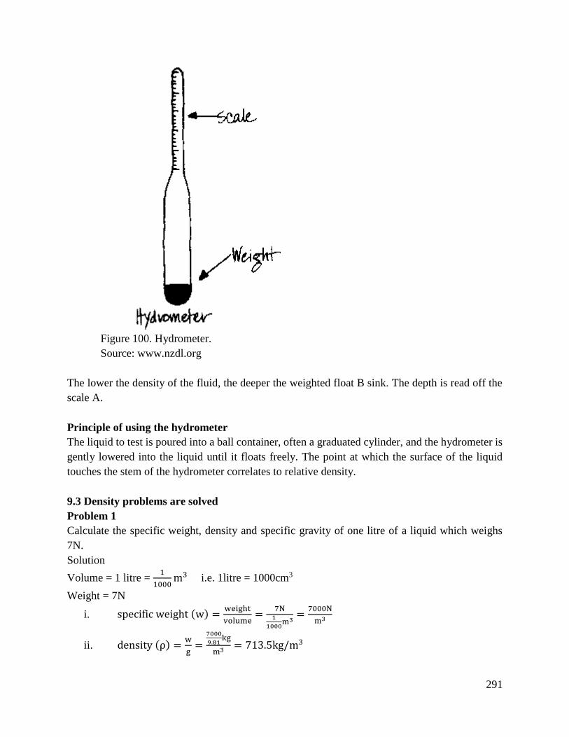
291
Figure 100. Hydrometer.
Source: www.nzdl.org
The lower the density of the fluid, the deeper the weighted float B sink. The depth is read off the
scale A.
Principle of using the hydrometer
The liquid to test is poured into a ball container, often a graduated cylinder, and the hydrometer is
gently lowered into the liquid until it floats freely. The point at which the surface of the liquid
touches the stem of the hydrometer correlates to relative density.
9.3 Density problems are solved
Problem 1
Calculate the specific weight, density and specific gravity of one litre of a liquid which weighs
7N.
Solution
Volume = 1 litre = 1
1000m3 i.e. 1litre = 1000cm3
Weight = 7N
i. specific weight (w) =weight
volume=
7N1
1000m3
=7000N
m3
ii. density (ρ) =w
g=
7000
9.81kg
m3 = 713.5kg/m3
292
iii. specific gravity =density of liquid
density of water=
713.5
1000= 0.7135
i.e. density of water = 1000kg/m3
Problem 2
Calculate the density, specific weight of one litre of petrol of specific gravity 0.7
Solution
Volume = 1 litre = 1 ∗ 1000cm3 =1000
106m3 = 0.001m3
S = 0.7 = s. p gravity
i. Density (ρ)
ρ = s ∗ 1000kg/m3
= 0.7 ∗ 1000
= 700kg/m3
ii. Specific weight (w)
w = weight ∗ gravity
= ρ ∗ g
= 700 ∗ 9.81 (N
m3) = 6867(N
m3)
iii. Weight (w)
specific weight =weight
volume
w =W
0.001or 6867 =
W
0.001
w = 6867 ∗ 0.001 = 6.867N
Problem 3
A body weighs 2.76N in air and 1.925N when completely immersed in water of density 1000kg/m3.
Calculate:
a) Volume of the body.
b) Density of the body
293
c) Relative density of the body. (Take g = 9.81m/s2)
Solution
a) The apparent loss of weight is 2.760N − 1.925N = 0.835N
0.835N is the weight of the water displaced, i.e. vρg where v = volume of body ρ= density
of water
0.835N = v ∗ 1000 (kg
m3) ∗ 9.81 (m
s2)
v =0.835
9.8∗103
= 8.512 ∗ 10−5m3
= 8.512 ∗ 104mm3
b) The density of the body
=mass
volume= weight/(g ∗ v)
=2.76N
9.81∗8.512∗10−5
= 3305 kg/m3
= 3.305 tons/m3
c) relative density =density
density of water
=3305
1000
= 3.305
Conclusion
The learning outcome covered or equipped the learner with knowledge, skills and attitude to
discuss the density terminologies, carry out the density measurements and solve density problems.
The learning outcome also equipped the learners on how to apply this knowledge on density in
real life situations.
294
Further Reading
1. Mei,J. Liu, Z, Wen; W and Sheng, P(2006). Effective Mass density of Fluid-Solid
Composites. Physical review letters 96(2), 024301.
2. Turner M.S.(1986), Cosmic and Local Mass Density of Invisible Axions. Physical review
letters 33(4) 889.
4.3.10.3 Self-Assessment
Written Assessment
1. State the SI unit of density
a) N
b) Kg/cm2
c) N/m3
d) Kg/m3
2. State the density of water
a) 100gm/cm3
b) 1000kg/m3
c) 1000kg/cm3
d) 1g/m3
3. Which of the following is specific weight
a) Ratio between the weight of a fluid to its volume
b) Ratio of weight density to mass
4. Which one is correct regardless of specific weight?
a) w =mass of fluid
volume of fluid
b) w =weight of fluid
volume of fluid
5. Identify the correct mathematical expression for specific volume
a) 1
Q
b) ρ
c) m
s
d) N
ρ
295
6. State the instrument for measuring relative density
a) Barometer
b) Hydrometer
c) Hygrometer
d) Manometer
7. Differentiate between density and weight density
a) Density is mass per unit volume while weight density is the ratio between the weight
of a fluid to its volume.
b) Density is weight per unit volume while weight density is mass per unit volume.
8. What do you understand by the following fluid properties:
a) Density
b) Specific volume
c) Weight density
9. Differentiate between specific weight and specific volume of a fluid.
10. One litre of crude oil weighs 9.6N, calculate its specific weight, density and specific gravity.
11. State the Archimedes’ principle.
12. A body weighs 243N in air and 125N when completely immersed in water, what will it weigh
when completely immersed in oil of relative density of 0.8?
Oral Assessment
1. Discuss the difference between a mercury and alcohol hydrometer when measuring the relative
density of a fluid.
2. Explain how a hydrometer works.
Practical Assessment
By using a hydrometer, list the difference between using a mercury and alcohol hydrometer when
measuring the relative densities of five different liquids.
Project
1. Using a hydrometer, measure the relative density of milk and explain the outcomes from the
experiment.
2. Using a hydrometer, measure the relative density of milk of different breeds and explain the
differences of the result obtained.
4.3.10.4 Tools, Equipment, Supplies and Materials
Scientific Calculators
Relevant reference materials
Hydrometer
Graph books
4.3.10.5 References

296
Mechanical engineering Principles by John Bird and Carl-Ross
Mei,J. Liu, Z, Wen; W and Sheng, P(2006). Effective Mass density of Fluid-Solid Composites.
Physical review letters 96(2), 024301.
Turner M.S. (1986), Cosmic and Local Mass Density of Invisible Axions. Physical review letters
33(4) 889.
297
4.3.11 Learning Outcome No 10: Apply pressure principles
4.3.11.1 Learning Activities
Learning Outcome No 10: Apply pressure principles
Learning Activities Special Instructions
10.1 Discuss pressure concepts
10.2 Discuss working principles of pressure
10.3 Solve pressure problems
10.4 Identify pressure applications (vacuum pump,
hydraulic pump and hydrometers)
Ensure that students understand all the
problems in pressure calculations.
4.3.11.2 Information Sheet No4/LO10: Apply pressure principles
Introduction
This learning outcome covers pressure, variation of pressure with depth in a liquid, properties of
fluid pressure, measurement of gauge pressure, the boundary gauge and measurement of
atmospheric pressure.
Definition of key terms
Pressure: Pressure acting on a surface is defined as the perpendicular force per unit area of the
surface. Pressure is force acting on a substance per unit area of that substance.
Archimedes’ principle: If a solid body floats or is submerged in a liquid, the liquid exerts an up
thrust in the body equal to the gravitational force on the liquid displaced by the body.
Atmospheric pressure: The atmospheric air is surrounded by layers of gases and so this air
surrounding the earth exerts pressure known as atmospheric pressure and is measured Using
mercury barometer.
Content/procedures/methods/illustrations
10.1Pressure concepts are discussed
The SI units of pressure is Pascal. Pa where 1 Pascal is equal to 1 Newton per square meter.
p =F
A
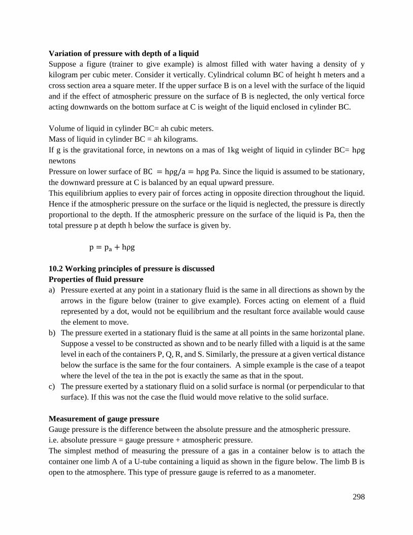
298
Variation of pressure with depth of a liquid
Suppose a figure (trainer to give example) is almost filled with water having a density of y
kilogram per cubic meter. Consider it vertically. Cylindrical column BC of height h meters and a
cross section area a square meter. If the upper surface B is on a level with the surface of the liquid
and if the effect of atmospheric pressure on the surface of B is neglected, the only vertical force
acting downwards on the bottom surface at C is weight of the liquid enclosed in cylinder BC.
Volume of liquid in cylinder BC= ah cubic meters.
Mass of liquid in cylinder BC = ah kilograms.
If g is the gravitational force, in newtons on a mas of 1kg weight of liquid in cylinder BC= hρg
newtons
Pressure on lower surface of BC = hρg/a = hρg Pa. Since the liquid is assumed to be stationary,
the downward pressure at C is balanced by an equal upward pressure.
This equilibrium applies to every pair of forces acting in opposite direction throughout the liquid.
Hence if the atmospheric pressure on the surface or the liquid is neglected, the pressure is directly
proportional to the depth. If the atmospheric pressure on the surface of the liquid is Pa, then the
total pressure p at depth h below the surface is given by.
p = pa + hρg
10.2 Working principles of pressure is discussed
Properties of fluid pressure
a) Pressure exerted at any point in a stationary fluid is the same in all directions as shown by the
arrows in the figure below (trainer to give example). Forces acting on element of a fluid
represented by a dot, would not be equilibrium and the resultant force available would cause
the element to move.
b) The pressure exerted in a stationary fluid is the same at all points in the same horizontal plane.
Suppose a vessel to be constructed as shown and to be nearly filled with a liquid is at the same
level in each of the containers P, Q, R, and S. Similarly, the pressure at a given vertical distance
below the surface is the same for the four containers. A simple example is the case of a teapot
where the level of the tea in the pot is exactly the same as that in the spout.
c) The pressure exerted by a stationary fluid on a solid surface is normal (or perpendicular to that
surface). If this was not the case the fluid would move relative to the solid surface.
Measurement of gauge pressure
Gauge pressure is the difference between the absolute pressure and the atmospheric pressure.
i.e. absolute pressure = gauge pressure + atmospheric pressure.
The simplest method of measuring the pressure of a gas in a container below is to attach the
container one limb A of a U-tube containing a liquid as shown in the figure below. The limb B is
open to the atmosphere. This type of pressure gauge is referred to as a manometer.
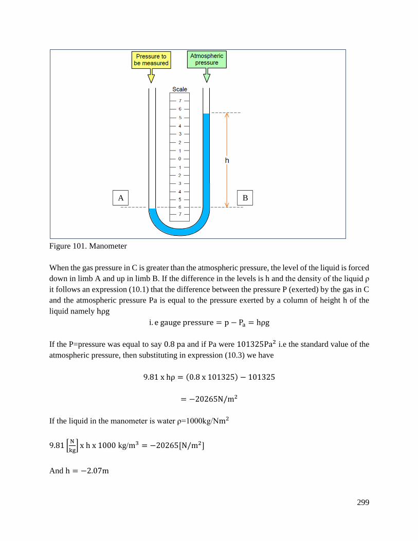
299
Figure 101. Manometer
When the gas pressure in C is greater than the atmospheric pressure, the level of the liquid is forced
down in limb A and up in limb B. If the difference in the levels is h and the density of the liquid ρ
it follows an expression (10.1) that the difference between the pressure P (exerted) by the gas in C
and the atmospheric pressure Pa is equal to the pressure exerted by a column of height h of the
liquid namely hρg
i. e gauge pressure = p − Pa = hρg
If the P=pressure was equal to say 0.8 pa and if Pa were 101325Pa2 i.e the standard value of the
atmospheric pressure, then substituting in expression (10.3) we have
9.81 x hρ = (0.8 x 101325) − 101325
= −20265N/m2
If the liquid in the manometer is water ρ=1000kg/Nm2
9.81 [N
kg] x h x 1000 kg/m3 = −20265[N/m2]
And h = −2.07m
A B
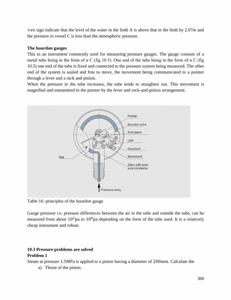
300
+ve sign indicate that the level of the water in the limb A is above that in the limb by 2.07m and
the pressure in vessel C is less than the atmospheric pressure.
The bourdon gauges
This in an instrument commonly used for measuring pressure gauges. The gauge consists of a
metal tube being in the form of α C (fig 10.5). One end of the tube being in the form of α C (fig
10.5) one end of the tube is fixed and connected to the pressure system being measured. The other
end of the system is sealed and free to move, the movement being communicated to a pointer
through a lever and a rack and pinion.
When the pressure in the tube increases, the tube tends to straighten out. This movement is
magnified and transmitted to the pointer by the lever and rock-and-pinion arrangement.
Table 16: principles of the bourdon gauge
Gauge pressure i.e. pressure differences between the air in the tube and outside the tube, can be
measured from about 103pa to 108pa depending on the form of the tube used. It is a relatively
cheap instrument and robust.
10.3 Pressure problems are solved
Problem 1
Steam at pressure 1.5MPa is applied to a piston having a diameter of 200mm. Calculate the
a) Thrust of the piston.
301
b) The work done when the piston moves through a distance of 350mm assuming the steam
pressure to be constant.
Solution
Area of a piston=π
4 x 2002 = 31400mm2
= 0.314m2
Pressure of the piston= 15MPa = 1.5 x 10⁶pa
Thrust of the system= 1.5 x 106pa x 0.0314[m2]
= 47100N
= 47.1kN
Displacement of piston= 350mm = 0.35m
Work done= 47100m2[N]x 0.35[m]
1600J = 16.5kJ
Problem 2
A rectangular tank 5m x 2m is 4m high. It is filled with oil having a relative density of 0.8.
Calculate: (neglect the effect of the atmospheric pressure)
a) The pressure at the depth of 2m
b) The pressure and the total thrust on the bottom of the tank
c) The total thrust on one of the end surfaces
Solution
Since density of water = 1000kg/m3
Density of oil = 0.8 x 1000 = 800kg/m3
From the expression,
Pressure at depth of 2m = (2[m] x 800 [kg
m3] x 9.81[N/kg])
= 15696Pa or N/m
≈ 15.7 kPa orkN/m2
Pressure on the bottom of tank = 4[m]x 800 [kg
m3] x9.81[N/Kg]
31392 Pa or N/m2
= 31.4kpa or kN/m2
Area of bottom tank= 5[m]x 2[m] = 10m2
302
Total thrust on bottom of the tank = 31.4 [kN
m2] x 10[m2]
= 314 kN
Area of one end of the surface= 2[m] x 4[m] = 8m2
From the figure it follows that the average pressure on each of the vertical surfaces occurs at the
depth of 2m and has already been found to be15.7 kPa.
Therefore, thrust on one end surface= 15.7 [kN
m2] x 8 [m2]
= 125.6kN
10.4 Pressure applications are identified
The following are application of pressure:
a. Syringes are used to take blood for blood tests. The pressure of the liquid (blood) force the
liquid to move into the syringe when its plunger is withdrawn.
b. A vacuum cleaner has a from inside that creates low pressure inside the device. Consequently,
air and dirt particles are sucked into the device.
Conclusion
The learning outcome covered or equipped the learner with knowledge, skills and attitude to
discuss pressure concepts, discuss the working principle of pressure, solve pressure problem and
identify application of pressure.
.
Further Reading
1. Engineering science by E-Hughes and C-Hughes.
2. Mechanical engineering principle by John Bird and Carl Ross
4.3.11.3 Self-Assessment
Written Assessment
1. Which one of the following is the SI units for pressure?

303
a) kJ/kg
b) N/m2
c) J/m2
d) N/m3
2. Which one of the following is true?
a) Pressure is directly proportional to the depth.
b) Pressure increases with decrease on depth.
3. What is gauge pressure?
a) Absolute pressure + atmospheric pressure
b) Difference between the absolute pressure and the atmospheric pressure.
4. Which one of the following cannot measure pressure?
a) Manometer
b) Bourdon gauge
c) Barometer
d) Hydrometer
5. Calculate the absolute pressure at a point on a sub marine at a depth of 30m below the surface
of the sea when the atmospheric pressure is 101kPa. Take density of sea water as 1030kg/m3
and the gravitational acceleration as 9.8m/s2.
a) 4.04kPa
b) 430MPa
c) 403.82kPa
d) 304.28kPa
6. State the instrument used to measure atmospheric pressure.
a) Barometer
b) Hydrometer
c) Hygrometer
7. State the difference between a barometer and a bourdon gauge.
a) Both are used insumer
b) Barometer uses fluid while bourdon gage uses pressure.
c) Bourdon gage has a gear mechanism but barometer has no any mechanism.
8. State the instrument used to measure pressure.
9. Explain the working principle of the following.
i. Barometer
ii. Manometer
10. What is pressure?
11. Sate the variation of pressure with depth.
12. List the properties of a fluid’s pressure
Oral Assessment
304
1. Discuss the properties of a fluid.
2. Elaborate the factors affecting atmospheric pressure
Practical Assessment
1. Using a tank 400m3 and another cylindrical container of 40m3 and water explain the variation
of pressure with depth in a liquid.
4.3.11.4 Tools, Equipment, Supplies and Materials
Scientific Calculators
Relevant reference materials
Stationeries
Electrical workshop
Relevant practical materials
Dice
Computers with internet connection
4.3.11.5 References
Bird, J., & Ross, C. (2014). Mechanical engineering principles. Routledge.
Blau, P. J. (2001). The significance and use of the friction coefficient. Tribology
International, 34(9), 585-591.
Zammit, S. J. (1987). Motor Vehicle Engineering Science for Technicians, Level 2. Longman
Scientific & Technical.
305
CHAPTER 5: FLUID MECHANICS/ APPLY FLUID MECHANICS PRINCIPLES
5.1 Introduction
Fluid Mechanics is among the common units of competencies offered in all the TVET level 6
engineering courses qualification This unit describes the competencies required by a technician in
order to apply a wide range of fluid mechanics principles in their work. It includes understanding
flow of fluids, demonstrating knowledge in viscous flow, performing dimensional analysis and
operating fluid pumps. The significance of Fluid Mechanics to TVET level 6 engineering
curriculum is to enable learners acquire knowledge and skills to demonstrate logical thinking,
problem solving, applying statistics, drawing graphs, using different measuring tools to get along
well in the workplace and task.
The critical aspect of competency to be covered includes identifying principles of mechanical
science, performing mechanical calculations of a system, identifying types of forces on a system,
calculating resultant forces on plane framework, identifying application of forces on the production
flow, testing mechanical properties of a materials, identifying tools and equipment for measuring
system parameters, recording and interpreting measured parameters, and operating power
transmission systems. The basic resources required includes access to relevant workplace or
appropriately simulated environment where assessment can take place, measuring tools and
equipment, sample materials to be tested among others. The unit of competency covers four
learning outcomes. Each of the learning outcome presents; learning activity that covers
performance criteria statements, thus creating trainee an opportunity to demonstrate knowledge
and skills in the occupational standards and content in curriculum. Information sheet provides;
definition of key terms, content and illustration to guide in training. The competency may be
assessed through direct observation, demonstration with oral questioning, case studies and written
tests. Self-assessment is provided at the end of each learning outcomes. Holistic assessment with
other units relevant to the industry sector workplace and job role is recommended.
5.2 Performance Standard
Understand flow of fluids, demonstrate knowledge in viscous flow and derive viscous flow
equation in circular pipes and apply them in problem solving, perform dimensional analysis and
apply them in problem solving and operate fluid pumps, pump equations in problem solving in
accordance with the set standards.
5.3 Learning Outcomes
5.3.1 List of Learning Outcomes
a) Understand flow of fluids
b) Demonstrate knowledge in viscous flow
c) Perform dimensional analysis
d) Operate fluid pumps
306
5.3.2 Learning Outcome No1: Understand flow of fluids
5.3.2.1 Learning Activities
Learning Outcome No 1:understand flow of fluids
Learning Activities Special Instructions
1.1 Measure flow rate in pipes
1.2 Determine losses in pipes
1.3 Determine causes of losses (friction, enlargement/reduction in cross-
sectional areas)in pipes
1.4 Apply flow losses equations in problem solving
Do an experiment
with a pipe
5.3.2.2 Information Sheet No5/LO1: Understand flow of fluids
Introduction
This learning outcome covers measurement of flow rate in pipes, measurement of flow rate in
pipes determine losses in pipes, determination of causes of losses (friction, enlargement/reduction
in cross-sectional areas) in pipes and application of flow losses equations in problem solving.
Definition of key terms
Steady and unsteady flow: Steady flow is defined as that type of flow in which the fluid
characteristics like velocity at a point do not change with time. Unsteady flow is that type of flow
in which the velocity, pressure and density at a point changes with respect to time.
Uniform and non-uniform flow: Uniform flow is defined as that type of flow in which the
velocity at any given time does not change with respect to length of direction of the flow. Non-
uniform flow is that type of flow in which the velocity at any given time changes with respect to
length of direction of the flow.
Laminar and turbulent flows: Laminar flow is defined as that type of flow in which the fluid
particles move along a well-defined path and all stream lines are straight and parallel. Thus, the
particles move in layers gliding smoothly over the adjacent layer. Turbulent flow is that type of
flow in which the fluid particles move in a zig-zag way.
Discharge: This is the quantity of a fluid flowing per second through a section of a pipe or a
channel.
Viscosity: The property of a fluid which offers resistance to the movement of one layer of fluid
over another adjacent layer of the fluid.
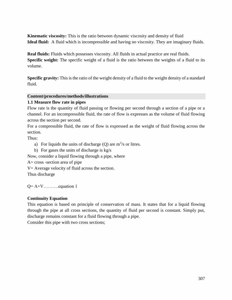
307
Kinematic viscosity: This is the ratio between dynamic viscosity and density of fluid
Ideal fluid: A fluid which is incompressible and having no viscosity. They are imaginary fluids.
Real fluids: Fluids which possesses viscosity. All fluids in actual practice are real fluids.
Specific weight: The specific weight of a fluid is the ratio between the weights of a fluid to its
volume.
Specific gravity: This is the ratio of the weight density of a fluid to the weight density of a standard
fluid.
Content/procedures/methods/illustrations
1.1 Measure flow rate in pipes
Flow rate is the quantity of fluid passing or flowing per second through a section of a pipe or a
channel. For an incompressible fluid, the rate of flow is expresses as the volume of fluid flowing
across the section per second.
For a compressible fluid, the rate of flow is expressed as the weight of fluid flowing across the
section.
Thus:
a) For liquids the units of discharge (Q) are m3/s or litres.
b) For gases the units of discharge is kg/s
Now, consider a liquid flowing through a pipe, where
A= cross -section area of pipe
V= Average velocity of fluid across the section.
Thus discharge
Q= A×V……….equation 1
Continuity Equation
This equation is based on principle of conservation of mass. It states that for a liquid flowing
through the pipe at all cross sections, the quantity of fluid per second is constant. Simply put,
discharge remains constant for a fluid flowing through a pipe.
Consider this pipe with two cross sections;
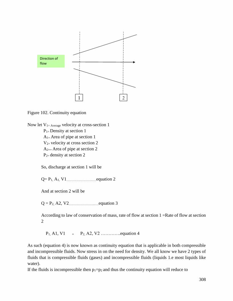
308
Figure 102. Continuity equation
Now let V1= Average velocity at cross-section 1
P1= Density at section 1
A1= Area of pipe at section 1
V2= velocity at cross section 2
A2== Area of pipe at section 2
P2= density at section 2
So, discharge at section 1 will be
Q= P1, A1, V1……………………..….equation 2
And at section 2 will be
Q = P2, A2, V2……………………..….equation 3
According to law of conservation of mass, rate of flow at section 1 =Rate of flow at section
2
P1, A1, V1 = P2, A2, V2 ………….equation 4
As such (equation 4) is now known as continuity equation that is applicable in both compressible
and incompressible fluids. Now stress in on the need for density. We all know we have 2 types of
fluids that is compressible fluids (gases) and incompressible fluids (liquids 1.e most liquids like
water).
If the fluids is incompressible then p1=p2 and thus the continuity equation will reduce to
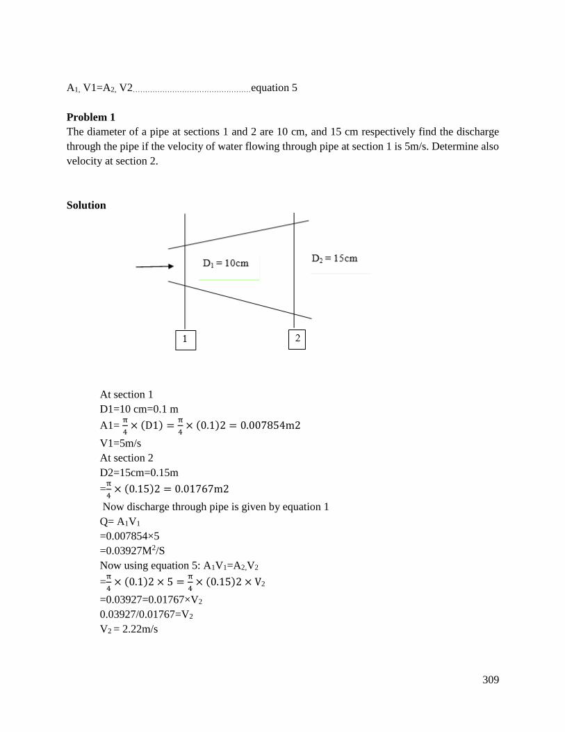
309
A1, V1=A2, V2…………………………………………equation 5
Problem 1
The diameter of a pipe at sections 1 and 2 are 10 cm, and 15 cm respectively find the discharge
through the pipe if the velocity of water flowing through pipe at section 1 is 5m/s. Determine also
velocity at section 2.
Solution
At section 1
D1=10 cm=0.1 m
A1= π
4× (D1) =
π
4× (0.1)2 = 0.007854m2
V1=5m/s
At section 2
D2=15cm=0.15m
=π
4× (0.15)2 = 0.01767m2
Now discharge through pipe is given by equation 1
Q= A1V1
=0.007854×5
=0.03927M2/S
Now using equation 5: A1V1=A2,V2
=π
4× (0.1)2 × 5 =
π
4× (0.15)2 × V2
=0.03927=0.01767×V2
0.03927/0.01767=V2
V2 = 2.22m/s
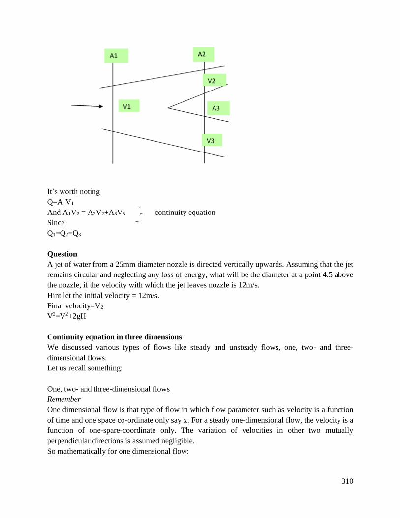
310
It’s worth noting
Q=A1V1
And A1V2 = A2V2+A3V3 continuity equation
Since
Q1=Q2=Q3
Question
A jet of water from a 25mm diameter nozzle is directed vertically upwards. Assuming that the jet
remains circular and neglecting any loss of energy, what will be the diameter at a point 4.5 above
the nozzle, if the velocity with which the jet leaves nozzle is 12m/s.
Hint let the initial velocity = 12m/s.
Final velocity=V2
V2=V2+2gH
Continuity equation in three dimensions
We discussed various types of flows like steady and unsteady flows, one, two- and three-
dimensional flows.
Let us recall something:
One, two- and three-dimensional flows
Remember
One dimensional flow is that type of flow in which flow parameter such as velocity is a function
of time and one space co-ordinate only say x. For a steady one-dimensional flow, the velocity is a
function of one-spare-coordinate only. The variation of velocities in other two mutually
perpendicular directions is assumed negligible.
So mathematically for one dimensional flow:
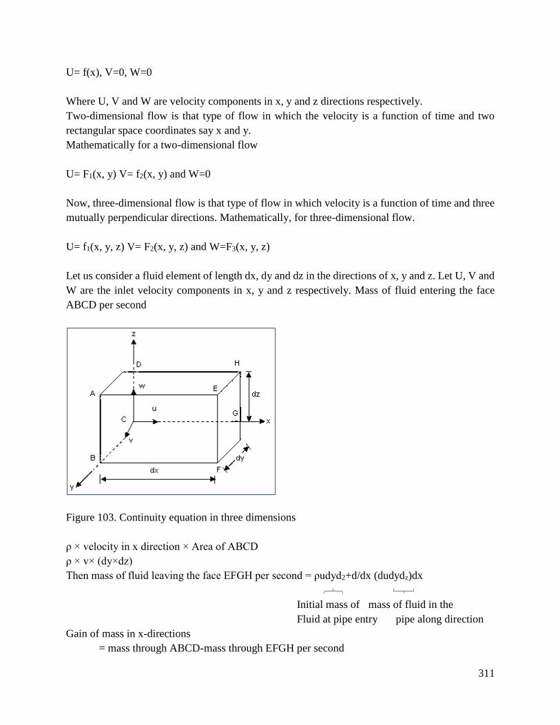
311
U= f(x), V=0, W=0
Where U, V and W are velocity components in x, y and z directions respectively.
Two-dimensional flow is that type of flow in which the velocity is a function of time and two
rectangular space coordinates say x and y.
Mathematically for a two-dimensional flow
U= F1(x, y) V= f2(x, y) and W=0
Now, three-dimensional flow is that type of flow in which velocity is a function of time and three
mutually perpendicular directions. Mathematically, for three-dimensional flow.
U= f1(x, y, z) V= F2(x, y, z) and W=F3(x, y, z)
Let us consider a fluid element of length dx, dy and dz in the directions of x, y and z. Let U, V and
W are the inlet velocity components in x, y and z respectively. Mass of fluid entering the face
ABCD per second
Figure 103. Continuity equation in three dimensions
ρ × velocity in x direction × Area of ABCD
ρ × v× (dy×dz)
Then mass of fluid leaving the face EFGH per second = ρudyd2+d/dx (dudydz)dx
Initial mass of mass of fluid in the
Fluid at pipe entry pipe along direction
Gain of mass in x-directions
= mass through ABCD-mass through EFGH per second
312
= ρ u dy dz – ρ u dy dz - (∂ / ∂x) (ρ u dy dz) dx
= - ∂ / ∂x (ρ u dy. dz) dx
Similarly, the net gain of mass in y directions
= - (∂ / ∂y) (ρ v) dx .dy. dz
And in 2 directions
= - (∂ / ∂z) (ρ w) dx. dy. Dz
Therefore dy.dz is constant
Since mass is neither created nor destroyed in the fluid element, the net increase of mass per unit
time in the fluid element must be equal to rate of increase of mass of fluid in the element. But the
mass of fluid in the element is P.dx.dy.dz and its rate of incase with time is:
∂ρ/∂t (ρ dx.dy.dz) or
∂ρ/∂t. dx.dy.dz
Equating the two expressions
- [∂ / ∂x (ρ u) + ∂ / ∂y (ρ v) + ∂ / ∂z (ρ w)] dx.dy.dz = ∂ρ/∂t. dx.dy.dz
∂ρ/∂t + ∂ / ∂x ρ u + ∂ / ∂y ρ v + ∂ / ∂z ρ w = 0
Now if fluid is incompressible, the P is constant and above equation becomes;
∂u / ∂x + ∂v / ∂y + ∂w / ∂z = 0………………………………equation 6
This is now continuity equation in three dimensions.
1.2 Determine losses in pipes
When a fluid is flowing through a pipe, the fluid experiences some resistance due to which some
of the energy of fluid is lost. When a liquid is flowing through a pipe, the velocity of the liquid
layer adjacent to the pipe wall is zero. The velocity of liquid goes on increasing from the wall and
thus velocity gradient hence shear stresses are produced in the whole liquid due to viscosity. Now
this viscose action causes loss of energy which is usually known as frictional loss. Now turbulent
flow is where the fluid particles moves in a random manner resulting in general mixing of the
particles. This flow is as a result of increase in fluid velocity, or the fluid is less viscous, as the
fluid particles do not move in a straight manner. A laminar flow is where the fluid particles move
along straight parallel path in layers, such that the paths of individual fluid particles do not cross
those of neighboring particles. Laminar flow is only possible at low velocities and when the liquid
is highly viscous like honey.
A laminar flow changes to turbulent flow when:
a) Velocity is increased
b) Diameter of pipe is increased
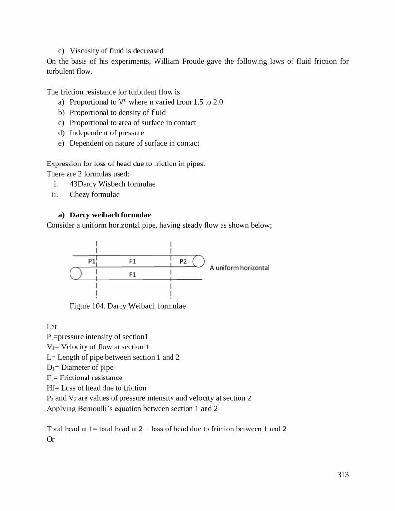
313
c) Viscosity of fluid is decreased
On the basis of his experiments, William Froude gave the following laws of fluid friction for
turbulent flow.
The friction resistance for turbulent flow is
a) Proportional to Vn where n varied from 1.5 to 2.0
b) Proportional to density of fluid
c) Proportional to area of surface in contact
d) Independent of pressure
e) Dependent on nature of surface in contact
Expression for loss of head due to friction in pipes.
There are 2 formulas used:
i. 43Darcy Wisbech formulae
ii. Chezy formulae
a) Darcy weibach formulae
Consider a uniform horizontal pipe, having steady flow as shown below;
Figure 104. Darcy Weibach formulae
Let
P1=pressure intensity of section1
V1= Velocity of flow at section 1
L= Length of pipe between section 1 and 2
D1= Diameter of pipe
F1= Frictional resistance
Hf= Loss of head due to friction
P2 and V2 are values of pressure intensity and velocity at section 2
Applying Bernoulli’s equation between section 1 and 2
Total head at 1= total head at 2 + loss of head due to friction between 1 and 2
Or
314
P1
ρg +
V12
2g + Z1=
P2
ρg +
V22
2g + Z2+ hf
P1
ρg =
P2
ρg + + hf
Hf = P1−P2
ρg…………………………………equation 1
But hf is the head lost due to friction and hence intensity of pressure will be reduced in the direction
of flow by frictional resistance.
Now:
Friction resistance = friction resistance per unit wetted area × velocity
Wetted area per unit velocity×
f’ × 𝜋dL × v2 [since wetted area =πdl]
Velocity = v= v1= v2
= f’ × p x L × v2 πd= perimeter =p
F = f’ × p x L × v2 ………………….equation ii
The forces acting on the fluid between section 1 and 2 are:
1. Pressure force at section 1 =P1 ×A
Where A=Area of pipe
2. Pressure force at section 2= P2× A
3. Frictional force f
Resolving all forces in the horizontal direction, we have
P1A-P2A-F1=0
Or
(P1-P2) A=F1×P×L×V2 (since F1=F1PLV2 from 2 equation……2
Or
P1=P2= f1×p×l×v2/A
PA = WettedperimeterArea
Area =
πd
πd2 = 4d
Now this equation borrows the Darcy-Welsbach equation. This equation is commonly used for
finding losses of head due to friction in pipes. Sometime it is written as
Hf = 4lv2
2gd
Where f is the friction factor.
A smooth pipe of diameter 80mm and 800m long carries water at the rate of 0.480m/minute.
Calculate the loss of head at 30mm from pipe wall. Take kinematic viscosity of water as 0.015
stokes. Take value of co-efficient of friction “F” from the relation given as:
F=0.0791/9re)1/4 where re=Reynold’s number.
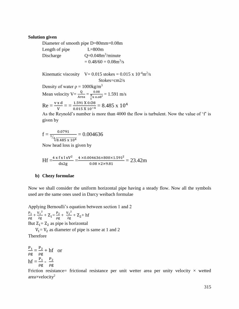
315
Solution given
Diameter of smooth pipe D=80mm=0.08m
Length of pipe L=800m
Discharge Q=0.048m3/minute
= 0.48/60 = 0.08m3/s
Kinematic viscosity V= 0.015 stokes = 0.015 x 10⁻⁴m2/s
Stokes=cm2/s
Density of water ρ = 1000kg/m3
Mean velocity V= Q
Area =
0.08π
4 x o.o8²
= 1.591 m/s
Re = v x d
V = =
1.591 X 0.O8
0.015 X 10−4 = 8.485 x 10⁴
As the Reynold’s number is more than 4000 the flow is turbulent. Now the value of ‘f’ is
given by
f = 0.0791
√8.485 x 1041
4⁄ = 0.004636
Now head loss is given by
Hf =4 x f x l xV2
dx2g =
4 ×0.004636×800×1.5912
0.08 ×2×9.81 = 23.42m
b) Chezy formulae
Now we shall consider the uniform horizontal pipe having a steady flow. Now all the symbols
used are the same ones used in Darcy weibach formulae
Applying Bernoulli’s equation between section 1 and 2
P1
ρg +
V12
2g + Z1=
P2
ρg +
V22
2g + Z2+ hf
But Z1= Z2 as pipe is horizontal
V1= V2 as diameter of pipe is same at 1 and 2
Therefore
P1
ρg =
P2
ρg + hf or
hf = P1
ρg -
P2
ρg
Friction resistance= frictional resistance per unit wetter area per unity velocity × wetted
area×velocity2
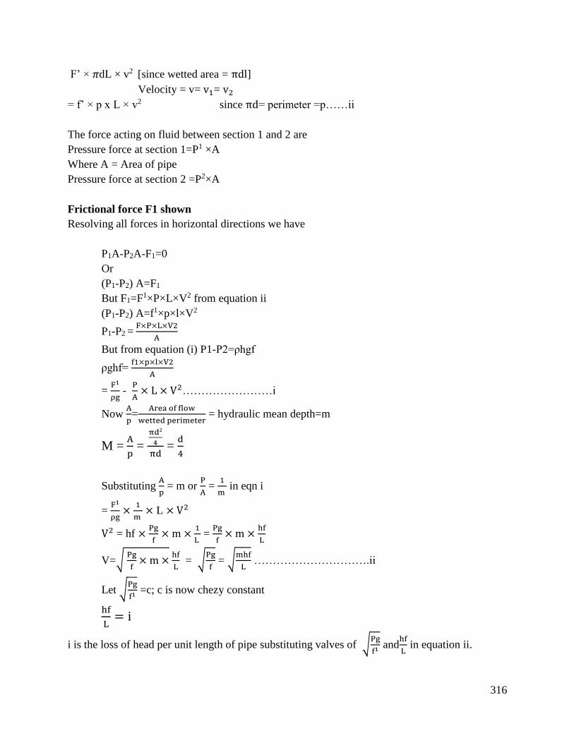
316
F’ × 𝜋dL × v2 [since wetted area = πdl]
Velocity = v= v1= v2
= f’ × p x L × v2 since πd= perimeter =p……ii
The force acting on fluid between section 1 and 2 are
Pressure force at section 1=P1 ×A
Where A = Area of pipe
Pressure force at section 2 =P2×A
Frictional force F1 shown
Resolving all forces in horizontal directions we have
P1A-P2A-F1=0
Or
(P1-P2) A=F1
But F1=F1×P×L×V2 from equation ii
(P1-P2) A=f1×p×l×V2
P1-P2 = F×P×L×V2
A
But from equation (i) P1-P2=ρhgf
ρghf= f1×p×l×V2
A
= F1
ρg -
P
A × L × V2……………………i
Now A
p=
Area of flow
wetted perimeter = hydraulic mean depth=m
M = A
p =
πd²
4
πd =
d
4
Substituting A
p = m or
P
A =
1
m in eqn i
= F1
ρg ×
1
m × L × V2
V2 = hf × Pg
f × m ×
1
L =
Pg
f× m ×
hf
L
V=√ Pg
f× m ×
hf
L = √
Pg
f = √
mhf
L ………………………….ii
Let √Pg
f1 =c; c is now chezy constant
hf
L= i
i is the loss of head per unit length of pipe substituting valves of √Pg
f1 and
hf
L in equation ii.
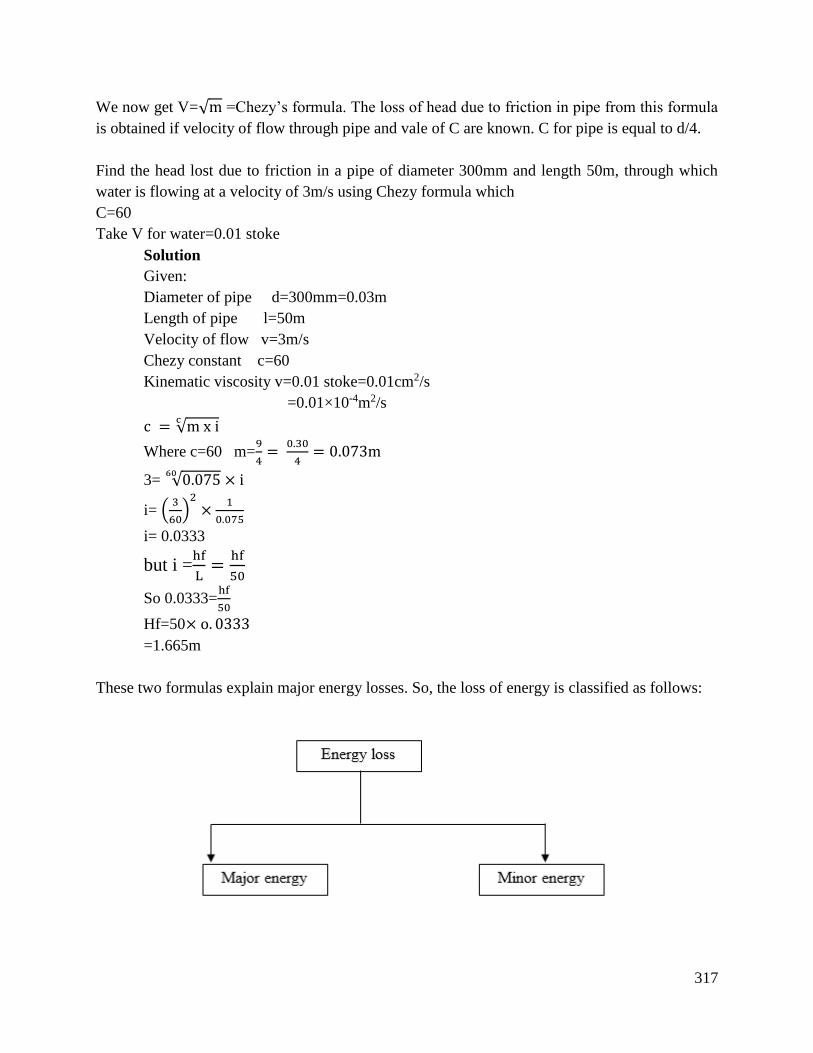
317
We now get V=√m =Chezy’s formula. The loss of head due to friction in pipe from this formula
is obtained if velocity of flow through pipe and vale of C are known. C for pipe is equal to d/4.
Find the head lost due to friction in a pipe of diameter 300mm and length 50m, through which
water is flowing at a velocity of 3m/s using Chezy formula which
C=60
Take V for water=0.01 stoke
Solution
Given:
Diameter of pipe d=300mm=0.03m
Length of pipe l=50m
Velocity of flow v=3m/s
Chezy constant c=60
Kinematic viscosity v=0.01 stoke=0.01cm2/s
=0.01×10⁻⁴m2/s
c = √m x ic
Where c=60 m=9
4=
0.30
4= 0.073m
3= √0.07560
× i
i= (3
60)2
×1
0.075
i= 0.0333
but i =hf
L=
hf
50
So 0.0333=hf
50
Hf=50× o. 0333
=1.665m
These two formulas explain major energy losses. So, the loss of energy is classified as follows:
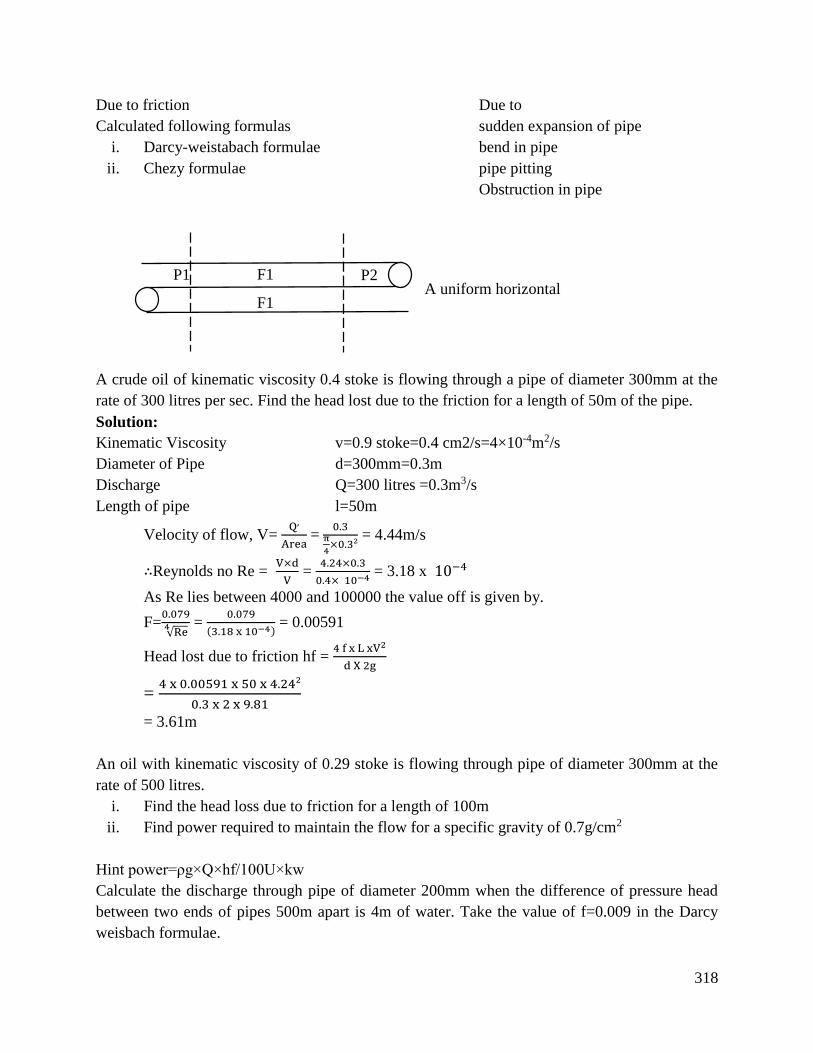
318
Due to friction Due to
Calculated following formulas sudden expansion of pipe
i. Darcy-weistabach formulae bend in pipe
ii. Chezy formulae pipe pitting
Obstruction in pipe
A crude oil of kinematic viscosity 0.4 stoke is flowing through a pipe of diameter 300mm at the
rate of 300 litres per sec. Find the head lost due to the friction for a length of 50m of the pipe.
Solution:
Kinematic Viscosity v=0.9 stoke=0.4 cm2/s=4×10-4m2/s
Diameter of Pipe d=300mm=0.3m
Discharge Q=300 litres =0.3m3/s
Length of pipe l=50m
Velocity of flow, V= Q׳
Area =
0.3π
4×0.3²
= 4.44m/s
∴Reynolds no Re = V×d
V =
4.24×0.3
0.4× 10−4 = 3.18 x 10⁻⁴
As Re lies between 4000 and 100000 the value off is given by.
F=0.079
√Re4 =
0.079
(3.18 x 10⁻⁴) = 0.00591
Head lost due to friction hf = 4 f x L xV2
d X 2g
= 4 x 0.00591 x 50 x 4.24²
0.3 x 2 x 9.81
= 3.61m
An oil with kinematic viscosity of 0.29 stoke is flowing through pipe of diameter 300mm at the
rate of 500 litres.
i. Find the head loss due to friction for a length of 100m
ii. Find power required to maintain the flow for a specific gravity of 0.7g/cm2
Hint power=ρg×Q×hf/100U×kw
Calculate the discharge through pipe of diameter 200mm when the difference of pressure head
between two ends of pipes 500m apart is 4m of water. Take the value of f=0.009 in the Darcy
weisbach formulae.
F1
P1 F1 P2 A uniform horizontal
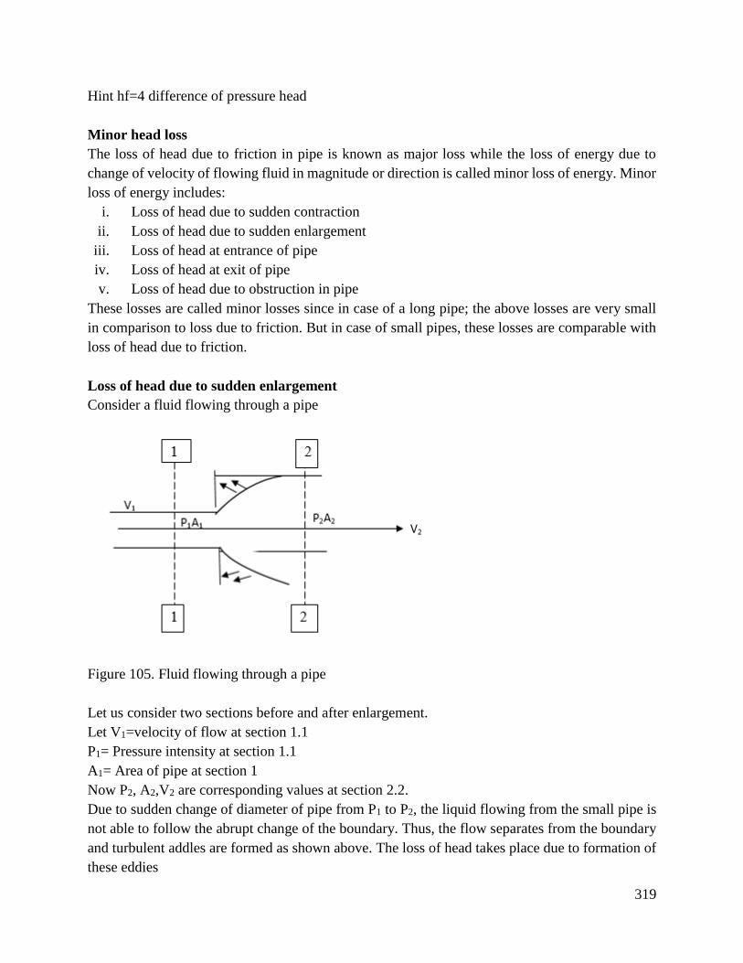
319
Hint hf=4 difference of pressure head
Minor head loss
The loss of head due to friction in pipe is known as major loss while the loss of energy due to
change of velocity of flowing fluid in magnitude or direction is called minor loss of energy. Minor
loss of energy includes:
i. Loss of head due to sudden contraction
ii. Loss of head due to sudden enlargement
iii. Loss of head at entrance of pipe
iv. Loss of head at exit of pipe
v. Loss of head due to obstruction in pipe
These losses are called minor losses since in case of a long pipe; the above losses are very small
in comparison to loss due to friction. But in case of small pipes, these losses are comparable with
loss of head due to friction.
Loss of head due to sudden enlargement
Consider a fluid flowing through a pipe
Figure 105. Fluid flowing through a pipe
Let us consider two sections before and after enlargement.
Let V1=velocity of flow at section 1.1
P1= Pressure intensity at section 1.1
A1= Area of pipe at section 1
Now P2, A2,V2 are corresponding values at section 2.2.
Due to sudden change of diameter of pipe from P1 to P2, the liquid flowing from the small pipe is
not able to follow the abrupt change of the boundary. Thus, the flow separates from the boundary
and turbulent addles are formed as shown above. The loss of head takes place due to formation of
these eddies
320
Let P=pressure intensity of liquid eddies on the area (A2-A1)
He=loss of head due to sudden enlargement.
Apply Bernoulli’s equation to section 1 and 2
p1/ρg + v12/2g + z1 + p2/ρg + v2
2/2g+z2
z1 = z2 as pipe is horizontal
[p1/ρg + v12/2g] + [p2/ρg + v2
2/2g] + he
he= [p1/ρg- p2/ρg ]+[ v12/2g- + v2
2/2g]……………………..i
Consider the control volume of liquid between sections 1 and 2. Then the force acting on the liquid
in the control volume in the direction of flow is given by;
fx= P1 A1 + P1(A 2− A1− )- P2 A2
But experimentally it is found thatP1P2
fx= P1 A1 + P1(A 2− A1− )- P2 A2 = P1 A2−P2 A2
= momentum of liquid section 1 = mass x velocity
p A1 V1 × V1
p A1 V21
Momentum of liquid see at section 2
= p A2V2 × V2
p A2 V22
Therefore change of momentum/sec
p A2V2 - p A1 V21
But from continuity equation we have
p A1 V1 − A2V2 or A1 = A2V2
V1
Therefore change of momentum/sec = p A2 V22 −
p A2 V22
V1 × V2
1
= p A2 V22 − p A2V1V2
= p A2 [ V22 − V1V2]………………………………………iii
Now net force acting on the control volume in the direction of flow must be equal to rate of change
of momentum or change of momentum per second. Hence equating ii and iii
(P1 −P2 ) A2 = p A2 ( V22 − V1V2)
P1 −P2
p = V2
2 − V1V2
Dividing by g to both sides we have
P1 −P2
pg =
V22−V1V2
g or
P1
Pg -
P2
Pg =
V22−V1V2
g
Substituting the value of [P1
Pg −
P2
Pg] in equation i
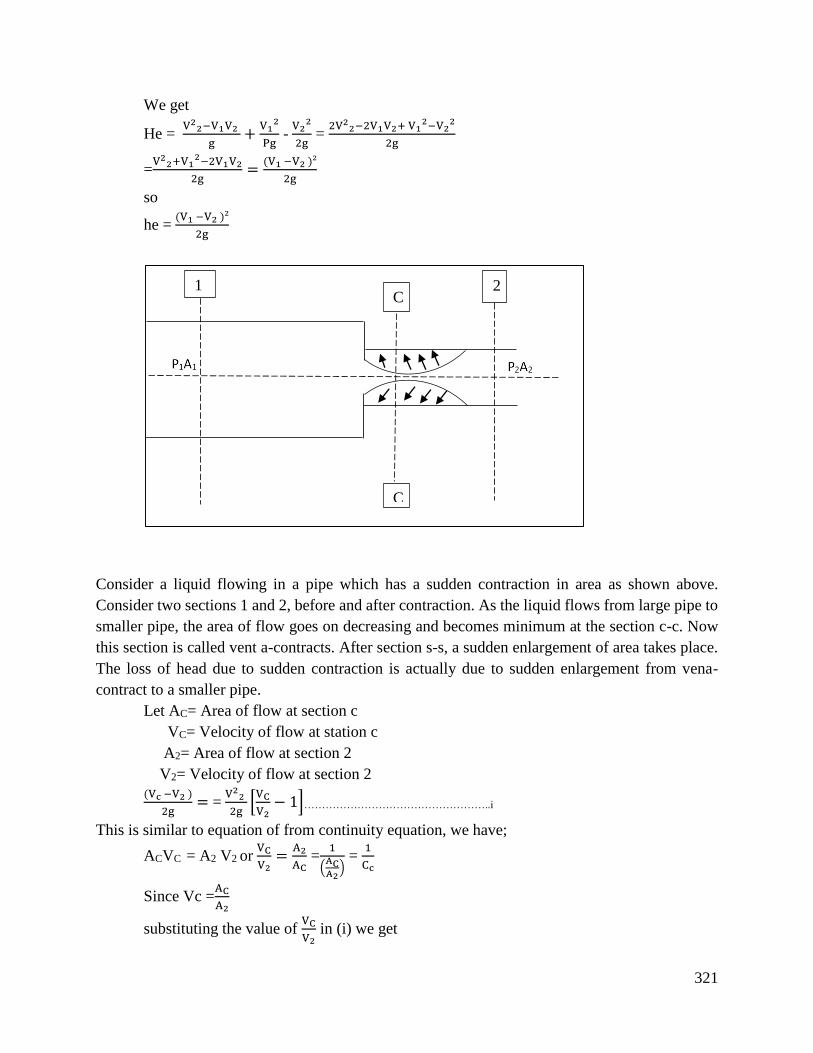
321
We get
He = V2
2−V1V2
g+
V12
Pg -
V22
2g =
2V22−2V1V2+ V1
2−V22
2g
=V2
2+V12−2V1V2
2g=
(V1 −V2 )²
2g
so
he = (V1 −V2 )²
2g
Consider a liquid flowing in a pipe which has a sudden contraction in area as shown above.
Consider two sections 1 and 2, before and after contraction. As the liquid flows from large pipe to
smaller pipe, the area of flow goes on decreasing and becomes minimum at the section c-c. Now
this section is called vent a-contracts. After section s-s, a sudden enlargement of area takes place.
The loss of head due to sudden contraction is actually due to sudden enlargement from vena-
contract to a smaller pipe.
Let AC= Area of flow at section c
VC= Velocity of flow at station c
A2= Area of flow at section 2
V2= Velocity of flow at section 2
(Vc −V2 )
2g= =
V22
2g[VC
V2− 1]……………………………………………..i
This is similar to equation of from continuity equation, we have;
ACVC = A2 V2 or VC
V2=
A2
AC =
1
(ACA2
) =
1
Cc
Since Vc =AC
A2
substituting the value of VC
V2 in (i) we get
1 C
2
C
322
hc = V2
2
2g[
1
Cc− 1] ²………………………………………eqn 10
KV22
2g ,where k =[
1
Cc− 1]
2
If the value ofCc , is assumed to be equal to 0.62, then
K=[1
Cc− 1]
2
= 0.375
Then hc becomes as
Hc =KV2
2
2g = 0.375
V22
2g
If the value of Cc is not given then the head loss due to contraction is taken as
0.5V2
2
2g or hc = 0.5
V22
2g………………………………equation 10
1. Find the loss of head when a pipe of diameter 200mm is suddenly enlarged to a diameter of
400mm. The rate of flow of water through the pipe is 250 liters.
Solution
Given:
Pia of small pipe P1 =200mm=0.2m
Area =A1 = π 4⁄ p12 =π
4⁄ x 0.4² = 0.0314m²
Diameter of large pipe D2 = 400mm = 0.4m
Area = A2 = π 4⁄ x 0.4² = 0.12564m²
Discharge= Q250 =׳ litres/s = 0.25mᵌ/s
Velocity = V1 = Q׳
A1
0.25
0.03141= 7.96m/s
And velocity, 2=
V2 = Q׳
A1 =
0.25
0.12564 = 1.99m/s
Loss of head due to sudden enlargement is given by equation q
V2 = 0.049 x 3
0.0314 = 4.68m/s
Mass rate of flow of oil = mass density x Qˏ
= p × A1 × V1
Sp.gr of oil = = density of oil
density of water
Density of oil = Sp. gr of oil x density of water
= 0.9 x 1000kg/mᵌ = 900kg/mᵌ
Mass rate of flow = 900x 0.049x 3.0 = 132.23kg/s
2. A horizontal pipe of diameter 500m is suddenly contracted to a diameter of 250mm. The
pressure intensifies in the large and smaller pipe from 13.74 N/cm2 to 11.772 N/cm2
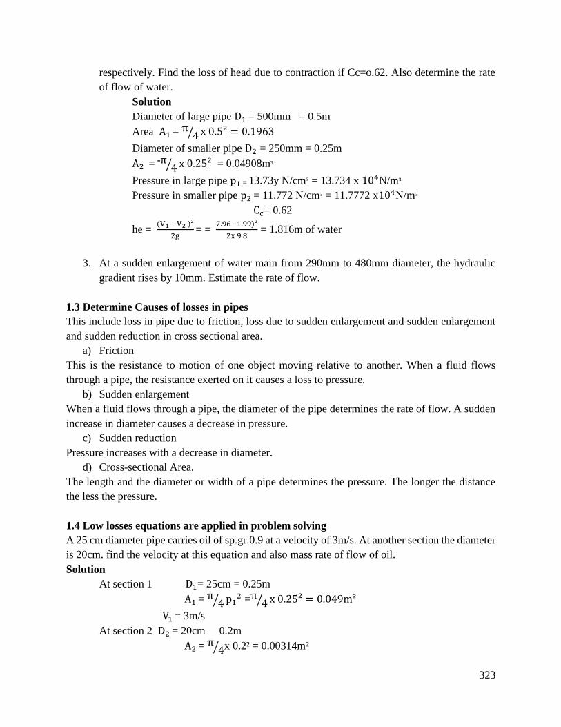
323
respectively. Find the loss of head due to contraction if Cc=o.62. Also determine the rate
of flow of water.
Solution
Diameter of large pipe D1 = 500mm = 0.5m
Area A1 = π 4⁄ x 0.5² = 0.1963
Diameter of smaller pipe D2 = 250mm = 0.25m
A2 = π 4⁄ x 0.25² = 0.04908mᵌ
Pressure in large pipe p1 = 13.73y N/cmᵌ = 13.734 x 10⁴N/mᵌ
Pressure in smaller pipe p2 = 11.772 N/cmᵌ = 11.7772 x10⁴N/mᵌ
Cc= 0.62
he = (V1 −V2 )²
2g = =
7.96−1.99)²
2x 9.8 = 1.816m of water
3. At a sudden enlargement of water main from 290mm to 480mm diameter, the hydraulic
gradient rises by 10mm. Estimate the rate of flow.
1.3 Determine Causes of losses in pipes
This include loss in pipe due to friction, loss due to sudden enlargement and sudden enlargement
and sudden reduction in cross sectional area.
a) Friction
This is the resistance to motion of one object moving relative to another. When a fluid flows
through a pipe, the resistance exerted on it causes a loss to pressure.
b) Sudden enlargement
When a fluid flows through a pipe, the diameter of the pipe determines the rate of flow. A sudden
increase in diameter causes a decrease in pressure.
c) Sudden reduction
Pressure increases with a decrease in diameter.
d) Cross-sectional Area.
The length and the diameter or width of a pipe determines the pressure. The longer the distance
the less the pressure.
1.4 Low losses equations are applied in problem solving
A 25 cm diameter pipe carries oil of sp.gr.0.9 at a velocity of 3m/s. At another section the diameter
is 20cm. find the velocity at this equation and also mass rate of flow of oil.
Solution
At section 1 D1= 25cm = 0.25m
A1 = π 4⁄ p12 =π
4⁄ x 0.25² = 0.049mᵌ
V1 = 3m/s
At section 2 D2 = 20cm 0.2m
A2 = π 4⁄ x 0.2² = 0.00314m²
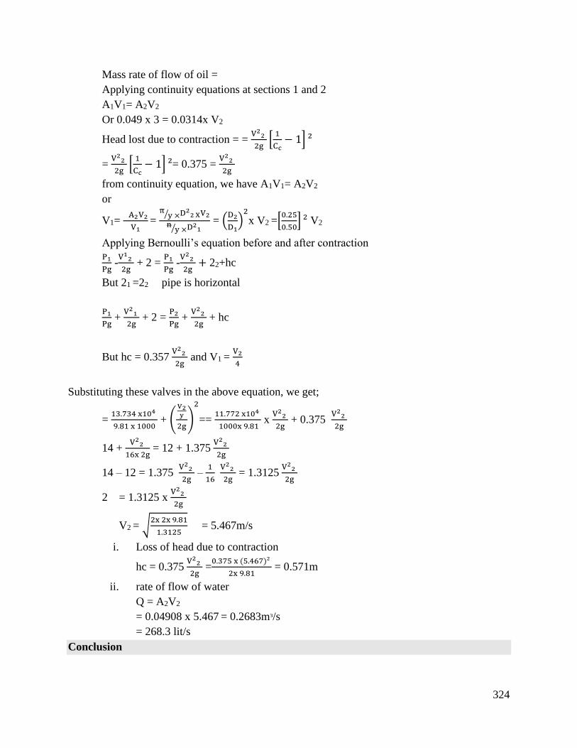
324
Mass rate of flow of oil =
Applying continuity equations at sections 1 and 2
A1V1= A2V2
Or 0.049 x 3 = 0.0314x V2
Head lost due to contraction = = V2
2
2g[
1
Cc− 1] ²
= V2
2
2g[
1
Cc− 1] ²= 0.375 =
V22
2g
from continuity equation, we have A1V1= A2V2
or
V1= A2V2
V1 =
πy ×⁄ D2
2 XV2
ny ×⁄ D2
1 = (
D2
D1)2
x V2 =[0.25
0.50] ² V2
Applying Bernoulli’s equation before and after contraction
P1
Pg -
V12
2g + 2 =
P1
Pg -
V22
2g+ 22+hc
But 21 =22 pipe is horizontal
P1
Pg +
V21
2g + 2 =
P2
Pg +
V22
2g + hc
But hc = 0.357 V2
2
2g and V1 =
V2
4
Substituting these valves in the above equation, we get;
= 13.734 x10⁴
9.81 x 1000 + (
V2y
2g)
2
== 11.772 x10⁴
1000x 9.81 x
V22
2g + 0.375
V22
2g
14 + V2
2
16x 2g = 12 + 1.375
V22
2g
14 – 12 = 1.375 V2
2
2g –
1
16 V2
2
2g = 1.3125
V22
2g
2 = 1.3125 x V2
2
2g
V2 = √2x 2x 9.81
1.3125 = 5.467m/s
i. Loss of head due to contraction
hc = 0.375 V2
2
2g =
0.375 x (5.467)²
2x 9.81 = 0.571m
ii. rate of flow of water
Q = A2V2
= 0.04908 x 5.467 = 0.2683mᵌ/s
= 268.3 lit/s
Conclusion
325
This learning outcome covers measurement of flowrate in pipes, measurement of flow rate in pipes
determine losses in pipes, determination of causes of losses (friction, enlargement/reduction in
cross-sectional areas) in pipes and application of flow losses equations in problem solving.
Further Reading
1. A textbook of Fluid Mechanics and Hydraulic Machines Dr. K. Bansal
5.3.2.3 Self-Assessment
Written Assessment
1. What are the methods of describing fluid flow?
2. Distinguish and explain in details:
a) Steady and unsteady flow
b) Uniform and non-uniform flow
3. Describe the following and give one practical example for each
a) Laminar flow
b) Turbulent flow
c) Steady flow
d) Uniform flow
4. Discuss the equation of continuity, obtain an expression for continuity of equation for a
three dimensional flow.
5. Explain two examples of unsteady flows. How can the unsteady flow be transformed to
steady flow?
6. Derive the Chezy formulae and list its application.
7. The diameter of a pipe at section 1 and 2 are 15cm and 20cm respectively. Find the
discharge through the pipe if the velocity of water at section 1 is 4m/s. Determine velocity
at section 2.
a) 7.0608m3/s, 1.11m/s
b) 0.07068m3/s, 1.26m/s
c) 0.07068m3/s, 2.25m/s
d) 7.068cm3/s, 2.25m/s
326
8. A 40cm diameter pipe, conveying water, branches into two pipes of diameters 30cm and
20cm respectively. If the average velocity in the 40cm diameter pipe is 3m/s find the
discharge in this pipe.
a) 0.3769m3/s
b) 0.3679m3/s
c) 0.376.9cm3/s
d) 376.9 litres
9. Find the head lost due to friction in a pipe of diameter 300mm, and length 50m, through
which water is flowing at a velocity of 3m/s using Darcy formulae and Chezy’s formulae
a) 0.7828m, 1.665m
b) 78.28m, 16.65m
c) 0.00256m, 0.033m
10. Find the diameter of a pipe of length 200m when the rate of flow of water through the
pipe is 200 litres and head loss due to friction is 4m. Take value of c=50 in Chezy
formulae.
a) 0.002m
b) 0.00509m
c) 0.0518m
d) 553mm
11. Water is flowing through a pipe of diameter 200mm with a velocity of 3m/s. Find head
lost due to friction for a length of 5m if co-efficient of friction is given by f=0.002
+0.09/Re 0.3 where Re is Reynold’s number. The kinematic viscosity of water =0.01
stoke
a) 0.02166m
b) 0.993m
c) 21.66m
d) 993m
Oral Assessment
1. What is Kinematics and how important is it in the fluid mechanics
2. Explain the relation between frictional losses and minor losses in a pipe
Practical Assessment
Reynold’s Experiment
A textbook of Fluid Mechanics and Hydraulic Machines Dr. K. Bansal.
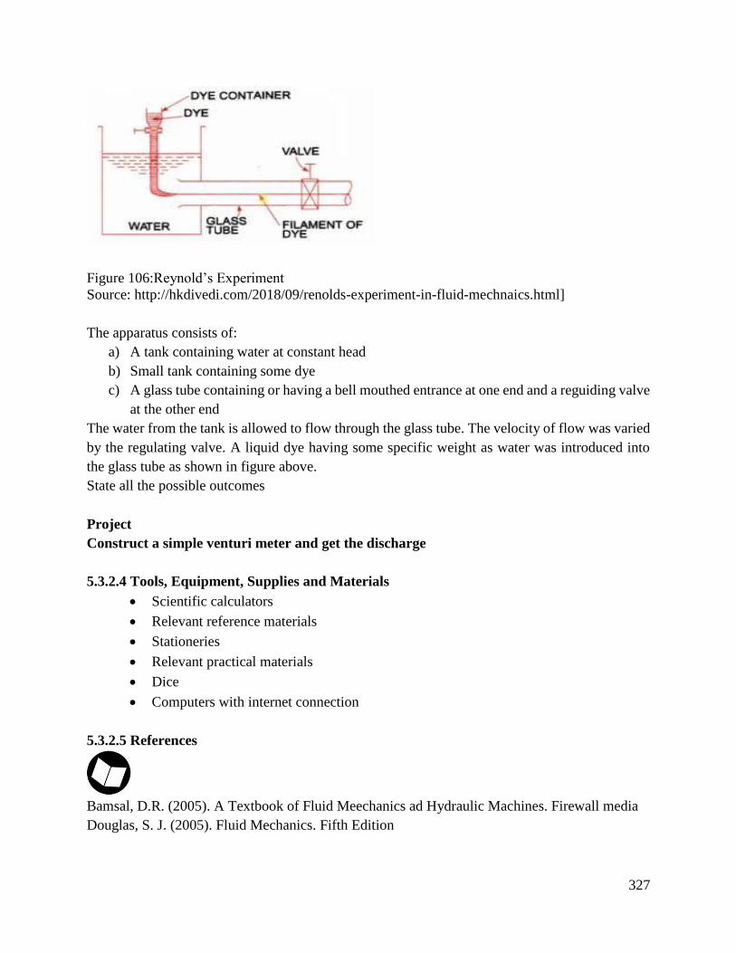
327
Source: http://hkdivedi.com/2018/09/renolds-experiment-in-fluid-mechnaics.html]
The apparatus consists of:
a) A tank containing water at constant head
b) Small tank containing some dye
c) A glass tube containing or having a bell mouthed entrance at one end and a reguiding valve
at the other end
The water from the tank is allowed to flow through the glass tube. The velocity of flow was varied
by the regulating valve. A liquid dye having some specific weight as water was introduced into
the glass tube as shown in figure above.
State all the possible outcomes
Project
Construct a simple venturi meter and get the discharge
5.3.2.4 Tools, Equipment, Supplies and Materials
Scientific calculators
Relevant reference materials
Stationeries
Relevant practical materials
Dice
Computers with internet connection
5.3.2.5 References
Bamsal, D.R. (2005). A Textbook of Fluid Meechanics ad Hydraulic Machines. Firewall media
Douglas, S. J. (2005). Fluid Mechanics. Fifth Edition
Figure 106:Reynold’s Experiment
328
5.3.3 Learning Outcome No 2: Demonstrate knowledge in viscous flow
5.3.3.1 Learning Activities
Learning Outcome No 2: Demonstrate knowledge in viscous flow
Learning Activities Special Instructions
2.1. Explain viscous flow between parallel surfaces
2.2. Derive and apply viscous flow equations between parallel
surfaces
2.3. Derive and apply viscous flow equations in circular pipes in
problem solving
5.3.2.2 Information Sheet No5/LO2: Demonstrate knowledge in viscous flow
Introduction
Viscous flow is a type of fluid flow in which there is a steady continuous motion of the particles.
It is also called streamline flow, laminal flow or steady flow. Fluid flow may be either viscous or
turbulent; the type of flow depending on the value of Reynolds number for flow in pipes, the
Reynolds number Re= Pvd/m where
P=mass density
C=mean velocity
D=pipe diameter
When Re is less than the critical value 2100 flow will be viscous; about 2100 there is a transitional
region and for higher values of Re flow will always be turbulent.
Definition of key terms
Fluid: This is substance that deforms continuously when subjected to a shear stress.
Shear force: Is the force component tangent to a surface and this force divided by the area of the
surface is the average shear stress over the area.
Viscosity: Is that property of a fluid by virtue of which it offers resistance to shear.
Density of a fluid: Is defined as its mass per unit volume.
Laminar flow: This is a very orderly flow in which the fluid particles move in smooth layers or
laminae sliding over particles in adjacent laminae without mixing them.
Turbulent flow: This refers to an irregular flow in which eddies, swirls and flow instabilities
occur.
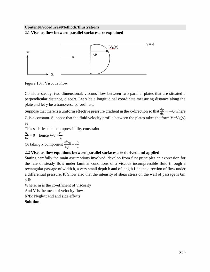
329
Content/Procedures/Methods/Illustrations
2.1 Viscous flow between parallel surfaces are explained
Figure 107: Viscous Flow
Consider steady, two-dimensional, viscous flow between two parallel plates that are situated a
perpendicular distance, d apart. Let x be a longitudinal coordinate measuring distance along the
plate and let y be a transverse co-ordinate.
Suppose that there is a uniform effective pressure gradient in the x-direction so that dp
dx= −G where
G is a constant. Suppose that the fluid velocity profile between the plates takes the form V=VX(y)
ex
This satisfies the incompressibility constraint Dv
Dt = 0 hence ∇²v =
∇p
μ
Or taking x component d2V2
dy2 = -
G
μ
2.2 Viscous flow equations between parallel surfaces are derived and applied
Stating carefully the main assumptions involved, develop from first principles an expression for
the rate of steady flow under laminar conditions of a viscous incompressible fluid through a
rectangular passage of width h, a very small depth h and of length L in the direction of flow under
a differential pressure, P. Show also that the intensity of shear stress on the wall of passage is 6m
× lh
Where, m is the co-efficient of viscosity
And V is the mean of velocity flow
N/B: Neglect end and side effects.
Solution
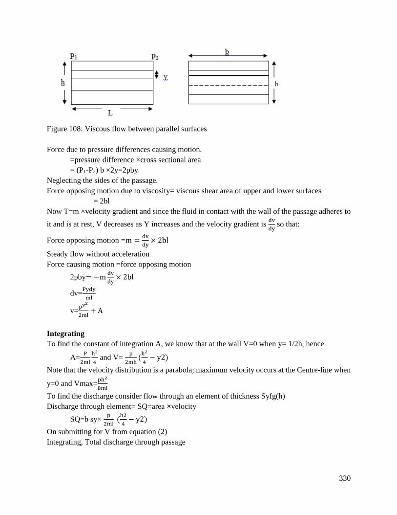
330
Figure 108: Viscous flow between parallel surfaces
Force due to pressure differences causing motion.
=pressure difference ×cross sectional area
= (P1-P2) b ×2y=2pby
Neglecting the sides of the passage.
Force opposing motion due to viscosity= viscous shear area of upper and lower surfaces
= 2bl
Now T=m ×velocity gradient and since the fluid in contact with the wall of the passage adheres to
it and is at rest, V decreases as Y increases and the velocity gradient is dv
dy so that:
Force opposing motion =m =dv
dy× 2bl
Steady flow without acceleration
Force causing motion =force opposing motion
2pby= −mdv
dy× 2bl
dv=Pydy
ml
v=py2
2ml+ A
Integrating
To find the constant of integration A, we know that at the wall V=0 when y= 1/2h, hence
A=P
2ml
h2
4 and V=
p
2mh(h2
4− y2)
Note that the velocity distribution is a parabola; maximum velocity occurs at the Centre-line when
y=0 and Vmax=ph2
8ml
To find the discharge consider flow through an element of thickness Syfg(h)
Discharge through element= SQ=area ×velocity
SQ=b sy× p
2ml (
h2
4− y2)
On submitting for V from equation (2)
Integrating, Total discharge through passage
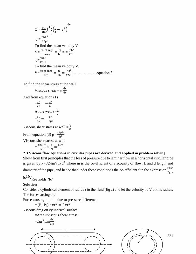
331
Q = pb
2μl∫ (
h
4− y2)
+h
4
− h
4
dy
Q = pbh3
12μl
To find the mean velocity V
V= discharge
area =
Q
bh = =
phᵌ
12μl
Q=pbh3
12ml
To find the mean velocity V.
V=discharge
are=
Q
bh=
ph2
12ml……………….equation 3
To find the shear stress at the wall
Viscous shear = μ dv
dy
And from equation (1)
=dv
dy= −
py
μl
At the well y=h
2
=dv
dy= −
ph
2μl
Viscous shear stress at wall =Pl
2l
From equation (3) p =12μlv
h2
Viscous shear stress at wall
= 12μLV
h2 ×h
2l=
6μv
h
2.3 Viscous flow equations in circular pipes are derived and applied in problem solving
Show from first principles that the loss of pressure due to laminar flow in a horizontal circular pipe
is given by P=324mVL/d2 where m is the co-efficient of viscousity of flow. L and d length and
diameter of the pipe, and hence that under these conditions the co-efficient f in the expression FLv²
2gm
is16Reynolds No⁄ .
Solution
Consider a cylindrical element of radius r in the fluid (fig a) and let the velocity be V at this radius.
The forces acting are
Force causing motion due to pressure difference
= (P1-P2) ×πr2 = Pπr2
Viscous drag on cylindrical surface
=Area ×viscous shear stress
=2πr2Lmdv
dm
L
8 r
332
Since flow is steady there is no resistant force and
Pπr2+2πLμdv
dr=0
dV=Prdr
2ml
Integrating V=Pr2
4μl+ A
At the wall V=0 and r= d/2, thus A=Pd2/16ml
V= p/4ml(d2
4− r2)
Consider an annular element (fig b)
Flow through element = dQ=area x velocity
𝛅Ǫ= 2πr2×𝛅r= 2πρ
4μl(d2
4− r2) r𝛅r
Integrating, total discharge δ =2πρ
4μl ∫ (
d2
4− r2)
d2
0r𝛅r
𝛅 = πρd²
128μl
Mean velocity = v=𝛅π
4d2
= Pd²
32μl
ρ= 32μlv
ρd² (eqn)
The expression FLv²
2gm is the Darcy formula for loss of head hf the team in being the hydraulic radius,
which is d
4 for a pipe thus,
FLv²
2gm =
4FLv²
2gd = hf =
p
ρg
Substituting for a pipe ρ from equation 1. 4FLv²
2gd =
32μlv
ρgd²
f= 16
ρVd
4
= 16
Reynolds number
Problem
Oil with viscosity 1.44kg/ms or Ns/m2 and density 900kg/m2 in a pipe 25mm diameter and 3m long
at 1/500 of the critical speed for which the Reynolds number is 2500. Calculate the head in meters
of oil required to maintain the flow.
Solution
333
In this case, m=1.44kg/ms
P=0.9×10³ kg/m2 d=0.025 m
Critical speed Corresponding to Re=2500 is given by
=PVcd
m= 2500
VC= 2500 × 1.44/ 0.9 × 103 × 0.025= 160m/s
Mean velocity inn pipe =V=Vc
500= 0.32m/s
Head required to maintain flow = head lost in friction
= 4Flv²l
2dg
Reynolds no. = Re + 1
500×2500 =5
F= 16
Re=
16
5= 3.2 L=3m, d= 0.025
Head required to maintain =4 × 3.2 × 3 ×(0.32)2
0.025× 2 × 9.81
=8.02m
2.4 Low losses equations are applied in problem solving
The loss of pressure head, h1 in a pipe of diameter D, in which a viscous fluid of velocity m is
flowing with a velocity is given by Hagen Poiseuille formula:
hf =32mGL
PgD D2
Where L= length of pipe
The loss of head due to friction is given by
Hf =4.fl.V2
2gD =
4.fl.u2
2gD
∴ Velocity in pipe is always average velocity ∴ V= ū
Where f = coefficient of friction between the pipe and fluid,
Equating (i) and (ii) we get,
f=32μūl x 2gD
4.L.u2 pg.D²=
16μ
μ.Ǫ.D
= 16 x μ
pVD = 16 x
1
R
Where μ
pVD =
1
R and R = Reynolds number =
PVD
μ
f= 16
R
Problem
Water is flowing via a 200mm diameter pipe with coefficient of friction=0.04. the shear stress at
a point 40mm from the pipe axis if 0.0098N/cm2. Calculate the shear stress at the pipe wall.
Using equation f = 16
R or 0.04 =
16
R
R1=16
0.04 = 400
334
This means flow is viscous hence T=δ.P
δX r
2
But δP
δx is constant across a section.
At the pipe wall, radius = 100mm and shear stress is to; τ
τ =
τo
100 on
0.00981
40 =
τO
100
τO = 100 x 0.00981
40 =0.0245N/cm²
At the pipe wall, radius =100mm and shear stress.
Conclusion
This learning outcome covered or equipped the learner with the knowledge of how to derive the
losses equation and how to apply it.
Further Reading
1. Dr. R. Bansal. Fluid Mechanics and Hydraulic Machines
5.3.3.3 Self-Assessment
Written Assessment
1. Newton’s law of viscosity depends upon the __________
a) Stress and strain in a fluid
b) Shear stress, pressure and velocity
c) Shear stress and rate of strain
d) Viscosity and shear stress
2. The shear stress developed in lubricating oil of viscosity 9.81 poise, filled between two
parallel plates 1cm apart and moving with relative velocity of 2m/s is:
a) 20 N/m2
b) 196.2 N/m2
c) 29.62 N/m2
d) 40 N/m2
3. What are the dimensions of kinematic viscosity of a fluid?
a) LT-2
b) L2 T-1
c) ML-1 T-1
d) ML -2T-2
4. An oil specific gravity 0.9m/s viscosity of 0.28 strokes at 380. What will be it’s
viscosity in Ns/m2?
335
a) 0.2520
b) 0.0311
c) 0.0252
d) 0.0206
5. For a Newtonian Fluid
a) Shear stress is proportional to shear strain
b) Rate of shear stress is proportional to shear strain
c) Shear stress is proportional to rate of shear strain
d) Rate of shear stress is proportional to rate of shear strain
6. Decrease in temperature, in general, results in
a) An increase in viscosities of both gases and liquids
b) A decrease in the viscosities of both liquids and gases
c) An increase in the viscosity of liquids and a decrease in that of gases
d) A decrease in the viscosity of liquids and an increase in that of gases
7. The radical clearance between a plunger and the walls of a cylinder is 0.075mm, the
length of the plunger is 250mm and its diameter 100m. There is a difference in pressure
of the water on the two ends of the plunger of 207kN/m2 and the viscosity of the water
is 1.3l×10-3kg/ms. Treating the flow as if it occurred between parallel flat plates,
estimate the rate of leakage in dm3/s
a) 6.98×10⁻³ dm3/s
b) 698 ×10-3 dm3/s
c) 69.8 ×10⁻⁴ dm3/s
d) 698 ×10-4 dm3/s
8. The SI unit of Kinematic viscosity is?
9. The dimension of surface of tension is?
10. What are the dimensions if kinematic viscosity of a fluid?
11. What do you understand by the coefficient of viscosity? Give the dimensions.
12. Which fluids do you think are the most viscous?
Oral Assessment
The sum of the pressure head and the evaluation head is called?
The point of minimum area in jet flow is called?
Practical Assessment
By what factor will the flow rate of a viscous fluid through a needle change if the needle radius is
double the fluid viscosity is doubled, the length is doubled and the pressure drop is reduced to a
quarter of its previous value?
5.3.3.4 Tools, Equipment, Supplies and Materials
Scientific Calculators

336
Relevant reference materials
Stationeries
Relevant practical materials
Dice
Computers with internet connection
5.3.2.5 References
Bansal, R. K. (2004). A textbook of fluid mechanics and hydraulic machines. Laxmi Publications.
Benamou, J. D., & Brenier, Y. (2000). A computational fluid mechanics solution to the Monge-
Kantorovich mass transfer problem. Numerische Mathematik, 84(3), 375-393.
Chanson, H. (2009). Applied hydrodynamics: an introduction to ideal and real fluid flows. CRC
Press.
John. F. Douglas. Fluid Mechanics fifth edition: Formerly of London South Bank University
337
5.3.4 Learning Outcome No3: Perform dimensional analysis
5.3.4.1 Learning Activities
Learning Outcome No3:perform dimensional analysis
Learning Activities Special Instructions
3.1 Explain dimensional analysis
3.2 Explain principle of dimensional homogeneity
3.3 State fundamental dimensions
3.4 Define dimensional units
3.5 Identify physical quantities (mass, force, density, velocity, and
acceleration)
3.6 Apply dimensional analysis in problem solving
Carry out an experiment
5.3.4.2 Information Sheet No5/LO3: Perform dimensional analysis
Introduction
This leaning outcome covers dimensional analysis principle of dimensional homogeneity,
fundamental dimensions, dimensional units, physical quantities and application of dimensional
analysis in problem solving.
Definition of key terms
Secondary or derived quantities: These are quantities which possess more than one fundamental
dimension. For example, velocity is denoted by distance per unit time (L/T), density by mass per
unit volume (M/L3) and acceleration by distance per second square (L/T2). Then velocity, density
and acceleration become secondary or derived quantities and the expressions (L/T), (M/L3) and
L/T2 are called the dimensions of velocity, density and acceleration respectively.
Dimension: A measure of a physical quantity. Examples include: mass (m) length (l), Time (T)
FLT system: force (F= MLT-2), Length (L), Time 9T).
Unit: A way to assign a number to that dimension.
Content/Procedures/Methods/Illustrations
3.1 Dimensional analysis is explained
Dimensional analysis is a method of dimensions. It is a mathematical technique used in research
work for design and for conducting model tests. It deals with the dimensions of physical quantities
involved in the phenomenon. All physical quantities are measured by comparison which is made
with respect to an arbitrary fixed value. Length L, Mass M and Time T are three fixed dimensions
which are important in this topic. If in any problem of fluid mechanics, heat is involved, then
338
temperature is also taken as fixed dimension. These fixed dimensions are called fundamental
dimensions or fundamental quantity.
3.2 Principle of dimensional homogeneity is explained
Dimension homogeneity means that dimensions of each terms in an equation on both sides equal.
Thus, if dimensions of each term on both sides of an equation are the same the equation is known
as dimensionally homogeneous equation. For a dimensionally homogeneous equation (1.e L, M,T)
on both sides of the equation will be identical. Such equations are independent of the system of
units.
Consider the equation V=√2gh
Dimension of L.H.S V=L/T=LT-1
Dimension of R.H.S = √2gh = √L/T2 × L= √L2/T2
= L/T=LT-1
Dimensional of L.H. S= Dimension of R.H.S= LT-1
Equation V=√2gh is dimensionally homogeneous and can be used in nay system of units.
3.3 Fundamental dimensions are stated
The most fundamental dimensions are MLT: mass, length and time. Other primary dimensions are
t (temperature) and I (current)).
3.4 Dimensional units
A dimensional unit is a definite magnitude of a quantity defined and adopted by convention or by
law that is used as a standard for measurement of same kind of quality. For example, a length is a
physical quantity. The meter is a unit of length that represents a definite predetermined length.
3.5 Quantities are identified
There are various physical quantities used in fluid mechanics the most fundamental ones being
length, mass and time. Other include geometric quantities (area, volume), kinematic quantities
(velocity, angular velocity, acceleration, angular acceleration, discharge, acceleration due to
gravity and kinematic viscosity). Dynamic quantities (force, weight, density, specific weight,
dynamic viscosity, pressure intensity, etc.)
3.6 Application of dimensional analysis in problem solving
Methods of dimensional analysis
If the number of variable involved in a physical phenomenon are known, the relation among the
variables can be determined by the following two methods:
i. Rayleigh method
ii. Buckingham’s π −theorem
Rayleigh’s method
This method is used for determining the expression for a variable which depend upon maximum
three or four variables only. If the number of independent variables becomes more than four, then
339
it is very difficult to find the expression for dependent variables. Let X be a variable, which
depends on X1, X2 and X3 variables. Then according to Rayleigh’s method X is a function of X1,X2
and X3 and mathematically it is written as X=F(X2, X2,X3).
This can also be written as X=KX (kx1a ⋅ x2
b ⋅ x3c )
Where K is constant and a, b and c are arbitrary powers. The values of a, b and c are obtained by
comparing the powers of the fundamental dimension on both sides. Thus, the expression is
obtained for dependent variable.
Problem 1
The time period (t) of a pendulum depends upon the length (l) of the pendulum and acceleration
due to gravity (g). Derive and expression for the time period
Solution
Time period t is a function of (i) L and (ii) g
T= KLa.gb where K is a constant…………..(i)
Substituting the dimensions on both sides
T1=KLa (LT-2)b
Equating the powers of M, L and T on both sides we have
Power of T 1=2B B=1/2
Power of L D=a+b a=-b=-(-1/2)=1/2
Substituting the values of a and b in equation (ii)
T=KL1/2.g-1/2= K√L
g
The value of K is determined from experiment which is given as K=2π
T=2π√L
g
Buckingham’s π-theorem
This method is used where the variables are more than the number of fundamentals dimensions
(M, L,T).
This theorem states that, ‘if there are n variables (independent and dependent variables) in a
physical phenomenon and if these variables contain M fundamental dimensions (M,L,T) then the
variables are arranged into (n-m) dimensionless terms. Each term is called π=term.
The functional relationship can be reduced to
ϕ(π1, π2…..πn-m) or equivalently π1= ϕ(π2… πn-m)
Problem 2
Using Buckingham’s π-theorem, show that the velocity through a circular or file is given by
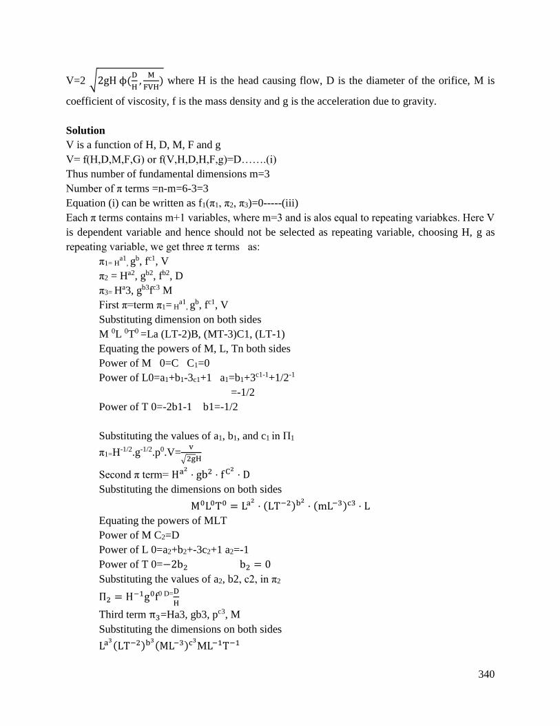
340
V=2 √2gH ϕ(D
H,
M
FVH) where H is the head causing flow, D is the diameter of the orifice, M is
coefficient of viscosity, f is the mass density and g is the acceleration due to gravity.
Solution
V is a function of H, D, M, F and g
V= f(H,D,M,F,G) or f(V,H,D,H,F,g)=D…….(i)
Thus number of fundamental dimensions m=3
Number of π terms =n-m=6-3=3
Equation (i) can be written as f1(π1, π2, π3)=0-----(iii)
Each π terms contains m+1 variables, where m=3 and is alos equal to repeating variabkes. Here V
is dependent variable and hence should not be selected as repeating variable, choosing H, g as
repeating variable, we get three π terms as:
π1= Ha1
, gb, fc1, V
π2 = Ha2, gb2, fb2, D
π3= Ha3, gb3fc3 M
First π=term π1= Ha1
, gb, fc1, V
Substituting dimension on both sides
M 0L 0T0 =La (LT-2)B, (MT-3)C1, (LT-1)
Equating the powers of M, L, Tn both sides
Power of M 0=C C1=0
Power of L0=a1+b1-3c1+1 a1=b1+3c1-1+1/2-1
=-1/2
Power of T 0=-2b1-1 b1=-1/2
Substituting the values of a1, b1, and c1 in Π1
π1=H-1/2.g-1/2.p0.V=v
√2gH
Second π term= Ha2⋅ gb2 ⋅ fC2
⋅ D
Substituting the dimensions on both sides
M0L0T0 = La2⋅ (LT−2)b2
⋅ (mL−3)c3 ⋅ L
Equating the powers of MLT
Power of M C2=D
Power of L 0=a2+b2+-3c2+1 a2=-1
Power of T 0=−2b2 b2 = 0
Substituting the values of a2, b2, c2, in π2
Π2 = H−1g0f0 D=D
H
Third term π3=Ha3, gb3, pc3, M
Substituting the dimensions on both sides
La3(LT−2)b3
(ML−3)c3ML−1T−1
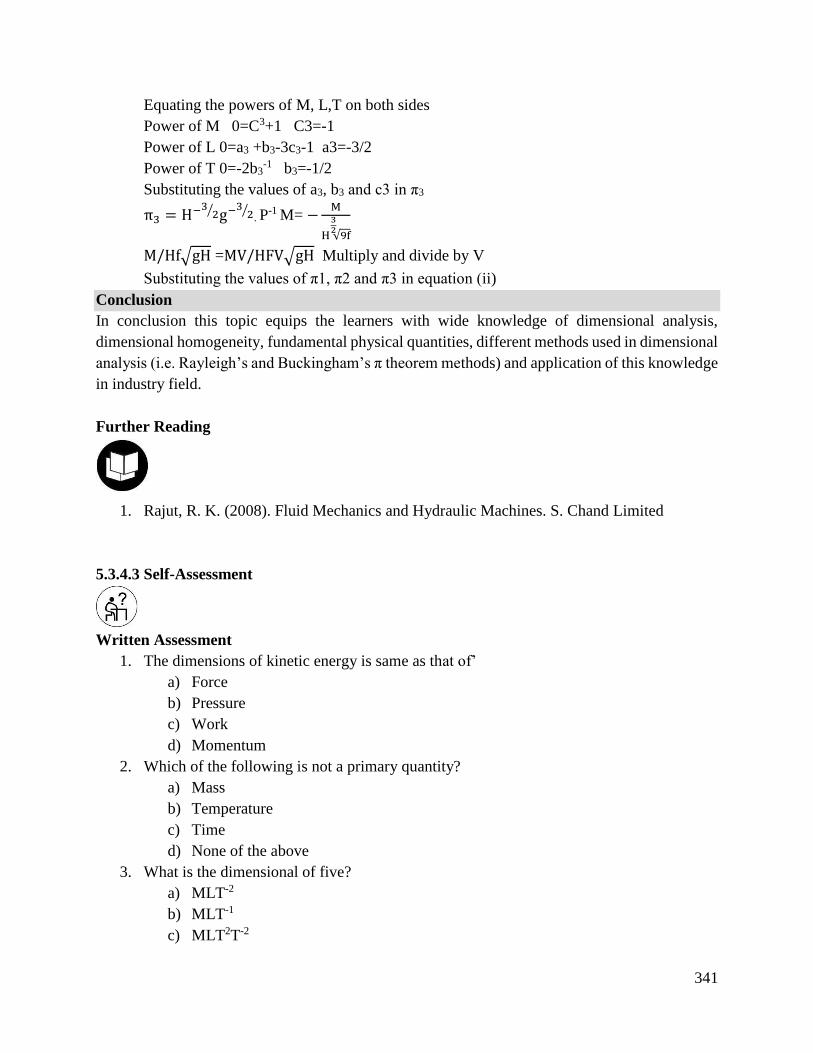
341
Equating the powers of M, L,T on both sides
Power of M 0=C3+1 C3=-1
Power of L 0=a3 +b3-3c3-1 a3=-3/2
Power of T 0=-2b3-1 b3=-1/2
Substituting the values of a3, b3 and c3 in π3
π3 = H−32⁄ g−3
2⁄ . P-1 M= −
M
H √9f
32
M/Hf√gH =MV/HFV√gH Multiply and divide by V
Substituting the values of π1, π2 and π3 in equation (ii)
Conclusion
In conclusion this topic equips the learners with wide knowledge of dimensional analysis,
dimensional homogeneity, fundamental physical quantities, different methods used in dimensional
analysis (i.e. Rayleigh’s and Buckingham’s π theorem methods) and application of this knowledge
in industry field.
Further Reading
1. Rajut, R. K. (2008). Fluid Mechanics and Hydraulic Machines. S. Chand Limited
5.3.4.3 Self-Assessment
Written Assessment
1. The dimensions of kinetic energy is same as that of’
a) Force
b) Pressure
c) Work
d) Momentum
2. Which of the following is not a primary quantity?
a) Mass
b) Temperature
c) Time
d) None of the above
3. What is the dimensional of five?
a) MLT-2
b) MLT-1
c) MLT2T-2
342
d) MLT2T2
4. Which of the following quantities has the dimensions (M0 L0 T0)
a) Density
b) Stress
c) Strain
d) Strain rate
5. Which of the following equations is not dimensionally homogeneous? Consider standard
symbols for quantities
a) (force) F=m × a
b) (head less due to friction) hf+(fbV2)/(2gd)
c) (Torque) T=F ×Distance
d) None of the above
6. The unit of physical quantity which does not depend on the unit of any other physical
quantity is called
a) Independent dimension
b) Fundamental dimension
c) Core dimension
d) None of the above
7. Match the following physical quantities in groups
i. Work done (Energy), W………A (ML2T-3)
ii. Power 9P)……….B. (ML-1T-1)
iii. Momentum (M)…….C(ML2T-2)
iv. Modules of elasticity ……D(MLT-1)
v. Dynamic viscosity (M)…..E(MK-1 T-2)
a) 1-(c), 2-(A), 3-(D), 4(E), 5(B)
b) 1-(A), 2-(C), 3-(D), 4-(E), 5(B)
c) 1-(C), 2-(A), 3-(E), 4-(B), 5(D)
d) 1-(D), 2-(E), 3-(B), 4(A), 5-(C)
8. State the primary qualities
9. What is the meaning of the word dimension
10. What is the SI unit of length?
11. What does MLT stand for in dimensional analysis?
12. Apart from MLT, which other dimensions are fundamental.
Oral Assessment
1. What is dimensional analysis?
2. What is the meaning of dimensional homogeneity.
343
Practical Assessment
A dimensional analysis experiment for the fluid mechanics.
Objectives
The main objective is to design and construct a fluid mechanics experiment to illustrate the concept
and usefulness of dimensional analysis.
Experimental apparatus and procedure
The upper tubing (91/2 and ¾ type l), including valves and fitting is mounted on ½ ply and board.
Allow air and water supplies to enter the upper tubing at left end of tubing. Use full-port ball valves
for selection of fluid and control of the flow rate. Mount the specimen at the right end of the copper
tubing. Water leaving the specimen (i.e. nozzle) is caught by a 1-1/2 inch diameter drain lime
which leads to a 12 gallon paltic rectangular tank. The tank has a sub-mersibe pump which
recirculates the water through the experiment. The air compressor for the air flow. The digital
meter measures the fluid pressure just upstream of the specimen Clamp the drain less support and
the air flow meter to tables for every removal for storage.
The specimen consists of ½ make pipe to tubing adapter with one-inch long aluminum rod instead.
The rod is 5/8 inch diameter so it snugly fit into the male adapter. Fabricate (nine) specimen each
specimen with a different diameter hole drilled through the aluminum rod. The diameters should
vary from 1.8 to 3.8 at 1/32 increments. Use gorilla glue to glue the rod to the adapter. Perform
the experimental runs with water and drop arrows nozzle varies with the nozzle dimensions and
the flow rate
Project
1. Fabricate a nozzle for each specimen with different diameter hole drilled through the
aluminum rod. The diameters should vary from 3.175 to 9.525, at 0.793 mm increments.
2. Fabricate a nozzle specimens each specimen with different diameter hole drilled through
the aluminum rod. The diameter should vary from 3.175 mm to 9.525mm at 0.793 mm
increment
5.3.4.4 Tools, Equipment, Supplies and Materials
Scientific Calculators
Relevant reference materials
Stationeries
Relevant practical materials
Dice

344
Computers with internet connection
5.3.4.5 References
Langhar, H. L., Robert, E. & Malabar, F. L. (n.d.). Dimensional Analysis and the Theory of
Models.
Rajut, R. K. (2008). Fluid Mechanics and Hydraulic Machines. S. Chand Limited
345
5.3.5 Learning Outcome No 4: Operate fluid pumps
5.3.5.1 Learning Activities
Learning Outcome No 4:operate fluid pumps
Learning Activities Special
Instructions
6.1. Describe principle of operation (reciprocating and centrifugal)of
pumps
6.2. Derive reciprocating pump equation(coefficient discharge,
percentage discharge, work done, acceleration head and pressure
head in the cylinder)
6.3. Derive centrifugal pump equation(effective head, manometric
head, manometric efficiency, mechanical efficiency, discharge,
torque, work done, unit weight and specific speed)
6.4. Apply pump equations in problem solving.
5.3.5.2 Information Sheet No5/LO4: Operate fluid pumps
Introduction
Describe principle of operation (reciprocating and centrifugal)of pumps and derivation coefficient
discharge, percentage discharge, work done, acceleration head and pressure head in the cylinder
and the derivation of centrifugal pump equation(effective head, manometric head, manometric
efficiency, mechanical efficiency, discharge, torque, work done, unit weight and specific speed).
Definition of key terms
Mechanical efficiency: Is the ratio of power available at the impeller to the power available at the
centrifugal pump. It is mathematically expressed as:
𝜂𝑚 =𝑝𝑜𝑤𝑒𝑟 𝑎𝑡 𝑡ℎ𝑒 𝑖𝑚𝑝𝑒𝑙𝑙𝑒𝑟
𝑝𝑜𝑤𝑒𝑟 𝑎𝑡 𝑡ℎ𝑒 𝑠ℎ𝑎𝑓𝑡
Discharge (Q): Is the area by the pipe velocity of flow of fluid. It is equal to point of entry and
discharge.
Q=Area × velocity of flow = ΠD1B1 × Vf1 = ΠD2B2 × Vf2
Coefficient of discharge (Cd): Is the ratio of actual discharge to that of the theoretical discharge
i.e. is the ratio of mass flow rate at discharge end to that of an ideal nozzle.
Mathematically expressed as;
𝐶𝑑 =𝑄𝑒𝑥𝑝
𝑄𝑡ℎ𝑒𝑜
346
Work done by reciprocating pump (W): Is the product of weight of fluid lifted per second and
the total height through which the fluid is lifted. Mathematically, it is expressed as;
Work done per second = W × ( hs +hd)
Where W is the weight of fluid
( hs +hd) is the total height which fluid is lifted.
Manometric suction head (hms): Is the negative gauge pressure shown by a manometer attached
to the pump inlet. It is given by:
Hms = - ZS + VS2 + ∑h 1S Where ZS is the suction of the pump VS is the swept volume.
Content/Procedures/Methods/Illustrations
4.1 Describe principle of operation of reciprocating and centrifugal pumps.
Centrifugal pumps
The centrifugal pump worked on the principle of forced vertex flow (When a certain mass of fluid
is rotated externally by a given torque, there is a rise in pressure head of the rotating liquid.)
This rise in pressure head at any point of the rotating liquid is proportional to the square of the
tangential velocity of liquid at that point. i.e.
Rise in pressure head = V2 2g (where V is the velocity and g is the gravitational pull).
Since at the outlet of the impeller, the radius is larger, there’s a rise in pressure head thus liquid
being lifted to a higher level.
Reciprocating pumps
This pump on a to and fro motion principle. The piston which is driven by a crank powered by
some prime mover such as electric motor moves to and fro in a cylinder.
Suction and delivery pipes with suction and delivery and suction valves are connected to the
cylinder. The two valves are non-return valves which allow the fluid to flow in one direction.
Operation
Rotation of the crank moves the piston to and fro in the cylinder. Movement of the piston away
from the valve end of the cylinder I.e. to the right (if fig 24.1) leads to reduction of pressure in the
cylinder. This enables atmospheric pressure (pa) acting on the free surface of the fluid in lower
reservoir to force the fluid p the suction pipe into the cylinder. Thus the outward movement of the
piston constitutes a suction stroke.
The suction stroke is followed by a delivery stroke (liquid in cylinder pushed to upper reservoir
through the delivery pipe). During the delivery stroke, delivery valve is closed because of the fluid
pressure exerted onto it.
The whole cycle is then repeated depending upon the rotation speed of the crank. The cycles can
be represented by a plot of pressure in the cylinder against volume of the fluid. Figure 24.2 shows
a basic pressure diagram for a reciprocating pump.
347
4.2 Reciprocating pump equation (derivation).
Work done by a reciprocating pump.
Work done by reciprocating pump per second is given by:
Work done per second =weight of water lifted per second × Total height which water is lifted.
= W × (hs+ hd)
Where (hs+ hd) = total height through which the fluid is lifted.
Weight W is given by;
𝑊 =𝜌𝑔 × 𝐴𝐿𝑁
60
Where ρ =density of the fluid
A = Area (cross-section area of the cylinder)
L = Length of the stroke
N 60 = Number of revolutions per second.
Therefore, Work done per second =[𝜌𝑔×𝐴𝐿𝑁
60 ] × (hs + hd)
The coefficient discharge.
Coefficient of discharge, Cd=𝑀𝑎𝑠𝑠 𝑓𝑙𝑜𝑤 𝑟𝑎𝑡𝑒
𝑑𝑒𝑛s𝑖𝑡𝑦 𝑜𝑓 𝑡ℎ𝑒 𝑓𝑙𝑢𝑖𝑑 ×𝑣𝑜𝑙𝑢𝑚𝑒𝑡𝑟𝑖𝑐 𝑓𝑙𝑜𝑤 𝑟𝑎𝑡𝑒
Cd = m/ρv
But v (volumetric flow rate) = A × u
Where A =cross-section area of the floe constriction
u is the velocity of the fluid through constriction,
Therefore Cd =𝑀
𝜌𝐴𝑢
Coefficient of discharge Cd =𝑄𝐴𝐶
𝑄+𝑛
Percentage discharge.
Percentage discharge =𝑠𝑙𝑖𝑝
𝑇ℎ𝑒𝑟𝑜𝑟𝑒𝑡𝑖𝑐𝑎𝑙 𝑑𝑖𝑑𝑐ℎ𝑎𝑟𝑔𝑒 × 100
Slip = Theoretical discharge – actual discharge = Qth –Qac
Therefore percentage discharge =𝑄𝑡ℎ –𝑄𝑎𝑐
𝑄𝑡ℎ × 100 = (1 −
𝑄𝑎𝑐
𝑄𝑡ℎ) × 100
But 𝑄𝑎𝑐
𝑄𝑡ℎ = Cd
Therefore percentage discharge = (1 –Cd) ×100
Where Cd = coefficient of discharge.
Acceleration Head
Acceleration head, ha = LVNC
Where L, is the length of the suction pipe
348
V, is the velocity of the fluid in the suction pipe
N, is the rotation of the crank
C, constant (reciprocating pump)
Acceleration head
Maximum pressure head due to acceleration is given by;
(ha)max =l g ×A aw2r
Given pressure head as
Ha =𝑖𝑛𝑡𝑒𝑛𝑠𝑖𝑡𝑦 𝑜𝑓 𝑝𝑟𝑒𝑠𝑠𝑢𝑟𝑒 𝑑𝑢𝑒 𝑡𝑜 𝑎𝑐𝑐𝑒𝑙𝑒r𝑎𝑡𝑖𝑜𝑛
𝑤𝑒𝑖𝑔ℎ 𝑑𝑒𝑛𝑠𝑖𝑡𝑦 𝑜𝑓 𝑡ℎ𝑒 𝑙𝑖𝑞𝑢𝑖𝑑
= 𝜌𝑙 ×𝐴 𝑎𝑤2 ×𝑐𝑜𝑠ɵ
𝜌𝑔= l g ×A aw2 r 𝑐𝑜𝑠ɵ
I. when ɵ = 0 , ha = l g ×A aw2r
II. when ɵ =90 ,ha = 0
III. when ɵ =180 , ha = - l g ×A aw2r
Thus the maximum pressure head due to acceleration
(ha)max = l g ×A aw2r
4.3 Centrifugal pump equation
Mechanical efficiency
Mechanical efficiency of a centrifugal pump is given by :
ηm=𝑝𝑜𝑤𝑒𝑟 𝑜𝑓 𝑖𝑚𝑝𝑒𝑙𝑙𝑒𝑟
𝑝𝑜𝑤𝑒𝑟 𝑜𝑓 𝑠ℎ𝑎𝑓𝑡where ηm, Mechanical efficiency.
Power at the impeller in KW =𝑤𝑜𝑟𝑘𝑑𝑜𝑛𝑒 𝑏𝑦 𝑖𝑚𝑝𝑒𝑙𝑙𝑒𝑟 𝑝𝑒𝑟 𝑠𝑒𝑐𝑜𝑛𝑑
1000 = W g ×
𝑉𝑤2 𝑈2
1000
Where W = Weight of fluid
𝑉𝑤2 = velocity of the outlet.
U2 = Tangential velocity of the impeller
Therefore ηm=𝑊 𝑔 ×(𝑉𝑤2 𝑈2) 1000
𝑠.𝑝 where s.p is the power at the shaft.
Manometric efficiency.
Manometric efficiency =𝑀𝑎𝑛𝑜𝑚𝑒𝑡𝑟𝑖𝑐 𝑓𝑖𝑒𝑙𝑑
𝐻𝑒𝑎𝑑 𝑖𝑚𝑝𝑒𝑟𝑡𝑒𝑑 𝑏𝑦 𝑖𝑚𝑝𝑒𝑙𝑙𝑒𝑟 𝑜𝑛 𝑡ℎ𝑒 𝑓𝑙𝑢𝑖𝑑 =
𝐻𝑚
(𝑉𝑤2 𝑈2) 𝑔 =
𝑔𝐻𝑚
𝑉𝑤2 𝑈2
ԧm = (𝑊×𝐻𝑚) 1000
𝑤 𝑔 ×( 𝑉𝑤2 𝑈2) 1000 =
𝑔 ×𝐻𝑚
𝑉𝑤2 𝑈2
349
Discharge
Discharge = area ×velocity of flow
Q = ΠD B × Vf
Where D is the diameter of the impeller at the inlet or the outlet
B is the width of the impeller at the inlet or the outlet
Vf is the velocity of flow at the inlet or outlet
Manometric head
Manometrichead =𝑉𝑤2 𝑈2
𝑔 – losses of head in impeller casing
Hmano = 𝑉𝑤2 𝑈2
𝑔 - (Kv2
2) 2g
Where V2 is the absolute velocity of the water at outlet of the impeller.
U2 is the velocity of the impeller at the outlet
K constant
Hm = hs+hd+hfi + hfd+V2d 2g
Work done
Using outlet and inlet triangles
Work done = -[ 1g(Vw1u1 - Vw2u2)]= [ 1g(Vw2u2 - Vw1u1)]
= 1gVw2u2
Where u1=tangent velocity of impeller at inlet
u2 =tangent velocity of impeller at outlet
Vw2, Vw1 = absolute velocities at inlet and outlet
Therefore: work done by impeller on water per second = Wg×Vw2u2
Effective head
Effective head = suction head + delivery head
Heff =Hs+ Hd
Unit weight
Weight of water = ρgQ
Where Q = volume of water = ΠDB × Vf1
Specific speed
Discharge Q = Area × velocity of flow =ΠD × B × vf…………………1
Where D = diameter of impeller
B =width of impeller
Tangent velocity is known to be; u = ΠDN 60 αDN.2
350
And the tangent velocity (u) and the velocity of flow (vf) are related to the manometric head (Hm)
as
u αvf α √Hm ……………………………………………3
Substituting value of u in 2 we have
√𝐻𝑚 𝛼 𝐷𝑁 𝑜𝑟 𝐷 𝛼 √𝐻𝑚/𝑁
Substituting value of D in 1 we get
𝑄 𝛼√𝐻𝑚 𝑁2 × 𝑣𝑓
𝛼√𝐻𝑚 𝑁2 × √𝐻𝑚 = 𝐻𝑚3/2 𝑁2
Q = k√Hm N2 k is constant of proportionality
Given Hm = 1m and Q = 1m2/s N becomes Ns
1 = 𝑘 13/2 𝑁𝑠2 = 𝑘 / 𝑁𝑠2
𝑘 = 𝑁𝑠2
𝑄 = 𝑁𝑠2 𝐻𝑚 𝑁2
Therefore 𝑁𝑠 = 𝑁√𝑄 𝐻𝑚3/2
4.4 Pump equations are applied in problem solving
1. A single acting reciprocating pump, running at 50RPM delivers 0.01 m3/s of water.
The diameter of the piston is 200mm and the stroke length is 400mm. Determine
a) The theoretical discharge of the pump
b) Coefficient of discharge
c) Slip and percentage discharge of the pump.
Solution
Speed of the pump N = 50 r.p.m
Actual discharge Qact = 01 m3/s
Diameter of the piston = 200mm = 0.2m
Therefore Area, 𝐴 = 𝜋 /4 × (0.2)2 =0.031416m2
Stroke = L = 400mm = 0.40m
i) Theoretical discharge
Qth=𝐴𝐿𝑁
60 =
0.031416×0.04 ×50
60= 0.01047 m3/s
351
ii) Coefficient of discharge
Cd =Qact/ Qth = 0.01/0.01047 = 0.955
iii) Slip and percentage of discount
Slip = Qth -Qact = .0.01047-0.01 = 0. 00047 m3/s
% discount =𝑄tℎ − 𝑄𝑎𝑐𝑡
𝑄𝑡ℎ × 100 =
0.01047−0.01
0.01047 × 100
= 4.489%
2. A centrifugal pump discharges 0.15 m3/s of water against a head 12.5 m.The speed of impeller
being 600 r.p.m. The outer and inner diameters of the impeller are 500mm and 250mm
respectively.
If the area of the flow is 0.07 m2 of inlet and outlet. Calculate, given vane angle= 35
i) Manometric efficiency of the pump
Solution given
Discharge Q = 0.15 m3/s
Head, Hm 12.5m
Speed, N = 600r.p.m
Outlet diameter, D2 = 500mm =0.5m, inner diameter D1 = 250mm = 0.25m
Area = 0.07m2
Discharge = Area of flow × velocity of flow
0.15 = 0.07 × velocity of flow
Velocity of flow 0.15/ 0.07 = 2.14 m/s
Vf1 = Vf2 = 2.14m/s since the area of the flow is constant.’
Tangential velocity of impeller at inlet and outlet
U1 = 𝜋𝐷1𝑁
60 =
𝜋×0.25×600
60 = 7.85m/s
U2= 𝜋𝐷2𝑁
60 =
𝜋×0.50 ×600
60 = 15.70m/s
From outlet velocity Vw2= U2 - Vf1 /tanɵ =15.70- 2.14 /tan35 = 12.64m/s
manometric efficiency= 𝑔×𝐻𝑚
𝑉𝑤2× 𝑈2 =
9.81 ×12.5
12.64×15.7 = 0.618 or 61.8%
Further reading
1. Fluid Mechanics John F Douglas 5th edition
352
2. R.K. Rajput, (2008). Fluid mechanics and hydraulic Machines. S. Chand Limited
5.3.5.3 Self-Assessment
Written Assessment
1. Discharge through a pump per second is given by?
a) Q=2𝐴𝐿𝑁
60
b) Q=AN
c) Q= 2ALN
d) Q =πDB×Vf
2. A Hydraulic machine that converts mechanical energy into pressure energy by the means
of centrifugal force is known as?
a) Reciprocating pump
b) pump
c) Centrifugal pump
d) turbine
3. Which one of the following is not the main part of a centrifugal pump?
a) Suction pipe
b) Delivery pipe
c) Impeller
d) Suction Valve
4. Which of the two pumps has a low velocity?
a) Reciprocating pump
b) Centrifugal pump
5. What does the word slip mean as applied in centrifugal pumps?
a) The difference between theoretical discharge and actual discharge
b) The ratio of actual discharge to theoretical discharge
c) The product of area and velocity of the flow
d) The product of area and velocity of flow
6. Which classification of reciprocating pumps according to number of cylinders is not true?
a) Double cylinder
b) Single cylinder pump
c) Single acting pump
d) Triple cylinder pump
7. Power required to driven a pump is given by _______________
a) 𝑊𝑜𝑟𝑘𝑑𝑜𝑛𝑒
1000
b) 2
3× 𝐵𝑎𝑠𝑒 × ℎ𝑒𝑖𝑔ℎ𝑡
c) Velocity of piston ×Area of piston
d) ΡgQ
353
8. Describe the word impeller as used in fluid pumps.
9. The fluid coming from the centrifugal pump is accelerated by?
10. Discuss the working principle of a centrifugal pump with aid of diagram.
11. Describe the main of a centrifugal pump.
12. Show that discharge Q =area × velocity of flow.
Oral Assessment
1. Classify reciprocating pumps according to number of cylinder
2. Describe the principle of operation of a reciprocating pump.
Practical Assessment
1. To find the efficiency of a reciprocating pump.
Objective: To determine the efficiency of reciprocating pump.
Apparatus
Motor(DC)
Gear
Piston and connecting rod
Cylinder
Delivery valve
Suction valve
Fluid (water)
Measuring tank to measure discharge fluid
Diagram (fig 20.1 pg. 985, a textbook of fluid mechanics and hydraulic machines by Dr R.K
Bansal)
Procedure
i. Fill up sufficient water in the sump tank (done after assembly of all parts of the
pump).
ii. Open gate valve in discharge pipe of the pump fully
iii. Connect the gear to the piston rod and connecting rod. (check nut bolts and driving
belt on the motor of proper tightening)
iv. Connect motor to electric supply and switch on the supply.
v. Close the discharge valve slightly and note down the speed delivery
vi. Repeat procedure for different gate valve
vii. Take different readings by changing the speed and the gate valve.
Project
Design and fabrication of a pedal operated reciprocating pump.
Apparatus
A pair of pedals
Two crank joined by chain
Bicycle assembly

354
Cylinder
Non return valve
Delivery pipe and suction pipe
Tank with water to act as a samp tank
Measuring tank to receive discharge water
Specification
Bicycle assembly fabricated is joined to the cylinder using the crank slider mechanism. The
cylinder has non return valves that is joined to a suction pipe. Then the deliver pipe is connected
to the cylinder at a specific height, h.
5.3.5.4 Tools, equipment supplies and materials
Scientific calculator
Relevant reference materials
Stationaries
Relevant practice materials
Computer with internet connection.
5.3.5.5 References
Bansal, D.R, (2005). A Text book of fluid Mechanics and Hydraulic Machines. Firewell Media
Douglas, J. F. (2008). Fluid mechanics. 5th edition
Rajput, R. K. (2008). Fluid Mechanics and Hydraulic Machines. S. Chand Limited.
355
CHAPTER 6: THERMODYNAMICS / APPLY FLUID MECHANICS PRINCIPLES
6.1 Introduction
Thermodynamics is among the common units of competencies offered in all the TVET level 6
engineering courses qualification. This unit describes the competencies required by a technician
in order to apply thermodynamics principles in their work. It includes understanding fundamentals
of thermodynamics, performing steady flow processes, performing non steady flow processes,
understanding perfect gases, generating steam, performing thermodynamics reversibility and
entropy, understanding idea gas cycle, demonstrating fuel and combustion, perform heat transfer,
understanding heat exchangers, understanding air compressors, understanding gas turbines and
understanding of impulse steam turbines. The significance of thermodynamics to TVET level 6
engineering curriculum is to enable learners acquire knowledge and skills to demonstrate logical
thinking, problem solving, applying statistics, drawing graphs, using different measuring tools to
get along well in the workplace and task.
The critical aspect of competency to be covered includes; carrying out troubleshooting,
Overhauled construction plant engines ,Serviced engine lubrication system, Serviced cooling
system ,Serviced fuel induction components ,Diagnosed and serviced starting devices and
Prepared engine repair and service report .The basic resources required includes access to relevant
workplace or appropriately simulated environment where assessment can take place, measuring
tools and equipment, Sample materials to be tested among others. The unit of competency covers
four learning outcomes. Each of the learning outcome presents; learning activity that covers
performance criteria statements, thus creating trainee’ an opportunity to demonstrate knowledge
and skills in the occupational standards and content in curriculum. Information sheet provides;
definition of key terms, content and illustration to guide in training. The competency may be
assessed through direct observation, demonstration with oral questioning, case studies and written
tests. Self-assessment is provided at the end of each learning outcomes. Holistic assessment with
other units relevant to the industry sector workplace and job role is recommended.
6.2 Performance Standard
Understand flow of fluids, demonstrate knowledge in viscous flow and derive viscous flow
equation in circular pipes and apply them in problem solving, perform dimensional analysis and
operate fluid pumps, pump equations in problem solving in accordance with the set standards.
6.3 Learning Outcomes.
6.3.1 List of Learning Outcomes
a) Understand fundamentals of thermodynamics
b) Perform steady flow processes
c) Perform non-steady flow processes

356
d) Understand perfect gases
e) Generate steam
f) Perform thermodynamics reversibility and entropy
g) Understand ideal gas cycle
h) Demonstrate fuel and combustion.
i) Perform heat transfer
j) Understand heat exchangers
k) Understand air compressors
l) Understand gas turbines
m) Understanding impulse steam turbines
357
6.3.2 Learning Outcome No 1: Understand fundamentals of thermodynamics
6.3.2.1 Learning Activities
Learning Outcome No1: Understand fundamentals of thermodynamics
Learning Activities Special Instructions
1.1 Describe terms used in thermodynamics
1.2 Describe thermodynamics processes and cycles
1.3 Apply first law of thermodynamics
Define first law as given.
Differentiate types of processes.
6.3.2.2 Information Sheet No.6/LO1: Understand fundamentals of thermodynamics
Introduction
This learning outcome covers; definition of terms, thermodynamics systems, types of working
fluids, thermodynamics cycles, definition of work, types of thermodynamic process and statement
of the first law of thermodynamics.
Definition of key terms
Thermodynamics: It is a branch of engineering science that deals with heat, work and their
relationship.
Thermodynamic systems: It consists of a mass of a fluid contained within defined boundary
together with the surrounding.
Energy: It is a property of a body which gives it a capacity to do work.
Content/procedures/methods/illustrations
1.1 Terms used in thermodynamics are described
Thermodynamics state: Is a value which defines two or more thermodynamic properties.
What is thermodynamic state function?
A state function describes the equilibrium state of a system and also describes the type of the
system. For example, internal energy, enthalpy and entropy are state quantities because they
describe quantitatively an equilibrium state of a thermodynamic system irrespective of how the
system arrived to that state.
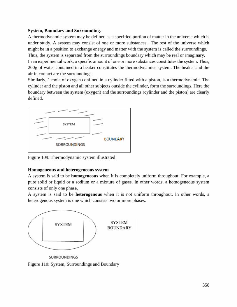
358
System, Boundary and Surrounding.
A thermodynamic system may be defined as a specified portion of matter in the universe which is
under study. A system may consist of one or more substances. The rest of the universe which
might be in a position to exchange energy and matter with the system is called the surroundings.
Thus, the system is separated from the surroundings boundary which may be real or imaginary.
In an experimental work, a specific amount of one or more substances constitutes the system. Thus,
200g of water contained in a beaker constitutes the thermodynamics system. The beaker and the
air in contact are the surroundings.
Similarly, 1 mole of oxygen confined in a cylinder fitted with a piston, is a thermodynamic. The
cylinder and the piston and all other subjects outside the cylinder, form the surroundings. Here the
boundary between the system (oxygen) and the surroundings (cylinder and the piston) are clearly
defined.
Figure 109: Thermodynamic system illustrated
Homogeneous and heterogeneous system
A system is said to be homogeneous when it is completely uniform throughout; For example, a
pure solid or liquid or a sodium or a mixture of gases. In other words, a homogeneous system
consists of only one phase.
A system is said to be heterogenous when it is not uniform throughout. In other words, a
heterogenous system is one which consists two or more phases.
Figure 110: System, Surroundings and Boundary

359
Water contained in a beaker constitutes a system
Water contained in beaker consists of a system. This system consisting of two or more immiscible
liquids or a solid in contact to a liquid in which it does not dissolve. It is a heterogeneous system.
A liquid in contact with its vapor is a heterogeneous system because it consists of two phases.
Types of thermodynamics system
There are three types of thermodynamic systems depending on the nature of the boundary which
it follows;
Isolated system: When the boundary is both sealed and insulated, no interaction is possible with
the surroundings. Therefore, an isolated system is one that can transfer neither matter nor energy
to and from its surroundings. A boiling water contained in a thermos flask is another example of
an isolated system.
Closed system: The boundary is sealed but not insulated. Therefore, closed system is one which
cannot transfer matter but can transfer energy in the form of heat, work and radiation from its
surroundings. A specific amount of hot water contained in a sealed tube is an example of a closed
system, while no water vapor can escape from the system, it can transfer heat through the walls of
the tube to the surroundings. A gas contained in a cylinder with a piston constitute a closed system.
As the piston is raised, the gas expands and transfer heat(energy) in the vapour to the surroundings.
Open system: In such a system the boundary is open and uninsulated therefore, an open system is
one which can transfer both energy and matter to and from its surroundings.
Extensive and intensive properties
All microscopic or bulk properties of the system (volume, pressure, mass etc.) irrespective of
whether they are state variables or not can be divided into two classes.
a) Extensive
b) intensive
An extensive property of a system is which depends upon the amount of the substance or
substances present in the system. Examples mass, volume, energy, heat, heat capacity, enthalpy,
entropy and free change.
An intensive property of a system is which is independent of the amount of the substance present
in the system. Examples are temperatures, pressure, density, velocity, retractive index, surface
tension and specific heat.
1.2 Description of Thermodynamic processes and cycles.
Thermodynamic processes: Is an activity which changes the thermodynamic state of a substance
of heating, compression, cooling etc.
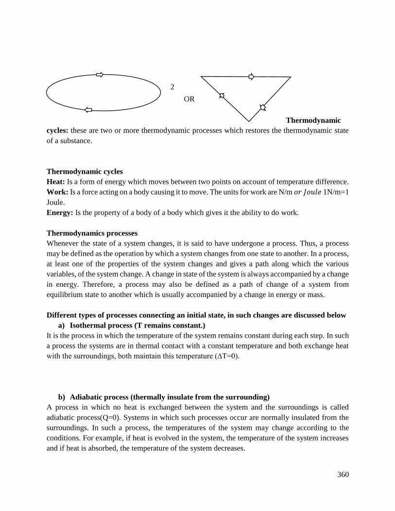
360
Thermodynamic
cycles: these are two or more thermodynamic processes which restores the thermodynamic state
of a substance.
Thermodynamic cycles
Heat: Is a form of energy which moves between two points on account of temperature difference.
Work: Is a force acting on a body causing it to move. The units for work are N/m 𝑜𝑟 𝐽𝑜𝑢𝑙𝑒 1N/m=1
Joule.
Energy: Is the property of a body of a body which gives it the ability to do work.
Thermodynamics processes
Whenever the state of a system changes, it is said to have undergone a process. Thus, a process
may be defined as the operation by which a system changes from one state to another. In a process,
at least one of the properties of the system changes and gives a path along which the various
variables, of the system change. A change in state of the system is always accompanied by a change
in energy. Therefore, a process may also be defined as a path of change of a system from
equilibrium state to another which is usually accompanied by a change in energy or mass.
Different types of processes connecting an initial state, in such changes are discussed below
a) Isothermal process (T remains constant.)
It is the process in which the temperature of the system remains constant during each step. In such
a process the systems are in thermal contact with a constant temperature and both exchange heat
with the surroundings, both maintain this temperature (∆T=0).
b) Adiabatic process (thermally insulate from the surrounding)
A process in which no heat is exchanged between the system and the surroundings is called
adiabatic process(Q=0). Systems in which such processes occur are normally insulated from the
surroundings. In such a process, the temperatures of the system may change according to the
conditions. For example, if heat is evolved in the system, the temperature of the system increases
and if heat is absorbed, the temperature of the system decreases.
OR
2
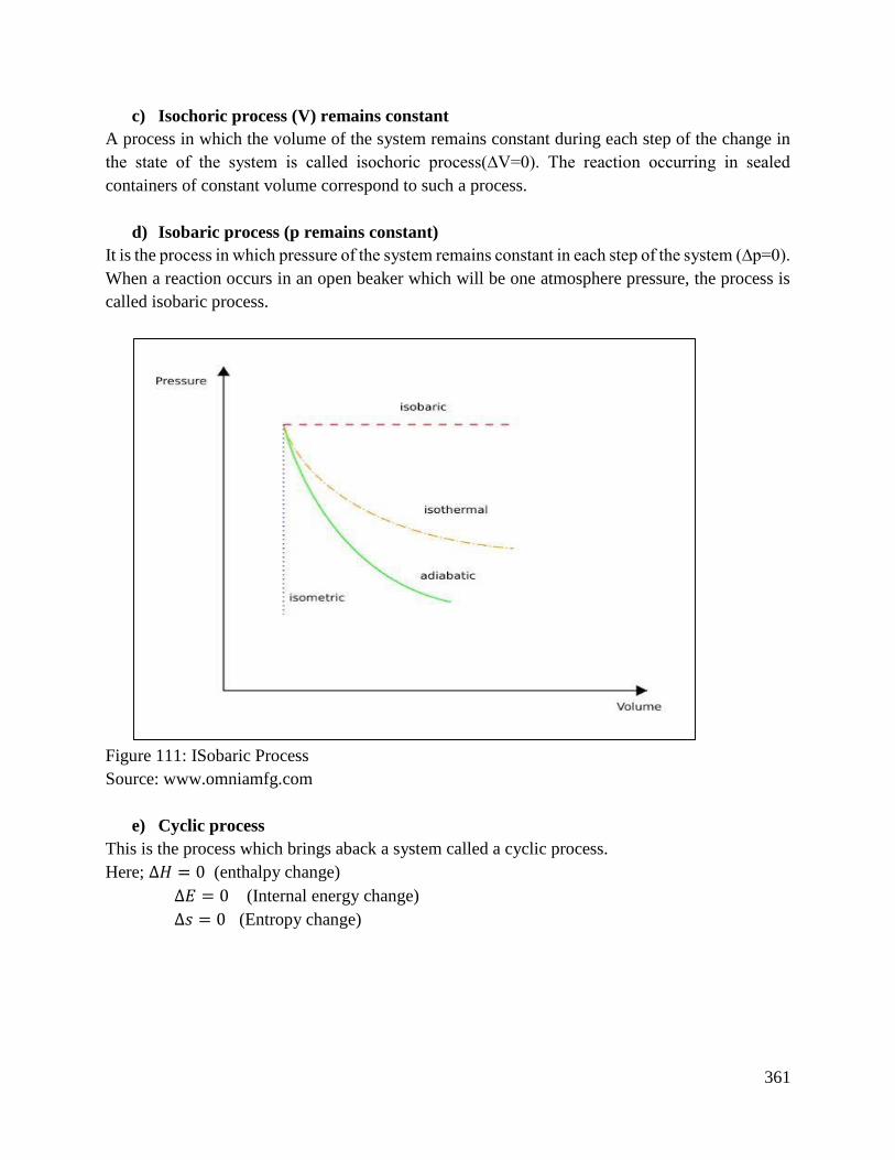
361
c) Isochoric process (V) remains constant
A process in which the volume of the system remains constant during each step of the change in
the state of the system is called isochoric process(∆V=0). The reaction occurring in sealed
containers of constant volume correspond to such a process.
d) Isobaric process (p remains constant)
It is the process in which pressure of the system remains constant in each step of the system (∆p=0).
When a reaction occurs in an open beaker which will be one atmosphere pressure, the process is
called isobaric process.
Figure 111: ISobaric Process
Source: www.omniamfg.com
e) Cyclic process
This is the process which brings aback a system called a cyclic process.
Here; ∆𝐻 = 0 (enthalpy change)
∆𝐸 = 0 (Internal energy change)
∆𝑠 = 0 (Entropy change)
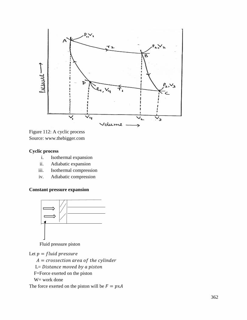
362
Figure 112: A cyclic process
Source: www.thebigger.com
Cyclic process
i. Isothermal expansion
ii. Adiabatic expansion
iii. Isothermal compression
iv. Adiabatic compression
Constant pressure expansion
Let 𝑝 = 𝑓𝑙𝑢𝑖𝑑 𝑝𝑟𝑒s𝑠𝑢𝑟𝑒
𝐴 = 𝑐𝑟𝑜𝑠𝑠𝑒𝑐𝑡𝑖𝑜𝑛 𝑎𝑟𝑒𝑎 𝑜𝑓 𝑡ℎ𝑒 𝑐𝑦𝑙𝑖𝑛𝑑𝑒𝑟
L= 𝐷𝑖𝑠𝑡𝑎𝑛𝑐𝑒 𝑚𝑜𝑣𝑒𝑑 𝑏𝑦 𝑎 𝑝𝑖𝑠𝑡𝑜𝑛
F=Force exerted on the piston
W= work done
The force exerted on the piston will be 𝐹 = 𝑝x𝐴
Fluid pressure piston
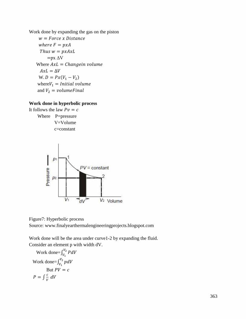
363
Work done by expanding the gas on the piston
𝑤 = 𝐹𝑜𝑟𝑐𝑒 𝑥 𝐷𝑖𝑠𝑡𝑎𝑛𝑐𝑒
𝑤ℎ𝑒𝑟𝑒 𝐹 = 𝑝𝑥𝐴
𝑇ℎ𝑢𝑠 𝑤 = 𝑝𝑥𝐴𝑥𝐿
=px ∆V
Where 𝐴𝑥𝐿 = 𝐶ℎ𝑎𝑛𝑔𝑒𝑖𝑛 𝑣𝑜𝑙𝑢𝑚𝑒
𝐴𝑥𝐿 = ∆𝑉
W. 𝐷 = 𝑃𝑥(𝑉1 − 𝑉2)
where𝑉1 = 𝐼𝑛𝑖𝑡𝑖𝑎𝑙 𝑣𝑜𝑙𝑢𝑚𝑒
and 𝑉2 = 𝑣𝑜𝑙𝑢𝑚𝑒𝐹𝑖𝑛𝑎𝑙
Work done in hyperbolic process
It follows the law 𝑃𝑣 = 𝑐
Where P=pressure
V=Volume
c=constant
Figure7: Hyperbolic process
Source: www.finalyearthermalengineeringprojects.blogspot.com
Work done will be the area under curve1-2 by expanding the fluid.
Consider an element p with width dV.
Work done=∫ 𝑃𝑑𝑉𝑉2
𝑉1
Work done=∫ 𝑝𝑑𝑉𝑉2
𝑉1
But 𝑃𝑉 = 𝑐
𝑃 = ∫𝑐
𝑉 𝑑𝑉
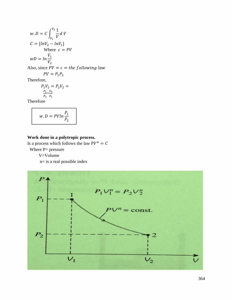
364
𝑤.𝐷 = 𝐶 ∫1
𝑉
𝑉2
𝑉1
𝑑 𝑉
𝐶 = [𝑙𝑛𝑉2 − 𝑙𝑛𝑉1]
Where 𝑐 = 𝑃𝑉
𝑤𝐷 = 𝑙𝑛𝑉1
𝑉2
Also, since 𝑃𝑉 = 𝑐 = 𝑡ℎ𝑒 𝑓𝑜𝑙𝑙𝑜𝑤𝑖𝑛𝑔 𝑙𝑎𝑤
𝑃𝑉 = 𝑃1𝑃2
Therefore,
𝑃1𝑉2 = 𝑃2𝑉2 =
𝑃1
𝑃2=
𝑉2
𝑉1
Therefore
Work done in a polytropic process.
Is a process which follows the law P𝑉𝑛 = 𝐶
Where P= pressure
V=Volume
n= is a real possible index
𝑤.𝐷 = 𝑃𝑉𝑙𝑛𝑃1
𝑃2
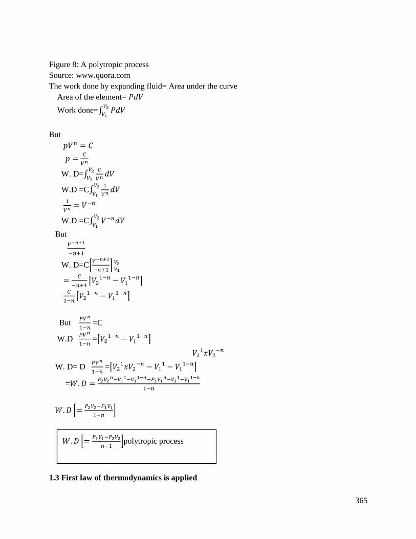
365
Figure 8: A polytropic process
Source: www.quora.com
The work done by expanding fluid= Area under the curve
Area of the element= 𝑃𝑑𝑉
Work done=∫ 𝑃𝑑𝑉𝑉2
𝑉1
But
𝑝𝑉𝑛 = 𝐶
𝑝 =𝐶
𝑉𝑛
W. D=∫𝐶
𝑉𝑛 𝑑𝑉𝑉2
𝑉1
W.D =C∫1
𝑉𝑛 𝑑𝑉𝑉2
𝑉1
1
𝑉𝑛 = 𝑉−𝑛
W.D =C∫ 𝑉−𝑛𝑑𝑉𝑉2
𝑉1
But
𝑉−𝑛+1
−𝑛+1
W. D=C⌈𝑉−𝑛+1
−𝑛+1⌉ 𝑉2
𝑉1
=𝐶
−𝑛+1⌈𝑉2
1−𝑛 − 𝑉11−𝑛⌉
𝐶
1−𝑛⌈𝑉2
1−𝑛 − 𝑉11−𝑛⌉
But 𝑃𝑉𝑛
1−𝑛 =C
W.D 𝑃𝑉𝑛
1−𝑛 =⌈𝑉2
1−𝑛 − 𝑉11−𝑛⌉
𝑉21𝑥𝑉2
−𝑛
W. D= D 𝑃𝑉𝑛
1−𝑛 =⌈𝑉2
1𝑥𝑉2−𝑛 − 𝑉1
1 − 𝑉11−n⌉
=𝑊.𝐷 =𝑃2𝑉2
𝑛−𝑉11−𝑉1
1−𝑛−𝑃1𝑉1𝑛−𝑉1
1−𝑉11−𝑛
1−𝑛
𝑊. 𝐷 [=𝑃2𝑉2−𝑃1𝑉1
1−𝑛]
1.3 First law of thermodynamics is applied
𝑊.𝐷 [=𝑃1𝑉1−𝑃2𝑉2
𝑛−1]polytropic process
366
The first law of thermodynamics states that when a system undergoes a thermodynamic cycle, then
the net heat supplied to the system from its surroundings plus the net input to the system from its
surroundings must be equal to zero. The first law of thermodynamics is a version of the law of
conservation of energy, adapted from the thermodynamic systems. The laws of conservation of
energy states that energy can neither be created nor destroyed but can be transformed from one
form to another.
∑𝑜𝑞 + ∑𝑜𝑊 = 0 where
Q =Heat supplied or rejected to the system from the surroundings.
W=net work input.
The heat inflow to the system is positive.
The work outflow from the system is negative.
Internal energy of a fluid
The energy responsible for random motion of the molecules of the fluid and is denoted as symbol
(µ).
Specific internal energy
It is the internal energy of a fluid per unit mass and per kg.
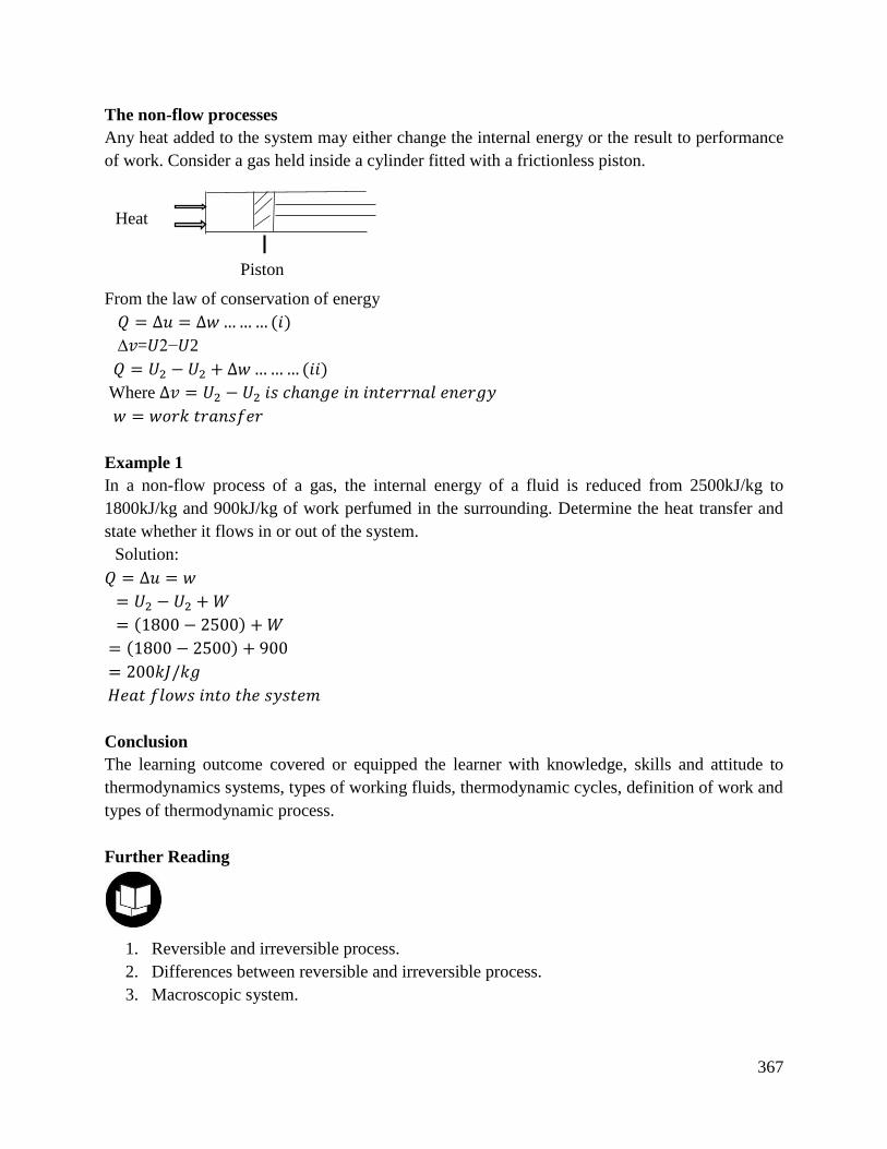
367
The non-flow processes
Any heat added to the system may either change the internal energy or the result to performance
of work. Consider a gas held inside a cylinder fitted with a frictionless piston.
From the law of conservation of energy
𝑄 = ∆𝑢 = ∆𝑤 ………(𝑖)
∆𝑣=𝑈2−𝑈2
𝑄 = 𝑈2 − 𝑈2 + ∆𝑤 ………(𝑖𝑖)
Where ∆𝑣 = 𝑈2 − 𝑈2 𝑖𝑠 𝑐ℎ𝑎𝑛𝑔𝑒 𝑖𝑛 𝑖𝑛𝑡𝑒𝑟𝑟𝑛𝑎𝑙 𝑒𝑛𝑒𝑟𝑔𝑦
𝑤 = 𝑤𝑜𝑟𝑘 𝑡𝑟𝑎𝑛𝑠𝑓𝑒𝑟
Example 1
In a non-flow process of a gas, the internal energy of a fluid is reduced from 2500kJ/kg to
1800kJ/kg and 900kJ/kg of work perfumed in the surrounding. Determine the heat transfer and
state whether it flows in or out of the system.
Solution:
𝑄 = ∆𝑢 = 𝑤
= 𝑈2 − 𝑈2 + 𝑊
= (1800 − 2500) + 𝑊
= (1800 − 2500) + 900
= 200𝑘𝐽/𝑘𝑔
𝐻𝑒𝑎𝑡 𝑓𝑙𝑜𝑤𝑠 𝑖𝑛𝑡𝑜 𝑡ℎ𝑒 𝑠𝑦𝑠𝑡𝑒𝑚
Conclusion
The learning outcome covered or equipped the learner with knowledge, skills and attitude to
thermodynamics systems, types of working fluids, thermodynamic cycles, definition of work and
types of thermodynamic process.
Further Reading
1. Reversible and irreversible process.
2. Differences between reversible and irreversible process.
3. Macroscopic system.
Piston
Heat
368
6.3.2.3 Self-Assessment
Written assessment
1. In the compression state of an initial combustion engine, the heat rejected to cooling water is
45kJ/kg and the work input is 90kJ/kg. Calculate the change in specific internal energy of the
working fluid stating whether it is a heat gain or loss.
a) ∆v=-236kJ/kg
b) ∆v=137k/J/kg
c) ∆v=-135kJ/kg
2. What does the law of conservation of energy state?
a) Energy can neither be created or destroyed but can be transformed from one form to
another.
b) Action and reaction force are the same.
c) No machine can produce energy without corresponding expenditure of energy.
3. A certain fluid at 10 bars is contained in a cylinder behind a piston, the initial volume being
0.05𝑚3. Calculate the work done by the fluid when it expands reversibly at a constant pressure
to a final volume of 0.2𝑚3.
a) 136kJ
b) 170kJ
c) 151.5kJ
4. 0.05𝑚3 of a gas at 6.9 bar expands reversibly in a cylinder behind a piston according to the
law 𝑃𝑉1.2 = 𝑐𝑜𝑛𝑠𝑡𝑎𝑛𝑡 until the volume is 0.08𝑚3. Calculate the work done by the gas and
sketch the process on a p-V diagram.
a) 𝑊.𝐷 = 2000𝑁/𝑚2
b) 𝑊.𝐷 = 23649.6𝑁/𝑚2
c) 𝑊.𝐷 = 15476.4𝑁/𝑚2
5. A Cylinder contains 0.15𝑚3 of a gas at a pressure of 4 bar. The gas expands to a final volume
of 0.85𝑚3. Determine the work done by the expanding gas, if the expansion occurs.
i. According to the hyperbolic law 𝑝𝑣 = 𝐶
a) 300kJ
b) 200 kJ
c) 282.8kJ
d) 490.545 kJ
ii. At a constant pressure
369
a) 600 kJ
b) 900kJ
c) 282.8kJ
iii. According to the law 𝑃𝑉1.38 = 𝑐𝑜𝑛𝑠𝑡𝑎𝑛𝑡
a) 111kJ
b) 112.36kJ
c) -744.21kJ
d) -634.9kJ
6. What is the meaning of the following terms.
i. Thermodynamics
ii. Heat
7. Give two types of thermodynamic processes.
8. What is the meaning of the following terms.
i. Work
ii. Energy
9. What does the law of conservation of energy state?
10. Differentiate between reversible and irreversible processes.
Oral Assessment
1. Describe the first law of thermodynamics.
2. Describe what is an isothermal process.
Practical Assessment
1. You are provided with the following to experiment what happens on an open system in a
laboratory.
Hot water
Table
beaker
Pour the hot water in a beaker and put them on a table.
Results
The water vapour (matter) and also heat(energy) is transferred to the surrounding through the
imaginary boundary, thus demonstrating an open system.
Project
Using a pencil and a graphical book. Draw the procession of a p-v diagram on work done in
polytropic process and derive the equation.
6.3.2.4 Tools, Equipment, Supplies and Materials 𝑊.𝐷 [=𝑃1𝑉1−𝑃2𝑉2
𝑛−1]polytropic process

370
• Scientific Calculators
• Relevant reference materials
• Stationeries
• Relevant practical materials
• Dice
• Computers with internet connection
6.3.2.5 References
Easton, T. D., & MacConkey, A. (1996). Applied thermodynamics for engineering technology.
Basic engineering by R. Joel
Sonntag, R. E., Borgnakke, C., Van Wyler, G. J., & Van Wyk, S. (1998). Fundamentals of
thermodynamics
Moran, M. J., Shapiro, H. N., Boettner, D. D., & Bailey, M. B. (2010). Fundamentals of
engineering thermodynamics. John Wiley & Sons. John Wiley & Vol. 6). New York:
Wiley.
371
6.3.3 Learning Outcome No. 2: Perform steady flow processes
6.3.2.1 Learning Activities
Learning Outcome No 2: Perform steady flow processes
Learning Activities Special Instructions
2.1 Derive steady flow energy equation
2.2 Apply steady flow energy equation in problem
solving
2.3 Apply steady flow energy equation in utilities
(boilers, condensers and compressors)
Group discussions on boiler,
condenser and compressor.
Derivation of equation
6.3.2.2 Information Sheet No6/LO2: Perform steady flow processes
Introduction
This learning outcome covers flow work (flow energy), total energy of a flowing fluid and steady
flow process.
Definition of key terms
Energy: It is the quantitative property that must be transferred to an in order to perform work, or
to heat the object.
Matter: Is that which occupies space and possess rest mass.
Enthalpy: It is the sum of the total energy and displacement energy.
Content/Procedures/Methods/Illustrations
2.1 Steady flow energy equation is derived
A steady flow process is process in which matter and energy flow in and out of an open system at
steady rates. Moreover, an open system undergoing a steady flow process does not experience any
change in the mass and energy of the system. A control volume may include one or more forms of
work at the same time. If the boundary of the control volume is stationary, the moving boundary
is zero, and the work term involved are shaft work and electric work. Another work form with the
fluid is flow work.
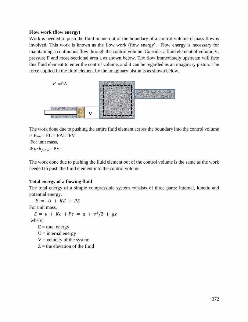
372
Flow work (flow energy)
Work is needed to push the fluid in and out of the boundary of a control volume if mass flow is
involved. This work is known as the flow work (flow energy). Flow energy is necessary for
maintaining a continuous flow through the control volume. Consider a fluid element of volume V,
pressure P and cross-sectional area a as shown below. The flow immediately upstream will face
this fluid element to enter the control volume, and it can be regarded as an imaginary piston. The
force applied in the fluid element by the imaginary piston is as shown below.
𝐹 =PA
The work done due to pushing the entire fluid element across the boundary into the control volume
is Flow = FL = PAL=PV
For unit mass,
𝑊𝑜𝑟𝑘𝑓𝑙𝑜𝑤= PV
The work done due to pushing the fluid element out of the control volume is the same as the work
needed to push the fluid element into the control volume.
Total energy of a flowing fluid
The total energy of a simple compressible system consists of three parts: internal, kinetic and
potential energy.
𝐸 = 𝑈 + 𝐾𝐸 + 𝑃𝐸
For unit mass,
𝐸 = 𝑢 + 𝐾𝑒 + 𝑃𝑒 = 𝑢 + 𝑣2/2 + 𝑔𝑧
where;
E = total energy
U = internal energy
V = velocity of the system
Z = the elevation of the fluid
V
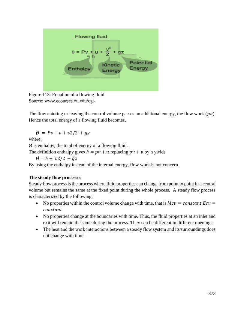
373
Figure 113: Equation of a flowing fluid
Source: www.ecourses.ou.edu/cgi-
The flow entering or leaving the control volume passes on additional energy, the flow work (𝑝𝑣).
Hence the total energy of a flowing fluid becomes,
Ø = 𝑃𝑣 + 𝑢 + 𝑣2/2 + 𝑔𝑧
where;
Ø is enthalpy, the total of energy of a flowing fluid.
The definition enthalpy gives ℎ = 𝑝𝑣 + 𝑢 replacing 𝑝𝑣 + 𝑣 by h yields
Ø = ℎ + 𝑣2/2 + 𝑔𝑧
By using the enthalpy instead of the internal energy, flow work is not concern.
The steady flow processes
Steady flow process is the process where fluid properties can change from point to point in a central
volume but remains the same at the fixed point during the whole process. A steady flow process
is characterized by the following:
No properties within the control volume change with time, that is 𝑀𝑐𝑣 = 𝑐𝑜𝑛𝑠𝑡𝑎𝑛𝑡 𝐸𝑐𝑣 =
𝑐𝑜𝑛𝑠𝑡𝑎𝑛𝑡
No properties change at the boundaries with time. Thus, the fluid properties at an inlet and
exit will remain the same during the process. They can be different in different openings.
The heat and the work interactions between a steady flow system and its surroundings does
not change with time.
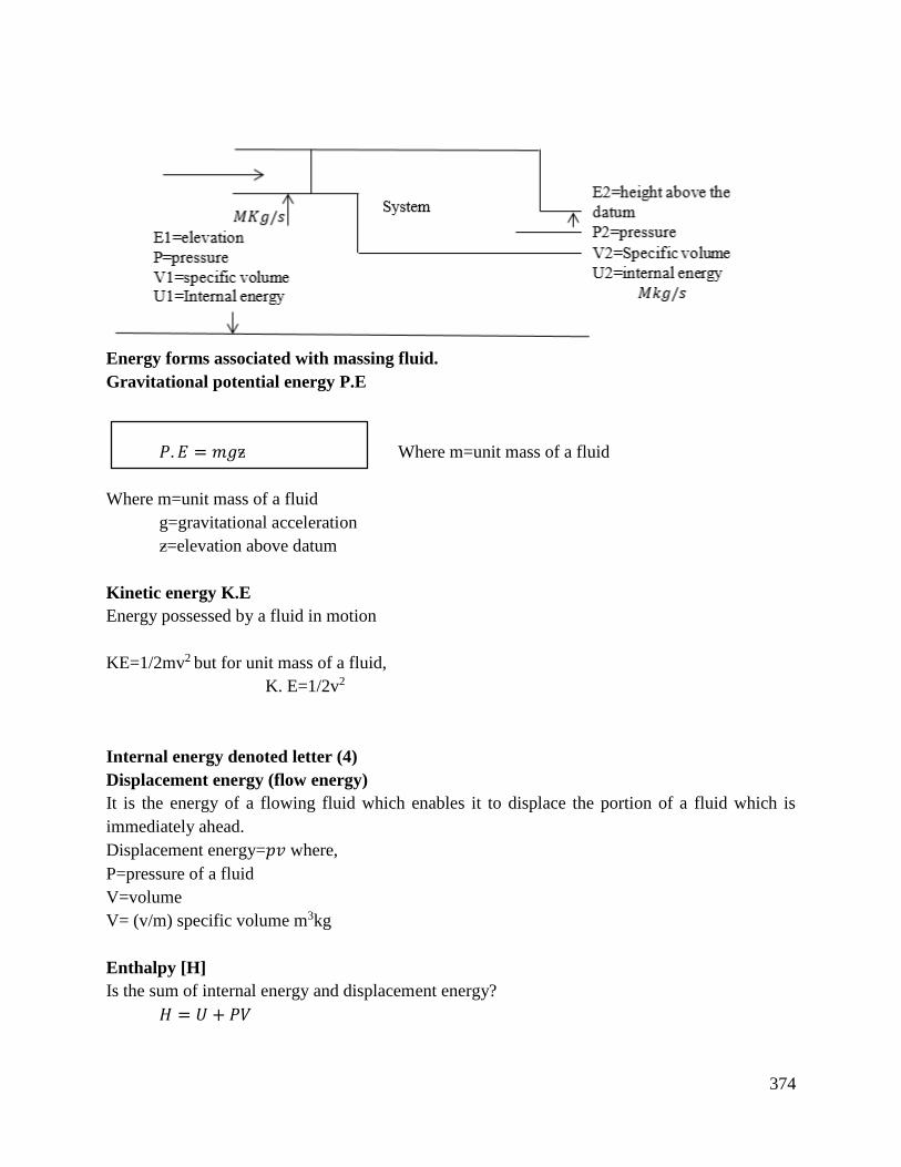
374
Energy forms associated with massing fluid.
Gravitational potential energy P.E
𝑃. 𝐸 = 𝑚𝑔ƶ Where m=unit mass of a fluid
Where m=unit mass of a fluid
g=gravitational acceleration
ƶ=elevation above datum
Kinetic energy K.E
Energy possessed by a fluid in motion
KE=1/2mv2 but for unit mass of a fluid,
K. E=1/2v2
Internal energy denoted letter (4)
Displacement energy (flow energy)
It is the energy of a flowing fluid which enables it to displace the portion of a fluid which is
immediately ahead.
Displacement energy=𝑝𝑣 where,
P=pressure of a fluid
V=volume
V= (v/m) specific volume m3kg
Enthalpy [H]
Is the sum of internal energy and displacement energy?
𝐻 = 𝑈 + 𝑃𝑉
375
A steady flow process refers to any process carried out in an open system in which mass rate of
inflow is equal to mass rate of outflow. From the law of conservation of energy assuming a steady
flow of fluids, for a unit mass fluid;
Total energy entering the system + heat added=Total energy of fluid leaving +work input.
𝑔𝑍1 +𝐶12
2+ 𝑉1 +𝑃1𝑉1 + 𝑞 + 𝑤 = 𝑔𝑍2 +
𝐶22
2+ 𝑉2+𝑃2𝑉2
But, h=U+PV
𝑔𝑍1𝐶12
2+ ℎ1 + 𝑞 + 𝑤 = 𝑔𝑍2 +
𝐶22
2+ ℎ2
Equation (𝑖) and (𝑖𝑖) are referred to as (S.F.E.E) - steady flow energy equation.
Volume flow rate q=A1C1=MV1 at inlet
𝑞 = 𝐴1𝐶1 + 𝑀1𝑉1
Volume flow rate=volume/mass (m3kg)
Similarly, 𝐴2𝐶2 = 𝐴2𝑉2 = at exit q=, 𝐴2𝐶2 = 𝑀𝑉2 =
A1C1=A2C2, 𝐴1𝐶1 = 𝐴2𝐶2 =
𝑔𝑍1 +𝐶12
2+ 𝑉1 +𝑃1𝑉1 + 𝑞 + 𝑤 = 𝑔𝑍2 +
𝐶22
2+ 𝑉2+𝑃2𝑉2…. Eqn. (1)
𝑔𝑍1𝐶12
2+ ℎ1 + 𝑞 + 𝑤 = 𝑔𝑍2 +
𝐶22
2+ ℎ2………. Eqn.(ii)
Steady flow energy equation is applied in problem solving
Example 1
In the turbine of a glass turbine unit of gases. Flow through the turbine at 17kg/s and power
developed by the turbines is 1400kw. The specific enthalpies of gat at inlet and outlet are 1200KJ
and 360KJ respectively and the velocities of the gas at inlet and out are 60m/s and 150m/s
respectively. Calculate the rate at which heat is rejected from the turbines. Find also the area of
the inlet pipe given the specific volume of the gases at inlet is 0.5 m3kg.
Solution
𝑔𝑍1𝐶12
2+ ℎ1 + 𝑞 + 𝑤 = 𝑔𝑍2 +
𝐶22
2+ ℎ2 + 𝑤
376
𝐶12
2+ ℎ1 + 𝑞 + 𝑤 = +
𝐶22
2+ ℎ2
But
𝑍1 = 𝑔𝑍2
Kinetic at inlet= 𝐶12
2
602
2
=1800J/Kg
=1.8KJ/Kg
At exit K. E = c22/2
𝐶12
2
1502
2
=11250J/Kg
=11.25KJ/Kg
Power developed by the turbine =14000kw
W=14000KJ/Kg
So,
𝐶12
2
𝐶12
2+ ℎ1 + 𝑞 + 𝑤 =
𝐶12
2+ ℎ2
17(1.8 + 1200) + 𝑞 − 14000 = (11.25 + 360)17
20430.6 + 𝑞 − 14000 = 6311.25
20430.6 + 𝑞 − 14000 = 6311.25
20430.6 + 𝑞 − 14000 = 6311.25
𝑞 = 119.35𝑘𝑤
𝑞 = +119.35𝑘𝑤 heat is rejected
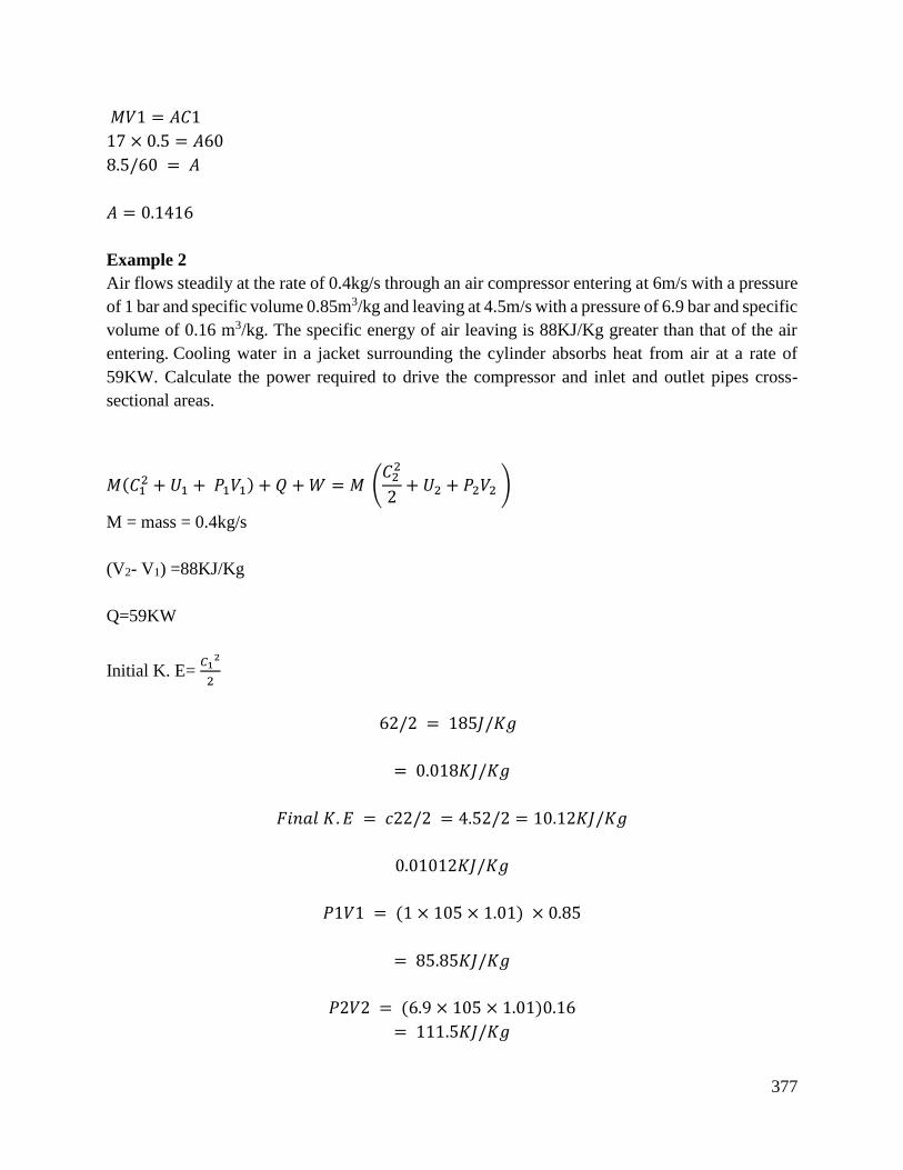
377
𝑀𝑉1 = 𝐴𝐶1
17 × 0.5 = 𝐴60
8.5/60 = 𝐴
𝐴 = 0.1416
Example 2
Air flows steadily at the rate of 0.4kg/s through an air compressor entering at 6m/s with a pressure
of 1 bar and specific volume 0.85m3/kg and leaving at 4.5m/s with a pressure of 6.9 bar and specific
volume of 0.16 m3/kg. The specific energy of air leaving is 88KJ/Kg greater than that of the air
entering. Cooling water in a jacket surrounding the cylinder absorbs heat from air at a rate of
59KW. Calculate the power required to drive the compressor and inlet and outlet pipes cross-
sectional areas.
𝑀(𝐶12 + 𝑈1 + 𝑃1𝑉1) + 𝑄 + 𝑊 = 𝑀 (
𝐶22
2+ 𝑈2 + 𝑃2𝑉2 )
M = mass = 0.4kg/s
(V2- V1) =88KJ/Kg
Q=59KW
Initial K. E= 𝐶1
2
2
62/2 = 185𝐽/𝐾𝑔
= 0.018𝐾𝐽/𝐾𝑔
𝐹𝑖𝑛𝑎𝑙 𝐾. 𝐸 = 𝑐22/2 = 4.52/2 = 10.12𝐾𝐽/𝐾𝑔
0.01012𝐾𝐽/𝐾𝑔
𝑃1𝑉1 = (1 × 105 × 1.01) × 0.85
= 85.85𝐾𝐽/𝐾𝑔
𝑃2𝑉2 = (6.9 × 105 × 1.01)0.16
= 111.5𝐾𝐽/𝐾𝑔

378
𝑄 + 𝑤 = 𝑚 (𝑉2 − 𝑉1) + 𝑃1𝑉2 − 𝑃1𝑉1) + (𝑐22/2 − 𝑐12/2)
𝑊 − 59 = 0.4(88) + 111.5 − 85.85) + (0.01012 − 0.018)
𝑊 = 104.46𝐾𝑊 𝑝𝑒𝑟 𝑢𝑛𝑖𝑡 𝑟𝑒𝑞𝑢𝑖𝑟𝑒𝑑
𝑀𝑉1 = 𝐴1𝐶1
𝐴2 = 𝑀𝑉2/𝐶
𝐴1 = 𝑀𝑉1/𝐶1
𝐴1 = 0.4 × 0.85/6
𝐴1 = 0.57𝑚2
𝑀𝑉2 = 𝐴2𝐶2
𝐴2 = 𝑀𝑉2/𝐶2
= 0.4 × 0.16
𝐴2 = 0.0142𝑚2
2.3 Steady flow energy equation is applied in utilities (boilers, condensers and compressors)
Boilers
A boiler transfers heat to the incoming water and generates the steam. The system is shown below.
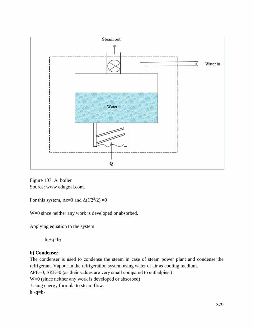
379
Figure 107: A boiler
Source: www edugoal.com.
For this system, ∆z=0 and ∆(C22/2) =0
W=0 since neither any work is developed or absorbed.
Applying equation to the system
h1+q=h2
b) Condenser
The condenser is used to condense the steam in case of steam power plant and condense the
refrigerant. Vapour in the refrigeration system using water or air as cooling medium.
∆PE=0, ∆KE=0 (as their values are very small compared to enthalpies.)
W=0 (since neither any work is developed or absorbed)
Using energy formula to steam flow.
h1-q=h2
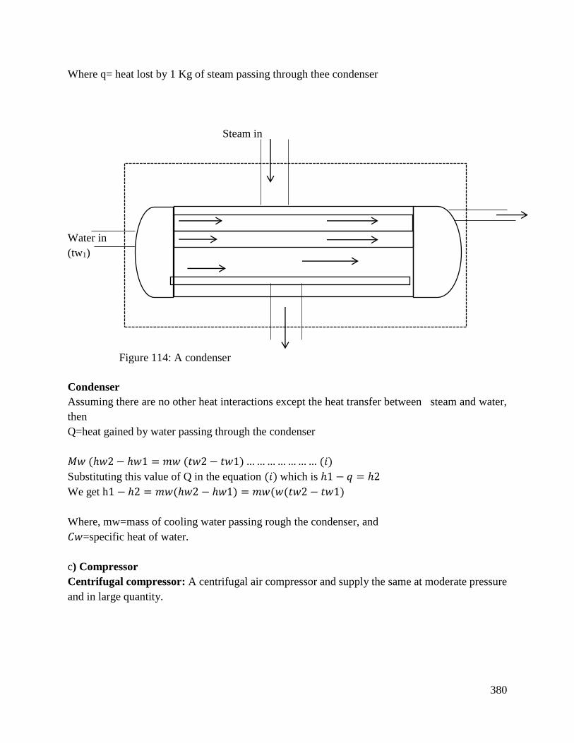
380
Where q= heat lost by 1 Kg of steam passing through thee condenser
Steam in
Water in
(tw1)
Condensate out
Condenser
Assuming there are no other heat interactions except the heat transfer between steam and water,
then
Q=heat gained by water passing through the condenser
𝑀𝑤 (ℎ𝑤2 − ℎ𝑤1 = 𝑚𝑤 (𝑡𝑤2 − 𝑡𝑤1)………………… (𝑖)
Substituting this value of Q in the equation (𝑖) which is ℎ1 − 𝑞 = ℎ2
We get h1 − ℎ2 = 𝑚𝑤(ℎ𝑤2 − ℎ𝑤1) = 𝑚𝑤(𝑤(𝑡𝑤2 − 𝑡𝑤1)
Where, mw=mass of cooling water passing rough the condenser, and
𝐶𝑤=specific heat of water.
c) Compressor
Centrifugal compressor: A centrifugal air compressor and supply the same at moderate pressure
and in large quantity.
Figure 114: A condenser
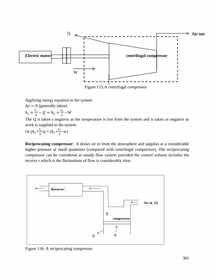
381
Q
Electric motor centrifugal compressor
W
Applying energy equation to the system
∆𝑧 = 0 (generally taken)
ℎ1 +𝐶1
2− 𝑄 = ℎ2 +
𝐶1
2−W
The Q is taken s negative as the temperature is lost from the system and is taken as negative as
work is supplied to the system
Or (ℎ1+𝐶1
2-q = (ℎ2+
𝐶1
2 -w)
Reciprocating compressor: It draws air in from the atmosphere and supplies at a considerable
higher pressure at small quantities (compared with centrifugal compressor). The reciprocating
compressor can be considered as steady flow system provided the control volume includes the
receive r which is the fluctuations of flow is considerably slow.
Figure 116: A reciprocating compressor
Air out
Figure 115:A centrifugal compressor
382
Reciprocating compressor
Applying energy equation to the system we have
∆ =0 and ∆KE=0 since the changes are negligible compared with their energies.
ℎ1-q=ℎ2-w
Conclusion
The learning outcome covered equipped the learner with knowledge, skills and attitude to flow
energy steady process and steady flow equation and using it to solve problems
Further Reading
1. Thermodynamics eBook: steady flow process
6.3.2.3 Self-Assessment
Written assessment
1) Is the flow energy also referred to as flow work?
a) Yes
b) No
2) Which of the following is the steady flow equation (S.F.EE)
a) 𝑔𝑧1 + 𝐶12/2 + 𝑞 = 𝑔𝑧2 + 𝐶22/2 + ℎ2
b) 𝑔𝑧1 + 𝐶12/2 + 𝑤 = 𝑔𝑧1 + 𝐶22/2 + ℎ2
c) 𝑔𝑧1 + 𝐶12/2 + ℎ1 + 𝑞 + 𝑤 = 𝑔𝑧2 + 𝐶22/2 + ℎ2𝑑
3) 10 kg of fluid per minute goes through a reversible steady flow process. The properties of
fluid at the inlet are p1=1.5 bar, p1=26kg/m3, C1=110m/s and v1=910kJ/Kg and the exit
are p2=5.5 bar, p2=5.5Kg/m3, C2=190m/s and v2=710KJ/Kg. during the passage the fluid
rejects 55kJ/s and rises through 55 meters. Determine;
The change in enthalpy (∆h);
a) ∆h =66.71 KJ/Kg
b) ∆h=53.9KJ/Kg
c) ∆h=105.77 KJ/Kg
d) ∆h=44.9KJ/Kg

383
4) Using question three above determine the work done during the process.
a) -26.4kw
b) -16.9kw
c) -3.9kw
d) 41.9kw
5) In a gas turbine unit, the gases flow through the turbine is 15kgs and the power developed
by the turbine is 12000kw. The enthalpies of gases at the inlet and the outlet are 1260 kJ/Kg
and 400kJ/Kg respectively, and the velocity of gases at the inlet and outlet are 50/s and
110m/s respectively. Calculate
a) The rate at which heat is rejected in the turbine
a) 496kw
b) 567kw
c) 828kw
d) 396kw
6) Using question 5 above, determine;
a. The area of the inlet pipe given that the specific volume of the gases at the inlet is
0.45m3/kg.
a) 0.140 m2
b) 0.697m2
c) 0.135m2
d) 400m2
7) The formula h-q-h2-w is applied in which compressor
a) Reciprocating compressor
b) Centrifugal compressor
8) What is the meaning of the term steady flow process
9) What do you understand by the following terms?
a) Matter
b) Energy
10) Derive an equation for kinetic energy
11) Derive the equation for potential energy
12) Give the formula for enthalpy
Oral Assessment
1) Describe what is meant by steady flow process
2) Describe with a diagram the steady flow energy
Practical Assessment
384
You are required by use of experiment to determine the capacity of a condenser
6.3.2.4 Tools, Equipment, Supplies and Materials
Scientific Calculators
Steam tables
Relevant reference materials
Stationeries
Relevant practical materials
Dice
Computers with internet connection
6.3.2.5 References
Eastop, T. D., & Mc Conkey, A. (1986). Applied Thermodynamics for engineering technologies.
Basic engineering thermodynamics by R.Joel.
Joel, R. (1996). Basic engineering thermodynamics. Pearson Education India.
Mayhew, Y. R., & Rogers, G. F. C. (1972). Thermodynamic and transport properties of fluids: SI
units. Blackwell.
385
6.3.4 Learning Outcome No. 3: perform non steady flow processes
6.3.4.1 Learning Activities
Learning Outcome No 3: Perform non steady flow processes
Learning Activities Special Instructions
3.1 Derive non-flow energy equation
3.2 Apply non-flow energy equation in problem solving
6.3.4.2 Information Sheet No6/LO3: perform non steady flow processes
Introduction
This learning outcome covers mass and energy balance of unsteady flow processes and uniform
flow process.
Definition of key terms
Energy: It is the quantitative property that must be transferred to an object in order to perform
work on or to heat the object.
Mass: It is the measure of the amount of matte in an object. It’s usually measured in grams (g) o
kilograms (kg).
Volume: It is the amount of space that a substance/object occupies
Content/procedures/methods/illustrations
3.1 Non-flow energy equation is derived
In engineering practice, the variable flow process applications are as common as the steady flow
process. The rate of energy and mass transfer into and out of the control volume are not the same
in the case of unstable (or variable or transient) flow process. Following two cases will be
discussed;
Filling a tank.
Emptying a tank or tank discharge.
Filling a tank
Let: 𝑀1=Initial mass of fluid.
𝑃1=Initial pressure.
VI=Initial specific volume.
T1=Initial temperature
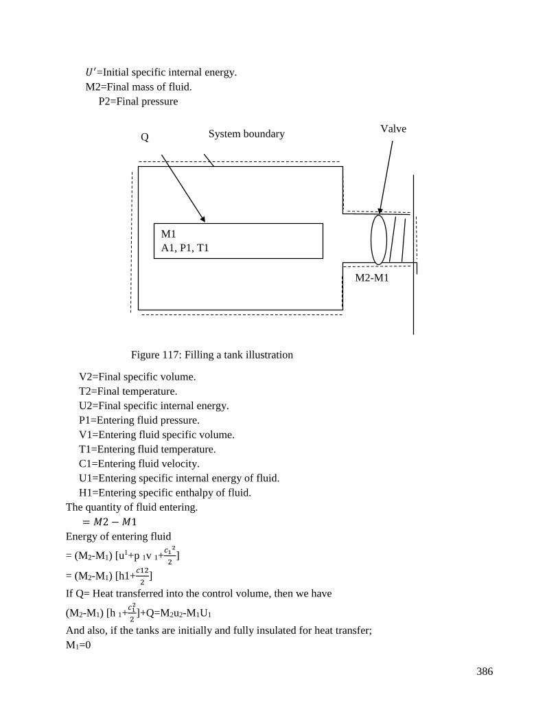
386
𝑈′=Initial specific internal energy.
M2=Final mass of fluid.
P2=Final pressure
V2=Final specific volume.
T2=Final temperature.
U2=Final specific internal energy.
P1=Entering fluid pressure.
V1=Entering fluid specific volume.
T1=Entering fluid temperature.
C1=Entering fluid velocity.
U1=Entering specific internal energy of fluid.
H1=Entering specific enthalpy of fluid.
The quantity of fluid entering.
= 𝑀2 − 𝑀1
Energy of entering fluid
= (M2-M1) [u1+p 1v 1+
𝑐12
2]
= (M2-M1) [h1+𝑐12
2]
If Q= Heat transferred into the control volume, then we have
(M2-M1) [h 1+𝑐12
2]+Q=M2u2-M1U1
And also, if the tanks are initially and fully insulated for heat transfer;
M1=0
System boundary
M2-M1
M1
A1, P1, T1
Q Valve
Figure 117: Filling a tank illustration
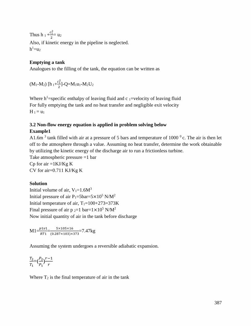
387
Thus h 1 +𝑐12
2= u2
Also, if kinetic energy in the pipeline is neglected.
h1=u2
Emptying a tank
Analogues to the filling of the tank, the equation can be written as
(M1-M2) [h 1+
𝑐12
2]-Q=M1u1-M2U2
Where h1=specific enthalpy of leaving fluid and c 1=velocity of leaving fluid
For fully emptying the tank and no heat transfer and negligible exit velocity
H 1 = u1
3.2 Non-flow energy equation is applied in problem solving below
Example1
A1.6m 3 tank filled with air at a pressure of 5 bars and temperature of 1000 0 c. The air is then let
off to the atmosphere through a value. Assuming no heat transfer, determine the work obtainable
by utilizing the kinetic energy of the discharge air to run a frictionless turbine.
Take atmospheric pressure =1 bar
Cp for air =1KJ/Kg K
CV for air=0.711 KJ/Kg K
Solution
Initial volume of air, V1=1.6M3
Initial pressure of air P1=5bar=5×10⁵ N/M2
Initial temperature of air, T1=100+273=373K
Final pressure of air p 2=1 bar=1×10⁵ N/M2
Now initial quantity of air in the tank before discharge
M1=𝑝1𝑣1
𝑅𝑇1=
5×105×16
(0.287×103)×373=7.47kg
Assuming the system undergoes a reversible adiabatic expansion.
𝑇2
𝑇1=(
𝑃2
𝑃1)𝑟−1
𝑟
Where T2 is the final temperature of air in the tank
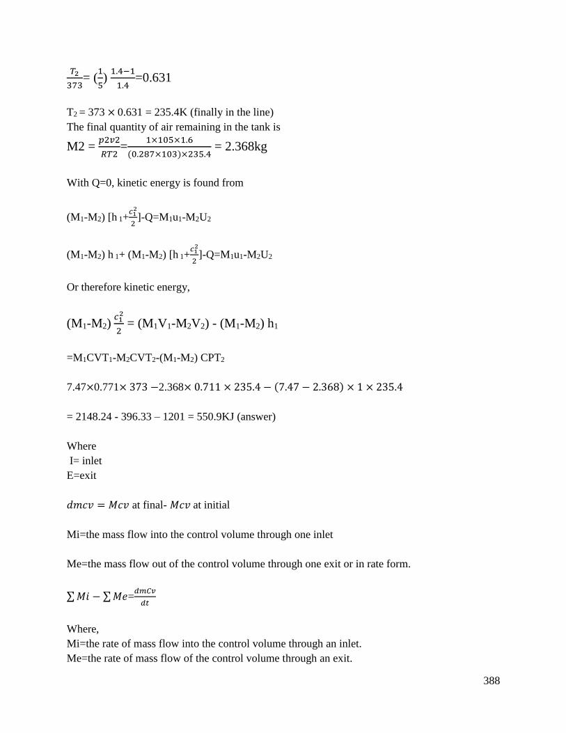
388
𝑇2
373= (
1
5)
1.4−1
1.4=0.631
T2 = 373 × 0.631 = 235.4K (finally in the line)
The final quantity of air remaining in the tank is
M2 = 𝑝2𝑣2
𝑅𝑇2=
1×105×1.6
(0.287×103)×235.4 = 2.368kg
With Q=0, kinetic energy is found from
(M1-M2) [h 1+
𝑐12
2]-Q=M1u1-M2U2
(M1-M2) h 1+ (M1-M2) [h
1+
𝑐12
2]-Q=M1u1-M2U2
Or therefore kinetic energy,
(M1-M2) 𝑐1
2
2 = (M1V1-M2V2) - (M1-M2) h1
=M1CVT1-M2CVT2-(M1-M2) CPT2
7.47×0.771× 373 −2.368× 0.711 × 235.4 − (7.47 − 2.368) × 1 × 235.4
= 2148.24 - 396.33 – 1201 = 550.9KJ (answer)
Where
I= inlet
E=exit
𝑑𝑚𝑐𝑣 = 𝑀𝑐𝑣 at final- 𝑀𝑐𝑣 at initial
Mi=the mass flow into the control volume through one inlet
Me=the mass flow out of the control volume through one exit or in rate form.
∑𝑀𝑖 − ∑𝑀𝑒=𝑑𝑚𝐶𝑣
𝑑𝑡
Where,
Mi=the rate of mass flow into the control volume through an inlet.
Me=the rate of mass flow of the control volume through an exit.
389
𝑑𝑚𝑐𝑣
𝑑𝑡=the rate of change of mass within the control volume.
Also, the energy content of a control volume changes with time during an unsteady flow process.
The general energy balance can be used for the central volume as 𝐸𝑖 − 𝐸𝑒 = 𝐷𝐸𝑐𝑣.
Conclusion
The learning outcome covered equipped the learner with knowledge, skills and attitude to know
the non-flow energy equation and how is derived and using the non-flow energy equation to solve
problems.
Further Reading
1. Uniform flow processes
2. The general energy balances
6.3.4.3 Self-Assessment
Written assessment
1. Steady flow occurs when?
a) Conditions do not change with time at any point.
b) Conditions are the same at adjacent points at any instant.
c) Conditions change steadily with the time.
d) (𝑑𝑣
𝑑𝑡) is constant.
2. Which one of the following is not a property of the system?
a) Specific volume.
b) Temperature.
c) Heat.
d) None of the above.
3. In reversible polytrophic process,
a) True heat transfer occurs.
b) The enthalpy remains constant.
c) The internal energy remains constant.
d) The temperature remains constant.
4. A control volume refers to,
390
a) A fixed region in space.
b) A specified mass.
c) An isolated system.
d) A reversible process only.
e) A closed system.
5. If all variables of a stream are independent of time, it is said to be in?
a) Steady flow.
b) Uniform flow.
c) Constant flow.
d) Unsteady flow
e) Closed flow
6. A gas which obeys kinetic theory perfectly is known as;
a) Real gas.
b) Perfect gas.
c) Pure gas.
d) Diatomic gas.
e) Mono atomic gas.
7. Work done in a free expansion process is?
a) Maximum.
b) Negative.
c) Zero.
d) Minimum.
e) Positive
8. What do you understand by internal energy? Prove that it is a property of a system.
9. State the first law of thermal dynamic and prove that for a non-flow process, it leads to the
energy equation Q=DU+W.
10. What is the mechanical equivalent of heat? Write down its value when heat is expressed in
N-M.
11. Explain clearly the difference between a non-flow and a steady flow process
12. For isothermal flow and non-flow steady processes, prove that
∫ 𝑝𝑑𝑣 = −∫ V − 𝑑𝑝2
1
2
1 Also state the assumptions made.
Oral Assessment

391
1. Why only in constant pressure non-flow process, the enthalpy change is equal to heat
transfer?
2. Explain clearly the difference between a non-flow and a steady flow process.
Practical Assessment
1. With the aid of a diagram show that the unsteady flow processes start and end over the
same final period time (Dt).
6.3.4.4 Tools, Equipment, Supplies and Materials
Scientific Calculators
Relevant reference materials
Stationeries
Relevant practical materials
Dice
Computers with internet connection
6.3.4.5 References
Bakhtar, F. (1993). Engineering Thermodynamics, Work and Heat Transfer:
Bratkovich T, Bussing T. A pulse detonation engine performance model. In31st Joint Propulsion
Conference/.
Balan, C. and Franco, J.M., 2001. Influence of the geometry on the transient and steady flow of
lubricating greases. Tribology Transactions, 44(1), pp.53-58.nce and Exhibit 1995 Jul (p.
3155).
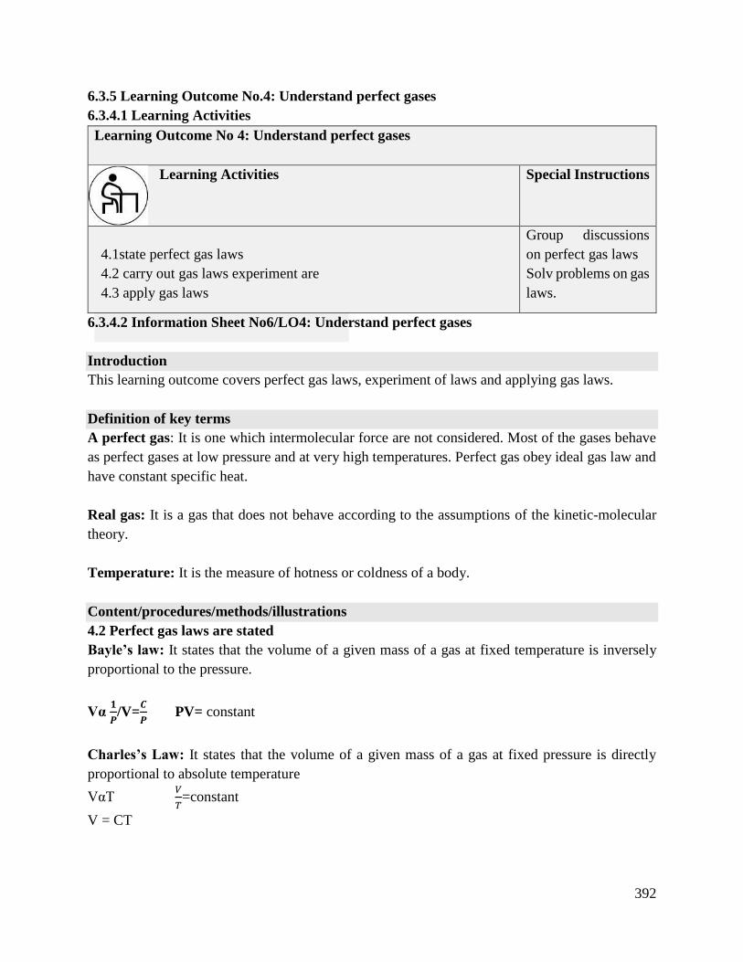
392
6.3.5 Learning Outcome No.4: Understand perfect gases
6.3.4.1 Learning Activities
Learning Outcome No 4: Understand perfect gases
Learning Activities Special Instructions
4.1state perfect gas laws
4.2 carry out gas laws experiment are
4.3 apply gas laws
Group discussions
on perfect gas laws
Solv problems on gas
laws.
6.3.4.2 Information Sheet No6/LO4: Understand perfect gases
Introduction
This learning outcome covers perfect gas laws, experiment of laws and applying gas laws.
Definition of key terms
A perfect gas: It is one which intermolecular force are not considered. Most of the gases behave
as perfect gases at low pressure and at very high temperatures. Perfect gas obey ideal gas law and
have constant specific heat.
Real gas: It is a gas that does not behave according to the assumptions of the kinetic-molecular
theory.
Temperature: It is the measure of hotness or coldness of a body.
Content/procedures/methods/illustrations
4.2 Perfect gas laws are stated
Bayle’s law: It states that the volume of a given mass of a gas at fixed temperature is inversely
proportional to the pressure.
Vα 𝟏
𝑷/V=
𝑪
𝑷 PV= constant
Charles’s Law: It states that the volume of a given mass of a gas at fixed pressure is directly
proportional to absolute temperature
VαT 𝑉
𝑇=constant
V = CT
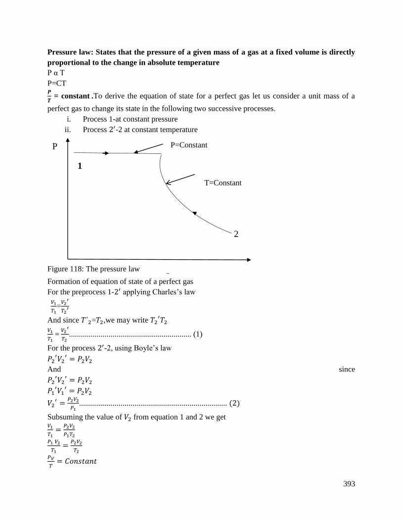
393
Pressure law: States that the pressure of a given mass of a gas at a fixed volume is directly
proportional to the change in absolute temperature
P α T
P=CT 𝑷
𝑻 = constant .To derive the equation of state for a perfect gas let us consider a unit mass of a
perfect gas to change its state in the following two successive processes.
i. Process 1-at constant pressure
ii. Process 2′-2 at constant temperature
2′
Formation of equation of state of a perfect gas
For the preprocess 1-2′ applying Charles’s law
𝑉1
𝑇1=
𝑉2′
𝑇2′
And since 𝑇´2=𝑇2,we may write 𝑇2′𝑇2
𝑉1
𝑇1 =
𝑉2′
𝑇2 .............................................................. (1)
For the process 2′-2, using Boyle’s law
𝑃2′𝑉2
′ = 𝑃2𝑉2
And since
𝑃2′𝑉2
′ = 𝑃2𝑉2
𝑃1′𝑉1
′ = 𝑃2𝑉2
𝑉2′ =
𝑃2𝑉2
𝑃1........................................................................... (2)
Subsuming the value of 𝑉2 from equation 1 and 2 we get 𝑉1
𝑇1=
𝑃2𝑉2
𝑃1𝑇2
𝑃1 𝑉2
𝑇1=
𝑃2𝑉2
𝑇2
𝑃𝑉
𝑇= 𝐶𝑜𝑛𝑠𝑡𝑎𝑛𝑡
2
2
P P=Constant
T=Constant
1
Figure 118: The pressure law
394
The magnitude of this constant depends upon the particular gas and it is denoted by R1 where R
is called the specific gas constant. Then: 𝑃𝑇
= 𝑅
The equation of the state for a perfect gas is then given by the equation:
Or for M&G occupying Vm
𝑃𝑉 = 𝑀𝑅𝑇
If the mass is chosen to be numerically equal to the molecular weight of the gas, then 1 mole of
the gas has been considered as 1Kg mole of oxygen is 32kg oxygen or 1kg 1mole of hydrogen is
2kg hydrogen
The equation may be written as:
𝑃𝑉0=MRT where
𝑉0=molar volume and
M=Molecular weight of the gas
Avogadro discovered that 𝑉0 is the same for all gases at the same pressure and temperature and
therefore it may be seen that 𝑀𝑅 = 𝑎 𝑐o𝑛𝑠𝑡𝑎𝑛𝑡 , 𝑅0 and thus P𝑉0 =𝑅0T
𝑅0 is called the molar or universal gas constant and is value is 8.3143 kJ/kg mole. If there are n
moles present then the ideal gas equation may be written as,
P𝑉 =𝑛𝑅0T
Where V is the volume occupied by n mole at pressure P and temperature T.
4.2 Gas laws experiment are carried out
Boyle’s Law
Torricelli experiment did more than just show that air has weight, it also provides a way of creating
a vacuum because the space above the column of mercury at the top of a barometer is almost
completely empty. (it is free of air or other gases except a negligible amount of mercury vapor).
Torricelli’s work with vacuum caught the eye of the British science Robert Boyle.
Boyle most famous experiment with gases dealt with what he called the spring of air. These
experiments were based on the observation that gases are elastic. (They return to their original size
and shape after being stretched or squeezed). Boyle studied the elasticity of gases in J. tube similar
to the apparatus Shan. By adding mercury to the open end of the tube, he wrapped a small volume
of air in the sealed end.
Figure 119: Figure 120: The Boyle’s law
395
Source www.chemedu.com
Boyle studied what happened to the volume of the gas in the sealed end of the tube as he added
mercury to the open end. He noticed that the product of the pressure times the volume for any
measurement in this table was equal to the product of the pressure times the volume for any other
measurement within experimental error.
𝑃1𝑉1 = 𝑃2𝑉2
This expression is equivalent to
𝑃 𝛼 1
𝑉 Known as Boyle’s law
Charles’s law: Charles noticed that the volume of gas is directly proportional to its temperature
V α T. This relationship between the temperature and volume of a gas, which became known as
Charles law, provides an explanation of how hot air balloons work. If a gas expands when heated,
then a given weight of air occupies a large volume that is the same weight of cold air. Hot air is
therefore less dense than cold air.
Once the air in a balloon gets hot enough, the weight of the balloon plus this hot air is less than the
weight of an equivalent volume of cold air, and the balloon starts to rise. When the gas in the
balloon is allowed to cool the balloon returns to the ground.
Charles law can be demonstrated with the apparatus shown below.
A 30-ml syringe and a thermometer are inserted through a rubber stopper into a flask that has been
cooled to 00C. The ice bath is then removed and the flask is immersed in a warm-water bath. The
gas in the flask expands as it warms, slowly pushing the piston out or the syringe. The total volume
of the gas in the system is equal to the volume of the flask plus the volume of the syringe.
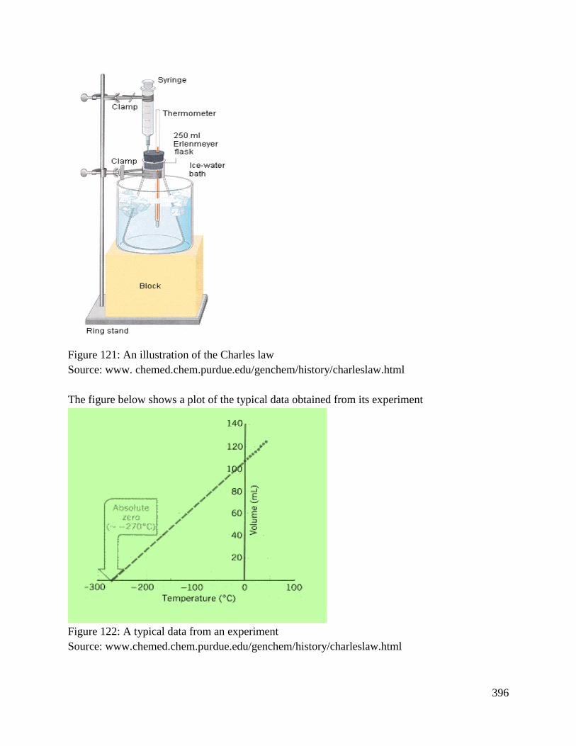
396
Figure 121: An illustration of the Charles law
Source: www. chemed.chem.purdue.edu/genchem/history/charleslaw.html
The figure below shows a plot of the typical data obtained from its experiment
Figure 122: A typical data from an experiment
Source: www.chemed.chem.purdue.edu/genchem/history/charleslaw.html
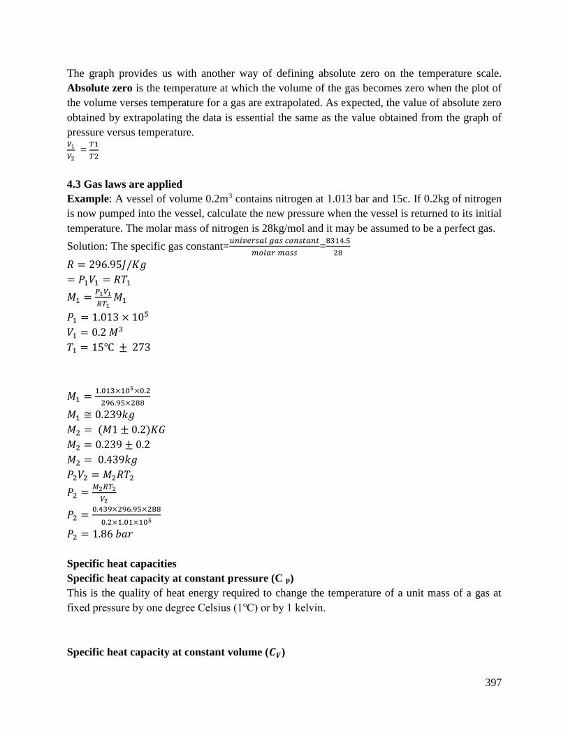
397
The graph provides us with another way of defining absolute zero on the temperature scale.
Absolute zero is the temperature at which the volume of the gas becomes zero when the plot of
the volume verses temperature for a gas are extrapolated. As expected, the value of absolute zero
obtained by extrapolating the data is essential the same as the value obtained from the graph of
pressure versus temperature. 𝑉1
𝑉2 =
𝑇1
𝑇2
4.3 Gas laws are applied
Example: A vessel of volume 0.2m3 contains nitrogen at 1.013 bar and 15c. If 0.2kg of nitrogen
is now pumped into the vessel, calculate the new pressure when the vessel is returned to its initial
temperature. The molar mass of nitrogen is 28kg/mol and it may be assumed to be a perfect gas.
Solution: The specific gas constant=𝑢𝑛𝑖𝑣𝑒𝑟𝑠𝑎𝑙 𝑔𝑎𝑠 𝑐𝑜𝑛𝑠𝑡𝑎𝑛𝑡
𝑚𝑜𝑙𝑎𝑟 𝑚𝑎𝑠𝑠=
8314.5
28
𝑅 = 296.95𝐽/𝐾𝑔
= 𝑃1𝑉1 = 𝑅𝑇1
𝑀1 =𝑃1𝑉1
𝑅𝑇1𝑀1
𝑃1 = 1.013 × 10⁵
𝑉1 = 0.2 𝑀3
𝑇1 = 15 ± 273
𝑀1 =1.013×105×0.2
296.95×288
𝑀1 ≅ 0.239𝑘𝑔
𝑀2 = (𝑀1 ± 0.2)𝐾𝐺
𝑀2 = 0.239 ± 0.2
𝑀2 = 0.439𝑘𝑔
𝑃2𝑉2 = 𝑀2𝑅𝑇2
𝑃2 =𝑀2𝑅𝑇2
𝑉2
𝑃2 =0.439×296.95×288
0.2×1.01×105
𝑃2 = 1.86 𝑏𝑎𝑟
Specific heat capacities
Specific heat capacity at constant pressure (C p)
This is the quality of heat energy required to change the temperature of a unit mass of a gas at
fixed pressure by one degree Celsius (1) or by 1 kelvin.
Specific heat capacity at constant volume (𝑪𝑽)
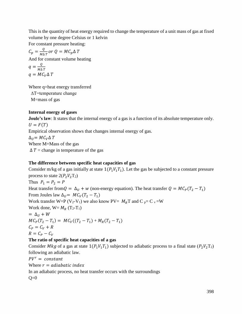
398
This is the quantity of heat energy required to change the temperature of a unit mass of gas at fixed
volume by one degree Celsius or 1 kelvin
For constant pressure heating:
𝐶𝑝 =𝑄
𝑀∆ 𝑇𝑜𝑟 𝑄 = 𝑀𝐶𝑝∆ 𝑇
And for constant volume heating
𝑞 =𝑄
𝑀∆ 𝑇
𝑞 = 𝑀𝐶𝑉∆ 𝑇
Where q=heat energy transferred
∆T=temperature change
M=mass of gas
Internal energy of gases
Joule’s law: It states that the internal energy of a gas is a function of its absolute temperature only.
𝑈 = 𝐹(𝑇)
Empirical observation shows that changes internal energy of gas.
∆𝑈= 𝑀𝐶𝑉∆ 𝑇
Where M=Mass of the gas
∆ 𝑇 = change in temperature of the gas
The difference between specific heat capacities of gas
Consider m/kg of a gas initially at state 1(𝑃1𝑉1𝑇1). Let the gas be subjected to a constant pressure
process to state 2(𝑃2𝑉2T2)
Thus 𝑃1 = 𝑃2 = 𝑃
Heat transfer from𝑄 = ∆𝑈 + 𝑤 (non-energy equation). The heat transfer 𝑄 = 𝑀𝐶𝑃(𝑇2 − 𝑇1)
From Joules law ∆𝑈= 𝑀𝐶𝑉(𝑇2 − 𝑇1)
Work transfer W=P (V2-V1) we also know PV= 𝑀𝑅T and C p= C v =W
Work done, W= 𝑀𝑅 (T2-T1)
= ∆𝑈 + 𝑊
𝑀𝐶𝑃(𝑇2 − 𝑇1) = 𝑀𝐶𝑉((𝑇2 − 𝑇1) + 𝑀𝑅(𝑇2 − 𝑇1)
𝐶𝑃 = 𝐶𝑉 + 𝑅
𝑅 = 𝐶𝑃 − 𝐶𝑉
The ratio of specific heat capacities of a gas
Consider 𝑀𝑘𝑔 of a gas at state 1(𝑃1𝑉1𝑇1) subjected to adiabatic process to a final state (𝑃2𝑉2T2)
following an adiabatic law.
𝑃𝑉𝑟 = 𝑐𝑜𝑛𝑠𝑡𝑎𝑛𝑡
Where 𝑟 = 𝑎𝑑𝑖𝑎𝑏𝑎𝑡𝑖𝑐 𝑖𝑛𝑑𝑒𝑥
In an adiabatic process, no heat transfer occurs with the surroundings
Q=0
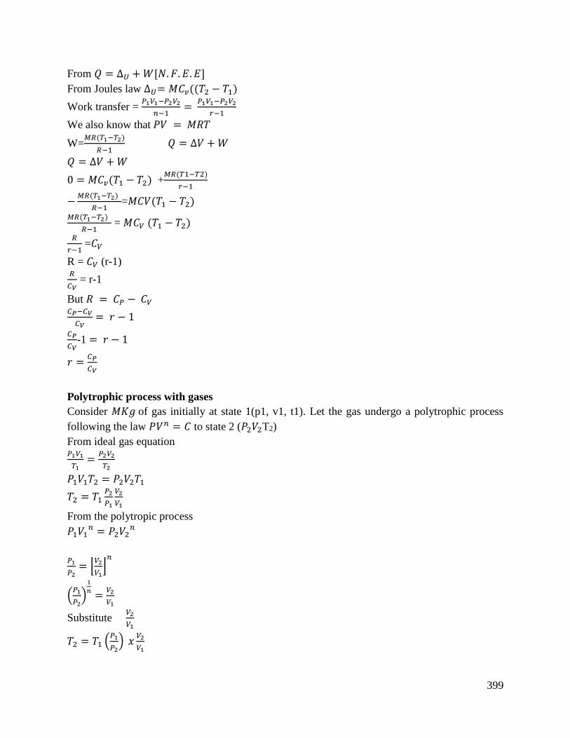
399
From 𝑄 = ∆𝑈 + 𝑊[𝑁. 𝐹. 𝐸. 𝐸]
From Joules law ∆𝑈= 𝑀𝐶𝑣((𝑇2 − 𝑇1)
Work transfer = 𝑃1𝑉1−𝑃2𝑉2
𝑛−1=
𝑃1𝑉1−𝑃2𝑉2
𝑟−1
We also know that 𝑃𝑉 = 𝑀𝑅𝑇
W=𝑀𝑅(𝑇1−𝑇2)
𝑅−1 𝑄 = ∆𝑉 + 𝑊
𝑄 = ∆𝑉 + 𝑊
0 = 𝑀𝐶𝑣(𝑇1 − 𝑇2) +𝑀𝑅(𝑇1−𝑇2)
𝑟−1
−𝑀𝑅(𝑇1−𝑇2)
𝑅−1=𝑀𝐶𝑉(𝑇1 − 𝑇2)
𝑀𝑅(𝑇1−𝑇2)
𝑅−1 = 𝑀𝐶𝑉 (𝑇1 − 𝑇2)
𝑅
𝑟−1 =𝐶𝑉
R = 𝐶𝑉 (r-1) 𝑅
𝐶𝑉 = r-1
But 𝑅 = 𝐶𝑃 − 𝐶𝑉 𝐶𝑃−𝐶𝑉
𝐶𝑉 = 𝑟 − 1
𝐶𝑃
𝐶𝑉-1 = 𝑟 − 1
𝑟 =𝐶𝑃
𝐶𝑉
Polytrophic process with gases
Consider 𝑀𝐾𝑔 of gas initially at state 1(p1, v1, t1). Let the gas undergo a polytrophic process
following the law 𝑃𝑉𝑛 = 𝐶 to state 2 (𝑃2𝑉2T2)
From ideal gas equation 𝑃1𝑉1
𝑇1=
𝑃2𝑉2
𝑇2
𝑃1𝑉1𝑇2 = 𝑃2𝑉2𝑇1
𝑇2 = 𝑇1𝑃2
𝑃1
𝑉2
𝑉1
From the polytropic process
𝑃1𝑉1𝑛 = 𝑃2𝑉2
𝑛
𝑃1
𝑃2= ⌊
𝑉2
𝑉1⌋𝑛
(𝑃1
𝑃2)
1
𝑛=
𝑉2
𝑉1
Substitute 𝑉2
𝑉1
𝑇2 = 𝑇1 (𝑃1
𝑃2) 𝑥
𝑉2
𝑉1
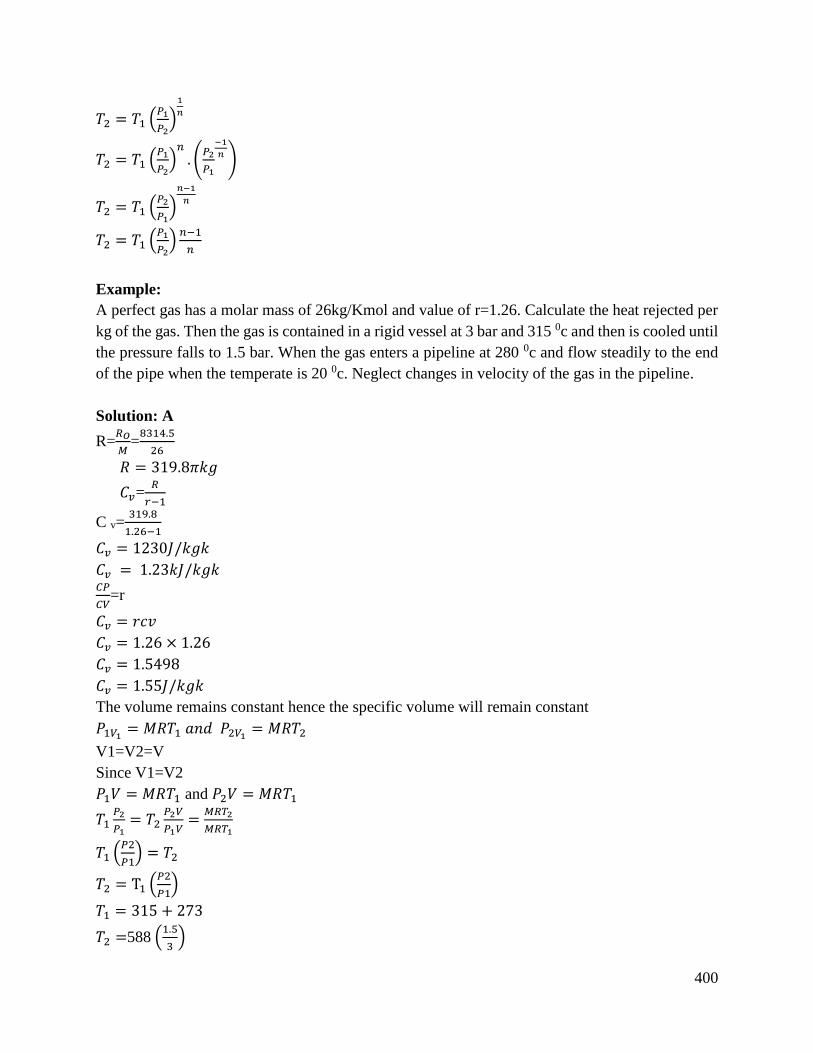
400
𝑇2 = 𝑇1 (𝑃1
𝑃2)
1
𝑛
𝑇2 = 𝑇1 (𝑃1
𝑃2)𝑛
. (𝑃2
𝑃1
−1
𝑛 )
𝑇2 = 𝑇1 (𝑃2
𝑃1)
𝑛−1
𝑛
𝑇2 = 𝑇1 (𝑃1
𝑃2)
𝑛−1
𝑛
Example:
A perfect gas has a molar mass of 26kg/Kmol and value of r=1.26. Calculate the heat rejected per
kg of the gas. Then the gas is contained in a rigid vessel at 3 bar and 315 0c and then is cooled until
the pressure falls to 1.5 bar. When the gas enters a pipeline at 280 0c and flow steadily to the end
of the pipe when the temperate is 20 0c. Neglect changes in velocity of the gas in the pipeline.
Solution: A
R=𝑅𝑂
𝑀=
8314.5
26
𝑅 = 319.8𝜋𝑘𝑔
𝐶𝑣=𝑅
𝑟−1
C v=319.8
1.26−1
𝐶𝑣 = 1230𝐽/𝑘𝑔𝑘
𝐶𝑣 = 1.23𝑘𝐽/𝑘𝑔𝑘 𝐶𝑃
𝐶𝑉=r
𝐶𝑣 = 𝑟𝑐𝑣
𝐶𝑣 = 1.26 × 1.26
𝐶𝑣 = 1.5498
𝐶𝑣 = 1.55𝐽/𝑘𝑔𝑘
The volume remains constant hence the specific volume will remain constant
𝑃1𝑉1= 𝑀𝑅𝑇1 𝑎𝑛𝑑 𝑃2𝑉1
= 𝑀𝑅𝑇2
V1=V2=V
Since V1=V2
𝑃1𝑉 = 𝑀𝑅𝑇1 and 𝑃2𝑉 = 𝑀𝑅𝑇1
𝑇1𝑃2
𝑃1= 𝑇2
𝑃2𝑉
𝑃1𝑉=
𝑀𝑅𝑇2
𝑀𝑅𝑇1
𝑇1 (𝑃2
𝑃1) = 𝑇2
𝑇2 = T1 (𝑃2
𝑃1)
𝑇1 = 315 + 273
𝑇2 =588 (1.5
3)
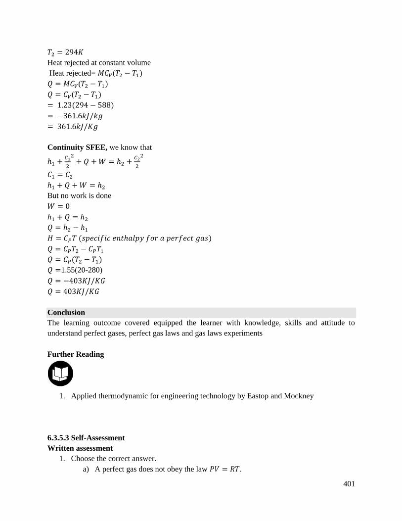
401
𝑇2 = 294𝐾
Heat rejected at constant volume
Heat rejected= 𝑀𝐶𝑉(𝑇2 − 𝑇1)
𝑄 = 𝑀𝐶𝑉(𝑇2 − 𝑇1)
𝑄 = 𝐶𝑉(𝑇2 − 𝑇1)
= 1.23(294 − 588)
= −361.6𝑘𝐽/𝑘𝑔
= 361.6𝑘𝐽/𝐾𝑔
Continuity SFEE, we know that
ℎ1 +𝐶1
2
2+ 𝑄 + 𝑊 = ℎ2 +
𝐶2
2
2
𝐶1 = 𝐶2
ℎ1 + 𝑄 + 𝑊 = ℎ2
But no work is done
𝑊 = 0
ℎ1 + 𝑄 = ℎ2
𝑄 = ℎ2 − ℎ1
𝐻 = 𝐶𝑃𝑇 (𝑠𝑝𝑒𝑐𝑖𝑓𝑖𝑐 𝑒𝑛𝑡ℎ𝑎𝑙𝑝𝑦 𝑓𝑜𝑟 𝑎 𝑝𝑒𝑟𝑓𝑒𝑐𝑡 𝑔𝑎𝑠)
𝑄 = 𝐶𝑃𝑇2 − 𝐶𝑃𝑇1
𝑄 = 𝐶𝑃(𝑇2 − 𝑇1)
𝑄 =1.55(20-280)
𝑄 = −403𝐾𝐽/𝐾𝐺
𝑄 = 403𝐾𝐽/𝐾𝐺
Conclusion
The learning outcome covered equipped the learner with knowledge, skills and attitude to
understand perfect gases, perfect gas laws and gas laws experiments
Further Reading
1. Applied thermodynamic for engineering technology by Eastop and Mockney
6.3.5.3 Self-Assessment
Written assessment
1. Choose the correct answer.
a) A perfect gas does not obey the law 𝑃𝑉 = 𝑅𝑇.
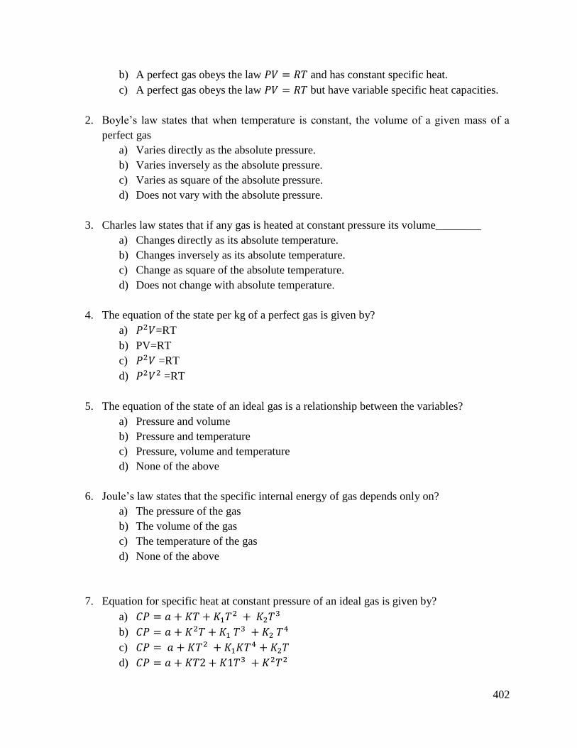
402
b) A perfect gas obeys the law 𝑃𝑉 = 𝑅𝑇 and has constant specific heat.
c) A perfect gas obeys the law 𝑃𝑉 = 𝑅𝑇 but have variable specific heat capacities.
2. Boyle’s law states that when temperature is constant, the volume of a given mass of a
perfect gas
a) Varies directly as the absolute pressure.
b) Varies inversely as the absolute pressure.
c) Varies as square of the absolute pressure.
d) Does not vary with the absolute pressure.
3. Charles law states that if any gas is heated at constant pressure its volume________
a) Changes directly as its absolute temperature.
b) Changes inversely as its absolute temperature.
c) Change as square of the absolute temperature.
d) Does not change with absolute temperature.
4. The equation of the state per kg of a perfect gas is given by?
a) 𝑃2𝑉=RT
b) PV=RT
c) 𝑃2𝑉 =RT
d) 𝑃2𝑉2 =RT
5. The equation of the state of an ideal gas is a relationship between the variables?
a) Pressure and volume
b) Pressure and temperature
c) Pressure, volume and temperature
d) None of the above
6. Joule’s law states that the specific internal energy of gas depends only on?
a) The pressure of the gas
b) The volume of the gas
c) The temperature of the gas
d) None of the above
7. Equation for specific heat at constant pressure of an ideal gas is given by?
a) 𝐶𝑃 = 𝑎 + 𝐾𝑇 + 𝐾1𝑇2 + 𝐾2𝑇
3
b) 𝐶𝑃 = 𝑎 + 𝐾2𝑇 + 𝐾1 𝑇3 + 𝐾2 𝑇
4
c) 𝐶𝑃 = 𝑎 + 𝐾𝑇2 + 𝐾1𝐾𝑇4 + 𝐾2𝑇
d) 𝐶𝑃 = 𝑎 + 𝐾𝑇2 + 𝐾1𝑇3 + 𝐾2𝑇2
403
8. What is an ideal gas?
9. What is the difference between an ideal gas and a perfect gas?
10. State equation of state
11. State Boyle’s law and derive an equation of the state for a perfect gas
12. What is the meaning of relationship between the two principal specific heat and
characteristic gas constant for a perfect gas
Oral Assessment
1. In a group discussion differentiate between Boyles law, Charles law and pressure law
2. What do you understand by the term perfect gas
Practical Assessment
1. Using the Charles law experiment draw a graph of temperature against volume
6.3.5.4 Tools, Equipment, Supplies and Materials
• Scientific Calculators
• Relevant reference materials
• Stationeries
• Relevant practical materials
• Dice
• Computers with internet connection
6.3.5.5 References
Eastop, T. D., & MacConkey, A. (1996). Applied thermodynamics for engineering technology.
Rogers, G. F. G., & Mayhew, Y. R. (1957). Engineering thermodynamics. Longmans, Green &
Company.
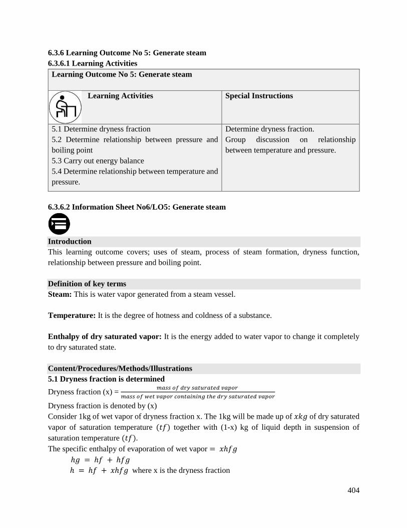
404
6.3.6 Learning Outcome No 5: Generate steam
6.3.6.1 Learning Activities
Learning Outcome No 5: Generate steam
Learning Activities Special Instructions
5.1 Determine dryness fraction
5.2 Determine relationship between pressure and
boiling point
5.3 Carry out energy balance
5.4 Determine relationship between temperature and
pressure.
Determine dryness fraction.
Group discussion on relationship
between temperature and pressure.
6.3.6.2 Information Sheet No6/LO5: Generate steam
Introduction
This learning outcome covers; uses of steam, process of steam formation, dryness function,
relationship between pressure and boiling point.
Definition of key terms
Steam: This is water vapor generated from a steam vessel.
Temperature: It is the degree of hotness and coldness of a substance.
Enthalpy of dry saturated vapor: It is the energy added to water vapor to change it completely
to dry saturated state.
Content/Procedures/Methods/Illustrations
5.1 Dryness fraction is determined
Dryness fraction (x) = 𝑚𝑎𝑠𝑠 𝑜𝑓 𝑑r𝑦 𝑠𝑎𝑡𝑢𝑟𝑎𝑡𝑒𝑑 𝑣𝑎𝑝𝑜𝑟
𝑚𝑎𝑠𝑠 𝑜𝑓 𝑤𝑒𝑡 𝑣𝑎𝑝𝑜𝑟 𝑐𝑜𝑛𝑡𝑎𝑖𝑛𝑖𝑛𝑔 𝑡ℎ𝑒 𝑑𝑟𝑦 𝑠𝑎𝑡𝑢𝑟𝑎𝑡𝑒𝑑 𝑣𝑎𝑝𝑜𝑟
Dryness fraction is denoted by (x)
Consider 1kg of wet vapor of dryness fraction x. The 1kg will be made up of 𝑥𝑘𝑔 of dry saturated
vapor of saturation temperature (𝑡𝑓) together with (1-x) kg of liquid depth in suspension of
saturation temperature (𝑡𝑓).
The specific enthalpy of evaporation of wet vapor = 𝑥ℎ𝑓𝑔
ℎ𝑔 = ℎ𝑓 + ℎ𝑓𝑔
ℎ = ℎ𝑓 + 𝑥ℎ𝑓𝑔 where x is the dryness fraction
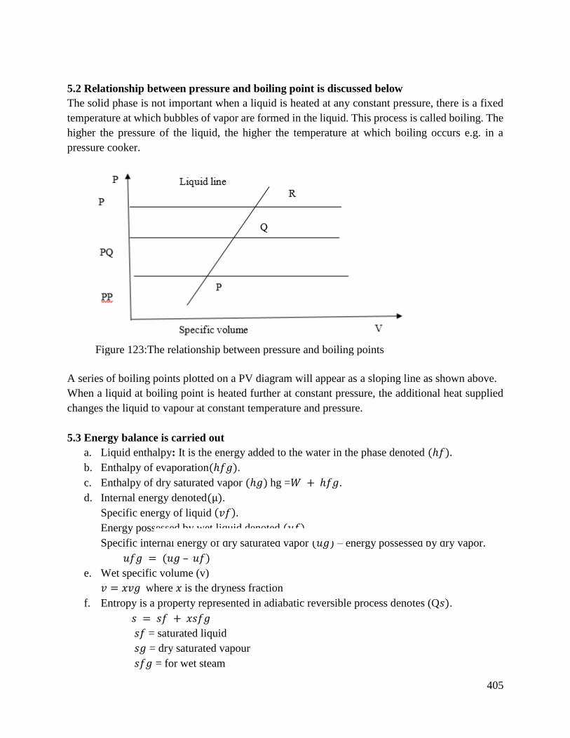
405
5.2 Relationship between pressure and boiling point is discussed below
The solid phase is not important when a liquid is heated at any constant pressure, there is a fixed
temperature at which bubbles of vapor are formed in the liquid. This process is called boiling. The
higher the pressure of the liquid, the higher the temperature at which boiling occurs e.g. in a
pressure cooker.
A series of boiling points plotted on a PV diagram will appear as a sloping line as shown above.
When a liquid at boiling point is heated further at constant pressure, the additional heat supplied
changes the liquid to vapour at constant temperature and pressure.
5.3 Energy balance is carried out
a. Liquid enthalpy: It is the energy added to the water in the phase denoted (ℎ𝑓).
b. Enthalpy of evaporation(ℎ𝑓𝑔).
c. Enthalpy of dry saturated vapor (ℎ𝑔) hg =𝑊 + ℎ𝑓𝑔.
d. Internal energy denoted(µ).
Specific energy of liquid (𝑣𝑓).
Energy possessed by wet liquid denoted (𝑢𝑓).
Specific internal energy of dry saturated vapor (𝑢𝑔) – energy possessed by dry vapor.
𝑢𝑓𝑔 = (𝑢𝑔 – 𝑢𝑓)
e. Wet specific volume (v)
𝑣 = 𝑥𝑣𝑔 where 𝑥 is the dryness fraction
f. Entropy is a property represented in adiabatic reversible process denotes (Q𝑠).
𝑠 = 𝑠𝑓 + 𝑥𝑠𝑓𝑔
𝑠𝑓 = saturated liquid
𝑠𝑔 = dry saturated vapour
𝑠𝑓𝑔 = for wet steam
Figure 123:The relationship between pressure and boiling points
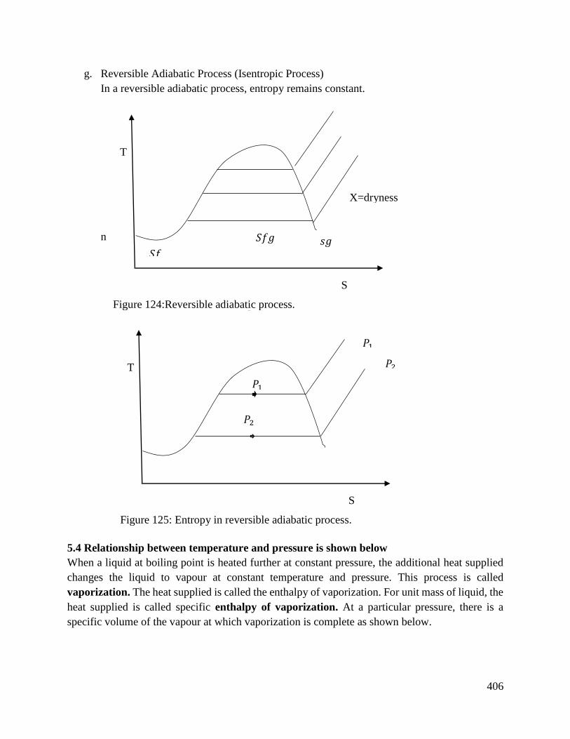
406
g. Reversible Adiabatic Process (Isentropic Process)
In a reversible adiabatic process, entropy remains constant.
n
5.4 Relationship between temperature and pressure is shown below
When a liquid at boiling point is heated further at constant pressure, the additional heat supplied
changes the liquid to vapour at constant temperature and pressure. This process is called
vaporization. The heat supplied is called the enthalpy of vaporization. For unit mass of liquid, the
heat supplied is called specific enthalpy of vaporization. At a particular pressure, there is a
specific volume of the vapour at which vaporization is complete as shown below.
T
𝑆𝑓
𝑆𝑓𝑔 𝑠𝑔
X=dryness
fraction
S
T A T-S on adiabatic reversible process
T
𝑃1
𝑃2
𝑃2
S
T
𝑃1
Figure 124:Reversible adiabatic process.
Figure 125: Entropy in reversible adiabatic process.
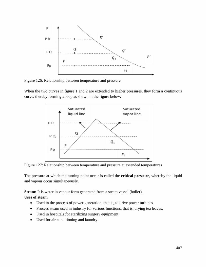
407
Figure 126: Relationship between temperature and pressure
When the two curves in figure 1 and 2 are extended to higher pressures, they form a continuous
curve, thereby forming a loop as shown in the figure below.
Figure 127: Relationship between temperature and pressure at extended temperatures
The pressure at which the turning point occur is called the critical pressure, whereby the liquid
and vapour occur simultaneously.
Steam: It is water in vapour form generated from a steam vessel (boiler).
Uses of steam
Used in the process of power generation, that is, to drive power turbines
Process steam used in industry for various functions, that is, drying tea leaves.
Used in hospitals for sterilizing surgery equipment.
Used for air conditioning and laundry.
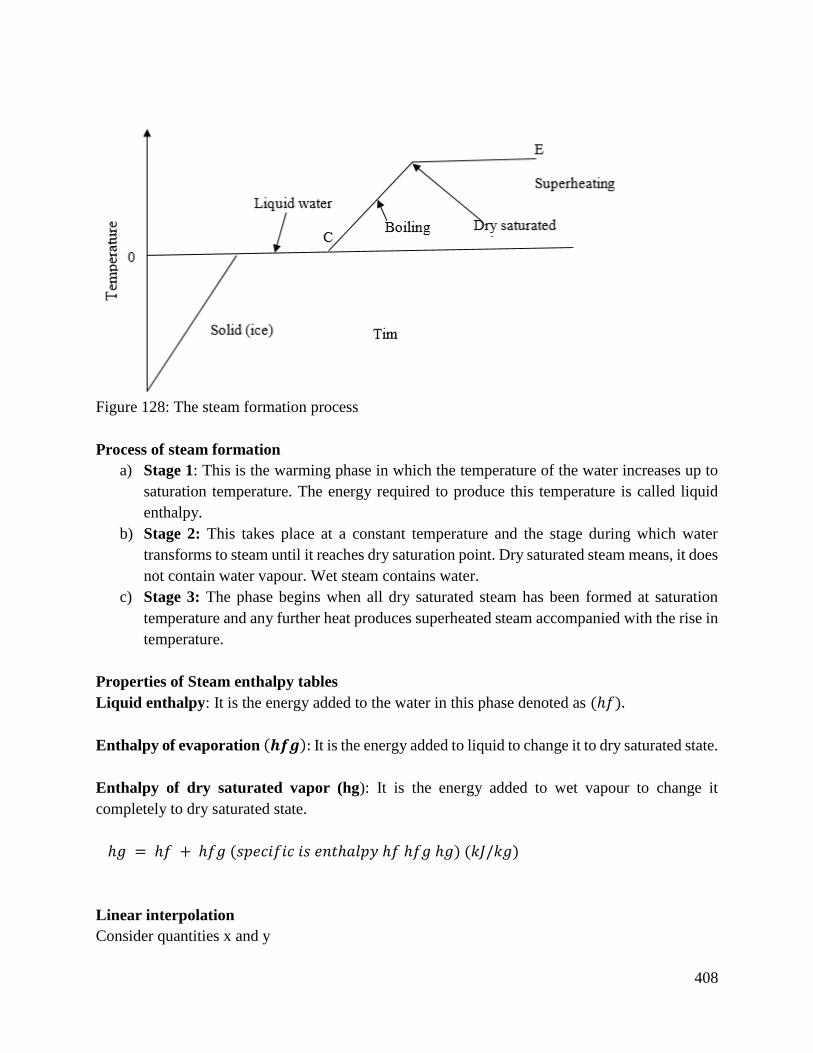
408
Figure 128: The steam formation process
Process of steam formation
a) Stage 1: This is the warming phase in which the temperature of the water increases up to
saturation temperature. The energy required to produce this temperature is called liquid
enthalpy.
b) Stage 2: This takes place at a constant temperature and the stage during which water
transforms to steam until it reaches dry saturation point. Dry saturated steam means, it does
not contain water vapour. Wet steam contains water.
c) Stage 3: The phase begins when all dry saturated steam has been formed at saturation
temperature and any further heat produces superheated steam accompanied with the rise in
temperature.
Properties of Steam enthalpy tables
Liquid enthalpy: It is the energy added to the water in this phase denoted as (ℎ𝑓).
Enthalpy of evaporation (𝒉𝒇𝒈): It is the energy added to liquid to change it to dry saturated state.
Enthalpy of dry saturated vapor (hg): It is the energy added to wet vapour to change it
completely to dry saturated state.
ℎ𝑔 = ℎ𝑓 + ℎ𝑓𝑔 (𝑠𝑝𝑒𝑐𝑖𝑓𝑖𝑐 𝑖𝑠 𝑒𝑛𝑡ℎ𝑎𝑙𝑝𝑦 ℎ𝑓 ℎ𝑓𝑔 ℎ𝑔) (𝑘𝐽/𝑘𝑔)
Linear interpolation
Consider quantities x and y
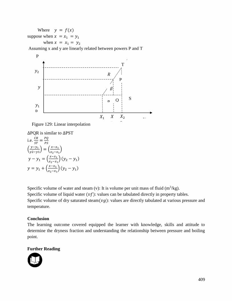
409
𝑋1
p
𝑋2
p
𝑋
p
Where 𝑦 = 𝑓(𝑥)
suppose when 𝑥 = 𝑥1 = 𝑦1
when 𝑥 = 𝑥1 = 𝑦2
Assuming x and y are linearly related between powers P and T
∆PQR is similar to ∆PST
i.e. 𝐶𝑅
𝑆𝑇=
𝑃𝑄
𝑃𝑆
(𝑦−𝑦1
𝑦2−𝑦1) = (
𝑥−𝑥1
𝑥2−𝑥1)
y − 𝑦1 = (𝑥−𝑥1
𝑥2−𝑥1) (𝑦2 − 𝑦1)
𝑦 = 𝑦1 + (𝑥−𝑥1
𝑥2−𝑥1) (𝑦2 − 𝑦1)
Specific volume of water and steam (v): It is volume per unit mass of fluid (m3/kg).
Specific volume of liquid water (𝑣𝑓): values can be tabulated directly in property tables.
Specific volume of dry saturated steam(𝑣𝑔): values are directly tabulated at various pressure and
temperature.
Conclusion
The learning outcome covered equipped the learner with knowledge, skills and attitude to
determine the dryness fraction and understanding the relationship between pressure and boiling
point.
Further Reading
S
𝑦2
𝑦
𝑦1
p
P
Q
T
P
V
𝑃
𝑅
𝛽
Figure 129: Linear interpolation
410
1. Basic Engineering Thermodynamics by R. Joel
6.3.6.3 Self-Assessment
Written assessment
1. Choose the correct answer.
a) Specific volume of water decreases on freezing.
b) Boiling point of water decreases with increasing pressure.
c) Specific volume of CO2 increases on freezing.
d) Freezing temperature of water decreases with increasing pressure.
2. Which one of the following is true?
a) The slope of vaporization curve is always negative.
b) The slope of vaporization curve is always positive.
c) The slope of sublimation curve is negative for all pure substances.
d) The slope of fusion curve is positive for all pure substances.
3. Which one of the following statements is correct?
a) The process of passing from liquid to vapor is condensation.
b) An isothermal line is also a constant pressure line during wet region.
c) Pressure and temperature are independent during phase change.
d) The term dryness fraction is used to describe the fraction by mass of liquid in the
mixture of liquid water and water vapor.
4. The latent heat of vaporization at critical point is?
a) Less than zero
b) Greater than zero
c) Equal to zero
d) None of the above
5. With the increase in pressure, one of the following happens. Which one is it?
a) Boiling point of water increases and enthalpy of evaporation increases.
b) Boiling point of water increases and enthalpy of evaporation decreases.
c) Boiling point of water decreases and enthalpy of evaporation increases.
6. With increase in pressure____________________
a) Enthalpy of dry saturated steam increases.
b) Enthalpy of dry saturated steam decreases.
c) Enthalpy of dry saturated steam remains the same.

411
d) Enthalpy of dry saturated steam first increases and then decreases.
7. Dryness fraction of steam is defined as ___________________
a) Mass of water vapor in suspension (mass of water vapor in suspension + mass of
dry steam).
b) Mass of dry steam/ mas of water vapor in suspension.
c) Mass of dry steam (mass of dry steam + mass of water vapor in suspension)
d) Mass of water vapor in suspension/ mass of dry steam.
8. What is a pure substance?
9. Draw and explain a PT (pressure temperature) diagram for a pure substance
10. Does wet steam obey laws of perfect gases?
11. Describe the process of formation of steam and give its graphical representation also.
12. Explain the following terms relating to steam formation.
a) Sensible heat of water
b) Latent heat of steam
Oral Assessment
1. What do you mean by the following?
a. Internal energy of steam.
b. Entropy of wet steam.
2. What advantages are obtained if superheated steam is used in steam prime movers?
Project
Design fabrication and testing of a steam generator.
6.3.6.4 Tools, Equipment, Supplies and Materials
Scientific calculators
Steam tables
Reference materials
Practical materials
6.3.6.5 References
Haywood, R.W., 2013. Analysis of engineering cycles: thermodynamics and fluid mechanics
series. Elsevier.
6.3.7 Learning Outcome No.6: Perform thermodynamics reversibility and entropy
6.3.2.1 Learning Activities
Learning Outcome No 6: Perform thermodynamics reversibility and entropy
412
Learning Activities Special Instructions
8.1 Explain thermodynamics reversibility
8.2 Explain principles of heat engine
8.3 Apply second law of thermodynamics
8.4 Explain entropy in thermodynamics
cycle
The student be ready to read and understand the
steam tables carefully.
The student be able to differentiate the different
thermal dynamic diagrams.
The student must understand the difference between
the Otto and Carnot cycle.
6.3.7.2 Information Sheet No6/LO6: Perform thermodynamics reversibility and entropy
Introduction
This learning outcome performs thermodynamic reversibility and entropy, covers the definition of
key terms used, content/procedures/methods and illustrations for each and every learning activity
under this learning outcome. It also covers the conclusion and the further reading that entails the
sources where more about the content development can be sourced. The learning outcome also
covers the self-assessment questions that contain written, oral, practical and project assessment
questions. Tools, equipment, supplies and materials to be used and also the reference books for the
outcome are also covered under the learning outcome.
Definition of key terms
Thermodynamics: It is a branch of engineering science that deals with the study of heat, work
and their interrelationship.
Heat engine cycle: It is the process by which heat flows in a circular system from isentropic
compression to reversible constant volume cooling.
Entropy: Is a property represented in an adiabatic reversible process and it is always denoted by
letter “S”. Also, it is the measure of energy which is not available to do work in a system.
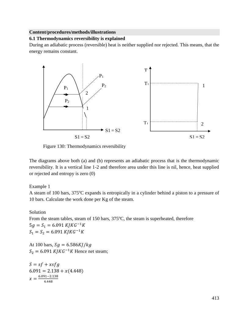
413
Content/procedures/methods/illustrations
6.1 Thermodynamics reversibility is explained
During an adiabatic process (reversible) heat is neither supplied nor rejected. This means, that the
energy remains constant.
The diagrams above both (a) and (b) represents an adiabatic process that is the thermodynamic
reversibility. It is a vertical line 1-2 and therefore area under this line is nil, hence, heat supplied
or rejected and entropy is zero (0)
Example 1
A steam of 100 bars, 375oC expands is entropically in a cylinder behind a piston to a pressure of
10 bars. Calculate the work done per Kg of the steam.
Solution
From the steam tables, steam of 150 bars, 375oC, the steam is superheated, therefore
5𝑔 = 𝑆1 = 6.091 𝐾𝐽𝐾𝐺−1𝐾
𝑆1 = 𝑆2 = 6.091 𝐾𝐽𝐾𝐺−1𝐾
At 100 bars, 𝑆𝑔 = 6.586𝐾𝐽/𝑘𝑔
𝑆2 = 6.091 𝐾𝐽𝐾𝐺−1𝐾 Hence net steam;
𝑆 = 𝑠𝑓 + 𝑥𝑠𝑓𝑔
6.091 = 2.138 + 𝑥(4.448)
𝑥 =6.091−2.138
4.448
P1
P2
S1 = S2
P1
P2
2
1
S1 = S2
2
S1 = S2
T1
T1
T
1
Figure 130: Thermodynamics reversibility
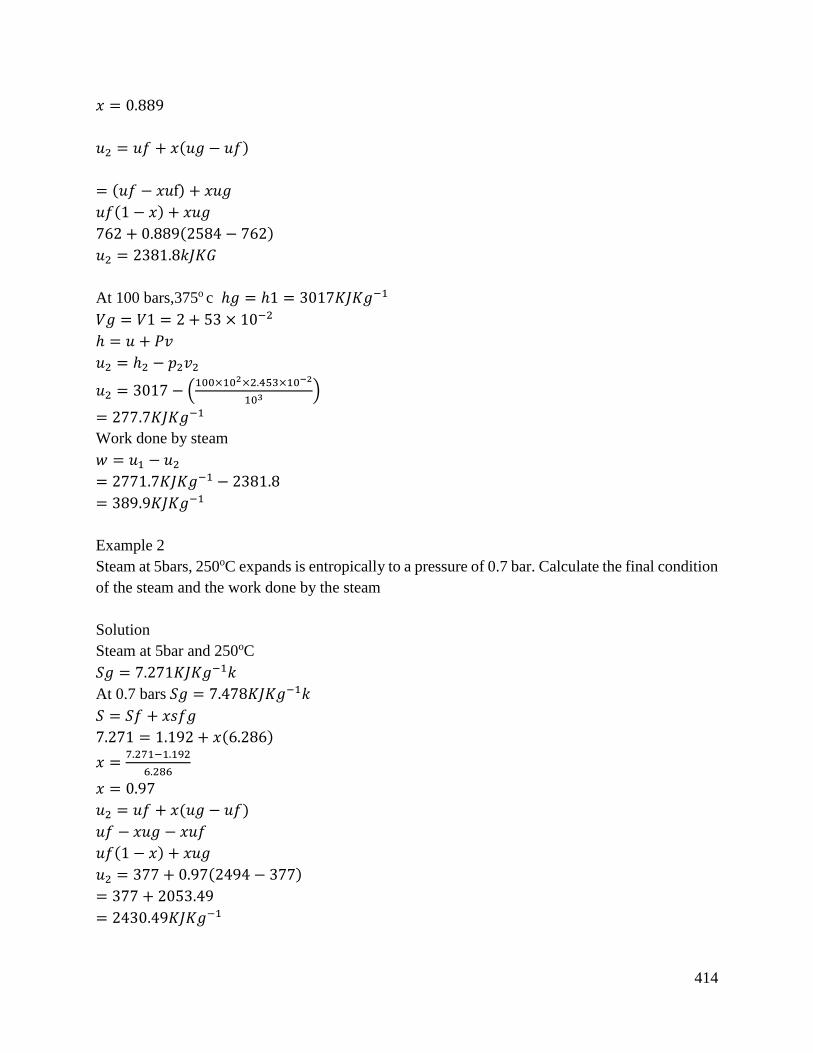
414
𝑥 = 0.889
𝑢2 = 𝑢𝑓 + 𝑥(𝑢𝑔 − 𝑢𝑓)
= (𝑢𝑓 − 𝑥𝑢f) + 𝑥𝑢𝑔
𝑢𝑓(1 − 𝑥) + 𝑥𝑢𝑔
762 + 0.889(2584 − 762)
𝑢2 = 2381.8𝑘𝐽𝐾𝐺
At 100 bars,375o c ℎ𝑔 = ℎ1 = 3017𝐾𝐽𝐾𝑔−1
𝑉𝑔 = 𝑉1 = 2 + 53 × 10−2
ℎ = 𝑢 + 𝑃𝑣
𝑢2 = ℎ2 − 𝑝2𝑣2
𝑢2 = 3017 − (100×102×2.453×10−2
103 )
= 277.7𝐾𝐽𝐾𝑔−1
Work done by steam
𝑤 = 𝑢1 − 𝑢2
= 2771.7𝐾𝐽𝐾𝑔−1 − 2381.8
= 389.9𝐾𝐽𝐾𝑔−1
Example 2
Steam at 5bars, 250oC expands is entropically to a pressure of 0.7 bar. Calculate the final condition
of the steam and the work done by the steam
Solution
Steam at 5bar and 250oC
𝑆𝑔 = 7.271𝐾𝐽𝐾𝑔−1𝑘
At 0.7 bars 𝑆𝑔 = 7.478𝐾𝐽𝐾𝑔−1𝑘
𝑆 = 𝑆𝑓 + 𝑥𝑠𝑓𝑔
7.271 = 1.192 + 𝑥(6.286)
𝑥 =7.271−1.192
6.286
𝑥 = 0.97
𝑢2 = 𝑢𝑓 + 𝑥(𝑢𝑔 − 𝑢𝑓)
𝑢𝑓 − 𝑥𝑢𝑔 − 𝑥𝑢𝑓
𝑢𝑓(1 − 𝑥) + 𝑥𝑢𝑔
𝑢2 = 377 + 0.97(2494 − 377)
= 377 + 2053.49
= 2430.49𝐾𝐽𝐾𝑔−1
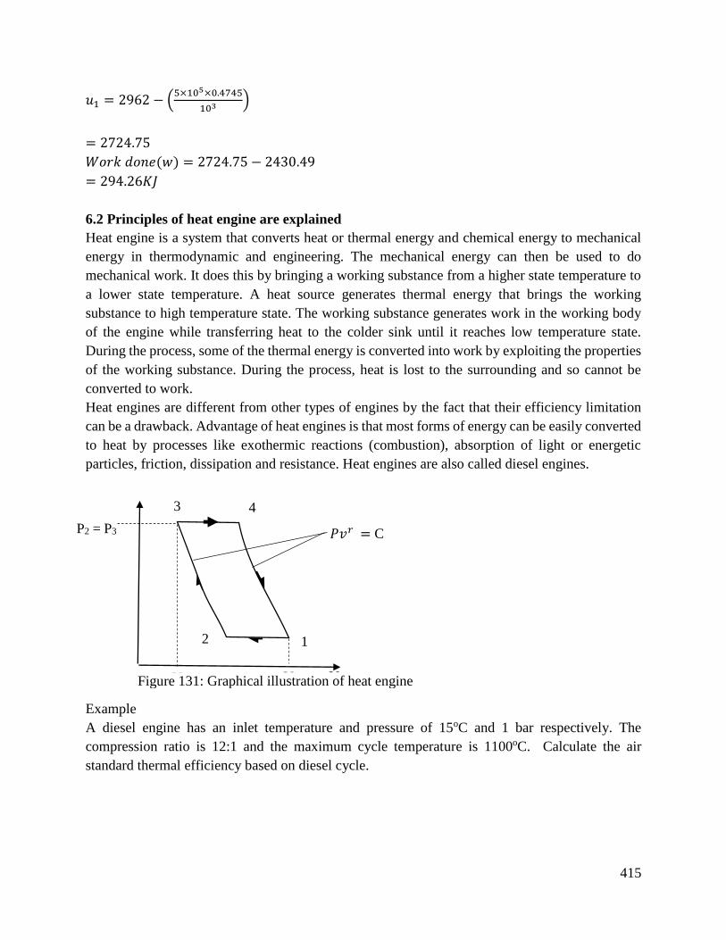
415
𝑢1 = 2962 − (5×105×0.4745
103)
= 2724.75
𝑊𝑜𝑟𝑘 𝑑𝑜𝑛𝑒(𝑤) = 2724.75 − 2430.49
= 294.26𝐾𝐽
6.2 Principles of heat engine are explained
Heat engine is a system that converts heat or thermal energy and chemical energy to mechanical
energy in thermodynamic and engineering. The mechanical energy can then be used to do
mechanical work. It does this by bringing a working substance from a higher state temperature to
a lower state temperature. A heat source generates thermal energy that brings the working
substance to high temperature state. The working substance generates work in the working body
of the engine while transferring heat to the colder sink until it reaches low temperature state.
During the process, some of the thermal energy is converted into work by exploiting the properties
of the working substance. During the process, heat is lost to the surrounding and so cannot be
converted to work.
Heat engines are different from other types of engines by the fact that their efficiency limitation
can be a drawback. Advantage of heat engines is that most forms of energy can be easily converted
to heat by processes like exothermic reactions (combustion), absorption of light or energetic
particles, friction, dissipation and resistance. Heat engines are also called diesel engines.
Example
A diesel engine has an inlet temperature and pressure of 15oC and 1 bar respectively. The
compression ratio is 12:1 and the maximum cycle temperature is 1100oC. Calculate the air
standard thermal efficiency based on diesel cycle.
1
4 3
2
𝑃𝑣𝑟 = C P2 = P3
V
2
V
1
V Figure 131: Graphical illustration of heat engine
416
Solution
𝑇1 = 15𝑂𝐶 + 273 = 288𝐾
𝑇3 = (1100 + 273) = 1373𝐾
𝑇3
𝑇1= (
𝑉1
𝑉2)𝑟−1
𝑟 = 1.4
𝑇2 = 𝑇1 (𝑉1
𝑉2)𝑟−1
= 288(12)1−4−1
= 288 × 120−4
= 778.15
𝑝2 = 𝑝3 𝑝2𝑣2
𝑇2 =𝑃3𝑣3
𝑇3
𝑉2
𝑇2=
𝑉3
𝑇3
1373
778.15=
𝑉3
𝑉2
= 1.764
But 𝑣4
𝑣3= (
𝑣4
𝑣2) (
𝑣2
𝑣3)
𝑣4
𝑣3= 12 ×
1
1.76
=6.82
𝑇3
𝑇4= (
𝑉4
𝑉3)𝑟−1
𝑇3
𝑇4= 6.81−4−1
1
𝑝𝑣𝑟 = 𝑐 2
4
Figure 132: The standard thermal
efficiency

417
𝑇4 =𝑇3
6.80.4
𝑇3 = 𝑇4 × 6.80.4
𝑇4 =1373
6.80.4
𝑇4 = 637.09𝑘
𝐶𝑃 = 1.005 𝑓𝑜𝑟 𝑎𝑖𝑟
𝑄1 = 𝐶𝑃(𝑇2 − 𝑇1)
= 597.8𝐾𝐽
𝐶𝑣 𝑓𝑜𝑟 𝑎𝑖𝑟 = 0.718𝑘𝑗𝑘𝐺
𝑄2 = 𝐶𝑣(74 − 71)
= 0.718(637.09 − 288 )
= 250.65𝐾𝐽𝐾𝑔−1
= 1 −𝑄2
𝑄1
= (1 −250.65
597.8) × 100
= 58.07%
Efficiency =𝑄1
𝑄1−
𝑄2
𝑄= 1 −
𝑄2
𝑄1
But a constant pressure (MCP4T)
𝑄1 = 𝐶𝑝(𝑇3 − 𝑇2)
Also, at constant volume
𝑄2 = 𝐶𝑣(𝑇4 − 𝑇1)
Since there is no heat in process 1-2 and 3-4, Q1 and Q2 are substituted into the equation
Diesel=1 −𝑄2
𝑄1
Where𝛽 =v3
𝑣2
= 1 −𝑐𝑣(𝑇4−𝑇1)
𝐶𝑝(𝑡3−𝑡2)
𝑃2𝑉2𝑟=𝑃3𝑉3
𝑟
𝑃2𝑉2𝑟/𝑇2=𝑃3𝑉3
𝑟/𝑇3
𝑇3 = 𝑇2 (𝑃3
𝑃2) (
𝑉3
𝑉2)
𝑃2𝑉2𝑟=𝑃3𝑉3
𝑟

418
𝑃2
𝑃3 =(
𝑉3
𝑉2)𝑟
(𝑃3
𝑃2)=(
𝑉3
𝑉2)−𝑟
𝑇3 = 𝑇2 (𝑃3
𝑃2) (
𝑉3
𝑉2)
𝑇3 = 𝑇2 (𝑉3
𝑉2)−𝑟
(𝑉3
𝑉2)1
𝑇3 = 𝑇2 (𝑉3
𝑉2)1−𝑟
𝑇3 = 𝑇2(𝛽)1−𝑟
Diesel=1-𝛽𝑟−𝑟
(𝛽−1)𝑟𝑟−1
𝑃1𝑉1𝑟=𝑃4𝑉4
𝑟 𝑃1𝑉1
𝑇1=
𝑃4𝑉4
T4
𝑇4 = 𝑇1 (𝑉4
𝑉1)−𝑟
(𝑉4
𝑉1)
𝑇4 = 𝑇1 (𝑉4
𝑉1)−𝑟
(𝑉4
𝑉1) (
𝑃4
𝑃1) = (
𝑉4
𝑉1)−𝑟
𝑇4 = 𝑇1 (𝑉4
𝑉1)−𝑟
𝑇4 = 𝑇1(𝛽)−1
=1−𝑇1(𝛽)1−𝑟−𝑇1
𝑇2(𝛽)1−𝑟−𝑇2
1−𝑇1[𝛽1−𝑟−1]
𝑇2 [𝛽1−𝑟−1]
But 𝑇2 = 𝑇1𝑉1𝑟−1
1−𝑇1[𝛽1−𝑟−1]
𝑇1𝑉1[𝛽1−𝑟−1]
Di=1 −[𝛽1−𝑟−1]
[𝛽1−𝑟−1]𝑟𝑟−1
1−𝛽^𝑟−1
(𝛽𝑟−1)𝑟𝑟−1.𝑟
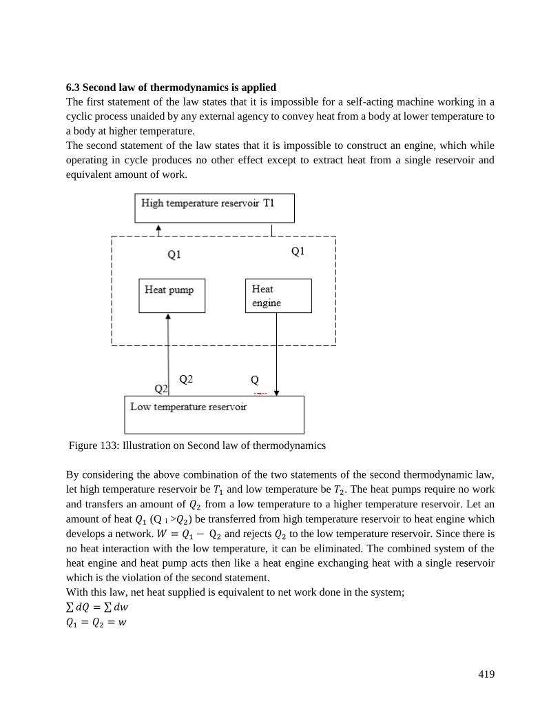
419
6.3 Second law of thermodynamics is applied
The first statement of the law states that it is impossible for a self-acting machine working in a
cyclic process unaided by any external agency to convey heat from a body at lower temperature to
a body at higher temperature.
The second statement of the law states that it is impossible to construct an engine, which while
operating in cycle produces no other effect except to extract heat from a single reservoir and
equivalent amount of work.
By considering the above combination of the two statements of the second thermodynamic law,
let high temperature reservoir be 𝑇1 and low temperature be 𝑇2. The heat pumps require no work
and transfers an amount of 𝑄2 from a low temperature to a higher temperature reservoir. Let an
amount of heat 𝑄1 (Q 1 >𝑄2) be transferred from high temperature reservoir to heat engine which
develops a network. 𝑊 = 𝑄1 − Q2 and rejects 𝑄2 to the low temperature reservoir. Since there is
no heat interaction with the low temperature, it can be eliminated. The combined system of the
heat engine and heat pump acts then like a heat engine exchanging heat with a single reservoir
which is the violation of the second statement.
With this law, net heat supplied is equivalent to net work done in the system;
∑𝑑𝑄 = ∑𝑑𝑤
𝑄1 = 𝑄2 = 𝑤
Figure 133: Illustration on Second law of thermodynamics
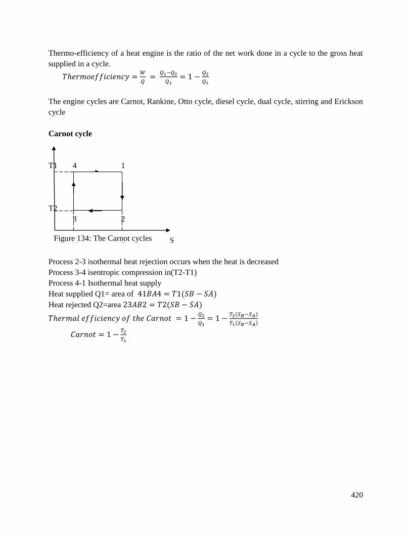
420
Thermo-efficiency of a heat engine is the ratio of the net work done in a cycle to the gross heat
supplied in a cycle.
𝑇ℎ𝑒𝑟𝑚𝑜𝑒𝑓𝑓𝑖𝑐𝑖𝑒𝑛𝑐𝑦 =𝑊
𝑄 =
𝑄1−𝑄2
𝑄1= 1 −
𝑄2
𝑄1
The engine cycles are Carnot, Rankine, Otto cycle, diesel cycle, dual cycle, stirring and Erickson
cycle
Carnot cycle
T1 4 1
T2
3 2
A B S
Process 2-3 isothermal heat rejection occurs when the heat is decreased
Process 3-4 isentropic compression in(T2-T1)
Process 4-1 Isothermal heat supply
Heat supplied Q1= area of 41𝐵𝐴4 = 𝑇1(𝑆𝐵 − 𝑆𝐴)
Heat rejected Q2=area 23𝐴𝐵2 = 𝑇2(𝑆𝐵 − 𝑆𝐴)
𝑇ℎ𝑒𝑟𝑚𝑎𝑙 𝑒𝑓𝑓𝑖𝑐𝑖𝑒𝑛𝑐𝑦 𝑜𝑓 𝑡ℎ𝑒 𝐶𝑎𝑟𝑛𝑜𝑡 = 1 −𝑄2
𝑄1= 1 −
𝑇2(𝑆𝐵−𝑆𝐴)
𝑇1(𝑆𝐵−𝑆𝐴)
𝐶𝑎𝑟𝑛𝑜𝑡 = 1 −𝑇2
𝑇1
Figure 134: The Carnot cycles
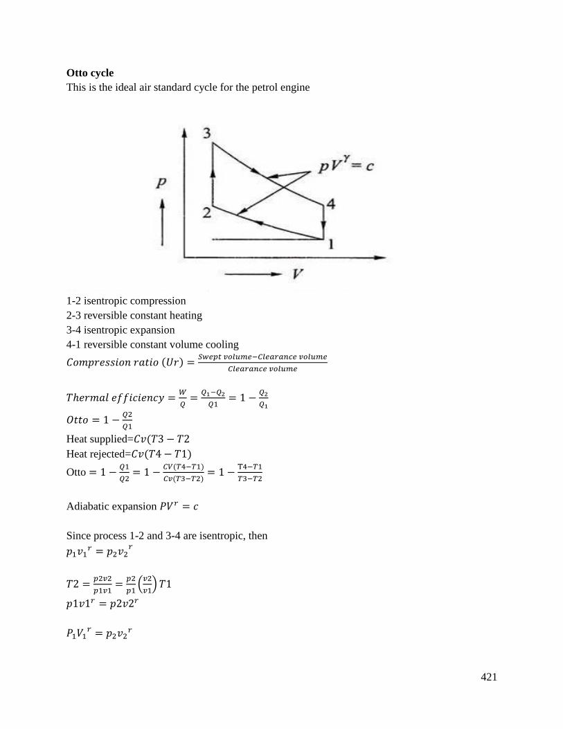
421
Otto cycle
This is the ideal air standard cycle for the petrol engine
1-2 isentropic compression
2-3 reversible constant heating
3-4 isentropic expansion
4-1 reversible constant volume cooling
𝐶𝑜𝑚𝑝𝑟𝑒𝑠𝑠𝑖𝑜𝑛 𝑟𝑎𝑡𝑖𝑜 (𝑈𝑟) =𝑆𝑤𝑒𝑝𝑡 𝑣𝑜𝑙𝑢𝑚𝑒−𝐶𝑙𝑒𝑎𝑟𝑎𝑛𝑐𝑒 𝑣𝑜𝑙𝑢𝑚𝑒
𝐶𝑙𝑒𝑎𝑟𝑎𝑛𝑐𝑒 𝑣𝑜𝑙𝑢𝑚𝑒
𝑇ℎ𝑒𝑟𝑚𝑎𝑙 𝑒𝑓𝑓𝑖𝑐𝑖𝑒𝑛𝑐𝑦 =𝑊
𝑄=
𝑄1−𝑄2
𝑄1= 1 −
𝑄2
𝑄1
𝑂𝑡𝑡𝑜 = 1 −𝑄2
𝑄1
Heat supplied=𝐶𝑣(𝑇3 − 𝑇2
Heat rejected=𝐶𝑣(𝑇4 − 𝑇1)
Otto = 1 −𝑄1
𝑄2= 1 −
𝐶𝑉(𝑇4−𝑇1)
𝐶𝑣(𝑇3−𝑇2)= 1 −
T4−𝑇1
𝑇3−𝑇2
Adiabatic expansion 𝑃𝑉𝑟 = 𝑐
Since process 1-2 and 3-4 are isentropic, then
𝑝1𝑣1𝑟 = 𝑝2𝑣2
𝑟
𝑇2 =𝑝2𝑣2
𝑝1𝑣1=
𝑝2
𝑝1(𝑣2
𝑣1) 𝑇1
𝑝1𝑣1𝑟 = 𝑝2𝑣2𝑟
𝑃1𝑉1𝑟 = 𝑝2𝑣2
𝑟
422
𝑝2
𝑝1= (
(𝑣1)
𝑣2 )𝑟
𝑇2 = (𝑉1
𝑉2)𝑟
(𝑉1
𝑉2)−1
𝑇1
𝑇2 = (𝑟𝑟)𝑟−1 − 𝑇1
𝑇2
𝑇1= (
𝑉1
𝑉2)𝑟−1
= (𝑣4
𝑣3)𝑟−1
=𝑇3
𝑇4
(𝑣4
𝑣3)𝑟−1
=𝑇3
𝑇4
𝑇3 = (𝑣4
𝑣3)𝑟−1
. 𝑇4
Otto= 1 − (𝑇4−𝑇1
𝑇3−𝑇2)
=1−𝑇4−𝑇1
(𝑟𝑟)𝑟−1(𝑇4−𝑇1)
= 1 −1
(𝑟𝑟)𝑟−1
6.4 Entropy is explained in thermodynamics cycle
Entropy is a function of a quantity of heat which shows the possibility of conversion of that heat
into work. The increase in entropy is small when heat is added at a higher temperature and is
greater when heat addition is made at a lower temperature. Thus, for a maximum entropy, there is
minimum availability for conversion into work and for minimum entropy there is maximum
availability for conversion into work.
Entropy – a property of a system
For instance, a system undergoes a reversible process from state 1 to state 2 along path 𝑙 and then
from state 2 to the original state 1 along path 𝑚. Applying the first statement of the second law of
thermodynamics to the system.
∮𝑅𝑑𝑄
𝑇= 0
Where ∮ reversible process
Hence when the system passes through the cycle 1 − 𝑙 − 2 − 𝑚 − 1, it becomes;
∫𝑑𝑄
𝑇+
2
1(𝑙)∫
𝑑𝑄
𝑇= 0
1
2(𝑚)……………………………… . (𝑖)
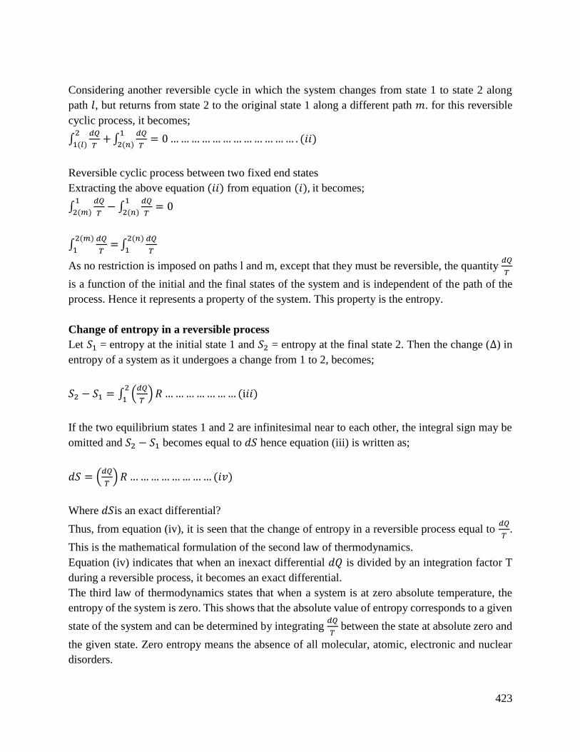
423
Considering another reversible cycle in which the system changes from state 1 to state 2 along
path 𝑙, but returns from state 2 to the original state 1 along a different path 𝑚. for this reversible
cyclic process, it becomes;
∫𝑑𝑄
𝑇+
2
1(𝑙)∫
𝑑𝑄
𝑇= 0
1
2(𝑛)……………………………… . (𝑖𝑖)
Reversible cyclic process between two fixed end states
Extracting the above equation (𝑖𝑖) from equation (𝑖), it becomes;
∫𝑑𝑄
𝑇
1
2(𝑚)− ∫
𝑑𝑄
𝑇= 0
1
2(𝑛)
∫𝑑𝑄
𝑇=
2(𝑚)
1∫
𝑑𝑄
𝑇
2(𝑛)
1
As no restriction is imposed on paths l and m, except that they must be reversible, the quantity 𝑑𝑄
𝑇
is a function of the initial and the final states of the system and is independent of the path of the
process. Hence it represents a property of the system. This property is the entropy.
Change of entropy in a reversible process
Let 𝑆1 = entropy at the initial state 1 and 𝑆2 = entropy at the final state 2. Then the change (∆) in
entropy of a system as it undergoes a change from 1 to 2, becomes;
𝑆2 − 𝑆1 = ∫ (𝑑𝑄
𝑇)𝑅
2
1…………………(i𝑖𝑖)
If the two equilibrium states 1 and 2 are infinitesimal near to each other, the integral sign may be
omitted and 𝑆2 − 𝑆1 becomes equal to 𝑑𝑆 hence equation (iii) is written as;
𝑑𝑆 = (𝑑𝑄
𝑇)𝑅 ……………………(𝑖𝑣)
Where 𝑑𝑆is an exact differential?
Thus, from equation (iv), it is seen that the change of entropy in a reversible process equal to 𝑑𝑄
𝑇.
This is the mathematical formulation of the second law of thermodynamics.
Equation (iv) indicates that when an inexact differential 𝑑𝑄 is divided by an integration factor T
during a reversible process, it becomes an exact differential.
The third law of thermodynamics states that when a system is at zero absolute temperature, the
entropy of the system is zero. This shows that the absolute value of entropy corresponds to a given
state of the system and can be determined by integrating 𝑑𝑄
𝑇 between the state at absolute zero and
the given state. Zero entropy means the absence of all molecular, atomic, electronic and nuclear
disorders.
424
N/B: It is possible to determine the change in entropy but not the absolute value of the entropy.
Conclusion
The learning outcome covered the key terms definitions, the contents, procedures and illustrations
for the learning activities.
Further Reading
1. Fundamentals of Engineering Thermodynamics by Moran and Shapiro
2. Fundamentals of Thermodynamics by Borgnakke and Sonntag
3. Engineering Thermodynamics by P. K. Nag
6.3.7.3 Self-Assessment
Written assessment
1. The second law of thermodynamics defines?
a) Heat
b) Work
c) Enthalpy
d) Entropy
2. For reversible adiabatic process, the change in entropy is?
a) Zero
b) Minimum
c) Maximum
d) Infinite
e) Unity
3. For any reversible process, the change in entropy of the system and the surrounding is?
a) Zero
b) Unity
c) Negative
d) Positive
e) Infinite
4. The second statement of the second law of thermodynamics deals with?
a) Conversation of energy

425
b) Conservation of heat
c) Conservation of mass
d) Conservation of heat into work
e) Conservation of work into heat
5. In a reversible cycle, the entropy of the system?
a) Increases
b) Decreases
c) Do not change
d) Increases then decreases
e) Depends on the properties of the working substances
6. The entropy may be express as a function of?
a) Pressure and temperature
b) Temperature and volume
c) Heat and work
d) All of the above
e) None of the above
7. The change of entropy when heat is absorbed by the gas is?
a) Positive
b) Negative
c) Positive or negative
d) None
8. What is entropy in thermodynamics?
9. State the second statement of the second law of thermodynamics
10. What is temperature-entropy diagram?
11. Prove that entropy is a property of a system
12. Give an expression for entropy changes for an open system
Oral Assessment
1. What is thermodynamic temperature?
2. What is heat engine cycle in thermodynamics?
Practical Assessment
1. Describe the working of a Carnot cycle
Project
Derive an expression for the efficiency of the reversible heat engine

426
6.3.7.4 Tools, Equipment, Supplies and Materials
Scientific Calculators
Relevant reference materials
Stationeries
Relevant practical materials
Dice
Computers with internet connection
6.3.7.5 References
Rost, C. M., Sachet, E., Borman, T., Moballegh, A., Dickey, E. C., Hou, D., ... & Maria, J. P.
(2015). Entropy-stabilized oxides. Nature communications, 6, 8485.
Del Rio, L., Åberg, J., Renner, R., Dahlsten, O., & Vedral, V. (2011). The thermodynamic meaning
of negative entropy. Nature, 474(7349), 61.
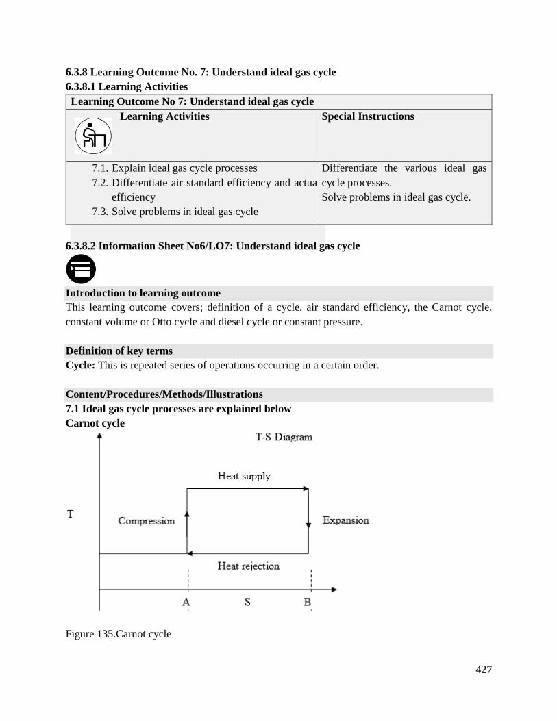
427
6.3.8 Learning Outcome No. 7: Understand ideal gas cycle
6.3.8.1 Learning Activities
Learning Outcome No 7: Understand ideal gas cycle
Learning Activities Special Instructions
7.1. Explain ideal gas cycle processes
7.2. Differentiate air standard efficiency and actual
efficiency
7.3. Solve problems in ideal gas cycle
Differentiate the various ideal gas
cycle processes.
Solve problems in ideal gas cycle.
6.3.8.2 Information Sheet No6/LO7: Understand ideal gas cycle
Introduction to learning outcome
This learning outcome covers; definition of a cycle, air standard efficiency, the Carnot cycle,
constant volume or Otto cycle and diesel cycle or constant pressure.
Definition of key terms
Cycle: This is repeated series of operations occurring in a certain order.
Content/Procedures/Methods/Illustrations
7.1 Ideal gas cycle processes are explained below
Carnot cycle
Figure 135.Carnot cycle
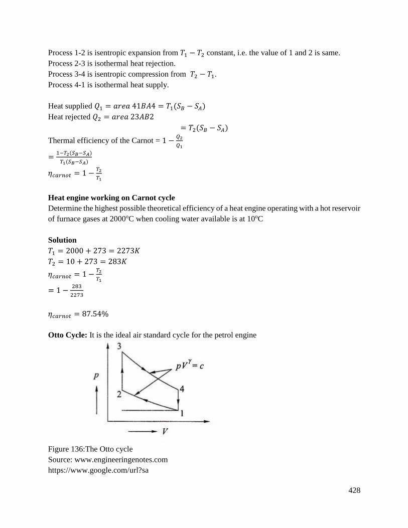
428
Process 1-2 is isentropic expansion from 𝑇1 − 𝑇2 constant, i.e. the value of 1 and 2 is same.
Process 2-3 is isothermal heat rejection.
Process 3-4 is isentropic compression from 𝑇2 − 𝑇1.
Process 4-1 is isothermal heat supply.
Heat supplied 𝑄1 = 𝑎𝑟𝑒𝑎 41𝐵𝐴4 = 𝑇1(𝑆𝐵 − 𝑆𝐴)
Heat rejected 𝑄2 = 𝑎𝑟𝑒𝑎 23𝐴𝐵2
= 𝑇2(𝑆𝐵 − 𝑆𝐴)
Thermal efficiency of the Carnot = 1 −𝑄2
𝑄1
=1−𝑇2(𝑆𝐵−𝑆𝐴)
𝑇1(𝑆𝐵−𝑆𝐴)
𝜂𝑐𝑎𝑟𝑛𝑜𝑡 = 1 −𝑇2
𝑇1
Heat engine working on Carnot cycle
Determine the highest possible theoretical efficiency of a heat engine operating with a hot reservoir
of furnace gases at 2000oC when cooling water available is at 10oC
Solution
𝑇1 = 2000 + 273 = 2273𝐾
𝑇2 = 10 + 273 = 283𝐾
𝜂𝑐𝑎𝑟𝑛o𝑡 = 1 −𝑇2
𝑇1
= 1 −283
2273
𝜂𝑐𝑎𝑟𝑛𝑜𝑡 = 87.54%
Otto Cycle: It is the ideal air standard cycle for the petrol engine
Figure 136:The Otto cycle
Source: www.engineeringenotes.com
https://www.google.com/url?sa
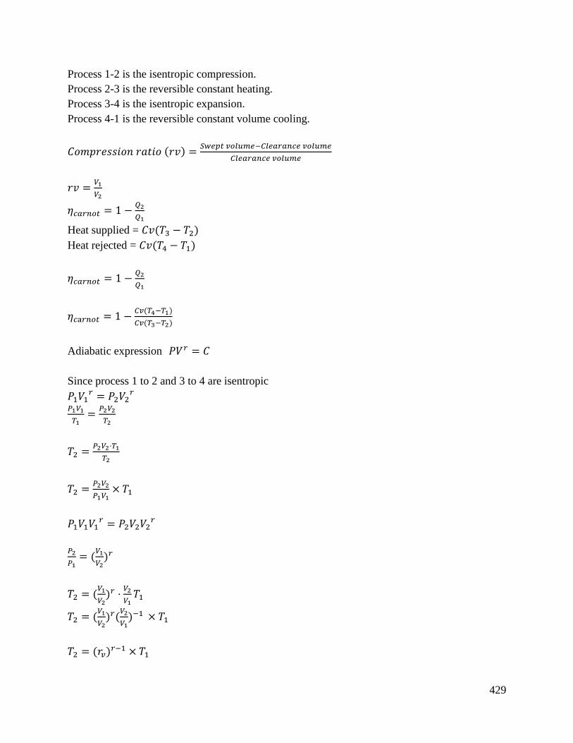
429
Process 1-2 is the isentropic compression.
Process 2-3 is the reversible constant heating.
Process 3-4 is the isentropic expansion.
Process 4-1 is the reversible constant volume cooling.
𝐶𝑜𝑚𝑝𝑟𝑒𝑠𝑠𝑖𝑜𝑛 𝑟𝑎𝑡𝑖𝑜 (𝑟𝑣) =𝑆𝑤𝑒𝑝𝑡 𝑣𝑜𝑙𝑢𝑚𝑒−𝐶𝑙𝑒𝑎𝑟𝑎𝑛𝑐𝑒 𝑣𝑜𝑙𝑢𝑚𝑒
𝐶𝑙𝑒𝑎𝑟𝑎𝑛𝑐𝑒 𝑣𝑜𝑙𝑢𝑚𝑒
𝑟𝑣 =𝑉1
𝑉2
𝜂𝑐𝑎𝑟𝑛𝑜𝑡 = 1 −𝑄2
𝑄1
Heat supplied = 𝐶𝑣(𝑇3 − 𝑇2)
Heat rejected = 𝐶𝑣(𝑇4 − 𝑇1)
𝜂𝑐𝑎𝑟𝑛𝑜𝑡 = 1 −𝑄2
𝑄1
𝜂𝑐a𝑟𝑛𝑜𝑡 = 1 −𝐶𝑣(𝑇4−𝑇1)
𝐶𝑣(𝑇3−𝑇2)
Adiabatic expression 𝑃𝑉𝑟 = 𝐶
Since process 1 to 2 and 3 to 4 are isentropic
𝑃1𝑉1𝑟 = 𝑃2𝑉2
𝑟 𝑃1𝑉1
𝑇1=
𝑃2𝑉2
𝑇2
𝑇2 =𝑃2𝑉2⋅𝑇1
𝑇2
𝑇2 =𝑃2𝑉2
𝑃1𝑉1× 𝑇1
𝑃1𝑉1𝑉1𝑟 = 𝑃2𝑉2𝑉2
𝑟
𝑃2
𝑃1= (
𝑉1
𝑉2)𝑟
𝑇2 = (𝑉1
𝑉2)𝑟 ⋅
𝑉2
𝑉1𝑇1
𝑇2 = (𝑉1
𝑉2)𝑟(
𝑉2
𝑉1)−1 × 𝑇1
𝑇2 = (𝑟𝑣)𝑟−1 × 𝑇1
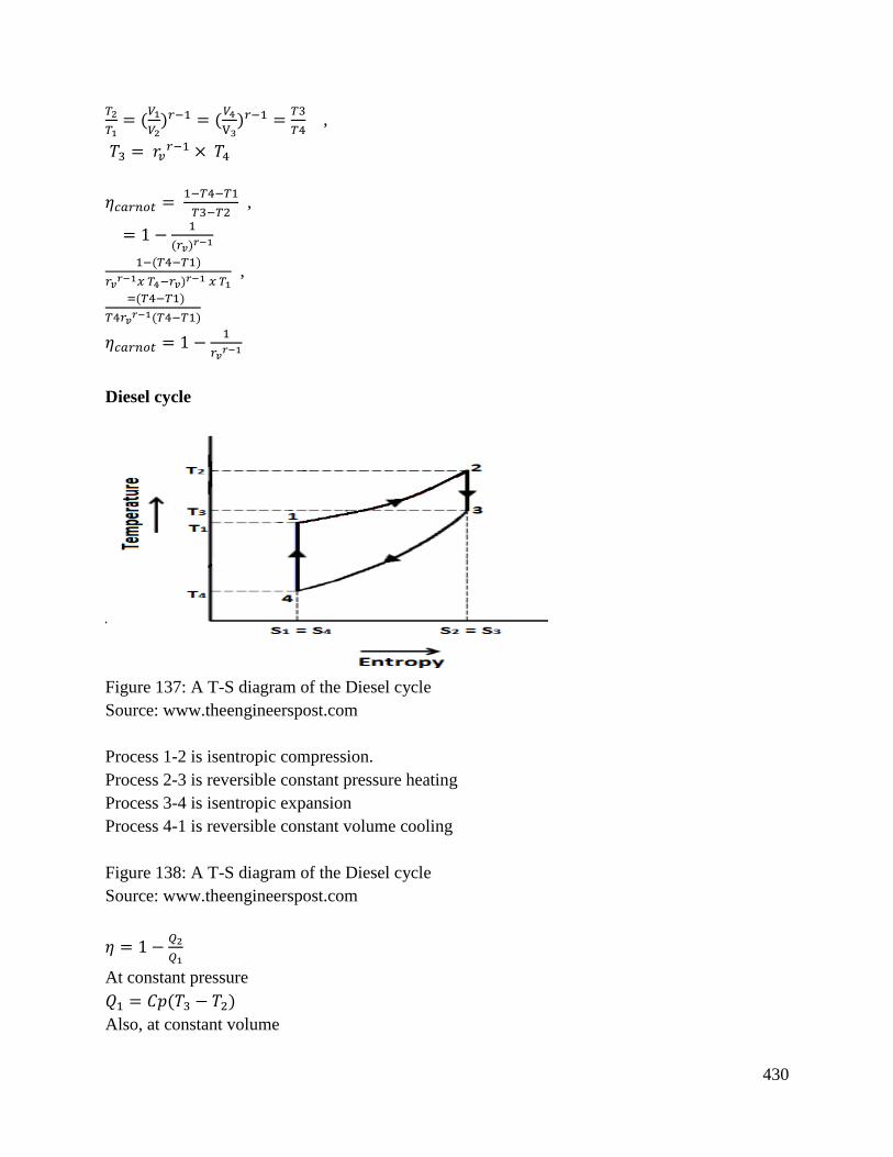
430
𝑇2
𝑇1= (
𝑉1
𝑉2)𝑟−1 = (
𝑉4
V3)𝑟−1 =
𝑇3
𝑇4 ,
𝑇3 = 𝑟𝑣𝑟−1 × 𝑇4
𝜂𝑐𝑎𝑟𝑛𝑜𝑡 = 1−𝑇4−𝑇1
𝑇3−𝑇2 ,
= 1 −1
(𝑟𝑣)𝑟−1
1−(𝑇4−𝑇1)
𝑟𝑣𝑟−1𝑥 𝑇4−𝑟𝑣)𝑟−1 𝑥 𝑇1 ,
=(𝑇4−𝑇1)
𝑇4𝑟𝑣𝑟−1(𝑇4−𝑇1)
𝜂𝑐𝑎𝑟𝑛𝑜𝑡 = 1 −1
𝑟𝑣𝑟−1
Diesel cycle
Figure 137: A T-S diagram of the Diesel cycle
Source: www.theengineerspost.com
Process 1-2 is isentropic compression.
Process 2-3 is reversible constant pressure heating
Process 3-4 is isentropic expansion
Process 4-1 is reversible constant volume cooling
Figure 138: A T-S diagram of the Diesel cycle
Source: www.theengineerspost.com
𝜂 = 1 −𝑄2
𝑄1
At constant pressure
𝑄1 = 𝐶𝑝(𝑇3 − 𝑇2)
Also, at constant volume
431
𝑄2 = 𝐶𝑣(𝑇4 − 𝑇1)
Since there is no heat in process 1 to 2 and 3 to 4, we can substitute 𝑄1 and 𝑄2 in the equation.
𝜂𝐷𝑖𝑒𝑠𝑒𝑙 = 1 −𝑄2
𝑄1
𝑤ℎe𝑟𝑒 𝛽 =𝑉3
𝑉2 𝑐𝑢𝑡 − 𝑜𝑓𝑓 𝑣𝑜𝑙𝑢𝑚𝑒
𝜂 =1−𝐶𝑣(𝑇4−𝑇1)
𝐶𝑣(𝑇3−𝑇2)
𝑃2𝑉2𝑟 = 𝑃3𝑉3
𝑟 𝑃2𝑉2
𝑇2=
𝑃3𝑉3
𝑇3
𝑇3𝑃2𝑉2 = 𝑇2𝑃3𝑉3
𝑇3 = 𝑇2(𝑃3
𝑃2)(
𝑉3
𝑉2)
𝑇3 = 𝑇2 (𝑉3
𝑉2)−𝑟
(𝑉3
𝑉2) = 𝑇2(𝛽)1−𝑟
𝑃𝑉1𝑟= 𝑃𝑉4
𝑟
𝑇4 = 𝑇1 (𝑃4
𝑃1)𝑉4/𝑉1
𝑃𝑉1𝑟= 𝑃𝑉4
𝑟 𝑃4
𝑃1= (
𝑉4
𝑉1)−𝑟
𝑇4 = 𝑇1 (𝑉4
𝑉1)𝑋 (
𝑉4
𝑉4)1−𝑟
= 𝑇1(𝛽)1−𝑟
𝜂 =1−𝑇1(𝛽)1−𝑟−𝑇1
𝑇2(𝛽)1−𝑟𝑥 𝑟 𝑥 𝑇2
=1−𝑇1 [𝛽1−𝑟−1]
𝑇2 [𝛽1−𝑟+𝑟−1]
𝑇2 = 𝑇1𝑟𝑣𝑟−1
𝜂 = 1 − 𝑇1 [𝛽1−𝑟 − 1]/(𝑇1𝑟𝑟−1 𝑥 [𝛽1−𝑟𝑟 − 1])
𝜂 = (1 − 𝛽𝑟 − 1) /((𝛽𝑟−1)𝑥𝑟𝑟−1 − 𝑟)
7.2 Air standard efficiency and actual efficiency
To compare the effects of different cycles, it is of paramount important that the effect of calorific
value of the fuel is altogether eliminated and this can be achieved by considering air (which is
assumed to behave as a perfect gas) as the working substance in the engine cylinder. The efficiency
of engine using air as the working medium is known as an air standard efficiency.
This efficiency is often called ideal efficiency. The actual efficiency of a cycle is always less than
the air-standard efficiency of that cycle under ideal conditions. This is taken into account by
introducing a new term, relative efficiency, which is defined as;
432
𝜂𝑅𝑒𝑙𝑎𝑡𝑖𝑣𝑒 = 𝐴𝑐𝑡𝑢𝑎𝑙 𝑡ℎ𝑒𝑟𝑚𝑎𝑙 𝑒𝑓𝑓𝑖𝑐𝑖𝑒𝑛𝑐𝑦
𝐴𝑖𝑟 𝑠𝑡𝑎𝑛𝑑𝑎𝑟𝑑 𝑒𝑓𝑓𝑖𝑐𝑖𝑒𝑛𝑐𝑦
The analysis of all air standard cycles is based upon the following assumptions;
a) The gas in the engine cylinder is a perfect gas, i.e. it obeys the gas laws and has constant
specific heats.
b) The physical constraints of the gas in the cylinder are the same as those of air at moderate
temperature, i.e. the molecular weight of cylinder gas is 29.
𝐶𝑝 = 1.005𝑘𝐽/𝐾𝑔 − 𝑘 , 𝐶𝑣 = 0.718𝑘𝐽/𝐾𝑔 − 𝑘
c) The compression and expansion processes are adiabatic and they take place without
internal friction, i.e. these processes are isentropic.
d) No chemical reaction takes place in the cylinder. Heat is supplied or rejected by bringing
a hot body or cold body in contract with cylinder at appropriate points during the process.
e) The cycle is considered closed with the same (air) always remaining in the cylinder to
repeat the cycle.
7.3 Problems are solved in ideal gas cycle
Examples
Calculate the ideal air standard cycle efficiency based on Otto cycle for a petrol engine cylinder
bar of 50mm and stroke of 75mm and clearance volume of 21.3cm3
Solution
𝑆𝑤𝑒𝑝𝑡 𝑣𝑜𝑙𝑢𝑚𝑒 =𝜋𝑑2
4× 𝑙
𝜋
4× 52 × 7.5
= 147.26𝑐𝑚2
𝑇𝑜𝑡𝑎𝑙 𝑣𝑜𝑙𝑢𝑚𝑒 𝑜𝑓 𝑐𝑦𝑙𝑖𝑛𝑑𝑒𝑟 = 𝑉5 + 𝑉𝑐
= 147.2 + 21.3
= 168.5𝑐𝑚3
𝐶𝑜𝑚𝑝𝑟𝑒𝑠𝑠𝑖𝑜𝑛 𝑟𝑎𝑡𝑖𝑜 (𝑟𝑣) =𝑇𝑜𝑡𝑎𝑙 𝑣𝑜𝑙𝑢𝑚𝑒
𝐶𝑙𝑒𝑎𝑟𝑎𝑛𝑐𝑒 𝑣𝑜𝑙𝑢𝑚𝑒=
𝑉5+𝑉𝑐
𝑉𝑐
=168.5𝑐𝑚3
21.3𝑐𝑚3
= 7.92
𝜂 = 1 −1
(𝑟𝑣)𝑟−1 𝑁𝐵 𝑟 𝑓𝑜𝑟 𝑎𝑖𝑟 = 1.4
= 1 −1
7.92(1.4−1)
= 0.563 = 56.3%
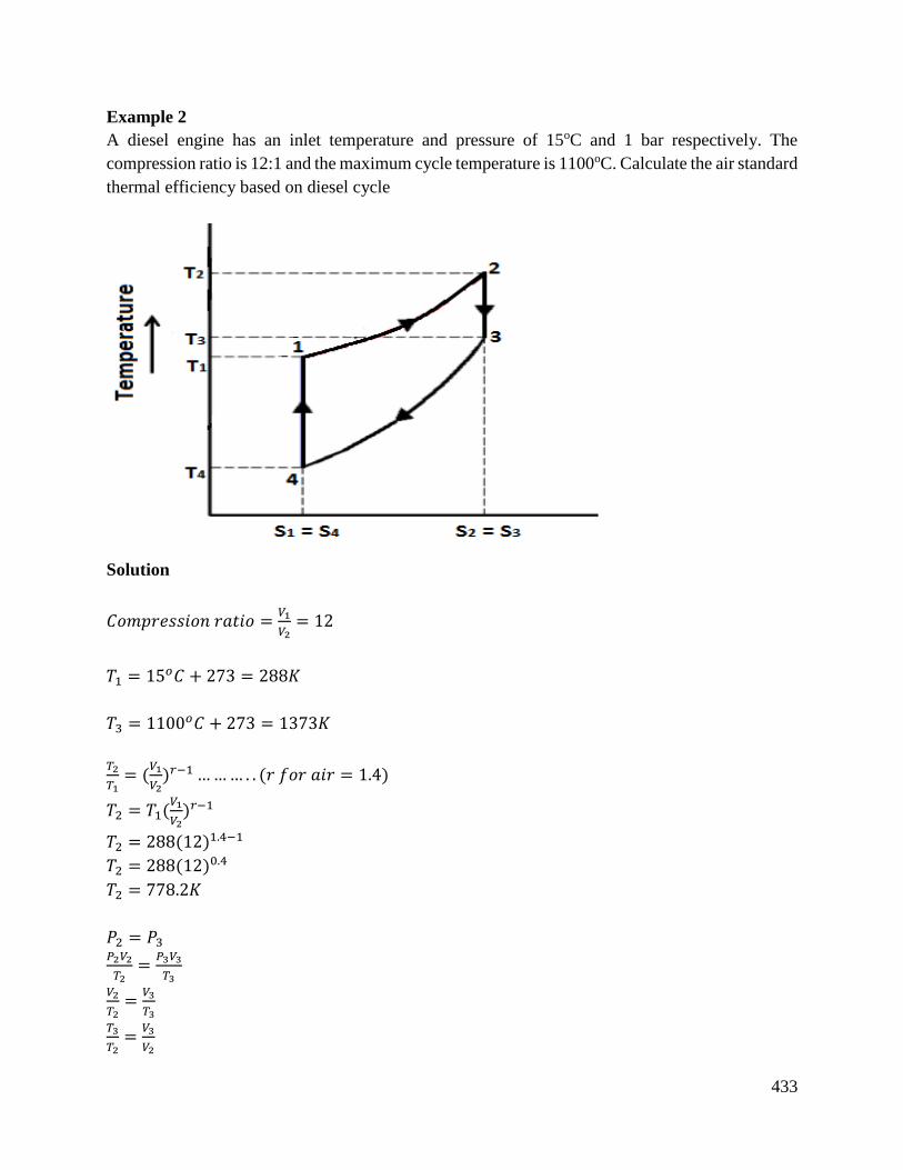
433
Example 2
A diesel engine has an inlet temperature and pressure of 15oC and 1 bar respectively. The
compression ratio is 12:1 and the maximum cycle temperature is 1100oC. Calculate the air standard
thermal efficiency based on diesel cycle
Solution
𝐶𝑜𝑚𝑝𝑟𝑒𝑠𝑠𝑖𝑜𝑛 𝑟𝑎𝑡𝑖𝑜 =𝑉1
𝑉2= 12
𝑇1 = 15𝑜𝐶 + 273 = 288𝐾
𝑇3 = 1100𝑜𝐶 + 273 = 1373𝐾
𝑇2
𝑇1= (
𝑉1
𝑉2)𝑟−1 ……… . . (𝑟 𝑓𝑜𝑟 𝑎𝑖𝑟 = 1.4)
𝑇2 = 𝑇1(𝑉1
𝑉2)𝑟−1
𝑇2 = 288(12)1.4−1
𝑇2 = 288(12)0.4
𝑇2 = 778.2𝐾
𝑃2 = 𝑃3 𝑃2𝑉2
𝑇2=
𝑃3𝑉3
𝑇3
𝑉2
𝑇2=
𝑉3
𝑇3
𝑇3
𝑇2=
𝑉3
𝑉2
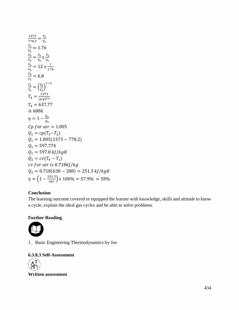
434
1373
778.2=
𝑉3
𝑉2
𝑉3
𝑉2= 1.76
𝑉4
𝑉3=
𝑉4
𝑉2𝑥
𝑉2
𝑉3
𝑉4
𝑉3= 12 𝑥
1
1.76
𝑉4
𝑉3= 6.8
𝑇3
𝑇4= (
𝑉4
𝑉3)𝑟−1
𝑇4 =1373
(6.8)0.4
𝑇4 = 637.77
≅ 688𝑘
𝜂 = 1 −𝑄2
𝑄1
𝐶𝑝 𝑓𝑜𝑟 𝑎𝑖𝑟 = 1.005
𝑄1 = 𝑐𝑝(𝑇3−𝑇2)
𝑄1 = 1.005(1373 − 778.2)
𝑄1 = 597.774
𝑄1 = 597.8 𝑘𝐽/𝑘𝑔𝐾
𝑄2 = 𝑐𝑣(𝑇4 − 𝑇1)
𝑐𝑣 𝑓𝑜𝑟 𝑎𝑖𝑟 𝑖𝑠 0.718𝑘𝐽/𝑘𝑔
𝑄2 = 0.718(638 − 288) = 251.3 𝑘𝐽/𝑘𝑔𝐾
𝜂 = (1 −251.3
597) 𝑥 100% = 57.9% ≃ 58%
Conclusion
The learning outcome covered or equipped the learner with knowledge, skills and attitude to know
a cycle, explain the ideal gas cycles and be able to solve problems.
Further Reading
1. Basic Engineering Thermodynamics by Joe
6.3.8.3 Self-Assessment
Written assessment
435
1. Thermal efficiency of a gas turbine plant as compared to diesel engine plant is?
a) Higher
b) Lower
c) Same
d) Maybe higher or lower.
2. The air standard Otto cycle comprises?
a) Two constant pressure processes and two constant energy processes.
b) Two constant pressure and two constant energy processes.
c) Two constant volume processes and two constant entropy processes.
d) None of the above.
3. The air standard efficiency of Otto cycle is given by?
a) 𝜂 = 1 +1
(𝑟)𝑟+1
b) 𝜂 = 1 −1
(𝑟)𝑟−1
c) 𝜂 = 1 −1
(𝑟)𝑟+1
d) 𝜂 = 2 −1
(𝑟)𝑟−1
4. The thermal efficiency of theoretical Otto cycle _________________.
a) Increases with increase in compression ratio.
b) Increases with increase in isentropic index 𝑟.
c) Does not depend upon the pressure ratio.
d) Follow all the above.
5. The work output of theoretical Otto cycle______________________.
a) Increases with increase in compression ratio
b) Increases with increase in pressure ratio
c) Increases with increase in adiabatic index 𝑟
d) Follows all the above
6. Thermal efficiency of a gas turbine cycle with ideal regenerative heat exchanger is?
a) Reheating
b) Intercooling
c) Regenerator
d) All of the above
7. What is a cycle?
8. What is the difference between an ideal and actual cycle?
9. What is an air standard efficiency?
10. What is relative efficiency?
11. Derive expressions of efficiency in the following cases
Oral Assessment
1. Outline the assumptions made in analysis of all air standard cycles

436
2. What is thermo efficiency of heat engines?
Practical Assessment
1. With the aid of a diagram, describe the Carnot cycle processes
6.3.8.4 Tools, Equipment, Supplies and Materials
Scientific Calculators
Relevant reference materials
Stationeries
Relevant practical materials
Dice
Computers with internet connection
6.3.8.5 References
Saleh, B., Koglbauer, G., Wendland, M., & Fischer, J. (2007). Working fluids for low-
temperature organic Rankine cycles. Energy, 32(7), 1210-1221.
Andresen, B., Berry, R. S., Nitzan, A., & Salamon, P. (1977). Thermodynamics in finite time.
I. The step-Carnot cycle. Physical Review A, 15(5), 2086.
437
6.3.9 Learning Outcome No 8: Demonstrate Fuel and Combustion
6.3.9.1 Learning Activities
Learning Outcome No 8: Demonstrate Fuel and Combustion
Learning Activities Special
Instructions
8.1. Classify fuels
8.2. Describe properties of fuels
8.3. Derive combustion equation
8.4. Apply combustion equation to combustion and exhaust gas
problems
Discussion and
illustrations
Introduction
This learning outcome covers; basic chemistry, classification of fuels, solid fuels, liquid fuels,
combustion equations, theoretical air and excess air, stoichiometric air fuel (AIF) ratio, air-fuel
from analysis of products, how to convert volumetric analysis to weight analysis and how to
convert weight analysis to volumetric analysis.
Definition of key terms
Reactants: Compromise of initial constituents which start the reaction.
Products: Compromise of final constituents which are formed by the chemical reaction.
Chemical fuel: A substance which releases energy on combustion.
Content/Procedures/Methods/Illustrations
8.1 Fuels are classified
Fuels can be classified according to whether:
1. They occur in nature called primary fuel or are prepared called secondary fuels.
2. They are either in solid, liquid or gaseous state.
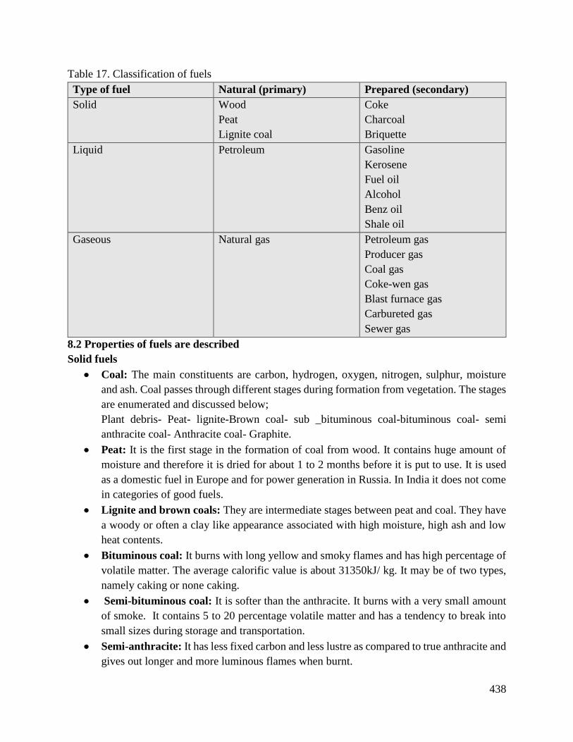
438
Table 17. Classification of fuels
Type of fuel Natural (primary) Prepared (secondary)
Solid
Wood
Peat
Lignite coal
Coke
Charcoal
Briquette
Liquid Petroleum Gasoline
Kerosene
Fuel oil
Alcohol
Benz oil
Shale oil
Gaseous Natural gas Petroleum gas
Producer gas
Coal gas
Coke-wen gas
Blast furnace gas
Carbureted gas
Sewer gas
8.2 Properties of fuels are described
Solid fuels
Coal: The main constituents are carbon, hydrogen, oxygen, nitrogen, sulphur, moisture
and ash. Coal passes through different stages during formation from vegetation. The stages
are enumerated and discussed below;
Plant debris- Peat- lignite-Brown coal- sub _bituminous coal-bituminous coal- semi
anthracite coal- Anthracite coal- Graphite.
Peat: It is the first stage in the formation of coal from wood. It contains huge amount of
moisture and therefore it is dried for about 1 to 2 months before it is put to use. It is used
as a domestic fuel in Europe and for power generation in Russia. In India it does not come
in categories of good fuels.
Lignite and brown coals: They are intermediate stages between peat and coal. They have
a woody or often a clay like appearance associated with high moisture, high ash and low
heat contents.
Bituminous coal: It burns with long yellow and smoky flames and has high percentage of
volatile matter. The average calorific value is about 31350kJ/ kg. It may be of two types,
namely caking or none caking.
Semi-bituminous coal: It is softer than the anthracite. It burns with a very small amount
of smoke. It contains 5 to 20 percentage volatile matter and has a tendency to break into
small sizes during storage and transportation.
Semi-anthracite: It has less fixed carbon and less lustre as compared to true anthracite and
gives out longer and more luminous flames when burnt.
439
Anthracite: Very hard coal and has a shining black lustre. It ignites slowly unless the
furnace temperature is high. It is non-caking and has high percentage of fixed carbon. It
burns either with short blue flames or without flames. The calorific value of this fuel is
high to the form of 35500kJ/ kg and as such its suitable for system generation.
Wood charcoal: It is obtained by destructive distillation of wood. During the process the
volatile matter and water are expelled. The physical properties of the residue (charcoal)
however depend upon the rate of heating and temperature.
Coke: It consists of carbon, mineral matter with about 2% sulphur and small quantities of
hydrogen, nitrogen and phosphorous. It is solid residue left after the destructive distillation
of certain kinds of coal. It is smokeless and clear fuel.
Liquid fuels
Source of liquid fuels is petroleum which is obtained from wells under the earth’s crust. These
fuels have proved more advantageous in comparison to solid fuels in the following respect.
Advantages
Require less space for storage
Higher calorific value
Early control of consumption
Staff economy
Absence of danger from spontaneous combustion
Easy handling and transportation
Cleanliness
No ash problem
No detraction of the fuel in storage
Gaseous fuels
Natural gas. The main constituents of natural gas are methane (𝐶𝐻4) and ethane (𝐶2𝐻6) . It has
calorific value nearly 2100kJ/M3 Natural gas is used alternatively or simultaneously with oil for
internal combustion engines.
Coal gas: Mainly consists of hydrogen, carbon monoxide and hydrocarbons. It is prepared by
carbonization of coal. This finds its use in boilers and is sometimes used for commercial purposes.
Coke-oven gas: Obtained during the production of coke by heating the bituminous coal. The
volatile content of coal is driven off by heating and major portion of the gas is utilized in heating
the ovens. Water or illuminating gas is produced by blowing steam into white hot coke or coal.
The decomposition of steam takes place liberating free hydrogen and oxygen from the steam which
combines with carbon to form carbon monoxide according to the reaction.
𝐶 + 𝐻20−> 𝐶𝑂 + 𝐻2
Advantages
Better control of combustion
Less excess air needed for complete combustion.
Economy in fuel and more efficiency of furnace operation.
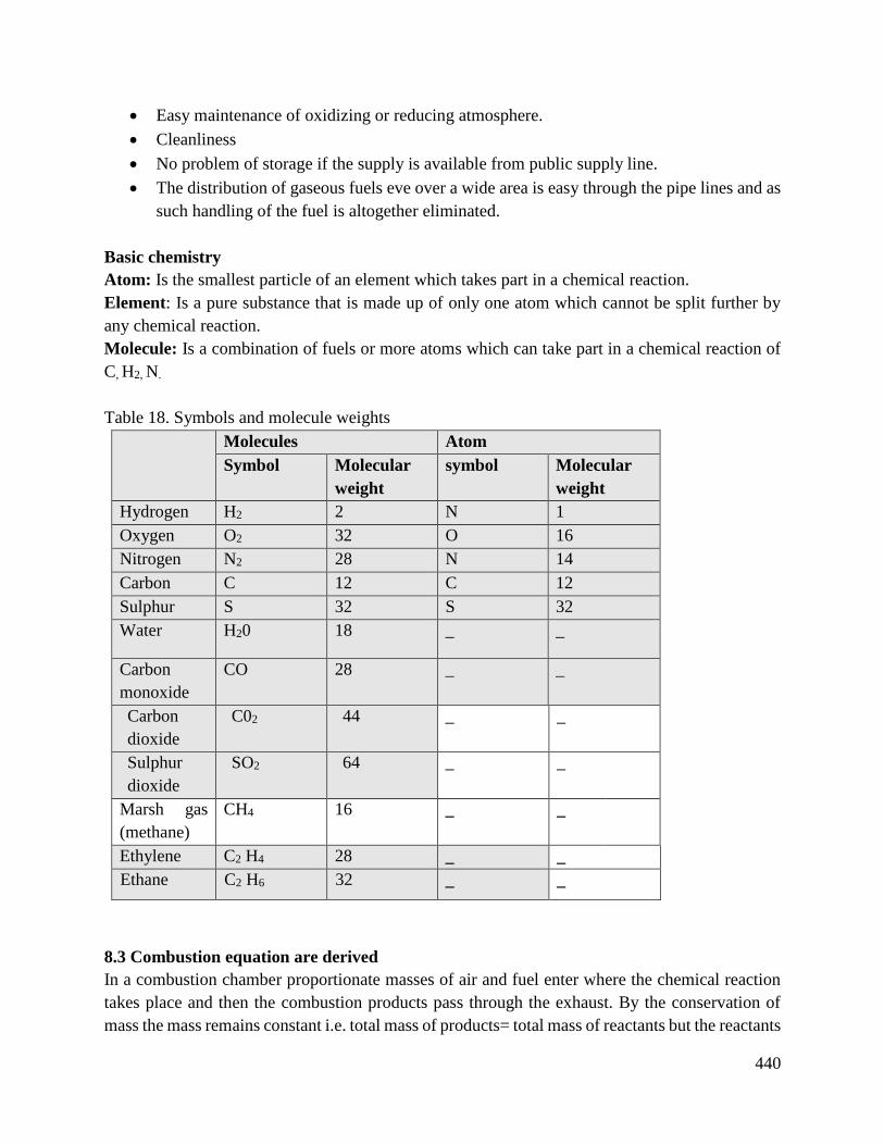
440
Easy maintenance of oxidizing or reducing atmosphere.
Cleanliness
No problem of storage if the supply is available from public supply line.
The distribution of gaseous fuels eve over a wide area is easy through the pipe lines and as
such handling of the fuel is altogether eliminated.
Basic chemistry
Atom: Is the smallest particle of an element which takes part in a chemical reaction.
Element: Is a pure substance that is made up of only one atom which cannot be split further by
any chemical reaction.
Molecule: Is a combination of fuels or more atoms which can take part in a chemical reaction of
C, H2, N.
Table 18. Symbols and molecule weights
Molecules Atom
Symbol Molecular
weight
symbol Molecular
weight
Hydrogen H2 2 N 1
Oxygen O2 32 O 16
Nitrogen N2 28 N 14
Carbon C 12 C 12
Sulphur S 32 S 32
Water H20 18 _ _
Carbon
monoxide
CO 28 _ _
Carbon
dioxide
C02 44 _ _
Sulphur
dioxide
SO2 64 _ _
Marsh gas
(methane)
CH4 16 _ _
Ethylene C2 H4 28 _ _
Ethane C2 H6 32 _ _
8.3 Combustion equation are derived
In a combustion chamber proportionate masses of air and fuel enter where the chemical reaction
takes place and then the combustion products pass through the exhaust. By the conservation of
mass the mass remains constant i.e. total mass of products= total mass of reactants but the reactants
441
are chemically different from the products and the products leave at a higher temperature. The total
number of atoms of each element concerned in the combustion remains constant but the atoms are
rearranged into groups having a different chemical property. This information is expressed in the
chemical equation which is shown below.
i. The relative quantities of the reactants and products.
1. Combustion of Hydrogen
2 H2O+ 2 H20
The above equation of combustion of hydrogen tells that:
i. Hydrogen reacts with oxygen to form steam or water.
ii. The two molecules of hydrogen react with one molecule of oxygen to give two
molecules of steam or water.
2volumes, H2 + 1 Volume, O2 = 3 VOLUMES, H20
The H20 may be liquid or a vapor depending on whether the product has been cooled sufficiently
to cause condensation.
The preparations by mass are obtained by using atomic weight as follows
2H2+O2= 2H20
2(2x1) +2x16→ 2(2x1+16)
4kg H2+32kg O2→36kg H20
1kg H2+8kg O2 → 9kg H20
2Volumes H2+1 volume O2 →3 Volumes.
The total volume of the product is only 2 volumes. There is therefore a volumetric contraction on
combustion. The oxygen is accompanied by nitrogen if air is supplied for the combustion, then
this nitrogen should be included in the equation. As nitrogen is inert as far as chemical reaction is
concerned, it will appear on both sides of the equation.
With one mole of oxygen there are 79/21 moles of nitrogen, hence
2𝐻2 + 𝑂2 +79
21𝑁2 → 2𝐻20 +
79
21 N2
2. Combustion of Carbon
i. Compute combustion of carbon to carbon dioxide
𝐶 + 𝑂2 →𝐶𝑂2
And including the nitrogen
𝐶 + 𝑂2 +79
21𝑁2 → 𝐶𝑂2 +
79
21𝑁2
By volume:
O volume C +1 volume 𝑂2 +79
21 𝑣𝑜𝑙𝑢𝑚𝑒𝑠 𝑁2 → 1 𝑣𝑜𝑙𝑢𝑚𝑒 𝐶𝑂2+
79
21 𝑣𝑜𝑙𝑢𝑚𝑒𝑠 𝑁2
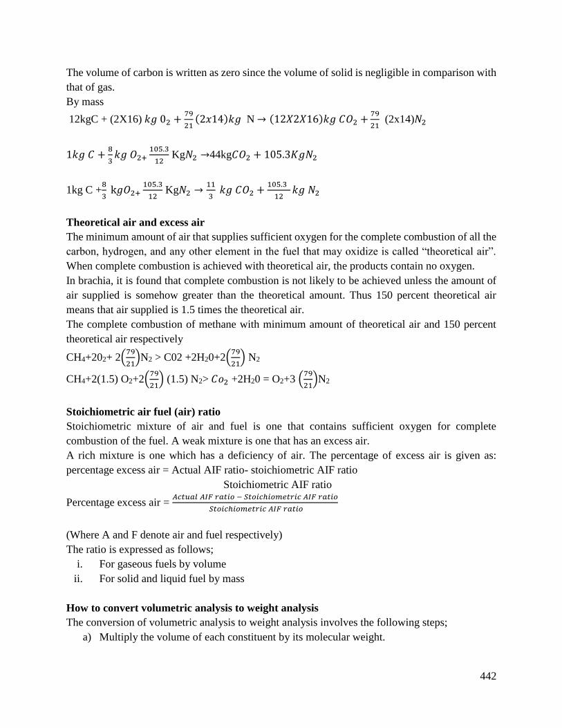
442
The volume of carbon is written as zero since the volume of solid is negligible in comparison with
that of gas.
By mass
12kgC + (2X16) 𝑘𝑔 02 +79
21(2𝑥14)𝑘𝑔 N → (12𝑋2𝑋16)𝑘𝑔 𝐶𝑂2 +
79
21 (2x14)𝑁2
1𝑘𝑔 𝐶 +8
3𝑘𝑔 𝑂2+
105.3
12 Kg𝑁2 →44kg𝐶𝑂2 + 105.3𝐾𝑔𝑁2
1kg C +8
3 k𝑔𝑂2+
105.3
12 Kg𝑁2 →
11
3 𝑘𝑔 𝐶𝑂2 +
105.3
12𝑘𝑔 𝑁2
Theoretical air and excess air
The minimum amount of air that supplies sufficient oxygen for the complete combustion of all the
carbon, hydrogen, and any other element in the fuel that may oxidize is called “theoretical air”.
When complete combustion is achieved with theoretical air, the products contain no oxygen.
In brachia, it is found that complete combustion is not likely to be achieved unless the amount of
air supplied is somehow greater than the theoretical amount. Thus 150 percent theoretical air
means that air supplied is 1.5 times the theoretical air.
The complete combustion of methane with minimum amount of theoretical air and 150 percent
theoretical air respectively
CH4+202+ 2(79
21)N2 > C02 +2H20+2(
79
21) N2
CH4+2(1.5) O2+2(79
21) (1.5) N2> 𝐶𝑜2 +2H20 = O2+3 (
79
21)N2
Stoichiometric air fuel (air) ratio
Stoichiometric mixture of air and fuel is one that contains sufficient oxygen for complete
combustion of the fuel. A weak mixture is one that has an excess air.
A rich mixture is one which has a deficiency of air. The percentage of excess air is given as:
percentage excess air = Actual AIF ratio- stoichiometric AIF ratio
Stoichiometric AIF ratio
Percentage excess air = 𝐴𝑐𝑡𝑢𝑎𝑙 𝐴𝐼𝐹 𝑟𝑎𝑡𝑖𝑜 − 𝑆𝑡𝑜𝑖𝑐ℎ𝑖𝑜𝑚𝑒𝑡𝑟𝑖𝑐 𝐴𝐼𝐹 𝑟𝑎𝑡𝑖𝑜
𝑆𝑡𝑜𝑖𝑐ℎ𝑖𝑜𝑚𝑒𝑡𝑟𝑖𝑐 𝐴𝐼𝐹 𝑟𝑎𝑡𝑖𝑜
(Where A and F denote air and fuel respectively)
The ratio is expressed as follows;
i. For gaseous fuels by volume
ii. For solid and liquid fuel by mass
How to convert volumetric analysis to weight analysis
The conversion of volumetric analysis to weight analysis involves the following steps;
a) Multiply the volume of each constituent by its molecular weight.
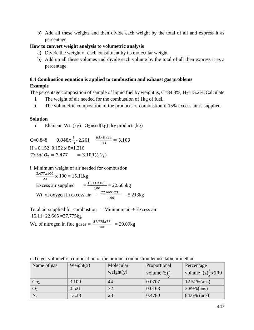
443
b) Add all these weights and then divide each weight by the total of all and express it as
percentage.
How to convert weight analysis to volumetric analysis
a) Divide the weight of each constituent by its molecular weight.
b) Add up all these volumes and divide each volume by the total of all then express it as a
percentage.
8.4 Combustion equation is applied to combustion and exhaust gas problems
Example
The percentage composition of sample of liquid fuel by weight is, C=84.8%, H2=15.2%. Calculate
i. The weight of air needed for the combustion of 1kg of fuel.
ii. The volumetric composition of the products of combustion if 15% excess air is supplied.
Solution
i. Element. Wt. (kg) O2 used(kg) dry products(kg)
C=0.848 0.848𝑥8
3 = 2.261
0.848 𝑥11
33= 3.109
H2= 0.152 0.152 x 8=1.216
𝑇𝑜𝑡𝑎𝑙 𝑂2 = 3.477 = 3.109(𝐶𝑂2)
i. Minimum weight of air needed for combustion
3.477𝑥100
23 x 100 = 15.11kg
Excess air supplied = 15.11 𝑥150
100 = 22.665kg
Wt. of oxygen in excess air = 22.665𝑥23
100 =5.213kg
Total air supplied for combustion = Minimum air + Excess air
15.11+22.665 =37.775kg
Wt. of nitrogen in flue gases = 37.775𝑥77
100 = 29.09kg
ii.To get volumetric composition of the product combustion let use tabular method
Name of gas Weight(x) Molecular
weight(y)
Proportional
volume (z)𝑥
𝑦
Percentage
volume=(z)𝑧
𝑧𝑥100
Co2 3.109 44 0.0707 12.51%(ans)
O2 0.521 32 0.0163 2.89%(ans)
N2 13.38 28 0.4780 84.6% (ans)
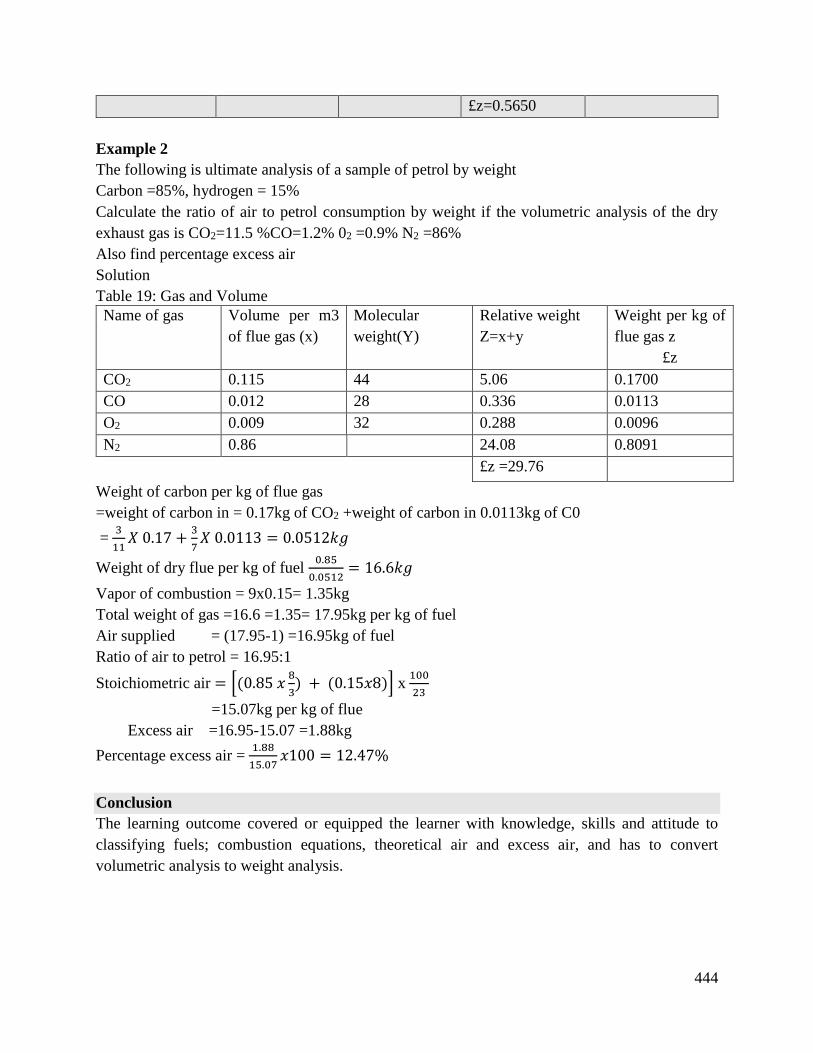
444
£z=0.5650
Example 2
The following is ultimate analysis of a sample of petrol by weight
Carbon =85%, hydrogen = 15%
Calculate the ratio of air to petrol consumption by weight if the volumetric analysis of the dry
exhaust gas is CO2=11.5 %CO=1.2% 02 =0.9% N2 =86%
Also find percentage excess air
Solution
Table 19: Gas and Volume
Name of gas Volume per m3
of flue gas (x)
Molecular
weight(Y)
Relative weight
Z=x+y
Weight per kg of
flue gas z
£z
CO2 0.115 44 5.06 0.1700
CO 0.012 28 0.336 0.0113
O2 0.009 32 0.288 0.0096
N2 0.86 24.08 0.8091
£z =29.76
Weight of carbon per kg of flue gas
=weight of carbon in = 0.17kg of CO2 +weight of carbon in 0.0113kg of C0
= 3
11𝑋 0.17 +
3
7𝑋 0.0113 = 0.0512𝑘𝑔
Weight of dry flue per kg of fuel 0.85
0.0512= 16.6𝑘𝑔
Vapor of combustion = 9x0.15= 1.35kg
Total weight of gas =16.6 =1.35= 17.95kg per kg of fuel
Air supplied = (17.95-1) =16.95kg of fuel
Ratio of air to petrol = 16.95:1
Stoichiometric air = [(0.85 𝑥8
3) + (0.15𝑥8)] x
100
23
=15.07kg per kg of flue
Excess air =16.95-15.07 =1.88kg
Percentage excess air = 1.88
15.07𝑥100 = 12.47%
Conclusion
The learning outcome covered or equipped the learner with knowledge, skills and attitude to
classifying fuels; combustion equations, theoretical air and excess air, and has to convert
volumetric analysis to weight analysis.

445
Further Reading
1. Applied thermodynamics for engineering technologist EAST and monkey.
6.3.9.3 Self-Assessment
Written assessment
1. The smallest particle which can take part in a chemical change is called?
a) Atom
b) Molecule
c) Electron
d) Compound
2. A chemical fuel is a substance which releases ______________on combustion.
a) Chemical energy
b) Heat
c) Sand energy
d) Magnetic energy
3. The most important solid fuel is?
a) Wood
b) Charcoal
c) Coal
d) All the above
4. For each mole of oxygen, number of moles of nitrogen required for complete combustion
of carbon is?
a) 20/21
b) 2/21
c) 77/21
d) 9/21
5. Modern practice is to use _____________excess air.
a) 5 to 10 percent
b) 15 to 20 percent
c) 20 to 25 percent
d) 25 to 50 percent
6. Stoichiometric air-fuel ratio by mass for combustion of petrol is?
a) 5
b) 10
c) 12
d) 15.05
446
7. An analysis which includes the steam in the exhaust is called?
a) Dry analysis
b) Wet analysis
c) Dry and Wet analysis
d) None of the above
8. What is chemical thermodynamics?
9. What is chemical fuel?
10. What are primary fuels/or some important primary fuels.
11. What do you understand by heating value of fuels.
12. Write short notes on ‘excess air’.
Oral Assessment
1. What is meant by chemical equilibrium?
2. How is analysis of exhaust flue gas carried out?
Practical Assessment
1. With the aid of a well labeled diagram show the ORSAT APPARATUS and its use
6.3.9.4 Tools, Equipment, Supplies and Materials
Scientific Calculators
Relevant reference materials
Stationeries
Relevant practical materials
Dice
Computers with internet connection
6.3.9.5 References
Balmer, R. T. (2011). Modern engineering thermodynamics-textbook with tables booklet.
Academic Press.
Bejan, A. (2016). Advanced engineering thermodynamics. John Wiley & Sons.
Raja, A. K., & Srivastava, A. P. (2006). Power plant engineering. New Age International.
447
6.3.10 Learning Outcome No9: Perform heat transfer
6.3.10.1 Learning Activities
Learning Outcome No9: Perform heat transfer
Learning Activities Special Instructions
9.1. Derive and apply conduction equation from
Fourier’s law
9.2. Derive and apply heat transfer equation from
Newton’s law of cooling and Fourier’s law
In groups practice the derivation of
the Fourier equation.
Solve problems involving the
Fourier’s law
6.3.10.2 Information Sheet No6/LO9: Perform heat transfer
Introduction to learning outcome
This learning outcome covers Fourier’s law of heat conduction and newton law of cooling and
their application.
Definition of key terms
Conduction: This is a transfer of heat from one substance to another in physical contact with it
without movement of molecules e.g. heat transfer in metals. I.e. heat is transfer in metals.
Convention: Heat transfer in fluids whereby it involves mixing of one portion of the fluid with
another. The movement of the fluid may be caused by temperature difference in natural
convention.
Radiation: Heat transfer through a vacuum place i.e. it does not require a material medium for it
to take place.
Content/Procedures/Methods/Illustrations
9.1 Conduction equation is derived and applied from Fourier’s law
Fourier’s law of heat
The law states that the rate of heat flow through a single homogenous solid is directly proportional
to area of cross-section at right angles, to the direction of heat flow and changes of temperature
along the length of path of heat flow.
NB: This law is based on Empirical of observation of one-dimensional steady heat flow through a
solid. Steady flow means temperature at any point does not change with time.
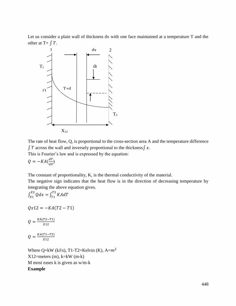
448
Let us consider a plain wall of thickness dx with one face maintained at a temperature T and the
other at T+ ∫𝑇.
The rate of heat flow, Q, is proportional to the cross-section area A and the temperature difference
∫𝑇 across the wall and inversely proportional to the thickness∫𝑥.
This is Fourier’s law and is expressed by the equation:
𝑄 = −𝐾𝐴(𝑑𝑇
𝑑𝑋)
The constant of proportionality, K, is the thermal conductivity of the material.
The negative sign indicates that the heat flow is in the direction of decreasing temperature by
integrating the above equation gives.
∫ 𝑄𝑑𝑥 =𝑋2
𝑋1∫ 𝐾𝐴𝑑𝑇
𝑇2
𝑇1
𝑄𝑥12 = −𝐾𝐴(𝑇2 − 𝑇1)
𝑄 =𝐾A(𝑇2−𝑇1)
𝑋12
𝑄 =𝐾𝐴(𝑇1−𝑇2)
𝑋12
Where Q=kW (kJ/s), T1-T2=Kelvin (K), A=𝑚2
X12=meters (m), k=kW (m-k)
M most eases k is given as w/m-k
Example
dx
dt
T+d
T1
T2
X12
Q
1 2
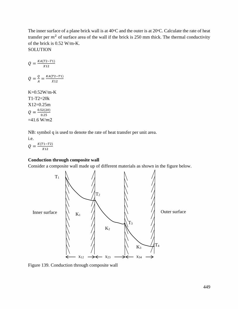
449
The inner surface of a plane brick wall is at 40ᵒC and the outer is at 20ᵒC. Calculate the rate of heat
transfer per 𝑚2 of surface area of the wall if the brick is 250 mm thick. The thermal conductivity
of the brick is 0.52 W/m-K.
SOLUTION
𝑄 =𝐾𝐴(𝑇2−𝑇1)
𝑋12
𝑄 =𝑄
𝐴=
𝐾𝐴(𝑇2−𝑇1)
𝑋12
K=0.52W/m-K
T1-T2=20k
X12=0.25m
𝑄 =0.52(20)
0.25
=41.6 W/𝑚2
NB: symbol q is used to denote the rate of heat transfer per unit area.
i.e.
𝑄 =𝐾(𝑇1−𝑇2)
𝑋12
Conduction through composite wall
Consider a composite wall made up of different materials as shown in the figure below.
Figure 139. Conduction through composite wall
T1
K3T4
T3
T2
K1
K2
x12 x23 x34
Outer surface Inner surface
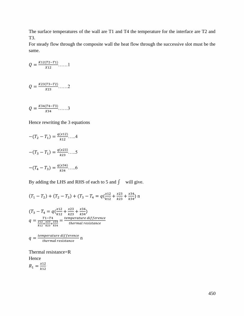
450
The surface temperatures of the wall are T1 and T4 the temperature for the interface are T2 and
T3.
For steady flow through the composite wall the heat flow through the successive slot must be the
same.
𝑄 =𝐾12(𝑇2−𝑇1)
𝑋12……1
𝑄 =𝐾23(𝑇3−𝑇2)
𝑋23……2
𝑄 =𝐾34(𝑇4−𝑇3)
𝑋34……3
Hence rewriting the 3 equations
−(𝑇2 − 𝑇1) =𝑞(𝑥12)
𝑘12…..4
−(𝑇3 − 𝑇1) =𝑞(𝑥23)
𝑘23…..5
−(𝑇4 − 𝑇3) =𝑞(𝑥34)
𝑘34…..6
By adding the LHS and RHS of each to 5 and ∫ will give.
(𝑇1 − 𝑇2) + (𝑇2 − 𝑇3) + (𝑇3 − 𝑇4 = 𝑞(𝑥12
𝑘12+
𝑥23
𝑘23+
𝑥34
𝑘34) n
(𝑇3 − 𝑇4 = 𝑞(𝑥12
𝑘12+
𝑥23
𝑘23+
𝑥34
𝑘34)
𝑞 =𝑇1−𝑇4
𝑥12
𝑘12+
𝑥23
𝑘23+
𝑥34
𝑘34
=𝑡𝑒𝑚𝑝𝑒𝑟𝑎𝑡𝑢𝑟𝑒 𝑑𝑖𝑓𝑓𝑒𝑟𝑒𝑛𝑐𝑒
𝑡ℎ𝑒𝑟𝑚𝑎𝑙 𝑟𝑒𝑠𝑖𝑠𝑡𝑎𝑛𝑐𝑒
𝑞 =𝑡𝑒𝑚𝑝𝑒𝑟𝑎𝑡𝑢𝑟𝑒 𝑑𝑖𝑓𝑓𝑒𝑟𝑒𝑛𝑐𝑒
𝑡ℎ𝑒𝑟𝑚𝑎l 𝑟𝑒𝑠𝑖𝑠𝑡𝑎𝑛𝑐𝑒 n
Thermal resistance=R
Hence
𝑅1 =𝑥12
𝑘12
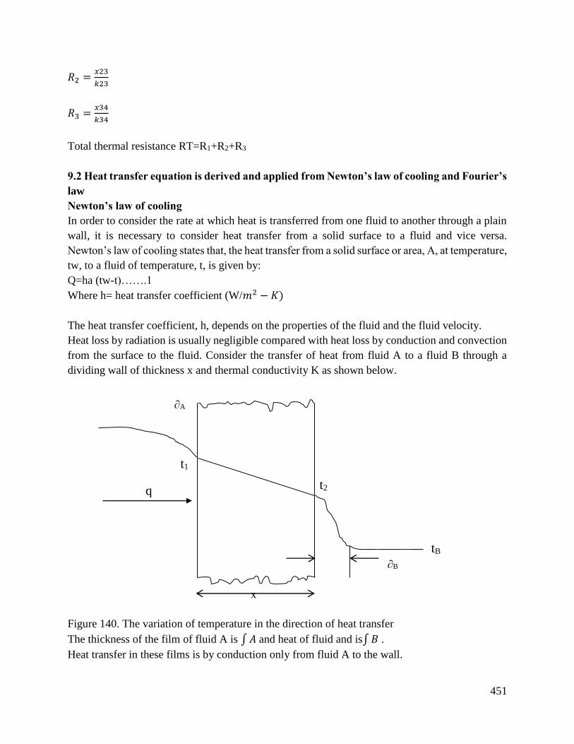
451
𝑅2 =𝑥23
𝑘23
𝑅3 =𝑥34
𝑘34
Total thermal resistance RT=R1+R2+R3
9.2 Heat transfer equation is derived and applied from Newton’s law of cooling and Fourier’s
law
Newton’s law of cooling
In order to consider the rate at which heat is transferred from one fluid to another through a plain
wall, it is necessary to consider heat transfer from a solid surface to a fluid and vice versa.
Newton’s law of cooling states that, the heat transfer from a solid surface or area, A, at temperature,
tw, to a fluid of temperature, t, is given by:
Q=ha (tw-t)…….1
Where h= heat transfer coefficient (W/𝑚2 − 𝐾)
The heat transfer coefficient, h, depends on the properties of the fluid and the fluid velocity.
Heat loss by radiation is usually negligible compared with heat loss by conduction and convection
from the surface to the fluid. Consider the transfer of heat from fluid A to a fluid B through a
dividing wall of thickness x and thermal conductivity K as shown below.
Figure 140. The variation of temperature in the direction of heat transfer
The thickness of the film of fluid A is ∫𝐴 and heat of fluid and is∫𝐵 .
Heat transfer in these films is by conduction only from fluid A to the wall.
t2
t1
q
x
tB
∂B
∂A
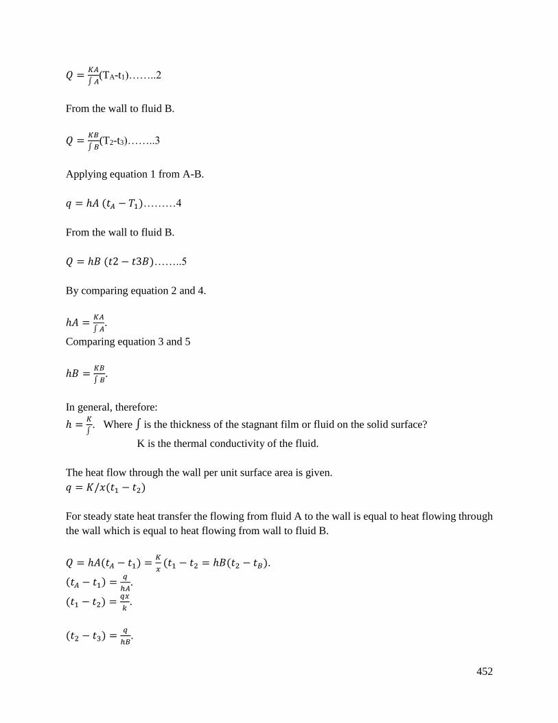
452
𝑄 =𝐾𝐴
∫ 𝐴(TA-t1)……..2
From the wall to fluid B.
𝑄 =𝐾𝐵
∫ 𝐵(T2-t3)……..3
Applying equation 1 from A-B.
𝑞 = ℎ𝐴 (𝑡𝐴 − 𝑇1)………4
From the wall to fluid B.
𝑄 = ℎ𝐵 (𝑡2 − 𝑡3𝐵)……..5
By comparing equation 2 and 4.
ℎ𝐴 =𝐾𝐴
∫ 𝐴.
Comparing equation 3 and 5
ℎ𝐵 =𝐾𝐵
∫ 𝐵.
In general, therefore:
ℎ =𝐾
∫. Where ∫ is the thickness of the stagnant film or fluid on the solid surface?
K is the thermal conductivity of the fluid.
The heat flow through the wall per unit surface area is given.
𝑞 = 𝐾/𝑥(𝑡1 − 𝑡2)
For steady state heat transfer the flowing from fluid A to the wall is equal to heat flowing through
the wall which is equal to heat flowing from wall to fluid B.
𝑄 = ℎ𝐴(𝑡𝐴 − 𝑡1) =𝐾
𝑥(𝑡1 − 𝑡2 = ℎ𝐵(𝑡2 − 𝑡𝐵).
(𝑡𝐴 − 𝑡1) =𝑞
ℎ𝐴.
(𝑡1 − 𝑡2) =𝑞𝑥
𝑘.
(𝑡2 − 𝑡3) =𝑞
ℎ𝐵.
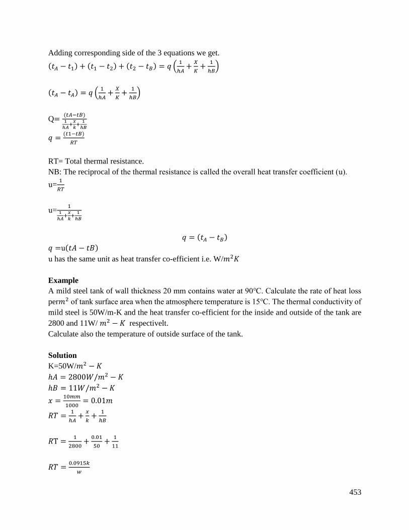
453
Adding corresponding side of the 3 equations we get.
(𝑡𝐴 − 𝑡1) + (𝑡1 − 𝑡2) + (𝑡2 − 𝑡𝐵) = 𝑞 (1
ℎ𝐴+
𝑋
𝐾+
1
ℎ𝐵)
(𝑡𝐴 − 𝑡𝐴) = 𝑞 (1
ℎ𝐴+
𝑋
𝐾+
1
ℎ𝐵)
Q=(𝑡𝐴−𝑡𝐵)1
ℎ𝐴+
𝑥
𝑘+
1
ℎ𝐵
𝑞 =(𝑡1−𝑡𝐵)
𝑅𝑇
RT= Total thermal resistance.
NB: The reciprocal of the thermal resistance is called the overall heat transfer coefficient (ꭒ).
ꭒ=1
𝑅𝑇
ꭒ=1
1
ℎ𝐴+
𝑥
𝑘+
1
ℎ𝐵
𝑞 = (𝑡𝐴 − 𝑡𝐵)
𝑞 =ꭒ(𝑡𝐴 − 𝑡𝐵)
ꭒ has the same unit as heat transfer co-efficient i.e. W/𝑚2𝐾
Example
A mild steel tank of wall thickness 20 mm contains water at 90. Calculate the rate of heat loss
per𝑚2 of tank surface area when the atmosphere temperature is 15. The thermal conductivity of
mild steel is 50W/m-K and the heat transfer co-efficient for the inside and outside of the tank are
2800 and 11W/ 𝑚2 − 𝐾 respectivelt.
Calculate also the temperature of outside surface of the tank.
Solution
K=50W/𝑚2 − 𝐾
ℎ𝐴 = 2800𝑊/𝑚2 − 𝐾
ℎ𝐵 = 11𝑊/𝑚2 − 𝐾
𝑥 =10𝑚𝑚
1000= 0.01𝑚
𝑅𝑇 =1
ℎ𝐴+
𝑥
𝑘+
1
ℎ𝐵
𝑅T =1
2800+
0.01
50+
1
11
𝑅𝑇 =0.0915𝑘
𝑤
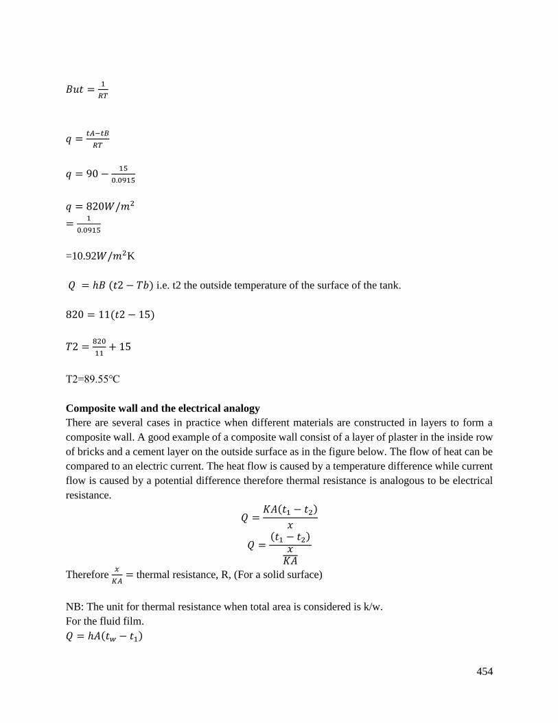
454
𝐵𝑢𝑡 =1
𝑅𝑇
𝑞 =𝑡𝐴−𝑡𝐵
𝑅𝑇
𝑞 = 90 −15
0.0915
𝑞 = 820𝑊/𝑚2
=1
0.0915
=10.92𝑊/𝑚2K
𝑄 = ℎ𝐵 (𝑡2 − 𝑇𝑏) i.e. t2 the outside temperature of the surface of the tank.
820 = 11(𝑡2 − 15)
𝑇2 =820
11+ 15
T2=89.55
Composite wall and the electrical analogy
There are several cases in practice when different materials are constructed in layers to form a
composite wall. A good example of a composite wall consist of a layer of plaster in the inside row
of bricks and a cement layer on the outside surface as in the figure below. The flow of heat can be
compared to an electric current. The heat flow is caused by a temperature difference while current
flow is caused by a potential difference therefore thermal resistance is analogous to be electrical
resistance.
𝑄 =𝐾𝐴(𝑡1 − 𝑡2)
𝑥
𝑄 =(𝑡1 − 𝑡2)
𝑥𝐾𝐴
Therefore 𝑥
𝐾𝐴= thermal resistance, R, (For a solid surface)
NB: The unit for thermal resistance when total area is considered is k/w.
For the fluid film.
𝑄 = ℎ𝐴(𝑡𝑤 − 𝑡1)

455
𝑄 =𝑡𝑤−𝑡1
1
ℎ𝐴
NB: For the 3 walls
R1=𝑥1
𝐾𝐴 , R2=
𝑥2
𝐾2𝐴 , R3=
𝑥3
𝐾3𝐴
For fluid A and B
RA=1
ℎ𝐴𝐴 , RB=
1
ℎ𝐵𝐴
Example
A furnace wall consist of 125mm which refractory brick separated by an air gap. The outside is
covered with 12mm thickness of plaster. The inner surface of the wall is at 1100ᵒc and the room
temperature is 25. Calculate the rate at which heat is lost per 𝑚2 of wall surface. The heat
transfer co-efficient from the outside wall surface to the air in the room is 17𝑊/m2 − 𝑘 and the
resistance which flow of the air gap is 0.16K/w. the thermal conductivities of refractory brick
insulating fire brick and plaster are 1.6,0.3 and 0.1W/m-K respectively. Calculate also the
temperature of the outside surface of the wall.
Solution
To determine the various resistance, the procedure follows.
a) Refractory brick
𝑅1 =𝑥1
𝐾1𝐴 A=1
tA = 90
tB = 15
Water
Air
Mild Steel
t
t2
=
Figure 141. Furnace wall
456
𝑅1 =0.125
1.6×1= 0.0781
𝑅1 = 0.0781𝑘/𝑤
b) Air gap
R=0.16 k/w
c) Fire brick
𝑅2 =𝑥2
𝑘2𝐴=
0.125
0.3𝑋1= 0.4167𝑘/𝑤
d) Plaster
𝑅3 =𝑥3
𝑘3𝐴=
0.012
0.14𝑋1= 0.0857𝑘/𝑤
e) Air film
𝑅𝐴 =1
ℎ𝐴=
1
17𝑋1=
0.0588𝐾
𝑊
Total RT=0.0781+0.4167+0.16+0.0857+0.0588
RT=0.7993=0.8k/w
𝑞 =𝑡𝐴−𝑡𝐵
𝑅𝑇=
1100−25
0.8
𝑞 = 1344𝑊/𝑚2
𝑞 = ℎ(𝑡 − 25)𝑖. 𝑒. 𝑡 = 𝑡𝑒𝑚𝑝𝑒𝑟𝑎𝑡𝑢𝑟𝑒 𝑜𝑢𝑡𝑠𝑖𝑑𝑒 𝑠𝑢𝑟𝑓𝑎𝑐𝑒
1344 = 17(𝑡 − 25)
𝑡 =1344
17+ 25
= 104.06
𝑡 = 104ᵒ𝐶
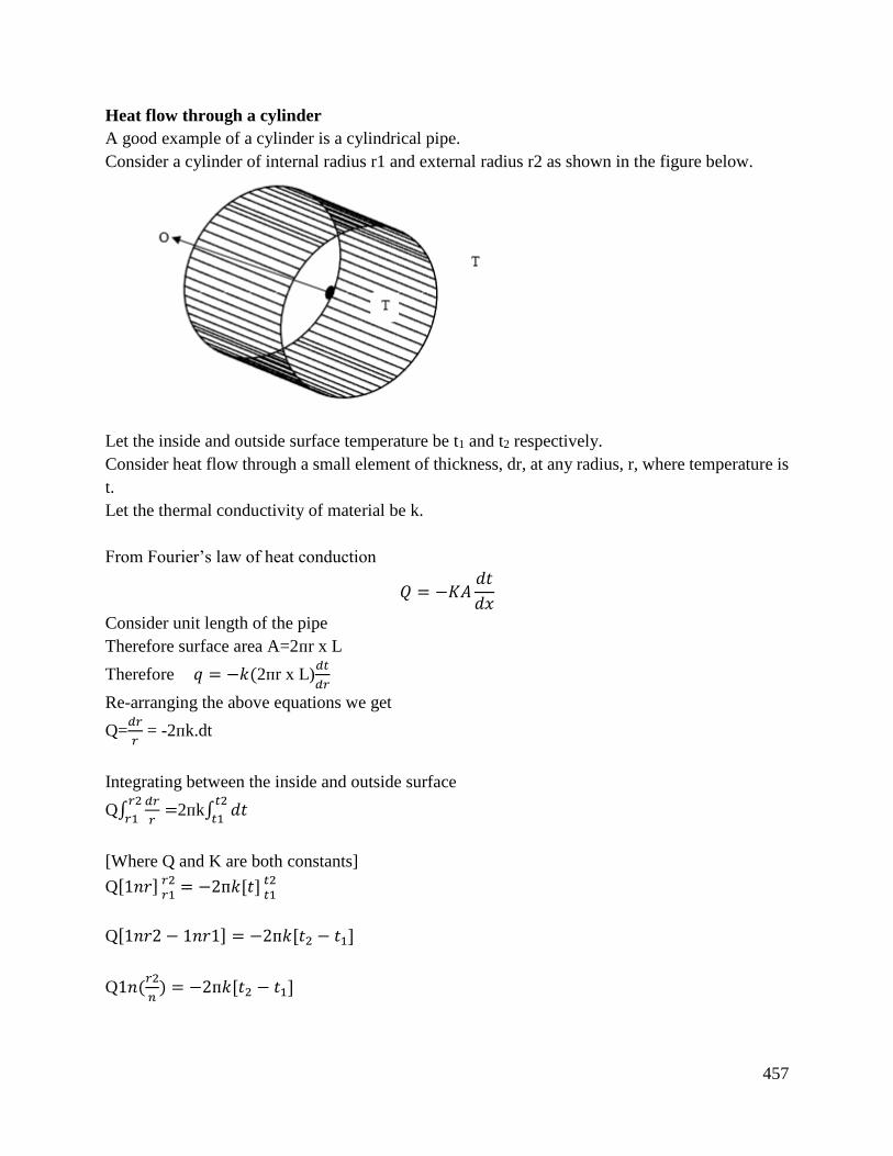
457
Heat flow through a cylinder
A good example of a cylinder is a cylindrical pipe.
Consider a cylinder of internal radius r1 and external radius r2 as shown in the figure below.
Let the inside and outside surface temperature be t1 and t2 respectively.
Consider heat flow through a small element of thickness, dr, at any radius, r, where temperature is
t.
Let the thermal conductivity of material be k.
From Fourier’s law of heat conduction
𝑄 = −𝐾𝐴𝑑𝑡
𝑑𝑥
Consider unit length of the pipe
Therefore surface area A=2ᴨr x L
Therefore 𝑞 = −𝑘(2ᴨr x L)𝑑𝑡
𝑑𝑟
Re-arranging the above equations we get
Q=𝑑𝑟
𝑟 = -2ᴨk.dt
Integrating between the inside and outside surface
Q∫𝑑𝑟
𝑟=
𝑟2
𝑟12ᴨk∫ 𝑑𝑡
𝑡2
𝑡1
[Where Q and K are both constants]
Q[1𝑛𝑟] 𝑟2𝑟1
= −2ᴨ𝑘[𝑡] 𝑡2𝑡1
Q[1𝑛𝑟2 − 1𝑛𝑟1] = −2ᴨ𝑘[𝑡2 − 𝑡1]
Q1𝑛(𝑟2
𝑛) = −2ᴨ𝑘[𝑡2 − 𝑡1]
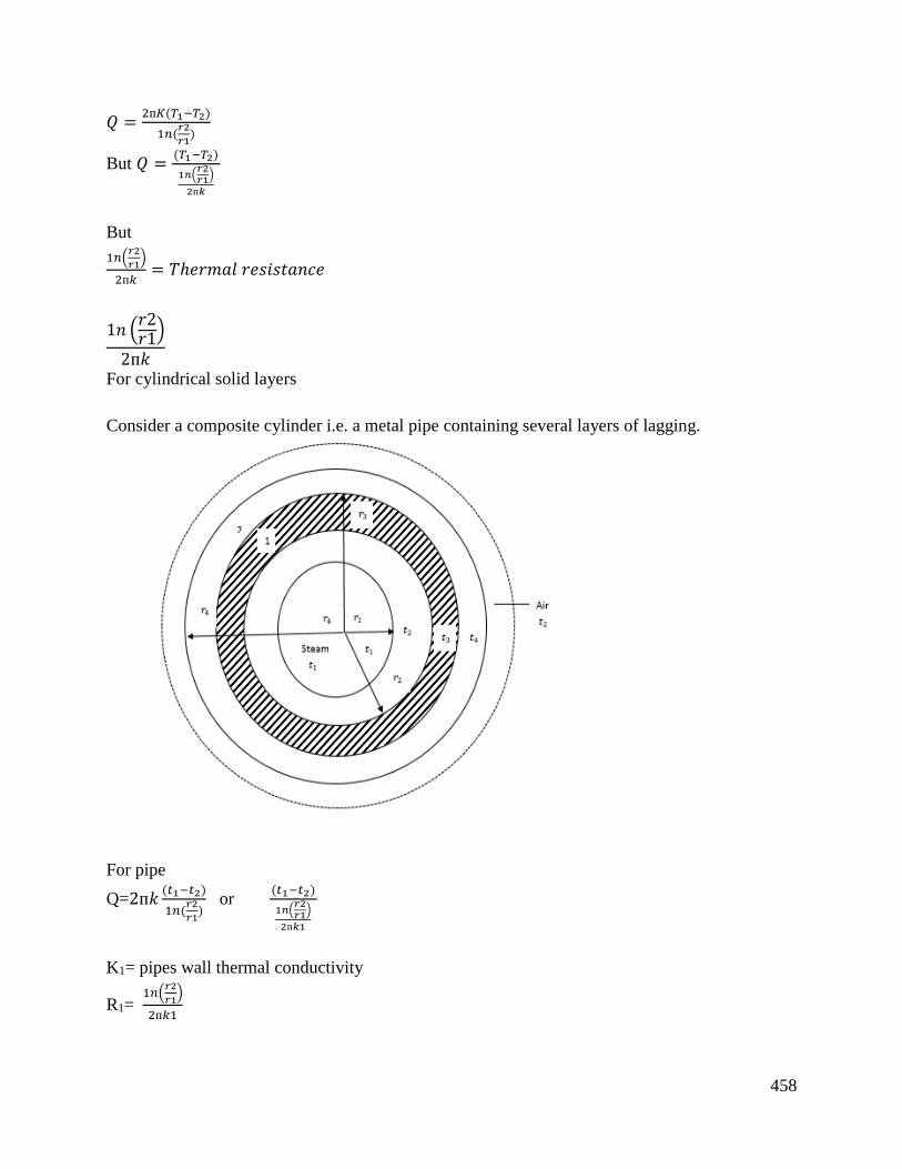
458
𝑄 =2ᴨ𝐾(𝑇1−𝑇2)
1𝑛(𝑟2
𝑟1)
But 𝑄 =(𝑇1−𝑇2)
1𝑛(𝑟2𝑟1
)
2ᴨ𝑘
But
1𝑛(𝑟2
𝑟1)
2ᴨ𝑘= 𝑇ℎ𝑒𝑟𝑚𝑎𝑙 𝑟𝑒𝑠𝑖𝑠𝑡𝑎𝑛𝑐𝑒
1𝑛 (𝑟2𝑟1)
2ᴨ𝑘
For cylindrical solid layers
Consider a composite cylinder i.e. a metal pipe containing several layers of lagging.
For pipe
Q=2ᴨ𝑘(𝑡1−𝑡2)
1𝑛(𝑟2
𝑟1) or
(𝑡1−𝑡2)
1𝑛(𝑟2𝑟1
)
2ᴨ𝑘1
K1= pipes wall thermal conductivity
R1= 1𝑛(
𝑟2
𝑟1)
2ᴨ𝑘1
459
For lagging 1
Q=2ᴨ𝑘2(𝑡2−𝑡3)
1𝑛(𝑟3
𝑟2)
R2=1𝑛(
𝑟3
𝑟2)
2ᴨ𝑘2
K2=thermal conductivity of lagging 1
R3=1𝑛(
𝑟4
𝑟3)
2ᴨ𝑘3
K3=thermal conductivity of lagging 2
For steam film
Q=hiA(ti-t1) i.e. ti=steam temperature
Hi=heat transfer coefficient of inside pipe.
A=surface area of the inside pipe.
Q=(𝑡𝑖−𝑡1)
1
ℎ𝐴
Ri=1
ℎ𝑖𝐴
For the inside air film
Ro=1
ℎ𝑜𝐴
Ho=heat transfer co-efficient for outside of pipe.
A=surface area of outside surface.
Example
A steel pipe of 100mm internal diameter and 7mm wall thickness carrying steam of 260 is
insulated with 40mm of diatomaceous earth covering and this covering is in turn insulated with
60mm of asbestos felt. The atmospheric temperature is 15. The heat transfer co-efficient for the
inside and outside surfaces are 550 and 15𝑊/𝑚2 − 𝐾 respectively and the thermal conductivities
of steel and diatomaceous and asbestos are 50, 0.09 and 0.07 W/m-K respectively calculate?
a) The rate of heat loss by the steam per unit length of pipe.
b) The temperature of the outside of the pipe.
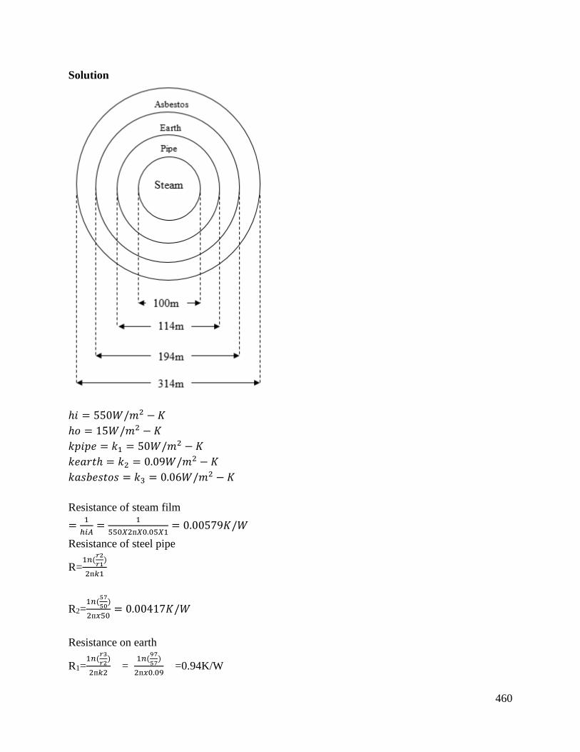
460
Solution
ℎ𝑖 = 550𝑊/𝑚2 − 𝐾
ℎ𝑜 = 15𝑊/𝑚2 − 𝐾
𝑘𝑝𝑖𝑝𝑒 = 𝑘1 = 50𝑊/𝑚2 − 𝐾
𝑘𝑒𝑎𝑟𝑡ℎ = 𝑘2 = 0.09𝑊/𝑚2 − 𝐾
𝑘𝑎𝑠𝑏𝑒𝑠𝑡𝑜𝑠 = 𝑘3 = 0.06𝑊/𝑚2 − 𝐾
Resistance of steam film
=1
ℎ𝑖𝐴=
1
550𝑋2ᴨ𝑋0.05𝑋1= 0.00579𝐾/𝑊
Resistance of steel pipe
R=1𝑛(
𝑟2
𝑟1)
2ᴨ𝑘1
R2=1𝑛(
57
50)
2ᴨ𝑥50= 0.00417𝐾/𝑊
Resistance on earth
R1=1𝑛(
𝑟3
𝑟2)
2ᴨ𝑘2 =
1𝑛(97
57)
2ᴨ𝑥0.09 =0.94K/W
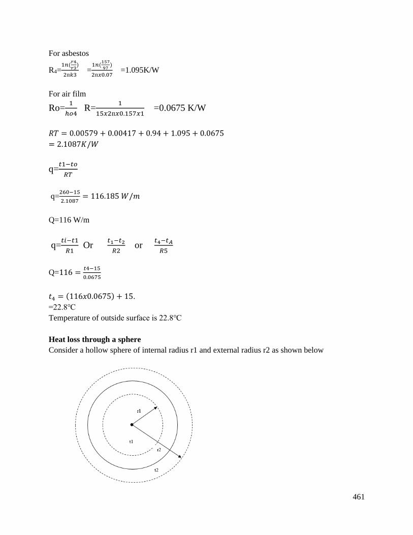
461
For asbestos
R4=1𝑛(
𝑟4
𝑟3)
2ᴨ𝑘3 =
1𝑛(157
97)
2ᴨ𝑥0.07 =1.095K/W
For air film
Ro=1
ℎ𝑜4 R=
1
15𝑥2ᴨ𝑥0.157𝑥1 =0.0675 K/W
𝑅𝑇 = 0.00579 + 0.00417 + 0.94 + 1.095 + 0.0675
= 2.1087𝐾/𝑊
q=𝑡1−𝑡𝑜
𝑅𝑇
q=260−15
2.1087= 116.185 𝑊/𝑚
Q=116 W/m
q=𝑡𝑖−𝑡1
𝑅1 Or
𝑡1−𝑡2
𝑅2 or
𝑡4−𝑡𝐴
𝑅5
Q=116 =𝑡4−15
0.0675
𝑡4 = (116𝑥0.0675) + 15.
=22.8
Temperature of outside surface is 22.8
Heat loss through a sphere
Consider a hollow sphere of internal radius r1 and external radius r2 as shown below
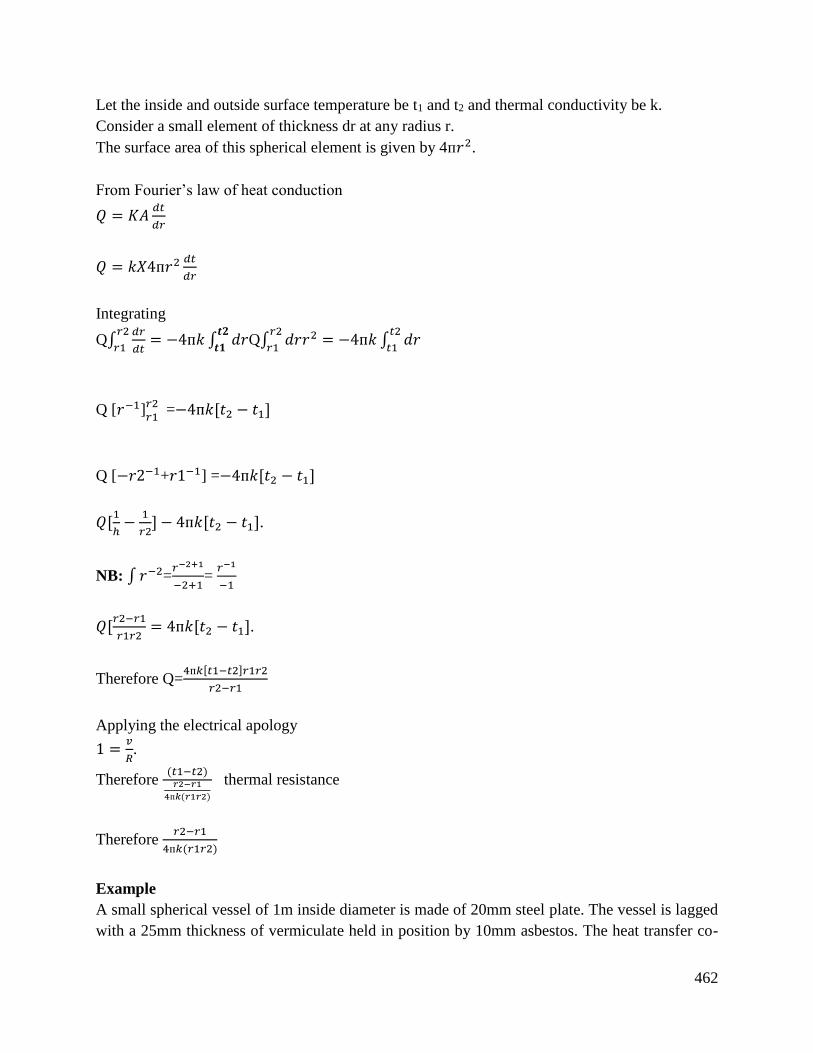
462
Let the inside and outside surface temperature be t1 and t2 and thermal conductivity be k.
Consider a small element of thickness dr at any radius r.
The surface area of this spherical element is given by 4ᴨ𝑟2.
From Fourier’s law of heat conduction
𝑄 = 𝐾𝐴𝑑𝑡
𝑑𝑟
𝑄 = 𝑘𝑋4ᴨ𝑟2 𝑑𝑡
𝑑𝑟
Integrating
Q∫𝑑𝑟
𝑑𝑡= −4ᴨ𝑘
𝑟2
𝑟1∫ 𝑑𝑟
𝒕𝟐
𝒕𝟏Q∫ 𝑑𝑟𝑟2 = −4ᴨ𝑘
𝑟2
𝑟1∫ 𝑑𝑟
𝑡2
𝑡1
Q [𝑟−1]𝑟2𝑟1
=−4ᴨ𝑘[𝑡2 − 𝑡1]
Q [−𝑟2−1+𝑟1−1] =−4ᴨ𝑘[𝑡2 − 𝑡1]
𝑄[1
ℎ−
1
𝑟2] − 4ᴨ𝑘[𝑡2 − 𝑡1].
NB: ∫ 𝑟−2=𝑟−2+1
−2+1=
𝑟−1
−1
𝑄[𝑟2−𝑟1
𝑟1𝑟2= 4ᴨ𝑘[𝑡2 − 𝑡1].
Therefore Q=4ᴨ𝑘[𝑡1−𝑡2]𝑟1𝑟2
𝑟2−𝑟1
Applying the electrical apology
1 =𝑣
𝑅.
Therefore (𝑡1−𝑡2)𝑟2−𝑟1
4ᴨ𝑘(𝑟1𝑟2)
thermal resistance
Therefore 𝑟2−𝑟1
4ᴨ𝑘(𝑟1𝑟2)
Example
A small spherical vessel of 1m inside diameter is made of 20mm steel plate. The vessel is lagged
with a 25mm thickness of vermiculate held in position by 10mm asbestos. The heat transfer co-
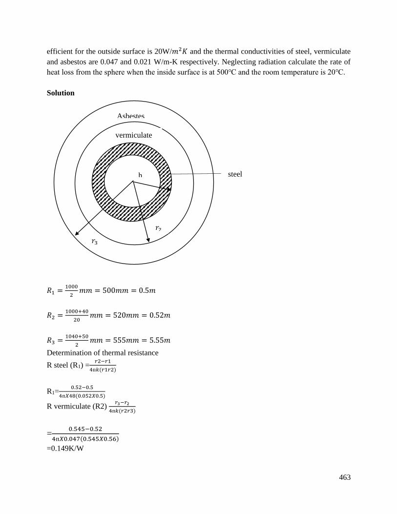
463
efficient for the outside surface is 20W/𝑚2𝐾 and the thermal conductivities of steel, vermiculate
and asbestos are 0.047 and 0.021 W/m-K respectively. Neglecting radiation calculate the rate of
heat loss from the sphere when the inside surface is at 500 and the room temperature is 20.
Solution
𝑅1 =1000
2𝑚𝑚 = 500𝑚𝑚 = 0.5𝑚
𝑅2 =1000+40
20𝑚𝑚 = 520𝑚𝑚 = 0.52𝑚
𝑅3 =1040+50
2𝑚𝑚 = 555𝑚𝑚 = 5.55𝑚
Determination of thermal resistance
R steel (R1) =𝑟2−𝑟1
4ᴨ𝑘(𝑟1𝑟2)
R1=0.52−0.5
4ᴨ𝑋48(0.052𝑋0.5)
R vermiculate (R2) 𝑟3−𝑟2
4ᴨ𝑘(𝑟2𝑟3)
=0.545−0.52
4ᴨ𝑋0.047(0.545𝑋0.56)
=0.149K/W
vermiculate
Asbestes
h
𝑟2
𝑟3
steel
464
R asbestos (R3) 𝑟4−𝑟3
4ᴨ𝑘(𝑟3𝑟4)
=0.555.0.5450
4ᴨ𝑋0.21(0.555𝑋0.545)
=0.01253 K/W
Resistance of outside film
RO=1
ℎ𝑜𝐴
=1
20 𝑋 4ᴨ 𝑋 0.552 =0.01292 K/W
Total resistance
RT= [0.000128+0.1494+0.01253+0.01297]
RT=0.17498K/W
𝑄 =𝑡1−𝑡2
𝑅𝑇.
𝑄 =500−20
0.17498
=2743W
=2.743 kW
Overall heat transfer coefficient (ꭒ)
ꭒ=1
𝑅+𝐴 Where A= is the surface area of the pipe
Q=ꭒ𝐴( 𝑡𝐴 − 𝑡𝐵)
Example
A steel pipe carrying a process fluid has a bore of 150mm and a thickness of 5mm. the pipe is
covered with 50mm layers of insulation of thermal conductivity 0.05W/m-K. The thermal
conductivity of the steel pipe maybe taken as 45W/m-K and the surface heat transfer function as
35 W/m2 –K. For the inner surface of the pipe and 7W/m2-K for the outer surface of the insulation.
Assuming the process fluid temperature to be constant as 300 and the ambient temperature as
16. Determine:
a) The overall heat transfer coefficient based on the outer surface of the insulation.
b) Heat lost per meter length from the pipe (10 marks)
Solution
Bore (internal diameter) =150mm
Thickness=5mm
Insulation=50mm

465
K steel=45 W/m-K
K insulation=0.05 W/m-K
Hi=35W/m2K
Ho=7W/m2-K
R1= (For the fluid film)
R1=1
ℎ𝑖𝐴𝑖
=1
35𝑋2ᴨ𝑋0.075𝑋1
=0.0606 K/W
R2=resistance for pipe
R2=1𝑛(
80
75)
2ᴨ𝑋45 = 0.000228 K/W
R3=resistance for the insulation
R3=1𝑛(
130
80)
2ᴨ𝑋0.05 = 1.545 K/W
R4=for air film
R4=1
ℎ𝑜𝐴𝑜 =
1
7𝑋2ᴨ𝑋0.13𝑋1
=0.175 K/W
RT=total resistance
=0.175+1.545+0.000228+0.0606
466
=1.781 kΩ
i) ꭒ=1
𝑅𝑡𝐴𝑜 =
1
1.78𝑥2ᴨ𝑥0.13
=0.6374 W/m2 K
ii) Q=𝑡𝑖−𝑡𝑜
𝑅𝑇 Or Q=ꭒAo(t1-ti)
300−16
1.781
=159.46
=159.5W/m
Conclusion
The learning outcome covered equipping the learner with knowledge, skills and derive conduction
evaluation and apply them from Fourier’s law. Derive heat transfer equation and apply from
Newton’s law of cooling and Fourier’s law.
Further Reading
1. Applied thermal dynamics for engineering technologies by EASTOP and MacConkey.
2. Basic engineering thermal dynamic by R-Joel.
3. Engineering thermodynamics by Rodgers Mayhew.
6.3.10.3 Self-Assessment
Written Assessment
1. Which heat transfer condition takes place through a vacuum?
a) Radiation.
b) Conduction.
c) Convention.
2. Which law is based on imperial observation of one dimensional steady heat flow through
a solid?
a) Newton’s law of cooling.
b) Fourier’s law of heat conduction.
3. Which is the Fourier’s law and its expression for heat conduction?
a) 𝑄 = 𝐾𝐴(𝑑𝑇
𝑑𝑋)
b) 𝑄 = 𝐾𝐴(𝑑𝑋
𝑑𝑇)
467
4. Wet steam at a pressure of 2N/m2 flows through a pipe 20m long. The pipe has an external
diameter of 80mm and is covered with lagging 35mm thick which has a co-efficient of
thermal conductivity 0.065W/m-K. The surface transfer coefficient is 4.5W/m2-K and the
ambient temperature is 15. the steam flow rate is 300kg/hr and centers the pipe with a
dryness fraction of 0.97. Assuming there is no temperature across the pipe determine
dryness reaction of the steam as it leaves the pipe.
5. A pipe has a length of 50m, internal and external diameter of 0.8m and 0.95m respectively.
The pipe has a thermal conductivity of 45W/m-K. It is insulated in two layers of asbestos
and magnesia of thickness 40mm and 15mm respectively. The thermal conductivities of
asbestos and magnesia are 0.11 and 0.067W/m-K respectively, the inside and outside heat
transfer coefficient are 290 and 7W/m2-K respectively. Determine the rate of heat loss if
the steam is a temperature of 350 and the ambient temperature is 240.
6. A small hemispherical oven is built of an inner layer of insulating fire brick 125mm thick
and outer covering of 85% magnesia 40mm thick. The inner surface of the oven is at 800
and the heat transfer coefficient for outside surface is 10W/m2K and the room temp is 20.
Calculate the rate of heat loss through the hemisphere if the inside surface radius is 0.6m.
Take the thermal conductivities of fire brick and 85% magnesia as 0.31 and 0.05W/m-K
respectively.
7. State Fourier’s law of heat conduction.
8. State 3 ways of which heat maybe transferred.
9. State Newton’s law of cooling.
10. Explain heat flow through a cylinder and show that
Q=2ᴨ𝑘(𝑡1−𝑡2)
1𝑛(𝑟2
𝑟1)
11. Explain the differences between heat loss through a sphere and of a cylinder.
Oral Assessment
1. Explain heat transfer using conduction.
2. Discuss conduction through a composite wall and show that:
𝑄 =𝑇1−𝑇4
𝑥12𝑘12
+𝑥23𝑘23
+𝑥34𝑘34
=𝑡𝑒𝑚𝑝𝑒𝑟𝑎𝑡𝑢𝑟𝑒 𝑑𝑖𝑓𝑓𝑒𝑟𝑒𝑛𝑐𝑒
𝑡ℎ𝑒𝑟𝑚𝑎𝑙 𝑟𝑒𝑠𝑖𝑠𝑡𝑎𝑛𝑐𝑒
Practical Assessment
1. By use of a cylinder real pipe from Fourier’s law conduction and show that
𝑅 =1𝑛(
𝑟2
𝑟1)
2𝑛𝑘
Where r1=internal radius

468
Where r2=external radius
Project
An experiment should be conducted in the lab to demonstrate heat loss in cylinders and sphere and
also see radiation, convention and conduction.
6.3.2.4 Tools, Equipment, Supplies and Materials
Scientific Calculators
Relevant reference materials
Stationeries
Relevant practical materials
Dice
Computers with internet connection
6.3.10.5 References
Maenkey, G. (2006). Applied thermal dynamics for engineering technologies. EASTOP
Publishing.
Joel, R. (2011). Basic engineering thermo-dynamics by. Frankfurt: Uprisers Limited.
Rodgers, M. (2003). Engineering thermo-dynamics. Horta: Jack & Crawford Ltd.
469
6.3.11 Learning Outcome No10: Understand heat exchangers
6.3.2.1 Learning Activities
Learning Outcome No10 :Understand heat exchangers
Learning Activities Special Instructions
10.1. Classify heat exchangers
10.2. Describe recuperative heat exchangers
10.3. Apply heat equations to solve heat exchanger problems
6.3.2.2 Information Sheet No6/LO10: Understand heat exchangers
Introduction to learning outcome
This learning outcome covers classification of heat exchangers, description of recuperative heat
exchangers and application of heat equations to solve heat exchanger problem.
Definition of key terms
Heat exchanger: A device used to transfer heat between a solid surface and a fluid or between
two or more fluids.
Coolant: Is a liquid that absorbs heat.
Content/Procedures/Methods/Illustrations
10.1 Heat exchangers are classified
Classification of heat exchangers
a) Direct contact/open contact heat exchanger
b) Indirect contact heat exchangers
Direct contact
In this exchanger, the exchange of heat takes place by direct mixing of hot and cold fluids.
Indirect contact heat exchanger
In this type of heat exchanger, the heat transfer between two fluids could be carried out by
transmission through wall which separates the two fluids. This includes the following;
a) Regenerators
b) Recuperators or surface exchangers
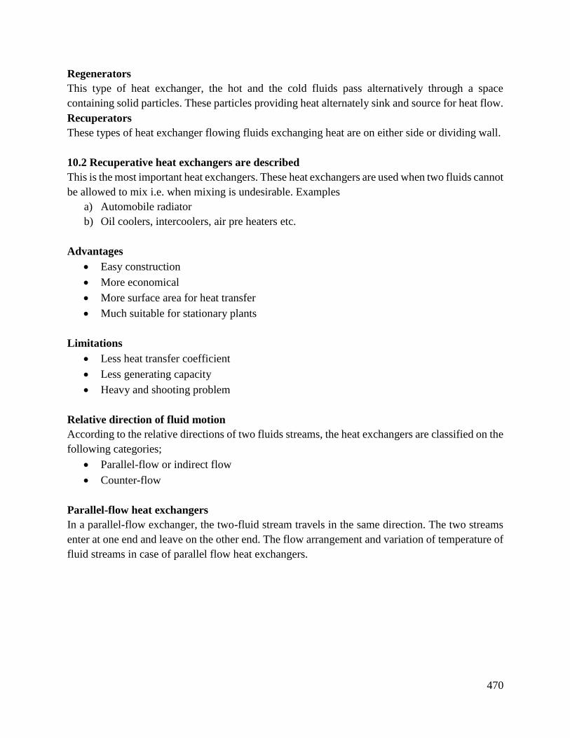
470
Regenerators
This type of heat exchanger, the hot and the cold fluids pass alternatively through a space
containing solid particles. These particles providing heat alternately sink and source for heat flow.
Recuperators
These types of heat exchanger flowing fluids exchanging heat are on either side or dividing wall.
10.2 Recuperative heat exchangers are described
This is the most important heat exchangers. These heat exchangers are used when two fluids cannot
be allowed to mix i.e. when mixing is undesirable. Examples
a) Automobile radiator
b) Oil coolers, intercoolers, air pre heaters etc.
Advantages
Easy construction
More economical
More surface area for heat transfer
Much suitable for stationary plants
Limitations
Less heat transfer coefficient
Less generating capacity
Heavy and shooting problem
Relative direction of fluid motion
According to the relative directions of two fluids streams, the heat exchangers are classified on the
following categories;
Parallel-flow or indirect flow
Counter-flow
Parallel-flow heat exchangers
In a parallel-flow exchanger, the two-fluid stream travels in the same direction. The two streams
enter at one end and leave on the other end. The flow arrangement and variation of temperature of
fluid streams in case of parallel flow heat exchangers.
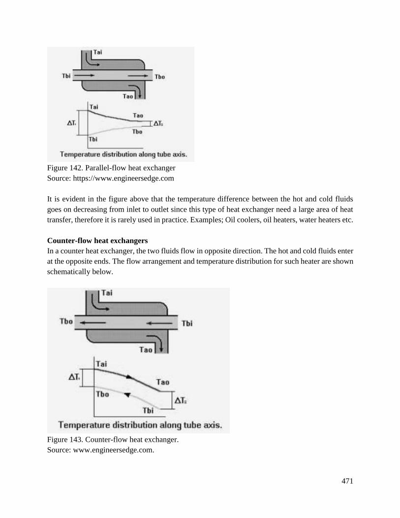
471
Figure 142. Parallel-flow heat exchanger
Source: https://www.engineersedge.com
It is evident in the figure above that the temperature difference between the hot and cold fluids
goes on decreasing from inlet to outlet since this type of heat exchanger need a large area of heat
transfer, therefore it is rarely used in practice. Examples; Oil coolers, oil heaters, water heaters etc.
Counter-flow heat exchangers
In a counter heat exchanger, the two fluids flow in opposite direction. The hot and cold fluids enter
at the opposite ends. The flow arrangement and temperature distribution for such heater are shown
schematically below.
Figure 143. Counter-flow heat exchanger.
Source: www.engineersedge.com.
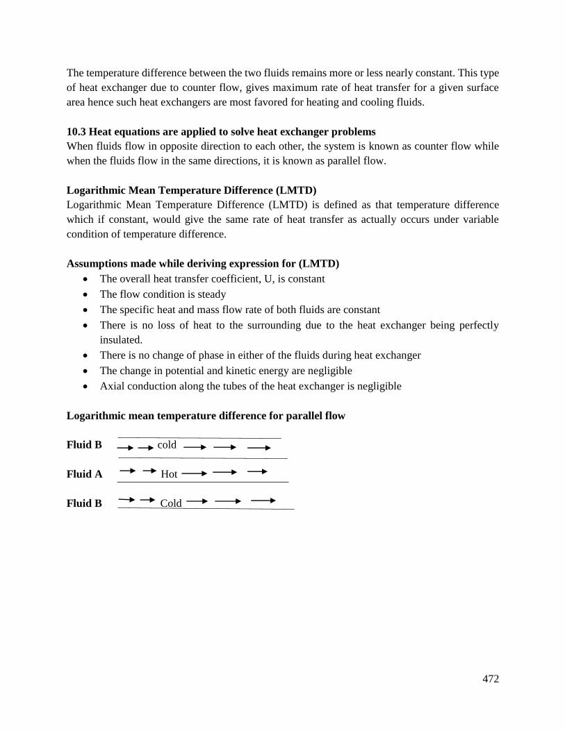
472
The temperature difference between the two fluids remains more or less nearly constant. This type
of heat exchanger due to counter flow, gives maximum rate of heat transfer for a given surface
area hence such heat exchangers are most favored for heating and cooling fluids.
10.3 Heat equations are applied to solve heat exchanger problems
When fluids flow in opposite direction to each other, the system is known as counter flow while
when the fluids flow in the same directions, it is known as parallel flow.
Logarithmic Mean Temperature Difference (LMTD)
Logarithmic Mean Temperature Difference (LMTD) is defined as that temperature difference
which if constant, would give the same rate of heat transfer as actually occurs under variable
condition of temperature difference.
Assumptions made while deriving expression for (LMTD)
The overall heat transfer coefficient, U, is constant
The flow condition is steady
The specific heat and mass flow rate of both fluids are constant
There is no loss of heat to the surrounding due to the heat exchanger being perfectly
insulated.
There is no change of phase in either of the fluids during heat exchanger
The change in potential and kinetic energy are negligible
Axial conduction along the tubes of the heat exchanger is negligible
Logarithmic mean temperature difference for parallel flow
Fluid B cold
Fluid A Hot
Fluid B Cold
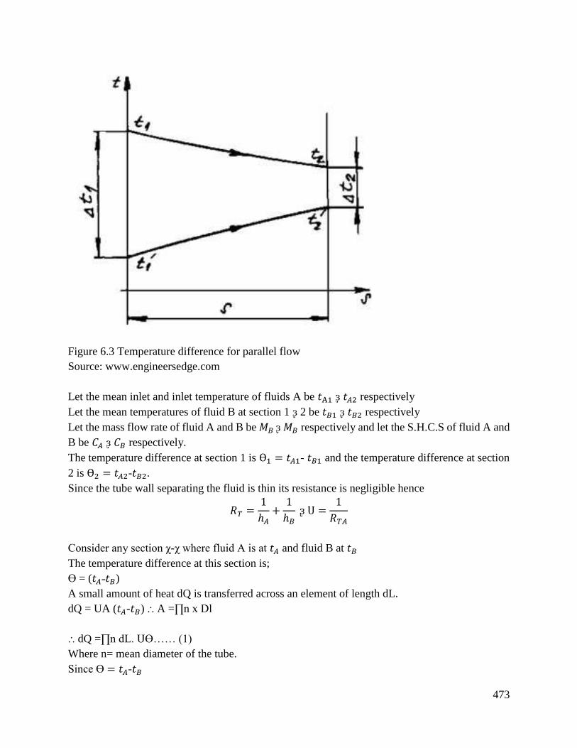
473
Figure 6.3 Temperature difference for parallel flow
Source: www.engineersedge.com
Let the mean inlet and inlet temperature of fluids A be 𝑡A1 ᶔ 𝑡𝐴2 respectively
Let the mean temperatures of fluid B at section 1 ᶔ 2 be 𝑡𝐵1 ᶔ 𝑡𝐵2 respectively
Let the mass flow rate of fluid A and B be 𝑀𝐵 ᶔ 𝑀𝐵 respectively and let the S.H.C.S of fluid A and
B be 𝐶𝐴 ᶔ 𝐶𝐵 respectively.
The temperature difference at section 1 is Ө1 = 𝑡𝐴1- 𝑡𝐵1 and the temperature difference at section
2 is Ө2 = 𝑡𝐴2-𝑡𝐵2.
Since the tube wall separating the fluid is thin its resistance is negligible hence
𝑅𝑇 =1
ℎ𝐴+
1
ℎ𝐵 ᶔ Ս =
1
𝑅𝑇𝐴
Consider any section ꭓ-ꭓ where fluid A is at 𝑡𝐴 and fluid B at 𝑡𝐵
The temperature difference at this section is;
Ө = (𝑡𝐴˗𝑡𝐵)
A small amount of heat dQ is transferred across an element of length dL.
dQ = UA (𝑡𝐴-𝑡𝐵) ⸫ A =∏n x Dl
⸫ dQ =∏n dL. ՍӨ…… (1)
Where n= mean diameter of the tube.
Since Ө = 𝑡𝐴-𝑡𝐵
474
dӨ = 𝑑𝑡𝐴- 𝑑𝑡𝐵……… (2)
For parallel flow 𝑡𝐴 decreases along length L while 𝑡𝐵 increases with length L.
The heat given up by fluid A must be equal to the heat received by fluid B.
dQ = −𝑀𝐴𝐶𝐴𝑑𝑡𝐴- 𝑀𝐵𝐶𝐵𝑑𝑡𝐵……. (3)
⸫𝑑𝑡𝐴 = −𝑑𝑄
𝑀𝐴𝐶𝐴𝑎𝑛𝑑𝑑𝑡𝐵 =
𝑑𝑄
𝑀𝐵𝐶𝐵
Substituting in equation 2 gives;
dӨ = −𝑑𝑄
𝑀𝐴𝐶𝐴−
𝑑𝑄
𝑀𝐵𝐶𝐵
dӨ =-dQ (1
𝑀𝐴𝐶𝐴+
1
𝑀𝐵𝐶𝐵)…… (4)
Integrating equation (4) between section (1) and (2)
∫ 𝑑Ө =2
1-∫ 𝑑𝑄 (
1
𝑀𝐴𝐶𝐴+
1
𝑀𝐵𝐶𝐵)
3
1
Ө2- Ө1 =-Q [1
𝑀𝐴𝐶𝐴+
1
𝑀𝐵𝐶𝐵]
Ө1-Ө2 =Q [1
𝑀𝐴𝐶𝐴+
1
𝑀𝐵𝐶𝐵] ……(5)
From equation (4)
dQ =−𝑑Ө
1
𝑀𝐴𝐶𝐴+
1
𝑀𝐵𝐶𝐵
……… (6)
Substituting for dQ in equation (1)
∏n dL.ՍӨ = −𝑑Ө
1
𝑀𝐴𝐶𝐴+
1
𝑀𝐵𝐶𝐵
…… (7)
−𝑑Ө
Ө=∏n dL.Ս [
1
𝑀𝐴𝐶𝐴+
1
𝑀𝐵𝐶𝐵]……. (8)
Integrating between section (1) and (2) you get;
- 𝑙𝑛Ө2
Ө1=∏nL.Ս [
1
𝑀𝐴𝐶𝐴+
1
𝑀𝐵𝐶𝐵]……. (9)
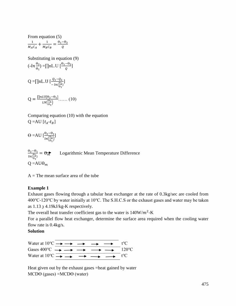
475
From equation (5) 1
𝑀𝐴𝐶𝐴+
1
𝑀𝐵𝐶𝐵=
Ө1−Ө2
𝑄
Substituting in equation (9)
(-𝑙𝑛Ө2
Ө1) =∏nL.U [
Ө1−Ө2
𝑄]
Q =∏nL.Ս [𝑄1−𝑄2
− 𝑙𝑛(Ө2Ө1
)]
Q =∏𝑛𝐿Ս[Ө2−Ө1]
𝐿𝑁(Ө2Ө1
)…… (10)
Comparing equation (10) with the equation
Q =AU [𝑡𝐴-𝑡𝐵]
Ө =AU [Ө2−Ө1
𝑙𝑛(Ө2Ө1
)]
Ө2−Ө1
𝑙𝑛(Ө2Ө1
)= Ө𝑚 Logarithmic Mean Temperature Difference
Q =AUӨ𝑚
A = The mean surface area of the tube
Example 1
Exhaust gases flowing through a tabular heat exchanger at the rate of 0.3kg/sec are cooled from
400-120 by water initially at 10. The S.H.C.S or the exhaust gases and water may be taken
as 1.13 ᶔ 4.19kJ/kg-K respectively.
The overall heat transfer coefficient gas to the water is 140W/𝑚2-K
For a parallel flow heat exchanger, determine the surface area required when the cooling water
flow rate is 0.4kg/s.
Solution
Water at 10 t
Gases 400 120
Water at 10 t
Heat given out by the exhaust gases =heat gained by water
MCDӨ (gases) =MCDӨ (water)
476
0.3×1.13(400-120) =0.4×4.19 (t-10)
(t-10) =0.3×1.13×280
0.4×4.19
(t-10) =56.63
t =66.6
Also
Q =0.3×1.13×280
=95kW
Q =UAӨM
Ө𝑚 =Ө2−Ө1
𝑙𝑛(Ө2
Ө1)
Ө1 =400-10
Ө1 =390K
Ө2 =120-66.6
Ө2 =53.34=53.4
Ө𝑚 =53.4 − 390
𝑙𝑛(53.4390)
=169K
But Q =AUӨ𝑚
95,000 =140A×169
A =4.02𝑚2
Logarithmic Mean Temperature for counter flow
The figure below shows the flow arrangement and temperature distribution in a single pass counter
flow heat exchanger.
Let’s consider an elementary area dA of the heat exchanger, the rate of flow of heat through this
elementary area is given by;
dQ =U. dA (𝑡𝑛−𝑡𝑐)=U. dA. Dt…….(1)
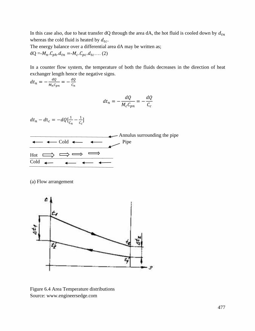
477
In this case also, due to heat transfer dQ through the area dA, the hot fluid is cooled down by 𝑑𝑡𝑛
whereas the cold fluid is heated by 𝑑𝑡𝑐.
The energy balance over a differential area dA may be written as;
dQ =-𝑀𝑛.𝐶𝑝ℎ.𝑑𝑡𝑛 =-𝑀𝑐.𝐶𝑝𝑐.𝑑𝑡𝑐…. (2)
In a counter flow system, the temperature of both the fluids decreases in the direction of heat
exchanger length hence the negative signs.
𝑑𝑡𝑛 = −𝑑𝑄
𝑀𝑛𝐶𝑝𝑛= −
𝑑𝑄
𝐶𝑛
𝑑𝑡𝑛 = −𝑑𝑄
𝑀𝑐𝐶𝑝𝑛= −
𝑑𝑄
𝐶𝑐
𝑑𝑡𝑛 − 𝑑t𝑐 = −𝑑𝑄[1
𝐶𝑛−
1
𝐶𝑐]
Annulus surrounding the pipe
Cold Pipe
Hot
Cold
(a) Flow arrangement
Figure 6.4 Area Temperature distributions
Source: www.engineersedge.com
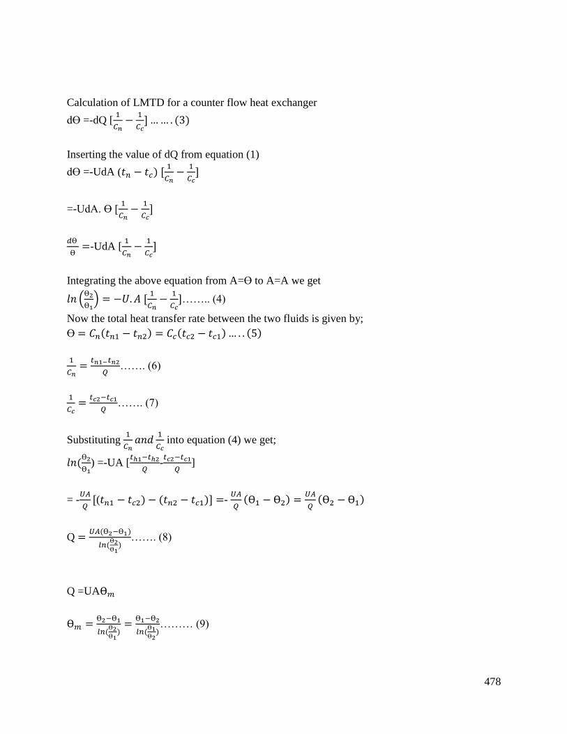
478
Calculation of LMTD for a counter flow heat exchanger
dӨ =-dQ [1
𝐶𝑛−
1
𝐶𝑐] …… . (3)
Inserting the value of dQ from equation (1)
dӨ =-UdA (𝑡𝑛 − 𝑡𝑐) [1
𝐶𝑛−
1
𝐶𝑐]
=-UdA. Ө [1
𝐶𝑛−
1
𝐶𝑐]
𝑑Ө
Ө=-UdA [
1
𝐶𝑛−
1
𝐶𝑐]
Integrating the above equation from A=Ө to A=A we get
𝑙𝑛 (Ө2
Ө1) = −𝑈. 𝐴 [
1
𝐶𝑛−
1
𝐶𝑐]…….. (4)
Now the total heat transfer rate between the two fluids is given by;
Ө = 𝐶𝑛(𝑡𝑛1 − 𝑡𝑛2) = 𝐶𝑐(𝑡𝑐2 − 𝑡𝑐1)… . . (5)
1
𝐶𝑛=
𝑡𝑛1−𝑡𝑛2
𝑄……. (6)
1
𝐶𝑐=
𝑡𝑐2−𝑡𝑐1
𝑄……. (7)
Substituting 1
𝐶𝑛𝑎𝑛𝑑
1
𝐶𝑐 into equation (4) we get;
𝑙𝑛(Ө2
Ө1) =-UA [
𝑡ℎ1−𝑡ℎ2
𝑄-𝑡𝑐2−𝑡𝑐1
𝑄]
= -𝑈𝐴
𝑄[(𝑡𝑛1 − 𝑡𝑐2) − (𝑡𝑛2 − 𝑡𝑐1)] =-
𝑈𝐴
𝑄(Ө1 − Ө2) =
𝑈𝐴
𝑄(Ө2 − Ө1)
Q =𝑈𝐴(Ө2−Ө1)
𝑙𝑛(Ө2Ө1
)……. (8)
Q =UAӨ𝑚
Ө𝑚 =Ө2−Ө1
𝑙𝑛(Ө2Ө1
)=
Ө1−Ө2
𝑙𝑛(Ө1Ө2
)……… (9)
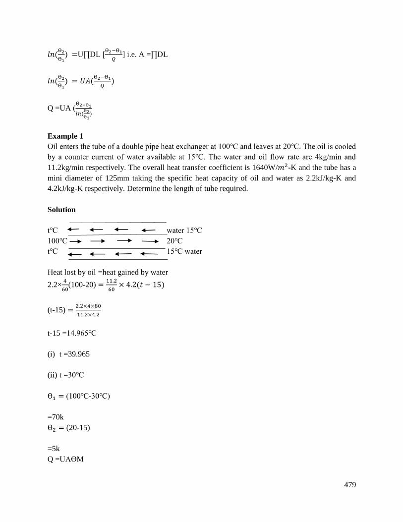
479
𝑙𝑛(Ө2
Ө1) =U∏DL [
Ө2−Ө1
𝑄] i.e. A =∏DL
𝑙𝑛(Ө2
Ө1) = 𝑈𝐴(
Ө2−Ө1
𝑄)
Q =UA (Ө2−Ө1
𝑙𝑛(Ө2Ө1
)
Example 1
Oil enters the tube of a double pipe heat exchanger at 100 and leaves at 20. The oil is cooled
by a counter current of water available at 15. The water and oil flow rate are 4kg/min and
11.2kg/min respectively. The overall heat transfer coefficient is 1640W/𝑚2-K and the tube has a
mini diameter of 125mm taking the specific heat capacity of oil and water as 2.2kJ/kg-K and
4.2kJ/kg-K respectively. Determine the length of tube required.
Solution
t water 15
100 20
t 15 water
Heat lost by oil =heat gained by water
2.2×4
60(100-20) =
11.2
60× 4.2(𝑡 − 15)
(t-15) =2.2×4×80
11.2×4.2
t-15 =14.965
(i) t =39.965
(ii) t =30
Ө1 = (100-30)
=70k
Ө2 = (20-15)
=5k
Q =UAӨM
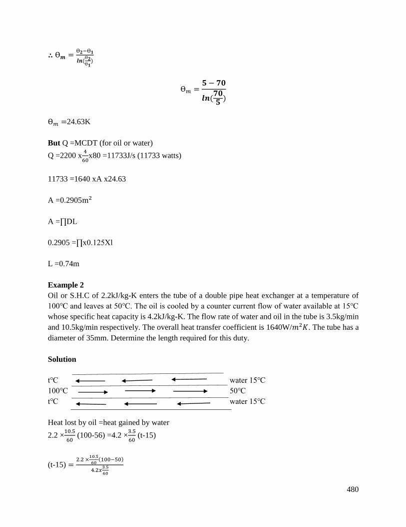
480
⸫ Ө𝒎 =Ө𝟐−Ө𝟏
𝒍𝒏(Ө𝟐Ө𝟏
)
Ө𝑚 =𝟓 − 𝟕𝟎
𝒍𝒏(𝟕𝟎𝟓
)
Ө𝑚 =24.63K
But Q =MCDT (for oil or water)
Q =2200 x4
60x80 =11733J/s (11733 watts)
11733 =1640 xA x24.63
A =0.2905m2
A =∏DL
0.2905 =∏x0.125Xl
L =0.74m
Example 2
Oil or S.H.C of 2.2kJ/kg-K enters the tube of a double pipe heat exchanger at a temperature of
100 and leaves at 50. The oil is cooled by a counter current flow of water available at 15
whose specific heat capacity is 4.2kJ/kg-K. The flow rate of water and oil in the tube is 3.5kg/min
and 10.5kg/min respectively. The overall heat transfer coefficient is 1640W/𝑚2𝐾. The tube has a
diameter of 35mm. Determine the length required for this duty.
Solution
t water 15
100 50
t water 15
Heat lost by oil =heat gained by water
2.2 ×10.5
60 (100-56) =4.2 ×
3.5
60 (t-15)
(t-15) =2.2 ×
10.5
60(100−50)
4.2𝑥3.5
60

481
t =93.57
Ө1 = (100 − 93.57) = 6.43𝐾
Ө2 = (50 − 15) = 35𝐾
Q =UAӨ𝑚
⸫Ө𝒎 =Ө𝟐−Ө𝟏
𝒍𝒏(Ө𝟐Ө𝟏
)
Ө𝒎 =𝟑𝟓−𝟔.𝟒𝟑
𝒍𝒏(𝟑.𝟓
𝟔.𝟒𝟑) =16.86k
But
𝑄 = 𝑀𝐶𝐷𝑇
𝑄 = 10.5/60 × 2200 × 60
𝑄 = 19250𝐽/𝑠 𝑜𝑟 19250 𝑤𝑎𝑡𝑡𝑠
19250 = 1640 × 𝐴 × 16 .88
𝐴 = 0.6962
𝐴 = 𝜋𝐷𝐿
0.6962 = 𝜋 × 0.035 × 𝐿
𝐿 = 6.33𝑚
Conclusion
The learning outcome covered or equipped the learner with knowledge, skills and attitude to
classify different heat exchangers, describe the recuperative heat exchangers and apply heat
equations to solve heat exchanger problems.
Further Reading
482
1. Applied thermodynamics by T.D. EASTOP and A. MacConkey
6.3.11.3 Self-Assessment
Written Assessment
1. Heat transfer is constant when?
a) Temperature remains constant with time
b) Temperature decreases with time
c) Temperature increases with time
d) Any of them
2. What do you understand by co-efficient of thermal conductivity
a) Quantity of heat transfer per unit area per one degree drop in temperature
b) Quantity of heat transfer per one-degree temperature drop per unit area
c) Quantity of heat transfer per unit time per unit area
d) Quantity of heat transfer per unit time per unit area per one-degree temperature
drop per unit length
3. Thermal conductivity is expresses as?
a) W/mK
b) W/𝑚2
c) Q/hmK
d) W/ℎ2𝑚2𝐾
4. Heat transfer from higher temperature to low temperature takes place according to?
a) Fourier law
b) First law of thermodynamics
c) Second law of thermodynamics
d) Zeroth law of thermodynamics
5. The radial heat transfer rate through hollow cylinder increases as the ratio of outer radius
to inner radius ____________
a) Decreases
b) Increases
c) Constant
d) None of the above
6. The Fourier law of heat transfer by conduction is expressed as?
a) Q = 𝑘𝐴2 𝑑𝑡
𝑑𝑥
b) Q = 𝑘𝐴𝑑𝑡
𝑑𝑥
483
c) Q =kA𝑑𝑥
𝑑𝑡
d) Q = 𝑘𝐴3 𝑑𝑥
𝑑𝑡
7. The quantity of heat by radiation is dependent on?
a) Area of the body only
b) Temperature of body only
c) Shape of body only
d) On all (a), (b) and (c)
8. What is the meaning of thermal conductivity of a material.
9. Enumerate the three modes by which heat can be transferred from one place to another
which is the slowest of all.
10. Prove that LMTD in parallel flow heat exchanger is given by LMTD = 𝑡1−𝑡2
𝑙𝑜𝑔𝑐𝑡1𝑡2
11. A 250mm steam main 225meters long is covered with 50mm of high temperature insulation
(k =0.095W/mK) and 40mm of low temperature insulation (k=0.065W/mK). The inner and
outer surface temperature as measured is 400 and50 respectively. Calculate;
Total heat loss per hour
a) 265514kj/h
b) 873.5kj/h
c) 1502.5kj/h
d) 215
Total heat loss per 𝑚2 of outer surface
The heat loss per 𝑚2 of pipe surface
The temperature between the two layers of insulation neglect heat conduction through pipe
all
12. The wall of a furnace is made up 250mm of fire brick k =1.05W/mK, 120mm of insulation
brick k=0.85W/mK and 200mm of red brick k =0.85W/mK. The inner and outer surface
temperatures of the wall are 850 and 65 respectively. Calculate the temperatures at
the contact surfaces. Neglect the resistance of mortar joints.
a) 703
b) 210
Oral Assessment
1. What do you understand by the term convective heat transfer co-efficient and overall heat
transfer co-efficient?
2. Discuss the term critical thickness or insulation for a cylinder and sphere.
Practical Assessment

484
1. By experiment, determine the rate of heat flow through a boiler wall made of 2cm thickness
steel and covered with an insulating material of 0.5cm thick. The temperature of the inner
and outer surface of the wall are determined by a given thermometer
K (steel) =58W/mK
K (insulation) =0.116W/mK
6.3.11.4 Tools, Equipment, Supplies and Materials
Scientific Calculators
Relevant reference materials
Stationeries
Relevant practical materials
Dice
Computers with internet connection
6.3.11.5 References
Gitobu, G. G. (2016). Model Organic Rankine Cycle For Brine at Olkaria Geothermal Field,
Kenya. United Nations University-Geothermal Training Programme, Tech. Rep, 15.
Li, K. (2018). Applied thermodynamics: availability method and energy conversion. Routledge.
Singh, O. (2003). Applied thermodynamics. New Age International.
485
6.3.12 Learning Outcome No 11: understand air compressors
6.3.12.1 Learning Activities
Learning Outcome No 11:understand air compressors
Learning Activities Special Instructions
11.1 Classify air compressors
11.2 Describe types of air compressors (reciprocating, blowers,
sliding valves)
11.3 Derive and apply equations of reciprocating compressors
6.3.12.2 Information Sheet No6/LO11: understand air compressors
Introduction
This learning outcome covers classification of air compressors, description of types of air
compressors, derivation and application of equation of reciprocating compressors.
Definition of key terms
Compressor: This is a machine that takes in air at low pressure and gives out at a higher pressure.
Content/Procedures/Methods/Illustrations
11.1 Air compressors are classified
a) Rotary type compressor
b) Reciprocating compressor
Rotary type: Has a high mass flow rate and low-pressure ratio.
𝐷𝑒𝑙𝑖𝑣𝑒𝑟𝑦 𝑝𝑟𝑒𝑠𝑠𝑢𝑟𝑒
𝐼𝑛𝑡𝑎𝑘𝑒 𝑝𝑟𝑒𝑠𝑠𝑢𝑟𝑒 = 𝑟𝑝
These are applied for exhausting work and also vacuum pumping. They are small in size and light
in weight.
Reciprocating compressor: They are used for high pressure ration and slow mass flow rate. For
a reciprocating compressor the properties at inlet and outlet are average values take over the cycle.
The basic mechanism involves the piston, connecting rod crank and the cylinder arrangement. The
working fluid is considered to be perfect gas and the clearance volume in the cylinder is initially
considered negligible.
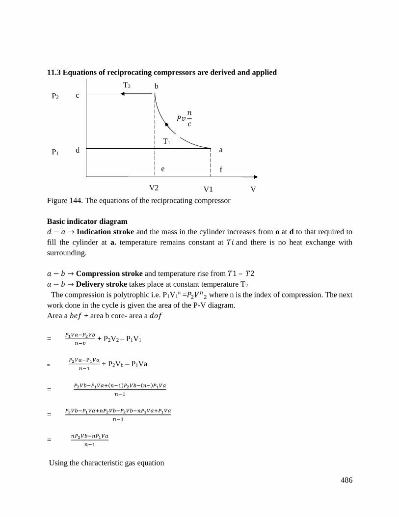
486
11.3 Equations of reciprocating compressors are derived and applied
Figure 144. The equations of the reciprocating compressor
Basic indicator diagram
𝑑 − 𝑎 → Indication stroke and the mass in the cylinder increases from o at d to that required to
fill the cylinder at a. temperature remains constant at 𝑇𝑖 and there is no heat exchange with
surrounding.
𝑎 − 𝑏 → Compression stroke and temperature rise from 𝑇1 – 𝑇2
𝑎 − 𝑏 → Delivery stroke takes place at constant temperature T2
The compression is polytrophic i.e. P1V1n =𝑃2𝑉
𝑛2 where n is the index of compression. The next
work done in the cycle is given the area of the P-V diagram.
Area a 𝑏𝑒𝑓 + area b core- area a 𝑑𝑜𝑓
= 𝑃1𝑉𝑎−𝑃2𝑉𝑏
𝑛−𝑣 + P2V2 – P1V1
= 𝑃2𝑉𝑎−P1𝑉𝑎
𝑛−1 + P2Vb – P1Va
= 𝑃2𝑉𝑏−𝑃1𝑉𝑎+(𝑛−1)𝑃2𝑉𝑏−(𝑛−)𝑃1𝑉𝑎
𝑛−1
= 𝑃2𝑉𝑏−𝑃1𝑉𝑎+𝑛𝑃2𝑉𝑏−𝑃2𝑉𝑏−𝑛𝑃1𝑉𝑎+𝑃1𝑉𝑎
𝑛−1
= 𝑛𝑃2𝑉𝑏−𝑛𝑃1𝑉𝑎
𝑛−1
Using the characteristic gas equation
𝑃𝑣𝑛
𝑐
V2 V1 V
f
a T1
b T2
P2
P1
e
d
c
487
𝑃𝑉 = 𝑀𝑅𝑇
𝑃1𝑉𝑎 = 𝑀𝑅𝑇 and 𝑃2𝑉𝑏 = 𝑚𝑅𝑇2
While m is the mass induced, and delivered per cycle.
= n (MRT2- MRT1)
𝑛 𝑛 − 1⁄ MR [T2- T1]
Also 𝑇2
𝑇1 = (
𝑃2
𝑃1)
𝑛−1
𝑛
T2 = T1 ( 𝑃2
𝑝1 )
𝑛−1
𝑛
W=𝑛
𝑛−1 M R [T1 (
𝑃2
𝑃1 )
𝑛−1
𝑛 - T1
W = 𝑛
𝑛−1 M R T1 [(
𝑃2
𝑃1 )
𝑛−1
𝑛 – 1
Example 1
A single stage reciprocating compressor takes 1m3 of air per min at 1.013 bar and 15 and delivers
at 7 bars. Assuming the law of compression is PV1.35 = constant. Calculate the indicated power.
Solution
V1 = 1m3/min
P1 = 1.013 x 10⁵ N/m2
T1 = 15 + 2.73 = 288K
P2 = 7x 15 N/m2
R = 287J/kg – K
From P1V1 = MRT,
M = 1.03 𝑥105 𝑥 1
287 𝑥 288 = 1.2256kg/min
W = 𝑛
𝑛−1 RT1 [(
𝑃2
𝑃1)
𝑛
𝑛−1]
W = 𝑛
𝑛−1 R [𝑇2 − 𝑇1]
𝑇2 = 𝑇1 (𝑃2
𝑃1)
𝑛−1
𝑛
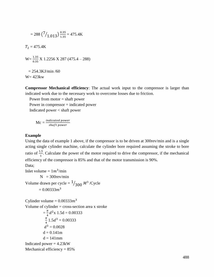
488
= 288 (7 1.013⁄ ) 0.35
1.35 = 475.4K
𝑇2 = 475.4K
W= 1.35
0.35 X 1.2256 X 287 (475.4 – 288)
= 254.3KJ/min /60
W= 423kw
Compressor Mechanical efficiency: The actual work input to the compressor is larger than
indicated work due to the necessary work to overcome losses due to friction.
Power from motor = shaft power
Power in compressor = indicated power
Indicated power < shaft power
Mc = 𝑖𝑛𝑑𝑖𝑐𝑎𝑡𝑒𝑑 𝑝𝑜𝑤𝑒𝑟
𝑠ℎ𝑎𝑓𝑡 𝑝𝑜𝑤𝑒𝑟
Example
Using the data of example 1 above, if the compressor is to be driven at 300rev/min and is a single
acting single cylinder machine, calculate the cylinder bore required assuming the stroke to bore
ratio of 1.5
1. Calculate the power of the motor required to drive the compressor, if the mechanical
efficiency of the compressor is 85% and that of the motor transmission is 90%.
Data;
Inlet volume = 1𝑚3/min
N = 300rev/min
Volume drawn per cycle = 1 300⁄ 𝑀3 /Cycle
= 0.00333𝑚3
Cylinder volume = 0.00333𝑚3
Volume of cylinder = cross-section area x stroke
= 𝜋
4𝑑2x 1.5d = 0.00333
𝜋
4 1.5𝑑3 = 0.00333
𝑑3 = 0.0028
d = 0.141m
d = 141mm
Indicated power = 4.23kW
Mechanical efficiency = 85%
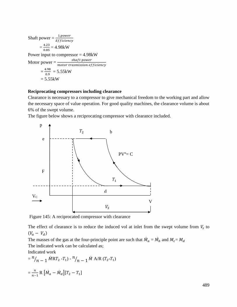
489
Shaft power = 1.𝑝𝑜𝑤𝑒𝑟
𝐸𝑓𝑓𝑖𝑐𝑖𝑒𝑛𝑐𝑦
= 4.23
0.85 = 4.98kW
Power input to compressor = 4.98kW
Motor power = 𝑠ℎ𝑎𝑓𝑡 𝑝𝑜𝑤𝑒𝑟
𝑚𝑜𝑡𝑜𝑟 𝑡𝑟𝑎𝑠𝑚𝑖𝑠𝑠𝑖𝑜𝑛 𝑒𝑓𝑓𝑖𝑐𝑖𝑒𝑛𝑐𝑦
= 4.98
0.9 = 5.55kW
= 5.55kW
Reciprocating compressors including clearance
Clearance is necessary to a compressor to give mechanical freedom to the working part and allow
the necessary space of value operation. For good quality machines, the clearance volume is about
6% of the swept volume.
The figure below shows a reciprocating compressor with clearance included.
F
The effect of clearance is to reduce the induced vol at inlet from the swept volume from 𝑉𝑠 to
(𝑉𝑎 − 𝑉𝑑)
The masses of the gas at the four-principle point are such that 𝑎 = 𝑀𝑏 and 𝑀𝑐= 𝑀𝑑
The indicated work can be calculated as;
Indicated work
= 𝑛 𝑛 − 1⁄ R𝑇2 -𝑇1) - 𝑛 𝑛 − 1⁄ A/R (𝑇2-𝑇1)
= 𝑛
𝑛−1 R [𝑀𝑎
− 𝑑][𝑇2 − 𝑇1]
𝑇1
d
𝑇2 b
𝑉𝑆
p
V
e
PVn= C
VC
Figure 145: A reciprocated compressor with clearance
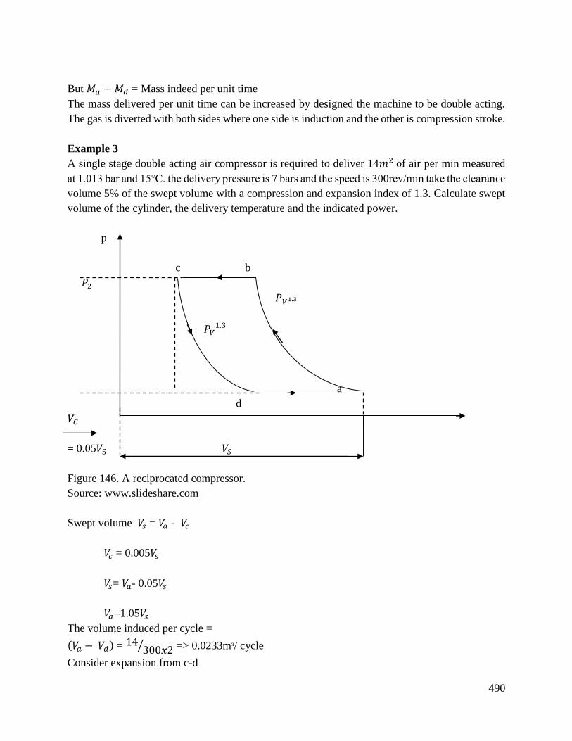
490
But 𝑀𝑎 − 𝑀𝑑 = Mass indeed per unit time
The mass delivered per unit time can be increased by designed the machine to be double acting.
The gas is diverted with both sides where one side is induction and the other is compression stroke.
Example 3
A single stage double acting air compressor is required to deliver 14𝑚2 of air per min measured
at 1.013 bar and 15. the delivery pressure is 7 bars and the speed is 300rev/min take the clearance
volume 5% of the swept volume with a compression and expansion index of 1.3. Calculate swept
volume of the cylinder, the delivery temperature and the indicated power.
p
c b
𝑃2
𝑃𝑉1.3
𝑃𝑉1.3
a
d
𝑉𝐶
= 0.05𝑉5 𝑉𝑆
Figure 146. A reciprocated compressor.
Source: www.slideshare.com
Swept volume 𝑉𝑠 = 𝑉𝑎 - 𝑉𝑐
𝑉𝑐 = 0.005𝑉𝑠
𝑉𝑠= 𝑉𝑎- 0.05𝑉𝑠
𝑉𝑎=1.05𝑉𝑠
The volume induced per cycle =
(𝑉𝑎 − 𝑉𝑑) = 14300𝑥2⁄ => 0.0233mᵌ/ cycle
Consider expansion from c-d
491
𝑃2 𝑉𝑐n = 𝑃1 𝑉𝑑
𝑛
𝑉𝑑 = 𝑉𝑐 ( 𝑃2
𝑃1)1
𝑛⁄
𝑉𝑑= 0.05𝑉𝑠 ( 7
1.013)1
1.3⁄
𝑉𝑑= 0.22𝑉𝑠
Therefore𝑉𝑎 −𝑉𝑑 = 1.05𝑉𝑠 − 0.0221𝑉𝑠
𝑉𝑎 − 𝑉𝑑 = 0.83𝑉𝑠
0.83𝑉𝑠 = 0.0233
𝑉𝑠 = 0.281𝑚ᵌ
𝑇2 = 𝑇1 ( 𝑃2
𝑃1)
𝑛−1
𝑛
= 288[7 1.013⁄ ] 0.31.3⁄ = 450𝐾
Induced mass 𝑀 =𝑃1𝑉𝑛
𝑅𝑇1
= 1.013 𝑥 105 𝑥14
288𝑋28.7 = 17.16kg/min
Indicated power = 𝑛 𝑛 − 1⁄ 𝑅(𝑇2 − 𝑇1)
= 1.3
0.3𝑥17.16x 287(450-288)
= 3457 kJ/min ÷ 60J/s
= 57.6kW
Isothermal Efficiency
Isothermal process for a perfect gas where W= MRT in ( 𝑃2
𝑃1) −positive work
Isothermal power =𝑅𝑇 𝐼𝑛 𝑃2
𝑃1
Isothermal efficiency= 𝐼𝑠𝑜𝑡ℎ𝑒𝑟𝑚𝑎𝑙 𝑝𝑜𝑤𝑒𝑟
𝑖𝑛𝑑𝑖𝑐𝑎𝑡𝑒𝑑 𝑤𝑜𝑟𝑘(𝑝𝑜𝑤𝑒𝑟 𝑜𝑢𝑡𝑝𝑢𝑡)
Free Air Delivery (FAD)
This is the volume flow rate measured at atmospheric and temperature conditions (1.013 bar,
15).
Volumetric Efficiency (𝒏𝒔)
This is defined as the volume of air delivered measured at the free air pressure and temperature
conditions to the swept volume of the cylinder.
Volumetric efficiency =𝑣𝑜𝑙𝑢𝑚𝑒 𝑜𝑓 𝑎𝑖𝑟 𝑑𝑒𝑙𝑖𝑣𝑒𝑟𝑒𝑑 𝑚𝑒𝑎𝑠𝑢𝑟𝑒𝑑 𝑎𝑡 𝑎𝑖𝑟 𝑝𝑟𝑒𝑠𝑠𝑢𝑟𝑒 𝑎𝑛𝑑 𝑡𝑒𝑚𝑝𝑟𝑒𝑡𝑢𝑟𝑒
𝑠𝑤𝑒𝑝𝑡 𝑣𝑜𝑙𝑢𝑚𝑒 𝑜𝑓 𝑐𝑦𝑙𝑖𝑛𝑑𝑒𝑟
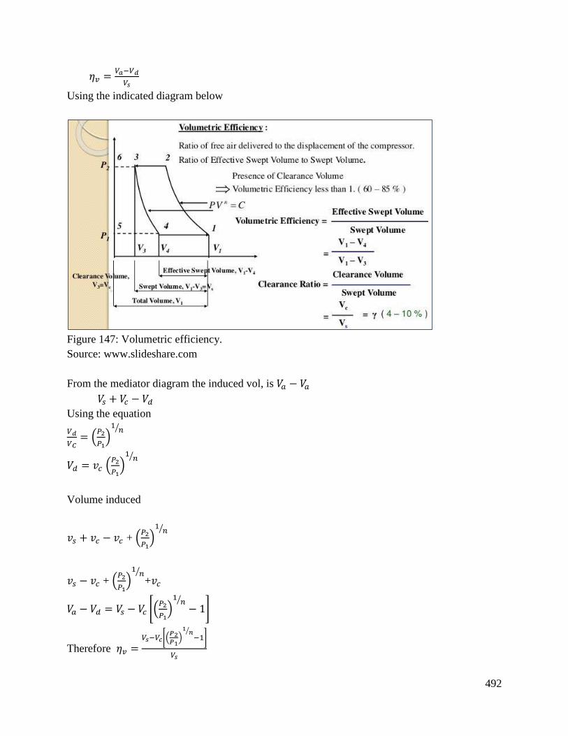
492
𝜂𝑣 =𝑉𝑎−𝑉𝑑
𝑉𝑠
Using the indicated diagram below
Figure 147: Volumetric efficiency.
Source: www.slideshare.com
From the mediator diagram the induced vol, is 𝑉𝑎 − 𝑉𝑎
𝑉𝑠 + 𝑉𝑐 − 𝑉𝑑
Using the equation
𝑉𝑑
𝑉𝐶= (
𝑃2
𝑃1)1
𝑛⁄
𝑉𝑑 = 𝑣𝑐 (𝑃2
𝑃1)1
𝑛⁄
Volume induced
𝑣𝑠 + 𝑣𝑐 − 𝑣𝑐 + (𝑃2
𝑃1)1
𝑛⁄
𝑣𝑠 − 𝑣𝑐 + (𝑃2
𝑃1)1
𝑛⁄
+𝑣𝑐
𝑉𝑎 − 𝑉𝑑 = 𝑉𝑠 − 𝑉𝑐 [(𝑃2
𝑃1)1
𝑛⁄
− 1]
Therefore 𝜂𝑣 = 𝑉𝑠−𝑉𝑐[(
𝑃2𝑃1
)1
𝑛⁄−1]
𝑉𝑠
493
𝜂𝑣 = 1 − 𝑉𝑐
𝑉𝑠 [(
𝑃2
𝑃1)1
𝑛⁄
− 1]
Example 1
A single stages, double acting air compressor has a free air delivery (FAD) of 14𝑚3/min measured
at 1.013 bar at 15. The pressure and temperature in the cylinder during the induction are 0.95
bar at 32. The delivery pressure is 7 bar and index of compression and expansion is n=1.3.
Calculate the indicated power required and volumetric efficiency given that the clearance volume
is 5% of the swept volume.
Solution
Data FAD = 14𝑚3/min at p=1.013 bar
T=15
Where P and T are the free air pressure of temperature conditions.
=𝑃𝑉𝑛
𝑅𝑇 =
1.013 𝑥 105𝑥14
287 𝑥 288
= 17.16kg/min
𝑇2 =𝑇1 (𝑃2
𝑃1)𝑛−1
𝑛⁄
𝑃1 =0.95 bar
𝑇1 = 32˚c + 273
= 305k
𝑃2 = 7 bars
𝑇2 = 305[7 0.95⁄ ]
0.3
1.3
𝑇2 = 483.57k = 483K
Indicated power
= 𝑛 𝑛 − 1⁄ 𝑀(𝑇2 − 𝑇1)
1.30.3⁄ 𝑥 17.16 𝑥 287[484 − 305)
= 3820.096kJ/min
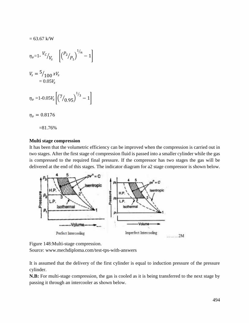
494
= 63.67 k/W
𝜂𝑣=1- 𝑉𝐶
𝑉𝑠⁄ [(
𝑃2𝑃1
⁄ )1
𝑛⁄
− 1]
𝑉𝑠 = 5 100⁄ 𝑥𝑉𝑠
= 0.05𝑉𝑠
𝜂𝑣 =1-0.05𝑉𝑠 [(7 0.95⁄ )1
3⁄
− 1]
𝜂𝑣 = 0.8176
=81.76%
Multi stage compression
It has been that the volumetric efficiency can be improved when the compression is carried out in
two stages. After the first stage of compression fluid is passed into a smaller cylinder while the gas
is compressed to the required final pressure. If the compressor has two stages the gas will be
delivered at the end of this stages. The indicator diagram for a2 stage compressor is shown below.
Figure 148:Multi-stage compression.
Source: www.mechdiploma.com/test-tps-with-answers
It is assumed that the delivery of the first cylinder is equal to induction pressure of the pressure
cylinder.
N.B: For multi-stage compression, the gas is cooled as it is being transferred to the next stage by
passing it through an intercooler as shown below.
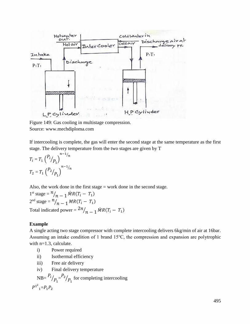
495
Figure 149: Gas cooling in multistage compression.
Source: www.mechdiploma.com
If intercooling is complete, the gas will enter the second stage at the same temperature as the first
stage. The delivery temperature from the two stages are given by T
𝑇𝑖 = 𝑇1 (𝑃𝑖
𝑃1⁄ )
𝑛−1𝑛⁄
𝑇2 = 𝑇1 (𝑃2
𝑃1⁄ )
𝑛−1𝑛⁄
Also, the work done in the first stage = work done in the second stage.
1st stage = 𝑛 𝑛 − 1⁄ 𝑅(𝑇𝑖 − 𝑇1)
2nd stage = 𝑛 𝑛 − 1⁄ 𝑀𝑅(𝑇𝑖 − 𝑇1)
Total indicated power = 2𝑛𝑛 − 1⁄ 𝑅(𝑇𝑖 − 𝑇1)
Example
A single acting two stage compressor with complete intercooling delivers 6kg/min of air at 16bar.
Assuming an intake condition of 1 brand 15, the compression and expansion are polytrophic
with n=1.3, calculate.
i) Power required
ii) Isothermal efficiency
iii) Free air delivery
iv) Final delivery temperature
NB= 𝑃𝑖
𝑃1⁄ =
𝑃2𝑃1
⁄ for completing intercooling
𝑃12
1=𝑃1𝑃2
P1T1
P2T2
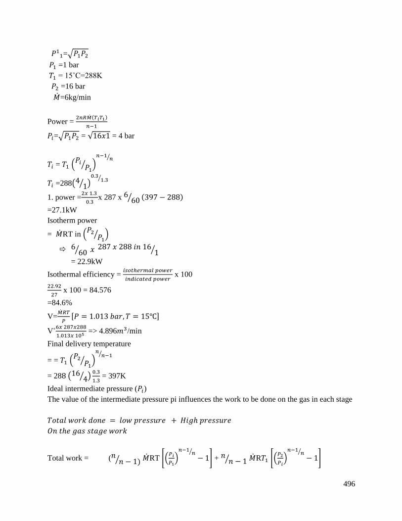
496
𝑃11=√𝑃1𝑃2
𝑃1 =1 bar
𝑇1 = 15˚C=288K
𝑃2 =16 bar
=6kg/min
Power = 2𝑛𝑅(𝑇𝑖𝑇1)
𝑛−1
𝑃𝑖=√𝑃1𝑃2 = √16𝑥1 = 4 bar
𝑇𝑖 = 𝑇1 (𝑃𝑖
𝑃1⁄ )
𝑛−1𝑛⁄
𝑇𝑖 =288(4 1⁄ )0.3
1.3⁄
1. power =2𝑥 1.3
0.3x 287 x 6 60⁄ (397 − 288)
=27.1kW
Isotherm power
= RT in (𝑃2
𝑃1⁄ )
660⁄ 𝑥 287 𝑥 288 𝑖𝑛 16
1⁄
= 22.9kW
Isothermal efficiency = 𝑖𝑠𝑜𝑡ℎ𝑒𝑟𝑚𝑎𝑙 𝑝𝑜𝑤𝑒𝑟
𝑖𝑛𝑑𝑖𝑐𝑎𝑡𝑒𝑑 𝑝𝑜𝑤𝑒𝑟 x 100
22.92
27 x 100 = 84.576
=84.6%
V=𝑅𝑇
𝑃[𝑃 = 1.013 𝑏𝑎𝑟, 𝑇 = 15]
V˚6𝑥 287𝑥288
1.013𝑥 105 => 4.896𝑚3/min
Final delivery temperature
= = 𝑇1 (𝑃2
𝑃1⁄ )
𝑛𝑛−1⁄
= 288 (164⁄ )
0.3
1.3 = 397K
Ideal intermediate pressure (𝑃𝑖)
The value of the intermediate pressure pi influences the work to be done on the gas in each stage
𝑇𝑜𝑡𝑎𝑙 𝑤𝑜𝑟𝑘 𝑑𝑜𝑛𝑒 = 𝑙𝑜𝑤 𝑝𝑟𝑒𝑠𝑠𝑢𝑟𝑒 + 𝐻𝑖𝑔ℎ 𝑝𝑟𝑒𝑠𝑠𝑢𝑟𝑒
𝑂𝑛 𝑡ℎ𝑒 𝑔𝑎𝑠 𝑠𝑡𝑎𝑔𝑒 𝑤𝑜𝑟𝑘
Total work = (𝑛 𝑛 − 1)⁄ RT [(𝑃𝑖
𝑃1)𝑛−1
𝑛⁄
− 1] + 𝑛 𝑛 − 1⁄ R𝑇1 [(𝑃2
𝑃𝑖)𝑛−1
𝑛⁄
− 1]

497
For complete intercooling temperature at start of each stage is t
Total work =𝑛𝑛 − 1⁄ RT [(
𝑃𝑖
𝑃1)𝑛−1
𝑛⁄
− 1]+ [(𝑃2
𝑃𝑖)𝑛−1
𝑛⁄
− 𝑛]
Let 𝑛 − 1𝑛⁄ =y
Total work = (𝑛 𝑛 − 1⁄ )R𝑇1 [(𝑃1
𝑃1)
𝑦
− 1] +[(𝑃2
𝑃1)
𝑦
− 1]
𝑇1 𝑃1 and 𝑃2 are fixed and hence the optimum value of R which make work to be maximum is got
by differentiation with respect to 𝑃𝑖
i.e. 𝑑𝑤
𝑑𝑝𝑖 = 0
Total work 𝑛 𝑛 − 1⁄ R𝑇1 +[ (𝑃𝑖
𝑃1)
𝑦
+ (𝑃2
𝑃𝑖)
𝑦
− 2]
𝑑
𝑑𝑃𝑖 [ (
𝑃𝑖
𝑃1)
𝑦
+ (𝑃2
𝑃𝑖) − 2]
= 𝑑
𝑑𝑃𝑖 [𝑃1𝑦
1 − 𝑃−𝑦1 + 𝑃−𝑦
1𝑃−𝑦
𝑖 − 2]
= [𝑦𝑃𝑖𝑦−1𝑃1
−𝑦 + 𝑃2𝑦 (−𝑦)𝑃𝑖
−𝑦−1]
=𝑦𝑃1𝑦
1
𝑃1 𝑃1
−𝑦 − 𝑦𝑃2𝑦𝑃𝑖
−𝑦−1 𝑃𝑖−𝑦
𝑃𝑖
𝑃𝑖
−𝑦
𝑃𝑖 . 𝑃1
−𝑦 = 𝑦𝑃2𝑦.
𝑃𝑖−𝑦
𝑃𝑖
𝑃11𝑦. 𝑃1
1
𝑃1𝑦1.𝑃𝑖
−𝑦 = 𝑃2
𝑦
𝑃1−𝑦⁄
𝑃1𝑦1. 𝑃
1𝑦1= 𝑃2. 𝑦 𝑃1
𝑦
𝑃2𝑦1= ( 𝑃1 𝑃2)
𝑦
𝑃112𝑌
(𝑛 − 1𝑛⁄ )=( 𝑃1 𝑃2)
𝑦
𝑃112
(𝑛 − 1𝑛⁄ ) = ( 𝑃1 𝑃2)
𝑛−1
𝑛
𝑃11=√ 𝑃1 𝑃2
For Z stages pressure ratio for each stage
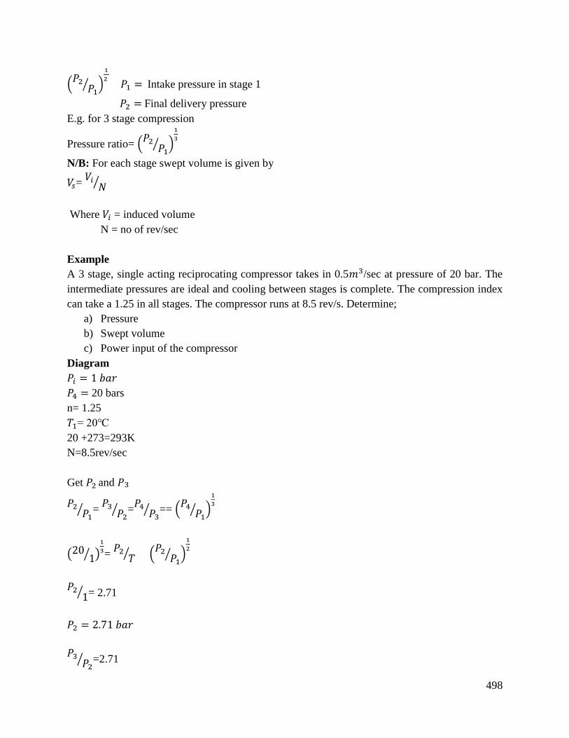
498
(𝑃2
𝑃1⁄ )
1
2 𝑃1 = Intake pressure in stage 1
𝑃2 = Final delivery pressure
E.g. for 3 stage compression
Pressure ratio= (𝑃2
𝑃1⁄ )
1
3
N/B: For each stage swept volume is given by
𝑉𝑠= 𝑉𝑖
𝑁⁄
Where 𝑉𝑖 = induced volume
N = no of rev/sec
Example
A 3 stage, single acting reciprocating compressor takes in 0.5𝑚3/sec at pressure of 20 bar. The
intermediate pressures are ideal and cooling between stages is complete. The compression index
can take a 1.25 in all stages. The compressor runs at 8.5 rev/s. Determine;
a) Pressure
b) Swept volume
c) Power input of the compressor
Diagram
𝑃𝑖 = 1 𝑏𝑎𝑟
𝑃4 = 20 bars
n= 1.25
𝑇1= 20
20 +273=293K
N=8.5rev/sec
Get 𝑃2 and 𝑃3
𝑃2𝑃1
⁄ = 𝑃3
𝑃2⁄ =
𝑃4𝑃3
⁄ == (𝑃4
𝑃1⁄ )
1
3
(201⁄ )
1
3= 𝑃2
𝑇⁄ (𝑃2
𝑃1⁄ )
1
2
𝑃21⁄ = 2.71
𝑃2 = 2.71 𝑏𝑎𝑟
𝑃3𝑃2
⁄ =2.71
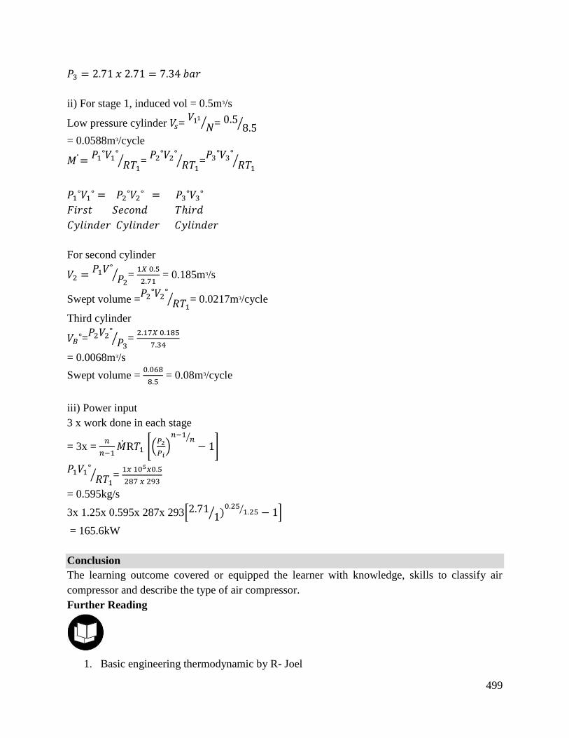
499
𝑃3 = 2.71 𝑥 2.71 = 7.34 𝑏𝑎𝑟
ii) For stage 1, induced vol = 0.5mᵌ/s
Low pressure cylinder 𝑉𝑠= 𝑉11
𝑁⁄ = 0.58.5⁄
= 0.0588mᵌ/cycle
𝑀 =𝑃1˚𝑉1˚
𝑅𝑇1⁄ =
𝑃2˚𝑉2˚𝑅𝑇1
⁄ =𝑃3˚𝑉3˚
𝑅𝑇1⁄
𝑃1˚𝑉1˚ = 𝑃2˚𝑉2˚ = 𝑃3˚𝑉3˚
𝐹𝑖𝑟𝑠𝑡 𝑆𝑒𝑐𝑜𝑛𝑑 𝑇ℎ𝑖𝑟𝑑
𝐶𝑦𝑙𝑖𝑛𝑑𝑒𝑟 𝐶𝑦𝑙𝑖𝑛𝑑𝑒𝑟 𝐶𝑦𝑙𝑖𝑛𝑑𝑒𝑟
For second cylinder
𝑉2 =𝑃1𝑉˚
𝑃2⁄ =
1𝑋 0.5
2.71 = 0.185mᵌ/s
Swept volume =𝑃2˚𝑉2˚
𝑅𝑇1⁄ = 0.0217mᵌ/cycle
Third cylinder
𝑉𝐵˚=𝑃2𝑉2˚
𝑃3⁄ =
2.17𝑋 0.185
7.34
= 0.0068mᵌ/s
Swept volume = 0.068
8.5 = 0.08mᵌ/cycle
iii) Power input
3 x work done in each stage
= 3x = 𝑛
𝑛−1R𝑇1 [(
𝑃2
𝑃𝑖)𝑛−1
𝑛⁄
− 1]
𝑃1𝑉1˚𝑅𝑇1
⁄ = 1𝑥 105𝑥0.5
287 𝑥 293
= 0.595kg/s
3x 1.25x 0.595x 287x 293[2.711⁄ )
0.251.25⁄ − 1]
= 165.6kW
Conclusion
The learning outcome covered or equipped the learner with knowledge, skills to classify air
compressor and describe the type of air compressor.
Further Reading
1. Basic engineering thermodynamic by R- Joel
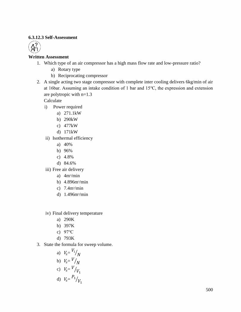
500
6.3.12.3 Self-Assessment
Written Assessment
1. Which type of an air compressor has a high mass flow rate and low-pressure ratio?
a) Rotary type
b) Reciprocating compressor
2. A single acting two stage compressor with complete inter cooling delivers 6kg/min of air
at 16bar. Assuming an intake condition of 1 bar and 15, the expression and extension
are polytropic with n=1.3
Calculate
i) Power required
a) 271.1kW
b) 290kW
c) 477kW
d) 171kW
ii) Isothermal efficiency
a) 40%
b) 96%
c) 4.8%
d) 84.6%
iii) Free air delivery
a) 4mᵌ/min
b) 4.896mᵌ/min
c) 7.4mᵌ/min
d) 1.496mᵌ/min
iv) Final delivery temperature
a) 290K
b) 397K
c) 97
d) 793K
3. State the formula for sweep volume.
a) 𝑉𝑠= 𝑉𝑖
𝑁⁄
b) 𝑉𝑠= 𝑉 𝑁⁄
c) 𝑉𝑠= 𝑉 𝑉1⁄
d) 𝑉𝑠= 𝑃1
𝑉1⁄
501
4. The volume of air delivered and measure of the air pressure and temperature condition to
the sweep of the cylinder is a determination of?
a) Isothermal efficiency
b) Volumetric efficiency
c) None of the above
5. What do you understand by the term volumetric efficiency.
6. State two types of compressor.
7. Discuss reciprocating compressor by use of a basic indication diagram.
8. State any difference between multistage and final stage compressor.
9. Using a sketch show that in a multi-stage compressor gas is cooled as it is being transferred
to the next stage by passing it through on intercooler.
Oral Assessment
1. Describe what is meant by a reciprocating compressor.
2. Discuss function of compressor and type of compressor.
Practical Assessment
1. By use of three different mini compressors show how efficiency is lost from first to the
last.
6.3.12.4 Tools, Equipment, Supplies and Materials
Scientific Calculators
Relevant reference materials
Stationeries
Relevant practical materials
Dice
Computers with internet connection
6.3.12.5 References
Chew, J. W., & Hills, N. J. (2007). Computational fluid dynamics for turbomachinery internal air
systems. Philosophical transactions of the royal society A: Mathematical, physical and
engineering sciences, 365(1859), 2587-2611.
Howell, A. R. (1945). Fluid dynamics of axial compressors. Proceedings of the Institution of
Mechanical Engineers, 153(1), 441-452.
Chung, T. J. (2010). Computational fluid dynamics. Cambridge university press.
502
6.3.13 Learning Outcome No 12: Understand gas turbine
6.3.13.1 Learning Activities
Learning Outcome No12 : Understand gas turbine
Learning Activities Special Instructions
12.1 Theoretical cycle for gas turbines is explained
12.2 Open cycle gas turbine is described
12.3 Closed cycle gas turbine is described
12.4 Gas turbine equations are derived and applied
Illustrate using oral
questions, short notes
and a practical example
6.3.13.2 Information Sheet No6/LO12: Understand gas turbine
Introduction
This learning outcome covers the theoretical cycle for gas turbine, open and close cycle gas turbine
and gas turbine equations derivations and applications.
Definition of key terms
Isentropic efficiency: This is the ratio of isentropic work to the actual work input required in the
compressor. It can also be defined as the ratio of the actual work input to the isentropic work output
between the same pressures
Turbine: This is a rotary mechanical device that extracts energy from a fluid and converts it into
a useful work
Turbulence: This is a fluid motion characterized by chaotic or irregular changes in pressure and
flow velocity
Content/procedures/methods/illustrations
12.1 Theoretical cycle for gas turbines is explained
The main use of gas turbine at present day is at the aircraft field although gas units for electric
power generation are being used increasingly. The gas turbine is also used in conjunction with oil
engine and as a part of total energy schemes in combination with steam plant. Practical gas turbine
cycle is the most basic gas turbine unit and is one operating on the open cycle which a rotary
compressor and a turbine are mounted on a common shaft as shown in the figure below;
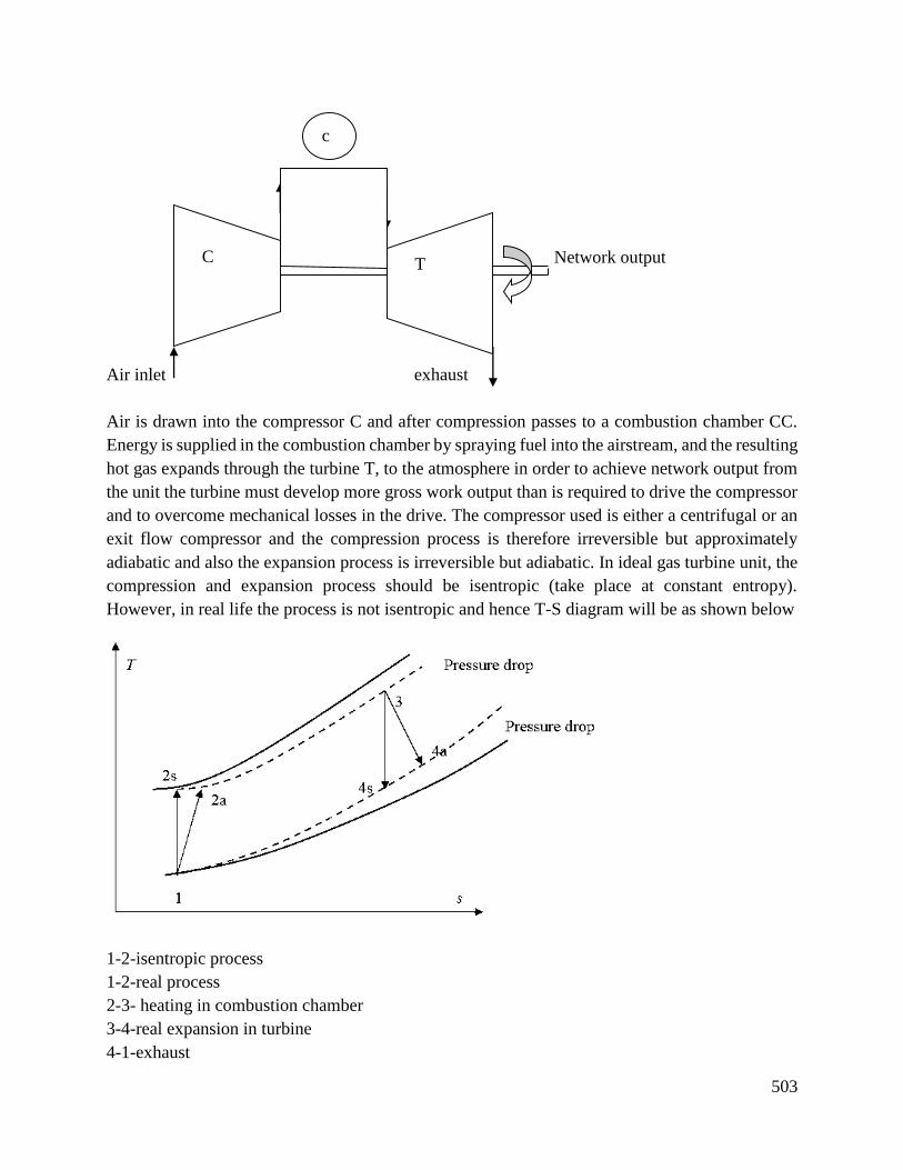
503
Network output
Air inlet exhaust
Air is drawn into the compressor C and after compression passes to a combustion chamber CC.
Energy is supplied in the combustion chamber by spraying fuel into the airstream, and the resulting
hot gas expands through the turbine T, to the atmosphere in order to achieve network output from
the unit the turbine must develop more gross work output than is required to drive the compressor
and to overcome mechanical losses in the drive. The compressor used is either a centrifugal or an
exit flow compressor and the compression process is therefore irreversible but approximately
adiabatic and also the expansion process is irreversible but adiabatic. In ideal gas turbine unit, the
compression and expansion process should be isentropic (take place at constant entropy).
However, in real life the process is not isentropic and hence T-S diagram will be as shown below
1-2-isentropic process
1-2-real process
2-3- heating in combustion chamber
3-4-real expansion in turbine
4-1-exhaust
c
c
C T
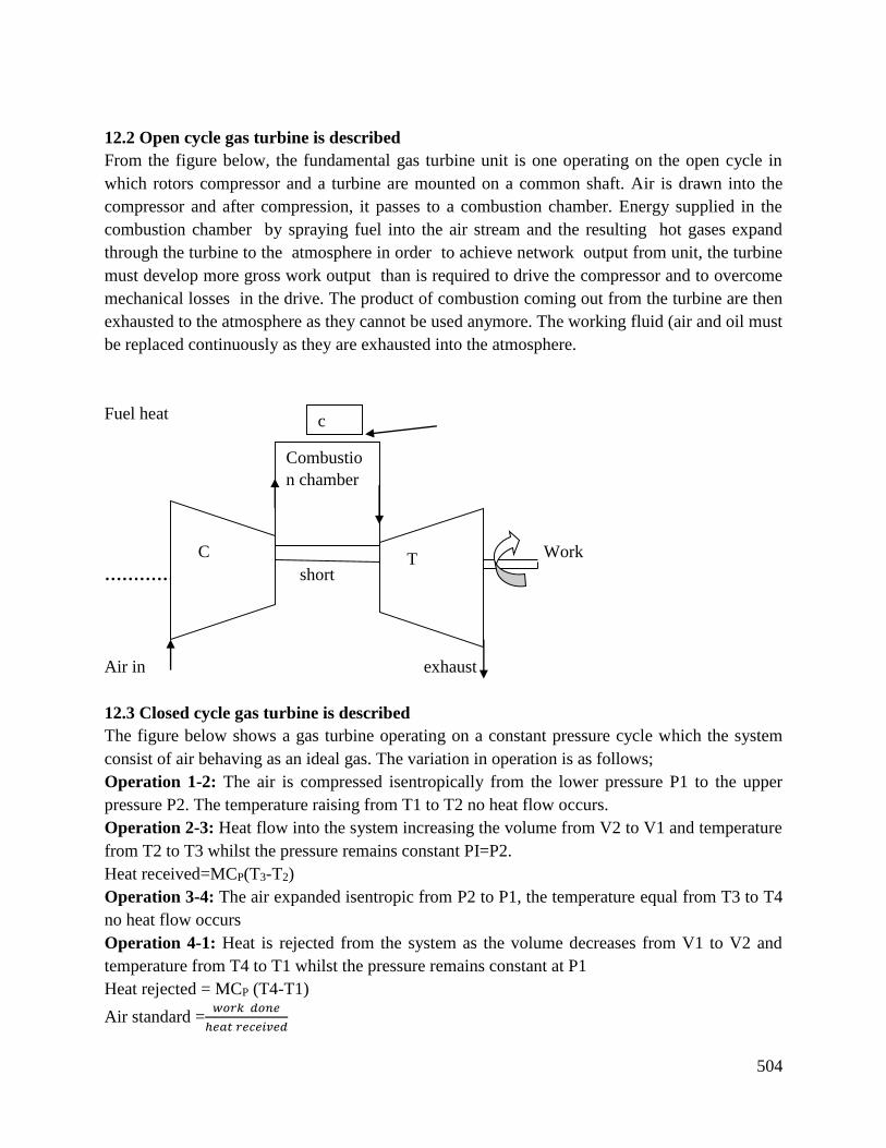
504
12.2 Open cycle gas turbine is described
From the figure below, the fundamental gas turbine unit is one operating on the open cycle in
which rotors compressor and a turbine are mounted on a common shaft. Air is drawn into the
compressor and after compression, it passes to a combustion chamber. Energy supplied in the
combustion chamber by spraying fuel into the air stream and the resulting hot gases expand
through the turbine to the atmosphere in order to achieve network output from unit, the turbine
must develop more gross work output than is required to drive the compressor and to overcome
mechanical losses in the drive. The product of combustion coming out from the turbine are then
exhausted to the atmosphere as they cannot be used anymore. The working fluid (air and oil must
be replaced continuously as they are exhausted into the atmosphere.
Fuel heat
Work
…………….short short
Air in exhaust
12.3 Closed cycle gas turbine is described
The figure below shows a gas turbine operating on a constant pressure cycle which the system
consist of air behaving as an ideal gas. The variation in operation is as follows;
Operation 1-2: The air is compressed isentropically from the lower pressure P1 to the upper
pressure P2. The temperature raising from T1 to T2 no heat flow occurs.
Operation 2-3: Heat flow into the system increasing the volume from V2 to V1 and temperature
from T2 to T3 whilst the pressure remains constant PI=P2.
Heat received=MCP(T3-T2)
Operation 3-4: The air expanded isentropic from P2 to P1, the temperature equal from T3 to T4
no heat flow occurs
Operation 4-1: Heat is rejected from the system as the volume decreases from V1 to V2 and
temperature from T4 to T1 whilst the pressure remains constant at P1
Heat rejected = MCP (T4-T1)
Air standard =𝑤𝑜𝑟𝑘 𝑑𝑜𝑛𝑒
ℎ𝑒𝑎𝑡 𝑟𝑒𝑐𝑒𝑖𝑣𝑒𝑑
C
Combustio
n chamber
T
c
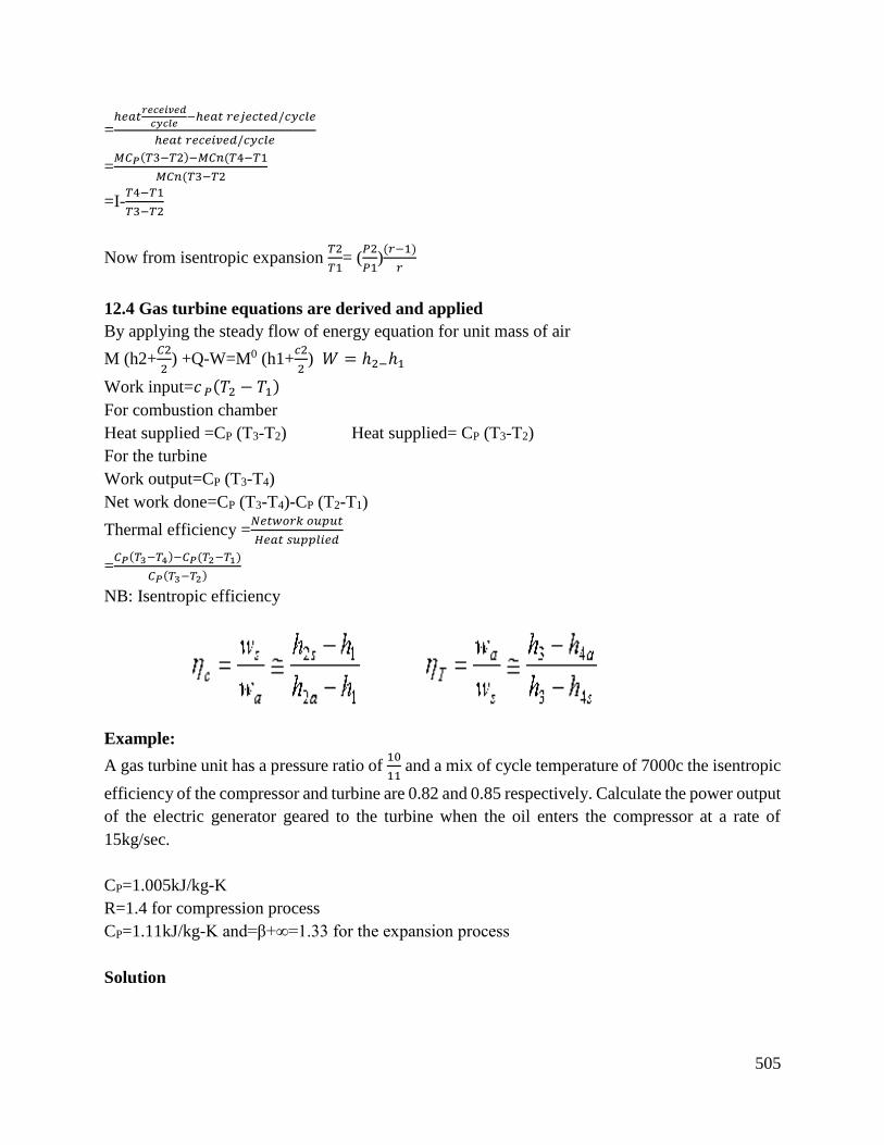
505
=ℎ𝑒𝑎𝑡
𝑟𝑒𝑐𝑒𝑖𝑣𝑒𝑑
𝑐𝑦𝑐𝑙𝑒−ℎ𝑒𝑎𝑡 𝑟𝑒𝑗𝑒𝑐𝑡𝑒𝑑/𝑐𝑦𝑐𝑙𝑒
ℎ𝑒𝑎𝑡 𝑟𝑒𝑐𝑒𝑖𝑣𝑒𝑑/𝑐𝑦𝑐𝑙𝑒
=𝑀𝐶𝑃(𝑇3−𝑇2)−𝑀𝐶𝑛(𝑇4−𝑇1
𝑀𝐶𝑛(𝑇3−𝑇2
=I-𝑇4−𝑇1
𝑇3−𝑇2
Now from isentropic expansion 𝑇2
𝑇1= (
𝑃2
𝑃1)(𝑟−1)
𝑟
12.4 Gas turbine equations are derived and applied
By applying the steady flow of energy equation for unit mass of air
M (h2+𝐶2
2) +Q-W=M0 (h1+
𝑐2
2) 𝑊 = ℎ2−ℎ1
Work input=𝑐 𝑃(𝑇2 − 𝑇1)
For combustion chamber
Heat supplied =CP (T3-T2) Heat supplied= CP (T3-T2)
For the turbine
Work output=CP (T3-T4)
Net work done=CP (T3-T4)-CP (T2-T1)
Thermal efficiency =𝑁𝑒𝑡𝑤𝑜𝑟𝑘 𝑜𝑢𝑝𝑢𝑡
𝐻𝑒𝑎𝑡 𝑠𝑢𝑝𝑝𝑙𝑖𝑒𝑑
=𝐶𝑃(𝑇3−𝑇4)−𝐶𝑃(𝑇2−𝑇1)
𝐶𝑃(𝑇3−𝑇2)
NB: Isentropic efficiency
Example:
A gas turbine unit has a pressure ratio of 10
11 and a mix of cycle temperature of 7000c the isentropic
efficiency of the compressor and turbine are 0.82 and 0.85 respectively. Calculate the power output
of the electric generator geared to the turbine when the oil enters the compressor at a rate of
15kg/sec.
CP=1.005kJ/kg-K
R=1.4 for compression process
CP=1.11kJ/kg-K and=β+∞=1.33 for the expansion process
Solution
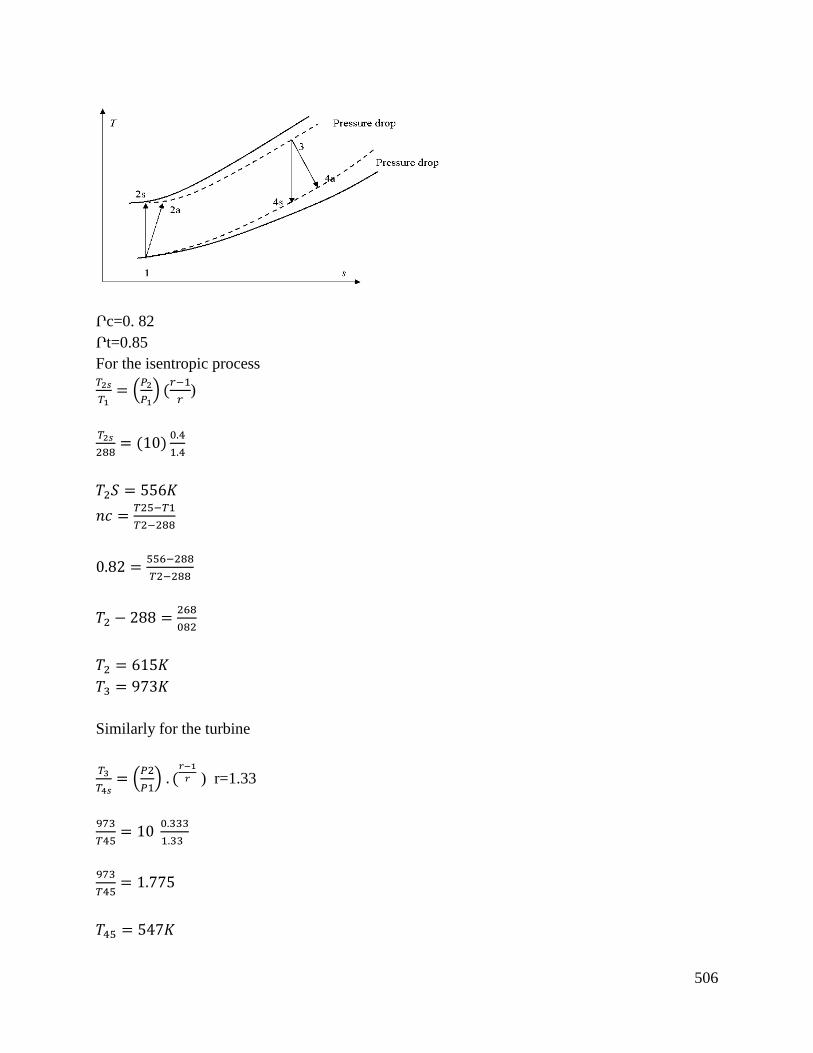
506
Րc=0. 82
Րt=0.85
For the isentropic process 𝑇2𝑠
𝑇1= (
𝑃2
𝑃1) (
𝑟−1
𝑟)
𝑇2𝑠
288= (10)
0.4
1.4
𝑇2𝑆 = 556𝐾
𝑛𝑐 =𝑇25−𝑇1
𝑇2−288
0.82 =556−288
𝑇2−288
𝑇2 − 288 =268
082
𝑇2 = 615𝐾
𝑇3 = 973𝐾
Similarly for the turbine
𝑇3
𝑇4𝑠= (
𝑃2
𝑃1) . (
𝑟−1
𝑟 ) r=1.33
973
𝑇45= 10
0.333
1.33
973
𝑇45= 1.775
𝑇45 = 547𝐾

507
R𝑡=𝑇3−𝑇4
𝑇3−𝑇4𝑠
0.85 =973−𝑇4
973−547
𝑇4 = 0.85 × (973 − 547) − 973
=611K
Hence compressor work input
𝐶𝑃(𝑇2 − 𝑇1)
=1.005(615-288)
=328.6 kJ/kg
Turbine work output= CP(T3-T4)
=1.11(973-611)
=401.8kJ/kg
Network output= (401.8-328.6)
=73.2 kJ/kg
But mass flow rule is 13kg/s
Power output=mass flow× 𝑛𝑒𝑡𝑤𝑜𝑟𝑘 𝑜𝑢𝑡𝑝𝑢𝑡
13 × 73.2 = 1098𝑘𝑊
Work ratio= 𝑛𝑒𝑡𝑤𝑜𝑟𝑘 𝑜𝑢𝑡𝑝𝑢𝑡
𝑡𝑢𝑟𝑏𝑖𝑛𝑒 𝑤𝑜𝑟𝑘
73.2
401.8= 𝑜. 182
Uses of a power turbine
In this case two turbines are used; one drives the compressor while the other one provides the
power output. The turbine that drives the compressor is called the high pressure turbine (HP) while
the turbine that provides the power output is called the low pressure turbine (LP). This improves
the efficiency of the gas turbine unit.
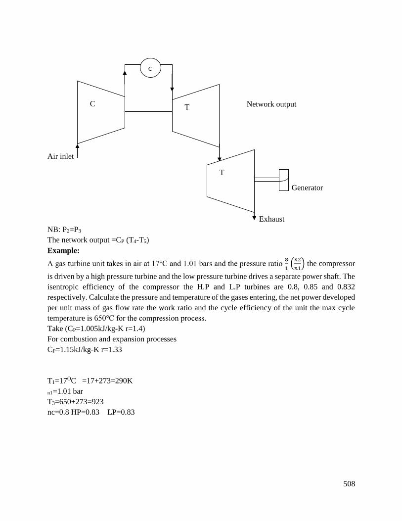
508
Network output
Air inlet
Generator
Exhaust
NB: P2=P3
The network output =CP (T4-T5)
Example:
A gas turbine unit takes in air at 17 and 1.01 bars and the pressure ratio 8
1 (
𝑛2
𝑛1) the compressor
is driven by a high pressure turbine and the low pressure turbine drives a separate power shaft. The
isentropic efficiency of the compressor the H.P and L.P turbines are 0.8, 0.85 and 0.832
respectively. Calculate the pressure and temperature of the gases entering, the net power developed
per unit mass of gas flow rate the work ratio and the cycle efficiency of the unit the max cycle
temperature is 650 for the compression process.
Take (CP=1.005kJ/kg-K r=1.4)
For combustion and expansion processes
CP=1.15kJ/kg-K r=1.33
T1=17OC =17+273=290K
n1=1.01 bar
T3=650+273=923
nc=0.8 HP=0.83 LP=0.83
C T
c
c
T
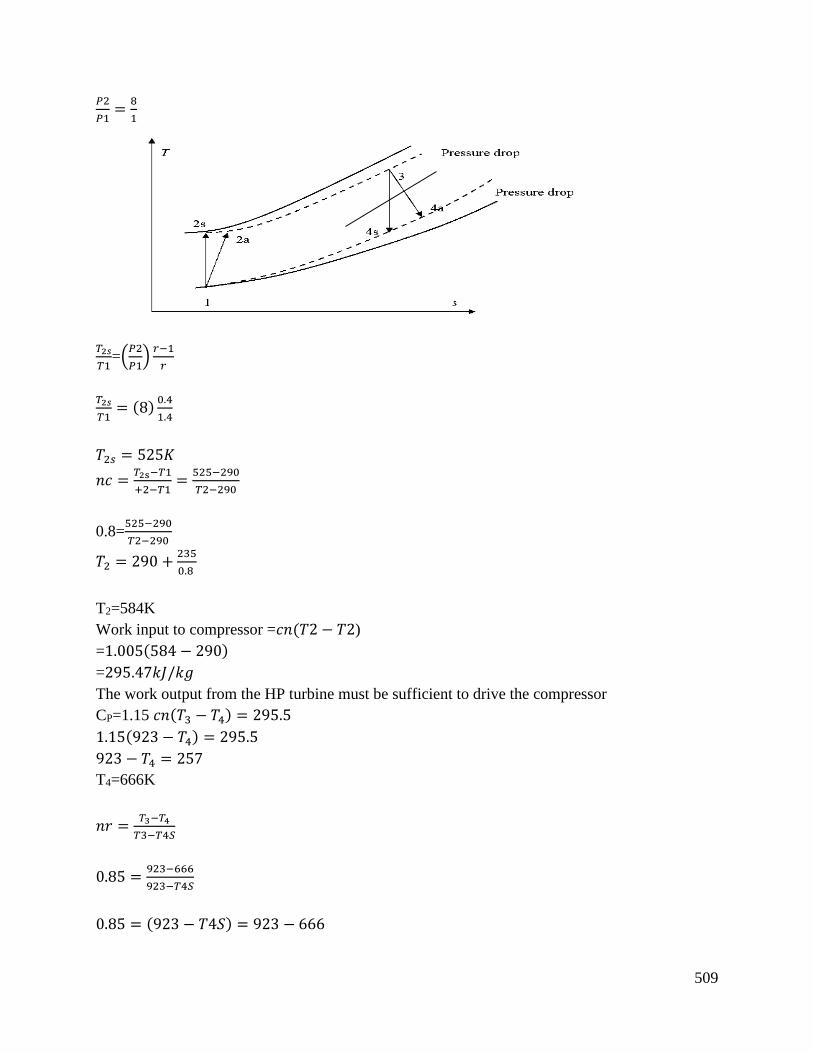
509
𝑃2
𝑃1=
8
1
𝑇2𝑠
𝑇1=(
𝑃2
𝑃1)
𝑟−1
𝑟
𝑇2𝑠
𝑇1= (8)
0.4
1.4
𝑇2𝑠 = 525𝐾
𝑛𝑐 =𝑇2s−𝑇1
+2−𝑇1=
525−290
𝑇2−290
0.8=525−290
𝑇2−290
𝑇2 = 290 +235
0.8
T2=584K
Work input to compressor =𝑐𝑛(𝑇2 − 𝑇2)
=1.005(584 − 290)
=295.47𝑘𝐽/𝑘𝑔
The work output from the HP turbine must be sufficient to drive the compressor
CP=1.15 𝑐𝑛(𝑇3 − 𝑇4) = 295.5
1.15(923 − 𝑇4) = 295.5
923 − 𝑇4 = 257
T4=666K
𝑛𝑟 =𝑇3−𝑇4
𝑇3−𝑇4𝑆
0.85 =923−666
923−𝑇4𝑆
0.85 = (923 − 𝑇4𝑆) = 923 − 666

510
T4S=621K
Also P2=P3
𝑃2 = 8𝑃1
8 × 1. 𝑂1 = 8.08 𝑏𝑎𝑟 𝑇3
𝑇4𝑠= (
𝑝3
𝑝4)
𝑟−1
𝑟
923
612= (
808
𝑝4)
0.333
1.333
(923
621)
1.333
0.333= (
8.08
𝑝4)
𝑝4 = 1.65 𝑏𝑎𝑟
Also overall pressure ratio 𝑝4
𝑝5=
𝑝4
𝑝3×
𝑝2
𝑝1
𝑝4
𝑝5=
1
4.9× 8
𝑇4
𝑇5=1.63
𝑇4
𝑇5𝑠= (
𝑝4
𝑝5)
𝑟−1
𝑟
660
𝑇5𝑠= (1.63)
0.333
1.333
T5S=589K
𝑛𝑟 =𝑇4𝑆−𝑇5
𝑇4−𝑇5𝑆
0.85 =923−666
923−𝑇4𝑆
0.85(923 − 𝑇4𝑠) = 923 − 666
T4S=621K
Also overall pressure ratio 𝑇4
𝑇5=
𝑇4
𝑇3×
𝑃2
𝑃1
𝑃4
𝑃5=
1
4.9× 8
𝑃4
𝑃5= 1.63

511
𝑇4
𝑇5s= (
𝑃4
𝑃5)
𝑟−1
𝑟
660
𝑇5𝑠= (1.63)
0.333
1.333
T5S=589K
𝑛𝑇 =𝑇4𝑠−𝑇5
𝑇4−𝑇5𝑠
0.83 =666−𝑇5
666−589
T5=602K
Power output is from the LP turbine
𝑐𝑛(𝑇4 − 𝑇5)
1.15(666-602)
73.6kJ/kg
For mass flow rate of kilograms
Power=73.6kW
Work ratio=73.6
73.67295
=0.7
Heat supplied =1.15(923 − 584)
=390kJ/kg 73.6
390× 100 = 19%
T2=549K
T4=644K
T5=575K 𝑇4
𝑇5= 2.12
𝑇3
𝑇4= 2.24
Power developed=98.5kW
Work ratio=0.227
Efficiency=23.79%
Modification to the basic cycle
Use of heat exchanger
Since the exhaust gases leaving the turbine are at high temperature probably 300 the energy can
be recovered by passing the gases from the turbine through a heat exchanger where the heat
transferred from the gases is used to heat air leaving the compressor.
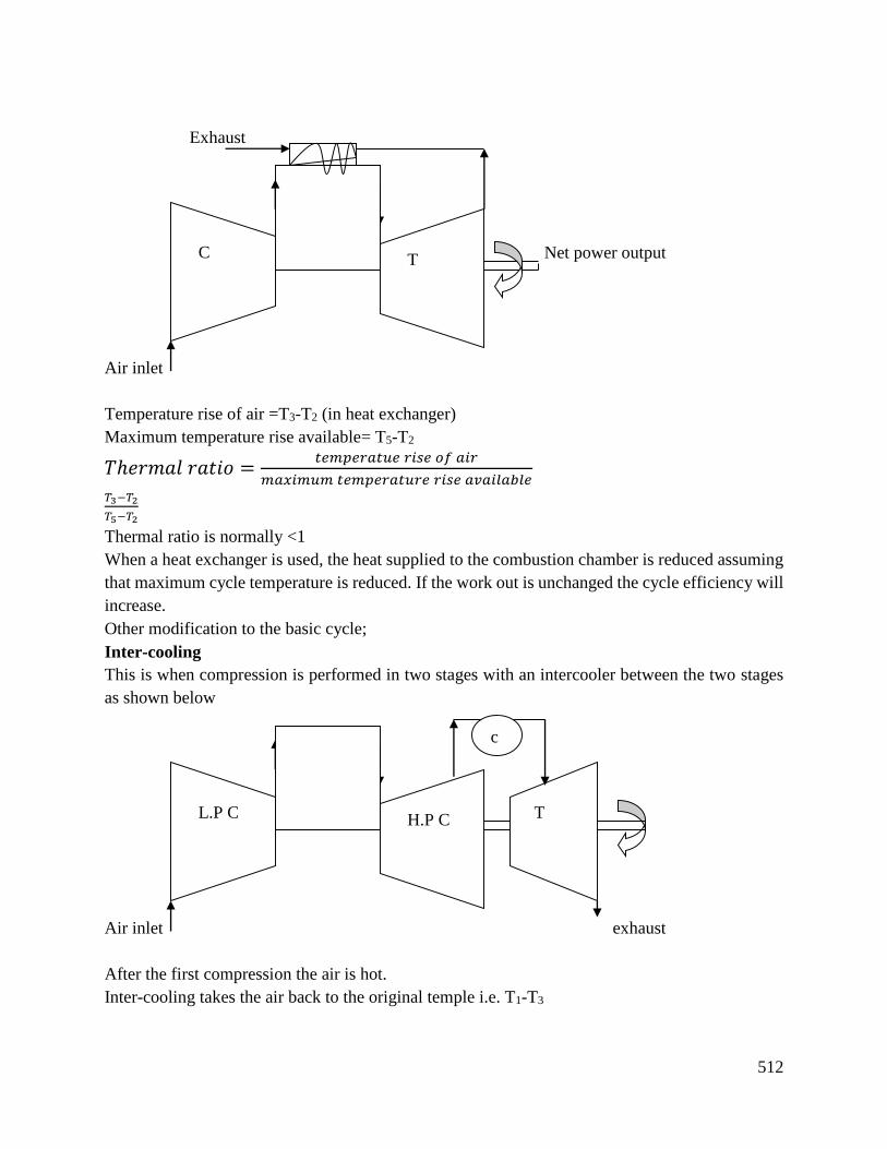
512
Exhaust
Net power output
Air inlet
Temperature rise of air =T3-T2 (in heat exchanger)
Maximum temperature rise available= T5-T2
𝑇ℎ𝑒𝑟𝑚𝑎𝑙 𝑟𝑎𝑡𝑖𝑜 =𝑡𝑒𝑚𝑝𝑒𝑟𝑎𝑡𝑢𝑒 𝑟𝑖𝑠𝑒 𝑜𝑓 𝑎𝑖𝑟
𝑚𝑎𝑥𝑖𝑚𝑢𝑚 𝑡𝑒𝑚𝑝𝑒𝑟𝑎𝑡𝑢𝑟𝑒 𝑟𝑖𝑠𝑒 𝑎𝑣𝑎𝑖𝑙𝑎𝑏𝑙𝑒
𝑇3−𝑇2
𝑇5−𝑇2
Thermal ratio is normally <1
When a heat exchanger is used, the heat supplied to the combustion chamber is reduced assuming
that maximum cycle temperature is reduced. If the work out is unchanged the cycle efficiency will
increase.
Other modification to the basic cycle;
Inter-cooling
This is when compression is performed in two stages with an intercooler between the two stages
as shown below
Air inlet exhaust
After the first compression the air is hot.
Inter-cooling takes the air back to the original temple i.e. T1-T3
C T
L.P C H.P C T
c
c
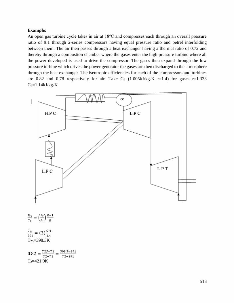
513
Example:
An open gas turbine cycle takes in air at 18 and compresses each through an overall pressure
ratio of 9:1 through 2-series compressors having equal pressure ratio and petrel interfolding
between them. The air then passes through a heat exchanger having a thermal ratio of 0.72 and
thereby through a combustion chamber where the gases enter the high pressure turbine where all
the power developed is used to drive the compressor. The gases then expand through the low
pressure turbine which drives the power generator the gases are then discharged to the atmosphere
through the heat exchanger .The isentropic efficiencies for each of the compressors and turbines
are 0.82 and 0.78 respectively for air. Take CP (1.005kJ/kg-K r=1.4) for gases r=1.333
CP=1.14kJ/kg-K
𝑇2𝑠
𝑇1= (
𝑃2
𝑃1)
𝑅−1
𝑅
𝑇2𝑠
291= (3)
𝑂.4
1.4
T2S=398.3K
0.82 =𝑇2𝑆−𝑇1
𝑇2−𝑇1=
398.3−291
𝑇2−291
T2=421.9K

514
Since the compressor is identical and pressure ratio is the same work input to each compressor is
the same
Work input= 𝐶𝑛𝑎[𝑇1 − 𝑇2]
=1.005[421.9 − 291]
=131.6kJ/kg
For the two compressors
Work=2 × 131.6 = 263.2𝑘𝐽/𝑘𝑔
Work output from HPT=Work input to compressor
𝑐𝑛(𝑇6 − 𝑇7) = 263.2
1.14(993 − 𝑇7) = 263.2
T7=762K 𝑇6−𝑇7
𝑇6−𝑇7𝑠
0.78 =993−762
993−𝑇7𝑆
T7S=697K 𝑇6
𝑇7𝑠= (
𝑃6
𝑃7)
𝑟−1
𝑟
𝑝6
𝑝7= (
𝑇6
175)
𝑟−1
𝑟
𝑝6
𝑝7= (
993
697)
1.33
0.33
𝑝6
𝑝7= 4.16
𝑝6
𝑝7×
𝑝7
𝑝8= 9
4.16 ×𝑃7
𝑃8= 9 Hence
𝑃7
𝑃8= 2.16
𝑇7
𝑇8𝑠=(
𝑛7
𝑃8)
𝑟−1
𝑟
762
785= (2.16)
1.33
0.33
T8S=629K
Also
0.78 =𝑇7−𝑇8
𝑇7−𝑇8𝑠
515
0.78 =762−𝑇8
762−629
T8=658K
Temperature rise of air=𝑇5−𝑇4
𝑇8−𝑇4
0.72 =𝑇5−421.9
658−421.9
𝑇5 = 592𝐾
Heat supplied in combustion chamber
= 𝑐𝑝𝑔[𝑇6 − 𝑇5]
1.14(993 − 592)
=457.14kJ/kg
Net output from turbine
𝐶𝑃𝑔(𝑇7 − 𝑇8)
1.14(762 − 658)
=118.56kJ/kg
𝑇ℎ𝑒𝑚𝑎𝑙 𝑒𝑓𝑓𝑖𝑐𝑖𝑒𝑛𝑐𝑦 =𝑛𝑒𝑡𝑤𝑜𝑟𝑘 𝑑𝑜𝑛𝑒
ℎ𝑒𝑎𝑡 𝑠𝑢𝑝𝑝𝑙𝑖𝑒𝑑
=118.6
(263.2+118.6)= 70.31
Conclusion
The learning outcome covered or equipped the learner with knowledge, skills and attitude to
explain theoretical cycle for gas turbines, describe open and close turbine and derive and apply gas
turbine equations.
Further Reading
1. Nordstrom, D.K. (1986) Geochemical thermodynamics
2. De Groot, S.R. (1951) Thermodynamics of irreversible process Amsterdam North island
3. Smith, J.M (1950) Introduction to chemical engineering thermodynamics.
6.3.13.3 Self-Assessment
516
Written Assessment
1. Mechanical efficiency of gas turbine as compared to internal combustion reciprocating
engine is
a) Higher
b) Lower
c) Some
d) Un-predictable
2. For a gas turbine pressure ratio may be in the range of
a) 2 to 3
b) 16 to 18
c) 3 to 5
d) 18 to 22
3. Thermal efficiency of closed cycle gas turbine plant is increased by
a) Re-heating
b) Regenerator
c) Inter cooling
d) All of the above
4. With the increase in pressure ratio thermal efficiency of a simple gas turbine plant with
fixed turbine inlet temperature
a) Decreases
b) Increases
c) First increase and then decrease
d) First decrees and then increases
5. For a jet propulsion unit ideally the compressor work and turbine work are,
a) Equal
b) Unequal
c) Not related to each other
d) Unpredictable
517
6. In a two stage gas turbine plant with inter cooling and receding
a) Both work ratio and thermal efficiency improve
b) Work ratio improves but thermal efficiency decreases
c) Thermal efficiency improves but work ratio decreases
d) Both work ratio and thermal efficiency decreases
7. The air standard efficiency of closed gas turbine cycle is given by (rn=pressure ratio of
compressor and turbine)
a) 𝑛 = 1 −1
(𝑟𝑝)𝑟−1
b) 𝑛 = 1 − (𝑟𝑝)𝑟 − 1
c) 𝑛 = 1 − (1
𝑟𝑝)
𝑟−1
𝑟
d) 𝑛 = 𝑟𝑝 (𝑟−1
𝑟) − 1
8. what is a cycle state difference between closed and open cycle
9. what is an air standard efficiency
10. what is relative efficiency
11. explain air standard analysis
12. derive expression of opened and closed turbine cycle efficiency
Oral Assessment
1. Explain briefly the open cycle
2. Describe how to increase efficiencies of closed and open gas turbine cycles
Practical Assessment
In groups of two assess the specifications of the air compressor in the electrical lab
Project
Develop a simple fan that can rotate upon blowing by mouth
6:3.13.4 Tools, Equipment, Supplies and Materials
Scientific Calculators
Relevant reference materials
Stationeries
Relevant practical materials
Dice
Computers with internet connection
6.3.13.5 References

518
Hanrahan, H., Young, M., & Muller, J. (2014). The evolution of engineering
knowledge. Knowledge, expertise and the professions, 109-127.
Mathias, P. M. (2005). Applied thermodynamics in chemical technology: current practice and
future challenges. Fluid Phase Equilibria, 228, 49-57.
Olayinka, O. S., Fagbenle, R. O., Adefila, S. S., & Alam, M. M. (2016). Thermodynamics
Modelling And Performance Assessment Of Gas Turbine Power Plant. International
Journal of IC Engines and Gas Turbines, 1(1), 11-35.
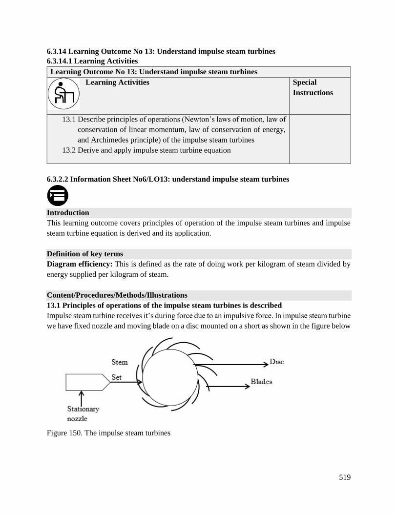
519
6.3.14 Learning Outcome No 13: Understand impulse steam turbines
6.3.14.1 Learning Activities
Learning Outcome No 13: Understand impulse steam turbines
Learning Activities Special
Instructions
13.1 Describe principles of operations (Newton’s laws of motion, law of
conservation of linear momentum, law of conservation of energy,
and Archimedes principle) of the impulse steam turbines
13.2 Derive and apply impulse steam turbine equation
6.3.2.2 Information Sheet No6/LO13: understand impulse steam turbines
Introduction
This learning outcome covers principles of operation of the impulse steam turbines and impulse
steam turbine equation is derived and its application.
Definition of key terms
Diagram efficiency: This is defined as the rate of doing work per kilogram of steam divided by
energy supplied per kilogram of steam.
Content/Procedures/Methods/Illustrations
13.1 Principles of operations of the impulse steam turbines is described
Impulse steam turbine receives it’s during force due to an impulsive force. In impulse steam turbine
we have fixed nozzle and moving blade on a disc mounted on a short as shown in the figure below
Figure 150. The impulse steam turbines
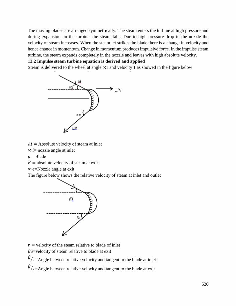
520
The moving blades are arranged symmetrically. The steam enters the turbine at high pressure and
during expansion, in the turbine, the steam falls. Due to high pressure drop in the nozzle the
velocity of steam increases. When the steam jet strikes the blade there is a change in velocity and
hence chance in momentum. Change in momentum produces impulsive force. In the impulse steam
turbine, the steam expands completely in the nozzle and leaves with high absolute velocity.
13.2 Impulse steam turbine equation is derived and applied
Steam is delivered to the wheel at angle ∝1 and velocity 1 as showed in the figure below
𝐴𝑖 = Absolute velocity of steam at inlet
∝ 𝑖= nozzle angle at inlet
𝜇 =Blade
𝐸 = absolute velocity of steam at exit
∝ 𝑒=Nozzle angle at exit
The figure below shows the relative velocity of steam at inlet and outlet
𝑟 = velocity of the steam relative to blade of inlet
𝛽𝑒=velocity of steam relative to blade at exit
𝛽1⁄ =Angle between relative velocity and tangent to the blade at inlet
𝛽1⁄ =Angle between relative velocity and tangent to the blade at exit
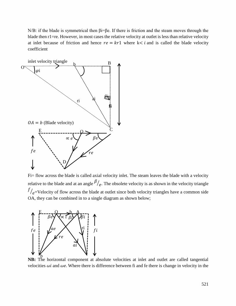
521
N/B: if the blade is symmetrical then βi=βe. If there is friction and the steam moves through the
blade then r1=re. However, in most cases the relative velocity at outlet is less than relative velocity
at inlet because of friction and hence 𝑟𝑒 = 𝑘𝑟1 where k< 𝑖 and is called the blade velocity
coefficient
inlet velocity triangle
𝑂𝐴 = 𝑏 (Blade velocity)
Fi= flow across the blade is called axial velocity inlet. The steam leaves the blade with a velocity
relative to the blade and at an angle 𝛽
𝑒⁄ . The obsolete velocity is as shown in the velocity triangle
𝑓𝑒⁄ =Velocity of flow across the blade at outlet since both velocity triangles have a common side
OA, they can be combined in to a single diagram as shown below;
NB: The horizontal component at absolute velocities at inlet and outlet are called tangential
velocities 𝜔𝑖 and 𝜔𝑒. Where there is difference between fi and fe there is change in velocity in the
D
∝ 𝑒
𝑟𝑒
𝛽e
A O E
𝑓𝑒
𝛽i ri
C
ai
O B b
𝜑i
fi
E
𝑓𝑒
O b A
𝑎𝑒
𝑟𝑒
𝑎𝑖
𝛽𝑖
𝛽e
𝑓𝑖
∝ 𝑖 𝛽𝑖
b
ri
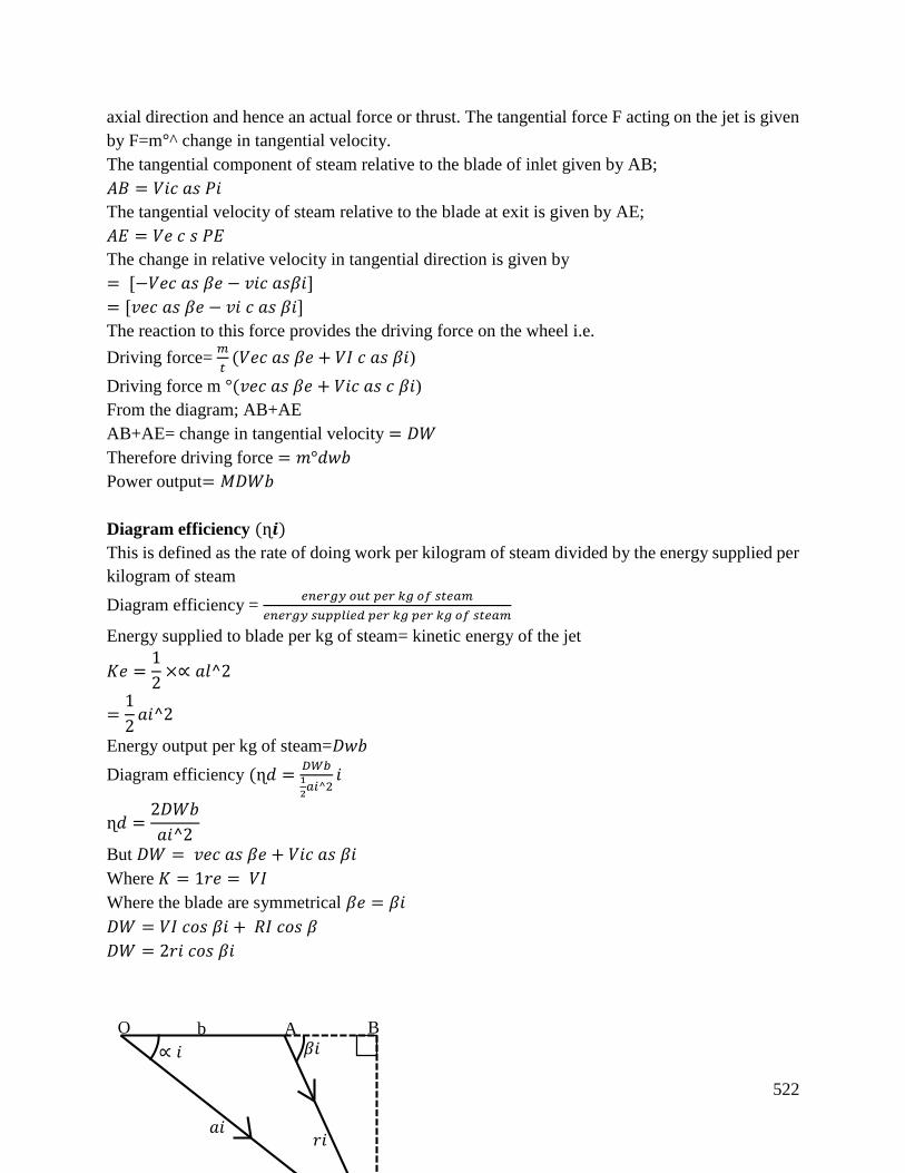
522
axial direction and hence an actual force or thrust. The tangential force F acting on the jet is given
by F=m°^ change in tangential velocity.
The tangential component of steam relative to the blade of inlet given by AB;
𝐴𝐵 = 𝑉𝑖𝑐 𝑎𝑠 𝑃𝑖
The tangential velocity of steam relative to the blade at exit is given by AE;
𝐴𝐸 = 𝑉𝑒 𝑐 𝑠 𝑃𝐸
The change in relative velocity in tangential direction is given by
= [−𝑉𝑒𝑐 𝑎𝑠 𝛽𝑒 − 𝑣𝑖𝑐 𝑎𝑠𝛽𝑖]
= [𝑣𝑒𝑐 𝑎𝑠 𝛽𝑒 − 𝑣𝑖 𝑐 𝑎𝑠 𝛽𝑖]
The reaction to this force provides the driving force on the wheel i.e.
Driving force= 𝑚
𝑡(𝑉𝑒𝑐 𝑎𝑠 𝛽𝑒 + 𝑉𝐼 𝑐 𝑎𝑠 𝛽𝑖)
Driving force m °(𝑣𝑒𝑐 𝑎𝑠 𝛽𝑒 + 𝑉𝑖𝑐 𝑎𝑠 𝑐 𝛽𝑖)
From the diagram; AB+AE
AB+AE= change in tangential velocity = 𝐷𝑊
Therefore driving force = 𝑚°𝑑𝑤𝑏
Power output= 𝑀𝐷𝑊𝑏
Diagram efficiency (ɳ𝒊)
This is defined as the rate of doing work per kilogram of steam divided by the energy supplied per
kilogram of steam
Diagram efficiency = 𝑒𝑛𝑒𝑟𝑔𝑦 𝑜𝑢𝑡 𝑝𝑒𝑟 𝑘𝑔 𝑜𝑓 𝑠𝑡𝑒𝑎𝑚
𝑒𝑛𝑒𝑟𝑔𝑦 𝑠𝑢𝑝𝑝𝑙𝑖𝑒𝑑 𝑝𝑒𝑟 𝑘𝑔 𝑝𝑒𝑟 𝑘𝑔 𝑜𝑓 𝑠𝑡𝑒𝑎𝑚
Energy supplied to blade per kg of steam= kinetic energy of the jet
𝐾𝑒 =1
2×∝ 𝑎𝑙^2
=1
2𝑎𝑖^2
Energy output per kg of steam=𝐷𝑤𝑏
Diagram efficiency (ɳ𝑑 =𝐷𝑊𝑏1
2𝑎𝑖^2
𝑖
ɳ𝑑 =2𝐷𝑊𝑏
𝑎𝑖^2
But 𝐷𝑊 = 𝑣𝑒𝑐 𝑎𝑠 𝛽𝑒 + 𝑉𝑖𝑐 𝑎𝑠 𝛽𝑖
Where 𝐾 = 1𝑟𝑒 = 𝑉𝐼
Where the blade are symmetrical 𝛽𝑒 = 𝛽𝑖
𝐷𝑊 = 𝑉𝐼 𝑐𝑜𝑠 𝛽𝑖 + 𝑅𝐼 𝑐𝑜𝑠 𝛽
𝐷𝑊 = 2𝑟𝑖 𝑐𝑜𝑠 𝛽𝑖
O b A B
∝ 𝑖
𝑎𝑖 𝑟𝑖
𝛽𝑖
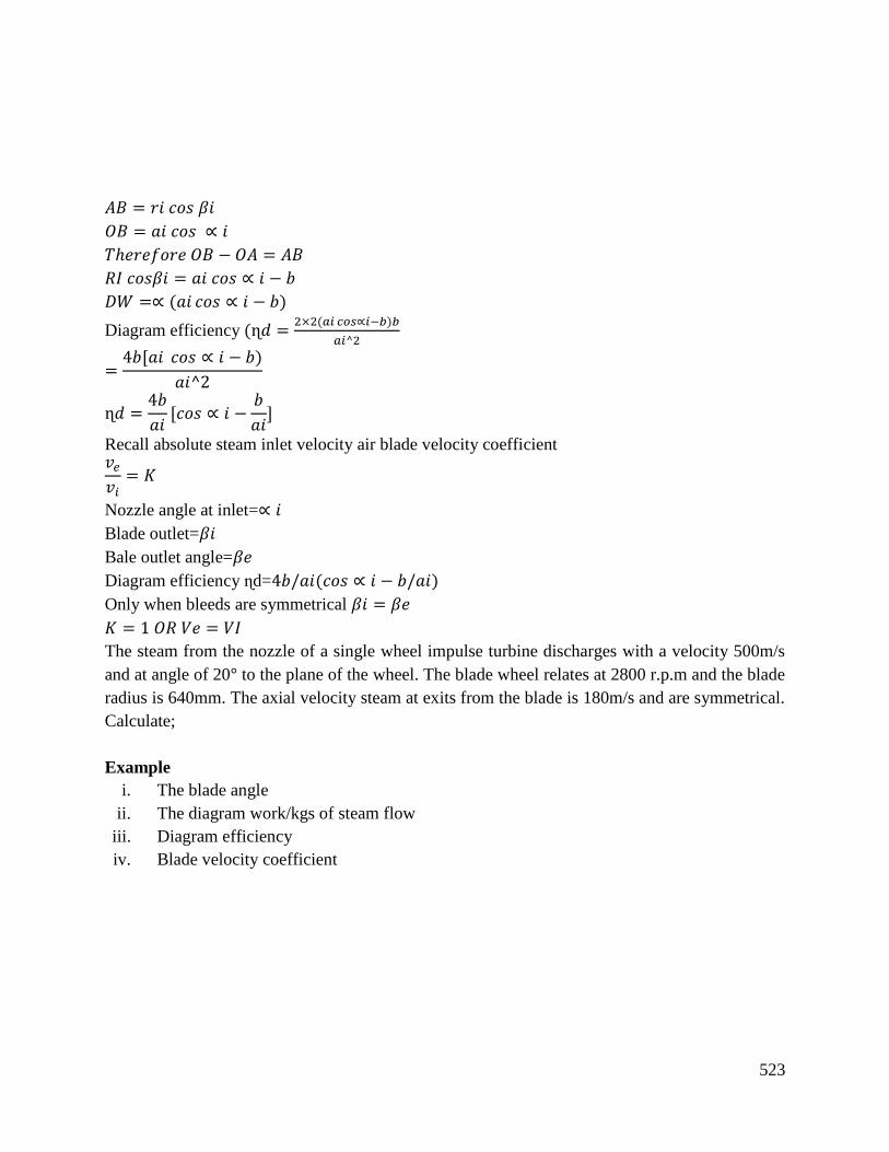
523
𝐴𝐵 = 𝑟𝑖 𝑐𝑜𝑠 𝛽𝑖
𝑂𝐵 = 𝑎𝑖 𝑐𝑜𝑠 ∝ 𝑖
𝑇ℎ𝑒𝑟𝑒𝑓𝑜𝑟𝑒 𝑂𝐵 − 𝑂𝐴 = 𝐴𝐵
𝑅𝐼 𝑐𝑜𝑠𝛽𝑖 = 𝑎𝑖 𝑐𝑜𝑠 ∝ 𝑖 − 𝑏
𝐷𝑊 =∝ (𝑎𝑖 𝑐𝑜𝑠 ∝ 𝑖 − 𝑏)
Diagram efficiency (ɳ𝑑 =2×2(𝑎𝑖 𝑐𝑜𝑠∝𝑖−𝑏)𝑏
𝑎𝑖^2
=4𝑏[𝑎𝑖 𝑐𝑜𝑠 ∝ 𝑖 − 𝑏)
𝑎𝑖^2
ɳ𝑑 =4𝑏
𝑎𝑖[𝑐𝑜𝑠 ∝ 𝑖 −
𝑏
𝑎𝑖]
Recall absolute steam inlet velocity air blade velocity coefficient 𝑣𝑒
𝑣𝑖= 𝐾
Nozzle angle at inlet=∝ 𝑖
Blade outlet=𝛽𝑖
Bale outlet angle=𝛽𝑒
Diagram efficiency ɳd=4𝑏/𝑎𝑖(𝑐𝑜𝑠 ∝ 𝑖 − 𝑏/𝑎𝑖)
Only when bleeds are symmetrical 𝛽𝑖 = 𝛽𝑒
𝐾 = 1 𝑂𝑅 𝑉𝑒 = 𝑉𝐼
The steam from the nozzle of a single wheel impulse turbine discharges with a velocity 500m/s
and at angle of 20° to the plane of the wheel. The blade wheel relates at 2800 r.p.m and the blade
radius is 640mm. The axial velocity steam at exits from the blade is 180m/s and are symmetrical.
Calculate;
Example
i. The blade angle
ii. The diagram work/kgs of steam flow
iii. Diagram efficiency
iv. Blade velocity coefficient
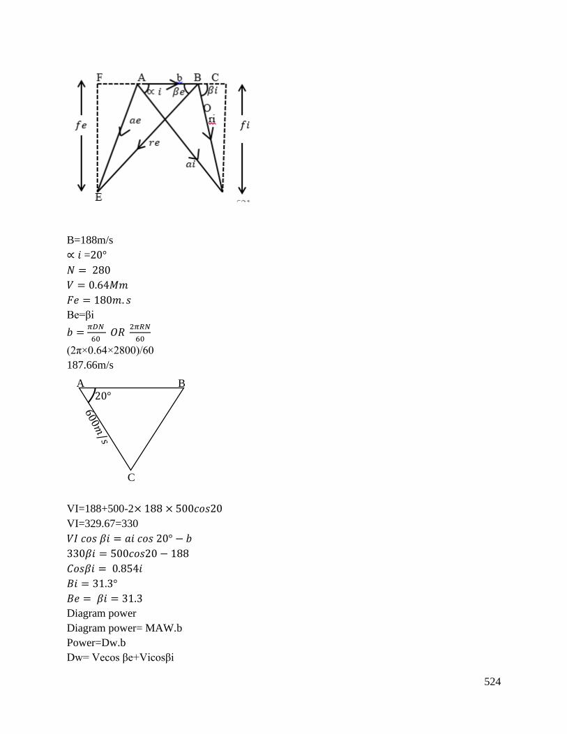
524
B=188m/s
∝ 𝑖 =20°
𝑁 = 280
𝑉 = 0.64𝑀𝑚
𝐹𝑒 = 180𝑚. 𝑠
Βe=βi
𝑏 = 𝜋𝐷𝑁
60 𝑂𝑅
2𝜋𝑅𝑁
60
(2π×0.64×2800)/60
187.66m/s
VI=188+500-2× 188 × 500𝑐𝑜𝑠20
VI=329.67=330
𝑉𝐼 𝑐𝑜𝑠 𝛽𝑖 = 𝑎𝑖 𝑐𝑜𝑠 20° − 𝑏
330𝛽𝑖 = 500𝑐𝑜𝑠20 − 188
𝐶𝑜𝑠𝛽𝑖 = 0.854𝑖
𝛣𝑖 = 31.3°
𝛣𝑒 = 𝛽𝑖 = 31.3
Diagram power
Diagram power= MAW.b
Power=Dw.b
Dw= Vecos βe+Vicosβi
20° B
A
C
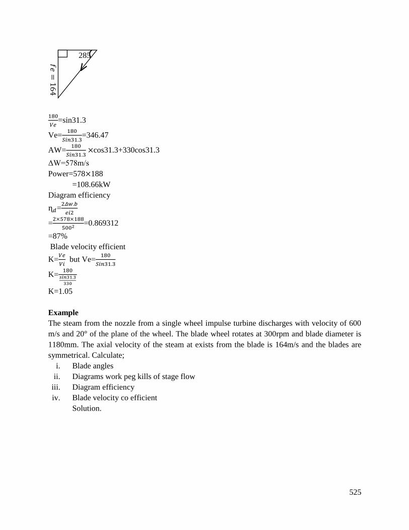
525
180
𝑉𝑒=sin31.3
Ve=180
𝑆𝑖𝑛31.3=346.47
AW=180
𝑆𝑖𝑛31.3×cos31.3+330cos31.3
ΔW=578m/s
Power=578×188
=108.66kW
Diagram efficiency
ɳ𝑑=2𝛥𝑤.𝑏
𝑒𝑖2
=2×578×188
5002 =0.869312
=87%
Blade velocity efficient
K=𝑉𝑒
𝑉𝑖 but Ve=
180
𝑆𝑖𝑛31.3
K=180
𝑠𝑖𝑛31.3
330
K=1.05
Example
The steam from the nozzle from a single wheel impulse turbine discharges with velocity of 600
m/s and 20° of the plane of the wheel. The blade wheel rotates at 300rpm and blade diameter is
1180mm. The axial velocity of the steam at exists from the blade is 164m/s and the blades are
symmetrical. Calculate;
i. Blade angles
ii. Diagrams work peg kills of stage flow
iii. Diagram efficiency
iv. Blade velocity co efficient
Solution.
𝑓𝑒
=164
285
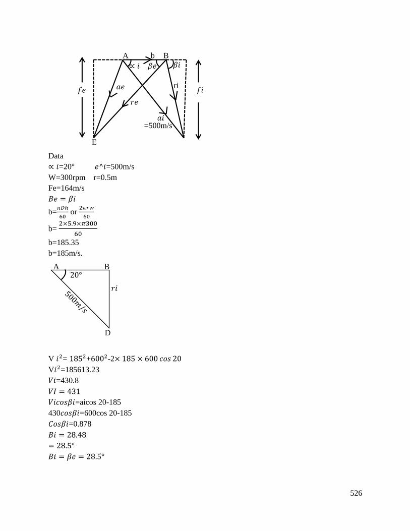
526
Data
∝ 𝑖=20° 𝑒^𝑖=500m/s
W=300rpm r=0.5m
Fe=164m/s
𝛣𝑒 = 𝛽𝑖
b=𝜋𝐷ℎ
60 or
2𝜋𝑟𝑤
60
b= 2×5.9×𝜋300
60
b=185.35
b=185m/s.
V 𝑖2= 1852+6002-2× 185 × 600 𝑐𝑜𝑠 20
V𝑖2=185613.23
𝑉𝑖=430.8
𝑉𝐼 = 431
𝑉𝑖𝑐𝑜𝑠𝛽𝑖=aicos 20-185
430𝑐𝑜𝑠𝛽𝑖=600cos 20-185
𝐶𝑜𝑠𝛽𝑖=0.878
𝛣𝑖 = 28.48
= 28.5°
𝛣𝑖 = 𝛽𝑒 = 28.5°
=500m/s
𝑓𝑒
A b B
𝑎𝑒
𝑟𝑒
𝑎𝑖
𝛽𝑖
𝑓𝑖
∝ 𝑖 𝛽𝑒
E
ri
20°
D
B A
𝑟𝑖

527
Diaphram power
=MAW.b
Power=AW.b
ΔW=𝑉𝑒 𝑐𝑜𝑠 𝛽𝑒 + 𝑉𝑖𝑐𝑜𝑠 𝛽𝑖
Sin28.5=164
𝑉𝑒
Δw=164
𝑠𝑖𝑛28.5× 𝑐𝑜𝑠 28.5 + 431 𝑐𝑜𝑠 28.5
ΔW=680.8× 185
Power=680,8× 185
=125.952kW
Diagram efficiency
ɳ𝑑=
2𝛥𝑊. 𝑏
𝑎𝑖2=
2 × 680.8 × 95 × 185
6002
ɳ𝑑=0.69017
≅70%
Blade velocity coefficient
K=𝑉𝑒
𝑉𝑖
=164
𝑠𝑖𝑛28.5
431
K=0.7974
Conclusion
The learning outcome covered or equipped the learner with knowledge, skills and attitude to equip
the learner with knowledge skill to describe the principle of operation of impulse turbine and apply
these principles in an operation and impulse turbine.
𝑟𝑒
180
313°
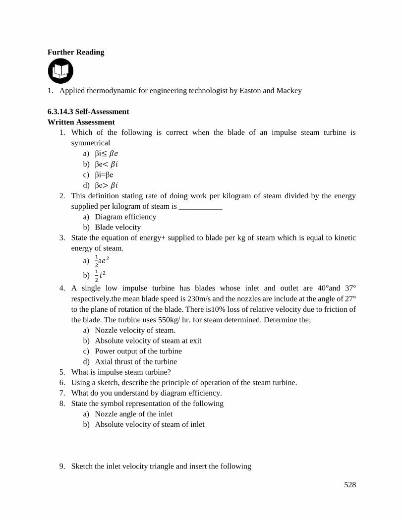
528
Further Reading
1. Applied thermodynamic for engineering technologist by Easton and Mackey
6.3.14.3 Self-Assessment
Written Assessment
1. Which of the following is correct when the blade of an impulse steam turbine is
symmetrical
a) βi≤ 𝛽𝑒
b) βe< 𝛽𝑖
c) βi=βe
d) βe> 𝛽𝑖
2. This definition stating rate of doing work per kilogram of steam divided by the energy
supplied per kilogram of steam is ___________
a) Diagram efficiency
b) Blade velocity
3. State the equation of energy+ supplied to blade per kg of steam which is equal to kinetic
energy of steam.
a) 1
2a𝑒2
b) 1
2𝑖2
4. A single low impulse turbine has blades whose inlet and outlet are 40°and 37°
respectively.the mean blade speed is 230m/s and the nozzles are include at the angle of 27°
to the plane of rotation of the blade. There is10% loss of relative velocity due to friction of
the blade. The turbine uses 550kg/ hr. for steam determined. Determine the;
a) Nozzle velocity of steam.
b) Absolute velocity of steam at exit
c) Power output of the turbine
d) Axial thrust of the turbine
5. What is impulse steam turbine?
6. Using a sketch, describe the principle of operation of the steam turbine.
7. What do you understand by diagram efficiency.
8. State the symbol representation of the following
a) Nozzle angle of the inlet
b) Absolute velocity of steam of inlet
9. Sketch the inlet velocity triangle and insert the following

529
a) air
b) αi
c) Vi
d) β
Oral Assessment
1. Explain the outcomes when the blade is symmetrical on an impulse turbine
2. Discuss the operation of impulse steam turbine
Practical Assessment
1. By use of an experiment on prototype impulse turbine explain how diagram efficiency can
be increased or lowered.
6.3.14.4 Tools, Equipment, Supplies and Materials
Scientific Calculators
Relevant reference materials
Stationeries
Relevant practical materials
Dice
Computers with internet connection
6.3.14.5 References
Balmer, R. T. (2011). Modern engineering thermodynamics-textbook with table’s booklet.
Academic Press.
Kondepudi, D. (2008). Introduction to modern thermodynamics. Wiley.
Nag, P. K. (2013). Engineering thermodynamics. Tata McGraw-Hill Education.
530
CHAPTER 7: MATERIAL SCIENCE AND METALLURGICAL PROCESSES/ APPLY
MATERIAL SCIENCE AND PERFORM METALLURGICAL PROCESSES
7.1 Introduction
Material science and metallurgical processes is among the basic competency units offered in TVET
level 6 engineering courses qualification. The learner will be introduced to performing material
testing and metallurgical processes. It involves analysing properties of engineering materials,
performing extraction processes, producing iron materials, ceramics, composites and alloys,
performing heat treatment, material testing, and identifying corrosion and its prevention. The
significance of material science and metallurgical processes to TVET level 6 engineering
curriculum is to enable learners acquire knowledge and skills to demonstrate measuring and
marking, material testing, use of hand tools and inspection, and testing to get along well in the
workplace and task.
The critical aspects of competency to be covered include; observed safety as per work place
procedures, demonstrated understanding of physical, chemical and mechanical properties of
engineering materials, performed extraction processes, produced iron materials, produced
ceramics, produced composite produced alloys, performed heat treatment, performed material
testing and demonstrated understanding of corrosion types and its prevention. The basic resources
required include testing materials, extraction materials, measuring instruments and inspection tools
among others. The unit of competency covers eleven learning outcomes. Each of the learning
outcomes presents; learning activity that covers performance criteria statements thus giving
trainees an opportunity to demonstrate knowledge and skills in the occupational standards and
content in curriculum. Information sheet provides definition of key terms, content and illustration
to guide in training. The competency may be assessed through the behavior of the learner in the
working environment, inspection of finished product and process analysis. Self-assessment is
provided at the end of each learning outcomes. Holistic assessment with other units relevant to the
industry sector workplace and job role is recommended.
7.2 Performance Standard
Analyse properties of engineering materials, perform ore extraction processes, produce iron
materials, produce alloy materials, produce non-ferrous materials, produce ceramics materials,
produce composite materials, utilize other engineering materials, perform heat treatment, perform
material testing and prevent material corrosions per work place procedures.
7.3 Learning Outcomes
7.3.1 List of Learning Outcomes
a) Analyze properties of engineering materials
b) Perform ore extraction processes
c) Produce iron materials

531
d) Produce alloy materials
e) Produce non-ferrous materials
f) Produce ceramics materials
g) Produce composite materials
h) Utilize other engineering materials
i) Perform heat treatment
j) Perform material testing
k) Prevent material corrosion
532
7.3.2 Learning Outcome No 1: Analyze properties of engineering materials
7.3.2.1 Learning Activities
Learning Outcome No 1: Analyze properties of engineering materials
Learning Activities Special Instructions
1.1 Identify type of engineering materials as per the procedures.
1.2 Determine physical properties (density, colour, texture, melting
point, thermal conductivity, electricity) of engineering material.
1.3 Test mechanical properties (ductility, malleability, elasticity,
toughness, hardness, brittleness, plasticity, strength) of
engineering materials.
1.4 Analysing crystal structure of materials.
1.4 analyze crystal structure of materials are analyzed
Conduct a visit to an
Engineering
workshop.
7.3.2.2 Information Sheet No7/LO1: Analyze properties of engineering materials
Introduction
This learning outcome covers analysis of properties of engineering materials, test mechanical
properties and analyze crystals structures of materials.
Definition of key terms
Stress: The internal resistant set up by the molecules of a material to resist deformation due to
application of external forces.
Stress S = 𝑓𝑜𝑟𝑐𝑒
𝑎𝑟𝑒𝑎 =
𝑓
𝑎(𝑢𝑛𝑖𝑡: 𝑛/𝑚2)
Strain: The deformation or change in length per unit length, under the action of external forces.
Strain E = 𝑎𝑙
𝑙 where
𝑙
𝑙 –
𝑐ℎ𝑎𝑛𝑔𝑒 𝑖𝑛 𝑙𝑒𝑛𝑔𝑡ℎ
𝑜𝑟𝑖𝑔𝑖𝑛𝑎𝑙 𝑙𝑒𝑛𝑔𝑡ℎ
Content/Procedures/Methods/Illustrations
1.1 Type of engineering materials is identified as per the procedures
The following are types of engineering materials;
Metals
Non-metals
Ceramics
Composites
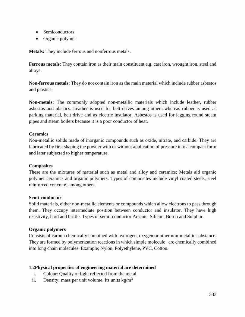
533
Semiconductors
Organic polymer
Metals: They include ferrous and nonferrous metals.
Ferrous metals: They contain iron as their main constituent e.g. cast iron, wrought iron, steel and
alloys.
Non-ferrous metals: They do not contain iron as the main material which include rubber asbestos
and plastics.
Non-metals: The commonly adopted non-metallic materials which include leather, rubber
asbestos and plastics. Leather is used for belt drives among others whereas rubber is used as
parking material, belt drive and as electric insulator. Asbestos is used for lagging round steam
pipes and steam boilers because it is a poor conductor of heat.
Ceramics
Non-metallic solids made of inorganic compounds such as oxide, nitrate, and carbide. They are
fabricated by first shaping the powder with or without application of pressure into a compact form
and later subjected to higher temperature.
Composites
These are the mixtures of material such as metal and alloy and ceramics; Metals aid organic
polymer ceramics and organic polymers. Types of composites include vinyl coated steels, steel
reinforced concrete, among others.
Semi-conductor
Solid materials, either non-metallic elements or compounds which allow electrons to pass through
them. They occupy intermediate position between conductor and insulator. They have high
resistivity, hard and brittle. Types of semi- conductor Arsenic, Silicon, Boron and Sulphur.
Organic polymers
Consists of carbon chemically combined with hydrogen, oxygen or other non-metallic substance.
They are formed by polymerization reactions in which simple molecule are chemically combined
into long chain molecules. Example; Nylon, Polyethylene, PVC, Cotton.
1.2Physical properties of engineering material are determined
i. Colour: Quality of light reflected from the metal.
ii. Density: mass per unit volume. Its units kg/m3
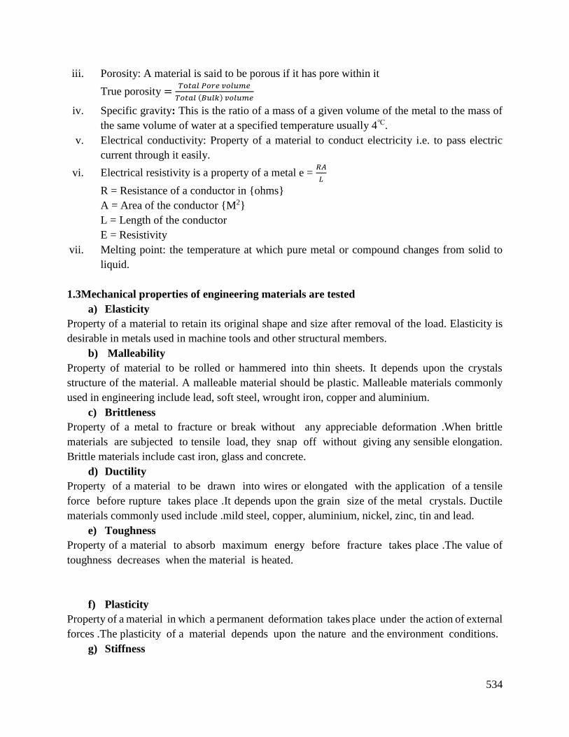
534
iii. Porosity: A material is said to be porous if it has pore within it
True porosity =𝑇o𝑡𝑎𝑙 𝑃𝑜𝑟𝑒 𝑣𝑜𝑙𝑢𝑚𝑒
𝑇𝑜𝑡𝑎𝑙 (𝐵𝑢𝑙𝑘) 𝑣𝑜𝑙𝑢𝑚𝑒
iv. Specific gravity: This is the ratio of a mass of a given volume of the metal to the mass of
the same volume of water at a specified temperature usually 4.
v. Electrical conductivity: Property of a material to conduct electricity i.e. to pass electric
current through it easily.
vi. Electrical resistivity is a property of a metal e = 𝑅𝐴
𝐿
R = Resistance of a conductor in ohms
A = Area of the conductor M2
L = Length of the conductor
E = Resistivity
vii. Melting point: the temperature at which pure metal or compound changes from solid to
liquid.
1.3Mechanical properties of engineering materials are tested
a) Elasticity
Property of a material to retain its original shape and size after removal of the load. Elasticity is
desirable in metals used in machine tools and other structural members.
b) Malleability
Property of material to be rolled or hammered into thin sheets. It depends upon the crystals
structure of the material. A malleable material should be plastic. Malleable materials commonly
used in engineering include lead, soft steel, wrought iron, copper and aluminium.
c) Brittleness
Property of a metal to fracture or break without any appreciable deformation .When brittle
materials are subjected to tensile load, they snap off without giving any sensible elongation.
Brittle materials include cast iron, glass and concrete.
d) Ductility
Property of a material to be drawn into wires or elongated with the application of a tensile
force before rupture takes place .It depends upon the grain size of the metal crystals. Ductile
materials commonly used include .mild steel, copper, aluminium, nickel, zinc, tin and lead.
e) Toughness
Property of a material to absorb maximum energy before fracture takes place .The value of
toughness decreases when the material is heated.
f) Plasticity
Property of a material in which a permanent deformation takes place under the action of external
forces .The plasticity of a material depends upon the nature and the environment conditions.
g) Stiffness
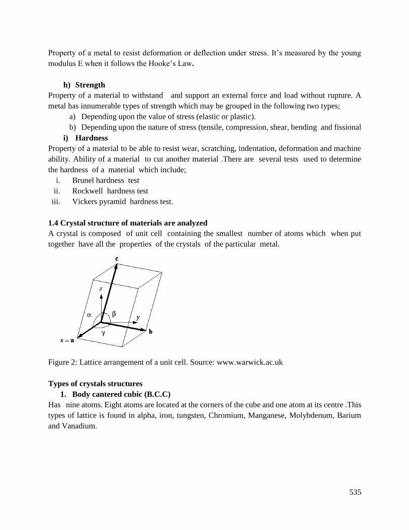
535
Property of a metal to resist deformation or deflection under stress. It’s measured by the young
modulus E when it follows the Hooke’s Law.
h) Strength
Property of a material to withstand and support an external force and load without rupture. A
metal has innumerable types of strength which may be grouped in the following two types;
a) Depending upon the value of stress (elastic or plastic).
b) Depending upon the nature of stress (tensile, compression, shear, bending and fissional
i) Hardness
Property of a material to be able to resist wear, scratching, indentation, deformation and machine
ability. Ability of a material to cut another material .There are several tests used to determine
the hardness of a material which include;
i. Brunel hardness test
ii. Rockwell hardness test
iii. Vickers pyramid hardness test.
1.4 Crystal structure of materials are analyzed
A crystal is composed of unit cell containing the smallest number of atoms which when put
together have all the properties of the crystals of the particular metal.
Figure 2: Lattice arrangement of a unit cell. Source: www.warwick.ac.uk
Types of crystals structures
1. Body cantered cubic (B.C.C)
Has nine atoms. Eight atoms are located at the corners of the cube and one atom at its centre .This
types of lattice is found in alpha, iron, tungsten, Chromium, Manganese, Molybdenum, Barium
and Vanadium.
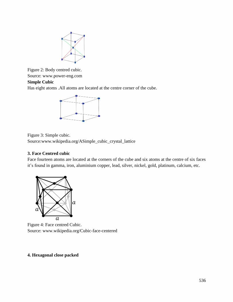
536
Figure 2: Body centred cubic.
Source: www.power-eng.com
Simple Cubic
Has eight atoms .All atoms are located at the centre corner of the cube.
Figure 3: Simple cubic.
Source:www.wikipedia.org/ASimple_cubic_crystal_lattice
3. Face Centred cubic
Face fourteen atoms are located at the corners of the cube and six atoms at the centre of six faces
it’s found in gamma, iron, aluminium copper, lead, silver, nickel, gold, platinum, calcium, etc.
Figure 4: Face centred Cubic.
Source: www.wikipedia.org/Cubic-face-centered
4. Hexagonal close packed
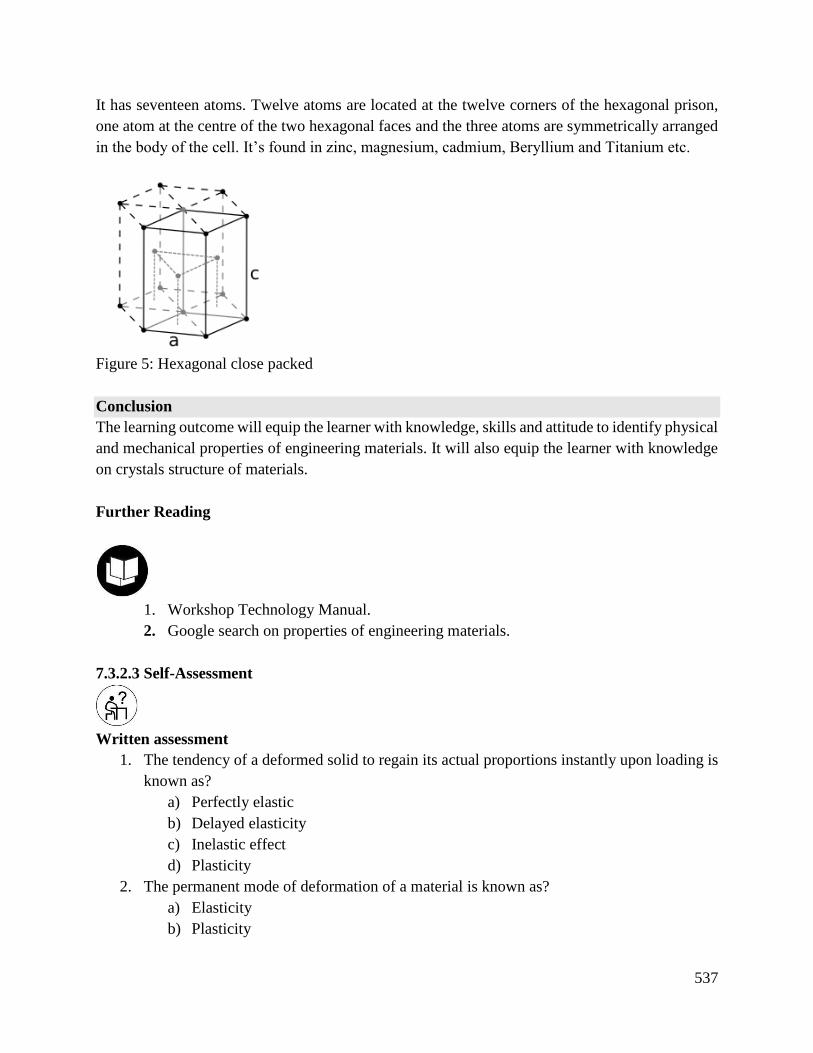
537
It has seventeen atoms. Twelve atoms are located at the twelve corners of the hexagonal prison,
one atom at the centre of the two hexagonal faces and the three atoms are symmetrically arranged
in the body of the cell. It’s found in zinc, magnesium, cadmium, Beryllium and Titanium etc.
Figure 5: Hexagonal close packed
Conclusion
The learning outcome will equip the learner with knowledge, skills and attitude to identify physical
and mechanical properties of engineering materials. It will also equip the learner with knowledge
on crystals structure of materials.
Further Reading
1. Workshop Technology Manual.
2. Google search on properties of engineering materials.
7.3.2.3 Self-Assessment
Written assessment
1. The tendency of a deformed solid to regain its actual proportions instantly upon loading is
known as?
a) Perfectly elastic
b) Delayed elasticity
c) Inelastic effect
d) Plasticity
2. The permanent mode of deformation of a material is known as?
a) Elasticity
b) Plasticity
538
c) Slip deformation
d) Twinning Deformation
3. The ability of materials to develop a characteristic behaviour under the repeated loading is
known as?
a) Toughness
b) Resilience
c) Hardness
d) Fatigue
4. Which of the following factors affect the mechanical properties of a material under applied
load?
a) Content of alloy
b) Grain size
c) Imperfection and defects
d) Shape of material
5. The ability of a material to resist plastic deformation is known as?
a) Tensile strength
b) Yield strength
c) Modulus of elasticity
d) Impact strength
6. Deformation that occurs due to stress over a period of time is known as?
a) Wear resistance
b) Fatigue
c) Creep
d) Fracture
7. What is the attribute of a material which resists the flow of electricity?
a) Conductivity
b) Thermo electricity
c) Dielectric strength
d) Resistivity
8. State four forms of engineering materials supply.
9. List four types of engineering materials.
10. Explain three physical properties of engineering material.
11. Explain four mechanical properties of engineering stating the metals they are found in.
12. Illustrate face centred cubic
Oral Assessment
1. What is a crystal structure?
2. Mention two types of defects in a crystal
539
Practical Assessment
1. Provide the learner with a material and carry out hardness test (Brinell hardness) on the
machine.
Project
1. Analysing stresses and deflection of beams, determine the bending stress and shear of a
beam mode in different materials?
7.3.2.4 Tools, Equipment, Supplies and Materials
Measuring tools and gauges
Marking out tools
Inspection tools and equipment
Dressing tools
Fire-fighting equipment
PPEs e.g. dust coat, dust masks, ear muffs, goggles
First Aid kit
Brooms and cleaning stuff
Cleaning detergents
Drawing papers
7.3.2.5 References
E.R.P. RAJPUT. 1989 Engineering Materials and Metallurgy
Bolton. (1992) Materials for engineering
Higgins, (2012) Materials for the engineering and Technician 5th Edition
540
7.3.3 Learning Outcome No. 2: Perform ore extraction processes
7.3.2.1 Learning Activities
Learning Outcome No. 2: Perform ore extraction processes
Learning Activities Special Instructions
2.1 Observe safety procedures according OSHA.
2.2 Determine method of extraction as per material properties and
its composition.
2.3 Determine procedure in extraction process as per extraction
method.
2.4 Store extraction byproducts as per SOPs.
2.5 Dispose extraction byproducts as per SOPs.
Do a practical
extraction.
7.3.2.2 Information Sheet No7/LO2: Perform ore extraction processes
Introduction
This learning outcome covers the performance on ore extraction process where we learn how to
observe safety procedures according to OSHA. We learn ore extraction methods as per material
properties and its composition. We also learn the procedure of each Ore extraction process as per
its extraction method, how to store the extracted by product and how to dispose extraction by
products as per Sops.
Definition of key terms
An Ore: A natural rock or sediment that contains desirable minerals, typically metals, that can be
extracted from it.
Mining: It is a process that involves exploitation processing and removal of minerals from the
earth, economically and with minimum damage to the environment.
Prospecting: This is the first stage of mineral deposits. It is the search of ores or other valuable
minerals.
Exploration: It’s the second stage of mining which is determines as accurately as possible, the
size and value of a mineral deposit, utilizing techniques similar to but more refined than those used
in prospecting.
541
Content/Procedures/Methods/Illustrations
2.1 Safety procedures that should be observed according OSHA
a) During blasting the miners should ensure they have done correctly and accordingly to the laid
down blasting procedure to avoid any harm.
b) During blasting there might be dry rocks which may cause injuries to persons mining or
damage to property to ensure you keep a good safety measures to prevent it.
c) When mining there may be instability of high walls. In order to control high wall instability
and rainfall for the miner’s safety and health administration requires that a ground plan be
established and implemented by all surface miners.
d) For the surface miners, they control dust by introducing wet drilling.
e) Equipment and machineries that may cause accidents must put emphasis on haulage trucks
accidents.
f) Miners are fitted with a collision avoidance system tag in their hard hats which transmit a
signal to the collision avoidance system receiver in the track.
2.2 Method of extraction determined as per material properties and their composition
Surface mining
This is done by removing surface vegetation, dirt and if necessary, layers of the bedrock in order
to reach the buried deposited. Techniques of surface mining include;
Open –pit mining: It is the recovery of materials from an open pit in the ground, quarrying;
Identical to open -pit mining except that it refers to sand, stones and clay.
Strip Mining: It consists of stripping surface layers off to reveal ore /seams underneath. Mountain
removal: commonly associated with coal mining which involves taking the top of the mountain
off to reach Ore deposits at depth.
Land Fill Mining: It involves sites where landfills are excavated and preserved. It has been
thought of as a solution to dealing with long time methane emission and local pollution.
High wall mining: In this method the coal seam is penetrated by the continuous miner propelled
by a hydraulic push beam transfer Mechanism (PTM) a typical cycle that includes sampling and
shearing. As the coal recovering cycle continues, the cutter is progressively launched into the coal
seam for 19.72 feet then, the push beam transfer mechanism automatically inserts a 19.72- feet
long rectangular push beam into the centre section of the machine between the power head and the
cutter head. The push beam system can penetrate nearly 1000 foot into the coal seam.
Underground mining: Underground mining consists of digging tunnels or shafts into the earth to
reach burned Ore deposits for processing. Waste rocks for disposal are brought to the surface
through the tunnels and shafts. Underground mining can be classified by the type of access shaft
used, the extraction method or the technique used to reach the mineral deposits.
542
Drift mining: Utilizes horizontal access tunnels.
Slope mining: Uses diagonal sloping access.
Shaft mining: Utilizes vertical access shaft. Mining in hard or soft formations require different
techniques.
Shrinkage Slope mining: It refers to mining upward, creating a sloping underground and a sloping
underground room.
Long wall mining: This is grinding along one surface underground and room and pitter.
Pillar mining: This is removing an ore from the room while leaving the pillars to support the roof
of the house.
Retreat mining: It is the process in which supporting pillars are removed as miners retreat,
allowing the room to cave in thereby loosening the Ore.
Hard rock mining: Refers to mining of hard rock materials, borehole mining, drift and fill mining,
long whole slope mining, sublevel caving and block caving.
2.3 Extraction by products is stored as per SOPs
Cult and fill mining
In this method, short hole mining is used in steep dipping or irregular Ore zones particularly where
a hanging wall limits the use of long hole method. The ore is mined in horizontal or slightly
inclined slices and then filled with waste rock, sand or tailings. Either fill option may be
consolidated with concrete or left unconsolidated.
Drift and fill mining
This is a method of mining which is used in Ore zones which are wider than the methods of drifting
will allow to be mined. In this case the first drift is developed in the Ore and is backfilled using
consolidated fill. The second drift is driven adjacent to first. This carries on until the one zone is
mined out to its full width at which time the second cut is started at the top of the first cut.
Shrinkage stopping mining
It’s a short-hole mining method which is suitable for steeply dipping one body. This method is
similar to cut and fill mining with the exception that affect being blasted. Broken Ore is left in the
stope where it is used to support the surroundings rock and as a platform from which to work. Only
543
enough ore is removed from the stope for drilling and blasting the next slice. The stopes are
empirical when a lot of the Ore has been blasted.
Room and pillar mining
This is commonly done in flat or gently dipping bedded ore bodies. Pillars are felt in a place in
regular pattern while the rooms are mined out. In many room and pillar mines, the pillars are taken
out starting at the farthest point from the access allowing the roof to collapse and fill the stopes.
This allows for greater recovery as less ore is left behind in pillars.
Vertical retreat mining
In this method the mine is divided in vertical zones with depth of about 50 M using open stooping,
bottom up mining. Long-hole large diameter hole are drilled vertically into the ore body using in
the hole drills and then blasting horizontal slices of the ore body into an undercut is done. Ore blast
in retrieval is taken in phases. This retrieval is done from bottom of the section developed. Last of
the ore is done through a remote-controlled machine.
2.4 Extraction of by product is spokes as per SOPS
1. Butter storage: Is sometimes called “The two-processing meaning that without a proper storage
throughout a continuous rock, mineral production up time will be gone.
Storage in operation
The main purpose of the storage is to smooth out;
Different production rate.
Shift variations.
Interruptions for repair
Size variations
How variations
Variations in mineral values.
Storage or Rock
A matter of material flow (retention time)
Storage of Ore and materials
A matter of materials flow (retention time) and blending
2.5 Extraction by- products disposal as per SOPs
Some of the extremely major problems and key challenges facing the contemporary word are
shortage of resources ever growing population and the environmental pollution. After extraction
of minerals, the waste materials remaining should be disposed in such way that there is no pollution
of eco environment.
544
a) Solid waste from Mines
Waste Rock: It’s one of maximum solid waste that occurs the mining industry. In order to extract
Ore, Large amount of rock is stripped or excavated and transported to the waste dump. When the
mineral resources are exploited by underground mining method, waste rocks are often rooted in
the excavation of mine shaft and decline and other development area.
Tailings: Are the major solid waste produced in the process of mineral beneficiation. In order to
extract usable minerals. Ore is crushed and milled to appropriate size, and then the usable minerals
were separate from unstable minerals via different beneficiating methods with the development
and utilization of mineral resources. The production and disposal of tailing has become the
important factor in the sustainable development of mining industries and endangering mining and
surroundings area ecological.
b) Reclamation of solid waste.
Comprehensive utilization of solid waste resources is an important disposal method of solid waste
from mines. Facing the problem that more and more solid waste is being produced, many mines
in China have begun to utilize tailings and waste rock as resources in various ways to reduce the
discharge of solid waste and to protect environment.
c) Producing Construction materials
In order to give real protection to the cultivated land to promote sustainable development of the
socialistic economy, the site improves restrictions on mining of clay soil for production of
constructions materials.
d) Utilization of waste rock
Waste rock resulting from stripping in an open, usually according to the different utilization of
waste rock could be used diversely or dressed to various size for using. The following embodies
utilization method of waste rock:
Good for dam construction
Good for beneficiary course and the fine aggregate to concrete.
Good for road construction etc.
e) Utilization of airings.
For most mines the coarse tiling could be used as the aggregate of concrete and the fine size tiling
are good materials for making bricks using iron tailing. Bastel succeeded in making floor tile and
wall brick for construction. These kinds of bricks have a higher intensity and rigidity than those of
convention bricks and a lower cost. The usage of tailings as construction materials are described
as follows.
545
Used for making wall bricks and floor tiles for construction.
Used in filling depression, the mine out areas or subsistence area.
Used for improving the soils.
f) Recycle sable minerals.
Because of the restricting of beneficiation of technological condition, processing recovery ratio
was at lower level in some old mines. These mines did not have comprehensive utilization of
mineral resources and tailing deposited in certain magnetic iron mines in Anshan area, located in
N. East of China.
g) Regeneration of ground vegetation
The society of solid waste induced increasing grievances about destruction on eco-environment
and water and soil conservation. If the vegetation is damaged on account of the mining or
construction, action must be taken to rehabilitate the top soil and vegetable, thereby preventing
soil erosion.
Conclusion
This learning outcome covered how to observe safety procedures according OSHA, determine
method of extraction as per material properties and its composition, determine procedure in
extraction process as per extraction method, store extraction by products as per SOPs, and disposal
of extraction by- products as per SOPs.
7.3.2.3 Self-Assessment
Written assessment
1. The type of vein commonly found in igneous rock is;
a) Fissure vein
b) Ladder vein
c) Gash veins
d) Stock works.
2. Which one of the following is not essential condition for hydrothermal deposits?
a) Highly active fluids
b) Highly enriched fluid.
c) Highly inactive fluids.
d) Suitable pathways.
546
3. The deposits occurring close to the roots of magmatic deposits are called?
a) Magmatic deposits
b) Pegmatite deposits
c) Hydrothermal deposits.
d) Met somatic.
6. Deposits that were found subsequent to the formation of the host rocks are called.
a) Syngenetic
b) Epigenetic
c) Syngenetic
d) cyclogenetic
5. The deposits that have formed simultaneously with the enclosing rock are called?
a) Syngenetic
b) Epigenetic.
c) Sync genetic.
d) Cyclogenetic
6. The non –Metallic associated with Ore minerals are called?
a) Non –metallic
b) Metallic minerals.
c) Gangue Minerals
d) Hux Mineral
7. What is the mineral which contain a metallic element that can economically exploited?
a) Ore mineral
b) Metallic Mineral.
c) Eco –Ore
d) Eco – Mineral.
8. In shale gas, what do you think about importance of sampling system in mining or mineral
processing plant?
9. What is the importance of the Ore handling by percent in mining operations?
10. Underground mining will not accept mistake and negligence. What are your thoughts on
the process safety?
11. Which factors should be considered in optimization of hydraulic fracturing in shale gas?
12. Describe the underground mining method.
Oral Assessment
1. What do you think comparing mining and agricultural industries which one is the first
from views of civilization?
547
Practical Assessment
1. What types of chemical are utilized in the mining industry, floatation, leaching and tailing
disposal process?
Project
1. Describe how to prepare pure Alloys Nan tubes from minerals rich in clay.
7.3.2.4 Tools, Equipment, Supplies and Materials
Measuring tools and gauges
Marking out tools
Inspection tools and equipment
Dressing tools
Fire-fighting equipment
PPEs –dust coat, dust masks, ear muffs, goggles
First Aid kit
Brooms and cleaning stuff
Cleaning detergents
Drawing papers
7.3.2.5 References
Higgins, (2012) Materials for the engineering and Technician 5th Edition
Procedia (2012) environmental Science
W.Bolton. (1992) Materials for engineering
548
7.3.4 Learning Outcome No 3: Produce iron materials
7.3.2.1 Learning Activities
Learning Outcome No.3: Produce iron materials
Learning Activities Special Instructions
3.1 Perform ore smelting according to standard operating
procedures.
3.2 Determine composition of iron (iron ii oxide, iron iii oxide)
3.3 Establish method of producing iron material
3.4 Identify refinement processes based on iron material required
Always observe safety
procedures during mining
Use the recommended
mining methods
Use correct refinement
process
7.3.2.2 Information Sheet No7/LO3: Perform ore extraction processes
Introduction
This learning outcome covers iron production; performing the ore smelting according to standard
operating procedures. Also, establish methods of producing iron materials and also how to identify
refinement process based on iron material required.
Definition of key terms
Ore: Is a naturally occurrence of rock or sediment that contain sufficient minerals with
economically important elements, typically metals, that can be economically extracted from the
deposit.
Iron ore: Are rocks and materials from which metallic iron can be economically extracted.
Mine: Is an excavation made in the earth to extract minerals.
Mineral: Is a naturally occurring inorganic element or compound having ordinary internal
structures and a characteristics chemical composition, crystals form and physical properties?
Content/Procedures/Methods/Illustrations
549
3.1 Perform ore smelting according to standard operating procedures.
Iron ores consists of oxygen and iron ore atoms bonded together into molecules. To convert it to
metallic iron it must be smelted or sent through a direct reduction process to remove the oxygen
Oxygen iron bonds are strong. A stronger elemental bond must be presented to attach to the
oxygen. The carbon is used because the strength of carbon oxygen bond is greater than that of the
iron-oxygen bond. At high temperature thus the iron is must be powdered and mixed with coke to
be burnt in the process of smelting. Carbon monoxide is the primary ingredient of chemically
stripping oxygen from iron thus, the iron and carbon smelting must be kept at an oxygen deficient
(reducing) state to promote burning of carbon to produce CO not CO2.
2C + O2 2 CO
Carbon monoxide (CO) is the principal reducing agent
Stage 1 3 Fe2 O3 +CO 2𝐹𝑒3 𝑂4 + 𝐶𝑂2
Stage 2 𝐹𝑒3 𝑂4 + CO 3FeO +𝐶𝑂2
Stage 3 Fe O +CO Fe +CO2
3.2 Composition of iron is determined.
The quality of raw ore and its viability for commercial exploitation is mainly determined by its
chemical composition. In this study, this was analysed together with the micro structure and
mineralogy of iron ores and compared with other exploited and exported iron ores in the world.
The most important elements and components of consideration in iron ores are the content of Fe-
gangue (SiO2 and 𝐴𝐿2O3) and contamination such as P and S. It can be observed that in its raw
form, ore occurs as hematite content and alumina, 0.41-1.20% and 0.35-1.00%, respectively. In
addition, lower hematite content [86.7%] and higher silica and alumina content [5.1 and 6.0 %]
respectively. In addition; the ore contain other impurities such as MnO, ZnO, PbO and others
which exist in considerably negligible amounts.
Alumina, Sulphur, and Phosphorus represent contaminations in the making process and are
specific targets during iron ore benefaction. For commercial viability, iron ore should preferably
have high Fe content and low impurity element contents, in order to justify the investment during
exploitation. In the world practices, no minimum standards have been set for iron, Silica, Alumina,
Calcium and Magnesium percentages in commercial iron ore for, although certain generalization
can be made. However, for classification evaluation of equality, the raw iron ore can be divided
into three basic classes depending on the total iron content:
High grade iron ore with total iron content above 65%.
Medium or average grade one with varied iron contents in the range between 62%-64%.
Low grade ore with iron content below 65%
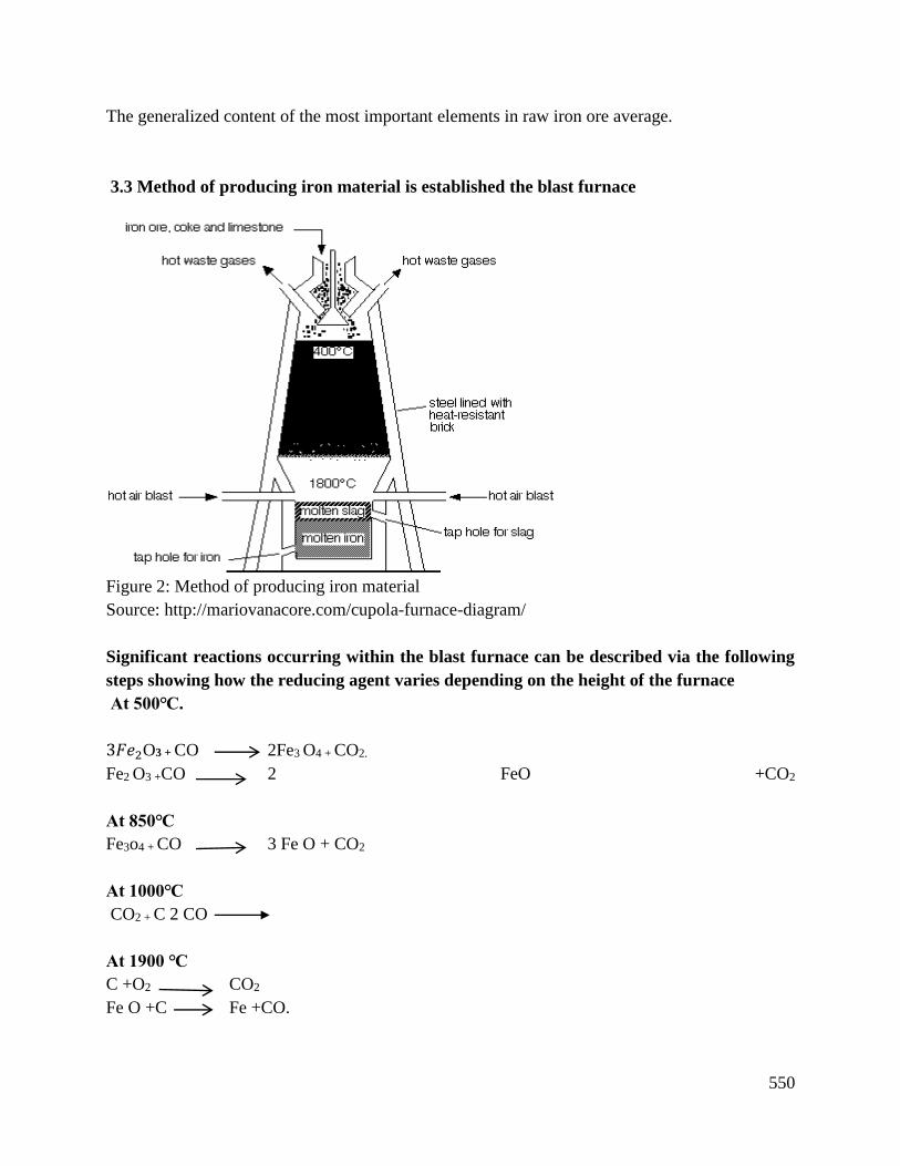
550
The generalized content of the most important elements in raw iron ore average.
3.3 Method of producing iron material is established the blast furnace
Figure 2: Method of producing iron material
Source: http://mariovanacore.com/cupola-furnace-diagram/
Significant reactions occurring within the blast furnace can be described via the following
steps showing how the reducing agent varies depending on the height of the furnace
At 500.
3𝐹𝑒2O3 + CO 2Fe3 O4 + CO2.
Fe2 O3 +CO 2 FeO +CO2
At 850
Fe3o4 + CO 3 Fe O + CO2
At 1000
CO2 + C 2 CO
At 1900
C +O2 CO2
Fe O +C Fe +CO.
551
The air blow in the bottom of the furnace is heated using the hot waste gases from the top. Heat
energy is valuable and it is important not to use any waste. The coke (essentially impure carbon)
burns in the blast of hot air to form carbon dioxide in a strong exothermic reaction. This reaction
is the main source of heat in the furnace. At the high temperature at the bottom of the furnace,
carbon dioxide reacts with carbon to produce carbon monoxide.
It’s the carbon monoxide which is the main reducing agent in the furnace. In the hotter part of the
furnace, the carbon itself also acts as a reducing agent. Notice that at this temperature, the other
product of the reaction is carbon monoxide and not carbon dioxide. The temperature of the furnace
is hot enough to melt the iron which trickles down the bottom where it can be tapped off.
3.4 Refinement processes are identified based on iron material required
The mined ore is crushed and sorted. The best grading of ore contain over 60% iron lesser grades
are treated or refined to remove various contaminants before the ore is shipped to the blast furnace.
Collectively, these refining metals are called benefaction and include further crushing, washing
with water to float sand and clay away, and magnetic separation, pelletizing and sintering.
As more of the world known supply of high iron content ore is depleted, these refining techniques
have become increasingly important. The refined ore is then loaded on trains or ships and
transported to the blast furnace site.
Conclusion
The learning outcome conversed or equipped the learner with knowledge on iron production of
iron from ore. The learners are aware of be exploited into the required content. The learners gain
the skills on the process by which iron goes.
I.e. Bras furnace reaction until the final product is obtained
6.3.2.3. Self-assessment
Written assessment
1. Which repair of elements are non –metals which will displace less reactive metal from their
oxide ore?
a) Chlorine argon
b) Nitrogen and Helium
c) Carbon and Hydrogen
d) Sulphur and oxygen
2. What substance must be present for rusting to occur?
a) Carbon and Hydrogen
552
b) Water and hydrogen
c) Water and hydrogen
d) Gas and water
3. Which one of the following is not a method of preventing the rusting of an object?
a) Coating the object with wax, painter or oil
b) Convert the object in hydrochloric acid
c) Coating the object with anhydrous calcium chloride
d) Using alloy.
4. What is an iron Ore?
a) The machine used to make mine ore from the ground
b) The primary reducing used agent of iron
c) The chemical process used during the extraction of iron
d) The mineral from which iron is extracted.
5. What is a blast furnace?
a) A structure used to extract iron from its ore.
b) A machine used to burn iron in order to turn it into aluminium
c) A sound made when the iron is compressed
d) A lethal chemical compound
6. Soluble metal compound tends to be found in the...................... Whereas insoluble metal
compounds tend to be found in the Ocean.
a) Ocean, earth crust
b) Earth s crust, oceans
c) Salt beds, ocean
d) Rivers,
7. Which metal can be found as the free elements?
a) Na
b) Mn
c) Fe
d) Cr
8. Some metals are found in the un-combined state what is a deciding factor?
a) Metals with negative reducing potentials occurs in the free state while metal with
positive reducing potential occur in the combined state
b) The active metals can occur in the Free states while less active occurs in combined
state.
c) Metal with positive reducing potential occurs in free-state while those with negative
reducing potential occur in the combined state.
d) There is no way we can predict which materials will be free or combined.
553
9. Aluminium is extracted from molten aluminium oxide by electrolysis. State and explain
how the production costs of Aluminium can be reduced.
10. Describe three disadvantages of obtaining copper using Phyto mining compared with the
traditional mining?
11. Iron is extracted from its ore in a blast furnace.
12 Write a balanced chemical equation for the reaction taking place
13. Iron iii Oxide is reduced during the reaction. Give the meaning of reduction.
14. When a mixture of iron iii Oxide and aluminium powder is heated, there is a violent
reaction. There is a bright flame, sparks are produced and molten iron is formed.
a) Write the word equation for the reaction taking place?
b) Explain this reaction in terms of reactivity.
15. State and explain how the production cost of aluminium is reduced.
Oral Assessment
1. What are the general principles of the melting practices?
2. What factors are considered during melting?
Practical Assessment
1. With the help of a neat sketch describe the construction and working of the blast furnace.
Project
1. Describe how you can avoid catastrophic failure of cable bolls in underground mines.
6:3.2.4 Tools, Equipment, Supplies and Materials
Tools and equipment
Measuring tools and gauges
Marking out tools
Inspection tools and equipment
Dressing tools
Fire-fighting equipment
Materials and supplies
• PPEs –dust coat, dust masks, ear muffs, goggles
• First Aid kit
• Brooms and cleaning stuff
• Cleaning detergents
• Drawing papers
Computer with internet connection.
Available reference materials.
7.3.4.5 References

554
Higgins (2012) Materials for the engineering and Technician 5th Edition
Metallurgy Higgins (2012) Engineering materials
W.Bolton (1992) Materials for engineering
555
7.3.5 Learning Outcome No 4: Produce alloy materials
7.3.2.1 Learning Activities
Learning Outcome No. 4: Produce alloy material
Learning Activities
Special Instructions
7.1. Identify materials in alloy formation
7.2. Identify alloy formation process based on alloy to be produced
7.3. Test alloy based on alloy production requirement
In testing, types of
tests carried out reason
for testing has to be
identified.
7.3.5.2 Information Sheet No7/LO4: Produce alloy materials
Introduction
This learning outcome covers the following activities; identification of materials in alloy formation
identification of alloy formation process based on alloys produced and testing of alloys based on
production equipment. In alloys formations, materials are identified by carrying out destructive
and non-destructive testing. In destructive testing, the allow formation undergoes mechanical
testing or destruction to obtain results. On the other hand, in non- destructive testing, the materials
are tested without destroying them and some of methods include (visual testing, magnetic particle
inspection, radiographic testing and may others.
Definition of key terms
Alloys: These are metallic compounds composed of one metal and one or more metal or non –
metal elements.
Mechanical properties: Properties of a material that reveals its strength and elastic behaviour.
Impurity: An element unintentionally allowed in a metal or alloy.
Metallurgy: Study of internal structures and properties of metal and the effects on them of various
processing methods.
Heat Treatment: A combination of heating and cooling operations to a metal or alloy to produce
desired properties.
556
Content/Procedures/Methods/Illustrations
4.1Materials in alloy formation are identified.
When one or more metals are added to another metal in the liquid state, it’s found that upon
solidification the atoms of the added element will either be a part of the lattice structure of the base
metal as a solid solution or another phase will appear in the microstructure. Either of these effects
will alter the engineering properties of the base metal, therefore alloying represents one of the
important methods for controlling them.
Frequently, the effects of alloying are combined with those of heat treatment to further influence
the properties. Metal alloys attempt to combine different properties e.g. electrical conductivity,
high strength and hardness or heat and corrosion resistance in order to create metals more useful
for particular applications than any of their components. To identify the best material for alloy
formation they go under a metal testing. Metal testing is a process or procedure used to check
composition of unknown metallic substance. There are destructive processes and non-destructive
processes.
Destructive Testing
In this kind of testing, the materials undergo mechanical testing and is discarded therefore test
results are compared with the alloy specifications; This includes;
Bend test: This deforms the test material at the midpoint causing a concave surface or a
bend to form without the occurrence of fracture and are typically performed to determine
the ductility or the resistance to facture of that material.
Impact test: This determines the amount of energy absorbed by the material during
fracture. The absorbed energy is a measure of given materials toughness.
Hardness test: Method of measuring the hardness of a material.
Tensile test: This process provides information about the tensile strength, yield strength
and ductility of the material.
Fatigue test: This is a method to determine the behaviour of materials under fluctuating
loads.
Corrosion resistance test: This refers to the processes conducted in order to find how
much an alloy material resists a corrosion.
Wear test: This test is performed to evaluate the wear property of material so as to
determine whether the materials are adequate for a specific wear application.
Non -Destructive Testing
This is the method of testing materials in alloys without destroying them. Methods of non-
destructive are as follows;
Visual testing: This is based on obtaining information about the testing materials with the
help of visual observation or of optical and measuring instruments
557
Dye penetration inspection: This method is used to check surface breaking defects in all
non-ferrous materials. The dye penetrates may be applied to all non-ferrous and ferrous
materials; it is often used due to its sub surface detection capability.
Magnetic particle inspection: This used in detecting surface and shallow sub-surface
discontinuities in ferromagnetic materials.
Radiographic testing: This provides a highly sensitive image of the internal structure of
the material by using a radiograph.
Vitrasonic tests: This uses high frequency sounds waves to locate cracks and other hidden
flaws in metals.
Leak testing
Eddy current testing: This includes detecting and sizing of defects, identifying
composition and structures and measuring thickness. Materials that need to be used in alloy
formation first undergo these testing methods in order to identify the best alloys materials
to be used.
4.2 Alloy formation process is identified based on alloy to be produced
Some alloys are naturally occurring and require little processing to be converted into industrial
grade materials, Ferro-alloys such as Ferro – Chromium and Ferro-Silicon for instance are
produced by smelting mixed ores and are used in the production of various steel. Commercial
and trade alloys generally require greater processing and are most often formed by mixing molten
metal’s in a controlled environment.
The procedure for combining molten metal’s or mixing metals with non-metals varies greatly
depending on the properties of the elements being used, because metal elements possess great
variances in their tolerance of heat and gasses. Factors such as melting, temperature of components
metals impurity levels, mixing environments and alloying procedure are central consideration for
a successful alloy process. While elements like the refractory metal are stable at high temperature,
others begin to interact with their environment, which affect purity levels and ultimately, the alloy
quality often in such cases intermediate alloy must be prepared in order to persuade elements
to combine. Some of the elements that can be used in the process of alloy formation include;
Chromium-It improves corrosion resistance
Vanadium-Improves toughness and wear resistance
Molybdenum-Improves hardness and strength
Tungsten-Improves high temperature resistance, toughness and wear resistance.
Magnesium-Improves much inability.
4.3 Alloy tested based on alloy production requirement
The purpose of ‘alloying is to improve:
558
Corrosion resistance
Wear resistance
Ability to retain shape at high temperature
Machine ability
Ability to resist distortion at elevated temperature
Cutting ability
Hardness, toughness and tensile strength
The final material should be tested using the destructive and non-destructive test and ensure that
it passes the production requirement.
Testing alloys for abrasive wear at ambient and temperature of up to 600˚c.
Procedure:
i. Assemble the specimen on the terrible test machine.
ii. Perform test under following conditions: a temperature of 20-600˚c, pressure on the
specimen of 1.0-2.5 mpa, a travelling speed of specimen of 0.12m/s.
iii. Record the results.
Some of the methods that can be used to increase the quality of the final product are;
Heat treatment: This is the combination of operations involving controlled heating and controlled
cooling of a metal or alloy the solid state with the purpose of changing the properties of materials.
Quenching: This is the process of suddenly cooling of the material by dropping in the cooling
medium. This also refers to hardening process.
Normalization: Its objectives are;
Internal structure is refined.
Internal stress caused during previous operations is removed.
Mechanical properties of steel are improved.
Tempering: Its objective is;
To remove internal stress.
To stabilize the structures.
To decrease the hardness.
Conclusion
The learning outcome covered or equipped the learner with knowledge, skills and attitude to the
Process of producing alloying materials, how to test the quality of the alloy material and how to
identify the best material to undergo the alloying process.

559
Further Reading
1. Street Arthur & Alexander, W.D.1994.Metal in the service of man 11th Edition 1998
2. Alloying, understanding the basic, ASM International, 2001rn,
3. Roberts - Austin William chandler, (2009) Alloys. Encyclopaedia Britannica (11th ad)
7.3.5.3 Self-Assessment
Written Assessment
1. The permanent mode of deformation of a metal is known as;
a) Elasticity.
b) Plasticity.
c) Slip deformation
d) Twinning deformation.
2. The ability of a material to develop a characteristic behaviour under repeated loading is known
as.
a) Toughness
b) Resilience.
c) Hardness.
d) Fatigue
3. Which of the following factors affect the mechanical properties of a material under applied
loads?
a) Content of alloy.
b) Grain size
c) Imperfection and defects
d) Shape of material
4. The tendency of a deformed solid to regain its actual proportions instantly upon unloading is
known as?
a) Perfectly elastic
b) Delayed elasticity
c) Inelastic effect
d) Plasticity
560
5. The ability of a material to be formed by hammering or rolling is known as?
a) Malleability
b) Ductility
c) Harness
d) Brittleness
6. Write type of wear occurs due to an interaction of surface due to adhesion of the metals.
a) Adhesive wear
b) Abrasive wear
c) Fretting wear
d) Erosive wear
7. Deformation that occurs due to stress over a period of time is known as?
a) Wear –resistance
b) Fatigue
c) Creep
d) Fracture
8. Describe three types of non-destructive testing.
9. Give five reasons for alloying materials.
10. What are the main five reasons for heat treatment?
11. Describe the process of annealing.
Oral Assessment
1. Discuss the need of heat treatment in alloys.
2. Why material testing should be carried in alloy formation.
Practical Assessment
1. Carryout a test on carbon steels for tracer impurities and tramp elements
Project
Design a project in the formation of steel and Chromium alloy. Write the steps that can be followed
and the alloy test needed.
6:3.2.4 Tools, Equipment, Supplies and Materials
Tools and equipment
• Measuring tools and gauges
• Marking out tools
• Inspection tools and equipment
• Dressing tools
• Fire-fighting equipment

561
• PPEs –dust coat, dust masks, ear muffs, goggles
• First Aid kit
• Brooms and cleaning stuff
• Cleaning detergents
• Drawing papers
6.3.2.5 References
ASM International Materials Park. OH, (1991) Handbook, Heat treating, Vol 4,
G.E Dieter, (1986) Mechanical Metallurgy, Third Edition, McGraw Hill, New York
William D Callister, Jr. (2004) Materials Science and Engineering An Introduction 6th, John Wiley
& Sons, Inc
562
7.3.6 Learning Outcome No 5: Produce non-ferrous materials
7.3.2.1 Learning Activities
Learning Outcome No.5: Produce non-ferrous materials
Learning Activities Special Instructions
5.1 Extract non-ferrous materials (aluminum, copper) according to
SOP
5.2 Smelt and purify extracted non-ferrous material as per the SOP
5.3 Test non-ferrous material according to SOP
5.4 Identify alloying elements for non-ferrous materials
5.5 Identify alloy formation process based on alloy to be produced
5.6 Test alloys for non-ferrous material based on production
requirement
Exposure limits
Dangerous
occurrence
Occupational
accidents.
7.3.6.2 Information Sheet No7/LO5: Produce non-ferrous materials
Introduction
This learning outcome covers extraction of non-ferrous materials smelting and purification of
extracted non-ferrous materials and testing non-ferrous materials according to SOPs, identify
alloying elements for non-ferrous materials. Also identifying of alloy formation process based on
alloy to be produced and test alloys for non-ferrous materials based on production requirement.
Definition of key term
Nonferrous metals: Are metals which have metal or an iron as their main constituent.
Pig-iron: It is a crude form of iron that is used as a raw material for the production of various
ferrous materials.
Ferrous metals: Metal which contain iron as their main constituent such as pig iron cast iron for
steels.
Content/Procedures/Methods/Illustrations
5.1 Non-ferrous materials are extracted according to SOP
Any extraction process will include a sequence of steps for separating highly pure metals from
undesirable in an economically efficient system. They are classified into:
Hydrometallurgy
Hydrometallurgy
Electrometallurgy
563
Hydrometallurgy: Here metal one is first oxidized through roasting of smelting. The target metal
is further refined at a high temperature and reduced to its pure form.
Hydrometallurgy: The object metal is first dissociated from other metals using a chemical
reaction, which is then extracted in pure form using electrolysis or precipitation.
Electrometallurgy: This involves electrolytic or electro thermal processing. The metal ore is
either distilled in an electrolyte or acid solution, then magnetically deposited into a cathode plate
(electro winning) or smelted then melted using an electric ore or plasma are furnace. (Electro-
thermal reactor)
5.2 Extracted non-ferrous material is smelted and purified as per SOP
Smelting
Is the process applying heat to the ore in order to extract a base metal? It is a form of extractive
metallurgy. It is used to extract many metals from their ores, including silver, iron, copper and
other base metals. Smelting uses heat and a chemical reducing agent to decompose the ore, driving
away other elements in form of gases or slag and leaving the metal base behind. The reducing
agent is commonly a source of carbon such as coke or earlier times charcoal. Carbon removes
oxygen from the ore leaving the element metal. Carbon thus oxidizes into two stages, reducing
carbon monoxide and then carbon dioxide. As most ores are impure, it is often necessary to use
flux such as limestone to remove the accompanying rock gauges as slag.
Roasting
In the case of carbonates and sulphides, the process of roasting drives out the unwanted carbon or
sulphur, leaving an oxide which can be directly reduced. Roasting is usually carried out in an
oxidizing environment.
Malachlre
The common copper ore is primarily copper carbonate hydroxide𝐶𝑢2(𝐶𝑂3)(𝑂𝐻)2. This mineral
undergoes thermal decomposition to 2𝐶𝑢𝑜, 𝐶𝑂2, 𝑎𝑛𝑑 𝐻2𝑂 several stages between 250 and
350. The carbon dioxide and water are expelled into the atmosphere leaving copper (ii) oxide
which is direly reduced to copper as described in the following section of reduction.
Galena
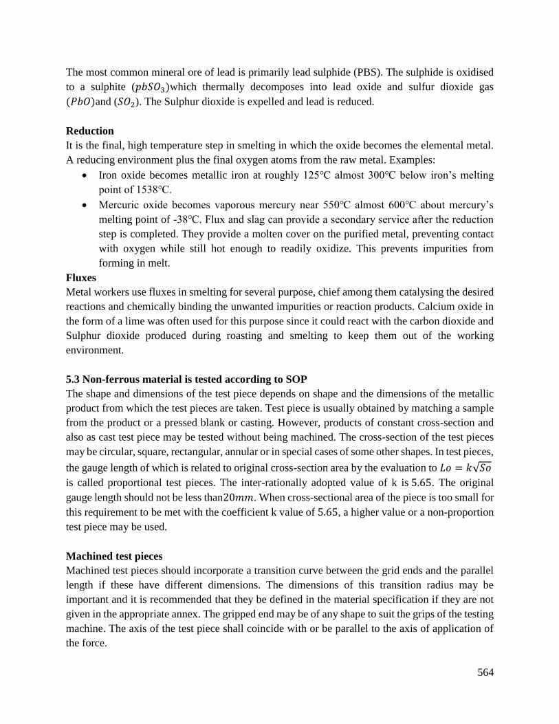
564
The most common mineral ore of lead is primarily lead sulphide (PBS). The sulphide is oxidised
to a sulphite (𝑝𝑏𝑆𝑂3)which thermally decomposes into lead oxide and sulfur dioxide gas
(𝑃𝑏𝑂)and (𝑆𝑂2). The Sulphur dioxide is expelled and lead is reduced.
Reduction
It is the final, high temperature step in smelting in which the oxide becomes the elemental metal.
A reducing environment plus the final oxygen atoms from the raw metal. Examples:
Iron oxide becomes metallic iron at roughly 125 almost 300 below iron’s melting
point of 1538.
Mercuric oxide becomes vaporous mercury near 550 almost 600 about mercury’s
melting point of -38. Flux and slag can provide a secondary service after the reduction
step is completed. They provide a molten cover on the purified metal, preventing contact
with oxygen while still hot enough to readily oxidize. This prevents impurities from
forming in melt.
Fluxes
Metal workers use fluxes in smelting for several purpose, chief among them catalysing the desired
reactions and chemically binding the unwanted impurities or reaction products. Calcium oxide in
the form of a lime was often used for this purpose since it could react with the carbon dioxide and
Sulphur dioxide produced during roasting and smelting to keep them out of the working
environment.
5.3 Non-ferrous material is tested according to SOP
The shape and dimensions of the test piece depends on shape and the dimensions of the metallic
product from which the test pieces are taken. Test piece is usually obtained by matching a sample
from the product or a pressed blank or casting. However, products of constant cross-section and
also as cast test piece may be tested without being machined. The cross-section of the test pieces
may be circular, square, rectangular, annular or in special cases of some other shapes. In test pieces,
the gauge length of which is related to original cross-section area by the evaluation to 𝐿𝑜 = 𝑘√𝑆𝑜
is called proportional test pieces. The inter-rationally adopted value of k is 5.65. The original
gauge length should not be less than20𝑚𝑚. When cross-sectional area of the piece is too small for
this requirement to be met with the coefficient k value of 5.65, a higher value or a non-proportion
test piece may be used.
Machined test pieces
Machined test pieces should incorporate a transition curve between the grid ends and the parallel
length if these have different dimensions. The dimensions of this transition radius may be
important and it is recommended that they be defined in the material specification if they are not
given in the appropriate annex. The gripped end may be of any shape to suit the grips of the testing
machine. The axis of the test piece shall coincide with or be parallel to the axis of application of
the force.
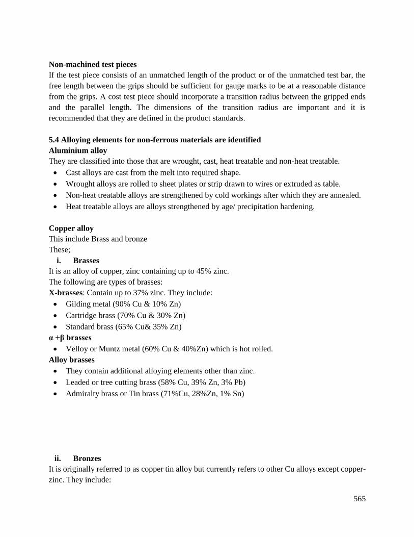
565
Non-machined test pieces
If the test piece consists of an unmatched length of the product or of the unmatched test bar, the
free length between the grips should be sufficient for gauge marks to be at a reasonable distance
from the grips. A cost test piece should incorporate a transition radius between the gripped ends
and the parallel length. The dimensions of the transition radius are important and it is
recommended that they are defined in the product standards.
5.4 Alloying elements for non-ferrous materials are identified
Aluminium alloy
They are classified into those that are wrought, cast, heat treatable and non-heat treatable.
Cast alloys are cast from the melt into required shape.
Wrought alloys are rolled to sheet plates or strip drawn to wires or extruded as table.
Non-heat treatable alloys are strengthened by cold workings after which they are annealed.
Heat treatable alloys are alloys strengthened by age/ precipitation hardening.
Copper alloy
This include Brass and bronze
These;
i. Brasses
It is an alloy of copper, zinc containing up to 45% zinc.
The following are types of brasses:
X-brasses: Contain up to 37% zinc. They include:
Gilding metal (90% Cu & 10% Zn)
Cartridge brass (70% Cu & 30% Zn)
Standard brass (65% Cu& 35% Zn)
α +β brasses
Velloy or Muntz metal (60% Cu & 40%Zn) which is hot rolled.
Alloy brasses
They contain additional alloying elements other than zinc.
Leaded or tree cutting brass (58% Cu, 39% Zn, 3% Pb)
Admiralty brass or Tin brass (71%Cu, 28%Zn, 1% Sn)
ii. Bronzes
It is originally referred to as copper tin alloy but currently refers to other Cu alloys except copper-
zinc. They include:
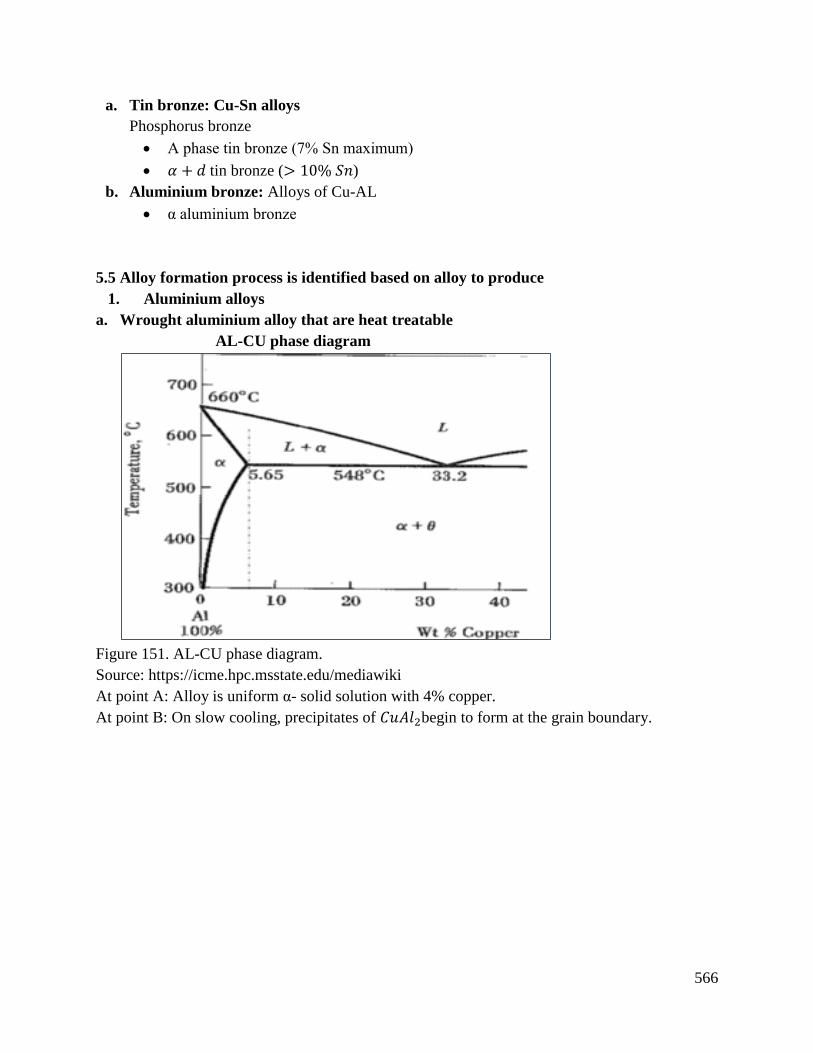
566
a. Tin bronze: Cu-Sn alloys
Phosphorus bronze
Α phase tin bronze (7% Sn maximum)
𝛼 + 𝑑 tin bronze (> 10% 𝑆𝑛)
b. Aluminium bronze: Alloys of Cu-AL
α aluminium bronze
5.5 Alloy formation process is identified based on alloy to produce
1. Aluminium alloys
a. Wrought aluminium alloy that are heat treatable
AL-CU phase diagram
Figure 151. AL-CU phase diagram.
Source: https://icme.hpc.msstate.edu/mediawiki
At point A: Alloy is uniform α- solid solution with 4% copper.
At point B: On slow cooling, precipitates of 𝐶𝑢𝐴𝑙2begin to form at the grain boundary.
567
Figure 152. Grain boundary diagram.
Source: https://commons.wikimedia.org/wiki
At point C: Most of copper is in form of 𝐶𝑢𝐴𝑙2at the grain boundary leaving only 0.2% in solid
solution making the alloy brittle and lack strength.
ii. Wrought aluminium alloys that are not heat treatable
Most widely used contain 10-13% silicon which improves gas tightness, humidity of casting,
reduces shrinkage and imparts excellent feeding characteristics.
Figure 153. Wrought aluminium alloys.
Source: https://www.diva-portal.org
These alloys are approximately eutectile (solidify at a constant temperature) making them suitable
for die casting where rapid ejection is desirable. Sand mould is broken up to remove casting.
Eutectic structure of 𝐴𝐿 − 𝑆𝑖 casting alloys is coarse but can be refined by Sodium.
2. Copper alloys: It contains up to 37%Zn
α
568
X-brasses
a. Grinding metal (90% Cu& 10% Zn) annealed is done.
Used for imitation jewellery on account of its gold-like colour.
b. Cartridge brass (70% Cu, 30% Zn) annealed is done.
Have best combination of strength and ductility.
Used for cartridges and shell cases radiators.
x +β brasses
Vellow and muntze metal (60%Cu& 40% Zn) is hot rolled. Presence of β phase makes alloy
heat treatable.
Used in sheet form for ship strengthening (coring), condenser tubes, brazing rods.
5.6 Alloys for non-ferrous material are tested based on production requirement
Test material
Fatigue tests were carried out on sample of 𝐴𝐿608𝑧 and 𝐴𝐿7075 alloys, whose chemical
composition was comprised in a range recommended by EN 5730-3 standard. The shape and
dimensions of the tested alloy samples are shown in figure I
Figure 154. Fatigue tests
Mechanical testing of 𝑨𝑳𝟔𝟎𝟖𝒛and 𝑨𝑳𝟕𝟎𝟕𝟓 alloys
Fatigue characteristics of 𝐴𝐿608𝑧 and 𝐴𝐿7075alloys were determined from the results of tests
carried out by the modifires low-cycle fatigue method. (MLCF). Fatigue test were carried out on
a Instron machine where the machine control software was written in a lab view environment using
Instron drivers
Conclusion
The learning outcome covered or equipped the learner with knowledge, skills and attitude to be
able to provide non-ferrous materials for industry use. Learners also learn different types of
methods of non-ferrous ore extraction and processes involved.
Further Reading

569
1. ArinashkambleValbharkulkarni. (2017) properties and applications of famous and non-
famous alloys.
2. U.C Jindal (2011) Material science and metallurgy
7.3.6.3 Self-Assessment
1. Discuss 2 methods on how to test non-ferrous materials.
2. Explain 3 methods on how to extract non-ferrous materials (Aluminium, copper) according
to SOP what is (SOP)- Standard Operating Procedures
Written assessment
1. Alloy of copper and zinc is known as?
a) Brass
b) Bronze
c) Duralumin
d) Nichrome
2. Major constituents of nichrome alloy are?
a) Copper
b) Nickel
c) Iron
d) zinc
3. Which of the following alloys is widely used in thermo couple?
a) Brass
b) Bronze
c) Beryllium
d) Nichrome
4. What is the approximate percentage of lead in the soft solder?
a) 60
b) 50
c) 90
d) 99.02
5. Which one of the following is not a non-ferrous material?
570
a) Aluminium
b) Zinc
c) Tin
d) sodium
6. Which one of the following non-ferrous materials is liquid at room temperature?
a) Platinum
b) Gold
c) Aluminium
d) Mercury.
7. Which non-ferrous material is use as antibacterial?
a) Mercury
b) Platinum
c) Gold
d) Silver
8. Explain on how to smelt and extract non-ferrous materials.
9. Describe the process of hydrometallurgy
10. Give to alloys aluminium and describe their foundation.
11. Explain the foundation of aluminium
12. Discuss the alloying elements of non- ferrous materials.
Oral Assessment
1. Describe the test carried out on non-ferrous materials.
Practical Assessment
1. Describe how you can machine test piece to be tested.
Project
As a learner, describe the way you can conserve the environment during non-ferrous ore
production.
7.3.2.4 Tools, Equipment, Supplies and Materials
Measuring tools and gauges
Marking out tools
Inspection tools and equipment
Dressing tools
Firefighting equipment
PPEs –dust coat, dust masks, ear muffs, goggles
First Aid kit
Brooms and cleaning stuff
Cleaning detergents

571
Drawing papers
7.3.2.5 References
H.S and Ray (2011) Extraction of non-ferrous materials
S.K Mandal (2014) non-ferrous materials
U.C.Jindal (2011) Material science and metallurgy
572
7.3.7 Learning Outcome No 6: Produce ceramics materials
7.3.2.1 Learning Activities
Learning Outcome No. 6: Produce ceramics materials
Learning Activities Special Instructions
6.1 Identify composition of ceramic materials (oxides, nitrides,
carbides, silica)
Identify manufacturing process
6.2 Produce ceramic materials according to manufacturing
processes
6.3 Identify finishing processes (lapping, fine grinding, polishing)
Use the correct items
when constructing.
Use material with right
properties.
7.3.2.2 Information Sheet No7/LO6: Produce ceramics materials
Introduction
This learning outcome covers composition of ceramic materials and manufacturing process and
identification of finishing processes.
Definition of key terms
Ceramics: These are non-metallic solids made of inorganic compound such as oxides, nitrates
borides and carbides.
Composition: This is the nature of something such as constituent of something.
Oxide: A chemical compound made up of oxygen combined with at least two other elements.
Sintering: A process by which small particles of material are bonded together by solid state
diffusion.
Content/Procedures/Methods/Illustrations
6.1 Composition of ceramic materials is identified
Silica ceramics: contains constituents of porcelain, magnesium silicates (MgO.SiO2) and mullile
(3Al2O3.2SiO2). Silicates are materials composed of generally silicon and oxygen. Silicate
ceramics are used in electronics and electrical engineering and acts as insulation infuses, circuit
breakers, thermostats and in lighting technology.
Porcelain: A ceramic material made by heating materials generally including clay in the form of
kaolin in a kiln temperature between 12000c to14000c.
Magnesium silicate: A chemical compound constituting of magnesium, silicon and oxygen.
Exists both natural and manufactured.
573
Mullite: A mineralogical name given to the chemically stable intermediate phase in the SiO2-
Al2O3 system.
Carbide ceramics:
Boron carbide: This is a crystalline compound of boron and carbon.
Silicon carbide: This is a synthetically produced crystalline compound of silicon and
carbon.
Tungsten carbide: contains equal parts of tungsten and carbon atoms
Oxide ceramics:
i. Aluminium oxide: A chemical compound of aluminium and oxygen.
ii. Magnesium oxide: A white hydroscopic solid mineral that occurs naturally as prericlose
and is a source of magnesium.
Nitride ceramics: Nitrides used in ceramics consists of nitrogen atoms bonded to elements such
as silicon and aluminium.
a) Silicon nitride: A chemical compound of the element silicon and nitrogen.
b) Aluminium Nitride: A covalently branded ceramic is synthesized from abundantly
available elements aluminium and nitrogen.
Other type of ceramics include; traditional i.e. glass, cement, ferrites concrete etc.
6.2 Manufacturing Process of Ceramics
Consist of four basic stages: shaping, drying, firing and glazing. Sometimes the glaze is applied
before firing (once firing) and sometimes the item is fired, then the glaze is applied and then the
item is re-fired (twice-firing).
Step 1: Shaping: The ingredients are mixed together and soaked in water. The excess water is
squeezed out to make clay with moisture of about 20% then the mixture is shaped appropriately.
This is done by forcing the clay into a mould or by pressing the mould into the clay while spinning
on a turn table.
Processing techniques:
Tape cashing
Slip cashing
Injection moulding
Step 2: Drying. The items are dried slowly in an oven. During this stage, they lose all the water
except that which is bound up in crystal lattices. Before the ware can be fired to high temperatures,
it must be dried to remove water. This results into a 3-7% volume reduction. Water is added to
increase the elasticity of the clay. This water is still present in the body after it has been formed
and can be removed only slowly as it must migrate through the spaces between the particles of
clay, silica and feldspar to evaporate from the surface. During the drying process, the body will
shrink by a significant amount. Shrinkage stops when its particles come into contact. However, if
drying is not uniform stress can build to the extent that the body warps or possibly cracks. Cast
574
ware is in the mould for 0.5-1 hour where some drying occurs, and then air dried for 1-4 days.
Jiggered-ware is dried at a little above ambient temperature for a little over an hour in a ‘mingle-
drier’ and then air dried for 1-5 days.
Step 3: Firing. The item is heated to temperatures up to 11700c during which time the clay
undergoes some chemical changes. The reaction of the clay can be summarized as follows
6Al2Si2O5 (OH) 4 6Al2Si7O7 3Al4SiO12 2Al5Si2O13
Kaolinite metakaolinite silicon spinel mullite.
Silica and water (from the crystal lattice) are also expelled during firing, resulting in a further 5-
7%volume reduction. This silica mixes with silica already present and melts to form a glass. It is
this glass which also includes metallic ions from the feldspar that makes the ceramic item non-
porous and water tight. Once the drying is complete, the body is ready for firing. All unglazed
articles and glazed ones are fired using the ‘once firing’ method.
However, a small number of articles are fired twice in a method where the glaze is applied after
the first biscuit firing and is fixed on by a second gloss firing. In this method, the dried article pas
through the first biscuit (or bisque) firing at a slow rate.
For hallow wares such as cups, the total time from cold through the kiln and back to cold is about
26 hours although modern kiln design is able to significantly decrease both times. After this the
glaze is applied and the ware is fired again. The maximum temperature in both kilns is 11700c. To
understand this process, it is necessary to consider what happens to the individual components of
the body when they are heated to high temperatures.
Step 4: Glazing. Glaze is a thin layer of a glass or glass and crystals that adheres to the surface of
the clay body. It provides a smooth, non-absorbent surface that can be coloured and textured in a
manner not possible on the clay body itself. Glazed are composed in various oxides in proportions
that will yield the desired properties. Silica, SiO2 and Boric oxide B2O3 are the glass formers but
oxides such as Na2O, K2O, CaO, PbO and Al2O3 must be present in the stoichiometric sense to
give the desired properties. These include lowering the viscosity of the molten, glass so that the
glaze will flow smoothly over the surface of the clay body at the temperature at which the glare is
fired.
The glaze is either applied before firing or between a first and a second firing. Glazes are glasses
substances used to provide a smooth surface on the item (which can then be textured if necessary)
and to colour the ceramic surface.
Glaze application:
If a plain coloured article is being produced the glaze is either applied by dipping or
spraying.
575
For patterns, the pattern is printed on a special machine, one colour at a time with a
maximum of 3 colours.
Some patterns are hand printed. When the glaze is applied the articles go through a second
glazing kiln taking up 12 hours of cold to cold to going a through and reaching maximum
of 10500C temperatures.
Some patterns are put on offer glazed by transfer process and these articles then go through
another oven at a temperature of 7200C.
6.4 Production Formula of Ceramic Materials
Extrusion: A process used to create an object of a fixed cross-sectional profile. The
material is pushed or drawn through a die of the desired cross-section. The process has the
ability to create a very complex cross-section and work on brittle materials.
Sintering: A process by which small particles of materials are bonded together by solid
state diffusion. Results in the transformation of porous compact into dewed coherent
product.
Pressing: Ceramic raw materials can be pressed in the dry, plastic or wet condition into a
die to form shaped product. Types of pressing
a) Dry pressing
b) Isostatic
c) hot pressing
Dry pressing: This is uniaxial comp active and shaping of a granular powder along with other
small amount of water and organic binder in a die.
Isostatic pressing: Ceramic powder is loaded into a flexible air light container inside a chamber
of hydraulic fluid to which pressure is applied. After cold isostatic pressing the part must be fired
(sintered) to achieve the require properties and microstructure. Ceramic products such as refractor,
bricks, and carbide tools among others are manufactured using this method.
Hot pressing: Ceramic parts of high density used and improved mechanical properties are
produced by combining properties the pressing and firing operations both uniaxial and isostatic
methods are used.
Slip casting: Slip liquid clay is poured into a plastic mould. The water in the slip is drawn out of
the slip, leaving an inside layer of slip clay. When this is thick enough, the excess slip can be
removed from the mould. When dry the solid clay can then be removed.
6.5 Finishing Process.
Grinding: The abrasives are typically bonded in a grinding wheel and brought into contact
with the ceramic surface at relatively high sliding speed.
Lapping: This is a four-body process that involves an abrasive, a carrier (paste or liquid)
to be applied between the work place surface and a lapping plate.
576
Polishing: The ceramic is pressed against a polishing block with the abrasive suspended
in between them in the form of slurry. The material removal resembles the body.
Conclusion
The learning outcome covered or equipped he learner with knowledge, skills and attitude to
identify manufacturing process of ceramics and their composition as well as identification of
fishing process.
Further Reading
1. Clay and ceramic raw material by DM Worrall
2. Properties of ceramic raw materials by WR Ryan
7.3.7.3 Self-Assessment
Written assessment
1) Porcelain is made for making crockery which is itself being prepared by
a) Mud
b) Soil
c) Clay
d) Silicon
2) Glass, furnace and abrasive for grinding is done by ceramic which contain?
a) Magnesium oxide
b) Aluminum oxide
c) Silicon oxide
d) All of the above
3) An inorganic non-metallic solid prepared by heating a substance to a very high
temperatures is called
a) Molten
b) Ceramic
c) Pirate
d) Metal
577
4) Ceramics can be moulded into different shapes at a very high temperature without affecting
its?
a) Strength
b) Effectiveness
c) Durability
d) None
5) Drawing and firing operations are done in which of this process?
a) Pressing
b) Fibre forming
c) Blowing
d) Slip casting
6) Which of the following is a property of porcelain?
a) Soft
b) Absorbent
c) Vitreous
d) Expensive
7) Salt glazing is manufacturing technique of ceramics
a) structural clay
b) porcelain
c) china
d) pottery
8) State three types of composite materials and their composition
9) List four steps in manufacturing process of ceramics
10) Explain two types of formally process ceramics
11) State two methods of finishing process in ceramics
12) What is the meaning of the term composite
Oral Assessment
1. What is the firing temperature of structural clay products?
2. What is fine grinding in ceramics?
Practical Assessment
1. Trainee to visit an industry dealing with clay works and see the manufacturing process of
ceramics.
Project
Make bricks and structural clay using ceramics materials and give the report after construction
(use ceramic materials with right properties).
7.3.7.4 Tools, Equipment, Supplies and Materials

578
Measuring tools and gauges
Marking out tools
Inspection tools and equipment
Dressing tools
Fire-fighting equipment
PPEs –dust coat, dust masks, ear muffs, goggles
First Aid kit
Brooms and cleaning stuff
Cleaning detergents
Drawing papers
7.3.7.5 References
Abdullah AL Mahmud and Shacmimur Rahman (2009) Ceramic raw material
Dondi, M., Raimondo, M., & Zanelli, C. (2014). Clays and bodies for ceramic tiles: Reappraisal
and technological classification. Applied Clay Science, 96, 91-109.
Ryan, W. (2013). Properties of ceramic raw materials. Elsevier.
579
7.3.8 Learning Outcome No 7: Produce composite materials
7.3.8.1 Learning Activities
Learning Outcome No7:Produce composite materials
Learning Activities Special Instructions
7.1 Identify type of composite to be produced
7.2 Identify elements involve in composite formation
7.3 Identify formation process of composite to be produced
7.4 Test composite as per composite production requirement
Illustrate the concept of
composite materials.
7.3.8.2 Information Sheet No7/LO7: Produce composite materials
Introduction
This learning outcome covers; the composite materials, their production types and formation. This
outcome also covers the formation processes and the testing of the produced materials. A
composite material is a material made from two or more constituent materials with significantly
different physical or chemical properties that when combined, produce a material with
characteristics different from the individual components.
Nowadays, composite materials are used in vehicle and equipment applications including panels,
frames, interior components and other parts. Composite materials are also used in infrastructure
applications such as buildings, roads, bridges and pilings. Composite materials are used for
structural purposes since they have an advantage of combining a number of properties not usually
found together in a single material. Use of composite materials rather than conventional materials
such as steel also provides major weight savings.
Definition of key terms
Composite material: Product made by combining two or more dissimilar materials such as fibres
and resins to create a product with exceptional structural properties not present in the original
materials.
Fibre glass: Filaments made by drawing molten glass, woven by Hexcel into fabrics and
commonly used e.g. a composite reinforcement.
Filament winding: Process to manufacture composite materials, components such as rocket
casings and cylinders.
580
Modules of elasticity: The physical measurement of stiffness in a material. A high module
indicates a stiff material.
Content/Procedures/Methods/Illustrations
7.1 Type of composite to be produced is identified
Depending on the type of materials used and the process involved in composite production, there
are several types of composite materials. Composite materials are classified by the type of
reinforcement they use. Common composite types include random fibre or short fibre
reinforcement, continuous fibre reinforcement particulate reinforcement, flake reinforcement and
filler reinforcement.
Mud building bricks
Brick formed by combining mud and straw. These bricks are flexible and support weight
and resist compression.
Concrete and reinforced concrete
Fibre glass
Types of composites (by reinforcement)
Fibre reinforced composites
Metal matrix composites
Ceramic matrix composites
Particle reinforce composites
Fibre orientation
Sandwich panels
Fibre whine fraction
7.2 Elements involve in composite formation are identified
Many composite materials do exist and depending on the type of composite material and formation
process, the elements to be used must be identified first. Composites being formed from different
materials do not mix the individual materials/components remain separate and distinct within the
finished structure, differentiating composites from mixtures and solid solutions. The new material
may be preferred for various reasons such as strength, weight and cost.
Typical engineered composite materials include:
Reinforced concrete and masonry
Composite wood such as plywood
Reinforced plastics such as fibre-reinforced polymer or fibre glass
Ceramic matrix composites (composite ceramic and metal matrix)
Metal matrix composites
Elements in composite material formation
581
i.Polymers are common matrices (especially used for fibre reinforced plastics).
ii.Road surfaces are often made from asphalt concrete which uses bitumen as a matrix.
iii.Polyester resin tends to have yellowish tint and is suitable for most backyard projects.
iv.Vinyl ester resin tends to have a purplish to bluish to greenish tint. This resin has lower
viscosity than polyester resin and is more transparent. Cement (concrete), metals, ceramics and
sometimes glasses are employed. Unusual matrices such as ice are sometime proposed as in
pylnecele.
v.Whenever one needs to produce composite materials, the elements and the properties of the
individual materials have to be identified. Typically, most common polymer-based composite
materials including fibre glass, carbon fibre and Kevlar, include at least two parts, the substrate
and the resin.
Types of resins include:
a) Thermosetting resins
Unsaturated polyester resins – condensed polyesters, vinyl esters, and allelic derivatives.
b) Polyester resins
Most widely used of all the resins. They have low productivity cost. A wide diversity that
offers many possibilities their adaptation to different fabrication processes that are easy to
carry out and to atomize.
c) Condensation resins
Phenolics, amyloplasts, furan resins.
Advantages include: excellent dimensional stability, good temperature stability, good
chemical resistance, low shrinkage, good mechanical properties and low cost.
d) Furan resins
e) Epoxide resins
f) Fillers and additives: Fillers include; reinforced fillers, spherical fillers, non-reinforcing
fillers, and fine retardant fillers, conductive and antistatic fillers. Additives are incorporated
in small quantities and processed as: mould release agents, pigments and dyes, anti-
shrinkage agents and light stabilizers.
7.3 Formation process of composite to be produced is identified
The basic aim of all composite forming techniques is to mix a resin with a reinforcement (which
may be as woven mat, long fibres or chopped fibres) to produce the desired shape. A variety of
processes exist for various shapes and scales o production. Hand lay-up is perhaps the most
familiar process. It can be used for components of virtually any size, but usually simple shapes.
Similar shapes can be made by spray up which is faster but more expensive. Both processes can
suffer from quality problems. These can be reduced by using vacuum bagging. A variant of
compression moulding called resin transfer moulding (RTM) can be used to make complex parts
or where greater dimensional accuracy is required. Hollow parts can be made by filament including
which can produce parts with optimized mechanical properties. Fibres, tapes and mats are
582
produced by process called pultrusion and continuous laminating. These can also be used to
produce prepares (composite tapes and mats with resin that has not cured).
Economics of processes
There are few composite forming processes and the decision of which to use is normally
determined first by shape and type of fibre and the volume of production. Composite forming
generally is more expensive than in other material classes. This is primarily because of the sow
production rate due to the curing time of the resins. Spray-up, RTM and filament winding can be
automated, so that they are used for mass production. The wear on the dries from the fibres is
significant in RTM and they need to be replaced after every few thousand injections.
7.4 Composite is tested as per composite production requirement
To aid in predicting and preventing failures, composites are tested before and after construction.
Pre-construction testing may use finite element analysis (FEA) for ply by ply analysis of current
surfaces and predicting wrinkling, crimping and dimpling of composites. Materials may be tested
during manufacturing and after construction through several non-destructive methods including
ultra-Sonics, thermograph, stereography and x-ray radiography and laser bond inspection for
relative bond strength integrity in a localized area.
Considerations made in choosing the method of testing
The composite material to be tested, including the type of constituents (fibre and matrix)
and the material form.
The material or structural properties desired stiffness properties or both.
The time, equipment and expertise required to perform the test.
Tensile testing
The fibre reinforced plastic samples are prepared with tabs to prevent a breath in the restraint. For
the tensile measurement, either a video extensometer or a play-in extensometer available in
different sizes is used. For different power ranges, we use force sensors. Mechanical parameters
are determined and the thermal behaviour is investigated in the temperature range between -2690c
to 6000c.
Bending tests
For measuring deflection and bending strength of fibre reinforced plastics. The mechanical
parameters are determined between -2690c to 6000c by use of a moving coil extensometer or cross
head movement of the machine. The tests carried out on a composite material depend on the
intended use of the end results. The tests should be carried out as per the material production
requirement.
Conclusion
583
The learning outcome covered or equipped the learner with knowledge, skills and attitude to
develop composite materials, use them and even recommend on the use of composite materials.
Composite material properties have been convened, the various elements of the composite
materials and the formation processes. Also, the various tests and reasons for the tests carried out
in the composite materials are convened. The learner now has confidence in majoring in the
production of composite materials.
Further Reading
1. Robert M. ones (1999). Mechanics of composite materials. 2nd edition. Taylor St. Francis
Polymers and polymeric composites: A reference series.
2. Leonard Holloway Handbook of polymer (1994) Composites for Engineers published
Wood head publishing.
7.3.8.3 Self-Assessment
Written assessment
1. Composite materials are classified based on?
a) Type of matrix
b) Size and shape of reinforcement
c) Both
d) None
2. Major load carrier in dispersion-strengthened composites?
a) Matrix
b) Fibre
c) Both
d) Cannot define
3. Usually softer constituent of a composite is?
a) Matrix
b) Reinforcement
c) Both are of equal strength
d) Cannot define
4. Usually stronger constituent of a composite is called
a) Matrix
b) Reinforcement
584
c) Both are of equal strength
d) Cannot define
5. Which one of the following is not a laminar composite?
a) Bimetallic
b) Cladding
c) Paints
d) Wood
6. Which one of the following has a greater impact on longitudinal strength of reinforced
composite?
a) Fibre orientation
b) Fibre strength
c) Fibre length
d) None of the mentioned
7. In sandwich composites, which of the following material can be used for filling purpose?
a) Wood
b) Cement
c) Polymer
d) All of the mentioned
8. Which are the methods of composite formation?
9. Outline four considerations made in choosing the method of composite material testing.
10. What are the advantages of using composite materials over single materials?
11. Discuss three types of composite materials.
Oral Assessment
1. Where are composite materials mostly used?
2. Why do we test composite materials?
Practical Assessment
In groups of 5, use the materials provided in the laboratory and produce three types of composite
materials. Carry out the bending tools, tension tests and write a report. What was the main reason
of testing the materials?
Project
In groups of 5, use the composite materials in the workshop and construct a structure of your own
choice. Ensure the structure is loaded and compare the loading strengths of the structure to a
structure constructed using the single materials. Assess the cost and strengths of these two
structures. Which one is more reliable between the two?
585
7.3.8.4 Tools, Equipment, Supplies and Materials
Measuring tools and gauges
Marking out tools
Inspection tools and equipment
Dressing tools
Firefighting equipment
PPEs –dust coat, dust masks, ear muffs, goggles
First Aid kit
Brooms and cleaning stuff
Cleaning detergents
Drawing papers
7.3.8.5 References
Berthelot J. M., Ling F. F (1999). Composite Materials: Mechanical Behaviour and Structural
Analysis. Springer. New York
Daniel I. M., Ishai V. (1994). Engineering Mechanics of Composite Materials. New York
Stankovich S., Dikin D. A., Dommett G. H., Kohlhaas K. M., Zimney E. J., Stach E. A., Runoff
R. S. (2006). Graphere-based Composite Materials. Nature
586
7.3.9 Learning Outcome No 8: Utilize other engineering materials
7.3.2.1 Learning Activities
Learning Outcome No. 8: Utilise other engineering materials
Learning Activities Special Instructions
8.1 Identify and select engineering material according to
production requirements.
8.2 Develop operation plan according to engineering drawing.
8.3 Set up appropriate machine according to manufacturer’s
manual
8.4 Set production parameters according to production
requirement
8.5 Production is performed
8.5 perform production
Use correct methods of
identifying materials.
Use correct engineering
drawing materials.
7.3.2.2 Information Sheet No7/LO8: Utilize other engineering materials
Introduction
This learning outcome covers how to identify and select engineering materials according to
production requirement where we shall focus on material selection. It also covers how to develop
an operation plan according to engineering drawing, where shall see the relationship between
operation plan and process plan. It covers how to set up appropriate machine according to
manufacturers’ manual, and also what an installation manual is. It also covers how to perform
production and considerations taken before the person’s production.
Definition of key terms
Assembly process: a production process in which the basis inputs are combined to create the
output.
Continuous process: a production process that uses long production runs lasting days without
equipment failure.
Customization: production of goods or services one at a time according to specific needs.
Intermittent process: a production process that uses short production runs to make batches of
different products.
Job shop: a manufacturing firm that produces goods in response to customer orders.
587
Mass production: manufacture of many identical goods at once.
Content/Procedures/Methods/Illustrations
8.1 Identify and select engineering material according to production requirements.
Material selection is one of the foremost functions of effective engineering design as it determines
the reliability of a system in terms of industrial and economical aspects.
We concentrate on the properties of the materials which are identified as the potential materials
for that specific design.
Mechanical properties
When a certain design is going to be actually produced it must be subjected to a number of
manufacturing practices depending on material and design process. At the completion of
production, it must be totally fit for the service phase, too in order to predict the reliability
of both requirements; the materials must be able to withstand certain load. Therefore, the
material must possess certain strength and stiffness. Selected materials are examined for
strength and stiffness values, and then potential materials are further inspected for other
desired values.
Wear of materials
Wear is a problem when the materials are contacting each other in a product. So it must be
ensured that the selected materials have sufficient wear resistance. This is done by
designing gears to cope with wear. There are many production techniques available to
improve the wear resistance and make the material more suitable for the application.
Corrosion
The importance of material selection in engineering is clearly visible in corrosive
environment. It is an important engineering design criterion for designs open to
environment for a longer period of time. Some materials are very likely to be corroded in
the service depending on the service environment. Painting or any other surface coating
method is possible ways to minimize the effect and increase the service life.
Ability to manufacture
Although the material is well capable of using for the design, it may be difficult to
manufacture. This is particularly applicable in mechanical engineering design. If this
selection criteria it is neglected the manufacture process might be very costly making it
unprofitable as a commercial product.
Cost
Cost is a critical factor to consider when selecting materials for a certain design for most
products because they are facing a severe competition in the market.
The cost further can be neglected when performance is given to priority. When estimating
costs, the entire associated cost factor must be considered to get a more reasonable value.
It may involve the transportation, processing costs. Other factors include:
Electrical conductivity is vital for electrical application.
588
Design for light weight materials for body vehicle parts.
8.2 Operation plan is developed according to engineering drawing.
Creating an operation plan involve making all the processes that target process engineering.
Process engineering is the art of preparing detailed work instructions to produce a part.
How do we process engineer? We ask ourselves 4 questions.
How can we make it?
How much does it cost?
How reliable will it be?
How much does it cost?
How can we recycle it?
How long will it take us to complete it?
Process plan: this is a detailed plan containing route, processes, process parameters, machine and
tool selection and fixtures. How detailed the plan is depends on the application. Operation plan: a
process containing the description of operation, it includes tools, and process parameters.
Of plan sequence: summary of a process plan.
Factors affecting process plan selection
Size
Tolerance
Shape
Surface finish
Material type
Quantity manufacturing system itself
Requirements in manual process planning
Ability to interpret an engineering drawing.
Familiar with manufacturing processes and practices.
Familiar with tooling and practices.
Know which resources are available at the top.
Know how to use reference books.
Able to do computations on machining time and cost.
Familiar with raw materials.
Know the relative costs of processes, tooling and raw materials.
Process planning steps
i. Study the overall shape of the part. Use this information to classify the part and determine
the type of workstation needed.
ii. Thoroughly study the drawing, try to identify every manufacturing features and notes.
589
iii. If raw stork is not given, determine the best raw material shape to use.
iv. Identify datum surface. Use information on datum surfaces to determine the setups.
v. Select machines for each step.
vi. For each setup determine the rough sequence of operations necessary to create all the
features.
vii. Sequence the operations determined in the previous step.
viii. Select tools for each operation. Try to use the same tools for several operations if it is
possible. Keep in the trade off on tool change time and estimated machining time.
ix. Select or design fixtures for each setup.
x. Evaluate the plan generate thus for and make necessary modifications.
xi. Select cutting parameters for each operation.
xii. Prepare the final process plan document.
8.3 Appropriate machine is set up according to manufacturer’s manual
An owner’s manual is an instructional book that is supplied with almost all technologically
advanced consumer products such vehicles, home appliances, etc.
Information contained in the owner’s manual typically includes:
Safety instructions for liability reasons.
Assembly instructions for products that arrive in pieces for easier shipping.
Installation instruction for products that need to be installed at home.
Setup instruction for devices which maintain user accessible state.
Programming instructions for microprocessor-controlled products.
Maintenance instructions.
Trouble shooting instructions for when product does not work as expected.
Service locations for when product requires repair by a factory authorized technician.
Product technical specifications.
Warranty information provided as a separate sheet.
Installation manual
Is a technical communication document intended to instruct people how to install a
product?
It is written by a technical staff.
Installation is the act of putting something in place so that it’s ready for use.
An installation manual must commonly describe the safe and correct installation of a
product.
The size, structure and content of an installation manual depend heavily on the nature of
the product and the needs and capabilities of intended target group.
There are various standards and directives that are available that provide guidance and
requirements for the design of instructions.
590
The international standard ICE 82079 prescribes the required installation topics for an
installation instruction.
Among these topics are procedures, diagrams, and conditions for installation activities,
such as unpacking, mounting and connecting.
For machines, the European machinery directive prescribes that instruction manual must
contain assembly installation and connecting instructions, including drawings, diagrams
and the means of attachment and designation of the chassis of installation on which
machinery is to be mounted.
8.4 Production parameters are set according to production requirement
We shall use the manufacturing execution module in Microsoft Dynamics AX 2012 R3. For one
to appreciate production parameters being set up the manufacturing execution module is primarily
targeted at manufacturing companies. It can be used to register time and consumption on
production jobs or projects. Production parameter settings affect inventory management,
production management and cost calculation. The parameters for integrating to the production
module are set up on the following tabs in production form:
General: general parameter settings for production jobs in manufacturing execution.
Start: parameters that are used when production operations are started.
Operations: parameters that are applied to production operation and feedback on
operations during production process.
Report as finished: parameters that are applied when terms are reported as finished on the
last operation of a production order.
Quantity validation: parameters for validating start and feedback quantities on production
orders.
Stages of automatic Boom consumption in production parameters
i. At the start the production set this up on the start-up.
ii. During the production process when an operation is completed set this up on the operations
tab.
iii. When a production order is reported as finished set this up on the report as finished tab.
8.5 Production is performed
Production involves converting inputs and outputs. In production planning, the first decision
involves which type of production process: the way a good or service is created, best fits with
company goals and customer demand. We consider the type of goods or service being produced,
because different goods may require different production process.
There are 3 types of production:
a) Mass production: manufacturing many identical goods at once. The emphasis in mass
production is on keeping manufacturing costs low by producing uniform products using
repetitive and standardized process.
591
b) Mass customization: goods are produced using mass production techniques, but only up
to a point. At that point, the product or service is custom, tailored to the needs or desires of
individual customers.
c) Customization: the firm produces goods or services one at time according to specific
needs of individual customers. Each product or service produced is unique.
In a manufacturing company, the inputs, the production process and final outputs are usually
obvious. But the production process in a service company involves a less obvious conversion.
There are two basic processes for converting inputs into outputs:
i. Process manufacturing: the basic inputs are broken down into one or more outputs.
ii. Assembly process: basic inputs are either combined to create the output or transformed into
an output.
A second consideration in choosing a production process is timing. A continuous process uses long
production runs that may last days, weeks without equipment shutdowns. In an intermittent
process, short production runs are used to make batches of different products. Used for low-
volume, high-variety products like those in mass customization. Mass production relies heavily on
standardization, mechanization and specialization.
Conclusion
This learning outcome covered how to develop operation plan according to engineering drawing,
how to perform production and considerations taken before one performs production.
Further Reading
1. G. E Dieter (2016) Mechanical metallurgy
2. R.A Higgins (2010) engineering metallurgy.
3. Richard C, Dorf The engineering handbook
7.3.9.3 Self-Assessment
Written assessment
Multiple choice questions
1. Mechanical properties are not one of the following material selection parameter.
a) True
b) False
c) Not sure
2. Wear is not a problem when materials are contacting each other.
a) True
592
b) Not sure
c) False
3. Creating an operation plan involves making all the process that target process planning.
a) True
b) False
c) Not sure
4. Operation plan is a process containing the description of operation.
a) True
b) False
c) Not sure
5. Operation plan sequence is a summary of process plan.
a) True
b) False
c) Not sure
6. A manufacturer’s manual helps in providing maintenance production.
a) True
b) Not sure
c) False
7. One of the information contained in owner’s manual is safety instruction for liability reasons.
a) True
b) False
c) Not sure
8. The following steps are used in process which one is not?
a) Selecting machine for each step
b) Prepare the final process plan document
c) Select cutting parameters for each operations
d) Know which resources are available to the top
9. Which of the following is not type of production?
a) Mass production
b) Mass customization
c) Product kit
d) Customization
10. Describe different types of production process.
11. How are inputs transformed into outputs in a variety of industries?
12. What types of production do manufacturers and service firms use?
13. Explain mass customization versus mass production.
14. State the importance of customization as a production process.
Oral Assessment
1. Discuss intermittent production in groups.

593
2. Discuss mass production in groups.
Practical Assessment
Carry out brine hardness test on samples and suggest their industrial use for data obtained.
Project
Perform welding of a male and female part and using destructive test, check the hardness index of
the pair.
7.3.9.4 Tools, Equipment, Supplies and Materials
Measuring tools and gauges
Marking out tools
Inspection tools and equipment
Dressing tools
Fire fighting equipment
PPEs –dust coat, dust masks, ear muffs, goggles
First Aid kit
Brooms and cleaning stuff
Cleaning detergents
Drawing papers
7.3.9.5 References
G. E (2010) mechanical metallurgy.
R. A Higgins (2010) engineering metallurgy.
Richard C. dorf,(2010) The engineering hand book
594
7.3.10 Learning Outcome No 9: Perform heat treatment
7.3.10.1 Learning Activities
Learning Outcome No.9: Perform heat treatment
Learning Activities Special Instructions
9.1. Observe safety practices according to OSHA 2007
9.2. Identify heat treatment processes
9.3. Procedure in heat treatment processes
9.4. Perform heat treatment of metals are performed
Use correct tools and
apparatus.
7.3.10.2 Information Sheet No7/LO9: Perform heat treatment
Introduction
This learning outcome covers heat treatment processes on engineering materials and performs heat
treatment of metals.
Definition of key terms
Age hardening: This is hardening of a material through precipitation from solid solution of
coherent transitional phases which produce a strain in the atomic lattice.
Heart treatment: Involves the use of heating or chilling normally to extreme temperature sure to
achieve desired result such as handling of softening of material.
Austempering: A heat-treating process for ferrous metals which increase hardness, fatigue
strength and impact resistance while reducing distortion of the parts.
Content/Procedures/Methods/Illustrations
9.1 Safety practices are observed according to OSHA 2007
The Occupational Health and Safety Act provides for the health, safety and welfare of persons
employed and all persons employed and all persons lawfully present at workplaces and related
matters.
General safety rules and regulations in the workplace
Avoid slippery floors.
Always keep the gangways clear.
Do not operate a machine without familiarization.
Always follow the correct procedures.
595
Report all work injuries and illness immediately.
Only authorized and trained employees may repair or adjust machinery and equipment.
Always wear the PPEs where necessary.
Keep work areas clean and clear.
Always identify the emergency switch.
Causes of accidents in the workshop
The causes of accidents may be classified in 3 categories: mechanical causes, work environment
causes and human causes.
Mechanical causes
They include: unsafe processes; improper plant layout; unsafe design and construction of building
structure; and use of unguarded or improper guarded machines or equipment.
Work environment causes
They include: improper noise level, improper height of working room, improper ventilation and
poor housekeeping (congestion, blocked exits etc.).
Human causes
They include: improper use of tools, failure to use personal protective devices, working at unsafe
speed and long working hours.
Classes of fire and their respective extinguishing agent
Class A: Fire caused by combustion materials such as wood paper or textiles. Water fire
extinguisher is used to put off the fire.
Class B: Fire caused by flammable liquids such as petrol, diesel, and gasoline. Foam fire
extinguisher is used to put off the fire.
Class C: Fire caused by electrical components e.g. motors, appliances and electronic
transformers. Carbon dioxide fire extinguisher is used to put off the fire.
Class D: Fire caused by laboratory chemicals such as titanium, magnesium, aluminium
and potassium. Dry powder fire extinguisher is used to put off the fire.
Class K: cooking fire involving combustion from liquids used in food preparation. Wet
chemical fire extinguishers are used to put off the fire.
First aid: This is preliminary treatment given to the person immediately after the accident before
taking patient to the doctor.
Components of a first aid kit include: rolled bandages 5cm\10cm wide, knife/scissors, Dental,
Burnol, sterilized dressings, safety pins, adhesive plaster, spirit ammonia and washing glass.
Learner performs various first aid to the victim depending on the accident.
9.2 Heat treatment processes are identified
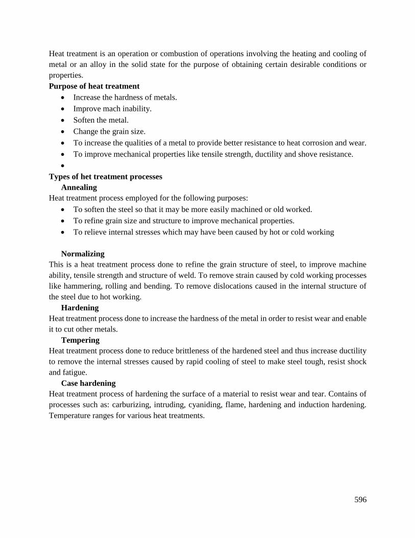
596
Heat treatment is an operation or combustion of operations involving the heating and cooling of
metal or an alloy in the solid state for the purpose of obtaining certain desirable conditions or
properties.
Purpose of heat treatment
Increase the hardness of metals.
Improve mach inability.
Soften the metal.
Change the grain size.
To increase the qualities of a metal to provide better resistance to heat corrosion and wear.
To improve mechanical properties like tensile strength, ductility and shove resistance.
Types of het treatment processes
Annealing
Heat treatment process employed for the following purposes:
To soften the steel so that it may be more easily machined or old worked.
To refine grain size and structure to improve mechanical properties.
To relieve internal stresses which may have been caused by hot or cold working
Normalizing
This is a heat treatment process done to refine the grain structure of steel, to improve machine
ability, tensile strength and structure of weld. To remove strain caused by cold working processes
like hammering, rolling and bending. To remove dislocations caused in the internal structure of
the steel due to hot working.
Hardening
Heat treatment process done to increase the hardness of the metal in order to resist wear and enable
it to cut other metals.
Tempering
Heat treatment process done to reduce brittleness of the hardened steel and thus increase ductility
to remove the internal stresses caused by rapid cooling of steel to make steel tough, resist shock
and fatigue.
Case hardening
Heat treatment process of hardening the surface of a material to resist wear and tear. Contains of
processes such as: carburizing, intruding, cyaniding, flame, hardening and induction hardening.
Temperature ranges for various heat treatments.
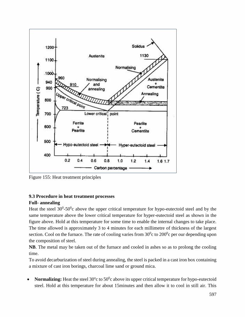
597
Figure 155: Heat treatment principles
9.3 Procedure in heat treatment processes
Full- annealing
Heat the steel 300-500c above the upper critical temperature for hypo-eutectoid steel and by the
same temperature above the lower critical temperature for hyper-eutectoid steel as shown in the
figure above. Hold at this temperature for some time to enable the internal changes to take place.
The time allowed is approximately 3 to 4 minutes for each millimetre of thickness of the largest
section. Cool on the furnace. The rate of cooling varies from 300c to 2000c per our depending upon
the composition of steel.
NB. The metal may be taken out of the furnace and cooled in ashes so as to prolong the cooling
time.
To avoid decarburization of steel during annealing, the steel is packed in a cast iron box containing
a mixture of cast iron borings, charcoal lime sand or ground mica.
Normalizing: Heat the steel 30oc to 500c above its upper critical temperature for hypo-eutectoid
steel. Hold at this temperature for about 15minutes and then allow it to cool in still air. This
598
process provides a homogeneous structure consisting of ferrite and pearlite for hypo-eutectoid
steels and pear lite and commentates for hyper-eutectoid steel.
Hardening: Heat the metal to a temperature of 300-500c above the upper critical temperature
for hypo-eutectoid steel and by the same temperature above the lower critical temperature for
hyper-eutectoid steel. Keep the metal at this temperature for a considerable time depending
upon its thickness.
Tempering: Reheat the hardened steel to some temperature below the lower critical
temperature, followed by any desired rate of cooling. The exact tempering temperature depends
upon the purpose for which the article is to be used. Tempering temperature may be judged by
the colour formed on the surface of the steel being tempered.
9.4 Heat treatment of metals are performed
Trains to perform heat treatment on the given metal, heat treatment is performed on furnaces such
as hearth furnaces and bath furnaces. The selection of a furnace depends upon the following
factors: the size and shape of the product; the volume of production; and the type of heat treatment.
Conclusion
The learning outcome covered or equipped the learner with knowledge, skills and attitude to heat
treatment processes and how they are performed with regard to OSHA.
Further Reading
-
1. Internet: Google on heat treatment PDF, PPT
2. Heat treatment manual
3. Khurm R.S and Ghupta.Heat treatment principles and tecchnixex by TV.Rajan and C.P
Sharma workshop technology (manufacturing process)
7.3.10.3 Self-Assessment
Written assessment
1. Which of the following is a case hardening process?
a) Carburizing
b) Nit riding
c) Cyaniding
d) All of the above
2. Age hardening is related to
a) Duralumin

599
b) Copper
c) Brass
d) Silver
3. The process in which carbon and nitrogen are absorbed by the metal surface to get it hardened
is known as?
a) Carburizing
b) Flame hardening
c) Cyaniding
d) Inclusion hardening
4. The purpose of heat treatment is to?
a) Change grain size
b) Soften the metal
c) Modify the structure of the material
d) Relieve the stresses set up in the material after hot or cold working
5. The temperature point at which the change starts on heating the steel is called.
a) Lower critical point
b) Upper critical point
c) Point of decalescence
d) Point of decalescence
6. In the austempering process of heat treatment, austenite changes into?
a) Marten site
b) Sorbet
c) Troostite
d) Bainite
7. The heat treatment process used for softening hardened steel is?
a) Carburizing
b) Annealing
c) Normalizing
d) Tempering
8. Explain three classes of fire.
9. Outline the process of normalizing.
10. State four types of fire extinguishers.
11. Distinguish between tempering and annealing.
Oral Assessment
1. What do you understand by case hardening?
2. Name various case hardening processes.
3. What is the process of heat treatment?
Practical Assessment
Trainees to be provided with steel metal and perform heat treatment process on it.

600
7.3.10.4 Tools, Equipment, Supplies and Materials
Inspection tools and equipment
Fire-fighting equipment
PPEs –dust coat, dust masks, ear muffs, goggles
First Aid kit
Brooms and cleaning stuff
Cleaning detergents
7.3.10.5 References
Khurm, R. S and Ghupta (2011) Workshop Technology (Manufacturing Processes)
S. K. Garg (2010) Workshop Technology Manufacturing Processes
TV Rajan and CP Sharma (2011) Heat treatment principles and techniques
601
7.3.11 Learning Outcome No 10: Perform material testing
7.3.11.1 Learning Activities
Learning Outcome No.10: Perform material testing
Learning Activities Special Instructions
10.1 Test safety is observed in material procedures
10.2 Identify material testing methods depending on material to
be tested
10.3 Follow procedure of material testing as per material testing
method
10.4 Tabulate, calculate and interpret material testing results
10.5 Take care of and maintain material testing equipment.
Materials testing
Methods should be
discussed on basis of
material to be tested
Material testing
equipment’s have to be
provided too.
7.3.11.2 Information Sheet No7/LO10: Perform material testing
Introduction
This learning outcome covers material testing, tabulation of material testing results. Materials
testing are a well-established technique used to determine the physical and mechanical properties
of materials and components including composite material and ceramics.
Definition of key terms
Destructive Test: The specimen of the material is tested until its complete structure falls in order
to find its mechanical properties and characteristics. After the test is over material (Specimen)
becomes useless.
Non-destructive test: Material under test possesses the same mechanical properties before and
after the test.
Brinell hardness number (B.H.N)
It is a number expressing Brinell hardness and denoting the load applied in testing in kilograms
divided by the spherical area of indentation produced by the specimen in square millimetres.
Elastic limit
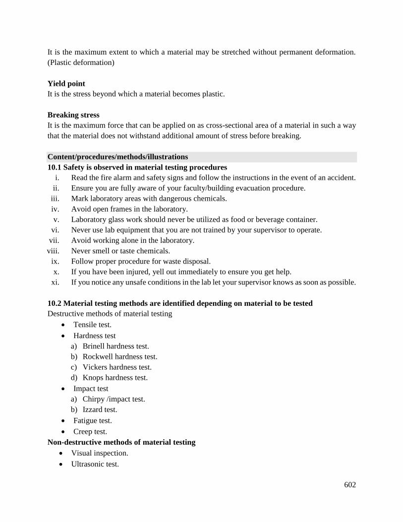
602
It is the maximum extent to which a material may be stretched without permanent deformation.
(Plastic deformation)
Yield point
It is the stress beyond which a material becomes plastic.
Breaking stress
It is the maximum force that can be applied on as cross-sectional area of a material in such a way
that the material does not withstand additional amount of stress before breaking.
Content/procedures/methods/illustrations
10.1 Safety is observed in material testing procedures
i. Read the fire alarm and safety signs and follow the instructions in the event of an accident.
ii. Ensure you are fully aware of your faculty/building evacuation procedure.
iii. Mark laboratory areas with dangerous chemicals.
iv. Avoid open frames in the laboratory.
v. Laboratory glass work should never be utilized as food or beverage container.
vi. Never use lab equipment that you are not trained by your supervisor to operate.
vii. Avoid working alone in the laboratory.
viii. Never smell or taste chemicals.
ix. Follow proper procedure for waste disposal.
x. If you have been injured, yell out immediately to ensure you get help.
xi. If you notice any unsafe conditions in the lab let your supervisor knows as soon as possible.
10.2 Material testing methods are identified depending on material to be tested
Destructive methods of material testing
Tensile test.
Hardness test
a) Brinell hardness test.
b) Rockwell hardness test.
c) Vickers hardness test.
d) Knops hardness test.
Impact test
a) Chirpy /impact test.
b) Izzard test.
Fatigue test.
Creep test.
Non-destructive methods of material testing
Visual inspection.
Ultrasonic test.
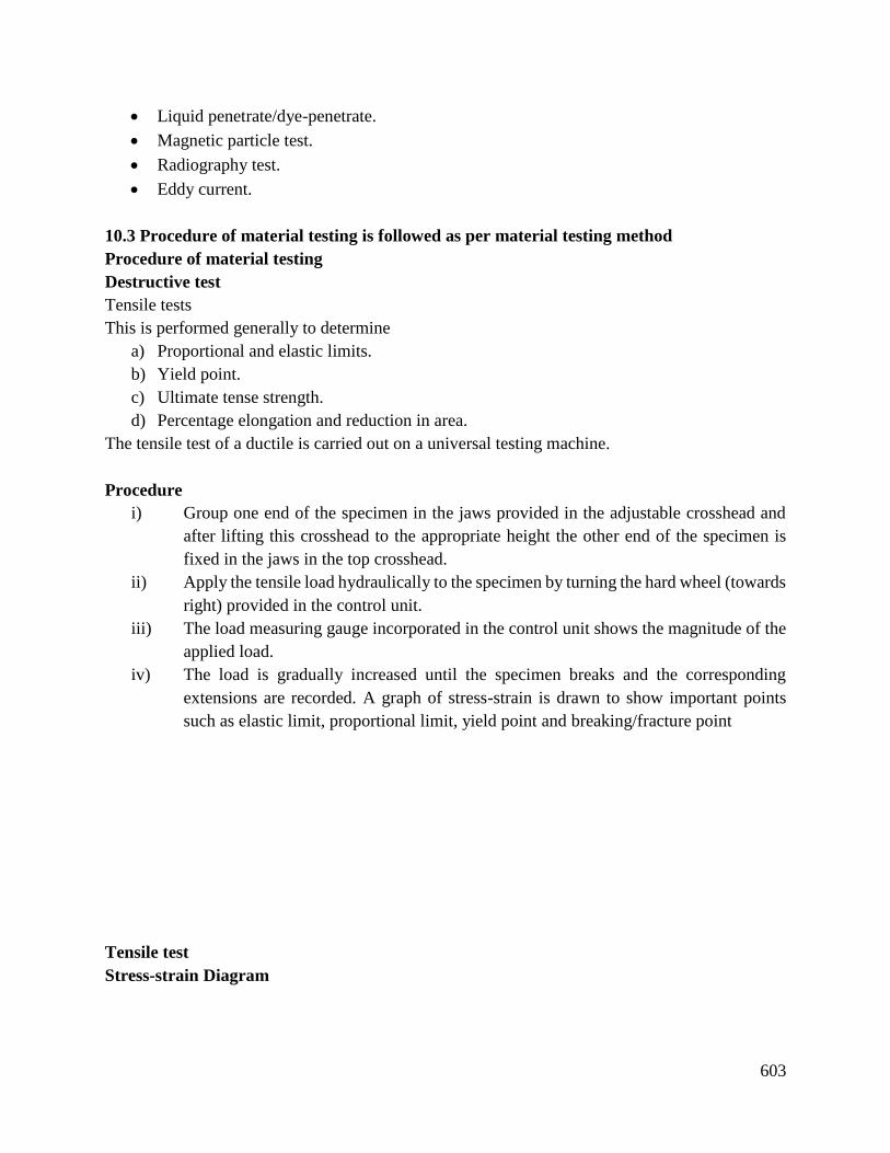
603
Liquid penetrate/dye-penetrate.
Magnetic particle test.
Radiography test.
Eddy current.
10.3 Procedure of material testing is followed as per material testing method
Procedure of material testing
Destructive test
Tensile tests
This is performed generally to determine
a) Proportional and elastic limits.
b) Yield point.
c) Ultimate tense strength.
d) Percentage elongation and reduction in area.
The tensile test of a ductile is carried out on a universal testing machine.
Procedure
i) Group one end of the specimen in the jaws provided in the adjustable crosshead and
after lifting this crosshead to the appropriate height the other end of the specimen is
fixed in the jaws in the top crosshead.
ii) Apply the tensile load hydraulically to the specimen by turning the hard wheel (towards
right) provided in the control unit.
iii) The load measuring gauge incorporated in the control unit shows the magnitude of the
applied load.
iv) The load is gradually increased until the specimen breaks and the corresponding
extensions are recorded. A graph of stress-strain is drawn to show important points
such as elastic limit, proportional limit, yield point and breaking/fracture point
Tensile test
Stress-strain Diagram
604
Figure 156: Strain Diagram
A= limit of proportionality.
The maximum stress up to which Hooke’s law is valid stress is directly proportional to strain.
B= Elastic limit.
The maximum stress which the material can withstand without causing permanent deformation.
C= Yield point upper.
D= Yield point lower.
If the material is stressed beyond elastic limit plastic stage will reach.
E= Ultimate point.
If further load is applied beyond point D the stress goes on increasing until the point E is reached.
F= Breaking stress.
A neck is formed which decreases the cross-sectional area of the specimen.
Hardness test
This method is used in all metals hard and soft and also on non-metallic material such as timber,
plastic, etc.
Types of hardness test
i. Brinell hardness test
The method uses a ball of 10mm diameter as indenter. The indenter is first placed upon the surface
whose hardness is to be measured and then a gradually increasing load of 300kg are applied upon
the indenter when the load is removed; an indent is left upon the surface. If the material is hard,
instead of a steel ball, a tunstel carbide indenter is used. For softer material a lower load of 500kg
605
is applied to avoid very deep indentation. The diameter of indentation is measured by lower power
microscope and tabulated.
Brinell hardness number. B.H. N=(𝑝
(𝜋𝐷
2)(𝐷−√𝐷2−𝑑2)
)
P= applied load
D= Diameter of the ball mm.
d=Diameter of indentation
Figure 157: Brinell test
Source: Principal of Material/ science and Engineering.
ii. Rockwell hardness test
Performed when quick and direct reading is desirable. Performed when materials have hardness
beyond range of Brinell hardness test. A standard ball indenter of hardened tool steel or tungsten
carbide of 1.588mm diameter or a diamond con indenter of 120˚C angle with spherical tip is used.
Procedure
i) The specimen is placed on the anvil and it is raised by the hard wheel till it comes in
contact with the indenter.
ii) A minor load of 100N is applied on the specimen and the small pointer indicates “set”.
iii) The main pointer is also brought to the set position.
iv) The major load is applied and allowed to continue for 3 to 5 seconds. The depth of
indentation (in mm) is read from the small pointer. The Rockwell number is obtained
mathematically.
HRB=130-𝐷𝑒𝑝𝑡ℎ 𝑜𝑓 𝑖𝑛𝑑𝑒𝑛𝑡𝑎𝑡𝑖𝑜𝑛 𝑖𝑛 𝑚𝑚
0.002
Hardness number on B scale
Hardness number on C scale
HRC=100-𝐷𝑒𝑝𝑡ℎ 𝑜𝑓 𝑖𝑛𝑑𝑒𝑛𝑡𝑎𝑡𝑖𝑜𝑛 𝑖𝑛 𝑚𝑚
0.002
iii. Vickers hardness test
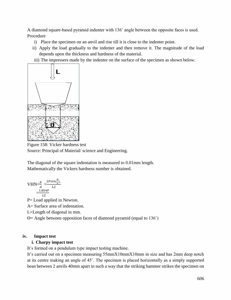
606
A diamond square-based pyramid indenter with 136˚ angle between the opposite faces is used.
Procedure
i) Place the specimen on an anvil and rise till it is close to the indenter point.
ii) Apply the load gradually to the indenter and then remove it. The magnitude of the load
depends upon the thickness and hardness of the material.
iii) The impressers made by the indenter on the surface of the specimen as shown below.
Figure 158: Vicker hardness test
Source: Principal of Material/ science and Engineering.
The diagonal of the square indentation is measured to 0.01mm length.
Mathematically the Vickers hardness number is obtained.
VHN=𝑝
𝐴 =
2𝑃𝑠𝑖𝑛(Ɵ
2)_
L2
=1.854𝑃
𝐿2
P= Load applied in Newton.
A= Surface area of indentation.
L=Length of diagonal in mm.
Ɵ= Angle between opposition faces of diamond pyramid (equal to 136˚)
iv. Impact test
i. Charpy impact test
It’s formed on a pendulum type impact testing machine.
It’s carried out on a specimen measuring 55mmX10mmX10mm in size and has 2mm deep notch
at its centre making an angle of 45˚. The specimen is placed horizontally as a simply supported
bean between 2 anvils 40mm apart in such a way that the striking hammer strikes the specimen on
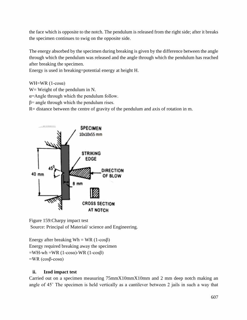
607
the face which is opposite to the notch. The pendulum is released from the right side; after it breaks
the specimen continues to swig on the opposite side.
The energy absorbed by the specimen during breaking is given by the difference between the angle
through which the pendulum was released and the angle through which the pendulum has reached
after breaking the specimen.
Energy is used in breaking=potential energy at height H.
WH=WR (1-cosα)
W= Weight of the pendulum in N.
α=Angle through which the pendulum follow.
β= angle through which the pendulum rises.
R= distance between the centre of gravity of the pendulum and axis of rotation in m.
Figure 159:Charpy impact test
Source: Principal of Material/ science and Engineering.
Energy after breaking Wh = WR (1-cosβ)
Energy required breaking away the specimen
=WH-wh =WR (1-cosα)-WR (1-cosβ)
=WR (cosβ-cosα)
ii. Izod impact test
Carried out on a specimen measuring 75mmX10mmX10mm and 2 mm deep notch making an
angle of 45˚ The specimen is held vertically as a cantilever between 2 jails in such a way that
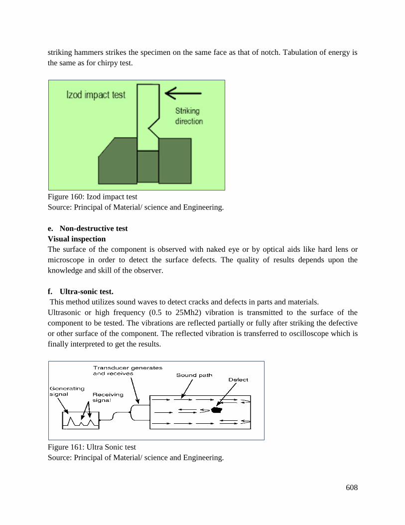
608
striking hammers strikes the specimen on the same face as that of notch. Tabulation of energy is
the same as for chirpy test.
Figure 160: Izod impact test
Source: Principal of Material/ science and Engineering.
e. Non-destructive test
Visual inspection
The surface of the component is observed with naked eye or by optical aids like hard lens or
microscope in order to detect the surface defects. The quality of results depends upon the
knowledge and skill of the observer.
f. Ultra-sonic test.
This method utilizes sound waves to detect cracks and defects in parts and materials.
Ultrasonic or high frequency (0.5 to 25Mh2) vibration is transmitted to the surface of the
component to be tested. The vibrations are reflected partially or fully after striking the defective
or other surface of the component. The reflected vibration is transferred to oscilloscope which is
finally interpreted to get the results.
Figure 161: Ultra Sonic test
Source: Principal of Material/ science and Engineering.
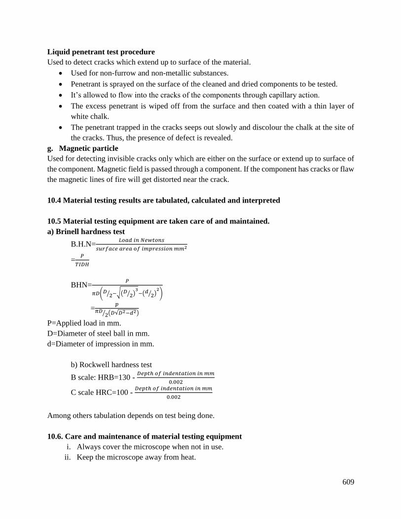
609
Liquid penetrant test procedure
Used to detect cracks which extend up to surface of the material.
Used for non-furrow and non-metallic substances.
Penetrant is sprayed on the surface of the cleaned and dried components to be tested.
It’s allowed to flow into the cracks of the components through capillary action.
The excess penetrant is wiped off from the surface and then coated with a thin layer of
white chalk.
The penetrant trapped in the cracks seeps out slowly and discolour the chalk at the site of
the cracks. Thus, the presence of defect is revealed.
g. Magnetic particle
Used for detecting invisible cracks only which are either on the surface or extend up to surface of
the component. Magnetic field is passed through a component. If the component has cracks or flaw
the magnetic lines of fire will get distorted near the crack.
10.4 Material testing results are tabulated, calculated and interpreted
10.5 Material testing equipment are taken care of and maintained.
a) Brinell hardness test
B.H.N=𝐿𝑜𝑎𝑑 𝑖𝑛 𝑁𝑒𝑤𝑡𝑜𝑛𝑠
𝑠𝑢𝑟𝑓𝑎𝑐𝑒 𝑎𝑟𝑒𝑎 o𝑓 𝑖𝑚𝑝𝑟𝑒𝑠𝑠𝑖𝑜𝑛 𝑚𝑚2
=𝑃
𝑇𝐼𝐷𝐻
BHN=𝑃
𝜋𝐷(𝐷2⁄ −√(𝐷 2⁄ )
3−(𝑑 2⁄ )
2)
=𝑝
𝜋𝐷2⁄ (𝐷√𝐷2−𝑑2)
P=Applied load in mm.
D=Diameter of steel ball in mm.
d=Diameter of impression in mm.
b) Rockwell hardness test
B scale: HRB=130 - 𝐷𝑒𝑝𝑡ℎ 𝑜𝑓 𝑖𝑛𝑑𝑒𝑛𝑡𝑎𝑡𝑖𝑜𝑛 𝑖𝑛 𝑚𝑚
0.002
C scale HRC=100 - 𝐷𝑒𝑝𝑡ℎ 𝑜𝑓 𝑖𝑛𝑑𝑒𝑛𝑡𝑎𝑡𝑖𝑜𝑛 𝑖𝑛 𝑚𝑚
0.002
Among others tabulation depends on test being done.
10.6. Care and maintenance of material testing equipment
i. Always cover the microscope when not in use.
ii. Keep the microscope away from heat.
610
iii. Always clear the machine after use.
iv. Oil and lubricate the machines regularly.
v. Avoid sharp objects on the machine.
vi. Store your test blocs in the plastic bag.
vii. Always send your tester back for yearly cleaning and re-calibration.
viii. Use the appropriate identifier, anvil for the application.
Conclusion
The learning outcome covered or equipped the learner with knowledge, skills and attitude to
perform material testing perfectly.
Further Reading
1. Ex. R.k. Rajput. Engineering Materials and Metallurgy. S. Chard.
2. Smith. W.F (1990). Principal of Material/ science and Engineering.
3. Mc Graw-Hill inc.US. New York USA
7.3.11.3 Self-Assessment
Written assessment
1. In a chirpy test specimen is placed _____as a simply supported beam between 2 anvils.
a) Horizontally.
b) Vertically.
2. The size of a specimen for 120d impact test is?
a) 45mmX4mmX4mm.
b) 65mmX8mmX8mm
c) 55mmX6mmX6mm.
d) 75mmX10mm
3. Which of the following is a non-destructive test?
a) Tensile test.
b) Compression test.
c) Ultrasonic test.
d) Creep test.
4. In Vickers hardness test. The angle between the opposite faces of diamond pyramid is?
a) 36˚.
b) 72˚.
c) 108˚.
611
d) 136˚.
5. The ultimate stress of a material is _________than the breaking stress.
a) Higher.
b) Lower.
6. The maximum amounts of energy which can be stored in a body up to the elastic limit is
known as?
a) Modulus of resilience.
b) Modulus of toughness.
c) Modulus of elasticity.
d) Proof resilience.
7. In order to find the Brinell hardness number of steel with an indenter of 10mm diameter,
the load is applied.
a) 30 KN.
b) 40KN.
c) 50KN.
d) 60KN.
8. What is the meaning of the following terms.
a) Stress.
b) Strain.
9. Distinguish between destruction and non-destruction material testing.
10. Draw a stress-strain diagram for a mild steel specimen under tensile testing.
11. List 5 care and maintenance of material testing equipment.
12. State 4 safety precautions to be observed in material testing?
Oral Assessment
1. What is material testing?
2. What is limit of proportionality?
Practical Assessment
1. Trainees to perform material testing on a steel ball. Check on the hardness number tabulates
it using Brinell hardness test.
Project
1. Through laboratory testing, the student will participate in a project that is aimed at
developing new protocols to be used by 4 searchers and industry to better characterize
performance of both unbound and bound materials, which are used base layers in road
pavements.
7.3.11.4 Tools, Equipment, Supplies and Materials
Measuring tools and gauges
Marking out tools

612
Inspection tools and equipment
Dressing tools
Fire fighting equipment
PPEs –dust coat, dust masks, ear muffs, goggles
First Aid kit
Brooms and cleaning stuff
Cleaning detergents
Drawing papers
7.3.11.5 References
Garg.S.K (2009). Workshop Technology (manufacturing processes). Laxmi Publication Pvt
Limited
Rajput. R.K. (2006). Engineering materials and metallurgy. S. Chand Limited
RsKhurmi,J.K Gupta. (2010). textbook of workshop technology: manufacturing processes. S.
chand&co.ltd. New Delhi, India.
613
7.3.12 Learning Outcome No 11: Prevent material corrosion
7.3.2.1 Learning Activities
Learning Outcome No. 11: Prevent material corrosion
Learning Activities Special Instructions
11.1 Observe safety during corrosion prevention
11.2 Identify corrosion type (galvanic, stress corrosion cracking)
11.3 Identify corrosive atmosphere
11.4 Identify methods of corrosion prevention (painting, electroplating,
galvanizing, cathode)
11.5 Prevent corrosion
Make sure to use the
correct methods
Use procedure as
indicated below
Use proper tools and
equipment for
prevention.
7.3.12.2 Information Sheet No7/LO11: Prevent material corrosion
Introduction
This learning outcome covers definition of key terms corrosion methods and its prevention.
Definition of key terms
Corrosion: Natural process that converts a refined metal into a more chemically stable form such
as oxide, hydroxide or sulphide.
Cladding: A covering or coating on a structure or material.
Content/Procedures/Methods/Illustrations
11.1 Safety is observed during corrosion prevention
Wear gloves, shield or goggles where necessary.
Beware of toxic compounds.
Always identify the chemicals as per the label.
Avoid skin contact. galvanic corrosion,
Avoid breathing corrosive vapour fumes, dusts or mists.
Always ensure good ventilation.
Allow only trained, authorized people to storage areas.
Inspect storage areas regularly for any defect clues including corrosive damage, leaking
containers or poor housekeeping.
Keep corrosive containers tightly closed.
614
Avoid touching yourself with contaminated hands.
Remove and clear contaminated clothing before wearing it again or discard it.
11.2 Corrosion type is identified
These include; galvanic corrosion, stress cracking, caustic agent corrosion, localized corrosion and
general corrosion
Galvanic corrosion: It occurs when two metals with different electrochemical charges are linked
through a conductive path. Corrosion occurs when one metal ion moves from the anodized metal
to the cathode metal. Galvanic corrosion can also occur when one impure metal is present.
Stress corrosion cracking (SCC): When a metal component is subjected to extreme tensile stress,
it can experience stress corrosion cracking along the grain boundary. Craves forms are the target
for further corrosion.
General corrosion: It occurs as a result of rust. When a metal is exposed to water, the surface is
oxidized and a thin layer of rust appears. It is electrochemical.
Localized corrosion: It occurs when a small part of a component experiences corrosion or comes
into contact with specific corrosion causing stresses.
Caustic agent corrosion: It occurs when impure gas, liquids or solids wear a material down.
Although most impure gases do not damage metals in dry form, when exposed to moisture, they
dissolve to form harmful corrosive droplets.
11.3 Corrosive atmosphere is identified
Atmospheric corrosion is the corrosive action that occurs on the surface of a metal in an
atmospheric environment. It occurs when the surface is wet by moisture formed due to rain, fog
and condensation. It is a complex process involving a large number of interacting and constantly
varying factors such as weather condition, air pollution, and material conditions among others.
The combined effect of these factors results in a great variation in corrosive rates.
11.4 Methods of corrosion prevention are identified
Iodization
The metal to be protected is bathed in a specific substance and electrochemical conditions are
adjusted e.g. cathode protection. This involves coating of iron alloy steel with zinc (galvanizing).
Painting and coating
Iron is painted or given a suitable coating to exclude the atmosphere. Oxide coating, phosphate
coating and concrete coating are used. Red lead is the commonly used paint.
Tarring
Metal is dipped in hot coal tar so that a film of it sticks to the surface which protects the surface
from rusting and corrosion.
615
Enamelling
High grade bases like zinc oxide or lead oxide ground in oil or varnish are used. They dry slowly
leaving a hard, tough and elastic film which is smooth and durable.
Galvanizing
This is depositing a fine film of zinc on the iron or steel surface. The surfaces to be galvanized are
first cleared of all foreign matter by giving it an acid wash to be followed by a wash of clear water.
It is then dried and dipped in molten zinc.
Sherardizing
Surface to be treated is cleaned of all foreign deposits by washing it with acid solution and then
with clean water. It is then dried and covered with zinc dust and enclosed in steel boxes to be
heated in a furnace under controlled temperatures. Molten zinc spread over the whole surface and
cooling forms a thin protective layer.
Tin plating
After cleaning the surface with acid wash followed by washing clean water and drying, it is dipped
in a bath of molten tin. A protective covering of tin is left on the surface.
Corrosion is prevented
Corrosion is prevented according to the nature of the material.
Methods of stopping and preventing metal corrosives
Turn to non-corrosive metal such as aluminium and stainless steel.
Keep the areas around the metal surface dry.
Use drying agents and moisture barriers products.
Make sure underground piping is laid in a lays of backfill such as limestone.
How Corrosion is prevented
Sacrificial protection: It is protection of iron or steal against corrosion by using more metals,
pieces at once or magnesium alloy are attached to pump bodies and pipes.
The protected metal becomes the cathode and does not corrode. The anode corrodes, thereby
providing the deserved sacrificial protect. The most common method of preventing is by removing
one or coating a metal surface with paint or enamel provide a barrier between metal and the
moisture.
Conclusion
The learning outcome covered or equipped the learner with knowledge, skills and attitude to
identify types of corrosion and their prevention methods.
616
Further Reading
1. Metallurgy by Higgins. Engineering materials
2. Chemistry Book 4
3. M. G. Fanatana. Corrosion engineering
7.3.12.3 Self-Assessment
Written assessment
1. Corrosion is reverse process of
a) Metal extraction
b) Metal production
c) Metal heating
d) Metal moulding
2. Which of the following property is not lost during corrosion?
a) Malleability
b) Ductility
c) Conductivity
d) Colour
3. In corrosion as a result of decay, the metals are converted into
a) Oxides
b) Hydroxides
c) Carbonates
d) Peroxides
4. Dry corrosion is also called
a) Chemical corrosion
b) Electrochemical corrosion
c) Wet corrosion
d) Oxidation corrosion
5. Which of the following process can minimize rusting?
a) Galvanization
b) Vulcanization
c) Sublimation
d) Condensation
6. Electrochemical corrosion takes place on
a) Anodic area
b) Cathodic area
617
c) Near cathode
d) Near anode
7. Which of the following is not a corrosion prevention method?
a) Sherardizing
b) Galvanizing
c) Tarring
d) None of the above
8. What is the meaning of the term corrosion.
9. What do you understand by electroplating as used in corrosion.
10. State five types of corrosion
11. Distinguish between sherardizing and anodization
12. State five safety rules to be observed in corrosion.
Oral Assessment
1. What is cladding as used in corrosion?
2. What is beam protection in corrosion?
Practical Assessment
Trainees to perform corrosion prevention methods on materials provided.
7.3.12.4 Tools, Equipment, Supplies and Materials
Specimen
Fire-fighting equipment
PPEs –dust coat, dust masks, ear muffs, goggles
First Aid kit
Brooms and cleaning stuff
Cleaning detergents
7.3.12.5 References
H. H. U hug and R. W. Rene (2011) Corrosion and in control
Higgins (2000) Engineering materials and metallurgy
M. G. Fontana (2014) Corrosion Engineering
CHAPTER 8: ELECTRICAL PRINCIPLES/ APPLY ELECTRICAL SCIENCE
PRINCIPLES
8.1 Introduction
Electrical Principles is among the common units of competencies offered in TVET level 6
engineering courses qualification. This unit describes the competencies required by a technician
618
in order to apply a wide range of Electrical principles skills in their work; use the concept of basic
Electrical quantities, use the concepts of D.C and A.C circuits in electrical installation, use of basic
electrical machine, use of power factor in electrical installation, use of earthling in Electrical
installations, use of earthling in Electrical installations and apply lightning protection measures.
The significance of Fluid Mechanics to TVET level 6 engineering curriculum is to enable learners
acquire knowledge and skills to demonstrate how to apply basic Electrical formulas, use of basic
Electrical instruments, perform various unit conversions of Electrical quantities, Electrical
earthing, lightening arrestors, Power factor correction, logical thinking, problem solving, applying
statistics, drawing graphs and using different measuring tools to get along well in the workplace
and task.
The critical aspect of competency to be covered includes identified applied the correct SI units of
Electrical quantities, Stated, Calculate and relates the quantities in Ohm’s law, Identified the
components of an earthing system, Stated and apply various laws in Electrical system,
differentiated between AC and DC network, applied correct formulas in the calculation of AC and
DC machines, used power triangle in calculating power factor, applied various methods in power
factor correction and Identified types of lightening arrestors and their applications. The basic
resources required includes access to relevant workplace or appropriately simulated environment
where assessment can take place, measuring tools and equipment, Sample materials to be tested
among others. The unit of competency covers twelve learning outcomes. Each of the learning
outcome presents; learning activity that covers performance criteria statements, thus creating
trainee’ an opportunity to demonstrate knowledge and skills in the occupational standards and
content in curriculum. Information sheet provides; definition of key terms, content and illustration
to guide in training. The competency may be assessed through direct observation, demonstration
with oral questioning and written tests. Self-assessment is provided at the end of each learning
outcomes. Holistic assessment with other units relevant to the industry sector workplace and job
role is recommended.
8.2 Performance Standard
Use the concept of basic electrical quantities, use the concepts of D.C and A.C circuits in electrical
installation, use of basic electrical machine, use of power factor in electrical installation, use of
earthing in electrical installations, apply lightning protection measures, apply electromagnetic field
theory, apply electrodynamics, apply energy and momentum in electromagnetic field, apply
transient in electrical circuit analysis, use two port network and demonstrate understanding of
refrigeration and air conditioning in accordance with the set standards.
8.3 Learning Outcomes
8.3.1 List of Learning Outcomes
a) Use the concept of basic Electrical quantities
b) Use the concepts of D.C and A.C circuits in electrical installation

619
c) Use of basic electrical machine
d) Use of power factor in electrical installation
e) Use of earthling in Electrical installations
f) Apply lightning protection measures
g) Apply Electromagnetic field theory
h) Apply Electrodynamics
i) Apply Energy and momentum in Electromagnetic field
j) Apply Transient in Electrical circuit analysis
k) Use two port networks
l) Demonstrate understanding of Refrigeration and Air conditioning
620
8.3.2 Learning Outcome No 1: Use the concept of basic Electrical quantities
8.3.2.1 Learning Activities
Learning Outcome No 1: Use the concept of basic Electrical quantities
Learning Activities Special Instructions
1.1 Identify basic SI units (Power-Watts (W), current – Amperes A,
resistance –OhmsΩ, and Voltage-Volts V) in Electrical.
1.2 Identify Quantities (charge, force, work, power) of Charge, force,
work and power.
1.3 Perform calculations involving various electrical quantities.
8.3.2.2 Information Sheet No8/LO1: Use the concept of basic Electrical quantities
Introduction
The basic electrical quantities are electrical current and voltage, electrical charge, resistance,
capacitance, inductance and electrical power.
This learning outcome covers these electrical quantities definitions, SI units, calculations involving
electrical quantities and how they relate to Ohm’s law. Understanding the basis electrical quantities
will equip one with competence required for the application of basics of electrical principles.
Definition of key terms
Electric current. It is defined as the rate of flow of electric current charge through the conductor
with respect to the time. Represented by I. The SI unit (International system of units) is Ampere
(A). Smaller currents are measured in mill amperes (mA). Mill amperes can be converted to
Amperes through this conversion.
1A= 1,000 mA
Voltage: Also called electromotive force, it is the potential difference in charge between two
points in an electric field.
The SI unit for voltage is volts (V).
Electrical Resistance: It is opposition to the flow of current to the flow of current in an electric
circuit. It is represented by R
The unit for of resistance is the Ohm, symbol Ω
Ohm’s law: It states that electric current is proportional to voltage and inversely proportional to
resistance.
621
That is, current= 𝑣𝑜𝑙𝑡𝑎𝑔𝑒
𝑟𝑒𝑠𝑖𝑠𝑡𝑎𝑛𝑐𝑒, I =
𝑉
𝑅
𝑉 = 𝐼𝑅
Where; 𝑉 = 𝑉𝑜𝑙𝑡𝑎𝑔𝑒
𝐼 = 𝐶𝑢𝑟𝑟𝑒𝑛𝑡
R= Resistance
Electric Power: Is the volts, per unit time, at which electrical current energy is transferred by an
electric circuit.
The SI unit of power is Walt (W).
I W= 1Joule per second
In Kenya, electric power is supplied to businesses and homes by the Kenya power and lighting
company (KPLC) through the natural power electric grid.
Capacitance: It is the ability of a system to store an electric charge. SI unit of capacitance is the
Farad (F).
Inductance: It is a property of an electric circuit by which an electromotive force is induced in it
by variation of current either in the circuit itself or in a neighboring circuit.
Electric charge: It is the physical property of matter that causes it to experience a force when
placed in an electromagnetic field. There are two types of electric charges: positive and negative.
(Commonly carried by protons and electrons respectively).
Content/procedures/methods/illustrations
1.1 Basic SI units in Electrical are identified
Table 20 Basic SI units
Derived Quantity Derived unit Derived symbol
Force Newton N
Energy, work Joule J
Electric Charge Coulomb C
Power Watt W (J/s)
Potential difference Volt V
Capacitance Farad F
Electrical resistance Ohm Ω
Inductance Henry H
Electric field strength Volt per meter V/m
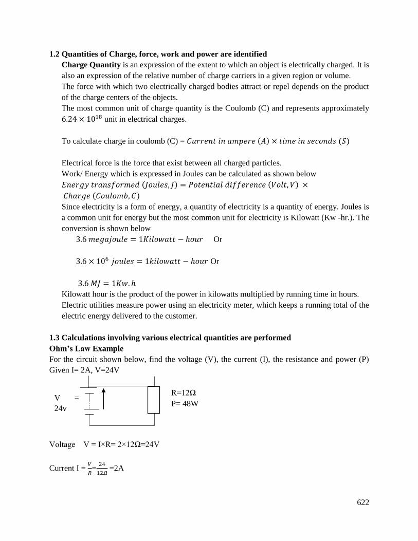
622
1.2 Quantities of Charge, force, work and power are identified
Charge Quantity is an expression of the extent to which an object is electrically charged. It is
also an expression of the relative number of charge carriers in a given region or volume.
The force with which two electrically charged bodies attract or repel depends on the product
of the charge centers of the objects.
The most common unit of charge quantity is the Coulomb (C) and represents approximately
6.24 × 10¹⁸ unit in electrical charges.
To calculate charge in coulomb (C) = 𝐶𝑢𝑟𝑟𝑒𝑛𝑡 𝑖𝑛 𝑎𝑚𝑝𝑒𝑟𝑒 (𝐴) × 𝑡𝑖𝑚𝑒 𝑖𝑛 𝑠𝑒𝑐𝑜𝑛𝑑𝑠 (𝑆)
Electrical force is the force that exist between all charged particles.
Work/ Energy which is expressed in Joules can be calculated as shown below
𝐸𝑛𝑒𝑟𝑔𝑦 𝑡𝑟𝑎𝑛𝑠𝑓𝑜𝑟𝑚𝑒𝑑 (𝐽𝑜𝑢𝑙𝑒𝑠, 𝐽) = 𝑃𝑜𝑡𝑒𝑛𝑡𝑖𝑎𝑙 𝑑𝑖𝑓𝑓𝑒𝑟𝑒𝑛𝑐𝑒 (𝑉𝑜𝑙𝑡, 𝑉) ×
𝐶ℎ𝑎𝑟𝑔𝑒 (𝐶𝑜𝑢𝑙𝑜𝑚𝑏, 𝐶)
Since electricity is a form of energy, a quantity of electricity is a quantity of energy. Joules is
a common unit for energy but the most common unit for electricity is Kilowatt (Kw -hr.). The
conversion is shown below
3.6 𝑚𝑒𝑔𝑎𝑗𝑜𝑢𝑙𝑒 = 1𝐾𝑖𝑙𝑜𝑤𝑎𝑡𝑡 − ℎ𝑜𝑢𝑟 Or
3.6 × 10⁶ 𝑗𝑜𝑢𝑙𝑒𝑠 = 1𝑘𝑖𝑙𝑜𝑤𝑎𝑡𝑡 − ℎ𝑜𝑢𝑟 Or
3.6 𝑀𝐽 = 1𝐾𝑤. ℎ
Kilowatt hour is the product of the power in kilowatts multiplied by running time in hours.
Electric utilities measure power using an electricity meter, which keeps a running total of the
electric energy delivered to the customer.
1.3 Calculations involving various electrical quantities are performed
Ohm’s Law Example
For the circuit shown below, find the voltage (V), the current (I), the resistance and power (P)
Given I= 2A, V=24V
Voltage V = I×R= 2×12Ω=24V
Current I = 𝑉
𝑅=
24
12𝛺 =2A
R=12Ω
P= 48W
V =
24v

623
Resistance R= 𝑉
𝐼 =
24
2= 12Ω
Power P = V×I= 24V ×2A=48W
To remember and be able to apply Ohm’s law, electric voltage triangle will be used V=IR
V
I R
V = IR R = 𝑉
𝐼 I =
𝑉
𝑅
For power, electric power triangle P= IV, will be used (Power law)
P
P = IV
I = 𝑃
𝑉
V = 𝑃
𝐼
Example
A 12 v battery is connected to a light bulb and draws 150mA of current.
a) What is the electrical resistance of the light bulb?
b) How much power does it consume?
c) How much will it cost to operate this bulb for a month if the cost of electricity is Ksh 11
per Kwh
I V
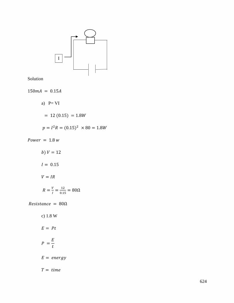
624
Solution
150𝑚𝐴 = 0.15𝐴
a) P= VI
= 12 (0.15) = 1.8𝑊
𝑝 = 𝐼2𝑅 = (0.15)2 × 80 = 1.8𝑊
𝑃𝑜𝑤𝑒𝑟 = 1.8 𝑤
𝑏) 𝑉 = 12
𝐼 = 0.15
𝑉 = 𝐼𝑅
𝑅 =𝑉
𝐼=
12
0.15= 80Ω
𝑅𝑒𝑠𝑖𝑠𝑡𝑎n𝑐𝑒 = 80Ω
c) 1.8 W
𝐸 = 𝑃𝑡
𝑃 =𝐸
𝑡
𝐸 = 𝑒𝑛𝑒𝑟𝑔𝑦
𝑇 = 𝑡𝑖𝑚𝑒
I
625
1.8𝑊
1 ×
1𝑘𝑊
1000𝑊 ×
1𝑚𝑜𝑛𝑡ℎ
1 ×
30 𝑑𝑎𝑦𝑠
1𝑚𝑜𝑛𝑡ℎ ×
24ℎ𝑟
1𝑑𝑎𝑦 ×
𝐾𝑠ℎ 11
𝐾𝑤ℎ
= 𝐾𝑠ℎ 14.256
Example
A portable heater with a resistance of 10 Ω is plugged into a 120 V electrical outlet. How much
current will flow for the heat?
𝐼 =𝑉
𝑅=
120𝑉
10Ω= 12𝐴
Example
Assuming that the cost of electricity is 5 shillings per Kwh, how much will it cost to operate a 100
W lamp continuously for 200 hours?
Solution
𝐾𝑤ℎ =100𝑊 × 200ℎ𝑟𝑠
1000= 20𝐾𝑤ℎ
𝐶𝑜𝑠𝑡 = 𝐾𝑤ℎ × 𝑟𝑎𝑡𝑒
= 20 × 5
= 𝐾𝑠ℎ 100
Conclusion
The learning outcome covered or equipped the learner with knowledge, skills and attitude to solve
various challenges that arise from the various uses of electricity which include lighting, heating,
operating appliances among other uses.
Further Reading
1. Read on essential parts of an electric circuit and the difference between a closed circuit and
an open circuit.
2. Bird, J. (2017). Electrical and electronic principles and technology, Rutledge
626
8.3.2.3 Self-Assessment
Written assessment
1. An iron draws 10 A from a 120 V house4hold supply. How much power is used?
a) 12Kw
b) 1,200W
c) 12,00Kw
d) 12W
2. What is the practical unit of electrical charge?
a) Coulomb
b) Ampere
c) Volt
d) Ohms
3. To increase the brightness of a desk bulb a student replaces a 50W light bulb with a 100W
light bulb. Compared to the 60W bulb the 100W light bulb has?
a) Less resistance and draws more current
b) Less resistance and draws less current
c) More resistance and draws more current
d) More resistance and draws less current
4. An operating lamp draws a current of 4 amperes. The amount of charge passing through the
lamp in 10 seconds is?
a) 0.045 C
b) 4.0 C
c) 5.0 C
d) 6.24 C
5. Which of the following is the correct expression of Ohm’s law?
a) I=𝑅
𝑉
b) R=𝑃
𝑉
c) I=𝑃
𝑉
d) I=𝑉
𝑅
6. If a 25 Ω resistor has a current flow of 2A through it, how much is the voltage across it?
627
a) 50V
b) 5V
c) 500V
d) 0.5V
7. What does a voltmeter measure?
a) Voltage
b) Current
c) Charge
d) Resistance
8. Convert the following data
A) 12,000 A to kA
B) 0.04 V to mV
C) 1.8mΩ to Ω
D) 40mA to A
9. Explain why a 140W soldering iron produce more heat than a 20W soldering iron.
10. A toaster draws 8 amperes when connected to a 120V source. What is the wattage rating of
the toaster?
11. What does Ohm’s law tell us about current flow in a circuit?
12. Is it more expensive to operate a 1000W hair dryer for 5 minutes or a 40W lamp for 1hour?
Why?
Oral Assessment
Ask learners the following
State Ohm’s law
Definition of electric power and electrical energy
What is the basic unit to measure electric power?
Practical Assessment
Measurement of electrical quantities (voltage, current, power) in RC circuit.
Project
Develop a circuit with LED lamp that will be able to indicate the amount of resistance in a
secondary circuit.
8.3.2.4 Tools, Equipment, Supplies and Materials
Scientific Calculators

628
Relevant reference materials
Stationeries
Electrical workshop
Relevant practical materials
Dice
Computers with internet connection
8.3.2.5 References
Despa, D., Kurniawihn, A., Komavudin, M. & Nama, and G.F. (2015, October).
Ferrero, A. (1998). Definitions of electrical quantities commonly used in non-sinusoidal
conditions. European transactions on electrical power, 8(4), 235-240
Smart Monitoring of electrical quantities based on Single board. Computer BCM 2835. In 2015
2nd International Conference on Information Technology, Computer, and Electrical
Engineering (ICITACEE) (pp.315-320). IEEE Bird, J. (2017). Electrical Circuit theory and
technology. Rutledge.
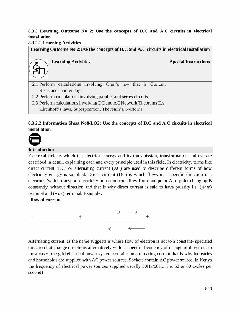
629
8.3.3 Learning Outcome No 2: Use the concepts of D.C and A.C circuits in electrical
installation
8.3.2.1 Learning Activities
Learning Outcome No 2:Use the concepts of D.C and A.C circuits in electrical installation
Learning Activities Special Instructions
2.1 Perform calculations involving Ohm’s law that is Current,
Resistance and voltage.
2.2 Perform calculations involving parallel and series circuits.
2.3 Perform calculations involving DC and AC Network Theorems E.g.
Kirchhoff’s laws, Superposition, Thevenin’s, Norton’s.
8.3.2.2 Information Sheet No8/LO2: Use the concepts of D.C and A.C circuits in electrical
installation
Introduction
Electrical field is which the electrical energy and its transmission, transformation and use are
described in detail, explaining each and every principle used in this field. In electricity, terms like
direct current (DC) or alternating current (AC) are used to describe different forms of how
electricity energy is supplied. Direct current (DC) is which flows in a specific direction i.e.,
electrons,(which transport electricity in a conductor flow from one point A to point changing B
constantly, without direction and that is why direct current is said to have polarity i.e. (+𝑣𝑒)
terminal and (– 𝑣𝑒) terminal. Example:
flow of current
Alternating current, as the name suggests is where flow of electron is not to a constant- specified
direction but change directions alternatively with as specific frequency of change of direction. In
most cases, the grid electrical power system contains an alternating current that is why industries
and households are supplied with AC power sources. Sockets contain AC power source. In Kenya
the frequency of electrical power sources supplied usually 50Hz/60Hz (i.e. 50 or 60 cycles per
second)
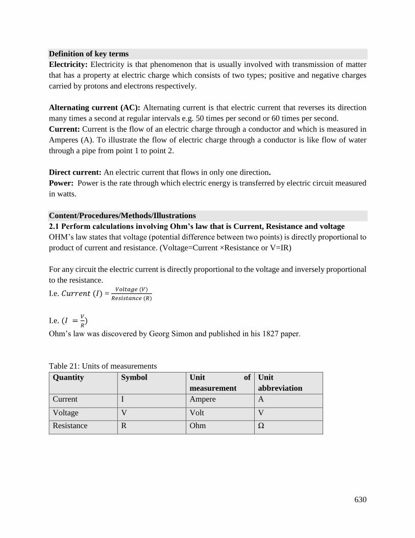
630
Definition of key terms
Electricity: Electricity is that phenomenon that is usually involved with transmission of matter
that has a property at electric charge which consists of two types; positive and negative charges
carried by protons and electrons respectively.
Alternating current (AC): Alternating current is that electric current that reverses its direction
many times a second at regular intervals e.g. 50 times per second or 60 times per second.
Current: Current is the flow of an electric charge through a conductor and which is measured in
Amperes (A). To illustrate the flow of electric charge through a conductor is like flow of water
through a pipe from point 1 to point 2.
Direct current: An electric current that flows in only one direction.
Power: Power is the rate through which electric energy is transferred by electric circuit measured
in watts.
Content/Procedures/Methods/Illustrations
2.1 Perform calculations involving Ohm’s law that is Current, Resistance and voltage
OHM’s law states that voltage (potential difference between two points) is directly proportional to
product of current and resistance. (Voltage=Current ×Resistance or V=IR)
For any circuit the electric current is directly proportional to the voltage and inversely proportional
to the resistance.
I.e. 𝐶𝑢𝑟𝑟𝑒𝑛𝑡 (𝐼) = 𝑉𝑜𝑙𝑡𝑎𝑔𝑒 (𝑉)
𝑅𝑒𝑠𝑖𝑠𝑡𝑎𝑛𝑐𝑒 (𝑅)
I.e. (𝐼 =𝑉
𝑅)
Ohm’s law was discovered by Georg Simon and published in his 1827 paper.
Table 21: Units of measurements
Quantity Symbol Unit of
measurement
Unit
abbreviation
Current I Ampere A
Voltage V Volt V
Resistance R Ohm Ω
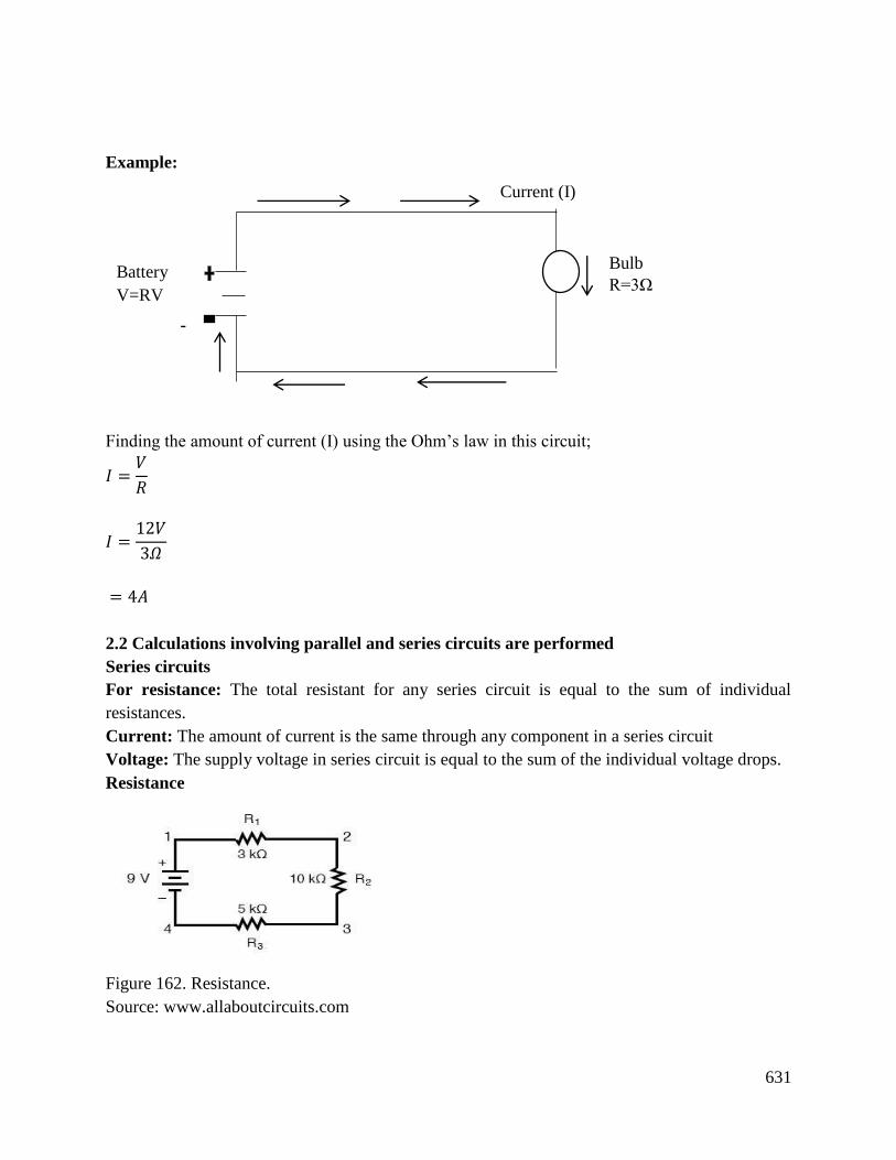
631
Example:
-
Finding the amount of current (I) using the Ohm’s law in this circuit;
𝐼 =𝑉
𝑅
𝐼 =12𝑉
3𝛺
= 4𝐴
2.2 Calculations involving parallel and series circuits are performed
Series circuits
For resistance: The total resistant for any series circuit is equal to the sum of individual
resistances.
Current: The amount of current is the same through any component in a series circuit
Voltage: The supply voltage in series circuit is equal to the sum of the individual voltage drops.
Resistance
Figure 162. Resistance.
Source: www.allaboutcircuits.com
Battery
V=RV
Bulb
R=3Ω
Current (I)
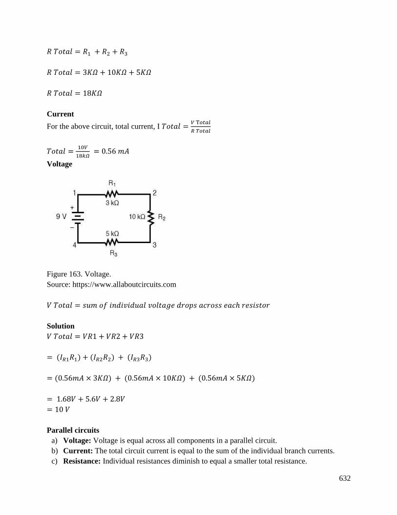
632
𝑅 𝑇𝑜𝑡𝑎𝑙 = 𝑅1 + 𝑅2 + 𝑅3
𝑅 𝑇𝑜𝑡𝑎𝑙 = 3𝐾𝛺 + 10𝐾𝛺 + 5𝐾𝛺
𝑅 𝑇𝑜𝑡𝑎𝑙 = 18𝐾𝛺
Current
For the above circuit, total current, I 𝑇𝑜𝑡𝑎𝑙 =𝑉 T𝑜𝑡𝑎𝑙
𝑅 𝑇𝑜𝑡𝑎𝑙
𝑇𝑜𝑡𝑎𝑙 =10𝑉
18𝑘𝛺 = 0.56 𝑚𝐴
Voltage
Figure 163. Voltage.
Source: https://www.allaboutcircuits.com
𝑉 𝑇𝑜𝑡𝑎𝑙 = 𝑠𝑢𝑚 𝑜𝑓 𝑖𝑛𝑑𝑖𝑣𝑖𝑑𝑢𝑎𝑙 𝑣𝑜𝑙𝑡𝑎𝑔𝑒 𝑑𝑟𝑜𝑝𝑠 𝑎𝑐𝑟𝑜𝑠𝑠 𝑒𝑎𝑐ℎ 𝑟𝑒𝑠𝑖𝑠𝑡𝑜𝑟
Solution
𝑉 𝑇𝑜𝑡𝑎𝑙 = 𝑉𝑅1 + 𝑉𝑅2 + 𝑉𝑅3
= (𝐼𝑅1𝑅1) + (𝐼𝑅2𝑅2) + (𝐼𝑅3𝑅3)
= (0.56𝑚𝐴 × 3𝐾𝛺) + (0.56𝑚𝐴 × 10𝐾𝛺) + (0.56𝑚𝐴 × 5𝐾𝛺)
= 1.68𝑉 + 5.6𝑉 + 2.8𝑉
= 10 𝑉
Parallel circuits
a) Voltage: Voltage is equal across all components in a parallel circuit.
b) Current: The total circuit current is equal to the sum of the individual branch currents.
c) Resistance: Individual resistances diminish to equal a smaller total resistance.
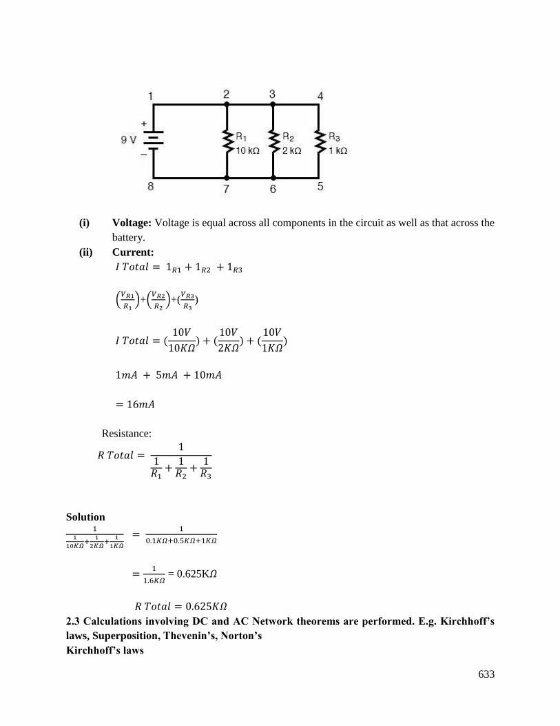
633
(i) Voltage: Voltage is equal across all components in the circuit as well as that across the
battery.
(ii) Current:
𝐼 𝑇𝑜𝑡𝑎𝑙 = 1𝑅1 + 1𝑅2 + 1𝑅3
(𝑉𝑅1
𝑅1)+(
𝑉𝑅2
𝑅2)+(
𝑉𝑅3
𝑅3)
𝐼 𝑇𝑜𝑡𝑎𝑙 = (10𝑉
10𝐾𝛺) + (
10𝑉
2𝐾𝛺) + (
10𝑉
1𝐾𝛺)
1𝑚𝐴 + 5𝑚𝐴 + 10𝑚𝐴
= 16𝑚𝐴
Resistance:
𝑅 𝑇𝑜𝑡𝑎𝑙 = 1
1𝑅1
+1𝑅2
+1𝑅3
Solution 1
1
10𝐾𝛺+
1
2𝐾𝛺+
1
1𝐾𝛺
= 1
0.1𝐾𝛺+0.5𝐾𝛺+1𝐾𝛺
=1
1.6𝐾𝛺 = 0.625K𝛺
𝑅 𝑇𝑜𝑡𝑎𝑙 = 0.625𝐾𝛺
2.3 Calculations involving DC and AC Network theorems are performed. E.g. Kirchhoff’s
laws, Superposition, Thevenin’s, Norton’s
Kirchhoff’s laws
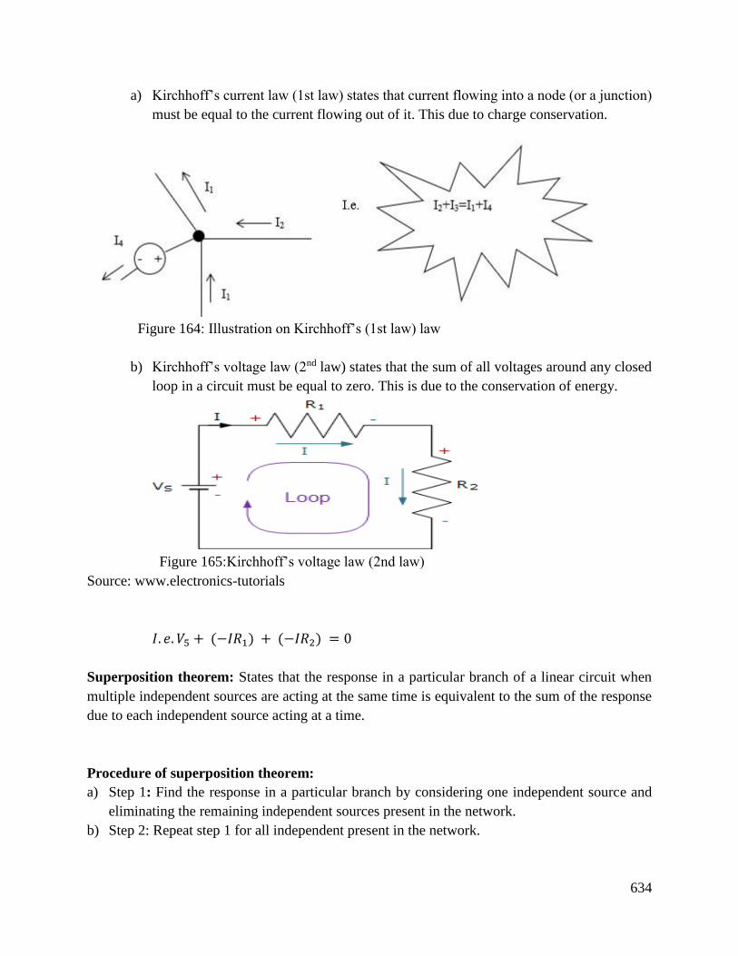
634
a) Kirchhoff’s current law (1st law) states that current flowing into a node (or a junction)
must be equal to the current flowing out of it. This due to charge conservation.
Figure 164: Illustration on Kirchhoff’s (1st law) law
b) Kirchhoff’s voltage law (2nd law) states that the sum of all voltages around any closed
loop in a circuit must be equal to zero. This is due to the conservation of energy.
Figure 165:Kirchhoff’s voltage law (2nd law)
Source: www.electronics-tutorials
𝐼. 𝑒. 𝑉5 + (−𝐼𝑅1) + (−𝐼𝑅2) = 0
Superposition theorem: States that the response in a particular branch of a linear circuit when
multiple independent sources are acting at the same time is equivalent to the sum of the response
due to each independent source acting at a time.
Procedure of superposition theorem:
a) Step 1: Find the response in a particular branch by considering one independent source and
eliminating the remaining independent sources present in the network.
b) Step 2: Repeat step 1 for all independent present in the network.
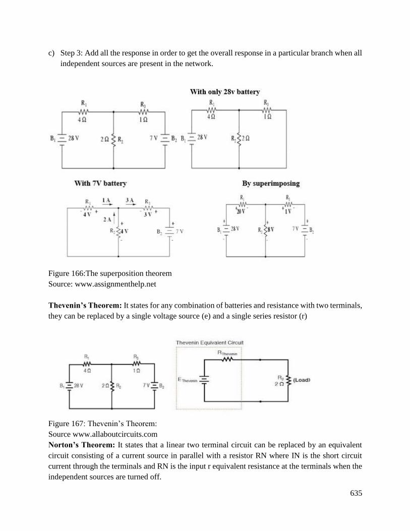
635
c) Step 3: Add all the response in order to get the overall response in a particular branch when all
independent sources are present in the network.
Figure 166:The superposition theorem
Source: www.assignmenthelp.net
Thevenin’s Theorem: It states for any combination of batteries and resistance with two terminals,
they can be replaced by a single voltage source (e) and a single series resistor (r)
Figure 167: Thevenin’s Theorem:
Source www.allaboutcircuits.com
Norton’s Theorem: It states that a linear two terminal circuit can be replaced by an equivalent
circuit consisting of a current source in parallel with a resistor RN where IN is the short circuit
current through the terminals and RN is the input r equivalent resistance at the terminals when the
independent sources are turned off.
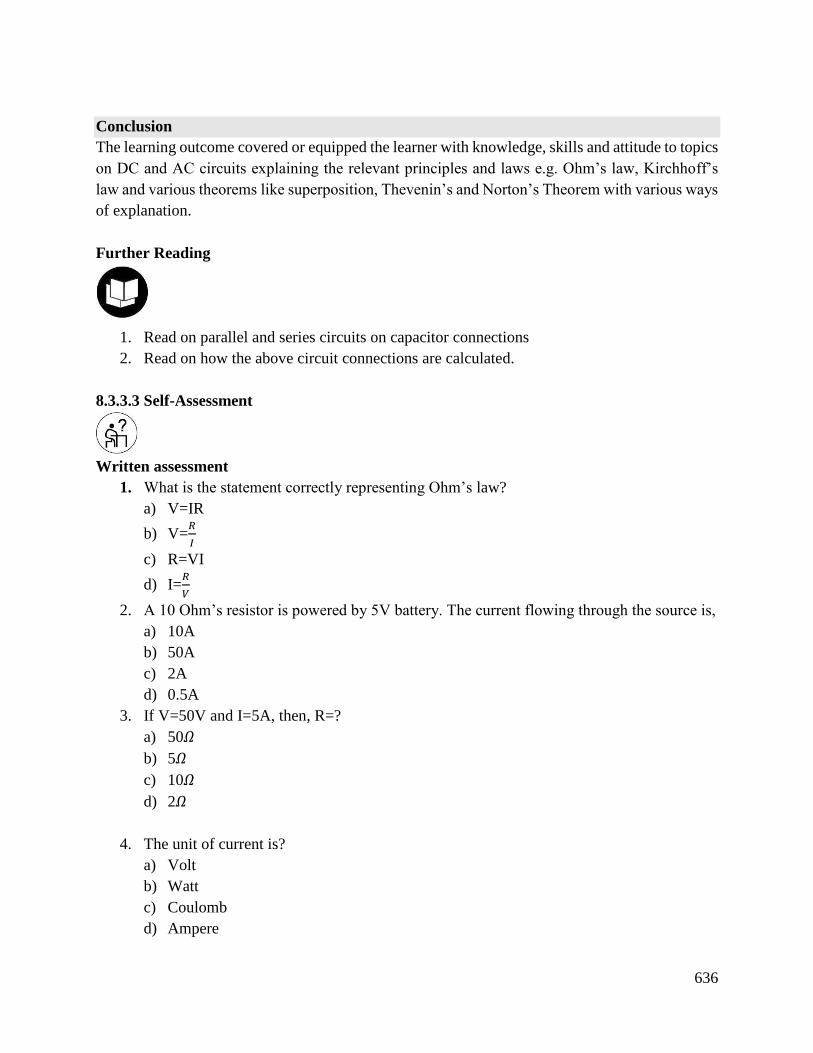
636
Conclusion
The learning outcome covered or equipped the learner with knowledge, skills and attitude to topics
on DC and AC circuits explaining the relevant principles and laws e.g. Ohm’s law, Kirchhoff’s
law and various theorems like superposition, Thevenin’s and Norton’s Theorem with various ways
of explanation.
Further Reading
1. Read on parallel and series circuits on capacitor connections
2. Read on how the above circuit connections are calculated.
8.3.3.3 Self-Assessment
Written assessment
1. What is the statement correctly representing Ohm’s law?
a) V=IR
b) V=𝑅
𝐼
c) R=VI
d) I=𝑅
𝑉
2. A 10 Ohm’s resistor is powered by 5V battery. The current flowing through the source is,
a) 10A
b) 50A
c) 2A
d) 0.5A
3. If V=50V and I=5A, then, R=?
a) 50𝛺
b) 5𝛺
c) 10𝛺
d) 2𝛺
4. The unit of current is?
a) Volt
b) Watt
c) Coulomb
d) Ampere
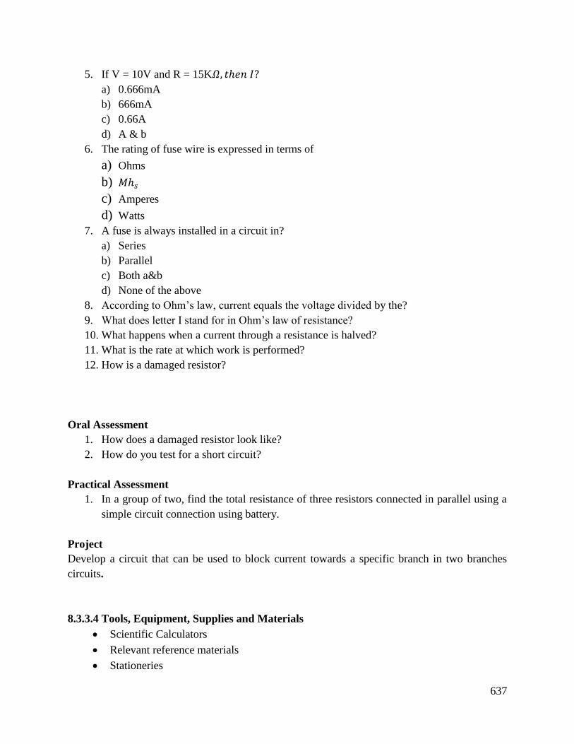
637
5. If V = 10V and R = 15K𝛺, 𝑡ℎ𝑒𝑛 𝐼?
a) 0.666mA
b) 666mA
c) 0.66A
d) A & b
6. The rating of fuse wire is expressed in terms of
a) Ohms
b) 𝑀ℎ𝑠
c) Amperes
d) Watts
7. A fuse is always installed in a circuit in?
a) Series
b) Parallel
c) Both a&b
d) None of the above
8. According to Ohm’s law, current equals the voltage divided by the?
9. What does letter I stand for in Ohm’s law of resistance?
10. What happens when a current through a resistance is halved?
11. What is the rate at which work is performed?
12. How is a damaged resistor?
Oral Assessment
1. How does a damaged resistor look like?
2. How do you test for a short circuit?
Practical Assessment
1. In a group of two, find the total resistance of three resistors connected in parallel using a
simple circuit connection using battery.
Project
Develop a circuit that can be used to block current towards a specific branch in two branches
circuits.
8.3.3.4 Tools, Equipment, Supplies and Materials
Scientific Calculators
Relevant reference materials
Stationeries

638
Electrical workshop
Relevant practical materials
Dice
Computers with internet connection
8.3.3.5 References
Ciechonska. M,Sturrock.M,Grob, A,Larruy-maumus. G. Shahrezaei. V & Isalan. M (2019).
Ohm’s law for emergent gene expansion under fitness pressure. bioRXiv,693234
Davies, T.H (1981). Kirchhoff’s circulation law applied to multiloop kinematic chains. Mechanism
and Machine theory, 16(3), 171-183.
Ezzat, M. A, &Ellal, M.ZA (2009). Generalized magnet thermoelectricity with modified Ohm’s
law. “Mechanics of Advanced Materials and structures 17(1), 74-84

639
8.3.4 Learning Outcome No 3: Use of basic electrical machine
8.3.4.1 Learning Activities
Learning Outcome No3 :Use of basic electrical machine
Learning Activities Special Instructions
3.1 Identify types of various electrical machines
3.2 Perform calculations involving single phase and three phase AC and
DC Motors
3.3 Perform calculations involving single and three phase AC and DC
transformers
3.4 Perform calculations involving single and three phase generators
8.3.4.2 Information Sheet No8/LO3: Use of basic electrical machine
Introduction
This learning outcome covers different types of electrical machines used in electrical engineering
work .These machines include motors, transformers and generators. The learning outcome covers
the working principles of these machines and calculations involved in them and their uses.
Definition of key terms
Generator: This is a machine which converts mechanical energy to electric energy.
Motor: This is a machine which converts electrical energy to mechanical energy.
Transformer: It’s a machine used for changing voltage value in a circuit.
Content/procedures/methods/illustrations
3.1 Types of various electrical machines are identified
Transformer
The following are the various types of a transformer:
Double-wound transformer
Auto transformer
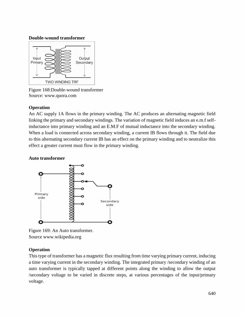
640
Double-wound transformer
Source: www.quora.com
Operation
An AC supply 1A flows in the primary winding. The AC produces an alternating magnetic field
linking the primary and secondary windings. The variation of magnetic field induces an e.m.f self-
inductance into primary winding and an E.M.F of mutual inductance into the secondary winding.
When a load is connected across secondary winding, a current IB flows through it. The field due
to this alternating secondary current IB has an effect on the primary winding and to neutralize this
effect a greater current must flow in the primary winding.
Auto transformer
Figure 169: An Auto transformer.
Source www.wikipedia.org
Operation
This type of transformer has a magnetic flux resulting from time varying primary current, inducing
a time varying current in the secondary winding. The integrated primary /secondary winding of an
auto transformer is typically tapped at different points along the winding to allow the output
/secondary voltage to be varied in discrete steps, at various percentages of the input/primary
voltage.
Figure 168:Double-wound transformer
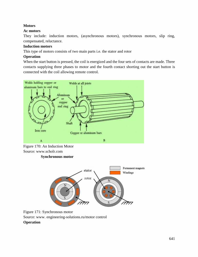
641
Motors
Ac motors
They include: induction motors, (asynchronous motors), synchronous motors, slip ring,
compensated, reluctance.
Induction motors
This type of motors consists of two main parts i.e. the stator and rotor
Operation
When the start button is pressed, the coil is energized and the four sets of contacts are made. Three
contacts supplying three phases to motor and the fourth contact shorting out the start button is
connected with the coil allowing remote control.
Figure 170: An Induction Motor
Source: www.scholr.com
Synchronous motor
Figure 171: Synchronous motor
Source: www. engineering-solutions.ru/motor control
Operation
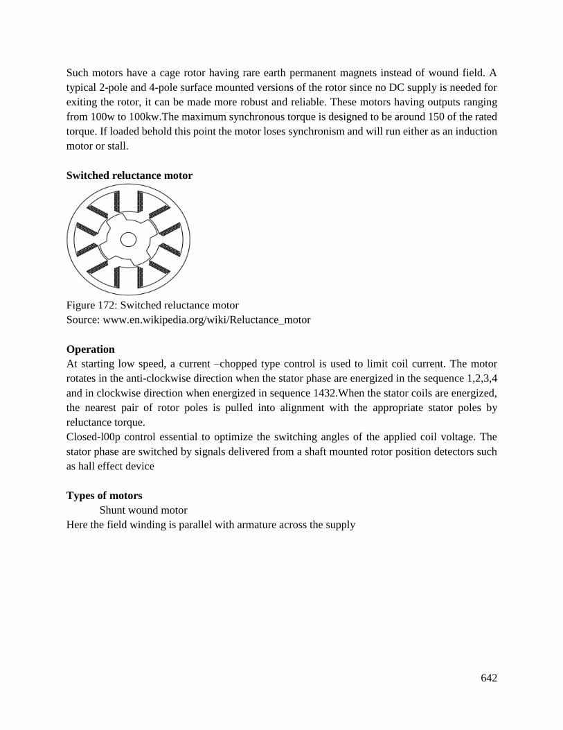
642
Such motors have a cage rotor having rare earth permanent magnets instead of wound field. A
typical 2-pole and 4-pole surface mounted versions of the rotor since no DC supply is needed for
exiting the rotor, it can be made more robust and reliable. These motors having outputs ranging
from 100w to 100kw.The maximum synchronous torque is designed to be around 150 of the rated
torque. If loaded behold this point the motor loses synchronism and will run either as an induction
motor or stall.
Switched reluctance motor
Figure 172: Switched reluctance motor
Source: www.en.wikipedia.org/wiki/Reluctance_motor
Operation
At starting low speed, a current –chopped type control is used to limit coil current. The motor
rotates in the anti-clockwise direction when the stator phase are energized in the sequence 1,2,3,4
and in clockwise direction when energized in sequence 1432.When the stator coils are energized,
the nearest pair of rotor poles is pulled into alignment with the appropriate stator poles by
reluctance torque.
Closed-l00p control essential to optimize the switching angles of the applied coil voltage. The
stator phase are switched by signals delivered from a shaft mounted rotor position detectors such
as hall effect device
Types of motors
Shunt wound motor
Here the field winding is parallel with armature across the supply
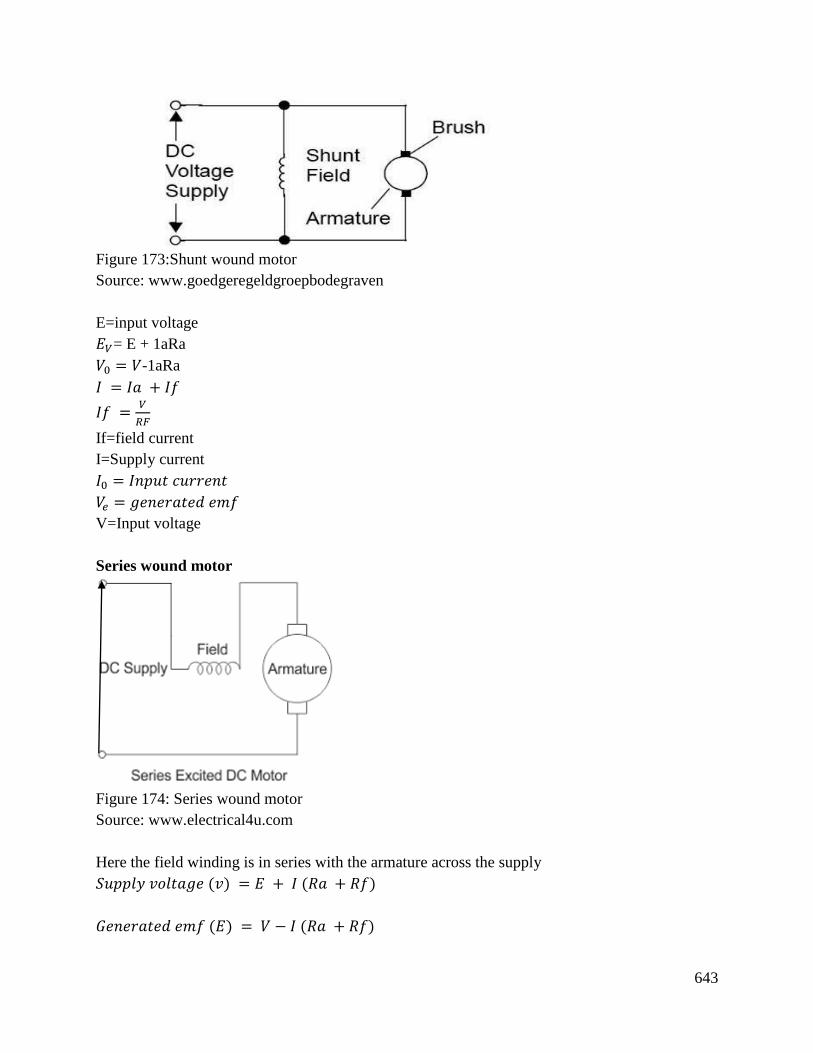
643
Figure 173:Shunt wound motor
Source: www.goedgeregeldgroepbodegraven
E=input voltage
𝐸𝑉= E + 1aRa
𝑉0 = 𝑉-1aRa
𝐼 = 𝐼𝑎 + 𝐼𝑓
𝐼𝑓 =𝑉
𝑅𝐹
If=field current
I=Supply current
𝐼0 = 𝐼𝑛𝑝𝑢𝑡 𝑐𝑢𝑟𝑟𝑒𝑛𝑡
𝑉𝑒 = 𝑔𝑒𝑛𝑒𝑟𝑎𝑡𝑒𝑑 𝑒𝑚𝑓
V=Input voltage
Series wound motor
Figure 174: Series wound motor
Source: www.electrical4u.com
Here the field winding is in series with the armature across the supply
𝑆𝑢𝑝𝑝𝑙𝑦 𝑣𝑜𝑙𝑡𝑎𝑔𝑒 (𝑣) = 𝐸 + 𝐼 (𝑅𝑎 + 𝑅𝑓)
𝐺𝑒𝑛𝑒𝑟𝑎𝑡𝑒𝑑 𝑒𝑚𝑓 (𝐸) = 𝑉 − 𝐼 (𝑅𝑎 + 𝑅𝑓)
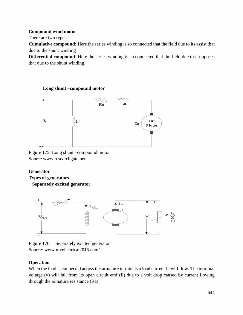
644
Compound wind motor
There are two types:
Cumulative compound: Here the series winding is so connected that the field due to its assist that
due to the shunt winding
Differential compound: Here the series winding is so connected that the field due to it opposes
that due to the shunt winding.
Long shunt –compound motor
Figure 175: Long shunt –compound motor
Source www.researchgate.net
Generator
Types of generators
Separately excited generator
Figure 176: Separately excited generator
Source: www.myelectrical2015.com/
Operation
When the load is connected across the armature terminals a load current Ia will flow. The terminal
voltage (v) will fall from its open circuit emf (E) due to a volt drop caused by current flowing
through the armature resistance (Ra)
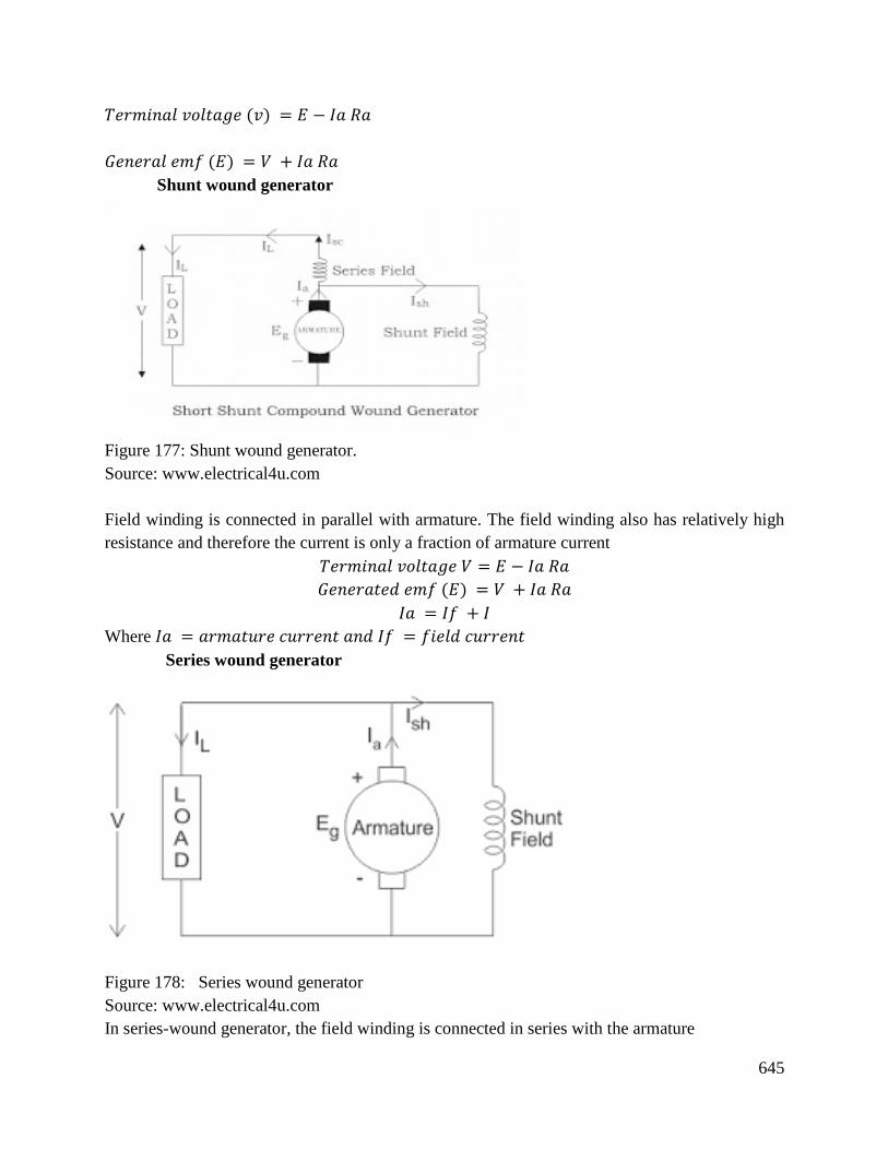
645
𝑇𝑒𝑟𝑚𝑖𝑛𝑎𝑙 𝑣𝑜𝑙𝑡𝑎𝑔𝑒 (𝑣) = 𝐸 − 𝐼𝑎 𝑅𝑎
𝐺𝑒𝑛𝑒𝑟𝑎𝑙 𝑒𝑚𝑓 (𝐸) = 𝑉 + 𝐼𝑎 𝑅𝑎
Shunt wound generator
Figure 177: Shunt wound generator.
Source: www.electrical4u.com
Field winding is connected in parallel with armature. The field winding also has relatively high
resistance and therefore the current is only a fraction of armature current
𝑇𝑒𝑟𝑚𝑖𝑛𝑎𝑙 𝑣𝑜𝑙𝑡𝑎𝑔𝑒 𝑉 = 𝐸 − 𝐼𝑎 𝑅𝑎
𝐺𝑒𝑛𝑒𝑟𝑎𝑡𝑒𝑑 𝑒𝑚𝑓 (𝐸) = 𝑉 + 𝐼𝑎 𝑅𝑎
𝐼𝑎 = 𝐼𝑓 + 𝐼
Where 𝐼𝑎 = 𝑎𝑟𝑚𝑎𝑡𝑢𝑟𝑒 𝑐𝑢𝑟𝑟𝑒𝑛𝑡 𝑎𝑛𝑑 𝐼𝑓 = 𝑓𝑖𝑒𝑙𝑑 𝑐𝑢𝑟𝑟𝑒𝑛𝑡
Series wound generator
Figure 178: Series wound generator
Source: www.electrical4u.com
In series-wound generator, the field winding is connected in series with the armature
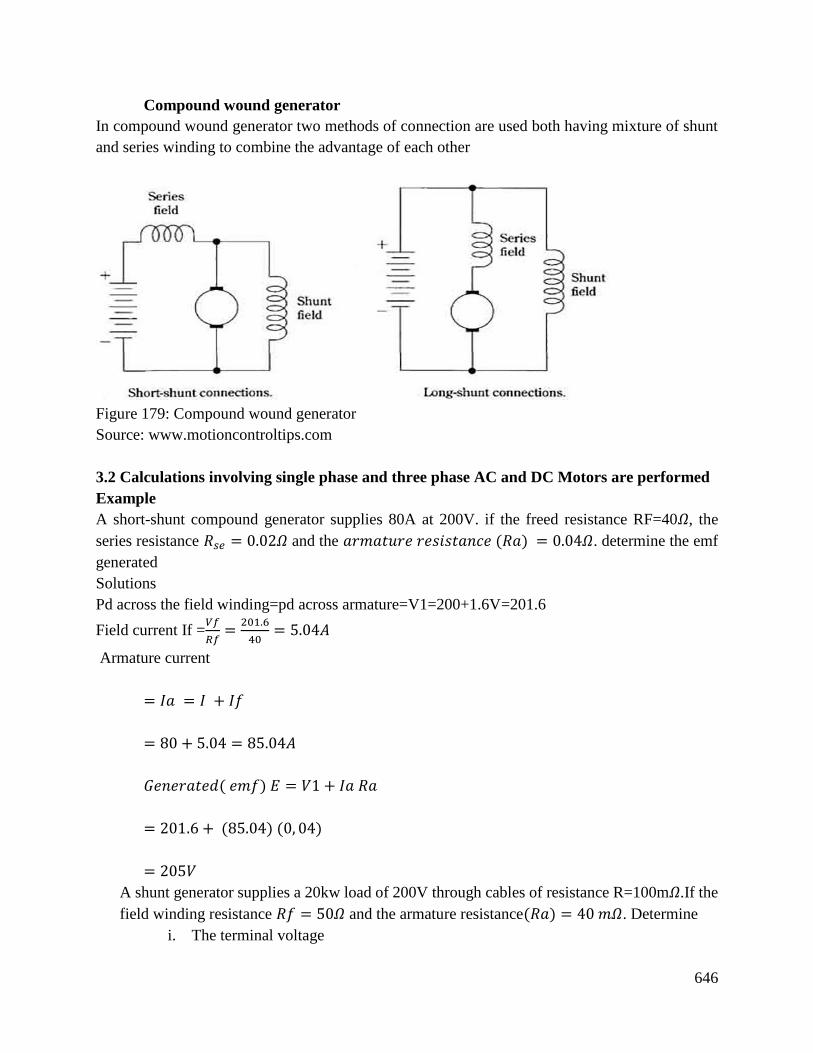
646
Compound wound generator
In compound wound generator two methods of connection are used both having mixture of shunt
and series winding to combine the advantage of each other
Figure 179: Compound wound generator
Source: www.motioncontroltips.com
3.2 Calculations involving single phase and three phase AC and DC Motors are performed
Example
A short-shunt compound generator supplies 80A at 200V. if the freed resistance RF=40𝛺, the
series resistance 𝑅𝑠𝑒 = 0.02𝛺 and the 𝑎𝑟𝑚𝑎𝑡𝑢𝑟𝑒 𝑟𝑒𝑠𝑖𝑠𝑡𝑎𝑛𝑐𝑒 (𝑅𝑎) = 0.04𝛺. determine the emf
generated
Solutions
Pd across the field winding=pd across armature=V1=200+1.6V=201.6
Field current If =𝑉𝑓
𝑅𝑓=
201.6
40= 5.04𝐴
Armature current
= 𝐼𝑎 = 𝐼 + 𝐼𝑓
= 80 + 5.04 = 85.04𝐴
𝐺𝑒𝑛𝑒𝑟𝑎𝑡𝑒𝑑( 𝑒𝑚𝑓) 𝐸 = 𝑉1 + 𝐼𝑎 𝑅𝑎
= 201.6 + (85.04) (0, 04)
= 205𝑉
A shunt generator supplies a 20kw load of 200V through cables of resistance R=100m𝛺.If the
field winding resistance 𝑅𝑓 = 50𝛺 and the armature resistance(𝑅𝑎) = 40 𝑚𝛺. Determine
i. The terminal voltage
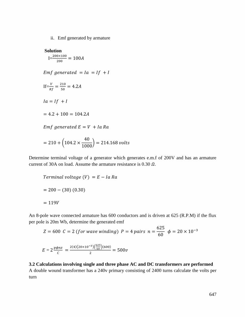
647
ii. Emf generated by armature
Solution
I=200×100
200= 100𝐴
𝐸𝑚𝑓 𝑔𝑒𝑛𝑒𝑟𝑎𝑡𝑒𝑑 = 𝐼𝑎 = 𝐼𝑓 + 𝐼
If=𝑉
𝑅𝑓=
210
50= 4.2𝐴
𝐼𝑎 = 𝐼𝑓 + 𝐼
= 4.2 + 100 = 104.2𝐴
𝐸𝑚𝑓 𝑔𝑒𝑛𝑒𝑟𝑎𝑡𝑒𝑑 𝐸 = 𝑉 + 𝐼𝑎 𝑅𝑎
= 210 + (104.2 ×40
1000) = 214.168 𝑣𝑜𝑙𝑡𝑠
Determine terminal voltage of a generator which generates e.m.f of 200V and has an armature
current of 30A on load. Assume the armature resistance is 0.30 𝛺.
𝑇𝑒𝑟𝑚𝑖𝑛𝑎𝑙 𝑣𝑜𝑙𝑡𝑎𝑔𝑒 (𝑉) = 𝐸 − 𝐼𝑎 𝑅𝑎
= 200 − (30) (0.30)
= 119𝑉
An 8-pole wave connected armature has 600 conductors and is driven at 625 (R.P.M) if the flux
per pole is 20m Wb, determine the generated emf
𝑍 = 600 𝐶 = 2 (𝑓𝑜𝑟 𝑤𝑎𝑣𝑒 𝑤𝑖𝑛𝑑𝑖𝑛𝑔) 𝑃 = 4 𝑝𝑎𝑖𝑟𝑠 𝑛 =625
60 𝜙 = 20 × 10−3
𝐸 = 2𝑝𝜙𝑛𝑧
𝐶 =
2(4)(20×10−3)(625
60)(600)
2= 500𝑣
3.2 Calculations involving single and three phase AC and DC transformers are performed
A double wound transformer has a 240v primary consisting of 2400 turns calculate the volts per
turn
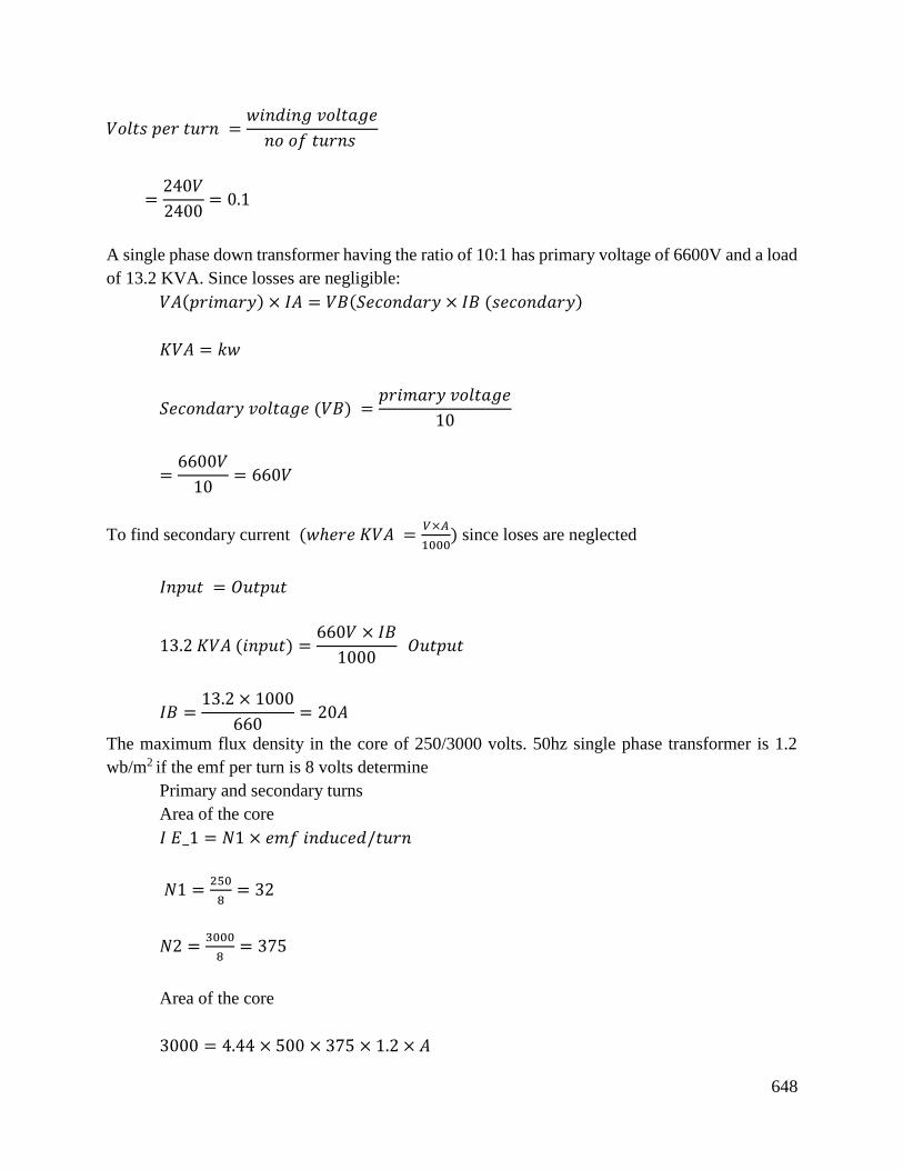
648
𝑉𝑜𝑙𝑡𝑠 𝑝𝑒𝑟 𝑡𝑢𝑟𝑛 =𝑤𝑖𝑛𝑑𝑖𝑛𝑔 𝑣𝑜𝑙𝑡𝑎𝑔𝑒
𝑛𝑜 𝑜𝑓 𝑡𝑢𝑟𝑛𝑠
=240𝑉
2400= 0.1
A single phase down transformer having the ratio of 10:1 has primary voltage of 6600V and a load
of 13.2 KVA. Since losses are negligible:
𝑉𝐴(𝑝𝑟𝑖𝑚𝑎𝑟𝑦) × 𝐼𝐴 = 𝑉𝐵(𝑆𝑒𝑐𝑜𝑛𝑑𝑎𝑟𝑦 × 𝐼𝐵 (𝑠𝑒𝑐𝑜𝑛𝑑𝑎𝑟𝑦)
𝐾𝑉𝐴 = 𝑘𝑤
𝑆𝑒𝑐𝑜𝑛𝑑𝑎𝑟𝑦 𝑣𝑜𝑙𝑡𝑎𝑔𝑒 (𝑉𝐵) =𝑝𝑟𝑖𝑚𝑎𝑟𝑦 𝑣𝑜𝑙𝑡𝑎𝑔𝑒
10
=6600𝑉
10= 660𝑉
To find secondary current (𝑤ℎ𝑒𝑟𝑒 𝐾𝑉𝐴 =𝑉×𝐴
1000) since loses are neglected
𝐼𝑛𝑝𝑢𝑡 = 𝑂𝑢𝑡𝑝𝑢𝑡
13.2 𝐾𝑉𝐴 (𝑖𝑛𝑝𝑢𝑡) =660𝑉 × 𝐼𝐵
1000 𝑂𝑢𝑡𝑝𝑢𝑡
𝐼𝐵 =13.2 × 1000
660= 20𝐴
The maximum flux density in the core of 250/3000 volts. 50hz single phase transformer is 1.2
wb/m2 if the emf per turn is 8 volts determine
Primary and secondary turns
Area of the core
𝐼 𝐸_1 = 𝑁1 × 𝑒𝑚𝑓 𝑖𝑛𝑑𝑢𝑐𝑒𝑑/𝑡𝑢𝑟𝑛
𝑁1 =250
8= 32
𝑁2 =3000
8= 375
Area of the core
3000 = 4.44 × 500 × 375 × 1.2 × 𝐴
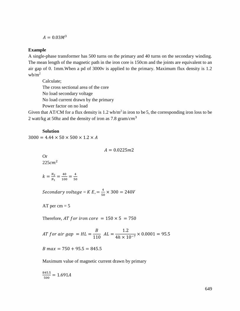
649
𝐴 = 0.03𝑀3
Example
A single-phase transformer has 500 turns on the primary and 40 turns on the secondary winding.
The mean length of the magnetic path in the iron core is 150cm and the joints are equivalent to an
air gap of 0. 1mm.When a pd of 3000v is applied to the primary. Maximum flux density is 1.2
wb/m2
Calculate;
The cross sectional area of the core
No load secondary voltage
No load current drawn by the primary
Power factor on no load
Given that AT/CM for a flux density is 1.2 wb/m2 in iron to be 5, the corresponding iron loss to be
2 watt/kg at 50hz and the density of iron as 7.8 gram/𝑐𝑚3
Solution
3000 = 4.44 × 50 × 500 × 1.2 × 𝐴
𝐴 = 0.0225𝑚2
Or
225𝑐𝑚2
𝑘 =𝑁2
𝑁1=
40
100=
4
50
𝑆𝑒𝑐𝑜𝑛𝑑𝑎𝑟𝑦 𝑣𝑜𝑙t𝑎𝑔𝑒 = 𝐾 𝐸, =4
50 × 300 = 240𝑉
AT per cm = 5
Therefore, 𝐴𝑇 𝑓𝑜𝑟 𝑖𝑟𝑜𝑛 𝑐𝑜𝑟𝑒 = 150 × 5 = 750
𝐴𝑇 𝑓𝑜𝑟 𝑎𝑖𝑟 𝑔𝑎𝑝 = 𝐻𝐿 =𝐵
110 𝐴𝐿 =
1.2
4ℎ × 10−7× 0.0001 = 95.5
𝐵 𝑚𝑎𝑥 = 750 + 95.5 = 845.5
Maximum value of magnetic current drawn by primary
845.5
500= 1.691𝐴
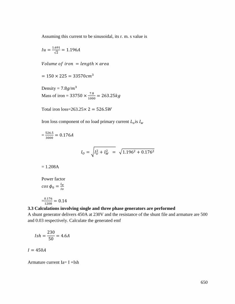
650
Assuming this current to be sinusoidal, its r. m. s value is
𝐼𝑢 =1.691
√2= 1.196𝐴
𝑉𝑜𝑙𝑢𝑚𝑒 𝑜𝑓 𝑖𝑟𝑜𝑛 = 𝑙𝑒𝑛𝑔𝑡ℎ × 𝑎𝑟𝑒𝑎
= 150 × 225 = 33570𝑐𝑚3
Density = 7.8𝑔/𝑚3
Mass of iron = 33750 ×7.8
1000= 263.25𝑘𝑔
Total iron loss=263.25× 2 = 526.5𝑊
Iron loss component of no load primary current 𝐿𝑜is 𝐼𝑤
= 526.5
3000= 0.176𝐴
𝐼𝑂 = √𝐼𝑈2 + 𝐼𝑊
2 = √1.1962 + 0.1762
= 1.208A
Power factor
𝑐𝑜𝑠 𝜙0 =𝐼𝑤
𝐼𝑜
=0.176
1208= 0.14
3.3 Calculations involving single and three phase generators are performed
A shunt generator delivers 450A at 230V and the resistance of the shunt file and armature are 500
and 0.03 respectively. Calculate the generated emf
𝐼𝑠ℎ =230
50= 4.6𝐴
𝐼 = 450𝐴
Armature current Ia= I +Ish
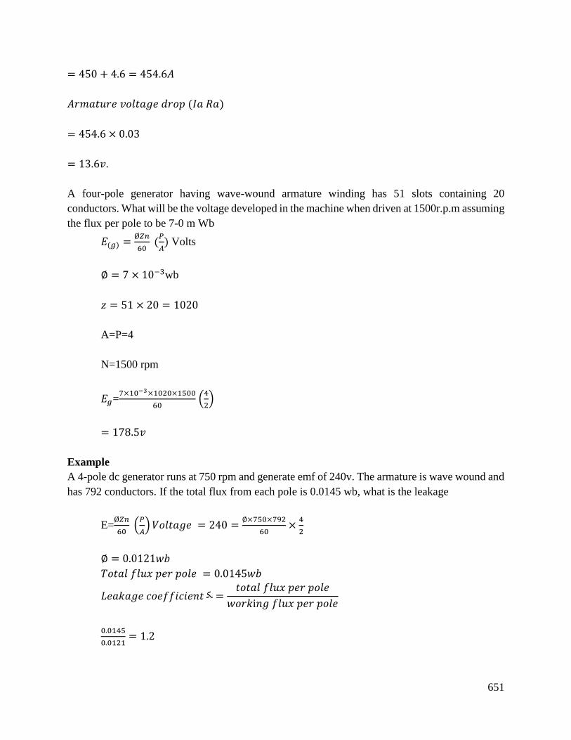
651
= 450 + 4.6 = 454.6𝐴
𝐴𝑟𝑚𝑎𝑡𝑢𝑟𝑒 𝑣𝑜𝑙𝑡𝑎𝑔𝑒 𝑑𝑟𝑜𝑝 (𝐼𝑎 𝑅𝑎)
= 454.6 × 0.03
= 13.6𝑣.
A four-pole generator having wave-wound armature winding has 51 slots containing 20
conductors. What will be the voltage developed in the machine when driven at 1500r.p.m assuming
the flux per pole to be 7-0 m Wb
𝐸(𝑔) =Ø𝑍𝑛
60 (
𝑃
𝐴) Volts
∅ = 7 × 10⁻³wb
𝑧 = 51 × 20 = 1020
A=P=4
N=1500 rpm
𝐸𝑔=7×10−3×1020×1500
60 (
4
2)
= 178.5𝑣
Example
A 4-pole dc generator runs at 750 rpm and generate emf of 240v. The armature is wave wound and
has 792 conductors. If the total flux from each pole is 0.0145 wb, what is the leakage
E=Ø𝑍𝑛
60 (
𝑃
𝐴)𝑉𝑜𝑙𝑡𝑎𝑔𝑒 = 240 =
∅×750×792
60×
4
2
∅ = 0.0121𝑤𝑏
𝑇𝑜𝑡𝑎𝑙 𝑓𝑙𝑢𝑥 𝑝𝑒𝑟 𝑝𝑜𝑙𝑒 = 0.0145𝑤𝑏
𝐿𝑒𝑎𝑘𝑎𝑔𝑒 𝑐𝑜𝑒𝑓𝑓𝑖𝑐𝑖𝑒𝑛𝑡 ک =𝑡𝑜𝑡𝑎𝑙 𝑓𝑙𝑢𝑥 𝑝𝑒𝑟 𝑝𝑜𝑙𝑒
𝑤𝑜𝑟𝑘i𝑛𝑔 𝑓𝑙𝑢𝑥 𝑝𝑒𝑟 𝑝𝑜𝑙𝑒
0.0145
0.0121= 1.2
652
Conclusion
The learning outcome equipped the learner with knowledge of the machine operation and develop
positive attitude towards the machine.
8.3.4.3 Self-Assessment
Written assessment
1. A long shunt dynamo running at 1000rpm supplies 20kw at a terminal voltage of 220V.the
resistance of armature, shunt field, and series field are 0.04,110 and 0.05hm respectively.
Overall efficiency at the above load is 85% find,
i. Copper loss
a) 4900 watts
b) 500 watts
c) 3529 watts
d) 4530 watts
ii. Iron or friction loss
a) 3000watts
b) 2500 watts
c) 2500 watts
d) 2312 watts
iii. Torque developed by the prime mover
a) 248.2 Nw-m
b) 245.3 Nw-m
c) 200 Nw-m
d) 224.0 Nw-m
2. A short shunt i.c. compound generator supplies 200A at 100v.The resistance of armature,
series field and shunt field windings are 0.04, 0.03 and 60 ohms respectively. Find the emf
generated.
a) 100v
b) 102v
c) 110v
d) 114.07
3. A 4 pole dc generator with 1200 conductors generates 250v on open circuit ,when driven
at 500rpm the pole shoes have a bore of 35cm and the ratio of pole arc to pole pitch is
0.7,while the length of the pole shoe is 20cm find the mean flux density in the air gap
a) 2.65wb/m2
b) 0.65 wb/m2
c) 2.85 wb/m2
653
d) 3.67 wb/m2
4. A 4 pole dc shunt generator with a shunt field resistance of 100𝛺 and an armature resistance
of 1𝛺 has 378 wave connected conductors in its armature. The flux per pole is 0.02 wb. If
a load resistance of 10𝛺 is connected across the armature terminals and the generator is
driven at 1000rpm calculate the power absorbed by the load.
a) 4000w
b) 4502w
c) 5153w
d) 5150w
5. A single-phase transformer with a ratio of 440:110v takes a no-load current of 5A at 0.2
power factor lagging. If the secondary supplies current of 120 A at pf of 0.8 lagging
estimate the current taken by the primary windings.
a) 24.5A
b) 34.45A
c) 45A
d) 54.54A
6. The primary of a certain transformer takes 1A at the power factor of 0.4 when it is
connected across a 200-v ,50hz supply and the secondary is on open circuit. The number
of turns on the primary is twice that of the secondary. Its load taking 50A at a lagging
power factor of 0.8 is now connected across the secondary. what is now the value of
primary current?
a) 25.9A
b) 30.2A
c) 45.3A
d) 50.5A
7. The number of turns on the primary and secondary windings of single phase transformer is
350. And 38 respectively. If the primary winding is connected to a 2.2kw, 50Hz. Supply.
i. Determine the secondary voltage on no load
a) 240v
b) 295v
c) 239v
d) 355v
ii. The primary current when secondary current is 200A at lagging. If the no load current
is 5A at 0.2 pf lagging ,
a) 25-65A
654
b) 25-70A
c) 30-65A
d) 75-60A
8. What is the main purpose of using core in a transformer?
9. In a transformer, the leakage flux of each winding is proportional to the current in the winding.
what is the reason
10. State characteristics of primary and secondary winding of ordinary 2 winding transformer
11. Describe the construction and operation of a d.c generator
12. With an aid of a diagram explain the operation of a dc motor
Oral Assessment
Describe the characteristics of all types of dc motor as applied to engineering.
Practical Assessment
Discuss maintenance practices made to motors, generators and transformers.
Project
In a certain organization it was discovered that the generator was very noisy .Discuss how can
rectify that issue.
8.3.4.4 Tools, Equipment, Supplies and Materials
Scientific Calculators
Relevant reference materials
Stationeries
Electrical workshop
Relevant practical materials
Dice
Computers with internet connection
8.3.4.5 References
Judson, J. (2001). U.S. Patent No. 6,326,713. Washington, DC: U.S. Patent and Trademark Office.
Mueller, M. A. (2002). Electrical generators for direct drive wave energy converters. IEE
Proceedings-generation, transmission and distribution, 149(4), 446-456.
Rickson, C. (1986, May). Electrical machine core imperfection detection. In IEE Proceedings B
(Electric Power Applications) (Vol. 133, No. 3, pp. 190-195). IET Digital Library.
655
8.3.5 Learning Outcome No 4: Use of power factor in electrical installation
8.3.5.1 Learning Activities
Learning Outcome No 4: Use of power factor in electrical installation
Learning Activities Special Instructions
4.1 Identify power triangle i.e. Active, Apparent and reactive power
4.2 Perform the use of power factor
4.3 Perform calculations involving power factor correction
4.4 Apply methods of power factor correction
8.3.5.2 Information Sheet No8/LO4: Use of power factor in electrical installation
Introduction
This learning outcome covers on introduction to power factors, power triangle, the use of power
factor, calculations involving and methods of power factor collection in electrical installation.
The understanding of the use of power factor helps in determining the percentage of electricity
that is being used to do useful work. Any industrial process using electric motors (to drive pumps,
fans, conveys among others) introduces in efficiencies into the electricity supply network by
drawing additional currents called “inductive reactive currents”
Although these currents produce no useful power, they increase the load on the supplier’s
switchgear and distribution network and on consumer’s switchgear and cabling. The inefficiency
is expressed as the ratio of useful power to total power (KW/KVA) , known as power factor. The
typical “un-corrected power factor” by different sectors of industry are as follows;
Table 22:Typical un-improved power factor by industry
Industry Power factor
Auto parts 75-80
Brewery 75-80
Coal mine 65-80
Plastic 75-80
Typical unconverted industrial power is 0.8. This means that a MUA transformer can only supply
800KW or that a consumer can only draw 80 useful Amps from a 100 Amp supply.
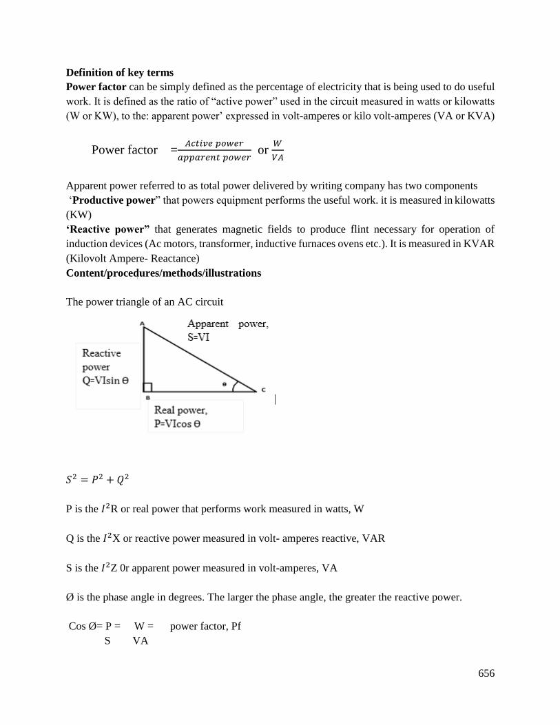
656
Definition of key terms
Power factor can be simply defined as the percentage of electricity that is being used to do useful
work. It is defined as the ratio of “active power” used in the circuit measured in watts or kilowatts
(W or KW), to the: apparent power’ expressed in volt-amperes or kilo volt-amperes (VA or KVA)
Power factor =𝐴𝑐𝑡𝑖𝑣𝑒 𝑝𝑜𝑤𝑒𝑟
𝑎𝑝𝑝𝑎𝑟𝑒𝑛𝑡 𝑝𝑜𝑤𝑒𝑟 or
𝑊
𝑉𝐴
Apparent power referred to as total power delivered by writing company has two components
‘Productive power” that powers equipment performs the useful work. it is measured in kilowatts
(KW)
‘Reactive power” that generates magnetic fields to produce flint necessary for operation of
induction devices (Ac motors, transformer, inductive furnaces ovens etc.). It is measured in KVAR
(Kilovolt Ampere- Reactance)
Content/procedures/methods/illustrations
The power triangle of an AC circuit
𝑆2 = 𝑃2 + 𝑄2
P is the 𝐼2R or real power that performs work measured in watts, W
Q is the 𝐼2X or reactive power measured in volt- amperes reactive, VAR
S is the 𝐼2Z 0r apparent power measured in volt-amperes, VA
Ø is the phase angle in degrees. The larger the phase angle, the greater the reactive power.
Cos Ø= P = W = power factor, Pf
S VA
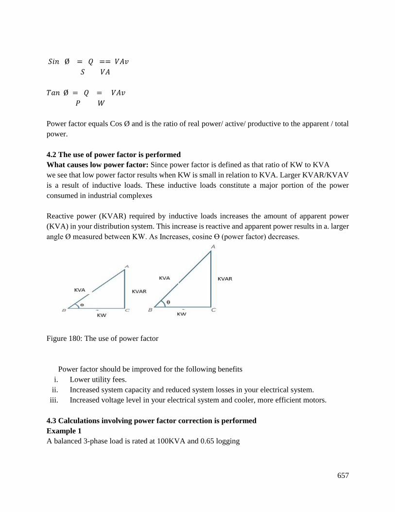
657
𝑆𝑖𝑛 Ø = 𝑄 == 𝑉𝐴𝑣
𝑆 𝑉𝐴
𝑇𝑎𝑛 Ø = 𝑄 = 𝑉𝐴𝑣
𝑃 𝑊
Power factor equals Cos Ø and is the ratio of real power/ active/ productive to the apparent / total
power.
4.2 The use of power factor is performed
What causes low power factor: Since power factor is defined as that ratio of KW to KVA
we see that low power factor results when KW is small in relation to KVA. Larger KVAR/KVAV
is a result of inductive loads. These inductive loads constitute a major portion of the power
consumed in industrial complexes
Reactive power (KVAR) required by inductive loads increases the amount of apparent power
(KVA) in your distribution system. This increase is reactive and apparent power results in a. larger
angle Ø measured between KW. As Increases, cosine Ө (power factor) decreases.
Figure 180: The use of power factor
Power factor should be improved for the following benefits
i. Lower utility fees.
ii. Increased system capacity and reduced system losses in your electrical system.
iii. Increased voltage level in your electrical system and cooler, more efficient motors.
4.3 Calculations involving power factor correction is performed
Example 1
A balanced 3-phase load is rated at 100KVA and 0.65 logging
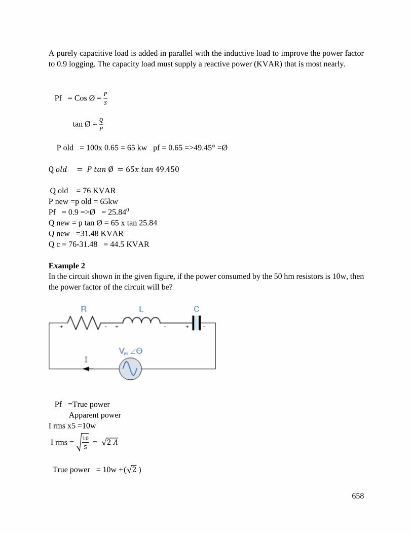
658
A purely capacitive load is added in parallel with the inductive load to improve the power factor
to 0.9 logging. The capacity load must supply a reactive power (KVAR) that is most nearly.
Pf = Cos Ø = 𝑃
𝑆
tan Ø = 𝑄
𝑃
P old = 100x 0.65 = 65 kw pf = 0.65 =>49.45° =Ø
Q 𝑜𝑙𝑑 = 𝑃 𝑡𝑎𝑛 Ø = 65𝑥 𝑡𝑎𝑛 49.450
Q old = 76 KVAR
P new =p old = 65kw
Pf = 0.9 =>Ø = 25.840
Q new = p tan Ø = 65 x tan 25.84
Q new =31.48 KVAR
Q c = 76-31.48 = 44.5 KVAR
Example 2
In the circuit shown in the given figure, if the power consumed by the 50 hm resistors is 10w, then
the power factor of the circuit will be?
Pf =True power
Apparent power
I rms x5 =10w
I rms = √10
5 = √2 𝐴
True power = 10w +(√2 )
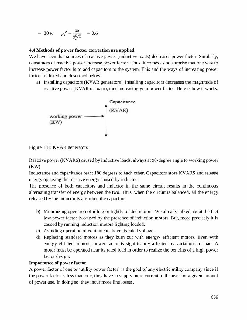
659
= 30 𝑤 𝑝𝑓 =30
50
√2√2
= 0.6
4.4 Methods of power factor correction are applied
We have seen that sources of reactive power (inductive loads) decreases power factor. Similarly,
consumers of reactive power increase power factor. Thus, it comes as no surprise that one way to
increase power factor is to add capacitors to the system. This and the ways of increasing power
factor are listed and described below.
a) Installing capacitors (KVAR generators). Installing capacitors decreases the magnitude of
reactive power (KVAR or foam), thus increasing your power factor. Here is how it works.
Figure 181: KVAR generators
Reactive power (KVARS) caused by inductive loads, always at 90-degree angle to working power
(KW)
Inductance and capacitance react 180 degrees to each other. Capacitors store KVARS and release
energy opposing the reactive energy caused by inductor.
The presence of both capacitors and inductor in the same circuit results in the continuous
alternating transfer of energy between the two. Thus, when the circuit is balanced, all the energy
released by the inductor is absorbed the capacitor.
b) Minimizing operation of idling or lightly loaded motors. We already talked about the fact
low power factor is caused by the presence of induction motors. But, more precisely it is
caused by running induction motors lighting loaded.
c) Avoiding operation of equipment above its rated voltage.
d) Replacing standard motors as they burn out with energy- efficient motors. Even with
energy efficient motors, power factor is significantly affected by variations in load. A
motor must be operated near its rated load in order to realize the benefits of a high power
factor design.
Importance of power factor
A power factor of one or ‘utility power factor’ is the goal of any electric utility company since if
the power factor is less than one, they have to supply more current to the user for a given amount
of power use. In doing so, they incur more line losses.
660
They also must have larger capacity equipment in place than would be otherwise necessary. As a
result, industrial facility will be charged a penalty if its power factor is much different from utility
power, industrial facilities tend to have a “lagging power factor” where the current lags the voltage
(like an inductor). This is primarily the result of having a lot of electric induction motors. The
windings of motors act as inductors as seen by the power supply. Capacitors have the opposite
effect and can compensate for the inductive motor windings. Some industrial sites have large banks
of capacitors strictly for the purpose of correcting the power factor back forward one to save on
utility company charges.
Conclusion
The learning outcome covered or equipped the learner with knowledge, skills and attitude to be
able to determine the amount of electricity that is being used to do useful work in machines and
industrial setups. Also, the learner acquired knowledge and skills of correcting or improving power
factor in industries and as a result lower utility fees.
Further Reading
Garcia, O. Combos, J.A, Presto, R, Alcon, P., Ucenda, J. (2001, June) Power factor
correction; a survey in 2001 IEEE 32nd Annual power
Wild, T. (2002). Electrical machines, drives and power systems. New Jersey; Upper Saddle River
8.3.5.3 Self-Assessment
1. The power factor of a circuit lies between?
a) 0 and 1
b) -1 and 1
c) 0 and -1
d) None of the above
2. The power factor of an ac circuit is equal to?
a) co line of the phase angle
b) line of the phase angle
c) Tangent of the phase angle
d) co tangent of the phase angle
3. The heat developed in a circuit iron is attributed to ___________ power.
a) Apparent

661
b) Reactive
c) True
d) True and reactive
4. In a circuit low reactive power to true power indicates?
a) Low power factor
b) High power factor
c) Low efficiency
d) High efficiency
5. When the power factor in the transmission line is leading, which device is employed at
substation to reduce power factor?
a) CVT
b) Reactor
c) Synchronous condenser
d) None of the above
6. A circuit of zero lagging power factor behaves as?
a. An inductive circuit
b. A capacitive circuit
c. R-L circuit
d. R-C circuit
7. In order to improve the power factors which device should be connected to the power
system.
a) Series capacitor
b) Shunt capacitor
c) Series indicator
d) Shunt indicator
8. If an alternator is supplying load of 350 kw at 0.6 p.f lagging and its power factor is raised
to unity then to supply the alternator for the same KVA loading , the extra required
kilowatts will be ?
9. power factor of a load can be improved by using?
10. What is the maximum value of power factor?
11. What is meant by power factor correction?
12. How does power factor correction save?
13. What is the use of power factor and why is it important?
14. Briefly explain the power triangle showing the active , apparent and reactive power
15. What are the various ways of power factor correction in an industrial set up?
Practical Assessment
The learners with the help of an electrician to measure the power of an AC electric motor using an
oscilloscope. measure voltage and current and interpret the oscilloscopes image to calculate power

662
factor. Since it would be impractical to directly measure voltage and current seeing as how the
voltage is 4160 volts AC and the current is excess of 200 amps
. Fortunately, PT (Potential transformer) and CT (Current transformer) units are to be installed in
the motor circuit to facilitate measurements.
Project
A large electrical land is outfitted with a wattmeter to measure its true power. If the land voltage
is 7.2KV and the load current is 24 amps. Calculate the load’s apparent power.
Calculate the power factor and also the phase angle between voltage and current in the circuit if
the wattmeter registers 155KV at those same voltage and current values.
Draw a power triangle for this circuit, graphically showing the relationship between apparent
power, true power and phase angle.
8.3.5.4 Tools, Equipment, Supplies and Materials
Scientific Calculators
Relevant reference materials
Stationeries
Electrical workshop
Relevant practical materials
Dice
Computers with internet connection
8.3.5.5 References
Khan, S., Ahmed, G. (2018). Industrial power systems are press.
Nat rayon, R. (2018). Power system capacitors. CRC press
Jeong, I.W , Sah, B. S. , and Park. M. G. (2013). U. S Patent No. 9, 214,856. Washington DC; US.
Patent and Trademark office.
663
8.3.6 Learning Outcome No 5: Use of earthling in Electrical installations
8.3.2.1 Learning Activities
Learning Outcome No 5: Use of earthling in Electrical installations
Learning Activities Special Instructions
5.1 Identify earthling types
5.2 Identify earthling points on Electrical installation
5.3 Perform calculation involved in determining the earthling type
5.4 Perform test on an earthling system in line with the IEE regulations
8.3.2.2 Information Sheet No8/LO 5: Use of earthling in Electrical installations
Introduction
This learning outcome covers the installation of earthing in electrical engineering. The learner
would be able to know different types of earthing, to identify earthing points on electrical
installation. Calculations involved in determining earthing types and the perform test on an
earthing system in the line with IEF regulations.
Definition of key terms
Earthing: is the situation where connection of specific parts of the installation with earth’s
conductive surface is done for safety and functional purpose.
Earth electrode: It is the system of electrical connection consisting of components of an electrical
system and metal work associated with the equipment, apparatus and appliances.
Earth: Is a conductor covered with the resistive material such as soil.
Content/procedures/methods/illustrations
5.1 Earthling types are identified
T: Earth
N: Neutral
S: Separate
C: Combined
I: Isolated
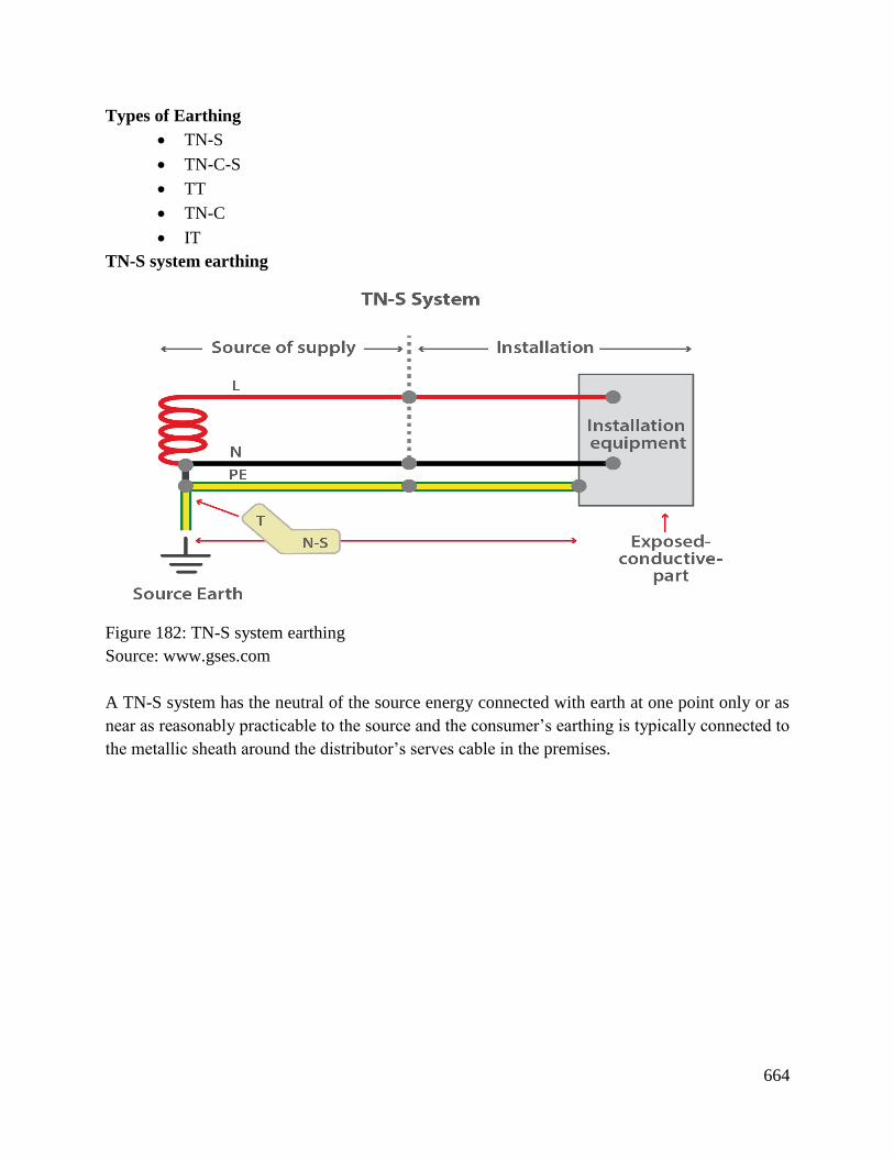
664
Types of Earthing
TN-S
TN-C-S
TT
TN-C
IT
TN-S system earthing
Figure 182: TN-S system earthing
Source: www.gses.com
A TN-S system has the neutral of the source energy connected with earth at one point only or as
near as reasonably practicable to the source and the consumer’s earthing is typically connected to
the metallic sheath around the distributor’s serves cable in the premises.

665
Over view of TN-S earthing system
Figure 183: TN-S earthing system
Source: www.clarvis.co.uk
TN-C-S earthing system
Figure 184: TN-C-S earthing system
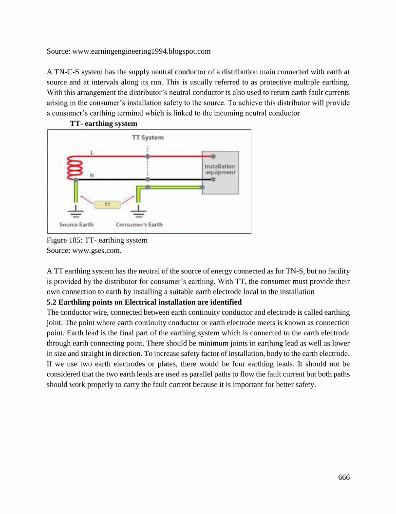
666
Source: www.earningengineering1994.blogspot.com
A TN-C-S system has the supply neutral conductor of a distribution main connected with earth at
source and at intervals along its run. This is usually referred to as protective multiple earthing.
With this arrangement the distributor’s neutral conductor is also used to return earth fault currents
arising in the consumer’s installation safety to the source. To achieve this distributor will provide
a consumer’s earthing terminal which is linked to the incoming neutral conductor
TT- earthing system
Figure 185: TT- earthing system
Source: www.gses.com.
A TT earthing system has the neutral of the source of energy connected as for TN-S, but no facility
is provided by the distributor for consumer’s earthing. With TT, the consumer must provide their
own connection to earth by installing a suitable earth electrode local to the installation
5.2 Earthling points on Electrical installation are identified
The conductor wire, connected between earth continuity conductor and electrode is called earthing
joint. The point where earth continuity conductor or earth electrode meets is known as connection
point. Earth lead is the final part of the earthing system which is connected to the earth electrode
through earth connecting point. There should be minimum joints in earthing lead as well as lower
in size and straight in direction. To increase safety factor of installation, body to the earth electrode.
If we use two earth electrodes or plates, there would be four earthing leads. It should not be
considered that the two earth leads are used as parallel paths to flow the fault current but both paths
should work properly to carry the fault current because it is important for better safety.
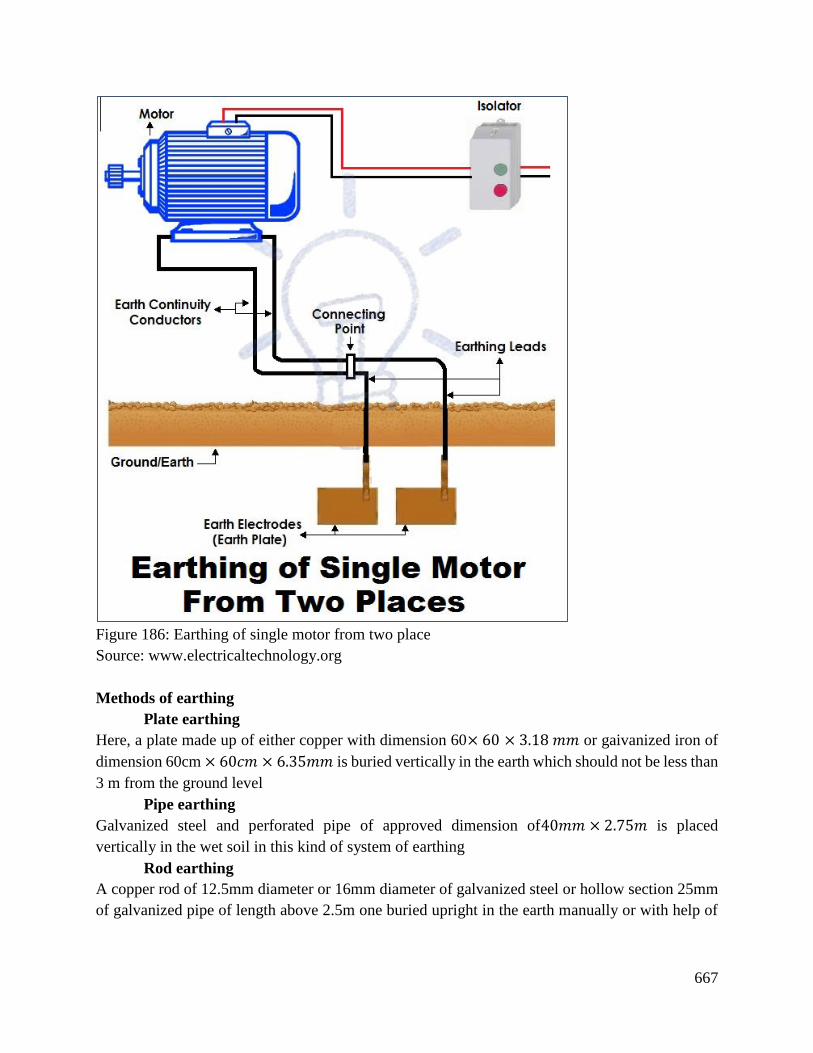
667
Figure 186: Earthing of single motor from two place
Source: www.electricaltechnology.org
Methods of earthing
Plate earthing
Here, a plate made up of either copper with dimension 60× 60 × 3.18 𝑚𝑚 or gaivanized iron of
dimension 60cm × 60𝑐𝑚 × 6.35𝑚𝑚 is buried vertically in the earth which should not be less than
3 m from the ground level
Pipe earthing
Galvanized steel and perforated pipe of approved dimension of40𝑚𝑚 × 2.75𝑚 is placed
vertically in the wet soil in this kind of system of earthing
Rod earthing
A copper rod of 12.5mm diameter or 16mm diameter of galvanized steel or hollow section 25mm
of galvanized pipe of length above 2.5m one buried upright in the earth manually or with help of
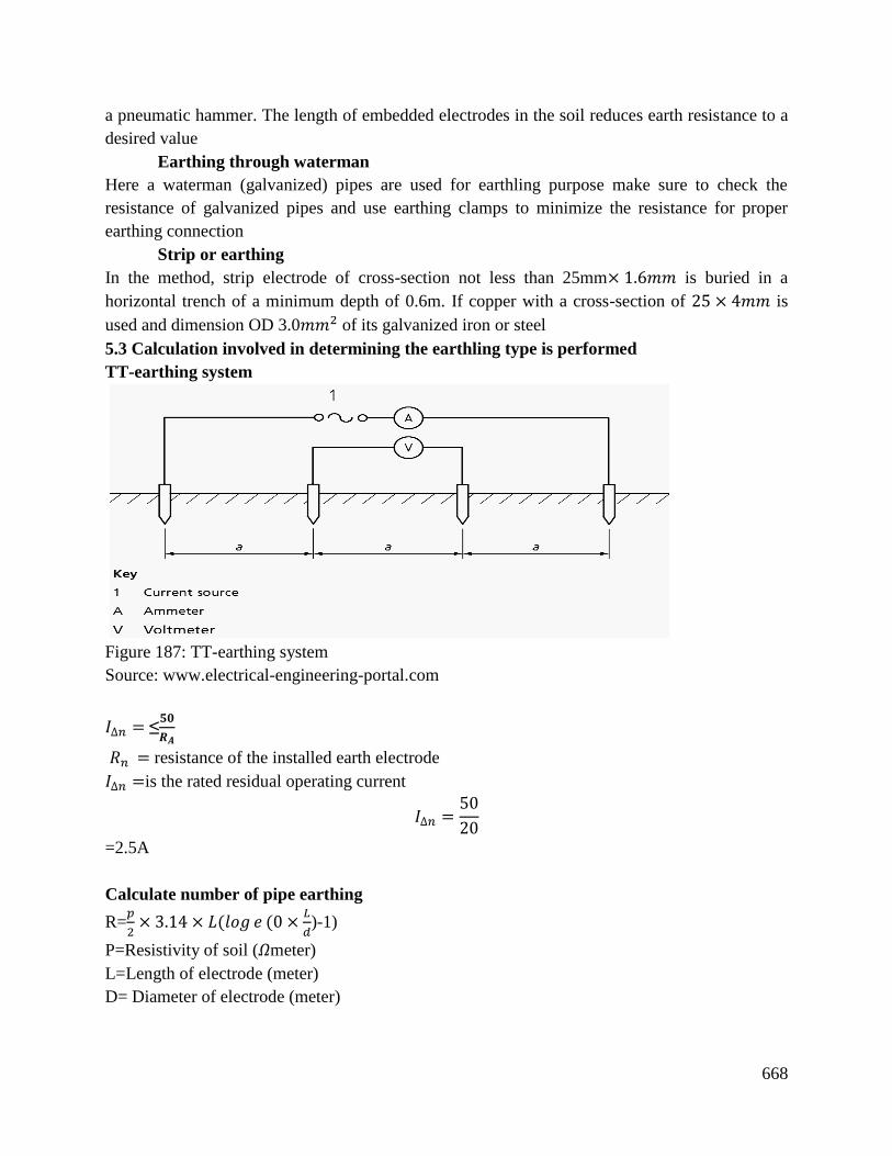
668
a pneumatic hammer. The length of embedded electrodes in the soil reduces earth resistance to a
desired value
Earthing through waterman
Here a waterman (galvanized) pipes are used for earthling purpose make sure to check the
resistance of galvanized pipes and use earthing clamps to minimize the resistance for proper
earthing connection
Strip or earthing
In the method, strip electrode of cross-section not less than 25mm× 1.6𝑚𝑚 is buried in a
horizontal trench of a minimum depth of 0.6m. If copper with a cross-section of 25 × 4𝑚𝑚 is
used and dimension OD 3.0𝑚𝑚2 of its galvanized iron or steel
5.3 Calculation involved in determining the earthling type is performed
TT-earthing system
Figure 187: TT-earthing system
Source: www.electrical-engineering-portal.com
𝐼∆𝑛 = ≤𝟓𝟎
𝑹𝑨
𝑅𝑛 = resistance of the installed earth electrode
𝐼∆𝑛 =is the rated residual operating current
𝐼∆𝑛 =50
20
=2.5A
Calculate number of pipe earthing
R=𝑝
2× 3.14 × 𝐿(𝑙𝑜𝑔 𝑒 (0 ×
𝐿
𝑑)-1)
P=Resistivity of soil (𝛺meter)
L=Length of electrode (meter)
D= Diameter of electrode (meter)
669
Example:
Calculate isolated earthing rod resistance. The earthing rod is 4m long having 12.2mm diameter,
soil sensitivity 500𝛺meter
R=𝑃
2× 3.14𝐿(𝑙𝑜𝑔 (8 ×
𝐿
𝐷) -1)
R=500
2×3.14×4× (𝑙𝑜𝑔 e (8 ×
4
0.0125)-1 )
= 156.1aὨ
Earth resistance of single rod or pipe electrode
R=100×𝑝
2×3.14𝐿(𝑙𝑜𝑔 𝑒 (4
𝑙
𝑑×
𝐿
𝐷)
Where P= Resistivity of soil (𝛺m)
L= Length of electrode (km)
D= Diameter of electrode (cm)
Example:
Calculate number of CL earthing pipe of 100mm diameter 3m, length the system has fault current
of 50KA for 1 sec and soil resistivity is 7.244𝛺m.
Solution
Maximum allowable current density (I)
= 7.57×1000
√𝑝×𝑡A/𝑚2
=7.57×1000
√72.44×1
=889.419A/𝑚2
Surface area of the 100mm diameter 3m length pipe
=2 × 3.14 ×𝑟
𝐿
=2 × 3.14 × 0.05 × 3
=0.942𝑚2
Maximum current dissipated by one earthing pipe
=Current density× 𝑠𝑢𝑟𝑓𝑎𝑐𝑒 𝑎𝑟𝑒𝑎 𝑜𝑓 𝑒𝑙𝑒𝑐𝑡𝑟𝑜𝑑𝑒
=889.419× 0.942
=838A
Number of earthing pipe required
=𝑓𝑎𝑢𝑙𝑡 𝑐𝑢𝑟𝑟𝑒𝑛𝑡
𝑚𝑎𝑥𝑖𝑚𝑢𝑚 𝑐𝑢𝑟𝑟𝑒𝑛𝑡 𝑑𝑖𝑠𝑠𝑖𝑝𝑎𝑡𝑒𝑑 𝑏𝑦 𝑜𝑛𝑒 𝑒𝑎𝑟𝑡ℎ𝑖n𝑔 𝑝𝑖𝑝𝑒
=50000
838
=59.66 or 60
Resistance of earthing
=100×𝑃
2×3.14×𝐿× (𝑙𝑜𝑔 𝑒 (4 ×
𝐿
𝐷)
R=100 ×72.44
2× 3.14 × 3000 × (𝑙𝑜𝑔 𝑒 (4 ×
300
10)
=7.99Ὠ/Pipe
670
1 pipe=60
? =7.99 7.99
60=0.133Ὠ
Earthing resistance and number of rod for isolated earth pit
R=𝑃
2×3.14×𝐿× (𝑙𝑜𝑔 𝑒 (2 × 𝐿 ×
𝐿
𝑤𝑡)
Example
A galvanized strip having width of 12mm, length of 2200m is buried in ground at depth of
2200mm, soil where resistivity is 72.44Ὠ.m. calculate;
i. Resistance of earth ®=
72.44
2× 3.14 × 2200 × (𝑙𝑜𝑔 𝑒(2 × 2200 × 2 × 0.012)
=0.057Ὠ
From the above calculations overall resistance of 60 of earthing pipes (𝑅𝑃) = 0.133Ὠ
ii. Net earthing resistance= (𝑅𝑃×𝑅𝐸
𝑅𝑃+𝑅𝑒
)
=(0.133×0.05
(0.133+0.05)
=0.036Ὠ
iii. Total earthing resistance and number of electrodes for group
Ra=R (1+𝑎ک
𝑛)
Where a=𝑃2 × 3.14 × 𝑅 × 𝑆
S= Distance between adjustment rod (m)
ᴧ=Factor given in the table below
n=Number of electrodes
P= Resistivity of soil (𝛺m)
R= Resistance of single rod in isolation
Factors for parallel electrodes in line BS 7430
No of electrodes(n) Factorᴧ
2 1.0
3 1.66
4 2.15
5 2.54
6 2.87
7 3.15
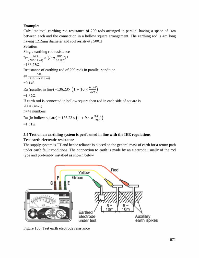
671
Example:
Calculate total earthing rod resistance of 200 rods arranged in parallel having a space of 4m
between each and the connection in a hollow square arrangement. The earthing rod is 4m long
having 12.2mm diameter and soil resistivity 500Ὠ
Solution
Single earthing rod resistance
R=500
(2×3.14×4)× (𝑙𝑜𝑔
8×4
0.0125)-1
=136.23Ω
Resistance of earthing rod of 200 rods in parallel condition
a= 500
(2×3.14×136×4)
=0.146
Ra (parallel in line) =136.23× (1 + 10 ×0.146
200)
=1.67Ω
If earth rod is connected in hollow square then rod in each side of square is
200= (4n-1)
n=4a numbers
Ra (in hollow square) = 136.23× (1 + 9.4 ×0.146
200)
=1.61Ω
5.4 Test on an earthling system is performed in line with the IEE regulations
Test earth electrode resistance
The supply system is TT and hence reliance is placed on the general mass of earth for a return path
under earth fault conditions. The connection to earth is made by an electrode usually of the rod
type and preferably installed as shown below
Figure 188: Test earth electrode resistance
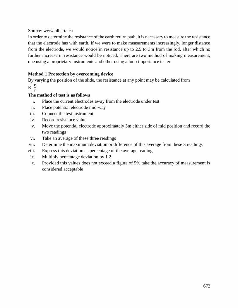
672
Source: www.alberta.ca
In order to determine the resistance of the earth return path, it is necessary to measure the resistance
that the electrode has with earth. If we were to make measurements increasingly, longer distance
from the electrode, we would notice in resistance up to 2.5 to 3m from the rod, after which no
further increase in resistance would be noticed. There are two method of making measurement,
one using a proprietary instruments and other using a loop importance tester
Method 1 Protection by overcoming device
By varying the position of the slide, the resistance at any point may be calculated from
R=𝑽
𝑰
The method of test is as follows
i. Place the current electrodes away from the electrode under test
ii. Place potential electrode mid-way
iii. Connect the test instrument
iv. Record resistance value
v. Move the potential electrode approximately 3m either side of mid position and record the
two readings
vi. Take an average of these three readings
vii. Determine the maximum deviation or difference of this average from these 3 readings
viii. Express this deviation as percentage of the average reading
ix. Multiply percentage deviation by 1.2
x. Provided this values does not exceed a figure of 5% take the accuracy of measurement is
considered acceptable
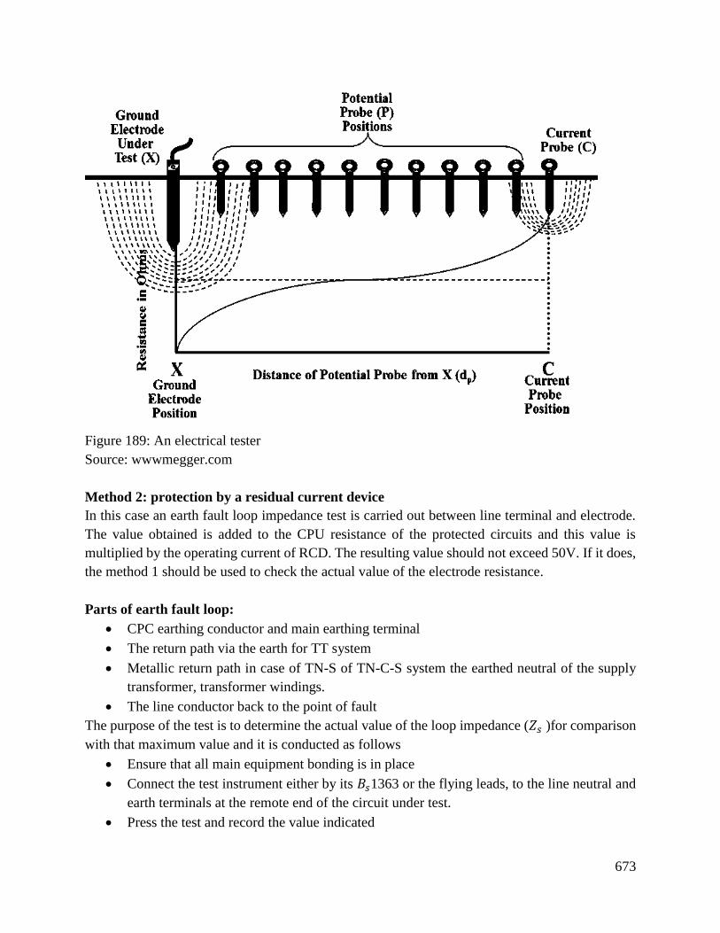
673
Figure 189: An electrical tester
Source: wwwmegger.com
Method 2: protection by a residual current device
In this case an earth fault loop impedance test is carried out between line terminal and electrode.
The value obtained is added to the CPU resistance of the protected circuits and this value is
multiplied by the operating current of RCD. The resulting value should not exceed 50V. If it does,
the method 1 should be used to check the actual value of the electrode resistance.
Parts of earth fault loop:
CPC earthing conductor and main earthing terminal
The return path via the earth for TT system
Metallic return path in case of TN-S of TN-C-S system the earthed neutral of the supply
transformer, transformer windings.
The line conductor back to the point of fault
The purpose of the test is to determine the actual value of the loop impedance (𝑍𝑠 )for comparison
with that maximum value and it is conducted as follows
Ensure that all main equipment bonding is in place
Connect the test instrument either by its 𝐵𝑠1363 or the flying leads, to the line neutral and
earth terminals at the remote end of the circuit under test.
Press the test and record the value indicated
674
Figure 190: Base earth fault loop impedance
Source: www.mycableengineering.com
It must be understood that this instrument heading is not valid for direct comparison with the
tabulated maximum value, as accountability must be taken for the ambient temperature at test time
and maximum conductor operating temperature both of which will have maximum conductor
resistance.
Conclusion
The learning outcome covered or equipped the learner with knowledge, skills on how to perform
different types of earthing system. This will help them to ensure the in stored electronics have
good working conditions.
Further Reading
John Bird 4th edition: Electrical and electronic principles and technology.
8.3.6.3 Self-Assessment
Written assessment
1. Ground resistance should be designed for which reason?
a) Should be as low as possible
b) Should be as high as possible
c) Should be always zero
d) Should be always vertical
675
2. Discuss what happens when earth fault occurs.
a) Voltage potential at the earth mat increases due to grounding
b) Voltage potential at the earth mat decreases due to grounding
c) Voltage potential at earth ma remains zero irrespective of fault
d) Voltage potential behaves abnormally or grinding
3. Describe the objective of earthing or grounding.
a) To provide as low resistance possible to the ground
b) To provide as high resistance possible to the ground
c) To provide hoe of positive, negative and zero sequence current
d) To provide equal resistance possible to the ground
4. Moisture content in the soil _____________ the earth soil resistance.
a) Increase
b) Decrease
c) Do not affect
d) It effects
5. Factors on which soil resistance depends are?
a) Depth of the electrode
b) Moisture
c) Nacl
d) Diameter of the electrode
6. Which one of the following is not on the types of earthing?
a) TN-S
b) TN-C
c) TN-C-Z
d) TT
7. Which one is not a method of earthing?
a) Plate earthing
b) Pipe earthing
c) Rod earthing
d) Silver earthing
8. What is a proving unit used for earthing?
9. What is meant by consuming terminal?
10. Describe the procedure of protection by over current device.
11. With an aid of well labeled diagram discuss how to test earth fault loop impedance.
Oral Assessment
1. What are the basic requirement for earthing?
Practical Assessment

676
1. During motor installation describe how you would ensure the earthing is done correctly.
Project
1. As an electrical engineer describe how you would install an earthing to a storey building
using three phase power.
8.3.6.4 Tools, Equipment, Supplies and Materials
• Scientific Calculators
• Relevant reference materials
• Stationeries
• Electrical workshop
• Relevant practical materials
• Dice
• Computers with internet connection
8.3.6.5 References
Kumar, A., Ranjan, S., Singh, M. B. K., Kumari, P., & Ramesh, L. (2015). Electrical energy audit
in residential house. Procedia Technology, 21, 625-630.
Agrawal, N. (2015, November). Electrical safety practices in cement industry for sustainable
operation. In 2015 IEEE IAS Joint Industrial and Commercial Power Systems/Petroleum and
Chemical Industry Conference (ICPSPCIC) (pp. 214-219). IEEE.
677
8.3.7 Learning Outcome No 6: Apply lightning protection measures
8.3.2.1 Learning Activities
Learning Outcome No6: Apply lightning protection measures
Learning Activities Special Instructions
6.1 Identify types of lightening strokes
6.2 Identify components of lightening protection system
6.3 Establish test to be carried out in lightening protection system
6.4 Determine application of lightening protection system
8.3.7.2 Information Sheet No8/LO6: Apply lightning protection measures
Introduction
This learning outcome covers; lighting protection system (LPS); transfer the lighting current safely
to the ground. This system includes air termination, down conductor and earth termination system
which is also known as lighting protection grounding system that intended to provide a low
resistance path to dissipate high current into the soil. The lighting protection system elements
should be selected from materials which are resistant to corrosion and should be protected from
fast degradation.
Definition of key terms
Arrester: Component/circuit used to suppress or divert the electrical (surge and transient) energy
to ground.
Bonding: The joining of metallic parts to form an electrically conductive path to assure electrical
continuity and capacity to conduct current imposed between the metallic parts.
Coupling: Energy transfer between circuits, equipment or systems.
Lightning stroke: Single discharge in a lightning flash to earth.
Lightning detector: Device which provide indication of lighting.
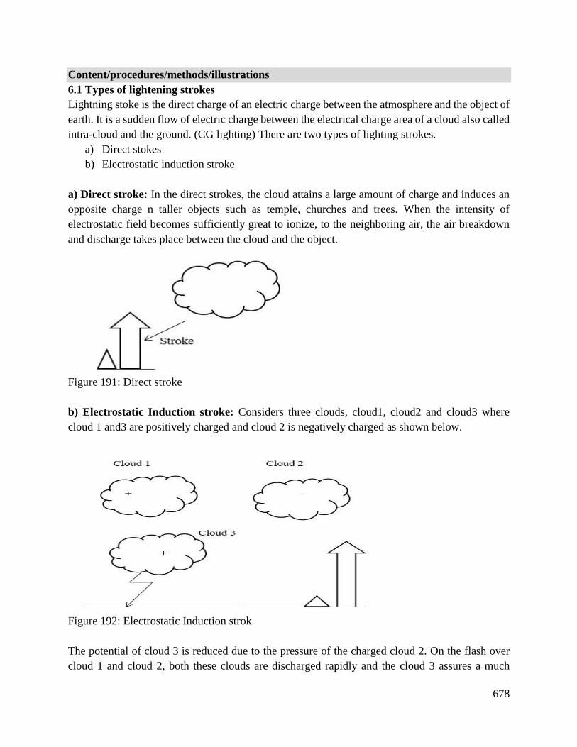
678
Content/procedures/methods/illustrations
6.1 Types of lightening strokes
Lightning stoke is the direct charge of an electric charge between the atmosphere and the object of
earth. It is a sudden flow of electric charge between the electrical charge area of a cloud also called
intra-cloud and the ground. (CG lighting) There are two types of lighting strokes.
a) Direct stokes
b) Electrostatic induction stroke
a) Direct stroke: In the direct strokes, the cloud attains a large amount of charge and induces an
opposite charge n taller objects such as temple, churches and trees. When the intensity of
electrostatic field becomes sufficiently great to ionize, to the neighboring air, the air breakdown
and discharge takes place between the cloud and the object.
Figure 191: Direct stroke
b) Electrostatic Induction stroke: Considers three clouds, cloud1, cloud2 and cloud3 where
cloud 1 and3 are positively charged and cloud 2 is negatively charged as shown below.
Figure 192: Electrostatic Induction strok
The potential of cloud 3 is reduced due to the pressure of the charged cloud 2. On the flash over
cloud 1 and cloud 2, both these clouds are discharged rapidly and the cloud 3 assures a much
679
potential and flashes to the earth very rapidly. It is the most dangerous as it ignores the taller
buildings and reaches directly to the ground.
6.2 Components of lightening protection system are identified
A protection lightning system is composed of 4 main components:
Lightning rods and air terminals
Conductor cables
Ground rods
Surge protection devices
Bonds
Lightning rods and air terminals: Made of copper or aluminum and are placed at intervals
around the root of a tall structure to intercept the lightning stroke.
Conductor cables: They are connected to air terminals and feed the electrical charge received at
the air terminals to the grounding, where it is dissipated aimlessly to the ground by assistance of
ground rods.
Surge protection devices: help protect electrical appliances in a house and prevent fires in the
event of a lighting stroke.
Bonds: Help preventing lighting from jumping two objects.
6.3 Test to be carried out in lightening protection system are established
Test procedures are carried out for small and medium sized earthing systems as well as larger
earthing systems using the earth resistance procedure or continuity tests for small and medium
sized earth terminals systems, “fall potential” method is carried out while for larger earthing
systems the “Tag method” of testing is recommended.
a) Continuity test: Helps to confirm whether the conductors are well connected.
b) Earth resistance test procedure: The fall in potential method helps test the DC resistance of
an earthing system for small and medium sizes earthing systems.
c) Earth resistance test:
Test procedure for small and medium sized earthing systems:
Place the potential probe L1 along a straight line with that of the geometric Centre of the earthing;
the system is aligned with the current probe L2 where under ideal conditions L1=0.62L2. The DC
resistance should be obtained directly in Ohm’s and where;
For lightning protection systems=10 Ohms or less
For mains/electrical earthing systems=1 Ohms or less
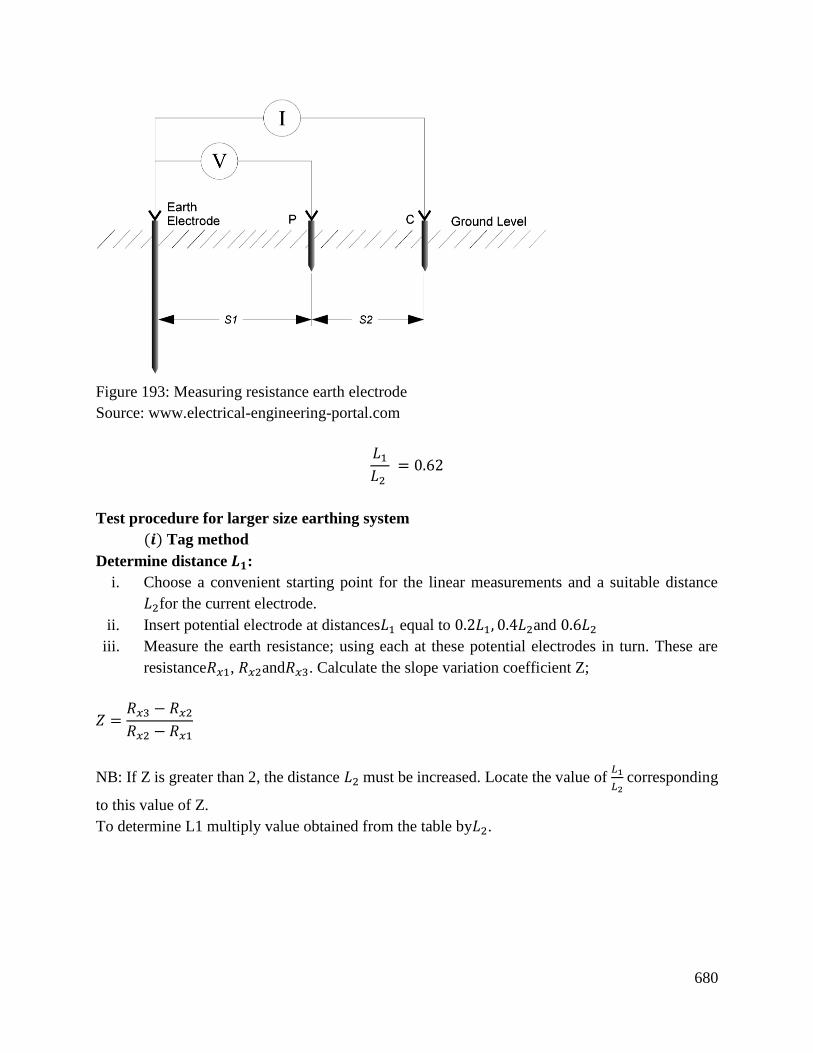
680
Figure 193: Measuring resistance earth electrode
Source: www.electrical-engineering-portal.com
𝐿1
𝐿2 = 0.62
Test procedure for larger size earthing system
(𝒊) Tag method
Determine distance 𝑳𝟏:
i. Choose a convenient starting point for the linear measurements and a suitable distance
𝐿2for the current electrode.
ii. Insert potential electrode at distances𝐿1 equal to 0.2𝐿1, 0.4𝐿2and 0.6𝐿2
iii. Measure the earth resistance; using each at these potential electrodes in turn. These are
resistance𝑅𝑥1, 𝑅𝑥2and𝑅𝑥3. Calculate the slope variation coefficient Z;
𝑍 =𝑅𝑥3 − 𝑅𝑥2
𝑅𝑥2 − 𝑅𝑥1
NB: If Z is greater than 2, the distance 𝐿2 must be increased. Locate the value of 𝐿1
𝐿2 corresponding
to this value of Z.
To determine L1 multiply value obtained from the table by𝐿2.
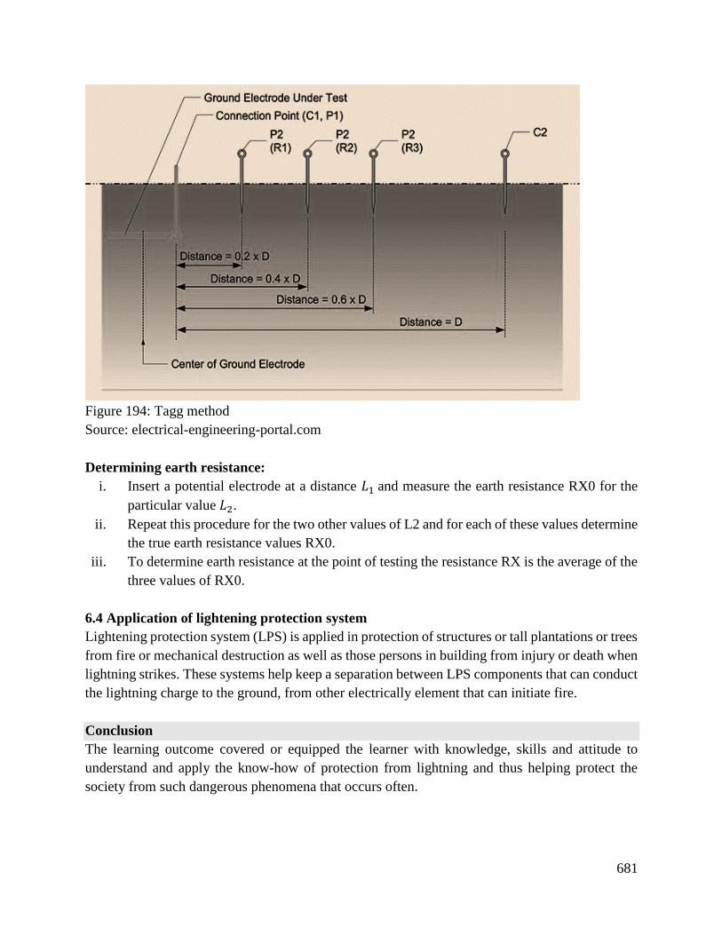
681
Figure 194: Tagg method
Source: electrical-engineering-portal.com
Determining earth resistance:
i. Insert a potential electrode at a distance 𝐿1 and measure the earth resistance RX0 for the
particular value 𝐿2.
ii. Repeat this procedure for the two other values of L2 and for each of these values determine
the true earth resistance values RX0.
iii. To determine earth resistance at the point of testing the resistance RX is the average of the
three values of RX0.
6.4 Application of lightening protection system
Lightening protection system (LPS) is applied in protection of structures or tall plantations or trees
from fire or mechanical destruction as well as those persons in building from injury or death when
lightning strikes. These systems help keep a separation between LPS components that can conduct
the lightning charge to the ground, from other electrically element that can initiate fire.
Conclusion
The learning outcome covered or equipped the learner with knowledge, skills and attitude to
understand and apply the know-how of protection from lightning and thus helping protect the
society from such dangerous phenomena that occurs often.
682
Further Reading
Further reading should be done on surge protection devices (LPS)
Further reading be acquired from Northeast lightning Protection LLC company website.
Fisher; F.A&Plumer, J.A (1980) “Lightning Protection for Aircraft”
8.3.7.3 Self-Assessment
Written assessment
1) In case of extreme high voltage surge, surge due protection device acts as conductor and
connects the voltage surge to ground.
a) True
b) False
2) The property of surge protection device is to have highly linear (V-I) characteristics.
a) True
b) False
3) Electrical surge are being caused because of which one of the following?
a) Both lightning strikes and EHV switching
b) EHV switching
c) Lightning strikes
4) An air termination should exceed a minimum of above the object that is to be
protected?
a) 15 inches
b) 10 inches
c) 25 inches
d) 20 inches
5) Angle of zone f protection of lightning protection system is approximately?
a) 200
b) 4500
c) 100
d) 700
6) A grounding connection to earth from lightning protection system should be made at
diagonals corners of the structure.
a) True)
b) False
7) The resistance between lightning protection system and earth should be?
a) Low
683
b) High
8) The zone of protection (surrounding area that lightning protection system protects) is
approximately times the height of a building protected.
9) In case of air termination for continuous roof ridges air terminal should be spaced
feet.
10) Impulse ratios of insulators and lightning arrestors should be?
11) Basically, a lightning arrestor is a surge ?
12) Give an example of potential sources of surge.
Oral Assessment
1. Which colour is copper material?
2. Why does air terminal have three tips?
Practical Assessment
1. In three student groups try to carry. Out resistance test on the institutions ground.
Project
1. Develop a circuit that can be able to indicate/detect a small amount of electric surge.
8.3.7.4 Tools, Equipment, Supplies and Materials
Scientific Calculators
Relevant reference materials
Stationeries
Electrical workshop
Relevant practical materials
Dice
Computers with internet connection
8.3.7.5 References
Bazelyan, E.M&Raizer, V.P (2000) Lightning physics and lightning protection. CRC Press.
Cao, W., Wan, S., Gu, S., Xu, H., Chen, J., Wang, J., & Lv, J. (2019). Development and application
of lightning flashover limited equipment for 220 kV AC transmission line. The Journal of
Engineering, 2019(16), 802-805.
Wang, Q., Li, J., & Lu, J. (2018, September). Study On Lightning Protection Of Wind Turbine
Blades. In 2018 IEEE International Conference on High Voltage Engineering and
Application (ICHVE) (pp. 1-4). IEEE.
684
8.3.8 Learning Outcome No 7: Apply Electromagnetic field theory
8.3.2.1 Learning Activities
Learning Outcome No 7:Apply Electromagnetic field theory
Learning Activities Special Instructions
7.1 Apply Electromagnetic field theory
8.3.2.2 Information Sheet No8/LO7: Apply Electrodynamics
Introduction
This learning outcome covers how to apply the electromagnetic field theory.
Definition of key terms
Magnetic field strength (H): It is a vector quantity having both magnitude and direction. Its unit
is N/wb. r3
F=𝑀𝑋1
4𝑀𝜋𝑅𝟐 N H=
𝑀
4𝑀ῼ𝑅3 NWb H=
𝑀
4𝑀ῼ𝑅2 R=
𝑀
4𝑀ῼ.𝑟3 r
Flux density (B): It is a vector quantity which is the total magnetic flux passing normally through
an area of. 𝐵 = ᴓ/𝐴𝑤𝑏/𝑚2 or 𝑡𝑒𝑠𝑖𝑎 (𝑇), 𝑎𝑚 2
1. Intensity or magnetization (I)- It is the induced pole strength developed per unit area of the bar
or flux density produced in it due to its own induced magnetism.
𝐼 = 𝑀/𝐴 𝑤𝑏/𝑚2 where A= Force or pole area of the bar in m2
M=pole strength induced in the bar in 𝑤𝑏.
4 Susceptibility (k) – the ratio of intensity of magnetization I to the magnetizing force (H).
K= 𝐼
𝐻 henry/ meter.
Meaning of electromagnetic field theory
Electromagnetic field theory: When magnetic flux linking a conductor changes an e.m.f is
induced in the conductor.
Source of electromagnetic fields.
Earth, sun and atmosphere are all natural sources of electromagnetic fields. They exist everywhere
in the environment. Electromagnetic fields are generated by either natural or human made sources.;
Production of electromagnetic fields.
685
An installed coil whose terminals are connected to a sensitive galvanometer G. It is placed close
to a stationery bar magnet initially at position AB. Some flux from the N- pole of the magnet is
linked with the threads through the coil but there is no deflection of the galvanometer that indicates
production of electromagnetic field.
Detectors of electromagnetic radiation.
1. Galvanometer- the deflection of galvanometer indicated production of electromagnetic
field in the coil.
Application of electromagnetic waves.
Electromagnetic waves are a self-propagating transverse wave or oscillating electric and magnetic
field.
Applications.
Radio wave- electromagnetic radiation having wavelength about 5 cm and 30,000m used
for the broadcasting of radio and television signals.
Conductors- a material which contains movable electric charges conduct electricity and
heat.
Telecommunication- the science and technology of the communication or messages over
distance especially using electrics, electronics or electromagnetic impulse.
Electromagnetic laws
(a) Faraday’s law
Faraday’s perform a series of experiments to demonstrate electromagnetic induction.
First Law: It states that when a magnetic flux linking a conductor or coil changes, an e.m.f it
induces in it.
Second law: It states that the magnitude of induced e.m.f in a coil is equal to the rate of charge of
magnetic flux linkages.
When a coil having N turns and magnetic flux is linking, the coil increases from ᴓ1 to ᴓ2 wb in
seconds. Now magnetic flux linkages means the product of magnetic flux and a number of turns.
Initial magnetic flux linkages = Nᴓ1
Final magnetic flux linkages =Nᴓ2
E= Rate of charge of magnetic flux linkages.
In different form we have
𝐸 = 𝑁 𝑑ᴓ1
𝑑𝑡 𝑣𝑜𝑙𝑡𝑠.
The minus sign comes from Lenz’s law and indicates that the voltage is induced in a direction
to oppose the change in flux that produced it.
𝐸 = 𝑁𝑑ᴓ
𝑑𝑡 𝑣𝑜𝑙𝑡𝑠.
Example
686
A coil of 100 turns of wire is wound on a magnetic circuit of reluctance 2000 AT/mwb. It is a
current of 1A flowing in the coil is reversed in 10ms. Find the average e.m.f induced by the coil.
Solution
Change in magnetic flux 𝑑ᴓ = 20 − (−20) = 40𝑚𝑊𝑏 = 40𝑥10𝑤𝑏. Change In time taken, 𝑑+=
2 𝑥 10−3𝑠𝑒𝑐.
𝐸 = 𝑁𝑑ᴓ
𝑑𝑡= 100𝑥
40𝑋10 − 3
2𝑋10 − 3= 2000𝑣
(b) Lenz’s law
it states that in effect that electromagnetically induced current always flow in such a direction that
action of the magnetic field set up by it tends to oppose the very cause which produces it. It may
be noted here that Lenz’s law directly follows from the law of conservation of energy that some
energy must be expanded .when the m-pole of the magnet is approaching the coil , the induced
current will flow in the coil in such a direction that the left hand face of the coil becomes the N-
pole. The mechanical energy spent is overcoming this opposition is converted into electrical
energy which appears in the coil.
(c) Fleming’s law
it states that when one stretches his forefinger, middle finger and thumb of the right hand so that
they are at a right angle to one another, if the finger points in the direction of the magnetic field,
thumb in the direction of motion of the conductor, then the middle finger will point in the direction
of the induced current.
Properties and effects of electromagnetic waves
They move energy as well as momentum from one place to another.
They travel in a direction perpendicular to partial vibration.
They can bounce off from a surface.
Their direction can change in moving from one medium to another.
They can spread round corners.
They can travel through an empty space
They obey general wave equation speed=frequency x wavelength.
The shorter the wavelength or higher the frequency, the higher the energy and the more
dangerous.
Effects of electromagnetic waves.
It causes cancer.
Produce excessive intercellular calcium and excessive calcium signating.
It causes fertility problems.
Cellular DNA attacks.
Oxidative stress and radio damage.
687
The steroid hormone level drop with e.m.f exposure whereas other hormones level increase
with initial exposure.
It causes nervous system and brain.
Characteristics of waves.
Medium material through which wave transfer energy are solid, liquid and gas or
combination.
Electromagnetic waves don’t need a medium e.g visible light.
Transverse waves medium vibrates perpendicularly to the direction of wave motion.
Longitudinal waves medium moves in the same direction as the waves motion.
Electromagnetic wave shielding.
It is the practice of reducing the electromagnetic field in a space by blocking the field with barriers
made of conductive or magnetic materials. Shielding is typically applied to enclosure or isolate
electrical devices from the surroundings, to cables to isolate waves from the environment through
which the cables runs. Electromagnetic shielding that blocks radio frequency electromagnetic
radiation is known as radio frequency shielding.
Skin effects.
It is the tendency of an alternating electric current (AC) to become distributed within a conductors
such that the current density is largest near the surface of the conductor and decreases with greater
depths in the conductor. The electric current flows mainly at the skin of the conductor between the
outer surface and a level called skin depth. The skin effect causes effective resistance of the
conductor to increase at higher frequency where the skin depth is smaller thus reducing the
effective cross section of the conductor. The skin effect is due to opposing eddy currents induced
by the changing magnetic field resulting from the alternating current.
Conclusion
In conclusion electromagnetic waves are of greater importance as it lead to introduction of
technology such as televisions, radios and telephones. On the other hand, electromagnetic waves
are harmful to the human body as they cause diseases to the nervous system, the brain cancer etc.
Therefore people should come up with a measure to protect themselves from its effect.
Further Reading
John Bird 4th edition: Elemental and electronic principles.
8.3.7.3 Self-Assessment
688
Written assessment
1. A coil of 100 turns is linked by a magnetic flux of 20mWb. If this magnetic flux is reversed
in a time of 20 ms, calculate the average e.m.f induced in the coil.
a) 200V
b) 3000V
c) 2000V
d) 400V.
2. A coil of 200 turns of wire is wound on a magnetic circuit of reluctance 2000 AT/m Wb. If a
current of 1A flowing in the coil is reversed is reversed in 10 ms, find the average e.m.f
induced in the coil.
a) 3V
b) 6V
c) 4V
d) 10V
3. The field winding of 4 poles dc generator consist of 4 coils connected in a series , each coil
being wound with 1200 turns. When the field is exited, there is a magnetic flux of
0.04wn/pole. If the field switch is opened at such a speed that the magnetic flux falls to the
residual value of 0.004 Wb/pole in 0.1 sec. calculate the average value of e.m.f induced across
the field winding terminals.
a) 6912V
b) 512V
c) 7004V
d) 5000V
4. A coil of resistance 100π is laced in a magnetic field of 1mWb. The coil has 100turnss and a
galvanometer of 400 π resistance is connected in series with it. Find the average e.m.f and the
current if the coil is moved in 1
10𝑡ℎ second from the given field of 0.2mWb.
a) 1.6 MA
b) 2.5MA
c) 2.5 MA
d) 12MA.
5. The two coils are wound closer together on the same paxolin tube. Current is passed through
the first coil varied at a uniform rate of 500 MA per second, including an e.m.f of 0.1v in the
second coil. The second coil has 100 turns. calculate the numbers of turns in the first coil if
its inductance is 0.4H
a) 200 turns
b) 500 turns
c) 400 turns
d) 1000turns.
689
6. A coil consists of 500 turns having a mean diameter of 3 cm placed co-axially at the center of
2A. determine mutual inductance of the arrangement.
a) 0.215mH
b) 0.185Mh
c) 1.234Mh
d) 2.123MH
7. According to faradays law of electromagnetic induction, an emf is induced in a conductor
whenever it;
a) Lies in a magnetic field.
b) Cuts magnetic flux.
c) Moves parallel to the direction of the magnetic field.
d) lies perpendicular to magnetic flux.
8. State Fleming’s right hand rule and also mention its applications.
9. State faraday’s law of electromagnetic induction. Distinguish between statically induced emf
and dynamically induced emf with examples.
10. Derive the faraday’s law.
11. State the laws of electromagnetic induction.
12. Discuss the application of electromagnetic induction.
Oral assessment
1. Discuss the characteristics of electromagnetic waves.
Practical assessment
2. A square of side 5 cm contains 100 loops and is positioned perpendicular to a uniform
magnetic field of 0.6T. It is quickly removed from the field to a region where magnetic
field is zero. It takes 0.1 sec for the whole coil to reach the field tree region. If resistance
of the coil is 100π, how, much energy is dissipated in the coil?
2. Discuss how eddy current affect skin leading to change of magnetic field.
8.3.7.4 Tools, Equipment, Supplies and Materials
Scientific calculator.
Relevant reference materials.
Computer with network connection.
8.3.7.5 References
Hatfield, B. (2018). Quantum field theory of point particles and strings. CRC Press.

690
Yarymbash, D., Kotsur, M., Yarymbash, S., Kylymnyk, I., & Divchuk, T. (2018, February). An
application of scheme and field models for simulation of electromagnetic processes of
power transformers. In 2018 14th International Conference on Advanced Trends in Radio
electronics, Telecommunications and Computer Engineering (TCSET) (pp. 308-313).
IEEE.
691
8.3.9 Learning Outcome No 8: Apply Electrodynamics
8.3.2.1 Learning Activities
Learning Outcome No 8:Apply Electrodynamics
Learning Activities Special Instructions
8.1 Apply Electrodynamics
8.3.2.2 Information Sheet No8/LO 8: Apply Electrodynamics
Introduction
This learning outcome covers the concept and application of electrodynamics which is a branch of
science that deals with rapidly changing electric and magnetic fields. It also deals with the effects
arising from the interactions of electric currents with magnets, with other currents or with
themselves. The learning outcome thus will therefore deal with the principles around the
electrodynamics/electrostatics.
Definition of key terms
Electrostatics: It is the study of electromagnetic phenomena that occur when there are no moving
charges or when a static equilibrium has been established.
Electric filed: An imaginary force that begins on positive charge and terminate on negative charge
and usually represented by lines.
Neutral particles. Those with equal number of protons and neutrons i.e. (+vely) charged and (-
vely) charged respectively.
Content/Procedures/Methods/Illustrations
8.1 Apply Electrodynamics
Meaning of Electrostatics
Electrostatics is a phenomena which describes the properties of stationary or slow moving electric
charge and this phenomena arises from the forces that electric charges exert on each other and are
described by coulombs law, coulomb’s law states that the force of attraction between two charged
bodies is directly proportional to the product of their charges and inversely proportional to the
square of the distance between them.
i.e. 𝐹 𝛼𝑞1𝑞2/𝑑2
692
Electrostatics terminologies
Electric field: Region around an electric charge of q in which an electric force, F is exerted on
another charge.
Ion: An atom, molecule or radical that has gained or lost one or more electrons.
Magnetic field: Field produced by either a magnetic or by current flow.
dielectric materials: An insulating material or a very poor conductor of electric current.
Electrical potential: Is the amount of energy needed to move a unit charge, from a reference point
to a specific point against an electric field.
Faraday’s constant: It is the amount of charge in one mole of electrons.
Magnetostatics: Unlike electrostatics which deals with static electric charges magnetostatics deals
with stationary electric currents. This branch of electromagnetic studies also involves the magnetic
fields that are produced by steady, lational motion.
Identification of Electrostatic terms and their meaning
Magnetic field: It is the field produced by either a magnet or current flowing through s conductor.
Magnetic field intensity: This gives the quantitative measure of weakness or strongness of the
magnetic field.
Magnetic flux density: It is the total magnetic lines of force or the magnetic flux per unit area in
a plane that is perpendicular to the direction of the magnetitic field.
Magneto static energy: This is the energy that can be stored by an inductor, as a magnetic field.
Electrodynamics laws
The first law in electrodynamics is the
Coulomb’s law
It states that the force of attraction between two charged bodies is directly proportional to the
product of their charges and inversely proportional to the square of the distance between them.
It is represented in the following formula;
𝐹12 =1
4𝜋£0
𝑞1𝑞2
𝑑2=
𝑞1𝑞2
4𝜋£0
𝑑2 − 𝑑1
(𝑑2 − 𝑑1)3
Where 𝑞1charge 1and is 𝑞2 is charge 2, d is the distance between the two charges with 𝜋£0 as
constant.
Gauss’s law
Gauss’s law of magneto statics states that no magnetic monopole do exist and that the total flux
through a closed surface must be zero.
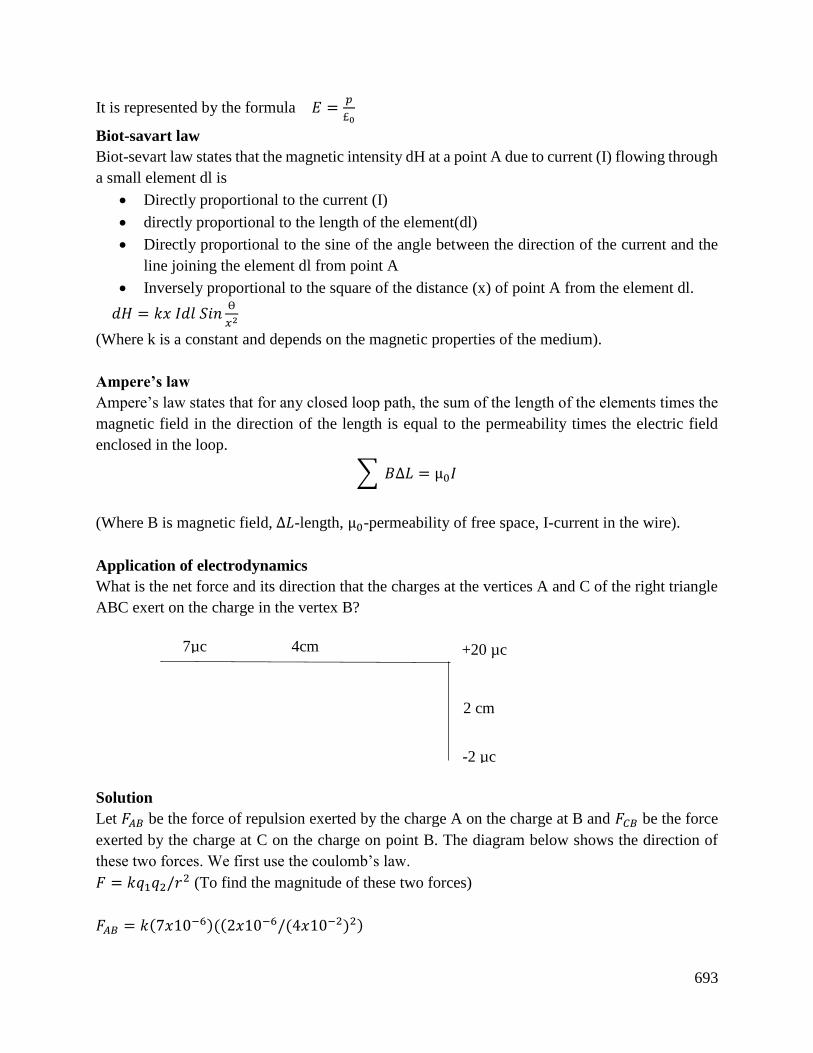
693
It is represented by the formula 𝐸 =𝑝
£0
Biot-savart law
Biot-sevart law states that the magnetic intensity dH at a point A due to current (I) flowing through
a small element dl is
Directly proportional to the current (I)
directly proportional to the length of the element(dl)
Directly proportional to the sine of the angle between the direction of the current and the
line joining the element dl from point A
Inversely proportional to the square of the distance (x) of point A from the element dl.
𝑑𝐻 = 𝑘𝑥 𝐼𝑑𝑙 𝑆𝑖𝑛Ѳ
𝑥2
(Where k is a constant and depends on the magnetic properties of the medium).
Ampere’s law
Ampere’s law states that for any closed loop path, the sum of the length of the elements times the
magnetic field in the direction of the length is equal to the permeability times the electric field
enclosed in the loop.
∑ 𝐵∆𝐿 = µ0𝐼
(Where B is magnetic field, ∆𝐿-length, µ0-permeability of free space, I-current in the wire).
Application of electrodynamics
What is the net force and its direction that the charges at the vertices A and C of the right triangle
ABC exert on the charge in the vertex B?
Solution
Let 𝐹𝐴𝐵 be the force of repulsion exerted by the charge A on the charge at B and 𝐹𝐶𝐵 be the force
exerted by the charge at C on the charge on point B. The diagram below shows the direction of
these two forces. We first use the coulomb’s law.
𝐹 = 𝑘𝑞1𝑞2/𝑟2 (To find the magnitude of these two forces)
𝐹𝐴𝐵 = 𝑘(7𝑥10−6)((2𝑥10−6/(4𝑥10−2)2)
7µc 4cm +20 µc
2 cm
-2 µc
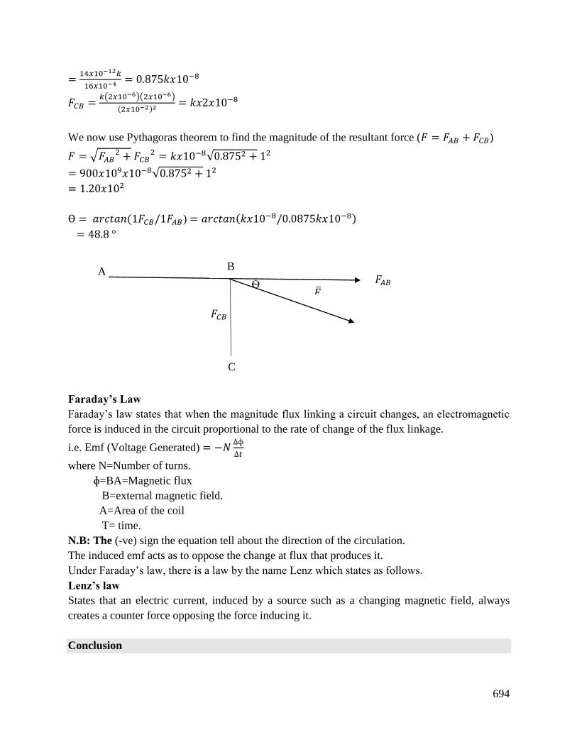
694
Ѳ 𝐹𝐴𝐵
B
C
𝐹𝐶𝐵
=14𝑥10−12𝑘
16𝑥10−4= 0.875𝑘𝑥10−8
𝐹𝐶𝐵 =𝑘(2𝑥10−6)(2𝑥10−6)
(2𝑥10−2)2= 𝑘𝑥2𝑥10−8
We now use Pythagoras theorem to find the magnitude of the resultant force (𝐹 = 𝐹𝐴𝐵 + 𝐹𝐶𝐵)
𝐹 = √𝐹𝐴𝐵2 + 𝐹𝐶𝐵
2 = 𝑘𝑥10−8√0.8752 + 12
= 900𝑥109𝑥10−8√0.8752 + 12
= 1.20𝑥102
Ѳ = 𝑎𝑟𝑐𝑡𝑎𝑛(1𝐹𝐶𝐵/1𝐹𝐴𝐵) = 𝑎𝑟𝑐𝑡𝑎𝑛(𝑘𝑥10−8/0.0875𝑘𝑥10−8)
= 48.8 °
Faraday’s Law
Faraday’s law states that when the magnitude flux linking a circuit changes, an electromagnetic
force is induced in the circuit proportional to the rate of change of the flux linkage.
i.e. Emf (Voltage Generated) = −𝑁∆ɸ
∆𝑡
where N=Number of turns.
ɸ=BA=Magnetic flux
B=external magnetic field.
A=Area of the coil
T= time.
N.B: The (-ve) sign the equation tell about the direction of the circulation.
The induced emf acts as to oppose the change at flux that produces it.
Under Faraday’s law, there is a law by the name Lenz which states as follows.
Lenz’s law
States that an electric current, induced by a source such as a changing magnetic field, always
creates a counter force opposing the force inducing it.
Conclusion
𝐹ത
A
695
The learning outcome covered or equipped the learner with knowledge, skills and attitude
regarding the electrodynamics and its application where details on electrostatics and magneto
statics are tackled extensively to ensure full knowledge of the learner, to be able to apply those
principles comfortably in the modern society.
Further Reading
1. Jackson, J.D (1999). Classical electrodynamics.
2. Berestetakii , V. B . Landan, L.D, Lifshitz. E.M & Pitaerskii, L.P (1998). Quantum
electrodynamics (Vol 4). Butterworth Heineman.
3. Griffiths, D.J. (2005). Introduction to thermodynamics.
8.3.9.3 Self-Assessment
Written assessment
1. There are repulsive forces between two charged objects when?
a) Charges are of unlike signs
b) They have the same number of protons
c) Charges are of like sign
d) They have the same number of electrons
2. When there is an equal amount of positive and negative charges in an object, the object is?
a) positively charged
b) negatively charged
c) neutral
d) super charged
3. What is the electrical potential difference between two places measured in?
a) amperes
b) coulombs
c) volts
d) joules
4. Who first discovered the relationship between electricity and magnetism?
a) Faraday
b) Newton
c) Maxwell
d) Oersted
5. For making a strong electromagnet, the material of the core should be?
696
a) Soft iron
b) Steel
c) Brass
d) copper
6. The magnetic field lines due to straight wires carrying a current are:
a) straight
b) Circular
c) Parabolic
d) elliptic
7. static electricity is produced due to?
a) friction
b) conduction
c) induction
d) Both A and C
8. Coulombs law is only true for point charges whose sizes are____________ in size.
9. If F is a force acting on a test charge 𝑞0 , electric field intensity E would be given by? E=?
10. A device which stores charges is called a?
11. Amount of work done in bringing unit positive charges from infinity to a point in electric field
is called?
12. Direction of electric field intensity in an electric field can be represented by drawing
of________?
Oral Assessment
1. What principle is used in painting of new cars in an automotive garage?
2. What device is used to store charge?
Practical Assessment
1. In group, try rub your plastic rulers against your hair and try bring the ruler over small pieces
of paper and record what happens.
Project
Develop a charge storage device, containing a series of capacitors and which should have a
capability of storing the charge for a minute while discharging.
8.3.9.4 Tools, Equipment, Supplies and Materials
Scientific Calculators
Relevant reference materials

697
Stationeries
Electrical workshop
Relevant practical materials
Dice
Computers with internet connection
8.3.9.5 References
Berman, P. R (1994). Cavity quantum electrodynamics.
Griffiths, D.J. (2005). Introduction to thermodynamics.
Jackson, J.D (1999). Classical electrodynamics.
Berestetakii, V. B. Landan, L.D, Lifshitz. E.M & Pitaerskii, L.P (1998). Quantum electrodynamics
(Vol 4). Butterworth Heineman.
698
8.3.10 Learning Outcome No 9: Apply Energy and momentum in Electromagnetic field
8.3.2.1 Learning Activities
Learning Outcome No9 :Apply Energy and momentum in Electromagnetic field
Learning Activities Special Instructions
9.1 Apply Energy and momentum in Electromagnetic field
8.3.10.2 Information Sheet No8/LO9: Apply Energy and momentum in Electromagnetic
field
Introduction
This learning outcome covers how to apply energy and momentum in electromagnetic fields.
Definition of key terms
Electromagnetic field: it is a magnetic field produced by moving electrically charged objects.
Photon: a photon is a particle of an electromagnetic radiation carrying a specific amount of energy
measured in electron volts (eV)
For parts of the electromagnetic spectrum with a low frequency and long wavelength, photon
energy is relatively low; but for parts of EM spectrum with high frequency and short wavelength,
the value of the photon is very high.
Radiation: radiation is the transfer of energy by means of electromagnetic field which require no
physical medium (for example water or air) for transfer.
Electric polarization: it refers to the separation of center of positive charge and the center of
negative charge in a material. It is caused by sufficiently high electric field.
Magnetic polarization: it is the vector field that expresses the density of permanent or induced
magnetic dipole moments in a magnetic material.
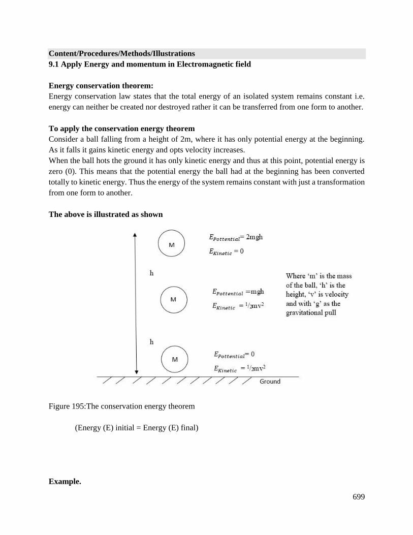
699
Content/Procedures/Methods/Illustrations
9.1 Apply Energy and momentum in Electromagnetic field
Energy conservation theorem:
Energy conservation law states that the total energy of an isolated system remains constant i.e.
energy can neither be created nor destroyed rather it can be transferred from one form to another.
To apply the conservation energy theorem
Consider a ball falling from a height of 2m, where it has only potential energy at the beginning.
As it falls it gains kinetic energy and opts velocity increases.
When the ball hots the ground it has only kinetic energy and thus at this point, potential energy is
zero (0). This means that the potential energy the ball had at the beginning has been converted
totally to kinetic energy. Thus the energy of the system remains constant with just a transformation
from one form to another.
The above is illustrated as shown
Figure 195:The conservation energy theorem
(Energy (E) initial = Energy (E) final)
Example.
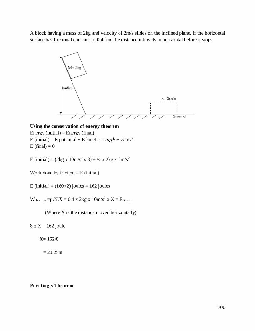
700
A block having a mass of 2kg and velocity of 2m/s slides on the inclined plane. If the horizontal
surface has frictional constant µ=0.4 find the distance it travels in horizontal before it stops
Using the conservation of energy theorem
Energy (initial) = Energy (final)
E (initial) = E potential + E kinetic = 𝑚𝑔ℎ + ½ mv2
E (final) = 0
E (initial) = (2kg x 10m/s2 x 8) + ½ x 2kg x 2m/s2
Work done by friction = E (initial)
E (initial) = (160+2) joules = 162 joules
W friction =µ.N.X = 0.4 x 2kg x 10m/s2 x X = E initial
(Where X is the distance moved horizontally)
8 x X = 162 joule
X= 162/8
= 20.25m
Poynting’s Theorem
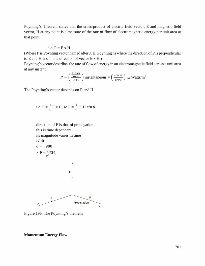
701
Poynting’s Theorem states that the cross-product of electric field vector, E and magnetic field
vector, H at any point is a measure of the rate of flow of electromagnetic energy per unit area at
that point.
i.e. P = E x H
(Where P is Poynting vector named after J. H. Poynting ns where the direction of P is perpendicular
to E and H and in the direction of vector E x H.)
Poynting’s vector describes the rate of flow of energy in an electromagnetic field across a unit area
at any instant.
𝑃 = ( 𝑒𝑛𝑒𝑟𝑔𝑦
𝑡𝑖𝑚𝑒
𝑎𝑟𝑒𝑎 ) instantaneous = (
𝑝𝑜𝑤𝑒𝑟
𝑎𝑟𝑒𝑎 ) inst Watts/m2
The Poynting’s vector depends on E and H
i.e. P = 𝑖
𝜇𝑜E x H, so P =
𝑖
𝜇𝑜 E H 𝑠𝑖𝑛 𝜃
direction of P is that of propagation
this is time dependent
its magnitude varies in time
𝑖/µ0
𝜃 = 900
⸫ P = 𝑖
µ0EH,
Figure 196: The Poynting’s theorem
Momentum Energy Flow
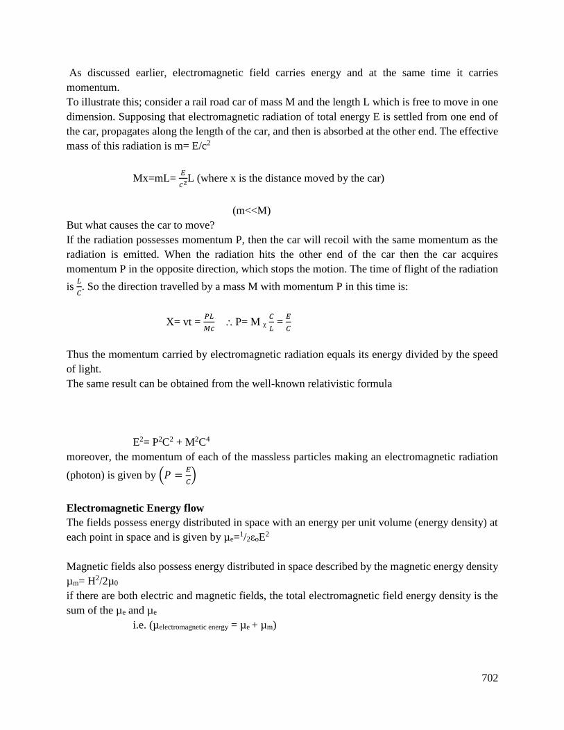
702
As discussed earlier, electromagnetic field carries energy and at the same time it carries
momentum.
To illustrate this; consider a rail road car of mass M and the length L which is free to move in one
dimension. Supposing that electromagnetic radiation of total energy E is settled from one end of
the car, propagates along the length of the car, and then is absorbed at the other end. The effective
mass of this radiation is m= E/c2
Mx=mL= 𝐸
𝑐2L (where x is the distance moved by the car)
(m<<M)
But what causes the car to move?
If the radiation possesses momentum P, then the car will recoil with the same momentum as the
radiation is emitted. When the radiation hits the other end of the car then the car acquires
momentum P in the opposite direction, which stops the motion. The time of flight of the radiation
is 𝐿
𝐶. So the direction travelled by a mass M with momentum P in this time is:
X= vt = 𝑃𝐿
𝑀𝑐 ⸫ P= M ᵪ
𝐶
𝐿 =
𝐸
𝐶
Thus the momentum carried by electromagnetic radiation equals its energy divided by the speed
of light.
The same result can be obtained from the well-known relativistic formula
E2= P2C2 + M2C4
moreover, the momentum of each of the massless particles making an electromagnetic radiation
(photon) is given by (𝑃 =𝐸
𝐶)
Electromagnetic Energy flow
The fields possess energy distributed in space with an energy per unit volume (energy density) at
each point in space and is given by µe=1/2εoE
2
Magnetic fields also possess energy distributed in space described by the magnetic energy density
µm= H2/2µ0
if there are both electric and magnetic fields, the total electromagnetic field energy density is the
sum of the µe and µe
i.e. (µelectromagnetic energy = µe + µm)
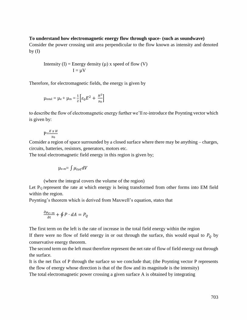
703
To understand how electromagnetic energy flow through space- (such as soundwave)
Consider the power crossing unit area perpendicular to the flow known as intensity and denoted
by (I)
Intensity (I) = Energy density (µ) x speed of flow (V)
I = µV
Therefore, for electromagnetic fields, the energy is given by
µtotal = µe + µm = 1
2[𝜀0𝐸
2 + 𝐻2
µ0]
to describe the flow of electromagnetic energy further we’ll re-introduce the Poynting vector which
is given by:
P=𝐸 𝑥 𝐻
µ0
Consider a region of space surrounded by a closed surface where there may be anything – charges,
circuits, batteries, resistors, generators, motors etc.
The total electromagnetic field energy in this region is given by;
µe-m= ∫𝜇𝑡𝑜𝑡𝑑𝑉
(where the integral covers the volume of the region)
Let PQ represent the rate at which energy is being transformed from other forms into EM field
within the region.
Poynting’s theorem which is derived from Maxwell’s equation, states that
𝜕𝜇𝑒−𝑚
𝜕𝑡+ ∮𝑃 ∙ 𝑑𝐴 = 𝑃𝑄
The first term on the left is the rate of increase in the total field energy within the region
If there were no flow of field energy in or out through the surface, this would equal to 𝑃𝑄 by
conservative energy theorem.
The second term on the left must therefore represent the net rate of flow of field energy out through
the surface.
It is the net flux of P through the surface so we conclude that; (the Poynting vector P represents
the flow of energy whose direction is that of the flow and its magnitude is the intensity)
The total electromagnetic power crossing a given surface A is obtained by integrating
704
𝑃𝑜𝑤𝑒𝑟(𝑎𝑐𝑟𝑜𝑠𝑠 𝐴 = ∫ 𝑃 ∙ 𝑑𝐴𝐵
𝐴
Conclusion
The learning outcome covered or equipped the learner with knowledge, skills and attitude to tackle
and apply the electromagnetic field and its properties for the betterment of the modern society and
advancement of modern technology in communication and other sectors. The learner upon reading
and understanding the content by help of illustrations is in a position to understand the
characteristics of electromagnetic fields, its momentum and energy and thus be able to come up
with innovative ways to utilize them.
Further Reading
Maxwell, J. C. (1865). VIII. A dynamical theory of the electromagnetic field. Philosophical
transactions of the royal society of London (155), 459-512
Lindell, I. V. (1992). Methods for electromagnetic field analysis.
Gor’Kov, L. P. & Eliashberg G. M. (1965). Minute metallic particles in an electromagnetic field.
Sov Phys. JETP 21 (940)
8.3.10.3 Self-Assessment
Written assessment
1. Identify which of the following is the unit of magnetic flex density?
a) Weber
b) Webber/m
c) Tesla
d) Weber-1
2. Magnetic behavior of a material depends on its structure particularly its?
a) Electron configuration
b) Proton configuration
c) Holes configuration
d) Neutron configuration
3. Identify the diamagnetic material.
a) Silicon
b) Germanium
c) Silver
d) cobalt
705
4. Which of the following materials is ferromagnetic?
a) Fe
b) Sn
c) Fe2O3
d) FeCl
5. The depth of penetration of a wave in a loss dielectric increases with increasing?
a) Conductivity
b) Permeability
c) Wavelength
d) Permittivity
6. The magnetic flux density is directly proportional to the magnetic field intensity.
a) True
b) False
7. Given the magnetic field is 2.4 units. Find the flux density in air (in 10-6order)
8. What is the name used to refer to the energy possessed by an object resting on position x meters
from the ground?
9. Give an example of energy transferred by electromagnetic field.
10. What happens when white light strikes a black object?
11. Give an example of a magnetic material.
Oral Assessment
1. What causes the Earth’s magnetic field?
2. Why do you think iron is considered a suitable material for the core of a transformer?
Practical Assessment
1. In groups of three people, use a magnet to determine the magnetics materials given, copper,
brass, iron and silver pieces of metals
Project
1. Improvise a circuit that will be able to generate a magnetic field using small power source and
a solenoid
8.3.10.4 Tools, Equipment, Supplies and Materials
Scientific Calculators
Relevant reference materials
Stationeries
Electrical workshop
Relevant practical materials
Dice
Computers with internet connection

706
8.3.10.5 References
Gor’Kov, L. P. & Eliashberg G. M. (1965). Minute metallic particles in an electromagnetic field.
Sov Phys. JETP 21 (940).
Lindell, I. V. (1992). Methods for electromagnetic field analysis.
Maxwell, J. C. (1865). VIII. A dynamical theory of the electromagnetic field. Philosophical
transactions of the royal society of London (155), 459-512
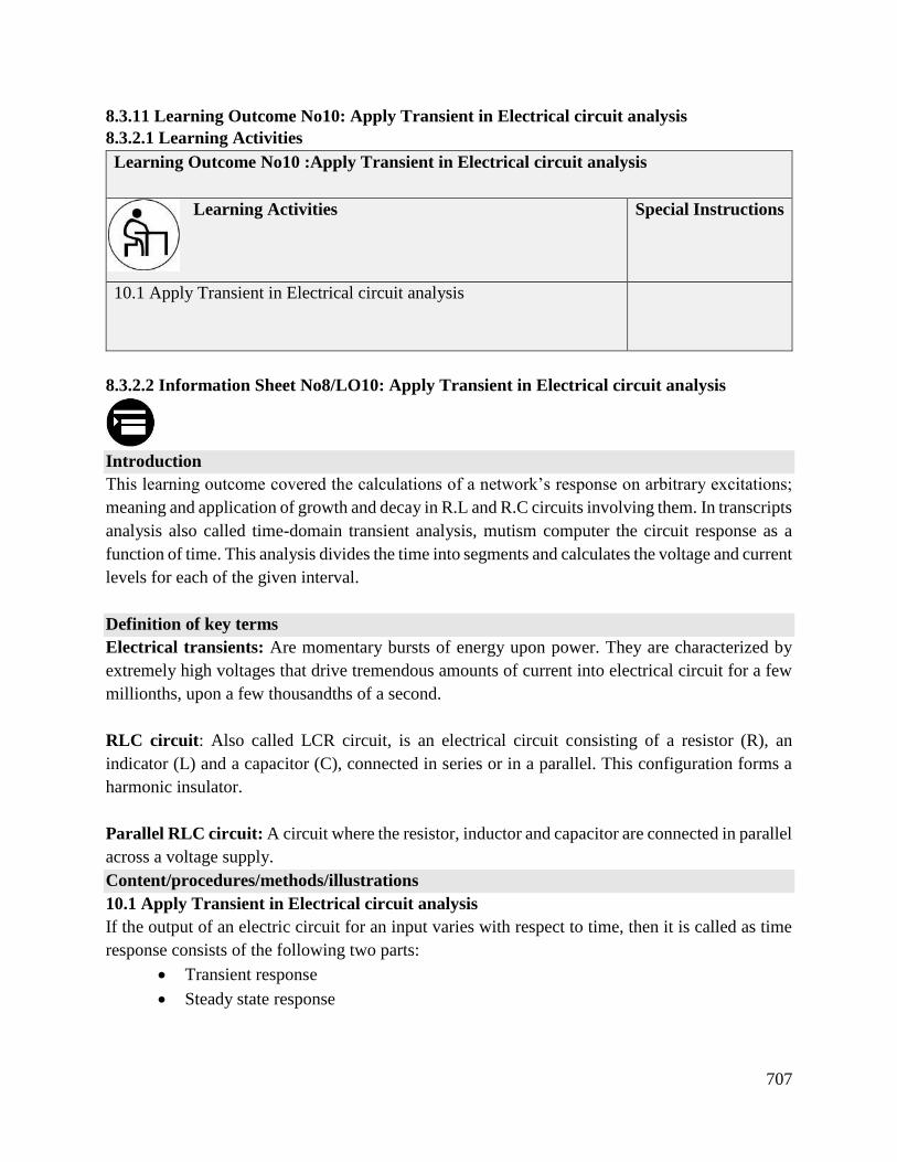
707
8.3.11 Learning Outcome No10: Apply Transient in Electrical circuit analysis
8.3.2.1 Learning Activities
Learning Outcome No10 :Apply Transient in Electrical circuit analysis
Learning Activities Special Instructions
10.1 Apply Transient in Electrical circuit analysis
8.3.2.2 Information Sheet No8/LO10: Apply Transient in Electrical circuit analysis
Introduction
This learning outcome covered the calculations of a network’s response on arbitrary excitations;
meaning and application of growth and decay in R.L and R.C circuits involving them. In transcripts
analysis also called time-domain transient analysis, mutism computer the circuit response as a
function of time. This analysis divides the time into segments and calculates the voltage and current
levels for each of the given interval.
Definition of key terms
Electrical transients: Are momentary bursts of energy upon power. They are characterized by
extremely high voltages that drive tremendous amounts of current into electrical circuit for a few
millionths, upon a few thousandths of a second.
RLC circuit: Also called LCR circuit, is an electrical circuit consisting of a resistor (R), an
indicator (L) and a capacitor (C), connected in series or in a parallel. This configuration forms a
harmonic insulator.
Parallel RLC circuit: A circuit where the resistor, inductor and capacitor are connected in parallel
across a voltage supply.
Content/procedures/methods/illustrations
10.1 Apply Transient in Electrical circuit analysis
If the output of an electric circuit for an input varies with respect to time, then it is called as time
response consists of the following two parts:
Transient response
Steady state response
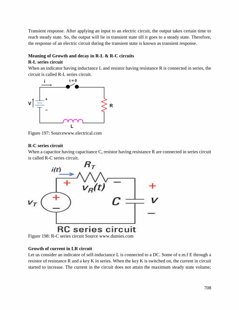
708
Transient response. After applying an input to an electric circuit, the output takes certain time to
reach steady state. So, the output will lie in transient state till it goes to a steady state. Therefore,
the response of an electric circuit during the transient state is known as transient response.
Meaning of Growth and decay in R-L & R-C circuits
R-L series circuit
When an indicator having inductance L and resistor having resistance R is connected in series, the
circuit is called R-L series circuit.
Figure 197: Sourcewww.electrical.com
R-C series circuit
When a capacitor having capacitance C, resistor having resistance R are connected in series circuit
is called R-C series circuit.
Figure 198: R-C series circuit Source www.dumies.com
Growth of current in LR circuit
Let us consider an indicator of self-inductance L is connected to a DC. Some of e.m.f E through a
resistor of resistance R and a key K in series. When the key K is switched on, the current in circuit
started to increase. The current in the circuit does not attain the maximum steady state volume;
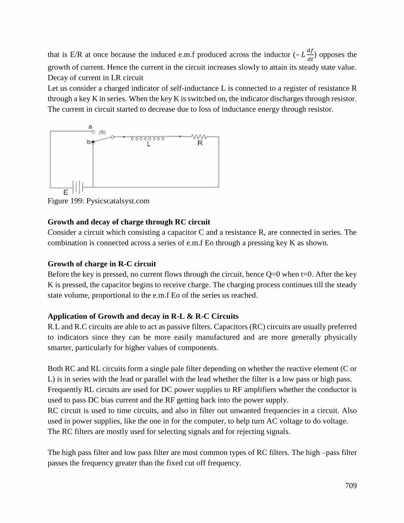
709
that is E/R at once because the induced e.m.f produced across the inductor (– 𝐿𝑑𝑓
𝑑𝑡) opposes the
growth of current. Hence the current in the circuit increases slowly to attain its steady state value.
Decay of current in LR circuit
Let us consider a charged indicator of self-inductance L is connected to a register of resistance R
through a key K in series. When the key K is switched on, the indicator discharges through resistor.
The current in circuit started to decrease due to loss of inductance energy through resistor.
Figure 199: Pysicscatalsyst.com
Growth and decay of charge through RC circuit
Consider a circuit which consisting a capacitor C and a resistance R, are connected in series. The
combination is connected across a series of e.m.f Eo through a pressing key K as shown.
Growth of charge in R-C circuit
Before the key is pressed, no current flows through the circuit, hence Q=0 when t=0. After the key
K is pressed, the capacitor begins to receive charge. The charging process continues till the steady
state volume, proportional to the e.m.f Eo of the series us reached.
Application of Growth and decay in R-L & R-C Circuits
R.L and R.C circuits are able to act as passive filters. Capacitors (RC) circuits are usually preferred
to indicators since they can be more easily manufactured and are more generally physically
smarter, particularly for higher values of components.
Both RC and RL circuits form a single pale filter depending on whether the reactive element (C or
L) is in series with the lead or parallel with the lead whether the filter is a low pass or high pass.
Frequently RL circuits are used for DC power supplies to RF amplifiers whether the conductor is
used to pass DC bias current and the RF getting back into the power supply.
RC circuit is used to time circuits, and also in filter out unwanted frequencies in a circuit. Also
used in power supplies, like the one in for the computer, to help turn AC voltage to do voltage.
The RC filters are mostly used for selecting signals and for rejecting signals.
The high pass filter and low pass filter are most common types of RC filters. The high –pass filter
passes the frequency greater than the fixed cut off frequency.
710
The low-pass filter allows the frequency lower than the fixed cut-off frequency and alternates the
frequency higher than the fixed cut-off frequency.
Growth and decay of current in RL circuit is applied in most electric machines. For instance, the
winding of an electric motor which is represented in RL circuit.
Conclusion
The learning outcome covered or equipped the learner with knowledge, skills and attitude to some
and understand various electrical circuits mainly R.L and R.C circuits and their applications.
Further Reading
1. Rodwan, Ahmed G. and Khaled N, Salama. “Fractional order RC and RL circuits”. Circuits
systems and signal processing 31, no. 6 (2012): 1901-1915.
2. Nilson, J. W., and Riedel, S.A (2015). Electrical circuits. Upper Sandle River,
person.
3. Das, J. C (2010). Transients in electrical systems. Mc Graw-Hill professional publishing.
8.3.11.3 Self-Assessment
Written assessment
1. An RL network is one which consists of?
a) Resistor and capacitor in parallel
b) Resistor and capacitor in series
c) Resistor and inductor in parallel
d) Resistor and inductor in series
2. The derived unit of charge, coulomb (C) is equivalent to an?
a) Ampere
b) Ampere per second
c) Ampere second
d) Ampere per second square
3. In a parallel RL circuit, there are 3 A rms in the resistive branch and 3 A rms current is
a) 6 A
b) 424 mA
c) 4.24 A
d) 42.4 A
4. In 1.2 kr resistor is in series with a 15mH cell across a 10kH2 as source. The magnitude of
the total impendence is
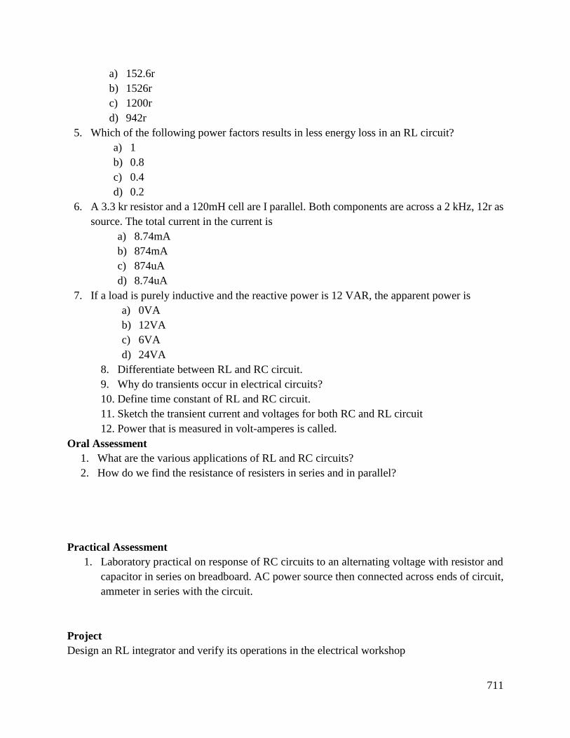
711
a) 152.6r
b) 1526r
c) 1200r
d) 942r
5. Which of the following power factors results in less energy loss in an RL circuit?
a) 1
b) 0.8
c) 0.4
d) 0.2
6. A 3.3 kr resistor and a 120mH cell are I parallel. Both components are across a 2 kHz, 12r as
source. The total current in the current is
a) 8.74mA
b) 874mA
c) 874uA
d) 8.74uA
7. If a load is purely inductive and the reactive power is 12 VAR, the apparent power is
a) 0VA
b) 12VA
c) 6VA
d) 24VA
8. Differentiate between RL and RC circuit.
9. Why do transients occur in electrical circuits?
10. Define time constant of RL and RC circuit.
11. Sketch the transient current and voltages for both RC and RL circuit
12. Power that is measured in volt-amperes is called.
Oral Assessment
1. What are the various applications of RL and RC circuits?
2. How do we find the resistance of resisters in series and in parallel?
Practical Assessment
1. Laboratory practical on response of RC circuits to an alternating voltage with resistor and
capacitor in series on breadboard. AC power source then connected across ends of circuit,
ammeter in series with the circuit.
Project
Design an RL integrator and verify its operations in the electrical workshop

712
8.3.11.4 Tools, Equipment, Supplies and Materials
• Scientific Calculators
• Relevant reference materials
• Stationeries
• Electrical workshop
• Relevant practical materials
• Dice
• Computers with internet connection
6.3.2.5 References
Kezerashvili R.Y (2012). Teaching RC and RL circuits using computer supported experiments ieri
procedia, 2, 609-615
Robbins, A. H., & Miller, W. C. (2012). Circuits analysis: theory and practice congage learning.

713
8.3.12 Learning Outcome No 11: Use two port networks
8.3.12.1 Learning Activities
Learning Outcome No11 :Use two port network
Learning Activities Special Instructions
11.1 Use two port networks
8.3.12.2 Information Sheet No8/LO 11: Use two port network
Introduction
This learning outcome covers the use of two port network, passive network, T and Pie
characteristic, impedance and design, transmission lines, ABCD contents and network in cascades.
A two port network has two separate ports
A port is a pair of terminals through which a current may enter or leave the network.
The two ports can be shown as sketched below.
Figure 200: A two port network
source: www.researchgate.net
The current entering from one terminal must leave from the other terminal. For the two port
network, current entering both the ports is the standard notation for it (two port network).
Two ports can be connected in a series as shown below.
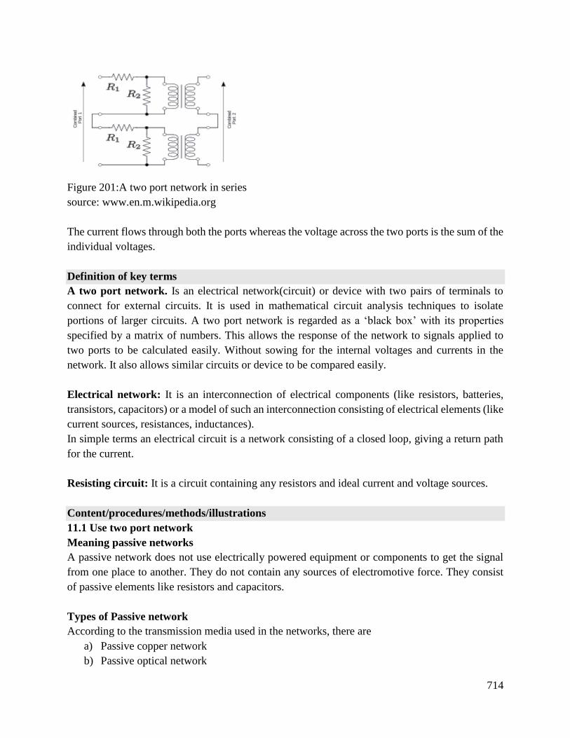
714
Figure 201:A two port network in series
source: www.en.m.wikipedia.org
The current flows through both the ports whereas the voltage across the two ports is the sum of the
individual voltages.
Definition of key terms
A two port network. Is an electrical network(circuit) or device with two pairs of terminals to
connect for external circuits. It is used in mathematical circuit analysis techniques to isolate
portions of larger circuits. A two port network is regarded as a ‘black box’ with its properties
specified by a matrix of numbers. This allows the response of the network to signals applied to
two ports to be calculated easily. Without sowing for the internal voltages and currents in the
network. It also allows similar circuits or device to be compared easily.
Electrical network: It is an interconnection of electrical components (like resistors, batteries,
transistors, capacitors) or a model of such an interconnection consisting of electrical elements (like
current sources, resistances, inductances).
In simple terms an electrical circuit is a network consisting of a closed loop, giving a return path
for the current.
Resisting circuit: It is a circuit containing any resistors and ideal current and voltage sources.
Content/procedures/methods/illustrations
11.1 Use two port network
Meaning passive networks
A passive network does not use electrically powered equipment or components to get the signal
from one place to another. They do not contain any sources of electromotive force. They consist
of passive elements like resistors and capacitors.
Types of Passive network
According to the transmission media used in the networks, there are
a) Passive copper network
b) Passive optical network
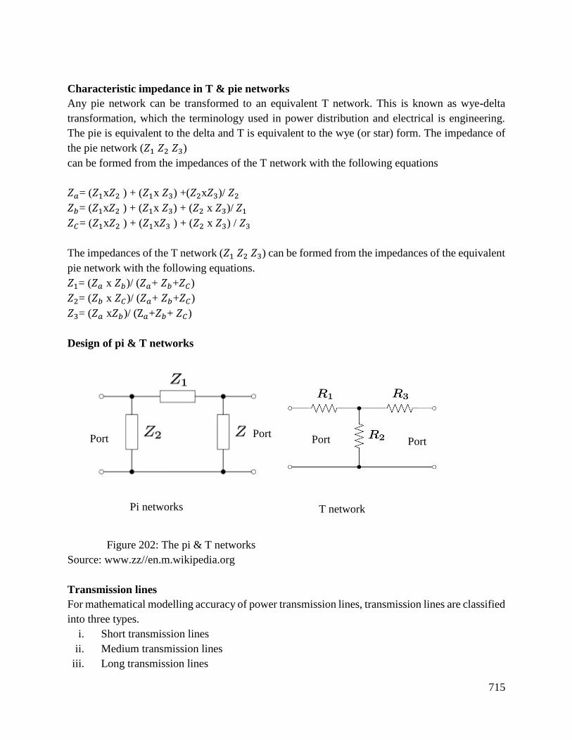
715
Characteristic impedance in T & pie networks
Any pie network can be transformed to an equivalent T network. This is known as wye-delta
transformation, which the terminology used in power distribution and electrical is engineering.
The pie is equivalent to the delta and T is equivalent to the wye (or star) form. The impedance of
the pie network (𝑍1 𝑍2 𝑍3)
can be formed from the impedances of the T network with the following equations
𝑍𝑎= (𝑍1x𝑍2 ) + (𝑍1x 𝑍3) +(𝑍2x𝑍3)/ 𝑍2
𝑍𝑏= (𝑍1x𝑍2 ) + (𝑍1x 𝑍3) + (𝑍2 x 𝑍3)/ 𝑍1
𝑍𝐶= (𝑍1x𝑍2 ) + (𝑍1x𝑍3 ) + (𝑍2 x 𝑍3) / 𝑍3
The impedances of the T network (𝑍1 𝑍2 𝑍3) can be formed from the impedances of the equivalent
pie network with the following equations.
𝑍1= (𝑍𝑎 x 𝑍𝑏)/ (𝑍𝑎+ 𝑍𝑏+𝑍𝐶)
𝑍2= (𝑍𝑏 x 𝑍𝐶)/ (𝑍𝑎+ 𝑍𝑏+𝑍𝐶)
𝑍3= (𝑍𝑎 x𝑍𝑏)/ (Z𝑎+𝑍𝑏+ 𝑍𝐶)
Design of pi & T networks
Figure 202: The pi & T networks
Source: www.zz//en.m.wikipedia.org
Transmission lines
For mathematical modelling accuracy of power transmission lines, transmission lines are classified
into three types.
i. Short transmission lines
ii. Medium transmission lines
iii. Long transmission lines
Pi networks T network
Port
2
Port
2 Port
1
Port
1
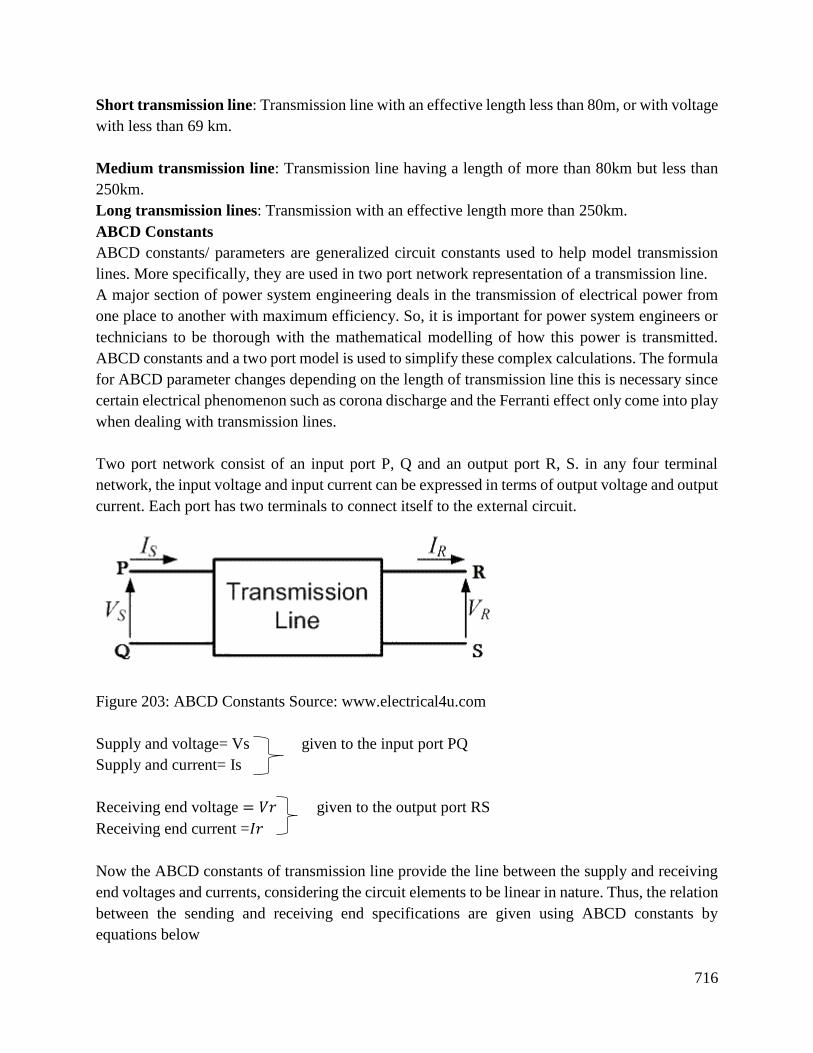
716
Short transmission line: Transmission line with an effective length less than 80m, or with voltage
with less than 69 km.
Medium transmission line: Transmission line having a length of more than 80km but less than
250km.
Long transmission lines: Transmission with an effective length more than 250km.
ABCD Constants
ABCD constants/ parameters are generalized circuit constants used to help model transmission
lines. More specifically, they are used in two port network representation of a transmission line.
A major section of power system engineering deals in the transmission of electrical power from
one place to another with maximum efficiency. So, it is important for power system engineers or
technicians to be thorough with the mathematical modelling of how this power is transmitted.
ABCD constants and a two port model is used to simplify these complex calculations. The formula
for ABCD parameter changes depending on the length of transmission line this is necessary since
certain electrical phenomenon such as corona discharge and the Ferranti effect only come into play
when dealing with transmission lines.
Two port network consist of an input port P, Q and an output port R, S. in any four terminal
network, the input voltage and input current can be expressed in terms of output voltage and output
current. Each port has two terminals to connect itself to the external circuit.
Figure 203: ABCD Constants Source: www.electrical4u.com
Supply and voltage= Vs given to the input port PQ
Supply and current= Is
Receiving end voltage = 𝑉𝑟 given to the output port RS
Receiving end current =𝐼𝑟
Now the ABCD constants of transmission line provide the line between the supply and receiving
end voltages and currents, considering the circuit elements to be linear in nature. Thus, the relation
between the sending and receiving end specifications are given using ABCD constants by
equations below
717
𝑉𝑠 = 𝐴𝑉𝑟 + 𝐵𝐼𝑟
𝐼𝑠 = 𝐶𝑉𝑟 + 𝐷𝑖𝑟
Conclusion
The learning outcome covered or equipped the learner with knowledge, skills and attitude to
understand and apply two networks in various machines and in T and Pie networks design.
Further Reading
1. Kurth, C., & Moschngtz, G. (1979). Two-part analysis of switched capacitor networks
using four port equivalent circuits in the Z domain.
Lee Transactions on Circuits and Systems, 26 (3), 166-188
2. Bai, M.R., Lo, Y. Y., & Chen, Y. S. (2015). Impedance measurement techniques for one
port and two port networks.
The journal of the Acoustical Society of America, 138 (4), 2279-2290.
8.3.12.3 Self-Assessment
Written assessment
1. Which among the following represents the precise condition of reciprocity for transmission
parameters?
a) AB-CD=1
b) AD-BC=1
c) AC-BD=1
d) None of the above
2. If 2 parameters are 𝑍11 = 40, 𝑍22 = 50 and 𝑍12 = 𝑍21 = 20, what would be the value
of Y22 in the matrix form or Y parameters given below?
5/160 − 2/160
−2/160 ?
a) 4/160
b) 5/160
c) 10/160
d) 15/150

718
3. Which is the correct condition of symmetry observed in Z-parameters?
a) 𝑍11 = 𝑍22
b) 𝑍11 = 𝑍12
c) 𝑍12 = 𝑍22
d) 𝑍12 = 𝑍21
4. Which elements behave as an open circuit especially under the consideration of d.c
quantities?
a) Inductors
b) Resistors
c) Capacitors
d) All of the above
5. Which among the following is regarded as short circuit forward transfer admittance?
a) 𝑌11
b) 𝑌12
c) 𝑌21
d) 𝑌22
6. A two-port network is simply a network inside a block box and the network has only?
a) Two terminals
b) Two pairs of accessible terminals
c) Two pairs of ports
d) None of these
7. The number of possible combinations generated by four variables taken two at a time in a
two-port network is?
a) Four
b) Two
c) Six
d) None of these
8. What is a two-port network?
9. Give examples of two port network application
10. State the three types of transmission lines in two port networks
11. Explain briefly ABCD parameters, when receiving end is open circuited and when it is
short circuited
12. A two port resistive network satisfy the condition A=D=3/2B=4/3C. The Z11of the
network is´?
Oral Assessment
1. Give examples where you think two port networks are used.
Practical Assessment

719
1. In groups of three, identify a circuit where you can input a signal into one port and obtain
an output system from the other ort.
Project
Design two two-port network in series showing the input and output currents and voltage
8.3.12.4 Tools, Equipment, Supplies and Materials
Scientific Calculators
Relevant reference materials
Stationeries
Electrical workshop
Relevant practical materials
Dice
Computers with internet connection
8.3.12.5 References
Fouda, M.E., Elwaki, A.S., Radwan, A.G., &Maundy, B.S. (2016). Fructional-order two-port
networks. Mathematical Problems in Engineering, 2016.
Elwakil, A.S. (2009). On the two-port network classification of colpitts oscillators. CET circuits,
devices & systems, 3(5), 223-232
Fouda, M.E., Elwaki, A.S., Radwan, A.G., &Maundy, B.S. (2016). Fructional-order two-port
networks. Mathematical Problems in Engineering, 2016.
Said, L.A., Radwan, A.G., Madian, A.H., & Soliman, A.M.(2016). Two-port two impedances
fractional order oscillators. Microelectronics Journal, 55, 40-52.
720
CHAPTER 9: TECHNICAL DRAWING/PREPARE AND INTERPRET TECHNICAL
DRAWINGS
9.1 Introduction
Technical drawing is among the common units of competencies offered in all the TVET level 6
engineering courses qualification. This unit covers the competencies required to prepare and
interpret technical drawings. It involves competencies to select, use and maintain drawing
equipment and materials. It also involves producing plain geometry drawings, solid geometry
drawings, pictorial and orthographic drawings of components and application of CAD packages.
The significance of technical drawings to TVET level 6 engineering curriculum is to enable
learners acquire knowledge and skills to demonstrate critical thinking, communication, analysis
and synthesis, lettering, sketches and drawings of simple patterns to get along well in the
workplaces.
The critical aspect of competency to be covered includes applied and adhered to safety procedures,
maintained drawing equipment, interpreted circuit, assembly and lay out diagrams, applied
appropriate technical standards, used proper tools and equipment for a given task, produced
sketches and drawings and applied CAD packages in production of drawings according to standard
drawing conventions. The basic resources required includes drawing room, computer lab, drawing
equipment and materials, computers, CAD package, overhead projector among others. This unit
of competency covers six learning outcomes. Each of the learning outcome presents; learning
activity that covers performance criteria statements, thus creating trainee’ an opportunity to
demonstrate knowledge and skills in the occupational standards and content in curriculum.
Information sheet provides; definition of key terms, content and illustration to guide in training.
The competency may be assessed through practical tests and observation. Self-assessment is
provided at the end of each learning outcomes. Holistic assessment with other units relevant to the
industry sector workplace and job role is recommended.
9.2 Performance Standard
Use drawing equipment and materials according to task requirements, per workplace procedures
and maintained as per manufacturer’s instructions, waste materials are disposed in accordance with
workplace procedures and environmental legislations, use personal protective equipment
according to occupational safety and health regulations, produce plain geometry drawings, produce
solid geometry drawings, produce pictorial and orthographic drawings of components and apply
CAD packages in drawings according to standard drawing conventions and task requirements.
9.3 Learning Outcomes
9.3.1 List of learning outcomes
a) Use and maintain drawing equipment and materials
b) Produce plain geometry drawings

721
c) Produce solid geometry drawings
d) Produce pictorial and orthographic drawings of components
e) Produce mechanical drawings
f) Apply CAD packages
722
9.3.2 Learning Outcome No 1: Use and maintain drawing equipment and materials
9.3.2.1 Learning Activities
Learning Outcome No 1: Use and maintain drawing equipment and materials
Learning Activities Special Instructions
1.1. Identify and gather drawing equipment (drawing boards, set
squares, drawing set and computers with CAD packages)
according to task requirements
1.2. Identify and gather drawing materials (drawing papers, pencils,
erasers, masking tapes and paper clips) according to task
requirements
1.3. Use and maintain drawing equipment as per manufacturer’s
instructions
1.4. Use drawing materials as per workplace procedures
1.5. Dispose waste materials in accordance with workplace
procedures and environmental legislations
1.6. Use Personal Protective Equipment (dust coats, gloves and
closed leather shoes) according to occupational safety and
health regulations
Demonstration and
group discussion
9.3.2.2 Information Sheet No9/LO1: Use and maintain drawing equipment and materials
Introduction
This learning outcome covers drawing equipment, drawing materials, maintenance of drawing
equipment as per manufacturer’s instructions as per workplace procedures. It also covers on how
to dispose waste materials in accordance with workplace procedures and proper use of personal
equipment. Use and maintain drawing equipment and materials.
Definition of key terms
Drawing: This is the use of lines, shapes, and sizes to construct objects or structures either in
2-dimesnional or 3-dimensional view.
Technical drawing: This is a precise detailed representation of an idea using symbols, lines, and
signs in creating objects in the manufacturing of engineering articles.
723
Drafting: This is the act of producing a picture/sketch either in 2-dimesnional or 3-dimensional
view and providing dimensions and notes. It is usually a quick sketch/ presentation with details
and not to scale.
Designing: This is the act of producing drawings to clearly define the requirements for concepts
or products in order to be in line with the expected outcome.
Maintenance: It is an excellent means of improving the performance and condition of equipment
and facilities.
A maintenance program: Is a comprehensive list of maintenance and its incidents.
A maintenance schedule: Is a list allocating specific maintenance of an area, including equipment
and tools to a specific period.
A maintenance checklist: Is a list of maintenance tasks (preventive or predictive) typically
derived through some form of analysis, generated automatically as work orders at a predetermined
frequency.
Content/Procedures/Methods/Illustrations
Use and maintain drawing equipment as per manufacturer’s instructions
Maintenance is an excellent means of improving the performance and condition of equipment and
facilities. An effective maintenance program identifies problems long before any equipment or
facility breaks down or deteriorate. A good maintenance system presents the early discovery of
problems, thus providing plenty of lead time for effective maintenance planning. The trainer has
to value the importance of maintaining the training facilities, equipment and tools s/he is using or
under his/her care if he values the presence and availability of these resources for effective training
and learning processes. Training equipment is usually placed in the practical work area or the
trainees’ resource area. The sizes and uses of equipment vary in the different training qualifications
and generally classified into five (5):
a) Large items of equipment; motor vehicles, industrial sewing machines
b) Small items of equipment
c) Simple equipment; electric fan, floor polisher
d) Complex equipment; plasma cutting machine, simulator (automotive)
e) Equipment with significant health and safety implications; duplicator machine
Reasons for maintenance
To extend the useful life of physical facilities
To assure the operational readiness of installed equipment and maximum possible return
on investments
To properly discard hazardous wastes
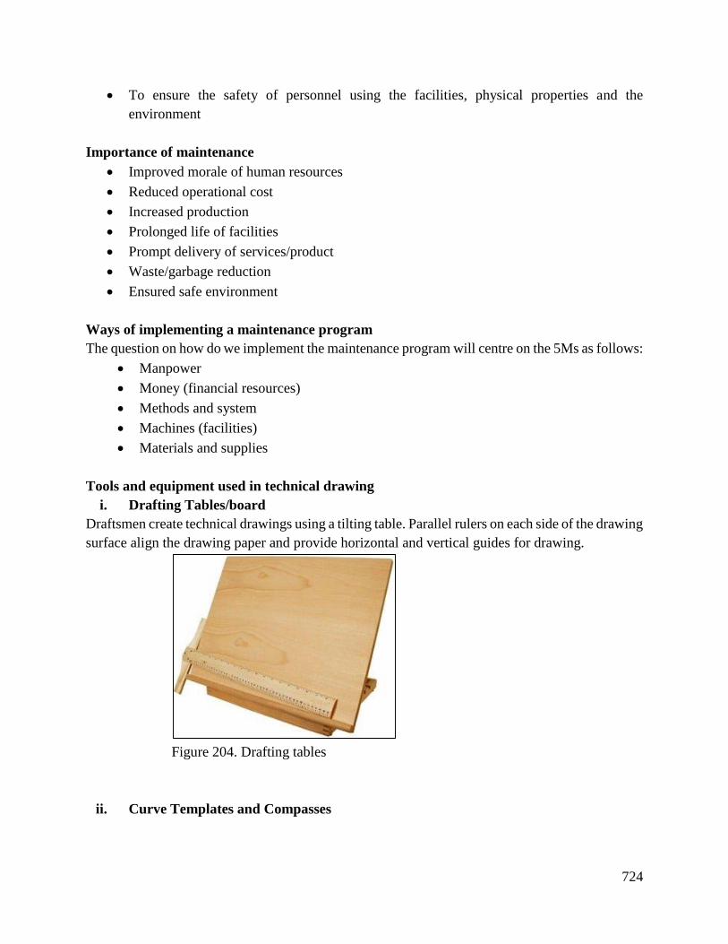
724
To ensure the safety of personnel using the facilities, physical properties and the
environment
Importance of maintenance
Improved morale of human resources
Reduced operational cost
Increased production
Prolonged life of facilities
Prompt delivery of services/product
Waste/garbage reduction
Ensured safe environment
Ways of implementing a maintenance program
The question on how do we implement the maintenance program will centre on the 5Ms as follows:
Manpower
Money (financial resources)
Methods and system
Machines (facilities)
Materials and supplies
Tools and equipment used in technical drawing
i. Drafting Tables/board
Draftsmen create technical drawings using a tilting table. Parallel rulers on each side of the drawing
surface align the drawing paper and provide horizontal and vertical guides for drawing.
Figure 204. Drafting tables
ii. Curve Templates and Compasses
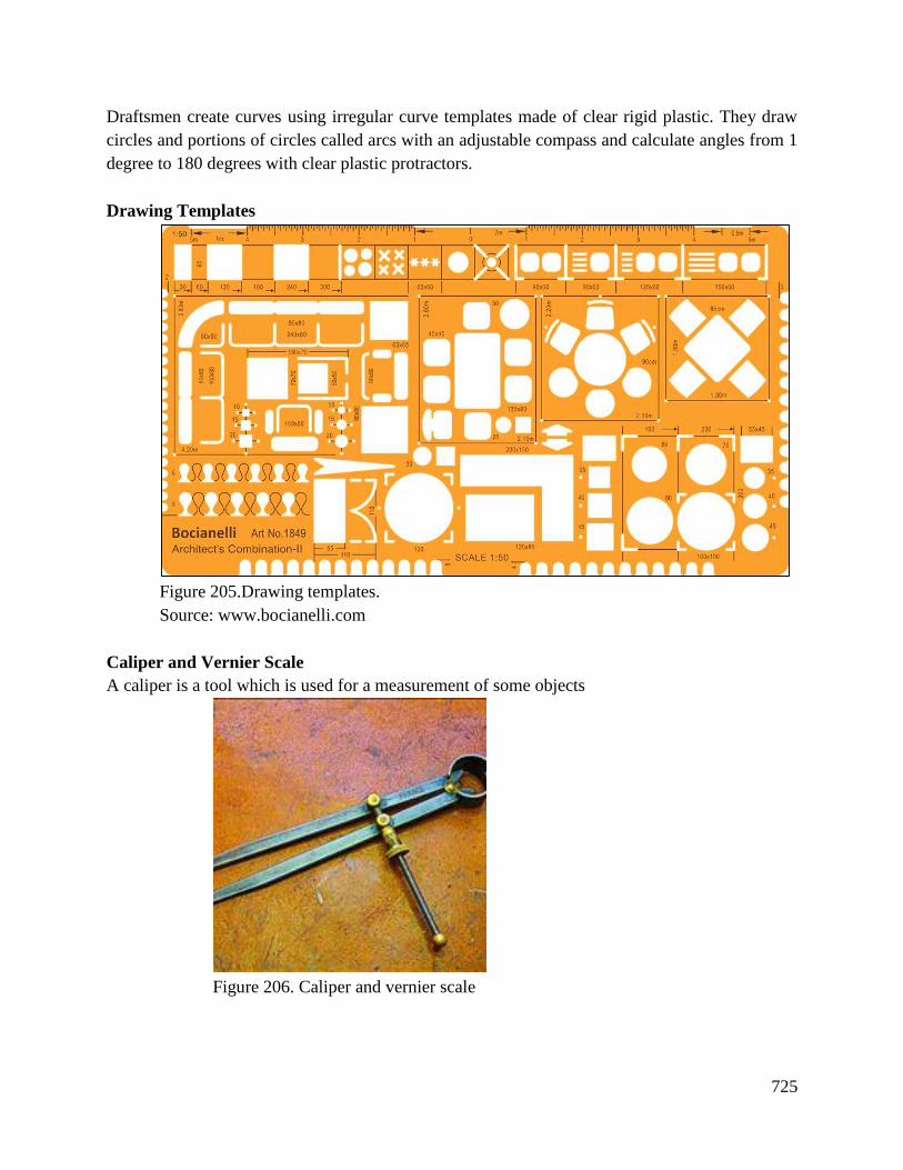
725
Draftsmen create curves using irregular curve templates made of clear rigid plastic. They draw
circles and portions of circles called arcs with an adjustable compass and calculate angles from 1
degree to 180 degrees with clear plastic protractors.
Drawing Templates
Figure 205.Drawing templates.
Source: www.bocianelli.com
Caliper and Vernier Scale
A caliper is a tool which is used for a measurement of some objects
Figure 206. Caliper and vernier scale
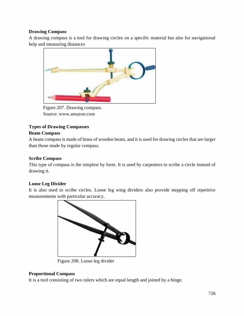
726
Drawing Compass
A drawing compass is a tool for drawing circles on a specific material but also for navigational
help and measuring distances
Figure 207. Drawing compass.
Source: www.amazon.com
Types of Drawing Compasses
Beam Compass
A beam compass is made of brass of wooden beam, and it is used for drawing circles that are larger
than those made by regular compass.
Scribe Compass
This type of compass is the simplest by form. It is used by carpenters to scribe a circle instead of
drawing it.
Loose Leg Divider
It is also used to scribe circles. Loose leg wing dividers also provide stepping off repetitive
measurements with particular accuracy.
Figure 208. Loose leg divider
Proportional Compass
It is a tool consisting of two rulers which are equal length and joined by a hinge.
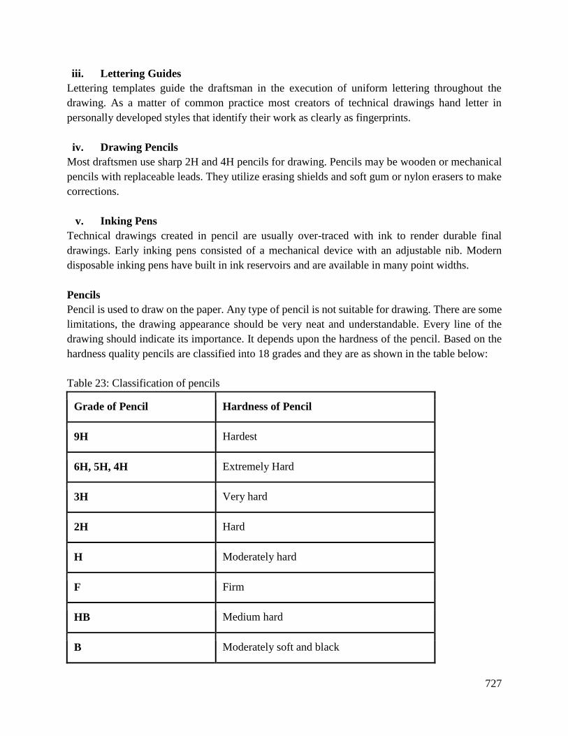
727
iii. Lettering Guides
Lettering templates guide the draftsman in the execution of uniform lettering throughout the
drawing. As a matter of common practice most creators of technical drawings hand letter in
personally developed styles that identify their work as clearly as fingerprints.
iv. Drawing Pencils
Most draftsmen use sharp 2H and 4H pencils for drawing. Pencils may be wooden or mechanical
pencils with replaceable leads. They utilize erasing shields and soft gum or nylon erasers to make
corrections.
v. Inking Pens
Technical drawings created in pencil are usually over-traced with ink to render durable final
drawings. Early inking pens consisted of a mechanical device with an adjustable nib. Modern
disposable inking pens have built in ink reservoirs and are available in many point widths.
Pencils
Pencil is used to draw on the paper. Any type of pencil is not suitable for drawing. There are some
limitations, the drawing appearance should be very neat and understandable. Every line of the
drawing should indicate its importance. It depends upon the hardness of the pencil. Based on the
hardness quality pencils are classified into 18 grades and they are as shown in the table below:
Table 23: Classification of pencils
Grade of Pencil Hardness of Pencil
9H Hardest
6H, 5H, 4H Extremely Hard
3H Very hard
2H Hard
H Moderately hard
F Firm
HB Medium hard
B Moderately soft and black
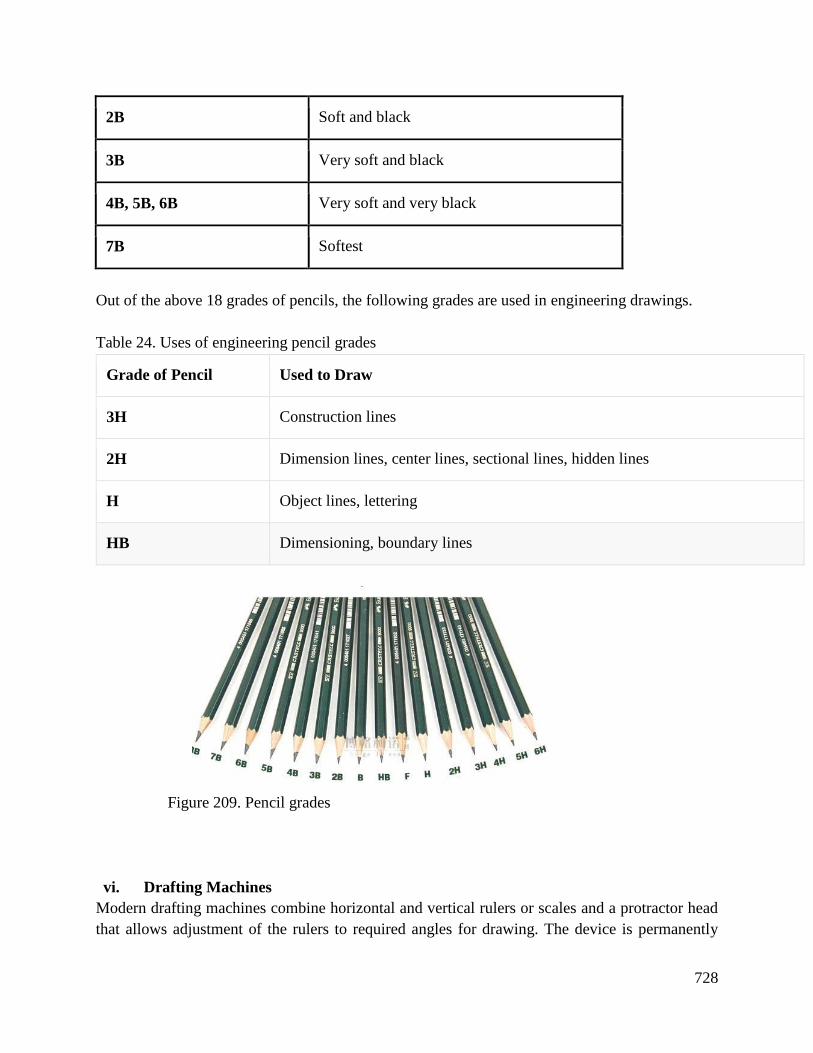
728
2B Soft and black
3B Very soft and black
4B, 5B, 6B Very soft and very black
7B Softest
Out of the above 18 grades of pencils, the following grades are used in engineering drawings.
Table 24. Uses of engineering pencil grades
Grade of Pencil Used to Draw
3H Construction lines
2H Dimension lines, center lines, sectional lines, hidden lines
H Object lines, lettering
HB Dimensioning, boundary lines
Figure 209. Pencil grades
vi. Drafting Machines
Modern drafting machines combine horizontal and vertical rulers or scales and a protractor head
that allows adjustment of the rulers to required angles for drawing. The device is permanently
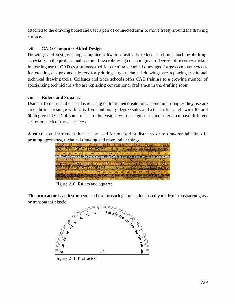
729
attached to the drawing board and uses a pair of connected arms to move freely around the drawing
surface.
vii. CAD: Computer Aided Design
Drawings and designs using computer software drastically reduce hand and machine drafting,
especially in the professional sectors. Lower drawing cost and greater degrees of accuracy dictate
increasing use of CAD as a primary tool for creating technical drawings. Large computer screens
for creating designs and plotters for printing large technical drawings are replacing traditional
technical drawing tools. Colleges and trade schools offer CAD training to a growing number of
specializing technicians who are replacing conventional draftsmen in the drafting room.
viii. Rulers and Squares
Using a T-square and clear plastic triangle, draftsmen create lines. Common triangles they use are
an eight-inch triangle with forty-five- and ninety-degree sides and a ten-inch triangle with 30- and
60-degree sides. Draftsmen measure dimensions with triangular shaped rulers that have different
scales on each of three surfaces.
A ruler is an instrument that can be used for measuring distances or to draw straight lines in
printing, geometry, technical drawing and many other things.
Figure 210. Rulers and squares
The protractor is an instrument used for measuring angles. It is usually made of transparent glass
or transparent plastic
Figure 211. Protractor
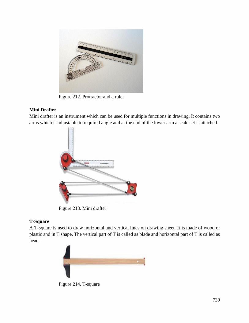
730
Figure 212. Protractor and a ruler
Mini Drafter
Mini drafter is an instrument which can be used for multiple functions in drawing. It contains two
arms which is adjustable to required angle and at the end of the lower arm a scale set is attached.
Figure 213. Mini drafter
T-Square
A T-square is used to draw horizontal and vertical lines on drawing sheet. It is made of wood or
plastic and in T shape. The vertical part of T is called as blade and horizontal part of T is called as
head.
Figure 214. T-square
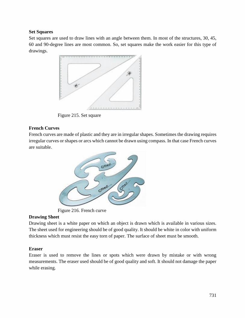
731
Set Squares
Set squares are used to draw lines with an angle between them. In most of the structures, 30, 45,
60 and 90-degree lines are most common. So, set squares make the work easier for this type of
drawings.
Figure 215. Set square
French Curves
French curves are made of plastic and they are in irregular shapes. Sometimes the drawing requires
irregular curves or shapes or arcs which cannot be drawn using compass. In that case French curves
are suitable.
Figure 216. French curve
Drawing Sheet
Drawing sheet is a white paper on which an object is drawn which is available in various sizes.
The sheet used for engineering should be of good quality. It should be white in color with uniform
thickness which must resist the easy torn of paper. The surface of sheet must be smooth.
Eraser
Eraser is used to remove the lines or spots which were drawn by mistake or with wrong
measurements. The eraser used should be of good quality and soft. It should not damage the paper
while erasing.
732
Figure 217. Eraser
Paper Holders
When the drawing sheet is placed on the board it may not be in fixed position. To fix the drawing
sheet to the board paper holders are used.
Figure 218. Paper holder
Disposing of waste materials so as to prevent air pollution is a recent requirement in the history of
waste disposal. Proper disposal of waste resulting from technical drawing must be followed.
Degradable waste must be disposed separately with non-degraded waste. Broken compasses and
rules must be disposed properly as they can cause harm to the trainee in the work place.
Personal protective equipment, or PPE, is designed to protect you from hazards found on or off
the job. The PPE prevent the draftsmen from hazards when they are working in the drawing rooms.
These PPE include:
Grooves
Closed shoes
Dust coat
Helmets
Proper procedures must be observed and adhered to know when to put on the protective gears to
minimize injuries during and after the exercise.
Conclusion
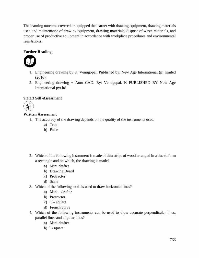
733
The learning outcome covered or equipped the learner with drawing equipment, drawing materials
used and maintenance of drawing equipment, drawing materials, dispose of waste materials, and
proper use of productive equipment in accordance with workplace procedures and environmental
legislations.
Further Reading
1. Engineering drawing by K. Venugopal. Published by: New Age International (p) limited
(2016).
2. Engineering drawing + Auto CAD. By: Venugopal. K PUBLISHED BY New Age
International pvt ltd
9.3.2.3 Self-Assessment
Written Assessment
1. The accuracy of the drawing depends on the quality of the instruments used.
a) True
b) False
2. Which of the following instrument is made of thin strips of wood arranged in a line to form
a rectangle and on which, the drawing is made?
a) Mini-drafter
b) Drawing Board
c) Protractor
d) Scale
3. Which of the following tools is used to draw horizontal lines?
a) Mini – drafter
b) Protractor
c) T – square
d) French curve
4. Which of the following instruments can be used to draw accurate perpendicular lines,
parallel lines and angular lines?
a) Mini-drafter
b) T-square
734
c) Protractor
d) Set square
5. According to the Indian Standard Institute (ISI), which among the following designation
has the size 1000 x 700 (in mm)?
a) B0
b) B1
c) B2
d) B3
6. Which is the most common tool used for drawing circles?
a) French curve
b) Mini – drafter
c) Divider
d) Compass
7. For drawing circles with a large radius, which of the following tool is used?
a) Bow compass
b) Lengthening bar compass
c) Divider
d) Protractors
8. The preferred size of the drawing sheets is recommended by the ______
a) B.I.S.
b) ASME
c) ASTM
d) NIST
9. SP: 46 (2003) recommends the borders of _______ mm width for the sheet sizes A0 and
A1, and _______ mm for the sizes A2, A3, A4 and A5.
a) 10, 20
b) 15, 20
c) 20, 10
d) 15, 10
10. The false statement regarding orientation mark.
a) The orientation mark coincides with one of the centering marks
b) Represents the direction to which sheet is placed
c) Orientation mark can be used for the orientation of drawing sheet on the
drawing board
d) Facilitate positioning of the drawing for reproduction purpose
11. Select and apply different drawing paper holders
12. Discuss the best methods of drawing waste materials disposal which is environmental
friendly.
13. State three importance of drawing tools maintenance
735
Oral Assessment
1. State two uses of protractors in technical drawing
2. Give two types of pencils used to make faint lines
Practical Assessment
a) Make a sketch
9.3.2.4 Tools, Equipment, Supplies and Materials
Drawing room
Computer lab
Drawing equipment and materials
Computers
CAD package
Overhead projector
9.3.2.5 References
Davies, B. L., Robotham, A. J., & Yarwood, A. (1991). Computer-aided drawing and design.
London: Chapman & Hall.
Hubka, V. (2015). Principles of engineering design. Elsevier.
Morling, K. (2010). Geometric and engineering drawing. Routledge.
Shrock, C. R. (2009). Advanced AutoCAD 2010 Exercise Workbook. Industrial Press Inc.
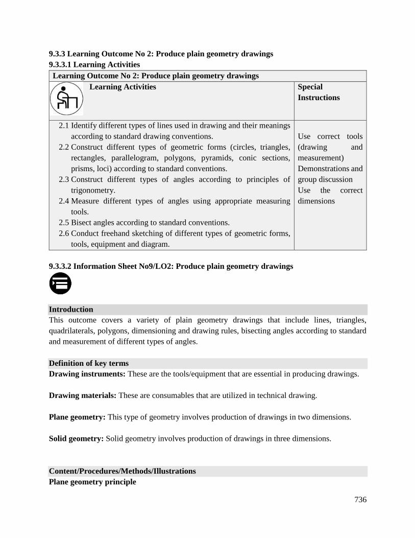
736
9.3.3 Learning Outcome No 2: Produce plain geometry drawings
9.3.3.1 Learning Activities
Learning Outcome No 2: Produce plain geometry drawings
Learning Activities Special
Instructions
2.1 Identify different types of lines used in drawing and their meanings
according to standard drawing conventions.
2.2 Construct different types of geometric forms (circles, triangles,
rectangles, parallelogram, polygons, pyramids, conic sections,
prisms, loci) according to standard conventions.
2.3 Construct different types of angles according to principles of
trigonometry.
2.4 Measure different types of angles using appropriate measuring
tools.
2.5 Bisect angles according to standard conventions.
2.6 Conduct freehand sketching of different types of geometric forms,
tools, equipment and diagram.
Use correct tools
(drawing and
measurement)
Demonstrations and
group discussion
Use the correct
dimensions
9.3.3.2 Information Sheet No9/LO2: Produce plain geometry drawings
Introduction
This outcome covers a variety of plain geometry drawings that include lines, triangles,
quadrilaterals, polygons, dimensioning and drawing rules, bisecting angles according to standard
and measurement of different types of angles.
Definition of key terms
Drawing instruments: These are the tools/equipment that are essential in producing drawings.
Drawing materials: These are consumables that are utilized in technical drawing.
Plane geometry: This type of geometry involves production of drawings in two dimensions.
Solid geometry: Solid geometry involves production of drawings in three dimensions.
Content/Procedures/Methods/Illustrations
Plane geometry principle
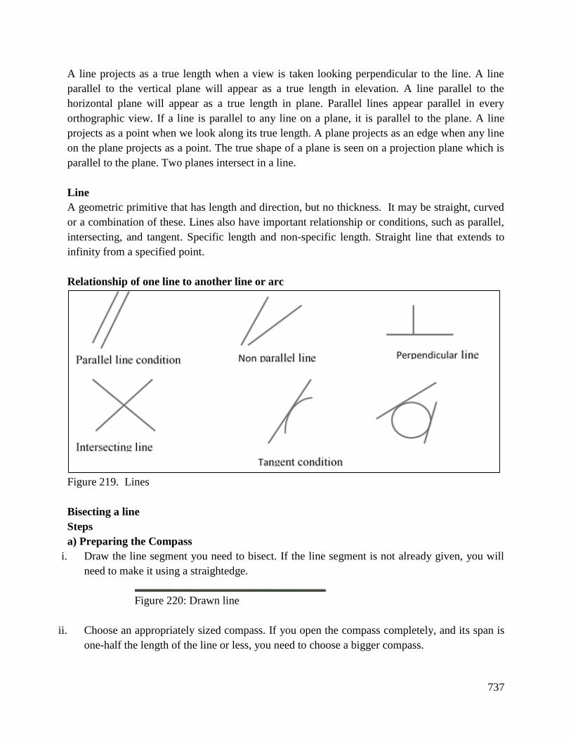
737
A line projects as a true length when a view is taken looking perpendicular to the line. A line
parallel to the vertical plane will appear as a true length in elevation. A line parallel to the
horizontal plane will appear as a true length in plane. Parallel lines appear parallel in every
orthographic view. If a line is parallel to any line on a plane, it is parallel to the plane. A line
projects as a point when we look along its true length. A plane projects as an edge when any line
on the plane projects as a point. The true shape of a plane is seen on a projection plane which is
parallel to the plane. Two planes intersect in a line.
Line
A geometric primitive that has length and direction, but no thickness. It may be straight, curved
or a combination of these. Lines also have important relationship or conditions, such as parallel,
intersecting, and tangent. Specific length and non-specific length. Straight line that extends to
infinity from a specified point.
Relationship of one line to another line or arc
Figure 219. Lines
Bisecting a line
Steps
a) Preparing the Compass
i. Draw the line segment you need to bisect. If the line segment is not already given, you will
need to make it using a straightedge.
Figure 220: Drawn line
ii. Choose an appropriately sized compass. If you open the compass completely, and its span is
one-half the length of the line or less, you need to choose a bigger compass.
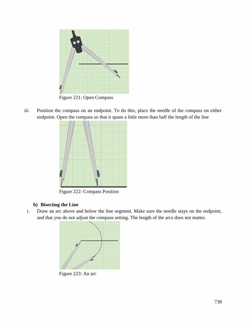
738
Figure 221: Open Compass
iii. Position the compass on an endpoint. To do this, place the needle of the compass on either
endpoint. Open the compass so that it spans a little more than half the length of the line
Figure 222: Compass Position
b) Bisecting the Line
i. Draw an arc above and below the line segment. Make sure the needle stays on the endpoint,
and that you do not adjust the compass setting. The length of the arcs does not matter.
Figure 223: An arc
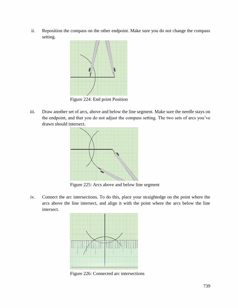
739
ii. Reposition the compass on the other endpoint. Make sure you do not change the compass
setting.
Figure 224: End point Position
iii. Draw another set of arcs, above and below the line segment. Make sure the needle stays on
the endpoint, and that you do not adjust the compass setting. The two sets of arcs you’ve
drawn should intersect.
Figure 225: Arcs above and below line segment
iv. Connect the arc intersections. To do this, place your straightedge on the point where the
arcs above the line intersect, and align it with the point where the arcs below the line
intersect.
Figure 226: Connected arc intersections
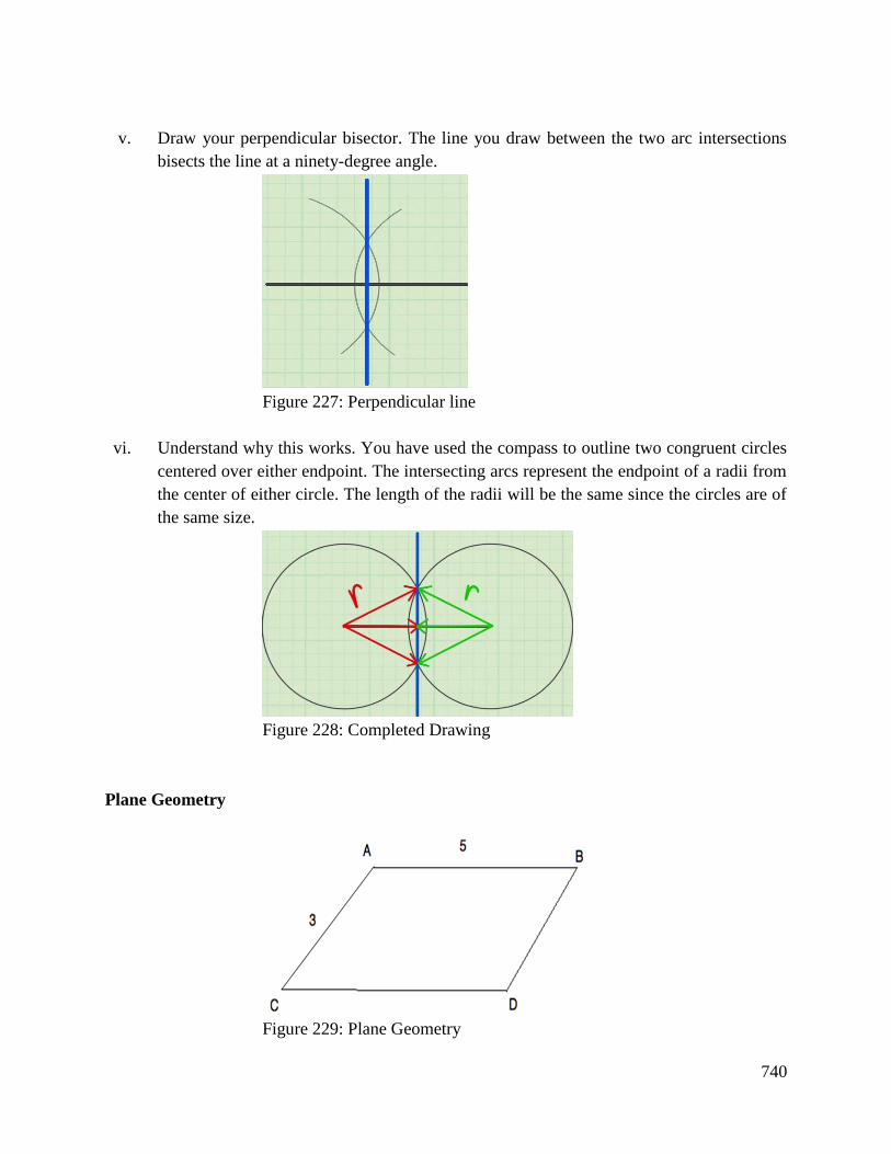
740
v. Draw your perpendicular bisector. The line you draw between the two arc intersections
bisects the line at a ninety-degree angle.
Figure 227: Perpendicular line
vi. Understand why this works. You have used the compass to outline two congruent circles
centered over either endpoint. The intersecting arcs represent the endpoint of a radii from
the center of either circle. The length of the radii will be the same since the circles are of
the same size.
Figure 228: Completed Drawing
Plane Geometry
Figure 229: Plane Geometry
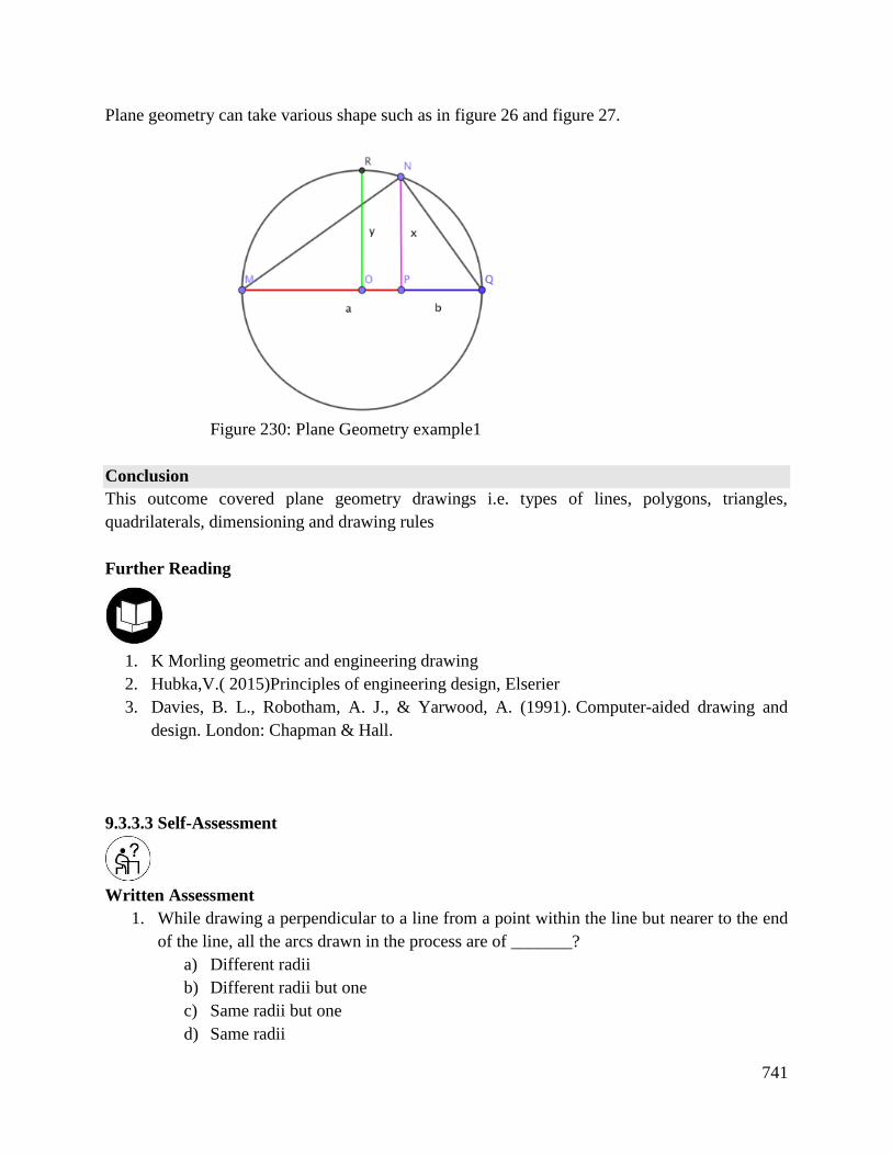
741
Plane geometry can take various shape such as in figure 26 and figure 27.
Figure 230: Plane Geometry example1
Conclusion
This outcome covered plane geometry drawings i.e. types of lines, polygons, triangles,
quadrilaterals, dimensioning and drawing rules
Further Reading
1. K Morling geometric and engineering drawing
2. Hubka,V.( 2015)Principles of engineering design, Elserier
3. Davies, B. L., Robotham, A. J., & Yarwood, A. (1991). Computer-aided drawing and
design. London: Chapman & Hall.
9.3.3.3 Self-Assessment
Written Assessment
1. While drawing a perpendicular to a line from a point within the line but nearer to the end
of the line, all the arcs drawn in the process are of _______?
a) Different radii
b) Different radii but one
c) Same radii but one
d) Same radii
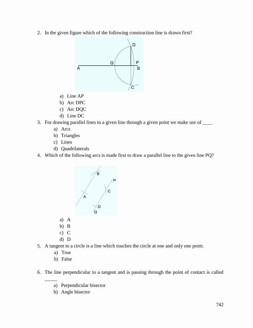
742
2. In the given figure which of the following construction line is drawn first?
a) Line AP
b) Arc DPC
c) Arc DQC
d) Line DC
3. For drawing parallel lines to a given line through a given point we make use of ____
a) Arcs
b) Triangles
c) Lines
d) Quadrilaterals
4. Which of the following arcs is made first to draw a parallel line to the given line PQ?
a) A
b) B
c) C
d) D
5. A tangent to a circle is a line which touches the circle at one and only one point.
a) True
b) False
6. The line perpendicular to a tangent and is passing through the point of contact is called
_____
a) Perpendicular bisector
b) Angle bisector
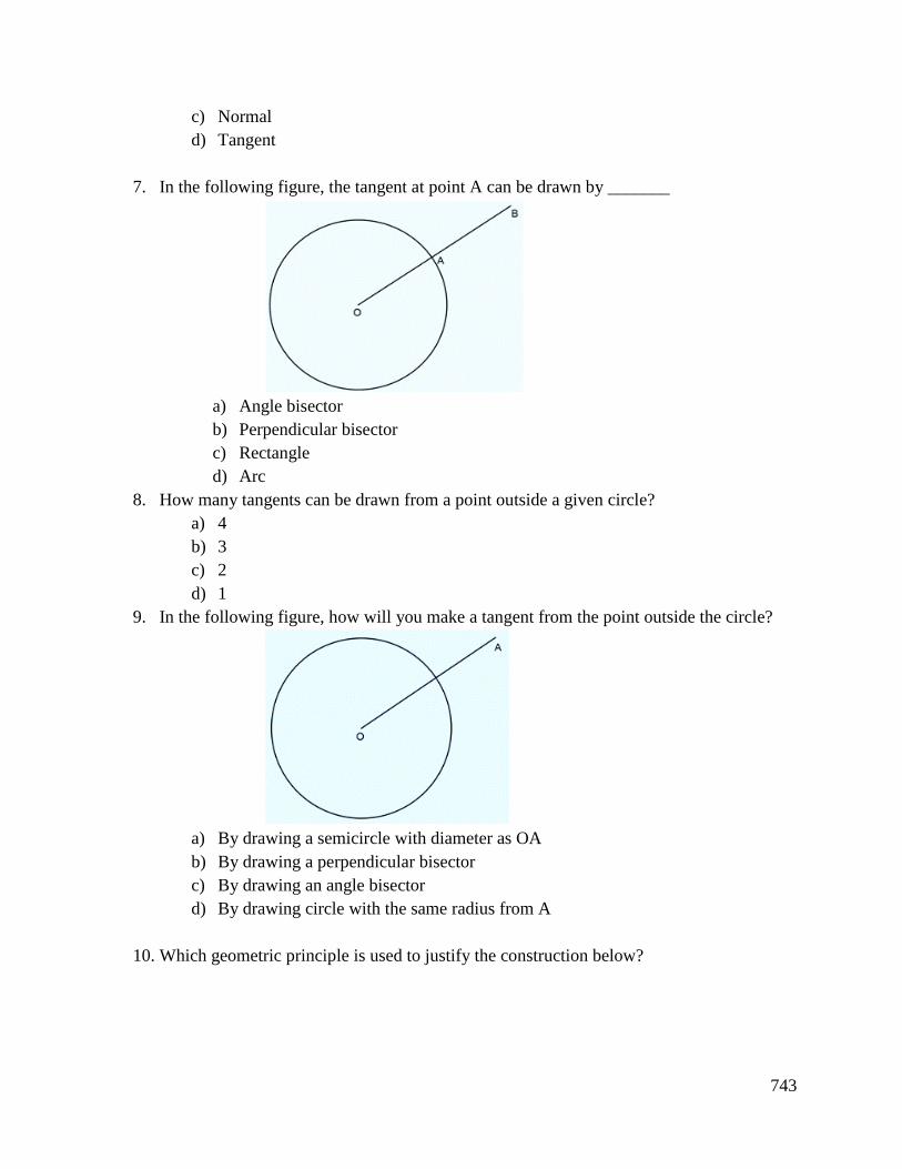
743
c) Normal
d) Tangent
7. In the following figure, the tangent at point A can be drawn by _______
a) Angle bisector
b) Perpendicular bisector
c) Rectangle
d) Arc
8. How many tangents can be drawn from a point outside a given circle?
a) 4
b) 3
c) 2
d) 1
9. In the following figure, how will you make a tangent from the point outside the circle?
a) By drawing a semicircle with diameter as OA
b) By drawing a perpendicular bisector
c) By drawing an angle bisector
d) By drawing circle with the same radius from A
10. Which geometric principle is used to justify the construction below?
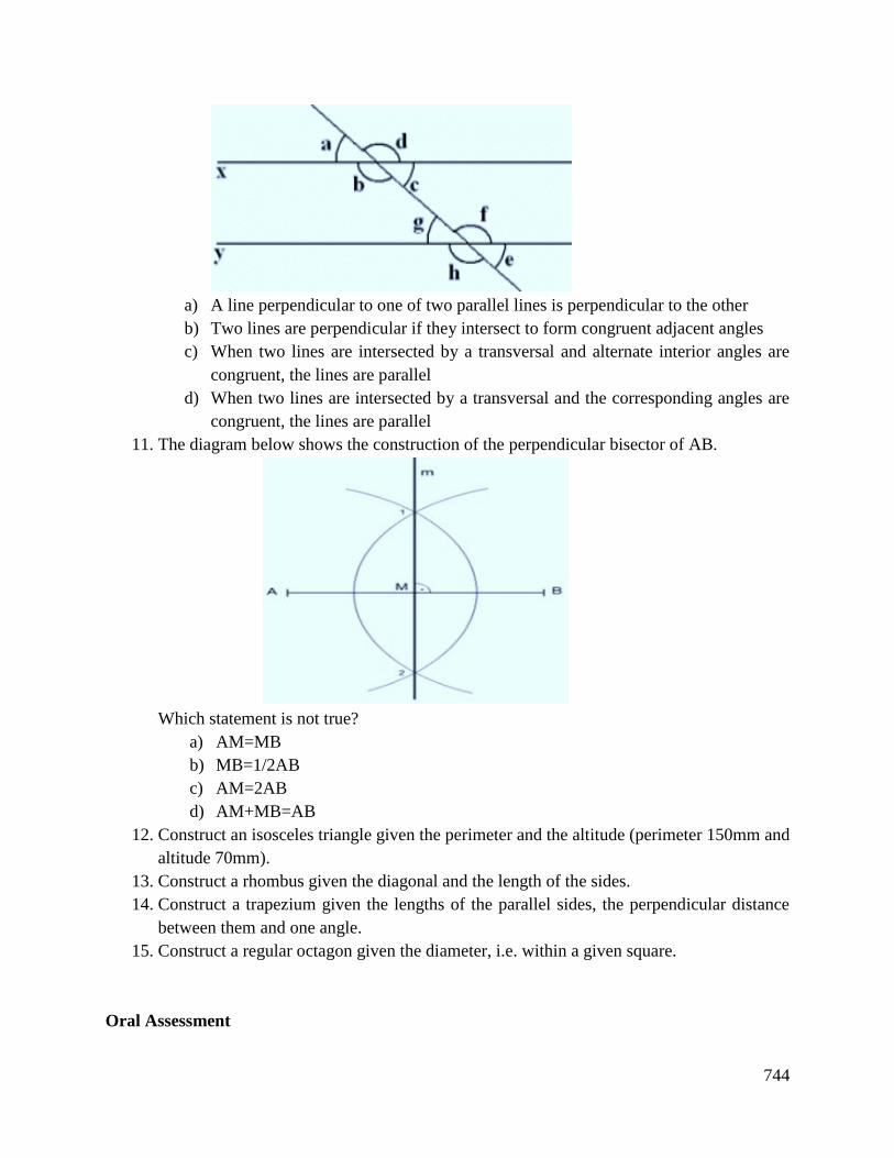
744
a) A line perpendicular to one of two parallel lines is perpendicular to the other
b) Two lines are perpendicular if they intersect to form congruent adjacent angles
c) When two lines are intersected by a transversal and alternate interior angles are
congruent, the lines are parallel
d) When two lines are intersected by a transversal and the corresponding angles are
congruent, the lines are parallel
11. The diagram below shows the construction of the perpendicular bisector of AB.
Which statement is not true?
a) AM=MB
b) MB=1/2AB
c) AM=2AB
d) AM+MB=AB
12. Construct an isosceles triangle given the perimeter and the altitude (perimeter 150mm and
altitude 70mm).
13. Construct a rhombus given the diagonal and the length of the sides.
14. Construct a trapezium given the lengths of the parallel sides, the perpendicular distance
between them and one angle.
15. Construct a regular octagon given the diameter, i.e. within a given square.
Oral Assessment
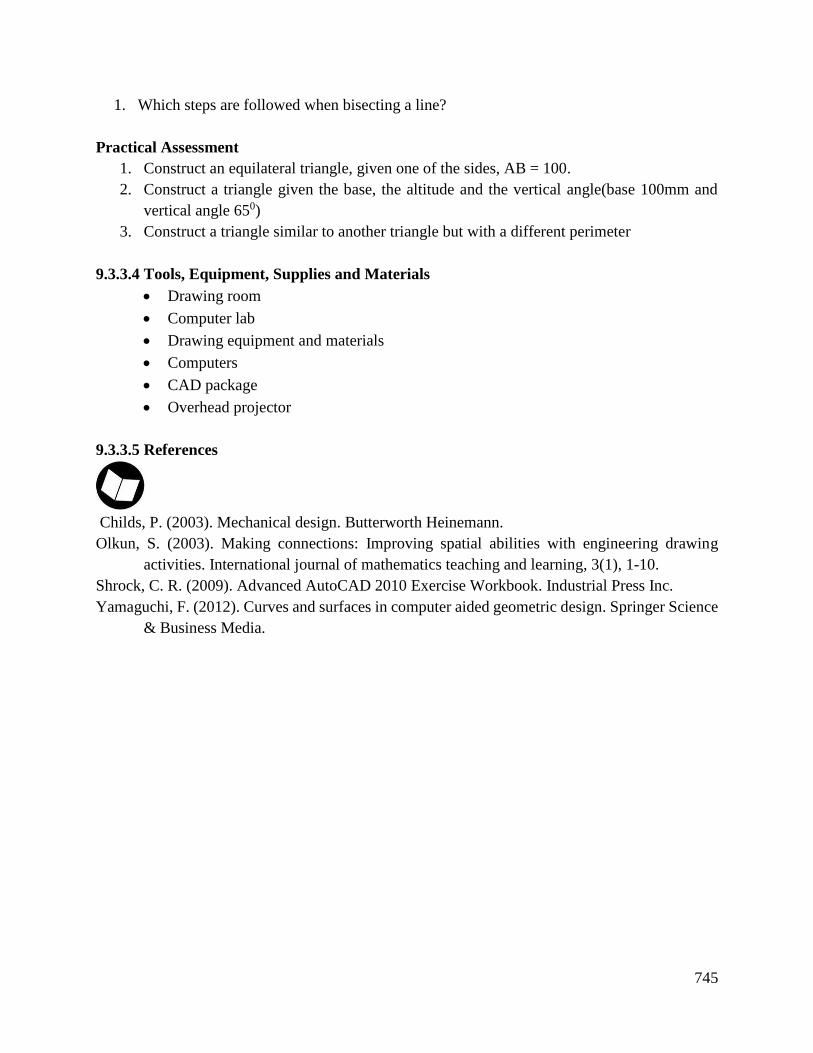
745
1. Which steps are followed when bisecting a line?
Practical Assessment
1. Construct an equilateral triangle, given one of the sides, AB = 100.
2. Construct a triangle given the base, the altitude and the vertical angle(base 100mm and
vertical angle 650)
3. Construct a triangle similar to another triangle but with a different perimeter
9.3.3.4 Tools, Equipment, Supplies and Materials
Drawing room
Computer lab
Drawing equipment and materials
Computers
CAD package
Overhead projector
9.3.3.5 References
Childs, P. (2003). Mechanical design. Butterworth Heinemann.
Olkun, S. (2003). Making connections: Improving spatial abilities with engineering drawing
activities. International journal of mathematics teaching and learning, 3(1), 1-10.
Shrock, C. R. (2009). Advanced AutoCAD 2010 Exercise Workbook. Industrial Press Inc.
Yamaguchi, F. (2012). Curves and surfaces in computer aided geometric design. Springer Science
& Business Media.
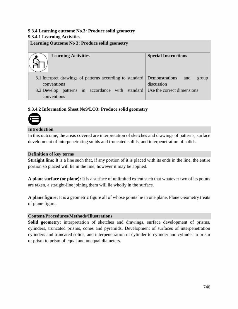
746
9.3.4 Learning outcome No.3: Produce solid geometry
9.3.4.1 Learning Activities
Learning Outcome No 3: Produce solid geometry
Learning Activities Special Instructions
3.1 Interpret drawings of patterns according to standard
conventions
3.2 Develop patterns in accordance with standard
conventions
Demonstrations and group
discussion
Use the correct dimensions
9.3.4.2 Information Sheet No9/LO3: Produce solid geometry
Introduction
In this outcome, the areas covered are interpretation of sketches and drawings of patterns, surface
development of interpenetrating solids and truncated solids, and interpenetration of solids.
Definition of key terms
Straight line: It is a line such that, if any portion of it is placed with its ends in the line, the entire
portion so placed will lie in the line, however it may be applied.
A plane surface (or plane): It is a surface of unlimited extent such that whatever two of its points
are taken, a straight-line joining them will lie wholly in the surface.
A plane figure: It is a geometric figure all of whose points lie in one plane. Plane Geometry treats
of plane figure.
Content/Procedures/Methods/Illustrations
Solid geometry: interpretation of sketches and drawings, surface development of prisms,
cylinders, truncated prisms, cones and pyramids. Development of surfaces of interpenetration
cylinders and truncated solids, and interpenetration of cylinder to cylinder and cylinder to prism
or prism to prism of equal and unequal diameters.
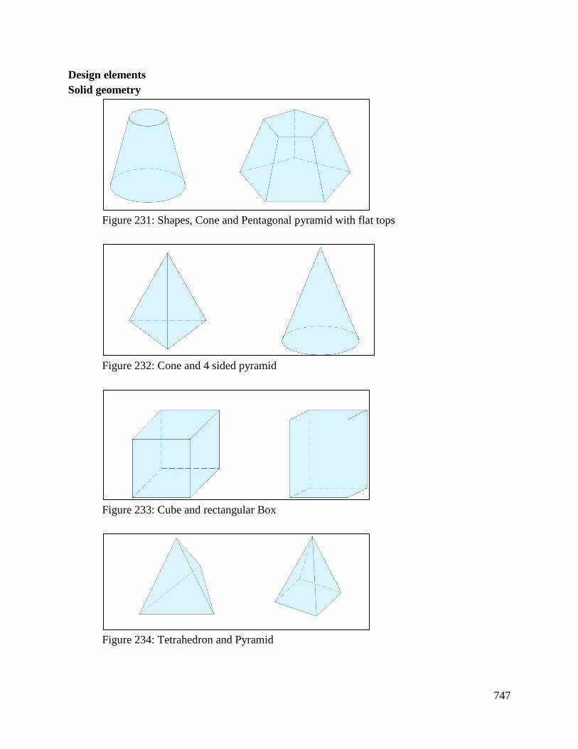
747
Design elements
Solid geometry
Figure 231: Shapes, Cone and Pentagonal pyramid with flat tops
Figure 232: Cone and 4 sided pyramid
Figure 233: Cube and rectangular Box
Figure 234: Tetrahedron and Pyramid
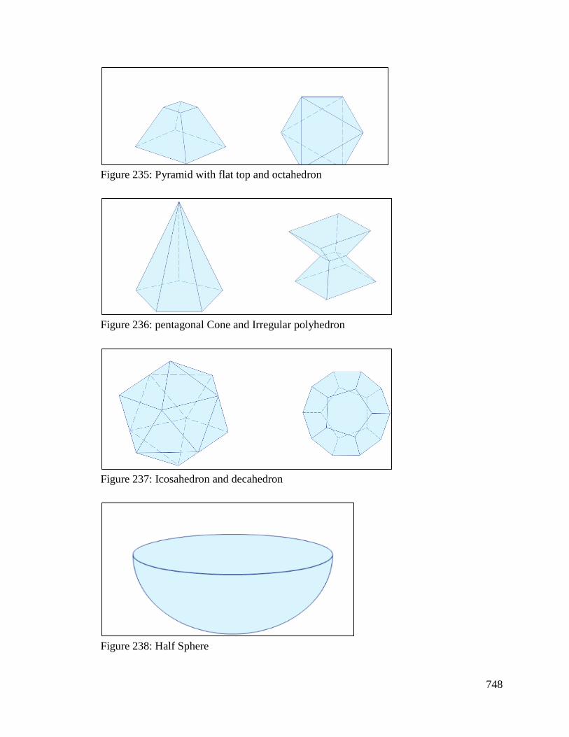
748
Figure 235: Pyramid with flat top and octahedron
Figure 236: pentagonal Cone and Irregular polyhedron
Figure 237: Icosahedron and decahedron
Figure 238: Half Sphere
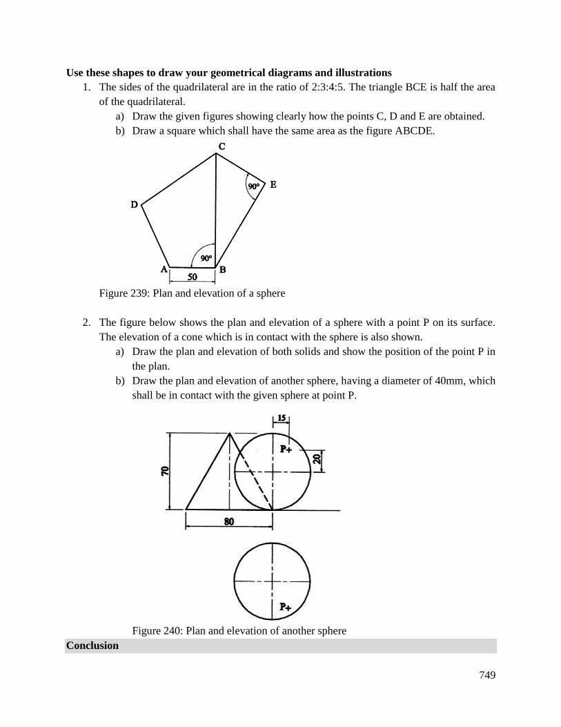
749
Use these shapes to draw your geometrical diagrams and illustrations
1. The sides of the quadrilateral are in the ratio of 2:3:4:5. The triangle BCE is half the area
of the quadrilateral.
a) Draw the given figures showing clearly how the points C, D and E are obtained.
b) Draw a square which shall have the same area as the figure ABCDE.
Figure 239: Plan and elevation of a sphere
2. The figure below shows the plan and elevation of a sphere with a point P on its surface.
The elevation of a cone which is in contact with the sphere is also shown.
a) Draw the plan and elevation of both solids and show the position of the point P in
the plan.
b) Draw the plan and elevation of another sphere, having a diameter of 40mm, which
shall be in contact with the given sphere at point P.
Figure 240: Plan and elevation of another sphere
Conclusion
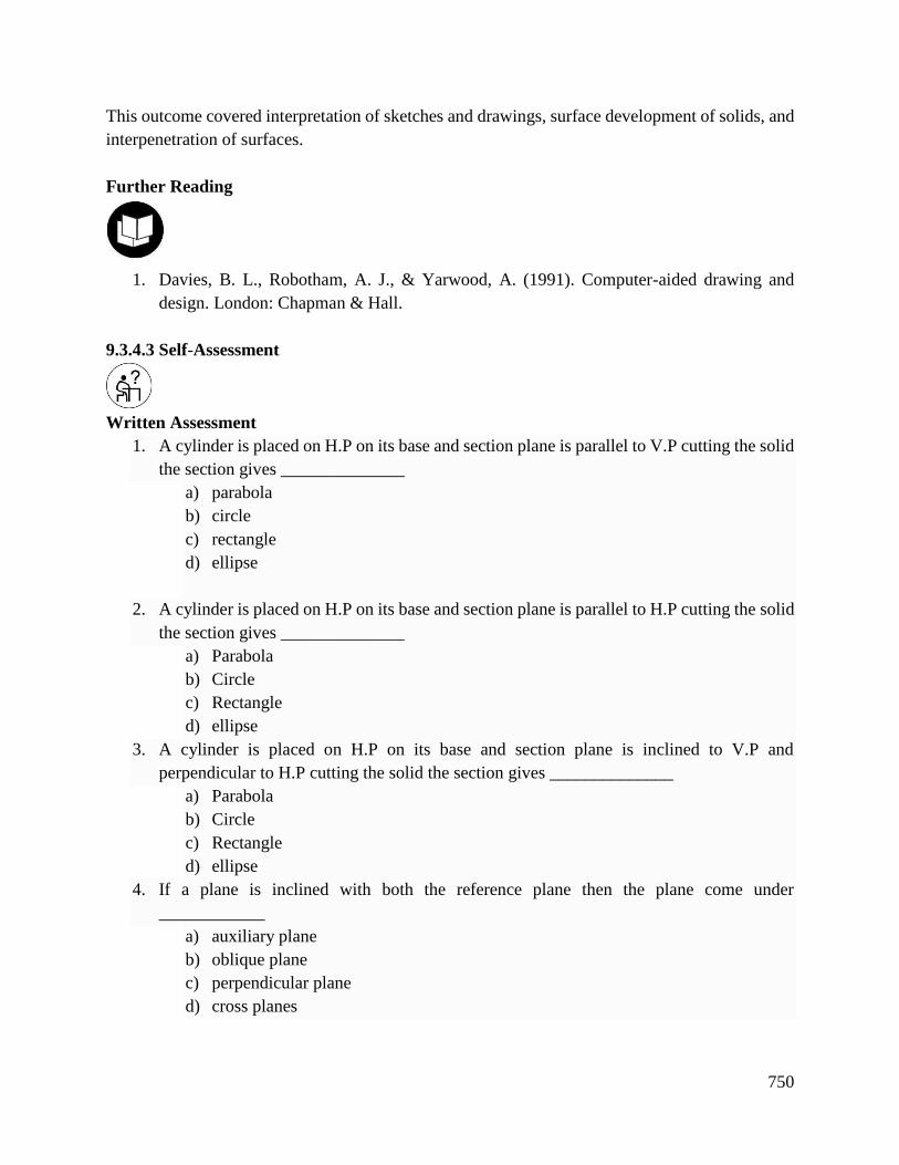
750
This outcome covered interpretation of sketches and drawings, surface development of solids, and
interpenetration of surfaces.
Further Reading
1. Davies, B. L., Robotham, A. J., & Yarwood, A. (1991). Computer-aided drawing and
design. London: Chapman & Hall.
9.3.4.3 Self-Assessment
Written Assessment
1. A cylinder is placed on H.P on its base and section plane is parallel to V.P cutting the solid
the section gives ______________
a) parabola
b) circle
c) rectangle
d) ellipse
2. A cylinder is placed on H.P on its base and section plane is parallel to H.P cutting the solid
the section gives ______________
a) Parabola
b) Circle
c) Rectangle
d) ellipse
3. A cylinder is placed on H.P on its base and section plane is inclined to V.P and
perpendicular to H.P cutting the solid the section gives ______________
a) Parabola
b) Circle
c) Rectangle
d) ellipse
4. If a plane is inclined with both the reference plane then the plane come under
____________
a) auxiliary plane
b) oblique plane
c) perpendicular plane
d) cross planes
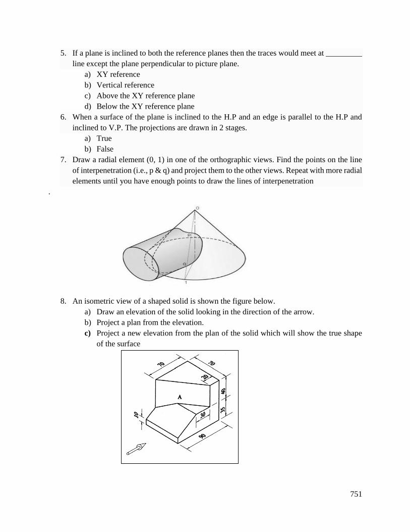
751
5. If a plane is inclined to both the reference planes then the traces would meet at _________
line except the plane perpendicular to picture plane.
a) XY reference
b) Vertical reference
c) Above the XY reference plane
d) Below the XY reference plane
6. When a surface of the plane is inclined to the H.P and an edge is parallel to the H.P and
inclined to V.P. The projections are drawn in 2 stages.
a) True
b) False
7. Draw a radial element (0, 1) in one of the orthographic views. Find the points on the line
of interpenetration (i.e., p & q) and project them to the other views. Repeat with more radial
elements until you have enough points to draw the lines of interpenetration
.
8. An isometric view of a shaped solid is shown the figure below.
a) Draw an elevation of the solid looking in the direction of the arrow.
b) Project a plan from the elevation.
c) Project a new elevation from the plan of the solid which will show the true shape
of the surface
752
Oral Assessment
1. What is solid geometry
Practical Assessment
Given pyramid is cut by plane, ⊥ to the frontal plane and inclined at 70o to the top plane. The
cutting plane cuts the axis of the pyramid at 15mm from the apex. Draw the projections of the
remaining part of the pyramid and the true shape of the cut section.
9.3.4.4 Tools, Equipment, Supplies and Materials
Drawing room
Computer lab
Drawing equipment and materials
Computers
CAD package
Overhead projector
9.3.4.5 References
Aouad, G., Wu, S., Lee, A., & Onyenobi, T. (2013). Computer aided design guide for architecture,
engineering and construction. Routledge.
Bergen, S. D., Bolton, S. M., & Fridley, J. L. (2001). Design principles for ecological engineering.
Ecological Engineering, 18(2), 201-210.
Liu, S. X., Hu, S. M., Chen, Y. J., & Sun, J. G. (2001). Reconstruction of curved solids from
engineering drawings. Computer-Aided Design, 33(14), 1059-1072.
753
9.3.5 Learning Outcome No 4: Produce pictorial and orthographic drawings of components
9.3.5.1 Learning Activities
Learning Outcome No 4: Produce pictorial and orthographic drawings of components
Learning Activities Special Instructions
4.1 Identify and interpret the meaning of symbols and abbreviations
according to standard drawing conventions
4.2 Interpret and produce first and third angle orthographic drawings
in accordance with the standard conventions
4.3 Dimension orthographic elevations in accordance with standard
conventions
4.4 Interpret and produce isometric drawings in accordance with
standard conventions
4.5 Produce and interpret assembly drawing in line with the operating
standards
9.3.5.2 Information Sheet No9/LO4: Produce pictorial and orthographic drawings of
components
Introduction
This outcome covers meaning of pictorial and orthographic drawings, sectioning, symbols and
abbreviations, drawing of isometric, oblique, axonometric, auxiliary and perspective views,
drawing of first and third angle projections, sectioning of components, and free hand sketching of
tools, equipment, components, geometric forms and diagrams.
Definition of key terms
Axonometric (Pictorial) Projections- These are drawings in which the object is drawn in three
dimensions (3-D) i.e. three sides of the object
Content/Procedures/Methods/Illustrations
4.1 Solid geometry principles
All views presented in a solid geometry are assumed to be from the same object, and only the
particular object but from different points of view and that all views are at the same scale. All the
visible edge is depicted by a line and assumptions are made that those edge progress away from
the viewer to form faces that are flat but at right angles. The true angle between a line and a plane
is seen in a view showing the line as a true length and the plane as an edge. All horizontal sections
of an upright or inverted right cone are circles. A sphere appears as a circle in every view. A sphere
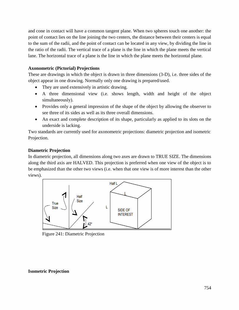
754
and cone in contact will have a common tangent plane. When two spheres touch one another: the
point of contact lies on the line joining the two centers, the distance between their centers is equal
to the sum of the radii, and the point of contact can be located in any view, by dividing the line in
the ratio of the radii. The vertical trace of a plane is the line in which the plane meets the vertical
lane. The horizontal trace of a plane is the line in which the plane meets the horizontal plane.
Axonometric (Pictorial) Projections
These are drawings in which the object is drawn in three dimensions (3-D), i.e. three sides of the
object appear in one drawing. Normally only one drawing is prepared/used.
They are used extensively in artistic drawing.
A three dimensional view (i.e. shows length, width and height of the object
simultaneously).
Provides only a general impression of the shape of the object by allowing the observer to
see three of its sides as well as its three overall dimensions.
An exact and complete description of its shape, particularly as applied to its slots on the
underside is lacking.
Two standards are currently used for axonometric projections: diametric projection and isometric
Projection.
Diametric Projection
In diametric projection, all dimensions along two axes are drawn to TRUE SIZE. The dimensions
along the third axis are HALVED. This projection is preferred when one view of the object is to
be emphasized than the other two views (i.e. when that one view is of more interest than the other
views).
Figure 241: Diametric Projection
Isometric Projection
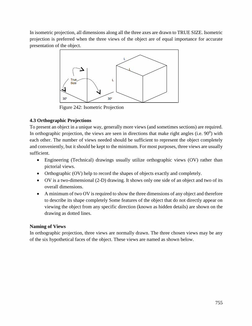
755
In isometric projection, all dimensions along all the three axes are drawn to TRUE SIZE. Isometric
projection is preferred when the three views of the object are of equal importance for accurate
presentation of the object.
Figure 242: Isometric Projection
4.3 Orthographic Projections
To present an object in a unique way, generally more views (and sometimes sections) are required.
In orthographic projection, the views are seen in directions that make right angles (i.e. 900) with
each other. The number of views needed should be sufficient to represent the object completely
and conveniently, but it should be kept to the minimum. For most purposes, three views are usually
sufficient.
Engineering (Technical) drawings usually utilize orthographic views (OV) rather than
pictorial views.
Orthographic (OV) help to record the shapes of objects exactly and completely.
OV is a two-dimensional (2-D) drawing. It shows only one side of an object and two of its
overall dimensions.
A minimum of two OV is required to show the three dimensions of any object and therefore
to describe its shape completely Some features of the object that do not directly appear on
viewing the object from any specific direction (known as hidden details) are shown on the
drawing as dotted lines.
Naming of Views
In orthographic projection, three views are normally drawn. The three chosen views may be any
of the six hypothetical faces of the object. These views are named as shown below.
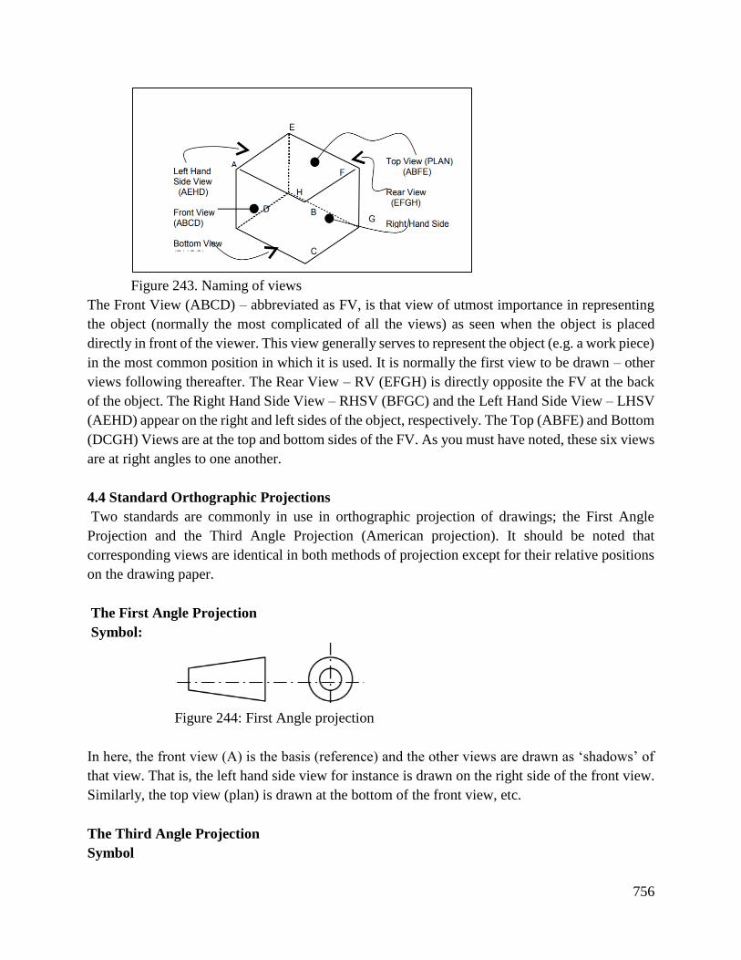
756
Figure 243. Naming of views
The Front View (ABCD) – abbreviated as FV, is that view of utmost importance in representing
the object (normally the most complicated of all the views) as seen when the object is placed
directly in front of the viewer. This view generally serves to represent the object (e.g. a work piece)
in the most common position in which it is used. It is normally the first view to be drawn – other
views following thereafter. The Rear View – RV (EFGH) is directly opposite the FV at the back
of the object. The Right Hand Side View – RHSV (BFGC) and the Left Hand Side View – LHSV
(AEHD) appear on the right and left sides of the object, respectively. The Top (ABFE) and Bottom
(DCGH) Views are at the top and bottom sides of the FV. As you must have noted, these six views
are at right angles to one another.
4.4 Standard Orthographic Projections
Two standards are commonly in use in orthographic projection of drawings; the First Angle
Projection and the Third Angle Projection (American projection). It should be noted that
corresponding views are identical in both methods of projection except for their relative positions
on the drawing paper.
The First Angle Projection
Symbol:
Figure 244: First Angle projection
In here, the front view (A) is the basis (reference) and the other views are drawn as ‘shadows’ of
that view. That is, the left hand side view for instance is drawn on the right side of the front view.
Similarly, the top view (plan) is drawn at the bottom of the front view, etc.
The Third Angle Projection
Symbol
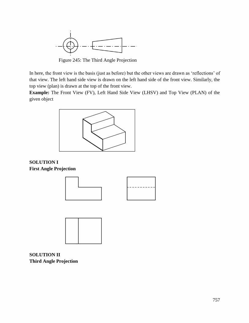
757
Figure 245: The Third Angle Projection
In here, the front view is the basis (just as before) but the other views are drawn as ‘reflections’ of
that view. The left hand side view is drawn on the left hand side of the front view. Similarly, the
top view (plan) is drawn at the top of the front view.
Example: The Front View (FV), Left Hand Side View (LHSV) and Top View (PLAN) of the
given object
SOLUTION I
First Angle Projection
SOLUTION II
Third Angle Projection
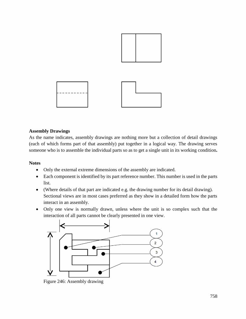
758
Assembly Drawings
As the name indicates, assembly drawings are nothing more but a collection of detail drawings
(each of which forms part of that assembly) put together in a logical way. The drawing serves
someone who is to assemble the individual parts so as to get a single unit in its working condition.
Notes
Only the external extreme dimensions of the assembly are indicated.
Each component is identified by its part reference number. This number is used in the parts
list.
(Where details of that part are indicated e.g. the drawing number for its detail drawing).
Sectional views are in most cases preferred as they show in a detailed form how the parts
interact in an assembly.
Only one view is normally drawn, unless where the unit is so complex such that the
interaction of all parts cannot be clearly presented in one view.
Figure 246: Assembly drawing
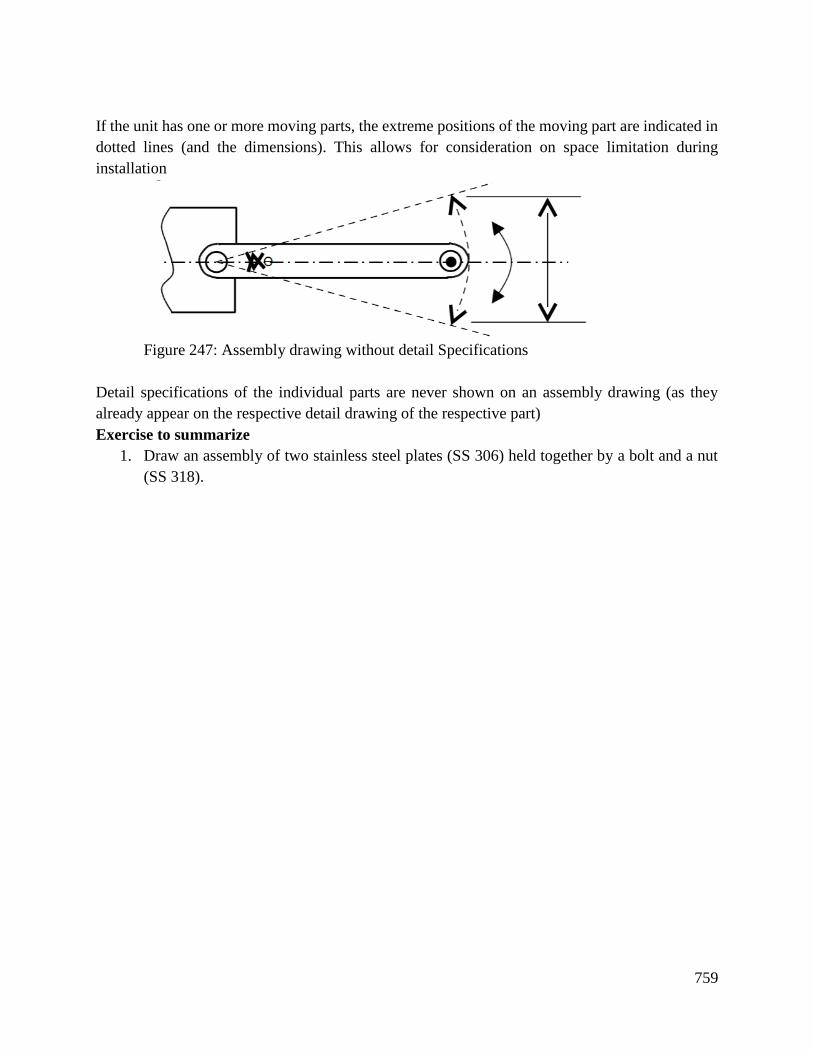
759
If the unit has one or more moving parts, the extreme positions of the moving part are indicated in
dotted lines (and the dimensions). This allows for consideration on space limitation during
installation
Figure 247: Assembly drawing without detail Specifications
Detail specifications of the individual parts are never shown on an assembly drawing (as they
already appear on the respective detail drawing of the respective part)
Exercise to summarize
1. Draw an assembly of two stainless steel plates (SS 306) held together by a bolt and a nut
(SS 318).
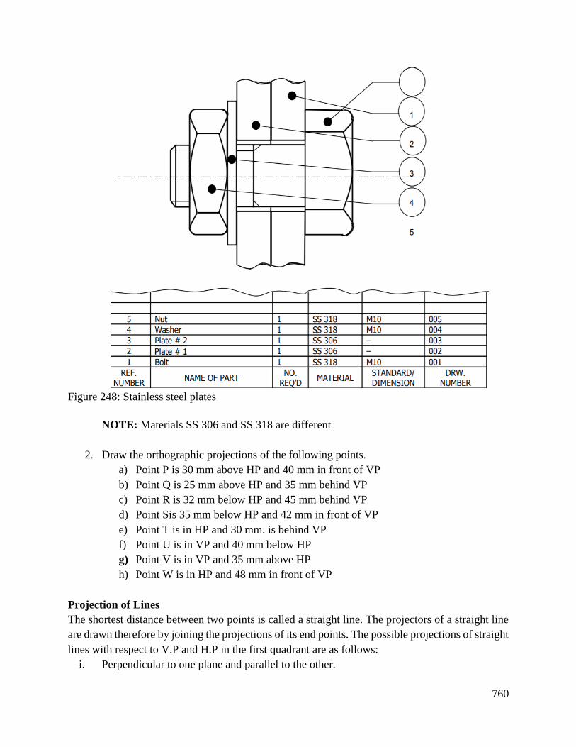
760
Figure 248: Stainless steel plates
NOTE: Materials SS 306 and SS 318 are different
2. Draw the orthographic projections of the following points.
a) Point P is 30 mm above HP and 40 mm in front of VP
b) Point Q is 25 mm above HP and 35 mm behind VP
c) Point R is 32 mm below HP and 45 mm behind VP
d) Point Sis 35 mm below HP and 42 mm in front of VP
e) Point T is in HP and 30 mm. is behind VP
f) Point U is in VP and 40 mm below HP
g) Point V is in VP and 35 mm above HP
h) Point W is in HP and 48 mm in front of VP
Projection of Lines
The shortest distance between two points is called a straight line. The projectors of a straight line
are drawn therefore by joining the projections of its end points. The possible projections of straight
lines with respect to V.P and H.P in the first quadrant are as follows:
i. Perpendicular to one plane and parallel to the other.
761
ii. Parallel to both the planes.
iii. Parallel to one plane and inclined to the other.
iv. Inclined to both the planes.
Conclusion
This outcome covered orthographic views, pictorial drawing, oblique drawings, sectioning,
axonometric, auxiliary first, and third angle projections, and free hand sketching.
Further Reading
1. Geometric and Engineering drawing Third Edition K Morling.
2. Engineering Drawing with CAD Applications by O. OSTROWSKY
9.3.4.3 Self-Assessment
Written Assessment
1. Orthographic projection is drawn using two methods which is ___________
a) Second angle and third angle method
b) First angle and third angle method
c) First angle and fourth angle method
d) Second angle and fourth angle method
2. The method in which the object is placed in the first quadrant is known as ____ method.
a) Third angle
b) Second angle
c) First angle
d) Fourth angle
3. In first angle method the top view is drawn _______ of the front view.
a) Above
b) Right Side
c) Left side
d) Bottom
4. The method in which the object is placed in the third quadrant is known as __________
method.
a) Third angle
b) Second angle
c) First angle
d) Fourth angle
5. In third angle method the top view is drawn _______ of the front view.
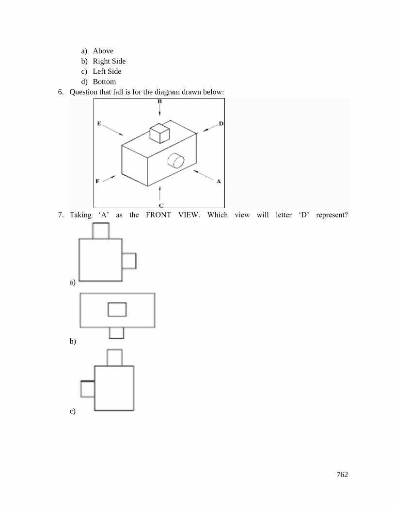
762
a) Above
b) Right Side
c) Left Side
d) Bottom
6. Question that fall is for the diagram drawn below:
7. Taking ‘A’ as the FRONT VIEW. Which view will letter ‘D’ represent?
a)
b)
c)
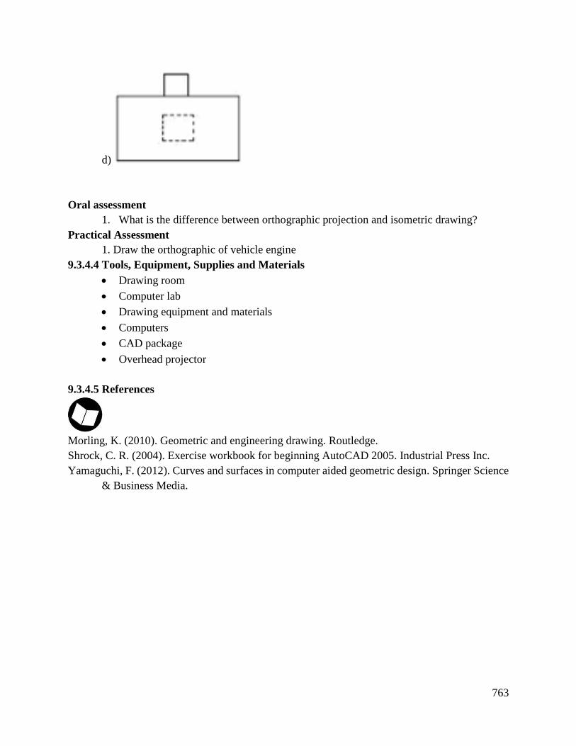
763
d)
Oral assessment
1. What is the difference between orthographic projection and isometric drawing?
Practical Assessment
1. Draw the orthographic of vehicle engine
9.3.4.4 Tools, Equipment, Supplies and Materials
Drawing room
Computer lab
Drawing equipment and materials
Computers
CAD package
Overhead projector
9.3.4.5 References
Morling, K. (2010). Geometric and engineering drawing. Routledge.
Shrock, C. R. (2004). Exercise workbook for beginning AutoCAD 2005. Industrial Press Inc.
Yamaguchi, F. (2012). Curves and surfaces in computer aided geometric design. Springer Science
& Business Media.
764
9.3.6 Learning Outcome No 5: Produce mechanical drawings
9.3.6.1 Learning Activities
Learning Outcome No 5: Produce mechanical drawings
Learning Activities Special Instructions
5.1 Identify and interpret the meaning of Mechanical
symbols and abbreviations according to BS 3939.
5.2 Mechanical drawings are produced in accordance
with BS 3939.
All drawings should be made in mm
Always use correct dimensions while
drawing
Use correct line type while drawing
9.3.6.2 Information Sheet No9/LO5: produce mechanical drawings
Introduction
This learning outcome covers mechanical symbols and abbreviations and mechanical drawings
production.
Definition of key terms
Drawing: It is using drawing instruments, from compasses to computers to bring precision to the
drawings.
Sketching: Means freehand drawing.
A plane: Is an imaginary surface on which pictures are prepared imaginably.
Dimension line: Is a thin line, broken in the middle to allow the placement of the dimension value,
with arrowheads at each end
Content/Procedures/Methods/Illustrations
Engineering drawing abbreviations and symbols are used to communicate and detail the
characteristics of an engineering drawing. This list includes abbreviations common to the
vocabulary of people who work with engineering drawings in the manufacture and inspection of
parts and assemblies. Technical standards exist to provide glossaries of abbreviations, acronyms,
and symbols that may be found on engineering drawings. Many corporations have such standards,
which define some terms and symbols specific to them; on the national and international level,
ASME standard Y14.38 is probably the most widely used.
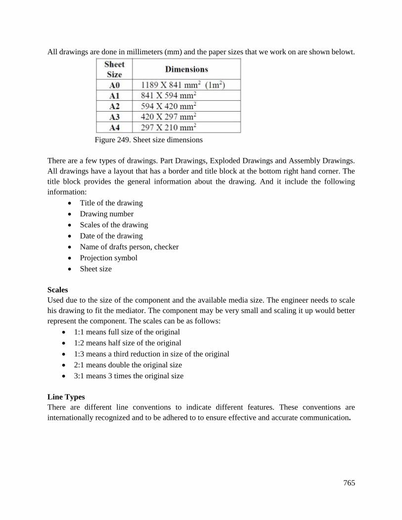
765
All drawings are done in millimeters (mm) and the paper sizes that we work on are shown belowt.
Figure 249. Sheet size dimensions
There are a few types of drawings. Part Drawings, Exploded Drawings and Assembly Drawings.
All drawings have a layout that has a border and title block at the bottom right hand corner. The
title block provides the general information about the drawing. And it include the following
information:
Title of the drawing
Drawing number
Scales of the drawing
Date of the drawing
Name of drafts person, checker
Projection symbol
Sheet size
Scales
Used due to the size of the component and the available media size. The engineer needs to scale
his drawing to fit the mediator. The component may be very small and scaling it up would better
represent the component. The scales can be as follows:
1:1 means full size of the original
1:2 means half size of the original
1:3 means a third reduction in size of the original
2:1 means double the original size
3:1 means 3 times the original size
Line Types
There are different line conventions to indicate different features. These conventions are
internationally recognized and to be adhered to to ensure effective and accurate communication.
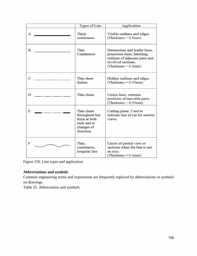
766
Figure 250. Line types and application
Abbreviations and symbols
Common engineering terms and expressions are frequently replaced by abbreviations or symbols
on drawings.
Table 25. Abbreviation and symbols
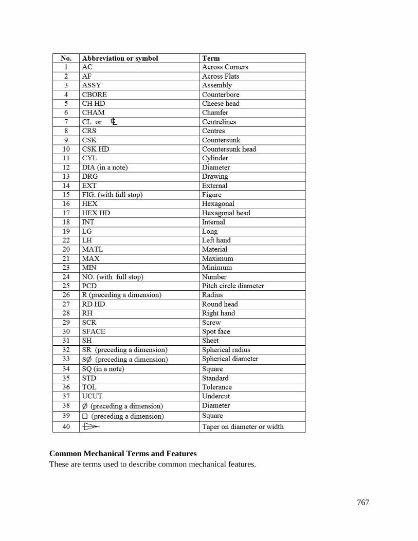
767
Common Mechanical Terms and Features
These are terms used to describe common mechanical features.
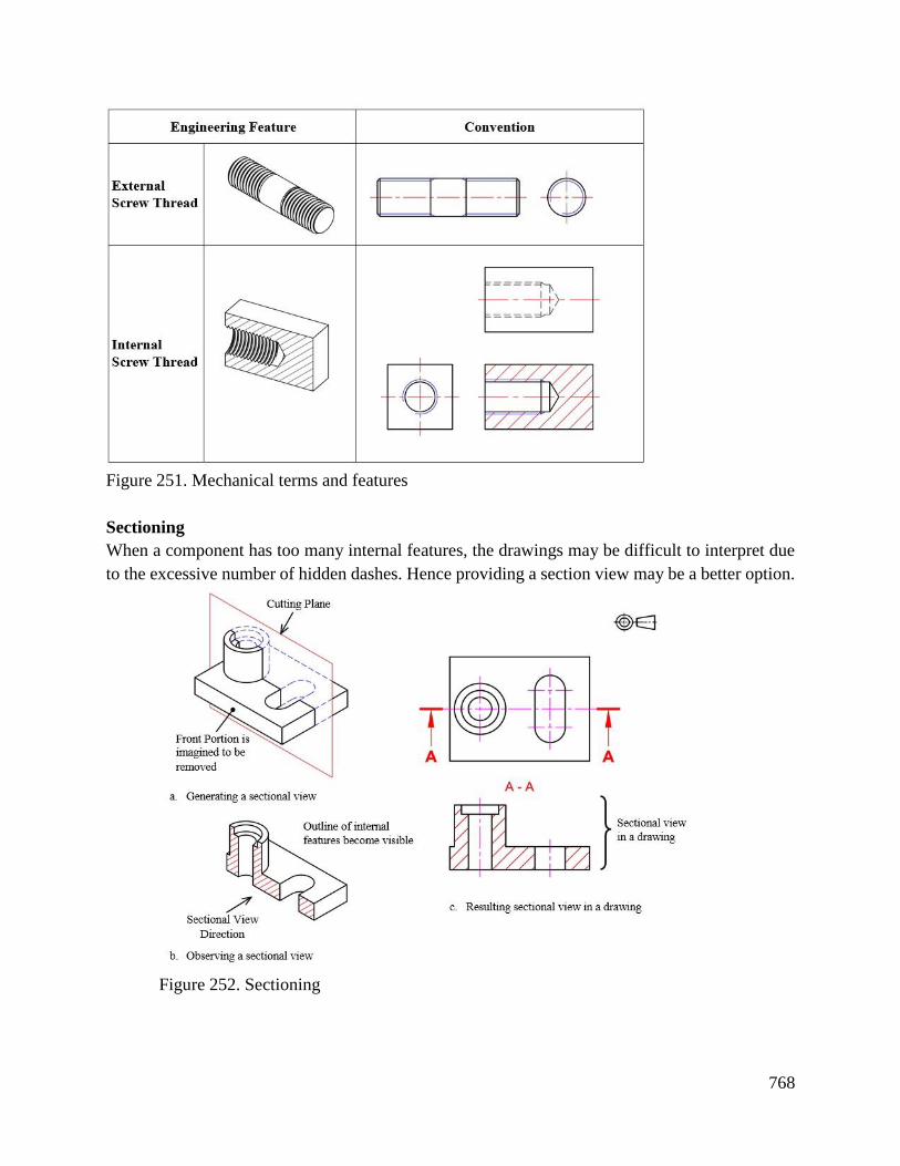
768
Figure 251. Mechanical terms and features
Sectioning
When a component has too many internal features, the drawings may be difficult to interpret due
to the excessive number of hidden dashes. Hence providing a section view may be a better option.
Figure 252. Sectioning
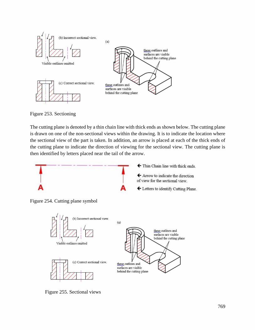
769
Figure 253. Sectioning
The cutting plane is denoted by a thin chain line with thick ends as shown below. The cutting plane
is drawn on one of the non-sectional views within the drawing. It is to indicate the location where
the sectional view of the part is taken. In addition, an arrow is placed at each of the thick ends of
the cutting plane to indicate the direction of viewing for the sectional view. The cutting plane is
then identified by letters placed near the tail of the arrow.
Figure 254. Cutting plane symbol
Figure 255. Sectional views
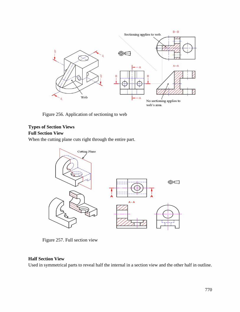
770
Figure 256. Application of sectioning to web
Types of Section Views
Full Section View
When the cutting plane cuts right through the entire part.
Figure 257. Full section view
Half Section View
Used in symmetrical parts to reveal half the internal in a section view and the other half in outline.
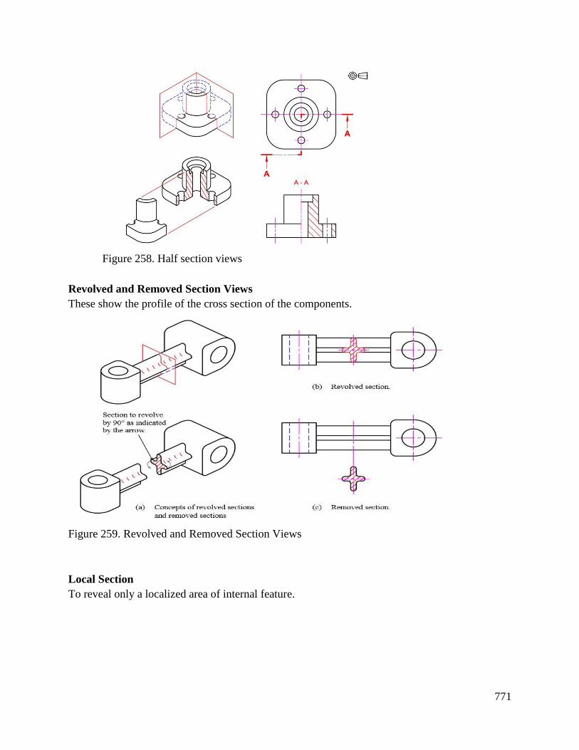
771
Figure 258. Half section views
Revolved and Removed Section Views
These show the profile of the cross section of the components.
Figure 259. Revolved and Removed Section Views
Local Section
To reveal only a localized area of internal feature.
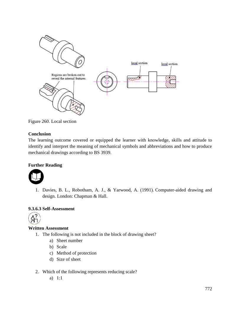
772
Figure 260. Local section
Conclusion
The learning outcome covered or equipped the learner with knowledge, skills and attitude to
identify and interpret the meaning of mechanical symbols and abbreviations and how to produce
mechanical drawings according to BS 3939.
Further Reading
1. Davies, B. L., Robotham, A. J., & Yarwood, A. (1991). Computer-aided drawing and
design. London: Chapman & Hall.
9.3.6.3 Self-Assessment
Written Assessment
1. The following is not included in the block of drawing sheet?
a) Sheet number
b) Scale
c) Method of protection
d) Size of sheet
2. Which of the following represents reducing scale?
a) 1:1

773
b) 1:2
c) 2:1
d) 10:1
3. In the first angle projection method, object is assumed to be placed in?
a) First quadrant
b) Second quadrant
c) Third quadrant
d) Fourth quadrant
4. The following line is used for visible outlines
a) Continuous thick
b) Continuous thin
c) Chain thin line
d) Short zigzag thin
5. The following line is used for dimension line
a) Continuous thick
b) Continuous thin
c) Chain thin line
d) Short zigzag thin
6. The dotted lines represent?
a) Hidden edges
b) Projection line
c) Centre line
d) Hatching line
7. Hatching lines are drawn at _________ degree to reference line.
8. What do you understand by the term:
a) Reducing scale
b) Enlarging scale
9. What is the difference between plane and a lamina?
10. What is principle of projection?
11. What do you mean by truncated?
Oral Assessment
1. Briefly describe the term mechanical
2. Explain the key features of a mechanical drawing
Project
1. Using a CAD application, draw 3D image of the above diagram in practical assessment.

774
9.3.6.4 Tools, Equipment, Supplies and Materials
Drawing room
Computer lab
Drawing equipment and materials
Computers
CAD package
Overhead projector
9.3.6.5 References
Davies, B. L., Robotham, A. J., & Yarwood, A. (1991). Computer-aided drawing and design.
London: Chapman & Hall.
Hubka, V. (2015). Principles of engineering design. Elsevier.
Suchman, L. (2000). Embodied practices of engineering work. Mind, Culture, and activity, 7(1-
2), 4-18.
Zammit, S. J. (1987). Motor Vehicle Engineering Science for Technicians, Level 2. Longman
Scientific & Technical.
775
9.3.7 Learning Outcome No 6: Apply CAD packages in drawings
9.3.7.1 Learning Activities
Learning Outcome No 6: Apply CAD packages in drawings
Learning Activities Special Instructions
6.1 Select CAD packages according to task requirements
6.2 Apply CAD packages in production of electrical
drawings
Provide all the information of
the object to be drawn i.e.
dimensions
9.3.7.2 Information Sheet No2/LO6: Apply CAD packages in drawings
Introduction
This outcome covers use of CAD applications to draw pictorial and orthographic drawings and
sectioning, symbols and abbreviations, 2D and 3D drafting technique and apply CAD packages in
production of electrical drawings.
Definition of key terms
CAD (Computer Aided Design): It is the use of computer software to design and document a
product’s design process.
Engineering drawing: The use of graphical symbols such as points, lines, curves, planes and
shapes.
Content/Procedures/Methods/Illustrations
CAD (Computer Aided Design) is the use of computer software to design and document a
product’s design process. To many engineering problems, a solution requires a combination of
organization, analysis, problem solving principles and a graphical representation of the problem.
Objects in engineering are represented by a technical drawing/drafting that represents designs and
specifications of the physical object and data relationships. Since a technical drawing is precise
and communicates all information of the object clearly by use of Computer Aided Design. CAD
is used to design, develop and optimize products. CAD is used in the design of tools and equipment
required in the manufacturing process as well as in the construction domain.
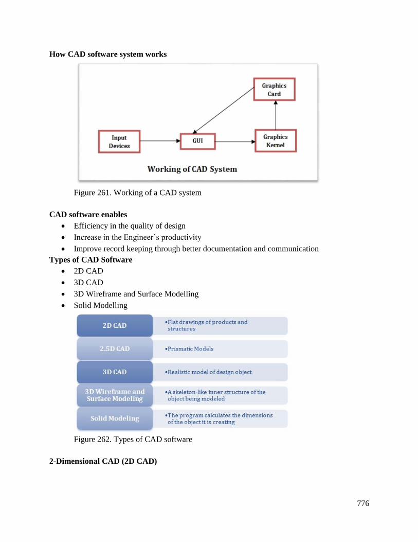
776
How CAD software system works
Figure 261. Working of a CAD system
CAD software enables
Efficiency in the quality of design
Increase in the Engineer’s productivity
Improve record keeping through better documentation and communication
Types of CAD Software
2D CAD
3D CAD
3D Wireframe and Surface Modelling
Solid Modelling
Figure 262. Types of CAD software
2-Dimensional CAD (2D CAD)

777
2D CAD is the pioneer of CAD software, developed in the early 70s. It relies on basic geometric
shapes like lines, rectangles, circles, etc. to produce flat drawings. Autodesk is one of the
pioneering companies that has played a significant role in developing CAD software
3-Dimensional CAD (3D CAD)
It is a step up from the 2D CAD software. It allows creation of 3D images that are realistic. These
images are called 3D models as they can be viewed and rotated in any direction – X, Y or Z.
Classification of CAD software in terms of their operating parameters
a) Single-file-mode systems: This type of CAD software that allows only a single user to
work on a single file at a time.
b) Referenced file-mode systems: This type of software, users work on their own files with
the files of other users attached as a background. This enables users to leverage other users'
work as background data.
c) Collaborative-mode systems: These CAD systems take the referenced-mode system to
the next level. They allow a team of users to collaboratively work with each other's data
and see the changes other users make to the data as they go. The giants in this field e.g.
AutoCAD is used in different modes of an operation.
d) Wire-frame models: They create skeleton like models with lines and arcs. Since they
appear to be made of wires, and everything in the background is visible, they are called
wire-frame models.
e) Surface models: These models are created by joining 3D surfaces. The surface models
are quite realistic.
f) Solid models: They are the most useful CAD models. They also have additional properties
like weight, volume and density, just like actual physical objects. These models are
commonly used as prototypes to study engineering designs.
g) Nano CAD: It is a professional grade CAD tool that is used by thousands of engineers and
designers around the world. Nano CAD plus comes with some additional features. Both of
the versions are available at a low-cost annual subscription including timely updates and
priority online support.
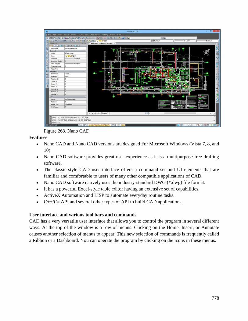
778
Figure 263. Nano CAD
Features
Nano CAD and Nano CAD versions are designed For Microsoft Windows (Vista 7, 8, and
10).
Nano CAD software provides great user experience as it is a multipurpose free drafting
software.
The classic-style CAD user interface offers a command set and UI elements that are
familiar and comfortable to users of many other compatible applications of CAD.
Nano CAD software natively uses the industry-standard DWG (*.dwg) file format.
It has a powerful Excel-style table editor having an extensive set of capabilities.
ActiveX Automation and LISP to automate everyday routine tasks.
C++/C# API and several other types of API to build CAD applications.
User interface and various tool bars and commands
CAD has a very versatile user interface that allows you to control the program in several different
ways. At the top of the window is a row of menus. Clicking on the Home, Insert, or Annotate
causes another selection of menus to appear. This new selection of commands is frequently called
a Ribbon or a Dashboard. You can operate the program by clicking on the icons in these menus.
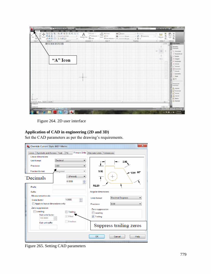
779
Figure 264. 2D user interface
Application of CAD in engineering (2D and 3D)
Set the CAD parameters as per the drawing’s requirements.
Figure 265. Setting CAD parameters
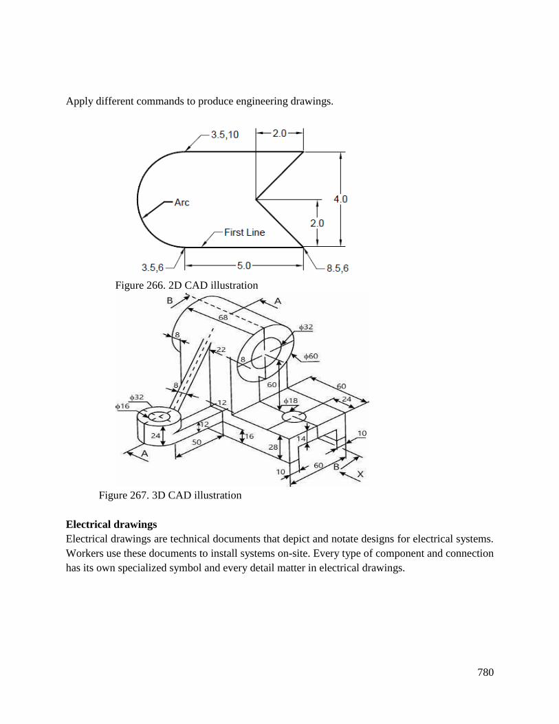
780
Apply different commands to produce engineering drawings.
Figure 266. 2D CAD illustration
Figure 267. 3D CAD illustration
Electrical drawings
Electrical drawings are technical documents that depict and notate designs for electrical systems.
Workers use these documents to install systems on-site. Every type of component and connection
has its own specialized symbol and every detail matter in electrical drawings.
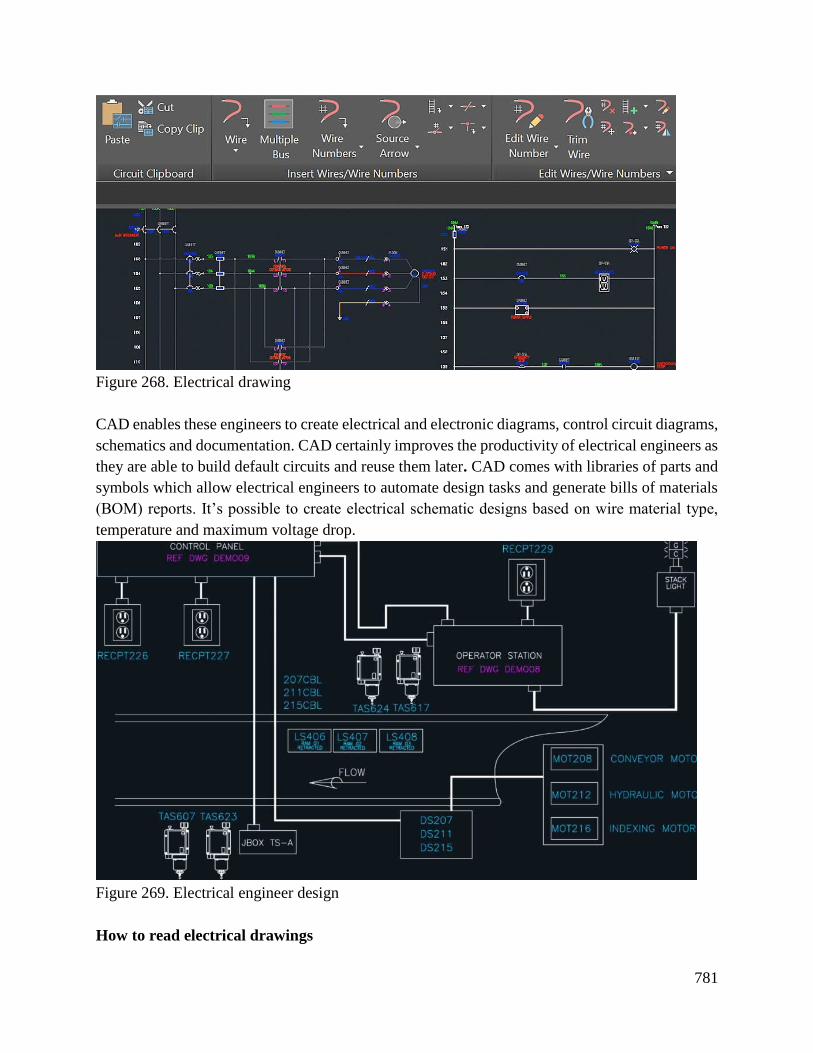
781
Figure 268. Electrical drawing
CAD enables these engineers to create electrical and electronic diagrams, control circuit diagrams,
schematics and documentation. CAD certainly improves the productivity of electrical engineers as
they are able to build default circuits and reuse them later. CAD comes with libraries of parts and
symbols which allow electrical engineers to automate design tasks and generate bills of materials
(BOM) reports. It’s possible to create electrical schematic designs based on wire material type,
temperature and maximum voltage drop.
Figure 269. Electrical engineer design
How to read electrical drawings
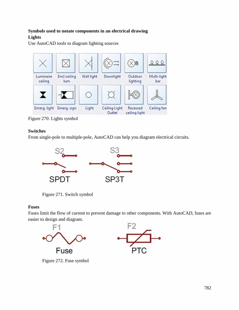
782
Symbols used to notate components in an electrical drawing
Lights
Use AutoCAD tools to diagram lighting sources
Figure 270. Lights symbol
Switches
From single-pole to multiple-pole, AutoCAD can help you diagram electrical circuits.
Figure 271. Switch symbol
Fuses
Fuses limit the flow of current to prevent damage to other components. With AutoCAD, fuses are
easier to design and diagram.
Figure 272. Fuse symbol
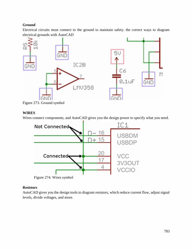
783
Ground
Electrical circuits must connect to the ground to maintain safety. the correct ways to diagram
electrical grounds with AutoCAD
Figure 273. Ground symbol
WIRES
Wires connect components, and AutoCAD gives you the design power to specify what you need.
Figure 274. Wires symbol
Resistors
AutoCAD gives you the design tools to diagram resistors, which reduce current flow, adjust signal
levels, divide voltages, and more.

784
Figure 275. Resistor symbols
Capacitors
Capacitors store potential energy; they're polarized or non-polarized. The AutoCAD Electrical
toolset enables you to diagram capacitors correctly.
Figure 276. Capacitor
Power sources
AutoCAD makes the planning and design from DC to AC currents and batteries process easy.
Figure 277. Power sources symbols
Mechanical Engineering
Mechanical engineers are concerned with the improvement and modification of mechanical
components and systems. They research, design, develop and test mechanical devices. They also
research designs and make recommendations based on industry standards and regulations. CAD
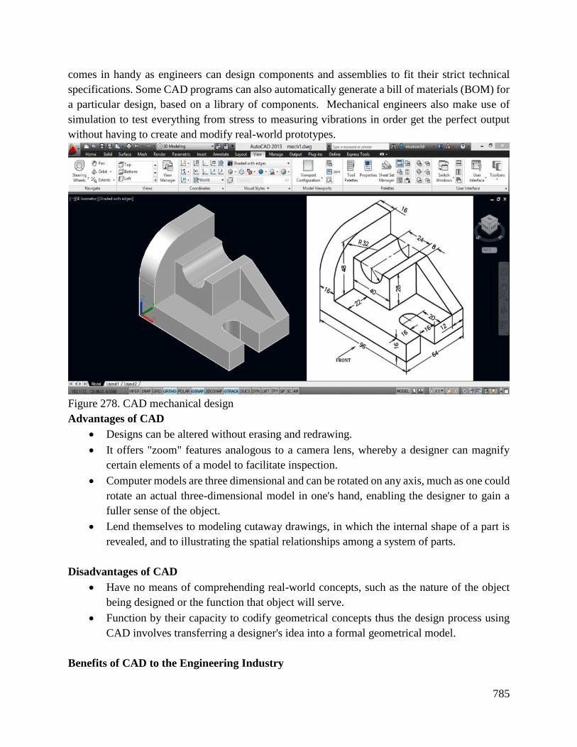
785
comes in handy as engineers can design components and assemblies to fit their strict technical
specifications. Some CAD programs can also automatically generate a bill of materials (BOM) for
a particular design, based on a library of components. Mechanical engineers also make use of
simulation to test everything from stress to measuring vibrations in order get the perfect output
without having to create and modify real-world prototypes.
Figure 278. CAD mechanical design
Advantages of CAD
Designs can be altered without erasing and redrawing.
It offers "zoom" features analogous to a camera lens, whereby a designer can magnify
certain elements of a model to facilitate inspection.
Computer models are three dimensional and can be rotated on any axis, much as one could
rotate an actual three-dimensional model in one's hand, enabling the designer to gain a
fuller sense of the object.
Lend themselves to modeling cutaway drawings, in which the internal shape of a part is
revealed, and to illustrating the spatial relationships among a system of parts.
Disadvantages of CAD
Have no means of comprehending real-world concepts, such as the nature of the object
being designed or the function that object will serve.
Function by their capacity to codify geometrical concepts thus the design process using
CAD involves transferring a designer's idea into a formal geometrical model.
Benefits of CAD to the Engineering Industry

786
More precision and control
Faster design execution
Cost efficiency
Better documentation and collaboration
Conclusion
The learning outcome covered types of CAD and 2D and 3D drafting technique.
Further Reading
1. https://www.scan2cad.com/cad/how-engineers-use-cad/
9.3.7.3 Self-Assessment
Written Assessment
1. The computer-aided design (CAD) hardware doesn’t include ___________
a) Graphic display terminals
b) Computer
c) Computer programs
d) Keyboard
2. How many types of CAD are there?
a) 6
b) 4
c) 2
d) 5
3. Modem CAD systems are based on ____________
a) ICG
b) GCI
c) GIF
d) IFG
4. The computer communicates with the user via ___________
a) CPU
b) CRT
c) Graphics
d) Display button
5. The process of designing consists of __________ identifiable steps.
a) 8
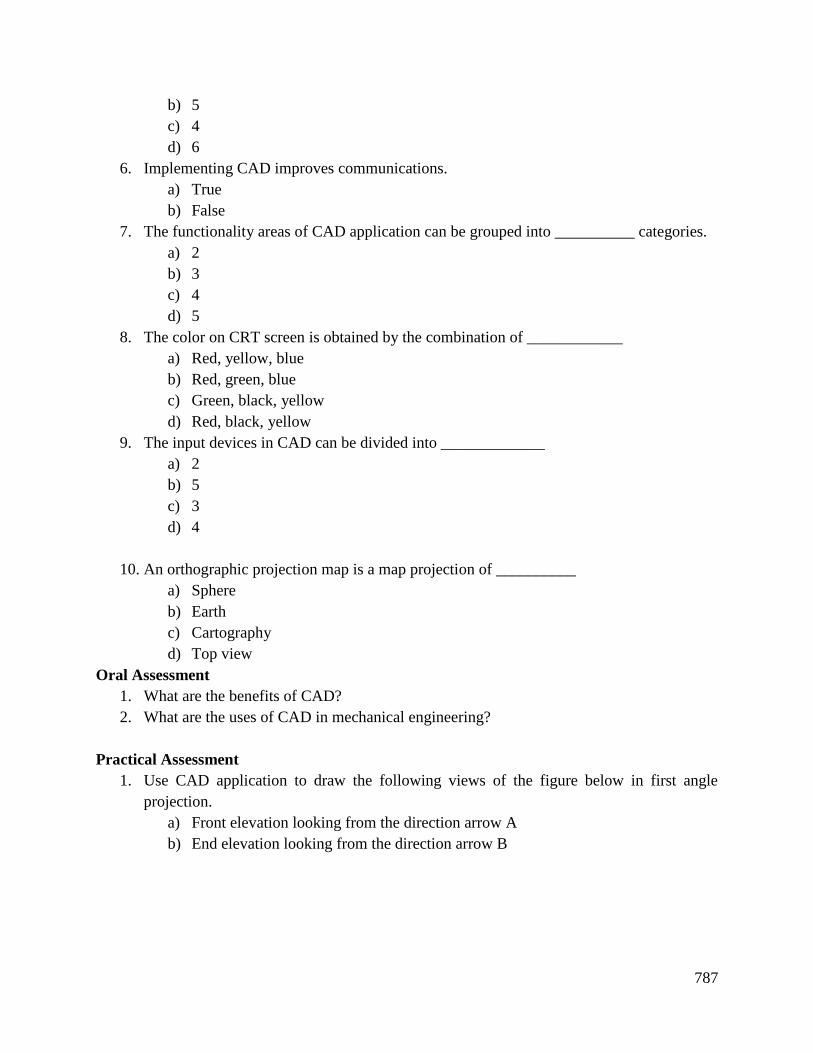
787
b) 5
c) 4
d) 6
6. Implementing CAD improves communications.
a) True
b) False
7. The functionality areas of CAD application can be grouped into __________ categories.
a) 2
b) 3
c) 4
d) 5
8. The color on CRT screen is obtained by the combination of ____________
a) Red, yellow, blue
b) Red, green, blue
c) Green, black, yellow
d) Red, black, yellow
9. The input devices in CAD can be divided into _____________
a) 2
b) 5
c) 3
d) 4
10. An orthographic projection map is a map projection of __________
a) Sphere
b) Earth
c) Cartography
d) Top view
Oral Assessment
1. What are the benefits of CAD?
2. What are the uses of CAD in mechanical engineering?
Practical Assessment
1. Use CAD application to draw the following views of the figure below in first angle
projection.
a) Front elevation looking from the direction arrow A
b) End elevation looking from the direction arrow B
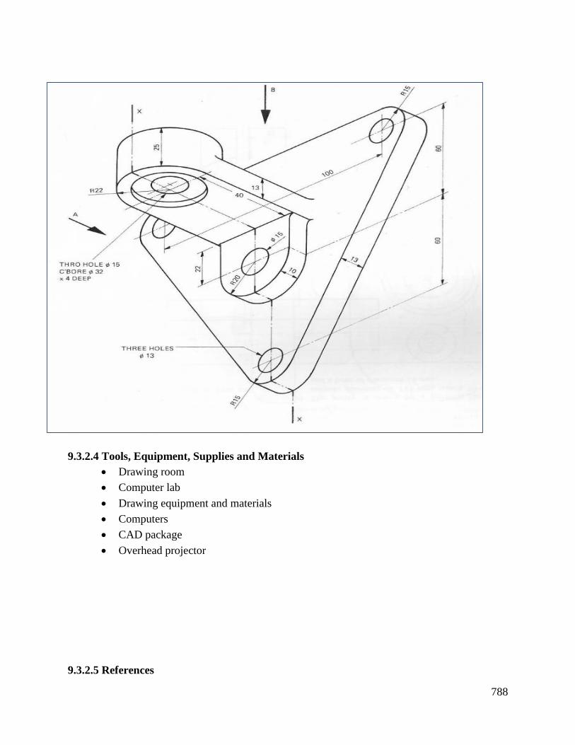
788
9.3.2.4 Tools, Equipment, Supplies and Materials
Drawing room
Computer lab
Drawing equipment and materials
Computers
CAD package
Overhead projector
9.3.2.5 References

789
Davies, B. L., Robotham, A. J., & Yarwood, A. (1991). Computer-aided drawing and design.
London: Chapman & Hall.
Hubka, V. (2015). Principles of engineering design. Elsevier.
Morling, K. (2012). Geometric and Engineering Drawing. Routledge, amazon
Zammit S.J (1987), Motor vehicle engineering science for technicians, Longman Group UK Ltd,
London

790