Reporting Heterogeneity in Health Status A study across Population Sub-groups in India Using...

1

Reporting Heterogeneity in Health Status

A study across Population Sub-groups in India Using Vignettes

Abstract

Self-reported health is a widely used proxy in modeling health as a determinant in

economic decisions, in the evaluation of health status for individuals, and often important

for evaluation of social policies. However the likely presence of non-random

measurement error in self-assessed health response by socio-economic and demographic

characteristics can potentially bias the measurement thus making interpersonal

comparisons problematic. This paper examines the pattern of reporting bias in self

reported health data across population subgroups using an unique data from the World

Health Survey (WHS)-SAGE survey (wave 1) from India, that has self-reported

assessments of health linked to anchoring vignettes as well as objective measures like

measured anthropometrics and performance tests on a range of different domains of

health. The ordered probit estimation analysis for vignettes responses reveals strong

systematic reporting bias with respect to level of development in community, gender, age

and sector. Controlling for a battery of objective health measures, we implicitly test the

assumption of ‘response consistency’ in vignettes and confirm its validity by finding the

presence of similar systematic bias in self-reported health responses across the sub-

groups. Further examination of reporting bias by exploiting the individual fixed effects

reveals that substantial variation in self-reported health remains unexplained even after

controlling for the usual covariates. Thus the results seem to suggest that systematic

differences in self-reported health response needs to be accounted for while making inter

group comparisons valid and lends support to the use of the vignette technique for

identifying this bias.

Keywords: Self-assessed health; vignettes approach; measurement error; response

consistency

2

2.1 Introduction

Empirical research modeling health as a determinant in economic decisions such

as work and retirement, utilization of health services and analysis of economic

consequences of ill health typically relies on some form of subjective health measure

(Johnston et al. 2009). One of the most widely used measures in this regard is self

assessed health (SAH) , which is convenient1 and informative instrument often shown to

be correlated with actual health, mortality, morbidity and health access(Rohrer 20092).

Most studies using data from developing countries focus on measures of self-rated health,

nutritional status, activities of daily living, presence or absence of health conditions, and

utilization of care, that are often self-reported and for which the validation data is hard to

obtain (Currie et. al 1999).

Health and morbidity profile based on National level household surveys like the

National Sample Survey in India are typically used to study the utilization of public and

private health services by population subgroups (Mishra 2004). Notably it is the primary

source of health information that has been extensively used for policy design. An

individual is typically asked to indicate whether his health status is excellent, good, fair

or poor. Now, any variation in reported health status can come from the following

possible sources: variation related to differences in true (latent) health, and/or variation in

reporting which is driven by the respondent’s personal characteristics. Hence, if health

perceptions are systematically correlated with socioeconomic characteristics such as

1 The use of reported health state/ morbidity indicators in health surveys has been often justified because of

the difficulties involved in collecting objective and other diagnostic information, which requires rigorous

standardization and has greater costs.

2 Gives a comprehensive review of policy action at community level that relied on self-reported health

measures.

3

income and exposure to health care systems, self-assessed health status can be

misleading. Strauss and Thomas (2007) mention that self reported health measures are

potentially measured with error. This measure has the disadvantage that people may

perceive health differently so that ‘good health’ might not mean the same thing to all

people.

Although SAH measure is widely used in empirical research, for a given true but

unobserved health state, if survey respondents report their health differently depending on

certain characteristics like conceptions of general health, utilization of health services,

expectations for own health, financial incentives to report ill health, comprehension of the

survey questions, measurement error in SAH is no longer random. As perceived health

may vary systematically by population sub-groups even for same level of latent health, its

validity has been challenged in the recent literature (Sen 1993, Currie et. al 1999, Strauss

et. al 2007,Schultz et al 2008) as it potentially induces biases in estimates thus making

statistical inferences on the SAH data problematic. However there has been no formal

testing of systematic reporting bias in self-reported health within a developing country,

where one can expect this measurement error to be greater.

Antman et al (2006); Escobal et al.(2008) points a number of reasons to in

developing country settings, for which validation data are not readily available. In

particular, the literacy level of the general population is lower and health awareness may

be lower. This becomes more problematic as self report is often the only source of

information on health status in case of developing countries.

4

Bound (2001) highlights that wrong assumption of measurement error in a given

variable to be "classical3" can introduce serious biases in estimates leading to simple

attenuation to misattributing relationships that are not present in the error free data.

Furthermore, the study points out that standard methods for correcting for measurement

error bias, such as instrumental variables estimation, are valid only when errors are

classical in nature and the underlying model is linear, but not, in general, otherwise.

One of the ways to examine systematic measurement error in self-reported health

is to formalize the problem of heterogeneous reporting behavior and to formulate tests for

its occurrence in the context of subjective health information. In order to correct for

systematic differences in reporting heterogeneity across sub-populations, a proposed

solution to this measurement error problem is to anchor an individual’s self assessed

response on her rating of a vignette description of a hypothetical situation that is fixed for

all respondents (King et. al 2004; Bago d’Uva et. al 2011). The idea is based on the

underlying assumption that since a vignette depicts a fixed level of latent health, variation

in its rating would identify systematic reporting bias, which can then be adjusted in the

individual’s subjective assessment of her own situation.

Anchoring vignettes have been proposed as a solution to this problem, since they

permit statistical adjustment for rating style, and thus enable valid intergroup

comparisons. However the validity of the vignette approach relies on two important

assumptions viz. “vignette equivalence” (requires that all individuals perceive the

vignette description as corresponding to a given state of the same underlying construct)

3 where measurement error is independent of the true level of that variable and all other variables in the

model and measurement error in other variables

5

and “response consistency” which implies that individuals use the same response

categories for their subjective assessment (e.g. of own health) as the categories used for

the hypothetical scenarios presented to them in vignettes (Bago d’Uva 2009). This

assumption will not hold if there are strategic influences on the reporting of the

individual’s own situation that are absent from evaluation of the vignette (Bago d’Uva

2011). If this did not hold, then information from the vignette responses cannot be used in

identifying, and thus correcting for, the reporting heterogeneity.

While in recent studies this method has been used to correct for systematic

reporting bias in some developed country settings very few such attempts have been done

for the case of less developed countries, where measurement error in survey data has

been increasingly acknowledged in empirical studies (Strauss and Thomas 2007). Currie

et al (1999) suggests that estimates of the effects of health on labor market activity may

be very sensitive to the measure of health used, and to the way in which the estimation

procedure takes account of potential measurement error. Moreover, there is a serious

concern when the error in measurement is not random even after controlling for the

observable socio-economic characteristics and thus can lead to a bias similar to ``ability

bias4'' in standard human capital models. Thus, measurement error in such self-reported

health variables may represent a source of significant bias in models used to explain work

behavior.

The paper first tries to present a framework for individual reporting behavior

which enables us to formally test the existence of systematic measurement error across

socio-demographic sub-groups in a developing country setting using two different

4 For instance, if healthier individuals are likely to get more education, then failure to control for health in a

wage equation will result in over-estimates of the effects of education.

6

approaches. Second, we examine what part of this reporting bias cannot be explained

even after controlling for the socio economic characteristics.

For the first objective we examine the nature of reporting biases using vignettes

responses across different health domains and then check the validity of this approach by

implicitly testing the ‘response consistency’ assumption. Essentially we compare the

pattern of reporting bias in self reported health response after controlling for their

‘objective’ counterparts from the same health domain, permitting us to identify reporting

effects by socio-demographic covariates. For the second objective we tease out the

individual level variation in reporting using repeated ratings from the same individual

across different vignettes and examine how much of this variation can be explained by

the individual’s socio-economic characteristics and what part still remains unaccounted

for. This exercise is feasible by the unique set up of the data in our analysis which has

information for the same individual on vignettes rating, self-reported as well as objective

health measures on the same health domain.

This study is be important in finding out the nature of biases in an existing

nationally representative survey data from a developing country setting. One of the very

first papers Bago d’uva (2008) to test for systematic differences in reporting behavior

across developing countries using a pilot data (which was not nationally representative)

from Indonesia, India5 and China rejected reporting homogeneity by different educational

groups. However their study did not include any analysis of either objective (biomarkers)

or subjective (reported) self health status which my study is able to include to cross-

validate the results obtained from the vignette approach. In this regard it provides a

methodological contribution to check the validity of response consistency in vignettes

5 for India only a pilot data from Andhra Pradesh was analyzed in her paper

7

approach which has been debated in the recent literature. It has been argued that

individuals may use different thresholds for rating vignette questions as opposed to rating

self-reported health questions. Moreover studying the interstate variations within a

country was beyond the scope of their study which the present study aims to include to

examine the extent of reporting bias across policy relevant subgroups within a country.

The paper is organized as follows. In the next section, a brief literature review is

presented followed by the empirical model in Section III. Section IV presents the

description of the data along with descriptive statistics. In Section V, the main results are

discussed followed by some robustness checks. Section VI concludes the discussion

along with policy implications and future work.

2.2 Literature Review

Bound et al.(2001) points out that reporting heterogeneity need not be a major

concern provided that it is random (the “classical” measurement error case), although it

can lead to attenuation bias resulting from the same. As Currie (1999) mentions the main

problem with self-reported measures is not that they are not strongly correlated with

underlying health status, rather, the problem is that the measurement error is unlikely to

be random.

Schultz et al (2008) points that interpretation of evidence that relies on self-

reports will be problematic to the extent that those indicators reflect not only true health

status but other influences that are systematically related to outcomes of interest in

specific models. For instance, if higher wage earners are more likely to access health care

8

services and, because of that, are more likely to report their ill-health, then it will be very

difficult to interpret the relationship between wages and self-assessed health status.

Differences in health measures derived from self-reported and more objective

indicators are suggestive of systematic variation in reporting behavior (Bago d’uva 2008).

A number of papers including Sen (1993, 2002) draws instances from developing

countries, where reported illnesses or morbidities indicate that children in the poorest

households are the healthiest. Noteworthy is the fact that the state of Kerala (with one of

the lowest levels of mortality among Indian states) has consistently reported the highest

morbidity rate(approximately three times the all-India average) in three successive rounds

of nationally represented survey NSS, whereas in contrast, Bihar -with one of the highest

mortality rates reported the lowest morbidity. Now it remains to be examined

systematically how much of this can be attributed to perception bias and how much can

be explained by survivorship burden of disease. Sen (2002) attributed this discrepancy to

a perception bias; that people from states with more education and greater access to

health and medical facilities are in a better position to assess their own health than people

from disadvantaged states. Banerjee et al., (2004) mentions that sick individuals in a

poor disease endemic area, with limited health access or opportunities for medical

treatment may report being in good health because some type of illnesses may be

perceived as ‘normal’ phenomena due to their prolonged, widespread occurrence in the

area, where people might be adapted to the sickness that they experience.

Using data from the National Health and Nutrition Examination Survey

(NHANES) Strauss and Thomas (1996) observe that the gap between maternal reports

and measurements of child height is smaller among higher income and better educated

9

mothers and the gaps are smaller among older children. They attribute this finding to the

likely differences in the frequency with which children were measured, and argue that

mothers of higher socioeconomic status (SES) were more likely visit health centers

(where measurements are taken) than women of lower SES.

Van Doorslaer and Jones (2003) analyze differences in reporting that may be

influenced by socioeconomic characteristics such as age, gender, education, individual

experience with illness and the health care system. They find sub-groups of the

population systematically use different thresholds in classifying their health into a

categorical measure. Individuals from different population sub-groups are likely to

interpret the SAH question within their own specific context and thus use different

reference points when asked to respond to the same question (Lindeboom & van

Doorslaer, 2004). Baron-Epel et. al (2001) showed that higher educated people tend to

assess their health in an optimistic way, even when they have common characteristics

such as nationality and religion. Gerdtham et. al(2001) using Swedish micro-data, found

SAH to be higher for higher income class, the highly educated and the married.

With respect to the subjective dimension of SAH, Krause et. al (1994) found that

people of different age groups tend to think about different aspects of their health when

making evaluations. The study found that people with the same ‘true health’ may end up

reporting different levels of SAH depending on their age. Schultz et al.(2008) mentions

some illnesses such as blindness, ringworms or malaria may be perceived as normal

phenomena due to their prolonged, widespread occurrence in a disease prone area

without health access, where individuals may not see themselves as particularly

unhealthy.

10

While various techniques have been proposed for achieving comparable response

scales across groups, recent reviews (Murray et. al 2002) indicate anchoring vignettes as

“the most promising” of available strategies. Anchoring vignettes, in short, reveal how

groups may differ in their use of response categories, i.e., in where along the health

spectrum individuals locate thresholds between the ordered categories. Although it is

becoming popular however, thus far anchoring vignettes have not been applied to the

general self-rated health question (Prokopczyk 2012), despite the widespread use of self

reported health and clear indications of measurement bias in the self reported data. Also,

the assumption of response consistency has been debated in the recent literature (Bago

d’Uva et. al 2011; Van Soest et. al 2011) and it has not been tested in a developing

country setting thus far. Further there is no systematic evidence on how much of this bias

remains unaccounted for even after including the typical SES variables in a

regression.The next section of the paper chalks out the empirical strategy for this.

2.3 Empirical Strategy

In the light of the empirical literature discussed so far, in the current analysis we

test whether sub-groups of the population systematically use different thresholds in

classifying their health into a categorical measure. In order to test the existence of

systematic measurement error in the SAH across population subgroups we first estimate

the ordered probit model for the vignettes responses and try to identify the reporting

biases across the covariates. The first approach of our empirical strategy closely follows

the model of King (2004) with some modifications.

Let HiV be the reported ordered health status (with options ‘very good’=1,

‘good=2’, ‘moderate=3’, ‘bad=4’ and ‘very bad=5’) for the vignette question, the vector

11

Xi is a vector of observed characteristics (the socio demographic covariates across which

we are interested to examine systematic reporting bias for example age, gender,

education, income, location etc.).

Estimating Equation: Hiv = Xiβ + ui (1)

The underlying assumption for this identification is that since the vignette

represents a fixed level of latent health, the difference in cut points by covariates can be

attributed to the systematic reporting associated with the Xi s viz. age, gender, education

level, income quintiles, sector (rural/urban) or location. The idea is to vary the health

status exogenously in each of the hypothetical cases, where any difference in rating of

these fixed latent health situations can come from the ‘biases’ one has in estimation of

health state. Hence in estimation (1) the coefficient β would identify the reporting bias,

where a positive (negative) and significant coefficient would imply over-report (under-

report) of worse health, as degree of worse health /difficulty increases from 1 to 5 in the

categorical response of the dependent variable.

Economic circumstances and geographic location may alter health expectations

through factors like peer effects, societal norm and access to medical care hence we

include the sector and a dummy for level of development in the state6. Reporting of

health may vary with education through the awareness factor i.e. conceptions of illness,

understanding of disease and knowledge of the availability, access and effectiveness of

health care. Etilé and Milcent (2006) provide evidence of a convex relationship between

6 We use the WHS ranking of development in the sample state (based infant mortality rate, female literacy

rate, percentage of safe deliveries and per capita income at the state level).

12

reporting heterogeneity and income. Banerjee et al., (2004) finds that individuals in the

upper third income group report the most symptoms over the last 30 days, and attribute

this to higher awareness of health status. Thus, in order to identify any nonlinear effect of

income on reporting bias we include expenditure quintiles constructed from average

overall monthly household spending. In order to see whether reporting bias varies by true

health we include the measured body mass index categories (viz. underweight, normal,

overweight and obese).

Thus, reporting of health status can be influenced by expectations for own health,

tolerance of illness, health norm in one’s society, which may be in part affected by an

individual’s socio-economic environment and demographic characteristics. Hence the X

vector includes education categories, gender, age groups, body mass index (BMI

categories), expenditure quintiles, religion, ethnic groups, sector (urban/rural),

underdeveloped state dummy- capturing development in the state (which implicitly

captures and controls for the access to effective health care and can be a rough measure

for tolerance of illness in the society).

Reporting of health may vary with education through the awareness factor i.e.

conceptions of illness, understanding of disease and knowledge of the availability and

effectiveness of health care. To test for this we include six education categories capturing

the highest level of education completed: no formal education (reference category), less

than primary education, primary, secondary, high school and college or above. Age is

categorized into four groups: 18 to 29.9 years (reference category), 30 to 44.9 years, 45 to

60 years and greater than 60.

13

In our second empirical approach we attempt to identify reporting behavior from

variation in self-reported health beyond what is explained by ‘true’ health as

approximated by a battery of objective health measures/performance tests, to cross-

examine the reporting behavior as indicated by variation in the evaluation of given health

states represented by hypothetical case vignettes. By this exercise we implicitly check

whether ‘response consistency’ assumption holds which is necessary for any vignette

study to be valid.

We consider a sufficiently comprehensive set of objective indicators of health that

include physical measurements, scores from performance tests and interviewer

impressions. We specifically examine if for a given level of true health (as approximated

by an array of measured tests, clinical diagnosis and measured anthropometrics) there

exists reporting bias by the socio-demographic covariates (like education, gender, age,

income, sector and location) in a systematic way, and whether this pattern of bias

identified for each covariate is same as indicated by the earlier approach.

Let Hrep

be the response to any self-reported health question (for example ‘how

would you rate your health today’) having the following values for the options; ‘very

good’=1, ‘good=2’, ‘moderate=3’, ‘bad=4’ and ‘very bad=5’. We regress the self

reported health on the same set of covariates (Xi) but now controlling for a battery of

‘objective’ health measures. The underlying idea is any systematic variation in subjective

assessments that remains after conditioning on the objective indicators can be attributed

to systematic biases in reporting behavior.

Hirep

= αHiobj

+ Xib +Vi (2)

14

This specification hinges on the fact that after correcting for ‘true’ health the

reporting heterogeneity (if any) would be reflected as the coefficients of the covariates in

the second equation. Specifically, the assumption is, adding the precise set of objective

indicators in the estimation would soak up the variation coming from the true/latent

health, leaving aside the reporting effects to be identified. So a statistically significant

negative coefficient for any covariate would mean the higher probability to report better

health in that subgroup compared to the reference group.

The next section discusses the data that we use to estimate these two equations,

followed by a brief discussion of the summary statistics for the key variables of interest.

2.4 Data and Summary Statistics

The analysis uses the World Health Survey (WHS)-SAGE Wave 1 survey (carried

out from 2007 to 2009) in India7. The survey implemented a multistage cluster sampling

design resulting in nationally representative cohorts. The data collected included self-

reported assessments of health linked to anchoring vignettes, which are hypothetical

stories that describe the health problems of third parties in several health domains. This

data is special in the sense that it has the information of both ‘subjective’ and ‘objective’/

clinical counterpart of identical health questions in addition to the vignettes.

For India the survey covered six states8 namely Maharashtra, Karnataka, West

Bengal, Rajasthan, Uttar Pradesh and Assam. The states were selected randomly such

that one state was selected from each region as well as from each level of development

7 Implementation of SAGE Wave 1 was from 2007 to 2010 in six countries over different regions of the

world (China, Ghana, India, Mexico, Russian Federation and South Africa)

8 The 19 states were grouped into six regions: north, central, east, north east, west and south. The sample

was stratified by state and locality (urban/rural) resulting in 12 strata and is nationally representative. Of

the 28 states, 19 were included in the design which covered 96% of the population.

15

category. The level of development was based on four indicators9 namely: infant

mortality rate, female literacy rate, percentage of safe deliveries and per capita income at

the state level. We use the development classification10

used in WHS to construct a

dummy for underdevelopment (=1 for the two least developed states, viz. Rajasthan and

Uttar Pradesh, and =0 for the other four states).

2.4.1 Information on Vignettes

The following sets of vignettes11

in the data included: Mobility and Affect, Pain

and Personal Relationships and Vision, Sleep and Energy, Cognition and Self-care. Each

individual questionnaire includes only one set of vignettes and each respondent is asked

two questions from each vignette. So, around one-fourth of the total sample responds to

vignettes questions on each health domain. In all vignettes the region-specific

female/male first names are used to match the sex of the respondent. Before reading out

the vignette the interviewer insisted the respondents to think about these people's

experiences as if they were their own. The interviews were done face-to-face with the

selected respondents in the local language(s).

The respondent was asked to describe how much of a problem or difficulty the

person in the vignette has, in an ordered scale response from 1 to 5 - the same way that

they described their own health.

9 A composite index of the level of development was computed by giving equal weightage to the four

indicators.

10

The states were ranked in this decreasing order of development (Maharashtra> Karnataka> West

Bengal> Assam> Rajasthan > Uttar Pradesh) based on the composite index of infant mortality rate, female

literacy rate, percentage of safe deliveries and per capita income.

11

A list of the vignette questions are included in the appendix.

16

2.4.2 Self-reported and Objective measures of health

The survey data includes perceptions of well-being and more objective measures

of health, including measured performance tests: rapid walk; cognitive tests (verbal

fluency, immediate and delayed recall capacity, digit span forward and backward). In the

self-evaluation, interviewees responded to direct questions about their own health state,

aimed at capturing their perceptions regarding each state of health domain, formulated as,

“Overall, in the last 30 days, how much difficulty did you have in carrying out such

activity?”,the responses of which were obtained on a scale of 1 to 5 (1 = none; 2 = mild;

3 = moderate;4 = severe; 5 = extreme/cannot do). The key question on self reported

health in the analysis is ‘How would you rate your health today?’ The response categories

were ordered starting from very good, good, moderate, bad, very bad taking value 1 to 5

respectively. Figure 2.1 shows the distribution of the response categories for self reported

health question. As expected, the percentage of individuals who actually report ‘extreme

good’ or ‘extreme bad’ health is very less. However, as it is evident from Figure 2.1,

there is enough variation in the SAH to be utilized in regression equation (2) coming

from the ‘good’, ‘moderate’, and ‘bad’ categories.

For each adult respondent, the health worker measured height, weight, grip

strength, lung capacity, blood pressure, pulse rate and undertook a battery of performance

tests for the respondent in various health domains including memory and mobility. We

construct four categories of individuals by body mass index by using the measured height

and weight: Underweight (BMI < 18.5) ,( Normal BMI 18.5-24.9- reference category in

regression), Overweight (BMI 25-29.9), Obese (BMI >30). Body mass index (BMI)

17

information was included in equation to control for a respondent's risk for different health

conditions. The distribution of BMI in the sample is shown in Figure 2.2.

For the domain of mobility we have a set of self-reported variables pertaining to

difficulty level in moving around and performance of daily activities in the last 30 days.

The distribution of the key question on self-reported mobility in the sample is shown in

Figure 2.3.

For objective mobility indicators we have a rapid walk test along with the

interviewer’s impression of any walking difficulty of the respondent. In the domain of

cognition we have self-reported measures of how the individuals would rate their

memory and cognition. The following tests are taken to measure cognitive ability:

immediate and delayed recall (memory); digit span (concentration and memory); verbal

fluency12

.

We have some information of semi-objective measures comprised of reported

diagnosed chronic disease including arthritis, stroke, angina, diabetes chronic lung

disease, asthma, depression, hypertension, cataracts, oral health, injuries, cancer

screening, that we include in estimation (2) for robustness checks. We take the total

number of reported chronic illness in the estimation. This is implicitly assigning the same

weight for all the diseases, and we check also including these as dummies.

The total number of individuals who have the complete information13

across

measured health are 10873 individuals for which the summary statistics are presented in

Table 2.1. The comparison of measured and self-reported height across population

12

Respondent is given one minute to tell the names of as many animals (including birds, insects and fish)

that they can think of. 13

Around 500 observations do not have scores/not measured on some performance tests, i.e. less than 5%

of the sample had missing information on X’s, however they were not dropped from the analysis.

18

subgroups yields very interesting results. Figure 2.4 and Figure 2.5 depicts the graph of

average measured and self reported heights across expenditure quintiles and education

categories respectively. The education categories capture the highest level of education

which is categorized into six groups: No formal education (=1), below primary(=2),

primary (=3), secondary(=4), high school(=5), college and above(=6).

From Figure 2.4, we find on average individuals underreport their true height,

which is statistically different than measured height across all expenditure quintiles.

Quite as per our expectation this difference becomes smaller as we go up the expenditure

quintiles and for higher education categories. For individuals with highest education that

of college and above, this gap is no longer statistically significant. However, this trend is

more or less similar by gender.

Disaggregating by development level of the states (Figure 2.6), we find this

difference in reported height and measured height is most prominent across individuals

from the poorest quintiles, and the pattern of reporting bias is different for each state.

While in relatively more developed states this gap reduces for higher expenditure

quintiles(Maharashtra and West Bengal), we do find for less developed states (Rajasthan,

Uttar Pradesh, Assam) that this gap persists even for higher expenditure quintiles. By

contrast, in the most developed state from our sample, this gap is no longer significant for

individuals from second expenditure quintile onwards. Interestingly, while we find

individuals on average individuals under-report their true height in Assam, Rajasthan,

West Bengal and Maharashtra, there is significant over-report of true height on average in

Uttar Pradesh and Karnataka (Figure 2.6).

19

The picture is very similar across education categories as well (perhaps because of

high correlation between education and income), where the difference between average

true and reported height is the largest and significant in the lowest education groups

across all the states under consideration. We compare the most developed state from our

sample, viz. Maharashtra, with a lesser developed state, Rajasthan in this regard (Figure

2.7). Interestingly, we find that the gap between true and self reported height is

significant in Maharashtra for only individuals with education level below primary.

However, it is not the case in Rajasthan where this difference is significant and persists

for individuals even with secondary schooling.

While doing a similar exercise examining the difference between the mean of

measured and self-reported weight (Figure 2.8) by expenditure quintiles and level of

development we find that the gap between the mean measured and self-reported weight is

significant across all expenditure quintiles (except the richest quintile) for less developed

states. However this is not so in developed states, where this gap is not statistically

significant for any of the expenditure quintiles. The findings seem to suggest that

individuals from lesser developed states (correlated with lesser education and lower

access to health facilities) are likely to have different reporting behavior as compared to

the ones from developed states. This has important implications given that heterogeneity

at the state level do not typically gets controlled in estimations. In the next section we

discuss and attempt to connect this suggestive finding of the summary statistics with our

regression estimates followed by robustness checks.

2.5 Results

20

Equation (1) is estimated separately for 10 health state vignettes from each health

domains. The regression estimates of the domains ‘Mobility and Affect’ ‘Pain and

Personal Relationships’, ‘Vision, Sleep and Energy’, and ‘Cognition and Self-care’ are

presented in Table 2.2.1, Table 2.2.2, Table 2.23, Table 2.2.4 respectively and the sign

and statistical significance of the parameters from these forty separate regressions are

summarized in the Table 2.2. All the ten specifications for each health domain include

dummies for education categories, gender, age groups, marital status, body mass index

categories, household expenditure quintiles, religion, caste, sector and level of

development in one’s state.

From the regression estimates of equation (1) we do find a strong evidence of

reporting bias across specific population sub-groups for all the health domains. In

mobility and affect domain (Table 2.2.1) we find that the ‘male’ dummy is negative and

statistically significant for all the vignette questions for mobility14

. This finding reveals

that males have a greater probability of underreporting worse health than females in the

sphere of mobility. We get an interesting result by the expenditure quintiles. We find that

individuals from both lower as well as higher quintile have higher probability to report

better health compared to the middle income group. Individuals from urban are more

likely to under-report worse health, however the effect is statistically significant in half of

the regressions. In this domain, individuals who are above 60 years of age have higher

probability of reporting ill health, statistically significant in half the cases. The dummy

for underdevelopment is negative and statistically significant in almost all of the

regressions.

14

The dependent variable in specification 1,2,5,6,9 and10 deals with Mobility, while dependent variable in

specification 3,4,7 is on Affect.

21

To summarize the regression estimates of the vignette questions across all the

health domains we find some interesting results (Table 2.2). Males, on average, show a

clear pattern of under-reporting of worse health consistent across all the health domains15

.

Out of 40 regression estimates in 72% of the cases, the coefficient on male dummy was

found to be negative where it is statistically significant more than half of the time. With

regards to the age group, we find with reference to young individuals 18-30 years of age,

individuals over 60 years age tend to over-report illness. (The concerned coefficient is

positive in 32 cases out of 40 estimations and statistically significant around 50% of the

time). This is a pretty standard result in the literature where over-report of worse health is

observed for aged individuals. With reference to marital status, we find compared to

unmarried/divorced/widowed individual group, currently married individuals tend to

under-report illness, although this is not statistically significant most of the time.

Interestingly, those who are underweight and obese mostly tend to over-report

worse health compared to individuals with normal body-mass index. With respect to

household expenditure quintiles, we find that individuals from the poorest expenditure

quintile tends to under-report ill health as compared to individuals from the third quintile,

consistently across all the health domains. We do not get any clear pattern of reporting

bias across religion or caste groups, although we see some pattern by specific health

domains. For instance, in the domain of mobility- while hindus were found to underreport

ill-health, scheduled castes were more likely to over-report ill-health. The urban dummy

is consistently negative across all the domains suggesting urban individuals tend to under

15

The only exception being in the health domain of pain and discomfort, where male dummy changes sign

and is actually positive and significant in 3 estimations (Table 2B).

22

report ill health as compared to rural, and the effect is statistically significant for 57% of

the total cases.

Perhaps the most interesting result out of this exercise is the evidence obtained for

systematic reporting bias by different states in India. In comparison to the developed

states, the underdeveloped state dummy is negative 88% of the cases, and statistically

significant around 80% of the time. Quite strikingly, for the health domains of vision,

sleep and energy (Table 2.2.3), ‘cognition and self-care’ (Table 2.2.4) we find the

underdeveloped dummy is negative and statistically significant for all the estimates

without any exception.

Hence, if we think that this current definition of underdevelopment captures the

health access and health standards in the community, we find a stark difference in

reporting pattern from the social disadvantaged states. This is perhaps suggestive of the

hypothesis that socially disadvantaged individuals fail to perceive and report the presence

of illness or health-deficits because an individual’s assessment of their health is directly

contingent on their social experience. It can perhaps be attributed to lower expectation for

own health/higher tolerance for diseases where a particular individual may not see herself

as being unhealthy conditional on the health norm/standard prevailing in one’s

community.

We now discuss the findings from the cross-validation exercise estimating

equation (2) and comment on the validity of ‘response consistency’ assumption across

different health domains. We first estimate the dependent variable ‘how would you rate

your health today’ on the same set of covariates as used in earlier estimation of

equation(1), but now including a set of performance tests and interviewer assessments

23

across different health domains in Table 2.3. We gradually add objective health

information in our specification from (1) through (4) and examine if the addition of more

objective information on several health domains completely absorb the variation coming

from variation in latent health, leaving only effects that identifies reporting bias.

Specification (1) includes dummies for highest education level, gender, age

groups, marital status, expenditure quintiles, religion, caste, sector and level of

development in the state. Specification (2) also controls for body mass index categories in

addition to controls included in specification (1). We further add (i) the performance test

scores for mobility and cognitive ability (ii) biomarkers including tests for lung function;

blood pressure (systolic and diastolic);pulse rate; total number of chronic illness

diagnosed from(arthritis, stroke, angina, diabetes chronic lung disease, asthma,

depression, hypertension, cataracts, oral health, injuries, cancer screening) in

specification (3) on top of the controls in specification (2). The last specification (4) adds

interviewer assessment dummies for whether the respondent had any problem in the

following domain: hearing, vision, walking, shortness of breath, and whether she/he had

any overall health problem.

We find individuals with education level secondary and above are more likely to

under-report illness that is statistically significant at 1% level across all specifications.

The result can perhaps be explained if highly educated respondents feel greater

confidence regarding their capacity to handle a given level of health impairment, and thus

under rate it more, after controlling for other factors.

Males show consistent patterns of under reporting illness as compared to females,

which is again statistically significant for all the specifications. We find compared to the

24

young age group of 18-30 years, with higher age- particularly individuals over 60 years-

significantly over report illness, which is consistent with our earlier finding from vignette

approach.

We do not find significant difference in reporting bias by marital status. Once we

control for objective health information the coefficients lose statistical significance in

specification (3) and (4). With respect to household expenditure quintiles we find

compared to the middle expenditure group both the poor and the rich tend to understate

illness, however this effect is statistically significant only for the highest expenditure

group. We also do find statistically significant under-reporting of worse health among

urban cohort, hindu and scheduled castes.

To confirm our earlier findings about reporting bias by development level in the

state- we find a very strong evidence from this estimation exercise- the underdeveloped

dummy is found to be consistently negative and statistically significant across all the

specifications, implying a underreporting of worse health among the disadvantaged

group. Once we control for the interviewer assessments of health states in specification

(4) the magnitude of the coefficient on the underdeveloped dummy even rises,

confirming that it is picking up reporting bias.

Interestingly across the body-mass index categories we do find statistically

significant evidence of over-reporting of worse health among the underweight

population, as indicated by our earlier findings. The objective health indicators of rapid

walking ability, cognitive score, chronic illness, and interviewer assessments of health

situation were all found to be significant and with expected signs, which is reassuring as

25

it implies that better objective/measured health leads to more probability of reporting

better health.

We further estimate a vector of self reported functioning measures in the domain

of mobility (results shown in Table 2.4) and daily activities (in Table 2.5). In the

estimation for self-reported mobility we include walking speed, which is predictive of

overall health and mobility, level of disability. Specifications (1) through (12) control for

some objective health measures that are likely to approximate mobility level

(performance tests for timed and rapid walk, interviewer assessment for difficulty in

mobility and dummies for body mass index categories) along with the usual covariates:

highest education level, gender, age groups, marital status, expenditure quintiles, religion,

caste, sector and level of development in the state.

The dependent variables in all the specifications in both Table 2.4 and Table 2.5

takes value 1-5 measuring self reported difficulty level (1=no difficulty; 5=extreme

difficulty) faced by the respondent in the specific activity describing some form of

mobility (for example in moving around, walking, picking up, crouching, vigorous

activities etc.) and daily activity( for example performing household activities, getting to

places, washing body, using toilet, carrying etc.). The summary of signs and statistical

significance of the estimated coefficients from both these set of regressions from Table

2.4 and Table 2.5 are summarized in Table 2.6. The findings reveal systematic

underreporting of worse health among higher educated group, urban and underdeveloped

states, again reconfirming our earlier findings.

In the similar spirit we regress self-reported cognitive outcomes (for example

how much difficulty one had in remembering and concentrating thing) including

26

objective measures (test of words recalled after delay, digital recall test and verbal

fluency) on the same set of covariates as before. The findings (Table 2.7) reveal again the

same pattern of reporting bias as identified earlier in vignettes study and resemble the

findings from equation (2) in the domains of mobility and general health.

As a further robustness check we regress the objective scores of memory on these

covariates (Table 2.8) and check whether males, underdeveloped actually fare better on

this. Now this would be a weak test for accepting reporting bias if the covariates which

are likely to underreport worse health were also likely to have better objective health;

however, one can assume that this serves as a strong test to identify reporting bias in case

the direction of bias/sign of coefficients obtained from self-reported response are found to

be opposite in comparison to that obtained in estimation of objective health. Interestingly

for the dependent variable ‘words recalled’ we find quite the opposite result for male

dummy compared to what was suggested by self-reported memory. While estimation of

self-report measure for memory would suggest that males fare better, we find contrary

result when we estimate objective memory test for words recalled. This robustness check

provides support that males do in fact understate worse health. Similarly, while self-

reported memory measure suggested that individuals from underdeveloped states are

better off, in contrast when we estimate the objective measures on the same set of

covariates we get individuals from underdeveloped states fare worse in this regard, which

is statistically significant, confirming our previous findings. As expected individuals from

underdeveloped states were found to score lower on both cognitive tests as indicated by

the negative and statistically significant coefficient in specification in (2) and (3) in Table

2.8.

27

In the similar spirit as a further robustness check we estimate objective measures

of mobility and general health in Table 2.9 using interviewer assessments on the same

set of covariates (specification 1 and 3), and also controlling also for body mass index

categories (specification 2 and 4). We find that after controlling for body mass index

categories males in fact fare worse in assessed walking difficulty, which falls in line to

what was suggested by our earlier results about systematic under-reporting of worse

health in self reported health. Interestingly, coefficient on the underdeveloped dummy for

interviewer assessed health problem reveals that individuals from underdeveloped states

were more likely to have health problems, which is statistically significant for both

specification (2) and (3). This reconfirms our earlier findings and supports the prevailing

view of perception bias.

We further utilize individual fixed effects16

to figure out how much of the

variation in individual reporting heterogeneity still remains even after inclusion of the

covariates in the estimation of vignette response. The idea behind this exercise is that

even though systematic reporting heterogeneity by observables can be accounted for

controlling for the covariates in the regression, it remains to be seen how much of the

variation remains even after accounting these, i.e., what remains to unexplained due to

unobservables . This exposes the gravity of the underlying problem that non-random

measurement error can be accounted as far as the observables allow, and also helps to

check the robustness of the previous findings.

We carry this exercise using two-stage regression estimation. In the first stage we

regress the vignette responses (10 questions per vignette set for each individual) on

16

Each individual answers 10 vignette questions in a set

28

individual dummies IDi to get their corresponding coefficients µ’s which we use in the

second stage as dependent variables to be explained by the usual covariates. Precisely we

examine to see how much of individual reporting bias can be explained by including the

observables and what part remains to unexplained even after accounting for the usual

covariates. We estimate the following set of equations:

Hiv = IDi µ +vi (3)

µ = Xiβ + ui (4)

We present the results in table 2.10. We present the histogram of the estimated

coefficients in Figure 2.9, Figure 2.10, Figure 2.11, Figure 2.12. The distribution reveals

substantial reporting heterogeneity across individuals (significantly different from zero),

for which we examine how much of this can be explained by the covariates. The OLS

regression estimates are presented in Table 2.10. The results confirm our previous

findings. Precisely we get males were more likely to favorably rank their health state

(statistically significant for vignette set A and C); individuals above 60 years were likely

to overstate bad health (statistically significant for vignette set A, C and D). Both the

quintiles above and below the middle expenditure group were likely to understate ill

health. Again we get striking result for the level of development in the state, where the

underdeveloped dummy is always significant and negative for all the four sets of

vignettes.

This has important implications given the fact that heterogeneity within country,

at the state level is often not included as control, and as we find we have substantial

systematic heterogeneity along this line, that can mess up the statistical inference.

However it is reassuring to find that the pattern of systematic bias indicated by the

29

vignettes exercise through equation (1) seems to be in line with the results obtained from

the two-stage estimation, and hence this lends support to the use of vignettes in

identifying this bias.

Also, important to note here is that the R-square for estimations (1) to (4) is just

explaining 3% (in domain of Mobility and affect)to 7% (in domain of Cognition and self

care) of the variation in the self reported behavior. This is alarming given that we get to

only control for the observables in the regression, which even after adjusted for leaves

much reporting heterogeneity at the individual level typically unaccounted for. We did

try to check including the interaction terms of the covariates without much improvement

in the R square. Hence this reinstates the point that biases in self-reported measure cannot

even be fully controlled by identifying and accounting for the sources of systematic

measurement error across the observables.

2.6 Conclusion and Policy insights

One of the key challenges in the analysis and interpretation of health survey data

is improving the interpersonal comparability of subjective indicators- that comes with

systematic measurement error- as a consequence of differences in the ways that

individuals understand and use the available responses for a given question. In this paper

we examine the pattern of reporting differences in SAH from a nationally representative

survey in India and find evidence that measurement error in SAH systematically varies

with demographic characteristics, such as the age, gender, education and community

characteristics such as sector and level of development in the state. This has important

implications on several aspects.

30

First one should be careful in inter-personal comparison of health status using

self-reported health data. This will be particularly important with regard to measuring

performance in achievement of the government targets in improving population health,

for instance one of the Millennium Development Goals has been targeting to reduce child

and maternal morbidity, where reporting of diagnosed illness is the primary source for

identifying the incidence of a disease, collected through household surveys (Dixon et al.

2007).

With the increased interest in health issues in children, women of reproductive

age and elderly, self-reported data on morbidity, utilization and expenditure on health

care, perceived well being17

,self-rated ranking of health service delivery used in citizen

and community report cards needs to be carefully used in inter-personal comparison.

Government reports based on self-reported indicators collected on maternity care and

immunization for a comparison of health expenditure profile across households or in

drawing causal inference of a program needs to be re-examined in the light of this

problem. Further one has to reflect on the problem that non-random measurement error

cannot be simply dealt with by controlling for the covariates in a typical regression

framework.

The findings provide a strong empirical evidence to confirm the prevailing view

that socially disadvantaged individuals (as captured here by residing in a less developed

state) fail to perceive and report the presence of illness or health-deficits. Hence, even

within a country there is strong evidence on systematic reporting bias, hence the problem

of cross-population comparability with self-reported data remains a serious issue. This

17

Gilligan & Hoddinott 2009 use self-perceived well being as an outcome of interest in examining the

causal impact of PSNP-food security program in Ethiopia.

31

also calls for paying special attention to account for state-level heterogeneities in typical

regression estimations to reduce some of the issues with systematic bias by the socio-

economic disadvantage level of the community.

The findings presented here suggest that it is necessary to account for how

different population subgroups/individuals see and evaluate their health using different

thresholds and thus it calls for adjustment for systematic variation in measurements of

self-rated health. The current evidence indicates that self-reported measures of health

cannot be directly compared across population sub-groups, because groups differ in how

they use subjective response categories. The problem is further complicated as this

systematic variation cannot be accounted for by just including the socio-economic

characteristics in a typical regression framework. The challenge is to develop alternative

strategies to reduce the subjective variation in health perception in its various domains

and to make possible greater comparability between distinct socio-economic groups.

This analysis lends support to the use of vignettes data to use them to identify the

bias in SAH data in a developing country setting and obtain bounds on the bias as well.

One of the policy insights that comes out of this analysis is that it would be prudent to

enrich the individual and household surveys by adding questionnaire with a section on

the vignettes that would help identify the thresholds one is using for SAH thus making it

feasible to be used for statistical inference.

For future work we plan use the external vignette information to separately

identify the thresholds and cut-offs of any systematic reporting heterogeneity, which can

be imposed on the model for the self–reports with respect to the individual’s own health,

so that estimates would reflect true health differences rather than a mixture of health

32

differences and reporting heterogeneity. We also plan to examine the extent of bias

induced by using self-reported health as opposed to objective measures in estimation of

wage/ employment in human capital model, taking data from this survey. Additionally we

plan to examine more clear patterns of reporting bias by incorporating the interaction of

the covariates as controls to help identify the finer sources of variation.

33

References

Antman, Francisca, and David McKenzie. (2007) Earnings Mobility and Measurement

Error: A Pseudo-Panel Approach, Economic Development and Cultural Change

56(1):125.

Baron‐Epel, O., Dushenat, M., & Friedman, N. (2001) Evaluation of the consumer

model: relationship between patients' expectations, perceptions and satisfaction with care,

International Journal for Quality in Health Care, 13(4), 317-323.

Bago d'Uva, T., Doorslaer, E.V., Lindeboom, M., O'Donnell, O.,(2008) Does reporting

heterogeneity bias the measurement of health disparities? Health Economics 17,351–375.

Bago d’Uva, T., Lindeboom, M., O’Donnell, O., Van Doorslaer, E. (2010) Slipping

anchor? Testing the vignettes approach to identification and correction of reporting

heterogeneity. mimeo. Erasmus School of Economics.

Banerjee, A., Deaton, A., & Duflo, E. (2004) Health, health care, and economic

development: Wealth, health, and health services in rural Rajasthan., American Economic

Review, 94(2), 326.

Bound John(1991) Self Reported Versus Objective Measures of Health in Retirement

Models,Journal of Human Resources.;26(1):107–137.

Currie, J., Madrian, B.C. (1999) Health, health insurance and the labour market,

Handbook of Labour Economics, Vol. 3, Ashenfelter, O., Card D. (eds.). Elsevier:

Amsterdam.

Datta Gupta, Nicolai Kristensen and Dario Pozzoli (2010) External validation of the use

of vignettes in cross-country health studies, Economic Modeling 27 (2010) 854–865.

Dixon-Mueller, R., & Germain, A. (2007). Fertility regulation and reproductive health in

the Millennium Development Goals: the search for a perfect indicator. Journal

Information, 97(1).

Escobal, J., & Laszlo, S. (2008) Measurement Error in Access to Markets, Oxford

bulletin of economics and statistics, 70(2), 209-243.

Etile, F and Carine Milcent (2006) Income-related reporting heterogeneity in self

assessed health: evidence from France, Health Economics, Vol. 15, pp 965-981.

Gerdtham, U-G., Johannesson, M. (2001) The relationship between happiness, health,

and socio-economic factors: Results based on Swedish micro data, Journal of Socio-

Economics 30, 553-557.

34

Grol-Prokopczyk, H., Freese, J., & Hauser, R. M. (2011) Using anchoring vignettes to

assess group differences in general self-rated health, Journal of health and social

behavior, 52(2), 246-261.

Gwatkin (2000)Health inequalities and the health of the poor: What do we know? What

can we do? Bulletin of the World Health Organization, vol.78.

Jones, A and Angel Nicholas (2002) The importance of individual heterogeneity in the

decomposition of measures of socioeconomic inequality in health : an approach based on

quantile regression, Ecuity II Project.

Johnston, D. W., Propper, C., & Shields, M. A. (2009). Comparing subjective and

objective measures of health: Evidence from hypertension for the income/health gradient,

Journal of health economics, 28(3), 540-552.

Jürges, H. (2007) True Health vs Response Styles: Exploring Cross-Country Differences

in Self-Reported Health, Health Economics, 16(2), 163-178.

Kakwani N, Wagstaff, A., and E. van Doorslaer (1997)Socioeconomic inequalities in

health: Measurement, computation, and statistical inference, Journal of Econometrics

77,pp 87-103.

Kapteyn, A., Smith, J.P., van Soest, A., (2007) Vignettes and self-reports of work

disability in the United States and the Netherlands, American Economic Review 97 (1),

461–473.

Kerkhofs, M.K.M., Lindeboom, M., (1995) Subjective health measurements and state

dependent reporting errors, Health Economics 4, 221–235

King, G.A., Murray, C.J.L., Salomon, J.A., Tandon, A., (2004) Enhancing the validity

and cross-cultural comparability of measurement in survey research, American Political

Science Review 98 (1), 191–207.

Krause, N. M., & Jay, G. M. (1994) What do global self-rated health items measure?

Medical care, 930-942.

Lindeboom, M. and E. van Doorslaer (2004) Cut-point shift and index shift in self

reported health, Journal of Health Economics 23 (6), 1083–1099.

Mishra, S. (2004). Public health scenario in India. India development report, 5, 62-83.

Murray, C.J.L., A. Tandon, J. Salomon, C.D. Mathers, and R. Sadana (2001) “Cross-

Population Comparability of Evidence for Health Policy,” Global Programme on

Evidence for Health Policy Discussion Paper, Geneva: World Health Organization.

35

Rohrer, J. E. (2009). Use of published self-rated health-impact studies in community

health needs assessment, Journal of Public Health Management and Practice, 15(4), 363-

366.

Schultz, T. P., and A. Tansel, (1997) “Wage and labor supply effects of illness in Cote d

Ivoire and Ghana:instrumental variable estimates for days disabled”, Journal of

Development Economics, 53 (2): 251-286.

Schultz, T. (2005) Productive benefits of health: Evidence from low-income countries.

Schultz, T. P., & Strauss, J. (Eds.). (2008) Handbook of development economics (Vol. 4).

North Holland.

Sen, A.(1993) Positional objectivity, Philosophy & public affairs 22.2: 126-145.

Sen, A. (2002) Health: Perception versus observation: Self reported morbidity has severe

limitations and can be extremely misleading,BMJ: British Medical Journal, 324(7342),

860.

Strauss, J., & Thomas, D. (2007) Health over the life course, Handbook of development

economics, 4, 3375-3474.

Strauss, J. and D. Thomas (1996) Measurement and mismeasurement of social indicators,

American Economic Review, 86.2:30-34.

Strauss, J., & Thomas, D. (1998) Health, nutrition, and economic development,Journal of

economic literature, 36(2), 766-817.

Thomas, D. and J. Strauss (1997) Health, wealth and wages of men and women in urban

Brazil, Journal of Econometrics , 77: 159-185.

Thomas, Duncan, and Elizabeth Frankenberg (2002) The measurement and interpretation

of health in social surveys, Measurement of the global burden of disease: 387-420.

Van Doorslaer, E and A. M. Jones (2002) Inequalities in self-reported health ; validation

of a new approach to measurement, Journal of Health Economics ,pp 61-87.

van Soest Arthur, Delaney Liam, Harmon Colm, Kapteyn Arie, Smith James. (2011)

Validating the use of anchoring vignettes for the correction of response scale differences

in subjective questions, Journal of the Royal Statistical Society Series. 3. A 174; pp. 575–

595.

Wagstaff, A., Eddy van Doorslaer and Naoko Watanabe (2003) On decomposing the

causes of health sector inequalities with an application to malnutrition inequalities in

Vietnam, Journal of Econometrics 77,pp 207-223.

36

Table 2.1: Descriptive Statistics

Variables

Education Categories Mean Std. Dev.

No Formal Education 0.45 0.50

Below Primary 0.10 0.31

Primary 0.16 0.36

Secondary 0.12 0.33

High School 0.11 0.31

College and Above 0.06 0.24

Individual Characteristics

Male 0.39 0.49

Age groups

18-29.9 0.14 0.34

30-44.9 0.22 0.41

45-60 0.32 0.47

Above 60 0.32 0.47

Marital Status

Currently Married 0.78 0.42

BMI Categories (measured)

Underweight (BMI< 18.5) 0.35 0.48

Normal (BMI 18.5-24.9) 0.51 0.50

Overweight (BMI 25-29.9) 0.11 0.31

Obese (BMI>30) 0.03 0.17

Household Characteristics

Household’s Expenditure Quintiles

Q1 0.21 0.41

Q2 0.16 0.37

Q3 0.22 0.42

Q4 0.22 0.41

Q5 0.17 0.38

Religion (Hindu=1) 0.84 0.37

Caste (SC/ST=1) 0.41 0.49

Regional characteristics

Urban 0.25 0.43

Underdeveloped dummy

(=1 for states: Rajasthan, UP) 0.38 0.49

N=10873 73

37

Figure 2.1: Distribution of Self-reported health response

Note :SAH is on a 1-5 scale , where 1=very good; 5=very poor

0

10

00

20

00

30

00

40

00

50

00

Fre

qu

en

cy

1 2 3 4 5Q2000: Health today

Self reported health distribution

38

Figure 2.2: Distribution of Body Mass Index (BMI) in sample

Figure 2.3: Distribution of Self reported mobility

Note :SAH is on a 1-5 scale , where 1=very good; 5=very poor

05

10

15

20

Perc

ent

0 20 40 60 80Body Mass Index

020

40

60

Perc

ent

1 2 3 4 5Q2002: Moving around

39

Figure 2.4: Average self reported and measured height by expenditure quintiles

Figure 2.5: Average self reported and measured height by education categories

Note: Categories include:No formal education (=1), below primary(=2), primary (=3),

secondary(=4), high school(=5), college (=6) Post-graduate degree completed(=7)

14

515

015

516

0

1 2 3 4 5Expenditure Quintiles

Measured Height lb1/ub1

Self reported Height lb2/ub2

across expenditure quintiles

Average self reported and measured height14

515

015

516

016

5

1 2 3 4 5 6 7Education Categories

Self reported Height lb2_e/ub2_e

Measured Height lb2_e0/ub2_e0

across education categories

Average self reported and measured height

40

Figure 2.6. Average Self reported and Measured height by expenditure quintiles

and state

13

014

015

016

017

0


Self reported height

Measured height

Assam

15

415

615

816

016

216

4



Measured height

Karnataka

13

014

015

016

017

0



Measured height

Maharashtra

14

515

015

516

0



Measured height

Rajasthan

13

014

015

016

017

018

0



Measured height

Uttar Pradesh

10

012

014

016

01 2 3 4 5

Expenditure Quintiles


Measured height

West Bengal

41

Figure 2.7: Comparison of Self reported and Measured height by

education categories in two states.

Note: Categories include:No formal education (=1), below primary(=2),

primary (=3), secondary(=4), high school(=5), college and above (=6)

Figure 2.8: Comparison of Self reported and Measured weight by

development level and expenditure

13

014

015

016

017

0

0 2 4 6Education categories


Measured height

Maharashtra

14

515

015

516

016

517

0

0 2 4 6Education categories


Measured height

Rajasthan

30

40

50

60


Measured weight lbw2/ubw2

Self reported weight lbw02/ubw02

Less Developed states

45

50

55

60


Measured weight lbw2/ubw2

Self reported weight lbw02/ubw02

Developed states

42

Table 2.2: Summary Table of 40 Ordered Probit Regressions with Vignettes data

Variables

Positive and

Significant

Positive and

Insignificant

Negative and

Significant

Negative and

Insignificant

Education Categories

(Ref category: No formal education)

Below Primary 2 22 3 13

Primary 0 17 8 15

Secondary 3 13 4 20

High School 5 14 3 18

College and Above 7 15 3 1 5


Male 4 7 19 10

Age groups

(Ref category: Age 18-29.9 years)

30-44.9 3 27 2 8

45-60 5 20 3 12

Above 60 13 19 1 7

Marital Status

Currently Married 2 13 6 19


(Ref category: Normal BMI 18.5-

24.9)

Underweight (BMI< 18.5) 5 24 0 11

Overweight (BMI 25-29.9) 2 14 2 22

Obese (BMI>30) 3 19 3 15


(Ref category: Q3)

Q1 0 8 12 20

Q2 1 17 4 18

Q4 1 16 7 16

Q5 4 18 3 15

Religion (Hindu=1) 1 14 5 20

Caste (SC/ST=1) 16 8 8 8

Regional characteristics 0 1 4 32

Urban 0 6 11 23

Underdeveloped 1 4 32 3

43

Table 2.2.1: Vignettes set 1: Mobility and Affect VARIABLES (1) (2) (3) (4) (5) (6) (7) (8) (9) (10)



Below Primary 0.02 -0.03 0.19** 0.12 0.01 -0.06 0.07 0.01 0.01 -0.04

Primary -0.01 -0.07 0.10 0.01 0.04 0.01 0.09 0.03 0.00 0.00

Secondary 0.08 -0.07 0.09 -0.05 0.00 -0.01 -0.09 -0.12* 0.14* 0.03

High School 0.06 -0.09 0.11 -0.01 0.14* -0.00 -0.09 -0.18** 0.09 0.06

College and Above -0.07 -0.21** 0.09 -0.07 0.18 0.15 -0.03 -0.10 0.02 0.03


Male -0.12** 0.12** -0.18*** -0.18*** -0.25*** -0.10* -0.03 -0.10** -0.15*** -0.05

Age groups


30-44.9 -0.02 0.09 0.03 0.01 0.03 0.02 0.12 0.04 0.17** 0.15**

45-60 0.04 0.09 0.05 0.03 -0.03 -0.03 -0.01 -0.09 0.12* 0.20***

Above 60 0.15** 0.21*** 0.13* 0.11 0.12 0.11 0.08 0.03 0.23*** 0.26***

Marital Status

Currently Married 0.06 -0.03 0.01 0.05 0.00 -0.02 -0.02 0.01 -0.06 -0.07


(Ref category: Normal BMI 18.5-24.9)

Underweight (BMI< 18.5) 0.01 0.04 -0.07 -0.06 -0.05 0.02 0.03 0.00 -0.06 -0.03

Overweight (BMI 25-29.9) 0.03 -0.01 -0.06 -0.05 0.13* 0.08 -0.20*** -0.15** -0.02 0.06

Obese (BMI>30) -0.00 0.23* -0.15 -0.25* 0.11 0.21 0.01 0.03 0.24* 0.10


(Ref category: Q3)

Q1 -0.08 -0.16** -0.21*** -0.22*** -0.07 -0.18*** -0.10* -0.13** -0.17*** -0.14**

Q2 -0.06 -0.06 -0.14** -0.14** 0.05 0.02 -0.03 -0.06 -0.09 -0.07

Q4 -0.04 -0.06 -0.13** -0.12** -0.04 -0.09 -0.04 -0.12* -0.12** -0.17***

Q5 0.00 0.06 -0.14* -0.10 -0.01 -0.02 0.03 -0.02 -0.06 -0.05

Religion (Hindu=1) -0.06 -0.10* 0.01 0.08 -0.15*** -0.12** -0.06 -0.05 0.01 -0.07

Caste (SC/ST=1) 0.12*** 0.05 0.03 0.03 0.10** 0.10** -0.03 0.02 0.22*** 0.16***


Urban -0.12** -0.12** -0.05 -0.02 -0.04 -0.09* -0.04 -0.01 -0.09* -0.14***

Underdeveloped -0.14*** 0.12*** -0.26*** -0.12** -0.36*** -0.13*** -0.02 0.02 -0.20*** 0.05

Observations 2,674 2,674 2,674 2,674 2,674 2,674 2,674 2,674 2,674 2,674

*** p<0.01, ** p<0.05, * p<0.1

44

Table 2.2.2: Vignettes set 2: Pain and Personal Relationships VARIABLES (1) (2) (3) (4) (5) (6) (7) (8) (9) (10)



Below Primary -0.05 -0.09 0.03 0.15** 0.07 0.05 -0.12 -0.05 -0.08 -0.09

Primary -0.17*** -0.12** -0.03 -0.02 0.04 0.03 -0.04 -0.01 -0.10 -0.09

Secondary -0.02 -0.21*** 0.09 0.20*** -0.07 -0.02 -0.02 -0.01 -0.01 0.00

High School -0.01 -0.11 0.03 0.07 0.07 0.03 -0.08 -0.10 -0.01 -0.01

College and Above -0.19* -0.25** 0.16 0.23** 0.07 -0.01 -0.13 -0.07 -0.00 0.00


Male -0.06 -0.03 -0.08 -0.13*** -0.11** -0.14*** 0.15*** 0.13*** 0.09* -0.03

Age groups


30-44.9 0.05 -0.03 0.06 0.11 0.01 0.09 0.02 -0.06 0.01 0.05

45-60 0.02 -0.03 -0.01 0.07 -0.12* -0.01 0.02 -0.08 -0.03 0.07

Above 60 0.10 0.03 -0.05 0.02 -0.12 0.00 -0.03 -0.09 -0.08 0.05

Marital Status

Currently Married -0.05 0.04 -0.11** -0.09* -0.08 -0.04 -0.14*** -0.10* -0.07 -0.02



Underweight (BMI< 18.5) 0.01 -0.02 0.05 0.04 0.02 0.02 0.04 0.04 0.03 -0.01

Overweight (BMI 25-29.9) -0.02 -0.08 -0.03 -0.02 -0.02 0.04 0.10 0.10 -0.03 -0.01

Obese (BMI>30) 0.10 -0.14 0.05 0.09 0.04 0.01 -0.19 -0.08 -0.21* -0.18


(Ref category: Q3)

Q1 -0.09 -0.11* -0.15** -0.05 -0.09 -0.03 -0.11* -0.08 -0.03 -0.07

Q2 0.07 0.05 -0.08 -0.05 -0.12* -0.08 0.05 0.09 0.06 0.12*

Q4 0.04 0.09 -0.04 -0.10 -0.08 -0.00 0.04 0.04 0.04 0.02

Q5 -0.05 0.00 -0.13* -0.16** 0.07 -0.06 0.06 0.08 0.02 0.05

Religion (Hindu=1) -0.02 0.13** -0.08 0.00 0.07 0.01 -0.08 -0.06 -0.12** -0.13**

Caste (SC/ST=1) 0.13*** 0.08* -0.04 -0.09** 0.15*** 0.06 -0.12*** -0.11** -0.06 -0.06


Urban -0.06 -0.07 -0.01 -0.02 -0.08 -0.00 0.01 -0.03 0.01 -0.03

Underdeveloped -0.05 0.03 -0.20*** 0.01 -0.25*** -0.15*** -0.37*** -0.19*** -0.23*** -0.02

Observations 2,729 2,729 2,729 2,729 2,729 2,729 2,729 2,729 2,729 2,729

*** p<0.01, ** p<0.05, * p<0.1

45

Table 2.2.3: Vignettes set 3: Vision, Sleep and Energy VARIABLES (1) (2) (3) (4) (5) (6) (7) (8) (9) (10)



Below Primary 0.12 0.11 0.01 -0.01 0.06 0.09 0.06 0.06 0.03 0.01

Primary 0.01 -0.13** -0.03 0.03 0.01 -0.11* -0.08 -0.08 -0.00 -0.08

Secondary 0.08 0.00 -0.04 -0.09 0.18** 0.09 0.07 0.08 0.01 0.00

High School 0.30*** 0.14* -0.06 -0.16** 0.12 -0.00 -0.11 -0.08 0.03 -0.15*

College and Above 0.47*** 0.26*** 0.05 -0.14 0.17* 0.03 0.24** 0.15 0.18* -0.03


Male -0.07 -0.04 -0.05 -0.08 0.01 0.01 -0.18*** -0.21*** -0.13*** -0.09*

Age groups


30-44.9 -0.04 0.00 -0.03 -0.11 0.15** 0.07 0.05 0.02 -0.02 -0.07

45-60 0.03 0.05 0.09 -0.00 0.14** 0.12* 0.02 -0.01 0.01 -0.04

Above 60 0.08 0.07 0.11 0.08 0.20*** 0.11 0.00 0.01 0.05 -0.01

Marital Status

Currently Married -0.08 -0.09* 0.00 0.07 0.01 -0.08 -0.02 -0.02 0.06 -0.02



Underweight (BMI< 18.5) 0.00 -0.02 0.03 0.05 0.03 -0.00 0.09** 0.08* 0.09** 0.10**

Overweight (BMI 25-29.9) -0.10 0.02 0.01 0.01 -0.11 -0.06 0.04 0.12* -0.00 -0.02

Obese (BMI>30) -0.05 0.07 -0.19 0.02 -0.20* -0.08 0.11 0.22* 0.09 0.13


(Ref category: Q3)

Q1 0.00 -0.05 -0.06 -0.04 0.02 -0.05 0.05 -0.00 0.03 -0.04

Q2 -0.01 -0.06 -0.09 0.00 -0.05 0.00 0.03 0.08 0.07 0.05

Q4 -0.10 -0.12** -0.08 0.06 -0.02 -0.02 0.08 0.02 0.09 0.02

Q5 -0.08 -0.04 -0.06 0.05 0.05 0.07 0.07 -0.02 0.07 0.10

Religion (Hindu=1) -0.04 -0.02 0.01 -0.03 -0.02 0.06 -0.02 0.05 -0.04 0.06

Caste (SC/ST=1) 0.08* 0.11*** -0.04 -0.17*** -0.08* 0.01 -0.02 -0.06 -0.20*** -0.12***


Urban -0.13** -0.12** -0.01 0.05 -0.08 -0.10* -0.08 -0.02 -0.12** -0.03

Underdeveloped -0.37*** -0.09** -0.25*** -0.21*** -0.10** -0.10** -0.42*** -0.23*** -0.36*** -0.30***

Observations 2,771 2,771 2,771 2,771 2,771 2,771 2,771 2,771 2,771 2,771

*** p<0.01, ** p<0.05, * p<0.1

46

Table 2.2.4: Vignettes set 4: Cognition and Self-care VARIABLES (1) (2) (3) (4) (5) (6) (7) (8) (9) (10)



Below Primary -0.12* -0.09 -0.12* -0.13* 0.06 0.03 -0.02 0.07 0.01 -0.03

Primary -0.11* -0.11* -0.09 -0.05 0.08 0.02 0.02 0.04 -0.12* -0.15**

Secondary -0.13* -0.05 -0.04 -0.08 -0.09 -0.04 -0.15** -0.10 -0.01 -0.03

High School -0.04 -0.01 -0.08 -0.07 0.09 0.11 0.18** 0.15** 0.02 0.04

College and Above -0.06 -0.08 -0.01 -0.04 0.06 0.10 0.18* 0.16 0.05 -0.03


Male 0.03 0.01 0.01 -0.09* -0.12** -0.19*** -0.16*** -0.19*** 0.07 0.02

Age groups


30-44.9 0.05 0.03 0.08 0.09 0.06 0.01 -0.15** -0.16** 0.11 0.10

45-60 0.11 0.05 0.10 0.08 0.07 0.07 -0.19*** -0.18** 0.13* 0.04

Above 60 0.24*** 0.19*** 0.18** 0.21*** 0.12* 0.15** -0.14* -0.12 0.11 0.14**

Marital Status

Currently Married -0.06 -0.03 -0.01 0.05 0.08 0.09* 0.05 0.09* -0.10* -0.09



Underweight (BMI< 18.5) -0.00 0.07 0.05 0.04 0.04 0.00 0.01 -0.04 0.10** 0.05

Overweight (BMI 25-29.9) -0.03 -0.05 -0.02 -0.06 -0.07 -0.03 0.06 0.02 0.01 0.04

Obese (BMI>30) -0.13 -0.07 -0.13 0.01 0.06 -0.11 -0.09 -0.02 0.01 0.09


(Ref category: Q3)

Q1 0.02 -0.01 -0.09 -0.15** 0.03 -0.06 0.06 0.08 -0.04 -0.03

Q2 0.04 0.05 -0.01 -0.09 -0.01 -0.11* 0.09 0.05 -0.06 -0.04

Q4 0.13** 0.09 -0.04 -0.11* -0.05 -0.05 0.03 0.09 0.07 0.03

Q5 0.13* 0.10 -0.01 0.00 0.13* 0.09 0.11* 0.15** -0.02 -0.05

Religion (Hindu=1) -0.07 -0.04 -0.00 -0.06 -0.00 0.05 0.02 0.03 0.03 -0.01

Caste (SC/ ST=1) 0.19*** 0.17*** 0.01 0.02 0.12*** 0.16*** 0.13*** 0.13*** -0.12*** -0.06


Urban -0.02 -0.06 -0.11** -0.11** 0.04 -0.01 0.07 -0.02 -0.01 0.03

Underdeveloped -0.52*** -0.41*** -0.25*** -0.08* -0.38*** -0.19*** -0.28*** -0.23*** -0.23*** -0.09**

Observations 2,699 2,699 2,699 2,699 2,699 2,699 2,699 2,699 2,699 2,699

*** p<0.01, ** p<0.05, * p<0.1

47

Inte

rvie

wer

Ass

essm

ents

Per

form

an

ce T

ests

BM

I C

ate

go

ries

(m

easu

red

)

(Ref

ca

teg

ory

: N

orm

al

bm

i

18

.5-2

4.9

)

Reg

ion

al

cha

ract

eris

tics

Ho

use

ho

ld’s

Ex

pen

dit

ure

Qu

inti

les

(Ref

ca

teg

ory

: Q

3)

Ma

rita

l S

tatu

s

Ag

e g

rou

ps

(Ref

ca

teg

ory

: A

ge

18

-29

.9

yea

rs)

Ind

ivid

ua

l C

ha

ract

eris

tics

Ed

uca

tio

n C

ate

go

ries

(Ref

ca

teg

ory

: N

o f

orm

al

edu

cati

on

)

Hea

lth

To

da

y

VA

RIA

BL

ES

Ob

serv

atio

ns

Ov

eral

l h

ealt

h p

rob

lem

Sh

ort

nes

s o

f b

reat

h

Wal

kin

g

Vis

ion

Hea

rin

g

Pu

lse

rate

Blo

od

Pre

ssu

re D

iast

oli

c

Blo

od

Pre

ssu

re S

yst

oli

c

Lu

ng

fu

nct

ion

Ch

ron

ic i

lln

ess

Co

gn

itiv

e sc

ore

3

Co

gn

itiv

e sc

ore

2

Co

gn

itiv

e sc

ore

1

Rap

id W

alk

Ob

ese

(bm

i>3

0)

Ov

erw

eig

ht

(bm

i 2

5-2

9.9

)

Un

der

wei

gh

t (b

mi<

18

.5)

Un

der

dev

elo

ped

Urb

an

Cas

te (

SC

/ST

=1

)

Rel

igio

n (

Hin

du

=1

)

Q5

Q4

Q2

Q1

Cu

rren

tly

Mar

ried

Ab

ov

e 6

0

45

-60

30

-44

.9

Mal

e

Co

lleg

e an

d A

bo

ve

Hig

h S

cho

ol

Sec

on

dar

y

Pri

mar

y

Bel

ow

Pri

mar

y

10

,87

3

10

,87

3

10

,87

3

10

,87

3

10

87

3

-0.2

7*

**

-0.1

1*

**

-0.0

5*

*

-0.1

9*

**

-0.0

9*

*

-0.0

1

-0.0

4

-0.0

2

-0.0

6*

*

1.1

8*

**

0.8

2*

**

0.5

1*

**

-0.1

2*

**

-0.6

3*

**

-0.3

8*

**

-0.2

5*

**

-0.1

0*

**

-0.1

0*

**

(1

)

10

87

3

0.0

8

0.0

2

0.2

0*

**

-0.2

7*

**

-0.1

0*

**

-0.0

6*

**

-0.1

9*

**

-0.0

7*

*

0.0

0

0

-0.0

5

-0.0

4

-0.0

5*

1.1

9*

**

0.8

5*

**

0.5

3*

**

-0.1

3*

**

-0.6

0*

**

-0.3

6*

**

-0.2

3*

**

-0.0

8*

*

-0.0

9*

*

(2

)

10

,87

3

10

,87

3

10

,87

3

10

,87

3

10

87

3

0.0

0*

**

0.0

0

0

0.0

0

0

0.0

0

0.2

5*

**

0.0

0

0

-0.0

6*

**

-0.0

2

-0.3

2*

**

0.0

1

0.0

0

0

0.1

7*

**

-0.2

6*

**

-0.1

0*

**

-0.0

8*

**

-0.1

8*

**

-0.0

9*

*

0.0

2

-0.0

5

-0.0

2

-0.0

4

1.0

4*

**

0.7

6*

**

0.5

0*

**

-0.0

9*

**

-0.4

6*

**

-0.2

5*

**

-0.1

6*

**

-0.0

4

-0.0

7*

(3

)

10

87

3

0.3

3*

**

0.2

8*

**

0.3

6*

**

0.1

7*

**

0.3

5*

**

0.0

0*

**

0.0

0

0

0.0

0

0

0.0

0

0

0.2

0*

**

0.0

0

0

-0.0

6*

**

-0.0

2

-0.0

8

0.0

0

0

-0.0

1

0.1

5*

**

-0.3

2*

**

-0.0

8*

**

-0.1

1*

**

-0.1

7*

**

-0.0

8*

*

0.0

3

-0.0

5

-0.0

3

-0.0

3

0.9

1*

**

0.7

0*

**

0.4

7*

**

-0.0

8*

**

-0.4

4*

**

-0.2

3*

**

-0.1

4*

**

-0.0

3

-0.0

7*

(4

)

Tab

le 2

.3:

Dep

end

ent

vari

ab

le:

Sel

f re

port

ed h

ealt

h

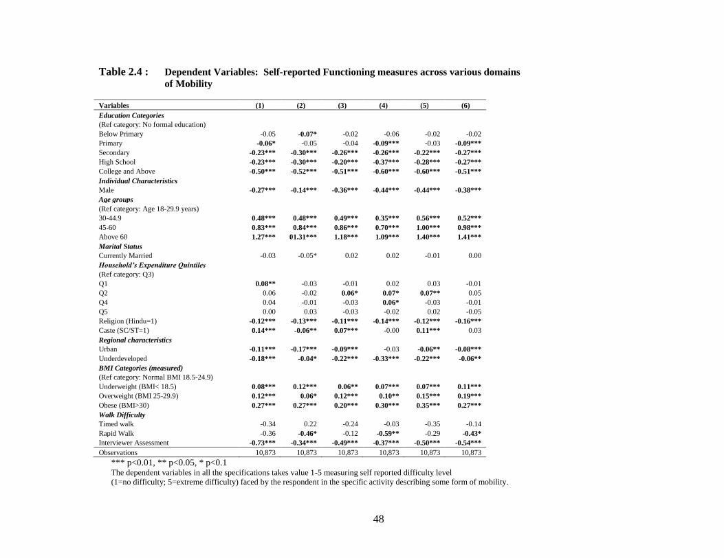
48

Table 2.4 : Dependent Variables: Self-reported Functioning measures across various domains

of Mobility

Variables (1) (2) (3) (4) (5) (6)



Below Primary -0.05 -0.07* -0.02 -0.06 -0.02 -0.02

Primary -0.06* -0.05 -0.04 -0.09*** -0.03 -0.09***

Secondary -0.23*** -0.30*** -0.26*** -0.26*** -0.22*** -0.27***

High School -0.23*** -0.30*** -0.20*** -0.37*** -0.28*** -0.27***

College and Above -0.50*** -0.52*** -0.51*** -0.60*** -0.60*** -0.51***


Male -0.27*** -0.14*** -0.36*** -0.44*** -0.44*** -0.38***

Age groups


30-44.9 0.48*** 0.48*** 0.49*** 0.35*** 0.56*** 0.52***

45-60 0.83*** 0.84*** 0.86*** 0.70*** 1.00*** 0.98***

Above 60 1.27*** 01.31*** 1.18*** 1.09*** 1.40*** 1.41***

Marital Status

Currently Married -0.03 -0.05* 0.02 0.02 -0.01 0.00


(Ref category: Q3)

Q1 0.08** -0.03 -0.01 0.02 0.03 -0.01

Q2 0.06 -0.02 0.06* 0.07* 0.07** 0.05

Q4 0.04 -0.01 -0.03 0.06* -0.03 -0.01

Q5 0.00 0.03 -0.03 -0.02 0.02 -0.05

Religion (Hindu=1) -0.12*** -0.13*** -0.11*** -0.14*** -0.12*** -0.16***

Caste (SC/ST=1) 0.14*** -0.06** 0.07*** -0.00 0.11*** 0.03


Urban -0.11*** -0.17*** -0.09*** -0.03 -0.06** -0.08***

Underdeveloped -0.18*** -0.04* -0.22*** -0.33*** -0.22*** -0.06**



Underweight (BMI< 18.5) 0.08*** 0.12*** 0.06** 0.07*** 0.07*** 0.11***

Overweight (BMI 25-29.9) 0.12*** 0.06* 0.12*** 0.10** 0.15*** 0.19***

Obese (BMI>30) 0.27*** 0.27*** 0.20*** 0.30*** 0.35*** 0.27***

Walk Difficulty

Timed walk -0.34 0.22 -0.24 -0.03 -0.35 -0.14

Rapid Walk -0.36 -0.46* -0.12 -0.59** -0.29 -0.43*

Interviewer Assessment -0.73*** -0.34*** -0.49*** -0.37*** -0.50*** -0.54***

Observations 10,873 10,873 10,873 10,873 10,873 10,873

*** p<0.01, ** p<0.05, * p<0.1 The dependent variables in all the specifications takes value 1-5 measuring self reported difficulty level

(1=no difficulty; 5=extreme difficulty) faced by the respondent in the specific activity describing some form of mobility.

49

Continuation of Table 2.4: Dependent Variables: Self-reported functioning measures across

various domains of Mobility Variables (7) (8) (9) (10) (11) (12)



Below Primary -0.00 -0.02 -0.06 0.01 -0.08** -0.04

Primary -0.08** -0.07* -0.10** -0.08** -0.10*** -0.21***

Secondary -0.28*** -0.22*** -0.18*** -0.26*** -0.25*** -0.25***

High School -0.24*** -0.24*** -0.17*** -0.21*** -0.38*** -0.34***

College and Above -0.55*** -0.49*** -0.42*** -0.62*** -0.56*** -0.45***


Male -0.42*** -0.28*** -0.09*** -0.15*** -0.18*** -0.18***

Age groups


30-44.9 0.44*** 0.51*** 0.35*** 0.42*** 0.21*** 0.44***

45-60 0.80*** 1.03*** 0.76*** 0.77*** 0.44*** 0.84***

Above 60 1.23*** 1.50*** 1.19*** 1.13*** 0.76*** 1.15***

Marital Status

Currently Married 0.02 -0.01 -0.02 -0.09*** -0.14*** 0.02


(Ref category: Q3)

Q1 0.03 0.04 0.12*** 0.07** -0.05 0.06

Q2 0.04 0.04 0.13*** 0.06* -0.04 0.08**

Q4 -0.02 -0.01 -0.07 0.01 -0.02 0.04

Q5 -0.03 -0.03 -0.10** -0.08** 0.00 -0.06

Religion (Hindu=1) -0.14*** -0.11*** -0.08** -0.12*** -0.08** -0.00

Caste (SC/ST=1) 0.14*** 0.08*** 0.09*** 0.18*** -0.10*** 0.13***


Urban -0.16*** -0.13*** 0.03 -0.05* -0.06** -0.05

Underdeveloped -0.34*** -0.20*** -0.05 -0.08*** -0.30*** -0.30***



Underweight (BMI< 18.5) 0.11*** 0.03 0.06** 0.09*** 0.10*** 0.04

Overweight (BMI 25-29.9) 0.05 0.17*** 0.07 0.04 0.09** 0.09**

Obese (BMI>30) 0.19*** 0.32*** 0.10 0.14** 0.18*** 0.17**

Walk Difficulty

Timed walk 0.41 0.24 -0.69** -0.15 0.01 -0.43

Rapid Walk -0.88*** -0.78*** 0.17 -0.36 -0.33 0.19

Interviewer Assessment -0.36*** -0.46*** -0.29*** -0.39*** -0.37*** -0.52***

Observations 10,873 10,873 10,873 10,873 10,873 10,873

*** p<0.01, ** p<0.05, * p<0.1 The dependent variables in all the specifications takes value 1-5 measuring self reported difficulty level

(1=no difficulty; 5=extreme difficulty) faced by the respondent in the specific activity describing some form of mobility.

50

Table 2.5: Dependent Variables: Self reported Functioning measures across various domains of Daily Activities

Variables (1) (2) (3) (4) (5) (6) (7) (8) (9) (10) (11)



Below Primary -0.05 -0.04 -0.06 -0.09** -0.08** -0.12** -0.06 0.01 -0.07 -0.05 -0.09**

Primary -0.09*** -0.16*** -0.16*** -0.12*** -0.09** -0.12*** -0.19*** -0.17*** -0.18*** -0.14*** -0.19***

Secondary -0.27*** -0.22*** -0.16** -0.31*** -0.23*** -0.21*** -0.09* -0.22*** -0.23*** -0.31*** -0.40***

High School -0.29*** -0.28*** -0.33*** -0.25*** -0.26*** -0.22*** -0.18*** -0.33*** -0.30*** -0.43*** -0.45***

College and Above -0.58*** -0.50*** -0.54*** -0.57*** -0.44*** -0.49*** -0.39*** -0.61*** -0.61*** -0.59*** -0.69***


Male -0.39*** -0.07* -0.03 -0.29*** -0.20*** -0.18*** -0.16*** -0.25*** -0.19*** -0.30*** -0.16***

Age groups


30-44.9 0.31*** 0.22*** 0.38*** 0.32*** 0.39*** 0.35*** 0.34*** 0.50*** 0.43*** 0.31*** 0.29***

45-60 0.70*** 0.58*** 0.68*** 0.73*** 0.82*** 0.73*** 0.66*** 0.89*** 0.76*** 0.65*** 0.70***

Above 60 1.15*** 0.95*** 1.00*** 1.06*** 1.23*** 1.11*** 1.04*** 1.24*** 1.14*** 1.09*** 1.16***

Marital Status

Currently Married 0.03 -0.06 -0.07* -0.03 -0.06** -0.02 -0.07** -0.03 -0.01 -0.05* -0.05


(Ref category: Q3)

Q1 0.03 0.00 0.03 0.01 -0.04 -0.00 -0.01 0.03 0.06 -0.04 -0.09***

Q2 0.02 0.01 -0.04 -0.01 -0.02 0.03 -0.02 0.06 0.00 0.03 -0.02

Q4 0.02 -0.02 -0.02 -0.02 0.06* -0.01 -0.01 -0.00 -0.03 0.00 -0.02

Q5 0.02 -0.03 -0.05 -0.08** 0.02 0.02 -0.05 -0.04 -0.12*** -0.05 -0.06*

Religion (Hindu=1) -0.18*** -0.14*** -0.15*** -0.17*** -0.16*** -0.10*** -0.01 -0.07** -0.01 -0.09*** -0.11***

Caste (SC/ST=1) 0.06*** 0.02 -0.04 0.06** 0.03 -0.01 0.03 0.07*** 0.07** 0.08*** -0.01


Urban -0.07*** 0.00 0.00 -0.06** -0.20*** -0.06* 0.03 -0.09*** -0.10*** -0.11*** -0.01

Underdeveloped -0.27*** -0.17*** -0.21*** -0.28*** -0.16*** -0.23*** 0.25*** -0.30*** 0.02 0.15*** 0.19***



Underweight (BMI< 18.5) 0.11*** 0.15*** 0.10*** 0.08*** 0.13*** 0.11*** 0.10*** 0.07*** 0.07** 0.10*** 0.12***

Overweight (BMI 25-29.9) 0.14*** 0.08 0.05 0.02 0.08** 0.10** -0.03 0.15*** 0.11** 0.10** 0.13***

Obese (BMI>30) 0.36*** 0.20** 0.22** 0.21*** 0.26*** 0.24*** 0.06 0.33*** 0.27*** 0.23*** 0.28***

Walk Difficulty

Timed walk 0.08 -0.48 -1.00*** 0.13 0.39 -0.55* -0.31 -0.22 -0.55* -0.26 -0.22

Rapid Walk -0.71*** -0.14 0.35 -0.65** -0.92*** -0.17 -0.04 -0.13 -0.04 -0.46* -0.44*

Interviewer Assessment -0.55*** -0.51*** -0.63*** -0.50*** -0.39*** -0.56*** -0.36*** -0.64*** -0.59*** -0.43*** -0.55***

Observations 10,873 10,873 10,873 10,873 10,873 10,873 10,873 10,873 10,873 10,873 10,873

*** p<0.01, ** p<0.05, * p<0.1

The dependent variables in all the specifications takes value 1-5 measuring self reported difficulty level (1=no difficulty; 5=extreme difficulty)

faced by the respondent in the specific activity describing some form of daily activities.

51

Table 2.6 : Summary Table of Ordered Probit Regressions with Self reported data

Positive and

Significant

Positive and

Insignificant

Negative and

Significant

Negative and

Insignificant



Below Primary 0 2 6 15

Primary 0 0 20 3

Secondary 0 0 23 0

High School 0 0 23 0

College and Above 0 0 23 0


Male 0 0 22 1

Age groups


30-44.9 23 0 0 0

45-60 23 0 0 0

Above 60 23 0 0 0

Marital Status

Currently Married 0 6 7 10


(Ref category: Q3)

Q1 3 11 1 8

Q2 6 10 0 7

Q4 2 5 0 16

Q5 0 7 5 11

Religion (Hindu=1) 0 0 20 3

Caste (SC/ST=1) 13 4 2 4


Urban 0 4 16 3

Underdeveloped 3 1 18 1



Underweight (BMI< 18.5) 21 2 0 0

Overweight (BMI 25-29.9) 16 6 0 1

Obese (BMI>30) 21 2 0 0

Walk Difficulty

Timed walk 0 7 4 12

Rapid Walk 0 3 10 10

Interviewer Assessment 0 0 23 0

52

Table 2.7: Dependent Variable: Self reported Cognitive difficulty

VARIABLES (1) (2)

Self reported cognition Memory Concentration



Below Primary -0.12*** -0.11***

Primary -0.09** -0.10***

Secondary -0.30*** -0.33***

High School -0.38*** -0.42***

College and Above -0.52*** -0.69***


Male -0.18*** -0.07**

Age groups


30-44.9 0.53*** 0.48***

45-60 0.88*** 0.81***

Above 60 1.22*** 1.23***

Marital Status

Currently Married -0.08*** -0.08***


(Ref category: Q3)

Q1 -0.00 -0.02

Q2 -0.01 -0.01

Q4 0.03 -0.00

Q5 -0.01 -0.03

Religion (Hindu=1) -0.15*** -0.05

Caste (SC/ST=1) 0.01 -0.01


Urban -0.23*** -0.13***

Underdeveloped -0.10*** -0.10***

Cognitive tests

Cognitive Score 1 -0.04*** -0.04***

Cognitive Score 2 -0.08*** -0.07***

Words recalled -0.03*** -0.02***

*** p<0.01, ** p<0.05, * p<0.1 The dependent variables in both the specifications takes value 1-5 measuring self reported difficulty level

(1=no difficulty; 5=extreme difficulty) faced by the respondent in remembering and concentrating things

Objective measures include (test of words recalled after delay, digital recall test and verbal fluency)

53

Table 2.8: Dependent Variable: Objective Memory and Cognitive tests

VARIABLES (1) (2) (3)

Objective memory tests Words recalled Score1 Score2



Below Primary 0.24*** 0.43*** 0.51***

Primary 0.39*** 0.71*** 0.78***

Secondary 0.57*** 0.94*** 1.11***

High School 0.80*** 1.22*** 1.46***

College and Above 0.98*** 1.55*** 1.84***


Male -0.07*** 0.31*** 0.40***

Age groups


30-44.9 -0.25*** -0.21*** -0.20***

45-60 -0.56*** -0.42*** -0.34***

Above 60 -0.85*** -0.63*** -0.49***

Marital Status

Currently Married 0.08*** 0.07*** 0.05*


(Ref category: Q3)

Q1 -0.12*** -0.10*** -0.03

Q2 -0.05 -0.06* -0.03

Q4 0.04 0.03 0.08**

Q5 0.12*** 0.14*** 0.20***

Religion (Hindu=1) 0.04 -0.02 -0.05*

Caste (SC/ST=1) -0.01 -0.13*** -0.08***


Urban 0.16*** 0.09*** 0.15***

Underdeveloped 0.11*** -0.11*** -0.23***

*** p<0.01, ** p<0.05, * p<0.1 The dependent variables in all the specifications are objective measures of Memory and Cognition including

(test of words recalled after delay, digital recall test and verbal fluency.)

54

Table 2.9: Dependent Variable: Objective measures of difficulty in Mobility and General health

(1) (2) (3) (4)

Objective Mobility Measures

Assessed

Walk

Assessed

Walk

Assessed

Health Assessed Health



Below Primary -0.11 -0.11 -0.03 -0.04

Primary -0.12 -0.13* -0.02 -0.03

Secondary -0.16* -0.16* -0.23*** -0.24***

High School -0.31*** -0.32*** -0.11** -0.12**

College and Above -0.29** -0.31** -0.17** -0.18***


Male 0.08 0.09* -0.13*** -0.12***

Age groups


30-44.9 0.32** 0.31* 0.26*** 0.25***

45-60 0.79*** 0.77*** 0.47*** 0.45***

Above 60 1.34*** 1.32*** 0.73*** 0.72***

Marital Status

Currently Married -0.12** -0.12** -0.00 -0.00


(Ref category: Q3)

Q1 0.08 0.08 -0.05 -0.05

Q2 -0.06 -0.06 -0.04 -0.04

Q4 -0.02 -0.02 -0.09** -0.09**

Q5 -0.16** -0.16** -0.08* -0.09**

Religion (Hindu=1) -0.01 -0.00 -0.02 -0.02

Caste (SC/ST=1) 0.06 0.06 0.22*** 0.22***


Urban 0.01 0 -0.11*** -0.12***

Underdeveloped 0.53*** 0.53*** 0.14*** 0.14***

Underweight 0.07 0.03

Overweight 0.15* 0.15***

Obese 0.32** 0.17**

Observations 10,873 10,873 10,873 10,873 10,873 *** p<0.01, ** p<0.05, * p<0.1

The dependent variables in all the specifications are interviewer assessed difficulty (dummy variable) in Mobility and General health

Specification (2) and (4) controls for body mass index categories.

55

Table 2.10 Estimations of two-stage regressions using individual fixed effects

(1) (2) (3) (4)

VARIABLES Vignette Set A Vignette Set B Vignette Set C Vignette Set D


Below Primary 0.02 -0.03 0.04 -0.11

Primary 0.00 -0.05 -0.05 -0.10*

Secondary -0.01 -0.02 0.03 -0.11*

High School 0.00 -0.01 -0.01 -0.03

College and Above 0.01 -0.02 0.11** -0.05


Male -0.08*** -0.01 -0.07*** 0.03

Age groups

30-44.9 0.05 0.03 0.00 0.04

45-60 0.02 -0.01 0.04 0.10

Above 60 0.11*** -0.01 0.07* 0.21***

Marital Status

Currently Married -0.01 -0.06** -0.02 -0.05


Underweight (bmi< 18.5) -0.01 0.02 0.04* 0.00

Overweight (bmi 25-29.9) -0.02 -0.01 -0.01 -0.03

Obese (bmi>30) 0.05 -0.05 0.01 -0.12


Q1 -0.16*** -0.07** -0.01 0.02

Q2 -0.08** 0.01 0.01 0.03

Q4 -0.11*** 0.01 -0.00 0.11*

Q5 -0.05 -0.01 0.02 0.11*

Religion (Hindu=1) -0.04 -0.01 -0.00 -0.06

Caste (SC/ST=1) 0.08*** -0.01 -0.05** 0.17***


Urban -0.06** -0.02 -0.06** -0.02

Underdeveloped -0.09*** -0.12*** -0.22*** -0.47***

Constant -0.29*** -0.16*** -0.44*** 2.45***

Observations 2,673 2,728 2,770 2,698

R-squared 0.03 0.02 0.04 0.07

*** p<0.01, ** p<0.05, * p<0.1

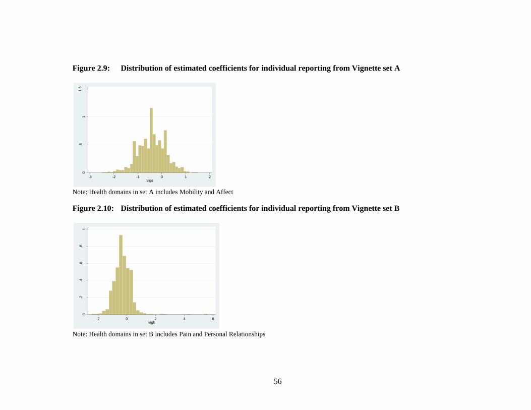
56

Figure 2.9: Distribution of estimated coefficients for individual reporting from Vignette set A

Note: Health domains in set A includes Mobility and Affect

Figure 2.10: Distribution of estimated coefficients for individual reporting from Vignette set B

Note: Health domains in set B includes Pain and Personal Relationships

0.5

11.5

De

nsity

-3 -2 -1 0 1 2viga

0.2

.4.6

.81

De

nsity

-2 0 2 4 6vigb

57

Figure 2.11: Distribution of estimated coefficients for individual reporting from Vignette set C

Note: Health domains in set A includes Vision, Sleep and Energy

Figure 2.12: Distribution of estimated coefficients for individual reporting from Vignette set D

Note: Health domains in set A includes Cognition and Self-Care

0.2

.4.6

.81

De

nsity

-2 0 2 4 6vigc

0.5

11.5

De

nsity

-3 -2 -1 0 1vigd

58

Appendix

List of five sample vignettes from each health domain in WHS-SAGE Survey questionnaire

Set A Affect and Mobility

[Alan] is able to walk distances of up to 200 metres without any problems but feels tired after walking one kilometre or

climbing up more than one flight of stairs. He has no problems with day-to-day physical activities, such as carrying food from

the market.

[Manjima] enjoys her work and social activities and is generally satisfied with her life. She gets depressed every 3 weeks for a

day or two and loses interest in what she usually enjoys but is able to carry on with her day to day activities.

[Miriam] does not exercise. She cannot climb stairs or do other physical activities because she is obese. She is able to carry the

groceries and do some light household work.

[Vladimir] is paralyzed from the neck down. He is unable to move his arms and legs or to shift body position. He is confined to

bed.

[Ang] has already had five admissions into the hospital because she has attempted suicide twice in the past year and has

harmed herself on three other occasions. She is very distressed every day for the most part of the day, and sees no hope of

things ever getting better. She is thinking of trying to end her life again.

59

Set B Pain and Personal Relationships

[Elizabeth] has difficulty climbing up and down the stairs and walking. She is not able to go out as much as she would like to

but has many friends who come and visit her at home. Her friends find her a source of great comfort.

[Markus] has pain in his knees, elbows, wrists and fingers, and the pain is present almost all the time. It gets worse during the

first half of the day. Although medication helps, he feels uncomforTable when moving around, holding and lifting things.

[Nobu] is blind and lives in a remote rural area. His family does not allow him to leave the house because they fear he will get

hurt. His family tells him that he is a burden to them. Their criticism upsets him and he cries.

[Laura] has a headache once a month that is relieved one hour after taking a pill. During the headache she can carry on with

her day to day affairs.

[Isabelle] has pain that radiates down her right arm and wrist during her day at work. This is slightly relieved in the evenings

when she is no longer working on her computer.

Set C Vision, Sleep and Energy

[Damien] wakes up almost once every hour during the night. When he wakes up in the night, it takes around 15 minutes for

him to go back to sleep. In the morning he does not feel well-rested and feels slow and tired all day.

Antonio] can read words in newspaper articles (and can recognize faces on a postcard size photograph). He can recognize

shapes and colours from across 20 metres but misses out the fine details.

60

[Paolo] has no trouble falling asleep at night and does not wake up during the night, but every morning he finds it difficult to

wake up. He uses an alarm clock but falls back asleep after the alarm goes off. He is late to work on four out of five days and

feels tired in the mornings.

[Jennifer] only reads if the text is in very large print, such as 10 lines per page. Otherwise she does not read anything. Even

when people are close to her, she sees them blurred.

[Noemi] falls asleep easily at night, but two nights a week she wakes up in the middle of the night and cannot go back to sleep

for the rest of the night. On these days she is exhausted at work and cannot concentrate on her job.

Set D Cognition and Self-Care

[Anne] takes twice as long as others to put on and take off clothes, but needs no help with this. Although It requires an effort,

she is able to bathe and groom herself, though less frequently than before. She does not require help with feeding.

[Sue] can find her way around the neighborhood and know where her own belongings are kept, but struggles to remember how

to get to a place she has only visited once or twice. She is keen to learn new recipes but finds that she often makes mistakes

and has to reread several times before she is able to do them properly

[Theo] cannot concentrate for more than 15 minutes and has difficulty paying attention to what is being said to him. Whenever

he starts a task, he never manages to finish it and often forgets what he was doing. He is able to learn the names of people he

meets but cannot be trusted to follow directions to a store by himself

61

[Sandra] lives on her own and has no relatives or friends nearby. Because of her arthritis, she is housebound. She often stays

all day in the same clothes that she has slept in, as changing clothes is too painful. A neighbour helps her wash herself.

[Victor] requires no assistance with cleanliness, dressing and eating. He occasionally suffers from back pain and when this

happens he needs help with bathing and dressing. He always keeps himself tidy.

Reporting Heterogeneity in Health Status A study across Population Sub-groups in India Using...

Documents

Transcript of Reporting Heterogeneity in Health Status A study across Population Sub-groups in India Using...