Remote Sensing of Wetlands: Case Studies Comparing Practical Techniques

www.cerf-jcr.org

Remote Sensing of Wetlands: Case Studies ComparingPractical Techniques

Victor Klemas

College of Earth,Ocean and Environment

University of DelawareNewark, DE 19716, [email protected]

ABSTRACT

KLEMAS, V., 2011. Remote sensing of wetlands: case studies comparing practical techniques. Journal of CoastalResearch, 27(3), 418–427. West Palm Beach (Florida), ISSN 0749-0208.

To plan for wetland protection and sensible coastal development, scientists and managers need to monitor the changes incoastal wetlands as the sea level continues to rise and the coastal population keeps expanding. Advances in sensor designand data analysis techniques are making remote sensing systems practical and attractive for monitoring natural andman-induced wetland changes. The objective of this paper is to review and compare wetland remote sensing techniquesthat are cost-effective and practical and to illustrate their use through two case studies. The results of the case studiesshow that analysis of satellite and aircraft imagery, combined with on-the-ground observations, allows researchers toeffectively determine long-term trends and short-term changes of wetland vegetation and hydrology.

ADDITIONAL INDEX WORDS: Wetland remote sensing, wetland case studies, remote sensor comparison, coastalecosystems, sea level rise.

INTRODUCTION AND BACKGROUND

Wetlands and estuaries are highly productive and act as

critical habitats for a variety of plants, fish, shellfish, and other

wildlife. Wetlands also provide flood protection, protection from

storm and wave damage, water quality improvement through

filtering of agricultural and industrial waste, and recharge of

aquifers (Morris et al., 2002; Odum, 1993). However, wetlands

have been exposed to a range of stress-inducing alterations,

including dredge and fill operations, hydrologic modifications,

pollutant runoff, eutrophication, impoundments, and fragmen-

tation by roads and ditches.

Recently, there has also been considerable concern regarding

the impact of climate change on coastal wetlands, especially

due to relative sea level rise, increasing temperatures, and

changes in precipitation. Climate change is considered a cause

for habitat destruction, shift in species composition, and

habitat degradation in existing wetlands (Baldwin and Men-

delssohn, 1998; Titus et al., 2009). Coastal wetlands have

already proved susceptible to climate change, with a net loss of

33,230 acres from 1998 to 2004 in the United States alone

(Dahl, 2006). This loss was primarily due to conversion of

coastal salt marsh to open saltwater. Rising sea levels not only

can cause the drowning of salt marsh habitats but also can

reduce germination periods (Noe and Zedler, 2001). The impact

of global change in the form of accelerating sea level rise and

more frequent storms is of particular concern for coastal

wetlands managers.

Vegetated wetlands are stable only when the marsh platform

is able to accrete sediment at a rate equal to the prevailing rate

of sea level rise. This ability to accrete is proportional to the

biomass density of the plants, concentration of suspended

sediment, time of submergence, and depth of the marsh surface

and the tidal range. Many coastal wetlands, such as the tidal

salt marshes along the Louisiana coast, are generally within

fractions of a meter of sea level and will be lost, especially if the

impact of sea level rise is amplified by coastal storms. Man-

made modifications of wetland hydrology and extensive urban

development will further limit the ability of wetlands to survive

sea level rise. For instance, man-made channelization of the

Mississippi River flow causes much of the river sediment to be

carried into the Gulf of Mexico, rather than to be deposited in

the wetlands along the Louisiana coast (Farris, 2005; Pinet,

2009).

County, state, and federal officials are concerned about the

impact of climate change and sea level rise on fisheries,

wetlands, estuaries, and shorelines; municipal infrastructure,

such as water, wastewater, and street systems; storm water

drainage and flooding; salinity intrusion into groundwater

supplies; etc. (Nicholas Institute, 2010). To plan for wetland

protection and sensible coastal development, scientists and

managers need to monitor the changes in coastal ecosystems as

the sea level continues to rise and the coastal population keeps

expanding. Recent advances in sensor design and data analysis

techniques are making some remote sensing systems practical

and attractive for monitoring natural and man-induced coastal

ecosystem changes. Hyperspectral imagers can differentiate

DOI: 10.2112/JCOASTRES-D-10-00174.1 received 16 November2010; accepted in revision 19 December 2010.Published Pre-print online 21 March 2011.’ Coastal Education & Research Foundation 2011

Journal of Coastal Research 27 3 418–427 West Palm Beach, Florida May 2011

wetland types using spectral bands specially selected for a

given application. High resolution multispectral mappers are

available for mapping small patchy upstream wetlands.

Thermal infrared scanners can map coastal water tempera-

tures, while microwave radiometers can measure water

salinity, soil moisture, and other hydrologic parameters.

Synthetic Aperture Radars (SAR) help distinguish forested

wetlands from upland forests. Airborne light detection and

ranging (LIDAR) systems can be used to map wetland

topography, produce beach profiles and bathymetric maps

(Purkis and Klemas, 2011; Ramsey, 1995).

With the rapid development of new remote sensors, databas-

es, and image analysis techniques, there is a need to help

potential users choose remote sensors and data analysis

methods that are most appropriate and practical for wetland

studies (Phinn et al., 2000). The objective of this paper is to

review and compare wetland remote sensing techniques that are

cost-effective and practical and to illustrate their use through

two case studies. The wetland sites and projects selected for the

case studies are facing environmental problems, such as urban

development in their watersheds or major vegetation and

hydrologic changes due to rapid local sea level rise.

WETLAND AND LAND COVER MAPPING

For more than three decades, remote sensing techniques

have been used successfully by academic researchers and

government agencies to map and monitor wetlands (Dahl,

2006; Tiner, 1996). For instance, the U.S. Fish and Wildlife

Service (FWS) has used remote sensing techniques to deter-

mine the biologic extent of wetlands for the past 30 years.

Through its National Wetlands Inventory, FWS has provided

federal and state agencies, the private sector, and citizens with

scientific data on wetlands location, extent, status, and trends.

To accomplish this important task, FWS has used multiple

sources of aircraft and satellite imagery and on-the-ground

observations (Tiner, 1996). Most states have also conducted a

range of wetland inventories, using both aircraft and satellite

imagery. The aircraft imagery frequently included natural

color and color infrared images. The satellite data consisted of

both high-resolution (1–4 m) and medium-resolution (10–30 m)

multispectral imagery.

More recently, the availability of high spatial and spectral

resolution satellite data has significantly improved the capac-

ity for upstream wetland, salt marsh, and other coastal

vegetation mapping (Jensen et al., 2007; Wang, Christiano,

and Traber, 2010). Furthermore, new techniques have been

developed for mapping wetlands and even identifying wetland

types and plant species (Jensen et al., 2007; Klemas, 2009;

Schmidt et al., 2004; Yang et al., 2009). Using hyperspectral

imagery and narrow-band vegetation indices, researchers have

been able to identify some wetland species and to make

progress on estimating biochemical and biophysical parame-

ters of wetland vegetation, such as water content, biomass, and

leaf area index (Adam, Mutanga, and Rugege, 2010). Hyper-

spectral imagers may provide several hundred spectral bands;

multispectral imagers use less than a dozen bands.

The integration of hyperspectral imagery and LIDAR-

derived elevation has also significantly improved the accuracy

of mapping salt marsh vegetation. The hyperspectral images

help distinguish high marsh from other salt marsh communi-

ties, using its high reflectance in the near-infrared region of the

spectrum, and the LIDAR data help separate invasive

Phragmites australis from low marsh plants (Yang and

Artigas, 2010). Major plant species within a complex, hetero-

geneous tidal marsh have been classified using multitemporal,

high-resolution QuickBird images, field reflectance spectra,

and LIDAR height information. Phragmites, Typha, and

Spartina patens were spectrally distinguishable at particular

times of the year, likely due to differences in biomass and

pigments and the rate at which these change throughout the

growing season. Classification accuracies for Phragmites were

high due to the uniquely high near-infrared reflectance and the

height of this plant in the early fall (Gilmore et al., 2010).

High-resolution imagery is more sensitive to within-class

spectral variance, making separation of spectrally mixed land

cover types more difficult than when using medium-resolution

imagery. Therefore, pixel-based techniques are sometimes

replaced by object-based methods, which incorporate spatial

neighborhood properties by segmenting or partitioning the

image into a series of closed objects that coincide with the

actual spatial pattern and then classifying the image. ‘‘Region

growing’’ is among the most commonly used segmentation

methods. This procedure starts with the generation of seed

points over the whole scene, followed by grouping of neighbor-

ing pixels into an object under a specific homogeneity criterion.

Thus, the object keeps growing until its spectral closeness

metric exceeds a predefined break-off value (Kelly and Tuxen,

2009; Shan and Hussain, 2010; Wang, Sousa, and Gong, 2004).

Wetland health is strongly affected by runoff from land and

its use within the same watershed. To study the impact of land

runoff on estuarine and wetland ecosystems, a combination of

models is frequently used, including watershed, hydrodynam-

ic, water quality, and living resource models (Li et al., 2006;

Linker et al., 1993). Most coastal watershed models require

land cover or land use as an input. Knowing how the land cover

is changing, these models, together with a few other inputs like

slope and precipitation, can predict the amount and type of

runoff into rivers, wetlands, and estuaries and how their

ecosystems will be affected (Jensen, 2007). For instance, some

models predict that severe degradation in stream water quality

will occur when the agricultural land use in watersheds

exceeds 50% or urban land use exceeds 20% (Tiner et al., 2000).

The Landsat Thematic Mapper (TM) has been a reliable

source for land cover data (Lunetta and Balogh, 1999). Its 30-m

resolution and spectral bands have proved adequate for

observing land cover changes in large coastal watersheds

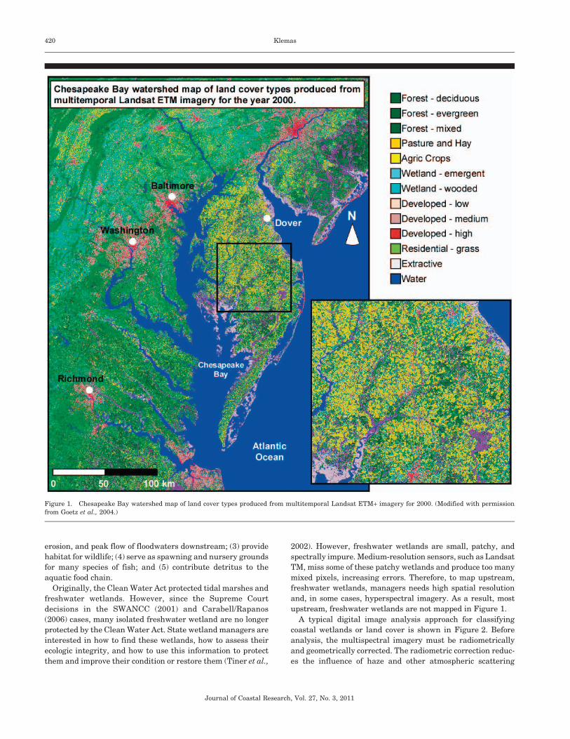
(e.g., Chesapeake Bay). Figure 1 shows a land cover map of the

Chesapeake Bay watershed derived from Landsat Enhanced

Thematic Mapper Plus (ETM+) imagery. Thirteen land cover

classes are mapped in Figure 1, including two wetland classes.

Other satellites with medium-resolution imagers can also be

used (Klemas, 2005).

As shown in Figure 1, the Chesapeake Bay watershed

contains many streams and, consequently, upstream freshwa-

ter wetlands. Upstream wetlands are no less valuable than

tidal marshes because they (1) improve the water quality of

adjacent rivers by removing pollutants; (2) reduce velocity,

Remote Sensing of Wetlands 419

Journal of Coastal Research, Vol. 27, No. 3, 2011

erosion, and peak flow of floodwaters downstream; (3) provide

habitat for wildlife; (4) serve as spawning and nursery grounds

for many species of fish; and (5) contribute detritus to the

aquatic food chain.

Originally, the Clean Water Act protected tidal marshes and

freshwater wetlands. However, since the Supreme Court

decisions in the SWANCC (2001) and Carabell/Rapanos

(2006) cases, many isolated freshwater wetland are no longer

protected by the Clean Water Act. State wetland managers are

interested in how to find these wetlands, how to assess their

ecologic integrity, and how to use this information to protect

them and improve their condition or restore them (Tiner et al.,

2002). However, freshwater wetlands are small, patchy, and

spectrally impure. Medium-resolution sensors, such as Landsat

TM, miss some of these patchy wetlands and produce too many

mixed pixels, increasing errors. Therefore, to map upstream,

freshwater wetlands, managers needs high spatial resolution

and, in some cases, hyperspectral imagery. As a result, most

upstream, freshwater wetlands are not mapped in Figure 1.

A typical digital image analysis approach for classifying

coastal wetlands or land cover is shown in Figure 2. Before

analysis, the multispectral imagery must be radiometrically

and geometrically corrected. The radiometric correction reduc-

es the influence of haze and other atmospheric scattering

Figure 1. Chesapeake Bay watershed map of land cover types produced from multitemporal Landsat ETM+ imagery for 2000. (Modified with permission

from Goetz et al., 2004.)

420 Klemas


particles and any sensor anomalies. The geometric correction

compensates for the Earth’s rotation and for variations in the

position and attitude of the satellite. Image segmentation

simplifies the analysis by first dividing the image into

homogeneous patches or ecologically distinct areas. Supervised

classification requires the analyst to select training samples

from the data that represent the themes to be classified

(Jensen, 1996). The training sites are geographic areas

previously identified using field visits or other reference data,

such as aerial photographs. The spectral reflectances of these

training sites are then used to develop spectral ‘‘signatures,’’

which are used to assign each pixel in the image to a thematic

class.

Next, an unsupervised classification is performed to identify

variations in the image not contained in the training sites. In

unsupervised classification, the computer automatically iden-

tifies the spectral clusters representing all features on the

ground. Training site spectral clusters and unsupervised

spectral classes are then compared and analyzed using cluster

analysis to develop an optimum set of spectral signatures. Final

image classification is then performed to match the classified

themes with the project requirements (Jensen, 1996). Through-

out the process, ancillary data are used whenever available

(e.g., aerial photos, maps, and field samples).

When studying small wetland sites, researchers can use

aircraft or high-resolution satellite systems (Klemas, 2005).

Airborne georeferenced digital cameras, providing color and

color infrared digital imagery, are particularly suitable for

accurate mapping or interpreting satellite data. Most digital

cameras are capable of recording reflected visible to near-

infrared light. A filter is placed over the lens that transmits

only selected portions of the wavelength spectrum. For a single-

camera operation, a filter is chosen that generates natural color

(blue–green–red wavelengths) or color-infrared (green–red–

near-infrared wavelengths) imagery. For a multiple-camera

operation, filters that transmit narrower bands are chosen. For

example, a four-camera system may be configured so that each

camera filter passes a band matching a specific satellite

imaging band, e.g., blue, green, red, and near-infrared bands

matching the bands of the IKONOS satellite multispectral

sensor (Ellis and Dodd, 2000).

Digital camera imagery can be integrated with global

positioning system position information and used as layers in

a geographic information system for a range of modeling

applications (Lyon and McCarthy, 1995). Small aircraft flown

at low altitudes (e.g., 100–500 m) can be used to supplement

field data. High-resolution imagery (0.6–4 m) can also be

obtained from satellites, such as IKONOS and QuickBird

(Table 1). However, cost becomes excessive if the site is larger

than a few hundred square kilometers. In those cases, medium-

resolution sensors, such as Landsat TM (30 m) and Satellite

Pour l’Observation de la Terre (SPOT) (20 m), become more

cost-effective.

Mapping submerged aquatic vegetation (SAV), coral reefs,

and general bottom characteristics requires high-resolution (1–

4 m) multispectral or hyperspectral imagery (Mishra et al.,

2006; Mumby and Edwards, 2002; Purkis et al., 2002). Coral

reef ecosystems usually exist in clear water and can be

classified to show different forms of coral reef, dead coral, coral

rubble, algal cover, sand, lagoons, different densities of sea

grasses, etc. SAV sometimes grows in more turbid water and

thus is more difficult to map. Aerial hyperspectral scanners

and high-resolution multispectral satellite imagers, such as

IKONOS and QuickBird, have been used in the past to map

SAV with accuracies of about 75% for classes including high-

density sea grass, low-density sea grass, and unvegetated

bottom (Akins, Wang, and Zhou, 2010; Dierssen et al., 2003;

Wolter, Johnston, and Niemi, 2005).

MONITORING WETLAND CHANGES

To identify long-term trends and short-term variations, such

as the impact of rising sea levels and hurricanes on wetlands,

researchers need to analyze time series of remotely sensed

imagery. The acquisition and analysis of time series of

multispectral imagery is a difficult task. The imagery must

be acquired under similar environmental conditions (e.g., same

time of year and sun angle) and in the same or similar spectral

bands. There are changes in both time and spectral content.

One way to approach this problem is to reduce the spectral

information to a single index, reducing the multispectral

imagery into one field of the index for each time step. In this

way, the problem is simplified to the analysis of time series of a

single variable, one for each pixel of the images.

The most common index used is the Normalized Difference

Vegetation Index (NDVI), which is expressed as the difference

between the red and the near-infrared reflectances divided by

their sum. These two spectral bands represent the most

detectable spectral characteristic of green plants. This is

because the red (and blue) radiation is absorbed by the

chlorophyll in the surface layers of the plant (Palisade

parenchyma) and the near-infrared is reflected from the inner

leaf cell structure (Spongy mesophyll) as it penetrates several

leaf layers in a canopy. Thus, the NDVI can be related to plant

biomass or stress, since the near-infrared reflectance depends

on the abundance of plant tissue and the red reflectance

indicates the surface condition of the plant. It has been shown

by researchers that time series of remote sensing data can be

Figure 2. Typical image analysis approach.



used effectively to identify long-term trends and subtle changes

of NDVI by means of principal component analysis (Jensen,

2007; Young and Wang, 2001; Yuan, Elvidge, and Lunetta,

1998).

The preprocessing of multidate sensor imagery, when

absolute comparisons among different dates are to be carried

out, is more demanding than the single-date case. It requires a

sequence of operations, including calibration to radiance or at-

satellite reflectance, atmospheric correction, image registra-

tion, geometric correction, mosaicking, subsetting, and mask-

ing out clouds and irrelevant features. In the preprocessing of

multidate images, the most critical steps are the registration of

the multidate images and their radiometric rectification. To

minimize errors, registration accuracies of a fraction of a pixel

must be attained. The second critical requirement for change

detection is attaining a common radiometric response for the

quantitative analysis for one or more of the image pairs

acquired on different dates. This means that variations in solar

illumination, atmospheric scattering and absorption, and

detector performance must be normalized, i.e., the radiometric

properties of each image must be adjusted to those of a

reference image (Coppin et al., 2004; Lunetta and Elvidge,

1998).

Detecting changes between two registered and radiometri-

cally corrected images from different dates can be accomplished

by employing one of several techniques, including postclassi-

fication comparison and spectral image differencing (change

detection). In postclassification comparison, two images from

different dates are independently classified. The two maps are

then compared pixel by pixel. This avoids the difficulties in

change detection associated with the analysis of images

acquired at different times of the year or day or by different

sensors, thereby minimizing the problem of radiometric

calibration across dates. One disadvantage is that every error

in the individual date classification maps is also present in the

final change detection map (Dobson et al., 1995; Jensen, 1996;

Lunetta and Elvidge, 1998).

Spectral change detection (spectral image differencing) is the

most widely applied change detection algorithm. Spectral

change techniques rely on the principle that land cover changes

result in changes in the spectral signature of the affected land

surface. These techniques involve the transformation of two

original images to a new single-band or multiband image in

which the areas of spectral change are highlighted. This is

accomplished by subtracting one date of raw or transformed

(e.g., vegetation indices or albedo) imagery from a second date

that has been precisely registered to the image of the first date.

Pixel difference values exceeding a selected threshold are

considered changed. A change–no change binary mask is

overlaid onto the second date image, and only the pixels

labeled as having changed are classified in the second date

imagery. While the unchanged pixels remain in the same

classes as in the first date imagery, the spectrally changed

pixels must be further processed by other methods, such as a

classifier, to produce a labeled land cover change map. This

approach eliminates the need to identify land cover changes in

areas where no significant spectral change has occurred

between the two dates of imagery (Coppin et al., 2004; Jensen,

1996; Yuan, Elvidge, and Lunetta, 1998). However, to obtain

accurate results, radiometric normalization must be applied to

one date of imagery to match the radiometric condition of the

two dates of data before image subtraction. An evaluation of the

spectral image differencing and the post-classification compar-

ison change detection algorithms is provided by Macleod and

Congalton (1998).

The spectral change (image differencing) detection methods

and the classification-based methods are often combined in a

hybrid approach. For instance, spectral change detection can

be used to identify areas of significant spectral change, and

then postclassification comparison can be applied within areas

where spectral change was detected to obtain class-to-class

change information. As shown in Figure 3, change analysis

results can be further improved by including probability

filtering that allows only certain changes and forbids others

Table 1. High-resolution satellite parameters and spectral bands.*

Sponsor

IKONOS QuickBird OrbView-3 WorldView-1 GeoEye-1 WorldView-2

Space Imaging DigitalGlobe Orbimage DigitalGlobe GeoEye DigitalGlobe

Launched Sept. 1999 Oct. 2001 June 2003 Sept. 2007 Sept. 2008 Oct. 2009

Spatial Resolution (m)

Panchromatic 1.0 0.61 1.0 0.5 0.41 0.5

Multispectral 4.0 2.44 4.0 NA 1.65 2

Spectral Range (nm)

Panchromatic 525–928 450–900 450–900 400–900 450–800 450–800

Coastal blue NA NA NA NA NA 400–450

Blue 450–520 450–520 450–520 NA 450–510 450–510

Green 510–600 520–600 520–600 NA 510–580 510–580

Yellow NA NA NA NA NA 585–625

Red 630–690 630–690 625–695 NA 655–690 630–690

Red edge NA NA NA NA NA 705–745

Near-infrared 760–850 760–890 760–900 NA 780–920 770–1040

Swath width (km) 11.3 16.5 8 17.6 15.2 16.4

Off nadir pointing (u) 626 630 645 645 630 645

Revisit time (d) 2.3–3.4 1–3.5 1.5–3 1.7–3.8 2.1–8.3 1.1–2.7

Orbital altitude (km) 681 450 470 496 681 770

* From DigitalGlobe (2003), Orbimage (2003), Parkinson (2003), and Space Imaging (2003).

422 Klemas


(e.g., urban to forest). A detailed, step-by-step procedure for

performing change detection was developed by the National

Oceanic and Atmospheric Administration’s (NOAA’s) Coastal

Change Analysis Program and is described in Dobson et al.

(1995) and Klemas et al. (1993).

CASE STUDIES

The following two case studies were selected to illustrate and

compare the use of practical remote sensing techniques for

studying key problems at different wetland sites and to try to

answer wetland managers’ questions, such as the following: (1)

How are urban sprawl and development affecting wetlands in

coastal watersheds? (2) How is accelerated local sea level rise

changing the vegetation, inundation levels, and hydrology in

tidal wetlands? (3) Should one intervene in the hydraulic

regime by channel modification to accelerate or delay marsh

development in a particular direction?

The case studies do not represent all possible uses of remote

sensing in wetlands but are typical of some problems

encountered by wetland scientists and managers. The choice

of case studies was also based on the author’s personal

experience.

Remote Sensing Applications AssessmentProject (RESAAP)

Managers of NOAA’s National Estuarine Research Reserve

System (NERRS) have a continuing need to use remote sensing

to address typical questions, such as the following: (1) What is

the extent of emergent, intertidal, and submerged habitats? (2)

How are the emergent, intertidal, and submerged habitats

changing? (3) How are suburban sprawl and coastal develop-

ment affecting reserve watersheds? (4) How have invasive

plants affected habitat? (5) How diverse is each NERRS site in

terms of habitat types?

While remote sensing was being actively used within

NERRS, the multitude of new satellite and aircraft sensors

and image analysis techniques that are becoming available

make it difficult for research reserve managers to select the

most cost-effective sensing and analysis techniques. Therefore,

in 2004, NOAA’s NERRS program funded a team of remote

sensing experts to compare the cost, accuracy, reliability, and

user-friendliness of four remote sensing approaches for

mapping land cover, emergent wetlands, and SAV. Four

NERRS test sites were selected for the project, including the

Ashepoo, Combahee, and South Edisto Basin, South Carolina;

Grand Bay, Michigan; St. Jones River and Blackbird Creek,

Delaware; and Padilla Bay, Washington (Porter et al., 2006).

The research described here was primarily conducted at

Delaware’s St. Jones River and Blackbird Creek NERRS sites,

where wetland changes at the sites and the land cover of their

watersheds were studied and mapped.

The Blackbird Creek study site consists of the estuarine and

freshwater tidal wetlands within the Blackbird Creek drainage

basin and some contiguous wetland areas from two adjacent

drainage basins. The study area is approximately 100 km2 and

covers 19.1 km (11.9 mi.) of the creek. Blackbird Creek is

located in southern New Castle County, Delaware, and the

upper Blackbird Creek is one component of Delaware’s NERRS

sites. The upland land use in Blackbird Creek basin is

primarily agriculture (51%) and forested (48%), with a small

proportion of developed land (1%). Within the wetlands of

Blackbird Creek, the amount of direct physical alteration—

diking, ditching, channel straightening, and impounding—has

been minimal compared to that at many other coastal wetlands

in Delaware (Field and Philipp, 2000b).

The Delaware St. Jones River NERRS study site provides a

contrast to the Blackbird Creek site in several ways. The total

area of the study site is approximately 80 km2, and it covers

14.3 km (8.9 mi.) of the main river channel. The amount of

agriculture in the St. Jones River basin is 51%, forested area is

38%, and developed land equals 11%, including higher-density

residential areas and commercial or industrial developments.

The St. Jones River has been subjected to much direct human

manipulation. The natural course of the river’s main channel

has been straightened, and parallel grid ditches were dug in a

portion of the wetlands for mosquito control. These hydrologic

alterations have undoubtedly affected the wetland ecosystem

structure and functions in this river.

The RESAAP team also included scientists from the

University of South Carolina and NOAA who were performing

similar studies of emergent wetlands and SAV at three other

NERRS sites (Porter et al., 2006). Results were compared to

determine which imagery and analysis approach should be

recommended for use at other NERRS sites.

The four remote sensing systems evaluated were the

hyperspectral airborne imaging spectrometer for applications

(AISA), an aerial multispectral (ADS 40) digital modular

camera, the IKONOS (or QuickBird) high-resolution satellite,

and Landsat TM. A comparison of approximate data acquisi-

tion costs is shown in Table 2. The high-resolution imagery per

square kilometer of coverage is much more expensive than the

medium-resolution imagery.

Completed in 2006, this study found that aerial hyperspec-

tral image analysis is too complicated for typical NERRS site

personnel and the imagery is too expensive for large NERRS

sites or entire watersheds. Furthermore, it was difficult to

discriminate wetlands species even with hyperspectral imag-

Figure 3. Change detection using probability filters.



ery (Porter et al., 2006). Due to different sun angles for each

flight strip, a separate atmospheric correction had to be

implemented for each strip. Also, the aircraft roll due to wind

conditions produced uneven swaths.

In the NERRS study, the highest accuracy for mapping

clusters of different plant species over small critical areas was

obtained by visually analyzing orthophotos produced by

airborne digital cameras. The visual interpretation was

performed after image segmentation and with the help of field

training sites visited before and after the interpretation

process. For larger sites, combining IKONOS and Landsat

TM proved cost-effective and user-friendly. The Landsat TM

imagery was used to map land cover for the large site or entire

watershed, and the IKONOS high-resolution imagery was used

for detailed mapping of critical NERRS areas or those

identified by Landsat TM as having changed. A particularly

effective technique developed by the team is based on using

biomass change as a wetland change indicator (Porter et al.,

2006; Weatherbee, 2000).

Monitoring Accelerated Local Sea Level Risein Wetlands

The primary objectives of this project were to study changes

at a unique Delaware Bay tidal wetland site, which faces an

accelerated sea level rise due to a canal breach, and to show

how remote sensors and related techniques can be used for

studying the impact of sea level rise and man-made influences

on coastal wetlands. The improved understanding of the

processes occurring at this rapidly changing site will help

wetland managers decide whether to intervene in the hydraulic

regime by channel modification to accelerate or delay marsh

development in a particular direction.

The study site was the Milford Neck Conservation Area

(MNCA), which is located along the southwestern shore of

Delaware Bay. It contains 10,000 acres of tidal marsh and 9 mi.

of shoreline. The complex, dynamic landscape of this site is

characterized by a transgressing shoreline, extensive tidal

wetlands, island hammocks, and upland forests. A canal

(Greco’s Canal) separates the site from a narrow barrier beach

along Delaware Bay. Recent changes in the shoreline and tidal

marsh have resulted in dramatic habitat conversion and loss

that may have significant immediate and long-term impacts on

the biologic resources and ecologic integrity of the MNCA (Field

and Philipp, 2000b).

The barrier beach of the MNCA was breached during the

winter of 1985–86, making a direct connection between

Delaware Bay and Greco’s Canal. Before the breach, the

hydraulic regime of the marsh west of Big Stone Beach was

controlled through the canal to the Mispillion River far to the

south (Figure 4). The breach through the barrier beach

resulted in a shorter and direct linkage of the marsh to the

tidal forcing of Delaware Bay. This has changed the tide

regimes experienced in the various sections of the marsh and

the resulting patterns of tide marsh vegetation.

A newly established gravel sill in the mouth of the canal at

the breach seems to regulate the interior hydrology by

establishing base water levels in Greco’s Canal, which are

higher than low water levels in the bay. Continuing beach

overwash and continuing westward migration of the beach

provide a source of sand and gravel to maintain and enlarge the

sill. The sill is growing northward in the canal in response to

the large hydraulic head established during spring tide and

storms in the bay. During ebb tide, the sill can be only slowly

eroded because of the relatively small hydraulic head above the

sill to drive drainage from a lagoon (Field and Philipp, 2000a).

As shown in Figure 4, AISA hyperspectral and IKONOS

satellite imagery was used to determine that in just 2 years,

from 1999 to 2001, the area of open water plus scoured mud

bank increased by about 50% due to the increased tidal flushing

after the canal breach. Since the canal breach allowed tidal

waters to flow directly into the marshes, the average width of

some major creeks changed from 5.1 to 7.3 m and the bank

widths affected by tidal scouring increased from about 9.1 to

16.2 m. On the right sides of the images, you can clearly see

Grecos Canal and the breach connecting it to Delaware Bay

(Field and Philipp, 2000a).

At the MNCA site, there has been a general trend for high

salt marsh to be replaced by lower salt marsh vegetation,

mudflats, and open water. Thus, there are decreases in the

extent of salt hay cover (S. patens and Distichlis spicata) and

increases in the expanse of open water, mudflats, Spartina

alterniflora, and Phragmites australis. The less desirable

common reed (P. australis) has been expanding despite

treatments with herbicides since 1999. Large areas of tidal

marsh NW of the breach have become permanently inundated

and converted into subtidal marsh. Analysis of Landsat TM

images for 1984 and 1993 shows that the area of open water

west of Greco’s Canal has increased from about 40 to 160 ha,

with a corresponding loss of highly productive S. alterniflora

marsh. The area of open water and mudflats lying to the east of

the canal has also increased dramatically during this period.

Vegetation bordering natural ponds within the marsh and near

the interface of marsh and upland forest shifted toward a less

diverse, more salt-tolerant community (Field and Philipp,

2000a).

The general direction of the vegetation changes was not

surprising; i.e., uplands changed to high marsh, high marsh

changed to low marsh, and low marsh was in many places

inundated to produce open water and mudflats. What was

Table 2. Imagery acquisition costs (Porter et al., 2006).

Description Resolution (m) Other Features Cost ($/km2)

Digital camera imagery, ADS40 0.3 Cell area 5 2.3 3 2.3 km 330

Aerial hyperspectral, AISA 2.3 Swath width 5 600 m; spectral channels 5 35 (0.44–0.87 mm) 175

High-resolution satellite, IKONOS 1–4 Swath width 5 13 km 30

Medium-resolution satellite, Landsat TM 30 Swath width 5 180 km 0.02 ($600 per scene)

424 Klemas


surprising was the rapid pace at which these changes took

place as the ‘‘accelerated’’ local sea level kept rising.

SUMMARY AND CONCLUSIONS

The advent of new satellite and airborne remote sensing

systems having high spectral (hyperspectral) and spatial

resolutions, has improved our capacity for mapping upstream

wetlands, salt marshes, and general coastal vegetation. Using

hyperspectral imagery and narrow-band vegetation indices,

researchers have been able to identify some wetland species

and to make progress on estimating biochemical parameters of

wetland vegetation, such as water content, biomass, and leaf

area index. The higher spatial resolution makes it possible to

study small critical sites, including rapidly changing or patchy

upstream wetlands.

The integration of hyperspectral imagery and LIDAR-

derived data has improved the accuracy of mapping salt marsh

vegetation and can also provide information on marsh

topography, beach profiles, and bathymetry. High-resolution

synthetic aperture radar allows researchers to distinguish

between forested wetlands and upland forests.

Since wetlands and estuaries have high spatial complexity

and temporal variability, satellite observations must usually be

supplemented by aircraft and field data to obtain the required

spatial, spectral, and temporal resolutions. Similarly, mapping

coral reefs and SAV requires high-resolution satellite or

aircraft imagery and, in some cases, hyperspectral data.

To identify long-term trends and short-term variations, such

as the impact of rising sea levels and hurricanes on wetlands,

researchers need to analyze time series of remotely sensed

imagery. The images must be acquired under similar environ-

mental conditions (e.g., same time of year and sun angle) and in

similar spectral bands. In the preprocessing of multidate

images. the most critical steps are the registration of the

multidate images and their radiometric rectification. To

minimize errors, registration accuracies of a fraction of a pixel

must be attained. To detect changes between two corrected

images from different dates several techniques can be

employed, including postclassification comparison and spectral

image differencing.

The two case studies presented in this paper clearly

illustrate the practical aspects of wetland remote sensing. In

the NERRS study, the highest accuracy for mapping clusters of

different plant species over small critical areas was obtained by

visually analyzing orthophotos produced by airborne digital

cameras. To achieve cost-effectiveness, Landsat TM imagery

was used to map land cover for large sites or entire watersheds,

Figure 4. Images showing vegetation, inundation, and hydrologic changes at the MNCA site between 1999 and 2001. (Left) An AISA hyperspectral image of

1-m resolution obtained on 18 September 1999. (Right) An IKONOS satellite image of merged 1–4-m resolution captured on 24 August 2001. (Modified from

Field and Philipp, 2000a.)



and IKONOS high-resolution imagery was used only for

detailed mapping of critical NERRS areas or those identified

by Landsat TM as having changed. The changes observed in

the satellite imagery include land cover change, buffer

degradation, wetland loss, biomass change, wetland fragmen-

tation, and invasive species expansion.

In a study of changes at a unique Delaware Bay tidal wetland

site, which faces an accelerated sea level rise due to a canal

breach, satellite and airborne digital sensors of 1- and 2-m

ground resolution enabled researchers to track annual changes

in the details of the vegetation patterns and hydrologic

networks. For instance, by comparing AISA hyperspectral

imagery with 1- and 4-m resolution IKONOS images acquired

in October 2000 and September 2001, respectively, it was

possible to measure major changes in the width of tide

channels, width of scoured creek banks, areas of open water,

and length of open water (Figure 4). Analysis of Landsat TM

images, acquired over a decade, were used to determine that

the area of open water to the west of Greco’s Canal had

increased from 40 to 160 ha. (Field and Philipp, 2000a).The

case studies showed that satellite and aircraft remote sensors,

supported by a reasonable number of site visits, are suitable

and practical for mapping and studying coastal wetlands,

including long-term trends and short-term changes of vegeta-

tion and hydrology. Some practical recommendations can be

made, based on the results of the case studies:

(1) The cost per square kilometer of imagery and its analysis

rises rapidly with the shift from medium- to high-

resolution imagery. Therefore, large wetland areas or

entire watersheds should be mapped using medium-

resolution sensors (e.g., Landsat TM at 30 m), and only

small, critical areas should be examined with high-

resolution sensors (e.g., IKONOS at 1–4 m).

(2) Multispectral imagery should be used for most applica-

tions, with hyperspectral imagery reserved for difficult

species identification cases, larger budgets, and highly

experienced image analysts.

(3) Airborne digital camera imagery is not only useful for

mapping coastal land cover but also helpful in interpret-

ing satellite images.

(4) The combined use of LIDAR and hyperspectral imagery

can improve the accuracy of wetland species discrimina-

tion and provide a better understanding of the topogra-

phy, bathymetry, and hydrologic conditions.

(5) High-resolution imagery is more sensitive to within-class

spectral variance, making separation of spectrally mixed

land cover types more difficult. Therefore, pixel-based

techniques are sometimes replaced by object-based

methods, which incorporate spatial neighborhood prop-

erties (Shan and Hussain, 2010; Wang, Sousa, and Gong,

2004).

ACKNOWLEDGMENTS

This research was partly supported by a NOAA Sea Grant

(NA09OAR4170070-R/ETE-15) and by the NASA-EPSCoR

Program at the University of Delaware.

LITERATURE CITED

Adam, E.; Mutanga, O., and Rugege, D., 2010. Multispectral andhyperspectral remote sensing for identification and mapping ofwetland vegetation: a review. Wetlands Ecology and Management,18, 281–296.

Akins, E.R.; Wang, Y., and Zhou, Y., 2010. EO-1 Advanced LandImager data in submerged aquatic vegetation mapping. In: Wang,J. (ed.), Remote Sensing of Coastal Environment. Boca Raton,Florida: CRC Press.

Baldwin, A.H. and Mendelssohn, I.A., 1998. Effects of salinity andwater level on coastal marshes: an experimental test of disturbanceas a catalyst for vegetation change. Aquatic Botany, 61, 255–268.

Carabell/Rapanos, 2006. Federal Wetlands Programs: Rapanos/Cara-bell. http://www.aswm.org/fwp/rapanos_state2006.htm (accessedNovember 19, 2010).

Coppin, P.; Jonckhere, I.; Nackaerts, K.; Mays, B., and Lambin, E.,2004. Digital change detection methods in ecosystem monitoring: areview. International Journal of Remote Sensing, 25, 1565–1596.

Dahl, T.E., 2006. Status and Trends of Wetlands in the ConterminousUnited States 1998 to 2004. Washington, D.C.: U.S. Department ofthe Interior, Fish and Wildlife Service Publication, 112p.

Dierssen, H.M.; Zimmermann, R.C.; Leathers, R.A.; Downes, V., andDavis, C.O., 2003. Ocean color remote sensing of seagrass andbathymetry in the Bahamas banks by high resolution airborneimagery. Limnology and Oceanography, 48, 444–455.

DigitalGlobe, 2003. QuickBird Imagery Products and Product Guide(revision 4). Longmont, Colorado: DigitalGlobe.

Dobson, J.E.; Bright, E.A.; Ferguson, R.L.; Field, D.W.; Wood, L.L.;Haddad, K.D.; Iredale, III, H.; Jensen, J.R.; Klemas, V.; Orth, R.J.,and Thomas, J.P., 1995. NOAA Coastal Change Analysis Program(C-CAP): Guidance for Regional Implementation. NOAA TechnicalReport NMFS-123. Washington, D.C.: U.S. Department of Com-merce, 92p.

Ellis, J.M. and Dodd, H.S., 2000. Applications and lessons learnedwith airborne multispectral imaging. 14th International Confer-ence on Applied Geologic Remote Sensing (Las Vegas, Nevada).

Farris, G.S., 2005. USGS reports new wetland loss from HurricaneKatrina in southeastern Louisiana. http://www.usgs.gov/ (accessedNovember 19, 2010).

Field, R.T. and Philipp, K.R., 2000a. Tidal Inundation, VegetationType, and Elevation at Milford Neck Wildlife Conservation Area:An Exploratory Analysis. Report prepared for Delaware Division ofFish and Wildlife, under contract AGR 199990726 and the NatureConservancy under contract DEFO-0215000-01.

Field, R.T. and Philipp, K.R., 2000b. Vegetation changes in thefreshwater tidal marsh of the Delaware estuary. Wetlands Ecologyand Management, 8, 79–88.

Gilmore, M.S.; Civco, D.L.; Wilson, E.H.; Barrett, N.; Prisloe, S.;Hurd, J.D., and Chadwick, C., 2010. Remote sensing and in situmeasurements for delineation and assessment of coastal marshesand their constituent species. In: Wang, J. (ed.), Remote Sensing ofCoastal Environment. Boca Raton, Florida: CRC Press.

Goetz, S.J.; Jantz, C.A.; Prince, S.D.; Smith, A.J.; Varlyguin, D., andWright, R.K., 2004. Integrated analysis of ecosystem interactionswith land use change: the Chesapeake Bay watershed. Ecosystemsand Land Use Change Geophysical Monograph Series, 153, 263–275.

Jensen, J.R., 1996. Introductory Digital Image Processing: A RemoteSensing Perspective, 2nd edition. Upper Saddle River, New Jersey:Prentice Hall.

Jensen, J.R., 2007. Remote Sensing of the Environment: An EarthResource Perspective. Upper Saddle River, New Jersey: PrenticeHall.

Jensen, R.R.; Mausel P.; Dias N.; Gonser R.; Yang C.; Everitt, J., andFletcher, R., 2007. Spectral analysis of coastal vegetation and landcover using AISA+ hyperspectral data. Geocarto International, 22,17–28.

Kelly, M. and Tuxen, K., 2009. Remote sensing support for tidalwetland vegetation research and management. In: Yang, X. (ed.),Remote Sensing and Geospatial Technologies for Coastal EcosystemAssessment and Management. Berlin: Springer-Verlag.

426 Klemas


Klemas, V., 2005. Remote sensing: wetlands classification. In:Schwartz, M.L. (ed.), Encyclopedia of Coastal Science. Dordrecht,the Netherlands: Springer. pp. 804–807.

Klemas, V., 2009. Sensors and techniques for observing coastalecosystems. In: Yang, X. (ed.), Remote Sensing and GeospatialTechnologies for Coastal Ecosystem Assessment and Management.Berlin: Springer-Verlag.

Klemas, V.; Dobson, J.E.; Ferguson, R.L., and Haddad, K.D., 1993. Acoastal land cover classification system for the NOAA CoastwatchChange Analysis Project. Journal of Coastal Research, 9, 862–872.

Li, M.; Zhong, L.; Boicourt, W.C.; Zhang S., and Zhang, D., 2006.Hurricane-induced storm surges, currents and destratification in asemi-enclosed bay. Geophysical Research Letters, 33, L02604, 1–4.

Linker, L.C.; Stigall, G.E.; Chang, C.H., and Donigian, A.S., 1993. TheChesapeake Bay Watershed Model. U.S. Environmental ProtectionAgency and Computer Sciences Corporation, Report CSC.MD1J.7/93. pp. 1–9.

Lunetta, R.S. and Balogh, M.E., 1999. Application of multi-temporalLandsat 5 TM imagery for wetland identification. PhotogrammetricEngineering and Remote Sensing, 65, 1303–1310.

Lunetta, R.S. and Elvidge, C.D., 1998. Remote Sensing ChangeDetection: Environmental Monitoring Methods and Applications.Chelsea, Michigan: Ann Arbor Press.

Lyon, J.G. and McCarthy, J., 1995. Wetland and EnvironmentalApplications of GIS. New York: Lewis Publishers.

Macleod, R.D. and Congalton, R.G., 1998. A quantitative comparisonof change algorithms for monitoring eelgrass from remotely senseddata. Photogrammetric Engineering and Remote Sensing, 64, 207–216.

Mishra, D.; Narumalani, S.; Rundquist, D., and Lawson, M., 2006.Benthic habitat mapping in tropical marine environments usingQuickBird multispectral data. Photogrammetric Engineering andRemote Sensing, 72, 1037–1048.

Morris, J.T.; Sundareshwar, P.V.; Nietch, C.T.; Kjerfve, B., andCahoon, D.R., 2002. Responses of coastal wetlands to rising sealevel. Ecology, 83, 2869–2877.

Mumby, P.J. and Edwards, A.J., 2002. Mapping marine environmentswith IKONOS imagery: enhanced spatial resolution can delivergreater thematic accuracy. Remote Sensing of Environment, 82,248–257.

Nicholas Institute, 2010. Climate-Ready Estuaries. Report by Nicho-las Institute for Environmental Policy Solutions at Duke Univer-sity. http://nicholasinstitute.duke.edu/search?Subject%3Alist5

adaptation (accessed November 19, 2010).Noe, G.B. and Zedler, J.B., 2001. Variable rainfall limits the

germination of upper intertidal marsh plants in Southern Califor-nia. Estuaries, 24, 30–40.

Odum, E.P., 1993. Ecology and Our Endangered Life-SupportSystems, 2nd edition. Sunderland, Massachusetts: Sinauer Associ-ates.

Orbimage, 2003. OrbView-3 Satellite and Ground Systems Specifica-tions. Dulles, Virginia: Orbimage Inc.

Parkinson, C.L., 2003. Aqua: an Earth-observing satellite mission toexamine water and other climate variables. IEEE Transactions onGeoscience and Remote Sensing, 41, 173–183.

Phinn, S.R.; Menges, C.; Hill, G.J.E., and Standford, M., 2000.Optimizing remotely sensed solution for monitoring, modeling andmanaging coastal environments. Remote Sensing of Environment,73, 117–132.

Pinet, P.R., 2009. Invitation to Oceanography, 5th edition. Sudbury,Ontario, Canada: Jones & Bartlett.

Porter, D.E.; Field, D.W.; Klemas, V.V.; Jensen, J.R.; Malhotra, A.;Field, R.T., and Walker, S.P., 2006. RESAAP Final Report: NOAA/NERRS Remote Sensing Applications Assessment Project. Aiken,South Carolina: University of South Carolina.

Purkis, S.J.; Kenter, J.A.M.; Oikonomou, E.K., and Robinson, I.S.,2002. High-resolution ground verification, cluster analysis andoptical model of reef substrate coverage on Landsat TM imagery

(Red Sea, Egypt). International Journal of Remote Sensing, 23,1677–1698.

Purkis, S. and Klemas, V., 2011. Remote Sensing and GlobalEnvironmental Change. Oxford: Wiley-Blackwell.

Ramsey, E., 1995. Monitoring flooding in coastal wetlands by usingradar imagery and ground-based measurements. InternationalJournal of Remote Sensing, 16, 2495–2502.

Schmidt, K.S.; Skidmore, A.K.; Kloosterman, E.H.; Van Oosten, H.;Kumar, L., and Janssen, J.A.M., 2004. Mapping coastal vegetationusing an expert system and hyperspectral imagery. Photogram-metric Engineering and Remote Sensing, 70, 703–716.

Shan, J. and Hussain, E., 2010. Object-based data integration andclassification for high-resolution coastal mapping. In: Wang, J.(ed.), Remote Sensing of Coastal Environment. Boca Raton, Florida:CRC Press.

Space Imaging, 2003. IKONOS Imagery Products and Product Guide,version 1.3. Thornton, Colorado: Space Imaging.

SWANCC, 2001. The SWANCC decision: implications for wetlandsand waterfowl. http://www.ducks.org/conservation/public-policy/swancc-report (accessed November 19, 2010).

Tiner, R.W., 1996. Wetlands. In: Manual of Photographic Interpreta-tion, 2nd edition. Falls Church, Virginia: American Society forPhotogrammetry and Remote Sensing, 2440p.

Tiner, R.W.; Bergquist, H.C.; DeAlessio, G.P., and Starr, M.J., 2002.Geographically Isolated Wetlands: A Preliminary Assessment oftheir Characteristics and Status in Selected Areas of the UnitedStates. Hadley, Massachusetts: U.S. Department of the Interior,Fish and Wildlife Service, Northeast Region.

Titus, J.G.; Hudgens, D.E.; Trescott, D.L.; Craghan, M.; Nuckols,W.H.; Hreshner, C.H.; Kassakian, J.M.; Linn, C.J.; Merritt, P.G.;McCue, T.M.; O’Connell, J.F.; Tanski, J., and Wang, J., 2009. Stateand local government plan for development of most land vulnerableto rising sea level along the U.S. Atlantic coast. EnvironmentalResearch Letters, 4, 7.

Wang, L.; Sousa, W.P., and Gong, P., 2004. Integration of object-basedand pixel-based classification for mapping mangroves with IKO-NOS imagery. International Journal of Remote Sensing, 25, 5655–5668.

Wang, Y.; Christiano, M., and Traber, M., 2010. Mapping saltmarshes in Jamaica Bay and terrestrial vegetation in Fire IslandNational Seashore using QuickBird satellite data. In: Wang, J.(ed.), Remote Sensing of Coastal Environment. Boca Raton, Florida:CRC Press.

Weatherbee, O.P., 2000. Application of satellite remote sensing formonitoring and management of coastal wetland health. In:Gutierrez, J. (ed.), Improving the Management of Coastal Ecosys-tems through Management Analysis and Remote Sensing/GISApplications. Sea Grant Report. Newark, Delaware: University ofDelaware, pp. 122–142.

Wolter, P.T.; Johnston, C.A., and Niemi, G.J., 2005. Mappingsubmerged aquatic vegetation in the U.S. Great Lakes usingQuickBird satellite data. International Journal of Remote Sensing,26, 5255–5274.

Yang, C.; Everitt J.H.; Fletcher R.S.; Jensen, J.R., and Mausel, P.W.,2009. Mapping black mangrove along the south Texas gulf coastusing AISA+ hyperspectral imagery. Photogrammetric Engineering& Remote Sensing, 75, 425–436.

Yang, J. and Artigas, F.J., 2010. Mapping salt marsh vegetation byintegrating hyperspectral and LiDAR remote sensing. In: Wang, J.(ed.), Remote Sensing of Coastal Environment. Boca Raton, Florida:CRC Press.

Young, S.S. and Wang, C.Y., 2001. Land-cover change analysis ofChina using global-scale Pathfinder AVHRR Landcover (PAL) data,1982–92. International Journal of Remote Sensing, 22, 1457–1477.

Yuan, D.; Elvidge, C.D., and Lunetta, R.S., 1998. Survey ofmultispectral methods for land cover change analysis. In: Lunetta,R.S. and Elvidge, C.D. (eds.), Remote Sensing Change Detection:Environmental Monitoring Methods and Applications. Chelsea,Michigan: Ann Arbor Press.



Remote Sensing of Wetlands: Case Studies Comparing Practical Techniques

Documents

Transcript of Remote Sensing of Wetlands: Case Studies Comparing Practical Techniques