Relicensing as a Secondary Market Strategy

Nektarios Oraiopoulos∗

Mark E. Ferguson†

L. Beril Toktay‡

November 2007

Abstract

Secondary markets in the Information Technology (IT) industry, where used or refurbishedequipment is traded, have been growing steadily. For Original Equipment Manufacturers (OEMs)in this industry, the importance of secondary markets has grown in parallel, not only as a sourceof revenue, but also because of their impact on these firms’ competitive advantage and marketstrategy. Recent articles in the press have severely criticized some OEMs who are perceived tobe actively trying to eliminate the secondary market for their products. Others have policiesthat enhance their secondary markets. The goal of this paper is to understand how an OEM’sincentives and optimal strategies vis-a-vis the secondary market are shaped contingent on herrelative competitive advantage, product characteristics and consumer preferences. The criticaltradeoff that we examine is whether the indirect benefit from maintaining an active secondarymarket (the resale value effect) can outweigh the potentially negative effect of the sales of usedproducts at the expense of new product sales (the cannibalization effect). To that end, wedevelop a model where the OEM can directly affect the resale value of her product through arelicensing fee charged to the buyer of the refurbished equipment. Moreover, we introduce ameasure of the consumers’ willingness to return their used products to account for the fact thatthe higher the price offered by a third-party entrant, the higher the ratio of returned products attheir end-of-use. We analyze the OEM’s decision in both the monopoly and the duopoly cases,characterize the optimal relicensing fee set by the OEM, and draw conclusions on the conditionsthat favor stimulating or deterring the secondary market.

Keywords: Cannibalization, Secondary Market, Relicensing Fee, Remanufacturing, Closed-LoopSupply Chain

∗ Nektarios Oraiopoulos, College of Management, Georgia Institute of Technology, Atlanta, GA 30332. Phone:(404)385-4887 , e-mail: nektarios@gatech.edu.

† Mark E. Ferguson, College of Management, Georgia Institute of Technology, Atlanta, GA 30332. Phone:(404)894-4330, e-mail: mark.ferguson@mgt.gatech.edu.

‡ L. Beril Toktay, College of Management, Georgia Institute of Technology, Atlanta, GA 30332. Phone: (404)385-0104, e-mail: beril.toktay@mgt.gatech.edu.

1 Introduction

Today, Original Equipment Manufacturers (OEMs) in the Information Technology (IT) industry

often face difficult decisions when forming strategies involving secondary markets for their products.

In the years before the dot-com bubble of the late 1990s, there was a limited secondary IT market.

Some reasons for this lack of demand for refurbished IT equipment included: 1) IT OEMs focused

on their primary sales channels and discouraged customers from considering refurbished equipment;

2) buyers of IT equipment were leery of the quality level of a refurbished product; and 3) there

was a lack of independent secondary market firms to refurbish, resell, and support IT equipment.

Shortages of higher-end IT equipment such as servers and routers during the late 1990s however,

led to unmet demand that was often satisfied by a new market of third-party IT equipment brokers

and refurbishers1. In the years following, the dot-com bust resulted in a large surplus of barely

used IT equipment for sale from companies who failed when the bubble burst. The availability of

so much inexpensive used IT equipment led to significant price discounts compared to the price of

new equipment and even more brokers and refurbishers entering the secondary market (Berinato

2002).

One of the lasting effects from the dot-com era is that major customers of IT equipment have

started accepting refurbished IT equipment as a viable alternative to new equipment and a new

body of IT refurbishers has entered the market to meet this demand. According to a 2002 survey

of 187 IT executives in CIO magazine, 77 percent said they were purchasing secondary market

equipment and 46 percent expected to increase their spending on refurbished equipment in the

next year by an average of 15 percent (Berinato 2002). In another article, Computer Business

Review highlights that “third-party companies have built $100+ million per year businesses in

buying used computer equipment, refurbishing it, and selling or leasing it out to someone else”

(CBRonline.com 2005). Given the size and growth of the secondary market, the days of ignoring it

and only focusing on the sale of new products are over for all major IT OEMs. OEMs may either

embrace the secondary market or try to eliminate it, but one thing is now evident, they must form

strategies to respond to it.1Third-party refurbishers do not manufacture their own products, but instead rebuild and reconfigure used OEM

products that they buy from IT users who upgrade or no longer need those products. Unlike other markets suchas the automotive market, potential customers in the used IT equipment market typically expect the equipmentto be refurbished before purchasing; thus the vast majority of the sales in the IT secondary market are betweenrefurbishers and the end-users rather than between the end-users themselves. Following industry usage, we will usethe terms “refurbished” and “remanufactured” interchangeably in this paper; for a detailed definition of these terms,see Thierry et al. (1995).

1

Some of the major OEMs in the IT industry have not only embraced the existence of a secondary

market, but also deploy it to obtain competitive advantage over their rivals. IBM and Hewlett

Packard, for instance, create high resale values for their used equipment by facilitating the resale

process and secondary use (e.g. charging small relicensing fees, offering maintenance and inspection)

so that the original customers gain a higher net benefit from their new product purchases. Such

a proactive, and in a sense cooperative, relationship with third-party brokers and refurbishers,

however, is not a standard policy among all IT OEMs. An alternative strategy is to institute policies

and fees that attempt to eliminate the secondary market. For example, Sun Microsystems (Sun),

one of the leading firms in the IT server business, was “under fire for deliberately attempting to

eliminate the secondary market for its machines worldwide through their new pricing and licensing

schemes” (Marion 2004). Cisco is another company that requires each buyer of its refurbished

equipment to pay high relicensing fees for the proprietary software that makes the equipment run.

The following excerpts, typical of the IT industry, shed some light on how the relicensing mech-

anism works. “Cisco adopts a policy of non-transferability of its software to protect its intellectual

property rights.” What this means is that owners of Cisco products are only allowed to transfer,

resell, or re-lease used Cisco hardware and not the embedded software that runs on it. This practice,

in effect, eliminates the secondary market and creates customer dissatisfaction. Cisco’s response

to this criticism was to institute relicensing fees, albeit significant: “As Cisco’s installed base of

equipment has grown to such large numbers over the years, our customers have become more in-

terested in selling and leasing used Cisco equipment on the secondary market. In order to provide

our valued customers and partners with this capability, Cisco is now setting up a program where

companies who are interested in buying used equipment, may now purchase a new software license

to do so” (Cisco.com 2007).

Despite such statements that a relicensing fee mechanism allows reselling refurbished equipment

on the secondary market, many industry observers argue that some OEMs use unreasonably high

relicensing fees as a means of limiting the secondary market. In the case of Sun, Marion (2004)

highlights the fact that the relicensing fee is deliberately set so high that the overall cost of a unit

of refurbished equipment, including hardware and software, reaches that of a new one: “In the

end, the potential buyer for the refurbished equipment may have no choice but to return to Sun

for a new product.” He concludes by stressing another interesting facet of the problem: “End users

need to know this and take action to adjust the Sun hardware values reflected on their respective

balance sheets to account for the impact that Sun’s actions, described above, will have on resale

2

and residual values.” In other words, users should be aware that Sun’s practices result in very low

resale values of used equipment and this information should be factored into their original purchase

decision. In fact, many IT consulting companies (e.g. www.computereconomics.com) offer detailed

forecasts regarding future resale values of used IT equipment, underlining the critical role of the

resale value in the initial IT purchase decision.

From a research perspective, the discussion above raises the fundamental question addressed

in this paper. Given the OEM’s ability to interfere with the IT secondary market through pricing

and relicensing schemes, is limiting this market or, conversely, encouraging its existence, a more

profitable strategy? If one strategy is dominant over the other, the winner is currently not clear

based on anecdotal evidence alone. Our goal is to understand how the OEM’s incentives and optimal

strategies are shaped contingent on costs, consumer preferences and the intensity of remanufacturing

competition. Motivated by the industry articles concerning Sun, a company that has historically

been considered the premium brand in the server market (Sun.com 2007), we also examine whether

such a brand premium could justify an aggressive strategy vis-a-vis the secondary market.

We begin our analysis by studying the optimal strategy of an OEM that has a monopoly on

the new product market, but faces future competition from a third-party entrant who purchases

the used products from the OEM’s customers, refurbishes them, and resells them in competition

with the OEM’s new products. The OEM collects a relicensing fee on every product sold by the

entrant; and can effectively “shut down” the secondary market by charging a high fee. Our key

finding is that whether or not consumers take the resale value into account is a key determinant of

the OEM strategy. When consumers act strategically (taking into account the resale value effect

in their purchase of new products), and when the refurbishing cost is low, it is suboptimal for the

OEM to shut down the secondary market. Note that the latter condition is counter-intuitive since

it suggests that as the entrant becomes more competitive, the OEM is more willing to support the

secondary market. This is because a low refurbishing cost allows for a larger secondary market,

and therefore a significant resale value. In contrast, when consumers act myopically, the resale

value effect vanishes, the benefit from supporting the secondary market is significantly weakened

and shutting down the secondary market becomes an optimal strategy under a much wider range

of conditions (e.g. even at a low refurbishing cost).

We examine how the OEM’s strategy changes as the number of the independent entrants in-

creases, i.e. the secondary market becomes more competitive. We find that both the OEM’s profits

as well as the size of the secondary market grow with an increase in the number of entrants. Inter-

3

estingly, the OEM decreases her relicensing fee even as the sales volume of refurbished equipment

grows, and the cannibalization of new products increases. This is because an increasing network of

resellers strengthens the marginal impact of the relicensing fee on the resale value effect relative to

the corresponding impact on the cannibalization effect. As a result, the OEM chooses to lower the

relicensing fee, further stimulating the procurement competition among the entrants, and benefiting

from the higher resale value of its used product.

We conclude by analyzing OEM strategies in a differentiated new product duopoly setting. Our

numerical results show the high-end OEM always charges a higher relicensing fee than the low-end

OEM and the difference between relicensing fees can be significant. Thus, a high relicensing fee need

not be indicative of an attempt to shut down the secondary market, but rather reflect the brand

premium the high-end OEM commands. This result may help explain the significantly different

relicensing fees observed in practice. Overall, our research highlights the strategic importance of

supporting an active secondary market under a wide range of circumstances, particularly in the

presence of strategic consumers and low refurbishing costs.

2 Literature Review

A rapidly growing stream of literature on remanufacturing has focused on the competition between

the OEM and independent refurbishers/remanufacturers. Debo et al. (2005) determine the optimal

pricing and remanufacturability level decisions of a firm competing with independent remanufactur-

ers. They find that an increase in the competitive intensity reduces the OEM’s incentive to invest

in the remanufacturability of its products. Ferrer and Swaminathan (2006) study the optimal pric-

ing schemes for an OEM and a single entrant in a multiperiod setting where consumers show a

higher preference for the OEM’s product over the entrant’s product. They show an OEM may

forgo some of the first-period profits by making additional units to increase the number of cores

available for remanufacturing in subsequent periods. Majumder and Groenevelt (2001) derive the

Nash equilibrium quantity solutions between an OEM and an entrant contingent on the availability

of used products. Ferguson and Toktay (2006) analyze two common entry-deterrent strategies:

remanufacturing and preemptive collection. They find a firm may choose to remanufacture or pre-

emptively collect its used products to deter entry, even when the firm would not have chosen to do

so under a pure monopoly environment. Atasu et al. (2007) identify the conditions under which

remanufacturing can be used as a strategic marketing tool in the presence of a green segment, and

4

show that competition in the primary market is a reason for an OEM to remanufacture its own

products; this works best against a low-cost competitor with a strong brand.

Although the above models provide a theoretical framework for analyzing the competition

between the OEM and potential entrants that refurbish and sell the OEM’s product, with the

exception of an extension in Debo et al. (2005), they do not incorporate the effect of the resale

value on the consumers’ net utility from purchasing a new product. As a result, they focus only on

the cannibalization effect, and therefore, the existence of independent remanufacturers is always

detrimental for the OEM’s profit. We contribute to the existing literature on remanufacturing by

endogenizing the resale value, and more importantly, by linking it to the consumers’ willingness

to pay for a new product. Thus, competition from an independent refurbisher has both a positive

(resale value effect) and a negative (cannibalization of new product sales) impact on the OEM’s

profit. Debo et al. (2005) find that as the number of remanufacturers increases (cannibalization

increases), the OEM’s profit decreases despite the positive resale value effect. With the relicensing

fee mechanism, we show the resale value effect can dominate, and a higher competitive intensity

in the secondary market can benefit the OEM. This happens because the relicensing fee allows

the OEM to directly impact the secondary market: The OEM increases its profits by reducing the

relicensing fee and increasing the product’s resale value as remanufacturing competition increases.

While the idea that a secondary market can benefit the OEM is relatively new in the remanufac-

turing literature, it is well established in the durable goods literature, a thorough review of which

can be found in Waldman (2003). Until the early 1970s, the main conclusion regarding the impact

of secondary markets on a monopolist’s profitability was due to the cannibalization effect between

new and used products. In the words of Gaskins (1974), “conventional economic wisdom. . . contends

that the existence of a competitive secondhand market constitutes a major long-run restraint on

monopoly power in a primary market.” Motivated by the market for diamonds, however, Miller

(1974) argues that “the buyer of a newly produced diamond pays a price consistent with what the

diamond can be sold for to others including members of later generations” and thus “the initial

price captures the present value of all subsequent transactions.” In essence, he points out the “resale

value effect,” arguing that a secondary market might increase the value derived by the consumer,

and in turn, the price that the monopolist can charge for it. This argument is also stressed by

Benjamin and Kormendi (1974), Liebowitz (1982), Rust (1986), and Levinthal and Purohit (1989),

who all argue that whether or not a monopolist has the incentive to eliminate the secondary market

is not clear-cut. A limitation of these papers is the assumption that the demand side is modeled by

5

a representative consumer (homogeneous consumer preferences). Anderson and Ginsburgh (1994)

argue that in those models, the size of the second-hand market is indeterminate since the repre-

sentative consumer buys both new goods and used goods each period and essentially sells the used

good to herself. By introducing a model in which consumers have heterogeneous tastes, they show

that the existence of a secondary market enables the monopolist to achieve price discrimination

between high and low valuation consumers who buy new and used products, respectively.

Models allowing consumers to have heterogeneous tastes are refined in further research by

Waldman (1996, 1997), Desai and Purohit (1998), Hendel and Lizzeri (1999) and Desai et al.

(2004, 2007). Waldman (1996) employs the seminal Mussa and Rosen (1978) analysis of market

segmentation and product-line pricing to allow customers to vary in their valuations of quality. His

main result is that because of the substitution effect between new and used products, the price

at which old units trade on the secondary market constrains the price that the monopolist can

charge for the new units. Therefore, he demonstrates that the monopolist may have an incentive to

“shut down” the market by reducing durability to “sufficiently low” values. In a follow-up paper,

Waldman (1997) demonstrates that leasing versus selling can be used to eliminate the secondary

market, and argues that this motivation might have been the primary reason for many prominent

anti-trust leasing cases (United Shoe, IBM, Xerox). Hendel and Lizzeri (1999) study leasing and

selling strategies under secondary markets when durability is endogenous and the OEM can either

allow a fully functioning secondary market (perfectly competitive with no restrictions) or shut down

the secondary market completely. They show conditions where the OEM would not want to shut

down the secondary market but prefers reducing the durability instead. Finally, Desai and Purohit

(1998) and Desai et al. (2004, 2007) include the discounted resale price (resulting from perfect

competition in the second period) in the customer’s first-period valuation of the new product, but

their primary focus is on evaluating leasing versus selling, solving the time-consistency problem, or

evaluating the impact of demand uncertainty, respectively.

We extend the above literature on the economics of the secondary markets in three directions.

First, we relax the assumption of perfect competition in the secondary market and allow for a profit-

maximizing entrant to collect and refurbish the used products (in the durable goods literature,

consumers are allowed to sell the used product to each other, creating a perfectly competitive

secondary market). The value offered to the consumers for the used product by the entrant is

determined as his optimal response to the OEM’s decisions. Thus, the purchase price for used

units and the prices charged to consumers for new and refurbished products arise as the Nash

6

equilibrium of the game between the OEM and entrant. This allows us to examine the impact of

the refurbishing cost on the size of the secondary market and on the OEM’s strategy (there is no

refurbishing cost in the durable goods literature). In addition, we study how the above strategy

changes with respect to the number of entrants. Second, by explicitly incorporating the relicensing

fee component in our decision framework, we are the first to capture the strategic implications of

this widespread mechanism. By treating the relicensing fee as a continuous decision variable, we

avoid restricting the OEM to either fully supporting or completely shutting down the secondary

market as in Hendel and Lizzeri (1999). Third, in an extension, we relax the assumption of a

monopolist OEM by allowing vertically differentiated products to compete in the primary market.

We find that the high-end OEM always charges a higher relicensing fee than the low-end OEM

and that the difference between relicensing fees can be significant. Yet, whether a high-end or a

low-end OEM has a greater secondary market depends on the market conditions and the relative

brand differential between the two OEMs. Our results indicate that even with competition in the

primary market, it remains rare for either OEM to eliminate the secondary market, although the

total size of the secondary market decreases as the brand premium of the high-end OEM decreases.

To our knowledge, we are the first to model differentiated new and refurbished products competing

in both the primary and secondary markets.

3 Key Assumptions and Notation

Our base-line analysis assumes the OEM holds a monopoly in the new product market, but potential

third-party entrants may create a secondary market by refurbishing and reselling used products

collected from the OEM’s customers. Our goal is to examine the OEM’s relicensing fee strategy in

the face of future competition in the secondary market. The link between current and future sales

is captured by a two-period model with a one-period useful product life; refurbishing extends the

product’s life to two-periods. Other papers that use a two-period model with a one-period useful

product life include Majumder and Groenevelt (2001), Ray et al. (2005), Ferrer and Swaminathan

(2006), Ferguson and Toktay (2006), and Atasu et al. (2007).

The sequence of events is as follows: In the first period, the OEM sells the new product as a

monopolist. Used IT equipment, before it can be reused, requires some costly refurbishing effort

that the original consumers do not have the technical capability to perform. Thus, we assume that

consumers cannot sell their used products directly to each other. Instead, a third-party refurbisher

7

buys used products from first-period consumers (the volume depends on the price offered by the

entrant), and enters the market in the second period by refurbishing and reselling these products.

This assumption reflects the current practice in the used IT market where most used equipment,

before it can be resold, requires software updates and the replacement of wearable parts that the

original consumers do not have the technical capability to perform. Note that consumers who do

not resell their used product cannot continue to use it in the second period because the product’s

useful life (in the absence of being refurbished by the entrant) is only one period. These customers

re-enter the market in the second period and can buy another new product or a refurbished product.

Consumers purchasing the refurbished product from the entrant must also pay a relicensing fee to

the OEM to operate the product. Thus, in the second period, the OEM’s new product sales face

competition from the refurbished products offered by the entrant. At the same time, the OEM

generates relicensing fee revenues from the refurbished products.

In this competitive setting, the OEM has a significant advantage over the entrant: she controls

the relicensing fee that consumers of refurbished products need to pay on top of the purchase price

charged by the entrant. As the relicensing fee increases, the cost to consumers of the refurbished

product increases, which in turn reduces demand and shifts consumers to the new product. At first

sight, a high value for the relicensing fee may seem like a good idea for the OEM, since it eliminates

the competition from the refurbished product. Eliminating the secondary market, however, has an

important impact on first-period profits. Since consumers can no longer sell their used products

to an entrant, the net utility they obtain from the new product decreases. Consequently, the price

charged by the monopolist OEM, along with her first-period profits, is lower than it would have

been had the consumers foreseen a positive resale value for their used products. Hence, the OEM

needs to balance the impact of two opposite forces: A lower relicensing fee leads to competition in

the second period, but allows the OEM to charge a premium in the first period that reflects the

consumer’s ability to resell the product in the second period. We now discuss our key assumptions.

Assumption 1. Consumer willingness-to-pay is heterogeneous and uniformly distributed in the

interval [0, 1].

We assume that consumers’ types are distributed uniformly in the interval [0, 1] where a con-

sumer of type θ ∈ [0, 1] has a willingness-to-pay of θ for a new product. In any period, each

consumer uses at most one unit. The market size is normalized to 1. In the first period when only

the new product is available, if no secondary market existed for the product (zero resale value), the

consumer utility function would be U1 = θ − p1, where U1 represents the consumer’s utility in the

8

first period and p1 is the price paid for the new product. This would lead to the familiar inverse

demand function p1 = 1− q1, where q1 is the quantity of new product sold in the first period.

Assumption 2. Each consumer’s willingness-to-pay for the refurbished product is a fraction δ of

their willingness-to pay for the new product.

Under this assumption, a consumer with a willingness-to-pay θ for the new product has a

willingness-to-pay δθ for the refurbished one. The nature of competition between new and refur-

bished units is thus one of vertical differentiation. That is, for the same price consumers prefer a

new product to a refurbished one. This assumption is driven by the evidence that consumers are

concerned about the quality of a refurbished product and this is reflected in their willingness to pay

for it. Guide and Li (2007) show empirical evidence of this phenomenon by recording the selling

prices of both new and refurbished versions of the same product on eBay auctions. This perspective

is also reflected in a number of articles in the practitioner and academic literature (Lund and Skeels

1983, Hauser and Lund 2003, Kandra 2002, Debo et al. 2005, Vorasayan and Ryan 2006, Jin et al.

2007). Note that if δ = 0, consumers are not willing to pay anything for the refurbished product;

this eliminates the option of maintaining a secondary market. If δ = 1, consumers view the new

and refurbished units as being identical and are willing to pay the same amount for either product.

Most products fall between the two extremes; we assume 0 < δ < 1.

Assumption 3. The disutility to a customer of reselling a used product is a fraction of his original

willingness-to-pay for the new product.

We assume that a consumer with a willingness-to-pay θ for a new product will incur a perceived

transactional disutility (hereafter disutility) of γθ (where 0 < γ < δ) to sell his used product to

the entrant (e.g. perceived disutility of searching for IT resellers, removing sensitive data, etc.).

Therefore, he will sell only if the purchase price s offered to him is more than γθ. Hence, a higher

incentive is needed to induce a higher willingness-to-pay customer to resell his used product. This

behavioral characteristic forms the basis behind the common use of product rebates that allow price

discrimination between consumers who will take the time to send in the rebate and those who will

not (Gerstner and Hess 1991, 1995). Obviously, the higher the rebate, the higher the percentage

of customers that claim it. Similarly, with this assumption, the higher the price offered by the

entrant, the higher the percentage of customers who will sell their used products to the entrant.

In line with previous research on reverse logistics and remanufacturing, this assumption ensures

that the average cost of acquisition increases in the quantity of the products collected (Guide 2000,

Guide and Van Wassenhove 2001, Galbreth and Blackburn 2006, Ferguson and Toktay 2006).

9

Assumption 4. Customers are strategic.

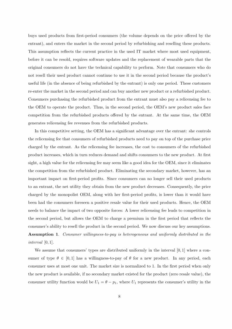
There is empirical evidence that IT customers are strategic in their purchasing behavior (Song

and Chintagunta 2003, Nair 2004, Plambeck and Wang 2006). Accordingly, we assume that cus-

tomers take into account the future resale value of the product in making their purchase decisions.

This is facilitated in practice by the existence of IT consulting companies that offer resale value

forecasts. In our model, consumer θ chooses to sell the used product to the entrant for a price s,

as long as this value is greater than the disutility γθ. Therefore, a strategic consumer of type θ

derives a net utility of U1(θ) = θ− p1 + (s− γθ)I(s≥γθ) from purchasing a new product in period 1,

where I(s≥γθ) = 1 when s ≥ γθ and 0 otherwise. The reason for the indicator variable in the utility

expression is that the consumers with a large disutility for selling their old unit to the entrant

choose not to do so.

Figure 1: Consumer state space and corresponding utilities from selling versus not selling the usedproduct,

As shown in Figure 1, contingent on their type, first-period consumers fall in one of three

segments. If θ ≤ p1−s1−γ , consumers do not purchase the new product, while for p1−s

1−γ < θ ≤ sγ ,

consumers purchase the new product and subsequently resell it. Finally, for sγ < θ ≤ 1, consumers

purchase the new product and do not resell it. Therefore, the total sales quantity in period 1 is

q1 = 1− p1−s1−γ , or, p1 = (1− γ)(1− q1) + s, and the total number of units acquired by the entrant

is given by qu = sγ − p1−s

1−γ . Note that the entrant would never set s > γ, as s = γ is sufficient to

ensure all consumers sell their used products (qu = q1).

Assumption 5. The OEM charges a relicensing fee h in the second period to any consumer who

10

purchases a refurbished product.

The establishment of a relicensing fee, typically called a Digital License Agreement (DLA),

has been widely employed by OEMs as a means of protecting their intellectual property rights.

A DLA allows a consumer to re-install the necessary software for the equipment to operate and

thus, a refurbished product is of no use without it. OEMs publish list prices for new equipment

(that implicitly includes both hardware and software cost) and most publish a separate list where

their relicensing policies are explicitly laid out. The relicensing fee, declared in the first period,

constitutes an important element of our model, since it affects the resale value, which is taken into

account by strategic consumers of new products.

The utility that each consumer derives from purchasing a refurbished product is given by the

difference of their willingness-to-pay and the price plus the relicensing fee. Let p2 and pr denote the

second-period prices of new and refurbished products, respectively. The corresponding consumer

utilities obtained by purchasing each type of product in the second-period are U2 = θ − p2 for the

new product and Ur = δθ − pr − h for the refurbished product. From these utility functions, and

letting q2 and qr represent the second-period quantities of new and refurbished product respectively,

the inverse demand functions are

p2 = 1− q2 − δqr

pr = δ(1− qr − q2)− h.

4 Analysis

In this section, we present our baseline analysis of a single OEM who sells a new product in the

first period and charges a relicensing fee for refurbished products that are acquired, refurbished

and resold by a single entrant in the second period. Under this scenario, we find that unless the

per unit refurbishing cost of the entrant is above a threshold, it is not optimal for the OEM to

charge a relicensing fee that is so high that it effectively eliminates the secondary market. Recall

that the timeline is as follows. In the first period, the OEM is the only firm in the market and

only sells the new product. At the end of the first period, the entrant buys used products from a

portion of the consumers who purchased the new product and resells them as refurbished products

in the second period to lower willingness-to-pay consumers. The OEM also sells new products in

the second period and faces cannibalization from the refurbished units. We solve the problem by

backward induction, starting with the second period.

11

Let Π2 and Πe denote the OEM’s and the entrant’s second-period profit, respectively. At this

stage, the OEM decides the quantity of new products that she will sell in the market, while the

entrant decides both the price s that he will offer to the consumers to obtain their used products,

as well as the quantity of refurbished products that he will make available in the market, denoted

by qr. The unit production cost is c < 1, and the unit refurbishing cost is cr < c.

The OEM’s second-period objective given the entrant’s choice of qr is

Maxq2 Π2(q2|qr) = (p2 − c)q2 + hqr = (1− q2 − δqr − c) q2 + hqr s.t. q2 ≥ 0. (1)

The first part of (1) captures the profit obtained from selling q2 units of new products while the

second part represents the profit from the relicensing fee (h), obtained from the qr customers who

purchase the refurbished units from the entrant. The quantity of new products to sell is the only

decision variable for the OEM in the second period as the relicensing fee is set in the first period.

The entrant’s corresponding objective given the OEM’s choice of q2 is

Maxqr,s Πe(qr, s|q2)=(pr − cr)qr − squ s.t. 0 ≤ qr ≤ qu (2)

where qu =s

γ− p1 − s

1− γ.

The constraint in (2) ensures the quantity of refurbished product is no greater than the number of

units collected from the consumers at a resale price of s, given by qu = sγ − p1−s

1−γ (see Figure 1).

In practice, the amount collected falls far short of the volume of existing used products, so we do

not explicitly model the constraint qu ≤ q1 and limit the analysis to parameters where q∗u ≤ q∗1 in

equilibrium. Where appropriate, the potential effect of this constraint is discussed. The following

lemmas characterize the price the entrant will pay for the used units.

Lemma 1 At optimality, the entrant has no incentive to collect more units than the ones he intends

to sell in the market. That is, the constraint qr ≤ qu is binding and the optimal resale price offered

by the entrant satisfies

s∗(qr) = γ(1− γ)qr + γp1. (3)

Proof All proofs are provided in Appendix A.

Lemma 2 For equilibria where both new and refurbished products co-exist in period 2, the equi-

librium resale value is given by s∗(q1, h) = γδc−γ[2γ(1−γ)+δ(2−δ)]q1−2γ(h−cr)2γ(2−γ)+δ(4−δ) while the corresponding

12

second-period quantities are q∗2(q1, h) = δh−γδq1−δ(δ−γ)+δcr−(1−c)[γ(γ−2)−2δ]2γ(2−γ)+δ(4−δ) and

q∗r (q1, h) = 2γq1−2h−2(γ+cr)+δ(1+c)2γ(2−γ)+δ(4−δ) .

The second lemma reveals two interesting properties of the equilibrium resale value. First, s∗

decreases in the quantity of new products sold in the first period. This observation is consistent

with the resale values we observe in practice; whenever a large supply of a specific used model

becomes available, its resale value drops dramatically. Second, s∗ increases as the relicensing fee h

decreases: A low value of h means a higher profit potential from the secondary market, thus the

entrant is willing to offer a higher resale price to first-period consumers. In addition, the entrant’s

decision of whether to enter the market or not is directly related to the relicensing fee h, since the

latter affects the profitability of refurbished products. Therefore, the OEM acts as a Stackelberg

leader who decides between allowing the existence of a secondary market or not by her choice of h.

To characterize the optimal OEM strategy, we need to examine the total profit across both periods.

Thus, we now move to the OEM’s first-period decisions.

In the first period, the OEM’s decisions include the quantity of new units to sell as well as the

relicensing fee to announce. More specifically, the OEM’s problem is

Maxq1,h Π(q1, h) = Π1(q1, h) + Π∗2(q1, h) s.t. q1 ≥ 0, h ≥ 0, (4)

where Π1(q1, h) denotes the profit from the sales of new products in the first period.

Π1(q1, h)= [p1(q1, h)− c] q1 = [(1− γ)(1− q1) + s∗(q1, h)− c] q1,

where s∗(q1, h) is characterized in Lemma 2. Although we ignore discounting in our formulation,

the addition of a discount factor to the second-period profit does not fundamentally change our

results, but reinforces the resale value effect, as the OEM cares more about first-period profits.

We are now ready to state our main result for this section. The following proposition states

that as long as the refurbishing cost is below a threshold value, the OEM is always better off by

maintaining a secondary market for her products.

Proposition 1 For cr < c(δ − γ), A) It is not optimal for the OEM to eliminate the secondary

market: q∗r > 0; B) The OEM charges a positive relicensing fee: h∗(δ, γ, c, cr) > 0; C) For c ≥c(δ, γ, cr)

.= δ(8−3δ+2cr)+8γ(1−γ)δ (8−δ−2γ)+8γ(1−γ) , the OEM does not sell any new products in the second period

(q∗2 = 0); and for cr ≥ c(δ − γ), there is no market for refurbished products (q∗r = 0).

13

Part A in Proposition 1 may appear counter-intuitive at first glance; as the entrant becomes

more competitive in relation to the OEM (cr decreases in relation to c), the OEM chooses not

to eliminate the secondary market. In fact, this result is counter to the previous results in the

remanufacturing competition paper of Ferguson and Toktay (2006) who find that as the entrant

becomes more competitive (cr becomes lower) and the cannibalization threat increases, the OEM

should increase her efforts to deter the secondary market. The difference in these findings is driven

by the inclusion of the positive effect of a strong secondary market on the utility of the first-

period customers (the resale value effect) in the current model. This new result demonstrates the

importance of including the resale value effect in an OEM’s secondary market strategy and warns

against the common perception of many OEMs that competition from an outside firm through the

secondary market is always detrimental to their profits.

The other interesting observation about part A of proposition 1 is the condition crc ≤ (δ − γ).

Ferguson and Koenigsberg (2007) explore when an OEM should sell a depreciated used product

that incurs holding cost cr, but no acquisition cost, in competition with new units of the same

product (no external competition). They show that offering both versions of the product is prof-

itable when crc ≤ δ. Note that both conditions compare the relative cost advantage (cr

c ) with the

consumers’ relative willingness-to-pay. In our model, however, this relative willingness-to-pay for

the refurbished product versus the new product is discounted by the consumer’s disutility from

returning the product, which acts as an acquisition cost for the entrant and therefore a barrier to

the profitability of the secondary market. Thus, when γ = 0 (all customers return the product

for free) the OEM’s decision to facilitate a secondary market is the same as if she were selling the

refurbished product herself. At the other extreme, when γ = δ (the entrant must pay an amount

equal to the consumer’s willingness-to-pay for a refurbished product to acquire the old units), there

is no secondary market because it is not profitable for the entrant at any value of cr.

Part B states that even though the OEM allows the secondary market to exist, she does so

while charging a positive relicensing fee. Thus, the common practice of IT companies charging

relicensing fees has some theoretical merit. Part C states the optimal policy depends on the unit

production cost. If the production cost is above a certain threshold (c ≥ c(δ, γ, cr)), the OEM is

better off completely abstaining from the second period (q∗2 = 0), and therefore, fully promoting

the secondary market and reaping the benefit of the resale value effect. The latter result has some

similarities with the seminal paper of Bulow (1982) on the incentives of a durable good monopolist

to invest in reducing his unit production cost. He shows that as the production cost increases, the

14

monopolist sells fewer new products in the second period, which in turn, raises the prices of new

products sold in the first period. In contrast, for low values of the production cost (c < c(δ, γ, cr)),

the OEM is in a stronger competitive position vis-a-vis the entrant and maximizes her profits by

a more aggressive competition strategy in the second period. The gain in market share outweighs

the loss in first-period profits.

Lastly, the condition cr ≥ c(δ − γ) merits further clarification. In particular, for c(δ − γ) ≤cr ≤ 1

2 ( δ − γ) (1 + c), the OEM sets h∗ > 0 so as to eliminate the secondary market (q∗r = 0) since

the high refurbishing cost prevents the entrant from offering a high enough resale price. Hence, the

resale value benefit from maintaining an active secondary market does not outweigh the detrimental

effect of cannibalization. For even higher values of the refurbishing cost, cr > 12 ( δ − γ) (1+ c), the

secondary market is not viable: q∗r = 0 even if the relicensing fee was set to zero. We now focus on

the most interesting case where the refurbishing cost is low, cr < c(δ − γ), and examine how the

optimal relicensing fee changes with respect to the consumer and product characteristics.

Corollary 1 When cr < c(δ − γ), the optimal relicensing fee h∗ increases in δ and decreases in γ.

If the OEM participates in the market in the second period, c < c(δ, γ, cr), then h∗ decreases in c,

otherwise it does not depend on c.

The relationship between δ and h∗ is to be expected: All else being equal, when consumers value

the refurbished product more, the OEM can charge a higher fee for licensing the software to use it.

Similarly, the more willing they are to return their products (lower γ), the lower the procurement

cost for the entrant, and therefore the OEM can charge more for the relicensing fee without affecting

the positive impact of the secondary market on her profits. Interestingly, when the OEM produces

new products in the second period, a higher production cost leads to lower marginal profits from

selling new products and shifts the OEM’s focus to exploiting the resale value effect by decreasing

h∗. The OEM produces fewer new products since production is more expensive, but she charges a

higher premium for them in the first period. In contrast, when the OEM abstains from the market

in the second period, the optimal relicensing fee does not depend on c.

5 Extensions

Our key finding from our baseline model was that unless the refurbishing cost is high enough, the

IT OEM is better off by maintaining an active secondary market. Through this secondary market,

15

consumers of new products enjoy a higher net utility, and the OEM is able to charge a higher

price for her new products. This result clearly highlights the importance of an active secondary

market on the OEM’s profitability and questions the validity of strategies aiming to shut down the

secondary market.

To further explore how specific market conditions and customer characteristics affect the OEM’s

optimal strategy, we relax three key assumptions of our baseline model. First, we examine the case

of non-strategic customers who do not take into account the resale value when they purchase a new

product. We find that when consumers are non-strategic, it is optimal for the OEM to eliminate

the secondary market under a much wider range of conditions (e.g. even for zero refurbishing

cost). Second, we increase the competitive intensity within the secondary market by allowing more

than one entrant to collect and resell the used products. Interestingly, we find that the OEM

lowers her relicensing fee to further stimulate procurement competition among the entrants. This,

in turn, leads to higher resale values for the consumers and, as a result, the OEM’s profits are

concave increasing in the number of entrants. Thus, competition among the entrants intensifies the

positive impact of the secondary market and makes the OEM more willing to support it. Finally,

we introduce competition in both the primary and secondary markets by examining the case where

both new and refurbished products are differentiated by quality (one OEM has a brand premium

over the other OEM). By doing so, we can directly compare the optimal pricing and relicensing

schemes of different OEMs as well as the corresponding equilibrium quantities for each market

segment. We find that the high-end OEM always charges a significantly higher relicensing fee than

the low-end OEM. Thus, a high relicensing fee need not be indicative of an attempt to shut down

the secondary market, but could reflect the brand premium of the high-end OEM instead. This

result may help explain the large range of relicensing fees observed in practice.

5.1 Non-strategic consumers

In this subsection, we examine the case where the first-period consumers act non-strategically (they

do not take into account the potential resale value of the product during their first-period purchase

decisions). In terms of the utility of first-period consumers, acting myopically means the derived

utility is given by U1 = θ−p1 and only consumers with θ ≥ p1 will buy the product. At the end of the

first period, consumers will resell their products as long as s ≥ θγ, or, θ ≤ sγ . Therefore, the total

supply of used products for a given resale price s is qu,non−strategic = sγ −p1 < s

γ − p1−s1−γ = qu,strategic

(see Figure 1). The following proposition provides the condition for when the OEM will eliminate

16

the secondary market.

Proposition 2 For cr < c(δ − γ)− 12γ(1− c), A) It is not optimal for the OEM to eliminate the

secondary market: q∗r > 0; B) The OEM charges a positive relicensing fee h∗(δ, γ, c, cr) > 0; C) For

c ≥ c(δ, γ, cr).= δ(8−3δ+2cr−γ)+γ(8−γ)

δ (8−δ−γ)+γ(8−γ) , the OEM does not sell any new products in the second period

(q∗2 = 0), and for cr ≥ c(δ − γ)− 12γ(1− c), there is no market for refurbished products (q∗r = 0).

Note that the refurbishing cost threshold below which an active secondary market exists is lower

than the corresponding threshold of Proposition 1. With non-strategic customers, the benefit from

supporting a secondary market is significantly weakened and shutting down the secondary market

becomes an optimal strategy under a much wider range of conditions. According to Proposition 2,

the OEM will eliminate the secondary market even for zero refurbishing cost (cr = 0); as long as the

production of new products is relatively inexpensive (c < γ2δ−γ ). In addition, the production cost

threshold c(δ, γ, cr) above which the OEM abstains from the market in the second period is higher

than the corresponding threshold of Proposition 1. That is, a non-strategic customer base does not

allow the OEM to exploit the resale value effect and forces her to make her profits by producing new

products in the second period, despite the relatively high production cost. Moreover, it can easily

be shown that although h∗non−strategic > h∗strategic, the OEM’s profit is lower since she can no longer

charge a premium to the first-period consumers. Thus, the OEM is worse off under non-strategic

customers.

The above analysis demonstrates that a forward-looking consumer base can influence the OEM’s

secondary market strategy. The common perception in the IT industry is that historically, cus-

tomers of IT products did not take into account the future resale value in their initial purchases.

This could explain why some IT OEMs have historically deployed policies to deter the secondary

market for their products. As mentioned in the introduction however, there are indications that

customers of IT equipment are becoming increasingly concerned about resale values during their

initial purchase decisions. Our results suggest that this is not necessarily a bad trend for the OEM

but her secondary market strategies need to evolve with the market.

5.2 Competition in the secondary market (N entrants)

The significant profit opportunities to be made in the secondary market has given rise to a number

of firms founded with the sole purpose of buying and refurbishing used IT equipment (CBRon-

line.com 2005). To deepen our understanding of the optimal OEM strategy, we next study the

17

impact of competition within the secondary market. In this setting, while the OEM maintains her

monopolistic position in the market for new products, N independent entrants compete on both

acquiring the used units from the customers as well as refurbishing and reselling them. The critical

question is: How are the OEM’s profit and relicensing fee affected by an increasing number of

entrants?

To answer this question, we assume N symmetric entrants who are in Cournot competition

with each other (similar to Debo et al. 2005), and at the same time face competition from new

products under the vertical differentiation model outlined in the previous section. Thus, if we let qir

denote the quantity of refurbished products offered by entrant i, the total quantity of refurbished

products in the second period will beN∑

i=1qir. Paralleling our analysis in Section 4, the inverse

demand functions are given by

p2 = 1− q2 − δN∑

i=1

qir and pr = δ − q2δ − h− δ

N∑

i=1

qir ,

and the OEM’s second-period objective is

Maxq2 Π2 =

(1− q2 − δ

N∑

i=1

qir − c

)q2 + h

N∑

i=1

qir s.t. q2 ≥ 0 ,

while the ith entrant’s objective is

Maxqir

Πie =(pr − s− cr)qi

r

s.t.N∑

i=1qir ≤ s

γ − p1−s1−γ , and qi

r ≥ 0.

As in the baseline case, the OEM’s optimization problem is

Maxq1,h Π(q1, h) = Π1(q1, h) + Π∗2(q1, h) s.t. q1 ≥ 0, h ≥ 0,

where Π1(q1, h) = [p1(q1, h)− c] q1 denotes the profit from the sales of new products in the first

period. Because the entrants are symmetric, at equilibrium we have Q∗r

.=N∑

i=1qi ∗r = Nq1 ∗

r . As in

the single entrant case, the equilibrium resale price s∗ satisfies Nq1 ∗r = s∗

γ − p1−s∗1−γ . Solving the

problem in a similar way as the baseline case (presented in Appendix A), we obtain the following

result:

18

Proposition 3 If cr < c(δ − γ), A) The OEM allows for an active secondary market (qi ∗r > 0),

B) The OEM charges a positive relicensing fee h∗ > 0. The OEM’s total profit (Π∗OEM ) and the

total quantity of refurbished products (Q∗r) are concave increasing in N ; C) For c < c(δ, γ, cr, N) .=

[δ(4−3δ+2cr)+8γ(1−γ)]N+4δ[−δ (δ−4+2γ)−8γ(γ−1)]N−4δ , both new and refurbished products compete in the second period, and the

optimal relicensing fee is convex decreasing in N ; D) For c ≥ c(δ, γ, cr, N), the OEM does not sell

any new products in the second period (q∗2 = 0), and for cr ≥ c(δ − γ), there is no market for

refurbished products (qi ∗r = 0 ∀ i).

Proposition 3 reveals some interesting insights about the internal competition among the en-

trants and how this competition affects the consumer purchasing behavior along with the OEM’s

profit. First, note that Proposition 3 essentially has the same structure as Proposition 1. Moreover,

similar to Debo et al. (2005), the necessary condition for the OEM to allow an active secondary

market does not depend on the number of entrants. One may expect that as the number of en-

trants increases, the OEM employs a more aggressive strategy vis-a-vis the secondary market and

her profit decreases. Interestingly, however, we show the OEM’s relicensing fee is decreasing and

her profit is concave increasing in the number of entrants. Consistent with standard economic the-

ory, as the number of entrants increases, internal competition drives the prices of the refurbished

units down and the secondary market attracts more consumers (the overall quantity of refurbished

products increases). This leads to higher cannibalization of new units in the second period, but

also to a higher resale value. In fact, adding an additional entrant increases the marginal impact of

the relicensing fee on the resale value more than it increases the detrimental cannibalization effect.

As a result, the OEM charges a lower relicensing fee, providing greater support to the secondary

market. This result differs from Debo et al. (2005) who find that an increase in the competitive

intensity of the secondary market reduces both the OEM’s incentive to invest in remanufacturabil-

ity and her profit. This difference can be explained through the strategic as well as the economic

role of the relicensing fee: The OEM not only has a more powerful mechanism of controlling the

demand for refurbished products, she also derives revenues from the relicensed equipment. Finally,

the production cost threshold above which the OEM does not sell new units in the second period

is decreasing in the number of entrants: A more competitive secondary market strengthens the

impact of the resale value effect on the OEM’s profit, causing her to produce fewer units in the

second period but charging a higher price for the new units in the first period.

19

5.3 Competition in both the primary and secondary markets with quality dif-

ferentiation

Thus far, we have assumed a monopolist setting in the primary market with the competition being

restricted to the secondary market. We now relax the monopolistic primary market assumption and

develop a differentiated duopoly model where consumers place a higher value on firm A’s product

than on firm B’s product. This assumption allows us to address two critical questions: What are

the pricing and relicensing strategies of each OEM and how do they differ? What is the impact of

the brand differential on those strategies?

We capture the difference in the perceived utility between firms as follows: A consumer who

derives utility θ from a new product by firm A derives utility (1−α)θ from a new product by firm

B. Without loss of generality, we assume that α > 0 so that firm B represents the low-end firm.

The relative difference in customers’ valuations, α, is called the brand differential or the brand

premium of the high-end OEM. We also assume an equal rate of perceived utility depreciation for

both firms. That is, a consumer derives utility δθ from firm A’s refurbished product, while he

derives utility (1 − α)δθ from firm B’s. This assumption allows us to maintain the same relative

brand differential between OEMs on the secondary market. We assume that δ < (1 − α) so that

a given consumer values the low-end firm’s new product strictly more than the high-end firm’s

refurbished product. This is a reasonable assumption based on observations of the current state

of the IT industry and eliminates the trivial case where one firm dominates both the primary and

secondary markets. In addition, we normalize the cost of refurbishing to zero for both products.

This rules out refurbishing cost disparity from explaining the differences in the OEMs’ strategies

and corresponds to the more interesting cases in Propositions 1 and 3 where the existence of a

secondary market is beneficial for the OEM. Finally, we assume a perfectly competitive secondary

markets for each type of refurbished product. This implies that for any given used product purchase

prices, sA and sB, pA2,r = sA and pB

2,r = sB. While we do this for tractability, Propositions 1 and

3 suggest the structure of the optimal policy is essentially the same for any level of competitive

intensity on the secondary market.

Similar to our baseline model, we solve the problem by backward induction, starting with the

second period (Appendix B). Unlike our previous analysis, however, deriving the Nash equilib-

rium (q∗1A,h∗A, q∗1B,h

∗B) for any arbitrary set of parameters is much more complex for two reasons.

First, the profit expressions are long and do not allow easy algebraic handling. Second, and more

20

importantly, the resulting game of two OEMs with two-dimensional action spaces contains joint

constraints. In general, even for relatively simple settings (unidimensional action space), con-

strained games in which the constraints for each player, as well as his payoff function, depends on

the strategy of the other player, are difficult to solve analytically (Rosen 1965) and have received

limited attention in the literature. Rather, our approach is to solve the unconstrained game and

subsequently identify the range of parameter values in which the results are meaningful (e.g. Desai

2001). Therefore, hereafter, we focus on those parameter values for which all non-negativity con-

straints are satisfied, namely, all market segments have positive quantities in equilibrium. For those

parameters, we conduct an extensive numerical investigation and explore how the optimal OEM

strategies (relicensing fee and quantity decisions) change as a function of the brand differential. In

the numerical study, we calculate the equilibrium quantity and relicensing fee decisions for every

combination of the parameter values δ ∈ [0.3, 0.8], γ ∈ [0.01, 0.15], and c ∈ [0.01, 0.5] (discretized

in increments of 0.1, 0.03, and 0.05, respectively). We find that as long as all non-negativity con-

straints are satisfied, the insights remain the same across all the parameter combinations. These

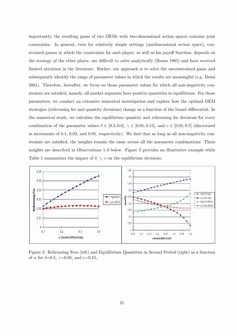
insights are described in Observations 1-3 below. Figure 2 provides an illustrative example while

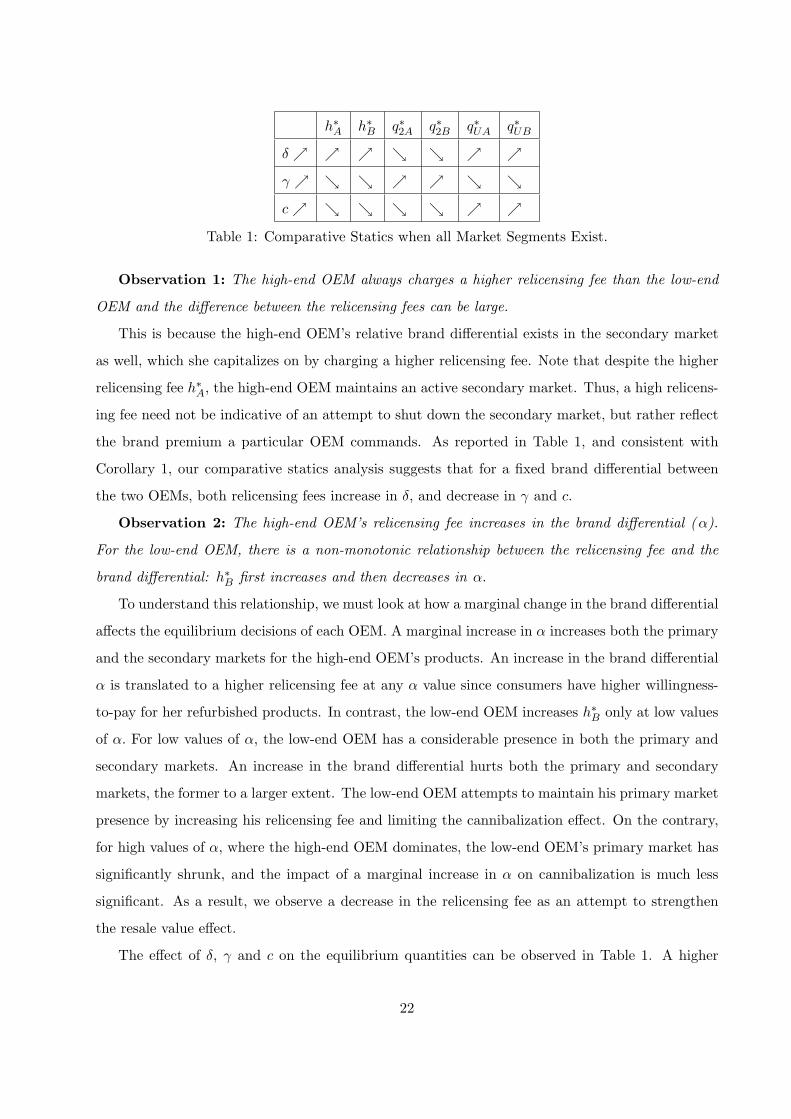
Table 1 summarizes the impact of δ, γ, c on the equilibrium decisions.

Figure 2: Relicensing Fees (left) and Equilibrium Quantities in Second Period (right) as a functionof α for δ=0.5, γ=0.05, and c=0.15,

21

h∗A h∗B q∗2A q∗2B q∗UA q∗UB

δ ↗ ↗ ↗ ↘ ↘ ↗ ↗γ ↗ ↘ ↘ ↗ ↗ ↘ ↘c ↗ ↘ ↘ ↘ ↘ ↗ ↗

Table 1: Comparative Statics when all Market Segments Exist.

Observation 1: The high-end OEM always charges a higher relicensing fee than the low-end

OEM and the difference between the relicensing fees can be large.

This is because the high-end OEM’s relative brand differential exists in the secondary market

as well, which she capitalizes on by charging a higher relicensing fee. Note that despite the higher

relicensing fee h∗A, the high-end OEM maintains an active secondary market. Thus, a high relicens-

ing fee need not be indicative of an attempt to shut down the secondary market, but rather reflect

the brand premium a particular OEM commands. As reported in Table 1, and consistent with

Corollary 1, our comparative statics analysis suggests that for a fixed brand differential between

the two OEMs, both relicensing fees increase in δ, and decrease in γ and c.

Observation 2: The high-end OEM’s relicensing fee increases in the brand differential (α).

For the low-end OEM, there is a non-monotonic relationship between the relicensing fee and the

brand differential: h∗B first increases and then decreases in α.

To understand this relationship, we must look at how a marginal change in the brand differential

affects the equilibrium decisions of each OEM. A marginal increase in α increases both the primary

and the secondary markets for the high-end OEM’s products. An increase in the brand differential

α is translated to a higher relicensing fee at any α value since consumers have higher willingness-

to-pay for her refurbished products. In contrast, the low-end OEM increases h∗B only at low values

of α. For low values of α, the low-end OEM has a considerable presence in both the primary and

secondary markets. An increase in the brand differential hurts both the primary and secondary

markets, the former to a larger extent. The low-end OEM attempts to maintain his primary market

presence by increasing his relicensing fee and limiting the cannibalization effect. On the contrary,

for high values of α, where the high-end OEM dominates, the low-end OEM’s primary market has

significantly shrunk, and the impact of a marginal increase in α on cannibalization is much less

significant. As a result, we observe a decrease in the relicensing fee as an attempt to strengthen

the resale value effect.

The effect of δ, γ and c on the equilibrium quantities can be observed in Table 1. A higher

22

δ makes the secondary market more profitable, so the secondary market grows at the expense of

the primary. A higher γ makes the secondary market less profitable, so the opposite effect is seen.

Finally, a higher c lowers the profitability of new products, so the primary market shrinks and the

secondary market grows.

Observation 3: There is a threshold value for the brand differential α below which the low-end

OEM’s product makes up a larger share of the secondary market. This threshold increases as δ

decreases, γ increases, or c decreases.

Observation 3 suggests that although a positive brand differential always translates to a larger

market share in the primary market (under symmetric production costs), the same is not true for the

corresponding secondary markets. This result could explain the strategy of some high-end OEMs

who choose not to have large secondary markets for their refurbished products despite the brand

premium they command. Note also that a lower c makes the primary market more profitable, while

a lower δ or a higher γ reduces the margins of the secondary market. Thus, the above conditions

make the primary market more attractive to the high-end OEM, who has a leadership advantage,

leaving the low-end OEM to focus on the secondary market (via relicensing fees).

In our analysis, we assume an equal unit production cost for both the high-end and low-end

OEM; thus the differentiation is along the brand differential dimension. This is a reasonable as-

sumption for many IT products since they can be characterized as development-intensive-products,

i.e. products whose fixed costs of development far outweigh the unit variable costs (Krishnan and

Zhu 2006). Because our focus is on a firm’s decisions for a given product line, we do not consider

these initial fixed costs. If the assumption of equal production costs is relaxed and the high-end

OEM has a higher production cost, we expect her to decrease her relicensing fee to increase the

resale value of her primary product.

6 Conclusions

Secondary markets in the IT industry have grown steadily, forcing OEMs to form strategies to

respond to them. For products such as servers and storage devices, OEMs have a powerful mech-

anism at their disposal: instituting a software relicensing fee charged to secondary users. A high

relicensing fee can virtually shut down the secondary market, while a low relicensing fee can allow it

to thrive. The optimal strategy is not obvious: An active secondary market has an indirect positive

benefit for the OEM by increasing the product’s resale value, which in turn, increases the price

23

that can be charged for the new product (resale value effect). At the same time, it has a direct

detrimental effect as the refurbished product competes with the OEM’s new product (cannibal-

ization effect). In practice, comparable OEMs have surprisingly different relicensing fee strategies.

The existing literature on secondary markets does not provide guidance concerning this widespread

mechanism. Our paper fills this gap by contributing to the theory of secondary markets and by

providing managerial guidelines on the use of relicensing fees.

Our research makes several theoretical contributions. First, we extend the literature on the eco-

nomics of secondary markets by studying the relicensing fee mechanism. By treating the relicensing

fee as a continuous decision variable, we avoid restricting the OEM to either fully supporting or

completely shutting down the secondary market as is the case with other forms of secondary market

intervention such as leasing. Second, we model the incentives of independent entrants to purchase,

refurbish and sell the used equipment contingent on product characteristics and consumer behavior.

A novel feature is the inclusion of the consumers’ propensity to sell a used product such that the

supply of used products is determined endogenously. Third, we capture the equilibrium secondary

market strategies of competing OEMs and compare how they evolve as the brand differential be-

tween them increases. To our knowledge, our model is the first to study differentiated new and

refurbished products competing in both the primary and secondary markets. In addition, we com-

plement the rapidly growing literature on remanufacturing by linking consumers’ willingness to

pay for a new product to the potential resale value of the product at the end of use. By doing

so, we show that a market for refurbished products can benefit the OEM even if it is operated by

independent entrants.

Our results help IT OEMs think more comprehensively about their relicensing fee strategies,

along the dimensions of consumers’ awareness, refurbishing cost, production cost, attractiveness

of refurbished products, consumers’ inertia in returning products, secondary market competitive

intensity and brand differential. We find that consumers’ awareness of the resale value of the

product is a key determinant of the OEM strategy. An OEM operating in a market with strategic

customers has an incentive to support the existence of a secondary market since significant profits

can be obtained through the resale value effect and the revenues from relicensing. If, however,

customers act myopically, the OEM’s support of the secondary market should decrease since the

resale value effect may no longer outweigh the threat of cannibalization. This suggests that OEMs

should be active in promoting their products’ resale values, an approach adopted for example by

IBM (Johnson 2006).

24

A second critical factor in the OEM’s decision is the refurbishing cost. Interestingly, a low

refurbishing cost should make an OEM more willing to support her secondary market, even though

this means the entrant is more competitive. This is because the OEM can then exploit the high

margin of the secondary market through the resale value effect and the relicensing revenues. This

is especially important for an OEM with high production costs: The right combination of price

and relicensing fee allows the OEM to mitigate the low margins of new products by producing

fewer units but charging a price premium for them due to the resale value effect. Our experience

is that OEMs are very concerned with cannibalization and tend to overlook the resale value effect.

It is precisely in cases where cannibalization is a strong threat that the OEMs should embrace the

secondary market to benefit from the strong resale value effect and relicensing fee revenues.

These results highlight the strategic and economic value of an active secondary market, but

how should an OEM respond to the entry of more refurbishers? Despite the increased size of the

secondary market and competitive intensity, we show the OEM can still use the secondary market

to her advantage and further increase her profits by lowering the relicensing fee and strengthening

the resale value effect.

In practice, IT OEMs often operate in a competitive primary market. Our differentiated duopoly

model offers insights for the strategies of low-end and high-end OEMs. As we would expect, the

high-end OEM always charges a higher relicensing fee since the brand differential is maintained in

the secondary markets. In fact, the high-end OEM should monotonically increase her relicensing

fee as her brand differential is strengthened. One might expect the opposite effect for the low-

end OEM - that his relicensing fee should decrease as the brand differential increases. We find

that due to the interplay of the resale value and cannibalization effects, there is a non-monotonic

relationship between the relicensing fee of the low-end OEM and the brand differential. When the

brand differential is low, the optimal response of the low-end OEM to an increase in the brand

differential is to increase his relicensing fee and further decrease the demand for his refurbished

products. By doing so, he attempts to mitigate the losses in the primary market at the expense of

increasing his losses in the secondary market.

To conclude, our paper highlights the strategic importance of supporting an active secondary

market under a wide range of circumstances, particularly in the presence of strategic consumers

and low refurbishing costs. These conditions are valid in the IT industry today: There exist a large

number of industry analyst firms who specialize in forecasting the resale value of IT equipment

and who offer comprehensive cost/benefit analyses over the life cycle of the IT equipment. The

25

modularity of IT solutions makes refurbishment a cost-effective proposition for many products.

Thus, charging very high relicensing fees with the purpose of shutting down the secondary market,

a strategy attributed to some IT OEMs, appears to be myopic and suboptimal in the presence of

strategic consumers. At the same time, we demonstrate that charging higher relicensing fees than

its competitors need not mean a firm is doing so with the sole purpose of eliminating the secondary

market, but rather that it is capitalizing on its brand premium.

Although we believe our model to be representative of the key trade-offs in IT secondary markets,

we recognize that relicensing fee strategies may be moderated by factors beyond the scope of the

model, such as OEMs deploying a service versus product oriented strategy, or targeting specific

niche markets. We assume that the secondary market is exploited only by independent entrants

while the OEM only focuses on new product sales. In practice, however, some OEMs have developed

a strong infrastructure to collect, refurbish, and resell IT equipment. Allowing the OEM to enter

the secondary market would strengthen the case for supporting the secondary market. Finally,

we assumed there is no technological improvement in the product between the two time periods.

In the reality of the IT industry, we often observe significant improvements in quality (product

innovation) or reductions in the production cost (process innovation) between successive generations

of a product. Future research should aim to understand the interactions of balancing new product

introductions and support for the secondary market.

Acknowledgements. The authors would like to thank James Chin, Steve Hyser, Shirley Johnson,

Oded Koenigsberg, Erica Plambeck, Saibal Ray, Gilvan C. Souza, Ravi Subramanian, and Dong Jun

Wu for their insightful comments. The research was supported by NSF DMI Grant No. 0522557.

References

Anderson, S. and V. Ginsburgh. 1994. Price Discrimination via Second-Hand Markets. European Economic

Review. 38, 23-44.

Atasu A., M. Sarvary, and L. N. Van Wassenhove. 2007. Remanufacturing as a Marketing Strategy. INSEAD

Working Paper. 2007/58/TOM/MKT.

Benjamin, D. and R. Kormendi. 1974. The Interrelationship Between the Markets for New and Used Durable

Goods. Journal of Law and Economics. 17, 381-401.

Berinato, S. 2002. Good Stuff Cheap. CIO Magazine. Oct. 15. Retrieved June 14, 2007,

http://www.cio.com/archive/101502/cheap.html

Bulow, J. 1982. Durable Goods Monopolists. Journal of Political Economy. 90, 314-332.

26

CBRonline.com. 2005. Big Players Emerge in Fragmented Brokerage Market. Retrieved June 14, 2007,

http://www.cbronline.com/news archives.asp?show= 2005-09.

Cisco.com. 2007. Software Transfer and Licensing. Retrieved October 4, 2007,

http://www.cisco.com/warp/public/csc/refurb equipment/swlicense.html.

Debo, L.G., L.B. Toktay, and L. N. Van Wassenhove. 2005. Market Segmentation and Production Technology

Selection for Remanufacturable Products. Management Science. 51(8), 1193-1205.

Desai, P. 2001. Quality Segmentation in Spatial Markets: When Does Cannibalization Affect Product Line

Design? Marketing Science. 20(3), 265-283.

Desai, P and D. Purohit. 1998. Leasing and Selling: Optimal Marketing Strategies for a Durable Goods

Firm. Management Science. 44:11(Part 2), 19-34.

Desai, P., O. Koenigsberg, and D. Purohit. 2004. Strategic Decentralization and Channel Coordination.

Quantitative Marketing and Economics. 2(1), 5-22.

Desai, P., O. Koenigsberg, and D. Purohit. 2007. A Research Note on the Role of Production Lead Time

and Demand Uncertainty in Marketing Durable Goods. Management Science. 53(1), 150-158.

Ferguson, M. and O. Koenigsberg. 2007. Production and Pricing Decisions: How Should a Firm Manage a

Product With Deteriorating Quality, Production and Operations Management. 16(3), 306-321.

Ferguson, M. and L.B. Toktay. 2006. The Effect of Competition on Recovery Strategies. Production and

Operations Management. 15(3), 351-368.

Ferrer, G. and J. Swaminathan. 2006. Managing New and Remanufactured Products. Management Science.

52(1), 15-26.

Galbreth, M.R., and J.D. Blackburn. 2006. Optimal Acquisition and Sorting Policies for Remanufacturing.

Production and Operations Management. 15(3), 384-392.

Gaskins, D. W. 1974. Alcoa Revisited: The Welfare Implications of a Second Hand Market. Journal of

Economic Theory. 7, 254-71.

Gerstner, E. and J. D. Hess. 1991. A Theory of Channel Price Promotions. The American Economic Review

81, 872-886.

Gerstner, E. and J. D. Hess. 1995. Pull Promotions and Channel Coordination. Marketing Science. 14, 43-60.

Guide, Jr., V.D.R. 2000. Production Planning and Control for Remanufacturing: Industry Practice and

Research Needs. Journal of Operations Management. 18(4), 467 -483.

Guide Jr., V.D.R. and L.N. Van Wassenhove. 2001. Managing Product Returns for Remanufacturing. Pro-

duction and Operations Management. 10(2), 142-155.

Guide, Jr. V.D.R. and K. Li. 2007. Market Cannibalization of New Product Sales by Remanufactured

Products. Working Paper, Penn State University.

Hauser, W. and R. T. Lund. 2003. Remanufacturing: An American Resource. Presentation available at

http://www.bu.edu/reman/RemanSlides.pdf, Boston University, Boston, MA.

Hendel, I. and A. Lizzeri. 1999. Interfering with Secondary Markets. Rand Journal of Economics. 30, 1-21.

27

Jin, Y., A. Muriel, and Y. Lu. 2007. On the Profitability of Remanufactured Products. Working Paper,

Department of Mechanical and Industrial Engineering, University of Massachusetts, Amherst.

Johnson, S. 2006. Director of Global Assets Recovery Systems, IBM. Personal Interview.

Kandra A. 2002. Refurbished PCs: Sweet Deals of Lemons? PC World Magazine.

Krishnan, V. and W. Zhu. 2006. Designing a Family of Development-Intensive Products. Management Sci-

ence. 52(6), 813-825.

Levinthal, D. and D. Purohit. 1989. Durable Goods and Product Obsolescence. Marketing Science 8(1),

35-56.

Liebowitz, S. 1982. Durability, Market Structure, and New-Used Goods Models. American Economic Review.

72, 816-824.

Lund, R. T., F.D. Skeels. 1983. Start-up Guidelines for the Independent Remanufacturer. Center for Policy

Alternatives, Massachusetts Institute of Technology.

Majumder, P. and H. Groenevelt. 2001. Competition in Remanufacturing. Production and Operations Man-

agement. 10(2), 125-141.

Marion, J. 2004. Sun Under Fire - for Fixing Solaris OS Costs to Reduce Competition in Used Sun Market.

Association of Service and Computer Dealers International (ASCDI), June 8, Retrieved October 07,

2007, http://www.sparcproductdirectory.com/view56.html.

Miller, H.L. 1974. On Killing the Market for Used Textbooks and the Relationship Between Markets for New

and Secondhand Goods. Journal of Political Economy. 82, 612-619.

Mussa, M. and S. Rosen. 1978. Monopoly and Product Quality. Journal of Economic Theory. 18, 301-317.

Nair, H. 2004. Intertemporal Price Discrimination with Forward-looking Consumers: Application to the US

market for Console Video-games. Working Paper, Stanford Graduate School of Business.

Plambeck, E.L. and Q. Wang. 2007. Effects of E-Waste Regulation on New Product Introduction. Working

Paper, Stanford Graduate School of Business.

Ray, S., T. Boyacı, and N. Aras. 2005. Optimal Prices and Trade-in Rebates for Durable, Remanufacturable

Products. Manufacturing & Service Operations Management. 7(3), 208-228

Rosen, J.B. 1965. Existence and Uniqueness of Equilibrium Points for Concave N-person Games. Economet-

rica. 33(3), 520-534.

Rust, J. 1986. When is it Optimal to Kill off the Market for Used Durable Goods? Econometrica. 54, 65-86.

Song, S.C. and P.K. Chintagunta. 2003. A Micromodel of New Product Adoption with Heterogeneous and

Forward-looking Consumers: Application to the digital camera category. Quantitative Marketing and

Economics. 1, 371-407.

Sun.com. 2007. Sun Fire 15K Server Performance. Retrieved October 4, 2007,

http://www.sun.com/servers/highend/sunfire15k/performance.html

Thierry, M, M. Salomon, J. Van Nunen, L.N. Van Wassenhove. Strategic Issues in Product Recovery Man-

agement. California Management Review. 37(2), 114-135.

28

Vorasayan, J. and S.M. Ryan. 2006. Optimal Price and Quantity of Refurbished Products. Production and

Operations Management. 15(3), 369-383.

Waldman, M. 1996. Durable Goods Pricing When Quality Matters. Journal of Business. 69, 489-510.

Waldman, M. 1997. Eliminating the Market for Secondhand Goods: An Alternative Explanation for Leasing,

Journal of Law and Economics. 40, 61-92.

Waldman, M. 2003. Durable Goods Theory for Real World Markets. Journal of Economic Perspectives.

17(1), 131-154

Appendices

Appendix A: Proofs

Proof of Lemma 1. The entrant’s optimization problem given the OEM’s choice of q2 is

Maxqr,sΠe(qr, s|q2)= [δ(1− qr − q2)− h− cr] qr − s(s

γ− p1 − s

1− γ)

s.t. 0 ≤ qr ≤ s

γ− p1 − s

1− γ. (1)

The Lagrangian for the entrant’s problem is L(qr, s, λ1, λ2) = [δ(1− qr − q2)− h− cr] qr − s( sγ −

p1−s1−γ ) + λ1( s

γ − p1−s1−γ − qr) + µ1qr.

The Kuhn-Tucker conditions for optimality are: ∂L∂qr

= 0, ∂L∂s = 0, λ1( s

γ − p1−s1−γ − qr) = 0 and

µ1qr = 0, with 0 ≤ qr ≤ sγ − p1−s

1−γ , λ1 ≥ 0, µ1 ≥ 0.

Assume sγ − p1−s

1−γ − qr > 0. Then, at optimality, λ1 = 0. Solving ∂L∂s = 0, we get s∗ = γp1

2 , which

gives s∗γ − p1−s∗

1−γ = − p1

2(1−γ) < 0, which violates the original condition sγ − p1−s

1−γ − qr > 0.

Since this case cannot meet the KT conditions, we hereafter assume that the right constraint

in (1) is binding. Intuitively, the entrant would not be willing to acquire more used units than

the quantity she would sell in the secondary market. Rewriting this equality, we obtain s∗(qr) =

γ(1− γ)qr + γp1, where we suppress dependence on p1 determined in period 1.

Proof of Lemma 2. Based on Lemma 1 we can reduce the entrant’s problem to a single decision

variable optimization problem in qr:

MaxqrΠe= [pr − s∗(qr)− cr] qr = [pr − γ(1− γ)qr − γp1 − cr] qr s.t. qr ≥ 0. (2)

29

We also know the profit function of the OEM

Maxq2Π2(q2|qr) = (p2 − c)q2 + hqr = (1− q2 − δqr − c) q2 + hqr s.t. q2 ≥ 0. (3)

Here, Πe and Π2 are concave in qr and q2, respectively. By solving the first-order conditions

simultaneously, we can obtain the following Nash equilibrium:

q∗2(p1, h) =2(δ + γ − γ2)(1− c)− δ2 + δh + δγp1 + δcr

4γ(1− γ) + δ(4− δ)(4)

q∗r (p1, h) =δ(1 + c)− 2cr − 2h− 2γp1

4γ(1− γ) + δ(4− δ). (5)

Substituting q∗r from (5) into the expression derived in Lemma 1 gives

s∗(p1, h) =γ[(2 γ(1− γ) + δ (4− δ)]p1 − 2γ(1− γ)(h− cr) + γδ(1− γ)c

4γ(1− γ) + δ(4− δ). (6)

Recall that the quantity of new units sold in the first period by the OEM can be expressed as

q1 = 1− p1 − s

1− γ, or, p1 = (1− γ)(1− q1) + s. (7)

Substituting p1 from (7) into (6), we obtain the equilibrium price s∗ that the entrant pays the

first-period consumers to collect used products as a function of q1 and h:

s∗(q1, h) =γδc− γ[2γ(1− γ) + δ(2− δ)]q1 − 2γ(h− cr)

2γ(2− γ) + δ(4− δ). (8)

Moreover, from (6) and (7) we can rewrite (4) and (5) in terms of q1 and h:

q∗2(q1, h) =δh− γδq1 − δ(δ − γ) + δcr − (1− c)[γ(γ − 2)− 2δ]

2γ(2− γ) + δ(4− δ)(9)

q∗r (q1, h) =2γq1 − 2h− 2(γ + cr) + δ(1 + c)

2γ(2− γ) + δ(4− δ). (10)

This Nash equilibrium is valid as long as the right-hand sides of (9) and (10) are non-negative,

respectively, which can be written as h − γq1 ≥ A and h − γq1 ≤ B, where A.= (δ − γ) − cr +

(1−c)γ(γ−2)δ − 2(1− c) and B

.= −(γ + cr) + 12δ(1 + c).

Proof of Proposition 1. In period 1, the OEM chooses q1 ≥ 0 and h ≥ 0 so as to maximize

the sum of first- and second-period profits. The OEM’s second-period profit can be obtained using

30

(9 - 10) as long as q1 and h satisfy h − γq1 ≥ A and h − γq1 ≤ B. For completeness, we need to

characterize the OEM’s second-period profit outside this range, or argue that the optimal solution

will satisfy the two conditions. For a given q1, it is in fact sufficient to restrict the domain of h

to values yielding a non-negative quantity in (10), h − γq1 ≤ B, since once the secondary market

has been eliminated, increasing h does not improve the OEM’s profits. The same need not be true

however for (9); even when the OEM abstains from the primary market in the second period, he

can improve his profits by decreasing h and increasing first-period resale value, and we cannot use

the expressions in Lemma 2 to calculate second-period profits in this range (h − γq1 < A). We

proceed by enforcing h− γq1 ≤ B, but determining the optimal OEM strategy for those values of

q1 and h yielding h− γq1 ≥ A (Case A) and h− γq1 ≤ A (Case B), separately, and then combining

the results.

Case A (h− γq1 ≥ A). The OEM’s optimization problem is

Maxq1,h Π(q1, h) = Π1(q1, h)+ Π∗2(q1, h)

s.t. A ≤ h− γq1 ≤ B

q1 ≥ 0, h ≥ 0,

where Π1(q1, h) = (p1(q1, h) − c)q1 denotes the profit from the sales of new products in the first

period and Π∗2(q1, h) is calculated using (9) and (10).

The determinant of the Hessian of the objective function Π(q1, h) is 4(8δ−δ2+8γ(1−γ)[2γ(γ−2)+δ(δ−4)]2

> 0 with∂2Π(q1,h)

∂q21

< 0. Thus, the Hessian is negative definite and the profit function is concave in (q1, h).

Define the Lagrangean L(q1, h, λ1, λ2) =Π(q1, h)+λ1(h − γq1 − A) + λ2(B − h + γq1) + µ1h. The

Kuhn-Tucker conditions for optimality are:

∂L

∂q1= 0 (11)

∂L

∂h= 0 (12)

λ1(h− γq1 −A) = 0 (13)

λ2(B − h + γq1) = 0 (14)

µ1h = 0 (15)

31

and λ1 ≥ 0, λ2 ≥ 0, µ1 ≥ 0. The constraint q1 ≥ 0 will be checked separately. Note that λ1λ2 = 0,

since otherwise both constaints (13) and (14) would be binding, which is not possible.

Case A.I : λ1 = 0, λ2 6= 0, µ1 = 0.

λ2 6= 0 implies B−h∗+γq∗1 = 0. Solving the KT conditions, we obtain h∗ = 12 ( δ − γ) (1+c)−cr,

q∗1 = 12 (1 − c) > 0, and λ2 = 2 c(δ−γ)−cr

2 γ(γ−2)+δ(δ−4) with corresponding profit (1−c)2

2 . Case I is valid for

λ2 > 0 and h∗ ≥ 0, or, c(δ − γ) < cr ≤ 12 ( δ − γ) (1 + c) and represents the case of having no

refurbished products in the second period due to the high remanufacturing cost and the positive

relicensing fee.

Case A.II : λ1 = 0, λ2 6= 0, µ1 6= 0.

λ2 6= 0 implies B − h∗ + γq∗1 = 0. Moreover, µ1 6= 0 implies h∗ = 0. Solving the KT con-

ditions, we obtain q∗1 = 12

2(γ+cr)− δ(1+c)γ and µ1 = (1+c)(γ−δ)+2cr

γ2 . This case is valid for λ2 > 0.

From the expression for λ2 (omitted for brevity), we have∂λ2

∂cr= 2δ2−8δ+6γ2−8γ

(2 γ2−4 γ−4 δ+δ2)> 0, so λ2

is increasing in cr. Therefore it is sufficient to show that λ2(cr = 0) > 0. But λ2(cr = 0) =(δ−γ)[(2 γ2−4 γ−4 δ+δ2)c+4 γ2−4 γ−4 δ+δ2)]

γ2(2 γ2−4 γ−4 δ+δ2)> 0, so λ2 > 0.

We also need µ1 > 0, which is true for cr > 12 ( δ − γ) (1 + c) and represents the case of having

no refurbished products in the second period due to the high remanufacturing cost even if the OEM

sets the relicensing fee to zero. This condition also ensures that q∗1 > 0.

Case A.III : λ1 6= 0, λ2 = 0, µ1 = 0.

λ1 6= 0 implies h∗ − γq∗1 = A. Solving the KT conditions, we obtain q∗1 = 12

(1−c)(δ+2γ)δ > 0,

h∗ = 12

[4 γ(1− γ)+δ (4−γ]c+4 γ(γ−1)+2 δ(δ−cr)−δ(4+γ)δ , and λ1 = [δ (δ−8+2γ)+8γ(γ−1)]c+δ(8−3δ+2cr)+8γ(1−γ)

δ (2 γ2−4 γ−4 δ+δ2).

Case III is valid for λ1 > 0 and h∗ ≥ 0 or, c ≥ max{ δ(8−3δ+2cr)+8γ(1−γ)−δ (δ−8+2γ)−8γ(γ−1) ,

4 γ(γ−1)+2 δ(δ−cr)−δ(4+γ)4 γ(γ−1)+δ (γ−4] } =

max{cλ1 , ch∗}, where cλ1 = δ(8−3δ+2cr)+8γ(1−γ)δ (8−δ−2γ)+8γ(1−γ) and ch∗ = 4 γ(γ−1)+2 δ(δ−cr)−δ(4+γ)

4 γ(γ−1)+δ (γ−4] are the values of c

that satisfy λ1(c) = 0 and h∗(c) = 0, respectively. But cλ1−ch∗ = − 2δ(4γ2−4γ+δ γ−4 δ+δ2)(δ−γ−cr)(8 γ2−8 γ+2δ γ−8 δ+δ2)(4 γ2−4 γ−4 δ+δγ)

>

0 because c(δ − γ) > cr (for if we assume that c(δ − γ) ≤ cr, λ1 < 0 and this case becomes

impossible) and c < 1. Therefore, max{cλ1 , ch∗} = cλ1 and h∗ > 0.

Case III represents the case of having no new products in the second period due to the high unit

production cost, but charging a positive relicensing fee, and is valid for c > δ(8−3δ+2cr)+8γ(1−γ)δ (8−δ−2γ)+8γ(1−γ) .

Case A.IV : λ1 6= 0, λ2 = 0, µ1 6= 0.

λ1 6= 0 implies h∗ − γq∗1 = A. Moreover, µ1 6= 0 implies h∗ = 0. Solving the KT conditions, we

obtain q∗1 = −δ2+[2(1−c)+(γ+cr)]δ+γ(2−γ)(1−c)δ and µ1 = − [4 γ(1− γ)+δ (4−γ]c+4 γ(γ−1)+2 δ(δ−cr)−δ(4+γ)

δ γ2 .

Case IV is valid for λ1 > 0 and µ1 > 0. However, µ1 is linearly decreasing in c, λ1 is linearly

increasing in c, and cµ1 < cλ1 . Therefore, λ1 and µ1 can never be positive at the same time, and

32

this case is impossible.

Case A.V : λ1 = 0, λ2 = 0, µ1 = 0.

Solving the KT conditions we obtain h∗ = 12

δ2(δ−γ)c−8 γ2(γ−1+cr−δ) +4 δ2(2+cr)−8 cr(γ+δ)+3 δ2(γ− δ)8 γ(γ−1)+3 δ2−8 δ

,

q∗1 = 12

[−3 δ2+8 δ−4 γ(γ+δ−2)]c+4 γcr+8(γ2−γ−δ)+3 δ2

8 γ(γ−1)+3 δ2−8 δ, q∗2 = 1

2[δ (δ−8+2γ)+8γ(γ−1)]c+δ(8−3δ+2cr)+8γ(1−γ)

8 γ(γ−1)+3 δ2−8 δ, and

q∗r = 2(cr−c(δ−γ))8 γ(γ−1)+3 δ2−8 δ

. We can see that q∗2 ≥ 0 for c ≤ cq∗2 = δ(8−3δ+2cr)+8γ(1−γ)δ (8−δ−2γ)+8γ(1−γ) , while q∗r ≥ 0

for cr ≤ c(δ − γ). Moreover, h∗ ≥ 0 for c ≤ ch∗ = 8 γ2(γ−1+cr−δ) +4 δ2(2+cr)−8 cr(γ+δ)+3 δ2(γ− δ)δ2(δ−γ)

.

But ch∗ − cq∗2 = − (3δ2−8δ+8γ2)(δ2−4δ+δγ−4γ+4γ2)(δ−γ−cr)δ2(δ−γ)(δ2−8δ+2δγ−8γ+8γ2)

> 0 and therefore this case is valid for

c ≤ δ(8−3δ+2cr)+8γ(1−γ)δ (8−δ−2γ)+8γ(1−γ) . Case V represents the case where both new and refurbished products exist

in the second period with a positive relicensing fee.

Case A.VI : λ1 = 0, λ2 = 0, µ1 6= 0.

Here q∗2 > 0 and h∗ = 0. This case was also found to be impossible because q∗2µ1 < 0. Another

of way of seeing this is to note that both q∗2 and h∗ decrease in c, but as c increases, it is always

q∗2 that becomes zero first (ch∗ > cq∗2 ). Therefore the case of q∗2 > 0 and h∗ = 0 is not possible.

Case B (h−γq1 ≤ A). Solving for the Nash equilibrium in the second period under this condition,

we obtain q∗2(q1, h) = 0 and q∗r (q1, h) = γq1−h+δ−γ−cr

2(δ+γ)−γ2 . The OEM’s optimization problem is:

Maxq1,h Π(q1, h) = Π1(q1, h) + hq∗r (q1, h) = (p1(q1, h)− c)q1 + hγq1 − h+δ − γ − cr

2(δ + γ)− γ2(16)

s.t. h− γq1 ≤ A (17)

h− γq1 ≤ B (18)

q1 ≥ 0, h ≥ 0.

Note that since A < B, constraint (18) will never be binding at the optimal solution, and

therefore can be eliminated. Solving the constrained maximization problem, we have the following

cases:

Case B.I : For c ≥ δ(8−3δ+2cr)+8γ(1−γ)δ (8−δ−2γ)+8γ(1−γ) , constraint (17) is non-binding and the optimal values are

q∗1 = 14

δ(2+γ)+2γ(1−γ)−γcr−(2γ+2δ−γ2)cδ+γ−γ2 and h∗ = 1

2(δ − γ − cr), yielding q∗r = 14

δ−γc−cr

δ+γ−γ2 . In this

parameter range, cr < c(δ − γ), which is in turn less than δ − γ, so h∗ > 0, q∗r > 0 and q∗1 > 0.

Case B.II : For c ≤ δ(8−3δ+2cr)+8γ(1−γ)δ (8−δ−2γ)+8γ(1−γ) , constraint (17) is binding and the optimal values are

q∗1 = 12

(1−c)(δ+2γ)δ , h∗ = 1

2[4 γ(1− γ)+δ (4−γ]c+4 γ(γ−1)+2 δ(δ−cr)−δ(4+γ)

δ , yielding q∗r = 1−cδ . Note that

this case yields the same optimal solution and objective function value with Case A.III.

33

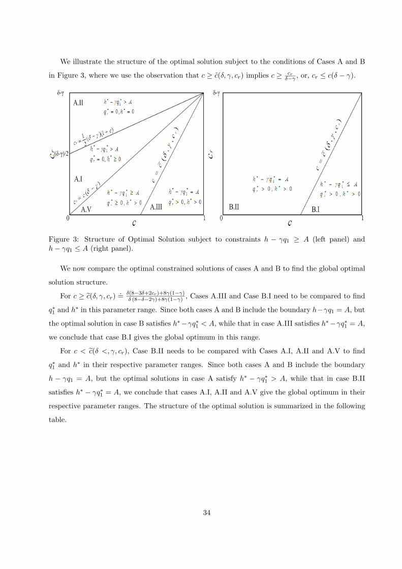
We illustrate the structure of the optimal solution subject to the conditions of Cases A and B

in Figure 3, where we use the observation that c ≥ c(δ, γ, cr) implies c ≥ crδ−γ , or, cr ≤ c(δ − γ).

Figure 3: Structure of Optimal Solution subject to constraints h − γq1 ≥ A (left panel) andh− γq1 ≤ A (right panel).

We now compare the optimal constrained solutions of cases A and B to find the global optimal

solution structure.

For c ≥ c(δ, γ, cr).= δ(8−3δ+2cr)+8γ(1−γ)

δ (8−δ−2γ)+8γ(1−γ) , Cases A.III and Case B.I need to be compared to find

q∗1 and h∗ in this parameter range. Since both cases A and B include the boundary h−γq1 = A, but

the optimal solution in case B satisfies h∗−γq∗1 < A, while that in case A.III satisfies h∗−γq∗1 = A,

we conclude that case B.I gives the global optimum in this range.

For c < c(δ <, γ, cr), Case B.II needs to be compared with Cases A.I, A.II and A.V to find

q∗1 and h∗ in their respective parameter ranges. Since both cases A and B include the boundary

h − γq1 = A, but the optimal solutions in case A satisfy h∗ − γq∗1 > A, while that in case B.II

satisfies h∗ − γq∗1 = A, we conclude that cases A.I, A.II and A.V give the global optimum in their

respective parameter ranges. The structure of the optimal solution is summarized in the following

table.

34

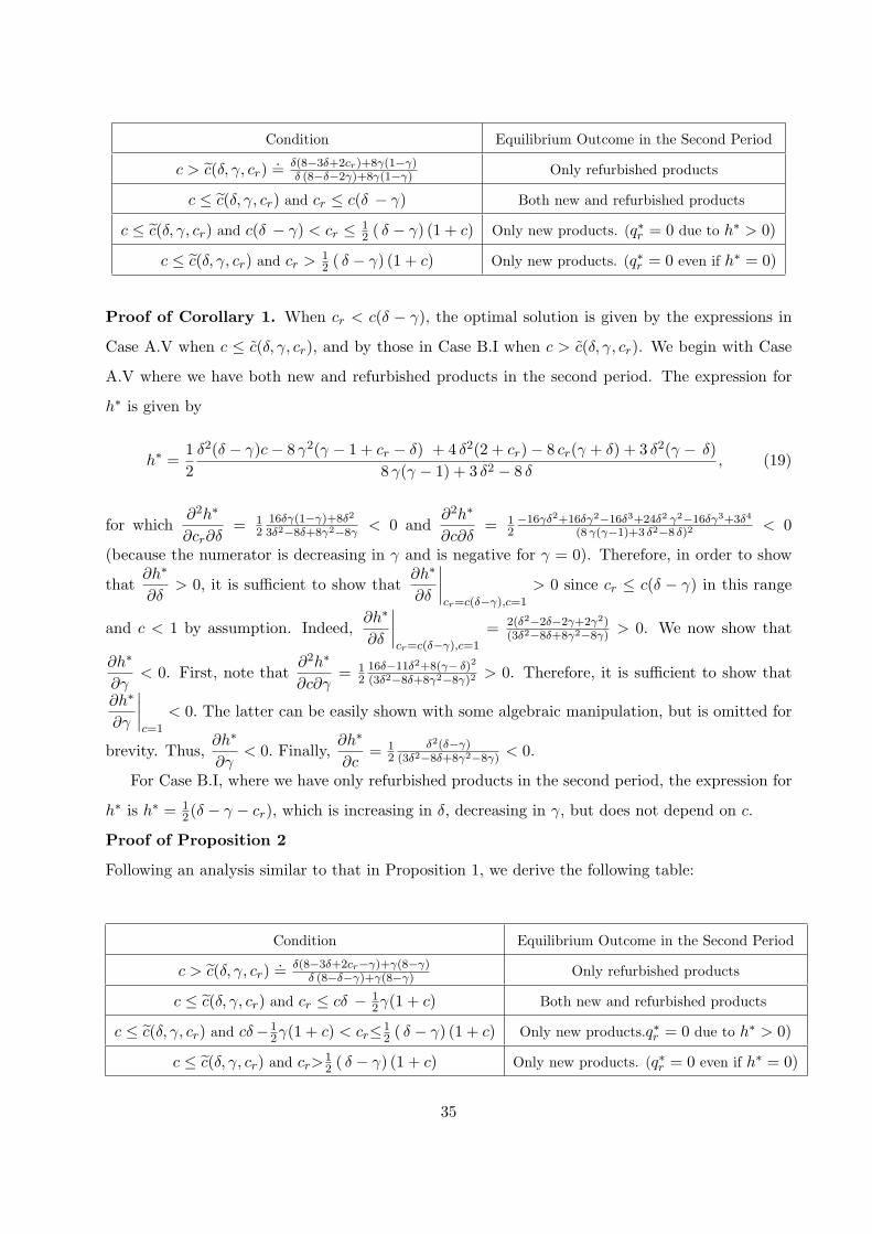
Condition Equilibrium Outcome in the Second Period

c > c(δ, γ, cr).= δ(8−3δ+2cr)+8γ(1−γ)

δ (8−δ−2γ)+8γ(1−γ) Only refurbished products

c ≤ c(δ, γ, cr) and cr ≤ c(δ − γ) Both new and refurbished products

c ≤ c(δ, γ, cr) and c(δ − γ) < cr ≤ 12 ( δ − γ) (1 + c) Only new products. (q∗r = 0 due to h∗ > 0)

c ≤ c(δ, γ, cr) and cr > 12 ( δ − γ) (1 + c) Only new products. (q∗r = 0 even if h∗ = 0)

Proof of Corollary 1. When cr < c(δ − γ), the optimal solution is given by the expressions in

Case A.V when c ≤ c(δ, γ, cr), and by those in Case B.I when c > c(δ, γ, cr). We begin with Case

A.V where we have both new and refurbished products in the second period. The expression for

h∗ is given by

h∗ =12

δ2(δ − γ)c− 8 γ2(γ − 1 + cr − δ) + 4 δ2(2 + cr)− 8 cr(γ + δ) + 3 δ2(γ − δ)8 γ(γ − 1) + 3 δ2 − 8 δ

, (19)

for which∂2h∗

∂cr∂δ= 1

216δγ(1−γ)+8δ2

3δ2−8δ+8γ2−8γ< 0 and

∂2h∗

∂c∂δ= 1

2−16γδ2+16δγ2−16δ3+24δ2 γ2−16δγ3+3δ4

(8 γ(γ−1)+3 δ2−8 δ)2< 0

(because the numerator is decreasing in γ and is negative for γ = 0). Therefore, in order to show

that∂h∗

∂δ> 0, it is sufficient to show that

∂h∗

∂δ

∣∣∣∣cr=c(δ−γ),c=1

> 0 since cr ≤ c(δ − γ) in this range

and c < 1 by assumption. Indeed,∂h∗

∂δ

∣∣∣∣cr=c(δ−γ),c=1

= 2(δ2−2δ−2γ+2γ2)(3δ2−8δ+8γ2−8γ)

> 0. We now show that

∂h∗

∂γ< 0. First, note that

∂2h∗

∂c∂γ= 1

216δ−11δ2+8(γ− δ)2

(3δ2−8δ+8γ2−8γ)2> 0. Therefore, it is sufficient to show that

∂h∗

∂γ

∣∣∣∣c=1

< 0. The latter can be easily shown with some algebraic manipulation, but is omitted for

brevity. Thus,∂h∗

∂γ< 0. Finally,

∂h∗

∂c= 1

2δ2(δ−γ)

(3δ2−8δ+8γ2−8γ)< 0.

For Case B.I, where we have only refurbished products in the second period, the expression for

h∗ is h∗ = 12(δ − γ − cr), which is increasing in δ, decreasing in γ, but does not depend on c.

Proof of Proposition 2

Following an analysis similar to that in Proposition 1, we derive the following table:

Condition Equilibrium Outcome in the Second Period

c > c(δ, γ, cr).= δ(8−3δ+2cr−γ)+γ(8−γ)

δ (8−δ−γ)+γ(8−γ) Only refurbished products

c ≤ c(δ, γ, cr) and cr ≤ cδ − 12γ(1 + c) Both new and refurbished products

c ≤ c(δ, γ, cr) and cδ−12γ(1 + c) < cr≤1

2 ( δ − γ) (1 + c) Only new products.q∗r = 0 due to h∗ > 0)

c ≤ c(δ, γ, cr) and cr>12 ( δ − γ) (1 + c) Only new products. (q∗r = 0 even if h∗ = 0)

35

Proof of Proposition 3. Let Q−ir =

N∑j=1,j 6=i

qjr . Then we can rewrite the OEM’s and entrants’

problems as :

Maxq2Π2 =(1− q2 − δqi

r − δQ−ir − c

)q2 + h(qi

r + Q−ir )

s.t. q2 ≥ 0

MaxqirΠe =(δ − q2δ − h− δqi

r − δQ−ir − s− cr)qi

r

s.t. qir + Q−i

r ≤ sγ − p1−s

1−γ

qir ≥ 0

The FOC with respect to q2 and qir give

−2q∗2 + 1− δqi∗r − δQ−i∗

r − c = 0

δ − q∗2δ − h− 2δqi∗r − δQ−i∗

r − s− cr = 0.

Since we assume N symmetric entrants, Q−i∗r = (N − 1)qi∗

r and the FOC can be rewritten as

−2q∗2 + 1− δNqi∗r − c = 0 (20)

δ − q∗2δ − h− δ(N + 1)qi∗r − s− cr = 0. (21)

In addition, the market clearing price s∗ satisfies

Nqi∗r =

s∗

γ− p1 − s∗

1− γ. (22)

Solving (20), (21), and (22) simultaneously, we obtain the equilibrium quantities for the second

period for the case where both new and refurbished products exists in the market.

From hereafter we proceed as in the case of one entrant since from the OEM’s standpoint,

what determines the optimal policy is the aggregate demand for refurbished products (Nqi∗r ) in the

second period. Following an analysis similar to that in Proposition 1, we derive the following table:

Condition Equilibrium Outcome in the Second Period

c > c(δ, γ, cr, N) .= [δ(4−3δ+2cr)+8γ(1−γ)]N+4δ[δ (4−δ−2γ)+8γ(1−γ)]N+4δ Only refurbished products

c ≤ c(δ, γ, cr, N) and cr ≤ c(δ − γ) Both new and refurbished products

c ≤ c(δ, γ, cr, N) and c(δ − γ) < cr≤12 ( δ − γ) (1 + c) Only new products. (q∗r = 0 due to h∗ > 0)

c ≤ c(δ, γ, cr, N) and cr >12 ( δ − γ) (1 + c) Only new products. (q∗r = 0 even if h∗ = 0)

36

Note that the threshold value for the remanufacturing cost below which the secondary market

exists remains the same as in the case of one entrant (cr < c(δ−γ)). The production cost threshold

c.= [δ(4−3δ+2cr)+8γ(1−γ)]N+4δ

[δ (4−δ−2γ)+8γ(1−γ)]N+4δ above which the OEM does not sell new units in the second period

now decreases in N : ∂c∂N = − 8δ2(δ−γ−cr)

[(δ (4−δ−2γ)+8γ(1−γ))N+4δ]2< 0.

For c < c, the optimal values are:

q∗2 =12

[(δ (4− δ − 2γ) + 8γ(1− γ))c− δ(4− 3δ + 2cr)− 8γ(1− γ)]N − 4δ(1− c)[8γ(1− γ) + 4 δ − 3 δ2]N + 4 δ

qi∗r =

2(c(δ − γ)− cr)[8γ(1− γ) + 4 δ − 3 δ2]N + 4 δ

∂h∗

∂N= −2

δ3 ((δ − γ) c− cr)[4Nγ(1− γ) + 3 δN(1− δ) + δ (N + 4) ]2

< 0

∂2h∗

∂N2= 4

δ3 ((δ − γ) c− cr) [4 γ(1− γ) + 3 δ(1− δ) + δ][4Nγ(1− γ) + 3 δN(1− δ) + δ (N + 4) ]3

> 0

∂Π∗OEM

∂N=

4δ[(δ − γ) c− cr][4Nγ(1− γ) + 3 δN(1− δ) + δ (N + 4) ]2

> 0

∂2Π∗OEM

∂N2= −8

δ[(δ − γ) c− cr][4 γ(1− γ) + 3 δ(1− δ) + δ][4Nγ(1− γ) + 3 δN(1− δ) + δ (N + 4) ]3

< 0

For c ≥ c, the optimal values are:

q∗2 = 0

qi∗r =

12

(δ − γc− cr)δ(N + 1) + Nγ(1− γ)

h∗ =12(δ − γ − cr)

∂Π∗OEM

∂N=

14

δ(δ − γc− cr)2

[δ(N + 1) + Nγ(1− γ) ]2> 0

∂2Π∗OEM

∂N2= −1

2δ(δ + γ − γ2))(δ − γc− cr)

2

[δ(N + 1) + Nγ(1− γ) ]3< 0

37

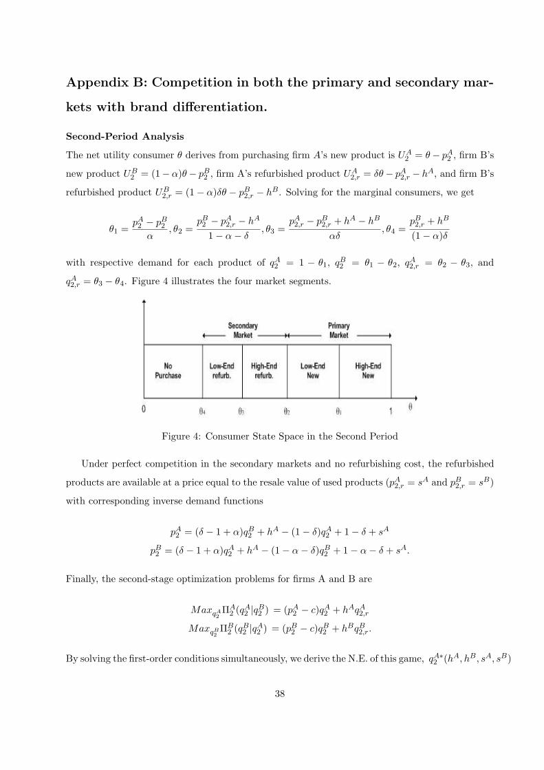
Appendix B: Competition in both the primary and secondary mar-

kets with brand differentiation.

Second-Period Analysis

The net utility consumer θ derives from purchasing firm A’s new product is UA2 = θ− pA

2 , firm B’s

new product UB2 = (1−α)θ− pB

2 , firm A’s refurbished product UA2,r = δθ− pA

2,r − hA, and firm B’s

refurbished product UB2,r = (1− α)δθ − pB

2,r − hB. Solving for the marginal consumers, we get

θ1 =pA2 − pB

2

α, θ2 =

pB2 − pA

2,r − hA

1− α− δ, θ3 =

pA2,r − pB

2,r + hA − hB

αδ, θ4 =

pB2,r + hB

(1− α)δ

with respective demand for each product of qA2 = 1 − θ1, qB

2 = θ1 − θ2, qA2,r = θ2 − θ3, and

qA2,r = θ3 − θ4. Figure 4 illustrates the four market segments.

Figure 4: Consumer State Space in the Second Period

Under perfect competition in the secondary markets and no refurbishing cost, the refurbished

products are available at a price equal to the resale value of used products (pA2,r = sA and pB

2,r = sB)

with corresponding inverse demand functions

pA2 = (δ − 1 + α)qB

2 + hA − (1− δ)qA2 + 1− δ + sA

pB2 = (δ − 1 + α)qA

2 + hA − (1− α− δ)qB2 + 1− α− δ + sA.

Finally, the second-stage optimization problems for firms A and B are

MaxqA2ΠA

2 (qA2 |qB

2 ) = (pA2 − c)qA

2 + hAqA2,r

MaxqB2ΠB

2 (qB2 |qA

2 ) = (pB2 − c)qB

2 + hBqB2,r.

By solving the first-order conditions simultaneously, we derive the N.E. of this game, qA∗2 (hA, hB, sA, sB)

38

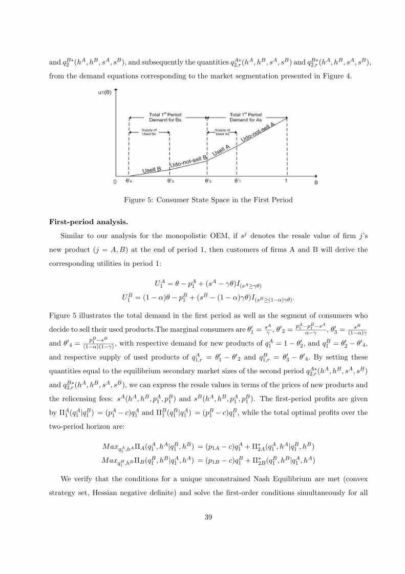
and qB∗2 (hA, hB, sA, sB), and subsequently the quantities qA∗

2,r(hA, hB, sA, sB) and qB∗

2,r (hA, hB, sA, sB),

from the demand equations corresponding to the market segmentation presented in Figure 4.

Figure 5: Consumer State Space in the First Period

First-period analysis.

Similar to our analysis for the monopolistic OEM, if sj denotes the resale value of firm j’s

new product (j = A,B) at the end of period 1, then customers of firms A and B will derive the

corresponding utilities in period 1:

UA1 = θ − pA

1 + (sA − γθ)I(sA≥γθ)

UB1 = (1− α)θ − pB

1 + (sB − (1− α)γθ)I(sB≥(1−α)γθ).

Figure 5 illustrates the total demand in the first period as well as the segment of consumers who

decide to sell their used products.The marginal consumers are θ′1 = sA

γ , θ′2 = pA1 −pB

1 −sA

α−γ , θ′3 = sB

(1−α)γ

and θ′4 = pB1 −sB

(1−α)(1−γ) , with respective demand for new products of qA1 = 1− θ′2, and qB

1 = θ′2 − θ′4,

and respective supply of used products of qA1,r = θ′1 − θ′2 and qB

1,r = θ′3 − θ′4. By setting these

quantities equal to the equilibrium secondary market sizes of the second period qA∗2,r(h

A, hB, sA, sB)

and qB∗2,r (hA, hB, sA, sB), we can express the resale values in terms of the prices of new products and

the relicensing fees: sA(hA, hB, pA1 , pB

1 ) and sB(hA, hB, pA1 , pB

1 ). The first-period profits are given

by ΠA1 (qA

1 |qB1 ) = (pA

1 − c)qA1 and ΠB

1 (qB1 |qA

1 ) = (pB1 − c)qB

1 , while the total optimal profits over the

two-period horizon are:

MaxqA1 ,hAΠA(qA

1 , hA|qB1 , hB) = (p1A − c)qA

1 + Π∗2A(qA1 , hA|qB

1 , hB)

MaxqB1 ,hBΠB(qB

1 , hB|qA1 , hA) = (p1B − c)qB

1 + Π∗2B(qB1 , hB|qA

1 , hA)

We verify that the conditions for a unique unconstrained Nash Equilibrium are met (convex

strategy set, Hessian negative definite) and solve the first-order conditions simultaneously for all

39

the decision variables to derive the values qA∗1 , hA∗, qB∗

1 , hB∗. The equilibrium is valid only for

parameters yielding positive quantities, thus, the analysis in the paper is reflective of this set. For

example, Figure 2 in the paper is plotted for α ∈ [0.1, 0.4]. The upper threshold α is the highest

value of α ∈ (0, 1 − δ) for which the low-end OEM produces new products in the second period.

That is, for values of α above that point, the low-end OEM is priced out of the primary market in

the second period (this constraint is always the first to be violated). On the other hand, the lower

threshold α = γ denotes the lowest value of α for which the ordering of the consumer state space

in Figure 5 is valid (low-end OEM’s new product above high-end OEM’s refurbished product).

40