Reliability Growth & Repairable System Data Analysis Reference ReliaSoft Corporation Worldwide Headquarters 1450 South Eastside Loop Tucson, Arizona 85710-6703, USA http://www.ReliaSoft.com Notice of Rights: The content is the Property and Copyright of ReliaSoft Corporation, Tucson, Arizona, USA. It is licensed under a Creative Commons Attribution-NonCommercial-ShareAlike 4.0 International License. See the next pages for a complete legal description of the license or go to http://creativecommons.org/licenses/by-nc-sa/4.0/legalcode.

Quick License Summary Overview

You are Free to:

Share: Copy and redistribute the material in any medium or format

Adapt: Remix, transform, and build upon the material

Under the following terms:

Attribution: You must give appropriate credit, provide a link to the license, and indicate if changes were made. You may do so in any reasonable manner, but not in any way that suggests the licensor endorses you or your use. See example at http://www.reliawiki.org/index.php/Attribution_Example

NonCommercial: You may not use this material for commercial purposes (sell or distribute for profit). Commercial use is the distribution of the material for profit (selling a book based on the material) or adaptations of this material.

ShareAlike: If you remix, transform, or build upon the material, you must distribute your contributions under the same license as the original.

Generation Date: This document was generated on May 8, 2015 based on the current state of the online reference book posted on ReliaWiki.org. Information in this document is subject to change without notice and does not represent a commitment on the part of ReliaSoft Corporation. The content in the online reference book posted on ReliaWiki.org may be more up-to-date.

Disclaimer: Companies, names and data used herein are fictitious unless otherwise noted. This documentation and ReliaSoft’s software tools were developed at private expense; no portion was developed with U.S. government funds.

Trademarks: ReliaSoft, Synthesis Platform, Weibull++, ALTA, DOE++, RGA, BlockSim, RENO, Lambda Predict, Xfmea, RCM++ and XFRACAS are trademarks of ReliaSoft Corporation. Other product names and services identified in this document are trademarks of their respective trademark holders, and are used for illustration purposes. Their use in no way conveys endorsement or other affiliation with ReliaSoft Corporation.

Attribution-NonCommercial-ShareAlike 4.0 International

License Agreement

Creative Commons Attribution-NonCommercial-ShareAlike 4.0 International Public License

By exercising the Licensed Rights (defined below), You accept and agree to be bound by the terms and conditions of this Creative Commons Attribution-NonCommercial-ShareAlike 4.0 International Public License ("Public License"). To the extent this Public License may be interpreted as a contract, You are granted the Licensed Rights in consideration of Your acceptance of these terms and conditions, and the Licensor grants You such rights in consideration of benefits the Licensor receives from making the Licensed Material available under these terms and conditions.

Section 1 – Definitions.

a. Adapted Material means material subject to Copyright and Similar Rights that is derived from or based upon the Licensed Material and in which the Licensed Material is translated, altered, arranged, transformed, or otherwise modified in a manner requiring permission under the Copyright and Similar Rights held by the Licensor. For purposes of this Public License, where the Licensed Material is a musical work, performance, or sound recording, Adapted Material is always produced where the Licensed Material is synched in timed relation with a moving image.

b. Adapter's License means the license You apply to Your Copyright and Similar Rights in Your contributions to Adapted Material in accordance with the terms and conditions of this Public License.

c. BY-NC-SA Compatible License means a license listed at creativecommons.org/compatiblelicenses, approved by Creative Commons as essentially the equivalent of this Public License.

d. Copyright and Similar Rights means copyright and/or similar rights closely related to copyright including, without limitation, performance, broadcast, sound recording, and Sui Generis Database Rights, without regard to how the rights are labeled or categorized. For purposes of this Public License, the rights specified in Section 2(b)(1)-(2) are not Copyright and Similar Rights.

e. Effective Technological Measures means those measures that, in the absence of proper authority, may not be circumvented under laws fulfilling obligations under Article 11 of the WIPO Copyright Treaty adopted on December 20, 1996, and/or similar international agreements.

f. Exceptions and Limitations means fair use, fair dealing, and/or any other exception or limitation to Copyright and Similar Rights that applies to Your use of the Licensed Material.

g. License Elements means the license attributes listed in the name of a Creative Commons Public License. The License Elements of this Public License are Attribution, NonCommercial, and ShareAlike.

h. Licensed Material means the artistic or literary work, database, or other material to which the Licensor applied this Public License.

i. Licensed Rights means the rights granted to You subject to the terms and conditions of this Public License, which are limited to all Copyright and Similar Rights that apply to Your use of the Licensed Material and that the Licensor has authority to license.

j. Licensor means ReliaSoft Corporation, 1450 Eastside Loop, Tucson, AZ 85710. k. NonCommercial means not primarily intended for or directed towards commercial

advantage or monetary compensation. For purposes of this Public License, the exchange of the Licensed Material for other material subject to Copyright and Similar Rights by digital file-sharing or similar means is NonCommercial provided there is no payment of monetary compensation in connection with the exchange.

l. Share means to provide material to the public by any means or process that requires permission under the Licensed Rights, such as reproduction, public display, public performance, distribution, dissemination, communication, or importation, and to make material available to the public including in ways that members of the public may access the material from a place and at a time individually chosen by them.

m. Sui Generis Database Rights means rights other than copyright resulting from Directive 96/9/EC of the European Parliament and of the Council of 11 March 1996 on the legal protection of databases, as amended and/or succeeded, as well as other essentially equivalent rights anywhere in the world.

n. You means the individual or entity exercising the Licensed Rights under this Public License. Your has a corresponding meaning.

Section 2 – Scope.

a. License grant. 1. Subject to the terms and conditions of this Public License, the Licensor hereby grants

You a worldwide, royalty-free, non-sublicensable, non-exclusive, irrevocable license to exercise the Licensed Rights in the Licensed Material to:

A. reproduce and Share the Licensed Material, in whole or in part, for NonCommercial purposes only; and

B. produce, reproduce, and Share Adapted Material for NonCommercial purposes only.

2. Exceptions and Limitations. For the avoidance of doubt, where Exceptions and Limitations apply to Your use, this Public License does not apply, and You do not need to comply with its terms and conditions.

3. Term. The term of this Public License is specified in Section 6(a). 4. Media and formats; technical modifications allowed. The Licensor authorizes You to

exercise the Licensed Rights in all media and formats whether now known or hereafter created, and to make technical modifications necessary to do so. The Licensor waives and/or agrees not to assert any right or authority to forbid You from making technical modifications necessary to exercise the Licensed Rights, including technical modifications necessary to circumvent Effective Technological Measures. For purposes of this Public License, simply making modifications authorized by this Section 2(a)(4) never produces Adapted Material.

5. Downstream recipients. A. Offer from the Licensor – Licensed Material. Every recipient of the Licensed

Material automatically receives an offer from the Licensor to exercise the Licensed Rights under the terms and conditions of this Public License.

B. Additional offer from the Licensor – Adapted Material. Every recipient of Adapted Material from You automatically receives an offer from the Licensor to exercise the Licensed Rights in the Adapted Material under the conditions of the Adapter’s License You apply.

C. No downstream restrictions. You may not offer or impose any additional or different terms or conditions on, or apply any Effective Technological Measures to, the Licensed Material if doing so restricts exercise of the Licensed Rights by any recipient of the Licensed Material.

6. No endorsement. Nothing in this Public License constitutes or may be construed as permission to assert or imply that You are, or that Your use of the Licensed Material is, connected with, or sponsored, endorsed, or granted official status by, the Licensor or others designated to receive attribution as provided in Section 3(a)(1)(A)(i).

b. Other rights. 1. Moral rights, such as the right of integrity, are not licensed under this Public License,

nor are publicity, privacy, and/or other similar personality rights; however, to the extent possible, the Licensor waives and/or agrees not to assert any such rights held by the Licensor to the limited extent necessary to allow You to exercise the Licensed Rights, but not otherwise.

2. Patent and trademark rights are not licensed under this Public License. 3. To the extent possible, the Licensor waives any right to collect royalties from You for

the exercise of the Licensed Rights, whether directly or through a collecting society under any voluntary or waivable statutory or compulsory licensing scheme. In all other cases the Licensor expressly reserves any right to collect such royalties, including when the Licensed Material is used other than for NonCommercial purposes.

Section 3 – License Conditions.

Your exercise of the Licensed Rights is expressly made subject to the following conditions.

a. Attribution. 1. If You Share the Licensed Material (including in modified form), You must:

A. retain the following if it is supplied by the Licensor with the Licensed Material:

i. identification of the creator(s) of the Licensed Material and any others designated to receive attribution, in any reasonable manner requested by the Licensor (including by pseudonym if designated);

ii. a copyright notice; iii. a notice that refers to this Public License; iv. a notice that refers to the disclaimer of warranties; v. a URI or hyperlink to the Licensed Material to the extent reasonably

practicable; B. indicate if You modified the Licensed Material and retain an indication of

any previous modifications; and C. indicate the Licensed Material is licensed under this Public License, and

include the text of, or the URI or hyperlink to, this Public License. 2. You may satisfy the conditions in Section 3(a)(1) in any reasonable manner based on

the medium, means, and context in which You Share the Licensed Material. For example, it may be reasonable to satisfy the conditions by providing a URI or hyperlink to a resource that includes the required information.

3. If requested by the Licensor, You must remove any of the information required by Section 3(a)(1)(A) to the extent reasonably practicable.

b. ShareAlike.

In addition to the conditions in Section 3(a), if You Share Adapted Material You produce, the following conditions also apply.

1. The Adapter’s License You apply must be a Creative Commons license with the same License Elements, this version or later, or a BY-NC-SA Compatible License.

2. You must include the text of, or the URI or hyperlink to, the Adapter's License You apply. You may satisfy this condition in any reasonable manner based on the medium, means, and context in which You Share Adapted Material.

3. You may not offer or impose any additional or different terms or conditions on, or apply any Effective Technological Measures to, Adapted Material that restrict exercise of the rights granted under the Adapter's License You apply.

Section 4 – Sui Generis Database Rights.

Where the Licensed Rights include Sui Generis Database Rights that apply to Your use of the Licensed Material:

a. for the avoidance of doubt, Section 2(a)(1) grants You the right to extract, reuse, reproduce, and Share all or a substantial portion of the contents of the database for NonCommercial purposes only;

b. if You include all or a substantial portion of the database contents in a database in which You have Sui Generis Database Rights, then the database in which You have Sui Generis Database Rights (but not its individual contents) is Adapted Material, including for purposes of Section 3(b); and

c. You must comply with the conditions in Section 3(a) if You Share all or a substantial portion of the contents of the database.

For the avoidance of doubt, this Section 4 supplements and does not replace Your obligations under this Public License where the Licensed Rights include other Copyright and Similar Rights.

Section 5 – Disclaimer of Warranties and Limitation of Liability.

a. Unless otherwise separately undertaken by the Licensor, to the extent possible, the Licensor offers the Licensed Material as-is and as-available, and makes no representations or warranties of any kind concerning the Licensed Material, whether express, implied, statutory, or other. This includes, without limitation, warranties of title, merchantability, fitness for a particular purpose, non-infringement, absence of latent or other defects, accuracy, or the presence or absence of errors, whether or not known or discoverable. Where disclaimers of warranties are not allowed in full or in part, this disclaimer may not apply to You.

b. To the extent possible, in no event will the Licensor be liable to You on any legal theory (including, without limitation, negligence) or otherwise for any direct, special, indirect, incidental, consequential, punitive, exemplary, or other losses, costs, expenses, or damages arising out of this Public License or use of the Licensed Material, even if the Licensor has been advised of the possibility of such losses, costs, expenses, or damages. Where a limitation of liability is not allowed in full or in part, this limitation may not apply to You.

c. The disclaimer of warranties and limitation of liability provided above shall be interpreted in a manner that, to the extent possible, most closely approximates an absolute disclaimer and waiver of all liability.

Section 6 – Term and Termination.

a. This Public License applies for the term of the Copyright and Similar Rights licensed here. However, if You fail to comply with this Public License, then Your rights under this Public License terminate automatically.

b. Where Your right to use the Licensed Material has terminated under Section 6(a), it reinstates:

1. automatically as of the date the violation is cured, provided it is cured within 30 days of Your discovery of the violation; or

2. upon express reinstatement by the Licensor.

For the avoidance of doubt, this Section 6(b) does not affect any right the Licensor may have to seek remedies for Your violations of this Public License.

c. For the avoidance of doubt, the Licensor may also offer the Licensed Material under separate terms or conditions or stop distributing the Licensed Material at any time; however, doing so will not terminate this Public License.

d. Sections 1, 5, 6, 7, and 8 survive termination of this Public License.

Section 7 – Other Terms and Conditions.

a. The Licensor shall not be bound by any additional or different terms or conditions communicated by You unless expressly agreed.

b. Any arrangements, understandings, or agreements regarding the Licensed Material not stated herein are separate from and independent of the terms and conditions of this Public License.

Section 8 – Interpretation.

a. For the avoidance of doubt, this Public License does not, and shall not be interpreted to, reduce, limit, restrict, or impose conditions on any use of the Licensed Material that could lawfully be made without permission under this Public License.

b. To the extent possible, if any provision of this Public License is deemed unenforceable, it shall be automatically reformed to the minimum extent necessary to make it enforceable. If the provision cannot be reformed, it shall be severed from this Public License without affecting the enforceability of the remaining terms and conditions.

c. No term or condition of this Public License will be waived and no failure to comply consented to unless expressly agreed to by the Licensor.

d. Nothing in this Public License constitutes or may be interpreted as a limitation upon, or waiver of, any privileges and immunities that apply to the Licensor or You, including from the legal processes of any jurisdiction or authority.

Contents

Chapter 1 1

RGA Overview 1

Chapter 2 8

RGA Data Types 8

Chapter 3 23

Developmental Testing 23

Chapter 3.1 26

Duane Model 26

Chapter 3.2 56

Crow-AMSAA (NHPP) 56

Chapter 3.3 107

Crow Extended 107

Chapter 3.4 160

Crow Extended - Continuous Evaluation 160

Chapter 3.5 187

Lloyd-Lipow 187

Chapter 3.6 204

Gompertz Models 204

Chapter 3.7 226

Logistic 226

Chapter 4 245

Reliability Growth Planning 245

Chapter 5 266

Operational Mission Profile Testing 266

Chapter 6 277

Fielded Systems 277

Chapter 6.1 278

Repairable Systems Analysis 278

Chapter 6.2 296

Operational Testing 296

Chapter 6.3 300

Fleet Data Analysis 300

Chapter 7 312

Simulation with RGA Models 312

Chapter 8 326

Reliability Demonstration Test Design for Repairable Systems 326

Appendix A 330

Appendix A: Failure Discounting 330

Appendix B 336

Appendix B: Hypothesis Tests 336

Appendix C 339

Appendix C: Crow-AMSAA Confidence Bounds 339

Appendix D 360

Appendix D: Crow Extended Confidence Bounds 360

Appendix E 364

Appendix E: Confidence Bounds for Repairable Systems Analysis 364

Appendix F 377

Appendix F: Glossary 377

Appendix G 381

Appendix G: References 381

1

Chapter 1

RGA Overview

IntroductionWhen conducting distribution analysis (and life data analysis), the events that are observed are assumed to bestatistically independent and identically distributed (IID). A sequence or collection of random variables is IID if:•• Each has the same probability distribution as any of the others.•• All are mutually independent, which implies that knowing whether or not one occurred makes it neither more nor

less probable that the other occurred.In life data analysis, the unit/component placed on test is assumed to be as-good-as-new. However, this is not thecase when dealing with repairable systems that have more than one life. They are able to have multiple lives as theyfail, are repaired and then put back into service. The age just after the repair is basically the same as it was justbefore the failure. This is called as-bad-as-old. For reliability growth and repairable systems analysis, the events thatare observed are part of a stochastic process. A stochastic process is defined as a sequence of inter-dependentrandom events. Therefore, the events are dependent and are not identically distributed.•• The time-to-failure of a product after a redesign is dependent on how good or bad the redesign action was.•• The time-to-failure of the product after the redesign may follow a distribution that is different than the

times-to-failure distribution before the redesign.There is a dependency between the failures that occur on a repairable system. Events that occur first will affect futurefailures. Given this dependency, applying a Weibull distribution, for example, is not valid since life data analysisassumes that the events are IID. Reliability growth and repairable systems analysis provide methodologies foranalyzing data/events that are associated with systems that are part of a stochastic process.

What is Reliability Growth?In general, the first prototypes produced during the development of a new complex system will contain design,manufacturing and/or engineering deficiencies. Because of these deficiencies, the initial reliability of the prototypesmay be below the system's reliability goal or requirement. In order to identify and correct these deficiencies, theprototypes are often subjected to a rigorous testing program. During testing, problem areas are identified andappropriate corrective actions (or redesigns) are taken. Reliability growth is defined as the positive improvement in areliability metric (or parameter) of a product (component, subsystem or system) over a period of time due to changesin the product's design and/or the manufacturing process. A reliability growth program is a well-structured process offinding reliability problems by testing, incorporating corrective actions and monitoring the increase of the product'sreliability throughout the test phases. The term "growth" is used since it is assumed that the reliability of the productwill increase over time as design changes and fixes are implemented. However, in practice, no growth or negativegrowth may occur.Reliability goals are generally associated with a reliability growth program. A program may have more than onereliability goal. For example, there may be a reliability goal associated with failures resulting in unscheduledmaintenance actions and a separate goal associated with those failures causing a mission abort or catastrophic failure.Other reliability goals may be associated with failure modes that are safety related. The monitoring of the increase ofthe product's reliability through successive phases in a reliability growth testing program is an important aspect ofattaining these goals. Reliability growth analysis (RGA) concerns itself with the quantification and assessment of

RGA Overview 2

parameters (or metrics) relating to the product's reliability growth over time. Reliability growth managementaddresses the attainment of the reliability objectives through planning and controlling of the reliability growthprocess.Reliability growth testing can take place at the system, major subsystem or lower unit level. For a comprehensiveprogram, the testing may employ two general approaches: integrated and dedicated. Most development programshave considerable testing that takes place for reasons other than reliability. Integrated reliability growth utilizes thisexisting testing to uncover reliability problems and incorporate corrective actions. Dedicated reliability growthtesting is a test program focused on uncovering reliability problems, incorporating corrective actions and typically,the achievement of a reliability goal. With lower level testing, the primary focus is to improve the reliability of a unitof the system, such as an engine, water pump, etc. Lower level testing, which may be dedicated or integrated, maytake place, for example, during the early part of the design phase. Later, the system and subsystem prototypes maybe subjected to dedicated reliability growth testing, integrated reliability growth testing or both. Modern applicationsof reliability growth extend these methods to early design and to in-service customer use. Reliability growthmanagement concerns itself with the planning and management of an item's reliability growth as a function of timeand resources.Reliability growth occurs from corrective and/or preventive actions based on experience gained from failures andfrom analysis of the equipment, design, production and operation processes. The reliability growth"Test-Analyze-Fix" concept in design is applied by uncovering weaknesses during the testing stages and performingappropriate corrective actions before full-scale production. A corrective action takes place at the problem and rootcause level. Therefore, a failure mode is a problem and root cause. Reliability growth addresses failure modes. Forexample, a problem such as a seal leak may have more than one cause. Each problem and cause constitutes aseparate failure mode and, in some cases, requires separate corrective actions. Consequently, there may be severalfailure modes and design corrections corresponding to a seal leak problem. The formal procedures and manualsassociated with the maintenance and support of the product are part of the system design and may requireimprovement. Reliability growth is due to permanent improvements in the reliability of a product that result fromchanges in the product design and/or the manufacturing process. Rework, repair and temporary fixes do notconstitute reliability growth.Screening addresses the reliability of an individual unit and not the inherent reliability of the design. If thepopulation of devices is heterogeneous then the high failure rate items are naturally screened out through operationaluse or testing. Such screening can improve the mixture of a heterogeneous population, generating an apparentgrowth phenomenon when in fact the devices themselves are not improving. This is not considered reliabilitygrowth. Screening is a form of rework. Reliability growth is concerned with permanent corrective actions focused onprevention of problems.Learning by operator and maintenance personnel also plays an important role in the improvement scenario. Throughcontinued use of the equipment, operator and maintenance personnel become more familiar with it. This is callednatural learning. Natural learning is a continuous process that improves reliability as fewer mistakes are made inoperation and maintenance, since the equipment is being used more effectively. The learning rate will be increasingin early stages and then level off when familiarity is achieved. Natural learning can generate lessons learned and maybe accompanied by revisions of technical manuals or even specialized training for improved operation andmaintenance. Reliability improvement due to written and institutionalized formal procedures and manuals that are apermanent implementation to the system design is part of the reliability growth process. Natural learning is anindividual characteristic and is not reliability growth.The concept of reliability growth is not just theoretical or absolute. Reliability growth is related to factors such as themanagement strategy toward taking corrective actions, effectiveness of the fixes, reliability requirements, the initialreliability level, reliability funding and competitive factors. For example, one management team may take correctiveactions for 90% of the failures seen during testing, while another management team with the same design and test

RGA Overview 3

information may take corrective actions on only 65% of the failures seen during testing. Different managementstrategies may attain different reliability values with the same basic design. The effectiveness of the correctiveactions is also relative when compared to the initial reliability at the beginning of testing. If corrective actions give a400% improvement in reliability for equipment that initially had one tenth of the reliability goal, this is not assignificant as a 50% improvement in reliability if the system initially had one half the reliability goal.

Why Reliability Growth?It is typical in the development of a new technology or complex system to have reliability goals. Each goal willgenerally be associated with a failure definition. The attainment of the various reliability goals usually involvesimplementing a reliability program and performing reliability tasks. These tasks will vary from program to program.A reference of common reliability tasks is MIL-STD-785B. It is widely used and readily available. The followingtable presents the tasks included in MIL-STD 785B.

MIL-STD-785B reliability tasks

Design and Evaluation Program Surveillance and Control Development and ProductionTesting

101 Reliability Program Plan 201 Reliability modeling 301 Environmental Stress Screening(ESS)

102 Monitor/Control of Subcontractors andSuppliers

202 Reliability Allocations 302 Reliability Development/GrowthTest (RDGT) Program

103 Program Reviews 203 Reliability Predictions 303 Reliability Qualification Test (RGT)Program

104 Failure Reporting, Analysis andCorrective Action System (FRACAS)

204 Failure Modes, Effects and Criticality Analysis(FMECA)

304 Production Reliability AcceptanceTest (PRAT) Program

105 Failure Review Board (FRB) 205 Sneak Circuit Analysis (SCA)

206 Electronic Parts/Circuit Tolerance Analysis

207 Parts Program

208 Reliability Critical Items

209 Effects of Functional Testing, Storage, Handling,Packaging, Transportation and Maintenance

The Program Surveillance and Control tasks (101-105) and Design and Evaluation tasks (201-209) can be combinedinto a group called basic reliability tasks. These are basic tasks in the sense that many of these tasks are included in acomprehensive reliability program. Of the MIL-STD-785B Development & Production Testing tasks (301-304) onlythe RDGT reliability growth testing task is specifically directed toward finding and correcting reliabilitydeficiencies.For discussion purposes, consider the reliability metric mean time between failures (MTBF). This term is used forcontinuous systems, as well as one shot systems. For one shot systems this metric is the mean trial or shot betweenfailures and is equal to .

The MTBF of the prototypes immediately after the basic reliability tasks are completed is called the initial MTBF.This is a key basic reliability task output parameter. If the system is tested after the completion of the basic reliabilitytasks then the initial MTBF is the mean time between failures as demonstrated from actual data. The initial MTBF isthe reliability achieved by the basic reliability tasks and would be the system MTBF if the reliability program werestopped after the basic reliability tasks had been completed.

RGA Overview 4

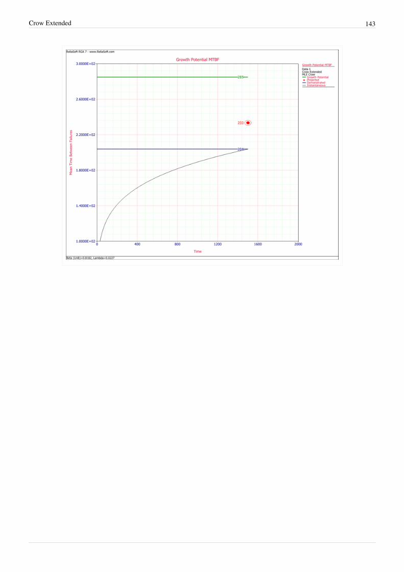
The initial MTBF after the completion of the basic reliability tasks will generally be lower than the goal. If this is thecase then a reliability growth program is appropriate. Formal reliability growth testing is usually conducted after thebasic reliability tasks have been completed. For a system subjected to RDGT, the initial MTBF is the systemreliability at the beginning of the test. The objective of the testing is to find problems, implement corrective actionsand increase the initial reliability. During RDGT, failures are observed and an underlying failure mode is associatedwith each failure. A failure mode is defined by a problem and a cause. When a new failure mode is observed duringtesting, management makes a decision not to correct or to correct the failure mode in accordance with themanagement strategy. Failure modes that are not corrected are called A modes and failure modes that receive acorrective action are called B modes. If the corrective action is effective for a B mode, then the failure intensity forthe failure mode will decrease. The effectiveness of the corrective actions is part of the overall management strategy.If the RDGT testing and corrective action process are conducted long enough, the system MTBF will grow to amature MTBF value in which further corrective actions are very infrequent. This mature MTBF value is called thegrowth potential. It is a direct function of the design and management strategy. The system growth potential MTBFis the MTBF that would be attained at the end of the basic reliability tasks if all the problem failure modes wereuncovered in early design and corrected in accordance with the management strategy.In summary, the initial MTBF is the value actually achieved by the basic reliability tasks. The growth potential is theMTBF that can be attained if the test is conducted long enough with the current management strategy. See the figurebelow.[[Image:rga2.1.png|center|450px]

Elements of a Reliability Growth ProgramIn a formal reliability growth program, one or more reliability goals are set and should be achieved during thedevelopment testing program with the necessary allocation or reallocation of resources. Therefore, planning andevaluating are essential factors in a growth process program. A comprehensive reliability growth program needswell-structured planning of the assessment techniques. A reliability growth program differs from a conventionalreliability program in that there is a more objectively developed growth standard against which assessmenttechniques are compared. A comparison between the assessment and the planned value provides a good estimate ofwhether or not the program is progressing as scheduled. If the program does not progress as planned, then newstrategies should be considered. For example, a reexamination of the problem areas may result in changing themanagement strategy so that more problem failure modes that surface during the testing actually receive a correctiveaction instead of a repair. Several important factors for an effective reliability growth program are:•• Management: the decisions made regarding the management strategy to correct problems or not correct problems

and the effectiveness of the corrective actions•• Testing: provides opportunities to identify the weaknesses and failure modes in the design and manufacturing

process•• Failure mode root cause identification: funding, personnel and procedures are provided to analyze, isolate and

identify the cause of failures•• Corrective action effectiveness: design resources to implement corrective actions that are effective and support

attainment of the reliability goals•• Valid reliability assessments: using valid statistical methodologies to analyze test data in order to assess reliabilityThe management strategy may be driven by budget and schedule but it is defined by the actual decisions ofmanagement in correcting reliability problems. If the reliability of a failure mode is known through analysis ortesting, then management makes the decision either not to fix (no corrective action) or to fix (implement a correctiveaction) that failure mode. Generally, if the reliability of the failure mode meets the expectations of management, thenno corrective actions would be expected. If the reliability of the failure mode is below expectations, the management

RGA Overview 5

strategy would generally call for the implementation of a corrective action.Another part of the management strategy is the effectiveness of the corrective actions. A corrective action typicallydoes not eliminate a failure mode from occurring again. It simply reduces its rate of occurrence. A corrective action,or fix, for a problem failure mode typically removes a certain amount of the mode's failure intensity, but a certainamount will remain in the system. The fraction decrease in the problem mode failure intensity due to the correctiveaction is called the effectiveness factor (EF). The EF will vary from failure mode to failure mode but a typicalaverage for government and industry systems has been reported to be about 0.70. With an EF equal to 0.70, acorrective action for a failure mode removes about 70% of the failure intensity, but 30% remains in the system.Corrective action implementation raises the following question: "What if some of the fixes cannot be incorporatedduring testing?" It is possible that only some fixes can be incorporated into the product during testing. However,others may be delayed until the end of the test since it may be too expensive to stop and then restart the test, or theequipment may be too complex for performing a complete teardown. Implementing delayed fixes usually results in adistinct jump in the reliability of the system at the end of the test phase. For corrective actions implemented duringtesting, the additional follow-on testing provides feedback on how effective the corrective actions are and providesopportunity to uncover additional problems that can be corrected.Evaluation of the delayed corrective actions is provided by projected reliability values. The demonstrated reliabilityis based on the actual current system performance and estimates the system reliability due to corrective actionsincorporated during testing. The projected reliability is based on the impact of the delayed fixes that will beincorporated at the end of the test or between test phases.When does a reliability growth program take place in the development process? Actually, there is more than oneanswer to this question. The modern approach to reliability realizes that typical reliability tasks often do not yield asystem that has attained the reliability goals or attained the cost-effective reliability potential in the system.Therefore, reliability growth may start very early in a program, utilizing Integrated Reliability Growth Testing(IRGT). This approach recognizes that reliability problems often surface early in engineering tests. The focus ofthese engineering tests is typically on performance and not reliability. IRGT simply piggybacks reliability failurereporting, in an informal fashion, on all engineering tests. When a potential reliability problem is observed,reliability engineering is notified and appropriate design action is taken. IRGT will usually be implemented at thesame time as the basic reliability tasks. In addition to IRGT, reliability growth may take place during early prototypetesting, during dedicated system testing, during production testing, and from feedback through any manufacturing orquality testing or inspections. The formal dedicated testing or RDGT will typically take place after the basicreliability tasks have been completed.Note that when testing and assessing against a product's specifications, the test environment must be consistent withthe specified environmental conditions under which the product specifications are defined. In addition, when testingsubsystems it is important to realize that interaction failure modes may not be generated until the subsystems areintegrated into the total system.

Why Are Reliability Growth Models Needed?In order to effectively manage a reliability growth program and attain the reliability goals, it is imperative that valid reliability assessments of the system be available. Assessments of interest generally include estimating the current reliability of the system configuration under test and estimating the projected increase in reliability if proposed corrective actions are incorporated into the system. These and other metrics give management information on what actions to take in order to attain the reliability goals. Reliability growth assessments are made in a dynamic environment where the reliability is changing due to corrective actions. The objective of most reliability growth models is to account for this changing situation in order to estimate the current and future reliability and other metrics of interest. The decision for choosing a particular growth model is typically based on how well it is expected to provide useful information to management and engineering. Reliability growth can be quantified by looking at

RGA Overview 6

various metrics of interest such as the increase in the MTBF, the decrease in the failure intensity or the increase inthe mission success probability, which are generally mathematically related and can be derived from each other. Allkey estimates used in reliability growth management such as demonstrated reliability, projected reliability andestimates of the growth potential can generally be expressed in terms of the MTBF, failure intensity or missionreliability. Changes in these values, typically as a function of test time, are collectively called reliability growthtrends and are usually presented as reliability growth curves. These curves are often constructed based on certainmathematical and statistical models called reliability growth models. The ability to accurately estimate thedemonstrated reliability and calculate projections to some point in the future can help determine the following:•• Whether the stated reliability requirements will be achieved•• The associated time for meeting such requirements•• The associated costs of meeting such requirements•• The correlation of reliability changes with reliability activitiesIn addition, demonstrated reliability and projections assessments aid in:•• Establishing warranties•• Planning for maintenance resources and logistic activities•• Life-cycle-cost analysis

TerminologySome basic terms that relate to reliability growth and repairable systems analysis are presented below. Additionalinformation on terminology in RGA can be found in the RGA Glossary.

Failure Rate vs. Failure IntensityFailure rate and failure intensity are very similar concepts. The term failure intensity typically refers to a processsuch as a reliability growth program. The system age when a system is first put into service is time 0. Under thenon-homogeneous Poisson process (NHPP), the first failure is governed by a distribution with failure rate of

. Each succeeding failure is governed by the intensity function of the process. Let be the age of thesystem and let be a very small value. The probability that a system of age fails between and is givenby the intensity function . Notice that this probability is not conditioned on not having any system failuresup to time , as is the case for a failure rate. The failure intensity for the NHPP has the same functional form asthe failure rate governing the first system failure. Therefore, , where is the failure rate for thedistribution function of the first system failure. If the first system failure follows the Weibull distribution, the failurerate is:

Under minimal repair, the system intensity function is:

This is the power law model. It can be viewed as an extension of the Weibull distribution. The Weibull distributiongoverns the first system failure and the power law model governs each succeeding system failure. Additionalinformation on the power law model is available in Repairable Systems Analysis.

Instantaneous vs. CumulativeIn RGA, metrics such as MTBF and failure intensity can be calculated as instantaneous or cumulative. Cumulative MTBF is the average time-between-failure from the beginning of the test (i.e., t = 0) up to time t. The instantaneous MTBF is the average time-between-failure in a given interval, dt. Consider a grouped data set, where 4 failures are found in the interval 0-100 hours and 2 failures are found in the second interval 100-180 hours. The cumulative MTBF at 180 hours of test time is equal to 180/6 = 30 hours. However, the instantaneous MTBF is equal to 80/2 =

RGA Overview 7

40 hours. Another analogy for this relates to the miles per gallon (mpg) that your car gets. In many cars, there arereadouts that indicates the current mpg as you are driving. This is the instantaneous value. The average mpg on thecurrent tank of gas is the cumulative value.Relative to the Crow-AMSAA (NHPP) model, when beta is equal to one, the system's MTBF is not changing overtime; therefore, the cumulative MTBF equals the instantaneous MTBF. If beta is greater than one, then the system'sMTBF is decreasing over time and the cumulative MTBF is greater than the instantaneous MTBF. If beta is less thanone, then the system's MTBF is increasing over time and the cumulative MTBF is less than the instantaneous MTBF.Now the concern is, how do you know whether you should estimate the instantaneous or cumulative value of ametric (e.g., MTBF or failure intensity)? In general, system requirements are usually represented as instantaneousvalues. After all, you want to know where the system is now in terms of its MTBF. The cumulative MTBF can beused to observe trends in the data.

Time Terminated vs. Failure TerminatedWhen a reliability growth test is conducted, it must be determined how much operation time the system willaccumulate during the test (i.e., the point at which the test will reach its end). There are two possible options underwhich a reliability growth test may be terminated (or truncated): time terminated or failure terminated.•• A time terminated test is stopped after a certain amount of test time.•• A failure terminated test is stopped at a time which corresponds to a failure (e.g., the time of the tenth failure).It is determined a priori whether a test is time terminated or failure terminated. The test data does not determine this.

8

Chapter 2

RGA Data TypesReliability growth analysis can be conducted using different data types. This chapter explores and examines thepossible data schemes, and outlines the available models for each data type. The data types for developmental testing(traditional reliability growth analysis) will be discussed first. Then we will discuss the data types that support theuse of RGA models for analyzing fielded systems (either for repairable systems analysis or fleet data analysis).

Developmental Testing Data Types

Time-to-Failure DataTime-to-failure (continuous) data is the most commonly observed type of reliability growth data. It involvesrecording the times-to-failure for the unit(s) under test. Time-to-failure data can be applied to a single unit or systemor to multiple units or systems. There are multiple data entry schemes for this data type and each is presented next.

Failure Times Data

This data type is used for tests where the actual system failure times are tracked and recorded. The data can beentered in a cumulative format (where each row shows the total amount of test time) or non-cumulative format(where each row shows the incremental test time), as shown next.

RGA Data Types 9

Grouped Failure Times

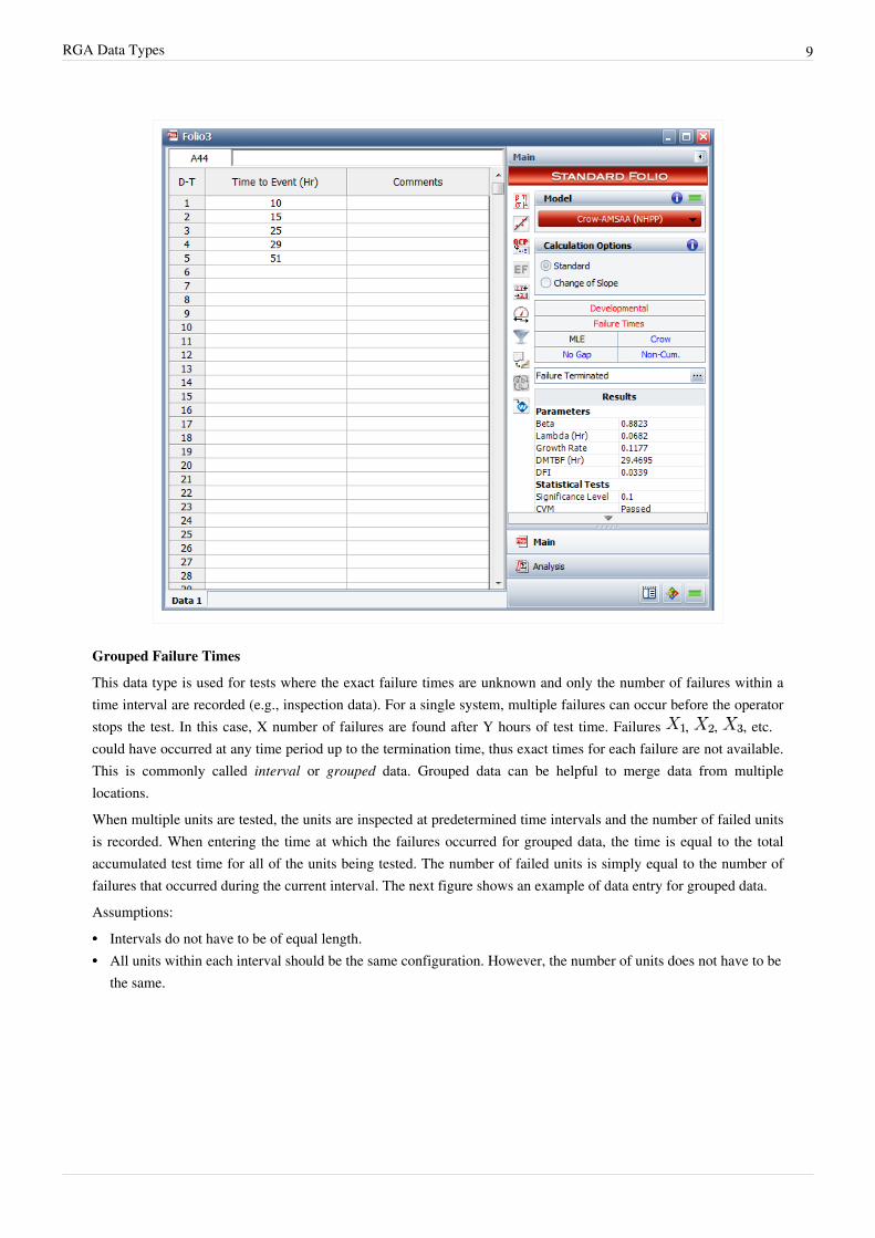
This data type is used for tests where the exact failure times are unknown and only the number of failures within atime interval are recorded (e.g., inspection data). For a single system, multiple failures can occur before the operatorstops the test. In this case, X number of failures are found after Y hours of test time. Failures , , , etc.could have occurred at any time period up to the termination time, thus exact times for each failure are not available.This is commonly called interval or grouped data. Grouped data can be helpful to merge data from multiplelocations.When multiple units are tested, the units are inspected at predetermined time intervals and the number of failed unitsis recorded. When entering the time at which the failures occurred for grouped data, the time is equal to the totalaccumulated test time for all of the units being tested. The number of failed units is simply equal to the number offailures that occurred during the current interval. The next figure shows an example of data entry for grouped data.Assumptions:•• Intervals do not have to be of equal length.•• All units within each interval should be the same configuration. However, the number of units does not have to be

the same.

RGA Data Types 10

Multiple Systems (Known Operating Times)

This data type is used for tests where a number of systems are tested, and if a failure occurs in any system, acorrective action is taken on the failed unit and any design changes are incorporated into all test systems. Once thecorrective actions have been implemented, the test is resumed. In this data type, the systems can accumulate usage atdifferent rates. In addition, the systems do not have to start the test at the same time. The basic idea of MultipleSystems (Known Operating Times) is that when one system fails, the usage on the other systems on test must also beknown. This is a flexible data type, but it is also the most demanding given the information required on all systems.The time-to-failure for the failed system, along with the current operating times of all other systems, is recorded. Thedata can be cumulative or non-cumulative. Consider the following data sheet where the Failed Unit ID columnindicates which unit failed. For example, if you enter 2 into the "Failed Unit ID" column, this indicates that the unitin the Time Unit 2 column is the one that has failed. For the units that did not fail, you must enter the operating timeat the time of the other unit's failure.

RGA Data Types 11

In this example, two units are undergoing testing and the units do not accumulate age at the same rate. At 10 hoursinto the test, unit 1 fails and corrective action is taken on both units 1 and 2. By this time, both units haveaccumulated 10 hours of operation. At 17 hours, unit 2 fails, and corrective action is again implemented on bothunits; however, unit 1 has accumulated 5 hours of operating time and unit 2 has accumulated 7 hours since the lastevent. The rest of the data can be interpreted in a similar manner.

Multiple Systems (Concurrent Operating Times)

This data type is used for tests where a number of systems are tested. The start time, failure time(s) and end time foreach system are recorded. This data type assumes uniform time accumulation and that the systems are testedsimultaneously. When a corrective action is implemented on a failed system, the fix is also applied to the non-failedsystems. This results in all systems on test having the same configuration throughout the test. As an example,consider the data of two systems shown in the following figure. In this case, the folio is shown in Normal view.

RGA Data Types 12

System 1 begins testing at time equals 0 (with a start event, S). Note that when entering data within the Normal view,each system must be initiated with a start event. The failures encountered by System1 are corrected at 281, 312 and776 (with failure events, F). Testing stops at 1000 hours (with an end event, E). System 2 begins testing at timeequals 0 and failures are encountered and corrected at 40, 222 and 436. Testing stops at 500 hours. The next figureshows the folio and the same data set in the Advanced Systems view.

Multiple Systems with Dates

This data type is similar to Multiple Systems (Concurrent Operating Times) except that a date is now associated witheach failure time, as well as for the start and end time of each system. This assumes noncontinuous usage, and thesoftware computes equivalent (average) usage rates. To determine when dates are important and whether or not theyshould be included in your analysis, consider the picture below (not drawn to scale).

RGA Data Types 13

Two systems are placed in a reliability growth test. System 1 starts testing on January 1, 2013 and System 2 does notstart testing until January 10, 2013. When testing begins on System 2, what is its configuration? Does theconfiguration of System 2 on January 10 match System 1 on January 10 (there was a fix implemented on System 1on January 8) or does it match System 1's configuration on January 1? If the configuration of System 2 matchesSystem 1 on January 1, then dates are not important. This means the previous data type, Multiple Systems(Concurrent Operating Times) can be used, and the timeline for System 2 can be shifted to the left. However, if theconfiguration of System 2 matches System 1 on January 10, then dates are important and the Multiple Systems withDates data type should be used.The goal is to sum up the accumulated hours across all systems with the same configuration. If System 2 on January10 matches System 1 on January 10, then it would not be correct to shift System 2 to the left to t = 0. If this weredone, the first failure on System 1 on January 5 would correspond to 80 hours: 40 hours for System 1 plus 40 hoursfor System 2 on the equivalent system timeline. However, with dates this same failure now corresponds to 40 hourson the equivalent system timeline since System 2 is not operating yet. For the failure on January 14 on System 2, thetotal test time on this date must also account for the test time accumulated on System 1. However, there is not anevent on System 1 on January 14. Therefore, RGA uses linear interpolation to estimate the operating time on System1 on January 14.The next figure shows an example of Multiple Systems with Dates in RGA.

Multiple Systems with Event Codes

The Multiple Systems with Event Codes data type is basically the same as the Multiple Systems (ConcurrentOperating Times) data type. These data types are used to analyze the failure data from a reliability growth test inwhich a number of systems are tested concurrently and the implemented fixes are tracked during the test phase. Allof the systems under test are assumed to have the same system hours at any given time. However, the MultipleSystems with Event Codes data type does have two differences:• The Crow Extended model is always the underlying model.• Event codes, similar to the ones used for the Crow Extended - Continuous Evaluation model, are part of the data

entry.Even though event codes are added to the data entry, the underlying assumptions associated with the Crow Extendedmodel have not changed. Additional information on Multiple Systems with Event Codes is presented on the CrowExtended page. The next figure shows an example of this type of data.

RGA Data Types 14

Models for Time-to-Failure (Continuous) Data

The following models can be used to analyze time-to-failure (continuous) data sets. Models and examples using thedifferent data types are discussed in later chapters.•• Duane•• Crow-AMSAA (NHPP)•• Crow Extended

Discrete DataDiscrete data are also referred to as success/failure or attribute data. These data sets consist of data from a test wherea unit is tested with only two possible outcomes: success or failure. An example of this is a missile that gets firedonce and it either succeeds or fails. The data types available for analyzing discrete data with the RGA software are:•• Sequential•• Sequential with Mode•• Grouped per Configuration•• Mixed Data

Sequential Data

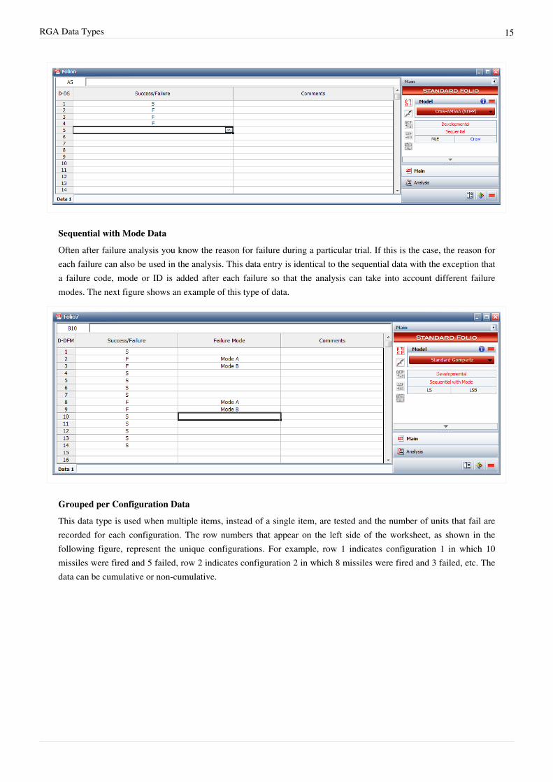
For sequential data, an item is tested with only two possible outcomes: success or failure. This could be a one-shotitem such as a missile or an entire system that either succeeds or fails. The item is then inspected after each trial andredesigned/repaired before the next trial. The following figure shows an example of this data type, where the rownumber in the data sheet represents the sequence of the trials. In this data set, trial #1 succeeded, trial #2 failed, andso on.

RGA Data Types 15

Sequential with Mode Data

Often after failure analysis you know the reason for failure during a particular trial. If this is the case, the reason foreach failure can also be used in the analysis. This data entry is identical to the sequential data with the exception thata failure code, mode or ID is added after each failure so that the analysis can take into account different failuremodes. The next figure shows an example of this type of data.

Grouped per Configuration Data

This data type is used when multiple items, instead of a single item, are tested and the number of units that fail arerecorded for each configuration. The row numbers that appear on the left side of the worksheet, as shown in thefollowing figure, represent the unique configurations. For example, row 1 indicates configuration 1 in which 10missiles were fired and 5 failed, row 2 indicates configuration 2 in which 8 missiles were fired and 3 failed, etc. Thedata can be cumulative or non-cumulative.

RGA Data Types 16

Mixed Data

The Mixed data type is basically a combination of Grouped per Configuration and Sequential data. It allows fortesting to be conducted in groups of configurations, individual trial by trial or a combination of individual trials andconfigurations where more than one trial is tested. The following figure shows an example of this data type. Forexample the first row of this data sheet shows that 3 failures occurred in the first 4 trials, the second row shows thatthere were no failures in the next trial, while the third row shows that 3 failures occurred in the next 4 trials.

Models for Discrete Data

The following models can be used to analyze discrete data. Models and examples using the different data types arediscussed in later chapters.•• Duane•• Crow-AMSAA (NHPP)•• Crow Extended•• Lloyd-Lipow•• Gompertz and Modified Gompertz•• Logistic

RGA Data Types 17

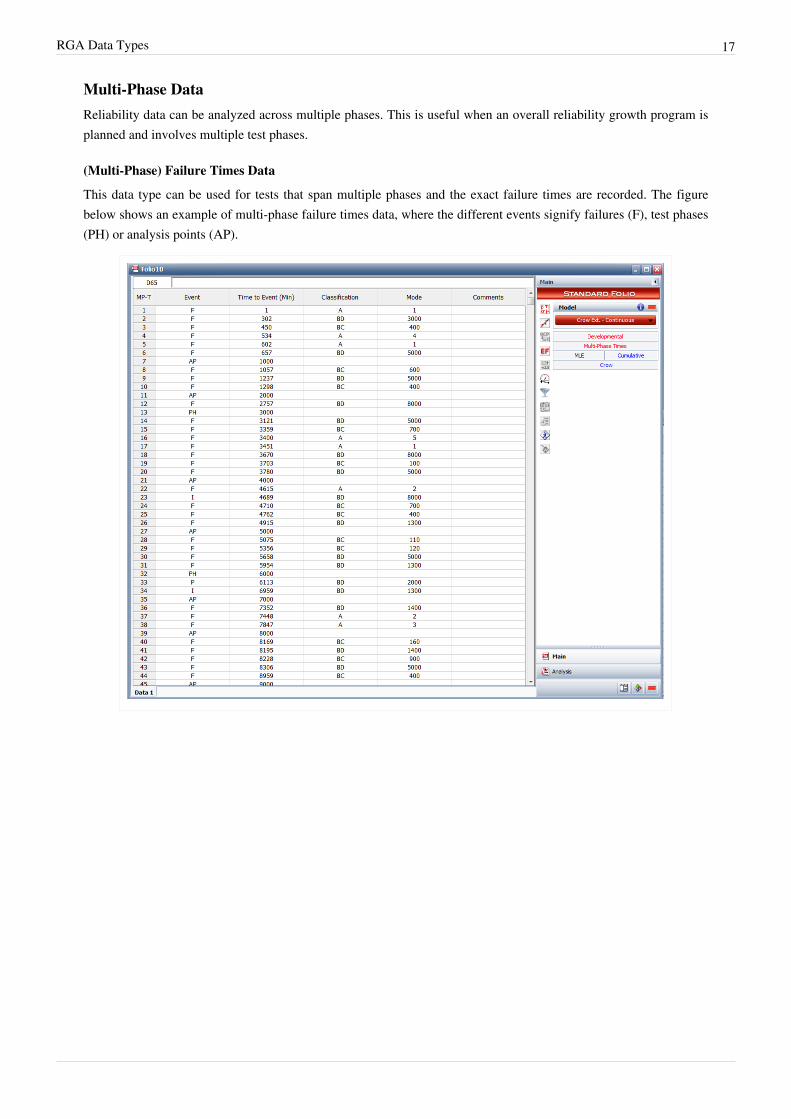
Multi-Phase DataReliability data can be analyzed across multiple phases. This is useful when an overall reliability growth program isplanned and involves multiple test phases.

(Multi-Phase) Failure Times Data

This data type can be used for tests that span multiple phases and the exact failure times are recorded. The figurebelow shows an example of multi-phase failure times data, where the different events signify failures (F), test phases(PH) or analysis points (AP).

RGA Data Types 18

(Multi-Phase) Grouped Failure Times Data

This data type can be used for tests that span multiple phases and the exact failure times are unknown. Only thenumber of failures within a time interval are recorded, as shown in the figure below.

RGA Data Types 19

(Multi-Phase) Mixed Data

This data type can be used for tests that span multiple phases and it allows for configuration in groups, individualtrial by trial, or a mixed combination of individual trials and configurations of more than one trial. An example ofthis data type can be seen in the figure below.

Models for Multi-Phase Data

The Crow Extended - Continuous Evaluation model is used to analyze data across multiple phases.

Reliability DataReliability data consists of entering the reliability of the equipment at different times or stages. An example is shownin the figure below. In this case, the process is monitored at pre-defined time intervals and the reliability is recorded.The reliability can be computed by a simple ratio of the number of units still functioning vs. the number of units thatentered the test stage or by using life data analysis and related methods (e.g., Weibull analysis).

RGA Data Types 20

Models for Reliability Data

The following models can be used to analyze reliability data sets. Models and examples using different data types arediscussed in later chapters.•• Lloyd-Lipow•• Gompertz and Modified Gompertz•• Logistic

Fielded SystemsFielded systems are systems that are used by customers in the field and for which failure information is not derivedfrom an in-house test. This type of data is analogous to warranty data. The data types available for fielded systemsdata entry are:•• Repairable Systems•• Fleet

RGA Data Types 21

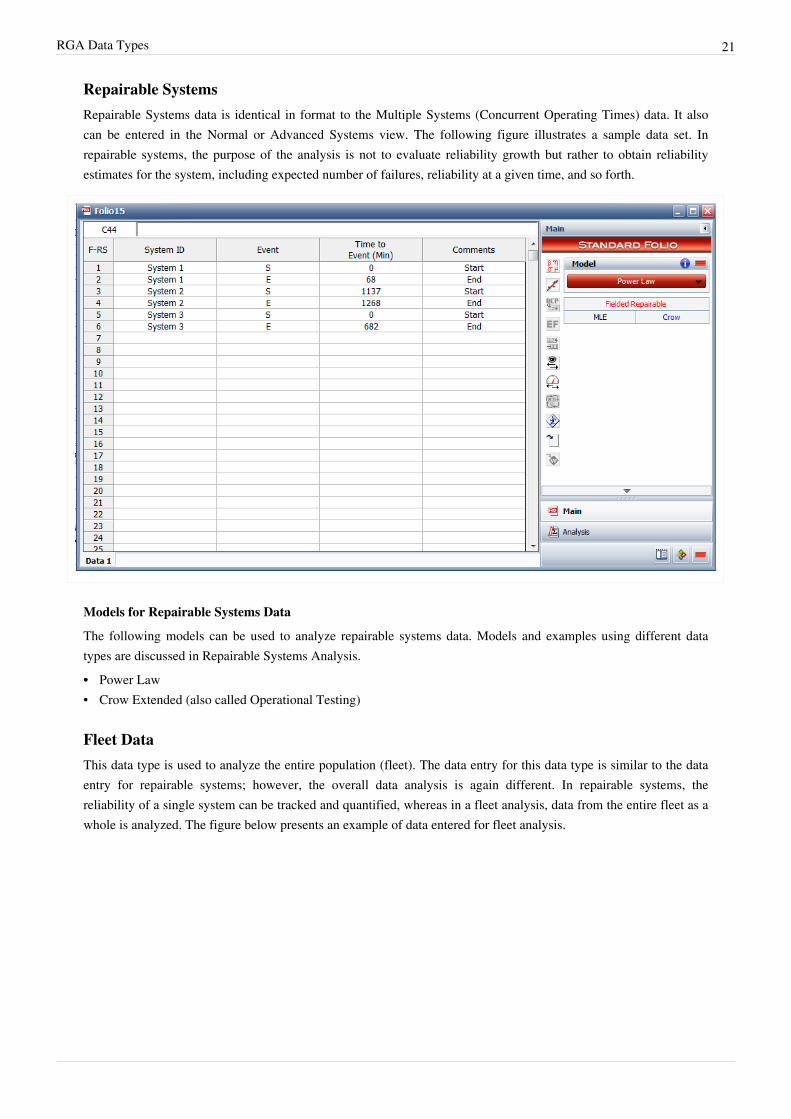
Repairable SystemsRepairable Systems data is identical in format to the Multiple Systems (Concurrent Operating Times) data. It alsocan be entered in the Normal or Advanced Systems view. The following figure illustrates a sample data set. Inrepairable systems, the purpose of the analysis is not to evaluate reliability growth but rather to obtain reliabilityestimates for the system, including expected number of failures, reliability at a given time, and so forth.

Models for Repairable Systems Data

The following models can be used to analyze repairable systems data. Models and examples using different datatypes are discussed in Repairable Systems Analysis.•• Power Law• Crow Extended (also called Operational Testing)

Fleet DataThis data type is used to analyze the entire population (fleet). The data entry for this data type is similar to the dataentry for repairable systems; however, the overall data analysis is again different. In repairable systems, thereliability of a single system can be tracked and quantified, whereas in a fleet analysis, data from the entire fleet as awhole is analyzed. The figure below presents an example of data entered for fleet analysis.

RGA Data Types 22

Models for Fleet Data

The following models can be used to analyze fleet data. Models and examples using different data types arediscussed in later chapters.•• Crow-AMSAA (NHPP)•• Crow Extended

23

Chapter 3

Developmental TestingReliability growth analysis is the process of collecting, modeling, analyzing and interpreting data from the reliabilitygrowth development test program (development testing). In addition, reliability growth models can be applied fordata collected from the field (fielded systems). Fielded systems analysis also includes the ability to analyze data ofcomplex repairable systems. Depending on the metric(s) of interest and the data collection method, different modelscan be utilized (or developed) to analyze the growth processes.

ExampleAs an example of such a model development, consider the simple case of a wine glass designed to withstand a fall ofthree feet onto a level cement surface.

The success/failure result of such a drop is determined by whether or not the glass breaks.Furthermore, assume that:•• You will continue to drop the glass, looking at the results and then adjusting the design after each failure until you

are sure that the glass will not break.

• Any redesign effort is either completely successful or it does not change the inherent reliability ( ). In otherwords, the reliability is either 1 or , .

•• When testing the product, if a success is encountered on any given trial, no corrective action or redesign isimplemented.

•• If the trial fails, then you will redesign the product.• When the product is redesigned, assume that the probability of fixing the product permanently before the next

trial is . In other words, the glass may or may not have been fixed.

• Let and be the probabilities that the glass is unreliable and reliable, respectively, just before thetrial, and that the glass is in the unreliable state just before the first trial, .

Developmental Testing 24

Now given the above assumptions, the question of how the glass could be in the unreliable state just before trial can be answered in two mutually exclusive ways:

The first possibility is the probability of a successful trial, , where is the probability of failure in trial, while being in the unreliable state, , before the trial, or:

Secondly, the glass could have failed the trial, with probability , when in the unreliable state, , andhaving failed the trial, an unsuccessful attempt was made to fix, with probability , or:

Therefore, the sum of these two probabilities, or possible events, gives the probability of being unreliable just beforetrial :

or:

By induction, since :

To determine the probability of being in the reliable state just before trial , the above equation is subtracted from 1,therefore:

Define the reliability of the glass as the probability of not failing at trial . The probability of not failing at trialis the sum of being reliable just before trial , , and being unreliable just before trial but

not failing , thus:

or:

Now instead of , assume that the glass has some initial reliability or that the probability that the glass isin the unreliable state at , , then:

Developmental Testing 25

When , the reliability at the trial is larger than when it was certain that the device was unreliable at trial. A trend of reliability growth is observed in the above equation.

Let and , then:

This equation is now a model that can be utilized to obtain the reliability (or probability that the glass will not break)after the trial.

Applicable ModelsThe following chapters contain additional information on each of the models that are available for developmentaltesting:•• Duane•• Crow-AMSAA (NHPP)•• Crow Extended - Continuous Evaluation•• Lloyd-Lipow•• Gompertz Models•• Logistic

26

Chapter 3.1

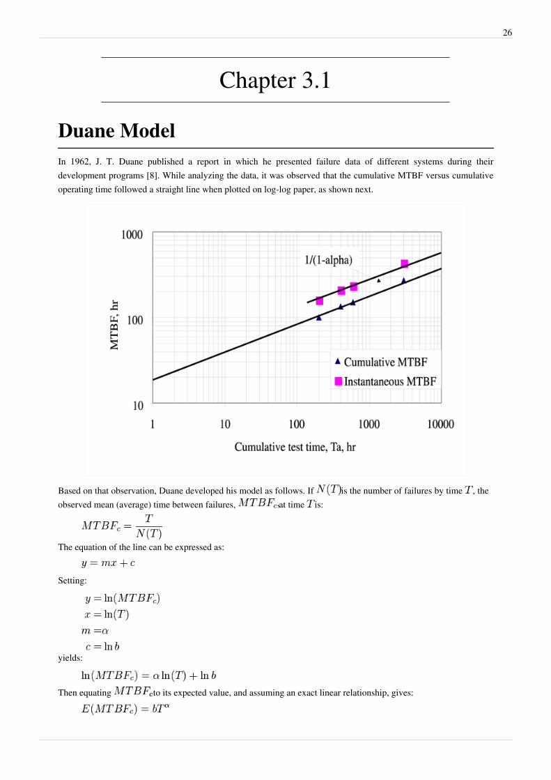
Duane ModelIn 1962, J. T. Duane published a report in which he presented failure data of different systems during theirdevelopment programs [8]. While analyzing the data, it was observed that the cumulative MTBF versus cumulativeoperating time followed a straight line when plotted on log-log paper, as shown next.

Based on that observation, Duane developed his model as follows. If is the number of failures by time , theobserved mean (average) time between failures, at time is:

The equation of the line can be expressed as:

Setting:

yields:

Then equating to its expected value, and assuming an exact linear relationship, gives:

Duane Model 27

or:

And, if you assume a constant failure intensity, then the cumulative failure intensity, , is:

or:

Also, the expected number of failures up to time is:

where:

• is the average estimate of the cumulative failure intensity, failures/hour.• is the total accumulated unit hours of test and/or development time.• is the cumulative failure intensity at or at the beginning of the test, or the earliest time at which the

first is predicted, or the for the equipment at the start of the design and development process.• is the improvement rate in the .The corresponding , or , is equal to:

where cumulative MTBF at or at the beginning of the test, or the earliest time at which the first canbe determined, or the predicted at the start of the design and development process ( ).

The cumulative MTBF, , and tell whether is increasing or is decreasing with time, utilizing all data up tothat time. You may want to know, however, the instantaneous or to see what you are doing at a specificinstant or after a specific test and development time. The instantaneous failure intensity, , is:

Similarly, using the equation for the expected number of failures up to time , this procedure yields:

where implies infinite MTBF growth.As shown in these derivations, the instantaneous failure intensity improvement line is obtained by shifting thecumulative failure intensity line down, parallel to itself, by a distance of . Similarly, the current orinstantaneous MTBF growth line is obtained by shifting the cumulative MTBF line up, parallel to itself, by adistance of , as illustrated in the figure below.

Duane Model 28

Parameter EstimationThe Duane model is a two parameter model. Therefore, to use this model as a basis for predicting the reliabilitygrowth that could be expected in an equipment development program, procedures must be defined for estimatingthese parameters as a function of equipment characteristics. Note that, while these parameters can be estimated for agiven data set using curve-fitting methods, there exists no underlying theory for the Duane model that could providea basis for a priori estimation.

One of the parameters of the Duane model is . The second parameter can be represented as or where .

There is an option within the Application Setup that allows you to determine whether to display or for theDuane model. All formulation within this reference uses the parameter .

Duane Model 29

Graphical MethodThe Duane model for the cumulative failure intensity is:

This equation may be linearized by taking the natural log of both sides:

Consequently, plotting versus on log-log paper will result in a straight line with a negative slope, such that:

• is the y-intercept at

• is the cumulative failure intensity at • is the slope of the straight line on the log-log plotSimilarly, the corresponding MTBF of the cumulative failure intensity can also be linearized by taking the naturallog of both sides:

Plotting versus on log-log paper will result in a straight line with a positive slope such that:• is the y-intercept at • is the cumulative mean time between failure at • is the slope of the straight line on the log-log plotTwo ways of determining these curves are as follows:

1. Predict the and of the system from its reliability block diagram and available component failure intensities. Plot this value on log-log plotting paper at From past experience and from past data for similar

Duane Model 30

equipment, find values of , the slope of the improvement lines for or . Modify this as necessary. If a better designeffort is expected and a more intensive research, test and development or TAAF program is to be implemented, thena 15% improvement in the growth rate may be attainable. Consequently, the available value for slope , and , shouldbe adjusted by this amount. The value to be used will then be A line is then drawn through point and with the justdetermined slope , keeping in mind that is negative for the curve. This line should be extended to the design,development and test time scheduled to be expended to see if the failure intensity goal will indeed be achieved onschedule. It is also possible to find that the design, development and test time to achieve the goal may be earlier thanthe delivery date or later. If earlier, then either the reliability program effort can be judiciously and appropriatelytrimmed; or if it is an incentive contract, full advantage is taken of the fact that the failure intensity goal can beexceeded with the associated increased profits to the company. A similar approach may be used for the MTBFgrowth model, where is plotted at , and a line is drawn through the point and with slope to obtain the MTBF growthline. If values are not available, consult the table below, which gives actual values for various types of equipment.These have been obtained from literature or by MTBF growth tests. It may be seen from the following table that values range between 0.24 and 0.65. The lower values reflect slow early growth and the higher values reflect fastearly growth.

Sample Slope Values for Various Equipment

Equipment Slope( )

Computer system Actual 0.24

Easy to find failures were eliminated 0.26

All known failure causes were eliminated 0.36

Mainframe computer 0.50

Aerospace electronics All malfunctions 0.57

Relevant failures only 0.65

Attack radar 0.60

Rocket engine 0.46

Afterburning turbojet 0.35

Complex hydromechanical system 0.60

Aircraft generator 0.38

Modern dry turbojet 0.48

2. During the design, development and test phase and at specific milestones, the is calculated from the totalfailures and values. These values of or are plotted above the corresponding values on log-log paper. Astraight line is drawn favoring these points to minimize the distance between the points and the line, thus establishingthe improvement or growth model and its parameters graphically. If needed, linear regression analysis techniquescan be used to determine these parameters.

Duane Model 31

Graphical Method Example

A complex system's reliability growth is being monitored and the data set is given in the table below.

Cumulative Test Hours and the Corresponding Observed Failures for the Complex System

Point Number Cumulative Test Time(hours) Cumulative Failures Cumulative MTBF(hours) Instantaneous MTBF(hours)

1 200 2 100.0 100

2 400 3 133.0 200

3 600 4 150.0 200

4 3,000 11 273.0 342.8

Do the following:1.1. Plot the cumulative MTBF growth curve.2.2. Write the equation of this growth curve.3.3. Write the equation of the instantaneous MTBF growth model.4.4. Plot the instantaneous MTBF growth curve.Solution

1. Given the data in the second and third columns of the above table, the cumulative MTBF, , values arecalculated in the fourth column. The information in the second and fourth columns are then plotted. The firstfigure below shows the cumulative MTBF while the second figure below shows the instantaneous MTBF. It canbe seen that a straight line represents the MTBF growth very well on log-log scales.

Cumulative MTBF plot

Duane Model 32

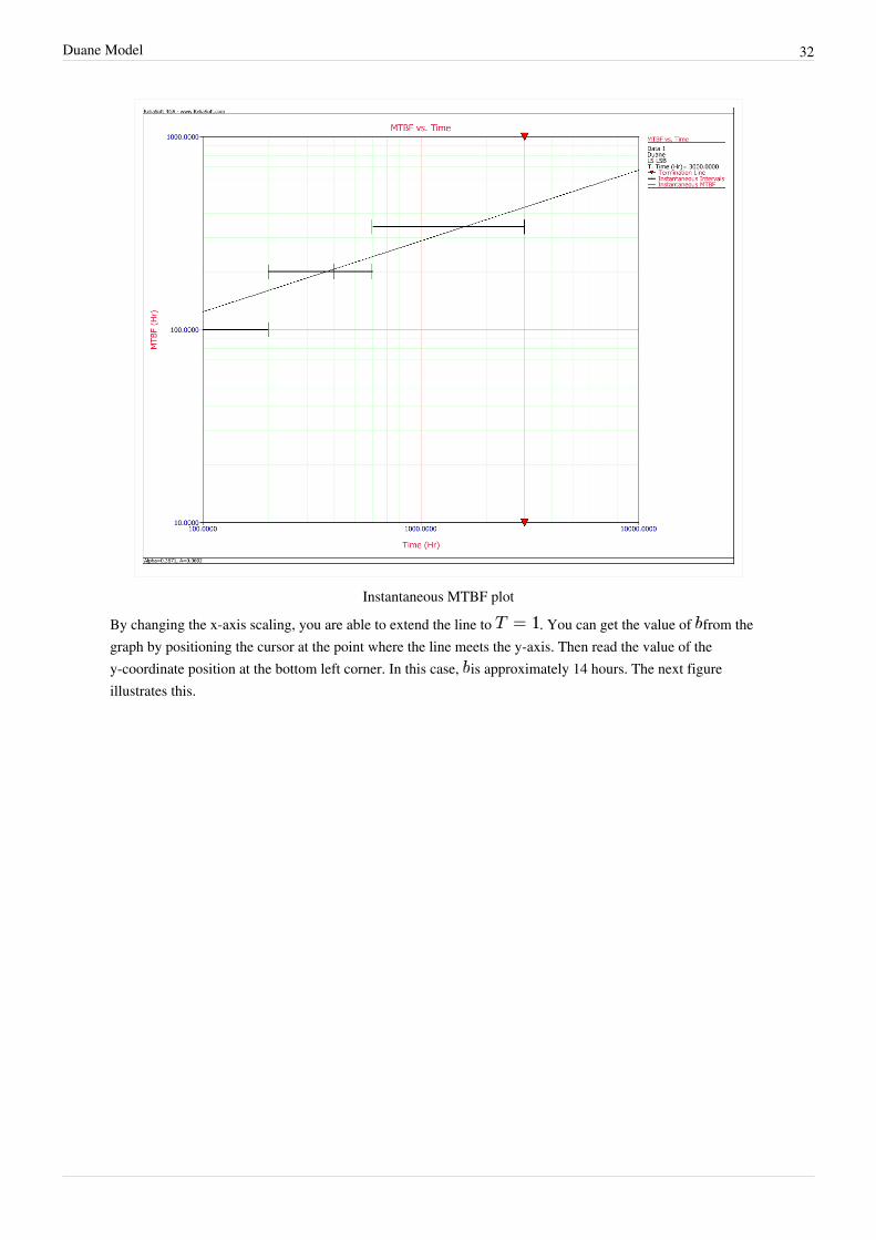
Instantaneous MTBF plot

By changing the x-axis scaling, you are able to extend the line to . You can get the value of from thegraph by positioning the cursor at the point where the line meets the y-axis. Then read the value of they-coordinate position at the bottom left corner. In this case, is approximately 14 hours. The next figureillustrates this.

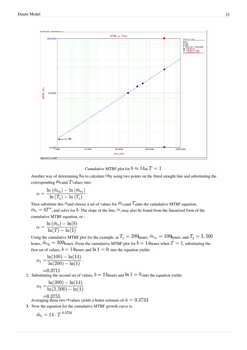
Duane Model 33

Cumulative MTBF plot for at Another way of determining is to calculate by using two points on the fitted straight line and substituting thecorresponding and values into:

Then substitute this and choose a set of values for and into the cumulative MTBF equation,, and solve for . The slope of the line, , may also be found from the linearized form of the

cumulative MTBF equation, or :

Using the cumulative MTBF plot for the example, at hours, hours, and hours, hours. From the cumulative MTBF plot for hours when , substituting thefirst set of values, hours and , into the equation yields:

2. Substituting the second set of values, hours and into the equation yields:

Averaging these two values yields a better estimate of .3.3. Now the equation for the cumulative MTBF growth curve is:

Duane Model 34

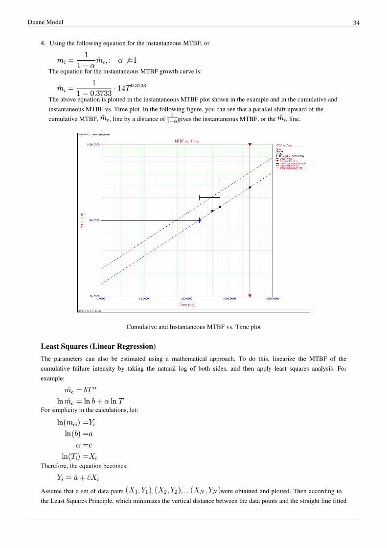
4.4. Using the following equation for the instantaneous MTBF, or

The equation for the instantaneous MTBF growth curve is:

The above equation is plotted in the instantaneous MTBF plot shown in the example and in the cumulative andinstantaneous MTBF vs. Time plot. In the following figure, you can see that a parallel shift upward of thecumulative MTBF, , line by a distance of gives the instantaneous MTBF, or the , line.

Cumulative and Instantaneous MTBF vs. Time plot

Least Squares (Linear Regression)The parameters can also be estimated using a mathematical approach. To do this, linearize the MTBF of thecumulative failure intensity by taking the natural log of both sides, and then apply least squares analysis. Forexample:

For simplicity in the calculations, let:

Therefore, the equation becomes:

Assume that a set of data pairs , ,..., were obtained and plotted. Then according to the Least Squares Principle, which minimizes the vertical distance between the data points and the straight line fitted

Duane Model 35

to the data, the best fitting straight line to this data set is the straight line such that:

where and are the least squares estimates of and . To obtain and , let:

Differentiating with respect to and yields:

and:

Set those two equations equal to zero:

and:

Solve the equations simultaneously:

and:

Now substituting back and we have:

where:

Duane Model 36

Example 1

Using the same data set from the graphical approach example, estimate the parameters of the MTBF model usingleast squares.Solution

From the data table:

Obtain the value of from the least squares analysis, or:

Obtain the value from the least squares analysis, or:

Therefore, the cumulative MTBF becomes:

The equation for the instantaneous MTBF growth curve is:

Duane Model 37

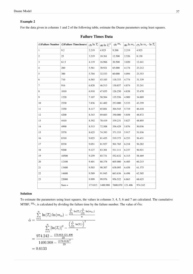
Example 2

For the data given in columns 1 and 2 of the following table, estimate the Duane parameters using least squares.

Failure Times Data

(1)Failure Number (2)Failure Time(hours) (3) (4) (5) (6) (7)

1 9.2 2.219 4.925 9.200 2.219 4.925

2 25 3.219 10.361 12.500 2.526 8.130

3 61.5 4.119 16.966 20.500 3.020 12.441

4 260 5.561 30.921 65.000 4.174 23.212

5 300 5.704 32.533 60.000 4.094 23.353

6 710 6.565 43.103 118.333 4.774 31.339

7 916 6.820 46.513 130.857 4.874 33.241

8 1010 6.918 47.855 126.250 4.838 33.470

9 1220 7.107 50.504 135.556 4.909 34.889

10 2530 7.836 61.402 253.000 5.533 43.359

11 3350 8.117 65.881 304.545 5.719 46.418

12 4200 8.343 69.603 350.000 5.858 48.872

13 4410 8.392 70.419 339.231 5.827 48.895

14 4990 8.515 72.508 356.429 5.876 50.036

15 5570 8.625 74.393 371.333 5.917 51.036

16 8310 9.025 81.455 519.375 6.253 56.431

17 8530 9.051 81.927 501.765 6.218 56.282

18 9200 9.127 83.301 511.111 6.237 56.921

19 10500 9.259 85.731 552.632 6.315 58.469

20 12100 9.401 88.378 605.000 6.405 60.215

21 13400 9.503 90.307 638.095 6.458 61.375

22 14600 9.589 91.945 663.636 6.498 62.305

23 22000 9.999 99.976 956.522 6.863 68.625

Sum = 173.013 1400.908 7600.870 121.406 974.242

Solution

To estimate the parameters using least squares, the values in columns 3, 4, 5, 6 and 7 are calculated. The cumulativeMTBF, , is calculated by dividing the failure time by the failure number. The value of is:

Duane Model 38

The estimator of is estimated to be:

Therefore, the cumulative MTBF becomes:

Using the equation for the instantaneous MTBF growth curve,

Example 3

For the data given in the following table, estimate the Duane parameters using least squares.

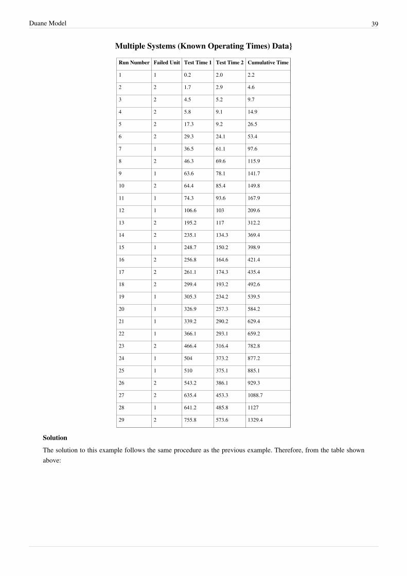
Duane Model 39

Multiple Systems (Known Operating Times) Data}

Run Number Failed Unit Test Time 1 Test Time 2 Cumulative Time

1 1 0.2 2.0 2.2

2 2 1.7 2.9 4.6

3 2 4.5 5.2 9.7

4 2 5.8 9.1 14.9

5 2 17.3 9.2 26.5

6 2 29.3 24.1 53.4

7 1 36.5 61.1 97.6

8 2 46.3 69.6 115.9

9 1 63.6 78.1 141.7

10 2 64.4 85.4 149.8

11 1 74.3 93.6 167.9

12 1 106.6 103 209.6

13 2 195.2 117 312.2

14 2 235.1 134.3 369.4

15 1 248.7 150.2 398.9

16 2 256.8 164.6 421.4

17 2 261.1 174.3 435.4

18 2 299.4 193.2 492.6

19 1 305.3 234.2 539.5

20 1 326.9 257.3 584.2

21 1 339.2 290.2 629.4

22 1 366.1 293.1 659.2

23 2 466.4 316.4 782.8

24 1 504 373.2 877.2

25 1 510 375.1 885.1

26 2 543.2 386.1 929.3

27 2 635.4 453.3 1088.7

28 1 641.2 485.8 1127

29 2 755.8 573.6 1329.4

Solution

The solution to this example follows the same procedure as the previous example. Therefore, from the table shownabove:

Duane Model 40

For least squares, the value of is:

The value of the estimator is:

Therefore, the cumulative MTBF is:

Using the equation for the instantaneous MTBF growth,

Maximum Likelihood EstimatorsL. H. Crow [17] noted that the Duane model could be stochastically represented as a Weibull process, allowing forstatistical procedures to be used in the application of this model in reliability growth. This statistical extensionbecame what is known as the Crow-AMSAA (NHPP) model. The Crow-AMSAA model, which is described in theCrow-AMSAA (NHPP) chapter, provides a complete Maximum Likelihood Estimation (MLE) solution to the Duanemodel.

Duane Model 41

Confidence BoundsLeast squares confidence bounds can be computed for both the model parameters and metrics of interest for theDuane model.

Parameter BoundsApply least squares analysis on the Duane model:

The unbiased estimator of can be obtained from:

where:

Thus, the confidence bounds on and are:

where denotes the percentage point of the distribution with degrees of freedom such thatand:

Other BoundsConfidence bounds also can be obtained on the cumulative MTBF and the cumulative failure intensity:

When is large, the approximate confidence bounds for instantaneous MTBF are given by:

and

therefore, the confidence bounds on the instantaneous failure intensity are:

Duane Model 42

Duane Confidence Bounds Example

Using the values of and estimated from the least squares analysis in Least Squares Example 2:

Calculate the 90% confidence bounds for the following:

1. The parameters and .2.2. The cumulative and instantaneous failure intensity.3.3. The cumulative and instantaneous MTBF.Solution

1. Use the values of and estimated from the least squares analysis. Then:

Thus, the 90% confidence bounds on parameter are:

And 90% confidence bounds on parameter are:

2.2. The cumulative failure intensity is:

And the instantaneous failure intensity is equal to:

Duane Model 43

So, at the 90% confidence level and for hours, the confidence bounds on cumulative failureintensity are:

For the instantaneous failure intensity:

The following figures show the graphs of the cumulative and instantaneous failure intensity. Both are plotted withconfidence bounds.

Duane Model 44

3.3. The cumulative MTBF is:

And the instantaneous MTBF is:

So, at 90% confidence level and for hours, the confidence bounds on the cumulative MTBF are:

The confidence bounds for the instantaneous MTBF are:

The figure below displays the cumulative MTBF.

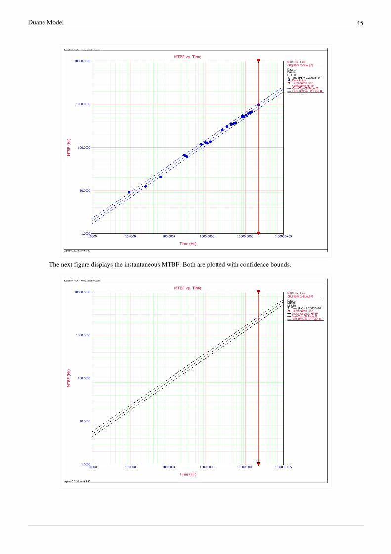
Duane Model 45

The next figure displays the instantaneous MTBF. Both are plotted with confidence bounds.

Duane Model 46

More Examples

Estimating the Time Required to Meet an MTBF GoalA prototype of a system was tested with design changes incorporated during the test. A total of 12 failures occurred.The data set is given in the following table.

Developmental Test Data

Failure Number Cumulative Test Time(hours)

1 80

2 175

3 265

4 400

5 590

6 1100

7 1650

8 2010

9 2400

10 3380

11 5100

12 6400

Do the following:1.1. Estimate the Duane parameters.2.2. Plot the cumulative and instantaneous MTBF curves.3. How many cumulative test and development hours are required to meet an instantaneous MTBF goal of 500

hours?4. How many cumulative test and development hours are required to meet a cumulative MTBF goal of 500 hours?Solution

1.1. The next figure shows the data entered into RGA along with the estimated Duane parameters.

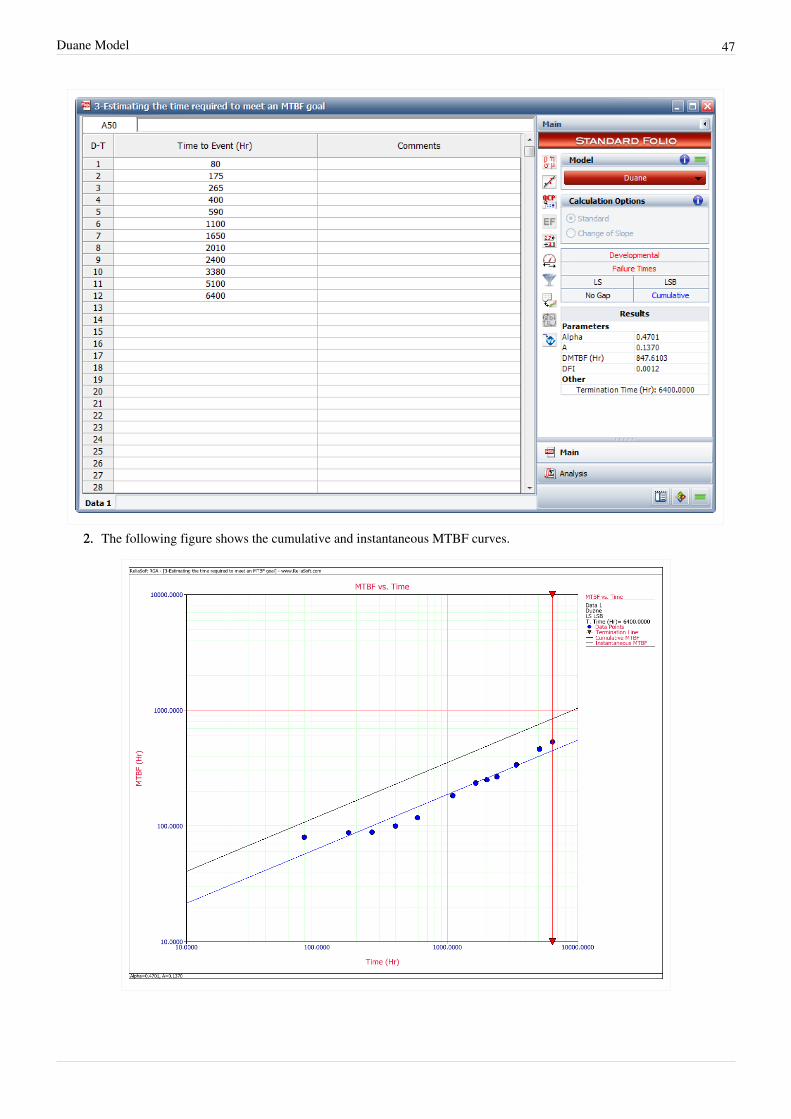
Duane Model 47

2.2. The following figure shows the cumulative and instantaneous MTBF curves.

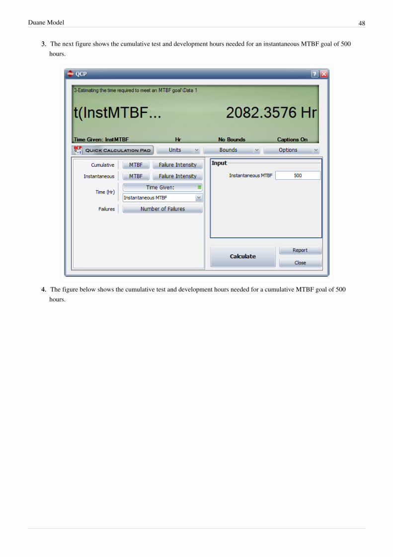
Duane Model 48

3.3. The next figure shows the cumulative test and development hours needed for an instantaneous MTBF goal of 500hours.

4.4. The figure below shows the cumulative test and development hours needed for a cumulative MTBF goal of 500hours.

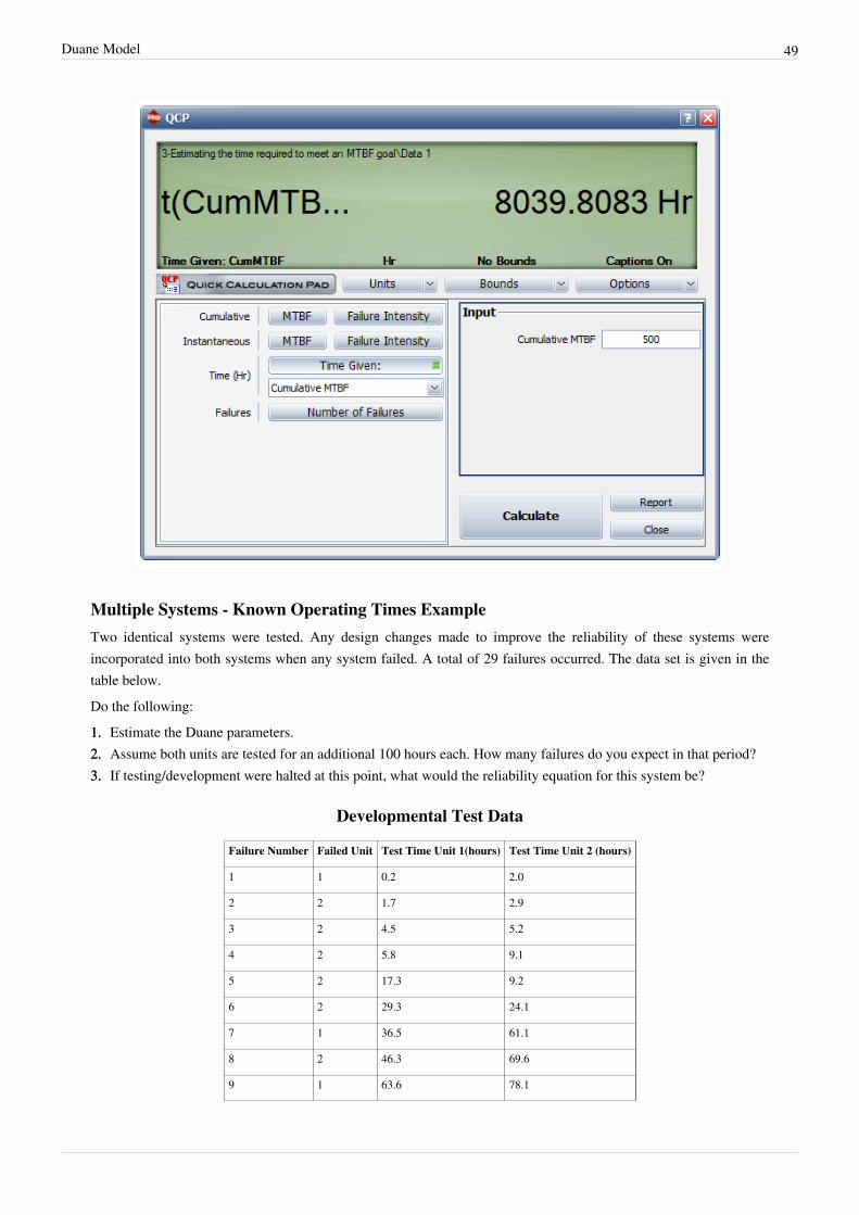
Duane Model 49

Multiple Systems - Known Operating Times ExampleTwo identical systems were tested. Any design changes made to improve the reliability of these systems wereincorporated into both systems when any system failed. A total of 29 failures occurred. The data set is given in thetable below.Do the following:1.1. Estimate the Duane parameters.2.2. Assume both units are tested for an additional 100 hours each. How many failures do you expect in that period?3.3. If testing/development were halted at this point, what would the reliability equation for this system be?

Developmental Test Data

Failure Number Failed Unit Test Time Unit 1(hours) Test Time Unit 2 (hours)

1 1 0.2 2.0

2 2 1.7 2.9

3 2 4.5 5.2

4 2 5.8 9.1

5 2 17.3 9.2

6 2 29.3 24.1

7 1 36.5 61.1

8 2 46.3 69.6

9 1 63.6 78.1

Duane Model 50

10 2 64.4 85.4

11 1 74.3 93.6

12 1 106.6 103

13 2 195.2 117

14 2 235.1 134.3

15 1 248.7 150.2

16 2 256.8 164.6

17 2 261.1 174.3

18 2 299.4 193.2

19 1 305.3 234.2

20 1 326.9 257.3

21 1 339.2 290.2

22 1 366.1 293.1

23 2 466.4 316.4

24 1 504 373.2

25 1 510 375.1

26 2 543.2 386.1

27 2 635.4 453.3

28 1 641.2 485.8

29 2 755.8 573.6

Solution

1.1. The figure below shows the data entered into RGA along with the estimated Duane parameters.

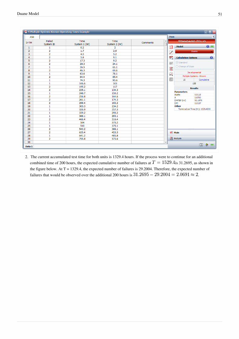
Duane Model 51

2. The current accumulated test time for both units is 1329.4 hours. If the process were to continue for an additionalcombined time of 200 hours, the expected cumulative number of failures at is 31.2695, as shown inthe figure below. At T = 1329.4, the expected number of failures is 29.2004. Therefore, the expected number offailures that would be observed over the additional 200 hours is .

Duane Model 52

3. If testing/development were halted at this point, the system failure intensity would be equal to the instantaneousfailure intensity at that time, or failures/hour. See the following figure.

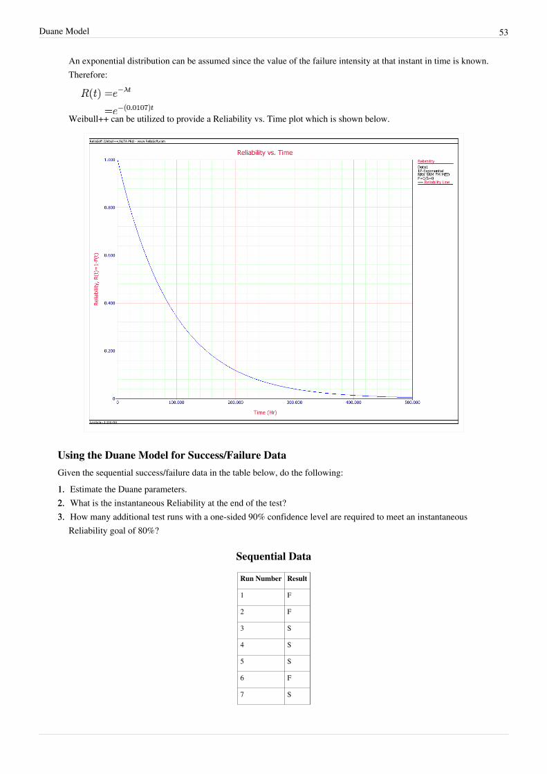
Duane Model 53

An exponential distribution can be assumed since the value of the failure intensity at that instant in time is known.Therefore:

Weibull++ can be utilized to provide a Reliability vs. Time plot which is shown below.

Using the Duane Model for Success/Failure DataGiven the sequential success/failure data in the table below, do the following:1.1. Estimate the Duane parameters.2.2. What is the instantaneous Reliability at the end of the test?3.3. How many additional test runs with a one-sided 90% confidence level are required to meet an instantaneous

Reliability goal of 80%?

Sequential Data

Run Number Result

1 F

2 F

3 S

4 S

5 S

6 F

7 S

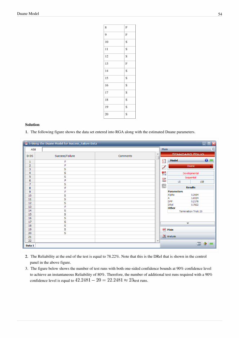
Duane Model 54

8 F

9 F

10 S

11 S

12 S

13 F

14 S

15 S

16 S

17 S

18 S

19 S

20 S

Solution

1.1. The following figure shows the data set entered into RGA along with the estimated Duane parameters.

2.2. The Reliability at the end of the test is equal to 78.22%. Note that this is the DRel that is shown in the controlpanel in the above figure.

3. The figure below shows the number of test runs with both one-sided confidence bounds at 90% confidence levelto achieve an instantaneous Reliability of 80%. Therefore, the number of additional test runs required with a 90%confidence level is equal to test runs.

Duane Model 55

56

Chapter 3.2

Crow-AMSAA (NHPP)Dr. Larry H. Crow [17] noted that the Duane Model could be stochastically represented as a Weibull process,allowing for statistical procedures to be used in the application of this model in reliability growth. This statisticalextension became what is known as the Crow-AMSAA (NHPP) model. This method was first developed at the U.S.Army Materiel Systems Analysis Activity (AMSAA). It is frequently used on systems when usage is measured on acontinuous scale. It can also be applied for the analysis of one shot items when there is high reliability and a largenumber of trials.Test programs are generally conducted on a phase by phase basis. The Crow-AMSAA model is designed for trackingthe reliability within a test phase and not across test phases. A development testing program may consist of severalseparate test phases. If corrective actions are introduced during a particular test phase, then this type of testing andthe associated data are appropriate for analysis by the Crow-AMSAA model. The model analyzes the reliabilitygrowth progress within each test phase and can aid in determining the following:•• Reliability of the configuration currently on test•• Reliability of the configuration on test at the end of the test phase•• Expected reliability if the test time for the phase is extended•• Growth rate•• Confidence intervals•• Applicable goodness-of-fit tests

BackgroundThe reliability growth pattern for the Crow-AMSAA model is exactly the same pattern as for the Duane postulate,that is, the cumulative number of failures is linear when plotted on ln-ln scale. Unlike the Duane postulate, theCrow-AMSAA model is statistically based. Under the Duane postulate, the failure rate is linear on ln-ln scale.However, for the Crow-AMSAA model statistical structure, the failure intensity of the underlying non-homogeneousPoisson process (NHPP) is linear when plotted on ln-ln scale.

Let be the cumulative number of failures observed in cumulative test time , and let be the failureintensity for the Crow-AMSAA model. Under the NHPP model, is approximately the probably of a failureoccurring over the interval for small . In addition, the expected number of failures experienced overthe test interval under the Crow-AMSAA model is given by:

The Crow-AMSAA model assumes that may be approximated by the Weibull failure rate function:

Therefore, if the intensity function, or the instantaneous failure intensity, , is defined as:

In the special case of exponential failure times, there is no growth and the failure intensity, , is equal to . Inthis case, the expected number of failures is given by:

Crow-AMSAA (NHPP) 57

In order for the plot to be linear when plotted on ln-ln scale under the general reliability growth case, the followingmust hold true where the expected number of failures is equal to:

To put a statistical structure on the reliability growth process, consider again the special case of no growth. In thiscase the number of failures, experienced during the testing over is random. The expected number offailures, is said to follow the homogeneous (constant) Poisson process with mean and is given by:

The Crow-AMSAA model generalizes this no growth case to allow for reliability growth due to corrective actions.This generalization keeps the Poisson distribution for the number of failures but allows for the expected number offailures, to be linear when plotted on ln-ln scale. The Crow-AMSAA model lets .The probability that the number of failures, will be equal to under growth is then given by the Poissondistribution:

This is the general growth situation, and the number of failures, , follows a non-homogeneous Poissonprocess. The exponential, "no growth" homogeneous Poisson process is a special case of the non-homogeneousCrow-AMSAA model. This is reflected in the Crow-AMSAA model parameter where . The cumulativefailure rate, , is:

The cumulative is:

As mentioned above, the local pattern for reliability growth within a test phase is the same as the growth patternobserved by Duane. The Duane is equal to:

And the Duane cumulative failure rate, , is:

Thus a relationship between Crow-AMSAA parameters and Duane parameters can be developed, such that:

Note that these relationships are not absolute. They change according to how the parameters (slopes, intercepts, etc.)are defined when the analysis of the data is performed. For the exponential case, , then , aconstant. For , is increasing. This indicates a deterioration in system reliability. For , isdecreasing. This is indicative of reliability growth. Note that the model assumes a Poisson process with the Weibullintensity function, not the Weibull distribution. Therefore, statistical procedures for the Weibull distribution do notapply for this model. The parameter is called a scale parameter because it depends upon the unit of measurementchosen for , while is the shape parameter that characterizes the shape of the graph of the intensity function.

Crow-AMSAA (NHPP) 58

The total number of failures, , is a random variable with Poisson distribution. Therefore, the probability thatexactly failures occur by time is:

The number of failures occurring in the interval from to is a random variable having a Poisson distributionwith mean:

The number of failures in any interval is statistically independent of the number of failures in any interval that doesnot overlap the first interval. At time , the failure intensity is . If improvements are not madeto the system after time , it is assumed that failures would continue to occur at the constant rate

. Future failures would then follow an exponential distribution with mean .The instantaneous MTBF of the system at time is:

is also called the demonstrated (or achieved) MTBF.

Note About ApplicabilityThe Duane and Crow-AMSAA models are the most frequently used reliability growth models. Their relationshipcomes from the fact that both make use of the underlying observed linear relationship between the logarithm ofcumulative MTBF and cumulative test time. However, the Duane model does not provide a capability to test whetherthe change in MTBF observed over time is significantly different from what might be seen due to random errorbetween phases. The Crow-AMSAA model allows for such assessments. Also, the Crow-AMSAA allows fordevelopment of hypothesis testing procedures to determine growth presence in the data (where indicates thatthere is growth in MTBF, indicates a constant MTBF and indicates a decreasing MTBF).Additionally, the Crow-AMSAA model views the process of reliability growth as probabilistic, while the Duanemodel views the process as deterministic.

Failure Times DataA description of Failure Times Data is presented in the RGA Data Types page.

Parameter Estimation for Failure Times DataThe parameters for the Crow-AMSAA (NHPP) model are estimated using maximum likelihood estimation (MLE).The probability density function (pdf) of the event given that the event occurred at is:

The likelihood function is:

where is the termination time and is given by:

Taking the natural log on both sides:

Crow-AMSAA (NHPP) 59

And differentiating with respect to yields:

Set equal to zero and solve for :

Now differentiate with respect to :

Set equal to zero and solve for :

This equation is used for both failure terminated and time terminated test data.

Biasing and Unbiasing of Beta

The equation above returns the biased estimate, . The unbiased estimate, , can be calculated by using thefollowing relationships. For time terminated data (the test ends after a specified test time):

For failure terminated data (the test ends after a specified number of failures):

By default is returned. can be returned by selecting the Calculate unbiased beta option on the Calculations tabof the Application Setup.

Cramér-von Mises TestThe Cramér-von Mises (CVM) goodness-of-fit test validates the hypothesis that the data follows anon-homogeneous Poisson process with a failure intensity equal to . This test can be applied whenthe failure data is complete over the continuous interval with no gaps in the data. The CVM data type appliesto all data types when the failure times are known, except for Fleet data.If the individual failure times are known, a Cramér-von Mises statistic is used to test the null hypothesis that anon-homogeneous Poisson process with the failure intensity function properly describes the reliability growth of a system. The Cramér-von Mises goodness-of-fit statistic is then given bythe following expression:

where:

The failure times, , must be ordered so that . If the statistic is less than the critical value corresponding to for a chosen significance level, then you can fail to reject the null hypothesis that the

Crow-AMSAA (NHPP) 60

Crow-AMSAA model adequately fits the data.

Critical Values

The following table displays the critical values for the Cramér-von Mises goodness-of-fit test given the sample size,, and the significance level, .

Critical values for Cramér-von Mises test

0.20 0.15 0.10 0.05 0.01

2 0.138 0.149 0.162 0.175 0.186

3 0.121 0.135 0.154 0.184 0.23

4 0.121 0.134 0.155 0.191 0.28

5 0.121 0.137 0.160 0.199 0.30

6 0.123 0.139 0.162 0.204 0.31

7 0.124 0.140 0.165 0.208 0.32

8 0.124 0.141 0.165 0.210 0.32

9 0.125 0.142 0.167 0.212 0.32

10 0.125 0.142 0.167 0.212 0.32

11 0.126 0.143 0.169 0.214 0.32

12 0.126 0.144 0.169 0.214 0.32

13 0.126 0.144 0.169 0.214 0.33

14 0.126 0.144 0.169 0.214 0.33

15 0.126 0.144 0.169 0.215 0.33

16 0.127 0.145 0.171 0.216 0.33

17 0.127 0.145 0.171 0.217 0.33

18 0.127 0.146 0.171 0.217 0.33

19 0.127 0.146 0.171 0.217 0.33

20 0.128 0.146 0.172 0.217 0.33

30 0.128 0.146 0.172 0.218 0.33

60 0.128 0.147 0.173 0.220 0.33

100 0.129 0.147 0.173 0.220 0.34

The significance level represents the probability of rejecting the hypothesis even if it's true. So, there is a riskassociated with applying the goodness-of-fit test (i.e., there is a chance that the CVM will indicate that the modeldoes not fit, when in fact it does). As the significance level is increased, the CVM test becomes more stringent. Keepin mind that the CVM test passes when the test statistic is less than the critical value. Therefore, the larger the criticalvalue, the more room there is to work with (e.g., a CVM test with a significance level equal to 0.1 is more strict thana test with 0.01).

Crow-AMSAA (NHPP) 61

Confidence BoundsThe RGA software provides two methods to estimate the confidence bounds for the Crow Extended model whenapplied to developmental testing data. The Fisher Matrix approach is based on the Fisher Information Matrix and iscommonly employed in the reliability field. The Crow bounds were developed by Dr. Larry Crow. See theCrow-AMSAA Confidence Bounds chapter for details on how the confidence bounds are calculated.

Failure Times Data Examples

Example - Parameter Estimation

A prototype of a system was tested with design changes incorporated during the test. The following table presentsthe data collected over the entire test. Find the Crow-AMSAA parameters and the intensity function using maximumlikelihood estimators.

Developmental Test Data

Row Time to Event (hr)

1 2.7 0.99325

2 10.3 2.33214

3 12.5 2.52573

4 30.6 3.42100

5 57.0 4.04305

6 61.3 4.11578

7 80.0 4.38203

8 109.5 4.69592

9 125.0 4.82831

10 128.6 4.85671

11 143.8 4.96842

12 167.9 5.12337

13 229.2 5.43459

14 296.7 5.69272

15 320.6 5.77019

16 328.2 5.79362

17 366.2 5.90318

18 396.7 5.98318

19 421.1 6.04287

20 438.2 6.08268

21 501.2 6.21701

22 620.0 6.42972

Solution

For the failure terminated test, is:

Crow-AMSAA (NHPP) 62

where:

Then:

And for :

Therefore, becomes:

The next figure shows the plot of the failure rate. If no further changes are made, the estimated MTBF is or46 hours.

Crow-AMSAA (NHPP) 63

Example - Confidence Bounds on Failure Intensity

Using the values of and estimated in the example given above, calculate the 90% 2-sided confidence bounds onthe cumulative and instantaneous failure intensity.Solution

Fisher Matrix Bounds

The partial derivatives for the Fisher Matrix confidence bounds are:

The Fisher Matrix then becomes:

For hours, the partial derivatives of the cumulative and instantaneous failure intensities are:

Therefore, the variances become:

The cumulative and instantaneous failure intensities at hours are:

So, at the 90% confidence level and for hours, the Fisher Matrix confidence bounds for the cumulativefailure intensity are:

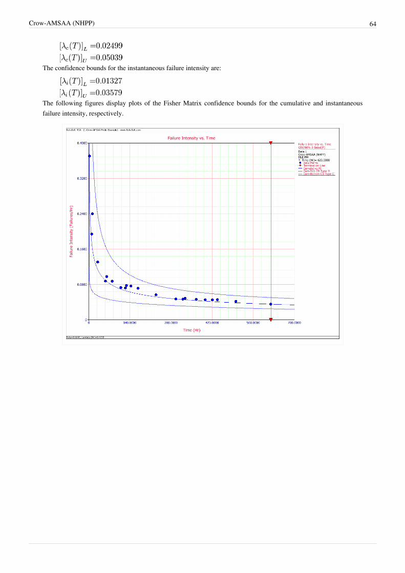
Crow-AMSAA (NHPP) 64

The confidence bounds for the instantaneous failure intensity are:

The following figures display plots of the Fisher Matrix confidence bounds for the cumulative and instantaneousfailure intensity, respectively.

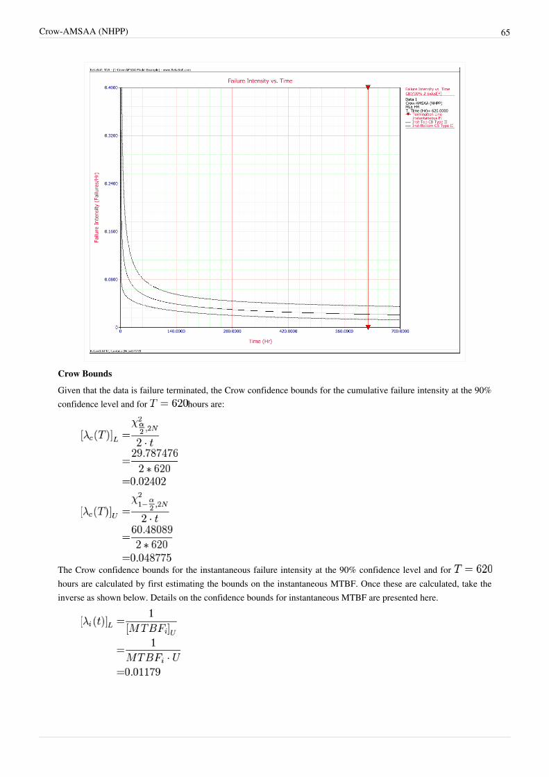
Crow-AMSAA (NHPP) 65

Crow Bounds

Given that the data is failure terminated, the Crow confidence bounds for the cumulative failure intensity at the 90%confidence level and for hours are:

The Crow confidence bounds for the instantaneous failure intensity at the 90% confidence level and for hours are calculated by first estimating the bounds on the instantaneous MTBF. Once these are calculated, take theinverse as shown below. Details on the confidence bounds for instantaneous MTBF are presented here.

Crow-AMSAA (NHPP) 66

The following figures display plots of the Crow confidence bounds for the cumulative and instantaneous failureintensity, respectively.

Crow-AMSAA (NHPP) 67

Example - Confidence Bounds on MTBF

Calculate the confidence bounds on the cumulative and instantaneous MTBF for the data from the example givenabove.Solution

Fisher Matrix Bounds

From the previous example:

And for hours, the partial derivatives of the cumulative and instantaneous MTBF are:

Crow-AMSAA (NHPP) 68

Therefore, the variances become:

So, at 90% confidence level and hours, the Fisher Matrix confidence bounds are:

The following two figures show plots of the Fisher Matrix confidence bounds for the cumulative and instantaneousMTBFs.

Crow-AMSAA (NHPP) 69

Crow Bounds

Crow-AMSAA (NHPP) 70

The Crow confidence bounds for the cumulative MTBF and the instantaneous MTBF at the 90% confidence leveland for hours are:

The figures below show plots of the Crow confidence bounds for the cumulative and instantaneous MTBF.

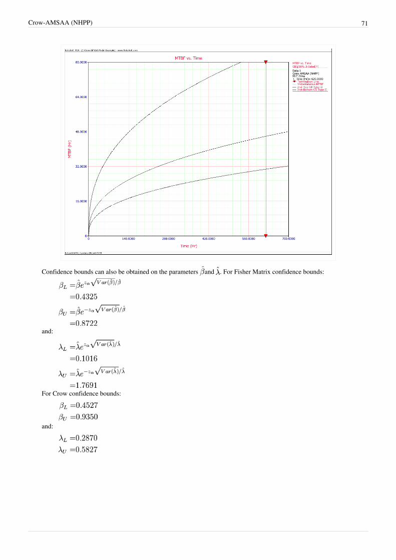
Crow-AMSAA (NHPP) 71

Confidence bounds can also be obtained on the parameters and . For Fisher Matrix confidence bounds:

and:

For Crow confidence bounds:

and:

Crow-AMSAA (NHPP) 72

Multiple SystemsWhen more than one system is placed on test during developmental testing, there are multiple data types which areavailable depending on the testing strategy and the format of the data. The data types that allow for the analysis ofmultiple systems using the Crow-AMSAA (NHPP) model are given below:•• Multiple Systems (Known Operating Times)•• Multiple Systems (Concurrent Operating Times)•• Multiple Systems with Dates

Goodness-of-fit TestsFor all multiple systems data types, the Cramér-von Mises (CVM) Test is available. For Multiple Systems(Concurrent Operating Times) and Multiple Systems with Dates, two additional tests are also available: LaplaceTrend Test and Common Beta Hypothesis.

Multiple Systems (Known Operating Times)A description of Multiple Systems (Known Operating Times) is presented on the RGA Data Types page.Consider the data in the table below for two prototypes that were placed in a reliability growth test.

Developmental Test Data for Two Identical Systems

Failure Number Failed Unit Test Time Unit 1 (hr) Test Time Unit 2 (hr) Total Test Time (hr)

1 1 1.0 1.7 2.7 0.99325

2 1 7.3 3.0 10.3 2.33214

3 2 8.7 3.8 12.5 2.52573

4 2 23.3 7.3 30.6 3.42100

5 2 46.4 10.6 57.0 4.04305

6 1 50.1 11.2 61.3 4.11578

7 1 57.8 22.2 80.0 4.38203

8 2 82.1 27.4 109.5 4.69592

9 2 86.6 38.4 125.0 4.82831

10 1 87.0 41.6 128.6 4.85671

11 2 98.7 45.1 143.8 4.96842

12 1 102.2 65.7 167.9 5.12337

13 1 139.2 90.0 229.2 5.43459

14 1 166.6 130.1 296.7 5.69272

15 2 180.8 139.8 320.6 5.77019

16 1 181.3 146.9 328.2 5.79362

17 2 207.9 158.3 366.2 5.90318

18 2 209.8 186.9 396.7 5.98318

19 2 226.9 194.2 421.1 6.04287

20 1 232.2 206.0 438.2 6.08268

21 2 267.5 233.7 501.2 6.21701

22 2 330.1 289.9 620.0 6.42972

Crow-AMSAA (NHPP) 73

The Failed Unit column indicates the system that failed and is meant to be informative, but it does not affect thecalculations. To combine the data from both systems, the system ages are added together at the times when a failureoccurred. This is seen in the Total Test Time column above. Once the single timeline is generated, then thecalculations for the parameters Beta and Lambda are the same as the process presented for Failure Times Data. Theresults of this analysis would match the results of Failure Times - Example 1.

Multiple Systems (Concurrent Operating Times)A description of Multiple Systems (Concurrent Operating Times) is presented on the RGA Data Types page.

Parameter Estimation for Multiple Systems (Concurrent Operating Times)

To estimate the parameters, the equivalent system must first be determined. The equivalent single system (ESS) iscalculated by summing the usage across all systems when a failure occurs. Keep in mind that Multiple Systems(Concurrent Operating Times) assumes that the systems are running simultaneously and accumulate the same usage.If the systems have different end times then the equivalent system must only account for the systems that areoperating when a failure occurred. Systems with a start time greater than zero are shifted back to t = 0. This is thesame as having a start time equal to zero and the converted end time is equal to the end time minus the start time. Inaddition, all failures times are adjusted by subtracting the start time from each value to ensure that all values occurwithin t = 0 and the adjusted end time. A start time greater than zero indicates that it is not known as to what eventsoccurred at a time less than the start time. This may have been caused by the events during this period not beingtracked and/or recorded properly.As an example, consider two systems have entered a reliability growth test. Both systems have a start time equal tozero and both begin the test with the same configuration. System 1 operated for 100 hours and System 2 operated for125 hours. The failure times for each system are given below:•• System 1: 25, 47, 80•• System 2: 15, 62, 89, 110To build the ESS, the total accumulated hours across both systems is taken into account when a failure occurs.Therefore, given the data for Systems 1 and 2, the ESS is comprised of the following events: 30, 50, 94, 124, 160,178, 210.The ESS combines the data from both systems into a single timeline. The termination time for the ESS is (100 +125) = 225 hours. The parameter estimates for and are then calculated using the ESS. This process is the same asthe method for Failure Times data.

Example - Concurrent Operating Times

Six systems were subjected to a reliability growth test, and a total of 82 failures were observed. Given the data in thetable below, which presents the start/end times and times-to-failure for each system, do the following:1.1. Estimate the parameters of the Crow-AMSAA model using maximum likelihood estimation.2.2. Determine how many additional failures would be generated if testing continues until 3,000 hours.

Crow-AMSAA (NHPP) 74

Multiple Systems (Concurrent Operating Times) Data

System # 1 2 3 4 5 6

Start Time (Hr) 0 0 0 0 0 0

End Time (Hr) 504 541 454 474 436 500

Failure Times (Hr) 21 83 26 36 23 7

29 83 26 306 46 13

43 83 57 306 127 13

43 169 64 334 166 31

43 213 169 354 169 31

66 299 213 395 213 82

115 375 231 403 213 109

159 431 231 448 255 137

199 231 456 369 166

202 231 461 374 200

222 304 380 210

248 383 415 220

248 301

255 422

286 437

286 469

304 469

320

348

364

404

410

429

Solution

1. To estimate the parameters and , the equivalent single system (ESS) must first be determined. The ESS isgiven below:

Equivalent Single System

Crow-AMSAA (NHPP) 75

Row Time to Event (hr) Row Time to Event (hr) Row Time to Event (hr) Row Time to Event (hr)

1 42 22 498 43 1386 64 2214

2 78 23 654 44 1386 65 2244

3 78 24 690 45 1386 66 2250

4 126 25 762 46 1386 67 2280

5 138 26 822 47 1488 68 2298

6 156 27 954 48 1488 69 2370

7 156 28 996 49 1530 70 2418

8 174 29 996 50 1530 71 2424

9 186 30 1014 51 1716 72 2460

10 186 31 1014 52 1716 73 2490

11 216 32 1014 53 1794 74 2532

12 258 33 1194 54 1806 75 2574

13 258 34 1200 55 1824 76 2586

14 258 35 1212 56 1824 77 2621

15 276 36 1260 57 1836 78 2676

16 342 37 1278 58 1836 79 2714

17 384 38 1278 59 1920 80 2734

18 396 39 1278 60 2004 81 2766

19 492 40 1278 61 2088 82 2766

20 498 41 1320 62 2124

21 498 42 1332 63 2184

Given the ESS data, the value of is calculated using:

where is the number of failures and is the termination time. The termination time is the sum of end times foreach of the systems, which equals 2,909. is estimated with:

The next figure shows the parameters estimated using RGA.

Crow-AMSAA (NHPP) 76

2. The number of failures can be estimated using the Quick Calculation Pad, as shown next. The estimated numberof failures at 3,000 hours is equal to 84.2892 and 82 failures were observed during testing. Therefore, the numberof additional failures generated if testing continues until 3,000 hours is equal to

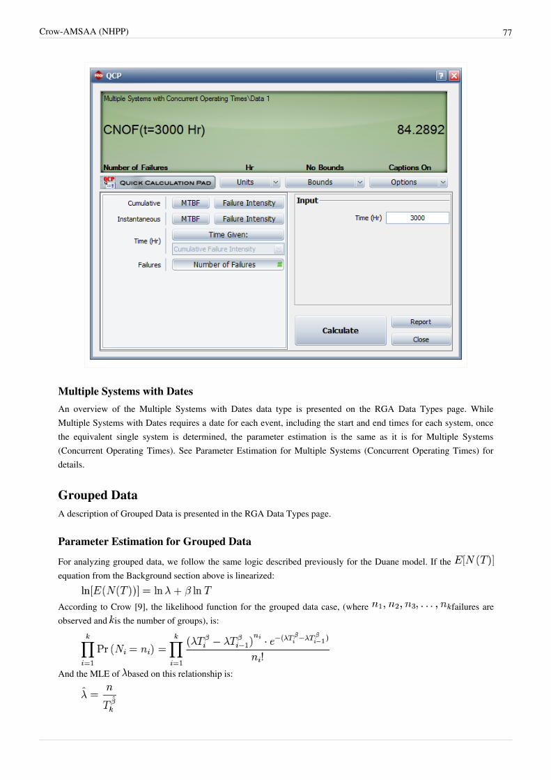
Crow-AMSAA (NHPP) 77

Multiple Systems with DatesAn overview of the Multiple Systems with Dates data type is presented on the RGA Data Types page. WhileMultiple Systems with Dates requires a date for each event, including the start and end times for each system, oncethe equivalent single system is determined, the parameter estimation is the same as it is for Multiple Systems(Concurrent Operating Times). See Parameter Estimation for Multiple Systems (Concurrent Operating Times) fordetails.

Grouped DataA description of Grouped Data is presented in the RGA Data Types page.

Parameter Estimation for Grouped Data

For analyzing grouped data, we follow the same logic described previously for the Duane model. If the equation from the Background section above is linearized:

According to Crow [9], the likelihood function for the grouped data case, (where failures areobserved and is the number of groups), is:

And the MLE of based on this relationship is:

Crow-AMSAA (NHPP) 78

where is the total number of failures from all the groups.

The estimate of is the value that satisfies:

See Crow-AMSAA Confidence Bounds for details on how confidence bounds for grouped data are calculated.

Chi-Squared TestA chi-squared goodness-of-fit test is used to test the null hypothesis that the Crow-AMSAA reliability modeladequately represents a set of grouped data. This test is applied only when the data is grouped. The expected numberof failures in the interval from to is approximated by:

For each interval, shall not be less than 5 and, if necessary, adjacent intervals may have to be combined so that theexpected number of failures in any combined interval is at least 5. Let the number of intervals after thisrecombination be , and let the observed number of failures in the new interval be . Finally, let the expectednumber of failures in the new interval be . Then the following statistic is approximately distributed as achi-squared random variable with degrees of freedom .

The null hypothesis is rejected if the statistic exceeds the critical value for a chosen significance level. In thiscase, the hypothesis that the Crow-AMSAA model adequately fits the grouped data shall be rejected. Critical valuesfor this statistic can be found in chi-squared distribution tables.

Grouped Data Examples

Example - Simple Grouped

Consider the grouped failure times data given in the following table. Solve for the Crow-AMSAA parameters usingMLE.

Grouped Failure Times Data

Run Number Cumulative Failures End Time(hours)

1 2 200 5.298 28.072 0.693 3.673

2 3 400 5.991 35.898 1.099 6.582

3 4 600 6.397 40.921 1.386 8.868

4 11 3000 8.006 64.102 2.398 19.198

Sum = 25.693 168.992 5.576 38.321

Solution

Using RGA, the value of , which must be solved numerically, is 0.6315. Using this value, the estimator of is:

Therefore, the intensity function becomes:

Crow-AMSAA (NHPP) 79

Example - Helicopter System

A new helicopter system is under development. System failure data has been collected on five helicopters during thefinal test phase. The actual failure times cannot be determined since the failures are not discovered until after thehelicopters are brought into the maintenance area. However, total flying hours are known when the helicopters arebrought in for service, and every 2 weeks each helicopter undergoes a thorough inspection to uncover any failuresthat may have occurred since the last inspection. Therefore, the cumulative total number of flight hours and thecumulative total number of failures for the 5 helicopters are known for each 2-week period. The total number offlight hours from the test phase is 500, which was accrued over a period of 12 weeks (six 2-week intervals). For each2-week interval, the total number of flight hours and total number of failures for the 5 helicopters were recorded. Thegrouped data set is displayed in the following table.

Grouped Data for a New Helicopter System

Interval Interval Length Failures in Interval

1 0 - 62 12

2 62 -100 6

3 100 - 187 15

4 187 - 210 3

5 210 - 350 18

6 350 - 500 16

Do the following:1.1. Estimate the parameters of the Crow-AMSAA model using maximum likelihood estimation.2.2. Calculate the confidence bounds on the cumulative and instantaneous MTBF using the Fisher Matrix and Crow

methods.Solution

1. Using RGA, the value of , must be solved numerically. Once has been estimated then the value of can bedetermined. The parameter values are displayed below:

The grouped Fisher Matrix confidence bounds can be obtained on the parameters and at the 90% confidencelevel by:

and:

Crow-AMSAA (NHPP) 80

Crow confidence bounds can also be obtained on the parameters and at the 90% confidence level, as:

and:

2. The Fisher Matrix confidence bounds for the cumulative MTBF and the instantaneous MTBF at the 90% 2-sidedconfidence level and for hour are:

and:

The next two figures show plots of the Fisher Matrix confidence bounds for the cumulative and instantaneousMTBF.

Crow-AMSAA (NHPP) 81

The Crow confidence bounds for the cumulative and instantaneous MTBF at the 90% 2-sided confidence leveland for hours are:

Crow-AMSAA (NHPP) 82

and:

The next two figures show plots of the Crow confidence bounds for the cumulative and instantaneous MTBF.

Crow-AMSAA (NHPP) 83

More grouped data examples are available! See also: Simple MTBF Determination [1]

Missing DataMost of the reliability growth models used for estimating and tracking reliability growth based on test data assumethat the data set represents all actual system failure times consistent with a uniform definition of failure (completedata). In practice, this may not always be the case and may result in too few or too many failures being reported oversome interval of test time. This may result in distorted estimates of the growth rate and current system reliability.This section discusses a practical reliability growth estimation and analysis procedure based on the assumption thatanomalies may exist within the data over some interval of the test period but the remaining failure data follows theCrow-AMSAA reliability growth model. In particular, it is assumed that the beginning and ending points in whichthe anomalies lie are generated independently of the underlying reliability growth process. The approach forestimating the parameters of the growth model with problem data over some interval of time is basically to not usethis failure information. The analysis retains the contribution of the interval to the total test time, but no assumptionsare made regarding the actual number of failures over the interval. This is often referred to as gap analysis.

Consider the case where a system is tested for time and the actual failure times are recorded. The time maypossibly be an observed failure time. Also, the end points of the gap interval may or may not correspond to arecorded failure time. The underlying assumption is that the data used in the maximum likelihood estimation followsthe Crow-AMSAA model with a Weibull intensity function . It is not assumed that zero failures occurredduring the gap interval, rather, it is assumed that the actual number of failures is unknown, and hence no informationat all regarding these failure is used to estimate and .

Crow-AMSAA (NHPP) 84

Let , denote the end points of the gap interval, Let be thefailure times over and let be the failure times over . Themaximum likelihood estimates of and are values and satisfying the following equations.

In general, these equations cannot be solved explicitly for and , but must be solved by an iterative procedure.

Example - Gap Analysis

Consider a system under development that was subjected to a reliability growth test for hours. Eachmonth, the successive failure times, on a cumulative test time basis, were reported. According to the test plan, 125hours of test time were accumulated on each prototype system each month. The total reliability growth test programlasted for 7 months. One prototype was tested for each of the months 1, 3, 4, 5, 6 and 7 with 125 hours of test time.During the second month, two prototypes were tested for a total of 250 hours of test time. The next table shows thesuccessive failure times that were reported for hours of testing.

,

.5 .6 10.7 16.6 18.3 19.2 19.5 25.3

39.2 39.4 43.2 44.8 47.4 65.7 88.1 97.2

104.9 105.1 120.8 195.7 217.1 219 257.5 260.4

281.3 283.7 289.8 306.6 328.6 357.0 371.7 374.7

393.2 403.2 466.5 500.9 501.5 518.4 520.7 522.7

524.6 526.9 527.8 533.6 536.5 542.6 543.2 545.0

547.4 554.0 554.1 554.2 554.8 556.5 570.6 571.4

574.9 576.8 578.8 583.4 584.9 590.6 596.1 599.1

600.1 602.5 613.9 616.0 616.2 617.1 621.4 622.6

624.7 628.8 642.4 684.8 731.9 735.1 753.6 792.5

803.7 805.4 832.5 836.2 873.2 975.1

The observed and cumulative number of failures for each month are:

Month Time Period Observed Failure Times Cumulative Failure Times

1 0-125 19 19

2 125-375 13 32

3 375-500 3 35

4 500-625 38 73

5 625-750 5 78

6 750-875 7 85

7 875-1000 1 86

1.1. Determine the maximum likelihood estimators for the Crow-AMSAA model.2.2. Evaluate the goodness-of-fit for the model.

Crow-AMSAA (NHPP) 85

3. Consider as the gap interval and determine the maximum likelihood estimates of and .Solution

1.1. For the time terminated test:

2.2. The Cramér-von Mises goodness-of-fit test for this data set yields:

The critical value at the 10% significance level is 0.173. Therefore, the test indicated that the analyst should rejectthe hypothesis that the data set follows the Crow-AMSAA reliability growth model. The following plot shows

versus with the fitted line , where and are the maximumlikelihood estimates.

Observing the data during the fourth month (between 500 and 625 hours), 38 failures were reported. This numberis very high in comparison to the failures reported in the other months. A quick investigation found that a numberof new data collectors were assigned to the project during this month. It was also discovered that extensive designchanges were made during this period, which involved the removal of a large number of parts. It is possible thatthese removals, which were not failures, were incorrectly reported as failed parts. Based on knowledge of thesystem and the test program, it was clear that such a large number of actual system failures was extremelyunlikely. The consensus was that this anomaly was due to the failure reporting. For this analysis, it was decidedthat the actual number of failures over this month is assumed to be unknown, but consistent with the remainingdata and the Crow-AMSAA reliability growth model.

3. Considering the problem interval as the gap interval, we will use the data over the interval and over the interval The equations for analyzing missing data are the appropriate equations to estimate and because the failure times are known. In this case and

Crow-AMSAA (NHPP) 86

. The maximum likelihood estimates of and are:

The next figure is a plot of the cumulative number of failures versus time. This plot is approximately linear,which also indicates a good fit of the model.

Discrete DataThe Crow-AMSAA model can be adapted for the analysis of success/failure data (also called discrete or attributedata). The following discrete data types are available:•• Sequential•• Grouped per Configuration•• MixedSequential data and Grouped per Configuration are very similar as the parameter estimation methodology is the samefor both data types. Mixed data is a combination of Sequential Data and Grouped per Configuration and is presentedin Mixed Data.

Crow-AMSAA (NHPP) 87

Grouped per Configuration

Suppose system development is represented by configurations. This corresponds to configuration changes,unless fixes are applied at the end of the test phase, in which case there would be configuration changes. Let bethe number of trials during configuration and let be the number of failures during configuration . Then thecumulative number of trials through configuration , namely , is the sum of the for all , or:

And the cumulative number of failures through configuration , namely , is the sum of the for all , or:

The expected value of can be expressed as and defined as the expected number of failures by the end ofconfiguration . Applying the learning curve property to implies:

Denote as the probability of failure for configuration 1 and use it to develop a generalized equation for in termsof the and . From the equation above, the expected number of failures by the end of configuration 1 is:

Applying the equation again and noting that the expected number of failures by the end of configuration 2 isthe sum of the expected number of failures in configuration 1 and the expected number of failures in configuration 2:

By this method of inductive reasoning, a generalized equation for the failure probability on a configuration basis, ,is obtained, such that:

In this equation, represents the trial number. Thus, an equation for the reliability (probability of success) for the configuration is obtained:

Sequential DataFrom the Grouped per Configuration section, the following equation is given:

For the special case where for all , the equation above becomes a smooth curve, , that represents theprobability of failure for trial by trial data, or:

When , this is the same as Sequential Data where systems are tested on a trial-by-trial basis. The equationfor the reliability for the trial is:

Crow-AMSAA (NHPP) 88

Parameter Estimation for Discrete DataThis section describes procedures for estimating the parameters of the Crow-AMSAA model for success/failure datawhich includes Sequential data and Grouped per Configuration. An example is presented illustrating these concepts.The estimation procedures provide maximum likelihood estimates (MLEs) for the model's two parameters, and .The MLEs for and allow for point estimates for the probability of failure, given by:

And the probability of success (reliability) for each configuration is equal to:

The likelihood function is:

Taking the natural log on both sides yields:

Taking the derivative with respect to and respectively, exact MLEs for and are values satisfying thefollowing two equations:

where:

Example - Grouped per ConfigurationA one-shot system underwent reliability growth development testing for a total of 68 trials. Delayed correctiveactions were incorporated after the 14th, 33rd and 48th trials. From trial 49 to trial 68, the configuration was notchanged.•• Configuration 1 experienced 5 failures,•• Configuration 2 experienced 3 failures,•• Configuration 3 experienced 4 failures and•• Configuration 4 experienced 4 failures.Do the following:1.1. Estimate the parameters of the Crow-AMSAA model using maximum likelihood estimation.

Crow-AMSAA (NHPP) 89

2.2. Estimate the unreliability and reliability by configuration.Solution

1. The parameter estimates for the Crow-AMSAA model using the parameter estimation for discrete datamethodology yields and .

2.2. The following table displays the results for probability of failure and reliability, and these results are displayed inthe next two plots.

Estimated Failure Probability and Reliability by Configuration

Configuration( ) Estimated Failure Probability Estimated Reliability

1 0.333 0.667

2 0.234 0.766

3 0.206 0.794

4 0.190 0.810

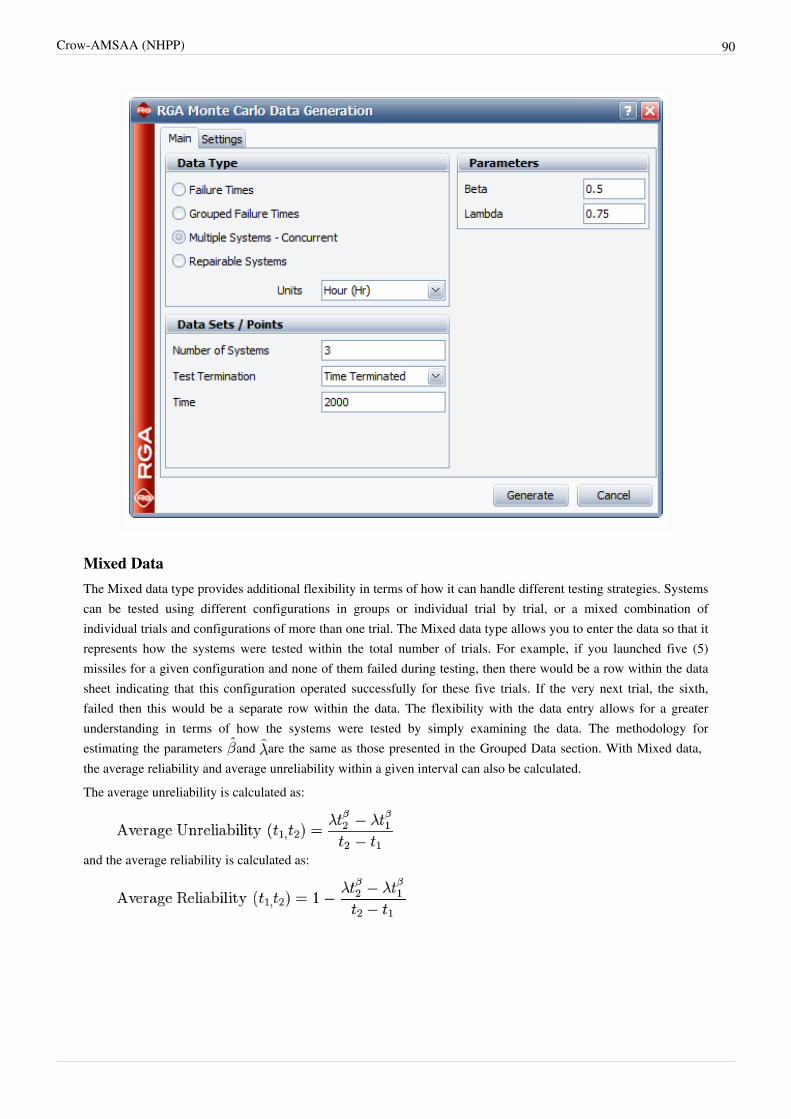
Crow-AMSAA (NHPP) 90

Mixed DataThe Mixed data type provides additional flexibility in terms of how it can handle different testing strategies. Systemscan be tested using different configurations in groups or individual trial by trial, or a mixed combination ofindividual trials and configurations of more than one trial. The Mixed data type allows you to enter the data so that itrepresents how the systems were tested within the total number of trials. For example, if you launched five (5)missiles for a given configuration and none of them failed during testing, then there would be a row within the datasheet indicating that this configuration operated successfully for these five trials. If the very next trial, the sixth,failed then this would be a separate row within the data. The flexibility with the data entry allows for a greaterunderstanding in terms of how the systems were tested by simply examining the data. The methodology forestimating the parameters and are the same as those presented in the Grouped Data section. With Mixed data,the average reliability and average unreliability within a given interval can also be calculated.The average unreliability is calculated as:

and the average reliability is calculated as:

Crow-AMSAA (NHPP) 91

Mixed Data Confidence Bounds

Bounds on Average Failure ProbabilityThe process to calculate the average unreliability confidence bounds for Mixed data is as follows:

1. Calculate the average failure probability .2. There will exist a between and such that the instantaneous unreliability at equals the average

unreliability . The confidence intervals for the instantaneous unreliability at are the confidenceintervals for the average unreliability .

Bounds on Average ReliabilityThe process to calculate the average reliability confidence bounds for Mixed data is as follows:

1. Calculate confidence bounds for average unreliability as described above.2.2. The confidence bounds for reliability are 1 minus these confidence bounds for average unreliability.

Example - Mixed Data

The table below shows the number of failures of each interval of trials and the cumulative number of trials in eachinterval for a reliability growth test. For example, the first row indicates that for an interval of 14 trials, 5 failuresoccurred.

Mixed Data

Failures in Interval Cumulative Trials

5 14

3 33

4 48

0 52

1 53

0 57

1 58

0 62

1 63

0 67

1 68

Using the RGA software, the parameters of the Crow-AMSAA model are estimated as follows:

and:

As we have seen, the Crow-AMSAA instantaneous failure intensity, , is defined as:

Using the parameter estimates, we can calculate the instantaneous unreliability at the end of the test, or

This result that can be obtained from the Quick Calculation Pad (QCP), for as seen in the followingpicture.

Crow-AMSAA (NHPP) 92

The instantaneous reliability can then be calculated as:

Change of SlopeThe assumption of the Crow-AMSAA (NHPP) model is that the failure intensity is monotonically increasing,decreasing or remaining constant over time. However, there might be cases in which the system design or theoperational environment experiences major changes during the observation period and, therefore, a single model willnot be appropriate to describe the failure behavior for the entire timeline. RGA incorporates a methodology that canbe applied to scenarios where a major change occurs during a reliability growth test. The test data can be broken intotwo segments with a separate Crow-AMSAA (NHPP) model applied to each segment.Consider the data in the following plot from a reliability growth test.

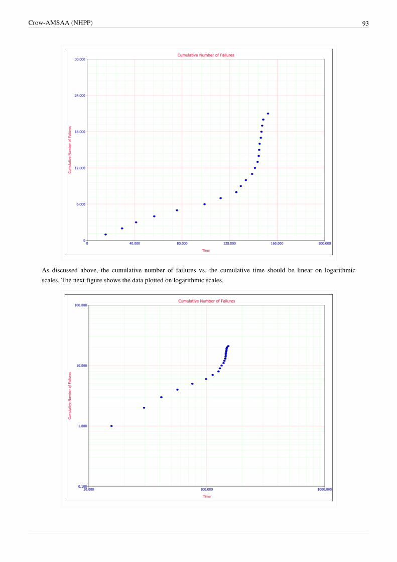
Crow-AMSAA (NHPP) 93

As discussed above, the cumulative number of failures vs. the cumulative time should be linear on logarithmicscales. The next figure shows the data plotted on logarithmic scales.

Crow-AMSAA (NHPP) 94

One can easily recognize that the failure behavior is not constant throughout the duration of the test. Just byobserving the data, it can be asserted that a major change occurred at around 140 hours that resulted in a change inthe rate of failures. Therefore, using a single model to analyze this data set likely will not be appropriate.The Change of Slope methodology proposes to split the data into two segments and apply a Crow-AMSAA (NHPP)model to each segment. The time of change that will be used to split the data into the two segments (it will bereferred to as ) could be estimated just by observing the data, but will most likely be dictated by engineeringknowledge of the specific change to the system design or operating conditions. It is important to note that althoughtwo separate models will be applied to each segment, the information collected in the first segment (i.e., data up to

) will be considered when creating the model for the second segment (i.e., data after ). The models presentednext can be applied to the reliability growth analysis of a single system or multiple systems.

Model for First Segment (Data up to T1)

The data up to the point of the change that occurs at will be analyzed using the Crow-AMSAA (NHPP) model.Based on the ML equations for and (in the section Maximum Likelihood Estimators), the ML estimators of themodel are:

and

where:

• is the time when the change occurs• is the number of failures observed up to time • is the time at which each corresponding failure was observed

The equation for can be rewritten as follows:

or

Crow-AMSAA (NHPP) 95

Model for Second Segment (Data after T1)

The Crow-AMSAA (NHPP) model will be used again to analyze the data after . However, the informationcollected during the first segment will be used when creating the model for the second segment. Given that, the MLestimators of the model parameters in the second segment are:

and:

where:

• is the number of failures that were observed after • is the total number of failures observed throughout the test• is the end time of the test. The test can either be failure terminated or time terminated

Example - Multiple MLEThe following table gives the failure times obtained from a reliability growth test of a newly designed system. Thetest has a duration of 660 hours.

Failure Times From a Reliability Growth Test

First, apply a single Crow-AMSAA (NHPP) model to all of the data. The following plot shows the expected failuresobtained from the model (the line) along with the observed failures (the points).

Crow-AMSAA (NHPP) 96

The plot shows that the model does not seem to accurately track the data. This is confirmed by performing theCramér-von Mises goodness-of-fit test, which checks the hypothesis that the data follows a non-homogeneousPoisson process with a power law failure intensity. The model fails the goodness-of-fit test because the test statistic(0.3309) is higher than the critical value (0.1729) at the 0.1 significance level. The next figure shows a customizedreport that displays both the calculated parameters and the statistical test results.

Crow-AMSAA (NHPP) 97

Through further investigation, it is discovered that a significant design change occurred at 400 hours of test time. It issuspected that this modification is responsible for the change in the failure behavior.In RGA, you have the option to perform a standard Crow-AMSAA (NHPP) analysis, or perform a Change of Slopeanalysis where you specify a specific breakpoint, as shown in the following figure. RGA actually creates a groupeddata set where the data in Segment 1 is included and defined by a single interval to calculate the Segment 2parameters. However, these results are equivalent to the parameters estimated using the equations presented here.

Therefore, the Change of Slope methodology is applied to break the data into two segments for analysis. The firstsegment is set from 0 to 400 hours and the second segment is from 401 to 660 hours (which is the end time of thetest). The Crow-AMSAA (NHPP) parameters for the first segment (0-400 hours) are:

and

The Crow-AMSAA (NHPP) parameters for the second segment (401-660 hours) are:

Crow-AMSAA (NHPP) 98

The following figure shows a plot of the two-segment analysis along with the observed data. It is obvious that theChange of Slope method tracks the data more accurately.

This can also be verified by performing a chi-squared goodness-of-fit test. The chi-squared statistic is 1.2956, whichis lower than the critical value of 12.017 at the 0.1 significance level; therefore, the analysis passes the test. The nextfigure shows a customized report that displays both the calculated parameters and the statistical test results.

Crow-AMSAA (NHPP) 99

When you have a model that fits the data, it can be used to make accurate predictions and calculations. Metrics suchas the demonstrated MTBF at the end of the test or the expected number of failures at later times can be calculated.For example, the following plot shows the instantaneous MTBF vs. time, together with the two-sided 90%confidence bounds. Note that confidence bounds are available for the second segment only. For times up to 400hours, the parameters of the first segment were used to calculate the MTBF, while the parameters of the secondsegment were used for times after 400 hours. Also note that the number of failures at the end of segment 1 is notassumed to be equal to the number of failures at the start of segment 2. This can result in a visible jump in the plot,as in this example.

Crow-AMSAA (NHPP) 100

The next figure shows the use of the Quick Calculation Pad (QCP) in the RGA software to calculate theDemonstrated MTBF at the end of the test (instantaneous MTBF at time = 660), together with the two-sided 90%confidence bounds. All the calculations were based on the parameters of the second segment.

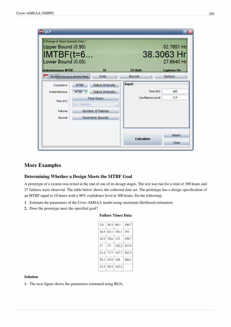
Crow-AMSAA (NHPP) 101

More Examples

Determining Whether a Design Meets the MTBF GoalA prototype of a system was tested at the end of one of its design stages. The test was run for a total of 300 hours and27 failures were observed. The table below shows the collected data set. The prototype has a design specification ofan MTBF equal to 10 hours with a 90% confidence level at 300 hours. Do the following:1.1. Estimate the parameters of the Crow-AMSAA model using maximum likelihood estimation.2.2. Does the prototype meet the specified goal?

Failure Times Data

2.6 56.5 98.1 190.7

16.5 63.1 101.1 193

16.5 70.6 132 198.7

17 73 142.2 251.9

21.4 77.7 147.7 282.5

29.1 93.9 149 286.1

33.3 95.5 167.2

Solution

1.1. The next figure shows the parameters estimated using RGA.

Crow-AMSAA (NHPP) 102

2.2. The instantaneous MTBF with one-sided 90% confidence bounds can be calculated using the Quick CalculationPad (QCP), as shown next. From the QCP, it is estimated that the lower limit on the MTBF at 300 hours with a90% confidence level is equal to 10.8170 hours. Therefore, the prototype has met the specified goal.

Crow-AMSAA (NHPP) 103

Analyzing Mixed Data for a One-Shot SystemA one-shot system underwent reliability growth development for a total of 50 trials. The test was performed as acombination of configuration in groups and individual trial by trial. The table below shows the data set obtainedfrom the test. The first column specifies the number of failures that occurred in each interval, and the second columnshows the cumulative number of trials in that interval. Do the following:1.1. Estimate the parameters of the Crow-AMSAA model using maximum likelihood estimators.2.2. What are the instantaneous reliability and the 2-sided 90% confidence bounds at the end of the test?3.3. Plot the cumulative reliability with 2-sided 90% confidence bounds.4.4. If the test was continued for another 25 trials what would the expected number of additional failures be?

Mixed Data

Failures in Interval Cumulative Trials Failures in Interval Cumulative Trials

3 4 1 25

0 5 1 28

4 9 0 32

1 12 2 37

0 13 0 39

1 15 1 40

2 19 1 44

1 20 0 46

1 22 1 49

Crow-AMSAA (NHPP) 104

0 24 0 50

Solution

1.1. The next figure shows the parameters estimated using RGA.

2.2. The figure below shows the calculation of the instantaneous reliability with the 2-sided 90% confidence bounds.From the QCP, it is estimated that the instantaneous reliability at stage 50 (or at the end of the test) is 72.70%with an upper and lower 2-sided 90% confidence bound of 82.36% and 39.59%, respectively.

Crow-AMSAA (NHPP) 105

3.3. The following plot shows the cumulative reliability with the 2-sided 90% confidence bounds.

Crow-AMSAA (NHPP) 106

4. The last figure shows the calculation of the expected number of failures after 75 trials. From the QCP, it isestimated that the cumulative number of failures after 75 trials is . Since 20 failures occurred inthe first 50 trials, the estimated number of additional failures is 7.

References[1] http:/ / www. reliasoft. com/ rga/ examples/ rgex1/ index. htm

107

Chapter 3.3

Crow ExtendedIn reliability growth analysis, the Crow-AMSAA (NHPP) model assumes that the corrective actions for the observedfailure modes are incorporated during the test (test-fix-test). However, in actual practice, fixes may be delayed untilafter the completion of the test (test-find-test) or some fixes may be implemented during the test while others aredelayed (test-fix-find-test). At the end of a test phase, two reliability estimates are of concern: demonstratedreliability and projected reliability. The demonstrated reliability, which is based on data generated during the testphase, is an estimate of the system reliability for its configuration at the end of the test phase. The projectedreliability measures the impact of the delayed fixes at the end of the current test phase.Most of the reliability growth literature are concerned with procedures and models for calculating the demonstratedreliability, and very little attention has been paid to techniques for reliability projections. The procedure for makingreliability projections utilizes engineering assessments of the effectiveness of the delayed fixes for each observedfailure mode. These effectiveness factors are then used with the data generated during the test phase to obtain aprojected estimate for the updated configuration by adjusting the number of failures observed during the test phase.The process of estimating the projected reliability is accomplished using the Crow Extended model. The CrowExtended model allows for a flexible growth strategy that can include corrective actions performed during the test, aswell as delayed corrective actions. The test-find-test and test-fix-find-test scenarios are simply subsets of the CrowExtended model.For developmental testing, the Crow Extended model can be applied when using any of the following data types:•• Failure Times Data•• Multiple Systems (Known Operating Times)•• Multiple Systems (Concurrent Operating Times)•• Multiple Systems with Dates•• Multiple Systems with Event Codes•• Grouped Failure Times•• Mixed DataAs the name implies, Crow Extended is simply an "extension" of the Crow-AMSAA (NHPP) model. Thecalculations for Crow Extended still incorporate the methods for Crow-AMSAA based on the data type, as describedon the Crow-AMSAA (NHPP) page. The Crow-AMSAA model estimates the growth during the test, while the CrowExtended model accounts for the growth after the test based on the delayed corrective actions. Additional detailsregarding the calculations for the Crow Extended model are presented in the sections below.

BackgroundWhen a system is tested and failure modes are observed, management can make one of two possible decisions: to fixor to not fix the failure modes. Failure modes that are not fixed are called A modes and failure modes that receive acorrective action are called B modes. The A modes account for all failure modes that management considers to benot economical or not justified to receive corrective action. The B modes provide the assessment and managementmetric structure for corrective actions during and after a test. There are two types of B modes: BC modes, which arecorrected during the test, and BD modes, which are corrected only at the end of the test. The management strategy isdefined by how the corrective actions, if any, will be implemented. In summary, the classifications are defined asfollows:

Crow Extended 108

• A indicates that no corrective action was performed or will be performed (management chooses not to address fortechnical, financial or other reasons).

• BC indicates that the corrective action was implemented during the test. The analysis assumes that the effect ofthe corrective action was experienced during the test (as with other test-fix-test reliability growth analyses).

• BD indicates that the corrective action will be delayed until after the completion of the current test. BD modeswill provide a jump in the system's MTBF at the termination time.

In terms of assessing a system's reliability, there are three specific metrics of interest:• Demonstrated (or achieved) MTBF (DMTBF) is the system's instantaneous MTBF at the termination time.• Projected MTBF (PMTBF) is the system's expected instantaneous MTBF after the implementation of the

delayed corrective actions.• Growth Potential MTBF (GPMTBF) is the maximum MTBF that can be attained for the system design and

management strategy.These metrics can also be displayed in RGA in terms of failure intensity (FI). The demonstrated MTBF is calculatedusing basically the same methods, depending on data type, as presented on the Crow-AMSAA (NHPP) page.Projected MTBF/FI and growth potential MTBF/FI are presented in detail in the sections below.The following picture shows an example of data entered for the Crow Extended model.

As you can see, each failure is indicated with A, BC or BD in the Classification column. In addition, any number ortext can be used to specify the failure mode. In this example, numbers were used in the Mode column for simplicity,but you could just as easily use "Seal Leak," or whatever designation you deem appropriate for identifying the mode.In RGA, a failure mode is defined as a problem and a cause.Reliability growth is achieved by decreasing the failure intensity. The failure intensity for the A failure modes willnot change; therefore, reliability growth can only be achieved by decreasing the BC and BD mode failure intensity.In general, the only part of the BD mode failure intensity that can be decreased is that which has been seen duringtesting, since the failure intensity due to BD modes that were unseen during testing still remains. The BC failure

Crow Extended 109

modes are corrected during test, and the BC failure intensity will not change any more at the end of test.It is very important to note that once a BD failure mode is in the system, it is rarely totally eliminated by a correctiveaction. After a BD mode has been found and fixed, a certain percentage of the failure intensity will be removed, buta certain percentage of the failure intensity will generally remain. For each BD mode, an effectiveness factor (EF) isrequired to estimate how effective the corrective action will be in eliminating the failure intensity due to the failuremode. The EF is the fractional decrease in a mode's failure intensity after a corrective action has been made, and itmust be a value between 0 and 1. It has been shown empirically that an average EF, , is about 70%. Therefore,about 30 percent, (i.e., 100 percent), of the BD mode failure intensity will typically remain in the systemafter all of the corrective actions have been implemented. However, individual EFs for the failure modes may belarger or smaller than the average. The next figure displays the RGA software's Effectiveness Factor window wherethe effectiveness factors for each unique BD failure mode can be specified.

The EF does not account for the scenario where additional failure modes are created from the corrective actions. Ifthis happens, then the actual EF will be lower than the assumed value. An EF greater than or equal to 0.9 indicates asignificant improvement in a failure mode's MTBF (or reduction in failure intensity). This is indicative of a designchange. The increase in a failure mode's MTBF, given an EF, can be calculated using:

Using this equation, an corresponds to an increase of 3.3X. Therefore, if a failure mode had an MTBFof 100 and a delayed fix was applied, an estimate of the failure mode's MTBF after the fix is equal to . An

corresponds to a 10X increase in the failure mode's MTBF. So there is a large increase between EF =0.7 and EF = 0.9. Before assigning an EF to a BD mode, it is recommended to run a test to verify the fix and tovalidate the assumed EF value. Ideally, you want to have some sort of justification for using the entered EF value. Ifyou do not know the EF value for each BD mode, then you can also specify a fixed EF which is then applied to allmodes. The average value of EF = 0.7 is a good place to start, but if you want to be a bit more conservative, then anEF = 0.4, or a smaller value, could be used.

Crow Extended 110

Test-Find-TestTest-find-test is a testing strategy where all corrective actions are delayed until after the test. Therefore, there are notany BC modes when analyzing test-find-test data (only A and BD modes). This scenario is also called theCrow-AMSAA Projection model, but for the purposes of the RGA software, it is simply a special case of the CrowExtended model. The picture below presents the test-find-test scenario.

Since there are no fixes applied during the test, the assumption is that the system's MTBF does not change during thetest. In other words, the system's MTBF is constant. The system should not be exhibiting an increasing or decreasingtrend in its reliability if changes are not being made. Therefore, the assumption is that . RGA will return two

values; Beta (hyp) which always shows a value equal to 1 since this is the underlying assumption, and Beta whichis the Crow-AMSAA (NHPP) estimate that considers all of the failure times. The assumption of can beverified by looking at the confidence bounds on . If the confidence bounds on include one, then you can fail toreject the hypothesis that . RGA does this check automatically and uses a confidence level equal to 1 minusthe specified significance level to check if the confidence bounds on include one. If the assumption isviolated, then the value for Beta (hyp) will be displayed in red text. If the confidence bounds on do not include 1,then the following questions should be considered as they relate to the data:•• If multiple systems were tested, did they have the same configuration throughout the test? Were the corrective

actions applied to all systems?•• Were the test conditions consistent for each system?•• Was there a change in the failure definition?•• Any issues with data entry?

is then used to estimate the demonstrated MTBF of the system and it is also used in the goodness-of-fit tests.

Projected Failure Intensity

Suppose a system is subjected to development testing for a period of time, . The system can be considered asconsisting of two types of failure modes: A modes and BD modes. It is assumed that all BD modes are in series andfail independently according to the exponential distribution. Also assume that the rate of occurrence of A modesfollows an exponential distribution with failure intensity . The system MTBF is constant throughout the testphase since all of the corrective actions are delayed until after the completion of the test. After the delayed fixes havebeen implemented, the system MTBF will then jump to a higher value.

Crow Extended 111

Let denote the total number of BD modes in the system, and let denote the failure intensity for the BDmode, such that . Then, at time equal to zero, the system failure intensity is:

where:

.

During the test , a random number of distinct BD modes will be observed, such that . Denotethe effectiveness factor (EF) for the BD mode as , . The effectiveness factor is thepercent decrease in after a corrective action has been made for the BD mode. That is, the corrective action forthe BD mode removes percent of the failure rate, and percent remains. The failureintensity for the BD failure mode after a corrective action is . If corrective actions are taken on the

BD modes observed by time , then the system failure intensity is reduced from to:

where:

• is the failure intensity for the modes after the corrective actions

• is the remaining failure intensity for all unseen BD modes

All BD modes observed by test time may not be fixed by time so the actual failure intensity at time maynot be . However, can be viewed as the achieved failure intensity at time if all fixes were updated andincorporated into the system. All of the fixes for the BD modes found during the test are incorporated as delayedfixes at the end of the test phase. Therefore, the system failure intensity is constant at throughthe test phase and will then jump to a lower value after the delayed fixes have been implemented. Let and

be the total number of A and BD failures observed during the test and let . Inaddition, there are distinct BD modes observed during the test. After implementing the fixes, the failureintensity for the system at time (after the jump) is given by the function .

is actually the demonstrated failure intensity, which is based on actual system performance of the hardwaretested and not of some future configuration. A demonstrated reliability value should be determined at the end of eachtest phase. The demonstrated failure intensity is:

The demonstrated MTBF is given by:

The detailed procedure for estimating is given in Crow [20] and is reviewed here.Let denote the expected value:

Under realistic assumptions, also may be expressed as:

Crow Extended 112

where is the mean effectiveness factor and is the instantaneous rate at which a new BD mode will occur attime . is the bias term (or sometimes called the 3rd term), such that:

The mean is given by:

Therefore, the projected failure intensity is then estimated at the end of the test phase by:

The projected MTBF is:

Mathematical Formulation

As indicated previously, the failure intensity of the system at is given by:

The estimate for the projected failure intensity, after the corrective actions have been implemented, is then:

This is the basic format of the equation for the projected failure intensity when the Crow Extended model is usedwith the test-find-test strategy.

h(t) Functionh(t) is defined as the unseen BD mode failure intensity. It is also defined as the rate at which new unique BD modesare being discovered. The maximum likelihood estimate of is calculated using:

where is the unbiased estimate. The unbiased estimate is always used when calculating .The parameters of the function, and , are calculated using the first occurrence of each BD mode. Inorder to have growth, must be less than one. If is close to one then it is possible that the program could bein trouble since this indicates that there are very few repeat occurrences. In this case, each failure tends to be aunique mode. If is less than one then the rate at which new unique BD modes are occurring is decreasing.Let denote the cumulative test times for the first occurrences of BD modes. Then,the maximum likelihood estimates of and are:

The unbiased estimate of is:

Crow Extended 113

In particular, the maximum likelihood estimate for the rate of occurrence for the distinct BD modes at thetermination time, , is:

The parameters associated with can be viewed in RGA by selecting BD modes from the dropdown to the rightof Results (All Modes) in the Results Area on the control panel to the right of the data sheet. The displayed value forthe failure intensity, FI, is .

Growth PotentialGrowth Potential, when represented in terms of MTBF, is the maximum system reliability that can be attained for thesystem design with the current management strategy. The maximum MTBF will be attained when all BD modeshave been observed and fixed with EFs . If the system is tested long enough then the failures that are observed inthis case will be either repeat BD modes or A modes. In other words, there is not another unique BD mode to findwithin the system, and in most cases the growth potential is a value that may never actually be achieved. The growthpotential can be thought of as an upper bound on the system's MTBF and ideally, should be about 30% above thesystem's requirement. As the system's MTBF gets closer to the growth potential, it becomes more difficult toincrease the system's MTBF because it is taking more and more test time to propagate the next unique BD mode. TheBD modes present opportunities for growth, but the rate of occurrence for unique BD modes goes down due to thedecrease in . The growth potential is reached when is equal to zero. In other words, the difference betweenthe projected failure intensity and the growth potential is . At about 2/3 of the growth potential it becomesincreasingly difficult to increase the system's MTBF as function starts to flatten out.

The failure intensity will depend on the management strategy that determines the classification of the A andBD failure modes. The engineering effort applied to the corrective actions determines the effectiveness factors. Inaddition, depends on , which is the rate at which problem failure modes are being seen during testing.

drives the opportunity to take corrective actions based on the seen failure modes and it is an important factor inthe overall reliability growth rate. The reliability growth potential is the limiting value of as increases. Thislimit is the maximum MTBF that can be attained with the current management strategy. In terms of failure intensity,the growth potential is expressed by the following equation:

In terms of the MTBF, the growth potential is given by:

The procedure for estimating the growth potential is as follows. Suppose that the system is tested for a period of timeand that failures have been observed. According to the management strategy, of these failures are A

modes and of these failures are BD modes. For the BD modes, there will be distinct fixes. As before, isthe total number of failures for the BD mode and is the corresponding assigned EF. From this data, the growthpotential failure intensity is estimated by:

The growth potential MTBF is estimated by:

Crow Extended 114

Example - Test-Find-Test Data

Consider the data in the first table below. A system was tested for hours. There were a total of failures and all corrective actions will be delayed until after the end of the 400 hour test. Each failure has beendesignated as either an A failure mode (the cause will not receive a corrective action) or a BD mode (the cause willreceive a corrective action). There are A mode failures and BD mode failures. In addition,there are distinct BD failure modes, which means 16 distinct corrective actions will be incorporated intothe system at the end of test. The total number of failures for the observed distinct BD mode is denoted by ,

and the total number of BD failures during the test is . These values and effectiveness factors are

given in the second tableDo the following:1.1. Determine the projected MTBF and failure intensity.2.2. Determine the growth potential MTBF and failure intensity.3.3. Determine the demonstrated MTBF and failure intensity.

Test-Find-Test Data

Mode Mode

1 15 BD1 22 260.1 BD1

2 25.3 BD2 23 263.5 BD8

3 47.5 BD3 24 273.1 A

4 54 BD4 25 274.7 BD6

5 56.4 BD5 26 285 BD13

6 63.6 A 27 304 BD9

7 72.2 BD5 28 315.4 BD4

8 99.6 BD6 29 317.1 A

9 100.3 BD7 30 320.6 A

10 102.5 A 31 324.5 BD12

11 112 BD8 32 324.9 BD10

12 120.9 BD2 33 342 BD5

13 125.5 BD9 34 350.2 BD3

14 133.4 BD10 35 364.6 BD10

15 164.7 BD9 36 364.9 A

16 177.4 BD10 37 366.3 BD2

17 192.7 BD11 38 373 BD8

18 213 A 39 379.4 BD14

19 244.8 A 40 389 BD15

20 249 BD12 41 394.9 A

21 250.8 A 42 395.2 BD16

Crow Extended 115

Effectiveness Factors for the Unique BD Modes

BD Mode Number First Occurrence EF

1 2 15.0 .67

2 3 25.3 .72

3 2 47.5 .77

4 2 54.0 .77

5 3 54.0 .87

6 2 99.6 .92

7 1 100.3 .50

8 3 112.0 .85

9 3 125.5 .89

10 4 133.4 .74

11 1 192.7 .70

12 2 249.0 .63

13 1 285.0 .64

14 1 379.4 .72

15 1 389.0 .69

16 1 395.2 .46

Solution

1. The maximum likelihood estimates of and are determined to be:

The unbiased estimate of is:

Based on the test data, . Therefore, . The projected

failure intensity due to incorporating the 16 corrective actions is:

The projected MTBF is:

2.2. To estimate the maximum reliability that can be attained with this management strategy, use the followingcalculations.

Crow Extended 116

The growth potential failure intensity is estimated by:

The growth potential MTBF is:

3.3. The demonstrated failure intensity and MTBF are estimated by:

The first chart below shows the demonstrated, projected and growth potential MTBF. The second shows thedemonstrated, projected and growth potential failure intensity.

Crow Extended 117

Test-Fix-Find-TestTraditional reliability growth models provide assessments for two types of testing and corrective action strategies:test-fix-test and test-find-test. In test-fix-test, failure modes are found during testing and corrective actions for thesemodes are incorporated during the test. Data from this type of test can be modeled appropriately with theCrow-AMSAA model. In test-find-test, modes are found during testing, but all of the corrective actions are delayedand incorporated after the completion of the test. Data from this type of test can be modeled appropriately with theCrow-AMSAA Projection model, which was described above in the Test-Find-Test section. However, a commonstrategy involves a combination of these two approaches, where some corrective actions are incorporated during thetest and some corrective actions are delayed and incorporated at the end of the test. This strategy is referred to astest-fix-find-test. Data from this test can be modeled appropriately with the Crow Extended reliability growth model,which is described next.Recall that B failure modes are all failure modes that will receive a corrective action. In order to provide theassessment and management metric structure for corrective actions during and after a test, two types of B modes aredefined. BC failure modes are corrected during the test and BD failure modes are delayed until the end of the test.Type A failure modes are defined as before; (i.e., those failure modes that will not receive a corrective action, eitherduring or at the end of the test).

Crow Extended 118

Development of the Crow Extended Model

Let denote the constant failure intensity for the BD failure modes, and let denote the first occurrencefunction for the BD failure modes. In addition, as before, let be the number of BD failure modes, let be theeffectiveness factor for the BD failure mode and let be the average effectiveness factor.The Crow Extended model projected failure intensity is given by:

where is the achieved failure intensity at time .The Crow Extended model projected MTBF is:

This is the MTBF after the delayed fixes have been implemented. Under the extended reliability growth model, thedemonstrated failure intensity before the delayed fixes is the first term, . The demonstrated MTBF at time before the delayed fixes is given by:

If you assume that there are no delayed corrective actions (BD modes), then the model reduces to a special case ofthe Crow-AMSAA model where the achieved MTBF equals the projection, . That is, there is no jump. If youassume that there are no corrective actions during the test (BC modes) then the model reduces to the test-find-testscenario described in the previous section.

Estimation of the ModelIn the general estimation of the Crow Extended model, it is required that all failure times during the test are known.Furthermore, the ID of each A, BC and BD failure mode needs to be entered.The estimate of the projected failure intensity for the Crow Extended model is given by:

where is the total number of failures for the BD mode and is the corresponding assigned EF. In order toobtain the first term, , fit all of the data (regardless of mode classification) to the Crow-AMSAA model toestimate and , thus:

The remaining terms are analyzed with the Crow Extended model, which is applied only to the BD data.

is the unbiased estimated of for the Crow-AMSAA model based on the first occurrence of distinct BDmodes.The structure for the Crow Extended model includes the following special data analysis cases:1. Test-fix-test with no failure modes known or with BC failure modes known. With this type of data, the Crow

Extended model will take the form of the traditional Crow-AMSAA analysis.2. Test-find-test with BD failure modes known. With this type of data, the Crow Extended model will take the form

of the Crow-AMSAA Projection analysis described previously in the Test-Find-Test section.

Crow Extended 119

3.3. Test-fix-find-test with BC and BD failure modes known. With this type of data, the full capabilities of the CrowExtended model will be applied, as described in the following sections.

Reliability Growth Potential and Maturity MetricsThe growth potential and some maturity metrics for the Crow Extended model are calculated as follows.•• Initial system MTBF and failure intensity are given by:

and:

where and are the estimators of the Crow-AMSAA model for all data regardless of the failure modeclassification (i.e., A, BC or BD).•• The A mode failure intensity and MTBF are given by:

•• The Initial BD mode failure intensity is given by:

•• The BC mode initial failure intensity and MTBF are given by:

• Failure intensity and instantaneous MTBF for new BC failure modes at the end of testtime are given by:

where and are the estimators of the Crow-AMSAA model for the first occurrence of distinct BC modes.•• Average effectiveness factor for BC failure modes is given by:

where is the total number of observed BC modes, is the number of unique BC modes and isthe MLE for the first occurrence of distinct BC modes. If then equals zero.

•• Growth potential failure intensity and growth potential MTBF are given by:

Crow Extended 120

Failure Mode Management StrategyManagement controls the resources for corrective actions. Consequently, the effectiveness factors are part of themanagement strategy. For the BD mode failure intensity that has been seen during development testing, 100 percent will be removed and 100 percent will remain in the system. Therefore, after the corrective actionshave been made, the current system instantaneous failure intensity consists of the failure intensity due to the Amodes plus the failure intensity for the unseen BC modes, and plus the failure intensity for the unseen BD modesplus the failure intensity for the BD modes that have been seen. The following pie chart shows how the system'sinstantaneous failure intensity can be broken down into its individual pieces based on the current failure modestrategy.

Keep in mind that the individual components of the system's instantaneous failure intensity will depend on theclassifications defined in the data. For example, if BC modes are not present within the data, then the BC modeMTBF will not be a part of the overall system MTBF. The individual pieces of the pie, as shown in the above figure,are calculated using the following equations.Let:

where is the test time and and are the maximum likelihood estimates of the Crow-AMSAA model for all ofthe data. is the biased estimate of . Therefore:

Crow Extended 121

where is the total number of failures, and is the time-to-failure. Let the successive failuresbe partitioned into the A mode failures ( ), BC first occurrence failures (

), BC remaining failures ( ), BD first occurrence failure ( ) and the BD remaining failures (). For continuous data, each portion of the pie chart, due to each of the modes, is calculated as follows:

•• A modes

•• BC modes unseen

•• BC modes seen

•• BD modes unseen

•• BD modes seen

•• BD modes remain

•• BD modes removed

For grouped data, the maximum likelihood estimates of and from the Crow-AMSAA (NHPP) model arecalculated such that the following equations are satisfied:

where is the number of groups and .

•• A modes

Crow Extended 122

•• BC modes unseen

•• BC modes seen

•• BD modes unseen

•• BD modes seen

•• BD modes remain

•• BD modes removed

Example - Test-Fix-Find-Test Data

Consider the data given in the first table below. There were 56 total failures and . The effectivenessfactors of the unique BD modes are given in the second table. Determine the following:1.1. Calculate the demonstrated MTBF and failure intensity.2.2. Calculate the projected MTBF and failure intensity.3.3. What is the rate at which unique BD modes are being generated during this test?4.4. If the test continues for an additional 50 hours, what is the minimum number of new unique BD modes expected

to be generated?

Test-Fix-Find-Test Data

Mode Mode

1 0.7 BC17 29 192.7 BD11

2 3.7 BC17 30 213 A

3 13.2 BC17 31 244.8 A

4 15 BD1 32 249 BD12

5 17.6 BC18 33 250.8 A

6 25.3 BD2 34 260.1 BD1

7 47.5 BD3 35 263.5 BD8

8 54 BD4 36 273.1 A

Crow Extended 123

9 54.5 BC19 37 274.7 BD6

10 56.4 BD5 38 282.8 BC27

11 63.6 A 39 285 BD13

12 72.2 BD5 40 304 BD9

13 99.2 BC20 41 315.4 BD4

14 99.6 BD6 42 317.1 A

15 100.3 BD7 43 320.6 A

16 102.5 A 44 324.5 BD12

17 112 BD8 45 324.9 BD10

18 112.2 BC21 46 342 BD5

19 120.9 BD2 47 350.2 BD3

20 121.9 BC22 48 355.2 BC28

21 125.5 BD9 49 364.6 BD10

22 133.4 BD10 50 364.9 A

23 151 BC23 51 366.3 BD2

24 163 BC24 52 373 BD8

25 164.7 BD9 53 379.4 BD14

26 174.5 BC25 54 389 BD15

27 177.4 BD10 55 394.9 A

28 191.6 BC26 56 395.2 BD16

Effectiveness Factors for the Unique BD Modes

BD Mode EF

1 .67

2 .72

3 .77

4 .77

5 .87

6 .92

7 .50

8 .85

9 .89

10 .74

11 .70

12 .63

13 .64

14 .72

15 .69

16 .46

Crow Extended 124

Solution

1. In order to obtain , use the traditional Crow-AMSAA model for test-fix-test to fit all 56 data points,regardless of the failure mode classification to get:

Thus the achieved or demonstrated failure intensity is estimated by:

The achieved or demonstrated MTBF, , is the system reliability attained at the end of test, , andis estimated by:

2. For this data set, and .

Calculate maximum likelihood estimates, and , of the BD modes:

Then:

Therefore:

The Crow Extended model projected MTBF is:

Consequently, based on the Crow Extended model and the data shown in the tables above, the MTBF grew to7.85 as a result of the corrective actions for the BC failure modes during the test. The MTBF then jumped to11.29 after the test as a result of the delayed corrective actions for the BD failure modes. The managementstrategy can be summarized by the Failure Mode Strategy plot, as shown next.

Crow Extended 125

This pie chart shows that 9.48% of the system's failure intensity has been left in (A modes), 31.81% of the failureintensity due to the BC modes has not been seen yet and 13.40% was removed during the test (BC modes - seen).In addition, 33.23% of the failure intensity due to the BD modes has not been seen yet, 3.37% will remain in thesystem since the corrective actions will not be completely effective at eliminating the identified failure modes,and 8.72% will be removed after the delayed corrective actions.

3. The rate at which unique BD modes are being generated is equal to , where:

4.4. Unique BD modes are being generated every 33.4605 hours. If the test continues for another 50 hours, then atleast one new unique BD mode would be expected to be seen from this additional testing. As shown in the nextfigure, the MTBF of each individual failure mode can be plotted, and the failure modes with the lowest MTBFcan be identified. These are the failure modes that cause the majority of the system failures.

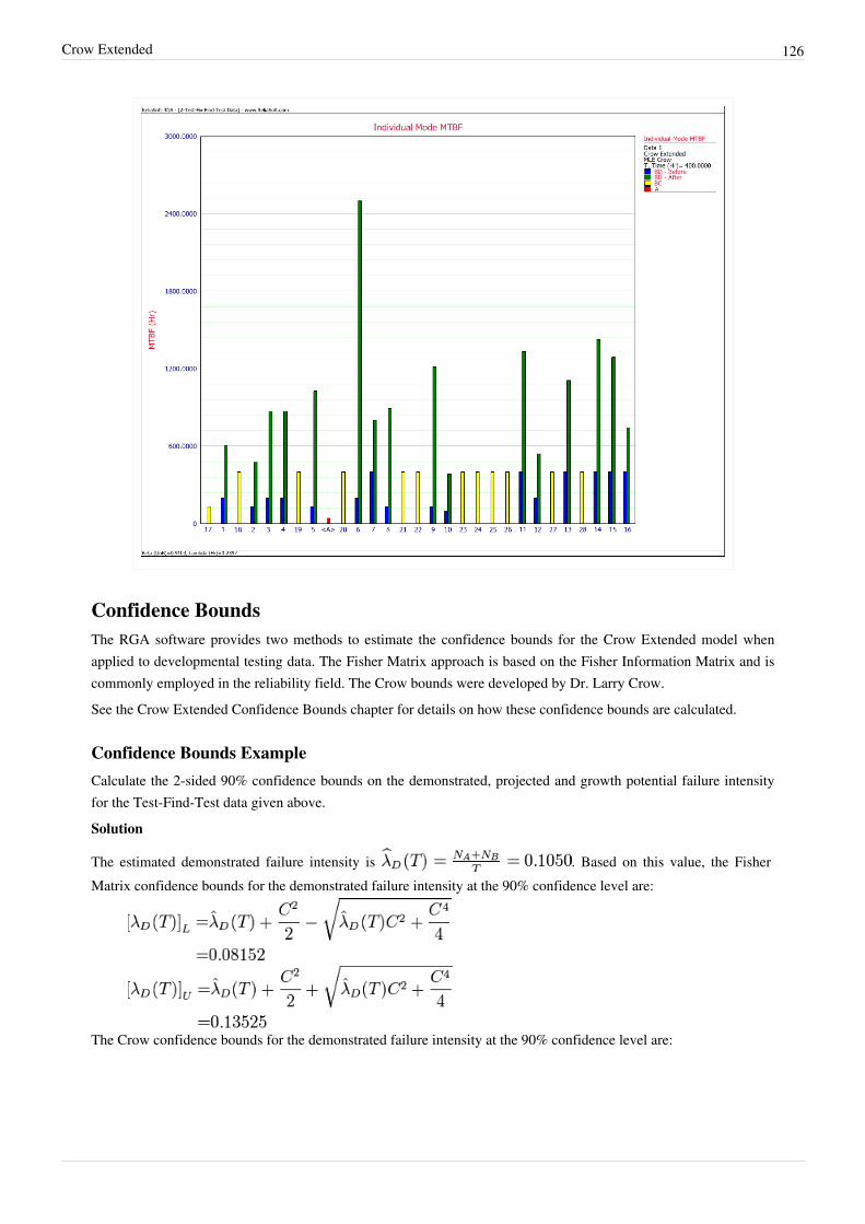
Crow Extended 126

Confidence BoundsThe RGA software provides two methods to estimate the confidence bounds for the Crow Extended model whenapplied to developmental testing data. The Fisher Matrix approach is based on the Fisher Information Matrix and iscommonly employed in the reliability field. The Crow bounds were developed by Dr. Larry Crow.See the Crow Extended Confidence Bounds chapter for details on how these confidence bounds are calculated.

Confidence Bounds ExampleCalculate the 2-sided 90% confidence bounds on the demonstrated, projected and growth potential failure intensityfor the Test-Find-Test data given above.Solution

The estimated demonstrated failure intensity is . Based on this value, the FisherMatrix confidence bounds for the demonstrated failure intensity at the 90% confidence level are:

The Crow confidence bounds for the demonstrated failure intensity at the 90% confidence level are:

Crow Extended 127

The projected failure intensity is:

Based on this value, the Fisher Matrix confidence bounds at the 90% confidence level for the projected failureintensity are:

The Crow confidence bounds for the projected failure intensity are:

The growth potential failure intensity is:

.

Based on this value, the Fisher Matrix and Crow confidence bounds at the 90% confidence level for the growthpotential failure intensity are:

The figure below shows the Fisher Matrix confidence bounds at the 90% confidence level for the demonstrated,projected and growth potential failure intensity.

Crow Extended 128

The following figure shows these bounds based on the Crow method.

Crow Extended 129

Another Confidence Bounds ExampleCalculate the 2-sided confidence bounds at the 90% confidence level on the demonstrated, projected and growthpotential MTBF for the Test-Fix-Find-Test data given above.SolutionFor this example, there are A, BC and BD failure modes, so the estimated demonstrated failure intensity, , issimply the Crow-AMSAA model applied to all A, BC, and BD data.

Therefore, the demonstrated MTBF is:

Based on this value, the Fisher Matrix confidence bounds for the demonstrated failure intensity at the 90%confidence level are:

The Fisher Matrix confidence bounds for the demonstrated MTBF at the 90% confidence level are:

The Crow confidence bounds for the demonstrated MTBF at the 90% confidence level are:

The projected failure intensity is:

Based on this value, the Fisher Matrix confidence bounds at the 90% confidence level for the projected failureintensity are:

Crow Extended 130

The Fisher Matrix confidence bounds for the projected MTBF at the 90% confidence level are:

The Crow confidence bounds for the projected failure intensity are:

The Crow confidence bounds for the projected MTBF at the 90% confidence level are:

The growth potential failure intensity is:

Based on this value, the Fisher Matrix and Crow confidence bounds at the 90% confidence level for the growthpotential failure intensity are:

The Fisher Matrix and Crow confidence bounds for the growth potential MTBF at the 90% confidence level are:

The figure below shows the Fisher Matrix confidence bounds at the 90% confidence level for the demonstrated,projected and growth potential MTBF.

Crow Extended 131

The next figure shows these bounds based on the Crow method.

Crow Extended 132

Grouped DataParameter estimation for grouped data using the Crow Extended model is the same as the procedure used for thetraditional Crow-AMSAA (NHPP) model. The equations used to estimate the parameters of the Crow Extendedmodel are presented next. For test-find-test data, the maximum likelihood estimates of and are calculatedusing the first occurrences of the BD modes such that:

where is the number of distinct BD modes within the interval. For test-fix-find-test data, the maximumlikelihood estimates of and are estimated in the same manner using the first occurrences of the BC modes.

Confidence Bounds for Grouped Data• Parameters: The confidence bounds on the parameters for the Crow Extended model for grouped data are

calculated using the same procedure presented in the Crow-AMSAA Confidence Bounds chapter.•• Failure Intensity and MTBF:

• If there are no BC modes, the confidence bounds on the demonstrated failure intensity and MTBF, projectedfailure intensity and MTBF and growth potential failure intensity and MTBF are the same as the procedurepresented for non-grouped data.

•• If there are BC modes, then the confidence bounds on the demonstrated failure intensity and MTBF are thesame as the procedure presented in the Crow-AMSAA Confidence Bounds chapter, and the confidence boundson the projected failure intensity and MTBF and growth potential failure intensity and MTBF are the same asfor non-grouped data.

• Time: The confidence bounds on time are the same as the procedure presented in the Crow-AMSAA ConfidenceBounds chapter.

Mixed DataThe Crow Extended model can also be applied to discrete data from one-shot (success/failure) testing. In the RGAsoftware, the Discrete Data > Mixed Data option creates a data sheet that can accommodate data from tests where asingle unit is tested for each successive configuration (individual trial-by-trial), where multiple units are tested foreach successive configuration (configurations in groups) or a combination of both. This data sheet can be analyzedwith either the Crow-AMSAA (NHPP) model or the Crow Extended model.For discrete data, corrective actions cannot take place at the time of failure. With that in mind, the mixed data typedoes not allow for BC modes. For discrete data there are only A or BD modes. In terms of practical applications,think of a growth test for missile systems. Because missiles are one-shot items, any corrective actions applied to thefailure modes are delayed until at least the next trial.Note that for calculation purposes, it is required to have at least three failures in the first interval. If that is not thecase, then the data set needs to be grouped before calculating. The RGA software performs this operation in thebackground.

Crow Extended 133

ExampleA one-shot system underwent reliability growth testing for a total of 20 trials. The test was performed as acombination of groups of units with the same configuration and individual trials. The following table shows the dataset. The Failures in Interval column specifies the number of failures that occurred in each interval and theCumulative Trials column specifies the cumulative number of trials at the end of that interval. In other words, thefirst three rows contain the data from the first trial, in which 8 units with the same configuration were tested and 3failures (with different failure modes) were observed. The next row contains data from the second trial, in which 2units with the same configuration were tested and no failures occurred. And so on.

Mixed Data

Failures in Interval Cumulative Trials Classification Mode

1 8 BD 1

1 8 BD 2

1 8 BD 3

0 10

0 11

0 12

1 13 BD 2

0 14

0 15

1 16 BD 4

0 17

0 18

0 19

1 20 BD 5

The table also gives the classifications of the failure modes. There are 5 BD modes. The average effectiveness factorfor the BD modes is 0.7. Do the following:1.1. Calculate the demonstrated reliability at the end of the test.2.2. Calculate the growth potential reliability.Solution

1. Based on the equations presented in Crow-AMSAA (NHPP), the parameters of the Crow-AMSAA (NHPP)model are estimated as follows:

and:

However, because there are only A or BD modes for mixed data, there is no growth during the test. In otherwords, the hypothesis for the parameter is that From the Crow-AMSAA (NHPP) model, we know that:

or, if , this becomes:

Crow Extended 134

As we have seen, the Crow-AMSAA instantaneous failure intensity, , is defined as:

Using trials instead of time, and accommodating for , we can calculate the instantaneous failureprobability at the end of the test, or :

So the instantaneous reliability at the end of the test, or demonstrated reliability, is:

The next figure shows the data sheet as calculated in the RGA software.

2.2. The growth potential unreliability is:

So the growth potential reliability is:

Crow Extended 135

The figures below show the calculation of the growth potential reliability for the mixed data using the RGAsoftware's QCP, followed by the growth potential plot.

Crow Extended 136

Multiple Systems with Event CodesThe Multiple Systems with Event Codes data type is used to analyze the failure data from a reliability growth test inwhich a number of systems are tested concurrently and the implemented fixes are tracked during the test phase. Withthis data type, all of the systems under test are assumed to have the same system hours at any given time. The CrowExtended model is used for this data type, so all the underlying assumptions regarding the Crow Extended modelapply. As such, this data type is applicable only to data from within a single test phase.As previously presented, the failure mode classifications for the Crow Extended model are defined as follows:• A indicates that no corrective action was performed or will be performed (management chooses not to address for

technical, financial or other reasons).• BC indicates that the corrective action was implemented during the test. The analysis assumes that the effect of

the corrective action was experienced during the test (as with other test-fix-test reliability growth analyses).• BD indicates that the corrective action will be delayed until after the completion of the current test.Therefore, implemented fixes can be applied only to BC modes since all BD modes are assumed to be delayed untilthe end of the test. For each BC mode, there must be a separate entry in the data set that records the time when thefix was implemented during the test.

Crow Extended 137

Event CodesA Multiple Systems with Event Codes data sheet that is analyzed with the Crow Extended model has an Eventcolumn that allows you to indicate the types of events that occurred during a test phase. The possible event codesthat can be used in the analysis are:• I: denotes that a certain BC failure mode has been corrected at the specific time; in other words, a fix has been

implemented. For this data type, each BC mode must have an associated I event. The I event is essentially atimestamp for when the fix was implemented during the test.

• Q: indicates that the failure was due to a quality issue. An example of this might be a failure caused by a bolt notbeing tightened down properly. You have the option to decide whether or not to include quality issues in theanalysis. This option can be specified by checking or clearing the Include Q Events check box under Event CodeOptions on the Analysis tab.

• P: indicates that the failure was due to a performance issue. You can determine whether or not to includeperformance issues in the analysis. This option can be specified by checking or clearing the Include P Eventscheck box under Event Code Options on the Analysis tab.

• X: indicates that you wish to exclude the data point from the analysis. An X can be placed in front of any existingevent code (e.g., XF to exclude a particular failure time) or entered by itself. The row of data with the X will notbe included in the analysis.

• S: indicates the system start time. This event code is only selectable in the Normal View.• F: indicates a failure time.• E: indicates the system end time. This event code is only selectable in the Normal View.The analysis is based on the equivalent system that combines the operating hours of all the systems.

Equivalent Single SystemIn order to analyze a Multiple Systems with Event Codes data sheet, the data are converted into a Crow Extendedequivalent single system. The implemented fixes (I events) are taken into account when building the equivalentsingle system from the data for multiple systems.The basic assumptions and constraints for the use of this data type are listed below:• Failure modes are assumed to be independent of each other and with respect to the system configuration. The

same applies to their related implemented fixes (I events). As such, each mode and its related implemented fixes(I events) are examined separately in terms of their impact to the system configuration.

•• If there are BC modes in the data set, there must be at least 3 unique BC modes to analyze the data (together withimplemented fixes for each one of them).

•• If there are BD modes in the data set, there must be at least 3 unique BD modes to analyze the data.• To be consistent with the definition of BC modes in the Crow Extended model, every BC mode must have at least

one implemented fix (I event) on at least one system.• Implemented fixes (I events) cannot be delayed to a later phase, because the Crow Extended model applies to a

single phase only.The following list shows the basic rules for calculating the equivalent single system on which the Crow Extendedmodel is applied. Note that the list is not exhaustive since there is an infinite number of scenarios that can occur.These rules cover the most common scenarios. The main concept is to add the time that each system was testedunder the same configuration.1. To get to the equivalent single system, each failure time for A modes and BD modes is calculated by adding the

time that each system was tested under the same configuration. In practice this means multiplying the failure time in the system by the number of total systems under test. For example, if we have 4 total systems, and system 2 has

Crow Extended 138

a BD1 mode at time 30, the BD1 mode failure time in the equivalent single system would be . If system 3 hadanother BD1 mode at time 40, then that would yield another BD1 mode in the equivalent single system at time .These calculations are done assuming that the start time for the systems are at time zero. If the start time isdifferent than zero, then that time would have to be subtracted from the failure time on each system. For example,if system 1 started at time S=10, and there was a failure at time 30, the equivalent system time would be .

2. Each failure time for a BC mode that occurred before an implemented fix (I event) for that mode is alsocalculated by multiplying the failure time in the system by the number of total systems in test, as described above.

3. The implemented fix (I event) time in the equivalent single system is calculated by adding the test time investedin each system before that I event takes place. It is the total time that the system has spent at the sameconfiguration in terms of that specific mode.

4. If the same BC mode occurs in another system after a fix (I event) has been implemented in one or more systems,the failure time in the equivalent single system is calculated by adding the test time for that BC mode, and one ofthe following for each of the other systems:

• If a BC mode occurs in a system that has already seen an I event for that mode, then you add the time upto the I event.

or• If the I events occurred later than the BC failure time or those systems did not have any I events for that

mode, then you add the time of the BC failure.5. If the same BC mode occurs in the same system after a fix (I event) has been implemented in one or more

systems, the failure time in the equivalent single system is calculated by adding the test time of each system afterthat I event was implemented to the I event time in the equivalent single system, or zero if an I event was notpresent in that system.

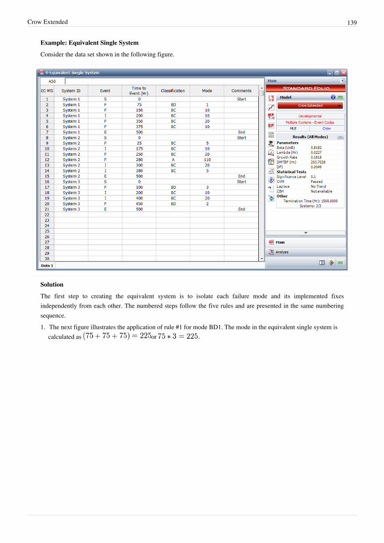
Crow Extended 139

Example: Equivalent Single System

Consider the data set shown in the following figure.

Solution

The first step to creating the equivalent system is to isolate each failure mode and its implemented fixesindependently from each other. The numbered steps follow the five rules and are presented in the same numberingsequence.1. The next figure illustrates the application of rule #1 for mode BD1. The mode in the equivalent single system is

calculated as or

Crow Extended 140

The next figure illustrates the application of rule #1 for mode A110. The mode in the equivalent single system iscalculated as or

2. The next figure illustrates the application of rule #2 for the first occurrence of the mode BC10 in system 1. Themode in the equivalent single system is calculated as or

Crow Extended 141

3. The next figure illustrates the application of rule #3 for implemented fixes (I events) of the mode BC10. In thegraph, the I events are symbolized by having the letter "I" before the naming of the mode. In this case, IBC10 isfor the implemented fix of mode BC10. The IBC10 in the equivalent single system is calculated as

.

4. The next figure illustrates the application of rule #4 for the mode BC20 in system 1, which occurs after a fix forthe same mode was implemented in system 2. The mode in the equivalent single system is calculated as

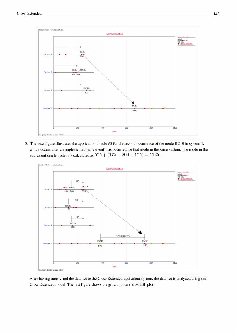
Crow Extended 142

5. The next figure illustrates the application of rule #5 for the second occurrence of the mode BC10 in system 1,which occurs after an implemented fix (I event) has occurred for that mode in the same system. The mode in theequivalent single system is calculated as

After having transferred the data set to the Crow Extended equivalent system, the data set is analyzed using theCrow Extended model. The last figure shows the growth potential MTBF plot.

Crow Extended 143

Crow Extended 144

Transferring Data to an Equivalent Single SystemRGA provides the capability to transfer a Multiple Systems with Event Codes data sheet to various other data types.The following picture shows the available data types that the data sheet can be converted into. When selecting totransfer to an equivalent single system, the data sheet is converted to a Crow Extended - Continuous Evaluation datasheet.

The Crow Extended - Continuous Evaluation model is designed for analyzing data across multiple test phases, whileconsidering the data for all phases as one data set. Familiarity with this model is necessary for the discussionpresented in this section.When using the Crow Extended - Continuous Evaluation model to transfer the data sheet from Multiple Systemswith Event Codes to an equivalent single system, the following rules are used (in addition to the five basic rulespresented earlier for calculating the equivalent single system):•• BD modes in the Crow Extended data sheet become BD modes in the equivalent single system of the Crow

Extended - Continuous Evaluation data sheet.• BC modes in the Crow Extended data sheet become BD modes in the equivalent single system of the Crow

Extended - Continuous Evaluation data sheet. These BD modes will have associated implemented fixes (I events).Implemented fixes (I events) for BC modes in the Crow Extended data sheet become implemented fixes (I events)for the converted BD modes in the equivalent single system of the Crow Extended - Continuous Evaluation datasheet.

• If an implemented fix (I event) occurred at the same time as the failure, and was implemented at that exact timeacross all systems, then this becomes a BC mode in the equivalent single system. If the fixes (I events) were notall implemented at the same time or if the fix was not implemented on all systems at the failure time, then thisbecomes a BD mode in the equivalent single system.

The next figure shows the transferred equivalent single system Crow Extended - Continuous Evaluation data sheetfrom the Multiple Systems with Event Codes data sheet for the data from the Equivalent Single System examplegiven above.

Crow Extended 145

Iteration Method for Naming Repeated ModesWhen recording modes for transfer from the Multiple Systems with Event Codes to a Crow Extended -ContinuousEvaluation equivalent single system, it is recommended to consider using an iteration method to name subsequentrecurrences of the same mode. This will help alleviate any issues with the conversion of the definitions of the modesfrom the Crow Extended model to the Crow Extended - Continuous Evaluation model. For example, if the firstoccurrence of a mode is BC25, then the second occurrence is suggested to be named as BC25.1. The reasoningbehind this recommendation is that in the case that BC25 in the Multiple Systems with Event Codes data sheet hasreceived implemented fixes (I events) at the same time that the failure occurred in all systems, then this mode will betranslated as a BC mode in the Crow Extended - Continuous Evaluation equivalent single system. The next recurringfailure would also be treated as a BC mode, but in reality it did not have an implemented fix (I event) at the time offailure.For example, consider the data set shown in the following figure, which represents one system only for simplicity.Notice that the modes BC25, BC35 and BC45 received implemented fixes at the time of failure. Based on that, whenthey get transferred to the Crow Extended - Continuous Evaluation equivalent single system, they will be consideredas BC modes. The subsequent failures of the modes 25, 35 and 45 will also be converted to BC modes, when inreality they had implemented fixes (I events) at a later time.

Crow Extended 146

The RGA software will display a warning if you try to convert this data sheet without using iterations.The next figure shows the same data sheet with the use of iterations for the modes 25, 35 and 45. The subsequentfailures are named as BC25.1, BC35.1 and BC45.1.

Crow Extended 147

This way, the conversion to the Crow Extended - Continuous Evaluation model occurs in a valid fashion, becausealthough the original BC modes are converted to BC25, BC35 and BC45, the subsequent failures are converted toBD25.1, BD35.1 and BD45.1 together with their respective implemented fixes (I events). This is shown in the nextfigure below. Note that the use of iterations is recommended only when transferring to the Crow Extended -Continuous Evaluation equivalent single system; it is not necessary when using the Multiple Systems with EventCodes data sheet that is calculated with the Crow Extended model.

More Examples

Adjusting the Failure Mode Management StrategyThree systems were subjected to a reliability growth test to evaluate the prototype of a new product. Based on afailure analysis on the results of the test, the proposed management strategy is to delay corrective actions until afterthe test. The tables shown next display the data set and the associated effectiveness factors for the unique BD modes.

Multiple Systems (Concurrent Operating Times) Data

System 1 System 2 System 3

Start Time 0 0 0

End Time 541 454 436

Times-to-Failure 83 BD37 26 BD25 23 BD30

83 BD43 26 BD43 46 BD49

83 BD46 57 BD37 127 BD47

169 A45 64 BD19 166 A2

213 A18 169 A45 169 BD23

299 A42 213 A32 213 BD7

375 A1 231 BD8 213 BD29

431 BD16 231 BD25 255 BD26

231 BD27 369 A33

Crow Extended 148

231 A28 374 BD29

304 BD24 380 BD22

383 BD40 415 BD7

Effectiveness factors

BD Mode Effectiveness Factor

30 0.75

43 0.5

25 0.5

49 0.75

37 0.9

19 0.75

46 0.75

47 0.25

23 0.5

7 0.25

29 0.25

8 0.5

27 0.5

26 0.75

24 0.5

22 0.5

40 0.75

16 0.75

The prototype is required to meet a projected MTBF goal of 55 hours. Do the following:1.1. Estimate the parameters of the Crow Extended model.2.2. Based on the current management strategy what is the projected MTBF?3.3. If the projected MTBF goal is not met, alter the current management strategy to meet this requirement with as

little adjustment as possible and without changing the EFs of the existing BD modes. Assume an EF = 0.7 for anynewly assigned BD modes.

Solution

1.1. The next figure shows the estimated Crow Extended parameters.

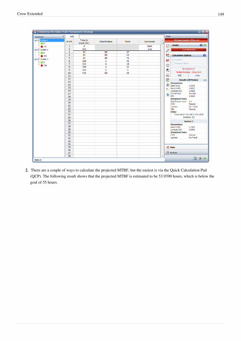
Crow Extended 149

2.2. There are a couple of ways to calculate the projected MTBF, but the easiest is via the Quick Calculation Pad(QCP). The following result shows that the projected MTBF is estimated to be 53.9390 hours, which is below thegoal of 55 hours.

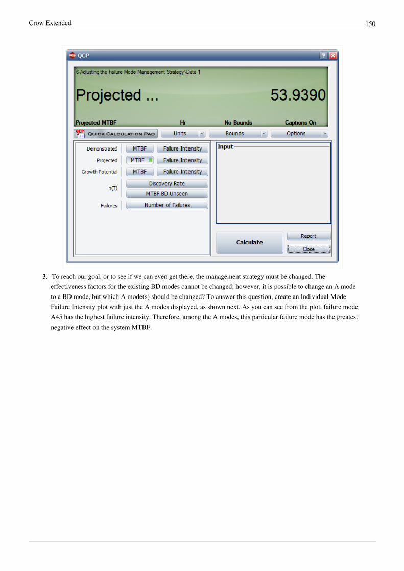
Crow Extended 150

3.3. To reach our goal, or to see if we can even get there, the management strategy must be changed. Theeffectiveness factors for the existing BD modes cannot be changed; however, it is possible to change an A modeto a BD mode, but which A mode(s) should be changed? To answer this question, create an Individual ModeFailure Intensity plot with just the A modes displayed, as shown next. As you can see from the plot, failure modeA45 has the highest failure intensity. Therefore, among the A modes, this particular failure mode has the greatestnegative effect on the system MTBF.

Crow Extended 151

Change A45 to BD45. Be sure to change all instances of A45 to a BD mode. Enter an effectiveness factor of 0.7for BD45, and then recalculate the parameters of the Crow Extended model. Now go back to the QCP to calculatethe projected MTBF, as shown below. The projected MTBF is now estimated to be 55.5903 hours. Based on thechange in the management strategy, the projected MTBF goal is now expected to be met.

Crow Extended 152

Estimating the Failure Intensity Remaining After FixesA reliability growth test was conducted for 200 hours. Some of the corrective actions were applied during the testwhile others were delayed until after the test was completed. The tables below give the data set and the effectivenessfactors for the BD modes. Do the following:1.1. Estimate the parameters of the Crow Extended model.2.2. Determine the average effectiveness factor of the BC modes using the Function Wizard.3.3. What percent of the failure intensity will be left in the system due to the BD modes after implementing the

delayed fixes?

Grouped Failure Times Data

Number at Event Time to Event Classification Mode

3 25 BC 1

1 25 BD 9

1 25 BC 2

1 50 BD 10

1 50 BD 11

1 75 BD 12

1 75 BC 3

2 75 BD 13

1 75 A

1 100 BC 4

Crow Extended 153

1 100 BD 14

1 125 BD 15

1 125 A

1 125 A

1 125 BC 5

1 125 BD 10

1 125 BC 6

1 150 A

1 150 BD 16

1 175 BC 4

1 175 BC 8

1 175 A

1 175 BC 7

1 200 BD 16

1 200 BC 3

1 200 BD 17

Effectiveness Factors

BD Mode Effectiveness Factor

9 0.75

10 0.5

11 0.9

12 0.6

13 0.8

14 0.8

15 0.25

16 0.75

17 0.8

Solution

1.1. The next figure shows the estimated parameters of the Crow Extended model.

Crow Extended 154

2. Insert a general spreadsheet into the folio, and then access the Function Wizard. In the Function Wizard, selectAverage Effectiveness Factor from the list of available functions and under Avg. Eff. Factor select BC modes,as shown next. Click Insert and the result will be inserted into the general spreadsheet. The average effectivenessfactor for the BC modes is 0.6983.

Crow Extended 155

3. The failure intensity left in the system due to the BD modes can be determined using the Failure Mode Strategyplot, as shown next. Therefore, the failure intensity left in the system due to the BD modes is 1.79%.

Determining if Design Will Meet MTBF GoalTwo prototypes of a new design are tested simultaneously. Whenever a failure is observed for one unit, the currentoperating time of the other unit is also recorded. The test is terminated after 300 hours. All of the design changes forthe prototypes were delayed until after completing the test. The data set is given in the table below. Assume a fixedeffectiveness factor equal to 0.7. The MTBF goal for the new design is 30 hours. Do the following:1.1. Estimate the parameters of the Crow Extended model.2.2. What is the projected MTBF and growth potential?3.3. Under the current management strategy, is it even possible to reach the MTBF goal of 30 hours?

Multiple Systems (Known Operating Times) Data

Failed Unit ID Time Unit 1 Time Unit 2 Classification Mode

1 16.5 0 BD seal leak

1 16.5 0 BD valve

1 17 0 A

2 20.5 0.9 A

2 25.3 3.8 BD hose

2 28.7 4.6 BD operator error

1 41.8 14.7 BD bearing

1 45.5 17.6 A

2 48.6 22 A

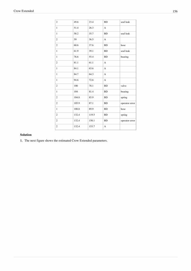
Crow Extended 156

2 49.6 23.4 BD seal leak

1 51.4 26.3 A

1 58.2 35.7 BD seal leak

2 59 36.5 A

2 60.6 37.6 BD hose

1 61.9 39.1 BD seal leak

1 76.6 55.4 BD bearing

2 81.1 61.1 A

1 84.1 63.6 A

1 84.7 64.3 A

1 94.6 72.6 A

2 100 78.1 BD valve

1 104 81.4 BD bearing

2 104.8 85.9 BD spring

2 105.9 87.1 BD operator error

1 108.8 89.9 BD hose

2 132.4 119.5 BD spring

2 132.4 150.1 BD operator error

2 132.4 153.7 A

Solution

1.1. The next figure shows the estimated Crow Extended parameters.

Crow Extended 157

2.2. One possible method for calculating the projected MTBF and growth potential is to use the Quick CalculationPad, but you can also view these two values at the same time by viewing the Growth Potential MTBF plot, asshown next. From the plot, the projected MTBF is equal to 16.87 hours and the growth potential is equal to 18.63hours.

Crow Extended 158

3.3. The current projected MTBF and growth potential MTBF are both well below the required goal of 30 hours. Tocheck if this goal can even be reached, you can set the effectiveness factor equal to 1. In other words, if all of thecorrective actions were to remove the failure modes completely, what would be the projected and growthpotential MTBF? Change the fixed effectiveness factor to 1, then recalculate the parameters and refresh theGrowth Potential plot, as shown next. Even if you assume an effectiveness factor equal to 1, the growth potentialis still only 27.27 hours. Based on the current design process, it will not be possible to reach the MTBF goal of 30hours. Therefore, you have two options: start a new design stage or reduce the required MTBF goal.

Crow Extended 159

160

Chapter 3.4

Crow Extended - Continuous EvaluationThe Crow Extended model is designed for a single test phase. However, in most cases, testing for a system will beconducted in multiple phases. The Crow Extended - Continuous Evaluation model is designed for analyzing dataacross multiple test phases, while considering the data for all phases as one data set. To perform the analysis in theRGA software, you would use the Multi-Phase data sheet.The Crow Extended - Continuous Evaluation (3-parameter) model is an extension of the Crow Extended model, andis designed for practical testing situations where we need the flexibility to apply corrective actions at the time offailure or at a later time during the test, at the end of the current test or during a subsequent test phase. Thisthree-parameter model is free of the constraint where the test must be stopped and all BD modes must be corrected atthe end of the test, as in the Crow Extended model. The failure modes can be corrected during the test or when thetesting is stopped for the incorporation of the fixes, or even not corrected at all at the end of the test phase. Based onthis flexibility, the end time of the test is also not predefined, and it can be continuously updated with new test data.This is the reason behind the name, "continuous evaluation."

Definitions

ClassificationsUnder the Crow Extended - Continuous Evaluation model, corrective actions can be fixed at the time of failure ordelayed to a later time (before time , at time or after time , where indicates the test's end time). Thedefinition of delayed is expanded to include all type B failure modes corrected after the time of failure. This willinclude most, if not all, design-related failure modes requiring a root cause failure analysis. Failure modes that arecorrected at the time of failure are typically related to human factors, such as manufacturing, operator error, etc.For the Crow Extended - Continuous Evaluation model, the classifications are defined as follows:• A indicates that a corrective action will not be performed (management chooses not to address these modes for

technical, financial or other reasons).• BC is defined as a failure mode that receives a corrective action at the time of failure and before the testing

resumes. Typically, a type BC failure mode does not require extensive root cause failure analysis, and thereforecan be corrected quickly. Type BC modes are generally easy to fix, and are usually related to issues such asquality, manufacturing, operator, etc.

• BD is defined as a failure mode that receives a corrective action at a test time after the first occurrence of thefailure mode. Therefore, a fix is considered delayed if it is not implemented at the time of failure. A delayed fixcan then occur at a later time during the test, at the end of the test (before the next phase) or during another testphase. Type BD failure modes typically require failure analysis and time to fabricate the corrective action. Duringthe period into the test, there may be BD modes with corrective actions incorporated into the systems andother BD modes that have been seen, but not yet fixed.

The following table shows a comparison between the definitions of the classifications in the Crow Extended andCrow Extended - Continuous Evaluation models:

Crow Extended - Continuous Evaluation 161

Comparison of Classification Definitions

Classification Crow Extended Crow Extended - Continuous Evaluation

A Corrective action will not be performed Same as Crow Extended

BC Corrective action during the test Corrective action at the time of failure

BD Corrective action delayed until after the completion ofthe test

Corrective action delayed to a test time after the first occurrence of thefailure mode

Reliability growth is achieved by decreasing the failure intensity. The failure intensity for the A failure modes willnot change. Therefore, reliability growth can be achieved only by decreasing the BC and BD mode failureintensities. In general, the only part of the BD mode failure intensity that can be decreased is the part that has beenseen during testing. The BC failure modes and fixed BD modes (delayed fixes implemented during the test) arecorrected during testing, and their failure intensities will not change any more at the end of test.

Event CodesA Multi-Phase data sheet that is analyzed with the Crow Extended - Continuous Evaluation model has an Eventcolumn that allows you to indicate the types of events that occurred during testing. The possible event codes that canbe used in the analysis are:• F: indicates a failure time.• I: denotes that a fix has been implemented for a BD failure mode at the specific time. BD modes that have not

received a corrective action by time would not have an associated I event in the data set.• Q: indicates that the failure was due to a quality issue. An example of this might be a failure caused by a bolt not

being tightened down properly. You have the option to decide whether or not to include quality issues in theanalysis. This option can be specified by checking or clearing the Include Q Events check box under ContinuousOptions on the Analysis tab.

• P: indicates that the failure was due to a performance issue. You can determine whether or not to includeperformance issues in the analysis. This option can be specified by checking or clearing the Include P Eventscheck box under Continuous Options on the Analysis tab.

• AP: indicates an analysis point. Analysis points can be shown in a multi-phase plot to track overall projectprogress and can be compared to an idealized growth curve.

• PH: indicates the end of a test phase. Test phases can be shown in a multi-phase plot to track overall projectprogress and can be compared to planned growth phases. The RGA software allows for a maximum of seven testphases to be defined.

• X: indicates that the data point will be excluded from the analysis. An X can be placed in front of any existingevent code or entered by itself. The row of data with the the X will not be included in the analysis.

The next figure shows an example of a Crow Extended - Continuous Evaluation folio with all of the possible eventcodes. As you can see, each failure is indicated with A, BC or BD in the Classification column. In addition, any textcan be used to specify the mode. In this figure, failure codes were used in the Mode column for simplicity, but youcould just as easily use Seal Leak, or whatever designation you deem appropriate for the failure mode.

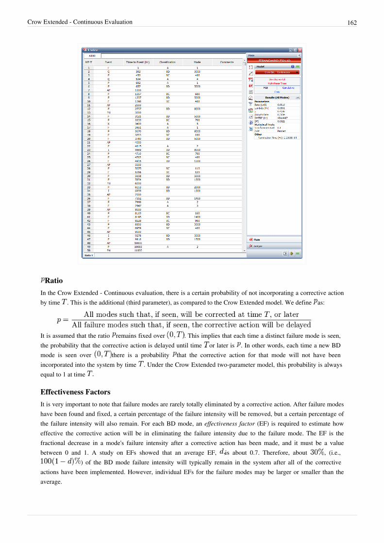
Crow Extended - Continuous Evaluation 162

RatioIn the Crow Extended - Continuous evaluation, there is a certain probability of not incorporating a corrective actionby time . This is the additional (third parameter), as compared to the Crow Extended model. We define as:

It is assumed that the ratio remains fixed over . This implies that each time a distinct failure mode is seen,the probability that the corrective action is delayed until time or later is . In other words, each time a new BDmode is seen over there is a probability that the corrective action for that mode will not have beenincorporated into the system by time . Under the Crow Extended two-parameter model, this probability is alwaysequal to 1 at time

Effectiveness FactorsIt is very important to note that failure modes are rarely totally eliminated by a corrective action. After failure modeshave been found and fixed, a certain percentage of the failure intensity will be removed, but a certain percentage ofthe failure intensity will also remain. For each BD mode, an effectiveness factor (EF) is required to estimate howeffective the corrective action will be in eliminating the failure intensity due to the failure mode. The EF is thefractional decrease in a mode's failure intensity after a corrective action has been made, and it must be a valuebetween 0 and 1. A study on EFs showed that an average EF, is about 0.7. Therefore, about , (i.e.,

) of the BD mode failure intensity will typically remain in the system after all of the correctiveactions have been implemented. However, individual EFs for the failure modes may be larger or smaller than theaverage.

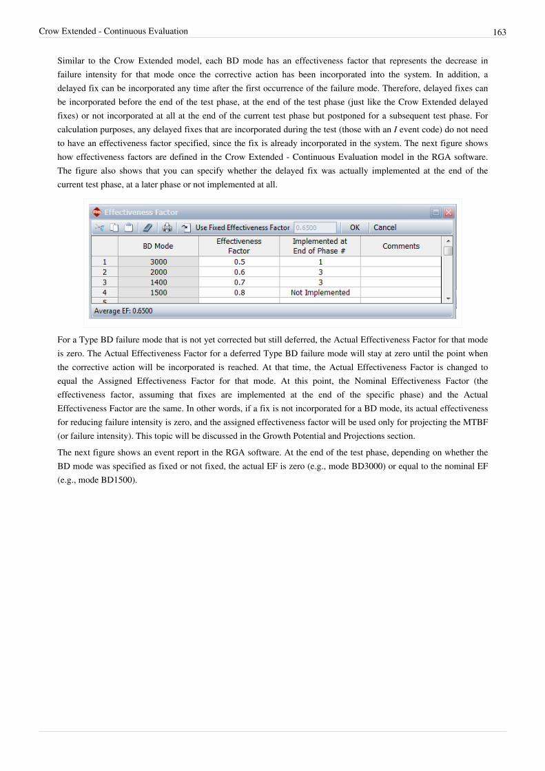
Crow Extended - Continuous Evaluation 163

Similar to the Crow Extended model, each BD mode has an effectiveness factor that represents the decrease infailure intensity for that mode once the corrective action has been incorporated into the system. In addition, adelayed fix can be incorporated any time after the first occurrence of the failure mode. Therefore, delayed fixes canbe incorporated before the end of the test phase, at the end of the test phase (just like the Crow Extended delayedfixes) or not incorporated at all at the end of the current test phase but postponed for a subsequent test phase. Forcalculation purposes, any delayed fixes that are incorporated during the test (those with an I event code) do not needto have an effectiveness factor specified, since the fix is already incorporated in the system. The next figure showshow effectiveness factors are defined in the Crow Extended - Continuous Evaluation model in the RGA software.The figure also shows that you can specify whether the delayed fix was actually implemented at the end of thecurrent test phase, at a later phase or not implemented at all.

For a Type BD failure mode that is not yet corrected but still deferred, the Actual Effectiveness Factor for that modeis zero. The Actual Effectiveness Factor for a deferred Type BD failure mode will stay at zero until the point whenthe corrective action will be incorporated is reached. At that time, the Actual Effectiveness Factor is changed toequal the Assigned Effectiveness Factor for that mode. At this point, the Nominal Effectiveness Factor (theeffectiveness factor, assuming that fixes are implemented at the end of the specific phase) and the ActualEffectiveness Factor are the same. In other words, if a fix is not incorporated for a BD mode, its actual effectivenessfor reducing failure intensity is zero, and the assigned effectiveness factor will be used only for projecting the MTBF(or failure intensity). This topic will be discussed in the Growth Potential and Projections section.The next figure shows an event report in the RGA software. At the end of the test phase, depending on whether theBD mode was specified as fixed or not fixed, the actual EF is zero (e.g., mode BD3000) or equal to the nominal EF(e.g., mode BD1500).

Crow Extended - Continuous Evaluation 164

The Average Nominal EF is:

where is the total number of open and distinct BD modes at time , and is the Nominal EffectivenessFactor as specified for each of the BD mode.The Average Actual EF is:

where is the total number of open and distinct BD modes at time , and is the Actual Effectiveness Factorat time for each BD mode.

Growth Potential and ProjectionsThe failure intensity that remains in the system will depend on the management strategy that determines theclassification of the A, BC and BD failure modes. The engineering effort applied to the corrective actions determinesthe effectiveness factors. In addition, the failure intensity depends on , which is the rate at which unique BDfailure modes are being discovered during testing. The rate of discovery drives the opportunity to take correctiveactions based on the seen failure modes and it is an important factor in the overall reliability growth rate. Thereliability growth potential is the limiting value of the failure intensity as time increases. This limit is themaximum MTBF that can be attained with the current management strategy. The maximum MTBF will be attainedwhen all BD modes have been observed and fixed.

Crow Extended - Continuous Evaluation 165

If all seen BD modes are corrected by time , that is, no deferred corrective actions at time , then the growthpotential is the maximum attainable based on the type BD designation of the failure modes, the correspondingassigned effectiveness factors and the remaining A modes in the system. This is called the nominal growth potential.If some seen BD modes are not corrected at the end of the current test phase, then the prevailing growth potential isbelow the maximum attainable with the type BD designation of the failure modes and the corresponding assignedeffectiveness factors.

The Crow-AMSAA (NHPP) model is used to estimate the current demonstrated MTBF or Thedemonstrated MTBF does not take into account any type of projected improvements. Refer to the Crow-AMSAA(NHPP) chapter for more details.The corresponding current demonstrated failure intensity is:

or:

The nominal growth potential factor is:

where:

• is the total number of distinct unfixed BD modes at time .• is the assigned (nominal) EF for the unfixed BD mode at time • is the total number of failures over (0, ) for the distinct unfixed BD mode .The nominal growth potential factor signifies the failure intensity of the modes after corrective actions have beenimplemented for them, using the nominal values for the effectiveness factors.Similarly, the actual growth potential factor is:

where is the actual EF for the unfixed BD mode at time The actual growth potential factor signifies the failure intensity of the modes after corrective actions have beenimplemented for them, using the actual values for the effectiveness factors.Based on the definition of BD modes for the Crow Extended - Continuous Evaluation model, the estimate of attime is calculated as follows:

The unfixed BD mode failure intensity at time is:

Similar to the Crow Extended model, the discovery function at time for the Crow Extended - ContinuousEvaluation model is calculated using all the first occurrences of the all the BD modes, both fixed and unfixed. isthe unseen BD mode failure intensity and is also the rate at which new unique BD modes are being discovered.

Crow Extended - Continuous Evaluation 166

where:

• is the unbiased estimated of for the Crow-AMSAA (NHPP) model based on the first occurrence of distinct BD modes.

• is the unbiased estimated of for the Crow-AMSAA (NHPP) model based on the first occurrence of distinct BD modes.

The parameters and are also known as the Rate of Discovery Parameters.The nominal growth potential failure intensity is:

and the nominal growth potential MTBF is:

The nominal projected failure intensity at time is:

and the nominal projected MTBF at time is:

The actual growth potential failure intensity is:

and the actual growth potential MTBF is:

The actual projected failure intensity at time is:

and the actual projected MTBF at time is:

In terms of confidence intervals and goodness-of-fit tests, the calculations are the same as for the Crow Extendedmodel.

Example - Single PhaseThe following table shows a date set with failure and fix implementation events.

Multi-Phase Data for a Time Terminated Test at

Event Time to Event Classification Mode Event Time to Event Classification Mode

F 0.7 BD 1000 F 244.8 A 3

F 15 BD 2000 F 249 BD 13000

F 17.6 BC 200 F 250.8 A 2

F 25.3 BD 3000 F 260.1 BD 2000

F 47.5 BD 4000 F 273.1 A 5

I 50 BD 1000 F 274.7 BD 11000

F 54 BD 5000 I 280 BD 9000

F 54.5 BC 300 F 282.8 BC 902

Crow Extended - Continuous Evaluation 167

F 56.4 BD 6000 F 285 BD 14000

F 63.6 A 1 F 315.4 BD 4000

F 72.2 BD 5000 F 317.1 A 3

F 99.2 BC 400 F 320.6 A 1

F 99.6 BD 7000 F 324.5 BD 12000

F 100.3 BD 8000 F 324.9 BD 10000

F 102.5 A 2 F 342 BD 5000

F 112 BD 9000 F 350.2 BD 3000

F 112.2 BC 500 F 355.2 BC 903

F 120.9 BD 2000 F 364.6 BD 10000

F 121.9 BC 600 F 364.9 A 1

F 125.5 BD 10000 I 365 BD 10000

F 133.4 BD 11000 F 366.3 BD 2000

F 151 BC 700 F 379.4 BD 15000

F 163 BC 800 F 389 BD 16000

F 174.5 BC 900 I 390 BD 15000

F 177.4 BD 10000 I 393 BD 16000

F 191.6 BC 901 F 394.9 A 3

F 192.7 BD 12000 F 395.2 BD 17000

F 213 A 1

The following figure shows the data set entered in the RGA software's Multi-Phase data sheet. Note that because thisis a time terminated test with a single phase ending at , the last event entry is a phase (PH) with time toevent = 400.

Crow Extended - Continuous Evaluation 168

The next figure shows the effectiveness factors for the unfixed BD modes, and information concerning whether thefix will be implemented. Since we have only one test phase for this example, the notation "1" indicates that the fixwill be implemented at the end of the first (and only) phase.

Do the following:

1. Determine the current demonstrated MTBF and failure intensity at time .2. Determine the nominal and actual average effectiveness factor at time .3. Determine the ratio.4.4. Determine the nominal and actual growth potential factor.

Crow Extended - Continuous Evaluation 169

5. Determine the unfixed BD mode failure intensity at time 6. Determine the rate of discovery parameters and the rate of discovery function at time 7. Determine the nominal growth potential failure intensity and MTBF at time 8. Determine the nominal projected failure intensity and MTBF at time 9. Determine the actual growth potential failure intensity and MTBF at time 10. Determine the actual projected failure intensity and MTBF at time Solution

1. As described in the Crow-AMSAA (NHPP) chapter, for a time terminated test, is estimated by the followingequation:

where is the termination time and is the total number of failures. In this example, and .Note that there are 5 fix implementation events and 1 event that marks the end of the phase. These should not becounted as failures. So in this case, we find that We calculated the biased estimate of , but notethat we could have used the unbiased estimate as presented in the Crow-AMSAA (NHPP) chapter. The choice ofcalculating the biased or unbiased estimate of can be configured in the Application Setup window in the RGAsoftware. Solve for based on the Crow-AMSAA (NHPP) equation explained in the Crow_AMSAA (NHPP)chapter:

The demonstrated MTBF of the system at time is:

The corresponding current demonstrated failure intensity is:

2. The average nominal effectiveness factor at time is:

The average actual effectiveness factor at time is given by:

3. The ratio is calculated by:

Crow Extended - Continuous Evaluation 170

4.4. The nominal growth potential factor is:

The total number of distinct unfixed BD modes at time 400 is

is the assigned (nominal) EF for the unfixed BD mode at time (which is shown in the picture ofthe Effectiveness Factors window given above).

is the total number of failures over (0, 400) for the distinct unfixed BD mode . This is summarized in thefollowing table.

Number of Failures for Unfixed BD Modes

Classification Mode Number of Failures

BD 2000 4

BD 3000 2

BD 4000 2

BD 5000 3

BD 6000 1

BD 7000 1

BD 8000 1

BD 11000 2

BD 12000 2

BD 13000 1

BD 14000 1

BD 17000 1

Sum = 21

Based on the information given above, the nominal growth potential factor is calculated as:

The actual growth potential factor is:

where is the actual EF for the unfixed BD mode at time 400, depending on whether a fix wasimplemented at time 400 or not. The next figure shows an event report from the RGA software where the actualEF is zero if a fix was not implemented at 400, or equal to the nominal EF if the fix was implemented at 400.

Crow Extended - Continuous Evaluation 171

Based on the information given above, the actual growth potential factor is calculated as:

5.5. The total number of unfixed BD modes listed in the data table is 21. The unfixed BD mode failure intensity attime 400 is:

6. The discovery rate parameters at time 400 are calculated by using all the first occurrences of all the BD modes,both fixed and unfixed. is the unbiased estimated of for the Crow-AMSAA (NHPP) model based on thefirst occurrence of the 17 distinct BD modes in our example. is the unbiased estimate of for theCrow-AMSAA (NHPP) model based on the first occurrence of the 17 distinct BD modes. The next figure showsthe first time to failure for each of the 17 distinct modes and the results of the analysis using the Crow-AMSAA(NHPP) model in the RGA software (note that in this case, the calculation settings in the User Setup is configuredto calculate the unbiased ).

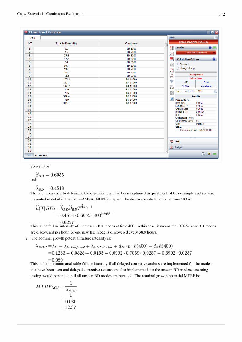
Crow Extended - Continuous Evaluation 172

So we have:

and:

The equations used to determine these parameters have been explained in question 1 of this example and are alsopresented in detail in the Crow-AMSA (NHPP) chapter. The discovery rate function at time 400 is:

This is the failure intensity of the unseen BD modes at time 400. In this case, it means that 0.0257 new BD modesare discovered per hour, or one new BD mode is discovered every 38.9 hours.

7.7. The nominal growth potential failure intensity is:

This is the minimum attainable failure intensity if all delayed corrective actions are implemented for the modesthat have been seen and delayed corrective actions are also implemented for the unseen BD modes, assumingtesting would continue until all unseen BD modes are revealed. The nominal growth potential MTBF is:

Crow Extended - Continuous Evaluation 173

This is the maximum attainable MTBF if all delayed corrective actions are implemented for the modes that havebeen seen and delayed corrective actions are also implemented for the unseen BD modes, assuming testing wouldcontinue until all unseen BD modes are revealed.

8. The nominal projected failure intensity at time is:

This is the projected failure intensity assuming all delayed fixes have been implemented for the modes that havebeen seen. The nominal projected MTBF at time 400 is:

This is the projected MTBF assuming all delayed fixes have been implemented for the modes that have been seen.9.9. The actual growth potential failure intensity is:

This is the minimum attainable failure intensity based on the current management strategy. The actual growthpotential MTBF is:

This is the maximum attainable MTBF based on the current management strategy.10.10. The actual projected failure intensity at time 400 is:

This is the projected failure intensity based on the current management strategy. The actual projected MTBF attime 400 is:

This is the projected MTBF based on the current management strategy. The next figure demonstrates how we canderive the results of this example by using the software's Quick Calculation Pad (QCP). Here we chose tocalculate the actual projected MTBF.

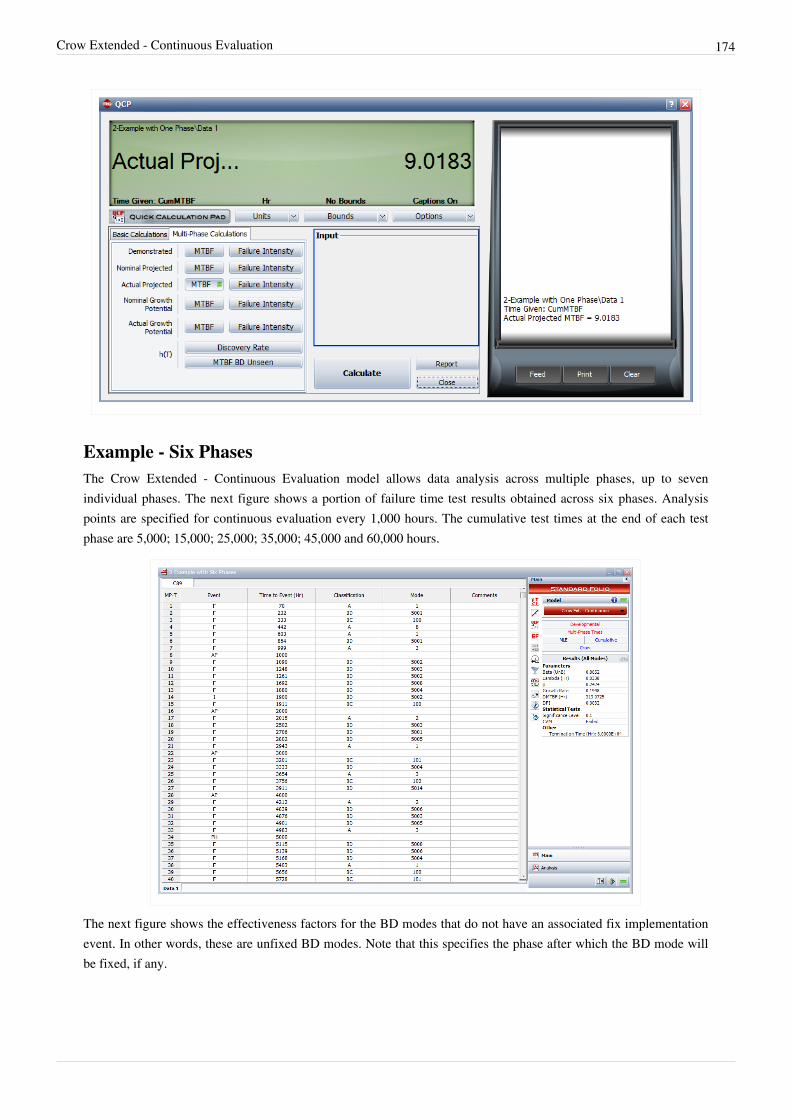
Crow Extended - Continuous Evaluation 174

Example - Six PhasesThe Crow Extended - Continuous Evaluation model allows data analysis across multiple phases, up to sevenindividual phases. The next figure shows a portion of failure time test results obtained across six phases. Analysispoints are specified for continuous evaluation every 1,000 hours. The cumulative test times at the end of each testphase are 5,000; 15,000; 25,000; 35,000; 45,000 and 60,000 hours.

The next figure shows the effectiveness factors for the BD modes that do not have an associated fix implementationevent. In other words, these are unfixed BD modes. Note that this specifies the phase after which the BD mode willbe fixed, if any.

Crow Extended - Continuous Evaluation 175

The next plot shows the overall test results in terms of demonstrated, projected and growth potential MTBF.

The next chart shows the "before" and "after" MTBFs for all the individual modes. Note that the "after" MTBFs arecalculated by taking into account the respective effectiveness factors for each of the unfixed BD modes.

Crow Extended - Continuous Evaluation 176

The analysis points are used to track overall growth inside and across phases, at desired intervals. The RGA softwareallows you to create a multi-phase plot that is associated with a multi-phase data sheet. In addition, if you have anexisting growth planning folio in your RGA project, the multi-phase plot can plot the results from the multi-phasedata sheet together with the reliability growth model from the growth planning folio. This allows you to track theoverall reliability program against the goals, and set plans at each stage of the test. Additional information oncombining a growth planning folio and a multi-phase plot is presented in the Reliability Growth Planning chapter.The next figure shows the multi-phase plot for the six phases of the reliability growth test program. This plot can bea powerful tool for overall tracking of the reliability growth program. It displays the termination time for each phaseof testing, along with the demonstrated, projected and growth potential MTBFs at those times. The plot also displaysthe calculated MTBFs at specified analysis points, which are determined based on the "AP" events in the data sheet.

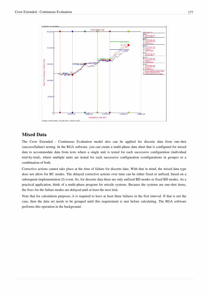
Crow Extended - Continuous Evaluation 177

Mixed DataThe Crow Extended - Continuous Evaluation model also can be applied for discrete data from one-shot(success/failure) testing. In the RGA software, you can create a multi-phase data sheet that is configured for mixeddata to accommodate data from tests where a single unit is tested for each successive configuration (individualtrial-by-trial), where multiple units are tested for each successive configuration (configurations in groups) or acombination of both.Corrective actions cannot take place at the time of failure for discrete data. With that in mind, the mixed data typedoes not allow for BC modes. The delayed corrective actions over time can be either fixed or unfixed, based on asubsequent implementation (I) event. So, for discrete data there are only unfixed BD modes or fixed BD modes. As apractical application, think of a multi-phase program for missile systems. Because the systems are one-shot items,the fixes for the failure modes are delayed until at least the next trial.Note that for calculation purposes, it is required to have at least three failures in the first interval. If that is not thecase, then the data set needs to be grouped until this requirement is met before calculating. The RGA softwareperforms this operation in the background.

Crow Extended - Continuous Evaluation 178

Example - Multi-Phase Discrete DataA one-shot system underwent reliability growth development for a total of 20 trials. The test was performed as acombination of configuration in groups and individual trial-by-trial. The following table shows the obtained data set.The Failures in Interval column specifies the number of failures that occurred in each interval, and the CumulativeTrials column specifies the cumulative number of trials at the end of that interval.

Mixed Data

Event Failures in Interval Cumulative Trials Classification Mode

F 1 8 BD 1

F 1 8 BD 2

F 1 8 BD 3

F 0 10 A

F 0 11 A

F 0 12 A

F 1 13 BD 2

F 0 14 A

F 0 15 A

I 0 15 BD 3

F 1 16 BD 4

F 0 17 A

I 0 17 BD 4

F 0 18 A

F 0 18 A

F 1 20 BD 5

The table also gives the classifications of the failure modes. There are 5 BD modes. Of these 5 modes, 2 arecorrected during the test (BD3 and BD4) and 3 have not been corrected by time (BD1, BD2 and BD5). Dothe following:1.1. Calculate the parameters of the Crow Extended - Continuous Evaluation model.2.2. Calculated the demonstrated reliability at the end of the test.3. Calculate parameter .4.4. Calculate the unfixed BD mode failure probability.5.5. Calculate the nominal growth potential factor.6.6. Calculate the nominal average effectiveness factor.7.7. Calculate the discovery failure intensity function at the end of the test.8.8. Calculate the nominal projected reliability at the end of the test.9.9. Calculate the nominal growth potential reliability at the end of the test.Solution

1.1. The next figure shows the data entered in the RGA software.

Crow Extended - Continuous Evaluation 179

The parameters and are calculated as follows (the calculations for these parameters are presented in detail inthe Crow-AMSAA (NHPP) chapter):

and:

2.2. The corresponding demonstrated unreliability is calculated as:

Using the parameter estimates given above, the instantaneous unreliability at the end of the test (or ) isequal to:

The demonstrated reliability is:

Note that in discrete data, we calculate the reliability and not MTBF because we are dealing with the number oftrials and not test time.

3.3. Assume that the following effectiveness factors are assigned to the unfixed BD modes:

Crow Extended - Continuous Evaluation 180

Classification Mode Effectiveness Factor Implemented at End of Phase

BD 1 0.65 Phase 1

BD 2 0.70 Phase 1

BD 5 0.75 Phase 1

The parameter is the total number of distinct unfixed BD modes at time divided by the total number ofdistinct BD (fixed and unfixed) modes. In this example:

4. The unfixed BD mode failure probability at time is the total number of unfixed BD failures (classified at time) divided by the total trials. Based on the table at the beginning of the example, we have:

5.5. The nominal growth potential factor is:

6.6. The nominal average effectiveness factor is:

7. The discovery function at time is calculated using all the first occurrences of all the BD modes, both fixed andunfixed. In our example, we calculate and using only the unfixed BD modes and excluding the secondoccurrence of BD2, which results in the following:

and:

So the discovery failure intensity function at time is:

The next figure shows the plot for the discovery failure intensity function.

Crow Extended - Continuous Evaluation 181

8. The nominal projected failure probability at time is:

Therefore, the nominal projected reliability is:

9.9. The nominal growth potential unreliability is:

Based on the previous calculation for this example, we have:

So the nominal growth potential reliability is:

The next figure shows the plot for the instantaneous demonstrated, projected and growth potential reliability.

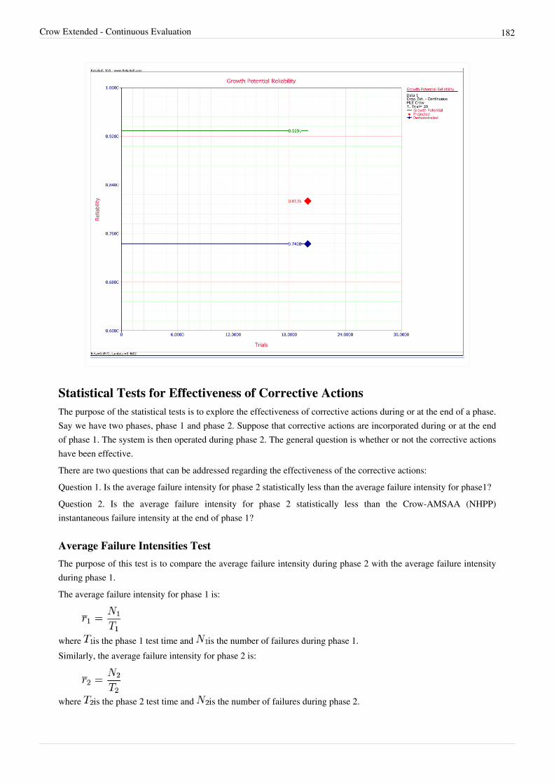
Crow Extended - Continuous Evaluation 182

Statistical Tests for Effectiveness of Corrective ActionsThe purpose of the statistical tests is to explore the effectiveness of corrective actions during or at the end of a phase.Say we have two phases, phase 1 and phase 2. Suppose that corrective actions are incorporated during or at the endof phase 1. The system is then operated during phase 2. The general question is whether or not the corrective actionshave been effective.There are two questions that can be addressed regarding the effectiveness of the corrective actions:Question 1. Is the average failure intensity for phase 2 statistically less than the average failure intensity for phase1?Question 2. Is the average failure intensity for phase 2 statistically less than the Crow-AMSAA (NHPP)instantaneous failure intensity at the end of phase 1?

Average Failure Intensities TestThe purpose of this test is to compare the average failure intensity during phase 2 with the average failure intensityduring phase 1.The average failure intensity for phase 1 is:

where is the phase 1 test time and is the number of failures during phase 1.Similarly, the average failure intensity for phase 2 is:

where is the phase 2 test time and is the number of failures during phase 2.

Crow Extended - Continuous Evaluation 183

The overall test time, , is:

The overall number of failures, , is:

Define as:

If the cumulative binomial probability of up to failures is less than or equal to the statisticalsignificance , then the average failure intensity for phase 2 is statistically less than the average failure intensity forphase 1 at the specific significance level.The cumulative binomial distribution probability is given by:

which gives the probability that the test failures, , are less than or equal to the number of allowable failures, oracceptance number in trials, when each trial has a probability of succeeding of .

Example

Suppose a test is being conducted and is divided into two phases. The test time for the first phase is days,and the test time for the second phase is days. The number of failures during phase 1 is , and thenumber of failures during phase 2 is The average failure intensity for phase 1 is:

Similarly, the average failure intensity for phase 2 is:

Although the average failure intensities are different, we want to see, if at the 10% statistical significance level, theaverage failure intensity for phase 2 is statistically less than the average failure intensity for phase 1.Solution

Concerning the total test time, we have:

The total number of failures is equal to:

Then, we calculate as:

Using the cumulative binomial distribution probability equation, we have:

Crow Extended - Continuous Evaluation 184

Because 0.058 is lower than 0.10, the conclusion is that at the 10% significance level of the the average failureintensity for phase 2 is statistically less than the average failure intensity for phase 1. The conclusion would bedifferent for a different significance level. For example, at the 5% significance level, since 0.058 is not lower than0.05, we fail to reject the null hypothesis. In other words, we cannot statistically prove any significant differencebetween the average failure intensities at the 5% level.

Average vs. Demonstrated Failure Intensities TestThe purpose of this test is to compare the average failure intensity during phase 2 with the Crow-AMSAA (NHPP)instantaneous (demonstrated) failure intensity at the end of phase 1.Once again, the average failure intensity for phase 2 is given by:

where is the phase 2 test time and is the number of failures during phase 2.

The Crow-AMSAA (NHPP) model estimate of failure intensity at time is . Dr. Larry H. Crow [16] showedthat the Crow-AMSAA (NHPP) estimate is approximately distributed as a random variable with standard deviation

.

We therefore treat as an approximate Poisson random variable with number of failures:

We also set:

Then we define:

and:

Let:

If the cumulative binomial probability of up to failures is less than or equal to the statisticalsignificance , then the average failure intensity for phase 2 is statistically less than the Crow-AMSAA (NHPP)instantaneous failure intensity at the end of phase 1, at the specific significance level. The cumulative binomialdistribution probability is again given by:

Crow Extended - Continuous Evaluation 185

Example

Suppose a test is being conducted and is divided into two phases. The test time for the first phase is days,and the test time for the second phase is days. The number of failures during phase 1 is and thenumber of failures during phase 2 is . The Crow-AMSAA (NHPP) parameters for the first phase are

and .The demonstrated failure intensity at the end of phase 1 is calculated as follows:

The average failure intensity for phase 2 is:

Determine if the average failure intensity for phase 2 is statistically less than the demonstrated failure intensity at theend of phase 1 at the 10% significance level.Solution

We calculate the number of failures as:

Then:

Concerning the total test time, we have:

Concerning the total number of failures, we have:

Then we calculate as:

Since the number of failures is not an integer, we are going to calculate the cumulative binomialprobabilities for and , and then interpolate to .For , we have:

And for , we have:

Crow Extended - Continuous Evaluation 186

A linear interpolation between two data points and at the interpolant is given by:

So for we would have that:

Since 0.201 is greater than 0.10, the conclusion is that at the 10% significance level the average failure intensity forphase 2 is not statistically different compared to the demonstrated failure intensity at the end of phase 1.Using the example with the six phases that was given earlier in this chapter, the following figure shows theapplication of the two statistical tests in RGA.

187

Chapter 3.5

Lloyd-LipowLloyd and Lipow (1962) considered a situation in which a test program is conducted in stages. Each stageconsists of a certain number of trials of an item undergoing testing, and the data set is recorded as successes orfailures. All tests in a given stage of testing involve similar items. The results of each stage of testing are used toimprove the item for further testing in the next stage. For the group of data, taken in chronological order, thereare tests with observed successes. The reliability growth function is then given in Lloyd and Lipow [6]:

where:

• the actual reliability during the stage of testing• the ultimate reliability attained if • modifies the rate of growth

Note that essentially, . If the data set consists of reliability data, then is assumed to be the observedreliability given and is considered 1.

Parameter EstimationWhen analyzing reliability data in the RGA software, you have the option to enter the reliability values in percent orin decimal format. However, will always be returned in decimal format and not in percent. The estimatedparameters in the RGA software are unitless.

Maximum Likelihood Estimators

For the stage:

And assuming that the results are independent between stages:

Then taking the natural log gives:

Differentiating with respect to and yields:

Rearranging the equations and setting them equal to zero gives:

Lloyd-Lipow 188

The resulting equations can be solved simultaneously for and . It should be noted that a closed form solutiondoes not exist for either of the parameters; thus, they must be estimated numerically.

Least Squares Estimators

To obtain least squares estimators for and , the sum of squares, , of the deviations of the observedsuccess-ratio, , is minimized from its expected value, , with respect to the parameters and Therefore, is expressed as:

Taking the derivatives with respect to and and setting equal to zero yields:

Solving the equations simultaneously, the least squares estimates of and are:

or:

and:

or:

Lloyd-Lipow 189

Example - Least Squares

After a 20-stage reliability development test program, 20 groups of success/failure data were obtained and are givenin the table below. Do the following:1.1. Fit the Lloyd-Lipow model to the data using least squares.2.2. Plot the reliabilities predicted by the Lloyd-Lipow model along with the observed reliabilities, and compare the

results.

The Test Results and Reliabilities of Each Stage Calculated from Raw Data and thePredicted Reliability

Test Stage Number( ) Number of Tests in Stage( ) Number of Successful Tests( ) Raw Data Reliability Lloyd-Lipow Reliability

1 9 6 0.667 0.7002

2 9 5 0.556 0.7369

3 8 7 0.875 0.7552

4 10 6 0.600 0.7662

5 9 7 0.778 0.7736

6 10 8 0.800 0.7788

7 10 7 0.700 0.7827

8 10 6 0.600 0.7858

9 11 7 0.636 0.7882

10 11 9 0.818 0.7902

11 9 9 1.000 0.7919

12 12 10 0.833 0.7933

13 12 9 0.750 0.7945

14 11 8 0.727 0.7956

15 10 7 0.700 0.7965

16 10 8 0.800 0.7973

17 11 10 0.909 0.7980

18 10 9 0.900 0.7987

19 9 8 0.889 0.7992

20 8 7 0.875 0.7998

Solution

1.1. The least squares estimates are:

Lloyd-Lipow 190

and:

Using these estimates to obtain and yields:

and:

Therefore, the Lloyd-Lipow reliability growth model is as follows, where is the test stage.

2.2. The reliabilities from the raw data and the reliabilities predicted from the Lloyd-Lipow reliability growth modelare given in the last two columns of the table. The figure below shows the plot. Based on the given data, themodel cannot do much more than to basically fit a line through the middle of the points.

Lloyd-Lipow 191

Confidence BoundsThis section presents the methods used in the RGA software to estimate the confidence bounds under theLloyd-Lipow model. One of the properties of maximum likelihood estimators is that they are asymptotically normal.This indicates that they are normally distributed for large samples [6, 7]. Additionally, since the parameter must bepositive, is treated as being normally distributed as well. The parameter represents the ultimate reliabilitythat would be attained if . is the actual reliability during the stage of testing. Therefore, and

will be between 0 and 1. Consequently, the endpoints of the confidence intervals of the parameters and also will be between 0 and 1. To obtain the confidence interval, it is common practice to use the logit transformation.

The confidence bounds on the parameters and are given by:

where represents the percentage points of the distribution such that .The confidence bounds on reliability are given by:

where:

All the variances can be calculated using the Fisher Matrix:

Lloyd-Lipow 192

From the ML estimators of the Lloyd-Lipow model, taking the second partial derivatives yields:

and:

The confidence bounds can be obtained by solving for the three equations shown above and the equation for, and then substituting the values into the Fisher Matrix.

As an example, you can calculate and plot the confidence bounds for the data set given above in the Least Squaresexample as:

The variances can be calculated using the Fisher Matrix:

The variance of is obtained such that:

The confidence bounds on reliability can now be calculated. The associated confidence bounds at the 90%confidence level are plotted in the figure below with the predicted reliability, .

Lloyd-Lipow 193

Example - Lloyd-Lipow Confidence BoundsConsider the success/failure data given in the following table. Solve for the Lloyd-Lipow parameters using leastsquares analysis, and plot the Lloyd-Lipow reliability with 2-sided confidence bounds at the 90% confidence level.

Success/Failure Data for a Variable Number of Tests Performed in Each Test Stage

Test Stage Number( ) Result Number of Tests( > Successful Tests( )

1 F 1 0

2 F 1 0

3 F 1 0

4 S 1 0.2500

5 F 1 0.2000

6 F 1 0.1667

7 S 1 0.2857

8 S 1 0.3750

9 S 1 0.4444

10 S 1 0.5000

11 S 1 0.5455

12 S 1 0.5833

13 S 1 0.6154

14 S 1 0.6429

Lloyd-Lipow 194

15 S 1 0.6667

16 S 1 0.6875

17 F 1 0.6471

18 S 1 0.6667

19 F 1 0.6316

20 S 1 0.6500

21 S 1 0.6667

22 S 1 0.6818

Solution

Note that the data set contains three consecutive failures at the beginning of the test. These failures will be ignoredthroughout the analysis because it is considered that the test starts when the reliability is not equal to zero or one.The number of data points is now reduced to 19. Also, note that the only time that the first three first failures areconsidered is to calculate the observed reliability in the test. For example, given this data set, the observed reliabilityat stage 4 is . This is considered to be the reliability at stage 1.From the table, the least squares estimates can be calculated as follows:

and:

Using these estimates to obtain and yields:

and:

Therefore, the Lloyd-Lipow reliability growth model is as follows, where is the number of the test stage.

Using the data from the table:

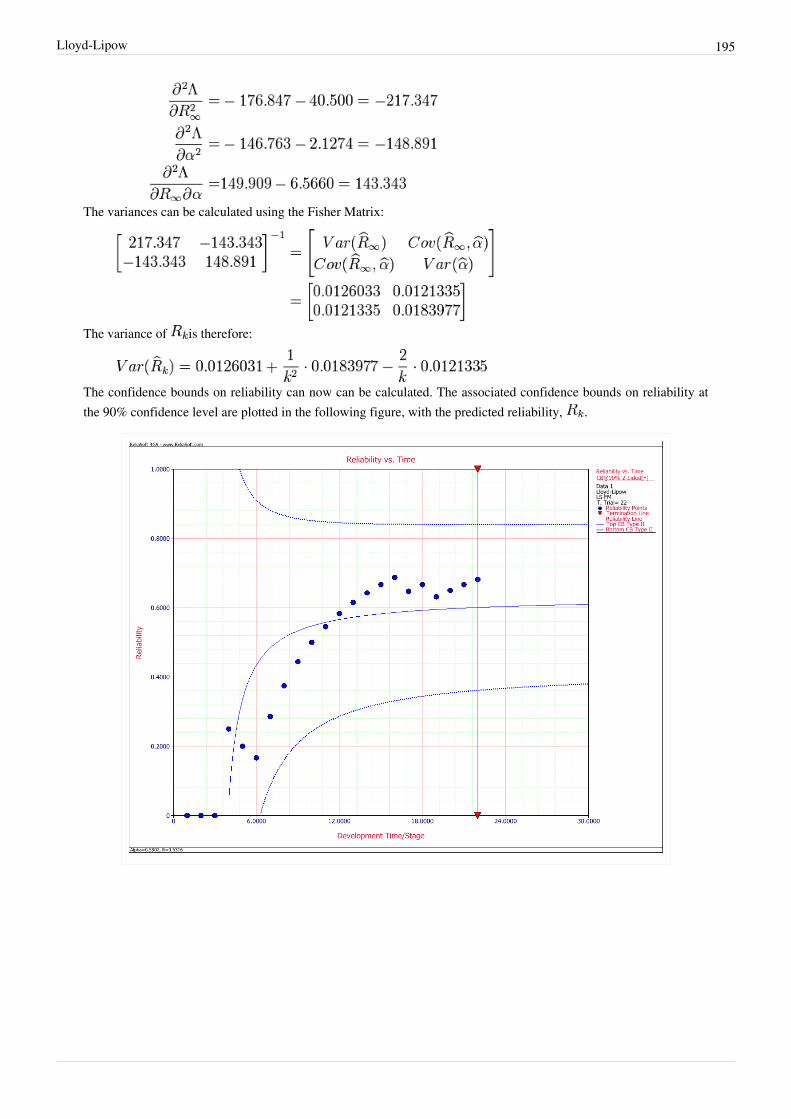
Lloyd-Lipow 195

The variances can be calculated using the Fisher Matrix:

The variance of is therefore:

The confidence bounds on reliability can now can be calculated. The associated confidence bounds on reliability atthe 90% confidence level are plotted in the following figure, with the predicted reliability, .

Lloyd-Lipow 196

More Examples

Grouped per Configuration ExampleA 15-stage reliability development test program was performed. The grouped per configuration data set is shown inthe following table. Do the following:1.1. Fit the Lloyd-Lipow model to the data using MLE.2.2. What is the maximum reliability attained as the number of test stages approaches infinity?3.3. What is the maximum achievable reliability with a 90% confidence level?

Grouped per Configuration Data

Stage, Number of Tests ( ) Number of Successes ( )

1 10 3

2 10 3

3 10 4

4 10 5

5 10 5

6 12 6

7 12 5

8 12 7

9 14 8

10 14 8

11 14 10

12 14 12

13 14 11

14 14 12

15 14 12

Solution

1.1. The figure below displays the entered data and the estimated Lloyd-Lipow parameters.

Lloyd-Lipow 197

2. The maximum achievable reliability as the number of test stages approaches infinity is equal to the value of .Therefore, .

3. The maximum achievable reliability with a 90% confidence level can be estimated by viewing the confidencebounds on the parameters in the QCP, as shown in the figure below. The lower bound on the value of is equalto 0.6691 .

Lloyd-Lipow 198

Reliability Data ExampleGiven the reliability data in the table below, do the following:1.1. Fit the Lloyd-Lipow model to the data using least squares analysis.2.2. Plot the Lloyd-Lipow reliability with 90% 2-sided confidence bounds.3.3. How many months of testing are required to achieve a reliability goal of 90%?4.4. What is the attainable reliability if the maximum duration of testing is 30 months?

Reliability Data

Time (months) Reliability (%)

1 33.35

2 42.50

3 58.02

4 68.50

5 74.20

6 80.00

7 82.30

8 89.50

9 91.00

10 92.10

Solution

1.1. The next figure displays the estimated parameters.

2.2. The figure below displays Reliability vs. Time plot with 90% 2-sided confidence bounds.

Lloyd-Lipow 199

3.3. The next figure shows the number of months of testing required to achieve a reliability goal of 90%.

4.4. The figure below displays the reliability achieved after 30 months of testing.

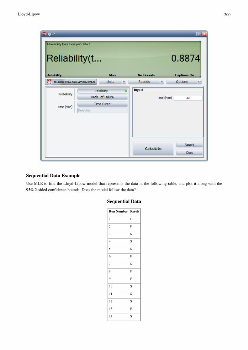
Lloyd-Lipow 200

Sequential Data ExampleUse MLE to find the Lloyd-Lipow model that represents the data in the following table, and plot it along with the95% 2-sided confidence bounds. Does the model follow the data?

Sequential Data

Run Number Result

1 F

2 F

3 S

4 S

5 S

6 F

7 S

8 F

9 F

10 S

11 S

12 S

13 F

14 S

Lloyd-Lipow 201

15 S

16 S

17 S

18 S

19 S

20 S

Solution

The two figures below demonstrate the solution. As can be seen from the Reliability vs. Time plot with 95% 2-sidedconfidence bounds, the model does not seem to follow the data. You may want to consider another model for thisdata set.

Lloyd-Lipow 202

Sequential Data with Failure Modes ExampleUse least squares to find the Lloyd-Lipow model that represents the data in the following table. This data setincludes information about the failure mode that was responsible for each failure, so that the probability of eachfailure mode recurring is taken into account in the analysis.

Sequential with Mode Data

Run Number Result Mode

1 S

2 F 1

3 F 2

4 F 3

5 S

6 S

7 S

8 F 3

9 F 2

10 S

11 F 2

12 S

13 S

14 S

Lloyd-Lipow 203

15 S

Solution

The following figure shows the analysis.

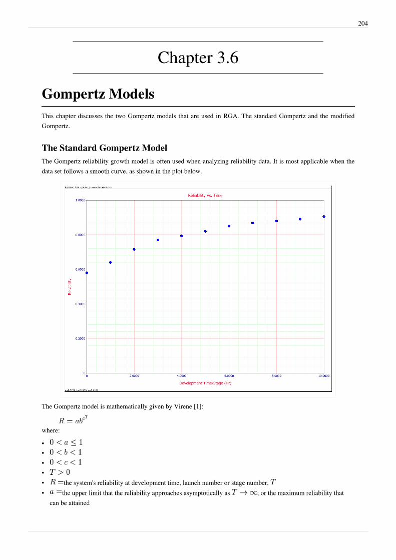
204

Chapter 3.6

Gompertz ModelsThis chapter discusses the two Gompertz models that are used in RGA. The standard Gompertz and the modifiedGompertz.

The Standard Gompertz ModelThe Gompertz reliability growth model is often used when analyzing reliability data. It is most applicable when thedata set follows a smooth curve, as shown in the plot below.

The Gompertz model is mathematically given by Virene [1]:

where:

••••• the system's reliability at development time, launch number or stage number, • the upper limit that the reliability approaches asymptotically as , or the maximum reliability that

can be attained

Gompertz Models 205

• initial reliability at • the growth pattern indicator (small values of indicate rapid early reliability growth and large values of

indicate slow reliability growth)As it can be seen from the mathematical definition, the Gompertz model is a 3-parameter model with the parameters

, and . The solution for the parameters, given and , is accomplished by fitting the best possible linethrough the data points. Many methods are available; all of which tend to be numerically intensive. When analyzingreliability data in the RGA software, you have the option to enter the reliability values in percent or in decimalformat. However, will always be returned in decimal format and not in percent. The estimated parameters in theRGA software are unitless. The next section presents an overview and background on some of the most commonlyused algorithms/methods for obtaining these parameters.

Parameter Estimation

Linear Regression

The method of least squares requires that a straight line be fitted to a set of data points. If the regression is on ,then the sum of the squares of the vertical deviations from the points to the line is minimized. If the regression is on

, the line is fitted to a set of data points such that the sum of the squares of the horizontal deviations from thepoints to the line is minimized. To illustrate the method, this section presents a regression on . Consider the linearmodel given by Seber and Wild [2]:

or in matrix form where bold letters indicate matrices:

where:

and:

The vector holds the values of the parameters. Now let be the estimates of these parameters, or the regressioncoefficients. The vector of estimated regression coefficients is denoted by:

Gompertz Models 206

Solving for in the matrix form of the equation requires the analyst to left multiply both sides by the transpose of , , or :

Now the term becomes a square and invertible matrix. Then taking it to the other side of the equation gives:

Non-linear Regression

Non-linear regression is similar to linear regression, except that a curve is fitted to the data set instead of a straightline. Just as in the linear scenario, the sum of the squares of the horizontal and vertical distances between the line andthe points are to be minimized. In the case of the non-linear Gompertz model , let:

where:

and:

The Gauss-Newton method can be used to solve for the parameters , and by performing a Taylor seriesexpansion on Then approximate the non-linear model with linear terms and employ ordinary least squaresto estimate the parameters. This procedure is performed in an iterative manner and it generally leads to a solution ofthe non-linear problem.

This procedure starts by using initial estimates of the parameters , and , denoted as and whereis the iteration number. The Taylor series expansion approximates the mean response, , around the

starting values, and For the observation:

where:

Let:

So the equation becomes:

Gompertz Models 207

or by shifting to the left of the equation:

In matrix form this is given by:

where:

and:

Note that the equation is in the form of the general linear regression model given in the LinearRegression section. Therefore, the estimate of the parameters is given by:

The revised estimated regression coefficients in matrix form are:

The least squares criterion measure, should be checked to examine whether the revised regression coefficientswill lead to a reasonable result. According to the Least Squares Principle, the solution to the values of the parametersare those values that minimize . With the starting coefficients, , is:

And with the coefficients at the end of the first iteration, , is:

Gompertz Models 208

For the Gauss-Newton method to work properly and to satisfy the Least Squares Principle, the relationshiphas to hold for all , meaning that gives a better estimate than . The problem is not yet

completely solved. Now are the starting values, producing a new set of values . The process is continueduntil the following relationship has been satisfied:

When using the Gauss-Newton method or some other estimation procedure, it is advisable to try several sets ofstarting values to make sure that the solution gives relatively consistent results.

Choice of Initial Values

The choice of the starting values for the nonlinear regression is not an easy task. A poor choice may result in alengthy computation with many iterations. It may also lead to divergence, or to a convergence due to a localminimum. Therefore, good initial values will result in fast computations with few iterations, and if multiple minimaexist, it will lead to a solution that is a minimum.Various methods were developed for obtaining valid initial values for the regression parameters. The followingprocedure is described by Virene [1] in estimating the Gompertz parameters. This procedure is rather simple. It willbe used to get the starting values for the Gauss-Newton method, or for any other method that requires initial values.Some analysts use this method to calculate the parameters when the data set is divisible into three groups of equalsize. However, if the data set is not equally divisible, it can still provide good initial estimates.

Consider the case where observations are available in the form shown next. Each reliability value, , ismeasured at the specified times, .

where:

• is equal to the number of items in each equally sized group••The Gompertz reliability equation is given by:

and:

Define:

Then:

Gompertz Models 209

Without loss of generality, take ; then:

Solving for yields:

Considering the definitions for and , given above, then:

or:

Reordering the equation yields:

If the reliability values are in percent then needs to be divided by 100 to return the estimate in decimal format.Consider the definitions for and again, where:

Reordering the equation above yields:

Therefore, for the special case where , the parameters are:

Gompertz Models 210

To estimate the values of the parameters and , do the following:1. Arrange the currently available data in terms of and as in the table below. The values should be chosen at

equal intervals and increasing in value by 1, such as one month, one hour, etc.

Design and Development Time vs. Demonstrated Reliability Data for a Device

Group Number Growth Time (months) Reliability (%)

0 58 4.060

1 1 66 4.190

= 8.250

2 72.5 4.284

2 3 78 4.357

= 8.641

4 82 4.407

3 5 85 4.443

= 8.850

2. Calculate the natural log .3. Divide the column of values for log into three groups of equal size, each containing items. There should

always be three groups. Each group should always have the same number, , of items, measurements or values.4. Add the values of the natural log in each group, obtaining the sums identified as , and , starting with

the lowest values of the natural log .5. Calculate using the following equation:

6. Calculate using the following equation:

7. Calculate using the following equation:

8.8. Write the Gompertz reliability growth equation.9. Substitute the value of , the time at which the reliability goal is to be achieved, to see if the reliability is indeed

to be attained or exceeded by .

Gompertz Models 211

Confidence BoundsThe approximate reliability confidence bounds under the Gompertz model can be obtained with non-linearregression. Additionally, the reliability is always between 0 and 1. In order to keep the endpoints of the confidenceinterval, the logit transformation is used to obtain the confidence bounds on reliability.

where is the total number of groups (in this case 3) and is the total number of items in each group.

Example - Standard Gompertz for Reliability DataA device is required to have a reliability of 92% at the end of a 12-month design and development period. Thefollowing table gives the data obtained for the first five moths.1.1. What will the reliability be at the end of this 12-month period?2.2. What will the maximum achievable reliability be if the reliability program plan pursued during the first 5 months

is continued?3.3. How do the predicted reliability values compare with the actual values?

Design and Development Time vs. Demonstrated Reliability Data for a Device

Group Number Growth Time (months) Reliability (%)

0 58 4.060

1 1 66 4.190

= 8.250

2 72.5 4.284

2 3 78 4.357

= 8.641

4 82 4.407

3 5 85 4.443

= 8.850

Solution

After generating the table above and calculating the last column to find , and , proceed as follows:a. Solve for the value of :

b. Solve for the value of :

This is the upper limit for the reliability as .c. Solve for the value of :

Gompertz Models 212

Now, that the initial values have been determined, the Gauss-Newton method can be used. Therefore, substituting become:

The estimate of the parameters is given by:

The revised estimated regression coefficients in matrix form are:

If the Gauss-Newton method works effectively, then the relationship has to hold, meaning thatgives better estimates than , after . With the starting coefficients, , is:

And with the coefficients at the end of the first iteration, , is:

Gompertz Models 213

Therefore, it can be justified that the Gauss-Newton method works in the right direction. The iterations are continueduntil the relationship is satisfied. Note that the RGA software uses a different analysis methodcalled the Levenberg-Marquardt. This method utilizes the best features of the Gauss-Newton method and the methodof the steepest descent, and occupies a middle ground between these two methods. The estimated parameters usingRGA are shown in the figure below.

They are:

The Gompertz reliability growth curve is:

1.1. The achievable reliability at the end of the 12-month period of design and development is:

The required reliability is 92%. Consequently, from the previous result, this requirement will be barely met. Everyeffort should therefore be expended to implement the reliability program plan fully, and perhaps augment itslightly to assure that the reliability goal will be met.

2. The maximum achievable reliability from Step 2, or from the value of , is 0.9422.3.3. The predicted reliability values, as calculated from the standard Gompertz model, are compared with the actual

data in the table below. It may be seen in the table that the Gompertz curve appears to provide a very good fit forthe data used because the equation reproduces the available data with less than 1% error. The standard Gompertzmodel is plotted in the figure below the table. The plot identifies the type of reliability growth curve that theequation represents.

Gompertz Models 214

Comparison of the Predicted Reliabilities with the Actual Data

Growth Time (months) Gompertz Reliability(%) Raw Data Reliability(%)

0 57.97 58.00

1 66.02 66.00

2 72.62 72.50

3 77.87 78.00

4 81.95 82.00

5 85.07 85.00

6 87.43

7 89.20

8 90.52

9 91.50

10 92.22

11 92.75

12 93.14

Gompertz Models 215

Example - Standard Gompertz for Sequential DataCalculate the parameters of the Gompertz model using the sequential data in the following table.

Sequential Data

Run Number Result Successes Observed Reliability(%)

1 F 0

2 F 0

3 F 0

4 S 1 25.00

5 F 1 20.00

6 F 1 16.67

7 S 2 28.57

8 S 3 37.50

9 S 4 44.44

10 S 5 50.00

11 S 6 54.55

12 S 7 58.33

13 S 8 61.54

14 S 9 64.29

15 S 10 66.67

16 S 11 68.75

17 F 11 64.71

18 S 12 66.67

19 F 12 63.16

20 S 13 65.00

21 S 14 66.67

22 S 15 68.18

Solution

Using RGA, the parameter estimates are shown in the following figure.

Gompertz Models 216

Cumulative ReliabilityFor many kinds of equipment, especially missiles and space systems, only success/failure data (also called discreteor attribute data) is obtained. Conservatively, the cumulative reliability can be used to estimate the trend of reliabilitygrowth. The cumulative reliability is given by Kececioglu [3]:

where:

• is the current number of trials• is the number of failuresIt must be emphasized that the instantaneous reliability of the developed equipment is increasing as thetest-analyze-fix-and-test process continues. In addition, the instantaneous reliability is higher than the cumulativereliability. Therefore, the reliability growth curve based on the cumulative reliability can be thought of as the lowerbound of the true reliability growth curve.

The Modified Gompertz ModelSometimes, reliability growth data with an S-shaped trend cannot be described accurately by the Standard Gompertzor Logistic curves. Because these two models have fixed values of reliability at the inflection points, only a fewreliability growth data sets following an S-shaped reliability growth curve can be fitted to them. A modification ofthe Gompertz curve, which overcomes this shortcoming, is given next [5].If we apply a shift in the vertical coordinate, then the Gompertz model is defined by:

where:

•

Gompertz Models 217

•• is the system's reliability at development time or at launch number , or stage number • is the shift parameter• is the upper limit that the reliability approaches asymptotically as • is the initial reliability at • is the growth pattern indicator (small values of indicate rapid early reliability growth and large values of

indicate slow reliability growth)The modified Gompertz model is more flexible than the original, especially when fitting growth data with S-shapedtrends.

Parameter Estimation

To implement the modified Gompertz growth model, initial values of the parameters , , and must bedetermined. When analyzing reliability data in RGA, you have the option to enter the reliability values in percent orin decimal format. However, and will always be returned in decimal format and not in percent. The estimatedparameters in RGA are unitless.

Given that and , it follows that , and , as defined in thederivation of the Standard Gompertz model, can be expressed as functions of .

Modifying the equations for estimating parameters , , , as functions of , yields:

where is the time interval increment. At this point, you can use the initial constraint of:

Now there are four unknowns, , , and , and four corresponding equations. The simultaneous solution of theseequations yields the four initial values for the parameters of the modified Gompertz model. This procedure is similarto the one discussed before. It starts by using initial estimates of the parameters, , , and , denoted as

and where is the iteration number.

The Taylor series expansion approximates the mean response, , around the starting values, and . For the observation:

where:

Gompertz Models 218

Let:

Therefore:

or by shifting to the left of the equation:

In matrix form, this is given by:

where:

The same reasoning as before is followed here, and the estimate of the parameters is given by:

The revised estimated regression coefficients in matrix form are:

Gompertz Models 219

To see if the revised regression coefficients will lead to a reasonable result, the least squares criterion measure, ,should be checked. According to the Least Squares Principle, the solution to the values of the parameters are thosevalues that minimize . With the starting coefficients, , is:

With the coefficients at the end of the first iteration, , is:

For the Gauss-Newton method to work properly, and to satisfy the Least Squares Principle, the relationshiphas to hold for all , meaning that gives a better estimate than . The problem is not yet

completely solved. Now are the starting values, producing a new set of values The process is continueduntil the following relationship has been satisfied.

As mentioned previously, when using the Gauss-Newton method or some other estimation procedure, it is advisableto try several sets of starting values to make sure that the solution gives relatively consistent results. Note that RGAuses a different analysis method called the Levenberg-Marquardt. This method utilizes the best features of theGauss-Newton method and the method of the steepest descent, and occupies a middle ground between these twomethods.

Confidence BoundsThe approximate reliability confidence bounds under the modified Gompertz model can be obtained using non-linearregression. Additionally, the reliability is always between 0 and 1. In order to keep the endpoints of the confidenceinterval, the logit transformation can be used to obtain the confidence bounds on reliability.

where is the total number of groups (in this case 4) and is the total number of items in each group.

Example - Modified Gompertz for Reliability DataA reliability growth data set is given in columns 1 and 2 of the following table. Find the modified Gompertz curvethat represents the data and plot it comparatively with the raw data.

Development Time vs. Observed Reliability Data and Predicted Reliabilities

Time(months) Raw Data Reliability(%) Gompertz Reliability(%) Logistic Reliability(%) Modified Gompertz Reliability(%)

0 31.00 25.17 22.70 31.18

1 35.50 38.33 38.10 35.08

2 49.30 51.35 56.40 49.92

3 70.10 62.92 73.00 69.23

4 83.00 72.47 85.00 83.72

5 92.20 79.94 93.20 92.06

6 96.40 85.59 96.10 96.29

Gompertz Models 220

7 98.60 89.75 98.10 98.32

8 99.00 92.76 99.10 99.27

Solution

To determine the parameters of the modified Gompertz curve, use:

and:

for , the equation above may be rewritten as:

The equations for parameters , and can now be solved simultaneously. One method for solving these equationsnumerically is to substitute different values of , which must be less than , into the last equation shown above,and plot the results along the y-axis with the value of along the x-axis. The value of can then be read from thex-intercept. This can be repeated for greater accuracy using smaller and smaller increments of . Once the desiredaccuracy on has been achieved, the value of can then be used to solve for , and . For this case, the initialestimates of the parameters are:

Now, since the initial values have been determined, the Gauss-Newton method can be used. Therefore, substituting and , become:

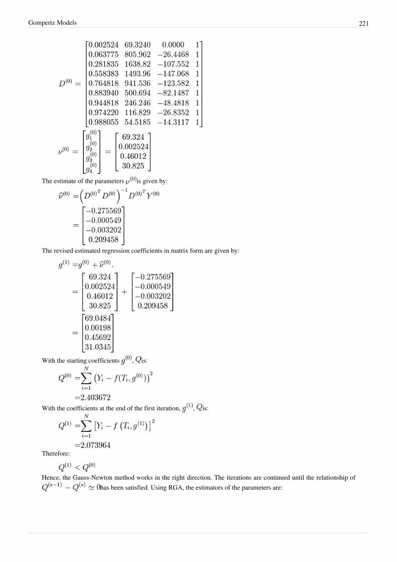
Gompertz Models 221

The estimate of the parameters is given by:

The revised estimated regression coefficients in matrix form are given by:

With the starting coefficients , is:

With the coefficients at the end of the first iteration, , is:

Therefore:

Hence, the Gauss-Newton method works in the right direction. The iterations are continued until the relationship ofhas been satisfied. Using RGA, the estimators of the parameters are:

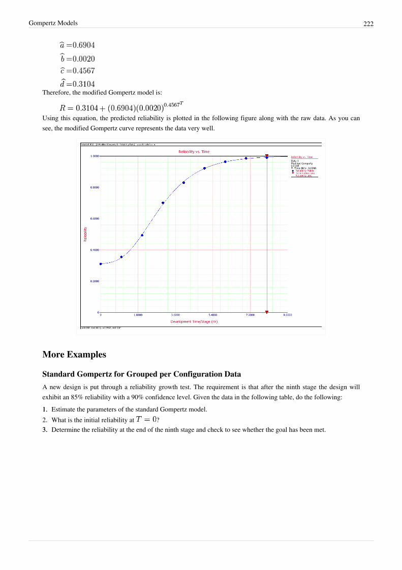
Gompertz Models 222

Therefore, the modified Gompertz model is:

Using this equation, the predicted reliability is plotted in the following figure along with the raw data. As you cansee, the modified Gompertz curve represents the data very well.

More Examples

Standard Gompertz for Grouped per Configuration DataA new design is put through a reliability growth test. The requirement is that after the ninth stage the design willexhibit an 85% reliability with a 90% confidence level. Given the data in the following table, do the following:1.1. Estimate the parameters of the standard Gompertz model.2. What is the initial reliability at ?3.3. Determine the reliability at the end of the ninth stage and check to see whether the goal has been met.

Gompertz Models 223

Grouped per Configuration Data

Stage Number of Units Number of Failures

1 10 5

2 8 3

3 9 3

4 9 2

5 10 2

6 10 1

7 10 1

8 10 1

9 10 1

Solution

1.1. The data is entered in cumulative format and the estimated standard Gompertz parameters are shown in thefollowing figure.

2. The initial reliability at is equal to:

3.3. The reliability at the ninth stage can be calculated using the Quick Calculation Pad (QCP) as shown in the figurebelow.

Gompertz Models 224

The estimated reliability at the end of the ninth stage is equal to 91.92%. However, the lower limit at the 90%1-sided confidence bound is equal to 82.15%. Therefore, the required goal of 85% reliability at a 90% confidencelevel has not been met.

Comparing Standard and Modified GompertzUsing the data in the following table, determine whether the standard Gompertz or modified Gompertz would bebetter suited for analyzing the given data.

Reliability Data

Stage Reliability (%)

0 36

1 38

2 46

3 58

4 71

5 80

6 86

7 88

8 90

9 91

Gompertz Models 225

SolutionThe standard Gompertz Reliability vs. Time plot is shown next.

The standard Gompertz seems to do a fairly good job of modeling the data. However, it appears that it is havingdifficulty modeling the S-shape of the data. The modified Gompertz Reliability vs. Time plot is shown next. Asexpected, the modified Gompertz does a much better job of handling the S-shape presented by the data and providesa better fit for this data.

226

Chapter 3.7

LogisticThe Logistic reliability growth model has an S-shaped curve and is given by Kececioglu [3]:

where and are parameters. Similar to the analysis given for the Gompertz curve, the following may be concluded:1.1. The point of inflection is given by:

2. When , then and an S-shaped curve will be generated. However, when , then and the Logistic reliability growth model will not be described by an S-shaped curve.

3. The value of is equal to 0.5 at the inflection point.

Parameter EstimationIn this section, we will demonstrate the parameter estimation method for the Logistic model using three examples fordifferent types of data.

Example: Logistic for Reliability DataUsing the reliability growth data given in the table below, do the following:1.1. Find a Gompertz curve that represents the data and plot it with the raw data.2.2. Find a Logistic reliability growth curve that represents the data and plot it with the raw data.

Development Time vs. Observed Reliability data and Predicted Reliabilities

Time, months Raw Data Reliability (%) Gompertz Reliability (%) Logistic Reliablity (%)

0 31.00 24.85 22.73

1 35.50 38.48 38.14

2 49.30 51.95 56.37

3 70.10 63.82 73.02

4 83.00 73.49 85.01

5 92.20 80.95 92.24

6 96.40 86.51 96.14

7 98.60 90.54 98.12

8 99.00 93.41 99.09

Solution

1.1. The figure below shows the entered data and the estimated parameters using the standard Gompertz model.

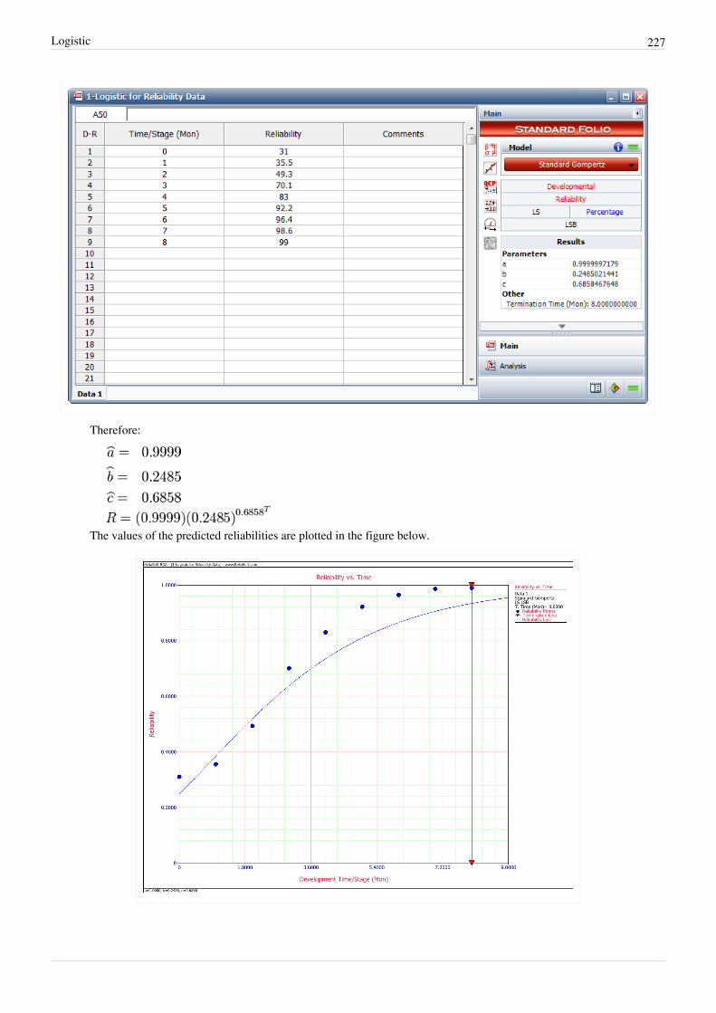
Logistic 227

Therefore:

The values of the predicted reliabilities are plotted in the figure below.

Logistic 228

Notice how the standard Gompertz model is not really capable of handling the S-shaped characteristics of thisdata.

2. The least squares estimators of the Logistic growth curve parameters are given by Crow [9]: where:

In this example , which gives:

From the equations for and :

And from the least squares estimators for and :

Therefore, the Logistic reliability growth curve that represents this data set is given by:

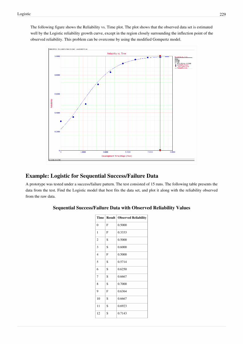
Logistic 229

The following figure shows the Reliability vs. Time plot. The plot shows that the observed data set is estimatedwell by the Logistic reliability growth curve, except in the region closely surrounding the inflection point of theobserved reliability. This problem can be overcome by using the modified Gompertz model.

Example: Logistic for Sequential Success/Failure DataA prototype was tested under a success/failure pattern. The test consisted of 15 runs. The following table presents thedata from the test. Find the Logistic model that best fits the data set, and plot it along with the reliability observedfrom the raw data.

Sequential Success/Failure Data with Observed Reliability Values

Time Result Observed Reliability

0 F 0.5000

1 F 0.3333

2 S 0.5000

3 S 0.6000

4 F 0.5000

5 S 0.5714

6 S 0.6250

7 S 0.6667

8 S 0.7000

9 F 0.6364

10 S 0.6667

11 S 0.6923

12 S 0.7143

Logistic 230

13 S 0.7333

Solution

The first run is ignored because it was a success, and the reliability at that point was 100%. This failure will beignored throughout the analysis because it is considered that the test starts when the reliability is not equal to zero orone. The test essentially begins at time 1, and is now considered as time 0 with . The observed reliability isshown in the last column of the table. Keep in mind that the observed reliability values still account for the initialsuspension.Therefore:

and:

Now, from the least squares estimators, the values are:

Therefore:

The Logistic reliability model that best fits the data is given by:

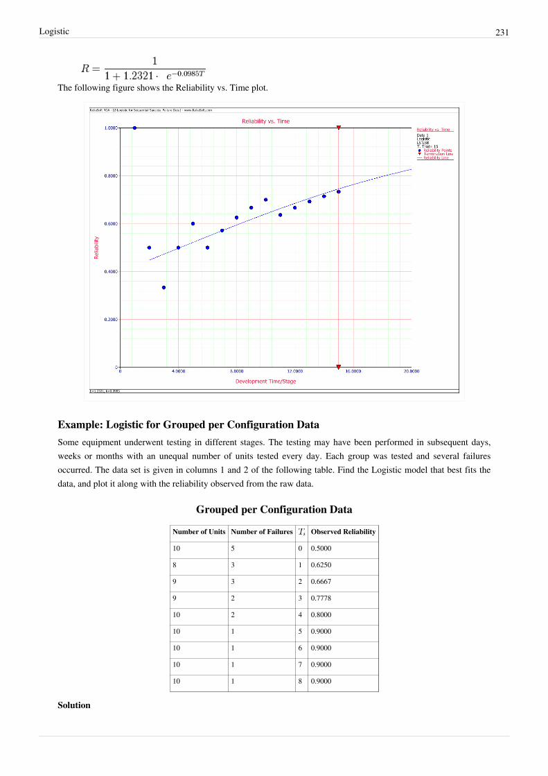
Logistic 231

The following figure shows the Reliability vs. Time plot.

Example: Logistic for Grouped per Configuration DataSome equipment underwent testing in different stages. The testing may have been performed in subsequent days,weeks or months with an unequal number of units tested every day. Each group was tested and several failuresoccurred. The data set is given in columns 1 and 2 of the following table. Find the Logistic model that best fits thedata, and plot it along with the reliability observed from the raw data.

Grouped per Configuration Data

Number of Units Number of Failures Observed Reliability

10 5 0 0.5000

8 3 1 0.6250

9 3 2 0.6667

9 2 3 0.7778

10 2 4 0.8000

10 1 5 0.9000

10 1 6 0.9000

10 1 7 0.9000

10 1 8 0.9000

Solution

Logistic 232

The observed reliability is and the last column of the table above shows the values for each group.With , the least square estimator becomes:

and:

Now from the least squares estimators, and , we have:

Therefore:

The Logistic reliability model that best fits the data is given by:

The figure below shows the Reliability vs. Time plot.

Logistic 233

Confidence BoundsLeast squares is used to estimate the parameters of the following Logistic model.

Thus, the confidence bounds on the parameter are given by:

where:

and the confidence bounds on the parameter are:

where:

Since the reliability is always between 0 and 1, the logit transformation is used to obtain the confidence bounds onreliability, which is:

Logistic 234

Example: Logistic Confidence BoundsFor the data given above for the reliability data example, calculate the 2-sided 90% confidence bounds under theLogistic model for the following:

1. The parameters and .2.2. Reliability at month 5.Solution

1. The values of and that were estimated from the least squares analysis in the reliability data example are:

Thus, the 2-sided 90% confidence bounds on parameter are:

The 2-sided 90% confidence bounds on parameter are:

2.2. First, calculate the reliability estimation at month 5:

Thus, the 2-sided 90% confidence bounds on reliability at month 5 are:

The next figure shows a graph of the reliability plotted with 2-sided 90% confidence bounds.

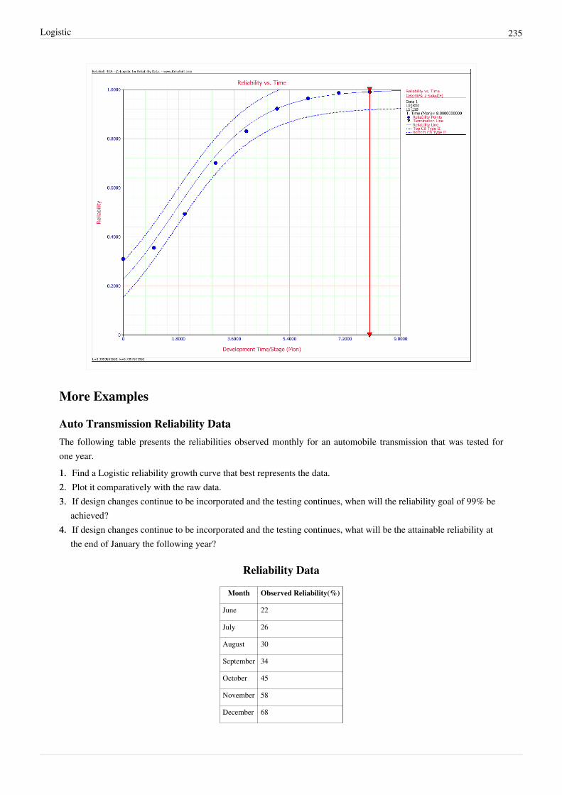
Logistic 235

More Examples

Auto Transmission Reliability DataThe following table presents the reliabilities observed monthly for an automobile transmission that was tested forone year.1.1. Find a Logistic reliability growth curve that best represents the data.2.2. Plot it comparatively with the raw data.3.3. If design changes continue to be incorporated and the testing continues, when will the reliability goal of 99% be

achieved?4.4. If design changes continue to be incorporated and the testing continues, what will be the attainable reliability at

the end of January the following year?

Reliability Data

Month Observed Reliability(%)

June 22

July 26

August 30

September 34

October 45

November 58

December 68

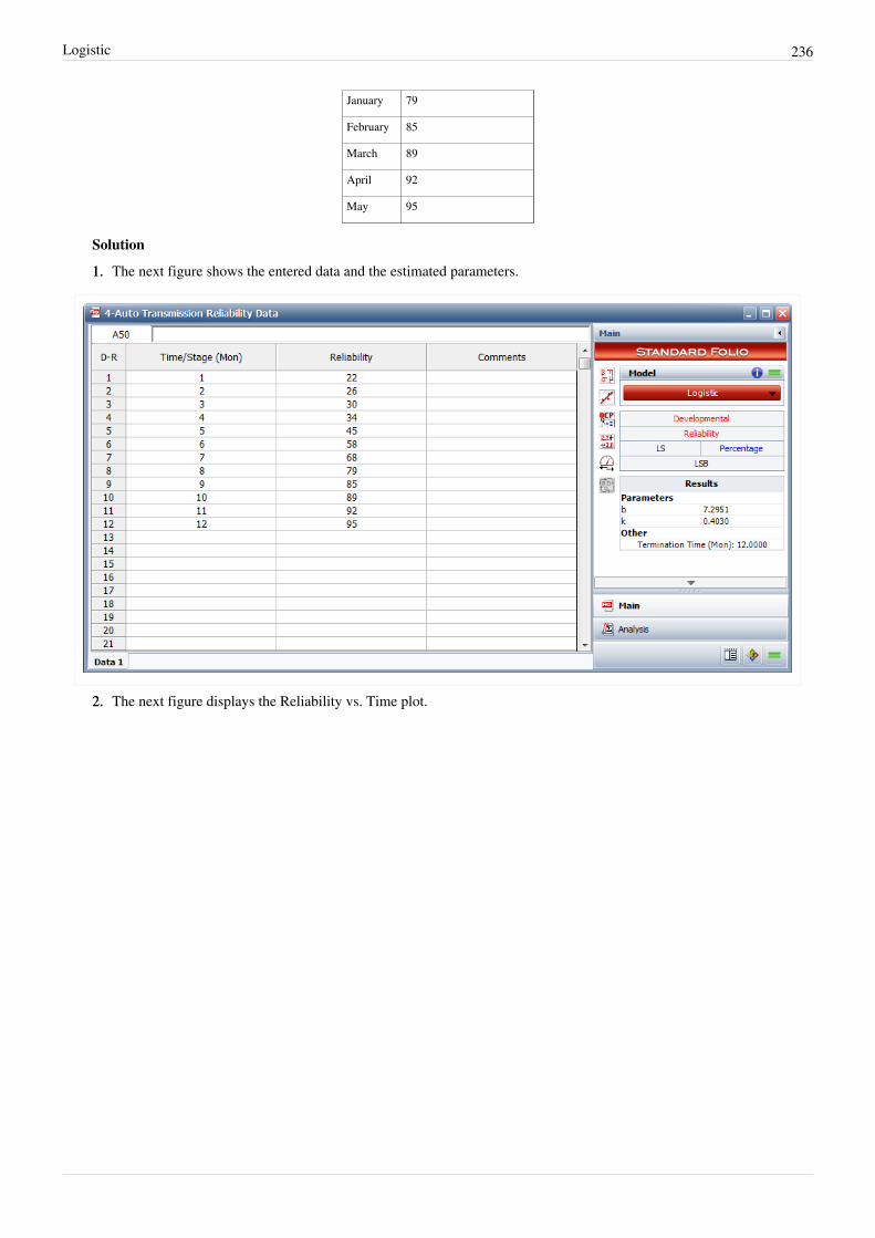
Logistic 236

January 79

February 85

March 89

April 92

May 95

Solution

1.1. The next figure shows the entered data and the estimated parameters.

2.2. The next figure displays the Reliability vs. Time plot.

Logistic 237

3.3. Using the QCP, the next figure displays, in months, when the reliability goal of 99% will be achieved.

Logistic 238

4.4. The last figure shows the reliability at the end of January the following year (i.e., after 20 months of testing anddevelopment).

Sequential Data from Missile Launch TestThe following table presents the results for a missile launch test. The test consisted of 20 attempts. If the missilelaunched, it was recorded as a success. If not, it was recorded as a failure. Note that, at this development stage, thetest did not consider whether or not the target was destroyed.1.1. Find a Logistic reliability growth curve that best represents the data.2.2. Plot it comparatively with the raw data.3.3. If design changes continue to be incorporated and the testing continues, when will the reliability goal of 99.5%

with a 90% confidence level be achieved?4.4. If design changes continue to be incorporated and the testing continues, what will be the attainable reliability at

the end of the 35th launch?

Logistic 239

Sequential Success/Failure Data

Launch Number Result

1 F

2 F

3 S

4 F

5 F

6 S

7 S

8 S

9 F

10 S

11 F

12 S

13 S

14 S

15 S

16 S

17 S

18 S

19 S

20 S

Solution

1.1. The next figure shows the entered data and the estimated parameters.

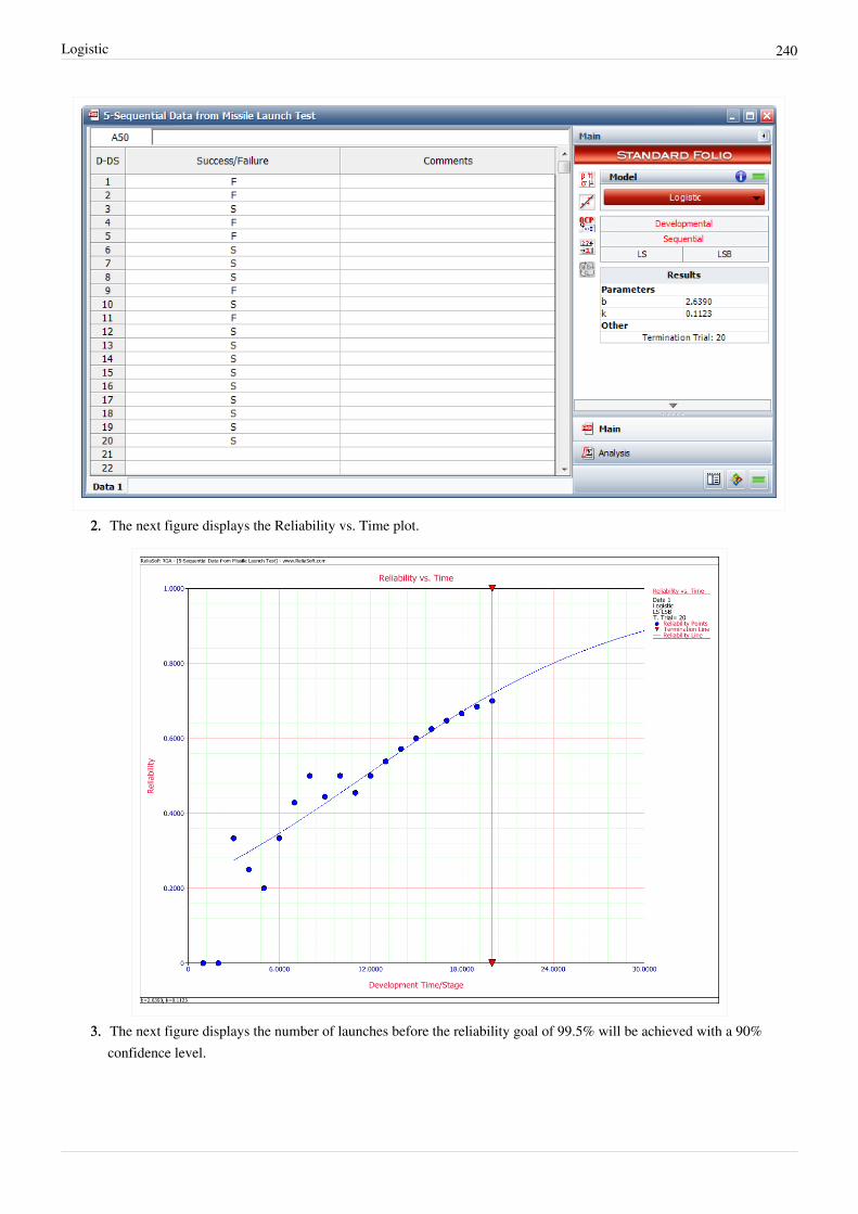
Logistic 240

2.2. The next figure displays the Reliability vs. Time plot.

3.3. The next figure displays the number of launches before the reliability goal of 99.5% will be achieved with a 90%confidence level.

Logistic 241

4.4. The next figure displays the reliability achieved after the 35th launch.

Logistic 242

Sequential Data with Failure ModesConsider the data given in the previous example. Now suppose that the engineers assigned failure modes to eachfailure and that the appropriate corrective actions were taken.The table below presents the data.1.1. Find the Logistic reliability growth curve that best represents the data.2.2. Plot it comparatively with the raw data.3.3. If design changes continue to be incorporated and the testing continues, when will the reliability goal of 99.50%

be achieved?4.4. If design changes continue to be incorporated and the testing continues, what will be the attainable reliability at

the end of the 35th launch?

Sequential Success/Failure Data with Modes

Launch Number Result Mode

1 F 2

2 F 1

3 S

4 F 3

5 F 3

6 S

7 S

8 S

9 F 2

10 S

11 F 1

12 S

13 S

14 S

15 S

16 S

17 S

18 S

19 S

20 S

Solution

1.1. The next figure shows the entered data and the estimated parameters.

Logistic 243

2.2. The next figure displays the Reliability vs. Time plot.

3.3. The next figure displays the number of launches before the reliability goal of 99.5% will be achieved.

Logistic 244

4.4. The last figure displays the reliability after the 35th launch.

245

Chapter 4

Reliability Growth PlanningIn developmental reliability growth testing, the objective is to test a system, find problem failure modes, and at somepoint, incorporate corrective actions in order to increase the reliability of the system. This process is continued forthe duration of the test time. If the corrective actions are effective, then the system mean time between failures(MTBF) will move from an initial low value to a higher value. Typically, the objective of reliability growth testing isnot just to increase the MTBF, but to increase it to a particular value. In other words, we want to increase the MTBFto meet a specific goal or requirement. Therefore, determining how much test time is needed for a particular systemis generally always of interest in reliability growth testing. This brings us to the topic of growth planning.In this chapter, we will address the common questions engineers and managers face at the planning stage of productdevelopment, in terms of meeting the design reliability goals. Planning for required test time, setting realisticreliability goals and creating a strategy for meeting those goals are all essential parts of project management. It istherefore necessary to have a tool that can be utilized for such planning purposes. The basis of the tool will be theDuane postulate. A model that incorporates the realities faced during development and generates a plan that can beused as a guideline during developmental testing will be developed.

BackgroundThe Duane postulate is based on empirical observations, and it reflects a learning curve pattern for reliability growth.This identical learning curve pattern forms the basis of the Crow-AMSAA (NHPP) model. The Duane postulate isalso reflected in the Crow extended model in the form of the discovery function .The discovery function is the rate in which new, distinct problems are being discovered during reliability growthdevelopment testing. The Crow-AMSAA (NHPP) model is a special case of the discovery function. Consider thatwhen a new and distinct failure mode is first seen, the testing is stopped and a corrective action is incorporatedbefore the testing is resumed. In addition, suppose that the corrective action is highly effective that the failure modeis unlikely to be seen again. In this case, the only failures observed during the reliability growth test are the firstoccurrences of the failure modes. Therefore, if the Crow-AMSAA (NHPP) model and the Duane postulate areaccepted as the pattern for a test-fix-test reliability growth testing program, then the form of the Crow-AMSAA(NHPP) model must be the form for the discovery function, .To be consistent with the Duane postulate and the Crow-AMSAA (NHPP) model, the discovery function must be ofthe same form. This form of the discovery function is an important property of the Crow extended model and itsapplication in growth planning. As with the Crow-AMSAA (NHPP) model, this form of the discovery function tiesthe model directly to real-world data and experiences.The use of the Duane postulate as a reliability growth planning model poses two significant drawbacks: The firstdrawback is that the Duane postulate's MTBF is zero at time equal to zero. This was addressed in MIL-HDBK-189by specifying a time where growth starts after and the Duane postulate applies [13]. However, determining is subjective and is not a desirable property of the MIL-HDBK-189. The second drawback is that the MTBF for theDuane postulate increases indefinitely to infinity, which is not realistic.Therefore, the desirable features of a planning model are:1.1. The discovery function must have the form of the Crow-AMSAA (NHPP) model and the Duane postulate.2. The start time is not required as an input.

Reliability Growth Planning 246

3.3. An upper bound on the system MTBF is specified in the model.All of these desirable features are included in the planning model discussed in this chapter, which is based on theCrow extended model.The Crow extended model for reliability growth planning is a revised and improved version of the MIL-HDBK-189growth curve [13]. MIL-HDBK-189 can be considered as the growth curve based on the Crow-AMSAA (NHPP)model. Using MIL-HDBK-189 for reliability growth planning assumes that the corrective actions for the observedfailure modes are incorporated during the test and at the specific time of failure. However, in actual practice, fixesmay be delayed until after the completion of the test or some fixes may be implemented during the test while othersare delayed and some are not fixed at all. The Crow extended model for reliability growth planning providesadditional inputs that accounts for specific management strategies and delayed fixes with specified effectivenessfactors.

Growth Planning Inputs

Management Strategy Ratio & Initial Failure IntensityWhen a system is tested and failure modes are observed, management can make one of two possible decisions, eitherto fix or to not fix the failure mode. Therefore, the management strategy places failure modes into two categories: Amodes and B modes. The A modes are all failure modes such that, when seen during the test, no corrective actionwill be taken. This accounts for all modes for which management determines that it is not economical or otherwisejustified to take a corrective action. The B modes are either corrected during the test or the corrective action isdelayed to a later time. The management strategy is defined by what portion of the failures will be fixed.

Let be the initial failure intensity of the system in test. is defined as the A mode's initial failure intensity andis defined as the B mode's initial failure intensity. is the failure intensity of the system that will not be

addressed by corrective actions even if a failure mode is seen during test. is the failure intensity of the systemthat will be addressed by corrective actions if a failure mode is seen during testing.Then, the initial failure intensity of the system is:

The initial system MTBF is:

Based on the initial failure intensity definitions, the management strategy ratio is defined as:

The is the portion of the initial system failure intensity that will be addressed by corrective actions, if seenduring the test.The failure mode intensities of the type A and type B modes are:

Effectiveness FactorWhen a delayed corrective action is implemented for a type B failure mode, in other words a BD mode, the failure intensity for that mode is reduced if the corrective action is effective. Once a BD mode is discovered, it is rarely totally eliminated by a corrective action. After a BD mode has been found and fixed, a certain percentage of the failure intensity will be removed, but a certain percentage of the failure intensity will generally remain. The fraction decrease in the BD mode failure intensity due to corrective actions, , is called the effectiveness

Reliability Growth Planning 247

factor (EF).

A study on EFs showed that an average EF, , is about 70%. Therefore, about 30%, (i.e., ), of theBD mode failure intensity will typically remain in the system after all of the corrective actions have beenimplemented. However, individual EFs for the failure modes may be larger or smaller than the average. This averagevalue of 70% can be used for planning purposes, or if such information is recorded, an average effectiveness factorfrom a previous reliability growth program can be used.

MTBF Goal

When putting together a reliability growth plan, a goal MTBF (or goal failure intensity ) is defined as therequirement or target for the product at the end of the growth program.

Growth PotentialThe failure intensity remaining in the system at the end of the test will depend on the management strategy given bythe classification of the type A and type B failure modes. The engineering effort applied to the corrective actionsdetermines the effectiveness factors. In addition, the failure intensity depends on , which is the rate at whichproblem failure modes are being discovered during testing. The rate of discovery drives the opportunity to takecorrective actions based on the seen failure modes, and it is an important factor in the overall reliability growth rate.The reliability growth potential is the limiting value of the failure intensity as time increases. This limit is themaximum MTBF that can be attained with the current management strategy. The maximum MTBF will be attainedwhen all type B modes have been observed and fixed.

If all the discovered type B modes are corrected by time , that is, no deferred corrective actions at time , thenthe growth potential is the maximum attainable with the type B designation of the failure modes and thecorresponding assigned effectiveness factors. This is called the nominal growth potential. In other words, thenominal growth potential is the maximum attainable growth potential assuming corrective actions are implementedfor every mode that is planned to be fixed. In reality, some corrective actions might be implemented at a later timedue to schedule, budget, engineering, etc.If some of the discovered type B modes are not corrected at the end of the current test phase, then the prevailinggrowth potential is below the maximum attainable with the type B designation of the failure modes and thecorresponding assigned effectiveness factors.

If all type B failure modes are discovered and corrected with an average effectiveness factor, , then the maximumreduction in the initial system failure intensity is the growth potential failure intensity:

The growth potential MTBF is:

Note that based on the equations for the initial failure intensity and the management strategy ratio (given in theManagement Strategy and Initial Failure Intensity section), the initial failure intensity is equal to:

Reliability Growth Planning 248

Growth Potential Design Margin

The Growth Potential Design Margin ( ) can be considered as a safety margin when setting target MTBFvalues for the reliability growth plan. It is common for systems to degrade in terms of reliability when a prototypeproduct is going into full manufacturing. This is due to variations in materials, processes, etc. Furthermore, thein-house reliability growth testing usually overestimates the actual product reliability because the field usageconditions may not be perfectly simulated during testing. Typical values for the are around 1.2. Highervalues yield less risk for the program, but require a more rigorous reliability growth test plan. Lower values implyhigher program risk, with less safety margin.

During the planning stage, the growth potential MTBF, can be calculated based on the goal MTBF, andthe growth potential design margin, .

or in terms of failure intensity:

Nominal Idealized Growth CurveDuring developmental testing, management should expect that certain levels of reliability will be attained at variouspoints in the program in order to have assurance that reliability growth is progressing at a sufficient rate to meet theproduct reliability requirement. The idealized curve portrays an overall characteristic pattern, which is used todetermine and evaluate intermediate levels of reliability and construct the program planned growth curve. Note thatgrowth profiles on previously developed, similar systems provide significant insight into the reliability growthprocess and are valuable in the construction of idealized growth curves.The nominal idealized growth curve portrays a general profile for reliability growth throughout system testing. Theidealized curve has the baseline value until an initialization time, when reliability growth occurs. From thattime and until the end of testing, which can be a single or, most commonly, multiple test phases, the idealized curveincreases steadily according to a learning curve pattern until it reaches the final reliability requirement, . Theslope of this curve on a log-log plot is the growth rate of the Crow extended model [13].

Nominal Failure Intensity Function

The nominal idealized growth curve failure intensity as a function of test time is:

and:

where is the initial system failure intensity, is test time and is the initialization time, which is discussed in thenext section.

It can be seen that the first equation for is the failure intensity equation of the Crow extended model.

Reliability Growth Planning 249

Initialization TimeReliability growth can only begin after a type B failure mode occurs, which cannot be at a time equal to zero.Therefore, there is a need to define an initialization time that is different from zero. The nominal idealized growthcurve failure intensity is initially set to be equal to the initial failure intensity, until the initialization time, :

Therefore:

Then:

Using the equation for initial failure intensity:

we substitute to get:

Then:

The initialization time, allows for growth to start after a type B failure mode has occurred.

Nominal Time to Reach GoalAssuming that we have a target MTBF or failure intensity goal, we can solve the equation for the nominal failureintensity to find out how much test time, , is required (based on the Crow extended model and the nominalidealized growth curve) to reach that goal:

Note that when or, in other words, the initial failure intensity is lower than the goal failure intensity, thenthere is no need to solve for the nominal time to reach the goal because the goal is already met. In this case, nofurther reliability growth testing is needed.

Growth Rate for Nominal Idealized CurveThe growth rate for the nominal idealized curve is defined in the same context as the growth rate for the Duanepostulate [8]. The nominal idealized curve has the same functional form for the growth rate as the Duane postulateand the Crow-AMSAA (NHPP) model.For both the Duane postulate and the Crow-AMSAA (NHPP) model, the average failure intensity is given by:

Also, for both the Duane postulate and the Crow-AMSAA (NHPP) model, the instantaneous failure intensity is givenby:

Reliability Growth Planning 250

Taking the difference, between the average failure intensity, and the instantaneous failure intensity,, yields:

Then:

For reliability growth to occur, must be decreasing.The growth rate for both the Duane postulate and the Crow-AMSAA (NHPP) model is the negative of the slope of

as a function of :

The slope is negative under reliability growth and equals:

The growth rate for both the Duane postulate and the Crow-AMSAA (NHPP) model is equal to the negative of thisslope:

The instantaneous failure intensity for the nominal idealized curve is:

The cumulative failure intensity for the nominal idealized curve is:

therefore:

and:

Therefore, in accordance with the Duane postulate and the Crow-AMSAA (NHPP) model, is the growthrate for the reliability growth plan.

Lambda - Beta Parameter RelationshipUnder the Crow-AMSAA (NHPP) model, the time to first failure is a Weibull random variable. The MTTF of aWeibull distributed random variable with parameters and is:

The parameter lambda is defined as:

Using the equation for lambda in the MTTF relationship, we have:

or, in terms of failure intensity:

Reliability Growth Planning 251

Actual Idealized Growth CurveThe actual idealized growth curve differs from the nominal idealized curve in that it takes into account the averagefix delay that might occur in each test phase. The actual idealized growth curve is continuous and goes through eachof the test phase target MTBFs.

Fix Delays and Test Phase Target MTBFFix delays reflect how long it takes from the time a problem failure mode is discovered in testing, to the time thecorrective action is incorporated into the system and reliability growth is realized. The consideration of the fix delayis often in terms of how much calendar time it takes to incorporate a corrective action fix after the problem is firstseen. However, the impact of the delay on reliability growth is reflected in the average test time it takes betweenfinding a problem failure mode and incorporating a corrective action. The fix delay is reflected in the actual idealizedgrowth curve in terms of test time.In other words, the average fix delay is calendar time converted to test hours. For example, say that we expect anaverage fix delay of two weeks. If in two weeks the total test time is 1,000 hours, then the average fix delay is 1,000hours. If in the same two weeks the total test time is 2,000 hours (maybe there are more units available or moreshifts), then the average fix delay is 2,000 hours.There can be a constant fix delay across all test phases or, as a practical matter, each test phase can have a differentfix delay time. In practice, the fix delay will generally be constant over a particular test phase. denotes the fixdelay for phase where is the total number of phases in the test. The RGA software allows for amaximum of ten test phases.

Actual Failure Intensity Function

Consider a test plan consisting of phases. Taking into account the fix delay within each phase, we expect the actualfailure intensity to be different (i.e., shifted) from the nominal failure intensity. This is because fixes are notincorporated instantaneously; thus, growth is realized at a later time compared to the nominal case.Specifically, the actual failure intensity will be estimated as follows:Test Phase 1

For the first phase of a test plan, the actual idealized curve failure intensity, , is :

Note that the end time of Phase 1, must be greater than . That is, .

The actual idealized curve initialization time for Phase 1, is calculated from:

where Therefore, using the equation for the initialization time, we have:

By obtaining the initial failure intensity for , we get:

Test Phase

Reliability Growth Planning 252

For any test phase , the actual idealized curve failure intensity is given by:

where and is the test time of each corresponding test phase.The actual idealized curve MTBF is:

Actual Time to Reach Goal

The actual time to reach the target MTBF or failure intensity goal, can be found by solving for the actualidealized curve failure intensity:

Since the actual idealized growth curve depends on the phase durations and average fix delays, there are threedifferent cases that need to be treated differently in order to determine the actual time to reach the MTBF goal. Thecases depend on when the actual MTBF that can be reached within the specific phase durations and fix delaysbecomes equal to the MTBF goal. This can be determined by solving for the actual idealized curve failure intensityfor phases through , and then solving in terms of actual idealized curve MTBF for each phase and finding thephase during which the actual MTBF becomes equal to the goal MTBF. The three cases are presented next.Case 1: MTBF goal is met during the last phase

If indicates the cumulative end phase time for the last phase, and indicates the fix delay for the last phase,then we have:

Starting to solve for yields:

We can substitute the left term by solving for the nominal time to reach the goal; thus, we have:

therefore:

Case 2: MTBF goal is met before the last phase

The equation for that was derived for case 1 still applies, but in this case and are the time and fixdelay of the phase during which the goal is met.Case 3: MTBF goal is met after the final phase

If the goal MTBF, is met after the final test phase, then the actual time to reach the goal is not calculated sinceadditional phases have to be added with specific duration and fix delays. The reliability growth program needs to bere-evaluated with the following options:•• Add more phase(s) to the program.

Reliability Growth Planning 253

•• Re-examine the phase duration of the existing phases.•• Investigate whether there are potential process improvements in the program that can reduce the average fix delay

for the phases.Other alternative routes for consideration would be to investigate the rest of the inputs in the model:•• Change the management strategy.•• Consider if further program risk can be acceptable, and if so, reduce the growth potential design margin.•• Consider if it is feasible to increase the effectiveness factors of the delayed fixes by using more robust

engineering redesign methods.Note that each change of input variables into the model can significantly influence the results.With that in mind, any alteration in the input parameters should be justified by actionable decisions that willinfluence the reliability growth program. For example, increasing the average effectiveness factor value should bedone only when there is proof that the program will pursue a different, more effective path in terms of addressingfixes.

Reliability Growth Planning Examples

Growth Plan for 3 PhasesA complex system is under design. The reliability team wants to create an overall reliability growth plan based onthe Crow extended model. The inputs to the model are the following:

• The requirement or goal MTBF is hours.• The growth potential design margin factor is .• The average effectiveness factor is • The management strategy is .• The beta parameter for the discovery function, of the type B failure modes is • The test will be conducted in three phases. The cumulative phase end times are and

hours. The average fix delays for each phase are , and testhours, respectively.

Determine the following:1.1. The growth potential MTBF and failure intensity.2.2. The initial failure intensity.3.3. The type A and type B initial failure intensity.4. The parameter of the Crow extended model.5.5. The type B failure mode discovery function.6. The initialization time, for the nominal failure intensity function.7.7. The nominal idealized failure intensity function.8.8. The nominal time to reach the MTBF goal.9.9. The MTBF that can be reached at the end of the last test phase based on the nominal idealized growth curve.10. The actual initialization time for phase 1, 11.11. The MTBF that can be reached at the end of the last test phase based on the actual idealized growth curve.12.12. The actual time to reach the MTBF goal.13. The actual time to reach the MTBF goal if the cumulative end phase time for the third (last) phase is

hours.14. Use the RGA software to generate the results for this example. Consider the cumulative last phase as

hours, as given in question 13.Solution

Reliability Growth Planning 254

1.1. The growth potential MTBF is:

The growth potential failure intensity is:

2.2. The initial failure intensity is given by:

3. The type A failure mode intensity, is:

The type B failure mode intensity, is:

4. Using the inputs of and in the failure intensity equation for the Crow-AMSAA (NHPP) model, we have:

or:

or:

5.5. The type B failure mode discovery function is:

Since we know the and parameters, we have:

6. The initialization time, is:

or:

Reliability Growth Planning 255

7.7. The nominal idealized growth curve is given by the following equation:

or:

8.8. The nominal time to reach the MTBF goal is:

For the goal failure intensity we have:

So the nominal time to reach the MTBF goal is:

9. Using the equation for the nominal failure intensity, we find the failure intensity that can be reached at the end ofthe last test phase based on the nominal idealized growth curve, . The total (cumulative) test time is

hours. Therefore we have:

So the nominal final MTBF that can be reached at 4500 hours of test time is:

10.10. We can find the actual initialization time by using:

For question 6, we had found that . So we have:

11. The failure intensity that can be reached at the end of the last test phase based on the actual idealized growthcurve for hours is given by:

Reliability Growth Planning 256

Then:

Therefore:

So the actual final MTBF that can be reached at 4500 hours of test time is:

12. From question 11, it is shown that the actual final MTBF that can be reached at 4,500 hours of test time is lessthan the MTBF goal for the program. So, in accordance with the third case that is described in Actual Time toReach Goal section, this is the scenario where the actual time to meet the MTBF goal will not be calculated sincethe reliability growth program needs to be redesigned.

13. The failure intensity that can be reached at the end of the last test phase based on the actual idealized growthcurve for hours is given by:

Then:

Therefore:

So, the actual final MTBF that can be reached at 6000 hours of test time is:

In this case, the actual MTBF goal becomes higher than the target MTBF sometime during the last phase.Therefore, we can determine the actual time to reach the MTBF goal by using:

therefore:

then:

14. To use RGA to obtain the results for this example, first we create a growth planning folio by choosing Insert >Folios > Growth Planning. In the growth planning folio, specify the number of phases, the cumulative phasetime and average fix delays for each of the three phases, as shown in the figure below.

Reliability Growth Planning 257

We then enter the remaining input needed by the Crow extended model, as shown in the following figure.

The input provided is the required MTBF goal of 56, the growth potential design margin of 1.35, the managementstrategy of 0.95 and the discovery beta of 0.7. The results show the initialization time, , the initial MTBF, thefinal actual MTBF that can be reached for this growth program and the actual time when the MTBF goal is met.Note that in this case we provided the goal MTBF and solved for the initial MTBF. Different calculation optionsare available depending on the desired input and output. For example, we could provide the initial and goalMTBF and solve for the growth potential design margin, as shown in the figure below.

Reliability Growth Planning 258

Click the Plot icon to generate a plot that shows the nominal and actual idealized growth curve, the testtermination time, the MTBF goal and the planned growth for each phase, as shown in the figure below.

Reliability Growth Planning 259

Growth Plan for 7 PhasesThe reliability team of a product manufacturer is putting together a reliability growth plan for one of the newproducts under design. The team wants to create an overall reliability growth plan based on the Crow extendedmodel. The inputs to the model are the following:

• The requirement or goal MTBF is hours.• The growth potential design margin factor is .• The average effectiveness factor is based on historical information for similar products developed by

the company.• The management strategy is .• The beta parameter for the discovery function, of the type B failure modes is , based on a data

analysis of the previous product development project that was of similar nature.• The test will be conducted in seven phases. The cumulative phase end times are ,

and hours. The average fix delay foreach phase is one week.• For the first two phases, the plan is to test 1,000 hours per week, so the average fix delay in terms of test hours

for phases 1 and 2 is and hours.• For phases 3 and 4, the prototype test units are planned to be doubled, so the average fix delay in terms of test

hours within one week is also going to be doubled, so we have: and hours.• For phases 5 and 6, a second shift is going to be added, so the amount of test hours within a week is going to

be doubled again. Therefore, the average fix delay in terms of test hours within one week is also going to bedoubled: and hours. ***For the last phase, more units and weekend shifts areplanned to be added, so the total test hours within one week are going to be 6,000 hours. In accordance, theaverage fix delay in terms of test hours will be hours.

Determine the following: Construct a reliability growth plan using the RGA software and make sure that the goalMTBF can be met within the total test hours allocated for growth testing. If not, make necessary changes in thephase durations in order to meet the goal.Solution

The following figure shows the planning input in the RGA software.

Reliability Growth Planning 260

The next figure shows the planning calculations based on the goal MTBF of 100 hours and the rest of the knowninputs into the model. As seen by the planning calculation results, the final actual MTBF at the end of the seventhphase is 98.66 hours, which is less than the MTBF goal of 100 hours.

Also, the next figure shows that the nominal time to meet the MTBF goal is 48,420 hours, which is higher than thetotal test time that is currently planned to be allocated for reliability growth.

A new plan needs to be considered. The reliability team decides to increase the test time for phases 5 and 6 to be10,000 hours each, instead of the 5,000 hours that were considered in the initial plan. Also, the team decides toincrease the duration of the 7th phase to 15,000 hours. Since this is going to be achieved by testing for more calendartime in phases 5, 6 and 7, the average fix delay during those phases is the same as the one in the initial plan. The testtime per week is not going to be affected, only more weeks will be added to the schedule. The next figure shows therevised plan, together with the calculated results. The actual time to meet the MTBF goal is now 54,331 hours. Thefinal MTBF that can be achieved at the end of the 55,000 hours of growth testing is 100.04, which is slightly higherthan the goal MTBF of 100 hours. The reliability team considers this plan as acceptable, since the MTBF goal willbe met.

Reliability Growth Planning 261

The next plot shows the overall reliability growth plan, with the nominal and actual growth curves, the MTBF goalline and the planned MTBF for each of the seven phases.

Reliability Growth Planning 262

Growth Plan for 4 PhasesThe reliability team of a product manufacturer has put together a reliability growth plan, based on the CrowExtended model, for one of their new products. The reliability growth model was constructed with the followinginputs:

• The requirement or goal MTBF is hours.• The growth potential design margin factor is .• The average effectiveness factor is • The management strategy is .• The beta parameter for the discovery function, of the type B failure modes is .• The test is planned to be conducted in four phases. The cumulative phase end times are

, and . The average fix delay in terms of test hoursfor each phase is: , and hours.

Determine the following:1.1. Plot the nominal and actual reliability growth curves for this program, using the RGA software.2.2. The reliability program was initiated and actual test data from phase 1 is now available. The test data were

analyzed using the Crow extended-continuous evaluation model and the following figure shows the results.Note that the I events, which represent the times for implementation of fixes for BD modes, occur at least 10,000hours after the first occurrence of the specific BD mode. This is a reflection of the average fix delay being equal to10,000 hours for the first test phase. Of course we could have some exceptions that could have been fixed before10,000 hours after the first occurrence (i.e., discovery) of the mode, but on average, they should be fixed after 10,000hours.

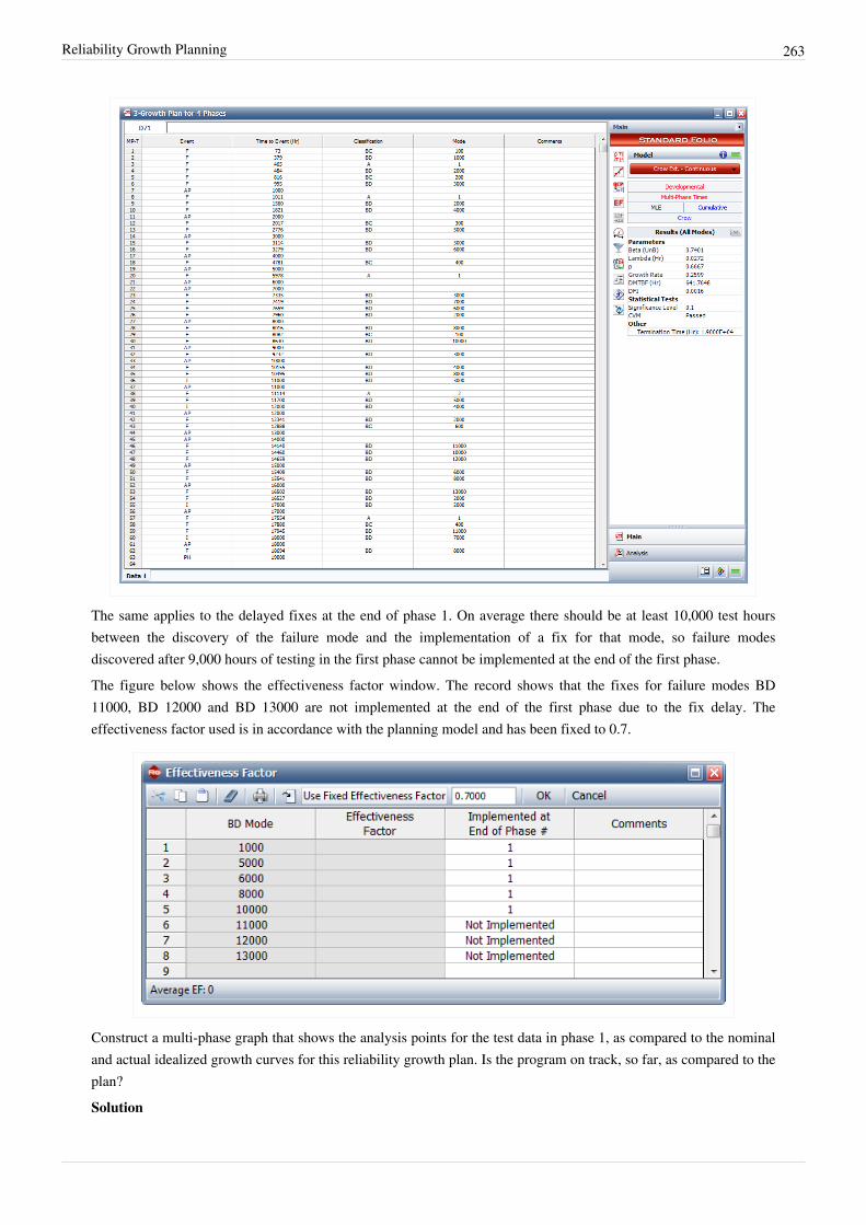
Reliability Growth Planning 263

The same applies to the delayed fixes at the end of phase 1. On average there should be at least 10,000 test hoursbetween the discovery of the failure mode and the implementation of a fix for that mode, so failure modesdiscovered after 9,000 hours of testing in the first phase cannot be implemented at the end of the first phase.The figure below shows the effectiveness factor window. The record shows that the fixes for failure modes BD11000, BD 12000 and BD 13000 are not implemented at the end of the first phase due to the fix delay. Theeffectiveness factor used is in accordance with the planning model and has been fixed to 0.7.

Construct a multi-phase graph that shows the analysis points for the test data in phase 1, as compared to the nominaland actual idealized growth curves for this reliability growth plan. Is the program on track, so far, as compared to theplan?Solution

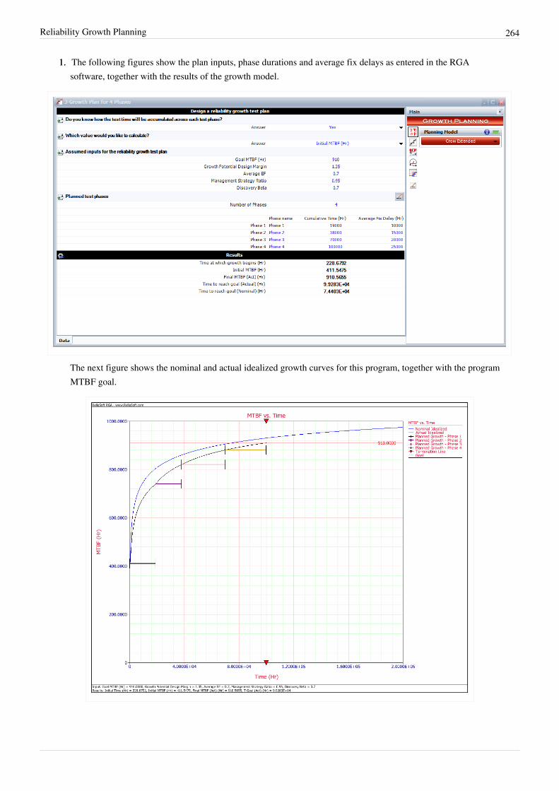
Reliability Growth Planning 264

1.1. The following figures show the plan inputs, phase durations and average fix delays as entered in the RGAsoftware, together with the results of the growth model.

The next figure shows the nominal and actual idealized growth curves for this program, together with the programMTBF goal.

Reliability Growth Planning 265

2. The next step is to associate the reliability growth plan with the data from phase 1. To do that, right-click theAdditional Plots header in the Current Project Explorer and choose Add MultiPhase Plot from the shortcutmenu, then follow the wizard to specify the data sheet that contains the phase 1 data with the folio that defines thegrowth plan. The figure below shows the generated multiphase plot, which brings together the reliability growthplanning model with the actual test results. This plot shows the demonstrated MTBF for each analysis pointduring the first phase of testing. Analysis points for projected and growth potential MTBF can also be plotted. Forthis example, it can be said that the program is on track since the demonstrated MTBF of the first phase is higherthan the planned MTBF for that phase.

The multiphase plot can be updated continuously as the growth program progresses and more test data becomeavailable. In that manner, the reliability team can assess the actual reliability performance against the establishedgoals.

266

Chapter 5

Operational Mission Profile TestingIt is common practice for systems to be subjected to operational testing during a development program. Theobjective of this testing is to evaluate the performance of the system, including reliability, under conditions thatrepresent actual use. Because of budget, resources, schedule and other considerations, these operational tests rarelymatch exactly the actual use conditions. Usually, stated mission profile conditions are used for operational testing.These mission profile conditions are typically general statements that guide testing on an average basis. For example,a copier might be required to print 3,000 pages by time T=10 days and 5,000 pages by time T=15 days. In additionthe copier is required to scan 200 documents by time T=10 days, 250 documents by time T=15 days, etc.Because of practical constraints, these full mission profile conditions are typically not repeated one after the otherduring testing. Instead, the elements that make up the mission profile conditions are tested under varying scheduleswith the intent that, on average, the mission profile conditions are met. In practice, reliability corrective actions aregenerally incorporated into the system as a result of this type of testing.Because of a lack of structure for managing the elements that make up the mission profile, it is difficult to have anagreed upon methodology for estimating the system's reliability. Many systems fail operational testing because keyassessments such as growth potential and projections cannot be made in a straightforward manner so thatmanagement can take appropriate action. The RGA software addresses this issue by incorporating a systematicmission profile methodology for operational reliability testing and reliability growth assessments.

IntroductionOperational testing is an attempt to subject the system to conditions close to the actual environment that is expectedunder customer use. Often this is an extension of reliability growth testing where operation induced failure modesand corrective actions are of prime interest. Sometimes the stated intent is for a demonstration test where correctiveactions are not the prime objective. However, it is not unusual for a system to fail the demonstration test, and themanagement issue is what to do next. In both cases, important and valid key parameters are needed to properlyassess this situation and make cost-effective and timely decisions. This is often difficult in practice.For example, a system may be required to:•• Conduct a specific task a fixed number times for each hour of operation (task 1).•• Move a fixed number of miles under a specific operating condition for each hour of operation (task 2).•• Move a fixed number of miles under another operating condition for each hour of operation (task 3).During operational testing, these guidelines are met individually as averages. For example, the actual as-testedprofile for task 1 may not be uniform relative to the stated mission guidelines during the testing. What is often thecase is that some of the tasks (for example task 1) could be operated below the stated guidelines. This can mask amajor reliability problem. In other cases during testing, tasks 1, 2 and 3 might never meet their stated averages,except perhaps at the end of the test. This becomes an issue because an important aspect of effective reliability riskmanagement is to not wait until the end of the test to have an assessment of the reliability performance.Because the elements of the mission profile during the testing will rarely, if ever, balance continuously to the statedaverages, a common analysis method is to piece the reliability assessments together by evaluating each element ofthe profile separately. This is not a well-defined methodology and does not account for improvement during thetesting. It is therefore not unusual for two separate organizations (e.g., the customer and the developer) to analyze the

Operational Mission Profile Testing 267

same data and obtain different MTBF numbers. In addition, this method does not address the delayed correctiveactions that are to be incorporated at the end of the test nor does it estimate growth potential or interaction effects.Therefore, to reduce this risk there is a need for a rigorous methodology for reliability during operational testing thatdoes not rely on piecewise analysis and avoids the issues noted above.The RGA software incorporates a new methodology to manage system reliability during operational mission profiletesting. This methodology draws information from particular plots of the operational test data and inserts keyinformation into a growth model. The improved methodology does not piece the analysis together, but gives a directMTBF mission profile estimate of the system's reliability that is directly compared to the MTBF requirement. Themethodology will reflect any reliability growth improvement during the test, and will also give management a higherprojected MTBF for the system mission profile reliability after delayed corrected actions are incorporated at the endof the test. In addition, the methodology also gives an estimate of the system's growth potential, and providesmanagement metrics to evaluate whether changes in the program need to be made. A key advantage is that themethodology is well-defined and all organizations will arrive at the same reliability assessment with the same data.

Testing MethodologyThe methodology described here will use the Crow extended model for data analysis. In order to have valid Crowextended model assessments, it is required that the operational mission profile be conducted in a structured manner.Therefore, this testing methodology involves convergence and stopping points during the testing. A stopping point iswhen the testing is stopped for the expressed purpose of incorporating the type BD delayed corrective actions. Theremay be more than one stopping point during a particular testing phase. For simplicity, the methodology with onlyone stopping point will be described; however, the methodology can be extended to the case of more than onestopping point. A convergence point is a time during the test when all the operational mission profile tasks meet theirexpected averages or fall within an acceptable range. At least three convergence points are required for awell-balanced test. The end of the test, time , must be a convergence point. The test times between theconvergence points do not have to be the same.The objective of having the convergence points is to be able to apply the Crow extended model directly in such away that the projection and other key reliability growth parameters can be estimated in a valid fashion. To do this,the grouped data methodology is applied. Note that the methodology can also be used with the Crow-AMSAA(NHPP) model for a simpler analysis without the ability to estimate projected and growth potential reliability. Seethe Grouped Data for the Crow-AMSAA (NHPP) model or for the Crow extended model.

Example - Mission Profile TestingConsider the test-fix-find-test data set that was introduced in the Crow Extended model chapter and is shown againin the table below. The total test time for this test is 400 hours. Note that for this example we assume one stoppingpoint at the end of the test for the incorporation of the delayed fixes. Also, suppose that the data set represents amilitary system with:•• Task 1 = firing a gun.•• Task 2 = moving under environment E1.•• Task 3 = moving under environment E2.For every hour of operation, the operational profile states that the system operates in the E1 environment for 70% ofthe time and in the E2 environment for 30% of the time. In addition, for each hour of operation, the gun must befired 10 times.

Operational Mission Profile Testing 268

Test-Fix-Find-Test Data

Mode Mode

1 0.7 BC17 29 192.7 BD11

2 3.7 BC17 30 213 A

3 13.2 BC17 31 244.8 A

4 15 BD1 32 249 BD12

5 17.6 BC18 33 250.8 A

6 25.3 BD2 34 260.1 BD1

7 47.5 BD3 35 263.5 BD8

8 54 BD4 36 273.1 A

9 54.5 BC19 37 274.7 BD6

10 56.4 BD5 38 282.8 BC27

11 63.6 A 39 285 BD13

12 72.2 BD5 40 304 BD9

13 99.2 BC20 41 315.4 BD4

14 99.6 BD6 42 317.1 A

15 100.3 BD7 43 320.6 A

16 102.5 A 44 324.5 BD12

17 112 BD8 45 324.9 BD10

18 112.2 BC21 46 342 BD5

19 120.9 BD2 47 350.2 BD3

20 121.9 BC22 48 355.2 BC28

21 125.5 BD9 49 364.6 BD10

22 133.4 BD10 50 364.9 A

23 151 BC23 51 366.3 BD2

24 163 BC24 52 373 BD8

25 164.7 BD9 53 379.4 BD14

26 174.5 BC25 54 389 BD15

27 177.4 BD10 55 394.9 A

28 191.6 BC26 56 395.2 BD16

In general, it is difficult to manage an operational test so that these operational profiles are continuously metthroughout the test. However, the operational mission profile methodology requires that these conditions be met onaverage at the convergence points. In practice, this almost always can be done with proper program and testmanagement. The convergence points are set for the testing, often at interim assessment points. The process forcontrolling the convergence at these points involves monitoring a graph for each of the tasks.The following table shows the expected and actual results for each of the operational mission profiles.

Operational Mission Profile Testing 269

Expected and Actual Results for Profiles 1, 2, 3

Profile 1(gun firings) Profile 2(E1) Profile 3(E2)

Time Expected Actual Expected Actual Expected Actual

5 50 0 3.5 5 1.5 0

10 100 0 7 10 3 0

15 150 0 10.5 15 4.5 0

20 200 0 14 20 6 0

25 250 100 17.5 25 7.5 0

30 300 150 21 30 9 0

35 350 400 24.5 30 10.5 5

40 400 600 28 30 12 10

45 450 600 31.5 30 13.5 15

50 500 600 35 30 15 20

55 550 800 38.5 35 16.5 20

60 600 800 42 40 18 20

65 650 800 45.5 45 19.5 20

70 700 800 49 50 21 20

75 750 800 52.5 55 22.5 20

80 800 900 56 55 24 25

85 850 950 59.5 55 25.5 30

90 900 1000 63 60 27 30

95 950 1000 66.5 65 28.5 30

100 1000 1000 70 70 30 30

105 1050 1000 73.5 70 31.5 35

... ... ... ... ... ...

... ... ... ... ... ...

355 3550 3440 248.5 259 106.5 96

360 3600 3690 252 264 108 96

365 3650 3690 255.5 269 109.5 96

370 3700 3850 259 274 111 96

375 3750 3850 262.5 279 112.5 96

380 3800 3850 266 280 114 100

385 3850 3850 269.5 280 115.5 105

390 3900 3850 273 280 117 110

395 3950 4000 276.5 280 118.5 115

400 4000 4000 280 280 120 120

The next figure shows a portion of the expected and actual results for mission profile 1, as entered in the RGAsoftware.

Operational Mission Profile Testing 270

A graph exists for each of the three tasks in this example. Each graph has a line with the expected average as afunction of hours, and the corresponding actual value. When the actual value for a task meets the expected value thenit is a convergence for that task. A convergence point occurs when all of the tasks converge at the same time. At leastthree convergence points are required, one of which is the stopping point . In our example, the total test time is400 hours. The convergence points were chosen to be at 100, 250, 320 and 400 hours. The next figure shows the datasheet that contains the convergence points in the RGA software.

The testing profiles are managed so that at these times the actual operational test profile equals the expected valuesfor the three tasks or falls within an acceptable range. The next graph shows the expected and actual gun firings.

Operational Mission Profile Testing 271

While the next two graphs show the expected and actual time in environments E1 and E2, respectively.

Operational Mission Profile Testing 272

The objective of having the convergence points is to be able to apply the Crow extended model directly in such away that the projection and other key reliability growth parameters can be estimated in a valid fashion. To do this,grouped data is applied using the Crow extended model. For reliability growth assessments using grouped data, onlythe information between time points in the testing is used. In our application, these time points are the convergencepoints 100, 250, 320, and 400. The next figure shows all three mission profiles plotted in the same graph, togetherwith the convergence points.

Operational Mission Profile Testing 273

The following table gives the grouped data input corresponding to the original data set.

Grouped Data at Convergence Points 100, 250, 320 and 400 Hours

Number at Event Time to Event Classification Mode Number at Event Time to Event Classification Mode

3 100 BC 17 1 250 BC 26

1 100 BD 1 1 250 BD 11

1 100 BC 18 1 250 BD 12

1 100 BD 2 3 320 A

1 100 BD 3 1 320 BD 1

1 100 BD 4 1 320 BD 8

1 100 BC 19 1 320 BD 6

2 100 BD 5 1 320 BC 27

1 100 A 1 320 BD 13

1 100 BC 20 1 320 BD 9

1 100 BD 6 1 320 BD 4

1 250 BD 7 3 400 A

3 250 A 1 400 BD 12

1 250 BD 8 2 400 BD 10

1 250 BC 21 1 400 BD 5

1 250 BD 2 1 400 BD 3

1 250 BC 22 1 400 BC 28

Operational Mission Profile Testing 274

2 250 BD 9 1 400 BD 2

2 250 BD 10 1 400 BD 8

1 250 BC 23 1 400 BD 14

1 250 BC 24 1 400 BD 15

1 250 BC 25 1 400 BD 16

The parameters of the Crow extended model for grouped data are then estimated, as explained in the Grouped Datasection of the Crow Extended chapter. The following table shows the effectiveness factors (EFs) for the BD modes.

Effectiveness Factors for Delayed Fixes

Mode Effectiveness Factor

1 0.67

2 0.72

3 0.77

4 0.77

5 0.87

6 0.92

7 0.50

8 0.85

9 0.89

10 0.74

11 0.70

12 0.63

13 0.64

14 0.72

15 0.69

16 0.46

Using the failure times data sheet shown next, we can analyze this data set based on a specified mission profile. Thiswill group the failure times data into groups based on the convergence points that have already been specified whenconstructing the mission profile.

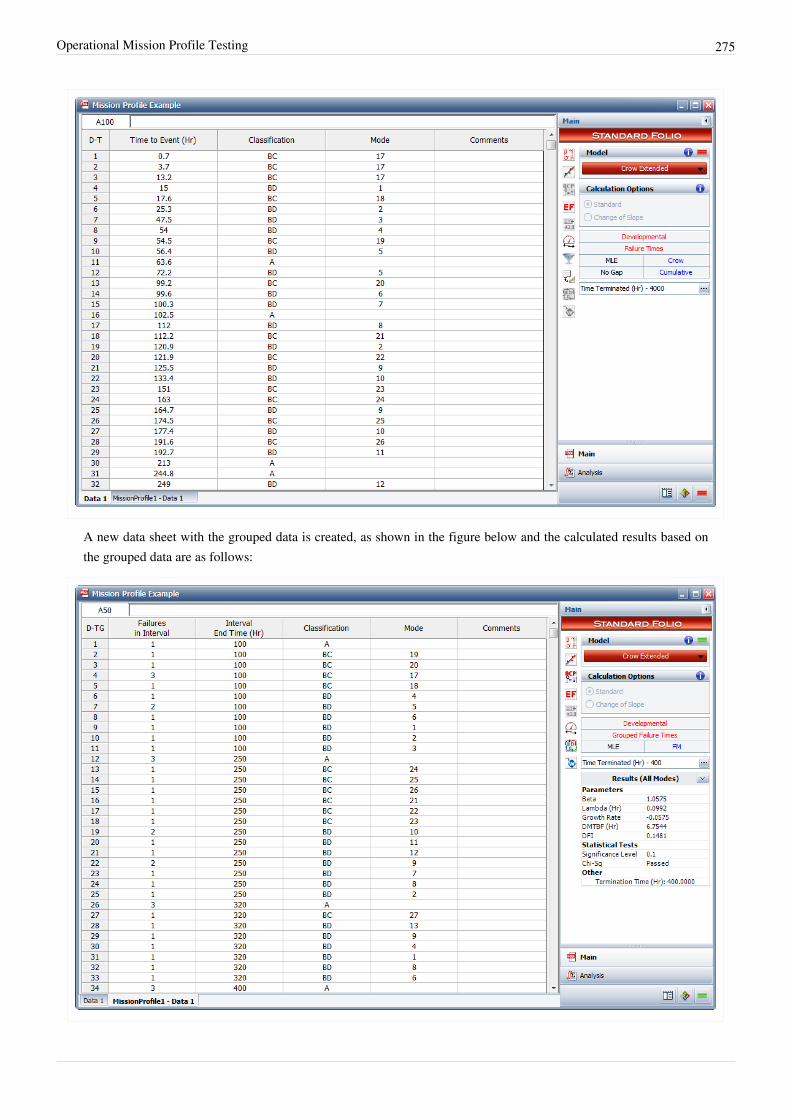
Operational Mission Profile Testing 275

A new data sheet with the grouped data is created, as shown in the figure below and the calculated results based onthe grouped data are as follows:

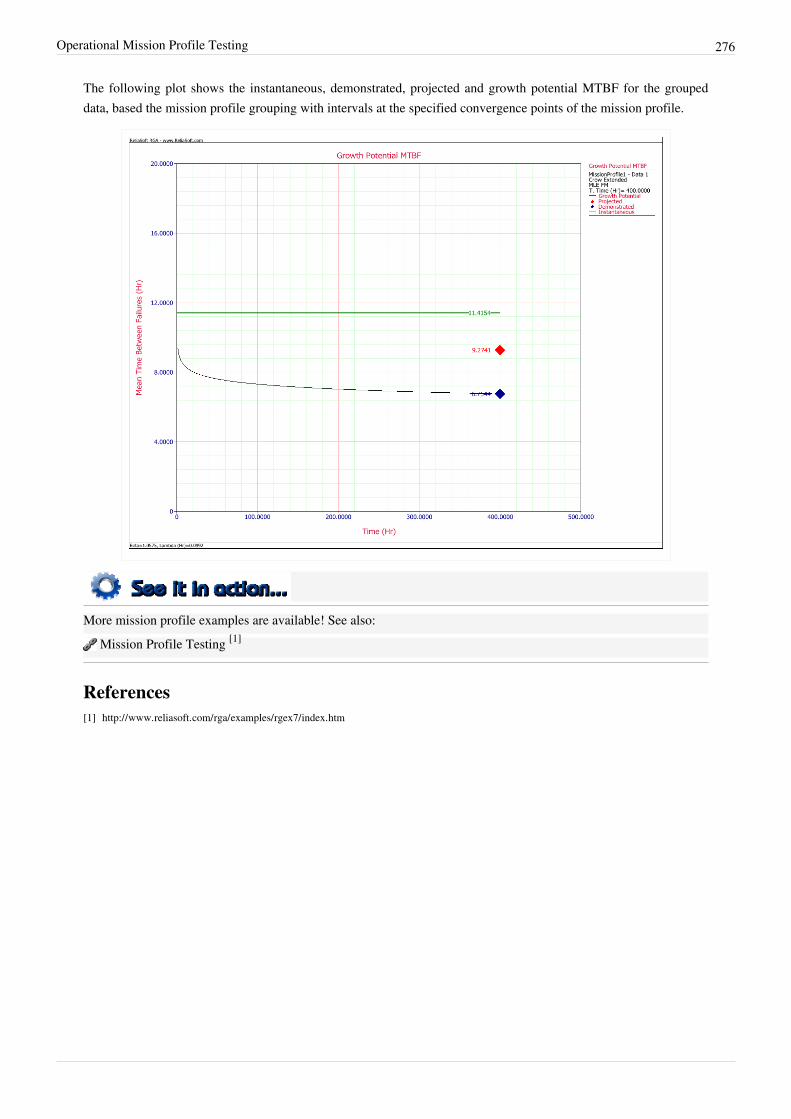
Operational Mission Profile Testing 276

The following plot shows the instantaneous, demonstrated, projected and growth potential MTBF for the groupeddata, based the mission profile grouping with intervals at the specified convergence points of the mission profile.

More mission profile examples are available! See also: Mission Profile Testing [1]

References[1] http:/ / www. reliasoft. com/ rga/ examples/ rgex7/ index. htm

277

Chapter 6

Fielded SystemsWhen a complex system with new technology is fielded and subjected to a customer use environment, there is oftenconsiderable interest in assessing its reliability and other related performance metrics, such as availability. Thisinterest in evaluating the system reliability based on actual customer usage failure data may be motivated by anumber of factors. For example, the reliability that is generally measured during development is typically related tothe system's inherent reliability capability. This inherent capability may differ from actual use experience because ofdifferent operating conditions or environment, different maintenance policies, different levels of experience ofmaintenance personnel, etc. Although operational tests are conducted for many systems during development, it isgenerally recognized that in many cases these tests may not yield complete data representative of an actual useenvironment. Moreover, the testing during development is typically limited by the usual cost and scheduleconstraints, which prevent obtaining a system's reliability profile over an extended portion of its life. Other interestsin measuring the reliability of a fielded system may center on, for example, logistics and maintenance policies,quality and manufacturing issues, burn-in, wearout, mission reliability or warranties.Most complex systems are repaired, not replaced, when they fail. For example, a complex communication system ora truck would be repaired upon failure, not thrown away and replaced by a new system. A number of books andpapers in literature have stressed that the usual non-repairable reliability analysis methodologies, such as the Weibulldistribution, are not appropriate for repairable system reliability analyses and have suggested the use ofnon-homogeneous Poisson process models instead.The homogeneous process is equivalent to the widely used Poisson distribution, and exponential times betweensystem failures can be modeled appropriately when the system's failure intensity is not affected by the system's age.However, to realistically consider burn-in, wearout, useful life, maintenance policies, warranties, mission reliability,etc., the analyst will often require an approach that recognizes that the failure intensity of these systems may not beconstant over the operating life of interest but may change with system age. A useful, and generally practical,extension of the homogeneous Poisson process, is the non-homogeneous Poisson process, which allows for thesystem failure intensity to change with system age. Typically, the reliability analysis of a repairable system undercustomer use will involve data generated by multiple systems. Crow [17] proposed the Weibull process or power lawnon-homogeneous Poisson process for this type of analysis, and developed appropriate statistical procedures formaximum likelihood estimation, goodness-of-fit and confidence bounds.

Applicable AnalysesThe following chapters contain additional information on each of the analyses that can be used with data fromfielded systems:•• Repairable Systems Analysis•• Operational Testing•• Fleet Data Analysis

278

Chapter 6.1

Repairable Systems AnalysisData from systems in the field can be analyzed in the RGA software. This type of data is called fielded systems dataand is analogous to warranty data. Fielded systems can be categorized into two basic types: one-time ornon-repairable systems, and reusable or repairable systems. In the latter case, under continuous operation, the systemis repaired, but not replaced after each failure. For example, if a water pump in a vehicle fails, the water pump isreplaced and the vehicle is repaired.This chapter presents repairable systems analysis, where the reliability of a system can be tracked and quantifiedbased on data from multiple systems in the field. The next chapter will present fleet analysis, where data frommultiple systems in the field can be collected and analyzed so that reliability metrics for the fleet as a whole can bequantified.

BackgroundMost complex systems, such as automobiles, communication systems, aircraft, printers, medical diagnostics systems,helicopters, etc., are repaired and not replaced when they fail. When these systems are fielded or subjected to acustomer use environment, it is often of considerable interest to determine the reliability and other performancecharacteristics under these conditions. Areas of interest may include assessing the expected number of failuresduring the warranty period, maintaining a minimum mission reliability, evaluating the rate of wearout, determiningwhen to replace or overhaul a system and minimizing life cycle costs. In general, a lifetime distribution, such as theWeibull distribution, cannot be used to address these issues. In order to address the reliability characteristics ofcomplex repairable systems, a process is often used instead of a distribution. The most popular process model is thePower Law model. This model is popular for several reasons. One is that it has a very practical foundation in termsof minimal repair, which is a situation where the repair of a failed system is just enough to get the system operationalagain. Second, if the time to first failure follows the Weibull distribution, then each succeeding failure is governedby the Power Law model as in the case of minimal repair. From this point of view, the Power Law model is anextension of the Weibull distribution.Sometimes, the Crow Extended model, which was introduced in a previous chapter for analyzing developmentaldata, is also applied for fielded repairable systems. Applying the Crow Extended model on repairable system dataallows analysts to project the system MTBF after reliability-related issues are addressed during the field operation.Projections are calculated based on the mode classifications (A, BC and BD). The calculation procedure is the sameas the one for the developmental data, and is not repeated in this chapter.

Distribution ExampleVisualize a socket into which a component is inserted at time 0. When the component fails, it is replacedimmediately with a new one of the same kind. After each replacement, the socket is put back into an as good as newcondition. Each component has a time-to-failure that is determined by the underlying distribution. It is important tonote that a distribution relates to a single failure. The sequence of failures for the socket constitutes a random processcalled a renewal process. In the illustration below, the component life is , and is the system time to the failure.

Repairable Systems Analysis 279

Each component life in the socket is governed by the same distribution .A distribution, such as Weibull, governs a single lifetime. There is only one event associated with a distribution. Thedistribution is the probability that the life of the component in the socket is less than . In the illustrationabove, is the life of the first component in the socket. is the probability that the first component in thesocket fails in time . When the first component fails, it is replaced in the socket with a new component of the sametype. The probability that the life of the second component is less than is given by the same distribution function,

. For the Weibull distribution:

A distribution is also characterized by its density function, such that:

The density function for the Weibull distribution is:

In addition, an important reliability property of a distribution function is the failure rate, which is given by:

The interpretation of the failure rate is that for a small interval of time , is approximately theprobability that a component in the socket will fail between time and time , given that the component hasnot failed by time . For the Weibull distribution, the failure rate is given by:

It is important to note the condition that the component has not failed by time . Again, a distribution deals with onelifetime of a component and does not allow for more than one failure. The socket has many failures and each failuretime is individually governed by the same distribution. In other words, the failure times are independent of eachother. If the failure rate is increasing, then this is indicative of component wearout. If the failure rate is decreasing,then this is indicative of infant mortality. If the failure rate is constant, then the component failures follow anexponential distribution. For the Weibull distribution, the failure rate is increasing for , decreasing for and constant for . Each time a component in the socket is replaced, the failure rate of the new componentgoes back to the value at time 0. This means that the socket is as good as new after each failure and each subsequentreplacement by a new component. This process is continued for the operation of the socket.

Process ExampleNow suppose that a system consists of many components with each component in a socket. A failure in any socketconstitutes a failure of the system. Each component in a socket is a renewal process governed by its respectivedistribution function. When the system fails due to a failure in a socket, the component is replaced and the socket isagain as good as new. The system has been repaired. Because there are many other components still operating withvarious ages, the system is not typically put back into a like new condition after the replacement of a singlecomponent. For example, a car is not as good as new after the replacement of a failed water pump. Therefore,distribution theory does not apply to the failures of a complex system, such as a car. In general, the intervals between

Repairable Systems Analysis 280

failures for a complex repairable system do not follow the same distribution. Distributions apply to the componentsthat are replaced in the sockets, but not at the system level. At the system level, a distribution applies to the very firstfailure. There is one failure associated with a distribution. For example, the very first system failure may follow aWeibull distribution.For many systems in a real world environment, a repair may only be enough to get the system operational again. Ifthe water pump fails on the car, the repair consists only of installing a new water pump. Similarly, if a seal leaks, theseal is replaced but no additional maintenance is done. This is the concept of minimal repair. For a system withmany failure modes, the repair of a single failure mode does not greatly improve the system reliability from what itwas just before the failure. Under minimal repair for a complex system with many failure modes, the systemreliability after a repair is the same as it was just before the failure. In this case, the sequence of failures at the systemlevel follows a non-homogeneous Poisson process (NHPP).The system age when the system is first put into service is time 0. Under the NHPP, the first failure is governed by adistribution with failure rate . Each succeeding failure is governed by the intensity function of theprocess. Let be the age of the system and is very small. The probability that a system of age fails between and is given by the intensity function . Notice that this probability is not conditioned on not havingany system failures up to time , as is the case for a failure rate. The failure intensity for the NHPP has thesame functional form as the failure rate governing the first system failure. Therefore, , where isthe failure rate for the distribution function of the first system failure. If the first system failure follows the Weibulldistribution, the failure rate is:

Under minimal repair, the system intensity function is:

This is the Power Law model. It can be viewed as an extension of the Weibull distribution. The Weibull distributiongoverns the first system failure, and the Power Law model governs each succeeding system failure. If the system hasa constant failure intensity , then the intervals between system failures follow an exponential distributionwith failure rate . If the system operates for time , then the random number of failures over 0 to isgiven by the Power Law mean value function.

Therefore, the probability is given by the Poisson probability.

This is referred to as a homogeneous Poisson process because there is no change in the intensity function. This is aspecial case of the Power Law model for . The Power Law model is a generalization of the homogeneousPoisson process and allows for change in the intensity function as the repairable system ages. For the Power Lawmodel, the failure intensity is increasing for (wearout), decreasing for (infant mortality) and constantfor (useful life).

Power Law ModelThe Power Law model is often used to analyze the reliability of complex repairable systems in the field. The systemof interest may be the total system, such as a helicopter, or it may be subsystems, such as the helicopter transmissionor rotator blades. When these systems are new and first put into operation, the start time is 0. As these systems areoperated, they accumulate age (e.g., miles on automobiles, number of pages on copiers, flights of helicopters). Whenthese systems fail, they are repaired and put back into service.Some system types may be overhauled and some may not, depending on the maintenance policy. For example, anautomobile may not be overhauled but helicopter transmissions may be overhauled after a period of time. In practice,

Repairable Systems Analysis 281

an overhaul may not convert the system reliability back to where it was when the system was new. However, anoverhaul will generally make the system more reliable. Appropriate data for the Power Law model is over cycles. Ifa system is not overhauled, then there is only one cycle and the zero time is when the system is first put intooperation. If a system is overhauled, then the same serial number system may generate many cycles. Each cycle willstart a new zero time, the beginning of the cycle. The age of the system is from the beginning of the cycle. Forsystems that are not overhauled, there is only one cycle and the reliability characteristics of a system as the systemages during its life is of interest. For systems that are overhauled, you are interested in the reliability characteristicsof the system as it ages during its cycle.

For the Power Law model, a data set for a system will consist of a starting time , an ending time and theaccumulated ages of the system during the cycle when it had failures. Assume that the data exists from the beginningof a cycle (i.e., the starting time is 0), although non-zero starting times are possible with the Power Law model. Forexample, suppose data has been collected for a system with 2,000 hours of operation during a cycle. The startingtime is and the ending time is . Over this period, failures occurred at system ages of 50.6, 840.7,1060.5, 1186.5, 1613.6 and 1843.4 hours. These are the accumulated operating times within the cycle, and therewere no failures between 1843.4 and 2000 hours. It may be of interest to determine how the systems perform as partof a fleet. For a fleet, it must be verified that the systems have the same configuration, same maintenance policy andsame operational environment. In this case, a random sample must be gathered from the fleet. Each item in thesample will have a cycle starting time , an ending time for the data period and the accumulated operatingtimes during this period when the system failed.There are many ways to generate a random sample of systems. One way is to generate random serial numbersfrom the fleet. Then go to the records corresponding to the randomly selected systems. If the systems are notoverhauled, then record when each system was first put into service. For example, the system may have been put intoservice when the odometer mileage equaled zero. Each system may have a different amount of total usage, so theending times, , may be different. If the systems are overhauled, then the records for the last completed cycle willbe needed. The starting and ending times and the accumulated times to failure for the systems constitute therandom sample from the fleet. There is a useful and efficient method for generating a random sample for systemsthat are overhauled. If the overhauled systems have been in service for a considerable period of time, then each serialnumber system in the fleet would go through many overhaul cycles. In this case, the systems coming in for overhaulactually represent a random sample from the fleet. As systems come in for overhaul, the data for the currentcompleted cycles would be a random sample of size .In addition, the warranty period may be of particular interest. In this case, randomly choose serial numbers forsystems that have been in customer use for a period longer than the warranty period. Then check the warrantyrecords. For each of the systems that had warranty work, the ages corresponding to this service are the failuretimes. If a system did not have warranty work, then the number of failures recorded for that system is zero. Thestarting times are all equal to zero and the ending time for each of the systems is equal to the warranty operatingusage time (e.g., hours, copies, miles).

In addition to the intensity function and the mean value function, which were given in the section above, otherrelationships based on the Power Law are often of practical interest. For example, the probability that the system willsurvive to age without failure is given by:

This is the mission reliability for a system of age and mission length .

Repairable Systems Analysis 282

Parameter Estimation

Suppose that the number of systems under study is and the system is observed continuously from time totime , . During the period , let be the number of failures experienced by the system and let be the age of this system at the occurrence of failure, . It is also possiblethat the times and may be the observed failure times for the system. If , then the data on the

system is said to be failure terminated, and is a random variable with fixed. If , then thedata on the system is said to be time terminated with a random variable. The maximum likelihood estimatesof and are values satisfying the equations shown next.

where is defined to be 0. In general, these equations cannot be solved explicitly for and but must besolved by iterative procedures. Once and have been estimated, the maximum likelihood estimate of the intensityfunction is given by:

If and then the maximum likelihoodestimates and are in closed form.

The following example illustrates these estimation procedures.

Power Law Model ExampleFor the data in the following table, the starting time for each system is equal to 0 and the ending time for each systemis 2,000 hours. Calculate the maximum likelihood estimates and .

Repairable Systems Analysis 283

Repairable System Failure Data

System 1 ( ) System 2 ( ) System 3 ( )

1.2 1.4 0.3

55.6 35.0 32.6

72.7 46.8 33.4

111.9 65.9 241.7

121.9 181.1 396.2

303.6 712.6 444.4

326.9 1005.7 480.8

1568.4 1029.9 588.9

1913.5 1675.7 1043.9

1787.5 1136.1

1867.0 1288.1

1408.1

1439.4

1604.8

Solution

Because the starting time for each system is equal to zero and each system has an equivalent ending time, the generalequations for and reduce to the closed form equations. The maximum likelihood estimates of and are thencalculated as follows:

The system failure intensity function is then estimated by:

The next figure is a plot of over the period (0, 3000). Clearly, the estimated failure intensity function is mostrepresentative over the range of the data and any extrapolation should be viewed with the usual caution.

Repairable Systems Analysis 284

Goodness-of-Fit Tests for Repairable System AnalysisIt is generally desirable to test the compatibility of a model and data by a statistical goodness-of-fit test. A parametricCramér-von Mises goodness-of-fit test is used for the multiple system and repairable system Power Law model, asproposed by Crow in [17]. This goodness-of-fit test is appropriate whenever the start time for each system is 0 andthe failure data is complete over the continuous interval with no gaps in the data. The Chi-Squared test is agoodness-of-fit test that can be applied under more general circumstances. In addition, the Common Beta Hypothesistest also can be used to compare the intensity functions of the individual systems by comparing the values of eachsystem. Lastly, the Laplace Trend test checks for trends within the data. Due to their general application, theCommon Beta Hypothesis test and the Laplace Trend test are both presented in Appendix B. The Cramér-von Misesand Chi-Squared goodness-of-fit tests are illustrated next.

Cramér-von Mises Test

To illustrate the application of the Cramér-von Mises statistic for multiple systems data, suppose that like systemsare under study and you wish to test the hypothesis that their failure times follow a non-homogeneous Poissonprocess. Suppose information is available for the system over the interval , with successive failure times ,

. The Cramér-von Mises test can be performed with the following steps:

Step 1: If (failure terminated), let , and if (time terminated), let . Then:

Step 2: For each system, divide each successive failure time by the corresponding end time , Calculate the values:

Repairable Systems Analysis 285

Step 3: Next calculate , the unbiased estimate of , from:

Step 4: Treat the values as one group, and order them from smallest to largest. Name these ordered values, such that .

Step 5: Calculate the parametric Cramér-von Mises statistic.

Critical values for the Cramér-von Mises test are presented in the Crow-AMSAA (NHPP) page.

Step 6: If the calculated is less than the critical value, then accept the hypothesis that the failure times for the systems follow the non-homogeneous Poisson process with intensity function .

Chi-Squared Test

The parametric Cramér-von Mises test described above requires that the starting time, , be equal to 0 for each ofthe systems. Although not as powerful as the Cramér-von Mises test, the chi-squared test can be appliedregardless of the starting times. The expected number of failures for a system over its age for the chi-squaredtest is estimated by , where and are the maximum likelihood estimates.

The computed statistic is:

where is the total number of intervals. The random variable is approximately chi-square distributed withdegrees of freedom. There must be at least three intervals and the length of the intervals do not have to

be equal. It is common practice to require that the expected number of failures for each interval, , be at leastfive. If or if , reject the null hypothesis.

Cramér-von Mises ExampleFor the data from power law model example given above, use the Cramér-von Mises test to examine thecompatibility of the model at a significance level Solution

Step 1:

Step 2: Calculate treat the values as one group and order them from smallest to largest. Name these orderedvalues .Step 3: Calculate:

Repairable Systems Analysis 286

Step 4: Calculate:

Step 5: From the table of critical values for the Cramér-von Mises test, find the critical value (CV) for at asignificance level . .

Step 6: Since , accept the hypothesis that the failure times for the repairable systems follow thenon-homogeneous Poisson process with intensity function .

Confidence Bounds for Repairable Systems AnalysisThe RGA software provides two methods to estimate the confidence bounds for repairable systems analysis. TheFisher matrix approach is based on the Fisher information matrix and is commonly employed in the reliability field.The Crow bounds were developed by Dr. Larry Crow. See Confidence Bounds for Repairable Systems Analysis fordetails on how these confidence bounds are calculated.

Confidence Bounds Example

Using the data from the power law model example given above, calculate the mission reliability at hoursand mission time hours along with the confidence bounds at the 90% confidence level.Solution

The maximum likelihood estimates of and from the example are:

The mission reliability at for mission time is:

At the 90% confidence level and hours, the Fisher matrix confidence bounds for the mission reliabilityfor mission time are given by:

The Crow confidence bounds for the mission reliability are:

Repairable Systems Analysis 287

The next two figures show the Fisher matrix and Crow confidence bounds on mission reliability for mission time.

Repairable Systems Analysis 288

Economical Life ModelOne consideration in reducing the cost to maintain repairable systems is to establish an overhaul policy that willminimize the total life cost of the system. However, an overhaul policy makes sense only if . It does notmake sense to implement an overhaul policy if since wearout is not present. If you assume that there is apoint at which it is cheaper to overhaul a system than to continue repairs, what is the overhaul time that willminimize the total life cycle cost while considering repair cost and the cost of overhaul?

Denote as the average repair cost (unscheduled), as the replacement or overhaul cost and as the averagecost of scheduled maintenance. Scheduled maintenance is performed for every miles or time interval. In addition,let be the number of failures in , and let be the number of replacements in . Suppose thatreplacement or overhaul occurs at times , , and . The problem is to select the optimum overhaul time

so as to minimize the long term average system cost (unscheduled maintenance, replacement cost andscheduled maintenance). Since , the average system cost is minimized when the system is overhauled (orreplaced) at time such that the instantaneous maintenance cost equals the average system cost. The total systemcost between overhaul or replacement is:

So the average system cost is:

The instantaneous maintenance cost at time is equal to:

The following equation holds at optimum overhaul time :

Therefore:

But when there is no scheduled maintenance, the equation becomes:

and the equation for the optimum overhaul time, , is the same as in the previous case. Therefore, for periodicmaintenance scheduled every miles, the replacement or overhaul time is the same as for the unscheduled andreplacement or overhaul cost model.

More Examples

Automatic Transmission Data ExampleThis case study is based on the data given in the article "Graphical Analysis of Repair Data" by Dr. Wayne Nelson [23]. The following table contains repair data on an automatic transmission from a sample of 34 cars. For each car, the data set shows mileage at the time of each transmission repair, along with the latest mileage. The + indicates the latest mileage observed without failure. Car 1, for example, had a repair at 7068 miles and was observed until 26,744

Repairable Systems Analysis 289

miles. Do the following:1.1. Estimate the parameters of the Power Law model.2.2. Estimate the number of warranty claims for a 36,000 mile warranty policy for an estimated fleet of 35,000

vehicles.

Automatic Transmission Data

Car Mileage Car Mileage

1 7068, 26744+ 18 17955+

2 28, 13809+ 19 19507+

3 48, 1440, 29834+ 20 24177+

4 530, 25660+ 21 22854+

5 21762+ 22 17844+

6 14235+ 23 22637+

7 1388, 18228+ 24 375, 19607+

8 21401+ 25 19403+

9 21876+ 26 20997+

10 5094, 18228+ 27 19175+

11 21691+ 28 20425+

12 20890+ 29 22149+

13 22486+ 30 21144+

14 19321+ 31 21237+

15 21585+ 32 14281+

16 18676+ 33 8250, 21974+

17 23520+ 34 19250, 21888+

Solution

1.1. The estimated Power Law parameters are shown next.

Repairable Systems Analysis 290

2.2. The expected number of failures at 36,000 miles can be estimated using the QCP as shown next. The modelpredicts that 0.3559 failures per system will occur by 36,000 miles. This means that for a fleet of 35,000 vehicles,the expected warranty claims are 0.3559 * 35,000 = 12,456.

Repairable Systems Analysis 291

Optimum Overhaul ExampleField data have been collected for a system that begins its wearout phase at time zero. The start time for each systemis equal to zero and the end time for each system is 10,000 miles. Each system is scheduled to undergo an overhaulafter a certain number of miles. It has been determined that the cost of an overhaul is four times more expensive thana repair. The table below presents the data. Do the following:1.1. Estimate the parameters of the Power Law model.2.2. Determine the optimum overhaul interval.3. If , would it be cost-effective to implement an overhaul policy?

Field Data

System 1 System 2 System 3

1006.3 722.7 619.1

2261.2 1950.9 1519.1

2367 3259.6 2956.6

2615.5 4733.9 3114.8

2848.1 5105.1 3657.9

4073 5624.1 4268.9

5708.1 5806.3 6690.2

6464.1 5855.6 6803.1

6519.7 6325.2 7323.9

6799.1 6999.4 7501.4

Repairable Systems Analysis 292

7342.9 7084.4 7641.2

7736 7105.9 7851.6

8246.1 7290.9 8147.6

7614.2 8221.9

8332.1 9560.5

8368.5 9575.4

8947.9

9012.3

9135.9

9147.5

9601

Solution

1.1. The next figure shows the estimated Power Law parameters.

2.2. The QCP can be used to calculate the optimum overhaul interval, as shown next.

Repairable Systems Analysis 293

3. Since the systems are wearing out and it would be cost-effective to implement an overhaul policy. Anoverhaul policy makes sense only if the systems are wearing out.

Crow Extended for Repairable Systems Analysis ExampleThe failures and fixes of two repairable systems in the field are recorded. Both systems started operating from time0. System 1 ends at time = 504 and system 2 ends at time = 541. All the BD modes are fixed at the end of the test. Afixed effectiveness factor equal to 0.6 is used. Answer the following questions:1.1. Estimate the parameters of the Crow Extended model.2.2. Calculate the projected MTBF after the delayed fixes.3.3. If no fixes were performed for the future failures, what would be the expected number of failures at time 1,000?Solution

1.1. The next figure shows the estimated Crow Extended parameters.

Repairable Systems Analysis 294

2.2. The next figure shows the projected MTBF at time = 541 (i.e., the age of the oldest system).

Repairable Systems Analysis 295

3.3. The next figure shows the expected number of failures at time = 1,000.

296

Chapter 6.2

Operational Testing

BackgroundOperational testing is basically repairable systems analysis using the Crow Extended model. The generalassumptions associated with the Crow Extended model do not change. However, in operational testing, thecalculations are conducted with the assumption that . Therefore, only delayed fixes, BD modes(test-find-test), are allowed. BC modes and fixes during the test cannot be entered. In this scenario, you want a stablesystem such that the estimate of is close to one. The assumption can be verified by checking theconfidence bounds on . If the confidence bounds include one, then you can fail to reject the hypothesis that .Under operational testing:•• The final product has been fielded, why is why this is not developmental testing.•• Only delayed fixes (BD modes) are allowed.•• The configuration is fixed and design changes are kept to a minimum.•• The focus is on age-dependent reliability.•• Testing is generally conducted prior to full production.Operational testing analysis could also be applied to a system that is already in production and being used bycustomers in the field. In this case, you will be able to verify the improvement in the system's MTBF based on thespecified delayed fixes. Based on this information, along with the cost and time to implement, you can determine if itis cost-effective to apply the fixes to the fielded systems.

Example - Operational TestingConsider two systems that have been placed into operational testing. The data for each system are given below. Dothe following:

1. After estimating the parameters, verify the assumption of .2.2. Estimate the instantaneous MTBF of the system at the end of the test (demonstrated MTBF).3.3. Estimate the MTBF that can be expected after the BD failure modes are addressed (projected MTBF) and the

maximum MTBF that can be achieved if all BD modes that exist in the system were discovered and fixedaccording to the current maintenance strategy (growth potential MTBF).

Operational Testing 297

Operational Testing Data

System # 1 2

Start Time (Hr) 0 0

End Time (Hr) 504 541

Failure Times (Hr)andFailure Modes

21 BD43 83 BD37

29 A42 83 BD43

43 BD10 83 BD46

43 BD11 169 A45

43 A39 213 A18

66 A20 299 A42

115 BD34 375 A1

159 BD49 431 BD16

199 BD47

202 BD47

222 BD47

248 BD14

248 BD15

255 BD41

286 BD40

286 BD48

304 BD47

320 BD13

348 BD11

364 BD44

404 BD44

410 BD4

429 BD47

The BD modes are implemented at the end of the test and assume a fixed effectiveness factor equal to 0.6 (i.e., 40%of the failure intensity will remain after the fixes are implemented).Solution

1.1. The entered operational testing data and the estimated parameters are given below.

Operational Testing 298

The assumption of can be verified by looking at the confidence bounds on via the Quick CalculationPad (QCP). The 90% 2-sided Crow confidence bounds on are shown next.

Since the confidence bounds on include one, then you can fail to reject the hypothesis that .2.2. From #1, the demonstrated MTBF (DMTBF) equals 33.7097 hours.3.3. The projected MTBF and growth potential values can be displayed via the Growth Potential MTBF plot.

Operational Testing 299

The plot shows that the projected MTBF equals 42.3824 hours, and the growth potential MTBF equals 62.9518hours.

300

Chapter 6.3

Fleet Data AnalysisFleet analysis is similar to the repairable systems analysis described in the previous chapter. The main difference isthat a fleet of systems is considered and the models are applied to the fleet failures rather than to the system failures.In other words, repairable system analysis models the number of system failures versus system time, whereas fleetanalysis models the number of fleet failures versus fleet time.The main motivation for fleet analysis is to enable the application of the Crow Extended model for fielded data. Inmany cases, reliability improvements might be necessary on systems that are already in the field. These types ofreliability improvements are essentially delayed fixes (BD modes) as described in the Crow Extended chapter.

IntroductionRecall from the previous chapter that in order to make projections using the Crow Extended model, the of thecombined A and BD modes should be equal to 1. Since the failure intensity in a fielded system might be changingover time (e.g., increasing if the system wears out), this assumption might be violated. In such a scenario, the CrowExtended model cannot be used. However, if a fleet of systems is considered and the number of fleet failures versusfleet time is modeled, the failures might become random. This is because there is a mixture of systems within a fleet,new and old, and when the failures of this mixture of systems are viewed from a cumulative fleet time point of view,they may be random. The next two figures illustrate this concept. The first picture shows the number of failures oversystem age. It can be clearly seen that as the systems age, the intensity of the failures increases (wearout). Thesuperposition system line, which brings the failures from the different systems under a single timeline, alsoillustrates this observation. On the other hand, if you take the same four systems and combine their failures from afleet perspective, and consider fleet failures over cumulative fleet hours, then the failures seem to be random. Thesecond picture illustrates this concept in the System Operation plot when you consider the Cum. Time Line. In thiscase, the of the fleet will be equal to 1 and the Crow Extended model can be used for quantifying the effects offuture reliability improvements on the fleet.

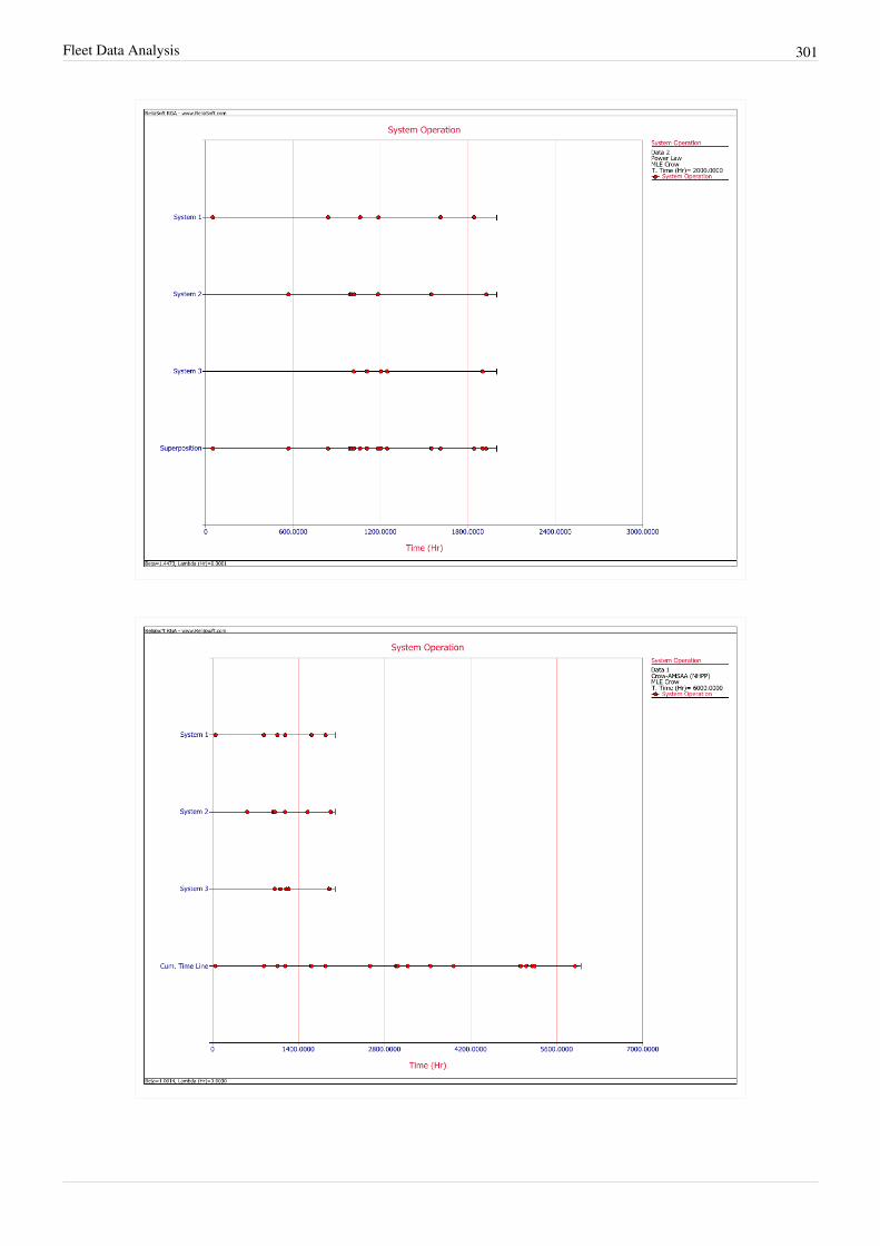
Fleet Data Analysis 301

Fleet Data Analysis 302

MethodologyThe figures above illustrate that the difference between repairable system data analysis and fleet analysis is the waythat the data set is treated. In fleet analysis, the time-to-failure data from each system is stacked to a cumulativetimeline. For example, consider the two systems in the following table.

System Data

System Failure Times (hr) End Time (hr)

1 3, 7 10

2 4, 9, 13 15

Convert to Accumulated TimelineThe data set is first converted to an accumulated timeline, as follows:•• System 1 is considered first. The accumulated timeline is therefore 3 and 7 hours.•• System 1's end time is 10 hours. System 2's first failure is at 4 hours. This failure time is added to System 1's end

time to give an accumulated failure time of 14 hours.•• The second failure for System 2 occurred 5 hours after the first failure. This time interval is added to the

accumulated timeline to give 19 hours.•• The third failure for System 2 occurred 4 hours after the second failure. The accumulated failure time is 19 + 4 =

23 hours.•• System 2's end time is 15 hours, or 2 hours after the last failure. The total accumulated operating time for the fleet

is 25 hours (23 + 2 = 25).

In general, the accumulated operating time is calculated by:

where:

• is the failure of the system• is the end time of the system• is the total number of systems

• is the total number of failures from all systems ( )

As this example demonstrates, the accumulated timeline is determined based on the order of the systems. So if youconsider the data in the table by taking System 2 first, the accumulated timeline would be: 4, 9, 13, 18, 22, with anend time of 25. Therefore, the order in which the systems are considered is somewhat important. However, in thenext step of the analysis, the data from the accumulated timeline will be grouped into time intervals, effectivelyeliminating the importance of the order of the systems. Keep in mind that this will NOT always be true. This is trueonly when the order of the systems was random to begin with. If there is some logic/pattern in the order of thesystems, then it will remain even if the cumulative timeline is converted to grouped data. For example, consider asystem that wears out with age. This means that more failures will be observed as this system ages and these failureswill occur more frequently. Within a fleet of such systems, there will be new and old systems in operation. If the dataset collected is considered from the newest to the oldest system, then even if the data points are grouped, the patternof fewer failures at the beginning and more failures at later time intervals will still be present. If the objective of theanalysis is to determine the difference between newer and older systems, then that order for the data will beacceptable. However, if the objective of the analysis is to determine the reliability of the fleet, then the systemsshould be randomly ordered.

Fleet Data Analysis 303

Analyze the Grouped DataOnce the accumulated timeline has been generated, it is then converted into grouped data. To accomplish this, agroup interval is required. The group interval length should be chosen so that it is representative of the data. Alsonote that the intervals do not have to be of equal length. Once the data points have been grouped, the parameters canbe obtained using maximum likelihood estimation as described in the Crow-AMSAA (NHPP) chapter. The datafrom the table above can be grouped into 5 hour intervals. This interval length is sufficiently large to insure that thereare failures within each interval. The grouped data set is given in the following table.

Grouped Data

Failures in Interval Interval End Time

1 5

1 10

1 15

1 20

1 25

The Crow-AMSAA model for grouped failure times is used for the data, and the parameters of the model are solvedby satisfying the following maximum likelihood equations (See Crow-AMSAA (NHPP)):

Fleet Analysis ExampleThe following table presents data for a fleet of 27 systems. A cycle is a complete history from overhaul to overhaul.The failure history for the last completed cycle for each system is recorded. This is a random sample of data from thefleet. These systems are in the order in which they were selected. Suppose the intervals to group the current data are10,000; 20,000; 30,000; 40,000 and the final interval is defined by the termination time. Conduct the fleet analysis.

Sample Fleet Data

System Cycle Time Number of failures Failure Time

1 1396 1 1396

2 4497 1 4497

3 525 1 525

4 1232 1 1232

5 227 1 227

6 135 1 135

7 19 1 19

8 812 1 812

9 2024 1 2024

10 943 2 316, 943

11 60 1 60

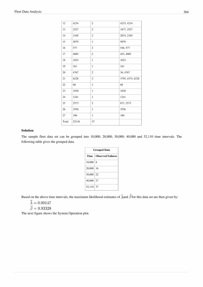
Fleet Data Analysis 304

12 4234 2 4233, 4234

13 2527 2 1877, 2527

14 2105 2 2074, 2105

15 5079 1 5079

16 577 2 546, 577

17 4085 2 453, 4085

18 1023 1 1023

19 161 1 161

20 4767 2 36, 4767

21 6228 3 3795, 4375, 6228

22 68 1 68

23 1830 1 1830

24 1241 1 1241

25 2573 2 871, 2573

26 3556 1 3556

27 186 1 186

Total 52110 37

Solution

The sample fleet data set can be grouped into 10,000; 20,000; 30,000; 40,000 and 52,110 time intervals. Thefollowing table gives the grouped data.

Grouped Data

Time Observed Failures

10,000 8

20,000 16

30,000 22

40,000 27

52,110 37

Based on the above time intervals, the maximum likelihood estimates of and for this data set are then given by:

The next figure shows the System Operation plot.

Fleet Data Analysis 305

Applying the Crow Extended Model to Fleet DataAs it was mentioned previously, the main motivation of the fleet analysis is to apply the Crow Extended model forin-service reliability improvements. The methodology to be used is identical to the application of the Crow Extendedmodel for Grouped Data described in a previous chapter. Consider the fleet data from the example above. In order toapply the Crow Extended model, put failure times on a cumulative time scale over , where

. In the example, each corresponds to a failure time . This is often not the situation. However,in all cases the accumulated operating time at a failure time is:

And indexes the successive order of the failures. Thus, in this example. See the table below.

Fleet Data Analysis 306

Test-Find-Test Fleet Data

Mode Mode

1 1396 BD1 20 26361 BD1

2 5893 BD2 21 26392 A

3 6418 A 22 26845 BD8

4 7650 BD3 23 30477 BD1

5 7877 BD4 24 31500 A

6 8012 BD2 25 31661 BD3

7 8031 BD2 26 31697 BD2

8 8843 BD1 27 36428 BD1

9 10867 BD1 28 40223 BD1

10 11183 BD5 29 40803 BD9

11 11810 A 30 42656 BD1

12 11870 BD1 31 42724 BD10

13 16139 BD2 32 44554 BD1

14 16104 BD6 33 45795 BD11

15 18178 BD7 34 46666 BD12

16 18677 BD2 35 48368 BD1

17 20751 BD4 36 51924 BD13

18 20772 BD2 37 52110 BD2

19 25815 BD1

Each system failure time in the table above corresponds to a problem and a cause (failure mode). The managementstrategy can be to not fix the failure mode (A mode) or to fix the failure mode with a delayed corrective action (BDmode). There are failures due to A failure modes. There are total failures due to distinct BD failure modes. Some of the distinct BD modes had repeats of the same problem. For example, mode BD1had 12 occurrences of the same problem. Therefore, in this example, there are 13 distinct corrective actionscorresponding to 13 distinct BD failure modes.The objective of the Crow Extended model is to estimate the impact of the 13 distinct corrective actions.The analystwill choose an average effectiveness factor (EF) based on the proposed corrective actions and historical experience.Historical industry and government data supports a typical average effectiveness factor for many systems.In this example, an average EF of was assumed in order to be conservative regarding the impact of theproposed corrective actions. Since there are no BC failure modes (corrective actions applied during the test), theprojected failure intensity is:

The first term is estimated by:

The second term is:

Fleet Data Analysis 307

This estimates the growth potential failure intensity:

To estimate the last term of the Crow Extended model, partition the data in the table into intervals. Thispartition consists of successive intervals. The length of the interval is . It is notrequired that the intervals be of the same length, but there should be several (e.g., at least 5) cycles per interval onaverage. Also, let etc. be the accumulated time through the interval. For the

interval, note the number of distinct BD modes, , appearing for the first time, . See thefollowing table.

Grouped Data for Distinct BD Modes

Interval No. of Distinct BD Mode Failures Length Accumulated Time

1

2

. . . .

. . . .

. . . .

D

The term is calculated as and the values and satisfy the maximum likelihoodequations for grouped data (given in the Methodology section). This is the grouped data version of theCrow-AMSAA model applied only to the first occurrence of distinct BD modes.For the data in the first table, the first 4 intervals had a length of 10,000 and the last interval was 12,110. Therefore,

. This choice gives an average of about 5 overhaul cycles per interval. See the table below.

Grouped Data for Distinct BD Modes from Data in"Applying the Crow Extended Model to Fleet Data"

Interval No. of Distinct BD Mode Failures Length Accumulated Time

1 4 10000 10000

2 3 10000 20000

3 1 10000 30000

4 0 10000 40000

5 5 12110 52110

Total 13

Thus:

This gives:

Fleet Data Analysis 308

Consequently, for the last term of the Crow Extended model is given by:

The projected failure intensity is:

This estimates that the 13 proposed corrective actions will reduce the number of failures per cycle of operation hoursfrom the current to The average time between failures isestimated to increase from the current 1408.38 hours to 1876.93 hours.

Confidence BoundsFor fleet data analysis using the Crow-AMSAA model, the confidence bounds are calculated using the sameprocedure described for the Crow-AMSAA (NHPP) model (See Crow-AMSAA Confidence Bounds). For fleet dataanalysis using the Crow Extended model, the confidence bounds are calculated using the same procedure describedfor the Crow Extended model (See Crow Extended Confidence Bounds).

More Examples

Predicting the Number of Failures for Fleet Operation11 systems from the field were chosen for fleet analysis. Each system had at least one failure. All of the systems hada start time equal to zero and the last failure for each system corresponds to the end time. Group the data based on afixed interval of 3,000 hours, and assume a fixed effectiveness factor equal to 0.4. Do the following:1.1. Estimate the parameters of the Crow Extended model.2.2. Based on the analysis, does it appear that the systems were randomly ordered?3.3. After the implementation of the delayed fixes, how many failures would you expect within the next 4,000 hours

of fleet operation.

Fleet Data

System Times-to-Failure

1 1137 BD1, 1268 BD2

2 682 BD3, 744 A, 1336 BD1

3 95 BD1, 1593 BD3

4 1421 A

5 1091 A, 1574 BD2

6 1415 BD4

7 598 BD4, 1290 BD1

8 1556 BD5

9 55 BD4

10 730 BD1, 1124 BD3

Fleet Data Analysis 309

11 1400 BD4, 1568 A

Solution

1.1. The next figure shows the estimated Crow Extended parameters.

2. Upon observing the estimated parameter , it does appear that the systems were randomly ordered since. This value is close to 1. You can also verify that the confidence bounds on include 1 by going

to the QCP and calculating the parameter bounds or by viewing the Beta Bounds plot. However, you can alsodetermine graphically if the systems were randomly ordered by using the System Operation plot as shown below.Looking at the Cum. Time Line, it does not appear that the failures have a trend associated with them. Therefore,the systems can be assumed to be randomly ordered.

Fleet Data Analysis 310

3. After implementing the delayed fixes, the system's projected MTBF is equal to as shown in the plotbelow.

Fleet Data Analysis 311

To estimate the number of failures during the next 4,000 hours, calculate the following:

Therefore, it is estimated that 4 failures will be observed during the next 4,000 hours of fleet operation.

312

Chapter 7

Simulation with RGA ModelsWhen analyzing developmental systems for reliability growth, and conducting data analysis of fielded repairablesystems, it is often useful to experiment with various what if scenarios or put together hypothetical analyses beforedata sets become available in order to plan for the best way to perform the analysis. With that in mind, the RGAsoftware offers applications based on Monte Carlo simulation that can be used in order to:a.a. Better understand reliability growth concepts.b.b. Experiment with the impact of sample size, test time and growth parameters on analysis results.c.c. Construct simulation-based confidence intervals.d.d. Better understand concepts behind confidence intervals.e.e. Design reliability demonstration tests.There are two applications of the Monte Carlo simulation in the RGA software. One is called Generate Monte CarloData and the other is called SimuMatic.

Generate Monte Carlo DataMonte Carlo simulation is a computational algorithm in which we randomly generate input variables that follow aspecified probability distribution. In the case of reliability growth and repairable system data analysis, we areinterested in generating failure times for systems that we assume to have specific characteristics. In our applicationswe want the inter-arrival times of the failures to follow a non-homogeneous Poisson process with a Weibull failureintensity, as specified in the Crow-AMSAA (NHPP) model.

The first time to failure, is assumed to follow a Weibull distribution. It is obtained by solving for :

where:

Solving for yields:

The failure times are then obtained based on the conditional unreliability equation that describes thenon-homogeneous Poisson process (NHPP):

and then solving for yields:

To access the data generation utility, choose Home > Tools > Generate Monte Carlo Data. There are different data types that can be generated with the Monte Carlo utility. For all of them, the basic parameters that are always specified are the beta and lambda parameters of the Crow-AMSAA (NHPP) model. That does not mean that the generated data can be analyzed only with the Crow-AMSAA (NHPP) model. Depending on the data type, the

Simulation with RGA Models 313

Duane, Crow extended and power law models can also be used. They share the same growth patterns, which arebased on the and parameters. In the case of the Duane model, , where is the growth parameter for the Duane model.Below we present the available data types that can generated with the Monte Carlo utility.• Failure Times: The data set is generated assuming a single system. There is a choice between a time terminated

test, where the termination time needs to be specified, or a failure terminated test, where the number of failuresneeds to be specified. The generated failure times data can then be analyzed using the Duane or Crow-AMSAA(NHPP) models, or the Crow extended model if classifications and modes are entered for the failures.

• Grouped Failure Times: The data is generated assuming a single system. There is a choice between a timeterminated test, where the termination time needs to be specified, or a failure terminated test, where the number offailures needs to be specified. In addition, constant or user-defined intervals need to be specified for the groupingof the data. The generated grouped data can then be analyzed using the Duane or Crow-AMSAA (NHPP) models,or the Crow Extended model if classifications and modes are entered for the failures.

• Multiple Systems - Concurrent: In this case, the number of systems needs to be specified. There is a choicebetween a time terminated test, where the termination time needs to be specified, or a failure terminated test,where the number of failures needs to be specified. The generated folio contains failure times for each of thesystems. The data can then be analyzed using the Duane or Crow-AMSAA (NHPP) models, or the CrowExtended model if classifications and modes are entered for the failures.

• Repairable Systems: In this case, the number of systems needs to be specified. There is a choice between a timeterminated test, where the termination time needs to be specified, or a failure terminated test, where the number offailures needs to be specified. The generated folio contains failure times for each of the systems. The data canthen be analyzed using the power law model, or the Crow extended model if classifications and modes are enteredfor the failures.

The next figure shows the Monte Carlo utility and all the necessary user inputs.

Simulation with RGA Models 314

The seed determines the starting point from which the random numbers will be generated. The use of a seed forcesthe software to use the same sequence of random numbers, resulting in repeatability. In other words, the same failuretimes can be generated if the same seed, data type, parameters and number of points/systems are used. If no seed isprovided, the computer's clock is used to initialize the random number generator and a different set of failure timeswill be generated at each new request.

Monte Carlo Data ExampleA reliability engineer wants to experiment with different testing scenarios as the reliability growth test of thecompany's new product is being prepared. From the reliability growth test data of a similar product that wasdeveloped previously, the beta and lambda parameters are and Three systems are to be used togenerate a representative data set of expected times-to-failure for the upcoming test. The purpose is to exploredifferent test durations in order to demonstrate an MTBF of 200 hours.Solution

In the Monte Carlo window, the parameters are set to and Since we have three systems, we usethe "multiple systems - concurrent" data sheet and then set the number of systems to 3. Initially, the test is set to betime terminated with 2,000 operating hours per system, for a total of 6,000 operating hours. The next figure showsthe Monte Carlo window for this example.

The next figure shows the generated failure times data. In this folio, the Advanced Systems View is used, so the datasheet shows the times-to-failure for system 2.

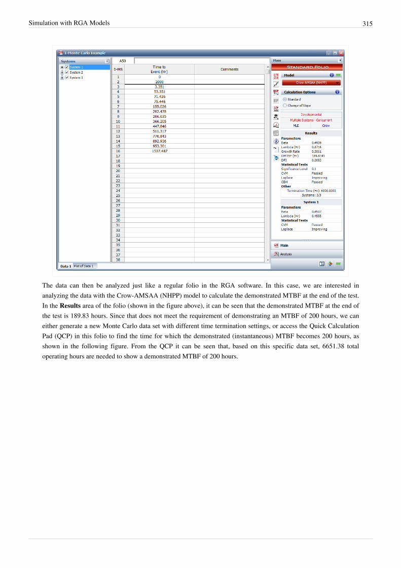
Simulation with RGA Models 315

The data can then be analyzed just like a regular folio in the RGA software. In this case, we are interested inanalyzing the data with the Crow-AMSAA (NHPP) model to calculate the demonstrated MTBF at the end of the test.In the Results area of the folio (shown in the figure above), it can be seen that the demonstrated MTBF at the end ofthe test is 189.83 hours. Since that does not meet the requirement of demonstrating an MTBF of 200 hours, we caneither generate a new Monte Carlo data set with different time termination settings, or access the Quick CalculationPad (QCP) in this folio to find the time for which the demonstrated (instantaneous) MTBF becomes 200 hours, asshown in the following figure. From the QCP it can be seen that, based on this specific data set, 6651.38 totaloperating hours are needed to show a demonstrated MTBF of 200 hours.

Simulation with RGA Models 316

Note that since the Monte Carlo routine generates random input variables that follow the NHPP based on the specificand values, if the same seed is not used the failure times will be different the next time you run the Monte Carlo

routine. Also, because the input variables are pulled from an NHPP with the expected values of and it shouldnot be expected that the calculated parameters of the generated data set will match exactly the input parameters thatwere specified. In this example, the input parameters were set as and , and the data set based onthe Monte Carlo generated failure times yielded Crow-AMSAA (NHPP) parameters of and

. The next time a data set is generated with a random seed, the calculated parameters will be slightlydifferent, since we are essentially pulling input variables from a predefined distribution. The more simulations thatare run, the more the calculated parameters will converge with the expected parameters. In the RGA software, thetotal number of generated failures with the Monte Carlo utility has to be less than 64,000.

SimuMaticReliability growth analysis using simulation can be a valuable tool for reliability practitioners. With this approach,reliability growth analyses are performed a large number of times on data sets that have been created using MonteCarlo simulation.The RGA software's SimuMatic utility generates calculated values of beta and lambda parameters, based on userspecified input parameters of beta and lambda. SimuMatic essentially performs a number of Monte Carlosimulations based on user-defined required test time or failure termination settings, and then recalculates the beta andlambda parameters for each of the generated data sets. The number of times that the Monte Carlo data sets aregenerated and the parameters are re-calculated is also user defined. The final output presents the calculated values ofbeta and lambda, and allows for various types of analysis.To access the SimuMatic utility, choose Insert > Tools > Add SimuMatic. For all of the data sets, the basic parameters that are always specified are the beta and lambda parameters of the Crow-AMSAA (NHPP)

Simulation with RGA Models 317

model or the power law model.• Failure Times: The data set is generated assuming a single system. There is a choice between a time terminated

test, where the termination time needs to be specified, or a failure terminated test, where the number of failuresneeds to be specified. SimuMatic will return the calculated values of and for a specified number of data sets.

• Grouped Failure Times: The data set is generated assuming a single system. There is a choice between a timeterminated test, where the termination time needs to be specified, or a failure terminated test, where the number offailures needs to be specified. In addition, constant or user-defined intervals need to be specified for the groupingof the data. SimuMatic will return the calculated values of and for a specified number of data sets.

• Multiple Systems - Concurrent: In this case, the number of systems needs to be specified. There is a choicebetween a time terminated test, where the termination time needs to be specified, or a failure terminated test,where the number of failures needs to be specified. SimuMatic will return the calculated values of and for aspecified number of data sets.

• Repairable Systems: In this case, the number of systems needs to be specified. There is a choice between a timeterminated test, where the termination time needs to be specified, or a failure terminated test, where the number offailures needs to be specified. SimuMatic will return the calculated values of and for a specified number ofdata sets.

The next figure shows the Main tab of the SimuMatic window where all the necessary user inputs for a multiplesystems - concurrent data set have been entered. The Analysis tab allows you to specify the confidence level forsimulation-generated confidence bounds, while the Results tab gives you the option to compute for additional results,such as the instantaneous MTBF given a specific test time.

The next figure shows the generated results based on the inputs shown above. The data sheet called "Sorted" allowsus to extract conclusions about the simulation-generated confidence bounds because the lambda and beta parametersand any other additional output are sorted by percentage.

Simulation with RGA Models 318

The following plot shows the simulation-confidence bounds for the cumulative number of failures based on the inputparameters specified.

Simulation with RGA Models 319

SimuMatic ExampleA manufacturer wants to design a reliability growth test for a redesigned product, in order to achieve an MTBF of1,000 hours. Simulation is chosen to estimate the 1-sided 90% confidence bound on the required time to achieve thegoal MTBF of 1,000 hours and the 1-sided 90% lower confidence bound on the MTBF at the end of the test time.The total test time is expected to be 15,000 hours. Based on historical data for the previous version, the expected betaand lambda parameters of the test are 0.5 and 0.3, respectively. Do the following:1.1. Generate 1,000 data sets using SimuMatic along with the required output.2.2. Plot the instantaneous MTBF vs. time with the 90% confidence bounds.3.3. Estimate the 1-sided 90% lower confidence bound on time for an MTBF of 1,000 hours.4.4. Estimate the 1-sided 90% lower confidence bound on the instantaneous MTBF at the end of the test.Solution

1.1. The next figure shows the SimuMatic window with all the appropriate inputs for creating the data sets.

Simulation with RGA Models 320

The next three figures show the settings in the Analysis, Test Design and Results tab of the SimuMatic window inorder to obtain the desired outputs.

Simulation with RGA Models 321

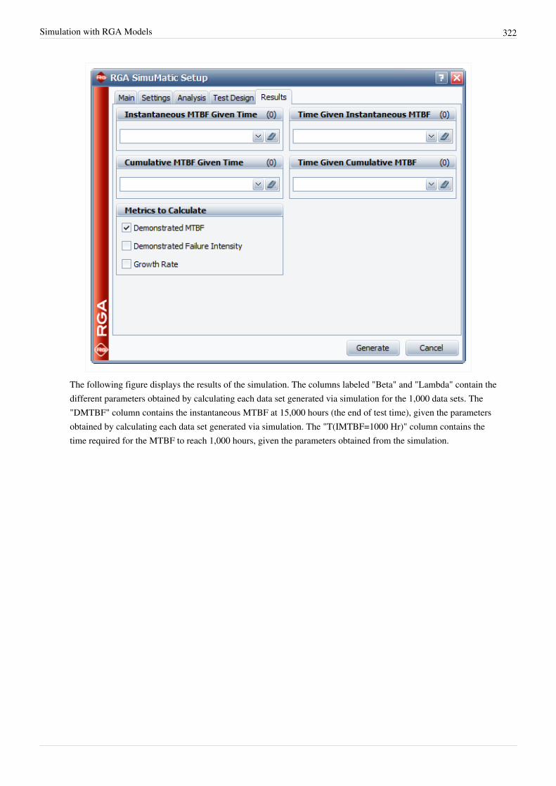
Simulation with RGA Models 322

The following figure displays the results of the simulation. The columns labeled "Beta" and "Lambda" contain thedifferent parameters obtained by calculating each data set generated via simulation for the 1,000 data sets. The"DMTBF" column contains the instantaneous MTBF at 15,000 hours (the end of test time), given the parametersobtained by calculating each data set generated via simulation. The "T(IMTBF=1000 Hr)" column contains thetime required for the MTBF to reach 1,000 hours, given the parameters obtained from the simulation.

Simulation with RGA Models 323

2.2. The next figure shows the plot of the instantaneous MTBF with the 90% confidence bounds.

Simulation with RGA Models 324

3.3. The 1-sided 90% lower confidence bound on time, assuming MTBF = 1,000 hours, can be obtained from theresults of the simulation. In the "Sorted" data sheet, this is the target DMTBF value that corresponds to 10.00%,as shown in the next figure. Therefore the 1-sided 90% lower confidence bound on time is 12,642.21 hours.

4.4. The next figure shows the 1-sided 90% lower confidence bound on time in the instantaneous MTBF plot. This isindicated by the target lines on the plot.

Simulation with RGA Models 325

5.5. The 1-sided 90% lower confidence bound on the instantaneous MTBF at the end of the test is again obtainedfrom the "Sorted" data sheet by looking at the value in the "IMTBF(15,000)" column that corresponds to 10.00%.As seen in the simulation results shown above, the 1-sided 90% lower confidence bound on the instantaneousMTBF at the end of the test is 605.93 hours.

326

Chapter 8

Reliability Demonstration Test Design forRepairable SystemsThe RGA software provides a utility that allows you to design reliability demonstration tests for repairable systems.For example, you may want to design a test to demonstrate a specific cumulative MTBF for a specific operatingperiod at a specific confidence level for a repairable system. The same applies for demonstrating an instantaneousMTBF or cumulative and instantaneous failure intensity at a given time

Underlying TheoryThe failure process in a repairable system is considered to be a non-homogeneous Poisson process (NHPP) withpower law failure intensity. The instantaneous failure intensity at time is:

So, the cumulative failure intensity at time is:

The instantaneous MTTF is:

The cumulative MTBF at time is:

The relation between the confidence level, required test time, number of systems under test and allowed total numberof failures in the test is:

where:

• is the total test time for each system.• is the number of systems under test.• is the number of allowed failures in the test.• is the confidence level.Given any three of the parameters, the equation above can be solved for the fourth unknown parameter. Note thatwhen the number of failures is a homogeneous Poisson process, and the time between failures is given bythe exponential distribution.

Reliability Demonstration Test Design for Repairable Systems 327

Example: Solve for TimeThe objective is to design a test to demonstrate that the number of failures per system in five years is less than orequal to 10. In other words, demonstrate that the cumulative MTBF for a repairable system is less than or equal to0.5 during a five year operating period, with 80% confidence level. Assume that , the number of systems forthe test is and that the number of allowed failures in the test is Solution

Since the given requirement is the number of failures, we transfer the requirement to the cumulative MTBF orcumulative failure intensity.

then:

We can then solve for :

For the five year period:

Using the values of and , we have:

Then solving for yields:

We can then solve for the required test time, for each system:

or:

or:

Solving the above equation numerically yields:

In other words, for this example we have to test for 0.36 years to demonstrate that the number of failures per systemin five years is less than or equal to 10.The same result can be obtained in the RGA software, by using the Design of Reliability Tests (DRT) tool. The nextfigure shows the calculated required test time per system of 0.3566 on the results of the example.

Reliability Demonstration Test Design for Repairable Systems 328

Example: Solve for Number of SamplesAt the end of a reliability growth testing program, a manufacturer wants to demonstrate that a new product hasachieved an MTBF of 10,000 hours with 80% confidence. The available time for the demonstration test is 4,000hours for each test unit. Assuming zero failures are allowed, what is the required number of units to be tested inorder to demonstrate the desired MTBF?Solution

We can obtain the required number of units by using the Design of Reliability Tests (DRT) tool in the RGAsoftware. Since this is a demonstration test then , and no growth will be achieved. The results are shown next.It can be seen that in order to demonstrate a 10,000 hours MTBF with 80% confidence, 5 test units will be required.

Reliability Demonstration Test Design for Repairable Systems 329

The next figure shows the different combinations of test time per unit, and the number of units in the test fordifferent numbers of allowable failures. It helps to visually examine other possible test scenarios.

330

Appendix A

Appendix A: Failure DiscountingDuring a reliability growth test, once a failure has been analyzed and corrective actions for that specific failure modehave been implemented, the probability of its recurrence is diminished, as given in Lloyd [4]. Then for thesuccess/failure data that follow, the value of the failure for which corrective actions have already been implementedshould be subtracted from the total number of failures. However, certain questions arise, such as to what extentshould the failure value be diminished or discounted, and how should the failure value be defined? One answerwould be to use engineering judgment (e.g., a panel of specialists would agree that the probability of failure has beenreduced by 50% or 90% and therefore, that failure should be given a value of 0.5 or 0.9). The obvious disadvantageof this approach is its arbitrariness and the difficulty of reaching an agreement. Therefore, a statistical basis needs tobe selected, one that is repeatable and less arbitrary. Failure discounting is applied when using the Lloyd-Lipow,logistic, and the standard and modified Gompertz models.

The value of the failure, , is chosen to be the upper confidence limit on the probability of failure based on thenumber of successful tests following implementation of the corrective action. The failure value is given by thefollowing equation:

where:

• is the confidence level.• is the number of successful tests after the first success following the corrective action.For example, after one successful test following a corrective action, , the failure is given a value of 0.9based on a 90% confidence level. After two successful tests, , the failure is given a value of 0.684, and soon. The procedure for applying this method is illustrated in the next example.Example

Assume that during the 22 launches given in the first table below, the first failure was caused by Mode 1, the secondand fourth failures were caused by Mode 2, the third and fifth failures were caused by Mode 3, the sixth failure wascaused by Mode 4 and the seventh failure was caused by Mode 5.1.1. Find the standard Gompertz reliability growth curve using the results of the first 15 launches.2.2. Find the predicted reliability after launch 22.3.3. Calculate the reliability after launch 22 based on the full data set from the second table, and compare it with the

estimate obtained for question 2.

Appendix A: Failure Discounting 331

Launch Sequence with Failure Modes and Failure Values

Launch Number Result/Mode Failure 1 Failure 2 Failure 3 Failure 4 Failure 5 Failure 6 Failure 7 Sum of Failures

1 F1 1.000 1.000

2 F2 1.000 1.000 2.000

3 F3 0.900 1.000 1.000 2.900

4 S 0.684 0.900 1.000 2.584

5 F2 0.536 1.000 0.900 1.000 3.436

6 F3 0.438 1.000 1.000 1.000 1.000 4.438

7 S 0.369 0.900 1.000 0.900 1.000 4.169

8 S 0.319 0.684 0.900 0.684 0.900 3.486

9 S 0.280 0.536 0.684 0.536 0.684 2.720

10 S 0.250 0.438 0.536 0.438 0.536 2.197

11 S 0.226 0.369 0.438 0.369 0.438 1.839

12 S 0.206 0.319 0.369 0.319 0.369 1.581

13 S 0.189 0.280 0.319 0.280 0.319 1.387

14 S 0.175 0.250 0.280 0.250 0.280 1.235

15 S 0.162 0.226 0.250 0.226 0.250 1.114

16 S 0.152 0.206 0.226 0.206 0.226 1.014

17 F4 0.142 0.189 0.206 0.189 0.206 1.000 1.931

18 S 0.134 0.175 0.189 0.175 0.189 1.000 1.861

19 F5 0.127 0.162 0.175 0.162 0.175 0.900 1.000 2.701

20 S 0.120 0.152 0.162 0.152 0.162 0.684 1.000 2.432

21 S 0.114 0.142 0.152 0.142 0.152 0.536 0.900 2.138

22 S 0.109 0.134 0.142 0.134 0.142 0.438 0.684 1.783

Comparison of the Predicted Reliability with the Actual Data

Launch Number Calculated Reliability (%) ln(R) Gompertz Reliability (%)

1 0.000

2 0.000

3 3.333 1.204

4 35.406 3.567 16.426

5 31.283 3.443 26.691

6 26.039 3.260 37.858

7 40.442 3.670 48.691

8 56.422 4.033 58.363

9 69.783 4.245 66.496

= 22.218

10 78.029 4.357 73.044

11 83.281 4.422 78.155

Appendix A: Failure Discounting 332

12 86.824 4.464 82.055

13 89.331 4.492 84.983

14 91.175 4.513 87.155

15 92.573 4.528 88.754

= 26.776

16 93.660 4.540 89.923

17 88.639 4.484 90.774

18 89.661 4.496 91.392

19 85.787 4.452 91.839

20 87.841 4.476 92.163

21 89.820 4.498 92.396

= 26.946

22 91.896 4.521 92.565

Solution

1. In the table above, the failures are represented by columns "Failure 1", "Failure 2", etc. The "Result/Mode"column shows whether each launch is a failure (indicated by the failure modes F1, F2, etc.) or a success (S). Thevalues of failure are based on and are calculated from:

These values are summed and the reliability is calculated from:

where is the number of failures and is the number of events, tests, runs or launches.

• Failure 1 is Mode 1; it occurs at launch 1 and it does not recur throughout the process. So at launch 3, , and so on.

• Failure 2 is Mode 2; it occurs at launch 2 and it recurs at launch 5. Therefore, at launch 4 and atlaunch 7, and so on.

• Failure 3 is Mode 3; it occurs at launch 3 and it recurs at launch 6. Therefore, at launch 5 and atlaunch 8, and so on.

• Failure 6 is Mode 4; it occurs at launch 17 and it does not recur throughout the process. So at launch 19,, and so on.

• Failure 7 is Mode 5; it occurs at launch 19 and it does not recur throughout the process. So at launch 21,, and so on.

For launch 3 and failure 1, .

For launch 4 and failure 1, .

And so on. Calculate the initial values of the Gompertz parameters using the second table above. Based on theequations from the Gompertz Models chapter, the initial values are:

Appendix A: Failure Discounting 333

Now, since the initial values have been determined, the Gauss-Newton method can be used. Substituting . The iterations are continued to solve for the

parameters. Using the RGA software, the estimators of the parameters for the given example are:

The next figure shows the entered data and the estimated parameters.

The Gompertz reliability growth curve may now be written as follows where is the number of launches, withthe first successful launch being counted as . Therefore, is equal to 19, since reliability growth startswith launch 4.

Appendix A: Failure Discounting 334

2.2. The predicted reliability after launch 22 is therefore:

The predicted reliability after launch 22 is calculated using the Quick Calculation Pad (QCP), as shown next.

3.3. In the second table, the predicted reliability values are compared with the reliabilities that are calculated from theraw data using failure discounting. It can be seen in the table, and in the following figure, that the Gompertz curveappears to provide a good fit to the actual data.

Appendix A: Failure Discounting 335

336

Appendix B

Appendix B: Hypothesis TestsThe RGA software provides two types of hypothesis tests: common beta hypothesis (CBH) and Laplace trend. Bothtests are applicable to the following data types:•• Times-to-failure data

•• Multiple Systems - Concurrent Operating Times•• Multiple Systems with Dates•• Multiple Systems with Event Codes

•• Fielded data•• Repairable Systems•• Fleet

Common Beta Hypothesis TestThe common beta hypothesis (CBH) tests the hypothesis that all systems in the data set have similar values of beta.As shown by Crow [17], suppose that number of systems are under test. Each system has an intensity functiongiven by:

where . You can compare the intensity functions of each of the systems by comparing the of eachsystem. When conducting an analysis of data consisting of multiple systems, you expect that each of the systemsperformed in a similar manner. In particular, you would expect the interarrival rate of the failures across the systemsto be fairly consistent. Therefore, the CBH test evaluates the hypothesis, , such that .Let denote the conditional maximum likelihood estimate of , which is given by:

where:

•• if data on the system is time terminated or if data on the system is failure

terminated ( is the number of failures on the system).• is the time-to-failure on the system.Then for each system, assume that:

are conditionally distributed as independent chi-squared random variables with degrees of freedom. When, you can test the null hypothesis, , using the following statistic:

Appendix B: Hypothesis Tests 337

If is true, then equals and conditionally has an F-distribution with degrees of freedom. Thecritical value, , can then be determined by referring to the chi-squared tables. Now, if , then the likelihoodratio procedure can be used to test the hypothesis , as discussed in Crow [17]. Consider thefollowing statistic:

where:

•

•

Also, let:

Calculate the statistic , such that:

The statistic is approximately distributed as a chi-squared random variable with degrees of freedom.Then after calculating , refer to the chi-squared tables with degrees of freedom to determine the criticalpoints. is true if the statistic falls between the critical points.

Common Beta Hypothesis ExampleConsider the data in the following table.

Repairable System Data

System 1 System 2 System 3

Start 0 0 0

End 2000 2000 2000

Failures 1.2 1.4 0.3

55.6 35 32.6

72.7 46.8 33.4

111.9 65.9 241.7

121.9 181.1 396.2

303.6 712.6 444.4

326.9 1005.7 480.8

1568.4 1029.9 588.9

1913.5 1675.7 1043.9

1787.5 1136.1

1867 1288.1

1408.1

1439.4

Appendix B: Hypothesis Tests 338

1604.8

Given that the intensity function for the system is , test the hypothesis that whileassuming a significance level equal to 0.05. Calculate the maximum likelihood estimates of and . Therefore:

Then . Calculate the statistic with a significance level of 0.05.

Since we fail to reject the null hypothesis that at the 5% significance level.Now suppose that we test the hypothesis that . Calculate the statistic .

Using the chi-square tables with degrees of freedom, the critical values at the 2.5 and 97.5 percentilesare 0.1026 and 5.9915, respectively. Since , we fail to reject the null hypothesis that

at the 5% significance level.

Laplace Trend TestThe Laplace trend test evaluates the hypothesis that a trend does not exist within the data. The Laplace trend test candetermine whether the system is deteriorating, improving, or if there is no trend at all. Calculate the test statistic, ,using the following equation:

where:

• = total operating time (termination time)• = age of the system at the successive failure• = total number of failuresThe test statistic is approximately a standard normal random variable. The critical value is read from the standardnormal tables with a given significance level, .

Laplace Trend Test ExampleConsider once again the data given in the table above. Check for a trend within System 1 assuming a significancelevel of 0.10. Calculate the test statistic for System 1.

From the standard normal tables with a significance level of 0.10, the critical value is equal to 1.645. Ifthen we would fail to reject the hypothesis of no trend. However, since

then an improving trend exists within System 1. If then a deteriorating trend would exist.

339

Appendix C

Appendix C: Crow-AMSAA Confidence BoundsIn this appendix, we will present the two methods used in the RGA software to estimate the confidence bounds forthe Crow-AMSAA (NHPP) model when applied to developmental testing data. The Fisher matrix approach is basedon the Fisher information matrix and is commonly employed in the reliability field. The Crow bounds weredeveloped by Dr. Larry Crow.Note regarding the Crow Bounds calculations: The equations that involve the use of the chi-squared distributionassume left-tail probability.

Individual (Non-Grouped) DataThis section presents the confidence bounds for the Crow-AMSAA model under developmental testing when thefailure times are known. The confidence bounds for when the failure times are not known are presented in theGrouped Data section.

Beta

Fisher Matrix Bounds

The parameter must be positive, thus is treated as being normally distributed as well.

The approximate confidence bounds are given as:

in is different ( , ) according to a 2-sided confidence interval or a 1-sided confidence interval, andvariances can be calculated using the Fisher matrix.

is the natural log-likelihood function:

And:

Appendix C: Crow-AMSAA Confidence Bounds 340

Crow Bounds

Failure Terminated

For the 2-sided 100% confidence interval on , calculate:

Thus, the confidence bounds on are:

Time Terminated

For the 2-sided 100% confidence interval on , calculate:

The confidence bounds on are:

Growth Rate

Since the growth rate, , is equal to , the confidence bounds for both the Fisher matrix and Crow methodsare:

and are obtained using the methods described above in the confidence bounds on Beta.

Lambda

Fisher Matrix Bounds

The parameter must be positive; thus, is treated as being normally distributed as well. These bounds are basedon:

The approximate confidence bounds on are given as:

where:

The variance calculation is the same as given above in the confidence bounds on Beta.

Appendix C: Crow-AMSAA Confidence Bounds 341

Crow Bounds

Failure Terminated

For the 2-sided 100% confidence interval, the confidence bounds on are:

where:

• = total number of failures.• = termination time.Time Terminated

For the 2-sided 100% confidence interval, the confidence bounds on are:

where:

• = total number of failures.• = termination time.

Cumulative Number of Failures

Fisher Matrix Bounds

The cumulative number of failures, , must be positive, thus is treated as being normally distributed.

where:

The variance calculation is the same as given above in the confidence bounds on Beta. And:

Appendix C: Crow-AMSAA Confidence Bounds 342

Crow Bounds

The Crow cumulative number of failure confidence bounds are:

where and are calculated using the process for calculating the confidence bounds oninstantaneous failure intensity.

Cumulative Failure Intensity

Fisher Matrix Bounds

The cumulative failure intensity, , must be positive, thus is treated as being normally distributed.

The approximate confidence bounds on the cumulative failure intensity are then estimated from:

where:

and:

The variance calculation is the same as given above in the confidence bounds on Beta. And:

Crow Bounds

The Crow bounds on the cumulative failure intensity are given below. Let:

Failure Terminated

Time Terminated

Appendix C: Crow-AMSAA Confidence Bounds 343

Cumulative MTBF

Fisher Matrix Bounds

The cumulative MTBF, , must be positive, thus is treated as being normally distributed as well.

The approximate confidence bounds on the cumulative MTBF are then estimated from:

where:

The variance calculation is the same as given above in the confidence bounds on Beta. And:

Crow Bounds

The 2-sided confidence bounds on the cumulative MTBF are given by:

where and are calculated using the process for calculating the confidence bounds on cumulativefailure intensity.

Appendix C: Crow-AMSAA Confidence Bounds 344

Instantaneous MTBF

Fisher Matrix Bounds

The instantaneous MTBF, , must be positive, thus is treated as being normally distributed as well.

The approximate confidence bounds on the instantaneous MTBF are then estimated from:

where:

The variance calculation is the same as given above in the confidence bounds on Beta. And:

Crow Bounds

Failure Terminated

For failure terminated data and the 2-sided confidence bounds on instantaneous MTBF , consider thefollowing equation:

Find the values and by finding the solution and for the lower and

upper bounds, respectively.If using the biased parameters, and , then the upper and lower confidence bounds are:

where .If using the unbiased parameters, and , then the upper and lower confidence bounds are:

where .Time Terminated

Consider the following equation where is the modified Bessel function of order one:

Appendix C: Crow-AMSAA Confidence Bounds 345

Find the values and by finding the solution to and in the casescorresponding to the lower and upper bounds, respectively. Calculate for each case.

If using the biased parameters, and , then the upper and lower confidence bounds are:

where .If using the unbiased parameters, and , then the upper and lower confidence bounds are:

where .

Instantaneous Failure Intensity

Fisher Matrix Bounds

The instantaneous failure intensity, , must be positive, thus is treated as being normally distributed.

The approximate confidence bounds on the instantaneous failure intensity are then estimated from:

where

The variance calculation is the same as given above in the confidence bounds on Beta. And:

Appendix C: Crow-AMSAA Confidence Bounds 346

Crow Bounds

The 2-sided confidence bounds on the instantaneous failure intensity are given by:

where and are calculated using the process presented for the confidence bounds on theinstantaneous MTBF.

Time Given Cumulative Failure Intensity

Fisher Matrix Bounds

The time, , must be positive, thus is treated as being normally distributed.

Confidence bounds on the time are given by:

where:

The variance calculation is the same as given above in the confidence bounds on Beta. And:

Crow Bounds

The 2-sided confidence bounds on time given cumulative failure intensity are given by:

Then estimate the number of failures, , such that:

The lower and upper confidence bounds on time are then estimated using:

Appendix C: Crow-AMSAA Confidence Bounds 347

Time Given Cumulative MTBF

Fisher Matrix Bounds

The time, , must be positive, thus is treated as being normally distributed.

Confidence bounds on the time are given by:

where:

The variance calculation is the same as given above in the confidence bounds on Beta. And:

Crow Bounds

The 2-sided confidence bounds on time given cumulative MTBF are estimated using the process for

calculating the confidence bounds on time given cumulative failure intensity where .

Time Given Instantaneous MTBF

Fisher Matrix Bounds

The time, , must be positive, thus is treated as being normally distributed.

Confidence bounds on the time are given by:

where:

The variance calculation is the same as given above in the confidence bounds on Beta. And:

Appendix C: Crow-AMSAA Confidence Bounds 348

Crow Bounds

Failure Terminated

If the unbiased value is used then:

where:

• = instantaneous MTBF.• = total number of failures.Calculate the constants and using procedures described for the confidence bounds on instantaneous MTBF.The lower and upper confidence bounds on time are then given by:

Time Terminated

If the unbiased value is used then:

where:

• = instantaneous MTBF.• = total number of failures.

Calculate the constants and using procedures described for the confidence bounds on instantaneous MTBF.The lower and upper confidence bounds on time are then given by:

Appendix C: Crow-AMSAA Confidence Bounds 349

Time Given Instantaneous Failure Intensity

Fisher Matrix Bounds

The time, , must be positive, thus is treated as being normally distributed.

Confidence bounds on the time are given by:

where:

The variance calculation is the same as given above in the confidence bounds on Beta. And:

Crow Bounds

The 2-sided confidence bounds on time given instantaneous failure intensity are estimated using the process

for calculating the confidence bounds on time given instantaneous MTBF where .

Grouped DataThis section presents the confidence bounds for the Crow-AMSAA model when using Grouped data.

Beta (Grouped)

Fisher Matrix Bounds

The parameter must be positive, thus is treated as being normally distributed as well.

The approximate confidence bounds are given as:

can be obtained by .

All variance can be calculated using the Fisher matrix:

Appendix C: Crow-AMSAA Confidence Bounds 350

is the natural log-likelihood function where and:

Crow Bounds

The 2-sided confidence bounds on are given by first calculating:

where:

• = interval end time for the interval.• = number of intervals.• = end time for the last interval.Next:

And:

Then:

where:

• = inverse standard normal.• = number of failures.

The 2-sided confidence bounds on are then .

Appendix C: Crow-AMSAA Confidence Bounds 351

Growth Rate (Grouped)

Since the growth rate, , is equal to , the confidence bounds for both the Fisher matrix and Crow methodsare:

and are obtained using the methods described above in the confidence bounds on Beta.

Lambda (Grouped)

Fisher Matrix Bounds

The parameter must be positive, thus is treated as being normally distributed as well. These bounds are basedon:

The approximate confidence bounds on are given as:

where:

The variance calculation is the same as given above in the confidence bounds on Beta.

Crow Bounds

Failure Terminated

For failure terminated data, the 2-sided 100% confidence interval, the confidence bounds on are:

where:

• = total number of failures.• = end time of last interval.Time Terminated

For time terminated data, the 2-sided 100% confidence interval, the confidence bounds on are:

where:

• = total number of failures.• = end time of last interval.

Appendix C: Crow-AMSAA Confidence Bounds 352

Cumulative Number of Failures (Grouped)

Fisher Matrix Bounds

The cumulative number of failures, , must be positive, thus is treated as being normally distributed.

where:

The variance calculation is the same as given above in the confidence bounds on Beta. And:

Crow Bounds

The 2-sided confidence bounds on the cumulative number of failures are given by:

where and are calculated based on the procedures for the confidence bounds on the instantaneousfailure intensity.

Cumulative Failure Intensity (Grouped)

Fisher Matrix Bounds

The cumulative failure intensity, , must be positive, thus is treated as being normally distributed.

The approximate confidence bounds on the cumulative failure intensity are then estimated from:

where:

and:

Appendix C: Crow-AMSAA Confidence Bounds 353

The variance calculation is the same as given above in the confidence bounds on Beta. And:

Crow Bounds

The 2-sided confidence bounds on the cumulative failure intensity are given below. Let:

Then:

Cumulative MTBF (Grouped)

Fisher Matrix Bounds

The cumulative MTBF, , must be positive, thus is treated as being normally distributed as well.

The approximate confidence bounds on the cumulative MTBF are then estimated from:

where:

The variance calculation is the same as given above in the confidence bounds on Beta. And:

Appendix C: Crow-AMSAA Confidence Bounds 354

Crow Bounds

The 2-sided confidence bounds on cumulative MTBF are given by:

where and are calculating using the process for calculating the confidence bounds on the cumulativefailure intensity.

Instantaneous MTBF (Grouped)

Fisher Matrix Bounds

The instantaneous MTBF, , must be positive, thus is approximately treated as being normallydistributed as well.

The approximate confidence bounds on the instantaneous MTBF are then estimated from:

where:

The variance calculation is the same as given above in the confidence bounds on Beta. And:

Crow Bounds

The 2-sided confidence bounds on instantaneous MTBF are given by first calculating:

where:

• = interval end time for the interval.• = number of intervals.• = end time for the last interval.Calculate:

Next:

Appendix C: Crow-AMSAA Confidence Bounds 355

And:

where:

• = inverse standard normal.• = number of failures.

The 2-sided confidence bounds on instantaneous MTBF are then .

Instantaneous Failure Intensity (Grouped)

Fisher Matrix Bounds

The instantaneous failure intensity, , must be positive, thus is treated as being normally distributed.

The approximate confidence bounds on the instantaneous failure intensity are then estimated from:

where and:

The variance calculation is the same as given above in the confidence bounds on Beta. And:

Crow Bounds

The 2-sided confidence bounds on the instantaneous failure intensity are given by:

where and are calculated using the process for calculating the confidence bounds on theinstantaneous MTBF.

Appendix C: Crow-AMSAA Confidence Bounds 356

Time Given Cumulative Failure Intensity (Grouped)

Fisher Matrix Bounds

The time, , must be positive, thus is treated as being normally distributed.

Confidence bounds on the time are given by:

where:

The variance calculation is the same as given above in the confidence bounds on Beta. And:

Crow Bounds

The 2-sided confidence bounds on time given cumulative failure intensity are presented below. Let:

Then estimate the number of failures:

The confidence bounds on time given the cumulative failure intensity are then given by:

Appendix C: Crow-AMSAA Confidence Bounds 357

Time Given Cumulative MTBF (Grouped)

Fisher Matrix Bounds

The time, , must be positive, thus is treated as being normally distributed.

Confidence bounds on the time are given by:

where:

The variance calculation is the same as given above in the confidence bounds on Beta. And:

Crow Bounds

The 2-sided confidence bounds on time given cumulative MTBF are estimated using the process for

calculating the confidence bounds on time given cumulative failure intensity where .

Time Given Instantaneous MTBF (Grouped)

Fisher Matrix Bounds

The time, , must be positive, thus is treated as being normally distributed.

Confidence bounds on the time are given by:

where:

The variance calculation is the same as given above in the confidence bounds on Beta. And:

Appendix C: Crow-AMSAA Confidence Bounds 358

Crow Bounds

Failure Terminated

Calculate the constants and using procedures described for the confidence bounds on instantaneous MTBF.The lower and upper confidence bounds on time are then given by:

Time Terminated

Calculate the constants and using procedures described for the confidence bounds on instantaneous MTBF.The lower and upper confidence bounds on time are then given by:

Time Given Instantaneous Failure Intensity (Grouped)

Fisher Matrix Bounds

The time, , must be positive, thus is treated as being normally distributed.

Confidence bounds on the time are given by:

where:

The variance calculation is the same as given above in the confidence bounds on Beta. And:

Appendix C: Crow-AMSAA Confidence Bounds 359

Crow Bounds

The 2-sided confidence bounds on time given instantaneous failure intensity are estimated using the process

for calculating the confidence bounds on time given instantaneous MTBF where .

360

Appendix D

Appendix D: Crow Extended Confidence BoundsIn this appendix, we will present the two methods used in the RGA software to estimate the confidence bounds forthe Crow extended model when applied to developmental testing data. The Fisher Matrix approach is based on theFisher Information Matrix and is commonly employed in the reliability field. The Crow bounds were developed byDr. Larry Crow.

Bounds on Demonstrated Failure Intensity

Fisher Matrix Bounds

If there are no BC failure modes, the demonstrated failure intensity is

.Thus:

and:

where .

If there are BC failure modes, the demonstrated failure intensity, , is actually the instantaneousfailure intensity based on all of the data. must be positive; thus, is approximately treated asbeing normally distributed.

The approximate confidence bounds on the instantaneous failure intensity are then estimated from:

where .

The variance calculation is the same as described in the Crow-AMSAA Confidence Bounds appendix.

Appendix D: Crow Extended Confidence Bounds 361

Crow Bounds

If there are no BC failure modes then:

where .If there are BC modes then the confidence bounds on the demonstrated failure intensity are calculated as presented inthe Crow-AMSAA Confidence Bounds appendix.

Bounds on Demonstrated MTBF

Fisher Matrix Bounds

where and can be obtained from the equation given above for Bounds on DemonstratedFailure Intensity.

Crow Bounds

where and can be obtained from the equation given above for Bounds on DemonstratedFailure Intensity.

Bounds on Projected Failure Intensity

Fisher Matrix Bounds

The projected failure intensity must be positive; thus, is approximately treated as being normallydistributed as well:

where:

• when there are no BC modes.

• when there are BC modes.

• is the total failure number of the distinct BD mode.You can then get:

Appendix D: Crow Extended Confidence Bounds 362

where:

The can be obtained from Fisher Matrix based on distinct BD modes.

Crow Bounds

where .

Bounds on Projected MTBF

Fisher Matrix Bounds

and can be obtained from the equation given above for Bounds on Projected Failure Intensity.

Crow Bounds

and can be obtained from the equation given above for Bounds on Projected Failure Intensity.

Bounds on Growth Potential Failure Intensity

Fisher Matrix Bounds

If there are no BC failure modes, the growth potential failure intensity is

.

Then:

Appendix D: Crow Extended Confidence Bounds 363

If there are BC failure modes, the growth potential failure intensity is

.

Therefore:

The confidence bounds on the growth potential failure intensity are as follows:

where .

Crow Bounds

The Crow bounds for the growth potential failure intensity are the same as the Fisher Matrix bounds.

Bounds on Growth Potential MTBF

Fisher Matrix Bounds

where and can be obtained from the equation given above for Bounds on Growth Potential Failure Intensity.

Crow Bounds

The Crow bounds for the growth potential MTBF are the same as the Fisher Matrix bounds.

364

Appendix E

Appendix E: Confidence Bounds for RepairableSystems AnalysisIn this appendix, we will present the two methods used in the RGA software to estimate the confidence bounds forRepairable Systems Analysis. The Fisher Matrix approach is based on the Fisher Information Matrix and iscommonly employed in the reliability field. The Crow bounds were developed by Dr. Larry Crow.

Beta

Fisher Matrix Bounds

The parameter must be positive, thus is approximately treated as being normally distributed.

All variance can be calculated using the Fisher Information Matrix. is the natural log-likelihood function.

Crow Bounds

Calculate the conditional maximum likelihood estimate of :

The Crow 2-sided 100% confidence bounds on are:

Appendix E: Confidence Bounds for Repairable Systems Analysis 365

Lambda

Fisher Matrix Bounds

The parameter must be positive, thus is approximately treated as being normally distributed. These boundsare based on:

The approximate confidence bounds on are given as:

where .The variance calculation is the same the equations given in the confidence bounds on Beta.

Crow Bounds

Failure Terminated

The confidence bounds on for failure terminated data are calculated using:

where:

• = total number of failures.• = number of systems.• = end time for the system.Time Terminated

The confidence bounds on for time terminated data are calculated using:

where:

• = total number of failures.

Appendix E: Confidence Bounds for Repairable Systems Analysis 366

• = number of systems.• = end time for the system.

Cumulative Number of Failures

Fisher Matrix Bounds

The cumulative number of failures, . must be positive, thus is approximately treated as beingnormally distributed.

where:

The variance calculation is the same as the calculations in the confidence bounds on Beta.

Crow Bounds

The 2-sided confidence bounds on the cumulative number of failures are given by:

where:

• = total number of failures across all systems. This is not the number of failures up to time .

•

• = time at which calculations are being conducted.

Appendix E: Confidence Bounds for Repairable Systems Analysis 367

Cumulative Failure Intensity

Fisher Matrix Bounds

The cumulative failure intensity, must be positive, thus is approximately treated as being normallydistributed.

The approximate confidence bounds on the cumulative failure intensity are then estimated using:

where:

and:

The variance calculation is the same as the calculations in the confidence bounds on Beta.

Crow Bounds

The 2-sided confidence bounds on the cumulative failure intensity are given by:

where:

• = total number of failures across all systems. This is not the number of failures up to time .

•

• = time at which calculations are being conducted.

Appendix E: Confidence Bounds for Repairable Systems Analysis 368

Cumulative MTBF

Fisher Matrix Bounds

The cumulative MTBF, . must be positive, thus is approximately treated as being normallydistributed.

The approximate confidence bounds on the cumulative MTBF are then estimated from:

where:

The variance calculation is the same as the calculations given in the confidence bounds on Beta.

Crow Bounds

The 2-sided confidence bounds on the cumulative MTBF are given by:

where and are calculated using the process for the confidence bounds on cumulative failure intensity.

Instantaneous MTBF

Fisher Matrix Bounds

The instantaneous MTBF, . must be positive, thus is approximately treated as being normallydistributed.

The approximate confidence bounds on the instantaneous MTBF are then estimated from:

where:

Appendix E: Confidence Bounds for Repairable Systems Analysis 369

The variance calculation is the same as the calculations given in the confidence bounds on Beta.

Crow Bounds

Failure Terminated

For failure terminated data and the 2-sided confidence bounds on instantaneous MTBF , consider thefollowing equation:

Find the values and by finding the solution and for the lower and

upper bounds, respectively.If using the biased parameters, and , then the upper and lower confidence bounds are:

where .If using the unbiased parameters, and , then the upper and lower confidence bounds are:

where .Time Terminated

Consider the following equation where is the modified Bessel function of order one:

Find the values and by finding the solution to and in the casescorresponding to the lower and upper bounds, respectively. Calculate for each case.

If using the biased parameters, and , then the upper and lower confidence bounds are:

where .If using the unbiased parameters, and , then the upper and lower confidence bounds are:

Appendix E: Confidence Bounds for Repairable Systems Analysis 370

where .

Instantaneous Failure Intensity

Fisher Matrix Bounds

The instantaneous failure intensity, . must be positive, thus is approximately treated as beingnormally distributed.

The approximate confidence bounds on the instantaneous failure intensity are then estimated from:

where and:

The variance calculation is the same as the calculations in the confidence bounds on Beta.

Crow Bounds

The 2-sided confidence bounds on the instantaneous failure intensity are given by:

where and are calculated using the process presented for the confidence bounds on theinstantaneous MTBF.

Appendix E: Confidence Bounds for Repairable Systems Analysis 371

Time Given Cumulative Failure Intensity

Fisher Matrix Bounds

The time, . must be positive, thus is approximately treated as being normally distributed.

The confidence bounds on the time are given by:

where:

The variance calculation is the same as the calculations given in the confidence bounds on Beta.

Crow Bounds

The 2-sided confidence bounds on time given cumulative failure intensity are given by:

Then estimate, the number of failures, , such that:

The lower and upper confidence bounds on time are then estimated using:

Appendix E: Confidence Bounds for Repairable Systems Analysis 372

Time Given Cumulative MTBF

Fisher Matrix Bounds

The time, . must be positive, thus is approximately treated as being normally distributed.

The confidence bounds on the time are given by:

where:

The variance calculation is the same as the calculations in the confidence bounds on Beta.

Crow Bounds

The 2-sided confidence bounds on time given cumulative MTBF are estimated using the process for

the confidence bounds on time given cumulative failure intensity where .

Time Given Instantaneous MTBF

Fisher Matrix Bounds

The time, . must be positive, thus is approximately treated as being normally distributed.

The confidence bounds on the time are given by:

where:

The variance calculation is the same as the calculations in the confidence bounds on Beta.

Appendix E: Confidence Bounds for Repairable Systems Analysis 373

Crow Bounds

Failure Terminated

Calculate the constants and using procedures described for the confidence bounds on instantaneous MTBF.The lower and upper confidence bounds on time are then given by:

Time Terminated

Calculate the constants and using procedures described for the confidence bounds on instantaneous MTBF.The lower and upper confidence bounds on time are then given by:

Time Given Instantaneous Failure Intensity

Fisher Matrix Bounds

These bounds are based on:

The confidence bounds on the time are given by:

where:

The variance calculation is the same as the calculations given in the confidence bounds on Beta.

Appendix E: Confidence Bounds for Repairable Systems Analysis 374

Crow Bounds

The 2-sided confidence bounds on time given instantaneous failure intensity are estimated using the process

for the confidence bounds on time given instantaneous MTBF where .

Reliability

Fisher Matrix Bounds

These bounds are based on:

The confidence bounds on reliability are given by:

The variance calculation is the same as the calculations in the confidence bounds on Beta.

Crow Bounds

Failure Terminated

For failure terminated data, the 100( )% confidence interval on the current reliability at time for a specifiedmission duration is:

where:

•• and are obtained from the confidence bounds on instantaneous MTBF for failure terminated data.Time Terminated

For time terminated data, the 100( )% confidence interval on the current reliability at time for a specifiedmission duration is:

where:

•• and are obtained from the confidence bounds on instantaneous MTBF for time terminated data.

Appendix E: Confidence Bounds for Repairable Systems Analysis 375

Time Given Reliability and Mission Time

Fisher Matrix Bounds

The time, . must be positive, thus is approximately treated as being normally distributed.

The confidence bounds on time are calculated by using:

where:

is calculated numerically from:

The variance calculations are done by:

Crow Bounds

Failure Terminated

For failure terminated data, the 2-sided confidence bounds on time given reliability and mission time estimated bycalculating:

where and are obtained from the confidence bounds on instantaneous MTBF for failure terminated data.

Let and solve numerically for using .

Let and solve numerically for using .If then and . If then and .Time Terminated

For time terminated data, the 2-sided confidence bounds on time given reliability and mission time estimated bycalculating:

.

where and are obtained from the confidence bounds on instantaneous MTBF for time terminated data.

Let and solve numerically for using .

Let and solve numerically for using .If . then and . If . then and .

Appendix E: Confidence Bounds for Repairable Systems Analysis 376

Mission Time Given Reliability and Time

Fisher Matrix Bounds

The mission time, . must be positive, thus is approximately treated as being normally distributed.

The confidence bounds on mission time are given by using:

where:

Calculate from:

The variance calculations are done by:

Crow Bounds

Failure Terminated

Step 1: Calculate .

Step 2: Let and solve for such that:

Step 3: Let and solve for such that:

Step 4: If . then and . If . then and .Time Terminated

Step 1: Calculate .

Step 2: Let and solve for using the same equation given for the failure terminated data.

Step 3: Let and solve for using the same equation given for the failure terminated data.Step 4: If . then and . If . then and .

377

Appendix F

Appendix F: Glossary• "A" Mode: A failure mode for which a corrective action will not be implemented.• Actual Growth Potential Factor: The failure intensity of the M modes (total number of distinct unfixed BD

modes) after corrective actions have been implemented for them, using the actual values for the effectivenessfactors. This metric is used in the Crow Extended - Continuous Evaluation model.

• Actual Growth Potential Failure Intensity: The minimum attainable failure intensity based on the currentmanagement strategy. This metric is used in the Crow Extended - Continuous Evaluation model.

• Actual Growth Potential MTBF: The maximum attainable MTBF based on the current management strategy.This metric is used in the Crow Extended - Continuous Evaluation model.

• Actual Idealized Growth Curve: The reliability growth planning curve for the Crow extended model that takesinto account the fix delay.

• Actual Projected Failure Intensity: The projected failure intensity based on the current management strategy.This metric is used in the Crow Extended - Continuous Evaluation model.

• Actual Projected MTBF: The projected MTBF based on the current management strategy.• Allowable Failures: Maximum number of failures that can occur during the demonstration test and still pass the

test. Used in the design of reliability tests for repairable systems.• AMSAA: Army Materiel Systems Analysis Activity.• Average Actual EF: An average of the effectiveness factors (EF) for the BD modes that takes into account the

point at which the corrective action will be implemented. If the fix is going to be implemented at a later time orduring another phase, then the EF value for the mode at the current analysis point is set to zero. If the delayed fixis going to be implemented at the current analysis point, then the EF value is set to the specified value for themode. This metric is used in the Crow Extended - Continuous Evaluation model.

• Average Fix Delay: The average test time required to incorporate corrective actions into the configuration. A fixdelay can be specified for each phase of the reliability growth plan.

• Average Nominal EF: An average of the effectiveness factors (EF) for the BD modes assuming all fixes for theseen BD modes will be implemented.

• "BC" Mode: For the Crow Extended model, it is a failure mode for which a corrective action will beimplemented during the test. For the Crow Extended - Continuous Evaluation model, it is a failure mode forwhich a corrective action will be implemented at the time of failure.

• "BD" Mode: For the Crow Extended model, it is a failure mode for which a corrective action will be delayeduntil the end of the test. For the Crow Extended - Continuous Evaluation model, a failure mode for which acorrective action will be implemented at some point in time after the failure time.

• BD Mode Failure Intensity: See Discovery Rate Failure Intensity.• Beta: The shape parameter for the Crow-AMSAA (NHPP) and Crow Extended models. Beta must be greater than

zero.• Chi-Squared GOF Test: A goodness-of-fit test that evaluates the hypothesis that the data follows a

non-homogeneous Poisson process (NHPP). This goodness-of-fit test is used in grouped data types.• Common Beta Hypothesis Test: Tests the hypothesis that all systems in the data set have similar values of beta.

Appendix F: Glossary 378

• Cramér-von Mises: A goodness-of-fit test that evaluates the hypothesis that the data follows a non-homogeneousPoisson process (NHPP). This goodness-of-fit test is used for non-grouped data types.

• Discovery Rate Beta: Indicates whether the interarrival times between unique BD modes are getting larger orsmaller. In most cases, we want this value to be less than 1 assuming that most failures will be identified early onand that their inter-arrival times will become larger as the test progresses.

• Discovery Rate Failure Intensity: The failure intensity of the unseen BD modes. This is represented by .• Discovery Rate MTBF: The rate at which the next new unique BD mode will be observed. This is represented by

the inverse of .• Demonstrated/Achieved Failure Intensity: The Instantaneous failure intensity at the termination time.• Demonstrated/Achieved MTBF: The Instantaneous MTBF at the termination time.• Effectiveness Factor: The portion of the BD mode's failure intensity that is expected to be removed based on the

planned corrective action. This applies only to delayed fixes.

• Failure Intensity: The probability of failure within the next given that the system may or may not havefailed.

• Failure Intensity Modes Seen: The failure intensity for the failure modes that have been seen during the test.This is calculated by subtracting the failure intensity of the modes that have not been seen from the total systemfailure intensity.

• Failure Truncated: Indicates that the test was stopped at a failure time. A test can either be failure truncated ortime truncated.

• Goal MTBF: The MTBF requirement when determining a reliability growth plan.• Growth Potential Design Margin (GPDM): A safety margin when setting target MTBF values for the reliability

growth plan. It is common for systems to degrade in terms of reliability when a prototype product is going intofull manufacturing. The degradation is due to variations in material, processes, etc. Furthermore, the in-housereliability growth testing usually overestimates the actual product reliability because the field usage conditionsmay not be perfectly simulated during growth testing. Typical values for the GPDM are around 1.2. Higher valuesyield less risk for the program, but require a more rigorous reliability growth test plan. Lower values imply higherprogram risk, with less "safety margin."

• Growth Potential Failure Intensity: Minimum failure intensity that can be attained with the currentmanagement strategy. The minimum failure intensity will be attained when all unique BD modes have beenobserved and fixed. This metric is used in the Crow Extended model.

• Growth Potential MTBF: Maximum MTBF that can be attained with the current management strategy. Themaximum MTBF will be attained when all unique BD modes have been observed and fixed.

• Growth Rate: Represents the rate at which the MTBF of the system is increasing. The growth rate for theCrow-AMSAA (NHPP) model is equal to and is therefore a value greater than or equal to zero,but lessthan 1. For the Duane Model, the growth rate ( ) is the negative of the slope of the line on the cumulative failureintensity vs. time plot. A growth rate that is equal to 1 implies an infinite MTBF growth.

• Homogeneous Poisson Process (HPP): A homogeneous process is equivalent to the widely used Poissondistribution. In this scenario, the system's failure intensity is not affected by age. Therefore, the expected numberof failures associated with the system is accumulated at a constant rate. It is a special case of the Crow-AMSAA(NHPP) model when .

• Initial Failure Intensity: The failure intensity inherent to the system prior to any testing.• Initial MTBF: The MTBF inherent to the system prior to any testing.• Integrated Reliability Growth Testing (IRGT): A process where reliability growth testing is conducted as part

of existing testing procedures. This is less expensive than conducting a formal reliability growth test. IRGT is

Appendix F: Glossary 379

usually implemented at the same time as the basic reliability tasks. The test conditions under IRGT are usuallyless than the actual customer use conditions.

• Lambda: The scale parameter for the Crow-AMSAA (NHPP) and Crow Extended models. Lambda must begreater than zero.

• Laplace Trend Test: Tests the hypothesis that a trend does not exist within the data. The Laplace trend test candetermine if the system is deteriorating, improving or if a trend does not exist.

• Likelihood Value: The log-likelihood value returned by the likelihood function given the estimated parameters.This value is returned when maximum likelihood estimation (MLE) is used to estimate the parameters.

• Management Strategy Ratio: Defines the portion of the system's failure intensity that will be addressed bycorrective actions. A management strategy ratio equal to 1 indicates a perfect management strategy. In this case, acorrective action will be implemented for every mode that is seen. A typical value is 0.95, which indicates that5% of the system's failure intensity will not be addressed (i.e., 5% will be "A" Modes).

• Maturity Factor: The ratio of the initial MTBF to the final MTBF.• MIL-HDBK-189: Military handbook for reliability growth management. MIL-HDBK-189C can be downloaded

by clicking here [1].• Minimal Repair: This is a situation where the repair of a failed system is just enough to get the system

operational again (i.e., no renewal).• MTBF Modes Seen: The inverse of the failure intensity for the modes that have been seen during the test. See

Failure Intensity Modes Seen.• Nominal Growth Potential Factor: The failure intensity of the M modes (total number of distinct unfixed BD

modes) after corrective actions have been implemented for them, using the nominal values for the effectivenessfactors. This metric is used in the Crow Extended - Continuous Evaluation model.

• Nominal Growth Potential Failure Intensity: The minimum attainable failure intensity if all delayed correctiveactions are implemented for the modes that have been seen, and delayed corrective actions are also implementedfor the unseen BD modes, assuming testing would continue until all unseen BD modes are revealed. This metric isused in the Crow Extended - Continuous Evaluation model.

• Nominal Growth Potential MTBF: The maximum attainable MTBF if all delayed corrective actions areimplemented for the modes that have been seen, and delayed corrective actions are also implemented for theunseen BD modes, assuming testing would continue until all unseen BD modes are revealed. This metric is usedin the Crow Extended - Continuous Evaluation model.

• Nominal Idealized Growth Curve: The reliability growth planning curve for the Crow Extended model thatdoes not take into account the fix delay. The nominal curve assumes that all fixes are implementedinstantaneously. Reliability growth is realized instantaneously on this curve since there is not a delay associatedwith the implemented fixes.

• Nominal Projected Failure Intensity: The projected failure intensity assuming all delayed fixes for the modesthat have been seen are implemented.

• Nominal Projected MTBF: The projected MTBF assuming all delayed fixes for the modes that have been seenare implemented. This metric is used in the Crow Extended - Continuous Evaluation model.

• Non-Homogeneous Poisson Process (NHPP): The NHPP is generally used to model the reliability of arepairable system. An NHPP is an extension of the HPP process. The NHPP allows for the system failureintensity to change with system age. Therefore, the expected number of failures associated with the system is notaccumulated at a constant rate.

• p ratio: The probability of not incorporating a corrective action by time .

Appendix F: Glossary 380

• Planned Growth: MTBF or failure intensity specified during a phase for the Crow Extended model for reliabilitygrowth planning.

• Projected Failure Intensity: The estimated failure intensity that will be reached if the proposed delayedcorrective actions are implemented, with the specified effectiveness factors. This metric is used in the CrowExtended model.

• Projected MTBF: The estimated MTBF that will be reached if the proposed delayed corrective actions areimplemented with the specified effectiveness factors. This metric is used in the Crow Extended model.

• Reliability Growth: The positive improvement in a parameter or metric over a period of time due to changes inthe system's design or manufacturing process.

• Statistical Test for Effectiveness of Corrective Actions: A statistical test that can determine if the averagefailure intensity for phase 2 is statistically less than the average failure intensity for phase 1. This test can alsodetermine if the average failure intensity for phase 2 is statistically less than the demonstrated failure intensity atthe end of phase 1. This test is used with multi-phase data sets.

• Stochastic Process: A sequence of interdependent random events.• Termination Time: In developmental testing, this is equal to the total accumulated test time of all systems. For

repairable systems, this is equal to the age of the oldest system.• Test-Fix-Test: A testing procedure where all corrective actions are implemented during the test.• Test-Find-Test: A testing procedure where all corrective actions are delayed until the end of the test.• Test-Fix-Find-Test: A testing procedure where some corrective actions are implemented during the test, while

others are delayed until the end of the test.• Time Truncated: Indicates that the test was stopped after a specific amount of test time. A test can either be

failure truncated or time truncated.

References[1] http:/ / www. weibull. com/ mil_std/ mil_hdbk_189c. pdf

381

Appendix G

Appendix G: References1.1. Virene, E.P., "Reliability Growth and the Upper Reliability Limit, How to Use Available Data to Calculate,"

Report No. D2-24142-1, 31p, AD-804 150, December 1966, Boeing Company, Seattle, Washington. Also"Reliability Growth and Its Upper Limit," Proceedings of 1968 Annual Symposium on Reliability, (IEEE CatalogNo. 68 C33-R), pp. 265-270, January 1968.

2. Seber, G.A.F., and Wild, C.J., Nonlinear Regression, John Wiley & Sons, New York, 1989.3.3. Kececioglu, D.B., "Reliability Growth," Reliability Engineering Handbook, Ed. 4, Vol. 2, Prentice-Hall,

Englewood Cliffs, New Jersey, pp. 415-418, 1991.4.4. Lloyd, D.K., "Forecasting Reliability Growth," IEEE Quality and Reliability Engineering International, pp.

19-23, 1986.5.5. Jiang, S., Kececioglu, D.B., and Vassiliou, P., "Modified Gompertz," Proceedings of the Annual Reliability and

Maintainability Symposium, 1994.6.6. Lloyd, D.K., and Lipow, M., "Reliability Growth Models," Reliability: Management, Methods, and Mathematics,

Prentice-Hall Space Technology Series, Prentice-Hall, Inc. Englewood Cliffs, New Jersey, pp. 330-348, 1962.7. Nelson, W., Applied Life Data Analysis, John Wiley & Sons, New York, New York, 1982.8.8. Duane, J.T., "Learning Curve Approach To Reliability Monitoring," IEEE Transactions on Aerospace, Vol. 2, pp.

563-566, 1964.9.9. Crow, L.H., "Reliability Growth Estimation With Missing Data - II," IEEE Proceedings Annual Reliability and

Maintainability Symposium, pp. 248-253, 1988.10.10. Crow, L.H., "Reliability Growth Projection from Delayed Fixes," IEEE Proceedings Annual Reliability and

Maintainability Symposium, pp. 84-89, 1983.11.11. Crow, L.H., "Methods for Assessing Reliability Growth Potential," IEEE Proceedings Annual Reliability and

Maintainability Symposium, pp. 484-489, 1984.12.12. Crow, L. H. "Methods for Reliability Growth Assessment During Development," Electronic Systems

Effectiveness and Life Cycle Testing, ed. by J. K. Skwirzynski, Springer-Verlag, 1983.13.13. Military Handbook 189, Reliability Growth Management, Department of Defense, Philadelphia: Naval

Publications and Forms Center, 1981.14.14. Military Handbook 781, Reliability Test Methods, Plans, and Environments for Engineering Development,

Qualification, and Production, Department of Defense, Philadelphia: Naval Publications and Forms Center, 1987.15.15. IEC International Standard, Reliability Growth- Statistical test and estimation methods, IEC 1164 International

Electrotechnical Commission, 1995.16.16. Crow, L.H., "Confidence Interval Procedures for the Weibull Process with Applications to Reliability Growth,"

Technometrics, Vol. 24, No.1, pp. 67-72, 1982.17.17. Crow, L.H., "Reliability Analysis for Complex, Repairable Systems in Reliability and Biometry," SIAM, ed. by

Proschan and R. J. Serfling, Philadelphia, Pennsylvania, pp. 379-410, 1974.18.18. Crow, L.H., "Evaluating the Reliability of Repairable Systems," IEEE Proceedings Annual Reliability and

Maintainability Symposium, pp. 275-279, 1990.19.19. Crow, L.H., "Confidence Intervals on the Reliability of Repairable Systems," IEEE Proceedings Annual

Reliability and Maintainability Symposium, pp. 126-134, 1993.20.20. Crow, L.H., "An Extended Reliability Growth Model for Managing and Assessing Corrective Actions," IEEE

Proceedings Annual Reliability and Maintainability Symposium, pp. 73-80, 2004.

Appendix G: References 382

21.21. Crow, L.H., "Methods for Reducing the Cost to Maintain a Fleet of Repairable Systems," IEEE ProceedingsAnnual Reliability and Maintainability Symposium, pp. 392-399, 2003.

22.22. Crow, L.H., "A Methodology for Managing Reliability Growth During Operational Mission Profile Testing,"IEEE Proceedings Annual Reliability and Maintainability Symposium, pp. 48-53, 2008.

23.23. Nelson, W., "An Application of Graphical Analysis of Repair Data," Quality and Reliability EngineeringInternational, Vol. 14, pp. 49-52, 1998.