Relay Selection for Geographical Forwarding in Sleep-Wake Cycling Wireless Sensor Networks
14
Relay Selection for Geographical Forwarding in Sleep-Wake Cycling Wireless Sensor Networks K.P. Naveen, Student Member, IEEE, and Anurag Kumar, Fellow, IEEE Abstract—Our work is motivated by geographical forwarding of sporadic alarm packets to a base station in a wireless sensor network (WSN), where the nodes are sleep-wake cycling periodically and asynchronously. We seek to develop local forwarding algorithms that can be tuned so as to tradeoff the end-to-end delay against a total cost, such as the hop count or total energy. Our approach is to solve, at each forwarding node enroute to the sink, the local forwarding problem of minimizing one-hop waiting delay subject to a lower bound constraint on a suitable reward offered by the next-hop relay; the constraint serves to tune the tradeoff. The reward metric used for the local problem is based on the end-to-end total cost objective (for instance, when the total cost is hop count, we choose to use the progress toward sink made by a relay as the reward). The forwarding node, to begin with, is uncertain about the number of relays, their wake-up times, and the reward values, but knows the probability distributions of these quantities. At each relay wake-up instant, when a relay reveals its reward value, the forwarding node’s problem is to forward the packet or to wait for further relays to wake-up. In terms of the operations research literature, our work can be considered as a variant of the asset selling problem. We formulate our local forwarding problem as a partially observable Markov decision process (POMDP) and obtain inner and outer bounds for the optimal policy. Motivated by the computational complexity involved in the policies derived out of these bounds, we formulate an alternate simplified model, the optimal policy for which is a simple threshold rule. We provide simulation results to compare the performance of the inner and outer bound policies against the simple policy, and also against the optimal policy when the source knows the exact number of relays. Observing the good performance and the ease of implementation of the simple policy, we apply it to our motivating problem, i.e., local geographical routing of sporadic alarm packets in a large WSN. We compare the end-to-end performance (i.e., average total delay and average total cost) obtained by the simple policy, when used for local geographical forwarding, against that obtained by the globally optimal forwarding algorithm proposed by Kim et al. [1]. Index Terms—Relay selection, wireless sensor networks, sleep-wake cycling, geographical forwarding, asset selling problem, wireless networks with intermittent links, opportunistic forwarding Ç 1 INTRODUCTION W E are interested in the problem of packet forwarding in a class of wireless sensor networks (WSNs) in which local inferences based on sensor measurements could result in the generation of occasional “alarm” packets that need to be routed to a base-station, where some sort of action could be taken [1], [2], [3]. Such a situation could arise, for example, in a WSN for human intrusion detection or fire detection in a large region. Such WSNs often need to run on batteries or on harvested energy and, hence, must be energy conscious in all their operations. To conserve energy and also since the events are rare, it is best if the nodes are allowed to sleep-wake cycle, waking up only periodically to perform their tasks. In this work, we consider asynchronous sleep-wake cycling [1], [4], where the sleep-wake process of each node is statistically independent of the sleep-wake process of any other node in the network. Due to the asynchronous sleep-wake behavior of the nodes, an alarm packet has to incur a random waiting delay at each hop enroute to the sink. The end-to-end perfor- mance metrics we are interested in are the average total delay and an average total cost (e.g., hop count, total power, etc.). To optimize the performance metrics one could use a distributed Bellman-Ford algorithm, e.g., the LOCAL-OPT algorithm proposed by Kim et al. [1]. However such a global solution requires a preconfiguration phase during which a globally optimal forwarding policy is obtained, and involves substantial control packets exchange. The focus of our research is, instead, toward designing simple forwarding rules based only on the local information available at a forwarding node (see Fig. 1). Toward this end the approach of geographical forwarding turns out to be useful. In geographical forwarding [5], [6] nodes know their own locations and that of the sink, and forward packets to neighbors that are closer to sink, i.e., to neighbors within the forwarding region (which is the hatched area in Fig. 1). The local problem setting is the following. Somewhere in the network a node has just received a packet to forward (refer Fig. 1); for the local problem we refer to this forwarding node as the source and think of the time at which it gets the packet as 0. There is an unknown number of relays in the forwarding region of the source. In the geographical forwarding context, this lack of information on the number of relays could model the fact that the neighborhood of a forwarding node could vary over time due, for example, to node failures, variation in channel conditions, or (in a mobile network) the entry or exit of mobile relays. The source desires to forward the packet within the interval ð0;T Þ, while knowing that the relays wake-up independently and IEEE TRANSACTIONS ON MOBILE COMPUTING, VOL. 12, NO. 3, MARCH 2013 475 . The authors are with the Department of Electrical Communication Engineering, Indian Institute of Science, Bangalore 560 012, India. E-mail: {naveenkp, anurag}@ece.iisc.ernet.in. Manuscript received 3 Feb. 2011; revised 7 Nov. 2011; accepted 22 Dec. 2011; published online 28 Dec. 2011. For information on obtaining reprints of this article, please send e-mail to: [email protected], and reference IEEECS Log Number TMC-2011-02-0061. Digital Object Identifier no. 10.1109/TMC.2011.279. 1536-1233/13/$31.00 ß 2013 IEEE Published by the IEEE CS, CASS, ComSoc, IES, & SPS
Transcript of Relay Selection for Geographical Forwarding in Sleep-Wake Cycling Wireless Sensor Networks
Relay Selection for Geographical Forwarding inSleep-Wake Cycling Wireless Sensor Networks
K.P. Naveen, Student Member, IEEE, and Anurag Kumar, Fellow, IEEE
Abstract—Our work is motivated by geographical forwarding of sporadic alarm packets to a base station in a wireless sensor network
(WSN), where the nodes are sleep-wake cycling periodically and asynchronously. We seek to develop local forwarding algorithms that
can be tuned so as to tradeoff the end-to-end delay against a total cost, such as the hop count or total energy. Our approach is to solve,
at each forwarding node enroute to the sink, the local forwarding problem of minimizing one-hop waiting delay subject to a lower bound
constraint on a suitable reward offered by the next-hop relay; the constraint serves to tune the tradeoff. The reward metric used for the
local problem is based on the end-to-end total cost objective (for instance, when the total cost is hop count, we choose to use the
progress toward sink made by a relay as the reward). The forwarding node, to begin with, is uncertain about the number of relays, their
wake-up times, and the reward values, but knows the probability distributions of these quantities. At each relay wake-up instant, when
a relay reveals its reward value, the forwarding node’s problem is to forward the packet or to wait for further relays to wake-up. In terms
of the operations research literature, our work can be considered as a variant of the asset selling problem. We formulate our local
forwarding problem as a partially observable Markov decision process (POMDP) and obtain inner and outer bounds for the optimal
policy. Motivated by the computational complexity involved in the policies derived out of these bounds, we formulate an alternate
simplified model, the optimal policy for which is a simple threshold rule. We provide simulation results to compare the performance of
the inner and outer bound policies against the simple policy, and also against the optimal policy when the source knows the exact
number of relays. Observing the good performance and the ease of implementation of the simple policy, we apply it to our motivating
problem, i.e., local geographical routing of sporadic alarm packets in a large WSN. We compare the end-to-end performance (i.e.,
average total delay and average total cost) obtained by the simple policy, when used for local geographical forwarding, against that
obtained by the globally optimal forwarding algorithm proposed by Kim et al. [1].
Index Terms—Relay selection, wireless sensor networks, sleep-wake cycling, geographical forwarding, asset selling problem,
wireless networks with intermittent links, opportunistic forwarding
Ç
1 INTRODUCTION
WE are interested in the problem of packet forwardingin a class of wireless sensor networks (WSNs) in
which local inferences based on sensor measurements couldresult in the generation of occasional “alarm” packets thatneed to be routed to a base-station, where some sort ofaction could be taken [1], [2], [3]. Such a situation couldarise, for example, in a WSN for human intrusion detectionor fire detection in a large region. Such WSNs often need torun on batteries or on harvested energy and, hence, must beenergy conscious in all their operations. To conserve energyand also since the events are rare, it is best if the nodes areallowed to sleep-wake cycle, waking up only periodically toperform their tasks. In this work, we consider asynchronoussleep-wake cycling [1], [4], where the sleep-wake process ofeach node is statistically independent of the sleep-wakeprocess of any other node in the network.
Due to the asynchronous sleep-wake behavior of thenodes, an alarm packet has to incur a random waiting delayat each hop enroute to the sink. The end-to-end perfor-mance metrics we are interested in are the average total
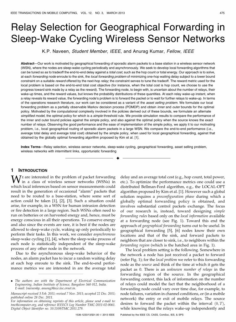
delay and an average total cost (e.g., hop count, total power,etc.). To optimize the performance metrics one could use adistributed Bellman-Ford algorithm, e.g., the LOCAL-OPTalgorithm proposed by Kim et al. [1]. However such a globalsolution requires a preconfiguration phase during which aglobally optimal forwarding policy is obtained, andinvolves substantial control packets exchange. The focusof our research is, instead, toward designing simpleforwarding rules based only on the local information availableat a forwarding node (see Fig. 1). Toward this end theapproach of geographical forwarding turns out to be useful. Ingeographical forwarding [5], [6] nodes know their ownlocations and that of the sink, and forward packets toneighbors that are closer to sink, i.e., to neighbors within theforwarding region (which is the hatched area in Fig. 1).
The local problem setting is the following. Somewhere inthe network a node has just received a packet to forward(refer Fig. 1); for the local problem we refer to this forwardingnode as the source and think of the time at which it gets thepacket as 0. There is an unknown number of relays in theforwarding region of the source. In the geographicalforwarding context, this lack of information on the numberof relays could model the fact that the neighborhood of aforwarding node could vary over time due, for example, tonode failures, variation in channel conditions, or (in a mobilenetwork) the entry or exit of mobile relays. The sourcedesires to forward the packet within the interval ð0; T Þ,while knowing that the relays wake-up independently and
IEEE TRANSACTIONS ON MOBILE COMPUTING, VOL. 12, NO. 3, MARCH 2013 475
. The authors are with the Department of Electrical CommunicationEngineering, Indian Institute of Science, Bangalore 560 012, India.E-mail: {naveenkp, anurag}@ece.iisc.ernet.in.
Manuscript received 3 Feb. 2011; revised 7 Nov. 2011; accepted 22 Dec. 2011;published online 28 Dec. 2011.For information on obtaining reprints of this article, please send e-mail to:[email protected], and reference IEEECS Log Number TMC-2011-02-0061.Digital Object Identifier no. 10.1109/TMC.2011.279.
1536-1233/13/$31.00 � 2013 IEEE Published by the IEEE CS, CASS, ComSoc, IES, & SPS
uniformly over ð0; T Þ. When a neighbor node wakes up, thesource can evaluate it for its use as a relay, e.g., in terms ofthe progress it makes toward the destination node, thequality of the channel to the relay, the energy level of therelay, etc., (see [7], [8] for different routing metrics based onthe above mentioned quantities). We think of this as a rewardoffered by the potential relay. Thus, at each relay wake-upinstant, given the reward values of the relays that havewoken up thus far, the source is faced with the sequentialdecision problem of whether to forward the packet or waitfor further relays to wake-up.
By solving the local problem using a “suitable” rewardmetric, and then applying its solution at each hop toward thesink, we expect to capture the end-to-end problem ofminimizing total delay subject to a constraint on an end-to-end total cost metric (e.g., hop count or total power). Forinstance, if the constraint is on hop count then it is reasonableto choose the local reward metric to be the progress, towardsink, made by a relay. Smaller end-to-end hop count can beachieved by using a larger progress constraint at each hopand vice versa. For total-power constraint we find that usinga combination of one-hop power and progress as a rewardfor the local problem performs well for the end-to-endproblem. We will formally introduce our local forwardingproblem in Section 2 and discuss the end-to-end results inSection 7.2. Next we discuss related work and highlight ourcontributions.
1.1 Related Work
Although our work has been motivated by the geographicalforwarding problem, outlined earlier, the local forwardingproblem that we study also arises during channel selectionin cognitive radio networks. Further, the local problembelongs to the class of asset selling problems, studied in theoperations research literature. For completeness, we reviewthe related literature from these areas as well.
Geographical forwarding problems. In our prior work[4], we have considered a simple model where the numberof relays is a constant which is known to the source. Therethe reward is simply the progress made by a relay nodetoward the sink. In the current work, we have generalizedour earlier model by allowing the number of relays to benot known to the source. Also, here we allow a generalreward structure.
There has been other work in the context of geographicalforwarding and anycast routing, where the problem ofchoosing one among several neighboring nodes arises.Zorzi and Rao [9] propose a distributed relaying algorithm
called Geographical Random Forwarding (GeRaF) whoseobjective is to carry a packet to its destination in as few hopsas possible, by making as large progress as possible at eachrelaying stage. These authors do not consider the tradeoffbetween the relay selection delay and the reward gained byselecting a relay, which is a major contribution of our work.Liu et al. [10] propose a relay selection approach as a part ofCMAC, a protocol for geographical packet forwarding.Under CMAC, node i chooses an r0 that minimizes theexpected normalized latency (which is the average ratio ofone-hop delay and progress). The Random AsynchronousWakeup (RAW) protocol [11] also considers transmitting tothe first node to wake-up that makes a progress of greaterthan a threshold. Interestingly, this is the structure of theoptimal policy for our simplified model in Section 6. Thuswe have provided analytical support for using such athreshold policy.
For a sleep-wake cycling network, Kim et al. [1] haveconsidered the problem of minimizing average end-to-enddelay as a stochastic shortest path problem and havedeveloped a distributed Bellman-Ford algorithm (referredto as the LOCAL-OPT) which yields optimal forwardingstrategies for each node. However a major drawback is thata preconfiguration phase is required to run the LOCAL-OPTalgorithm. We will discuss the work of Kim et al. [1] indetail in Section 7.2.
Channel selection problems. Akin to the relay selectionproblem is the problem of channel selection. The authors in[12], [13] consider a model where there are several channelsavailable to choose from. The transmitter has to probe thechannels to learn their quality. Probing many channels mayyield one with a good gain but reduces the effective time fortransmission within the channel coherence period. Theproblem is to obtain optimal strategies to decide when tostop probing and start transmitting. Here the number ofchannels is known and all the channels are available at thevery beginning of the decision process. In our problemthe number of relays is not known, and they becomeavailable at random times.
Asset selling problems. The basic asset selling problem[14], [15], comprises N offers that arrive sequentially overdiscrete time slots. The offers are independent and identi-cally distributed (iid). As the offers arrive, the seller has todecide whether to take an offer or wait for future ones. Theseller has to pay a cost to observe the next offer. Previousoffers cannot be recalled. The decision process ends with theseller choosing an offer. Over the years, several variants ofthe basic problem have been studied, both with and withoutrecalling the previous offers. Recently Kang [16] hasconsidered a model where a cost has to be paid to recallthe previous best offer. Further, the previous best offer canbe lost at the next time instant with some probability. See[16] for further references to literature on models withuncertain recall. In [17], David and Levi consider a model inwhich the offers arrive at the points of a renewal process. Inthese models, either the number of potential offers is knownor is infinite. In [18], a variant is studied in which the assetselling process can reach a deadline in the next slot withsome fixed probability, provided that the process hasproceeded up to the present slot.
476 IEEE TRANSACTIONS ON MOBILE COMPUTING, VOL. 12, NO. 3, MARCH 2013
Fig. 1. Illustration of the local forwarding problem.
In our work the number of offers (i.e., relays) is notknown. Also the successive instants at which the offersarrive are the order statistics of an unknown number of iiduniform random variables over an interval ð0; T Þ. Afterobserving a relay, the probability that there are no morerelays to go (which is the probability that the present stageis the last one) is not fixed. This probability has to beupdated depending on the previous such probabilities andthe inter wake-up times between the successive relays.Although our problem falls in the class of asset sellingproblems, to the best of our knowledge the particularsetting we have considered in this paper has not beenstudied before.
1.2 Outline and Our Contributions
In Section 2, we formally describe our local forwardingproblem of choosing a relay when the number of relays inthe forwarding region is unknown. We then formulate it asa POMDP in Section 3. Before analysing the POMDP case,in Section 4 we recall, from our earlier work [4], thesolution for the Completely Observable MDP (COMDP)version of the problem where the number of relays in theforwarding region is known to the source. For the POMDP,the optimal policy is characterized in terms of optimumstopping sets (Section 5). The main technical contributionsare as follow:
1. We prove that the optimum stopping sets are convex(Section 5.1), and provide inner (subset, Section 5.2)and outer bounds (superset, Section 5.3) for it.
2. The computational complexity of the above boundsmotivates us to consider a simplified model (Section 6).We prove that the optimal policy for this simplifiedmodel is a simple threshold rule.
3. We first perform one-hop simulations (Section 7.1) tocompare the performance of the various policiesderived out of the analysis. The performance of thesimple policy turns out to be close to optimal.
4. Finally, we simulate a large WSN with sleep-wakecycling nodes and apply our simple policy at eachhop enroute to the sink (Section 7.2). We comparethe average total delay and average total costobtained by the simple policy with that obtainedby a distributed Bellman-Ford algorithm proposedby Kim et al. [1].
For the ease of presentation, we do not provide anyproofs here. An interested reader can refer to our technicalreport [19].
2 LOCAL FORWARDING PROBLEM
Recall that our local problem is motivated by the end-to-end problem of minimizing total delay subject to a totalcost constraint. The total (end-to-end) cost is translatedinto a reward metric for the local problem. Formally, thelocal forwarding problem we consider is the following. Anode in the network has just received a packet to forward.Abusing terminology, we call this node the “source” andthe nodes that it could potentially forward the packet toare called “relays.” The local problem is taken to start attime 0, and some of the associated processes are depictedin Fig. 2.
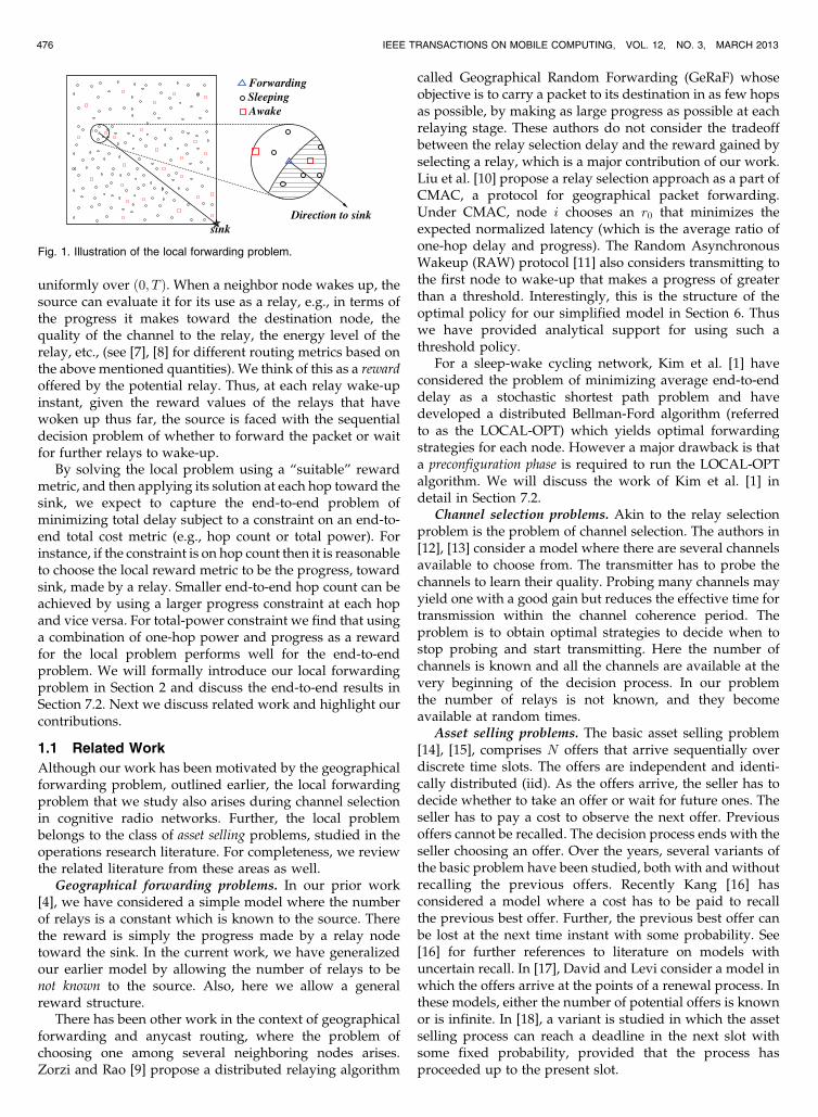
There is a nonempty set of N relay nodes, labeled bythe indices 1; 2; . . . ; N . N is a random variable boundedabove by K, a system parameter that is known to the sourcenode, i.e., the support of N is f1; 2; . . . ; Kg. The source doesnot know N , but knows the bound K, and a probabilitymass function (pmf) p0 on f1; 2; . . . ; Kg, which is the initialpmf of N . A relay node i, 1 � i � N , becomes available tothe source at the instant Ti. The source knows that theinstants fTig are iid uniformly distributed on ð0; T Þ.1 Wecall Ti the wake-up instant of relay i. Given that N ¼ n(throughout this discussion we will focus on the eventðN ¼ nÞ), let W1;W2; . . . ;Wn represent the order statistics ofT1; T2; . . . ; Tn, i.e., the fWkg sequence is the fTig sequencesorted in the increasing order. Let W0 ¼ 0 and define Uk ¼Wk �Wk�1 for k ¼ 1; 2; . . . ; n. Uk are the interwake-up timeinstants between the consecutive nodes (see Fig. 2).
Definition 1. For Simplicity we will use the following notationsto denote the conditional pdf of Ukþ1ðk ¼ 0; 1; . . . ; n� 1Þ andthe conditional expectation (both conditioned on Wk and N),
fkðujw; nÞ :¼ fUkþ1jWk;Nðujw; nÞ;IEk½�jw; n� :¼ IE½�jWk ¼ w;N ¼ n�:
If the source forwards the packet to the relay i, then areward of Ri is accrued. The rewards Ri; i ¼ 1; 2; . . . ; n, areiid random variables with probability density function(pdf) fR. The support of fR is ½0; R�. The source knows thisstatistical characterisation of the rewards, and also that thefRig are independent of the wake-up instants fTig. When arelay wakes up at Ti and reveals its reward Ri, the sourcehas to decide whether to transmit to relay i or to wait forfurther relays. If the source decides to wait, then it instructs therelay with the best reward to stay awake, while letting the rest goback to sleep. This way the source can always forward to arelay with the best reward among those that have wokenup so far.
Since the reward sequence R1; R2; . . . ; Rn is iid andindependent of the wake-up instants T1; T2; . . . ; Tn, we writeðWk;RkÞ as the pairs of ordered wake-up instants and thecorresponding rewards. Evidently, fRkþ1jWk;Nðrjw; nÞ ¼ fRðrÞ
NAVEEN AND KUMAR: RELAY SELECTION FOR GEOGRAPHICAL FORWARDING IN SLEEP-WAKE CYCLING WIRELESS SENSOR... 477
Fig. 2. When there are N ¼ n relays, then, for k ¼ 1; 2; . . . ; n, ðWk;RkÞrepresents the wake-up instant and reward respectively, of the kth relay.
These are shown as points in ½0; T � � ½0; R�.
1. Such a model would arise if each node wakes up periodically withperiod T , and the point processes of the wake up instants across the nodesare stationary and independent versions of the wake-up process withperiod T .
for k ¼ 0; 1; . . . ; n� 1. Further, we define (when N ¼ n)Wnþ1 :¼ T , Unþ1 :¼ ðT �WnÞ, and Rnþ1 :¼ 0. AlsoIEn½Unþ1jw; n� :¼ T � w. All these variables are depicted inFig. 2.
Decision instants and actions. We assume that the timeinstants at which the relays wake-up, i.e., W1;W2; . . . ,constitute the decision instants or stages.2 At each decisioninstant, there are two possible actions available to thesource, denoted 0 and 1, where
. 0 represents the action to continue waiting for morerelays to wake-up, and
. 1 represents the action to stop and forward thepacket to the relay that provides the best rewardamong those that have woken up thus far.
Since there can be at most K relays, the total number ofpossible decision instants is K.
Stopping rules and the optimization problem. If thesource has not forwarded the packet until stage k� 1 thendefine, Ik :¼ ðp0; ðW1; R1Þ; . . . ; ðWk;RkÞÞ to be the informationvector (or the history) available at the source when thekth relay (provided N � k) wakes up. Now, the source’sdecision whether to stop or continue should be based on Ik.Formally, define a stopping rule or a policy, �, as a sequenceof mappings ð�1; . . . ; �KÞ where each �k maps Ik to theaction set f0; 1g. Let � represent the set of all policies.The delay, D�, incurred using policy � is the instant atwhich the source forwards the packet. It could be either oneof the Wk, or the instant T (which is possible if, even at WN ,the source decides to continue, not knowing that it has seenall the relays). The reward R� is the reward associated withthe relay to which the packet is forwarded. It is possiblefor the source to maximize the reward by waiting until timeT (incurring maximum delay) and then choosing the bestrelay. On the other hand, the source can minimize the delayby forwarding to the first relay, irrespective of its rewardvalue, but at the expense of depriving itself of anopportunity to choose a better relay that could wake-uplater. Thus, there is a tradeoff between these two quantitieswhich we are interested in studying. Formally, the problemwe are interested in is the following,
min�2�
IED�
Subject to IER� � �:ð1Þ
We introduce a Lagrange multiplier � > 0 and considersolving the following unconstrained problem
min�2�ðIED� � �IER�Þ: ð2Þ
The following lemma relates both the problems:
Lemma 1. Let �� be an optimal policy for the unconstrainedproblem in (2). Suppose the chosen � is such that IER�� ¼ �,then �� is optimal for the main problem in (1) as well.
Proof. See [19, Lemma 1]. tu
3 POMDP FORMULATION
With the number of relays being unknown, the natural
approach is to formulate the problem as a partiallyobserved Markov decision process (POMDP). A POMDP
is a generalization of an MDP, where at each stage theactual internal state of the system is not available to the
controller. Instead, the controller can observe a value from
an observation space. The observation probabilisticallydepends on the current actual state and the previous action.
In some cases, a POMDP can be converted to an equivalent
MDP by regarding a belief (i.e., a probability distribution)on the state space as the state of the equivalent MDP. For a
survey of POMDPs see [20], [21, ch. 5]. In this section, we
will set up the unconstrained problem in (2) as a POMDP.
3.1 Belief State and Belief State Transition
Since the source does not know the actual number of relaysN , the state is only partially observable. As mentioned
earlier the source’s decision should be based on the entire
history of the information vector Ik ¼ ðp0; ðw1; b1Þ; . . . ;
ðwk; bkÞÞ where w1; . . . ; wk represents the wake-up instants
of relays waking up at stages 1; . . . ; k, and b1; . . . ; bk are the
corresponding best rewards. Define pk to be the belief state
about N at stage k given the information vector Ik, i.e.,
pkðnÞ ¼ IPðN ¼ njIkÞ for n ¼ k; kþ 1; . . . ; K (note that pkðkÞis the probability that the kth relay is the last one). Thus, pk is
a pmf in the K � k dimensional probability simplex. Let us
denote this simplex as Pk.Definition 2. For k ¼ 1; 2; . . . ; K, let Pk :¼ set of all pmfs on
the set fk; kþ 1; . . . ; Kg. Pk is the K � k dimensional
probability simplex in <K�kþ1.
The “observation” ðwk; bkÞ at stage k is a part of the actual
state ðN;wk; bkÞ. For a general POMDP problem theobservation can belong to a completely different space than
the actual state space. Moreover the distribution of the
observation at any stage can in general depend on all theprevious states, observations, actions, and disturbances.
Suppose this distribution depends only on the state, action,
and disturbance of the immediately preceding stage, then abelief on the actual state given the entire history turns out to
be sufficient for taking decisions [21, ch. 5]. For our case,
this condition is met and hence at stage k, ðpk; wk; bkÞ is asufficient statistic to take decision. Hence, the state space at
stage k ¼ 1; 2; . . . ; K, for our POMDP problem is
Sk ¼ fðp; w; bÞ : p 2 Pk; w 2 ð0; T �; b 2 ½0; R�g [ f g; ð3Þ
with the initial state (i.e., state at stage 0) being ðp0; 0; 0Þ.Here is the terminating state. The state at stage k will be , if the source has already forwarded the packet at an
earlier stage. The decision process ends once the system
enters .After seeing k relays, suppose the source chooses not to
forward the packet, then upon the next relay waking up
(if any), the source needs to update its belief about the
number of relays. Formally, if ðp; w; bÞ 2 Sk is the state atstage k and ðwþ uÞ is the wake-up instant of the next relay
then, using Bayes rule, the next belief state can be obtained
478 IEEE TRANSACTIONS ON MOBILE COMPUTING, VOL. 12, NO. 3, MARCH 2013
2. A better choice for the decision instants may be to allow the source totake decision at any time t 2 ð0; T �. When N is known to the source it can beargued that it is optimal to take decisions only at relay wake-up instances.However, this may not hold for our case where N is unknown. In thispaper, we proceed with our restriction on the decision instants and considerthe general case as a topic for future work.
via the following belief state transition function which yieldsa pmf in Pkþ1,
�kþ1ðp; w; uÞðnÞ ¼pðnÞfkðujw; nÞPK‘¼kþ1 pð‘Þfkðujw; ‘Þ
; ð4Þ
for n ¼ kþ 1; . . . ; K. Note that this function does notdepend on b. Thus, if at stage k 2 f0; 1; . . . ; K � 1g, thestate is ðp; w; bÞ 2 Sk, then the next state is
skþ1 ¼ ; if w ¼ T and=or ak ¼ 1;ð�kþ1ðp; w; Ukþ1Þ; wþ Ukþ1;maxfb; Rkþ1gÞ;otherwise:
8<: ð5Þ
When the action ak ¼ 1 the source enters . Further thesource decides to stop (i.e., enter ) even when w ¼ T . Thisis because it knows that the wake-up time of each relay isstrictly less than T . Such a situation can arise when, atstage k, the actual number of relays happened to be k andthe source decides to continue (possible because the sourcedoes not know the actual number). Then the source will endup waiting until time T and then transmit to the relay withthe best reward.
3.2 One-Step Costs
The objective in (2) can be seen as accumulating additivelyover each step. If the decision at a stage is to continue thenthe delay until the next relay wakes up (or until T ) getsadded to the cost. On the other hand if the decision is tostop then the source collects the reward offered by the relayto which it forwards the packet and the decision processenters the state . The cost in state is 0. Suppose ðp; w; bÞ isthe state at stage k. Then the one-step-cost function is, fork ¼ 0; 1; . . . ; K � 1,
gkððp; w; bÞ; akÞ ¼��b; if w ¼ T and=or ak ¼ 1;Ukþ1; otherwise:
�ð6Þ
The cost of termination is gKðp; w; bÞ ¼ ��b. Also note thatfor k ¼ 0, the possible state is ðp0; 0; 0Þ and the only possibleaction is a0 ¼ 1, so that g0ððp; 0; 0Þ; a0Þ ¼ U1. Note that, for agiven policy � if sk represent the state at stage k then,PK
k¼0 gkðsk; �kðskÞÞ ¼ D� � �R�.
3.3 Optimal Cost-to-Go Functions
For k ¼ 1; 2; . . . ; K, let Jkð�Þ represent the optimal cost-to-gofunction at stage k. For any state sk 2 Sk, JkðskÞ can bewritten as
JkðskÞ ¼ minfstopping cost; continuing costg; ð7Þ
where stopping cost (continuing cost) represents the averagecost incurred, if the source, at the current stage decides tostop (continue), and takes optimal action at the subsequentstages. For the termination state, since the one step cost iszero and since the system remains in in all the subsequentstages, we have Jkð Þ ¼ 0. For a state ðp; w; bÞ 2 Sk, we nextevaluate the two costs.
First let us obtain the stopping cost. Suppose that therewere K relay nodes and the source has seen them all. Insuch a case if ðp; w; bÞ 2 SK (note that p will just be apoint mass on K) is the state at stage K then the optimalcost is simply the cost of termination, i.e., JKðp; w; bÞ ¼gKðp; w; bÞ ¼ ��b. For k ¼ 1; 2; . . . ; K � 1, if the action is to
stop then the one step cost is ��b and the next state is sothat the further cost is Jkþ1ð Þ ¼ 0. Therefore, the stoppingcost at any stage is simply ��b.
On the other hand the cost for continuing, when the stateat stage k is ðp; w; bÞ 2 Sk, using the total expectation law,can be written as
ckðp; w; bÞ ¼ pðkÞðT � w� �bÞ þXKn¼kþ1
pðnÞck;nðp; w; bÞ; ð8Þ
where ck;nðp; w; bÞ is the average cost to continue condi-tioned on the event ðN ¼ nÞ, the probability of which ispðnÞ. The expression for ck;nðp; w; bÞ is
ck;nðp; w; bÞ ¼ IEk½Ukþ1 þ Jkþ1ð�kþ1ðp; w; Ukþ1Þ; wþ Ukþ1;maxfb; Rkþ1gÞjw; n�:
ð9Þ
In the above expression, Ukþ1 is the (random) time until thenext relay wakes up (Ukþ1 is the one step cost) and Jkþ1ð�Þ isthe optimal cost-to-go from the next stage onwards (Jkþ1ð�Þconstitutes the future cost). The next state is obtained via thestate transition equation (5).
The term ðT � w� �bÞ in (8) associated with pðkÞ is thecost of continuing when the number of relays happen to bek, i.e., ðN ¼ kÞ and there are no more relays to go. Recallthat we had defined (in Section 2) Ukþ1 ¼ T � w and Rkþ1 ¼0 when the actual number of relays is N ¼ k. Therefore,T � w is the one step cost when N ¼ k. Also wþ Ukþ1 ¼ Tand maxfb; Rkþ1g ¼ b so that at the next stage (which occursat T ) the process will terminate (enter ) with a cost of ��b(see (5) and (6)), which represents the future cost.
Thus the optimal cost-to-go function (7) at stagek ¼ 1; 2; . . . ; K � 1, can be written as
Jkðp; w; bÞ ¼ minf��b; ckðp; w; bÞg: ð10Þ
From (10), it is clear that at stage k when the state isðp; w; bÞ, the source has to compare the stopping cost, ��b,with the cost of continuing, ckðp; w; bÞ, and stop iff��b � ckðp; w; bÞ. Later in Section 5, we will use thiscondition (��b � ckðp; w; bÞ) and define, the optimum stop-ping set. We will prove that the continuing cost, ckðp; w; bÞ,is concave in p, leading to the result that the optimumstopping set is convex. Equations (8) and (10) areextensively used in the subsequent development.
4 RELATIONSHIP WITH THE CASE WHERE N IS
KNOWN (THE COMDP VERSION)
In the previous section (Section 3), we detailed our problemformulation as a POMDP. The state is partially observablebecause the source does not know the exact number ofrelays. It is interesting to first consider the simpler casewhere this number is known, which is the contribution ofour earlier work in [4]. Hence, in this section, we willconsider the case when the initial pmf, p0, has all the massonly on some n, i.e., p0ðnÞ ¼ 1. We call this, the COMDPversion of the problem.
First we define a sequence of threshold functions whichwill be useful in the subsequent proofs. These are the samethreshold functions that characterize the optimal policy forour model in [4].
NAVEEN AND KUMAR: RELAY SELECTION FOR GEOGRAPHICAL FORWARDING IN SLEEP-WAKE CYCLING WIRELESS SENSOR... 479
Definition 3. For ðw; bÞ 2 ð0; T Þ � ½0; R�, define f�‘ : ‘ ¼0; 1; . . . ; K � 1g inductively as follows: for all ðw; bÞ �0 ðw;bÞ ¼ 0 and for ‘ ¼ 1; 2; . . . ; K � 1 (recall Definition 1),
�‘ðw; bÞ ¼
IEK�‘ maxfb; R; �‘�1ðwþ U;maxfb; RgÞg � U�
����w;K� �
:ð11Þ
In the above expression, we have suppressed the subscriptK � ‘þ 1 from R and U for notational simplicity. The pdfused to take the expectation in the above expression isfRð�ÞfK�‘ð�jw;KÞ (again recall Definition 1).
We will need the following simple property of thethreshold functions in a later section.
Lemma 2. For ‘ ¼ 1; 2; . . . ; K � 1, ���‘ðw; bÞ � ðT � w� �bÞ.Proof. See [19, Appendix I.A], which can be found on the
Computer Society Digital Library at http://doi.ieeecomputersociety.org/10.1109/TMC.2011.279. tu
Next, we state the main lemma of this section. We callthis the One-point Lemma, because it gives the optimal cost,Jkðpk; w; bÞ, at stage k when the belief state pk 2 Pk is suchthat it has all the mass on some n � k.
Lemma 3 (One-Point). Fix some n 2 f1; 2; . . . ; Kg andðw; bÞ 2 ð0; T Þ � ½0; R�. For any k ¼ 1; 2; . . . ; n, if pk 2 Pkis such that pkðnÞ ¼ 1 then
Jkðpk; w; bÞ ¼ minf��b;���n�kðw; bÞg:
Proof. The proof is by induction. We make use of the factthat if at some stage k < n the belief state pk is such thatpkðnÞ ¼ 1 then the next belief state pkþ1ð2 Pkþ1Þ, obtainedby using the belief transition (4), is also of the formpkþ1ðnÞ ¼ 1. We complete the proof by using Definition 3and the induction hypothesis. For a complete proof, see[19, Appendix I.B], which is available in the onlinesupplemental material. tu
Discussion of Lemma 3. At stage k if the state is ðpk; w; bÞ,where pk is such that pkðnÞ ¼ 1 for some n � k, then fromthe One-point Lemma it follows that the optimal policy is tostop and transmit iff b � �n�kðw; bÞ. The subscript n� k ofthe function �n�k signifies the number of more relays to go.For instance, if we know that there are exactly four morerelays to go then the threshold to be used is �4. Suppose atstage k if it was optimal to continue, then from (4) it followsthat the next belief state pkþ1 2 Pkþ1 also has mass only onðN ¼ nÞ and hence at this stage it is optimal to use thethreshold function �n�ðkþ1Þ. Therefore, if we begin with aninitial belief p0 2 P1 such that p0ðnÞ ¼ 1 for some n, then theoptimal policy is to stop at the first stage k such that b ��n�kðw; bÞ where Wk ¼ w is the wake-up instant of thekth relay and Bk ¼ maxfR1; . . . ; Rkg ¼ b. Note that, since atstage n the threshold to be used is �0ðw; bÞ ¼ 0 (seeDefinition 3), we invariably have to stop at stage n if wehave not terminated earlier. This is exactly the same as ouroptimal policy in [4], where the number of relays is knownto the source (instead of knowing the number wp1, as inour One-point Lemma here).
5 POMDP VERSION: BOUNDS ON THE OPTIMUM
STOPPING SET
In this section, we will consider the general case developed
in Section 3 where the number of relays N is not known tothe source. There are several algorithms available to exactlyobtain the optimal policy for a POMDP problem when the
actual state space is finite [22], starting from the seminalwork of Smallwood and Sondik [23]. However when thenumber of states is large, these algorithms are computa-tionally intensive. In general, it is not easy to obtain an
optimal policy for a POMDP. In this section, we havecharacterized the optimal policy in terms of optimum
stopping sets and prove inner and outer bounds for this set.
Definition 4 (Optimum Stopping Set). For 1 � k � K � 1,
let Ckðw; bÞ ¼ fp 2 Pk : ��b � ckðp; w; bÞg. Referring to (11)
it follows that, for a given ðw; bÞ, Ckðw; bÞ represents the set of
all beliefs p 2 Pk at stage k at which it is optimal to stop. We
call Ckðw; bÞ the optimum stopping set at stage k when the
delay (Wk) and best reward (Bk) values are w and b,
respectively.
5.1 Convexity of the Optimum Stopping Sets
We will prove (in Lemma 4) that the continuing cost,ckðp; w; bÞ, in (9) is concave in p 2 Pk. From the form of the
stopping set Ckðw; bÞ, a simple consequence of this lemmawill be that the optimum stopping set is convex. We furtherextend the concavity result of ckðp; w; bÞ for p 2 Pk, where
Pk is the affine set containing Pk (to be defined shortly inthis section).
Lemma 4. For k ¼ 1; 2; . . . ; K � 1, and any given ðw; bÞ, the
cost of continuing (defined in (9)), ckð�; w; bÞ, is concave on Pk.Proof. The essence of the proof is same as that in [24,
Lemma 1]. Formal proof is available in our technical
report [19, Appendix II.A], which is available in theonline supplemental material. tu
The following theorem is a straight forward application
of the above lemma.
Theorem 1. For k ¼ 1; 2; . . . ; K � 1, and any given ðw; bÞ,Ckðw; bÞð PkÞ is a convex set.
Proof. From Lemma 4 we know that ckðp; w; bÞ is a concavefunction of p 2 Pk. Hence, Ckðw; bÞ (see Definition 4), beinga super level set of a concave function, is convex [25]. tu
In the next section while proving an inner bound forthe stopping set Ckðw; bÞ, we will identify a set of pointsthat could lie outside the probability simplex Pk. We can
obtain a better inner bound if we extend the concavityresult to the affine set, Pk ¼ fp 2 <K�kþ1 : p;1h i ¼ 1g,where p;1h i ¼
PKn¼k pðnÞ, i.e., in Pk the vectors sum to
one, but we do not require nonnegativity of the vectors.
This can be done as follows: define �kþ1ðp; w; uÞ using (4)for every p 2 Pk. Then �kþ1ð:; w; uÞ as a function of p, is theextension of �kþ1ð:; w; uÞ from Pk to Pk. Similarly, for every
p 2 Pk, define ckðp; w; bÞ and Jkðp; w; bÞ using (9) and (10).These are the extensions of ckð�; w; bÞ and Jkð�; w; bÞ,
480 IEEE TRANSACTIONS ON MOBILE COMPUTING, VOL. 12, NO. 3, MARCH 2013
respectively. Then again, using the proof technique sameas that in Lemma 4, we can obtain the following lemma,
Lemma 5. For k ¼ 1; 2; . . . ; K � 1, and any given ðw; bÞ,ckð�; w; bÞ is concave on the affine set Pk.
Using the above lemma, Ckðw; bÞ can be written as
Ckðw; bÞ ¼ Pk \ fp 2 <K�kþ1 : p;1h i ¼ 1
� �b � ckðp; w; bÞg:ð12Þ
5.2 Inner Bound on the Optimum Stopping Set
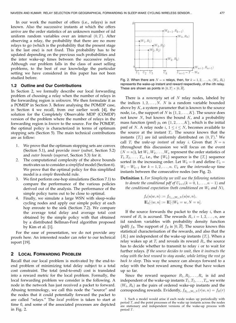
We have showed that the optimum stopping set is convex.In this section, we will identify points that lie along certainedges of the simplex Pk. A convex hull of these points willyield an inner bound to the optimum stopping set. This willfirst require us to prove the following lemma, referred to asthe Two-point Lemma, and is a generalization of the One-point Lemma (Lemma 3). It gives the optimal cost,Jkðp; w; bÞ, at stage k when p 2 Pk is such that it places allits mass on k and on some n > k, i.e., pðkÞ þ pðnÞ ¼ 1.Throughout this and the next section (on an outer bound)ðWk;BkÞ ¼ ðw; bÞ is fixed and hence, for the ease ofpresentation (and readability), we drop ðw; bÞ from thenotations �‘ðw; bÞ, a‘kðw; bÞ, and b‘kðw; bÞ (to appear in thesesections later). However, it is understood that these thresh-olds are, in general, functions of ðw; bÞ.Lemma 6 (Two-Points). For k ¼ 1; 2; . . . ; K � 1, if p 2 Pk is
such that pðkÞ þ pðnÞ ¼ 1, where k < n � K then
Jkðp; w; bÞ ¼ minf��b; pðkÞðT � w� �bÞþ pðnÞð���n�kðw; bÞÞg:
Proof. Available in our technical report [19, Lemma 5]. tu
Discussion of Lemma 6. The Two-point Lemma (Lemma 6)can be used to obtain certain threshold points in thefollowing way. When p 2 Pk has mass only on k and onsome n, k < n � K, then using Lemma 6, the continuingcost can be written as a function of pðnÞ as
ckðp; w; bÞ ¼ ðT � w� �bÞ� pðnÞðT � w� �ðb� �n�kðw; bÞÞÞ:
ð13Þ
From Lemma 2, it follows that ckðp; w; bÞ in (13) is adecreasing function of pðnÞ. Let p
ðkÞk and p
ðnÞk be pmfs in Pk
with mass only on N ¼ k and N ¼ n, respectively. These aretwo of the corner points of the simplex Pk (as an example,
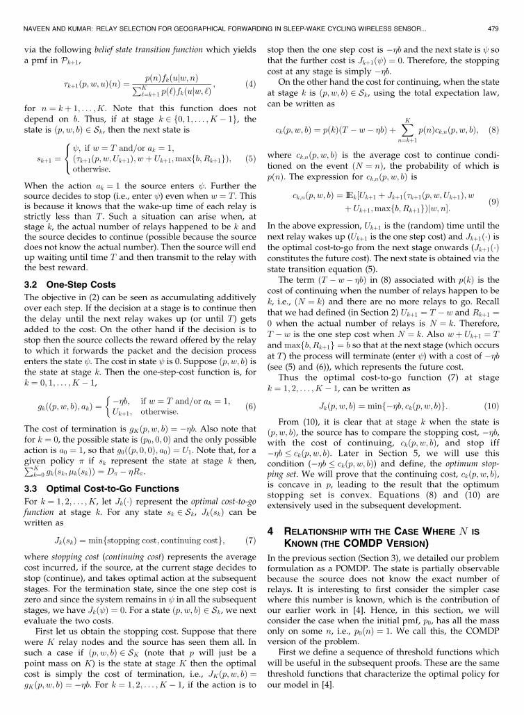
Fig. 3a illustrates the simplex and the corner points for stagek ¼ K � 2. With at most two more nodes to go, PK�2 is a 2Dsimplex in <3. p
ðK�2ÞK�2 , p
ðK�1ÞK�2 , and p
ðKÞK�2 are the corner points
of this simplex).At stage k as we move along the line joining the points
pðkÞk and p
ðnÞk (Figs. 3b and 3c illustrate this as pðnÞ going
from 0 to 1), the cost of continuing in (13) decreases andthere is a threshold below which it is optimal to transmitand beyond which it is optimal to continue. The value ofthis threshold is that value of pðnÞ in (13) at which thecontinuing cost becomes equal to ��b. Let �n�k denote thisthreshold value, then
�n�k ¼T � w
T � w� �ðb� �n�kðw; bÞÞ:
The cost of continuing in (13) as a function of pðnÞ alongwith the stopping cost, ��b, is shown in Figs. 3b and 3c. Thethreshold �n�k is the point of intersection of these two costfunctions. The value of the continuing cost ckðp; w; bÞ atpðnÞ ¼ 1 is ���n�kðw; bÞ. Note that in the case when b >
�n�kðw; bÞ the threshold �n�k will be greater than 1 in whichcase it is optimal to stop for any p on the line joining p
ðkÞk
and pðnÞk .
There are similar thresholds along each edge of thesimplex Pk starting from the corner point p
ðkÞk . In general, let
us define for ‘ ¼ 1; 2; . . . ; K,
�‘ ¼T � w
T � w� �ðb� �‘ðw; bÞÞ: ð14Þ
Remark. Note that (13) will also hold for the extendedfunction ckðp; w; bÞ, where now p 2 Pk. In terms of theextended function, �n�k represents the value of pðnÞ (in(13) with ck replaced by ck) at which ckðp; w; bÞ ¼ ��b.
Recall that (from Lemma 6) the above discussion began
with a p 2 Pk such that pðkÞ þ pðnÞ ¼ 1. At the threshold of
interest we have pðnÞ ¼ �n�k and hence pðkÞ ¼ 1� �n�k, and
the rest of the components are zero. We denote this vector
as an�kk . For instance in Fig. 4, where the face of the 2D
simplex PK�2 is shown, the threshold along the lower edge
of the simplex is a1K�2 ¼ ½1� �1; �1; 0� and that along the
other edge is a2K�2 ¼ ½1� �2; 0; �2�. Since it is possible for
�n�k > 1, therefore the vector threshold an�kk is not restricted
to lie in the simplex Pk, however it always stays in the affine
set Pk. We formally define these thresholds next.
NAVEEN AND KUMAR: RELAY SELECTION FOR GEOGRAPHICAL FORWARDING IN SLEEP-WAKE CYCLING WIRELESS SENSOR... 481
Fig. 3. (a) Probability simplex, PK�2 at stage K � 2. A belief at stage K � 2 is a pmf on the points K � 2, K � 1 and K (i.e., no-more, one-more andtwo-more relays to go, respectively). Thus PK�2 is a 2D simplex in <3. (b) and (c): ckðp; w; bÞ in (13) is plotted as a function of pðnÞ. Also shown is theconstant function ��b which is the stopping cost. �n�k is the point of intersection of these two functions. (b) When b � �n�k. (c) When b > �n�kðw; bÞ.
Definition 5. For a given k 2 f1; 2; . . . ; K � 1g, for each ‘ ¼1; 2; . . . ; K � k define a‘k as a K � kþ 1 dimensional pointwith the first and the ‘þ 1th components equal to 1� �‘ and�‘, respectively, the rest of the components are zeros. Asmentioned before, a‘k lies on the line joining p
ðkÞk and p
ðkþ‘Þk . At
stage k there are K � k such points, one corresponding to eachedge in Pk emanating from the corner point p
ðkÞk . For an
illustration of these points see Fig. 4 for the case k ¼ K � 2.
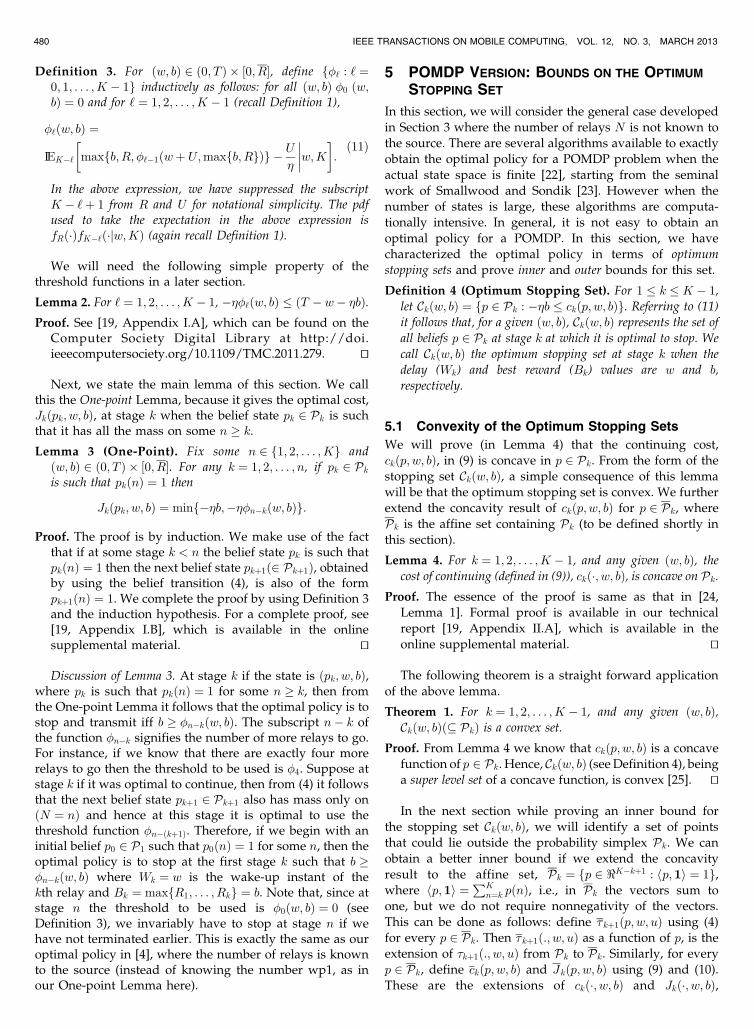
Referring to Fig. 4a (which depicts the case, k ¼ K � 2),suppose all the vector thresholds, alk, lie within the simplexPk then, since at these points the stopping cost ð��bÞ isequal to the continuing cost (ckðalk; w; bÞ), all these pointslie in the optimum stopping set Ckðw; bÞ. Note that thecorner point p
ðkÞk (belief with all the mass on no-more
relays to go) also lies in Ckðw; bÞ. Since we have alreadyshown that Ckðw; bÞ is convex, the convex hull of thesepoints will yield an inner bound. However as mentionedearlier (and as depicted in Figs. 4b and 4c) it is possible forsome or all the thresholds alk to lie outside the simplex(and hence these thresholds do not belong to Ckðw; bÞ). Thisis where we will use Lemma 5, where the concavity resultof the continuing cost, ckðp; w; bÞ, is extended to the affineset Pk. We next state this inner bound theorem.
Theorem 2 (Inner Bound). For k ¼ 1; 2; . . . ; K � 1, recallingthat p
ðkÞk is the pmf in Pk with point mass on k, define
Ckðw; bÞ :¼ Pk \ conv�pðkÞk ; a1
k; . . . ; aK�kk
�;
where conv denotes the convex hull of the given points. Then,Ckðw; bÞ Ckðw; bÞ.
Proof. See our technical report [19, Theorem 1]. tu
In Fig. 4, for stage k ¼ K � 2, we illustrate the variouscases that can arise. In each of the figures the shaded
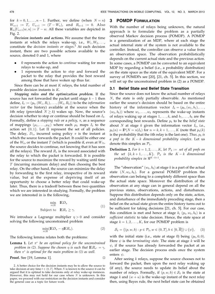
region is the inner bound. In Fig. 4a, all the thresholdslie within the simplex and simply the convex hull of thesepoints gives the inner bound. When some or all thethresholds lie outside the simplex, as in Figs. 4b and 4c,then the inner bound is obtained by intersecting theconvex hull of the thresholds with the simplex. In Fig. 4c,where all the thresholds lie outside the simplex, the innerbound is the entire simplex, PK�2, so that at stage K � 2with ðWK�2; BK�2Þ ¼ ðw; bÞ it is optimal to stop for anybelief state.
5.3 Outer Bound on the Optimum Stopping Set
In this section, we will obtain an outer bound (a superset)for the optimum stopping set. Again, as in the case of theinner bound, we will identify certain threshold pointswhose convex hull will contain the optimum stopping set.This will require us to first prove a monotonicity resultwhich compares the cost of continuing at two belief statesp; q 2 Pk which are ordered, for instance for k ¼ K � 2, asin Fig. 4d. q in Fig. 4d is such that qðK � 2Þ ¼ pðK � 2Þ(i.e., the probability that there is no-more relays to go issame in both p and q) and qðK � 1Þ ¼ 1� pðK � 2Þ (i.e., allthe remaining probability in q is on the event that there isone-more relay to go, while in p it can be on one-more ortwo-more relays to go). Thus q lies on the lower edge ofthe simplex. We will show that the cost of continuing at pis less than that at q.
Lemma 7. Given p 2 Pk for k ¼ 1; 2; . . . ; K � 1, define qðkÞ ¼pðkÞ and qðkþ 1Þ ¼ 1� pðkÞ, then ckðp; w; bÞ � ckðq; w; bÞfor any ðw; bÞ.
Proof. See [19, Appendix II.B], which is available in theonline supplemental material. tu
Discussion of Lemma 7. This lemma proves the intuitiveresult that the continuing cost with a pmf p that gives masson a larger number of relays should be smaller than with apmf q that concentrates all such mass in p on just one morerelay to go. With more relays, the cost of continuing isexpected to decrease.
Similar to the thresholds a‘k we define the thresholds b‘kthat lie along certain edges of the simplex. We will identifythe threshold a‘k that is at a maximum distance from thecorner point p
ðkÞk (in Fig. 4d, this point is a1
K�2 ¼ ½1� �1; �1; 0�).Next, we define the thresholds b‘k to be the points on theedges emanating from p
ðkÞk , which are at this same distance.
Thus in Fig. 4d, b1K�2 ¼ a1
K�2 and b2K�2 ¼ ½1� �1; 0; �1�.
Definition 6. For a given k 2 f1; 2; . . . ; K � 1g, let ‘max ¼arg max‘¼1;2;...;K�k�‘. Now for ‘ ¼ 1; 2; . . . ; K � k define b‘kas a K�kþ 1 dimensional point with the first and the ‘þ 1th
components equal to 1� �‘max and �‘max , respectively, the rest
of the components are zeros. Each of the b‘k are at equal
distance from pðkÞk but on a different edge starting from p
ðkÞk .
Using Lemma 7, we show that the convex hull of thethresholds blk along with the corner point p
ðkÞk constitutes an
outer bound for the optimum stopping set. The idea of theproof can be illustrated using Fig. 4d. p in Fig. 4d is outsidethe convex hull and q is obtained from p as in Lemma 7. At qit is optimal to continue since it is beyond the threshold
482 IEEE TRANSACTIONS ON MOBILE COMPUTING, VOL. 12, NO. 3, MARCH 2013
Fig. 4. Illustration of the inner and outer bounds. In all the above figures,only the face of the simplex, PK�2 (in Fig. 3a) is shown. The shadedregions in (a), (b), and (c) are the inner bound when (a) �1 and �2 areboth less than 1 (b) �1 > 1 and �2 < 1 and (c) �1 > 1 and �2 > 1,respectively. The outer bound is the union of the light and the darkshaded regions in (d).
a1K�2 and hence the continuing cost at q, ckðq; w; bÞ, is less
than the stopping cost ��b. From Lemma 7 it follows thatthe continuing cost at p, ckðp; w; bÞ, is also less than ��bso that it is optimal to continue at p as well, proving that pdoes not belong to the optimum stopping set. Thus theconvex hull contains the optimum stopping set. Weformally state and prove this outer bound theorem next.
Theorem 3 (Outer Bound). For k ¼ 1; 2; . . . ; K � 1, define
Ckðw; bÞ ¼ Pk \ conv�pðkÞk ; b1
k; . . . ; bK�kk
�:
Then, Ckðw; bÞ Ckðw; bÞ.Proof. See [19, Theorem 2]. tu
The outer bound for k ¼ K � 2 is illustrated in Fig. 4d.The light shaded region is the inner bound. The outerbound is the union of the light and the dark shadedregions. The boundary of the optimum stopping set fallswithin the dark shaded region. For any p within the innerbound we know that it is optimal to stop and for any poutside the outer bound it is optimal to continue. We areuncertain about the optimal action for belief states withinthe dark shaded region.
6 RELAY SELECTION IN A SIMPLIFIED MODEL
The bounds obtained in the previous section require us to
compute the thresholds f�‘ : ‘ ¼ 0; 1; . . . ; K � 1g (see Defi-
nition 3) recursively. These are computationally very
intensive to obtain. Hence, in this section we simplify the
exact model and extract a simple selection rule. Our aim is
to apply this simple rule to the exact model and compare its
performance with the other policies.
6.1 The Simplified Model
Now we describe our simplified model. There are ~N relays.
Here, ~N is a constant and is known to the source. The key
simplification in this model is that here the relay nodes
wake-up at the first ~N points of a Poisson process of rate~NT . The
following are the motivations for considering such a
simplification. Note that in our actual model (Section 2),
when N ¼ ~N , the inter wake-up times fUk : 1 � k � ~Ng are
identically distributed [26, ch. 2], but not independent.
Their common cumulative distribution function (cdf) is
FUkjNðuj ~NÞ ¼ 1� ð1� uTÞ
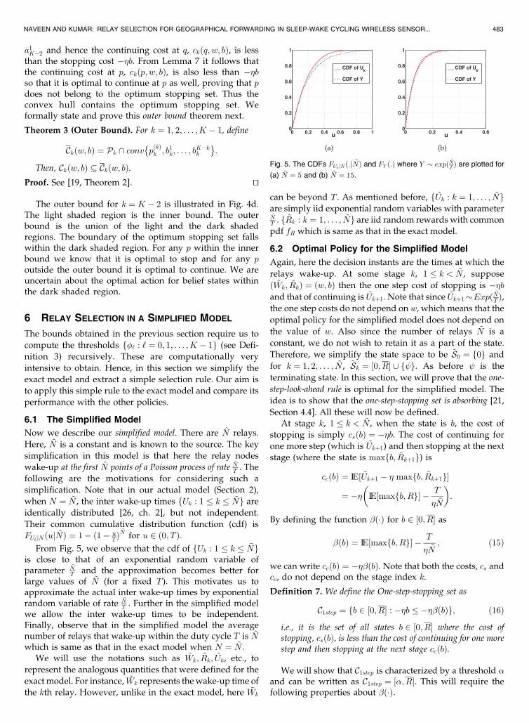
~N for u 2 ð0; T Þ.From Fig. 5, we observe that the cdf of fUk : 1 � k � ~Ng
is close to that of an exponential random variable ofparameter
~NT and the approximation becomes better for
large values of ~N (for a fixed T ). This motivates us toapproximate the actual inter wake-up times by exponentialrandom variable of rate
~NT . Further in the simplified model
we allow the inter wake-up times to be independent.Finally, observe that in the simplified model the averagenumber of relays that wake-up within the duty cycle T is ~Nwhich is same as that in the exact model when N ¼ ~N .
We will use the notations such as ~Wk; ~Rk; ~Uk, etc., to
represent the analogous quantities that were defined for the
exact model. For instance, ~Wk represents the wake-up time of
the kth relay. However, unlike in the exact model, here ~Wk
can be beyond T . As mentioned before, f ~Uk : k ¼ 1; . . . ; ~Ngare simply iid exponential random variables with parameter~NT . f ~Rk : k ¼ 1; . . . ; ~Ng are iid random rewards with common
pdf fR which is same as that in the exact model.
6.2 Optimal Policy for the Simplified Model
Again, here the decision instants are the times at which the
relays wake-up. At some stage k, 1 � k < ~N , suppose
ð ~Wk; ~RkÞ ¼ ðw; bÞ then the one step cost of stopping is ��band that of continuing is ~Ukþ1. Note that since ~Ukþ1Expð ~N
T Þ,the one step costs do not depend on w, which means that the
optimal policy for the simplified model does not depend on
the value of w. Also since the number of relays ~N is a
constant, we do not wish to retain it as a part of the state.
Therefore, we simplify the state space to be ~S0 ¼ f0g and
for k ¼ 1; 2; . . . ; ~N , ~Sk ¼ ½0; R� [ f g. As before is the
terminating state. In this section, we will prove that the one-
step-look-ahead rule is optimal for the simplified model. The
idea is to show that the one-step-stopping set is absorbing [21,
Section 4.4]. All these will now be defined.
At stage k, 1 � k < ~N , when the state is b, the cost of
stopping is simply csðbÞ ¼ ��b. The cost of continuing for
one more step (which is ~Ukþ1) and then stopping at the next
stage (where the state is maxfb; ~Rkþ1g) is
ccðbÞ ¼ IE½ ~Ukþ1 � � maxfb; ~Rkþ1g�
¼ �� IE½maxfb; Rg� � T
� ~N
� :
By defining the function ð�Þ for b 2 ½0; R� as
ðbÞ ¼ IE½maxfb; Rg� � T
� ~N; ð15Þ
we can write ccðbÞ ¼ ��ðbÞ. Note that both the costs, cs andcc, do not depend on the stage index k.
Definition 7. We define the One-step-stopping set as
C1step ¼ fb 2 ½0; R� : ��b � ��ðbÞg; ð16Þ
i.e., it is the set of all states b 2 ½0; R� where the cost ofstopping, csðbÞ, is less than the cost of continuing for one morestep and then stopping at the next stage ccðbÞ.
We will show that C1step is characterized by a threshold and can be written as C1step ¼ ½;R�. This will require thefollowing properties about ð�Þ.
NAVEEN AND KUMAR: RELAY SELECTION FOR GEOGRAPHICAL FORWARDING IN SLEEP-WAKE CYCLING WIRELESS SENSOR... 483
Fig. 5. The CDFs FUk jN ð:j ~NÞ and FY ð:Þ where Y expð ~NT Þ are plotted for
(a) ~N ¼ 5 and (b) ~N ¼ 15.
Lemma 8.
1. is continuous, increasing and convex in b.2. If ð0Þ < 0, then ðbÞ < b for all b 2 ½0; R�.3. If ð0Þ � 0, then 9 a unique such that ¼ ðÞ.4. If ð0Þ � 0, then ðbÞ < b for b 2 ð;R� and ðbÞ > b
for b 2 ½0; Þ.Proof. See our technical report [19, Appendix III.A], which
is available in the online supplemental material. tu
Discussion of Lemma 8. When ð0Þ � 0 then usingLemmas 8.3 and 8.4, we can write C1step in (16) asC1step ¼ ½;R�. For the other case where ð0Þ < 0, fromLemma 8.2 it follows that C1step ¼ ½0; R�. Thus by defining ¼ 0 whenever ð0Þ < 0 we can write C1step ¼ ½;R� foreither case.
Definition 8. Depending on the value of ð0Þ, define asfollows: ¼ ðÞ if ð0Þ � 0. Otherwise fix ¼ 0.
Definition 9. A policy is said to be one-step-look-ahead if at stagek, 1 � k < ~N , it stops iff the b 2 C1step, i.e., iff the cost ofstopping, csðbÞ, is less than the cost of continuing for one morestep and then stopping, ccðbÞ.
Definition 10. Let C be some subset of the state space ½0; R�, i.e.,C ½0; R�. We say that C is absorbing if for every b 2 C, if theaction at stage k, 1 � k < ~N , is to continue, then the nextstate, skþ1 at stage kþ 1, also falls into C.
Since we have expressed C1step as ½;R� and since skþ1 ¼maxfb; ~Rkþ1g it is clear that C1step is absorbing. Finally,referring to [21, Section 4.4], it follows that, for optimalstopping problems, whenever the one-step-stopping set isabsorbing then the one-step-look-ahead rule is optimal. Thus,the optimal policy for the simplified model is to choose thefirst relay whose reward is more than . If none ofthe relays’ reward values are more than then at the laststage choose the one with the maximum reward.
7 NUMERICAL AND SIMULATION RESULTS
For simulations we have considered the context of geogra-phical forwarding in a dense sensor network with sleep-wakecycling nodes, which is the primary motivation for this work.We will first perform simulations to compare the one-hopperformance of the various policies obtained from the analysisin the previous sections. Next, after observing the goodperformance of A-SIMPL, we apply this policy to route apacket in a large network and study its end-to-end performance.
7.1 One-Hop Performance
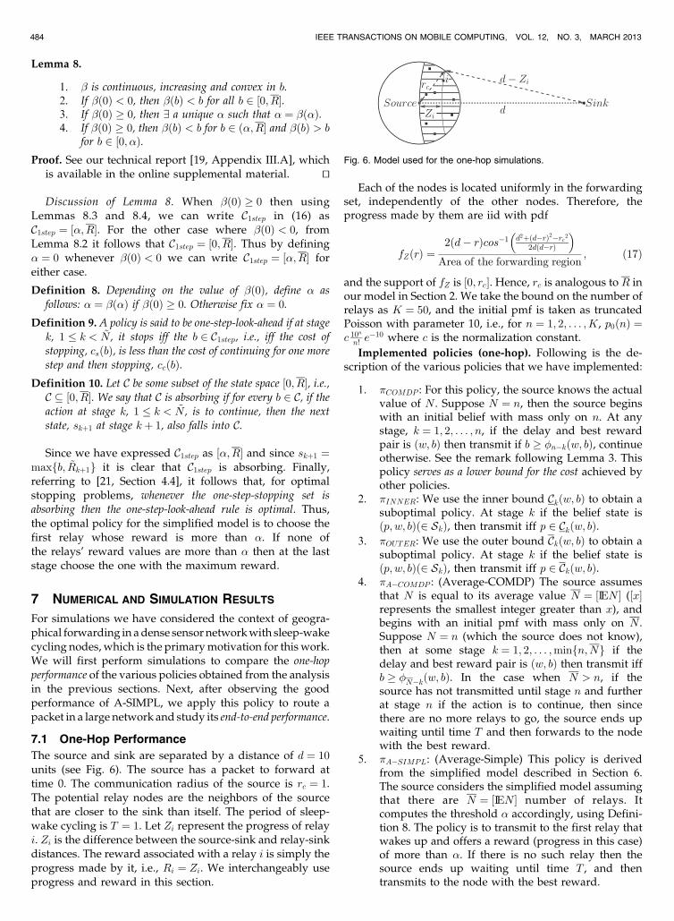
The source and sink are separated by a distance of d ¼ 10units (see Fig. 6). The source has a packet to forward attime 0. The communication radius of the source is rc ¼ 1.The potential relay nodes are the neighbors of the sourcethat are closer to the sink than itself. The period of sleep-wake cycling is T ¼ 1. Let Zi represent the progress of relayi. Zi is the difference between the source-sink and relay-sinkdistances. The reward associated with a relay i is simply theprogress made by it, i.e., Ri ¼ Zi. We interchangeably useprogress and reward in this section.
Each of the nodes is located uniformly in the forwardingset, independently of the other nodes. Therefore, theprogress made by them are iid with pdf
fZðrÞ ¼2ðd� rÞcos�1 d2þðd�rÞ2�rc2
2dðd�rÞ
�Area of the forwarding region
; ð17Þ
and the support of fZ is ½0; rc�. Hence, rc is analogous to R inour model in Section 2. We take the bound on the number ofrelays as K ¼ 50, and the initial pmf is taken as truncatedPoisson with parameter 10, i.e., for n ¼ 1; 2; . . . ; K, p0ðnÞ ¼c 10n
n! e�10 where c is the normalization constant.
Implemented policies (one-hop). Following is the de-scription of the various policies that we have implemented:
1. �COMDP : For this policy, the source knows the actualvalue of N . Suppose N ¼ n, then the source beginswith an initial belief with mass only on n. At anystage, k ¼ 1; 2; . . . ; n, if the delay and best rewardpair is ðw; bÞ then transmit if b � �n�kðw; bÞ, continueotherwise. See the remark following Lemma 3. Thispolicy serves as a lower bound for the cost achieved byother policies.
2. �INNER: We use the inner bound Ckðw; bÞ to obtain asuboptimal policy. At stage k if the belief state isðp; w; bÞð2 SkÞ, then transmit iff p 2 Ckðw; bÞ.
3. �OUTER: We use the outer bound Ckðw; bÞ to obtain asuboptimal policy. At stage k if the belief state isðp; w; bÞð2 SkÞ, then transmit iff p 2 Ckðw; bÞ.
4. �A�COMDP : (Average-COMDP) The source assumesthat N is equal to its average value N ¼ ½IEN � (½x�represents the smallest integer greater than x), andbegins with an initial pmf with mass only on N .Suppose N ¼ n (which the source does not know),then at some stage k ¼ 1; 2; . . . ;minfn;Ng if thedelay and best reward pair is ðw; bÞ then transmit iffb � �N�kðw; bÞ. In the case when N > n, if thesource has not transmitted until stage n and furtherat stage n if the action is to continue, then sincethere are no more relays to go, the source ends upwaiting until time T and then forwards to the nodewith the best reward.
5. �A�SIMPL: (Average-Simple) This policy is derivedfrom the simplified model described in Section 6.The source considers the simplified model assumingthat there are N ¼ ½IEN� number of relays. Itcomputes the threshold accordingly, using Defini-tion 8. The policy is to transmit to the first relay thatwakes up and offers a reward (progress in this case)of more than . If there is no such relay then thesource ends up waiting until time T , and thentransmits to the node with the best reward.
484 IEEE TRANSACTIONS ON MOBILE COMPUTING, VOL. 12, NO. 3, MARCH 2013
Fig. 6. Model used for the one-hop simulations.
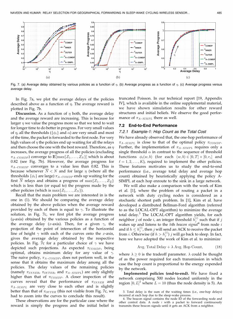
In Fig. 7a, we plot the average delays of the policiesdescribed above as a function of �. The average reward isplotted in Fig. 7b.
Discussion. As a function of � both, the average delayand the average reward are increasing. This is because forlarger � we value the progress more so that we tend to waitfor longer time to do better in progress. For very small valuesof �, all the thresholds (f�‘g and ) are very small and mostof the time, the packet is forwarded to the first node. For veryhigh values of � the policies end up waiting for all the relaysand then choose the one with the best reward. Therefore, as �increases, the average progress of all the policies (excluding�A�COMDP ) converge to IE½maxfZ1; . . . ; ZNg� which is about0.82 (see Fig. 7b). However, the average progress for�A�COMDP converges to a value less than 0.82. This isbecause whenever N < N and for large � (where all thethresholds f�‘g are large) �A�COMDP ends up waiting for thefirst N relays and obtains a progress of maxfZ1; . . . ; ZNgwhich is less than (or equal to) the progress made by theother policies (which is maxfZ1; . . . ; ZNg).
Recall that the main problem we are interested in is theone in (1). We should be comparing the average delayobtained by the above policies when the average rewardprovided by each of them is equal to �. To illustrate thesolution, in Fig. 7c, we first plot the average progress(y-axis) obtained by the various policies as a function ofthe average delay (x-axis). Then, for a given �, theprojection of the point of intersection of the horizontalline of height � with each of the curves onto the x-axis,gives the average delay obtained by the respectivepolicies. In Fig. 7c for a particular choice of � we havedepicted such projections. As expected �COMDP , beingoptimal, obtains minimum delay for any value of �.The naive policy, �A�COMDP , does not perform well, in thesense that it obtains the maximum delay among all thepolicies. The delay values of the remaining policies(namely �INNER, �OUTER, and �A�SIMPL) are only slightlyhigher than that of �COMDP . A closer inspection of thecurves reveal that the performance of �INNER and�A�SIMPL are very close to each other and is slightlybetter than that of �OUTER (this not visible from Fig. 7c, wehad to zoom into the curves to conclude this result).
These observations are for the particular case where thereward is simply the progress and the initial belief is
truncated Poisson. In our technical report [19, AppendixIV], which is available in the online supplemental material,we have shown simulation results for other rewardstructures and initial beliefs. We observe the good perfor-mance of �A�SIMPL there as well.
7.2 End-to-End Performance
7.2.1 Example-1: Hop Count as the Total Cost
We have already observed that, the one-hop performance of�A�SIMPL is close to that of the optimal policy �COMDP .Further, the implementation of �A�SIMPL requires only asingle threshold in contrast to the sequence of thresholdfunctions �‘ðw; bÞ (for each ðw; bÞ 2 ½0; T � � ½0; rc� and‘ ¼ 1; 2; . . . ; K), required to implement the other policies.These features motivates us to study the end-to-endperformance (i.e., average total delay and average hopcount) obtained by heuristically applying the policy A-SIMPL at each hop enroute to the sink in a large network.
We will also make a comparison with the work of Kimet al. [1], where the problem of routing a packet in anetwork with duty cycling nodes is considered as astochastic shortest path problem. In [1], Kim et al. havedeveloped a distributed Bellman-Ford algorithm (referredto as the LOCAL-OPT algorithm) to minimize the averagetotal delay.3 The LOCAL-OPT algorithm yields, for eachneighbor j of node i, an integer threshold h
ðiÞj such that if j
wakes up and listens to the hth beacon signal4 from node iand if h � hðiÞj , then j will send an ACK to receive the packetfrom i. Otherwise (if h > h
ðiÞj ) j will go back to sleep. In fact,
here we have adopted the work of Kim et al. to minimize
Avg: Total Delayþ � Avg: Hop Count; ð18Þ
where � � 0 is the tradeoff parameter. � could be thoughtof as the power required for each transmission in whichcase the hop count is proportional to the energy expendedby the network.
Implemented policies (end-to-end). We have fixed anetwork comprising 500 nodes located uniformly in theregion ½0; L�2 where L ¼ 10 (thus the node density is 5). An
NAVEEN AND KUMAR: RELAY SELECTION FOR GEOGRAPHICAL FORWARDING IN SLEEP-WAKE CYCLING WIRELESS SENSOR... 485
Fig. 7. (a) Average delay obtained by various policies as a function of �. (b) Average progress as a function of �. (c) Average progress versus
average delay.
3. Total delay is the sum of the waiting times (i.e., one-hop delays)incurred at each hop due to the sleep-wake process.
4. The beacon signal contains the node ID of the forwarding node andother control data. A node i with a packet to forward continuouslytransmits these beacon signals until it gets an ACK from a neighbor.
additional sink node is placed at the location ð0; LÞ as
shown in Fig. 1. As before we fix the radius of commu-
nication of each node to be rc ¼ 1. Events occur at random
locations within ½0; L�2. Each time an event occurs, a node
nearest to its location generates an alarm packet which
needs to be forwarded to the sink, possibly through
multiple hops. We will refer to the time at which the
packet is generated as time 0. Now the wake-up times of the
nodes are sampled independently and randomly from
½0; T �, where T ¼ 1 is the period of the sleep-wake cycle
(for each event we generate fresh samples for the wake-up
times). Thus a node i wakes-up at the periodic instances
Ti; T þ Ti; 2T þ Ti; . . . , where Ti is uniform on ½0; T �. At
each wake-up instant, node i listens for a beacon signal, if
any, before going back to sleep. The duration of the beacon
signal is tI ¼ 5 ms. Thus a forwarding node has to send at
most TtI¼ 200 beacon signals before all its neighbors wake-
up. Description of the forwarding policies that we have
implemented is given below.
1. First Forward (FF): forward to the first node thatwakes up within the forwarding region irrespectiveof the progress it makes toward the sink.
2. Max Forward (MF): wait for the entire duration Tand then choose a neighbor with the maximumprogress.
3. Simple Forward (SF): obtained by applying the one-hop policy, �A�SIMPL, at each hop enroute to thesink. First, knowing the node density each node icomputes the average number of neighbors, Ni,within its forwarding region. Then, for a given �,node i computes a threshold i such that the averageprogress obtained (by assuming the simplifiedmodel with Ni relays) using i is �. Now, when anode j wakes up and if it hears a beacon signal fromi, it waits for the ID signal and then sends an ACKsignal containing its location information. If theprogress made by j is more than the threshold i,then i forwards the packet to j. If the progress madeby j is less than the threshold, then i asks j to stayawake if its progress is the maximum among all thenodes that have woken up thus far, otherwise i asksj to return to sleep. If more than one node wakes upduring the same beacon signal, then contentions areresolved by selecting the one which makes the mostprogress among them. In the simulation, thishappens instantly (as also for the Kim et al.algorithm that we compare with); in practice thiswill require a splitting algorithm; see, for example,[27, ch. 4.3]. We assume that within tI ¼ 5 ms allthese transactions (beacon signal, ID, ACK, andcontention resolution if any) are over. FF and MF canbe thought of as special cases of A-SIMPL withthresholds of 0 and 1, respectively.
4. Kim et al.: For a given �, we run the LOCAL-OPT
algorithm on the network and obtain the values hðiÞj
for each neighbor pair ði; jÞ. We use these thresholds
to route from source to sink. Contentions, if any, are
resolved (instantly, in the simulation) by selecting a
node j with the highest hðiÞj index.
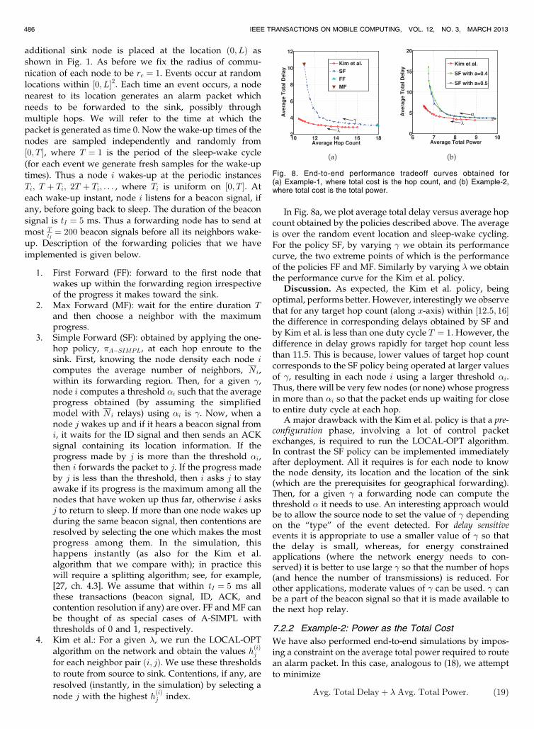
In Fig. 8a, we plot average total delay versus average hopcount obtained by the policies described above. The averageis over the random event location and sleep-wake cycling.For the policy SF, by varying � we obtain its performancecurve, the two extreme points of which is the performanceof the policies FF and MF. Similarly by varying � we obtainthe performance curve for the Kim et al. policy.
Discussion. As expected, the Kim et al. policy, beingoptimal, performs better. However, interestingly we observethat for any target hop count (along x-axis) within ½12:5; 16�the difference in corresponding delays obtained by SF andby Kim et al. is less than one duty cycle T ¼ 1. However, thedifference in delay grows rapidly for target hop count lessthan 11.5. This is because, lower values of target hop countcorresponds to the SF policy being operated at larger valuesof �, resulting in each node i using a larger threshold i.Thus, there will be very few nodes (or none) whose progressin more than i so that the packet ends up waiting for closeto entire duty cycle at each hop.
A major drawback with the Kim et al. policy is that a pre-configuration phase, involving a lot of control packetexchanges, is required to run the LOCAL-OPT algorithm.In contrast the SF policy can be implemented immediatelyafter deployment. All it requires is for each node to knowthe node density, its location and the location of the sink(which are the prerequisites for geographical forwarding).Then, for a given � a forwarding node can compute thethreshold it needs to use. An interesting approach wouldbe to allow the source node to set the value of � dependingon the “type” of the event detected. For delay sensitiveevents it is appropriate to use a smaller value of � so thatthe delay is small, whereas, for energy constrainedapplications (where the network energy needs to con-served) it is better to use large � so that the number of hops(and hence the number of transmissions) is reduced. Forother applications, moderate values of � can be used. � canbe a part of the beacon signal so that it is made available tothe next hop relay.
7.2.2 Example-2: Power as the Total Cost
We have also performed end-to-end simulations by impos-ing a constraint on the average total power required to routean alarm packet. In this case, analogous to (18), we attemptto minimize
Avg: Total Delayþ � Avg: Total Power: ð19Þ
486 IEEE TRANSACTIONS ON MOBILE COMPUTING, VOL. 12, NO. 3, MARCH 2013
Fig. 8. End-to-end performance tradeoff curves obtained for(a) Example-1, where total cost is the hop count, and (b) Example-2,where total cost is the total power.
We have assumed a model where the one-hop power
required by the forwarding node to forward the alarm
packet to relay i at a distance Di from it is Pi ¼ Pmin þ �Di ,
where is the path loss attenuation factor usually in the
range 2 to 5 and � > 0 is a constant containing the noise
variance and the signal to noise ratio (SNR) threshold
beyond which decoding is successful. In our simulations
we have fixed Pmin ¼ 0:1 and � ¼ 1. Now the total power is
simply the sum of all one-hop powers. For the local
problem we define the reward associated with a relay i
as Ri ¼ ZaiPð1�aÞi
where a 2 ½0; 1� is used to tradeoff between the
progress and the one-hop power. Zi in the reward ex-
pression is essential to give a sense of direction, toward the
sink, to the packet.In Fig. 8b, we have plotted the end-to-end performance
tradeoff curves obtained by the simple policy SF (for twodifferent values of the parameter a namely, a ¼ 0:4 anda ¼ 0:5) and that obtained by Kim et al. This time, to furtherease the implementation of SF, we allow all the nodes to usethe same threshold . Again, as in Example 1 (see Fig. 8a),we observe that the SF policy (for both the values of a)performs well for target total power in the range ½7:5; 9:75�and worsens for target total power less than 7. We haveperformed simulations for few other values of a as well(plots are not shown). However, we found that theperformance of SF for these values of a are not as good asfor a ¼ 0:4 and a ¼ 0:5, thus suggesting that these values ofa best capture the tradeoff between progress and power inthe “reward” expression.
8 CONCLUSION
Our work in this paper was motivated by the problem ofgeographical forwarding of packets in a wireless sensornetworks whose function is to detect certain infrequentevents and forward these alarms to a base station, andwhose nodes are sleep-wake cycling to conserve energy.This end-to-end problem motivated the local problem facedby a packet forwarding node, i.e., that of choosing oneamong a set of potential relays, so as to minimize theaverage delay in selecting a relay subject to a constraint onthe average progress (or some reward, in general). Furtherthe source does not know the number of available relays.We formulated the problem as a finite horizon POMDP andcharacterized the optimal policy in terms of optimumstopping sets. We proved inner and outer bounds for thisset (Theorems 2 and 3, respectively). We also obtained asimple threshold rule by formulating an alternate simplifiedmodel (Section 6). We performed one-hop simulations andobserved the good performance of the simple policy(�A�SIMPL). Finally, we applied the policy �A�SIMPL toroute an alarm packet in a large network and observed thatits performance, over some range of target hop count (ortotal cost), is comparable to that of a distributed Bellman-Ford algorithm proposed by Kim et al.
ACKNOWLEDGMENTS
This research was supported in part by the Indo-FrenchCenter for the Promotion of Advanced Research (IFCPAR
Project 4000-IT-1), and in part by the following fundingagencies of the Government of India: Defence Research andDevelopment Organisation (DRDO) and the Department ofScience and Technology (DST).
REFERENCES
[1] J. Kim, X. Lin, and N. Shroff, “Optimal Anycast Technique forDelay-Sensitive Energy-Constrained Asynchronous Sensor Net-works,” Proc. IEEE INFOCOM, pp. 612-620, Apr. 2009.
[2] Q. Cao, T. Abdelzaher, T. He, and J. Stankovic, “Towards OptimalSleep Scheduling in Sensor Networks for Rare-Event Detection,”Proc. Fourth Int’l Symp. Information Processing in Sensor Networks(IPSN ’05), 2005.
[3] K. Premkumar, A. Kumar, and J. Kuri, “Distributed Detection andLocalization of Events in Large Ad Hoc Wireless Sensor Net-works,” Proc. 47th Ann. Allerton Conf. Comm., Control, andComputing, pp. 178-185, Sept. 2009.
[4] K.P. Naveen and A. Kumar, “Tunable Locally-Optimal Geogra-phical Forwarding in Wireless Sensor Networks with Sleep-WakeCycling Nodes,” Proc. IEEE INFOCOM, pp. 1-9, Mar. 2010.
[5] K. Akkaya and M. Younis, “A Survey on Routing Protocols forWireless Sensor Networks,” Ad Hoc Networks, vol. 3, no. 3, pp. 325-349, 2005.
[6] M. Mauve, J. Widmer, and H. Hartenstein, “A Survey on Position-Based Routing in Mobile Ad-Hoc Networks,” IEEE Network,vol. 15, no. 6, pp. 30-39, Nov./Dec. 2001.
[7] J.H. Chang and L. Tassiulas, “Maximum Lifetime Routing inWireless Sensor Networks,” IEEE/ACM Trans. Networking, vol. 12,no. 4, pp. 609-619, Aug. 2004.
[8] J. Xu, B. Peric, and B. Vojcic, “Performance of Energy-Aware andLink-Adaptive Routing Metrics for Ultra Wideband Sensor Net-works,” Mobile Network Applications, vol. 11, no. 4, pp. 509-519,2006.
[9] M. Zorzi and R.R. Rao, “Geographic Random Forwarding(GeRaF) for Ad Hoc and Sensor Networks: Multihop Perfor-mance,” IEEE Trans. Mobile Computing, vol. 2, no. 4, pp. 337-348,Oct.-Dec. 2003.
[10] S. Liu, K.W. Fan, and P. Sinha, “CMAC: An Energy EfficientMAC Layer Protocol Using Convergent Packet Forwarding forWireless Sensor Networks,” Proc. IEEE CS Conf. Fourth Ann.Sensor, Mesh and Ad Hoc Comm. and Networks (SECON ’07), pp. 11-20, June 2007.
[11] V. Paruchuri, S. Basavaraju, A. Durresi, R. Kannan, and S.S.Iyengar, “Random Asynchronous Wakeup Protocol for SensorNetworks,” Proc. Int’l Conf. Broadband Networks, pp. 710-717, 2004.
[12] P. Chaporkar and A. Proutiere, “Optimal Joint Probing andTransmission Strategy for Maximizing throughput in WirelessSystems,” IEEE J. Selected Areas in Comm., vol. 26, no. 8, pp. 1546-1555, Oct. 2008.
[13] N.B. Chang and M. Liu, “Optimal Channel Probing andTransmission Scheduling for Opportunistic Spectrum Access,”Proc. ACM MobiCom, pp. 27-38, 2007.
[14] M. Sakaguchi, “Dynamic Programming of Some SequentialSampling Design,” J. Math. Analysis and Applications, vol. 2,no. 3, pp. 446-466, 1961.
[15] S. Karlin, “Stochastic Models and Optimal Policy for Selling anAsset,” Studies in Applied Probability and Management Science,K.J. Arrow, S. Karlin, and H. Scarf, eds. Stanford Univ., 1962.
[16] B.K. Kang, “Optimal Stopping Problem with Double ReservationValue Property,” European J. Operational Research, vol. 165, no. 3,pp. 765-785, 2005.
[17] I. David and O. Levi, “A New Algorithm for the Multi-ItemExponentially Discounted Optimal Selection Problem,” EuropeanJ. Operational Research, vol. 153, no. 3, pp. 782-789, 2004.
[18] M.S. Ee, “Asset-Selling Problem with an Uncertain Deadline,Quitting Offer, and Search Skipping Option,” European J. Opera-tional Research, vol. 198, no. 1, pp. 215-222, 2009.
[19] K.P. Naveen and A. Kumar, “Relay Selection with PartialInformation in Wireless Sensor Networks,” technical report,http://arxiv.org/abs/1101.3835, 2011.
[20] G.E. Monahan, “A Survey of Partially Observable MarkovDecision Processes: Theory, Models, and Algorithms,” Manage-ment Sciences, vol. 28, no. 1, pp. 1-16, Jan. 1982.
[21] D.P. Bertsekas, Dynamic Programming and Optimal Control, vol. I.Athena Scientific, 2005.
NAVEEN AND KUMAR: RELAY SELECTION FOR GEOGRAPHICAL FORWARDING IN SLEEP-WAKE CYCLING WIRELESS SENSOR... 487
[22] W.S. Lovejoy, “A Survey of Algorithmic Methods for PartiallyObserved Markov Decision Processes,” Annals Operations Research,vol. 28, nos. 1-4, pp. 47-66, 1991.
[23] R.D. Smallwood and E.J. Sondik, “The Optimal Control ofPartially Observable Markov Processes over a Finite Horizon,”Operations Research, vol. 21, no. 5, pp. 1071-1088, 1973.
[24] J.M. Porta, N. Vlassis, M.T.J. Spaan, and P. Poupart, “Point-BasedValue Iteration for Continuous POMDPs,” J. Machine LearningResearch, vol. 7, pp. 2329-2367, 2006.
[25] S. Boyd and L. Vandenberghe, Convex Optimization. CambridgeUniv., Mar. 2004.
[26] H.A. David and H.N. Nagaraja, Order Statistics, Wiley Series inProbability and Statistics. Wiley-Interscience, Aug. 2003.
[27] D. Bertsekas and R. Gallager, Data Networks. Prentice-Hall, 1992.
K.P. Naveen received the BE degree from theVisveswaraiah Technological University, Bel-gaum, in 2005. Subsequently, he worked at theISRO Satellite Centre, Bangalore. Currently, heis working toward the PhD degree in theDepartment of Electrical Communication Engi-neering, Indian Institute of Science, Bangalore.His research interests include stochastic controland optimization of wireless networks. He is astudent member of the IEEE.
Anurag Kumar received the BTech degree fromIIT Kanpur and the PhD degree from CornellUniversity, both in electrical engineering. He waswith Bell Labs, Holmdel, for more than 6 years.He is now a professor in the Department ofElectrical Communication Engineering at theIndian Institute of Science, Bangalore, and chairof the Division of Electrical Sciences. His area ofresearch is communication networking, and hehas recently focused on wireless networking. He
was an associate editor of the IEEE Transactions on Networking andIEEE Communications Surveys and Tutorials. He is a coauthor of thegraduate textbooks Communication Networking: An Analytical Approachand Wireless Networking by Kumar, Manjunath, and Kuri, published byMorgan-Kaufman/Elsevier. He is a fellow of the IEEE, the IndianNational Science Academy, the Indian National Academy of Engineer-ing, and Indian Academy of Sciences.
. For more information on this or any other computing topic,please visit our Digital Library at www.computer.org/publications/dlib.
488 IEEE TRANSACTIONS ON MOBILE COMPUTING, VOL. 12, NO. 3, MARCH 2013