Forwarding Emails from Office 365 / @Link to Your Personal ...
Upload
khangminh22Category
view
2download
0
UNIVERSITÉ DE STRASBOURG
ÉCOLE DOCTORALE MATHÉMATIQUES, SCIENCES DE
L’INFORMATION ET DE L’INGÉNIEUR
Laboratoire ICube — UMR7357
THÈSE présentée par :
Julián Martín DEL FIOREsoutenue le : 08 février 2021
pour obtenir le grade de : Docteur de l’Université de Strasbourg
Discipline/ Spécialité : Informatique
Detecting Hidden Broken Piecesof the Internet: BGP Lies, Forwarding
Detours and Failed IXPs
THÈSE dirigée par :Mme. PELSSER Cristel Professeure, Université de Strasbourg
THÈSE co-encadré par :M. MERINDOL Pascal Maître de conférence, Université de Strasbourg
PRÉSIDENTE DU JURY :Mme. MAGNIEN Clémence Directrice de recherche, Sorbonne Université
RAPPORTEURS :M. DONNET Benoit Professeur, Université de LiègeM. URVOY-KELLER Guillaume Professeur, Université Nice Sophia Antipolis


Julián Martín DEL FIORE
Detecting Hidden Broken Piecesof the Internet: BGP Lies,
Forwarding Detours and Failed IXPs
Résumé
L'objectif de cette thèse est de détecter des éléments défaillants d'Internet. Tout d'abord, nousétudions le déploiement des points d'échange Internet (IXP) en Amérique latine et constatons quecertains pays sont en situation d'échec dans leur déploiement IXP, c'est-à-dire aucun IXP du tout, oubien que l'IXP n'a pas réussi à attirer suffisamment de membres. Deuxièmement, nous étudionsBGP, le protocole de routage utilisé sur Internet, et en particulier s'il existe des mensonges BGP,c’est à dire si les routes par lesquelles les paquets circulent réellement sur Internet divergent deschemins que les systèmes autonomes (AS) annoncent. Nous trouvons effectivement des cas où leschemins ne correspondent pas. Enfin, nous étudions comment le trafic circule à l'intérieur des AS etnous nous concentrons sur la détection des détours d'acheminement, c'est-à-dire les cas où lesitinéraires d'acheminement ne correspondent pas aux meilleurs itinéraires disponibles, selon leprotocole de routage utilisé. Nous mettons ainsi en évidence des détours dans plusieurs AS.
Mots clés : BGP, IP-to-AS mapping, IXPs, Latin America, IGPs, Forwarding Detours, LoadBalancing, Traffic Engineering, Multipath Routing, Scalability, Forwarding Information Base
Abstract
The objective of this thesis is to detect hidden broken pieces of the Internet. First, we study thedeployment of Internet exchange points (IXPs) in Latin America and find that while some IXPsacross the region have managed to proliferate, some countries have failed IXPs, i.e., no IXP at all, orthe IXP has not succeeded to attract members. Second, we focus on the border gateway protocol(BGP), the routing protocol used on the Internet, and study whether ASes carry on BGP lies, i.e., ifthe forwarding routes through which packets actually flow on the Internet diverge from the AS-pathsthat ASes advertise on BGP. We find cases where the paths indeed mismatch. Finally, we study howtraffic flows inside ASes and focus on the detection of forwarding detours, i.e., cases in which theforwarding routes do not match the best available routes, according to the internal gateway protocol(IGP) in use. We reveal such forwarding detours in multiple ASes.
Keywords : BGP, IP-to-AS mapping, IXPs, Latin America, IGPs, Forwarding Detours, LoadBalancing, Traffic Engineering, Multipath Routing, Scalability, Forwarding Information Base


The turtle is slow, painfully slow......but wise, it chooses its steps thoughtfully...
...the seek of perfection drives it, it will never settle with less......it does not need motivation, recognition nor validation, the words of fools.


Acknowledgments
A journey of more than 3 years is coming to an end. The things I have learned,and the title of doctor will carry on with me from now onwards. Wherever I go,whatever I do, I hope I will be able to work with the same passion as I have duringmy PhD. The future is to come, but now is rather the moment to express somegratitude.
I thank Cristel Pelsser, la directrice de ma thèse, for all the effort she put inhelping me during this process. From the initial discussions while I was discoveringthe field, to her very precise and accurate feedback usually leading to the improve-ment of our articles. In addition, all the recommendation letters she wrote for mecome to my mind: they allowed me to participate in two TMA PhD schools, extendmy contract, etc. I was Cristel’s first PhD student, and even though many bureau-cratic requirements may have been initially unknown to her, she never hesitated infighting the system side-by-side with me, always finding solutions to the enigmaticsituations that every now and then came up. I will always remember that she alsolet me take her place in the AIMS-KISMET workshop, how she always tried to findopportunities to make me go present my work and make it more known. In addi-tion, I appreciate how she is now helping me to find a path to continue my research.Lastly, I am very grateful for the speech she dedicated to me the day that I defendedmy PhD: it makes me happy to see that she values all the effort that I put in mywork, and that she enjoyed working together all this time. Thank you for sayingthat publicly and for not saving words to express it.
I am very grateful to Pascal Merindol, my co-encadrant, for so many reasons thatit is hard to put it into words, though I will still try. My best souvenirs of the PhDwill always be the outstanding amount of endless meetings that we had to discussour work. To me, the memorable intellectual fights we had and the way we pushedeach other to the limits of their knowledge are what I hope every PhD studentexperiences with its advisors, i.e., research in its pure state. We were the “kings” ofthe “what if?”, the key question in the manual of perfectionists, and the one thatshould also often appear in the mind of any (good) researcher. I also gave lessons atthe university with Pascal, where again we gave our best, but this time to teach ourstudents, even when the covid-era begun. Thanks for all what you taught me, youradvice, your commitment to help, the passion with which you work. Thank you alsofor being such a good person, starting and finishing every email with a smiley, andfor all the informal discussions we had about life. To conclude, I want to express
vii
viii
that the fact that you started calling me a researcher collegue long before my PhDdefense was held meant a lot to me. Thank you for trusting my work, choices andcapacity.
All in all, I also thank my two advisors because I appreciate that back in 2017,when they had to make the choice, they considered me the best candidate for thisPhD, even when they knew that (i) I worked well according to a collegue, but theydid not have a certain way to know who I really was, and; (ii) my background,though very solid, was from a different area. In any case, I thank them for beingable to recognize my potential in the interview we had, and for having the courageto invest on me. Being chosen made me happy back then, and it still does, so Iam grateful to them for that. Considering the work we have done together, I amconvinced that they do not regret it neither.
Moving forward, I want to thank the complementary part of the jury in my PhDdefense, i.e., Guillaume Urvoy-Keller, Benoit Donnet and Clémence Magnien, forunanimously deciding I that deserved the PhD title, as written in the report of mydefense. I thank them for reading the manuscript, and for expressing that they feltthat my work improved the state-of-the-art. To me it is nice that they also noticedhow enthusiastic and didactic I am when I talk about my work. In particular, Iam specially thankful to Guillaume, who wrote a report that helps to quantify theamount of work I did, and highlights the passion that guides the research I carryon. Finally, I thank Clémence for taking care of the extra work she had as presidentof the jury.
In addition, besides my advisors, I want to thank all the remaining co-authorsof the publications I worked in, with a special mention for Esteban Carisimo andValerio Persico. I have known Esteban for more than 10 years, and it makes mevery happy that our PhDs have brought our paths closer, making us meet in BuenosAires, Vienna and Paris. I particularly enjoy that he and I were able to shed somelight on the status of the Internet in Latin America, a region deeply attached toour hearts. I would say that most of the work we have done with Esteban remainsyet unpublished, and I hope that we will be able to honor our efforts in the future.On the other hand, I am happy to have met Valerio more than two years ago whenhe stayed as a research fellow in Strasbourg for some months. Thank you Valeriofor being my touristic guide in Napoli and for making sure that I made it to all thegood pizzerias, coffee and pasta places. I will always remember returning from thelab with you, and this view of the Vesuvio appearing in the back after one turn. Themoments that Melanie and I spent with you and Marianna in Napoli and Barcelonawill turn into, and in fact already are, anecdotes we will never forget. In conclusion,I think of both Esteban and Valerio as examples to follow, both as researchers andhumans overall. I deeply thank the two of them for being so thorough in their work,and for making a difference in my daily life as a PhD student.
I want to thank the permanent people that make the Network Research Team inthe ICube Laboratory for being nice co-workers. I wish we had been able to spendmore time together over the last year, but the covid-19 reduced our chances. I willalways remember the lunches at 11.45, the barbecue at the lab, the Christmas dinnerin 2017 and 2018, and the nice talk we had in Academie de la Biere with StéphaneCateloin and Julien Montavont. In particular, thanks to Fabrice Theoleyre for themultiple occasions where he helped me to deal with bureaucratic stuff, Guillaume

ix
Schreiner for the technical support setting up VMs, Pierre David for the orangechocolate bars of each monday, and Thomas Noel for replying my emails in recordtime. A very special thank goes to Quentin Bramas, who was a main speaker in theseminar I organized in 2018, with whom I enjoyed a lot concurrently giving lessons,and with whom I look forward to carry on some research in future work.
Further, I want to thank the PhD students that were in the same working teamas me chronologically in the period that goes from 2017 to 2021. Thanks JeanRomain Luttringer for the interesting research discussions, Philippe Pittoli for thevery interesting talks about the meaning of life and the purpose of research, LoicMiller for the chess games, and the same for Jean-Philippe Abegg that, despitestealing my bench in the PhD students room when he started his PhD (I recognizethat I was away in Barcelona at that time, so he did not know), also made me smilewhen he shared his knowledge about Argentina and talked to me about Fernet andRodrigo. I thank Rodrigo Teles Hermeto for his help before and right after I arrivedto Strasbourg, for being the delegated to prepare coffee at midday, for bringingboard games to play on the pauses, for the Christmas day we spent together andwith our wives in 2018, etc. To continue with the Brazilian side, I thank RenatoJuacaba Neto for always bringing happiness with his characteristic laugh, for ourjokes comprising AR » BR or the opposite (we both know the truth), for comingto visit me in Barcelona in 2019, for his special sense of humor, for always beingpresent when needed as a friend, etc. I am grateful to Sebastián Lucas Sampayoand his wife that together gave the Argentinian touch that made me feel closer tohome during my stay in France, for all the nice moments we spent together in barsand restaurants, and for all the help, advice and information you always providedme. I am also grateful to Andreas Guillot since he was always trying to help withany problem I might have had, hosting the gatherings of the PhD students in whichwe had such a fun and were able to enjoy pure friendship, visiting me in Barcelonain 2019, and also for essentially listening to me when I needed someone to talk with.I also want to thank Amine Falek because, despite the fact that he is difficult toreach, he is a good friend and as perfectionist as I am; he always listened when Iexplained him the problems I was trying to solve in my PhD and gave me usefulfeedback. I hope I will work with him in the future, and also play some guitar andchess as we did before.
In addition, I want to thank Georgios Z. Papadopoulos, my former advisor inthe research lab in Rennes who recommended me to Cristel and Pascal as a goodcandidate for the PhD. I also want to thank Renzo E. Navas for making me feellike if I was in Argentina while I stayed in Rennes, for still being present duringmy PhD despite the distance, and for the invaluable feedback he gave me while Iwas making the final arrangements in the slides I presented on my defense. I wantto thank Andra Lutu for taking me as an intern in Telefonica I+D for 3 monthsin Barcelona, an experience I will always remember. Similarly, I thank AntonioPescape for receiving me as a research fellow in his lab at the University of NapoliFederico II for almost during 1 month.
There are also special friends I made over these years that I want to thankfor making my life happier during my PhD. I have many positive things to sayabout all of them, but I will be short because, as good friends always do, theyalready know what I think about them. I do not have enough words to express

x
my love towards Nadja Groysbeck, Antonella Zerpa, Odnan Ref Sanchez and AnaAlice Torres. The same applies to the Serbian team composed by Jelica Vasiljević,Mihailo Obrenovic and his wife Aleksandra. Thanks for all the friends I made inSpain during my internship in Telefonica: Mariona Caros Roca, Gabriele Castellano,María Lara Gauder, Guillermo Cámbara. I also enjoyed meeting with SantiagoPascual, Marcos Paulucci, Patricio Pavón, Federico Longhi and Lynelle Sigona. I amalso very grateful to my friends in Argentina, that sent me their support while I wasaway: Gonzalo J. Figueroa, Cecilia Osorio, Mathias E. Garcia, Patricio Olaberría,Philippe Clavier. I also thank Pablo Machin that sent me his support from the US.
I also want to thank my family, and that of my wife, for sending their love to bothof us across the ocean, from Argentina straight to France, and also for embracingus every time we went back to visit them. In particular, I enjoyed each and everytalk I shared with my grandparents and my aunt. I will always be grateful to myparents, that gave me everything I could have asked for and more, without whom Iwould not have been able to come all along this way. I miss them all every day ofmy life, but the effort has paid back, and it will continue to do so.
Finally, the person I want to thank the most is my wife, Melanie Belen Castagno.She is an extraordinary person that, from the big heart that she has, irradiates love24/7. Through these more than 3 years, I have done the research you will soondiscover in the manuscript, but it is actually her that has done the hard job. She hashad extraordinary patience with me, she has listened to my complaints, encouragedme when I felt out of energies, helped me to deal with my anxiety close to thedeadlines, heard me telling her every day about a new pain that I had, providedme with her company when I felt sad. In short, it is her love that has been next tome all this time, and without which my PhD would not have been the same. I willalways be grateful to her. I hope one day I will be able to be there for her, the sameway she has been there for me.


Summary
The Internet is an interconnection of independent networks known as AutonomousSystems (ASes). Given that ASes are built on top of hardware and software, andthat network operators, i.e., humans, manage ASes, then the Internet is constrainedto some limitations. For example, humans are error-prone and eventually take arbi-trary decisions, enterprises are generally greedy from a revenue point of view, andhardware may fail and require maintenance or replacement. All these factors maylead the Internet to have broken pieces, i.e., malfunctioning components, networksfacing limitations and even selfish networks prioritizing their own revenue ratherthan the better performance of the Internet.
The objective of this thesis is to detect broken pieces of the Inter-net. First, we study the deployment of Internet exchange points (IXPs) in LatinAmerica, a region that has previously received little attention in Internet studies.We construct the most comprehensive dataset of the status of the Internet in LatinAmerica and characterize the AS ecosystem in the region. We find that while someIXPs across Latin America have managed to proliferate, some countries have failedIXPs, i.e., no IXP at all, or the IXP has not succeeded to attract members. Second,we focus on the border gateway protocol (BGP), the routing protocol used on theInternet, and study whether ASes carry on BGP lies, i.e., if the forwarding routesthrough which packets actually flow on the Internet diverge from the AS-paths thatASes advertise on BGP. In practice, performing this comparison is complex sincebesides the multiple levels at which data needs to be synchronized, missing hops,third-party addresses and AS siblings may introduce errors by wrongly triggeringthe detection of BGP lies. In particular we develop a methodology allowing to filterthis noise, and run measurements in the wild. We find cases where after sanitizingthe dataset with our framework, paths still mismatch. Finally, we study how trafficflows inside ASes and focus on the detection of forwarding detours, i.e., casesin which the forwarding routes do not match the best available routes, accordingto the internal gateway protocol (IGP) in use. We develop a formalism explainingwhen forwarding detours occur, and implement a detector allowing to differentiateforwarding detours from load balancing and traffic engineering techniques. We runmeasurements with our detector and find detours in multiple ASes with a remark-able binary pattern such that transit traffic traversing between two border routersof an AS either never detours, or always does.
xiii

xiv

List of publications during the PhD
Journals
• Julián M. Del Fiore, Valerio Persico, Pascal Merindol, Cristel Pelsser andAntonio Pescapè. The Art of Detecting Forwarding Detours, in IEEE Trans-actions on Network and Service Management (IEEE TNSM) 2021 [1].
• Esteban Carisimo, Julián M. Del Fiore, Diego Dujovne, Cristel Pelsser, andJ. Ignacio Alvarez-Hamelin. 2020. A first look at the Latin American IXPs,in SIGCOMM Comput. Commun. Rev. 50, 1 (January 2020), 18–24 [2].
Conferences
• Julián M. Del Fiore, Pascal Merindol, Valerio Persico, Cristel Pelsser andAntonio Pescapè. Filtering the Noise to Reveal Inter-Domain Lies, in 2019Network Traffic Measurement and Analysis Conference (TMA), pages 17–24,2019, IEEE [3].
Posters
• Julián M. Del Fiore, Pascal Merindol, Valerio Persico, Cristel Pelsser andAntonio Pescapè. Routing Inconsistencies at the FIB level, in 2019 NetworkTraffic Measurement and Analysis Conference (TMA), IEEE.
• Esteban Carisimo, Julián M. Del Fiore, Diego Dujovne, Cristel Pelsser,J. Ignacio Alvarez-Hamelin, Country-level influence of IXPs in Latin Amer-ica, in Latin American Student Workshop on Data Communication Networks(LANCOMM) 2019.
• Julián M. Del Fiore, Pascal Merindol, Valerio Persico, Cristel Pelsser andAntonio Pescapè. A BGP-lying Tale: Stop Blamming the Mapping, in 2018Network Traffic Measurement and Analysis Conference (TMA), IEEE.
xv

xvi

Contents
1 Research Questions and State-of-the-Art 1
1.1 Internet Exchange Points in Latin America . . . . . . . . . . . . . . 1
1.2 Seeking for BGP Lies . . . . . . . . . . . . . . . . . . . . . . . . . . . 3
1.3 Modeling and Detection of Forwarding Detours . . . . . . . . . . . . 6
2 Background 9
2.1 Internet . . . . . . . . . . . . . . . . . . . . . . . . . . . . . . . . . . 10
2.1.1 BGP . . . . . . . . . . . . . . . . . . . . . . . . . . . . . . . . 10
2.1.2 IXPs . . . . . . . . . . . . . . . . . . . . . . . . . . . . . . . . 15
2.2 Intra-domain networks . . . . . . . . . . . . . . . . . . . . . . . . . . 17
2.2.1 IGPs . . . . . . . . . . . . . . . . . . . . . . . . . . . . . . . . 17
2.2.2 Load balancing . . . . . . . . . . . . . . . . . . . . . . . . . . 18
2.2.3 Tunneling mechanisms . . . . . . . . . . . . . . . . . . . . . . 19
2.3 Traceroute . . . . . . . . . . . . . . . . . . . . . . . . . . . . . . . . . 20
2.3.1 Standard version . . . . . . . . . . . . . . . . . . . . . . . . . 20
2.3.2 Paris traceroute . . . . . . . . . . . . . . . . . . . . . . . . . . 22
2.3.3 Multi-path detection algorithm . . . . . . . . . . . . . . . . . 23
3 Success and Failure of IXPs in LatAm 29
3.1 Dataset . . . . . . . . . . . . . . . . . . . . . . . . . . . . . . . . . . 31
3.1.1 Searching for IXPs in LatAm . . . . . . . . . . . . . . . . . . 31
3.1.2 Collecting data sources . . . . . . . . . . . . . . . . . . . . . . 32
3.1.3 Pre-processing BGP data . . . . . . . . . . . . . . . . . . . . 33
3.2 Public policies and IXPs . . . . . . . . . . . . . . . . . . . . . . . . . 33
3.3 IXP networks topology . . . . . . . . . . . . . . . . . . . . . . . . . . 34
3.3.1 CABASE . . . . . . . . . . . . . . . . . . . . . . . . . . . . . 36
xvii
xviii Contents
3.3.2 PIT-CL . . . . . . . . . . . . . . . . . . . . . . . . . . . . . . 36
3.3.3 IX.br . . . . . . . . . . . . . . . . . . . . . . . . . . . . . . . . 37
3.3.4 DE-CIX . . . . . . . . . . . . . . . . . . . . . . . . . . . . . . 37
3.3.5 Takeaways . . . . . . . . . . . . . . . . . . . . . . . . . . . . . 38
3.4 IXPs: domestic, regional or worldwide? . . . . . . . . . . . . . . . . . 38
3.4.1 IXP members . . . . . . . . . . . . . . . . . . . . . . . . . . . 38
3.4.2 Visible ASes: domestic impact and foreign attraction . . . . . 39
3.5 Reaching IXPs: from stubs to large transit providers . . . . . . . . . 41
3.5.1 Transit members . . . . . . . . . . . . . . . . . . . . . . . . . 41
3.5.2 Non-transit members . . . . . . . . . . . . . . . . . . . . . . . 44
3.6 IXPs and concentration . . . . . . . . . . . . . . . . . . . . . . . . . 46
3.7 Conclusions . . . . . . . . . . . . . . . . . . . . . . . . . . . . . . . . 47
4 Filtering the Noise to Reveal BGP Lies 49
4.1 Modeling BGP lies . . . . . . . . . . . . . . . . . . . . . . . . . . . . 51
4.2 Problem Statement . . . . . . . . . . . . . . . . . . . . . . . . . . . . 53
4.3 A Modular framework to detect BGP lies . . . . . . . . . . . . . . . 55
4.3.1 Preparation stage . . . . . . . . . . . . . . . . . . . . . . . . . 58
4.3.2 Mapping relaxation . . . . . . . . . . . . . . . . . . . . . . . . 59
4.3.3 Wildcards correction stage . . . . . . . . . . . . . . . . . . . . 61
4.4 The measurement platform and our campaign . . . . . . . . . . . . . 63
4.5 Rate of BGP lies in the wild . . . . . . . . . . . . . . . . . . . . . . . 64
4.5.1 Performance of the different noise-filtering models . . . . . . . 64
4.5.2 Effect of SIB and TPA rules on the mismatch rate . . . . . . . 66
4.5.3 Looking closer at high mismatch rates . . . . . . . . . . . . . 67
4.6 Conclusion . . . . . . . . . . . . . . . . . . . . . . . . . . . . . . . . . 67
5 The Art of Modeling and Detecting Forwarding Detours 69
5.1 The origin of FDs: routing inconsistencies and forwarding alterations 71
5.1.1 RIes, FAs and FDs in a practical example . . . . . . . . . . . 71
5.1.2 Lookup functions: prefixes, gateways and next-hops . . . . . 72
5.1.3 What is an internal route of an AS? . . . . . . . . . . . . . . 73
5.1.4 When is the routing consistent? . . . . . . . . . . . . . . . . . 75
5.1.5 What produces routing inconsistencies? . . . . . . . . . . . . 75
5.1.6 What leads to forwarding alterations? . . . . . . . . . . . . . 77
5.1.7 When do forwarding detours occur? . . . . . . . . . . . . . . 78
5.2 Similarities and differences between FDs, LB and TE . . . . . . . . . 79

xix
5.2.1 Simple but naive methods to detect FDs . . . . . . . . . . . . 80
5.2.2 Forwarding patterns for LB, TE and FDs . . . . . . . . . . . 81
5.3 A detector of prefix-based forwarding patterns . . . . . . . . . . . . . 83
5.3.1 Exploration phase . . . . . . . . . . . . . . . . . . . . . . . . 84
5.3.2 Prefix-grouping phase . . . . . . . . . . . . . . . . . . . . . . 84
5.3.3 Multi-route discovery phase . . . . . . . . . . . . . . . . . . . 85
5.3.4 Merging phase . . . . . . . . . . . . . . . . . . . . . . . . . . 86
5.4 An FD-detector . . . . . . . . . . . . . . . . . . . . . . . . . . . . . . 87
5.4.1 The FD-verdict: looking for a lonely DIR . . . . . . . . . . . 88
5.4.2 The FD-detector: a tool to be run in the wild . . . . . . . . . 89
5.5 Capturing forwarding detours in the wild . . . . . . . . . . . . . . . 91
5.5.1 Measurement campaigns and coverage . . . . . . . . . . . . . 91
5.5.2 Fowarding patterns and the binary effect of FDs . . . . . . . 92
5.5.3 Distribution of FDs per AS and ASBR-couples . . . . . . . . 93
5.5.4 Correlation between ingress-ASBRs and FDs . . . . . . . . . 94
5.5.5 Speculating on the root causes generating FDs . . . . . . . . 96
5.5.6 Validation: emulations and ground truth . . . . . . . . . . . . 97
5.6 Discussion: robustness of the FD-detector . . . . . . . . . . . . . . . 98
5.6.1 An FD-verdict handling all interactions of FDs and LB . . . . 98
5.6.2 A binary effect that unlikely results from routing changes . . 99
5.6.3 On the (in)sensibility of flawed ASBR detection . . . . . . . . 100
5.6.4 Measurement stopping points . . . . . . . . . . . . . . . . . . 100
5.6.5 Alias Resolution: a nice, but dangerous additional feature . . 100
5.7 Conclusion . . . . . . . . . . . . . . . . . . . . . . . . . . . . . . . . . 101
6 Conclusion and Research Directions 103
6.1 Takeaways . . . . . . . . . . . . . . . . . . . . . . . . . . . . . . . . . 103
6.2 Future Work . . . . . . . . . . . . . . . . . . . . . . . . . . . . . . . 105
6.2.1 BGP lies: more VPs, anomaly detection and malicious ASes . 105
6.2.2 Forwarding detours: finding the forwarding alteration and an
FD-detector-lite . . . . . . . . . . . . . . . . . . . . . . . . . . 107
6.2.3 Where BGP lies and FDs meet: a partial-FIB detector . . . . 109
6.2.4 A better model of LB, a more efficient MDA . . . . . . . . . . 110
List of Figures 129
List of Tables 135


Chapter 1Research Questions andState-of-the-Art
The Internet appears as an infallible system that never fails, however, this is not thecase. Actually, the Internet is simply an interconnection of independent networks,known as Autonomous Systems (ASes). Given that ASes are built on top of hard-ware and software, and that network operators, i.e., humans, manage ASes, thenthe Internet is constrained to some limitations. First, humans not only are natu-rally error-prone, but also sometimes take arbitrary decisions that are not alwaysthe best. Moreover, for the same problem, different people may consider discrepantconstraints as the most relevant, and thus propose diverging solutions as the bestone, contributing another level of randomness surrounding the behavior of the Inter-net. In addition, from a business point of view, we could argue that enterprises aregenerally greedy, thus turning the Internet into a profit-driven ecosystem. Besidesthis, human-built systems are usually not perfect: they tend to comprise modulesthat may fail and require maintenance, or that after a given time may become ob-solete and need replacement. All these factors may lead the Internet to have brokenpieces, i.e., malfunctioning components, networks facing limitations and even selfishnetworks prioritizing their own revenue rather than the better performance of theInternet. The objective of this thesis is to detect problems such as these. This taskis challeniging since the phenomena we want to uncover may be hidden anywhereon the Internet, which counts with approximately 70K ASes as of November 2020.
1.1 Internet Exchange Points in Latin America
The first component of the Internet we study on this thesis are Internet exchangepoints (IXPs), the interconnection facilities commonly used by ASes. The structureof the Internet, i.e., how ASes establish connections with each other, was largelymodified by the irruption of IXPs in the 2000s [4]. IXPs allow ASes to establishconnections at a larger scale, and to produce monetary savings. However, the popu-larity of IXPs varies across regions. In some cases, countries may have failed IXPs,i.e., no IXP at all, or an IXP that has not succeeded to attract members. Whereas
1

2 Chapter 1. Research Questions and State-of-the-Art
there exist large IXPs in Europe, such as DE-CIX, LINX and AMS-IX that havebeen subject of study [5], there are no reports showing a similar story of success inNorth America. Recent studies have focused on the role of IXPs in the African ASecosystem [6, 7, 8]. In other regions, in contrast, little is known about IXPs andeven about the Internet as a whole.
In particular, the case of Latin America (LatAm), corresponding with the Re-gional Internet Registry (RIR) named LACNIC, is an interesting case of study.LatAm covers 20 million km2 [9] and comprises 20 countries: right after NorthAmerica, it has the largest urban population rate (80%) [10]. Moreover, LatAm ishome of 652 million people [11] and has three out of the four largest metropolitanareas in the Americas (Sao Paulo, Mexico City and Buenos Aires with populationsof 21.3M, 21.2M and 15.3M habitants respectively) [12]. The region also has ap-pealing numbers regarding to Internet considering it contributes to the global ASecosystem with 14.5% (9,988/68,912) of the active ASes. Furthermore, 6458 ASNshave been delegated by NIC.br (Brazilian national Internet registry) to Brazilian-based organizations. Between 2005-2015, LatAm experienced significant progress infixed and mobile penetration rates, reaching 40.57% and 57.41% of the population,respectively [13]. Moreover, several countries of the region have recently benefitedfrom the creation of domestic IXPs [14].
Despite the progressing development of the Internet in LatAm, the shape of theLatin American network remains relatively unmapped. This encourages us to ex-plore its interconnection and structure. Given that IXPs contributed to flatten theInternet in the 2000s, it is natural to wonder if 20 years later, these peering infras-tructures are also benefiting developing countries, many with much larger surface,to embrace the Internet. This brings us to our first research question.
Have all IXPs in LatAm managed to proliferate or are there failedIXPs? If some have failed, why?
Research Question
A priori, LatAm has remained quite unexplored, presumably due to a historicalscarcity of representative Internet data. For example, the footprint of RIPE Atlasand Ark CAIDA in LatAm is composed of 285 out of 11,142 (2.56%), and 12 outof 190 (6.32%) probes, respectively. The numbers decrease considering IPv6: just2.22% (101/4,556) of RIPE’s IPv6-capable probes are located in Latin America.On the other hand, it is known that the lack of BGP data allows to draw a fairlyincomplete representation of AS ecosystems [15]. In that sense, Routeviews 1 andRIPE RIS 2 have only respectively deployed two and one BGP data collectors inthe region, two being redundant since they are placed at the same Brazilian IXP inSao Paulo.
Despite the aforementioned limitations, some Internet studies have focused onthis region. Berenguer et al. [16] applied graph-theoretical metrics to evaluate
1http://www.routeviews.org/2https://www.ripe.net/analyse/internet-measurements/routing-information-service-ris

1.2. Seeking for BGP Lies 3
dataset augmentation when routes collected from local looking glasses are addedto RIPE RIS and RouteViews BGP dumps. Brito et al. [17] gathered one BGPdump per each looking glass co-located in each regional IXP of IX.br, the BrazilianIXP network, and then compared them with IXPs from other regions in terms ofconnected networks and peering policies prevalence. A complementary study of thesame authors included an analysis of IPv6 deployment [18], however, it is limitedto IPv6 prefix size and the number of IPv6 entries in routing tables. Muller etal. [19] relied on sFlow data gathered at a regional IXP of IX.br to infer spoofedtraffic traversing the IXP. Formoso et al. [20] relied on RIPE Atlas probes deployedin LatAm to measure inter-country latency, inferring asymmetric paths and poorlyinterconnected countries.
In particular, Chapter 3 studies the deployment of IXPs in LatAm, and showsthe first broken piece of the Internet we find. Indeed, IXPs are a story of eithersuccess or failure depending on the country considered in Latin America. WhileArgentina, Brazil and Chile count with IXPs that have managed to proliferate,other countries have failed IXPs. We dive into the reasons of why some IXPs areable to gather a large number of members that announce multiple IP addresseswhile others not. We find a negative correlation between success of IXPs and thepresence of monopolistic ASes concentrating the IPv4 address space delegated tocountries. In addition, since LatAm has never been closely analyzed, we take theopportunity and also characterize the AS ecosystem in the region. We see that IXPsin LatAm, similar to others in developing regions, are mainly populated by domesticor regional players, whereas those internationally renown in Europe rather behaveas international hubs.
1.2 Seeking for BGP Lies
The second element of the Internet we look at in this thesis is the border gatewayprotocol (BGP), the routing protocol used on the Internet. BGP dictates how ASesexchange reachability information concerning the IP prefixes each of them owns.With BGP, each AS announces the prefixes it owns to its neigbouring ASes, and inturn these relay the message to other ASes. In this process, the exchanged routingmessages keep track of the AS-path that was followed, i.e., a list of the ASes, fromthe first to the last, that advertised the prefix. In this thesis, we refer to the AS-path as the control path (CP), since it is built on the control plane of BGP. On theother hand, we refer to the set of ASes that packets actually traverse towards theirdestinations as data paths (DPs), since this occurs at the data plane of BGP. Ananalogy of an AS advertising a prefix with a given CP to a neighbouring AS, is theoffer of a contract. More precisely, the BGP announcement plays the role of thecontract, and the service that gets offered is that, to reach a given prefix, the DPwill replicate the ordered set of ASes expressed in the CP. Hence, DPs are expectedto match the CPs advertised for all prefixes.
The underlying assumption that CPs match DPs for all prefixes advertised inBGP is not trivial to verify: the current troubleshooting tools, e.g. traceroute,usually allow to recover IP-paths, but not the forwarding AS-level route that wasfollowed. As a consequence, the implicit trust that ASes advertise the paths theyuse for packet forwarding may be misplaced. Network operators may manipulate

4 Chapter 1. Research Questions and State-of-the-Art
CPs [21] and DPs [22, 23] potentially leading them to mismatch. Whenever the CPand DP for a prefix mismatch, we say that a BGP lie occurred. We choose this namebecause if the paths mismatch, then the ASes that advertise the CP are lying, sincethe DP differs. Note that this nomenclature applies irrespectively of whether CPsand/or DPs are tweaked, or if this results from a deliberate or unintended behavior.
The objective behind BGP lies may be multiple. An AS may try to redirectand intercept traffic, or hinder its tracking with consequences on the ability to trou-bleshoot connectivity issues. Moreover, BGP lies may lead to the violation of agree-ments between adjacent ASes, with potential subsequent legal retaliation. Theselies may be deliberate to obfuscate traffic interceptions or be driven by economicalinterests, e.g. attracting traffic by promising interesting routes but using cheaperalternatives. On the other hand, they can result from incongruent logical and physi-cal topologies, in particular when BGP sessions are not set on simple point-to-pointinter-domain links. Others may be rooted in technical limitations, such as limitedmemory on the routers hampering the storage of the full routing table, i.e. resultingin a partial-FIB. In conclusion, BGP lies generate a broken piece of the Internet.
We set our goal to detect BGP lies, however, carrying out this task requiresaddressing a considerable practical challenge: the CPs and DPs that need to begathered with measurements and the IP-to-AS mapping tools usually used to trans-form the DPs from IP-level to AS-level paths are noisy, hence, BGP lies may bemisinterpreted as noise, or vice versa. Therefore, to draw representative conclu-sions, the developed framework should filter the noise affecting the measurements.This motivates our second research question.
Can we develop a framework that, filtering the noise affecting thecomparison of CPs and DPs, allows to quantify the daily rate ofBGP lies that occur on the Internet?
Research Question
There exist many papers that have focused on the comparison of CPs and DPs,and in characterizing different souces of noise affecting this task. Mao et al. [24]find that IXPs, AS siblings, and ASes announcing IP prefixes for which they are notthe real originating AS (OAS) are predominant causes for mismatches among CPsand DPs. In a follow-up work [25], they develop a systematic approach to correctinaccurate IP-to-AS mappings by reassigning the OAS of prefixes. Hyun et al. [26]also analyze the discrepancies between CPs and DPs and conclude that insertionsof IXPs in the DPs and of ASes under the same ownership are the main cause thatleads to mismatches. However, in their study, incomplete traces are discarded andthe comparison does not rely on the latest BGP updates, i.e. CPs and DPs arenot well time-synchronized. Zhang et al. [27] extract the mismatching fragmentsof CPs and DPs and show that the main pitfall of using traceroute in AS-leveltopology measurements originates from the appearance of IP addresses assignedfrom AS neighbors. However, their measurement platform suffers from the inability

1.2. Seeking for BGP Lies 5
to ensure that the data and control plane vantage points are co-located, i.e., thatthe DPs exit the AS (or at least traverse) the BGP speaker sharing the CPs. On theother hand, Hyun et al. [28] introduced the concept of third-party addresses (TPAs),i.e., IP address appearing in traceroute that be mapped to an AS that is off-path.Their study concludes that TPAs are not common and that they do not distort ASmaps significantly. In addition, according to the authors, finding multiple TPAs ina row mapping to the same AS is unlikely, although possible. A later analysis ofMarchetta et al. [29] using IP timestamp options states the contrary. They findthat consecutive TPAs are common, and may even entirely hide an AS from anAS-level path. However, a subsequent study from Luckie et al. [30] reports thatmost observed IPs in traceroute traces are from in-bound interfaces, thus on-path.They argue that techniques using IP timestamps are not reliable to detect TPAs.Ahmed et. al [31] propose an offline method that tags up to two IPs that appear ina row as possible TPAs if they introduce an AS that either violates valley-free pathsor translate into new AS relationships. Further work concerning detection of TPAsfor correctly determining AS boundaries include bdrmap [32], MAP-IT [33] andbdrmapIT [34]. In the case of bdrmap, inter-AS link interface addresses between anetwork with a traceroute vantage point and directly connected networks are inferredrelying on alias resolution probing techniques, and AS relationship inferences. Onthe other hand, MAP-IT attempts to achieve the same for all connected ASes basedon traceroute results collected from multiple vantage points distributed in differentASes. Finally, bdrmapIT combine the previous two, improving the inference ofrouter-ownership and identification of links between ASes.
In Chapter 4 we model how ASes may introduce BGP lies and we propose amethodology to detect them. In particular, we present a framework allowing tofilter noise, i.e., mapping inaccuracies introduced by AS siblings, TPAs or IXPs andmissing hops, that may affect the comparison between CPs adverised in BGP andthe DPs that packets follow on the Internet. In particular, our methodology relieson heuristics to estimate whether noise may be affecting the paths we collect, andthen attempts to correct them. Our framework is modular, i.e., the user can se-lect among multiple filters that vary how they estimate what results from noise ornot, and thus allow to implement different noise-filtering models. We run long-termmeasurements on the Internet and sanitize the dataset with our framework. Ourresults show that, even relying on the most conservative noise-filtering model, somemismatches between the CPs and DPs we collect still remain, likely representingBGP lies. Compared to the literature, our study not only deploys more vantagepoints, but also goes beyond what had previously been done by providing resultsbased on daily-analysis. Comparing the results with basic IP-to-AS mapping toolsand with our framework, we see that in the vantage points where our framework iseffective to filter the noise, eliminating numerous false positives, the results are sta-ble in time. On the other hand, when both methods output a high and comparablenumber of inferred discrepant paths, we see that results have a larger variation overtime. While most of the related work essentially blames the IP-to-AS mapping forthe observed discrepancies between CPs and DPs, our work relies on conservativeheuristics that remove the noise in the measurements and the mapping errors, at-tempting to minimize false positives in the detection of BGP lies. In other words,different to previous studies, our aim is to detect “real” BGP lies, hence our frame-
6 Chapter 1. Research Questions and State-of-the-Art
work is designed to provide a lower bound of mismatches between CPs and DPs.The mismatches we find after applying our filters show that the IP-to-AS mappingis not the only culprit for them.
1.3 Modeling and Detection of Forwarding Detours
The last component of the Internet we analyze are internal gateway protocols (IGPs),the routing protocols that ASes use inside their networks. IGPs characterize forresulting in a forwarding scheme such that traffic traversing ASes flows throughbest paths that minimize the distance or cost according to a metric of choice.
In this case, the broken piece we are interested in are forwarding detours, i.e.,cases where traffic flows through forwarding routes that divert or diverge from theexpected best IGP paths. Contrary to hot-potato routing, FDs increase the IGPdistance required to traverse an AS and arguably result in waste of resource uti-lization inside the network. Attempting to suppress FDs, network operators mayimplement tunneling techniques. However, these mechanisms only allow to FDswithin each tunnel/segment (for BGP-free core routers in particular) but may failto do so between endpoints of an AS.
In particular, FDs may result from side effects of scalability workarounds. In-deed, the full Internet feed, reaching ∼867K prefixes as of February 2021, has beengrowing at ≈50K prefixes/year over the last 10 years. The sustained increase in thenumber of prefixes advertised on the BGP has led ASes to exchange more updatemessages [35, 36, 37], and to suffer from scalability issues. Indeed, considering thecurrent trend, maintaining a full forwarding information base (FIB) may be challeng-ing, specially for ASes incapable of upgrading their network devices regularly [38,39, 40, 41]. In this context, networks operators have found alternatives to endurewith legacy routers unable to maintain a complete FIB in memory. For example, ina BGP-free core, tunneling techniques reduce the size of the FIB on core routers [42].In addition, partial iBGP dissemination relying on route-reflector hierarchies mayalso boost scalability [43]. This technique allows routers to maintain less BGP peersand, in some rare cases, may even prevent the full redistribution of BGP prefixeswithin the AS [44]. In addition, memory-constrained routers may aggregate routesto limit the number of FIB entries [45]. Other type of workarounds consist in storinga partial-FIB [46], and redirecting traffic via default routes towards more capablerouters (e.g. having a full-FIB). Some network operators even apply this techniqueon switches with IP capabilities [47]. While the aforementioned techniques may lookeffective at first glance, ASes relying on them may suffer from forwarding detours.This may happen when routers along a route choose different exit ASBRs for thesame prefix.
In addition, besides side effects of scalability workarounds, misconfigurationsand bugs in router’s software, such as BGP zombies [48], may also create FDs.Consequently, network operators may ignore FDs occur on their AS, and providedegraded performance to customer ASes. This brings us to a third research question.
1.3. Modeling and Detection of Forwarding Detours 7
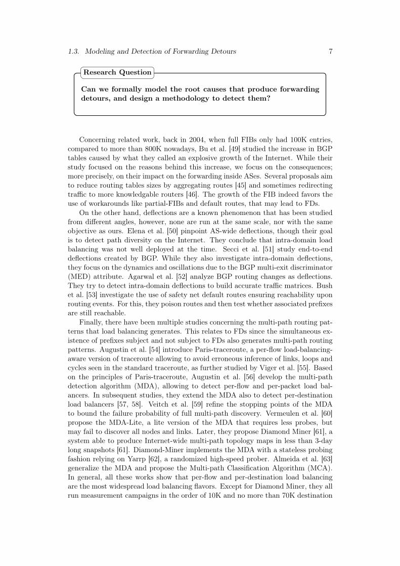
Can we formally model the root causes that produce forwardingdetours, and design a methodology to detect them?
Research Question
Concerning related work, back in 2004, when full FIBs only had 100K entries,compared to more than 800K nowadays, Bu et al. [49] studied the increase in BGPtables caused by what they called an explosive growth of the Internet. While theirstudy focused on the reasons behind this increase, we focus on the consequences;more precisely, on their impact on the forwarding inside ASes. Several proposals aimto reduce routing tables sizes by aggregating routes [45] and sometimes redirectingtraffic to more knowledgable routers [46]. The growth of the FIB indeed favors theuse of workarounds like partial-FIBs and default routes, that may lead to FDs.
On the other hand, deflections are a known phenomenon that has been studiedfrom different angles, however, none are run at the same scale, nor with the sameobjective as ours. Elena et al. [50] pinpoint AS-wide deflections, though their goalis to detect path diversity on the Internet. They conclude that intra-domain loadbalancing was not well deployed at the time. Secci et al. [51] study end-to-enddeflections created by BGP. While they also investigate intra-domain deflections,they focus on the dynamics and oscillations due to the BGP multi-exit discriminator(MED) attribute. Agarwal et al. [52] analyze BGP routing changes as deflections.They try to detect intra-domain deflections to build accurate traffic matrices. Bushet al. [53] investigate the use of safety net default routes ensuring reachability uponrouting events. For this, they poison routes and then test whether associated prefixesare still reachable.
Finally, there have been multiple studies concerning the multi-path routing pat-terns that load balancing generates. This relates to FDs since the simultaneous ex-istence of prefixes subject and not subject to FDs also generates multi-path routingpatterns. Augustin et al. [54] introduce Paris-traceroute, a per-flow load-balancing-aware version of traceroute allowing to avoid erroneous inference of links, loops andcycles seen in the standard traceroute, as further studied by Viger et al. [55]. Basedon the principles of Paris-traceroute, Augustin et al. [56] develop the multi-pathdetection algorithm (MDA), allowing to detect per-flow and per-packet load bal-ancers. In subsequent studies, they extend the MDA also to detect per-destinationload balancers [57, 58]. Veitch et al. [59] refine the stopping points of the MDAto bound the failure probability of full multi-path discovery. Vermeulen et al. [60]propose the MDA-Lite, a lite version of the MDA that requires less probes, butmay fail to discover all nodes and links. Later, they propose Diamond Miner [61], asystem able to produce Internet-wide multi-path topology maps in less than 3-daylong snapshots [61]. Diamond-Miner implements the MDA with a stateless probingfashion relying on Yarrp [62], a randomized high-speed prober. Almeida et al. [63]generalize the MDA and propose the Multi-path Classification Algorithm (MCA).In general, all these works show that per-flow and per-destination load balancingare the most widespread load balancing flavors. Except for Diamond Miner, they allrun measurement campaigns in the order of 10K and no more than 70K destination

8 Chapter 1. Research Questions and State-of-the-Art
IP addresses from at most 32 vantage points.In particular, Chapter 5 describes why detecting FDs is complex, and shows
the tool we develop to tackle this objective. While the related work has focusedon the effect of one particular cause that could potentially create FDs, our solutionallows for a systematic analysis that can be applied to detect FDs inside ASes of anykind. The methodology we propose closely analyzes how traffic flows inside ASesand does not require privileged knowledge concerning the networks being analyzed,e.g. knowing the IGP metric in use, to conclude whether FDs occur not. Note thatdetecting FDs is a particularly challenging task under these circumstances, i.e., whenno assumption is made about the IGP metric that ASes use, since forwarding detoursand best IGP paths in the end are simply forwarding routes. Moreover, similar toFDs, techniques such as load balancing and traffic engineering also generate multi-path routing patterns. Opposed to forwarding detours, these are still consideredoptimal in the sense of the IGP cost or for the specific needs of the AS deployingthem, respectively. Our analysis may complement the studies focusing on loadbalancing since we also contemplate per-prefix load balancing, a flavor not discussedin the literature. Our detector not only addresses all these challenges, but alsouses novel prefix-grouping step, that may allow to decrease the probing cost ofload balancing discovery campaigns, and to discover additional next-hops of per-destination load balancers. We test our FD-detector in the wild and find forwardingdetours in multiple ASes, with a remarkable binary pattern in which transit traffictraversing between two border routers of an AS either never detours, or alwaysdoes. Finally, the concept of forwarding detours focuses on the consequences, i.e.,on paths differing from best IGP paths, but does not tell anything on how these aregenerated, i.e., on the root causes. To shed light on this previously unexplored topic,we develop a formalism around forwarding detours allowing to formally describe thephenomenons that lead to the occurrence of forwarding detours.

Chapter 2Background
Contents2.1 Internet . . . . . . . . . . . . . . . . . . . . . . . . . . . . . 10
2.1.1 BGP . . . . . . . . . . . . . . . . . . . . . . . . . . . . . . 10
2.1.2 IXPs . . . . . . . . . . . . . . . . . . . . . . . . . . . . . . 15
2.2 Intra-domain networks . . . . . . . . . . . . . . . . . . . . 17
2.2.1 IGPs . . . . . . . . . . . . . . . . . . . . . . . . . . . . . . 17
2.2.2 Load balancing . . . . . . . . . . . . . . . . . . . . . . . . 18
2.2.3 Tunneling mechanisms . . . . . . . . . . . . . . . . . . . . 19
2.3 Traceroute . . . . . . . . . . . . . . . . . . . . . . . . . . . . 20
2.3.1 Standard version . . . . . . . . . . . . . . . . . . . . . . . 20
2.3.2 Paris traceroute . . . . . . . . . . . . . . . . . . . . . . . . 22
2.3.3 Multi-path detection algorithm . . . . . . . . . . . . . . . 23
In this chapter we interpret background knowledge and condense it into the set ofbasic topics on top of which the research of this thesis is built, particularly providingcomplementary knowledge and insights in Sec. 2.2.2 and 2.3.3. First, Sec. 2.1presents how the Internet works, i.e., how ASes are able to communicate with BGP.In addition, we study IXPs, the peering facilities allowing multiple ASes to peer in asingle location. Then, Sec. 2.2 zooms into ASes and studies the characteristics of therouting protocols that networks operators may deploy for intra-domain routing, i.e.IGPs. Moreover, we explain how load balancing and traffic engineering techniquescan be deployed to modify the forwarding routes used inside ASes. Lastly, Sec. 2.3focuses on traceroute, the main troubleshooting and debugging tool allowing todiscover the routes that packets traverse on the Internet. Moreover, we shou howthe output of traceroute, lists of traversed IP addresses, can be translated intoAS-level forwarding paths with the use of an IP-to-AS mapping. We study thestandard version of traceroute and the Paris implementation. Finally, we presentthe multi-path discovery algorithm that allows to convert Paris traceroute into atool uncovering multi-path routing, essentially load balanced paths, inside ASes.
9
10 Chapter 2. Background
AS 3001
AS 1010
AS 703
AS 10
AS 666
AS 3142
AS 2718
Expression Definition
Internet Interconnection of autonomous systems
Autonomous system Independent network, e.g. belonging to an ISP
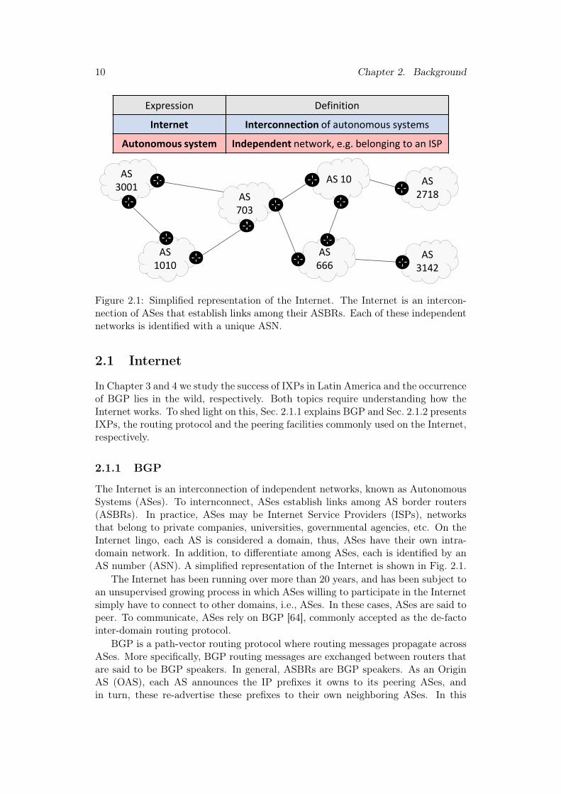
Figure 2.1: Simplified representation of the Internet. The Internet is an intercon-nection of ASes that establish links among their ASBRs. Each of these independentnetworks is identified with a unique ASN.
2.1 Internet
In Chapter 3 and 4 we study the success of IXPs in Latin America and the occurrenceof BGP lies in the wild, respectively. Both topics require understanding how theInternet works. To shed light on this, Sec. 2.1.1 explains BGP and Sec. 2.1.2 presentsIXPs, the routing protocol and the peering facilities commonly used on the Internet,respectively.
2.1.1 BGP
The Internet is an interconnection of independent networks, known as AutonomousSystems (ASes). To internconnect, ASes establish links among AS border routers(ASBRs). In practice, ASes may be Internet Service Providers (ISPs), networksthat belong to private companies, universities, governmental agencies, etc. On theInternet lingo, each AS is considered a domain, thus, ASes have their own intra-domain network. In addition, to differentiate among ASes, each is identified by anAS number (ASN). A simplified representation of the Internet is shown in Fig. 2.1.
The Internet has been running over more than 20 years, and has been subject toan unsupervised growing process in which ASes willing to participate in the Internetsimply have to connect to other domains, i.e., ASes. In these cases, ASes are said topeer. To communicate, ASes rely on BGP [64], commonly accepted as the de-factointer-domain routing protocol.
BGP is a path-vector routing protocol where routing messages propagate acrossASes. More specifically, BGP routing messages are exchanged between routers thatare said to be BGP speakers. In general, ASBRs are BGP speakers. As an OriginAS (OAS), each AS announces the IP prefixes it owns to its peering ASes, andin turn, these re-advertise these prefixes to their own neighboring ASes. In this

2.1. Internet 11
AS X
Prefix: Pj
AS Y AS Z
Prefix: Pj CP: X
x1 y1 y2 z1
Prefix: Pj CP: Y X
Figure 2.2: Example of the basic operation of BGP. ASX announces prefix Pj as theOAS, and the prefix is further advertised by AS Y that updates the CP includingitself in the path.
process, routing messages get updated, e.g. the path they follow is tracked in a fieldknown as BGP AS-path, and often referred to as control path (CP) in this thesis.In general, if an ASBR finds a loop in the CP, i.e., sees the ASN of the AS to whichit belongs already in the CP, then the message is dropped. This basic operation ofBGP is exemplified in Fig. 2.2.
As BGP speakers receive multiple announcements concerning the same prefix,they select the best route running a BGP decision process. This selection mechanismtakes into account the value of 7 attributes, in decreasing order of importance, untila tie-breaker is found [64]. Among these, the local preference is the most relevantone. ASes tune the value of the local preference to express preference of some routesdepending on the peer that announced them the prefix. The higher this metricis, the more appealing the route is considered. Following the local preference, thelength of the control path is the attribute that matters the most. In this case,routes are only discriminated based on the length of the path, the shortest onesbeing the preferred ones. In some cases, ASes use AS prepending, adding multipletimes their ASN to the CPs, in order to influence the likelihood that they may endup being chosen as best paths. An exhaustive list of the remaining attributes can befound in [64]. Among them, we highlight that the IGP cost appears as one of suchattributes, coupling BGP with intra-domain routing protocols. This compels withhot-potato routing in which the potato that burns, i.e., transit traffic traversingASes, flows through best paths and exits the AS as soon as possible, according to aIGP metric of choice.
BGP speakers run two different sessions, namely external-BGP (eBGP) andinternal-BGP (iBGP), as illustrated in Fig 2.3. In particular, eBGP and iBGP con-cern the exchange of information across ASBRs of different ASes and BGP speakerswithin the same AS, respectively. With eBGP, each ASBR in an AS announcesto each peering ASBR belonging to another AS only the best path to each pre-fix. Thorough iBGP, the situation replicates between the BGP speakers of an AS.This allows each BGP speaker to find, among all routes considered the best by thedifferent BGP speakers within the AS, the overall best route.
BGP speakers maintain a BGP routing table called BGP Routing InformationBase (RIB). As routing messages are received, routers populate the RIB. There existdifferent fields that are completed for each entry: the prefix that was advertised inBGP, the BGP next-hop, i.e., the ASBR that announced the prefix, and the attributevalues included in the message in which the prefix was advertised. For each prefix,the overall best path is chosen relying on the aforementioned BGP decision process.
12 Chapter 2. Background
Session Acronym Description
Internal iBGP (-) Run among BGP speakers within the same AS
External eBGP (-) Run among ASBRs in different ASes
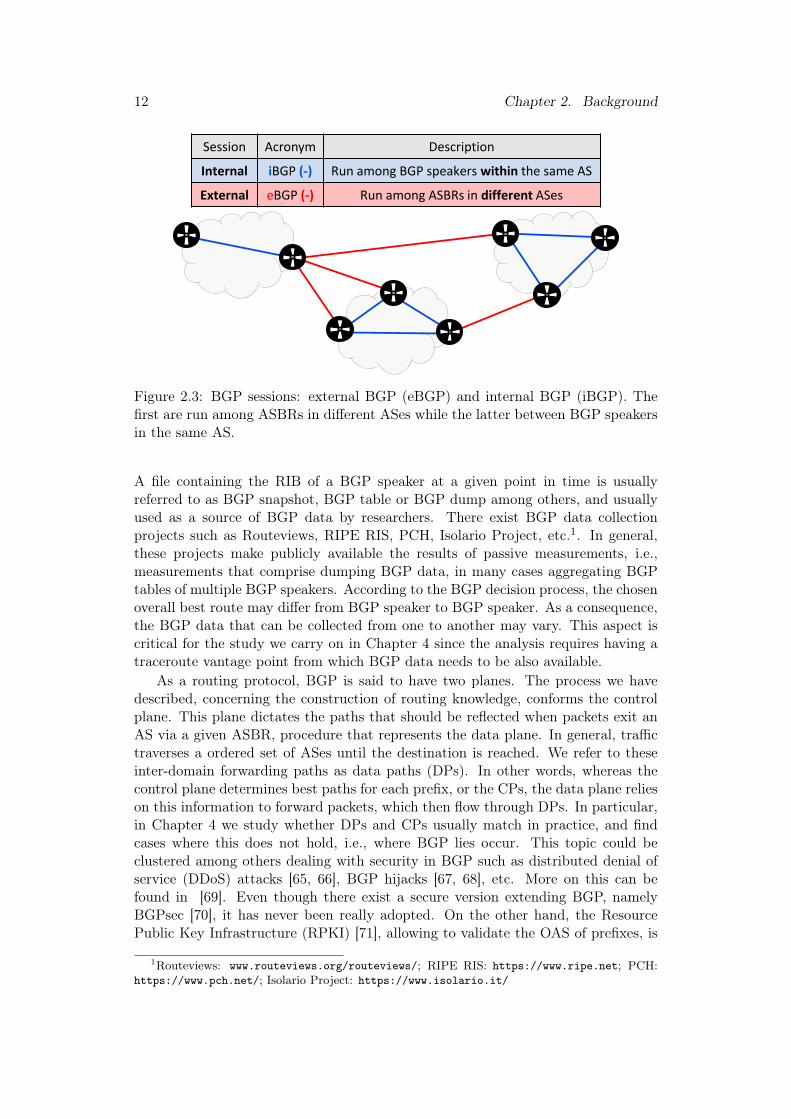
Figure 2.3: BGP sessions: external BGP (eBGP) and internal BGP (iBGP). Thefirst are run among ASBRs in different ASes while the latter between BGP speakersin the same AS.
A file containing the RIB of a BGP speaker at a given point in time is usuallyreferred to as BGP snapshot, BGP table or BGP dump among others, and usuallyused as a source of BGP data by researchers. There exist BGP data collectionprojects such as Routeviews, RIPE RIS, PCH, Isolario Project, etc.1. In general,these projects make publicly available the results of passive measurements, i.e.,measurements that comprise dumping BGP data, in many cases aggregating BGPtables of multiple BGP speakers. According to the BGP decision process, the chosenoverall best route may differ from BGP speaker to BGP speaker. As a consequence,the BGP data that can be collected from one to another may vary. This aspect iscritical for the study we carry on in Chapter 4 since the analysis requires having atraceroute vantage point from which BGP data needs to be also available.
As a routing protocol, BGP is said to have two planes. The process we havedescribed, concerning the construction of routing knowledge, conforms the controlplane. This plane dictates the paths that should be reflected when packets exit anAS via a given ASBR, procedure that represents the data plane. In general, traffictraverses a ordered set of ASes until the destination is reached. We refer to theseinter-domain forwarding paths as data paths (DPs). In other words, whereas thecontrol plane determines best paths for each prefix, or the CPs, the data plane relieson this information to forward packets, which then flow through DPs. In particular,in Chapter 4 we study whether DPs and CPs usually match in practice, and findcases where this does not hold, i.e., where BGP lies occur. This topic could beclustered among others dealing with security in BGP such as distributed denial ofservice (DDoS) attacks [65, 66], BGP hijacks [67, 68], etc. More on this can befound in [69]. Even though there exist a secure version extending BGP, namelyBGPsec [70], it has never been really adopted. On the other hand, the ResourcePublic Key Infrastructure (RPKI) [71], allowing to validate the OAS of prefixes, is
1Routeviews: www.routeviews.org/routeviews/; RIPE RIS: https://www.ripe.net; PCH:https://www.pch.net/; Isolario Project: https://www.isolario.it/

2.1. Internet 13
nowadays becoming more extensively used.2. Arguably, this partially occurs sinceRPKI is central in in the mutually agreed norms for routing security (MANRS). 3
Another important aspect of BGP is that it allows ASes to apply filtering poli-cies, and choose to which ASes they announce the prefixes they learn. In general,this depends on the business relationships that ASes establish [72, 73]. These rela-tionships are dictated by who pays to whom when traffic gets exchanged: an AS paysits provider ASes, peers freely with sibling ASes and peer ASes, and gets paid bycustomer ASes. Hence, when choosing among available routes for the same prefix,the order of preference grows from last to first, and ASes set up the local preferenceaccordingly. In other words, ASes apply import policies in which an AS choosespaths:
• advertised by customers as priority since this generates revenue;
• learned via peer-to-peer links that have a shared-cost, if no customer offerstransit and;
• involving links to providers where the AS has to pay as the last option.
These policies, aiming to maximize the revenue, partially explain why BGPsecdid not succeed. Indeed, BGPsec requires prioritizing security above local preferencein the BGP decision process to be effective against routing attacks [74], somethingthat numerous network operators are not willing to do [75]. In addition, whenadvertising prefixes, ASes apply export policies making sure control paths are valley-free, meaning that they do not provide transit for free to providers or peers. Inpractice, ASes enforce this by:
• advertising all paths they learn to customers and siblings;
• announcing to providers only those paths learnt via customers or siblings, and;
• filtering paths learnt via providers when advertising paths to peers.
These rules are usually referred to as Gao-Rexford policies. This study, and inparticular the proposed rules, form part of research concerning BGP convergence orBGP safety, i.e., the conditions that guarantee that BGP will eventually converge toa stable routing outcome [76, 77, 78, 79, 80]. As shown in Fig. 2.4, the Gao-Rexfordrules imply that:
• prefixes learned via customers and siblings are advertised to all ASes (Fig. 2.4a);
• prefixes learned via peers and providers are only announced to customers andsiblings (Fig. 2.4b and 2.4c, respectively).
Though these policies are still considered the norm, studies have reported on casesassociated with the application of more complex policies [81, 82, 83]. As we showin Chapter 4, BGP lies may relate to ASes attempting to avoid paying for usingcustomer-to-provider links by sending traffic towards peer-to-peer links.

14 Chapter 2. Background
(a) Customers to everyone
(b) Peers to customers
(c) Providers to customers
Figure 2.4: BGP policies following Gao-Rexford rules. The AS in the center an-nounces all prefixes learnt via customers (green ASes) to all remaining ASes, butthose learned via peers (yellow ASes) and providers (red ASes) are only exportedto customer ASes.

2.1. Internet 15
Tier-1
ASes
Small
ISPs
Stub
ASes
Large
ISPs
(a) Internet structure before 2000s.
Tier1
AS
Big
ISPIXP
Big
ISP
Stub
ASCDN
Stub
AS
Stub
AS
ISPIXPISP
Tier1
AS
(b) Current shape of the Internet.
Figure 2.5: Evolution of the (simplified) structure of the Internet. Lines with arrowsindicate provider-to-customer links, and those dashed peer-to-peer links. While be-fore the Internet had a clear pyramidal structure, the appearance of IXPs increasedthe number of peer-to-peer links and the Internet flattened. In addition, multiplecontent providers developed their own CDNs, which further accelerated this process.
2.1.2 IXPs
As a result of the business relationships that ASes tend to establish, i.e., provider,customer and peer ASes, the Internet naturally adopted a hierarchical structure,as illustrated in Fig. 2.5a. The ordering among ASes is still usually described as
2See https://rpki-monitor.antd.nist.gov/ and https://rov.rpki.net/3https://www.manrs.org/

16 Chapter 2. Background
a pyramid in which, from base to tip, three types of ASes can be distinguished:stub ASes, transit ASes and tier-1 ASes. The set of stub ASes is composed bythose ASes without customers, whereas transit and tier-1 ASes are mainly ISPs.Since stub ASes do not have customers, they only forward traffic either destinedto or originated from themselves or siblings. On the other hand, transit ASes havecustomers ASes of which they forward traffic, but also have provider ASes. Ingeneral, transit ASes may be described as those ranging from small to large/big ISPs,usually providing a service constrained to a specific region or continent, whereas tier-1 ASes usually characterize for being ISPs with a geographical footprint coveringmultiple continents, thus not needing to buy transit service from any other AS.4 Ingeneral, a communication between stub ASes located in different continents requiredpackets to traverse up and then down the pyramid.
The structure of the Internet begun a flattening process in the early 2000s, largelymotivated by the massive irruption of Internet Exchange Points (IXPs) [84, 4]. Acloser representation of what the Internet looks like nowadays is shown in Fig. 2.5b,where we also highlight the appearance of content distribution networks (CDNs),i.e., networks belonging to content providers. IXPs are facilities that allow multipleASes to peer at a single location. To interconnect ASes, IXPs use layer-2-devices,i.e., switches. In addition, IXPs usually count with route servers to which ASes mayopt to connect. An AS willing to participate in an IXP establishes a unique sessionwith the IXP and, accessing the route server, is able to simultaneously peer with allthe other participants in the IXP, known as IXP members or connected networks.In general, IXP members establish peer-to-peer relationships and only announcetheir customer cone [85] at IXPs, i.e., prefixes with AS-paths leading to customerASes, and customers of these. Besides peering with the route server, IXPs usuallyallow ASes to peer privately, i.e., carry out announcements that are not advertisedin the route server. In short, IXPs allow ASes to peer at a larger scale, and thusare known as peering fabrics. Indeed, the use of IXPs broke the mechanics of thehierarchical pyramid, and terms such as tier-1 ASes could arguably be consideredas rather legacy. Nowadays, metrics such as the AS-rank [86] are considered moreinformative to give a sense of the size of the business an AS runs.
The major success of IXPs is backed by many reasons. First, IXPs allow tooffload upstream traffic, resulting in monetary savings for IXP members. Second,IXPs allow to exchange local traffic within the same region, shortening end-to-endpaths and reducing latency [87, 88]. Third, IXPs attract CDNs [84], and CDNs at-tract members. Indeed, CDNs place caches in IXPs to get to (multiple) eyeballs froma single peering point [5], thus allowing IXPs to offer low-cost access to content [89].
In particular, in Chapter 3 we study the multiple IXPs deployed across LatinAmerica, a region that has received little attention in Internet studies. Besidesshedding light on the status of the Internet in Latin America, we investigate whetherIXPs have had a similar success than in the 2000s in the region.
4The way I describe the geographical footprint of small and large/big transit and tier-1 ASes isonly an interpretation that provides a fast way of classifying ASes into these different categories,but should not be considered strict definitions to which no exceptions exist.

2.2. Intra-domain networks 17
2.2 Intra-domain networks
In Chapter 5 we develop a methodology to detect forwarding detours inside ASes,i.e., whether traffic traversing an AS does not flow through the best available pathsin the network. Therefore, understanding how the routing works inside ASes isnecessary. To build a strong foundation on such topic, while Sec. 2.2.1 studiesthe main characteristics of IGPs, Sec. 2.2.2 and 2.2.3 show how load balancingand tunneling techniques allow to modify the standard behavior of the usual intra-domain routing protocols.
2.2.1 IGPs
Besides BGP, ASes additionally use an Internal Gateway Protocol (IGP), i.e., a dedi-cated routing protocol for intra-domain routing. In particular, renown IGPs includeOpen Shortest Path First (OSPF) [90] and Intermediate System to IntermediateSystem (IS-IS) [91].
OSPF and IS-IS are link-state routing protocols, meaning that routers build agraph of the intra-domain network. This graph represents the connectivity statusof the network, i.e., shows which nodes are connected to which other nodes.
To construct their routing knowledge, routers exchange routing messages indi-cating the links they have with other routers. In addition, every advertised link isweighted with a given IGP cost or IGP distance, according to a pre-defined IGPmetric. As an example, a hop-count metric assigns a constant IGP cost of 1 to everylink, but other metrics may for example vary the cost depending on the bandwidthavailable on each link.
With OSPF and IS-IS, each router considers that, for every destination adver-tised in the IGP, the shortest path according to the IGP metric in use representsthe best IGP path. To determine such paths, routers run Dijkstra’s algorithm [92].Once the best path to reach a prefix is decided, routers take note of the routerthat announced the path, and use it as IGP next-hop or next-hop towards thatprefix. When the considered prefix is actually a BGP prefix, a recursive lookup isperformed, and the next-hop matches the neighboring router offering the best pathtowards the BGP next-hop of that prefix. In general, the next-hops are furtherinstalled in a table known as Forwarding Information Base (FIB), that is optimizedto perform fast the actual forwarding of packets. As we study in Chapter 5, somerouters sometimes are not able to keep a full-FIB in memory, and the workaroundsimplemented in these scenarios may lead to forwarding detours.
The concept of best paths across IGPs and BGP do not imply the same, thereare two key differences: (i) the information that routers or ASes receive to actuallydecide which is the best path, and; (ii) the conceptual meaning of the metrics thatare taken into account to choose best paths.
While IGP best paths are globally optimal, this may not be the case in BGP. Ac-cording to IGPs, since all routers in the network receive the same routing messages,all subpaths of any best path are also best paths. This property results from the factthat routers have the same view of the network: what a router considers the best,is also seen as the best for the remaining routers. We refer to this agreement amongthe devices of a network as the existence of routing consistency in the network. As
18 Chapter 2. Background
we study in Chapter 5, when this property is not met, forwarding detours may likelyoccur. In contrast, in BGP, the opportunity to apply filtering policies breaks downthis property: not all ASes receive the same information, so ASes choose best pathsfrom a set of routes that may be just a subset of all those actually available. In otherwords, contrary to IGPs, the best paths BGP chooses are locally optimal instead ofglobally [80].
On the other hand, IGPs attempt to maximize the efficiency of the routing andforwarding, however, BGP rather minimizes the monetary cost of handling traffic.The purpose of using hop-count or bandwidth-available metrics in IGPs is to enforce“fastest” paths as best paths, i.e., those through which traffic traverses the networkwith the least required IGP distance. On the contrary, for BGP, the importanceof end-to-end delay is secondary. This results from the fact that the BGP decisionprocess weights the local preference more than any other attribute, and this metriconly reflects business relationships, as previously explained. For BGP, comparingthe length of the control paths comes as the second criteria, hence, shorter paths viaproviders will usually be neglected even when faced against longer paths, given thatthese were advertised by peers or customers. In fact, since not necessarily all ASescomply to the same policies, and thus may take conflicting decisions, this has leadto the research concerning BGP convergence, a concept introduced in Sec. 2.1.1.
2.2.2 Load balancing
Load balancing (LB) is a technique that network operators may deploy to bothenhance and increase the resource utilization of their network. LB provides a meansto distribute the load across multiple paths, named LB paths. In general, LB relieson the equal-cost multi-path (ECMP) routing feature of the intra-domain routingprocols OSPF [90] and IS-IS [91], such that all parallel paths that are used share thesame IGP cost [93]. Note, however, that LB may also be used across inter-domainlinks, for example, with the use of multi-path BGP [94].
The routers that enable ECMP and apply LB are known as load balancers or LBrouters. LB routers have the capability to choose among different next-hops towardsa destination. Every time load balancers have to forward a packet, they send it to thenext-hop they select out of a set of available next-hops towards each destination.As we show in Chapter 5, similar to LB, forwarding detours generate multi-pathrouting patterns between endpoints of ASes and, therefore, differentiating amongthese two, requires understanding the details of how LB operates. Indeed, LB canbe deployed in different LB flavors, or flavors [95]. To balance packets across next-hops, load balancers take into account either (some) packet header fields, or noneat all [54, 55]. In the following we describe the usual LB flavors.
The simplest mode of LB, namely per-packet LB [96, 97], assigns packets to next-hops blindly, in a round-robin fashion. Consequently, with this approach, packetsexchanged in a TCP connection are subject to reordering, a fact known to degradethe performance of TCP [98, 99, 100]. Moreover, faced to this LB flavor, toolsaiming to retrieve the forwarding paths used on the Internet may fail to reveal somelinks, and even infer false ones [54, 55]. Fortunately, per-packet LB is rarely foundin practice [59, 61, 63].
Other more sophisticated LB methods, which we call hash-based LB, decide

2.2. Intra-domain networks 19
next-hops relying on the use of a hash function, rather than blindly. More precisely,load balancers apply a hash on packet header values, and use the outcome of suchcomputation to choose one among the available next-hops. As a consequence, incontrast with per-packet LB, packets belonging to the same TCP connection arealways forwarded to the same next-hop. Due to this, such packets are said to belongto the same flow, and to have a similar flow-identifier, or simply flow-ID. Dependingon the fields used to compute the hash, hash-based LB methods have historicallybeen subdivided in two types: per-destination LB, or in short per-dest LB [96], andper-flow LB [96, 97, 101]. While the source and destination IP addresses are usedas input in per-dest LB, the source and destination transport ports or the ICMPchecksum are additionally taken into consideration in per-flow LB for UDP and TCP,and ICMP packets respectively. In addition, the IP type of service (TOS) or DSCPand ICMP code fields have also been identified as fields that load balancers maytake into account to choose among next-hops [54, 63]. Moreover, a per-applicationLB scheme, only relying in the transport port numbers has also been proposed [102].However, results in [63] suggest that, as of today, these flavors are not as widespreadas per-dest and per-flow LB.
Previous work has mainly focused on per-dest and per-flow LB, however, thereexists a third hash-based LB flavor that has been systematically omitted in theliterature, known as per-prefix LB [101, 103], which we consider in this thesis. Withper-prefix LB, the hash function is evaluated on the most specific prefix associatedwith the destination IP address of each packet. Note how this LB flavor contrastswith the other two hash-based LB methods, where the destination IP address ishashed at once. Due to this, in this thesis we propose a new nomenclature: we saythat per-prefix LB is a coarse-grained LB type (C-LB), while per-dest and per-flowLB are fine-grained LB types (F-LB).
Finally, to mimic distinct hashing functions, load balancers also rely on addi-tional parameters, such as the router-id or a configured seed value, to determinenext-hops. Note that these complementary inputs neither depend nor are extractedfrom the packets being forwarded. This allows to avoid polarization effects that, pre-venting the use of redundant routes, concentrate traffic on a subset of the availableLB routes [104]. On the other hand, the rebooting of routers, and the consequentrecompute of the seed value, has been suggested to produce next-hops re-mappingevents often mistakenly attributed to routing changes [61].
2.2.3 Tunneling mechanisms
In an ISP, transit traffic usually traverses the AS from ingress-ASBRs to egress-ASBRs. For this to be handled efficiently and correctly, all routers in the networkwould be required to speak BGP, or at least to know the best gateway for eachexternal prefix. To reduce the load on devices, ISPs and ASes in general may optto run a network with a BGP-free core, and rely on tunneling mechanisms [105].With this alternative option, traffic is tunneled between edge routers, that are theonly devices that require having a full BGP feed. On the other hand, core devicestake forwarding decisions based not on the destination IP addresses, but ratherdepending on the ingress point through which traffic enters the AS and the egresspoint to which it needs to be redirected.

20 Chapter 2. Background
There exist different tunneling protocols, e.g. IP in IP, generic routing encapsula-tion (GRE), but multi-protocol label switching (MPLS) [106] is usually consideredthe de-facto standard. With MPLS, traffic is tunneled via label-switched paths(LSPs), where labels are appended to packets by the ingress node of the path, re-ferred to as label switched router (LSR). The forwarding is then performed basedon the labels values, that get updated at each hop.
Network operators may implement MPLS over the core with the combinationof an IGP and the label distribution protocol (LDP) [107], or segment routing(SR) [108]. In general, this option encompasses scalability purposes related to run-ning BGP-free cores, ensuring traffic traverses the network through best IGP pathsbetween LSRs. As we study in Chapter 5, networks operators may use these tech-niques to avoid suffering from forwarding detours in their networks, but still mayfail to achieve this goal.
On the other hand, tunneling mechanisms may be used for traffic engineering,with the resource reservation protocol for traffic engineering (RSVP-TE) [109]. Withthis option, network operators can implement LSPs with constrained requirementsconcerning bandwidth, jitter, etc. and hence use it for traffic engineering purposes.In general, this solution is used for a reduced set of prefixes since RSVP-TE suffersfrom well-known scalability issues, that increase with the quantity of TE pathsthat are deployed [110]. As a variant to RSVP-TE, segment routing implements alightweight control plane that allows it to scale better, and thus is now consideredthe new state-of-the-art TE and fast-reroute technology deployed in most ISPs.As we model in Chapter 5, TE generates multi-path routing patterns. As such,constrained paths resulting from TE may be confused with forwarding detours. Inparticular, in Chapter 5 we address the difficulty of differentiating between both.
2.3 Traceroute
Traceroute is the most widespread tool allowing to collect IP forwarding paths.In addition, we make extensively use of it in Chapter 4 and 5, thus present itsfunctioning principle in detail in this section. In particular, Sec. 2.3.1 explains howthe original version of traceroute works and a basic method allowing to translate theIP path that this tool outputs into an AS-level forwarding path. Then, Sec. 2.3.2presents Paris traceroute, an updated load-balancing-aware version of traceroute.In addition, Sec. 2.3.3 shows how Paris traceroute can be converted into a multi-pathdetection tool.
2.3.1 Standard version
Van Jacobson introduced traceroute, a tool allowing a host on the Internet to dis-cover the forward IP path towards a destination IP address [111].
Traceroute manipulates the Time-To-Live (TTL) field in the IP header of packetsto elicit responses from the intermediate network-layer devices that are traversed inthe path towards the destination IP address. This field expresses the number oftimes that a packet can still be forwarded before it needs to be dropped, and isdecreased by routers at each hop [112] (though this has been shown not to hold inpractice sometimes [54, 55, 113]). As a packet moves along towards the destination,

2.3. Traceroute 21
each intermediate router that receives it first checks whether the destination IPaddress coincides with any of the IP addresses assigned to its interfaces. If this isnot the case, the router may proceed in two different ways depending on the value inTTL field of the packet header. If the value is greater than one, the router decreasesit by one unit and forwards the packet to the next-hop towards the destination.Instead, if the value equals one, the packet is said to have expired, and is discarded.However, before doing so, the router handling the packet sends an ICMP TimeExceeded message back to the source. This message encapsulates the IP header ofthe probe packet, and the first 64 bits that follow it [114]. Since traceroute doesnot use IP options, then these 8 bytes comprise, depending on the probe packetprotocol, the complete UDP or ICMP Echo Request headers, or partially the TCPheader. The router uses as source IP address of this message that of the outgoinginterface it uses to forward the packet [115, 116]. When the routing is symmetric,this IP address coincides with that of the incoming interface that received the probepacket.
Traceroute sends packets in succesive rounds towards a destination IP address,with increasing TTL values: in the first round packets have a TTL = 1, the secondone TTL = 2, and so on. As these packets expire at increasing hop distances,all the intermediate routers finish replying with ICMP Time Exceeed messages.The entity running traceroute, by inspecting the source IP address of each of themessages it receives, is thus able to learn the IP addresses that are traversed towardsthe destination IP address. However, at this point, two questions remain to beaddressed: (i) how is traceroute able to determine the order in which the IP addressit learns were crossed? and; (ii) how does traceroute know when to stop sendingpackets?
Concerning (i), besides continuously changing the TTL values, traceroute en-codes additional data in other packet header fields, allowing it to reconstruct thetraversed IP path in the correct order. To retrieve this data, traceroute wiselychooses the encoding fields, from either the IP header, or the first 8 bytes of IPpayload. This way, traceroute makes sure that the fields it uses are quoted inthe ICMP Time Exceeded messages it receives. The exact fields depend on thetransport-protocol that traceroute uses. For UDP probes, TCP SYN and ICMPEcho Request messages, traceroute systematically varies the destination port, IPID and ICMP sequence number fields, respectively [54]. Using a unique value perpacket that is sent, traceroute is thus able to match each response message to eachoriginal packet it sent, and thus to infer the correct IP path.
Regarding (ii), the basic assumption is that, as the source is continuously launch-ing probes with an increasing TTL value, at a given moment a packet will arriveto the destination IP address. When the destination actually receives the packet,it will corroborate that the destination IP address in the IP header field coincideswith one of the IP addresses in its interfaces. In this case, rather than an ICMPTime Exceeded message, the destination will reply to the source IP address withanother type of message. For UDP probes, TCP SYN and ICMP Echo Request mes-sages, these replies will usually be an ICMP Destination Port Unreachable, TCPACK+SYN or Reset and ICMP Echo Reply messages, respectively. Upon receptionof this different type of packet, the source is thus able to determine that the tracingcan be stopped. Besides the options enumerated above, where traceroute ends with
22 Chapter 2. Background
a successful status, there exist cases where traceroute (partially) fails. These in-clude cases where, the host, network or protocol is unreachable, the communicationis administratively prohibited, etc. A more exhaustive list can be found in [117]. Inother words, traceroute may halt with a failing status, and only provide a partialIP path towards a destination.
Traceroute also keeps a timer for each packet it sends, and thus it is able toestimate the round-trip time (RTT) towards each IP address it finds in the pathtowards the destination. In addition, traceroute also uses these timers to declarepackets as lost. Indeed, this is assumed to have happened once a timer exceedsa given threshold that can usually be pre-configured. In these cases, traceroutewill include missing hops, which are usually indicated as ‘*’. Whether the packettraceroute sent or the reply itself was lost cannot be known. In addition, if therouter received the packet, but applied ICMP rate limiting, i.e., could not reply atthat moment, or will never do so, requires additional analysis [118, 119].
Traceroute is a tool that runs active measurements, i.e., that allows to obtaindata by actively sending packets towards a host. There exist looking glasses andmeasurements platforms such as RIPE ATLAS, NLNOG RING infrastructure, thePEERING testbed, CAIDA’s Ark, among others that allow to perform traceroutefrom nodes distributed around the globe.5. In addition, it is important to know thateven though traceroute is the state of the art tool to gather data paths, there existother tracing tools to obtain forwarding IP paths. This is the case of packets withIP options, such as the IP record route [112]. These type of packets were seen to bedropped in edge networks, and their practical usefulness questioned [120]. However,lately, other studies have argued the opposite [121] and even constructed a reverseIP path tracer relying on them [122]. A limitation of the record route option isthat, contrary to traceroute, it is constrained in the number of IP addresses it canreport, to no more than 9 [112]. Besides this, my personal experience is more alignedwith [120].
Finally, the output of traceroute is an IP-level path, however, in multiple oc-casions it is valuable to translate this into AS-level paths, i.e, understand whichASes were traversed in the path towards the destination IP address. This is usuallydone with an IP-to-AS mapping tool. To map from IP paths to AS-level paths,the standard method is to rely on BGP snapshots, and map each IP address tothe OAS announcing its best covering prefix. As we study in Chapter 4, this pro-cess is error-prone, and usually requires refining. Moreover, this chapter presents anew framework we propose to filter inaccuracies resulting from the basic IP-to-ASmapping method.
2.3.2 Paris traceroute
The standard version of traceroute has the limitation that, in the presence of loadbalancers, it may likely provide incorrect route inferences [54]. This problem re-sults from the fact that load balancers may likely forward the multiple packets thattraceroute sends across different next-hops. This may lead to both missing links and
5RIPE ATLAS: https://atlas.ripe.net/; NLNOG RING infrastructure: https://ring.nlnog.net/, PEERING testbed: https://peering.usc.edu; CAIDA’s Ark: https://www.caida.org/projects/ark/

2.3. Traceroute 23
false links, and has be shown to explain most anomalies, such as loops and cycles,seen in the standard traceroute [54, 55].
The aforementioned problem only occurs for per-packet and per-flow LB. For per-packet LB, this issue appears due to the non-deterministic nature in the selectionof next-hops. Consquently, a priori, this problem cannot be solved for this flavor.On the other hand, for hash-based LB flavors, the difficulty originates from thefact that the fields that load balancers use to ascribe packets to different flows aremodified by traceroute. Indeed, this happens because these fields are either (i) thesame encoding fields that traceroute uses to be able to reconstruct the IP paths inthe correct order, or; (ii) indirectly modified by the encoding traceroute uses. Fora fixed source IP address, since traceroute also keeps the destination IP addressconstant per trace, these situations can only arise in the presence of per-flow loadbalancers.
The artifacts that the presence of per-flow load balancers produce depends on thetype of packets that traceroute uses. The problem exists for UDP and ICMP probes,since traceroute deliberately changes the destination port number and indirectlythe ICMP checksum when updating the ICMP sequence number, respectively. ForTCP, instead, traceroute keeps the port numbers constant, in particular choosingthe value 80 for the destination port number to emulate web traffic. In these cases,traceroute relies on the IP ID field as the encoding field, thus TCP probes launchedby traceroute are not subject to load balancing artifacts.
Paris traceroute was introduced in 2006 as a per-flow load-balancing-aware ver-sion of traceroute [54, 55]. Basically, Paris traceroute only changes the encodingfields that the standard traceroute uses to other assumed not to be used for LB.Hence, for all transport-layer protocols, Paris traceroute manages to keep the fieldsthat are used by per-flow load balancers with a fixed value. This ensures that loadbalancers forward all packets issued in a trace to the same next-hop, and fixes mostartifacts described in [54, 55]. For UDP probes, Paris traceroute fixes the desti-nation port number, and uses the transport-layer checksum as the encoding field.For this, Paris traceroute carefully crafts the payload these UDP packets carry suchthat the UDP checksum, besides increasing by a unit each time a packet is sent,is also valid. On the other hand, for ICMP probes, the ICMP sequence number isstill used as the encoding field. However, Paris traceroute additionally modifies theICMP identifier field to offset the change in the ICMP sequence number, ensuringthat the ICMP checksum remains constant in all packets. Finally, Paris traceroutealso implements a TCP version that, compared to that of the standard traceroute,simply replaces the encoding field from the IP ID to the TCP sequence number. Themotivation behind this TCP implementation, however, is only to uniformize the useof the IP ID field across all probe packet protocols as the process encoding field,i.e., the field that relates to the running process identifier (PID) of each tracerouteinstance that is launched.
2.3.3 Multi-path detection algorithm
To detect the set of load-balanced paths between a source and a destination onthe Internet, the multi-path detection algorithm (MDA) was introduced in 2007as a variation of Paris traceroute [56]. In short, the MDA is a stochastic probing

24 Chapter 2. Background
algorithm that can be used to find, with a pre-defined high-confidence, all interfacesand links at every hop towards a destination. In particular, MDA is able to gatherall these results when only per-dest or per-flow load balancers are traversed, butmay fail to reveal true links faced to per-packet load balancers.
The MDA has been subject to multiple refinements over time [57, 58, 59]. How-ever, the basic working principle always remains the same. This section focuseson the latest implementation, that relies on the assumptions that: (i) load bal-ancers are independent among themselves, i.e., the next-hop a load balancer choosesdoes not affect the one that another load balancer may choose; (ii) load balancerschoose any of their next-hops with equal probability (for per-packet or per-dest/flowload balancers, this should be interpreted at the packet or flow level, respectively);(iii) MPLS is not deployed; (iv) no routing change occurs while the MDA is tracinga destination, and; (v) routers reply to probe packets. When the aforementionedhypothesis are not met, the MDA may provide incomplete or inaccurate results.
The MDA has two modes of operation, either at the node level or end-to-endpath level, that mainly differ in the probing that each requires. While the first isable to conclude with a high significance level α that all next-hops of one incominginterface have been discovered, the latter bounds, for a given theoretical maximumnumber of interfaces QI along the path, the failure probability β of discoveringall next-hops of all interfaces across the path. In practice, the arbitrarily chosenvalues α = β = 0.05 and QI = 30 are often used. The effects of varying α or QI
have never been studied, while that of changing β from 0.01 up to 0.5 has shownimpact in the probing cost, but not on performance [59]. In other words, the end-to-end path model does not provide a tight bound to the probability of failure. Asa consequence, the actual interpretation of the parameter β becomes blurred, beingrather an indicator of how many extra measurements the user may afford to waste.I believe that tuning QI differently may allow not only to consider more realisticscenarios, but also will likely translate into a significant save of probing cost.
In general terms, the underlying behavior of the MDA is similar regardless of themode of operation. Indeed, the MDA works in multiple rounds that are repeatedat every interface that is revealed, until the probing reaches the destination. In thefollowing, we will analyze the procedure of the MDA considering an arbitrary hoph at which an interface rh with N next-hops is being analyzed. The MDA sendspackets through rn and declares the interfaces that are revealed at hop h+ 1 as thenext-hops of rh. The MDA studies all interfaces at hop h, and then continues withthose discovered at hop h+ 1. The notation we use is summarized in Table 2.1
The MDA initially assumes load balancers are per-flow load balancers, and seeksat least n flow-IDs φ1, φ2, . . . φn for which rh is traversed. The flow-IDs are variedby choosing different destination IP addresses. This is done progressively increasingthe size of the IP prefix from which the IP addresses are obtained, until the /24granularity is reached. Beyond that point, [57] and [58] do not describe what shouldbe done, however it has been recently proposed to continue varying flow-IDs bychanging port numbers [61]. Though effective for per-flow load balancers, this strat-egy may fail to detect additional next-hops in case per-destination load balancersare traversed. In this thesis, we propose an alternative that may help to solve thisproblem, as discussed in Chapter 5. In any case, since rh is at least the next-hop ofone interface rh−1 previously analyzed, then the flow-IDs for which both rh−1 and

2.3. Traceroute 25
h Hop numberrh Interface at hop hφi Flow-ID iα Significance level that all next-hops of one interface have been discoveredQI Theoretical maximum number of interfaces along the pathβ Failure probability of discovering all next-hops of all interfaces across the path.N Number of next-hops of interface rhN̂ Number of next-hops estimated for of interface rh by the MDA
n , nN̂ Stopping point the MDA uses given N̂ next-hops have been discovered
Table 2.1: Notation used to describe the functioning principle of the MDA..
rh were revealed, can be reused to discover next-hops of rh. In a more general sense,all of the flow-IDs φ1, φ2, . . . φj associated with paths for which rh is reached can bereused. If j < n, then the MDA searches the n− j missing ones in a trial-and-errorfashion, i.e., sending successive probes carrying a random flow-ID.
Relying on hypothesis (ii), i.e., that load balancers uniformly distribute flow-IDsacross their next-hops, the MDA calculates the value of n to meet the requirementsestablished by the mode of operation, i.e., according to α or β and QI . In particular,the values are calculated for the scenario with least chances of revealing all interfaces,that corresponds to the case where N̂ , the number of next-hops already discovered,equals N − 1. In other words, the question that the MDA addresses is “after nmeasurements and N̂ next-hops that have been respectively carried and discovered,could it be that we are still missing one next-hop?”. The reason of why asking if onlyone and not more, intuitively, is that the less next-hops remain to be discovered, theharder it becomes to find them. As a consequence, when estimating the additionalprobing required to ensure that the probability of missing any number of next-hops is low (or at least bounded below a certain value), this represents the mostconservative approach. Adopting this criteria, n can be shown to depend only onN̂ and α or β and QI . Moreover, considering the latter parameters are pre-definedby the user, n is usually indicated as nN̂ and referred to as stopping point. Whilethe values of the stopping points implemented by the end-to-end path level versionof the MDA can be found in [59], for the node level version, after re-arranging theformulas and conditions in [56], nN̂ is the minimum value such that the followingconstraint holds
N̂∑i=0
(−1)N̂−i(N̂ + 1
i
)(i
N̂ + 1
)nN̂
< α
Proof. I find the explanation in [56] quite hard to follow, therefore I will providethe complete demonstration. The question to answer is “given that an interface hasN next-hops, what is the probability Pf that only one might not be revealed, i.e.,N = N̂ + 1, after the MDA uses nN̂ probes? ”. We can model the scenario as thewell-known problems involving balls that are thrown into urns. The parallelismdictates that urns are next-hops, and balls are the probes that the MDA sends.

26 Chapter 2. Background
Therefore the question can be reformulated as: Given that there are N urns, whatis the probability that after throwing nN̂ balls, one urn might be empty? ”. Definingthe random variables
Ui : number of balls inside urn i
what we want to find is the probability Pf that any Ui might be null, i.e.,
Pf = P (U1 = 0 ∪ U2 = 0 ∪ , . . . , ∪ UN = 0) = P
(N⋃i=1
Ui
)To solve this, first we can use the inclusion-exclusion principle that generalizes
the property stating that P (A ∪B) = P (A) + P (B)− P (A ∪B), which gives
Pf =N∑k=1
(−1)k−1∑
I⊂{1,...,N}|I|=k
P (UI)
such that UI ,⋂
i∈I Ui. Since the probability of the events UI depends on thecardinality of I, then we can rewrite Pf as
Pf =N∑k=1
(−1)k−1(N
k
)(N − kN
)nN̂
where(Nk
)is the number of events that have cardinality k, and (N−kN )nN̂ is the
probability of the event that k given urns might be empty after throwing nN̂ balls.Considering the property that
(Nk
)=(
NN−k
)and defining i = N − k, then
Pf =
N−1∑i=0
(−1)k−1(N
i
)(i
N
)nN̂
and recalling that N = N̂ + 1, we have
Pf =
N̂∑i=0
(−1)N̂−i(N̂ + 1
i
)(i
N̂ + 1
)nN̂
Once Pf is known, the question that remains is: what should be the value of nN̂so that Pf is less than α? The value of nN̂ has to be calculated so that
N̂∑i=0
(−1)N̂−i(N̂ + 1
i
)(i
N̂ + 1
)nN̂
< α
�
There is actually no closed form to express the values that nN̂ should take, sothey need to be manually calculated to comply with the aforementioned constraint.Table 2.2 displays the values nN̂ takes for different values of N̂ . As measurements are

2.3. Traceroute 27
N̂ 1 2 3 4 5 6 7 8 9 10 11 12 13 14 15 16
nN̂ 6 11 16 21 27 33 38 44 51 57 63 70 76 83 90 96
Table 2.2: Stopping points used by the node level version of the MDA given thatα = 0.05. Each column indicates that if N̂ next-hops have been discovered for oneinterface, once nN̂ are sent and no new next-hop appears, the MDA stops probingthis interface and continues with another one. Note that the table in this manuscriptdiffers with that in [56] since they show N instead of N̂ , where N = N̂ + 1.
.
carried and more next-hops of rh are discovered, the value of N̂ increases, and thusthat of nN̂ needs to be iteratively updated. The process continues until, eventually,nN̂ flow-IDs are tested and no new interface is discovered, and thus the probingon the interface halts. When this happens, the discovered N̂ next-hops of rh areassumed to be all the available next-hops of rh.
The methodology that the MDA carries out can be interpreted as follows. Ini-tially, except for the destination, we always have N̂ = 1 for all interfaces, even ifthe next-hops for each of them are still unknown. Consequently, the first stoppingpoint n1 = 6, can be considered as the MDA testing if the interface rh belongsto a load balancer. If rh is not a load balancer, then N = 1. In this case, forthe 6 flow-IDs that the MDA generates, the same unique next-hop of rh is alwaysdiscovered. Consequently, with a relatively low probing cost, the MDA is able torapidly conclude that rh does not belong to a load balancer, and thus continues toinvestigate other interfaces. On the other hand, when rh is a load balancer, thenN > 1. If N = 2, for example, then the MDA begins sending 6 probes with differentflow-IDs. The first probe reveals one of the 2 available next-hops, and the successiveones may either also discover the remaining next-hop or fail to do so. In the firstcase, then N̂ = 2 and the stopping point is updated. Hence, the probing continuesuntil n2 = 11 probes are sent. Indeed, even though N̂ = N before the nN̂ probes aresent, MDA has no means to know at this moment that all next-hops have alreadybeen discovered, and thus some extra probing is wasted. In the latter case, instead,since N̂ = 1, then once MDA sends n1 = 6 probes, the probing stops early, savingprobing cost, but failing to reveal all next-hops. Note, however, that the probabilityof this event occurring is bound by design when selecting the value of α or β andQI . The outcome N = 2 and N̂ = 1 is an interesting case since MDA fails to detectthat rh belongs to a load balancer. For N > 2, though the same may apply, it ismore likely that N̂ > 1, i.e., that MDA will detect the load balancer and thus mayfail to reveal some additional next-hops of rh. Finally, it is important to notice thatas N̂ increases, nN̂ also becomes larger. Therefore, it is likely that, beyond a givennN̂ , MDA will also need to search, by randomly probing, for new flow-IDs meetingthe requirement of traversing rh.
As a last step, the MDA infers which LB flavor the discovered load balancersapply. The MDA tests this one interface at a time, first sending k packets that carrythe same fixed flow-ID for which rh is known to be traversed. If different next-hopsare revealed in the k trials, then MDA concludes that the interface belongs to aper-packet load balancer. If, on the contrary, the same next-hop is always revealed,

28 Chapter 2. Background
then the MDA proceeds to send another set of k probes, but this time only keepinga fixed IP destination address while varying the port numbers. If different next-hopsare revealed, then this time the MDA concludes that rh belongs to a per-flow loadbalancer, otherwise to a per-destination load balancer. Relying on hypothesis (ii),and requiring a 95% confidence level of not missing a next-hop when N = 2 andN̂ = 1 (similar as before, this represents a worst case scenario), the MDA sets k = 6,which coincides with n1 when α = 0.05.

Chapter 3Success and Failure of IXPs in LatAm
Contents3.1 Dataset . . . . . . . . . . . . . . . . . . . . . . . . . . . . . 31
3.1.1 Searching for IXPs in LatAm . . . . . . . . . . . . . . . . 313.1.2 Collecting data sources . . . . . . . . . . . . . . . . . . . 323.1.3 Pre-processing BGP data . . . . . . . . . . . . . . . . . . 33
3.2 Public policies and IXPs . . . . . . . . . . . . . . . . . . . 333.3 IXP networks topology . . . . . . . . . . . . . . . . . . . . 34
3.3.1 CABASE . . . . . . . . . . . . . . . . . . . . . . . . . . . 363.3.2 PIT-CL . . . . . . . . . . . . . . . . . . . . . . . . . . . . 363.3.3 IX.br . . . . . . . . . . . . . . . . . . . . . . . . . . . . . 373.3.4 DE-CIX . . . . . . . . . . . . . . . . . . . . . . . . . . . . 373.3.5 Takeaways . . . . . . . . . . . . . . . . . . . . . . . . . . . 38
3.4 IXPs: domestic, regional or worldwide? . . . . . . . . . . 383.4.1 IXP members . . . . . . . . . . . . . . . . . . . . . . . . . 383.4.2 Visible ASes: domestic impact and foreign attraction . . . 39
3.5 Reaching IXPs: from stubs to large transit providers . . 413.5.1 Transit members . . . . . . . . . . . . . . . . . . . . . . . 413.5.2 Non-transit members . . . . . . . . . . . . . . . . . . . . . 44
3.6 IXPs and concentration . . . . . . . . . . . . . . . . . . . . 463.7 Conclusions . . . . . . . . . . . . . . . . . . . . . . . . . . . 47
In this chapter we study the deployment of IXPs in LatAm. Indeed, this studysheds light on whether IXPs, that had a major sucess in the 2000s, are nowadaysalso benefiting the development of the Internet in regions other than Europe. Weare interested in the public policies that lead to the creation of Latin AmericanIXPs, their growth and development over time, and the role each of them plays intheir national AS ecosystem to determine whether they are failed IXPs, i.e., the IXPhas failed to attract members or there is even no IXP at all in the country, or havesucceeded to proliferate. To provide a broader view, we compare IXPs deployedacross multiple continents. In short, our contributions are:
29

30 Chapter 3. Success and Failure of IXPs in LatAm
1. We determine countries in LatAm with IXPs and construct the so far mostcomprehensive dataset gathering information about IXPs in LatAm in Sec. 3.1.In particular, we gather BGP data from multiple collectors of Packet ClearingHouse (PCH) located in the region. To the best of our knowledge, we are thefirst to explore this dataset. In addition, we extended the BGP view in Brazilleveraging a collector of Routeviews and several looking glasses distributedacross multiple Brazilian IXPs. Moreover, we combine multiple additionaldata sources to derive metrics that help quantify the growth of IXPs and tobetter understand the role of transit providers at IXPs.
2. We provide insights in Sec. 3.2 about how countries’ public policies have en-couraged the development of IXPs in Latin America. Interestingly, local gov-ernments of each country were involved in the creation of more than 55% of theLatin American IXPs. Similar to the European IXP model, in Latin Americaa large number of non-profit organizations run IXPs (and also created themin some cases).
3. We study in Sec. 3.3 the topology, peering policy and infrastructure of thelargest Latin American IXPs and compare them with the domestic IXPs ofDE-CIX, i.e., a renown German IXP. Our findings show that IXPs are di-verse, with heterogeneous deployments: they may have either one or multiplepeering facility per IXP, with or without an associated ASN, and range fromthose where no peering policy to a mandatory peering requirement among allconnected networks are enforced.
4. We analyze how IXPs have been increasingly gaining importance since theircreation, and the members that compose them in Sec. 3.4 . While IXPs inLatAm and in developing regions in general have been able to attract domesticand regional members, European IXPs have also managed to gather membersfrom different regions, which allows to speculate that there is room for theseIXPs to continue growing in the future.
5. We focus on how traffic is carried from/to Latin American IXPs in 3.5. Wefind that transit providers peering at the IXPs in Latin America are mainlyregional, but also find large international transit providers providing local ser-vice to domestic ASes in LatAm. In addition, we look for non-transit membersof IXPs, i.e., ASes that only announce prefixes owned by themselves in theIXP. Interestingly, we find transit ASes actively choosing not to announceprefixes of their customers.
6. We analyze the success and failure of IXPs in LatAm in Sec. 3.6 attemptingto relate this phenomenon with the presence of a balanced AS ecosystem, i.e.,where IP addresses are more fairly distributed among ASes of the country. Wefind a negative correlation between the absence of monopolistic transit/accessASes owning most IP addresses assigned to a country and the success of na-tional IXPs.
7. We release the code that allows both to fetch the publicly available data we

3.1. Dataset 31
used and to replicate our results1. In addition, we make publicly available thedumps we manually collected at the Brazilian looking glasses2.
In addition, we derive the main conclusions of this chapter in Sec. 3.7. Theresearch presented in this chapter lead to the following pieces of work:
• Esteban Carisimo, Julián M. Del Fiore, Diego Dujovne, Cristel Pelsser, andJ. Ignacio Alvarez-Hamelin. 2020. A first look at the Latin American IXPs,in SIGCOMM Comput. Commun. Rev. 50, 1 (January 2020), 18–24.
• Esteban Carisimo, Julián M. Del Fiore, Diego Dujovne, Cristel Pelsser,J. Ignacio Alvarez-Hamelin, Country-level influence of IXPs in Latin Amer-ica, in Latin American Student Workshop on Data Communication Networks(LANCOMM) 2019.
3.1 Dataset
In this section we present the dataset we gathered to carry out our analysis. Inparticular, Sec. 3.1.1 shows preliminary findings concerning the countries in LatAmwith IXPs, Sec. 3.1.2 describes the different sources of data we collected to analyzethese IXPs, and Sec. 3.1.3 focuses on how we pre-processed BGP dumps.
3.1.1 Searching for IXPs in LatAm
To create a preliminary dataset listing IXPs operating in LatAm, we start by ex-ploring PCH’s Internet Exchange Directory [123], Internet eXchange Federation’sIXP Database (IXPDB) [124], LACNIC’s website reporting regional IXPs [125] andICANN LAC’s IXP list [126]. We then sanitize this dataset by validating each en-try with either PeeringDB or the website reported in the original data source forthe supposed IXP. This allows us to filter out duplicate entries with similar names(IX.br Paraná and IX.br Curitiba), IXPs not yet released (CABASE Corrientes)or peering facilities mistakenly reported as IXPs (Diveo NAP). To the best of ourknowledge, our list is the most comprehensive gathered for the region.
Fig. 3.1 shows the number of IXPs per each country in LatAm in June 2020,excluding European overseas territories.3 We found the existence of at least oneIXP in 18 out of 24 countries. Remarkably, Brazil and Argentina count with 36and 28 IXPs, respectively, and are followed by Chile, with 7 IXPs. The widespreadsuccess of IXPs in these countries shares a point in common: the majority ofthe regional IXPs in Brazil (31) and Chile (5), and all in Argentina, areadministrated by the same entities. Even more, in both Argentina and Chile,their regional IXPs are interconnected. The network of IXPs in Brazil is operatedby IX.br, a network partially supported by the Brazilian state; in Argentina, bythe trade organization CABASE; and in Chile by PIT Chile (PIT-CL), a non-profitorganization. We refer to these three as networks of IXPs. The remaining countries
1https://github.com/CoNexDat/latam-ixp-obs2https://cnet.fi.uba.ar/latam-ixp-obs/lg-ribs/3European overseas territories in Latin America: Aruba, French Guyana, Bonaire, Curacao,
Saint Martin.
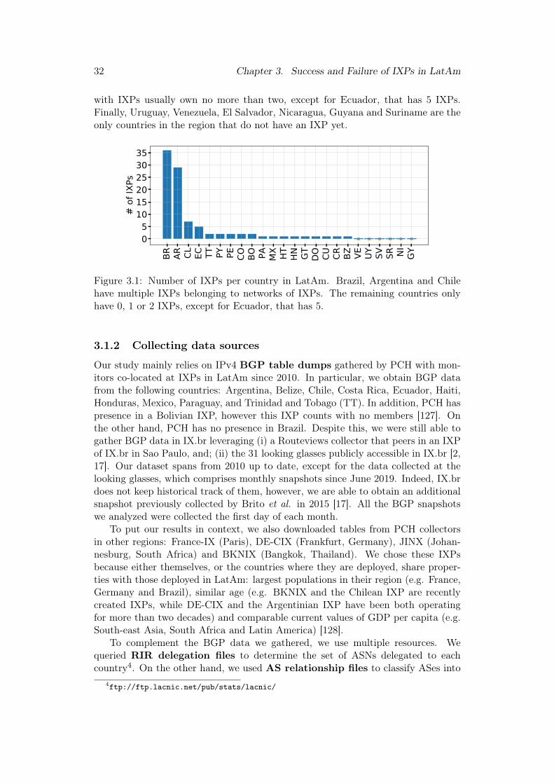
32 Chapter 3. Success and Failure of IXPs in LatAm
with IXPs usually own no more than two, except for Ecuador, that has 5 IXPs.Finally, Uruguay, Venezuela, El Salvador, Nicaragua, Guyana and Suriname are theonly countries in the region that do not have an IXP yet.
BR AR CL EC TT PY PE CO BO PA MX HT HN GT DO CU CR BZ VE UY SV SR NI GY
05
101520253035
# of
IXPs
Figure 3.1: Number of IXPs per country in LatAm. Brazil, Argentina and Chilehave multiple IXPs belonging to networks of IXPs. The remaining countries onlyhave 0, 1 or 2 IXPs, except for Ecuador, that has 5.
3.1.2 Collecting data sources
Our study mainly relies on IPv4 BGP table dumps gathered by PCH with mon-itors co-located at IXPs in LatAm since 2010. In particular, we obtain BGP datafrom the following countries: Argentina, Belize, Chile, Costa Rica, Ecuador, Haiti,Honduras, Mexico, Paraguay, and Trinidad and Tobago (TT). In addition, PCH haspresence in a Bolivian IXP, however this IXP counts with no members [127]. Onthe other hand, PCH has no presence in Brazil. Despite this, we were still able togather BGP data in IX.br leveraging (i) a Routeviews collector that peers in an IXPof IX.br in Sao Paulo, and; (ii) the 31 looking glasses publicly accessible in IX.br [2,17]. Our dataset spans from 2010 up to date, except for the data collected at thelooking glasses, which comprises monthly snapshots since June 2019. Indeed, IX.brdoes not keep historical track of them, however, we are able to obtain an additionalsnapshot previously collected by Brito et al. in 2015 [17]. All the BGP snapshotswe analyzed were collected the first day of each month.
To put our results in context, we also downloaded tables from PCH collectorsin other regions: France-IX (Paris), DE-CIX (Frankfurt, Germany), JINX (Johan-nesburg, South Africa) and BKNIX (Bangkok, Thailand). We chose these IXPsbecause either themselves, or the countries where they are deployed, share proper-ties with those deployed in LatAm: largest populations in their region (e.g. France,Germany and Brazil), similar age (e.g. BKNIX and the Chilean IXP are recentlycreated IXPs, while DE-CIX and the Argentinian IXP have been both operatingfor more than two decades) and comparable current values of GDP per capita (e.g.South-east Asia, South Africa and Latin America) [128].
To complement the BGP data we gathered, we use multiple resources. Wequeried RIR delegation files to determine the set of ASNs delegated to eachcountry4. On the other hand, we used AS relationship files to classify ASes into
4ftp://ftp.lacnic.net/pub/stats/lacnic/

3.2. Public policies and IXPs 33
either stub or transit, AS classification lists to further differentiate between con-tent providers, enterprises, etc., and prefix-to-AS files to compute the addressspace originated by each AS. All these files were obtained from CAIDA.5 More-over, we queried CAIDA’s AS-rank API to quantify the relevance in the transitecosystem of each AS in our dataset.6 We use a snapshot of the APNIC eyeballsdataset [129, 130] collected on June 1st 2020 to identify the domestic eyeballs ofeach country. We used PeeringDB to determine regional IXPs names and RouteServer ASNs of IX.br, CABASE and PIT Chile.7 In addition, we gathered digital-ized documents, e.g. legal documents, newspapers, websites and presentations,concerning Internet’s public policies applied by LatAm’s governments.
3.1.3 Pre-processing BGP data
After gathering the BGP dumps, we pre-processed them. We observed that someASes share full tables, and we argue that this not what actually gets advertisedin the IXPs, i.e., following Gao-Rexford principles [131], no AS would offer cost-free transit via its upstream providers. Consequently, when analyzing each IXP, werelied only on entries provided by their route server: in these cases, the revealedroutes are usually from ASes advertising their customers, at least partially. Finally,all tables were sanitized removing AS-path prepending and dropping entries withAS sets (less than 1%).
After sanitizing the BGP tables dumps, we extracted different sets of ASes fromthem. In particular, IXP members or connected networks were inferred as thefirst AS found in each AS path after the IXP’s ASNs (e.g., Route Server, regionalIXPs). Besides the IXP members, we also look at ASes connected via members,or visible ASes, that correspond to the set of ASes seen in BGP dumps, i.e. thatappear in the AS paths of prefixes announced at the IXP.
We complement the previous data looking for insights about ASes in the addi-tional data sources we used. From the list of all delegated ASNs we obtained fromthe RIR delegation files, we compute the set of local ASes or domestic ASesof each country. For this, we consider that ASes using ASNs that were delegatedto a given country have the country nationality. Finally, the AS relationship filesallow us to identify active ASes or ASNs at each month, i.e., those with at leastone inferred AS relationship. Indeed, an ASN might be delegated, but not used inpractice.
Finally, note that, we compute the aforementioned sets of ASes month aftermonth for each IXP and country.
3.2 Public policies and IXPs
In this section we investigate the public policies behind the creation of IXPs inLatin America. For this, we rely on the set of digitalized documents we gathered.Table 3.2 shows the organizations that currently run these IXPs and that fosteredtheir creation.
5data.caida.org/datasets6https://asrank.caida.org/doc7https://www.peeringdb.com
34 Chapter 3. Success and Failure of IXPs in LatAm
Notably, out of 16 countries in LatAm, governments were involved inthe creation of their national IXPs in more than 55% of the cases. Thepresident of Costa Rica signed an Executive Order [132, 133] while parliament inBolivia passed a law [14]. Also, federal agencies such as Senatics in Paraguay [134],PUC in Belize [135] and SENACYT in Panama [136] fostered IXP’s creation. Reg-ulators were involved in Mexico (IFT) [137], Honduras (CONATEL-HN) [138] andParaguay (CONATEL-PY) [139]. In Brazil, the Internet Steering Committee (CGI),a multi-stakeholder board with several state representatives, was responsible for cre-ating IX.br, the Brazilian IXP [140]. Further, Belize, Honduras and Paraguay havedelegated IXP operations to universities.
On the other hand, Table 3.2 also indicates that, similar to the EuropeanIXP model [141], in Latin America a large number of non-profit organi-zations created and run IXPs. In particular, CABASE (AR) and CCIT (CO)are operated by organizations related to local ISPs associations as it happens inIXPs outside the region, e.g. DE-CIX (DE) [142] and JINX (ZA) [143]. In addition,presence of state regulations also influenced the development of peering facilities inChile. Undersecretary of telecommunications singed Resolution 1483 [144] in 1999which forced traffic between Chilean ISPs to be carried by their local infrastructure.To fulfill this requirement, ISPs rapidly joined NAP Chile, a Chilean IXP. Morerecently, in 2016, PIT Chile was established on top of the dense interconnectedinfrastructure of NAP Chile, though bringing significant changes to the Chileanpeering ecosystem: whereas NAP Chile was strictly limited to domestic ASes, PITChile was envisioned as a neutral IXP also allowing the presence of non-nationalASes.
Finally, note that most countries that host a BGP monitor have small IXPs(e.g. with less than 30 connected networks that announce less than 2M unique IPs).Since this limits the conclusions that can be drawn in them, our analysis focuseson CABASE, IX.br and PIT CL, the networks of IXPs in LatAm.
3.3 IXP networks topology
In this section we study the topology, peering policy and infrastructure of networks ofIXPs. We investigate those operated by CABASE, IX.br and PIT-CL in Argentina,Brazil and Chile, respectively. Furthermore, to provide some context, we comparethem with the domestic IXPs of DE-CIX, i.e., only with those located in Germany.More precisely, we look at the number of IXPs per network, the number of peeringfacilities per IXP, and whether regional IXPs have their own ASNs. In addition, wedetermine if there exists interconnection among regional IXPs, and if IXP operatorsenforce any peering policy on their members. For all these analysis, we queriedPeeringDB to obtain the list of the regional IXPs in CABASE, PIT-CL and IX.br,the codes that operators use to tag them (e.g., IX.br Fortaleza has been tagged asce) and AS numbers. We found that, as of July 2019, IX.br, CABASE and PITChile run 31, 28 and 6 regional IXPs respectively in Brazil, Argentina and Chile.Table 3.1 summarizes the main characteristics of the IXP networks of CABASE,PIT-CL, IX.br and DE-CIX (only in Germany), which we now detail.

3.3. IXP networks topology 35
Country
AR
BO
BR
BZ
CL
CO
CR
CU
ECH
TH
NM
XP
AP
YP
ETT
Spo
nso
red
by
CA
BA
SELa
wC
GI
PU
CP
IT C
LC
CIT
Ex.O
rd.
Stat
eIX
P.E
CA
HTI
CC
ON
ATE
LIF
TSE
NA
CYT
SEN
ATI
CS
NA
P.P
ETT
IX
Op
erat
edb
yC
AB
ASE
Stat
eN
IC.b
rU
oB
ZP
IT C
LC
CIT
NIC
.cr
NA
P.C
UIX
P.E
CA
HTI
CU
NA
HC
ITI
Inte
RED
NIC
.py
NA
P.P
ETT
IX
BGP
TDs
Mo
nit
or
PC
H
RV
s/LG
sP
CH
PC
H
PC
H
PC
HP
CH
PC
HP
CH
PC
H
PC
H
#Mem
b1
27
11
56
67
22
85
44
61
55
#Agg
IPs
7.9
M2
6M
67
K1
9.4
M4
01
K2
8K
10
2K
13
1K
79
5K
1.5
M1
96
K
Figure3.2:
IXPsin
LatinAmericaexclud
ingEurop
eanoverseas
territoriesinJu
ne20
19.Cou
ntries
areab
breviatedby
theirISO
-stand
ard
code.Colorsblue,yello
wan
dmag
enta
representstateag
encies,no
n-profi
torga
nization
san
dun
iversities,respectively.#Agg
IPsis
compu
tedon
thead
dressspacean
noun
cedby
IXP
mem
bers
(excluding
theircu
stom
ercone
andrepe
ated
prefi
xesdu
eto
MOASe
s).

36 Chapter 3. Success and Failure of IXPs in LatAm
Y COR RCN BUE X
Y COR-Y RCN-COR-Y
XBUE-XRCN-BUE-X
CABASE
Figure 3.3: Mandatory multilateral peering policy in CABASE. Arrows indicate thedirection of BGP announcements and their respective AS path. RCN is a centralnode that interconnects regional IXPs (e.g. BUE, COR) and forwards all announce-ments to all regional IXPs.
3.3.1 CABASE
From the topological point of view, this network has a central IXP, CABASE-RCN(AS52376). This IXP is located in the area of Buenos Aires, the province includingthe capital of Argentina. CABASE-RCN hosts PoPs and caches of content providerssuch as Netflix (AS2906), Google (AS15169) and Amazon (AS16509) [145].
Aware of the presence of content providers, network operators outside BuenosAires city are looking forward to peer in CABASE-RCN. Hence, operators from asimilar far region usually (i) build a regional IXP where they peer locally (sometimesactually encouraged by CABASE), and; (ii) hire a L2 carrier that links the regionalIXP with CABASE-RCN. This not only reduces the wiring costs that each of theseoperators would have needed to pay to reach CABASE-RCN, but also allows themto negotiate better bidding rates [14, 145]. All in all, the network is composed of28 IXPs, with 9 in the province of Buenos Aires, and the remaining ones scatteredacross the country. CABASE sponsors all the regional IXPs, and gives each of theman AS number (e.g, BUE-AS11058, COR-AS52374).
At the same time, CABASE applies a mandatory multilateral peering policy(MMPP) such that prefixes advertised in an IXP are announced to all members inthe country-wide network via the central node [146]. This is illustrated in Fig. 3.3 forCABASE-BUE and CABASE-COR. The MMPP has two effects. First, all membersbenefit from the presence of the content providers peering in CABASE-RCN. Second,the BGP data gathered in only one IXP of CABASE allows to obtain a complete viewof CABASE’s members, i.e., where they are connected and their customer cones.We further verified this contrasting PCH’s BGP snapshots collected in multipleof regional IXPs of CABASE. In particular, we rely on PCH’s BGP collector inCABASE-BUE (eze) to study this network of IXPs.
3.3.2 PIT-CL
This network is composed of 5 IXPs. As so does CABASE, PIT-CL identifies each ofits IXPs with an AS number (e.g, SCL-AS61522, ARI-AS61527). The larger IXP ofPIT-CL is the one in Satiago de Chile, the capital. In particular, after its creation,PIT-CL-SCL incorporated four ISP NAPs CenturyLink/Level3, Claro, Entel andTelefonica. These NAPs dated from the late 90s, time when ISPs had to createdomestic peering infrastructure to fulfill Chile’s SubTel Resolution 1483 obligingChilean traffic to be exchanged locally [144]. By inspecting the BGP data in PCH’sBGP collector Santiago de Chile (SCL), we discovered that all the remaining IXPs
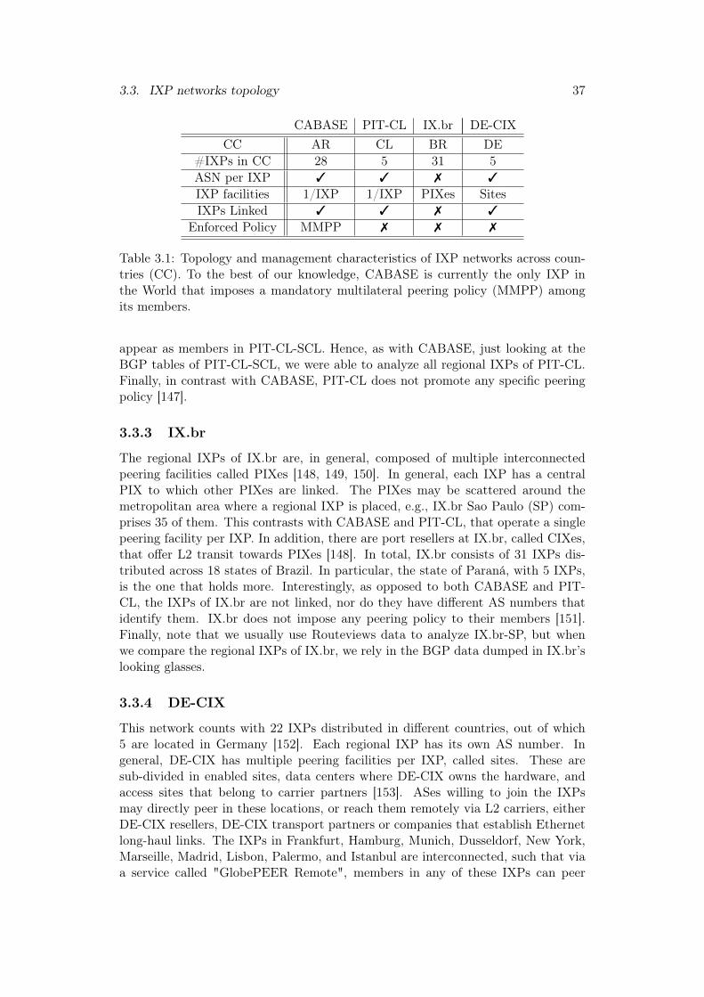
3.3. IXP networks topology 37
CABASE PIT-CL IX.br DE-CIXCC AR CL BR DE
#IXPs in CC 28 5 31 5ASN per IXP 3 3 7 3
IXP facilities 1/IXP 1/IXP PIXes SitesIXPs Linked 3 3 7 3
Enforced Policy MMPP 7 7 7
Table 3.1: Topology and management characteristics of IXP networks across coun-tries (CC). To the best of our knowledge, CABASE is currently the only IXP inthe World that imposes a mandatory multilateral peering policy (MMPP) amongits members.
appear as members in PIT-CL-SCL. Hence, as with CABASE, just looking at theBGP tables of PIT-CL-SCL, we were able to analyze all regional IXPs of PIT-CL.Finally, in contrast with CABASE, PIT-CL does not promote any specific peeringpolicy [147].
3.3.3 IX.br
The regional IXPs of IX.br are, in general, composed of multiple interconnectedpeering facilities called PIXes [148, 149, 150]. In general, each IXP has a centralPIX to which other PIXes are linked. The PIXes may be scattered around themetropolitan area where a regional IXP is placed, e.g., IX.br Sao Paulo (SP) com-prises 35 of them. This contrasts with CABASE and PIT-CL, that operate a singlepeering facility per IXP. In addition, there are port resellers at IX.br, called CIXes,that offer L2 transit towards PIXes [148]. In total, IX.br consists of 31 IXPs dis-tributed across 18 states of Brazil. In particular, the state of Paraná, with 5 IXPs,is the one that holds more. Interestingly, as opposed to both CABASE and PIT-CL, the IXPs of IX.br are not linked, nor do they have different AS numbers thatidentify them. IX.br does not impose any peering policy to their members [151].Finally, note that we usually use Routeviews data to analyze IX.br-SP, but whenwe compare the regional IXPs of IX.br, we rely in the BGP data dumped in IX.br’slooking glasses.
3.3.4 DE-CIX
This network counts with 22 IXPs distributed in different countries, out of which5 are located in Germany [152]. Each regional IXP has its own AS number. Ingeneral, DE-CIX has multiple peering facilities per IXP, called sites. These aresub-divided in enabled sites, data centers where DE-CIX owns the hardware, andaccess sites that belong to carrier partners [153]. ASes willing to join the IXPsmay directly peer in these locations, or reach them remotely via L2 carriers, eitherDE-CIX resellers, DE-CIX transport partners or companies that establish Ethernetlong-haul links. The IXPs in Frankfurt, Hamburg, Munich, Dusseldorf, New York,Marseille, Madrid, Lisbon, Palermo, and Istanbul are interconnected, such that viaa service called "GlobePEER Remote", members in any of these IXPs can peer

38 Chapter 3. Success and Failure of IXPs in LatAm
remotely at all these locations via VLANs. In addition, members in the IXP ofBerlin have access to the announcements in Frankfurt, and vice versa. Finally, DE-CIX may filter invalid announcements, but does not impose any peering policy fortheir members [154, 155].
3.3.5 Takeaways
In conclusion, the fact that no row in Table 3.1 has a unique constant value across allcolumns highlights that networks of IXPs are diverse. Indeed, the characteristics, ingeneral, depend on the particular network analyzed. An important point to noticeis that IX.br and DE-CIX, tend to have multiple peering facilities per IXP, butCABASE and PIT-CL do not. As we will see, the first two are networks of IXPswith numerous members, in particular many more than the latter two. Finally, webelieve that, in general, IXPs do not impose any peering policy on their members.Therefore, in this sense, CABASE represents an interesting case of study.
3.4 IXPs: domestic, regional or worldwide?
Many of the IXPs in Latin America have already been running for years. Conse-quently, we aim to understand whether these IXPs have been able to consolidate intheir region, as so have others in different geographical areas. We are also interestedin how many foreign networks are attracted to Latin American IXPs. For this, welook at IXP members and visible ASes of each IXP in Sec. 3.4.1 and Sec. 3.4.2, re-spectively. Indeed, despite some ASes might not be members of the IXP, they mightstill indirectly benefit from it via their providers. Moreover, we want to understandif IXPs in other regions show similar behaviors.
3.4.1 IXP members
Fig. 3.4 displays the number of members and the fraction that are dual-stackadopters across regional IXPs of IX.br, CABASE, PIT-CL and DE-CIX. We ob-serve that the size of IX.br San Paulo (sp) is remarkable: with 1294members, it holds more than DE-CIX-Frankfurt (824) and is also aroundan order of magnitude larger than CABASE-BUE (138) and PIT-CL-SCL(91). Besides IX.br-SP, we note that IX.br operates other IXPs with more than100 members. These are Rio de Janeiro - rj: 304, Fortaleza - ce: 219, Porto Alegre- rs: 175, Curitiba - pr: 113). For the remaining networks of IXPs in LatAm, thisonly holds for CABASE-BUE. Notably, IX.br’s largest regional IXPs are of compa-rable size, or even hold more participants than DE-CIX Dusseldorf (141), Hamburg(134), Munich (130) and Berlin (95). On the other hand, concerning the fraction ofmembers that are dual-stack adopters, while CABASE and PIT-CL at most reach0.5 in Fig. 3.4, the values for all regional IXPs of IX.br except Brasilia and San Josedos Campos are over this threshold. This evidences that IPv6 adoption in Brazil isa nation-wide process not just limited to largest IXPs. Lastly, we note that IX.br-SP and IX.br-rj and DE-CIX-fra have a similar dual-stack prevalence, around 0.75.This finding evidences that IPv6 adoption in Brazil is a nation-wide process andit is not just limited to the largest IXPs. Lastly, we note that the IXPs of IX.br

3.4. IXPs: domestic, regional or worldwide? 39
100 101 102 103
# of members
0.00.10.20.30.40.50.60.70.80.91.0
dual
-sta
ck p
reva
lenc
e
rjrs spcepr
BUESC
L
fra
CABASEPIT ChileIX.brDE-CIX
Figure 3.4: Number of connected networks and dual-stack adoption across regionalIXPs in IX.br, CABASE, PIT Chile and DE-CIX in June 2020.
in San Paulo and Rio de Janeiro, and that of DE-CIX in Frankfurt have a similardual-stack prevalence, around 0.75.
We are interested in the common properties across the larger regional IXPs inLatAm. We note that CABASE-BUE, PIT-CL-SCL, IX.br-SP and IX.br-rj are located in large cities (21.3, 6.3, 15.3 and 5.6 million inhabitantsrespectively in Sao Paulo, Rio de Janeiro, Buenos Aires and Santiago deChile), economically central in their respective countries. In addition, wenote that these IXPs usually host CDNs and include renown transit providers amongtheir members. For example, in CABASE-BUE and PIT-CL-SCL we find AS13335-Cloudflare (CDN) and AS3549-CenturyLink/Level3 (Tier-1 transit provider). Notethat CABASE-BUE used to host more CDNs, but after CABASE-RCN was de-ployed, most CDNs peer now in the latter IXP. On the other hand, concerning theIXPs of IX.br, in Sao Paulo and Rio de Janeiro, we note the presence of severalCDNs such as AS15169-Google, AS16509-Amazon, AS54113-Fastly (also presentin Curitiba) and AS13335-CloudFlare (also present in Curitiba, Porto Alegre andFortaleza). We also find several large international transit providers such as AS2906-NTT and AS3303-Swisscom peering at the IXP in Fortaleza. In addition, we seeAS37468-Angola Cables at Fortaleza (until May 2020) and Sao Paulo, and AS4809-China-Telecom at Sao Paulo, Rio de Janeiro and Curitiba. Angola Cables deployed atransatlantic cable between Angola and Brazil, and only then irrupted in the Brazil-ian AS ecosystem [156]. Similarly, China Telecom’s map also displays submarineconnectivity in the Brazilian shores [157].
3.4.2 Visible ASes: domestic impact and foreign attraction
Fig. 3.5 displays the ratio of local visible ASes to all delegated-and-active ASNsfor IX.br-SP, CABASE-BUE and PIT CL-SCL in Latin America, and France-IX,DE-CIX, JINX and BKNIX from other regions. To compute this graphic, first we

40 Chapter 3. Success and Failure of IXPs in LatAm
2011 2012 2013 2015 2016 2017 2018 20190.00.10.20.30.40.50.60.70.80.91.0
Frac
tion
DE-CIX-fraFrance-IX-ParisBKNIX
JINXIX.br
CABASE-BUEPIT Chile-SCL
Figure 3.5: Fraction country’s delegated-and-active ASNs visible at the IXPs.
determine all delegated-and-active ASNs for each country, and thus for each IXP.For this, we simply filter out delegated but inactive ASNs, i.e., ASNs with no inferredAS relationship. Then we look for ASes that: i) are visible in each IXP and; ii) arelocal, i.e., own an ASN delegated to the country where the IXP is deployed. Finally,we compute the ratio between both values month after month.
Fig. 3.5 reveals that 80% of the Brazilian and Argentinian country delegated-and-active ASNs are visible at IX.br-SP and CABASE-BUE, respectively. Thisfraction is similar to the one observed in DE-CIX (Frankfurt) and by far larger thanin France-IX (Paris), despite the large wealth gap (i.e. GDP per capita) between theEuropean Union and Latin America [128]. Indeed, even though LatAm spansa larger geographical extension than Europe, IXPs of the region havestill managed to deploy an infrastructure that allows them to host alarge fraction of their local ASes. In addition, while DE-CIX has been stuckin this fraction value since 2011, CABASE-BUE and IX.br-SP have been steadilygrowing since the beginning of the decade when they just had around 60%. TheBrazilian IXP network growth in the past decade was driven by the investments intelecommunications to host the 2014 FIFA World Cup as well as the 2016 SummerOlympics [158, 159]. On the other hand, CABASE’s fraction of visible ASes, as wellas number of regional IXPs, has increased since Google joined the IXP in late 2011.
In addition, Fig. 3.5 also shows that PIT Chile-SCL, that started operating in2016, has a striking fraction of 90% even from the first snapshot we got from thePCH collector in 2017. This is the highest historical value in Latin America, andindeed high for an infant IXP: for example, BKNIX, which was launched in 2015,covers just 60% of the current delegated-and-active ASNs in Thailand. To growrapidly, PIT Chile leveraged Chilean public policies (see Sec. 3.2).
Finally, note that JINX, the IXP in South Africa, has also been increasing thefraction of visible country delegated-and-active ASNs over time. The similaritieswith the IXPs in Brazil and Argentina in terms of the same 20% of increase andthe fact that the three IXPs have reached a value comparable to a big IXP suchas DE-CIX, allows to speculate on a matureness process that replicates across con-tinents: regions where the Internet is rather underrepresented seem to,after many years, have been able to attract as many local ASes as some

3.5. Reaching IXPs: from stubs to large transit providers 41
well-established IXPs in Europe.On the other hand, Fig. 3.6 shows8 the prevalence of AS nationalities at each
IXP, i.e., out of all visible ASes in an IXP, how many come from each country. Ascan be seen, the three bigger Latin American IXPs mainly provide local support:the largest fraction of visible ASes, around 75% in all cases, are from the countrieswhere the IXPs are deployed. However, these IXPs are also able to extend to othercountries in the region, which usually add up most of the remaining fraction inFig. 3.6. These results are similar to the ones seen in BKNIK and JINX. Indeed,all these IXPs are not so internationally widespread, i.e., the ASes they host comefrom less than 50 different countries in all cases. All this is in clear contrast withwhat happens in European IXPs that rather act as international hubs: not onlythe number of visible nationalities is greater than 100 for France-IX and over 200for DE-CIX, but also most of their visible ASes are actually not local regarding towhere the IXPs are deployed. Despite these differences, it is remarkable that theUS is always within the five most prevalent AS nationalities9 for all IXPs: this islikely due to the advertisement of prefixes of relevant US-based companies (e.g.,Google, Facebook, Netflix, CloudFlare, Fastly). Indeed, the fact that CDNs find inIXPs a way to remain close to their customers and to offer them a better service isparticularly also true in Latin America, Asia and Africa.
3.5 Reaching IXPs: from stubs to large transit providers
We are interested in how traffic is carried from/to Latin American IXPs. Moreprecisely, since ASes in LatAm could be potentially scattered throughout vast geo-graphic extensions, we would like to identify transit providers that have contributedto the consolidation of IXPs in their local country. We argue that finding largetransit providers in an IXP might encourage other ASes to join it. On the otherhand, ASes usually advertise their customer cone at IXPs. However, we wonderwhether there exist non-transit members, i.e., ASes that only announce prefixesowned by themselves in the IXP. Interestingly, we find that there exist, and thatthis set of members is not only composed by stub ASes: there are transit ASesactively choosing not to announce prefixes of their customers.
3.5.1 Transit members
Fig. 3.7 shows a heatmap of the number of transit members with AS-rank withineach reported interval for each IXP. We argue that this metric can capture theinterest of large transit providers in participating at the IXPs.
Large European IXPs, are notably attractive for transit providers at the topof AS-rank since the number of transit members in the TOP10 peering at DE-CIX, AMS-IX and LINX is 4, 3 and 3, respectively. In addition, more than athird of transit providers in the TOP100 are members of these European IXPs.On the other hand, IX.br only hosts one transit member in the TOP10, however,
8For this analysis, we filtered out the large number of prefixes announced by Hurricane Electric(AS6939), probably just on account of its open peering policy [160], in IX.br, JINX, DE-CIX andFrance-IX.
9By nationality we mean an AS that have been delegated to the US
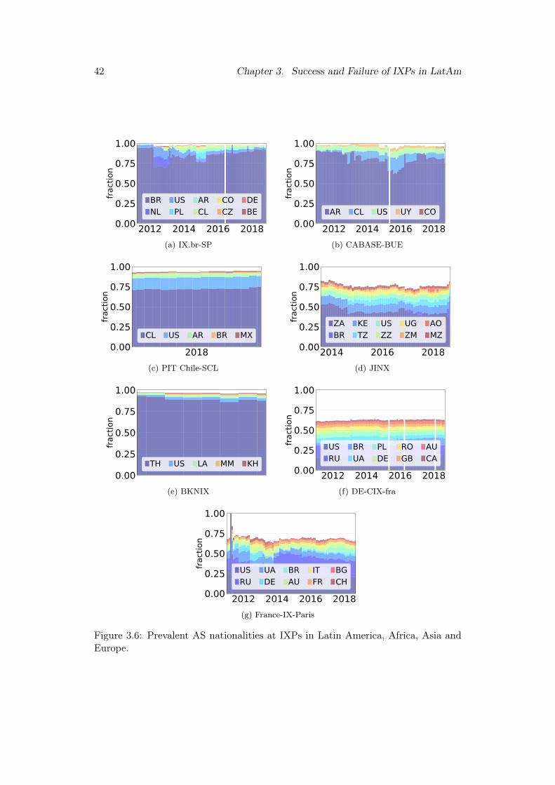
42 Chapter 3. Success and Failure of IXPs in LatAm
2012 2014 2016 20180.00
0.25
0.50
0.75
1.00
fract
ion
BRNL
USPL
ARCL
COCZ
DEBE
(a) IX.br-SP
2012 2014 2016 20180.00
0.25
0.50
0.75
1.00
fract
ion
AR CL US UY CO
(b) CABASE-BUE
20180.00
0.25
0.50
0.75
1.00
fract
ion
CL US AR BR MX
(c) PIT Chile-SCL
2014 2016 20180.00
0.25
0.50
0.75
1.00
fract
ion
ZABR
KETZ
USZZ
UGZM
AOMZ
(d) JINX
0.00
0.25
0.50
0.75
1.00
fract
ion
TH US LA MM KH
(e) BKNIX
2012 2014 2016 20180.00
0.25
0.50
0.75
1.00
fract
ion
USRU
BRUA
PLDE
ROGB
AUCA
(f) DE-CIX-fra
2012 2014 2016 20180.00
0.25
0.50
0.75
1.00
fract
ion
USRU
UADE
BRAU
ITFR
BGCH
(g) France-IX-Paris
Figure 3.6: Prevalent AS nationalities at IXPs in Latin America, Africa, Asia andEurope.

3.5. Reaching IXPs: from stubs to large transit providers 43
CABA
SE
IX.b
r
PIT-
CL
DE-C
IX
FR-IX
BKNI
X
JINX
1-1010-100100-1k1k-10k
11
1216
11695
404
017
12
439
216299
11342
118
006
11
11
1225
Figure 3.7: Relevance of IXP members in the global transit system. Bins representan interval for CAIDA’s AS-RANK while number on each cell counts the numberof members within that interval.
IX.br-SP ASN 16735 262589 7049 61832 28329# 903 381 218 209 207
CABASE-BUE ASN 3549 52361 7049 19037 11664# 219 113 100 82 81
PIT Chile-SCL ASN 7004 22661 52280 19228 14259# 88 87 70 57 57
Table 3.2: Largest sizes (#) of visible AS sets per upstream AS in IX.br-SP,CABASE-BUE and PIT Chile-SCL.
when we extend the limit to ASes in TOP100, IX.br hosts 17 ASes within thatrange. We manually examine the 17 TOP100 transit providers peering at IX.br-SPand we found that 13 out of 17 are ASes that have been delegated to Brazilianorganizations.10 Furthermore, we counted the number of Brazilian ASes in theAS-rank TOP100 finding 18 transits providers, only 5 of which do not peer atIX.br-SP. Lastly, CABASE and PIT Chile, countries with no domestic transits inthe AS-RANK TOP100, have been able to attract to 2 (Telecom Italia-6267 andLevel3-AS3549) and 1 (Internexa-262589) foreign transits in TOP100, respectively.
Despite an AS might have a high AS-rank, this does not imply that it announcesa large number of downstream ASes in the IXP. To shed light on this, Table 3.2displays the five IXP members that announce the largest visible customer cones inIX.br-SP, CABASE-BUE and PIT Chile-SCL. Results show a richer AS ecosystemin Brazil: Algar (AS16375) alone announces more downstream ASes in IX.br-SPthan all the visible ASes seen in CABASE-BUE as well as in PIT Chile-SCL. Onthe other hand, looking at the nationality of the TOP5 upstream ASes in eachIXP, we see mainly domestic transit providers. Yet, there are exceptions: Internexa(AS262589, Colombia) and Silica (AS7049, Argentina) in IX.br, Level3 (AS3549,US) in CABASE-BUE and Internexa (AS52880, Colombia) in PIT Chile-SCL.
In addition, Table 3.2 shows that Level3 is the largest upstream AS in CABASE-BUE (AS3549) and, though not displayed in Table 3.2, also ranked sixth in PITChile-SCL (AS21838, legacy number of an acquired network [161]). We furtherinvestigated Level3’s role in both IXPs and determined that this ISP actually actsas a domestic transit provider in LatAm: 204 out of 219 and 37 out of 43 downstreamASes announced by Level3 in CABASE-BUE and PIT Chile-SCL were delegated byLACNIC to Argentina and Chile, respectively.
10The other four ASes are: HE-6939, ACS-37468, Seabras-13786, China Telecom-4809.

44 Chapter 3. Success and Failure of IXPs in LatAm
0.00.20.40.60.81.0
ECDF
(v4)
0.0 0.1 0.2 0.3 0.4 0.5 0.6 0.7 0.8 0.9 1.0fraction of non-transit members
0.00.20.40.60.81.0
ECDF
(v6) CABASE
DE-CIXIX.brPIT Chile
Figure 3.8: Fraction of non-transit members, i.e., that only announce prefixes ownedby themselves at the IXP.
Finally, Table 3.2 also unveils the presence of state-owned ISPs among the largestupstream ASes: Internexa (AS262589, AS262195) and ARSAT (AS52361). In-ternexa is a partially state-owned Colombian AS in which the Ministry of Financeand Public Credit holds 51% of the shares while Medellin county (Colombia) holdsanother 10% [162]. On the other hand, ARSAT (AS52361) is a fully state-ownedArgentinian transit provider [163]. Note that, while ARSAT’s transit service fo-cuses in Argentina, Internexa’s transit footprint comprises foreign countries, suchas Argentina and Brazil.
3.5.2 Non-transit members
Fig. 3.8 presents the ECDF of the fraction of non-transit members across the IXPneworks of IX.br, CABASE, PIT-CL and DE-CIX, for IPv4 (top) and IPv6 (down).For IPv4, the median values across IX.br and DECIX are 0.48 and 0.39, respectively.Remarkably, the values are exactly 1 for CABASE and PIT-CL, which seems toconfirm that these IXPs are mainly populated by small operators. In fact, 18/28and 3/4 of CABASE’s and PIT-CL’s regional IXPs, respectively, only host non-transit members. On the other hand, we observe that the prevalence of non-transitmembers tends to be higher in IPv6. It is worth noting that CABASE has less dotsin IPv6 when compared to IPv4 since in some regional IXPs, e.g. CABASE-SFE,we did not find any member announcing IPv6 prefixes. Similarly, in PIT-CL, weonly note IPv6 operations in PIT-CL-SCL.
To gather more insights, we refine the classification in Fig. 3.8 by differentiatingamong non-transit members that are either transit or stub ASes, i.e., ASes withor without customers, respectively. Note that transit ASes that are non-transitmembers are ASes that deliberately choose not to announce their customers at theIXPs. Recall that we use AS-relationship files to identify stub ASes, and since thesedo not take into account IPv6, we are only able to spot them for IPv4.

3.5. Reaching IXPs: from stubs to large transit providers 45
sp rj ce rs pr pe df sc ba mg
nat
lda
cas
vix
bel
cpv laj
mao the
mcz sjp igu slz gyn
jpa ria sjc cxj0.0
0.20.40.60.81.0
mem
b.' f
ract
ion
stub ASesTransit ASes
102
# of
mem
bers
(a) IX.br.
BUE
COR
MZA
NQN
LPL
ROS
SZP
UAQ
MDQ NG
BPO
SBH
B JUJ
JUN
PER
DLC
BRC
SFE
PMY
SLT
TDL
RST
SLU
OGB
VDM0.0
0.20.40.60.81.0
mem
b.' f
ract
ion
stub ASesTransit ASes
101
# of
mem
bers
(b) CABASE
SCL Ari
Con
Tem0.0
0.20.40.60.81.0
mem
b.' f
ract
ion
stub ASesTransit ASes
100
101#
of m
embe
rs
(c) PIT-CLfra du
s
ham
muc be
r0.00.20.40.60.81.0
mem
b.' f
ract
ion
stub ASesTransit ASes
102 # of
mem
bers
(d) DE-CIX
Figure 3.9: Classification of non-transit members across the networks of IXPs intostub or transit ASes for IPv4.
Fig. 3.9 shows the prevalence of stub and transit ASes among non-transit mem-bers in IX.br, CABASE, PIT-CL and DE-CIX networks. In particular, the regionalIXPs are sorted by number of members. We see that despite non-transit membersare mostly stub ASes, there are some that are actually transit ASes not announcingtheir customer cone. In other words, transit ASes seem to benefit themselves fromthe announcements in the IXP, but do not seem to offer this service to their cus-tomers. We argue this case is worth of study in future work, as it may result fromcomplex AS relationships among ASes. However, for regular customer-to-providerrelationships, i.e., if transit ASes advertise the paths they learn in the IXP to theirrespective customer cones11, this practice may likely lead to asymmetrical forwardand return paths for customers of these non-transit members. The asymmetry arisesif: (i) the non-transit member chooses an announcement done by another memberin the IXP as having the best path towards a prefix; (ii) the non-transit memberannounces this path to its customers, some of which choose it as best path too.This way, traffic originated in customers flows via the IXP, but on the oppositedirection this does not hold since the non-transit member does not announce itscustomer cone at the IXP. Finally, we verify that in the Latin American networks ofIXPs, most IXP members peer in only one IXP, therefore not announcing customersdoes not seem to relate to ASes applying traffic engineering techniques in betweenregional IXPs.
11An AS could filter such announcements, e.g., relying on BGP communities.

46 Chapter 3. Success and Failure of IXPs in LatAm
UY PY CR VE DO MX PE PA BO CO EC AR CL BR0.00.20.40.60.81.0
HH in
dex No IXP
IXP
Figure 3.10: Herfindahl-Hirschman Index to determine originated address spaceconcentration in countries that have been delegated more than 1M IP addresses.
3.6 IXPs and concentration
In this section we provide a plausible explanation of why some IXPs in LatAm aresuccesfull while others have failed. We argue that the presence of monopolistic ASesmay discourage the deployment and growth of IXPs. Hence, we look whether theIPv4 address space delegated to Latin American countries is fairly distributed, i.e.,if no AS owns most IP addresses assigned to a country.
We compute the address space announced by each AS according to what isreported in the prefix-to-AS files, and the total of each country aggregating that oftheir domestic ASes. To measure the fairness of the market, we use the Herfindahl-Hirschman Index (HHI), a statistical measure of concentration that ranges from1 (single monopolistic origin) to 0. This metric is used by the US Departmentof Justice to apply antitrust regulations [164] and in ecology, known as Simpson’sDiversity Index, to measure diversity.
Fig. 3.10 displays the HHI for Latin American countries delegated more than1M IP addresses. The right end shows countries with low concentration ratio, suchas Brazil, Chile and Argentina. Indeed, these countries host the largest IXP net-works. On the contrary, the left side includes countries such as Uruguay, DominicanRepublic and Venezuela, that do not have any IXP, and Paraguay, Costa Rica andMexico, all possessing an HHI of more than 0.3.
We take Uruguay, Venezuela, Costa Rica and Mexico as cases of study anddisplay in Table 3.3 the first and second dominant ASes that concentrate most ofthe IPs delegated to these countries. In all cases, the first dominant AS not onlyoriginates between 55% to 90% of its respective national address space, but alsoowns at least 47% more than the second. In particular, countries dominated bylarge state-owed providers such as Venezuela (CANTV) and Uruguay (ANTEL) arenot even planning to release an IXP [165, 166]. Costa Rica is the opposite example:while the state owns ICE, the main ISP that originates 63% of the national addressspace, the first national IXP was created by an executive order in 2014. Remarkably,ICE has never joined the IXP [167]. Mexico is another country with high HHI whoseIXP just has 6 members. We suspect that, despite the fact that the creation of theIXP in 2014 was sponsored by the Mexican government as a recommendation of theOECD [168], the absence of Telmex (AS8151) [169], by far the first dominant AS inthe country, discouraged the IXP growth.
In general, therefore, we see that the countries where no IXP at all exist
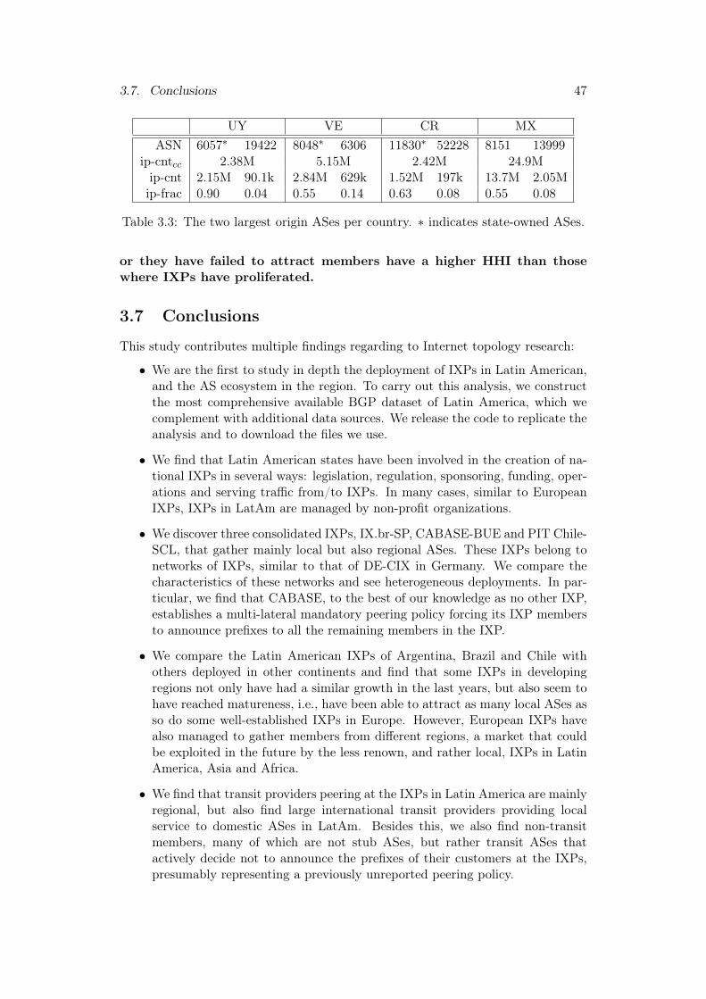
3.7. Conclusions 47
UY VE CR MXASN 6057∗ 19422 8048∗ 6306 11830∗ 52228 8151 13999
ip-cntcc 2.38M 5.15M 2.42M 24.9Mip-cnt 2.15M 90.1k 2.84M 629k 1.52M 197k 13.7M 2.05Mip-frac 0.90 0.04 0.55 0.14 0.63 0.08 0.55 0.08
Table 3.3: The two largest origin ASes per country. ∗ indicates state-owned ASes.
or they have failed to attract members have a higher HHI than thosewhere IXPs have proliferated.
3.7 Conclusions
This study contributes multiple findings regarding to Internet topology research:
• We are the first to study in depth the deployment of IXPs in Latin American,and the AS ecosystem in the region. To carry out this analysis, we constructthe most comprehensive available BGP dataset of Latin America, which wecomplement with additional data sources. We release the code to replicate theanalysis and to download the files we use.
• We find that Latin American states have been involved in the creation of na-tional IXPs in several ways: legislation, regulation, sponsoring, funding, oper-ations and serving traffic from/to IXPs. In many cases, similar to EuropeanIXPs, IXPs in LatAm are managed by non-profit organizations.
• We discover three consolidated IXPs, IX.br-SP, CABASE-BUE and PIT Chile-SCL, that gather mainly local but also regional ASes. These IXPs belong tonetworks of IXPs, similar to that of DE-CIX in Germany. We compare thecharacteristics of these networks and see heterogeneous deployments. In par-ticular, we find that CABASE, to the best of our knowledge as no other IXP,establishes a multi-lateral mandatory peering policy forcing its IXP membersto announce prefixes to all the remaining members in the IXP.
• We compare the Latin American IXPs of Argentina, Brazil and Chile withothers deployed in other continents and find that some IXPs in developingregions not only have had a similar growth in the last years, but also seem tohave reached matureness, i.e., have been able to attract as many local ASes asso do some well-established IXPs in Europe. However, European IXPs havealso managed to gather members from different regions, a market that couldbe exploited in the future by the less renown, and rather local, IXPs in LatinAmerica, Asia and Africa.
• We find that transit providers peering at the IXPs in Latin America are mainlyregional, but also find large international transit providers providing localservice to domestic ASes in LatAm. Besides this, we also find non-transitmembers, many of which are not stub ASes, but rather transit ASes thatactively decide not to announce the prefixes of their customers at the IXPs,presumably representing a previously unreported peering policy.

48 Chapter 3. Success and Failure of IXPs in LatAm
• We study the correlation between the existence of ASes concentrating addressspace and the development and consolidation of IXPs. We notice that, inseveral Latin American countries, the existence of monopolistic ASes, somestate-owned, seem to have prevented the proliferation of IXPs, and lead themto be failed IXPs.
We believe there are several studies that could enlarge our understanding onthe status of the Internet in Latin America. In that sense, we want to study thedeployment of CDNs in LatAm, and their co-location at IXPs. Moreover, we wouldlike to compare peering policies across IXPs in all countries of LatAm. In addition,we would like to study the existence of multi-location members, i.e. members thatpeer at multiple IXPs of the same network of IXPs. Finally, we specially believethat it is worth to take closer look at Brazilian AS ecosystem, which represents 75%of LACNIC active ASes and has the largest IXP in the world.
In a longer term, despite the vantage points in the region are still scarce, wewould like to design active-measurement campaigns to investigate Latin America’saccess to content and the role of IXPs in such phenomenon. At the same time,we want to investigate the IPv6 rollout in LatAm. Lastly, we are interested inextending our analysis to a larger number of countries, to have a wider perspectiveof how IXPs contribute to their domestic AS ecosystem.

Chapter 4Filtering the Noise to Reveal BGP Lies
Contents4.1 Modeling BGP lies . . . . . . . . . . . . . . . . . . . . . . 514.2 Problem Statement . . . . . . . . . . . . . . . . . . . . . . 534.3 A Modular framework to detect BGP lies . . . . . . . . 55
4.3.1 Preparation stage . . . . . . . . . . . . . . . . . . . . . . . 584.3.2 Mapping relaxation . . . . . . . . . . . . . . . . . . . . . 594.3.3 Wildcards correction stage . . . . . . . . . . . . . . . . . . 61
4.4 The measurement platform and our campaign . . . . . . 634.5 Rate of BGP lies in the wild . . . . . . . . . . . . . . . . . 64
4.5.1 Performance of the different noise-filtering models . . . . 644.5.2 Effect of SIB and TPA rules on the mismatch rate . . . . . 664.5.3 Looking closer at high mismatch rates . . . . . . . . . . . 67
4.6 Conclusion . . . . . . . . . . . . . . . . . . . . . . . . . . . 67
In this chapter we discuss the methodology we propose to detect highly-potentialBGP lies by eliminating all sources of errors interfering with the collected data,i.e., by filtering noise affecting the comparison of CPs and DPs. While most of therelated work essentially blames the IP-to-AS mapping for the observed discrepanciesbetween CPs and DPs, our work relies on conservative heuristics that remove thenoise in the measurements and the mapping errors. The mismatches we find afterapplying our filters show that the IP-to-AS mapping is not the only culprit for them.In short, our contributions are:
1. We study multiple cases of studies showing different causes that may lead toBGP lies in Sec. 4.1. In particular, these examples exemplify why pinpointingthe root cause of BGP lies, a problem beyond the scope of this thesis, ischallenging.
2. We model in Sec. 4.2 the different practical challenges that need to be ad-dressed in order to be able to detect BGP lies. This ranges from the need oftime synchronizing measurements, being able to measure in a platform where
49
50 Chapter 4. Filtering the Noise to Reveal BGP Lies
both control paths and data paths can be collected in the same network, up todescribing the multiple sources of noise that may interfere in the comparisonof CPs and DPs, i.e. AS siblings, TPAs or IXPs and missing hops.
3. We develop a methodology allowing to compute the rate of BGP lies for agiven vantage point in Sec. 4.3. Our modular framework has three steps:
• a preparation stage that synchronizes CPs and DPs in time and semanticlevel, i.e., converts DPs from IP-paths to AS-paths;
• a mapping relaxation stage that looks at DPs and CPs separately andtries to infer the noise affecting each of them. In this task, we uniformizeAS siblings assigning them a unique mapping for both CPs and DPs, andconvert possible TPAs affecting DPs into wildcards that may be mappedto any AS. The filtering rules and the order in which they are appliedin this step can be modified, thus allowing to implement different noise-filtering models;
• a wildcards correction stage that, while comparing CPs and DPs, at-tempts to infer values of the wildcards (including missing hops) presentin the DPs (if any), and determines whether CPs and DPs match ormismatch.
4. We deploy 8 co-located vantage points, 6 in the Peering Testbed and two inprivate networks, and carry out a long-term search of BGP lies in Sec. 4.4. Tothe best of our knowledge, our analysis is the first to extend over time and todeploy such large number of vantage points for a comparison of DPs and CPs.
5. We sanitize the dataset with different noise-filtering models we construct withour framework and compute the rate of BGP lies we find in the wild for each ofthem in Sec. 4.5. Our most conservative model, i.e., the one that filters moreaggressively the noise and allows to obtain a lower bound of BGP lies, revealsa non-negligible amount of highly-potential lies. In addition, we find that inthe vantage points where our framework is very effective to reduce the numberof mismatches between CPs and DPs, the results usually remain quite stableover time. On the other hand, when our framework reveals a large number ofpotential BGP lies, the results have a larger per-day variation.
6. We release the dataset we collected and our code to foster replicability andreproducibility1.
In addition, Sec. 4.6 draws final remarks of our study. The work presented inthis chapter lead to the following publications:
• Julián M. Del Fiore, Pascal Merindol, Valerio Persico, Cristel Pelsser andAntonio Pescapè. Filtering the Noise to Reveal Inter-Domain Lies, in 2019Network Traffic Measurement and Analysis Conference (TMA), pages 17–24,2019, IEEE.
1See https://github.com/julian10m/BGP-lies-detector

4.1. Modeling BGP lies 51
• Julián M. Del Fiore, Pascal Merindol, Valerio Persico, Cristel Pelsser andAntonio Pescapè. A BGP-lying Tale: Stop Blamming the Mapping, posterpresented in TMA 2018.
4.1 Modeling BGP lies
BGP lies may be rooted in different causes, and alter either DPs or CPs. The firstinclude lies from an interested AS willing to save money avoiding to use a customer-to-provider link by using a peer-to-peer link, technical limitations, etc. On the otherhand, the latter stems from AS poisoning and AS deletions, among others. Fig. 4.1illustrates these type of lies assuming that Gao-Rexford policies are verified. Inall cases, we consider that traffic is flowing from A towards a prefix owned by F .Although the traversed DP is always equal to ABXDEF , the CP obtained via BGPvaries, as well as the reasons why it mismatches the DP.
Focusing on those lies manipulating DPs, Fig. 4.1a shows a case where an inter-ested lie occurs (green link) or a technical limitation (orange link) leads CPs andDPs to differ. In both cases we assume X learns the path XDEF towards theorigin F . As a first example, if B and X are engaged in a peer-to-peer relationship(link indicated in green), X does not export this path to B. Hence, B and A canonly reach F via C: the CP for A is ABCDEF . However, in an attempt to avoidpaying for transit, B assumes that X knows a path to reach F , and forwards it thetraffic, e.g. using a static route. If X does not filter any traffic it receives from B,then DP equals ABXDEF and differs from CP. In this scenario, B carries out adeliberate lie against A and X. On the other hand, if instead B is a customer of X(link displayed in orange), then B learns two paths to reach F : via X or, as before,via C. Since both paths have the same length, then R3 and R2 opt for the paths viaC and X, respectively. Assuming R1 has a shorter internal path to R3 than to R2,then A learns the same CP as before: the traffic should flow from R1 to R3 in B,and from there to C. However, because R1 has a partial-FIB and uses R2 as defaultgateway, the traffic finishes exiting B via X, through R2. In this second example,the same mismatch as before between the CP and DP is now caused by a technicallimitation in R1.
On the other hand, lies affecting CPs, such as AS poisoning and AS deletions,are displayed in Fig. 4.1b and Fig. 4.1c, respectively. With AS poisoning, an AScan interfere with a competitor AS by poisoning it, i.e by prepending the ASNof the latter to the path. In such cases, the competitor AS finds itself already inthe path and rejects the BGP update, possibly incurring in a loss of revenue. Forexample, in Fig. 4.1b, as E poisons C, then only X accepts the path advertisedby D. Consequently, A finishes learning ABXDECF as CP. Since C had beenartificially added to the CP, the traffic does not actually traverse it, naturally leadingto a mismatch between CP and DP. Other manipulations, such as AS deletions inCPs, can be used. As an example, in Fig 4.1c, B advertises to A a path where Xpreviously deleted D and E, then CP equals ABXF . However, in practice, the DPcrosses extra inter-domain links that do not appear in the CP.
Finally, note that beyond detecting lies, pinpointing their type could be consideritself a different research topic. This is highlighted by the examples in Fig. 4.1, wherethe same mismatch between CPs and DPs may actually result from different root

52 Chapter 4. Filtering the Noise to Reveal BGP Lies
AS F
AS EAS B
AS C
AS A
AS X
AS D
p2pc2p ($)
CP: A B C D E FDP: A B X D E F
R2
R3
R1
(a) Interested lies and technical limitations
AS F
AS EAS B
AS C
AS A
AS X
AS D
CP: A B X D E C FDP: A B X D E F
ECFDECF
F
Loop
AS poisoning
XDECF
BXDECF
DECF
(b) AS poisoning
AS F
AS EAS B
AS C
AS A
AS X
AS D
CP: A B X FDP: A B X D E F
EFDEF
F
XF
BXF
DEFCDEF
(c) AS deletions
Figure 4.1: BGP lies rooted in manipulations of either DPs (Fig. 4.1a) or CPs(Fig. 4.1b and 4.1c). In Fig. 4.1a, the green peer-to-peer (p2p) link highlightsthe case in which AS B carries an interested lie, whereas the orange customer-to-provider link (c2p) shows no monetary incentive to lie, and is produced due totechnical limitations. On the other hand, while Fig. 4.1b shows a case concerningAS poisoning, adding ASNs that were actually not crossed to CPs Fig. 4.1c focuseson the contrary effect produced by AS deletions, in which ASNs are removed.
causes.

4.2. Problem Statement 53
Misaligned VP
VP
CPs
DPs
(a)
Single-homed network
VP
CPs
DPs
(b)
Co-located VP
VP
CPs
DPs
(c)
Figure 4.2: Illustration of different vantage points. To compare CPs and DPs,misaligned VPs (Fig. 4.2a) could generate false mismatches if DPs exit the ASthrough an ASBR different than the one that shares the CPs. A solution would beto only rely on single-homed networks (Fig. 4.2b), where since an AS has a uniqueingress/exit point, the location of the VP is not critical. Generalizing the conceptof singled-homed networks, co-located VPs (Fig. 4.2c) are those in which, CPs andDPs are ensured to be collected in the same place, and thus the comparison ofCPs and DPs is valid. Notice however that, in the latter case, depending on theposition of the VP inside the network, the co-located VP could potentially turn intomisaligned VP, which highlights the difficulty in obtaining such type of VPs.
4.2 Problem Statement
In practice, to be able to compare CPs and DPs, synchronizing both paths inspace and time is mandatory. While achieving time synchronization is simple,and can be done just relying on timestamps extracted from measurements, space-synchronization actually depends on the measuring platform. Both CPs and DPs,obtained from BGP peers and traceroute vantage points (VPs), respectively, needto be measured in the same location, i.e. collected within the same local network.In these cases, we refer to the VP as a co-located VP. For co-located VPs, in the-ory, DPs should match CPs for all destinations. To better illustrate this concept,Fig. 4.2 shows three cases: a misaligned VP, a VP in a single-homed network anda co-located VP. In the first one, DPs exit through an ASBR that is not the onefrom which CPs are gathered, potentially leading to a false inference of BGP lies.

54 Chapter 4. Filtering the Noise to Reveal BGP Lies
Org A
AS A1AS A0
CP: Z A0 A1 B DP: Z A0 B
(a)
Org A
AS A1AS A0
CP: Z A0 A1 B DP: Z A1 A0 B
(b)
Org A
AS A1AS A0
CP: Z A1 B DP: Z A0 B
(c)
Figure 4.3: Mismatches between CPs and DPs due to noise generated by AS siblings.
On the other hand, single-homed networks ensure this property, but are not easilyfound in practice. Lastly, co-located VPs are those which, due to the location of theVP, CPs and DPs should theoretically match since packets exit the AS through theAS that shares the BGP data.
In addition to all this, DPs and CPs do not natively come at the same semanticlevel: the former are collected at the ground IP-level, while the latter are provided byBGP at the AS-level. Therefore, the collected traceroute data has to be converted,with the use of an IP-to-AS mapping function, into AS-level paths. However, thisprocess is noisy and error-prone, and may lead CPs and DPs to mismatch even inthe absence of real BGP lies. In general, the noise may either affect the IP-to-ASmapping tool in use, or the output of traceroute itself.
Concerning the IP-to-AS mapping process, IP addresses may either fail to bemapped due to an undefined mapping, i.e., the mapping is not defined or the IP ad-dress is mapped to multiple ASes, e.g. due to organizations that use interchangeablythe ASNs of the AS siblings they own [24]. The case of AS siblings can generatemismatches between CPs and DPs in different ways, as shown in Fig. 4.3, WhileCPs may indicate that two AS siblings will be traversed, DPs may only reveal one(Fig. 4.3a), or both but in the inverse order (Fig. 4.3b). In addition, CPs maytraverse one AS sibling, but DPs another one (Fig. 4.3c).
Besides the mapping errors, traceroute may provide both unreliable data in-cluding third-party addresses (TPAs) [31, 29] possibly due to IXPs [26, 170] or ASboundary allocation policies [27] and incomplete traces including missing hops [24,171, 113]. Fig. 4.4 illustrates both what TPAs are (Fig. 4.4a) and how they intro-duce noise affecting the search of BGP lies (Fig. 4.4b). In general, TPAs may occur

4.3. A Modular framework to detect BGP lies 55
TTL = 1
AS A
AS B
AS X x1
x2
Reply
b2
b1
(a)
AS C
AS A
AS B
AS X
CP: Z A B CDP: Z A x B C
(b)
Figure 4.4: Noise generated by TPAs introduced due to IXPs or AS boundaryallocation policies. While Fig. 4.4a shows what a TPA conceptually is, Fig. 4.4billustrates how this becomes a source of mismatches when comparing DPs and CPs.
when a router replies with an interface other than the incoming one, as shown inFig. 4.4a, where the router in question replies to traceroute using x2 as source IPaddress instead of b2. When this IP address belongs to an off-path AS, as is the casein Fig. 4.4b, the DP obtained after IP-to-AS mapping the outcome of tracerouteintroduces false links, between A and X, and X and B in the example. On theother hand, Fig. 4.1c shows an example where missing hops in traceroute (indicatedas “*”) do not allow to retrieve complete DPs. However, as we see in the figure,DPs do not match CPs. This particular example highlights that ASes, like AS A inFig. 4.1c, may not only carry interested lies, but also be malicious ASes and try tohide the evidence dropping traceroute packets.
4.3 A Modular framework to detect BGP lies
The framework we propose to detect BGP lies is illustrated in Fig. 4.6. The threeviolet boxes are the blocks in which CPs and DPs are modified, and the additionalblocks provide the logic and loops needed to carry both the filtering of noise andthe comparison of the paths.
First, the preparation stage synchronizes CPs and DPs and translates the
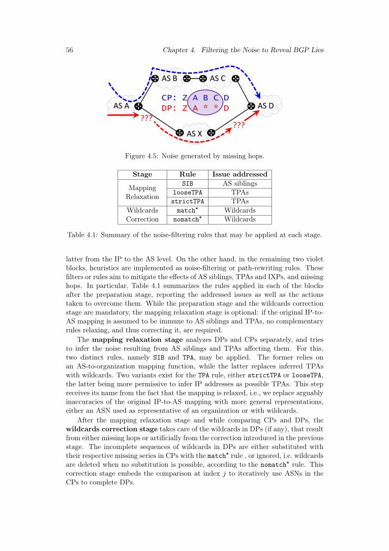
56 Chapter 4. Filtering the Noise to Reveal BGP Lies
AS ACP: Z A B C DDP: Z A * * D
AS B AS C
AS D
AS X
??????
Figure 4.5: Noise generated by missing hops.
Stage Rule Issue addressed
MappingRelaxation
SIB AS siblingslooseTPA TPAsstrictTPA TPAs
WildcardsCorrection
match* Wildcardsnomatch* Wildcards
Table 4.1: Summary of the noise-filtering rules that may be applied at each stage.
latter from the IP to the AS level. On the other hand, in the remaining two violetblocks, heuristics are implemented as noise-filtering or path-rewriting rules. Thesefilters or rules aim to mitigate the effects of AS siblings, TPAs and IXPs, and missinghops. In particular, Table 4.1 summarizes the rules applied in each of the blocksafter the preparation stage, reporting the addressed issues as well as the actionstaken to overcome them. While the preparation stage and the wildcards correctionstage are mandatory, the mapping relaxation stage is optional: if the original IP-to-AS mapping is assumed to be immune to AS siblings and TPAs, no complementaryrules relaxing, and thus correcting it, are required.
The mapping relaxation stage analyzes DPs and CPs separately, and triesto infer the noise resulting from AS siblings and TPAs affecting them. For this,two distinct rules, namely SIB and TPA, may be applied. The former relies onan AS-to-organization mapping function, while the latter replaces inferred TPAswith wildcards. Two variants exist for the TPA rule, either strictTPA or looseTPA,the latter being more permissive to infer IP addresses as possible TPAs. This stepreceives its name from the fact that the mapping is relaxed, i.e., we replace arguablyinaccuracies of the original IP-to-AS mapping with more general representations,either an ASN used as representative of an organization or with wildcards.
After the mapping relaxation stage and while comparing CPs and DPs, thewildcards correction stage takes care of the wildcards in DPs (if any), that resultfrom either missing hops or artificially from the correction introduced in the previousstage. The incomplete sequences of wildcards in DPs are either substituted withtheir respective missing series in CPs with the match* rule , or ignored, i.e. wildcardsare deleted when no substitution is possible, according to the nomatch* rule. Thiscorrection stage embeds the comparison at index j to iteratively use ASNs in theCPs to complete DPs.

4.3. A Modular framework to detect BGP lies 57
Compute j
MAPPING RELAXATION
WILDCARDSCORRECTION
MATCH++
MISMATCH++
MISMATCHING RATEScomputing MM bounds
j’=jj=min(m,n)<j’
j<j’<min(m,n)
j < min(m,n)
PREPARATION STAGEsynchronizing both paths
START: i=0 STOP: end of list
j=min(m,n)
i++
Compute next j’
CP i, DP i
Figure 4.6: Our modular framework. The preparation stage synchronizes CPs andDPs in time and semantic AS-level. On the other hand, the mapping relaxationstage relaxes the original IP-to-AS mapping by gathering AS siblings into a uniquerepresentation and replacing inferred TPAs with wildcards. Finally, the wildcardscorrection stage infers values for wildcards resulting from either missing hops orartificially introduced in the previous step.
The rules applied inside each block are not commutative. Indeed, for exam-ple, the TPA rule may convert inferred TPAs into wildcards that could have beenotherwise grouped among AS siblings with the SIB rule. This example highlightsthat applying any of the TPA rules before the SIB results into a more conservativenoise-filtering model. On the other hand, the nomatch* rule would eliminate wild-cards that the match* rule could have leveraged to complete missing pieces of DPs.Therefore, to obtain a more conservative model, the match* rule should precede thenomatch* rule.
In conclusion, depending on whether the mapping relaxation stage is used ornot, which rules are applied and in which order they are implemented inside the

58 Chapter 4. Filtering the Noise to Reveal BGP Lies
Mapping Relaxation Wildcards Correction
Model/Rules SIB looseTPA strictTPA match* nomatch*
Raw 7 7 7 7 i
Upper 7 7 7 i ii
Restricted i 7 ii iii iv
Lower ii i 7 iii iv
Table 4.2: Path-rewriting rules (columns) applied for different noise-filtering quan-tification models (rows). The Roman numbers report the order in which the rulesare applied. In addition, 7 denotes rules that are not applied in the given model.
blocks, several noise-filtering models can be designed in the seek of BGP lies. Inparticular, Table 4.2 shows the different models we implement. From green to gray,the mismatching rate of CPs and DPs, i.e, the resulting bound of plausible BGPlies, is expected to increase. The Raw and Upper models do not use the mappingrelaxation stage, thus are expected to perform the worse, the latter better since itat least implements the match* rule. On the other hand, comparing the Lower andRestricted models, the first not only applies rules in a more conservative ordering inthe mapping relaxation stage, but also implements the looseTPA rule rather thanthe strictTPA.
4.3.1 Preparation stage
The preparation stage is fed with a set of raw CPs and DPs, and outputs a pre-processed AS-formatted list of (CPi, DPi) couples by:
• synchronizing CPs and DPs, i.e. coupling each DP to a specific CP;
• IP-to-AS mapping each IP address appearing in the IP-level raw DPs;
• pre-processing each couple to purge them from minor mapping limitations.
Concerning the synchronizing of CPs and DPs, each DP obtained runningtraceroute is associated to the CP of the longest matching prefix that covers thetarget IP in the last RIB dumped before the traceroute was run. This overallprocess results in a list of synchronized couples, where DP is still at the IP level.
DPs are then converted into AS-level paths with an initial IP-to-AS mappingfunction. We map each IP address in the DPs to the OAS of the longest matchingprefix covering the IP.2 This process in general is not perfect: traceroute tracesmay include private IP addresses and missing hops. Moreover, some IP addressesmay not necessarily be mapped to an unique and/or valid AS. OASes may includeprivate, or more generally, prohibited ASNs (pASNs) that should not be advertised3,
2The OASes of all prefixes were assumed to remain constant in the course of a day, and extractedfrom the first RIBs dumped every day.
3https://www.iana.org/assignments/as-numbers

4.3. A Modular framework to detect BGP lies 59
and also AS sets. For all these cases, the mapping is undefined. Consequently, wedecide to conservatively map each of these as wildcards (‘*’), that can be eventuallyreplaced by any ASN in the wildcards correction stage.
On the IP-to-AS mapping is performed, pre-processing the couples is re-quired. Indeed, CPs may still include, and be affected by, AS Sets, pASNs, orAS prepending. Hence, a list of actions to purge them is required: (i) pASNs areremoved when appearing at the end of a path; (ii) path couples with CPs contain-ing AS sets or pASNs are discarded (less than 0.1% of the cases); (iii) repeatedconsecutive ASNs in CPs (AS prepending) are eliminated. Finally, (iv) in case ofprematurely ending CPs (e.g. due to coarse grained prefixes) where DPs reveal extrapath after the OAS, the remaining part of the path (if any) is trimmed.
After this stage, CPs and DPs are still subject to limitations introduced by ASsiblings, TPAs or IXPs, and wildcard sequences. These sources of noise are filteredin the mapping relaxation (if enabled) and wildcards correction stages.
4.3.2 Mapping relaxation
Once the preparation stage is over, CPs and DPs may still suffer from AS siblingsand TPAs from DPs. Both are accounted for in this block, relying on two rules,namely SIB and TPA. The former links AS siblings to unique representatives via anAS-to-organization mapping function, while the latter modifies DPs by replacinginferred TPAs with wildcards. Although their respective mode of operation is basedon distinct conditions, both rules relax the mapping, i.e. they re-map ASes by eithergrouping them by organizations, or turning them into wildcards. Note that this stagedoes not compare DPs and CPs, but rather simplifies both independently.
4.3.2.1 SIB rule
To filter the noise resulting from AS siblings, we propose describing CPs and DPs atan organization-level rather than at AS-level. We thus rely on aAS-to-ORG map-ping function denoted CH (· ). Similar to an IP-to-AS mapping, the AS-to-ORGmapping consists in condensing paths: the former groups IPs into ASes whereas thelatter gathers ASes into organizations. Note that the AS-to-ORG mapping has tobe applied to both DPs and CPs to guarantee consistency. Algorithm 1 shows howwe implement the SIB rule.
Algorithm 1: SIB rule. CPs and DPs are AS-to-ORG mapped.Input: Control or Data path P
AS-to-ORG mapping CH (· )1 for all i ∈ J0, nJ do // n = len(P)
2 P [i ]← CH (P [i ])3 if P [i] = P [i− 1] and P [i] 6= ∗ then // n −−4 Delete P [i]
5 return P
To construct CH (· ), we rely based on the OrgID field of CAIDA’s AS Or-

60 Chapter 4. Filtering the Noise to Reveal BGP Lies
ganizations Dataset.4 We consider that each organization Org owns an AS sib-ling set SOrg = {S1, S2, ..., SN} with N ≥ 1. For each AS sibling set SOrg , wearbitrarily define one of its AS siblings as the cluster head, denoted S . Then,∀Si ∈ SOrg , CH (Si) = S . Applying this additional mapping to the ASes in a pathensures that they are all mapped to the cluster head of the organization they belongto while leaving wildcards unchanged, i.e., CH (∗) = ∗.
Additionally, possibly redundant ASNs resulting from multiple ASes being mappedto the same organization are purged. For example, let us consider a path P (eithera DP or a CP) where each AS natively depicts the cluster head of its organization,except for B1, B2 ∈ BOrg such that CH (Bi) = B:
P = A B1 B2 * * C D SIB−−→ P = A B * * C D
Finally, note that the SIB rule keeps track of the number of IPs in each or-ganization such that rules that are applied after it can take this parameter intoaccount.
4.3.2.2 TPA rules
Traffic flows through paths that are usually represented by the IP addresses ofthe incoming interfaces of the routers that are traversed towards the destinations.Although routers most likely respond to traceroute with the IP of their incominginterface, they can be configured differently: the reply may report the IP addressof another interface and specific inter-domain addressing allocation policies appliedin IXPs or between incongruent remote BGP sessions may favor the occurrenceof TPAs, that result in the insertion of off-path ASNs in AS-level DPs. The TPArules aims to filter the noise resulting from TPAs. According to Algorithm 2, theTPA rules first locate candidate TPAs, and then depending on which between thestrictTPA or looseTPA rules are applied, further tests are performed to validatethe candidates. In all cases, rather than blindly and arbitrarily assigned to eitherthe preceding or following AS, the inferred TPAs are conservatively replaced withwildcards.
Algorithm 2: TPA rules. The rules strictTPA and looseTPA differ onlyin that the triggering conditions, the latter being more permissive.Input: P ← DP ,NH (· ), p
1 for all i ∈ J0, nJ do // n = len(P)
2 if NH (i) < p then3 if TPA rule = looseTPA then4 P [i ]← ∗5 else if TPA rule = strictTPA then6 if NH (i ± 1 ) ≥ p and P [i ± 1 ] 6= ∗ then7 P [i ]← ∗8 return P
4http://www.caida.org/data/as-organizations/20180703.as-org2info.txt
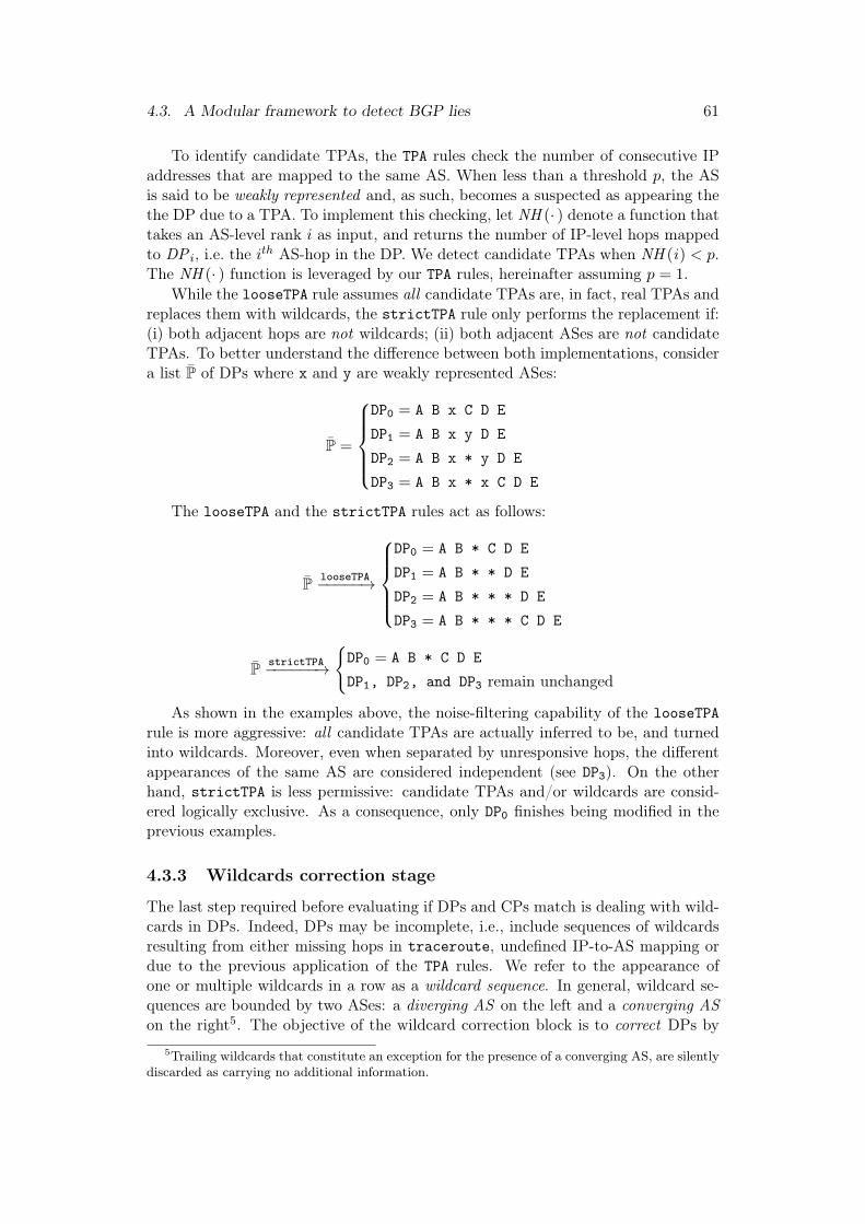
4.3. A Modular framework to detect BGP lies 61
To identify candidate TPAs, the TPA rules check the number of consecutive IPaddresses that are mapped to the same AS. When less than a threshold p, the ASis said to be weakly represented and, as such, becomes a suspected as appearing thethe DP due to a TPA. To implement this checking, let NH (· ) denote a function thattakes an AS-level rank i as input, and returns the number of IP-level hops mappedto DP i, i.e. the ith AS-hop in the DP. We detect candidate TPAs when NH (i) < p.The NH (· ) function is leveraged by our TPA rules, hereinafter assuming p = 1.
While the looseTPA rule assumes all candidate TPAs are, in fact, real TPAs andreplaces them with wildcards, the strictTPA rule only performs the replacement if:(i) both adjacent hops are not wildcards; (ii) both adjacent ASes are not candidateTPAs. To better understand the difference between both implementations, considera list P̄ of DPs where x and y are weakly represented ASes:
P̄ =
DP0 = A B x C D E
DP1 = A B x y D E
DP2 = A B x * y D E
DP3 = A B x * x C D E
The looseTPA and the strictTPA rules act as follows:
P̄ looseTPA−−−−−→
DP0 = A B * C D E
DP1 = A B * * D E
DP2 = A B * * * D E
DP3 = A B * * * C D E
P̄ strictTPA−−−−−−→
{DP0 = A B * C D E
DP1, DP2, and DP3 remain unchanged
As shown in the examples above, the noise-filtering capability of the looseTPArule is more aggressive: all candidate TPAs are actually inferred to be, and turnedinto wildcards. Moreover, even when separated by unresponsive hops, the differentappearances of the same AS are considered independent (see DP3). On the otherhand, strictTPA is less permissive: candidate TPAs and/or wildcards are consid-ered logically exclusive. As a consequence, only DP0 finishes being modified in theprevious examples.
4.3.3 Wildcards correction stage
The last step required before evaluating if DPs and CPs match is dealing with wild-cards in DPs. Indeed, DPs may be incomplete, i.e., include sequences of wildcardsresulting from either missing hops in traceroute, undefined IP-to-AS mapping ordue to the previous application of the TPA rules. We refer to the appearance ofone or multiple wildcards in a row as a wildcard sequence. In general, wildcard se-quences are bounded by two ASes: a diverging AS on the left and a converging ASon the right5. The objective of the wildcard correction block is to correct DPs by
5Trailing wildcards that constitute an exception for the presence of a converging AS, are silentlydiscarded as carrying no additional information.

62 Chapter 4. Filtering the Noise to Reveal BGP Lies
replacing wildcard sequences with their respective CP sequence (rule match*). How-ever, when substitutions cannot be performed, or simply systematically by the Rawmodel, wildcards are deleted (rule nomatch*). Both rules require knowing the AS-hop j where the first wildcard appears (right after the diverging AS) to be appliedin each wildcard sequence, as implemented in Algorithm 3.
To apply the match* rule, both the diverging and the converging ASes are re-quired to appear in the CP. If so, and considering there is at least one intermediaryAS in the CP sub-sequence between these two ASes, two possibilities may arise:(i) the number of ASes in the CP sub-sequence is smaller or equal to the length ofthe wildcard sequence in the DP or; (ii) the opposite. If (i) holds, the match* rule isable to correct the DP: the complete sequence of wildcards is substituted with theCP sub-sequence (extra wildcards, if any, being discarded); otherwise, the match*
rule cannot rewrite the DP. In such cases, the DP may be further corrected with thenomatch* rule, that simply deletes the remaining wildcards and also the divergingAS when it matches the converging AS.
Algorithm 3: match*/nomatch* rules. While in rule match* wildcards aresubstituted (matched) with sequences of ASes in CPs, in rule nomatch*
they are deleted.1 match* rule =⇒ Input: P ← DP,R← CP, j2 if (∃ k > j | P [l] = ∗ ∀ l ∈ Jj, kJ) then3 if (∃ i ∈Kj, kK | P [k] = R[i]) then4 Substitute P [j], ..., P [k − 1] with R[j], ..., R[i− 1]
5 return P
6 nomatch* rule =⇒ Input: P ← DP, j7 if (∃ k > j | P [l] = ∗ ∀ l ∈ Jj, kJ) then8 Delete P [j], ..., P [k − 1]9 if P [j] = P [j − 1] then
10 Delete P [j]
11 return P
In the following examples, let P̄ represent a list of DPs, each of which includesone or more sequences of wildcards, and that should be compared with the controlpath CP:
CP = A B C D E F G H
P̄ =
DP1 = A B C D * * * G H
DP2 = A B C D * G H
DP3 = A B * B C D E * G H
If rules match* and nomatch* are consecutively applied (e.g., in an if/else con-dition), as for all models except the Raw model, then:

4.4. The measurement platform and our campaign 63
Peer
MuxNH
VPAS 47065
CPs
DPs
AS XTunnel
Figure 4.7: Simplified representation of a co-located VP provided by the PeeringTestbed.
P̄ match*/nomatch*−−−−−−−−−−→
CP = DP1 = A B C D E F G H
CP 6= DP2 = A B C D G H
CP = DP3 = A B C D E F G H
Whereas in DP1, rule match* replaces the three wildcards with the sub-sequence EF (j = 5, k = 8, i = 7), the substitution cannot be applied in DP2 since the availablewildcards are not enough. Moreover, even the subsequent use of rule nomatch* doesnot solve the difference between CP and DP2. On the contrary, DP3 matches CP afterthe first and second wildcard sequences are solved with rules nomatch* and match*,respectively.
The rules applied in this block allow to conservatively bound the rate of BGPlies since for them each single wildcard can represent, despite unlikely, up to oneentire AS (see DP3 on the previous example).
4.4 The measurement platform and our campaign
We run our measurement campaign using co-located VPs: 6 are obtained fromthe Peering testbed [172], and 2 additional ones are homemade, i.e., manuallydeployed by us. With 8 co-located VPs, our analysis reaches a scale never achievedbefore for studies comparing CPs and DPs.
According to Fig. 4.7, the Peering testbed ensures that DPs and CPs are gatheredin the same place by constructing tunnels to an ASBR called Mux (in practice thereexist multiple Muxes, and we can choose which one to connect with). By setting adefault route towards the next-hop NH, packets flow to Mux, that then relays traffictowards NH. This allows to select the peer from which DPs are obtained. In addition,relying on the configurations of the Peering Testbed, CPs can be obtained from theASBR that has the IP address NH assigned to one of its interfaces. We focus onthe peers reported in Table 4.3, which provide full-RIBs, i.e., transit for all prefixesusually announced on the Internet [173]. On the other hand, the homemade VPsare setup with virtual machines that use as default gateway an ASBR from whichwe can collect BGP data.
We collect CPs from BGP speakers both at the Peering testbed and the home-made VPs (hmX ) every 2 hours. On the other hand, we gather DPs with Scam-per [174], running ICMP Paris-traceroute from VPs placed next to the gateway

64 Chapter 4. Filtering the Noise to Reveal BGP Lies
Peer Organization ASN CP-DP match [%]
isi Los Nettos 226 77.92uw University of Washington 101 77.93neu Northeastern University 156 76.84uth University of Utah 210 69.51grt GRNet 5408 77.93cle Clemson University 12148 77.93
hm1 University of Strasbourg 2259 77.94hm2 RGnet, LLC 3130 77.90
Table 4.3: Peers that provide transit and full RIBs that were used as VPs. Theones on top are obtained from the Peering Testbed, and the ones below manuallydeployed by us.
for the homemade VPs, or tunneling through the Peering testbed up to the routersthat provide the RIBs. The measurement campaign was designed to run daily with80k traces per day. We chose the destinations we trace by uniformly sampling /24prefixes in blocks allocated by RIRs [175]. We pick one IP from each of these pre-fixes. However, for a fraction of the traces, despite the prefixes are allocated, theyare not advertised in BGP (even in full RIBs). Table 4.3 shows that more than 20%of the selected IPs disclosed the absence of a CP, with no matching BGP prefix.This effect is even worse in uth, that exhibits RIBs with slightly less entries thanthe other VPs.
4.5 Rate of BGP lies in the wild
In this section we present the bounds of BGP lies we find in the wild. The resultsare computed based on the daily measurements we carried between 05.10.2018 and17.11.2018 for the VPs belonging to the Peering testbed and during approximately 8months (from 18.04.2018 to 19.12.2018) in the case the homemade VPs. In Sec. 4.5.1we provide an overall view of the mismatch rate for the four noise-filtering models wepropose. Then, our study focuses in the Lower model, that has the most conservativedesign and presents the lowest bound of BGP lies. First, we analyze the impact ofthe set of rules that compose its mapping relaxation stage, in Sec. 4.5.2. Finally, inSec. 4.5.3 we gather the VPs where the Lower model outputs the highest rates ofBGP lies and try to identify the type of BGP lies that cause these results.
4.5.1 Performance of the different noise-filtering models
The rate of presumable BGP lies (µ ± σ) found in the measured peers with eachof the noise-filtering models (Table 4.3) is shown in Fig. 4.8. Results are consistentacross VPs, i.e. the bounds of mismatches from the Lower to Raw model alwaysreport an increasing number of BGP lies. Yet, distinct patterns among the differentpeers can be quantitatively observed, specially for cle and hm1.
Analyzing Fig. 4.8 in more detail, we note the results for the Restrictedand Lower models differ in less than 5% for all VPs. Moreover, their values

4.5. Rate of BGP lies in the wild 65
isi uw neu uth grt cle hm1 hm2Peer
0.00.10.20.30.40.50.60.70.80.91.0
MM
Rat
eRawUpperRestrictedLower
Figure 4.8: Mismatch (MM) rate according to the model in use. The bounds ob-tained for the Restricted and Lower model differ in less than 5% for all VPs. Therate of BGP lies for the lower bound is more than 35% for cle and hm1, more than7 times compared to what is seen in the remaining VPs.
isi uw neu uth grt cle hm1 hm2Peer
0.00.10.20.30.40.50.60.70.80.91.0
Ratio
Of M
atch
es
Only looseTPAOnly SIBBoth Rules
Figure 4.9: Ratio of matches in the Lower model that result from of extending theUpper model by including the mapping relaxation stage. In general, the SIB ratherthan the looseTPA rule proves to be more useful.

66 Chapter 4. Filtering the Noise to Reveal BGP Lies
are lower than 5% in most cases. This small difference suggests that TPAs andwildcards resulting from missing hops and/or undefined mapping areeither not frequently found in sequence or, when they are, the DP stillmatches the CP. Recalling Sec. 4.3, this result shows that the Lower model doesnot gain much from implementing looseTPA rather than strictTPA, neither fromthe more conservative ordering of the rules applied in the mapping relaxation stage(SIB rule after TPA rule).
On the other hand, the Raw and Upper model also perform similarly, though thelatter generally shows a mismatch rate just a bit lower than the former. Therefore, inmost cases, wildcards resulting from unresponsive hops and/or undefined mappingcan be silently discarded. The only exception is cle, where the difference amountsto 23% due to missing hops that occur at the beginning of many DPs. Also, notethat in the Lower and Restricted models, TPA rules in the mapping relaxation stageexchange inferred TPAs for wildcards, thus increasing the need of the wildcardcorrection step.
According to the design of the proposed framework, the real rate of BGP liesobserved by VP is expected to be between the bounds that the Lower and Uppermodels respectively produce. In other words, the mismatches observed only throughthe Upper model are potential false negatives for the Lower model, i.e. potential lieswrongly filtered as noise. Consequently, the rate of lies may be as significant asthe Upper bound, at worst. On the other hand, its value could be closer to thefully-conservative Lower bound, usually less than 5%. While this value is low, it isnot negligible: according to its conservative design, the Lower model isexpected to filter most of the noise and to capture many actual lies.
4.5.2 Effect of SIB and TPA rules on the mismatch rate
Our models can be grouped both in terms of design and performance: Raw andUpper on one side, and Restricted and Lower on the other. As illustrated in Fig 4.8,there exists a large gap in terms of the plausible BGP lies seen for these two groups,except in hm2 where all bounds are surprisingly close to each other. While the Rawand Upper models just use the wildcards correction stage, the Restricted and Lowerones make also extensive use of the mapping relaxation stage. We now analyzeif any of the rules in this latter block is more effective to decrease the number ofmismatches, or if it is rather their combination that is required. Since each rulewas designed to treat a specific limitation affecting DPs and CPs, this would alsoreveal if there is an outstanding kind of noise biasing severely the ground data. Inparticular, since the Restricted and Lower bounds perform similarly, we focus onlyon the Lower bound, and thus SIB and looseTPA rules.
The difference between red and green bars for each peer in Fig. 4.8 represents theamount of mismatches observed via the Upper model and not via the Lower one.In other words, it is the share of cases that benefit from the mapping relaxationstage. We analyze which of these cases actually profit from applying (i) only theSIB rule, (ii) only the looseTPA rule, and (iii) both. As shown in Fig. 4.9, less than3% of the total cases across all VPs are filtered concurrently using both the SIBand looseTPA rules. Indeed, this small proportion indicates that, in general, pathsdo not include simultaneously AS siblings and TPAs. In addition, between

4.6. Conclusion 67
68% and 97% of the cases across all VPs (cle and hm2 being the exception with lessthan 32% and 50%, respectively) require only using the SIB rule.
4.5.3 Looking closer at high mismatch rates
Although pinpointing and understanding the root causes of observed MMs —anddefining whether they are deliberate or not— is challenging (see Sec. 4.1), the highmismatch rate observed for the Lower model in cle and hm1 (together with theirhigher variability over time) encourage us to further investigate these cases. We seethat cle’s provider sends traffic directly to the AS that is expected to be two AS-hops away, according to advertised CPs. While the presence of an unintended lie isa likely cause—also in line with the high variability observed—neither an interestedlie nor AS poisoning can be discarded. On the other hand, a privileged view in hm1allows us to access the ground truth and to determine that most mismatches seen inthis peer originate from technical limitations in the infrastructure of its provider AS.Indeed, the ASBR connecting to hm1 had a partial-FIB with a persistent defaultroute, and this lead traffic to exit the provider AS through a peering AS that wasnot necessarily the one included in CPs.
4.6 Conclusion
BGP lies are not straightforward to detect: noise in the ground data can generatemismatches between CPs and DPs. Since this noise can be confused as lies—andvice versa—filtering it is imperative. We propose a framework based on multiplepath-rewriting rules that allows to produce four noise-filtering models to overcomethe shortcomings produced by the noise, and to estimate bounds of BGP lies inthe wild. We leveraged the Peering testbed that provides full-RIBs from multiplepeers as well as co-located CPs and DPs, and carried out a longitudinal analysisas never done before, that spanned 8 VPs and up to 8 months of measurements.While the noise from TPAs was more prevalent for a limited number of VPs, thenoise due to AS siblings generated most mismatches. We believe that this effect islargely VP-dependent.
Finally, we quantified the lower bound of the mismatch rate seen in the wildas being less than 5%. This value is small, but not negligible: since our approachis conservative, we expect to have filtered most of the noise and have capturedmany actual BGP lies. Moreover, this also means that there might be many falsenegatives, i.e. many lies that finished being filtered as if they were noise. At thesame time, we further analyzed the nature of mismatches persisting after applyingthe most conservative filter in a VP where we have a privileged view, concludingthat technical limitations related to a partial-FIB router relying on a default routein the infrastructure of the provider AS were causing the BGP lies.
In future work we plan on extending the measurement infrastructure and thecoverage of our analysis. A difficulty to sort out in this aspect is that the studyin this chapter requires using co-located VPs. The Peering Testbed allowed us tofulfill this requirement, but only for a reduced number of ASes that shared full-RIBs. As a first solution, we plan on relaxing the need of full-RIBs, and to craft theIP list to be measured on a per-peer basis, according to the prefixes that each AS

68 Chapter 4. Filtering the Noise to Reveal BGP Lies
advertises. This will allow us to increase the number of VPs and the success rateof our measurements. In particular, considering that Routeviews and CAIDA areplanning to implement Scamper at BGP collectors co-located at IXPs, this createsa good opportunity to extend our work.6
6https://www.caida.org/publications/presentations/2020/scamper_routeviews_kismet/
Chapter 5The Art of Modeling and DetectingForwarding Detours
Contents5.1 The origin of FDs: routing inconsistencies and forward-
ing alterations . . . . . . . . . . . . . . . . . . . . . . . . . 715.1.1 RIes, FAs and FDs in a practical example . . . . . . . . . 715.1.2 Lookup functions: prefixes, gateways and next-hops . . . 725.1.3 What is an internal route of an AS? . . . . . . . . . . . . 735.1.4 When is the routing consistent? . . . . . . . . . . . . . . . 755.1.5 What produces routing inconsistencies? . . . . . . . . . . 755.1.6 What leads to forwarding alterations? . . . . . . . . . . . 775.1.7 When do forwarding detours occur? . . . . . . . . . . . . 78
5.2 Similarities and differences between FDs, LB and TE . 795.2.1 Simple but naive methods to detect FDs . . . . . . . . . . 805.2.2 Forwarding patterns for LB, TE and FDs . . . . . . . . . 81
5.3 A detector of prefix-based forwarding patterns . . . . . 835.3.1 Exploration phase . . . . . . . . . . . . . . . . . . . . . . 845.3.2 Prefix-grouping phase . . . . . . . . . . . . . . . . . . . . 845.3.3 Multi-route discovery phase . . . . . . . . . . . . . . . . . 855.3.4 Merging phase . . . . . . . . . . . . . . . . . . . . . . . . 86
5.4 An FD-detector . . . . . . . . . . . . . . . . . . . . . . . . 875.4.1 The FD-verdict: looking for a lonely DIR . . . . . . . . . 885.4.2 The FD-detector: a tool to be run in the wild . . . . . . . 89
5.5 Capturing forwarding detours in the wild . . . . . . . . . 915.5.1 Measurement campaigns and coverage . . . . . . . . . . . 915.5.2 Fowarding patterns and the binary effect of FDs . . . . . 925.5.3 Distribution of FDs per AS and ASBR-couples . . . . . . 935.5.4 Correlation between ingress-ASBRs and FDs . . . . . . . 945.5.5 Speculating on the root causes generating FDs . . . . . . 96
69
70 Chapter 5. The Art of Modeling and Detecting Forwarding Detours
5.5.6 Validation: emulations and ground truth . . . . . . . . . . 975.6 Discussion: robustness of the FD-detector . . . . . . . . 98
5.6.1 An FD-verdict handling all interactions of FDs and LB . 985.6.2 A binary effect that unlikely results from routing changes 995.6.3 On the (in)sensibility of flawed ASBR detection . . . . . . 1005.6.4 Measurement stopping points . . . . . . . . . . . . . . . . 1005.6.5 Alias Resolution: a nice, but dangerous additional feature 100
5.7 Conclusion . . . . . . . . . . . . . . . . . . . . . . . . . . . 101
In this chapter we take a close look at the phenomenon of forwarding detours.To the best of our knowledge, we are the first to tackle the problem of detectingforwarding detours, indistinctly of the underlying causes generating them, whilefiltering load balancing and traffic engineering techniques. In a nutshell, we makethe following contributions:
• We develop a formalism around forwarding detours in Sec. 5.1. In particu-lar, we construct a forwarding model and show that routing inconsistenciesmay evolve into forwarding alterations which then may originate forwardingdetours.
• We study in Sec. 5.2 the forwarding pattern that FDs originate inside ASes,i.e., whether traffic between two fixed endpoints flows through different routesdepending on the considered prefix, and compare it with that generated by loadbalancing and traffic engineering techniques. In particular, FDs, per-prefix LBand TE generate a similar forwarding pattern, which we call prefix-based.
• We design an algorithm able to detect prefix-based forwarding patterns inSec. 5.3. Our framework relies only on IP-to-AS mapping data and data-planeinformation collected with traceroute. We present a novel strategy to seek formulti-path routing patterns, in multiple steps. Our technique groups prefixesfor which the same internal routes of ASes are revealed, an idea that may beincorporated in topology discovery studies to reduce their associated probingcost.
• We propose an FD-detector in Sec. 5.4. Our solution adds a last phase to theprevious algorithm: it applies an FD-verdict allowing to discriminate FDs fromthe other mechanisms that also generate prefix-based forwarding patterns. Forthis, we focus on extreme-FDs cases, i.e., scenarios where FDs affect numerousprefixes. We build a detector of forwarding detours as a tool ready to be runin the wild.
• We analyze the FD-phenomenon in the wild in Sec. 5.5, running our FD-detector from 100 nodes of the NLNOG RING monitoring infrastructure, andfind FDs in 25 out of 54 ASes. We find a remarkable binary pattern in whichtransit traffic traversing between two border routers of an AS either neverdetours, or always does. We validated the behavior of the FD-detector withemulations and on a network where we have ground truth.

5.1. The origin of FDs: routing inconsistencies and forwarding alterations 71
• We release the dataset we collected, the emulations setups and our code tofoster replicability and reproducibility1.
In addition, we discuss the robustness of the FD-detector we implemented inSec.5.6, and draw final remarks in Sec. 5.7. The work presented in this chapter leadto the writing of the following article and poster:
• Julián M. Del Fiore, Valerio Persico, Pascal Merindol, Cristel Pelsser andAntonio Pescapè. The Art of Detecting Forwarding Detours, in IEEE Trans-actions on Network and Service Management (IEEE TNSM) 2021.
• Julián M. Del Fiore, Pascal Merindol, Valerio Persico, Cristel Pelsser andAntonio Pescapè. Routing Inconsistencies at the FIB level, poster presentedin TMA 2019.
5.1 The origin of FDs: routing inconsistencies and for-warding alterations
This section formally defines the concepts of routing inconsistencies (RIes), forward-ing alterations (FAs) and forwarding detours (FDs). First, Sec. 5.1.1 illustrates theintuition behind these concepts and how they relate. Then, in Sec. 5.1.2, we proposea simple, yet realistic, forwarding model that describes how routers take forwardingdecisions. Then, in Sec. 5.1.3 we explain how the combination of these distributeddecisions result into forwarding routes and internal routes of ASes. Second, we studywhen the forwarding is consistent in Sec. 5.1.4 and define the conditions leading tothe existence of RIes in Sec. 5.1.5. Third, in Sec. 5.1.6 we describe how RIes may, inturn, evolve into FAs, and further show how these may generate FDs in Sec. 5.1.7.Finally, in Sec. 5.2.2 we analyze how FDs, LB and TE have similarities and differ-ences in the forwarding patterns they generate, i.e., in how traffic subject to each ofthem flows inside ASes.
5.1.1 RIes, FAs and FDs in a practical example
To illustrate how FDs originate, Fig. 5.1 compares the scenarios when either a net-work with a fixed topology is composed of only full-FIB routers (5.1a), or includesan ASBR with a partial-FIB and a default route (5.1b). In Fig. 5.1a, ASBR1 for-wards transit traffic through optimal paths, according to the IGP metric in use,to reach all possible exit points, i.e., the other ASBRs. On the other hand, inFig. 5.1b, ASBR1 has a partial-FIB and forwards traffic destined to prefix PB
via its default route, relying on ASBR2 (blue dotted line). Since ASBR2 con-siders ASBR3 the best ASBR for PB, ASBR2 redirects traffic targeting PB towardsASBR3 . In this way, ASBR2 introduces a forwarding alteration, i.e., changes theexpected forwarding route. While the best IGP path from ASBR1 to ASBR3 is(ASBR1 , r3, r4,ASBR3 ), and is used for PG, the forwarding route for PB differs,being (ASBR1 , r1,ASBR2 , r2, r4,ASBR3 ). Consequently, PB is subject to FDs,but PG is not, thus generating a multi-path routing pattern between ASBR1 and
1See https://github.com/julian10m/FD-detector.git

72 Chapter 5. The Art of Modeling and Detecting Forwarding Detours
ASBR2
ASBR1
ASBR2
Pfx BGP NH Int
PR 𝑠𝑒𝑙𝑓 𝑖0PG ASBR3 𝑖1PB ASBR3 𝑖1
0/0 𝑠𝑒𝑙𝑓 𝑖0
ASBR1
Pfx BGP NH Int
PR ASBR2 𝑖0PG ASBR3 𝑖1PB ASBR3 𝑖1
0/0 ASBR2 𝑖0
ASBR3
1
23
4
PBPG
𝑖0
𝑖1
PR𝑖0
𝑖1
(a) All ASBRs have a full-FIB
ASBR2
ASBR3
ASBR1
1
23
4
PB
ASBR2
Pfx BGP NH Int
PR 𝑠𝑒𝑙𝑓 𝑖0PG ASBR3 𝑖1PB ASBR3 𝑖1
0/0 𝑠𝑒𝑙𝑓 𝑖0
ASBR1
Pfx BGP NH Int
PR ASBR2 𝑖0PG ASBR3 𝑖1
0/0 ASBR2 𝑖0 PG
𝑖0
𝑖1
PR𝑖0
𝑖1
(b) ASBR1 has a partial-FIB
Figure 5.1: Routing consistence vs. forwarding detours. In the left case, transittraffic entering the AS through ASBR1 always flows in the AS towards the remainingASBRs through the best IGP paths. In contrast, in the right figure, ASBR1 hasa partial-FIB lacking the entry for the blue prefix PB, leading to FDs for thisprefix, and for multi-path routing patterns between ASBR1 and ASBR3 , as trafficconcerning prefix PG does not detour.
ASBR3 . Moreover, even if tunnels mechanisms were used between ASBRs, e.g. be-tween ASBR1 and ASBR2 , once traffic concerning PB exited the tunnel, ASBR2
would still redirect it to ASBR3 .
5.1.2 Lookup functions: prefixes, gateways and next-hops
In our forwarding model, each router r inside any ASX determines next-hops relyingon three lookup functions, namely Nr(G), Gr(P ) and Pr(d). Each of these functionsconveys a different objective:
The function Pr(d) receives a destination IP address d, and returns the mostspecific prefix covering d. Therefore, Pr(d) can be either an internal or external

5.1. The origin of FDs: routing inconsistencies and forwarding alterations 73
prefix, i.e.,
Pr(d) =
{Internal prefix, d ∈ XExternal prefix, otherwise
where d is advertised in the IGP of X in the first case, and learned via BGP, andthus associated to transit traffic, in the latter.
The function Gr(P ) takes a prefix P as argument and outputs the IP addressinside X to be reached in order to eventually access prefix P . We refer to Gr(P )as the gateway for P . The interpretation of the gateway Gr(P ) varies depending onwhether P is internal or external, i.e.
Gr(P ) =
{d, P is an internal prefixBGP(P ), otherwise
where BGP(P ) returns the iBGP next-hop for P .2 Hence, the gateway Gr(P )should be, theoretically, the egress-ASBR for transit traffic, i.e., the last hop in Xthat forwards transit traffic to the eBGP next-hop that advertised P .
The function Nr(G) computes the next-hop towards an IP address G, usually agateway, inside X, i.e. the router linked via an outgoing interface of r to which apacket has to be sent in order to ultimately reach G. The value of Nr(G) dependson that of G, i.e.,
Nr(G) =
{δ(d), G = r
IGP(G), otherwise
where IGP(G) provides the IGP next-hop towards G and δ(d) is a function of d thattakes different values depending on whether d = r or d 6= r. In the first case, theforwarding stops and the packet is handled by the higher layers of the protocol stack,i.e., Nr(G) = δ(r) = ∅. On the other hand, if r is not the destination, then r acts asthe egress-ASBR used to reach the external destination d, and thus Nr(G) = δ(d)is the eBGP next-hop for P .
To forward packets towards a destination IP address d, routers apply the lookupfunctions we have defined in sequence. Like this, packets are forwarded to the next-hop Nr◦Gr◦Pr(d) leading to the gateway Gr◦Pr(d) defined for the longest matchingprefix Pr(d) of d.
5.1.3 What is an internal route of an AS?
As routers at each hop receive and forward packets, the chaining of these eventsresults into a forwarding route.
Forwarding route: a forwarding route of an AS X towards a destination d, de-noted RX(d), is a sequence of routers RX(d) , [r0, r1, ..., rj , ..., rn], where, we con-sider implicit that rj , rj(d) to simplify notation, such that:
∀j ∈ {0, ..., n− 1}, rj+1 = Nrj ◦ Grj ◦ Prj (d)
2When the BGP next-hop-self option is enabled, this is exactly the case. We design our modelrelying on this feature for convenience, to simplify the illustrations in this section that wouldotherwise require showing a neighboring AS, but without loss of generality.

74 Chapter 5. The Art of Modeling and Detecting Forwarding Detours
l
AS 𝑋
𝑚 𝑛 𝑜l
AS 𝑋
𝑚 𝑛 𝑜
Direct internal route Transit internal route
Figure 5.2: Direct internal routes and transit internal routes inside an AS X. Thefirst are those internal routes for which the destination, n in this case, belongs tothe same AS that owns the routers, that is, X. On the other hand, for the latter,traffic is only transiting through AS X and exits through an egress-ASBR, namelyo. For both types of internal routes, the first router l is an ingress-ASBR of X.
The condition only defines how routers should choose next-hops to create aforwarding route, however, it does not apply on router rn that could either equal dor not. This is not critical since, from forwarding routes, we will usually be interestedin extracting the internal routes of the ASes that are traversed.
Internal route: an internal route of an AS X towards a destination d, is a for-warding route RX(d) such that:
i) ∀j ∈ {0, ..., n}, rj ∈ Xii) r0 is an ingress-ASBR of Xiii) Grn ◦ Prn(d) = rn
A priori, the strict notion of what an internal route is only requires condition i,but we narrow their scope additionally considering conditions ii and iii to align ourmodel to the FD-detector we implement later. While condition ii is self-explanatory,according to condition iii, router rn chooses itself as gateway, hence Nrn ◦ Grn ◦Prn(d) = Nrn(rn). Given this holds, rn is the last hop in X, and there exist twooptions:
• rn is directly the destination d and Nrn(rn) = Nrn(d) = ∅. We refer to theseroutes as direct internal routes (DIRs).
• rn 6= d and acts as egress-ASBR of X, consequently Nrn(rn) /∈ X. The packetsbeing forwarded represent transit traffic in these cases, hence we say the routesare transit internal routes (TIRs).
To better illustrate the difference between TIRs and DIRs, Fig. 5.2 presentsan example. In both scenarios, packets enter AS X through the ingress-ASBR l,however, while on the left case traffic stops in router n, that is the destination,router o acts as egress-ASBR for the transiting traffic on the right side.

5.1. The origin of FDs: routing inconsistencies and forwarding alterations 75
l
AS 𝑋
𝑚 𝑛 𝑜l
AS 𝑋
𝑚 𝑛 𝑜
Routing Consistency
Figure 5.3: Routing consistency. In both cases, all routers along the internal routeschoose the same best covering prefix for the destination (not explicitly shown) andthe same gateway, n and o on the left and right side, respectively.
5.1.4 When is the routing consistent?
According to our definition of internal routes, indistinctly of being TIRs or DIRs,the actual gateway and best covering prefix that each router along the route choosesis not defined. The only exception is the gateway of rn, that selects itself, asemphasized in Fig. 5.2 with the blue (looping) arrows in routers n and o, respectively.In particular, when all routers along the route choose the same best covering prefixP and gateway G, we say that the resulting internal route RX(d) is consistent.
Routing consistency: an internal route RX(d) is consistent when all routers alongthe route choose the same best covering prefix P and gateway G for d, i.e., when
∀ rj ∈ RX(d), Prj (d) = P ∧ Grj ◦ Prj (d) = Grj (P ) = G
.
In particular, note that r0, the first router in RX(d), imposes conditions, i.e., itmust hold that P , Pr0(d) and G , Gr0 ◦ Pr0(d) = rn = Grn ◦ Prn(d).
An example is illustrated in Fig. 5.3, where compared to Fig. 5.2, we explicitlyshow the gateway chosen by the routers along the routes. Since all blue arrows pointto n and o, and we assume that all routers select the same best covering prefix ford, then both the TIR and DIR are consistent.
5.1.5 What produces routing inconsistencies?
An internal route RX(d) may be inconsistent at two different levels depending onthe best covering prefixes and gateways that routers along the route choose for d.
Routing inconsistency at the prefix level: there exists a routing inconsistencyat the prefix level in an internal route RX(d) when an upstream router rk of RX(d)chooses a different best covering prefix than a downstream router rj of RX(d), i.e.,
∃ j < k ≤ n | Prj (d) 6= Prk(d)

76 Chapter 5. The Art of Modeling and Detecting Forwarding Detours
l 𝑚 𝑛 𝑜
AS 𝑋
l
AS 𝑋
𝑚 𝑛 𝑜
𝑝
𝑞
Routing InconsistenciesRouting consistency
Figure 5.4: Routing consistency vs inconsistency. While all routers choose o asgateway on the left side, all blue arrows point to different routers on the right side.In this particular example, the resulting forwarding route is the same in both cases,though as we study next, for some RIes, this is not always true.
Routing inconsistency at the gateway level: there exists a routing inconsis-tency at the prefix gateway level in an internal route RX(d) when an upstream routerrk of RX(d) chooses a different gateway than a downstream router rj of RX(d), i.e.,
∃ j < k ≤ n | Grj ◦ Prj (d) 6= Grj ◦ Prk(d)
Note that both types of RIes are not exclusive: the one at the prefix levelmay lead to another at the gateway level. As an example, if rj and rk are routers inRX(d), such that rj is a partial-FIB router with a default route and rk is full-FIBrouter, this will likely generate RIes at both levels. As rj has a partial-FIB, multipleoriginally disaggregated prefixes present in rk are aggregated in the FIB of rj intoa default route, which originates RIes at the prefix level. While rk may associatedifferent gateways to each of these prefixes, a unique arbitrarily chose, a default one,is used by rj . Consequently, this may likely potentially leading to additional RIesat the gateway level.
Another important detail is that RIes at the prefix level that do not generateothers at the gateway level are not detectable. Indeed, despite the best coveringprefix selected for the same destinations may vary from router to router, as longas they continue choosing the same gateway, the forwarding is not impacted. Moregenerally, in practice only RIes at the gateway level can be detected, though it isnot possible to determine at which level these were actually originated without priv-ileged knowledge, e.g., being able to check the routing table of all traversed routers.Therefore, to simplify our notation and to focus on detectable RIes, we will con-sider implicit that when we say that there exists a routing inconsistencyin an internal route, we refer to at the gateway level, and it may also be atthe prefix level.
Fig. 5.4 illustrates the difference between cases where the routing is consistent(left) or there exist RIes (right). While all blue arrows point to o on the left side,the routers along the route choose all different gateways on the right side. In this

5.1. The origin of FDs: routing inconsistencies and forwarding alterations 77
l
AS 𝑋
𝑚 𝑛
𝑜
l
AS 𝑋
𝑚 𝑛
𝑝
𝑜
𝑝
Forwarding AlterationNo Forwarding Alteration
Figure 5.5: Routing inconsistencies and forwarding alterations. In both cases thereexist RIes, however, while on the left case the action of router m does not produceFAs, in the right case router n deviates traffic towards router o, generating FAs.
particular example, the resulting forwarding route is the same in both cases, thoughas we study next, this is not always the case.
5.1.6 What leads to forwarding alterations?
When the resulting internal route RX(d) is different to the forwarding route thatwould have been used if all routers had chosen the same gateway, we say that thedifference was generated by a FA in RX(d).
Forwarding alteration: there exists a forwarding alteration in an internal routeRX(d) if an upstream router rk uses different next-hops for the gateway it choosesand the gateway a downstream router rj selects, i.e.,
∃ j < k ≤ n | Nrk ◦ Grk ◦ Prk(d) 6= Nrk ◦ Grj ◦ Prj (d)
Theorem – Forwarding alterations imply routing inconsistencies: if thereexists a forwarding alteration in an internal route RX(d), then RX(d) is inconsistent.
Proof. Assume there exists a forwarding alteration in RX(d), but no routing incon-sistency occurs. If RX(d) is not subject to RIes, then ∀j, Grj ◦ Prj (d) = G. As aconsequence Nrk ◦ Grk ◦ Prk(d) = Nrk(G) and Nrk ◦ Grj ◦ Prj (d) = Nrk(G), i.e., ifthe gateways match, so does the next-hop rk uses. This contradicts our originalhypothesis stating that FAs occur, proving that FAs imply RIes. �
Note that FAs imply RIes, but the converse may not hold, i.e., the relationshipis FAs ⇒ RIes. Indeed, for j < k, even though routers rj and rk may choosedifferent gateways, Gj and Gk respectively, when Nrk(Gk) = Nrk(Gj), then no FAoccurs. In these cases, we say that the existing RIes are not visible. This mayparticularly happen in networks that lack path diversity, e.g. if the disagreeingrouter rk only has one possible next-hop, then it can never introduce a FA.

78 Chapter 5. The Art of Modeling and Detecting Forwarding Detours
Forwarding DetourBest IGP Path
l 𝑚
𝑛
𝑜
𝑝
AS 𝑋 AS 𝑋
l 𝑚
𝑛
𝑜
𝑝
Figure 5.6: Best IGP path vs Forwarding Detour. On the left, all routers choose oas gateway, hence no RIes occur and traffic flows through the best IGP path froml to o. On the contrary, on the right, router p introduces RIes choosing o insteadof itself as gateway. As p should act as egress-ASBR, but instead sends traffic tom, then p< introduces a FA. Since l would have straightforwardly sent traffic to m,had it selected o as gateway, then the resulting internal route is subject to FDs.
An example is illustrated in Fig. 5.5 where RIes either do not introduce FAs(left) or do so (right). In the left case, there exists a routing inconsistency as routerm chooses router o as gateway while router l chooses p. However, the forwardingroute still ends up in p, being the same it would have been if m had chosen p asgateway, therefore no FA occurs. On the other hand, on the right figure there existRIes as router n chooses different gateways than routers l and m, and a FA occurs:router n pushes traffic towards o instead of p. This affects the resulting route, whichwould have been the same as in the left side figure if n had chosen p as gateway.
5.1.7 When do forwarding detours occur?
A forwarding detour occurs when the internal route in use inside an AS does notmatch the best IGP path between the endpoints of the route, i.e., r0 and rn. Theillustrations in Fig. 5.6 show the difference between best IGP paths and FDs. Inthe left case, the routing is consistent since all routers choose the same gateway o,and thus the forwarding route coincides with the best IGP path available between land o. On the contrary, on the right case, router p introduces RIes, and a FA suchthat packets exit the AS via o. Since l would have used the direct link with m toforward packets towards o, instead of that via n, the FA translates into a FD.
Forwarding detour: an internal route RX(d) detours, i.e., a forwarding detouroccurs for destination d, when an upstream router rj in RX(d) would not have usedrj+1 in RX(d) as next-hop to reach a downstream router rz of RX(d), i.e.,
∃ j < z ≤ n | Nrj (rz) 6= rj+1
Theorem – Forwarding detours imply forwarding alterations: if an internalroute RX(d) detours, then RX(d) is subject to forwarding alterations.

5.2. Similarities and differences between FDs, LB and TE 79
Proof. Assume RX(d) is subject to forwarding detours, but no forwarding alterationoccurs in RX(d). If RX(d) is not subject to FAs, then it must hold that ∀j < k, Nrk◦Grk ◦Prk(d) = Nrk ◦Grj ◦Prj (d). This means that, even though gateways Grj ◦Prj (d)and Grk ◦Prk(d) may differ for different routers, the next-hop that all routers choose,besides matching the IGP next-hop for their respective gateway, also matches theIGP next-hop for the gateways chosen by the other routers. By definition, thisimplies that RX(d) is the best IGP path leading to all these gateways and, therefore,no detours can occur. This contradicts our original hypothesis stating that RX(d)was subject to forwarding detours, proving that FDs imply FAs. However, for thesake of completeness, we complete the proof. For this, recall that a property ofIGPs is that sub-paths of best IGP paths are also best paths. This means that ifany router rz ∈ RX(d) would have been the destination d, then the sub-path leadingto it would still have been a best IGP path. Since when d = rz, the destinationwould be internal, therefore ∀j < z, Grj ◦ Prj (d) = rz would hold. ConsequentlyNrj ◦ Grj ◦ Prj (d) , rj+1 = Nrj (rz), which contradicts the formal definition offorwarding detours. Again, this proves that FDs imply FAs. �
Note that FDs imply FAs, but the converse may not hold, i.e., the relationshipis FDs ⇒ FAs. This is highlighted by the right side of Fig. 5.5, where router ndeviates traffic towards router o, but the resulting route is still the best IGP pathbetween routers l and o. In general, this occurs when the the best IGP path betweenr0 and rn either includes the sub-path from r0 to rk, the router that introduces theFA, or is a sub-path of the path between r0 and Gr0 ◦ Pr0(d).
By combining our two theorems, we thus have that FDs⇒ FAs⇒ RIes. WhenFDs occur, there is a router rk between rj and rz that introduces a RI choosing adifferent gateway than rj . This router rk uses different next-hops to reach bothgateways, i.e., Nrk ◦ Grk ◦ Prk(d) 6= Nrk ◦ Grj ◦ Prj (d), and introduces a FA. Sincerk (re)directs traffic towards Grk ◦ Prk(d), when rj would not have chosen rj+1 asnext-hop for this gateway, a FD results. This is exactly the case in the right side ofFig. 5.6 where rj = l, rk = p and rz could be either m or o.
Finally, note that when FDs occur, they create multi-path routing patternsinside ASes. This results from the fact that the best IGP path between the endpointsis used to forward traffic of prefixes either non-subject to RIes, or subject to FAsbut not FDs (left side of Fig, 5.6), but for those destinations and prefixes subjectto FDs, the resulting internal routes differs (e.g. right side of Fig. 5.6).
In general, between two routers i and e of AS X, different root causes maylead to distinct FDs between these endpoints, forming a set RFD
X (i, e) of detouringroutes. Each detouring route of RFD
X (i, e) will be associated to a specific sets ofprefixes, all subject to the same FAs. This is illustrated in Fig 5.7 whereRFD
X (l, o) ={R1, R2, R3} such that R1 = [l, n, p,m, o], R2 = [l,m, q, o] and R1 = [l, n, p,m, q, o],each respectively shown in Fig 5.7a, 5.7b and 5.7c, while the best IGP path betweenl and o actually is [l,m, o].
5.2 Similarities and differences between FDs, LB and TE
In this section we show why differentiating between FDs, LB and TE is not trivial.While Sec. 5.2.1 provides examples of simple but inaccurate FD-detectors, Sec. 5.2.2

80 Chapter 5. The Art of Modeling and Detecting Forwarding Detours
Forwarding Detour I
AS 𝑋
l 𝑚
𝑛
𝑝
𝑞
𝑜
(a)
Forwarding Detour II
AS 𝑋
l 𝑚
𝑛
𝑜
𝑝
𝑞(b)
Forwarding Detour III
AS 𝑋
l 𝑚
𝑛
𝑜
𝑝
𝑞AS 𝑋
l 𝑚
𝑛
𝑜
𝑝
𝑞
(c)
Figure 5.7: Multiple distinct forwarding detours between the same endpoints. InFig. 5.7a, router p introduces a FA, and this leads to a FD. The cases of Fig. 5.7band 5.7c represent more complex scenarios where multiple FAs occur. In particular,the FAs are introduced by m and q on the first case, and additionally by p on thelatter. The three scenarios produce forwarding routes subject to distinct FDs thatmay co-exist when they affect different sets of prefixes.
explains why looking at which routes are revealed when different prefixes are targetedis the first step to develop a more effective approach to detect FDs.
5.2.1 Simple but naive methods to detect FDs
In practice, observing a multi-path routing pattern between any two routers i and eof an AS X is not enough to declare the occurrence of FDs: the use of LB and TEcan also produce the same effect. With LB methods such as equal-cost multi-path(ECMP), the strict notion of best IGP path is generalized to a set of paths RLB
X (i, e)sharing the same IGP distance. The purpose of ECMP is to evenly spread the loadacross such set of best parallel IGP paths. On the other hand, TE allows to createsets of constrained paths RTE
X (i, e) that are commonly used for specific usages re-garding a limited number of external prefixes, but not for best-effort traffic. Consid-ering Fig. 5.8, where RFD
X (i, e) = {R1}, RLBX (i, e) = {R2, R3}, RTE
X (i, e) = {R4},the question we aim to address is, by simply collecting routes with traceroute, howcan we distinguish FDs?

5.2. Similarities and differences between FDs, LB and TE 81
𝑅4𝑅3
𝑅2𝑅1
AS 𝑋Figure 5.8: Forwarding pattern when RFD
X (i, e) = {R1}, RLBX (i, e) = {R2, R3} and
TE RTEX (i, e) = {R4}. The size of every arrow is proportional to number of prefixes
for which each route is used.
A first attempt to solve this problem would be to assume that hop count is usedas the IGP metric, compare routes by their length, and conclude for FDs whenroutes of different lengths are discovered between i and e. However, for other IGPmetrics, such heuristic may lead to misclassify ECMP as FDs, e.g. R3 in Fig. 5.8,and vice-versa. On the other hand, TE routes are not restricted to be shortest pathsbetween two endpoints. Hence, this highlights that, to avoid both false positivesand negatives in the detection of FDs, the designed method should be valid for anyIGP metric and contemplate TE.
Another naive solution would be to assume that transit traffic traverses exactlytwo ASBRs inside an AS. Under this assumption, we could first learn the ASBRsfrom all traces, and then pinpoint FDs looking if three or more ASBRs of the sameAS were traversed in any trace. For example, in Fig. 5.1b, the blue path thatdetours traverses ASBR1 , ASBR2 and ASBR3 . Though apparently effective, thistechnique only works in specific network topologies where ASBRs are never used astransit core routers. For example, if router r3 in Fig. 5.1a was also used as ASBRfor some prefixes, then prefix PG would incorrectly look as subject to FDs. In short,this technique cannot be used since, in practice, it is likely that traces will usuallytraverse multiple ASBRs of the same AS, even in the absence of FDs.
To correctly detect FDs, rather than computing misleading metrics for eachroute and/or comparing them one at a time, we propose to analyze the forwardingpattern for (i, e) in AS X, as we detail next.
5.2.2 Forwarding patterns for LB, TE and FDs
To better understand the similarities and differences between FDs, LB and TE,we propose to analyze the forwarding pattern between i and e, i.e., whetherthe routes of X leading from i to e which traffic traverses vary depending on theconsidered prefixes. In other words, we propose to closely study which routes of X,leading from i to e, are used depending on the targeted prefixes. In particular, LBmay be deployed with different LB flavors that produce specific forwarding patterns.In particular, we focus on hash-based LB flavors, recalling that per-packet LB is
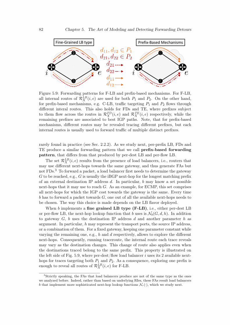
82 Chapter 5. The Art of Modeling and Detecting Forwarding Detours
Fine-Grained LB type Prefix-Based Mechanisms
Figure 5.9: Forwarding patterns for F-LB and prefix-based mechanisms. For F-LB,all internal routes of RLB
X (i, e) are used for both P1 and P2. On the other hand,for prefix-based mechanisms, e.g. C-LB, traffic targeting P1 and P2 flows throughdifferent interal routes. This also holds for FDs and TE, where prefixes subjectto them flow across the routes in RFD
X (i, e) and RTEX (i, e) respectively, while the
remaining prefixes are associated to best IGP paths. Note, that for prefix-basedmechanisms, different routes may be revealed tracing different prefixes, but eachinternal routes is usually used to forward traffic of multiple distinct prefixes.
rarely found in practice (see Sec. 2.2.2). As we study next, per-prefix LB, FDs andTE produce a similar forwarding pattern that we call prefix-based forwardingpattern, that differs from that produced by per-dest LB and per-flow LB.
The set RLBX (i, e) results from the presence of load balancers, i.e., routers that
may use different next-hops towards the same gateway, and thus generate FAs butnot FDs.3 To forward a packet, a load balancer first needs to determine the gatewayG to be reached, e.g., G is usually the iBGP next-hop for the longest matching prefixof an external destination IP address d. In particular, b may know a set possiblenext-hops that it may use to reach G. As an example, for ECMP, this set comprisesall next-hops for which the IGP cost towards the gateway is the same. Every timeb has to forward a packet towards G, one out of all the available next-hops needs tobe chosen. The way this choice is made depends on the LB flavor deployed.
When b implements a fine grained LB type (F-LB), i.e., either per-dest LBor per-flow LB, the next-hop lookup function that b uses is Nb(G, d, h). In additionto gateway G, b uses the destination IP address d and another parameter h asargument. In particular, h may represent the transport ports, the source IP address,or a combination of them. For a fixed gateway, keeping one parameter constant whilevarying the remaining one, e.g., h and d respectively, allows to explore the differentnext-hops. Consequently, running traceroute, the internal route each trace revealsmay vary as the destination changes. This change of route also applies even whenthe destinations traced belong to the same prefix. This property is illustrated onthe left side of Fig. 5.9, where per-dest/flow load balancer i uses its 2 available next-hops for traces targeting both P1 and P2. As a consequence, exploring one prefix isenough to reveal all routes of RLB
X (i, e) for F-LB.
3Strictly speaking, the FAs that load balancers produce are not of the same type as the oneswe analyzed before. Indeed, rather than based on underlying RIes, these FAs result load balancersb that implement more sophisticated next-hop lookup functions Nr(·), which we study next.

5.3. A detector of prefix-based forwarding patterns 83
On the other hand, for coarse-grained LB types (C-LB), namely per-prefixLB, b relies on the outcome of a function Nb(G,Pb(d)) to determine the next-hopused, where Pb(d) represents the most specific prefix covering d according to b.In contrast with F-LB, besides gateway G, only Pb(d) is used as argument. As aconsequence, packets are discriminated on a prefix basis and thus, for each prefix,the same next-hop is consistently chosen. Hence, each route ofRLB
X (i, e) is used onlyto forward traffic destined to the specific set of prefixes for which the same next-hop is chosen. For this reason, we say that C-LB is a prefix-based mechanism.As an example, on the right side of Fig. 5.9, per-prefix load balancer i choosesdifferent next-hops for prefixes P1 and P2, but always the same and unique fortraces belonging to the same prefix. Indeed, with C-LB, there is no route variationfor destinations belonging to the same prefix.
From this analysis, we can derive a critical concept: the forwarding pattern ofC-LB, besides being different to that produced by F-LB, is similar to thatof FDs and TE. This occurs since the three of them are prefix-based mechanisms.Indeed, in the same vein as the route used in per-prefix LB may change or notdepending on the prefix that is considered, so does the occurrence of FDs, andthe use of constrained TE paths. Hence, we say that per-prefix LB, FDs and TEproduce a prefix-based forwarding pattern. As we will see, by actively probingdestinations across multiple prefixes, and taking note of which routes are used foreach prefix, it is possible to differentiate F-LB and from prefix-based mechanisms.While for the first, all prefixes tend to group into a unique set associated to acommon set of routes, for the latter disjoint sets of prefixes, one per route, appearinstead. As per-prefix LB, FDs and TE are alike, differentiating among them ismore challenging than when just considering per-dest/flow LB.
The proposal of studying forwarding patterns, though more promising than theheuristics in Sec. 5.2.1, still does not explain how to actually identify the existence ofRFD
X (i, e), i.e., how to differentiate the underlying cause generating a prefix-basedmechanism. We first focus on being able to detect prefix-based mechanisms inSec. 5.3 and then explain how this can be turned into an FD-detector in Sec. 5.4.
5.3 A detector of prefix-based forwarding patterns
In this section we build a framework that investigates the forwarding pattern insideASes, and determines whether they are prefix-based. To tackle this problem, wepropose an analysis in four steps, referred to as exploration, prefix-grouping, multi-route discovery and merging phases, respectively. The exploration phase collectstraces and identifies ASBR-couples of each AS, i.e., the ingress-ASBR and egress-ASBR of an AS that are simultaneously traversed by a trace.4 For these ASBR-couples, we determine their associated internal routes, i.e., the routes inside theAS that connect each couple. Then, the prefix-grouping phase looks for multi-pathrouting patterns across different ASes, i.e., whether depending on the traced prefix,the internal route revealed for an ASBR-couple varies. For each couple where suchpattern is found, we continue the study with the multi-route discovery phase. Thisstep extends the probing, aiming to reveal all internal routes that are used for each
4To ease the reading, we often refer to ASBR-couples simply as couples.

84 Chapter 5. The Art of Modeling and Detecting Forwarding Detours
of the prefixes for which an ASBR-couple is observed. Finally, the merging phasediscriminates between F-LB and prefix-based mechanisms for each ASBR-couple.Next, we detail these steps relying on the following notation: R is used to denote aroute, R a set of routes, and R a set of sets of routes. The same convention is usedfor prefixes, i.e., we use P , P and P, respectively. We postpone the explanation ofhow this methodology can be turned into an FD-detector to Sec. 5.4.
5.3.1 Exploration phase
This step collects ASBR-couples and internal routes across ASes. For this, weperform a lightweight traceroute campaign, launching one trace per prefix (e.g. a/24 subnet). An IP-to-AS mapping tool is used to determine ASBR-couples, andthe internal routes inside each AS. Since the internal routes of each AS are collectedfor transit traffic, they are actually TIRs. Since the destinations that are used arerandomly chosen, it could happen that few TIRs are gathered for some couples. Toenlarge the set of internal routes for each of them, we also collect their DIRs. EachDIR is obtained by tracing the egress-ASBR of each couple, and has a key role inthe detection of FDs, as we will detail in Sec. 5.4. We discard those couples forwhich the DIR cannot be determined (see Sec. 5.4.2).
As a last step, we annotate the prefixes for which each internal route was re-vealed. For TIRs, this is the /24 subnet (usual longest BGP prefix [176]) coveringthe destination IP of the trace from which the internal route was extracted. On theother hand, we consider /32 prefixes for DIRs, e.g. for a couple (i, e), then e/32.In the left table of Fig. 5.10 we show the outcome of the exploration phase for acouple (i, e): tracing the prefixes of the left column {P1, . . . P7, e/32}, the routes onthe right column {R1, R2, R3, R4} are revealed.
5.3.2 Prefix-grouping phase
For the ASBR-couples that remain at this stage, we seek for a multi-path routingpattern by grouping the prefixes for which the same internal route was revealed.The outcome of the prefix-grouping phase for an ASBR-couple (i, e) is illustratedin the middle matrices of Fig. 5.10, for both prefix-based mechanisms and F-LB.Indeed, the prefixes for which the same route is observed, e.g. P1 = {P1, e/32},P2 = {P3, P7} are respectively associated with R1 and R2, etc. As shown on thefigure, the prefix-grouping phase returns the same result for F-LB and prefix-basedmechanisms. Thus, further analysis is required to be able to differentiate betweenthem.
Finally, for each ASBR-couple (i, e) of each AS X, two sets are stored: (i) a setof prefixes PX(i, e) grouping the sets of prefixes for which the same internal route inX from i to e is observed; (ii) a set of corresponding internal routes RX(i, e), one foreach set of prefixes in PX(i, e). Note that, at this stage, PX(i, e) = {P1,P2, . . . ,Pr}is a set of sets of prefixes, whereas RX(i, e) = {R1, R2, . . . , Rr} is a set of routes,such that r = |PX(i, e)| = |RX(i, e)|. In particular, for the couples where r = 1, nomulti-path routing pattern is observed and, therefore, there is no need to continueexploring them. On the contrary, when r > 1, then PX(i, e) and RX(i, e) aretransferred to the multi-route discovery phase. This is the case in Fig. 5.10, wherer = 4.

5.3. A detector of prefix-based forwarding patterns 85
𝑅1 𝑅2 𝑅3 𝑅4
⦿⦿
⦿⦿
⦿⦿
⦿⦿
𝑅1 𝑅2 𝑅3 𝑅4
⦿⦿
⦿⦿
⦿⦿
⦿⦿
𝑅1 𝑅2 𝑅3 𝑅4⦿⦿⦿⦿
⦿⦿⦿⦿
⦿⦿⦿⦿
⦿⦿⦿⦿
𝑅1 𝑅2 𝑅3 𝑅4
⦿⦿ ⦿ ⦿
⦿⦿ ⦿ ⦿
⦿ ⦿ ⦿ ⦿
⦿ ⦿⦿ ⦿
Pre
fix-
Bas
ed M
ech
anis
ms
Per-
des
t/fl
ow
LB
𝑃1 𝑅1
𝑃2 𝑅4
𝑃3 𝑅2
𝑃4 𝑅3
𝑃5 𝑅3
𝑃6 𝑅4
𝑃7 𝑅2
𝑒 𝑅1
ExplorationPhase
Prefix-GroupingPhase
Multi-RouteDiscovery Phase
32
Figure 5.10: Detecting the type of forwarding pattern for an ASBR-couple (i, e).While the colored cells represent the routes associated with each set of prefixes, thedots show those revealed while tracing. The exploration phase runs tracerouteand reveals one internal route per measured prefix. The prefix-grouping phase thengroups those prefixes for which the same route was revealed. At this stage, the resultis the same for F-LB and prefix-based mechanisms. The multi-route discovery phaseextends the measurements to find the complete set of routes associated with each setof prefixes. For F-LB we see that routes in common emerge across the different setsof prefixes. However this does not occur for prefix-based mechanisms. Ultimately,the merging phase will expose the nature of the forwarding pattern, merging allroutes and prefixes into a unique set for F-LB, but failing to do so for prefix-basedmechanisms.Therefore, in the cases where more than one set remains at the finalstep, we can conclude that the forwarding pattern for (i, e) is prefix-based.
5.3.3 Multi-route discovery phase
This block extends the probing and collection of TIRs for the ASBR-couples deliv-ered from the prefix-grouping phase. Our aim is to determine all the internal routesassociated with each set of prefixes for which traces traverse an ASBR-couple. Inother words, for each ASBR-couple (i, e) in any AS X, for each Pj ∈ PX(i, e), welook whether routes inside AS X other than Rj ∈ RX(i, e) can be revealed probingdestinations in Pj . For this, we replace each route Rj with a set of routes Rj where

86 Chapter 5. The Art of Modeling and Detecting Forwarding Detours
we keep track of all internal routes in AS X from i to e that are found probingPj . As a result, note that while r remains constant, RX(i, e) becomes a set of setsof routes RX(i, e), i.e. RX(i, e) = {R1,R2, . . . ,Rr}. The unaltered set of prefixesPX(i, e) and the (possibly enlarged) set of routes RX(i, e) are then passed to themerging phase.
The right matrices of Fig. 5.10 show the result of the multi-route discoveryphase run for the couple (i, e) with PX(i, e) = {P1,P2,P3,P4} and RX(i, e) ={R1, R2, R3, R4} as delivered from the prefix-grouping phase. Contrary to what wasobserved in the previous step, and recalling the analysis in Sec. 5.2.2, the outcomeof the multi-route discovery phase is different for prefix-based mechanisms and F-LB. For the first, each set of RX(i, e) ends up containing a unique route, the onediscovered in the exploration phase, i.e., ∀j, Rj = {Rj}. Indeed, for prefix-basedmechanisms, the route observed for any set of prefixes Pj remains constant indis-tinctly of the IP target inside Pj that is traced. On the other hand, for F-LB, addi-tional internal routes are discovered for each set of prefixes, e.g., R1 = {R1, R2, R4},R2 = {R2, R3, R4}, etc. This happens because for F-LB, i.e. either per-dest LB orper-flow LB, the destination IP address is directly used as argument in the imple-mentation of function Nb(·). Consequently, probing several IP addresses includedin Pj , it is likely that Rj will include more routes than just Rj . In an ideal case,for F-LB, it holds that for ∀j ∈ {1, 2, . . . , r}, Rj = RLB
X (i, e), as what happens forP3 in Fig. 5.10.
5.3.4 Merging phase
For each ASBR-couple (i, e), this step analyzes PX(i, e) and RX(i, e) to determinewhether the forwarding pattern observed between i and e inside AS X correspondsto that of F-LB or prefix-based mechanisms. During the multi-route discovery phase,while the sets composing RX(i, e) do not change for prefix-based mechanisms, it islikely that they are enlarged and contain internal routes in common for F-LB. Hence,we (always) proceed to convert RX(i, e) into a partition, i.e., we repeatedly mergethe intersecting sets of routes until no more overlaps exist among the merged sets.In this process, we also merge the subsets of PX(i, e) accordingly. This operationresults in s ≤ r sets composing RX(i, e) and PX(i, e).
The merging phase outputs different results for F-LB and prefix-based mecha-nisms, and thus allows to determine if the forwarding pattern for an ASBR-couple(i, e) inside AS X is prefix-based.5 For F-LB, it holds that s = 1, such thatRX(i, e) = {RLB
X (i, e)} and all prefixes in PX(i, e) are also grouped into a unique set.In the example of Fig. 5.10, all sets overlap6, and thus the merging phase outputsRX(i, e) = {{R1, R2, R3, R4}} and PX(i, e) = {{P1, . . . , P7, e/32}}. On the otherhand, for prefix-based mechanisms, since the sets do not overlap, as shown in thebottom-right matrix in Fig. 5.10, the composition of PX(i, e) and RX(i, e) does notchange, thus it holds that s = r > 1, being s = 4 in this particular example. 7
5Note that F-LB and prefix-based mechanisms may interfere with each other, generating morecomplex forwarding patterns. As we discuss in Sec. 5.6, our method remains valid in all cases.
6This condition is sufficient, but not necessary for s = 1 to hold.7Indeed, for the multi-route discovery and merging phases to be applied on any ASBR-couple, a
multi-path routing pattern must have been discovered in the prefix-grouping phase, meaning r > 1.

5.4. An FD-detector 87
𝑅4𝑅3
𝑅2𝑅1
FDs + LB + TE Extreme-FDs + LB + TE
𝑅4𝑅3
𝑅2𝑅1
AS 𝑋 AS 𝑋
Figure 5.11: Impact of extreme-FDs on forwarding patterns. For both cases,RFD
X (i, e) = {R1}, RLBX (i, e) = {R2, R3} and TE RTE
X (i, e) = {R4}. The sizeof every arrow is proportional to number of prefixes for which each route is used.While the forwarding pattern inside AS X on the left case undergoes no majorchange due to FDs, on the right case it is largely modified by the occurrence ofextreme-FDs, i.e., FDs for most prefixes.
In the next section we show how our detector of prefix-based forwarding patternscan be refined, and turned into an FD-detector. Indeed, to allow the detection ofFDs even when per-prefix LB and TE are jointly present, looking at the number ofsets composing PX(i, e) and RX(i, e) is not enough. The size and content of theirmerged subsets need to be analyzed.
5.4 An FD-detector
In this section we present the FD-detector we designed. To tackle the challengingtask of differentiating among prefix-based mechanisms, i.e., to correctly detect FDswhile avoiding to misclassify per-prefix LB and TE, we propose to focus on casesinvolving extreme-FDs. In the scenarios, since most prefixes are subject to FDs,we expect to see a remarkably distinct forwarding pattern in which a large fractionof external prefixes is aggregated on RFD
X (i, e). This is illustrated in Fig. 5.11, whereRFD
X (i, e) = {R1}, RLBX (i, e) = {R2, R3} and RTE
X (i, e) = {R4}. On the left caseof Fig 5.11, the forwarding pattern indicates that few prefixes are subject to FDs,and thus differentiating them from TE and LB might not be simple. The main bulkof prefixes evenly spreads over RLB
X (i, e) and only a reduced number of prefixes areforwarded across RFD
X (i, e) and RTEX (i, e). On the contrary, on the right side of
Fig. 5.11, extreme-FDs occur and the forwarding pattern notoriously contrasts withthat described before.
In particular, Sec. 5.4.1 explains how the detector of prefix-based forwardingpatterns can be turned into an FD-detector by adding a last phase: an FD-verdictlooking for a lonely DIR, i.e., a DIR in a set of routes associated with few prefixes.Finally, Sec. 5.4.2 describes how we implemented our FD-detector based on current

88 Chapter 5. The Art of Modeling and Detecting Forwarding Detours
probing tools.
5.4.1 The FD-verdict: looking for a lonely DIR
To detect FDs for an ASBR-couple (i, e) of AS X, we propose looking at the setof prefixes associated with the DIR of the couple. Recall that the DIR, denotedDX(i, e), is the route inside X from i to e obtained by tracing e. This internal routeis particularly important since it must hold that
DX(i, e) ∈ RLBX (i, e)
The networking rationale for this assumption is that, presumably, internal pre-fixes of ASes, such as the internal destination e of AS X, are not subject to FDs.In other words, regarding internal destinations, it is reasonable to assume that alldevices are full-FIB routers.8 Hence, DX(i, e) is not expected to detour, and alwaysto represent a best IGP path, which by definition is included in RLB
X (i, e).When we conclude for a prefix-based forwarding pattern relying on the detector
of Sec. 5.3, i.e., s ≥ 2, then we declare that extreme-FDs occur only if we see alonely DIR, i.e., when
DX(i, e) ∈ Rj ∧ |Pj | < t(Z,PX(i, e))
t(Z,PX(i, e)) =Z
|PX(i, e)|∑
∀Pk∈PX(i,e)
|Pk| = Z · 1
s
s∑k=1
|Pk|
where t(Z,PX(i, e)) is an adaptive threshold, 0 < Z ≤ 1 is an adjustable parameterand 1
s
∑sk=1 |Pk| is the number of prefixes that each set of prefixes Pm ∈ PX(i, e)
should contain assuming a uniform distribution. Note that, for each ASBR-couple(i, e), in general
∑sk=1 |Pk|, the total number of prefixes for which the couple is
revealed, and s, the number of sets conforming the partitions PX(i, e) and RX(i, e)change. On the other hand, the value of Z can be used to tune the precision andrecall of the FD-verdict, i.e., to adjust how cautious we are to declare that FDsoccur. The lower Z, the stricter the condition.
The reasoning for the threshold we compute is as follows. In the absence of FDs,while the constrained routes composing RTE
X (i, e) may carry the traffic of a limitednumber of prefixes, the LB routes RLB
X (i, e) evenly distribute the load of the mainbulk of prefixes. When FDs occur, some prefixes are forwarded across the routesin RFD
X (i, e). This modifies the usual distribution of prefixes across routes: fewerprefixes are associated with LB routes, as seen in the left side of Fig. 5.11. The moreprefixes subject to FDs, the less the IGP routes are used to carry transit traffic. Inparticular, in the event of extreme-FDs, most prefixes are subject to FDs, as seenon the right side of Fig. 5.11. Hence, looking at the set containing the DIR, we caninfer whether the LB set is associated with few or no external prefixes, and we arguethat this is a strong hint revealing the occurrence of extreme-FDs.
8Since the IGP does not suffer from similar scalability issues as BGP does, all internal prefixesare expected to be installed in all routers. In addition, IGP prefixes constitute the backbone of anAS and removing them from the FIB of any router would represent a minor scalability gain whileletting BGP running on top of a flawed IGP network.

5.4. An FD-detector 89
To illustrate the behavior of the FD-verdict, let us recall the example of Fig. 5.10,and assume that while tracing a complementary set of prefixes P5 = {P9, P10, . . . , Pq}a new detouring route R5 was always revealed. Note that, in the updated example,in total q prefixes are measured, 8 from Fig. 5.10, and the remaining included inP5. Hence, the higher q, the more prefixes subject to FDs. Since R5 was not re-vealed before, then s increases by one for both F-LB and prefix-based mechanisms.Indeed, for the first, instead of s = 1, we would now have s = 2: the new setP5, and {P1, P2, . . . , P7, e/32}, the previously merged one. A uniform distributionwould thus require finding q/2 prefixes in each set. Assuming Z = 0.1, our FD-verdict concludes for extreme-FDs if less than 0.1 · q/2 prefixes are associated withthe DIR, i.e., if q > 20 · 8. On the other hand, for the prefix-based mechanisms, wewould go from s = 4 to s = 5, each set containing 2 prefixes, except for P5. In thiscase, following the same reasoning as before, the condition to declare extreme-FDsis q > 50 · 2. In particular, these examples highlight that, for the FD-verdict to berobust, the number of prefixes analyzed per ASBR-couple needs to be high, e.g. atleast 100 prefixes.
5.4.2 The FD-detector: a tool to be run in the wild
In this section we describe how we turned the algorithm of Sec. 5.3, incorporatingthe FD-verdict, into a tool able to detect FDs in the wild.
Measurement Infrastructure We run our FD-detector leveraging 100 vantagepoints (VPs) of the NLNOG RING monitoring infrastructure on May 26th 2020.9
We choose this platform since, besides benefiting from geographically-spread VPshosted across various tier-1, transit and stub ASes, we are able to run our own scriptsto carry out the required measurements. In addition, opposite to RIPE ATLAS, weare able to tune the probing rate and number of concurrent measurements.10 Weselected our set of VPs aiming to evenly distribute them across continents and typeof ASes, randomly re-assigning their location when the number of available VPs ina continent, or a kind of AS, is not enough to achieve a fair distribution.
Collecting Traces We used scamper [177] to run ICMP-Paris traceroute [178]at 200 pps towards a list of IP addresses extracted from the Internet Address Hitlistprovided by the USC/ISI ANT project [179], that covers every allocated /24 IPv4prefix. In particular, we randomly selected 100K IP addresses in distinct /24 pre-fixes, where the last byte of each IP address was also randomly chosen. For anydestination dj , the trace T (dj) is associated to the /24 prefix Pj containing dj . Ourmethod requires the destination dj to reply only when collecting DIRs, otherwisethey cannot be determined, as we study next. In all remaining traces, we are notsensitive to this, since we are only interested in gathering TIRs, i.e., internal routesof ASes traversed by transit traffic, that thus do not own the traced IP addresses.
Identifying robust ASBR-couples and extracting internal routes For eachtrace T (dj), for each AS X that is traversed, we identify the ASBR-couple (i, e) of
9https://ring.nlnog.net10https://atlas.ripe.net/docs/udm/#rate-limits
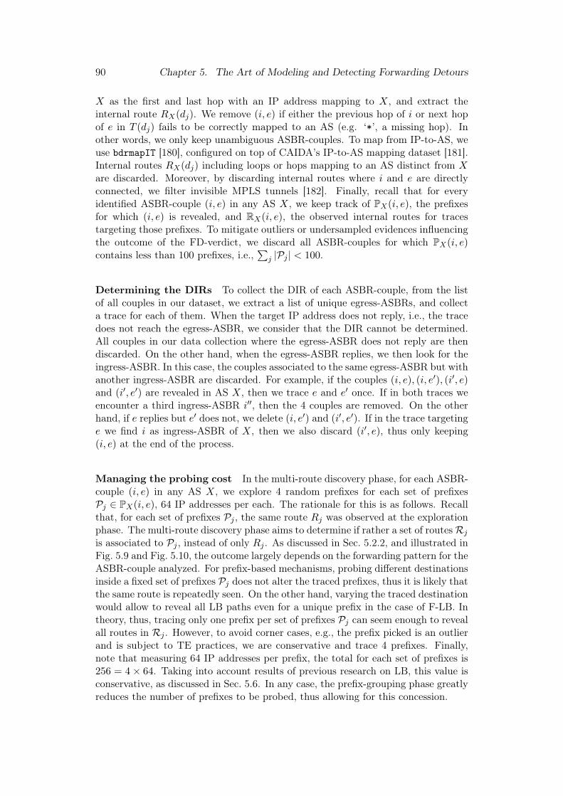
90 Chapter 5. The Art of Modeling and Detecting Forwarding Detours
X as the first and last hop with an IP address mapping to X, and extract theinternal route RX(dj). We remove (i, e) if either the previous hop of i or next hopof e in T (dj) fails to be correctly mapped to an AS (e.g. ‘*’, a missing hop). Inother words, we only keep unambiguous ASBR-couples. To map from IP-to-AS, weuse bdrmapIT [180], configured on top of CAIDA’s IP-to-AS mapping dataset [181].Internal routes RX(dj) including loops or hops mapping to an AS distinct from Xare discarded. Moreover, by discarding internal routes where i and e are directlyconnected, we filter invisible MPLS tunnels [182]. Finally, recall that for everyidentified ASBR-couple (i, e) in any AS X, we keep track of PX(i, e), the prefixesfor which (i, e) is revealed, and RX(i, e), the observed internal routes for tracestargeting those prefixes. To mitigate outliers or undersampled evidences influencingthe outcome of the FD-verdict, we discard all ASBR-couples for which PX(i, e)contains less than 100 prefixes, i.e.,
∑j |Pj | < 100.
Determining the DIRs To collect the DIR of each ASBR-couple, from the listof all couples in our dataset, we extract a list of unique egress-ASBRs, and collecta trace for each of them. When the target IP address does not reply, i.e., the tracedoes not reach the egress-ASBR, we consider that the DIR cannot be determined.All couples in our data collection where the egress-ASBR does not reply are thendiscarded. On the other hand, when the egress-ASBR replies, we then look for theingress-ASBR. In this case, the couples associated to the same egress-ASBR but withanother ingress-ASBR are discarded. For example, if the couples (i, e), (i, e′), (i′, e)and (i′, e′) are revealed in AS X, then we trace e and e′ once. If in both traces weencounter a third ingress-ASBR i′′, then the 4 couples are removed. On the otherhand, if e replies but e′ does not, we delete (i, e′) and (i′, e′). If in the trace targetinge we find i as ingress-ASBR of X, then we also discard (i′, e), thus only keeping(i, e) at the end of the process.
Managing the probing cost In the multi-route discovery phase, for each ASBR-couple (i, e) in any AS X, we explore 4 random prefixes for each set of prefixesPj ∈ PX(i, e), 64 IP addresses per each. The rationale for this is as follows. Recallthat, for each set of prefixes Pj , the same route Rj was observed at the explorationphase. The multi-route discovery phase aims to determine if rather a set of routesRj
is associated to Pj , instead of only Rj . As discussed in Sec. 5.2.2, and illustrated inFig. 5.9 and Fig. 5.10, the outcome largely depends on the forwarding pattern for theASBR-couple analyzed. For prefix-based mechanisms, probing different destinationsinside a fixed set of prefixes Pj does not alter the traced prefixes, thus it is likely thatthe same route is repeatedly seen. On the other hand, varying the traced destinationwould allow to reveal all LB paths even for a unique prefix in the case of F-LB. Intheory, thus, tracing only one prefix per set of prefixes Pj can seem enough to revealall routes in Rj . However, to avoid corner cases, e.g., the prefix picked is an outlierand is subject to TE practices, we are conservative and trace 4 prefixes. Finally,note that measuring 64 IP addresses per prefix, the total for each set of prefixes is256 = 4× 64. Taking into account results of previous research on LB, this value isconservative, as discussed in Sec. 5.6. In any case, the prefix-grouping phase greatlyreduces the number of prefixes to be probed, thus allowing for this concession.

5.5. Capturing forwarding detours in the wild 91
Dealing with missing hops The internal routes collected may include missinghops, that appear as “*”. When comparing whether two sets of routes Rj ,Rk ∈RX(i, e) intersect or not in the merging phase, we consider all missing hops aswildcards that may be matched to any IP address, but never replace them. Since theFD-verdict declares that a couple (i, e) is subject to FDs when the set containing theDIR is associated to less than t(Z,PX(i, e)) prefixes, then treating missing hops aswildcards relaxes the condition allowing to merge sets, and thus increases the chancesof not finding a lonely DIR. Consequently, this results into a stricter condition todeclare FDs, i.e., this is the most conservative approach to deal with missing hops:we may introduce false negatives, but no false positives.
5.5 Capturing forwarding detours in the wild
In this section we discuss the results we obtained running our FD-detector in thewild. First, Sec. 5.5.1 shows results concerning the underlying probing campaignswe performed. We detect FDs in 25 ASes out of 54, across 168 ASBR-couplesand 65 ingress-ASBRs. Then, in Sec. 5.5.2 we explore the forwarding patternswe found for each ASBR-couple. We discover a binary effect around FDs, i.e.,either all the observed transit traffic traversing a couple detours, or nonedoes. Then, in Sec. 5.5.3, we quantify the amount of extreme-FDs we captureper AS and per ASBR-couple. Our results depict the heterogeneity of the FD-phenomenon: from ASes with none or very few couples subject to FDs, to otherswhere thousands of prefixes, across multiple couples suffer from forwarding detours.Moreover, in Sec. 5.5.4, we investigate the relationship between ingress-ASBRs andFDs. A priori, we do not observe a clear correlation between the ingress-ASBRthrough which traffic enters any AS and the occurrence of FDs. Finally, we makean attempt to infer the most likely root cause generating the FDs we collect inSec. 5.5.5, i.e., with the observed binary characteristics, and present the efforts weinvested in validating our results in Sec. 5.5.6.
5.5.1 Measurement campaigns and coverage
We run measurements from 100 NLNOG RING’s VPs, however, we experiencedtechnical issues in 8 of them that did not allow us to complete the measurementsrequired by the FD-detector. In the following, the results refer to the 92 VPs wherewe could complete the analysis.
In the exploration phase, out of the 100K traces we run, we extracted on average3 internal routes per trace distributed across 7500 ASes. From those internal routeswith unambiguous borders, we see that we traverse from 1405 up to 2205 distinctingress-ASBRs (except one VP where the value raises up to 2335), between 5662and 8758 unique egress-ASBRs, and from 6475 to 11590 different ASBR-couples.However, our results indicate that most couples are not commonly encountered: atleast 50% appear only once, and 96% are traversed at most for 30 traces. Hence,while the requirement of finding 100 prefixes per couple has a limited effect on thefinal dataset we analyze, it allows us to be conservative, avoiding to introduce falsepositives/negatives (see Sec.5.4.2). On the other hand, when tracing the egress-ASBRs to collect DIRs, we had a success rate usually between 50% and 60%.

92 Chapter 5. The Art of Modeling and Detecting Forwarding Detours
1234
ASBR
-cou
ples
1e3
0 10 20 30 40 50 60 70 80 90Number of VPs
1020304050
ASes
Figure 5.12: Marginal utility of adding NLNOG RING’s VPs in terms of distinctASBR-couples (top) and unique ASes (bottom). For more than 70 VPs, the gain innegligible.
Our FD-detector was able to analyze 3963 ASBR-couples spanning 54 ASes.Fig. 5.12 reports the marginal utility of extending the set of NLNOG RING’s VPsin terms of couples covered and traversed ASes. Initially, the tendency shows almosta linear increase with the number of VPs. However, the decreasing slope of the curveand the plateau on the right side of the figure suggest that the gain after 70 VPs isnegligible. Indeed, beyond that point, we are able to investigate only 138 additionalcouples. In the end, we find extreme-FDs in 25 ASes, across 168 ASBR-couples and65 ingress-ASBRs.
5.5.2 Fowarding patterns and the binary effect of FDs
We are interested in determining the forwarding patterns we found for the ASBR-couples in our dataset. In this sense, Fig. 5.13 reports the CDF of the number ofsets composing PX(i, e) across couples before and after the merging phase (blue andred curve, respectively). Notably, while multiple sets of routes are visible in half ofthe couples we explore (blue distribution), less than 5% of them are not eventuallymerged in the final partition (red distribution). In more detail, observing the bluecurve, we see that r = 1 in 50% of the cases. These are ASBR-couples for which nomulti-path routing pattern was observed. In these cases, we conservatively concludethat these couples are not subject to FDs only running the exploration phase. Forthe remaining 50% of couples, the other phases are enforced since r > 1. At theend of the process, we observe that s = 1 for 96% of the couples. The differencein the value between s = 1 and r = 1 is 46% of the total, and are the cases wherewe discovered the forwarding pattern of F-LB. In other words, for most ASBR-couples e.g. (i, e), the multi-route phase enlarged the sets composing RX(i, e), andthen the merging phase was able to group them, since they had routes in common.This highlights the effectiveness of the multi-route discovery and merging phases.

5.5. Capturing forwarding detours in the wild 93
100 101 102
Sets composing X(i, e)
0.0
0.2
0.4
0.6
0.8
1.0
CDF
acro
ss A
SBR-
coup
les
s (after merging phase)r (before merging phase)
Figure 5.13: Cumulative number of sets composing PX(i, e) across ASBR-couplesbefore (r) and after (s) the merging phase. When r = 1, no multi-path routingpattern was observed. The difference with s = 1 relates to cases where we finda forwarding pattern that corresponds to that of per-dest/flow LB. Finally, whens ≥ 2 a prefix-based forwarding pattern is observed. In these cases, in general,s = 2, and they are FDs.
Moreover, recalling that we only measured 4 prefixes across the sets of PX(i, e), thisalso shows the potential of the prefix-grouping phase. Finally, for the remaining 4%of ASBR-couples, we find a prefix-based forwarding pattern where, except for a fewexceptions, s = 2.
From the cases where s = 2, we then extract the number of extreme-FDs.Fig. 5.14 shows the share of prefixes associated with the DIR for all ASBR-couples.Recall that the FD-verdict concludes that a couple (i, e) in AS X is subject toFDs when less than t(Z,PX(i, e)) prefixes are associated to the DIR DX(i, e) (seeSec. 5.4.1). The curve in Fig. 5.14 reveals a remarkable on/off pattern indicating thatall measured transit traffic that traverses any ASBR-couple either always detours,or never does. The right side of Fig. 5.14 relates to the ∼96% of the ASBR-couplesfor which s = 1 and all prefixes are forwarded along best IGP paths. On the otherhand, the ∼4% remaining in Fig. 5.14 are those ASBR-couples for which s = 2 inFig. 5.13. Since the rate of prefixes associated to the DIR is always 0%, then allthese couples are subject to FDs, i.e., the rate of prefixes subject to FDs is of 100%(except for the DIR, of course). In other words, no TIR follows the same path asthe one seen for the DIR. This shows that our FD-detector is not sensitive to anycalibration issue concerning the adaptive threshold t(Z,PX(i, e)) in the FD-verdict.In other words, there are no gray regions: when s = 2, no false negatives can occursince it always holds that 100% of the prefixes are not associated with the DIR, i.e.,lonely DIRs are always completely alone.
5.5.3 Distribution of FDs per AS and ASBR-couples
Fig. 5.15 shows the breakdown per AS of the 168 ASBR-couples subject to FDs,sorted by increasing relative fraction across ASes. We observe no general trend,indicating that the prevalence of FDs is AS-specific, e.g. depending on both router’s
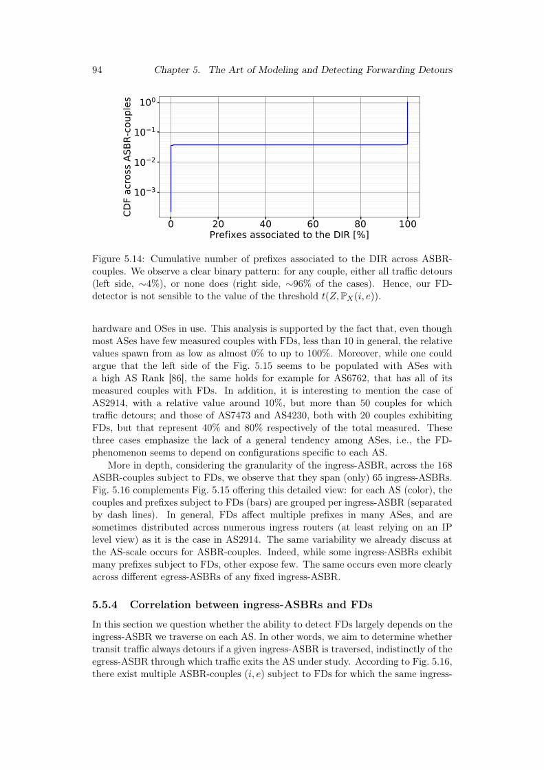
94 Chapter 5. The Art of Modeling and Detecting Forwarding Detours
0 20 40 60 80 100Prefixes associated to the DIR [%]
10 3
10 2
10 1
100
CDF
acro
ss A
SBR-
coup
les
Figure 5.14: Cumulative number of prefixes associated to the DIR across ASBR-couples. We observe a clear binary pattern: for any couple, either all traffic detours(left side, ∼4%), or none does (right side, ∼96% of the cases). Hence, our FD-detector is not sensible to the value of the threshold t(Z,PX(i, e)).
hardware and OSes in use. This analysis is supported by the fact that, even thoughmost ASes have few measured couples with FDs, less than 10 in general, the relativevalues spawn from as low as almost 0% to up to 100%. Moreover, while one couldargue that the left side of the Fig. 5.15 seems to be populated with ASes witha high AS Rank [86], the same holds for example for AS6762, that has all of itsmeasured couples with FDs. In addition, it is interesting to mention the case ofAS2914, with a relative value around 10%, but more than 50 couples for whichtraffic detours; and those of AS7473 and AS4230, both with 20 couples exhibitingFDs, but that represent 40% and 80% respectively of the total measured. Thesethree cases emphasize the lack of a general tendency among ASes, i.e., the FD-phenomenon seems to depend on configurations specific to each AS.
More in depth, considering the granularity of the ingress-ASBR, across the 168ASBR-couples subject to FDs, we observe that they span (only) 65 ingress-ASBRs.Fig. 5.16 complements Fig. 5.15 offering this detailed view: for each AS (color), thecouples and prefixes subject to FDs (bars) are grouped per ingress-ASBR (separatedby dash lines). In general, FDs affect multiple prefixes in many ASes, and aresometimes distributed across numerous ingress routers (at least relying on an IPlevel view) as it is the case in AS2914. The same variability we already discuss atthe AS-scale occurs for ASBR-couples. Indeed, while some ingress-ASBRs exhibitmany prefixes subject to FDs, other expose few. The same occurs even more clearlyacross different egress-ASBRs of any fixed ingress-ASBR.
5.5.4 Correlation between ingress-ASBRs and FDs
In this section we question whether the ability to detect FDs largely depends on theingress-ASBR we traverse on each AS. In other words, we aim to determine whethertransit traffic always detours if a given ingress-ASBR is traversed, indistinctly of theegress-ASBR through which traffic exits the AS under study. According to Fig. 5.16,there exist multiple ASBR-couples (i, e) subject to FDs for which the same ingress-

5.5. Capturing forwarding detours in the wild 95
1299
6939 17
464
6164
5329
1446
3720
965
4826
3491
1273
1295
611
537
5845
337
41 286
2516
7473
1916
2603
4230
1743
967
6224
785
2413
0
AS number
0
20
40
60
80
100
Frac
tion
of A
SBR-
coup
les
subj
ect t
o FD
s [%
]
0
10
20
30
40
50
ASBR
-cou
ples
subj
ect t
o FD
s
Figure 5.15: Quantification of ASBR-couples subject to FDs per AS. While mostASes have less than 10 couples subject to FDs (blue dots), the fraction they representout of the total in their AS (red bars) largely varies. This indicates that the problemof FDs is AS-dependent.
ASBR-couples grouped by the same ingress-ASBR102
103
104
Pref
ixes
subj
ect t
o FD
s AS4230AS2914
AS7473AS1916
AS3741AS17439
AS24130AS4637
AS24785AS1273
AS58453AS12956
AS11537AS2603
AS286AS174
AS6453AS4826
AS6939AS6762
AS2516AS3491
AS6461AS1299
AS20965
Figure 5.16: Number of prefixes subject to FDs per ASBR-couple. The bars areseparated by dashed lines to emphasize a distinct ingress-ASBRs. The number ofingress-ASBRs, ASBR-couples and prefixes subject to FDs strongly depends on theAS studied.

96 Chapter 5. The Art of Modeling and Detecting Forwarding Detours
0 10 20 30 40 50 60Ingress-ASBR subject to FDs
0
20
40
60
80
100Fr
actio
n of
Egr
ess-
ASBR
ssu
bjec
t to
FDs [
%]
100
101
102
Egre
ss-A
SBRs
Figure 5.17: Fraction of egress-ASBRs that are subject to extreme-FDs (red bars)out of the total (blue dots) for each ingress-ASBR. The tendency shows that the moreegress-ASBRs per ingress-ASBR, the less the fraction subject to FDs. However,for 17 ingress-ASBRs we cannot conclude anything since they only appear in oneASBR-couple.
ASBR i appears associated to different egress-ASBRs. e.g. e and e′. However, thisdoes not imply that there does not exist another distinct egress-ASBR e′′ for whichthe couple (i, e′′) is not subject to FDs. To clarify this aspect, Fig. 5.17 shows thefraction of egress-ASBRs subject to FDs associated to each ingress-ASBR, e.g. thecase comprising i, e, e′ and e′′ would result into a red bar of height 66, 6%, and ablue dot indicating the value of 3. We see a tendency that indicates that, the moreegress-ASBRs that we find for an ingess-ASBR, the fraction subject to FDs is less.However, there are still cases where we observe that an ingress-ASBR is associatedto multiple (2 or 3) egress-ASBRs, and we always find FDs. In addition, there are17/65 ingress-ASBRs for which we cannot derive any conclusion since they are onlyseen in a unique ASBR-couple. Hence, for the moment, we can only conservativelystate that a relationship between FDs and ingress-ASBRs is not clear, and wouldlike to better study this in future work.
5.5.5 Speculating on the root causes generating FDs
Based on previous results, this section elaborates an explanation of what may havegenerated the FDs we observed. Despite risky since the root causes behind for-warding detours may be multiple (see Sec. 1.3), we argue this is valuable since thepatterns observed seem clear cut. Indeed, even if the core contribution of this workis our methodology to detect FDs, the binary effect we found (Fig. 5.14) makes usbelieve that we are also able to pinpoint the most likely reason behind the FDswe collected. In short, the FDs we detect seem to result from scenarios involvingpartial-FIB routers, i.e., where routers keep IGP prefixes but delete a large fraction(if not all) of BGP prefixes from the FIB. Note that this is emphasized by the binaryeffect, that is even more severe that what we previously labeled as extreme-FDs.

5.5. Capturing forwarding detours in the wild 97
A partial-FIB router x with no BGP prefixes installed and relying on a defaultroute, systematically sends traffic towards a default gateway y. A priori, if y con-siders itself the best exit point of the AS for all BGP prefixes then, no FDs occur.However, depending on the best covering prefix of the destination IP address of thepackets being forwarded, y may likely redirect transit traffic towards another ASBRz. This is similar to what happens with prefixes PR and PB in the example shown inFig. 5.1 for x = ASBR1, y = ASBR2 and z = ASBR3, where traffic for PB detours,but that of PR does not. More generally, in all cases where the best IGP path fromx to z does not go through y, FDs occur.
The proportion of red in each bar of Fig. 5.17 could then be considered a measureof how bad it was to choose y as default gateway for x. In particular, the casesof complete red bars are of interest, since in them y never chooses itself as exitpoint of the AS, and all traffic detours. This could be the case, for example, ify was not an ASBR, but rather a core router. On the other hand, the shortestred bars also represent an interesting case of study that may result from multiplecauses. A trivial explanation could be that the default gateway was well chosen.However, other causes, more complex, are possible. For example, it could happenthat traffic exited the AS before reaching the gateway, hence avoiding FDs for theseegress-ASBRs. Another plausible explanation could be that the ingress-ASBR i wasactually not the partial-FIB router, but rather a core router x on which i relies. Insuch a scenario, only those prefixes for which traffic ingresses via i, and then x istraversed, will lead to few ASBR-couples subject to FDs.
We believe that these last examples highlight well the difficulty in finely validat-ing the root causes generating FDs, which besides being many, may be distributedacross the AS. This is also emphasized by the heterogeneous patterns found in theresults of Fig. 5.15, 5.16 and 5.17, which imply that ASes may employ multiplepartial-FIB routers located at different positions in the network and resulting inmany ASBR-couples identified as subject to FDs for varying number of prefixes.
5.5.6 Validation: emulations and ground truth
Relying on GNS3, we reproduce by emulation all the forwarding patterns we describein this paper, specially that of per-prefix LB. To mimic FDs, we rely on a staticdefault route having a higher priority than other FIB entries. In addition, we runour FD-detector on each LB flavor independently or combined with FDs and TE tocorroborate its potential and correctness on all the scenarios discussed in our work.
In addition, we corroborated the performance of our tool from a VP where we hadpreviously discovered the presence of a partial-FIB router. The example of Fig. 5.1accurately describes the network hosting such router. While for some prefixes therouter was generating BGP lies [3], i.e., traceroute AS-level forwarding routes todiffer from BGP paths, for others it was introducing FDs. Our tool was able todetect these FDs, probing its usefulness in a real life experiment.
Finally, at this stage, we cannot fully validate the origin of FDs for all cases.Despite this, we claim that similarly to LB tools tested on controlled environmentssuch as GNS3, our FD-detector has proven to be valid. In any case, we believe ouranalysis opens a door to develop a better understanding of the FD-phenomenon,that may be deepened in future research.

98 Chapter 5. The Art of Modeling and Detecting Forwarding Detours
Fine grained Load Balancing Coarse grained Load Balancing
F-LB
C-LB
C-LB
F-LB
F-LB
Coarse-Fine Load Balancing Fine-Coarse Load Balancing
F-LB
C-LB
C-LB
Figure 5.18: Complex LB flavors. In particular, coarse-fine LB implies that C-LB isfollowed by F-LB. This LB flavor generalizes C-LB: a set of prefixes is now associatedto more than one route, and these routes are reserved only for those prefixes. Aswith C-LB, for CF-LB it would hold that s > 1. On the other hand, fine-coarse LBresults from applying F-LB upstream of C-LB. Different to F-LB, with FC-LB notall routes are used for all prefixes. However, this LB flavor preserves the property ofF-LB where routes are not reserved for a unique specific set of prefixes, but ratherthey may be used for different ones. As a consequence, the merging phase wouldlikely output s = 1 for FC-LB.
5.6 Discussion: robustness of the FD-detector
In this section we analyze how our FD-detector performs face to complex forwardingpatterns in Sec. 5.6.1, explain why routing changes and IP-to-AS mapping errors donot induce the results we obtained in Sec. 5.6.2 and 5.6.3, illustrate why the probingcost of the multi-route discovery phase was sufficient in Sec. 5.6.4 and discuss whyour analysis does not require alias resolution techniques in Sec. 5.6.5.
5.6.1 An FD-verdict handling all interactions of FDs and LB
The LB types studied in Chapter 2, Sec 2.2.2, and Chapter 5, Sec. 5.2.2, F-LB andC-LB, may be mixed to produce hybrid LB flavors. For example, in the bottompanels of Fig. 5.18 we consider configurations where for a given gateway e, a loadbalancer i has n next-hops that are also load balancers with m possible next-hops.The top panels show the basic LB flavors we analyzed before, i.e. F-LB and C-LB, to emphasize how the hybrid LB flavors generalize them. As we detail next,our FD-detector is not affected by the hybrid LB flavors since the merging phasewould output a value of s equal to the one obtained with the simpler LB flavors

5.6. Discussion: robustness of the FD-detector 99
they generalize.When C-LB is applied upstream of F-LB, this combination results in a gener-
alization of C-LB, that we name coarse-fine grained LB (CF-LB). For tracesconcerning a fixed set of prefixes Pj , instead of a unique route Rj , a set of m routesRj are repeatedly revealed. In fact, the routes in Rj are only used to forward trafficconcerning the prefixes in Pj . Similar to C-LB, for CF-LB the property s > 1 stillholds (in particular it would be s = n). This is shown on the bottom-left topology ofFig. 5.18, where s = 2 and the two top routes and bottoms one are used for P1 andP2, respectively. On the other hand, when load balancers are applied in the reverseorder, that is, with F-LB followed by C-LB, we call the resulting LB flavor fine-coarse grained LB (FC-LB). With FC-LB each prefix is not anymore forwardedthorough all routes of RLB
X (i, e) as with F-LB. Indeed, in these cases, tracing a setof prefixes Pj , the same set of routes Rj is consistently found. It can be shown thateach set Rj contains n routes, and that there are mn sets such that, different toC-LB and CF-LB, ∀j, k,Rj ∩Rk 6= ∅. These intersections usually contain multipleroutes, and thus the merging phase would likely output the same as for F-LB, i.e.,s = 1. The effect of FC-LB is shown in the bottom-right topology of Fig. 5.18where we see that multiple routes are used to forward traffic concerning P1 and P2
respectively, some in common and others not.Finally, note that detouring traffic may traverse load balancers, thus FDs may
be subject to LB. In particular, if either F-LB or FC-LB was used, then no majorchanges would occur since the FD-detector would be able to group the detouringroutes into a unique set of routes during the merging phase. On the other hand, ifeither C-LB or CF-LB was applied, then the prefixes subject to FDs would be evenlydistributed across multiple non-overlapping routes or sets of routes, respectively.Hence, our FD-detector would not be able to merge these load balanced FDs intoa unique set of routes. A priori, this would generate that the extreme-FDs patternwould not be clear, since traffic would distribute across different sets of routes.However, we actually designed the FD-verdict to take this case into account: ratherthan searching for a set that presumably is the one resulting from FDs (that whenC-LB or CF-LB are applied would not be easy to spot), we look at the one containingthe DIR, that is associated to LB. When extreme-FDs occur, a lonely DIR is found,indistinctly of whether the FDs are load balanced or not, and thus we are still ableto detect FDs.
5.6.2 A binary effect that unlikely results from routing changes
To avoid issues related to routing events, since our study is performed at the scale ofASBR-couples (i, e), we only require the routing to remain stable within the studiedAS (while we are measuring each couple). Even if routing changes occured insidethe AS, since we always request to find i and e on the paths, such changes wouldaffect the collection of routes only if they occurred on links or routers in the pathsbetween i and e. Overall, our measurement campaign lasts less than one day; thisperiod, being lower than typical topology discovery campaigns, seems short enoughto limit the impact of IGP routing changes. In addtition, we collect again the DIRduring the multi-route discovery phase. Hence, we consider it is very unlikely thatIGP routing changes may have generated the binary effect wee detected. Indeed,
100 Chapter 5. The Art of Modeling and Detecting Forwarding Detours
for this to happen, it would mean that only the DIR got affected, but not the otherinternal routes that were collected at the same time.
5.6.3 On the (in)sensibility of flawed ASBR detection
While we expect the IP-to-AS mapping tool in use to be accurate, here we discusswhy our analysis should not be significantly impacted even if bdrmap-it [180] failedto work properly. We will assume that (i, e) is the real ASBR-couple, and (i′, e′) arethe borders identified in the mapping process. First, even though our FD-detectorspecifically checks whether FDs occur between ASBR-couples , our methodologyremains valid for any two IP addresses belonging to the same studied AS. Henceif i′ and e′ are actually core routers in the same AS as i and e, we may only losethe opportunity to detect some FDs. Indeed, this happens because we overlook thesubpaths between i and i′, and e and e′. On the other hand, when e′ actually belongsto a peering AS, as long as the prefix used in the point-to-point link between e and e′
is redistributed within the IGP of the targeted AS, our methodology remains valid.This holds because the DIR towards e′ still represents a valid IGP route associatedwith LB, thus we can continue to use it in the FD-verdict. Finally, when i′ belongsto a peering AS, this could potentially generate more problems since i′ may forwardtraffic to ingress-ASBRs in the studied AS other than i. While we argue that this isnot a common practice, we acknowledge that this could be perceived as a limitation.However, in these cases in particular and for all mapping errors in general, we expectthe FD-verdict to strongly mitigate their impact: finding a lonely DIR still impliesa case likely resulting from FDs.
5.6.4 Measurement stopping points
The MDA uses adaptive measurement stopping points (see Sec. 2.3.3) while welaunch a static number of traces per prefix (i.e., 64). The MDA works on a hop-by-hop fashion: as measurements are being carried, it adaptively updates its probingstopping points according to the probability of achieving the full discovery of allroutes. In our case, to ease the management of vantage points, we opted to feed allnodes with a fixed set of destinations to probe. This not only grants predictabil-ity of the full probing cost of the campaign and so its duration, but also allowsmeasurements to run faster than with the MDA, similar to the stateless fashionof Diamond-Miner [61]. Note that the number of traces we consider per group ofprefixes (4× 64) largely exceeds 11 and 96, the number of traces required to reveal2 and 16 next-hops of a load balancer [56]. Indeed, 2 and 16 represent the largelymost common and the maximum number of next-hops usually found in practice,respectively [63, 58, 183]. As discussed in Sec. 5.5.2, the patterns we observe in ourresults highlight the effectiveness of the merging and multi-route discovery phases.
5.6.5 Alias Resolution: a nice, but dangerous additional feature
Similar to the LB studies presented in Sec. 1.3, our methodology performs its analysisat the IP-level. However, alias resolutions techniques (e.g. MIDAR [184]) wouldallow us to produce a router-level view of the problem. In particular, by identifyingIP addresses belonging to the same ASBR, we would be able to refine our analysis of

5.7. Conclusion 101
forwarding patterns. In other words, this would allow us to detect all paths endingat the same ASBR, for all IP addresses of the ASBR, and thus better quantify thenumber of prefixes subject to FDs. Despite this, alias resolution techniques areknown to be error prone and to require extensive probing. Consequently, we arecautious, and leave this feature for future work.
5.7 Conclusion
With routing tables beyond 800K routes, not all devices are able to handle suchload. In these circumstances, ASes may deploy offloading workarounds to cope withthese scalability issues, e.g. some BGP entries, if not the vast majority, may not bepushed in the FIB of some routers. However, such workarounds increase the riskof introducing FDs inside these networks, thus losing the IGP optimality. Besidesthe use of partial-FIB routers and default routes, other reasons like bugs or prefixaggregation can also lead to the same phenomenon. At the same time, ASes usuallyrely on ECMP load balancers and TE to increase and control the distribution oftraffic in their network, respectively. With FDs, LB and TE, multi-path routingpatterns emerge. While exposing such multi-path routing patterns only requiresextensive probing, determining the underlying cause generating them is challenging.
In this chapter, first we model how RIes and FAs produce FDs, and then proposea method to detect FDs within an AS. More precisely, we show that studying theforwarding pattern between ASBRs of an AS, it is possible to discriminate LB andTE from FDs in the cases when multiple prefixes are subject to FDs. To the bestof our knowledge, we are the first to tackle this problem. We build an FD-detectorand, using large-scale measurement campaigns, we show that almost half of the ASesin our dataset suffer from FDs. Our results indicate that FDs are usually visiblefrom few ingress points of ASes, and can be revealed depending on the particularegress point that is observed. In addition, our analysis provides a notable takeaway:FDs look to be more extreme than we what we imagined, i.e., we systematicallyobserve a binary effect such that, between two ASBRs of an AS, either all prefixeswe measured were subject to FDs, or none were. Though beyond the scope of ourstudy, we argue that the root cause behind such FDs may be due to the use ofpartial-FIB routers. Finally, our study allows to refine previous work on topologydiscovery. Indeed, not only we consider an LB flavor omitted in the literature, i.e.per-prefix LB, but also propose a novel probing methodology that can be directlyplugged into LB discovery techniques to improve their probing cost.

102 Chapter 5. The Art of Modeling and Detecting Forwarding Detours

Chapter 6Conclusion and Research Directions
Contents6.1 Takeaways . . . . . . . . . . . . . . . . . . . . . . . . . . . . 1036.2 Future Work . . . . . . . . . . . . . . . . . . . . . . . . . . 105
6.2.1 BGP lies: more VPs, anomaly detection and malicious ASes1056.2.2 Forwarding detours: finding the forwarding alteration and
an FD-detector-lite . . . . . . . . . . . . . . . . . . . . . . 1076.2.3 Where BGP lies and FDs meet: a partial-FIB detector . . 1096.2.4 A better model of LB, a more efficient MDA . . . . . . . 110
In this section we conclude the thesis, highlighting our main scientific contribu-tions in Sec. 6.1 and pointing out future research directions in Sec. 6.2.
6.1 Takeaways
In this thesis, the objective is to detect hidden broken pieces of the Internet, i.e.,malfunctioning components, networks facing limitations and even selfish networksprioritizing their own revenue rather than the better performance of the Internet.
First, we investigate whether IXPs have been successful in Latin America, aregion that has previously received little attention in Internet studies. This studyhas four main contributions.
• We construct the most comprehensive available BGP dataset of Latin America.
• We find that Latin American states have been involved in the creation ofnational IXPs in several ways: legislation, regulation, sponsoring, funding,operations and serving traffic from/to IXPs. In many cases IXPs in LatAm,similar to others in Europe, are managed by non-profit organizations.
• We see that IXPs in developing regions such as Africa and Latin Americanot only have had a similar growth in the last years, but also seem to havereached maturity, i.e., have been able to attract as many local ASes as so dosome well-established IXPs in Europe. However, European IXPs are rather
103

104 Chapter 6. Conclusion and Research Directions
international hubs, meaning that they have also managed to gather membersfrom different regions. This internationalized market could be exploited in thefuture by the less renown, and rather local, IXPs in Latin America, Asia andAfrica.
• We notice that, in several Latin American countries, the existence of monop-olistic ASes, some state-owned, seem to have prevented the proliferation ofIXPs, and lead them to be failed IXPs, i.e., countries with no IXP at all, orwith IXPs that have not managed to attract a large number of members.
Second, we study whether BGP lies occur on the Internet, i.e., if packets flowon the Internet through AS-paths other than the ones advertised in BGP messages.In a nutshell, our contributions are:
• We explain different ways in which an AS may generate BGP lies, eitheraffecting the control paths that are advertised or the data path that packetsfollow. We show that detecting BGP lies is challenging since the detection oflies may be wrongly triggered by noise affecting the measurements, e.g. ASsiblings, third-party addresses and missing hops.
• We propose a modular framework allowing to detect highly-potential BGPlies. For this, we apply path-rewriting rules that filter the noise affectingthe comparison of control paths and data paths. Our framework is modular,allowing to implement multiple noise-filtering models, each of which tacklesdifferently the correction of errors interfering with the collected data.
• We run measurements from 8 vantage points and over time, a coverage neverachieved before for this kind of analysis. We find that, even relying on themost conservative noise-filtering model, some mismatches between control anddata paths remain, likely representing BGP lies. In the vantage points wherefew lies are found, the results are stable in time, otherwise we see that thenumber of discrepant paths per day have a larger variation.
Lastly we study forwarding detours, i.e., if traffic inside ASes eventually flowsthrough forwarding routes that divert or diverge from the expected best IGP paths.We make the following contributions:
• We investigate the root causes that produce forwarding detours, showing thatthey result from routing inconsistencies that generate forwarding alterations.However, not all routing inconsistencies and forwarding alterations generateforwarding detours.
• We explain why detecting forwarding detours is challenging: they generatemulti-path routing patterns similar to those introduced by load balancing andtraffic engineering techniques. Moreover, we take into account per-prefix LB,an LB flavor never previously studied in the literature, and propose a newtaxonomy differentiating between fine-grained and coarse-grained LB types,which vary the granularity at which flows are defined with respect to thedestination IP address of packets.

6.2. Future Work 105
• We design a methodology that, without requiring privileged knowledge fromthe networks being analyzed, e.g., knowing the IGP metric, is able to detectwhether forwarding detours occur inside them. Our methodology consists instudying the forwarding patterns inside ASes, i.e., the specific sets of forward-ing routes that are revealed for different prefixes when tracing multiple IPaddresses contained in each of them.
• We propose an FD-detector, to the best of our knowledge the first of its kind,tuned to detect extreme-FDs, i.e., FDs that affect numerous external prefixes.We validate the behavior of the FD-detector with emulations and on a networkwhere we have ground truth.
• We analyze the FD-phenomenon in the wild running our FD-detector from 100nodes of the NLNOG RING monitoring infrastructure, and find FDs in 25 outof 54 ASes. We find forwarding detours in multiple ASes, with a remarkablebinary pattern in which transit traffic traversing between two border routersof an AS either never detours, or always does.
All in all, the studies we carry on in this thesis expose that the Internet is not aninfallible system, and that its hidden broken pieces can be exposed by crafting refinedmethodologies as the ones we develop. To foster replicability and reproducibility, werelease the dataset we collected and the code we developed for each of the analysispresented in this thesis.
6.2 Future Work
In this section, we discuss research directions to continue the work in this thesisconcerning BGP lies in Sec. 6.2.1, forwarding detours in Sec. 6.2.2 and a combinationof both in Sec. 6.2.3. In addition, we present future work we envision in the field ofload balancing and topology discovery in Sec. 6.2.4.
6.2.1 BGP lies: more VPs, anomaly detection and malicious ASes
Recalling the analysis in Chapter 4, our results show that the number of mismatchesbetween control paths and data paths are usually stable, except in the cases wherethe plausible number of BGP lies is high. This leads us to the following question.
By continuously tracking the rate of BGP lies over time, can weturn our framework into an anomaly detector?
Research Question
We believe this is a plausible option for the mid-term. For this, first we wouldhave to identify VPs for which the number of observed discrepancies between controlpaths and data paths are stable. Notice that determining this does not require

106 Chapter 6. Conclusion and Research Directions
AS ACP: Z A B C DTP: Z A B C DDP: Z A X D
AS B AS C
AS D
AS X
Figure 6.1: BGP lies that are hid by the malicious behavior of AS A. In thisexample, A is able to discriminate probes issued by traceroute from regular traffic.As a consequence, A sends measuring probes thought B, i.e., the traceroute path(TP) matches the CP. In addition, A diverts regular traffic from the path advertisedin BGP, forwarding “regular” packets to X.
running our framework to filter noise, nor does it necessarily require finding co-located VPs, as long as the results are consistent over time. Finally, relying onmachine learning or deep learning techniques, we can build a system that keeps trackof the variation in time of the mismatch rate, and raise an alarm when anomalousevents occur.
In the long term we aim at shedding light on the root cause of the mismatchesbetween CPs and DPs, i.e. we will focus in the even more challenging task of detect-ing not only BGP lies, but also pinpointing their types and incentives. In that sense,a current limitation of the work in Chapter 4 is that we assume that BGP lies mayoccur at either the control or data plane, but we do not consider that an AS maybe malicious and simultaneously affect both CPs and DPs, forcing these paths tomatch only when measurements are being carried. In other words, the main problemis that our framework trusts traceroute blindly, and does not question whether thepath it reports may differ from the one that any other type of traffic might follow,as shown in Fig. 6.1. Indeed, traceroute may be handled differently from regulartraffic [22, 23]. For example, we tested configurations on routers and found that itis actually quite simple to enforce different routing policies based on the TTL valuein packets. Hence, a malicious AS may divert packets with a TTL above certainthreshold, and respect the paths for the ones below it, that are traceroute-like. Thisbrings us to a new research question.

6.2. Future Work 107
Can we extend our methodology to detect malicious ASes tryingto hide their lies?
Research Question
In this case, our task will be to play the role of detectives: the more questions(tests) are performed, the more chances the (malicious) liar may commit an error andthe BGP lies be exposed. In particular, for the moment we envision a complementarytest comparing the distribution of the RTT for packets with high and low TTLvalues, respectively. When the difference is high, we argue that this could representa lie, and trigger an alarm. Instead, when the values are similar, further analysiswould be required. For example, other options include re-running traceroute withdifferent transport protocols, or using the IP record route option.
6.2.2 Forwarding detours: finding the forwarding alteration andan FD-detector-lite
Our FD-detector of Chapter 5 detects FDs between ASBRs of an AS. Looking tocomplement the analysis, we propose the following research question.
Can we extend our FD-detector to also pinpoint the routers thatintroduce the RIes and FAs that generate the FDs we find?
Research Question
We argue that this can be achieved by generalizing the concept of the DIR.Rather than only targeting the egress-ASBR, we can target all interfaces seen inthe detouring paths. In the process of tracing the intermediate interfaces, fromthe egress-ASBR up to the ingress-ASBR, we expect that, eventually, there will bea DIR that will match a sub-path of the detouring route. This is the triggeringevent that allows us to identify the router that introduces the forwarding alterationthat leads to the FD. The complete procedure is illustrated in Fig. 6.2. First, theforwarding detour needs to be identified running the FD-detector of Chapter 5. Therevealed FD is shown in Fig. 6.2a. From o to l, each of the interfaces seen in thedetouring path are traced. The first step is to target m, as shown in Fig. 6.2b. Theviolet route that is revealed does not match the red sub-path extracted from theoriginal detouring route in Fig. 6.2a, hence the process continues. In the followingstep, displayed in Fig. 6.2c, p is traced. In this case, the red and violet pathsmatch. When this happens, the tracing stops and p is declared to be the router thatintroduces forwarding alterations.
Since there exists no previous study tackling the same problem of Chapter 5,our solution to detect FDs is as general as possible, considering almost all cornercases. Not only we address the difficulty of filtering per-prefix LB, but also we take

108 Chapter 6. Conclusion and Research Directions
Forwarding Detour
AS 𝑋
l 𝑚
𝑛
𝑝
𝑜
(a)
Step I - target 𝑚
AS 𝑋
l 𝑚
𝑛
𝑝
𝑜
(b)
Step II - target 𝑝
AS 𝑋
l 𝑚
𝑛
𝑝
𝑜
(c)
Figure 6.2: Methodology to detect the router that introduces the forwarding al-teration leading to a forwarding detour. The red arrows indicate sub-paths of thedetouring route, whereas the violet ones are the paths revealed running traceroutetowards intermediate interfaces found in the aforementioned path. Fig. 6.2a showsthe original detouring route found with the FD-detector of Chapter 5. In the firststep after detecting the FDs, shown in Fig. 6.2b, the violet path obtained targetingm and the red sub-path extracted from the path in Fig. 6.2a differ, and thus themeasuring process continues. Finally, when tracing p in Fig. 6.2c, the violet andred paths match. Consequently, p is identified as the router that introduces theforwarding alteration that leads to a forwarding detour between l and o.
into consideration how LB may interfere with FDs and design an adaptive thresholdto declare the occurrence of FDs. Our results, suggesting that all FDs are extreme-FDs, and that there exists a binary pattern where either all traffic detours or nonedoes suggest we could potentially envision a simpler FD-detector. This brings us tothe following question.
Can we leverage our better understanding of the FD-phenomenonto generate an FD-detector-lite, with a simpler design?
Research Question

6.2. Future Work 109
For this, first we would need to further characterize FDs, i.e., in future work weaim to study whether the RTT, the number of hops and the number of MPLS tunnelsobserved for detouring paths are greater than the ones for best IGP paths. Moreover,we want to study the number of paths related to the set of detouring routes andto the best IGP paths, respectively. We believe that leveraging this knowledge,we would be able to build an FD-detector-lite. This new detector, different fromthe one we present in this manuscript, could rely on assumptions based on thisFD-characterization.
6.2.3 Where BGP lies and FDs meet: a partial-FIB detector
No BGP Lies, No FDs
l 𝑚
𝑛𝑝
𝑜
𝑞
AS 𝑋
l 𝑚
𝑛
𝑞AS 𝑋
l 𝑚
𝑛
𝑜
𝑝
𝑞
BGP Lies and FDs
To AS 𝑌
To AS 𝑍
AS 𝑋
AS A AS X AS Y
AS Z
DPCP
AS A AS X AS Y
AS Z
Figure 6.3: Simultaneous BGP lies and forwarding detours. The top figure shows afull-FIB scenario. In this case, packets flow through best IGP paths inside AS X,in particular from l to o. Once o is reached, packets are forwarded towards AS Y ,the AS announced in CPs. Consequently, in this case no BGP lies nor FDs occur.On the other hand, the right side figure shows a new scenario where l has a partialFIB. As l uses p as default gateway, and p redirects traffic towards q, an FD occurs.Moreover, since q acts as egress-ASBR and sends packets to AS Z, besides the FD,a BGP lie also occurs. Indeed, instead of forwarding traffic to Y , X is pushing ittowards Z. This highlights the potential of combining the framework of Chapter 4and the FD-detector of Chapter 5.
The studies of Chapter 4 and 5 are closely related: besides the fact that both

110 Chapter 6. Conclusion and Research Directions
allow to detect different hidden broken pieces of the Internet, some of the root causesthat generate them may be the same. We previously saw that ASes with technicallimitations may use partial-FIB routers, but this may lead to BGP lies. In addition,scalability workarounds using partial-FIB routers with a default route may lead toFDs. Consequently, this brings us to the next question.
Can we combine the FD-detector and the noise-filtering frame-work to generate a partial-FIB detector?
Research Question
In general, even though a router may have a partial-FIB, it is likely that it isstill a full-RIB router. This happens because the memory routers use to maintainRIBs is not a constrained resource as is the one used for FIBs. As a consequence, interms of BGP data, a router usually has complete routing knowledge: it knows towhich ASBR packets should be sent for each prefix, and the AS-path that will becorrespondingly followed. Moreover, the router announces the related best paths toASBRs in neighbouring ASes. However, for those destinations that are not installedin the FIB, the router actually uses a default route pointing towards a defaultgateway. When the default gateway re-directs traffic towards an ASBR differentthan the iBGP next-hop the partial-FIB aimed to reach, it is likely that FDs occur.On the other hand, if the default gateway acts as egress-ASBR, it may introducea BGP lie if it pushes traffic to an AS other than the one appearing on the AS-path. Even more interestingly, when the default gateway pushes traffic to a thirdASBR both FDs and BGP lies may occur. The example of Fig. 6.3 illustrates thislatter case, and compares it with the case where no FDs nor BGP lies occur toemphasize the contrast. We would like to investigate the potential of combining themethodologies we derive in Chapter 4 and 5 to generate a partial-FIB detector infuture work.
6.2.4 A better model of LB, a more efficient MDA
The study we carry on in Chapter 5 allowed us to acquire a deep understandingof LB practices. Besides considering per-prefix LB, an LB flavor omitted in theliterature, we proposed a new taxonomy differentiating between coarse-grained andfine-grained LB types. We also modeled the function Nb(·) that load balancersof different LB flavors apply to choose next-hops. In future work, we would like tocontinue contributing to this field, looking to answer the following research questions.

6.2. Future Work 111
• Can we incorporate networking knowledge to the MDA,whose functioning rather relies only on a mathematicalmodel applicable to any generic problem?
• Can we plug the prefix-grouping phase of the FD-detectorinto the MDA to reduce the amount of probing?
• Can we use results extracted from previous LB surveys torecalculate the stopping points of the MDA?
Research Question
As a first step, a large set of studies concerning related work have suggestedthat load balancers apply different LB flavors for ICMP and UDP packets1, but wewould like to make a deep study of this phenomenon, not only to validate theseresults, but also to show the consequences in performance of such characteristic.An interesting point is that, if routers really mainly apply per-dest LB for ICMPpackets, the studies putting efforts and describing methodologies to fix the returnpath of probes are simply overkill and produce no real effect. Indeed, the returnpath would only depend on the source and destination IP addresses, and trying tofix the ICMP checksum would not produce any change. Therefore, we would liketo investigate the configuration of routers and check if there is actually a defaultoption in router’s software that triggers this particular behavior. In future work,we would like to study this effect in detail. The method for the moment is not welldefined, but we envision studying whether the RTT we obtain varies when targetingdifferent destination IP addresses while using different source IP addresses attachedto the same VP. In addition, we will contrast the obtained with ICMP and UDPprobes.
As a second step, complementing the modeling of function Nb(·), we plan onusing our forwarding model to shed light on how LB works, since fixing what I believeis a misconception in all the related work on LB I have presented in this manuscript,the probing cost of LB studies may be reduced. I argue that, in general, LB studiesadopt a mathematical perspective and wrongly assume that next-hops that loadbalancers use only depend on the destination IP address. Indeed, they miss thenetworking perspective, and therefore neglect the effect of the gateway that routersselect as the best one for each destination IP address. The conceptual difference iscritical: the current model adopted in LB and topology discovery studies implicitlyassumes that the Internet is flat, i.e., a unique network. However, the Internetis an interconnection of ASes, each of which may decide whether to apply LB ornot independently. In other words, end-to-end paths are a concatenation of theinternal routes that traverse each AS (plus the links between ASes). Therefore, LBor topology discovery studies should not be run on a per-destination basis, but ratherat the per-ASBR-couple scale. This does not mean that destination IP addresses
1This is clearly seen in the results in [63], which suggest that load balancers rather use per-destLB for ICMP. This result has been also suggested in previous studies, but no further analyzed.
112 Chapter 6. Conclusion and Research Directions
are not important: tracing them provides a means to reveal the ASBRs of each AS,and allows to seek for multi-path routing patterns across ASBR-couples (and linksbetween ASBRs of different ASes, assuming multi-path BGP eventually becomesmore popular). In addition, to be fair, running the MDA on a per-destinationbasis actually makes sense towards the end of paths. Indeed, at the edges, the lastAS-hops approach the destination IP address and are not repeatedly seen. Sincewhen comparing paths gathered for multiple destination IP addresses, the last hopsare usually disjoint, then exploring the ending hops of each trace, one by one, ismandatory. However, the idea that targeting different destination IP addresses mayhelp to continuously reveal new routes closer to where the VP is located seemsmisplaced, without hesitation. As an example, if the MDA is run towards 1000 IPaddresses, the network of the provider AS is measured an equal number of times,which largely seems unnecessary and a waste of probing if the same ASBR-couplesof the AS are repeatedly revealed and analyzed.
As a third step, we would like to build a new version of the MDA to reducethe probing cost, namely the Topology Feedback MDA, or TF-MDA in short. Byleveraging our understanding that LB applies based on gateways and not on desti-nation IP addresses, we would like to incorporate the exploration, prefix-groupingand multi-route discovery phases of our FD-detector (see Chapter 5) to the MDA.The name topology feedback results from the fact that we aim to split the measuringprocess that the standard MDA does at once, and blindly, in two. Indeed, recallthat the MDA analyzes one /24 prefix at a time, each independently. We proposeto analyze multiple prefixes concurrently, and to do it in two steps. The explorationand prefix-grouping phases are used to identify those prefixes for which traces tra-verse the same ASBR-couples of each AS. The topology knowledge extracted fromthese steps would be fed back to our algorithm. Taking advantage of the informationobtained in the previous step, the additional probing would be wisely crafted, e.g.,rather than measuring all prefixes as the MDA does, the TF-MDA could for exam-ple just pick one prefix per-ASBR couple. To achieve more robust results, we couldenvision measuring more prefixes, up to 4, as we do in the FD-detector. Beyondthe idea of picking one prefix per ASBR-couple, there is room to think of this asan optimization problem. The objective may be to study all ASBR-couples whileminimizing the associated cost or fixing the probing budget while maximizing thenumber of analyzed ASBR-couples.
Fourth, we plan on refining the stopping points that the MDA uses, and generatea Bayesian-MDA that reduces the required probing cost. The authors in [59] showwith their own results that the model they propose loosely bounds the probability offailing to discover all links when running the MDA. As a result, in practice, using theend-to-end path level version of the stopping points results in a waste of probing. AsI argued before in Sec. 2.3.3 of Chapter 2, this seems to be produced by an unrealistictuning of the parameter QI , the theoretical maximum number of interfaces expectedin a trace. Although the authors did not do it to defend their proposal, I am lookingforward to show in emulations or simulations that their model is actually correctdespite the inaccurate choice they make for the value of QI . The explanation tothe results they obtain is that most diamonds found on the Internet usually havea width of 16 at most, but the authors propose QI = 30. Hence, either emulatinga topology with load balancers with multiple next-hops or tuning QI differently

6.2. Future Work 113
would output different discovery success rates when changing the parameter β, thefailure probability of discovering all next-hops of all interfaces across the path beinganalyzed. In any case, besides this subtle issue, the more concerning problem isthat 13 years after the MDA was first proposed, the community has not yet beenable to generate any alternative version. Indeed, all the subsequent tools, suchas Diamond-Miner, MCA, MDA-lite, etc., still rely on the loosely defined stoppingpoints of the MDA. After such a long time of research, nowadays we have multi-pathrouting surveys with results that can, and should, be used to re-think the mechanicsof the MDA. In short, there is an opportunity similar to the one expressed whenproposing the TF-MDA: the MDA sins by not taking into consideration any feedbackfrom measurements or a priori knowledge. To produce an overcoming version ofthe MDA, we propose to use Bayesian inference, and to create a Bayesian-MDA.Rather than assuming that the number of next-hops that a load balancer may useare all equiprobable, we propose to study the empirical distribution obtained inthe available surveys. This knowdledge can be plugged into the MDA using Bayestheorem, and be used to guide the probing required, i.e., to generate a new formulato calculate stopping points. These new stopping points will have lower values thatthe one the MDA proposes, and allow to save probing cost.
Finally, we envision to combine TF-MDA and Bayesian-MDA, generating theUltimate-MDA, or U-MDA in short. The combination of both approaches, we be-lieve, would result in a significant saving of probing cost associated to multi-pathdiscovery campaigns, and allow to explore faster the topology of the Internet.

114 Chapter 6. Conclusion and Research Directions

Bibliography
[1] J. M. Del Fiore, V. Persico, P. Mérindol, C. Pelsser, and A. Pescapè. “The Artof Detecting Forwarding Detours”. In: IEEE Transactions on Network andService Management (2021), pp. 1–1. doi: 10.1109/TNSM.2021.3062151.
[2] Esteban Carisimo, Julián M. Del Fiore, Diego Dujovne, Cristel Pelsser, andJ. Ignacio Alvarez-Hamelin. “A First Look at the Latin American IXPs”. In:SIGCOMM Comput. Commun. Rev. 50.1 (Mar. 2020), 18–24. issn: 0146-4833. doi: 10.1145/3390251.3390255. url: https://doi.org/10.1145/3390251.3390255.
[3] J. M. Del Fiore, P. Merindol, V. Persico, C. Pelsser, and A. Pescapé. “Fil-tering the Noise to Reveal Inter-Domain Lies”. In: 2019 Network TrafficMeasurement and Analysis Conference (TMA). June 2019, pp. 17–24. doi:10.23919/TMA.2019.8784618.
[4] Amogh Dhamdhere and Constantine Dovrolis. “The Internet is flat: modelingthe transition from a transit hierarchy to a peering mesh”. In: CoNEXT 2010.2010, p. 21.
[5] Bernhard Ager, Nikolaos Chatzis, Anja Feldmann, Nadi Sarrar, Steve Uhlig,and Walter Willinger. “Anatomy of a large European IXP”. In: CCR 42.4(2012), pp. 163–174.
[6] Rodérick Fanou, Francisco Valera, and Amogh Dhamdhere. “Investigatingthe Causes of Congestion on the African IXP substrate”. In: IMC 2017. ACM.New York, NY, USA: ACM, 2017, pp. 57–63.
[7] Rodérick Fanou, Pierre Francois, and Emile Aben. “On the diversity of in-terdomain routing in africa”. In: PAM 2015. Springer. Cham: Springer Inter-national Publishing, 2015, pp. 41–54.
[8] Rodérick Fanou, Francisco Valera, Pierre Francois, and Amogh Dhamdhere.“Reshaping the African Internet: From scattered islands to a connected con-tinent”. In: Computer Communications 113 (2017), pp. 25–42.
[9] World Bank. World Development Indicators: Rural environment and landuse. http://wdi.worldbank.org/table/3.1. 2016.
[10] World Bank. The World Bank data: Urban population. https : / / data .worldbank.org/indicator/SP.URB.TOTL.IN.ZS?page=1. 2018.
115

116 BIBLIOGRAPHY
[11] UN. World Population Prospects 2017. https://population.un.org/wpp/Download/Standard/Population/. 2017.
[12] UN. The World’s Cities in 2016. https://bit.ly/36uMpaW. 2016.
[13] Raul Katz and Fernando Callorda. “Accelerating the development of LatinAmerican digital ecosystem and implications for broadband policy”. In: Telecom-munications Policy 42.9 (2018), pp. 661–681.
[14] Hernán Galperín. “Localizing Internet infrastructure: Cooperative peering inLatin America”. In: Telematics and Informatics 33.2 (2016), pp. 631–640.
[15] Anukool Lakhina, John W Byers, Mark Crovella, and Peng Xie. “Samplingbiases in IP topology measurements”. In: IEEE INFOCOM 2003. Vol. 1. 2003,pp. 332–341.
[16] Sofía Silva Berenguer, Esteban Carisimo, J Ignacio Alvarez-Hamelin, andFrancisco Valera Pintor. “Hidden internet topologies info: Truth or myth?”In: LANCOMM 2016. ACM. New York, NY, USA: ACM, 2016, pp. 4–6.
[17] S. H. B. Brito et al. “Dissecting the Largest National Ecosystem of PublicInternet eXchange Points in Brazil”. In: PAM 2016. Cham: Springer Interna-tional Publishing, 2016, pp. 333–345.
[18] S. H. B. Brito et al. “An Analysis of the Largest National Ecosystem of PublicInternet eXchange Points: The Case of Brazil”. In: Journal of Communicationand Information Systems 31.1 (2016).
[19] Lucas Müller, Matthew Luckie, Bradley Huffaker, Kc Claffy, and MarinhoBarcellos. “Challenges in inferring spoofed traffic at IXPs”. In: Proceedingsof the 15th International Conference on Emerging Networking ExperimentsAnd Technologies. 2019, pp. 96–109.
[20] Agustin Formoso and Pedro Casas. “Looking for network latency clusters inthe lac region”. In: LANCOMM 2016. ACM. New York, NY, USA: ACM,2016, pp. 10–12.
[21] S. Murphy. BGP Security Vulnerabilities Analysis. RFC 4272. Jan. ’06.
[22] Roland Meier, Petar Tsankov, Vincent Lenders, Laurent Vanbever, and Mar-tin Vechev. “NetHide: Secure and Practical Network Topology Obfuscation”.In: USENIX Security 2018.
[23] Samuel Trassare, Robert Beverly, and David Alderson. “A Technique forNetwork Topology Deception”. In: Proc of the MILCOM 2013.
[24] Zhuoqing Morley Mao, Jennifer Rexford, Jia Wang, and Randy H. Katz.“Towards an Accurate AS-level Traceroute Tool”. In: SIGCOMM 2003.
[25] Z. M. Mao, D. Johnson, J. Rexford, Jia Wang, and R. Katz. “Scalable andaccurate identification of AS-level forwarding paths”. In: IEEE INFOCOM2004.
[26] Y. Hyun, A. Broido, and k. claffy. Traceroute and BGP AS Path Incon-gruities. Tech. rep. CAIDA, Mar. 2003.
[27] Yu Zhang et al. “A Framework to Quantify the Pitfalls of Using Traceroutein AS-Level Topology Measurement”. In: IEEE JSAC 2011 ().

BIBLIOGRAPHY 117
[28] Y. Hyun, A. Broido, and k. claffy. “On Third-party Addresses in TraceroutePaths”. In: PAM 2013.
[29] Pietro Marchetta, Walter de Donato, and Antonio Pescapè. “Detecting Third-Party Addresses in Traceroute Traces with IP Timestamp Option”. In: PAM2013.
[30] Matthew Luckie and kc claffy. “A Second Look at Detecting Third-PartyAddresses in Traceroute Traces with the IP Timestamp Option”. In: PAM2014.
[31] N. Ahmed and K. Sarac. “An experimental study on inter-domain routingdynamics using IP-level path traces”. In: IEEE 40th Conference on LocalComputer Networks (LCN) 2015.
[32] M. Luckie, A. Dhamdhere, B. Huffaker, D. Clark, and k. claffy. “bdrmap:Inference of Borders Between IP Networks”. In: IMC 2016.
[33] Alexander Marder and Jonathan M. Smith. “MAP-IT: Multipass AccuratePassive Inferences from Traceroute”. In: IMC 2016.
[34] Alexander Marder, Matthew Luckie, Amogh Dhamdhere, Bradley Huffaker,kc claffy, and Jonathan M. Smith. “Pushing the Boundaries with bdrmapIT:Mapping Router Ownership at Internet Scale”. In: IMC 2018.
[35] Ahmed Elmokashfi and Amogh Dhamdhere. “Revisiting BGP churn growth”.In: ACM SIGCOMM Computer Communication Review 44.1 (2013), pp. 5–12.
[36] BGP in 2018 — BGP Churn. https://blog.apnic.net/2019/01/22/bgp-in-2018-bgp-churn/.
[37] David Hauweele, Bruno Quoitin, Cristel Pelsser, and Randy Bush. “What doparrots and BGP routers have in common?” In: ACM SIGCOMM ComputerCommunication Review 46.3 (2018), p. 2.
[38] Xiaoliang Zhao, Dante J Pacella, and Jason Schiller. “Routing scalability:an operator’s view”. In: IEEE Journal on Selected Areas in communications28.8 (2010), pp. 1262–1270.
[39] What caused today’s Internet hiccup. https://www.bgpmon.net/what-caused-todays-internet-hiccup/.
[40] Internet Touches Half Million Routes: Outages Possible Next Week. https://dyn.com/blog/internet-512k-global-routes/.
[41] 768k Day. Will it Happen? Did it Happen? https : / / labs . ripe . net /Members/emileaben/768k-day-will-it-happen-did-it-happen.
[42] Florin Coras, Damien Saucez, Loránd Jakab, Albert Cabellos-Aparicio, andJordi Domingo-Pascual. “Implementing a BGP-free ISP core with LISP”. In:2012.
[43] Stefano Vissicchio, Luca Cittadini, and Giuseppe Di Battista. “On iBGProuting policies”. In: IEEE/ACM Transactions on Networking 23.1 (2014),pp. 227–240.

118 BIBLIOGRAPHY
[44] Stefano Vissicchio, Luca Cittadini, Laurent Vanbever, and Olivier Bonaven-ture. “iBGP deceptions: More sessions, fewer routes”. In: Mar. 2012, pp. 2122–2130. doi: 10.1109/INFCOM.2012.6195595.
[45] Joao Luis Sobrinho, Laurent Vanbever, Franck Le, Andre Sousa, and JenniferRexford. “Scaling the Internet Routing System Through Distributed RouteAggregation”. In: IEEE/ACM Trans. Netw. 24.6 (Dec. 2016), pp. 3462–3476.issn: 1063-6692.
[46] Hitesh Ballani, Paul Francis, Tuan Cao, and Jia Wang. “Making RoutersLast Longer with ViAggre”. In: ACM NSDI 2009. Boston, MA, USA, Apr.2009.
[47] Slimming down the Internet routing table by Tore Anderson. url: https://www.redpill-linpro.com/sysadvent/2016/12/09/slimming-routing-table.html.
[48] Romain Fontugne et al. “BGP zombies: An analysis of beacons stuck routes”.In: International Conference on Passive and Active Network Measurement.Springer. 2019, pp. 197–209.
[49] Tian Bu, Lixin Gao, and Donald F Towsley. “On characterizing BGP routingtable growth.” In: Computer Networks () (2004).
[50] E. Elena, J. L. Rougier, and S. Secci. “Characterisation of AS-level pathdeviations and multipath in Internet routing”. In: 6th EURO-NGI Conferenceon Next Generation Internet. 2010.
[51] Stefano Secci, Jean-Louis Rougier, Achille Pattavina, Mauro Marinoni, GuidoMaier, and Estrellita M T Elena. “Detection of BGP route deflections acrosstop-tier interconnections”. In: 2009.
[52] Sharad Agarwal, Chen-Nee Chuah, Supratik Bhattacharyya, and ChristopheDiot. “The impact of BGP dynamics on intra-domain traffic.” In: SIGMET-RICS (2004).
[53] Randy Bush, Olaf Maennel, Matthew Roughan, and Steve Uhlig. “InternetOptometry: Assessing the Broken Glasses in Internet Reachability”. In: Pro-ceedings of the 9th ACM SIGCOMM Conference on Internet Measurement.IMC ’09. Chicago, Illinois, USA: ACM, 2009.
[54] Brice Augustin et al. “Avoiding traceroute anomalies with Paris traceroute”.In: Proceedings of the 6th ACM SIGCOMM conference on Internet measure-ment. 2006, pp. 153–158.
[55] Fabien Viger, Brice Augustin, Xavier Cuvellier, Clémence Magnien, MatthieuLatapy, Timur Friedman, and Renata Teixeira. “Detection, understanding,and prevention of traceroute measurement artifacts”. In: Computer Networks52.5 (2008), pp. 998 –1018.
[56] Brice Augustin, Timur Friedman, and Renata Teixeira. “Multipath tracingwith Paris traceroute”. In: 2007 Workshop on End-to-End Monitoring Tech-niques and Services. IEEE. 2007, pp. 1–8.
[57] Brice Augustin, Timur Friedman, and Renata Teixeira. “Measuring load-balanced paths in the Internet”. In: Proceedings of the 7th ACM SIGCOMMconference on Internet measurement. 2007, pp. 149–160.

BIBLIOGRAPHY 119
[58] Brice Augustin, Timur Friedman, and Renata Teixeira. “Measuring multipathrouting in the Internet”. In: IEEE/ACM Transactions on Networking 19.3(2010), pp. 830–840.
[59] D. Veitch, B. Augustin, R. Teixeira, and T. Friedman. “Failure Control inMultipath Route Tracing”. In: IEEE INFOCOM 2009. 2009, pp. 1395–1403.
[60] Kevin Vermeulen, Stephen D Strowes, Olivier Fourmaux, and Timur Fried-man. “Multilevel MDA-Lite Paris Traceroute”. In: Proceedings of the InternetMeasurement Conference 2018. 2018, pp. 29–42.
[61] Kevin Vermeulen, Justin P Rohrer, Robert Beverly, Olivier Fourmaux, andTimur Friedman. “Diamond-Miner: Comprehensive Discovery of the Inter-net’s Topology Diamonds”. In: 17th {USENIX} Symposium on NetworkedSystems Design and Implementation ({NSDI} 20). 2020, pp. 479–493.
[62] Robert Beverly. “Yarrp’ing the Internet: Randomized High-Speed Active Topol-ogy Discovery”. In: Proceedings of the Sixteenth ACM SIGCOMM/USENIXInternet Measurement Conference (IMC). Nov. 2016.
[63] Christophe Diot, Darryl Veitch, Italo Cunha, Rafael Almeida, and RenataCruz Teixeira. “Classification of load balancing in the Internet”. In: Proceed-ings of IEEE INFOCOM. Beijing, China, 2020.
[64] Yakov Rekhter, Tony Li, Susan Hares, et al. A border gateway protocol 4(BGP-4). 1994.
[65] Jelena Mirkovic and Peter Reiher. “A taxonomy of DDoS attack and DDoSdefense mechanisms”. In: ACM SIGCOMM Computer Communication Re-view 34.2 (2004), pp. 39–53.
[66] Saman Taghavi Zargar, James Joshi, and David Tipper. “A survey of defensemechanisms against distributed denial of service (DDoS) flooding attacks”.In: IEEE communications surveys & tutorials 15.4 (2013), pp. 2046–2069.
[67] Zheng Zhang, Ying Zhang, Y Charlie Hu, and Z Morley Mao. “Practicaldefenses against BGP prefix hijacking”. In: Proceedings of the 2007 ACMCoNEXT conference. 2007, pp. 1–12.
[68] Cecilia Testart, Philipp Richter, Alistair King, Alberto Dainotti, and DavidClark. “Profiling BGP serial hijackers: capturing persistent misbehavior inthe global routing table”. In: Proceedings of the Internet Measurement Con-ference. 2019, pp. 420–434.
[69] Kevin Butler, Toni R Farley, Patrick McDaniel, and Jennifer Rexford. “Asurvey of BGP security issues and solutions”. In: Proceedings of the IEEE98.1 (2009), pp. 100–122.
[70] Matt Lepinski and Kotikalapudi Sriram. BGPsec Protocol Specification. RFC8205. Sept. 2017. doi: 10.17487/RFC8205. url: https://rfc-editor.org/rfc/rfc8205.txt.
[71] Matt Lepinski and Stephen Kent. An Infrastructure to Support Secure Inter-net Routing. RFC 6480. Feb. 2012. doi: 10.17487/RFC6480. url: https://rfc-editor.org/rfc/rfc6480.txt.

120 BIBLIOGRAPHY
[72] Lixin Gao. “On Inferring Autonomous System Relationships in the Internet”.In: IEEE/ACM Trans. Netw. 9.6 (Dec. 2001), 733–745. issn: 1063-6692. doi:10.1109/90.974527. url: https://doi.org/10.1109/90.974527.
[73] Lixin Gao and Jennifer Rexford. “Stable Internet Routing Without GlobalCoordination”. In: IEEE/ACM Trans. Netw. 2001 ().
[74] Robert Lychev, Sharon Goldberg, and Michael Schapira. “BGP security inpartial deployment: Is the juice worth the squeeze?” In: Proceedings of theACM SIGCOMM 2013 conference on SIGCOMM. 2013, pp. 171–182.
[75] Phillipa Gill, Michael Schapira, and Sharon Goldberg. “A survey of inter-domain routing policies”. In: ACM SIGCOMM Computer CommunicationReview 44.1 (2013), pp. 28–34.
[76] Timothy G Griffin and Gordon Wilfong. “An analysis of BGP convergenceproperties”. In: ACM SIGCOMM Computer Communication Review 29.4(1999), pp. 277–288.
[77] Timothy G Griffin, F Bruce Shepherd, and Gordon Wilfong. “The stablepaths problem and interdomain routing”. In: IEEE/ACM Transactions OnNetworking 10.2 (2002), pp. 232–243.
[78] Lixin Gao, Timothy G Griffin, and Jennifer Rexford. “Inherently safe backuprouting with BGP”. In: Proceedings IEEE INFOCOM 2001. Conference onComputer Communications. Twentieth Annual Joint Conference of the IEEEComputer and Communications Society (Cat. No. 01CH37213). Vol. 1. IEEE.2001, pp. 547–556.
[79] Timothy G Griffin, Aaron D Jaggard, and Vijay Ramachandran. “Designprinciples of policy languages for path vector protocols”. In: Proceedings ofthe 2003 conference on Applications, technologies, architectures, and protocolsfor computer communications. 2003, pp. 61–72.
[80] Joao L Sobrinho. “An algebraic theory of dynamic network routing”. In:IEEE/ACM Transactions on Networking 13.5 (2005), pp. 1160–1173.
[81] Phillipa Gill, Michael Schapira, and Sharon Goldberg. “A survey of inter-domain routing policies”. In: ACM SIGCOMM Computer CommunicationReview 44.1 (2013), pp. 28–34.
[82] Vasileios Giotsas, Matthew Luckie, Bradley Huffaker, and kc claffy. “InferringComplex AS Relationships”. In: Proceedings of the 2014 Conference on In-ternet Measurement Conference. IMC ’14. New York, NY, USA: ACM, 2014,pp. 23–30. isbn: 978-1-4503-3213-2. doi: 10.1145/2663716.2663743. url:http://doi.acm.org/10.1145/2663716.2663743.
[83] Ruwaifa Anwar, Haseeb Niaz, David Choffnes, Ítalo Cunha, Phillipa Gill,and Ethan Katz-Bassett. “Investigating Interdomain Routing Policies in theWild”. In: Proceedings of the 2015 Internet Measurement Conference. IMC’15. Tokyo, Japan: ACM, 2015, pp. 71–77. isbn: 978-1-4503-3848-6. doi:10.1145/2815675.2815712. url: http://doi.acm.org/10.1145/2815675.2815712.
[84] Amogh Dhamdhere and Constantine Dovrolis. “Ten years in the evolution ofthe internet ecosystem”. In: IMC 2008. 2008, pp. 183–196.

BIBLIOGRAPHY 121
[85] M. Luckie, B. Huffaker, k. claffy, A. Dhamdhere, and V. Giotsas. “AS Rela-tionships, Customer Cones, and Validation”. In: ACM Internet MeasurementConference (IMC). Oct. 2013, pp. 243–256.
[86] AS Rank. https://asrank.caida.org.
[87] Esteban Carisimo, Carlos Selmo, J Ignacio Alvarez-Hamelin, and AmoghDhamdhere. “Studying the evolution of content providers in IPv4 and IPv6internet cores”. In: Computer Communications (2019).
[88] Toke Høiland-Jørgensen, Bengt Ahlgren, Per Hurtig, and Anna Brunstrom.“Measuring latency variation in the internet”. In: Proceedings of the 12th In-ternational on Conference on emerging Networking EXperiments and Tech-nologies. 2016, pp. 473–480.
[89] Peyman Faratin. “Economics of overlay networks: An industrial organizationperspective on network economics”. In: Proceedings of the NetEcon+ IBCworkshop. 2007.
[90] John Moy. OSPF Version 2. RFC 2328. Apr. 1998. doi: 10.17487/RFC2328.url: https://rfc-editor.org/rfc/rfc2328.txt.
[91] Use of OSI IS-IS for routing in TCP/IP and dual environments. RFC 1195.Dec. 1990. doi: 10.17487/RFC1195. url: https://rfc-editor.org/rfc/rfc1195.txt.
[92] Edsger W Dijkstra et al. “A note on two problems in connexion with graphs”.In: Numerische mathematik 1.1 (1959), pp. 269–271.
[93] MPLS: Layer 3 VPNs Configuration Guide, Cisco IOS XE Fuji 16.7.x (CiscoASR 920 Series). https://www.cisco.com/c/en/us/td/docs/routers/asr920/configuration/guide/mpls/16-7-1/b-mp-l3-vpns-xe-16-7-1-asr920/ecmp-load-balancing.html.
[94] BGP Best Path Selection Algorithm. https://www.cisco.com/c/en/us/support/docs/ip/border-gateway-protocol-bgp/13753-25.html.
[95] Sandeep Kumar Singh, Tamal Das, and Admela Jukan. “A survey on internetmultipath routing and provisioning”. In: IEEE Communications Surveys &Tutorials 17.4 (2015), pp. 2157–2175.
[96] How Does Load Balancing Work? https://www.cisco.com/c/en/us/support/docs/ip/border-gateway-protocol-bgp/5212-46.html.
[97] Per-Flow and Per-Packet Load Balancing. https://support.huawei.com/enterprise/en/doc/EDOC1100055041/ebc8ad42/per- flow- and- per-packet-load-balancing.
[98] Ka-Cheong Leung, Victor OK Li, and Daiqin Yang. “An overview of packetreordering in transmission control protocol (TCP): problems, solutions, andchallenges”. In: IEEE transactions on parallel and distributed systems 18.4(2007), pp. 522–535.
[99] Sumet Prabhavat, Hiroki Nishiyama, Nirwan Ansari, and Nei Kato. “On loaddistribution over multipath networks”. In: IEEE Communications Surveys &Tutorials 14.3 (2011), pp. 662–680.

122 BIBLIOGRAPHY
[100] John Bellardo and Stefan Savage. “Measuring packet reordering”. In: Proceed-ings of the 2nd ACM SIGCOMM Workshop on Internet measurment. 2002,pp. 97–105.
[101] Understanding the Algorithm Used to Load Balance Traffic on MX SeriesRouters. https : / / www . juniper . net / documentation / en _ US / junos /topics/concept/hash-computation-mpcs-understanding.html.
[102] ECMP load balancing with masquerade. https://wiki.mikrotik.com/wiki/ECMP_load_balancing_with_masquerade.
[103] Configuring Per-Prefix Load Balancing. https://www.juniper.net/documentation/en_US/junos/topics/usage- guidelines/policy- configuring- per-prefix-load-balancing.html.
[104] CEF Polarization. https://www.cisco.com/c/en/us/support/docs/ip/express-forwarding-cef/116376-technote-cef-00.html.
[105] Yves Vanaubel, Pascal Mérindol, Jean-Jacques Pansiot, and Benoit Donnet.“MPLS Under the Microscope”. In: the 2015 ACM Conference. New York,New York, USA: ACM Press, 2015, pp. 49–62.
[106] Arun Viswanathan, Eric C. Rosen, and Ross Callon. Multiprotocol LabelSwitching Architecture. RFC 3031. Jan. 2001. doi: 10.17487/RFC3031. url:https://rfc-editor.org/rfc/rfc3031.txt.
[107] Bob Thomas, Loa Andersson, and Ina Minei. LDP Specification. RFC 5036.Oct. 2007. doi: 10.17487/RFC5036. url: https://rfc-editor.org/rfc/rfc5036.
[108] Ahmed Bashandy, Clarence Filsfils, Stefano Previdi, Bruno Decraene, StephaneLitkowski, and Rob Shakir. Segment Routing with the MPLS Data Plane.RFC 8660. Dec. 2019. doi: 10.17487/RFC8660. url: https://rfc-editor.org/rfc/rfc8660.txt.
[109] Daniel O. Awduche, Lou Berger, Der-Hwa Gan, Tony Li, Dr. Vijay Srini-vasan, and George Swallow. RSVP-TE: Extensions to RSVP for LSP Tun-nels. RFC 3209. Dec. 2001. doi: 10.17487/RFC3209. url: https://rfc-editor.org/rfc/rfc3209.txt.
[110] Clarence Filsfils, Nagendra Kumar Nainar, Carlos Pignataro, Juan CamiloCardona, and Pierre Francois. “The segment routing architecture”. In: 2015IEEE Global Communications Conference (GLOBECOM). IEEE. 2015, pp. 1–6.
[111] V. Jacobsen. traceroute, Feb. 1989. url: ftp://ftp.ee.lbl.gov/traceroute.tar.gz.
[112] Internet Protocol. RFC 791. Sept. 1981. doi: 10 . 17487 / RFC0791. url:https://rfc-editor.org/rfc/rfc791.txt.
[113] Pietro Marchetta and Antonio Pescapè. “DRAGO: Detecting, quantifyingand locating hidden routers in Traceroute IP paths”. In: INFOCOM Work-shops 2013.
[114] Internet Control Message Protocol. RFC 792. Sept. 1981. doi: 10.17487/RFC0792. url: https://rfc-editor.org/rfc/rfc792.txt.

BIBLIOGRAPHY 123
[115] Fred Baker. Requirements for IP Version 4 Routers. RFC 1812. June 1995.doi: 10.17487/RFC1812. url: https://rfc-editor.org/rfc/rfc1812.txt.
[116] Alia Atlas, JR. Rivers, Naiming Shen, Ron Bonica, and Carlos Pignataro.Extending ICMP for Interface and Next-Hop Identification. RFC 5837. Apr.2010. doi: 10 . 17487 / RFC5837. url: https : / / rfc - editor . org / rfc /rfc5837.txt.
[117] Ubuntu Manpage Repository. traceroute. url: http://manpages.ubuntu.com/manpages/trusty/man1/traceroute.db.1.html.
[118] Riccardo Ravaioli, Guillaume Urvoy-Keller, and Chadi Barakat. “Character-izing ICMP rate limitation on routers”. In: 2015 IEEE International Confer-ence on Communications (ICC). IEEE. 2015, pp. 6043–6049.
[119] Hang Guo and John Heidemann. “Detecting ICMP rate limiting in the Inter-net”. In: International Conference on Passive and Active Network Measure-ment. Springer. 2018, pp. 3–17.
[120] Rodrigo Fonseca, George Porter, R Katz, Scott Shenker, and Ion Stoica. IPoptions are not an option. Tech. rep. Technical report, EECS Department,University of California Berkeley, 2005.
[121] Brian J Goodchild et al. “The record route option is an option!” In: Proceed-ings of the 2017 Internet Measurement Conference. 2017, pp. 311–317.
[122] Ethan Katz-Bassett et al. “Reverse traceroute.” In: NSDI. Vol. 10. 2010,pp. 219–234.
[123] Packet Clearing House. Internet Exchange Directory. https://www.pch.net/ixp/dir#\protect\kern-.1667em\relaxmt-sort=reg%2Cdesc. 2020.
[124] the IXP Database. https://ixpdb.euro-ix.net/en/. 2020.
[125] LACNIC. Internet Exchange Points en Amarica Latina y Caribe. https://www.lacnic.net/677/2/lacnic/internet- exchange- points- en-america-latina-y-caribe. 2020.
[126] ICANN LAC - IXPs. http: // icannlac. org/ IXPs . 2020.
[127] Mario Durán Chuquimia. Seminario sobre el PIT. http://desarrollotics.blogspot.com/2013/07/preparando-un-seminario-tecnico-sobre.html.2013.
[128] World Bank. GDP per capita in LAC, EU, East Asia, TH, ZA. https ://data.worldbank.org/indicator/NY.GDP.PCAP.CD?locations=ZJ-EU-Z4-TH-ZA&year_high_desc=false. 2019.
[129] APNIC. Customers per AS Measurements. https://stats.labs.apnic.net/aspop/. 2020.
[130] Geoff Huston. How Big is that Network? https://labs.apnic.net/?p=526.2014.
[131] Lixin Gao and Jennifer Rexford. “Stable Internet Routing Without GlobalCoordination”. In: IEEE/ACM Trans. Netw. 9.6 (Dec. 2001), pp. 681–692.issn: 1063-6692. doi: 10.1109/90.974523. url: http://dx.doi.org/10.1109/90.974523.

124 BIBLIOGRAPHY
[132] SCIJ. Decreto Ejecutivo 38388. https://bit.ly/2FljQ41. 2014.
[133] MICITT (Costa Rica). IXP Costa Rica: Una oportunidad estrategica. https://micit.go.cr/index.php?option=com_content&view=article&id=6329.2019.
[134] Ultima Hora. Proyecto de Senatics ayudara a abaratar acceso a internet.https://www.ultimahora.com/c864692. 2015.
[135] TeleGeography. Belize gets internet exchange point; BIXP becomes twelfthsuch facility in Caribbean. https://bit.ly/2sxgisc. 2016.
[136] InteRED. InteRED. http://intered.org.pa/intered/. 2019.
[137] IFT México. Consulta Publica. https://bit.ly/2OxPdxB. 2016.
[138] DEGT. Lanzan IXP-HN. https://blogs.unah.edu.hn/degt/lanzamiento-del-punto-de-intercambio-de-trafico-de-internet-de-honduras-ixp-hn/. 2016.
[139] ITU. Consultoria - IXP Paraguay. https://bit.ly/2Lay76N. 2016.
[140] E. Ascenco. Peering in Brazil. https://ix.br/doc/nic.br.ptt.br.ais-sandiego.20150405-02.pdf. Americas Interconnection Summit, 2015.
[141] Nikolaos Chatzis, Georgios Smaragdakis, Anja Feldmann, and Walter Will-inger. “There is more to IXPs than meets the eye”. In: CCR 43.5 (2013),pp. 19–28.
[142] DE-CIX. History of DECIX. https://bit.ly/2tuVHW2. 2019.
[143] JINX. About INX-ZA. https://www.inx.net.za. 2019.
[144] SubTel. Resolucion 1483. https://www.subtel.gob.cl/images/stories/articles/subtel/asocfile/res_1483conexiones_entre_isp.pdf. 1999.
[145] Hernan Seoane. NAPs CABASE. https://www.encuentrosregionales.com / anteriores / 2013 / presentaciones / CambiodeModeloINTERNETHOY .pdf. 2013.
[146] PCH. CABASE IXP Buenos Aires. https://www.pch.net/ixp/details/2.2020.
[147] PCH. PIT Chile - Santiago. https://www.pch.net/ixp/details/1931.2020.
[148] Julimar Lunguinho Mendes. IX.br - CIX - Solucao de entroncamento paraparticipantes. http://old.ix.br/doc/Solucao_de_entroncamento_para_participantes.pdf. 2016.
[149] Coorporacion Andina de Fomento. Submarine Cable Map. http://www.teleadvs.com/wp-content/uploads/CAF_IXP_Estudio.pdf. 2020.
[150] NIC.br. Technical Requirements Policy for IX.br - V1.0. https://nic.br/media/docs/publicacoes/9/RA_CGI_NIC_2016_livro_eletronico.pdf.2017.
[151] IX.br. Serviço de Route-Server do IX.br. https://ix.br/route-server-and-commmunities. 2013.
[152] DE-CIX. https://www.de-cix.net/en/locations. Accessed June 2020.

BIBLIOGRAPHY 125
[153] DE-CIX. How to access DE-CIX. https : / / www . de - cix . net / Files /405461939d95a1d8d858ea8bbcf8f1dcd0a238f7/How-to-access-DE-CIX.pdf. Accessed June 2020.
[154] DE-CIX. How to start peering at DE-CIX - Guidelines. https://www.de-cix.net/Files/b14a45b59f8e1e0343cb335ada06a9c0e00a8a51/How_to_start_peering_at_DE-CIX.pdf. 2016.
[155] DE-CIX. DE-CIX Frankfurt Route Server Guide. https://www.de-cix.net/en/locations/germany/frankfurt/routeserver- guide. AccessedJune 2020.
[156] Rodérick Fanou, Bradley Huffaker, Ricky Mok, and KC Claffy. “UnintendedConsequences: Effects of Submarine Cable Deployment on Internet Routing”.In: International Conference on Passive and Active Network Measurement.Springer. 2020, pp. 211–227.
[157] China Telecom. Global Infrastructure Map. https://ctamericas.com.ar/wp-content/uploads/2018/01/CTG-2018-Infrastructure-Map.pdf. 2018.
[158] Julimar L. Resultados Copa do Mundo. ftp://ftp.registro.br/pub/gter/gter41/02-IX.br-update.pdf. PTT Forum, 2008.
[159] Governo do Brasil. R$ 1.8 Billion in Telecommunications Investments for2014 FIFA World Cup. https://bit.ly/2OA86jp. 2014.
[160] Vasileios Giotsas, Matthew Luckie, Bradley Huffaker, and Kc Claffy. “IPv6ixbr-peering-policies AS relationships, cliques, and congruence”. In: PAM 2015.Springer. Cham: Springer International Publishing, 2015, pp. 111–122.
[161] La Nacion. GBLX adquirió Impsat. https : / / www . lanacion . com . ar /economia/global-crossing-adquirio-impsat-por-us-336-millones-nid853038. 2006.
[162] Accionistas ISA. http: // www. isa. co/ es/ nuestra-compania/ Paginas/quienes-somos/ composicion-accionaria. aspx . 2019.
[163] Mapa del Estado. Jefatura de Gabinete de Ministros de Argentina. https:// mapadelestado. jefatura. gob. ar/ organismos. php . 2019.
[164] S. A. Rhoades. The Herfindahl-Hirschman Index. 1993.
[165] Freedom House. Freedom on the Net 2018: Venezuela. https://freedomhouse.org/report/freedom-net/2018/venezuela. 2018.
[166] Camara de Telecomunicaciones de Uruguay. El monopolio de Antel. http://www.telecomunicaciones.org.uy/index.php/el- monopolio- de-antel/. 2019.
[167] La Nacion. ICE rechaza unirse a sistema para agilizar Internet a usuarios.https://bit.ly/37DSS3v. 2015.
[168] CITI. Inauguración del Primer IXP Mexicano. http://www.ixp.mx/noticias/14_04_30_inaguracion.php. 2014.
[169] ITU. IXP Mexico. https://bit.ly/2R5PCZL. 2016.
[170] George Nomikos and Xenofontas Dimitropoulos. “traIXroute: Detecting IXPsin traceroute paths”. In: PAM 2016.

126 BIBLIOGRAPHY
[171] X. Zhang and C. Phillips. “A Survey on Selective Routing Topology InferenceThrough Active Probing”. In: IEEE Commun. Surveys Tuts. 2012 ().
[172] Brandon Schlinker, Kyriakos Zarifis, Italo Cunha, Nick Feamster, and EthanKatz-Bassett. “PEERING: An AS for Us”. In: HotNets-XIII 2014.
[173] Peering testbed sessions. https://peering.usc.edu/peers/.
[174] Matthew Luckie. “Scamper: A Scalable and Extensible Packet Prober forActive Measurement of the Internet”. In: IMC 2010.
[175] RIRs prefixes. https://labs.apnic.net/delegated-nro-extended, Apr.’18.
[176] Stephen D. Strowes. Visibility of IPv4 and IPv6 Prefix Lengths in 2019. url:https://labs.ripe.net/Members/stephen_strowes/visibility-of-prefix-lengths-in-ipv4-and-ipv6.
[177] Scamper. https://www.caida.org/tools/measurement/scamper/. [Online;accessed October 2018].
[178] Paris Traceroute. https://paris-traceroute.net/. [Online; accessed Oc-tober 2018].
[179] Xun Fan and John Heidemann. “Selecting representative IP addresses forInternet topology studies”. In: Proceedings of the 10th ACM SIGCOMM con-ference on Internet measurement. ACM. 2010, pp. 411–423.
[180] Alexander Marder, Matthew Luckie, Amogh Dhamdhere, Bradley Huffaker,Jonathan M Smith, et al. “Pushing the Boundaries with bdrmapIT: Map-ping Router Ownership at Internet Scale”. In: Proceedings of the InternetMeasurement Conference 2018. ACM. 2018, pp. 56–69.
[181] CAIDA’s prefix2AS dataset. http : / / www . caida . org / data / routing /routeviews-prefix2as.xml.
[182] J. Luttringer, Y. Vanaubel, P. Mérindol, J. Pansiot, and B. Donnet. “LetThere Be Light: Revealing Hidden MPLS Tunnels with TNT”. In: IEEETransactions on Network and Service Management (2019), pp. 1–1.
[183] P. Marchetta, A. Montieri, V. Persico, A. Pescape, I. Cunha, and E. Katz-Bassett. “How and how much traceroute confuses our understanding of net-work paths”. In: 2016 IEEE International Symposium on Local and Metropoli-tan Area Networks (LANMAN). 2016, pp. 1–7.
[184] K. Keys, Y. Hyun, M. Luckie, and k. claffy. “Internet-Scale IPv4 Alias Reso-lution with MIDAR”. In: IEEE/ACM Transactions on Networking 21.2 (Apr.2013), pp. 383–399.

Glossary
AS Autonomous system
ASBR Autonomous system border router
ASN Autonomous system number
BGP Border gateway protocol
CDN Content distribution network
CF-LB Coarse-fine grained load balancing
C-LB Coarse grained load balancing
CP Control path
DIR Direct internal route
DP Data path
eBGP External border gateway protocol
ECMP Equal-cost multi-path
FA Forwarding alteration
FC-LB Fine-coarse grained LB
FD Forwarding detour
FIB Forwarding information base
F-LB Fine-grained LB
Flow-ID Flow identifier
iBGP Internal border gateway protocol
ICMP Internet control message protocol
IGP Internal gateway protocol
127

128 BIBLIOGRAPHY
IP Internet protocol
ISP Internal service provider
IXP Internet exchange point
LatAm Latin America
LB Load balancing
MDA Multi-path detection algorithm
OAS Originating autonomous system
Org Organization
UDP User datagram protocol
RIB Routing information base
RTT Round-trip time
TCP Transmission control protocol
TE Traffic engineering
TIR Transit internal route
TPA Third-party address
VP Vantage point

List of Figures
2.1 Simplified representation of the Internet. The Internet is an inter-connection of ASes that establish links among their ASBRs. Each ofthese independent networks is identified with a unique ASN. . . . . . 10
2.2 Example of the basic operation of BGP. AS X announces prefix Pj asthe OAS, and the prefix is further advertised by AS Y that updatesthe CP including itself in the path. . . . . . . . . . . . . . . . . . . 11
2.3 BGP sessions: external BGP (eBGP) and internal BGP (iBGP). Thefirst are run among ASBRs in different ASes while the latter betweenBGP speakers in the same AS. . . . . . . . . . . . . . . . . . . . . . 12
2.4 BGP policies following Gao-Rexford rules. The AS in the center an-nounces all prefixes learnt via customers (green ASes) to all remainingASes, but those learned via peers (yellow ASes) and providers (redASes) are only exported to customer ASes. . . . . . . . . . . . . . . 14
2.5 Evolution of the (simplified) structure of the Internet. Lines witharrows indicate provider-to-customer links, and those dashed peer-to-peer links. While before the Internet had a clear pyramidal structure,the appearance of IXPs increased the number of peer-to-peer linksand the Internet flattened. In addition, multiple content providersdeveloped their own CDNs, which further accelerated this process. . 15
3.1 Number of IXPs per country in LatAm. Brazil, Argentina and Chilehave multiple IXPs belonging to networks of IXPs. The remainingcountries only have 0, 1 or 2 IXPs, except for Ecuador, that has 5. . 32
3.2 IXPs in Latin America excluding European overseas territories inJune 2019. Countries are abbreviated by their ISO-standard code.Colors blue, yellow and magenta represent state agencies, non-profitorganizations and universities, respectively. #AggIPs is computedon the address space announced by IXP members (excluding theircustomer cone and repeated prefixes due to MOASes). . . . . . . . . 35
3.3 Mandatory multilateral peering policy in CABASE. Arrows indicatethe direction of BGP announcements and their respective AS path.RCN is a central node that interconnects regional IXPs (e.g. BUE,COR) and forwards all announcements to all regional IXPs. . . . . . 36
129
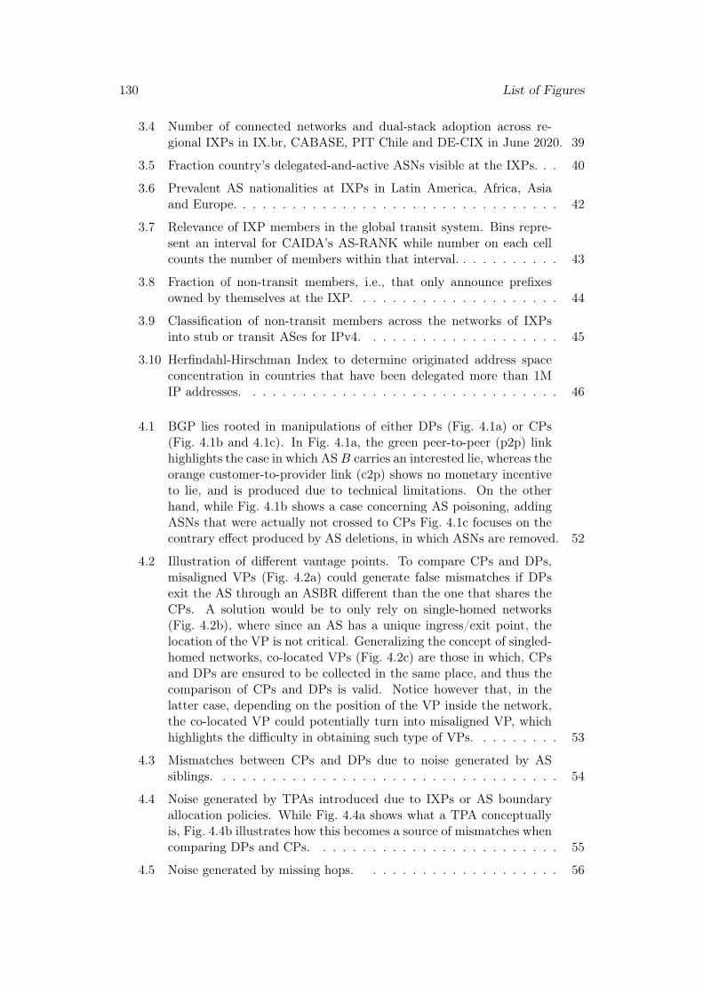
130 List of Figures
3.4 Number of connected networks and dual-stack adoption across re-gional IXPs in IX.br, CABASE, PIT Chile and DE-CIX in June 2020. 39
3.5 Fraction country’s delegated-and-active ASNs visible at the IXPs. . . 40
3.6 Prevalent AS nationalities at IXPs in Latin America, Africa, Asiaand Europe. . . . . . . . . . . . . . . . . . . . . . . . . . . . . . . . . 42
3.7 Relevance of IXP members in the global transit system. Bins repre-sent an interval for CAIDA’s AS-RANK while number on each cellcounts the number of members within that interval. . . . . . . . . . . 43
3.8 Fraction of non-transit members, i.e., that only announce prefixesowned by themselves at the IXP. . . . . . . . . . . . . . . . . . . . . 44
3.9 Classification of non-transit members across the networks of IXPsinto stub or transit ASes for IPv4. . . . . . . . . . . . . . . . . . . . 45
3.10 Herfindahl-Hirschman Index to determine originated address spaceconcentration in countries that have been delegated more than 1MIP addresses. . . . . . . . . . . . . . . . . . . . . . . . . . . . . . . . 46
4.1 BGP lies rooted in manipulations of either DPs (Fig. 4.1a) or CPs(Fig. 4.1b and 4.1c). In Fig. 4.1a, the green peer-to-peer (p2p) linkhighlights the case in which ASB carries an interested lie, whereas theorange customer-to-provider link (c2p) shows no monetary incentiveto lie, and is produced due to technical limitations. On the otherhand, while Fig. 4.1b shows a case concerning AS poisoning, addingASNs that were actually not crossed to CPs Fig. 4.1c focuses on thecontrary effect produced by AS deletions, in which ASNs are removed. 52
4.2 Illustration of different vantage points. To compare CPs and DPs,misaligned VPs (Fig. 4.2a) could generate false mismatches if DPsexit the AS through an ASBR different than the one that shares theCPs. A solution would be to only rely on single-homed networks(Fig. 4.2b), where since an AS has a unique ingress/exit point, thelocation of the VP is not critical. Generalizing the concept of singled-homed networks, co-located VPs (Fig. 4.2c) are those in which, CPsand DPs are ensured to be collected in the same place, and thus thecomparison of CPs and DPs is valid. Notice however that, in thelatter case, depending on the position of the VP inside the network,the co-located VP could potentially turn into misaligned VP, whichhighlights the difficulty in obtaining such type of VPs. . . . . . . . . 53
4.3 Mismatches between CPs and DPs due to noise generated by ASsiblings. . . . . . . . . . . . . . . . . . . . . . . . . . . . . . . . . . . 54
4.4 Noise generated by TPAs introduced due to IXPs or AS boundaryallocation policies. While Fig. 4.4a shows what a TPA conceptuallyis, Fig. 4.4b illustrates how this becomes a source of mismatches whencomparing DPs and CPs. . . . . . . . . . . . . . . . . . . . . . . . . 55
4.5 Noise generated by missing hops. . . . . . . . . . . . . . . . . . . . 56
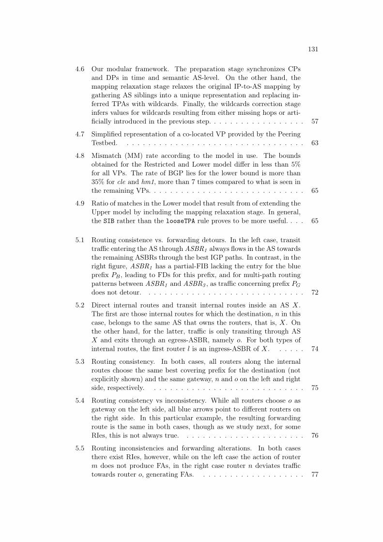
131
4.6 Our modular framework. The preparation stage synchronizes CPsand DPs in time and semantic AS-level. On the other hand, themapping relaxation stage relaxes the original IP-to-AS mapping bygathering AS siblings into a unique representation and replacing in-ferred TPAs with wildcards. Finally, the wildcards correction stageinfers values for wildcards resulting from either missing hops or arti-ficially introduced in the previous step. . . . . . . . . . . . . . . . . . 57
4.7 Simplified representation of a co-located VP provided by the PeeringTestbed. . . . . . . . . . . . . . . . . . . . . . . . . . . . . . . . . . 63
4.8 Mismatch (MM) rate according to the model in use. The boundsobtained for the Restricted and Lower model differ in less than 5%for all VPs. The rate of BGP lies for the lower bound is more than35% for cle and hm1, more than 7 times compared to what is seen inthe remaining VPs. . . . . . . . . . . . . . . . . . . . . . . . . . . . . 65
4.9 Ratio of matches in the Lower model that result from of extending theUpper model by including the mapping relaxation stage. In general,the SIB rather than the looseTPA rule proves to be more useful. . . . 65
5.1 Routing consistence vs. forwarding detours. In the left case, transittraffic entering the AS through ASBR1 always flows in the AS towardsthe remaining ASBRs through the best IGP paths. In contrast, in theright figure, ASBR1 has a partial-FIB lacking the entry for the blueprefix PB, leading to FDs for this prefix, and for multi-path routingpatterns between ASBR1 and ASBR3 , as traffic concerning prefix PG
does not detour. . . . . . . . . . . . . . . . . . . . . . . . . . . . . . 72
5.2 Direct internal routes and transit internal routes inside an AS X.The first are those internal routes for which the destination, n in thiscase, belongs to the same AS that owns the routers, that is, X. Onthe other hand, for the latter, traffic is only transiting through ASX and exits through an egress-ASBR, namely o. For both types ofinternal routes, the first router l is an ingress-ASBR of X. . . . . . 74
5.3 Routing consistency. In both cases, all routers along the internalroutes choose the same best covering prefix for the destination (notexplicitly shown) and the same gateway, n and o on the left and rightside, respectively. . . . . . . . . . . . . . . . . . . . . . . . . . . . . 75
5.4 Routing consistency vs inconsistency. While all routers choose o asgateway on the left side, all blue arrows point to different routers onthe right side. In this particular example, the resulting forwardingroute is the same in both cases, though as we study next, for someRIes, this is not always true. . . . . . . . . . . . . . . . . . . . . . . 76
5.5 Routing inconsistencies and forwarding alterations. In both casesthere exist RIes, however, while on the left case the action of routerm does not produce FAs, in the right case router n deviates traffictowards router o, generating FAs. . . . . . . . . . . . . . . . . . . . 77

132 List of Figures
5.6 Best IGP path vs Forwarding Detour. On the left, all routers choose oas gateway, hence no RIes occur and traffic flows through the best IGPpath from l to o. On the contrary, on the right, router p introducesRIes choosing o instead of itself as gateway. As p should act as egress-ASBR, but instead sends traffic to m, then p< introduces a FA. Sincel would have straightforwardly sent traffic to m, had it selected o asgateway, then the resulting internal route is subject to FDs. . . . . . 78
5.7 Multiple distinct forwarding detours between the same endpoints. InFig. 5.7a, router p introduces a FA, and this leads to a FD. The casesof Fig. 5.7b and 5.7c represent more complex scenarios where multipleFAs occur. In particular, the FAs are introduced by m and q on thefirst case, and additionally by p on the latter. The three scenariosproduce forwarding routes subject to distinct FDs that may co-existwhen they affect different sets of prefixes. . . . . . . . . . . . . . . . 80
5.8 Forwarding pattern when RFDX (i, e) = {R1}, RLB
X (i, e) = {R2, R3}and TE RTE
X (i, e) = {R4}. The size of every arrow is proportional tonumber of prefixes for which each route is used. . . . . . . . . . . . 81
5.9 Forwarding patterns for F-LB and prefix-based mechanisms. For F-LB, all internal routes of RLB
X (i, e) are used for both P1 and P2.On the other hand, for prefix-based mechanisms, e.g. C-LB, traffictargeting P1 and P2 flows through different interal routes. This alsoholds for FDs and TE, where prefixes subject to them flow across theroutes in RFD
X (i, e) and RTEX (i, e) respectively, while the remaining
prefixes are associated to best IGP paths. Note, that for prefix-based mechanisms, different routes may be revealed tracing differentprefixes, but each internal routes is usually used to forward traffic ofmultiple distinct prefixes. . . . . . . . . . . . . . . . . . . . . . . . . 82
5.10 Detecting the type of forwarding pattern for an ASBR-couple (i, e).While the colored cells represent the routes associated with each set ofprefixes, the dots show those revealed while tracing. The explorationphase runs traceroute and reveals one internal route per measuredprefix. The prefix-grouping phase then groups those prefixes for whichthe same route was revealed. At this stage, the result is the samefor F-LB and prefix-based mechanisms. The multi-route discoveryphase extends the measurements to find the complete set of routesassociated with each set of prefixes. For F-LB we see that routes incommon emerge across the different sets of prefixes. However thisdoes not occur for prefix-based mechanisms. Ultimately, the mergingphase will expose the nature of the forwarding pattern, merging allroutes and prefixes into a unique set for F-LB, but failing to do sofor prefix-based mechanisms.Therefore, in the cases where more thanone set remains at the final step, we can conclude that the forwardingpattern for (i, e) is prefix-based. . . . . . . . . . . . . . . . . . . . . 85

133
5.11 Impact of extreme-FDs on forwarding patterns. For both cases,RFD
X (i, e) = {R1}, RLBX (i, e) = {R2, R3} and TE RTE
X (i, e) = {R4}.The size of every arrow is proportional to number of prefixes for whicheach route is used. While the forwarding pattern inside AS X on theleft case undergoes no major change due to FDs, on the right caseit is largely modified by the occurrence of extreme-FDs, i.e., FDs formost prefixes. . . . . . . . . . . . . . . . . . . . . . . . . . . . . . . 87
5.12 Marginal utility of adding NLNOG RING’s VPs in terms of distinctASBR-couples (top) and unique ASes (bottom). For more than 70VPs, the gain in negligible. . . . . . . . . . . . . . . . . . . . . . . . 92
5.13 Cumulative number of sets composing PX(i, e) across ASBR-couplesbefore (r) and after (s) the merging phase. When r = 1, no multi-path routing pattern was observed. The difference with s = 1 relatesto cases where we find a forwarding pattern that corresponds to thatof per-dest/flow LB. Finally, when s ≥ 2 a prefix-based forwardingpattern is observed. In these cases, in general, s = 2, and they areFDs. . . . . . . . . . . . . . . . . . . . . . . . . . . . . . . . . . . . 93
5.14 Cumulative number of prefixes associated to the DIR across ASBR-couples. We observe a clear binary pattern: for any couple, eitherall traffic detours (left side, ∼4%), or none does (right side, ∼96% ofthe cases). Hence, our FD-detector is not sensible to the value of thethreshold t(Z,PX(i, e)). . . . . . . . . . . . . . . . . . . . . . . . . . 94
5.15 Quantification of ASBR-couples subject to FDs per AS. While mostASes have less than 10 couples subject to FDs (blue dots), the fractionthey represent out of the total in their AS (red bars) largely varies.This indicates that the problem of FDs is AS-dependent. . . . . . . . 95
5.16 Number of prefixes subject to FDs per ASBR-couple. The bars areseparated by dashed lines to emphasize a distinct ingress-ASBRs.The number of ingress-ASBRs, ASBR-couples and prefixes subjectto FDs strongly depends on the AS studied. . . . . . . . . . . . . . 95
5.17 Fraction of egress-ASBRs that are subject to extreme-FDs (red bars)out of the total (blue dots) for each ingress-ASBR. The tendencyshows that the more egress-ASBRs per ingress-ASBR, the less thefraction subject to FDs. However, for 17 ingress-ASBRs we cannotconclude anything since they only appear in one ASBR-couple. . . . 96
5.18 Complex LB flavors. In particular, coarse-fine LB implies that C-LB is followed by F-LB. This LB flavor generalizes C-LB: a set ofprefixes is now associated to more than one route, and these routesare reserved only for those prefixes. As with C-LB, for CF-LB itwould hold that s > 1. On the other hand, fine-coarse LB resultsfrom applying F-LB upstream of C-LB. Different to F-LB, with FC-LB not all routes are used for all prefixes. However, this LB flavorpreserves the property of F-LB where routes are not reserved fora unique specific set of prefixes, but rather they may be used fordifferent ones. As a consequence, the merging phase would likelyoutput s = 1 for FC-LB. . . . . . . . . . . . . . . . . . . . . . . . . 98

134 List of Figures
6.1 BGP lies that are hid by the malicious behavior of AS A. In thisexample, A is able to discriminate probes issued by traceroute fromregular traffic. As a consequence, A sends measuring probes thoughtB, i.e., the traceroute path (TP) matches the CP. In addition, Adiverts regular traffic from the path advertised in BGP, forwarding“regular” packets to X. . . . . . . . . . . . . . . . . . . . . . . . . . . 106
6.2 Methodology to detect the router that introduces the forwarding al-teration leading to a forwarding detour. The red arrows indicate sub-paths of the detouring route, whereas the violet ones are the pathsrevealed running traceroute towards intermediate interfaces found inthe aforementioned path. Fig. 6.2a shows the original detouring routefound with the FD-detector of Chapter 5. In the first step after de-tecting the FDs, shown in Fig. 6.2b, the violet path obtained targetingm and the red sub-path extracted from the path in Fig. 6.2a differ,and thus the measuring process continues. Finally, when tracing p inFig. 6.2c, the violet and red paths match. Consequently, p is identi-fied as the router that introduces the forwarding alteration that leadsto a forwarding detour between l and o. . . . . . . . . . . . . . . . . 108
6.3 Simultaneous BGP lies and forwarding detours. The top figure showsa full-FIB scenario. In this case, packets flow through best IGP pathsinside AS X, in particular from l to o. Once o is reached, packets areforwarded towards AS Y , the AS announced in CPs. Consequently,in this case no BGP lies nor FDs occur. On the other hand, the rightside figure shows a new scenario where l has a partial FIB. As l usesp as default gateway, and p redirects traffic towards q, an FD occurs.Moreover, since q acts as egress-ASBR and sends packets to AS Z,besides the FD, a BGP lie also occurs. Indeed, instead of forwardingtraffic to Y , X is pushing it towards Z. This highlights the potentialof combining the framework of Chapter 4 and the FD-detector ofChapter 5. . . . . . . . . . . . . . . . . . . . . . . . . . . . . . . . . 109

List of Tables
2.1 Notation used to describe the functioning principle of the MDA. . . . 252.2 Stopping points used by the node level version of the MDA given
that α = 0.05. Each column indicates that if N̂ next-hops have beendiscovered for one interface, once nN̂ are sent and no new next-hopappears, the MDA stops probing this interface and continues withanother one. Note that the table in this manuscript differs with thatin [56] since they show N instead of N̂ , where N = N̂ + 1. . . . . . . 27
3.1 Topology and management characteristics of IXP networks acrosscountries (CC). To the best of our knowledge, CABASE is currentlythe only IXP in the World that imposes a mandatory multilateralpeering policy (MMPP) among its members. . . . . . . . . . . . . . . 37
3.2 Largest sizes (#) of visible AS sets per upstream AS in IX.br-SP,CABASE-BUE and PIT Chile-SCL. . . . . . . . . . . . . . . . . . . 43
3.3 The two largest origin ASes per country. ∗ indicates state-owned ASes. 47
4.1 Summary of the noise-filtering rules that may be applied at each stage. 564.2 Path-rewriting rules (columns) applied for different noise-filtering quan-
tification models (rows). The Roman numbers report the order inwhich the rules are applied. In addition, 7 denotes rules that are notapplied in the given model. . . . . . . . . . . . . . . . . . . . . . . . 58
4.3 Peers that provide transit and full RIBs that were used as VPs. Theones on top are obtained from the Peering Testbed, and the onesbelow manually deployed by us. . . . . . . . . . . . . . . . . . . . . . 64
135

136 List of Tables
Extended Summary in French
Résumé
L’internet est une interconnexion de réseaux indépendants, appelés systèmes au-tonomes (AS). Étant donné que les AS sont construits sur du matériel et des logiciels,et que les opérateurs réseau, c’est-à-dire des administrateurs humains, gèrent les AS,l’internet est limité et génère certaines défaillances. Par exemple, les humains sontsujets à des erreurs et peuvent prendre des décisions arbitraires, les entreprises sontgénéralement avides de revenus et le matériel peut tomber en panne et nécessiterune maintenance ou un remplacement. Tous ces facteurs peuvent conduire à desdéfaillances de l’Internet, c’est-à-dire à des composants défectueux, à des réseauxconfrontés à des limitations ainsi qu’à des réseaux égoïstes qui donnent la prioritéà leurs propres revenus plutôt qu’aux meilleures performances de l’Internet.
L’objectif de cette thèse est de détecter des éléments défaillants del’Internet. Tout d’abord, nous étudions le déploiement des points d’échange Inter-net (IXP) en Amérique latine, une région qui n’avait jusqu’à présent reçu que peud’attention dans les études sur Internet. Nous construisons l’ensemble de données leplus complet sur l’état de l’Internet en Amérique latine et caractérisons l’écosystèmedes IXP dans la région. Nous constatons que si certains IXP en Amérique latine ontréussi à proliférer, certains pays sont en échec IXP, c’est-à-dire aucun IXP du tout,ou bien l’IXP n’a pas réussi à attirer des membres. Deuxièmement, nous étudions siles AS génèrent, intentionnellement ou non, desmensonges BGP, c’est-à-dire si lesroutes d’acheminement par lesquelles les paquets circulent réellement sur Internetdivergent des chemins que les AS annoncent sur BGP, le protocole de routage utilisésur Internet. En pratique, cette comparaison est complexe car, outre les multiplesniveaux auxquels les données doivent être synchronisées, les sauts manquants, lesadresses tierces et les AS jumeaux peuvent introduire des erreurs en déclenchant àtort la détection des mensonges BGP. Nous développons une méthodologie perme-ttant de filtrer ce bruit, et d’effectuer des mesures de terrain. Nous trouvons descas où, après avoir assaini l’ensemble des données avec notre cadre modulaire defiltrage, les chemins ne correspondent toujours pas. Enfin, nous étudions commentle trafic circule à l’intérieur des AS et nous nous concentrons sur la détection desdétours d’acheminement, c’est-à-dire les cas où les itinéraires d’acheminement necorrespondent pas aux meilleurs itinéraires disponibles, selon le protocole de routageutilisé. Nous développons un formalisme expliquant quand les détours de réachem-
137
138 List of Tables
inement se produisent, et mettons en œuvre un détecteur permettant de différencierles détours de réacheminement des techniques d’équilibrage de charge et d’ingénieriedu trafic. Nous effectuons des mesures avec notre détecteur et trouvons des détoursdans plusieurs AS avec un motif binaire remarquable, de sorte que le trafic de transitpassant entre deux routeurs de bordure d’un AS ne fait jamais de détour, ou en faitsystématiquement.
Introduction
L’Internet peut apparaître comme un système infaillible qui ne tombe jamais enpanne, mais ce n’est pas le cas. Internet est simplement une interconnexion deréseaux indépendants, appelés systèmes autonomes (AS). Les systèmes construitspar l’homme ne sont généralement pas parfaits : ils ont tendance à comporter desmodules qui peuvent tomber en panne et nécessiter une maintenance, ou qui, aprèsun certain temps, peuvent devenir obsolètes et nécessiter un remplacement. Tousces facteurs peuvent conduire à des défaillances de l’internet, c’est-à-dire à des com-posants défectueux, à des réseaux confrontés à des limitations et même à des réseauxégoïstes qui privilégient leurs propres revenus plutôt que les meilleures performancesde l’internet. L’objectif de cette thèse est de détecter de tels problèmes. Cette tâcheest difficile car les phénomènes que nous voulons découvrir peuvent être cachésn’importe où sur l’Internet, qui compte environ 70K ASes en novembre 2020.
Points d’échange Internet en Amérique latine La première composante del’Internet que nous étudions dans le cadre de cette thèse porte sur les points d’échangeInternet (IXP), les installations d’interconnexion communément utilisées par les AS.La structure de l’Internet, c’est-à-dire la manière dont les AS établissent des con-nexions entre eux, a été largement modifiée par l’irruption des IXP dans les années2000 [4]. Les IXP permettent aux AS d’établir des connexions à une plus grandeéchelle et de réaliser des économies. Toutefois, la popularité des IXP varie selon lesrégions. Dans certains cas, des pays peuvent avoir des IXP en échec, c’est-à-direaucun IXP du tout, ou un IXP qui n’a pas réussi à attirer suffisamment de membres.Alors qu’il existe de grands IXP en Europe, tels que DE-CIX, LINX et AMS-IX quiont fait l’objet d’une étude [5], il n’existe aucun rapport faisant état d’une réussitesimilaire en Amérique du Sud. Des études récentes se sont concentrées sur le rôle desIXP dans l’écosystème africain des SA [6, 7, 8]. Dans d’autres régions, en revanche,on sait peu de choses sur les IXP et même sur l’internet dans son ensemble.
En particulier, le cas de l’Amérique latine (LatAm), correspondant au RegistreInternet régional (RIR) nommé LACNIC, est un cas d’étude intéressant. L’Amériquelatine couvre 20 millions de km2 [9] et comprend 20 pays : juste après l’Amériquedu Nord, elle a le taux de population urbaine le plus élevé (80%) [10]. En outre,l’Amérique latine (LatAm) compte 652 millions d’habitants [11] et possède troisdes quatre plus grandes zones métropolitaines des Amériques (Sao Paulo, Mex-ico et Buenos Aires avec des populations respectives de 21,3M, 21,2M et 15,3Md’habitants) [12]. LatAm a également des chiffres intéressants en ce qui concernel’internet, étant donné qu’il contribue à l’écosystème mondial des sociétés anonymesavec 14,5 En outre, 6458 ASN ont été délégués par NIC.br (Brazilian NIR) à des

139
organisations basées au Brésil. Entre 2005 et 2015, cette région a connu une progres-sion significative des taux de pénétration de la téléphonie fixe et mobile, atteignantrespectivement 40,57% et 57,41% de la population [13]. En outre, plusieurs pays dela région ont récemment bénéficié de la création d’IXP nationaux [14].
Malgré le développement progressif de l’Internet en Amérique latine, la formedu réseau latino-américain reste relativement inexplorée. Cela nous encourage àexplorer son interconnexion et sa structure. Étant donné que les IXP ont contribuéà aplatir l’Internet dans les années 2000, il est naturel de se demander si, 20 ans plustard, ces infrastructures de peering profitent également aux pays en développement,dont beaucoup ont une surface beaucoup plus grande. Cela nous amène à notrepremière question de recherche.
Tous les IXP de LatAm ont-ils réussi à proliférer ou y a-t-il desIXP qui ont échoué ? Si certains ont échoué, pourquoi ?
Défi Scientifique
Les réseaux LatAm sont peu explorés, probablement en raison d’une rareté his-torique de données Internet représentatives. Par exemple, l’empreinte du RIPEAtlas et de l’Ark CAIDA dans le LatAm est composée de 285 sondes sur 11 142(2,56 %) et de 12 sondes sur 190 (6,32 %), respectivement. Ces chiffres diminuent sil’on considère l’IPv6 : seulement 2,22 % (101/4 556) des sondes compatibles IPv6 duRIPE sont situées en Amérique latine. D’autre part, on sait que le manque de don-nées BGP permet de dessiner une représentation assez incomplète des écosystèmesAS [15]. En ce sens, Routeviews 2 et RIPE RIS 3 n’ont déployé respectivementque deux et un collecteurs de données BGP dans la région, deux étant redondantspuisqu’ils sont placés au même IXP brésilien à Sao Paulo.
Malgré les limites susmentionnées, de rares études Internet se sont concentréessur cette région. Berenguer et al. [16] a appliqué des métriques de la théorie desgraphes pour évaluer l’augmentation de l’ensemble des données lorsque les itinérairescollectés à partir de lunettes locales sont ajoutés aux décharges RIPE RIS et Route-Views BGP. Brito et al. [17] a recueilli des données BGP par looking glass co-localisédans chaque IXP régional de IX.br, le réseau IXP brésilien, et les a ensuite comparésavec les IXP d’autres régions en termes de réseaux connectés et de prévalence despolitiques de peering. Une étude complémentaire des mêmes auteurs comprenaitune analyse du déploiement de l’IPv6 [18], toutefois, elle est limitée à la taille dupréfixe IPv6 et au nombre d’entrées IPv6 dans les tables de routage. Muller etal. [19] s’est appuyé sur les données sFlow recueillies à un IXP régional de IX.brpour déduire le trafic spoofé traversant l’IXP. Formoso et al. [20] s’est appuyé surles sondes de l’Atlas RIPE déployées en LatAm pour mesurer la latence entre lespays, en déduisant les trajets asymétriques et les pays mal interconnectés.
2http://www.routeviews.org/3https://www.ripe.net/analyse/internet-measurements/routing-information-service-ris

140 List of Tables
En particulier, le Chapitre 3 étudie le déploiement des IXP dans le LatAm, etexhibe le premier morceau d’Internet défaillant que nous analysons. En effet, lesIXP sont une histoire de succès ou d’échec selon le pays considéré en Amériquelatine. Alors que l’Argentine, le Brésil et le Chili comptent des IXP qui ont réussià proliférer, d’autres pays ont échoué. Nous nous plongeons dans les raisons pourlesquelles certains IXP sont capables de rassembler un grand nombre de membresqui annoncent plusieurs adresses IP alors que d’autres non. Nous constatons unecorrélation négative entre le succès des IXP et la présence d’AS monopolistiques con-centrant l’espace d’adresses IPv4 déléguées aux pays. En outre, comme cette régionn’a jamais été analysée de près, nous saisissons l’occasion et caractérisons égale-ment l’écosystème des AS dans la région. Nous constatons que les points d’échangeInternet dans la région LatAm, comme dans d’autres régions en développement,sont principalement peuplés d’acteurs nationaux ou régionaux, alors que ceux quisont de renommée internationale en Europe se comportent plutôt comme des pointsd’échange internationaux.
À la recherche de mensonges BGP Le deuxième élément de l’Internet quenous examinons dans cette thèse est le protocole Border Gateway Protocol (BGP),utilisé sur l’Internet pour le routage entre AS. BGP dicte la manière dont les ASéchangent des informations d’accessibilité concernant les préfixes IP que chacund’entre-eux possède. En bref, chaque AS annonce à ses AS voisins les préfixes qu’ilpossède en BGP, et ceux-ci relaient à leur tour le message aux autres AS. Dans ceprocessus, les messages de routage qui sont envoyés conservent la trace du cheminsuivi par l’AS, c’est-à-dire une liste des AS, du premier au dernier, qui ont annoncéle préfixe. Dans cette thèse, nous appelons le chemin AS le chemin de contrôle (CP),puisqu’il est construit sur le plan de contrôle de BGP. D’autre part, nous faisonsréférence à l’ensemble des AS que les paquets parcourent effectivement vers leurdestination comme des chemins de données (DP), puisque cela se produit au niveaudu plan de données de BGP. Une analogie d’un AS annonçant un préfixe avec unCP donné à un AS voisin, est la signature d’un contrat. Plus précisément, l’annoncede BGP joue le rôle du contrat, et le service qui est offert est que, pour atteindreun préfixe donné, le DP répliquera l’ensemble ordonné d’AS exprimé dans le CP.Par conséquent, les DP sont censés correspondre aux CP annoncés pour tous lespréfixes.
L’hypothèse sous-jacente selon laquelle les CP correspondent aux DP pour tousles préfixes annoncés dans BGP n’est pas triviale à vérifier : les outils de dépannageactuels, par exemple traceroute, permettent généralement de récupérer les cheminsIP, mais pas directement la route de transfert au niveau des AS qui a été suivie.La confiance implicite qui présume que les AS annoncent les chemins qu’ils utilisentpour le transfert de paquets peut être naive. Les opérateurs de réseau peuvent ma-nipuler les CP [21] et les DP [22, 23], ce qui peut les conduire à une non-concordance.Chaque fois que le CP et le DP d’un préfixe ne correspondent pas, on dira qu’unmensonge BGP s’est produit. Notez que ce terme s’applique indépendamment dufait que les CP et/ou les DP soient modifiés, ou si cela résulte d’un comportementdélibéré ou involontaire.
L’objectif qui se cache derrière les mensonges de BGP peut être multiple. UnAS peut tenter de rediriger et d’intercepter le trafic, ou entraver son suivi avec des

141
conséquences sur la capacité à résoudre les problèmes de connectivité. De plus, lesmensonges de BGP peuvent conduire à la violation d’accords entre des AS adjacents,avec des représailles juridiques potentielles. Ces mensonges peuvent être délibéréspour brouiller les interceptions de trafic ou être motivés par des intérêts économiques,par exemple attirer du trafic en promettant des itinéraires intéressants mais enutilisant des alternatives moins coûteuses. D’autre part, ils peuvent résulter detopologies logiques et physiques incongrues, en particulier lorsque les sessions BGPne sont pas établies sur de simples liaisons inter-domaines point à point. D’autrespeuvent être dues à des limitations techniques, telles qu’une mémoire limitée surles routeurs empêchant le stockage de la table de routage complète, c’est-à-direrésultant d’une FIB partiel. En conclusion, la facilité avec laquelle les mensongesBGP peuvent se produire constitue la seconde pièce cassée d’Internet que nous allonsétudier et quantifier.
Cette tâche de détection des mensonges BGP nécessite de relever un défi pratiqueconsidérable : les données recueillies à partir des mesures et des outils nécessaires àcette analyse sont bruitées, de sorte que les mensonges BGP peuvent être mal inter-prétés (comme du bruit, ou vice versa). Par conséquent, pour tirer des conclusionsreprésentatives, le cadre élaboré doit filtrer le bruit affectant les mesures. C’est cequi motive notre deuxième question de recherche.
Pouvons-nous développer un cadre qui filtre le bruit affectant lacomparaison CP-vs-DP et qui permette de quantifier le taux quo-tidien de mensonges BGP qui se produisent sur Internet ?
Défi Scientifique
Il existe de nombreux documents qui se sont concentrés sur la comparaison desCP et des DP, et sur la caractérisation des différentes sources de bruit affectantcette tâche. Mao et al. [24] constate que les IXP, les AS jumeaux et ASes annonçantdes préfixes IP pour lesquels ils ne sont pas les véritables origines sont les causesprédominantes des décalages entre CP et DP. Dans un travail de suivi [25], ilsdéveloppent une approche systématique pour corriger les correspondances IP-ASinexactes en réaffectant l’origine des préfixes. Hyun et al. [26] analysent égalementles divergences entre les CP et les DP et concluent que les insertions d’IXP dansles DP et d’AS sous la même propriété sont la principale cause qui conduit à desdiscordances. Toutefois, dans leur étude, les traces incomplètes sont écartées et lacomparaison ne repose pas sur les dernières mises à jour du BGP, c’est-à-dire que lesCP et les DP ne sont pas synchronisés. Zhang et al. [27] extraient les fragments dediscordance des CP et des DP et montrent que le principal écueil de l’utilisation detraceroute dans les mesures de topologie au niveau des AS provient de l’apparitiond’adresses IP attribuées par les voisins des AS. Cependant, leur plateforme de mesuresouffre de l’incapacité à garantir que les VP du plan de données et de contrôle sontco-localisés. D’autre part, Hyun et al. [28] ont introduit le concept d’adresses IPtierces, ou TPAs. Selon les auteurs, il est peu probable, bien que possible, de trouver
142 List of Tables
plusieurs TPA d’affilée cartographiés sur le même AS. Leur étude conclut que lesTPA ne sont pas courants et qu’ils ne déforment pas les cartes des AD de manièresignificative. Une analyse ultérieure de Marchetta et al. [29] utilisant les optionsd’horodatage IP affirme le contraire. Ils constatent que les TPA consécutifs sontcourants, et peuvent même cacher entièrement un AS d’un chemin de niveau AS.Cependant, une étude ultérieure de Luckie et al. [30] rapporte que la plupart desIPs observés dans les traces traceroute proviennent d’interfaces en liaison, doncsur le chemin. Ils affirment que les techniques utilisant les horodatages IP ne sontpas fiables pour détecter les TPA. Ahmed et. al [31] proposent une méthode horsligne qui marque jusqu’à deux IP qui apparaissent dans une rangée comme des TPApossibles s’ils introduisent un AS qui soit viole des chemins sans vallée, soit se traduitpar de nouvelles relations AS. D’autres travaux concernant la détection des TPApour déterminer correctement les limites des AS comprennent bdrmap [32], MAP-IT [33] et bdrmapIT [34]. Bdrmap déduit les adresses d’interface de liaison inter-ASentre un réseau avec un VP traceroute et les réseaux directement connectés quis’appuient sur des techniques de sondage de résolution d’alias, et les déductions derelations AS. D’autre part, MAP-IT tente d’obtenir la même chose pour tous les ASconnectés en se basant sur les résultats du traceroute collectés à partir de plusieursVP distribués dans différents AS. Enfin, bdrmapIT combine les deux précédentes,améliorant l’inférence de la propriété des routeurs et l’identification des liens entreles AS.
Dans le Chapitre 4 nous modélisons comment les AS peuvent introduire des men-songes BGP et nous proposons une méthodologie pour les détecter. En particulier,nous présentons un cadre permettant de filtrer le bruit, c’est-à-dire les inexactitudesde cartographie introduites par les AS jumeaux, les TPA et les sauts manquants, quipeuvent affecter la comparaison entre les chemins de contrôle annoncés dans BGPet les chemins de données que suivent les paquets sur l’internet. En particulier,notre méthodologie repose sur une heuristique estimant si le bruit peut affecter leschemins que nous collectons, puis tente de les corriger. Notre cadre est modulaire,c’est-à-dire que l’utilisateur peut choisir parmi plusieurs filtres qui varient la manièredont il estime ce qui résulte du bruit ou non, et permettent ainsi de mettre en œuvredifférents modèles de filtrage du bruit. Nous effectuons des mesures à long terme surl’internet et assainissons l’ensemble des données grâce à notre outil. Nos résultatsmontrent que, même en se basant sur le modèle de filtrage du bruit le plus con-servateur, il subsiste encore quelques décalages entre les itinéraires de transmissionet de contrôle que nous recueillons sur l’internet, ce qui représente probablementdes mensonges BGP. Dans les points de collecte où l’on trouve peu de mensonges,les résultats sont stables dans le temps, sinon nous constatons que le nombre dechemins divergents par jour présente une plus grande variation. Par rapport à lalittérature, notre étude déploie non seulement plus de points de mesure, mais vaégalement au-delà de ce qui avait été fait auparavant en fournissant des résultatsbasés sur une analyse quotidienne. Alors que la plupart des travaux connexes blâ-ment essentiellement la cartographie IP-AS pour les écarts observés entre les CP etles DP, notre travail repose sur des heuristiques conservatrices qui éliminent le bruitdans les mesures et les erreurs de cartographie, en essayant de minimiser les fauxpositifs dans la détection des mensonges BGP. En d’autres termes, à la différencedes études précédentes, notre objectif est de détecter les "vrais" mensonges BGP,

143
d’où notre cadre de travail conçu pour fournir une borne inférieure. Les erreursque nous constatons après avoir appliqué nos filtres montrent que la cartographieIP-to-AS n’est pas la seule coupable.
Modélisation et détection des détours d’acheminement La dernière com-posante de l’Internet que nous analysons sont les protocoles de routage interne(IGP), les protocoles de routage que les AS utilisent à l’intérieur de leurs réseaux.Les IGP se caractérisent par le fait qu’ils aboutissent à un schéma d’acheminementtel que le trafic traversant les AS passe par les meilleurs chemins qui minimisentla distance ou le coût selon une métrique laissée au choix de l’opérateur réseau dechaque AS.
Le flux Internet complet, qui atteignait 854 000 de préfixes en novembre 2020,a augmenté d’environ 50 000 préfixes par an au cours des dix dernières années.L’augmentation soutenue du nombre de préfixes annoncés sur le BGP a conduit lesASes à échanger davantage de messages de mise à jour [35, 36, 37], et à souffrir deproblèmes d’évolutivité. En effet, compte tenu de la tendance actuelle, le maintiend’un FIB complet peut s’avérer difficile, en particulier pour les AS incapables demettre à jour régulièrement leurs équipements réseau [38, 39, 40, 41].
Dans ce contexte, les opérateurs de réseaux se repose sur des alternatives peuonéreuses pour supporter d’anciens routeurs incapables de maintenir une FIB com-plet en mémoire. Par exemple, dans un coeur d’infrastructure sans BGP, les tech-niques de tunneling réduisent la taille de la FIB sur ces routeurs [42]. En outre, ladiffusion partielle d’iBGP reposant sur des hiérarchies de réflecteurs de route peutégalement accroître l’extensibilité [43]. Cette technique permet aux routeurs deconserver moins de pairs BGP et, dans certains cas rares, peut même empêcher laredistribution complète des préfixes BGP dans l’AS [44]. En outre, les routeurs à mé-moire limitée peuvent regrouper les routes pour limiter le nombre d’entrées FIB [45].D’autres types de contournement consistent à stocker une FIB partielle [46], et àrediriger le trafic via des routes par défaut vers des routeurs plus performants (parexemple, ayant une FIB complète). Certains opérateurs réseau appliquent mêmecette technique sur les commutateurs dotés de capacités IP [47].
Si les techniques susmentionnées peuvent paraître efficaces à première vue, lesAS qui s’y fient peuvent souffrir de détournements d’acheminement, c’est-à-dire quele trafic peut passer par des itinéraires d’acheminement qui dévient ou s’écartentdes meilleures chemins IGP attendus. Cela peut se produire lorsque les routeursle long d’une route choisissent différentes passerelles de sortie, ou ASBR, pour lemême préfixe. Pour cette raison, nous disons que ces préfixes subissent des FD.En général, l’existence simultanée de préfixes soumis ou non aux FD génère desmodèles multi-path routing. Cependant, contrairement au routage "hot-potato", lesFDs augmentent la distance IGP nécessaire pour traverser un AS et entraînent sansdoute un gaspillage de ressources à l’intérieur du réseau. Pour tenter de supprimer lesFD, les opérateurs de réseau peuvent mettre en œuvre des techniques de tunneling.Cependant, ces mécanismes ne permettent de contourner les FD qu’à l’intérieur dechaque tunnel/segment (pour les routeurs de coeur non ASBR BGP en particulier)mais peuvent ne pas le faire entre les points d’extrémité d’un AS. De plus, outreles effets secondaires des solutions de contournement de l’extensibilité, des boguesdans le logiciel du routeur, tels que les zombies BGP [48], peuvent également créer

144 List of Tables
des FD. Par conséquent, les opérateurs de réseau peuvent ignorer les FD qui seproduisent sur leur AS, et fournir des performances dégradées aux AS des clients.Cela nous amène à une troisième question de recherche.
Pouvons-nous modéliser formellement les causes profondesqui produisent les détours d’acheminement, et concevoir uneméthodologie efficace pour les détecter ?
Défi Scientifique
Concernant les travaux connexes, en 2004, lorsque les FIB completes ne comp-taient que 100 000 entrées, contre plus de 800 000 aujourd’hui, Bu et al. [49] ontétudié l’augmentation des tables BGP causée par ce qu’ils ont appelé une croissanceexponentielle de l’internet. Alors que leur étude s’est concentrée sur les raisons decette augmentation, nous nous intéressons aux conséquences; plus précisément, àleur impact sur l’acheminement des données à l’intérieur des AS. Plusieurs propo-sitions visent à réduire la taille des tables de routage en agrégeant les routes [45] eten redirigeant parfois le trafic vers des routeurs plus performants [46]. La croissancedes FIB favorise en effet l’utilisation de solutions de contournement comme les FIBpartiels et les routes par défaut, qui peuvent à leur tour conduire à des FD.
D’autre part, les déviations de route sont un phénomène connu qui a été étudiésous différents angles, cependant, aucun n’est exécuté à la même échelle, ni avecle même objectif que le nôtre. Elena et al. [50] mettent en évidence les déviationsà l’échelle d’un AS, bien que leur objectif soit de détecter la diversité des cheminssur Internet. Ils concluent que l’équilibrage de charge (LB ou multi-path routing)intra-domaine n’était pas bien déployée à l’époque. Secci et al. [51] étudient lesdéviations de bout en bout créées par BGP. S’ils étudient également les déviationsintra-domaine, ils se concentrent sur la dynamique et les oscillations dues à l’attributMED. Agarwal et al. [52] analysent les changements de routage de BGP en tant quedéviations. Ils essaient de détecter les déviations intra-domaine pour construiredes matrices de trafic précises. Bush et al. [53] étudient l’utilisation de routes pardéfaut, ou filet de sécurité, assurant l’accessibilité lors des événements de routage.Pour cela, ils empoisonnent les routes et vérifient ensuite si les préfixes associés sonttoujours accessibles.
Enfin, de nombreuses études ont été menées sur les schémas de routage à tra-jets multiples (LB). Augustin et al. [54] présentent Paris-traceroute, une version detraceroute prenant en compte l’équilibrage des charges par flux, permettant d’éviterl’inférence erronée de liens, de boucles et de cycles vus dans le traceroute stan-dard, comme l’a étudié plus en détail Viger et al. [55]. Sur la base des principesde Paris-traceroute, Augustin et al. [56] développent l’algorithme MDA, permet-tant de détecter les équilibreurs de charge par flux et par paquet. Dans des étudesultérieures, ils étendent MDA pour détecter également les équilibres de charge pardestination [57, 58]. Veitch et al. [59] affinent la génération de la liste des pointsd’arrêt de MDA pour limiter la probabilité d’échec de la découverte complète par

145
plusieurs chemins. Vermeulen et al. [60] proposent MDA-Lite, une version allégéede la MDA qui nécessite moins de sondes, mais qui peut échouer à découvrir tousles nœuds et liens. Plus récemment, ils proposent Diamond Miner [61], un systèmecapable de produire des cartes topologiques multi-trajets sur Internet en moins de 3jours de mesure [61]. DiamondMiner met en œuvre MDA avec un mode de sondagesans état s’appuyant sur Yarrp [62], un outil de sondage à grande vitesse randomisé.Almeida et al. [63] généralisent MDA et proposent l’Algorithme de classificationmulti-chemins (MCA). En général, tous ces travaux montrent que les LB par flux etpar destination sont les options LB les plus répandues. À l’exception de DiamondMiner, ils mènent tous des campagnes de mesure de l’ordre de 10K et pas plus de70K d’adresses IP de destination à partir de 32 points de mesure au maximum.
Le chapitre 5 décrit pourquoi la détection des FD est complexe, et montre l’outilque nous développons pour atteindre cet objectif. Alors que les travaux connexesse sont concentrés sur l’effet d’une cause particulière qui pourrait potentiellementcréer des FD, notre solution permet une analyse systématique qui peut être appliquéepour détecter les FD à l’intérieur des AS de toute sorte. La méthodologie que nousproposons analyse de près la manière dont le trafic circule à l’intérieur des AS et nenécessite pas de connaissances privilégiées concernant les réseaux analysés, par ex-emple la connaissance de la métrique IGP utilisée, pour conclure à l’absence de FD.Il est à noter que la détection des FD est une tâche particulièrement difficile dans cescirconstances, c’est-à-dire lorsqu’aucune hypothèse n’est faite sur la métrique IGPutilisée par les AS, puisque les détours d’acheminement et les meilleurs chemins IGPsont en fin de compte simplement des itinéraires d’acheminement. En outre, commepour les FD, des techniques telles que l’équilibrage de la charge et l’ingénierie dutrafic génèrent également des modèles de routage à trajets multiples. Contrairementaux détours de réacheminement, ceux-ci sont toujours considérés comme optimauxen termes de coût IGP ou pour les besoins spécifiques de l’AS qui les déploie, respec-tivement. Notre analyse peut compléter les études axées sur l’équilibrage de chargepuisque nous envisageons également le LB par préfixe, une option de déploiementqui n’est pas abordée dans la littérature. Notre détecteur ne se contente pas derelever tous ces défis, mais utilise également une nouvelle étape de regroupementdes préfixes, qui pourrait permettre de réduire le coût de sondage des campagnesde découverte des chemins LB, et de découvrir d’autres possibilités d’équilibrage decharge par destination. Nous testons notre détecteur FD dans l’Internet et décou-vrons des détours d’acheminement dans plusieurs AS, avec un remarquable motifbinaire dans lequel le trafic de transit passant entre deux routeurs de bordure d’unAS ne fait jamais de détour, ou en fait pour chaque préfixe. Enfin, le concept des dé-tours d’acheminement se concentre sur les conséquences, c’est-à-dire sur les cheminsqui diffèrent des meilleurs chemins IGP, mais ne dit rien sur la manière dont ilssont générés, c’est-à-dire sur leurs causes profondes. Pour éclairer ce sujet encoreinexploré, nous développons un formalisme autour des détours d’acheminement per-mettant de décrire formellement les phénomènes qui conduisent à l’apparition deces détours.

146 List of Tables
Résumé Chapitre 3
Dans ce chapitre, nous étudions si les IXP, qui ont connu un grand succès dans lesannées 2000, profitent aujourd’hui également au développement de l’Internet dansd’autres régions que l’Europe. Nous nous concentrons en particulier sur l’Amériquelatine, une région qui est restée assez inexplorée malgré ses caractéristiques at-trayantes. Nous nous intéressons aux politiques publiques qui ont conduit à lacréation des IXP d’Amérique latine, à leur croissance et à leur développement dansle temps, et au rôle que chacun d’entre eux joue dans l’écosystème national des AS,c’est-à-dire s’ils sont échec des IXP ou ont réussi à proliférer. Pour avoir une visionplus large, nous comparons les IXP déployés sur plusieurs continents. En bref, noscontributions sont les suivantes :
1. Nous déterminons les pays en LatAm avec des IXP et construisons l’ensemblede données le plus complet à ce jour en rassemblant des informations sur lesIXP en LatAm dans Sec. 3.1. En particulier, nous recueillons des données BGPauprès de plusieurs collecteurs situés dans la région. À notre connaissance,nous sommes les premiers à explorer cet ensemble de données. En outre, nousavons étendu la vue BGP au Brésil en utilisant un collecteur de vues de routeset plusieurs lunettes de visée réparties sur plusieurs IXP brésiliens. En outre,nous combinons plusieurs sources de données supplémentaires pour obtenir desmesures qui aident à quantifier la croissance des IXP et à mieux comprendrele rôle de leurs membres fournisseurs de transit.
2. Nous donnons un aperçu dans Sec. 3.2 de la manière dont les politiquespubliques des pays ont encouragé le développement des IXP en Amériquelatine. Il est intéressant de noter que les gouvernements locaux de chaquepays ont été impliqués dans la création de plus de 55% des IXP d’Amériquelatine. Comme pour le modèle européen des IXP, en Amérique latine, ungrand nombre d’organisations à but non lucratif gèrent des IXP (et les ontégalement créés dans certains cas).
3. Nous étudions comment les IXP ont gagné en importance depuis leur création,et les membres qui les composent. Tandis que les IXP en Amérique latine etdans les régions en développement en général ont été capables d’attirer desmembres nationaux et régionaux, les IXP européens ont également réussi àrassembler des membres de différentes régions, ce qui permet de spéculer surla possibilité pour ces IXP de continuer à se développer à l’avenir.
4. Nous analysons le succès et l’échec des IXP en LatAm dans Sec. 3.4 en essayantde relier ce phénomène avec la présence d’un écosystème AS équilibré, c’est-à-dire où les adresses IP sont plus équitablement réparties entre les AS du pays.Nous constatons une corrélation négative entre l’absence de monopole des ASde transit/accès possédant la plupart des adresses IP attribuées à un pays etle succès des IXP nationaux.
5. Nous publions le code qui permet à la fois de récupérer les données publiquesque nous avons utilisées et de reproduire nos résultats4. En outre, nous met-
4https://github.com/CoNexDat/latam-ixp-obs

147
tons à la disposition du public les données que nous avons recueillies manuelle-ment dans les looking glass brésiliens5.
De plus, nous tirons les principales conclusions de ce chapitre dans la Sec. 3.7,tandis que les annexes de la Sec. 3.3 et de la Sec. 3.5 fournissent des résultatscomplémentaires à notre étude. Les recherches présentées dans ce chapitre ontconduit aux travaux suivants :
• Esteban Carisimo, Julián M. Del Fiore, Diego Dujovne, Cristel Pelsser, etJ. Ignacio Alvarez-Hamelin. 2020. A first look at the Latin American IXPs,dans SIGCOMM Comput. Commun. Rev. 50, 1 (janvier 2020), 18-24.
• Esteban Carisimo, Julián M. Del Fiore, Diego Dujovne, Cristel Pelsser, J.Ignacio Alvarez-Hamelin, Country-level influence of IXPs in Latin America,dans l’Atelier des étudiants d’Amérique latine sur les réseaux de communica-tion de données (LANCOMM) 2019.
Résumé Chapitre 4
Dans ce chapitre, nous présentons la méthodologie que nous proposons pour dé-tecter les discordances entre les trajets AS-transfert et les trajets AS BGP, quenous appelons les mensonges BGP. Cette tâche nécessite notamment de relever undéfi pratique considérable : tant les techniques de mesure active de pointe, parexemple traceroute, que les outils de cartographie IP-to-AS utilisés de nos jourssont bruitées. Par conséquent, puisque les mensonges peuvent être mal interprétéscomme du bruit, ou vice versa, il est impératif de filtrer ce bruit. Pour résoudre ceproblème, nous proposons un cadre modulaire permettant de détecter les mensongesBGP et leurs bornes en éliminant toutes les sources d’erreurs interférant avec lesdonnées collectées, c’est-à-dire en filtrant le bruit affectant la comparaison des CPet des DP. En bref, nos contributions sont les suivantes :
1. Nous étudions de multiples cas d’études montrant différentes causes pouvantconduire à des mensonges BGP dans Sec. 4.1. En particulier, ces exemples il-lustrent pourquoi il est difficile de déterminer la cause première des mensongesBGP, un problème qui dépasse le cadre de cette thèse.
2. Nous modélisons dans Sec. 4.2 les différents défis pratiques qui doivent êtrerelevés afin de pouvoir détecter les mensonges BGP. Cela va de la nécessité desynchroniser les mesures dans le temps, de pouvoir mesurer dans une plate-forme où les chemins de contrôle et les chemins de données peuvent être collec-tés dans le même réseau, jusqu’à la description des multiples sources de bruitqui peuvent interférer dans la comparaison des CP et des DP, c’est-à-dire lesAS jumeaux, les TPA ou les IXP et les sauts manquants.
3. Nous développons une méthodologie permettant de calculer le taux de men-songes BGP pour un point de mesure donné dans le cadre de la Sec. 4.3. Notrecadre comporte trois étapes :
5https://cnet.fi.uba.ar/latam-ixp-obs/lg-ribs/

148 List of Tables
• a étape de préparation qui synchronise les CP et les DP dans le temps etau niveau sémantique, c’est-à-dire qui convertit les DP des chemins IPen chemins AS ;
• un étape de relaxation cartographique qui examine les DP et les CPséparément et tente de déduire le bruit affectant chacun d’eux. Danscette tâche, nous uniformisons les AS jumeaux en leur attribuant unecartographie unique pour les CP et les DP, et nous convertissons lesTPA possibles affectant les DP en éléments neutres qui peuvent être misen correspondance avec n’importe quel AS;
• a étape de correction des éléments neutres qui, en comparant les CP etles DP, tente de déduire les valeurs des éléments neutres (y compris lessauts manquants) présents dans les DP (le cas échéant), et détermine siles CP et les DP correspondent ou non.
Notre cadre est modulaire : les règles de filtrage sur la relaxation de la cartogra-phie, et l’ordre dans lequel elles sont appliquées, peuvent être sélectionnées,ce qui permet de mettre en œuvre différents modèles de filtrage du bruit.
4. Nous déployons 8 points d’observation co-localisés, 6 dans les Peering Testbedet deux dans les réseaux privés, et la travail effectué sur cette recherche lon-gitudinale se trouve dans Sec. 4.4. À notre connaissance, notre analyse est lapremière à s’étendre dans le temps et à déployer un si grand nombre de pointsd’observation pour une comparaison des DP et des CP.
5. Nous assainissons l’ensemble des données avec différents modèles de filtrage dubruit que nous construisons avec notre cadre et calculons le taux de mensongesBGP que nous mesurons pour chacun d’eux dans Sec. 4.5. Notre modèle le plusconservateur, c’est-à-dire celui qui filtre plus agressivement le bruit et permetd’obtenir une limite inférieure de mensonges BGP, révèle une quantité nonnégligeable de mensonges. En outre, nous constatons que dans les points demesure où notre cadre est très efficace pour réduire le nombre de discordancesentre les PC et les PD, les résultats restent généralement assez stables dans letemps. D’autre part, lorsque notre cadre révèle un grand nombre de mensongesBGP potentiels, les résultats présentent une plus grande variation par jour.
La Sec. 4.6 tire les dernières remarques de notre étude. Les travaux présentésdans ce chapitre ont donné lieu à la publication suivante :
• Julián M. Del Fiore, Pascal Merindol, Valerio Persico, Cristel Pelsser etAntonio Pescapè. Filtering the Noise to Reveal Inter-Domain Lies, dans 2019Network Traffic Measurement and Analysis Conference (TMA), pages 17–24,2019, IEEE.
• Julián M. Del Fiore, Pascal Merindol, Valerio Persico, Cristel Pelsser andAntonio Pescapè. A BGP-lying Tale: Stop Blamming the Mapping, posterdans TMA 2018.

149
Résumé Chapitre 5
Dans ce chapitre, nous examinons de près le phénomène des détours d’acheminement.À notre connaissance, nous sommes les premiers à nous attaquer au problème de ladétection des détours d’acheminement, sans distinction des causes sous-jacentes quiles génèrent, tout en filtrant les techniques d’équilibrage des charges et d’ingénieriedu trafic. En bref, nous apportons les contributions suivantes :
• Nous développons un formalisme autour des détours d’acheminement dans leSec. 5.1. En particulier, nous construisons un modèle d’acheminement et mon-trons que les incohérences d’acheminement peuvent évoluer en modificationsd’acheminement qui peuvent alors être à l’origine de détours d’acheminement.En outre, nous étudions le modèle de réacheminement : les détours de réa-cheminement prennent naissance à l’intérieur des AS, c’est-à-dire si le traficentre deux points d’extrémité fixes emprunte des itinéraires différents selonle préfixe considéré, et nous le comparons à celui généré par les techniquesd’équilibrage de charge et d’ingénierie du trafic. En particulier, les FD, les LBet les TE par préfixe génèrent un schéma d’acheminement similaire, que nousappelons "basé sur le préfixe".
• Nous concevons un algorithme capable de détecter les modèles de transfertbasés sur les préfixes dans les Sec. 5.3. Notre cadre repose uniquement sur lesdonnées de cartographie IP-AS et les informations de plan de données collec-tées avec traceroute. Nous présentons une nouvelle stratégie pour rechercherdes modèles de routage multi-chemins, en plusieurs étapes. Notre techniqueregroupe des préfixes pour lesquels les mêmes routes internes des AS sontrévélées, une idée qui peut être incorporée dans les études de découverte detopologie pour réduire leur coût de sondage associé.
• Nous proposons un détecteur FD dans Sec. 5.4. Notre solution ajoute unedernière phase à l’algorithme précédent : elle applique un verdict permettantde discriminer les FD des autres mécanismes qui génèrent également des sché-mas d’acheminement basés sur des préfixes. Pour cela, nous nous concentronssur les cas extremes, c’est-à-dire les scénarios où les FDs affectent de nom-breux préfixes. Nous construisons un détecteur de détours de réacheminementcomme un outil prêt à être utilisé sur le terrain.
• Nous analysons le phénomène des FD sur le terrain dans Sec. 5.5, en faisantfonctionner notre détecteur de FD à partir de 100 nœuds de l’infrastructurede surpervision NLNOG RING, et nous trouvons des FD dans 25 des 54 ASsondés. Nous trouvons un motif binaire remarquable dans lequel le trafic detransit passant entre deux routeurs de bordure d’un AS ne fait jamais dedétour, ou en fait toujours. Nous avons validé le comportement du détecteurde FD avec des émulations et sur un réseau où nous avons le contrôle.
• Nous publions l’ensemble des données que nous avons collectées, les configu-rations d’émulations et notre code pour favoriser la reproductibilité.
150 List of Tables
Nous discutons de la robustesse du détecteur FD que nous avons mis en œuvredans la Sec.5.6, et nous tirons des remarques finales dans la Sec. 5.7. Les travauxprésentés dans ce chapitre ont conduit à la rédaction de l’article suivant :
• Julián M. Del Fiore, Valerio Persico, Pascal Merindol, Cristel Pelsser etAntonio Pescapè. The Art of Detecting Forwarding Detours, dans l’IEEETransactions on Network and Service Management (IEEE TNSM) 2021.
• Julián M. Del Fiore, Pascal Merindol, Valerio Persico, Cristel Pelsser andAntonio Pescapè. Routing Inconsistencies at the FIB level, poster dans TMA2019.
Dans l’ensemble, les études que nous menons dans le cadre de cette thèse révèlentqu’Internet n’est pas un système infaillible et que ses pièces défaillantes peuvent êtremises en lumière en élaborant des méthodologies comme celles que nous dévelop-pons.
Copyright © 2022 FDOKUMEN