Relationship between floristic similarity and vegetated land surface phenology: Implications for the...

Relationship between floristic similarity and vegetated land surface phenology:Implications for the synoptic monitoring of species diversity at broadgeographic regions

Andrés Viña a,⁎, Mao-Ning Tuanmu a, Weihua Xu b, Yu Li a, Jiaguo Qi c, Zhiyun Ouyang b, Jianguo Liu a

a Center for Systems Integration and Sustainability, Department of Fisheries and Wildlife, Michigan State University, East Lansing, MI, USAb State Key Lab of Urban and Regional Ecology, Research Center for Eco-Environmental Sciences, Chinese Academy of Sciences, Beijing, Chinac Center for Global Change and Earth Observations, Department of Geography, Michigan State University, East Lansing, MI, USA

a b s t r a c ta r t i c l e i n f o

Article history:Received 24 August 2011Received in revised form 10 February 2012Accepted 11 February 2012Available online xxxx

Keywords:BiodiversityChinaMODISPhenologyQinling MountainsSpectral vegetation indicesVisible Atmospherically Resistant Index

Assessing species composition and its changes through time across broad geographic regions is time consum-ing and a difficult endeavor. The synoptic view provided by imaging remote sensors offers an alternative. Butwhile many studies have developed procedures for assessing biodiversity using multi- and hyper-spectralimagery, they may only provide snapshots at particular months/seasons due to the seasonal variability ofspectral characteristics induced by vegetated land surface phenologies. Thus, procedures for remotely asses-sing biodiversity patterns may not fully represent the biodiversity on the ground if vegetated land surfacephenologies are not considered. Using Mantel tests, ordinarily least square regression models and spatialautoregressive models, we assessed the relationship between floristic diversity and vegetated land surfacephenologies, as captured by time series of vegetation indices derived from data acquired by the ModerateResolution Imaging Spectroradiometer (MODIS). The relationship was calibrated with data from temperatemontane forests of the Qinling Mountains region, Shaanxi Province, China. Our results show that floristicallysimilar areas also exhibit a comparable similarity in phenological characteristics. However, phenological sim-ilarity obtained using the Visible Atmospherically Resistant Index (VARI), a spectral vegetation index found tobe not only sensitive to changes in chlorophyll content but also linearly related with the relative content offoliar anthocyanins, exhibited the strongest relationship with floristic similarity. Therefore, analysis of thetemporal dynamics of pigments through the use of satellite-derived metrics, such as VARI, may be used forevaluating the spatial patterns and temporal dynamics of species composition across broad geographicregions.

© 2012 Elsevier Inc. All rights reserved.

1. Introduction

Information on the spatial patterns of biodiversity across broadgeographic regions and their changes through time is important formany applications in ecology, biogeography and conservation biolo-gy, among many others (Ferrier, 2002; Liu and Ashton, 1999). How-ever, acquisition of such information requires a synoptic and largespatial extent view that is seldom provided by the limited spatial ex-tents of traditional and labor-intensive field surveys. The direct use ofsynoptic data acquired by remote sensors constitutes an alternativeapproach for analyzing the spatial patterns of biodiversity from localto regional and continental scales (Turner et al., 2003).

Many attempts to assess biodiversity patterns through remotesensing techniques have relied on the relationships between

biodiversity and land cover types (Laurent et al., 2005), the latterobtained from numerical classifications of remotely sensed data(Nagendra, 2001). But information acquired through such relation-ships is insufficient for assessing biodiversity patterns within a singleland cover type, which by definition is assumed to be spatially homo-geneous. Alternatively, recent studies have discerned pixel-based re-lationships between patterns of biodiversity across broad geographicregions and multispectral imagery (Rocchini, 2007; Rocchini et al.,2010; Thessler et al., 2005; Tuomisto et al., 2003a). Others haveamassed spectral libraries of several plant species to develop relation-ships based on hyper-spectral imagery (Asner and Martin, 2008,2009; Carlson et al., 2007). Although successful, many of thesemethods are constrained to particular geographic locations, individu-al species and/or species assemblages and have not been widelyadopted due to the low availability and high cost of the required re-motely sensed data, particularly those acquired by hyper-spectral im-aging sensors. Further, and perhaps more important, these methodsdo not necessarily account for the spectral variability that occurs inresponse to vegetation phenology.

Remote Sensing of Environment 121 (2012) 488–496

⁎ Corresponding author at: Center for Systems Integration and Sustainability, 1405 S.Harrison Road, Suite 115 Manly Miles Bldg., Michigan State University, East Lansing, MI48823-5243, USA. Tel.: +1 517 432 5078.

E-mail address: [email protected] (A. Viña).

0034-4257/$ – see front matter © 2012 Elsevier Inc. All rights reserved.doi:10.1016/j.rse.2012.02.013

Contents lists available at SciVerse ScienceDirect

Remote Sensing of Environment

j ourna l homepage: www.e lsev ie r .com/ locate / rse

In contrast, multispectral synoptic data acquired by different opera-tional satellite sensor systems, such as the Advanced Very High Resolu-tion Radiometer (AVHRR) or the Moderate Resolution ImagingSpectroradiometer (MODIS) on-board the National Aeronautics andSpace Administration's (NASA) Terra and Aqua satellites, are freelyavailable and provide nearly global coverage. While these data arebeing acquired in broad spectral bands and at coarse spatial resolutions(ca. 250×250 m/pixel or larger), their usefulness stems from their hightemporal resolution (e.g., daily acquisition). This makes them suitablefor assessing land surface phenology and its changes through time in re-sponse to natural (de Beurs and Henebry, 2008a; Viña and Henebry,2005) and human processes (de Beurs and Henebry, 2004, 2008b).From the perspective of biodiversity assessment, land surface phenolo-gy (as detected by remote sensors collecting data at a high frequency;e.g., MODIS) has been used to map the distribution of plant functionaltypes (Sun et al., 2008), to evaluate the spatial distribution of understo-ry species (Tuanmu et al., 2010), to assess the probability of occurrenceof invasive species (Morisette et al., 2006), to analyze wildlife habitatsuitability (Tuanmu et al., 2011; Viña et al., 2008, 2010), and to evaluatespecies richness (Fairbanks and McGwire, 2004) and species turnoveracross space (He et al., 2009). However, in all these cases vegetationphenology has been characterized using remotely sensed metrics suchas the Normalized Difference Vegetation Index (NDVI), the EnhancedVegetation Index (EVI) or the Wide Dynamic Range Vegetation Index(WDRVI), which are related more to the variability of photosyntheticbiomass, thus chlorophyll content, and less to the variability in the con-tent of other pigments.

Foliar pigment content and composition have been shown to be re-lated to species diversity (Asner and Martin, 2008, 2009; Carlson et al.,2007), but we hypothesize that because plant species assemblageshave distinctive phenologies associated with changes in pigment con-tent and composition, a close relationship may exist between floristicsimilarity and the similarity in the seasonality of pigment expression.Thus, the seasonality of pigment expression may constitute a suitablesurrogate for evaluating the spatio-temporal dynamics of floristic diver-sity patterns across broad geographic regions. Here we show the resultsof a study performed to evaluate this proposition.

2. Methods

2.1. Study region

The Qinling Mountains lie in an east–west direction in the south-ern portion of Shaanxi Province, China (Fig. 1). Because it forms the

divide between two major watersheds drained by the Yellow andYangtze rivers, this mountain region forms a natural boundary be-tween northern and southern China and also constitutes a climatictransition, from cold and dry in its northern slopes to warm andwet in its southern slopes. Due to this north–south climatic transitionand its gradients in elevation (Fig. 1), the Qinling Mountains harborhigh biodiversity, supporting more than 3000 plant species, over300 bird species, and more than 85 mammal species, including theendangered giant panda (Pan et al., 1988). The distribution of vegeta-tion in the Qinling Mountains follows an elevation gradient, with co-niferous forests located mostly above 2500 m, mixed broadleaf/coniferous forests located mostly between 2000 and 2500 m andbroadleaf deciduous forests located mostly between 1400 and2000 m (Yue et al., 1999). Areas below 1400 m are dominated by ag-ricultural activities, which historically remained below 1400 m sinceclimatic and edaphic conditions above this elevation restrict year-round cultivation (Loucks et al., 2003). But human disturbanceabove 1400 m has increased during recent decades, particularly inthe form of logging, expansion of human settlements, and infrastruc-ture development (e.g., roads), which have fragmented and degradedthe forests of the region (Loucks et al., 2003). In response, 15 naturereserves have been established primarily for the conservation ofgiant pandas and their habitat (Fig. 1). These reserves also promotethe conservation of other taxa, since the giant panda habitat com-prises different types of forest ecosystems (Reid and Hu, 1991).

2.2. Field data

Between June and August of 2007 and 2008 a total of 104 circularplots (10 m radius) were randomly established in broadleaf decidu-ous, coniferous and mixed forests across the study region, within anelevation range of 1000 to 3000 m (Fig. 1). Plots were located atleast 1 km inside the forests to minimize edge effects. Species compo-sition of all tree stems (with a diameter at breast height, dbh≥5 cm)within each plot was recorded, together with forest structural charac-teristics (i.e., stem density, basal area and canopy closure) and topo-graphic variables (i.e., elevation, slope and aspect). The center ofeach plot was geo-referenced using Global Positioning System (GPS)receivers, which were also used to collect elevation data. Stem densi-ty was established by counting all the stems (dbh≥5 cm) within eachplot. Basal area was determined from the measured dbh of all thetrees counted in the plot. Per-plot canopy closure was determinedas the average canopy closure estimated in three to five images ofthe canopy taken with a digital camera at breast height facing

Fig. 1. Topographic map of the study region (i.e., Qinling Mountains) showing the location and extent of nature reserves and of the 104 circular field plots (black dots) establishedduring the summers of 2007 and 2008.

489A. Viña et al. / Remote Sensing of Environment 121 (2012) 488–496

upward. Slope and aspect (i.e., slope azimuth) were determined usinga clinometer and a compass. The aspect was later converted into soilmoisture classes, ranging from 1 (dry) to 20 (wet). These discrete soilmoisture classes derive from the observation that north-facing slopesin mountainous regions of the temperate zone in the northern hemi-sphere tend to be more moist than south-facing slopes, as they tendto receive less direct solar radiation (Parker, 1982). As understorybamboo is a conspicuous and dominant characteristic of the forestsin the Qinling Mountains, we also recorded bamboo species composi-tion in each plot, when present.

2.3. Remotely sensed data

A time-series of 184 images acquired between January 2004 andDecember 2007 by the MODIS system onboard NASA's Terra satellite(MOD09A1 — Collection 5) was used to analyze land surface phenol-ogy in the pixels containing the field plots. This image dataset is madeup of eight-day composite surface reflectance values collected inseven spectral bands, and corrected for the effects of atmosphericgasses, aerosols and thin cirrus clouds (Vermote et al., 1997). Landsurface phenology was assessed through the temporal analysis offour different vegetation indices calculated from the MODIS surfacereflectance time series: the Normalized Difference Vegetation Index(NDVI) (Rouse et al., 1973), the Wide Dynamic Range VegetationIndex (WDRVI) (Gitelson, 2004), the Enhanced Vegetation Index(EVI) (Huete et al., 1997) and the Visible Atmospherically ResistantIndex (VARI) (Gitelson et al., 2002) (Table 1).

The NDVI has been widely used for the analysis of land surfacephenology (de Beurs and Henebry, 2004) and its temporal variabilityhas been associated with biodiversity patterns (He et al., 2009). How-ever, because NDVI approaches an asymptotic saturation under con-ditions of moderate to high biomass, other vegetation indices, suchas the EVI and the WDRVI, were developed and their use has in-creased over the last few years. The EVI is a feedback-based soil andatmospherically resistant index specifically designed for the MODISsystem that has been successfully used to evaluate phenological pat-terns in high biomass systems such as tropical humid forests (Xiao etal., 2006). The WDRVI is a non-linear transformation of the NDVI thathas been shown to exhibit a linear relationship with the fraction ofphotosynthetically active radiation absorbed by vegetation (Viñaand Gitelson, 2005). Phenological asynchronies detected using thisindex have been successfully used to discriminate individual under-story bamboo species (Tuanmu et al., 2010) and to assess wildlifehabitat suitability at local (Viña et al., 2008) and regional (Viña etal., 2010) scales. Because these three indices are based on the contrastbetween the near-infrared and red spectral regions (Table 1), theymainly provide information on spatio-temporal changes in theamount of photosynthetic biomass. Thus, they are responsive tochanges in chlorophyll content but may neglect phenological dynam-ics associated with other pigments and processes. In response, alter-native vegetation indices based on different spectral bands havebeen developed. Such is the case of the VARI (Table 1), which has

been shown to be sensitive not only to changes in chlorophyll content(Gitelson et al., 2002; Perry and Roberts, 2008), but also to changes inthe relative content of other foliar pigments, particularly anthocya-nins (Viña and Gitelson, 2011). Therefore, the VARI is useful fordetecting changes associated with phenophases that go beyond theseasonal variability of photosynthetic biomass (e.g., flowering, fruit-ing, senescence) (Viña et al., 2004). This index has also been used todetect live fuel moisture (Roberts et al., 2006), canopy moisture con-tent (Stow et al., 2005) and water stress (Perry and Roberts, 2008),using various remote sensors.

To reduce the effects of a temporally and spatially extensive cloudcover observed over the study region, we smoothed the time series ofeach vegetation index by means of an adaptive filter (Savitzky andGolay, 1964). In addition, to reduce the inter-annual variabilitycaused by short-term climate fluctuations, we obtained a final timeseries of 46 eight-day composites for each vegetation index(Table 1), using the maximum value composite approach (Holben,1986) applied across years (i.e., 2004–2007).

2.4. Numerical analyses

To evaluate floristic similarity among field plots, inter-plot simi-larity index matrices were calculated using both presence–absencedata, as well as abundance (i.e., stem density) data. In the case ofpresence–absence we used the Jaccard index (Jaccard, 1908), and inthe case of abundance we used the Morisita index (Morisita, 1959).The Jaccard index was calculated for the tree species, as well as forthe tree and bamboo species combined, while the Morisita indexwas calculated for the tree species only, since stem densities of treeand bamboo species are not comparable. To evaluate the phenologicalsimilarity among the pixels where the field plots were located, wecalculated inter-pixel Euclidean distance matrices (converted to sim-ilarity by changing their signs) for each of the four vegetation indeximage time series (i.e., NDVI, EVI, WDRVI and VARI). The correlationbetween floristic and phenological similarity matrices was calculatedusing Mantel tests, to adjust for the increased number of cases deriv-ing from the use of distances (Legendre, 2000). The significance of theMantel tests was determined through a Monte Carlo permutationanalysis in which the rows and columns in one of the similarity matri-ces were randomly permuted 999 times. The significance measurecorresponds to the number of times the Mantel correlation coefficientof the permuted matrices exceeded the original (i.e., non-permuted)coefficient (Legendre, 2000). To control for the potential effects ofgeographic distance (e.g., spatial autocorrelation) (Borcard et al.,1992), partial Mantel tests (Legendre, 2000) were also calculatedusing an inter-plot geographic distance matrix as a co-variable.

Linear models were developed to predict floristic similarity basedon phenological similarity. For this, ordination procedures were usedto locate the field plots in multi-dimensional coordinate systemsbased on their floristic and phenological similarities. For floristic sim-ilarity, a non-metric multidimensional scaling (NMDS) procedurewas employed, which maximizes the rank-order correlation betweenthe similarity measures and the relative distances within the ordina-tion space (Legendre and Legendre, 1998). For phenological similari-ty, a principal components analysis (PCA) was applied to thevegetation index image time series. Multiple linear regression modelswere then developed using the floristic ordination axes (i.e., derivedfrom the NMDS) as dependent variables, and the phenological ordi-nation axes (i.e., derived from the PCA) as independent predictivevariables. Model residuals were used to evaluate spatial autocorrela-tion through the calculation of Moran's I correlograms (Legendreand Legendre, 1998). If spatial autocorrelation of the residuals wassignificant, spatial autoregressive models (Besag, 1974; Lichstein etal., 2002) were developed to estimate spatially unbiased regressioncoefficients. Lag, error and mixed autoregressive models were

Table 1Vegetation indices evaluated in the study.

Index Formulation Reference

Normalized DifferenceVegetation Index

NDVI ¼ ρNIR−ρRed

ρNIR þ ρRedRouse et al. (1973)

Enhanced VegetationIndex

EVI ¼ 2:5ρNIR−ρRed

1þ ρNIR þ 6ρRed−7:5ρBlueHuete et al. (1997)

Wide Dynamic RangeVegetation Indexa

WDRVI ¼ α·ρNIR−ρRed

α·ρNIR þ ρRedGitelson (2004)

Visible AtmosphericallyResistant Index

VARI ¼ ρGreen−ρRed

ρGreen þ ρRed−ρBlueGitelson et al. (2002)

a α=0.2, as determined by a heuristic procedure (Henebry et al., 2004).

490 A. Viña et al. / Remote Sensing of Environment 121 (2012) 488–496

computed (Lichstein et al., 2002) and the most appropriate for ourdatasets was selected.

To invert and validate the models, the entire field dataset (i.e., 104field plots) was divided into k mutually exclusive groups following ak-fold cross-validation partitioning design (Kohavi, 1995). In ourcase the data were randomly split into k=3 sets, two of whichwere used iteratively for model calibration (ca. 70 field plots) andthe remaining (ca. 34 field plots) for validation. The advantages ofthis cross-validation method are that: (1) it reduces the dependenceon a single random partition into calibration and validation datasets; and (2) all observations are used for both calibration and valida-tion, with each observation used for validation exactly one time. Pre-dictions of the floristic ordination axis (i.e., NMDS axes) values forevery field plot were obtained using their corresponding phenologicalordination axis values (i.e., from the PCA) and the coefficients of thelinear regressions described above. A Euclidean distance matrixamong all field plots was then calculated based on the predictedNMDS axes values. This matrix was correlated (using a Mantel testwith 999 random permutations) with the inter-plot floristic similari-ty matrix obtained using the Jaccard index for the tree and bamboospecies combined, described above. Through this cross-validationprocedure we inverted the model to assess the operational accuracyof the prediction of floristic similarity using phenological similarity.

3. Results

3.1. Spatio-temporal characteristics of land surface phenology

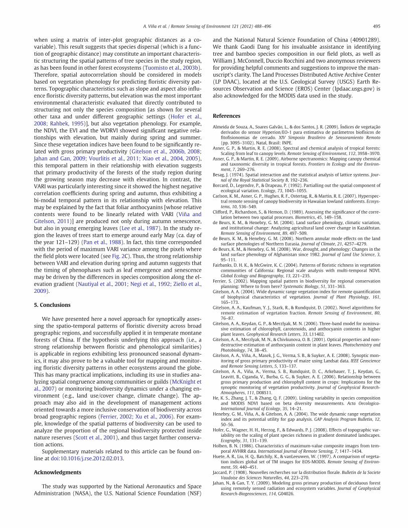
The average temporal variability of the forests studied exhibitedthe typical seasonal pattern of the temperate region (i.e., high andlow vegetation index values during seasons with high and low sunangles, respectively). This pattern was depicted by the four differentvegetation indices evaluated (Fig. 2A). However, the indices exhibiteddifferent temporal dynamics in the inter-pixel variance among theMODIS pixels where the field plots were located (Fig. 1). For instance,the NDVI exhibited the highest inter-pixel variance during winter andthe lowest during summer, while the EVI exhibited an opposite pat-tern, with the highest variance during summer and the lowest duringwinter (Fig. 2B). The WDRVI exhibited the highest inter-pixel vari-ance during winter and spring, while the VARI exhibited the highestvariance during spring and summer (Fig. 2B). These distinctive pat-terns in the timing of highest and lowest inter-pixel variance showthe particular sensitivities of each vegetation index to differencesamong the forests of the study region throughout the year.

The NDVI, the EVI and the WDRVI exhibited a significant negativecorrelation with elevation during late spring and summer (Fig. 2C). Incontrast, the VARI experienced a significant negative correlation dur-ing spring and autumn (Fig. 2C). Therefore, while the NDVI, the EVIand the WDRVI exhibited unimodal temporal patterns in their rela-tionship with elevation, the VARI exhibited a bi-modal pattern(Fig. 2C).

3.2. Floristic and structural characteristics

As shown by the relationship between phenological patterns andelevation (Fig. 2C), the vegetation of the study region is highly influ-enced by elevation. However, with the exception of canopy closure(Fig. 3A), no statistically significant differences were found in averageforest structural characteristics evaluated along this gradient(Fig. 3B–D). Nevertheless, while at elevations between 1000 and2500 m the species richness did not exhibit a significant trend withelevation, above 2500 m the number of species per plot exhibited asignificant decline (Fig. 3D). Thus, a threshold of significant reductionin species richness was conspicuous at elevations of ca. 2500 m.

With respect to species composition, a total of 115 tree specieswere sampled in the 104 field plots surveyed (see on-line

Supplementary data). The species Quercus aliena, Betula albo-sinensis, Prunus scopulorum, Toxicodendron vernicifluum, and Pinusarmandii were the most widespread (i.e., each occurring in morethan 20% of the plots). Understory bamboo was a particularly con-spicuous feature of the forests in the study region, as it was foundin ca. 82% of the field plots. However, most of the bamboo sampledbelonged to three species: Fargesia qinlingensis (present in ca. 38%of the plots), Bashania fargesii (present in ca. 37% of the plots) andF. dracocephala (present in ca. 11% of the plots). These three specieswere among the most widely distributed in the study region.

3.3. Relationship between floristic and phenological similarities

A strong and significant relationship was found between the sim-ilarity in floristic composition and the similarity in phenology. AllMantel tests performed to assess this relationship showed significant(pb0.001) correlations (Table 2). However, Mantel correlations werehighest using the phenological similarity matrix based on the VARI(Table 2). In addition, Mantel correlations were higher when using in-formation on tree and bamboo species combined, than when onlyusing information on tree species (Table 2). In the case of tree speciesinformation alone (i.e., excluding bamboo), Mantel correlations werehigher when using presence–absence data (i.e., using the Jaccardindex), than when using abundance data (i.e., using the Morisita

Fig. 2. Temporal profiles of the (A) average, (B) standard deviation and (C) Pearson'scorrelation coefficient with elevation, of the four different vegetation indices evaluated(see Table 1), obtained from the pixels where the field plots were located.


index; Table 2). Partial Mantel tests, using geographic distance as aco-variable to account for potential spatial autocorrelation amongfield plots, exhibited higher Mantel correlations in all cases, withthe exception of those using the phenological similarity matrixbased on the NDVI image time series (Table 2).

3.4. Prediction of floristic similarity using phenological similarity

A Non-Metric Multidimensional Scaling (NMDS) ordination pro-cedure was applied to the inter-plot floristic similarity matrixobtained using presence–absence data of tree and bamboo speciescombined (i.e., using the Jaccard index), since this matrix exhibitedthe highest Mantel correlation coefficients with phenological similar-ity matrices (Table 2). The NMDS procedure generated two orthogo-nal axes that represent a two-dimensional floristic space. Patterns inthe distribution of topographic characteristics (i.e., elevation, slopeand aspect) among field plots, together with forest types (i.e., pre-dominantly coniferous, predominantly deciduous broadleaf ormixed coniferous-deciduous) are conspicuous in this floristic space(Fig. 4). For instance, the elevational gradient follows a right–left pat-tern (Fig. 4A), while aspect, expressed as discrete relative soil mois-ture classes (Parker, 1982), follows an upper-right lower-left

pattern in the floristic space (Fig. 4B). Although not as clear, slopetends to show a lower-left, upper-right pattern (Fig. 4C). Finally,while mixed forests exhibited no clear pattern, predominantly conif-erous forests tended to be located towards the upper-left, and pre-dominantly deciduous broadleaf forests tended to be located towardthe lower part of the floristic space (Fig. 4D). However, elevationexhibited the highest effect since the first NMDS axis exhibited a sta-tistically significant (pb0.05) negative linear relation with elevation(Fig. 5A).

A principal components analysis was applied on the image timeseries of the VARI, as the similarity matrix of this index exhibitedthe highest Mantel correlation coefficients with the floristic similaritymatrices (Table 2). We retained the first six principal components,which together explained ca. 99% of the image time series variance.Similar to the NMDS, the first principal component exhibited a statis-tically significant (pb0.05) negative linear relationship with elevation(Fig. 5B). In addition, principal component loadings show differentsensitivities of the VARI index along the year. For instance, the firstprincipal component exhibited high positive loadings along theyear, but particularly during spring and autumn (Fig. 6). Thus, load-ings of this component exhibited a similar bi-modal temporal pattern(albeit with a different sign) as the bi-modal temporal pattern ob-served with elevation (Fig. 2C). This is related to the fact that thefirst principal component of the VARI time series was significantlyand negatively related to elevation (Fig. 5B). The second componentexhibited the highest positive and negative loadings during summerand winter, respectively, while the third component was positivelyrelated with autumn VARI values but negatively related with springvalues (Fig. 6). This reflects the sensitivity of VARI to changes in theforests of the region during these seasons.

Significant linear models to predict floristic similarity (i.e., NMDSaxes) using phenological similarity (i.e., principal component axes)were obtained (Table 3). Thus, phenological ordination axes obtainedusing satellite imagery with a high temporal resolution may be usedas significant predictors of floristic ordination axes obtained usingdata from field surveys. The regression model developed for the firstfloristic NMDS axis was not affected by spatial autocorrelation. Incontrast, the model developed for the second floristic NMDS axisdid exhibit significant spatial autocorrelation (Table 3). Therefore,we developed an ordinary least square regression model in the firstcase, and a spatial autoregressive model in the second case. As thelag coefficient in the spatial autoregressive model was significant(pb0.001; Table 3) while the spatial correlation coefficient in theerror model was not, the spatial lag model was selected as the mostappropriate spatial autoregressive model for our data. In these linear

Fig. 3. Average structural characteristics (A: canopy closure; B: basal area; C: stem den-sity; D: tree species richness) of the forests studied among different elevation ranges.Elevation ranges with different letters exhibit significantly (pb0.01) different structur-al characteristics, as determined by Bonferroni-corrected post-hoc Mann–Whitney Utests. Error bars correspond to 2 SEM.

Table 2Mantel correlation coefficients of the relationship between floristic similarity (usingthe Jaccard index for presence–absence data and the Morisita index for abundancedata) and phenological similarity (using the Euclidean distance with a changed sign)calculated using four vegetation index image time series. Values in parentheses repre-sent the correlation coefficients obtained from partial Mantel tests performed using amatrix of inter-plot geographic distances as a co-variable. All Mantel correlation coef-ficients were significant (pb0.001) based on a Monte Carlo permutation test with999 permutations.

NDVIa

(Euclidean)WDRVIb

(Euclidean)EVIc

(Euclidean)VARId

(Euclidean)

Tree species(Jaccard)

0.152 (0.148) 0.203 (0.208) 0.280 (0.288) 0.255 (0.258)

Tree species(Morisita)

0.140 (0.135) 0.177 (0.181) 0.213 (0.220) 0.235 (0.238)

Tree and bamboospecies (Jaccard)

0.191 (0.187) 0.242 (0.249) 0.307 (0.317) 0.325 (0.331)

a Normalized Difference Vegetation Index.b Wide Dynamic Range Vegetation Index.c Enhanced Vegetation Index.d Visible Atmospherically Resistant Index.


models, the first, third, fourth and sixth principal components weresignificant predictors of the first NMDS axis, while the second andfourth components constituted significant predictors of the secondNMDS axis (Table 3).

Results of the model inversion using the k-fold cross-validationpartitioning design (k=3) showed a statistically significant(pb0.001) Mantel correlation of 0.37. This Mantel correlation wascalculated using the Euclidean distance matrix derived from the pre-dicted NMDS axes (using PCA in VARI time series) and the observedJaccard Index matrix derived from the presence/absence of tree andbamboo species observed in the field. Therefore, inter-pixel pheno-logical similarity obtained using the VARI image time series can bereasonably used for assessing floristic similarity.

4. Discussion

The results of this study show that there is a significant relation-ship between floristic similarity and phenological similarity obtainedusing all four vegetation indices evaluated. These results agree with aprevious study showing a significant relationship between MODIS-NDVI time series and species composition (He et al., 2009). However,in this study it was the phenological similarity based on the VARI thatexhibited the highest correlation. Several studies have shown thatVARI is sensitive to changes in the photosynthetic biomass (thus chlo-rophyll content) not only at foliar (Viña and Gitelson, 2011) but alsoat canopy levels using both close range (Gitelson et al., 2002) and re-mote (Almeida de Souza et al., 2009; Perry and Roberts, 2008) sen-sors. But because anthocyanins absorb radiation primarily in thegreen spectral range (i.e., around 540–560 nm), it has been reportedthat vegetation indices using the green spectral region (such asVARI) are sensitive to their presence (Gitelson et al., 2006a, 2001).

Fig. 4. Two-dimensional ordination space derived from a non-metric multidimensional scaling (NMDS) procedure applied to the floristic similarity among 104 field plots, using theJaccard index for the presence–absence of tree and bamboo species. Symbol letters in (A) correspond to different elevation ranges (i.e., a: 1000–1500 m; b: 1500–2000 m; c: 2000–2500 m; d: 2500–3000 m). Symbol numbers in (B) correspond to aspect [converted into soil moisture classes (Parker, 1982), ranging from dry=1 to wet=20]. Symbol letters in(C) correspond to different slope ranges (i.e., A: b10°; B: 11–20°; C: 21–30°; D: >30°). Symbol letters in (D) correspond to different forest types (i.e., D: predominantly deciduousbroadleaf; M: mixed coniferous–deciduous; C: predominantly coniferous).

Fig. 5. Linear regressions of (A) axis 1 of the Non-Metric Multidimensional Scaling(NMDS) procedure applied to the floristic similarity among 104 field plots, using theJaccard index for the presence–absence of tree and bamboo species, and (B) first com-ponent of the principal component analysis (PCA) applied to 46 eight-day maximumvalue composite image time series of the Visible Atmospherically Resistant Index(VARI), vs. elevation. Regression lines are significant (pb0.05) after accounting for spa-tial autocorrelation (Clifford et al., 1989).


Furthermore, it has been reported that VARI is a suitable surrogate ofthe relative composition of foliar anthocyanins in at least five treespecies (Viña and Gitelson, 2011). Therefore, while changes in othercanopy components may also be important, changes in pigment con-tent and composition are important drivers of the seasonal variabilityof VARI.

Previous studies have found that information on the amount andcomposition of foliar pigments can be used to assess floristic diversity(Asner and Martin, 2008, 2009; Carlson et al., 2007). The results ofthis study suggest that information on the seasonal variability of pig-ment content and composition, using metrics such as VARI, may

improve this assessment. In addition, as VARI can be easily obtainedusing currently operational satellites, it allows evaluating floristic di-versity patterns across broad geographic regions. Nevertheless, a fun-damental assumption in these analyses was that the sampled foreststands are homogeneous, at least within each of the MODIS pixelsevaluated. Thus, the species composition in each field plot was as-sumed to be representative of the entire MODIS pixel. The strongand significant relationship found between floristic and phenologicalsimilarities suggests that this assumption was satisfactory. However,floristic similarity based on presence–absence data (i.e., using the Jac-card similarity index) exhibited a stronger correlation with phenolog-ical similarity than the similarity obtained based on abundance (i.e.,stem density) data (i.e., using the Morisita similarity index). These re-sults seem to relate to the scale mismatch between field plots andMODIS pixels, since the species present in a field plot may be repre-sentative of the entire MODIS pixel, but relative species abundanceper plot may not fully represent that of the entire pixel. In addition,higher correlations between floristic and phenological similaritieswere obtained using both tree and bamboo species composition,than when using tree species alone. Thus, bamboo species, whichare conspicuously dominant understory components in the forestsof the region, strongly contribute to the overall spectral and pheno-logical characteristics of the forest canopy (Tuanmu et al., 2010;Viña et al., 2008). The use of phenological similarity to evaluate spa-tial patterns of floristic diversity, therefore, provides information onboth overstory and understory canopy components. This may also ex-plain why vegetation phenology can be successfully used for identify-ing the occurrence of understory bamboo species growing below thecanopy of trees (Tuanmu et al., 2010).

Environmental characteristics influence not only the patterns offloristic diversity and vegetation phenology but also their relation-ship. For instance, the geographic distance among plots had a signifi-cant effect on the relationship between floristic and phenologicalsimilarities (e.g., partial Mantel correlations tended to be higher

Fig. 6. Principal component (PC) loadings (which indicate the correlation of each component with members of the original image time series) of the first six principal componentsobtained from the eight-day maximum value composite image time series (46 images) of the Visible Atmospherically Resistant Index (VARI).

Table 3Coefficients of the multiple linear regression models between the Non-Metric Multidi-mensional Scaling (NMDS) axes (dependent variables) obtained from the floristic sim-ilarity (Jaccard index for presence–absence of tree and bamboo species) among 104field plots, and the first six principal components (PC) obtained from 46 eight-daymaximum value composite image time series of the Visible Atmospherically ResistantIndex (VARI). Values in parentheses represent standard errors of model coefficients.

Variable NMDS axis 1 NMDS axis 2

OLS (SE) SAR (SE)

Intercept −0.0004 (0.0033) −0.0004 (0.0035)PC1 0.1943§ (0.0126) −0.0194 (0.0132)PC2 0.0454 (0.0250) −0.1403§ (0.0292)PC3 −0.1692† (0.0693) −0.0710 (0.0727)PC4 0.7582§ (0.0859) 0.2142⁎ (0.0922)PC5 0.0105 (0.1708) −0.2890 (0.1792)PC6 0.9241† (0.2979) −0.2662 (0.3188)Spatial lag N/A 0.4211§ (0.0970)R2 0.7821 0.5235

OLS — ordinary least squares model; SAR — spatial auto-regressive model; SE — stan-dard error.⁎ pb0.05.† pb0.01.§ pb0.001.


when using a matrix of inter-plot geographic distances as a co-variable). This result suggests that species dispersal (which is a func-tion of geographic distance) may constitute an important characteris-tic structuring the spatial patterns of tree species in the study region,as has been found in other forest ecosystems (Tuomisto et al., 2003b).Therefore, spatial autocorrelation should be considered in modelsbased on vegetation phenology for predicting floristic diversity pat-terns. Topographic characteristics such as slope and aspect also influ-ence floristic diversity patterns, but elevation was the most importantenvironmental characteristic evaluated that directly contributed tostructuring not only the species composition [as shown for severalother taxa and under different geographic settings (Hofer et al.,2008; Rahbek, 1995)], but also vegetation phenology. For example,the NDVI, the EVI and the WDRVI showed significant negative rela-tionships with elevation, but mainly during spring and summer.Since these vegetation indices have been found to be significantly re-lated with gross primary productivity (Gitelson et al., 2006b, 2008;Jahan and Gan, 2009; Vourlitis et al., 2011; Xiao et al., 2004, 2005),this temporal pattern in their relationship with elevation suggeststhat primary productivity of the forests of the study region duringthe growing season may decrease with elevation. In contrast, theVARI was particularly interesting since it showed the highest negativecorrelation coefficients during spring and autumn, thus exhibiting abi-modal temporal pattern in its relationship with elevation. Thismay be explained by the fact that foliar anthocyanins [whose relativecontents were found to be linearly related with VARI (Viña andGitelson, 2011)] are produced not only during autumn senescence,but also in young emerging leaves (Lee et al., 1987). In the study re-gion the leaves of trees start to emerge around early May (ca. day ofthe year 121–129) (Pan et al., 1988). In fact, this time correspondedwith the period of maximum VARI variance among the pixels wherethe field plots were located (see Fig. 2C). Thus, the strong relationshipbetween VARI and elevation during spring and autumn suggests thatthe timing of phenophases such as leaf emergence and senescencemay be driven by the differences in species composition along the el-evation gradient (Nautiyal et al., 2001; Negi et al., 1992; Ziello et al.,2009).

5. Conclusions

We have presented here a novel approach for synoptically asses-sing the spatio-temporal patterns of floristic diversity across broadgeographic regions, and successfully applied it in temperate montaneforests of China. If the hypothesis underlying this approach (i.e., astrong relationship between floristic and phenological similarities)is applicable in regions exhibiting less pronounced seasonal dynam-ics, it may also prove to be a valuable tool for mapping and monitor-ing floristic diversity patterns in other ecosystems around the globe.This has many practical implications, including its use in studies ana-lyzing spatial congruence among communities or guilds (McKnight etal., 2007) or monitoring biodiversity dynamics under a changing en-vironment (e.g., land use/cover change, climate change). The ap-proach may also aid in the development of management actionsoriented towards a more inclusive conservation of biodiversity acrossbroad geographic regions (Ferrier, 2002; Xu et al., 2006). For exam-ple, knowledge of the spatial patterns of biodiversity can be used toanalyze the proportion of the regional biodiversity protected insidenature reserves (Scott et al., 2001), and thus target further conserva-tion actions.

Supplementary materials related to this article can be found on-line at doi:10.1016/j.rse.2012.02.013.

Acknowledgments

The study was supported by the National Aeronautics and SpaceAdministration (NASA), the U.S. National Science Foundation (NSF)

and the National Natural Science Foundation of China (40901289).We thank Gaodi Dang for his invaluable assistance in identifyingtree and bamboo species composition in our field plots, as well asWilliam J. McConnell, Duccio Rocchini and two anonymous reviewersfor providing helpful comments and suggestions to improve the man-uscript's clarity. The Land Processes Distributed Active Archive Center(LP DAAC), located at the U.S. Geological Survey (USGS) Earth Re-sources Observation and Science (EROS) Center (lpdaac.usgs.gov) isalso acknowledged for the MODIS data used in the study.

References

Almeida de Souza, A., Soares Galvão, L., & dos Santos, J. R. (2009). Índices de vegetaçãoderivados do sensor Hyperion/EO-1 para estimativa de parâmetros biofísicos defitofisionomias de cerrado. XIV Simposio Brasileiro de Sensoramiento Remoto(pp. 3095–3102). Natal, Brasil: INPE.

Asner, G. P., & Martin, R. E. (2008). Spectral and chemical analysis of tropical forests:Scaling from leaf to canopy levels. Remote Sensing of Environment, 112, 3958–3970.

Asner, G. P., & Martin, R. E. (2009). Airborne spectranomics: Mapping canopy chemicaland taxonomic diversity in tropical forests. Frontiers in Ecology and the Environ-ment, 7, 269–276.

Besag, J. (1974). Spatial interaction and the statistical analysis of lattice systems. Jour-nal of the Royal Statistical Society B, 192–236.

Borcard, D., Legendre, P., & Drapeau, P. (1992). Partialling out the spatial component ofecological variation. Ecology, 73, 1045–1055.

Carlson, K. M., Asner, G. P., Hughes, R. F., Ostertag, R., & Martin, R. E. (2007). Hyperspec-tral remote sensing of canopy biodiversity in Hawaiian lowland rainforests. Ecosys-tems, 10, 536–549.

Clifford, P., Richardson, S., & Hemon, D. (1989). Assessing the significance of the corre-lation between two spatial processes. Biometrics, 45, 149–158.

de Beurs, K. M., & Henebry, G. M. (2004). Land surface phenology, climatic variation,and institutional change: Analyzing agricultural land cover change in Kazakhstan.Remote Sensing of Environment, 89, 497–509.

de Beurs, K. M., & Henebry, G. M. (2008). Northern annular mode effects on the landsurface phenologies of Northern Eurasia. Journal of Climate, 21, 4257–4279.

de Beurs, K. M., & Henebry, G. M. (2008). War, drought, and phenology: Changes in theland surface phenology of Afghanistan since 1982. Journal of Land Use Science, 3,95–111.

Fairbanks, D. H. K., & McGwire, K. C. (2004). Patterns of floristic richness in vegetationcommunities of California: Regional scale analysis with multi-temporal NDVI.Global Ecology and Biogeography, 13, 221–235.

Ferrier, S. (2002). Mapping spatial pattern in biodiversity for regional conservationplanning: Where to from here? Systematic Biology, 51, 331–363.

Gitelson, A. A. (2004). Wide dynamic range vegetation index for remote quantificationof biophysical characteristics of vegetation. Journal of Plant Physiology, 161,165–173.

Gitelson, A. A., Kaufman, Y. J., Stark, R., & Rundquist, D. (2002). Novel algorithms forremote estimation of vegetation fraction. Remote Sensing of Environment, 80,76–87.

Gitelson, A. A., Keydan, G. P., & Merzlyak, M. N. (2006). Three-band model for noninva-sive estimation of chlorophyll, carotenoids, and anthocyanin contents in higherplant leaves. Geophysical Research Letters, 33, L11402.

Gitelson, A. A., Merzlyak, M. N., & Chivkunova, O. B. (2001). Optical properties and non-destructive estimation of anthocyanin content in plant leaves. Photochemistry andPhotobiology, 74, 38–45.

Gitelson, A. A., Viña, A., Masek, J. G., Verma, S. B., & Suyker, A. E. (2008). Synoptic mon-itoring of gross primary productivity of maize using Landsat data. IEEE Geoscienceand Remote Sensing Letters, 5, 133–137.

Gitelson, A. A., Viña, A., Verma, S. B., Rundquist, D. C., Arkebauer, T. J., Keydan, G.,Leavitt, B., Ciganda, V., Burba, G. G., & Suyker, A. E. (2006). Relationship betweengross primary production and chlorophyll content in crops: Implications for thesynoptic monitoring of vegetation productivity. Journal of Geophysical Research-Atmospheres, 111, D08S11.

He, K. S., Zhang, J. T., & Zhang, Q. F. (2009). Linking variability in species compositionand MODIS NDVI based on beta diversity measurements. Acta Oecologica-International Journal of Ecology, 35, 14–21.

Henebry, G. M., Viña, A., & Gitelson, A. A. (2004). The wide dynamic range vegetationindex and its potential utility for gap analysis. GAP Analysis Program Bulletin, 12,50–56.

Hofer, G., Wagner, H. H., Herzog, F., & Edwards, P. J. (2008). Effects of topographic var-iability on the scaling of plant species richness in gradient dominated landscapes.Ecography, 31, 131–139.

Holben, B. N. (1986). Characteristics of maximum-value composite images from tem-poral AVHRR data. International Journal of Remote Sensing, 7, 1417–1434.

Huete, A. R., Liu, H. Q., Batchily, K., & vanLeeuwen, W. (1997). A comparison of vegeta-tion indices global set of TM images for EOS-MODIS. Remote Sensing of Environ-ment, 59, 440–451.

Jaccard, P. (1908). Nouvelles recherches sur la distribution florale. Bulletin de la SocieteVaudoise des Sciences Naturelles, 44, 223–270.

Jahan, N., & Gan, T. Y. (2009). Modeling gross primary production of deciduous forestusing remotely sensed radiation and ecosystem variables. Journal of GeophysicalResearch-Biogeosciences, 114, G04026.


Kohavi, R. (1995). A study of cross-validation and bootstrap for accuracy estimation andmodel selection. In C. S. Mellish (Ed.), International joint conference on artificial intel-ligence (IJCAI) (pp. 1137–1143). Montreal, Quebec, Canada: Morgan Kaufmann, LosAltos, CA.

Laurent, E. J., Shi, H. J., Gatziolis, D., LeBouton, J. P., Walters, M. B., & Liu, J. (2005). Usingthe spatial and spectral precision of satellite imagery to predict wildlife occurrencepatterns. Remote Sensing of Environment, 97, 249–262.

Lee, D. W., Brammeier, S., & Smith, A. P. (1987). The selective advantages of anthocya-nins in developing leaves of mango and cacao. Biotropica, 19, 40–49.

Legendre, P. (2000). Comparison of permutation methods for the partial correlation andpartial Mantel tests. Journal of Statistical Computation and Simulation, 67, 37–73.

Legendre, P., & Legendre, L. (1998). Numerical ecology. The Netherlands: ElsevierScience.

Lichstein, J. W., Simons, T. R., Shriner, S. A., & Franzreb, K. E. (2002). Spatial autocorre-lation and autoregressive models in ecology. Ecological Monographs, 72, 445–463.

Liu, J., & Ashton, P. S. (1999). Simulating effects of landscape context and timber har-vest on tree species diversity. Ecological Applications, 9, 186–201.

Loucks, C. J., Lu, Z., Dinerstein, E., Wang, D. J., Fu, D. L., & Wang, H. (2003). The giantpandas of the Qinling mountains, China: A case study in designing conservationlandscapes for elevational migrants. Conservation Biology, 17, 558–565.

McKnight, M. W., White, P. S., McDonald, R. I., Lamoreux, J. F., Sechrest, W., Ridgely, R.S., & Stuart, S. N. (2007). Putting beta-diversity on the map: Broad-scale congru-ence and coincidence in the extremes. PLoS Biology, 5, 2424–2432.

Morisette, J. T., Jarnevich, C. S., Ullah, A., Cai, W. J., Pedelty, J. A., Gentle, J. E., Stohlgren, T.J., & Schnase, J. L. (2006). A tamarisk habitat suitability map for the continentalUnited States. Frontiers in Ecology and the Environment, 4, 11–17.

Morisita, M. (1959). Measuring of the dispersion and analysis of distribution patterns.Memoires of the Faculty of Science, Kyushu University, Series E. Biology, 2, 215–235.

Nagendra, H. (2001). Using remote sensing to assess biodiversity. International Journalof Remote Sensing, 22, 2377–2400.

Nautiyal, M. C., Nautiyal, B. P., & Prakash, V. (2001). Phenology and growth from distri-bution in an alpine pasture at Tungnath, Garhwal, Himalaya. Mountain Researchand Development, 21, 168–174.

Negi, G. C. S., Rikhari, H. C., & Singh, S. P. (1992). Phenological features in relation togrowth forms and biomass accumulation in an alpine meadow of the central Hima-laya. Vegetatio, 101, 161–170.

Pan, W., Gao, Z. S., & Lu, Z. (1988). The giant panda's natural refuge in the Qinling moun-tains. Beijing: Beijing University Press.

Parker, A. J. (1982). The topographic relative moisture index: An approach to soil-moisture assessment in mountain terrain. Physical Geography, 3, 160–168.

Perry, E. M., & Roberts, D. A. (2008). Sensitivity of narrow-band and broad-band indicesfor assessing nitrogen availability and water stress in an annual crop. AgronomyJournal, 100, 1211–1219.

Rahbek, C. (1995). The elevational gradient of species richness — a uniform pattern.Ecography, 18, 200–205.

Reid, D. G., & Hu, J. (1991). Giant panda selection between Bashania fangiana bamboohabitats in Wolong reserve, Sichuan, China. Journal of Applied Ecology, 28, 228–243.

Roberts, D. A., Dennison, P. E., Peterson, S., Sweeney, S., & Rechel, J. (2006). Evaluationof airborne visible/infrared imaging spectrometer (AVIRIS) and moderate resolu-tion imaging spectrometer (MODIS) measures of live fuel moisture and fuel condi-tion in a shrubland ecosystem in Southern California. Journal of GeophysicalResearch-Biogeosciences, 111, G01S02.

Rocchini, D. (2007). Distance decay in spectral space in analysing ecosystem beta-diversity. International Journal of Remote Sensing, 28, 2635–2644.

Rocchini, D., Balkenhol, N., Carter, G. A., Foody, G. M., Gillespie, T. W., He, K. S., Kark, S.,Levin, N., Lucas, K., Luoto, M., Nagendra, H., Oldeland, J., Ricotta, C., Southworth, J.,& Neteler, M. (2010). Remotely sensed spectral heterogeneity as a proxy of speciesdiversity: Recent advances and open challenges. Ecological Informatics, 5, 318–329.

Rouse, J. W., Haas, R. H., Schell, J. A., & Deering, D. W. (1973). Monitoring the vernal ad-vancement and retrogradation (green wave effect) of natural vegetation. : CollegeStation, Remote Sensing Center, Texas A&M University.

Savitzky, A., & Golay, M. J. E. (1964). Smoothing and differentiation of data by simpli-fied least squares procedures. Analytical Chemistry, 36, 1627–1639.

Scott, J. M., Davis, F. W., McGhie, R. G., Wright, R. G., Groves, C., & Estes, J. (2001). Naturereserves: Do they capture the full range of America's biological diversity? EcologicalApplications, 11, 999–1007.

Stow, D., Niphadkar, M., & Kaiser, J. (2005). MODIS-derived visible atmospherically re-sistant index for monitoring chaparral moisture content. International Journal ofRemote Sensing, 26, 3867–3873.

Sun, W. X., Liang, S. L., Xu, G., Fang, H. L., & Dickinson, R. (2008). Mapping plant func-tional types fromMODIS data using multisource evidential reasoning. Remote Sens-ing of Environment, 112, 1010–1024.

Thessler, S., Ruokolainen, K., Tuomisto, H., & Tomppo, E. (2005). Mapping graduallandscape-scale floristic changes in Amazonian primary rain forests by combin-ing ordination and remote sensing. Global Ecology and Biogeography, 14,315–325.

Tuanmu, M. -N., Viña, A., Bearer, S., Xu, W., Ouyang, Z., Zhang, H., & Liu, J. (2010). Map-ping understory vegetation using phenological characteristics derived from re-motely sensed data. Remote Sensing of Environment, 114, 1833–1844.

Tuanmu, M. N., Viña, A., Roloff, G. J., Liu, W., Ouyang, Z. Y., Zhang, H. M., & Liu, J. (2011).Temporal transferability of wildlife habitat models: Implications for habitat moni-toring. Journal of Biogeography, 38, 1510–1523.

Tuomisto, H., Poulsen, A. D., Ruokolainen, K., Moran, R. C., Quintana, C., Celi, J., & Canas,G. (2003). Linking floristic patterns with soil heterogeneity and satellite imagery inEcuadorian Amazonia. Ecological Applications, 13, 352–371.

Tuomisto, H., Ruokolainen, K., & Yli-Halla, M. (2003). Dispersal, environment, and flo-ristic variation of Western Amazonian forests. Science, 299, 241–244.

Turner, W., Spector, S., Gardiner, N., Fladeland, M., Sterling, E., & Steininger, M. (2003).Remote sensing for biodiversity science and conservation. Trends in Ecology & Evo-lution, 18, 306–314.

Vermote, E. F., ElSaleous, N., Justice, C. O., Kaufman, Y. J., Privette, J. L., Remer, L., Roger,J. C., & Tanre, D. (1997). Atmospheric correction of visible to middle-infrared EOS-MODIS data over land surfaces: Background, operational algorithm and validation.Journal of Geophysical Research-Atmospheres, 102, 17131–17141.

Viña, A., Bearer, S., Zhang, H., Ouyang, Z., & Liu, J. (2008). Evaluating MODIS data formapping wildlife habitat distribution. Remote Sensing of Environment, 112,2160–2169.

Viña, A., & Gitelson, A. A. (2005). New developments in the remote estimation of thefraction of absorbed photosynthetically active radiation in crops. Geophysical Re-search Letters, 32, L17403.

Viña, A., & Gitelson, A. A. (2011). Sensitivity to foliar anthocyanin content of vegetationindices using green reflectance. IEEE Geoscience and Remote Sensing Letters, 8,464–468.

Viña, A., Gitelson, A. A., Rundquist, D. C., Keydan, G., Leavitt, B., & Schepers, J. (2004).Monitoring maize (Zea mays l.) phenology with remote sensing. Agronomy Journal,96, 1139–1147.

Viña, A., & Henebry, G. M. (2005). Spatio-temporal change analysis to identify anoma-lous variation in the vegetated land surface: ENSO effects in tropical South Amer-ica. Geophysical Research Letters, 32, L21402.

Viña, A., Tuanmu, M. -N., Xu, W., Li, Y., Ouyang, Z., DeFries, R., & Liu, J. (2010). Range-wide analysis of wildlife habitat: Implications for conservation. Biological Conserva-tion, 143, 1960–1969.

Vourlitis, G. L., Lobo, F. D., Zeilhofer, P., & Nogueira, J. D. (2011). Temporal patterns ofnet CO2 exchange for a tropical semideciduous forest of the Southern Amazonbasin. Journal of Geophysical Research-Biogeosciences, 116.

Xiao, X. M., Hagen, S., Zhang, Q. Y., Keller, M., & Moore, B. (2006). Detecting leaf phenol-ogy of seasonally moist tropical forests in South America with multi-temporalMODIS images. Remote Sensing of Environment, 103, 465–473.

Xiao, X. M., Zhang, Q. Y., Braswell, B., Urbanski, S., Boles, S., Wofsy, S., Berrien, M., &Ojima, D. (2004). Modeling gross primary production of temperate deciduousbroadleaf forest using satellite images and climate data. Remote Sensing of Environ-ment, 91, 256–270.

Xiao, X. M., Zhang, Q. Y., Saleska, S., Hutyra, L., De Camargo, P., Wofsy, S., Frolking, S.,Boles, S., Keller, M., & Moore, B. (2005). Satellite-based modeling of gross primaryproduction in a seasonally moist tropical evergreen forest. Remote Sensing of Envi-ronment, 94, 105–122.

Xu, W. H., Ouyang, Z., Viña, A., Zheng, H., Liu, J. G., & Xiao, Y. (2006). Designing a con-servation plan for protecting the habitat for giant pandas in the Qionglai mountainrange, China. Diversity and Distributions, 12, 610–619.

Yue, M., Dang, G. D., & Yong, L. J. (1999). The basic features of vegetation of Foping na-ture reserve in Shaanxi province. Journal of Wuhan Botanical Research, 17, 22–28.

Ziello, C., Estrella, N., Kostova, M., Koch, E., & Menzel, A. (2009). Influence of altitude onphenology of selected plant species in the alpine region (1971–2000). Climate Re-search, 39, 227–234.


Relationship between floristic similarity and vegetated land surface phenology: Implications for the...

Documents

Transcript of Relationship between floristic similarity and vegetated land surface phenology: Implications for the...