Regulation of the Demographic Structure in Isomorphic Biphasic Life Cycles at the Spatial Fine Scale

Regulation of the Demographic Structure in IsomorphicBiphasic Life Cycles at the Spatial Fine ScaleVasco Manuel Nobre de Carvalho da Silva Vieira*, Marcos Duarte Mateus

MARETEC, Instituto Superior Tecnico, Universidade Tecnica de Lisboa, Lisboa, Portugal

Abstract

Isomorphic biphasic algal life cycles often occur in the environment at ploidy abundance ratios (Haploid:Diploid) differentfrom 1. Its spatial variability occurs within populations related to intertidal height and hydrodynamic stress, possiblyreflecting the niche partitioning driven by their diverging adaptation to the environment argued necessary for theirprevalence (evolutionary stability). Demographic models based in matrix algebra were developed to investigate which vitalrates may efficiently generate an H:D variability at a fine spatial resolution. It was also taken into account time variation andtype of life strategy. Ploidy dissimilarities in fecundity rates set an H:D spatial structure miss-fitting the ploidy fitness ratio.The same happened with ploidy dissimilarities in ramet growth whenever reproductive output dominated the populationdemography. Only through ploidy dissimilarities in looping rates (stasis, breakage and clonal growth) did the life cyclerespond to a spatially heterogeneous environment efficiently creating a niche partition. Marginal locations were moresensitive than central locations. Related results have been obtained experimentally and numerically for widely different lifecycles from the plant and animal kingdoms. Spore dispersal smoothed the effects of ploidy dissimilarities in fertility andenhanced the effects of ploidy dissimilarities looping rates. Ploidy dissimilarities in spore dispersal could also create thenecessary niche partition, both over the space and time dimensions, even in spatial homogeneous environments andwithout the need for conditional differentiation of the ramets. Fine scale spatial variability may be the key for the prevalenceof isomorphic biphasic life cycles, which has been neglected so far.

Citation: Vieira VMNdCdS, Mateus MD (2014) Regulation of the Demographic Structure in Isomorphic Biphasic Life Cycles at the Spatial Fine Scale. PLoS ONE 9(3):e92602. doi:10.1371/journal.pone.0092602

Editor: John F. Valentine, Dauphin Island Sea Lab, United States of America

Received June 11, 2013; Accepted February 24, 2014; Published March 21, 2014

Copyright: � 2014 Vieira, Mateus. This is an open-access article distributed under the terms of the Creative Commons Attribution License, which permitsunrestricted use, distribution, and reproduction in any medium, provided the original author and source are credited.

Funding: V.V. was supported by a Ph D grant from the Portuguese Science Foundation (FCT), SFRH/BD/19339/2004/MS47. M.M. was supported by thePortuguese Science Foundation (FCT) program Ciencia2008. www.fct.pt. The funders had no role in study design, data collection and analysis, decision to publish,or preparation of the manuscript.

Competing Interests: The authors have declared that no competing interests exist.

* E-mail: [email protected]

Introduction

Algae species with isomorphic biphasic life cycles have their

alternating haploid and diploid generations cohabiting. The ratio

between the field abundances of these opposite ploidy phases

(H:D, or G:T for Gametophyte:Tetrasporophyte) has long been an

intriguing subject. It would be expected to find balanced

abundances between ploidy phases as a consequence of isomor-

phicity. However, these often are uneven as reported in several

studies [1–7]. The persistency of uneven ploidy phase abundances

may be taken as evidence of niche partitioning. Hughes and Otto

[8] have mathematically proved the necessity for a niche partition

for one of the ploidy phases to not exclude the other, eliminating

the biphasic life cycle and fixing it as a monophasic one. In their

non-spatial model solved for steady-state, the niche partition was

due to conditional differentiation of the ploidy phases and led to a

fixed H:D.

Conditional differentiation means separate entities differen-

tiating the way they adapt to the environment in order to

coexist. Haploids and diploids of isomorphic biphasic life cycles

have shown to possess subtle morphological differences [9],

divergent metabolic rates [10] and distinct biochemical

constitutions [11], besides their well established cytological

differences in spore production (i.e. meiosis vs syngamy). These

characteristics affect the individual vital rates [11–16], which in

algae are commonly classified as fecundity, spore survival,

ramet growth and ramet survival. Furthermore, when a species

focuses its energy budget and demography on a type of vital

rate it is said to have its life strategy dominated by that type.

Conditional differentiation implies that if one ploidy is best

adapted to some circumstances, the other is best adapted to

others. Gonzalez and Meneses [13] observed haploids of the

red algae Chondracanthus chamissoi perform better at spore

settlement and germination whereas the diploids perform

better at drifting spore survival, ramet growth and fecundity.

Pacheco-Ruız et al. [16] observed Chondracanthus squarrulosus

released much more carpospores than tetraspores but the latter

had much higher germination rates. Furthermore, the diploid

ramets responded negatively to high temperatures whereas the

haploid ramets did not.

For any particular location the environment changes season-

ally. Thus, it is expected for the two ploidy phases that

conditionally differentiate to seasonally shift their field domi-

nance, as observed by Dyck and DeWreede [7], Engel et al. [2],

Otaiza et al. [17] and Thornber and Gaines [3]. Nevertheless,

using a theoretical modeling approach, Vieira and Santos [18]

have determined cyclic alternations in phase dominance may

arise as a sole consequence of a ploidy asymmetrical life cycle

structure with fixed ploidy differences in features like size of first

reproduction or maximum frond size. Habitats also change

PLOS ONE | www.plosone.org 1 March 2014 | Volume 9 | Issue 3 | e92602

http://creativecommons.org/licenses/by/4.0/

widely with geographical location and the H:D of a particular

species changes accordingly [3,7]. In another theoretical

modeling study Vieira and Santos [19] have demonstrated the

large geographical variation of the H:D observed by Engel et al.

[2] and Thornber and Gaines [3] could easily be generated by

ploidy dissimilar looping (stasis, breakage and clonal growth)

rates in species with looping dominated life strategies, whereas it

could hardly be generated by ploidy dissimilar fertility rates.

Yet, the spatial variability of the H:D does not occur only at a

large geographical scale between populations clearly set apart

and subject to distinct environments. It has also been

documented within the same population related to intertidal

height, degree of hydrodynamic stress and distance from shore

[2,4,6,7,12,20]. It was the objective of this work to determine

which ploidy differences may induce (more or less efficiently) the

required niche partition at a fine spatial resolution (i.e. intra-

population). Modeling population dynamics with simulated data

were used to investigate the effects of ploidy dissimilarities in

growth and looping of the ramets, in fecundity and in spore

dispersal. The last two do not necessarily result from conditional

differentiation but rather from the differences in haploid and

diploid cytologies [21–23].

Methods

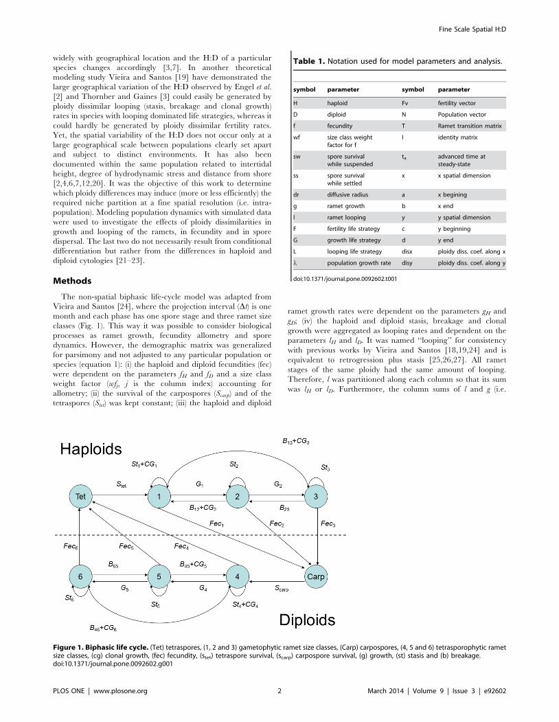
The non-spatial biphasic life-cycle model was adapted from

Vieira and Santos [24], where the projection interval (Dt) is one

month and each phase has one spore stage and three ramet size

classes (Fig. 1). This way it was possible to consider biological

processes as ramet growth, fecundity allometry and spore

dynamics. However, the demographic matrix was generalized

for parsimony and not adjusted to any particular population or

species (equation 1): (i) the haploid and diploid fecundities (fec)

were dependent on the parameters fH and fD and a size class

weight factor (wfj, j is the column index) accounting for

allometry; (ii) the survival of the carpospores (Scarp) and of the

tetraspores (Stet) was kept constant; (iii) the haploid and diploid

ramet growth rates were dependent on the parameters gH and

gD; (iv) the haploid and diploid stasis, breakage and clonal

growth were aggregated as looping rates and dependent on the

parameters lH and lD. It was named ‘‘looping’’ for consistency

with previous works by Vieira and Santos [18,19,24] and is

equivalent to retrogression plus stasis [25,26,27]. All ramet

stages of the same ploidy had the same amount of looping.

Therefore, l was partitioned along each column so that its sum

was lH or lD. Furthermore, the column sums of l and g (i.e.

Table 1. Notation used for model parameters and analysis.

symbol parameter symbol parameter

H haploid Fv fertility vector

D diploid N Population vector

f fecundity T Ramet transition matrix

wf size class weightfactor for f

I identity matrix

sw spore survivalwhile suspended

ta advanced time atsteady-state

ss spore survivalwhile settled

x x spatial dimension

dr diffusive radius a x begining

g ramet growth b x end

l ramet looping y y spatial dimension

F fertility life strategy c y beginning

G growth life strategy d y end

L looping life strategy disx ploidy diss. coef. along x

l population growth rate disy ploidy diss. coef. along y

doi:10.1371/journal.pone.0092602.t001

Figure 1. Biphasic life cycle. (Tet) tetraspores, (1, 2 and 3) gametophytic ramet size classes, (Carp) carpospores, (4, 5 and 6) tetrasporophytic rametsize classes, (cg) clonal growth, (fec) fecundity, (stet) tetraspore survival, (scarp) carpospore survival, (g) growth, (st) stasis and (b) breakage.doi:10.1371/journal.pone.0092602.g001

Fine Scale Spatial H:D


survival) could not exceed 1. Table 1 shows the notation used

for the model parameters and analysis.

0 0 0 0 0 fD:wfj fD:wfj fD:wfj

Stet lH lH=4lH=8 0 0 0 0

0 gH3lH=4

lH=8 0 0 0 0

0 0 gH6lH=8 0 0 0 0

0 fH :wfj fH :wfj fH :wfj 0 0 0 0

0 0 0 0 Scarp lD lD=4lD=8

0 0 0 0 0 gD3lD=4

lD=8

0 0 0 0 0 0 gD6lD=8

266666666666666666664

377777777777777777775

|

0Tet:0

010

020

030

0Carp:0

040

050

060

2666666666666666664

3777777777777777775

ðeqn1Þ

Spatial discretization was inserted assuming a population

scattered over a grid defined by two orthogonal axes. The x

dimension was evaluated from point ‘a’ to ‘b’ at intervals of Dx

whereas the y dimension was evaluated from point ‘c’ to ‘d’ at

intervals of Dy. These axis are scalars, meaning that they are

unitless. The fundamental aspect is that space discretization is

unitless throughout this work, thus providing the possibility to

choose the most suited units for each particular case. Typically

these units are within meters to decameters. A demographic

matrix was estimated for each point with its specific ploidy

dissimilarities for fecundity (f), growth (g) and looping (l) rates.

These dissimilarities were tested according to two different

hypotheses:

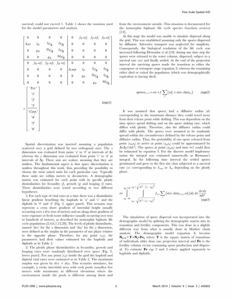
1) For each type of vital rates at a time there was a dissimilarity

linear gradient benefiting the haploids in ‘a’ and ‘c’ and the

diploids in ‘b’ and ‘d’ (Fig. 2, upper panel). This scenario may

represent a cross shore gradient of intertidal height (usually

occurring over a few tens of meters) and an along shore gradient of

wave exposure or fresh water influence (usually occurring over tens

to hundreds of meters), as described for isomorphic biphasic life

cycle populations [2,4,6,7,12,28]. The levels of ploidy dissimilarity,

named ‘disx’ for the x dimension and ‘disy’ for the y dimension,

were defined as the surplus in the parameter of one phase relative

to the opposite phase. Therefore, for any point (x,y), the

parameters had their values estimated for the haploids and

diploids as in Table 2.

2) The ploidy phase dissimilarities in fecundity, growth and

looping rates were randomly distributed over space (Fig. 2,

lower panel). For any point (x,y) inside the grid the haploid and

diploid vital rates were estimated as in Table 2. The maximum

surplus was given by disx 6 disy. This scenario simulates, for

example, a rocky intertidal area with rock pools (usuallya few

meters wide maximum) at different elevations where the

environment inside the pools is different among them and

from the environment outside. This situation is documented for

the isomorphic biphasic life cycle species Gracilaria verrucosa

[12].

At this stage the model was unable to simulate dispersal along

the grid. This was established assuming only the spores dispersed

by diffusion. Advective transport was neglected for simplicity.

Consequently, the biological resolution of the life cycle was

increased following Destombe et al [10]: during one time step the

spores were released to the water column, dispersed, subject to a

survival rate (sw) and finally settled. At the end of the projection

interval the surviving spores made the transition to either the

carpospore or tetraspore stage (equation 2) whereas the remaining

either died or exited the population (which was demographically

equivalent to having died):

sporestz1~sw|fX

j

wfj|size classj,t

� �ðeqn2Þ

It was assumed that spores had a diffusive radius (dr)

corresponding to the maximum distance they could travel away

from their release point while drifting. This was dependent on the

time spores spend drifting and on the spore sinking rate, which

differs with ploidy. Therefore, also the diffusive radius could

differ with ploidy. The spores were assumed to be randomly

spread within the circumference defined by the release point and

diffusive radius. Thus, the probability of one spore released from

point (x0,y0) to arrive at point (xp,yp) could be approximated by

DxDy/(pdr2). The spores at point (x0,y0) and time t+1 could then

be estimated by equation 3. For the discrete model implemen-

tation the integral was estimated numerically as Riemann’s

integral. In the following time interval the settled spores

germinated and grew to the first size class subjected to a survival

rate (ss) corresponding to Scarp or Stet depending on the ploidy

phase.

sw

ðx0zdr

x0{dr

ðy0z

ffiffiffiffiffiffiffiffiffiffiffiffiffiffiffiffiffiffiffiffiffiffiffiffidr2{ x{x0ð Þ2

q

y0{

ffiffiffiffiffiffiffiffiffiffiffiffiffiffiffiffiffiffiffiffiffiffiffiffidr2{ x{x0ð Þ2

q fx,y

Xj

size classj,x,y,twfj

� �dy dx

DxDy

pdr2

ðeqn3Þ

The simulation of spore dispersal was incorporated into the

demographic model by splitting the demographic matrix into its

transition and fertility components. This was done in a slightly

different way from what is usually done in Markov chain

analysis. The demographic model (equation 4) became

Nt+1 = T6Nt+Fvt where T is the square matrix of transitions

of individuals older than one projection interval and Fv is the

fertility column vector containing spore production and dispers-

al. To estimate Fv eqs 2 and 3 where applied separately to

haploids and diploids.

(eqn1)

---------------------------------------------------------

------

---------------------------------



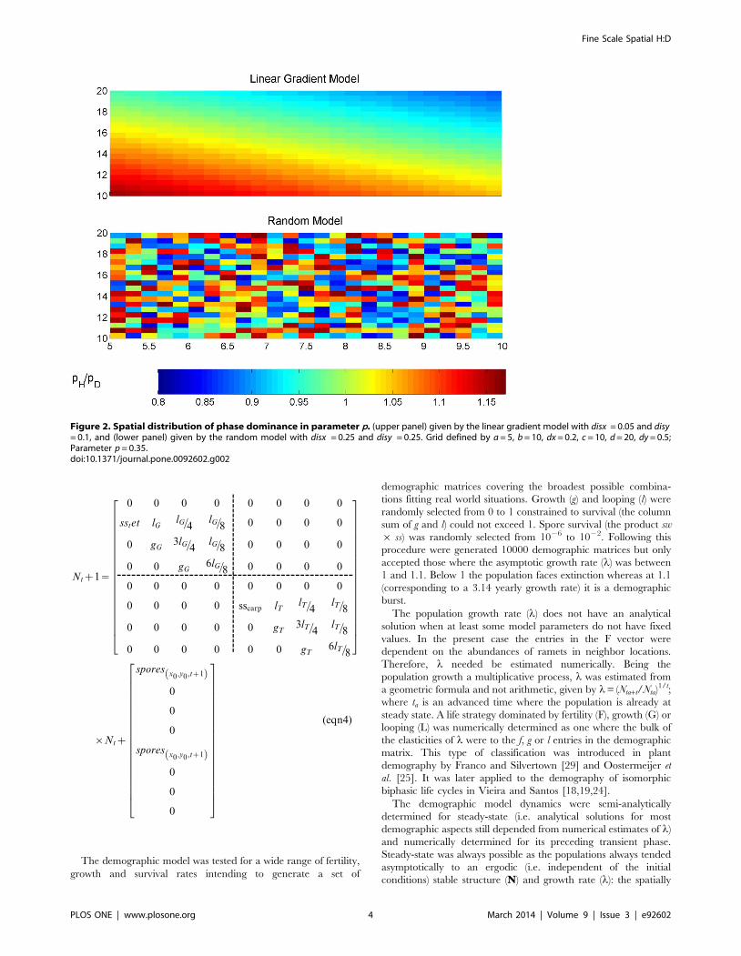
Ntz1~

0 0 0 0 0 0 0 0

sstet lG lG=4lG=8 0 0 0 0

0 gG3lG=4

lG=8 0 0 0 0

0 0 gG6lG=8 0 0 0 0

0 0 0 0 0 0 0 0

0 0 0 0 sscarp lT lT=4lT=8

0 0 0 0 0 gT3lT=4

lT=8

0 0 0 0 0 0 gT6lT=8

26666666666666666664

37777777777777777775

|Ntz

spores x0,y0,tz1ð Þ0

0

0

spores x0,y0,tz1ð Þ0

0

0

26666666666666666664

37777777777777777775

ðeqn4Þ

The demographic model was tested for a wide range of fertility,

growth and survival rates intending to generate a set of

demographic matrices covering the broadest possible combina-

tions fitting real world situations. Growth (g) and looping (l) were

randomly selected from 0 to 1 constrained to survival (the column

sum of g and l) could not exceed 1. Spore survival (the product sw

6 ss) was randomly selected from 1026 to 1022. Following this

procedure were generated 10000 demographic matrices but only

accepted those where the asymptotic growth rate (l) was between

1 and 1.1. Below 1 the population faces extinction whereas at 1.1

(corresponding to a 3.14 yearly growth rate) it is a demographic

burst.

The population growth rate (l) does not have an analytical

solution when at least some model parameters do not have fixed

values. In the present case the entries in the F vector were

dependent on the abundances of ramets in neighbor locations.

Therefore, l needed be estimated numerically. Being the

population growth a multiplicative process, l was estimated from

a geometric formula and not arithmetic, given by l= (Nta+t/Nta)1/t;

where ta is an advanced time where the population is already at

steady state. A life strategy dominated by fertility (F), growth (G) or

looping (L) was numerically determined as one where the bulk of

the elasticities of l were to the f, g or l entries in the demographic

matrix. This type of classification was introduced in plant

demography by Franco and Silvertown [29] and Oostermeijer et

al. [25]. It was later applied to the demography of isomorphic

biphasic life cycles in Vieira and Santos [18,19,24].

The demographic model dynamics were semi-analytically

determined for steady-state (i.e. analytical solutions for most

demographic aspects still depended from numerical estimates of l)

and numerically determined for its preceding transient phase.

Steady-state was always possible as the populations always tended

asymptotically to an ergodic (i.e. independent of the initial

conditions) stable structure (N) and growth rate (l): the spatially

Figure 2. Spatial distribution of phase dominance in parameter p. (upper panel) given by the linear gradient model with disx = 0.05 and disy= 0.1, and (lower panel) given by the random model with disx = 0.25 and disy = 0.25. Grid defined by a = 5, b = 10, dx = 0.2, c = 10, d = 20, dy = 0.5;Parameter p = 0.35.doi:10.1371/journal.pone.0092602.g002

(eqn4)

-------------------------------------------------

---------------------------------



explicit population model could be alternatively written as one

single demographic matrix with a main diagonal of blocks (with a

specific T for each location in each block) whereas the upper and

lower triangles would have the blocks with the specific spore

migration between pair-wise locations. This matrix is irreducible

and primitive according to the Perron-Frobenius theorem, having

a dominant eigenvalue which sets the asymptotic growth rate and

an associated eigenvector which sets the asymptotic population

structure [30]. Following the model presented in equation 4 at any

point (x0,y0) inside the population grid it was possible to determine

a semi-analytical solution to the stable population structure

(equation 5):

N x0,y0,tað Þ~ limt?z?

N x0,y0,tztað Þlt

~l{1inv I{Tx0,y0ð Þl

{1� �

Fvx0,y0,tað Þ ðeqn5Þ

where the Fv and N vectors are standardized to the population

size at time ta and I is the identity matrix. Eqn. 5 has affinity with

the Lotka’s integral equation for the instantaneous growth rate r,

Volterra’s integral equations and the McKendrick-von Forster

models. Its deduction is available in Appendix S1. The maternity

or birth functions integrate Fv and include immigrant spores.

There are many estimates of vital rates from natural populations

and/or artificial cultures. Some of these works focus on particular

rates ignoring the simulation of a full life cycle [12,13,14,16].

Others allow a full cycle simulation [2,22] but relate to largely

different model structures disabling any honest fit to the present

model. Incompatibilities include (i) one year projection intervals,

(ii) haploids split into males and females, and (iii) absence of size

classes turning ramet growth rates undetermined. The model was

tested with the Gelidium sesquipedale’s vital rates previously estimated

by Santos and Duarte [9] and Santos and Nyman [1] and

summarized in Vieira and Santos [24]. These neglected differ-

ences between ploidies when estimating the growth and looping

rates. However, Carmona and Santos [10] found growth of re-

attached diploid fronds to be about 1.2 times that of haploid

fronds. The G. sesquipedale matrix T was adapted accordingly

(equation 6). Carmona and Santos [10] also found reproductive

structures releasing carpospores for twice as much time as

tetraspores. This was consistent with the previous works estimating

haploid fertility about twice as high. Thus, the model was tested

with f = 7000 and wf = [0 0 2 4 0 0 1 2]. Furthermore, Carmona

and Santos [10] found temperature dependent ploidy dissimilar-

ities in spore attachment and germination, benefiting opposite

ploidies in winter and summer extremes. At 13uC carpospores

attached to the substrate about twice as better as the tetraspores,

whereas at 21uC it was the opposite situation. Although this

represents a seasonal variability it was decided to convert this data

to a spatial variability and test it as merely an indicative of the

potential effects of such ploidy dissimilarities. This was done post-

multiplying the carpospores and tetraspores in the F vector by a

0.5 attachment rate and simulating its spatial evolution accord-

ingly to the linear gradient model (in Table 2) with disx = 1.

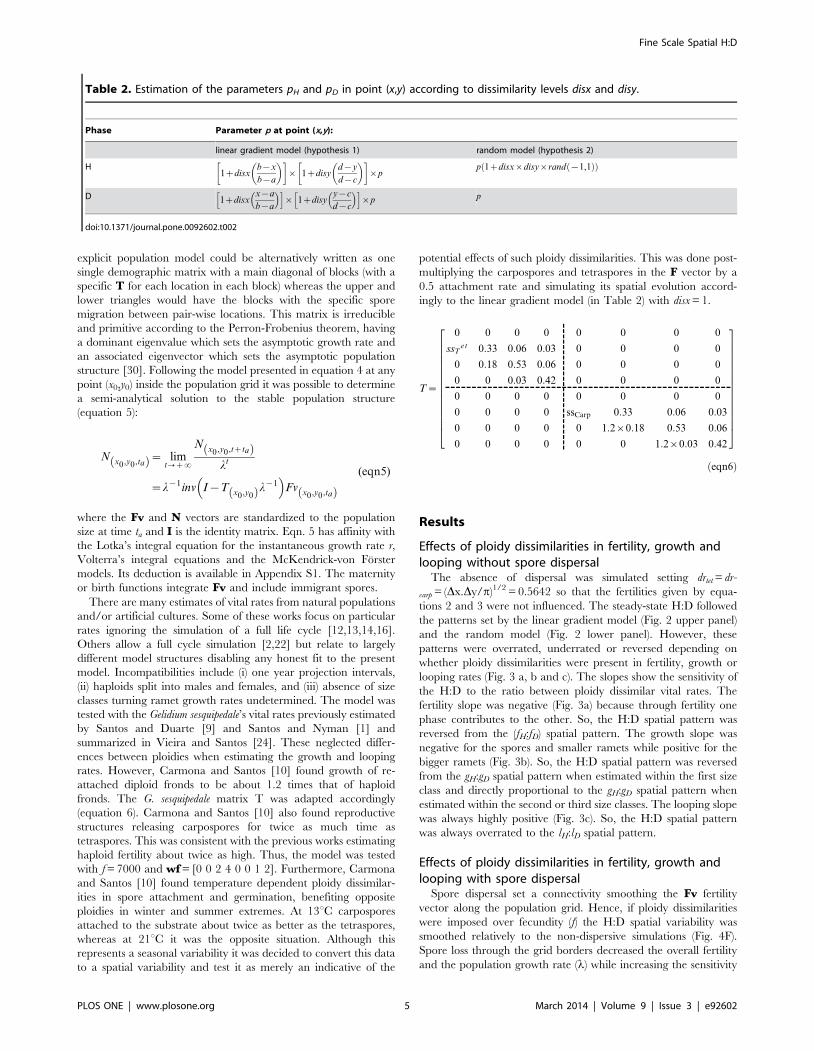
T~

0 0 0 0 0 0 0 0

ssTet 0:33 0:06 0:03 0 0 0 0

0 0:18 0:53 0:06 0 0 0 0

0 0 0:03 0:42 0 0 0 0

0 0 0 0 0 0 0 0

0 0 0 0 ssCarp 0:33 0:06 0:03

0 0 0 0 0 1:2|0:18 0:53 0:06

0 0 0 0 0 0 1:2|0:03 0:42

266666666666664

377777777777775

ðeqn6Þ

Results

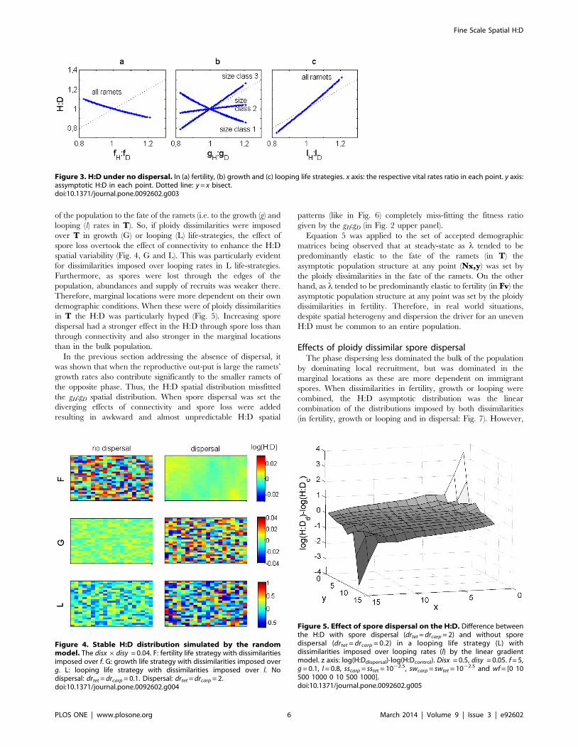
Effects of ploidy dissimilarities in fertility, growth andlooping without spore dispersal

The absence of dispersal was simulated setting drtet = dr-

carp = (Dx.Dy/p)1/2 = 0.5642 so that the fertilities given by equa-

tions 2 and 3 were not influenced. The steady-state H:D followed

the patterns set by the linear gradient model (Fig. 2 upper panel)

and the random model (Fig. 2 lower panel). However, these

patterns were overrated, underrated or reversed depending on

whether ploidy dissimilarities were present in fertility, growth or

looping rates (Fig. 3 a, b and c). The slopes show the sensitivity of

the H:D to the ratio between ploidy dissimilar vital rates. The

fertility slope was negative (Fig. 3a) because through fertility one

phase contributes to the other. So, the H:D spatial pattern was

reversed from the (fH:fD) spatial pattern. The growth slope was

negative for the spores and smaller ramets while positive for the

bigger ramets (Fig. 3b). So, the H:D spatial pattern was reversed

from the gH:gD spatial pattern when estimated within the first size

class and directly proportional to the gH:gD spatial pattern when

estimated within the second or third size classes. The looping slope

was always highly positive (Fig. 3c). So, the H:D spatial pattern

was always overrated to the lH:lD spatial pattern.

Effects of ploidy dissimilarities in fertility, growth andlooping with spore dispersal

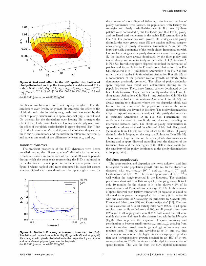
Spore dispersal set a connectivity smoothing the Fv fertility

vector along the population grid. Hence, if ploidy dissimilarities

were imposed over fecundity (f) the H:D spatial variability was

smoothed relatively to the non-dispersive simulations (Fig. 4F).

Spore loss through the grid borders decreased the overall fertility

and the population growth rate (l) while increasing the sensitivity

Table 2. Estimation of the parameters pH and pD in point (x,y) according to dissimilarity levels disx and disy.

Phase Parameter p at point (x,y):

linear gradient model (hypothesis 1) random model (hypothesis 2)

H1zdisx

b{x

b{a

� � | 1zdisy

d{y

d{c

� � |p

p 1zdisx|disy|rand {1,1ð Þð Þ

D 1zdisxx{a

b{a

� �h i| 1zdisy

y{c

d{c

� �h i|p p

doi:10.1371/journal.pone.0092602.t002

(eqn5)

------------------------------------------------------

------------------------



of the population to the fate of the ramets (i.e. to the growth (g) and

looping (l) rates in T). So, if ploidy dissimilarities were imposed

over T in growth (G) or looping (L) life-strategies, the effect of

spore loss overtook the effect of connectivity to enhance the H:D

spatial variability (Fig. 4, G and L). This was particularly evident

for dissimilarities imposed over looping rates in L life-strategies.

Furthermore, as spores were lost through the edges of the

population, abundances and supply of recruits was weaker there.

Therefore, marginal locations were more dependent on their own

demographic conditions. When these were of ploidy dissimilarities

in T the H:D was particularly hyped (Fig. 5). Increasing spore

dispersal had a stronger effect in the H:D through spore loss than

through connectivity and also stronger in the marginal locations

than in the bulk population.

In the previous section addressing the absence of dispersal, it

was shown that when the reproductive out-put is large the ramets’

growth rates also contribute significantly to the smaller ramets of

the opposite phase. Thus, the H:D spatial distribution missfitted

the gH:gD spatial distribution. When spore dispersal was set the

diverging effects of connectivity and spore loss were added

resulting in awkward and almost unpredictable H:D spatial

patterns (like in Fig. 6) completely miss-fitting the fitness ratio

given by the gH:gD (in Fig. 2 upper panel).

Equation 5 was applied to the set of accepted demographic

matrices being observed that at steady-state as l tended to be

predominantly elastic to the fate of the ramets (in T) the

asymptotic population structure at any point (Nx,y) was set by

the ploidy dissimilarities in the fate of the ramets. On the other

hand, as l tended to be predominantly elastic to fertility (in Fv) the

asymptotic population structure at any point was set by the ploidy

dissimilarities in fertility. Therefore, in real world situations,

despite spatial heterogeny and dispersion the driver for an uneven

H:D must be common to an entire population.

Effects of ploidy dissimilar spore dispersalThe phase dispersing less dominated the bulk of the population

by dominating local recruitment, but was dominated in the

marginal locations as these are more dependent on immigrant

spores. When dissimilarities in fertility, growth or looping were

combined, the H:D asymptotic distribution was the linear

combination of the distributions imposed by both dissimilarities

(in fertility, growth or looping and in dispersal: Fig. 7). However,

Figure 3. H:D under no dispersal. In (a) fertility, (b) growth and (c) looping life strategies. x axis: the respective vital rates ratio in each point. y axis:assymptotic H:D in each point. Dotted line: y = x bisect.doi:10.1371/journal.pone.0092602.g003

Figure 4. Stable H:D distribution simulated by the randommodel. The disx6disy = 0.04. F: fertility life strategy with dissimilaritiesimposed over f. G: growth life strategy with dissimilarities imposed overg. L: looping life strategy with dissimilarities imposed over l. Nodispersal: drtet = drcarp = 0.1. Dispersal: drtet = drcarp = 2.doi:10.1371/journal.pone.0092602.g004

Figure 5. Effect of spore dispersal on the H:D. Difference betweenthe H:D with spore dispersal (drtet = drcarp = 2) and without sporedispersal (drtet = drcarp = 0.2) in a looping life strategy (L) withdissimilarities imposed over looping rates (l) by the linear gradientmodel. z axis: log(H:Ddispersal)-log(H:Dcontrol). Disx = 0.5, disy = 0.05. f = 5,g = 0.1, l = 0.8, sscarp = sstet = 1022.5, swcarp = swtet = 1022.5 and wf = [0 10500 1000 0 10 500 1000].doi:10.1371/journal.pone.0092602.g005



the linear combinations were not equally weighted. For the

simulations over fertility or growth life strategies the effect of the

ploidy dissimilarities in fertility or growth rates was veiled by the

effect of ploidy dissimilarities in spore dispersal (Fig. 7 lines F and

G), whereas for the simulations over looping life strategies the

effect of the ploidy dissimilarities in looping rates largely overcame

the effect of the ploidy dissimilarities in spore dispersal (Fig. 7 line

L). In this L simulation disx and disy were half of what they were in

the F and G simulations and the maximum difference between lHand lD was one tenth of the difference between drcarp and drtet.

Transient dynamicsThe transient properties of the H:D dynamics were better

unveiled testing the ‘‘linear gradient’’ dissimilarity hypothesis.

Results are shown in animations of the initial 60 month periods

during which the color scale representing the H:D is adjusted at

particular times. It was imposed in the same spatial pattern as in

figure 1 where haploid vital rates dominated in lower-left corner

whereas diploid vital rates dominated the upper-right corner. In

the absence of spore dispersal following colonization patches of

ploidy dominance were formed. In populations with fertility life

strategies and ploidy dissimilarities over fertility rates (F) these

patches were dominated by the less fertile (and thus less fit) ploidy

and oscillated until settlement in the stable H:D (Animation A in

File S1). For populations with growth life strategies and ploidy

dissimilarities over growth rates (G) the patches suffered conspic-

uous changes in ploidy dominance (Animation A in File S2)

implying cyclic dominance of the less fit phase. In populations with

looping life strategies with ploidy dissimilarities over looping rates

(L) the patches were always dominated by the fitter ploidy and

tended slowly and monotonically to the stable H:D (Animation A

in File S3). Introducing spore dispersal smoothed the formation of

patches and its oscillation in F simulations (Animation B in File

S1), enhanced it in L simulations (Animation B in File S3) and

turned them irregular in G simulations (Animation B in File S2), as

a consequence of the peculiar role of growth on ploidy phase

dominance previously presented. The effect of ploidy dissimilar

spore dispersal was tested with colonization starting in the

population centre. Then, were formed patches dominated by the

first ploidy to arrive. These patches quickly oscillated in F and G

simulations (Animations C in File S1 and Animation C in File S2)

and slowly evolved in L simulations (Animation C in File S3), but

always tending to a situation where the less dispersive ploidy was

favored in the center of the population whereas the more

dispersive ploidy was favored in its edges. The ploidy dissimilarities

in spore dispersal conjugated evenly with the ploidy dissimilarities

in fecundity (Animation D in File S1). Furthermore, the

oscillations increased in amplitude and duration, revealing an

interaction between both. The effects of ploidy dissimilarities in

spore dispersal overwhelmed the effects of ploidy dissimilar growth

(Animation D in File S2) but were offset by the effects of ploidy

dissimilarities in looping on the long run (Animation D in File S3).

There was a huge interaction between ploidy dissimilarities in

looping and in spore dispersal extending both the duration of the

transient phase and the heterogeny of the H:D at steady-state (i.e.

the sensitivity of the ploidy dominance to the ploidy dissimilarities

in looping rates).

Gelidium sesquipedaleThe spore survival and dispersion rates were unknown and thus

fit to yield realistic population growth rates (l). In the absence of

dispersal, with swtet = swcarp = 1021.8 and sstet = sscarp = 1022 each

location grew at l= 1.028. The overall spore survival of 1023.8 is

well within the range reported in the literature. The transient

phase was short with oscillations quickly damping away. It took

only 10 months for the change in l to be always ,1% of its

current value and 15 months to be always ,0.1%. In the absence

of spore dispersal each fertility component (in equation 2) could be

allocated to its proper demographic matrix entry (in equation 6)

with the elasticities of l following the principles by Caswell [30],

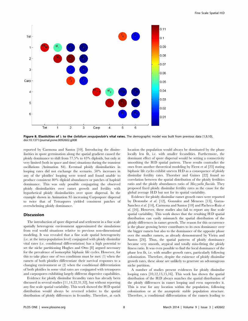
Franco and Silvertown [29] and Oostermeijer et al. [25]. The sum

of the elasticities of l to all fertility rates were 0.206, to all spore

survival rates while settled were 0.206, to all growth rates were

0.235 and to all looping rates were 0.353. Both l and the HD were

mainly elastic to vital rates in the shortest loop within the life cycle

(Fig.8). This loop was the sequence of spores surviving and

germinating to become small ramets (sstet and sscarp), growing from

small to medium sized ramets (g1 and g4), reproducing once

medium sized (f2 and f5) and surviving as so (st2 and st4), thus

extending reproduction. The higher rates of carpospore produc-

tion and tetrasporophyte growth resulted in an HD of 0.736,

corresponding to 57.6% dominance of the diploids irrespective of

space location. This was far from the 80% diploid dominance

Figure 6. Awkward effect in the H:D spatial distribution ofploidy dissimilarities in g. The linear gradient model was used. Colorscale: H:D. disx = 0.2, disy = 0.2, drtet = drcarp = 3, swtet = swcarp = 1021.5,sstet = sscarp = 1022, f = 5, wf = [0 10 500 1000 0 10 500 1000], g = 0.5 andl = 0.1.doi:10.1371/journal.pone.0092602.g006

Figure 7. Stable H:D along a transect from (a,c) to (b,d).Simulations of populations with fertility (F), growth (G) and looping (L)life strategies with ploidy dissimilarities in the respective f, g and l ratesand in dr. Gametophytes (gam) are the haploids.doi:10.1371/journal.pone.0092602.g007



reported by Carmona and Santos [10]. Introducing the dissim-

ilarities in spore germination along the spatial gradient caused the

ploidy dominance to shift from 77.5% to 43% diploids, but only at

very limited (both in space and time) situations during the transient

oscillations (Animation S4). Eventual ploidy dissimilarities in

looping rates did not exchange the scenario. 50% increases in

any of the ploidies’ looping were tested and found unable to

produce consistent 80% diploid abundances or patches of haploid

dominance. This was only possible conjugating the observed

ploidy dissimilarities over ramet growth and fertility with

hypothetical ploidy dissimilarities over spore dispersal. In the

example shown in Animation S5 increasing Carpospore dispersal

to twice that of Tetraspores yielded consistent patches of

overwhelming ploidy dominance.

Discussion

The introduction of spore dispersal and settlement in a fine scale

spatially heterogenic environment approximated the simulations

from real world situations relative to previous non-dimensional

modeling. It was revealed that a fine scale spatial heterogeneity

(i.e. at the intra-population level) conjugated with ploidy dissimilar

vital rates (i.e. conditional differentiation) has a high potential to

set the niche partitioning Hughes and Otto [8] argued necessary

for the prevalence of isomorphic biphasic life cycles. However, for

this to take place one of two conditions must be met: (1) when the

ramets of both ploidies differentiate their survival responses to a

changing environment or (2) when the conditional differentiation

of both ploidies in some vital rates are conjugated with tetraspores

and carpospores exhibiting largely different dispersive capabilities.

Evidence for ploidy dissimilar fecundity rates has already been

discussed in several studies [11,14,22,31,32], but without reporting

any fine scale spatial variability. This work showed the H:D spatial

distribution would always be reversed relative to the spatial

distribution of ploidy differences in fecundity. Therefore, at each

location the population would always be dominated by the phase

locally less fit, i.e. with smaller fecundities. Furthermore, the

dominant effect of spore dispersal would be setting a connectivity

smoothing the H:D spatial pattern. These results contradict the

ones from another theoretical modeling by Fierst et al [23] stating

biphasic life cycles exhibit uneven H:D as a consequence of ploidy

dissimilar fertility rates. Thornber and Gaines [22] found no

correlation between the spatial distribution of the ploidy fertilities

ratio and the ploidy abundances ratio of Mazzaella flaccida. They

proposed fixed ploidy dissimilar fertility rates as the cause for the

global average H:D but not for its spatial variability.

Evidence for ploidy dissimilar ramet growth rates were reported

by Destombe et al. [12], Gonzalez and Meneses [13], Garza-

Sanchez et al. [14], Carmona and Santos [10] and Pacheco-Ruiz et

al. [16]. However, these studies also fail to report any fine scale

spatial variability. This work shows that the resulting H:D spatial

distribution can easily mismatch the spatial distribution of the

ploidy differences in ramet growth. The reason for this occurrence

is the phase growing better contributes to its own dominance over

the bigger ramets but also to the dominance of the opposite phase

over the smaller ramets, as already demonstrated by Vieira and

Santos [24]. Thus, the spatial patterns of ploidy dominance

became very smooth, atypical and totally miss-fitting the ploidy

fitness ratio. It was even possible to find the local dominance of the

phase less fit, i.e. with smaller growth rates, particularly following

colonization. Therefore, despite the existence of ploidy dissimilar

growth rates, these alone are unlikely to generate an advantageous

niche partition.

A number of studies present evidences for ploidy dissimilar

looping rates [10,12,13,15,16]. This work has shown the spatial

distribution of the H:D always matches the spatial distribution of

the ploidy differences in ramet looping and even supersedes it.

This is true for any location within the population, following

colonization or at the asymptotic stable population structure.

Therefore, a conditional differentiation of the ramets leading to

Figure 8. Elasticities of l to the Gelidium sesquipedale’s vital rates. The demographic model was built from previous data [1,9,10].doi:10.1371/journal.pone.0092602.g008



ploidy dissimilar looping rates are an excellent means for the niche

partition required for the stability and evolution of biphasic life-

cycles [8] and observed at a spatially fine scale [2,4,6,7,12,20]. It is

particularly interesting the shift of phase dominance at a very short

spatial scale (few meters) for populations of Gelidium canarensis in the

stable population structure [20]. The present work suggests such

shifts can hardly be caused by anything else besides ploidy

dissimilar looping rates in populations with survival life strategies.

Barbuti et al. [33] studied the role of sexual reproduction (fertility)

vs asexual reproduction (a looping rate) in the population structure

and dynamics of Carassius gibelio, a cyprinid fish with a life cycle

entirely different from the isomorphic biphasic of some seaweeds.

These authors also found the looping rate to be of utmost

importance by amplifying the locally fitter genotypes. Contrary to

the results by previous non-spatial modeling attempts, ploidy

differences in looping rates need not be balanced by ploidy

differences in some other demographic trait: they are self-balanced

by their fine scale spatial variability. Furthermore, there is a

synergistic effect between eventual ploidy dissimilarities in looping

rates and the fact that spores disperse: with a reasonable amount of

spores inevitably lost from the population through its edges the

peripheral locations become particularly sensitive to the fate of the

ramets and their ploidy dissimilarities. Then, niche partition

becomes particularly evident and effective in these marginal

locations. In a study about the spatial genetic structure of Thuja

occidentalis, a conifer with a life cycle entirely different from the

isomorphic biphasic of some seaweeds, Panday and Rajora [34]

also determined that peripheral populations were much more

heterogenic than the bulk populations.

In the current model the spore dispersal was simulated by giving

it a maximum dispersive range over the projection interval of one

month. With a finer temporal and biological resolution this can be

traced back to the amount of time spores take to settle and their

mortality rates while suspended. Such spore performance has often

been reported to be ploidy dissimilar [10,12,13,14,29,35] and its

effect on an uneven H:D was experimentally demonstrated by

Pacheco-Ruiz et al. [16]. The current work has demonstrated

ploidy dissimilarities in the spores’ ability to disperse can also

create the required niche partition even in spatially homogeneous

environments. Then, in populations with looping life strategies the

H:D patches formed show great constancy, whereas in populations

with fertility or growth life strategies the patches may oscillate

backward and forward at a fast rate. A similar transient behaviour

was obtained in Vieira and Santos [18] for the non-spatial case.

The Gelidium sesquipedale’s estimated demography corresponds to

those predicted by Vieira and Santos [18,24] being approximately

evenly elastic to fertility, growth and looping rates. In these,

individuals flow mainly through the shortest life-cycle loop

generating short period oscillations on both l and the H:D

quickly damping away. Demographic properties like l or the HD

are little elastic to any vital rates thus requiring huge ploidy

dissimilarities, even in looping rates, to yield conspicuous ploidy

field dominances. Therefore it was not surprisingly that the

simulations of the ploidy dissimilarities estimated by Carmona and

Santos [10] were unable to consistently generate the ploidy field

dominance observed by these same authors or a spatial niche

partition. Ranges of spore dispersal are unknown and their

simulation may be a wild guess. Nevertheless, given the cytological

differences between tetraspores and carpospores it is reasonable to

expect them having largely different dispersive abilities. Such

simulations generated patches that although transient exhibited

enormous dominance (sometimes close to 100%) for either ploidy

over wide areas and long periods. Most often diploids dominated

often overcoming the 80% dominance observed by Carmona and

Santos [10]. However, they also generated patches of transient

field dominance by the ploidy locally less fit casting doubts about

the efficiency of conjugating ploidy uneven spore dispersal with

conditional differentiation of the ramets or germinating spores.

Supporting Information

Appendix S1 Analytical solution of the local stablepopulation structure.(DOC)

Animation S1 H:D transient trajectory for a populationwith a F life strategy. Ploidy dissimilarities in the f rates according

to the linear gradient hypothesis. Ploidy even colonization (A, B)

along the entire population or (C, D) on its centre. The colour scale is

log(H:D) and it changes bounds for t.13. (A) with ploidy

dissimilarities in f and without spore dispersal. drcarp = drtet = 0.5,

disx = disy = 0.5, f = 10; (B) with ploidy dissimilarities in f and with

spore dispersal. drcarp = drtet = 5, disx = disy = 0.5, f = 15; (C) with ploidy

dissimilarities only in spore dispersal. drcarp = 3, drtet = 6, disx = disy = 0

and f = 15; (D) with ploidy dissimilarities in f and in spore dispersal.

drcarp = 3, drtet = 6, disx = disy = 0.5 and f = 10; (all) sstet = sscarp = 1021.8,

swtet = swcarp = 1021.2, g = 0.12, l = 0.05, wf = [0 10 500 1000 0 10 500

1000], a = 1, b = 15, c = 1, d = 15 and Dx =Dy = 1.

(AVI)

Animation S2 H:D transient trajectory for a populationwith a G life strategy. Ploidy dissimilarities in the g rates

according to the linear gradient hypothesis. Ploidy even coloni-

zation (A, B) along the entire population or (C, D) on its centre.

The colour scale is log(H:D) and it changes bounds for t.20 and

t.40. (A) with ploidy dissimilarities in g and without spore

dispersal. drcarp = drtet = 0.5, disx = disy = 0.2, f = 3; (B) with ploidy

dissimilarities in g and with spore dispersal. drcarp = drtet = 3,

disx = disy = 0.2, f = 4; (C) with ploidy dissimilarities only in spore

dispersal. drcarp = 3, drtet = 6, disx = disy = 0, f = 5; (D) with ploidy

dissimilarities in g and in spore dispersal. drcarp = 3, drtet = 6,

disx = disy = 0.2, f = 5; (all) sstet = sscarp = 1022, swtet = swcarp = 1021.5,

g = 0.6, l = 0.05, wf = [0 10 500 1000 0 10 500 1000], a = 1, b = 15,

c = 1, d = 15 and Dx =Dy = 1.

(AVI)

Animation S3 H:D transient trajectory for a populationwith a L life strategy. Ploidy dissimilarities in the l rates

according to the linear gradient hypothesis. Ploidy even coloni-

zation (A, B) along the entire population or (C, D) on its centre.

The colour scale is log(H:D) and it changes bounds for t.20 and

t.50. (A) with ploidy dissimilarities in l and without spore

dispersal. drcarp = drtet = 0.5, disx = disy = 0.1, f = 3;.(B) with ploidy

dissimilarities in l and with spore dispersal. drcarp = drtet = 5,

disx = disy = 0.1, f = 3; (C) with ploidy dissimilarities only in spore

dispersal. drcarp = 3, drtet = 6, disx = disy = 0, f = 6; (D) with ploidy

dissimilarities in l and in spore dispersal. drcarp = 3, drtet = 6,

disx = disy = 0.1, f = 5; (all) sstet = sscarp = 1021.8, swtet = sw-

carp = 1021.2, g = 0.02, l = 0.8, wf = [0 10 500 1000 0 10 500

1000], a = 1, b = 15, c = 1, d = 15 and Dx =Dy = 1.

(AVI)

Animation S4 Predicted transient ploidy dominance forG. sesquipedale. Simulation over a 4 year period starting with

ploidy even colonization in 7 random points along the population.

Ploidy dissimilarities in spore attachment simulated according to

the linear gradient hypothesis with disx = 1 and disy = 0.

drcarp = drtet = 2, f = 7000, wf = [0 0 2 4 0 0 1 2], sstet = sscarp = 1022,

swtet = swcarp = 1021.5, Matrix T entries given by equation 6. a = 1,

b = 20, c = 1, d = 20 and Dx =Dy = 1.

(AVI)



Animation S5 Predicted transient ploidy dominance forG. sesquipedale with hypothetical ploidy uneven sporedispersal. Simulation over a 4 year period starting with ploidy

even colonization in 7 random points along the population. Ploidy

dissimilarities in spore attachment simulated according to the

linear gradient hypothesis with disx = 1 and disy = 0. drcarp = 4,

drtet = 2, f = 7000, wf = [0 0 2 4 0 0 1 2], sstet = sscarp = 1022,

swtet = swcarp = 1021.5, Matrix T entries given by equation 6. a = 1,

b = 20, c = 1, d = 20 and Dx =Dy = 1.

(AVI)

Acknowledgments

We would like to acknowledge the anonymous reviewer for its valuable

contribution.

Author Contributions

Conceived and designed the experiments: VV. Performed the experiments:

VV. Analyzed the data: VV MDM. Contributed reagents/materials/

analysis tools: VV. Wrote the paper: VV MDM.

References

1. Santos R, Nyman M (1998) Population modeling of Gelidium sesquipedale

(Rhodophyta, Gelidiales). J Appl Phycol 10: 261–272.2. Engel C, Aberg P, Gaggiotti OE, Destombe C, Valero M (2001) Population

dynamics and stage structure in a haploid-diploid red seaweed, Gracilaria gracilis. JEcol 89:(3) 436–450.

3. Thornber CS, Gaines SD (2003) Spatial and temporal variation of haploids anddiploids in populations of four congeners of the marine alga Mazzaella. Mar Ecol

Prog Ser 258: 65–77.

4. Mudge B, Scrosati R (2003) Effects of wave exposure on the proportion ofgametophytes and tetrasporophytes of Mazzaella oregona (Rhodophyta: Gigar-

tinales) from Pacific Canada. J Mar Biol Assoc UK 83: 701–704.5. Scrosati R, Mudge B (2004) Persistence of gametophyte predominance in

Chondrus crispus (Rhodophyta, Gigartinaceae) from Nova Scotia after 12 years.

Hydrobiologia 519: 215–218.6. Scrosati R, Mudge B (2004). Effects of elevation, wave exposure, and year on the

proportion of gametophytes and tetrasporophytes in Mazzaella parksii (Rhodo-phyta, Gigartinaceae) populations. Hydrobiologia 520: 199–205.

7. Dyck LJ, DeWreede RE (2006) Seasonal and spatial patterns of populationdensity in the marine macroalga Mazzaella splendens (Gigartinales, Rhodophyta).

Phycol Res 54: 21–31.

8. Hughes JS, Otto SP (1999) Ecology and the Evolution of Biphasic Life-cycles.Am Nat 154: 306–320.

9. Santos R, Duarte P (1996) Fecundity, spore recruitment and size in Gelidium

sesquipedale (Gelidiales, Rhodophyta). Hydrobiologia, 326–327: 223–228.

10. Carmona R, Santos R (2006) Is there an ecophysiological explanation for the

gametophyte-tetrasporophyte ratio in Gelidium sesquipedale (Rhodophyta)? J.Phycol 42:(2) 259–269.

11. Thornber C, Stachowicz JJ, Gaines S (2006) Tissue type matters: selectiveherbivory on different life history stages of an isomorphic alga. Ecology 87:

2255–2263.

12. Destombe C, Valero M, Vernet P, Couvet D (1989) What controls haploid-diploid ratio in the red alga, Gracilaria verrucosa? J Evol Biol 2:(5) 317–338.

13. Gonzalez J, Meneses I (1996) Differences in the early stages of development ofgametophytes and tetrasporophytes of Chondracanthus chamissoi (C.Ag.) Kutzing

from Puerto Aldea, northern Chile. Aquaculture 143: 91–107.14. Garza-Sanchez F, Zertuche-Gonzalez JA, Chapman DJ (2000) Effect of

temperature and irradiance on the release, attachment, and survival of spores

of Gracilaria pacifica Abbot (Rhodophyta). Bot Mar 43: 205–212.15. Verges A, Paul NA, Steinberg PD (2008) Sex and life-history stage alter

herbivore responses to a chemically defended red alga. Ecology 89: 1334–1343.16. Pacheco-Ruız I, Cabello-Pasini A, Zertuche-Gonzalez JA, Murray S, Espinoze-

Avalos J, et al. (2011) Carpospore and tetraspore release and survival in

Chondracanthus squarrulosus (Rhodophyta Gigartinaceae) from the Gulf ofCalifornia. Bot Mar 54:(2) 127–134.

17. Otaiza RD, Abades SR, Brante AJ (2001) Seasonal changes in abundance andshifts in dominance of life history stages of the carrageenophyte Sarcothalia crispata

(Rhodophyta, Gigartinales) in south-central Chile. J Appl Phycol 13: 161–71.18. Vieira VMNCS, Santos ROP (2012) Responses of the haploid to diploid ratio of

isomorphic biphasic life cycles to time instability. J Biol Dynam 6(2): 1067–1087.

19. Vieira VMNCS, Santos ROP (2012) Factors that drive the geographical

variability of the haploid:diplod ratio of biphasic life cycles. J Phycol 48: 1012–

1019.

20. Lindgren A, Bouza AN, Aberg P, Sosa PA (1998) Spatial and temporal variation

in distribution of Gelidium canarensis (Rhodophyta) from natural populations of the

Canary Islands. J Appl Phycol 10:(3) 273–278.

21. Scrosati R, DeWreede RE (1999) Demographic models to simulate the stable

ratio between ecologically similar gametophytes and tetrasporophytes in

populations of the Gigartinaceae (Rhodophyta). Phycol Res 47: 153–157.

22. Thornber CS, Gaines SD (2004) Population demographics in species with

biphasic life-cycles. Ecology 85:(6) 1661–1674.

23. Fierst J, terHorst C, Kubler JE, Dudgeon S (2005) Fertilization success can drive

patterns of phase dominance in complex life histories. J Phycol 41(2): 238–249.

24. Vieira VMNCS, Santos ROP (2010) Demographic mechanisms determining the

dynamics of the relative abundance of phases in biphasic life cycles. J Phycol 46:

1128–1137.

25. Oostermeijer JGB, Brugman ML, De Boer ER, Den Nijs HCM (1996)

Temporal and spatial variation in the demography of Gentiana pneumonanthe, a

rare perennial herb. J Ecol 84: 153–166.

26. Rojas-Sandoval J, Melendez-Ackerman E. (2013) Population dynamics of a

threatened cactus species: general assessment and effects of matrix dimension-

ality. Popul Ecol DOI: 10.1007/s10144-013-0378-1.

27. Ehrlen J (1999) Modelling and measuring plant life histories. Life history

evolution in plants. Eds: Vuorisalo TO, Mutikainen PK., Kluwer Academic

Publishers. Dordrecht, the Netherlands. 351pp.

28. Prathep A, Lewmanomont K, Buapet P (2009) Effects of wave exposure on

population and reproductive phenology of an algal turf, Gelidium pusillum

(Gelidiales, Rhodophyta), Songkhla, Thailand. Aquat Bot 90:(2) 179–183.

29. Franco M, Silvertown J (1996) Life history variation in plants: an exploration of

the fast-slow continuum hypothesis. Philos T Roy Soc B 351: 1341–1348.

30. Caswell H (2001) Matrix Population Models: Construction, Analysis and

Interpretation, 2nd ed., Sinauer Associates, Sunderland, Massachusetts, USA.

31. Scrosati R, Garbary DJ, McLachlan J (1994) Reproductive Ecology of Chondrus

crispus (Rhodophyta, Gigartinales) from Nova Scotia, Canada. Bot Mar 37: 293–

300.

32. Serviere-Zaragoza E, Scrosati R (2002) Reproductive Phenology of Pterocladia

capillacea (Rhodophyta: Gelidiales) from Southern Baja California, Mexico. Pac

Sci 56:(3) 285–290.

33. Barbuti R, Mautner S, Carnevale G, Milazzo P, Rama A, et al. (2012)

Population dynamics with a mixed type of sexual and asexual reproduction in a

fluctuating environment. BMC Evol Biol 12:49.

34. Panday M, Rajora OP (2012) Higher fine-scale genetic structure in peripheral

than core populations of a long-lived and mixed-mating conifer - eastern white

cedar (Thuja occidentalis L.) BMC Evol Biol 12:48.

35. Roleda YM, Zacher K, Wulff A, Hanelt D, Wiencke C (2008) Susceptibility of

spores of different ploidy levels from Antartic Gigartina skottsbergii (Gigartinales,

Rhodophyta) to ultraviolet radiation. Phycologia 47:(4) 361–370.



Regulation of the Demographic Structure in Isomorphic Biphasic Life Cycles at the Spatial Fine Scale

Documents

Transcript of Regulation of the Demographic Structure in Isomorphic Biphasic Life Cycles at the Spatial Fine Scale