Public Choice (2013) 157:245–267DOI 10.1007/s11127-012-9943-y

Political budget cycles and election outcomes

Jeroen Klomp · Jakob de Haan

Received: 20 February 2011 / Accepted: 12 April 2012 / Published online: 26 April 2012© The Author(s) 2012. This article is published with open access at Springerlink.com

Abstract This paper addresses two empirical questions. Is fiscal policy affected by up-coming elections? If so, do election-motivated fiscal policies enhance the probability ofre-election of the incumbent? Employing data for 65 democratic countries over 1975–2005in a semi-pooled panel model, we find that in most countries fiscal policy is hardly affectedby elections. The countries for which we find a significant political budget cycle are verydiverse. They include ‘young’ democracies but also ‘established’ democracies. In countrieswith a political budget cycle, election-motivated fiscal policies have a significant positive(but fairly small) effect on the electoral support for the political parties in government.

Keywords Election outcomes · Political budget cycles · Multilevel model

JEL Classification E62 · H62

1 Introduction

This paper addresses two empirical questions. Is fiscal policy affected by upcoming elec-tions? If so, do election-motivated fiscal policies enhance the probability of re-election ofthe incumbent?

As to the first issue: several recent studies suggest that political budget cycles occur, butthere is disagreement about the circumstances making election-motivated budget deficits

J. KlompWageningen University, Wageningen, The Netherlands

J. de HaanUniversity of Groningen, Groningen, The Netherlands

J. de Haan (�)De Nederlandsche Bank, PO Box 98, 1000 AB Amsterdam, The Netherlandse-mail: j.de.haan@dnb.nl

J. de HaanCESifo, Munich, Germany

246 Public Choice (2013) 157:245–267

more likely. For instance, opinions differ as to whether political budget cycles are morelikely in ‘young’ democracies compared to ‘established’ democracies (Persson and Tabellini2002; Shi and Svensson 2006; Brender and Drazen 2005).

It is quite surprising that the second issue has hardly been researched. Brender andDrazen (2008) do not find evidence that election-motivated budget deficits enhance thechances of re-election of the incumbent. In fact, they even report that these deficits reduce theprobability that an incumbent is re-elected as voters punish politicians who create deficits.1

Our analysis is based on data for 65 democratic countries over the period 1975 to 2005.To estimate the impact of election-induced fiscal policy on the incumbent’s support we usea two-step approach. In the first step, we estimate whether elections affect the government’sbudget balance and government spending. Most recent studies on election-motivated fiscalpolicy at the national level use panel models for a large sample of countries, pooling thedata. However, in view of the heterogeneity of the countries included in those studies, it isquestionable whether the data can be pooled (Pesaran et al. 1996). According to Pesaranet al. (1999), neglecting parameter heterogeneity in a pooled panel estimation procedurecan produce inconsistent and misleading estimates of the long-run coefficients. Tests ofheterogeneity indicate that our data cannot be pooled. We therefore use a semi-pooled modelsuggested by Hsiao et al. (1999). In this model, the political budget cycle (PBC) effectvaries across countries, while the other control variables are restricted to be homogenous.Employing an election variable that takes the timing of the election in the course of the yearinto account as suggested by Franzese (2000), we find that fiscal policy in most—but notall—countries in our sample is hardly affected by upcoming elections. The countries forwhich we find a significant political budget cycle are very diverse. They include ‘young’democracies but also ‘established’ democracies.

In the second step of our analysis, we examine for countries with election-motivated fiscalpolicy, whether this PBC increases electoral support for the incumbent. In contrast to Bren-der and Drazen (2008), we take into account that many countries have coalition governments(Hanusch 2012). We therefore focus on votes received by political parties participating inthe government. We conclude that government spending has a significant positive (but fairlysmall) effect on the electoral support for the parties in government. We also find an indirectpositive effect of election-motivated fiscal policy through its impact on economic growth.

The remainder of the paper is structured as follows. The next section discusses in moredetail how our contribution is related to previous studies of political budget cycles and eco-nomic voting. Section 3 shows our results for the influence of elections on fiscal policy,while Sect. 4 presents our estimates of the relationship between political budget cycles andelection outcomes. The final section offers our conclusions.

2 Previous studies

We combine two strands of the political economy literature. The first one addresses theexistence of a political budget cycle. Older theoretical PBC models emphasize the incum-bent’s intention to secure re-election by maximizing his/her expected vote share at the nextelection (Nordhaus 1975). It is assumed that the electorate is backward looking and eval-uates the government on the basis of its past track record. As a result, these models implythat governments, regardless of ideological orientation, adopt expansionary fiscal policies in

1In Sect. 2, we will also discuss some recent studies on the effect of fiscal policy on local election outcomes.

Public Choice (2013) 157:245–267 247

the late year(s) of their terms in office in order to stimulate the economy (Potrafke 2012).More recent PBC models emphasize the role of temporary information asymmetries regard-ing the politicians’ competence level in explaining electoral cycles in fiscal policy. In thesemodels, signalling is the driving force behind the PBC (see, e.g., Rogoff and Sibert 1988;Persson and Tabellini 2002; and Shi and Svensson 2006). For instance, in the moral haz-ard model of political competition of Shi and Svensson (2006), politicians may behaveopportunistically even if most voters know the government’s policy, but some voters areuninformed. The larger is the number of voters that fail (ex ante) to distinguish election-motivated fiscal policy manipulations from incumbent competence, the more the incumbentprofits from boosting expenditures before an election. Alt and Lassen (2006) argue that thegreater is the transparency of the political process, the lower is the probability that politiciansbehave opportunistically. Drazen and Eslava (2006, 2010) explain the relationship betweenopportunistic spending of the government and the election outcome within a game theoreticframework. The incumbent uses public expenditure to attract votes. In equilibrium, expen-ditures targeted to particular voters are higher in an election period than in a non-electionperiod. Swing voters will rationally vote for the incumbent who provides more targetedexpenditures even though they know that such expenditures may be electorally motivated.

Brender and Drazen (2005) argue that until recently a PBC was generally thought tobe a phenomenon of less developed economies. For instance, Schuknecht (1996) reportsevidence for a PBC in his sample of 35 developing countries over the period 1975–1992.Likewise, Block (2002) finds for a cross-section of 44 Sub-Saharan African countries thatthe government’s budget deficit increases by 1.2 percentage points in election years.2 How-ever, several recent studies present evidence for the existence of a PBC in a large cross-section of both advanced and developing countries. For instance, Shi and Svensson (2006)report significant pre-electoral increases in the government budget deficit for their panel of85 developing and advanced countries over the period 1975–1995. Moreover, Persson andTabellini (2002) find statistically significant tax decreases before elections in their sampleof 60 democracies over the period 1960–1998. According to Brender and Drazen (2005),the results of the studies of Shi and Svensson (2006) and Persson and Tabellini (2002) aredriven by the experiences of so-called ‘new democracies’, where fiscal manipulation maybe effective because of the lack of familiarity with electoral politics in these countries. Theyargue that once the ‘new democracies’ are removed from the sample, evidence in support ofthe PBC disappears.

However, several recent studies also focusing on ‘established democracies’ report evi-dence on the existence of a PBC. For instance, Grier (2008) reports that the timing of elec-tions exerts a significant influence on quarterly real GDP growth in the US, while Tujula andWolswijk (2007) find support for a PBC in their sample of OECD countries for the period1975–2002. Mink and De Haan (2006) provide similar evidence for European Union (EU)member states after the start of the monetary union.3 Similarly, Efthyvoulou (2011) reportsfor the 27 EU member states over the period 1997–2008 that incumbent governments tend to

2Similarly, Schuknecht (2000) finds for a sample of twenty-four developing countries over 1973–1992 thatincumbent governments tend to increase public investment prior to elections. Vergne (2009), using data on24 developing countries from 1975 to 2001, reports that elections shift the composition of spending towardscurrent expenditures and away from capital expenditures.3Also several studies of local elections report evidence of a PBC. A recent example is the study of Aidtet al. (2011), who also provide references to previous studies. Aidt et al. use data from 278 Portuguesemunicipalities from 1979 to 2005 and find that the cycle is largest when the need for the incumbent to signalcompetency is at its peak.

248 Public Choice (2013) 157:245–267

manipulate fiscal policy in order to maximize their chances of being re-elected. He finds thatthe relative importance of non-economic issues prior to elections and the uncertainty overthe electoral outcome can to a large extent explain the variability in the sizes of PBCs acrossand within the EU countries. Katsimi and Sarantides (2012) examine the impact of electionson different types of fiscal expenditure and revenue for a sample of 19 ‘old’ democraciesover the period 1972–1999. They report that elections shift the composition of public ex-penditures towards current expenditures and away from capital expenditures. However, theydo not find evidence of an electoral cycle for government deficits and expenditures, but dofind a negative effect of elections on revenues.

In view of the heterogeneity of our sample, we allow the impact of elections to vary acrosscountries.4 Our results suggest that fiscal policy in most—but not all—countries in our sam-ple is hardly affected by upcoming elections. The countries for which we find a significantpolitical budget cycle are very diverse. Some of them are developing countries, while othersare OECD countries. They include ‘young’ democracies but also ‘old’ democracies.

The second strand of literature on which the current paper is based focuses on the eco-nomic determinants of election outcomes. Following studies such as those of Kramer (1971),Tufte (1978) and Hibbs (1987)—who all find that outcomes of U.S. presidential electionsare influenced by the performance of the U.S. economy—many subsequent studies haveexamined the impact of the state of the economy on voting behavior. There is substantial ev-idence that the state of the economy affects voting behavior. Lewis-Beck (1988) finds this,for instance, for Germany, France, Italy, Spain, and the United Kingdom. Indeed, in their re-view of the economic voting literature Lewis-Beck and Stegmaier (2000: 211) conclude that“Economics and elections form a tight weave. . . . For all democratic nations that have re-ceived a reasonable amount of study, plausible economic indicators, objective or subjective,can be shown to account for much of the variance in government support.”

Brender and Drazen (2008) provide three reasons why expansionary fiscal policies ina pre-election year may lead to a higher re-election probability. First, a fiscal expansioncould stimulate economic growth. Voters may interpret more vigorous economic growth asa signal of a talented incumbent, thereby making reelection more likely. Second, governmentexpenditures for special target groups may increase the number of votes given by this groupto the incumbent. Finally, voters may simply prefer low taxes and high spending and rewardpoliticians who deliver these.

A few recent studies use local election data to examine whether fiscal policy affectsthe incumbent’s re-election chances. These studies report mixed results. Brender (2003)does not find robust results using data for Israel, while Aidt et al. (2011) conclude thatexpansionary fiscal policy increases the win margin of Portuguese mayors. Using data forColombian municipalities, Drazen and Eslava (2010) provide evidence that a pre-electoralincrease in targeted expenditures combined with a contraction of other types of expenditureaffect voter behavior.

Brender and Drazen (2008) is the only study of which we are aware that refers to theeffect of election-induced fiscal policy at the national level. Employing data for a sample of74 countries over the period 1960–2003, these authors do not find evidence that election-motivated budget deficits enhance the chances of re-election of the incumbent. In fact, theyeven report that these deficits reduce the incumbent’s chances of reelection as voters punishpoliticians who create deficits. Our study differs from Brender and Drazen’s work, as we do

4Similarly, Bayar and Smeets (2009) use a dynamic random coefficient model to explain the relation betweengovernment deficits and elections in EU countries. In line with the results of Mink and De Haan (2006), theyfind evidence for opportunistic behavior of policymakers in the majority of the EU countries.

Public Choice (2013) 157:245–267 249

not analyze whether the Chief Executive benefits from election-motivated fiscal policies. AsHanusch (2012) points out, certainly in the OECD but also in other parts of the world, thegovernment is formed by a coalition of parties. Although it seems safe to assume that eachcoalition member seeks re-election, some parties may gain more from budget manipulationthan others. That is why we focus on the electoral support that the political parties in gov-ernment receive. We also take the potential indirect effect of election-induced expansionaryfiscal policies on economic growth into account as economic growth has been found to bean important determinant of election outcomes in the voting literature.

3 Political budget cycles

3.1 Data and method

We use a large unbalanced cross-country time-series dataset for 65 advanced and developingcountries over the period 1975 to 2005. We consider only country-years with a minimumlevel of democracy as the theory of the PBC presumes that competitive elections take place.We therefore enter only country-years with a Polity IV democracy score of at least six.5

Appendix 1 lists all countries and years in our dataset. The fiscal data are taken from theInternational Financial Statistics and the Government Finance Statistics of the IMF, whilethe election data come from electionsource.org and various issues of the Political Handbookof the World. Appendix 2 provides a detailed description of all data used and their sources.The model can be specified as6:

fit = (α + ηi) + βfit−1 + γXjit−1 + λELECit × ηi + εit . (1)

The variable fit is a fiscal indicator (budget balance or total spending) in country i in yeart , Xjit−1 is a vector of (lagged) control variables with j elements, ELECit is an electionvariable, ηi is a country fixed effect, and εit is an error term. Several election studies, suchas Persson and Tabellini (2002), Brender and Drazen (2005) and Shi and Svensson (2006),use pooled time-series to identify the presence of a political budget cycle. However, it isquestionable whether a pooled estimator is the appropriate estimation technique in viewof the possible heterogeneity in our large sample. To examine this issue in more detail,we perform a modified Chow test on the election coefficient suggested by Baltagi (1995).This test compares the model under the restriction of common slopes across countries withthe model that allows for heterogeneous slopes. The test statistic indicates that the nullhypothesis that the data can be pooled is rejected at conventional significance levels (thep-value of the test is 0.03).

We therefore estimate a semi-pooled model in which all control variables have a ho-mogenous impact, while the effect of the PBC variable is allowed to vary across countries.7

Following Franzese (2000), our election variable takes the timing of an election in the course

5According to the definition of Polity IV, countries with a score higher than six are regarded as democratic(Jaggers et al. 2006). However, we have also adopted cut-off points of the Polity IV score of two, four andseven. This yields very similar results (available on request).6We also test the model with time dummies, but they turn out to be insignificant as do the interaction termsbetween the time dummies and the election variable.7We have also estimated individual regressions for each country. The results remain in line with our mainresults throughout the paper. However, this reduces the degrees of freedom per country dramatically andtherefore evaluating the consistencies of the coefficients is not warranted.

250 Public Choice (2013) 157:245–267

of the year into account. It is calculated as M/12 in an election year and (12 − M)/12 in apre-election year, where M is the month of the election. In all other years its value is set tozero.

We consider elections only if the government has sufficient opportunity to change itsfiscal policies. It usually takes some time before the impact of election-motivated fiscalpolicies becomes visible. When there are, for instance, elections shortly after the fall of acabinet, the government may have little chance for pursuing expansionary fiscal policy. As acut-off point, we use one year. So, an election is included if it is held on the fixed date (year)specified by the constitution, or if the election occurs in the last year of a constitutionallyfixed term for the legislature. Also when an election is announced more than one year inadvance, it is taken up in the analysis.8

The vector Xjit−1 contains control variables suggested by previous studies. The controlsare entered with a one-year lag. We include real GDP per capita to control for the levelof development of a country as this could influence voters’ preferences for public goodsas well as the size of the tax base. The growth rate of real GDP captures the influenceof the business cycle. Sometimes globalization is argued to restrain governments’ fiscalpolicies. We use the KOF globalization index (Dreher 2006; Dreher et al. 2008) to control forthis. Also demographic factors may affect fiscal policies. We therefore include the so-calleddependency ratio, which measures the ratio of the elderly to people of working age. A largershare of the elderly will lead to increases in government spending due to, for example,greater social security and health care spending. Inflation may affect government receiptsand expenditures through nominal progression in tax rates and tax brackets, and via price-indexation of receipts and expenditures. On the other hand, unexpected inflation erodes thereal value of nominal government debt so that the overall effect of inflation on the budgetbalance is not clear a priori (Mink and De Haan 2006). Higher unemployment will increasegovernment spending on social security and decrease revenues, and hence raise the budgetdeficit. Finally, we include a dummy variable that is one when a country is a member of amonetary union at time t . Most monetary unions impose constraints on the public budget’sbalance, like the Stability and Growth Pact within the European Economic and MonetaryUnion (EMU).9

We also include several political control variables suggested by previous studies. Perssonand Tabellini (2002) argue that elections may have a different effect on fiscal policy un-der proportional and majoritarian electoral rules. Proportional elections induce politiciansto seek support from larger groups in the electorate. It is then plausible to expect budgetdeficits to be larger under proportional electoral rules than under majoritarian electoralrules. Likewise, there may be differences between parliamentary versus presidential sys-tems. In contrast to a parliamentary system, in a presidential system the executive cannot bebrought down by the legislature, but he or she is directly accountable to the voters and this

8However, as governments were perhaps already using expansionary fiscal policy before announcing theelection date, we have also estimated all regressions reported in this paper including all elections. Our mainfindings are very similar to those presented in the paper. The results are available on request.9We have experimented with three alternatives. The first dummy takes the value one in EMU countries be-tween 1992 and 1998. The second dummy takes the value one in EMU countries after 1998 and the finaldummy also takes the value one in monetary unions other than the EMU. The results of the models using thefirst two dummies instead of the third one are very similar to those reported.

Public Choice (2013) 157:245–267 251

may affect fiscal policy. We therefore include dummy variables that are 1 for majoritariansystems and parliamentary systems, respectively.10

Furthermore, coalition governments arguably have different fiscal policies than single-party governments. Due to the common pool problem, government expenditures and budgetdeficits are expected to be larger the more parties take part in government.

We also include a partisan variable to control for differences between right and left winggovernments in fiscal policy. According to the partisan approach, politicians focus on the in-terests of their respective constituencies. There is evidence suggesting that spending prioriesdiffer among right and left wing governments, but whether partisan factors influence budgetdeficits is less clear (cf. Hallerberg and Clark 2000). Our partisan variable is measured on ascale running from −1 (full left wing) to +1 (full right wing). The variable is based on thedata provided by the Database on Political Institutions of the World Bank. All explanatoryvariables are lagged to avoid simultaneity and endogeneity problems. The lag structure isdetermined by Akaike’s Information Criterion.

3.2 Empirical results

Table 1 presents the estimation results of Eq. (1). To obtain robust and consistent standarderrors we use the bootstrap method with 1,000 replications.11

We find a significant effect of the dependency ratio on fiscal policy. A larger popula-tion share of the elderly raises government spending and lowers government revenues andtherefore the budget deficit rises. Also the unemployment rate and economic growth affectfiscal policy outcomes, but income per capita and inflation turn out to be insignificant. Ourresults suggest that left-wing governments have larger budget deficits than right-wing gov-ernments. Left-wing governments spend more than right-wing governments, but do not raisetaxes accordingly. The coefficient of the KOF globalization indicator is not significantly dif-ferent from zero. Our results also suggest that governments in a majoritarian electoral systemspend more than governments in a proportional electoral system and that membership in amonetary union reduces the budget deficit.

Most importantly, we find that on average elections hardly affect fiscal policy. The elec-tion variable is significant only at the 10 % level in the model for government spending,but not in the model for the government budget balance. However, we do find significantpolitical budget cycle effects in some countries, which are identified in Appendix 1. ThePBC effect for each country is determined by estimating the cross-partial derivative and thecorresponding t-value. The countries for which we find a significant political budget cycleare very diverse. Some of them are developing countries, while others are OECD countries.They include ‘young’ democracies but also ‘old’ democracies. The latter finding does notlend support to the view that PBCs occur only in countries that have little experience withdemocratic elections. In Sect. 4.3 we will examine this argument of Brender and Drazen(2005) in more detail.

In 23 countries we find a significant effect of elections on the budget balance. As the de-tailed results in Appendix 1 show, the significant effect varies between −2.56 % for Turkeyto −0.13 % for Italy. For government spending we find for 24 countries a significant electioneffect; the estimated coefficient varies between 2.45 for Japan to 0.19 for Norway.

10We examine whether a president has legislative powers in the realm of fiscal policy. If not, and if thegovernment is accountable to parliament through a confidence requirement, the country is classified as aparliamentary regime.11We clustered the standard errors using the Huber-White procedure.

252 Public Choice (2013) 157:245–267

Table 1 Semi-pooled model—estimation results for Eq. (1)

Dependent variable

Budget balance Total spending

(1) (2)

Lagged dependent variable 0.375** 0.769**

[2.86] [2.63]Partisan variable 0.408** −0.553*

[2.80] [−1.74]Parliamentary electoral system −1.429 1.871

[−1.31] [1.42]Majoritarian electoral system −2.032** 1.986**

[−2.06] [2.00]Number of coalition parties −0.509 0.467

[−0.35] [0.31]Globalization −0.347 0.838

[−1.26] [0.90]Age dependency ratio −0.989** 0.329**

[−2.95] [2.26]Unemployment rate −0.591** 0.180*

[−2.25] [1.80]Economic growth 0.029** −0.027

[3.03] [−2.77]Income per capita 0.529* −0.440

[1.66] [−1.07]Inflation rate −0.151 −0.110

[−1.06] [−0.94]Monetary union 0.101** −0.089

[2.01] [1.43]Election −0.888 0.311*

[−1.47] [1.79]Number of observations 1493 1493

Number of countries 65 65

Log likelihood test (p-value) 0.000 0.000

Note: t-values are shown in parentheses. */** indicates significance at 10/5 percent, respectively

4 Effect of political budget cycles on election outcomes

4.1 Method

Next, we estimate the effect (if any) of election-motivated fiscal policy on election outcomes.Most election studies focus on the re-election of (the party of) the chief executive (see, forexample, Brender and Drazen 2005 and Dreher 2004). This makes sense in a one-party-government system, but less so in a multi-party coalition system. In such a system, oneparty in government may lose support from the electorate, while other coalition parties maygain votes.

Public Choice (2013) 157:245–267 253

We therefore focus on the effect of fiscal policy on the votes received by individual partiesin (coalition) governments. We formulate a multilevel (i.e., party b and coalition q)12 modelgiven by:

�vbqe = αbq + βq�yEqe + θbqXjbqe + γqPBCqe + uv

be + uvqe, (2)

where �vbqe is the change in the percentage of votes to party b that is in government coali-tion q in election e,13 �yE

qe is the economic growth rate in an election year that we include toexamine a possible indirect effect of election-motivated expansionary fiscal policy on �vbqe .The parameters uv

be , and uvqe are the error terms on party and coalition level, respectively.

The election year economic growth rate is computed as follows:

�yEqe = M × �yqt + (12 − M) × �yqt−1

12, (3)

where M is the election month and �yqt is the economic growth rate in period t .14

The variable Xjbqe is a vector of control variables with j elements. The variables inXjbqe are defined as averages during the incumbent government’s term in office. This vectorcontains variables suggested by the literature on economic voting, political controls, andcontrols referring to the incumbent government and individual political parties.

In the first place, the findings of Kramer (1971), Tufte (1978), Hibbs (1987), Lewis-Beck(1988), Nannestad and Paldam (1994) suggest not only that stronger economic growth, butalso that lower inflation and less unemployment may have a positive effect on the re-electionof the incumbent. Likewise, Hobolt and Klemmensen (2006) argue that the level of welfarespending also increases the number of votes received by the incumbent party.15 Since incomeinequality may affect the number of votes received by the incumbent, we also take it up as acontrol variable.

In the second place, we control for some political variables. First, we include a measureof political protest, calculated as the first principal component of government crises, cabinetchanges, anti-governmental demonstrations, and strikes (taken from Databanks International2005). A high level of protest activity indicates that the government is not popular amongvoters.

Second, we add a proxy for political polarization in a country. It is measured by thedifference between the ideology of the incumbent government and the ideology of the twolargest opposition parties. In a highly polarized environment the probability of policy dis-agreements is relatively high, which, in turn may lead to a less effective government andtherefore less support from the electorate for the parties in government.

Third, we include two indicators of the political system (majoritarian versus proportionalsystems and parliamentary versus presidential systems).

Finally, an increase in the number of parties participating in the election may affect thenumber of votes received by the (parties of the) incumbent government due to a competitioneffect. We therefore control for this. Likewise, we also control for voter turnout.

12Following Roubini and Sachs (1989), a presidential system is treated in the same way as a one-partygovernment.13Using the change in the number of seats in parliament yields the same conclusion. The correlation betweenvotes received and seats received is about 0.9.14As a robustness test, we have also used a pre-election economic growth period of six months. The resultsremain in line with the results reported in the main text and are available upon request.15We leave out total government spending because of multicollinearity with welfare spending.

254 Public Choice (2013) 157:245–267

In the third place, we include several variables that represent some characteristics of theincumbent coalition. First, we include a dummy variable that is one if the chief executive isin his last term, thereby controlling for a ‘personality effect’ according to which voters casttheir vote primarily on the basis of the popularity of the chief executive. Second, we takeup a variable reflecting the coalition’s ideological position to control for partisan effects.Third, we include the Herfindahl-Hirschman index based on the number of seats of thegoverning parties in parliament as an indicator of the division of power within the coalition.The larger is the index, the more powerful one coalition party is and therefore the more likelythat government policies will be attributed to this party. Fourth, we add a dummy variablethat reflects that a government is a minority government. Fifth, we include the number ofcoalition parties. Sixth, we consider the number of years a party has been in government.This variable is included, since after a number of years in power voters often demand change.So the number of years in government will have a negative effect on votes received in thenext election. Finally, we take up a dummy that is one in case a political party is the largestcoalition party and zero for the other parties in the coalition.

In the fourth place, we take individual government party characteristics into accountby adding two party ideology dummies. The first dummy is one if a government party isnationalistic, and zero otherwise. The second dummy is one if a political party is a specialinterest party based on region or political issues, and zero otherwise. These variables aretaken from the updated figures from Beck et al. (2001).16

Finally, we include a measure reflecting the political budget cycle (PBC). We use twodifferent PBC indicators. First, we re-estimate Eq. (1), dropping the election variable. Theerror term captures the unexplained part of the fiscal variable concerned along with theelection effect. As our first PBC indicator, we use the difference between the error term in anelection year and the average error term during the term in office of the government (PBC1).To calculate our second PBC indicator, we use the election coefficient λ in regression (1).Based on the statistical significance of λ we construct a dummy variable taking the valueone when λ is significant at a 10 % significance level and zero otherwise.17 So, PBC2 iscomputed as follows:

PBC2qe ={

1 if (Pλ ≤ 0.10),

0 if (Pλ > 0.10).(4)

We also take into account that election-motivated expansionary fiscal policies may increaseeconomic growth right before the elections, which, in turn, may increase the number of votesreceived by the government parties. We estimate the following equation:

�yEqe = ϕq + φjZjqe + χqPBCqe + μ

yt + η

y

i + uyqt , (5)

where �yEqt represents economic growth per capita according to Eq. (3) in an election year E

and Zjqe is a vector with explanatory variables used by Mankiw et al. (1992), which includesinitial real GDP per capita, investment, secondary school enrollment, and the growth of thepopulation. The control variables are defined as averages during the incumbent government’sterm in office excluding the election year. The variables μ

yt and η

y

i measure the fixed time

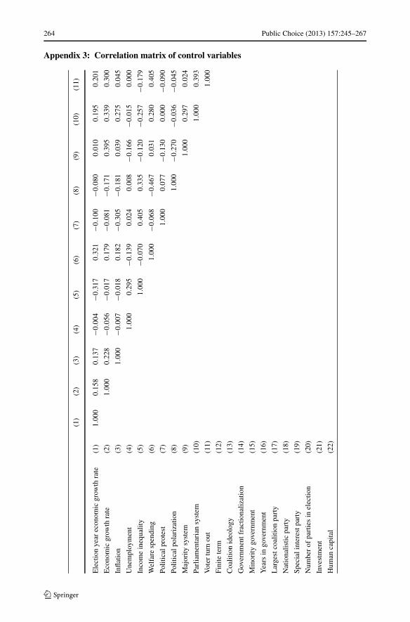
16We also tested a government party ideology variable. However, the correlation between the coalition ideol-ogy and government party ideology exceeds 0.8. We therefore include only the ideology of the coalition. Thecorrelation matrix is shown in Appendix 3.17Our qualitative results do not change when we use 5 % significance level as cut-off point (results areavailable on request).

Public Choice (2013) 157:245–267 255

and country effects, respectively, while uyqt is an error term. Eqs. (2) and (5) are estimated

with a multilevel simultaneous equation model.18

4.2 Results

Table 2 reports our estimation results for Eqs. (2) and (5). Due to data limitations, the num-ber of countries drops to 59. Column (1) shows our baseline model for the electoral sup-port received by the parties in government that is derived using the general-to-specific ap-proach. That is, we start by estimating a model including all explanatory variables outlinedin Sect. 4.1. Next, we drop the least significant variable from the regression specification andestimate the model again. We repeat this procedure until only variables that are significant atthe 10 % level remain (see Hendry 1993). An increase in the share of votes to the incumbentparty indicates a vote loss of other political parties participating in the election. Thereforewe cluster the standard errors at the election level.

The results for the intra-class correlation, which measures the distribution of the totalvariance, shows that about half of the total variance is due to the variance at the coalitionlevel. This indicates that a multilevel model is appropriate.

We find a significantly negative effect of the number of parties participating in the elec-tion. Also political protest has a negative effect on the electoral support for the parties ingovernment. Furthermore, fractionalization reduces the share of the votes received by theparties in government. Also the coefficients of the variable reflecting the number of yearsthat a party has been in government and of the dummy for the largest coalition party arenegative.

Our results for the economic variables are in line with the conclusions of Kramer (1971),Tufte (1978), Hibbs (1987), Lewis-Beck (1988) and Nannestad and Paldam (1994) as infla-tion and economic growth19 are important determinants of the popularity of the incumbent.Also spending on welfare has a positive effect on the votes received by the governmentparties.

Our model for economic growth confirms the findings of Mankiw et al. (1992) that initialGDP (measured by the 10-year lagged GDP per capita) and (human and physical) capitalare significantly related to real GDP growth per capita.

In columns (2) and (3) of Table 2 we add our PBC indicators based on the impact of elec-tions on the budget balance. As shown in column (2) of Table 2, election-induced increasesin the budget deficit as measured by PBC1 raise the electoral support for the incumbentgovernment parties. We find that a one-point increase in PBC1 increases the vote share ofthe parties in government by 0.41 % (p = 0.06). As shown in column (3), PBC2 also issignificant indicating that an increase in the budget deficit for electoral reasons increasesthe number of votes for the incumbent political parties in the next election. The estimatessuggest that a political cycle in the government deficit increases the vote share of the partiesin government by 1.1 % (p = 0.06). So although the PBC2 measure is significant, the sizeof the effect is quite small. In contrast to the direct impact, there is no indirect impact ofelection-induced budget deficits as the PBC1 and PBC2 variables are not significant in thegrowth regression.

18We do not present the reduced form of the vote equation in which we substitute the pre-election growthregression into the vote regression, because we are interested in the separate effect of PBCs on voting andeconomic growth. However, we have also estimated the reduced form and the results are in line with the mainmodel.19We exclude economic growth during the election year because this variable is taken up in the regressionseparately.

256 Public Choice (2013) 157:245–267

Tabl

e2

Est

imat

ion

resu

ltsfo

rE

qs.(

2)an

d(5

)

Bas

elin

eB

udge

tbal

ance

Gov

ernm

ents

pend

ing

Bud

getb

alan

ceG

over

nmen

tspe

ndin

g

PB

C1

PB

C2

PB

C1

PB

C2

PB

C1

PB

C2

PB

C1

PB

C2

OL

SIV

(1)

(2)

(3)

(4)

(5)

(6)

(7)

(8)

(9)

Ele

ctio

nre

gres

sion

Num

ber

ofpa

rtie

sin

elec

tion

−0.2

23−0

.171

−0.1

99−0

.126

−0.1

87−0

.170

−0.1

96−0

.133

−0.1

78

[−2.

85]**

[−2.

13]**

[−2.

05]**

[−2.

14]**

[−2.

78]**

[−2.

63]**

[−2.

33]**

[−2.

61]**

[−2.

34]**

Polit

ical

prot

est

−0.3

30−0

.287

−0.2

36−0

.267

−0.2

86−0

.252

−0.2

88−0

.275

−0.2

44

[2.27

]**[2.

10]**

[2.15

]**[2.

18]**

[2.90

]**[2.

95]**

[2.34

]**[2.

97]**

[2.88

]**

Gov

ernm

entf

ract

iona

lizat

ion

−0.0

78−0

.076

−0.1

08−0

.077

−0.0

61−0

.086

−0.0

93−0

.066

−0.0

56

[−1.

81]*

[−1.

76]*

[−1.

82]*

[−1.

65]

[−1.

71]*

[−1.

56]

[−1.

69]*

[−1.

48]

[−1.

86]*

Ave

rage

econ

omic

grow

th0.

477

0.38

00.

684

0.64

00.

469

0.41

00.

616

0.53

60.

586

[3.97

]**[3.

14]**

[3.37

]**[3.

59]**

[3.85

]**[3.

06]**

[3.40

]**[3.

44]**

[3.65

]**

Ave

rage

infla

tion

−0.5

26−0

.310

−0.2

36−0

.275

−0.2

99−0

.359

−0.2

94−0

.302

−0.3

34

[−2.

50]**

[−2.

43]**

[−2.

91]**

[−2.

57]**

[−2.

97]**

[−2.

79]**

[−2.

85]**

[−2.

87]**

[−3.

32]**

Ave

rage

wel

fare

spen

ding

0.14

30.

188

0.13

20.

180

0.15

90.

170

0.14

50.

210

0.14

6

[2.10

]**[1.

97]**

[1.96

]*[1.

95]*

[1.87

]*[1.

99]**

[1.98

]**[2.

16]**

[2.19

]**

Num

ber

ofye

ars

inco

aliti

on−0

.324

−0.1

91−0

.248

−0.1

89−0

.226

−0.2

08−0

.250

−0.1

99−0

.204

[−1.

93]*

[−2.

08]**

[−2.

20]**

[−2.

03]**

[−1.

94]*

[−2.

05]**

[−1.

88]*

[−2.

00]**

[−1.

68]*

Lar

gest

coal

ition

part

y−0

.187

−0.2

37−0

.286

−0.1

73−0

.154

−0.2

72−0

.239

−0.1

70−0

.133

[−1.

89]*

[−2.

29]**

[−2.

23]**

[−1.

89]*

[−1.

85]*

[−2.

07]**

[−2.

15]**

[−1.

79]*

[−1.

74]**

Eco

nom

icgr

owth

elec

tion

year

0.12

90.

102

0.12

50.

164

0.13

50.

106

0.11

50.

161

0.15

3

[2.48

]**[2.

31]**

[1.94

]*[2.

68]**

[2.30

]**[2.

36]**

[1.96

]*[2.

44]**

[2.42

]**

Polit

ical

budg

etcy

cle

−0.4

131.

081

0.56

92.

500

−0.3

871.

321

0.48

32.

193

[−1.

91]*

[1.86

]*[2.

23]**

[2.09

]**[−

1.84

]*[1.

76]*

[2.22

]**[2.

45]**

Public Choice (2013) 157:245–267 257

Tabl

e2

(Con

tinu

ed)

Bas

elin

eB

udge

tbal

ance

Gov

ernm

ents

pend

ing

Bud

getb

alan

ceG

over

nmen

tspe

ndin

g

PB

C1

PB

C2

PB

C1

PB

C2

PB

C1

PB

C2

PB

C1

PB

C2

OL

SIV

(1)

(2)

(3)

(4)

(5)

(6)

(7)

(8)

(9)

Eco

nom

icgr

owth

regr

essi

onIn

itial

GD

Ppe

rca

pita

1970

−0.0

74−0

.090

−0.0

95−0

.095

−0.0

89−0

.097

−0.0

96−0

.082

−0.0

85

[−3.

61]**

[−4.

03]**

[−4.

16]**

[−4.

14]**

[−4.

15]**

[−4.

42]**

[−3.

76]**

[−4.

20]**

[−3.

88]**

Inve

stm

ent

0.12

70.

102

0.10

90.

160

0.14

10.

117

0.13

00.

147

0.16

6

[3.15

]**[3.

93]**

[3.58

]**[3.

28]**

[3.60

]**[3.

83]**

[3.70

]**[3.

32]**

[4.11

]**

Hum

anca

pita

l0.

081

0.08

50.

074

0.10

10.

095

0.07

30.

090

0.10

20.

099

[2.27

]**[2.

32]**

[1.94

]*[2.

80]

[2.24

]**[2.

24]**

[2.27

]**[2.

77]**

[2.52

]**

Polit

ical

budg

etcy

cle

−0.1

470.

249

0.09

90.

355

−0.1

760.

248

0.11

70.

340

[−1.

62]

[1.59

][2.

66]**

[2.08

]**[−

1.56

][1.

61]

[2.47

]**[1.

96]**

Num

ber

ofob

serv

atio

ns66

366

366

366

366

366

366

366

366

3

Num

ber

ofco

untr

ies

5959

5959

5959

5959

59

Log

likel

ihoo

dp-

valu

e0.

000

0.00

00.

000

0.00

00.

000

0.00

00.

000

0.00

00.

000

F-st

atis

ticfir

stst

age

regr

essi

on–

––

––

31.5

4837

.895

41.0

4539

.948

Not

e:t-

valu

esar

esh

own

inpa

rent

hese

s.*/**

indi

cate

ssi

gnifi

canc

eat

10/5

perc

ent,

resp

ectiv

ely.

PBC

1is

base

don

the

erro

rte

rmof

Eq.

(1)

with

oute

lect

ions

(see

mai

nte

xtfo

ra

furt

her

expl

anat

ion)

and

PBC

2is

give

nby

Eq.

(4)

258 Public Choice (2013) 157:245–267

Next we add our PBC variables that are based on the impact of elections on governmentspending. Both PBC1 (column 4) and PBC2 (column 5) are significant. A one-point increasein PBC1 increases the voting share of the parties in government by 0.57 % (p = 0.02).So although the marginal effect of the PBC1 measure is significant, the size of the effectis again quite small. According to the coefficient of PBC2, election-induced increases ingovernment spending increase the voting share by 2.5 % (p = 0.04). Furthermore, we finda significantly positive indirect effect of expansionary fiscal policy on the election outcomethrough higher economic growth in an election year. However, this effect also is rather small.The incumbent government parties increase their share of votes by only 0.03 % through thepre-election economic growth channel.

In conclusion, even though we find evidence that election motivated fiscal policies in-crease the electoral support for the political parties in the government, the increase in elec-toral support is rather minor. This can be illustrated by calculating the effect of election-motivated fiscal policy on the votes received by the parties in government for the five coun-tries with the strongest PBCs. These countries are Turkey, Zambia, Japan, Nicaragua andMalaysia for the PBC in the budget balance and Japan, Malaysia, Turkey, Romania andColombia for the PBC in government spending. Our estimates suggest that in these coun-tries election-motivated increases in the budget deficit increase the share of the votes ofthe parties in government by about 0.76 %, while election-induced increases in governmentspending increases the share of votes by about 5.07 %.

However, pre-election growth and the election outcome on the one hand and the exis-tence of a PBC on the other may be determined by similar factors. For instance, institutionalfactors are important determinants of economic growth and some of these (such as the pres-ence of checks and balances) may also affect the existence of political budget cycles. Whenwe fail to control explicitly for these factors, our results might be biased. We therefore useinstrumental variables. Brender and Drazen (2005) argue that the existence of a PBC is pri-marily a phenomenon in new democracies and we therefore use the number of years that acountry has been a democracy since 1945 according to Polity IV as an instrument. In ad-dition, we use the level of democracy, also taken from Polity IV, and the lagged dependentvariable as instruments.

We check the validity of our instrumental variables used by the Sargan test under thenull hypothesis that our set of instruments is valid, i.e., they are uncorrelated with the errorterm in the structural equation. The results indicate that we cannot reject the null hypothesisindicating that our set of instruments is valid (p > 0.05). Next, we apply the Wald test ofexogeneity under the null hypothesis that the instrumented variable is exogenous (p < 0.05).The results confirm that our set of instruments is valid. The results of the IV regression,presented in columns (6)–(9), are similar to the OLS results presented in columns (2)–(5) ofTable 2.20

4.3 Robustness checks

It is possible that outliers affect the estimation results. Therefore, we re-estimate the regres-sions in columns (3) and (5) of Table 2 excluding country-years where the dependent orthe PBC variable are classified as outlier to test for the sensitivity of our findings for the

20As suggested by the referee, we have also included the instruments as covariates in the model. The results(available on request) are in line with the results reported in the paper.

Public Choice (2013) 157:245–267 259

Table 3 Sensitivity analysis using PBC2

Vote regression Growth regression

Coefficient t-ratio p-value Coefficient t-ratio p-value

(1) Outlier correction

Budget balance cycle 1.650 1.721 0.086 −0.260 1.450 0.147

Spending cycle 2.734 2.536 0.011 0.334 2.145 0.032

(2) Learning effect sample

Budget balance cycle 1.200 1.566 0.118 0.217 1.571 0.116

Spending cycle 1.957 1.922 0.055 0.275 1.752 0.080

(3) Low governance countries

Budget balance cycle 1.775 1.823 0.069 −0.302 1.316 0.189

Spending cycle 3.473 2.736 0.006 0.468 2.769 0.006

(4) High governance countries

Budget balance cycle 0.995 1.864 0.063 −0.201 1.113 0.266

Spending cycle 2.197 1.601 0.110 0.216 1.845 0.065

(5) Largest party

Budget balance cycle 0.616 1.781 0.075 0.318 1.715 0.087

Spending cycle 1.238 1.924 0.055 0.397 2.593 0.010

(6) Coalition

Budget balance cycle 2.053 1.832 0.067 −0.512 1.553 0.121

Spending cycle 4.765 2.875 0.004 0.368 2.184 0.029

Note: Column (1) shows the results for the impact of a PBC when we delete the observations which are notin the range: x < Q(25) − 3IQR or x > Q(75) + 3IQR; column (2) shows the results for the impact of aPBC for countries which have been democratic for the last fifteen out of twenty years; column (3) shows theresults for the impact of a PBC in a sample of countries with low levels of governance; column (4) shows theresults for the impact of a PBC for a sample of countries with high levels of governance; column (5) showsthe results for the impact of a PBC on the votes for the largest party in cabinet; and column (6) shows theresults for the impact of a PBC using the change of votes of the total coalition as dependent variable

selection of countries in our sample.21 As follows from the first part of Table 3, the resultsare similar to those reported earlier.

Brender and Drazen (2005) argue that voters punish incumbents for deficits and wastefulspending. However, to punish the government voters need to have the information necessaryto draw such inferences, as well as the ability to process that information correctly. Thisrequires some experience with the electoral process. In the absence of this experience, itis more likely that fiscal manipulation will be rewarded rather than punished. To controlfor the learning effect suggested by Brender and Drazen (2005), we re-estimate our modelsincluding country-years only if the country concerned has been democratic for at least 15of the last 20 years.22 We still find a mixed sample of countries in which elections have aneffect on spending and the budget balance (results are available upon request). The resultsfor the voting model (shown in the second part of Table 3) confirm most of our previousfindings. We find a significant direct popularity effect through government spending and an

21Outliers are defined as: x < Q(25) − 3IQR or x > Q(75) + 3IQR, where Q is the quantile and IQR theinterquantile range given by 75th percentile–25th percentile.22See also Akhmedov and Zhuravskaya (2004).

260 Public Choice (2013) 157:245–267

indirect growth effect through government spending. However, the coefficient of the PBC2budget deficit indicator is no longer significant.

As an additional test, we include in the regressions of Table 1 a variable measuring thenumber of years since 1945 that a country has been democratic and make the PBC effectconditional on this variable by including an interaction term between it and the electionvariable. Following Brambor et al. (2006), we calculate the total marginal effect of the in-teraction term evaluated at the mean of the number of democratic years since 1945 in acountry.23 The results for the PBC are similar to our earlier results. Also the findings forthe second stage regression for votes received by political parties do not change much (allresults are available upon request).24

Next, earlier studies of the existence of political budget cycles point out that electoralbudgetary policies are stronger when politicians are less credible and fiscal policy is lesstransparent (Alt and Lassen 2006; Keefer and Vlaicu 2008). To examine whether this notionaffects our results, we split our sample into two equal-sized groups based on the level ofgovernance. We measure the level of governance by the first principal component of var-ious indicators of corruption, democratic accountability, bureaucracy and rule of law in aparticular country-year taken from the International Country Risk Guide. The results in Ta-ble 3 show that in both samples the expansionary election effect is significant, although, theimpact is larger in the ‘low governance’ sample.

Finally, our dependent variable is measured at the party level. However, it may be arguedthat coalition members are considered to be jointly responsible for fiscal policy. Therefore,we use two alternative dependent variables in the second step of our estimation. First, weuse the change in votes for the largest coalition party. Second, we use the change in votesfor the total coalition. The results in the bottom rows of Table 3 show a similar pattern as inour main model of Table 2.

5 Conclusions

In this paper, we combine two strands of the political economy literature. The first strandfocuses on the existence of political budget cycles, while the second strand is concernedwith the political and economic determinants of election outcomes.

We find that in most countries fiscal policy is hardly used for electoral purposes. Using amultilevel voting model for coalition parties in government with a large number of controlvariables, we find that parties in government can influence the election outcome significantlyby manipulating government spending. Government spending also has an indirect positiveeffect on the support received by the parties in government by promoting faster economicgrowth in the election year. Although we find a statistically significant effect of election-induced government spending on election outcomes, its economic significance is relativelysmall. This could explain why fiscal policy is used for election purposes in only a fewcountries.

23In contrast, Greene (2010) argues that the significance of the interaction term should be examined usingthe t-statistic. An insignificant t-statistic indicates a mis-specified econometric model. However, in our case,the interaction term has a p-value of 0.04, which is significant at a 5 % significance level.24We also consider an interaction between the election variable and the number of coalition parties. However,the results remain in line with those reported.

Public Choice (2013) 157:245–267 261

Acknowledgements We like to thank participants in seminars at the University of Groningen, the FreeUniversity of Berlin, the 2009 conferences of the European Public Choice Society in Athens, the EuropeanEconomic Association (EEA) in Barcelona, and the International Institute of Public Finance (IIPF) in CapeTown for their comments on previous versions of the paper. We also like to thank an anonymous referee,Helge Berger, Richard Jong-A-Pin and James Vreeland for their very helpful comments.

Open Access This article is distributed under the terms of the Creative Commons Attribution Licensewhich permits any use, distribution, and reproduction in any medium, provided the original author(s) and thesource are credited.

Appendix 1: Sample of countries and years

Country Includedsince

Balance Spending Country Includedsince

Balance Spending

Albania 1991 −2.44 1.37 Japan 1975 −1.75 ◦ 2.45 ◦Argentina 1983 −1.70 1.61 Korea (South) 1975 −0.15 0.16

Australia 1976 −0.97 0.29 Lithuania* 1992 −1.11 1.70

Austria 1975 −0.97 1.06 Luxembourg 1976 −0.84 0.62

Bangladesh 1977 −0.81 1.04 Malaysia 1978 −1.37 ◦ 2.11

Belgium 1977 −0.38 0.29 Mali 1979 −0.20 0.34 ◦Bolivia 1985 −1.46 0.97 ◦ Mauritius 1981 −0.65 ◦ 0.60

Brazil 1982 −0.37 ◦ 0.37 ◦ Mexico 1976 −0.47 0.36 ◦Bulgaria 1990 −0.40 1.32 ◦ Nepal* 1981 −2.40 1.84

Canada 1986 −0.28 0.23 Netherlands 1977 −2.37 2.20

Chile 1975 −1.19 0.39 New Zealand 1977 −0.76 ◦ 0.86 ◦Colombia 1975 −1.13 ◦ 1.40 ◦ Nicaragua 1984 −1.79 ◦ 1.50

Costa Rica 1975 0.06 0.40 ◦ Norway 1977 −0.20 0.19 ◦Cyprus 1975 −0.27 0.62 ◦ Panama 1989 −2.30 1.53

Czech Republic 1993 −0.57 ◦ 0.44 ◦ Paraguay 1978 −1.26 1.01

Denmark 1977 −0.15 ◦ 0.30 Peru 1980 −1.16 1.39 ◦Dominican Rep 1978 −0.09 1.63 Philippines 1960 −1.12 ◦ 0.89

Ecuador 1979 −1.69 ◦ 1.53 ◦ Poland* 1991 −0.54 0.95

El Salvador 1977 −1.36 1.08 Portugal 1976 −0.42 0.56 ◦Estonia* 1991 0.13 1.27 Romania 1990 −1.24 ◦ 2.00 ◦Fiji 1975 −0.59 0.89 Slovakia 1994 −0.52 0.18

Finland 1975 −0.58 0.61 South Africa 1994 −1.08 1.73

France 1977 −0.75 ◦ 0.95 Spain 1978 −0.82 ◦ 0.80 ◦Germany 1976 −0.60 ◦ 0.71 Sri Lanka 1978 −1.63 ◦ 0.96

Greece 1975 −0.69 ◦ 0.62 Sweden 1978 −0.42 0.52

Guatemala 1975 0.10 0.34 ◦ Switzerland 1975 −0.54 ◦ 0.34

Honduras 1982 −0.49 ◦ 0.49 ◦ Trinidad* 1976 −0.29 0.38

Hungary 1990 −1.69 1.72 Turkey 1976 −2.56 ◦ 1.79 ◦Iceland* 1975 −1.08 0.54 United Kingdom 1975 −0.52 0.69

India 1977 −0.55 1.65 ◦ United States 1976 −0.92 1.05

Ireland 1977 −0.55 0.35 Uruguay 1985 −0.81 ◦ 1.23 ◦

262 Public Choice (2013) 157:245–267

Country Includedsince

Balance Spending Country Includedsince

Balance Spending

Israel 1977 −0.79 1.11 ◦ Zambia 1978 −1.95 ◦ 1.04

Italy 1975 −0.13 ◦ 0.23 ◦

Note: The figures in the columns show the estimated effect of elections on the fiscal variables. The figuresare based on the cross-partial derivative of the PBC coefficient from the semi-pooled model; ◦ indicates asignificant political budget cycle effect (at 10 percent significance level) in the semi-pooled model

Appendix 2: Data sources

Variable Definition Source

Election Election variable (see main text for details) Own calculations based onPolitical Handbook of theWorld (various issues)

Per capita realincome

GDP per capita in 1970 in constant US dollars of2000

World Bank (2006)

Economic growth Growth rate of real GDP per capita Heston et al. (2006)

Globalization KOF Globalization index Dreher (2008)

Dependency ratio The ratio of the population older then 65 to thepopulation between 15 and 64

World Bank (2006)

Inflation rate Change in Consumer Price Index IMF (2006)

Unemploymentrate

Total rate of unemployment of people ofworking age

IMF (2006), World Bank(2006), UN (2006), ILO(2006), OECD (2006)

Partisan variable Government ideology measure ranging from −1(full left wing) to +1 (full right wing)

Update of Beck et al. (2001)

Majoritariansystem

Dummy variable that is one if the election is in amajority electoral system

Update of Beck et al. (2001),Election Resources (2007)

Parliamentarysystem

Dummy variable that is one if the election is in aparliamentary system

Update of Beck et al. (2001),Election Resources (2007)

Number ofcoalition parties

Number of coalition parties Update of Beck et al. (2001),Election Resources (2007)

Monetary union Dummy variable taken the value 1 if a countryyear is a member of a monetary union, otherwise0

IMF (2006)

Change in votes Change in the share of votes of governmentparty q

Election Resources (2007)

Average welfarespending

Sum of government spending on health,education and social security as a share of GDP

IMF (2006), World Bank(2006), UN (2006), ILO(2006), OECD (2006)

Change incomedistribution

Change in household income inequality withinthe government term

University of Texas inequalityproject (2006), World Bank(2006)

Budget balance Government budget balance within thegovernment term (see main text for details)

IMF (2006), World Bank(2006), UN (2006), ILO(2006), OECD (2006)

Political protest First principle component of anti-governmentaldemonstrations, strikes, government crises andcabinet changes.

Own estimations based onDatabanks International(2005)

Public Choice (2013) 157:245–267 263

Variable Definition Source

Polarization Difference between the ideology of theincumbent government and the ideology of thetwo largest opposition parties

Update of Beck et al. (2001)

Majority vs.proportional

Dummy variable that is one if the election is in amajority electoral system

Update of Beck et al. (2001),Election Resources (2007)

Parliamentary vs.presidential

Dummy variable that is one if the election is in aparliamentary system

Update of Beck et al. (2001),Election Resources (2007)

Number ofparties

Number of competing parties in an election Election Resources (2007)

Voter turnout Number of voters divided by the population inthe voting age

Election Resource (2007)

Term limit chiefexecutive

Dummy variable that is one if the chiefexecutive is in his final legal term

Update of Beck et al. (2001)

Fractionalizationindex

Herfindahl index of the number of seats ofcoalition parties

Update of Beck et al. (2001),Election Resources (2007)

Minoritygovernment

Dummy variable that is one if the share of seatsof the government coalition in parliament is lessthen 50 %

Update of Beck et al. (2001),Election Resources (2007)

Number ofcoalition parties

Number of government parties Update of Beck et al. (2001),Election Resources (2007)

Largest coalitionparty

Dummy variable if the party is the largestcoalition party

Election Resources (2007)

Number of yearsin coalition

Total number of years in the coalition without aswitch

Update of Beck et al. (2001)and own calculations byextending Beck et al. (2001)

Nationalisticparty

Dummy variable if the party is nationalistic Update of Beck et al. (2001)and own calculations byextending Beck et al. (2001)

Special interestparty

Dummy variable if the party is based on specialinterest issues

Update of Beck et al. (2001)and own calculations byextending Beck et al. (2001)

Political budgetcycle

The PBC indicator (see main text for details) Own calculations

Election yeargrowth rate

Weighted growth rate of real GDP per capita(see main text for details)

Heston et al. (2006)

Investment Gross fixed investment as a share of GDP World Bank (2006)

Populationgrowth

Growth rate of the population World Bank (2006)

Human capital Secondary education attainment EDUSTAT (2006), Barro andLee (2001), own calculationby extending the five yearperiods to time series

264 Public Choice (2013) 157:245–267

Appendix 3: Correlation matrix of control variables

(1)

(2)

(3)

(4)

(5)

(6)

(7)

(8)

(9)

(10)

(11)

Ele

ctio

nye

arec

onom

icgr

owth

rate

(1)

1.00

00.

158

0.13

7−0

.004

−0.3

170.

321

−0.1

00−0

.080

0.01

00.

195

0.20

1

Eco

nom

icgr

owth

rate

(2)

1.00

00.

228

−0.0

56−0

.017

0.17

9−0

.081

−0.1

710.

395

0.33

90.

300

Infla

tion

(3)

1.00

0−0

.007

−0.0

180.

182

−0.3

05−0

.181

0.03

90.

275

0.04

5

Une

mpl

oym

ent

(4)

1.00

00.

295

−0.1

390.

024

0.00

8− 0

.166

−0.0

150.

000

Inco

me

ineq

ualit

y(5

)1.

000

−0.0

700.

405

0.33

5−0

.120

−0.2

57−0

.179

Wel

fare

spen

ding

(6)

1.00

0−0

.068

−0.4

670.

031

0.28

00.

405

Polit

ical

prot

est

(7)

1.00

00.

077

−0.1

300.

000

−0.0

90

Polit

ical

pola

riza

tion

(8)

1.00

0−0

.270

−0.0

36−0

.045

Maj

ority

syst

em(9

)1.

000

0.29

70.

024

Parl

iam

enta

rian

syst

em(1

0)1.

000

0.39

3

Vot

ertu

rnou

t(1

1)1.

000

Fini

tete

rm(1

2)

Coa

litio

nid

eolo

gy(1

3)

Gov

ernm

entf

ract

iona

lizat

ion

(14)

Min

ority

gove

rnm

ent

(15)

Yea

rsin

gove

rnm

ent

(16)

Lar

gest

coal

ition

part

y(1

7)

Nat

iona

listic

part

y(1

8)

Spec

iali

nter

estp

arty

(19)

Num

ber

ofpa

rtie

sin

elec

tion

(20)

Inve

stm

ent

(21)

Hum

anca

pita

l(2

2)

Public Choice (2013) 157:245–267 265

(12)

(13)

(14)

(15)

(16)

(17)

(18)

(19)

(20)

(21)

(22)

Ele

ctio

nye

arec

onom

icgr

owth

rate

(1)

−0.2

090.

047

−0.0

92−0

.005

−0.0

550.

300

0.23

70.

316

0.09

90.

222

0.26

0

Eco

nom

icgr

owth

rate

(2)

−0.1

220.

002

−0.0

28−0

.164

−0.0

010.

238

0.46

80.

153

0.05

00.

059

0.26

0

Infla

tion

(3)

−0.1

670.

305

−0.4

42−0

.305

−0.1

910.

396

0.07

60.

284

0.32

30.

311

0.07

4

Une

mpl

oym

ent

(4)

0.16

9−0

.141

0.17

20.

091

0.10

8−0

.004

−0.0

39−0

.194

0.23

30.

210

0.22

5

Inco

me

ineq

ualit

y(5

)0.

388

−0.4

250.

430

0.16

80.

036

−0.0

07−0

.003

−0.0

330.

010

0.24

80.

028

Wel

fare

spen

ding

(6)

−0.0

330.

334

−0.4

48−0

.025

−0.4

140.

413

0.01

30.

267

0.03

50.

246

0.00

6

Polit

ical

prot

est

(7)

0.33

7−0

.418

0.29

70.

250

0.41

0−0

. 129

−0.3

99−0

.071

−0.3

01−0

.155

−0.0

91

Polit

ical

pola

riza

tion

(8)

0.38

5−0

.024

0.28

40.

007

0.08

5−0

.311

−0.0

21−0

.105

−0.1

75−0

.301

−0.2

94

Maj

ority

syst

em(9

)−0

.087

0.05

5−0

.416

−0.0

37−0

.092

0.27

80.

001

0.17

90.

091

0.26

70.

129

Parl

iam

enta

rian

syst

em(1

0)−0

.017

0.44

2−0

.201

−0.0

79−0

.176

0.06

20.

424

0.07

20.

310

0.34

20.

144

Vot

ertu

rnou

t(1

1)−0

.223

0.00

1−0

.436

−0.1

53−0

.343

0.19

70.

004

0.06

80.

015

0.24

40.

192

Fini

tete

rm(1

2)1.

000

−0.0

300.

287

0.02

90.

005

0.00

0−0

.017

−0.3

490.

324

0.12

10.

309

Coa

litio

nid

eolo

gy(1

3)1.

000

−0.1

61−0

.282

−0.3

240.

443

0.23

80.

138

0.24

80.

107

0.02

0

Gov

ernm

entf

ract

iona

lizat

ion

(14)

1.00

00.

024

0.11

2−0

.030

−0.4

38−0

.276

0.06

6−0

.285

−0.2

10

Min

ority

gove

rnm

ent

(15)

1.00

00.

101

−0.1

44−0

.011

−0.1

480.

205

0.04

30.

006

Yea

rsin

gove

rnm

ent

(16)

1.00

00.

000

−0.0

99−0

.272

0.23

30.

029

0.00

1

Lar

gest

coal

ition

part

y(1

7)1.

000

0.22

50.

177

0.04

30.

184

0.05

7

Nat

iona

listic

part

y(1

8)1.

000

0.24

50.

159

0.07

60.

026

Spec

iali

nter

estp

arty

(19)

1.00

00.

216

0.03

00.

050

Num

ber

ofpa

rtie

sin

elec

tion

(20)

1.00

00.

125

0.21

0

Inve

stm

ent

(21)

1.00

00.

066

Hum

anca

pita

l(2

2)1.

000

266 Public Choice (2013) 157:245–267

References

Aidt, T. S., Veiga, F. J., & Goncalves Veiga, L. (2011). Election results and opportunistic policies: a new testof the rational political business cycle model. Public Choice, 148, 21–44.

Akhemedov, A., & Zhuravskaya, E. (2004). Opportunistic political cycles: test in a young democracy setting.Quarterly Journal of Economics, 119, 1301–1338.

Alt, J., & Lassen, D. (2006). Transparency, political polarization and political budget cycles in OECD coun-tries. American Journal of Political Science, 50, 530–550.

Baltagi, B. H. (1995). Econometric analysis of panel data. New York: Wiley.Banks, A. S., Muller, T. C., & Overstreet, W. R. (Eds.) (various issues). Political handbook of the world.

Washington: CQ Press.Barro, R. J., & Lee, J.-W. (2001). International data on educational attainment: updates and implications.

Oxford Economic Papers, 53, 541–563.Bayar, A., & Smeets, B. (2009). Economic and political determinants of budget deficits in the European

Union: a dynamic random coefficient approach. CESifo Working Paper 2546.Beck, T., Clarke, G., Groff, A., Keefer, P., & Walsh, P. (2001). New tools in comparative political economy:

the database of political institutions. World Bank Economic Review, 15, 165–176.Block, S. A. (2002). Political business cycles, democratization, and economic reform: the case of Africa.

Journal of Development Economics, 67, 205–228.Brambor, T., Clark, W., & Golder, M. (2006). Understanding interaction models: improving empirical analy-

sis. Political Analysis, 14, 63–82.Brender, A. (2003). The effect of fiscal performance on local government election results in Israel: 1989–

1998. Journal of Public Economics, 87, 2187–2205.Brender, A., & Drazen, A. (2005). Political budget cycles in new versus established democracies. Journal of

Monetary Economics, 52, 1271–1295.Brender, A., & Drazen, A. (2008). How do budget deficits and economic growth affect reelection prospects?

Evidence from a large cross-section of countries. American Economic Review, 98, 2203–2220.Databanks International (2005). Cross-national time-series data archive. Binghamton: Databanks Interna-

tional.Drazen, A., & Eslava, M. (2006). Pork barrel cycles. NBER Working Paper 12190.Drazen, A., & Eslava, M. (2010). Electoral manipulation via voter-friendly spending: theory and evidence.

Journal of Development Economics, 92, 39–52.Dreher, A. (2004). The influence of IMF programs on the re-election of debtor governments. Economics and

Politics, 16, 53–75.Dreher, A. (2006). Does globalization affect growth? Evidence from a new index of globalization. Applied

Economics, 38, 1091–1110.Dreher, A., Sturm, J.-E., & Ursprung, H. W. (2008). The impact of globalization on the composition of

government expenditures: evidence from panel data. Public Choice, 134, 263–292.EDUSTAT (2006). Edustat. http://www.edustat.org.Election Resources (2007). http://electionresources.org.Efthyvoulou, G. (2011). Political budget cycles in the European Union and the impact of political pressures.

Public Choice. doi:10.1007/s11127-011-9795-x. Forthcoming.Franzese, R. (2000). Electoral and partisan manipulation of public debt in developed democracies, 1956–

1990. In R. Strauch & J. Von Hagen (Eds.), Institutions, politics and fiscal policy (pp. 61–83). Dordrecht:Kluwer Academic.

Greene, W. (2010). Testing hypotheses about interaction terms in nonlinear models. Economic Letters, 107,291–296.

Grier, K. (2008). US presidential elections and real GDP growth, 1961–2004. Public Choice, 135, 337–352.Hallerberg, M., & Clark, W. R. (2000). Mobile capital, domestic institutions, and electorally induced mone-

tary and fiscal policy. American Political Science Review, 94, 323–346.Hanusch, M. (2012). Coalition incentives for political budget cycles. Public Choice, 151, 121–136.Hendry, D. F. (1993). Econometrics: alchemy or science? Essays in econometric methodology. Oxford:

Blackwell.Heston, A., Summers, R., & Aten, B. (2006). Penn World Table Version 6.2. Center for international compar-

isons of production, income and prices. University of Pennsylvania.Hibbs, D. A. (1987). The American political economy: macroeconomics and electoral politics in the United

States. Cambridge: Harvard University Press.Hobolt, S., & Klemmensen, R. (2006). Welfare to vote: the effect of government spending on turnout. Midwest

Political Science Association Annual Meeting 2006.Hsiao, C., Pesaran, M., & Tahmiscioglu, A. (1999). Bayes estimation of short-run coefficients in dynamic

panel data models. In C. Hsiao, L. Lee, K. Lahiri, & M. Pesaran (Eds.), Analysis of panels and limiteddependent variables models (pp. 268–296). Cambridge: Cambridge University Press.

Public Choice (2013) 157:245–267 267

ILO (2006). International Labor Statistics. http://www.ilo.org.IMF (2006). International financial statistics. Washington: IMF.Jaggers, K., Marshall, M. G., & Gurr, T. (2006). Polity IV: political regime characteristics and transitions,

1800–2006. Center for Systemic Peace at George Mason University.Katsimi, M., & Sarantides, V. (2012). Do elections affect the composition of fiscal policy in developed,

established democracies? Public Choice, 151, 352–362.Keefer, P., & Vlaicu, R. (2008). Democracy, credibility and clientelism. Journal of Law, Economics and

Organization, 24, 371–406.Kramer, G. (1971). Short-term fluctuations in U.S. voting behavior, 1896–1964. American Political Science

Review, 65, 131–143.Lewis-Beck, M. S. (1988). Economics and elections: the major western democracies. Ann Arbor: University

of Michigan Press.Lewis-Beck, M. S., & Stegmaier, M. (2000). Economic determinants of electoral outcomes. Annual Review

of Political Science, 3, 183–219.Mankiw, N. G., Romer, D., & Weil, D. N. (1992). A contribution to the empirics of economic growth. Quar-

terly Journal of Economics, 107, 407–437.Mink, M., & De Haan, J. (2006). Are there political budget cycles in the euro area? European Union Politics,

7, 191–211.Nannestad, P., & Paldam, M. (1994). The VP-function: a survey of the literature on vote and popularity

functions after 25 years. Public Choice, 79, 213–245.Nordhaus, W. D. (1975). The political business cycle. Review of Economic Studies, 42, 169–190.OECD (2006). OECD statistics. http://www.oecd.org.Persson, T., & Tabellini, G. (2002). Do electoral cycles differ across political systems? Mimeo. IIES, Stock-

holm University.Pesaran, H., Smith, R. P., & Im, K. S. (1996). Dynamic linear models for heterogenous panels. In L. Mátyás

& P. Sevestre (Eds.), The econometrics of panel data: a handbook of the theory with applications (pp.145–195). Dordrecht: Kluwer Academic.

Pesaran, M., Shin, Y., & Smith, R. (1999). Pooled mean group estimation of dynamic heterogeneous panels.Journal of the American Statistical Association, 94(446), 621–634.

Potrafke, N. (2012). Political cycles and economic performance in OECD countries: empirical evidence from1951–2006. Public Choice, 150, 155–179.

Rogoff, K., & Sibert, A. (1988). Elections and macroeconomic policy cycles. Review of Economic Studies,55, 1–16.

Roubini, N., & Sachs, J. D. (1989). Political and economic determinants of budget deficits in the industrialdemocracies. European Economic Review, 33, 903–933.

Schuknecht, L. (1996). Political business cycles and fiscal policies in developing countries. Kyklos, 49, 155–170.

Schuknecht, L. (2000). Fiscal policy cycles and public expenditure in developing countries. Public Choice,102, 115–130.

Shi, M., & Svensson, J. (2006). Political budget cycles: do they differ across countries and why? Journal ofPublic Economics, 90, 1367–1389.

Tufte, E. R. (1978). Political control of the economy. Princeton: Princeton University Press.Tujula, M., & Wolswijk, G. (2007). Budget balances in OECD countries: what makes them change? Empirica,

34, 1–14.United Nations (2006). United Nations statistics. New York: United Nations.University of Texas (2006). University of Texas Inequality project. http://utip.gov.utexas.edu.Vergne, C. (2009). Democracy, elections and allocation of public expenditures in developing countries. Eu-

ropean Journal of Political Economy, 25, 63–77.World Bank (2006). World development indicators. CD Rom.