INTERNATIONAL JOURNAL OF CLIMATOLOGY

Int. J. Climatol. 21: 1779–1801 (2001)

DOI: 10.1002/joc.689

REGIONAL TEMPERATURE VARIABILITY IN THE EUROPEANALPS: 1760–1998 FROM HOMOGENIZED INSTRUMENTAL TIME

SERIESREINHARD BO� HMa,*, INGEBORG AUERa, MICHELE BRUNETTIb, MAURIZIO MAUGERIc, TERESA NANNIb and

WOLFGANG SCHO� NERa

a Central Institute for Meteorology and Geodynamics, Hohe Warte 38, A-1190 Vienna, Austriab Istituto ISAO-CNR, Via Godetti, 101, I-40129 Bologna, Italy

c Istituto di Fisica Generale Applicata, Uni�ersita di Milano, Via Brera, 28, I-20121 Milano, Italy

Recei�ed 24 No�ember 2000Re�ised 19 April 2001

Accepted 23 April 2001

ABSTRACT

This paper investigates temperature variability in the Alps and their surroundings based on 97 instrumental series ofmonthly mean temperatures. A discussion of the initial homogenizing procedure illustrates its advantages and risks.A comparison of the homogenized series with the original series clearly shows the necessity to homogenize. Each ofthe original series had breaks (an average of five per series) and the mean of all series was systematically biased bynon-climatic noise. This noise has subdued the long-term amplitude of the temperature evolution in the region by 0.5K. The relatively high spatial resolution of the data enabled a regionalization within the study area of 680000 km2

into six sub-regions based on principal component analysis of the monthly series. Long-term temperature evolutionproved to be highly similar across the region—thus making a mean series (averaged over all 97 single series)representative of the study area. Trend analysis (based on progressive forward and backward Mann–Kendallstatistics and on progressive analysis of linear regression coefficients) was performed on seasonal and annual series.The results diverge from those of global datasets. This is mainly due to the extension of the 240-year Alpine datasetby 100 years prior to the mid-19th century, and also due to the advantages of a dense and homogenized regionaldataset. The long-term features include an initial decrease of the annual and seasonal series to a minimum followedby a positive trend until 1998. The minima are 1890 for the entire year and winter, 1840 for spring and 1920 forsummer and autumn, respectively. The initial decreasing trend is more evident in spring and summer, less in autumnand smallest in winter. The mean annual temperature increase since 1890 in the Alps is 1.1 K, which is twice as muchas the 0.55 K in the respective grid boxes of the most frequently used global dataset of the Climatic Research Unit(CRU), University of East Anglia. To enable an easier and more systematic handling of the dataset, these data havebeen interpolated to a 1°×1° longitude–latitude grid. The 105 low-elevation and 16 high-elevation grid point seriesare widely available without restrictions for scientific research and can be obtained from the authors. Copyright© 2001 Royal Meteorological Society.

KEY WORDS: gridded dataset; homogeneity; instrumental period; regionalization; temperature time series; trends

1. INTRODUCTION

The European Alps constitute a region of high potential in terms of climatological research. They offerdifferent climates ranging from Mediterranean and Atlantic influences in the south and west tocontinental features in the east, and from low-elevation plains, valleys and basins to high-elevationmountain climate in regions above the tree-line and above the snow-line. They also offer a wealth ofclimate data not easily obtainable elsewhere. The climatological part of the EC project ALPCLIM(environmental and climate information from ice cores in high elevated Alpine sites; Wagenbach et al.,1998) aims to analyse climate-relevant stable isotope information in ice cores from the summit regions of

* Correspondence to: Central Institute for Meteorology and Geodynamics, Hohe Warte 38, A-1190 Wien, Austria; e-mail:reinhard.boehm@zamg.ac.at

Copyright © 2001 Royal Meteorological Society

R. BO� HM ET AL.1780

Monte Rosa and Mont Blanc and to combine them with instrumental time series to proxy temperatureseries. The strength of the Alpine ice core proxies against those from remote regions, like Greenland orAntarctica, is given by the dense and long-term instrumental data information around the core sites. Thisallows a better fitting of the stable isotope records to the instrumental series and it also allows the spatialrepresentation of the high-level climate information to be studied on regional and continental scales. Tomeet these objectives we generated a homogenized, high-resolution, gridded dataset of long-terminstrumental temperature series, which will be introduced and analysed in this paper.

2. DATA

The task of data collection for ALPCLIM illustrates the richness of the region with regard to climateinformation. However, it also provides a good example of the difficulties that have to be overcome byinternational research activities created by the fact that the region is split into a number of differentcountries with an even larger number of single data holders. Although in most of the cases there wasmuch goodwill and a high degree of co-operation from the data holders, a great deal of time and efforthad to be spent to assess firstly the data potential and then to accurately collect the data. Table I includesthe different sources from which the ALPCLIM temperature dataset was constructed. In some cases, datacollection also had positive aspects in terms of providing vital information regarding the complicatedpolitical history in some parts of the regions. For example, two Italian–Austrian and Italian–Croatiancollaborations showed that old problems can now easily be overcome in order to remove existing gaps inlong time series or to re-unite climate series from times with different political borders. Finally, 120 singleseries were collected, all based on monthly means, most of them being at least centennial-length series, thelongest series starting in the 1750s.

3. HOMOGENIZING

Many studies during the past two decades have demonstrated that climate variability research is notpossible without a clear knowledge about the state of the data in terms of homogeneity. The real climatesignal in original series is hidden behind non-climatic noise caused by the relocation of stations; changesin instruments and instrument screens; changes in observing times, observers and observing regulations;algorithms for the calculation of means and many others. Overviews focusing on the homogeneityproblem and different ways to solve it are given in Peterson et al. (1998) and in the two volumes of theproceedings of the homogeneity seminars in Budapest (HMS-WMO, 1997, 1999).

Table I. Data sources of the ALPCLIM temperatures series

Data source Region

Meteo France, Toulouse NW and SW of FranceNOAA-GHCN, Asheville SE and NE of FranceUEA-CRU, Norwich Gridded data of Europe

S GermanyDWD, OffenbachSwitzerlandMeteo-SwissN ItalyCNR-ISAO, Bologna

I. di Fisica Gen. Appl., Univ. di Milano N ItalyNW ItalySoc.Met.Subalpina, Torino

HA-APB, Bolzano/Bozen Prov. Bozen/BolzanoCroatiaMHSC, Zagreb

SHMI, Ljubljana SloveriaW HungaryHMS, BudapestW SlovakiaSHMI, Bratislava

ZAMG, Vienna Austria

Copyright © 2001 Royal Meteorological Society Int. J. Climatol. 21: 1779–1801 (2001)

REGIONAL TEMPERATURE VARIABILITY IN THE EUROPEAN ALPS 1781

Evidence from the studies of Moberg and Alexandersson (1997) and Auer et al. (1998), Auer et al. (inpress) shows that existing global datasets (Jones, 1994; Jones et al., 1999) are good measures oftemperature variability at the continental to global scale, but are less effective at describing regional- andlocal-scale climate variability. The main reasons for this are a low station spatial density and a lack ofstation history information (‘metadata’) associated with these data. As the objective of this study was tocreate and analyse a dataset of high spatial resolution, it was clear right from the start of the project thatthe existing Alpine data had to be checked for inhomogeneities before using them for climate analysis. ForAustria, parts of Slovakia and Hungary (ALOCLIM—Auer et al., 1998; Auer et al., in press) and forItaly (CNR project ‘Reconstruction of the Climate of the Past in the Mediterranean Area’—see, e.g.Maugeri and Nanni, 1998), pre-homogenized series already existed from previous projects. Meteo-Franceprovided a set of homogenized data for France, west of 4°E (Mestre, 1999). The eastern part of France(the part within the ALPCLIM region) had to be homogenized within the project. For the Swiss part ofthe Alps, some homogenized series could be taken from ALOCLIM and from the Swiss project‘Klima-90’ (Aschwanden et al., 1996a,b), some were digitized and homogenized from Swiss yearbooks andsome were included from the NOAA-GHCN dataset (Vose et al., 1993). For Slovenia, Hungary andSlovakia, there exists a well-established collaboration of data exchange with Austria based on projectALOCLIM. The Croatian Meteorological Service contributed quality checked temperature series.

All series, original and pre-homogenized, were re-analysed for inhomogeneities based on the followingsystem: homogeneity testing, adjusting and gap-closing was performed in 13 regional sub-groups of tenseries using the MASH-test of Szentimrey (1999) and the HOCLIS procedure (Auer et al., 1999). HOCLIS(and also the system used by Meteo-France; Mestre, 1999) rejects the a priori existence of homogeneousreference series. They test each series against other series in sub-groups of ten series. The break signals ofone series against all others are then collected in a decision matrix and the breaks are assigned to thesingle series according to probability. This system also avoids trend imports and an inadmissibleadjustment of all series to one or a few ‘homogeneous reference series’.

One additional sub-group was created for the pre-1820 parts of the ten bicentennial series. This was nota regional series, but was distributed over the whole study area. The high spatial correlation also amongremote series, allowed the relative homogeneity testing to be performed even for this extended group. Thelast homogenizing groups consisted of two high-elevation sites with series above 1500 m above sea level(a.s.l.) for the western and for the eastern Alps.

Not all of the 120 series fulfilled the requirements in terms of homogeneity. A final total of 97 singleseries proved to be homogenizable. A short summary about the homogenizing of the series and thedetected breaks is given in Table II. A total of 451 breaks were detected in the original, pre-homogenizedseries. This represents an average of five breaks per series or in other words a homogeneous sub-intervalof an average series not longer than 30 years. The availability and the quality of the metadata are differentfor the different regions and, besides stations with well-documented histories, the dataset also containsstations for which only limited metadata were available. As a consequence, it was not possible to performa complete comparison of the identified inhomogeneities with the history of the stations. It is, however,worth noticing that a high percentage of the breaks could be explained through metadata, wherehigh-quality information was available (for details see Auer et al., in press).

Table II. Summary of detected breaks in ALPCLIM temperature series

Homogeneous series 97 seriesPre-homogenized 12 seriesTotal of homogenized years 12 258 years

1403 yearsPre-homogenized yearsMean length of series 140.8 yearsMean starting year of series 1858Detected breaks 431 breaks

28.4 yearsMean homogeneous sub-interval5.1 breaksMean number of breaks per series

Copyright © 2001 Royal Meteorological Society Int. J. Climatol. 21: 1779–1801 (2001)

R. BO� HM ET AL.1782

Figures 1 and 2 show the spatial and temporal coverage of the study region by homogeneous timeseries. The mean station distance is 80 km. Three homogenized series start as early as 1760 and ten earlierthan 1801. The greatest increase in station density occurred in the 1860s but the 25 series of 1850underline the potential of the dataset in the early instrumental period. Before analysing the homogenizeddata, the differences between the original and homogenized data are discussed. Of special interest is thedegree of bias of the original data—are data systematically biased or are all adjustments random? Thisissue can be investigated by analysing the adjustment series. As these series contain the values that wereadded to the original records in order to produce homogeneous data, this analysis will reveal anysystematic errors in the original records. Figure 3 shows the mean adjustment curves for the summer andthe winter half-year and for the entire year (homogenized minus original, averaged over all single series)plus the standard deviation and the absolute range of the adjustments for the study region. The largeabsolute range of adjustments (the thin lines), as well as standard deviation range, underline again theabsolute necessity to homogenize in order to get any reasonable single-station series. The mean of all

Figure 1. The ALPCLIM network of homogenized long-term temperature time series. Dots, low level series (�1500 m a.s.l.);triangles, high level series (�1500 m a.s.l.). Orography: 1000, 2000 and 3000 m altitude lines separating different shades of grey

Figure 2. Temporal coverage of the instrumental area in the Alps by homogenized temperature records

Copyright © 2001 Royal Meteorological Society Int. J. Climatol. 21: 1779–1801 (2001)

REGIONAL TEMPERATURE VARIABILITY IN THE EUROPEAN ALPS 1783

Figure 3. Long-term adjustment curves (homogenized minus original) averaged over all 97 ALPCLIM sites for summer-half year(top), winter-half year (below) and year (bottom). Bold line, mean; medium lines, standard deviation range; thin lines, absolute range

adjustments over the complete station sample (the bold line) is not zero, indicating that the non-climaticinhomogeneties are not random—some systematic biases in the adjustment curves are evident. As thenumber of stations is limited in the early period (see Figure 2), the adjustment curve shows greatervariability before the mid-19th century and reflects single site peculiarities more than general systematicevolutions (before 1801 standard deviations were not calculated due to a sample size less than 10). Withthe founding of Meteorological Services in the Alpine countries in the 1850s and 1860s, the number ofseries quickly increases and the adjustment curve becomes less noisy. The average of the adjusted seriesreveals a general increasing trend of approximately 0.5 K for the 150 years from the mid-19th to the endof the 20th century.

The reasons for this systematic trend can be found in a mixture of specific national items and somegeneral evolutions in the study area. Figure 4 shows three examples of national subsets— those covering

Copyright © 2001 Royal Meteorological Society Int. J. Climatol. 21: 1779–1801 (2001)

R. BO� HM ET AL.1784

Figure 4. Mean adjustment curves (homogenized minus original) for three national ALPCLIM subsets. Bold line, summer-half year(months 4–9); thin line, winter-half year (months 10–3)

the majority of ALPCLIM series (more than 70%) and also those with the best metadata coverage.Besides the already discussed statistically noisy ‘pre-met-services period’, the older data of the recent 150years seem to be biased, in comparison with the modern ones, with a positive error. For Italy and Austria,the increase of the adjusting series occurred in two main stages. The first was in the late-19th andearly-20th centuries and seems to be related to the progressive evolution of the meteorological stationsfrom the typical 19th century situation. At this time, thermometers were generally located inmeteorological windows and subjected to both building and urban influences. These were then moved tothe well-known modern situation associated with Stevenson screens, which are set in open surroundings.There was also a change of the observing times, which were standardized during the late-19th andearly-20th centuries from a multitude of different observing times to an international standard defined inthe 1870s. Auer et al. (in press) showed that for the Austrian network, a typical break, which wasidentified by a shift from higher temperatures in the original data to lower temperatures in thehomogenized data, was due to the standardization of the observing times. The second stage is located inthe mid-20th century and can be assigned to a strong tendency to relocate stations from city centres(where most of the old institute buildings, museums, schools and other historical measuring sites havebeen) to airports and airfields. In Europe, this evolution started suddenly with World War II and itsstrong concentration on aerial warfare. In Austria, for example, the percentage of measuring sites withurban surroundings decreased from 50% in 1935 to 30% in 1945 due to city-to-airport relocations. As aresult of this there is an increase in temperature between the original and the homogenized data of nearly0.3 K. A similar evolution occurred in Italy, where the city-to-airport relocations also started with WorldWar II but continued throughout the 1960s and 1970s. Another national inhomogeneity (the 1970/1971Austrian nationwide change in observing time—Auer et al., in press) suddenly caused another +0.3 Kstep of the adjusting curve in Austria.

Copyright © 2001 Royal Meteorological Society Int. J. Climatol. 21: 1779–1801 (2001)

REGIONAL TEMPERATURE VARIABILITY IN THE EUROPEAN ALPS 1785

For Switzerland the situation is different. The adjustment curve is mostly characterized by two mainsteps due to the use of three different data sources: GHCN data (Global Historic Climate Network ofNOAA, Asheville, USA) for the pre-1864 period, the already partly pre-homogenized Meteo-Swiss seriesfrom 1864 to 1960, and the well-homogenized ‘Klima-90’ data since 1960 (Aschwanden et al., 1996a,b).

The examples from the three countries with good metadata information, which cover 72% of thehomogenized ALPCLIM series, together with the described system of mathematical testing and adjusting,enable us to conclude, with a high degree of certainty, that the detected positive bias of the older originaldata in the region is real. The well-documented decreasing urban influence in many of the series isparticularly interesting. This is in contradiction to the widely held view that encourages the increasingurban influence on temperature time series in order to reflect the worldwide increase of urbanization.

The described homogenizing procedure produced 97 instrumental series of mean monthly temperatures.The mean station distance for the 682000 km2 of the ALPCLIM region is 80 km. Such a relatively highstation density makes the dataset usable for studying not only mean climate variability but also itsregional structure and patterns within the region.

4. STATION CLUSTERING AND REGIONAL AVERAGE SERIES

The first step in analysing the data was the transformation of the 97 homogenized series into anomalyseries. Anomalies were calculated on a monthly basis, subtracting the monthly mean for the 1901–1988period (hereafter referred to as the ‘20th century mean’). A correlation analysis was then performed. Theresults show that the monthly temperature anomalies have a high spatial correlation over the ALPCLIMregion and that the difference in height affects the correlation more than the horizontal distance. This isevident from Figure 5, where the correlation coefficients, as a function of the distance of the

Figure 5. Correlation coefficients between annual mean temperatures for all pairs of stations versus their distance—single valuesplus linear regression of three sub-groups. Black triangles (plus dashed line), high level-high level correlations; Xs (plus dash-double

dotted line), low level-low level correlations; circles (plus dash-dotted line), high level-low level correlations

Copyright © 2001 Royal Meteorological Society Int. J. Climatol. 21: 1779–1801 (2001)

R. BO� HM ET AL.1786

corresponding stations, are represented for the 4656 possible combinations of the 97 series, grouped in thethree sub-groups: high-level/high-level, low-level/low-level and high-level/low-level. The relatively largedeviations from the linear regression lines highlight the fact that other factors, such as the geographiclocation similarity, may affect the correlation more than the distance. This can be clarified considering,for example, the station at Sion (Switzerland, Rhone valley site, 482 m a.s.l.). This site is located northof the main Alpine divide, but is also near to some Po plain stations. In spite of the greater distance, Sionhas a better correlation with a number of northern Alpine stations (six stations correlate better than 0.90,18 better than 0.85) than with the much nearer southern Alpine stations of Aosta, Torino, TorinoMoncalieri, Lugano and Milano, which all have correlation coefficients around 0.8).

Globally, the results of the correlation analysis suggest that most of the signal in the ALPCLIMmonthly temperature anomalies can be captured by a small number of regional average series. Followingthis result, we clustered our series into homogeneous temperature areas by means of principal componentanalysis (PCA). PCA allows the identification of a small number of variables known as principalcomponents (PCs), which are linear functions of the original data, which maximize the amount of theirexplained variance. The technique can be applied both to correlation and covariance matrixes. We usedthe correlation matrix R (in order to avoid a domination of the continental sites with stronger variance)based on the monthly anomalies (in order to avoid the dominance of the annual cycle) for the sub-sample1933–1998 (for which all 97 series are available). R is defined by ZZ t, Z being a matrix containing the97 standardized temperature anomalies series (for a review of PCA see Joliffe, 1990, 1993; for a review ofthe clustering of temperature series see, for example, von Storch, 1995 or Hanssen-Bauer and Nordli,1998).

The eigenvalues of R reveal that only six PCs account for more variance than the original variables(having eigenvalues greater than 1) and that these six PCs account globally for 91% of the variance of thestandardized data. The weight of each station in each PC is given by the eigenvector components (thefactor loadings) corresponding to the eigenvalues. The components of each eigenvector (the factorloadings) represent the correlation between the station series and the corresponding PC.

The identified PCs (and consequently the corresponding loadings) are, however, not unique. By rotatingthe PCs it is possible to obtain other sets of six PCs that account for the same fraction of variance of thedata. The benefit of rotation is that it can be carried out to allow a more simple physical interpretationof the loadings. In our analysis we used VARIMAX rotation (see, e.g. Richman, 1986).

The resulting loadings are six vectors of the 97 components. One has particularly high components forthe high level stations, the others have the highest components for stations in different sub-regions of theALPCLIM region. Instead of displaying these vectors as columns of numbers, we prefer to use figures. Inparticular for the ‘high-level’ PC we display a graph of station heights versus loadings (Figure 6), whereasfor the other ones we represent the loadings on geographic maps, drawing contours through the pointswith the same loadings (Figure 7). The loadings patterns allow the following regions to be identified:

� High-le�el Alpine areas: These include the scattered areas lying above 1500 m a.s.l. This station clusteris clearly separated from the low-level areas (see Figure 6). Most of its group members are located atremote places on mountain peaks. The series from this group may well be described as ‘climaticbackground information’ right in the centre of densely populated Europe. Moreover, some of them are‘mid-troposphere series’ from the 700-hPa level and thus are also interesting for use in studies of thepossible vertical effects of climate change;

� The East: A region of mainly continental features, framing the Alps in the north, the east and thesouth-east;

� The West: A region of maritime influences from the Atlantic and the western Mediterranean. Theborder to region East is a zone of gentle transition rather than a clear line;

� The South: A region covering the Adriatic coast and the northern part of the Italian peninsula;� The Po plain: A region covering most of the northern continental part of Italy. It has definite borders

in the West and North (towards the Alps) in contrast with the situation in the East, which ischaracterized by a gentle transition into the Adriatic cluster;

Copyright © 2001 Royal Meteorological Society Int. J. Climatol. 21: 1779–1801 (2001)

REGIONAL TEMPERATURE VARIABILITY IN THE EUROPEAN ALPS 1787

Figure 6. High-level factor loadings versus altitude based on all months of the year

� The central Alpine low-le�el areas: A region that concentrates on valley stations in the central part ofthe Alps where they have their maximum north–south extension plus parts of the eastern Alps. It isunclear if this cluster also represents the valleys of the western Alps because there is only one typicalwestern Alpine low-level site (Aosta).

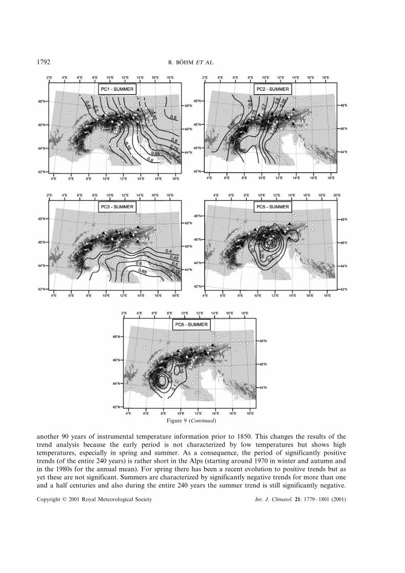
The previous analysis was performed using all months of the year. It is also interesting to compare theresults obtained considering the anomalies corresponding to winter and summer months (summercorresponds to April–September while winter corresponds to October–March). In this case this divisionof the year, which is different from the usual meteorological division (DJF for winter and JJA forsummer) is used so that we do not reduce the number of months of each series too much. The resultsprovide evidence that the same regions identified from the PCA of the complete series have also beenidentified in the seasonal PCA, and in both cases the first six PCs account for 91% of the variance of thedata. The main difference is between the summer and winter analyses. The PCs that correspond to theEast, the West and the South account for more than 80% of the data variance, whereas in winter theyaccount for around 60%. During summer the correlation extends over larger areas both in the horizontalplane and along the vertical, whereas in winter the local effects (e.g. Po plain climate, high-level versuslow-level, etc.) are more important. Figure 9(a) and (b) show factor loading maps of the five low-levelrotated PCs for winter and summer, and Figure 8 shows the high-level seasonal PC loadings versusaltitude. In Table III the single series are assigned to the six clusters. Figure 10 shows the sub-regions,which will be the basis for the following regional trend analysis.

After clustering the stations, we constructed mean regional anomalies series performing the arithmeticmean of the series located by PCA in each of these six regions. It is interesting to observe from Table IVthat beside the high correlations identified between the regional mean series and their correspondingcluster members, there are also significant correlations between the different regional mean series(0.8�r�0.9 for the low-level regions, and only slightly lower for the high Alpine area). On average, theoverall sites have very high correlation with all low-level regional series (0.92�r�0.96) and also goodcorrelation with the high level series (r=0.88).

Copyright © 2001 Royal Meteorological Society Int. J. Climatol. 21: 1779–1801 (2001)

R. BO� HM ET AL.1788

Table III. Grouping of the single series according to PCA

Sub-regional clusters

East (Continental) West (Maritime) South Po plainHigh level Central alpinelow level(Adriatic) (�1500 m

a.s.l.)

Assignment to PCs

Ann-PC-1 Ann-PC-2 Ann-PC-3 Ann-PC-4 Ann-PC-5 Ann-PC-6Sum-PC-1 Sum-PC-2 Sum-PC-3 Sum-PC-4 Sum-PC-5 Sum-PC-6Win-PC-1 Win-PC-4 Win-PC-3 Win-PC-2 Win-PC-6 Win-PC-5

Single series

Bad Gleichenberg Altdorf Arezzo Davos Bad Gastein AlessandriaBad Ischl Basel Bologna Feuerkogel Beluno AostaBratislava Bern Crikvenica Gr.St.Bemhard Bozen/Bolzano CuneoCelje Bregenz Ferrara Jungfraujooh Brixen/ Genova

BressanoneFreistadt Dijon Gospic Lago Gabiet Innsbruck LuganoGraz Feldkirch Hvar Patscherkofel Kufstein MantovaHurbanovo Geneve Livomo Santis Marienberg/ Milano

Mt.MariaKlagenfurt Hohenpeißenberg Padova Schmittenhohe Radstadt ParmaKollerschlag Lyon Pesaro Sonnblick Riva PaviaKrememunster Marseille Perugia Villacher Alpe Rovereto PiacenzaLjubijana Montpellier Pula Zugspitze Trento Reggio EmigliaMosonmagyarovar Nancy Rovigo Zell am see TorinoMunchen Neuchatel Split Torino-MoncalieriOsijek Nice TriestePecs NimesRadenthein SionReichenau/Rax StrasbourgRetz StuttgartRied ZurichSalzburgSt.Andra/LavanttalSeckauSopronSzombathelyWaidhofen/YbbsWeinZagrebZwettl

5. TREND ANALYSIS

The first step in trend analysis was the calculation of seasonal and annual average regional series. Annualvalues correspond to the period from December to November and are dated by the year in which Januaryis included. Thus, the annual mean covers the same months as the seasonal means, where winter valuesrefer to the December–February interval, spring to March–May, summer to June–August and autumnto September–November. All values are anomalies from the 20th century mean.

Figure 11 shows the annual anomalies of the six regional average series filtered with an 11-year 3�

Gaussian low-pass filter. It is evident that the regional temperature anomalies are highly correlated, notonly on an annual time scale (Table IV) but also on a secular time scale with a range of the filtered curvesgenerally less than 0.5 K. Prior to 1850, the range gently increases, which might be due to the muchsmaller station density in the early parts of the series (see Figure 2).

Copyright © 2001 Royal Meteorological Society Int. J. Climatol. 21: 1779–1801 (2001)

REGIONAL TEMPERATURE VARIABILITY IN THE EUROPEAN ALPS 1789

Figure 7. Maps of five low-level rotated PCs for the year

The high similarity between the ALPCLIM regional averages gives a preliminary representation of thewhole area by means of only one series: the mean for all ALPCLIM sites (hereafter MA). Figure 12presents the annual and seasonal MA series together with the filtered series (again the 11-year 3�

Gaussian low-pass filter). The annual data show a start from lower values before 1785, followed by tworelative maxima in the 1790s and the 1820s, interrupted by a sudden cold event in the 1810s. After the1820s there is a gradual trend toward two minima in the 1840s and 1850s and the 1880s and 1890s witha relative maximum in the 1860s and early 1870s. The whole 20th century is characterized by risingtemperatures toward a first maximum at 1950 and a second in the 1990s, which is the main maximum ofthe 240 ALPCLIM years. The analysis of the seasonal series provides evidence that, beside some commonfeatures, the temperature evolution shows strong seasonal differences. Concentration on the long-term

Copyright © 2001 Royal Meteorological Society Int. J. Climatol. 21: 1779–1801 (2001)

R. BO� HM ET AL.1790

Figure 8. High-level factor loadings versus altitude for summer (April–September) and for winter (October–March)

features alone, annual and seasonal MA series initially decrease to a minimum, which is then followed bya positive trend until 1998. The location of the minima is different however: 1890 for the entire year andwinter, 1840 for spring and 1920 for summer and autumn. The initial decreasing trend is more evident inspring and summer, less in autumn and least in winter.

In order to quantify these results, the slopes of the trends were calculated by least square linear fittingand their confidences were estimated by means of the non-parametric Mann–Kendall test (Sneyers, 1990).The test was also used for a progressive analysis of the series, consisting of its application to all the seriesstarting with the first term and ending with the ith term and to those starting with the ith term and endingwith the last term. In the absence of any trend the graphical representation of the direct (ui) and the backward(ui�) series obtained with this method provides curves that overlap several times, whereas in the case of asignificant trend, the intersection of the curves enables the detection of the approximate time of occurrenceof the phenomenon (Sneyers, 1990).

In Figure 13 the progressive regression coefficients of the seasonal and annual MA series are representedfor (a) the periods beginning in 1760+ i and ending in 1998 (i=0, . . . , 199; 1760= first year of theALPCLIM data); (b) the periods beginning in 1760 and ending in 1998− i (i=199, . . . , 0; 1998= last yearof the ALPCLIM data). The upper limit for i (199) has been selected in order to estimate the regressioncoefficients over at least 40-year periods. The bold lines indicate regression coefficients with a confidencelevel greater than 95%. Confidence levels have been deduced from Figure 14, where the inverse and directcurves resulting from the progressive application of the Mann–Kendall test to the seasonal and annual MAseries are represented. In fact, the inverse curves indicate the significance level of the trends for the periodsstarting in 1760+ i and ending in 1998 (with i=0, . . . , n ; n=series length−2), whereas the direct curvesindicate the significance level of the trends for the periods starting in 1760 and ending in 1998− i(i=n, . . . , 0; n=series length−2).

In Figure 15 regional details are provided for the annual series and (due to the different starting pointsof the series) only for the periods beginning in 1760+ i and ending in 1998 (i=0, . . . , 199). Also in thiscase, the bold lines indicate regression coefficients with a confidence level greater than 95% (deduced asfor Figure 13).

Copyright © 2001 Royal Meteorological Society Int. J. Climatol. 21: 1779–1801 (2001)

REGIONAL TEMPERATURE VARIABILITY IN THE EUROPEAN ALPS 1791

Globally, trend analysis shows that the significance and the slope of the trends depend strictly on theselected periods, with generally higher values in winter than in summer. However, for a given period andseason, the results are highly similar for all the different ALPCIM regions. The length of the ALPCLIMseries enables an analysis of data covering the ‘pre-industrial’ period, which is frequently used forcomparison with the warmer 20th century climate. For global datasets, data coverage limits the length tostarting points not earlier than the mid-19th century. In the Alps and their surroundings, there are

Figure 9. (a) Maps of five low-level rotated PCs for the winter-half year (months 10–3). (b). Maps of five low-level rotated PCs forthe summer-half year (months 4–9)

Copyright © 2001 Royal Meteorological Society Int. J. Climatol. 21: 1779–1801 (2001)

R. BO� HM ET AL.1792

Figure 9 (Continued)

another 90 years of instrumental temperature information prior to 1850. This changes the results of thetrend analysis because the early period is not characterized by low temperatures but shows hightemperatures, especially in spring and summer. As a consequence, the period of significantly positivetrends (of the entire 240 years) is rather short in the Alps (starting around 1970 in winter and autumn andin the 1980s for the annual mean). For spring there has been a recent evolution to positive trends but asyet these are not significant. Summers are characterized by significantly negative trends for more than oneand a half centuries and also during the entire 240 years the summer trend is still significantly negative.

Copyright © 2001 Royal Meteorological Society Int. J. Climatol. 21: 1779–1801 (2001)

REGIONAL TEMPERATURE VARIABILITY IN THE EUROPEAN ALPS 1793

Figure 10. Map of the sub-regions based on PCA

Table IV. Annual correlations among sub-regions and of sub-regions versus low-level average and average of allALPCLIM series

West SouthEast Po plain Central Alpine Low level ALPCLIMaverage average(Adriatic) low level series

0.85 0.79 0.81 0.88 0.85 0.88High level 0.750.85 0.89 0.81 0.88 0.96 0.95East

0.84West 0.88 0.90 0.94 0.940.89 0.89 0.94 0.94South (Adriatic)

Po plain 0.90 0.92 0.92Central alpine low 0.96 0.96

level areas1.00Low level average

Figure 11. Annual regional mean temperature series (deviations in K from 20th century mean) smoothed with a 3� Gaussian lowpass filter (11-year-wide running window)

Copyright © 2001 Royal Meteorological Society Int. J. Climatol. 21: 1779–1801 (2001)

R. BO� HM ET AL.1794

Figure 12. Seasonal and annual MA temperature series (MA=mean of all 97 series, deviation in K from 20th centurymean)—single values and smoothed with a 3� Gaussian low pass filter (11-year-wide running window): winter, months 12–2; spring,

months 3–5; summer, months 6–8; autumn, months 9–11; year, months 12–11

6. GRIDDING

For easier and more systematic mathematical handling, and to enable a comparison with other griddeddatasets, the single series were interpolated to grid points. Again, it was not the absolute values of the singleseries, but the deviations from the 20th century mean (1901–1998) that were gridded. The idea behindgridding was not a further data compression, but more a shifting of information to equidistant points. Theratio of single series to the number of grid points is not far from one at the chosen grid spacing of 1°longitude and latitude. Interpolation was performed by a Gauss-weighting function with weight 1 at thelocation of the grid point and quickly decreasing to 0.1 at a distance of 200 km. In principle, all singleseries contribute to each grid point but at very small weights and at larger distances from the grid point.

Copyright © 2001 Royal Meteorological Society Int. J. Climatol. 21: 1779–1801 (2001)

REGIONAL TEMPERATURE VARIABILITY IN THE EUROPEAN ALPS 1795

Figure 13. Progressive linear regression coefficients for seasonal and annual MA anomaly series. Black curves are relative to seriesending at 1998 and starting from 1760+ i (i=0, 190); grey curves are relative to series starting from 1760 and ending at 1998− i(i=190, 0). Bold parts indicate that the values correspond to a Mann–Kendall coefficient with significance level greater than 95%

(see Figure 14)

To avoid large distance information transport in cases where no series exist near the grid point (this istypical for the older parts of the series with sparse spatial resolution), interpolation was truncated at thestart year of the longest single series within 200 km of a grid point. Three additional borders of truncationwere defined: no information transport was (i) allowed across the main Alpine divide, (ii) from coastalseries to continental ones and (iii) across the 1500 m altitude line. The gridded dataset has been testedalready. It contains 105 low-elevation and 16 high-elevation grid point series and can be obtained viae-mail from the authors. Figure 16 shows the available grid point series and their starting year.

7. COMPARISON WITH THE CRU DATASET

It is interesting to check if the ALPCLIM dataset as a whole is different from other existing datasets. Thebest known and most frequently used is the Climatic Research Unit of the University of East Anglia(CRU) dataset, described, e.g. by Jones (1994) and Jones et al. (1999). It has been mentioned already thatother authors, e.g. Moberg and Alexandersson (1997), have shown that even the high-quality CRUdataset has certain limitations in describing regional- and local-scale climate variability. Reasons for thismight be a lower station density and therefore less reliable results of mathematical tests and the lack ofinformation regarding station history. Both factors are given at a much higher level in homogenizingattempts in smaller regions as for ALPCLIM and should therefore produce more reliable results.

Copyright © 2001 Royal Meteorological Society Int. J. Climatol. 21: 1779–1801 (2001)

R. BO� HM ET AL.1796

Figure 14. Progressive Mann–Kendall test statistics: forward series ui (bold line) and backward series ui� (thin line) for annual andseasonal MA. Straight lines indicate a confidence level of 95% (significance levels not valid for the first 10 years of ui and for the

last 10 years of ui�)

Six of the 5°×5° CRU grid boxes have common areas with ALPCLIM and can serve to compare thetwo datasets. The most frequent numbers used in the climate change discussion are the generaltemperature trends over the entire CRU period, which started in 1856. Table V shows the linear trends,1856–1998, for the six grid boxes for annual and seasonal series of ALPCLIM and CRU. In each of thesix grid boxes there are systematically different long-term trends; the ALPCLIM series show strongerwarming in each season and for the annual evolution. As the three southern grid boxes and thenortheastern grid box have common areas of only 56% or less, they will not be used for furtherquantitative discussion, which will concentrate on two boxes with more than 80% common coverage in thenorthwestern and the north-central part of ALPCLIM. The differences between the two datasets areastonishingly high and they are systematic with no summer warming at all in the CRU dataset, whereasthe ALPCLIM series has a 0.5 K per 100 years warming trend in summer. In winter, the CRU trend is0.6–0.7 K per 100 years, the ALPCLIM trend is 1.1–1.3 K. As already mentioned, there are good reasonsto believe that the ALPCLIM data are nearer to the real climate than the CRU data. A comparison with

Copyright © 2001 Royal Meteorological Society Int. J. Climatol. 21: 1779–1801 (2001)

REGIONAL TEMPERATURE VARIABILITY IN THE EUROPEAN ALPS 1797

Figure 15. Progressive regression coefficients for annual regional average series ending at 1998 and starting from X+ i (i=0, n−40;n=series length), where X is the first year of each regional series. Bold parts indicate the coefficients corresponding to a significant

trend (significance level greater then 95%) as result from the Mann–Kendall test applied to that part of the series

another Alpine temperature time series developed by Bohm et al. (1998) may serve as another argumentin favour of ALPCLIM. This is a temperature time series derived from air pressure series of a number ofhigh-level and low-level sites in the Alps. Without going into details (these are given in the mentionedreference) the authors of the study used the fact that the warming of an air column between a low-leveland a high-level site must produce a decreasing difference of low-level versus high-level air pressure dueto thermal expansion of the air between. In fact, it is not the difference but a logarithmic ratio based onthe barometric height formula, and it is not temperature but virtual temperature—but the latter could beshown to be negligible. Table VI shows modelled centennial Alpine temperature trends derived from ninelow-level/high-level station pairs with carefully homogenized air pressure series together with the directlymeasured ALPCLIM and CRU trends. The result is clear, the independent modelled temperature seriesstrongly support the credibility of the ALPCLIM data with a twice as strong centennial trend as the CRUtrend.

The difference series shown in Figure 17 (only the two with more than 80% common area) can beargued to be biases of the global dataset rather than of the regional ALPCLIM dataset. The magnitudeof the bias is similar to that shown by Moberg and Alexandersson (1997) for six grid boxes in Sweden.Both studies should serve as an impetus to strengthen the efforts of the climate change research

Copyright © 2001 Royal Meteorological Society Int. J. Climatol. 21: 1779–1801 (2001)

R. BO� HM ET AL.1798

Figure 16. The ALPCLIM-grid— top: starting years of low level grid-point series, bottom: same for high level series. Low-levelseries representative for �1500 m a.s.l., high-level series for �1500 m a.s.l.

Table V. Seasonal and annual long-term temperature trends (1856–1998) in ALPCLIM and CRU data for sixgrid boxes with common area

Grid boxes Common Linear trend 1856–1998 (K per 100 years)area (%)

Summer 4–9 Winter 10–3 Annual 1–12

ALPCLIM 5°–10°E, 45°–49°N 83 0.50 1.26 0.86CRU 5°–10°E, 45°–50°N 0.00 0.75 0.36ALPCLIM 10°–15°E, 45°–49°N 83 0.48 1.06 0.76CRU 10°–15°E, 45°–50°N 0.03 0.64 0.33ALPCLIM 15°–18°E, 45°–49°N 56 0.49 1.05 0.76CRU 15°–20°E, 45°–50°N 0.25 1.05 0.64ALPCLIM 5°–10°E, 43°–45°N 50 0.57 1.24 0.89CRU 5°–10°E, 40°–45°N 0.43 0.01 0.22ALPCLIM 10°–15°E, 43°–45°N 50 0.47 0.96 0.70CRU 10°–15°E, 40°–45°N 0.02 0.80 0.40ALPCLIM 15°–18°E, 43°–45°N 33 0.47 0.92 0.67CRU 15°–20°E, 40°–45°N −0.05 0.31 0.16

Copyright © 2001 Royal Meteorological Society Int. J. Climatol. 21: 1779–1801 (2001)

REGIONAL TEMPERATURE VARIABILITY IN THE EUROPEAN ALPS 1799

Table VI. Annual temperature trends 1887–1996 modelled via air pressure series versusmeasured trends (ALPCLIM and CRU)

z-rel (m) Linear trend(K/100 years)

1 Santis-Zurich 1925 1.222 Santis-Innsbruck 1883 1.223 Sonnblick-Munchen 2583 1.274 Sonnblick-Innsbruck 2514 1.225 Sonnblick-Salzburg 2667 1.236 Sonnblick-Kremsmunster 2730 1.147 Sonnblick-Klagenfurt 2656 1.048 Villacher Alpe-Klagenfurt 1685 1.119 Villacher Alpe-Graz 1761 1.27

10 ALPCLIM 10°–15°E, 45°–49°N 1.09

11 CRU 10°–15°E, 45°–50°N 0.55

Modelled via pressure series of station pairs according to Bo� hm et al. (1998) (lines 1–9) respectiveeast alpine ALPCLIM grid box (line 10) respective CRU grid box (line 11; Jones, 1994).

Figure 17. Difference series (ALPCLIM minus CRU) 1856–1998 for the two grid boxes with 83% common coverage. Both relativeto 20th century mean; bold, summer-half year (months 4–9); thin, winter-half year (months 10–3)

community to utilize the under-exploited potential of instrumental time series with higher spatialresolutions and for a better use of station history information.

Copyright © 2001 Royal Meteorological Society Int. J. Climatol. 21: 1779–1801 (2001)

R. BO� HM ET AL.1800

8. CONCLUSIONS

This paper discusses the methods used to produce an Alpine-wide dataset of homogenized monthlytemperature series. Initial results should illustrate the research potential of such regional supra-nationalclimate datasets in Europe. The difficulties associated with the access of data in Europe, i.e. related to thespread of data among a multitude of national and sub-national data-holders, still greatly limits climatevariability research. The paper should serve as an example of common activities in a region that is richin climate data and interesting in terms of climatological research. We wanted to illustrate the potentialof a long-term regional homogenized dataset mainly in three areas:

(i) the high spatial density, which allows the study of small scale spatial variability patterns;(ii) the length of the series in the region which shows clear features concerning trends starting early in

the pre-industrial period; and(iii) the vertical component in climate variability up to the 700-hPa level.

All these illustrate the advantage of using carefully homogenized data in climate variability research.

ACKNOWLEDGEMENTS

We express our thanks to the colleagues and institutions in Table I for their co-operation in providingdata. The study is based on the homogenizing work funded by EC-project ALPCLIM(ENV4-CT97-06389).

REFERENCES

Aschwanden A, Beck M, Haberli Ch, Haller G, Keine M, Roesch A, Sie R, Stutz M. 1996a. Bereinigte Zeitreihen—Die Ergebnissedes Projekts Klima90, Bd. 1: Auswertungen. Klimatologie der Schweiz, Jg. 1996, SMA-Zurich.

Aschwanden A, Beck M, Haberli Ch, Haller G, Keine M, Roesch A, Sie R, Stutz M. 1996b. Bereinigte Zeitreihen—Die Ergebnissedes Projekts Klima90, Bd. 2: Methoden. Klimatologie der Schweiz, Jg. 1996, SMA-Zurich.

Auer I, Bohm R, Schoner W, Hagen M. 1998. Final Project Report ALOCLIM. ZAMG: Vienna.Auer I, Bohm R, Schoner W, Hagen M. 1999. ALOCLIM—Austrian–Central European long-term climate—creation of a multiple

homogenised long-term climate data-set. In Proceedings of the 2nd Seminar for Homogenisation of Surface Climatological Data.Budapest, 9–13 November 1998, WCDMP-No. 41, WMO-TD No. 962; 47–71.

Auer I, Bohm R, Schoner W. in press. Austrian long-term climate: multiple instrumental climate time series in Central Europe(1767–2000). In O� sterreichische Beitrage zu Meteorologie und Geophysik. ZAMG: Vienna; accepted.

Bohm R, Auer I, Schoner W, Hagen M. 1998. Long alpine barometric time series in different altitude as a measure for 19th/20thcentury warming [preprints, Proceedings of the 8th Conference on Mountain Meteorology, in Flagstaff, Arizona]. AMS, Boston;72–76.

Hanssen-Bauer I, Nordli PØ. 1998. Annual and seasonal temperature variations in Norway 1876–1997. DNMI Report 25/98.HMS-WMO. 1997. Proceedings of the 1st Seminar for Homogenisation of Surface Climatological Data. Budapest, 6–12 October

1996.HMS-WMO. 1999. Proceedings of the 2nd Seminar for Homogenisation of Surface Climatological Data. Budapest, 9–13 November

1998, WCDMP-No. 41, WMO-TD No. 962.Jones PD. 1994. Hemispheric surface air temperature variations: a reanalysis and an update to 1993. Journal of Climate 7:

1794–1802.Jones PD, New M, Parker DE, Martin S, Rigor IG. 1999. Surface air temperature and its changes over the past 150 years. Re�iews

on Geophysics 37(2): 173–199.Joliffe IT. 1990. Principal component analysis: a beginner’s guide— introduction and application. Weather 45: 375–382.Joliffe IT. 1993. Principal component analysis: a beginner’s guide. Pitfalls, myths and extensions. Weather 48: 246–253.

Maugeri M, Nanni T. 1998. Surface air temperature variations in Italy: recent trends and an updated to 1998. Theoretical andApplied Climatology 61: 191–196.

Mestre O. 1999. Step by step procedures for choosing a model with change-points. In Proceedings of the 2nd Seminar forHomogenisation of Surface Climatological Data. Budapest, 9–13 November 1998, WCDMP-No. 41, WMO-TD No. 962; 15–26.

Moberg A, Alexandersson H. 1997. Homogenisation of Swedish temperature data. Part II: homogenised gridded air temperaturecompared with a subset of global air temperature since 1861. International Journal of Climatology 17: 35–54.

Peterson TC, Easterling DR, Karl TR, Groisman P, Auer I, Bohm R, Plummer N, Nicholis N, Torok S, Vincent L, TuomenvirtaH, Salinger J, Førland EJ, Hanssen-Bauer I, Alexandersson H, Jones P, Parker D. 1998. Homogeneity adjustments of in situclimate data: a review. International Journal of Climatology 18: 1493–1517.

Richman MB. 1986. Rotation of principle components. Journal of Climatology 6: 293–335.Sneyers R. 1990. On the statistical analysis of series of observations. WMO-TN 143.

Copyright © 2001 Royal Meteorological Society Int. J. Climatol. 21: 1779–1801 (2001)

REGIONAL TEMPERATURE VARIABILITY IN THE EUROPEAN ALPS 1801

von Storch H. 1995. Spatial patterns: EOFs and CCA. In Analysis of Climate Variability, von Storch H, Navarra A (eds). Springer:New York; 227–258.

Szentimrey T. 1999. Multiple analysis of series for homogenisation (MASH). In Proceedings of the 2nd Seminar for Homogenisationof Surface Climatological Data. Budapest, 9–13 November 1998, WCDMP-No. 41, WMO-TD No. 962; 27–46.

Vose RS, Peterson TC, Schmoyer RL, Eischeid JK, Steurer PM, Heim RR, Karl TR. 1993. The Global Historical ClimatologyNetwork: Long-term Monthly Temperature, Precipitation, and Pressure Data. 4th AMS Symposium on Global Change Studies,Anaheim, CA, 17–22 January.

Wagenbach D, Bohm R, Cachier H, Haeberli W, Hoelzle M, Legrand M, Maggi V, Stocker T. 1998. En�ironmental and ClimateRecords from High Ele�ation Alpine Glaciers (ALPCLIM). Proceedings of ECSC (European Commission’s Science Conference)1998, Vienna.

Copyright © 2001 Royal Meteorological Society Int. J. Climatol. 21: 1779–1801 (2001)