ARTICLE

Received 17 Jan 2013 | Accepted 22 Aug 2013 | Published 1 Oct 2013

Regional population collapse followed initialagriculture booms in mid-Holocene EuropeStephen Shennan1, Sean S. Downey1,2, Adrian Timpson1,3, Kevan Edinborough1, Sue Colledge1, Tim Kerig1,

Katie Manning1 & Mark G. Thomas3

Following its initial arrival in SE Europe 8,500 years ago agriculture spread throughout the

continent, changing food production and consumption patterns and increasing population

densities. Here we show that, in contrast to the steady population growth usually assumed,

the introduction of agriculture into Europe was followed by a boom-and-bust pattern in the

density of regional populations. We demonstrate that summed calibrated radiocarbon date

distributions and simulation can be used to test the significance of these demographic booms

and busts in the context of uncertainty in the radiocarbon date calibration curve and

archaeological sampling. We report these results for Central and Northwest Europe between

8,000 and 4,000 cal. BP and investigate the relationship between these patterns and climate.

However, we find no evidence to support a relationship. Our results thus suggest that the

demographic patterns may have arisen from endogenous causes, although this remains

speculative.

DOI: 10.1038/ncomms3486 OPEN

1 Institute of Archaeology, University College London, 31-34 Gordon Square, London WC1H 0PY, UK. 2 Department of Anthropology, University of Maryland,1111 Woods Hall, College Park, Maryland 20742, USA. 3 Research Department of Genetics, Evolution and Environment, University College London, DarwinBuilding, Gower Street, London WC1E 6BT, UK. Correspondence and requests for materials should be addressed to S.S.D. (email: sdowney2@umd.edu).

NATURE COMMUNICATIONS | 4:2486 | DOI: 10.1038/ncomms3486 | www.nature.com/naturecommunications 1

& 2013 Macmillan Publishers Limited. All rights reserved.

Early farming economies spread into the Aegean from SWAsia by 8,500 years ago; by 8,000 years ago, they had spreadnorth of the river Danube as far as present-day Hungary

and Romania. At the same time, they spread along the northcoast of the Mediterranean, reaching southern France around7,800–7,700 years ago and Iberia shortly afterwards. From around7,500 years ago there was a very rapid spread of farming practicesacross the loess plains of Central Europe, reaching the Paris Basinby c. 7,200–7,100 years ago. Subsequently, there was a standstillof c. 1,000 years before farming spread to Britain, Ireland andnorthern Europe c. 6,000 years ago1. There is increasing evidencefrom ancient DNA and other sources2,3 that colonizingpopulations introduced farming over much of this area,although at the northern margins there may have been someadoption by indigenous hunter gatherers4–6.

It has long been argued that the basis for expansion was newfood production and consumption patterns7 leading to increasedpopulation growth rates and higher population densities8.Ammerman and Cavalli-Sforza9 showed that, to a first order ofapproximation, the overall rate of spread into Europe could beaccounted for by the population ‘wave of advance’ model, firstproposed by Fisher10, which assumes logistic population growth.Some years ago, Bocquet-Appel11 demonstrated that thepredicted demographic impact of farming could be detected byevidence for an increase in fertility, reflected in an elevated

proportion of young individuals in European cemeteries at thetime. Subsequently, this ‘Neolithic Demographic Transition’ hasbeen shown to be a globally widespread phenomenon11–13.

However, there have been few attempts to examine regionalscale demography after the arrival of farming. It has beengenerally assumed that populations grew steadily, in line withlong-term continental and global trends14. In this study, weexamine summed calibrated date probability distributions(SCDPD) for 7,944 radiocarbon dates in 12 regions acrosswestern Europe as a demographic proxy and explore therelationship between human demography and climate15 before,during and after the arrival of farming by cross-correlatingchanges in SCDPD-inferred population densities with sevenclimate proxies (see Methods, Fig. 1). In addition, we compare thespatial variability in recent climate between three adjacent sub-regions with contrasting demographic proxy patterns, and, on theassumption that prehistoric spatial climate variability would havebeen similar to that in the recent past, assess the extent to whichthis can account for the differences in the same sub-regions’SCDPDs.

Although age-at-death distributions give us an indication ofchanging fertility patterns at the continental scale11,12, andgenetic data can be used to make inferences on populationgrowth, decline and replacement, in principle neither approachcan track local population density change with the spatiotemporal

Scotland

Ireland

Wessex Sussex

Paris basin

Rhineland–Hesse

Southern Germany

Central Germany

Northern Germany

Danish Islands

JutlandScania

Rhone Languedoc

Figure 1 | Map of Central and North Western Europe. Points indicate archaeological site locations and colours delineate the sub-regions used to estimate

demographic patterns.

ARTICLE NATURE COMMUNICATIONS | DOI: 10.1038/ncomms3486

2 NATURE COMMUNICATIONS | 4:2486 | DOI: 10.1038/ncomms3486 | www.nature.com/naturecommunications

& 2013 Macmillan Publishers Limited. All rights reserved.

precision provided by radiocarbon dates from archaeologicalsites16. The basis for this demographic proxy is the assumptionthat there is a relationship between the number of datedarchaeological sites falling within a given time interval in agiven region (or their summed date probabilities) and populationdensity17. Clearly, a variety of factors can potentially disturb thisrelationship. Sampling error could lead to misleading features inSCDPDs, particularly if sample sizes are small. In addition,spatiotemporal variation in site preservation and archaeologicalsampling biases, choice of samples to radiocarbon date, samplepreparation contamination and laboratory protocols are allpotential sources of systematic error18. Finally, the calibrationcurve itself demonstrates a non-monotonic relationship between14C production rates and time; therefore, the calibration processintroduces date uncertainty19.

Here we test the significance of fluctuations and autocorrela-tion in SCDPDs, and the cross-correlation between SCDPDs andclimate proxy records, by using computer simulation of 14C datesgenerated under a null model of exponential increase in theSCDPD through time as a result of population increase and bettersurvival of the archaeological record towards the present. Ourmethod accommodates numerous biases including samplingerror, and potential spurious deviations and cross-correlationsbecause of the calibration curve. We show that althoughpopulations did indeed grow rapidly in many areas with theonset of farming, the characteristic regional pattern is one ofinstability; of boom and bust. We find little evidence that, at thetime scales considered, the variation in population levels throughtime is associated with climate, and that the very small variationin recent climate between three closely adjacent regions, ifprojected into the past, is not enough to explain the much largerinter-region variation in demography. We discuss other possiblecauses, and argue that whatever the cause, it is most likelyendogenous and has to some extent affected demography invirtually all regions.

ResultsModelling population dynamics. To a first order of approx-imation, we expect both preindustrial long-term human popula-tion growth14, and taphonomic processes20, to generate anexponential increase in dateable samples forward in time. For thisreason we fitted an exponential generalized linear model (GLM;see Methods and Supplementary Table S1) with a quasi-Poissondistributed error to the SCDPD of all 13,658 dates in our databasefor western Europe, using a date range of 10,000–4,000 cal. BP(Fig. 2) to provide an appropriate null model against which thehypothesis of booms and busts could be tested.

We then tested the SCDPDs for the 12 regions in this specificstudy for departure from the null model (Fig. 3). Ten of the 12—the exceptions are Central and north Germany—show evidence ofa significant increase in population with the local appearance offarming, and then subsequently drop back to trend; populationsin Scotland and Ireland drop significantly below trend. Allregions except Central and North Germany show evidence ofdemographic fluctuations significant beyond expectation underour exponential null model, positive and/or negative and large inscale, over the course of the Neolithic (all data and demographicpatterns are summarized in Table 1). For comparison, we alsoapply a bootstrap procedure to the SCDPDs as an alternativemethod of illustrating uncertainty in population density estima-tion (Supplementary Fig. S1). It is important to note that strongsupport for these demographic patterns in Britain is found inindependent evidence such as indicators of anthropogenic impacton forest cover from pollen diagrams21 and the fluctuationsin the number of directly dated cereal grains and hazel nut

shells—indicators of subsistence type and intensity—from Neo-lithic and Bronze Age sites22. Similarly, independent support forthe patterns shown in the Rhineland has been found23,24.

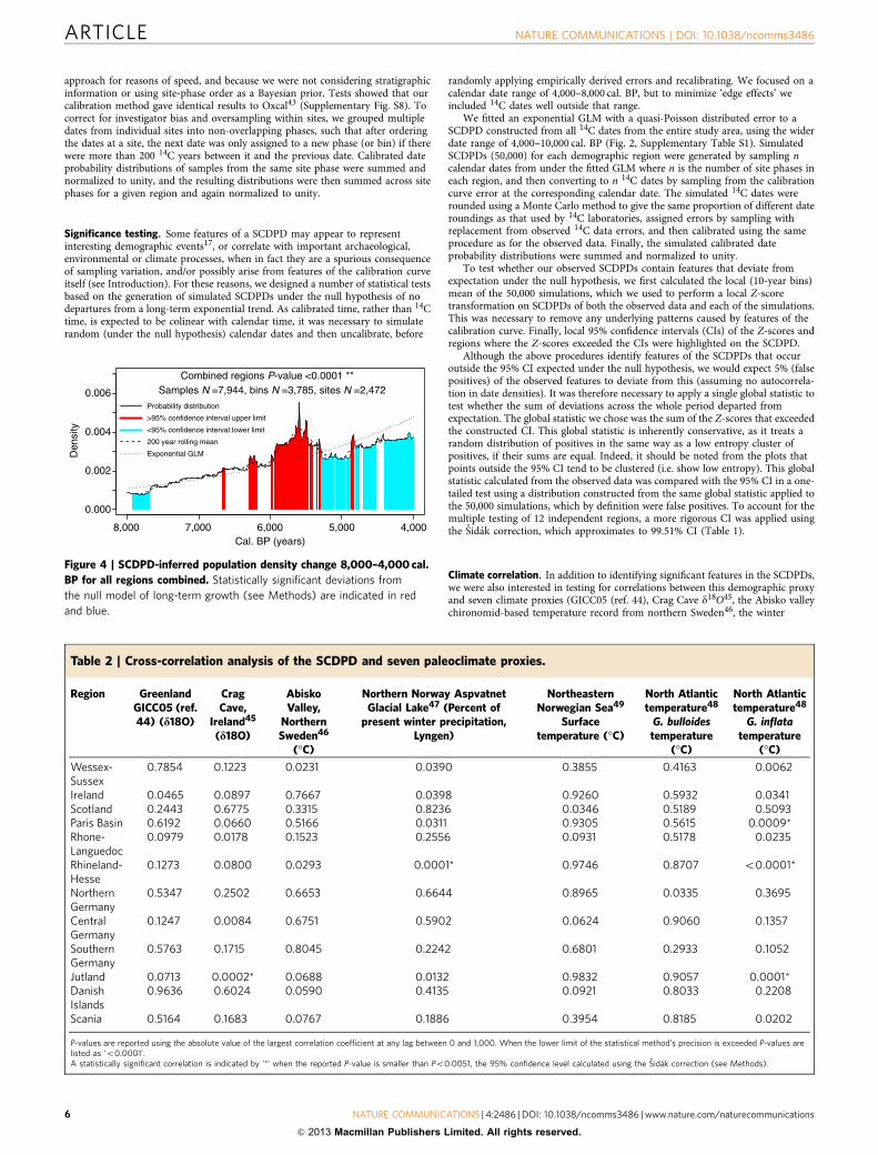
We then tested the SCDPD of the 12 regions in our studycombined for departure from the null model. There aresignificant positive deviations from the fitted exponential GLM,especially after 6,000 cal. BP. The later sixth and early-fifthmillennia cal. BP, on the other hand, are characterized bydensities significantly below the fitted GLM trend, before a returnto trend at the end of the fifth millennium (Fig. 4).

Correlation with paleoclimate proxies. There has been extensivediscussion in the literature of the impact of climate on earlyfarming populations in Europe25–27; hence, the question ariseswhether the inferred demographic patterns correlate withpaleoclimate. Cross-correlation analyses were performed usingseven climate proxies (see Methods). However, it is conceivablethat any initially apparent correlations are not causal but ratherreflect a relationship between climate and atmospheric 14C levelsor reservoir effects28. For example, d14C residual values have beenlinked with lower levels of solar activity and the 11-year sunspotcycle29. Again, therefore, it was necessary to take into account thefluctuations in the calibration curve when comparing the climateproxy values with the SCDPD patterns (see Methods). In mostcases there is no correlation. In the small number of regionsshowing significant results at the 95% confidence level adjustedfor the multiple testing of the regions the cross-correlationsare similar at all lags, indicating only a very broad general trendof long-term correlation between climate and demographicproxies. The P-values are summarized in Table 2 and details ofanalyses for all regions and paleoclimate proxies can be foundin Supplementary Fig. S2. A comparison of recent spatialvariation in temperature and precipitation with regional differ-ences in demographic trajectories also produced negative results(see Methods, Supplementary Figs S3–S6 and SupplementaryTables S2 and S3).

10,000 9,000 8,000 7,000 6,000 5,000 4,000

0.001

0.002

0.003

0.004

Cal. BP (years)

Den

sity

All dates in entire study areaSamples N =13,658, bins N =6,497

Probability distribution200 year rolling meanExponential GLM

Figure 2 | SCDPD-inferred population density change 10,000–4,000 cal.

BP using all radiocarbon dates in the western Europe database. The fitted

null model of exponential population growth is used to calculate the

statistical significance of regional (Fig. 3) and combined regional growth

deviations (Fig. 4).

NATURE COMMUNICATIONS | DOI: 10.1038/ncomms3486 ARTICLE

NATURE COMMUNICATIONS | 4:2486 | DOI: 10.1038/ncomms3486 | www.nature.com/naturecommunications 3

& 2013 Macmillan Publishers Limited. All rights reserved.

DiscussionOur analyses of SCDPDs have provided a new rigour in theirtreatment by addressing the problems caused by fluctuations inthe calibration curve and by sampling variation in the availabledates. They thus provide a basis for increased confidence inSCDPDs as valid demographic proxies. As noted above, inregions where independent evidence is available the validity of theSCDPD demographic proxy has been confirmed30. Moreover,most regions show more than one boom–bust pattern, contra-dicting suggestions that they are simply a result of a bias on thepart of archaeologists towards trying to date the first appearanceof farming in their region.

Although the European population follows an approximatelyexponential long-term growth trend (Fig. 2), considerableregional variation is evident. In virtually all the regions examinedhere, there are significant demographic fluctuations and in mostthere are indications at certain points of population decline of theorder of the 30–60% estimated by historians for the much laterBlack Death31, although of course absolute population sizesduring the Neolithic were much smaller than that duringthe Middle Ages. It is particularly important to note that thebust following the initial farming boom is found in twohistorically separate agricultural expansions, the first intoCentral Europe c. 7,500 years ago and the second intoNorthwest Europe 1,500 years later. It is possible that some ofthese regional declines represent out-migration to neighbouringareas rather than a real decline in numbers, for example, from theParis Basin into Britain, but, in some cases, for example, Ireland,

Scotland and Wessex, it is very clear that the rising and fallingtrends are roughly synchronous with one another—there is littleindication of one going up as the others go down. On presentevidence the decline in the initially raised population levelsfollowing the introduction of agriculture does not seem to beclimate-related, but of course this still leaves open a variety ofpossible causes that remain to be explored in the future. Onepossibility is disease, as the reference to the Black Death aboveimplies, although this would have to be occurring on multipleoccasions at different times in different places, given the patternsshown. It is perhaps more likely that it arose from endogenouscauses; for example, rapid population growth driven by farmingto unsustainable levels, soil depletion or erosion arising fromearly farming practices, or simply the risk arising from relyingon a small number of exploitable species32. However, thesesuggestions remain speculative and an autocorrelation analysis ofthe demographic data did not find evidence of a cyclical pattern,which would be one indicator of the operation of endogenousprocesses (Supplementary Fig. S7). Regardless of the cause,collapsing Neolithic populations must have had a major impacton social, economic and cultural processes.

MethodsData. A database of 13,658 radiocarbon dates and their contexts from the westernhalf of temperate Europe in the period 10,000–3,500 cal. BP was collated frompublications and public databases33–41. A number of distinct regions representingmajor areas of settlement during the Neolithic were selected: Ireland; Wessex andadjacent areas in southern England; Scotland; the Paris Basin and Normandy; the

0.000

0.002

0.004

0.006

0.008

0.010

0.012D

ensi

tyIreland P-value <0.0001 **

Samples N =1,732, bins N =928, Sites N =610Scotland P-value <0.0001 **

Samples N =612, bins N =339, Sites N =213Wessex Sussex P-value <0.0001 **

Samples N =589, bins N =284, Sites N =179

0.000

0.002

0.004

0.006

0.008

0.010

0.012

Den

sity

Paris basin P-value <0.0001 **Samples N =689, bins N =363, Sites N =228

Rhone Languedoc P-value <0.0001 **Samples N =1,064, bins N =592, Sites N =371

Rhineland−Hesse P-value <0.0001 **Samples N =333, bins N =151, Sites N =96

0.000

0.002

0.004

0.006

0.008

0.010

0.012

Den

sity

Northern Germany P-value =0.5098 Samples N =689, bins N =176, Sites N =107

Central Germany P-value =0.3044 Samples N =376, bins N =212, Sites N =155

Southern Germany P-value <0.0001 **Samples N =841, bins N =246, Sites N =154

8,000 7,000 6,000 5,000 4,0000.000

0.002

0.004

0.006

0.008

0.010

0.012

Cal. BP (years)

Den

sity

Jutland P-value <0.0001 **Samples N =409, bins N =175, Sites N =138

8,000 7,000 6,000 5,000 4,000

Cal. BP (years)

Danish Islands P-value <0.0001 **Samples N =329, bins N =161, Sites N =120

8,000 7,000 6,000 5,000 4,000

Cal. BP (years)

Scania P-value =0.0002 **Samples N =281, bins N =158, sites N =101

Probability distribution>95% confidence interval upper limit<95% confidence interval lower limit200 year rolling meanExponential GLMEarliest farming

Figure 3 | SCDPD-inferred population density change 8,000–4,000 cal. BP for each sub-region. Statistically significant deviations from the null

model (see Methods) are indicated in red and blue, and blue arrows indicate the first evidence for agriculture in each region. **P-values smaller than

Po0.0051, the 95% confidence level calculated using the Sidak correction (see Methods).

ARTICLE NATURE COMMUNICATIONS | DOI: 10.1038/ncomms3486

4 NATURE COMMUNICATIONS | 4:2486 | DOI: 10.1038/ncomms3486 | www.nature.com/naturecommunications

& 2013 Macmillan Publishers Limited. All rights reserved.

Rhone valley and adjacent areas; Jutland; the Danish Islands; Scania (southernmostSweden); northern Germany; the lower Rhine-Hesse region; central Germany; andsouthern Germany, including the adjacent loess areas of eastern France. Similar toCollard et al.17, we took an inclusive approach to date selection from the availablesources and excluded dates regarded as invalid by the laboratory, and those thatwere clearly incorrect in relation to the cultural context they claimed to be dating.All others were included on the grounds that the inclusion of imprecise dates andothers that might not survive rigorous ‘chronometric hygiene’ tests would tend to

obscure and smear any real fluctuations in population densities of interest to us,rather than accentuating them, and so have a conservative effect on hypothesistests.

Radiocarbon date calibration. Radiocarbon dates and their associated errors werecalibrated using scripts written in the ‘R’ programming language (http://www.r-project.org/) and the IntCal09 calibration curve42. We used an arithmetical

Table 1 | Regional summed radiocarbon date probability distributions analysis.

Data summary Significanttest

Timing and duration Archaeological interpretation

Region Dates(n)

Sitephases

(n)

Sites(n)

Boom/bust(P)

Approximatebeginning offarming (BP)

Pop. increaseafter

beginningof farming

Firstsignificantagricultureboom (BP)

Boomduration(years)

Wessex-Sussex

589 284 179 o0.0001* 6,000 Yes 5,600–5,300 300 A boom at mid-sixth millennium with arrival offarming after which population drops back totrend.

Ireland 1,732 928 610 o0.0001* 6,000 Yes 5,730–5,480 250 A boom–bust-boom pattern during the Neolithic.Scotland 612 339 213 o0.0001* 6,000 Yes 5,920–5,470 450 A major boom–bust, preceded by small

Mesolithic booms.Paris Basin 689 363 228 o0.0001* 7,200 Yes 7,160–6,190 970 A major Neolithic boom beginning in the late-

eighth millennium lasting with some fluctuationsthrough to the late-seventh millennium, withother slight indications in the early- and mid-sixthmillennium. These are followed by a fall back totrend and a crash in the late-sixth millennium thatlasts for the whole of the fifth.

Rhone-Languedoc

1,064 592 371 o0.0001* 7,700 Yes 6,770–5,750 1,020 Evidence for a boom associated with the firstappearance of farming in the mid-eighthmillennium, but the main boom is in the mid-seventh and early-sixth millennium, followed by acrash in the mid-sixth. Some indications ofanother millennium boom–bust cycle in the fifthmillennium, although edge effects are alsopossible.

Rhineland-Hesse

333 151 96 o0.0001* 7,400 Yes 7,410–6,500 910 A boom with the arrival of farming from the mid-eighth millennium to mid-seventh followed by afall back to trend. Low population at the end ofthe sixth millennium and most of the fifth,although possible edge effects.

NorthernGermany

689 176 107 0.5098 6,000 No – – No significant departure from long-termexponential model, although hints of fluctuationsin the early- and mid-sixth millennium followingthe beginning of farming. Negative deviations latein the fifth millennium are likely an edge effect.

CentralGermany

376 212 155 0.3044 7,400 No – – No significant departure from the exponentialmodel, although suggestions of a bust at the endof the seventh millennium.

SouthernGermany

841 246 154 o0.0001* 7,400 Yes 7,150–6,900 250 A boom following the arrival of farming, followedby a drop back to trend, and another boom in thelate-seventh millennium. These are followed byseveral slight positive indications and a bust laterin the fifth millennium, although edge effects arepossible.

Jutland 409 175 138 o0.0001* 6,000 Yes 5,640–5,300 340 A boom in the mid-sixth millennium after thearrival of farming, followed by a decrease at theend of the sixth millennium. Then another boomearly in the fifth millennium, followed by a returnto trend.

DanishIslands

329 161 120 o0.0001* 6,000 Yes 5,910–5,050 860 A positive deviation during the late Mesolithic,and a much more marked boom in the sixthmillennium associated with the beginning offarming, followed by a major decrease later in thefifth that might be in part because of edge effects.

Scania 281 158 101 0.0002* 6,000 Yes 5,730–5,430 300 Strong indications of a boom in the mid-sixthmillennium following the arrival of farming andagain in the early-fifth millennium with a dropback to trend in between.

All regionscombined

7,944 3,785 2,472 o0.0001* 6,700(weighted

mean)

Yes 6,000–5,400 600 Sub-continental scale population expansion in theearly- to mid-sixth millennium, mainly but notentirely associated with the spread of farminginto North Western Europe. This is followed by acrash in the late-sixth millennium, then slowexpansion after that, apart from indications of ashort boom episode at 4,800.

Sampling information, boom/bust significance test results, agriculture dates and timing information, and archaeological interpretations are included. When the lower limit of the statistical method’sprecision is exceeded P-values are listed as ‘o0.0001’.A statistically significant departure from the null model is indicated by ‘*’ when the reported P-value is smaller than Po0.0051, the 95% confidence level calculated using the Sidak correction (seeMethods).

NATURE COMMUNICATIONS | DOI: 10.1038/ncomms3486 ARTICLE

NATURE COMMUNICATIONS | 4:2486 | DOI: 10.1038/ncomms3486 | www.nature.com/naturecommunications 5

& 2013 Macmillan Publishers Limited. All rights reserved.

approach for reasons of speed, and because we were not considering stratigraphicinformation or using site-phase order as a Bayesian prior. Tests showed that ourcalibration method gave identical results to Oxcal43 (Supplementary Fig. S8). Tocorrect for investigator bias and oversampling within sites, we grouped multipledates from individual sites into non-overlapping phases, such that after orderingthe dates at a site, the next date was only assigned to a new phase (or bin) if therewere more than 200 14C years between it and the previous date. Calibrated dateprobability distributions of samples from the same site phase were summed andnormalized to unity, and the resulting distributions were then summed across sitephases for a given region and again normalized to unity.

Significance testing. Some features of a SCDPD may appear to representinteresting demographic events17, or correlate with important archaeological,environmental or climate processes, when in fact they are a spurious consequenceof sampling variation, and/or possibly arise from features of the calibration curveitself (see Introduction). For these reasons, we designed a number of statistical testsbased on the generation of simulated SCDPDs under the null hypothesis of nodepartures from a long-term exponential trend. As calibrated time, rather than 14Ctime, is expected to be colinear with calendar time, it was necessary to simulaterandom (under the null hypothesis) calendar dates and then uncalibrate, before

randomly applying empirically derived errors and recalibrating. We focused on acalendar date range of 4,000–8,000 cal. BP, but to minimize ‘edge effects’ weincluded 14C dates well outside that range.

We fitted an exponential GLM with a quasi-Poisson distributed error to aSCDPD constructed from all 14C dates from the entire study area, using the widerdate range of 4,000–10,000 cal. BP (Fig. 2, Supplementary Table S1). SimulatedSCDPDs (50,000) for each demographic region were generated by sampling ncalendar dates from under the fitted GLM where n is the number of site phases ineach region, and then converting to n 14C dates by sampling from the calibrationcurve error at the corresponding calendar date. The simulated 14C dates wererounded using a Monte Carlo method to give the same proportion of different dateroundings as that used by 14C laboratories, assigned errors by sampling withreplacement from observed 14C data errors, and then calibrated using the sameprocedure as for the observed data. Finally, the simulated calibrated dateprobability distributions were summed and normalized to unity.

To test whether our observed SCDPDs contain features that deviate fromexpectation under the null hypothesis, we first calculated the local (10-year bins)mean of the 50,000 simulations, which we used to perform a local Z-scoretransformation on SCDPDs of both the observed data and each of the simulations.This was necessary to remove any underlying patterns caused by features of thecalibration curve. Finally, local 95% confidence intervals (CIs) of the Z-scores andregions where the Z-scores exceeded the CIs were highlighted on the SCDPD.

Although the above procedures identify features of the SCDPDs that occuroutside the 95% CI expected under the null hypothesis, we would expect 5% (falsepositives) of the observed features to deviate from this (assuming no autocorrela-tion in date densities). It was therefore necessary to apply a single global statistic totest whether the sum of deviations across the whole period departed fromexpectation. The global statistic we chose was the sum of the Z-scores that exceededthe constructed CI. This global statistic is inherently conservative, as it treats arandom distribution of positives in the same way as a low entropy cluster ofpositives, if their sums are equal. Indeed, it should be noted from the plots thatpoints outside the 95% CI tend to be clustered (i.e. show low entropy). This globalstatistic calculated from the observed data was compared with the 95% CI in a one-tailed test using a distribution constructed from the same global statistic applied tothe 50,000 simulations, which by definition were false positives. To account for themultiple testing of 12 independent regions, a more rigorous CI was applied usingthe Sidak correction, which approximates to 99.51% CI (Table 1).

Climate correlation. In addition to identifying significant features in the SCDPDs,we were also interested in testing for correlations between this demographic proxyand seven climate proxies (GICC05 (ref. 44), Crag Cave d18O45, the Abisko valleychironomid-based temperature record from northern Sweden46, the winter

8,000 7,000 6,000 5,000 4,000

0.000

0.002

0.004

0.006

Cal. BP (years)

Den

sity

Combined regions P-value <0.0001 **Samples N =7,944, bins N =3,785, sites N =2,472

Probability distribution

>95% confidence interval upper limit

<95% confidence interval lower limit

200 year rolling mean

Exponential GLM

Figure 4 | SCDPD-inferred population density change 8,000–4,000 cal.

BP for all regions combined. Statistically significant deviations from

the null model of long-term growth (see Methods) are indicated in red

and blue.

Table 2 | Cross-correlation analysis of the SCDPD and seven paleoclimate proxies.

Region GreenlandGICC05 (ref.44) (d18O)

CragCave,

Ireland45

(d18O)

AbiskoValley,

NorthernSweden46

(�C)

Northern Norway AspvatnetGlacial Lake47 (Percent of

present winter precipitation,Lyngen)

NortheasternNorwegian Sea49

Surfacetemperature (�C)

North Atlantictemperature48

G. bulloidestemperature

(�C)

North Atlantictemperature48

G. inflatatemperature

(�C)

Wessex-Sussex

0.7854 0.1223 0.0231 0.0390 0.3855 0.4163 0.0062

Ireland 0.0465 0.0897 0.7667 0.0398 0.9260 0.5932 0.0341Scotland 0.2443 0.6775 0.3315 0.8236 0.0346 0.5189 0.5093Paris Basin 0.6192 0.0660 0.5166 0.0311 0.9305 0.5615 0.0009*Rhone-Languedoc

0.0979 0.0178 0.1523 0.2556 0.0931 0.5178 0.0235

Rhineland-Hesse

0.1273 0.0800 0.0293 0.0001* 0.9746 0.8707 o0.0001*

NorthernGermany

0.5347 0.2502 0.6653 0.6644 0.8965 0.0335 0.3695

CentralGermany

0.1247 0.0084 0.6751 0.5902 0.0624 0.9060 0.1357

SouthernGermany

0.5763 0.1715 0.8045 0.2242 0.6801 0.2933 0.1052

Jutland 0.0713 0.0002* 0.0688 0.0132 0.9832 0.9057 0.0001*DanishIslands

0.9636 0.6024 0.0590 0.4135 0.0921 0.8033 0.2208

Scania 0.5164 0.1683 0.0767 0.1886 0.3954 0.8185 0.0202

P-values are reported using the absolute value of the largest correlation coefficient at any lag between 0 and 1,000. When the lower limit of the statistical method’s precision is exceeded P-values arelisted as ‘o0.0001’.A statistically significant correlation is indicated by ‘*’ when the reported P-value is smaller than Po0.0051, the 95% confidence level calculated using the Sidak correction (see Methods).

ARTICLE NATURE COMMUNICATIONS | DOI: 10.1038/ncomms3486

6 NATURE COMMUNICATIONS | 4:2486 | DOI: 10.1038/ncomms3486 | www.nature.com/naturecommunications

& 2013 Macmillan Publishers Limited. All rights reserved.

precipitation record from the Aspvatnet glacial lake in northern Norway47 and twoseparate North Atlantic sea surface temperature proxies, RAPiD-12-1K48 and GIK23258-2 (ref. 49)). To account for uncertainty in the calibration curve, bothsimulated and real residuals were cross-correlated with the climate proxies, allinterpolated to the 10-year resolution of the demography for consistency, and 95%CIs were calculated from simulated correlation coefficients. To take into accountthe possibility of false positives, each region’s cross-correlation distribution wasthen tested for significance in a one-tailed test that compared a single globalstatistic (the absolute value of the largest correlation coefficient) from eachsimulation with the real data, by considering whether this statistic falls outside the95% CI of the simulated distribution of the same statistic for that single region. Toaccount for the multiple tests of 12 data sets, we again applied the Sidak correction(Table 2 and Supplementary Fig. S2).

To further investigate the relationship between population and climate, we alsocompared historic (1 October 1972–14 January 1996) spatial variation intemperature and precipitation from weather station instrumental data of threeclosely adjacent regions at the same latitude—Jutland, Scania and the DanishIslands (Supplementary Fig. S3, Supplementary Table S2). Their historictemperature and precipitation patterns are all highly correlated (SupplementaryFigs S4–S6, Supplementary Table S3), suggesting that their paleoclimates wouldalso have been extremely similar to each other, and although the inferreddemographic patterns of the first two regions have similar trajectories, the third isvery different (Fig. 3), indicating that climatic variation cannot account for thedifferences between them.

In the light of the negative results of the climate analysis, an autocorrelationanalysis of the demographic series was carried out on each region’s residuals to seewhether they provided evidence of endogenous cyclicity (Supplementary Fig. S7).This analysis was performed to explore lags between 0 and 1,000 years by using a‘sliding window’ of 3,000 years to avoid imputing data outside the window ofoverlap. CIs were generated by repeating this process on each of the 50,000simulations and estimating the local 95% CI. No evidence of cyclicity (typicallycharacterized by at least one peak of positive correlation preceded by a peak ofnegative correlation at half the wavelength) was observed. In some regions, apositive correlation outside 95% CI was observed, suggesting a broad long-termautocorrelation because of a long-term increase or decrease. This result is inagreement with visual inspection of the SCDPDs.

Bootstrap analysis. As an alternative method of illustrating uncertainty in esti-mated population density because of sampling error in SCDPDs, we applied abootstrap procedure (Supplementary Fig. S1). Within each region, uncalibrateddates were repeatedly sampled with replacement, calibrated and plotted to con-struct a running CI through calendar time. In most cases, there appears to be amarked demographic expansion after the first evidence of agriculture, followed bypopulation declines.

References1. Bocquet-Appel, J. P. et al. Understanding the rates of expansion of the farming

system in Europe. J. Archaeol. Sci. 39, 531–546 (2012).2. Bramanti, B. et al. Genetic discontinuity between local hunter-gatherers and

central Europe’s first farmers. Science 326, 137–140 (2009).3. Pinhasi, R., Thomas, M. G., Hofreiter, M., Currat, M. & Burger, J. The genetic

history of Europeans. Trends Genet. 28, 496–505 (2012).4. Malmstrom, H. et al. Ancient DNA reveals lack of continuity between Neolithic

hunter-gatherers and contemporary Scandinavians. Curr. Biol. 19, 1758–1762(2009).

5. von Cramon-Taubadel, N. & Pinhasi, R. Craniometric data support a mosaicmodel of demic and cultural Neolithic diffusion to outlying regions of Europe.P. Roy. Soc. B-Biol. Sci. 278, 2874–2880 (2011).

6. Skoglund, P. et al. Origins and genetic legacy of Neolithic farmers and hunter-gatherers in Europe. Science 336, 466–469 (2012).

7. Itan, Y., Powell, A., Beaumont, M. A., Burger, J. & Thomas, M. G. The originsof lactase persistence in Europe. PLoS Comput. Biol. 5, e1000491 (2009).

8. Binford, L. R. in New Perspectives in Archaeology (ed. Binford, S. R.) 313–342(Aldine, 1968).

9. Ammerman, A. J. & Cavalli-Sforza, L. L. Measuring the rate of spread of earlyfarming in Europe. Man 6, 674–688 (1971).

10. Fisher, R. A. The wave of advance of advantageous genes. Ann. Hum. Genet. 7,355–369 (1937).

11. Bocquet-Appel, J. P. Paleoanthropological traces of a Neolithic demographictransition. Curr. Anthropol. 43, 637–650 (2002).

12. Bocquet-Appel, J. P. When the world’s population took off: the springboard ofthe Neolithic demographic transition. Science 333, 560 (2011).

13. Gignoux, C. R., Henn, B. M. & Mountain, J. L. Rapid, global demographicexpansions after the origins of agriculture. Proc. Natl Acad. Sci. USA 108,6044–6049 (2011).

14. McEvedy, C. & Jones, R. Atlas of World Population History (Penguin BooksLtd., 1978).

15. Tallavaara, M. & Seppa, H. Did the mid-Holocene environmental changescause the boom and bust of hunter-gatherer population size in easternFennoscandia? Holocene 1–11 (2011).

16. Williams, A. The use of summed radiocarbon probability distributions inarchaeology: a review of methods. J. Archaeol. Sci. 39, 578–589 (2011).

17. Collard, M., Edinborough, K., Shennan, S. & Thomas, M. G. Radiocarbonevidence indicates that migrants introduced farming to Britain. J. Archaeol. Sci.37, 866–870 (2010).

18. Scott, E. M. The fourth international radiocarbon intercomparison (FIRI).Radiocarbon 45, 135–328 (2003).

19. Reimer, P. J. et al. IntCal09 and Marine09 radiocarbon age calibration curves,0–50,000 years cal BP. Radiocarbon 51, 1111–1150 (2009).

20. Surovell, T. A., Byrd Finley, J., Smith, G. M., Brantingham, P. J. & Kelly, R.Correcting temporal frequency distributions for taphonomic bias. J. Archaeol.Sci. 36, 1715–1724 (2009).

21. Woodbridge, J. et al. The impact of the Neolithic agricultural transition inBritain: a comparison of pollen-based land cover and archaeological 14Cdate-inferred population change. J. Archaeol. Sci. doi:10.1016/j.jas.2012.10.025(2012).

22. Stevens, C. J. & Fuller, D. Q. Did Neolithic farming fail? The case for aBronze Age agricultural revolution in the British Isles. Antiquity 86, 707–722(2012).

23. Zimmermann, A., Meurers-Balke, J. & Kalis, A. J. Das Neolithikum imRheinland. Bonner Jahrbucher 205, 1–63 (2005).

24. Zimmermann, A., Hilpert, J. & Wendt, K. P. Estimations of population densityfor selected periods between the Neolithic and AD 1800. Hum. Biol. 81,357–380 (2009).

25. Petrequin, P. Management of architectural woods and variations in populationdensity in the fourth and third millennia BC (Lakes Chalain and Clairvaux,Jura, France). J. Anthropol. Archaeol. 15, 1–19 (1996).

26. Gronenborn, G. in The spread of the Neolithic to Central Europe (edsGroneborn, G. & Petrasch, J.) 61–80 (RGZM, 2010).

27. Verrill, L. & Tipping, R. Use and abandonment of a Neolithic field system atBelderrig, Co. Mayo, Ireland: evidence for economic marginality. Holocene 20,1011–1021 (2010).

28. Stuiver, M. & Pollach, H. Discussions of reporting 14C data. Radiocarbon 19,355–363 (1977).

29. Stuiver, M. & Braziunas, T. F. Sun, ocean, climate and atmospheric 14CO2: anevaluation of causal and spectral relationships. Holocene 3, 289 (1993).

30. Hinz, M., Feeser, I., Sjogren, K. G. & Muller, J. Demography and the intensity ofcultural activities: an evaluation of funnel beaker societies (4200-2800 cal BC).J. Archaeol. Sci. 39, 3331–3340 (2012).

31. Barry, S. & Gualde, N. La plus grande epidemie de l’histoire. L’Histoire 45–46(2006).

32. Bowles, S. Cultivation of cereals by the first farmers was not more productivethan foraging. Proc. Natl Acad. Sci. USA 108, 4760–4765 (2011).

33. Gamble, C., Davies, W., Pettitt, P., Hazelwood, L. & Richards, M. Thearchaeological and genetic foundations of the European population during theLate Glacial: implications for agricultural thinking. Cambridge Archaeol. J. 15,193–223 (2005).

34. Guilaine, J. Atlas du Neolithique Europeen. Volume 2A & 2B, L’Europeoccidentale (Universite de Liege, 1998).

35. Weninger, B. in Chronology and Evolution in the Mesolithic of NorthwestEurope (eds Crombe, P., Van Strydonk, M., Boudin, M. & Batz, M.) 143–176(Cambridge Scholars Publishing, 2009).

36. Chapple, R. M. Catalogue of Radiocarbon Determinations & DendrochronologyDates (Oculus Obscura Press, 2011).

37. Steele, J. & Shennan, S. J. Spatial and Chronological Patterns in theNeolithisation of Europe, http://www.archaeologydataservice.ac.uk/archives/view/c14_meso/ (2003).

38. Galate, P. BANADORA, Banque de donnees des dates radiocarbones de Lyonpour l’Europe et le Proche-Orient (Universite Claude Bernard, 2011).

39. Council for British Archaeology. Archaeological Site Index to RadiocarbonDates from Great Britain and Ireland, http://www.archaeologydataservice.ac.uk/archives/view/c14_cba/ (2008).

40. Hinz, M. RADON - Radiocarbon dates online 2012. Central European databaseof 14C dates for the Neolithic and Early Bronze Age, University of Kiel,Available at http://www.radon.ufg.uni-kiel.de (2012).

41. Vermeersch, P. Radiocarbon Palaeolithic Europe Database v13 (Dept. of Earthand Environmental Sciences, Katholieke Universiteit, Leuver. http://www.ees.kuleuven.be/geography/projects/14c-palaeolithic/index.html, 2011).

42. Heaton, T. J., Blackwell, P. G. & Buck, C. E. A Bayesian approach to theestimation of radiocarbon calibration curves: the IntCal09 methodology.Radiocarbon 51, 1151 (2009).

43. Ramsey, C. B. Bayesian analysis of radiocarbon dates. Radiocarbon 51, 337–360(2009).

44. Vinther, B. M. et al. Holocene thinning of the Greenland ice sheet. Nature 461,385 (2009).

NATURE COMMUNICATIONS | DOI: 10.1038/ncomms3486 ARTICLE

NATURE COMMUNICATIONS | 4:2486 | DOI: 10.1038/ncomms3486 | www.nature.com/naturecommunications 7

& 2013 Macmillan Publishers Limited. All rights reserved.

45. McDermott, F., Mattey, D. P. & Hawkesworth, C. Centennial-scale Holoceneclimate variability revealed by a high-resolution speleothem d18O record fromSW Ireland. Science 294, 1328 (2001).

46. Larocque, I. & Hall, R. I. Holocene temperature estimates and chironomidcommunity composition in the Abisko Valley, northern Sweden. Quat. Sci. Rev.23, 2453–2465 (2004).

47. Bakke, J., Dahl, S. O., Paasche, Løvlie, R. & Nesje, A. Glacier fluctuations,equilibrium-line altitudes and palaeoclimate in Lyngen, northern Norway,during the Lateglacial and Holocene. Holocene 15, 518–540 (2005).

48. Thornalley, D. J. R., Elderfield, H. & McCave, I. N. Holocene oscillations intemperature and salinity of the surface subpolar North Atlantic. Nature 457,711–714 (2009).

49. Sarnthein, M. et al. Centennial-to-millennial-scale periodicities of Holoceneclimate and sediment injections off the western Barents shelf, 75�N. Boreas 32,447–461 (2008).

AcknowledgementsWe are grateful to all those who provided radiocarbon data. This research was funded bythe European Research Council Advanced Grant number 249390 to Shennan for theEUROEVOL project.

Author contributionsS.S. and M.G.T. designed the research; K.E., S.C., T.K. and K.M. collected data; A.T. andS.S.D. analysed data; S.S., M.G.T., S.S.D. and A.T. wrote the paper. All authors discussedthe results and approved the final manuscript.

Additional informationSupplementary Information accompanies this paper at http://www.nature.com/naturecommunications

Competing financial interests: The authors declare no competing financial interests.

Reprints and permission information is available online at http://npg.nature.com/reprintsandpermissions/

How to cite this article: Shennan, S. et al. Regional population collapse followed initialagriculture booms in mid-Holocene Europe. Nat. Commun. 4:2486 doi: 10.1038/ncomms3486 (2013).

This work is licensed under a Creative Commons Attribution-NonCommercial-ShareAlike 3.0 Unported License. To view a copy of

this license, visit http://creativecommons.org/licenses/by-nc-sa/3.0/

ARTICLE NATURE COMMUNICATIONS | DOI: 10.1038/ncomms3486

8 NATURE COMMUNICATIONS | 4:2486 | DOI: 10.1038/ncomms3486 | www.nature.com/naturecommunications

& 2013 Macmillan Publishers Limited. All rights reserved.