Capital Scarcity and Industrial Decline:

Evidence from 172 Real Estate Booms in China

Harald Hau∗

University of Geneva, CEPR and Swiss Finance Institute

Difei Ouyang∗∗

University of Geneva

August 26, 2019

Abstract

In geographically segmented credit markets, local real estate booms can divert capi-tal away from manufacturing firms, create capital scarcity, increase local real interestrates, lower real wages, and cause underinvestment and relative decline in the indus-trial sector. Using exogenous variation in the administrative land supply across 172Chinese cities, we show that the predicted variation in real estate prices does indeedcause substantially higher capital costs for manufacturing firms, reduce their banklending, lower their capital intensity and labor productivity, weaken firms’ financialperformance, and reduce their TFP growth by economically significant magnitudes.This evidence highlights macroeconomic stability concerns associated with real es-tate booms.

Key words: Factor price externalities, real estate booms, firm growth, industrial competi-tivenessJEL codes: D22, D24, R31

∗Geneva Finance Research Institute, 42 Bd du Pont d’Arve, 1211 Genève 4, Switzerland. Tel.: (++41) 22 379

9581. E-mail: prof@haraldhau.com. Web page: http://www.haraldhau.com.∗∗Geneva Finance Research Institute, 42 Bd du Pont d’Arve, 1211 Genève 4, Switzerland. Tel.: (++41) 78 945

1656. E-mail: Difei.Ouyang@unige.ch

Acknowledgments

We are grateful to Meng Miao, Hongyi Chen, Sebastian Dörr, Fansheng Jia, Chen Lin, Olivier Scaillet, René

M. Stulz, Jin Tao, Fabio Trojani, Zexi Wang, Hao Zhou, Michel Habib and Daragh Clancy for their comments.

We also thank seminar participants at Renmin University of China, Peking University, Tsinghua University,

University of Geneva, and University of Hong Kong and conference partipants at SFI Research Days, 2018 Asian

Meeting of the Econometric Society and the 33rd Annual Congress of the European Economic Association,

6th Annual Workshop in “Banking, Finance, Macroeconomics, and the Real Economy”, 2019 Spring Meeting of

Young Economists, 2019 China Finance Research Conference and 2019 China International Conference in Finance

for their remarks. This research project benefited from a grant from the Swiss National Science Foundation

(SNSF). The authors declare that they have no relevant or material financial interests that relate to the research

described in this paper.

1 Introduction

In geographically segmented credit markets, real estate investments competes with corporate

investments for the local household savings. During real estate booms with a strong surge in

value of housing investment, the residual capital available for corporate investment can become

scarce and expensive–thus undermining the competitiveness and growth potential of the local

manufacturing sector, which competes with firms in more capital-abundant locations. Empiri-

cally, the negative effect on local corporate growth is difficult to establish because cross-country

studies are plagued by many confounding effects and exogenous factors, making real estate

investment booms generally hard to identify.

Our paper makes four new contributions to the literature. First, China’s segmented capital

market provides the ideal empirical setting for identifying and measuring real effects of local

capital market distortions induced by local real estate booms. Our empirical analysis goes

beyond the evidence in Chakraborty et al. (2018) which identifies substitution effects in bank

lending. Our new contribution is to show that such bank lending substitution can have strong

real effects on local industrial competitiveness based on a variety of firm variables like firm value

added, profitability, total factor productivity, and export performance. While a recent literature

has focused on banking crisis as the source of adverse real effects on firm employment, output,

export or investment (Amiti and Weinstein, 2011; Chodorow-Reich 2013; Paravisini et al. 2014;

Cingano et al. 2016; Bentolila et al. 2017; Acharya et al. 2018; Huber 2018), we demonstrate

that such negative real effects can alternatively originate in real estate booms.

Second, a more integrated capital market like in the U.S. tends to diffuses real effects of local

bank lending booms to real estate to the macro level. Traditional macroeconomics has found

it difficult to identify the long-run persistent firm effects of reduced bank lending for lack of a

proper counterfactual scenario.1 This paper identifies the effect of capital shortages in the cross

section and thus identifies real firm effects much better than any intertemporal macroeconomic

analysis can.

Third, we develop a simple neoclassical framework in which a segmented capital market

implies different local real effects for local housing supply variation. The simple model generates

1We highlight that contemporaneous local capital shortages may have more extreme effects on firms becauseof competitive advantage enjoyed by the financially unconstrained firms. By contrast, marcroeconomics capitalshortages during recessions may not imply competitive distortions within a closed economy.

1

predictions not only for the local real estate price level, but also for the local capital costs, and

the real wages–thus broadening the scope of the analysis on the real side of the economy. Our

two sector Harrod-Balassa-Samuelson model predicts that real estate booms lower the local real

wage–which is borne out by the data–and contrast with alternative models on financial sector

linkages.

Fourth, we propose different instrumental variable (IV) strategies based on monopolistic land

supply or housing supply elasticities. Time variation in the local land supply allows for a new

intertemporal identification of real estate price effects where firm fixed effects control for time-

invariant firm heterogeneity. Alternatively, we implement a strictly cross-sectional identification

strategy based on local housing supply elasticities similar to Mian and Sufi (2011, 2014), and

obtain quantitatively similar results.

The land supply in Chinese cities is shown to be a good predictor of local real estate booms,

which channel local household savings into real estate investment rather than corporate invest-

ment. We find that the larger the real estate boom in any Chinese city for the period 2002—2007,

the more severe the credit and capital scarcity for the local corporate sector became. Such city-

level capital scarcity manifests itself in higher interest rates for corporate loans, a lower share

of firms with bank credit, significantly lower corporate investment rates, and large negative

externalities on the growth and competitiveness of local manufacturing firms.

Real estate booms have many links to local economic conditions. Productivity shocks can

boost local output, increase housing demand through migration or income effects, and induce a

positive correlation between housing prices and the performance of local manufacturing firms.

We therefore need a valid instrument that accounts for exogenous variation in the housing

price and the ensuing capital diversion into real estate investment. The institutional features

of China’s housing market provide such an instrument: Constructible land is supplied monop-

olistically by the local government, governed by an autonomous administrative process, and

subject to exogenous constraints on land availability in a city. We define the annual Adjusted

Land Supply as the surface of new constructible residential land scaled by the size of the existing

housing stock and local population density. While this supply measure is a very good predictor

for the (log) housing price level, it is itself unrelated to local economic conditions such as local

GDP, local population, local government expenditure or revenue. The Adjusted Land Supply

is neither predicted by past economic performance measure of a city nor related to its future

2

(infrastructure) development.

We use the Adjusted Land Supply as an instrument for explaining the large cross-sectional

and intertemporal variation in Chinese real estate prices. Figure 1 sorts 251 prefecture-level

cities by their initial real estate price index in 2003 (blue spikes) and shows the large variation

of the same price index in 2010 (red spike). We are able to construct panel data on land supply

in 172 prefecture-level cities and use firm-level data from these cities for our main analysis. Our

first-stage regression can explain a large share of the price variation between 2002 and 2007

by the Adjusted Land Supply in each city. The second-stage regression then documents how

real estate price variation traced back to land supply variation impacts firm development. We

measure corporate capital scarcity directly at the firm level by examining measures of firm bank

access and bank credit costs–showing their strong relationship to the instrumented real estate

price.

China’s highly segmented capital market for small and medium-size firm finance provides an

excellent case for studying the equilibrium effects of capital scarcity. Such capital market seg-

mentation at the prefecture-city level has been documented through the crowding out of corpo-

rate finance by local government borrowing (Huang, Pagano, and Panizza, 2017, 2018). Other

studies also provide evidences of low interregional capital mobility in China using Feldstein-

Horioka saving-investment or the Campbell-Mankiw consumption-smoothing framework (Boyreau-

Debray and Wei, 2004; Chan et al., 2011). Moreover, real estate companies can only borrow

from local commercial banks and consumers can only acquire mortgage loans from local banks

due to policy restrictions2 so that bank lending to local real estate related business will com-

pete with loans to local manufacturing firms. While there are no explicit restriction for firm to

borrow from banks in other cities, the observed share of out-of-city corporate borrowing is very

small–suggesting important non-regulatory barriers. Finally, shadow banking can alleviate lo-

cal credit constrains only to a limited extent as bank lending still represents almost 7/8th of

outstanding credit in 2008 (Elliott et al. 2015).

Our main finding is the strong economic effects of exogenous variations in real estate prices on

corporate capital costs, the availability of bank credit, corporate investment and growth. A 50%

2Real estate loans issued by commercial banks can only be used for local real estate projects. Local personalhousing provident fund loans cannot be used for purchasing houses in other cities. And local individual housingmortgage loans can only be used for local housing purchases.

3

relative increase in a city’s real estate price due to a shortage in local land supply over the period

2002—2007 increases the borrowing costs of firms by an average 0.9 percentage points annually

and reduces the share of firms with bank credit by 3.2 percentage points, which represents a 9%

reduction relative to the sample mean. This local credit crunch reduces the average corporate

net investment share (net new investment to book capital) by 7.3 percentage points, which

represents a 21.4% reduction relative to the sample mean. The long-run relative output decline

amounts to a staggering 35.5% of value-added output and total factor productivity features a

relative decline of nearly 12% for the average manufacturing firms.

We cross-check these large real effects with independent data sourced from the Chinese

customs authorities. Real estate booms can potentially create local product demand effects

through expenditure switching to real estate or through wealth effects. But these demand

effects should not influence firm exports as the international product demand is unlikely to

covary with local Chinese real estate prices. Moreover, Chinese customs data record product-

level data on real quantities for each exporting firm. Using these accounting data on exports

has an additional advantage: Unlike the revenue-based output measures based on industry price

deflator, it is not subject to price measurement error. Yet the recorded export quantities (for

firms that export more than 75% of their output) also show a staggering 17.3% shortfall in

exports for firms in cities with a 50% higher real estate price index. This strong economic effect

of real estate prices on export performance cannot be explained by local demand effects. In

addition, export prices show no pass-through effect of real estate prices and thus confirm that

output deflators are not subject to any systematic measurement biases across cities.

A challenge for our instruments is to exclude confounding effects on outcome variables which

correlate with housing price variation. We adopt a variety of strategies to convince the scep-

tical reader: First, we verify that our instrument (i.e., Adjusted Land Supply) is unrelated to

local economic and fiscal variables except the local real estate price. Moreover, we find that

our instrument has no relationship to measures of past or future city development. Second, we

highlight that our regression analysis generally includes firm fixed effects so that identification is

achieved through the intertemporal variation in local land supply related to random contingen-

cies within the bureaucratic planning process. This should alleviate concerns that unobserved

cross-sectional factors drive our results. Third, we develop a structural model of saving diversion

into residential housing investment and confirm its predicted effects on local factor prices (i.e.,

4

corporate loan costs and firm wages) and many other firm variables (i.e., net investment share,

gross investment share, bank loan dummy, log employment, log output, log labor productivity,

firm exit dummy, return on assets, log total factor productivity). In particular, the factor price

evidence supports the transmission channel through local capital costs and is unlikely to be ex-

plained by other channels linking new residential land supply to corporate development. Fourth,

we confirm the predicted heterogeneity in firm effects resulting from unequal bank access. Firms

with large fixed assets and state-owned enterprises (SOEs) enjoy privileged credit access to the

“big five” national banks. We show that this greatly attenuates their exposure to the capital

scarcity induced by local real estate booms and reduces their relative competitive decline. For

example, the average SOE shows a reduction in the investment share of only 1.9 percentage

points for a 50% higher local real estate price relative to an investment shortfall of 8.4 percent-

age points observed for privately owned firms. Fifth, we show robustness of our results using an

alternative instrument for real estate prices–namely the elasticity of new Chinese residential

housing construction taken from Wang et. al. (2012). This purely cross-sectional approach

resembles recent work by Mian and Sufi (2011, 2014), Mian et al. (2013), Adelino et al. (2015)

on the U.S. data.

Finally, we note that any endogeneity of land supply due to city-level politics should predict

an increased supply of residential land in response to local real estate inflation.3 Such policy

endogeneity will tend to attenuate the 2SLS coefficients and bias the real effects towards zero.

Any endogenous policy response at the city level thus implies that the quantitative effects we

estimate could be even larger in the absence of a supply response.

We also point out that the evidence does not support a “Dutch Disease” effect in which all

factor prices increase. Instead, we find that real wages fall significantly wherever real estate

prices boom and interest rates increase. This reverse factor price dynamics is best captured by

a modified Harrod—Balassa—Samuelson (HBS) model we develop in which a construction sector

and the industrial sector compete for scarce labor and capital resources. But unlike in the

traditional HBS model, the factor price externality of the construction sector operates through

inflated capital costs, whereas real wages decrease under competitive pricing both in the model

and the data.

3For example, the State Council of the central government in a meeting on January 26, 2011, instructed localgovernments to increase land supply for residential housing in order to control housing price inflation.

5

The macroeconomic economic literature has recognized that real estate markets and mort-

gage institutions can have an influence on the savings rate of households (Deaton and Laroque,

2001) and possibly growth. For example, cross-country variations in the loan to value ratios

in mortgage markets affect the liquidity constraints of households, influence household saving

rates and appear to correlate negatively with corporate investment rates and growth rates (Jap-

pelli and Pagano, 1994). The channel we highlight in this paper focuses not so much on the

equilibrium saving rate per se, but more directly on savings that are diverted from corporate to

housing investments if the latter promise higher returns during real estate booms.

Recent finance research has examined the relationship between real estate booms and cor-

porate investment by U.S. firms. For firms with real estate property, a local property price

increase can relax borrowing constraints and increase firm investment (Chaney et al., 2012;

Jiminez et al., 2014). For Chinese firms this balance sheet effect may not matter much because

of a lack of real estate assets on firms’ balance sheets and the state’s monopoly of land devel-

opment. Among Chinese listed firms in 2007, only 35.1% report positive real estate assets and

their aggregate value accounts for only 2.56% of aggregate assets. For all firms, including those

that do not hold real estate assets, the real estate value share is lower at 1.12% of aggregate

assets–suggesting that smaller non-listed manufacturing firms own only negligible amounts of

real estate assets. Wu et al. (2015) confirms that there is no evidence of a collateral channel

effect in China. Real estate booms can also increase local consumption through a collateral

effect and/or wealth effect (Cloyne et al., 2019). We highlight that any collateral effect related

to real estate booms–either for firms or households–should reinforce local firm growth rather

than contribute to the industrial decline documented in this paper.

Unlike a collateral channel, the equilibrium effect of corporate underinvestment due to saving

diversion concerns all firms and has potentially larger economic ramifications. The literature

on financial stability has often highlighted real estate booms as a precursor of financial crisis

through imprudent bank lending (IMF, 2011). The negative effects of such booms on the real

sector through reduced credit and a loss of competitiveness are apparently important features

of recent financial crises in southern Europe (Sinn, 2014; Martín et al., 2018) – yet identifying

a clear causal link between real estate booms and reduced firm investment has generally been

difficult. An exception here is recent evidence by Chakraborty et al. (2018) showing that

local real estate booms adversely affect the volume and cost of business loans from U.S. banks:

6

A one standard deviation increase in U.S. housing price increases the corporate borrowing

costs of financially constrained U.S. firms by 0.53 percentage points and reduces corporate

investment rate by an average of 6.2 percentage points. A higher degree of regional credit

market fragmentation and large geographic variations in housing booms make China a very good

candidate to study sectorial competition for local credit. In China, a one standard deviation

increase in the real estate prices implies an average increase of corporate borrowing costs by a

much larger 1.1 percentage points and reduces the investment rate by 8.7 percentage points. The

influence of real estate booms on China’s internal capital allocation has been highlighted by two

related working papers. Wu et al. (2016) present evidence on a significant and robust negative

association between housing prices and corporate investment. Chen et al. (2016) emphasize

both speculative real estate investment and the crowding out of corporate investment for the

same data period.

In Section 2 we develop the two-sector model and contrast the effect of diverging capital

costs with the Harrod-Balassa-Samuelson model of diverging labor costs. The testable model

implications are spelled out in two propositions in Section 2.2., followed by two additional

hypothesis on firm heterogeneity and firm performance in Section 2.3. In Section 3 we explain

the data and the estimation strategy based on within-city land supply variation. Our empirical

analysis first validates the model implications for factor prices, namely capital costs and wages,

in Section 4.1, and then for other firm variables in Section 4.2. Section 4.3 uses firm data

from the Chinese custom statistics export to discard local demand effects as an alternative

explanation for the observed firm performance. The role of firm heterogeneity in capital access

is studied in Section 4.4, and we examine additional firm performance measures in Section 4.5.

Robustness is discussed in Section 5 followed by our conclusions in Section 6.

2 Theoretical Framework

One of the best documented stylized facts about relative competitiveness is the Harrod-Balassa-

Samuelson effect. Productivity growth in a country drives factor costs and in particular real

wage growth. This makes non-tradeable labor-intensive service sectors expensive and non-

competitive by international comparison; yet their very non-tradability implies that high wage

costs can be passed on to high prices for non-tradeables. The following section presents a

7

similar two-sector economy in which one booming sector adversely influences the other sector

through factor prices. We argue that in a Chinese city with a booming real estate sector and

increasing housing prices, local savings are predominantly channeled into real estate investment

where rapid price inflation promises a high return. Unlike the Harrod-Balassa-Samuelson world

with its perfect capital market, China’s corporate credit market is highly segmented so that

the large capital demand of the real estate sector dramatically increases the local interest rate.

High local capital costs and/or capital scarcity undermine the competitiveness of the local

manufacturing sector. Unlike the non-tradeable sector in the Harrod-Balassa-Samuelson world,

the manufacturing sector cannot pass on a higher factor cost to a competitive international

market price and instead faces industrial decline and demise. We develop this modified or

“inverted” Harrod-Balassa-Samuelson world of factor price externalities more formally in the

next section before applying it empirically to the Chinese economy.4

2.1 A Two-Sector Model

We retain the two-sector structure of the Harrod-Balassa-Samuelson model and replace the

non-tradeable sector with a real estate sector.

Assumption 1: Real Estate and Tradeable Sector

Consider a competitive real estate sector (R) producing housing YR and a compet-

itive manufacturing sector (T ) producing tradeables YT . Both sectors compete for

capital with inputs KR and KT , respectively. The real estate sector requires a gov-

ernmental land supply S as a complementary factor and a high real estate price P

requires proportionately more capital to produce the same amount of housing. The

production function for real estate is given by

YR = ARmin(S,KR/P ) (1)

where land supply S and real capital KR/P are strictly complementary. The trade-

able sector features a Cobb-Douglas production function with labor input L (capital

4In the context of investment booms triggered by natural resources, negative cross-industry externalitiesare sometimes referred to as a “Dutch Disease”, and consist of rising real wages, that undermine industrialcompetitiveness. But in the Chinese context the factor price for capital increases, whereas wages decrease incities with real estate booms. References to a “Dutch Disease” are therefore misleading.

8

input KT ) and labor (capital) elasticity µ (1− µ) given by

YT = ATLµK1−µ

T . (2)

For simplicity, we assume real estate production does not require any labor input. This

assumption can be easily relaxed and is not critical for our analysis. More important is the

assumption that the capital requirements for real estate production increase linearly in the

price of real estate P . This assumption is motivated by the monopolistic land supply S, where

local government rations land supply and increases land prices in line with the real estate price.

Hence, the same real housing production requires an increasing amount of private capital as

real estate prices increase. This implies that a real estate boom in our model does not require

that more real resources are allocated to housing. Yet, inflated costs of new housing reduce the

share of private savings available for corporate investment. We assume that the revenue from

land sales is consumed by the government (or invested otherwise) and does not relax the limited

supply of local (private) capital.5 In particular, we assume a fixed local factor supply for both

labor and capital.

Assumption 2: Factor Supplies

The local capital and labor supply are both price inelastic and fixed; hence

KR +KT = K (3)

L = L. (4)

Completely price inelastic local factor supplies in both capital and labor are two simplifying

assumptions. However, these are not essential for the qualitative implications of the model. In

Appendix A we solve the model for the general case of price elastic factor supplies. We find

that all qualitative predictions are robust to this generalization. We also note that housing price

inflation can be further accelerated by speculative buying of housing in view of future capital

gains; yet we do not explicitly model any additional speculative housing demand here (Chen

5If local government does not consume (or invest) its gains from land sales, but instead deposits these revenuesin local banks, then we do not obtain a local capital scarcity effect under real estate price inflation. A generalequilibrium model therefore needs to model government expenditure decisions in addition to private savingdecisions.

9

et al., 2016; Shi Yu, 2017). Finally, the local capital K generally depend on the local saving

rate, which in turn could depends on real estate prices. Yet, we find no evidence that the local

household saving rate correlates with local real estate prices.6

The traditional Harrod-Balassa-Samuelson literature generally assumes perfect capital mar-

ket integration. However, a constrained local capital supply provides a better empirical bench-

mark for China: its internal capital market appears to be segmented with only limited capital

flows compensating for capital demand shocks across cities (Huang, Pagano, and Panizza, 2017,

2018). Many restrictions on banking across various administrative units contribute to the re-

gional segmentation of the corporate credit market. The lack of true capital market integration

leaves plenty of scope for geographically diverging real interest rates and capital. In Appendix

B, we estimate an error correction model for the median corporate bank loan rate in any city

relative to the median rate of all firms in neighboring cities. The variation in the median cor-

porate bank loan rate across cities ranges from 3.8% for a city at the 10% quantile to 6.4% for

a city at the 90% quantile. The mean reversion of only 13.8% between a city’s median loan

rate and those of firms in the neighboring cities illustrates the strong geographic segmentation

of China’s corporate credit markets.

We close the model with a housing demand function of low price elasticity.

Assumption 3: Housing Demand

The (log) housing demand is price elastic and for strictly positive parameters γ0, γ1

with 0 � γp < 1, total housing demand follows as

lnY DR (P ) = γ0 − γp lnP. (5)

Under 0 � γp < 1 housing demand features a low price elasticity. As the local housing

production is constrained by the land supply S, the equilibrium real estate price follows directly

as

lnP =1

γp[γ0 − lnAR − lnS] , (6)

6Using household data from China’s Urban Household Survey over the period of 2002—2007, we regress thehousehold-level saving rate on local real estate prices in a regression with household and time fixed effects. Thepositive coefficient for the local real estate price in this panel regression is economically small and statisticallyinsignificant.

10

and the capital demand of the real estate sector is given by

lnKR = γ0 + (1− γp) lnP − lnAR = (7)

=1

γp(γ0 − lnAR)−

1− γpγp

lnS.

An insufficient land supply by local government therefore inflates the real estate price P and at

the same time increases the capital demand lnKR by the real estate sector.

2.2 Model Implications

To simplify notation, we express all variables in percentage changes relative to steady state log

values, that is X = dX/X. The zero profit condition in the tradeable sector implies the following

relationship for changes in the equilibrium wage w and the local interest rate i

AT = µw + (1− µ)i, (8)

where we abstract from any productivity growth by assuming AT = AR = 0. Profit maximization

in the tradeable sector also implies

YT = w + L = i+ KT , (9)

and the factor supply conditions give L = 0 and KTKT + KRKR = 0. Combining these rela-

tionships implies the following proposition.

Proposition 1: Wage and Interest Rate Channel:

Under Assumptions 1—3, and a limited supply of constructible land S, the local

interest rate change i (real wage changes w) is proportional (is inversely proportional)

to real estate prices inflation P with percentage changes characterized as

i = µKR

KT

(1− γp)P (10)

w = −(1− µ)KR

KT

(1− γp)P . (11)

11

Real estate inflation itself is proportional to changes in the local land supply S as

P = S × η, (12)

with a price elasticity of supply η = −1/γp.

The negative effect of the real estate boom on wages distinguishes our model from a so-called

“Dutch Disease” scenario, where an investment boom (often in natural resource industries)

increases real labor costs and exercises competitive pressures on other firms through a higher

local wage level. By contrast, our model predicts a decrease in the real wage level because of

corporate underinvestment under high interest rates.

The linear relationship between the real estate price and the land supply in Eq. (12) suggests

that land supply should be a good instrument for local real estate inflation. As land supply by

local government also conditions housing output, with YR = S absent any productivity growth

in construction (AR = 0), we can relate changes in the (new) housing supply YR and housing

sales HS = P + YR to change in the local housing price index, hence

YR = −γpP (13)

HS = (1− γp)P . (14)

Figure 2 shows the positive relationship between annual (log) changes in housing sales and the

annual (log) changes in the city housing price index. A “near unit” slope 1 − γp � 1 shows

that the housing demand is very price inelastic so that small changes in the land supply (and

consecutively new housing supply) translate into large housing price changes.

The first part of our empirical analysis consists in showing that local factor prices across

Chinese cities are indeed related to local real estate inflation P and constructible land supply S

as predicted in Proposition 1. The second part of our analysis explores the role of the implied

factor price variation for the manufacturing sector summarized in Proposition 2:

Proposition 2: Manufacturing Under a Real Estate Boom

Under Assumptions 1—3 and a limited supply of constructible land S, the local

production response in the manufacturing sector to real estate inflation P is char-

12

acterized by a relative (percentage) adjustment in capital KT , the net investment

share (NI/K)T , manufacturing output YT , and labor productivity (Y /L)T given by

KT = −KR

KT

(1− γp)P (15)

(NI/K)T = KT = −KR

KT

(1− γp)P (16)

YT = −(1− µ)KR

KT

(1− γp)P (17)

(Y /L)T = −(1− µ)KR

KT

(1− γp)P , (18)

where a low price elasticity of housing demand implies 0 � γp < 1.

Our model predicts the direct real effects of real estate booms on firm investment, output, and

labor productivity. We do not model financial intermediation and the banks’ role in channeling

credit into real estate rather than firm investment. For China, we do not dispose a disaggregate

data which allows us to document the credit allocation decision at the bank level similar to

Chakraborty et al. (2018). However, aggregate data suggests that the banking sector allocated

an increasing proportion of credit to housing development: The outstanding individual housing

loans increased fivefold from 560 billion Yuan in 2001 to 3 trillion Yuan in 2007. In the last

sample year 2007, roughly 13.8% of all new medium and long term bank loans were allocated to

the real estate companies compared to only 7.5% for the entire manufacturing (People’s Bank

of China, 2007).

2.3 Extensions to Firm Heterogeneity

The simple two-sector model presented in Section 2.1 does not allow for firm heterogeneity in

capital access. Naturally, some firms are exposed to local capital scarcity more than others. In

particular, firms with large fixed assets (available as collateral) and state-owned enterprises with

political support should find it much easier to maintain credit access even under local capital

scarcity. We therefore add the following testable hypothesis:

Hypothesis 1: Heterogeneous Capital Access Within Cities

Under real estate inflation, firms with large fixed assets or SOEs should find it

13

easier to maintain credit access and ceteris paribus experience a relative increase in

investment and capital growth, a larger loan growth, and larger growth in output

and labor productivity.

Our competitive model also ignores the additional consequences of higher capital costs and

underinvestment on (long-term) firm profitability, leverage, and factor productivity. However,

firm performance measures are likely to decline if real estate booms increase the capital costs

of local manufacturing firms (Dörr et al. 2017; Manaresi and Pierri 2018). Lower profitability

should predict higher leverage. We summarize these effects in a second testable proposition:

Hypothesis 2: Firm Profitability, Leverage, and Factor Productivity

For tradeable producers, increased local capital costs under real estate inflation

imply reduced profitability (lower ROA) and increased leverage. Moreover, credit

supply constraint adversely affects total factor productivity (TFP) growth because

of underinvestment. Within a city, these effects should be less pronounced for SOEs

or firms with large fixed assets enabling easier access to credit.

3 Data Issues

3.1 Data Sources

We use firm data from the annual survey of all industrial firms (ASIF) conducted by China’s Na-

tional Bureau of Statistics over the period of 1998—2007. The ASIF data cover state-owned and

private-owned enterprises in the mining, manufacturing, and utility sectors. Private enterprises

are covered if their annual operating income exceeds RMB 5 million.7 The survey consists of

a stratified firm sample for 31 provinces, 398 cities, 43 two-digit industries, and 195 three-digit

industries. The survey reports detail accounting data, allowing us to construct measures of

firm investment, productivity, and financial performance. The location of firm’s headquarters

is identified so that we can match additional city-level statistics–in particular to the local real

estate market.

Three main shortcomings of the data source should be highlighted. First, the firm sample is

unbalanced, smaller firms in particular are typically covered only for less than three consecutive

7RMB 5 million was equivalent to US$ 603,930 in 1998 and US$ 657,549 in 2007.

14

years. Second, the survey contains data errors and must be filtered for implausible data points.

We provide details of our data cleaning procedure in Appendix C, which produces a final sample

of around 900,000 firm-year observations for the period 2002—2007. Third, the survey data

do not report any plant-level information. Multi-plant firms can produce in multiple cities

with diverging real estate environments. However, the city level represents a relatively large

administrative unit with an average population of 3.5 million. Only very large corporations are

likely to operate in multiple cities and eliminating large firms from the sample does not appear

to influence our main estimation results.

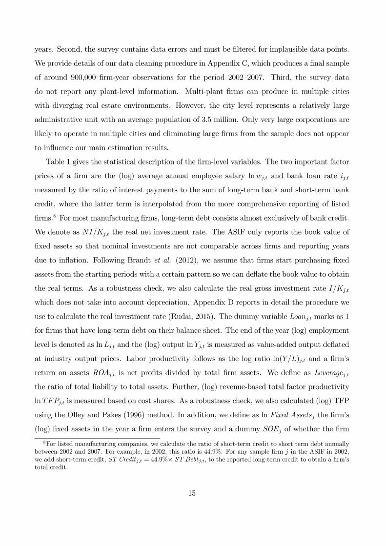
Table 1 gives the statistical description of the firm-level variables. The two important factor

prices of a firm are the (log) average annual employee salary lnwj,t and bank loan rate ij,t

measured by the ratio of interest payments to the sum of long-term bank and short-term bank

credit, where the latter term is interpolated from the more comprehensive reporting of listed

firms.8 For most manufacturing firms, long-term debt consists almost exclusively of bank credit.

We denote as NI/Kj,t the real net investment rate. The ASIF only reports the book value of

fixed assets so that nominal investments are not comparable across firms and reporting years

due to inflation. Following Brandt et al. (2012), we assume that firms start purchasing fixed

assets from the starting periods with a certain pattern so we can deflate the book value to obtain

the real terms. As a robustness check, we also calculate the real gross investment rate I/Kj,t

which does not take into account depreciation. Appendix D reports in detail the procedure we

use to calculate the real investment rate (Rudai, 2015). The dummy variable Loanj,t marks as 1

for firms that have long-term debt on their balance sheet. The end of the year (log) employment

level is denoted as lnLj,t and the (log) output lnYj,t is measured as value-added output deflated

at industry output prices. Labor productivity follows as the log ratio ln(Y/L)j,t and a firm’s

return on assets ROAj,t is net profits divided by total firm assets. We define as Leveragej,t

the ratio of total liability to total assets. Further, (log) revenue-based total factor productivity

lnTFPj,t is measured based on cost shares. As a robustness check, we also calculated (log) TFP

using the Olley and Pakes (1996) method. In addition, we define as ln Fixed Assetsj the firm’s

(log) fixed assets in the year a firm enters the survey and a dummy SOE j of whether the firm

8For listed manufacturing companies, we calculate the ratio of short-term credit to short term debt annuallybetween 2002 and 2007. For example, in 2002, this ratio is 44.9%. For any sample firm j in the ASIF in 2002,we add short-term credit, ST Creditj,t = 44.9%× ST Debtj,t, to the reported long-term credit to obtain a firm’stotal credit.

15

represents a state-owned enterprises.

Productivity research generally infers real quantities by applying industry-specific price de-

flators to revenue statistics. These deflators are not firm-specific and could potentially introduce

a measurement bias if firm-specific output prices and industry-wide averages systematically di-

verge as a function of local real estate prices. To address this concern, we match the ASIF data

with additional Chinese customs data that provide quantity and price information at the firm

and product level for the period of 2002—2006. Specifically, we retain all firms that export more

than 75% of their output and track their various exported items in time-consistent measure-

ment units, i.e. in number of units, weight, volume, etc. The product-level data (at the six-digit

product code) is aggregated for each firm into a maximum of 49 different product categories by

quantity and unit price. The aggregate quantity is the sum of items in the same measurement

units, and the unit price is the ratio of aggregate value to aggregate quantity. This procedure

provides a direct real measure of export quantity that is not subject to any price mismeasure-

ment. For export-oriented firms, such a quantity measure should be a good substitute for real

output and informative about firm performance. In conclusion, we define for each firm j one

or more product categories i and measure the annual (log) export value (lnExpValuei,j,t), the

(log) export quantity (lnExpQuantity i,j,t) and the (log) export (unit) price (lnExpPricei,j,t).

Focusing on export quantity allows a robust analysis without any price distortions.

A supplementary panel of city-level data comes from the China City Statistical Yearbook

(CSY) and China’s Regional Economic Statistical Yearbook (RESY). The RESY reports the

total sales value and surface area of so-called “commercial housing.” This term refers to resi-

dential housing sold at market prices by a “qualified real estate development company.” The

latter acquires land usage rights via land leasing, develops the real estate, and then sells it at a

profit. The ratio of the sales value of commercial housing to its surface area represents our local

(city-level) real estate price index. Table 1, Panel B, reports the (log) price level lnPc,t and the

annul real estate price inflation lnPc,t/Pc,t−1. The average annual (log) growth rate of inflation

is 9.4% with a large standard deviation of 13%. In the full sample is dominated by boom years:

We find annual price declines for only 20.7% of all city-year observation.

We instrument local real estate inflation by the local land supply for residential housing Lc

at the city level for the period 2002—2007. Unfortunately, the annual land supply for residential

housing is reported only at the province level as Lp,t. However, we know the city-level supply

16

of non-industrial land, which is composed of residential land and commercial (non-industrial)

land supply. To infer the component of the city-level land supply for residential housing, we

calculate the ratio (LNIc /LNIp ) of non-industrial land supply at the city relative to the province

averaged over the period 2003—2007. The city-level land supply for residential housing is then

constructed as

Lc,t = Lp,t(LNIc /LNIp ). (19)

Underlying this approximation is the assumption that the shares of commercial and residential

land supply are constant across cities in the same province. An alternative approach proxies

the city-level land supply for residential housing by the city-level non-industrial land supply –

thus treating the unobserved variations in the commercial land supply as an error term. This

method yields a weaker instrument because it does not use information on residential housing

supply at the province level.

A key identification strategy is that variation in the residential land supply does not directly

influence firm investment and performance through channels other than the residential housing

price. In this context we highlight that land supply policies for industrial land do not correlate

at economically significant magnitudes with residential land supply. The correlation between

the (log) non-industrial land supply lnLc,t and the industrial land supply lnLIc,t is very low

at 0.03. In addition, industrial land prices feature constantly low prices during our sample

period; with industrial land prices being on average only 20% of non-industrial land prices. The

correlation between the (log) price of non-industrial land and the (log) price of industrial land

is negligible at 0.008. Hence, there is no evidence that industrial land is a scarce production

factor in China. Also real estate booms for residential property generally do not spill over into

higher rental income for industrial property.

3.2 Land Supply Variations as Instrument

Recent work on the determinants of U.S. growth before and during the Great Recession has used

housing supply constraints as instruments for housing price inflation to explore causal effects on

household debt and consumption (Mian and Sufi, 2011; Mian et al., 2013). We apply a similar

logic to China’s housing market: We argue that the local housing price depends on the supply

of new constructible land for residential housing in a particular city c. We normalize the new

17

constructible land supply Lc,t by the size of the existing housing stock Stockc,t. A second scaling

variable for the price effect of new land supply is local population density PDc,t. We define

Adjusted Land Supply in city c and year t as

Adjusted Land Supplyc,t =Lc,t−1

Stockc,t−1 × PDc,t−3, (20)

where land supply and the housing stock are lagged by one year and the population density is

lagged by three years to reduce endogeneity concerns. Previous work has show that (log) land

supply in Chinese cities is linear in population growth or (log) changes in population density

(Hsu et al., 2017). The Adjusted Land Supply therefore captures variations in the land supply

which deviates from the trend growth implied by local population growth9.

We argue that this adjusted land supply for housing is reasonably exogenous to the economic

fortunes of the local manufacturing sector because of China’s unique institutional setting. Land

supply is a monopoly of the local government in China. This subjects housing construction to

the bottleneck of an bureaucratic planning process characterized by specific political interests.

Monopolistic revenue maximization has been alleged to motivate a restrictive land supply by

local governments in some locations (Ding, 2003). Other research has linked land sales to

the financing of ambitious city development projects motivated by the career and promotion

concerns of top city officials (Tian andMa, 2009; Lichtenberg and Deng, 2009). This implies that

idiosyncratic aspects related to local party leaders or city mayors play an important role in land

supply. Chen and Kung (2016) argue that ostentatious development projects were occasionally

financed by land sales. Hsu et al. (2017) find that supply for residential land is associated with

corruption and competition-for-promotion motive. Local land supply determinants thus relate

to local party politics and therefore largely exogenous to the development of the manufacturing

sector.

A second important factor influencing land supply is geography and geographic topology.

Liu et al. (2005) use satellite images to study the modes of geographic expansion for 13 Chinese

mega-cities and find important variation. For example, the urban land of Beijing and Chengdu

9We note that a linear regression

lnAdjusted Land Supplyc,t = α0 + α1 lnLc,t−1

Stockc,t−1+ α2 lnPDc,t−3 + ǫ

yields α0 ≈ 0 and α2 ≈ 1.

18

expanded evenly in all directions in the form of concentric expansion, whereas Guangzhou and

Chongqing sprawled along rivers or lakes and their expansion is subject to specific conditions of

terrain. Wuhan and Nanjing showed multi-nuclear urban land expansion constrained by their

respective terrains and the conditions imposed by city development planning. Generally, the

topology of the land surface also matters for urban expansion: a larger share of “flat” land

correlates positively with an expansion of the land supply, whereas a higher average slope of the

land inhibits the expansion of urban housing.

Our econometric strategy allows for unobservable economic factors influencing the cross-

sectional pattern of land supply as we include city fixed effects in all 2SLS regressions. Hence, our

identification relies on intertemporal variation in the land supply. The intertemporal variation

is subject to many exogenous uncertainties of the bureaucratic and administrative approval

process. Shenzhen was the first city to adopt land supply plan system in 1988, but most other

cities started only after 2000. Typically, planned and implemented land supply show large

discrepancies. For example, Beijing delivered only 33% of it planned housing supply in 2005,

and 49% of its target in 2006. Such (random) housing supply variation can be traced to a

variety of institutional features:

1. Ineffective intragovernmental coordination: Implementation of the land supply plan

relies on the coordination of various city-level government departments (e.g. Land and

Resources, Housing and Urban-Rural Development) and county-level institutions. Im-

plementation of the land supply plans therefore depends on successful intragovernmental

bargaining and faces many bureaucratic contingencies that can delay supply (Bo Qu,

2008).

2. Property right conflicts: The land supply requires (often conflictious) negotiations

over incumbent usage rights and local protest can hold up land deployment. For example,

China’s Central Television received 15,312 letters on such land conflicts in 2004 (Hui and

Bao, 2013). Even if local government can ultimately prevail, legal conflict can inflict

considerable delays in implementation.

3. Policy conflicts: The central government occasionally interferes with city level develop-

ment plans by stipulating particular quotas for the types and sizes of housing units that

19

city governments are allowed to approve. Imposed revisions to local land supply policies

can also result in supply delay (Bo Qu, 2008).

These three institutional features explain why actual and planned land supply show large

discrepancy and justifies why the intertemporal pattern of land supply is a plausible exogenous

source of variation.

A potential concern is that planned land supply anticipates population growth and is thus

influenced by local growth expectations. Column (7) includes measures of future population

growth in the three consecutive years as a potential determinant of the Adjusted Land Supply.

We find that current adjusted land supply for residential housing is not predicted by future pop-

ulation growth at any conventional level of statistical significance. Overall, Table 2 supports our

instrument choice because the Adjusted Land Supply is uncorrelated with various local economic

and fiscal variables that could influence simultaneously local factor prices and manufacturing

firms’ performance.

In Table 2, we further explore this exogenous nature of the variable Adjusted Land Supplyc,t

by correlating it with important economic variables. Panel A, Column (1), shows that higher

GDP or population growth are not related to our instrument. We also find that the Adjusted

Land Supply is not significantly correlated with city-level government expenditure and revenue,

which suggests that a city’s financial situation does not influence land supply during our data

period. Moreover, residential land supply appears unrelated to local infrastructure development

proxied by the (log) road surface area. A larger share of urban relative to total city surface

(Urban Share) does not explain variations in the Adjusted Land Supply. However, the share of

park area (Park Share) correlates negatively with our instrument–suggesting that geographic

constraints matter for the local land supply policy more than economic differences across cities.

As land supply policies may be subject to implementation lags, we verify in Column (2) that a

specification with lagged variables does not change the results.10 A potential endogeneity con-

cern is that residential land supply might substitute or be complementary to a city’s industrial

land supply policy. Column (3) explores such a relationship by using the industrial land supply

as an explanatory variable for the (residential) Adjusted Land Supply. Again, no systematic

relationship of statistical significance appears. Previous work by Li and Zhou (2005) and Hsu

10The regressions in Table 2, Column (1), pool all these variables. We note that regressions including eachvariable separately lead to the same conclusion.

20

et al. (2017) suggest that the age of the local party leader and his tenure (years in office)

influences local policies through promotion incentives. Panel A, Column (4) shows that these

variables do not covary with our instrument.

Panel B investigates if a city’s past GDP or population growth predicts the Adjusted Land

Supply. Also past growth in a city’s college population (∆ ln College Students) may create in-

centives for local government to improve living conditions for high-skill workers who might (in

the future) able to afford new housing. Yet, none of these (lagged) variable has any explanatory

power for our instrument. Furthermore, land supply could also plausibly correlate with a trans-

formation of industrial structure from a manufacturing to a service oriented economy. Hence,

we include in Column (2) the change in the ratio of output in the secondary sector relative to

total GDP (∆Secondary Industry Sharec,t−k) at lags k = 1 and k = 2. Again, this variable

features no explanatory power.

City development plans could motivate land sales as a source of revenue. Panel C picks a

variety of proxies for future infrastructure development such as (log) growth of local government

expenditure (ln Gov. Expenditurec,t) in Column (1), or growth of road surface (∆ln Roadc,t+1),

and growth in the number of public buses (∆ ln Busc,t+1) in Column (2). Overall, we find

no evidence that the residential land supply by local government is related to a city’s general

infrastructure plan. Improved local infrastructure could benefit the local manufacturing sector,

whereas it is hard to see how the latter could benefit directly from a higher residential land

supply.

Table 2 supports our instrument choice because the Adjusted Land Supply is uncorrelated

with meaningful measures of past, contemporaneous, and future city development that could

influence simultaneously local factor prices and manufacturing firms’ performance. It is difficult

to rule out a limited scope for reverse causality: city governments could supply more residential

land in direct response to high local real estate inflation.11 But this particular endogeneity has

simply an attenuating influence on the cross-sectional variation of real estate inflation docu-

mented in Figure 1, and biases the 2SLS estimates of all real effects towards zero. It cannot per

se generate false positive results.

11Most local government reacted to increasing real estate prices by imposing eligibility restriction on pur-chasers, raising down payment requirement, and increasing indemnificatory housing (only for low income families)rather than increase land supply for residential commodity housing.

21

3.3 Land Supply and Housing Price Inflation

Generally, a more restrictive Adjusted Land Supply Sc,t stimulates housing price inflation. How-

ever, the city-level response is also dependent on local (inverse) land supply elasticity ηc. For

example, cities with a larger elasticity experience a greater change in housing prices for the

same variation in Adjusted Land Supply. Hence, incorporating this elasticity is useful for con-

structing a stronger instrument for local housing prices. It is straightforward to estimate the

local house price elasticities in a panel regression regrouping the N = 172 cities in a vector

St = (S1,t, S2,t, ..SN,t) and run the random coefficient regression

lnPc,t = µc + lnAdjusted Land Supplyc,t × ηc + νt + εc,t , (21)

with city fixed effects µc, city-specific (inverse) land supply elasticities ηc (the slope parameters),

and time fixed effect νt. The predicted price then follows as

ln Pc,t = µc + lnAdjusted Land Supplyc,t × ηc + νt , (22)

which we use as our instrumental variable for the observed housing price level in each city. We

refer to this as the “city-specific instrument.” An alternative specification imposes that the price

elasticity of housing is identical across all cities. In this case we can stack the data matrices

and estimate a single average (inverse) supply elasticity ηc = η. We refer to this as the “pooled

instrument.”

Figure 3 compares observed (log) house prices lnPc,t in each city-year on the y-axis to the

(log) Adjusted Land Supply on the x-axis. Panel A depicts the pooled elasticity estimation

and Panel B uses city-specific elasticities. Both panels show that there is an strong negative

relationship between housing prices and adjusted land supply after controlling city and year fixed

effects. Yet, the specification with the random effect instruments provides a better fit to the data

as shown by the regression statistics reported in Table 3: the F -value increases from around 10

to more than 250. Hence, accounting for city variation in supply elasticity greatly strengthens

the quality of the land supply instrument. The housing price elasticity estimate ηc flexibly

characterizes city-level geographic constraints and might also embody expectations about future

residential land supply and housing prices. Such geographic constraints for residential housing

22

development need to be uncorrelated with changes in manufacturing firm performance that do

not operate through the real estate price channel for the exclusion restriction to hold.

4 Empirical Analysis

4.1 House Price Inflation and Factor Price Response

The first step in the empirical analysis is to verify the positive effect of the real estate price

level lnPc,t in city c on the capital costs ij,t of firm j in city c and the negative effect on its real

wage lnwj,t as stated in Proposition 1. A linear panel specification consists of the regression

ij,t = α0 + αp lnPc,t + αXXc,t + λj + νt + ǫj,t (23)

lnwj,t = β0 + βp lnPc,t + βXXc,t + λj + νt + ǫj,t, (24)

with predicted coefficient αp > 0 and βp < 0. The extended 2SLS specification controls for the

same macroeconomic variables Xc,t at the city level used in Table 3, namely local (log) GDP,

(log) population, share of urban area, share of park area, local (log) government expenditure and

revenue, and (log) surface road area. We also allow for firm fixed effects λj and time fixed effects

νt. The error term is ǫi,t is clustered at city level to address the concern that standard errors

among manufacturing firms within the same city are positively correlated. In total the panel

includes a cross-section of real estate prices for 172 Chinese cities. Bank loan rates are available

for 423, 014 firm-years and the average employee wage is recorded for 916, 051 firm-years.

Table 4, Column (1) shows the OLS estimates for the interest rate on bank loans. The point

estimate is positive at 0.009 and marginally significant at the 10% level. Yet, various economic

channels may simultaneously influence local interest rates and the real estate price level. For

example, local productivity shocks could increase local interest rates and higher interest rates

could moderate local housing price inflation. Table 4, Column (2) therefore proceeds to the

2SLS regression that instruments variations in the local real estate price with the land supply

interacted with (inverse) land supply elasticity. The first-stage regression corresponds to Table 3,

Column (3); the Kleibergen-Paap F -statistics of 97.8 indicate a very strong instrument. Under

the 2SLS specification, the point estimate increases to 0.022 and is statistically significant at

23

the conventional 5% level. We also estimate an extended specification that controls for other

potential determinants of the the real estate price level. The first-stage regression here follows

Table 3, Column (4). The coefficient for the interest rate effect of real estate inflation is similar

at 0.022. This coefficient implies that an increase of the local real estate price by 50% increases

the capital costs of local firms by approximately 0.9 percentage points [= 0.022× ln(1.5)], which

is large compared to a mean sample value of 6.1 percentage points (0.9/0.061 = 14.8% of the

sample mean). This represents an economically highly significant factor price effect that deters

capital investment.

The factor price effect of real estate prices on wages is documented in Table 4, Columns (4)—

(6). The OLS estimate in Column (4) is negative at −0.111 and statistically significant. Various

economic channels are likely to push the OLS estimate upward. First, lower local wages reduces

household incomes and could have a negative effect on real estate prices. Second, (omitted)

economic shock can produce a positive correlation between local wages and local housing prices.

To address these issues, we once again use the 2SLS estimator reported in Columns (5)—(6),

which features much more negative point estimates at −0.394 and −0.391, respectively. Now,

a 50% increase in real estate prices is associated with 15.9% [= −0.391 × ln(1.5)] decrease in

nominal wages. Hence, the wage effects of local capital scarcity induced by high real estate

prices is quantitatively large. The lower equilibrium manufacturing wage is a consequence of

less capital investment and lower labor productivity as we show in the next section.

4.2 Baseline Results for Firm Response

Having confirmed the predicted factor price response to real estate booms, we now test the

additional firm level implications articulated in Proposition 2. Local capital scarcity induced

by real estate booms implies lower firm investment, lower levels of bank lending to firms, less

output, and lower labor productivity. The corresponding panel regressions are reported in

Table 5. Panel A provides the OLS results. Panel B reports the simple 2SLS regressions that

instrument the (log) real estate price level lnPc,t with the Adjusted Land Supply. Panel C

documents the extended 2SLS regression with macroeconomic control variables. Panel D adds

additional industry year fixed effects.

The higher real estate price lnPc,t has a strong negative effect on net investment rates

24

(NI/K)j,t in all 2SLS regressions. A 50% higher real estate price implies a decrease in the

average firm investment rate by 7.3 percentage points [= −0.180 × ln(1.5)], which is large

compared to a mean sample value of 21.5 percentage points. Using firm’s gross investment rate

(I/K)j,t which does not wipe out depreciation of fixed assets, Column (2) shows that a 50%

higher real estate price leads to a decrease in the average firm investment rate of 9.9 percentage

points [= −0.244×ln(1.5)]–indicating a slightly smaller investment shortfall relative to a sample

mean of 33.7 percentage points for (I/K)j,t. The magnitude of coefficients in 2SLS regressions

double compared with OLS results. This difference is plausibly explained by the following

two effects: First, unobserved positive technology and demand shocks can stimulate corporate

investment and housing price inflation simultaneously and bias OLS estimates upwardly. Second,

better manufacturing firm performance can contribute to a local real estate boom–thus also

delivering a higher OLS estimate. Both endogeneity concerns apply equally to the OLS estimates

for other firm outcomes.

Column (3) suggests that booming real estate prices curtail bank lending to manufacturing

firms. A point estimate of −0.079 in Panel D implies that a 50% higher real estate price reduces

the percentage of firms with bank credit by 3.2 percentage points [= −0.079× ln(1.5)] relative to

a sample mean of 34.1 percentage point of firms with bank credit. Real estate investment booms

therefore dramatically increase the number of credit constrained firms. The main transmission

channel is therefore not the capital cost increase shown in Table 4, Columns (1)-(3), but the

economically more significant increase of manufacturing firms without bank credit access.

Columns (4)—(6) show the effect of real estate prices on (log) labor input lnLj,t, (log) value

added output lnYj,t, and (log) labor productivity ln(Y/L)j,t, respectively. All 2SLS estimations

in Panels B, C, and D document a dramatic decrease in both value added output and labor

productivity under higher (instrumented) real estate prices lnPc,t. A 50% higher real estate

price induces a output decrease of approximately 35.5% [= −0.876× ln(1.5)] in Panel D. And

labor productivity ln(Y/L)j,t decreases by a similar magnitude.

Our theoretical framework links (percentage) real wage changes (w) to the change in the

labor elasticity of tradeable production (µ) and the change in labor productivity of tradeable

[(Y /L)T ] according to

w = µ+ (Y /L)T .

25

In additional regressions not reported, we find that the labor elasticity of tradeable production

has a 2SLS coefficient of approximately 0.6 with respect to housing price changes, thus µ = 0.6×

P . Table 5, Column (6), Panel C finds for the change in labor productivity (Y /L)T = −1.01×P .

This implies for the real wage decline a predicted coefficient of w = −0.4× P , which is close to

the point estimate of −0.391 obtained in Table 4, Column (6). The separate 2SLS estimates for

the inflation elasticities of all three variables are therefore mutually consistent with each other.

The real effects of capital scarcity induced by local real estate booms for local manufactur-

ing firms are therefore dramatic in their economic magnitude–causing a substantial (relative)

industrial decline for firms located in cities with real estate booms. Also, we expect such in-

dustrial decline to be reflected in firm exit rates. Firms exit from the ASIF data whenever

their sales drops below a threshold of 5 million RMB and we label them with the dummy Exit.

These exiting firms tend to have lower productivity and profitability compared with non-exiting

firms. The 2SLS estimate in Column (7), Panel B shows statistically significant positive effect

of local real estate price on firm exit, but Panels C and D this effect becomes insignificant once

controlling for local economic conditions. A 50% increase in the real estate price increases the

probability of firm exit by approximately 2.2 percentage points [= −0.055 × ln(1.5)], which

presents an economically significant effect.12

As a robustness check, we substitute the level specification with firm fixed effects with a

specification in differences. Formally,

∆yj,t = β0 + βp∆ lnPj,t + νt + ǫj,t,

where ∆yj,t denotes the annual change in the outcome variable and ∆ lnPj,t the annual change

in the local real estate index. The latter is now instrumented by the annual change of (log)

the adjusted land supply interacted with (time-invariant) city elasticity, i.e. ∆lnAdjusted Land

Supplyj,t × ηc. Table A2 in the Appendix reports the results for this alternative 2SLS specifi-

cation.13 The results are consistent with the baseline results in Table 5: Larger housing price

growth implies lower growth in the investment rate and lower (value-added) output growth.

12The overall annual firm exit rate in the sample is high at 9%. Firms exit from the ASIF data whenever theirsales drops below a threshold of 5 million RMB and this may not always imply firm closure.13We exclude the city of Sanya as it represents an extreme outlier with respect to annual housing price growth.

26

4.3 Credit Supply versus Local Consumption Demand

Local real estate booms could change the demand for locally produced manufacturing goods

either positively (through a wealth effect) or negatively by substituting product demand for

housing demand. We can eliminate such endogenous demand effects from our analysis by

considering firm exports as a measure of firm performance. The identifying assumption is

that credit supply shocks adversely effect output independently from the product destination,

whereas demand effects are concentrated in local demand.

The Chinese customs authorities collect a comprehensive product-level data set on firm

exports that accounts separately for product price and quantity of exporting firms. We aggregate

similar products (in the same measurement units) into a single product category by value and

unit price. For firms that export more than 75% of their output, we consider the export statistics

as a good (real) performance measure devoid of any local demand effect. One average, these

firms export in 3.8 different product categories.

Table 6 analyzes the (real) export performance of Chinese firms as a function of local real

estate prices. Columns (1) and (2) replicate the 2SLS regression of Table 5, Panel D, Columns

(1) and (5) for the subsample of exporting firms to establish the benchmark results. At a

coefficient of −0.359, local real estate inflation shows an even stronger negative effect on the

investment rate for exporting firms than in the full sample (−0.180). The negative output effect

of real estate inflation is slightly lower at −0.699 compared to the full sample (−0.876).

Columns (3) of Table 6 estimates a firm’s the (log) export value (lnExpValuei,j,t) as a function

of the real estate price. The estimated export elasticity is at −0.421 large: the relative decline

in export value amounts to 17.1% [= −0.421 × ln(1.5)] for a 50% increase in local real estate

prices. However, the overall output elasticity is still larger at −0.699 and the discrepancy could

be explained by local demand effects. A high estimate for the export elasticity supports the

credit supply channel because export demand is presumably unrelated to local Chinese real

estate prices.

Table A3 in the Internet Appendix provides further evidence that local demand effects play

a secondary role for manufacturing firms. We define as Population size (%)2000c a city’s share of

the national population in the year 2000. The smaller the local city population should reduce

the relative importance of local manufacturing demand coming from variations in the real estate

27

price. We find that the interaction term lnPc,t × Population size (%)2000c in the output regression

is statistically significant and negative, but only of a small economic magnitude.14 Other firm

measures like investment or firm profitability show no sensitivity to the size of the local market

as a proxy for demand effects. We conclude that the credit supply channel is the primary

explanation for the observed industrial decline in locations with high real estate prices.

The Chinese export data also allow us to address an important measurement issue. Both

the investment rate measure and the (revenue-based) value-added output rely on industry-level

output and intermediate input prices that might be systematically biased downward for cities

with higher real estate prices. Any incorrect inflation adjustment could imply that the residuals

of the second-stage regression correlate with our instrument. Columns (4) and (5) of Table 6

decompose the export value (lnExpValuei,j,t) into the export quantity (lnExpQuantity i,j,t) and

the export price (lnExpPricei,j,t), respectively. We see clearly that higher real estate prices

covary with lower export quantities, but not with product prices. This implies that there is no

price pass-through from local real estate inflation to export prices. Using industry level price

deflators (rather than firm level price deflators) should therefore not pose a major inference

issue.

4.4 Firm Heterogeneity in Credit Access

Credit market frictions in China predict firm heterogeneity in bank credit access. Hypothesis

1 argues that firms with larger fixed assets and SOEs should be less affected by local capital

shortages brought about by real estate booms. Previous research has highlighted the privileged

capital market access of SOEs in China (Allen et al. 2005). Access to credit from the “big five”

national banks should greatly reduce the dependence of large (asset rich) firms and SOEs on

local credit market conditions.

Table 7 provides evidence to support this conjecture. In Panel A, we interact the real estate

price lnPc,t with a firm’s log fixed assets (ln Fixed Assetsj) at the beginning of the sample. Panel

B interacts the real estate price with a dummy variable marking SOEs (SOEj). We expect to

find higher investment rates for less financially constrained firms as well as lower output and

14The change in Population size (%)2000c between the 25% and 75% quantile is 0.29%. Similar coeffcients forthe level and interaction terms imply that the demand effects (captured by the interaction term) can accountfor 24.4%=[0.29×0.59/(0.53+0.29×0.59)] of the level effect.

28

labor productivity decline. Column (3) confirms that firms with more fixed assets (Panel A) and

SOEs (Panel B) do indeed face a smaller or no decline in access to bank loans. Accordingly, their

investment rates (NI/K)j,t hold up much better under local real estate booms than their more

more financially constrained peers in the same industry. For example, the average SOE shows

a reduction in investment share of only 1.9 percentage points [= (−0.206 + 0.158)× ln(1.5)] for

a 50% higher local real estate price relative to an investment shortfall of 8.4 percentage points

[= (−0.206)× ln(1.5)] observed for privately-owned firms. We also note that firms with better

financial market access feature lower output and labor productivity decline. However, the latter

effects are not statistically significant. Finally, we show in Column (7) that market Exit for

firms located in booming real estate markets is considerably less likely for firms with larger

fixed assets.

It is interesting to show the long-run differential performance of privately-owned firms and

SOEs as a function of predicted local real estate inflation. Figure 4 shows the average (log)

value added output change at the city level for all privately-owned firms (blue crosses) from

SOEs (red squares) from 2001 to 2007, in Panels A and B respectively. The x-axis represents

the instrumented log real estate inflation index relative to the initial (log) real estate price in

2002, i.e. ∆ ln P = ln P2007 − ln P2002, for each of the 172 cities in our sample. The y-axis value

shows the average (log) value added output change of all private-owned firms (Panel A) or SOEs

(Panel B) in a particular city relative to initial firm performance in 2002. Formally, we define

∆ lnYc,type =1

Nc,type

∑

j∈C, j∈Type

lnYj,2007 − lnYj,2002 ,

where C represents the set of all firms headquartered in city c, Nc,type the number of firms in

city c of a particular type, and firm type can be a privately-owned firm or a SOE. Subtracted

from the (log) firm output change are interacted industry and year fixed effects. The growth

experience of privately-owned firms in Panel A in particular shows a strong negative dependence

on relative real estate price growth. The growth of SOEs is generally lower, but also negatively

affected by higher local real estate inflation.

29

4.5 Additional Firm Performance Measures

Higher capital costs and underinvestment for firms in locations with real estate booms predict

additional negative effects on firm performance measures. Hypothesis 2 conjectures lower firm

profitability (ROA), higher leverage (measured by the debt to asset ratio), and lower (log) total

factor productivity. Table 8 reports panel regressions for all three firm performance measures.

The OLS coefficients are provided in Columns (1), (4), and (7). The 2SLS results for the

baseline specification are given in Columns (2), (5) and (8), whereas Columns (3), (6), and (9)

add interaction effects less financially constrained (asset rich) firms and SOEs.

Columns (1)—(3) show negative effect of real state investment booms on firm profitability

measured by return on assets (ROA). The 2SLS point estimate of −0.145 in Column (2) implies

that a 50% higher real estate price reduces ROA by 5.9 percentage points [= −0.145× ln(1.5)]

relative to the sample mean of only 7.2 percentage points. The negative effect on firm profitabil-

ity is even stronger for financially constrained firms as shown in Column (3) with a baseline

coefficient of −0.215. SOEs are again somewhat less affected as indicated by the positive coef-

ficient of 0.076 for the interaction term lnPc,t × SOE.

The results of local capital market scarcity for firm leverage (measured by the debt to asset

ratio) is provided in Columns (4)—(6). A 2SLS coefficient of 0.094 in Column (5) suggests

that for a 50% larger real estate price increase the average firm leverage by 3.8 percentage

points [= −0.094× ln(1.5)] compared to a sample mean of 57.7%. Lower profitability therefore

translates only into a modest increase in firm leverage under credit constraints. The leverage

increase comes mostly from expended trade credit (payables) as access to bank credit becomes

less likely [see Table 5, Column (3)].

The effects of high capital costs and relative underinvestment on TFP levels are again eco-

nomically more significant. The average manufacturing firm features a 2SLS coefficient of−0.298

in Column (8), which implies that a 50% increase in real estate prices translates into a TFP

shortfall of 12.1% [= −0.298× ln(1.5)]. Hence, firms in locations with real estate booms suffer a

considerable decline in industrial competitiveness. The positive interaction coefficients of 0.025

and 0.056 for asset rich firms and SOEs in Column (9) imply that this average effect varies con-

siderably with firm characteristics. But even for a large SOE, the average loss of competitiveness

is economically significant: At the 75% quantile of fixed asset size (ln Fixed Assetsj,t = 8.84),

30

the relative loss in TFP is still 8.5% [= (−0.487 + 0.025 × 8.84 + 0.056) × ln(1.5)] for a 50%

higher local real estate price.15

Our results on the adverse effect of local credit constrains on relative productivity growth

are similar to recent findings by Manaresi and Pierri (2018), who trace the a quarter of the

productivity slowdown in Italian firms in 2007—2009 to worsening credit conditions which imply

slower IT-adoption, lower export growth, and slower managerial improvements.

5 Robustness

5.1 Housing Supply Elasticity as an Alternative Instrument

Following Mian and Sufi (2011, 2014), Mian et al. (2013) and Adelino et al. (2015), we also

undertake a specification with time-invariant local housing supply elasticity as instrument. The

basic idea is that cities with an elastic housing supply experience only modest housing price

changes as they can quickly absorb housing demand shocks through new housing construction,

while cities with an inelastic housing supply encounter stronger price increases. As a first-stage

regression, we use

∆02−07 lnPc = µ0 + µ1 SupplyElastc + εc . (25)

The dependent variable is no longer the yearly log housing price index, but its change over the

entire period 2002—2007. As the city-specific elasticity is time-invariant, this specification dis-

penses with city and year fixed effects. For data on the housing supply elasticity SupplyElastc,

we draw on Wang et al. (2012), who estimate the response of new housing construction to

price shock for 35 major cities in China for the period 1998—2008. Table A5 reports some their

elasticity estimates for the five locations with the largest (Top 5 ) and lowest (Bottom 5 ) values.

The cities with lower elasticity (inelastic construction supply), such as Shenzhen and Beijing,

experience a greater increase in housing prices in 2003—2010 and feature the highest overall price

levels in 2010, as shown in Columns (2) and (3), respectively. By contrast, cities with a higher

supply elasticity, such as Yinchuan and Changsha, experience a modest increase in housing

15Generally, the adverse growth effects of local real estate booms are most pronounced for small firms as shownin Table A8 of the Appendix.

31

prices over the same period, and show much lower price levels as of 2010. Figure 5 shows a

strong negative relationship between the (log) change of housing prices in the period 2002—2007

and the respective housing supply elasticities. The t-value for the (first-stage) regression line is

above 5 and R-squared is above 40%, indicating a reasonably strong instrument.

The second-stage regression is also reduced to a pure cross-sectional specification given by

∆02−07yj = β0 + βp∆02−07 lnPc + βXXc + ξind + ǫj , (26)

where outcome variables ∆02−07yj are factor price changes given by the firm bank loan rate

change [∆02−07ij] and the (log) wage change [∆02−07 lnwj]; the net investment rate rate change

[∆02−07(NI/K)j]; the change in firm share with bank loans [∆02−07Loanj], the change in (log)

employment [∆02−07 lnLj], in (log) value-added output [∆02−07 lnYj], and (log) labor produc-

tivity [∆02−07 ln(Y/L)j]; the change in firm profitability [∆02−07ROAj], the change in leverage

[∆02−07Leveragej], and the change in (log) TFP [∆02−07 lnTFPj]. The city-level controls Xc

include the GDP per capita, population density, employment share of the secondary sector and

GDP share of the secondary sector in 2002 to capture differences across cities at the starting

date of the sample period. We also control for two-digit industry fixed effects ξind to capture

heterogeneity by industry. Table A6 reports the results for this alternative specification with

different (time invariant) instruments. The number of (cross-sectional) observations decreases

considerably because local housing supply elasticities are available for only 32 cities and a smaller

number of firms operate in these locations for the full period 2002—2007.

Column (1) confirms that firms in cities with greater housing price increase [∆02−07 lnPc]

experience an increase in their bank loan rate ∆02−07ij with a similar magnitude as in Table 4,

Column (3). For wage growth [∆02−07 lnwj] in Column (2) we confirm the negative coefficient

of similar magnitude as in Table 4, Column (6). Column (3) of Table A5 is also consistent with

the result in Table 5: housing price inflation lowers firms’ net investment shares at high levels

of economic and statistical significance. The point estimate of −0.184 in Table A6, Column

(3) is close to the comparable coefficient of −0.198 in Table 5, Panel D, Column (1). Column

(4) confirms the negative relationship between (instrumented) housing prices and firms’ bank

loan acquisition even though the coefficient is statistically insignificant. Columns (6) and (7)

confirm the negative effect of housing inflation on firm output and labor productivity with

32

similar magnitudes as results in Table 5. Very similar economic effects are obtained for ROA,

leverage and TFP, as shown in Columns (8)—(10). Overall, the pure cross-sectional specification

confirms the panel estimates in Table 8.

5.2 Initial Conditions of Capital Supply

The theoretical model assumes that the initial capital supply conditions are similar across cities

and that differences in firm development are caused by the diverging evolution in local real estate

prices and investment. However, it is plausible that cross-sectional differences in initial financial

development (around the year 2000) account for the diverging firm investment and development

thereafter, as different savings institutions might support long-run differences in growth (Deaton

and Laroque, 2001). In Table A7, we interact the (log) housing prices lnPc,t with ex-ante

measures of financial development at the province level. The 2SLS specification in Column (1)

repeats the regression in Table 5, Panel B, Column (1). Columns (2)—(5) add different province-

level measures of initial financial development as interaction terms with the (log) housing prices

lnPc,t. We also include these measures as control variables (without interaction). Column (2)

focuses on the ratio of (total) bank loans to GDP as the proxy for capital supply. Its interaction

term [lnPc,t× (Loan/GDP)2000p ] with housing prices is statistically insignificant, while the main

coefficient for housing prices (lnPc,t) remains significantly negative both in the economic and

statistical sense. Column (3) adds the ratio of corporate loans to GDP; Column (4) adds the

ratio of total deposit to GDP; and Column (5) uses the ratio of household deposit to GDP

as alternative proxies for local capital supply. The initial level of financial development does

not appear to matter for firm investment dynamics as all interaction terms are statistically

insignificant.

6 Conclusion

This paper addresses the important question of whether real estate investment booms can cause

local capital scarcity for corporate investment and so impact long-run corporate competitiveness

and growth. We argue that China’s state monopoly in residential land supply and its geograph-

ically segmented market for small and medium-size firm credit represent an ideal empirical

setting to address this question: exogenous variations in local land supply policies provide an

33

instrument that can partially account for the large variation of real estate prices across Chinese

cities in the period 2002—2007. Real estate inflation traced to exogenous land supply variation

can proxy for local capital scarcity as more household savings are channeled into real estate

investment rather than corporate investment. The geographic segmentation of China’s credit

market ensures that the real effects are localized and better identified unlike in countries with

more integrated credit markets.

Based on a sample of 172 prefecture-level cities in China, we show that local real estate

booms push up the cost of capital for the local manufacturing sector and cause strong underin-

vestment relative to industry peers located in cities with less real estate inflation. The median

corporate bank lending rate for cities at the 90 and 10 percent quantiles differ by an astonishing

2.6 percentage points and is highly persistent with a mean reversion of only 13.8%.16 For a

neo-classcial production function with capital-labor complementarities, higher corporate capital

costs imply lower real wages. We confirm this prediction by showing that real manufacturing

wages decrease under real estate sector booms–unlike in a Dutch disease scenario.

The ensuing corporate underinvestment virtually implies the demise of the manufacturing

sector in cities/prefectures with the strongest real estate booms. For a 50% higher real estate

price the corporate net investment rate drops by 7.3 percentage points (relative to a mean of

21.4 percentage points) and value-added firm output is lower by a staggering 35.5%. These

findings highlight that a lack of credit market integration can generate substantial competitive

distortions and large real effects.

As a robustness test, we also examine product-level (real) export data from the Chinese

customs authority and independently confirm a 17.3% relative decline in export quantities for

firms in cities with a 50% higher real estate price index. The large adverse effects of real

estate booms are therefore consistent across two independently collected data sets. Moreover,

international export demand discards any local product demand effects induced by a real estate

boom and thus represents a better identification of an adverse (credit) supply effect. The

quantity based evidence on exports also implies that we can discard price mismeasurement of

the industry deflator as an inference problem.

While real estate booms have long been recognized as a major issue for the financial stability

16Of cause, the percieved opportunity costs of corporate investment might be much higher if real estateinvestments promises extremely high returns.

34

of the banking sector, their important adverse effect on real growth and industrial competitive-

ness is less established. Yet such evidence provides an additional incentive for macroprudential

policies to pay close attention to real estate investment booms. The transmission channels high-

lighted in this paper are not specific to China and likely to operate in any real estate boom.

Notwithstanding such external validity, identification of adverse growth effects is extremely

difficult for any single country-level real estate boom.

More broadly, we contribute to a new macroeconomic literature on the effects of depressed

bank borrowing on firm competitiveness and economic growth (Amiti and Weinstein, 2011;

Chodorow-Reich 2013; Paravisini et al. 2014; Cingano et al. 2016; Bentolila et al. 2017;

Acharya et al. 2018; Huber 2018). Our cross-sectional analysis provides a proper counterfactual

scenario for identification which traditional intertemproal macroeconomic analysis is unable to

establish.

35

References

[1] Acharya, V. V., Eisert, T., Eufinger, C., and Hirsch, C. 2018. Real effects of the sovereign

debt crisis in Europe: Evidence from syndicated loans. The Review of Financial Studies,

31(8), 2855-2896.

[2] Adelino, M., Schoar, A., and Severino, F. 2015. House prices, collateral and self-

employment. Journal of Financial Economics, 117(2), 288-306.

[3] Allen, F., Qian, J., and Qian, M., 2005. Law, finance, and economic growth in China.

Journal of Financial Economics, 77(1), 57-116.

[4] Amiti, M., and Weinstein, D. E. 2011. Exports and financial shocks. The Quarterly Journal

of Economics, 126(4), 1841-1877.

[5] Bentolila, S., Jansen, M., and Jiménez, G. 2017. When credit dries up: Job losses in the

great recession. Journal of the European Economic Association, 16(3), 650-695.

[6] Boyreau-Debray, G. and Wei, S. J. 2004. Can China grow faster? A diagnosis on the

fragmentation of the domestic capital market. IMF Working Paper 04/76. International

Monetary Fund.

[7] Brandt, L., Van Biesebroeck, J., and Zhang, Y. 2012. Creative accounting or creative

destruction? Firm-level productivity growth in Chinese manufacturing. Journal of devel-

opment economics, 97(2), 339-351.

[8] Chakraborty, I., Goldstein, I., and MacKinlay, A. 2018. Housing Price Booms and

Crowding-Out Effects in Bank Lending, Review of Financial Studies, 31(7), 2806-2853.

[9] Chaney, T., Sraer, D., and Thesmar, D. 2012. The Collateral Channel: How Real Estate

Shocks Affect Corporate Investment. American Economic Review, 102(6), 2181-2409.

[10] Chan, K. S., Dang, V. Q. T., Jiang, M., and Yan, I. K. 2011. On China’s domestic capital

mobility and the role of the Government: empirical evidence over 1970—2006. The World

Economy, 34(7), 1216-1236.

[11] Chen, T., L.X. Liu, W. Xiong, and Li-An Zhou, 2016. The Speculative Channel and Crowd-

ing Out Channel: Real Estate Shocks and Corporate Investment in China, working paper.

[12] Chen, T., and Kung, J. S. 2016. Do land revenue windfalls create a political resource curse?

Evidence from China. Journal of Development Economics, 123, 86-106.

[13] Chodorow-Reich, G. 2013. The employment effects of credit market disruptions: Firm-level

evidence from the 2008—9 financial crisis. The Quarterly Journal of Economics, 129(1), 1-59.

36

[14] Cingano, F., Manaresi, F., and Sette, E. 2016. Does credit crunch investment down? New

evidence on the real effects of the bank-lending channel. The Review of Financial Studies,

29(10), 2737-2773.

[15] Cloyne, J., Huber, K., Ilzetzki, E., and Kleven, H. (2019). The effect of house prices on

household borrowing: a new approach. American Economic Review, 109(6), 2104-36.

[16] Deaton, A., and Laroque, G. 2001. Housing, land prices, and growth. Journal of Economic

Growth, 6(2), 87-105.

[17] Ding, C. 2003. Land policy reform in China: assessment and prospects. Land use policy,

20(2), 109-120.

[18] Döerr, S., Raissi, M. M., and Weber, A. 2018. Credit-supply shocks and firm productivity

in Italy. Journal of International Money and Finance, 87, 155-171.

[19] Elliott, D., Kroeber, A., and Qiao, Y. 2015. Shadow banking in China: A primer. Economic

Studies at Brookings, 3, 1-7.

[20] Huang, Y., Pagano, M., and Panizza, U. 2017. Local Crowding Out in China. Einaudi

Institute for Economics and Finance (EIEF).

[21] Huang, Y., Pagano, M., and Panizza, U. 2018. Public Debt and Private Firm Funding:

Evidence from Chinese Cities. HEID working paper.

[22] Hsu, W. T., Li, X., Tang, Y., and Wu, J. 2017. Determinants of Urban Land Supply in

China: How Do Political Factors Matter? (No. 7-2017). Singapore Management University,

School of Economics.

[23] Huber, K. 2018. Disentangling the effects of a banking crisis: evidence from German firms

and counties. American Economic Review, 108(3), 868-98.

[24] Hui, E. C., and Bao, H. 2013. The logic behind conflicts in land acquisitions in contemporary

China: A framework based upon game theory. Land Use Policy, 30(1), 373-380.

[25] International Monetary Fund, 2011. Housing Finance and Financial Stability–Back to

Basics? Global Financial Stability Report, Chapter 3, 111—57.

[26] Jappelli, T., and Pagano, M. 1994. Saving, growth, and liquidity constraints. The Quarterly

Journal of Economics, 109(1), 83-109.

[27] Jiménez, G., Mian, A., Peydró J. L., and Saurina, J. (2019). The real effects of the bank

lending channel. Journal of Monetary Economics.

37

[28] Li, H., and Zhou, L. A. 2005. Political turnover and economic performance: the incentive

role of personnel control in China. Journal of Public economics, 89(9-10), 1743-1762.

[29] Liu, J., Zhan, J., and Deng, X. 2005. Spatio-temporal patterns and driving forces of urban

land expansion in China during the economic reform era. AMBIO: A Journal of the Human

Environment, 34(6), 450-455.

[30] Lichtenberg, E., and Ding, C. 2009. Local officials as land developers: Urban spatial ex-

pansion in China. Journal of Urban Economics, 66(1), 57-64.

[31] Martín, A., Moral-Benito, E., and Schmitz, T. 2018. The financial transmission of housing

bubbles: evidence from Spain. CEPR discussion paper 12999.

[32] Manaresi, F., and Pierri, N. 2018. Credit supply and productivity growth. Bank of Italy

Temi di Discussione (Working Paper).

[33] Mian, A., and Sufi , A. 2011. House Prices, Home Equity-Based Borrowing, and the US

Household Leverage Crisis. American Economic Review, 101(5), 2132-56.

[34] Mian, A., Rao, K., and Sufi, A. 2013. Household balance sheets, consumption, and the

economic slump. The Quarterly Journal of Economics, 128(4), 1687-1726.

[35] Mian, A., and Sufi , A. 2014. What explains the 2007-2009 drop in employment? Econo-

metrica, 82(6), 2197-2223.

[36] Olley, G. S., and Pakes A. 1996. The dynamics of productivity in the telecommunications

equipment industry. Econometrica, 64(6), 1263-1297.

[37] Paravisini, D., Rappoport, V., Schnabl, P., and Wolfenzon, D. 2014. Dissecting the effect of

credit supply on trade: Evidence frommatched credit-export data.The Review of Economic

Studies, 82(1), 333-359.

[38] People’s Bank of China, 2007. Fourth quarter report of China’s monetary policy implemen-

tation.

[39] Bo, Q. 2008. Preparation and Implementation For Land Supply Plan in Beijing: Problems

and Countermeasures. China Land Science, 6, 51-56.

[40] Rudai, Y. 2015. Study on the total factor productivity of Chinese manufacturing enterprises.

Economic Research Journal, 2, 61-74.

[41] Shi, Y. 2017. Real Estate Booms and Endogenous Productivity Growth. working paper.

[42] Sinn, H. W. 2014. The Euro trap: On bursting bubbles, budgets, and beliefs. OUP Oxford.

38

[43] Tian, L., and Ma, W. 2009. Government intervention in city development of China: A tool

of land supply. Land Use Policy, 26(3), 599-609.

[44] Wang, S., Chan, S. H., and Xu, B. 2012. The estimation and determinants of the price

elasticity of housing supply: Evidence from China. Journal of Real Estate Research, 34(3),

311-344.

[45] Wu, Y., N. Heerink, L. Yu, 2016, Local effects of housing price appreciation on industrial

investment: firm-level evidence for China, working paper.

[46] Wu, J., Gyourko, J., and Deng, Y. 2015. Real estate collateral value and investment: The

case of China. Journal of Urban Economics, 86, 43-53.

39

Figure 1: We rank 251 Chinese cities by their local housing price index in 2003 (blue spikes) andcompare them the house price index in 2010 (red spikes).

40

Figure 2: Relationship between the (log) change of housing prices and the (log) change of housingsales over the period 2002—2007. The dashed black line represents the 45-degree line. The red linerepresents the fitted line.

41

Figure 3: Relationship between (log) housing prices and (log) adjusted land supply. The left-hand paneluses (log) adjusted land supply as the explanatory variable, the right-hand panel uses the interactionof (log) adjusted land supply with elasticity as the explanatory variable. City and year fixed effects arefiltered out. One city-year observation (for Sanya in 2002) was excluded from the graph as an outlier.

42

Figure 4: We graph the average (log) value added output change of all privately-owned firms (PanelA) and SOEs (Panel B) in each of 172 cities against the instrumented change in the (log) real estateprice index from 2002 to 2007. Subtracted from the value-added output growth are interacted industryand year fixed effects.

43

Figure 5: Relationship between the (log) change of housing prices between 2002 and 2007 and housingsupply elasticity estimated by Wang et al. (2012).

44

Table 1: Summary Statistics

Summary statistics at the firm level are the (log) average employees’ wage (lnwj,t), the firm bank loan rate (ij,t), the net

investment rate (NI/Kj,t), the gross investment rate (I/Kj,t), a dummy for whether a firm has long-run borrowing (Loanj,t),

the (log) employment size (lnLj,t), the (log) value-added output (lnYj,t), the (log) labor productivity (ln(Y/L)j,t), a dummy

variable for firms reported as “inactive” in period t + 1 (Exit j,t), the return on assets (ROAj,t), the firm leverage (Leveragej,t),

the (log) total factor productivity (lnTFPj,t), a dummy for whether a firm is a state-owned-enterprises (SOE j) at the beginning

of the sample, and the firm’s (log) fixed assets (ln Fixed Assetsj,t). We match additional product-level information from the

Chinese customs authorities, which decomposes the annual (log) export value (lnExpValuej,t) into firm-level export quantity

(lnExpQuantityj,t) and unit price (lnExpPricej,t). Summary statistics at the city level are the (log) average real house price

(lnPc,t), annual change of (log) average real house price (lnPc,t/Pc,t−1) and the log of the Adjusted Land Supplyc,t. We use a

generated instrumental variable ln Adjusted Land Supplyc,t × ηc, which is the interaction of the (log) adjusted land supply with

the city-level (inverse) land supply elasticity. We also report the median bank loan rate of all firms in a city as ic,t, its annual

change ic,t = ic,t − ic,t−1, and its difference to all firms located in neighboring cities/prefectures ic,t − ic_nb,t.

Obs. Mean SD Q25 Q50 Q75

(1) (2) (3) (4) (5) (6)

Panel A: Firm-level variables

Firm wage: lnwj.t 916, 051 2.588 0.552 2.246 2.561 2.912

Firm bank loan rate: ij,t 423, 014 0.061 0.042 0.028 0.051 0.084

NI/Kj,t 690, 424 0.214 0.957 −0.094 −0.021 0.164

I/Kj,t 690, 617 0.337 1.031 0 0.054 0.281

Loanj,t (dummy) 935, 412 0.337 0.473 0 0 1

lnLj,t 918, 040 4.758 1.009 4.043 4.682 5.394

lnYj,t 914, 345 8.788 1.188 7.908 8.644 9.534

ln(Y/L)j,t 915, 668 4.023 0.969 3.348 3.959 4.653

Exitj,t 935, 315 0.095 0.294 0 0 0

ROAj,t 916, 417 0.072 0.120 0.006 0.036 0.099

Leveragej,t 917, 449 0.576 0.256 0.390 0.596 0.774

lnTFPj,t 859, 742 1.140 0.337 0.981 1.193 1.367

ln Fixed Assetsj 313, 100 7.773 1.804 6.721 7.760 8.840

SOE j (Dummy) 313, 100 0.043 0.203 0 0 0

lnExpValuej,t 176, 883 11.70 3.271 9.393 12.15 14.29

lnExpQuantityj,t 176, 883 10.49 3.527 8.027 10.82 13.19

lnExpPricej,t 176, 883 1.225 1.736 0.258 1.099 2.050

Panel B: City-level variables

lnPc,t 1, 021 7.429 0.486 7.081 7.340 7.730

lnPc,t/Pc,t−1 844 0.096 0.134 0.020 0.093 0.179

ln Adjusted Land Supplyc,t 1, 021 −9.617 1.101 −10.31 −9.652 −8.961

ln Adjusted Land Supplyc,t × ηc 1, 021 −0.769 0.984 −1.354 −0.773 −0.179

ic,t 846 0.050 0.011 0.043 0.049 0.056

∆ic,t 846 0.001 0.008 −0.002 0.001 0.005

ic,t − ic_nb,t 846 −0.002 0.017 −0.009 −0.001 0.006

Table 2: Determinants of the Adjusted Land Supply

We define ln Adjusted Land Supplyc,t as the log of land purchases by the real estate sector for residential housing development

scaled by the lagged housing stock and predetermined population density in a city c in year t. We explore various determinants

of ln Adjusted Land Supplyc,t, namely city-level variables in Panel A, measures of past and future city development in Panels B

and C, respectively. In Panel A, the explanatory variables in Column (1) include annual city-level statistics for the (log) gross

domestic product (lnGDPc,t), (log) city population (ln Populationc,t), the annual (log) expenditure (ln Gov. Expenditurec,t) by

the city government, its annual (log) revenue (ln Gov. Revenuec,t), the (log) surface area of the urban road network (ln Road

Areac,t), the percentage of “urban” area within the city territory (Urban Sharec,t) and the percentage of park area within the

urban area (Park Sharec,t). In Column (2) all explanatory variables are lagged by one year. The explanatory variable in Column

(3) is the (log) land supply for industrial purpose (ln Industrial Landc,t). In Column (4), the explanatory variables are the age

of local communist party secretary (Party Leader Agec,t) and his or her tenure year (Party Leader Tenurec,t). In Panel B, the

explanatory variables in Column (1) include (log) growth of GDP, the population and number of college students (∆ln College

Studentc,t−k) at lags k = 1 and k = 2. In Column (2), the explanatory variable is the change in the ratio of output in the

secondary sector relative to total GDP (∆Secondary Industry Sharec,t−k) at lags k = 1 and k = 2. In Panel C, explanatory

variables in Column (1) are the (log) growth of government expenditure in the following two periods, and in Column (2) measures

of future infrastructure growth, namely the (log) growth in urban road surface (∆ln Roadc,t+k), and the number of public buses

(∆ ln Busc,t+k) at leads k = 1 and k = 2. All regressions control for the city and year fixed effects. Robust standard errors are

in parentheses and are clustered at city level. We use ***, **, and * to denote statistical significance at the 1%, 5%, and 10%

level, respectively.

Dependent variable: ln Adjusted Land Supplyc.tOLS OLS OLS OLS

k = 0 k = 1 k = 0 k = 0

(1) (2) (3) (4)

Panel A: City characteristics

lnGDPc,t−k −0.043 −0.079

(0.163) (0.152)ln Populationc,t−k −0.101 0.242

(0.202) (0.307)ln Gov. Expenditurec,t−k 0.156 0.267

(0.251) (0.163)ln Gov. Revenuec,t−k 0.085 −0.023

(0.126) (0.095)ln Road Areac,t−k 0.044 −0.073

(0.065) (0.046)

Urban Sharec,t−k −0.069 −0.237

(0.238) (0.211)

Park Sharec,t−k −0.017∗∗∗ −0.011∗∗

(0.006) (0.005)

ln Industrial land c,t−k 0.005

(0.021)

Party Leader Agec,t−k −0.003

(0.005)

Party Leader Tenurec,t−k 0.004

(0.008)

Observations 1, 021 1, 006 832 955

46

Table 2 continued

Dependent variable: ln Adjusted Land Supplyc.tOLS OLS

(1) (2)

Panel B: Past city development

∆ln GDP c,t−1 0.052

(0.132)

∆ ln GDP c,t−2 0.081

(0.186)

∆ ln Populationc,t−1 −0.246

(0.211)

∆ ln Populationc,t−2 −0.135

(0.227)

∆ ln College Studentc,t−1 −0.004

(0.019)

∆ ln College Studentc,t−2 −0.006

(0.011)

∆Secondary Industry Sharec,t−1 −0.001

(0.003)

∆ Secondary Industry Sharec,t−2 0.005

(0.005)

Observations 943 972

Panel C: Future city development

∆ln Gov. Expenditurec,t+1 0.015

(0.034)

∆ ln Gov. Expenditurec,t+2 −0.006

(0.020)

∆ ln Roadc,t+1 0.051

(0.046)

∆ ln Roadc,t+2 0.041

(0.032)

∆ ln Busc,t+1 −0.033

(0.065)

∆ ln Busc,t+2 0.002

(0.042)

Observations 1, 021 1, 014

47

Table 3: Housing Prices and Adjusted Land Supply

We define ln Adjusted Land Supplyc,t in city c and year t as the lagged land purchases by the real estate sector for residential

housing development scaled by the lagged housing stock and predetermined population density in a city c in year t. The (log)

real estate price lnPc,t is regressed in Columns (1) and (2) on ln Adjusted Land Supplyc,t assuming an identical real estate

price elasticity across cities (pooled elasticity: ηc = η), and in Columns (3) and (4) on the interaction term ln Adjusted Land

Supplyc,t × ηc using (estimated) city-level (inverse) land supply elasticity ηc. The control variables in Columns (2) and (4) include

annual city-level statistics for the (log) gross domestic product (lnGDPc,t), (log) population (ln Populationc,t), the annual (log)

expenditure (ln Gov. Expenditurec,t) of the city government, its annual (log) revenue (ln Revenuec,t), the (log) surface area of

the urban road network (ln Road Areac,t), the percentage of “urban” area within the city territory (Urban Sharec,t) and the

percentage of park area within the urban area (Park Sharec,t). Robust standard errors are in parentheses and are clustered at

city level. We use ***, **, and * to denote statistical significance at the 1%, 5%, and 10% level, respectively.

Dependent variable: lnPc,t

Pooled elasticity City-specific elasticity

OLS OLS OLS OLS

(1) (2) (3) (4)

ln Adjusted Land Supplyc,t −0.062∗∗∗ −0.066∗∗∗

(0.018) (0.018)

ln Adjusted Land Supplyc,t × ηc −1.215∗∗∗ −1.214∗∗∗

(0.067) (0.072)

lnGDPc,t 0.022 0.002

(0.066) (0.050)ln Populationc,t −0.126∗∗ −0.130∗∗

(0.055) (0.053)ln Gov. Expenditurec,t 0.069 0.082∗

(0.056) (0.049)ln Revenuec,t 0.077 0.061

(0.052) (0.044)ln Road Areac,t −0.020 −0.011

(0.029) (0.021)

Urban Sharec,t −0.049 −0.036

(0.065) (0.068)

Park Sharec,t −0.0004 −0.001

(0.001) (0.001)

F-value 11.68 13.06 334.3 270.0

Year fixed effects Yes Yes Yes Yes

City fixed effects Yes Yes Yes Yes

Observations 1, 021 1, 021 1, 021 1, 021

R-squared 0.709 0.715 0.763 0.768

Number of cities 172 172 172 172

48

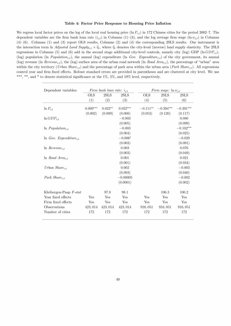
Table 4: Factor Price Response to Housing Price Inflation

We regress local factor prices on the log of the local real housing price (lnPc,t) in 172 Chinese cities for the period 2002—7. The

dependent variables are the firm bank loan rate (ij,t) in Columns (1)—(3), and the log average firm wage (lnwj,t) in Columns

(4)—(6). Columns (1) and (3) report OLS results, Columns (2) and (4) the corresponding 2SLS results. Our instrument is

the interaction term ln Adjusted Land Supplyc,t × ηc, where ηc denotes the city-leval (inverse) land supply elasticity. The 2SLS

regressions in Columns (5) and (6) add in the second stage additional city-level controls, namely city (log) GDP (lnGDPc,t),

(log) population (ln Populationc,t), the annual (log) expenditure (ln Gov. Expenditurec,t) of the city government, its annual

(log) revenue (ln Revenuec,t), the (log) surface area of the urban road network (ln Road Areac,t), the percentage of “urban” area

within the city territory (Urban Sharec,t) and the percentage of park area within the urban area (Park Sharec,t). All regressions

control year and firm fixed effects. Robust standard errors are provided in parentheses and are clustered at city level. We use

***, **, and * to denote statistical significance at the 1%, 5%, and 10% level, respectively.

Dependent variables: Firm bank loan rate: ij.t Firm wage: lnwj.tOLS 2SLS 2SLS OLS 2SLS 2SLS

(1) (2) (3) (4) (5) (6)

lnPc,t 0.009∗∗∗ 0.022∗∗ 0.022∗∗∗ −0.111∗∗ −0.394∗∗∗ −0.391∗∗∗

(0.002) (0.009) (0.008) (0.053) (0.120) (0.117)

lnGDPc,t −0.003 0.080

(0.005) (0.099)

ln Populationc,t −0.003 −0.102∗∗∗

(0.004) (0.025)

ln Gov. Expenditurec,t −0.006∗ −0.029

(0.003) (0.091)

ln Revenuec,t 0.003 0.076

(0.003) (0.049)

ln Road Areac,t 0.001 0.021

(0.001) (0.034)

Urban Sharec,t 0.002 −0.003

(0.003) (0.040)

Park Sharec,t −0.00005 −0.002

(0.0001) (0.002)

Kleibergen-Paap F-stat 97.8 98.1 106.3 100.2

Year fixed effects Yes Yes Yes Yes Yes Yes

Firm fixed effects Yes Yes Yes Yes Yes Yes

Observations 423, 014 423, 014 423, 014 916, 051 916, 051 916, 051

Number of cities 172 172 172 172 172 172

49

Table 5: House Prices and Firm Production Choices

Different measures of firm production are regressed on the local housing price level lnPc,t.The 2SLS regressions use the interaction

term ln Adjusted Land Supplyc,t × ηc as instruments, where ηc denotes the city-level (inverse) land supply elasticity. Panel A

reports the OLS regression, Panel B the baseline 2SLS regression, Panel C augments the 2SLS regression by macroeconomic

control variables, and Panel D further controls for interacted industry and year FEs. The dependent variables are the net

investment to capital share (NI/Kj,t) in Column (1), the gross investment rate (I/Kj,t) in Column (2), a dummy variable of

whether firm j has long-run bank lending (Loanj,t) in Column (3), the (log) firm employment (lnLj,t) in Column (4), the (log)

value-added firm output (lnYj,t) in Column (5), the (log) labor productivity (ln(Y/L)j,t) in Column (6), and a dummy variable

for firms exit from the sample in period t + 1 (Exitj,t) in Column (7). The macroeconomic controls in Panel C including the

percentage of park area within the urban area (Park Sharec,t), the city’s (log) GDP (lnGDPc,t), the (log) population size (ln

Populationc,t), the annual (log) expenditure (ln Expenditurec,t) of the city government, its annual (log) revenue (ln Revenuec,t),

the (log) surface area of the urban road network (ln Road Areac,t), the percentage of “urban” area within the city territory

(Urban Sharec,t) and the percentage of park area within the urban area (Park Sharec,t). All regressions control for year and firm

fixed effects. Standard errors are in parentheses and are clustered at the city level. We use ***, **, and * to denote statistical

significance at the 1%, 5%, and 10% level, respectively.

Dependent variables: NI/Kj,t I/Kj,t Loanj,t lnLj,t lnYj,t ln(Y/L)j,t Exitj,t(1) (2) (3) (4) (5) (6) (7)

Panel A: OLS regressions

lnPc,t −0.099∗∗ −0.120∗∗ −0.017 0.045 −0.231∗∗ −0.267∗∗∗ −0.021

(0.040) (0.046) (0.024) (0.037) (0.088) (0.081) (0.032)

Panel B: 2SLS regressions

lnPc,t −0.204∗∗∗ −0.265∗∗∗ −0.107∗∗ 0.166 −0.968∗∗∗ −1.108∗∗∗ 0.076∗∗

(0.045) (0.057) (0.045) (0.124) (0.181) (0.114) (0.036)

Kleibergen-Paap F-stat 97.2 97.0 106.5 105.9 106.0 106.0 107.6

Panel C: 2SLS regressions with macroeconomic controls

lnPc,t −0.190∗∗∗ −0.254∗∗∗ −0.096∗ 0.150 −0.889∗∗∗ −1.010∗∗∗ 0.052

(0.040) (0.055) (0.049) (0.114) (0.172) (0.122) (0.037)

Kleibergen-Paap F-stat 87.9 87.8 100.4 99.8 99.8 99.7 99.9

Panel D: 2SLS regressions with macroeconomic controls and industry × year FEs

lnPc,t −0.180∗∗∗ −0.244∗∗∗ −0.079∗∗ 0.132 −0.876∗∗∗ −0.978∗∗∗ 0.055

(0.045) (0.057) (0.036) (0.127) (0.184) (0.115) (0.036)

Kleibergen-Paap F-stat 91.5 91.4 103.5 102.3 102.6 102.6 102.7

Year fixed effects Yes Yes Yes Yes Yes Yes Yes

Firm fixed effects Yes Yes Yes Yes Yes Yes Yes

Observations 690, 424 690, 617 935, 412 918, 040 914, 345 915, 668 935, 315

50

Table 6: Real Firm Performance Measures at Product Level

For a subsample of exporting firms with an export share larger than 75% of output, we use product-level export statistics from

the Chinese customs authorities to decompose the yearly (log) export value of a firm’s exported products (lnExpValuej,t) into

(directly reported) export quantity (lnExpQuantityj,t) and export (unit) price (lnExpPricej,t). We repeat the 2SLS regression

in Table 5, Panel B, for this subsample in Columns (1)—(2), and the new export performance measure in Columns (3)—(5).

All regressions control for city level macroeconomic variables, interacted industry and year fixed effects and firm fixed effects.

Standard errors are in parenthesis and are clustered at the city level. We use ***, **, and * to denote statistical significance at

the 1%, 5%, and 10% level, respectively.

Export firms Product level firm performance

Dependent variables: NI/Kj,t lnYj,t lnExpValuej,t lnExpQuantityj,t lnExpPricej,t2SLS 2SLS 2SLS 2SLS 2SLS

(1) (2) (3) (4) (5)

lnPc,t −0.359∗∗ −0.699∗∗∗ −0.421∗∗ −0.426∗∗ 0.005

(0.157) (0.184) (0.204) (0.209) (0.089)

Kleibergen-Paap F-stat 31.2 34.3 37.2 37.2 37.2

Macroeconomic controls Yes Yes Yes Yes Yes

Industry × year fixed effects Yes Yes Yes Yes Yes

Firm fixed effects Yes Yes Yes Yes Yes

Observations 53, 558 65, 399 175, 001 175, 001 175, 001

51

Table 7: House Prices and Firm Heterogeneity in Bank Access

Different measures of firm production are regressed on the (log) local housing price level lnPc,t and the interaction terms of the

housing price level with a proxy for bank access. Panel A uses the ex-ante (log) fixed assets (ln Fixed Assetsj) as a measure of

collateral availability. Panel B creates interaction terms with the state-ownership dummy (SOE j), because Chinese SOEs enjoy

privileged bank access. All regressions control year and firm fixed effects. Standard errors are in parentheses and are clustered

at the city level. We use ***, **, and * to denote statistical significance at the 1%, 5%, and 10% level, respectively.

Dependent variables: NI/Kj,t I/Kj,t Loanj,t lnLj,t lnYj,t ln(Y/L)j,t Exit j,t2SLS 2SLS 2SLS 2SLS 2SLS 2SLS 2SLS

(1) (2) (3) (4) (5) (6) (7)

Panel A: Interaction with firm’s fixed assets

lnPc,t −1.088∗∗∗ −1.238∗∗∗ −0.272∗∗∗ 0.208∗ −1.084∗∗∗ −1.227∗∗∗ 0.319∗∗∗

(0.174) (0.224) (0.075) (0.120) (0.170) (0.136) (0.051)

lnPc,t × ln Fixed Assetsj 0.114∗∗∗ 0.125∗∗∗ 0.022∗∗∗ −0.006 0.015 0.016 −0.032∗∗∗

(0.020) (0.025) (0.006) (0.009) (0.020) (0.014) (0.004)

Kleibergen-Paap F-stat 85.8 85.5 76.6 80.9 81.5 77.9 84.4

Panel B: Interaction with SOE dummy

lnPc,t −0.206∗∗∗ −0.269∗∗∗ −0.109∗∗ 0.167 −0.974∗∗∗ −1.113∗∗∗ 0.078∗∗

(0.043) (0.054) (0.043) (0.122) (0.187) (0.117) (0.037)

lnPc,t × SOE j 0.158∗∗∗ 0.200∗∗∗ 0.112∗ −0.006 0.324 0.356 −0.126

(0.055) (0.062) (0.064) (0.189) (0.420) (0.229) (0.090)

Kleibergen-Paap F-stat 7.23 7.30 5.17 5.83 5.25 5.36 6.12

Year fixed effects Yes Yes Yes Yes Yes Yes Yes

Firm fixed effects Yes Yes Yes Yes Yes Yes Yes

Observations 690, 424 690, 617 935, 412 918, 040 914, 345 915, 668 935, 315

52

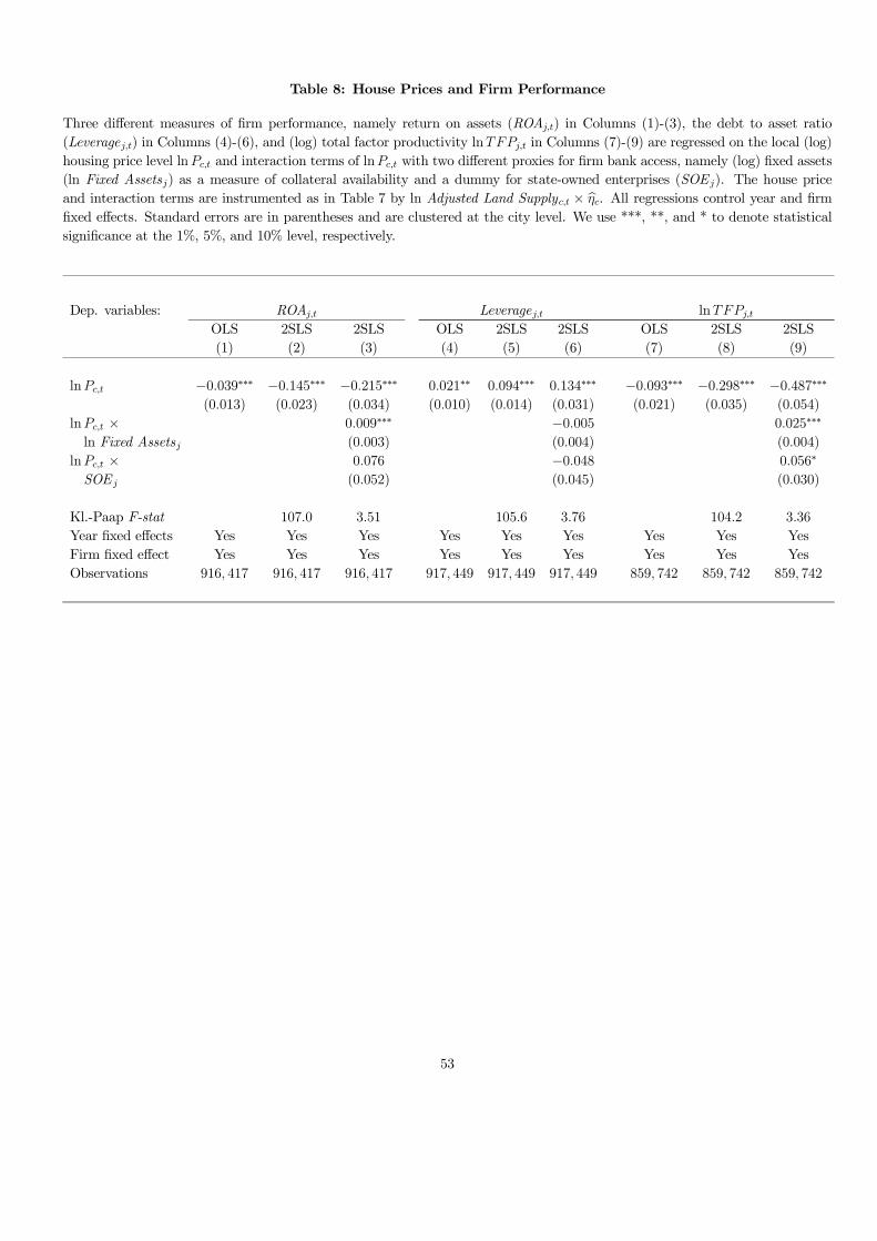
Table 8: House Prices and Firm Performance

Three different measures of firm performance, namely return on assets (ROAj,t) in Columns (1)-(3), the debt to asset ratio

(Leveragej,t) in Columns (4)-(6), and (log) total factor productivity lnTFPj,t in Columns (7)-(9) are regressed on the local (log)

housing price level lnPc,t and interaction terms of lnPc,t with two different proxies for firm bank access, namely (log) fixed assets

(ln Fixed Assetsj) as a measure of collateral availability and a dummy for state-owned enterprises (SOE j). The house price

and interaction terms are instrumented as in Table 7 by ln Adjusted Land Supplyc,t × ηc. All regressions control year and firm

fixed effects. Standard errors are in parentheses and are clustered at the city level. We use ***, **, and * to denote statistical

significance at the 1%, 5%, and 10% level, respectively.

Dep. variables: ROAj,t Leveragej,t lnTFPj,tOLS 2SLS 2SLS OLS 2SLS 2SLS OLS 2SLS 2SLS

(1) (2) (3) (4) (5) (6) (7) (8) (9)

lnPc,t −0.039∗∗∗ −0.145∗∗∗ −0.215∗∗∗ 0.021∗∗ 0.094∗∗∗ 0.134∗∗∗ −0.093∗∗∗ −0.298∗∗∗ −0.487∗∗∗

(0.013) (0.023) (0.034) (0.010) (0.014) (0.031) (0.021) (0.035) (0.054)

lnPc,t × 0.009∗∗∗ −0.005 0.025∗∗∗

ln Fixed Assetsj (0.003) (0.004) (0.004)

lnPc,t × 0.076 −0.048 0.056∗

SOE j (0.052) (0.045) (0.030)

Kl.-Paap F-stat 107.0 3.51 105.6 3.76 104.2 3.36

Year fixed effects Yes Yes Yes Yes Yes Yes Yes Yes Yes

Firm fixed effect Yes Yes Yes Yes Yes Yes Yes Yes Yes

Observations 916, 417 916, 417 916, 417 917, 449 917, 449 917, 449 859, 742 859, 742 859, 742

53

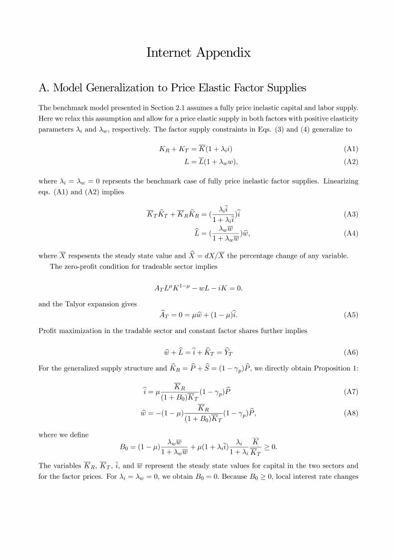
Internet Appendix

A. Model Generalization to Price Elastic Factor Supplies

The benchmark model presented in Section 2.1 assumes a fully price inelastic capital and labor supply.

Here we relax this assumption and allow for a price elastic supply in both factors with positive elasticity

parameters and respectively. The factor supply constraints in Eqs. (3) and (4) generalize to

+ = (1 + ) (A1)

= (1 + ) (A2)

where = = 0 reprsents the benchmark case of fully price inelastic factor supplies. Linearizing

eqs. (A1) and (A2) implies

b +

b = (

1 + )b (A3)

b = (

1 + ) b (A4)

where respesents the steady state value and b = the percentage change of any variable.

The zero-profit condition for tradeable sector implies

1− −− = 0

and the Talyor expansion gives b = 0 = b + (1− )b (A5)

Profit maximization in the tradable sector and constant factor shares further implies

b + b =b+ b = b (A6)

For the generalized supply structure and b = b + b = (1− )b , we directly obtain Proposition 1:

b =

(1 +0)

(1− )b (A7)

b = −(1− )

(1 +0)

(1− )b (A8)

where we define

0 = (1− )

1 + + (1 + )

1 +

≥ 0

The variables and represent the steady state values for capital in the two sectors and

for the factor prices. For = = 0, we obtain 0 = 0 Because 0 ≥ 0 local interest rate changes

b (real wage changes b) are again proportional (inversely proportional) to real estate prices inflationb .Proposition 2 generalizes to the following expressions:

b = −(1 +1)

(1 +0)

(1− )b (A9)

(b) = −(1 +1)

(1 +0)

(1− )b = b (A10)

b = −(1− )(1 +2)

(1 +0)

(1− )b (A11)

( b) = −(1− )

(1 +0)

(1− )b (A12)

where we define

1 = (1− )

1 + ≥ 0

2 =

1 + ≥ 0

For = = 0, we obtain 1 = 0 and 2 = 0. The capital stock change b , the net investment

change (b) , output change b , and labor productivity change ( b) of the manufacturingsector are still negative for a positive local housing price inflation b 0.

B. Persistence of Corporate Loans Rate Differences Across Cities

We identify the loan rate of corproate bank debt from balance sheet data: the annual interest expenses

are divided by the outstanding (bank) debt at the beginning of the year. For all firms with bank debt

in a given city we calculate the median city-level bank loan rate and compare it to the median

bank loan rate of all firms in the neigboring cities/prefectures denoted by _. Summary statistics

are reported in Table 1 of the paper. To evaluate persistence of loan rate differences across cities we

estimate an error correction model

∆+1 = +1 − = + ¡ − _

¢+

by pooling the data across 172 cities. We report the results in Table A1.

C. Sample Construction

Our data source is the Annual Survey of Industrial Firms (ASIF) over the period 1998—2008. This

survey covers industrial firms in the three sectors of mining, manufacturing, and utilities (water,

electricity, gas production and supply). This section describes the data-cleaning procedures:

2

1. We drop firm-year observations before 2001 and after 2007 to focus on the period 2002—2007.

Only in the calculation of net investment rates in 2002 do we use a firm’s capital stock in 2001.

2. We drop all firms in the mining and utility sector from the sample and focus on manufacturing

firms. Tthe corresponding two-digit industry codes are 13—43 according to GB/T 4574—2002.

3. We discard firms in Tibet because of data quality concerns.

4. We drop firm-year observations reported not to have an “operation status.”

5. We drop firm-year observations whenever the gross operating income is below RMB 5 million.

6. We discard all firm-year observations reporting fewer than eight employees.

7. We drop firm-year observations reporting negative value-added.

8. We drop firm-year observations reporting a firm age of more than 100 years.

9. We do not use firm-year observations where the corresponding city-year information on housing

prices and other macroeconomic control variables is not available.

10. We drop firms in the (i) tobacco and (ii) waste resources and waste materials recycling and

processing industry. These two industries have too few observations to allow us to control for

industry-year fixed effect in the panel regression.

The raw data comprise 2,635,787 firm-year observations, corresponding to 689,010 distinct firms.

After these cleaning procedures, the gross sample has 991,487 firm-year observations belonging to

313,100 distinct firms. To mitigate the role of reporting errors, we also discard firm-year observations

in the top 1% and bottom 1% percentiles for each variable. For the real interest rate i we only use firm-

year observations in the 10% to 90% percentiles because this variable is estimated as interest cost over

outstanding debt. Since a firm-year observation represents an outlier in one regression specification,

but does not feature in another, the sample size can vary depending on regression specification.

D. Real Investment and Capital Stock Calculation

Under price inflation, the purchasing year of new capital matters for the real book value of a firm’s

asset. To obtain the real value of capital, net new investment should be deflated with the deflator

corresponding to the investment year. Formally, the real book value follows as

=

X=

× f +

where is the (begining-of-year) initial real book value at the year of entering survey, f the

nominal net new investment in period and the price deflator for investment goods in

period . The intial real book value is unobservable and can at best be proxied by an adjustment

3

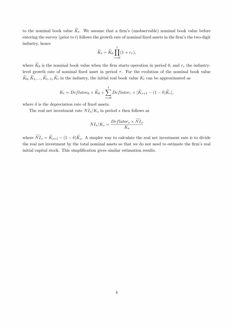
to the nominal book value e. We assume that a firm’s (unobservable) nominal book value before

entering the survey (prior to ) follows the growth rate of nominal fixed assets in the firm’s the two-digit

industry, hence e = e0

Y=0

(1 + )

where e0 is the nominal book value when the firm starts operation in period 0, and the industry-

level growth rate of nominal fixed asset in period . For the evolution of the nominal book valuee0 e1 e−1 e in the industry, the initial real book value can be approximated as

= 0 × e0 +

X=0

× [ e+1 − (1− ) e ]

where is the depreciation rate of fixed assets.

The real net investment rate in period then follows as

= × f

where f = e+1 − (1− ) e. A simpler way to calculate the real net investment rate is to divide

the real net investment by the total nominal assets so that we do not need to estimate the firm’s real

initial capital stock. This simplification gives similar estimation results.

4

Table A1: Persistence of the Corporate Loan Rate

We estimate an error correction model for the average corporate loan rate in each city relative to firms in neighboring cities. We use ***,

**, and * to denote statistical significance at the 1%, 5%, and 10% level, respectively.

Dependent variable: ∆+1

(1) (2) (3)

− _ −0105∗∗∗ −0138∗∗∗ −0138∗∗∗(0022) (0032) (0032)

City fixed effects No Yes Yes

Year fixed effects No No Yes

R-squared 0047 0133 0203

Observations 846 846 846

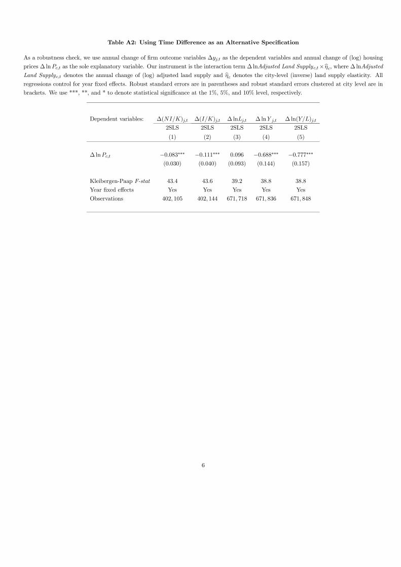
Table A2: Using Time Difference as an Alternative Specification

As a robustness check, we use annual change of firm outcome variables ∆ as the dependent variables and annual change of (log) housing

prices ∆ ln as the sole explanatory variable. Our instrument is the interaction term ∆ lnAdjusted Land Supply×b, where ∆ lnAdjustedLand Supply denotes the annual change of (log) adjusted land supply and b denotes the city-level (inverse) land supply elasticity. Allregressions control for year fixed effects. Robust standard errors are in parentheses and robust standard errors clustered at city level are in

brackets. We use ***, **, and * to denote statistical significance at the 1%, 5%, and 10% level, respectively.

Dependent variables: ∆() ∆() ∆ lnL ∆ lnY ∆ ln()

2SLS 2SLS 2SLS 2SLS 2SLS

(1) (2) (3) (4) (5)

∆ ln −0083∗∗∗ −0111∗∗∗ 0096 −0688∗∗∗ −0777∗∗∗(0030) (0040) (0093) (0144) (0157)

Kleibergen-Paap F-stat 434 436 392 388 388

Year fixed effects Yes Yes Yes Yes Yes

Observations 402 105 402 144 671 718 671 836 671 848

6

Table A3: Local Demand Shock Induced by Local Real Estate Booms

Different firm outcomes on credits and investment, output, financial performance and TFP are regressed on the (log) local housing price

level ln and the interaction terms ln × Population size (%)2000 of the housing price level with a proxy for local market size measured

by the share of local population to national population in the year 2000. All regressions control year and firm fixed effects. Standard errors

are in parentheses and are clustered at the city level. We use ***, **, and * to denote statistical significance at the 1%, 5%, and 10% level,

respectively.

Dependent variables: Loan ln ROA Leverage ln

2SLS 2SLS 2SLS 2SLS 2SLS 2SLS 2SLS

(1) (2) (3) (4) (5) (6) (7)

ln 0034∗∗∗ −0246∗∗∗ −0134∗∗ −0531∗∗∗ −0114∗∗∗ 0068∗∗∗ −0248∗∗∗(0008) (0072) (0053) (0231) (0034) (0020) (0054)

ln × Population size (%)2000 −0019 0059 0040 −0591∗∗∗ −0043 0036 −0066(0013) (0063) (0055) (0202) (0046) (0025) (0066)

Kleibergen-Paap F-stat 55 87 115 114 115 117 108

Year fixed effects Yes Yes Yes Yes Yes Yes Yes

Firm fixed effects Yes Yes Yes Yes Yes Yes Yes

Observations 422 632 689 636 934 034 912 985 915 087 916 101 858 696

7

Table A4: Housing Supply Elasticity of Major Cities

This table reports the local housing supply elasticity of major cities in China provided by Wang et al. (2012) in the top 5 and bottom

5 (Column 1), their corresponding increase of house prices over the period 2003—2010 (Column 2), and the level of house prices in 2010

(Column 3).

City Housing Housing Housing

supply prices growth price level

elasticity (2003—2010) (in 2010)

(1) (2) (3)

Top 5

Shenzhen 049 20178% 19 16989

Beijing 053 28083% 17 78201

Shanghai 152 18301% 14 40010

Ningbo 227 29474% 11 22362

Hangzhou 265 26761% 14 13306

Bottom 5

Hefei 133 18506% 5 90447

Zhengzhou 165 14371% 4 95734

Wulumuqi 1671 9540% 4 44326

Changsha 1714 11871% 4 41811

Yinchuan 2198 8879% 3 92893

8

Table A5: Using Housing Supply Elastcities as an Alternative Instrument

As a robustness check, we use the housing supply elasticities reported by Wang et al. (2012) as an alternative instrument in a cross-sectional

specification at the firm level with two-digit industry fixed effects. All regressions control city-level (log) GDP per capita, (log) population

density, employment share of the secondary sector and GDP share of the secondary sector in 2002. Robust standard errors are in parentheses

and robust standard errors clustered at city level are in brackets. We use ***, **, and * to denote statistical significance at the 1%, 5%, and

10% level, respectively.

Dependent variables: ∆02−07 ∆02−07 ln ∆02−07() ∆02−07Loan ∆02−07 ln

2SLS 2SLS 2SLS 2SLS 2SLS

(2) (1) (3) (4) (5)

∆02−07 ln 0022 −0217 −0184 −0013 −0174(0009)∗∗ (0061)∗∗∗ (0087)∗∗ (0050) (0072)∗∗

[0015]∗∗∗ [0253] [0064]∗∗∗ [0117] [0253]

Kleibergen-Paap F-stat 71 54 36 54 53

Controls Yes Yes Yes Yes Yes

Industry fixed effects Yes Yes Yes Yes Yes

Observations 9 717 27 339 20 307 28 359 27 448

Dep. variables: ∆02−07 ln ∆02−07 ln() ∆02−07ROA ∆02−07Leverage ∆02−07 ln2SLS 2SLS 2SLS 2SLS 2SLS

(6) (7) (8) (9) (10)

∆02−07 ln −1289 −0968 −0344 0183 −0333(0114)∗∗∗ (0102)∗∗∗ (0020)∗∗∗ (0028)∗∗∗ (0042)∗∗∗

[0596]∗∗ [0587]∗ [0228] [0113] [0145]∗∗

Kleibergen-Paap F-stat 53 53 53 54 53

Controls Yes Yes Yes Yes Yes

Industry fixed effects Yes Yes Yes Yes Yes

Observations 26 908 25 482 27 471 27 661 25 066

9

Table A6: Do Initial Conditions Matter for the Investment Effect of Real Estate Booms?

As a robustness check, we verify whether the initial conditions at province level matter for investment regressions. All regressions control

year and firm fixed effects. Robust standard errors are in parentheses and are clustered at city level. We use ***, **, and * to denote

statistical significance at the 1%, 5%, and 10% level, respectively.

Dependent variables:

2SLS 2SLS 2SLS 2SLS 2SLS

(1) (2) (3) (4) (5)

ln −0204∗∗∗ −0244∗∗∗ −0248∗∗∗ −0222∗∗∗ −0313∗∗∗(0045) (0077) (0064) (0071) (0114)

ln × (Loan/GDP)2000 0026

(0029)

ln × (Corporate Loan/GDP)2000 0206

(0134)

ln × (Deposit/GDP)2000 0007

(0016)

ln × (Household Deposit/GDP)2000 0139

(0111)

Kleibergen-Paap F-stat 972 343 369 390 364

Year fixed effects Yes Yes Yes Yes Yes

Firm fixed effect Yes Yes Yes Yes Yes

Observations 690 424 690 424 690 424 690 424 690 424

10

Table A7: Factor Price and Firm Performance Response by Firm Size

As a robustness check, we verify the factor price and firm performance responses by firm size. Specifically, small firms are firms with less than

200 employees, medium-size firms are have between 201 and 1000 employees, and large firms have more than 1000 employees. All regressions

control for year and firm fixed effects. Robust standard errors are in parentheses and are clustered at the city level. We use ***, **, and *

to denote statistical significance at the 1%, 5%, and 10% level, respectively.

Dep. variables: ln Loan ln ln() Exit ROA Leverage ln

(1) (2) (3) (4) (5) (6) (7) (8) (9) (10)

Panel A: Full sample

ln 0022∗∗ −0394∗∗∗ −0204∗∗∗ −0107∗∗ −0968∗∗∗ −1108∗∗∗ 0076∗∗ −0145∗∗∗ 0094∗∗∗ −0298∗∗∗(0086) (0120) (0045) (0045) (0181) (0114) (0036) (0023) (0014) (0035)

Kleib.-Paap F-stat 978 1063 972 1069 1060 1060 1076 1070 1056 1042

Observations 423 014 916 051 690 424 935 412 914 345 915 668 935 315 916 417 917 449 859 742

Panel B: Small firms

ln 0022∗∗∗ −0465∗∗∗ −0222∗∗∗ −0086∗∗ −1150∗∗∗ −1161∗∗∗ 0110∗∗ −0172∗∗∗ 0112∗∗∗ −0311∗∗∗(0008) (0132) (0058) (0035) (0181) (0124) (0043) (0028) (0017) (0037)

Kleib.-Paap F-stat 887 1074 1016 1086 1068 1072 1080 1083 1070 1045

Observations 297 700 684 531 493 600 698 702 688 212 685 222 698 631 685 059 686 358 640 334

Panel C: Medium-size firms

ln 0022∗∗ −0239∗∗ −0150∗∗∗ −0076 −0712∗∗∗ −0995∗∗∗ −0019 −0094∗∗∗ 0064∗∗∗ −0260∗∗∗(0010) (0120) (0046) (0059) (0173) (0131) (0029) (0016) (0015) (0046)

Kleib.-Paap F-stat 1031 945 833 943 951 936 965 941 931 929

Observations 107 165 202 489 170 559 206 870 202 448 201 703 206 850 202 083 201 968 192 164

Panel D: Large firms

ln 0010 −0047 0108 −0062 −0492∗ −0767∗∗∗ −0107∗ −0039∗∗∗ −0030 −0195∗∗∗(0010) (0138) (0089) (0059) (0268) (0186) (0060) (0010) (0025) (0055)

Kleib.-Paap F-stat 967 899 822 880 924 872 914 880 871 925

Observations 18 149 29 031 26 265 29 840 23 685 28 743 29 834 29 275 29 123 27 244

11