Geomorphology 134 (2011) 23–31

Contents lists available at ScienceDirect

Geomorphology

j ourna l homepage: www.e lsev ie r.com/ locate /geomorph

On the formation of collapse dolines: A modelling perspective

Franci Gabrovšek a,⁎, Uroš Stepišnik b

a Karst Research Institute ZRC SAZU, Titov trg 2, 6230 Postojna, Sloveniab Department of Geography, University of Ljubljana, Aškerčeva 2, 1000 Ljubljana, Slovenia

⁎ Corresponding author.E-mail address: gabrovsek@zrc-sazu.si (F. Gabrovšek

0169-555X/$ – see front matter © 2011 Elsevier B.V. Adoi:10.1016/j.geomorph.2011.06.007

a b s t r a c t

a r t i c l e i n f o

Article history:Received 28 December 2010Received in revised form 2 June 2011Accepted 6 June 2011Available online 13 June 2011

Keywords:KarstCollapse dolinesLimestone dissolutionNumerical model

Collapse dolines are among the most striking surface features in karst areas. Although they can be the result ofdifferent formation mechanisms, evidence suggests that large collapse dolines form due to chemical andmechanical removal of material at and below the level of groundwater. We have applied a genetic model of atwo-dimensional fracture network to calculate the rate of dissolutional bedrock removal in the heavilyfractured (crushed) zone intersecting a karst conduit in the phreatic zone. To account for infilling andbreakdown processes in the crushed zone two simple rules were added to the basic model: 1) continuousinfilling of dissolutionally created voids prevents fractures from growing beyond some limited aperture,although the dissolution proceeds, 2) discontinuous collapsing causes sudden closure of a fracture once somecritical aperture has been reached. Both rules limit the transmissivity of the network and the related flowrates. Therefore, the constant head difference between the input and the output points is sustained and theflow remains distributed over the entire crushed zone. Provided that restrictions posed by the two rulespermit turbulent flow, dissolution rates also remain high in the entire region. High surface area of water–rockcontact and high dissolution rates result in high overall removal rates of rock from the crushed zone, one ofthe necessary conditions for the formation of large closed depressions. Despite the fact that the modelneglects some processes and dynamics that would increase the removal rate, the results suggest that largeclosed depressions could form in the order of 1 million years.

).

ll rights reserved.

© 2011 Elsevier B.V. All rights reserved.

1. Introduction

Collapse dolines are surface karst depressions of various shapesand sizes. They are among the most fascinating forms of karstlandscape (Fig. 1). They can grow to a volume of over a hundredmillion cubic meters. Although they have been commonly defined asfeatures formed above caves, different processes of mass removal bygroundwater contribute to their development. The oldest explanationof formation of closed depressions on karstic surfaces is a suddencollapse (Cvijić, 1893), according to which the term “collapse doline”was coined. Modern definitions of collapse dolines are stronglyrelated to findings of Cramer (1941) that collapse dolines show clearconnection to underlying caves (Waltham et al., 2005).

A simple comparison of volumes of the largest known under-ground chambers and collapse dolines shows that the latter can bemore than two orders of magnitude larger. Therefore, the genesis oflarger collapse dolines cannot be related solely to a single collapse of acave chamber. Their development involves a long-term removal ofmaterial at the level of active cave passages and consequently, more orless continuous lowering of the overlying surface (Šušteršič, 1973;Mihevc, 2001; Palmer and Palmer, 2006; Stepišnik, 2010). The most

impressive forms of this type, locally called Tiankeng, are in China(Zhu and Chen, 2006). Large collapse dolines of comparable sizes arealso found elsewhere (Fig. 1). Table 1 lists some deep collapse dolinesin different parts of the world.

Most of the published work on collapse dolines has focused on theirmorphology and/or morphometry. Consequently, various morpholog-ical classifications of collapse dolines have been made. The mostcommon is the simple subdivision of collapse dolines into “immature”and “mature” or “degraded” (Šušteršič, 1984; Summerfield, 1991;Waltham et al., 2005).

1.1. Conceptual settings for the formation of collapse dolines

A small collapse doline can form as a single collapse of a cave ceiling.On the other hand, formation of large collapse dolines is far morecomplicated. Evidently, a variety of processes acts or interacts togradually removematerial and results in the formation of a large surfacedepression. Since material removal occurs in epiphreatic and phreaticzones, it is almost impossible toobserve it andevenharder tomeasure itsdynamics in nature. This probably has prevented more detailed studieson processes and conditions leading to the formation of collapse dolines.

Palmer and Palmer (2006) related the evolution of collapse dolinesto the hydraulics in a breakdown zone. According to their study, cavestreams can be blocked by breakdown collapses, resulting in anincreasing hydraulic gradient and flow velocity through the collapse

Fig. 1. Photo (a) and a simplified cross-section of Crveno jezero (Red lake), the largest collapse doline in the Dinaric karst at Imotski in Croatia. Photo by Franci Gabrovšek. Cross-section redrawn after Garašič (2001).

Table 1Some of the deepest collapse dolines in the world (Kranjc, 2006; Waltham, 2006).

Collapse doline Region Depth

Xiaozhai tiankeng China 662 mDashiwei tiankeng China 613 mCrveno jezero Croatia 530 mMinyé Papua New Guinea 431 mSótano del Barro Mexico 410 m

24 F. Gabrovšek, U. Stepišnik / Geomorphology 134 (2011) 23–31

material. Accelerated dissolution and erosion of the collapse materialtake place, and are most efficient during floods. As a consequence,floodwater-bypass routes develop. Further collapses take place whereblocks from breakdown have been removed by dissolution and erosionas well as in the growing network of diversion passages. Ongoingcollapses maintain high hydraulic gradient and result in continuousremoval of material from the area (Palmer and Palmer, 2006).

The ideas and conclusions of Palmer and Palmer surely deserve moreattention and further evaluation. To this end we applied a process-basedmodel to study thedynamics offlowanddissolution in thebreakdown(orcrushed) zone, which could give rise to the evolution of closed depres-sions. The concept is schematically shown in Fig. 2.We assume a block of

Fig. 2. The conceptual model of a conduit system interrupted by a crushed zone. Q, cin andrespectively. Arrows indicate the formation of a closed depression at the surface due to infilliis used to model dissolutional rock removal in the crushed zone, is shown at the level of co

tectonically crushed or highly fractured rock mass. Water chemicallyaggressive to limestone enters this zone through a solution conduit (theleft-hand side of Fig. 2). Within the crushed zone it flows along manyalternativepathways, dissolves the rockand transportsdissolvedmaterialout of the zone (through the conduit on the right-hand side of Fig. 2).Weassume that the crushed zone is mechanically weak enough for thedissolutionally enlarged fractures to be continuously or discontinuously(i.e. in a series of small collapses) filled with the material from the rockcolumn above. As indicated by the arrows in Fig. 2, in this manner thewhole block sinks into the dissolution zone, so that the volume removedthere appears on the surface in the form of a closed depression.

We focus on the processes occurring in the dissolution zone andexplore possible scenarios that sustain a high rate of chemical removalof soluble rock over large time scales, surely one of the preliminaryconditions for the formation of collapse dolines.

2. The numerical model

2.1. The modelling domain

We approximate the dissolution zone with a 1 m thick slice ofsoluble fractured rock between the input and output channels as shown

cout denote the recharge, input and output concentrations of dissolved ionic species,ng of the voids developed by dissolution of rock in the depth. A fracture network, whichnduits.

Fig. 3. a) The modelling domain and boundary conditions. The crushed zone is markedby a shaded area. The left and right boundary regions of the domain are mechanicallystable, i.e. infilling and collapsing rules are not valid there. Arrows indicate theinflowing and outflowing conduits. b) Frequency distribution of initial aperture offractures in the network. Frequency denotes the number of fractures with initialaperture width between a and a+Δa. Δa is chosen so that the range of aperture widthsis divided into 100 classes.

25F. Gabrovšek, U. Stepišnik / Geomorphology 134 (2011) 23–31

in Fig. 2. This slice represents the modelling domain that is used forsimulations presented later on. Fig. 3a shows the dissolution zone indetail. Its area is 200 m×200 m. It is composed of a rectangular grid of100×100 nodes, connected by 2 m long and 1 m wide fractures. Weapply a dual fracture network; that is, into a dense network of 2 m longfractures with statistically distributed apertures between 0.01 cm and0.04 cm, a sparser network with 20 m long fractures is randomlyembedded with initial aperture widths distributed between 0.04 cmand 0.08 cm. Fig. 3b shows the frequency distribution of initial aperturewidths. Upper and lower boundaries of the domain are impermeable.The water enters through a channel on the left-hand side at initial

saturation ratio c/ceq=0.9 andhydraulic headh=10mandexits on theright-hand side of the domain at h=0m. The crushed zone is shownshaded in Fig. 3a. Asmarkedon Fig. 3a, 20 mwide regions on the left andthe right side of the modelling domain are stable, where infilling orcollapsing rules are not valid. These regions represent a stable limestoneblock at the border of the crushed zone.

We assume twomechanisms whichmimic the processes related tothe instability of the crushed zone:

• Continuous infilling: fractures can grow only up to a certain limitingaperture alim, even though the dissolution proceeds. In principle, weassume that newly created voids are immediately filled by moresoluble material from the rock column above. We use the term(continuous) infillingwhenwe refer to this rule in the following text.

• Discontinuous collapsing: fractures evolve until some criticalaperture acrit is reached. Then they collapse back to the initial ormuch smaller aperture width, from where they start growing again.We use the term (discontinuous) collapsing when we refer to thisrule in the following text.

Note that both restrictions only prevent or reset the growth offractures, while the dissolution and chemical removal of materialcontinue on. Such conditions can be easily introduced into the basicgenetic model of fracture network evolution.

2.2. The modelling approach

Several genetic models of speleogenesis have been presented andused to study speleogenetic processes in different settings (Dreybrodtand Gabrovšek, 2000; Dreybrodt et al., 2005). These models simulategrowth of conduit networks in an initially fractured medium as aresult of bedrock dissolution by calcite aggressive groundwater. Themodel applied here has been presented in several publications(Gabrovšek et al., 2004; Skoglund et al., 2010). The only differenceis the implementation of the two rules related to the infillingprocesses in the crushed zone.

Here we give only a brief outline of its basic steps.The model algorithms work as follows:

1. Calculate flow Qi in each fracture for a given geometry andhydraulic boundary conditions.

2. Calculate concentration c of calcium in the solution in all fracturesof the network, and from this calculate dissolution rates F and thefracture widening rates.

3. Change the aperture widths in a given time step.4. Return to point 1 until the exit criteria (e.g. flow rate which

exceeds the capacity of reasonable drainage area) is reached.

The reader is referred to works cited above for more detaileddescription about each step of the algorithm.

3. Results

3.1. Evolution of conduit network in a mechanically stable fracturenetwork: unrestricted growth

First we present a case wherewidening of fractures is unrestricted,that is we assume that the whole network is mechanically stable andneither of the two infilling rules applies. The results are not novel, butserve as an end member comparison with the other two cases. Fig. 4shows four stages of evolution when the fracture growth is unrest-ricted. The left column presents the aperture widths and thedissolution rates; the right column presents the flow rates. Isolineson figures show the hydraulic head given in cm. At the onset (Fig. 4a,b), the highest flow rates and dissolution rates are close to the lineconnecting the input to the output. There a pathway of enlargedfractures evolves most efficiently (Fig. 4a–d). Isolines of hydraulichead show the highest gradients between the tip of the evolving

26 F. Gabrovšek, U. Stepišnik / Geomorphology 134 (2011) 23–31

Fig. 5. a) Evolution of the removal rate for unrestricted growth (dotted line), infilling(full black lines) and collapsing (full grey lines). Numbers on curves denote alim andacrit. b) Evolution of flow rate corresponding to curves in Fig. 5a.

27F. Gabrovšek, U. Stepišnik / Geomorphology 134 (2011) 23–31

pathway and the exit. The head drop along the evolved pathway issmall, leaving a flat gradient at the upstream region and thereforepreventing the evolution of other pathways.

As pointed out by several authors, the early evolution of fracturenetworks under constant head conditions is governed by a feedbackmechanism between flow and dissolution rates. As the flow rateincreases, high dissolution rates penetrate deeper into the networkresulting in even faster increase of flow rate, until an abrupt increaseof both quantities in an evolving pathway occurs (Palmer, 1991;Dreybrodt, 1990; Dreybrodt and Gabrovšek, 2000). This event, calledbreakthrough, ends the initial state of network development.

The first pathway in our network breaks through at 300 y (Fig. 4e, f).Soon after the breakthrough, the pathway is widened almost uniformlywith maximal dissolution rates, determined by the saturation ratio ofthe input solution (Dreybrodt and Gabrovšek, 2000; Palmer, 2007). Thebreakthrough event also marks a transition from a laminar to turbulentflow regime. The head distribution in the network is rearranged(compare Fig. 4 c, e and g), so that the gradient for other potentialpathways builds up again. The network of evolved (post-breakthroughpathways) is “inflating” towards upper and lower boundaries. At 800 yalmost half of the fractures in the domain have evolved beyond thebreakthrough and continue to grow with uniform widening rate.

Fig. 5 shows the evolution of discharge and the annual amount ofsolutionally removed rock (removal rate) for different scenariospresented in this paper. The removal rate R [L3 /T] is defined as thevolume of dissolved rock per unit time. It is calculated according to theformula R=QM(cout−cin) /ρ, where Q is the flow rate, cin and cout areinput and output concentrations of calcium, M is the molar mass ofcalcite and ρ its density. The unrestricted case is presented by thedotted line. If a constant head is kept at the input, the removal ratesincrease to a maximum value when turbulent flow invades the entirenetwork. However, for the unrestricted case this happens at flow rateswhich are unrealistically high for most catchments.

If widening of the fractures is unrestricted, the transmissivity ofthe network inevitably reaches a value at which the recharge cannotsustain the constant head. Boundary conditions become controlled bythe catchment. For the presented case, this would happen at 1.15 ky, ifthe catchment can provide 5 m3. As the network continues to evolve,the hydraulic head at the input and within the network drops untilone of the pathways becomes vadose and most of the other pathwayslose water. The end result is evolution of an open channel pathwayconnecting the input to the output.

3.2. The scenario of continuous infilling

Now we apply the rule of continuous infilling by limiting theevolution of fractures to a certain aperture alim. The fractures cannotgrow beyond alim, although the dissolution proceeds. Fig. 6 presents theevolution of aperture widths and dissolution rates and distribution offlow rates at four different time steps for for alim=1 cm. The initialphase is similar to theunrestricted case.When thefirst pathway reachesthe limiting aperture, the network expands toward the lateralboundaries as in the case of unrestricted growth. After 800 y morethan two thirds of the domain has evolved to alim. In the non-crushedregion, feeder channels evolve fromthepoint of input towardupper andlower boundaries and supply water to the crushed zone. Generally theresults are similar to those of the unrestricted case (Fig. 4), however thekey difference between both scenarios can be seen from the Fig. 5. Thetotal discharge increases until about 1 ky (Fig. 5a, thick black line)whenalmost all fractures in the crushed zone have widened to alim, andthe flow cannot increase anymore. The removal rate (Fig. 5b) shows aslow increase during the laminar regime and rapidly increases at the

Fig. 4.Distribution of aperture widths, dissolution rates and flow rate at four time steps for th(a0=0.03 cm) and the dissolution rates F (cm/y). The right column shows corresponding floflow rate in the crushed zone. The legends are given in Fig. 4f.

breakthrough. After the breakthrough, it grows almost linearly accord-ing to the growth of the evolved region, until it reaches a constant valueof about 3 m3/y. Fig. 5 contains several other curves for different limitingapertures as denoted. The pattern is the same for all cases. As alimincreases, the flow and removal rates approach those of unlimitedgrowth. Removal rates go through a maximum because at later stages,flow along fractures perpendicular to the general left–right directionceases so that the contact area between aggressive water and rock isreduced. This is partly an artefact of the model, which assumes that allfractures can grow to the same maximal width.

The restrictions imposed by the rule of continuous infilling preventhead drop at the input and transition to open channel flow, whenrecharge from few hundred litres to few cube metres per second isprovided by catchment. If alim is in the order of centimetre, highdissolution rates are distributed in the whole domain resulting in theremoval rate of few cube metres per year.

3.3. The scenario of discontinuous collapsing

In the last scenario we apply to the model a collapsing rule thatimplies that fractures “collapse” down to 0.1 cm once they reach acertain critical aperture width acrit. Again we discuss only evolutionafter the breakthrough. Fig. 7 presents six stages between 0.6 ky and

e case of unrestricted growth. The left column shows the aperture widths in units of a /a0w rates in units of Q /Qmax, where Qmax is the flow rate in the fracture with the highest

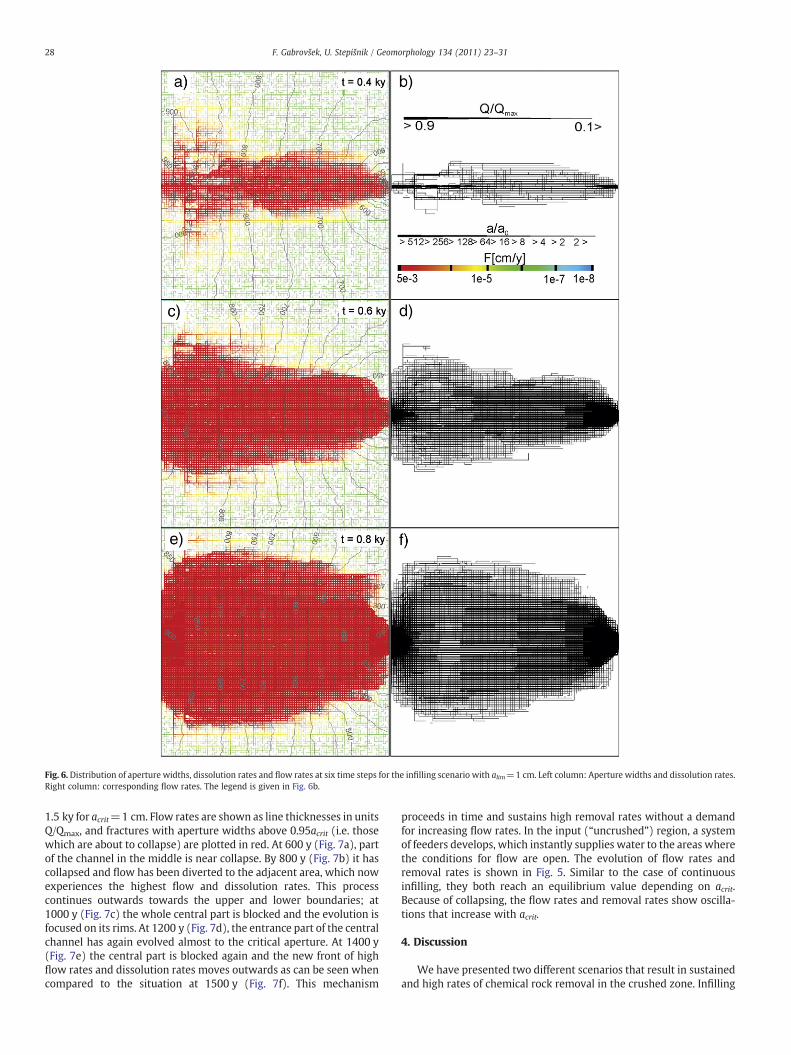
Fig. 6. Distribution of aperture widths, dissolution rates and flow rates at six time steps for the infilling scenario with alim=1 cm. Left column: Aperture widths and dissolution rates.Right column: corresponding flow rates. The legend is given in Fig. 6b.

28 F. Gabrovšek, U. Stepišnik / Geomorphology 134 (2011) 23–31

1.5 ky for acrit=1 cm. Flow rates are shown as line thicknesses in unitsQ/Qmax, and fractures with aperture widths above 0.95acrit (i.e. thosewhich are about to collapse) are plotted in red. At 600 y (Fig. 7a), partof the channel in the middle is near collapse. By 800 y (Fig. 7b) it hascollapsed and flow has been diverted to the adjacent area, which nowexperiences the highest flow and dissolution rates. This processcontinues outwards towards the upper and lower boundaries; at1000 y (Fig. 7c) the whole central part is blocked and the evolution isfocused on its rims. At 1200 y (Fig. 7d), the entrance part of the centralchannel has again evolved almost to the critical aperture. At 1400 y(Fig. 7e) the central part is blocked again and the new front of highflow rates and dissolution rates moves outwards as can be seen whencompared to the situation at 1500 y (Fig. 7f). This mechanism

proceeds in time and sustains high removal rates without a demandfor increasing flow rates. In the input (“uncrushed”) region, a systemof feeders develops, which instantly supplies water to the areas wherethe conditions for flow are open. The evolution of flow rates andremoval rates is shown in Fig. 5. Similar to the case of continuousinfilling, they both reach an equilibrium value depending on acrit.Because of collapsing, the flow rates and removal rates show oscilla-tions that increase with acrit.

4. Discussion

We have presented two different scenarios that result in sustainedand high rates of chemical rock removal in the crushed zone. Infilling

Fig. 7. Distribution of flow rates in units Q/Qmax for the collapsing scenario with acrit=5 cm at several time steps. Fractures with aperture widths aN0.95acrit are plotted in red.

29F. Gabrovšek, U. Stepišnik / Geomorphology 134 (2011) 23–31

and collapsing limit the growth of individual channels and distributethe flow into a wider region, providing a large surface of water–rockcontact. The flow rates and removal rates reach a long-term constantvalue depending on alim or acrit. Fig. 8 shows the long-term(equilibrium) removal and flow rates for a range of alim and acrit. Inboth cases removal rates show a steep rise while alim, critb1 cm andincrease only by about 0.5 m3/y in the range 1 cmbalim, critb5 cm.Within the same range flow rates increase from 1 m3/s to 15 m3/s forthe infilling scenario and from 0.2 m3/s to 4.3 m3/s for the collapsingscenario. For alim, crit on the order of a centimetre, removal rates arealready high, while flow rates are still below 1 m3/s. Therefore, closeddepressions are possible even in relatively small catchments.

To further elucidate these results, we make use of the concept ofpenetration length λ, the distance from the entrance where dissolu-tion rates drop by some factor (e.g. 1 /e, an e-folding length). At thebreakthrough λ increases dramatically, so that for most of the post-breakthrough pathways connecting input to output in our domain, wecan state that L/λ≪1, if L is the length of the pathway. Therefore,dissolution rates along the entire pathway can be considered almostconstant and are determined by the input concentration (Dreybrodtand Gabrovšek, 2000; Gabrovšek, 2000). An increase of concentrationalong a pathwaywith length L, perimeter P and flow rate Q is obtainedby a mass balance and yields Δc=F×P×L/Q, where F is thedissolution rate in mol/(cm2s). The removal rate R in cm3/s is then

Fig. 8. Equilibrium removal and flow rates for a range of alim and acrit.

30 F. Gabrovšek, U. Stepišnik / Geomorphology 134 (2011) 23–31

R=ΔV/Δt=(Q×M/ρ)Δc=F×P×L×M/ρ, where M is the molarmass of the dissolved mineral (100 g for CaCO3) and ρ the densityin g/cm3 (about 2.5 g/cm3). Note that R is independent of Q and isdefined by the surface area of water–rock contact PL and the initialsaturation ratio, which determines the dissolution rate F.

For the presented scenarios, a typical widening rate is aboutF×M/ρ=0.005 cm/y. Assuming 200 fractures with length of 200 mand water–rock contact of 8×104m2 are uniformly widened, theremoval rate is 4 m3/y. This value fits well to the results obtained bythe model.

4.1. A look beyond the model: 3D domain, transient recharge andmechanical erosion

We expect that a 2D model demonstrates most of the dynamicswhich are necessary for discussion on a qualitative level and givesreasonable quantitative estimations. This assumption is based on thecomparison of similar 2D and 3D speleogenetic models (Kaufmannet al., 2010). Flow in a three dimensional domain is not limited to aslice as in our case, but occupies a larger thickness of the breakdownzone. This increases the contact surface and the removal rate.Transient recharge has not been considered here. In the presentedmodels it would cause variations of the head at the input. Duringfloods the head would be higher and solution more aggressive,leading to a period of faster network spreading and higher removalrates. In three dimensions a flood increases the thickness of the flowdomain and consequently the surface of the water–rock contact,additionally leading to higher removal rates.

A different situation would occur when aggressive flow occupies alarger area only during floods. In this case, during low flow the domainwould become vadose, resulting in the evolution of a single pathway.If this process is efficient, increasingly higher flow rates would beneeded to flood the entire area.

The model calculates rock removal by dissolution and advectivetransport of dissolved species. However, if the flow velocities in thebreakdown zone are sufficient, mechanical erosion certainly plays animportant role. Observations by Gospodarič (1976) in Planinska jama,Slovenia, showed that material filling lower parts of epiphreatic cavepassages was in fact eroded and redeposited collapse debris. About80% of all collapse material was redeposited in the outflow part of thecave. He concluded that erosion is the most important process incollapse doline formation but that corrosion also takes place. Based onvarious examples from the northern Dinaric karst (Stepišnik, 2010)concluded that locally increased water gradient in the areasunderneath collapse dolines results in accelerated erosion.

The underlying mechanical processes are too complex to beaccounted for correctly in the present model. In some cases, infilling

may not proceed completely to the surface, but a stable ceiling mayform resulting in an underground chamber. Once the surfacedenudation reaches the chamber, this could become a collapse doline.One could also envisage other mechanisms resulting in high removalrates without a demand for increasing recharge. An example is ascenario modelled by Romanov et al. (2010), who statisticallydistributed insoluble fractures into the network. They also imple-mented the restricted growth into the model, where the dissolution isstopped once certain width is reached. Although the objective of theirwork differs from ours, their results also show highly distributed flowand dissolution within the entire network.

5. Conclusions

We have demonstrated by a numerical model that infilling and/orbreakdowns in a crushed zone result in continuous and distributeddissolutional removal of bedrock. Even though the model neglects oroversimplifies some of the active processes, it clearly supports theideas proposed by Palmer and Palmer (2006).

Removal rates on the order of a few m3/y beneath an area of200 m×200 m could result in lowering of the overlying surface by100 m per million years, provided that the crushed zone is weakenough that voids are continuously or stepwise filled by material.Higher fracture frequency, larger thickness of dissolutionally activecrushed zone and erosion processes could increase the removal ratefor an order of magnitude or more. Based on the sediment dating insome cave systems, one could easily envisage that the available timespan for the formation of large depressions could be up to severalmillion years. In ideal case all these factors together could also resultin the formation of Tiankengs.

The quantitative results of the model give a lower limit estimate ofthe removal rate from the crushed zone. The models can be furtheremployed to study simultaneous growth of clusters of dolines, and therelation between the evolution of closed depressions and adjacentcave systems.

References

Cramer, H., 1941. Die Systematik der Karstdolinen. Neues Jahrbuch für Mineralogie,Geologie und Paläontologie 85, 293–382.

Cvijić, J., 1893. Das Karstphänomen. Geographische Abhandlungen, Vienna. 113 pp.Dreybrodt, W., 1990. The role of dissolution kinetics in the development of karst

aquifers in limestone — a model simulation of karst evolution. J. Geol. 98, 639–655.Dreybrodt, W., Gabrovšek, F., 2000. Dynamics of the evolution of a single karst conduit.

In: Klimchouk, A.B., Ford, D.C., Palmer, A.N., Dreybrodt, W. (Eds.), Speleogenesis:Evolution of Karst Aquifers. National Speleological Society, Huntsville, pp. 184–193.

Dreybrodt, W., Gabrovšek, F., Romanov, D., 2005. Processes of speleogenesis: amodeling approach. Carsologica, 4. Založba ZRC, Ljubljana. 375pp.

Gabrovšek, F., 2000. Evolution of Early Karst Aquifers: from Simple Principles toComplex Models. Založba ZRC, Ljubljana. 150 pp.

Gabrovšek, F., Romanov, D., Dreybrodt, W., 2004. Early karstification in a dual-fractureaquifer: the role of exchange flow between prominent fractures and a dense net offissures. J. Hydrol. 299, 45–66.

Garašič, M., 2001. New Speleohydrogeological Research of Crveno jezero (Red Lake)near Imotski in Dinaric Karst Area (Croatia, Europe) — International speleodivingexpedition “Crveno jezero 98”. 13th International Congress of Speleology.International Speleological Union, Brasilia, DF, Brasil, pp. 555–559.

Gospodarič, R., 1976. The quaternary caves development between the Pivka basin andpolje of Planina. Acta Carsologica 7, 8–135.

Kaufmann, G., Romanov, D., Hiller, T., 2010. Modeling three-dimensional karst aquiferevolution using different matrix-flow contributions. J. Hydrol. 388, 241–250.

Kranjc, A., 2006. Some large dolines in the Dinaric karst. Speleogenesis and Evolution ofKarst Aquifers, 4, pp. 1–4. http://www.speleogenesis.info (last accessed May, 25th,2011).

Mihevc, A., 2001. Speleogeneza Divaškega krasa (Speleogenesis of the Divača karstarea). ZRC, 27. ZRC Publishing, Ljubljana. 180 pp.

Palmer, A.N., 1991. Origin and morphology of limestone caves. Geol. Soc. Am. Bull. 103,1–21.

Palmer, A.N., 2007. Cave Geology. Cave Books, Dayton, Ohio. 454 pp.Palmer, A.N., Palmer, M.V., 2006. Hydraulic considerations in the development of

tiankengs. Speleogenesis and Evolution of Karst Aquifers, 4, pp. 1–8. http://www.speleogenesis.info (last accessed May, 25th, 2011).

Romanov, D., Kaufmann, G., Hiller, T., 2010. Karstification of aquifers interspersed withnon-soluble rocks: from basic principles towards case studies. Eng. Geol. 116,261–273.

31F. Gabrovšek, U. Stepišnik / Geomorphology 134 (2011) 23–31

Skoglund, R., Lauritzen, S., Gabrovšek, F., 2010. The impact of glacier ice-contact andsubglacial hydrochemistry on evolution of maze caves: A modelling approach.J. Hydrol. 388, 157–172.

Stepišnik, U., 2010. Udornice v Sloveniji (Collapse dolines in Slovenia). Znanstvenazaložba Filozofske fakultete. 118 pp.

Summerfield, M.A., 1991. Global geomorphology: an introduction to the study oflandforms. Longman Scientific & Technical; Harlow, England. 537 pp.

Šušteršič, F., 1973. On the problems of collapse dolines and allied forms of highNotranjsko (Southcentral Slovenia). Geografski Vestnik 45, 71–84.

Šušteršič, F., 1984. Preprost model preoblikovanja udornic (A simple model of collapsedolines reshaping). Acta Carsologica 12, 107–138.

Waltham, A.C., 2006. Tiankengs of the world, outside China. Speleogenesis andEvolution of Karst Aquifers, 4, pp. 1–12. http://www.speleogenesis.info (lastaccessed May, 25th, 2011).

Waltham, T., Bell, F.G., Culshaw, M.G., 2005. Sinkholes and subsidence: karst andcavernous rocks in engineering and construction. Springer-Praxis Books inGeophysical Sciences. Springer/Praxis, Berlin; New York. 382 pp.

Zhu, X., Chen, W., 2006. Tiankengs in the karst of China. Speleogenesis and Evolution ofKarst Aquifers, 4, pp. 1–18. http://www.speleogenesis.info (last accessed May,25th, 2011).