Regional differences in returns to education for entrepreneurs versus wage earners

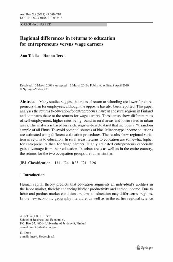
Ann Reg Sci (2011) 47:689–710DOI 10.1007/s00168-010-0374-8

ORIGINAL PAPER

Regional differences in returns to educationfor entrepreneurs versus wage earners

Anu Tokila · Hannu Tervo

Received: 10 March 2009 / Accepted: 13 March 2010 / Published online: 8 April 2010© Springer-Verlag 2010

Abstract Many studies suggest that rates of return to schooling are lower for entre-preneurs than for employees, although the opposite has also been reported. This paperanalyses the returns to education for entrepreneurs in urban and rural regions in Finlandand compares these to the returns for wage earners. These areas show different ratesof self-employment, higher rates being found in rural areas and lower rates in urbanareas. The analysis is based on a rich, register-based dataset that includes a 7% randomsample of all Finns. To avoid potential sources of bias, Mincer-type income equationsare estimated using different estimation procedures. The results show regional varia-tion in returns to education. In rural areas, returns to education are somewhat higherfor entrepreneurs than for wage earners. Highly educated entrepreneurs especiallygain advantage from their education. In urban areas as well as in the entire country,the returns for the two occupation groups are rather similar.

JEL Classification J31 · J24 · R23 · I21 · L26

1 Introduction

Human capital theory predicts that education augments an individual’s abilities inthe labor market, thereby enhancing his/her productivity and earned income. Due tolabor and product market conditions, returns to education may differ across regions.In the new economic geography literature, as well as in the earlier regional science

A. Tokila (B) · H. TervoSchool of Business and Economics,P.O. Box 35, 40014 University of Jyväskylä, Finlande-mail: [email protected]

H. Tervoe-mail: [email protected]

123

690 A. Tokila, H. Tervo

literature, agglomeration economies should lead to higher productivity of workers andhence higher wages and higher returns to education (Fujita et al. 1999; see also deBlasio and Di Addario 2005; Dalmazzo and de Blasio 2007; Lehmer and Möller 2009).Marshall (1890) was the first to find that spatial agglomerations create location advan-tages in terms of spillovers, such as labor pooling and co-operation between firms.Agglomeration economies may also enhance the earnings and returns to educationfor entrepreneurs. In addition, variation in relative returns to education across regionsmay account for the prevailing regional differences in entrepreneurship; these regionaldifferences in entrepreneurship are pronounced and persistent in many countries (e.g.Bernhardt 1994). On the other hand, labor and product market conditions may alsoaccount for the rate of entrepreneurship (Georgellis and Wall 2000; Parker 2004). Forinstance, less-educated individuals in a small, dispersed labor market may be pushedinto self-employment if they see no other realistic options (Carrasco and Ejrnæ 2003;Tervo 2008).

Apart from enhancing earnings, it is also generally believed that human capital,including education, increases an individual’s probability of becoming self-employed(e.g. Rees and Shah 1986). Thus, education can potentially be seen as a tool for sup-porting entrepreneurship. In order to be an attractive choice, an earnings premiummay be necessary to compensate for the greater uncertainty and higher inherent riskof entrepreneurship (Storey 1994; Hamilton 2000). If educated entrepreneurs do notachieve an adequate premium for their risk in a region, entrepreneurship may not bean attractive occupational choice, whereas high expected earnings will pull educatedindividuals into entrepreneurship. In many countries and regions, however, individualswith a higher level of education have a lower probability of being self-employed. Thisis the case in Finland (Johansson 2000; Niittykangas and Tervo 2005), which has oneof the most expensive education systems in the world. This prompts the question asto why highly educated individuals do not choose entrepreneurship, even though theyhave better abilities. Is it not profitable for them? In order to be an attractive choice,entrepreneurship should yield an adequate earnings premium for the higher inherentrisk it entails (Storey 1994).

The performance of educated entrepreneurs can be studied by comparing theirreturns to those of wage earners. No clear assumption on either theoretical or empiri-cal grounds can be made about whether the returns to education for entrepreneurs willbe higher or lower. Many previous studies suggest that the rates of return to school-ing are lower for entrepreneurs than for wage earners (Brown and Sessions 1998,1999; Hamilton 2000; García-Mainar and Montuenga-Gómez 2004), although theopposite also has been reported (Evans and Leighton 1990; Robinson and Sexton1994; Alba-Ramirez and Sansegundo 1995; van der Sluis et al. 2004). The impactof education on income varies according to the labor market and levels of education.van der Sluis et al. (2004) observed that studies that focused on the impact of educationon income in Europe more often indicated lower returns for entrepreneurs, while theevidence from the United States was the opposite. A study by Iversen et al. (2006) foundthat higher levels of schooling resulted in larger returns for the self-employed, whilelower levels of education indicated hardly any return in self-employment. In contrast,García-Mainar and Montuenga-Gómez (2004) concluded that secondary education isthe most profitable choice for the self-employed.

123

Regional differences in returns to education for entrepreneurs versus wage earners 691

In this paper, we are interested in how regional variation affects returns to educationfor entrepreneurs and wage earners. The role of region in general wage differentialshas been studied to some extent (e.g. Dumond et al. 1999; Duranton and Monastiriotis2002; Bernard et al. 2003; Goetz and Rupasingha 2004), but regional comparisonbetween entrepreneurs and wage earners has been largely ignored in the literature.We ask: does the education attained by an individual imply a higher rate of return forthe entrepreneur than for the wage earner, and are there regional differences in thesereturns? Typically, studies on regional wage differentials analyze specific regions. Weinstead focus on types of regions in order to provide more generalized results. In ouranalysis, Finnish regions are classified into urban and non-urban regions on the basisof the number of inhabitants and population density. These regions show differentrates of self-employment, with the rate being higher in rural areas and lower in urbanareas.

The analysis is based on a rich register-based dataset that includes a 7% randomsample of all Finns. In the analysis, we apply Mincer-type income equations that areestimated separately for employees and the self-employed (cf. Parker 2004). Differ-ent estimation procedures are used to avoid potential sources of bias in the results. Toavoid selection bias, we apply Heckman (1979) method. For the instrumentation of thepossible endogenous education variable, we also use a set of family background vari-ables as identifying instruments. For the sake of comparison, the standard OLS-methodis also applied.

Our estimation results suggest that returns to education are similar for entrepreneursand wage earners for the entire country. No clear-cut premium for entrepreneurs isdiscovered except in rural areas, where the return to higher education is much higherfor entrepreneurs. The estimated returns to higher education for entrepreneurs remainsmaller in urban areas than in rural areas. Even so, well-educated individuals in ruralareas do not opt for entrepreneurship, although the general level of entrepreneurshipis high. This result suggests that it is the push rather than the pull effect that accountsfor regional differences in entrepreneurship, meaning it is more likely that regionalvariation in entrepreneurship is due to weak employment conditions rather than higherexpected earnings.

The rest of the paper is organized as follows. Theoretical issues are discussed inSect. 2. Section 3 presents the model, data and variables, including basic definitionsand information on the income and educational choices in the two different types ofregions. In Sect. 4, the estimation results for the entire data set are presented first,followed by the results for the regions. Section 5 concludes the paper.

2 Theoretical issues and empirical antecedents

Human capital theory states that higher education levels should be rewarded in thelabor market for both entrepreneurs and wage earners. Higher education improvesseveral abilities needed in business, such as risk awareness and comprehension ofmarket prospects (Kangasharju and Pekkala 2002). However, the returns for the self-employed may be more dependent on factors other than formal education. For instance,many entrepreneurial skills such as motivation and salesmanship are non-academic in

123


nature (Parker 2004). This may lead to lower returns to education for entrepreneurs.In the case of wage earners, part of their return to productivity may be exploited by thefirm, thus lowering their returns to education (García-Mainar and Montuenga-Gómez2004).

Human capital can be divided into general and specific human capital (Becker1975). Education and work experience measured in years or levels representgeneral human capital. In the context of self-employment, specific human capi-tal is distributed as industry-specific and entrepreneurship-specific human capital.Industry-specific experience in paid work increases the productivity of entrepreneurs,as they already have familiarity with the main activities of the industry. In addition, itmay yield knowledge about potential niches in business. Entrepreneur-specific humancapital can best be obtained through self-employment, although some entrepreneur-ial skills may also be acquired through special entrepreneurial training (e.g. Firkin2003).

Spence (1973) was the first to claim that greater human capital is acquired only tosignal inherent productivity. The weak screening hypothesis concedes that the effectof education is manifested both through signaling and through increased productivity(Spence 1973; Arrow 1973). In the strong screening hypothesis, education operatesmerely as a signal of inherent productivity, having no role in enhancement of produc-tivity (Psacharopoulos 1979). In the case of the self-employed, the signaling role ofeducation is not that clear, as these individuals employ themselves. For wage earnersas well, more evidence has been presented for the weak hypothesis than for the strongone (e.g. Brown and Sessions 1998, 1999). This lends further support to the idea thateducation has an important role in the generation of earnings gains.

Earnings are an important incentive in occupational choice. Self-employment andpaid work represent the two largest sources of income. However, their characteristicsand degree of inequality are fundamentally different (Parker 1999). In most countries,the earnings of entrepreneurs range more widely than those of employees. This meansthat a relatively larger number of the self-employed are concentrated in the lower andupper tails of the income distribution compared to wage earners (Parker 2004). This isalso the case in Finland (Tervo and Haapanen 2010). Comparisons between the meanincome of entrepreneurs and paid workers may be strongly influenced by a few veryhigh-income entrepreneurial superstars (Rosen 1981; Hamilton 2000). For this reasonit might be better to use the median income in the comparative analyses.

In some studies, rural areas have been found to suffer from substantially lower ratesof returns to education than urban areas (Goetz and Rupasingha 2004). People mayaccept a lower income in exchange for other amenities in a region, such as scenery(see e.g., Power and Barrett 2001). On the other hand, for individuals with high qual-ifications, the gap in regional rates has been found to be relatively low (Bennett et al.1995). In peripheral regions, jobs with higher educational demands are more compa-rable in rates of pay with jobs in central areas, while for lower-skill jobs, rates aredetermined more by the local labor market. Yet, very little is known about the regionalvariation in returns to education between self-employment and paid work. Studies onregional wage differentials are commonly based on aggregate level approaches, whichare incapable of yielding explanations or sources for regional inequalities in returnsto education (see e.g. Duranton and Monastiriotis 2002).

123


3 Method, data and definitions

3.1 Methodology

It is important that the effect of education (formal schooling) on entrepreneurialperformance is measured consistently. We apply the income equations first sug-gested by Mincer (1974) to estimate causal effects that are not biased due to theneglect of unobserved heterogeneity or the endogenous nature of the occupationalchoice (employment/self-employment). According to the Mincerian approach, themain determinants of individual earnings are schooling and experience. The generalspecification for a Mincer-type earnings equation is:

ln Yi = f (edui ) + β Xi + ui , (1)

where Yi is the annual earnings of individual i, f (edui ) is a function of the educationalattainment of individual i, Xi contain labor market experience and other characteris-tics of the individual, and ui is a random error. In the standard version, f (edui ) isyears of education, i.e., it is assumed that the logarithm of earnings is a linear func-tion of years of completed education. In addition to this linear approach, we considera specification1 in which we use a dummy to compare the effect of having highereducation with the effect of not having higher education.

Since we are estimating earnings functions separately for entrepreneurs and wageearners, it is necessary to take account of possible selection bias. Those who enter self-employment or paid employment may not be a random sample from the population. Acommon way of removing possible selection bias is Heckman (1979) method in whichthe estimation is performed in two steps. In the first step, the selection (participation)equation is estimated:

zi = ω′Wi + vi , (2)

where zi indicates whether individual i is an entrepreneur/wage earner, Wi is a set ofexplanatory variables and vi is a disturbance term with unit variance. The selectionequation should contain at least one variable that is not in the outcome equation. In ourcase, several variables describing family background and regional features are used.Computing fitted values for zi yields the ‘inverse Mills ratios’:

λi = −φ(zi )/�(z), (3)

which are added to the earnings equation in the second step of the estimation.Another bias may follow from the endogenous nature of education. For this reason,

many previous studies on returns to education for entrepreneurs are potentially biased

1 Additional specifications with dummies for separate education levels and orders of the education poly-nomial (for years of schooling) were also performed. These estimations supported the hypothesis of non-linearity in the return to education and the highest returns for the higher education. However, the rate ofreturn was decreasing for the highest level of education (doctorate or equivalent level).

123


(van der Sluis et al. 2004). Their methodological approaches lag behind, especiallyin terms of identification. A cross-sectional correlation between education and earn-ings may not reflect the true causal effect of education (Card 1999). Generally, OLSestimates of the returns to education are biased downwards (Ashenfelter et al. 1999).These problems have long received attention in other types of studies on returns toeducation. A standard solution to the problem of identification is the instrumentalvariables (IV) estimation, where identifying instruments must satisfy two conditions:(i) the instrument should not be correlated with the error term and (ii) the instru-ment should be highly correlated with the endogenous variable of interest. The formerrelates to the validity of the instrument and the latter to its quality. Family backgroundis a widely used instrument for education. In our case, a set of variables for parents’education are used to instrument the schooling choice of an individual. Estimationsare performed using two-stage least squares (2SLS), in which the first stage estimatesthe structural form of the earnings equation, and the second stage reduces the formof the equation with instrument variables. Two recent studies suggest that correctingfor the endogeneity of schooling substantially increases the estimated rate of returnfor entrepreneurs (Parker and van Praag 2004; van der Sluis et al. 2004). To confrontboth types of biases in the same model, we use a combined Heckman-IV approach inwhich the inverse Mills ratios are included in the IV regression.

3.2 The dataset

The dataset is based on the Longitudinal Census File and the Longitudinal EmploymentStatistics File constructed by Statistics Finland. These two register-based datasets havebeen updated annually since 1987. They, together with some other registers, providepanel data on each resident of Finland. A 7% random sample of all the individuals inthis dataset in 2001 was taken for this study. The dataset includes very rich informa-tion on individuals’ educational attainments, labor market performance, regional andfamily characteristics, and many other variables from the period of 1987–2002 andfrom the earlier years of 1970, 1975, 1980, and 1985. We analyze the rates of returnin the base year 2001, as the dataset for this year contains the most comprehensiveinformation on earnings.

In this paper, the sample is restricted to persons from 18 to 64 years old, in paid orself-employment, and who had a net earned income in 2001. Persons employed in theagricultural sector are excluded from the sample due to the special nature of agricul-tural entrepreneurship (see e.g. Parker 2004). The total number of individuals in thesample is 148,861, of which 11,528 (7.7%) are self-employed and 137,333 (92.3%)are wage earners.

3.3 Definitions of entrepreneur and income

The first often-problematic task in studies of entrepreneurship is to define the conceptof ‘entrepreneur.’ Self-employment and entrepreneurship are concepts used in widelydiverse ways (see e.g., Parker 2004). In this analysis, the information of employmentstatus comes from the Longitudinal Census File. Thus, the concept of entrepreneurship

123


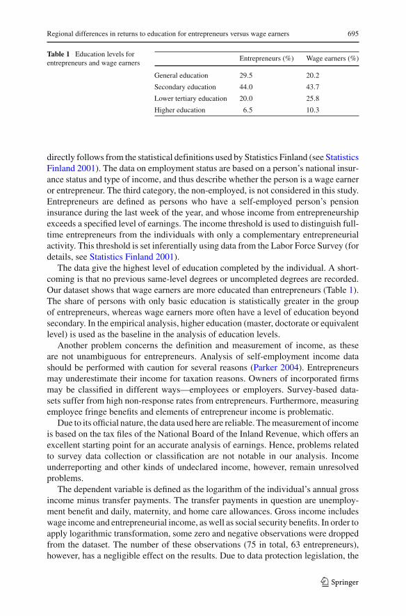
Table 1 Education levels forentrepreneurs and wage earners

Entrepreneurs (%) Wage earners (%)

General education 29.5 20.2

Secondary education 44.0 43.7

Lower tertiary education 20.0 25.8

Higher education 6.5 10.3

directly follows from the statistical definitions used by Statistics Finland (see StatisticsFinland 2001). The data on employment status are based on a person’s national insur-ance status and type of income, and thus describe whether the person is a wage earneror entrepreneur. The third category, the non-employed, is not considered in this study.Entrepreneurs are defined as persons who have a self-employed person’s pensioninsurance during the last week of the year, and whose income from entrepreneurshipexceeds a specified level of earnings. The income threshold is used to distinguish full-time entrepreneurs from the individuals with only a complementary entrepreneurialactivity. This threshold is set inferentially using data from the Labor Force Survey (fordetails, see Statistics Finland 2001).

The data give the highest level of education completed by the individual. A short-coming is that no previous same-level degrees or uncompleted degrees are recorded.Our dataset shows that wage earners are more educated than entrepreneurs (Table 1).The share of persons with only basic education is statistically greater in the groupof entrepreneurs, whereas wage earners more often have a level of education beyondsecondary. In the empirical analysis, higher education (master, doctorate or equivalentlevel) is used as the baseline in the analysis of education levels.

Another problem concerns the definition and measurement of income, as theseare not unambiguous for entrepreneurs. Analysis of self-employment income datashould be performed with caution for several reasons (Parker 2004). Entrepreneursmay underestimate their income for taxation reasons. Owners of incorporated firmsmay be classified in different ways—employees or employers. Survey-based data-sets suffer from high non-response rates from entrepreneurs. Furthermore, measuringemployee fringe benefits and elements of entrepreneur income is problematic.

Due to its official nature, the data used here are reliable. The measurement of incomeis based on the tax files of the National Board of the Inland Revenue, which offers anexcellent starting point for an accurate analysis of earnings. Hence, problems relatedto survey data collection or classification are not notable in our analysis. Incomeunderreporting and other kinds of undeclared income, however, remain unresolvedproblems.

The dependent variable is defined as the logarithm of the individual’s annual grossincome minus transfer payments. The transfer payments in question are unemploy-ment benefit and daily, maternity, and home care allowances. Gross income includeswage income and entrepreneurial income, as well as social security benefits. In order toapply logarithmic transformation, some zero and negative observations were droppedfrom the dataset. The number of these observations (75 in total, 63 entrepreneurs),however, has a negligible effect on the results. Due to data protection legislation, the

123


Table 2 Self-employment rate in the regions

General Secondary Lower tertiary Higher Alleducation education education education

Urban areas 8.3 5.8 5.0 4.8 6.0

Rural areas 16.6 12.6 9.9 6.4 12.7

Total 10.9 7.8 6.1 5.0 7.7

highest percentile in income subject to state taxation is given as a mean in the data.This should not have a significant influence on the results.

3.4 Regional classification

The analysis is based on the comparison between urban and rural areas. The basicregional unit used is a statistical grouping of municipalities into three groups. Here weuse location of workplace (instead of dwelling place) as a unit of observation, sincereturns are based on work and not on dwelling. In 2001, there were 488 municipalitiesin Finland. Urban municipalities are defined as those where at least 90% of the popula-tion lives in an urban settlement, or where the population of the largest urban settlementis at least 15,000. All other municipalities are defined as rural, despite the fact that theoriginal classification separates semi-urban municipalities from rural municipalities.Thus, the two groups of semi-urban and rural municipalities are combined in our anal-ysis. For the purposes of international comparison, Finnish semi-urban municipalitiesare more rural than urban. Also, according to Labridianis (2006), smaller-sized townsare more suited for inclusion in rural areas in the regional analysis.

Distinct differences are found in regional entrepreneurial activity by educationalclasses (Table 2). Overall intensity of entrepreneurship is more than double in ruralareas compared to urban ones. This can be explained by the fact that they offer fewerwage earning opportunities than urban areas (Tervo 2008). It is interesting to notethat entrepreneurial activity among the highly educated shows much less variation.For highly educated individuals, self-employment may be a less attractive choice thanemployment (Kangasharju and Pekkala 2002). There are several possible reasons forthis. According to some studies, highly educated individuals would earn more as paidworkers than as entrepreneurs (e.g. Hamilton 2000; Uusitalo 2001). In addition, com-pared to employees, entrepreneurs have a less constant income stream and less securitythan do employees (Storey 1994). Instead, the non-pecuniary benefits of the job areoften more important than financial benefits for the self-employed (Hamilton 2000).

Table 3 shows how median income varies according to the level of education andtype of region in the groups of entrepreneurs and wage earners. In general, medianincome is lower in rural areas than in urban areas, and the higher the education, thehigher the individual’s income. There are, however, a couple of exceptions, especiallyamong entrepreneurs. In rural areas, higher educated entrepreneurs earn significantlymore than wage earners. With respect to the level of education, entrepreneurs with asecondary education have a lower median income than those with a general education.In all, it seems that the income of entrepreneurs varies more than the income of wage

123


Tabl

e3

Med

ian

inco

me

ofen

trep

rene

urs

and

wag

eea

rner

sac

cord

ing

toed

ucat

ion

and

type

ofre

gion

Reg

ion

Gen

eral

Seco

ndar

yL

ower

tert

iary

Hig

her

All

educ

atio

ned

ucat

ion

educ

atio

ned

ucat

ion

EW

EW

EW

EW

EW

Urb

anar

eas

20,4

00(1

,774

)21

,400

(19,

519)

18,3

50(2

,668

)21

,300

(43,

330)

26,2

91(1

,457

)26

,500

(27,

816)

39,9

00(6

03)

38,5

00(1

1,96

8)22

,200

(6,3

71)

23,6

00(9

2,61

9)

Rur

alar

eas

18,1

00(1

,626

)19

,500

(8,1

76)

17,1

00(2

,409

)20

,300

(16,

737)

22,8

00(8

46)

24,4

00(7

,676

)40

,900

(145

)33

,989

(2,1

11)

18,8

00(5

,026

)21

,300

(34,

700)

Finl

and

inag

greg

ate

19,1

90(3

,400

)20

,800

(27,

695)

17,7

00(5

,077

)21

,000

(60,

067)

24,9

00(2

,303

)26

,000

(35,

492)

40,1

00(7

48)

37,7

00(1

4,07

9)20

,363

(11,

528)

23,1

00(1

37,3

33)

Een

trep

rene

urs,

Ww

age

earn

ers.

Num

ber

ofob

serv

atio

nsin

pare

nthe

ses

123


earners. This may also suggest that the returns to education for entrepreneurs and wageearners vary between regions.

3.5 Other variables

In addition to level of education, many other explanatory variables are used in the esti-mations. These include experience, field of education, age, gender and mother tongue.Experience is divided into experience in wage work and self-employment experience.In the IV estimations, the parental education is used as identifying instruments. In theHeckman estimations, parental self-employment history is used in the estimation ofthe selection equation in addition to other variables. Furthermore, the Heckman esti-mations include variables that describe regional characteristics, as well a variable thatindicates whether an individual is residing in his/her region of birth. The descriptionsand means of all the variables are given in Appendix (Table 7).

4 Estimation results

Our estimation strategy is to apply the Mincerian approach first to the data for theentire country and then to the two different types of regions. The aim is to estimatecausal effects that are not biased due to the endogenous nature of the decision to investin schooling or to the problem of self-selection. We apply the Heckman and combinedHeckman-instrumental variable (IV) approaches, and compare these results to theOLS estimates of the returns to education. In the estimations, the first specificationsconsider the impact of education on earnings in years, whereas the latter specificationscompare the effect of higher education on earnings to that of lower levels of education.Years of schooling are a standard measure where information is derived from the levelof education. A linear relationship is assumed to exist between years of education andlog-income, and the results indicate the marginal effect of an extra year of schooling.An alternative is to use levels of education, regardless of how many years it takes anindividual to attain. In this case, the annual marginal effect of schooling does not haveto be constant, but may vary according to education level. The level obtained by anindividual may be more informative than the number of years needed to attain it: avocational qualification or university degree may matter more than years of schoolingper se (Card 1999; García-Mainar and Montuenga-Gómez 2004). As we were espe-cially interested in the effect of higher education, the latter specifications use a dummythat separates the individuals with higher education from those without.

4.1 Results for the entire country

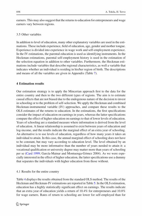
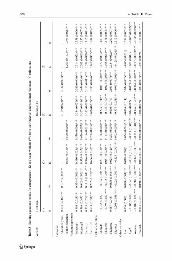
Table 4 displays the results obtained from the standard OLS method. The results of theHeckman and Heckman-IV estimations are reported in Table 5. In the OLS estimation,education has a highly statistically significant effect on earnings. The results indicatethat an extra year of education yields a return of 10.4% for entrepreneurs and 10.8%for wage earners. Rates of return to schooling are lower for self-employed than for

123


Table 4 Earnings equations: results for entrepreneurs (E) and wage workers (W) from OLS estimations(the entire country)

Variable E W E W

Education

Education years 0.104 (0.006)*** 0.108 (0.001)*** – –

Higher education – – 0.630 (0.040)*** 0.574 (0.005)***

Working experience

Wageexp1 0.317 (0.028)*** 0.361 (0.006)*** 0.319 (0.028)*** 0.357 (0.006)***

Wageexp2 0.585 (0.046)*** 0.653 (0.006)*** 0.590 (0.047)*** 0.648 (0.007)***

Entreexp1 0.370 (0.029)*** 0.109 (0.011)*** 0.368 (0.029)*** 0.100 (0.011)***

Entreexp2 0.681 (0.036)*** 0.274 (0.024)*** 0.665 (0.036)*** 0.254 (0.024)***

Field of education

Edutrade −0.041 (0.036) −0.027 (0.005)*** 0.219 (0.031)*** 0.204 (0.005)***

Edutechn −0.095 (0.027)*** 0.009 (0.004)* 0.098 (0.024)*** 0.173 (0.004)***

Eduhesoc 0.090 (0.045)* 0.058 (0.006)*** 272 (0.041)*** 0.232 (0.006)***

Eduservi −0.268 (0.036)*** −0.050 (0.006)*** −0.123 (0.035)*** 0.066 (0.006)***

Other variables

Age 0.005 (0.008) 0.049 (0.001)*** 0.008 (0.009) 0.042 (0.001)***

Age2 −0.004 (0.009) −0.039 (0.001)*** −0.008 (0.009) −0.044 (0.001)***

Woman −0.392 (0.023)*** −0.354 (0.004)*** −0.386 (0.023)*** −0.346 (0.004)***

Swedish 0.040 (0.038) 0.041 (0.007)*** 0.046 (0.038) 0.049 (0.007)***

Otherlan −0.177 (0.073)* −0.041 (0.013)** −0.208 (0.074)** −0.098 (0.013)***

Public sector – −0.137 (0.004)*** – −0.102 (0.004)***

Constant 8.205 (0.183)*** 7.587 (0.023)*** 9.187 (0.173)*** 8.651 (0.022)***

E entrepreneurs, W wage earners. Standard errors in parentheses. *p value ≤ 0.05, **p value ≤ 0.01 and***p value ≤ 0.001

employees, but the difference is small. van der Sluis et al. (2004) summarized thatthe average return to a marginal year of education for entrepreneurs was 6.1% across94 previous studies. Our estimates of returns are higher than in most of the existingliterature, but it should be noted that they are based on gross earnings. If we look atthe results according to level of education, we can see that they show a higher returnto highly educated entrepreneurs than for highly educated wage earners. For entrepre-neurs, the return for a highest academic degree is 63% higher than for those who donot have higher education, while for wage earners it is 57%.

Before commenting on the results for the other variables, it is necessary toincrease the quality of the estimates. The first step is to use the Heckman methodto correct for possible selection bias related to employment choice. Selectiv-ity is controlled by estimating a Heckman selection model and including theinverse Mill’s ratio (‘Heckman’s lambda’) in the second-step regressions. Severalvariables are used to correct for the non-random nature of choice of employ-ment. They include level of education and its field, gender, age, language, educa-tion of parents and regional factors. The results of the probit estimations for theself-employment decision, in which education is measured in years, are presented

123


Tabl

e5

Ear

ning

equa

tions

:res

ults

for

entr

epre

neur

s(E

)an

dw

age

wor

kers

(W)

from

the

Hec

kman

and

com

bine

dH

eckm

an-I

Ves

timat

ions

Var

iabl

eH

eckm

anH

eckm

an-I

V

(1)

(2)

(1)

(2)

EW

EW

EW

EW

Edu

catio

n

Edu

catio

nye

ars

0.10

3(0

.007

)***

0.10

7(0

.000

)***

––

0.16

9(0

.022

)***

0.13

2(0

.003

)***

––

Hig

her

educ

atio

n–

–0.

583

(0.0

43)*

**0.

570

(0.0

06)*

**–

–1.

200

(0.1

63)*

**0.

996

(0.0

25)*

**

Wor

king

expe

rien

ce

Wag

eexp

10.

316

(0.0

28)*

**0.

354

(0.0

06)*

**0.

310

(0.0

28)*

**0.

350

(0.0

06)*

**0.

314

(0.0

28)*

**0.

360

(0.0

06)*

**0.

314

(0.0

28)*

**0.

351

(0.0

06)*

**

Wag

eexp

20.

586

(0.0

47)*

**0.

642

(0.0

06)*

**0.

575

(0.0

47)*

**0.

636

(0.0

07)*

**0.

567

(0.0

48)*

**0.

656

(0.0

06)*

**0.

563

(0.0

48)*

**0.

655

(0.0

07)*

**

Ent

reex

p10.

375

(0.0

29)*

**0.

1114

(0.0

11)*

**0.

376

(0.0

29)*

**0.

106

(0.0

11)*

**0.

375

(0.0

29)*

**0.

112

(0.0

11)*

**0.

378

(0.0

29)*

**0.

116

(0.0

11)*

**

Ent

reex

p20.

683

(0.0

31)*

**0.

287

(0.0

23)*

**0.

666

(0.0

36)*

**0.

268

(0.0

25)*

**0.

686

(0.0

37)*

**0.

287

(0.0

24)*

**0.

668

(0.0

37)*

**0.

284

(0.0

25)*

**

Fiel

dof

educ

atio

n

Edu

trad

e−0

.035

(0.0

37)

−0.0

39(0

.006

)***

0.20

1(0

.031

)***

0.18

6(0

.006

)***

−0.2

23(0

.071

)**

−0.0

81(0

.008

)***

0.17

2(0

.033

)***

0.18

0(0

.005

)***

Edu

tech

n−0

.093

(0.0

27)*

**−0

.015

(0.0

05)*

*0.

081

(0.0

25)*

*0.

143

(0.0

05)*

**−0

.195

(0.0

42)*

**−0

.024

(0.0

05)*

**0.

108

(0.0

25)*

**0.

171

(0.0

05)*

**

Edu

heso

c0.

087

(0.0

45)

0.08

58(0

.006

)***

0.02

4(0

.042

)***

0.26

3(0

.007

)***

−0.0

96(0

.074

)0.

031

(0.0

07)*

**0.

134

(0.0

52)*

*0.

269

(0.0

07)*

**

Edu

serv

i−0

.268

(0.0

38)*

**−0

.026

(0.0

06)*

**−0

.125

(0.0

36)*

**0.

092

(0.0

07)*

**−0

.378

(0.0

51)*

**−0

.067

(0.0

08)*

**−0

.128

(0.0

36)*

**0.

113

(0.0

06)*

**

Oth

erva

riab

les

Age

0.00

6(0

.009

)0.

049

(0.0

01)*

**0.

018

(0.0

09)*

0.05

4(0

.001

)***

−0.0

14(0

.011

)0.

034

(0.0

02)*

**−0

.004

(0.0

11)

0.03

8(0

.002

)***

Age

2−0

.005

(0.0

10)

−0.0

46(0

.002

)***

−0.0

18(0

.010

)−0

.053

(0.0

02)*

**0.

014

(0.0

12)

−0.0

33(0

.002

)***

0.00

2(0

.011

)−0

.037

(0.0

02)*

**

Wom

an−0

.405

(0.0

31)*

**−0

.387

(0.0

04)*

**−0

.440

(0.0

30)*

**−0

.383

(0.0

04)*

**−0

.326

(0.0

40)*

**−0

.344

(0.0

08)*

**−0

.385

(0.0

23)*

**−0

.345

(0.0

09)*

**

Swed

ish

0.04

3(0

.038

)0.

050

(0.0

07)*

**0.

064

(0.0

38)

0.05

8(0

.008

)***

0.01

8(0

.039

)0.

033

(0.0

07)*

**0.

029

(0.0

39)

0.03

4(0

.007

)***

123


Tabl

e5

cont

inue

d

Var

iabl

eH

eckm

anH

eckm

an-

IV

(1)

(2)

(1)

(2)

EW

EW

EW

EW

Oth

erla

n−0

.179

(0.0

74)*

−0.0

34(0

.014

)*−0

.183

(0.0

73)*

−0.0

89(0

.015

)**

−0.1

82(0

.073

)*−0

.030

(0.0

13)*

−0.2

14(0

.075

)**

−0.0

74(0

.014

)***

Publ

icse

ctor

–−0

.269

(0.0

07)*

**–

−0.2

53(0

.007

)***

–−0

.162

(0.0

04)*

**–

−0.1

63(0

.005

)***

Con

stan

t8.

127

(0.2

53)*

**7.

474

(0.0

25)*

**8.

493

(0.2

53)*

**8.

510

(0.0

26)*

**8.

339

(0.2

43)*

**7.

473

(0.0

57)*

**9.

621

(0.3

55)*

**8.

607

(0.0

83)*

**

Lam

bda

0.03

6(0.

092)

−0.5

96(0

.024

)***

0.15

0(0.

055)

**−0

.680

(0.0

24)*

**

Sarg

anst

atis

tics

1.11

822

.207

***

3.55

186

.619

***

Num

ber

ofob

serv

atio

ns11

,359

135,

869

11,3

5913

5,86

911

,359

135,

869

11,3

5913

5,86

9

Een

trep

rene

urs,

Ww

age

earn

ers.

Stan

dard

erro

rsin

pare

nthe

ses.

*p

valu

e≤

0.05

,**

pva

lue

≤0.

01an

d**

*p

valu

e≤

0.00

1

123


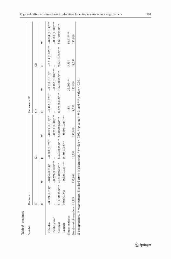
in Appendix (Table 8). However, these are not commented on here as they are not ofdirect interest.

The lambda turns out to be significantly negative for wage earners, which indicatesthe importance of controlling for self-selection bias. For entrepreneurs the lambdais positive, but significant only in the latter specification. A negative sign indicatesnegative covariance between the error terms in the employment choice and wage func-tions, whereas a positive sign indicates the opposite. Thus, a negative lambda suggeststhat unobserved factors tend to decrease the likelihood of selection to entrepreneur-ship, while they increase earned income. Due to the selection process, wage earnersmight have better earnings while self-employed. Comparison of the OLS and Heckmanresults shows them to be rather similar, with one important exception. The adjustmentfor selectivity has a substantial impact on the coefficient of the return to higher edu-cation for entrepreneurs, which is now much closer to (though still higher than) thereturn for wage earners. Thus, compared to the OLS estimation, this estimation showsa smaller risk premium for highly educated entrepreneurs. Otherwise, the effects onthe estimated coefficients are minor. In the specification in which education is definedin years, the rate of return is approximately 10% for a marginal year of education forboth groups, while still remaining slightly bigger for wage earners.

The next step is to control for the possible endogeneity of choice of educationtogether with self-selection. An instrumental variable method is combined with theHeckman method, in which the education of parents is used as identifying instrumentsfor the choice of education. First, the selection model is estimated, from which theinverse Mills ratios are then included in the IV regression. In line with previous studies(e.g., van der Sluis et al. 2004, 2008), the use of the IV method produces higher returnsto education. The estimated annual marginal effect of schooling is clearly higher forentrepreneurs than for wage earners: for entrepreneurs it is now 16.9% and for wageearners 13.4%. With respect to the results for wage earners, the estimated effects arehigher than in many previous studies conducted in Finland (e.g., Asplund 1993, 2000),but similar to the results obtained by Uusitalo (1999). The results of the latter speci-fications suggest that higher education levels raise the income of entrepreneurs by asmuch as 120%. For wage earners, the comparable rate of return is somewhat smaller(99.6%), but still substantially high.

Thus, these results show strikingly higher returns to education than previous results.Which are more credible?2 One approach is to test the validity and over-identificationof the instruments in the IV estimation. These are tested with the Hansen–Sargan test.The test indicates whether the instruments are uncorrelated with the error term andwhether the excluded instruments are correctly excluded from the estimated equation.

2 Uusitalo (1999) suggests three distinct explanations for the difference between the OLS and IV esti-mates. First, the OLS estimates may be downward biased because of measurement error in schooling, whilethe IV estimates are consistent in the presence of measurement errors. Second, the instruments may bewrongly specified, which could bias the instrumental variable estimates upwards. Third, individuals mayoptimize their behavior, which leads to a correlation between schooling and the earnings equation error andfurthermore to a bias in the OLS estimates. Griliches (1977) considered that this correlation is negative inpractice; educational attainment is cheaper for individuals who have less income to lose in the course ofeducation. Thus, their optimal amount of schooling is larger and the OLS estimates tend to be downwardbiased.

123


For entrepreneurs the over-identification test supports the null hypothesis, but it doesnot do so for wage earners. This suggests that the instruments are not valid for wageearners. The reason for this is not clear, as the education of parents is widely suggestedand used as an instrument of schooling choice. Another common instrument is the edu-cation of the spouse (see e.g. Iversen et al. 2006), but as all individuals do not havea spouse, this is not a workable solution.3 For these reasons, the results given by thecombined Heckman-IV estimation remain somewhat ambiguous, and more weightshould be given to the plain Heckman results.

To comment briefly on the results for the other variables, the first item of noteis the importance of the other main determinant of the Mincerian earning equation,namely experience. All the experience variables are highly statistically significant asexpected. Prior experience in wage work is a more important determinant of employ-ees’ earnings, whereas experience in entrepreneurship matters more for entrepreneurs.Interestingly, experience in entrepreneurship does not have such a big effect on theearnings of wage workers as experience in wage work has on the earnings of entrepre-neurs. The results suggest a non-linear relationship between earnings and age for wageearners, while age does not have a significant effect for entrepreneurs. Field of educa-tion has a widely significant effect, especially in the latter specifications. Gender hasa distinct effect: females earn less than males. The language dummies show, first, thatindividuals who speak a language other than Finland’s two official languages (Finnishor Swedish) as their mother tongue, i.e., immigrants, have lower earnings than natives,and second, that earnings are statistically higher for Swedish-speaking employees butnot for Swedish-speaking entrepreneurs. Employees in the public sector have lowerearnings than employees in the private sector.

Taken as a whole, most of our control variables proved to be significant and behaveas expected. The obtained results using different methods and specifications are mostlyconsistent. As to the estimated return to education measured in years, this proved to besimilar for entrepreneurs and wage earners in the plain OLS estimation and especiallyin the Heckman estimation in which choice of employment is controlled for. On thecontrary, in the comparison between higher education and other education, the resultssuggested a somewhat higher return for entrepreneurs than for wage earners. However,no clear sign of a risk premium was found for educated entrepreneurs.

4.2 Regional results

Let us now turn to the regional estimations (Table 6). Results by type of region giveus an insight into regional differences in returns to education for entrepreneurs andwage earners. The specifications include the same control variables as the equationsfor the entire country, but for brevity these results are not shown in Table 6.

To begin with, the results seem to diverge to some extent between the two typesof regions. In urban areas, the estimated return to education is fairly similar betweenwage earners and entrepreneurs. An exception is the Heckman-IV specification inwhich education is measured in years: these results would suggest a higher return for

3 Instead, information on parental education for all individuals is available.

123


Tabl

e6

Reg

iona

lear

ning

equa

tions

:res

ults

for

entr

epre

neur

s(E

)an

dw

age

wor

kers

(W)

Reg

ion

type

Var

iabl

eO

LS

Hec

kman

Hec

kman

-IV

(1)

(2)

(1)

(2)

(1)

(2)

EW

EW

EW

EW

EW

EW

Urb

anar

eas

Edu

catio

n0.

099

0.10

7−

−0.

109

0.10

7−

−0.

144

0.12

4−

−ye

ars

(0.0

08)*

**(0

.001

)***

(0.0

08)*

**(0

.001

)***

(0.0

22)*

**(0

.003

)***

Hig

her

−−

0.55

40.

559

−−

(0.5

75)

(0.5

61)

−−

(0.9

67)

(0.9

35)

educ

atio

n(0

.045

)***

(0.0

06)*

**(0

.047

)***

(0.0

06)*

**(0

.151

)***

(0.0

21)*

**

Rur

alar

eas

Edu

catio

n0.

098

0.10

2−

−0.

112

0.10

2–

–0.

120

0.10

3−

−ye

ars

(0.0

12)*

**(0

.002

)***

(0.0

13)*

**(0

.002

)***

(0.0

44)*

**(0

.006

)***

Hig

her

−−

0.77

00.

574

−−

0.80

20.

572

−−

1.21

90.

921

educ

atio

n(0

.089

)***

(0.0

13)*

**0.

092*

**(0

.014

)***

(0.4

68)*

*(0

.059

)***

Sarg

anst

atis

tics

2.44

717

.016

***

4.52

460

.015

***

1.47

95.

038*

**2.

133

18.9

18**

*

Een

trep

rene

urs,

Ww

age

earn

ers.

Stan

dard

erro

rsin

pare

nthe

ses.

*p

valu

e≤

0.05

,**

pva

lue

≤0.

01an

d**

*p

valu

e≤

0.00

1.T

hesp

ecifi

catio

nsco

ntai

nth

esa

me

cont

rol

vari

able

sas

the

spec

ifica

tions

for

the

entir

eco

untr

y(s

eeTa

ble

4),b

utth

ese

resu

ltsar

eno

tpre

sent

edhe

re

123


entrepreneurs than for wage earners. Unfortunately, the over-identification test is stillnot supported for wage earners. For rural areas, the results suggest more systematicallyhigher returns to education for entrepreneurs than for wage earners. The difference inimpact measured by years is minor, but a clearer difference is found for highly edu-cated entrepreneurs: for this group, the estimated return is clearly higher than for wageearners with the same level of education. The Heckman-IV estimation suggests a 3%point higher return for entrepreneurs. The return for an extra year of education was upto 1.7% points higher for these individuals depending on the estimation method used.

If we compare the results for the two types of regions, the estimations suggest thatreturns to education are higher for entrepreneurs in rural than in urban areas. In partic-ular, well-educated entrepreneurs receive high returns to education in the countryside.In the group of wage earners, returns to education prove to be more alike betweenurban and rural regions. However, an urban environment might be a more attractivechoice for employees in terms of returns to earnings.

These results support Bennett et al. (1995), who found that highly educated per-sons have relatively higher returns to education in rural areas compared to the lesseducated. In our study, this is especially true for entrepreneurs. The results are, how-ever, the reverse of those obtained by Goetz and Rupasingha (2004), who observedthat returns to higher degrees of schooling are lower in rural areas compared to urbanones. Particularly for entrepreneurs, the relationship between education and income ismore likely to be non-linear in rural areas (cf. Iversen et al. 2006). It is likely that thefirms owned by higher educated entrepreneurs are focused on wider markets, whilelow-skilled entrepreneurs confine themselves to the local market. This tends to raisethe relative returns for the highly educated. Online services provide an example of thekind of business run by the highly educated.

5 Conclusions

On average in Finland, entrepreneurs are less educated than wage earners. This paperanalyzed the returns to education for entrepreneurs and wage earners in two typesof Finnish regions, urban and rural. These regions differ in many respects, includingin entrepreneurial activity. In general, rural areas have a higher self-employment ratecompared to urban areas. However, if we look only at the group of highly educatedself-employed, regional differences in entrepreneurial activity become considerablysmaller.

According to our results, the returns to education turned out to be similar for entre-preneurs and wage earners, when educational attainment is measured in years. Inthe dichotomous comparison between the highly educated and others, the estimatedreturn is slightly higher for entrepreneurs than for employees, although no clear-cut riskpremium was found for educated entrepreneurs. Urban areas dominated the results forthe entire country, whereas rural areas showed divergent results. In rural areas, returnsto education are higher for entrepreneurs. Particularly high returns were found forhighly-educated entrepreneurs in rural areas.

What are the implications of these results for choice of employment and locationof workplace? Our results suggest that entrepreneurship is a more attractive employ-

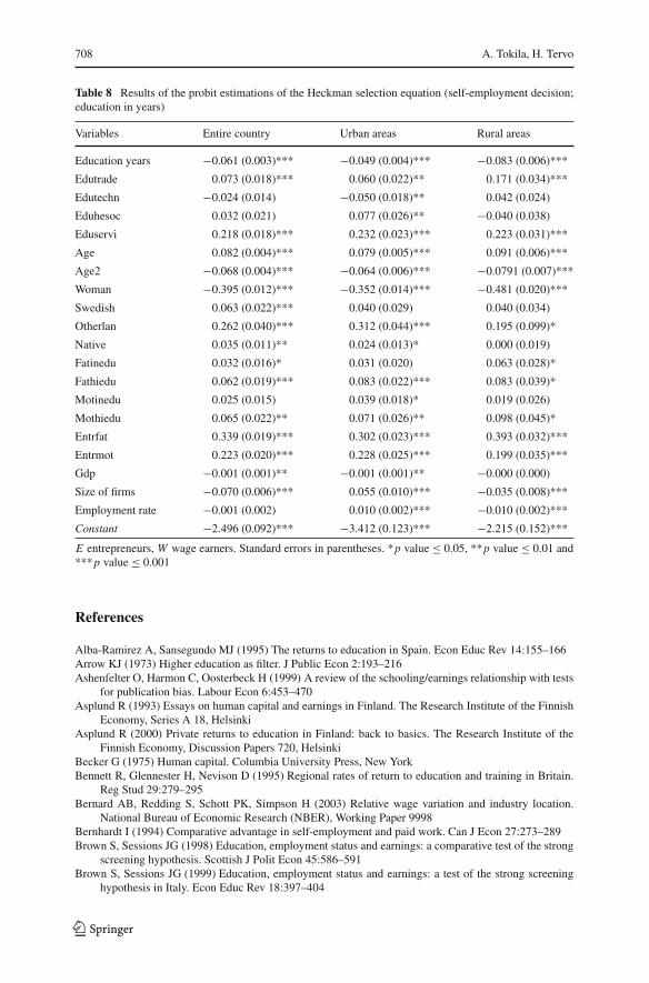
123


ment choice for highly educated individuals in rural areas, whereas in urban areas thereturn is about the same for both occupational choices. In terms of choosing location,educated entrepreneurs are financially better off in rural areas. For wage earners, regionof residence does not have such importance in terms of returns to education.

Regionally, these findings raise the question of the causes of regional variation inthe rate of entrepreneurship and the relative strength of pull and push factors. Are indi-viduals pulled or pushed into self-employment? Is it market pull and higher expectedearnings that dominate, or are individuals pulled into entrepreneurship because noth-ing else is available? Our results suggest that well-educated individuals get a highreturn to education, especially in rural areas. Agglomeration economies do not seemto play significant role. Even so, the option of entrepreneurship is not a highly popularone among the highly educated in rural areas. Regional differences in the intensity ofentrepreneurship do not stem from differences among the well educated, but ratherfrom differences among the less educated. Consequently, it is the push effect thatdominates, not the pull effect. Regional differences in the rate of self-employment aremore likely due to fewer paid-employment opportunities in rural and other weak eco-nomic areas than to higher expected earnings. Finally, variations in relative returns toeducation across regions do not seem to account for the prevailing regional differencesin entrepreneurship.

Acknowledgments This paper is a part of the Research Programme on Business Know-how (LIIKE2,project number 112116, and project number 127049), both financed by the Academy of Finland. Finan-cial support from the Yrjö Jahnsson Foundation (project 5597) and Finnish Concordia Fund is gratefullyacknowledged by the first author. The authors wish to thank Marcus Dejardin and two anonymous refereesfor their valuable comments as well as the participants at the special session “Entrepreneurship and theRegion” at the 47th Congress of the European Regional Science Association (29 August–2 September2008, Paris) for contributing to the earlier version of the paper.

Appendix

See Tables 7 and 8.

Table 7 Descriptions of variables and their means/share

Variable Definition Entrepreneurs Wage earners

Logincome ln(income subject to state taxation –unemployment benefit – dailyallowance and maternity allowance– home care allowance)

9.8 10.0

Urban 1 if location of workplace is in urbanarea, 0 otherwise

56.4 74.7

Explanatory variables

Education

Education in years Number of years of education 11.2 11.7

Higher education 1 if higher-degree level tertiaryeducation or doctorate orequivalent level tertiary, 0otherwise

6.5 10.3

123


Table 7 continued

Variable Definition Entrepreneurs Wage earners

Working experience

Wageexp1 1 if wage earning experience5–10 years, 0 otherwise

29.1 24.3

Wageexp2 1 if wage earning experience morethan 10 years, 0 otherwise

7.1 54.7

Entreexp1 1 if entrepreneurship experience5–10 years, 0 otherwise

29.2 2.3

Entreexp2 1 if entrepreneurship experience.more than 10 years, 0 otherwise

40.4 0.4

Field of education

Edutrade 1 if field of education business orsocial sciences, 0 otherwise

13.1 16.1

Edutechn 1 if field of education technology ornatural sciences, 0 otherwise

28.9 26.7

Eduhesoc 1 if field of education health orwelfare, 0 otherwise

6.9 10.9

Eduservi 1 if field of education services, 0otherwise

10.4 9.3

Personal characteristics

Age Age in years 45.2 40.2

Age2 Age-squared divided by 100 21.3 17.5

Woman 1 if female, 0 if male 33.1 50.5

Swedish 1 if native language is Swedish, 0otherwise

6.7 5.5

Otherlan 1 if native language other thanFinnish or Swedish, 0 otherwise

1.8 1.5

Native 1 if residing in sub-region of birth, 0otherwise

64.1 60.1

Family background

Fatinedu 1 if father has secondary education, 0otherwise

11.9 16.5

Fathiedu 1 if father has tertiary education, 0otherwise

9.9 14.7

Motinedu 1 if mother has secondary education,0 otherwise

15.0 20.4

Mothiedu 1 if mother has tertiary education, 0otherwise

6.7 10,9

Entrfat 1 if father was self-employed in1970, 1980 or 1990, 0 otherwise

16.3 9.2

Entrmot 1 if mother was self-employed in1970, 1980 or 1990, 0 otherwise

13.6 7.5

Regional characteristics

Gdp Annual index of gdp in the region 90.6 95.7

Size of firms Average size of firms in the region (employees) 4.5 4.8

Employment rate Unemployment rate in the region 12.6 12.0

Number of observations 11,528 137,333

123


Table 8 Results of the probit estimations of the Heckman selection equation (self-employment decision;education in years)

Variables Entire country Urban areas Rural areas

Education years −0.061 (0.003)*** −0.049 (0.004)*** −0.083 (0.006)***

Edutrade 0.073 (0.018)*** 0.060 (0.022)** 0.171 (0.034)***

Edutechn −0.024 (0.014) −0.050 (0.018)** 0.042 (0.024)

Eduhesoc 0.032 (0.021) 0.077 (0.026)** −0.040 (0.038)

Eduservi 0.218 (0.018)*** 0.232 (0.023)*** 0.223 (0.031)***

Age 0.082 (0.004)*** 0.079 (0.005)*** 0.091 (0.006)***

Age2 −0.068 (0.004)*** −0.064 (0.006)*** −0.0791 (0.007)***

Woman −0.395 (0.012)*** −0.352 (0.014)*** −0.481 (0.020)***

Swedish 0.063 (0.022)*** 0.040 (0.029) 0.040 (0.034)

Otherlan 0.262 (0.040)*** 0.312 (0.044)*** 0.195 (0.099)*

Native 0.035 (0.011)** 0.024 (0.013)* 0.000 (0.019)

Fatinedu 0.032 (0.016)* 0.031 (0.020) 0.063 (0.028)*

Fathiedu 0.062 (0.019)*** 0.083 (0.022)*** 0.083 (0.039)*

Motinedu 0.025 (0.015) 0.039 (0.018)* 0.019 (0.026)

Mothiedu 0.065 (0.022)** 0.071 (0.026)** 0.098 (0.045)*

Entrfat 0.339 (0.019)*** 0.302 (0.023)*** 0.393 (0.032)***

Entrmot 0.223 (0.020)*** 0.228 (0.025)*** 0.199 (0.035)***

Gdp −0.001 (0.001)** −0.001 (0.001)** −0.000 (0.000)

Size of firms −0.070 (0.006)*** 0.055 (0.010)*** −0.035 (0.008)***

Employment rate −0.001 (0.002) 0.010 (0.002)*** −0.010 (0.002)***

Constant −2.496 (0.092)*** −3.412 (0.123)*** −2.215 (0.152)***

E entrepreneurs, W wage earners. Standard errors in parentheses. *p value ≤ 0.05, **p value ≤ 0.01 and***p value ≤ 0.001

References

Alba-Ramirez A, Sansegundo MJ (1995) The returns to education in Spain. Econ Educ Rev 14:155–166Arrow KJ (1973) Higher education as filter. J Public Econ 2:193–216Ashenfelter O, Harmon C, Oosterbeck H (1999) A review of the schooling/earnings relationship with tests

for publication bias. Labour Econ 6:453–470Asplund R (1993) Essays on human capital and earnings in Finland. The Research Institute of the Finnish

Economy, Series A 18, HelsinkiAsplund R (2000) Private returns to education in Finland: back to basics. The Research Institute of the

Finnish Economy, Discussion Papers 720, HelsinkiBecker G (1975) Human capital. Columbia University Press, New YorkBennett R, Glennester H, Nevison D (1995) Regional rates of return to education and training in Britain.

Reg Stud 29:279–295Bernard AB, Redding S, Schott PK, Simpson H (2003) Relative wage variation and industry location.

National Bureau of Economic Research (NBER), Working Paper 9998Bernhardt I (1994) Comparative advantage in self-employment and paid work. Can J Econ 27:273–289Brown S, Sessions JG (1998) Education, employment status and earnings: a comparative test of the strong

screening hypothesis. Scottish J Polit Econ 45:586–591Brown S, Sessions JG (1999) Education, employment status and earnings: a test of the strong screening

hypothesis in Italy. Econ Educ Rev 18:397–404

123


Card D (1999) The causal effect of education on earnings. Handbook of labor economics 3:1801–1863.North-Holland, Amsterdam

Carrasco R, Ejrnæ M (2003) Self-employment in Denmark and Spain: institution, economic conditionsand gender differences. Centre for Applied Microeconometrics, Institute of Economics, University ofCopenhagen

Dalmazzo A, de Blasio G (2007) Social returns to education in Italian local labor markets. Ann Reg Sci41:51–69

de Blasio G, Di Addario S (2005) Do workers benefit from industrial agglomeration. J Reg Sci45:797–827

Dumond M, Barry H, Macperson D (1999) Wage differentials across labor markets: does cost of livingmatter. Econ Inquiry 37:577–589

Duranton G, Monastiriotis V (2002) Mind the gaps: the evolution of regional earnings inequalities in theU.K., 1982–1997. J Reg Sci 42:219–256

Evans DS, Leighton LS (1990) Small business formation by unemployed and employed workers. SmallBus Econ 2:319–330

Firkin P (2003) Entrepreneurial capital. In: De Bruin A, Dupuis A (eds) New perspectives in a global age.Ashgate, UK

Fujita M, Krugman P, Venables AJ (1999) The spatial economy. The MIT Press, CambridgeGarcía-Mainar I, Montuenga-Gómez VM (2004) Education returns of wage earners and self-employed

workers: Portugal vs. Spain. Econ Educ Rev 24:161–170Georgellis Y, Wall HJ (2000) What makes a region entrepreneurial? Evidence from Britain. Ann Reg Sci

34:385–403Goetz SJ, Rupasingha A (2004) The returns to education in rural areas. Rev Reg Stud 34:245–259Griliches Z (1977) Estimating the returns to schooling: some econometric problems. Econometrica 45:1–22Hamilton BH (2000) Does entrepreneurship pay? An empirical analysis of the returns to self-employment.

J Polit Econ 108:604–631Heckman J (1979) Sample selection bias as a specification error. Econometrica 47:153–161Iversen J, Malchow-Møller N, Sørensen A (2006) Returns to schooling in self-employment. Centre for

Economic and Business Research (CEBR), Discussion paper 19Johansson E (2000) Self-employment and the predicted earnings differential—evidence from Finland.

Finnish Econ Pap 13:45–55Kangasharju A, Pekkala S (2002) The role of education in self-employment success in Finland. Growth

Change 33:216–237Labridianis L (2006) Fostering entrepreneurship as a means to overcome barriers to development of rural

peripheral areas in Europe. Eur Plan Stud 14:3–8Lehmer F, Möller J (2009) Interrelations between the urban wage premium and firm-size wage differentials:

a microdata cohort for Germany. Ann Reg Sci (forthcoming)Marshall A (1890) The principles of economics. Macmillan, LondonMincer J (1974) Schooling, experience and earnings. Columbia University Press, New YorkNiittykangas H, Tervo H (2005) Spatial variations in intergenerational transmissions of self-employment.

Reg Stud 39:319–332Parker SC, van Praag M (2004) Schooling, capital constraints and entrepreneurial performance. Tinbergen

Institute Discussion Papers 04-106/3, Tinbergen Institute, AmsterdamParker SC (1999) The inequality of employment and self-employment incomes: a decomposition analysis

for the UK. Rev Income Wealth 45:263–274Parker SC (2004) The economics of self-employment and entrepreneurship. Cambridge University Press,

CambridgePower TM, Barrett RN (2001) Post-cowboy economics: pay and prosperity in the new American West.

Island Press, Washington DCPsacharopoulos G (1979) On the weak versus the strong version of screening hypothesis. Econ Lett

4:181–185Rees H, Shah A (1986) An empirical analysis of self-employment in the UK. J Appl Econom 1:95–108Robinson PB, Sexton EA (1994) The effect of education and experience on self-employment success. J Bus

Venturing 9:141–156Rosen S (1981) The economics of superstars. Am Econ Rev 71:845–858Spence M (1973) Job market signalling. J Labor Econ 87:355–374Statistics Finland (2001) Population census 2000 handbook. Helsinki

123


Storey D (1994) Understanding the small business. Routledge, LondonTervo H (2008) Self-employment transitions and alternation in Finnish rural and urban labour markets. Pap

Reg Sci 87:55–76Tervo H, Haapanen M (2010) The nature of self-employment: how does gender matter? Int J Entrepreneur-

ship Small Bus 9:349–371Uusitalo R (1999) Essays in economics of education. Academic Dissertation, February, University of

Helsinki, Faculty of Social Science, HelsinkiUusitalo R (2001) Homo entreprenaurus? Appl Econ 33:1631–1638van der Sluis JM, van Praag M, van Witteloostuijn A (2004) Entrepreneurship, selection and performance:

a meta-analysis of the role of education. Tinbergen Institute Discussion Paper 03-046/3, TinbergenInstitute, Amsterdam

van der Sluis J, van Praag M, Vijverberg W (2008) Education and entrepreneurship selection and perfor-mance: a review of the empirical literature. J Econ Surv 22(5):95–841

123

Regional differences in returns to education for entrepreneurs versus wage earners

Documents

Transcript of Regional differences in returns to education for entrepreneurs versus wage earners