HCEO WORKING PAPER SERIES

Working Paper

The University of Chicago1126 E. 59th Street Box 107

Chicago IL 60637

www.hceconomics.org

Top Earners: Cross-Country Facts∗

Alejandro BadelBureau of Labor Statistics andGeorgetown Universityale.badel@gmail.com

Moira DalyCopenhagen Business Schoolmoda.eco@cbs.dk

Mark HuggettGeorgetown Universitymh5@georgetown.edu

Martin NybomStockholm Universitymartin.nybom@sofi.su.se

this draft: June 22, 2017

Abstract

We provide a common set of life-cycle earnings statistics based on administrative data fromthe United States, Canada, Denmark and Sweden. We find three qualitative patterns, whichare common across countries. First, top-earnings inequality increases over the working lifetime.Second, the extreme right tail of the earnings distribution becomes thicker with age over theworking lifetime. Third, top lifetime earners exhibit dramatically higher earnings growth overtheir working lifetime. Models of top earners should account for these three patterns and,importantly, for how they quantitatively differ across countries.

Keywords: Earnings, Inequality, Top Earners, Top Incomes.

JEL Classification: D31, D91, H21, J31

∗We acknowledge financial support from Danish Social Science Research Council (FSE) grant No. 300279and from the St. Louis Fed. We also thank Bryan Noeth for research assistance.

1 Introduction

Over the last one hundred years, the inequality of top incomes has followed a U-shaped pattern

in the US, the UK and Canada. The recent increase in top-income inequality has become an

important topic in the academic, policy and media discussions in these countries. In other

countries, such as Denmark, France and Sweden, income inequality also decreased strongly in

the first half of the twentieth century, but did not rebound strongly afterwards. Figure 1 plots

the top 1 percent income share for all these countries.1

Wage and salary income play a very important role in shaping top-income inequality patterns.

First, wage and salary income has been the largest component of top incomes in the US and

Canada in recent decades (see Piketty and Saez (2003) and Saez and Veall (2005)). Second,

income inequality patterns resemble earnings inequality patterns over time. For example, Figure

1 shows that top income and earnings shares in the US have both increased over time starting

before 1980. For these reasons, discussions of the determinants of top-income inequality over

time and across countries have focused on theories of top-earnings inequality.

The goal of this paper is to document a common set of facts concerning the dynamics of the

earnings distribution over the working lifetime. We focus on the US, Canada, Denmark and

Sweden. For these four countries, administrative data on earnings are available to researchers

under strict privacy protection arrangements. The datasets we employ have four common

features: they are large, earnings are not truncated, they cover several decades and, importantly,

they track individuals over time. These features allow us to document the top of the earnings

distribution by age or by birth cohort. They also allow us to observe the annual earnings of

individuals for more than 30 years of their working lifetimes.

We find that the life-cycle evolution of the earnings distribution for males follows three patterns,

which are common across countries. First, top-earnings inequality increases over the working

lifetime. Second, the extreme right tail of the earnings distribution becomes thicker with age

over the working lifetime. Third, top lifetime earners exhibit dramatically higher earnings

growth between their early and late working years.2 There are important differences in the

magnitudes of these facts across countries.

The patterns that we document provide empirical guidance for the specification and calibration

of quantitative theoretical models aimed at understanding the distribution of earnings, income

and wealth within a given country. For many existing models of earnings distributions, these

1Roine, Vlachos and Waldenstrom (2009) and Alvaredo, Atkinson, Piketty and Saez (2013), among others,have documented inequality patterns over the last hundred years for many developed countries including thosein Figure 1.

2Lifetime earnings are defined as a present value (or weighted sum) taken over the full history of annualearnings of a worker’s life. Top lifetime earners are those in the top 1 percent of the lifetime earnings distribution.

2

patterns also provide a challenge because these models lack forces generating extremely large

earnings growth rates for top lifetime earners. The cross-country facts also provide a new

challenge for quantitative theoretical work directed at understanding the underlying sources

of cross-country differences in inequality. Ideally, a plausible quantitative theory should be

able to account for cross-country differences in cross-sectional inequality and, simultaneously,

account for the substantial cross-country differences in the three life-cycle earnings facts that

we document.

This paper is closest to two literatures. First, there is a large literature that documents the

life-cycle evolution of the distribution of earnings, wages and consumption.3 This literature

documents how summary measures of dispersion, such as the variance of log earnings, wages

or consumption, vary with age based on survey data, controlling for time or cohort effects.

Our work focuses on quantiles of the earnings distribution by age and properties of the top 1

percent by age. Focusing on quantiles is useful because these can fully describe a distribution.

Much larger sample sizes and the lack of top coding allow us to address the behavior of the

top 1 percent of the distribution by age. The very top of the distribution is critical for optimal

tax theory (see Piketty and Saez (2013) and Badel and Huggett (2017a)) as specific statistics

of the top of the distribution enter formulae that determine optimal top tax rates. Second, a

recent literature uses administrative data to describe the top of the earnings distribution over

time. See, for example, Guvenen, Kaplan and Song (2014) and Guvenen, Karahan, Ozkan and

Song (2015). We differ because we focus on how three life-cycle facts differ across countries.

This paper is organized in four sections. Section 2 describes basic features of each data set

and provides inequality facts. Section 3 documents three facts that characterize the dynamics

of earnings over the working lifetime. Section 4 discusses the ability of existing quantitative

models of earnings and labor productivity to produce the three life-cycle earnings facts that we

document.

2 Data

This section describes the earnings data, the samples and some background facts.

3See Deaton and Paxson (1994), Storesletten, Telmer and Yaron (2004), Heathcote, Storesletten and Violante(2005) or Huggett, Ventura and Yaron (2011) for the US, Creedy and Hart (1979) and Blundell and Etheridge(2010) for the UK, Brzozowski, Gervais, Klein and Suzuki (2010) for Canada and Domeij and Floden (2010)for Sweden.

3

2.1 Earnings Data

Our earnings data comes from records kept by government agencies for administrative purposes.

These data sets are not publicly available and are only accessible under special arrangements

that protect personally identifiable information. Except for the US, we directly access each

country’s microdata via the relevant statistical agency. For the US we lack access to the

microdata, so we use the summary tables provided by Guvenen, Ozkan and Song (2014) and

Guvenen, Karahan, Ozkan and Song (2015).

The US summary tables are based on data from W-2 forms of wage and salary workers held by

the Social Security Administration. Their earnings measure includes wages and salary, bonuses

and exercised stock options. The data consists of a 10 percent random sample of males with

a social security number in the period 1978-2011. The summary tables include minimum,

maximum, mean, and various percentiles of the earnings distribution for each year and include

percentiles by age and year.

The earnings data for Canada comes from the Longitudinal Administrative Databank (LAD)

administered by Statistics Canada. LAD is a 20 percent random sample of the Canadian pop-

ulation covering the period 1982 to 2013. The earnings measure we employ is total earnings

from T4 slips plus other employment income. T4 slips are issued by employers to the Cana-

dian Revenue Agency and contain employment income and taxes deducted. T4 slips include

wages, salaries and commissions and exercised stock option benefits. Other employment income

includes tips, gratuities and director’s fees not included in T4 slips.

The tax registers for Denmark are provided by Statistics Denmark. The sample period is

1980 to 2013. Over the sample period, the registers provide panel data on earnings for more

than 99.9 percent of Danish residents between the ages of 15 and 70. We focus on individuals

never classified as immigrants in the data. The earnings measure we employ is the sum of

two variables in the registers. The first variable measures taxable wage payments and includes

fringe benefits, jubilee and termination benefits and the value of exercised stock options.4 It

excludes contributions to pension plans and ATP (the Danish labour market supplementary

pension) contributions. The second variable is ATP contributions.

Earnings data for Sweden are provided by Statistics Sweden. We have access to earnings data

for the years 1980, 1982, and from year 1985 to year 2013. The data cover the entire Swedish

population with taxable income in a given year. The earnings measure is based on taxable

labor market earnings reported by the individual’s employer(s) to the national tax authority.5

4This variable, labeled LOENMV in the registers, has changed coverage over time. For example, the valueof exercised stock options were not included prior to 2000.

5The earnings measure comes from Statistics Sweden variable ARBINK up to 1985 and from variableLONEINK thereafter. These measures include some labor-related benefits such as parental leave benefits and

4

2.2 Sample Selection

Cross-sectional samples are used to produce statistics by year or by age and year. Our cross-

sectional samples for Canada, Denmark and Sweden are designed to mimic the sample selection

criteria employed in the US sample. Thus, we employ harmonized samples that allow cross-

country comparisons.

The US cross sectional sample includes an individual earnings observation in a given year t if (i)

the individual is a male age 25 to age 60, (ii) earnings are greater than a time-varying threshold

denoted eUSt and (iii) self-employment income does not account for more than 10 percent of the

earnings and does not exceed the eUSt threshold. The threshold eUS

t employed by Guvenen et

al. (2014, 2015) is defined as half of the minimum hourly wage in year t times 520 hours.

Our cross-sectional samples for Canada, Denmark and Sweden implement these three criteria.

First, each sample includes only males of age 25 to 60. Second, an earnings observation is

included for a given county if it exceeds a threshold (eCAt , eDK

t , eSWt ). Third, we implement the

self-employment income criteria described above.6

We provide a method to obtain harmonized samples across countries. For each country i ∈{CA,DK, SW} and year t, we calculate the minimum earnings threshold as the product of a

common factor at time t, denoted factort, and median earnings medianit:

eit = factort ×medianit

The common factort is based on the US threshold and US median earnings as follows: factort =

eUSt /medianUS

t .

2.3 Background Facts

We document a number of earnings facts based on our cross-sectional samples. Figure 2 shows

that, over the full sample period, the share of earnings obtained by the top 1 percent is substan-

tially higher in the US or Canada than in Denmark or Sweden. Futhermore, top earnings shares

trend upwards in the US and Canada over the sample period. Top earnings shares in Denmark

and Sweden also increased over the sample period but much less than in the US and Canada.7

short-term sick leave benefits. Variable LONEINK includes income from closely held businesses starting in 1994.Part of the value of realized stock options are included in the earnings measure.

6For Canada, self-employment income is measured with the LAD variable SEI which measures the sum of netincome from self-employment. For Denmark, self-employment income is measured with the Statistics Denmarkvariable NETOVSKUDGL. For Sweden it is measured with variable FINK which measures net entrepreneurialincome.

7Domeij and Floden (2010) provide evidence that the 99/50 earnings percentile ratio, based on familyearnings, rises from about 1.6 to 1.8 in Sweden between 1990 and 2000.

5

The top income share patterns in Figure 1 resemble the earnings patterns we document.

Figure 2 shows that the earnings distribution above the median in Denmark and Sweden is

more compressed compared to the US. The 90-50 earnings ratio for Denmark and Sweden is

about three quarters of the US ratio, whereas the 99-50 earnings ratio for Denmark and Sweden

is roughly half of the corresponding value for the US. Thus, compression is stronger above the

90th percentile in these countries. Dividing one half by three quarters implies that the 99-90

ratio in Denmark and Sweden has been roughly two thirds of the US 99-90 ratio. Figure 2 also

shows that earnings dispersion above the 50th percentile increases in all countries over time.

Specifically, over the sample period, the 90-50 and 99-50 earnings percentile ratios increase for

all countries.

Figure 2 documents the evolution of the Pareto statistic of earnings at the 99th percentile over

time. This statistic is defined as e99/(e99 − e99). That is, mean earnings beyond the 99th

percentile, e99, divided by the difference between e99 and the 99th percentile, e99.

Figure 2 shows that the Pareto statistic at the 99-th percentile has trended downward in all

countries over the sample period. A lower value for the Pareto statistic implies a thicker upper

tail in the sense that the mean, for observations above the threshold, is a higher multiple of the

threshold. The Pareto statistic is particularly important in theories of taxation of top incomes

or top earnings. It enters into formulas used to determine welfare or revenue maximizing top

tax rates (see Piketty and Saez (2013) and Badel and Huggett (2017a)). Lower values of the

Pareto statistic imply, other things equal, a higher revenue maximizing top tax rate.

3 Earnings Facts

We document the evolution of the earnings distribution over the working lifetime with a focus

on properties of the upper tail of the distribution.

3.1 Fact 1: Top-Earnings Inequality Increases with Age

We determine how the earnings distribution above the median evolves with age. For example,

we calculate the 99-50 earnings percentile ratio e99,j,t/e50,j,t for all ages j and all sample years t.

We then estimate the time and age effects (αt, βj) or, alternatively, the cohort and age effects

(γc, βj) in the regressions below. An individual’s birth year (i.e. cohort) is denoted c. Clearly,

cohort c, current age j and current year t are linearly related: c = t − j. The cohort-effects

regression controls for cohort-specific effects that impact the 99-50 ratio for a cohort at any age,

whereas the time-effects regression controls for time-specific effects that impact the 99-50 ratio

for all age groups alive at that time. The variables Dj, Dt, Dc are dummy variables that take

6

the value 1 when the observation occurs at age j, year t or cohort c, respectively. We employ

a full set of age, year and cohort dummy variables.

Time Effects: e99,j,t/e50,j,t = αtDt + βjDj + εj,t

Cohort Effects: e99,j,t/e50,j,t = γcDc + βjDj + εj,t

We use the estimated age effects βj to describe how the 99-50 earnings percentile ratio evolves

with age. We plot the estimated age coefficients adjusted by a constant βj + k. The constant

k is chosen so that the height of the age profile at age 45 equals the empirical 99-50 ratio for

45 year olds in 2010 for each country.8

Figure 3 presents the results. The main finding is that the 90-50 and the 99-50 ratios tend

to increase with age in all countries. In this sense there is fanning out in the top half of the

distribution with respect to the median in all countries. The cohort-effects view produces a

more dramatic pattern of fanning out compared to the time-effects view. The most striking

pattern occurs for the 99-50 ratio. First, the 99-50 ratio is much larger at any age in the US

and Canada compared to Denmark and Sweden. Second, the 99-50 ratio roughly doubles from

age 25 to age 55 in each country under the cohort-effects view. Thus, we conclude that there

is growing earnings dispersion with age above the median and that this is driven by earnings

beyond the 90-th percentile.

Many studies have documented growth in summary measures of earnings or income dispersion

with age for individuals or households based on dispersion measures such as the variance of log

earnings or the Gini coefficient. The results in Figure 3 indicate that one reason why summary

measures display growing dispersion with age is due to the behavior of the very top of the

distribution compared to the median.

To put these results into perspective, it is useful to characterize how real median earnings evolve

with age.9 Figure 4 provides the results of regressing real median earnings on age and time

effects or age and cohort effects. Median earnings display a hump-shaped pattern with age in

each country. Many previous studies have documented that male earnings or wage rates by age

are hump-shaped over the working life.10

Figure 4 shows that median earnings in the US and Canada approximately double with age from

age 25 to age 50. This holds regardless of whether one controls for time or for cohort effects.

8For the US, the available summary tables contain data for j ∈ {25, 35, ..., 55} so estimating one age coefficientβj for each j = 25, 26, 27, ..., 60 is not possible. Therefore, we replace the age effects βj in the regressions abovewith a third-order polynomial in age P (j; θ) = θ0 + θ1j + θ2j

2 + θ3j3 and set the estimated age effects to

βj = P (j; θ), where θ are the estimated polynomial coefficients.9Appendix A.3 states sources for the price indicies that are used to deflate earnings.

10For example, the Review of Economic Dynamics special issue on Cross Sectional Facts for Macroeconomistsin 2010 covers 9 countries and Lagakos et al. (2016) covers 18 countries.

7

In contrast, for Denmark and Sweden the time effects view implies that the median earnings

profile is flatter with less than a doubling of median earnings. Focusing on the time effects view

across countries reveals substantial differences in the timing of the peak of the earnings profile.

For the US and Canada median earnings peak near age 50, whereas for Denmark and Sweden

the peak occurs in the early 40’s.

3.2 Fact 2: The Upper Tail Becomes Thicker with Age

Next we analyze how the Pareto statistic at the 99-th percentile evolves with age. This is a

way to describe how the thickness of the upper tail of the earnings distribution evolves with

age. To do so, we run the two basic regressions from the last section after replacing ratios of

earnings percentiles with the Pareto statistic for each age-year pair.

Figure 5 shows that the Pareto statistic declines with age in all countries. This holds in both the

time and cohort-effects regressions. Thus, the upper tail of the earnings distribution becomes

thicker with age in each country in the sense that mean earnings beyond this threshold is a

growing multiple of the threshold with age. To the best of our knowledge, this fact has not

been documented in the existing literature for a wide collection of countries.

It is interesting to compare the Pareto statistic in different age groups to the Pareto statistic

in cross-sectional data previously documented in Figure 2. For the US, the Pareto statistic at

the 99-th percentile in cross-sectional data is below 2 in the last two decades of the sample

period. It is below 2 in the US in Figure 5 for age groups above age 40 while is above 2 for age

groups below age 40. This suggests that the cross-sectional Pareto statistic for the US is largely

determined by the earnings distribution for males age 40 and beyond. The same patterns hold

in Canadian data. Thus, the cross-sectional Pareto statistic seems to be driven by the tail

properties holding for older earners in both countries.

3.3 Fact 3: Top Lifetime Earners Have Dramatic Earnings Growth

We now use the longitudinal feature of each data set. For each male in the longitudinal sample,

we compute lifetime earnings LE as follows: LEi =∑

t∈Tmax{eit,et}

pt, where eit is individual i’s

nominal earnings in year t, et is the minimum earnings threshold used to construct the cross-

section sample, pt is a country price index in year t and T is the set of years for which earnings

observations are available.11 We then sort males in the longitudinal sample into 100 bins based

on the percentiles of the lifetime earnings distribution. Bin 100 corresponds to males with

11The set TUS is based on 1978-2011, TCA is based on 1982-2013, TDK is based on 1980-2013 and TSW isbased on 1980, 1982 and 1985 -2013. Price indicies are in Appendix A.3.

8

lifetime earnings above the 99-th percentile, whereas bin 1 corresponds to males with lifetime

earnings below the 1-st percentile of lifetime earnings. Appendix A.1 describes the construction

of the longitudinal data samples.

Figure 6 contains two plots for each country. It plots the ratio of mean real earnings at age 55

to mean real earnings at age 25 for individuals sorted by lifetime earnings bin and the ratio of

mean real earnings at age 55 to mean real earnings at age 30. In both plots the grouping of

individuals into lifetime earnings bins is unchanged. Thus, for a given country, the two plots

differ only insofar as there is growth in real mean earnings for the group from age 25 to age 30.

Figure 6 documents that earnings growth is greater for groups with larger lifetime earnings. It

also documents the remarkable fact that the highest lifetime earnings groups (i.e. groups in

lifetime earnings bins 96-100) have a much larger earnings growth rate than those with lifetime

earnings close to the median (i.e. those in bin 50). The top lifetime earnings bin in the US

and Canada have a 13-15 fold increase in earnings from age 25 to 55. The top lifetime earnings

bin in Denmark and Sweden have a 7-9 fold increase in earnings from age 25 to 55. Thus,

there are large, systematic differences in group earnings growth rates over the working lifetime

particularly at the very top. The large differences at the top imply that in each country top

lifetime earners tend to become top earners late in the working lifetime. We anticipate that

Fact 3 will be particularly useful in empirically disciplining quantitative theories of top earners.

We conjecture that theories built on temporary sources of earnings variation will struggle to

produce Fact 3.

4 Discussion

We close the paper by discussing the potential relevance of the three earnings facts that we doc-

ument for economic models of the distribution of earnings and wage rates over the working life-

time. We do so by briefly discussing two prominent papers that offer a quantitative-theoretical

account of the changes in US cross-sectional inequality measures.

Models of Changes in Cross-sectional Inequality

Heathcote, Storesletten and Violante (2010) provide a quantitative-theoretical account for the

changes in US cross-sectional earnings, consumption and hours inequality. The key exogenous

driving force in their model is changes in transitory and persistent idiosyncratic productivity

shocks. They measure the time-varying variances of these shocks from panel data on US wage

rates. They find that transitory and persistent innovation variances both increase over time.

They then show that their model accounts for the rise in measures of US household earnings

9

and consumption dispersion, among other facts, based on the measured process for productivity

shocks.

Kaymak and Poschke (2016) provide a quantitative-theoretical account for changes in US top-

end wealth inequality over the last half century. They consider three exogenous sources for the

increase in US wealth inequality: changes in taxes, transfers and productivity shocks. They

measure changes in US corporate, estate and income taxes over time and they measure changes

in the level and progressivity in social security benefits. Lastly, they calibrate an idiosyncratic

productivity shock process to match evidence for the rise in US earnings/wage dispersion over

time. Their shock process captures persistent and transitory sources of variation. They find

that the rise in wage dispersion, the change in taxes (i.e. decrease in some top tax rates) and

the increase in transfers all contributed to the increase in top-end US wealth inequality. They

find a particularly important contribution from the increase in top-end wage dispersion.

Idiosyncratic Productivity Shocks

The papers by Heathcote, Storesletten and Violante (2010) and Kaymak and Poschke (2016)

stress the role of idiosyncratic productivity shocks. Productivity in their models correspond to

wage rates in the data. We now compare properties of the process used in these papers to the

facts for earnings that we document.

While earnings and wage rates are not strictly comparable, we think that the comparison is

still useful. Many age patterns in wage rate data also hold in earnings data. For example,

Heathcote et al. (2005) show that the rise in the variance of log earnings and the variance in

log wage rates both rise with age in US data by similar amounts. In addition, cross-sectional

inequality in log earnings and in log wage rates rise by a similar magnitude as documented by

Heathcote et al. (2010). Lastly, it is widely believed that productivity differences (i.e earnings

per work hour) are key in accounting for the earnings of top earners in US data rather than

work hour differences.

The process used in each paper is summarized below. Kaymak and Poschke (2016) model a

worker’s productivity as a finite Markov process, where the transition probabilities are given

by the matrix Π. Productivity w takes on six values (z1, · · · , z6), where z6 corresponds to an

extraordinarily high level of productivity.12 Heathcote, Storesletten and Violante (2010) model

log productivity as the sum of an age component µj+1, a persistent shock ηj+1 and a purely

transitory shock νj+1. The age component is common to all agents of age j + 1 whereas the

shock components are agent specific.

(KP ) Prob(wj+1 = z′|wj = z) = Π(z′|z)

12The process sets (z1, z2, z3, z4, z5, z6) = (6.7, 19.2, 20.5, 58.4, 61.4, 1222).

10

(HSV ) logwj+1 = µj+1 + ηj+1 + νj+1, and ηj+1 = ρ ηj + ωj+1

We now simulate 2 million wage histories from age 20 to age 60 using the Kaymak-Poschke

process above. The inputs are an initial distribution, the workers matrix Π above and the six

productivity values.13 We highlight the implications of the Kaymak-Poschke process for Fact

3 from section 3.3.

Figure 7 presents ratios of earnings across ages for different lifetime earnings groups in US data

from Figure 6 and in the Kaymak-Poschke model. A measure of lifetime earnings is computed

for each agent in the model based on earnings from age 25 to age 60. Agents are then placed

into 100 bins according to their percentile of lifetime earnings. Thus, US data and model data

are treated symmetrically.

Figure 7 shows that the ratios in model data are typically below the corresponding ratios found

in US earnings data. This holds most strikingly for the highest several lifetime earnings bins.

For the highest bin in the Kaymak-Poschke model the bin earnings ratio is below 2.5 both for

the 55-25 age ratio and for the 55-30 age ratio. In contrast, the corresponding ratios for the

highest earnings bin in US data are roughly 15 and 7.

One possible reason for the difference between model and US data is that there is mean reversion

at the highest productivity state z6 back to lower productivity states. Such mean reversion is

one reason why the model successfully concentrates a large fraction of wealth held by top wealth

holders similar in magnitude to that found in US data. Agents with shock z6 save a large part

of their labor income because this state is to an important degree transitory.14

We conjecture that models that rely only upon purely temporary sources of earnings variation

to account for the extreme right tail of the earnings distribution will also fail to produce the

strong earnings growth for top lifetime earners documented in Figure 6. We suspect that

similations of productivity from the Heathcote-Storesletten-Violante model will also be below

the patterns found in US data for top lifetime earners. This is because their model relies on

a persistent but mean-reverting component and a purely temporary component to account for

the right tail of the productivity distribution.

We conjecture that models that allow for systematic differences in earnings growth over the

working lifetime will be important to account for the earnings profiles of top lifetime earners.

Human capital models are promising in this regard. Specifically, some human capital models

allow agents to permanently differ in learning ability. Those with high learning ability optimally

choose steeper mean earnings profiles via an investment in skill formation. Badel and Huggett

13The initial distribution mentioned above is the initial distribution of descendants productivity constructedfrom the relevant matrices in section 4 of Kaymak and Poschke (2016).

14The retirement period is also an important force in the Kaymak-Poschke model for wealth accumulationfor those with high productivity realizations.

11

(2017b) provide a model with this feature that can produce the properties that we document in

Facts 1-3. Learning ability differences also help produce Fact 2 - the fall in the Pareto statistic

with age. The mechanism is the same. High productivity agents make skill investments, even

late in the working lifetime, and these investments are a force that cause the earnings of agents

above the 99th percentile within an age group to grow faster than those at the 99th percentile.

12

References

Alvaredo, F., Atkinson, A., Piketty, T. and E. Saez (2013), The Top 1 Percent in Inter-

national and Historical Perspective, Journal of Economic Perspectives, 27, 3-20.

Alvaredo, F., Atkinson, A., Piketty, T. and E. Saez, The World Wealth and Income

Database, http://topincomes.g-mond.parisschoolofeconomics.eu/ .

Badel, A. and M. Huggett (2017a), The Sufficient Conditions Approach: Predicting the

Top of the Laffer Curve, Journal of Monetary Economics, 87, 1-12.

Badel, A. and M. Huggett (2017b), Taxing Top Earners: A Human Capital Perspective,

manuscript.

Blundell, R. and B. Etheridge (2010), Consumption, Income and Earnings Inequality in

Britain, Review of Economic Dynamics, 13, 76- 102.

Brzozowski, M., Gervais, M., Klein, P. and M. Suzuki (2010), Consumption, Income and

Wealth Inequality in Canada, , Review of Economic Dynamics, 13, 52 -75.

Creedy, J. and P. Hart (1979), Age and the Distribution of Earnings, Economic Journal,

89, 280-93.

Deaton, A. and C. Paxson (1994), Intertemporal Choice and Inequality, Journal of Polit-

ical Economy, 102, 437-67.

Domeij, D. and M. Floden (2010), Inequality Trends in Sweden 1978-2004, Review of

Economic Dynamics, 13, 179 -208.

Guvenen, F., Ozkan, S. and J. Song (2014), The Nature of Countercyclical Income Risk,

Journal of Political Economy, 122, 621-60.

Guvenen, F., Kaplan, G. and J. Song (2014), How Risky are Recessions for Top Earners?,

American Economic Review Papers and Proceedings, 104, 1-6.

Guvenen, F., Karahan, F., Ozkan, S. and J. Song (2015), What Do Data on Millions of

U.S. Workers Reveal about Life-Cycle Earnings Risk?, manuscript.

Heathcote, J., Storesletten, K. and G. Violante (2005), Two Views of Inequality Over the

Life-Cycle, Journal of the European Economic Association, 3, 543-52

Heathcote, J., Storesletten, K. and G. Violante (2010) The Macroeconomic Implications of

Rising Wage Inequality in the United States, Journal of Political Economy, 118, 681-722.

13

Huggett, M., Ventura, G. and A. Yaron (2011), Sources of Lifetime Inequality, American

Economic Review, 101, 2923-54.

Kaymak, B. and M. Poschke (2016), The Evolution of Weath Inequality Over Half a

Century: The Role of Taxes, Transfers and Technology, Journal of Monetary Economics,

77, 1-25.

Lagakos D., Moll, B., Porzio, T., Qian, N. and T. Schoellman (2016), Life-Cycle Wage

Growth Across Countries, Journal of Political Economy, forthcoming.

Piketty, T., and E. Saez (2003), Income Inequality in the United States, 1913-1998,

Quarterly Journal of Economics, 118, 1-39.

Piketty, T., and E. Saez (2013), Optimal Labor Income Taxation, Handbook of Public

Economics, Volume 5. editors A. Auerbach, R. Chetty, M. Feldstein and E. Saez, Elsevier.

Roine, J., Vlachos, J. and D. Waldenstrom (2009), The Long-run Determinants of In-

equality: What Can We Learn From Income Data?, Journal of Public Economics, 93,

974-88.

Saez, E. and M. Veall (2005), The Evolution of High Incomes in Northern America:

Lessons from Canadian Evidence, American Economic Review, 95, 831-49.

Storesletten, K., Telmer, C. and A. Yaron (2004), Consumption and Risk Sharing Over

the Life Cycle, Journal of Monetary Economics, 51, 609-33.

14

A Appendix

A.1 Longitudinal Samples

For Canada, our raw data consists of all individuals in the LAD dataset. The LAD is a

20 percent random subsample from the Canadian population that either filed a T1 form or

received Canadian child benefits in any year since 1982 and had a social insurance number.15

For Denmark we use tax registry data kept by Statistics Denmark. For Sweden we use tax

registers kept in the Income and Taxation Register of Statistics Sweden. These data come from

the Swedish Tax Agency, which collects information from virtually all persons who are Swedish

citizens or hold a residence permit.

We construct a longitudinal sample for Canada, Denmark and Sweden. These three samples

mimic the construction of the US longitudinal sample described in Guvenen, Karahan, Ozkan

and Song (2015). The sample period is 1982-2013 for Canada, 1980-2013 for Denmark and

is 1980, 1982 and 1985-2013 for Sweden. Thus, the sample period for each country spans a

horizon of more than thirty years.

Our longitudinal sample for each of these three countries contains all individual histories that

satisfy conditions 1-4 below. The following notation is employed: eit is individual i’s nominal

earnings, et is a minimum nominal earnings threshold and seit is individual i’s self-employment

income. (1) The individual is male with age 24, 25 or 26 in the first year of the sample period.

(2) The individual has a valid non-missing earnings observation in every year of the sample

period. (3) There are more than 15 years for which eit > et. (4) There are less than 9 years for

which seit > max{et, 0.1eit}.

We now provide a brief discussion of the specifics of imposing conditions 1-4 in the longitudinal

samples for each country. Condition 1 is straightforward to implement. All properties of mean

earnings for groups by age are understood to be for the central age within the group. Condition

3 is straightforward to implement in each country. We simply employ the threshold used in

the construction of each cross-sectional sample. We implement condition 4 in Canada and

Denmark by using the self-employment income measure described in section 2 and employed in

the construction of the cross-sectional sample. The longitudinal samples contain the following

number of males after rounding to the nearest 100: (1) Canada 65000, (2) Denmark 73300 and

(3) Sweden 143400.

15A person who is sampled in a particular reference year is also selected in all other available years.

15

A.2 Pareto Statistic from SSA Data

Pareto statistics at the 99th percentile are not provided by Guvenen et al. (2014, 2015). Based

on the statistics provided, we estimate the Pareto statistics for the US in two different ways.

First, the Pareto statistics depicted in Figure 2d, we use the 99-th and 99.999-th percentiles of

earnings, provided by Guvenen et al. (2014) for each sample year, to estimate the coefficient

of a Type-I Pareto distribution for earnings above the 99th percentile. Such coefficient is the

Pareto Statistic. For the Pareto statistic at the 99-th percentile by age group and year used to

create the life cycle profiles in Figure 5, we employ the method described in Badel and Huggett

(2017b), which uses the 95-th and 99-th percentiles, which are provided by age group and year,

to estimate a Pareto distribution for earnings above the 95-th percentile.

A.3 Price Index Data Sources

Sources for price indicies are as follows:

Canada: Series number CPALCY01CAA661N, Consumer Price Index: Total, All Items for

Canada, Index 2010=1, Annual, Not Seasonally Adjusted, https://fred.stlouisfed.org

Denmark: Available from Statistics Denmarks StatBank Danmark

(http://www.statbank.dk/statbank5a/default.asp?w=1280 ) 2000 was the base year used.

Sweden: Statistics Sweden’s official CPI series

(http://www.scb.se/hitta-statistik/statistik- efter-amne/priser- och-

konsumtion/konsumentprisindex/konsumentprisindex-kpi/pong/tabell- och-

diagram/konsumentprisindex-kpi/kpi- faststallda-tal- 1980100/)

A.4 Descriptive Statistics

Tables A1-3 present descriptive statistics for Canada, Denmark and Sweden for the cross-

sectional sample.

16

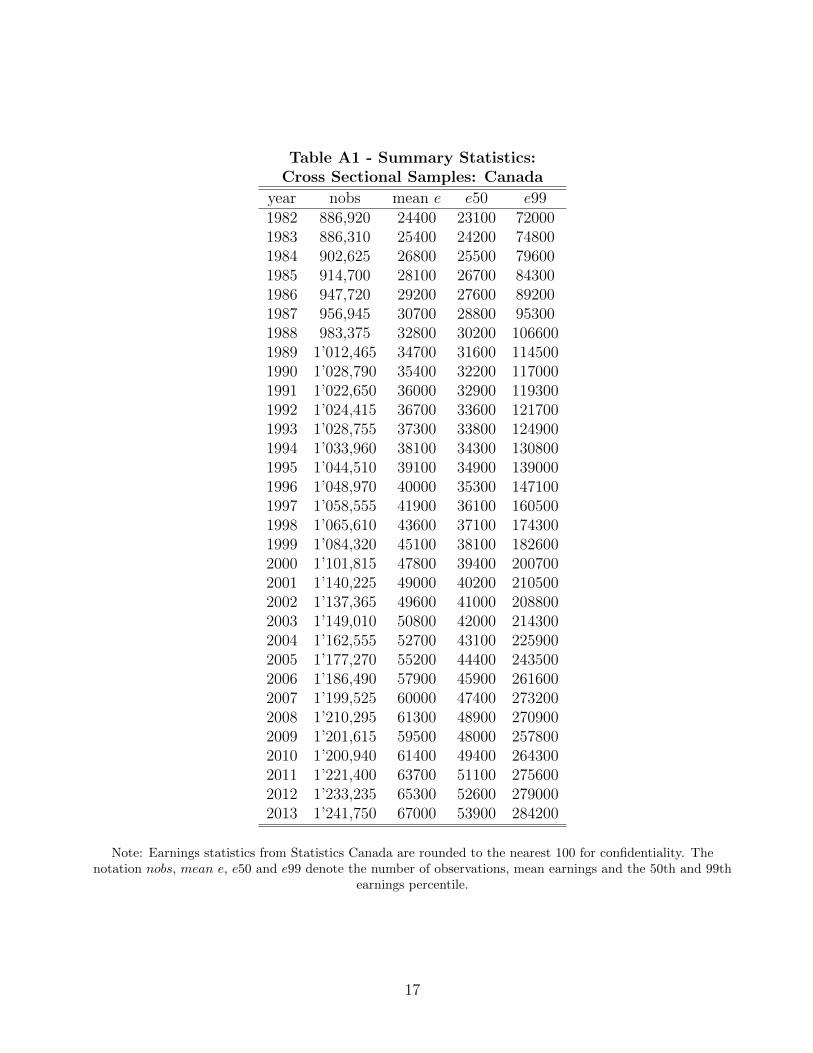
Table A1 - Summary Statistics:Cross Sectional Samples: Canada

year nobs mean e e50 e991982 886,920 24400 23100 720001983 886,310 25400 24200 748001984 902,625 26800 25500 796001985 914,700 28100 26700 843001986 947,720 29200 27600 892001987 956,945 30700 28800 953001988 983,375 32800 30200 1066001989 1’012,465 34700 31600 1145001990 1’028,790 35400 32200 1170001991 1’022,650 36000 32900 1193001992 1’024,415 36700 33600 1217001993 1’028,755 37300 33800 1249001994 1’033,960 38100 34300 1308001995 1’044,510 39100 34900 1390001996 1’048,970 40000 35300 1471001997 1’058,555 41900 36100 1605001998 1’065,610 43600 37100 1743001999 1’084,320 45100 38100 1826002000 1’101,815 47800 39400 2007002001 1’140,225 49000 40200 2105002002 1’137,365 49600 41000 2088002003 1’149,010 50800 42000 2143002004 1’162,555 52700 43100 2259002005 1’177,270 55200 44400 2435002006 1’186,490 57900 45900 2616002007 1’199,525 60000 47400 2732002008 1’210,295 61300 48900 2709002009 1’201,615 59500 48000 2578002010 1’200,940 61400 49400 2643002011 1’221,400 63700 51100 2756002012 1’233,235 65300 52600 2790002013 1’241,750 67000 53900 284200

Note: Earnings statistics from Statistics Canada are rounded to the nearest 100 for confidentiality. Thenotation nobs, mean e, e50 and e99 denote the number of observations, mean earnings and the 50th and 99th

earnings percentile.

17

Table A2 - Summary Statistics:Cross Sectional Samples: Denmark

year nobs mean e e50 e991980 871,620 118228 113579 2948731981 859,167 127065 122948 3184491982 866,315 141548 137413 3527951983 879,347 151118 146798 3796001984 890,302 160415 154354 4085691985 906,252 169582 161345 4358021986 917,972 181792 172378 4641361987 924,403 196046 185319 5081651988 926,431 206465 195574 5353901989 927,703 212492 200965 5603401990 936,043 217956 206008 5796971991 935,039 223188 211658 5896311992 943,109 228499 217469 6053391993 941,600 228247 218277 6067251994 951,024 239598 227380 6475931995 962,977 248388 234389 6756651996 972,286 255076 240615 6957491997 983,871 264676 248812 7254241998 998,120 273832 255626 7656771999 100,5814 285656 266406 8059582000 1’011,325 296760 275335 8508982001 1’012,968 307839 284840 8913032002 1’009,869 315493 292833 9179342003 999,303 320344 298258 9368812004 993,586 328709 306149 9609512005 990,605 338733 314951 9966712006 989,524 351789 325779 10403382007 984,137 368622 339457 11011632008 969,799 386238 353782 11607322009 942,820 382500 356390 11278682010 923,739 402285 365001 13044892011 918,254 409964 371298 13251422012 913,586 417780 376711 13555802013 911,549 424334 379914 1398553

Note: The notation nobs, mean e, e50 and e99 denote the number of observations, mean earnings and the50th and 99th earnings percentile. All percentiles calculated from Danish data are 6 observation local

averages, a confidentiality requirement.

18

Table A3 - Summary Statistics:Cross Sectional Samples: Sweden

year nobs mean e e50 e991980 1845140 79441 75031 2175791981 . . . .1982 1830333 91005 86952 2503361983 . . . .1984 . . . .1985 1615820 118882 111795 3116431986 1627315 128328 121011 3324801987 1644682 138457 130327 3635341988 1665408 149939 141447 3906811989 1691587 164961 156272 4238391990 1871002 175721 167993 4661351991 1898011 187592 178511 5249151992 1875173 187430 180315 5319281993 1840234 189948 183420 5546671994 1838130 197666 189330 6024501995 1856135 204850 197545 5941361996 1857699 215984 206560 6377121997 1860797 225708 215075 6721721998 1883857 235753 223189 7108401999 1914785 244286 229501 7459012000 1945461 257441 239017 8037022001 1962558 270076 248633 8530882002 1963068 277617 257149 8700172003 1945148 282512 263059 8804352004 1928007 288791 269771 9104262005 1914243 299104 278085 9461172006 1917082 311050 288703 9917292007 1913805 325196 300023 10437522008 1906596 340417 312946 10919042009 1875741 342493 316552 10973142010 1871732 352699 326069 11258632011 1885636 365852 336988 11660342012 1886082 375238 346504 11792562013 1886746 381534 353416 1193581

Note: The notation nobs, mean e, e50 and e99 denote the number of observations, mean earnings and the50th and 99th earnings percentile.

19

h!

Figure 1: Basic Top-End Inequality Facts

(a) Top 1 Percent Income Share: (b) Top 1 Percent Income Share:U.S., U.K. and Canada France, Denmark, Sweden

1920 1940 1960 1980 2000Year

0

5

10

15

20

25

30

Sha

re

1% US1% UK1% Canada

1920 1940 1960 1980 2000Year

0

5

10

15

20

25

30

Sha

re

1% France1% Denmark1% Sweden

(c) Earnings and Income Shares: US

1920 1940 1960 1980 2000Year

5

10

15

20

Sha

re

Top 1% EarningsTop 1% Income

Notes: Income comes from The World Wealth and Income Database. The earnings measure for the US is from

Piketty and Saez (2003 update). The income measure excludes capital gains and the earnings measure is based

on wages and salaries. For the UK, the sampling unit was changed in 1990 and there is a jump in the series in

that year.

20

Figure 2: Top-End Earnings Inequality Facts

(a) Top 1 Percent Share (b) 90-50 Ratio

1980 1985 1990 1995 2000 2005 2010Year

0

5

10

15 USDenmarkSwedenCanada

1980 1985 1990 1995 2000 2005 2010Year

0

0.5

1

1.5

2

2.5

(c) 99-50 Ratio (d) Pareto at 99th Percentile

1980 1985 1990 1995 2000 2005 2010Year

0

2

4

6

8

1980 1985 1990 1995 2000 2005 2010Year

0

1

2

3

4

5

Notes: Authors calculations based on the cross-sectional samples for each country. For the US, the top 1 percent

share and the Pareto statistic in each year are based on the assumption of a Pareto distribution within the top

1 percent and tabulated values for the 99-th and 99.999-th percentiles.

21

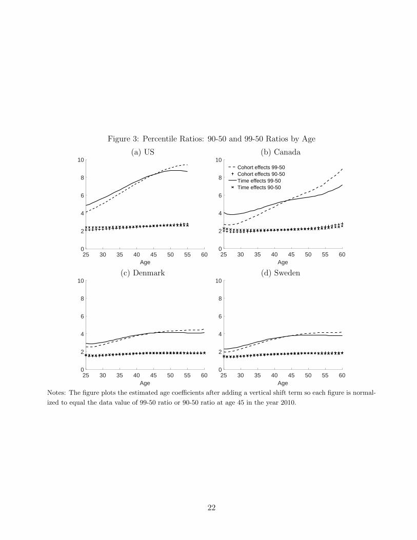
Figure 3: Percentile Ratios: 90-50 and 99-50 Ratios by Age

(a) US (b) Canada

25 30 35 40 45 50 55 60Age

0

2

4

6

8

10

25 30 35 40 45 50 55 60Age

0

2

4

6

8

10Cohort effects 99-50Cohort effects 90-50Time effects 99-50Time effects 90-50

(c) Denmark (d) Sweden

25 30 35 40 45 50 55 60Age

0

2

4

6

8

10

25 30 35 40 45 50 55 60Age

0

2

4

6

8

10

Notes: The figure plots the estimated age coefficients after adding a vertical shift term so each figure is normal-

ized to equal the data value of 99-50 ratio or 90-50 ratio at age 45 in the year 2010.

22

Figure 4: Median Earnings by Age

(a) US (b) Canada

25 30 35 40 45 50 55 60Age

0

20

40

60

80

100

120

Inde

x, A

ge 4

5=10

0

Cohort effectsTime effects

25 30 35 40 45 50 55 60Age

0

20

40

60

80

100

120

(c) Denmark (d) Sweden

25 30 35 40 45 50 55 60Age

0

20

40

60

80

100

120

Inde

x, A

ge 4

5=10

0

25 30 35 40 45 50 55 60Age

0

20

40

60

80

100

120

Notes: The figure plots the estimated age coefficients after adding a vertical shift term so each figure is normal-

ized to equal 100 at age 45.

23

Figure 5: Pareto Statistic at the 99th Percentile by Age

(a) US (b) Canada

25 30 35 40 45 50 55 60Age

0

2

4

6

8Cohort EffectsTime Effects

25 30 35 40 45 50 55 60Age

0

2

4

6

8

Par

eto

Sta

tistic

(c) Denmark (d) Sweden

25 30 35 40 45 50 55 60Age

0

2

4

6

8

Par

eto

Sta

tistic

25 30 35 40 45 50 55 60Age

0

2

4

6

8

Par

eto

Sta

tistic

Notes: The figure plots the estimated age coefficients after adding a vertical shift term so each figure is normal-

ized to equal the data value of the Pareto statistic at age 45 in the year 2010.

24

Figure 6: Earnings Growth by Lifetime Earnings Group

(a) US (b) Canada

20 40 60 80 100Percentile

0

5

10

15

20Ages 25 to 55Ages 30 to 55

20 40 60 80 100Percentile

0

5

10

15

20

(c) Denmark (d) Sweden

20 40 60 80 100Percentile

0

2

4

6

8

10

20 40 60 80 100Percentile

0

2

4

6

8

10

Notes: The figure plots the ratio of mean group earnings at age 55 to mean group earnings at age 25 as well

as the ratio of mean group earnings at age 55 to mean group earnings at age 30 for groups sorted by percentile

of lifetime earnings. US data is taken directly from Guvenen, Karahan, Ozkan and Song (2015). The result for

all the other countries is based on our calculations from country longitudinal data.

25

Figure 7: Earnings Ratios: Kaymak-Poschke Model and US Data

(a) Mean Earnings Ratios (b) Mean Earnings Ratios

20 40 60 80 100Percentile

0

5

10

15

20US: Ages 25 to 55KP: Ages 25 to 55

20 40 60 80 100Percentile

0

5

10

15

20US: Ages 30 to 55KP: Ages 30 to 55

Notes: Figure 7(a) plots the ratio of mean group earnings at age 55 to mean group earnings at age 25 both in

US data and in the Kaymak-Poschke model. Figure 7(b) repeats this plot but using data at age 55 and at age

30. The horizontal axis sorts males and model agents by percentiles of lifetime earnings.

26