Regional Climate Model Simulation of U.S. Precipitation during 1982 2002. Part I: Annual Cycle
20
3510 VOLUME 17 JOURNAL OF CLIMATE q 2004 American Meteorological Society Regional Climate Model Simulation of U.S. Precipitation during 1982–2002. Part I: Annual Cycle XIN-ZHONG LIANG,LI LI, AND KENNETH E. KUNKEL Illinois State Water Survey, University of Illinois, Urbana–Champaign, Champaign, Illinois MINGFANG TING Lamont-Doherty Earth Observatory, Columbia University, Palisades, New York JULIAN X. L. WANG Air Resources Laboratory, National Oceanic and Atmospheric Administration, Silver Spring, Maryland (Manuscript received 20 November 2003, in final form 23 February 2004) ABSTRACT The fifth-generation PSU–NCAR Mesoscale Model (MM5)-based regional climate model (CMM5) capability in simulating the U.S. precipitation annual cycle is evaluated with a 1982–2002 continuous baseline integration driven by the NCEP–DOE second Atmospheric Model Intercomparison Project (AMIP II) reanalysis. The causes for major model biases (differences from observations) are studied through supplementary seasonal sensitivity experiments with various driving lateral boundary conditions (LBCs) and physics representations. It is dem- onstrated that the CMM5 has a pronounced rainfall downscaling skill, producing more realistic regional details and overall smaller biases than the driving global reanalysis. The precipitation simulation is most skillful in the Northwest, where orographic forcing dominates throughout the year; in the Midwest, where mesoscale convective complexes prevail in summer; and in the central Great Plains, where nocturnal low-level jet and rainfall peaks occur in summer. The actual model skill, however, is masked by existing large LBC uncertainties over data- poor areas, especially over oceans. For example, winter dry biases in the Gulf States likely result from LBC errors in the south and east buffer zones. On the other hand, several important regional biases are identified with model physics deficiencies. In particular, summer dry biases in the North American monsoon region and along the east coast of the United States can be largely rectified by replacing the Grell with the Kain–Fritsch cumulus scheme. The latter scheme, however, yields excessive rainfall in the Atlantic Ocean but large deficits over the Midwest. The fall dry biases over the lower Mississippi River basin, common to all existing global and regional models, remain unexplained and the search for their responsible physical mechanisms will be challenging. In addition, the representation of cloud–radiation interaction is essential in determining the pre- cipitation distribution and regional water recycling, for which the new scheme implemented in the CMM5 yields significant improvement. 1. Introduction The development of a nested regional climate model (RCM) was first proposed by Dickinson et al. (1989) and Giorgi (1990). Following pioneering work by Gior- gi and Bates (1989), long-term continuous RCM sim- ulations have been increasingly available for a wide range of applications, including model validation, sen- sitivity studies, and climate change assessments (see a recent review by Giorgi and Mearns 1999). It is now commonly accepted that an RCM downscaling integra- tion is more skillful at resolving orographic climate ef- Corresponding author address: Dr. Xin-Zhong Liang, Illinois State Water Survey, University of Illinois, Urbana–Champaign, 2204 Grif- fith Dr., Champaign, IL 61820-7495. E-mail: [email protected] fects than the driving coarse-grid general circulation model (GCM) simulation, especially for near-surface variables (Giorgi 1990; Jones et al. 1995; Giorgi et al. 1997, 1998; Christensen et al. 1998; Laprise et al. 1998; Leung and Ghan 1999; Hong and Leetmaa 1999; Fen- nessy and Shukla 2000; Pan et al. 2001; Roads et al. 2003). However, there exist systematic RCM biases that cannot be fully explained and large downscaling skill uncertainties over regions with relatively flat terrain (Ta- kle et al. 1999; Leung et al. 1999; Pan et al. 2001; Anderson et al. 2003). In addition, the RCM results are sensitive to its dynamic configurations (e.g., domain and resolution) and physics representations (e.g., cloud–ra- diation and surface–atmosphere interactions). Therefore a typical RCM must be ‘‘customized’’ for each specific regional application (Giorgi and Mearns 1999). This
-
Upload
independent -
Category
Documents
-
view
2 -
download
0
Transcript of Regional Climate Model Simulation of U.S. Precipitation during 1982 2002. Part I: Annual Cycle
3510 VOLUME 17J O U R N A L O F C L I M A T E
q 2004 American Meteorological Society
Regional Climate Model Simulation of U.S. Precipitation during 1982–2002.Part I: Annual Cycle
XIN-ZHONG LIANG, LI LI, AND KENNETH E. KUNKEL
Illinois State Water Survey, University of Illinois, Urbana–Champaign, Champaign, Illinois
MINGFANG TING
Lamont-Doherty Earth Observatory, Columbia University, Palisades, New York
JULIAN X. L. WANG
Air Resources Laboratory, National Oceanic and Atmospheric Administration, Silver Spring, Maryland
(Manuscript received 20 November 2003, in final form 23 February 2004)
ABSTRACT
The fifth-generation PSU–NCAR Mesoscale Model (MM5)-based regional climate model (CMM5) capabilityin simulating the U.S. precipitation annual cycle is evaluated with a 1982–2002 continuous baseline integrationdriven by the NCEP–DOE second Atmospheric Model Intercomparison Project (AMIP II) reanalysis. The causesfor major model biases (differences from observations) are studied through supplementary seasonal sensitivityexperiments with various driving lateral boundary conditions (LBCs) and physics representations. It is dem-onstrated that the CMM5 has a pronounced rainfall downscaling skill, producing more realistic regional detailsand overall smaller biases than the driving global reanalysis. The precipitation simulation is most skillful in theNorthwest, where orographic forcing dominates throughout the year; in the Midwest, where mesoscale convectivecomplexes prevail in summer; and in the central Great Plains, where nocturnal low-level jet and rainfall peaksoccur in summer. The actual model skill, however, is masked by existing large LBC uncertainties over data-poor areas, especially over oceans. For example, winter dry biases in the Gulf States likely result from LBCerrors in the south and east buffer zones. On the other hand, several important regional biases are identifiedwith model physics deficiencies. In particular, summer dry biases in the North American monsoon region andalong the east coast of the United States can be largely rectified by replacing the Grell with the Kain–Fritschcumulus scheme. The latter scheme, however, yields excessive rainfall in the Atlantic Ocean but large deficitsover the Midwest. The fall dry biases over the lower Mississippi River basin, common to all existing globaland regional models, remain unexplained and the search for their responsible physical mechanisms will bechallenging. In addition, the representation of cloud–radiation interaction is essential in determining the pre-cipitation distribution and regional water recycling, for which the new scheme implemented in the CMM5 yieldssignificant improvement.
1. Introduction
The development of a nested regional climate model(RCM) was first proposed by Dickinson et al. (1989)and Giorgi (1990). Following pioneering work by Gior-gi and Bates (1989), long-term continuous RCM sim-ulations have been increasingly available for a widerange of applications, including model validation, sen-sitivity studies, and climate change assessments (see arecent review by Giorgi and Mearns 1999). It is nowcommonly accepted that an RCM downscaling integra-tion is more skillful at resolving orographic climate ef-
Corresponding author address: Dr. Xin-Zhong Liang, Illinois StateWater Survey, University of Illinois, Urbana–Champaign, 2204 Grif-fith Dr., Champaign, IL 61820-7495.E-mail: [email protected]
fects than the driving coarse-grid general circulationmodel (GCM) simulation, especially for near-surfacevariables (Giorgi 1990; Jones et al. 1995; Giorgi et al.1997, 1998; Christensen et al. 1998; Laprise et al. 1998;Leung and Ghan 1999; Hong and Leetmaa 1999; Fen-nessy and Shukla 2000; Pan et al. 2001; Roads et al.2003). However, there exist systematic RCM biases thatcannot be fully explained and large downscaling skilluncertainties over regions with relatively flat terrain (Ta-kle et al. 1999; Leung et al. 1999; Pan et al. 2001;Anderson et al. 2003). In addition, the RCM results aresensitive to its dynamic configurations (e.g., domain andresolution) and physics representations (e.g., cloud–ra-diation and surface–atmosphere interactions). Thereforea typical RCM must be ‘‘customized’’ for each specificregional application (Giorgi and Mearns 1999). This
15 SEPTEMBER 2004 3511L I A N G E T A L .
includes careful sensitivity experiments and rigorousvalidation studies using observed initial and lateralboundary conditions (LBCs).
For the United States, several studies have providedimportant references for RCM customization. Giorgi etal. (1993b) first developed an improved LBC assimi-lation scheme to facilitate more realistic RCM climatesimulations over large domains. Seth and Giorgi (1998)then found that small domains produce spurious LBCdynamical effects and thus cause the RCM to generateunrealistic responses to internal forcings. Liang et al.(2001) further demonstrated that the RCM performancedepends significantly on the accuracy of the drivingLBCs within the buffer zones. In contrast, Juang andHong (2001) showed that the impacts of the domainsize and LBC errors are small for a regional spectralmodel where the large-scale waves are preservedthrough the domain and spectral nesting. The differencein sensitivity arises because the large-scale waves in theformer are generated by the dynamic relaxation of LBCsonly within four narrow edge buffer zones, whereas forthe latter they are prescribed by the continuous nudgingtoward the driving general circulations throughout theentire computational domain. If the driving circulationsare perfect everywhere, both approaches shall producea similar result. However, the existing global reanalyses,which are the best available proxies for observations,contain large inconsistencies, especially over oceans andnear the Tropics where observational data are lackingand the RCM buffer zones are generally located (Lianget al. 2001). It is impossible for RCMs to produce arealistic regional climate via the dynamic relaxation oferroneous LBCs based on the reanalyses. In contrast,the nudging over the entire domain minimizes the LBCeffect and enables the RCM to force a more accurateregional climate with the realistic regional circulationof the reanalyses that assimilate the most complete insitu observational data. On the other hand, if the RCMis driven by a GCM simulation that likely contains re-gional circulation biases over the inner domain due tothe incomplete physics representation, the LBC relax-ation approach may yield a more realistic regional cli-mate because it gives more freedom for the more-com-plete RCM physics representation to be effective.
The preceding problems make it difficult in validationstudies to separate the RCM downscaling skill and itssensitivity to the physics representation from the un-certainties in the driving reanalyses. Giorgi and Shields(1999) showed that the cumulus parameterization ofGrell (1993) produces an overall more realistic regionalclimate over the continental United States than those ofKuo (Anthes 1977) and Zhang and McFarlane (1995).In contrast, Gochis et al. (2002) found that the Kain andFritsch (1993) scheme produces superior vertical ther-modynamic structures and hence more realistic convec-tive precipitation associated with the North Americanmonsoon (NAM) than the Betts–Miller–Janic (Betts andMiller 1986; Janic 1994) and Grell schemes. Leung et
al. (2003) also indicated the superiority of the Kain–Fritsch to Kuo and Grell schemes for the NAM simu-lation. On the other hand, Xu and Small (2002) dem-onstrated that the Kain–Fritsch scheme yields too muchNAM rainfall and fails to represent intraseasonal andinterannual variations, while the Grell scheme is gen-erally more realistic. It is essential to objectively de-termine whether the poor RCM performance is causedtruly by the unrealistic model physics representation orpurely by the LBC errors contained in the reanalyses.The findings are expected to strongly depend on climateregimes and locations.
The purpose of this study is to determine the capa-bility of an RCM to reproduce the observed annual cycleof U.S. precipitation and to better understand the caus-es of the corresponding model climatology biases. Thisis facilitated by a continuous RCM baseline integrationfor the period 1982–2002 as driven by a global re-analysis and a suite of seasonal sensitivity experimentswith various driving reanalyses and physics represen-tations. As recommended by Giorgi and Mearns(1999), long-term continuous RCM integrations offermany advantages over ensembles of short simulations,including minimal effect from atmospheric spinup, im-proved equilibrium between the regional climate andsurface hydrology cycle, accurate representation of themodel internal climatology and better detection of sys-tematic model physics deficiencies. Thus the 1982–2002 mean climatology provides a robust statisticaldescription to identify significant systematic model er-rors in the annual cycle. The sensitivity experimentsare carefully designed and branched off from the restartconditions of the baseline integration to provide phys-ical insights into the probable causes for specific RCMbiases.
2. Regional climate model and simulations
The RCM used in this study is a climate extensionof the fifth-generation Pennsylvania State University–National Center for Atmospheric Prediction (PSU–NCAR) Mesoscale Model (MM5) version 3.3 (Dudhiaet al. 2004), hereafter referred to CMM5. The CMM5is an improved version of Liang et al. (2001). Importantmodifications include incorporation of more realisticsurface boundary conditions and cloud cover predictionas well as LBCs from an updated global reanalysis. Abrief description of the CMM5 model configuration andclimate simulations is given next.
a. Physics configuration
The CMM5 incorporates the same physics configu-ration as in Liang et al. (2001) except for an improvedcloud–radiation interaction prediction. The land surfaceprocess is represented by the Oregon State University(OSU) model (Chen and Dudhia 2001). The planetaryboundary layer is parameterized by the Medium-Range
3512 VOLUME 17J O U R N A L O F C L I M A T E
Forecast Model (MRF) countergradient (nonlocal) tur-bulence transport scheme (Hong and Pan 1996). Pre-cipitation is determined by a combination of the God-dard Space Flight Center (GSFC) explicit cloud micro-physical solution (Tao and Simpson 1989), the Grell(1993) cumulus parameterization, and shallow convec-tion. Solar and infrared radiation are incorporated as inthe NCAR Community Climate Model (CCM2; Hacket al. 1993) and are calculated every 30 min, where theradiative effects of both cumulus and nonconvectiveclouds are considered. Liang et al. (2001) showed thatthis physics configuration simulates the overall structureand magnitude of the observed rainfall pattern over theMidwest and northern Plains during the 1993 summerflood. This is associated with the accurate representationof both the westerly jet stream and the Great Plains low-level jet (LLJ). The RCM reproduces the observed dif-ferent climate regimes, where rainfall was associatedwith the periodic (5 day) passage of midlatitude cy-clones in June and persistent synoptic circulations inJuly. The model also correctly simulates the major floodarea rainfall diurnal cycle (with the peak amount at 0900UTC), which follows the LLJ cycle by approximately3 h.
The CCM2 radiation requires distributions of cloudcover fraction CCF and cloud water path CWP (g m22)to determine cloud radiative effects. These two fieldswere originally parameterized in terms of mainly rela-tive humidity RH and air temperature T, respectively.For each vertical model layer, convective cloud coverCC was defined as
2D 2 DlCC 5 CC 1 (CC 2 CC )0 l s l 1 2D 2 Dl s
1/NCC 5 1 2 (1 2 CC ) , (1)0
where subscripts l and s denote large and small grid-size bounds; N 5 kt 2 kb 1 1 is the number of con-vective layers; and kt and kb are the cumulus top andbase levels, which are predicted by the cumulus param-eterization. The default values are Dl 5 200 km, Ds 510 km, CCl 5 0.3, CCs 5 1.0. For the current CMM5grid spacing D 5 30 km, the column total convectivecloud cover CC0 5 0.86. Note that CC 5 0 exceptwithin the cumulus column between layers kt, kb as inEq. (1), where clouds are assumed to randomly overlap.The resolvable or large-scale cloud cover CS was com-puted by
D 2 DlRH 5 RH 1 (RH 2 RH )c l s l D 2 Dl s
2 2CS 5 (RH 2 RH ) /(1 2 RH )0 c c
ds/0.05CS 5 1 2 (1 2 CS ) , (2)0
where ds is the layer thickness in the s coordinate. Thedefault values are Dl 5 100 km, Ds 5 10 km, RHl 50.75, RHs 5 0.9. For the current CMM5 grid spacingD 5 30 km, the threshold relative humidity RHc 5 0.867.The total layer cloud cover was then calculated as
CCF 5 max(CC, CS). (3)
When CCF . 0, the cloud water path was parameter-ized by
CWC , T # Tn nCWC 1 (CWC 2 CWC )(T 2 T )/(T 2 T ), T , T # Tn m n n m n n mCWF 5 dz (4)CWC 1 (CWC 2 CWC )(T 2 T )/(T 2 T ), T , T , Tm x m m x m m xCWC , T $ T , x x
where dz is the layer thickness (m). For temperaturebounds Tn, Tm, Tx 5 220, 265, 295 (K), the defaultcloud water contents are specified as CWCn, CWCm,CWCx 5 0.03, 0.2, 0.4 (g m23).
The preceding scheme was found to overestimate bothcloud cover fraction and cloud water path. This causesa deficit of up to 80 W m22 in solar radiation reachingthe surface as compared with station measurements inIllinois (see section 5). A similar deficit was found overthe NAM region (Xu and Small 2002). As a result, thesimulated surface air temperatures were colder than ob-servations by 28–58C during summer over broad regions.Note that the scheme does not make use of the cloudhydrometeors (liquid, ice, rain, snow, graupel), whichare predicted by the explicit cloud microphysical so-lution. Hence the cloud–radiation interactions are not
consistently represented. To overcome this problem, theCMM5 incorporates a new cloud prediction scheme.Following Xu and Randall (1996), the resolvable cloudcover is parameterized in terms of relative humidity andcloud hydrometeor concentrations:
q 5 q 1 q 1 q 1 q 1 qt c i r s g
0.25 20.49CS 5 RH ^1 2 exp{2100q [(1 2 RH)q*] }&, (5)t
where qc, ql, qr, qs, qg, qt are liquid, ice, rain, snow,graupel, and total cloud mixing ratios (kg kg21), q* isthe saturated water vapor mixing ratio (kg kg21). Equa-tion (1) is retained for convective cloud cover, whileEq. (3) is changed to
CCF 5 CC 1 (1 2 CC) CS. (6)
15 SEPTEMBER 2004 3513L I A N G E T A L .
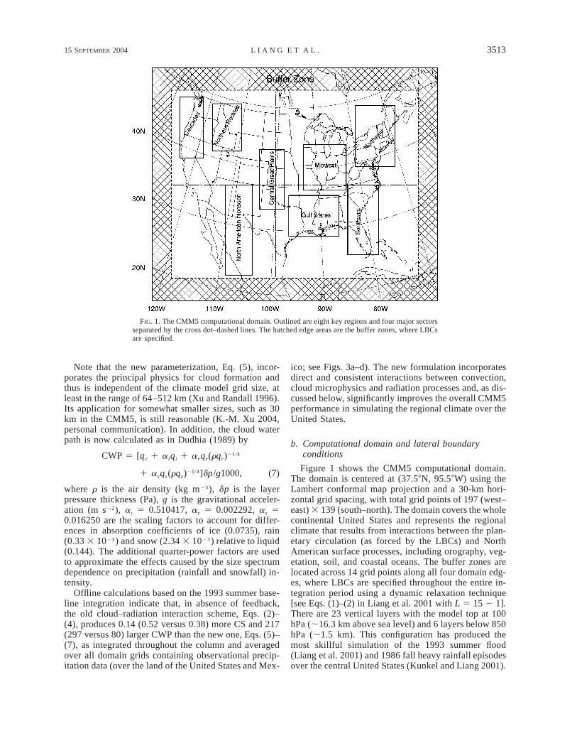
FIG. 1. The CMM5 computational domain. Outlined are eight key regions and four major sectorsseparated by the cross dot–dashed lines. The hatched edge areas are the buffer zones, where LBCsare specified.
Note that the new parameterization, Eq. (5), incor-porates the principal physics for cloud formation andthus is independent of the climate model grid size, atleast in the range of 64–512 km (Xu and Randall 1996).Its application for somewhat smaller sizes, such as 30km in the CMM5, is still reasonable (K.-M. Xu 2004,personal communication). In addition, the cloud waterpath is now calculated as in Dudhia (1989) by
21/4CWP 5 [q 1 a q 1 a q (rq )c i i r r r
21/41 a q (rq ) ]dp /g1000, (7)s s s
where r is the air density (kg m23), dp is the layerpressure thickness (Pa), g is the gravitational acceler-ation (m s22), ai 5 0.510417, ar 5 0.002292, as 50.016250 are the scaling factors to account for differ-ences in absorption coefficients of ice (0.0735), rain(0.33 3 1023) and snow (2.34 3 1023) relative to liquid(0.144). The additional quarter-power factors are usedto approximate the effects caused by the size spectrumdependence on precipitation (rainfall and snowfall) in-tensity.
Offline calculations based on the 1993 summer base-line integration indicate that, in absence of feedback,the old cloud–radiation interaction scheme, Eqs. (2)–(4), produces 0.14 (0.52 versus 0.38) more CS and 217(297 versus 80) larger CWP than the new one, Eqs. (5)–(7), as integrated throughout the column and averagedover all domain grids containing observational precip-itation data (over the land of the United States and Mex-
ico; see Figs. 3a–d). The new formulation incorporatesdirect and consistent interactions between convection,cloud microphysics and radiation processes and, as dis-cussed below, significantly improves the overall CMM5performance in simulating the regional climate over theUnited States.
b. Computational domain and lateral boundaryconditions
Figure 1 shows the CMM5 computational domain.The domain is centered at (37.58N, 95.58W) using theLambert conformal map projection and a 30-km hori-zontal grid spacing, with total grid points of 197 (west–east) 3 139 (south–north). The domain covers the wholecontinental United States and represents the regionalclimate that results from interactions between the plan-etary circulation (as forced by the LBCs) and NorthAmerican surface processes, including orography, veg-etation, soil, and coastal oceans. The buffer zones arelocated across 14 grid points along all four domain edg-es, where LBCs are specified throughout the entire in-tegration period using a dynamic relaxation technique[see Eqs. (1)–(2) in Liang et al. 2001 with L 5 15 2 1].There are 23 vertical layers with the model top at 100hPa (;16.3 km above sea level) and 6 layers below 850hPa (;1.5 km). This configuration has produced themost skillful simulation of the 1993 summer flood(Liang et al. 2001) and 1986 fall heavy rainfall episodesover the central United States (Kunkel and Liang 2001).
3514 VOLUME 17J O U R N A L O F C L I M A T E
The LBCs are constructed from the National Centersfor Environmental Prediction–Department of Energy(NCEP–DOE) AMIP II reanalysis (R-2; Kanamitsu etal. 2002). The R-2 is regarded as an updated and humanerror–corrected version of the NCEP–NCAR reanalysis(NRA; Kalnay et al. 1996). Liang et al. (2001) showedthat RCM simulations are less sensitive to domainchoice when the LBCs are based on the NRA ratherthan the European Centre for Medium–Range WeatherForecasts (ECMWF) reanalysis (ERA; Gibson et al.1997). This implies that large uncertainties exist in ERAwhen the domain size increases, especially if the southbuffer zone is located in the Tropics. In addition, theERA data is available only up to 1993 December, whilethe NRA and R-2 data continue to the present. Giventhese considerations, the R-2 is chosen to drive the base-line integration during 1982–2002, while the ERA isused in seasonal sensitivity experiments to depict theimpacts of LBC uncertainties. Important improvementsof the R-2 over NRA include soil moisture, that affectsthe CMM5 initialization, as well as land precipitation,which provide a better reference of the reanalysis modelproduct for CMM5 downscaling skill assessment. Allreanalysis data are the 2.58 latitude 3 2.58 longitudegrid and pressure-level product at a 6-hourly interval.
c. Surface boundary conditions
The CMM5 requires the specification of surfaceboundary conditions, including green vegetation frac-tion over land and sea surface temperature (SST) overoceans. Vegetation fraction was originally fixed in theMM5 at the initial condition. For climate applications,the CMM5 updates daily vegetation variations by lineartemporal interpolation of the monthly mean climatologyderived from the National Oceanic and AtmosphericAdministration/Advanced Very High Resolution Radi-ometer (NOAA/AVHRR) data (Gutman and Ignatov1998). The SST daily variations were first incorporatedby Liang et al. (2001) using the NRA surface skin tem-perature, which is a model product over land. This waslater found problematic in coastal oceans and the GreatLakes, where the coarse NRA grids cannot appropriatelyresolve land versus water points. For example, the Gulfof California is not resolved as a water surface, buttreated as land points. Given the strong diurnal cycleover land, the surface skin temperature at 0000 UTC(near 1630 local time) is 58–108C warmer than the ad-jacent ocean. This results in overwhelming deep con-vection and excessive precipitation in the Gulf of Cal-ifornia. To eliminate the problem, the CMM5 incor-porates observed daily variations based on conservativespline fit from the weekly optimum interpolation SST(OISST) data (Reynolds et al. 2002). The OISST isavailable over the global oceans on a 18 3 18 grid meshfrom 1981 November onward. A time series analysisshowed that peak SSTs in September over the Gulf ofCalifornia were about 58C colder in 1982 than all other
years. This unexplained bias did not occur elsewhere.Note that daily SSTs interpolated directly from weeklyvalues (treated as if they were at the middle of the week)do not conserve weekly means nor preserve the ex-tremes (Taylor et al. 2000). For this reason, an iterativespline-fit procedure was used to interpolate daily SSTvariations from the weekly data while conserving theweekly means. These daily SST variations were thenincorporated into the CMM5 by daily updates. This pro-cedure also effectively preserves the extremes revealedin the original weekly data.
Note that the CMM5 SST so constructed has smalldifferences from those of the R-2, since the latter alsoused the same OISST with a similar time interpolationprocedure (Kanamitsu et al. 2002; Fiorino 2000). Com-parisons between the two SST data, including monthlymean rms errors and interannual correlations, show thatthey are essentially identical except over limited coastaloceans and the Great Lakes where differences of 60.58–38C occur. Hence the differences do not affect regionalclimate signals forced by the planetary SST anomaliesnor explain the substantial precipitation contrasts be-tween the CMM5 and the driving R-2 discussed later.
d. Model simulations and validation data
Given the limited availability of the OISST data, theCMM5 baseline integration was initialized at 0000 UTC2 December 1981, and completed at the end of 2002.The initial month is considered as a spinup period,which is generally sufficient based on the examinationof daily rainfall variations. One exception is near theGulf of California, where the OISST contained apparentbiases in 1982. Analysis showed that the removal of1982 has little impact on the climatology. This studycompares the CMM5 baseline and observed climatol-ogies during 1982–2002 to determine the model biasesin simulating the precipitation annual cycle over theUnited States. The climatologies are also compared withthat produced by the reanalysis assimilation model toassess the skill enhancement in resolving regional cli-mate variations as a result of the CMM5 downscalingapproach. To understand these downscaling skills andbiases, many sensitivity experiments were conductedthat branch off from the restart conditions of the baselineintegration. These experiments vary in the simulationperiods (initial and length) depending on their specificapplication purposes. All experiments contain at leastone month spinup time, where the model outputs arenot used in the analysis. Note that some experimentscannot restart from the baseline conditions because anew physics scheme requires different or more initialstates. In this case, a spinup of 2 months is assumed.
Several major daily datasets are utilized in the val-idation. For the circulation fields (200/850 hPa windand sea level pressure), the R-2 data are taken as thebest proxy of observations because they assimilated allavailable measurements. They are available on a global
15 SEPTEMBER 2004 3515L I A N G E T A L .
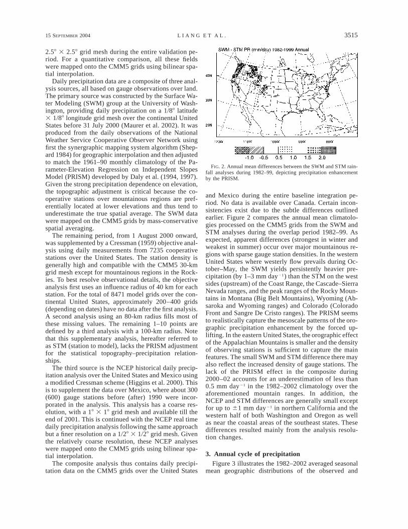
FIG. 2. Annual mean differences between the SWM and STM rain-fall analyses during 1982–99, depicting precipitation enhancementby the PRISM.
2.58 3 2.58 grid mesh during the entire validation pe-riod. For a quantitative comparison, all these fieldswere mapped onto the CMM5 grids using bilinear spa-tial interpolation.
Daily precipitation data are a composite of three anal-ysis sources, all based on gauge observations over land.The primary source was constructed by the Surface Wa-ter Modeling (SWM) group at the University of Wash-ington, providing daily precipitation on a 1/88 latitude3 1/88 longitude grid mesh over the continental UnitedStates before 31 July 2000 (Maurer et al. 2002). It wasproduced from the daily observations of the NationalWeather Service Cooperative Observer Network usingfirst the synergraphic mapping system algorithm (Shep-ard 1984) for geographic interpolation and then adjustedto match the 1961–90 monthly climatology of the Pa-rameter-Elevation Regression on Independent SlopesModel (PRISM) developed by Daly et al. (1994, 1997).Given the strong precipitation dependence on elevation,the topographic adjustment is critical because the co-operative stations over mountainous regions are pref-erentially located at lower elevations and thus tend tounderestimate the true spatial average. The SWM datawere mapped on the CMM5 grids by mass-conservativespatial averaging.
The remaining period, from 1 August 2000 onward,was supplemented by a Cressman (1959) objective anal-ysis using daily measurements from 7235 cooperativestations over the United States. The station density isgenerally high and compatible with the CMM5 30-kmgrid mesh except for mountainous regions in the Rock-ies. To best resolve observational details, the objectiveanalysis first uses an influence radius of 40 km for eachstation. For the total of 8471 model grids over the con-tinental United States, approximately 200–400 grids(depending on dates) have no data after the first analysis.A second analysis using an 80-km radius fills most ofthese missing values. The remaining 1–10 points aredefined by a third analysis with a 100-km radius. Notethat this supplementary analysis, hereafter referred toas STM (station to model), lacks the PRISM adjustmentfor the statistical topography–precipitation relation-ships.
The third source is the NCEP historical daily precip-itation analysis over the United States and Mexico usinga modified Cressman scheme (Higgins et al. 2000). Thisis to supplement the data over Mexico, where about 300(600) gauge stations before (after) 1990 were incor-porated in the analysis. This analysis has a coarse res-olution, with a 18 3 18 grid mesh and available till theend of 2001. This is continued with the NCEP real timedaily precipitation analysis following the same approachbut a finer resolution on a 1/28 3 1/28 grid mesh. Giventhe relatively coarse resolution, these NCEP analyseswere mapped onto the CMM5 grids using bilinear spa-tial interpolation.
The composite analysis thus contains daily precipi-tation data on the CMM5 grids over the United States
and Mexico during the entire baseline integration pe-riod. No data is available over Canada. Certain incon-sistencies exist due to the subtle differences outlinedearlier. Figure 2 compares the annual mean climatolo-gies processed on the CMM5 grids from the SWM andSTM analyses during the overlap period 1982–99. Asexpected, apparent differences (strongest in winter andweakest in summer) occur over major mountainous re-gions with sparse gauge station densities. In the westernUnited States where westerly flow prevails during Oc-tober–May, the SWM yields persistently heavier pre-cipitation (by 1–3 mm day21) than the STM on the westsides (upstream) of the Coast Range, the Cascade–SierraNevada ranges, and the peak ranges of the Rocky Moun-tains in Montana (Big Belt Mountains), Wyoming (Ab-saroka and Wyoming ranges) and Colorado (ColoradoFront and Sangre De Cristo ranges). The PRISM seemsto realistically capture the mesoscale patterns of the oro-graphic precipitation enhancement by the forced up-lifting. In the eastern United States, the orographic effectof the Appalachian Mountains is smaller and the densityof observing stations is sufficient to capture the mainfeatures. The small SWM and STM difference there mayalso reflect the increased density of gauge stations. Thelack of the PRISM effect in the composite during2000–02 accounts for an underestimation of less than0.5 mm day21 in the 1982–2002 climatology over theaforementioned mountain ranges. In addition, theNCEP and STM differences are generally small exceptfor up to 61 mm day21 in northern California and thewestern half of both Washington and Oregon as wellas near the coastal areas of the southeast states. Thesedifferences resulted mainly from the analysis resolu-tion changes.
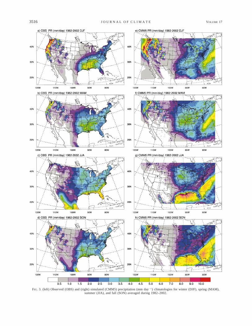
3. Annual cycle of precipitationFigure 3 illustrates the 1982–2002 averaged seasonal
mean geographic distributions of the observed and
3516 VOLUME 17J O U R N A L O F C L I M A T E
FIG. 3. (left) Observed (OBS) and (right) simulated (CMM5) precipitation (mm day21) climatologies for winter (DJF), spring (MAM),summer (JJA), and fall (SON) averaged during 1982–2002.
15 SEPTEMBER 2004 3517L I A N G E T A L .
CMM5 simulated precipitations. Observations exhibitgenerally wetness east of 1008W and west of the Rock-ies, with a dry zone in between along the downstreamslopes of the Rockies. Over the central United States,precipitation decreases rapidly from southeast to north-west in winter while remaining rather uniform in sum-mer, with transitions in spring and fall. The CMM5 wellreproduces these characteristics. The model downscal-ing skill, however, shows distinct regional dependen-cies.
The CMM5 realistically simulates mesoscale oro-graphic precipitation patterns and their seasonal varia-tions west of the Rockies. When compared to the com-posite data, the model produces generally more winterprecipitation west of the Rockies, especially over thewest slopes of all major peak mountain ranges exceptfor a deficit west of the Coast Range. The differencesdecrease in spring and fall, and are not evident in thesummer dry season. These regions overlap with the ar-eas of significant orographic precipitation effects (Fig.2) generated by upslope motions within the eastward-moving Pacific storm systems. Given the lack of directmeasurements at high elevations over steep mountain-ous regions, the uncertainties of the PRISM orographicadjustments, and hence the composite analysis, maylikely be large. The negative (positive) CMM5 differ-ences from the composite analysis along the west (east)side of the Coast Range, indicating a phase error, arelikely caused by the difference in terrain elevation at agrid spacing between 30 km for the model and 1/88 (;10km) for the PRISM.
The CMM5 accurately simulates the transition dryzone on the east downstream slopes of the Rockies dueto the precipitation shadowing effect of mountain rang-es. The model also correctly reproduces seasonal vari-ations of precipitation over the Midwest. The biases overthese regions are mostly within 60.5 mm day21, exceptfor the Great Lakes region in winter and spring whereoverestimations (by ,2 mm day21) occur. Data qualityanalysis indicated that rain gauge measurements in thisregion generally underestimate the actual snowfall waterequivalent (Groisman et al. 1994, 1996). This may alsoapply for the western mountainous regions. Hence theearlier CMM5 differences from the composite analysismay partially be attributed to observational uncertain-ties. The CMM5’s success in the central United States,especially in summer, is encouraging since it is a com-mon difficulty for other RCMs to realistically reproducethe local precipitation variations (Takle et al. 1999) thatare dominated by regional mesoscale circulations, in-cluding the nocturnal LLJ (Stensrud 1996; Higgins etal. 1997; Liang et al. 2001) and mesoscale convectivecomplexes (Maddox 1980; Fritsch et al. 1986).
On the other hand, the CMM5 essentially fails tosimulate the summer NAM rainfall pattern. The NAMresults from a combination of large-scale circulationforcing and local diabatic heating (Barlow et al. 1998).The former is incorporated into the CMM5 through the
dynamic relaxation of the LBCs, while the latter is de-termined by the model physics, especially surface–at-mosphere and cumulus-cloud–radiation interactions.The CMM5 failure is caused by substantial uncertaintiesin the LBCs over the west and south buffer zones dueto the lack of observations over oceans assimilated intothe reanalyses (Liang et al. 2001), large errors in surfaceforcing by the use of coarse-resolution SST data (Gaoet al. 2003), and strong diabatic heating sensitivities tophysics representations. The NAM simulation remainsa challenging issue in both RCM and GCM commu-nities. Even the global reanalyses cannot faithfully pro-duce a consistent NAM system (Barlow et al. 1998). Inaddition, the CMM5 underestimates rainfall (by ,3 mmday21) in the Gulf States throughout the year and easternstates in summer and fall. Similar underestimations wereidentified in other RCM simulations (Giorgi et al. 1994;Takle et al. 1999; Pan et al. 2001). This deficiency maypartially be explained by large LBC errors over the southand east buffer zones. The correct mechanisms respon-sible for these biases are not known and will be exploredin the subsequent sections through circulation analysesand sensitivity experiments.
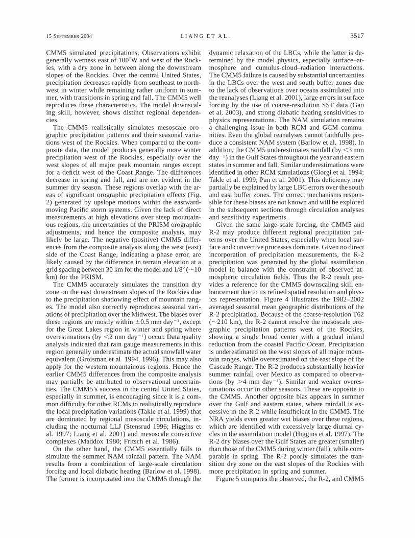
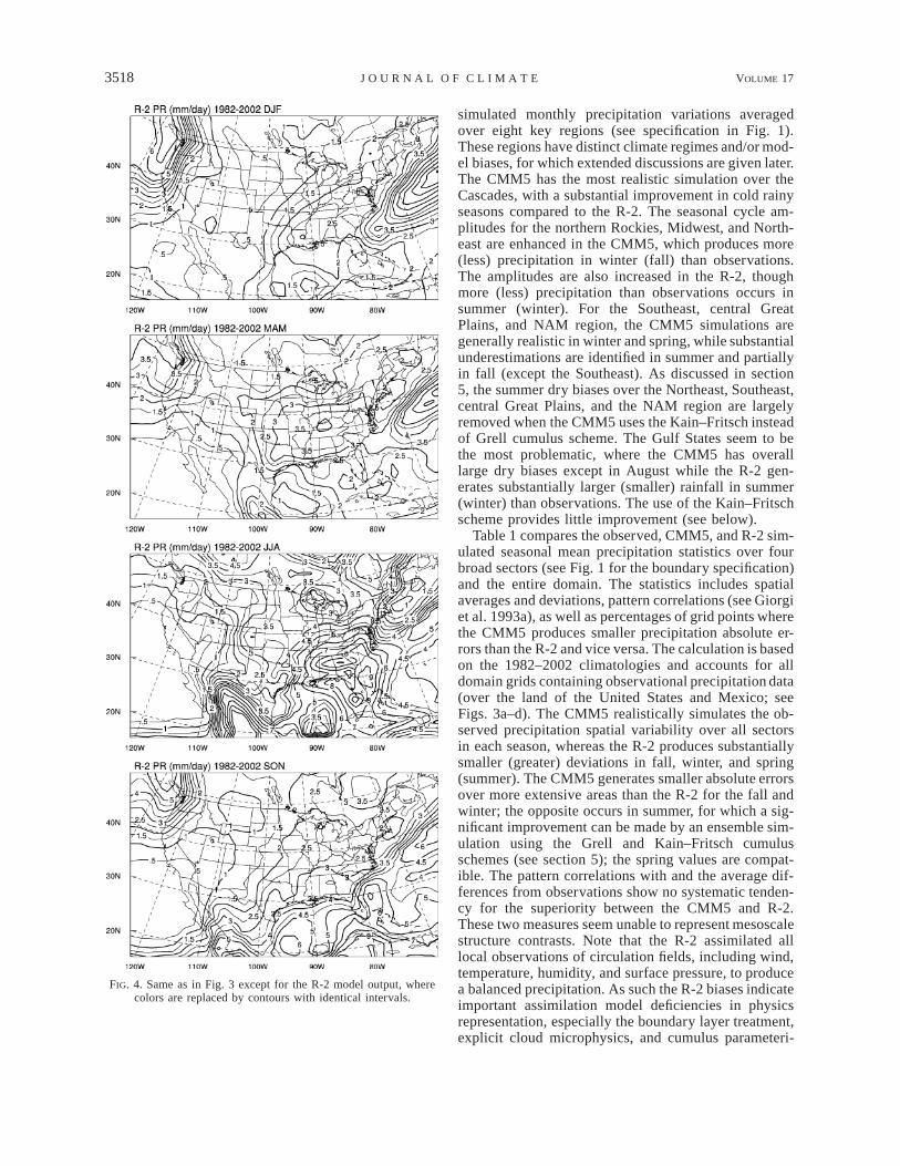
Given the same large-scale forcing, the CMM5 andR-2 may produce different regional precipitation pat-terns over the United States, especially when local sur-face and convective processes dominate. Given no directincorporation of precipitation measurements, the R-2precipitation was generated by the global assimilationmodel in balance with the constraint of observed at-mospheric circulation fields. Thus the R-2 result pro-vides a reference for the CMM5 downscaling skill en-hancement due to its refined spatial resolution and phys-ics representation. Figure 4 illustrates the 1982–2002averaged seasonal mean geographic distributions of theR-2 precipitation. Because of the coarse-resolution T62(;210 km), the R-2 cannot resolve the mesoscale oro-graphic precipitation patterns west of the Rockies,showing a single broad center with a gradual inlandreduction from the coastal Pacific Ocean. Precipitationis underestimated on the west slopes of all major moun-tain ranges, while overestimated on the east slope of theCascade Range. The R-2 produces substantially heaviersummer rainfall over Mexico as compared to observa-tions (by .4 mm day21). Similar and weaker overes-timations occur in other seasons. These are opposite tothe CMM5. Another opposite bias appears in summerover the Gulf and eastern states, where rainfall is ex-cessive in the R-2 while insufficient in the CMM5. TheNRA yields even greater wet biases over these regions,which are identified with excessively large diurnal cy-cles in the assimilation model (Higgins et al. 1997). TheR-2 dry biases over the Gulf States are greater (smaller)than those of the CMM5 during winter (fall), while com-parable in spring. The R-2 poorly simulates the tran-sition dry zone on the east slopes of the Rockies withmore precipitation in spring and summer.
Figure 5 compares the observed, the R-2, and CMM5
3518 VOLUME 17J O U R N A L O F C L I M A T E
FIG. 4. Same as in Fig. 3 except for the R-2 model output, wherecolors are replaced by contours with identical intervals.
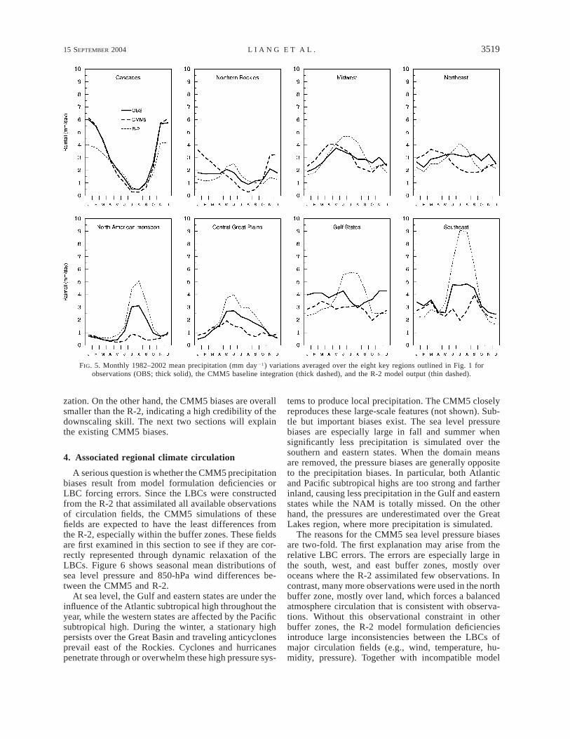
simulated monthly precipitation variations averagedover eight key regions (see specification in Fig. 1).These regions have distinct climate regimes and/or mod-el biases, for which extended discussions are given later.The CMM5 has the most realistic simulation over theCascades, with a substantial improvement in cold rainyseasons compared to the R-2. The seasonal cycle am-plitudes for the northern Rockies, Midwest, and North-east are enhanced in the CMM5, which produces more(less) precipitation in winter (fall) than observations.The amplitudes are also increased in the R-2, thoughmore (less) precipitation than observations occurs insummer (winter). For the Southeast, central GreatPlains, and NAM region, the CMM5 simulations aregenerally realistic in winter and spring, while substantialunderestimations are identified in summer and partiallyin fall (except the Southeast). As discussed in section5, the summer dry biases over the Northeast, Southeast,central Great Plains, and the NAM region are largelyremoved when the CMM5 uses the Kain–Fritsch insteadof Grell cumulus scheme. The Gulf States seem to bethe most problematic, where the CMM5 has overalllarge dry biases except in August while the R-2 gen-erates substantially larger (smaller) rainfall in summer(winter) than observations. The use of the Kain–Fritschscheme provides little improvement (see below).
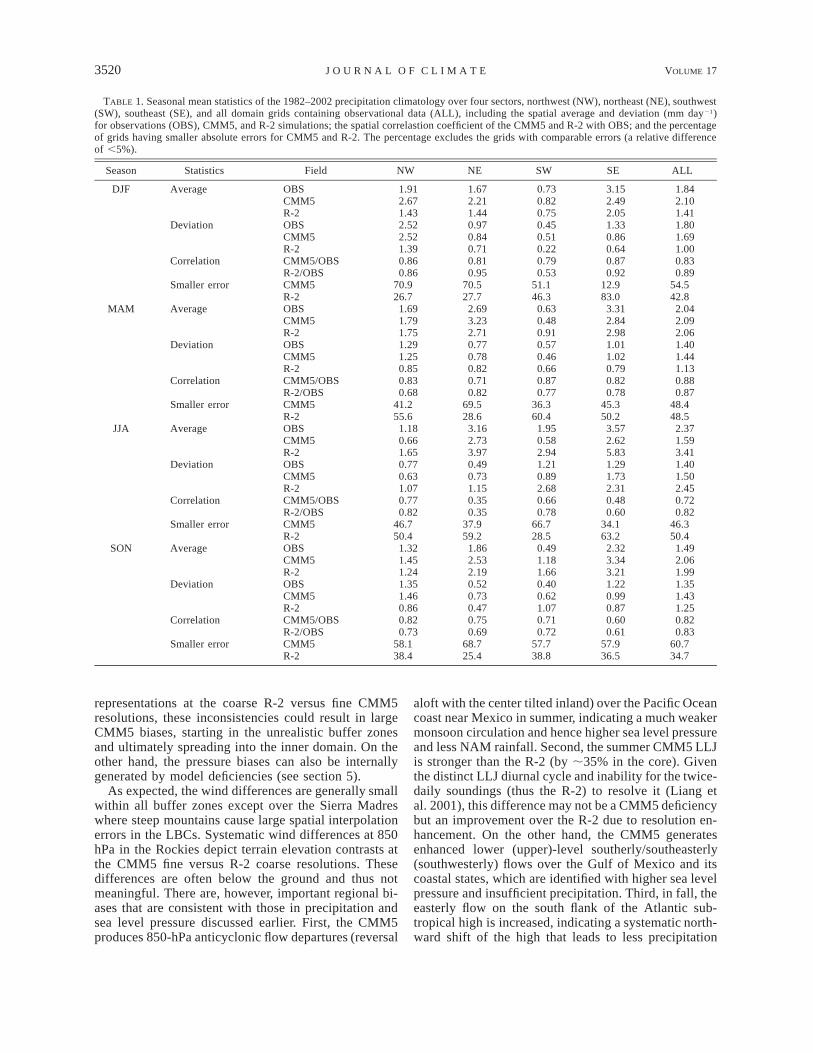
Table 1 compares the observed, CMM5, and R-2 sim-ulated seasonal mean precipitation statistics over fourbroad sectors (see Fig. 1 for the boundary specification)and the entire domain. The statistics includes spatialaverages and deviations, pattern correlations (see Giorgiet al. 1993a), as well as percentages of grid points wherethe CMM5 produces smaller precipitation absolute er-rors than the R-2 and vice versa. The calculation is basedon the 1982–2002 climatologies and accounts for alldomain grids containing observational precipitation data(over the land of the United States and Mexico; seeFigs. 3a–d). The CMM5 realistically simulates the ob-served precipitation spatial variability over all sectorsin each season, whereas the R-2 produces substantiallysmaller (greater) deviations in fall, winter, and spring(summer). The CMM5 generates smaller absolute errorsover more extensive areas than the R-2 for the fall andwinter; the opposite occurs in summer, for which a sig-nificant improvement can be made by an ensemble sim-ulation using the Grell and Kain–Fritsch cumulusschemes (see section 5); the spring values are compat-ible. The pattern correlations with and the average dif-ferences from observations show no systematic tenden-cy for the superiority between the CMM5 and R-2.These two measures seem unable to represent mesoscalestructure contrasts. Note that the R-2 assimilated alllocal observations of circulation fields, including wind,temperature, humidity, and surface pressure, to producea balanced precipitation. As such the R-2 biases indicateimportant assimilation model deficiencies in physicsrepresentation, especially the boundary layer treatment,explicit cloud microphysics, and cumulus parameteri-
15 SEPTEMBER 2004 3519L I A N G E T A L .
FIG. 5. Monthly 1982–2002 mean precipitation (mm day21) variations averaged over the eight key regions outlined in Fig. 1 forobservations (OBS; thick solid), the CMM5 baseline integration (thick dashed), and the R-2 model output (thin dashed).
zation. On the other hand, the CMM5 biases are overallsmaller than the R-2, indicating a high credibility of thedownscaling skill. The next two sections will explainthe existing CMM5 biases.
4. Associated regional climate circulation
A serious question is whether the CMM5 precipitationbiases result from model formulation deficiencies orLBC forcing errors. Since the LBCs were constructedfrom the R-2 that assimilated all available observationsof circulation fields, the CMM5 simulations of thesefields are expected to have the least differences fromthe R-2, especially within the buffer zones. These fieldsare first examined in this section to see if they are cor-rectly represented through dynamic relaxation of theLBCs. Figure 6 shows seasonal mean distributions ofsea level pressure and 850-hPa wind differences be-tween the CMM5 and R-2.
At sea level, the Gulf and eastern states are under theinfluence of the Atlantic subtropical high throughout theyear, while the western states are affected by the Pacificsubtropical high. During the winter, a stationary highpersists over the Great Basin and traveling anticyclonesprevail east of the Rockies. Cyclones and hurricanespenetrate through or overwhelm these high pressure sys-
tems to produce local precipitation. The CMM5 closelyreproduces these large-scale features (not shown). Sub-tle but important biases exist. The sea level pressurebiases are especially large in fall and summer whensignificantly less precipitation is simulated over thesouthern and eastern states. When the domain meansare removed, the pressure biases are generally oppositeto the precipitation biases. In particular, both Atlanticand Pacific subtropical highs are too strong and fartherinland, causing less precipitation in the Gulf and easternstates while the NAM is totally missed. On the otherhand, the pressures are underestimated over the GreatLakes region, where more precipitation is simulated.
The reasons for the CMM5 sea level pressure biasesare two-fold. The first explanation may arise from therelative LBC errors. The errors are especially large inthe south, west, and east buffer zones, mostly overoceans where the R-2 assimilated few observations. Incontrast, many more observations were used in the northbuffer zone, mostly over land, which forces a balancedatmosphere circulation that is consistent with observa-tions. Without this observational constraint in otherbuffer zones, the R-2 model formulation deficienciesintroduce large inconsistencies between the LBCs ofmajor circulation fields (e.g., wind, temperature, hu-midity, pressure). Together with incompatible model
3520 VOLUME 17J O U R N A L O F C L I M A T E
TABLE 1. Seasonal mean statistics of the 1982–2002 precipitation climatology over four sectors, northwest (NW), northeast (NE), southwest(SW), southeast (SE), and all domain grids containing observational data (ALL), including the spatial average and deviation (mm day21)for observations (OBS), CMM5, and R-2 simulations; the spatial correlastion coefficient of the CMM5 and R-2 with OBS; and the percentageof grids having smaller absolute errors for CMM5 and R-2. The percentage excludes the grids with comparable errors (a relative differenceof ,5%).
Season Statistics Field NW NE SW SE ALL
DJF Average OBSCMM5R-2
1.912.671.43
1.672.211.44
0.730.820.75
3.152.492.05
1.842.101.41
Deviation OBSCMM5R-2
2.522.521.39
0.970.840.71
0.450.510.22
1.330.860.64
1.801.691.00
Correlation CMM5/OBSR-2/OBS
0.860.86
0.810.95
0.790.53
0.870.92
0.830.89
Smaller error CMM5R-2
70.926.7
70.527.7
51.146.3
12.983.0
54.542.8
MAM Average OBSCMM5R-2
1.691.791.75
2.693.232.71
0.630.480.91
3.312.842.98
2.042.092.06
Deviation OBSCMM5R-2
1.291.250.85
0.770.780.82
0.570.460.66
1.011.020.79
1.401.441.13
Correlation CMM5/OBSR-2/OBS
0.830.68
0.710.82
0.870.77
0.820.78
0.880.87
Smaller error CMM5R-2
41.255.6
69.528.6
36.360.4
45.350.2
48.448.5
JJA Average OBSCMM5R-2
1.180.661.65
3.162.733.97
1.950.582.94
3.572.625.83
2.371.593.41
Deviation OBSCMM5R-2
0.770.631.07
0.490.731.15
1.210.892.68
1.291.732.31
1.401.502.45
Correlation CMM5/OBSR-2/OBS
0.770.82
0.350.35
0.660.78
0.480.60
0.720.82
Smaller error CMM5R-2
46.750.4
37.959.2
66.728.5
34.163.2
46.350.4
SON Average OBSCMM5R-2
1.321.451.24
1.862.532.19
0.491.181.66
2.323.343.21
1.492.061.99
Deviation OBSCMM5R-2
1.351.460.86
0.520.730.47
0.400.621.07
1.220.990.87
1.351.431.25
Correlation CMM5/OBSR-2/OBS
0.820.73
0.750.69
0.710.72
0.600.61
0.820.83
Smaller error CMM5R-2
58.138.4
68.725.4
57.738.8
57.936.5
60.734.7
representations at the coarse R-2 versus fine CMM5resolutions, these inconsistencies could result in largeCMM5 biases, starting in the unrealistic buffer zonesand ultimately spreading into the inner domain. On theother hand, the pressure biases can also be internallygenerated by model deficiencies (see section 5).
As expected, the wind differences are generally smallwithin all buffer zones except over the Sierra Madreswhere steep mountains cause large spatial interpolationerrors in the LBCs. Systematic wind differences at 850hPa in the Rockies depict terrain elevation contrasts atthe CMM5 fine versus R-2 coarse resolutions. Thesedifferences are often below the ground and thus notmeaningful. There are, however, important regional bi-ases that are consistent with those in precipitation andsea level pressure discussed earlier. First, the CMM5produces 850-hPa anticyclonic flow departures (reversal
aloft with the center tilted inland) over the Pacific Oceancoast near Mexico in summer, indicating a much weakermonsoon circulation and hence higher sea level pressureand less NAM rainfall. Second, the summer CMM5 LLJis stronger than the R-2 (by ;35% in the core). Giventhe distinct LLJ diurnal cycle and inability for the twice-daily soundings (thus the R-2) to resolve it (Liang etal. 2001), this difference may not be a CMM5 deficiencybut an improvement over the R-2 due to resolution en-hancement. On the other hand, the CMM5 generatesenhanced lower (upper)-level southerly/southeasterly(southwesterly) flows over the Gulf of Mexico and itscoastal states, which are identified with higher sea levelpressure and insufficient precipitation. Third, in fall, theeasterly flow on the south flank of the Atlantic sub-tropical high is increased, indicating a systematic north-ward shift of the high that leads to less precipitation
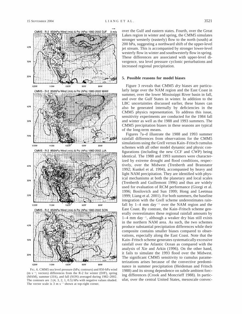
15 SEPTEMBER 2004 3521L I A N G E T A L .
FIG. 6. CMM5 sea level pressure (hPa; contours) and 850-hPa wind(m s21; vectors) differences from the R-2 for winter (DJF), spring(MAM), summer (JJA), and fall (SON) averaged during 1982–2002.The contours are 6(4, 3, 2, 1, 0.5) hPa with negative values shaded.The vector scale is 3 m s21 shown at top-right corner.
over the Gulf and eastern states. Fourth, over the GreatLakes region in winter and spring, the CMM5 simulatesstronger westerly (easterly) flow to the north (south) at200 hPa, suggesting a northward shift of the upper-leveljet stream. This is accompanied by stronger lower-levelwesterly flow in winter and southwesterly flow in spring.These differences are associated with upper-level di-vergence, sea level pressure cyclonic perturbations andincreased regional precipitation.
5. Possible reasons for model biases
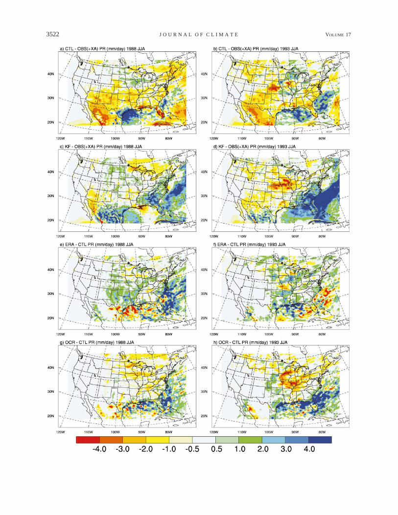
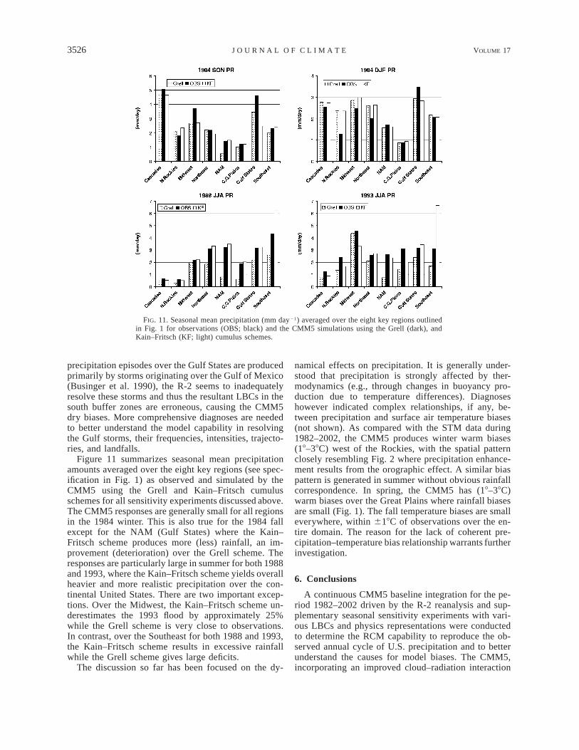
Figure 3 reveals that CMM5 dry biases are particu-larly large over the NAM region and the East Coast insummer, over the lower Mississippi River basin in fall,and over the Gulf States in winter. In addition to theLBC uncertainties discussed earlier, these biases canalso be generated internally by deficiencies in theCMM5 physics representation. To address this issue,sensitivity experiments are conducted for the 1984 falland winter as well as the 1988 and 1993 summers. TheCMM5 precipitation biases in these seasons are typicalof the long-term means.
Figures 7a–d illustrate the 1988 and 1993 summerrainfall differences from observations for the CMM5simulations using the Grell versus Kain–Fritsch cumulusschemes with all other model dynamic and physic con-figurations (including the new CCF and CWP) beingidentical. The 1988 and 1993 summers were character-ized by extreme drought and flood conditions, respec-tively, over the Midwest (Trenberth and Branstator1992; Kunkel et al. 1994), accompanied by heavy andlight NAM precipitation. They are identified with phys-ical mechanisms at both the planetary and local scales(Trenberth and Guillemont 1996) and thus are widelyused for evaluation of RCM performance (Giorgi et al.1996; Bosilovich and Sun 1999; Hong and Leetmaa1999; Liang et al. 2001). For both summers, the baselineintegration with the Grell scheme underestimates rain-fall by 1–4 mm day21 over the NAM region and theEast Coast. By contrast, the Kain–Fritsch scheme gen-erally overestimates these regional rainfall amounts by1–4 mm day21, although a weaker dry bias still existsin the northern NAM area. As such, the two schemesproduce substantial precipitation differences while theircomposite contains smaller biases compared to obser-vations, especially along the East Coast. Note that theKain–Fritsch scheme generates systematically excessiverainfall over the Atlantic Ocean as compared with theanalysis of Xie and Arkin (1996). On the other hand,it fails to simulate the 1993 flood over the Midwest.The significant CMM5 sensitivity to cumulus parame-terizations arises because of the convective predomi-nance in summer precipitation (Heideman and Fritsch1988) and its strong dependence on subtle ambient forc-ing differences (Crook and Moncrieff 1988). In partic-ular, over the central United States, mesoscale convec-
3522 VOLUME 17J O U R N A L O F C L I M A T E
15 SEPTEMBER 2004 3523L I A N G E T A L .
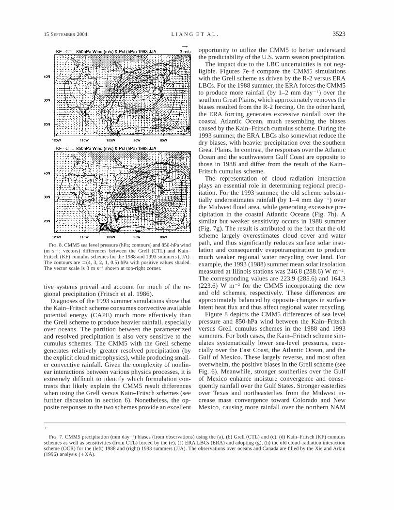
FIG. 8. CMM5 sea level pressure (hPa; contours) and 850-hPa wind(m s21; vectors) differences between the Grell (CTL) and Kain–Fritsch (KF) cumulus schemes for the 1988 and 1993 summers (JJA).The contours are 6(4, 3, 2, 1, 0.5) hPa with positive values shaded.The vector scale is 3 m s21 shown at top-right corner.
←
FIG. 7. CMM5 precipitation (mm day21) biases (from observations) using the (a), (b) Grell (CTL) and (c), (d) Kain–Fritsch (KF) cumulusschemes as well as sensitivities (from CTL) forced by the (e), (f ) ERA LBCs (ERA) and adopting (g), (h) the old cloud–radiation interactionscheme (OCR) for the (left) 1988 and (right) 1993 summers (JJA). The observations over oceans and Canada are filled by the Xie and Arkin(1996) analysis (1XA).
tive systems prevail and account for much of the re-gional precipitation (Fritsch et al. 1986).
Diagnoses of the 1993 summer simulations show thatthe Kain–Fritsch scheme consumes convective availablepotential energy (CAPE) much more effectively thanthe Grell scheme to produce heavier rainfall, especiallyover oceans. The partition between the parameterizedand resolved precipitation is also very sensitive to thecumulus schemes. The CMM5 with the Grell schemegenerates relatively greater resolved precipitation (bythe explicit cloud microphysics), while producing small-er convective rainfall. Given the complexity of nonlin-ear interactions between various physics processes, it isextremely difficult to identify which formulation con-trasts that likely explain the CMM5 result differenceswhen using the Grell versus Kain–Fritsch schemes (seefurther discussion in section 6). Nonetheless, the op-posite responses to the two schemes provide an excellent
opportunity to utilize the CMM5 to better understandthe predictability of the U.S. warm season precipitation.
The impact due to the LBC uncertainties is not neg-ligible. Figures 7e–f compare the CMM5 simulationswith the Grell scheme as driven by the R-2 versus ERALBCs. For the 1988 summer, the ERA forces the CMM5to produce more rainfall (by 1–2 mm day21) over thesouthern Great Plains, which approximately removes thebiases resulted from the R-2 forcing. On the other hand,the ERA forcing generates excessive rainfall over thecoastal Atlantic Ocean, much resembling the biasescaused by the Kain–Fritsch cumulus scheme. During the1993 summer, the ERA LBCs also somewhat reduce thedry biases, with heavier precipitation over the southernGreat Plains. In contrast, the responses over the AtlanticOcean and the southwestern Gulf Coast are opposite tothose in 1988 and differ from the result of the Kain–Fritsch cumulus scheme.
The representation of cloud–radiation interactionplays an essential role in determining regional precip-itation. For the 1993 summer, the old scheme substan-tially underestimates rainfall (by 1–4 mm day21) overthe Midwest flood area, while generating excessive pre-cipitation in the coastal Atlantic Oceans (Fig. 7h). Asimilar but weaker sensitivity occurs in 1988 summer(Fig. 7g). The result is attributed to the fact that the oldscheme largely overestimates cloud cover and waterpath, and thus significantly reduces surface solar inso-lation and consequently evapotranspiration to producemuch weaker regional water recycling over land. Forexample, the 1993 (1988) summer mean solar insolationmeasured at Illinois stations was 246.8 (288.6) W m22.The corresponding values are 223.9 (285.6) and 164.3(223.6) W m22 for the CMM5 incorporating the newand old schemes, respectively. These differences areapproximately balanced by opposite changes in surfacelatent heat flux and thus affect regional water recycling.
Figure 8 depicts the CMM5 differences of sea levelpressure and 850-hPa wind between the Kain–Fritschversus Grell cumulus schemes in the 1988 and 1993summers. For both cases, the Kain–Fritsch scheme sim-ulates systematically lower sea-level pressures, espe-cially over the East Coast, the Atlantic Ocean, and theGulf of Mexico. These largely reverse, and most oftenoverwhelm, the positive biases in the Grell scheme (seeFig. 6). Meanwhile, stronger southerlies over the Gulfof Mexico enhance moisture convergence and conse-quently rainfall over the Gulf States. Stronger easterliesover Texas and northeasterlies from the Midwest in-crease mass convergence toward Colorado and NewMexico, causing more rainfall over the northern NAM
3524 VOLUME 17J O U R N A L O F C L I M A T E
FIG. 9. CMM5 precipitation (mm day21) (a) biases (CTL 2 OBS) and (b) responses caused by replacing with the Kain–Fritsch cumulusscheme (KF 2 CTL), (c) the ERA LBC forcing (ERA 2 CTL), or (d) completely turning off precipitating processes over the Gulf of Mexico(GMo 2 CTL).
region while a deficit over the Midwest. Stronger south-westerlies lead to convergence and heavier rainfall overthe Atlantic coast. These circulation changes are theconsequence of differential heating differences due tothe latent heat release between the two schemes (Gochiset al. 2002). The result suggests that the cumulus pa-rameterization alone could explain a large portion of theCMM5 sea level pressure biases (Fig. 6).
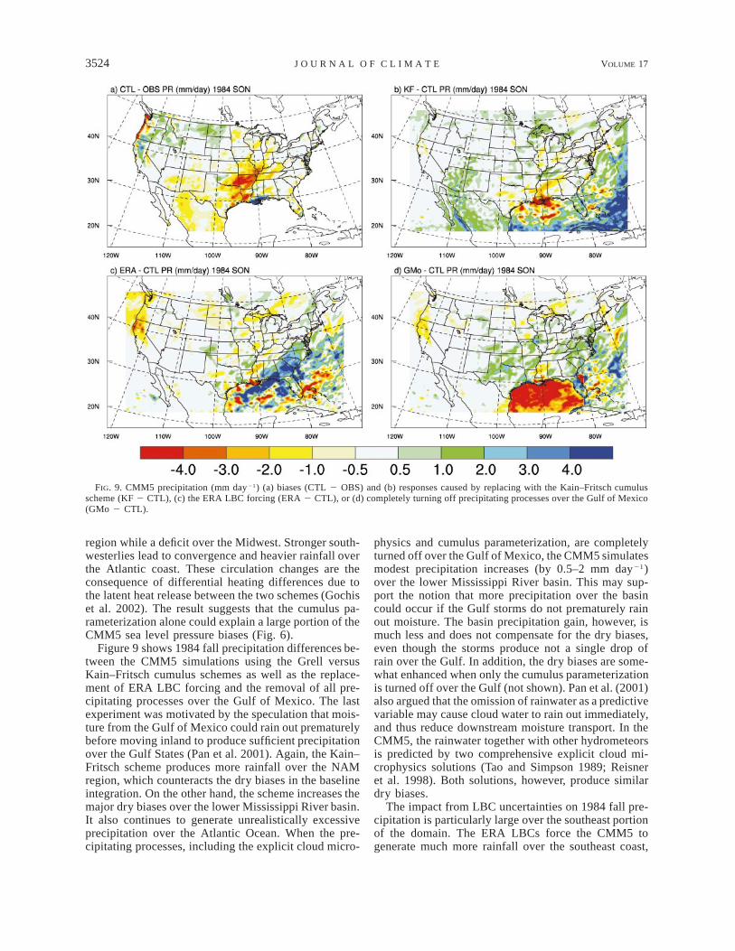
Figure 9 shows 1984 fall precipitation differences be-tween the CMM5 simulations using the Grell versusKain–Fritsch cumulus schemes as well as the replace-ment of ERA LBC forcing and the removal of all pre-cipitating processes over the Gulf of Mexico. The lastexperiment was motivated by the speculation that mois-ture from the Gulf of Mexico could rain out prematurelybefore moving inland to produce sufficient precipitationover the Gulf States (Pan et al. 2001). Again, the Kain–Fritsch scheme produces more rainfall over the NAMregion, which counteracts the dry biases in the baselineintegration. On the other hand, the scheme increases themajor dry biases over the lower Mississippi River basin.It also continues to generate unrealistically excessiveprecipitation over the Atlantic Ocean. When the pre-cipitating processes, including the explicit cloud micro-
physics and cumulus parameterization, are completelyturned off over the Gulf of Mexico, the CMM5 simulatesmodest precipitation increases (by 0.5–2 mm day21)over the lower Mississippi River basin. This may sup-port the notion that more precipitation over the basincould occur if the Gulf storms do not prematurely rainout moisture. The basin precipitation gain, however, ismuch less and does not compensate for the dry biases,even though the storms produce not a single drop ofrain over the Gulf. In addition, the dry biases are some-what enhanced when only the cumulus parameterizationis turned off over the Gulf (not shown). Pan et al. (2001)also argued that the omission of rainwater as a predictivevariable may cause cloud water to rain out immediately,and thus reduce downstream moisture transport. In theCMM5, the rainwater together with other hydrometeorsis predicted by two comprehensive explicit cloud mi-crophysics solutions (Tao and Simpson 1989; Reisneret al. 1998). Both solutions, however, produce similardry biases.
The impact from LBC uncertainties on 1984 fall pre-cipitation is particularly large over the southeast portionof the domain. The ERA LBCs force the CMM5 togenerate much more rainfall over the southeast coast,
15 SEPTEMBER 2004 3525L I A N G E T A L .
FIG. 10. Fall precipitation (mm day21) climatologies averaged over the Gulf States for obser-vations (OBS), CMM5, and R-2 simulations during 1982–2002, as well as all AMIP models in1979–95 and CMIP models of the last 30-yr control period.
where the baseline integration with the R-2 forcing isgenerally realistic. On the other hand, the sensitivityover the southern Great Plains is relatively small. Panet al. (2001) also found small regional precipitation in-fluences from a 1500-km equatorward shift of the southbuffer zone. None of these results, however, can justifyconcluding that LBC errors are not the cause of theproblem for the major dry biases over the lower Mis-sissippi River basin. Given any of the existing reanal-yses, LBC uncertainties are especially large over thesouth, east, and west buffer zones, mostly over oceanswhere observations are lacking for data assimilation. Itis not known, however, which reanalysis, and perhapsnone of them, best represents the reality. Since the southbuffer zone in the Pan et al. model and the currentCMM5 is located in an already problematic area, itsfurther southward expansion will not improve the lateralforcing but instead may worsen it (Liang et al. 2001).
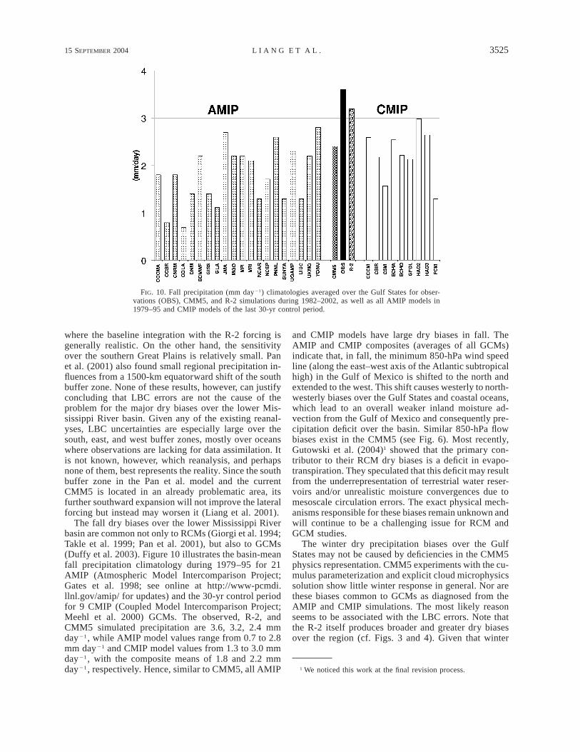
The fall dry biases over the lower Mississippi Riverbasin are common not only to RCMs (Giorgi et al. 1994;Takle et al. 1999; Pan et al. 2001), but also to GCMs(Duffy et al. 2003). Figure 10 illustrates the basin-meanfall precipitation climatology during 1979–95 for 21AMIP (Atmospheric Model Intercomparison Project;Gates et al. 1998; see online at http://www-pcmdi.llnl.gov/amip/ for updates) and the 30-yr control periodfor 9 CMIP (Coupled Model Intercomparison Project;Meehl et al. 2000) GCMs. The observed, R-2, andCMM5 simulated precipitation are 3.6, 3.2, 2.4 mmday21, while AMIP model values range from 0.7 to 2.8mm day21 and CMIP model values from 1.3 to 3.0 mmday21, with the composite means of 1.8 and 2.2 mmday21, respectively. Hence, similar to CMM5, all AMIP
and CMIP models have large dry biases in fall. TheAMIP and CMIP composites (averages of all GCMs)indicate that, in fall, the minimum 850-hPa wind speedline (along the east–west axis of the Atlantic subtropicalhigh) in the Gulf of Mexico is shifted to the north andextended to the west. This shift causes westerly to north-westerly biases over the Gulf States and coastal oceans,which lead to an overall weaker inland moisture ad-vection from the Gulf of Mexico and consequently pre-cipitation deficit over the basin. Similar 850-hPa flowbiases exist in the CMM5 (see Fig. 6). Most recently,Gutowski et al. (2004)1 showed that the primary con-tributor to their RCM dry biases is a deficit in evapo-transpiration. They speculated that this deficit may resultfrom the underrepresentation of terrestrial water reser-voirs and/or unrealistic moisture convergences due tomesoscale circulation errors. The exact physical mech-anisms responsible for these biases remain unknown andwill continue to be a challenging issue for RCM andGCM studies.
The winter dry precipitation biases over the GulfStates may not be caused by deficiencies in the CMM5physics representation. CMM5 experiments with the cu-mulus parameterization and explicit cloud microphysicssolution show little winter response in general. Nor arethese biases common to GCMs as diagnosed from theAMIP and CMIP simulations. The most likely reasonseems to be associated with the LBC errors. Note thatthe R-2 itself produces broader and greater dry biasesover the region (cf. Figs. 3 and 4). Given that winter
1 We noticed this work at the final revision process.
3526 VOLUME 17J O U R N A L O F C L I M A T E
FIG. 11. Seasonal mean precipitation (mm day21) averaged over the eight key regions outlinedin Fig. 1 for observations (OBS; black) and the CMM5 simulations using the Grell (dark), andKain–Fritsch (KF; light) cumulus schemes.
precipitation episodes over the Gulf States are producedprimarily by storms originating over the Gulf of Mexico(Businger et al. 1990), the R-2 seems to inadequatelyresolve these storms and thus the resultant LBCs in thesouth buffer zones are erroneous, causing the CMM5dry biases. More comprehensive diagnoses are neededto better understand the model capability in resolvingthe Gulf storms, their frequencies, intensities, trajecto-ries, and landfalls.
Figure 11 summarizes seasonal mean precipitationamounts averaged over the eight key regions (see spec-ification in Fig. 1) as observed and simulated by theCMM5 using the Grell and Kain–Fritsch cumulusschemes for all sensitivity experiments discussed above.The CMM5 responses are generally small for all regionsin the 1984 winter. This is also true for the 1984 fallexcept for the NAM (Gulf States) where the Kain–Fritsch scheme produces more (less) rainfall, an im-provement (deterioration) over the Grell scheme. Theresponses are particularly large in summer for both 1988and 1993, where the Kain–Fritsch scheme yields overallheavier and more realistic precipitation over the con-tinental United States. There are two important excep-tions. Over the Midwest, the Kain–Fritsch scheme un-derestimates the 1993 flood by approximately 25%while the Grell scheme is very close to observations.In contrast, over the Southeast for both 1988 and 1993,the Kain–Fritsch scheme results in excessive rainfallwhile the Grell scheme gives large deficits.
The discussion so far has been focused on the dy-
namical effects on precipitation. It is generally under-stood that precipitation is strongly affected by ther-modynamics (e.g., through changes in buoyancy pro-duction due to temperature differences). Diagnoseshowever indicated complex relationships, if any, be-tween precipitation and surface air temperature biases(not shown). As compared with the STM data during1982–2002, the CMM5 produces winter warm biases(18–38C) west of the Rockies, with the spatial patternclosely resembling Fig. 2 where precipitation enhance-ment results from the orographic effect. A similar biaspattern is generated in summer without obvious rainfallcorrespondence. In spring, the CMM5 has (18–38C)warm biases over the Great Plains where rainfall biasesare small (Fig. 1). The fall temperature biases are smalleverywhere, within 618C of observations over the en-tire domain. The reason for the lack of coherent pre-cipitation–temperature bias relationship warrants furtherinvestigation.
6. Conclusions
A continuous CMM5 baseline integration for the pe-riod 1982–2002 driven by the R-2 reanalysis and sup-plementary seasonal sensitivity experiments with vari-ous LBCs and physics representations were conductedto determine the RCM capability to reproduce the ob-served annual cycle of U.S. precipitation and to betterunderstand the causes for model biases. The CMM5,incorporating an improved cloud–radiation interaction
15 SEPTEMBER 2004 3527L I A N G E T A L .
parameterization, well reproduces the major character-istics of geographic distributions and seasonal variationsof observed precipitation. It simulates more realistic re-gional details with less overall biases than the R-2, in-dicating a high credibility of its downscaling skill.
Several important regional biases were identified.Sensitivity experiments using the ERA versus R-2 dataindicate that the LBC uncertainties, especially in thesouth, east, and west buffer zones, account for certainportions of these biases. The winter dry biases in theGulf States may likely result from the LBC errors. Thesummer dry biases in the NAM region and East Coastcan be largely removed by replacing the Grell with theKain–Fritsch cumulus scheme, although the latter oftenyields heavier rainfall than observations, especially inthe Atlantic Ocean. Over the Midwest, the Grell schemeproduces realistic summer rainfall, while the Kain–Fritsch scheme generates large dry biases. The CMM5simulations using the two cumulus schemes contain op-posite biases in summer and their composite tends tobe the best match for observations. The fall dry biasesover the lower Mississippi River basin are common toall existing RCMs and GCMs, but the responsible phys-ical mechanisms are not known. The winter and springwet biases over the Great Lake region and northernRockies may partially be attributed to the rain gaugeunderestimation of actual snowfall water equivalent andthe inaccurate representation of orographic precipitationenhancement by the PRISM with sparsely distributed,mainly low-elevation stations over the major mountains.We speculate that these wet biases could also result fromunrealistic model physics representations, though theavailable cumulus parameterization and explicit cloudmicrophysics schemes reveal little sensitivity.
In the coming series of the companion papers, wewill elaborate on the CMM5 capability to downscaleU.S. precipitation variability at various time scales, in-cluding the diurnal cycle, daily fluctuations, extremeevents, intraseasonal evolutions, and interannual vari-ations. In particular, we will further evaluate the CMM5responses to the Grell versus Kain–Fritsch cumulusschemes at these scales. Although many studies havedemonstrated the superiority of the Kain–Fritsch scheme(Kuo et al. 1996; Wang and Seaman 1997; Cohen 2002;Gochis et al. 2002), the Grell scheme has its own com-pelling advantages. As discussed in this and upcomingpapers, the Kain–Fritsch scheme generates excessiverainfall over the Atlantic Ocean, underestimates summerprecipitation in the Midwest, and fails to reproduce thediurnal cycle in the Great Plains, while the Grell schemedoes all of these reasonably well. Furthermore, theseregional responses may change when the CMM5 is cou-pled with different representations of cloud–radiationinteractions (Xu and Small 2002) and land surface pro-cesses (Pan et al. 1996) or driven by different LBCscontaining large uncertainties. Unfortunately, no generaltheory of cumulus parameterization is available, nor hasa single scheme been proven to work perfectly across
a wide range of weather systems and grid sizes, espe-cially at 10–50-km resolutions where mesoscale pro-cesses are partly resolved and parameterized (Molinariand Dudek 1992; Emanuel and Raymond 1993; Arak-awa 1993).
The Grell scheme is based on Arakawa and Schubert(1974) with a simplified single-cloud model, while theKain–Fritsch scheme is developed from Fritsch andChappell (1980) with a sophisticated cloud model. Al-though both represent updrafts and downdrafts, theKain–Fritsch scheme incorporates detailed cloud mi-crophysics as well as entrainment and detrainment be-tween the cloud and environment, all of which are ab-sent in the Grell scheme. When convection is triggered,the Kain–Fritsch scheme removes all CAPE within therelaxation time, whereas the Grell scheme adjusts thebuoyancy toward an equilibrium state depending on thestrength of cloud-base vertical motion. The rainfall isthen parameterized as the product of precipitation ef-ficiency with integrated water vapor and liquid fluxabout 150 hPa above the lifting condensation level inthe Kain–Fritsch scheme, but with total condensate andcloud-base mass flux in the updraft for the Grell scheme.The precipitation efficiency is a function of mean windshear of the convective column in both schemes, withadditional dependence on the cloud-base height for theKain–Fritsch scheme. It is beyond the scope of thisstudy to identify which, and perhaps all, of the previ-ously mentioned formulation contrasts that are respon-sible for the CMM5 result differences.
Acknowledgments. We thank Jimy Dudia and GeorgeGrell for numerous discussions on the model results,and Steven Hollinger, David Kristovich, and two anon-ymous reviewers for constructive comments on the man-uscript. We appreciate Wei Wang and John Michalakesfor their assistance during the MM5 implementation.We are grateful to Edwin Maurer for providing the SWMrainfall data. We acknowledge NCAR for access to theMM5 system and the NCEP–DOE and ECMWF globalreanalysis data, and FSL/NOAA and NCSA/UIUC forthe supercomputing support. Station data were providedby the Midwestern Regional Climate Center underNOAA Cooperative Agreement NA67RJ0146. The re-search was partially supported by NOAA/GAPP GrantNA06GP0393. The views expressed are those of theauthors and do not necessarily reflect those of the spon-soring agencies or the Illinois State Water Survey.
REFERENCES
Anderson, C. J., and Coauthors, 2003: Hydrological processes inregional climate model simulations of the central United Statesflood of June–July 1993. J. Hydrometeor., 4, 584–598.
Anthes, R. A., 1977: A cumulus parameterization scheme utilizing aone-dimensional cloud model. Mon. Wea. Rev., 105, 270–286.
Arakawa, A., 1993: Closure assumptions in the cumulus parameter-ization problem. The Representation of Cumulus Convection in
3528 VOLUME 17J O U R N A L O F C L I M A T E
Numerical Models, Meteor. Monger., No. 46, Amer. Meteor.Soc., 1–15.
——, and W. H. Schubert, 1974: Interaction of a cumulus cloudensemble with the large-scale environment. Part I. J. Atmos. Sci.,31, 674–701.
Barlow, M., S. Nigam, and E. H. Berbery, 1998: Evolution of theNorth American monsoon system. J. Climate, 11, 2238–2257.
Betts, A. K., and M. J. Miller, 1986: A new convective adjustmentscheme. Part II: Single column tests using GATE wave, BOMEX,and arctic air-mass data sets. Quart. J. Roy. Meteor. Soc., 112,693–709.
Bosilovich, M. G., and W.-Y. Sun, 1999: Numerical simulation of the1993 Midwestern flood: Land–atmosphere interactions. J. Cli-mate, 12, 1490–1505.
Businger, S., D. I. Knapp, and G. F. Watson, 1990: Storm followingclimatology of precipitation associated with winter cyclonesoriginating over the Gulf of Mexico. Wea. Forecasting, 5, 378–403.
Chen, F., and J. Dudhia, 2001: Coupling an advanced land surface–hydrology model with the Penn State–NCAR MM5 modelingsystem. Part I: Model implementation and sensitivity. Mon. Wea.Rev., 129, 569–585.
Christensen, O. B., J. H. Christensen, B. Machenauer, and M. Bozet,1998: Very high-resolution regional climate simulations overScandinavia—Present climate. J. Climate, 11, 3204–3229.
Cohen, C., 2002: A comparison of cumulus parameterizations in ide-alized sea-breeze simulations. Mon. Wea. Rev., 130, 2554–2571.
Cressman, G., 1959: An operational objective analysis system. Mon.Wea. Rev., 87, 367–374.
Crook, N. A., and M. W. Moncrieff, 1988: The effect of large-scaleconvergence on the generation and maintenance of deep moistconvection. J. Atmos. Sci., 45, 3606–3624.
Daly, C., R. P. Neilson, and D. L. Phillips, 1994: A statistical–to-pographic model for mapping climatological precipitation overmountainous terrain. J. Appl. Meteor., 33, 140–158.
——, G. H. Taylor, and W. P. Gibson, 1997: The PRISM approachto mapping precipitation and temperature. Preprints, 10th Conf.on Applied Climatology, Reno, NV, Amer. Meteor. Soc., 10–12.
Dickinson, R. E., R. M. Erroco, F. Giorgi, and G. T. Bates, 1989: Aregional climate model for the western United States. ClimateChange, 15, 383–422.
Dudhia, J., 1989: Numerical study of convection observed during thewinter monsoon experiment using a mesoscale two-dimensionalmodel. J. Atmos. Sci., 46, 3077–3107.
——, D. Gill, Y.-R. Guo, K. Manning, W. Wang, and J. Chriszar,cited 2004: PSU/NCAR Mesoscale Modeling System TutorialClass Notes and User’s Guide: MM5 Modeling System Version3. [Available online at http://www.mmm.ucar.edu/mm5/documents/MM5ptutpWebpnotes/TutTOC.html.]
Duffy, P. B., B. Govindasamy, K. Taylor, M. Wehner, A. Lamont,and S. Thompson, 2003: High resolution simulations of globalclimate. Part I: Present climate. Climate Dyn., 21, 371–390.
Emanuel, K. A., and D. J. Raymond, Eds., 1993: The Representationof Cumulus Convection in Numerical Models. Meteor. Monogr.,No. 46, Amer. Meteor. Soc., 246 pp.
Fennessy, M. J., and J. Shukla, 2000: Seasonal prediction over NorthAmerica with a regional model nested in a global model. J.Climate, 13, 2605–2627.
Fiorino, M., cited 2000: AMIP II sea surface temperature and sea iceconcentration observations. [Available online at http://www-pcmdi.llnl.go/amip/AMIP2EXPDSN/BCSpOBS/amip2pbcs.htm.]
Fritsch, J. M., and C. F. Chappell, 1980: Numerical prediction of aconvectively driven mesoscale pressure system. Part I: Convec-tive parameterization. J. Atmos. Sci., 37, 1722–1733.
——, R. J. Kane, and C. R. Chelius, 1986: The contribution of me-soscale convective weather systems to the warm season precip-itation of the United States. J. Climate Appl. Meteor., 25, 1333–1345.
Gao, X., S. Sorooshian, J. Li, and J. Xu, 2003: SST data improve
modeling of North American monsoon rainfall. Eos, Trans.Amer. Geophys. Union, 84.
Gates, W. L., and Coauthors, 1998: An overview of the results of theAtmospheric Model Intercomparison Project (AMIP I). Bull.Amer. Meteor. Soc., 73, 1962–1970.
Gibson, J. K., P. Kallberg, S. Uppala, A. Hernandez, A. Nomura, andE. Serrano, 1997: ERA description. ECMWF Reanalysis ProjectReport Series 1, ECMWF, 72 pp.
Giorgi, F., 1990: On the simulation of regional climate using a limitedarea model nested in a general circulation model. J. Climate, 3,941–963.
——, and G. T. Bates, 1989: On the climatological skill of a regionalmodel over complex terrain. Mon. Wea. Rev., 117, 2325–2347.
——, and L. O. Mearns, 1999: Introduction to special section: Re-gional climate modeling revisited. J. Geophys. Res., 104, 6335–6352.
——, and C. Shields, 1999: Tests of precipitation parameterizationsavailable in latest version of NCAR regional climate model(RegCM) over continental United States. J. Geophys. Res., 104,6353–6375.
——, C. S. Brodeur, and G. T. Bates, 1993a: Regional climate changescenarios over the United States produced with a nested regionalclimate model. J. Climate, 7, 375–399.
——, M. R. Marinucci, and G. T. Bates, 1993b: Development of asecond-generation regional climate model (RegCM2). Part II:Convective processes and assimilation of lateral boundary con-ditions. Mon. Wea. Rev., 121, 2814–2832.
——, C. Shields, and G. T. Bates, 1994: Regional climate changescenario over the United States produced with a nested regionalclimate model. J. Climate, 7, 375–399.
——, and L. O. Mearns, C. Shields, and L. Mayer, 1996: A regionalmodel study of the importance of local versus remote controlsof the 1988 drought and the 1993 flood over the central UnitedStates. J. Climate, 9, 1150–1162.
——, J. W. Hurrell, M. R. Marinucci, and M. Beniston, 1997: Ele-vation signal in surface climate change: A model study. J. Cli-mate, 10, 288–296.
——, L. Mearns, C. Shields, and L. McDaniel, 1998: Regional nestedmodel simulations of present day and 2xCO2 climate over thecentral Great Plains of the United States. Climate Change, 40,457–493.
Gochis, D. J., W. J. Shuttleworth, and Z.-L. Yang, 2002: Sensitivityof the modeled North American monsoon regional climate toconvection parameterization. Mon. Wea. Rev., 130, 1282–1298.
Grell, G. A., 1993: Prognostic evaluation of assumptions used bycumulus parameterizations. Mon. Wea. Rev., 121, 764–787.
Groisman, P. Y., and D. R. Legates, 1994: The accuracy of UnitedStates precipitation data. Bull. Amer. Meteor. Soc., 75, 215–227.
——, D. R. Easterling, R. G. Quayle, V. S. Golubev, A. N. Krenke,and A. Y. Mikhailov, 1996: Reducing biases in estimates ofprecipitation over the United States: Phase 3 adjustments. J.Geophys. Res., 101, 7185–7196.
Gutman, G., and A. Ignatov, 1998: The derivation of the green veg-etation fraction from NOAA/AVHRR data for use in numericalweather prediction models. Int. J. Remote Sens., 19, 1533–1543.
Gutowski, W. J., F. O. Otieno, A. W. Raymond, E. S. Takle, and Z.Pan, 2004: Diagnosis and attribution of a seasonal precipitationdeficit in a U.S. regional climate simulation. J. Hydrometeor.,5, 230–242.
Hack, J. J., B. A. Boville, B. P. Briegleb, J. T. Kiehl, P. J. Rasch, andD. L. Williamson, 1993: Description of the NCAR CommunityClimate Model (CCM2). NCAR Tech. Note NCAR/TN-3821STR, National Center for Atmospheric Research, Boulder,CO, 108 pp.
Heideman, K. F., and J. M. Fritsch, 1988: Forcing mechanisms andother characteristics of significant summertime precipitation.Wea. Forecasting, 3, 115–130.
Higgins, R. W., Y. Yao, E. S. Yarosh, J. E. Janowiak, and K. C. Mo,1997: Influence of the Great Plains low-level jet on summertime
15 SEPTEMBER 2004 3529L I A N G E T A L .
precipitation and moisture transport over the central UnitedStates. J. Climate, 10, 481–507.
——, W. Shi, and E. Yarosh, 2000: Improved United States precip-itation quality control system and analysis. NCEP/Climate Pre-diction Center Atlas No. 7, 40 pp. [Available from Climate Pre-diction Center, World Weather Building, Room 605, CampSprings, MD, 20746.]
Hong, S.-Y., and H.-L. Pan, 1996: Nonlocal boundary layer verticaldiffusion in a medium-range forecast model. Mon. Wea. Rev.,124, 2322–2339.
——, and A. Leetmaa, 1999: An evaluation of the NCEP RSM forregional climate modeling. J. Climate, 12, 592–609.
Janic, Z. I., 1994: The step-mountain eta coordinate model: Furtherdevelopment of the convection, viscous sublayer, and turbulenceclosure schemes. Mon. Wea. Rev., 122, 927–945.
Jones, R. G., J. M. Murphy, and M. Noguer, 1995: Simulation ofclimate change over Europe using a nested regional climate mod-el, I, Assessment of control climate, including sensitivity to lo-cation of lateral boundary conditions. Quart. J. Roy. Meteor.Soc., 121, 1413–1449.
Juang, H.-M. H., and S.-Y. Hong, 2001: Sensitivity of the NCEPregional spectral model to domain size and nesting strategy. Mon.Wea. Rev., 129, 2904–2922.
Kain, J. S., and J. M. Fritsch, 1993: Convective parameterization inmesoscale models: The Kain-Fritsch scheme. The Representationof Cumulus Convection in Numerical Models, Meteor. Monogr.,No. 46, Amer. Meteor. Soc., 165–170.
Kalnay, E., and Coauthors, 1996: The NCEP/NCAR 40-Year Re-analysis Project. Bull. Amer. Meteor. Soc., 77, 437–471.
Kanamitsu, M., W. Ebisuzaki, J. Woolen, S.-K. Yang, J. J. Hnilo, M.Fiorino, and G. L. Potter, 2002: The NCEP-DOE AMIP-II re-analysis (R-2). Bull. Amer. Meteor. Soc., 83, 1631–1643.
Kunkel, K. E., and X.-Z. Liang, 2001: Regional climate model sim-ulation of a multi week heavy precipitation episode in the centralU.S. Preprint, Symp. on Precipitation Extremes, Impacts, andResponses, Albuquerque, NM, Amer. Meteor. Soc., 185–188.
——, S. A. Changnon, and J. R. Angel, 1994: Climate aspects of the1993 upper Mississippi basin flood. Bull. Amer. Meteor. Soc.,75, 811–822.
Kuo, Y.-H., R. J. Reed, and Y. Liu, 1996: The ERICA IOP 5 strom.Part III: Mesoscale cyclogenesis and precipitation parameteri-zation. Mon. Wea. Rev., 124, 1409–1434.
Laprise, R., D. Caya, M. Giguere, G. Bergeron, H. Cote, J. P. Blan-chet, G. J. Boer, and N. A. McFarlane, 1998: Climate and climatechange in western Canada as simulated by the Canadian regionalclimate model. Atmos.–Ocean, 36, 119–167.
Leung, L. R., and S. J. Ghan, 1999: Pacific Northwest climate sen-sitivity simulated by a regional climate model driven by a GCM.Part I: Control simulations. J. Climate, 12, 2010–2030.
——, ——, Z.-C. Zhao, Y. Luo, W.-C. Wang, and H.-L. Wei, 1999:Intercomparison of regional climate simulations of the 1991summer monsoon in eastern Asia. J. Geophys. Res., 104, 6425–6454.
——, Y. Qian, and X. Bian, 2003: Hydroclimate of the western UnitedStates based on observations and regional climate simulation of1981–2000. Part I: Seasonal statistics. J. Climate, 16, 1892–1911.
Liang, X.-Z., K. E. Kunkel, and A. N. Samel, 2001: Development ofa regional climate model for U.S. Midwest applications. Part I:Sensitivity to buffer zone treatment. J. Climate, 14, 4363–4378.
Maddox, R. A., 1980: Mesoscale convective complexes. Bull. Amer.Meteor. Soc., 61, 1374–1387.
Maurer, E. P., A. W. Wood, J. C. Adam, D. P. Lettenmaier, and B.Nijssen, 2002: A long-term hydrologically based dataset of land
surface fluxes and states for the conterminous United States. J.Climate, 15, 3237–3251.
Meehl, G. A., G. J. Boer, C. Covey, M. Latif, and R. J. Stouffer,2000: The Coupled Model Intercomparison Project (CMIP). Bull.Amer. Meteor. Soc., 81, 313–318.
Molinari, J., and M. Dudek, 1992: Parameterization of convectiveprecipitation in mesoscale models: A critical review. Mon. Wea.Rev., 120, 326–344.
Pan, Z., E. Takle, M. Segal, and R. Turner, 1996: Influences of modelparameterization schemes on the response of rainfall to soil mois-ture in the central United States. Mon. Wea. Rev., 124, 1786–1802.
——, J. H. Christensen, R. W. Arritt, W. J. Gutowski Jr., E. S. Takle,and F. Otieno, 2001: Evaluation of uncertainties in regional cli-mate change simulations. J. Geophys. Res., 106, 17 735–17 751.
Reisner, J., R. J. Rasmussen, and R. T. Bruintjes, 1998: Explicit fore-casting of supercooled liquid water in winter storms using theMM5 mesoscale model. Quart. J. Roy. Meteor. Soc., 124B,1071–1107.
Reynolds, R. W., N. A. Rayner, T. M. Smith, D. C. Stokes, and W.Wang, 2002: An improved in situ and satellite SST analysis forclimate. J. Climate, 15, 1609–1625.
Roads, J., S.-C. Chen, and M. Kanamitsu, 2003: U.S. regional climatesimulations and seasonal forecasts. J. Geophys. Res., 108, 8606,doi:10.1029/2002JD002232.
Seth, A., and F. Giorgi, 1998: The effects of domain choice on summerprecipitation simulation and sensitivity in a regional climatemodel. J. Climate, 11, 2698–2712.
Shepard, D. S., 1984: Computer mapping: The SYMAP interpolationalgorithm. Spatial Statistics and Models, G. L. Gaile and C. J.Willmot, Eds., D. Reidel, 133–145.
Stensrud, D. J., 1996: Importance of low-level jets to climate: Areview. J. Climate, 9, 1798–1711.
Takle, E. S., and Coauthors, 1999: Project to intercompare regionalclimate simulations (PIRCS): Description and initial results. J.Geophys. Res., 104, 19 443–19 461.
Tao, W.-K., and J. Simpson, 1989: Modeling of a tropical squall-typeconvective line. J. Atmos. Sci., 46, 177–202.
Taylor, K. E., D. Williamson, and F. Zwiers, 2000: The sea surfacetemperature and sea-ice concentration boundary conditions forAMIP II simulations. PCMDI Rep. 60, UCRL-JC-125597, 24pp. [Available online at http://www-pcmdi.llnl.gov/pcmdi/pubs/pdf/60.pdf.]
Trenberth, K. E., and G. W. Branstator, 1992: Issues in establishingcauses of the 1988 drought over North America. J. Climate, 5,159–172.
——, and C. J. Guillemot, 1996: Physical processes involved in 1988drought and 1993 floods in North America. J. Climate, 9, 1288–1298.
Wang, W., and N. L. Seaman, 1997: A comparison study of convectiveparameterization schemes in a mesoscale model. Mon. Wea.Rev., 125, 252–278.
Xie, P., and P. Arkin, 1996: Analysis of global monthly precipitationusing guage observations, satellite estimates, and numericalmodel predictions. J. Climate, 9, 840–858.
Xu, J., and E. E. Small, 2002: Simulating summertime rainfall var-iability in the North American monsoon region: The influenceof convection and radiation parameterizations. J. Geophys. Res.,107, 4727, doi:10.1029/2001JD002047.
Xu, K.-M., and D. A. Randall, 1996: A semiempirical cloudinessparameterization for use in climate models. J. Atmos. Sci., 53,3084–3102.
Zhang, G. J., and N. A. McFarlane, 1995: Sensitivity of climatesimulations to the parameterization of cumulus convection in theCanadian Climate Centre general circulation model. Atmos.–Ocean, 33, 407–446.