EUROPEAN SURFACE WATERS

Reference conditions and WFD compliant class boundariesfor phytoplankton biomass and chlorophyll-a in Alpine lakes

Georg Wolfram Æ Christine Argillier Æ Julien de Bortoli Æ Fabio Buzzi ÆAntonio Dalmiglio Æ Martin T. Dokulil Æ Eberhard Hoehn Æ Aldo Marchetto ÆPierre-Jean Martinez Æ Giuseppe Morabito Æ Markus Reichmann ÆSpela Remec-Rekar Æ Ursula Riedmuller Æ Christelle Rioury Æ Jochen Schaumburg ÆLiselotte Schulz Æ Gorazd Urbanic

Published online: 29 July 2009

� Springer Science+Business Media B.V. 2009

Abstract The intercalibration (IC) exercise is a key

element in the implementation of the Water Frame-

work Directive (WFD) in Europe. Its focus lies on the

harmonization of national classification methods to

guarantee a common understanding of ‘Good Ecolog-

ical Status’ in surface waters. This article defines

reference conditions and sets class boundaries for deep

(mean depth [15 m, IC lake type L-AL3) and

moderately deep (mean depth 3–15 m, IC lake type

L-AL4) Alpine lakes [0.5 km2. Data were collated

from each of the five EU member states included in the

Alpine Geographical Intercalibration Group (Alpine

Guest editors: P. Noges, W. van de Bund, A. C. Cardoso,

A. Solimini & A.-S. Heiskanen

Assessment of the Ecological Status of European Surface

Waters

G. Wolfram (&) � M. T. Dokulil

DWS Hydro-Okologie GmbH, Zentagasse 47,

1050 Vienna, Austria

e-mail: georg.wolfram@dws-hydro-oekologie.at

C. Argillier � J. de Bortoli

Hydrobiology Research Unit, Cemagref, 3275 Route de

Cezanne CS 40061, 13182 Aix en Provence Cedex 5,

France

F. Buzzi � A. Dalmiglio

Dipartimento Sub-Provinciale Citta di Milano,

ARPA Lombardia, via Juvara 22, 20129 Milan, Italy

E. Hoehn � U. Riedmuller

Limnologieburo Hoehn, Glumerstraße 2a,

79102 Freiburg, Germany

A. Marchetto � G. Morabito

Istituto per lo Studio degli Ecosistemi, CNR, L.go Tonolli

50, 28922 Pallanza, Italy

P.-J. Martinez

DIREN Rhone-Alpes, delegation de bassin Rhone-

Mediterranee, 208 bis rue Garibaldi, 69422 Lyon Cedex

03, France

M. Reichmann � L. Schulz

Karntner Institut fur Seenforschung, Kirchengasse 43,

9020 Klagenfurt am Worthersee, Austria

S. Remec-Rekar

Environmental Agency of the Republic of Slovenia,

Vojkova 1b, 1000 Ljubljana, Slovenia

C. Rioury

Ministere de l’Ecologie et du Developpement Durable,

Grande Arche, Tour Pascal A et B, 92055 La Defense

Cedex, France

J. Schaumburg

Bayerisches Landesamt fur Umwelt, Referat 84: Qualitat

der Seen, Demollstraße 31, 82407 Wielenbach, Germany

G. Urbanic

Department of Biology, Biotechnical Faculty, University

of Ljubljana, Vecna pot 111, 1000 Ljubljana, Slovenia

123

Hydrobiologia (2009) 633:45–58

DOI 10.1007/s10750-009-9875-9

GIG: Austria, France, Germany, Italy and Slovenia).

Hydro-morphological, chemical and biological data

from 161 sites (sampling stations) in 144 Alpine lakes

over a period of seven decades were collated in a

database. Based on a set of reference criteria, 18

L-AL3 and 13 L-AL4 reference sites were selected.

Reference conditions were defined using a combined

approach, based on historical, paleolimnological and

monitoring data in conjunction with trophic modelling

and expert judgement. Reference values and class

boundaries were set for annual mean total biomass

(biovolume), and then derived for annual mean

chlorophyll-a using a regression between the two

parameters. In order to allow for geographical differ-

ences within the Alpine GIG and to facilitate the

inclusion of the broadly defined common IC types and

national lake types, ranges were defined for each

reference value. Range of reference values are 0.2–

0.3 mg l-1 (L-AL3) and 0.5–0.7 mg l-1 (L-AL4) for

total biovolume and 1.5–1.9 lg l-1 (L-AL3) and 2.7–

3.3 lg l-1 (L-AL4) for chlorophyll-a. Depending on

lake type and variable, the ecological quality ratios

(EQR) for setting the class boundaries lie between 0.60

and 0.75 for the high/good class boundary and between

0.25 and 0.41 for the good/moderate class boundary.

The response of sensitive phytoplankton taxa along a

nutrient gradient and the occurrence of ‘undesirable

conditions and secondary effects’ as defined in the

WFD was used to validate the class boundary values,

which are thus considered to be compliant with the

requirements of the WFD.

Keywords Alpine lakes � Phytoplankton biomass �Chlorophyll-a � Reference conditions �Water Framework Directive � Intercalibration

Introduction

Lake assessment using phytoplankton has a long

tradition in the Alpine region. It has tasked and shaped

limnology from its very beginning in the late nine-

teenth century until today (Forel, 1892–1902; Vol-

lenweider & Kerekes, 1980; Lyche Solheim et al.,

2008). During the twentieth century, our knowledge

about the limnology of Alpine lakes steadily increased.

For some lakes, there exists a continuous series of

limnological data covering several decades.

Predominantly, in the second half of the twentieth

century, many Alpine lakes were suffering from

eutrophication as an attendant symptom of increased

tourism in the Alps and the growing economic

prosperity. The problems arising for lakes and rivers

stimulated and intensified the effort of limnological

research on the functioning of aquatic ecosystems and

the role of nutrients for lake productivity.

The International Biological Programme (IBP;

Worthington, 1975) and the OECD research pro-

gramme on eutrophication (Fricker, 1980; OECD,

1982) were two milestones for limnological research

in Alpine lakes. These two programs provided a deep

knowledge of the driving processes in lakes, but

worked also as a platform for broad international co-

operation in theoretical and applied limnology. The

experience and the databases that arose from IBP and

OECD programmes provide the fundamental basis

for this article.

After substantial efforts to remediate Alpine lakes

by various measures, such as improving the sewage

treatment in the catchment area or building ring

channels, the limnological monitoring during the last

few decades has provided information on the re-

oligotrophication process in many lakes and the

response of the algal community. Data on the

quantity and composition of phytoplankton is now

available for Alpine lakes representative of all the

trophic states.

The introduction of the EU Water Framework

Directive (WFD; Directive, 2000) marks a new phase

of lake assessment, both from a scientific point of

view (Dokulil & Teubner, 2006) and as regards the

need for intensifying international co-operation and

data exchange. Lake classification under the WFD is

based on the degree of deviation of the present state

from type-specific reference conditions.

Phytoplankton is one of the biological quality

elements which are to be used for lake classification.

Sect. 1.1.2 of Annex V of the WFD names the

following criteria for lake assessment using phyto-

plankton: composition, abundance and biomass. This

article deals with the quantitative aspect of phyto-

plankton assessment in Alpine lakes larger than 0.5

km2 and located between 50 and 800 m above sea

level (a.s.l.). The objectives are to describe type-

specific reference conditions and the process of class

boundary setting for phytoplankton biomass and

chlorophyll-a. This article is the outcome of an

46 Hydrobiologia (2009) 633:45–58

123

ongoing intercalibration (IC) exercise, which is

carried out to ensure comparability of the ecological

classification scales and to obtain a common under-

standing of the good ecological status of surface

waters throughout the EU (CIS, 2003a).

Materials and methods

Lake typology

The Alpine Geographical Intercalibration Group

(GIG), which comprises Austria, France, Germany,

Italy and Slovenia, defined two common IC lake types.

They are characterized by a few and broad criteria

including altitude, mean lake depth, lake surface area

and alkalinity (Table 1). The values given for these

descriptors are not strict boundaries, but have to be

regarded as estimates, which may help assign Alpine

lakes to two groups of lakes with comparable abiotic

and biological reference conditions.

Sampling sites and dates

A database of 161 sites (sampling stations) in 144

Alpine lakes was compiled, which included abiotic

parameters as well as data on total phosphorus, total

biovolume and chlorophyll-a. Most of the lakes

belonged to the IC common types L-AL3 and L-AL4

(Table 2). In order to broaden the data base some

smaller lakes, which did not significantly differ from

L-AL4 lakes in terms of hydro-morphology except

for the lake area, were included in the regression

analyses. The IC criteria were, however, more strictly

applied to the site selection for the calculation of

ranges of reference values. Very large and deep lakes

(mean depth [100 m) were treated separately in the

regression analyses, but not defined as separate lake

type for the definition of reference values.

The number of years with data on total phyto-

plankton biomass ranged from 1 to 57 per site, total

number of site-years with biomass data was 783 in

116 lakes, with some time series starting as early as

the 1930s and ending in 2005. Total phosphorus data

were available for 764 site-years in 134 lakes,

chlorophyll-a data for 463 site-years in 126 lakes.

For 275 site-years, a complete data set with TP, total

biovolume and chlorophyll-a was available.

In most cases, only one sampling site was sampled

in each lake. Lake basins of some highly structured

lakes are regarded as separate sites in most monitor-

ing programs. The data from these sites were treated

Table 1 IC lake types in the Alpine GIG

Type Lake characterisation Altitude

(m a.s.l.)

Mean depth

(m)

Alkalinity

(mmol l-1)

Lake size

(km2)

L-AL3 Lowland or mid-altitude, deep, moderate

to high alkalinity (alpine influence), large

50–800 [15 [1 [0.5

L-AL4 Mid-altitude, shallow, moderate to high

alkalinity (alpine influence), large

200–800 3–15 [1 [0.5

Table 2 Database of Alpine lakes used for the calculations. For lake types see Table 1

L-AL3 L-AL4 \0.5 km2 Total

Lakes Sites Site-years Lakes Sites Site-years Lakes/Sites Site-years Lakes Sites Site-years

FR 12 14 41 5 5 5 17 19 46

IT 11 19 64 12 13 26 23 32 90

GE 16 18 138 23 23 70 39 41 208

AT 22 25 320 22 22 223 15 53 59 62 596

SI 2 2 19 2 2 19

CH 4 5 6 4 5 6

Total 67 83 588 62 63 324 15 53 144 161 965

Hydrobiologia (2009) 633:45–58 47

123

separately in the analyses and were not used to

calculate means for the whole lake.

In most cases, only years with at least four

sampling dates per year were considered for the data

analysis. From some sites with low interannual

trophic variability, where phytoplankton data from

subsequent years were available, also site-years with

less than four sampling dates were included in the

analyses.

Eight lakes with historical phytoplankton biomass

data given in Ruttner (1937) were not treated as

separate sites. The data were, however, averaged and

treated as one data set in the analyses, to minimize

errors due to methodological uncertainties (e.g. a

lower sampling frequency). For facilitating the read-

ability, this data set is termed and referred to as ‘site’

in the subsequent text.

Sampling of phytoplankton and chlorophyll-a

usually occurred during whole year, including the

spring peak of diatoms. All data stemmed from

integrated or mixed samples from the epilimnion or

the euphotic zone. No data from single depth samples

were included in the database.

Chlorophyll-a and biomass analysis

Chlorophyll-a data were available commencing from

1972. Chl-a concentrations were analysed with

spectrophotometry according to the procedure

described in ISO (1985). Ethanol or acetone was

used as extraction solvent. All chlorophyll-a data are

turbidity corrected following Lorenzen (1967).

Total phytoplankton biomass (including pico-

plankton) was calculated as total biovolume follow-

ing Utermohl (1958). Abundance counts and biomass

calculations were performed according to the princi-

ples as outlined in EN (2006) and CEN (2007).

Definition of natural trophic state

The Alpine GIG mainly adopted the spatial approach

using monitoring sites in defining reference condi-

tions (cf CIS, 2003b). In addition, historical data

(temporally based reference conditions), modelling of

anthropogenic nutrient load or natural trophic state,

and expert judgement were also used:

(i) Historical data: Earliest information on trophic

state can be derived from data on transparency

(e.g. Halbfaß, 1923). Historical quantitative data

on phytoplankton in Alpine lakes are available

from the 1930s for Carinthian lakes (Findenegg,

1935, 1954) and for several lakes in the Northern

Calcareous Alps (Ruttner, 1937). Since these

lakes were not affected by major anthropogenic

pressure from industrialisation, intensive urban-

isation or agriculture, the 1930s reflect reference

conditions with insignificant anthropogenic

impact.

In only a few Alpine lakes intensive urbanisation

had led to an increased discharge of nutrients

into lakes and subsequent eutrophication already

in the nineteenth century (e.g. Amann, 1918).

This is confirmed by paleolimnological data that

indicate that some Alpine lakes have suffered

from anthropogenic eutrophication more than

100 years ago due to major urbanisation (e.g.

Guilizzoni & Lami, 1992; Feuillade et al., 1995).

The time before the Second World War can thus

be accepted as a ‘reference period’ only if

impacts from anthropogenic land use and urban-

isation were negligible.

(ii) Paleolimnology: Paleolimnological data have

been checked for many lakes and indicated the

oligotrophic nature of many Alpine lakes (e.g.

Loffler, 1978; Guilizzoni et al., 1982; Klee &

Schmidt, 1987; Schmidt, 1989; Klee et al.,

1993; Marchetto & Bettinetti, 1995; Alefs et al.,

1996; Schaumburg, 1996; Loizeau et al., 2001;

Marchetto & Musazzi, 2001). However, paleo-

limnology has also proved that some Alpine

lakes clearly were oligo-mesotrophic or even

slightly eutrophic before any significant anthro-

pogenic impact (e.g. Frey, 1955; Loffler, 1978;

Danielopol et al., 1985; Higgitt et al., 1991;

Lotter, 2001; Schmidt et al., 2002; Hofmann &

Schaumburg, 2005). This was the case espe-

cially for some small, shallow and meromictic

lakes, which naturally had reached higher levels

of productivity.

(iii) Modelling data: Theoretical considerations

using the Vollenweider phosphorus loading

model (Vollenweider, 1976; OECD, 1982)

were used to check the natural trophic state

of Alpine lakes. This is done by converting

the critical total phosphorus load after Vol-

lenweider (1976) at the boundary oligo-/

mesotrophic

48 Hydrobiologia (2009) 633:45–58

123

Lc ¼ 10qs 1þffiffiffiffiffi

zm

qs

r

� �

ð1Þ

where Lc = critical TP load (mg m-2); qs =

Q/A = zm/sw = hydraulic load (m a-1); Q = annual

discharge (m3 a-1); A = lake surface area (km2) and

zm = mean depth (m)

to a critical export rate, ERc:

ERc ¼ Lc

A

E100 ð2Þ

For some shallow to moderately deep Alpine lakes,

the potential natural TP export rate turned out to be

significantly lower than the critical export rate, if the

catchment is assumed to be entirely covered by forest

(Fig. 1).

Definition of reference conditions

using monitoring data

Two sets of criteria were used by the Alpine GIG to

select reference lakes from monitoring data: (i) general

reference criteria, which focus on the level of anthro-

pogenic pressure exerted on reference lakes, and (ii)

specific reference criteria, which focus on ecological

changes caused by the anthropogenic pressure.

The criteria are based on the general requirements

for the selection of reference sites following the

‘Refcond Guidance’ (CIS, 2003b). They describe the

level of anthropogenic pressure in terms of catchment

use, direct nutrient input, hydrological and morpho-

logical changes, recreation pressure etc. (Table 3).

These descriptors were not used as strict exclusion/

inclusion criteria, especially those of minor relevance

for trophic state and phytoplankton such as connec-

tivity to tributaries or presence of non-indigenous

species.

In a second step, specific reference criteria, which

focussed particularly on eutrophication, were defined

(Table 4). Since phosphorus is the limiting factor for

primary productivity in almost all Alpine lakes and

data on the TP concentration (volume weighted

annual mean or during spring overturn) were avail-

able in most cases, a threshold value of the TP

concentration was used for a pre-selection of refer-

ence sites. Examples from the literature show that a

significant increase of phytoplankton biomass may

occur already below a TP concentration of 10 lg l-1,

but also the taxonomic composition of planktonic

algae may change along a TP gradient of 5–10 lg l-1

(e.g. Fricker, 1980; BMGU & BMWF, 1983; IGKB,

2004a, b). Hence, a TP threshold value of B8 lg l-1

was defined to select reference sites among L-AL3

lakes. The slightly higher natural trophic state of

shallow and moderately deep lakes was taken into

account, when a threshold value of TP B 12 lg l-1

was set for selecting reference sites among (pre-)

Alpine lakes of IC type L-AL4.

The TP threshold values were not used for

selecting reference sites in two cases: (1) Sites with

slightly higher TP concentrations were also accepted

as reference sites if nutrient load calculations had

proved that the anthropogenic contribution to the

total nutrient load was insignificant. (2) Sites that

Fig. 1 Critical total phosphorus (TP) load per lake area after

Vollenweider (mg m-2 a-1) (left) and critical TP export rate

from the catchment area (kg ha-1 a-1) in the Alpine lake types

L-AL3 (mean depth[15 m) and L-AL4 (mean depth 3–15 m,

see Table 1). The shaded bar in the right diagram indicates the

range of potential natural TP export rate for forest (e.g. LAWA,

1999; Dokulil et al., 2001)

Hydrobiologia (2009) 633:45–58 49

123

underwent a re-oligotrophication process were not

considered as reference sites even if they met the TP

criterion, as long as TP and chlorophyll-a concentra-

tions were still declining. A delay in re-oligotroph-

ication and especially in the response in one or more

biological quality elements has been shown by

Anneville & Pelletier (2000) and Kaiblinger et al.

(submitted).

Setting of reference and class boundary values

For each lake, the arithmetic mean of total biomass

was calculated by using data available from all

the years. The median of biomass values from the

population of reference lakes was defined as the

reference value and the 95% percentile as the high/

good (H/G) boundary. The reference value and the

H/G class boundary for chlorophyll-a were derived

from a regression with phytoplankton total biomass.

The boundaries between good and moderate status

were set, in a first step, by adopting boundary values

suggested by Nixdorf et al. (2005) for deep Alpine

lakes (L-AL3). In a second step, a 2–3-fold increase

of phytoplankton biomass was proposed as tolerable

within the good status. This is considered as being

compliant with ‘slight changes in the abundance’ as

defined in Annex V of the WFD. The values derived

as such were validated by the ‘undesirable conditions

and secondary effects’ (Annex V of the WFD) as well

as by the decline of sensitive taxa, such as some

Cyclotella species, which commonly dominate under

oligotrophic conditions in Alpine lakes (e.g. Wunsam

et al., 1995; Schaumburg et al., 2005). Finally, the

good/moderate (G/M) boundary for phytoplankton

total biomass was fixed by defining equal class widths

on a logarithmic scale. The same class widths—

applied to different H/G boundaries as starting

points—were used for IC lake type L-AL3 and

L-AL4. As in the cases of the reference value and H/G

boundary, the G/M boundary of the chlorophyll-a

concentration was derived from a regression with

phytoplankton total biomass.

For all the class boundaries, ecological quality

ratios (EQRs) were calculated by dividing the class

boundary values by the corresponding reference value.

Table 3 General reference criteria for selecting reference sites

in the Alpine GIG

Criteria Requirement

Catchment

area

[80–90% natural forest, wasteland, moors,

meadows, pasture

No (or insignificant) intensive crops, vines

No (or insignificant) urbanisation and

peri-urban areas

No deterioration of associated wetland areas

No (or insignificant) changes in the

hydrological and sediment regime

of the tributaries

Direct nutrient

input

No direct inflow of (treated or untreated)

waste water

No (or insignificant) diffuse discharges

Hydrology No (or insignificant) change of the natural

regime (regulation, artificial rise or fall,

internal circulation, withdrawal)

Morphology No (or insignificant) artificial modifications

of the shore line

Connectivity No loss of natural connectivity for fish

(upstream and downstream)

Fisheries No introduction of fish where they were

absent naturally (last decades)

No fish-farming activities

Other

pressures

No mass recreation (camping, swimming,

rowing)

Others No exotic or proliferating species (any

plant or animal group)

Table 4 Specific criteria for selecting reference sites

Criteria Requirement

Historical data Prior to major industrialisation,

urbanisation and intensification

of agriculture

Anthropogenic

nutrient load

Insignificant contribution to total

nutrient load

Trophic state No deviation of the actual from the

natural trophic state

Natural trophic state of L-AL3:

oligotrophic (threshold value for

the pre-selection of reference sites:

TP B 8 lg l-1)

Natural trophic state of L-AL4:

oligo-mesotrophic (threshold value

for the pre-selection of reference

sites: TP B 12 lg l-1)

The total phosphorus (TP) concentration is calculated as

volume weighted annual mean or as volume-weighted spring

overturn concentration. Both the annual mean and the spring

concentration have to remain below the suggested threshold

value over at least three subsequent years

50 Hydrobiologia (2009) 633:45–58

123

Ranges for reference values and class boundaries

of biomass and chlorophyll-a

According to an initial first test phase of lake

classifications in the Alpine GIG, ranges of reference

and class boundary values rather than fixed values

were defined. This was to cover geographical or other

typological differences within the Alpine region and

to facilitate transposing the values of the common IC

types to more detailed national typologies.

The range for the reference value of L-AL3 lakes

was set using the uncertainty in the regression

equation (95% confidence interval) between trophic

pressure (TP concentration) and phytoplankton

response (total biomass). The ranges for the class

boundaries of L-AL3 lakes were derived by applying

the same EQR as given for the fixed values. All

values were finally rounded to one digit.

The range for the reference value of L-AL4 lakes

was derived by combining two approaches: (1) by re-

calculating the reference value and boundaries with

new data (from 2006), but applying the same

boundary setting protocol, (2) by varying the set of

lakes used in the calculations (i.e. by excluding two

pre-selected reference sites with a surface area

\0.2 ha). The ranges for the class boundaries of

L-AL4 lakes were subsequently set in the same way

as for L-AL3, viz. by applying the same EQR as

given for L-AL4.

Results

The range of TP concentration in the lakes covered

for this article was 2–407 lg l-1. Total biovolume

data ranged from 0.1 to 10.2 mg l-1, chlorophyll-a

concentration between 0.3 and 75.8 lg l-1 (all the

values as annual means).

A regression between TP and total biovolume was

calculated separately for three groups of lakes: L-AL3,

very large and deep lakes (mean depth [100 m) and

L-AL4 (including some lakes \50 ha) (Fig. 2).

Despite the high variability (with r2 ranging between

0.33 and 0.40), the regression coefficients and inter-

cepts were significantly different between large lakes

of L-AL3 and the other two groups (P \ 0.01), but not

between L-AL3 and L-AL4 (P = 0.33).

No significant differences between the lake types

was found in the regressions of total biomass against

chlorophyll-a (L-AL3 vs. L-AL4: P [ 0.36, L-AL3

vs. ‘L-AL3 large’: P = 0.08, L-AL4 vs. ‘L-AL3

large’: P = 0.38). The regression equation given in

Fig. 3 was thus calculated for the whole data set.

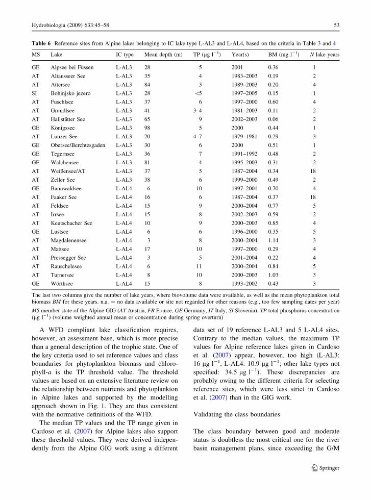
Based on the criteria given in Table 3 and 4,

reference sites were selected. The historical data from

the 1930s included five L-AL3 and two L-AL4 data

sets (Table 5), 14 L-AL3 and 12 L-AL4 data sets

came from monitoring programmes after 1978

(Table 6). Since Faaker See and Weißensee, which

were represented both in the historical and in the

monitoring data, were treated only once, the total sum

of reference sites belonging to IC lake type L-AL3

was 18, whereas 13 reference sites belonged to IC

lake type L-AL4.

Biomass values of deep (L-AL3) and shallow

(L-AL4) reference sites were significantly different

(Mann–Whitney test, P = 0.002). The median of the

phytoplankton total biomass in the L-AL3 reference

sites was 0.3 mg l-1, the median value for 13 L-AL4

lakes was 0.7 mg l-1. These values were defined as

reference values for total biomass in the two lake

types. The boundary between high and good ecolog-

ical status, which was set at the 95% percentile, is

0.5 mg l-1 for L-AL3 and 1.1 mg l-1 for L-AL4

(Table 7).

Fig. 2 Regression analysis between annual mean total phos-

phorus concentration and annual mean phytoplankton biomass

(biovolume) in lakes belonging to the Alpine lake types L-AL3

and L-AL4. Regressions are calculated separately for L-AL3,

very large lakes of L-AL3 (mean depth [100 m) and L-AL4

Hydrobiologia (2009) 633:45–58 51

123

The reference values for chlorophyll-a, which

were calculated using the regression given in Fig. 2,

are 1.9 lg l-1 in L-AL3 lakes and 3.3 lg l-1 in

L-AL4 lakes. Table 8 summarizes the reference

values and class boundaries for total biomass as well

as for chlorophyll-a, which were derived according to

the boundary setting protocol described above. It also

gives the ecological quality ratios, which lie between

0.60 and 0.75 for the H/G boundary and between 0.25

and 0.41 for the G/M boundary.

The ranges of the reference values, which were

calculated following the boundary setting protocol,

are 0.2–0.3 mg l-1 (L-AL3) and 0.5–0.7 mg l-1 (L-AL4)

for biomass and 1.5–1.9 lg l-1 (L-AL3) and

2.7–3.3 lg l-1 (L-AL4) for chlorophyll-a. The EQR

values given in Table 8 were used to set the ranges of

the class boundaries. Hence, only the absolute values

are different within each lake type, whereas the EQR

values are fixed. The final values for classifying lakes

using phytoplankton biomass or chlorophyll-a are

summarized in Table 9.

Discussion

The definition of type-specific reference conditions is

a major prerequisite for the WFD compliant assess-

ment of the ecological status of aquatic ecosystems.

Reference conditions for phytoplankton require a

clear description of the trophic state, which should

have as little variability as possible within each type.

Trophic state

The trophic state as defined in this article for deep

lakes (L-AL3, mean depth [15 m) complies well

with the general understanding of oligotrophy as a

reference trophic state in most Alpine lakes (LAWA,

1999; Premazzi et al., 2003; Buraschi et al., 2005).

The situation is less clear for moderately deep lakes

belonging to GIG type L-AL4. Whereas some lakes

are currently or previously oligotrophic (Hofmann &

Schaumburg, 2005; KIS, 2008), historical and paleo-

limnological data provide evidence that others have

been oligo-mesotrophic or mesotrophic prior to

significant anthropogenic impact (Frey, 1955).

Fig. 3 Regression analysis between annual mean phytoplank-

ton biomass (biovolume) and annual mean chlorophyll-aconcentration in lakes belonging to the Alpine lake types

L-AL3 and L-AL4. Very large and deep lakes of L-AL3 are not

calculated separately

Table 5 Reference sites from Alpine lakes belonging to IC lake type L-AL3 and L-AL4, based on historical data

MS Lake IC type Mean depth (m) Year(s) BM (mg l-1) N lake years

AT Millstatter See L-AL3 89 1932–1938 0.32 7

AT Ossiacher See L-AL3 20 1932–1938 0.29 7

AT Weißensee/AT L-AL3 37 1932–1934 0.15 3

AT Worthersee L-AL3 42 1931–1938 0.29 8

AT Data from Ruttner (1937) L-AL3 20–65 1931–1932 0.26 8

AT Faaker See L-AL4 16 1931–1937 0.32 5

AT Langsee L-AL4 13 1934–1935 0.86 2

MS member state of the Alpine GIG (AT = Austria), BM total phytoplankton biomass, N number of years available for each site

Due to methodological uncertainties, the data from Ruttner (1937) are treated as one data set (site) in the analyses

52 Hydrobiologia (2009) 633:45–58

123

A WFD compliant lake classification requires,

however, an assessment base, which is more precise

than a general description of the trophic state. One of

the key criteria used to set reference values and class

boundaries for phytoplankton biomass and chloro-

phyll-a is the TP threshold value. The threshold

values are based on an extensive literature review on

the relationship between nutrients and phytoplankton

in Alpine lakes and supported by the modelling

approach shown in Fig. 1. They are thus consistent

with the normative definitions of the WFD.

The median TP values and the TP range given in

Cardoso et al. (2007) for Alpine lakes also support

these threshold values. They were derived indepen-

dently from the Alpine GIG work using a different

data set of 19 reference L-AL3 and 5 L-AL4 sites.

Contrary to the median values, the maximum TP

values for Alpine reference lakes given in Cardoso

et al. (2007) appear, however, too high (L-AL3:

16 lg l-1, L-AL4: 10.9 lg l-1; other lake types not

specified: 34.5 lg l-1). These discrepancies are

probably owing to the different criteria for selecting

reference sites, which were less strict in Cardoso

et al. (2007) than in the GIG work.

Validating the class boundaries

The class boundary between good and moderate

status is doubtless the most critical one for the river

basin management plans, since exceeding the G/M

Table 6 Reference sites from Alpine lakes belonging to IC lake type L-AL3 and L-AL4, based on the criteria in Table 3 and 4

MS Lake IC type Mean depth (m) TP (lg l-1) Year(s) BM (mg l-1) N lake years

GE Alpsee bei Fussen L-AL3 28 5 2001 0.36 1

AT Altausseer See L-AL3 35 4 1983–2003 0.19 2

AT Attersee L-AL3 84 3 1989–2003 0.20 4

SI Bohinjsko jezero L-AL3 28 \5 1997–2005 0.15 1

AT Fuschlsee L-AL3 37 6 1997–2000 0.60 4

AT Grundlsee L-AL3 41 3–4 1981–2003 0.11 2

AT Hallstatter See L-AL3 65 9 2002–2003 0.06 2

GE Konigssee L-AL3 98 5 2000 0.44 1

AT Lunzer See L-AL3 20 4–7 1979–1981 0.29 3

GE Obersee/Berchtesgaden L-AL3 30 6 2000 0.51 1

GE Tegernsee L-AL3 36 7 1991–1992 0.48 2

GE Walchensee L-AL3 81 4 1995–2003 0.31 2

AT Weißensee/AT L-AL3 37 5 1987–2004 0.34 18

AT Zeller See L-AL3 38 6 1999–2000 0.49 2

GE Bannwaldsee L-AL4 6 10 1997–2001 0.70 4

AT Faaker See L-AL4 16 6 1987–2004 0.37 18

AT Feldsee L-AL4 15 9 2000–2004 0.77 5

AT Irrsee L-AL4 15 8 2002–2003 0.59 2

AT Keutschacher See L-AL4 10 9 2000–2003 0.85 4

GE Lustsee L-AL4 6 6 1996–2000 0.35 5

AT Magdalenensee L-AL4 3 8 2000–2004 1.14 3

AT Mattsee L-AL4 17 10 1997–2000 0.29 4

AT Pressegger See L-AL4 3 5 2001–2004 0.22 4

AT Rauschelesee L-AL4 6 11 2000–2004 0.84 5

AT Turnersee L-AL4 8 10 2000–2003 1.03 3

GE Worthsee L-AL4 15 8 1993–2002 0.43 3

The last two columns give the number of lake years, where biovolume data were available, as well as the mean phytoplankton total

biomass BM for these years. n.a. = no data available or site not regarded for other reasons (e.g., too few sampling dates per year)

MS member state of the Alpine GIG (AT Austria, FR France, GE Germany, IT Italy, SI Slovenia), TP total phosphorus concentration

(lg l-1) (volume weighted annual mean or concentration during spring overturn)

Hydrobiologia (2009) 633:45–58 53

123

boundary forces the member states to set actions for

improving the ecological status. A validation of the

values was done using the TP—biomass response

curves for several phytoplankton taxa, with sensitive

Cyclotella species as the most important taxon.

Cyclotella often dominates in nutrient poor Alpine

lakes (Wunsam et al., 1995; Schaumburg et al., 2005)

and may reach a relative proportion of annual mean

total biomass of up to 95% in single years and about

2/3 for lake annual means. A decline of the relative

proportion of Cyclotella to B20% corresponds to a

total biomass of about 1–2 mg l-1. The boundary set

for L-AL3 lakes lies well within this range.

Another approach for validating the boundary

setting is the detection of significant undesirable

disturbances in the condition of other biological

quality elements and the physicochemical quality of

the water or sediment. There are numerous examples

from Alpine lakes in the literature, such as the decline

of macrophytes, especially of charophytes and reeds

(e.g. Deufel, 1978; Lachavanne, 1979; Schroeder,

1979; Melzer et al., 2003), and of white fish,

Coregonus spp., and arctic charr, Salvelinus umbla

(L.), with increasing eutrophication (Brutschy &

Guntert, 1923; Stadelmann, 1984; Hartmann &

Quoss, 1993; Gassner et al., 2003). In some lakes

touristic use was heavily affected by Planktothrix

blooms in the 1970s (Schulz et al., 2005). Neverthe-

less, these examples of ‘undesirable conditions’ can

only be used for validating, but not for definitively

setting the class boundaries, since the responses

remain more or less descriptive in most articles and

reports. The interactions between phytoplankton and

other biological quality elements can vary a lot and in

many cases, and they are not well understood and/or

quantified. Besides, they are often different in phases

of eutrophication and re-oligotrophication (Anneville

& Pelletier, 2000; Dokulil et al., 2001).

Weak correlations were found also for other tools

for selecting reference values and setting class

Table 7 Statistics (minimum, median, arithmetic mean, percentiles) of the annual mean phytoplankton biomass (mg l-1) for Alpine

lakes, calculated from pre-selected reference sites (Tables 5 and 6)

IC lake type Min Median ref. Mean 75% perc. 90% perc. 95% perc H/G Max N

L-AL3 0.06 0.30 0.31 0.42 0.49 0.52 0.60 18

L-AL4 0.22 0.70 0.65 0.85 0.99 1.07 1.14 13

Ref reference value, H/G high/good class boundary

Table 8 Reference values, class boundaries and EQR (eco-

logical quality ratio, in italics) for the annual mean total bio-

mass (mg l-1) and the annual mean chlorophyll-aconcentration (lg l-1) in Alpine lakes

Parameter IC lake type Ref. H/G G/M M/P P/B

Total biomass

(mg l-1)

L-AL3 0.3 0.5 1.2 3.1 7.8

EQR 1.00 0.60 0.25 0.10 0.04

L-AL4 0.7 1.1 2.7 6.9 17.4

EQR 1.00 0.64 0.26 0.10 0.04

Chlorophyll-a(lg l-1)

L-AL3 1.9 2.7 4.7 8.7 15.8

EQR 1.00 0.70 0.40 0.22 0.12

L-AL4 3.3 4.4 8.0 14.6 26.7

EQR 1.00 0.75 0.41 0.23 0.12

H/G class boundary high/good status, G/M good/moderate,

M/P moderate/poor, P/B poor/bad

Table 9 Ranges for reference values and class boundaries for the annual mean total biomass (mg l-1) and the annual mean

chlorophyll-a concentration (lg l-1) in Alpine lakes

Parameter IC lake type Ref. H/G G/M M/P P/B

Total biomass (mg l-1) L-AL3 0.2–0.3 0.3–0.5 0.8–1.2 2.1–3.1 5.3–7.8

L-AL4 0.5–0.7 0.8–1.1 1.9–2.7 5.0–6.9 12.5–17.4

Chlorophyll-a (lg l-1) L-AL3 1.5–1.9 2.1–2.7 3.8–4.7 6.8–8.7 12.5–15.8

L-AL4 2.7–3.3 3.6–4.4 6.6–8.0 11.7–14.6 22.5–26.7

The EQR values given in Table 8 are fixed and apply to all the reference values and class boundaries

54 Hydrobiologia (2009) 633:45–58

123

boundaries. Pressure criteria such as land use (using

Corine land cover data) and population density

equivalents were poorly correlated with trophic state,

maybe because none of them include information

about sewage treatment for point sources in the

catchment area.

A simple site-specific predictive model based on the

morpho-edaphic index MEI (Vighi & Chiaudani, 1985)

was used by Cardoso et al. (2007) for defining total

phosphorus concentrations under reference conditions

of European lakes. According to the authors, the MEI

compared favourably to more sophisticated predictive

models. In the data set used for this article, it turned out

to be of limited use. Since the MEI regression of Vighi &

Chiaudani (1985) estimated significantly higher TP

concentrations for several (ultra-)oligotrophic lakes

than are currently present, the MEI approach to defining

reference status and setting boundaries was therefore

considered as being not precautionary enough and was

thus not pursued further.

Reference values

The reference values proposed in this article are of

the same magnitude as those published for compara-

ble lakes in Europe by Carvalho et al. (2008) as an

outcome of the REBECCA project. The chlorophyll-

a reference value of deep Alpine lakes was 2.8 lg l-1

in the analysis of Carvalho et al. (2008) and thus

slightly higher than those proposed for L-AL3 lakes

in this article (Table 8). This discrepancy comes

mainly from the different and much smaller data sets

used by Carvalho et al. (2008). It included only lakes

from Germany and focussed on the mean of the

vegetation season, whereas the annual mean is used

in this article. In the GIG data set, the mean

phytoplankton biomass in the period from March to

November was 5.3% (±1.3%, 95% C.L.) higher than

the annual mean, with the mean for the period April

to October differing even by 9.3% (±2.2%).

In other GIGs, reference values similar to those

proposed for Alpine lakes have been found in oligo-

trophic northern European lakes, in contrast to the

significantly higher values in moderately deep and

shallow lakes in the Central-Baltic region (EU Com-

mission, 2008). In comparable lakes in the United

States, chlorophyll-a reference values of 1.9 lg l-1

(ecoregion II, Western forested mountains), 2.4 lg l-1

(ecoregion VIII, Nutrient poor largely glaciated upper

Midwest and Northeast) and 2.8 lg l-1 (ecoregion XI,

Central and Eastern forested uplands) were defined

(U.S. EPA, 2000a, b, c). These values are broadly

similar to those proposed for L-AL-3 and L-AL4,

although the setting of the reference values was done in

a different way (viz. at the 25% percentile of all the

values occurring in the data set).

Methodological constraints and future prospects

Apart from the boundary setting protocol, which is

described in this article, there are two aspects which

strongly influence the confidence of the values: lake

types, and sampling and analytical methods. Differ-

ences between sites within each of the two lake types

of the Alpine GIG are probably well covered by the

ranges of reference values and class boundaries as

defined for L-AL3 and L-AL4.

An unknown proportion of variability, however, is

because of methodological differences in sampling

(e.g., frequency, sampling depth) and analytics (e.g.,

counting method). The fact that there are differences

in methods is not surprising while facing the long

period from which the data come from. It was tried to

minimize uncertainties due to these methodological

differences in the selection of the sites, which were

included in the analyses.

The monitoring programs carried out in each of the

Alpine countries will improve the data base by

providing not only more data, but data that will bear

less methodological uncertainties since they will

increasingly follow international standards in sam-

pling and analytics. Within a few years, it will be

possible to re-calculate reference values and class

boundaries with higher confidence.

Conclusion

The protocol to define reference conditions and set

boundaries as proposed by the Alpine GIG within the

IC exercise and described in this article proved to be

useful and applicable. It adopted a broad approach

including historical, paleolimnological and monitor-

ing data, but included also expert judgement and the

experience of several decades of limnological research

in Alpine lakes. The response of sensitive taxa to

increased nutrient levels as well as ‘undesirable

conditions and secondary effects’ (as described in

Hydrobiologia (2009) 633:45–58 55

123

Annex V in the WFD) was used to validate the

boundaries.

The values proposed here are partly implemented

in national law (e.g. Wolfram & Dokulil, 2008) and

form the basis for decisions within the national river

basin management plans as required by the WFD.

The intercalibration between the five Alpine EU

member states was thus an important step towards a

harmonization of the common understanding of

‘Good Ecological Status’. A second step has been

made by starting the intercalibration on the taxo-

nomic composition of phytoplankton. The final

intercalibration outcome—with both biomass/chloro-

phyll-a and taxonomic composition-based trophic

indices included—is expected in 2010.

Acknowledgements The authors thank the data owners and

providers of chemical and biological data (Gisela Ofenbock

and Veronika Koller-Kreimel/BMLFUW, Peter Schaber/Amt

der Salzburger Landesregierung, Ute Mischke/IGB, Hubert

Gassner/BAW Scharfling, IGKB) for their cooperation in the

establishment of the Alpine GIG phytoplankton intercalibration

data set. Thanks to the JRC, especially to Sandra Poikane, for

accompanying the Alpine GIG during the whole IC exercise,

and to numerous experts from other GIGs for fruitful

discussions and constructive criticism.

References

Alefs, J., J. Muller & B. Lenhart, 1996. Die jahrliche Anderung

der Diatomeenvergesellschaftung seit 1958 in einem

warvendatierten Sedimentkern aus dem Ammersee

(Oberbayern). Limnologica 26: 39–48.

Amann, H., 1918. Die Geschichte einer Wasserblute. Archiv

fur Hydrobiologie 11: 496–501.

Anneville, O. & J. P. Pelletier, 2000. Recovery of Lake Geneva

from eutrophication: quantitative response of phyto-

plankton. Archiv fur Hydrobiologie 148: 607–624.

BMGU & BMWF, 1983. Ergebnisse des osterreichischen Eu-

trophieprogrammes 1978–1982. Bundesministerium fur

Gesundheit und Umweltschutz, Bundesministerium fur

Wissenschaft und Forschung, Wien: 106 pp.

Brutschy, A. & A. Guntert, 1923. Gutachten uber den Ruck-

gang des Fischbestandes im Hallwilersee. Archiv fur

Hydrobiologie 14: 523–571.

Buraschi, E., F. Salerno, C. Monguzzi, G. Barbiero & G.

Tartari, 2005. Characterization of the Italian lake-types

and identification of their reference sites using anthropo-

genic pressure factors. Journal of Limnology 64: 75–84.

Cardoso, A. C., A. Solimini, G. Premazzi, L. Carvalho, A.

Lyche Solheim & S. Rekolainen, 2007. Phosphorus ref-

erence concentrations in European lakes. Hydrobiologia

584: 3–12.

Carvalho, L., A. Solimini, G. Phillips, M. van den Berg, O.-P.

Pietilainen, A. Lyche Solheim, S. Poikane & U. Mischke,

2008. Chlorophyll reference conditions for European lake

types used for intercalibration of ecological status.

Aquatic Ecology 45: 203–211.

CEN, 2007. Phytoplankton biovolume determination using

inverted microscopy (Utermohl technique). CEN TC 230/

WG 2/TG 3 (2007). Draft proposal 2006, Brussels.

CIS, 2003a. Towards a guidance on establishment of the

intercalibration network and the process on the intercali-

bration exercise. Common Implementation Strategy for

the Water Framework Directive (2000/60/EC), Guidance

document 6. Working Group 2.4—Intercalibration,

European Commission: 47 pp. http://circa.europa.eu.

CIS, 2003b. River and lakes—typology, reference conditions

and classification systems. Common Implementation

Strategy for the Water Framework Directive (2000/60/

EC), Guidance document 10, Working Group 2.3—

REFCOND, European Commission: 86 pp. http://circa.

europa.eu.

Danielopol, D., R. Schmidt & E. Schultze (eds), 1985. Con-

tributions to the paleolimnology of the Trumer Lakes

(Salzburg), and the Lakes Mondsee, Attersee and Traun-

see (Upper Austria). Limnologisches Institut der Oster-

reichischen Akademie der Wissenschaften, Wien.

Deufel, J., 1978. Veranderungen der Schilf- und Wasser-

pflanzenbestande im Bodensee wahrend der Eutrophie-

rung und ihre Auswirkungen auf die Fische. Arbeiten des

Deutschen Fischerei-Verbandes 25: 30–34.

Directive, 2000. Directive 2000/60/EC of the European Par-

liament and of the council of 23 October 2000 establish-

ing a framework for community action in the field of

water policy. Official Journal of the European Commu-

nities L 327: 1–72.

Dokulil, M.T., A. Hamm & J.-G. Kohl (eds), 2001. Okologie

und Schutz von Seen. UTB, Facultas-Universitats-Verlag,

Wien.

Dokulil, M. T. & K. Teubner, 2006. Bewertung der Phyto-

planktonstruktur stehender Gewasser gemaß der EU-

Wasserrahmenrichtlinie: Der modifizierte Brettum-Index.

Deutsche Gesellschaft fur Limnologie (DGL), Tag-

ungsbericht 2005 (Karlsruhe), Werder 2006: 356–360.

EN, 2006. Water quality—guidance standard on the enumer-

ation of phytoplankton using inverted microscopy (Uter-

mohl technique). EN 15204 (2006).

EU Commission, 2008. Decision of 30 October 2008 estab-

lishing, pursuant to Directive 2000/60/EC of the European

Parliament and of the Council, the values of the Member

State monitoring system classifications as a result of the

intercalibration exercise. Official Journal of the European

Union L 332/20 10.12.2008, Brussels.

Feuillade, M., J. Dominik, J.-C. Druart & J.-L. Loizeau, 1995.

Trophic status evolution of Lake Nantua as revealed by

biological records in sediment. Archiv fur Hydrobiologie

132: 337–362.

Findenegg, I., 1935. Limnologische Untersuchungen im

Karntner Seengebiet. Internationale Revue der gesamten

Hydrobiologie Hydrographie 32: 408–415.

Findenegg, I., 1954. Versuch einer soziologischen Gliederung

der Karntner Seen nach ihrem Phytoplankton. Angewandte

Pflanzensoziologie, Festschrift Aichinger 1: 299–309.

Forel, F.-A., 1892–1902. Lac Leman. Monographie Limno-

logique. Lausanne.

56 Hydrobiologia (2009) 633:45–58

123

Frey, D. G., 1955. Langsee: a history of meromixis. Memorie

dell’Istituto Italiano di Idrobiologia, Suppl. 8: 141–164.

Fricker, H. (ed.), 1980. OECD eutrophication programme

regional project Alpine lakes. Swiss Federal Board for

Environmental Protection (Bundesamt fur Umweltschutz),

Bern: 234 pp.

Gassner, H., D. Zick, J. Wanzenbock, B. Lahnsteiner & G.

Tischler, 2003. Die Fischartengemeinschaften der großen

osterreichischen Seen. Schriftenreihe des BAW 18: 1–83.

Guilizzoni, P. & A. Lami, 1992. Historical records of changes in

the chemistry and biology of Italian lakes. In Guilizzoni, P.,

G. Tartari, G. Giussani (eds), Limnology in Italy, Vol. 50.

Memorie dell’Istituto Italiano di Idrobiologia: 61–77.

Guilizzoni, P., G. Bonomi, G. Galanti & D. Ruggiu, 1982.

Basic trophic status and recent development of some

Italian lakes as revealed by plant pigments and other

chemical components in sediment cores. Memorie

dell’Istituto Italiano di Idrobiologia 40: 79–98.

Halbfaß, W., 1923. Grundzuge einer vergleichenden Seen-

kunde. Verlag der Gebruder Borntraeger, Berlin.

Hartmann, J. & H. Quoss, 1993. Fecundity of whitefish

(Coregonus lavaretus) during the eutrophication and oli-

gotrophication of Lake Constance. Journal of Fish Biol-

ogy 43: 81–87.

Higgitt, S. R., F. Oldfield & P. G. Appleby, 1991. The record of

land use change and soil erosion in the late Holocene

sediments of the Petit Lac d’Annecy, eastern France. The

Holocene 1: 14–28.

Hofmann, G. & J. Schaumburg, 2005. Seesedimente in Bayern:

Waginger-Tachinger See, Diatomeenflora in Sediment-

kernen August 2002. Bayerisches Landesamt fur Was-

serwirtschaft, Materialien 121: 1–76.

IGKB, 2004a. Der Bodensee, Zustand – Fakten – Perspektiven.

Bilanz 2004. IGKB, Bregenz.

IGKB, 2004b. Aktionsprogramm Bodensee 2004 bis 2009.

Schwerpunkt Ufer- und Flachwasserzone. IGKB,

Bregenz.

ISO, 1985. Bestimmung des Chlorophyll-a-Gehaltes von

Oberflachenwasser. ISO 38412-16:1985.DIN.

Kaiblinger C., O. Anneville, R. Tadonleke, F. Rimet, J. C.

Druart, J. Guillard & M. T. Dokulil, submitted. Central-

European Water Quality indices applied to long-term data

from peri-alpine lakes: test and possible improvements.

Hydrobiologia.

KIS, 2008. Karntner Seenbericht 2008. Karntner Institut fur

Seenforschung. www.kis.ktn.gv.at/seenbericht.htm.

Klee, R. & R. Schmidt, 1987. Eutrophication of Mondsee

(Upper Austria) as indicated by the diatom stratigraphy of

a sediment core. Diatom Research 2: 55–76.

Klee, R., R. Schmidt & J. Muller, 1993. Allerod diatom

assemblages in prealpine hardwater lakes of Bavaria and

Austria as preserved by the Laacher See eruption event.

Limnologica 23: 131–143.

Lachavanne, J.-B., 1979. Les macrophytes du lac de Morat.

Berichte der Schweizerischen Botanischen Gesellschaft

89: 114–132.

LAWA, 1999. Gewasserbewertung—stehende Gewasser.

Vorlaufige Richtlinie fur eine Erstbewertung von naturlich

entstandenen Seen nach trophischen Kriterien 1998.

Landerarbeitsgemeinschaft Wasser, Kulturbuch-Verlag

Berlin GmbH, Berlin.

Loffler, H., 1978. The paleolimnology of some Carinthian

lakes with special reference to Worthersee. Polish

Archives of Hydrobiology 25: 227–232.

Loizeau, J.-L., D. Span, V. Coppee & J. Dominik, 2001.Evolution of the trophic state of Lake Annecy (eastern

France) since the last glaciation as indicated by iron,

manganese, and phosphorus speciation. Journal of Paleo-

limnology 25: 205–214.

Lorenzen, C. J., 1967. Determination of chlorophyll and

phaeopigments: spectrophotometric equations. Limnology

and Oceanography 12: 343–346.

Lotter, A. F., 2001. The palaeolimnology of Soppensee (Cen-

tral Switzerland), as evidenced by diatom, pollen and

fossil-pigment analysis. Journal of Paleolimnology 25:

65–79.

Lyche Solheim, A., S. Rekolainen, S. J. Moe, L. Carvalho, G.

Phillips, R. Ptacnik, W. E. Penning, L. G. Toth, C.

O’Toole, A.-K. L. Schartau & T. Hesthagen, 2008. Eco-

logical threshold responses in European lakes and their

applicability for the Water Framework Directive (WFD)

implementation: synthesis of lakes results from the

REBECCA project. Aquatic Ecology 42: 317–334.

Marchetto, A. & R. Bettinetti, 1995. Reconstruction of the

phosphorus history of two deep, subalpine Italian lakes

from sedimentary diatoms, compared with long-term

chemical measurements. Memorie dell’Istituto Italiano di

Idrobiologia 53: 27–38.

Marchetto, A. & S. Musazzi, 2001. Comparison between sed-

imentary and living diatoms in Lago Maggiore (N. Italy):

implications of using transfer functions. Journal of Lim-

nology 60: 19–26.

Melzer, A., C. Scholze, F.-M. Goos & S. Zimmermann, 2003.

Seelitorale in Bayern, Chiemsee. Makrophyten-Kartie-

rungen 1985 und Bayer. Landesamt fur Wasserwirtschaft

Materialien 108: 83 pp.

Nixdorf, B., U. Mischke, E. Hoehn & U. Riedmuller, 2005.

Bewertung von Seen anhand des Phytoplanktons. Lim-

nologie aktuell 11: 105–120.

OECD, 1982. Eutrophication of waters—monitoring, assess-

ment and control. Organization for Economic Cooperation

and Development, Paris: 154.

Premazzi, G., A. Dalmiglio, A. C. Cardoso & G. Chiaudani,

2003. Lake management in Italy: the implications of the

Water Framework Directive. Lakes and Reservoirs:

Research and Management 8: 41–59.

Ruttner, F., 1937. Okotypen mit verschiedener Vertikalvertei-

lung im Plankton der Alpenseen. Internationale Revue der

gesamten Hydrobiologie 35: 7–34.

Schaumburg, J., 1996. Seen in Bayern—Limnologische

Entwicklung von 1980 bis 1994. Informationsberichte

Bayerisches Landesamt fur Wasserwirtschaft 1/96: 216 pp.

Schaumburg, J., M. Colling, I. Schloßer, B. Kopf & F. Fischer,

2005. Okologische Typisierung des Phytoplanktons. In-

formationsbericht des Bayerischen Landesamtes fur

Wasserwirtschaft 3/05: 61 pp.

Schmidt, R., 1989. Diatomeenstratigraphische Untersuchungen

zur Trophieanderung und Industrieschlammakkumulation

im Traunsee/Osterreich. Aquatic Sciences 51: 317–337.

Schmidt, R., R. Psenner, J. Muller, P. Indinger & C. Kamenik,

2002. Impact of late glacial climate variations on strati-

fication and trophic state of the meromictic lake Langsee

Hydrobiologia (2009) 633:45–58 57

123

(Austria): validation of a conceptual model by multi proxy

studies. Journal of Limnology 61: 49–60.

Schroeder, R., 1979. Decline of reed swamps in Lake Con-

stance. Symposium Biologica Hungarica 19: 43–48.

Schulz, L., R. Fresner, M. Reichmann, G. Santner, M. Mai-

ritsch, M. Ambros, W. Honsig-Erlenburg, G. Weissel, B.

Hummitzsch & J. Petutschnig, 2005. Der Millstatter

See—limnologische Langzeitentwicklung 1970–2002.

Veroffentlichungen des Karntner Institutes fur Seenfor-

schung, Klagenfurt.

Stadelmann, P., 1984. Die Zustandsentwicklung des Baldeg-

gersees (1900 bis 1980) und die Auswirkung von seein-

ternen Maßnahmen. Wasser, Energie, Luft 76: 85–95.

U.S. EPA, 2000a. Ambient water quality criteria recommen-

dations. Information supporting the development of state

and tribal nutrient criteria. Lakes and reservoirs in nutrient

ecoregion II. Office of Water, Environmental Protection

Agency 822-B-00-007.

U.S. EPA, 2000b. Ambient water quality criteria recommen-

dations. Information supporting the development of state

and tribal nutrient criteria. Lakes and reservoirs in nutrient

ecoregion VIII. Office of Water, Environmental Protec-

tion Agency 822-B-00-010.

U.S. EPA, 2000c. Ambient water quality criteria recommen-

dations. Information supporting the development of state

and tribal nutrient criteria. Lakes and reservoirs in nutrient

ecoregion XI. Office of Water, Environmental Protection

Agency 822-B-00-012.

Utermohl, H., 1958. Zur Vervollkommnung der quantitativen

Phytoplankton-Methodik. Mitteilungen der internationa-

len Vereinigung fur theoretische und angewandte Lim-

nologie 9: 1–38.

Vighi, M. & G. Chiaudani, 1985. A simple method to estimate

lake phosphorus concentrations resulting from natural

background loading. Water Research 10: 987–991.

Vollenweider, R. A., 1976. Advances in defining critical

loading levels for phosphorus in lake eutrophication.

Memorie dell’Istituto Italiano di Idrobiologia 33: 53–69.

Vollenweider, R. A. & K. Kerekes, 1980. The loading concept

as a basis for controlling eutrophication philosophy and

preliminary results of the OECD programme on eutro-

phication. Progress in Water Technology 12: 5–38.

Wolfram, G. & M. T. Dokulil, 2008. Leitfaden zur Erhebung

der Biologischen Qualitatselemente, Seen. Teil B2-01d—

phytoplankton. Handbuch des BMLFUW & des BAW,

Wien: 48 pp. (http://wasser.lebensministerium.at/article/

articleview/52972/1/5659/).

Wunsam, S., R. Schmidt & R. Klee, 1995. Cyclotella-taxa

(Bacillariophyceae) in lakes of the Alpine region and their

relationship to environmental variables. Aquatic Sciences

57: 360–386.

58 Hydrobiologia (2009) 633:45–58

123