Abstract: Mass customized products usually follow a non-standardized demand pattern. Thus, it is crucial for production managers to overcome such uncertainties in an effective way. During the last decades, Just In Time (JIT) systems seem to gain ground in this race of finding analogous solution spaces. On the other hand, forecasting techniques stand as an equivocal solution, and they gradually become more mature and useful as well. The procedure of managing demand uncertainty, by finding solution spaces, reflects the need for managers to be aware of possible future states of demand. Situation Awareness, specifically, requires the perception, comprehension, and projection of every operational state of the examined system. The current paper studies the demand uncertainty and its effect on production planning. It suggests a procedure for forming the awareness of demand uncertainty, and at the same time a ‘SA-inspired’ system for production planning in Mass Customization companies. Key Words: Demand Situation Awareness (DemSA), GM(1,1), Kanban, Production Planning

1. INTRODUCTION

In substance, awareness refers to the state or ability to perceive, feel, or be conscious of events, objects, or sensory patterns. Although it was initially considered a cognitive procedure, it was then acknowledged that the awareness of a situation is a significant task and process in every expression of engineering or science concepts in general. Yet, Situation Awareness (SA) is a ‘patented’ term, widely used since 1988, describing the observation and understanding of environmental elements with respect to time and space. It is a field of study concerned with the perception of the environment, critical to decision makers acting in complex and dynamic areas.

SA is used herein to prove the utility of gained experience in Mass Customization (MC) production lines and through this, we propose a method towards reducing demand uncertainty in terms of customized products. Thus, in order to form the Demand Situation Awareness ( DemSA ), regarding its uncertainty, a practical tool that delivers a quantitative indication to SA and a corresponding estimation of demand is needed.

Such a tool could possibly belong to the group of Grey Analysis (GA) mathematical modeling, on the grounds that its focus is on the problems of uncertainty of small samples and poor information that are difficult for probability and fuzzy mathematics to handle. What is more, grey models (GM) are a practical tool in case of having sequences of data, something common in production lines.

In a nutshell, the present work focuses on the applicability of GM to predicting, planning, and providing awareness of the posible future levels of demand. The paper’s utmost aim is to add value, stimulate, and enhance the attempts of coping with demand uncertainty. For one thing, and before elaborating on the proposed method, it is useful to make an introduction to SA and GA.

2. THE SIGNIFICANCE OF BEING AWARE OF PRODUCTION DEMAND

One widely cited definition proposes SA as a state of working knowledge of an individual; it is how much, and how accurately, humans are aware of their current situation and it concerns (1) the perception of the elements within a system, (2) the comprehension of their meaning, and (3) the projection of their future state [1]. Another definition [2] argues that SA is what someone needs to know in order not to be surprised.

In a MC company, a ‘surprise’ might be an unexpected fluctuation in production demand, for instance. Thus, in order to avoid or reduce ‘surprises’, i.e. to expect such fluctuations, organizations need to use production data, refering to a given customized product, perceive the current demand situation regarding sophisticated products or customer preferences, comprehend market trends, and, finally, project the possible impeding volume of demand aided by production data. These three fundamental steps of the DemSA formation process are depicted in Figure 1, specifically in the upper shape, which is a readaptation of Endsley’s three-level model [1] illustrated in the upper shape of Figure 1.

The perception-comprehension-projection process opens the path towards DemSA and sets the context

Reducing Uncertainty in a Mass Customization Company by Demand Situation Awareness

Maria Mikela Chatzimichailidou(1), Christos G. Chatzopoulos(2), Stefanos Katsavounis(2) (1)Democritus University of Thrace, Civil Engineering, Xanthi, Hellenic Republic

(2)Democritus University of Thrace, Production Engineering & Management, Xanthi, Hellenic Republic

27

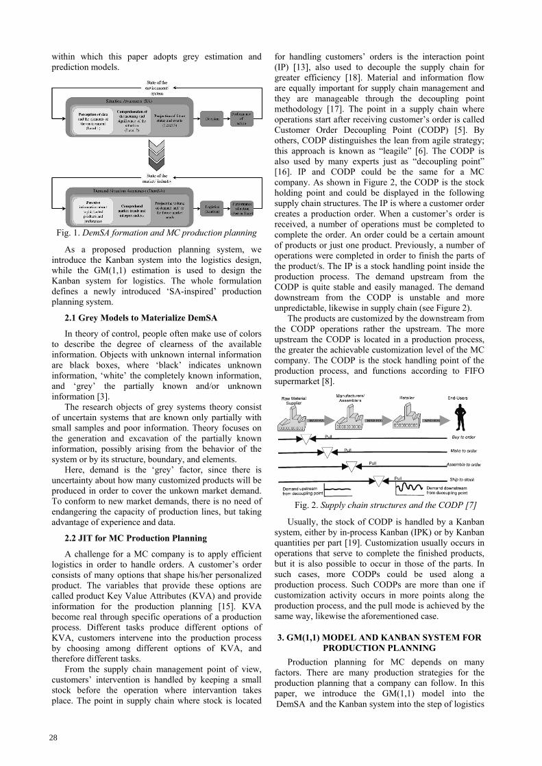
within which this paper adopts grey estimation and prediction models.

Fig. 1. DemSA formation and MC production planning

As a proposed production planning system, we introduce the Kanban system into the logistics design, while the GM(1,1) estimation is used to design the Kanban system for logistics. The whole formulation defines a newly introduced ‘SA-inspired’ production planning system.

2.1 Grey Models to Materialize DemSA

In theory of control, people often make use of colors to describe the degree of clearness of the available information. Objects with unknown internal information are black boxes, where ‘black’ indicates unknown information, ‘white’ the completely known information, and ‘grey’ the partially known and/or unknown information [3].

The research objects of grey systems theory consist of uncertain systems that are known only partially with small samples and poor information. Theory focuses on the generation and excavation of the partially known information, possibly arising from the behavior of the system or by its structure, boundary, and elements.

Here, demand is the ‘grey’ factor, since there is uncertainty about how many customized products will be produced in order to cover the unkown market demand. To conform to new market demands, there is no need of endangering the capacity of production lines, but taking advantage of experience and data.

2.2 JIT for MC Production Planning

A challenge for a MC company is to apply efficient logistics in order to handle orders. A customer’s order consists of many options that shape his/her personalized product. The variables that provide these options are called product Key Value Attributes (KVA) and provide information for the production planning [15]. KVA become real through specific operations of a production process. Different tasks produce different options of KVA, customers intervene into the production process by choosing among different options of KVA, and therefore different tasks.

From the supply chain management point of view, customers’ intervention is handled by keeping a small stock before the operation where intervantion takes place. The point in supply chain where stock is located

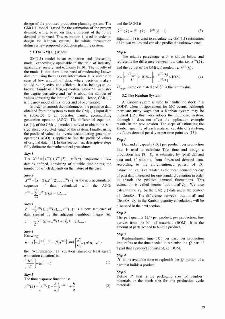
for handling customers’ orders is the interaction point (IP) [13], also used to decouple the supply chain for greater efficiency [18]. Material and information flow are equally important for supply chain management and they are manageable through the decoupling point methodology [17]. The point in a supply chain where operations start after receiving customer’s order is called Customer Order Decoupling Point (CODP) [5]. By others, CODP distinguishes the lean from agile strategy; this approach is known as “leagile” [6]. The CODP is also used by many experts just as “decoupling point” [16]. IP and CODP could be the same for a MC company. As shown in Figure 2, the CODP is the stock holding point and could be displayed in the following supply chain structures. The IP is where a customer order creates a production order. When a customer’s order is received, a number of operations must be completed to complete the order. An order could be a certain amount of products or just one product. Previously, a number of operations were completed in order to finish the parts of the product/s. The IP is a stock handling point inside the production process. The demand upstream from the CODP is quite stable and easily managed. The demand downstream from the CODP is unstable and more unpredictable, likewise in supply chain (see Figure 2).

The products are customized by the downstream from the CODP operations rather the upstream. The more upstream the CODP is located in a production process, the greater the achievable customization level of the MC company. The CODP is the stock handling point of the production process, and functions according to FIFO supermarket [8].

Fig. 2. Supply chain structures and the CODP [7]

Usually, the stock of CODP is handled by a Kanban system, either by in-process Kanban (IPK) or by Kanban quantities per part [19]. Customization usually occurs in operations that serve to complete the finished products, but it is also possible to occur in those of the parts. In such cases, more CODPs could be used along a production process. Such CODPs are more than one if customization activity occurs in more points along the production process, and the pull mode is achieved by the same way, likewise the aforementioned case.

3. GM(1,1) MODEL AND KANBAN SYSTEM FOR PRODUCTION PLANNING

Production planning for MC depends on many factors. There are many production strategies for the production planning that a company can follow. In this paper, we introduce the GM(1,1) model into the DemSA and the Kanban system into the step of logistics

28

design of the proposed production planning system. The GM(1,1) model is used for the estimation of the present demand, while, based on this, a forecast of the future demand is pursued. This estimation is used in order to design the Kanban system. The whole formulation defines a new proposed production planning system.

3.1 The GM(1,1) Model

GM(1,1) model is an estimation and forecasting model, exceedingly applicable in the field of industry, agriculture, society, and economy [9,10]. The novelty of the model is that there is no need of moderating known data, but using them as raw information. It is suitable in case of low amount of data, where decision makers should be objective and efficient. It also belongs to the broader family of GM(n,m) models, where ‘n’ indicates the degree derivative and ‘m’ is about the number of values consisting the input of the model. Hence, GM(1,1) is the grey model of first order and of one variable.

In order to smooth the randomness, the primitive data obtained from the system to form the GM(1,1) input data is subjected to an operator, named accumulating generation operator (AGO). The differential equation, i.e. (1), of the GM(1,1) model is solved to obtain the k -step ahead predicted value of the system. Finally, using the predicted value, the inverse accumulating generation operator (IAGO) is applied to find the predicted values of original data [11]. In this section, six descriptive steps fully delineate the mathematical procedure:

Step 1 The )(),...,2(),1( )0()0()0()0( nxxxX sequence of raw

data is defined, consisting of suitable time-points, the number of which depends on the nature of the case.

Step 2 )(),...,2(),1( )1()1()1()1( nxxxX is the new accumulated

sequence of data, calculated with the AGO:

k

i

nkixx1

)0()1( ,...,2,1),(

Step 3 )(),...,2(),1( )1()1()1()1( nxzz is a new sequence of

data created by the adjacent neighbour means [6]:

nkkxkxz ,...,3,2,)1()(2

1 )1()1()1(

Step 4 Knowing:

)1(ZfB , )0(XfY and YBBBb

a TT 1)(

the ‘whitenization’ [3] equation (image or least square estimation equation) is:

baxdt

dx

)1()1(

(1)

Step 5 The time response function is:

a

be

a

bxkx ka

)1()0()1( )1()(

(2)

and the IAGO is:

)1()()( )1()1()0( kxkxkx (3)

Equation (3) is used to calculate the GM(1,1) estimation of known values and can also predict the unknown ones.

Step 6 The relative percentage error is shown below and

represents the difference between raw data, i.e. )()0( kx ,

and the output of the GM(1,1) model, i.e. )()0( kx

.

(0)

(0)

( )1 100% 1 100%

( )

apprU x k

U x k

(4)

apprU is the estimated and U is the input value.

3.2 The Kanban System

A Kanban system is used to handle the stock in a CODP, when postponement for MC occurs. Although there are many ways that a Kanban system may be utilized [12], this work adopts the multi-card system, although it does not affect the application example results in the next session. The steps of estimating the Kanban quantity of each material capable of satisfying the future demand per day or per time-point are [13]:

Step 1 Demand at capacity ( cD ) per product, per production

line, is used to calculate Takt time and design a production line [8]. cD is estimated by (past) demand

data and, if possible, from forecasted demand data. According to the aforementioned pattern of cD

estimation, cD is calculated as the mean demand per day

of past data increased for one standard deviation in order to absorb the positive demand fluctuations. This estimation is called herein ‘traditional’ cD . We also

calculate the cD by the GM(1,1) data under the context

of DemSA . The difference between ‘traditional’ and DemSA cD in the Kanban quantity calculations will be

discussed in the next section.

Step 2 The part quantity ( Q ) per product, per production, line

derives from the bill of materials (BOM). It is the amount of parts needed to build a product.

Step 3 Replenishment time ( R ) per part, per production

line, refers to the time needed to replenish the Q part of

a part that a product consists of, i.e. BOM.

Step 4 H is the available time to replenish the Q portion of a

part that builds a product.

Step 5 Define P that is the packaging size for vendors’ materials or the batch size for one production cycle materials.

29

Step 6 We calculate the Kanban quantity, which refers to

pieces of a part, and is defined as [12]:

PH

RQDcKq

(5)

The calculation result is rounded up for this reason. cD

(Step 1) is the demand at capacity of the product that the part belongs to, used to design the logistics of the system that produces the product. Q (Step 2) is the quantity per

part of a product and derives from the BOM, R (Step 3) is the replenishment time for the part, H (Step 4) is the available production time, and P (Step 5) is the package or batch size of the part. The result of Eq. (5) has to be rounded up to the next integer, due to qK referring to

pieces of parts. After calculating the Kanban quantity for ‘traditional’

cD and DemSA Kanban quantity for simulated cD , the

question is which Kanban quantity is appropriate for logistics design, namely which Kanban quantity satisfies the demand? The data of demand is the actual data and the simulated data from the GM(1,1) model. Which Kanban quantity satisfies the actual demand? It is the second question. The following procedure compares the Kanban to the DemSA Kanban quantity and is called the “comparison procedure” for this work:

Step 1 Does the ‘traditional’ Kanban quantity satisfy the actual demand (Act.Dem.)? For each time-point:

(0) (0) (0) (0)Act.Dem. (1) (2) ( ), ,...,

q q q q qK K K K K

X x x x n

(6)

The Kanban quantity refers to the ‘traditional’ cD and is

calculated by equation (5).

Step 2 Does DemSA Kanban quantity satisfy the simulated demand (Sim.Dem.)? For each time-point:

(1)Sim.Dem.

DemSA DemSA q qK K

Z

(1) (1) (1)(1) (2) ( ), ...,

DemSA DemSA DemSA q q qK K K

z z z n

(7)

The DemSA Kanban quantity refers to the DemSA cD

and is calculated by equation (5).

Step 3 Does DemSA Kanban quantity satisfy the actual demand (Act.Dem.)? For each time-point:

(0)Act.Dem.

DemSA DemSA q qK

X

K

(0) (0 ) (0 )(1) (2) ( ), , ...,

DemSA DemSA DemSA q q q

x x x n

K K K

(8)

The DemSA Kanban quantity comes of the DemSA cD

and is calculated by equation (5).

Step 4 How many demand time-points are not satisfied by the ‘traditional’ and how many by the DemSA Kanban? For how many time-points are the above measurements greater than one (>1)? Each time-point denotes a working day. Namely,

(0)(0)

1

( )AtK= ( ) for 1

q

n

K

x nx n (9)

(1)(1)

1

( )StDemSAK= ( ) for 1

DemSA q

n

K

z nz n (10)

(0)(0)

1

( )AtDemSAK= ( ) for 1

DemSA q

n

K

x nx n (11)

Step 5 Compare the factors from Step 4 and come up with results. The AtK gives the number of how many times the Kanban quantity does not satisfy the actual demand. The StDemSAK gives how many times the DemSA Kanban quantity does not satisfy the simulated demand given by GM(1,1). The AtDemSAK shows how many times the DemSAK does not satisfy the actual demand. The comparison between AtK and AtDemSAK gives information on which Kanban quantity is more appropriate to satisfy the actual demand.

Step 6 The following percentage difference (Per_diff%) gives the relative change that GM(1,1) applies from Kanban quantity to DemSA Kanban quantity:

Act.Dem. Act.Dem.

DemSA Per_diff % = 100

Act.Dem.q q

q

K K

K

(12)

min AtK, AtDemSAK denotes which Kanban is

appropriate for the actual demand:

If min AtK, AtDemSAK AtK,

is chosen for Logistics Design.

Otherwise,

DemSA is chosen.

q

q

K

K

(13)

The chosen Kanban gives the amount of materials to be stored in the CODP.

4. SCENARIOS AND APPLICATION EXAMPLES

Aiming to illustrate how the GM(1,1) mathematical model applies in reality, a number of application examples with data from real production lines are presented below. To match and investigate the ‘behavior’ of uncertainty in terms of the demand of mass customized products, two scenarios were selected. The general context was to reinforce DemSA , in pursuance of taking a step forward towards reducing uncertainty, or at least comprehending its fluctuations, affected by

30

distinct or latent factors (mostly affected by market) that researchers and/or companies look but sometimes fail to see.

4.1 The Source of Data

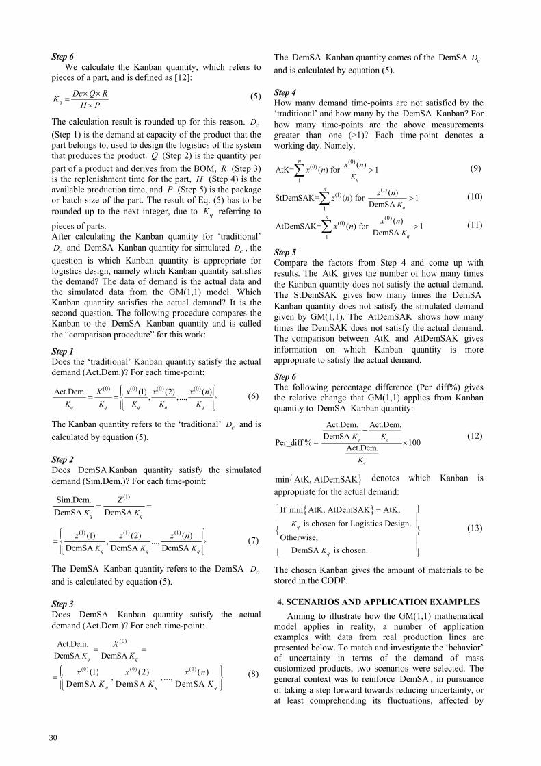
Raw data depicts the consumtion of two materials (part 1 and part 2) during a high season of three months; June, July, and August 2010. Raw data includes sales' quantities that differ from time-point to time-point. It includes, for example, the quantities of 9 time-points in June for part 1, and 8 time-points for part 2. For June, July and August the corresponding data is depicted in Table 1.

Fig. 3. Part 1 and part 2 of a fruit bushel

The two materials are plywood slats of fruit bushels. Fruit bushels are considered as seasonal products and customized as well. Their length and width differs from season to season and it is affected by the fruits’ size (fruits’ geometry), which depends on weather conditions, soil fertilization, waterization scheduling, and soil nutrients. The slats, named part 1 and part 2, are the basic customized materials of a fruit bushel as illustrated in Figure 3.

Raw data has no specific time sequence, meaning either that the company has no standard registrations in its database or that the demand was unexpected. Concerning the latter, it seems quite impossible that a company with many years of experience has no picture of the upcoming product demand, thus the former explanation seems to be more reasonble.

4.2 Application Example Results

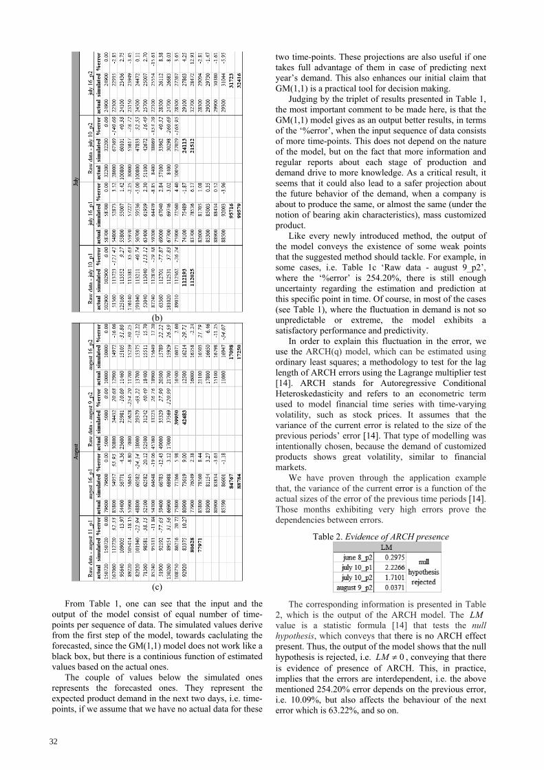
Table 1a, b, and c represents the three high season months regarding the demand of fruit bushels. Each table contains four main columns, e.g. ‘Raw data - june 9_p1’, ‘Raw data - june 8_p2’ etc, which signify the examined month, the time-points that constitute each sequence of data, and the part of the fruit bushel, given that each bushel consists of two main types of parts having different size. The designation ‘june 9_p1’, for example, means that the actual data, as well as the estimated by the GM(1,1) model, refer to June. The sequence of data that is used as an input to the model consists of ‘9’ time-points, as being taken by the company in the form of raw data, and the coresponding numbers address information about the 1st part, i.e. ‘p1’, of the bushel. Beside the actual values, we give the simulated ones. The values in bold are the predicted values. The ‘%error’ gives the divergence between actual and simulated data. The same explanation accounts for ‘Raw data - june 8_p2’, ‘Raw data - july 10_p1’, ‘Raw data - july 10_p2’, ‘Raw data - august 11_p1’, and ‘Raw data - august 9_p2’.

To explain the utility of the rest of the colums that bear no ‘Raw data’ designation we should first explain the two scenarios made in the present work:

Scenario 1: Raw data is used straight forward from the excel file that the company provided us with. In all cases, the raw data that shape the input sequence consists of less time-points compared to the second scenario data.

Scenario 2: The total demand of the parts is kept the same as in Scenario 1, but we divide them along more time-points than in the first scenario, in order to see how a wider distribution of data could possibly affect the estimation and forecasting of the demand.

Keeping in mind that every month has nineteen working days average and that, since the company produces parts of a product, they do not receive new orders every day, we conclude that sixteen working days are a rational amount of time-points to a sequance of data that represents a row of customized product demand registrations.

The reason for building those scenarios is to investigate if more time-points can support the robustness of future demand awareness. Since there is enough gained experience in the field of MC, and there are companies that produce such products for years, this experience is significant to be utilized in a more structured way. Awareness could enhance the alertness in production. An estimation and forecasting model, like those of GA, may be the means to achieve awareness and knowledge creation in terms of production issues.

Table 1. Application example results

(a)

31

(b)

(c)

From Table 1, one can see that the input and the output of the model consist of equal number of time-points per sequence of data. The simulated values derive from the first step of the model, towards caclulating the forecasted, since the GM(1,1) model does not work like a black box, but there is a continious function of estimated values based on the actual ones.

The couple of values below the simulated ones represents the forecasted ones. They represent the expected product demand in the next two days, i.e. time-points, if we assume that we have no actual data for these

two time-points. These projections are also useful if one takes full advantage of them in case of predicting next year’s demand. This also enhances our initial claim that GM(1,1) is a practical tool for decision making.

Judging by the triplet of results presented in Table 1, the most important comment to be made here, is that the GM(1,1) model gives as an output better results, in terms of the ‘%error’, when the input sequence of data consists of more time-points. This does not depend on the nature of the model, but on the fact that more information and regular reports about each stage of production and demand drive to more knowledge. As a critical result, it seems that it could also lead to a safer projection about the future behavior of the demand, when a company is about to produce the same, or almost the same (under the notion of bearing akin characteristics), mass customized product.

Like every newly introduced method, the output of the model conveys the existence of some weak points that the suggested method should tackle. For example, in some cases, i.e. Table 1c ‘Raw data - august 9_p2’, where the ‘%error’ is 254.20%, there is still enough uncertainty regarding the estimation and prediction at this specific point in time. Of course, in most of the cases (see Table 1), where the fluctuation in demand is not so unpredictable or extreme, the model exhibits a satisfactory performance and predictivity.

In order to explain this fluctuation in the error, we use the ARCH(q) model, which can be estimated using ordinary least squares; a methodology to test for the lag length of ARCH errors using the Lagrange multiplier test [14]. ARCH stands for Autoregressive Conditional Heteroskedasticity and refers to an econometric term used to model financial time series with time-varying volatility, such as stock prices. It assumes that the variance of the current error is related to the size of the previous periods’ error [14]. That type of modelling was intentionally chosen, because the demand of customized products shows great volatility, similar to financial markets.

We have proven through the application example that, the variance of the current error is a function of the actual sizes of the error of the previous time periods [14]. Those months exhibiting very high errors prove the dependencies between errors.

Table 2. Evidence of ARCH presence

The corresponding information is presented in Table 2, which is the output of the ARCH model. The LM value is a statistic formula [14] that tests the null hypothesis, which conveys that there is no ARCH effect present. Thus, the output of the model shows that the null hypothesis is rejected, i.e. 0LM , conveying that there is evidence of presence of ARCH. This, in practice, implies that the errors are interdependent, i.e. the above mentioned 254.20% error depends on the previous error, i.e. 10.09%, but also affects the behaviour of the next error which is 63.22%, and so on.

32

The same model can be tested for all sequences of data. Here, we chose to show only those with the higher errors, in order to convince that even in the cases where demand seem to fluctuate in an unexpected manner, data and gained experience could possibly aid an effort towards estimating and predicting the demand of customized products, at least to an extent.

Referring again to Table 1, the estimate and predictive capacity of the GM(1,1) model seems to be greater in the case of calculating the total amount of product demand on a monthly level, than examining demand as fragments. If for instance, we focus on Table 3 on the ‘%error’, we see that there is a faint diference between the actual and the estimated values of demand.

Table 3. Total application example results

4.3 Logistics Design Results

The comparison between Kanban quantity and DemSA Kanban quantity is illustrated in this section. But first, Kanban quantity should be defined by raw data (actual demand), and the DemSA Kanban quantity should be defined by GM(1,1) model data (simulated demand). In Step1 each data produces a cD , calculated

for a three month period. A Kanban system is also designed for those three months. In a case of using raw data for the whole season, cD and Kanban system would

be valid for this season and equally for one year, etc. The variables and calculations of the next steps for

Scenario 1 are presented in Table 4. The variables of Step 2 to 5 are identical. The only variable that influences the Kanban comparison procedure is demand, in Step 1. The same procedure stands for part 2 in Scenario 1 (see Table 5).

Table 4. qK and DemSA qK

Kanban for part 1, Scenario 1 Actual Simulated

Step 1

Mean 105996 107622.93 StDev 43848.31 23721.48

cD 149844.32 131343.41

Step 2 Q 1 pcs. 1 pcs. Step 3 R 420 min. 420 min. Step 4 H 420 min. 420 min. Step 5 P 1 pcs. 1 pcs.

Step 6 qK 149845 131344

Table 5. qK and DemSA qK

Kanban for part 2, Scenario 1 Actual Simulated

Step 1

Mean 43737.31 41292.1 StDev 34129.93 21828.56

cD 77867.34 63120.66

Step 2 Q 1 pcs. 1 pcs. Step 3 R 420 min. 420 min. Step 4 H 420 min. 420 min. Step 5 P 1 pcs. 1 pcs.

Step 6 qK 77868 63121

The following procedure compares Kanban quantity to DemSA Kanban quantity in order to find which one is more suitable to satisfy the actual demand. The analysis of each time-point, for part 1 during three months, using Step 2 and 3 from the comparison procedure for Scenario 1, is displayed in Table 6. The numbers in bold are the predicted values created by GM(1,1), likewise the 10th, 11th, 22th, 23th, 35th and 36th time-points for part 1. The Actual demand in the Kanban quantity column derives from the raw data demand of part 1 and part 2, respectively.

Table 6. Scenario 1 Kanban Suitability Analysis for part 1 per time-point

Time-points

Step 1 Step 2 Step 3 Eq.6 Eq.7 Eq.8

Act.dem. to qK

Sim.dem. to DemSA qK

Act.dem. to DemSA qK

1 0.17 0.19 0.19 2 0.47 0.68 0.53 3 0.40 0.73 0.46 4 1.02 0.78 1.16 5 0.77 0.83 0.88 6 1.06 0.89 1.20 7 0.54 0.94 0.61 8 0.88 1.01 1.00 9 0.93 1.07 1.06

10 0.69 1.15 1.15 11 0.34 1.22 1.22 12 0.84 0.78 0.78 13 1.18 0.87 0.39 14 1.27 0.86 0.95 15 0.35 0.86 1.34 16 0.58 0.86 1.45 17 0.42 0.86 0.40 18 1.21 0.86 0.66 19 0.59 0.86 0.48 20 1.01 0.86 1.38 21 1.11 0.86 0.68 22 0.64 0.85 0.85 23 0.60 0.85 0.85 24 0.55 1.15 1.15 25 0.48 0.86 1.27 26 057 0.83 0.73 27 0.35 0.80 0.68 28 0.87 0.78 0.63 29 0.73 0.75 0.54 30 0.62 0.73 0.65 31 0.70 0.40 32 0.68 0.99 33 0.66 0.83 34 0.63 0.71 35 0.61 0.61

33

36 0.59 0.59 >1

(Step 4) AtK =7 StDemSAK =5 AtDemSAK =10

The same procedure stands for part 2 in Scenario 1 (Table 7). The numbers in bold are the predicted values created by the GM(1,1) model.

Table 7. Scenario 1 Kanban Suitability Analysis for part 2 per time-point

Time-points

Step 1 Step 2 Step 3 Eq.6 Eq.7 Eq.8

Act.dem. to qK

Sim.dem. to DemSA qK

Act.dem. to DemSA qK

1 1.30 1.60 1.60 2 1.07 1.59 1.31 3 1.56 1.29 1.92 4 0.40 1.05 0.49 5 0.76 0.85 0.93 6 1.05 0.69 1.29 7 0.26 0.56 0.32 8 0.11 0.45 0.13 9 0.41 0.37 0.37 10 0.36 0.30 0.30 11 1.29 0.51 0.51 12 0.39 1.07 0.44 13 1.29 0.95 1.60 14 0.66 0.85 0.48 15 0.11 0.76 1.60 16 0.73 0.68 0.81 17 0.11 0.60 0.13 18 1.13 0.54 0.90 19 0.06 0.48 0.13 20 0.40 0.43 0.16 21 0.30 0.38 0.38 22 0.10 0.34 0.34 23 0.23 0.08 0.08 24 0.67 0.39 0.49 25 0.58 0.41 0.37 26 0.63 0.44 0.12 27 0.22 0.47 0.29 28 0.49 0.83 29 0.53 0.72 30 0.56 0.78 31 0.60 0.27 32 0.63 0.63 33 0.67 0.67 >1

(Step 4) AtK =6 StDemSAK =5 AtDemSAK =6

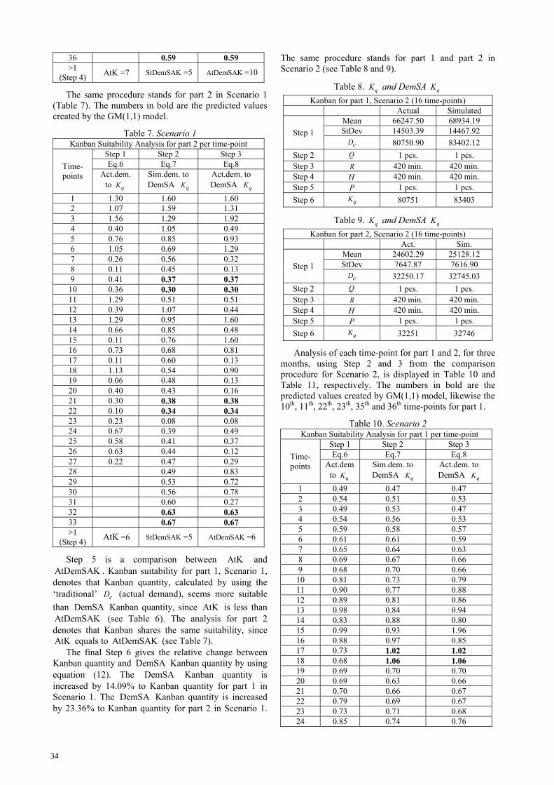
Step 5 is a comparison between AtK and AtDemSAK . Kanban suitability for part 1, Scenario 1, denotes that Kanban quantity, calculated by using the ‘traditional’ cD (actual demand), seems more suitable

than DemSA Kanban quantity, since AtK is less than AtDemSAK (see Table 6). The analysis for part 2 denotes that Kanban shares the same suitability, since AtK equals to AtDemSAK (see Table 7).

The final Step 6 gives the relative change between Kanban quantity and DemSA Kanban quantity by using equation (12). The DemSA Kanban quantity is increased by 14.09% to Kanban quantity for part 1 in Scenario 1. The DemSA Kanban quantity is increased by 23.36% to Kanban quantity for part 2 in Scenario 1.

The same procedure stands for part 1 and part 2 in Scenario 2 (see Table 8 and 9).

Table 8. qK and DemSA qK

Kanban for part 1, Scenario 2 (16 time-points) Actual Simulated

Step 1

Mean 66247.50 68934.19 StDev 14503.39 14467.92

cD 80750.90 83402.12

Step 2 Q 1 pcs. 1 pcs. Step 3 R 420 min. 420 min. Step 4 H 420 min. 420 min. Step 5 P 1 pcs. 1 pcs.

Step 6 qK 80751 83403

Table 9. qK and DemSA qK

Kanban for part 2, Scenario 2 (16 time-points) Act. Sim.

Step 1

Mean 24602.29 25128.12 StDev 7647.87 7616.90

cD 32250.17 32745.03

Step 2 Q 1 pcs. 1 pcs. Step 3 R 420 min. 420 min. Step 4 H 420 min. 420 min. Step 5 P 1 pcs. 1 pcs.

Step 6 qK 32251 32746

Analysis of each time-point for part 1 and 2, for three months, using Step 2 and 3 from the comparison procedure for Scenario 2, is displayed in Table 10 and Table 11, respectively. The numbers in bold are the predicted values created by GM(1,1) model, likewise the 10th, 11th, 22th, 23th, 35th and 36th time-points for part 1.

Table 10. Scenario 2 Kanban Suitability Analysis for part 1 per time-point

Time-points

Step 1 Step 2 Step 3 Eq.6 Eq.7 Eq.8

Act.dem. to qK

Sim.dem. to DemSA qK

Act.dem. to DemSA qK

1 0.49 0.47 0.47 2 0.54 0.51 0.53 3 0.49 0.53 0.47 4 0.54 0.56 0.53 5 0.59 0.58 0.57 6 0.61 0.61 0.59 7 0.65 0.64 0.63 8 0.69 0.67 0.66 9 0.68 0.70 0.66 10 0.81 0.73 0.79 11 0.90 0.77 0.88 12 0.89 0.81 0.86 13 0.98 0.84 0.94 14 0.83 0.88 0.80 15 0.99 0.93 1.96 16 0.88 0.97 0.85 17 0.73 1.02 1.02 18 0.68 1.06 1.06 19 0.69 0.70 0.70 20 0.69 0.63 0.66 21 0.70 0.66 0.67 22 0.79 0.69 0.67 23 0.73 0.71 0.68 24 0.85 0.74 0.76

34

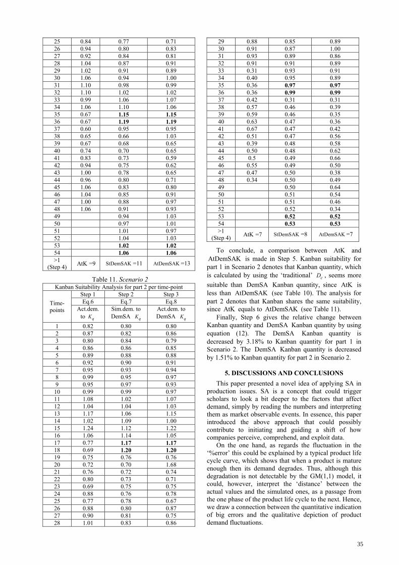
25 0.84 0.77 0.71 26 0.94 0.80 0.83 27 0.92 0.84 0.81 28 1.04 0.87 0.91 29 1.02 0.91 0.89 30 1.06 0.94 1.00 31 1.10 0.98 0.99 32 1.10 1.02 1.02 33 0.99 1.06 1.07 34 1.06 1.10 1.06 35 0.67 1.15 1.15 36 0.67 1.19 1.19 37 0.60 0.95 0.95 38 0.65 0.66 1.03 39 0.67 0.68 0.65 40 0.74 0.70 0.65 41 0.83 0.73 0.59 42 0.94 0.75 0.62 43 1.00 0.78 0.65 44 0.96 0.80 0.71 45 1.06 0.83 0.80 46 1.04 0.85 0.91 47 1.00 0.88 0.97 48 1.06 0.91 0.93 49 0.94 1.03 50 0.97 1.01 51 1.01 0.97 52 1.04 1.03 53 1.02 1.02 54 1.06 1.06 >1

(Step 4) AtK =9 StDemSAK =11 AtDemSAK =13

Table 11. Scenario 2 Kanban Suitability Analysis for part 2 per time-point

Time-points

Step 1 Step 2 Step 3 Eq.6 Eq.7 Eq.8

Act.dem. to qK

Sim.dem. to DemSA qK

Act.dem. to DemSA qK

1 0.82 0.80 0.80 2 0.87 0.82 0.86 3 0.80 0.84 0.79 4 0.86 0.86 0.85 5 0.89 0.88 0.88 6 0.92 0.90 0.91 7 0.95 0.93 0.94 8 0.99 0.95 0.97 9 0.95 0.97 0.93 10 0.99 0.99 0.97 11 1.08 1.02 1.07 12 1.04 1.04 1.03 13 1.17 1.06 1.15 14 1.02 1.09 1.00 15 1.24 1.12 1.22 16 1.06 1.14 1.05 17 0.77 1.17 1.17 18 0.69 1.20 1.20 19 0.75 0.76 0.76 20 0.72 0.70 1.68 21 0.76 0.72 0.74 22 0.80 0.73 0.71 23 0.69 0.75 0.75 24 0.88 0.76 0.78 25 0.77 0.78 0.67 26 0.88 0.80 0.87 27 0.90 0.81 0.75 28 1.01 0.83 0.86

29 0.88 0.85 0.89 30 0.91 0.87 1.00 31 0.93 0.89 0.86 32 0.91 0.91 0.89 33 0.31 0.93 0.91 34 0.40 0.95 0.89 35 0.36 0.97 0.97 36 0.36 0.99 0.99 37 0.42 0.31 0.31 38 0.57 0.46 0.39 39 0.59 0.46 0.35 40 0.63 0.47 0.36 41 0.67 0.47 0.42 42 0.51 0.47 0.56 43 0.39 0.48 0.58 44 0.50 0.48 0.62 45 0.5 0.49 0.66 46 0.55 0.49 0.50 47 0.47 0.50 0.38 48 0.34 0.50 0.49 49 0.50 0.64 50 0.51 0.54 51 0.51 0.46 52 0.52 0.34 53 0.52 0.52 54 0.53 0.53 >1

(Step 4) AtK =7 StDemSAK =8 AtDemSAK =7

To conclude, a comparison between AtK and AtDemSAK is made in Step 5. Kanban suitability for part 1 in Scenario 2 denotes that Kanban quantity, which is calculated by using the ‘traditional’ cD , seems more

suitable than DemSA Kanban quantity, since AtK is less than AtDemSAK (see Table 10). The analysis for part 2 denotes that Kanban shares the same suitability, since AtK equals to AtDemSAK (see Table 11).

Finally, Step 6 gives the relative change between Kanban quantity and DemSA Kanban quantity by using equation (12). The DemSA Kanban quantity is decreased by 3.18% to Kanban quantity for part 1 in Scenario 2. The DemSA Kanban quantity is decreased by 1.51% to Kanban quantity for part 2 in Scenario 2.

5. DISCUSSIONS AND CONCLUSIONS

This paper presented a novel idea of applying SA in production issues. SA is a concept that could trigger scholars to look a bit deeper to the factors that affect demand, simply by reading the numbers and interpreting them as market observable events. In essence, this paper introduced the above approach that could possibly contribute to initiating and guiding a shift of how companies perceive, comprehend, and exploit data.

On the one hand, as regards the fluctuation in the ‘%error’ this could be explained by a typical product life cycle curve, which shows that when a product is mature enough then its demand degrades. Thus, although this degradation is not detectable by the GM(1,1) model, it could, however, interpret the ‘distance’ between the actual values and the simulated ones, as a passage from the one phase of the product life cycle to the next. Hence, we draw a connection between the quantitative indication of big errors and the qualitative depiction of product demand fluctuations.

35

On the other hand, as regards the Kanban quantity, it is not affected by the GM(1,1) model. The logistics design procedure can define Kanban quantity either with ‘traditional’ or simulated cD . Besides, the Kanban

quantity seems to be quite more accurate than DemSA Kanban, and its calculation is not affected by the amount of time-points, namely there is no difference between Scenario 1 and Scenario 2. The Kanban quantity calculation is affected by demand, explained by the fact that AtK is lower than AtDemSAK for part 1 and equal for part 2. Kanban quantity with ‘traditional cD is good

enough material handling system for CODP to satisfy future demand. Kanban quantity with simulated cD that

is calculated by GM(1,10 model needs further investigation by more application examples.

After all, having acknowledged that the proposed method is not a panacea, we still argue that it could aid, at least as a pilot measure, in taking advantage of the lessons learned by the MC company experiences and the overabundance of data.

5. REFERENCES

[1] M.R. Endsley, “Toward a Theory of Situation Awareness in Dynamic Systems,” Human Factors: The Journal of the Human Factors and Ergonomics Society, vol. 37, no.1, pp. 32–64, 1995a.

[2] E. Jeannot, C. Kelly, and D. Thompson, The Development of Situation Awareness Measures in ATM Systems. Brussels: Eurocontrol, 2003.

[3] S.F. Liu, and Y. Lin, Grey Systems Theory and Applications. Berlin, Germany: Springer Verlag, 2010.

[4] C. Chandra, and A.K. Kamrani, Mass customization: a supply chain approach. Springer, 2004.

[5] F. Wang J. Lin, and X. Liu, “Three-dimensional model of customer order decoupling point position in mass customization.” International Journal of Production Research, vol. 48, no. 13, pp. 3741–3757, 2010.

[6] B.J. Naylor, M.N. Mohamed, and D. Berry, “Leagility: integrating the lean and agile manufacturing paradigms in the total supply chain.” International Journal of Production Economics, vol. 62, no. 1, pp. 107–118, 1999.

[7] S.M. Argelo, Integral logistic structures: developing customer-oriented goods flow. Eds. Sjoerd Hoekstra, and Jac Romme. Industrial Press Inc., 1992.

[8] M. Rother, and J. Shook. Learning to see: value stream mapping to add value and eliminate muda. Lean Enterprise Institute, 2003.

[9] J.L. Deng, Grey Prediction and Decision. Wuhang, China: Huazhong University of Science and Technology Press, 2002.

[10] S.F. Liu, Y.G. Dang, and Z.G. Fang, Grey System Theory and its Application. Beijing, China: Beijing Science Press, 2004.

[11] E. Kayacan, B. Ulutas, and O. Kaynak, “Grey Theory-based Models in Time Series Prediction,” Expert Systems with Applications, vol. 37, pp. 1784–1789, 2009.

[12] J. R. Costanza, USA Patent No. US6594535 (B1), 2003.

[13] A.C. Tsigkas, The Lean Enterprise: From the Mass Economy to the Economy of One (1st ed.): Springer Berlin Heidelberg, 2012.

[14] R.F. Engle, “GARCH 101: The Use of ARCH/GARCH Models in Applied Econometrics,” Journal of Economic Perspectives vol. 15, no. 4, pp. 157–168, 2001.

[15] B. MacCarthy, P.G. Brabazon, and J. Bramham, “Key Value Attributes in Mass Customization”, in C.Rautenstrauch, R.Seelmann-Eggbert and K.Turowski, eds., Moving into Mass Customization: Information Systems and management Principles, pp. 71–89, 2002.

[16] M. Christopher, and D.R. Towill, “Supply chain migration from lean and functional to agile and customised”, Supply Chain Management: An International Journal, vol. 5, no. 4, pp. 206–21, 2000.

[17] R. Mason-Jones, and D.R. Towill, “Using the Information Decoupling Point to Improve Supply Chain Performance”, International Journal of Logistics Management, vol. 10, no. 2, pp.13–26, 1999.

[18] S. Hoekstra, J. Romme, and S.M. Argelo, Integral logistic structures: developing customer-oriented goods flow: McGraw-Hill, 1992.

[19] D. Berry, The Analysis, Modelling and Simulation of a Re-engineered PC Supply Chain, PhD Thesis, University of Wales, College of Cardiff, 1994.

CORRESPONDENCE

Maria Mikela Chatzimichailidou, PhD Cand. Democritus University of Thrace Polytechnic School, Vas. Sofias 12 67100 Xanthi, Hellenic Republic mikelachatzimichailidou@gmail.gr

Christos G. Chatzopoulos, PhD Cand. Democritus University of Thrace Polytechnic School, Vas. Sofias 12 67100 Xanthi, Hellenic Republic cchatzop@pme.duth.gr

Stefanos Katsavounis, Ass. Prof. Democritus University of Thrace Polytechnic School, Vas. Sofias 12 67100 Xanthi, Hellenic Republic skatsav@pme.duth.gr

36