American Institute of Aeronautics and Astronautics

1

Reduced Order Modeling of a Turbulent Three Dimensional

Cylinder Wake

Jürgen Seidel1, Kelly Cohen

2, Selin Aradag

3, Stefan Siegel

4, and Thomas McLaughlin

5

United States Air Force Academy, USAF Academy, CO, 80840

The aim of this research program is flow state based feedback control of a circular cylinder wake flow at a

Reynolds number of Re=20,000. CFD simulations were performed with an unstructured grid of 4 diameters

span and periodic boundary conditions. In addition, wind tunnel experiments were performed to validate the

Strouhal number, surface pressures, drag coefficient and velocity profiles in the cylinder wake. The

simulation results were compared to both experiments in literature and the experimental results obtained in

this study. POD was performed on the surface pressure data and Double Proper Orthogonal Decomposition

(DPOD) was performed on the wake velocity field obtained from the CFD results. A low dimensional model

was developed based on the DPOD mode amplitudes. For flow field observation, a four sensor configuration

of surface mounted pressure sensors was heuristically selected based on the POD spatial Eigenfunctions of

the surface pressure. Then an artificial neural network estimator was designed to estimate the mode

amplitudes of the 6 dominant DPOD wake velocity modes from the sensor data. For the validation data set,

the estimation errors are relatively small and remain bounded. Also, it appears that all 6 DPOD modes are

observable at each of the nine spanwise planes that were analyzed.

Nomenclature

A = Frontal area

ak = POD mode amplitude

( ),ˆ ti j = Estimate of POD mode amplitude

*

,ˆ

i j = Regression matrix

cd = Drag coefficient

cp = Pressure coefficient

t = Time step

D = Cylinder diameter

k = Spatial POD mode

f = Mapping function

= Viscosity

P = Pressure

( )P ts = Filtered sensor signal

*

sP = Regression matrix

= Density

Re = UD/, Reynolds number

St = Strouhal number

t = Time

t = Dimensional time

T = Temperature

1 Visiting Researcher, Department of Aeronautics, Senior Member AIAA.

2 Visiting Researcher, Department of Aeronautics, Associate Fellow AIAA.

3 Visiting Researcher, Department of Aeronautics, Member AIAA.

4 Visiting Researcher, Department of Aeronautics, Senior Member AIAA.

5 Director, Aeronautics Research Center, Department of Aeronautics, Associate Fellow AIAA.

.

37th AIAA Fluid Dynamics Conference and Exhibit25 - 28 June 2007, Miami, FL

AIAA 2007-4503

This material is declared a work of the U.S. Government and is not subject to copyright protection in the United States.

Dow

nloa

ded

by U

NIV

ER

SIT

Y O

F C

INC

INN

AT

I on

Nov

embe

r 24

, 201

4 | h

ttp://

arc.

aiaa

.org

| D

OI:

10.

2514

/6.2

007-

4503

American Institute of Aeronautics and Astronautics

2

= Angular coordinate measured counter clockwise from rear stagnation point

U = Free stream velocity

' 'u u = Reynolds stress

u = Streamwise velocity

x = Streamwise direction

y = Spanwise direction

y+ = Wall normal distance in wall units

z = Cross stream direction

I. Introduction

HE phenomenon of vortex shedding behind bluff bodies has been a subject of extensive research. Many

flows of engineering interest produce this phenomenon and the associated periodic lift and drag response.

Applications include aircraft and missile aerodynamics, marine structures, underwater acoustics, civil and

wind engineering1. The control of the wake behind bluff bodies has been crucial in several engineering applications

during the past few decades. Especially, active feedback control to reduce the drag on vehicles has been a very

important area of research since drag reduction is directly related to energy saving. In order to be able to control the

vortex shedding behind bluff bodies, it is first important to predict the flow structure accurately both experimentally

and computationally and to create a valid low dimensional model of the flow since feedback of flow fields using low

dimensional modeling has been shown to be much more effective than ad-hoc approaches.2-4

A circular cylinder is a well-studied and documented benchmark for a bluff body wake problem. The near wake

for the flow past a circular cylinder determines the dominant instability in the flow which leads to the vortex street

formation5. It is also responsible for the secondary instability and the subsequent bifurcations that lead to a turbulent

state, as found both computationally6 and experimentally

7. There is no established way to define the near wake;

however it was defined as the region up to ten diameters downstream from the cylinder by Ma et al.8

There are several experimental and computational studies in the literature dealing with the instability and

transition in the near wake of a circular cylinder. Norberg9, Zdravkovich

10 and Lin et al.

11 are some of the theoretical

and experimental studies that give insight to the instability and transition in the near wake. Simulations have also

been performed by several researchers. Most of the current CFD approaches use Reynolds-Averaged Navier-Stokes

equations (RANS) for the prediction of turbulent flows. Although RANS models are sufficient for predicting time

averaged flow quantities, they are not adequate in predicting flows with large separation and the resulting

unsteadiness. These massively separated flows include geometry dependent and three dimensional turbulent eddies

which cannot be simulated by RANS turbulence models12

. Direct Numerical Simulations (DNS), on the other hand,

makes no modeling assumption but is the most expensive approach since all turbulent motions must be resolved by

the grid. Since the smallest scales of turbulence (the Kolmogorov length scale) decrease rapidly with increasing

Reynolds number, this approach is limited to relatively low Reynolds number flows. Large Eddy Simulations (LES)

is less expensive than DNS since it models only the small subgrid scales of motion and resolves the rest of the

turbulent motions. However, since the “large” scales in the boundary layer are on the order of the boundary layer

thickness (which is quite thin for high Reynolds number flows), this method is cost prohibitive at high Reynolds

numbers for wall bounded flows.

The flow at a Reynolds number of Re=3900 has been most extensively studied computationally in the transition

range since there are several experimental studies in literature for comparison purposes at this Reynolds number.

Beaudan and Moin13

performed LES of flow at this Reynolds number and they assessed the performance of the

dynamic subgrid-scale eddy viscosity model for the turbulent wake behind a circular cylinder. Mittal and Moin14

and

Kravchenko and Moin15

also numerically studied the flow over a circular cylinder at Re=3900 using LES. Direct

numerical simulations (DNS) of flow at Re= 3900 were performed by Ma et al.8 and Dong et al.

16 Jordan

17 studied a

higher Reynolds number of Re=8000 in the transitional range using LES. However, he collected only a short time

history which may affect the results. There are also two-dimensional simulations in the literature18

. However,

Beaudan and Moin13

performed both two and three dimensional computations and showed that the near wake is

highly three dimensional at transitional Reynolds numbers and it contains pairs of counter-rotating streamwise

vortices, the effect of which cannot be reproduced in two-dimensional computations and three-dimensional

computations are essential for predicting flow statistics of engineering interest.

Flow control aims to improve aerodynamic characteristics of air vehicles by bringing about increased mission

performance. It can be categorized into two main approaches, namely active and passive flow control, depending on

whether energy is added to the flow in order to modify the flow structure. Passive control methods are inexpensive

and simple; but once they are implemented, no geometry changes can easily be made. Active control methods are

T

Dow

nloa

ded

by U

NIV

ER

SIT

Y O

F C

INC

INN

AT

I on

Nov

embe

r 24

, 201

4 | h

ttp://

arc.

aiaa

.org

| D

OI:

10.

2514

/6.2

007-

4503

American Institute of Aeronautics and Astronautics

3

usually more effective and can be modified according to the flight conditions. They can further be divided into two

sub-categories: open-loop and closed-loop techniques. Gad-el-Hak19

discusses the advances in the field of flow

control. Closed-loop flow control methods have become more popular over the past two decades as researchers

developed an increased awareness of its potential. Closed-loop flow control has several advantages over other

techniques, including lowering the amount of energy required to manipulate the flow to induce the desired behavior,

effectively addressing fluid dynamic instabilities, enabling adaptability to a wider operating envelope and providing

design flexibility and robustness.

An effective way of suppressing the self-excited flow oscillations, without making changes to the geometry or

introducing vast amounts of energy, is by the incorporation of closed-loop flow control2. A closed-loop flow control

system is comprised of a set of sensors, a controller that determines the feedback, and a set of actuators. During the

past five years, the closed-loop flow control program at the United States Air Force Academy (USAFA) focused on

developing a suite of low-dimensional flow control tools based on the low Reynolds numbers (Re < 180) laminar

cylinder wake.20-24

Energy is introduced into the flow via actuators and the wake of a cylinder may be influenced using several

different forcing techniques. For low Reynolds numbers, the wake response is similar for various types of forcing.2

External acoustic excitation of the wake, longitudinal, lateral or rotational vibration of the cylinder, and alternating

blowing and suction at the separation points are some of the actuation methods employed in the literature.2

Low-dimensional modeling is a building block of a structured model-based closed-loop flow control strategy.

For control purposes, a practical procedure is needed to represent the complete flow field, governed by the Navier

Stokes equations, and to separate the space and time dependence of the flow variables. A common method used to

substantially reduce the order of the model is Proper Orthogonal Decomposition (POD). This method is an optimal

approach in that it will capture the largest amount of the flow energy in the fewest modes of any decomposition of

the flow.25

The two dimensional POD method was used to identify the characteristic features, or modes, of a

cylinder wake at Reynolds number of 100 as demonstrated by Gillies.2

The major building blocks of the structured approach are a reduced-order POD model, a state estimator and a

controller. The desired POD model contains an adequate number of modes to enable accurate modeling of the

temporal and spatial characteristics of the large scale coherent structures inherent in the flow. A common approach

referred to as the method of “snapshots” introduced by Sirovich26

is employed to generate the basis functions of the

POD spatial modes from flowfield information obtained using either experiments or numerical simulations. This

approach to controlling the global wake behavior behind a circular cylinder was effectively employed by Gillies2

and Noack et al.27

Recently, Siegel, Cohen, Seidel and McLaughlin28

developed an extension to the POD approach,

referred to as „Double Proper Orthogonal Decomposition‟ (DPOD), in which shift modes have been added to

account for the changes in the flow due to transient forcing.

For practical applications, it is important to estimate the state of the flow, i.e. the relevant POD mode amplitudes,

using body mounted sensors. The advantages of body mounted sensors are that they are simple, relatively

inexpensive and reliable, and they enable collocation of sensors and actuators. This eliminates substantial phase

delays affecting controller design and performance.

There are two main objectives of this study. The first objective is to perform the unforced simulations and

experiments of the three-dimensional flow over a circular cylinder at a Reynolds number of 20,000 and compare the

results for validation purposes. The second aim is to construct a low dimensional model of the turbulent cylinder

wake. This includes application of Double Proper Orthogonal Decomposition (DPOD) on wake velocity data

obtained from the CFD simulations to develop reduced order dynamical models and designing an Artificial Neural

Network Estimator (ANNE). The ultimate aim is feedback control in order to stabilize the wake of a circular

cylinder at turbulent Reynolds numbers. This should result in a significant reduction of drag as well as unsteady lift

force.

II. Computational Methodology

For the computations, the solver Cobalt from Cobalt Solutions, LLC, was used.30

In Cobalt, the compressible

Navier-Stokes equations are solved using a cell-centered finite volume approach applicable to arbitrary cell

topologies (e.g. prisms, tetrahedra). In order to provide second order accuracy in space, the spatial operator utilizes

the exact Riemann solver of Gottlieb and Groth30

and least squares gradient calculations use QR factorization. It also

employs TVD flux limiters to limit extremes at cell faces. A point implicit method using analytic first-order inviscid

and viscous Jacobians is used for advancement of the discretized system. Newton sub-iterations are employed to

achieve second order accuracy in time.

Dow

nloa

ded

by U

NIV

ER

SIT

Y O

F C

INC

INN

AT

I on

Nov

embe

r 24

, 201

4 | h

ttp://

arc.

aiaa

.org

| D

OI:

10.

2514

/6.2

007-

4503

American Institute of Aeronautics and Astronautics

4

The flow was simulated at a Mach number of 0.1 and the diameter of the cylinder was D=2m. The length to

diameter ratio of the cylinder was 4 with periodic boundary conditions at the cylinder ends. Modified Riemann

invariants were used as the farfield boundary condition (20 diameters away from the cylinder surface), whereas a no

slip, adiabatic wall was employed for the cylinder surface. A time step of 1.152·10-3

seconds corresponding to 0.02

non-dimensional time units ( /t tU D ) was used in the original computations; however a time step study was

also performed and a time step of 0.576·10-3

seconds (t=0.01) was also used to validate the results. The total

simulation spanned 10,000 time steps, corresponding to 200 non-dimensional time steps and 40 cycles of vortex

shedding for the computations with the larger time step. The static pressure and temperature are P=457.79Pa and

T=300K, respectively. In order to increase the stability, an advection damping coefficient of 0.01 was used in the

computations. No damping was used for diffusion; 3 Newton sub-iterations were used (see ref. 30 for more details).

As an initial perturbation to trigger the unsteadiness in the flow simulations, the incoming flow was skewed by an

angle of attack of 1 degree.

The simulations were performed without the use of a subgrid scale model because of the transitional nature of the

flow field. At a Reynolds number of Re=20,000, the attached boundary layer on the cylinder surface is laminar but

the wake is turbulent. The numerical dissipation of the code was relied upon to remove energy from the resolved

scales, mimicking the effect of turbulence at the subgrid level. This approach was also used by Hansen and

Forsythe12

for computations of a cylinder wake at Re=3,900.

The two grids employed in the computations consist of clustering of prismatic cells in the boundary layer and

tetrahedral cells outside the boundary layer. These were generated by Gridtool/VGRID using the method of Morton

et al.31

The minimum cell height is 1.10-3

m for the coarse grid, which corresponds to 5x10-4

when non-

dimensionalized by the cylinder diameter. The average non-dimensional first cell height on the cylinder is around

y+

average =0.3, which results in a grid with 879,603 cells. The fine grid consists of 2,311,000 cells. The coordinate

system used in the computations and the grid around the cylinder surface are shown in Figure 1; x is the streamwise

direction and the y axis is aligned with the cylinder axis. The origin is at the near end of the cylinder in the cylinder

center. Figure 1 shows the surface grid, a plane normal to the cylinder axis, and a zoom-in near the surface.

a)

b)

c)

Figure 1: a) Surface mesh, b) mesh at the periodic boundary plane, c) zoom-in near the surface.

III. Double Proper Orthogonal Decomposition (DPOD)

The POD for a quantity u can be written as

1

( , , ) ( ) ( , )K

k k

k

u x y t a t x y

, (1)

where the spatial modes k(x,y) and temporal coefficients ak(t) are the results of the decomposition.7 While this

decomposition is well suited for time periodic flow fields, additions to the basic POD procedure have to be made to

account for global flow field changes. The addition of a shift mode, as introduced independently by Noack,

Afanasiev, Morzynski and Thiele20

as well as Siegel, Cohen and McLaughlin21 is crucial to account for the change

in the length of the recirculation zone as the wake develops. However, the change in the formation length, i.e. the

location of the formation of the vortices in the cylinder wake, is not accounted for with this approach. To overcome

this shortfall, Siegel, Cohen, Seidel and McLaughlin11

recently developed a procedure named Double POD (DPOD)

to allow for the adjustment of the fluctuating modes of transient flow fields as well. In essence, DPOD provides

shift modes for all physical modes, i.e. the mean flow as well as the von Kármán modes in the case of the cylinder

Dow

nloa

ded

by U

NIV

ER

SIT

Y O

F C

INC

INN

AT

I on

Nov

embe

r 24

, 201

4 | h

ttp://

arc.

aiaa

.org

| D

OI:

10.

2514

/6.2

007-

4503

American Institute of Aeronautics and Astronautics

5

wake. A pictorial representation of the DPOD procedure is given in Figure 2. Starting in the top left corner, the data

is split into K bins and each bin is used as an input data set for its individual SPOD procedure.21

The resulting SPOD modes are then collected across the bins and POD is applied again to obtain the DPOD

modes, most importantly the shift modes. The procedure is expressed mathematically in Equation (2), where the

index i refers to the main (SPOD) modes of the first POD procedure, while the index j identifies the shift mode

order,

, ,

1 1

( , , ) ( ) ( , ).I J

i j i j

i j

u x y t t x y

(2)

This DPOD formulation extends the original concept of the “shift mode”: we can now develop a “shift mode”,

even a series of higher order shift modes, for all main modes i. The resulting mode set can be truncated in both i and

j, leading to a mode ensemble that is IM JM in size. After orthonormalization, the decomposition is again optimal in

the sense of POD. In the limit of J=1, the original POD decomposition is recovered. While the different modes

distinguished by the index i remain the main modes (the mean flow, von Kármán modes, etc.), the index j identifies

the transient changes of these main modes. If J = 2, then modes 1,1 and 1,2 are the mean flow and its “shift mode”

or “mean flow mode” as described by Noack et al.7 and Siegel et al.

10, respectively. Thus the modes with indices j>1

can be referred to as first, second and higher order “shift modes” that allow the POD mode ensemble to adjust for

changes in the spatial modes.

Figure 2: Flow chart of DPOD decomposition process.

IV. Experimental Setup

Experiments were also performed in the USAFA Low Speed Wind Tunnel (LSWT) to validate the main

quantities related to the flow such as the Strouhal number, surface pressure distribution, drag coefficient and

velocity distribution obtained from CFD simulations. This tunnel has a 914 mm x 914 mm (3 ft x 3ft) test section

with a usable velocity range of 3 m/s to 35 m/s. A 9 cm (3.5 in) diameter PVC cylinder spanned the entire height of

the test section. Due to the relative sizes of the cylinder model and the LSWT, blockage corrections were needed in

the analysis of data.

Dow

nloa

ded

by U

NIV

ER

SIT

Y O

F C

INC

INN

AT

I on

Nov

embe

r 24

, 201

4 | h

ttp://

arc.

aiaa

.org

| D

OI:

10.

2514

/6.2

007-

4503

American Institute of Aeronautics and Astronautics

6

In order to verify the computational approach used in this study, surface pressure data around the cylinder was

obtained using two different types of sensors, Validyne and Baratron. The Validyne pressure sensor has a pressure

range of ±0.03 psid, an analog output of ±10Vdc, and accuracy of 0.25% of full scale. The sensors were connected

to two different ports on the cylinder surface on centerplane and the cylinder was rotated with an increment of 10

degrees to obtain pressure data along the whole circumference of the cylinder. Using two different sensors enabled

checking the validity of the results by correlating readings from each instrument.

Single wire hot film probes were placed along the span of the model, the sensor axis parallel with the cylinder

axis. The hot film probes were positioned in line with the side of the cylinder, where the amplitude of the Kármán

Vortex Street induced oscillations is largest. They were initially placed 0.5 diameters downstream of the cylinder to

measure the frequency of the flow to compare to the CFD simulation data. Further data was taken to analyze the

lateral velocity profile in the wake of the cylinder. The four hotwire probes were placed 3D downstream of the

cylinder and moved laterally from z/D = +2.0 to -2.0 in increments of 0.2 diameters.

V. DPOD based low order modeling

A. Development of Effective Sensor Configuration

For low-dimensional control schemes to be implemented, a real-time estimation of the DPOD modes present in

the wake is necessary, since it is not realistic to measure the modes directly and be able to close the loop. Velocity

field data, provided by the CFD simulation, is fed into the DPOD procedure as described in the previous section.

Then, the estimation of the low-dimensional DPOD mode amplitudes is provided using an appropriate estimator.

Sensor measurements may take the form of wake measurements such as velocity, or, as in this effort, of body

mounted pressure measurements. This process leads to the identification of the measurement equation, required for

design of the control system. For practical applications it is desirable to reduce the sensors required for estimation to

the minimum.

The requirement for the estimation scheme is to behave as a modal filter that “combs out” the higher modes. The

main aim of this approach is to thereby circumvent the destabilizing effects of observation “spillover” as described

by Balas.32

Spillover has been the cause for instability in the control of flexible structures and modal filtering was

found to be an effective remedy.34

The intention of the proposed strategy is that the signals, provided by a certain

configuration of sensors placed in the wake, are processed by the estimator to provide the estimates of the first six

DPOD mode amplitudes across 9 x-z planes (y=0,0.5,1,…,4). An estimation scheme, often used in flow control

studies is the linear stochastic estimation (LSE) procedure introduced by Adrian.35

The LSE of low dimensional

mode amplitudes was successfully applied to the unforced Ginzburg-Landau wake model22

and the unforced circular

cylinder wake at low Reynolds numbers.23

A major challenge lies in finding an appropriate number of sensors and

determining locations that best enable the desired modal filtering.

The intent of the proposed strategy is that the surface pressure measurements provided by the body mounted

pressure sensors are processed by the estimator to provide the estimates of the first six DPOD mode amplitudes. All

the measurements were taken after ensuring that the simulation of the cylinder wake flow regime converges to

physically reasonable unforced behavior. The DPOD mode amplitudes, αi,j (i=1,2,3 & j=1,2) will be mapped onto

the extracted sensor signals from the pressure sensors, Ps, as follows:

* *

, ,ˆ ˆ( ) ( ( ), , )i j s i j st f P t P (1)

where ( ),ˆ ti j is the estimate of the 6 DPOD modes for i=1,2,3 and j=1,2; ( )P ts is the filtered sensor signal from „s‟

number of surface pressure sensors; *

,ˆ

i j and *

sP are the regression matrices of past DPOD estimates and filtered

pressure signals respectively; f is the non-linear mapping between the present and past sensor readings and past

DPOD estimates.

The issue of sensor placement and number has been dealt with in an ad-hoc manner in published studies

concerning closed-loop flow control.22,23

For effective closed-loop control system, the following questions need to

be answered:

How many sensors are required?

Where will the sensors be placed?

What are the criteria for judging an effective sensor configuration?

What are the robustness characteristics of a given sensor configuration?

In this effort, an attempt will be made to emulate some of the proven successes from the field of structural control.

Dow

nloa

ded

by U

NIV

ER

SIT

Y O

F C

INC

INN

AT

I on

Nov

embe

r 24

, 201

4 | h

ttp://

arc.

aiaa

.org

| D

OI:

10.

2514

/6.2

007-

4503

American Institute of Aeronautics and Astronautics

7

Heuristically speaking, when some very fine dust particles are placed on a flexible plate, excited at one of its

natural frequencies, after a short while the particles arrange themselves in a certain pattern typical of those

frequencies. The particles will be concentrated in the areas that do not experience any motion (the nodes). On the

other hand, the areas where the motion is large (the internodes) will be clean of particles. It is at the internodes that

the vibrational energy of a particular mode is at a maximum and sensors placed at these locations are extremely

effective in estimating that particular mode.36

The above heuristic approach has been used by Bayon de Noyer36

in finding effective sensor placements for

acceleration feedback control to alleviate tail buffeting of a high performance twin tail aircraft. Note the usage of the

term “effective sensor placements” as it is based on validated heuristics as opposed to “optimal sensor configuration”

that results from a mathematically optimal pattern search for a sensor configuration. What needs to be done to

determine an effective sensor configuration is to find the areas of the most energetic modal activity.

CFD data provided pressure signals at 151 x 201 locations distributed in a structured fashion along the entire

surface of the simulated cylinder (see the cylinder surface grid in Figure 1a). A three-step procedure is proposed for

determining sensor placement and number as follows:

Run a simple POD procedure, after removing the mean pressure mode, on the 151 x 201 pressure

signals. The first two surface pressure POD modes contain 85% of the total “energy”. As much as 58%

of this is in the first periodic mode, whereas the second seemingly non-periodic pressure mode has

approximately 27% of the energy. Furthermore, the frequency of the first mode correlates to the

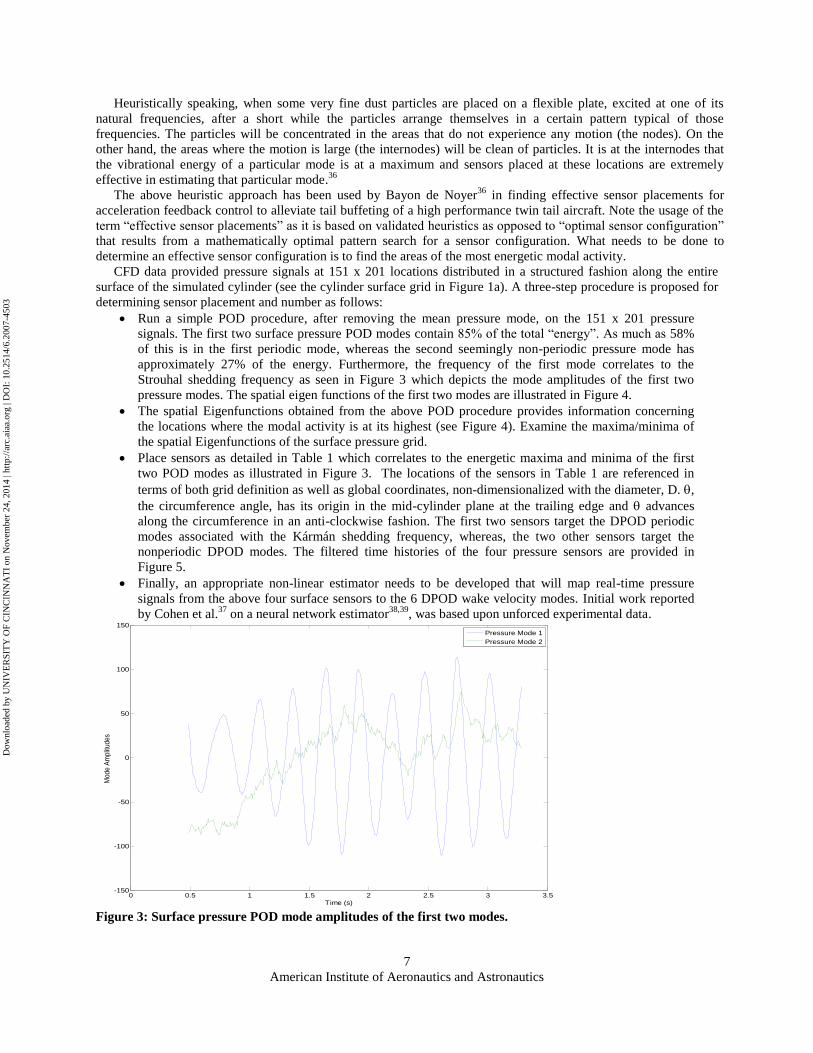
Strouhal shedding frequency as seen in Figure 3 which depicts the mode amplitudes of the first two

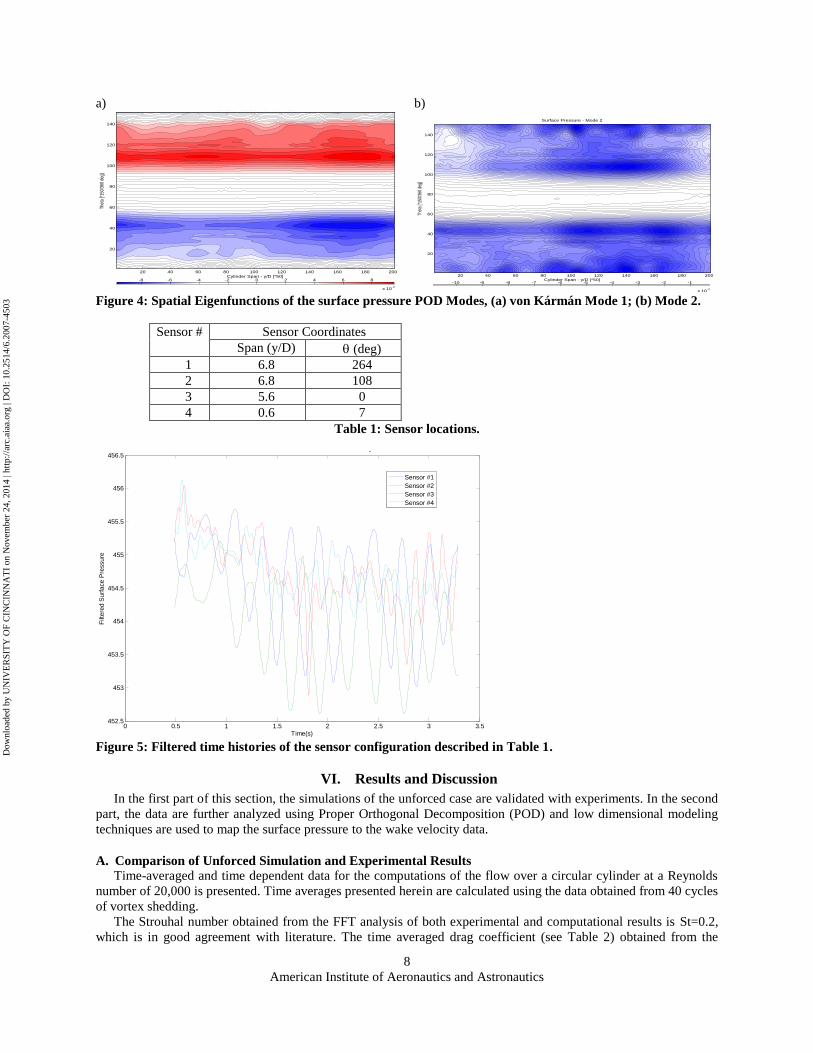
pressure modes. The spatial eigen functions of the first two modes are illustrated in Figure 4.

The spatial Eigenfunctions obtained from the above POD procedure provides information concerning

the locations where the modal activity is at its highest (see Figure 4). Examine the maxima/minima of

the spatial Eigenfunctions of the surface pressure grid.

Place sensors as detailed in Table 1 which correlates to the energetic maxima and minima of the first

two POD modes as illustrated in Figure 3. The locations of the sensors in Table 1 are referenced in

terms of both grid definition as well as global coordinates, non-dimensionalized with the diameter, D. ,

the circumference angle, has its origin in the mid-cylinder plane at the trailing edge and advances

along the circumference in an anti-clockwise fashion. The first two sensors target the DPOD periodic

modes associated with the Kármán shedding frequency, whereas, the two other sensors target the

nonperiodic DPOD modes. The filtered time histories of the four pressure sensors are provided in

Figure 5.

Finally, an appropriate non-linear estimator needs to be developed that will map real-time pressure

signals from the above four surface sensors to the 6 DPOD wake velocity modes. Initial work reported

by Cohen et al.37

on a neural network estimator38,39

, was based upon unforced experimental data.

0 0.5 1 1.5 2 2.5 3 3.5-150

-100

-50

0

50

100

150Time Coefficients of POD on Surface Pressure

Time (s)

Mod

e A

mpl

itude

s

Pressure Mode 1

Pressure Mode 2

Figure 3: Surface pressure POD mode amplitudes of the first two modes.

Dow

nloa

ded

by U

NIV

ER

SIT

Y O

F C

INC

INN

AT

I on

Nov

embe

r 24

, 201

4 | h

ttp://

arc.

aiaa

.org

| D

OI:

10.

2514

/6.2

007-

4503

American Institute of Aeronautics and Astronautics

8

a)

Cylinder Span - y/D [*50]

Thet

a [*

150/

360

deg]

Surface Pressure - Karman Mode

20 40 60 80 100 120 140 160 180 200

20

40

60

80

100

120

140

-8 -6 -4 -2 0 2 4 6 8

x 10-3

b)

Cylinder Span - y/D [*50]

Thet

a [*

150/

360

deg]

Surface Pressure - Mode 2

20 40 60 80 100 120 140 160 180 200

20

40

60

80

100

120

140

-10 -9 -8 -7 -6 -5 -4 -3 -2 -1

x 10-3

Figure 4: Spatial Eigenfunctions of the surface pressure POD Modes, (a) von Kármán Mode 1; (b) Mode 2.

Sensor # Sensor Coordinates

Span (y/D) (deg)

1 6.8 264

2 6.8 108

3 5.6 0

4 0.6 7

Table 1: Sensor locations.

0 0.5 1 1.5 2 2.5 3 3.5452.5

453

453.5

454

454.5

455

455.5

456

456.5Filtered Surface Pressure Sensors - Time History

Time(s)

Filt

ere

d S

urf

ace P

ressu

re

Sensor #1

Sensor #2

Sensor #3

Sensor #4

Figure 5: Filtered time histories of the sensor configuration described in Table 1.

VI. Results and Discussion

In the first part of this section, the simulations of the unforced case are validated with experiments. In the second

part, the data are further analyzed using Proper Orthogonal Decomposition (POD) and low dimensional modeling

techniques are used to map the surface pressure to the wake velocity data.

A. Comparison of Unforced Simulation and Experimental Results

Time-averaged and time dependent data for the computations of the flow over a circular cylinder at a Reynolds

number of 20,000 is presented. Time averages presented herein are calculated using the data obtained from 40 cycles

of vortex shedding.

The Strouhal number obtained from the FFT analysis of both experimental and computational results is St=0.2,

which is in good agreement with literature. The time averaged drag coefficient (see Table 2) obtained from the

Dow

nloa

ded

by U

NIV

ER

SIT

Y O

F C

INC

INN

AT

I on

Nov

embe

r 24

, 201

4 | h

ttp://

arc.

aiaa

.org

| D

OI:

10.

2514

/6.2

007-

4503

American Institute of Aeronautics and Astronautics

9

computations is cd =1.20, which is within the range of the experimental results provided by Anderson40

(cd=1.2) and

Lim and Lee40

(cd=1.16). The time averaging is started at t=60, corresponding to twelve vortex shedding cycles.

Since the friction drag only constitutes approximately 3% of the total drag at a Reynolds number of Re=20,000, the

average drag force was calculated based on the surface pressure measurements made in this study,

2

0

cos2

1dcC pD , (1)

where cp is the surface pressure coefficient obtained from surface pressure values measured with 10 degree

increments around the circumference of the cylinder, using:

21

2

P

P PC

U

. (2)

Table 2 shows the drag coefficient values obtained from CFD, experiments and literature.

Study Mean CD

Computation-Coarse grid 1.19

Computation-Fine grid 1.20

Lim and Lee (2002) 1.16

Anderson (1991) 1.20

Experiment (Blockage correction

of Allen and Vincenti41

applied)

1.19

Table 2: Comparison of mean drag coefficient.

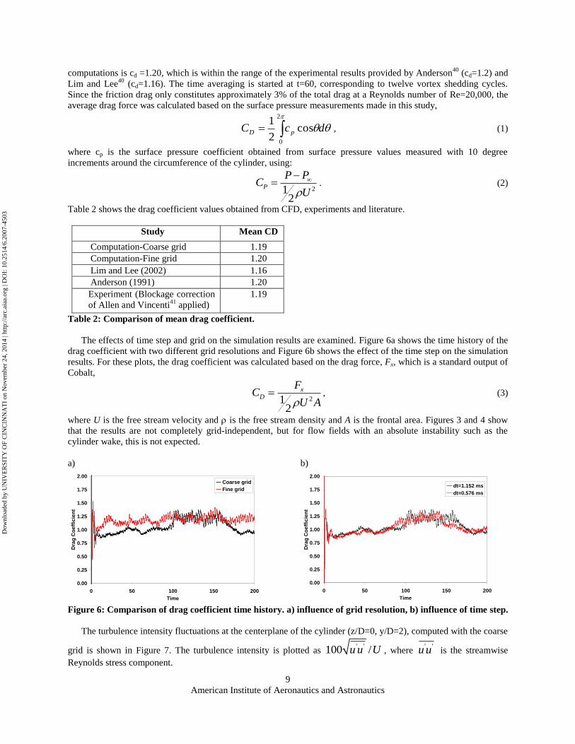
The effects of time step and grid on the simulation results are examined. Figure 6a shows the time history of the

drag coefficient with two different grid resolutions and Figure 6b shows the effect of the time step on the simulation

results. For these plots, the drag coefficient was calculated based on the drag force, Fx, which is a standard output of

Cobalt,

21

2

xD

FC

U A , (3)

where U is the free stream velocity and is the free stream density and A is the frontal area. Figures 3 and 4 show

that the results are not completely grid-independent, but for flow fields with an absolute instability such as the

cylinder wake, this is not expected.

a)

0.00

0.25

0.50

0.75

1.00

1.25

1.50

1.75

2.00

0 50 100 150 200

Time

Dra

g C

oe

ffic

ien

t

Coarse grid

Fine grid

b)

0.00

0.25

0.50

0.75

1.00

1.25

1.50

1.75

2.00

0 50 100 150 200

Time

Dra

g C

oe

ffic

ien

t

dt=1.152 ms

dt=0.576 ms

Figure 6: Comparison of drag coefficient time history. a) influence of grid resolution, b) influence of time step.

The turbulence intensity fluctuations at the centerplane of the cylinder (z/D=0, y/D=2), computed with the coarse

grid is shown in Figure 7. The turbulence intensity is plotted as ' '100 /u u U , where

' 'u u is the streamwise

Reynolds stress component.

Dow

nloa

ded

by U

NIV

ER

SIT

Y O

F C

INC

INN

AT

I on

Nov

embe

r 24

, 201

4 | h

ttp://

arc.

aiaa

.org

| D

OI:

10.

2514

/6.2

007-

4503

American Institute of Aeronautics and Astronautics

10

10

20

30

40

0 1 2 3 4 5 6 7 8

x/D

Turb

ule

nce Inte

nsity

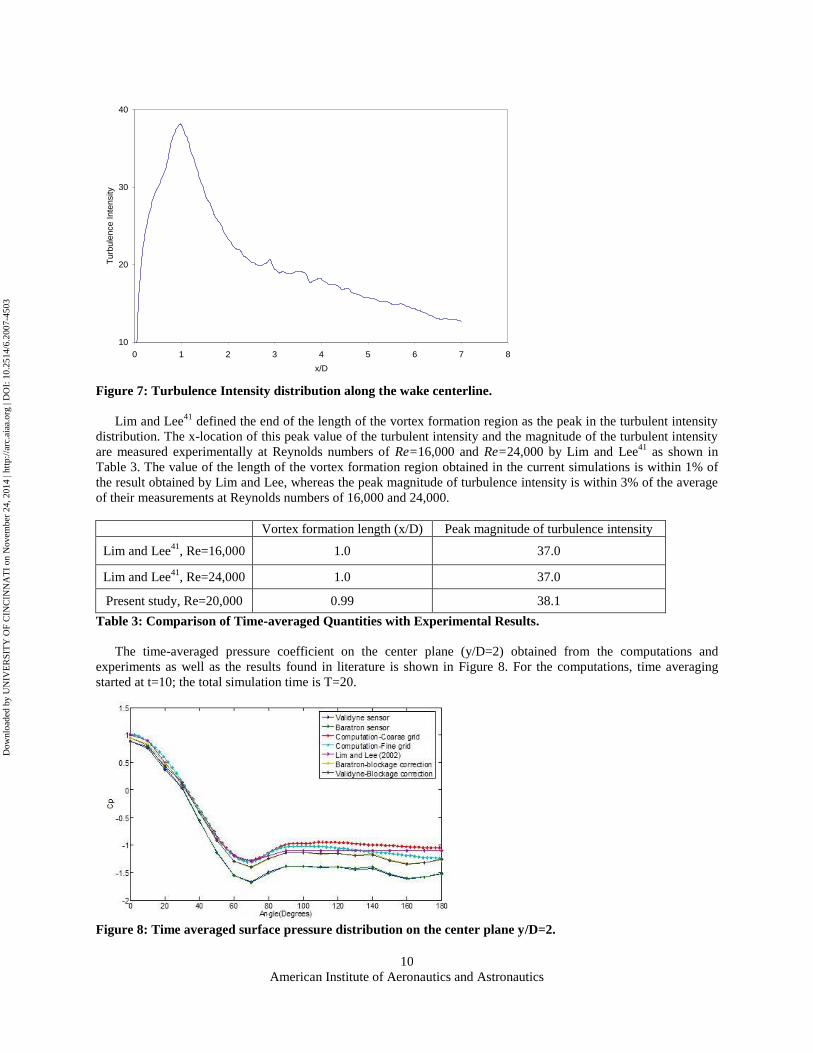
Figure 7: Turbulence Intensity distribution along the wake centerline.

Lim and Lee41

defined the end of the length of the vortex formation region as the peak in the turbulent intensity

distribution. The x-location of this peak value of the turbulent intensity and the magnitude of the turbulent intensity

are measured experimentally at Reynolds numbers of Re=16,000 and Re=24,000 by Lim and Lee41

as shown in

Table 3. The value of the length of the vortex formation region obtained in the current simulations is within 1% of

the result obtained by Lim and Lee, whereas the peak magnitude of turbulence intensity is within 3% of the average

of their measurements at Reynolds numbers of 16,000 and 24,000.

Vortex formation length (x/D) Peak magnitude of turbulence intensity

Lim and Lee41

, Re=16,000 1.0 37.0

Lim and Lee41

, Re=24,000 1.0 37.0

Present study, Re=20,000 0.99 38.1

Table 3: Comparison of Time-averaged Quantities with Experimental Results.

The time-averaged pressure coefficient on the center plane (y/D=2) obtained from the computations and

experiments as well as the results found in literature is shown in Figure 8. For the computations, time averaging

started at t=10; the total simulation time is T=20.

Figure 8: Time averaged surface pressure distribution on the center plane y/D=2.

Dow

nloa

ded

by U

NIV

ER

SIT

Y O

F C

INC

INN

AT

I on

Nov

embe

r 24

, 201

4 | h

ttp://

arc.

aiaa

.org

| D

OI:

10.

2514

/6.2

007-

4503

American Institute of Aeronautics and Astronautics

11

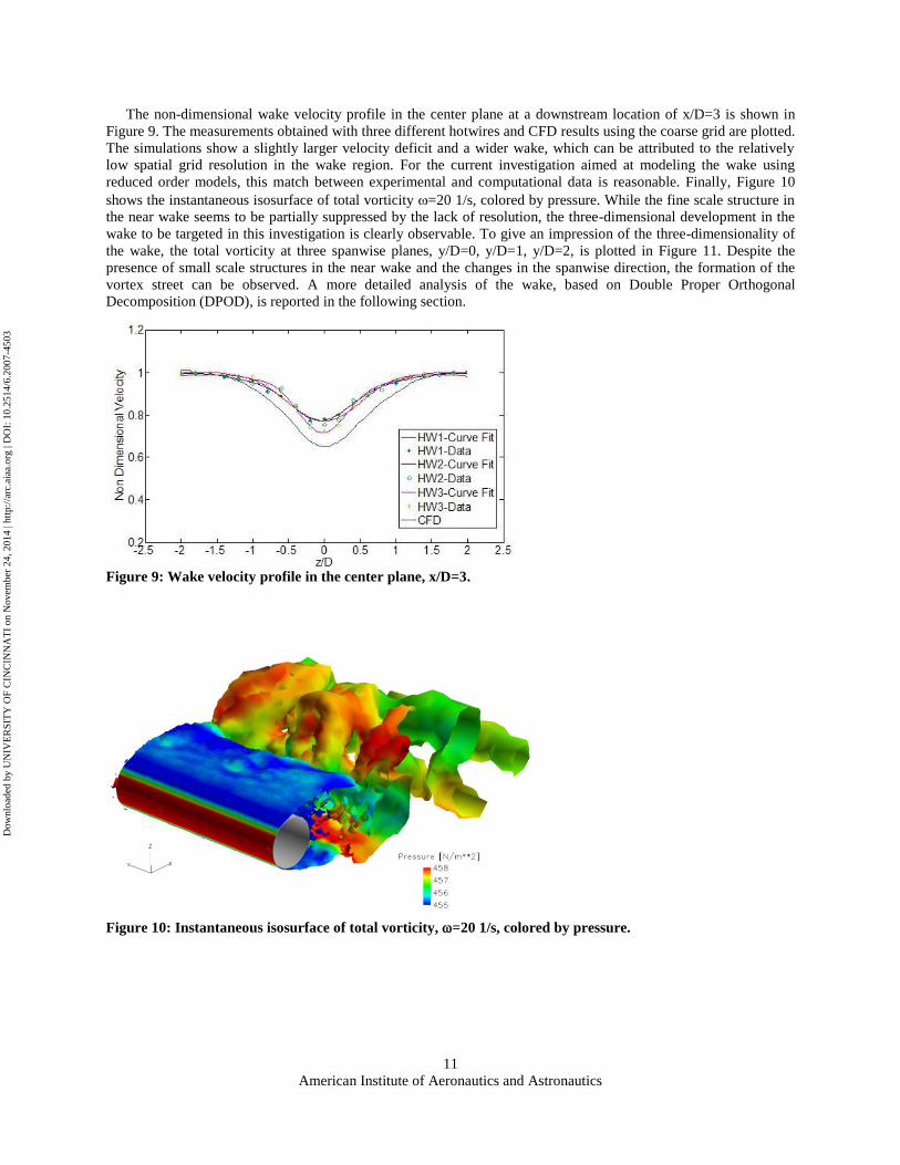
The non-dimensional wake velocity profile in the center plane at a downstream location of x/D=3 is shown in

Figure 9. The measurements obtained with three different hotwires and CFD results using the coarse grid are plotted.

The simulations show a slightly larger velocity deficit and a wider wake, which can be attributed to the relatively

low spatial grid resolution in the wake region. For the current investigation aimed at modeling the wake using

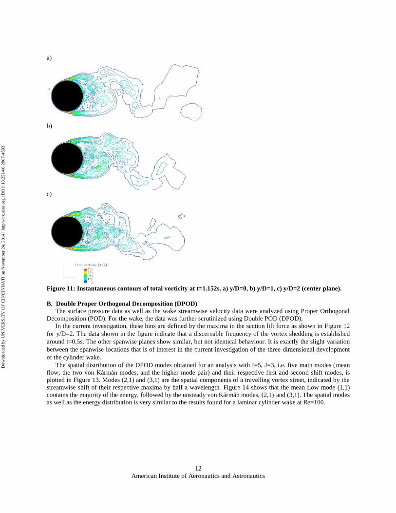
reduced order models, this match between experimental and computational data is reasonable. Finally, Figure 10

shows the instantaneous isosurface of total vorticity =20 1/s, colored by pressure. While the fine scale structure in

the near wake seems to be partially suppressed by the lack of resolution, the three-dimensional development in the

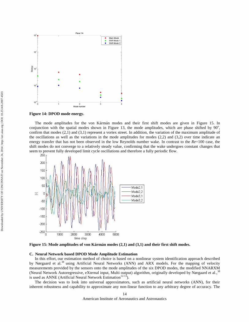
wake to be targeted in this investigation is clearly observable. To give an impression of the three-dimensionality of

the wake, the total vorticity at three spanwise planes, y/D=0, y/D=1, y/D=2, is plotted in Figure 11. Despite the

presence of small scale structures in the near wake and the changes in the spanwise direction, the formation of the

vortex street can be observed. A more detailed analysis of the wake, based on Double Proper Orthogonal

Decomposition (DPOD), is reported in the following section.

Figure 9: Wake velocity profile in the center plane, x/D=3.

Figure 10: Instantaneous isosurface of total vorticity, =20 1/s, colored by pressure.

Dow

nloa

ded

by U

NIV

ER

SIT

Y O

F C

INC

INN

AT

I on

Nov

embe

r 24

, 201

4 | h

ttp://

arc.

aiaa

.org

| D

OI:

10.

2514

/6.2

007-

4503

American Institute of Aeronautics and Astronautics

12

a)

b)

c)

Figure 11: Instantaneous contours of total vorticity at t=1.152s. a) y/D=0, b) y/D=1, c) y/D=2 (center plane).

B. Double Proper Orthogonal Decomposition (DPOD)

The surface pressure data as well as the wake streamwise velocity data were analyzed using Proper Orthogonal

Decomposition (POD). For the wake, the data was further scrutinized using Double POD (DPOD).

In the current investigation, these bins are defined by the maxima in the section lift force as shown in Figure 12

for y/D=2. The data shown in the figure indicate that a discernable frequency of the vortex shedding is established

around t=0.5s. The other spanwise planes show similar, but not identical behaviour. It is exactly the slight variation

between the spanwise locations that is of interest in the current investigation of the three-dimensional development

of the cylinder wake.

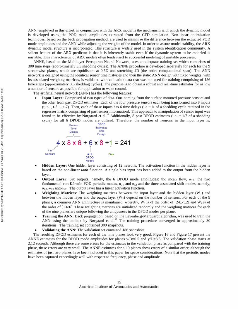
The spatial distribution of the DPOD modes obtained for an analysis with I=5, J=3, i.e. five main modes (mean

flow, the two von Kármán modes, and the higher mode pair) and their respective first and second shift modes, is

plotted in Figure 13. Modes (2,1) and (3,1) are the spatial components of a travelling vortex street, indicated by the

streamwise shift of their respective maxima by half a wavelength. Figure 14 shows that the mean flow mode (1,1)

contains the majority of the energy, followed by the unsteady von Kármán modes, (2,1) and (3,1). The spatial modes

as well as the energy distribution is very similar to the results found for a laminar cylinder wake at Re=100.

Dow

nloa

ded

by U

NIV

ER

SIT

Y O

F C

INC

INN

AT

I on

Nov

embe

r 24

, 201

4 | h

ttp://

arc.

aiaa

.org

| D

OI:

10.

2514

/6.2

007-

4503

American Institute of Aeronautics and Astronautics

13

Figure 12: Section lift force at center plane y/D=2.

Figure 13: Spatial DPOD modes of the 5x3 model. Mode (1,1) is the mean flow, modes (2,1) and (3,1)

represent the von Kármán vortex street.

Dow

nloa

ded

by U

NIV

ER

SIT

Y O

F C

INC

INN

AT

I on

Nov

embe

r 24

, 201

4 | h

ttp://

arc.

aiaa

.org

| D

OI:

10.

2514

/6.2

007-

4503

American Institute of Aeronautics and Astronautics

14

Figure 14: DPOD mode energy.

The mode amplitudes for the von Kármán modes and their first shift modes are given in Figure 15. In

conjunction with the spatial modes shown in Figure 13, the mode amplitudes, which are phase shifted by 90o,

confirm that modes (2,1) and (3,1) represent a vortex street. In addition, the variation of the maximum amplitude of

the oscillations as well as the variations in the mode amplitudes for modes (2,2) and (3,2) over time indicate an

energy transfer that has not been observed in the low Reynolds number wake. In contrast to the Re=100 case, the

shift modes do not converge to a relatively steady value, confirming that the wake undergoes constant changes that

seem to prevent fully developed limit cycle oscillations and therefore a fully periodic flow.

Figure 15: Mode amplitudes of von Kármán modes (2,1) and (3,1) and their first shift modes.

C. Neural Network based DPOD Mode Amplitude Estimation

In this effort, our estimation method of choice is based on a nonlinear system identification approach described

by Nørgaard et al.38

using Artificial Neural Networks (ANN) and ARX models. For the mapping of velocity

measurements provided by the sensors onto the mode amplitudes of the six DPOD modes, the modified NNARXM

(Neural Network Autoregressive, eXternal input, Multi output) algorithm, originally developed by Nørgaard et al.,38

is used as ANNE (Artificial Neural Network Estimation12-13

).

The decision was to look into universal approximators, such as artificial neural networks (ANN), for their

inherent robustness and capability to approximate any non-linear function to any arbitrary degree of accuracy. The

Dow

nloa

ded

by U

NIV

ER

SIT

Y O

F C

INC

INN

AT

I on

Nov

embe

r 24

, 201

4 | h

ttp://

arc.

aiaa

.org

| D

OI:

10.

2514

/6.2

007-

4503

American Institute of Aeronautics and Astronautics

15

ANN, employed in this effort, in conjunction with the ARX model is the mechanism with which the dynamic model

is developed using the POD mode amplitudes extracted from the CFD simulation. Non-linear optimization

techniques, based on the back propagation method, are used to minimize the difference between the extracted POD

mode amplitudes and the ANN while adjusting the weights of the model. In order to assure model stability, the ARX

dynamic model structure is incorporated. This structure is widely used in the system identification community. A

salient feature of the ARX predictor is that it is inherently stable even if the dynamic system to be modeled is

unstable. This characteristic of ARX models often lends itself to successful modeling of unstable processes.

ANNE, based on the Multilayer Perceptron Neural Network, uses an adequate training set which comprises of

300 time steps (approximately 5.5 shedding cycles). The ANNE procedure is developed separately for each for the 9

streamwise planes, which are equidistant at 0.5D and stretching 4D (the entire computational span). The ANN

network is designed using the identical sensor time histories and then the static ANN design with fixed weights, with

its associated weighing matrices, is validated with validation data that was not used for training comprising of 186

time steps (approximately 3.5 shedding cycles). The purpose is to obtain a robust and real-time estimator for as low

a number of sensors as possible for application to wake control.

The artificial neural network (ANN) has the following features:

Input Layer: Comprised of two types of data. One coming from the surface mounted pressure sensors and

the other from past DPOD estimates. Each of the four pressure sensors each being transformed into 8 inputs

(t, t-1, t-2…. t-7). Then, each of these inputs has 6 time delays (i.e ~ ¼ of a shedding cycle retained in the

regressor matrix comprising of past sensor information). This approach to manipulation of sensor input was

found to be effective by Nørgaard et al.37

Additionally, 8 past DPOD estimates (i.e. ~ 1/7 of a shedding

cycle) for all 6 DPOD modes are utilized. Therefore, the number of neurons in the input layer is:

Hidden Layer: One hidden layer consisting of 12 neurons. The activation function in the hidden layer is

based on the non-linear tanh function. A single bias input has been added to the output from the hidden

layer.

Output Layer: Six outputs, namely, the 6 DPOD mode amplitudes: the mean flow, α1,1, the two

fundamental von Kármán POD periodic modes, α2,1 and α3,1 and the three associated shift modes, namely,

α2,1, α2,2 and α3,2 . The output layer has a linear activation function.

Weighting Matrices: The weighting matrices between the input layer and the hidden layer (W1) and

between the hidden layer and the output layer (W2) depend on the number of sensors. For each of the 9

planes, a common ANN architecture is maintained, whereby, W1 is of the order of [24112] and W2 is of

the order of [136]. These weighting matrices are initialized randomly and the weighing matrices for each

of the nine planes are unique following the uniqueness in the DPOD modes per plane.

Training the ANN: Back propagation, based on the Levenberg-Marquardt algorithm, was used to train the

ANN using the toolbox by Nørgaard et al.38

The training procedure converged in approximately 30

iterations. The training set contained 300 snapshots.

Validating the ANN: The validation set contained 186 snapshots.

The resulting DPOD estimates for each of the nine planes look very good. Figure 16 and Figure 17 present the

ANNE estimates for the DPOD mode amplitudes for planes y/D=0.5 and y/D=3.5. The validation phase starts at

2.12 seconds. Although there are some errors for the estimates in the validation phase as compared with the training

phase, these errors are very small. The ANNE estimates for all 9 planes show errors of a similar order, although the

estimates of just two planes have been included in this paper for space considerations. Note that the periodic modes

have been captured exceedingly well with respect to frequency, phase and amplitude.

Dow

nloa

ded

by U

NIV

ER

SIT

Y O

F C

INC

INN

AT

I on

Nov

embe

r 24

, 201

4 | h

ttp://

arc.

aiaa

.org

| D

OI:

10.

2514

/6.2

007-

4503

American Institute of Aeronautics and Astronautics

16

0.5 1 1.5 2 2.5 3 3.5-300

-200

-100

0

100

200

300

Time [s]

Mode A

mplit

udes

DPOD Modes at Plane Y1

DNS-Mode 1,2

DNS-Mode 2,1

DNS-Mode 2,2

DNS-Mode 3,1

DNS-Mode 3,2

ANNE-Mode 1,2

ANNE-Mode 2,1

ANNE-Mode 2,2

ANNE-Mode 3,1

ANNE-Mode 3,2

0.5 1 1.5 2 2.5 3 3.5-1600

-1400

-1200

-1000

-800

-600

-400

-200

0

Time [s]

Mode A

mplit

udes

DNS-Mode 1,1

ANNE-Mode 1,1

Figure 16: DPOD Mode Amplitude Estimates using ANNE, plane y/D=0.5.

0.5 1 1.5 2 2.5 3 3.5-300

-200

-100

0

100

200

300

Time [s]

Mode A

mplit

udes

DPOD Modes at Plane Y7

DNS-Mode 1,2

DNS-Mode 2,1

DNS-Mode 2,2

DNS-Mode 3,1

DNS-Mode 3,2

ANNE-Mode 1,2

ANNE-Mode 2,1

ANNE-Mode 2,2

ANNE-Mode 3,1

ANNE-Mode 3,2

0.5 1 1.5 2 2.5 3 3.5-1600

-1400

-1200

-1000

-800

-600

-400

-200

0

Time [s]

Mode A

mplit

udes

DNS-Mode 1,1

ANNE-Mode 1,1

Figure 17: DPOD Mode Amplitude Estimates using ANNE, plane y/D=3.5.

Discussion and Conclusions

Three dimensional computations of the flow over a two dimensional circular cylinder at a Reynolds number of

Re=20,000 based on the cylinder diameter were performed using unstructured grids. Experiments were also

performed to validate the Strouhal number, surface pressures, drag coefficient and velocity profiles in the cylinder

wake. CFD results were validated with experiments performed in this study as well as the experiments in literature.

The CFD data was analyzed using the DPOD procedure. The data at nine spanwise planes was segmented using

the local lift force fluctuations and these SPOD data served as input for DPOD. The mode amplitudes of the first

Dow

nloa

ded

by U

NIV

ER

SIT

Y O

F C

INC

INN

AT

I on

Nov

embe

r 24

, 201

4 | h

ttp://

arc.

aiaa

.org

| D

OI:

10.

2514

/6.2

007-

4503

American Institute of Aeronautics and Astronautics

17

five main modes and their two shift modes were then utilized for the development of the low order model. The

model for the mean flow mode, von Kármán modes, and their shift modes, which was developed in this research

effort, matches the CFD simulations exceedingly well.

The implications of the research reported in this paper point to the fact that just 4 surface mounted sensors,

strategically placed, can provide accurate estimates of the DPOD mode amplitudes of the wake velocity. For the

validation data set, the estimation errors are relatively small and remain bounded. While we have not included

mathematical proof of observability, it appears that all 6 DPOD modes are observable at each of the nine spanwise

planes. The simulations will be continued to provide a longer time history for further testing and possible adaptation

of the developed model.

For future research, it will be interesting to see whether the above sensor configuration and ANN architecture

will provide a sufficiently accurate estimate or if other configurations need to be explored. For example, one might

consider a streamwise-spanwise plane on which to perform DPOD to obtain data for building a low dimensional

model of the wake.

As a next step, transient forcing needs to be introduced, within the actuation “lock-in” envelope, in order to

obtain the state equation which maps the behavior of the DPOD states as a result of control input. The ANNE

estimation process will have to be revisited with the introduction of control action since the plant is non-linear and

the separation principle, from linear time invariant systems no longer holds true. It may be reasonable to assume that

past control actions will have to be used as inputs to the regression matrix.

Acknowledgments

The authors would like to acknowledge funding by the Air Force Office of Scientific Research, Lt Col Scott

Wells, Program Manager. The authors would like to thank cadets Brian Brown-Dymkoski, Dan Helland and Lt Col

(Ret) Christopher Seaver for preparing the experimental aspects of this effort and collecting the experimental data in

the wind tunnel. We would like to thank Dr. Jim Forsythe and Mr. Bill Strang of Cobalt Solutions, LLC for their

support of the CFD simulations.The help of the technician SSgt Mary Church in set-up, tear-down, and everything

in between is also appreciated. The authors appreciate the contribution by Mr. Ken Ostasiewski in calibration of the

hot wires and the discussions concerning the experiment with Mr. Fred Porter and Dr. Tim Scully.

References 1

Cohen, K., Siegel, S., McLaughlin, T., Gillies, E. and Myatt, J., “Closed-loop approaches to control of a wake

flow modeled by the Ginzburg–Landau equation”, Computers and Fluids, Vol. 34, pp. 927-949, 2005. 2

Gillies E. A., “Low-dimensional Control of the Circular Cylinder Wake”, Journal of Fluid Mechanics, 1998,

Vol. 371, pp. 157-78. 3

Cohen, K., Siegel, S., and McLaughlin, T, "Control Issues in reduced-Order Feedback Flow Control", AIAA

Paper 2004-0575, 42nd AIAA Aerospace Sciences Meeting, Reno, Nevada, January 2004. 4

Roussopoulos, K., “Feedback Control of Vortex Shedding at Low Reynolds Numbers”, Journal of Fluid

Mechanics, Vol. 248, pp.267-296, 1993. 5

Unal, M. and Rockwell, D., “On Vortex Shedding from a Cylinder, Part 1: The Initial Instability”, Journal of

Fluid Mechanics, Vol. 190, pp. 491-512, 1988. 6

Karniadakis, G. E. and Triantafyllou, “Three Dimensional Dynamics and Transition to Turbulence in the Wake

of Bluff Objects”, Journal of Fluid Mechanics, Vol. 238, pp. 1-30, 1992. 7

Williamson, C., “Three Dimensional Wake Transition”, Journal of Fluid Mechanics, Vol. 328, pp. 345-407,

1996. 8

Ma, X., Karamanos, G. S. and Karniadakis, G. E., “Dynamics and Low-Dimensionality of a Turbulent Near

Wake”, Journal of Fluid Mechanics, Vol. 410, pp. 29-65, 2000. 9

Norberg, C., “An Experimental Investigation of the Flow around a Circular Cylinder: Influence of Aspect

Ratio”, Journal of Fluid Mechanics, Vol. 258, pp. 287-316, 1994. 10

Zdravkovich, M. M., “Conceptual Overview of Laminar and Turbulent Flows Past Smooth and Rough Circular

Cylinders”, J. Wind Engineering Indust. Aero, Vol. 33, pp. 53-62, 1990. 11

Lin, J. C., Towfighi, J. and Rockwell, D., “Instantaneous Structure of a Near Wake of a Cylinder: On the

Effect of Reynolds Number”, J. Fluids Struct., Vol. 9, pp. 409-418. 12

Hansen, R., Forsythe, J., “Large and Detached Eddy Simulations of a Circular Cylinder Using Unstructured

Grids”, 41st Aerospace Sciences Meeting and Exhibit, Reno, Nevada, AIAA-2003-775, January 2003. 13

Beaudan, P. and Moin, P., “Numerical Experiments on the Flow past a Circular Cylinder at Subcritical

Reynolds Number”, Report TF-62, Department of Mechanical Engineering, Stanford University.

Dow

nloa

ded

by U

NIV

ER

SIT

Y O

F C

INC

INN

AT

I on

Nov

embe

r 24

, 201

4 | h

ttp://

arc.

aiaa

.org

| D

OI:

10.

2514

/6.2

007-

4503

American Institute of Aeronautics and Astronautics

18

14 Mittal, R. and Moin, P., “Stability of Upwind-Biased Finite Difference Schemes for Large- Eddy Simulation of

Turbulent Flows”, AIAA Journal, VOl. 35, No.8, pp. 1415-1417, 1997. 15

Kravchenko, A. G. and Moin, P., “Numerical Studies of Flow over a Circular Cylinder at ReD=3900”, Physics

of Fluids, Vol. 12, Issue 2, pp. 403-417. 16

Dong, S., Karniadakis, G. E., Ekmekci, A. and Rockwell, D., “A Combined Direct Numerical Simulation-

Particle Image Velocimetry Study of the Turbulent Near Wake”, Journal of Fluid Mechanics, Vol 569, pp. 185-207. 17

Jordan, S. A., “Investigation of the Cylinder Separated Shear-Layer Physics by Large Eddy Simulation”,

International J. Heat Fluid Flow, Vol. 23, pp 1-12, 2002. 18

Braza, M., Chaissaing, P. and Ha Minch, H., “Prediction of Large Scale Transition Features in the Wake of a

Circular Cylinder”, Physics of Fluids, Vol A2, pp.1461-1521. 19

Gad-el-Hak, M., "Modern Developments in Flow Control", Applied Mechanics Reviews, vol. 49, 1996, pp.

365–379.

20 Cohen, K., Siegel S., McLaughlin T., Gillies E., and Myatt, J. ,"Closed-loop approaches to control of a wake

flow modeled by the Ginzburg-Landau equation", Computers and Fluids, Volume 34, Issue 8 , September 2005, pp.

927-949. 21

Siegel, S., Cohen, K., Seidel, J., and McLaughlin, T., “Short Time Proper Orthogonal Decomposition for State

Estimation of Transient Flow Fields”, AIAA-2005-296 22

Cohen, K., Siegel, S., Wetlesen, D., Cameron, J., and Sick, A., “Effective Sensor Placements for the

Estimation of Proper Orthogonal Decomposition Mode Coefficients in von Kármán Vortex Street”, Journal of

Vibration and Control, Vol. 10, No. 12, 1857-1880, December 2004. 23

Cohen, K., Siegel S., and McLaughlin T.,"A Heuristic Approach to Effective Sensor Placement for Modeling

of a Cylinder Wake”, Computers and Fluids, Volume 35, Issue 1, January 2006, pp. 103-120. 24

Siegel S., Cohen, K. and McLaughlin T., 2003, "Feedback Control of a Circular Cylinder Wake in Experiment

and Simulation", AIAA Paper 2003-3569, June 2003. 25

Cohen K., Siegel S., McLaughlin T., and Gillies E., 2003, “Feedback Control of a Cylinder Wake Low-

Dimensional Model”, AIAA Journal, Vol. 41, No. 8, August 2003. 26

Holmes, P., Lumley, J.L., and Berkooz, G. “Turbulence, Coherent Structures, Dynamical Systems and

Symmetry”, Cambridge University Press, Cambridge, 1996. 27

Sirovich, L., “Turbulence and the Dynamics of Coherent Structures Part I: Coherent Structures”, Quarterly of

Applied Mathematics, Vol. 45, No. 3, 1987, pp. 561-571.

28

Noack, B.R., Tadmor, G., and Morzynski, M., "Low-dimensional models for feedback flow control. Part I:

Empirical Galerkin models", 2nd AIAA Flow Control Conference, 28 Jun - 1 Jul 2004, Portland, Oregon, AIAA-

2004-2408. 29

S. Siegel., K. Cohen., J. Seidel and T. McLaughlin, “State estimation of transient flow fields using double

proper orthogonal decomposition (DPOD)”, presented at the International Conference on Active Flow Control,

Berlin, Germany, September 27-29, 2006. 30

Strang, W. Z., Tomaro, R. F., Grismer, M. J., “The Defining Methods of Cobalt60: A Parallel, Implicit,

Unstructured Euler/Navier Stokes Flow Solver”, AIAA 99-0786, January 1999. 31

Gottlieb, J. J. and Growth, C. P. T., “Assessment of Riemann Solvers for Unsteady One-Dimensional Inviscid

Flows of Perfect Gases”, Journal of Computational Physics, pp. 437-458, 1988. 32

Morton, S. A., Forsythe, J. R., Squires, K. D., Wurtzler, K. E., “Assessment of Unstructured Grids For

Detached Eddy Simulation of High Reynolds Number Separated Flows”, Proceedings of the Eight International

Conference on Numerical Grid Generation in Computational Field Simulations, 2002. 33

Balas, M.J., “Active Control of Flexible Systems”, Journal of Optimization Theory and Applications, Vol. 25,

No. 3, 1978, pp. 217-236.

34 Meirovitch, L., “Dynamics and Control of Structures”, John Wiley & Sons, Inc., New York, 1990, pp. 313-

351. 35

Adrian, R.J., “On the Role of Conditional Averages in Turbulence Theory”, Proceedings of the Fourth Biennial

Symposium on Turbulence in Liquids, J. Zakin and G. Patterson (Eds.), Science Press, Princeton, 1977, pp. 323-332. 36

Bayon de Noyer, “Tail Buffet Alleviation of High Performance Twin Tail Aircraft using Offset Piezoceramic

Stack Actuators and Acceleration Feedback Control”, Ph.D. Thesis, Aerospace Engineering, Georgia Institute of

Technology, Atlanta, Georgia 30332, November 1999. 37

Cohen, K., Siegel, S., Seidel, J., and McLaughlin, T.,“ "Reduced Order Modeling for Closed-Loop Control of

Three Dimensional Wakes", Invited lecture at Invited Session organized by AIAA Fluid Dynamics TC, Emerging

Experiments Discussion Group, 3rd AIAA Flow Control Conference, San Francisco, California, 5 - 8 June 2006,

AIAA-2006-3356.

Dow

nloa

ded

by U

NIV

ER

SIT

Y O

F C

INC

INN

AT

I on

Nov

embe

r 24

, 201

4 | h

ttp://

arc.

aiaa

.org

| D

OI:

10.

2514

/6.2

007-

4503

American Institute of Aeronautics and Astronautics

19

38 Nørgaard, M., Ravn, O., Poulsen, N. K., and Hansen, L. K., “Neural Networks for Modeling and Control of

Dynamic Systems”, Springer-Verlag, London, UK, 2000. 39

Cohen, K., Siegel, S., Seidel, J., and McLaughlin, T., "Neural Network Estimator for Low-Dimensional

Modeling of a Cylinder Wake”, 3rd AIAA Flow Control Conference, San Francisco, California, 5 - 8 June 2006,

AIAA-2006-3491. 40

Anderson, J. D., “Fundamentals of Aerodynamics, Second Edition, McGraw-Hill, New York, 1991. 41

Lim, H. and Lee, S., “Flow Control of Circular Cylinders with Longitudinal Grooved Surfaces”, AIAA

Journal, Vol. 40, No:10, October 2002. 42

Allen, H. J. and W. G. Vincenti. “Wall interference in a two-dimensional-flow wind tunnel, with consideration

of the effect of compressibility”, NACA Report 782, 1944.

Dow

nloa

ded

by U

NIV

ER

SIT

Y O

F C

INC

INN

AT

I on

Nov

embe

r 24

, 201

4 | h

ttp://

arc.

aiaa

.org

| D

OI:

10.

2514

/6.2

007-

4503