Reduced Basis for Nonlinear Diffusion Equations
170
Reduced Basis for Nonlinear Diffusion Equations Von der Fakult¨at f¨ ur Mathematik, Informatik und Naturwissenschaften der RWTH Aachen University zur Erlangung des akademischen Grades eines Doktors der Naturwissenschaften genehmigte Dissertation vorgelegt von Master of Science Mohammad Rasty Berichter: Univ.- Porf. Dr. Martin A. Grepl Univ.- Porf. Dr. Michael Herty Tag der m¨ undlichen Pr¨ ufung: 3. March 2016 Diese Dissertation ist auf den Internetseiten der Hochschulbibliothek online verf¨ ugbar.
-
Upload
khangminh22 -
Category
Documents
-
view
2 -
download
0
Transcript of Reduced Basis for Nonlinear Diffusion Equations

Reduced Basis for Nonlinear
Diffusion Equations
Von der Fakultat fur Mathematik, Informatik und Naturwissenschaftender RWTH Aachen University zur Erlangung des akademischen Grades
eines Doktors der Naturwissenschaften genehmigte Dissertation
vorgelegt von
Master of Science
Mohammad Rasty
Berichter: Univ.- Porf. Dr. Martin A. GreplUniv.- Porf. Dr. Michael Herty
Tag der mundlichen Prufung: 3. March 2016
Diese Dissertation ist auf den Internetseiten der Hochschulbibliothek online verfugbar.


To Elisa & Tayebeh


Abstract
The Reduced Basis Method (RBM) is a model order reduction technique for solv-ing parametric partial differential equations (PDEs) by reducing the dimension ofthe underlying problem. The essence of the RBM is to divide the computationalprocess into two stages: an offline and an online stage. In the offline stage, whichis performed only once, the reduced basis is generated and required informationneeded in the online stage is computed and saved. In the online stage, the param-eter dependent PDE is solved very efficiently by utilizing data provided from theoffline stage.
In this thesis, the RBM is extended to treat nonlinear diffusion equations. Wefirst consider an elliptic and parabolic quadratically nonlinear diffusion equation.In the elliptic case, the reduced basis approximation is based on a Galerkin projec-tion and the Brezzi-Rappaz-Raviart (BRR) framework is used to derive rigorousa posteriori error bounds. We subsequently extend these results to the paraboliccase by combining the BRR framework with the space-time method. We showthat the reduced basis approximation and the associated a posteriori bounds canbe computed using an efficient offline-online computational framework, both forthe elliptic and parabolic case.
In the second part of this thesis, we focus on higher order nonlinear diffusionequations. Higher order nonlinearities pose an additional challenge for model or-der reduction methods, since the dimensional reduction often does not result ina computational gain. The reason lies in the often expensive evaluation of thenonlinearity, i.e. there is no complete decoupling of the online stage from the un-derlying high-dimensional problem. One possible approach to solve this problem isthe Empirical Interpolation Method (EIM), which allows to approximate the non-linearity by an affine representation of previously computed basis functions usinginterpolation. We again consider both the steady-state and time-dependent case,and develop reduced basis approximations and associated a posteriori error boundsfor higher order nonlinear diffusion equations. We remark that although the EIMprovides an efficient offline-online computational procedure, the error estimatorsevaluated using the EIM might not be rigorous.
v


Zusammenfassung
Die Reduzierte-Basis-Methode (RBM) ist ein Modellreduktionsverfahren fur dasLosen von parametrisierten partiellen Differentialgleichungen durch das Reduzierender Dimension des Ausgangsproblems. Die Essenz der RBM ist das Aufspaltendes Rechenprozesses in zwei Phasen: Die Offline- und die Online-Phase. In derOffline-Phase, die bloß einmal ausgefuhrt wird, wird die reduzierte Basis erstelltund fur die Online-Phase notige Informationen werden berechnet und gespeichert.In der Online-Phase wird die parametrizierte Differentialgleichung sehr effizientgelost durch das Benutzen der Daten aus der Offline-Phase.
In dieser Arbeit erweitern wir die RBM um diese auch auf nichtlineare Diffu-sion anzuwenden. Zuerst betrachten wir elliptische und parabolische quadratischnichtlineare Diffusionsgleichungen. Im elliptischen Fall basiert die Reduzierte-Basis-Approximation auf einer Galerkin-Projektion und dann wird die Brezzi-Rappaz-Raviart (BRR) Theorie benutzt um rigorose a posteriori Fehlerschrankenherzuleiten. Danach erweitern wir diese Ergebnisse auf den parabolischen Falldurch die Kombination von der BRR Theorie mit der Orts-Zeit-Methode. Wirzeigen, dass die Reduzierte-Basis-Approximation und die zugehorige a posteri-ori Fehlerschranke durch einen effizienten offline-online Rahmen berechnet werdenkonnen; sowohl fur den elliptischen als auch parabolischen Fall.
Im zweiten Teil der Arbeit betrachten wir nichtlineare Diffusionsgleichungenmit hoherer Ordnung. Nichtlinearitaten hoherer Ordnung stellen eine zusatzlicheSchwierigkeit fur Modellreduktionsverfahren dar, weil die Dimensionsreduktionoft keine Berechnungsvorteile bringt. Der Grund dafur liegt in der oft teurenAuswertung der Nichtlinearitat, d.h. es existiert keine vollstandige Entkopplungder Online-Phase vom hochdimensionalen Problem. Ein moglicher Ansatz diesesProblem zu losen ist die Empirische-Interpolations-Methode (EIM), die eine inter-polierende Approximation der Nichtlinearitat liefert mithilfe von vorher berech-neten Basisfunktionen. Wieder betrachten wir den Gleichgewichtsfall und denZeit-abhangigen Fall und entwickeln eine Reduzierte-Basis-Approximation und diezugehorige a posteriori Fehlerschranken fur die Nichtlineare Diffusionsgleichungenhoherer Ordnung. Wir bemerken, dass, obwohl die EIM eine effiziente offline-online
vii

viii
Berechnung ermoglicht, die Fehlerschranken nicht rigoros sein konnen.
Contents
Abstract . . . . . . . . . . . . . . . . . . . . . . . . . . . . . . . . . . . . v
Zusammenfassung . . . . . . . . . . . . . . . . . . . . . . . . . . . . . . . vii
1 Introduction 1
1.1 Motivation . . . . . . . . . . . . . . . . . . . . . . . . . . . . . . . . 2
1.2 Model Order Reduction . . . . . . . . . . . . . . . . . . . . . . . . 3
1.3 Reduced Basis Method . . . . . . . . . . . . . . . . . . . . . . . . . 4
1.4 Nonlinear Diffusion Equations . . . . . . . . . . . . . . . . . . . . . 7
1.5 Scope . . . . . . . . . . . . . . . . . . . . . . . . . . . . . . . . . . 8
1.6 Structure of this Thesis . . . . . . . . . . . . . . . . . . . . . . . . . 8
2 Certified RBM for Stationary Nonlinear Diffusion Equations 11
2.1 Introduction . . . . . . . . . . . . . . . . . . . . . . . . . . . . . . . 12
2.2 Problem Statement . . . . . . . . . . . . . . . . . . . . . . . . . . . 13
2.2.1 Abstract Framework . . . . . . . . . . . . . . . . . . . . . . 13
2.2.2 Truth Approximation . . . . . . . . . . . . . . . . . . . . . . 14
2.2.3 Algebraic Equations . . . . . . . . . . . . . . . . . . . . . . 16
2.2.4 Model problem . . . . . . . . . . . . . . . . . . . . . . . . . 17
2.3 Reduced Basis Approximation . . . . . . . . . . . . . . . . . . . . . 18
2.3.1 Approximation . . . . . . . . . . . . . . . . . . . . . . . . . 18
2.3.2 Computational Procedure . . . . . . . . . . . . . . . . . . . 18
2.4 A Posteriori Error Estimation . . . . . . . . . . . . . . . . . . . . 20
ix

x Contents
2.4.1 Preliminaries . . . . . . . . . . . . . . . . . . . . . . . . . . 20
2.4.2 BRR Framework . . . . . . . . . . . . . . . . . . . . . . . . 20
2.5 Offline-Online Construction of Error Estimation . . . . . . . . . . . 26
2.5.1 Dual Norm of Residual . . . . . . . . . . . . . . . . . . . . . 27
2.5.2 The Sobolev Embedding Constant . . . . . . . . . . . . . . . 28
2.5.3 The inf-sup Lower Bound . . . . . . . . . . . . . . . . . . . 30
2.5.4 Offline-Online Decomposition for the SCM Process . . . . . 34
2.5.5 RB Greedy Sampling Procedure . . . . . . . . . . . . . . . . 34
2.6 Numerical Results . . . . . . . . . . . . . . . . . . . . . . . . . . . . 37
3 Certified RBM for Evolutionary Nonlinear Diffusion Equations 41
3.1 Introduction . . . . . . . . . . . . . . . . . . . . . . . . . . . . . . . 42
3.2 Problem Statement . . . . . . . . . . . . . . . . . . . . . . . . . . . 43
3.2.1 Why a Space-time Formulation? . . . . . . . . . . . . . . . . 43
3.2.2 Abstract Framework . . . . . . . . . . . . . . . . . . . . . . 47
3.2.3 Truth Approximation . . . . . . . . . . . . . . . . . . . . . . 49
3.2.4 Algebraic Formulation . . . . . . . . . . . . . . . . . . . . . 51
3.2.5 Space-Time Formulation . . . . . . . . . . . . . . . . . . . . 55
3.2.6 Model Problem . . . . . . . . . . . . . . . . . . . . . . . . . 58
3.3 Space-Time Reduced Basis Approximation . . . . . . . . . . . . . . 58
3.3.1 Reduced Basis Approximation . . . . . . . . . . . . . . . . . 58
3.3.2 Computational Procedure . . . . . . . . . . . . . . . . . . . 59
3.3.3 A posteriori Error Bound . . . . . . . . . . . . . . . . . . . . 61
3.4 Offline-Online Construction of the Error Bound . . . . . . . . . . . 63
3.4.1 Space-Time Dual Norm of Residual . . . . . . . . . . . . . . 63
3.4.2 Space-Time Sobolev Embedding constant . . . . . . . . . . . 67
3.4.3 Space-Time inf-sup Lower Bound . . . . . . . . . . . . . . . 69
3.4.4 Computational Framework . . . . . . . . . . . . . . . . . . . 75
3.4.5 Reference Parameter µ and βsp(µ) . . . . . . . . . . . . . . . 79

Contents xi
3.4.6 Reduced Basis POD-Greedy Sampling Procedure . . . . . . 81
3.5 Numerical Results . . . . . . . . . . . . . . . . . . . . . . . . . . . . 82
4 RBM for highly Nonlinear Diffusion Equations 87
4.1 Introduction . . . . . . . . . . . . . . . . . . . . . . . . . . . . . . . 88
4.2 Problem Statements . . . . . . . . . . . . . . . . . . . . . . . . . . 88
4.2.1 Model Problem . . . . . . . . . . . . . . . . . . . . . . . . . 90
4.3 Empirical Interpolation Method . . . . . . . . . . . . . . . . . . . . 91
4.3.1 EIM Algorithm . . . . . . . . . . . . . . . . . . . . . . . . . 91
4.3.2 EIM Error Analysis . . . . . . . . . . . . . . . . . . . . . . . 93
4.3.3 EIM for Nonlinear Model Problem . . . . . . . . . . . . . . 96
4.4 Reduced Basis Approximation . . . . . . . . . . . . . . . . . . . . . 97
4.4.1 Reduced Basis Formulation . . . . . . . . . . . . . . . . . . 99
4.4.2 Offline-Online Procedure . . . . . . . . . . . . . . . . . . . . 100
4.5 A posteriori Error Estimation . . . . . . . . . . . . . . . . . . . . . 101
4.5.1 Error Estimation for RB Approximation . . . . . . . . . . . 101
4.6 RB offline-online Procedure . . . . . . . . . . . . . . . . . . . . . . 104
4.6.1 Dual Norm Of Residual . . . . . . . . . . . . . . . . . . . . 104
4.6.2 Evaluating the dual norm ϑNM(µ) . . . . . . . . . . . . . . . 107
4.7 Numerical Results . . . . . . . . . . . . . . . . . . . . . . . . . . . . 107
5 RBM for highly Nonlinear Parabolic Diffusion Equations 113
5.1 Introduction . . . . . . . . . . . . . . . . . . . . . . . . . . . . . . . 114
5.2 Problem Statement . . . . . . . . . . . . . . . . . . . . . . . . . . . 114
5.2.1 Model Problem . . . . . . . . . . . . . . . . . . . . . . . . . 117
5.2.2 EIM for the nonlinear Model Problem . . . . . . . . . . . . 117
5.3 Reduced Basis Approximation . . . . . . . . . . . . . . . . . . . . . 120
5.3.1 Reduced Basis Formulation . . . . . . . . . . . . . . . . . . 122
5.3.2 Offline-Online Procedure . . . . . . . . . . . . . . . . . . . . 123

xii Contents
5.4 A posteriori Error Estimation . . . . . . . . . . . . . . . . . . . . . 124
5.5 RB Offline-Online Procedure . . . . . . . . . . . . . . . . . . . . . . 129
5.5.1 Dual Norm of Residual . . . . . . . . . . . . . . . . . . . . . 129
5.5.2 Dual norm ϑkNM(µ) . . . . . . . . . . . . . . . . . . . . . . . 132
5.6 Numerical Results . . . . . . . . . . . . . . . . . . . . . . . . . . . . 133
Appendices 139
A Dual Problem Associated to Nonlinear Stationary Equation 141
A.1 Offline-Online Computational Framework for the Dual Problem . . 146
Bibliography 147
List of Figures 147
Index 158

Chapter 1
Introduction
1
2 §1 Introduction
1.1 Motivation
Numerical simulation of mathematical models has been extremely successful instudying complex physical models. However, as physical problems become morecomplex and the mathematical models more involved, current computational meth-ods prove increasingly inadequate, especially in contexts requiring numerous so-lutions of parametrized partial differential equations (PDEs) for many differentvalues of parameters. For example, consider designing a thermal fin for the ther-mal management of a high-density electronic component, say a CPU. There arelots of parameters from the shape of the fin to the material we want to use to manu-facture it, the size of the stem, distance between each cooling blade, etc. which canaffect our design for this rather simple diffusion model. Using classical approachessuch as the finite element method (FEM) or finite volume method (FVM), canhelp us to solve this model by replacing the infinite dimensional solution spaceXe with a finite dimensional “truth” approximation space X of size N . We oftenhave to pick N very big in order to guarantee accuracy of our approximation.Unfortunately, despite the tremendous advances in computing power, numericalalgorithms and adaptive mesh refinement strategies, solving the thermal fin modelfor many different parameters in order to optimize the shape and the performancecan easily become infeasible with traditional FEM and FVM.
In many applications like inverse problems, optimal control, optimization, pa-rameter estimation problems, etc., we need to solve a parametric PDE for manydifferent parameters. Efficient solution techniques which can characterize manyparameter combinations are therefore important. Furthermore in some applica-tions, understanding, modeling and simulating of a parametrized PDE is oftenonly the first step and the actual goal is the design, optimization or real-timecontrol of a system. Model order reduction techniques are vital in achieving thesegoals, see e.g. [20, 55, 83] and [8, 84].
In this thesis, our goal is to use a suitable model order reduction techniqueto solve nonlinear parametric PDEs by evaluating an efficient and reliable ap-proximation of the finite dimensional “truth” approximation space X but witha considerable lower dimension. We therefore are looking for a space XN of di-mension N N , while we keep control over the accuracy of our approximation.Since using the RB method, we project the N -dimensional truth space on a muchsmaller N -dimensional RB space and considering that N is very small, we nowwould be able to solve the parametric PDE for many different parameters even inreal time.

1.2 Model Order Reduction 3
1.2 Model Order Reduction
The idea of replacing a very detailed model with a very high degree of freedomwith a much smaller dimensional surrogate model, while the most important partof the solution manifold for the original detailed problem is preserved, looks veryfascinating from a practical point of view. Therefore Model Order Reduction(MOR) techniques have absorbed considerable amount of attention lately as theyare able to solve very large detailed systems at considerably lower computationalcosts and yet keep the accuracy at an acceptable range. For an overview of differentmodel order reduction techniques, we refer to [3, 4, 11, 18, 28, 36, 70, 81].
In the first place, a good model reduction technique should be able to identifythe most crucial and important system properties which should be preserved bythe reduced order model. It also should be able to extract these valuable piecesof information and save them efficiently. Last but not least, a MOR techniqueshould inherit the numerical stability from the original model while providingan error estimation by which we can certify our approximation and control theerror. Based on different applications and preferences dictated by the model,each model reduction method addresses these characterizations differently and asa result we are given many different model reduction techniques, each having theirown weaknesses and strengths.
Proper Orthogonal Decomposition (POD) [85, 51, 77], is probably the mostwell-known MOR method applied in many scenarios ranging from signal analysis[87], data compression [80, 90], optimal control [31, 97, 44], turbulent flows [40],structural mechanics [50], fluid structure [27] etc. In POD, time is considered thevarying parameter and snapshots of the field variable at different time steps areobtained from either a numerical or experimental procedure. The optimal approx-imation space is then constructed by applying the singular value decompositionto these vectors and keeping only the N most important vectors corresponding tothe largest singular values.
One of the most important benefits of the POD method is its optimal dimensionreduction in the L2 norm. Since the singular values are related to the ”energy” ofthe system, only the modes preserving the most energy are taken into the reducedorder space. The downside of using the POD on the other hand is evaluationof the basis functions which is a computationally expensive process. Anotherissue is the stability as in some computational fluid dynamic applications, usingthe POD method sometimes yields unstable reduced ordered model despite theoriginal system being stable [99].
Another MOR method which has been shown to be effective specially for modelreduction of large systems is the Krylov subspace method [7, 28] and its differ-

4 §1 Introduction
ent variations [3]. In contrast to the POD method which is a SVD based MORtechnique, the family of Krylov subspace methods are based on moment matchingmethods. In general, since moment matching methods can be implemented itera-tively, they are numerically more efficient than SVD based methods. Nevertheless,like POD method, there are situations in which while the original model is stable,the reduced model is not. Moreover, since these methods are local in nature, it isusually difficult to find a rigorous error bound for the approximation [5]. We re-mark here that under suitable situations, both SVD based and moment matchingmethods can preserve stability and provide a bound for the approximation errorwhen they are applied to stable problems [100, 49, 30] and [36].
Another popular MOR technique specially in control theory is the balancedtruncation method [5, 70, 36]. As the name suggests, to obtain the reduced orderspace, the system should be first balanced and then truncated. To perform the”balance” part, the Hankel singular values of the controllability and observabilitygramians of the system are computed. The system is called balanced if thesetwo gramians coincide. Finally the state-space with lower Hankel singular valuesare truncated, giving us a reduced order model. Although balanced truncationmethod also cannot guarantee the stability of the reduced order model [99], becauseit is designed specifically for optimal control, it preserves the system propertiessuch as stability and passivity better that other MOR methods specially when itis combined with right MOR techniques [36]. But on the downside, calculatingHankel singular values can be computationally very expensive specially for largescale problems [70].
As we can see almost all model order reduction techniques have their strengthsand weaknesses. Some are very efficient but not stable. Some are more stable butnumerically inefficient. To overcome these limitations, these methods are oftencombined in a way that they cancel each others limitations. For example see[7, 28] for combination of the balance truncation method and Krylov subspacemethod. In [4, 5], the best features of the SVD based and moment matchingMOR methods are combined. In [99], by combining two not always stable MORtechniques, a new method is introduced which preserves stability.
1.3 Reduced Basis Method
As we explained earlier, our aim is to use an efficient model order reduction tech-nique which reduces the dimension of our approximation space and yet capturesthe system dynamics accurately over a big range of parameters. Since we are facingwith parametrized PDEs, we would like to use a model order reduction method

1.3 Reduced Basis Method 5
which not only is reliable, but also computationally efficient. To achieve this, wewill pursue the Reduced Basis (RB) method.
We have chosen the RB method for two reasons: First, as it is shown in [12], it isnot only a very powerful model order reduction technique with “almost” optimumconvergence rate, but also it provides a very useful a posteriori error estimationwhich helps us to validate our approximation. Second, it is computationally veryefficient and as we will see later, it divides the computations into two differentoffline and online stages which makes it very suitable for solving parametric PDEsin the many-query or real time contexts. Alternatively, as we will see in the nextchapters, —even in some nonlinear cases— there is a rigorous error bound for theRB approximation which again is very useful.
The main spirit of reduced basis method is recognizing that the field variableis not actually some member of the very high dimensional solution space associ-ated with the underlying PDE, rather, it resides or “evolves” on a much lowerdimensional manifold induced by the parametric dependence [66]. Assume we aregiven a parametric PDE with parameters µ ∈ D where D is a p dimensional space.Obviously, solving the truth model by the finite element or finite volume methodfor thousands of parameters µ ∈ D, is not feasible. The essence of reduced basismethod is based on this fact that if we solve the truth model for all parametersin D, the solution manifold M ≡ y(µ)|µ ∈ D, would be in a much smaller di-mensional space compared to the original truth model. The goal of reduced basismethod is in fact approximating this solution manifold. To do this we should firstfind some anchor points y(µ∗) on M by which we approximate the manifold M.Finding these anchor points is done through an efficient algorithm called greedyalgorithm [62, 31] which itself is based on an a posteriori error estimation.
The crucial part of the reduced basis method is the offline-online computationaldecomposition which puts the RB method a head and shoulders above other modelorder reduction techniques specially in many-query or real time applications. Theoffline part is done only once and is typically done on a powerful computer as it iscomputationally expensive. In the offline phase, we first solve the truth model forevery anchor point y(µ∗) and then pre-calculate all needed parameter independentcalculations to evaluate all the components we need later in the online phase.
The online phase on the other hand, is computationally very efficient and in factdoes not depend on the size of the original truth model. Since the computationalcosts in the online part only depends on N , the size of our RB space, using the pre-calculated offline information, we cannot only solve the model for each single µ ∈D, in the N -dimensional RB space, but also we are able to evaluate an upper boundfor the error introduced by RB approximation for each µ ∈ D and independentof the size of our truth model. This makes it possible to solve parametric PDEs
6 §1 Introduction
even on very small computers and in real time, while we have control over theapproximation error.
Having explained the offline-online decomposition, we are able now to constructour RB space via the greedy algorithm. To begin, we randomly start with ananchor point y(µ∗1) and solve the truth system for µ∗1 and use it as our first RBspace basis function and then do the offline phase for our one-dimensional RBspace. Providing data we have from the offline step, in the online part, we firstevaluate the error estimation ∆N(µ), for every µ ∈ D. We remark that the errorestimation is defined in a way which is independent of dimension of the truthspace and therefore is computationally very fast to perform. Calculating the errorestimation for all µ ∈ D, we pick µ∗2 corresponding to the parameter with thelargest error estimation. We can now go back to the offline phase and solve thetruth system for µ∗2 which after orthonormalization, gives us our second RB basisfunction. We continue this process until the error estimation ∆N(µ) becomessmaller than certain criterion for all µ ∈ D.
We remark here the importance of an efficient calculation of the error esti-mation as the efficiency of our greedy algorithm directly depends on it. In fact,evaluation of the error estimation components in an efficient offline-online com-putational step is the biggest challenge in the RB approximation of parametricPDEs. Evaluating the error estimation for some linear parametric PDEs is notvery hard [62]. For nonlinear equations though, as we will see in the next chapters,this can be complicated.
The reduced basis method was first introduced in the late 1970s for nonlinearanalysis of structures [2, 60] and subsequently abstracted and analyzed [10, 64, 76]and extended [43, 63] to a much larger class of parametrized PDEs. RB approxima-tion and its associated a posteriori error bound with an offline-online decomposi-tion strategy though is much younger [52, 53, 54]. Recently, RB approximation andits associated a posteriori error estimation procedure has been developed for manyproblems ranging from linear elliptic to nonlinear time-dependent problems: e.g.the steady and unsteady Navier-Stokes equations [47, 94], linear time-dependentconvection-diffusion equations [35, 37], steady and unsteady viscous Burgers equa-tions [59, 95], and nonlinear elliptic and parabolic problems [34]. In the recentyears, much of the research focused on the expansion to a very broad applicationsranging from acoustics [96] and electromagnetics [19, 46] to stochastics [13, 38]. Re-cently, the introduction of the Empirical Interpolation Method (EIM) [9, 22, 25],opened a whole new way to deal with nonaffine [34, 17, 78], and nonlinear [21]parametric PDEs. We encourage the interested readers to see [79, 67] and thereferences therein for more reviews and details about the reduced basis method.

1.4 Nonlinear Diffusion Equations 7
1.4 Nonlinear Diffusion Equations
In this Section, we focus on one of the most important family of partial differentialequations known as diffusion equations. The heat equation, ∂tu = ∆u, —one ofthe three classic linear partial differential equations of second kind— also belongsto this family. This very simple equation has inspired scientists to develop newtechniques and ideas in the field of numerical simulations.
The first big extension of the field was developing the theory of linear parabolicequations. As the theory for linear diffusion equations enjoyed fast progress, sci-entists recognized that most of equations which model physical phenomena are infact nonlinear. The study of nonlinear diffusion problems started in 1831, in theevolution of a two-phase system (water and ice) and then was led to a free bound-ary problem which came to be known as the Stefan problem. Results regardingthe existence and uniqueness of these equations was given almost 120 years later inthe context of weak solutions in [61]. The great development of functional analysisin the decades from the 1930 to the 1960, for the first time, made it possible tostart building theories for these nonlinear equations with full mathematical rigor.
In general, the family of diffusion equations consists of a very vast range ofequations each absorbing a lot of attention in recent years. Having applicationsin image processing and noise reduction [98], process of thermal propagation, andprocesses of matter diffusion [91], Biology [92], etc., made nonlinear diffusion equa-tions very important in applied science and engineering.
In this thesis, we consider the extension of RB technique to nonlinear PorousMedium Equations (PMEs), which are quadratic nonlinear modifications of theheat equation in the area of diffusion. It is well known that despite significantdimension reduction, most MOR techniques for nonlinear systems do not resultin computational saving compared to the underlying high-dimensional model [75].What we present here , shows that the reduced basis method significantly reducescomputational costs for solving this family of nonlinear parametric PDEs.
In most literature, the nonlinear PME is considered as a nonlinear parabolicdiffusion equation
∂tu = div(D(u)∇u
)+ f, (1.1)
where D(u) = m|u|m−1,m > 1. Although some references consider a larger classof Generalized Porous Medium Equations, GPME
∂tu = ∆Φ(u) + f, (1.2)
also known as filtration equation while Φ(u) is an increasing function R+ 7→ R+. Itis necessary to mention that results regarding existence, uniqueness and regularity
8 §1 Introduction
of the solution, for both elliptic and parabolic cases, even for more general domains,can be found in [16, 92].
There are many physical applications for this model, mainly to describe pro-cesses involving fluid flow, heat transfer or diffusion and the description of the flowof an isentropic gas through a porous medium. Other important applications referto heat radiation in plasmas [104], spread of viscous fluids, mathematical biology[92] and as considered in this thesis, heat-dependent conductivity in applicationslike welding.
1.5 Scope
As the title of this thesis suggests, the purpose of this thesis is applying the reducedbasis method to nonlinear diffusion equations. As we have explained before, thereduced basis method has been already applied to some nonlinear parametric PDEsin [94, 21, 33]. The aim of this thesis is to apply the reduced basis method to twodifferent families of nonlinear diffusion equations: quadratic nonlinear equationsand nonlinear equations with higher order nonlinearity. The reason we separatethese two families of equations from each other is the difference in the methodologywe will use to treat these equations.
For the quadratic nonlinear equations, we employ the Brezzi-Rappaz-Raviart(BRR) framework [14] to evaluate a rigorous error bound for our RB estima-tion. For the higher nonlinear cases, since combining the BRR framework withthe efficient RB offline-online computational framework was not computationallyfeasible, we followed another strategy using the Empirical Interpolation Method(EIM). The benefit of using the BRR framework for quadratically nonlinear equa-tions is obtaining a rigorous and reliable error bound for the RB approximationerror. Applying the EIM on the other hand, gives us an error estimation which wecannot prove to be rigorous. We should remark here that although we cannot the-oretically prove the rigor of our error estimation in higher order nonlinear cases,our experience shows that the error estimation is always larger than the actualerror as we will see in the next chapters.
1.6 Structure of this Thesis
In Chapter 2, we will focus our attention on a steady-state quadratic nonlineardiffusion equation. This nonlinear model is particularly important in heat transferapplications where the heat conductivity of a specific material during a process is
1.6 Structure of this Thesis 9
not constant and linearly depends on the temperature. Because of linear depen-dence of heat conductivity to temperature, investigation of a quadratic nonlinearversion of (1.1) specially in parametric form, absorbs quite a lot of attention bothin inverse problems and real-time applications. In Chapter 2, we develop an ef-ficient reduced basis approximation for this quadratically nonlinear equation andobtain a rigorous error estimation based on the BRR framework. Moreover anefficient offline-online computational framework is provided to serve the efficiencyof our reduced basis method. Chapter 2, is based on our work in [72, 73].
Chapter 3 is devoted to the extension of our reduced basis approximation pre-sented in Chapter 2 for parabolic problems. As in most applications we are dealingwith time-dependent problems, it is necessary to obtain an RB approximation forquadratically nonlinear time-dependent equations. To extend our methodology totime-dependent equations, we have combined the BRR framework from Chapter 2with the space-time method. As a result, we could achieve an efficient RB approx-imation with the offline-online computational stages even in the time-dependentcase. Chapter 3, is based on [71].
In Chapter 4, we turn our attention to higher order nonlinear diffusion equa-tions where any kind of nonlinearity is acceptable. To deal with the nonlinear partof our equation, we use the EIM method to approximate the nonlinear term inan efficient offline-online computational step. Combining the RB approximationand the EIM, we are able to solve any steady-state nonlinear diffusion equationin many-query or real time applications. The only drawback that comes fromhigher order nonlinearity is that we cannot prove the rigor of our RB-EIM errorestimation.
Chapter 5, is about extending the results we have obtained for elliptic nonlinearequations in Chapter 4 to parabolic nonlinear equations. In Chapter 5, we derivean error bound combining the EIM and RB approximation in an efficient way.Chapter 4, 5 is based on our work in [74].
Each chapter begins with an introduction in which we define the spaces andnorms we will use throughout that chapter. At the end of each Chapter, we presentnumerical results to confirm convergence rate, accuracy and computational savingswe achieve using the reduced basis method.


Chapter 2
Stationary QuadraticallyNonlinear Diffusion Equations
11

12 §2 Certified RBM for Stationary Nonlinear Diffusion Equations
2.1 Introduction
Starting from linear coercive elliptic PDEs with affine parameter dependence [66],the reduced basis method has been extended to a large class of parametrized PDEsover the last decade. As briefly discussed in Chapter 1, the essential ingredientsof the reduced basis method are: Galerkin projection onto a subspace spannedby solutions of the parametrized PDE at (greedily) selected parameter values;rigorous a posteriori error estimation procedures; and offline-online decompositionsfor the computation of the approximation and associated error bound. Nonlinearproblems, however, pose a special challenge in terms of rigorous a posteriori errorestimation procedures and a full decoupling of the offline and online computations.
In this chapter, we present a certified reduced basis method for quadraticallynonlinear diffusion equations of the form
div (G(u;µ)∇u) = f, (2.1)
where G(u;µ) is a µ-parametrized function which depends linearly on the fieldvariable u and f denotes a source term; see Section 2.2.4 for a detailed problemdescription. The Brezzi-Rappaz-Raviart (BRR) framework [14, 16] allows us toderive rigorous and efficiently evaluable a posteriori error bounds for the reducedbasis approximation of (2.1). We show that for this type of nonlinearity the com-putation of all necessary ingredients of the BRR framework can be decomposed inan offline-online fashion, i.e., the dual norm of the residual, the Sobolev embeddingconstant, and a lower bound of the solution-dependent inf-sup stability factor. Toobtain the latter, we employ the Successive Constraint Method (SCM) [42]. Non-linear diffusion problems like (2.1) appear for example in the area of nonlinearheat transfer, where the thermal conductivity of the material is not just assumedto be constant —an often used simplification to obtain the linear heat equation—but is more accurately modeled as temperature dependent; see e.g. [39, 88] fora reference article and book. In an inverse heat transfer setting, the goal wouldbe to estimate the parametrized function G(u;µ) from temperature measurementson the boundary, see e.g. [1, 26]. Furthermore, the model may also be consid-ered as a first order approximation to the higher-order nonlinear porous mediumequation [91, 92].
There are essentially two approaches that have been pursued in the reducedbasis literature for nonlinear problems. Problems involving at most quadraticallynonlinear terms —like the Burgers and Navier Stokes equations— have been suc-cessfully treated with the standard Galerkin recipe, which still allows to obtainan efficient offline-online decomposition. Furthermore, rigorous a posteriori errorbounds can be derived for such problems based on the BRR framework. For a cer-tified reduced basis method of the Burgers equation we refer to [95, 103] and for

2.2 Problem Statement 13
the steady and unsteady incompressible Navier-Stokes equations to [94, 101]; alsosee [48] for an alternative approach not involving the BRR framework. For prob-lems involving higher-order or nonpolynomial nonlinearities, on the other side, theEmpirical Interpolation Method [9] is typically used to approximate the nonlinearterms. The reason lies in the Galerkin recipe: an N -dimensional reduced basisapproximation of a problem involving a nonlinearity of order q results in an onlinecost of O(N2q) and is thus prohibitive for large q; nonpolynomial nonlinearities donot even allow a full offline-online decomposition [75]. The Empirical InterpolationMethod recovers the online efficiency — see [34, 58, 32] for applications to nonlinearelliptic and parabolic problems — but the a posteriori error bounds are rigorousonly under certain conditions on the nonlinear function approximation [32].
The rest of this chapter is organized as follows: In Section 2.2, we introduce theproblem statement as well as necessary definitions and assumptions and present amodel problem. In Section 2.3 we discuss the reduced basis approximation beforeturning to the a posteriori error estimation in Section 2.4. A detailed discussion onthe dual problem is also presented in Appendix A. The offline-online decompositionof all necessary quantities is presented in Section 2.5. Finally, in Section 2.6 wepresent numerical results to confirm the rapid convergence of the presented methodand the rigor and the sharpness of the associated a posteriori error bound.
2.2 Problem Statement
In this section, we first introduce an abstract problem statement for the followingparametric nonlinear PDE
div(G(u;µ)∇u
)= f, (2.2)
where G(u;µ) = µ0 + µ1u is a parameter dependent linear function of u. We thendevelop a numerical scheme to calculate its truth finite element solution. At theend, we present a concrete example of a quadratically nonlinear diffusion equationon a unit square domain which we will solve later in Section 2.6.
2.2.1 Abstract Framework
We first define the Hilbert space Xe ≡ H10 (Ω), or more generally, H1
0 (Ω) ⊂Xe ⊂ H1(Ω), where H1(Ω) =
v∣∣∣v ∈ L2(Ω),∇v ∈
(L2(Ω)
)d, H1
0 (Ω) =v∣∣v ∈
H1(Ω), v∣∣∂Ω
= 0
, and L2(Ω) is the space of square integrable functions over Ω.
Here Ω is a bounded domain in Rd, d = 1, 2, 3, with Lipschitz continuous boundary

14 §2 Certified RBM for Stationary Nonlinear Diffusion Equations
∂Ω. The inner product and norm associated with Xe are given by (· , · )Xe and
‖· ‖Xe = (· , · )1/2Xe respectively. For example
(w, v)Xe ≡∫
Ω
∇w∇v, ∀w, v ∈ Xe. (2.3)
The weak formulation of the underlying problem (2.2) can then be stated asfollows: given any parameter µ ∈ D ⊂ RP , we evaluate ue(µ) ∈ Xe, where ue(µ)is the solution of the following nonlinear system
a(ue(µ), v, G(ue(µ);µ)
)= f(v), ∀v ∈ Xe, (2.4)
where f(v) is an Xe-continuous linear form. Here D is the admissible parameterdomain, the trilinear form a(·, ·, ·) is given by
a(w, v,G(w;µ)
)=
∫Ω
G(w;µ)∇w∇v, ∀w, v ∈ Xe, (2.5)
with G(w;µ) = µ0 + µ1w. We can thus write
a(w, v,G(w;µ)
)= µ0
∫Ω
∇w∇v + µ1
∫Ω
w ∇w∇v (2.6)
= µ0
∫Ω
∂w
∂xj
∂v
∂xj+ µ1
∫Ω
w∂w
∂xj
∂v
∂xj= µ0a0(w, v) + µ1a1(w,w, v),
where, for simplicity, we have used the Einstein notation∫Ω
∂w
∂xj
∂v
∂xj=
∫Ω
d∑j=1
∂w
∂xj
∂v
∂xj. (2.7)
We can also define an output se : D 7→ R as
se(µ) = `(ue(µ)
), (2.8)
where `(v) is an Xe-continuous linear form. Results about the well-posedness of(2.4) can be found in [16].
2.2.2 Truth Approximation
In actual practice, of course, we do not have access to the exact solution. Wethus introduce a “truth” approximation subspace X ⊂ Xe and replace ue(µ) ∈ Xe
2.2 Problem Statement 15
with a “truth” approximation u(µ) ∈ X. Here, X is a suitably fine piecewise linearfinite element approximation space with very large dimension N . X shall inheritthe inner product and norm from Xe. Our truth approximation is thus: for anyµ ∈ D, evaluate the output s : D 7→ R from
s(µ) = `(u(µ)
). (2.9)
where u(µ) ∈ X satisfies
a(u(µ), v, G(u(µ);µ)
)= f(v), ∀v ∈ X. (2.10)
We shall assume that the discretization is sufficiently rich such that u(µ) andue(µ) are indistinguishable. The RB approximation shall be built upon this truthfinite element approximation and the RB error will thus be evaluated with respectto u(µ) ∈ X.
In order to formulate conditions for existence and uniqueness of the solution,for given z ∈ X and every w, v ∈ X, we define the Frechet derivative form dg :X3 ×D 7→ R as
dg(w, v; z;µ) = µ0a0(w, v) + µ1a1(z, w, v) + µ1a1(w, z, v). (2.11)
In addition, for every µ ∈ D, we need to define the inf-sup constant
βz(µ) = infw∈X
supv∈X
dg(w, v; z;µ)
‖w‖X‖v‖X, z ∈ X, (2.12)
and the continuity constant
γz(µ) = supw∈X
supv∈X
dg(w, v; z;µ)
‖w‖X‖v‖X, z ∈ X. (2.13)
We further assume that a0 and a1 satisfy
|a0(w, v)| ≤ ‖w‖X‖v‖X , ∀w, v ∈ X, (2.14)
|a1(z, w, v)| ≤ ρ‖z‖X‖w‖X‖v‖X ∀w, v, z ∈ X, (2.15)
where ρ is the Sobolev embedding constant. Assumptions (2.14), (2.15) imme-diately imply boundedness of dg. We also assume that there exists a constantβ0 > 0, such that
βz(µ) ≥ β0, ∀µ ∈ D. (2.16)
We can verify this hypothesis a posteriori [17].
16 §2 Certified RBM for Stationary Nonlinear Diffusion Equations
2.2.3 Algebraic Equations
We now express the solution u(µ) ∈ X as
u(µ) =N∑j=1
uj(µ)φj, (2.17)
where the φj, 1 ≤ j ≤ N , are the basis functions for our truth approximationspace X. Choosing basis functions φi, 1 ≤ i ≤ N , as test functions v in (2.10) wecan show that u(µ) = [u1(µ), u2(µ), · · · , uN (µ)] ∈ RN satisfies[
µ0A0 + µ1A1(u)]u = F, (2.18)
where A0 ∈ RN×N and F ∈ RN are parameter-independent matrix and vector withentries Ai,j0 = a0(φj, φi), 1 ≤ i, j ≤ N , and F i = f(φi), 1 ≤ i ≤ N , respectively.
Furthermore A1(u) ∈ RN×N has entries Ai,j1 (u) =∑N
n=1 unAi,j1,n, 1 ≤ i, j ≤ N ,
whereAi,j1,n = a1
(φn, φj, φi
), 1 ≤ i, j, n ≤ N . (2.19)
We now solve (2.18), for u(µ), using a Newton iterative scheme as follows:starting with an initial value uk, we find an increment δuk such that[
µ0A0 + µ1
(A1(uk) + A1(uk)
)]δuk = F −
[µ0A0 + µ1A1(uk)
]uk. (2.20)
We update uk+1 = uk + δuk and continue this process until ‖δuk‖1 < εnewtontol is
satisfied for some k ≥ 0. The matrices A1(uk) ∈ RN×N and A1(uk) ∈ RN×N aregiven by
A1(uk) =N∑n=1
uknA1,n, (2.21)
A1(uk) =N∑n=1
uknA1,n, (2.22)
where matrix A1,n is defined in (2.19) and A1,n is given by
Ai,j1,n = a1
(φj, φn, φi
), 1 ≤ i, j, n ≤ N . (2.23)
Finally, we evaluate the output function s(µ) from
s(µ) = LTu(µ), (2.24)
where L ∈ RN is the output vector defined as Li = `(φi), 1 ≤ i ≤ N .

2.2 Problem Statement 17
0
0.5
1
0
0.5
10
2
4
6
8
x 10−3
Ω
Tem
pera
ture
(a)
0
0.5
1
0
0.5
10
0.02
0.04
0.06
0.08
0.1
0.12
0.14
Ω
Tem
pera
ture
(b)
(0,0) (.2,.2) (.4,.4) (.6,.6) (.8,.8) (1,1)0
1
2
3
4
5
6
7
8x 10
−3
(c)
(0,0) (.2,.2) (.4,.4) (.6,.6) (.8,.8) (1,1)0
0.02
0.04
0.06
0.08
0.1
0.12
0.14
(d)
Figure 2.1: Behavior of the solution (temperature distribution over Ω in the modelproblem) for different parameter values.
2.2.4 Model problem
We introduce a “thermal block” model problem defined on the unit square Ω =[0, 1]2 with homogeneous Dirichlet boundary conditions on ∂Ω. We define thelinear functional f(v) =
∫Ωv dΩ and output functional `(v) = 1
|Ω|
∫Ωv dΩ; we also
specify the inner product (·, ·)X ≡ a0 (·, ·). We consider the parameter domainD ⊂ R2 given by D ≡ [10−2, 10] × [0, 10]. The non-dimensional temperatureu(µ) ∈ X then satisfies (2.10), where X ⊂ Xe ≡ H1(Ω) is a linear finite elementapproximation subspace of dimension N = 2601.
In Figure 2.1, we present the truth solutions for two “corners” of the parameter

18 §2 Certified RBM for Stationary Nonlinear Diffusion Equations
domain: at (µ0, µ1) = (10, 0) the problem simply reduces to the linear heat equa-tion whereas at (µ0, µ1) = (0.01, 10) the nonlinearity has the strongest influence,i.e., µ1 represents the strength of the nonlinearity. On the top row we show a plotof the temperature distribution over Ω, on the bottom row we present a cut alongthe diagonal of Ω (the x1 = x2 axis). We note that the shape of the linear solutionresembles the Gaussian profile and the shape of the nonlinear solution is closer tothe Barenblatt profile [91].
2.3 Reduced Basis Approximation
We now restrict our attention to a lower dimensional manifold induced by para-metric dependence and approximate the field variable by a space of dimensionN N .
2.3.1 Approximation
We first introduce a nested set of parameter samples S1 ≡ µ1 ∈ D ⊂ · · · ⊂SNmax ≡ µ1, µ2, · · · , µNmax ∈ D and associated reduced basis spaces XN ⊂ X,1 ≤ N ≤ Nmax as
XN ≡ spanξj, 1 ≤ j ≤ N
≡ span
u(µj), 1 ≤ j ≤ N
,
where the ξj, 1 ≤ j ≤ N , are mutually (·, ·)X-orthogonal basis functions. Weconstruct the samples using a weak greedy algorithm based on the inexpensive aposteriori error estimators introduced later.
The RB approximation is then clear: for every µ ∈ D, we find uN(µ) ∈ XN
such thata(uN(µ), v, G(uN(µ);µ)
)= f(v), ∀v ∈ XN . (2.25)
We also calculate the RB output sN(µ) from
sN(µ) = `(uN(µ)
). (2.26)
2.3.2 Computational Procedure
In this section we develop an efficient computational procedure to recover onlineN -independence for our nonlinear problem. First we express uN(µ) as
uN(µ) =N∑j=1
uNj(µ)ξj, (2.27)
2.3 Reduced Basis Approximation 19
and choose v = ξi, 1 ≤ i ≤ N in (2.25). It then follows that the vector uN =[uN1(µ), uN2(µ), · · · , uNN(µ)]T ∈ RN , satisfies[
µ0A0N + µ1A1N(uN)]uN = FN , (2.28)
where A0N ∈ RN×N and FN ∈ RN are parameter-independent matrix and vectorwith entries Ai,j0N = a0
(ξj, ξi
), 1 ≤ i, j ≤ N , and F i
N = f(ξi), 1 ≤ i ≤ N ,
respectively. A1N(uN) ∈ RN×N has entries Ai,j1N(uN) =∑N
n=1 uNnAi,j1N,n, 1 ≤ i, j ≤
N , whereAi,j1N,n = a1
(ξn, ξj, ξi
), 1 ≤ i, j, n ≤ N. (2.29)
We again use Newton’s method to solve the nonlinear system (2.28). Startingwith uN,k as initial value for the Newton iterations, we calculate δuN,k from thesystem[
µ0A0N + µ1
(A1N(uN,k) + A1N(uN,k)
)]δuN,k =
= FN −[µ0A0N + µ1A1N(uN,k)
]uN,k, (2.30)
and then update uN(µ) and continue this process until a certain level of accuracy
satisfied. The matrices A1N(uN,k) and A1N(uN,k) are given by
A1N(uN,k) =N∑n=1
uN,knA1N,n, (2.31)
A1N(uN,k) =N∑n=1
uN,knA1N,n, (2.32)
where the matrix Ai,j1N,n is defined in (2.29) and Ai,j1N,n has entries
Ai,j1N,n = a1
(ξj, ξn, ξi
), 1 ≤ i, j, n ≤ N. (2.33)
Finally, we evaluate the output function sN(µ) from
sN(µ) = LTNuN(µ), (2.34)
where LN ∈ RN is defined as LNi = `(ξi), 1 ≤ i ≤ N .
The Reduced Basis offline-online decomposition is now clear. In the offline stage—performed only once— we first compute and store the µ-independent quantitiesA0N , A1N , A1N , FN , and LN . In the online stage, we assemble —at each Newtonstep— the matrices A1N(uN) and A1N(uN) at cost O(2N3) and then solve (2.30)for δuN at cost O(N3) per Newton iteration. Finally, given uN(µ), we evaluatethe output sN(µ) from (2.34) at cost O(N). The online cost is thus independentof N even in the presence of the quadratically nonlinear term.

20 §2 Certified RBM for Stationary Nonlinear Diffusion Equations
2.4 A Posteriori Error Estimation
We will now develop a posteriori error estimator which helps us to (i) assess theerror introduced by the RB approximation (relative to the “truth” finite elementsolution); and (ii) devise an efficient procedure for generating the RB space XN .
2.4.1 Preliminaries
To begin, we assume that we are given a positive lower bound βLBz (µ) for theinf-sup constant βz(µ) introduced in (2.12), and the Sobolev embedding constantρ from (2.15). For the RB solution uN(µ) ∈ XN , the inf-sup lower bound βLBN (µ)is defined as follows
0 < βLBN (µ) ≤ βN(µ) ≡ infu∈X
supv∈X
dg(u, v;uN ;µ)
‖v‖X‖w‖X. (2.35)
We then define the dual norm of the residual
εN(µ) = supv∈X
g(uN(µ), v;µ
)‖v‖X
, ∀µ ∈ D, (2.36)
where g(uN(µ), v;µ
)is the residual operator defined as
g(uN(µ), v;µ
)= µ0a0
(uN(µ), v
)+µ1a1
(uN(µ), uN(µ), v
)−f(v), ∀v ∈ X, (2.37)
and uN(µ) is the solution of (2.25). It follows from the Riesz representation theo-rem that
εN(µ) =∥∥eN(µ)
∥∥X, (2.38)
where eN(µ) ∈ X, is the Riesz representation of the residual operator g and satisfies(eN(µ), v
)X
= g(uN(µ), v;µ
), ∀v ∈ X. (2.39)
2.4.2 BRR Framework
To construct our a posteriori error bound, we apply the BRR theory for analysis ofthe variational form of our nonlinear PDE problem [16]. Typically the BRR frame-work provides a non-quantitative a priori or a posteriori justification of asymptoticconvergence [94]. The goal here is the development of a posteriori error estimatorwhich is not only rigorous, quantitative and sharp, but also very easy to evaluatein our efficient offline-online context. We divide the process into two steps:

2.4 A Posteriori Error Estimation 21
Step 1: Existence and Uniqueness of the RB Solution
Here we want to show that for every µ ∈ D, there exists a neighborhood (ball)B(uN(µ), αµ) = w ∈ X
∣∣ ‖w−uN‖ < αµ around uN(µ), where there is a unique
solution u(µ) ∈ X and αµ = βLBN (µ)/2ρ. To begin, we first define the operatorG : X 7→ X ′ given by
〈G(w;µ), v〉 = g(w, v;µ), ∀w, v ∈ X, (2.40)
where 〈·, ·〉 denotes the dual pairing between X ′ and X. We also define the Frechetderivative for any z ∈ X by
〈dG(z;µ)w, v〉 = dg(w, v; z;µ), ∀w, v ∈ X, (2.41)
where g(·, ·;µ) and dg(·, ·; ·;µ) are defined in (2.37) and (2.11) respectively. Wenext introduce the mapping H(·;µ) : X 7→ X as
H(w;µ) = w − dG(uN(µ);µ)−1G(w;µ), ∀w ∈ X. (2.42)
We should remark here that since our space X is finite dimensional and β(µ) >0, this operator is well-defined. Although even in more general cases it can beshown that this definition is still well-defined by putting some restrictions on theoperator dG(w;µ), w ∈ X [16]. Here a fixed point of H(w;µ) implies a zero ofG(w;µ) or equivalently a solution u(µ) in X. The idea is using the contractionmapping theorem to show existence and uniqueness of a solution u(µ) ∈ X. Toshow contraction, we consider z1, z2 ∈ B(uN(µ), αµ). We now consider
H(z2;µ
)−H
(z1;µ
)= (z2 − z1)− dG
(uN(µ);µ
)−1G(z2;µ)−G(z1;µ). (2.43)
From Taylor expansion we know that
〈G(z2;µ)−G(z1;µ), v〉 =
∫ 1
0
⟨dG(z1 + t(z2 − z1);µ
)(z2 − z1)dt, v〉, ∀v ∈ X.
(2.44)Multiplying (2.43) from left by dG(uN(µ);µ) and invoking (2.44), we obtain
〈dG(uN(µ);µ)H(z2;µ)−H(z1;µ)
, v〉 = (2.45)
=
∫ 1
0
⟨dG(uN(µ);µ)− dG
(z1 + t(z2 − z1);µ
)(z2 − z1)dt, v
⟩.
We next note from (2.41) and (2.12) that
supw∈X
supv∈X
⟨dG(z1;µ)− dG(z2;µ)w, v
⟩‖w‖X‖v‖X
= supw∈X
supv∈X
dg(w, v; z2 − z1;µ)
‖w‖X‖v‖X

22 §2 Certified RBM for Stationary Nonlinear Diffusion Equations
≤ 2µ1ρ‖z2 − z1‖X , (2.46)
where we used (2.15) in the last step. It follows from (2.44) and (2.46) that
⟨dG(uN(µ);µ)
H(z2;µ)−H(z1;µ)
, v⟩≤
≤∫ 1
0
2µ1ρ∥∥uN(µ)− [z1 + t(z2 − z1)]
∥∥X· ‖z2 − z1‖X‖v‖Xdt. (2.47)
Note that since∥∥uN(µ)− [z1 + t(z2 − z1)]∥∥X
=∥∥t(z2 − uN(µ)) + (1− t)(z1 − uN(µ)
∥∥X
(2.48)
≤∥∥t(z2 − uN(µ))‖X + ‖(1− t)(z1 − uN(µ)
∥∥X,
and due the fact that z1, z2 ∈ B(uN(µ), αµ), we have
‖uN(µ)− z1‖X ≤ αµ, ‖uN(µ)− z2‖X ≤ αµ. (2.49)
From (2.48), (2.49) we can now rewrite (2.47) as follows:⟨dG(uN(µ);µ)
H(z2;µ)−H(z1;µ)
, v⟩≤ 2µ1ραµ‖z2 − z1‖X‖v‖X . (2.50)
On the other hand, form (2.12) and (2.93), we know that
βN(µ) ≤⟨dG(uN(µ);µ)
H(z2;µ)−H(z1;µ)
, T µ
(H(z2;µ)−H(z1;µ)
)⟩∥∥H(z2;µ)−H
(z1;µ
)∥∥X
∥∥T µ(H(z2;µ)−H(z1;µ))∥∥
X
.
(2.51)Combining (2.50) and (2.51), it follows that
‖H(z2;µ)−H(z1;µ)∥∥X≤ 2µ1ραµ
βN(µ)‖z2 − z1‖X , (2.52)
which means the operator H(·;µ) is a contraction mapping for
αµ <βN(µ)
2µ1ρ. (2.53)
Therefore for all αµ ∈[0, βLBN (µ)/2µ1ρ
), the operator H(·, µ) is contractive.
Using the contraction mapping theorem, we can be sure that there exists a uniquesolution u(µ) ∈ B
(uN(µ), βLBN (µ)/2µ1ρ
).

2.4 A Posteriori Error Estimation 23
Step 2: Obtaining a Rigorous Error Bound
Assuming that there is a solution u(µ) ∈ B(uN(µ), αµ), we try to find an upperbound for the distance between u(µ), uN(µ) i.e. ‖u(µ) − uN(µ)‖X . Let z ∈B (uN(µ), αµ) and consider H(z;µ)−uN(µ) which from (2.42) can be expressed as
H(z;µ)− uN(µ) = z − uN(µ)− dG(uN(µ);µ)−1G(z;µ)−G(uN(µ);µ)
−dG(uN(µ);µ)−1
G(uN(µ);µ)
. (2.54)
Following the same steps as (2.45) we obtain
〈dG(uN(µ);µ
)(H(z;µ)− uN(µ)
), v〉
=⟨dG(uN(µ);µ
)(z − uN(µ)
)−(G(z;µ)−G(uN(µ);µ)
), v⟩
−⟨G(uN(µ);µ), v
⟩=
∫ 1
0
⟨dG(uN(µ);µ)− dG
(uN(µ) + t(z − uN(µ));µ
)(z − uN(µ)), v
⟩−⟨G(uN(µ);µ), v
⟩≤∫ 1
0
2ρµ1
∥∥t(z − uN(µ))∥∥X
∥∥t(z − uN(µ))∥∥X‖v‖Xdt
+∥∥G(uN(µ);µ)
∥∥X′‖v‖X
≤ ρµ1α2µ‖v‖X + εN(µ)‖v‖X . (2.55)
Similar to (2.51), we have
βN(µ) ≤⟨dG(uN(µ);µ)
H(z;µ)− uN(µ)
, T µ
(H(z;µ)− uN(µ)
)⟩∥∥H(z;µ)− uN(µ)
∥∥X
∥∥T µ(H(z;µ)− uN(µ))∥∥
X
. (2.56)
Now from (2.55) and (2.56) we have
‖H(z;µ)− uN(µ)‖X ≤εN(µ)
βN(µ)+ρµ1α
2µ
βN(µ). (2.57)
To obtain a sharper error bound than βLBN (µ)/2µ1ρ, we find αµ such that:
1
βLBN (µ)
(εN(µ) + ρµ1α
2µ
)< αµ, (2.58)
which means αµ ∈[βLBN (µ)
2ρµ1
(1−
√1− τN(µ)
),βLBN (µ)
2ρµ1
(1 +
√1− τN(µ)
)]where
τN(µ) =4ρµ1εN(µ)
βLBN (µ)2< 1. (2.59)

24 §2 Certified RBM for Stationary Nonlinear Diffusion Equations
On the other hand, from the step 1, we know that αµ ∈[0, βLBN (µ)/2ρµ1
), so an
acceptable interval for αµ would be
[βLBN (µ)
2ρµ1
(1−
√1− τN(µ)
),βLBN (µ)
2ρµ1
). Therefore
we can define our rigorous error estimation as follows
∆uN(µ) =
βLBN (µ)
2ρµ1
(1−
√1− 4ρµ1εN(µ)
βLBN (µ)2
). (2.60)
Note that the error bound (2.60) is valid only when µ1 6= 0, i.e. cases withinvolved nonlinear terms. When µ1 → 0, using L’Hopital’s rule it is straightforwardto show that
limµ1→0
βLBN (µ)
2ρµ1
(1−
√1− τN(µ)
)=
εN(µ)
βLBN (µ). (2.61)
Therefore when µ1 = 0, the error bound is given by
∆uN(µ) =
εN(µ)
βLBN (µ), ∀µ ∈ D \ µ1 = 0, (2.62)
which is identical to the error bound for the linear heat equation. Hence the fol-lowing lemma gives us the possibility of a certified RB error bound:
Proposition 1. For
τN(µ) =4ρµ1εN(µ)
βLBN (µ)2< 1, (2.63)
and for every µ = (µ0, µ1) ∈ D, there exists a unique solution u(µ) ∈ X in theneighborhood of uN(µ) ∈ XN . Furthermore, there exists a rigorous upper boundfor the RB error, ‖u(µ)− uN(µ)‖X as follows:
∆uN(µ) =
βLBN (µ)
2ρµ1
(1−
√1− τN(µ)
), ∀µ ∈ D \ µ1 = 0;
εN (µ)
βLBN (µ)
, ∀µ ∈ D ∩ µ1 = 0.(2.64)
Note that if (2.63) does not hold, the error bound is still valid but may not berigorous. Since the RB method is exponentially convergent (because of the smoothparametrically induced manifold), and τN(µ) depends on the dual norm of resid-ual εN(µ), as would be shown in numerical experiments, the condition τN(µ) < 1holds just after a few iterations. We can also obtain a rigorous error bound for theoutput sN(µ) as follows:

2.4 A Posteriori Error Estimation 25
Proposition 2. If
τN(µ) =4ρµ1εN(µ)
2βLBN (µ)2
< 1, (2.65)
the error in the output satisfies: |s(µ)− sN(µ)| ≤ ∆sN(µ), ∀µ ∈ D, where
∆sN(µ) = ‖`‖X′∆u
N(µ), (2.66)
where ‖`‖X′ = supv∈X
`(v)
‖v‖Xis the dual norm of the X-continuous linear operator `.
Proof. The proof follows from the fact that
|s(µ)− sN(µ)| =∣∣`(u(µ)
)− `(uN(µ)
)∣∣, (2.67)
and ‖eN(µ)‖X ≤ ∆uN(µ), ∀µ ∈ D.
Another question that may arise about the obtained error bounds is its effec-tiveness. Since a pessimistic error estimation can deteriorate the online efficiency,it is always useful to know how close our error bound is to the actual error. Wedefine the effectivity for both field variable u and output function s as follows:
ηuN(µ) =∆uN(µ)∥∥eN(µ)
∥∥ , ηsN(µ) =∆sN(µ)∣∣s(µ)− sN(µ)
∣∣ , µ ∈ D. (2.68)
Proposition 3, provides an upper bound for the effectivity ηuN(µ). In Section2.6 we will present quantitative values to measure the effectivity of the error bound(2.64).
Proposition 3. For τN(µ) ≤ 12, ∀µ ∈ D, we can bound the effectivity ηuN(µ) by:
ηuN(µ) ≤ 4γN(µ)
βLBN (µ), ∀µ ∈ D, (2.69)
where γN(µ) is the continuity constant defined in (2.13).
Proof. From the Newton iterations we have
g(z + u, v;µ) = g(z, v;µ) + dg(u, v; z) + a1(u, u, v). (2.70)
26 §2 Certified RBM for Stationary Nonlinear Diffusion Equations
If we substitute z = uN(µ), u = eN(µ) and consider that g(uN(µ), v;µ
)=(
eN(µ), v), we can write∥∥eN(µ)
∥∥X≤ γN(µ)
∥∥eN(µ)∥∥X
+ ρ∥∥eN(µ)
∥∥2
X. (2.71)
First of all, since τN(µ) ≤ 1/2, we know that
∆uN(µ) ≤ 2εN(µ)
βLBN (µ), µ ∈ D. (2.72)
Moreover, it is not hard to show that
εN(µ) ≥ βLBN (µ)
2∆uN(µ). (2.73)
So we rewrite (2.71) as
1
2∆uN(µ) ≤ γN(µ)
βLBN (µ)‖eN(µ)‖X +
2µ1ρεN(µ)
βLBN (µ)2∆uN(µ). (2.74)
From τN(µ) ≤ 1/2, we have
1
2∆uN(µ) ≤ γN(µ)
βLBN (µ)‖eN(µ)‖X +
1
4∆uN(µ), (2.75)
which proves the desired result.
Since considering the dual problem can be useful to ensure fast convergence ofthe RB output function sN(µ), µ ∈ D, we consider the dual problem associated to(2.10), (2.9) and obtain an error estimation both for the state variable and outputfunction in Appendix A.
2.5 Offline-Online Construction of Error Estima-
tion
Having a rigorous and even sharp error estimation which is not easily and efficientlycalculable is not useful in the RB context. Therefore, in this section we considertechniques to calculate the necessary ingredients to calculate the error bound weobtained in the previous section very efficiently and independent of N , the size ofour finite element space.

2.5 Offline-Online Construction of Error Estimation 27
2.5.1 Dual Norm of Residual
We now consider the calculation of εN(µ). From the definition of the residualfunction (2.37) and dual norm definition we have
‖g(uN , v)‖X′ = ‖µ0a0(uN , v) + µ1a1(uN , uN , v)− f(v)‖X′ = ‖eN‖X . (2.76)
Using the Riesz representation theorem, we have
(eN , v
)= µ0
N∑j=1
a0(ζj, v)uNj + µ1
N∑j=1
N∑j′=1
a1(ζj, ζj′ , v)uNjuNj′ − f(v). (2.77)
It follows from linearity that
eN =N∑j=1
µ0zja0uNj +
N∑j=1
N∑j′=1
µ1zj,j′
a1 uNjuNj′ + zf , (2.78)
where
(zf , v) = −f(v), ∀v ∈ X, (2.79)(zja0, v
)= a0(ζj, v), ∀v ∈ X, (2.80)(
zj,j′
a1 , v)
= a1(ζj, ζ′j, v), ∀v ∈ X. (2.81)
We can write
‖eN‖2X = µ2
0
( N∑j=1
uNjzja0,
N∑j′=1
uNj′zj′
a0
)
+ 2µ0µ1
( N∑j=1
uNjzja0,
N∑j′,j′′=1
uNj′uNj′′zj′,j′′
a1
)+
+ 2µ0
( N∑j=1
uNjzja0, zf
)+ 2µ1
( N∑j=1
N∑j′=1
uNjuNj′zj,j′
a1 , zf
)+
+ µ21
( N∑j,j′=1
uNjuNj′zj,j′
a1 ,
N∑j′′,j′′′=1
uNj′′uNj′′′zj′′,j′′′
a1
)+(zf , zf
).
Defining
Cf =(zf , zf
), (2.82)

28 §2 Certified RBM for Stationary Nonlinear Diffusion Equations
Cf,Aj0
=(zf , z
ja0
), (2.83)
Cf,Aj,j′
1=(zf , z
j,j′
a1
), (2.84)
CAj
0,Aj′0
=(zja0, z
j′
a0
), (2.85)
CAj
0,Aj′,j′′1
=(zja0, z
j′,j′′
a1
), (2.86)
CAj,j′
1 ,Aj′′,j′′′1
=(zj,j
′
a1 , zj′′,j′′′
a1
), (2.87)
we than can write
‖eN‖2X = Cf + µ2
0
N∑j=1
N∑j′=1
uNjuNj′CAj0,A
j′0
(2.88)
+2µ0µ1
N∑j=1
N∑j′,j′′=1
uNjuNj′uNj′′CAj0,A
j′,j′′1
+2µ0
N∑j=1
uNjCf,Aj0
+ 2µ1
N∑j,j′=1
uNjuNj′Cf,Aj,j′1
+µ21
N∑j,j′=1
N∑j′′,j′′′=1
uNjuNj′uNj′′uNj′′′CAj,j′1 ,Aj′′,j′′′
1,
which is an efficient and N -independent calculation of the dual norm of the resid-ual. The offline-online decomposition is as follows: in the offline stage we firstcompute the µ-independent quantities from (2.79)–(2.81) which requires solving(to leading order) O(N2) linear system of equations of dimension N and then pre-calculate O(N4) N -inner products from (2.82)–(2.87). In the online stage, givena new parameter value µ ∈ D and associated RB solution uN(µ), we perform thesummation (2.88) at cost O(N4).
2.5.2 The Sobolev Embedding Constant
In Section 2.2.2, we needed assumption (2.15) to guarantee the well-posedness ofour problem. There is a constant ρ there which also comes in our RB error bound.Our aim here is to calculate this value. Fortunately, this Sobolev embedding con-stant depends only on the domain Ω and space X and once we calculate it, wecan use it for every parameter µ ∈ D. The following lemma helps us to properlydefine ρ.

2.5 Offline-Online Construction of Error Estimation 29
Lemma 1. For space X and norm ‖ · ‖X defined in Section 2.2.2, we have :
|a0(u, v)| ≤ ‖u‖X‖v‖X ,|a1(z, u, v)| ≤ ρ‖z‖X‖u‖X‖v‖X ,
where ρ here is the L2 −H1 Sobolev embedding constant.
Proof. From the Holder inequality we can write
a0(u, v) =
∫Ω
∂u
∂xj
∂v
∂xj≤∫
Ω
(2∑j=1
( ∂u∂xj
)2)1/2
.
(2∑j=1
( ∂v∂xj
)2)1/2
≤
[∫Ω
2∑j=1
( ∂u∂xj
)2]1/2
.
[∫Ω
2∑j=1
( ∂v∂xj
)2]1/2
= ‖u‖X‖v‖X ,
where we again used the Einstein notation (4.5). On the other hand, we have
|a1(z, u, v)| =
∫Ω
z∂u
∂xj
∂v
∂xj
≤
[∫Ω
z4
]1/4[∫Ω
( 2∑j=1
∂u
∂xj
∂v
∂xj
)4/3]3/4
≤ ‖z‖L4
[∫Ω
2∑j=1
(∂u
∂xj
)4]1/4[∫
Ω
2∑j=1
(∂v
∂xj
)2]1/2
.
From Theorem 5 in [65] we know that the solution u ∈ X ∩W 2,p where W 2,p
is the Sobolev space and 2 ≤ p <∞. Therefore, we can write
|a1(z, u, v)| ≤ ‖z‖L4‖∇u‖L4‖v‖X . (2.89)
Furthermore, since X is finite dimensional we have ‖ · ‖L4 ≤ ‖ · ‖L2 and we canthus write
|a1(z, u, v)| ≤ ‖z‖L2‖∇u‖L2‖v‖X≤ ρ‖z‖X‖u‖X‖v‖X ,
where ρ = supv∈X‖v‖L2
‖v‖Xis the L2-H1 Sobolev embedding constant and we used the
fact that ‖∇u‖L2 = ‖u‖X .

30 §2 Certified RBM for Stationary Nonlinear Diffusion Equations
Therefore, to evaluate the value ρ, we first define
ρ = supv∈X
‖v‖L2
‖v‖X, (2.90)
as the Sobolev L2 −H1 embedding factor. Note that ρ is finite thanks to the con-tinuous embedding of H1(Ω) in L2(Ω). In practice we can calculate this valueby solving the generalized eigenvalue problem (2.90). We set ρ =
√λ∗max where
(λ∗, ψ∗)max ∈ (R, X) is the maximum eigenvalue and eigenvector of (2.90) respec-tively. Since ρ is parameter independent, we calculate it offline.
We make one important remark here: Our discussion here relies on the factthat the truth approximation space X is finite dimensional. This also allows us toreplace the L4-H1 embedding constant —which requires the solution of a nonlineargeneralized eigenvalue problem [94]— with the L2-H1 embedding constant; also seethe discussion in [101] on the mesh-dependence of the L4-H1 embedding constantand the comparison with the L2-H1 embedding constant.
2.5.3 The inf-sup Lower Bound
Online efficient calculation of the inf-sup constant βLBN (µ), which is a lower boundsurrogate for the βN(µ) is always a big challenge in reduced basis context, espe-cially for nonlinear equations. There are many classical techniques for estimatingβN(µ) i.e. solving a generalized eigenvalue or singular value problem. One familyof methods use different variants of Greshgorin’s theorem [45]. The other group ofmethods are based on eigenfunction/eigenvalue (e.g. Rayleigh Ritz) approxima-tion and sub-sequence residual evaluations. Unfortunately, in neither case can weobtain the rigor, sharpness and online efficiency we require.
In this section, to serve our efficient offlie-online computational framework, weemploy a new strategy based on the Successive Constraint Method (SCM) [42] forour nonlinear diffusion problem. The idea of the SCM method is simply convertingthe process of evaluating βN(µ) by solving a generalized eigenvalue problem forevery µ ∈ D, into solving a linear optimization problem which is computationallyless expensive.
Since we are considering a nonlinear equation, we cannot directly apply theSCM method to our problem. First, we need to change the problem setup to beable to use standard SCM method for our nonlinear equation.
We require a lower bound βLBN (µ) for the inf-sup stability constant
βN(µ) = infv∈X
supw∈X
dg(w, v;uN(µ)
)‖w‖X‖v‖X
, (2.91)

2.5 Offline-Online Construction of Error Estimation 31
such that0 < βLBN (µ) ≤ βN(µ), ∀µ ∈ D. (2.92)
First of all, to reserve well-posedness of RB problem, we define a sequence ofoperators T µ : X 7→ X such that, ∀µ ∈ D and any w ∈ X,(
T µw, v)X
= dg(w, v, uN(µ)
), ∀v ∈ X. (2.93)
We then have
βN(µ) = infw∈X
∥∥T µw∥∥X
‖w‖X, (2.94)
and
αN(µ) =(βN(µ)
)2
= infw∈X
(T µw, T µw
)X
‖w‖2X
. (2.95)
We also recall the expansion
uN(µ) =N∑j=1
uNj(µ)ξj, µ ∈ D, (2.96)
and from (2.11) and (2.93) we can show that
(T µw, v
)= µ0a0(w, v) + µ1a1
( N∑q=1
uNqξq, w, v)
+ µ1a1
(w,
N∑q=1
uNqξq, v), ∀v ∈ X.
It thus follows that we can express T µw as
T µw =2N+1∑q=1
ΘqT (µ)T qw, (2.97)
where (T 1w, v
)= a0(w, v), ∀v ∈ X,(
T 1+qw, v)
= a1(ξq, w, v), ∀v ∈ X, 1 ≤ q ≤ N,(TN+1+qw, v
)= a1(w, ξq, v), ∀v ∈ X, 1 ≤ q ≤ N.
The parameter-dependent functions ΘqT (µ) are given by
Θ1T (µ) = µ0,

32 §2 Certified RBM for Stationary Nonlinear Diffusion Equations
Θ1+qT (µ) = µ1uNq(µ), 1 ≤ q ≤ 2N,
where µ ≡(µ0, µ1
)∈ D. Using (2.95), (2.97) we have
(T µw, T µw
)=
2N+1∑q=1
2N+1∑q′=q
(2− δqq′
)ΘqT (µ)Θq′
T (µ)(T qw, T q
′w), (2.98)
where δqq′ is the Kronecker δ. Now defining
Θq(µ) = ΘqT (µ)Θq′
T (µ), 1 ≤ q ≤ q′ ≤ 2N + 1,
aq(w, v) =(T qw, T q
′w), 1 ≤ q ≤ q′ ≤ 2N + 1,
we have
αLBN (µ) =(βLBN (µ)
)2
= infw∈X
Q∑q=1
ΘqT (µ)
aq(w,w)
‖w‖2X
, (2.99)
where 1 ≤ q ≤ Q = (2N + 1)(N + 1). We are now in a position to start thestandard SCM method [42] to calculate the lower bound βLBN (µ). To begin, wefirst rewrite (2.95) as
αN(µ) = miny∈Y
Q∑q=1
ΘqT (µ)yq, (2.100)
where
Y ≡y ∈ RQ
∣∣∣ ∃vy ∈ X, s.t. yq =aq(vy, vy
)‖vy‖2
X
, 1 ≤ q ≤ Q. (2.101)
The whole idea behind the SCM method is to define a set YLB ⊃ Y , and thentake the minimum over YLB. We try to define YLB in a way that not only Y ⊂ YLB,but also taking the minimum over YLB reduces (2.100) to a Linear Programming(LP) problem. To do that, we define
YLB(µ;PM ,M
)≡y ∈ B
∣∣∣ Q∑q=1
ΘqT (µ′)yq ≥ α(µ′), ∀µ′ ∈ PM
, (2.102)
where PM = µ′i ∈ D, i = 1, · · · ,M is a set of M parameter values for which
we pre-compute αN(µ′) for all µ′ ∈ PM , and B ≡∏Q
q=1[b−q , b+q ] is the continuity
constraint box with
b−q ≡ infv∈X
aq(v, v)
‖v‖2X
, 1 ≤ q ≤ Q, (2.103)

2.5 Offline-Online Construction of Error Estimation 33
b+q ≡ sup
v∈X
aq(v, v)
‖v‖2X
, 1 ≤ q ≤ Q. (2.104)
Now it’s not very hard to show that Y is a subset of YLB [42] and
αLBN (µ) ≡ miny∈YLB
Q∑q=1
ΘqT (µ)yq ≤ min
y∈Y
Q∑q=1
ΘqT (µ)yq = αN(µ). (2.105)
To make sure that our lower bound is close enough to the actual inf-sup con-stant, we should continue adding parameters to PM , until a certain level of accuracylike
αN(µ)− αLBN (µ)
αN(µ)≤ εSCM
N (µ), ∀µ ∈ D, (2.106)
is satisfied. But since we do not know αN(µ) for all µ ∈ D, we introduce anotherapproximation, this time an upper bound αUBN (µ) ≥ αN(µ), and try to satisfy
eSCMN (µ) ≡ αUBN (µ)− αLBN (µ)
αLBN (µ)≤ εSCM
N (µ), ∀µ ∈ D. (2.107)
Like before, we first try to define a set YUB ⊂ Y and then find αUBN (µ) throughsolving a minimization problem over YUB as follows
αUBN (µ) ≡ miny∈YUB
Q∑q=1
ΘqT (µ)yq ≥ min
y∈Y
Q∑q=1
ΘqT (µ)yq = αN(µ). (2.108)
To define YUB, we first introduce a set of K parameter CK = µ1SCM ∈
D, · · · , µKSCM ∈ D at which we pre-compute y∗(µ) ≡ arg miny∈Y
Q∑q=1
ΘqT (µ)yq, for
all µSCM ∈ CK . We may then define
YUB(µ;CK , K
)≡y∗(µ)
∣∣∣ µ ∈ D. (2.109)
Note that the choice of M and K, the number of parameters in PM and CK ,can be very important because they actually balance the offline vs. online compu-tational efforts in the SCM process [42].

34 §2 Certified RBM for Stationary Nonlinear Diffusion Equations
2.5.4 Offline-Online Decomposition for the SCM Process
Now the offline-online computational procedure for the SCM part is clear. In theoffline part, performed once, we first calculate 2N matrices a1
(ξq, w, v
), a1
(w, ξq, v
)for every ξq, 1 ≤ q ≤ N , and then solve (2N + 1)(2N + 2) generalized eigenvalue
problems to obtain b±q , 1 ≤ q ≤ Q. We also need to solve (N + 1)(2N + 1) linearsystem of equations to calculate T qw, 1 ≤ q ≤ N .
In the online part, performed many times, we first calculate (M + 1)K evalu-ations of Θq
T (µ) of order (N + 1)(2N + 1), and then solve the LP problem
αLBN (µ) = miny∈B
Q∑q=1
ΘqT (µ)yq, (2.110)
s.t.
Q∑q=1
ΘqT (µ)yq ≥ α(µ
′), ∀µ′ ∈ PM ,
which shows that the online computational cost is independent of N , the size ofour truth finite element space.
The SCM-greedy algorithm to adaptively construct the space YLB and YUBis then as follows: given M , the accepted error tolerance εSCM
tol ∈ (0, 1], and theparameter distribution ΞSCM
train ∈ D, we first set K = 1 and choose C1 = µ1SCM
arbitrarily. We then compute αLBN (µ) and αUBN (µ), for all µ ∈ ΞSCMtrain and put
µ∗k+1 = arg maxµ∈ΞSCM
train
eSCMN (µ) as the next candidate parameter to be added to CK .
We then continue this process until eSCMN (µ) ≤ εSCM
tol , for all µ ∈ ΞSCMtrain .
As we will see in the next section, a sharp lower bound for βN(µ) helps us toobtain a really sharp error estimation at the end. We should remark here thatthe training set ΞSCM
train over the parameter domain D should be taken quite largeto ensure that the evaluated αLB(µ) for every µ be positive.
2.5.5 RB Greedy Sampling Procedure
We discuss here the greedy parameter sampling procedure which lets us achieve“weak optimal” efficiency both in the offline and online stages. This techniquewas introduced in [96] for the first time in the context of RB methods, and thenplaced on a more solid theoretical basis in [12], [15]. Since the offline part of theSCM-greedy step is very expensive, we here follow a slightly different strategy tocalculate the RB approximation space XN ⊂ X, without directly using the SCM-greedy for each RB iteration. We first consider the construction of the standard

2.5 Offline-Online Construction of Error Estimation 35
RB approximation space and then at the end we apply the SCM-greedy algorithmto preserve the rigor of our approximation.
To begin, we first specify a very large training sample of ntrain points in Das Ξtrain which in fact is our computational surrogate for the parameter domainD. We then for all µ ∈ Ξtrain introduce a surrogate inf-sup lower bound βLBN (µ),which is very easy to calculate for all µ ∈ Ξtrain. In fact at the moment, to avoidextensive SCM-greedy costs, we just use a very rough prediction of βLBN (µ) to
calculate the surrogate error bound ∆uN(µ) for all µ ∈ Ξtrain. There are many
methods to make such an estimation. What we have done here is pre-calculationof the exact values of the βN(µc) for µc ∈ Ξcoarse, where Ξcoarse is a coarse uniformparameter distribution in D. We then calculated the βLBN (µ) for every µ ∈ Ξtrain
by taking a weighted average over four closest µc in Ξcoarse. We will see later thatgood predictions for βLBN (µ) can save a huge amount of offline computations.
Once we calculate the error bound surrogate for every µ ∈ Ξtrain, we can startthe standard greedy algorithm with an initial randomly chosen parameter µ1 andthen construct the RB space XN ≡ span
u(µ1)
. To optimally pick the next most
suitable parameter, we calculate ∆uN(µ) for all µ ∈ Ξtrain and pick the parameter
µ∗ corresponding to the biggest ∆uN(µ), to be added to the the basis. We then
continue this process until N = Nmax at which the condition
∆uNmax
(µ) ≤ εRBNmax
(µ), (2.111)
is satisfied for every µ ∈ Ξtrain. In short, we can summarize the algorithm as fol-lows:
Set N = 1, ∆u0(µ) = 1, µ ∈ Ξtrain;
while ∆uN(µ) ≥ εRB
Nmax(µ)
µ∗N = arg maxµ∈Ξtrain
∆uN(µ);
XN = XN−1 ∪ spanu(µ∗N);N = N + 1;
end
Clearly, because the surrogate error bound ∆uN(µ), is not using the correct inf–
sup constant, it may not be rigorous. To calculate the correct value for βLBN (µ),µ ∈ Ξtrain, we now start the SCM procedure with N = Nmax. Two scenarios mayhappen then: first, the actual error estimation ∆u
N(µ) still satisfies the condition∆uNmax
(µ) ≤ εRBNmax
(µ), which means the inf-sup predictions were close enough tothe actual inf-sup lower bound. In this case the greedy sampling procedure is done.
However, it may also happen that the condition (2.111) does not hold for

36 §2 Certified RBM for Stationary Nonlinear Diffusion Equations
10−2
10−1
100
101
10−2
10−1
100
101
µ0
βN,LB
βN
(a) µ1 = 1 and K = 45
10−2
10−1
100
101
10−1
100
101
µ0
βN,LB
βN
(b) µ1 = 1 and K = 83
10−2
10−1
100
101
10−1
100
101
µ0
βN,LB
βN
(c) µ1 = 10 and K = 45
10−2
10−1
100
101
10−1
100
101
µ0
βN,LB
βN
(d) µ1 = 10 and K = 83
Figure 2.2: Inf-sup constant βN (µ) and lower bound βLBN (µ) as a function of µ0, for
µ1 = 1 and 10 and K = 45 and 83.
∆uNmax
(µ) anymore. In this situation, our prediction for the inf-sup lower boundwas not accurate enough and we have to continue sampling based on the correct inf-sup lower bound βLBN (µ) for N = Nmax. By continuing the SCM-greedy algorithmbased on the true inf-sup lower bound, at the end, we are able to construct theRB approximation space XN with a certified error bound.

2.6 Numerical Results 37
0 2 4 6 8 10 12 14 16
10−6
10−4
10−2
100
102
X−
norm
rela
tive e
rror
N
∆N,max,rel
eN,max,rel
(a)
0 2 4 6 8 10 12 14 1610
−6
10−4
10−2
100
102
N
τN(µ
)
τN,avg
τN,max
(b)
Figure 2.3: (a) Maximum relative error bound and exact error and (b) maximum andaverage τN .
2.6 Numerical Results
We return to the model problem introduced in Section 2.2.4 and present numer-ical results for the reduced basis approximation and associated a posteriori errorestimation. We start by introducing the parameter domain Ξtrain ≡ ΞSCM
train ⊂ D ≡[10−2, 10] × [0, 10] of size ntrain = 2500. With the spatial domain and finite el-ement truth approximation space X defined in Section 2.2.2, we have evaluatedthe Sobolev embedding constant ρ = 0.225. We next turn to the reduced basisapproximation procedure and construct the RB space XN according to the greedyalgorithm introduced in Section 2.5.5. We should remark that we took CK = PMin the SCM-Greedy algorithm. Therefore K here is the number of constraints inthe LP problem. Notice that the LP problem has to have at least Kmin = 45constraints to make the inf-sup lower bound βLBN (µ) > 0 for all µ ∈ ΞSCM
train . Tosee how K, the size of CK effects on tightness of our approximation of the inf-supconstant βN(µ), we have plotted the exact inf-sup constant along with the inf-suplower bound βLBN (µ) over µ0 ∈ [10−2, 10] when µ1 is taken constant and K = 45, 83in Figure (2.2).
We next turn to the a posteriori error estimation. We plot the maximumrelative error euN,max,rel(µ) and bound ∆u
N,max,rel(µ) in Figure 2.3(a) and the max-imum and average proximity indicator τN,max and τN,avg in Figure 2.3(b). Here,
euN,max,rel(µ) and ∆uN,max,rel(µ) are the maximum of
‖euN (µ)‖X‖u(µ)‖X
and∆u
N (µ)
‖u(µ)‖Xover Ξtest,
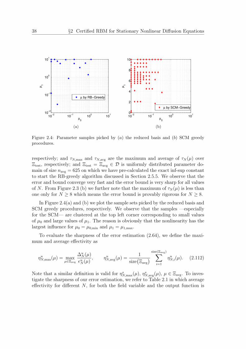
38 §2 Certified RBM for Stationary Nonlinear Diffusion Equations
10−2
10−1
100
101
10−2
10−1
100
101
µ0
µ1
µ by RB−Greedy
(a)
10−2
10−1
100
101
0
2
4
6
8
10
µ0
µ1
µ by SCM−Greedy
(b)
Figure 2.4: Parameter samples picked by (a) the reduced basis and (b) SCM greedyprocedures.
respectively; and τN,max and τN,avg are the maximum and average of τN(µ) overΞtest, respectively; and Ξtest = Ξavg ∈ D is uniformly distributed parameter do-main of size navg = 625 on which we have pre-calculated the exact inf-sup constantto start the RB-greedy algorithm discussed in Section 2.5.5. We observe that theerror and bound converge very fast and the error bound is very sharp for all valuesof N . From Figure 2.3 (b) we further note that the maximum of τN(µ) is less thanone only for N ≥ 8 which means the error bound is provably rigorous for N ≥ 8.
In Figure 2.4(a) and (b) we plot the sample sets picked by the reduced basis andSCM greedy procedures, respectively. We observe that the samples —especiallyfor the SCM— are clustered at the top left corner corresponding to small valuesof µ0 and large values of µ1. The reason is obviously that the nonlinearity has thelargest influence for µ0 = µ0,min and µ1 = µ1,max.
To evaluate the sharpness of the error estimation (2.64), we define the maxi-mum and average effectivity as
ηuN,max(µ) = maxµ∈Ξavg
∆uN(µ)
euN(µ), ηuN,avg(µ) =
1
size(Ξavg
) size(Ξavg)∑i=1
ηuN,i(µ). (2.112)
Note that a similar definition is valid for ηsN,max(µ), ηsN,avg(µ), µ ∈ Ξavg. To inves-tigate the sharpness of our error estimation, we refer to Table 2.1 in which averageeffectivity for different N , for both the field variable and the output function is

2.6 Numerical Results 39
given. Note that although the effectivity for the field variable, ηuN,avg is very closeto 1, due to very fast convergence of esN,max,rel, the effectivity number for the outputfunction ηsN,avg is quite large. One way to improve the output error bound is usinga primal-dual RB method [35] to increase the convergence rate of the ∆s
N,max,rel.Note that the average effectivity number ηuN,avg is less than 1 for N = 2 indicatingthat the error bound is not rigorous at some parameters when N = 2. However,the bound is provably rigorous for N ≥ 8 and as the effectivities show, the errorbound is also very sharp.
N euN,max,rel τN,max ∆uN,max,rel ηuN,avg esN,max,rel ∆s
N,max,rel ηsN,avg
2 2.59 E – 1 8.92 E + 1 5.09 E – 1 0.99 1.58 E – 2 9.54 E – 2 9.78 E + 24 4.87 E – 2 3.92 E + 1 9.03 E – 2 1.18 8.34 E – 5 1.69 E – 2 2.72 E + 38 2.32 E – 3 4.90 E – 2 2.85 E – 3 1.33 3.27 E – 6 5.33 E – 4 5.48 E + 312 2.52 E – 5 1.71 E – 3 2.69 E – 5 1.28 1.00 E – 9 5.03 E – 6 2.75 E + 416 4.69 E – 7 7.86 E – 4 2.51 E – 6 1.90 2.36 E – 10 4.71 E – 7 2.82 E + 3
Table 2.1: Proximity indicator, maximum relative error and bound as well as effectivityfor the field variable and the output for different values of N .
To have an idea about the computational savings we obtain using the RBmethod, we also define ∂tFEM/RB, ∂tFEM/∆N
, ∂t∆N/RB as
∂tFEM/RB ≡average CPU time to calculate u(µ)
CPU time to calculate uN(µ), (2.113)
∂tFEM/∆N≡ average CPU time to calculate uN(µ)
CPU time to calculate ∆uN(µ)
, (2.114)
∂t∆N/RB ≡average CPU time to calculate ∆u
N(µ)
CPU time to calculate uN(µ). (2.115)
We should remark that average is taken over Ξavg. Table 2.2 shows computationalsavings of order O(103). As it can be seen from the last column, thanks to theSCM method, evaluating the error estimation for each µ ∈ D is computationallyfrom the same order of calculating the RB solution.
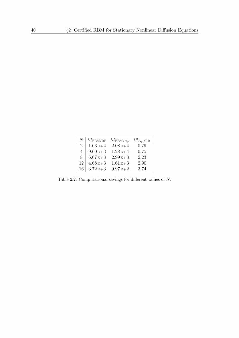
40 §2 Certified RBM for Stationary Nonlinear Diffusion Equations
N ∂tFEM/RB ∂tFEM/∆N∂t∆N/RB
2 1.63 E + 4 2.08 E + 4 0.794 9.60 E + 3 1.28 E + 4 0.758 6.67 E + 3 2.99 E + 3 2.2312 4.68 E + 3 1.61 E + 3 2.9016 3.72 E + 3 9.97 E + 2 3.74
Table 2.2: Computational savings for different values of N .
Chapter 3
Parabolic QuadraticallyNonlinear Diffusion Equations
41

42 §3 Certified RBM for Evolutionary Nonlinear Diffusion Equations
3.1 Introduction
In this Chapter, we present a certified RB method for time-dependent quadraticallynonlinear diffusion equations. As many practical problems are time-dependent,extending the introduced method explained in Chapter 2 to time-dependent equa-tions is interesting from a practical point of view. To do this, we follow the sameRB method we developed in Chapter 2, with some modifications to make the er-ror bound usable in time-dependent cases. Since the error bound introduced inChapter 2 is evaluated by applying the BRR framework —which is not applica-ble to time-dependent problems— we first reformulate our evolutionary probleminto a stationary-looking equation which satisfies the BRR configurations by usingspace-time formulation [68, 69].
Another motivation for using the space-time method comes from the fact thatstandard techniques do not promise a rigorous error bound in the nonlinear case.As we will see in Section 3.2.1, by extending the standard method [35] to nonlinearcase, we are not able to have a rigorous error estimation. Moreover, because thesemethods are mostly based on considering the worst case approximation at eachtime step, the error bound can grow exponentially in time even when the solutionis asymptotically stable [89, 79, 102]. Therefore even by having a rigorous errorestimation, using a standard time-stepping method for nonlinear equations wouldend up to a pessimistic error bound and therefore an inefficient reduced basisapproximation.
Applying the space-time method in reduced basis context is not unprecedented.See [89] for applying the space-time method on linear parabolic equation to obtainan improved error bound. In [102] the space-time approximation technique isapplied on a simple one dimensional Burgers’ equation with only one parameter.Finally the most recent work is done over a quadratically nonlinear Boussinesqequation in [101]. Apart from obtaining a rigorous error bound, evaluation of theinf-sup stability constant is the biggest challenge dealing with nonlinear equations.Since the parameter domain is only one dimensional in [102], evaluating the inf-sup constant and consequently the error bound is not hard. In [101] on the otherhand, because the parameter domain is more general, a successive constraintsmethod (SCM) is applied to approximate the inf-sup constant. Because of thenonlinearity in which the inf-sup constant depends on the solution at each time-step, basis functions are taken in the space-time space rather than spatial-onlyspace. This causes significant offline efforts and for problems with rather largenumber of time steps can be even infeasible.
In this Chapter, we will try to combine good aspects of both time-steppingand space-time methods. We invoke computational efficiency of the time-stepping

3.2 Problem Statement 43
method to solve our parabolic nonlinear equation both in the truth space X andreduced basis space XN . On the other hand, applying the space-time method, weevaluate a sharp error estimation based on the BRR framework we introduced inChapter 2. The major advantage of our combination is using spatial-only ratherthan space-time basis functions to construct our reduced basis space. Thereforewe are able to save huge amounts of both offline and online1 computational costswhen we approximate the space-time inf-sup constant.
The rest of this Chapter is organized as follows: In Section 3.2 we first introduceour problem statement as well as necessary definitions and assumptions and presenta model problem on which we apply our RB approximation. In Section 3.3 a space-time reduced basis approximation is presented and the space-time error estimationis obtained based on the BRR framework. Section 3.4 is devoted to efficientlycalculate components required by the space-time error estimation in offline-onlinecomputational steps and finally in Section 3.5, we present numerical results toconfirm the rapid convergence of the presented method and the rigor and thesharpness of its associated a posteriori error bound.
3.2 Problem Statement
In this section, we first discuss the necessity of applying the space-time formu-lation to apply the RB method on nonlinear evolutionary PDEs and consideranother easier alternative to it. We then introduce an abstract framework to solvea parametrized unsteady quadratically nonlinear equation
∂u
∂t+ div
(G(u;µ)∇u
)= f, (3.1)
where G(u;µ) = µ0 + µ1u is a parameter dependent linear function of u. We thenexpress our space–time formulation for (3.1) and using finite elements method,we calculate its truth solution. At the end, we present a concrete example oftime-dependent quadratically nonlinear diffusion equation on a unit square domainwhich we will solve later in Section 3.5.
3.2.1 Why a Space-time Formulation?
Let us assume we want to solve equation (3.1) with the same time-stepping tech-niques by which we used to solve linear parabolic equations. For linear equations,
1The online computational savings are due to having a sharper inf-sup lower bound and as aresult, a smaller RB space

44 §3 Certified RBM for Evolutionary Nonlinear Diffusion Equations
usually when we want to extend the technique applied to elliptic equations toparabolic equations, we combine the greedy algorithm with the POD method [35],and then based on the a posteriori error bound we already calculated at each timestep, we evaluate the error estimation at the final time K. The question is whathappens if we follow the same technique to our nonlinear equation (3.1). If it ispossible to follow the same policy, it could save us a lot of theoretical and compu-tational efforts. To address this question, we first try to apply the methodologyin [35] for our nonlinear parabolic diffusion equation (3.1) by calculating the errorbound at each time step and then adding it up to find the error bound at the finaltime T .
For our temporal discretization, we partition the interval I ≡ (0, T ] into Knon-overlapping intervals Ik = (tk−1, tk], with constant time step ∆t = tk − tk−1,k = 1, · · · , K ans t0 = 0, tK = T . For simplicity, we would use the Euler backwardmethod to solve (3.1). To begin, as in Chapter 2, we need to first write the weakform of (3.1) as
m(uk(µ)− uk−1(µ), v) + ∆tµ0a0(uk(µ), v) + ∆tµ1a1(uk(µ), uk(µ), v) = ∆tf(v),
∀v ∈ V, k = 1, · · · , K,(3.2)
where m(w, v) is the mass matrix defined as
m(w, v) =
∫Ω
wvdΩ, w, v ∈ V, (3.3)
and a0(w, v), a1(w,w, v) and f(v) are as defined in Chapter 2 and uk(µ) is thesolution of (3.2) at time step k, k = 1, · · · , K. Now for each time step k, we definethe residual function
g(ukN(µ), v;µ) = f(v)− 1
∆tm(ukN(µ)− uk−1
N (µ), v)− µ0a0(ukN(µ), v)
− a1(ukN(µ), ukN(µ), v), ∀v ∈ V. (3.4)
It is clear that for ekN(µ) = uk(µ)− ukN(µ) ∈ V , k = 1, · · · , K we have
m(ekN(µ)− ek−1N (µ), v) + ∆tµ0a0(ekN(µ), v) + ∆tµ1a1(uk(µ), uk(µ), v)
−∆tµ1a1(ukN(µ), ukN(µ), v) = ∆tf(v), ∀v ∈ V. (3.5)
Now if we take v = ekN(µ), we can show
a1(uk, uk, ekN)− a1(ukN , ukN , e
kN) = a1(ekN , e
kN , e
kN) + a1(ukN , e
kN , e
kN) (3.6)
+ a1(ekN , ukN , e
kN). (3.7)

3.2 Problem Statement 45
Using the Yong’s inequality
2|c||d| ≤ 1
ρ2c2 + ρ2d2, c, d ∈ R, ρ ∈ R+, (3.8)
and Cauchy-Schwarz, we can write
m(ek−1N , ekN) ≤ m1/2(ek−1
N , ek−1N )m1/2(ekN , e
kN) (3.9)
≤ 1
2
[m(ek−1
N , ek−1N ) +m(ekN , e
kN)]. (3.10)
On the other hand considering the definition of residual operator from (3.4),the dual norm of residual at each time step k is given by
εkN(µ) = supv∈V
g(ukN(µ), v;µ)
‖v‖V, ∀µ ∈ D. (3.11)
Therefore, from (3.11) we have
2 g(ukN(µ), ekN(µ);µ) ≤ 2 supv∈V
g(ukN(µ), v;µ)
‖v‖V‖ekN‖, ∀µ ∈ D. (3.12)
Now from (3.5), (3.8) and (3.11) we can write
m(ekN , ekN) − m(ek−1
N , ek−1N ) + 2∆t µ0a0(ekN(µ), ekN(µ))
+ 2 ∆t[a1(ekN , e
kN , e
kN) + a1(ukN , e
kN , e
kN) + a1(ekN , u
kN , e
kN)]
≤ 2 ∆t g(ukN(µ), ekN(µ);µ)
≤ ∆t( 1
αLB(µ)εkN(µ)2 + 2αLB‖ek‖2
X
), (3.13)
where αLB is the lower bound for the coercivity constant given by
αLB(µ) = infv∈V
a0(w,w;µ)
‖w‖V, ∀µ ∈ D, (3.14)
and εkN(µ) is the dual norm of residual defined by (3.11). Defining
ζkN,LB(µ) ≤ ζkN(µ) = infv∈V
a1(v, v, v) + a1(ukN , v, v) + a1(v, ukN , v)
‖v‖V, (3.15)
then we can rewrite (3.13) as
m(ekN , ekN)−m(ek−1
N , ek−1N ) + 2 ∆t ζkN,LB(µ)‖ekN(µ)‖2 ≤ ∆t
2αLB(µ)εkN(µ)2. (3.16)

46 §3 Certified RBM for Evolutionary Nonlinear Diffusion Equations
Now if we define the Y -norm (w,w)Y = m(w,w), the equation (3.16) would begiven given by
‖ekN(µ)‖2Y −
(1 + 2 ∆t ζkN,LB(µ)
)− ‖ek−1
N (µ)‖2Y ≤
∆t
2αLB(µ)εkN(µ)2. (3.17)
We now use the idea of multiplying the both sides of (3.17) tok−1∏j=1
(1+2∆tξjN,LB(µ)
).
We have
‖ekN(µ)‖2Y
k∏j=1
(1 + 2∆tξjN,LB(µ)
)− ‖ek−1
N (µ)‖2Y
k−1∏j=1
(1 + 2∆tξjN,LB(µ)
)(3.18)
≤ ∆t
2αLB(µ)εkN(µ)2
k−1∏j=1
(1 + 2∆tξjN,LB(µ)
).
Now getting summation over k = 1, · · · , K we have
‖ekN(µ)‖2Y
K∏j=1
(1 + 2∆tξjN,LB(µ)
)≤
K∑k=1
( ∆t
2αLB(µ)εkN(µ)2
k∏j=1
[1 + 2∆tξjN,LB(µ)
]).
(3.19)Therefore,
‖ekN(µ)‖2Y ≤
∆t2αLB(µ)
K∑k=1
(εkN(µ)2
k∏j=1
[1 + 2∆tξjN,LB(µ)
])K∏j=1
(1 + 2∆tξjN,LB(µ)
) , (3.20)
which gives us a rigorous error bound for ‖ekN(µ)‖2Y . Until now, we have shown that
using known RB method techniques for linear equations, it is actually possible toevaluate a rigorous error bound even for our nonlinear diffusion equation. There areunfortunately some drawbacks: by using Cauchy-Schwarz and Yong’s inequalityand other pessimistic substitutions like (3.11), (3.13) and (3.15), the sharpness ofthe error bound (3.20) can be severely jeopardized. Moreover, calculating a ratherpessimistic upper bound for the error at each time step and then adding them upto evaluate the error at the final time, does not seem to be the best idea if we arelooking for a sharp error bound.
But most importantly is the absence of an efficient offline-online computationalframework which makes the error bound (3.20) not suitable for our certified RB

3.2 Problem Statement 47
approximation. Unfortunately, there is no efficient way to calculate ζkN,LB(µ) from(3.15), for each µ ∈ D in an offline-online efficient way. As we know from Chapter1, an efficient offline-online strategy is one of the main components of the RBmethod. Therefore a rigorous error bound which is not offline-online calculablewould not be interesting in the RB context. That motivates for a new techniquewhich not only provides a rigorous error bound for our approximation, but alsofits in the offline-online computational framework. To pursue this goal, we invokethe space-time formulation.
3.2.2 Abstract Framework
To begin, we first define a few spaces and forms which we will need throughout thischapter. We define the standard Hilbert space L2(Ω) over our domain Ω ⊆ Rd, d =
1, 2, 3 equipped with the inner product (w,w)L2 =
∫Ω
wvdΩ and norm ‖w‖L2 =
(w,w)1/2
L2 . We need also the space H10 (Ω), or more specifically, H1
0 (Ω) ⊂ H1(Ω),
where H1(Ω) =v∣∣∣v ∈ L2(Ω),∇v ∈
(L2(Ω)
)d, H1
0 (Ω) =v∣∣v ∈ H1(Ω), v
∣∣∂Ω
=
0
. Here Ω is a bounded domain in Rd, d = 1, 2, 3, with Lipschitz continuousboundary ∂Ω. The inner product and norm associated with H1
0 are given by
(· , · )H10
and ‖· ‖H10
= (· , · )1/2
H10
respectively and
(w, v)H10≡∫
Ω
∇w∇vdΩ, ∀w, v ∈ H10 . (3.21)
We define the Gelfand triple (V,H, V ′) and associated duality pair 〈·, ·〉 wherein our context V = H1
0 (Ω) and H = L2(Ω). The norm of ` ∈ V is defined by
‖`‖V ′ = supφ∈V
〈`, φ〉V ′×V
‖φ‖V. (3.22)
The Riesz representator R` ∈ V satisfies ‖R`‖V = ‖`‖V ′ where R : V ′ 7→ V is theRiesz operator and (R`, φ)V = 〈`, φ〉V ′×V where `, φ are arbitrary vectors in V ′, Vrespectively.
Since we are going to use space–time formulation, we need to also define space–time spaces and norms. The space–time inner products and norms are very similarto spatial-only inner products and norms, except for presence of the time integra-tion. The space L2(I, V ) for example is defined as
(w, v)L2(I,V ) ≡∫I
⟨w(t), v(t)
⟩Vdt, (3.23)

48 §3 Certified RBM for Evolutionary Nonlinear Diffusion Equations
where I = (0, T ], is the time interval. Note that the space–time spaces are definednot only on the spatial domain but also on temporal domain on which the problemevolves. Associated norm for inner product (3.23) is defined as
‖w‖L2(I,V ) ≡ (w,w)1/2
L2(I,V ). (3.24)
We define the dual space of L2(I, V ) as L2(I, V ′) with inner product
(w, v)L2(I,V ′) ≡∫I
⟨Rw(t), Rv(t)
⟩V≡∫I
∫Ω
a(w, v
)dΩdt, (3.25)
where R : V ′ 7→ V is the Riesz operator. The space H10 (I, V ′) is equipped with
inner product
(w, v)H10 (I,V ′) ≡
∫I
⟨Rw(t), Rv(t)
⟩V≡∫I
∫Ω
a(w, v
)dΩdt, (3.26)
where w = ∂w∂t
is the temporal derivative and ‖w‖H10 (I,V ′) = (w,w)
1/2
H10 (I,V ′)
. Finally
we define the space Xe as our trial space-time space given by
Xe ≡ L2(I, V ) ∩H10 (I, V ′), (3.27)
equipped with the norm
(w,w)Xe = (w,w)L2(I,V ) + (w,w)H10 (I,V ′), (3.28)
while the space-time test space is defined as
Ye ≡ L2(I, V ). (3.29)
The weak formulation of the underlying problem (3.1) can be then stated asfollows: given any parameter µ ∈ D ⊂ RP , we evaluate uesp(µ) ∈ Xe, where uesp(µ)is the solution of the following nonlinear system
M(uesp(µ), v) + µ0A0(uesp(µ), v) + µ1A1(uesp(µ), uesp(µ), v) = F(v), ∀v ∈ Ye,(3.30)
with the space-time forms
M(w, v) ≡∫I
〈w(t), v(t)〉V ′×V dt, ∀w ∈ Xe,∀v ∈ Ye, (3.31)
A0(w, v) ≡∫I
a0
(w(t), v(t)
)dt, ∀w ∈ Xe,∀v ∈ Ye, (3.32)
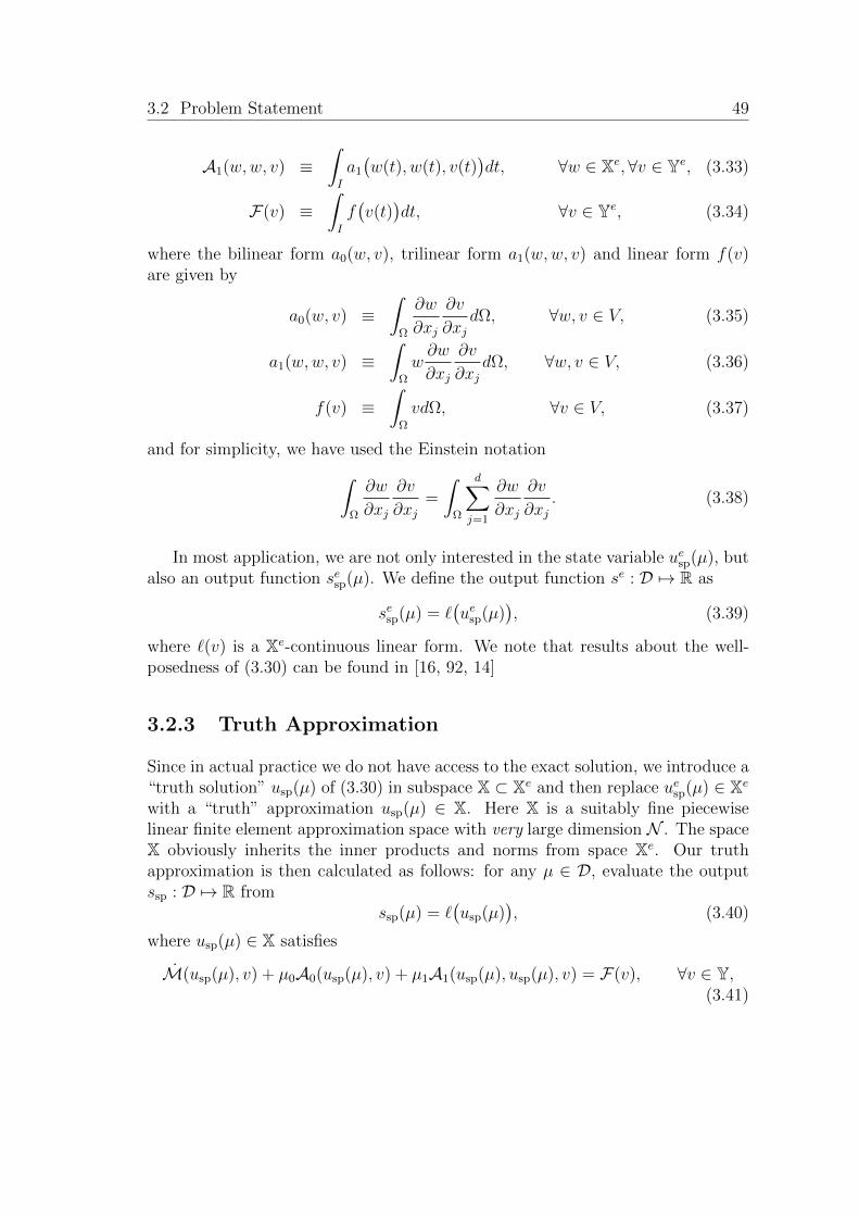
3.2 Problem Statement 49
A1(w,w, v) ≡∫I
a1
(w(t), w(t), v(t)
)dt, ∀w ∈ Xe,∀v ∈ Ye, (3.33)
F(v) ≡∫I
f(v(t)
)dt, ∀v ∈ Ye, (3.34)
where the bilinear form a0(w, v), trilinear form a1(w,w, v) and linear form f(v)are given by
a0(w, v) ≡∫
Ω
∂w
∂xj
∂v
∂xjdΩ, ∀w, v ∈ V, (3.35)
a1(w,w, v) ≡∫
Ω
w∂w
∂xj
∂v
∂xjdΩ, ∀w, v ∈ V, (3.36)
f(v) ≡∫
Ω
vdΩ, ∀v ∈ V, (3.37)
and for simplicity, we have used the Einstein notation∫Ω
∂w
∂xj
∂v
∂xj=
∫Ω
d∑j=1
∂w
∂xj
∂v
∂xj. (3.38)
In most application, we are not only interested in the state variable uesp(µ), butalso an output function sesp(µ). We define the output function se : D 7→ R as
sesp(µ) = `(uesp(µ)
), (3.39)
where `(v) is a Xe-continuous linear form. We note that results about the well-posedness of (3.30) can be found in [16, 92, 14]
3.2.3 Truth Approximation
Since in actual practice we do not have access to the exact solution, we introduce a“truth solution” usp(µ) of (3.30) in subspace X ⊂ Xe and then replace uesp(µ) ∈ Xe
with a “truth” approximation usp(µ) ∈ X. Here X is a suitably fine piecewiselinear finite element approximation space with very large dimension N . The spaceX obviously inherits the inner products and norms from space Xe. Our truthapproximation is then calculated as follows: for any µ ∈ D, evaluate the outputssp : D 7→ R from
ssp(µ) = `(usp(µ)
), (3.40)
where usp(µ) ∈ X satisfies
M(usp(µ), v) + µ0A0(usp(µ), v) + µ1A1(usp(µ), usp(µ), v) = F(v), ∀v ∈ Y,(3.41)

50 §3 Certified RBM for Evolutionary Nonlinear Diffusion Equations
where index sp stands for space-time.
Note that in practice, we do not solve the space-time problem (3.41). Insteadwe break the nonlinear system (3.41) into smaller problems and try to calculatethe solution usp(µ) at each time-step. To do this, we first divide the time interval(0, T ] into K non-overlapping intervals (tk−1, tk] where k = 1, · · · , K and t0 = 0.Then we can rewrite the space-time problem (3.41) as
m(uk(µ), v) + µ0a0(uk(µ), v) + µ1a1(uk(µ), uk(µ), v) = f(v), ∀v ∈ V, (3.42)
which is a spatial-only problem at any time step k and
m(w, v) =
∫Ω
wvdΩ, ∀w, v ∈ V, (3.43)
and uk(µ) = u(µ; k) which is the solution of (3.42) at time step k.
In order to provide conditions for existence and uniqueness of the discretesolution, for every z ∈ X, we need to define the Frechet derivative form dG :X3 ×D 7→ R as
dG(w, v; z;µ) =M(w, v)+µ0A0(w, v)+µ1A1(z, w, v)+µ1A1(w, z, v), ∀v ∈ Y.(3.44)
To make sure that there is a unique solution for (3.41), we assume that
|A1(z, w, v)| ≤
∣∣∣∣∣∫I
∫Ω
z∂w
∂xj
∂v
∂xjdΩdt
∣∣∣∣∣ ≤ ρ‖z‖X‖w‖X‖v‖X, ∀w, v,∈ X, (3.45)
where ρ is the L2(I, L2(Ω))− X Sobolev embedding constant defined as
ρ ≡ supw∈X
‖w‖L4(I,L2(Ω))
‖w‖X. (3.46)
Not that this parameter independent constant has a very important role inconstructing our a-posteriori error bound via the BRR framework at the end.Another constants which we need to evaluate is the inf–sup stability constant
βspz (µ) = inf
w∈Xsupv∈Y
dG(w, v; z;µ)
‖w‖X‖v‖Y, z ∈ X, (3.47)
and continuity constant
γspz (µ) = sup
w∈Xsupv∈Y
dG(w, v; z;µ)
‖w‖X‖v‖Y, z ∈ X. (3.48)
We also assume that there exists a constant β0 > 0, such that for every µ ∈ Dwe have βsp
z (µ) ≥ β02.
2This condition is actually equivalent to having a stable numerical discretization. Based onour simulations, this assumption holds

3.2 Problem Statement 51
3.2.4 Algebraic Formulation
In this section, we construct the algebraic form of our space-time operators in-troduced in previous the section. To evaluate the solution of (3.42) we performa Petrov-Galerkin finite element method in a time-stepping manner to minimizedthe computational efforts. Since our equation is a diffusion equation and to keepoffline calculations minimal, here we use the DG method of order zero. This willgive us a lower-triangular form for our space-time matrix dG(w, v; z;µ) which atthe end makes it possible to have RB-basis functions only in spatial space.
We denote our spatial space as V which in our context would be H10 (Ω). For
our temporal discretization, we first partition the time interval I = (0, T ] into Knon-overlapping sub-intervals Ik = (tk−1, tk], k = 1, · · · , K. We then define ourtemporal trial space S∆t, temporal test space Q∆t as
S∆t ≡ v ∈ H10 (I) : v|Ik ∈ P0(I), k = 1, · · · , K, (3.49)
Q∆t ≡ v ∈ L2(I) : v|Ik ∈ P0(I), k = 1, · · · , K. (3.50)
Defining our spatial approximation space V ⊆ H10 (Ω) by
V ≡ v ∈ H10 (Ω) : v|Ω(p) ∈ P1(Ω), (3.51)
our finite element trial and test spaces are given by
X = S∆t ⊗ V, Y = Q∆t ⊗ V, (3.52)
respectively, where the inner products are defined as
(w, v)X = (w, v)L2(I,V ) + (w, v)H10 (I,V ′), (3.53)
(w, v)Y = (w, v)L2(I,V ), (3.54)
respectively. Additionally the associated norms for spaces X,Y would be given by
‖w‖X = (w,w)1/2X , ‖w‖Y = (w,w)
1/2Y . (3.55)
Note that the well-posedness of the space-time formulation is verified in [14, 16].Now we are in a position in which we should transform the space-time problem(3.41) —which is hard to solve numerically— into a spatial-only problem at everytime step which keeps all the characteristics of the original equation but it iscomputationally easier to solve. To do this, we try to separate the temporal andspatial parts of vectors in the space-time space X. Therefore for every usp(µ) ∈ X,we write
usp(µ) =K∑k=1
N∑i=1
uki (µ)σk ⊗ ξi (3.56)

52 §3 Certified RBM for Evolutionary Nonlinear Diffusion Equations
where uki (µ) is the solution of equation (3.42) at time step k which can be calculatedby standard time-stepping method and σk, k = 1, · · · , K is the temporal basisfunctions for our temporal trial space S∆t and ξi, i = 1, · · · ,N are the spatialbasis functions for V . The test functions vsp ∈ Y can also be written as
vsp =K∑k=1
N∑i=1
vki τk ⊗ ξi, (3.57)
where τ k, k = 1, · · · , K is temporal basis functions for the temporal test spaceQ∆t. Therefore from (3.41), (3.42) we can write∫I
(〈usp(t;µ), vsp(t)〉X′×X + µ0a0(usp(t;µ), vsp(t)) + µ1a1(usp(t;µ), usp(t;µ), v(t)
)dt
=K∑
k,l=1
N∑i,j=1
uki (µ)vlj
[(σk, τ l)L2(I)(ξi, ξj)L2(Ω)
+ µ0(σk, τ l)L2(I)a0(ξi, ξj)]
+K∑
k,l,m=1
N∑i,j=1
µ1uki (µ)uli(µ)vmj
[(σkσl, τm)L2(I)a1(ξi, ξi, ξj)
]= f(τ l ⊗ ξi), i = 1, · · · ,N , l = 1, · · · , K. (3.58)
To make every thing more clear, we divide the process of evaluating the alge-braic forms into two parts:
Temporal Operators
As it is clear from (3.58), we need to evaluate three temporal matrices. ThePetrov-Galerkin temporal matrices M time,S
∆tand M time
∆t∈ RK×K are given by(
M time,S∆t
)k,l
= (σk, τ l)L2(I) = δk,l, k, l = 1, · · · , K, (3.59)(M time
∆t
)k,l
= (σk, τ l)L2(I) =1
∆t
(δk,l − δk−1,l
), k, l = 1, · · · , K, (3.60)
where δk,l is the Kronecher delta and ∆t = tk − tk−1, k = 1, · · · , K. Note thatsince we are using Euler backward method, we approximate the time derivative asthe difference of two temporal basis functions σk(t), σk−1(t) which are constantfunctions at two different time steps.

3.2 Problem Statement 53
The triple product (σkσl, τm)L2(I) resulting from the nonlinearity is evaluatedas follows:(
M time,tri∆t
)k,m
= (σkσl, τm)L2(I) = δk,mδl,m, k, l,m = 1, · · · , K. (3.61)
Additionally, to evaluate the space-time norm ‖ · ‖Y from (3.53), we also needto calculate temporal matrix M time,Q
∆t∈ RK×K from(
M time,Q∆t
)k,l
= (τ k, τ l)L2(I) = δk,l, k, l = 1, · · · , K, (3.62)
where as it is clear M time,Q∆t
is a diagonal matrix thanks to the definition of ourtemporal test space.
In addition, we also require the temporal matrix M time,S∆t
∈ RK×K , for evalua-tion of X-inner product which is given by(M time,S
∆t
)k,l
= (σk, σl)L2(I) =1
∆t(δk,l − δk−1,l − δk,l−1 + δk−1,l−1), k, l = 1, · · · , K.
(3.63)
Spatial Operators
The spatial matrices are very similar to what we have presented in Chapter 2 and[72] for the elliptic case. Here we focus only on spatial variable uk(µ) ∈ V , attime step k, k = 1, · · · , K, because the temporal information will be added astemporal operators later. Then we can show this vector uk(µ) ∈ V as a linearcombination of spatial basis functions ξj, j = 1, · · · ,N which construct our truthapproximation space V as follows:
uk(µ) =N∑j=1
ukj (µ)ξj. (3.64)
Taking the spatial test function v = ξj, j = 1, · · · ,N , the spatial part ofequation (3.42) is given by
N∑i=1
uki (µ)m(ξi, ξj) + µ0
N∑i=1
uki (µ)a0(ξi, ξj) + µ1
N∑n,i=1
uki (µ)ukn(µ)a1(ξi, ξn, ξj) = f(ξj),
j = 1, · · · ,N , (3.65)
or in matrix form by [M + µ0A0 + µ1A1(uk)
]uk = F, (3.66)

54 §3 Certified RBM for Evolutionary Nonlinear Diffusion Equations
where M,A0 ∈ RN×N are parameter-independent matrices with entries
M i,j = (ξi, ξj)V , Ai,j0 = a0(ξi, ξj), 1 ≤ i, j ≤ N , (3.67)
and F ∈ RN is a parameter independent vector with entries F i = f(ξi), 1 ≤i ≤ N . Furthermore A1(u) ∈ RN×N is a parameter dependent matrix — solutiondependent if we want to be more precise — which has entries
Ai,j1 (u) =N∑n=1
unAi,j1,n, 1 ≤ i, j ≤ N , (3.68)
where
Ai,j1,n = a1
(ξn, ξj, ξi
), 1 ≤ i, j, n ≤ N . (3.69)
We now solve (3.66), for uk(µ) using a Newton iterative scheme as follows:starting with an initial value ukp, we find an increment δukp such that[M + µ0A0 + µ1
(A1(ukp) + A1(ukp)
)]δukp = F −
[µ0A0 + µ1A1(ukp) +M
]ukp. (3.70)
We update ukp+1 = ukp + δukp and continue this process until ‖δukp‖1 < εnewtontol is
satisfied for some p ≥ 0. The matrices A1(ukp) ∈ RN×N and A1(ukp) ∈ RN×N aregiven by
A1(ukp) =N∑n=1
ukpnA1,n, (3.71)
A1(ukp) =N∑n=1
ukpnA1,n, (3.72)
where matrix A1,n is defined in (3.69) and has entries
A1,n = a1
(ξi, ξn, ξj
), 1 ≤ i, j, n ≤ N . (3.73)
Finally, we evaluate the output function s(µ) from
sk(µ) = LTuk(µ), (3.74)
where L ∈ RN is the output vector defined as Li = `(ξi), 1 ≤ i ≤ N andk = 1, · · · , K.
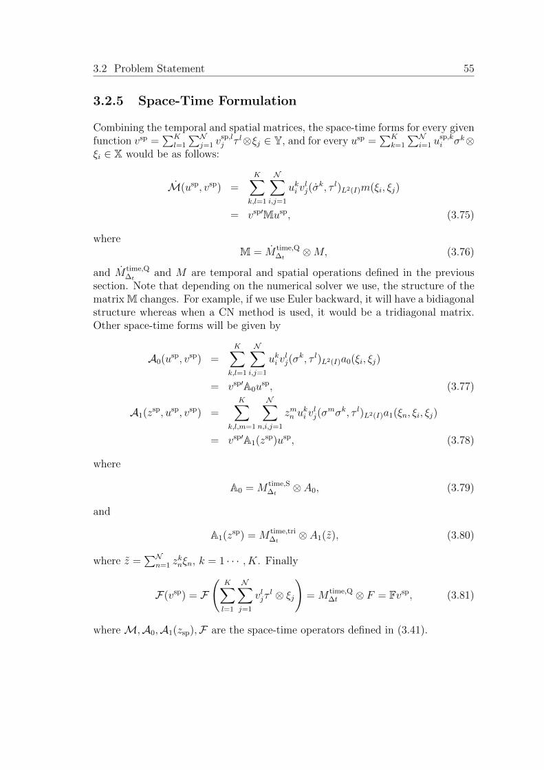
3.2 Problem Statement 55
3.2.5 Space-Time Formulation
Combining the temporal and spatial matrices, the space-time forms for every givenfunction vsp =
∑Kl=1
∑Nj=1 v
sp,lj τ l⊗ξj ∈ Y, and for every usp =
∑Kk=1
∑Ni=1 u
sp,ki σk⊗
ξi ∈ X would be as follows:
M(usp, vsp) =K∑
k,l=1
N∑i,j=1
uki vlj(σ
k, τ l)L2(I)m(ξi, ξj)
= vsp′Musp, (3.75)
whereM = M time,Q
∆t⊗M, (3.76)
and M time,Q∆t
and M are temporal and spatial operations defined in the previoussection. Note that depending on the numerical solver we use, the structure of thematrix M changes. For example, if we use Euler backward, it will have a bidiagonalstructure whereas when a CN method is used, it would be a tridiagonal matrix.Other space-time forms will be given by
A0(usp, vsp) =K∑
k,l=1
N∑i,j=1
uki vlj(σ
k, τ l)L2(I)a0(ξi, ξj)
= vsp′A0usp, (3.77)
A1(zsp, usp, vsp) =K∑
k,l,m=1
N∑n,i,j=1
zmn uki v
lj(σ
mσk, τ l)L2(I)a1(ξn, ξi, ξj)
= vsp′A1(zsp)usp, (3.78)
where
A0 = M time,S∆t
⊗ A0, (3.79)
and
A1(zsp) = M time,tri∆t
⊗ A1(z), (3.80)
where z =∑N
n=1 zknξn, k = 1 · · · , K. Finally
F(vsp) = F
(K∑l=1
N∑j=1
vljτl ⊗ ξj
)= M time,Q
∆t ⊗ F = Fvsp, (3.81)
where M,A0,A1(zsp),F are the space-time operators defined in (3.41).

56 §3 Certified RBM for Evolutionary Nonlinear Diffusion Equations
With the help of space-time matrices M,A0,A1(zsp) and space-time vector F,we now are able to write (3.58) in algebraic form as follows
[M + µ0A0 + µ1A1(usp)]usp = F. (3.82)
Note that (3.82) is an equivalent space-time algebraic form of (3.42). We remarkhere that, using space-time formulation is only necessary for evaluating error boundby applying BRR framework we introduced in Chapter 2. For computationalpurposes, we always use the time-stepping method and therefore equation (3.42)is our reference equation to be solved numerically.
Similarly, we can interpret the X-norm and Y-norm in matrix formulation:
X = M time,S∆t
⊗(MA−1
0 M)
+ ∆tM time,Q∆t
⊗ A0, (3.83)
Y = ∆tM time,Q∆t
⊗ A0. (3.84)
Notice that X is block tri-diagonal and Y is block-diagonal tensor.
0 0.2 0.4 0.6 0.8 1
0
0.1
0.2
0.3
0.4
0.5
0.6
0.7
0.8
0.9
1
−−X axis−−
−−
Y a
xis
−−
ell
Figure 3.1: Triangulation of our spatial domain Ω with 5000 elements on which we solvethe nonlinear problem (3.1). The mesh nodes are picked in a way that the resolution ishigher close to ∂Ω.

3.2 Problem Statement 57
0
0.5
1
0
0.5
10
1
2
3
x 10−3
(µ0,µ
1) = (10,0), k=1
Ω
Te
mp
era
ture
(a)
0 0.2 0.4 0.6 0.8 10
0.5
1
1.5
2
2.5
3
3.5
x 10−3
Te
mp
era
ture
(µ0,µ
1) = (10,0), k=1
(b) A 2-D cut from the 3-D plot
0
0.5
1
0
0.5
10
1
2
3
4
x 10−3
(µ0,µ
1) = (1,10), k=1
Ω
Te
mp
era
ture
(c)
0 0.2 0.4 0.6 0.8 10
1
2
3
4
5
x 10−3
Te
mp
era
ture
(µ0,µ
1) = (1,10), k=1
(d) A 2-D cut from the 3-D plot
0
0.5
1
0
0.5
10
2
4
x 10−3
(µ0,µ
1) = (0.01,10), k=1
Ω
Te
mp
era
ture
(e)
0 0.2 0.4 0.6 0.8 10
1
2
3
4
5
x 10−3
Te
mp
era
ture
(µ0,µ
1) = (0.01,10), k=1
(f) A 2-D cut from the 3-D plot
Figure 3.2: Behavior of the solution (temperature distribution over Ω in the modelproblem) for different parameter values.
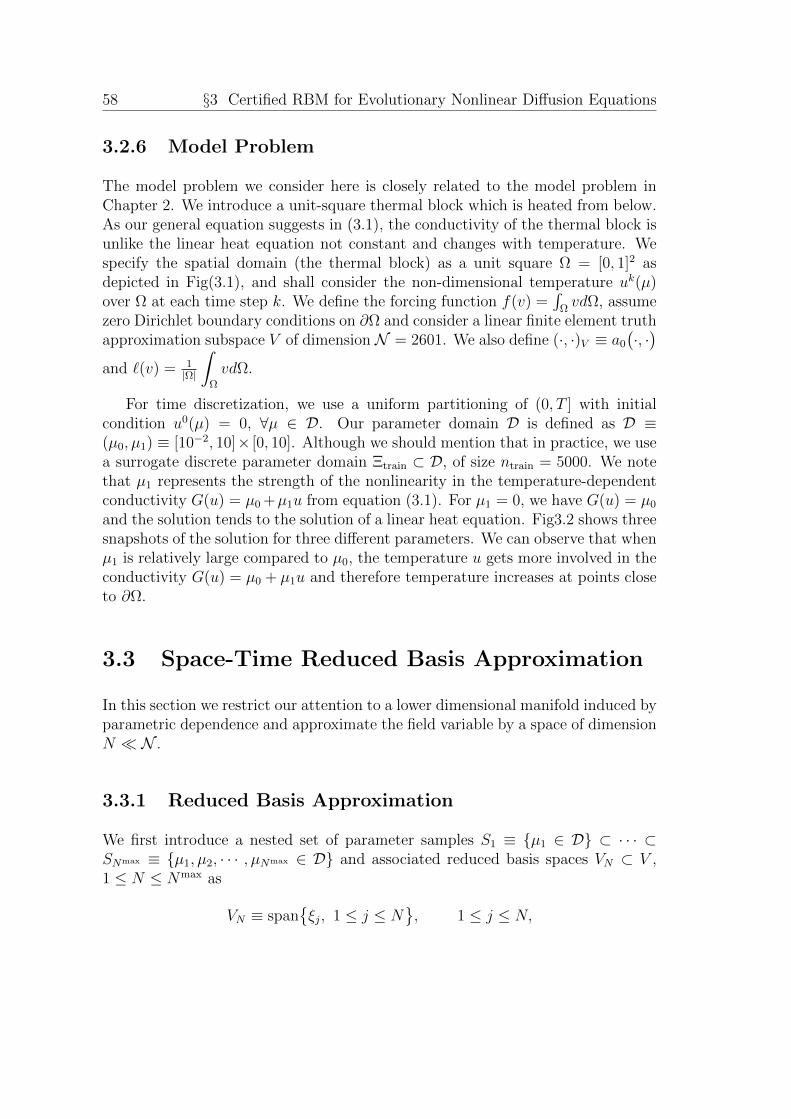
58 §3 Certified RBM for Evolutionary Nonlinear Diffusion Equations
3.2.6 Model Problem
The model problem we consider here is closely related to the model problem inChapter 2. We introduce a unit-square thermal block which is heated from below.As our general equation suggests in (3.1), the conductivity of the thermal block isunlike the linear heat equation not constant and changes with temperature. Wespecify the spatial domain (the thermal block) as a unit square Ω = [0, 1]2 asdepicted in Fig(3.1), and shall consider the non-dimensional temperature uk(µ)over Ω at each time step k. We define the forcing function f(v) =
∫ΩvdΩ, assume
zero Dirichlet boundary conditions on ∂Ω and consider a linear finite element truthapproximation subspace V of dimension N = 2601. We also define (·, ·)V ≡ a0
(·, ·)
and `(v) = 1|Ω|
∫Ω
vdΩ.
For time discretization, we use a uniform partitioning of (0, T ] with initialcondition u0(µ) = 0, ∀µ ∈ D. Our parameter domain D is defined as D ≡(µ0, µ1) ≡ [10−2, 10]× [0, 10]. Although we should mention that in practice, we usea surrogate discrete parameter domain Ξtrain ⊂ D, of size ntrain = 5000. We notethat µ1 represents the strength of the nonlinearity in the temperature-dependentconductivity G(u) = µ0 +µ1u from equation (3.1). For µ1 = 0, we have G(u) = µ0
and the solution tends to the solution of a linear heat equation. Fig3.2 shows threesnapshots of the solution for three different parameters. We can observe that whenµ1 is relatively large compared to µ0, the temperature u gets more involved in theconductivity G(u) = µ0 + µ1u and therefore temperature increases at points closeto ∂Ω.
3.3 Space-Time Reduced Basis Approximation
In this section we restrict our attention to a lower dimensional manifold induced byparametric dependence and approximate the field variable by a space of dimensionN N .
3.3.1 Reduced Basis Approximation
We first introduce a nested set of parameter samples S1 ≡ µ1 ∈ D ⊂ · · · ⊂SNmax ≡ µ1, µ2, · · · , µNmax ∈ D and associated reduced basis spaces VN ⊂ V ,1 ≤ N ≤ Nmax as
VN ≡ spanξj, 1 ≤ j ≤ N
, 1 ≤ j ≤ N,

3.3 Space-Time Reduced Basis Approximation 59
where the ξj ∈ V, 1 ≤ j ≤ N , are mutually (·, ·)V -orthogonal spatial-only basisfunctions. We construct the samples using a weak POD-greedy algorithm basedon an inexpensive a posteriori error estimator which will be introduced later.
The RB approximation is then clear: for every µ ∈ D, we find uspN (µ) ∈ XN
such that
M(uspN (µ), v) + µ0A0(usp
N (µ), v) + µ1A1(uspN (µ), usp
N (µ), v) = F(v), ∀v ∈ YN .(3.85)
Note that here the vector uspN (µ) ∈ X is in fact a reshaped ukN(µ) for k =
1, · · · , K, which lives in the space-time reduced basis space. Therefore unlike[101], our RB basis functions ξj, j = 1, · · · , Nmax are in V and not in X. As wewill see later, this can save huge amount of both offline and online calculations.We also calculate the RB output ssp
N (µ) from
sspN (µ) = `
(uspN (µ)
). (3.86)
3.3.2 Computational Procedure
In this section we develop an efficient computational procedure based on efficientreduced basis offline–online computational framework [62] to recover online N -independence for our nonlinear problem. Since we apply RB method only onfield variable, the temporal operators in our space-time RB space would be thesame as we defined in Section 3.2.4. The size of our spatial operators thoughwould be significantly reduced by approximating the spatial space V with a lowerdimensional space VN .
As we explained in the previous Section, the space-time RB solution uspN (µ) ∈
XN is in fact a reshaped version of ukN(µ) for k = 1, · · · , K created by adjoiningRB solutions ukN(µ) at each time step. Each of these blocks are in fact spatial-only solutions at some time steps. For sake of simplicity and considering that wewill add temporal information later to the equation, we focus only on spatial-onlyblocks uN(µ) by
uN(µ) =N∑j=1
uN,j(µ)ξj, (3.87)
where uN(µ) is the spatial-only solution of (3.42) at some arbitrary time step, andξj are our spatial basis functions defined in (3.85). Taking the spatial test functionv = ξj, j = 1, · · · , N , the spatial part of equation (3.42) is given by
N∑i=1
uN,i(µ)m(ξi, ξj) + µ0
N∑i=1
uN,i(µ)a0(ξi, ξj) (3.88)

60 §3 Certified RBM for Evolutionary Nonlinear Diffusion Equations
+ µ1
N∑n,i=1
uN,i(µ)uN,n(µ)a1(ξi, ξn, ξj) = f(ξj), j = 1, · · · , N,
or in matrix form by[MN + µ0A0,N + µ1A1,N(uN)
]uN = FN , (3.89)
where MN , A0,N ∈ RN×N are parameter-independent matrices with entries
M i,jN = m(ξi, ξj), Ai,j0,N = a0(ξi, ξj), 1 ≤ i, j ≤ N, (3.90)
and FN ∈ RN is a parameter independent vector with entries F i = f(ξi), 1 ≤j ≤ N . Furthermore A1,N(u) ∈ RN×N is a parameter dependent matrix which hasentries
Ai,j1,N(u) =N∑n=1
uN,nAi,j1,n, 1 ≤ i, j ≤ N, (3.91)
whereAi,j1,n = a1
(ξn, ξj, ξi
), 1 ≤ i, j, n ≤ N, (3.92)
where again vectors ξj, j = 1, · · · , N are the RB space basis functions.
We now solve (3.89), for uN(µ) using a Newton iterative scheme as follows:starting with an initial value uN,p, we find an increment δuN,p such that[
MN + µ0A0,N + µ1
(A1,N(uN,p) + A1(uN,p)
)]δuN,p =
= FN −[µ0AN,0 + µ1A1,N(uN,p) +MN
]uN,p. (3.93)
We update uN,p+1 = uN,p + δuN,p and continue this process until ‖δuN,p‖1 <
εnewtontol is satisfied for some p ≥ 0. The matrices A1(uN,p) ∈ RN×N and A1(uN,p) ∈RN×N are given by
A1(uN,p) =N∑n=1
uN,p,nA1,n, (3.94)
A1(uN,p) =N∑n=1
uN,p,nA1,n, (3.95)
where matrix A1,n is defined in (3.92) and has entries
A1,n = a1
(ξi, ξn, ξj
), 1 ≤ i, j, n ≤ N. (3.96)
3.3 Space-Time Reduced Basis Approximation 61
Finally, we evaluate the RB output function sN(µ) from
sN(µ) = LTNu(µ), (3.97)
where L ∈ RN is the output vector defined as Li = `(ξi), 1 ≤ i ≤ N .
Having the spatial-only solution, we now add temporal information to theequation. By including temporal information we can write equation (3.89) in thespace-time form as follows[
M time∆t ⊗MN + µ0M
time,S∆t ⊗ A0,N + µ1M
time,S∆t ⊗ A1,N(uN)
]uN =
= M time,Q∆t ⊗ FN . (3.98)
As we use the time-stepping Euler backward method to solve our time-dependentequation (3.98), for each time step k = 1, · · · , K, we solve the system
1
∆tMN
(uk − uk−1
)+[µ0A0,N + µ1A1,N(ukN)
]ukN = FN , k = 1, · · · , K, (3.99)
by the Newton method discussed above.
The Reduced Basis offline-online decomposition is now clear. In the offline stage—performed only once— we first compute and store all µ-independent quantitieslike A0,N , FN and A1,N from (3.90), (3.91). In the online stage, we first assem-
ble matrices A1,N(uN) and A1,N(uN) from (3.92), (3.96) which requires O(N2)operations and then solve (3.93) to evaluate δuN(µ) at cost O(N3) per Newtoniteration. Finally, given uN(µ), we evaluate the output sN(µ) from (3.97) at costO(N). Therefore a very efficient N -independent online algorithm can be appliedto solve nonlinear problem (3.85) to evaluate the solution ukN(µ) at each time stepk and for all µ ∈ D.
3.3.3 A posteriori Error Bound
In this section, we combine the space-time technique and results from Chapter2, to evaluate a rigorous a posteriori error estimation for the RB approximationof our nonlinear parabolic diffusion equation (3.1). The idea is to use the sameBRR framework we used in Chapter 2, but in the space-time setup. By using thespace-time method, in one hand we invoke the advantage of our very sharp errorbound which we calculated in elliptic case in Chapter 2, on the other hand, wekeep the efficient time-stepping method to solve our parabolic nonlinear PDE.
The a posteriori error bound then is very similar to proposition (1) in Chapter2, except that every component here is calculated in the space-time space. To begin
62 §3 Certified RBM for Evolutionary Nonlinear Diffusion Equations
we assume that we are given a positive space-time inf–sup lower bound βspN,LB(µ)
which is define in (3.47) for z = uN(µ).
We then define the space-time dual norm of residual
εspN = sup
v∈Y
G(uspN (µ), v;µ)
‖v‖Y, ∀µ ∈ D, (3.100)
where G(uspN (µ), v;µ) is the space-time residual operator defined as
G(uspN (µ), v;µ) = M(usp
N (µ), v) + µ0A0(uspN (µ), v) (3.101)
+ µ1A1(uspN (µ), usp
N (µ), v)−F(v), ∀v ∈ Y,
where uspN (µ) is the solution of (3.85). Then the error estimation ∆u,sp
N (µ) for eachµ ∈ D is given by
Proposition 4. For
τ spN (µ) =
4ρµ1εspN (µ)
βspN,LB(µ)2
< 1, (3.102)
and for every µ ∈ D, there exists a unique solution usp(µ) ∈ X in the neighborhoodof usp
N (µ) ∈ XN . Furthermore, there exists a rigorous upper bound for the RBerror, ‖usp(µ)− usp
N (µ)‖X as follows:
∆u,spN (µ) =
βspN,LB(µ)
2ρµ1
(1−
√1− τ sp
N (µ)), (3.103)
where ρ is the L4(I, L2(Ω))− X Sobolev constant defined in (3.46).
We can also obtain a rigorous error bound for the space-time output functionsspN (µ) which is defined in (3.86) as follows:
Proposition 5. When
τ spN (µ) =
4ρµ1εspN (µ)
βspN,LB(µ)2
< 1, (3.104)
the error in the output function satisfies: |ssp(µ) − sspN (µ)| ≤ ∆s,sp
N (µ), ∀µ ∈ D,where
∆s,spN (µ) = ‖`‖X′∆u,sp
N (µ), (3.105)
where ‖`‖X′ = supv∈X`(v)‖v‖X
is the dual norm of the linear operator ` in the space-time space.
3.4 Offline-Online Construction of the Error Bound 63
Note that the proof for these theorems is given in Chapter 2 and [72].
We should now develop a technique to evaluate µ-dependent space-time con-stants εsp
N (µ) and βspN,LB(µ) in an efficient way. Note that we will not use space-time
definitions for εspN (µ), βsp
N,LB(µ) from (3.100), (3.47) because it would be computa-tionally very expensive to do all the calculations in the space-time space, speciallywhen K, the number of time steps is big. In next Section, we develop a methodto calculate these parameter dependent constants in an equivalent time-steppingmethod which also fits in our offline-online computational framework.
3.4 Offline-Online Construction of the Error Bound
To efficiently calculate the error bound ∆u,spN (µ) for every µ ∈ D, we need to
develop an offline-online computational framework in which we calculate threemain components of the error bound efficiently and independent of the size of ourtruth finite element space.
3.4.1 Space-Time Dual Norm of Residual
We now consider calculation of εspN (µ). To start, we first remind that usp
N (µ) ∈ Xcan be written as
uspN (µ) =
K∑k=1
N∑j=1
ukNj(µ)σk ⊗ ξj. (3.106)
On the other hand, considering definition of space-time residual operatorG(usp
N (µ), v;µ) from (3.101) and using Riesz representation theorem, we have espN (µ) ∈
Y such that
G(uspN (µ), v;µ) = (esp
N (µ), v)Y, ∀v ∈ Y, (3.107)
which means
(espN (µ), v)Y = M(usp
N (µ), v) + µ0A0(uspN (µ), v) + µ1A1(usp
N (µ), uspN (µ), v)−F(v).
(3.108)
To follow offline-online calculations, considering (3.106) and for every v ∈ Y,we first define vectors XM , X0, X1 and XF ∈ X such that
(XM , v)Y = M
(K∑k=1
N∑j=1
ukNj(µ)σk ⊗ ξj, v
)(3.109)
64 §3 Certified RBM for Evolutionary Nonlinear Diffusion Equations
(X0, v)Y = µ0A0
(K∑k=1
N∑j=1
ukNj(µ)σk ⊗ ξj, v
), (3.110)
(X uspN1 , v)Y = µ1A1
(K∑k=1
N∑j=1
ukNj(µ)σk ⊗ ξj,K∑k=1
N∑j=1
ukNj(µ)σk ⊗ ξj, v
),(3.111)
(XF , v)Y = −F(v), ∀v ∈ Y. (3.112)
Based on (3.109)-(3.112) and (3.75), (3.77), (3.81) and for every v =K∑l=1
τl⊗ξi ∈ Y,
we can write
(X jM , v)Y =
K∑k,l=1
(σk, τ l)L2(I)m(ξj, ξi) i, j = 1, · · · , N, (3.113)
(X j0 , v)Y =
K∑k,l=1
(σk, τ l)L2(I)a0(ξj, ξi) i, j = 1, · · · , N, (3.114)
(X j,j′
1 , v)Y =K∑
k,l,m=1
(σkσl, τm)L2(I)a0(ξj, ξj′ , ξi), i, j, j′ = 1, · · · , N. (3.115)
It follows from linearity and (3.75), (3.77), (3.108) and (3.113)-(3.115) that
espN (µ) =
N∑j=1
uspNj(µ)
[X jM + µ0X j
0 + µ1
N∑j′=1
usp,kNj′X
j,j′
1
]+ XF . (3.116)
Now the only challenge is to evaluate space-time vectors X jM , X j
0 , X j,j′
1 for eachj, j′ = 1, · · · , N, independent of the size of our space-time space Y. To do this, wefirst evaluate vectors Xj
M , Xj0 , Xj,j′
1 ∈ V such that
(XjM , w)Y = m(ξj, w) w ∈ Y (3.117)
(Xj0 , w)Y = a0(ξj, w) w ∈ Y, (3.118)
(Xj,j′
1 , w)Y = a0(ξj, ξj′ , w) w ∈ Y . (3.119)
Using (3.117)-(3.119), (3.113)-(3.115) and considering (3.116), the space-timevector esp
N (µ) can be given by
espN (µ) =
1
∆t
N∑j=1
uspNj(µ)
[ K∑k=1
σk ⊗XjM + µ0
K∑k=1
σk ⊗Xj0 (3.120)

3.4 Offline-Online Construction of the Error Bound 65
+µ1
N∑j′=1
K∑k,l=1
σl ⊗ uspNj′ σ
k ⊗Xj,j′
1
]+
1
∆tM time,Q
∆t ⊗XF ,
where (XF , w)Y = −f(w) for every w ∈ Y .
Equation (3.120) is the space-time dual norm of residual with separated spatialand temporal variables. We are now in a position to use our time-stepping methodto evaluate the dual norm of residual ekN(µ) at time step k = 1, · · · , K and forevery µ ∈ D. Note that the space-time dual norm of residual esp
N (µ) is in fact arearranged version of ekN(µ) at time step k = 1, · · · , K.
Now from (3.107), (3.108) and considering the definition of M time,S∆t , M time,S
∆t forthe Euler backward method and the Y-norm definition in (3.84) we can write
ekN(µ) =1
∆t2
N∑j=1
(ukNj(µ)− uk−1
Nj (µ))XjM +
1
∆tµ0u
kNj(µ)Xj
0
+1
∆tµ1
N∑i,j=1
uNj(µ)uNi(µ)X i,j1 +
1
∆tXF . (3.121)
Therefore the dual norm of residual ‖ekN(µ)‖V at each time step k would begiven by(ekN(µ), ekN(µ)
)V
=( 1
∆t2
N∑j=1
(ukNj(µ)− uk−1
Nj (µ))XjM ,
1
∆t2
N∑j′=1
(ukNj′(µ)− uk−1
Nj′ (µ))Xj′
M
)V
+ 2( 1
∆t2
N∑j=1
(ukNj(µ)− uk−1
Nj (µ))XjM ,
µ0
∆t
N∑j′=1
ukNj′(µ)Xj′
0
)V
+ 2( 1
∆t2
N∑j=1
(ukNj(µ)− uk−1
Nj (µ))XjM ,
µ1
∆t
N∑j′,j′′=1
uNj′(µ)uNj′′(µ)Xj′,j′′
1
)V
+ 2( 1
∆t2
N∑j=1
(ukNj(µ)− uk−1
Nj (µ))XjM ,
1
∆tXF
)V
+( µ0
∆t
N∑j=1
ukNj(µ)Xj0 ,
µ0
∆t
N∑j′=1
ukNj′(µ)Xj′
0
)V
+ 2( µ0
∆t
N∑j=1
ukNj(µ)Xj0 ,
µ1
∆t
N∑j′,j′′=1
uNj′(µ)uNj′′(µ)Xj′,j′′
1
)V
+( µ1
∆t
N∑j,j′=1
uNj(µ)uNj′(µ)Xj,j′
1 ,µ1
∆t
N∑j′′,j′′′=1
uNj′′(µ)uNj′′′(µ)Xj′′,j′′′
1
)V

66 §3 Certified RBM for Evolutionary Nonlinear Diffusion Equations
+ 2( µ1
∆t
N∑j,j′=1
uNj(µ)uNj′(µ)Xj,j′
1 ,1
∆tXF
)V
+ 2( µ0
∆t
N∑j=1
ukNj(µ)zj0 ,1
∆tXF
)V
+( 1
∆tXF ,
1
∆tXF
)V. (3.122)
Now if we pre-calculate the following parameter independent inner products
CF,F =(XF , XF
)V, (3.123)
CjF,M =
(XF , Xj
M
)V, (3.124)
CjF,A0
=(XF , Xj
0
)V, (3.125)
Cj,j′
F,A1=
(XF , Xj,j′
1
)V, (3.126)
Cj,j′
M,M =(XjM , Xj′
M
)V, (3.127)
Cj,j′
M,A0=
(XjM , Xj′
0
)V, (3.128)
Cj,j′,j′′
M,A1=
(XjM , Xj′,j′′
1
)V, (3.129)
Cj,j′
A0,A0=
(Xj
0 , Xj′
0
)V, (3.130)
Cj,j′,j′′
A0,A1=
(Xj
0 , Xj′,j′′
1
)V, (3.131)
Cj,j′,j′′,j′′′
A1,A1=
(Xj,j′
1 , Xj′′,j′′′
1
)V, (3.132)
we can rewrite (3.122) as follows
(ekN(µ), ekN(µ)
)V
=1
∆t4
N∑j=1
(ukNj(µ)− uk−1
Nj (µ)) N∑
j′=1
(ukNj′(µ)− uk−1
Nj′ (µ))Cj,j′
M,M
+ 2µ01
∆t3
N∑j=1
(ukNj(µ)− uk−1
Nj (µ))ukNj′(µ) Cj,j′
M,A0
+ 2µ11
∆t3
N∑j=1
(ukNj(µ)− uk−1
Nj (µ)) N∑
j′,j′′=1
uNj′(µ)uNj′′(µ) Cj,j′,j′′
M,A1
+ 21
∆t2
N∑j=1
(ukNj(µ)− uk−1
Nj (µ))CjF,M
+ µ20
1
∆t2
N∑j,j′=1
ukNj(µ) ukNj′(µ) Cj,j′
A0,A0
+ 2 µ0µ11
∆t2
N∑j=1
ukNj(µ)N∑
j′,j′′=1
uNj′(µ)uNj′′(µ) Cj,j′,j′′
A0,A1

3.4 Offline-Online Construction of the Error Bound 67
+ µ11
∆t2
N∑j,j′=1
uNj(µ)uNj′(µ) CjF,A0
+ µ21
1
∆t2
N∑j,j′=1
uNj(µ)uNj′(µ)N∑
j′′,j′′′=1
uNj′′(µ)uNj′′′(µ) Cj,j′,j′′,j′′′
A1,A1
+ 2 µ11
∆t2
N∑j,j′=1
uNj(µ)uNj′(µ) Cj,j′
F,A1+
1
∆t2CF,F , (3.133)
which is efficient and N -independent if we pre-calculate the parameter indepen-dent inner products from (3.123)-(3.132) in the offline part. The offline-onlinecomputational cost then would be as follows: in the offline stage we first com-pute µ-independent quantities from (3.117)-(3.119) which requires (to the leadingorder) solving O(N2) linear system of equations each of dimension N . We thenneed to pre-calculate O(N4) N -inner products from (3.123)-(3.132). In the onlinestage, given a new parameter value µ ∈ D and its associated RB solution ukN(µ)at time step k, we perform the summation (3.133) with cost O(N4) at each timestep. At the end we add the dual norm of residual at each time step k = 1, · · · , Kand then multiply it by ∆t. Taking square root of the ‖esp
N (µ)‖2Y, the dual norm
of residual εspN (µ) is given.
3.4.2 Space-Time Sobolev Embedding constant
To evaluate an error bound for our space-time RB approximation, just like theelliptic case, we need to calculate the Sobolev embedding constant defined as
ρ = supw∈Xe
‖w‖L4(I;L2(Ω))
‖w‖Xe
, (3.134)
where
(w, v)L4(I;L2(Ω)) =
∫I
∫Ω
w4v4dΩdt, w, v ∈ L2(Ω). (3.135)
Normally, instead of using (3.134) to evaluate the L4(I;L2(Ω)) − Xe Sobolevembedding constant, we evaluate a L2(I;L2(Ω))−X embedding constant because(3.134) involves a nonlinear eigenproblem over the space Xe which is not possible tosolve [72]. An alternative technique is using a homotopy method to approximatethe L4(I;L2(Ω)) − Xe Sobolev constant over a discrete finite dimensional spaceX [94]. A similar technique is used in [102], in which the magnitude of Sobolevconstant grows up as the temporal and spatial mesh becomes finer. In [101] asimilar space-time method is applied on Bossinesq equations. Using discontinuous

68 §3 Certified RBM for Evolutionary Nonlinear Diffusion Equations
Galerkin method, it is shown that the mesh-dependence —and also dependence onthe final time T— is weaker compared to [102]. Note that since the original non-linear eigenproblem is not theoretically solvable, all of the efforts mentioned aboveto approximate the Sobolev embedding constant are based on the assumption ofbeing in a finite dimensional discrete space X.
In this section we first show that our error bound ∆u,spN (µ) is not actually
very sensitive to the magnitude of the Sobolev constant ρ. We then introducea technique based on [72] to approximate L2(I;L2(Ω)) − X Sobolev embeddingconstant.
Proposition 6. For any ρ ∈(
0,βspN,LB(µ)2
4µ1εspN (µ)
), we have
εspN (µ)
βspN,LB(µ)
≤ ∆u,spN (µ) ≤ 2
εspN (µ)
βspN,LB(µ)
, µ ∈ D. (3.136)
Proof. We first define the function ϕµN(ρ), for every µ ∈ D as
ϕµN(ρ) =βspN,LB(µ)
2ρµ1
(1−
√1− 4ρµ1ε
spN (µ)
βspN,LB(µ)2
). (3.137)
Considering that limρ−→0
ϕµN(ρ) =εspN (µ)
βspN,LB(µ)
, and noticing the fact that for all
ρ ∈(
0,βspN,LB(µ)2
4µ1εspN (µ)
), ϕµ
′
N (ρ) > 0, the function ϕµN(ρ) takes its maximum at ρmax =
βspN,LB(µ)2
4µ1εspN (µ)
. This means
ϕµN(ρmax) = 2εspN (µ)
βspN,LB(µ)
, (3.138)
which completes the proof. Not thatεspN (µ)
βspN,LB(µ)
is actually the RB error bound for a
linear diffusion equation.
According to proposition 6 and Fig 3.3, the magnitude of the Sobolev em-bedding constant has not a big effect on the sharpness of our error estimation∆u,spN (µ). Note that as N , the dimension of our RB space grows up, the neighbor-
hood(
0,βspN,LB(µ)2
4µ1εspN (µ)
)gets bigger and bigger. Therefore calculating a very close to
the actual Sobolev embedding constant is not necessary.

3.4 Offline-Online Construction of the Error Bound 69
1 2 3 4
x 108
10−7.7
10−7.5
10−7.3
10−7.1
ρ
∆Nµ(ρ
)
∆N
µ(ρ)
∆linear
2*∆linear
Figure 3.3: The comparison of the error estimation ∆u,spN (µ) over different ρ for µ =
(1, 1).
To evaluate the L2(I;L2(Ω)) − X Sobolev constant, we need to find λ−1/2min
where λmin is the minimum eigenvalue of eigenproblem Pw = λQw where P =L2(I;L2(Ω)), Q = X. Since ρ is a parameter independent constant, we do needto calculate it just once. Note that solving this generalized eigenvalue problemrequires generating the Krylov space K(P−1X) which can be done in time-steppingmethod without constructing the space-time matrices [101].
3.4.3 Space-Time inf-sup Lower Bound
An efficient calculation of the space-time inf-sup lower bound βspN,LB(µ), µ ∈ D is
probably the most difficult part of our RB method for nonlinear parabolic diffusionequations for different reasons. Since we need to evaluate this inf-sup constant forthousands of parameters µ ∈ D to generate our RB space, it should be very easy tocalculate and yet quite close to the actual inf-sup constant defined in (3.47). As wehave shown in Chapter 2, the closer the inf-sup lower bound is to the actual inf-supconstant, the sharper the error bound would be at the end. We have applied aneffective method to estimate this constant in Chapter 2 known as SCM method

70 §3 Certified RBM for Evolutionary Nonlinear Diffusion Equations
[42] which worked great in elliptic case. In the parabolic case though, becausethe number of terms in the SCM process increases quite rapidly due to presenceof time, following that technique may not be possible. Therefore we would usea more effective technique called Natural Norm SCM [41] which helps to reduceoffline calculations in the SCM process.
Natural Norm SCM has been previously used in different disciplines like [29,56, 23]. A recent good application of that is [101], in which a Natural Norm SCMis applied to evaluate the inf-sup lower bound for a nonlinear Boussinesq equation.Since in [101] space-time basis functions are used, significant offline calculationsmust have been done to evaluate matrices and vectors required by Natural NormSCM whereas if the number of time steps K increases, it can be not feasible.
The Natural Norm SCM we use has two major differences compared to [101].First of all, due to our numerical solver, we are able to use spatial-only basisfunctions for our space-time reduced basis method. This as we will see later, savesus lots of offline computations. Additionally, since we calculate the inf-sup lowerbound at each time-step instead of the whole temporal domain, the correspondingbounding box we use is tighter compared the bounding boxes introduced in [101]which at the end accelerates the online calculations. In this section, to serveour efficient offline-online computational framework, we employ our version ofNatural Norm SCM which can reduce both offline and online computational coststo evaluate the inf-sup lower bound βsp
N,LB(µ), µ ∈ D.
According to N-norm SCM [42], we need to first define a supremizer calculatedat some SCM reference points µ. We call it T µ : X 7→ Y:(
T µw, v)Y = dG(w, v;u(µ); µ), ∀w ∈ X, ∀v ∈ Y. (3.139)
It is clear that
βspN (µ) ≥ inf
w∈X
dG(w, T µw;uspN (µ);µ)
‖w‖X‖T µw‖Y
≥
[infw∈X
‖T µw‖Y‖w‖X
][infw∈X
dG(w, T µw;uspN (µ);µ)
‖T µw‖2Y
]= βsp(µ)βµ,spN (µ). (3.140)
Since βspN (µ) ≥ βsp(µ)βµ,spN (µ), therefore by having βsp(µ), a lower bound for
βµ,spN (µ) will give us a lower bound for βspN (µ), ∀µ ∈ D. From now on, we try to use
SCM method to find a lower bound for βµ,spN (µ). As it is clear from (3.140), solvinga generalized eigenvalue problem with vectors in the space-time space X, Y maynot be computationally viable, even in the offline phase. Therefore we will try to

3.4 Offline-Online Construction of the Error Bound 71
transfer the generalized eigenvalue problem (3.140) into an equivalent generalizedeigenvalue problem which is solvable in a time-stepping method. Developing sucha technique gives us the advantage of having spatial-only basis functions for ourRB space over space-time basis functions are used in [101] which at the end bringsus a more efficient offline and online calculations. To do this, we first investigatethe structure of our space-time Frechet derivative form dG. In an operator formwe can write
dG = M+ µ0A0 + µ1
[A1(µ) + A1(µ)
], (3.141)
where M, A0, A1(µ) are defined in (3.75)-(3.77). Considering our numericalsolver and definition of space-time operators from (3.75), (3.77) and (3.83), we cansee that space-time tensors dG has a lower block-triangular structure whereas Yhas a block-diagonal structure. Therefore utilizing the following lemma, we cancalculate the minimum eigenvalue of dG using minimum eigenvalues of each blockon the diagonal of dG.
Lemma 2. Let Λ, Π be two block-triangular matrices. Then λ is generalizedeigenvalue of Λ with respect to the matrix Π if and only if λ is a generalizedeigenvalue of diagonal-block Λi with respect to Πi where i = 1, · · · , K and K isnumber of blocks.
Proof. We use mathematical induction: first we assume
Λ =
(Λ1 0Σ Λ2
), Π =
(Π1 0Ξ Π2
), (3.142)
where Λ, Π are n× n block-triangular matrices with only two blocks. Now if λ isa generalized eigenvalue of Λ with respect to Π, that means
det(Λ− λΠ) = det
((Λ1 0Σ Λ2
)− λ
(Π1 0Ξ Π2
))= det
((Λ1 − λΠ1 0Σ− λΞ Λ2 − λΠ2
))= 0, (3.143)
which means either det(Λ1 − λΠ1) = 0 or det(Λ2 − λΠ2) = 0. Therefore λ isgeneralized eigenvalue of Λ1 or Λ2 with respect to Π1 or Π2 respectively. Converselyif λ is an eigenvalue of Λi, i = 1, 2 on the diagonal with respect to Πi, i = 1, 2,then from (3.143) we know that det(λΠ− Λ) = 0 which means λ is eigenvalue ofΛ. Now we assume that lemma is correct for K − 1 blocks. Due to structure ofΛ, Π and our previous argument, it is clear that generalized eigenvalues of Λ withK blocks is given by the set of all generalized eigenvalues of Λ with K − 1 blocksand generalized eigenvalues of the last block ΛK with respect to the matrix ΠK
which completes the proof.

72 §3 Certified RBM for Evolutionary Nonlinear Diffusion Equations
Therefore instead of calculating the minimum eigenvalue of huge block-triangularmatrix dG in the space-time space, we calculate the minimum eigenvalue of eachblock which is in fact the minimum eigenvalue of dG at each time step and at theend we take a minimum over all calculated eigenvalues to evaluate the space-timeinf-sup constant. In this way, we avoid extensive computational efforts dictatedby space-time space Y.
We now need to redefine the inf-sup constant given in (3.140) to convert space-time inf-sup constant into an equivalent spatial-only inf-sup constant. We firstdefine the operator T µ,k : X 7→ V for each reference parameter µ and time step kas follows3(
T µ,kw, v)V
= dg(w, v;uk(µ); µ), ∀w ∈ Xk ,∀v ∈ V, (3.144)
where X is the spatial-only part of the space-time space X. It is clear that
βkN(µ) ≥ infw∈X
dg(w, T µ,kw;ukN(µ);µ)
‖w‖X‖T µ,kw‖V
≥
[infw∈X
‖T µ,kw‖V‖w‖X
][infw∈V
dg(w, T µ,kw;ukN(µ);µ)
‖T µ,kw‖2V
]= βk(µ)βµ,kN (µ). (3.145)
Similar to the space-time case, to evaluate an inf-sup lower bound for the inf-sup constant βkN(µ) we will find a lower bound for βµ,kN (µ) by using the N-NormSCM method.
To begin, we know that
βµ,kN (µ) = infw∈V
dg(w, T µ,kw;ukN(µ);µ)
‖T µ,kw‖2V
(3.146)
= infw∈V
[m(w, T µ,kw) + µ0a0(w, T µ,kw)
‖T µ,kw‖2V
+µ1
[a1(w, ukN(µ), T µ,kw) + a1(ukN(µ), w, T µ,kw)
]‖T µ,kw‖2
V
].
Substituting v with T µ,kw in (3.144) and considering the definition ofdg(w, T µ,kw;uN(µ); µ), we can write
βµ,kN (µ) = infw∈V
[dg(w, T µ,kw;uN(µ); µ) + (µ0 − µ0)a0(w, T µ,kw)
‖T µ,kw‖2V
(3.147)
3The spatial space X does not change over time.

3.4 Offline-Online Construction of the Error Bound 73
+µ1
[a1(w, ukN(µ), T µ,kw) + a1(ukN(µ), w, T µ,kw)
]‖T µ,kw‖2
V
−µ1
[a1(w, ukN(µ), T µ,kw) + a1(ukN(µ), w, T µ,kw)
]‖T µ,kw‖2
V
].
Now considering that
a1(w, ukN(µ), T µ,kw) =N∑j=1
ukNj(µ)a1(w, ξj, Tµ,kw), (3.148)
and
a1(w, ukN(µ), T µ,kw) =N∑j=1
ukNj(µ)a1(w, ξj, Tµ,kw), (3.149)
and considering (3.147), we can write
βµ,kN (µ) = 1 + infw∈V
[(µ0 − µ0)a0(w, T µ,kw) +
(µ1
∑Nj=1 uNj(µ)− µ
∑Nj=1 uNj(µ)
‖T µ,kw‖V
.
[a1(w, ξj, T
µ,kw) + a1(ξj, w, Tµ,kw)
])‖T µ,kw‖V
], (3.150)
which can shortly be presented by
βµ,kN (µ) = 1 + infy∈Yk
τN(y;µ), k = 1, · · · , K, (3.151)
where
τN(y;µ) = (µ0 − µ0)y0 +N∑j=1
(µ1u
kNj(µ)− µ1u
kNj(µ)
)yj, (3.152)
and
Yk =
y ∈ RN+1
∣∣∣∣ ∃wy ∈ V, y0 =a0(wy, T
µ,kw)
‖T µ,kw‖2V
, (3.153)
yq =a1(w, ξq, T
µ,kw) + a1(ξq, w, Tµ,kw)
‖T µ,kw‖2V
, q = 1, · · · , N.
Now to follow N-Norm SCM method from [41], we need to first define µ-dependent bonding box Bµ,k to construct YkLB ⊃ Yk for each time step k =1, · · · , K. We start with
Bµ,k1 =
[infw∈V
a0(w, T µ,kw)
‖T µ,kw‖2V
, supw∈V
a0(w, T µ,kw)
‖T µ,kw‖2V
], (3.154)

74 §3 Certified RBM for Evolutionary Nonlinear Diffusion Equations
and
Bµ,k1+q =
[infw∈V
a1(w, ξq, Tµ,kw) + a1(ξq, w, T
µ,kw)
‖T µ,kw‖2V
, supw∈V
a1(w, ξq, Tµ,kw) + a1(ξq, w, T
µ,kw)
‖T µ,kw‖2V
],
(3.155)where q = 1, · · · , N . Now we are able to define the space YkLB as
YkLB(µ;PM ,M) =y ∈ Bµ,k
∣∣∣(µ′0 − µ0)y0 (3.156)
+N∑j=1
(µ′1u
kNj(µ)− µ1u
kNj(µ)
)yj ≥ βµ,kN (µ′)− 1, ∀µ′ ∈ PM
.
HerePM = µ′i ∈ D, i = 1, · · · ,M (3.157)
is a set of M parameters for which we pre-calculate βµ,kN (µ′). We will later explainhow these parameters are picked by a SCM-greedy algorithm to minimize onlinecalculations in the N-Norm SCM process. Now if we define
Θµ,k1 (µ) = µ0 − µ0, (3.158)
Θµ,k1+q(µ) = µ1u
kNq(µ)− µ1u
kNq(µ), q = 1, · · · , N,
then based on (3.151), (3.156) and (3.158), it is not hard to show
βµ,kN,LB(µ)− 1 = miny∈Yk
LB
N∑q=0
Θµ,k1+q(µ)yq ≤ min
y∈Yk
N∑q=0
Θµ,k1+q(µ)yq = βµ,kN (µ)− 1. (3.159)
Therefore evaluation of the inf-sup lower bound βµ,kN,LB(µ) is equivalent to solv-ing a linear optimization problem
βµ,kN,LB(µ) = 1 + miny∈Yk
LB
N∑q=0
Θµ,k1+q(µ)yq, (3.160)
which hasM constraints coming from definition of PM and YkLB(µ;PM ,M). Clearly,for bigger M the lower bound is closer to the actual inf-sup constant.
Similar to the normal SCM method we applied in Chapter 2, we also need todefine the space YkUB ⊂ Yk. To start using the set of M parameters in PM whichis already defined in (3.157), we define YkUB(µ;PM ,M) as
YkUB(µ;PM ,M) = yµ,k(µ)| µ ∈ PM, (3.161)

3.4 Offline-Online Construction of the Error Bound 75
where yµ,k(µ) =(yµ,k1 (µ), · · · , yµ,kN+1(µ)
)is given by
yµ,k(µ) = arg infy∈Yk
N∑q=0
Θµ,k1+q(µ)yµ,k1+q, (3.162)
in which yµ,kq , k = 1, · · · , K + 1 are defined as
yµ,k1 =a0(yk,µ
′, T µ,kyk,µ
′)
‖T µ,kyk,µ′‖2V
, (3.163)
yµ,k1+q =a1(yk,µ
′, ξq, T
µ,kyk,µ′) + a1(ξq, y
k,µ′ , T µ,kyk,µ′)
‖T µ,kyk,µ′‖2V
, q = 1, · · · , N,(3.164)
and
yk,µ′= arg inf
y∈Y
dg(w, T µ,kw, ukN(µ′)
)‖T µ,kw‖2
V
, µ′ ∈ PM . (3.165)
Therefore the algorithm to evaluate βµ,kN,UB(µ) would be as follows: first foreach µ′ ∈ PM , we compute the eigenvector y(µ′) corresponding to the minimumeigenvalue from equation (3.165) and then based on that we evaluate yµ,k1+q, q =
0, · · · , N from (3.163) and (3.164). Based on yµ,k1+q, q = 0, · · · , N and for different
µ′ ∈ PM , we calculate βµ,kN,UB(µ) for each µ ∈ D as follows:
βµ,kN,UB(µ) = 1 + infy∈Yk
UB
τ kN(y;µ), (3.166)
where
τ kN(y;µ) =N∑q=0
Θµ,k1+q(µ)yµ,k1+q. (3.167)
Obviously, because for bigger M you take the minimum over a bigger set, withbigger PM , the value of βµ,kN,UB(µ) becomes smaller.
3.4.4 Computational Framework
In this section, we present the algebraic forms which we use to compute the inf-suplower bound by N-Norm SCM method. Algebraic forms help us to understand theprocess of N-Norm SCM in a better way and makes it easier to explain the offlineand online stages. We start with the definition of time stepping version of ourspace-time Frechet derivative form dG. Since we calculate the inf-sup lower boundat each time step —which in fact is the inf-sup constant of each block-diagonal

76 §3 Certified RBM for Evolutionary Nonlinear Diffusion Equations
element of dG— we define the operator dGk ∈ RN×N at time step k = 1, · · · , Kas
dGkµ =
1
∆tM + µ0A0 + µ1
[A1
((uk(µ)
)+ A1
(uk(µ)
)], (3.168)
where A1
((uk(µ)
)and A1
(uk(µ)
)are defined in (3.71), (3.72) and M, A0 are mass
matrix and stiffness matrix defined in (3.67). The next step which is computa-tionally the most expensive part, is evaluation of bounding box Bµ,k which givesus the bounds for field variables in our linear optimization problem (3.160). Nowfor each reference parameter µ and each time step k = 1, · · · , K, we define
Bµ,k1 =
[infw∈V
a0(w, T µ,kw)
‖T µ,kw‖2V
, supw∈V
a0(w, T µ,kw)
‖T µ,kw‖2V
], (3.169)
Bµ,k1+q =
[infw∈V
a1(w, ξq, Tµ,kw)
‖T µ,kw‖2V
, supw∈V
a1(w, ξq, Tµ,kw)
‖T µ,kw‖2V
], q = 1, · · · , N,
Bµ,k1+N+q =
[infw∈V
a1(ξq, w, Tµ,kw)
‖T µ,kw‖2V
, supw∈V
a1(ξq, w, Tµ,kw)
‖T µ,kw‖2V
], q = 1, · · · , N.
To calculate infw∈V
a0(w, T µ,kw)
‖T µ,kw‖2V
, we should first calculate the vector T µ,kw. From
the definition(T µ,kw, v)V = dg
(w, v;uk(µ); µ
), (3.170)
and considering the algebraic form of matrix dGkµ defined in (3.168) and noting
that (·, ·)V = a0(·, ·), we can write
T µ,kw =N∑i=1
T µ,kwiξi, (3.171)
where ξi, i = 1, · · · ,N are the spatial basis functions for our truth space X andthe vector T µ,kw = [T µ,kw1, · · · , T µ,kwN ] is calculated from
T µ,kwi = A−10 dGk
µ ξi, i = 1, ·,N , (3.172)
whereAi,j0 = a0(ξi, ξj), i, j = 1, · · · ,N . (3.173)
Consequently
infw∈V
a0(w, T µ,kw)
‖T µ,kw‖2V
= infw∈V
wTdGkT
µ A−10 A0w
wTdGkTµ A−1
0 dGkw= inf
w∈V
wTP kw
wTQkw, (3.174)

3.4 Offline-Online Construction of the Error Bound 77
which is a generalized eigenvalue problem P kw = λQkw, where
P k = dGkT
µ , (3.175)
andQk = dGkT
µ A−10 dGk
µ. (3.176)
Similarly we can calculate infw∈V
a1(w, ξq, Tµ,kw)
‖T µ,kw‖2V
, infw∈V
a1(ξq, w, Tµ,kw)
‖T µ,kw‖2V
with P k =
dGkT
µ A−10 A1(ξq) and P k = dGkT
µ A−10 A1(ξq), q = 1, · · · , N respectively. Here A1(ξq),
A1(ξq) are given by
A1(ξq) = a1(w, ξq, Tµ,kw), A1(ξq) = a1(ξq, w, T
µ,kw). (3.177)
Now we start to construct the set PM which plays a very important role in ourN-Norm SCM-greedy algorithm. In fact PM contains parameters for which we solve(3.151) to evaluate the exact value of βµ,kN (µ′) for all µ′ ∈ PM and k = 1, · · · , K.We start with a randomly chosen parameter µ′ ∈ D and then perform a greedyalgorithm at each SCM iteration to pick the next best parameter to enter PM .First for each µ′ ∈ PM , we define matrices P µ,k
q (µ′), q = 1, · · · , 2N + 1 as
P µ,k1 (µ′) = (µ′0 − µ0)dGkT
µ′ , (3.178)
P µ,k1+q(µ
′) =N∑j=1
(µ′1uNj(µ
′)− µ1uNj(µ))dGkT
µ′ A−10 A1(ξq), q = 1, · · · , N,
P µ,k1+N+q(µ
′) =N∑j=1
(µ′1uNj(µ
′)− µ1uNj(µ))dGkT
µ′ A−10 A1(ξq), q = 1, · · · , N.
We now for each µ′ ∈ PM and k = 1, · · · , K, solve the generalized eigenvalueproblem P k(µ′)w = λ∗(µ′)Qkw in which
P k(µ′) =2N+1∑q=1
P µ,kq (µ′), k = 1, · · · , K, (3.179)
and Qk is defined in (3.176), λ∗(µ′) is the minimum eigenvalue of matrix P k(µ′).The βµ,kN (µ′) is then calculated as βµ,kN (µ′) = 1 + λ∗(µ′). Note that each µ′ ∈ PMgenerates one constraint for our linear optimization problem (3.160) at each timestep k = 1, · · · , K. Therefore to calculate the inf-sup lower bound βµ,kN (µ) from(3.160), we should solve the following linear optimization problem
βµ,kN,LB(µ) = 1 + min Θµ,kq (µ)yµ,kq (µ)

78 §3 Certified RBM for Evolutionary Nonlinear Diffusion Equations
s.t. Θµ,kq (µ′)yµ,kq (µ) ≤ βµ,kN (µ′), (3.180)
where Θµ,kq (µ) is defined in (3.158).
As we mentioned earlier, to construct the set of parameters PM , we need toperform a SCM-greedy algorithm in which we pick the next best parameter µ′new ∈D which maximizes the relative error to approximate the inf-sup constant for everyµ ∈ D. In other words
µ′new = arg supµ∈D
βµ,kN (µ)− βµ,kN,LB(µ)
βµ,kN (µ). (3.181)
Since the actual value of βµ,kN (µ) is unknown for any µ ∈ D, we instead use itssurrogate upper bound βµ,kN,UB(µ) which is very easy to evaluate from (3.166). TheN-Norm SCM-greedy is then clear. For each µ ∈ D, we define an upper bound forour N-Norm SCM error as
eSCM,kN (µ) =
βµ,kN,UB(µ)− βµ,kN,LB(µ)
βµ,kN,LB(µ), ∀µ ∈ D, (3.182)
which is very easy to calculate for each µ ∈ D. Then we choose the parameterµ′ ∈ D which maximizes the eSCM,k
N (µ) and add it to the PM . We continue thisprocess until a certain level of accuracy is satisfied.
We now focus on the evaluation of the βµ,kN,UB(µ) for each µ ∈ D. To begin, we
evaluate components of vector yµ,k(µ) =(yµ,k1 (µ), · · · , yµ,kN+1(µ)
)from (3.161) by
defining
yµ,k1 =a0(yk,µ
′, T µ,kyk,µ
′)
‖T µ,kyk,µ′‖2V
, (3.183)
yµ,k1+q =a1(yk,µ
′, ξq, T
µ,kyk,µ′)
‖T µ,kyk,µ′‖2V
, q = 1, · · · , N, (3.184)
yµ,k1+N+q =a1(ξq, y
k,µ′ , T µ,kyk,µ′)
‖T µ,kyk,µ′‖2V
, q = 1, · · · , N, (3.185)
where yk,µ′
is the eigenvector corresponding to the minimum eigenvalue λ∗(µ′)which we already have calculated from (3.178)-(3.179). Evaluating these innerproducts, we then calculate τ kN(y;µ) at each time step k = 1, · · · , K from (3.167)and finally the inf-sup upper bound βµ,kN,UB(µ) is evaluated from (3.166). As wewill see later, all of these computations fits in our Reduced Basis offline-onlinecomputational framework.

3.4 Offline-Online Construction of the Error Bound 79
Having explained the offline-online N-Norm SCM algorithm, we can now com-pare our method with [101]. By using a forward or backward numerical solver forsolving our time-dependent problem, we have shown that we can save lots of un-necessary offline calculations by constructing our RB space with spatial-only basisfunctions instead of space-time basis function in [101]. We think due to tighterbounding boxes defined in (3.169) compared to the bounding boxes defined onthe whole temporal domain [0, T ] in [101], the inf–sup lower bound evaluated byalgorithm presented in this chapter is in fact sharper than the inf–sup lower boundcalculated from a similar algorithm presented in [101].
3.4.5 Reference Parameter µ and βsp(µ)
As it is clear from (3.140), evaluation of the space-time inf-sup lower bound βspN (µ)
not only requires βµ,spN (µ), but also requires evaluation of βsp(µ) where µ ∈ Dref
is a reference parameter. In many applications it is a good idea to partitionthe parameter domain into some sub-domains on which a separate RB methodis applied. The most important benefit of this technique is reducing the onlinecosts and achieving a RB space with smaller dimesion. In [24, 23] a RB method ispresented in which the parameter domain is divided into some sub-domains witha reference parameter called anchor point. A RB approximation is then carriedout on each sub-domain instead of the whole domain D which at the end reducedthe size of RB space on each sub-domain compared to applying a RB method onthe whole domain D.
In [41] instead of evaluating a lower bound for the inf-sup constant over thewhole domain D, a local lower bound is evaluated on each sub-domain Dµ whichdepends on the reference parameter µ representing the sub-domain Dµ. What wewant to do now is very similar: To evaluate the inf-sup constant βsp
N (µ), for everyµ ∈ D, according to (3.140) we calculate the inf-sup constant βsp(µ), µ ∈ Dref andβµ,spN (µ) which is the inf-sup constant relative to the µ-dependent natural norm [82]for each µ ∈ D. The latter is calculated by the N-Norm SCM method explainedin previous section. βsp(µ) should be calculated offline for each µ ∈ Dref .
From (3.140) we know that
β(µ)2 = infw∈X
‖T µw‖2X
‖w‖2Y
= infw∈X
(T µw, T µw)Y‖w‖2
X= inf
w∈X
wTPwwTQw
, (3.186)
where P = dGTµY−1dGµ and Q = X. Although we need to calculate these µ-dependent inf-sup constant just for a few reference parameters, in most cases it isstill not viable to construct the space-time tensors P , Q. On the other hand dueto tri-diagonal structure of P , Q, we cannot perform the time-stepping technique

80 §3 Certified RBM for Evolutionary Nonlinear Diffusion Equations
we used in previous section to evaluate the space-time inf-sup from calculatingthe spatial-only inf-sup constant at each time-step. What we do is constructingthe Krylov space K(P−1Q) to locate the minimum eigenvalue of P with respectto Q. To do this efficiently and independent of the size of our space-time space,we first evaluate P−1 = dG−1
µ YdG−Tµ which requires calculating dG−1µ . Since dGµ is
a lower triangular block-matrix, calculating dG−1µ is possible by using spatial-only
blocks of dGµ. For simplicity we assume µ = (µ0, 0) which means each block issolution independent and therefore constant matrix for each diagonal element ofblock-diagonal tensor dGµ. Therefore to evaluate dG−1
µ we only need to solve Kindividual adjoint problem in spatial-only space.
It is easy to show that blocks on the diagonal of dG−1µ are in fact inverse of
blocks on the diagonal of dGµ. Therefore for every 1 ≤ i ≤ K, we have(dG−1
µ
)i,i
=(dGµ)−1
i,i. Other blocks of dG−1
µ are given by
(dG−1
µ
)j,i
= −(dG−1
µ
)j,j
(dGµ)i+1,i
(dG−1
µ
)i,i, 1 ≤ i < j ≤ K. (3.187)
The next step is multiplying the space-time matrices P−1, Q to a space-timevector χ without constructing them. If we define χ = P−1Qχ, we then can calcu-late each vector block of χ from
χi =i+1∑
k=i−1
P−1i,k ·
k+1∑j=k−1
Qk,jχj, (3.188)
where P−1i,k , Qk,j are spatial-only blocks of the space-time tensors P , Q which
we calculated before. Constructing the Krylov space, we can now evaluate theminimum eigenvalue of P with respect to Q. Note that even though in practicewe don’t construct P−1 and Q, but locating the inf-sup constant for the referenceparameter µ is computationally quite expensive compared to NN-SCM method weused in Section (3.4.3).
Therefore the role of µ is now clear: to calculate the inf-sup lower bound forevery µ ∈ D, we first identify the sub-domain Dµ ⊂ D, where µ ∈ Dref , to whichthe parameter µ belongs from the algorithm explained in [23]. After identifyingthe right µ corresponding to µ ∈ D, we multiply pre-calculated inf-sup constantβ(µ) with the lower bound βµ,spN,LB(µ) which is efficiently calculable using our N-Norm SCM procedure. We refer interested readers to [41] in which a sub-optimaldomain decomposition method based on greedy algorithm is presented to makethe sub-domains Dµ, µ ∈ Dref .

3.4 Offline-Online Construction of the Error Bound 81
3.4.6 Reduced Basis POD-Greedy Sampling Procedure
In this Section, we discuss the greedy parameter sampling procedure which givesus a “weak optimal” RB basis space. The sampling procedure is very similar towhat we have presented in [72] with only difference in applying the POD-greedyalgorithm instead of greedy algorithm. In order to avoid excessive computationalcosts in the SCM-greedy phase, we calculate the RB approximation space XN ⊂ X,without directly using the SCM-greedy algorithm for each RB iteration.
To begin, we first specify a very large training sample of ntrain points in Das Ξtrain which in fact is a finite dimensional surrogate for our parameter domainD. To avoid the trouble of doing expensive SCM-greedy algorithm at each RBiteration, we introduce a surrogate space-time inf-sup lower bound as βsp
N,LB(µ)which would be easy to calculate for each µ ∈ Ξtrain. There are many techniquesto approximate this βsp
N,LB(µ) for every µ ∈ Ξtrain. What we do is defining a coarseparameter sample Ξbeta ⊂ D of size nbeta for which we pre-calculate the truth inf-sup constant (3.47) for each µ ∈ Ξbeta and then evaluate the inf-sup lower boundsurrogate βsp
N,LB(µ) for all µ ∈ Ξtrain by linearly interpolating between the four
closest parameters in Ξbeta. Based on the evaluated βspN,LB(µ), we now are able to
calculate a surrogate error estimation ∆sp,uN (µ) for all µ ∈ Ξtrain.
Once we have calculated the surrogate error bound, we can start the standardRB POD-greedy algorithm [35] with an initial parameter µ1 and then constructour RB basis space XN ≡ spanξ1 where ξ1 is evaluated by applying the PODmethod on uk(µ1), k = 1, · · · , K. To pick the next best parameter, we calculate∆sp,uN (µ) for µ ∈ Ξtrain and then pick the parameter µ∗ corresponding to the biggest
∆sp,uN (µ), for adding to the basis. We continue this process until N = Nmax at which
the condition∆sp,uN (µ) ≤ εRB
Nmax(µ), (3.189)
is satisfied for each µ ∈ Ξtrain. Clearly because the surrogate error bound ∆sp,uN (µ),
is not using the correct inf-sup lower bound, it can be not rigorous. To calculatethe correct value for βsp
N,LB(µ), µ ∈ Ξtrain, we now start the SCM-greedy procedurewith N = Nmax. Two scenarios may happen: first scenario happens when theactual error estimation ∆sp,u
N (µ) still satisfies the condition ∆sp,uN (µ) ≤ εRB
Nmax(µ),
which means the inf-sup predictions were close enough to the actual inf-sup lowerbound. In this case the greedy sampling procedure is done.
Pessimistic scenario though happens when the condition (3.189) does not holdfor the actual error bound ∆sp,u
N (µ) anymore. In this situation, our predictionfor the inf-sup lower bound was not accurate enough and we have to continuesampling based on the correct inf-sup lower bound βsp
N,LB(µ) for N = Nmax. Aftersome additional offline computations, at the end, we are able to construct the

82 §3 Certified RBM for Evolutionary Nonlinear Diffusion Equations
10−2
10−1
100
101
100
101
102
103
µ0
β f
or
µ1=
1,
M=
8
βN,LB
sp
βN
sp
(a)
10−2
10−1
100
101
100
101
102
103
µ0
β f
or
µ1=
1,
M=
24
βN,LB
sp
βN
sp
(b)
10−2
10−1
100
101
100
101
102
103
µ0
β f
or
µ1=
10
, M
=8
βN,LB
sp
βN
sp
(c)
10−2
10−1
100
101
100
101
102
103
µ0
β f
or
µ1=
10
, M
=2
4
βN,LB
sp
βN
sp
(d)
Figure 3.4: Inf-sup constant βspN (µ) and lower bound βsp
N,LB(µ) at the final time step asa function of µ0 for µ1 = 1 and 10 and K = 8 and 24.
RB approximation space XN with a certified error bound. Note that all of thesecalculations can be done in a time-stepping manner which has no dependence ondimension of our space-time space.
3.5 Numerical Results
We return to the model problem introduced in section 3.2.6, and present numericalresults for the reduced basis approximation and associated a posteriori error esti-

3.5 Numerical Results 83
10−2
10−1
100
101
10−2
10−1
100
101
µ0
µ1
µ by RB−Greedy
(a)
10−2
10−1
100
101
10−1
100
101
µ0
µ1
µ by SCM−Greedy
(b)
Figure 3.5: Parameter samples picked by (a) the reduced basis greedy and (b) natural-norm SCM greedy procedures.
mation. We first construct the reduced basis space XN following the POD-greedyalgorithm discussed in Section 3.4.6. To do this, we first evaluate the space-timeSobolev embedding constant ρsp defined in (3.46) to obtain ρsp = 2.2214 andalso define the sample set Ξbeta of size nbeta = 625. We also set Nmax = 40 and∆t = 0.005 with K = 30, where K is the number of time steps. The train sampleΞtrain is defined as a union of linearly and logarithmically distributed grid in eachparameter dimension with size ntrain = 2500.
Given the reduced basis space XN , we now perform the SCM-greedy algorithmdiscussed is Section 3.4.4. Based on SCM-greedy algorithm, we need to constructthe parameter set PM by applying a greedy algorithm over our surrogate parameterdomain ΞSCM
train of size nSCMtrain = 2500. We remark that we take ΞSCM
train = Ξtrain. Bydefining an error tolerance εSCM
N = 0.25, we can see that the SCM-greedy procedurepicks M = 24 parameters for each of which we have one constraint in our linearoptimization problem (3.160). For simplicity, we set Dref = µ with µ = (1, 0).Although using more reference parameters can increase the sharpness of our errorbound, for our particular model problem, one reference parameter seems to beenough. The βsp(µ) is then evaluated as βsp(µ) = 86.829.
We present in Figure 3.4 the space-time inf-sup constant βspN (µ) and its lower
bound βspN,LB(µ) as a function of µ0 for µ1 = 1 and 10 as well as M = 8 and 24,
respectively. It is clear from the plots that with bigger M , since the number ofconstraints in our linear optimization problem increases, we achieve more accurateresults. Note that the gap between βN(µ) and βLB
N (µ) is due to using natural normSCM method instead of classic SCM method we had in Chapter 2. The size of

84 §3 Certified RBM for Evolutionary Nonlinear Diffusion Equations
0 10 20 30 40
10−4
10−2
100
X−
no
rm r
ela
tive
err
or
N
∆N,max,rel
eN,max,rel
(a)
0 10 20 30 40
10−4
10−2
100
102
N
τN(µ
)
τN,avg
τN,max
(b)
Figure 3.6: Maximum relative error, eN,max,rel, and bound, ∆N,max,rel and maximum andaverage proximity indicator, τN , as a function of N for M = 24.
the gap is controlled by the number of reference parameters we have in Dref . Thegap should be zero at each µ ∈ Dref . We henceforth use M = 24 for the numericalresults.
In Figure 3.5(a) and (b) we plot the sample sets picked by the reduced basis andSCM greedy procedures, respectively. We observe that the samples are clusteredat the top left corner corresponding to small values of µ0 and large values ofµ1. The reason is obviously that the nonlinearity has the largest influence forµ0 = µ0,min and µ1 = µ1,max. Note that in Figure 3.5(a), the diameter of eachcircle represents the abundance of that parameter in the RB basis. µ = (0.01, 10)has the largest repetition and is picked by the RB greedy algorithm 6 times.Therefore here in contrast to [101], we added basis functions to the basis when itwas necessary, whereas in [101] a space-time basis function is used, meaning thatfor each parameter in the basis, all the time-steps are added to the basis.
We next turn to the a posteriori error estimation. We plot the maximum rela-tive error eu,spN,max,rel(µ) and bound ∆u,sp
N,max,rel(µ) in Figure 3.6(a) and the maximumand average proximity indicator τ sp
N,max(µ) and τ spN,avg(µ) in Figure 3.6(b). Here,
eu,spN,max,rel(µ) and ∆u,spN,max,rel(µ) are defined as
eu,spN,max,rel(µ) = maxµ∈Ξtest
‖eu,spN (µ)‖X‖usp(µ)‖X
, ∆u,spN,max,rel(µ) = max
µ∈Ξtest
∆u,spN (µ)
‖usp(µ)‖X, (3.190)
respectively; and τ spN,max and τ sp
N,avg are the maximum and average of τ spN (µ) over
Ξtest, respectively; and Ξtest = Ξbeta. We observe that the error and bound converge

3.5 Numerical Results 85
very fast and the error bound is sharp for all values of N . As it can be seen fromFigure 3.6(b) the maximum of τ sp
N (µ) is less than one only for N ≥ 6. Thus,although the error bound holds for all values of N , it is provably rigorous only forN ≥ 6.
Finally, in Table 3.1 we present the maximum proximity indicator, the maxi-mum relative error and bound as well as the average effectivity for the field variableand outputs, for different values of N . Here ηu,spN,avg is the average effectivity num-ber for the field variable usp(µ) which is defined as ∆u,sp
N (µ)/‖eu,spN (µ)‖X over Ξtest
and ηs,spN,avg is the average effectivity number for output function s(usp(µ)) given by∆s,spN (µ)/|es,spN (µ)| over Ξtest. The maximum relative output error, es,spN,max,rel, and
bound ∆s,N,max,rel are given by
es,spN,max,rel(µ) = maxµ∈Ξtest
‖es,spN (µ)‖Xs(usp(µ))
, ∆s,spN,max,rel(µ) = max
µ∈Ξtest
∆s,spN (µ)
s(usp(µ)), (3.191)
We note that the effectivity of the field variable error bound is very smallfor a nonlinear time-dependent problem. We also observe that the output errorand bound converge very fast. Furthermore, the average output effectivity isconsiderably larger than ηuN,avg but certainly still acceptable for all values of N .
A the end, we present the average computational savings in the online stage,i.e., the ratio of the computational time to solve the truth finite element problemand the computational time to solve the reduced basis approximation and evalua-tion of the a posteriori error bound. To have an idea about computational savingswe obtain using RB method, we define scalars ∂tFEM/RB, ∂tFEM/∆N
, ∂t∆N/RB as
∂tFEM/RB ≡average CPU time to calculate u(µ)
CPU time to calculate uN(µ), (3.192)
N euN,max,rel τN,max ∆uN,max,rel ηuN,avg esN,max,rel ∆s
N,max,rel ηsN,avg
2 2.87 E – 1 2.47 E + 1 1.99 E + 0 5.96 8.45 E – 1 5.27 E + 0 4.21 E + 04 1.18 E – 1 7.43 E + 0 6.45 E – 1 6.56 3.12 E – 1 1.71 E – 0 6.85 E + 08 1.51 E – 2 1.23 E – 0 1.85 E – 1 7.44 4.19 E – 3 4.91 E – 1 2.24 E + 212 5.26 E – 3 2.10 E – 1 1.97 E – 2 6.65 8.22 E – 4 5.26 E – 2 4.37 E + 216 1.67 E – 3 9.07 E – 2 7.18 E – 3 7.11 9.20 E – 5 1.90 E – 2 1.05 E + 332 1.04 E – 4 6.44 E – 3 6.81 E – 4 6.42 4.07 E – 7 1.80 E – 3 2.82 E + 440 4.09 E – 5 1.74 E – 3 1.47 E – 4 6.81 8.24 E – 8 3.92 E – 4 4.21 E + 4
Table 3.1: Proximity indicator, maximum relative error and bound as well as effectivityfor the field variable and the output for different values of N .

86 §3 Certified RBM for Evolutionary Nonlinear Diffusion Equations
∂tFEM/∆N≡ average CPU time to calculate uN(µ)
CPU time to calculate ∆uN(µ)
, (3.193)
∂t∆N/RB ≡average CPU time to calculate ∆u
N(µ)
CPU time to calculate uN(µ). (3.194)
We should here remark that average is taken over Ξtest. Table 3.2 shows com-putational savings of order O(103).
N ∂tFEM/RB ∂tFEM/∆N∂t∆N/RB ∂teN/∆N
2 8.53 E + 3 4.15 E + 4 2.05 E – 1 4.36 E + 44 6.55 E + 3 3.80 E + 4 1.72 E – 1 4.06 E + 48 4.78 E + 3 3.44 E + 4 1.39 E – 1 3.67 E + 412 3.58 E + 3 3.11 E + 4 1.15 E – 1 3.32 E + 416 3.01 E + 3 2.79 E + 4 1.06 E – 1 3.02 E + 432 1.25 E + 3 1.99 E + 4 6.29 E – 2 2.13 E + 440 7.73 E + 2 1.76 E + 4 4.38 E – 2 1.88 E + 4
Table 3.2: Computational savings for different values of N .
As it is showed in the third column, thanks to the natural norm SCM method,evaluating the error estimation at each µ ∈ D is computationally cheaper thancalculating the RB solution. The last column shows the computational savings weobtain by evaluating the space time error bound ∆u,sp
N (µ) instead of calculatingthe exact error eu,spN (µ).

Chapter 4
Elliptic Higher order NonlinearDiffusion Equations
87

88 §4 RBM for highly Nonlinear Diffusion Equations
4.1 Introduction
Considering two very important quadratic nonlinear diffusion equations in Chapter2 and Chapter 3, we now extend the methodology to broader family of nonlineardiffusion equations. In this Chapter we consider a steady state high order nonlineardiffusion equation of the form
div(G(u;µ)∇u
)= f, (4.1)
where —unlike Chapter 2— G(u;µ) is a nonlinear function of u. To handle highnonlinear problem in construction of our RB space, we use a technique calledEmpirical Interpolation Method (EIM) [9]. This method is previously used tohandle non-affine problems [9, 17], nonlinear reaction equations [33, 34]. In thisChapter we extend the methodology to nonlinear diffusion equations.
The Empirical Interpolation Method is a technique to efficiently approximatethe nonlinear term in (4.1) in a way that the RB online-offline decomposition pro-cedure holds even in the nonlinear case. The rest of this Chapter is organizedas follows: In Section 4.2, we will introduce the problem statements as well asnecessary notations and definitions and present a model problem. In Section 4.3,a short overview of the EIM method is presented while in Section 4.4 we combinethe RB method with the EIM method to efficiently solve (4.1). Sections 4.5, 4.6are devoted to deriving a posteriori error estimation for our combined EIM-RBapproximation and the efficient offline-online calculations respectively. Finally, inSection 4.7 we provide some numerical results to verify efficiency and fast conver-gence of the presented technique.
4.2 Problem Statements
The spaces and norms used in this Chapter are identical to Chapter 2 and definedin Section 2.2. The weak formulation of problem (4.1) can be then stated asfollows: given any parameter µ ∈ D ⊂ RP , we evaluate ue(µ) ∈ Xe, where ue(µ)is the solution of the following nonlinear system
a(ue(µ), v, G(ue(µ);µ)
)= f(v), ∀v ∈ Xe, (4.2)
where f(v) is a Xe-continuous linear form. Here D is the admissible parameterdomain, the trilinear form a(·, ·, ·) is given by
a(w, v,G(w;µ)
)=
∫Ω
G(w;µ)∇w∇v, ∀w, v ∈ Xe, (4.3)

4.2 Problem Statements 89
with G(w;µ) = µ0 + g(w;µ), where g(w;µ) is a parameter dependent functionwhich is monotonic in its first argument and continues all in L∞(Ω). We can thuswrite
a(w, v,G(w;µ)
)= µ0
∫Ω
∇w∇v +
∫Ω
g(w;µ) ∇w∇v (4.4)
= µ0
∫Ω
∂w
∂xj
∂v
∂xj+
∫Ω
g(w;µ)∂w
∂xj
∂v
∂xj= µ0a0(w, v) + a1(g(w;µ), w, v),
where µ0 > 0, and for simplicity, we have used the Einstein notation∫Ω
∂w
∂xj
∂v
∂xj=
∫Ω
d∑j=1
∂w
∂xj
∂v
∂xj. (4.5)
Now we can rewrite (4.2) as follows
µ0a0(ue(µ), v) + a1
(g(ue(µ);x;µ), ue(µ), v
)= f(v), ∀v ∈ Xe. (4.6)
We can also define an output se : D 7→ R as
se(µ) = `(ue(µ)
), (4.7)
where `(v) is a Xe-continuous linear form. To provide conditions for wellposednessof (4.2), we assume
0 < α ≡ infw∈Xe
a0(w,w)
‖w‖2Xe
, (4.8)
γ ≡ supw∈Xe
supv∈Xe
a0(w, v)
‖w‖Xe‖v‖Xe
<∞, (4.9)
where α and γ are coercivity and continuity constant, respectively. We shall alsoassume the trilinear form a1(z, w, v) satisfies
a1(z, w, v) ≤ C‖w‖Xe‖v‖Xe‖z‖L∞(Ω), ∀w, v ∈ Xe,∀z ∈ L∞(Ω) ∩ C0(Ω), (4.10)
where C is a constant. Results about the well-posedness of (4.2) can be found in[16].
To numerically solve (4.2) we substitute the space Xe with a finite elementspace X. We assume this truth finite dimensional space X ⊂ Xe is a suitably finepiece-wise linear finite element approxination space with very larg dimension N .Following the same arguments we had in Chapter 2, instead of solving (4.2), wesolve
a(u(µ), v, G(u(µ);µ)
)= f(v), ∀v ∈ X, (4.11)
which —based on assumptions in Chapter 2— has a unique solution in X. Wealso note that a very similar Newton method explained in Chapter 2 can be usedto evaluate the truth solution u(µ) ∈ X.

90 §4 RBM for highly Nonlinear Diffusion Equations
0
0.5
1
0
0.5
1
2
4
6
(µ0,µ
1,µ
2) = (0.01,0,0)
Ω
Te
mp
era
ture
(a)
0
0.5
1
0
0.5
1
0.2
0.4
0.6
(µ0,µ
1,µ
2) = (0.01,0,1)
Ω
Te
mp
era
ture
(b)
0
0.5
1
0
0.5
1
0.1
0.2
0.3
(µ0,µ
1,µ
2) = (0.01,1,0)
Ω
Te
mp
era
ture
(c)
0 0.2 0.4 0.6 0.8 10
0.1
0.2
0.3
0.4
0.5
0.6
0.7
0.8T
em
pe
ratu
re
(µ0,µ
1,µ
2) = (0.01,0,1)
(µ0,µ
1,µ
2) = (0.01,1,0)
(d)
Figure 4.1: Behavior of the solution (temperature distribution over Ω in the modelproblem) for different parameter values.
4.2.1 Model Problem
Following the same model problem we used in the previous Chapters, we introducea thermal block model problem on the unit square Ω = [0, 1]2 with the sameboundary conditions and forcing function f(v), output function `(v), v ∈ X, wehad in previous Chapters. The only difference is the nonlinear term which isdefined as g(u;µ) = µ1u+ µ2u
3. We will then solve
µ0a0(u, v) +
∫Ω
(µ1u+ µ2u3)∂u
∂xj
∂v
∂xj= f(v), v ∈ X. (4.12)
The motivation comes again from a more realistic nonlinear model — comparedto Chapter 2 — in which the conductivity varies over temperature. In general,

4.3 Empirical Interpolation Method 91
when the temperature varies dramatically over a short time — in welding forexample — the conductivity of the metal is not constant anymore and varies withrespect to temperature. When the temperature difference is not very high, alinearized model for temperature dependent conductivity like what we presentedin Chapter 2 might be enough. If we want to be more accurate on the other hand,we need to consider higher order nonlinearity [26, 39, 88].
In contrast to the quadratic nonlinear case, here we have three parameters(µ0, µ1, µ2) ∈ D where D is our discrete parameter domain defined as D =[0.01, 1] × [0, 1] × [0, 1]. Note that like previous model problems we used before,here u(µ) ∈ X ≡ H1
0 is the temperature and the output function `(u(µ)) is theaverage temperature over Ω.
In Figure 4.1, we have plotted the truth solution for different values of µ. Itcan be seen that for smaller µ0 and bigger µ2, the nonlinearity has the strongestinfluence. As the function g(u;µ) suggests, when the temperature u(µ) increasesthe conductivity increases dramatically and as a result the temperature is reduced.That is why for bigger values of µ1, µ2, the shape of the solution is closer to theBarenblatt profile [91], instead of the Gaussian profile of the linear case.
4.3 Empirical Interpolation Method
In this section, we describe the Empirical Interpolation Method (EIM) to approxi-mate our nonlinearity g(w;µ) in (4.4) with an interpolant gM(x;µ). Applying EIMis specially useful when the underlying problem either has no affine decomposition[9, 17, 32], or is nonlinear [34, 33]. It can be even used not only for approximatingparametric functions, but also parametric derivatives of a parametric function asit is presented in [25].
As it is clear from its name, the empirical interpolation method is an inter-polation technique but in a very general form. To start the interpolation process–like other forms of interpolation– we need basis functions and some interpolationpoints. Both of these will be evaluated through a greedy algorithm which willbe explained later. We note that results regarding a priori and a posteriori erroranalysis of the method can be found in [34, 31].
4.3.1 EIM Algorithm
To begin, we start summarizing results from [9, 34, 32]. We assume that we aregiven a µ-dependent function g(w;x;µ) ∈ L∞(Ω)∩C0(Ω), µ ∈ D, w ∈ X, with suf-

92 §4 RBM for highly Nonlinear Diffusion Equations
0
0.5
1
0
0.5
1
0.2
0.4
0.6
0.8
1
Ω
EIM
ba
sis
fu
nctio
n
(a) q1(x)
0
0.5
1
0
0.5
10
0.5
1
Ω
EIM
ba
sis
fu
nctio
n
(b) q2(x)
0
0.5
1
0
0.5
1
−0.5
0
0.5
1
Ω
EIM
ba
sis
fu
nctio
n
(c) q3(x)
0
0.5
1
0
0.5
1
0
0.5
1
Ω
EIM
ba
sis
fu
nctio
n
(d) q4(x)
Figure 4.2: The first 4 empirical interpolation basis functions over Ω.
ficient regularity and we want to approximate it with its EIM expansion gwM(x;µ).1
Note that w ∈ X clearly depends also on x. For simplicity, we use g(w;x;µ) insteadof g(w(x);x;µ) except when it is necessary to clarify dependence of w in x. To be-gin, we introduce a nested set of parameters SgM = µ1 ∈ D, · · · , µM ∈ D, and itsassociated collateral RB spaces W g
M = spanξm ≡ g(w(µgm);x;µgm), 1 ≤ m ≤ Mby which we will approximate the function gwM(x;µ). Construction of SgM , W g
M isvery similar to construction of the RB space XN . We first choose µg1 ∈ Ξg and com-pute ξ1 ≡ g(w(µg1);x;µg1), define W g
1 ≡ spanξ1 and set x1 = arg supx∈Ω |ξ1|, andB1
11 = 1. Note that Ξg is chosen as suitably large discrete parameter set in D. Afterthe first step, for M ≥ 2, we set µgM = arg maxµ∈D ‖g(w(µ);x;µ)−gwM(x;µ)‖L∞(Ω),
1Note that if g(w;x;µ) /∈ C0(Ω), then the best approximation of gwM (x;µ) may not beunique [34]. Although in general, we can also work in a Banach space B like L2(Ω), the con-struction of the EIM space then should be done with respect to the L2-norm.

4.3 Empirical Interpolation Method 93
and set SgM = SgM−1∪µgM , ξM ≡ g(w(µgM);x;µgM). The space W g
M , 1 ≤M ≤Mmax,is then evaluated from W g
M = spanξm, 1 ≤ m ≤ M. Mmax is chosen in a waythat certain accuracy condition is satisfied.
To evaluate the interpolation points for M = 2, · · · ,Mmax, we first find coeffi-cients σMj from the following linear system
M−1∑j=1
σM−1j qj(xi) = ξM(xi), 1 ≤ i ≤M − 1, (4.13)
where qj(x), j = 1, · · · ,M−1 are the empirical interpolation basis functions2. Wethen evaluate
rM(x) = ξM(x)−M−1∑j=1
σM−1j qj(x), (4.14)
and setxM = arg sup
x∈Ω|rM(x)|, qM(x) = rM(x)/rM(xM), (4.15)
andBMij = qj(xi), 1 ≤ i, j ≤M. (4.16)
Therefore the interpolation points xM and the basis functions qM(x), M =1, · · · ,Mmax, are in fact the maximum point and the normalized residual functionrM(x) which is evaluated using coefficients from (4.13). Before jumping into solving(4.11) using our EIM-RB hybrid approximation space, we should first clear somepoints about constructing EIM space i.e. its well-posedness and a brief discussionabout the error introduced by using EIM procedure. We don’t provide the proofsfor this part and refer interested readers to [34].
4.3.2 EIM Error Analysis
Constructing the EIM space, we need to address potential questions about EIMbasis functions qM(x) and wellposedness of the linear system (4.13) [34].
Lemma 3. The construction of the interpolation points explained above is well-defined and the EIM basis functions q1(x), · · · , qM(x) form a basis for W g
M .Furthermore, the matrix BM is lower triangular with unity diagonal.
Lemma 4. For any M-tuple (αi)i=1,··· ,M of real numbers, there exists a uniqueelement wM ∈ W g
M such that
wM(xi) = αi, 1 ≤ i ≤M. (4.17)
2For j = 1 we set q1 = ξ1.

94 §4 RBM for highly Nonlinear Diffusion Equations
Now we are in a position to develop an efficient algorithm to obtain a goodcollateral reduced basis expansion gwM(x;µ) for our nonlinear term g(w(µ);x;µ).To do this, based on our EIM basis functions and interpolation points, we canwrite
gwM(x;µ) =M∑m=1
ϕMm(µ)qm(x), (4.18)
where parameter-dependent coefficients ϕM(µ) ∈ RM are given by
M∑j=1
BMij ϕMj(µ) = g(w(µ);xi;µ), 1 ≤ i ≤M. (4.19)
Note that the coefficients ϕM(µ) can be uniquely evaluated for every µ ∈ Dthanks to Lemma 3, 4.
We then define the EIM associated error by
εM(µ) = ‖g(w(µ);x;µ)− gwM(x;µ)‖L∞(Ω). (4.20)
To study the EIM associated interpolation error, we should compare it withthe best possible interpolant of the same degree. The following lemma gives us anupper bound for our interpolation error in terms of the Lebesgue constant [68, 86]ΛM = supx∈Ω
∑Mm=1 |V M
m (x)|, where V Mm (x) ∈ W g
M are characteristic functionssatisfying V M
i (xj) = δij, 1 ≤ i, j ≤ M , the existence and uniqueness of which isguaranteed by Lemma 3, 4. δij here stands for the Kronecker delta.
Lemma 5. For w ∈ X, the interpolation error εM(µ), satisfies
εM(µ) ≤ ε∗M(µ)(1 + ΛM), ∀µ ∈ D, (4.21)
where
ε∗M(µ) = arg minz∈W g
M
‖g(w;x;µ)− z‖L∞(Ω). (4.22)
Moreover
εM(µ) ≤ ε∗M(µ) + ‖gwM(x;µ)− gw,∗M (·;µ)‖L∞(Ω). (4.23)
To evaluate a more explicit a priori upper bound for the error, we can evenshow
Lemma 6. The Lebesgue constant ΛM satisfies ΛM ≤ 2M − 1.

4.3 Empirical Interpolation Method 95
0 20 40 60 80
10−10
10−5
100
M
ma
x ε
Mg(µ
)
(a) εgM (µ) = |g(·;µ)−gM (·;µ)|g(·;µ) , where µ ∈ Ξg.
0 20 40 60 800
5
10
15
20
25
30
35
M
ΛM
(b) Lebesgue constant for different M
Figure 4.3: Maximum relative EIM error and the parameter domain Ξg.
Note that Lemma 6 is interesting only from theoretical point of view and inpractice the actual ΛM is much smaller [6]. Theoretically though we can be surethat if ε∗M(µ) decays fast enough for every µ ∈ D, ε∗M(µ)ΛM → 0 as M →∞.
To obtain a more practical a posteriori error bound than (4.21), unfortunatelywe need to make compromise. Assume we are given an approximation gM(x;µ)of g(w;x;µ) for M ≤ Mmax − 1, w ∈ X. If we define %M(x;µ) ≡ εM(µ)qM+1(x),where εM(x;µ) = |g(w;xM+1;µ)− gwM(xM+1;µ)|, we can show [34]:
Lemma 7. If for every w ∈ X we have g(w;x;µ) ∈ W gM+1, then g(w;x;µ) −
gwM(x;µ) = ±%M(x;µ). Furthermore ‖g(w;x;µ)− gwM(x;µ)‖L∞(Ω) = εM(µ).
Obviously, in general g(w;x;µ) /∈ W gM+1, and hence our error estimator is not
rigorous. In spite of that, in the following we will use this error estimator becauseit is not only computationally very inexpensive, but also if εM(µ)→ 0 fast enough— which is the case most of the times — then εM(µ) and εM(µ) would be veryclose to each other. Note that from definition εM(µ) ≤ εM(µ).
Although the EIM error estimator turned out to be not rigorous, we need tomention that there are ways to improve the rigor of the estimator at a modestextra computational costs. We refer the reader for more detailed information to[31, 57].

96 §4 RBM for highly Nonlinear Diffusion Equations
4.3.3 EIM for Nonlinear Model Problem
In this section we present numerical results for our model problem introducedin Section 4.2.1 in which the nonlinearity is defined as g(u;µ) = µ1u + µ2u
3,µ = (µ0, µ1, µ2) ∈ D. Following the EIM algorithm explained in 4.3.1, we firstneed to define our discrete parameter set Ξg ∈ D for which we precalculate thetruth solution. Based on our model problem and its sensitivity to µ0, µ1, µ2, wesubstitute Ξg ≡ [0.01, 1]× [0, 1]× [0, 1] with a surrogate discrete parameter domainof size 4500. We use special partitioning technique —as we did in Chapter 2—to cover important parts of Ξg with higher number of sample points. The samplepoints are taken in a way that the resolution is higher at boundaries which havehigher chance to be picked by the EIM-greedy algorithm. Here we have taken theεtolM = 1e − 10 to ensure enough accuracy in our EIM approximation. Giving thisεtolM to the EIM-Greedy algorithm, we get Mmax = 90. Figure 4.3(a) shows thebehavior of the maximum relative EIM error for all µ ∈ Ξg.
To see how effective the EIM algorithm is, we additionally define another dis-crete parameter set Ξg
avg ∈ D of size 660. We then calculate εM,max = maxµ∈ΞgavgεM(µ)
and ηM which is the average of our EIM effectivity number defined by
ηM(µ) =εM(µ)
εM(µ), (4.24)
where εM(µ) = |g(w;xM+1;µ) − gwM(xM+1;µ)| and µ ∈ Ξgavg. In Table 5.1, we
present εM,max , εM,max, ηM and the Lebesgue constant ΛM for different M . Asit is clear, despite increasing magnitude, ΛM is much smaller than theoreticallysuggested upper bound 2M −1. From Table 5.1 we observe that the εM,max, εM,max
converge rapidly with M and the EIM error estimator effectivity is reasonablyclose to unity and finally from κM which is condition number of matrix BM , weobserve that system (4.19) is well-posed.
Running the EIM-Greedy algorithm, we can obtain the basis functions and theinterpolation points based on which we later approximate the function g(w;x;µ).As it is clear from Figure 5.4(a), parameters which are picked by the EIM-Greedyalgorithm are mostly distributed over an area with smaller µ0 which makes sensesince the nonlinearity has the highest effect for these parameters. As we havealready seen in Figure 4.1, when µ1, µ2 are large compared to µ0, the solution isvery smooth at the center and quite steep close to boundaries. From Figure 5.4(b),we can observe that the interpolation points are picked in a way to capture thesolution behavior and therefore the interpolation points are more dense close toboundaries.
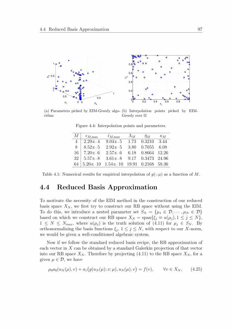
4.4 Reduced Basis Approximation 97
0
0.5
1
0
0.5
10
0.5
1
µ0
µ1
µ2
(a) Parameters picked by EIM-Greedy algo-rithm
0 0.2 0.4 0.6 0.8 10
0.2
0.4
0.6
0.8
1
x1
x2
(b) Interpolation points picked by EIM-Greedy over Ω
Figure 4.4: Interpolation points and parameters.
M εM,max εM,max ΛM ηM κM4 2.29 E – 4 9.04 E – 5 1.73 0.3210 3.448 8.52 E – 5 2.92 E – 5 3.80 0.7055 6.0816 7.20 E – 6 2.57 E – 6 6.18 0.8664 12.2632 5.57 E – 8 3.61 E – 8 9.17 0.3473 24.9664 5.20 E – 10 1.54 E – 10 19.91 0.2168 58.36
Table 4.1: Numerical results for empirical interpolation of g(·;µ) as a function of M .
4.4 Reduced Basis Approximation
To motivate the necessity of the EIM method in the construction of our reducedbasis space XN , we first try to construct our RB space without using the EIM.To do this, we introduce a nested parameter set SN = µ1 ∈ D, · · · , µN ∈ Dbased on which we construct our RB space XN = spanξj ≡ u(µj), 1 ≤ j ≤ N,1 ≤ N ≤ Nmax, where u(µj) is the truth solution of (4.11) for µj ∈ SN . Byorthonormalizing the basis functions ξj, 1 ≤ j ≤ N , with respect to our X-norm,we would be given a well-conditioned algebraic system.
Now if we follow the standard reduced basis recipe, the RB approximation ofeach vector in X can be obtained by a standard Galerkin projection of that vectorinto our RB space XN . Therefore by projecting (4.11) to the RB space XN , for agiven µ ∈ D, we have
µ0a0(uN(µ), v) + a1
(g(uN(µ);x;µ), uN(µ), v
)= f(v), ∀v ∈ XN , (4.25)
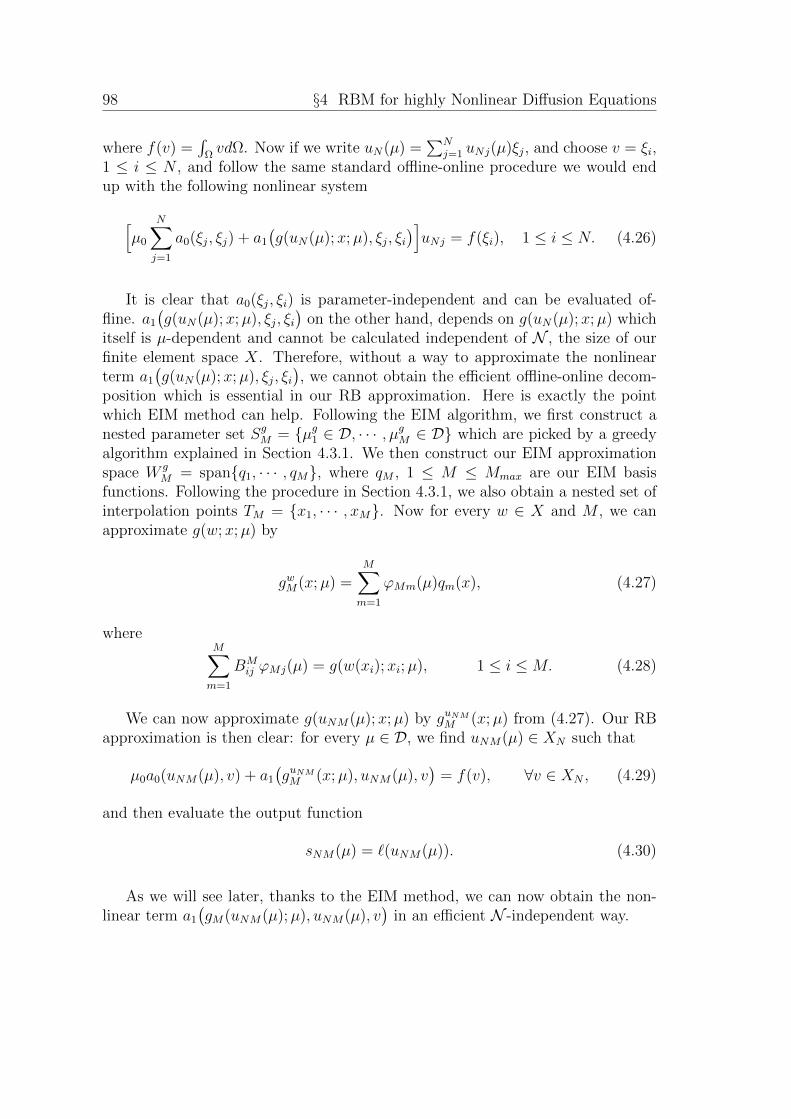
98 §4 RBM for highly Nonlinear Diffusion Equations
where f(v) =∫
ΩvdΩ. Now if we write uN(µ) =
∑Nj=1 uNj(µ)ξj, and choose v = ξi,
1 ≤ i ≤ N , and follow the same standard offline-online procedure we would endup with the following nonlinear system
[µ0
N∑j=1
a0(ξj, ξj) + a1
(g(uN(µ);x;µ), ξj, ξi
)]uNj = f(ξi), 1 ≤ i ≤ N. (4.26)
It is clear that a0(ξj, ξi) is parameter-independent and can be evaluated of-fline. a1
(g(uN(µ);x;µ), ξj, ξi
)on the other hand, depends on g(uN(µ);x;µ) which
itself is µ-dependent and cannot be calculated independent of N , the size of ourfinite element space X. Therefore, without a way to approximate the nonlinearterm a1
(g(uN(µ);x;µ), ξj, ξi
), we cannot obtain the efficient offline-online decom-
position which is essential in our RB approximation. Here is exactly the pointwhich EIM method can help. Following the EIM algorithm, we first construct anested parameter set SgM = µg1 ∈ D, · · · , µ
gM ∈ D which are picked by a greedy
algorithm explained in Section 4.3.1. We then construct our EIM approximationspace W g
M = spanq1, · · · , qM, where qM , 1 ≤ M ≤ Mmax are our EIM basisfunctions. Following the procedure in Section 4.3.1, we also obtain a nested set ofinterpolation points TM = x1, · · · , xM. Now for every w ∈ X and M , we canapproximate g(w;x;µ) by
gwM(x;µ) =M∑m=1
ϕMm(µ)qm(x), (4.27)
whereM∑m=1
BMij ϕMj(µ) = g(w(xi);xi;µ), 1 ≤ i ≤M. (4.28)
We can now approximate g(uNM(µ);x;µ) by guNMM (x;µ) from (4.27). Our RB
approximation is then clear: for every µ ∈ D, we find uNM(µ) ∈ XN such that
µ0a0(uNM(µ), v) + a1
(guNMM (x;µ), uNM(µ), v
)= f(v), ∀v ∈ XN , (4.29)
and then evaluate the output function
sNM(µ) = `(uNM(µ)). (4.30)
As we will see later, thanks to the EIM method, we can now obtain the non-linear term a1
(gM(uNM(µ);µ), uNM(µ), v
)in an efficient N -independent way.

4.4 Reduced Basis Approximation 99
4.4.1 Reduced Basis Formulation
In this section we evaluate the RB solution uNM(µ) from (4.29). Since (4.29) isa nonlinear problem, like Chapter 2, we apply a Newton iterative scheme to solveit. For simplicity, instead of (4.29), we first start with (4.26), and then add theinformation from EIM space into our system. We can rewrite (4.26) as
µ0
N∑j=1
a0(ξj, ξi)uNj(µ) +N∑j=1
uNj(µ)
∫Ω
g( N∑n=1
uNn(µ)ξn;x;µ) ∂ξj∂xj′
∂ξi∂xj′
= f(ξi),
1 ≤ i ≤ N. (4.31)
Applying the Newton method, in each iteration, we should evaluate an incre-ment δuN(µ) from
[µ0
N∑j=1
a0(ξj, ξi)uNj(µ) +N∑j=1
uNj(µ)
∫Ω
N∑p=1
ξp g1
( N∑n=1
uNn(µ)ξn;x;µ) ∂ξj∂xj′
∂ξi∂xj′
+
∫Ω
g( N∑n=1
uNn(µ)ξn;x;µ) ∂ξj∂xj′
∂ξi∂xj′
]δuN(µ) =
= f(ξi)− µ0
N∑j=1
a0(ξj, ξi)uNj(µ)
−N∑j=1
uNj(µ)
∫Ω
g( N∑n=1
uNn(µ)ξn;x;µ) ∂ξj∂xj′
∂ξi∂xj′
,
where g1 is the partial derivative with respect to our field variable uN(µ). Notethat when g(w;x;µ) is a low order polynomial with respect to u(µ), — as it wasthe case in Chapter 2 — we can simply extend the nonlinear term into its powerseries and still keep the efficient offline-online RB procedure. Unfortunately thoughfor higher order nonlinearity, this strategy wouldn’t be useful as online costs getsprohibitively large. In next Section, we show how can we keep the offline-onlineefficiency by using the EIM method.

100 §4 RBM for highly Nonlinear Diffusion Equations
4.4.2 Offline-Online Procedure
To recover online N -independence even in nonlinear form, we need to first definethe matrix Cj
NM ∈ RN×M , j = 1, · · · , N as
CjNM =
∫Ω
qn(x)∂ξj∂xj′
∂ξi∂xj′
, (4.32)
where qn(x), n = 1, · · · ,M are EIM basis functions and as always ξj, j = 1, · · · , Nare our RB basis functions. We then define the matrix Dj
NM ∈ RN×M , j =1, · · · , N , by
DjNM =
N∑j=1
CjNMB
−1M , (4.33)
where BM is given by (4.19). Now if we take uNM(µ) =∑N
j=1 uNMjξj, and sub-stitute guNM
M (x;µ) in (4.31), and considering (4.32), (4.33), we can rewrite (4.31)as
µ0
N∑j=1
a0(ξj, ξi)uNMj(µ) +N∑j=1
uNMj(µ)DjNMg
uNMM (x;µ) = f(ξi), 1 ≤ i ≤ N.
(4.34)
To apply the Newton method, we need to evaluate derivative of the left handside of (4.34) using the chain rule as[
µ0
N∑j=1
a0(ξj, ξi) +N∑j=1
DjNMg
uNMM (x;µ) +
+N∑
j,p=1
uNMj(µ)DjNMg
uNMM1 (x;µ)ξp
]δuNM(µ) =
= f(ξi)− µ0
N∑j=1
uNMj(µ)a0(ξj, ξi)
−N∑j=1
uNMj(µ)DjNMg
uNMM (x;µ), 1 ≤ i ≤ N, (4.35)
where again gM1 is derivative of gM with respect to uNM(µ).
Doing the Newton iterations, we update ukNM = uk−1NM(µ) + δuNM(µ), until
certain level of accuracy is achieved. Finally we evaluate the output functionsNM(µ) from
sNM(µ) = `(uNM(µ)) = LTNuNM(µ), µ ∈ D, (4.36)

4.5 A posteriori Error Estimation 101
where LN ∈ RN is the output vector with entries LNi = `(ξi), 1 ≤ i ≤ N .
The offline-online decomposition is then clear: in the offline part which isperformed only once, we first construct our EIM space W g
M using the algorithmexplained in Section 4.3.1. Having obtained the EIM basis functions and inter-polation points, we evaluate all µ–independent matrices and vectors like f(ξi),a0(ξj, ξi), C
jNM , Dj
NM , 1 ≤ i, j ≤ N . In the online stage which is performed manytimes for each µ ∈ D, we solve (4.35) by using a Newton iterative scheme. Theoperation count is then O(M2N2 + N3) per each Newton iteration. Finally, weare able to evaluate the RB output function sNM(µ) completely independent ofN , the size of our finite element space X from (4.36).
4.5 A posteriori Error Estimation
Unlike in the quadratic nonlinear case, obtaining an error estimation does notrequire the BRR framework we used in Chapter 2 when we use EIM method.Although our error bound here is not certified like it was in quadratic nonlinearcase, thanks to the EIM algorithm, obtaining an error bound is very similar tostandard error estimation for linear equations with some minor differences. Inthis Section, we first derive an error bound for our RB approximation and thenintroduce an efficient offline-online procedure to evaluate it.
4.5.1 Error Estimation for RB Approximation
As always, to develop an error bound for our RB approximation, we need to startwith the residual function rNM(v;µ) which is defined as
rNM(v;µ) = f(v)− µ0a0(uNM(µ), v)− a1
(guNMM (x;µ), uNM(µ), v
), ∀v ∈ X.
(4.37)
We next define the dual norm of residual εNM(µ) as
εNM(µ) ≡ supv∈X
rNM(v;µ)
‖v‖X. (4.38)
To evaluate the error bound, we also need to define the dual norm
ϑNM(µ) ≡ supv∈X
∫Ω
qM+1∇uNM(µ)∇v
‖v‖X, (4.39)

102 §4 RBM for highly Nonlinear Diffusion Equations
and an error bound ε(µ) for the nonlinear term approximation given by
ε(µ) =∣∣g(uNM(µ;xM+1);xM+1;µ
)− guNM
M
(xM+1;µ
)∣∣, (4.40)
where guNMM
(xM+1;µ
)is guNM
M (x;µ) calculated at (M + 1)th interpolation point.
To begin, considering (4.6), (4.25), we start rewriting (4.37) as follows
rNM(v;µ) = µ0a0(u(µ), v) + a1
(g(u(µ);x;µ), u(µ), v
)−µ0a0(uNM(µ), v)− a1
(guNMM (x;µ), uNM(µ), v
), ∀v ∈ Y,
= µ0a0(eNM(µ), v) + a1
(g(u(µ);x;µ), u(µ), v
)−a1
(guNMM (x;µ), uNM(µ), v
), ∀v ∈ Y, (4.41)
where eNM(µ) = u(µ)−uNM(µ). Now if we subtract a1
(g(uNM(µ);x;µ), uNM(µ), v
)from both sides of (4.41), we would have
µ0a0(eNM(µ), v) + a1
(g(u(µ);x;µ), u(µ), v
)− a1
(g(uNM(µ);x;µ), uNM(µ), v
)= rNM(v;µ) + a1
(guNMM (x;µ), uNM(µ), v
)−a1
(g(uNM(µ);x;µ), uNM(µ), v
), ∀v ∈ Y. (4.42)
Here if for v = eNM(µ), we assume
τNM(µ) = a1
(g(u(µ);x;µ), u(µ), v
)− a1
(g(uNM(µ);x;µ), uNM(µ), v
)≥ 0, (4.43)
then from (4.42), we have
µ0a0(eNM(µ), eNM(µ)) ≤ rNM(eNM ;µ)
+ a1
(guNMM (x;µ)− g(uNM(µ);x;µ), uNM(µ), eNM(µ)
). (4.44)
We remark here that even though we cannot theoretically prove (4.43), weexpect it to be a valid assumption specially when u(µ) and uNM(µ), µ ∈ D, areclose to each other. To support this assumption, we have calculated τNM(µ) forall µ ∈ Ξg
avg and plotted the result in Figure 4.5. As it is clear, the magnitude ofτNM(µ) is quite small throughout the whole parameter domain Ξg
avg which meansthe upper bound of µ0a0(eNM(µ), eNM(µ)) in (4.44) is a sharp upper bound.
On the other hand, from Lemma 7, we know that
guNMM (x;µ)− g(uNM(µ);x;µ) = ±εN(µ)qM+1(x), (4.45)
and
rNM(eNM ;µ) ≤ supv∈X
rNM(v;µ)
‖v‖X‖eNM(µ)‖X . (4.46)

4.5 A posteriori Error Estimation 103
0 100 200 300 400 500 600
10−20
10−15
10−10
10−5
τN
M(µ
)
Figure 4.5: Behavior of τNM (µ), over Ξgavg with 660 sample points for N = 20, M = 20.
Moreover, we can rewrite (4.45) as∣∣a1
(guNMM (x;µ)− g(uNM(µ);x;µ), uNM(µ), eNM(µ)
)∣∣ ≤supv∈X
∣∣a1
(guNMM (x;µ)− g(uNM(µ);x;µ), uNM(µ), v
)∣∣‖v‖X
‖eNM(µ)‖X . (4.47)
Now from (4.44)–(4.47), we have
‖eNM(µ)‖X ≤1
µ0αLB
(εNM(µ) + εNM(µ)ϑNM(µ)
), (4.48)
where ϑNM(µ) is defined in (4.39), and αLB is the coercivity lower bound. There-fore, we can obtain an error estimation for our RB approximation from
Proposition 7. Let g(uNM(µ);x;µ) ∈ W gM+1, and assume that for every µ ∈ D
a1
(g(u(µ);x;µ), u(µ), v
)− a1
(g(uNM(µ);x;µ), uNM(µ), v
)≥ 0. (4.49)
Then the error bound ∆NM(µ) for our RB error eNM(µ) = u(µ) − uNM(µ),would be given by
‖eNM(µ)‖X ≤ ∆NM(µ) =1
µ0αLB
(εNM(µ) + εNM(µ)ϑNM(µ)
), (4.50)
where εNM(µ), εNM(µ), ϑNM(µ) are given by (4.38), (4.40), (4.39) respectively.

104 §4 RBM for highly Nonlinear Diffusion Equations
We remark that since our space W gM is constructed based on g(u(µ);x;µ) and
not g(uNM(µ);x;µ), the condition g(uNM(µ);x;µ) ∈ W gM+1, µ ∈ D is very unlikely
to hold. Therefore our choice for M and N is particularly more important. We alsonote that the second part of our error estimation which involves the non-rigorouspart of our error bound ∆NM(µ) is small compared to contribution of the rigorouspart which involves in the dual norm of residual εNM(µ).
Based on our error estimation for the field variable u(µ), we can also obtain anerror bound for the output function s(µ) as follows
Proposition 8. Let g(uNM(µ);x;µ) ∈ W gM+1, and assume that for every µ ∈ D
a1
(g(u(µ);x;µ), u(µ), v
)− a1
(g(uNM(µ);x;µ), uNM(µ), v
)≥ 0. (4.51)
Then the error bound ∆sNM(µ) for our RB error output bound esNM(µ) = s(µ)−
sNM(µ), is given by
‖esNM(µ)‖X ≤ ∆sNM(µ) = sup
v∈X
`(v)
‖v‖X∆NM(µ). (4.52)
4.6 RB offline-online Procedure
In this Section, we explain how we construct the RB space using a greedy algorithmbased on the defined a posteriori error estimation presented in the previoussection. Looking again at the error estimation (4.50), we need to evaluate fourcomponents. Calculating the αLB can be done offline since it is µ-independent.The other three though should be calculated online for every single parameterµ ∈ D which means we need to calculate them very fast and independent of N ,the size of our FE space. We already defined and explained how to evaluate ε(µ),µ ∈ D, in Section 4.3.2. Therefore, in this Section we should only evaluate thedual norm of residual εNM(µ), and ϑNM(µ) for all µ ∈ D.
4.6.1 Dual Norm Of Residual
Evaluating the dual norm of residual εNM(µ) is very similar to the procedure wepresented in Cahpter 2. We divide the process into two main offline and onlinesteps. First of all, ∀v ∈ X, we write the residual operator rNM(v;µ) as
rNM(v;µ) = f(v)−N∑j=1
uNMj(µ)µ0a0(ξj, v) +N∑j=1
uNMj(µ)a1
(guNMM (x;µ), ξj, v
).
(4.53)

4.6 RB offline-online Procedure 105
From the Riesz representation theorem, we know there exists a vector eNM(µ)for which (
eNM(µ), v)X
= rNM(v;µ), (4.54)
where X = H10 (Ω).
On the other hand, from our EIM approximation, we know that∫Ω
gM(uNM(µ);µ
) ∂ξj∂xj′
∂ξi∂xj′
=
∫Ω
M∑m=1
ϕm(µ)qm(x)∂ξj∂xj′
∂ξi∂xj′
=M∑m=1
ϕm(µ)
∫Ω
qm(x)∂ξj∂xj′
∂ξi∂xj′
=M∑m=1
ϕm(µ)CmNN , (4.55)
where CmNN ∈ RN×N , m = 1 · · · ,M are defined by
CmNN =
∫Ω
qm(x)∂ξj∂xj′
∂ξi∂xj′
, i, j = 1, · · · , N, (4.56)
and ξj, j = 1, · · · , N , are our RB basis functions. Note that CmNN ∈ RN×N is
different from the CjNM we defined in (5.21). Although it is possible to use the
same CjNN , j = 1, · · · , N defined in (5.21) and save some offline costs, for simplicity,
we do here define and calculate CmNM ∈ RN×N separately which at the end not
only makes calculating gM1(·;µ) easier, but also gives us control over changing Mto balance offline and online costs. We will discus this further in the last Section.Now if for every v ∈ Y , we define
(zf , v)X = f(v), (4.57)
(zja0 , v)X = −a0(ξj, v), (4.58)
(zm,ja1, v)X = −
∫Ω
qm(x)∂ξj∂xj′
∂v
∂xj′, (4.59)
from linearity and (4.54), we can rewrite (4.53) as follows
eNM(µ) = zf + µ0
N∑j=1
uNMj(µ)zja0 +N∑j=1
M∑m=1
uNMj(µ)ϕm(µ)zm,ja1. (4.60)
Therefore,
∥∥eNM(µ)∥∥2
X= (zf , zf )X + 2µ0
(zf ,
N∑j=1
uNMj(µ)zja0
)X
+ (4.61)

106 §4 RBM for highly Nonlinear Diffusion Equations
+2
(zf ,
N∑j=1
M∑m=1
uNMj(µ)ϕm(µ)zm,ja1
)
+µ20
(N∑j=1
uNMj(µ)zja0 ,N∑j′=1
uNMj′(µ)zj′
a0
)X
+
+2µ0
(N∑j=1
uNMj(µ)zja0 ,N∑j′=1
M∑m=1
uNMj′(µ)ϕm(µ)zm,j′
a1
)
+
(N∑j=1
M∑m=1
uNMj(µ)ϕm(µ)zm,ja1,
N∑j′=1
M∑m′=1
uNMj′(µ)ϕm′(µ)zm,j′
a1
).
Now by defining
CF = (zf , zf )X , (4.62)
CF,Aj0
=(zf , z
ja0
)X, (4.63)
CF,Am,j1
=(zf , z
m,ja1
)X, (4.64)
CAj
0,Aj′0
=(zja0 , z
j′
a0
)X, (4.65)
CAj
0,Am,j′1
=(zja0 , z
m,j′
a1
)X, (4.66)
CAm,j
1 ,Am′,j′1
=(zm,ja1
, zm′,j′
a1
)X, (4.67)
we can separate the offline and online calculations by rewriting (5.64) as follows
∥∥eNM(µ)∥∥2
X= CF + 2µ0
N∑j=1
uNMj(µ)CF,Aj0
+ 2N∑j=1
M∑m=1
uNMj(µ)ϕm(µ)CF,Am,j1
+
+µ20
N∑j=1
N∑j′=1
uNMj(µ)uNMj′(µ)CAj
0,Aj′0
+
+2µ0
N∑j=1
uNMj(µ)N∑j′=1
M∑m=1
uNMj′(µ)ϕm(µ)CAj
0,Am,j′1
+N∑j=1
M∑m=1
N∑j′=1
M∑m′=1
uNMj′(µ)uNMj(µ)ϕm(µ)ϕm′(µ)CAm,j
1 ,Am′,j′1
.
The offline-online procedure for calculating the dual norm of residual thenis clear: In the offline phase, we first evaluate Cm
NM ∈ RN×N with computa-

4.7 Numerical Results 107
tional cost O(MNN •). We then evaluate vectors zf , zja0, zm,ja1
from (5.59)–(5.62) with costs O(N •), O(NN •), O(MNN •) respectively. Finally we evalu-ate CF , CF,Aj
0, CF,Am,j
1, C
Aj0,A
j′0, C
Aj0,A
m,j′1
and CAm,j
1 ,Am′,j′1
from (5.65)–(5.74), with
computational cost with leading order O(M2N2N •). In the online phase, we sim-ply calculate the summations with costs of the leading order O(M2N2).
4.6.2 Evaluating the dual norm ϑNM(µ)
Unlike nonlinear reaction-diffusion equations [33], where the dual norm ϑNM(µ)was parameter independent, for nonlinear diffusion equations (4.1), we need toevaluate this value online for every µ ∈ D. To minimize the online calculations,instead of evaluating ϑNM(µ), µ ∈ D, we calculate an upper bound for it. As it isdefined in (4.39), for every µ ∈ D, ϑNM(µ) is given by
ϑNM(µ) ≡ supv∈X
∫Ω
qM+1∇uNM(µ)∇v
‖v‖X. (4.68)
It is clear that
supv∈X
∫Ω
qM+1∇uNM(µ)∇v
‖v‖X≤ sup
v∈X
‖qM+1‖L∞
∫Ω
∇uNM(µ)∇v
‖v‖X
≤ ‖qM+1‖L∞ supv∈X
γa0‖uNM(µ)‖X‖v‖X‖v‖X
≤ ‖qM+1‖L∞γa0‖uNM(µ)‖X , (4.69)
where µ-independent γa0 is given by
γa0 ≡ supv∈X
a0(w, v)
‖w‖X‖v‖X, (4.70)
and w ∈ X. Note that since based on (4.50), ϑNM(µ) is multiplied by εNM(µ),µ ∈ D, where εNM(µ) is very small, substituting this very inexpensive upper boundof ϑNM(µ) instead of its correct value, would not deteriorate sharpness of our errorbound.
4.7 Numerical Results
We now return to our model problem introduced in Section 4.2.1, and presentnumerical results for the reduced basis approximation and its a posteriori error
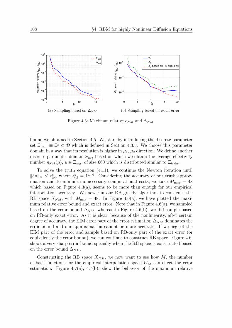
108 §4 RBM for highly Nonlinear Diffusion Equations
0 5 10 1510
−4
10−3
10−2
10−1
100
101
M
Ma
xim
um
re
lative
eN
M,
∆N
M
eNM
∆NM
(a) Sampling based on ∆NM
0 5 10 15 20
10−4
10−2
100
M
Ma
xim
um
re
lative
eN
M,
∆N
M
eN
∆N
eN based on RB error only
(b) Sampling based on exact error
Figure 4.6: Maximum relative eNM and ∆NM .
bound we obtained in Section 4.5. We start by introducing the discrete parameterset Ξtrain ≡ Ξg ⊂ D which is defined in Section 4.3.3. We choose this parameterdomain in a way that its resolution is higher in µ1, µ2 direction. We define anotherdiscrete parameter domain Ξavg based on which we obtain the average effectivitynumber ηNM(µ), µ ∈ Ξavg, of size 660 which is distributed similar to Ξtrain.
To solve the truth equation (4.11), we continue the Newton iteration until‖δu‖X ≤ εutol, where εutol = 1e−6. Considering the accuracy of our truth approx-imation and to minimize unnecessary computational costs, we take Mmax = 48which based on Figure 4.3(a), seems to be more than enough for our empiricalinterpolation accuracy. We now run our RB greedy algorithm to construct theRB space XNM , with Mmax = 48. In Figure 4.6(a), we have plotted the maxi-mum relative error bound and exact error. Note that in Figure 4.6(a), we sampledbased on the error bound ∆NM , whereas in Figure 4.6(b), we did sample basedon RB-only exact error. As it is clear, because of the nonlinearity, after certaindegree of accuracy, the EIM error part of the error estimation ∆NM dominates theerror bound and our approximation cannot be more accurate. If we neglect theEIM part of the error and sample based on RB-only part of the exact error (orequivalently the error bound), we can continue to construct RB space. Figure 4.6,shows a very sharp error bound specially when the RB space is constructed basedon the error bound ∆NM .
Constructing the RB space XNM , we now want to see how M , the numberof basis functions for the empirical interpolation space WM can effect the errorestimation. Figure 4.7(a), 4.7(b), show the behavior of the maximum relative

4.7 Numerical Results 109
0 5 10 1510
−4
10−2
100
N
Ma
xim
um
re
lative
∆N
M
M=4
M=8
M=12
M=16
M=20
(a) ∆NM for different M
0 5 10 15
10−4
10−2
100
N
Ma
xim
um
re
lative
eN
M
M=4
M=8
M=12
M=16
M=20
(b) eNM for different M
Figure 4.7: Maximum relative eNM and ∆NM when the size of empirical interpolationspace varies.
error bound ∆NM , and maximum relative exact error eNM(µ) for different M .Based on these plots, even using Mmax = 48 is unnecessary and as it can be seen,for M ≥ 20 the error does not change.
0
0.5
1
0
0.5
10
0.5
1
µ0
µ1
µ2
(a) SN , Picked parameters by the RB greedy
0
0.5
1
0
0.5
10
0.5
1
µ0
µ1
µ2
(b) SM , Picked parameters by the EIMgreedy
Figure 4.8: Picked parameter by the RB and EIM greedy algorithm.
In Figure 4.8(a), Figure 4.8(b), we show the parameters picked by RB greedyand EIM greedy respectively. As it is expected, these picked parameters are clus-tered more in an area with smaller µ0.

110 §4 RBM for highly Nonlinear Diffusion Equations
0 5 10 15 201.5
2
2.5
3
3.5
4
4.5
5
N
ηN
M
avg
M=8
M=12
M=16
M=20
M=24
(a) Average effectivity number
0 5 10 150
0.002
0.004
0.006
0.008
0.01
N
se
co
nd
M=4
M=8
M=12
M=16
M=20
M=24
(b) Average computational time to evaluate∆NM
Figure 4.9: Average is taken over Ξavg.
We now turn our attention to the effectivity number ηNM(µ), which is the ratioof the error bound ∆NM(µ) to the exact error eNM(µ), µ ∈ Ξavg. Figure 4.9(a)shows the average effectivity over µ ∈ Ξavg. Clearly as M increases, the effectivitygets smaller and smaller due to fast convergence of ∆NM(µ). Although we are notable to theoretically prove the rigor of our error estimation as we shown before, inpractice, we can see that the error bound is not only rigorous but also sharp. Asthe most important benefit of applying reduced basis method is online efficiency,we also study the computational costs both in finite element and RB space. InFigure 4.9(b), we see that the average computational cost to evaluate the errorbound is of millisecond magnitude. As we will see in Tabel 4.2, the required timeto evaluate the RB solution uNM(µ), µ ∈ D, is even smaller. Comparing it withthe time we need to solve the truth problem (4.11), we can see huge computationalsavings.
N M = 4 M = 8 M = 12 M = 16 M = 20 M = 242 9.52 E + 3 8.99 E + 3 7.41 E + 3 6.57 E + 3 5.85 E + 3 5.27 E + 34 8.52 E + 3 8.12 E + 3 5.88 E + 3 6.36 E + 3 5.61 E + 3 5.29 E + 38 7.20 E + 3 7.15 E + 3 6.19 E + 3 5.70 E + 3 5.11 E + 3 4.71 E + 312 5.57 E + 3 6.01 E + 3 5.48 E + 3 4.97 E + 3 4.47 E + 3 4.10 E + 316 5.20 E + 3 5.12 E + 3 4.68 E + 3 4.35 E + 3 3.81 E + 3 3.52 E + 3
Table 4.2: Ratio of the average computational time to evaluate the truth solution to RBsolution for different values of N,M .

4.7 Numerical Results 111
0 5 10 15 204
6
8
10
12
14x 10
−4
N
se
co
nd
M=8
M=12
M=16
M=20
M=24
(a) Average computational time to evaluateuNM
0 5 10 153000
4000
5000
6000
7000
8000
9000
10000
N
t FE
M/t
RB
M=8
M=12
M=16
M=20
M=24
(b) Average computational time ratio foruFEM , uNM
Figure 4.10: Average is taken over Ξavg.
0 5 10 150
1
2
3
4
5
6
7
8
N
t ∆N
M
/tu
NM
M=8
M=12
M=16
M=20
M=24
(a) Average computational time ratio for∆NM , uNM
Figure 4.11: Average is taken over Ξavg.


Chapter 5
Higher order Parabolic NonlinearDiffusion Equations
113

114 §5 RBM for highly Nonlinear Parabolic Diffusion Equations
5.1 Introduction
In the previous Chapter, we have developed a reduced basis technique and asso-ciated a posteriori error estimation procedure for high order nonlinear ellipticequations. On the other hand, in Chapter 3, we used a rather theoretically compli-cated space-time technique to apply RB method on quadratic nonlinear diffusionequations. In this Chapter we combine higher order nonlinearity with time depen-dent diffusion equations and will extend our methodology to treat parabolic highlynonlinear equations. Unlike Chapter 3, here we use the Empirical InterpolationMethod (EIM) to handle the nonlinearity.
In this Chapter, we consider a time-dependent high order nonlinear diffusionequation of the form
∂u
∂t+ div
(G(u;µ)∇u
)= f, (5.1)
where unlike Chapter 3, G(u;µ) can be any function in L∞(Ω) ∩ C0(Ω). As wementioned earlier, to handle the nonlinearity in construction of our reduced basismethod, like previous Chapter, we use the Empirical Interpolation Method (EIM).
5.2 Problem Statement
In this section we introduce the spaces and norms we would use throughout thisChapter. The spatial space Xe ≡ H1
0 (Ω) is the same we had in previous Chapter.For our temporal discretization, we first partition the time interval I = (0, T ]into K non-overlapping sub-intervals Ik = (tk−1, tk], k = 1, · · · , K where t0 = 0,tK = T . In this Chapter, for each time step k = 1, · · · , K, we define an energynorm
|||wk|||2 = m(wk, wk) + µ0∆tk∑
k′=1
a0(wk′, wk
′), (5.2)
where bilinear forms m(w, v) and a0(w, v) are given by
m(w, v) =
∫Ω
wvdΩ, ∀w, v ∈ Xe, (5.3)
a0(w, v) =
∫Ω
∂w
∂xj
∂v
∂xj, ∀w, v ∈ Xe, (5.4)
and µ ≡ (µ0, µ1, µ2) ∈ D. As before we rewrite equation (5.1) in a weak formas follows: given any parameter µ ∈ D ⊂ R3, for every time step k = 1, · · · , K,

5.2 Problem Statement 115
we evaluate uke(µ) ∈ Xe, where uke(µ) satisfies the nonlinear system
m(uke(µ), v) + a(uke(µ), v, G(uke(µ);µ)
)= f(v), ∀v ∈ Xe, (5.5)
where as before, f(v) is a Xe-continuous linear form and e stands for the exactanalytical solution. The trilinear form a(·, ·, ·) is defined by
a (w, v,G(w;µ)) =
∫Ω
G(w;µ)∇w∇v, ∀w, v ∈ Xe, (5.6)
with G(w;µ) = µ0 + g(w;µ), where g(w;µ) is a parameter dependent functionwhich is monotonic in its first argument and continuous in all of its arguments inL∞(Ω). Therefore, we can write
a(w, v,G(w;µ)
)= µ0
∫Ω
∇w∇v +
∫Ω
g(w;µ) ∇w∇v (5.7)
= µ0
∫Ω
∂w
∂xj
∂v
∂xj+
∫Ω
g(w;µ)∂w
∂xj
∂v
∂xj= µ0a0(w, v) + a1(g(w;µ), w, v).
Now we can rewrite (5.5) as follows
m(uke(µ), v) + µ0a0(uke(µ), v) + a1
(g(uke(µ);µ), uke(µ), v
)= f(v), ∀v ∈ Xe,
(5.8)where m(w, v) and a0(w, v) are given by (5.3), (5.4). We also define an outputfunction ske : D 7→ R as
ske(µ) = `(uek(µ)
), µ ∈ D, (5.9)
where `(v) is a Xe-continuous linear form. To keep problem (5.1) well-posed, wemake the same assumptions we had in previous chapter regarding continuity of allour bilinear and trilineaer forms. As we always did in this thesis, since the exactsolution uke(µ), µ ∈ D, may not be easy to evaluate, we project the equation (5.8)on a finite dimensional space X with N degrees of freedom where N is typicallya very large number. Following this strategy, instead of (5.8), we solve
m(uk(µ), v) + µ0a0(uk(µ), v) + a1
(g(uk(µ);µ), uk(µ), v
)= f(v), ∀v ∈ X,
(5.10)where uk(µ) is the solution of (5.10) at time step k, k = 1, · · · , K. Since here weuse the Euler backward method, the time derivative would be given by
uk(µ) =1
∆t
(uk(µ)− uk−1(µ)
), µ ∈ D. (5.11)
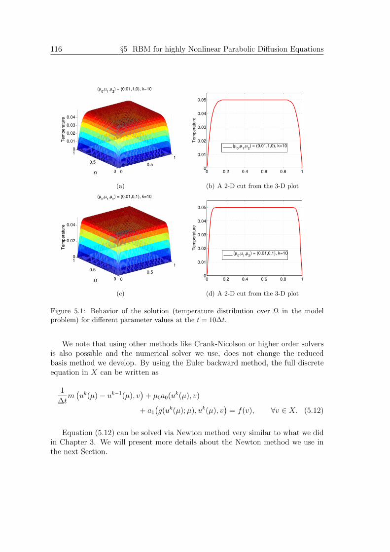
116 §5 RBM for highly Nonlinear Parabolic Diffusion Equations
0
0.5
1
0
0.5
10
0.01
0.02
0.03
0.04
(µ0,µ
1,µ
2) = (0.01,1,0), k=10
Ω
Te
mp
era
ture
(a)
0 0.2 0.4 0.6 0.8 10
0.01
0.02
0.03
0.04
0.05
Te
mp
era
ture
(µ0,µ
1,µ
2) = (0.01,1,0), k=10
(b) A 2-D cut from the 3-D plot
0
0.5
1
0
0.5
10
0.02
0.04
(µ0,µ
1,µ
2) = (0.01,0,1), k=10
Ω
Te
mp
era
ture
(c)
0 0.2 0.4 0.6 0.8 10
0.01
0.02
0.03
0.04
0.05
Te
mp
era
ture
(µ0,µ
1,µ
2) = (0.01,0,1), k=10
(d) A 2-D cut from the 3-D plot
Figure 5.1: Behavior of the solution (temperature distribution over Ω in the modelproblem) for different parameter values at the t = 10∆t.
We note that using other methods like Crank-Nicolson or higher order solversis also possible and the numerical solver we use, does not change the reducedbasis method we develop. By using the Euler backward method, the full discreteequation in X can be written as
1
∆tm(uk(µ)− uk−1(µ), v
)+ µ0a0(uk(µ), v)
+ a1
(g(uk(µ);µ), uk(µ), v
)= f(v), ∀v ∈ X. (5.12)
Equation (5.12) can be solved via Newton method very similar to what we didin Chapter 3. We will present more details about the Newton method we use inthe next Section.

5.2 Problem Statement 117
5.2.1 Model Problem
In this Section we introduce our model problem based on which, we present ournumerical results in Section 5.6. Following the same model problem we had inprevious Chapters, we introduce a thermal block model problem on the unit squareΩ = [0, 1]2 with the same boundary conditions and forcing function f(v), outputfunction `(v), v ∈ X, we had in previous Chapters. As the thermal block Ω isheated from below, we study the temperature behavior uk(µ) at each time stepk = 1, · · · , K and for each µ ∈ D with u0(µ) = 0. In practice, we substitute ourthree dimensional parameter domain D ≡ [10−2, 1]× [0, 1]× [0, 1] with a surrogatediscrete parameter domain Ξtrain ⊂ D, of size 2000. Compared to Chapter 3 wherethe temperature-dependent conductivity G(u) was a linear function of u, in thisChapter we have a more realistic temperature-dependent conductivity functionG(u;µ) = µ0 + µ1u+ µ2u
3 which is closer to what happens in reality [26, 39, 88].Here like before, the µ0 is the linear part of our conductivity function and µ1,µ2 represent the strength of the nonlinearity in G(u;µ). As we can see from thesnapshots taken from the solution uk(µ) at the time step 10∆t in Figure 5.1,for smaller µ0 and larger µ1, µ2, the temperature u(µ) gets more involved in theconductivity functionG(u;µ) and areas with lower temperature would have smallerconductivity and as a result, the temperature distribution has Barenblatt profileinstead of the Gaussian profile of the linear case. We note that as we did beforein previous Chapters, we set zero Dirichlet boundary condition on the boundaryof Ω and as a result, the temperature at the boundaries are always zero.
5.2.2 EIM for the nonlinear Model Problem
In this section, we run the EIM algorithm on our model problem to constructa collateral EIM space specifically developed to approximate our nonlinearity in(5.12). EIM for time-dependent equations is not that much different from whatwe presented in the previous Chapter. The only major difference is in fact usingthe POD method in construction of the EIM collateral space. Following the EIMalgorithm explained in the previous Chapter, we need to first define a discreteparameter set Ξg ∈ D for which we need to pre-calculate the truth solution uk(µ),µ ∈ Ξg at each time step. Based on our model problem and its sensitivity toµ0, µ1, µ2, we substitute Ξg ≡ [0.01, 1] × [0, 1] × [0, 1] with a surrogate discreteparameter set of size 2000. Like previous Chapter we use a special partitioningtechnique in a way that the sample points are denser closer to the boundaries.Here we define our accuracy criteria εtolM = 1e − 10 and set ∆t = 0.005 withK = 20, where K is the number of time steps. With this setup, as depicted inFigure 5.3, we obtain Mmax = 193 which is more than double than what we had

118 §5 RBM for highly Nonlinear Parabolic Diffusion Equations
0
0.5
1
0
0.5
10
0.5
1
Ω
EIM
ba
sis
fu
nctio
n
(a) q1(x)
0
0.5
1
0
0.5
10
0.5
1
Ω
EIM
ba
sis
fu
nctio
n
(b) q2(x)
0
0.5
1
0
0.5
1
−0.5
0
0.5
1
Ω
EIM
ba
sis
fu
nctio
n
(c) q3(x)
0
0.5
1
0
0.5
1
0
0.5
1
Ω
EIM
ba
sis
fu
nctio
n
(d) q4(x)
0
0.5
1
0
0.5
1
0
0.5
1
Ω
EIM
ba
sis
fu
nctio
n
(e) q5(x)
0
0.5
1
0
0.5
1
0
0.5
1
Ω
EIM
ba
sis
fu
nctio
n
(f) q6(x)
Figure 5.2: The first 6 empirical interpolation basis functions over Ω.
in Chapter 4 for the elliptic case with the same parameter domain. The reason issimply the more complicated solution manifold in time-dependent case compared

5.2 Problem Statement 119
0 50 100 150 200
10−10
10−5
100
M
max ε
Mg(µ
)
Figure 5.3: εgM (µ) = |g(·;µ)−gM (·;µ)|g(·;µ) , where µ ∈ Ξg.
to steady-state case. As it is shown in Figure 5.4(a), unlike the elliptic case, heresome parameters —considering their importance in approximating the solutionmanifold— are picked more than once by the EIM-greedy algorithm. Diameterof each circle in Figure 5.4(a), shows the multiplicity of each parameter withmaximum multiplicity of 7. As expected, most parameters with higher multiplicityare picked in the areas of D with smaller µ0 and larger µ1, µ2. Figure 5.4(b) showsthe interpolation points which has a similar distribution compared to the ellipticcase with denser interpolation points picked near the boundaries.
To see how effective the EIM algorithm is, we additionally define another dis-crete parameter domain Ξg
avg ∈ D of size 660. We then for every w ∈ X, calculateεKM,max = maxµ∈Ξg
avgεKM(µ) and ηKM which is the average of our EIM effectivity
number defined by
ηKM(µ) =εKM(·;µ)
εKM(·;µ), (5.13)
where εKM(x;µ) = |g(wK ;xM+1;µ) − gwK
M (xM+1;µ)| and µ ∈ Ξgavg, and K is the
final time step. In Table 5.1, we present εKM,max , εKM,max, ηKM and the Lebesgueconstant ΛM for different M . As it is clear, despite increasing magnitude, ΛM ismuch smaller than theoretically suggested upper bound 2M − 1. From Table 5.1we observe that the εKM,max, εKM,max converge rapidly with M and the EIM errorestimator effectivity is reasonably close to unity which means although we are not

120 §5 RBM for highly Nonlinear Parabolic Diffusion Equations
0
0.5
1
0
0.5
10
0.5
1
µ0
µ1
µ2
(a) Parameters picked by EIM-Greedy algo-rithm.
0 0.2 0.4 0.6 0.8 10
0.2
0.4
0.6
0.8
1
x1
x2
(b) Interpolation points picked by EIM-Greedy over Ω
Figure 5.4: Interpolation points and parameters.
using exact value of the interpolation error in the EIM greedy algorithm, but ourerror estimation εKM,max is not far from the actual interpolation error εKM,max. Finallyfrom κM which is condition number of matrix BM , we observe that our empiricalinterpolation system to evaluate interpolation coefficients ϕm, m = 1, · · · ,M , iswell-posed.
M εM,maxK εKM,max ΛM ηKM κM4 4.72 E – 3 2.93 E – 3 1.79 0.5793 3.018 5.08 E – 5 1.54 E – 5 3.49 0.3675 4.8316 5.07 E – 6 2.09 E – 6 7.28 0.5192 12.0932 5.54 E – 7 3.43 E – 7 13.22 0.5793 27.7964 1.91 E – 8 1.21 E – 8 19.78 0.5152 52.97
Table 5.1: Numerical results for empirical interpolation of g(wK ;x;µ) as a function ofM .
5.3 Reduced Basis Approximation
In the previous Chapter, we explained the necessity of the EIM method in con-struction of our reduced basis space in an efficient offline-online manner. In this

5.3 Reduced Basis Approximation 121
Section, we first explain the RB-greedy algorithm for our parabolic nonlinear equa-tion and then formulate our nonlinear problem in the RB space and last but notleast, we derive an efficient offline-online procedure to construct our reduced basisspace.
To begin, we introduce a nested set of parameters SN = µ1 ∈ D, · · · , µN ∈ Dbased on which we later construct our RB space XN = spanξj, 1 ≤ j ≤ N,1 ≤ N ≤ Nmax, where ξj is obtained from applying the POD method [35] onuk(µj) the solution of (5.12) at each time step k = 1, · · · , K and µj ∈ SN .
Now by following the standard RB recipe, we project each vector in the truthfinite element space X, into our well-conditioned RB space XN . Therefore thesystem (5.12) can be written as
1
∆tm(ukNM(µ)− uk−1
NM(µ), v)
+ µ0a0(ukNM(µ), v)
+ a1
(g(ukNM(µ);x;µ), ukNM(µ), v
)= f(v), ∀v ∈ XN , (5.14)
where ukNM(µ) here is the Galerkin projection of uk(µ) over XN for each µ ∈ Dand k = 1, · · · , K. Considering that each vector in XN can be uniquely writtenin terms of basis functions ξj, 1 ≤ j ≤ N , we can write ukN(µ) =
∑Nj=1 u
kNj(µ)ξj.
Substituting that in (5.14) and for v = ξi, i = 1, · · · , N , we have
1
∆t
N∑j=1
(ukNMj(µ)− uk−1
NMj(µ))m(ξj, ξi) + µ0
N∑j=1
ukNMj(µ)a0(ξj, ξi)+
+N∑j=1
ukNMj(µ)a1
(g(ukN(µ);x;µ), ξj, ξi
)= f(ξi), i = 1, · · · , N. (5.15)
Now to serve the efficient offline-online computational framework, we need toinvoke the EIM algorithm to approximate the nonlinear term a1
(g(ukN(µ);x;µ), ξj, ξi
)by a collateral EIM space of dimension M . Following the EIM algorithm pre-sented in Section 5.2.2, we first construct a nested parameter set SgM = µg1 ∈D, · · · , µgM ∈ D which are picked by the explained EIM-greedy algorithm. Hav-ing these parameters, we now are able to construct the EIM approximation spaceW gM = spanq1, · · · , qM, where qM , 1 ≤ M ≤ Mmax are our EIM basis func-
tions. Following the procedure in Section 5.2.2, we also obtain a nested set ofinterpolation points TM = x1, · · · , xM. Now for each µ ∈ D, we approximateg(ukN(µ);x;µ) with
gukNM (x;µ) =
M∑m=1
ϕkMm(µ)qm(x), (5.16)

122 §5 RBM for highly Nonlinear Parabolic Diffusion Equations
where the coefficients ϕkMm(µ) are evaluated from the linear system
M∑m=1
BMij ϕ
kMj(µ) = g(ukN(xi;µ);xi;µ), 1 ≤ i ≤M, (5.17)
and xi ∈ Ω.
By substituting the EIM approximation of g(ukN(µ);x;µ) in (5.15), as we willsee later, we are able to evaluate ukN(µ) from
1
∆t
N∑j=1
(ukNMj(µ)− uk−1
NMj(µ))m(ξj, ξi) + µ0
N∑j=1
ukNMj(µ)a0(ξj, ξi)+
+N∑j=1
ukNMj(µ)a1
(gukNM (x;µ), ξj, ξi
)= f(ξi), i = 1, · · · , N, (5.18)
for every µ ∈ D at each time step k = 1, · · · , K, independent of the size of ourtruth finite element space N .
5.3.1 Reduced Basis Formulation
In this section, we formulate the RB problem and solve the nonlinear system (5.18)via Newton method. For simplicity we first start with (5.15) and then add theinformation from our EIM approximation into the system. It is clear that we canrewrite (5.15) as
1
∆t
N∑j=1
(ukNMj(µ)− uk−1
NMj(µ))m(ξj, ξi) + µ0
N∑j=1
ukNMj(µ)a0(ξj, ξi)+
+N∑j=1
ukNMj(µ)
∫Ω
g( N∑n=1
ukNn(µ)ξn;x;µ) ∂ξj∂xj′
∂ξi∂xj′
= f(ξi), i = 1, · · · , N.
(5.19)
Following Newton’s method, for each µ ∈ D and the first time step k = 1,we begin with an initial value uk,0NM(µ). Then in the first Newton iteration, weevaluate the increment δuk,0N (µ) from[
1
∆tm(ξj, ξi)+µ0a0(ξj, ξi)+
N∑j=1
ukNMj(µ)
∫Ω
N∑p=1
ξp g1
( N∑n=1
ukNn(µ)ξn;x;µ) ∂ξj∂xj′
∂ξi∂xj′
+

5.3 Reduced Basis Approximation 123
+
∫Ω
g( N∑n=1
ukNn(µ)ξn;x;µ) ∂ξj∂xj′
∂ξi∂xj′
]δuk,0N (µ) =
f(ξi)−1
∆t
N∑j=1
(ukNMj(µ)− uk−1
NMj(µ))m(ξj, ξi)− µ0
N∑j=1
ukNMj(µ)a0(ξj, ξi)
−N∑j=1
ukNMj(µ)
∫Ω
g( N∑n=1
ukNn(µ)ξn;x;µ) ∂ξj∂xj′
∂ξi∂xj′
, i, · · · , N, (5.20)
where g1 is the partial derivative with respect to our field variable ukNM(µ). Cal-culating the increment δuk,0N (µ), we update our initial guess by uk,1N (µ) = uk,0N (µ) +δuk,0N (µ). Continuing this process until δuk,pN (µ) < εtolNewton for some p > 1, we repeatthe process for each the time step k = 2, · · ·K.
5.3.2 Offline-Online Procedure
To recover online N -independence even in nonlinear case, we need to first definethe matrix Cj
NM ∈ RN×M , j = 1, · · · , N as
CjNM =
∫Ω
qn(x)∂ξj∂xj′
∂ξi∂xj′
, (5.21)
where qn(x), n = 1, · · · ,M are EIM basis functions and as always ξj, j = 1, · · · , Nare our RB basis functions. We then define the matrix Dj
NM ∈ RN×M , j =1, · · · , N , by
DjNM =
N∑j=1
CjNMB
−1M , (5.22)
where BM is defined in (4.19). Now if we take ukNM(µ) =∑N
j=1 ukNMj(µ)ξj, and
substitute gukNMM (x;µ) in (5.19), and considering (5.21), (5.22), we can rewrite (5.19)
as
1
∆t
N∑j=1
(ukNMj(µ)− uk−1
NMj(µ))m(ξj, ξi) + µ0
N∑j=1
ukNMj(µ)a0(ξj, ξi)+
+N∑j=1
ukNMj(µ)DjNMg
ukNMM (x;µ) = f(ξi), i = 1, · · · , N. (5.23)
We now start the Newton iteration again by starting with an initial guessuk,0NM(µ) for k = 1 and find the increment δuk,0N (µ) from

124 §5 RBM for highly Nonlinear Parabolic Diffusion Equations
[1
∆tm(ξj, ξi) + µ0a0(ξj, ξi) +
N∑j,p=1
ukNMj(µ)DjNMg
ukNMM1 (x;µ)ξp+
+N∑j=1
DjNMg
ukNMM (x;µ)
]δuk,0N (µ) =
f(ξi)−1
∆t
N∑j=1
(ukNMj(µ)− uk−1
NMj(µ))m(ξj, ξi)− µ0
N∑j=1
ukNMj(µ)a0(ξj, ξi)
−N∑j=1
ukNMj(µ)DjNMg
ukNMM (x;µ), i = 1, · · · , N, (5.24)
where gM1 here is derivative of gM with respect to the solution ukNM(µ), k = 1.
Doing the first Newton iteration, we update our initial guess by uk,1N (µ) =uk,0N (µ) + δuk,0N (µ) and continue this process as explained in Section 5.3.1 until wecompute the solution at all time steps k = 1, · · · , K. Finally we compute our RBoutput function skNM(µ) for all µ ∈ D from
skNM(µ) = `(ukNM(µ)) = LTNukNM(µ), (5.25)
where LN ∈ RN is the output vector with entries LNi = `(ξi), 1 ≤ i ≤ N .
The offline-online decomposition is then clear: in the offline part which isperformed only once, we first construct our EIM space W g
M using the algorithmexplained in Section 5.2.2. Having obtained the EIM basis functions and EIMinterpolation points, we evaluate all µ–independent matrices and vectors like f(ξi),a0(ξj, ξi), C
jNM , Dj
NM , 1 ≤ i, j ≤ N . In the online stage which is performed manytimes for each µ ∈ D, we solve (5.24) by using a Newton iterative scheme. Theoperation count is then O(KM2N2 + KN3) per each Newton iteration. Finally,we are able to evaluate the RB output function skNM(µ) completely independentof N , the size of our finite element space X from (5.25).
5.4 A posteriori Error Estimation
Like the previous Chapter, here we use the EIM method to approximate nonlin-earity and because of this, we unfortunately would not be able to obtain a rigorouserror bound like we did in Chapters 2, 3. The benefit of the EIM method, as wewill see later, is the versatility to apply it for all types of nonlinear diffusion equa-tions instead of just quadratic nonlinearity we discussed in Chapter 2, Chapter3.

5.4 A posteriori Error Estimation 125
The nonlinear equation in the time-dependent case can be written as follows
1
∆tm(uk(µ)− u(µ)k−1, v) + µ0a0(uk(µ), v) + a1(g(uk(µ);x;µ), uk(µ), v) = f(v),
∀v ∈ X, (5.26)
where
g(w;x;µ) = µ1w(x) + µ2w(x)3, µ = (µ0, µ1µ2) ∈ D, (5.27)
and x ∈ Ω.
The residual function rkNM(v;µ) is then defined as
rkNM(v;µ) = f(v)− 1
∆tm(ukNM(µ)− uk−1
NM(µ), v)− µ0a0(ukNM(µ), v)
− a1(gukNMM (x;µ), ukNM(µ), v), ∀v ∈ X, (5.28)
where ukNM(µ) ∈ XNM is the EIM-RB solution of (5.26) at each time step k =
1, · · · , K, and gukNMM (x;µ) is the EIM approximation of g(ukNM(µ);x;µ), x ∈ Ω.
Based on the residual function rkNM(v;µ), k = 1, · · · , K, we define the dual normof residual εkNM(µ) as
εkNM(µ) ≡ supv∈X
rkNM(v;µ)
‖v‖X. (5.29)
To successfully evaluate the error estimation, similar to the elliptic case, weneed to define the dual norm
ϑkNM(µ) ≡ supv∈X
∫Ω
qM+1∇ukNM(µ)∇v
‖v‖X, (5.30)
and an error bound εk(µ) for the nonlinear term approximation, given by
εk(µ) =∣∣g(ukNM(xM+1;µ);xM+1;µ
)− gu
kNMM (xM+1;µ)
∣∣, (5.31)
where gukNMM (xM+1;µ) is calculated at (M + 1)th interpolation point. Substituting
f(v) from (5.26), we can rewrite (5.28) as follows
rkNM(v;µ) =1
∆tm(ekNM(µ)− ek−1
NM(µ), v) + µ0a0(ekNM(µ), v)
+ a1(g(uk(µ);x;µ), uk(µ), v)− a1(gukNMM (x;µ), ukNM(µ), v), ∀v ∈ X, (5.32)

126 §5 RBM for highly Nonlinear Parabolic Diffusion Equations
where ekNM(µ) = uk(µ)−ukNM(µ), µ ∈ D. Now if we subtract a1(g(ukNM(µ);x;µ), ukNM(µ), v)form both sides of (5.32), we have
rkNM(v;µ) + a1(gukNMM (x;µ), ukNM(µ), v)− a1(g(ukNM(µ);x;µ), ukNM(µ), v) =
=1
∆tm(ekNM(µ)− ek−1
NM(µ), v) + µ0a0(ekNM(µ), v) + a1(g(uk(µ);x;µ), uk(µ), v)
− a1(g(ukNM(µ);x;µ), ukNM(µ), v), ∀v ∈ X. (5.33)
Defining τ kNM(µ), for each k = 1, · · · , K, as
τ kNM(µ) = a1(g(uk(µ);x;µ), uk(µ), v)− a1(g(ukNM(µ);x;µ), ukNM(µ), v), (5.34)
and assuming τ kNM(µ) ≥ 0, for every k = 1, · · · , K, and from (5.33) with v =ekNM(µ), we have
1
∆tm(ekNM(µ)− ek−1
NM(µ), ekNM(µ)) + µ0a0(ekNM(µ), ekNM(µ)) ≤ rkNM(ekNM(µ);µ)
+ a1(gukNMM (x;µ)− g(ukNM(µ);µ), ukNM(µ), ekNM(µ)). (5.35)
On the other hand, using the Young’s inequality
2|c||d| ≤ 1
ρ2c2 + ρ2d2, c, d ∈ R, ρ ∈ R+, (5.36)
and the Cauchy-Schwarz, we can show
m(ek−1NM(µ), ekNM(µ)) ≤ m
12 (ek−1
NM(µ), ek−1NM(µ)) m
12 (ekNM(µ), ekNM(µ)) (5.37)
≤ 1
2
[m(ek−1
NM(µ), ek−1NM(µ)) +m(ekNM(µ), ekNM(µ))
].
Now if we multiply both sides of (5.35) by ∆t and consider (5.37), we canrewrite (5.35) as follows
m(ekNM(µ), ekNM(µ)) + ∆tµ0a0(ekNM(µ), ekNM(µ)) ≤
≤ 1
2
[m(ek−1
NM(µ), ek−1NM(µ)) +m(ekNM(µ), ekNM(µ))
]+ ∆trkNM(ekNM(µ);µ)
+ ∆ta1(gukNMM (x;µ)− g(ukNM(µ);µ), ukNM(µ), ekNM(µ)). (5.38)
Therefore for each k = 1, · · · , K, we have
1
2m(ekNM(µ), ekNM(µ))− 1
2m(ek−1
NM(µ), ek−1NM(µ))
5.4 A posteriori Error Estimation 127
+ ∆tµ0a0(ekNM(µ), ekNM(µ)) ≤ ∆t rkNM(ekNM(µ);µ)+
∆ta1(gukNMM (x;µ)− g(ukNM(µ);µ), ukNM(µ), ekNM(µ)). (5.39)
Now by defining our energy norm ||| · ||| as
|||uk(µ)||| =
(m(uk(µ), uk(µ)) + ∆tµ0
k∑k′=1
a0(uk(µ), uk(µ))
) 12
, (5.40)
and performing a sum over k′ = 1, · · · , k in (5.39), considering that e0NM(µ) = 0,
we are able to write (5.39) as follows
|||ekNM(µ)|||2 + ∆tµ0
k∑k′=1
a0(ekNM(µ), ekNM(µ)) ≤ 2∆tk∑
k′=1
rkNM(ekNM(µ);µ)+
2∆tk∑
k′=1
a1(gukNMM (x;µ)− g(ukNM(µ);µ), ukNM(µ), ekNM(µ)). (5.41)
On the other hand, from the discussion we had in the last Chapter, we knowthat
gukNMM (x;µ)− g(ukNM(µ);µ) = εk(µ)qM+1(x), (5.42)
and from (5.29), we have
rkNM(ekNM(µ);µ) ≤ εkNM(µ)‖ekNM(µ)‖X . (5.43)
Moreover, we know∣∣a1
(gukNMM (x;µ)− g(ukNM(µ);x;µ), ukNM(µ), ekNM(µ)
)∣∣ ≤supv∈X
∣∣a1
(gukNMM (x;µ)− g(ukNM(µ);x;µ), ukNM(µ), v
)∣∣‖v‖X
‖ekNM(µ)‖X . (5.44)
Clearly, from (5.30), (5.42), (5.44), we have∣∣a1
(gukNMM (x;µ)− g(ukNM(µ);x;µ), ukNM(µ), ekNM(µ)
)∣∣≤ εkNM(µ)ϑkNM(µ)‖ekNM(µ)‖X . (5.45)
We now apply (5.36) for (5.43) with c = εkNM(µ), d = ‖ekNM(µ)‖X and ρ =(µ0αLB
) 12 , where αLB is our coercivity lower bound given by
αLB = infv∈X
a0(v, v)
‖v‖2X
, (5.46)

128 §5 RBM for highly Nonlinear Parabolic Diffusion Equations
and obtain
2 εkNM(µ) ‖ekNM(µ)‖X =1
µ0αLBεkNM(µ)2 + µ0αLB‖ekNM(µ)‖2
X . (5.47)
Applying (5.36) again for (5.45) with c = εkNM(µ)ϑkNM(µ), d = ‖ekNM(µ)‖X and
ρ =(µ0αLB
) 12 , we have
2 εkNM(µ)ϑkNM(µ) ‖ekNM(µ)‖X ≤1
µ0αLBεkNM(µ)2ϑkNM(µ)2 + µ0αLB‖ekNM(µ)‖2
X .
(5.48)
Now from (5.40), (5.41), (5.45), (5.47), (5.48), we can evaluate the error esti-mation ∆k
NM(µ) as
|||ekNM(µ)|||2 ≤ ∆kNM(µ)2 ≡ ∆t
µ0αLB
k∑k′=1
(εk
′
NM(µ)2 + εk′
NM(µ)2ϑk′
NM(µ)2). (5.49)
Proposition 9. Let for every time step k = 1, · · · , K, g(ukNM(µ);x;µ) ∈ W gM+1,
and assume that for every µ ∈ D
a1
(g(uk(µ);x;µ), uk(µ), v
)− a1
(g(ukNM(µ);x;µ), ukNM(µ), v
)≥ 0. (5.50)
Then the error estimate ∆kNM(µ) for our RB error ekNM(µ) = uk(µ)−ukNM(µ),
is given by
‖ekNM(µ)‖X ≤ ∆kNM(µ) =
(∆t
µ0αLB
k∑k′=1
(εk
′
NM(µ)2 + εk′
NM(µ)2ϑk′
NM(µ)2)) 1
2
, (5.51)
where εkNM(µ), εkNM(µ), ϑkNM(µ) are given by (5.29), (5.31), (5.30) respectively.
Based on our error estimation for the field variable uk(µ), k = 1, · · · , K, wecan obtain an error estimate for the output function sk(µ) as follows
Proposition 10. Let for every time step k = 1, · · · , K, g(ukNM(µ);x;µ) ∈ W gM+1,
and assume that for every µ ∈ D
a1
(g(uk(µ);x;µ), uk(µ), v
)− a1
(g(ukNM(µ);x;µ), ukNM(µ), v
)≥ 0. (5.52)
Then the error bound ∆s,kNM(µ) for our RB error output bound es,kNM(µ) = sk(µ)−
skNM(µ), is given by
‖es,kNM(µ)‖X ≤ ∆s,kNM(µ) = sup
v∈X
`(v)
‖v‖X∆kNM(µ). (5.53)

5.5 RB Offline-Online Procedure 129
5.5 RB Offline-Online Procedure
In this section we discuss the calculation of the error estimation we obtained in thelast section in a very efficient way which fits the RB offline-online computationalframework. The key ingredient is designing the algorithm in a way that the onlinepart be completely independent of the size of our truth solution space. Looking atthe error estimate (5.51), we see three parameter-dependent values which shouldbe calculated online for each µ ∈ D. As we already defined and evaluated theinterpolation error ε(µ) before, in this Section we focus on calculating the dualnorm of residual εkNM(µ), and the dual norm ϑkNM(µ) defined in (5.30), for everyµ ∈ D.
5.5.1 Dual Norm of Residual
To begin, we first focus on the offline phase. First of all, we write the residualoperator for each k = 1, · · · , K and every v ∈ X as follows
rkNM(v;µ) = f(v)− 1
∆t
N∑j=1
(ukNMj(µ)−uk−1
NMj(µ))m(ξj, v)−µ0
N∑j=1
ukNMj(µ)a0(ξj, v)
−N∑j=1
ukNMj(µ)a1(gM(ukNM(µ);µ), ξj, v). (5.54)
From the Riesz representation theorem, we know that there exists a vectorekNM(µ), k = 1, · · · , K, such that(
ekNM(µ), v)X
= rkNM(v;µ), (5.55)
where X = H10 (Ω).
On the other hand, from our empirical interpolation approximation, we have
a1(gM(ukNM(µ);µ), ξj, v) =
∫Ω
gM(ukNM(µ);µ
) ∂ξj∂xj′
∂v
∂xj′(5.56)
=
∫Ω
M∑m=1
ϕkm(µ)qm(x)∂ξj∂xj′
∂v
∂xj′
=M∑m=1
ϕkm(µ)
∫Ω
qm(x)∂ξj∂xj′
∂v
∂xj′

130 §5 RBM for highly Nonlinear Parabolic Diffusion Equations
=M∑m=1
ϕkm(µ)CmNN , (5.57)
where CmNN ∈ RN×N , m = 1 · · · ,M is given by
CmNN =
∫Ω
qm(x)∂ξj∂xj′
∂v
∂xj′, ∀v ∈ X, (5.58)
and ξj, j = 1, · · · , N , are our RB basis functions.
Now if for every v ∈ X, we define
(zf , v)X = f(v), (5.59)
(zjm, v)X = − 1
∆tm(ξj, v), (5.60)
(zja0 , v)X = −a0(ξj, v), (5.61)
(zm,ja1, v)X = −
∫Ω
qm(x)∂ξj∂xj′
∂v
∂xj′, (5.62)
from linearity and (5.55) and for k = 1, · · · , K, we can rewrite (5.54) as follows
ekNM(µ) = zf +N∑j=1
(ukNMj(µ)− uk−1
NMj(µ))zjm + µ0
N∑j=1
ukNMj(µ)zja0
+N∑j=1
M∑m=1
ukNMj(µ)ϕkm(µ)zm,ja1. (5.63)
Therefore for each time step k = 1, · · · , K, the dual norm of residual ‖ekNM(µ)‖X ,would be given by
∥∥ekNM(µ)∥∥2
X= (zf , zf )X + 2
(zf ,
N∑j=1
(ukNMj(µ)− uk−1
NMj(µ))zjm
)X
+
+2µ0
(zf ,
N∑j=1
uNMj(µ)zja0
)X
+ (5.64)
+2
(zf ,
N∑j=1
M∑m=1
uNMj(µ)ϕkm(µ)zm,ja1
)
+
(N∑j=1
(ukNMj(µ)− uk−1
NMj(µ))zjm,
N∑j′=1
(ukNMj′(µ)− uk−1
NMj′(µ))zj
′
m
)X
+

5.5 RB Offline-Online Procedure 131
+2µ0
(N∑j=1
(ukNMj(µ)− uk−1
NMj(µ))zjm,
N∑j′=1
ukNMj′(µ)zj′
a0
)X
+
+2
(N∑j=1
(ukNMj(µ)− uk−1
NMj(µ))zjm,
N∑j′=1
M∑m=1
uNMj′(µ)ϕkm(µ)zm,j′
a1
)X
+
+µ20
(N∑j=1
uNMj(µ)zja0 ,N∑j′=1
uNMj′(µ)zj′
a0
)X
+
+2µ0
(N∑j=1
uNMj(µ)zja0 ,N∑j′=1
M∑m=1
uNMj′(µ)ϕm(µ)zm,j′
a1
)
+
(N∑j=1
M∑m=1
uNMj(µ)ϕm(µ)zm,ja1,
N∑j′=1
M∑m′=1
uNMj′(µ)ϕm′(µ)zm,j′
a1
).
Now to efficiently divide the computations into two separate offline and onlinephases, in the offline phase we pre-calculate
CF = (zf , zf )X , (5.65)
CF,Mj =(zf , z
jm
)X, (5.66)
CF,Aj0
=(zf , z
ja0
)X, (5.67)
CF,Am,j1
=(zf , z
m,ja1
)X, (5.68)
CMj ,Mj′ =(zjm, z
j′
m
)X, (5.69)
CMj ,Aj′
0=
(zjm, z
j′
a0
)X, (5.70)
CMj ,Am,j′
1=
(zjm, z
m,j′
a1
)X, (5.71)
CAj
0,Aj′0
=(zja0 , z
j′
a0
)X, (5.72)
CAj
0,Am,j′1
=(zja0 , z
m,j′
a1
)X, (5.73)
CAm,j
1 ,Am′,j′1
=(zm,ja1
, zm′,j′
a1
)X. (5.74)
Using N -dependent matrices we have already calculated from (5.65)-(5.74)in the offline phase, we evaluate the dual norm of residual at each time stepk = 1, · · · , K, just by doing the summation
∥∥ekNM(µ)∥∥2
X= CF + 2
N∑j=1
(ukNMj(µ)− uk−1
NMj(µ))CF,Mj + (5.75)
132 §5 RBM for highly Nonlinear Parabolic Diffusion Equations
+2µ0
N∑j=1
ukNMj(µ)CF,Aj0
+ 2N∑j=1
M∑m=1
ukNMj(µ)ϕm(µ)CF,Am,j1
+
+N∑j=1
N∑j′=1
(ukNMj(µ)− uk−1
NMj(µ))(ukNMj′(µ)− uk−1
NMj′(µ))CMj ,Mj′ +
+µ0
N∑j=1
N∑j′=1
(ukNMj(µ)− uk−1
NMj(µ))ukNMj′(µ)C
Mj ,Aj′0
+
+2N∑j=1
N∑j′=1
M∑m=1
(ukNMj(µ)− uk−1
NMj(µ))ukNMj′(µ)ϕkm(µ)C
Mj ,Am,j′1
+
+µ20
N∑j=1
N∑j′=1
uNMj(µ)uNMj′(µ)CAj
0,Aj′0
+
+2µ0
N∑j=1
N∑j′=1
M∑m=1
uNMj(µ)uNMj′(µ)ϕkm(µ)CAj
0,Am,j′1
+N∑j=1
M∑m=1
N∑j′=1
M∑m′=1
uNMj′(µ)uNMj(µ)ϕm(µ)ϕm′(µ)CAm,j
1 ,Am′,j′1
.
As it can be seen here, the major computational efforts is in the offline phase:we first evaluate Cm
NM ∈ RN×N defined in (5.58) with computational costO(MNN •).We then find vectors zf , z
jm, zja0 and zm,ja1 from (5.59)-(5.62) with cost O(N •),
O(NN •), O(NN •) and O(MNN •) respectively. Finally we compute matrices de-fined in (5.65)-(5.74) with computational cost with the leading order O(M2N2N •).In the online phase, we just calculate the summation (5.75) with cost O(M2N2),for each time step k = 1, · · · , K, where K is the number of time step. Note thatthe computational costs in the online part in independent of N , the size of ourtruth space X.
5.5.2 Dual norm ϑkNM(µ)
We have already used a very computationally efficient technique in previous Chap-ter to evaluate ϑNM(µ) for each µ ∈ D in a nonlinear elliptic problem. Forparabolic problems though, we need to evaluate it not only for each µ ∈ D, butalso at each time step k = 1, · · · , K. As it is defined in (5.30), for every µ ∈ D,

5.6 Numerical Results 133
the dual norm ϑkNM(µ) is given by
ϑkNM(µ) ≡ supv∈X
∫Ω
qM+1∇ukNM(µ)∇v
‖v‖X, (5.76)
where qM+1 is the M+1th EIM basis function and ukNM(µ) is our EIM-RB solutionof (5.18). From the definition of ϑkNM(µ), we can write
supv∈X
∫Ω
qM+1∇ukNM(µ)∇v
‖v‖X≤ sup
v∈X
‖qM+1‖L∞
∫Ω
∇ukNM(µ)∇v
‖v‖X
≤ ‖qM+1‖L∞ supv∈X
γa0‖ukNM(µ)‖X‖v‖X‖v‖X
≤ ‖qM+1‖L∞γa0‖ukNM(µ)‖X , (5.77)
where µ-independent γa0 is given by
γa0 ≡ supv∈X
a0(w, v)
‖w‖X‖v‖X, (5.78)
and w ∈ X. Therefore it is clear that the evaluation of ϑkNM(µ) for each µ ∈ D andat each time step can be done online very easily just by evaluating ‖ukNM(µ)‖X .We note that since based on (5.51), ϑkNM(µ) is first squared and then multiplied byεkNM(µ), µ ∈ D, where εkNM(µ) is typically very small, substituting this very inex-pensive upper bound for ϑkNM(µ) instead of its correct value, would not deterioratesharpness of our error bound.
5.6 Numerical Results
In this Section, we return to our model problem introduced in Section 5.2.1 andpresent numerical results for the reduced basis approximation and its a posteriorierror bound we obtained in the previous sections. We begin with introducingtwo different discrete surrogate parameter domain: We start by defining Ξtrain ≡Ξg ⊂ D which we already used to construct our EIM approximation space andRB space. Additionally, we need a smaller parameter domain Ξavg with size 660to obtain some benchmarks about performance of the EIM-RB algorithm such asaverage effectivity number ηNM(µ) which is evaluated over all µ ∈ Ξavg.
To solve the truth equation (5.12), we start the Newton iterations with εtolNewton =1e − 6 with K = 20. Considering the accuracy of our truth approximation and

134 §5 RBM for highly Nonlinear Parabolic Diffusion Equations
0 5 10 15 20
10−4
10−3
10−2
10−1
100
N
Maxim
um
rela
tive e
NM
K,
∆N
M
K
eNM
K
∆NM
K
Figure 5.5: Maximum relative emax,relNM and ∆max,rel
NM at the final time step K.
to minimize unnecessary computational costs, we take Mmax = 100 which basedon Figure 5.3, seems to be more than enough for our empirical interpolation ac-curacy. We now run our RB greedy algorithm to construct the RB space XNM ,with Mmax = 100. In Figure 5.5, we have plotted the maximum relative errorbound ∆max,rel
NM and the maximum relative exact error emax,relNM at the final time step
K = 20. Figure 5.5 shows a very fast convergence for both ∆max,relNM , emax,rel
NM overN , the size of the RB space.
Constructing the RB space XNM , we now want to see how M , the numberof basis functions for the empirical interpolation space WM can effect the errorestimation. Figure 5.6(a), 5.6(b), show behavior of the maximum relative errorestimation ∆NM , and maximum relative exact error eNM(µ) for different M . Basedon these plots, we see that choosing Mmax = 100 was not necessary and even usingM = 16 we can reach enough accuracy.
In Figure 5.7(a), Figure 5.7(b), we show the parameters picked by RB greedyand EIM greedy for M = 100. As it is expected, these picked parameters areclustered more in an area whit smaller µ0 and bigger µ1, µ2. Note that in bothEIM space and RB space, some more important parameters are picked severaltimes.
We now turn our attention to the effectivity number ηNM(µ), which is the ratioof the error bound ∆NM(µ) to the exact error eNM(µ), µ ∈ Ξavg. Table 5.2 shows

5.6 Numerical Results 135
0 5 10 15 20
10−4
10−3
10−2
10−1
100
N
Ma
xim
um
re
lative
eN
M
M=4
M=8
M=12
M=16
M=20
M=24
(a) Maximum relative eKNM for different Mat the final time step K over µ ∈ Ξavg.
0 5 10 15 20
10−4
10−3
10−2
10−1
100
N
Ma
xim
um
re
lative
∆N
M
M=4
M=8
M=12
M=16
M=20
M=24
(b) Maximum relative ∆KNM for different M
at the final time step K over µ ∈ Ξavg.
Figure 5.6: Maximum relative eKNM and ∆KNM when the size of empirical interpolation
space varies.
0
0.5
1
0
0.5
10
0.5
1
µ0
µ1
µ2
(a) SN , Picked parameters by the RB greedy.Diameter shows the multiplicity with maxi-mum 9.
0
0.5
1
0
0.5
10
0.5
1
(b) SM , Picked parameters by the EIMgreedy for M = 100. Diameter shows themultiplicity with maximum 7.
Figure 5.7: Picked parameter by the RB and EIM greedy algorithm.
the average effectivity over µ ∈ Ξavg. Clearly as M grows up, the effectivity getssmaller and smaller due to fast convergence of ∆NM(µ). Although we are notable to theoretically prove the rigor of our error estimation as we shown before, inpractice, we can see that the error bound is not only rigorous but also sharp.
As the most important benefit of applying reduced basis method is online

136 §5 RBM for highly Nonlinear Parabolic Diffusion Equations
efficiency, we also study the computational costs both in finite element and RBspace. In Figure 5.8(b), we see that the average computational cost to evaluatethe RB solution for each µ ∈ Ξavg is of millisecond magnitude. That means we cansolve a nonlinear parametric PDE with enough accuracy in real time. When wecompare this time with the time we need to solve the problem in the truth finiteelement space, we see that using the reduced basis method, we can solve problemsseveral thousand times faster as we see in Tabel 5.3.
N M = 4 M = 8 M = 12 M = 16 M = 20 M = 242 1.65 1.64 1.64 1.64 1.64 1.644 1.69 1.67 1.67 1.67 1.67 1.678 1.82 1.37 1.37 1.37 1.37 1.3612 2.98 1.40 1.40 1.40 1.40 1.4016 3.49 1.29 1.30 1.33 1.33 1.3320 3.59 1.26 1.22 1.44 1.45 1.45
Table 5.2: Average effectivity number ηNM (µ) over all µ ∈ Ξavg for different N,M .
0 5 10 15 20
0.05
0.1
0.15
0.2
0.25
0.3
N
Se
co
nd
M=4
M=8
M=12
M=16
M=20
M=24
(a) Average computational time to evaluate∆NM (µ) over µ ∈ Ξavg.
0 5 10 15 20
0.002
0.004
0.006
0.008
0.01
0.012
0.014
0.016
0.018
N
Se
co
nd
M=4
M=8
M=12
M=16
M=20
M=24
(b) Average computational time to evaluate∆NM (µ) over µ ∈ Ξavg.
Figure 5.8: Average computational time for eKNM and ∆KNM when the size of empirical
interpolation space varies.
In Figure 5.8(a), we have plotted the average computational time for evaluatingthe error estimation ∆NM(µ), µ ∈ Ξavg. As it is clear, by increasing M , thecomputational time dramatically increases due to the fact that the online costs for

5.6 Numerical Results 137
N M = 4 M = 8 M = 12 M = 16 M = 20 M = 242 1.52 E + 4 1.12 E + 4 9.34 E + 3 8.51 E + 3 7.45 E + 3 6.85 E + 34 1.25 E + 4 9.70 E + 3 8.31 E + 3 7.59 E + 3 6.80 E + 3 6.31 E + 38 1.07 E + 4 8.80 E + 3 7.51 E + 3 6.94 E + 3 6.16 E + 3 5.78 E + 312 9.15 E + 3 7.39 E + 3 6.61 E + 3 6.11 E + 3 5.53 E + 3 5.13 E + 316 8.85 E + 3 6.78 E + 3 5.95 E + 3 5.52 E + 3 4.96 E + 3 4.61 E + 320 6.79 E + 3 5.56 E + 3 4.99 E + 3 4.57 E + 3 4.25 E + 3 3.89 E + 3
Table 5.3: Ratio of the average computational time of the truth solution to RB solutionfor different values of N,M .
evaluating the dual norm of residual heavily depends on M , N as we discussed inSection 5.5.1. Therefore, to keep online costs minimum, we need to choose M andN very carefully. Based on the results we have obtained in this Section, it seemsthat choosing M = 16 gives us the best balance for online efficiency and accuracy.


Appendices
139


Appendix A
Dual Problem Associated toNonlinear Stationary Equation
Considering the dual problem is quite common in many problems in which we areinterested not only in the state variable but also a linear output. Sometimes itis a good idea to consider the dual problem in the RB context, specially in caseswhere it can hugely increase the convergence of the output error bound ∆s
N(µ).In this section we consider the dual problem associated to (2.10), (2.9) and thendevelop an error estimation both for the state variable and output function.
To begin, we first define the dual problem for (2.10) as
dg(φ, ψNdu
N (µ);uN(µ) +1
2eN(µ);µ
)= −`(φ), ∀φ ∈ X, (A.1)
where dg is defined in (2.11) and
eN(µ) = u(µ)− uN(µ), ∀µ ∈ D, (A.2)
where uN is the solution of (2.25). It is necessary to mention that, in contrast tothe primal problem (2.10), the dual problem (A.1) is a linear problem, thereforesolving it is quite easier than the primal problem. Before evaluating the errorestimation for our dual problem, we need to define the RB-dual space. Assumethat ψNdu
i (µ) is the solution of (A.1) for all parameters µi ∈ SduN where Sdu
N is theset of all parameters picked by a greedy algorithm. Then the RB-dual space wouldbe defined as Xdu
N = spanψi(µ), µi ∈ SduN . With this notation, we can obtain
the RB-dual problem as
dg(φ, ψNdu
N (µ);uN(µ);µ)
= `(φ), ∀φ ∈ XduN . (A.3)
141

142 Dual Problem Associated to Nonlinear Stationary Equation
Notice that the algebraic forms for the dual problem can be calculated verysimilar to Section 2.2.3. We are now in a position to define the dual residualfunction gdu
N (φ;µ) as follows:
gNduN (φ;µ) = −`(φ)− dg
(φ, ψNdu
N (µ);uN(µ);µ), ∀φ ∈ X. (A.4)
The dual norm of the adjoint residual function can also be defined as
εNduN (µ) ≡ sup
φ∈X
gNduN (φ;µ)
‖φ‖X. (A.5)
To evaluate the RB-dual error estimation, we need the following lemma:
Lemma 8. If s(µ)
= `(u(µ)) then for every φ ∈ X, we have
s(µ)− sN
(µ)
= g(uN(µ), φ;µ
)+ g(uN(µ), ψNdu
N (µ)− φ;µ), (A.6)
where ψNduN (µ) is the solution of (A.1) for any µ ∈ D.
Proof. First we set φ = eN(µ) in (A.1)
dg(eN(µ), ψNdu
N (µ);uN(µ) +1
2eN(µ);µ
)= µ0a0(eN(µ), ψNdu
N (µ))
+µ1
[a1(uN(µ) +
1
2eN(µ), eN(µ), ψNdu
N (µ))
+a1(eN(µ), uN(µ) +1
2eN(µ), ψNdu
N (µ))
].
Considering uN(µ) + 12eN(µ) = 1
2(u(µ) + uN(µ)), we can write
dg(eN(µ), ψNdu
N (µ);uN(µ) +1
2eN(µ);µ
)= µ0a0(u(µ)− uN(µ), ψNdu
N (µ))
+1
2µ1a1(u(µ) + uN , u(µ)− uN(µ), ψNdu
N (µ))
+1
2µ1a1(u(µ)− uN(µ), u(µ) + uN , ψ
NduN (µ))
= −`(eN(µ)).
On the other hand
s(µ)− sN(µ) = `(u(µ)− uN(µ))

Dual Problem Associated to Nonlinear Stationary Equation 143
= −µ0a0(u(µ)− uN(µ), ψNduN (µ))
−1
2µ1a1(u(µ) + uN , u(µ)− uN(µ), ψNdu
N (µ))
−1
2µ1a1(u(µ)− uN(µ), u(µ) + uN , ψN)
= µ0a0(u(µ), ψNduN (µ))− µ1a1(u(µ), u(µ), ψNdu
N (µ))
+µ0a0(uN(µ), ψN) + µ1a1(uN(µ), uN(µ), ψNduN (µ))
= −f(ψN) + µ0a0(uN(µ), ψN) + µ1a1(uN(µ), uN(µ), ψNduN (µ))
= g(uN(µ), ψNduN (µ);µ)
= g(uN(µ), φ;µ
)+ g(uN(µ), ψNdu
N (µ)− φ;µ).
Now we can evaluate an error bound for the RB-dual error eψN,Ndu(µ) = ψN(µ)−
ψNdu
N (µ).
Proposition 11. For τN(µ) < 1, we have
‖eNdu
N (µ)‖Xdu ≤ ∆u,Ndu
N (µ), (A.7)
where
∆u,Ndu
N (µ) =
εNduN (µ) + 1
2βN(µ)‖ψNdu
N (µ)‖Xdu
(1−
√1− τN(µ)
)12βN(µ)
(1 +
√1− τN(µ)
) . (A.8)
Proof. Using the inf–sup constant definition (2.12), we can write
βN(µ)‖eNdu
N (µ)‖Xdu ≤ supv∈Xdu
‖dg(v, eNdu
N (µ);uN(µ))‖Xdu
‖v‖Xdu
. (A.9)
To evaluate the right-hand side of (A.9) we have
dg(v, eNdu
N (µ);uN(µ)) = dg(v, ψN(µ)− ψNdu
N ;uN(µ))
= dg(v, ψN(µ)− ψNdu
N ;uN(µ) + 1/2eN(µ))
−dg(v, ψN(µ)− ψNdu
N ; 1/2eN(µ))
= −`(v)− dg(v, ψNdu
N ;uN(µ) + 1/2eN(µ))
−dg(v, ψN(µ); 1/2eN(µ)) + dg(v, ψNdu
N ; 1/2eN(µ))
= −`(v)− dg(v, ψNdu
N ;uN(µ))− dg(v, ψN(µ); 1/2eN(µ))

144 Dual Problem Associated to Nonlinear Stationary Equation
= gduN (v;µ)− dg(v, ψN(µ); 1/2eN(µ)). (A.10)
Now from (A.9), (A.10) we have
βN(µ)‖eNdu
N (µ)‖Xdu ≤ gduN (v;µ) + ‖dg(v, ψN(µ); 1/2eN(µ))‖Xdu . (A.11)
To evaluate the last term, we note that
dg(v, ψN(µ); 1/2eN(µ)) =1
2dg(v, ψN(µ)− ψNdu
N ; eN(µ)) +1
2dg(v, ψN
du
N ; eN(µ))
≤ ρ‖v‖Xdu‖eNdu
N (µ)‖Xdu‖eN(µ)‖Xdu
+ρ‖v‖Xdu‖ψNdu
N (µ)‖Xdu‖eN(µ)‖Xdu
≤ ρ∆uN(µ)‖v‖Xdu
(‖eNdu
N (µ)‖Xdu + ‖ψNdu
N (µ)‖Xdu
)(A.12)
According to (A.10), we can now write
βN(µ)‖eNdu
N (µ)‖Xdu ≤ εNduN (µ) + ρ∆u
N(µ)‖v‖Xdu
(‖eNdu
N (µ)‖Xdu + ‖ψNdu
N (µ)‖Xdu
).
(A.13)Therefore
‖eNdu
N (µ)‖Xdu ≤ εNduN (µ) + ρ∆u
N(µ)‖ψNdu
N ‖Xdu
βN(µ)− ρ∆uN(µ)
. (A.14)
From the definition of ∆uN(µ) in (2.64), we know that
ρ∆uN(µ) =
1
2βN(µ)
(1−
√1− τN(µ)
), (A.15)
βN(µ)− ρ∆uN(µ) =
1
2βN(µ)
(1 +
√1− τN(µ)
). (A.16)
Finally
‖eNdu
N (µ)‖Xdu ≤εNduN (µ) + 1
2βN(µ)‖ψNdu
N ‖Xdu
(1−
√1− τN(µ)
)12βN(µ)
(1 +
√1− τN(µ)
) . (A.17)
To find an error bound for the dual output function ∆s,Ndu
N (µ) = |sdu(µ) −sduN (µ)|, we need to first note that
sduN (µ) = g(uN(µ), ψN
du
N (µ);µ), (A.18)

Dual Problem Associated to Nonlinear Stationary Equation 145
and
sN(µ) = `(uN(µ)) + sduN (µ). (A.19)
On the other hand, from Lemma 8 and for v = ψNdu
N (µ), we know that
s(µ)− sN(µ) = g(uN(µ), ψN
du
N (µ);µ)
+ g(uN(µ), ψN(µ)− ψNdu
N (µ);µ). (A.20)
Therefore, we can write
s(µ)− sN(µ) = s(µ)−(`(uN(µ)) + sdu
N (µ)
)= g(uN(µ), ψN(µ)− ψNdu
N (µ);µ)
≤ εN(µ)∆u,Ndu
N (µ).
The error bound for the output function is then calculated as follows:
Proposition 12. For τN(µ) < 1,
|s(µ)− sN(µ)| ≤ ∆s,Ndu
N (µ), (A.21)
where s(µ) is the output function and ∆s,Ndu
N (µ) is defined as
∆s,Ndu
N (µ) = εN(µ)∆u,Ndu
N (µ). (A.22)
Not that, we can also find an upper bound for the dual output function sduN (µ)
as follows:
Proposition 13. For τN(µ) < 1,
|sdu(µ)− sduN (µ)| ≤ ∆sdu,Ndu
N (µ), (A.23)
where sdu(µ) is the dual output function defined in (A.18) and
∆sdu,Ndu
N (µ) = εN(µ)‖ψNdu
N (µ)‖. (A.24)
Proof. The proof is not hard considering the definition of the dual output functionand equation (A.18).

146 §A Dual Problem Associated to Nonlinear Stationary Equation
A.1 Offline-Online Computational Framework for
the Dual Problem
If we want to pursue the primal-dual technique for our stationary nonlinear dif-fusion equation, we also should find a way to efficiently calculate the constantsprovided in the error bound for the dual problem. In the evaluation of the errorbound for the dual problem, some constants like βN(µ) or εN(µ) are considered inthe previous sections. The only constant which we need to calculate offline-onlineis the dual norm of adjoint residual function εNdu
N (µ). Since the dual problem (A.1)is a linear problem, techniques to calculate εNdu
N (µ) are known and can be foundin [35, 93, 31, 62].
List of Figures
2.1 Behavior of the solution for different parameter values . . . . . . . . 17
2.2 Inf-sup constant βN(µ) and lower bound βLBN (µ) as a function of µ0,
for µ1 = 1 and 10 and K = 45 and 83 . . . . . . . . . . . . . . . . 36
2.3 (a) Maximum relative error bound and exact error and (b) maximumand average τN . . . . . . . . . . . . . . . . . . . . . . . . . . . . . 37
2.4 Parameter samples picked by (a) the reduced basis and (b) SCMgreedy procedures . . . . . . . . . . . . . . . . . . . . . . . . . . . 38
3.1 Triangulation of our spatial domain Ω . . . . . . . . . . . . . . . . 56
3.2 Behavior of the solution for different parameter values . . . . . . . . 57
3.3 The comparison of the error estimation ∆u,spN (µ) over different ρ . . 69
3.4 Inf-sup constant βspN (µ) and lower bound βsp
N,LB(µ) at the final timestep as a function of µ0 for µ1 = 1 and 10 and K = 8 and 24 . . . . 82
3.5 Parameter samples picked by (a) the reduced basis greedy and (b)natural-norm SCM greedy procedures . . . . . . . . . . . . . . . . . 83
3.6 Maximum relative error, eN,max,rel, and bound, ∆N,max,rel and max-imum and average proximity indicator, τN , as a function of N forM = 24 . . . . . . . . . . . . . . . . . . . . . . . . . . . . . . . . . 84
4.1 Behavior of the solution for different parameter values . . . . . . . 90
4.2 The first 4 empirical interpolation basis functions over Ω . . . . . . 92
4.3 Maximum relative EIM error and the parameter domain Ξg . . . . . 95
4.4 Interpolation points and parameters . . . . . . . . . . . . . . . . . . 97
4.5 Behavior of τNM(µ), over Ξgavg . . . . . . . . . . . . . . . . . . . . . 103
147

148 List of Figures
4.6 Maximum relative eNM and ∆NM . . . . . . . . . . . . . . . . . . . 108
4.7 Maximum relative eNM and ∆NM when the size of empirical inter-polation space varies . . . . . . . . . . . . . . . . . . . . . . . . . . 109
4.8 Picked parameter by the RB and EIM greedy algorithm . . . . . . . 109
4.9 Average effectivity number and average computational time . . . . 110
4.10 Average computational time to calculate RB solution vs averagecomputational time for truth solution . . . . . . . . . . . . . . . . . 111
4.11 Average computational time ratio for ∆NM , uNM . . . . . . . . . . 111
5.1 Behavior of the solution for different parameter values at the t =10∆t . . . . . . . . . . . . . . . . . . . . . . . . . . . . . . . . . . 116
5.2 The first 6 empirical interpolation basis functions over Ω . . . . . . 118
5.3 Behavior εgM(µ) for µ ∈ Ξg . . . . . . . . . . . . . . . . . . . . . . . 119
5.4 Interpolation points and parameters . . . . . . . . . . . . . . . . . . 120
5.5 Maximum relative emax,relNM and ∆max,rel
NM at the final time step K . . . 134
5.6 Maximum relative eKNM and ∆KNM when the size of empirical inter-
polation space varies . . . . . . . . . . . . . . . . . . . . . . . . . . 135
5.7 Picked parameter by the RB and EIM greedy algorithm . . . . . . . 135
5.8 Average computational time for eKNM and ∆KNM when the size of
empirical interpolation space varies . . . . . . . . . . . . . . . . . . 136

Bibliography
[1] O. M. Alifanov, Inverse Heat Transfer Problems, Springer-Verlag, 1994.
[2] B. O. ALMROTH, Automatic choice of global shape functions in structuralanalysis, AIAA Journal, 16 (1978), pp. 525–528.
[3] A. C. Antoulas, Approximation of Large-Scale Dynamical Systems, Ad-vances in Design and Control, SIAM, 2005.
[4] A. C. Antoulas and D. C. Sorensen, Approximation of large-scaledynamical systems: an overwiev, Int. J. Appl. Math. Comp., 11 (2001),pp. 1093–1121.
[5] A. C. Antoulas, D. C. Sorensen, and S. Gugercin, A survey of modelreduction methods for large-scale systems, Contemporary Mathematics, 280(2001), pp. 193–219.
[6] K. Atkinson and W. Han, Theoretical Numerical Analysis. A FunctionalAnalysis Framework, Springer Science and Business Media, 3rd ed., 2009.
[7] Z. Bai, Krylov subspace techniques for reduced-order modeling of large-scaledynamical systems, Appl. Numer. Math., 43 (2002), pp. 9 – 44.
[8] E. Balsa-Canto, A. A. Alonso, and J. R. Banga, Reduced-order mod-els for nonlinear distributed process systems and their application in dynamicoptimization, Industrial and Engineering Chemistry Research, 43 (2004),pp. 3353–3363.
[9] M. Barrault, Y. Maday, N. C. Nguyen, and A. T. Patera, An’empirical interpolation’ method: application to efficient reduced-basis dis-cretization of partial differential equations, C. R. Math., 339 (2004), pp. 667– 672.
[10] A. Barret and G. Reddin, On the reduced basis method, Z. Angew. Math.Mech., 75 (1995), pp. 543–549.
149

150 Bibliography
[11] P. Benner, V. Mehrmann, and D. Sorensen, eds., Dimension reduc-tion of large-scale systems, vol. 45 of Lecture Notes in Computational Scienceand Engineering, Berlin, 2005, Springer.
[12] P. Binev, A. Cohen, W. Dahmen, R. DeVore, G. Petrova, andP. Wojtaszczyk, Convergence rates for greedy algorithms in reduced basismethods, SIAM J. Math. Anal., 43 (2011), pp. 1457–1472.
[13] S. Boyaval, C. LeBris, T. Lelivre, Y. Maday, N. Nguyen, andA. Patera, Reduced basis techniques for stochastic problems, Arch. Comput.Method. E., 17 (2010), pp. 435–454.
[14] F. Brezzi, J. Rappaz, and P. A. Raviart, Finite dimensional ap-proximation of nonlinear problems, Numer. Math., 38 (1980), pp. 1–30.10.1007/BF01395805.
[15] A. Buffa, Y. Maday, A. T. Patera, C. Prudhomme, andG. Turinici, A priori convergence of the greedy algorithm for theparametrized reduced basis method, ESAIM: Math. Model. Num., 46 (2012),pp. 595–603.
[16] G. Caloz and J. Rappaz, Handbook of Numerical Analysis, vol. 5, ElsevierScience B.V.: Amsterdam, 1997, ch. Numerical analysis for nonlinear andbifurcation problems, p. 487637. Techniques of Scientific Computing (Part2).
[17] C. Canuto, T. Tonn, and K. Urban, A-posteriori error analysis of thereduced basis method for non-affine parameterized nonlinear pde’s, SIAM J.Numer. Anal., 47 (2009), pp. 2001–2022.
[18] A. Chatterjee, An introduction to the proper orthogonal decomposition,Current Science, 78 (2000), p. 808817.
[19] Y. Chen, J. S. Hesthaven, Y. Maday, and J. Rodrıguez, Improvedsuccessive constraint method based a posteriori error estimate for reducedbasis approximation of 2d maxwell’s problem, ESAIM: Math. Model. Num.,null (2009), pp. 1099–1116.
[20] P. D. Christofides, Control of nonlinear distributed process systems: Re-cent developments and challenges, AIChE Journal, 47 (2001), pp. 514–518.
[21] M. Drohmann, B. Haasdonk, and M. Ohlberger, Reduced basis ap-proximation for nonlinear parametrized evolution equations based on empiri-cal operator interpolation, SIAM J. Sci. Comput., 34 (2012), pp. A937–A969.
Bibliography 151
[22] J. Eftang, M. Grepl, A. Patera, and E. Rnquist, Approximation ofparametric derivatives by the empirical interpolation method, Foundations ofComputational Mathematics, (2012), pp. 1–25. 10.1007/s10208-012-9125-9.
[23] J. Eftang, D. Huynh, D. Knezevic, and A. Patera, A two-step cer-tified reduced basis method, J. Sci. Comput., 51 (2012), pp. 28–58.
[24] J. Eftang, A. Patera, and E.M. Rønquist, An hp certified reducedbasis method for parametrized elliptic partial differential equations, SIAM J.Sci. Comput., 32 (2010), pp. 3170–3200.
[25] J. L. Eftang, M. A. Grepl, E. M. Rnquist, and A. T. Patera, Ap-proximation of parametric derivatives by the empirical interpolation method,Tech. Report Numerics No. 04/2011, Norwegian University of Science andTechnology Trondheim, Norway, 2011.
[26] H. Egger, J.-F. Pietschmann, and M. Schlottbom, Numerical iden-tification of a nonlinear diffusion law via regularization in hilbert scales, In-verse Problems, 30 (2014), p. 025004.
[27] D. EH and K. Hall, Modeling of fluid-structure interaction, Annual reviewof fluid mechanics, 33 (2001), pp. 445–490.
[28] R. W. Freund, Model reduction methods based on krylov subspaces, ActaNumerica, 12 (2003), pp. 267–319.
[29] A.-L. Gerner and K. Veroy, Certified reduced basis methods forparametrized saddle point problems, SIAM J. Sci. Comput., 34 (2012),pp. A2812–A2836.
[30] K. Glover, All optimal hankel-norm approximations of linear multivariablesystems and their l-error bounds, Internat. J. Control, 39 (1984), p. 11151193.
[31] M. A. Grepl, Reduced-Basis Approximation and A Posteriori Error Es-timation for Parabolic Partial Differential Equations, PhD thesis, Mas-sachusetts Institute of Technology, June 2005.
[32] , Certified reduced basis methods for nonaffine linear time-varying andnonlinear parabolic partial differential equations, M3AS: Mathematical Mod-els and Methods in Applied Sciences, 22 (2012), p. 40.
[33] , Model order reduction of parametrized nonlinear reaction-diffusion sys-tems, Computers and Chemical Engineering, 43 (2012), pp. 33 – 44.

152 Bibliography
[34] M. A. Grepl, Y. Maday, N. C. Nguyen, and A. T. Patera, Effi-cient reduced-basis treatment of nonaffine and nonlinear partial differentialequations, ESAIM: Math. Model. Num., 41 (2007), pp. 575–605.
[35] M. A. Grepl and A. T. Patera, A posteriori error bounds for reduced-basis approximations of parametrized parabolic partial differential equations,ESAIM: Math. Model. Num., 39 (2005), pp. 157–181.
[36] S. Gugercin and A. Antoulas., A survey of model reduction by balancedtruncation and some new results, International Journal of Control, 77 (2004),pp. 748–766.
[37] B. Haasdonk and M. Ohlberger, Reduced basis method for finite volumeapproximations of parametrized linear evolution equations, ESAIM: Math.Model. Num., 42 (2008), pp. 277–302.
[38] B. Haasdonk, K. Urban, and B. Wieland, Reduced basis methods forparameterized partial differential equations with stochastic influences usingthe karhunen–love expansion, SIAM/ASA Journal on Uncertainty Quantifi-cation, 1 (2013), pp. 79–105.
[39] C. Y. Ho, R. W. Powell, and P. E. Liley, Thermal conductivity ofthe elements, Journal of Physical and Chemical Reference Data, 1 (1972),pp. 279–421.
[40] P. Holmes, J. L. Lumley, and G. Berkooz, Turbulence, CoherentStructures, Dynamical Systems and Symmetry, Cambridge University Press,1996.
[41] D. Huynh, D. Knezevic, Y. Chen, J. Hesthaven, and A. Patera, Anatural-norm successive constraint method for inf-sup lower bounds, Comput.Methods Appl. Mech. Engrg., 199 (2010), pp. 1963–1975.
[42] D. B. P. Huynh, G. Rozza, S. Sen, and A. T. Patera, A successiveconstraint linear optimization method for lower bounds of parametric coer-civity and inf-sup stability constants, C. R. Math., 345 (2007), pp. 473–478.
[43] K. Ito and S. S. Ravindran, A reduced-order method for simulation andcontrol of fluid flows, Journal of Computational Physics, 143 (1998), pp. 403– 425.
[44] P. Jamet, Galerkin-type approximations which are discontinuous in timefor parabolic equations in a variable domain, SIAM Journal on NumericalAnalysis, (1978).

Bibliography 153
[45] C. R. Johnson, A greshgorin-type lower bound for the smllest singularvalue, Linear Algebra Appl., 112 (1989), pp. 1–7.
[46] N. Jung, A. T. Patera, B. Haasdonk, and B. Lohmann, Model or-der reduction and error estimation with an application to the parameter-dependent eddy current equation, Math. Comput. Model. Dyn., 17 (2011),pp. 561–582.
[47] D. J. Knezevic, N. C. Nguyen, and A. T. Patera, Reduced basisapproximation and a posteriori error estimation for the parametrized un-steady boussinesq equations. Mathematical Models and Methods in AppliedSciences (revised and extended), 2010.
[48] D. J. Knezevic, N.-C. Nguyen, and A. T. Patera, Reduced basisapproximation and a posteriori error estimation for the parametrized un-steady boussinesq equations, Mathematical Models and Methods in AppliedSciences, 21 (2011), pp. 1415–1442.
[49] P. V. Kokotovi, J. O’Malley, R. E., and P. Sannuti, Singularperturbations and order reduction in control theory, J. IFAC, 12 (1976),p. 123132.
[50] P. Krysl, S. Lall, and J. E. Marsden, Dimensional model reduction innon-linear finite element dynamics of solids and structures, Int. J. Numer.Methods Eng., 51 (2001), pp. 479–504.
[51] K. Kunisch and S. Volkwein, Control of the Burgers equation by areduced-order approach using proper orthogonal decomposition, J. Optimiz.Theory App., 102 (1999), pp. 345–371.
[52] L. Machiels, Y. Maday, and A. T. Patera, Output bounds for reduced-order approximations of elliptic partial differential equations, Comput. Meth-ods Appl. Mech. Engrg., 190 (2001), pp. 3413 – 3426.
[53] L. Machiels, J. Peraire, and A. T. Patera, A posteriori finite-elementoutput bounds for the incompressible navier-stokes equations: Application toa natural convection problem, J. Comput. Phys., 172 (2001), pp. 401 – 425.
[54] Y. Maday, A. T. Patera, and J. Peraire, A general formulation fora posteriori bounds for output functionals of partial differential equations;application to the eigenvalue problem, Comptes Rendus de l’Academie desSciences - Series I - Mathematics, 328 (1999), pp. 823 – 828.
154 Bibliography
[55] W. Marquardt, Nonlinear model reduction for optimization based controlof transient chemical processes, in Proceedings of the CPC VI, 2001, pp. 30–60.
[56] F. Negri, G. Rozza, A. Manzoni, and A. Quarteroni, Reduced ba-sis method for parametrized elliptic optimal control problems, SIAM J. Sci.Comput., 35 (2013), pp. A2316–A2340.
[57] N. Nguyen, Reduced-Basis Approximations and A Posteriori Error Boundsfor Nonaffine and Nonlinear Partial Differential Equations: Application toInverse Analysis, PhD thesis, Singapore-MIT Alliance, June 2005.
[58] N. C. Nguyen and J. Peraire, An efficient reduced-order modeling ap-proach for non-linear parametrized partial differential equations, Int. J. Nu-mer. Methods Eng., 76 (2008), pp. 27–55.
[59] N.-C. Nguyen, G. Rozza, and A. Patera, Reduced basis approxima-tion and a posteriori error estimation for the time-dependent viscous burgersequation, Calcolo, 46 (2009), pp. 157–185.
[60] A. K. Noor and J. M. Peters, Reduced basis technique for nonlinearanalysis of structures, AIAA Journal, 18 (1980), pp. 455–462.
[61] O. A. Oleinik, A. S. Kalashnikov, and Y.-I. Chzou, The cauchy prob-lem and boundary problems for equations of the type of unsteady filtration,Izv. Akad. Nauk SSR Ser. Math., 22 (1958), pp. 667–704.
[62] A. T. Patera and G. Rozza, Reduced Basis Approximation and A Pos-teriori Error Estimation for Parametrized Partial Differential Equations,M.I.T., 2007. to appear in (tentative rubric) MIT Pappalardo GraduateMonographs in Mechanical Engineering.
[63] J. S. Peterson, The reduced basis method for inconpressible viscous flowcalculations, SIAM J. Sci. Stat. Comput., 10 (1989), pp. 777–786.
[64] T. A. Porsching, Estimation of the error in the reduced basis methodsolution of nonlinear equations, Math. Comp., 45 (1985), pp. 487–496.
[65] J. Pousin and J. Rappaz, Consistency, stability, a priori and a posteriorierrors for petrov-galerkin methods applied to nonlinear problems, Numer.Math., 69 (1994), pp. 213–231.
[66] C. Prud’homme, D. V. Rovas, K. Veroy, L. Machiels, Y. Ma-day, A. T. Patera, and G. Turinici, Reliable real-time solution of

Bibliography 155
parametrized partial differential equations: Reduced-basis output bound meth-ods, J. Fluid. Eng., 124 (2002), pp. 70–80.
[67] A. Quarteroni, G. Rozza, and A. Manzoni, Certified reduced basis ap-proximation for parametrized partial differential equations and applications,Journal of Mathematics in Industry, 1 (2011), p. 3.
[68] A. Quarteroni, R. Sacco, and F. Saleri, Numerical Mathematics,Springer, second edition ed., 2007.
[69] A. M. Quarteroni and A. Valli, Numerical Approximation of PartialDifferential Equations, vol. 23 of Springer Series in Computational Mathe-matics, Springer, 2008.
[70] B. Rahn, A balanced truncation primer. tech. report, California Instituteof Technology, Pasadena, 2001.
[71] M. Rasty, A certified reduced basis method for evolutionary nonlinear dif-fusion equations, In preparation, (2015).
[72] M. Rasty and M. A. Grepl, A certified reduced basis method for quadrat-ically nonlinear diffusion equations. In preparation (2015).
[73] M. Rasty and M. A. Grepl, Efficient reduced basis solution of quadrati-cally nonlinear diffusion equations, in Proceedings of 7th Vienna Conferenceon Mathematical Modelling – MATHMOD 2012, 2012. accepted.
[74] M. Rasty and M. A. Grepl, Reduced basis method for high order non-linear diffusion equations, In preparation, (2015).
[75] M. Rathinam and L. R. Petzold, A new look at proper orthogonal de-composition, SIAM J. Numer. Anal., 41 (2004), pp. 1893–1925.
[76] M. Rheinboldt, On the theory and error estimation of the reduced basismethod for multy-parameter problems, Annals. Theory Methods. Appl., 21(1993), pp. 849–858.
[77] C. Rowley, Model reduction for fluids, using balanced proper orthogonaldecomposition, International Journal of Bifurcation and Chaos (IJBC), 15(2005), pp. 997–1013.
[78] G. Rozza, Reduced basis methods for stokes equations in domains with non-affine parameter dependence, Computing and Visualization in Science, 12(2009), pp. 23–35. 10.1007/s00791-006-0044-7.

156 Bibliography
[79] G. Rozza, D. B. P. Huynh, and A. T. Patera, Reduced basis approx-imation and a posteriori error estimation for affinely parametrized ellipticcoercive partial differential equations, Arch. Comput. Method. E., 15 (2008),pp. 229–275.
[80] D. Ruana, H. Hec, D. Castanb, and C. K. Mehtac, Normalizedproper orthogonal decomposition (npod) for building pressure data compres-sion, J. of Wind Engineering and Ind. Aerodynamics, 94 (2006), p. 447461.
[81] W. Schilders, H. van der Vorst, and J. Rommes, eds., Model orderreduction: Theory, research aspects and applications, vol. 13 of Mathematicsin Industry, Springer-Verlag, Berlin, 2008.
[82] S. Sen, K. Veroy, D. B. P. Huynh, S. Deparis, N. C. Nguyen, andA. T. Patera, “Natural norm” a posteriori error estimators for reducedbasis approximations, J. Comput. Phys., 217 (2006), pp. 37–62.
[83] S. Shvartsman, C. Theodoropoulos, R. Rico-MartI,I. Kevrekidis, E. Titi, and T. Mountziaris, Order reductionfor nonlinear dynamic models of distributed reacting systems, Journal ofProcess Control, 10 (2000), pp. 177 – 184.
[84] S. Y. Shvartsman and I. G. Kevrekidis, Nonlinear model reduction forcontrol of distributed systems: A computer-assisted study, AIChE Journal,44 (1998), pp. 1579–1595.
[85] L. Sirovich and M. Kirby, Low-dimensional procedure for the character-ization of human faces, J. Opt. Soc. Am., 4 (1987), pp. 519–524.
[86] J. Stoer and R. Bulirsch, Introduction to Numerical Analysis, ThirdEdition, Springer, 3rd ed., 2002.
[87] Z. Ting and J. Hui, Eeg signal processing based on proper orthogonaldecomposition, IEEE Xplore, (2012), pp. 636 – 640.
[88] Y. S. Touloukian, R. W. Powell, C. Y. Ho, and P. G. Klemens,Thermophysical Properties of Matter - The TPRC Data Series. Volume 1.Thermal Conductivity - Metallic Elements and Alloys, Plenum Press, NewYork, 1972.
[89] K. Urban and A. T. Patera, An improved error bound for reduced basisapproximation of linear parabolic problems, Mathematics of Computation,83 (2014), pp. 1599–1615.
Bibliography 157
[90] F. van Belzen; S. Weiland, A tensor decomposition approach to datacompression and approximation of nd systems, Multidimensional Systemsand Signal Processing, 23 (2012), pp. 209–236.
[91] J. L. Vazquez, Perspectives in nonlinear diffusion: between analysis,physics and geometry, in Proceedings oh the International Congress of Math-ematicians, vol. 1, August 22-30 2006, pp. 609–634.
[92] J. L. Vazquez, The porous medium equation. Mathematical Theory, OxfordUniversity Press, 2006.
[93] K. Veroy, Reduced-Basis Methods Applied to Problems in Elasticity: Anal-ysis and Applications, PhD thesis, Massachusetts Institute of Technology,2003.
[94] K. Veroy and A. T. Patera, Certified real-time solution of theparametrized steady incompressible Navier-Stokes equations: rigorousreduced-basis a posteriori error bounds, Internat. J. Numer. Methods Flu-ids, 47 (2005), pp. 773–788.
[95] K. Veroy, C. Prud’homme, and A. T. Patera, Reduced-basis approx-imation of the viscous burgers equation: rigorous a posteriori error bounds,C. R. Math., 337 (2003), pp. 619–624.
[96] K. Veroy, C. Prud’homme, D. V. Rovas, and A. T. Patera, Aposteriori error bounds for reduced-basis approximation of parametrized non-coercive and nonlinear elliptic partial differential equations, in Proceedingsof the 16th AIAA Computational Fluid Dynamics Conference, 2003. AIAAPaper 2003-3847.
[97] S. Volkwein, Optimality system pod and a-posteriori error analysis forlinear-quadratic problems, Control Cybern., 4 (2011), pp. 1109–1125.
[98] J. Weickert, Applications of nonlinear diffusion in image processing andcomputer vision, Acta. Math. Univ. Comenianae, 1 (2001), pp. 35–50.
[99] K. Willcox and A. Megretski, Fourier series for accurate, stable,reduced-order models in large-scale linear applications, SIAM J.Sci. Com-put., 26 (2005), pp. 944–962.
[100] B. A. Y. Liu, Singular perturbation approximation of balanced system, Int.J. Control, 50 (1989), pp. 1379–1405.
158 Bibliography
[101] M. Yano, A space-time Petrov-Galerkin certified reduced basis method: Ap-plication to the Boussinesq equations, SIAM Journal on Scientific Comput-ing, (2013 (accepted for publication)).
[102] M. Yano, A. T. Patera, and K. Urban, A space-time certified reducedbasis method for burgers’ equation, submitted to Mathematical Models andMethods in Applied Sciences, (2012).
[103] M. Yano, A. T. Patera, and K. Urban, A space-time hp-interpolation-based certified reduced basis method for burgers’ equation, MathematicalModels and Methods in Applied Sciences, (2013 (accepted for publication)).
[104] Y. B. Zel’dovich and Y. P. Raizer, Physics of schock waves and hightemperature hydrodynamic phenomena II, Academic Press, 1966.