Redalyc.Intrathermocline eddies at the Juan Fernández ...

Latin American Journal of Aquatic

Research

E-ISSN: 0718-560X

[email protected]

Pontificia Universidad Católica de

Valparaíso

Chile

Andrade, Isabel; Hormazábal, Samuel; Combes, Vincent

Intrathermocline eddies at the Juan Fernández Archipelago, southeastern Pacific Ocean

Latin American Journal of Aquatic Research, vol. 42, núm. 4, octubre, 2014, pp. 888-906

Pontificia Universidad Católica de Valparaíso

Valparaíso, Chile

Available in: http://www.redalyc.org/articulo.oa?id=175032366014

How to cite

Complete issue

More information about this article

Journal's homepage in redalyc.org

Scientific Information System

Network of Scientific Journals from Latin America, the Caribbean, Spain and Portugal

Non-profit academic project, developed under the open access initiative

http://www.redalyc.org/revista.oa?id=1750



http://www.redalyc.org/articulo.oa?id=175032366014

http://www.redalyc.org/comocitar.oa?id=175032366014

http://www.redalyc.org/fasciculo.oa?id=1750&numero=32366

http://www.redalyc.org/articulo.oa?id=175032366014


http://www.redalyc.org

Intrathermocline eddies at the Juan Fernández Archipelago 1

Lat. Am. J. Aquat. Res., 42(4): 888-906, 2014

“Oceanography and Marine Resources of Oceanic Islands of Southeastern Pacific”

M. Fernández & S. Hormazábal (Guest Editors)

DOI: 10.3856/vol42-issue4-fulltext-14

Research Article

Intrathermocline eddies at the Juan Fernández Archipelago,

southeastern Pacific Ocean

Isabel Andrade1, Samuel Hormazábal

1 & Vincent Combes

2

1Escuela de Ciencias del Mar, Pontificia Universidad Católica de Valparaíso

P.O. Box 1020, Valparaíso, Chile 2College of Oceanic and Atmospheric Sciences, Oregon State University, Corvallis, Oregon, USA

ABSTRACT. Regional Ocean Modeling System (ROMS) results, combined with chlorophyll-a (Chl-a) and satellite altimetry information as well as information from oceanographic cruises were analyzed to identify

interactions between intrathermocline eddies (ITEs) and the Juan Fernández Archipelago (JFA), and discuss their potential impact on surface Chl-a concentrations. The JFA is located off the coast of central Chile (33°S),

and is composed of three main islands: Robinson Crusoe (RC), Alejandro Selkirk (AS) and Santa Clara (SC). Results indicate that the surface and subsurface anticyclonic eddies that interact with the JFA are formed

primarily within the coastal transition zone between 33° and 39°S. ITEs are present within the JFA region with a semiannual frequency, mainly during the austral autumn, and have a weak surface expression in relation to the

adjacent surface eddies, with a slow displacement (1.16 to 1.4 km d-1) in a northwest direction and a coherent structure for periods of ≥1 year. During the ITEs’ interaction with RC-SC islands and an adjacent seamount, a

slight (prominent) thermocline deflection of the upper limit (lower) was observed. The horizontal extent (~70-100 km) was greater than the internal Rossby deformation radius and the average vertical extent was ~400 m.

The interaction between the weak surface expression of ITEs, identified with satellite altimetry, and the JFA persisted during autumn for nine weeks until reaching the winter period. Approximately one month after the

beginning of the interaction between ITEs and the islands, increases in surface Chl-a associated with the eddy were observed, with values up to three times higher than adjacent oceanic waters.

Keywords: intrathermocline eddies, Juan Fernández Archipelago, southeastern Pacific Ocean.

Remolinos intratermoclina en el Archipiélago Juan Fernández,

Océano Pacífico suroriental

RESUMEN. Se analizaron los resultados de un modelo oceánico regional (ROMS), combinado con información de clorofila-a (Clo-a) y altimetría satelital, además de información proveniente de cruceros oceanográficos, para

identificar la interacción entre los remolinos intratermoclina (ITEs) y el Archipiélago Juan Fernández (AJF), y discutir su potencial impacto sobre las concentraciones de Clo-a superficial. El AJF se encuentra ubicado frente

a la costa central de Chile (33°S), y está conformado por las islas Robinson Crusoe, Santa Clara y Alejandro Selkirk. Los resultados indican que los remolinos anticiclónicos superficiales y subsuperficiales que interactúan

con el AJF se forman principalmente en la zona de transición costera entre 33° y 39°S. Los ITEs se presentan en la región del AJF con una frecuencia semianual, principalmente durante el período de otoño austral, y poseen

una débil expresión superficial respecto de los remolinos superficiales adyacentes, un lento desplazamiento (1,16-1,4 km d-1) con dirección noroeste y una estructura coherente por períodos ≥1 año. Durante la interacción

de los ITEs con las islas RC-SC y el monte submarino adyacente, se observó una leve (prominente) deflexión

del límite superior (inferior) de la termoclina. La escala horizontal (~70-100 km) fue mayor que el radio interno de deformación de Rossby y la escala vertical promedio fue de ~400 m. La interacción entre el ITE de débil

expresión superficial identificada con altimetría satelital durante el período de otoño y el AJF perduró durante nueve semanas alcanzando el período invierno. Aproximadamente un mes después del comienzo de la

interacción entre el ITE y las islas, se observaron incrementos de Clo-a superficial asociados al remolino con valores hasta tres veces mayores, respecto de las aguas oceánicas adyacentes.

Palabras clave: remolinos intratermoclina, Archipiélago Juan Fernández, Océano Pacífico suroriental.

___________________

Corresponding author: Isabel Andrade ([email protected])

888

2 Latin American Journal of Aquatic Research

INTRODUCTION

Intrathermocline eddies (ITEs) are mesoscale vortices

characterized by a lens-like shape with maximum

velocity 200-300 m below the thermocline (Dugan et al., 1982; Gordon et al., 2002; Colas et al., 2011). Each

ITE plays an important role in the transport of coastal

waters into the deep ocean (~1 Sv) and can live for

several years (Filyushkin et al., 2011a; Nauw et al., 2006). ITEs have already been observed and named

according to their region of origin: “Cuddies” off

California (Garfield et al., 1999), “Meddies” on the

slope of the Iberian Peninsula (Armi & Zenk, 1984),

“Swoddies” in the Bay of Biscay (Pingree & Le Cann,

1992), “Reddies” in the Red Sea (Shapiro &

Meschanov, 1991) or “UWE” for the ITEs formed in

the Ulleung Basin in the southeastern area of the East

Sea of Japan (An et al., 1994). In the southeast Pacific,

the spatial structure and origin of these eddies have

been previously identified and characterized using

Argo float data (Johnson & McTaggart, 2010),

oceanographic cruises (Morales et al., 2012), satellite

altimetry and numerical model results (Chaigneau et al., 2011; Colas et al., 2011; Hormazábal et al., 2013).

It has been postulated that, off the coast of Chile, the

ITEs would be formed in the Coastal Transition Zone

(CTZ; Hormazábal et al., 2004) mainly during the

austral spring-summer (Hormazábal et al., 2013), when

the wind stress is favorable for coastal upwelling. ITEs

are generally triggered by the instability of the Perú-

Chile Undercurrent (PCUC) but can also been altered

by a change of coastal upwelling which induces a

change of zonal density gradient (i.e., vorticity) (Leth

& Shaffer, 2001; Hormazábal et al., 2004, 2013; Colas

et al., 2011). When the ITEs detach from the PCUC,

they transport high-nutrient and low-oxygen

concentrations from the Equatorial Subsurface Water

(ESSW) into the open ocean (Johnson & McTaggart,

2010; Hormazábal et al., 2013). Previous studies

estimated a transport on the order of ~1Sv per ITE

(Hormazábal et al., 2013). Similar to surface-

intensified eddies, ITEs can also modify productivity

offshore through the transport of nutrient-rich ESSW

waters. Previous studies have also reported that the

mixing of waters within the ITEs core redistributes the

water column’s chemical properties and impacts the

phytoplankton surface concentration (McGillicuddy et

al., 1998, 2007; Bakun, 2006; Siegel et al., 2011). In

the southeastern Pacific, the impact of the ITEs on the

biological-pelagic system in the open ocean remains

unclear. In particular, the interaction of the ITEs with

bathymetric features (e.g., islands, seamounts) has not been assessed. We argue that ITEs generated off central

Chile affect the water properties within the Juan

Fernández Archipelago, favoring the horizontal and

vertical transport of nutrients/heat known as eddy

pumping, that corresponds to one of the mechanisms

associated with the biological production increase at

these oceanic zones (Falkowski et al., 1991; Aristegui et al., 1997; McGillicuddy et al., 2007).

In Chile, the Juan Fernández Archipelago is located ~650 km off the coast of Valparaíso (~33°S) and consists of three islands of volcanic origin (González-Ferrán, 1987): Robinson Crusoe (RC), Santa Clara (SC) and Alejandro Selkirk (AS). This archipelago is the surface expression of an underwater ridge with an east-west orientation ~424 km in length, beginning at Bajo O'Higgins seamount (~72°W) and ending in a seamount located immediately west of the AS island (~83°W). Around RC, SC and AS islands, a high biological production (e.g., fish, crustaceans; Rozbaczylo & Castilla, 1987; Pequeño & Sáez, 2000; Landaeta & Castro, 2004) has been observed, associated with high chlorophyll-a (Chl-a) concentrations (Pizarro et al., 2006; Andrade et al., 2012, 2014). Also known as Island Mass Effect (Doty & Ogury, 1956), the increase of local Chl-a in the vicinity of these islands results from the increase of nutrients in the euphotic zone from the interaction between mesoscale eddies and island topography (Andrade et al., 2012, 2014). The goal of this study is to identify and characterize the interaction between ITEs generated in CTZ off Chile with the Juan Fernández Archipelago and to discuss the potential impact on surface Chl-a concentrations observed at the archipelago.

MATERIALES AND METHODS

Satellite data

Satellite Chl-a and geostrophic currents derived from satellite altimetry are used to evaluate the spatial and temporal trajectory of anticyclonic eddies generated in the CTZ, their interaction with the Juan Fernández Archipelago, and the potential effect on Chl-a concentrations. We used daily Chl-a data from the level-2 MODIS Aqua product (http://www.oceancolor web.com). The Chl-a data has a spatial resolution of 1 km and was analyzed for the period 2002-2007. Gaps in the Chl-a time series due to clouds were filled using a “Data Interpolating Empirical Orthogonal Function” (DINEOF) method (Beckers & Rixen, 2003; Alvera-Azcárate et al., 2005, 2007). The weekly geostrophic currents (0.25° resolution) were derived from the AVISO sea surface height anomaly (http://www.aviso. oceanobs.com/).

The eddy tracking method and eddy radius were based on the closed contours of Okubo-Weiss parameter (W; Isern-Fontanet et al., 2004), which is derived from geostrophic currents. We defined as “eddy” any closed W contour of -5x10-12 s-2 with a

889


diameter greater than 50 km (Correa-Ramírez et al., 2007; Morales et al., 2012; Hormazábal et al., 2013). The cyclonic and anticyclonic rotation directions were determined by the sign of the vorticity.

Hydrographic data

Observed ITEs off central Chile were characterized by

vertical sections of temperature (°C), salinity, density

(sigma-t) and dissolved oxygen (mL L-1) obtained

through CTD measurements between 0 and 600 m.

Measurements were made during a research cruise

conducted between June 2nd and June 28th, 2006 by the

Banco Integrado de Proyectos (BIP). The area

considered for the cruise was between 32°-44°S to 72°-

86°W, within which a total of 21 transects were

performed (not shown). Transects conducted during the

cruise reported 13 ITEs within the CTZ and only 1

reaching the Juan Fernández Archipelago. This ITE

was observed in transect N°6 at 37°05'S and between 75°-77°W (Figs. 1-2).

Data model

To further describe the ITEs off Central Chile, we

examined the solution of a model experiment. The

model used in this study was the Regional Ocean

Modeling System (ROMS). ROMS is a three

dimensional, free surface, hydrostatic, eddy-resolving

primitive equation ocean model with orthogonal

curvilinear coordinates in the horizontal and terrain-

following coordinates in the vertical (Shchepetkin &

McWilliams, 2005). We used the AGRIF version of

ROMS (http://roms.mpl.ird.fr/), which offers the

capability of a 2-way nesting procedure with a high

resolution “child” model embedded into a coarser

resolution “parent” model (Fig. A1; Debreu et al., 2011).

The parent grid encompassed the central Chile

region (40°-24.8°S, 85°-70°W), had a spatial resolution

of 1/20° (~4.6 km) and 40 vertical levels, with

enhanced resolution at the surface. The child grid

extended eastward from 82° to 76°W and northward

from 35.7° to 31.5°S (Fig. A1). The child grid had a

spatial resolution of 1/60° (~1.5 km) and 40 vertical

levels. This configuration allowed the generation of

ITEs at the coast within the parent grid and propagation

into the higher resolution child grid afterward. Within

the child grid, the ITEs could interact with the bottom

bathymetry at 1/60° resolution. The bottom topography

was a smooth version of the ETOPO1 dataset (Amante & Eakins, 2009).

At the surface the model was forced by daily

QuickSCAT wind stress and climatological heat and

fresh water fluxes from the COADS dataset (Da Silva

et al., 1994). At the lateral open boundaries of the

parent grid, we imposed a modified radiation boundary

condition (Marchesiello et al., 2001) with adjustment to

the monthly mean climatology provided by the high-

resolution MOM3-based Ocean General Circulation

Model code optimized for the Earth Simulator (OFES;

global 0.1° ocean circulation model, Masumoto et al.,

2004; Sasaki et al., 2004, 2008). The initial condition

was obtained from the OFES global ocean model for

the month of January. The model was run from January

2000 to December 2007. Throughout this section, we

will analyze the result of the child grid only. Some

validation of the model experiment is shown Appendix A.

To identify the model ITEs’ main spatial and

temporal variability in the study region, we applied a

the MultiTaper Method-Singular Value Descompo-

sition (MTM-SVD) method, which combines the

multitaper method (Multitaper Method, MTM), and the

singular value decomposition method (Singular Value

Descomposition, SVD), which allows the description

of spatial characteristics for the frequencies of interest

through reconstruction (Mann & Park, 1999; Correa-

Ramírez & Hormazábal, 2012). A detailed guide to the

features of the aforementioned method can be found in

Correa-Ramírez & Hormazábal (2012).

RESULTS

ITEs observation off the coast of Chile

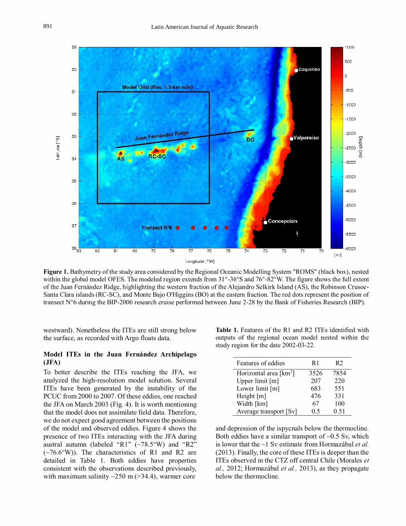
Figure 2 shows the vertical profile of temperature,

salinity, density and dissolved oxygen along transect

N°6 (37°05'S) during June 2006. Around 100-170 nm

from the coast, the data indicate the presence of an ITE.

Consistent with previous hydrographic studies

(Hormazábal et al., 2013), this ITE is associated with a

bi-convex lens shape density, high salinity core (>34.5),

low oxygen (<1 mL L-1) and a depression of the

isotherm below the thermocline. Although most of the

ITEs show similar characteristics, their vertical

structure may strongly depend on the PCUC vorticity

and local wind stress curl (Colas et al., 2011;

Hormazábal et al., 2013). To describe the trajectory of

this particular eddy, we used the AVISO satellite sea

surface height. Figure 3 shows the evolution of the

geostrophic current derived from June 2006 to May

2007. Although the surface expression is weak during

its initial phase, the tracking method can be used to

follow the eddy for ~1 year. Compared to previous

observed ITE, this ITE has a slow (~1.16 km d-1)

northwest displacement and reaches the southwest part

of the AS after 49 weeks and ~400 km. Note that the

surface expression of ITEs weakens while the ITEs

move westward below the thermocline (which deepens

890


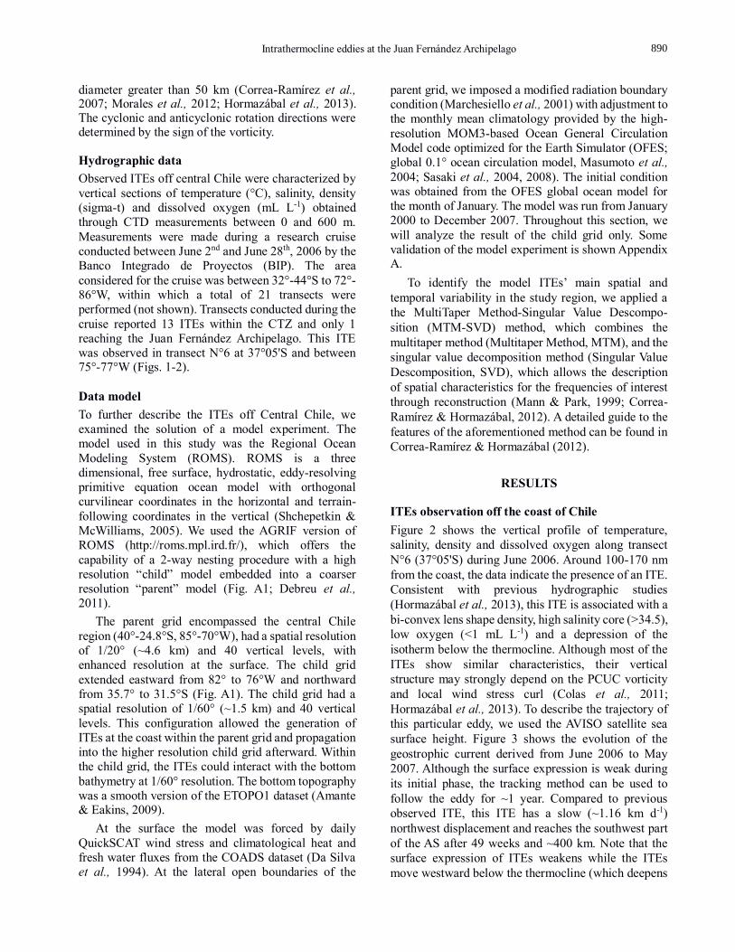
Figure 1. Bathymetry of the study area considered by the Regional Oceanic Modelling System "ROMS" (black box), nested within the global model OFES. The modeled region extends from 31°-36°S and 76°-82°W. The figure shows the full extent

of the Juan Fernández Ridge, highlighting the western fraction of the Alejandro Selkirk Island (AS), the Robinson Crusoe-

Santa Clara islands (RC-SC), and Monte Bajo O'Higgins (BO) at the eastern fraction. The red dots represent the position of

transect N°6 during the BIP-2006 research cruise performed between June 2-28 by the Bank of Fisheries Research (BIP).

westward). Nonetheless the ITEs are still strong below the surface, as recorded with Argo floats data.

Model ITEs in the Juan Fernández Archipelago

(JFA)

To better describe the ITEs reaching the JFA, we

analyzed the high-resolution model solution. Several

ITEs have been generated by the instability of the

PCUC from 2000 to 2007. Of these eddies, one reached

the JFA on March 2003 (Fig. 4). It is worth mentioning

that the model does not assimilate field data. Therefore,

we do not expect good agreement between the positions

of the model and observed eddies. Figure 4 shows the

presence of two ITEs interacting with the JFA during

austral autumn (labeled “R1” (~78.5°W) and “R2”

(~76.6°W)). The characteristics of R1 and R2 are

detailed in Table 1. Both eddies have properties

consistent with the observations described previously, with maximum salinity ~250 m (>34.4), warmer core

Table 1. Features of the R1 and R2 ITEs identified with outputs of the regional ocean model nested within the

study region for the date 2002-03-22.

Features of eddies R1 R2

Horizontal area [km2] 3526 7854

Upper limit [m] 207 220

Lower limit [m] 683 551 Height [m] 476 331

Width [km] 67 100

Average transport [Sv] 0.5 0.51

and depression of the ispycnals below the thermocline.

Both eddies have a similar transport of ~0.5 Sv, which

is lower that the ~1 Sv estimate from Hormazábal et al.

(2013). Finally, the core of these ITEs is deeper than the ITEs observed in the CTZ off central Chile (Morales et al., 2012; Hormazábal et al., 2013), as they propagate

below the thermocline.

De

pth

(m)

891


Figure 2. Vertical sections (0-600 m) of temperature (°C), salinity, density (sigma-t) and dissolved oxygen (mL L-1) at

37°05'S obtained through measurements with CTD during the BIP-2006 research cruise performed between June 2-28. Dotted lines represent the location of the five stations from transect N°6 taken by the cruise (Fig.1).

However, the differences between R1 and R2 are

important in the horizontal. Figure 5 shows the salinity

distribution at 50 m (~euphotic layer depth) and 250 m

(depth of the ITEs). While R2 is a well-defined rounded

eddy, R1 presents a more elongated deformation. This

shows the trajectory of the ESSW waters transported by

ITEs after interacting with the RC-SC islands and

adjacent seamounts. Note that R1 has a higher surface

salinity than that presented by R2, a difference

associated with the vertical elevation of the isohalines

produced by the interaction of R1 with the dorsal’s

topography (Figs. 4-5). The R1 surface expression at 50 m deep suggests that the interaction between the eddy and

topography may favor the ascent of the nutricline

within the euphotic layer and may also inject the

nutrients needed to promote an increase in phyto-plankton population.

Eddies and chlorophyll-a satellite data around the Juan Fernández Archipelago

With a mean velocity of ~2 km d-1 (Hormazábal et al., 2013), it takes around six months to the ITE travel from the CTZ to the JFA. Since ITEs tend to begin during the spring season (CTZ), it is more likely to observe ITEs in the vicinity of the JFA in the autumn.

We have therefore listed all the anticyclonic eddies with weak surface expression crossing the JFA during autumn. Figure 6 shows the trajectory of one particular eddy, which agrees the previous criteria. While it is not certain this anticyclone is an ITE, it was first detected

892


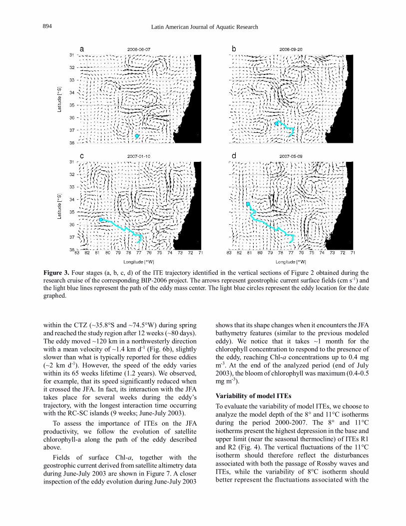
Figure 3. Four stages (a, b, c, d) of the ITE trajectory identified in the vertical sections of Figure 2 obtained during the

research cruise of the corresponding BIP-2006 project. The arrows represent geostrophic current surface fields (cm s-1) and the light blue lines represent the path of the eddy mass center. The light blue circles represent the eddy location for the date

graphed.

within the CTZ (~35.8°S and ~74.5°W) during spring

and reached the study region after 12 weeks (~80 days).

The eddy moved ~120 km in a northwesterly direction

with a mean velocity of ~1.4 km d-1 (Fig. 6b), slightly

slower than what is typically reported for these eddies

(~2 km d-1). However, the speed of the eddy varies

within its 65 weeks lifetime (1.2 years). We observed,

for example, that its speed significantly reduced when

it crossed the JFA. In fact, its interaction with the JFA

takes place for several weeks during the eddy’s

trajectory, with the longest interaction time occurring with the RC-SC islands (9 weeks; June-July 2003).

To assess the importance of ITEs on the JFA

productivity, we follow the evolution of satellite

chlorophyll-a along the path of the eddy described above.

Fields of surface Chl-a, together with the

geostrophic current derived from satellite altimetry data

during June-July 2003 are shown in Figure 7. A closer

inspection of the eddy evolution during June-July 2003

shows that its shape changes when it encounters the JFA

bathymetry features (similar to the previous modeled

eddy). We notice that it takes ~1 month for the

chlorophyll concentration to respond to the presence of

the eddy, reaching Chl-a concentrations up to 0.4 mg

m-3. At the end of the analyzed period (end of July

2003), the bloom of chlorophyll was maximum (0.4-0.5 mg m-3).

Variability of model ITEs

To evaluate the variability of model ITEs, we choose to

analyze the model depth of the 8° and 11°C isotherms

during the period 2000-2007. The 8° and 11°C

isotherms present the highest depression in the base and

upper limit (near the seasonal thermocline) of ITEs R1

and R2 (Fig. 4). The vertical fluctuations of the 11°C

isotherm should therefore reflect the disturbances

associated with both the passage of Rossby waves and

ITEs, while the variability of 8°C isotherm should

better represent the fluctuations associated with the

894


Figure 4. Vertical distribution (0-700 m depth) of a-b) salinity, c-d) temperature (°C), and e-f) density (sigma-t) around the

RC-SC islands for the date 2003-03-22. The left panels show the section at 33.64°S and between 76°-82°W, and the right

panels show a magnified view of two ITEs identified between 76°-79°W.

passage of ITEs. Thus, based on the behavior of the 8°

and 11°C isotherms depth, one can differentiate

between the disturbance generated by the presence of

ITE and Rossby waves.

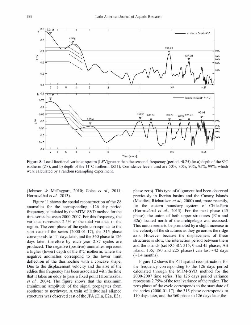
The spatial and temporal variability of fluctuations

in the depths of the 8°C (Z8) and 11°C (Z11) isotherms

for the 2000-2007 period were analyzed using the

MTM-SVD method. The local fractional variance

spectra obtained with the MTM-SVD method for Z8

and Z11 are shown in Figure 8. The Z8 spectrum (Fig.

8a) present significant variance in the 7 and 4.3 years

periods, which are usually associated with large-scale

processes such as El Niño Southern Oscillation

(Correa-Ramírez et al., 2012). Within the semiannual

and seasonal bands, significant fluctuations are

observed at periods of ~195 days (>95%) and ~127

days (>80%), respectively. These fluctuations might be

linked to mesoscale variability present in the study

region. Considering that Z8 is located at an average

depth of ~400 m, it suggest that annual scale processes do not have any great impact at mesobatic depths.

The spectrum of Z11 showed significant values at

interannual, annual, semi-annual and seasonal

frequencies (Fig. 8b). Fluctuations in the low-

frequency band (~7 and ~3 years) are generally

associated with large-scale processes such as El Niño

Southern Oscillation (Correa-Ramírez et al., 2012).

Unlike the Z8 depth, the Z11 depth exhibits energy maxima at 1 year and ~288 days. In general, the

increase of energy at these frequency bands has been

associated with Rossby wave propagation (Chelton & Schlax, 1996; Correa-Ramírez et al., 2012). Similar

a b

c d

e f

895


Figure 5. Salinity fields, obtained with ROMS, for one

horizontal section at a) 50 m, and b) 250 m depth for the

date 2003-03-22 in the region between 31°-36°S and 76°-

82°W. R1 and R2 are the ITEs selected for analysis.

to the Z8 spectrum, significant frequencies are found in

the semiannual (~193) and seasonal (~126) band, which

suggests that the disturbances observed in Z8 and Z11

correspond to a disturbance covering several hundred

meters in the water column and could be related to mesoscale variability generated by ITEs.

Space reconstruction

Because the Z8 and Z11 local fractional variance

spectra (Fig. 8) share a significant maximum in the

semiannual and seasonal bands with a similar period

(195 and 127 days), the respective frequencies were

reconstructed to evaluate whether these fluctuations are

associated with mesoscale variability generated by ITEs.

The spatial reconstruction of the anomalies in Z8

frequency corresponding to the 195 days period calcu-

lated through the MTM-SVD method for the 2000-

2007 time series is shown in Figure 9. The 195 day

period represents 4.6% of the total variance in the

region. The zero phase of the cycle corresponds to the

start date of the series (2000-07-17), the 315 phase

corresponds to 171 days later, and the 360 phase to 195

days after the start date of the time series, therefore by

each year 1.8 cycles are produced. The negative

(positive) anomalies represent a higher (lower) depth of

the 8°C isotherm. The figure shows that disturbance of

the isotherm depth presents closed structures of an

elongated oval shape that spread from the southeast to

the northwest of the study region. Propagation towards

the northwest indicates a non-linear signal, differing

from the linear Rossby wave propagation in these

latitudes (Chelton et al., 2007). Moreover, it was

observed that the structures presented a propagation

speed slightly higher than the theoretical propagation

speed for the first baroclinic mode of a Rossby wave

(gray dashed line). Furthermore, the horizontal spatial

scale associated with these structures had a greater size

than expected for Rossby waves. In general, the

features described for the figure suggest that these

structures are not Rossby waves. When those structures

interact with the RC-SC islands (45 and 90 phases), a

slight increase in speed is observed (Fig. 9), which may

correspond to an effect of the ridge on the incident

flows. In addition, it was observed that the islands have

a different impact on the propagation of the structures.

While the RC-SC islands generate increased speed in

propagation towards the northwest, the AS island

diverts the trajectory of the structures slightly to the

south (180, 225 and 270 phases), without affect significantly their velocity.

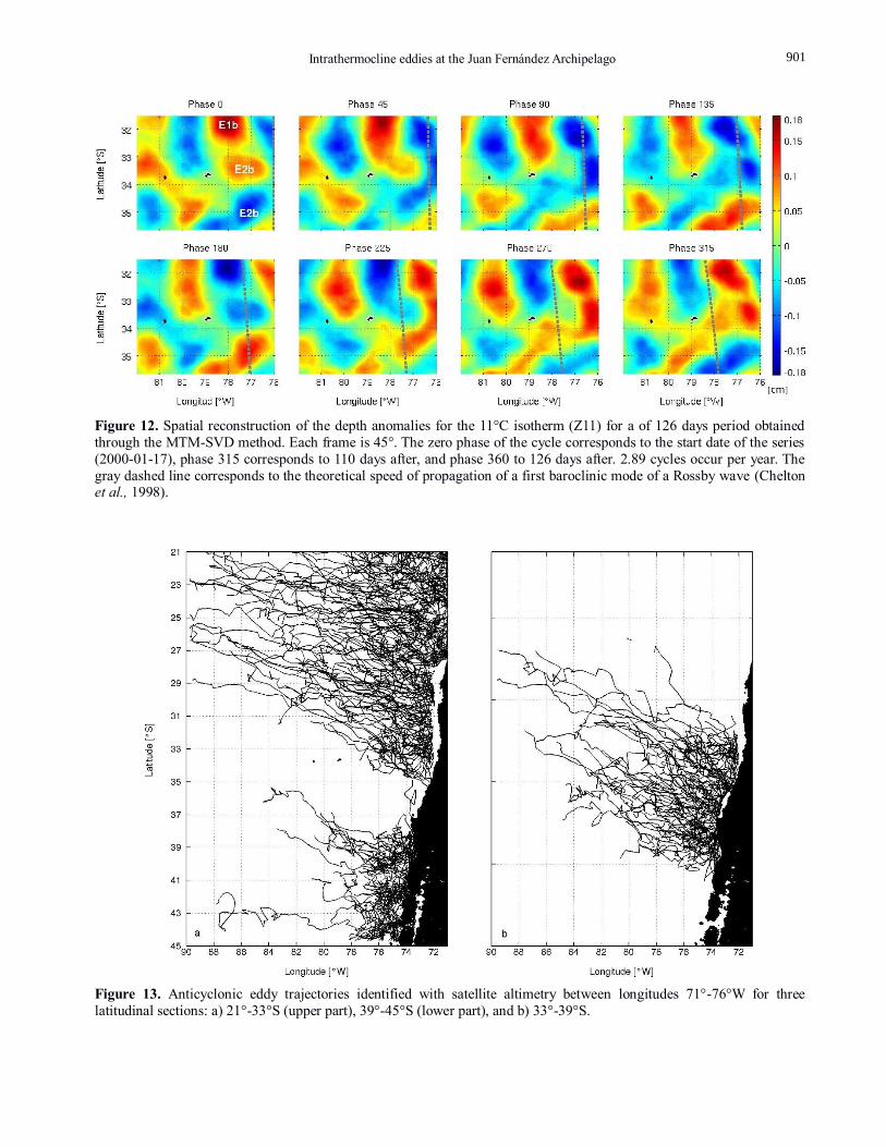
Figure 10 shows the spatial reconstruction of the Z11 anomalies in the frequency corresponding to the

193 days period calculated through the MTM-SVD method for the time series between 2000-2007. The

variance for the 193 days period represents 4.7% of the

total variance in the region. The zero phase of the cycle corresponds to the start date of the series (2000-01-17),

the 315 phase corresponds to 169 days later, and the 360 phase to 193 days later, therefore, each year contains

1.9 cycles. The negative (positive) anomalies represent a higher (lower) depth of the 11°C isotherm. In this

figure we note that Z11 fluctuations present a spatial

structure similar to Z8 (Fig. 10), with the same propagation pattern from southeast to northwest. The

structures in Z11 are slightly smaller in relation to those observed in Z8, suggesting that they represent the most

superficial fraction of a process developed at a greater depth. The features observed in both reconstructions allow the dismissal of the idea that the observed

fluctuations in this frequency band correspond to Rossby waves coinciding with those expected for ITEs

896


Figure 6. Four stages (a, b, c, d) of the ITE trajectory formed in the continental coastal zone. The arrows represent the

surface field of geostrophic currents (cm s-1) obtained by satellite altimetry and the light blue lines represent the path of the

eddy mass center through the Okubo-Weiss parameter. The light blue circles represent the eddy location for the date graphed.

Figure 7. Chlorophyll-a fields (color, mg m-3) superimposed on the surface field of geostrophic current (cm s-1) for the period in which the interaction of an anticyclonic eddy (identified by satellite, Fig. 6) is observed with the JFA. The contours

are chlorophyll-a isolines of 0.4 and 0.5 mg m-3.

897


Figure 8. Local fractional variance spectra (LFV)greater than the seasonal frequency (period >0.25) for a) depth of the 8°C

isotherm (Z8), and b) depth of the 11°C isotherm (Z11). Confidence levels used are 50%, 80%, 90%, 95%, 99%, which

were calculated by a random resampling experiment.

(Johnson & McTaggart, 2010; Colas et al., 2011;

Hormazábal et al., 2013).

Figure 11 shows the spatial reconstruction of the Z8

anomalies for the corresponding ~126 day period

frequency, calculated by the MTM-SVD method for the

time series between 2000-2007. For this frequency, the

variance represents 2.5% of the total variance in the

region. The zero phase of the cycle corresponds to the

start date of the series (2000-01-17), the 315 phase

corresponds to 111 days later, and the 360 phase to 126

days later, therefore by each year 2.87 cycles are

produced. The negative (positive) anomalies represent

a higher (lower) depth of the 8°C isotherm, where the

negative anomalies correspond to the lower limit

deflection of the thermocline with a concave shape.

Due to the displacement velocity and the size of the

eddies this frequency has been associated with the time

that it takes an eddy to pass a fixed point (Hormazábal

et al., 2004). The figure shows that the maximum (minimum) amplitude of the signal propagates from

southeast to northwest. A train of latitudinal aligned

structures was observed east of the JFA (E1a, E2a, E3a;

phase zero). This type of alignment had been observed

previously in Iberian basins and the Canary Islands

(Meddies; Richardson et al., 2000) and, more recently,

for the eastern boundary system of Chile-Perú

(Hormazábal et al., 2013). For the next phase (45

phase), the union of both upper structures (E1a and

E2a) located north of the archipelago was assessed.

This union seems to be promoted by a slight increase in

the velocity of the structures as they go across the ridge

axis. However because the displacement of these

structures is slow, the interaction period between them

and the islands (set RC-SC: 315, 0 and 45 phases; AS

island: 135, 180 and 225 phases) can last ~42 days (~1.4 months).

Figure 12 shows the Z11 spatial reconstruction, for

the frequency corresponding to the 126 days period calculated through the MTM-SVD method for the

2000-2007 time series. The 126 days period variance represents 2.75% of the total variance of the region. The zero phase of the cycle corresponds to the start date of

the series (2000-01-17), the 315 phase corresponds to 110 days later, and the 360 phase to 126 days later,the-

898


Figure 9. Spatial reconstruction of depth anomalies for the 8°C isotherm (Z8) for the 195 days period obtained through the

MTM-SVD method. Each frame is 45°. The zero phase of the cycle corresponds to the start date of the series (2000-01-17),

phase 315 corresponds to 171 days after, and phase 360 to 195 days after. 1.8 cycles occur per year. The gray dashed line

corresponds to the theoretical speed of propagation of a first baroclinic mode of a Rossby wave (Chelton et al., 1998).

Figure 10. Depth anomaly spatial reconstruction for the 11°C isotherm (Z11) for the 193 days period obtained through the


phase 315 corresponds to 169 days after, and phase 360 to 195 days after. 1.9 cycles occur per year. The gray dashed line

corresponds to the theoretical propagation speed of a first baroclinic mode of a Rossby wave (Chelton et al., 1998).

refore 2.89 cycles are produced each year. The positive

(negative) anomalies represent a lower (higher) depth

for the 11°C isotherm. A propagation pattern that differs slightly from that presented in Figure 11 was observed.

The maximum (minimum) signal amplitude spreads from southeast to northwest under below the ridge axis

of the JFA, and from east to west over the ridge axis,

suggesting that the western fraction of the ridge (82°-

76°W) represents a physical barrier for the incident

flow. Similar to the Z8 reconstruction (Fig. 11), at the zero phase a train of structures (E1b, E2b, E3b) at the

east of the archipelago are observed, but in opposite phase, which means that in this isotherm the deflection

is represented as a convex form in the upper limit of the

899


Figure 11. Depth anomaly spatial reconstruction for the 8°C isotherm (Z8) for a 127 days period of obtained through the


phase 315 corresponds to 111 days after, and the phase 360 to 127 days after. 2.87 cycles occur per year. The gray dashed

line corresponds to the theoretical speed of propagation of a first baroclinic mode of a Rossby wave (Chelton et al., 1998).

thermocline, reinforcing the idea that the observed structures correspond to ITEs. Nevertheless, the convex

deflection shape of the 11°C isotherm is not observed

for those structures located south of the Juan Fernández ridge axis (E3b). This might be associated to a

latitudinal difference in the stratification on top of the water column or the presence of another forcing that

operates on the same frequency. Moreover, the

propagation of the Z11 structure, relative to that observed with Z8, presents less interaction with the

islands that form the archipelago where the interaction with the AS island is the most intense.

DISCUSSION

The results of this study revealed the presence of long-

life (≥1 year) and weak surface expression ITEs

interacting with the topography of the JFA with a

semiannual frequency, mainly in the austral autumn

period. This agrees with what was described by

Morales et al. (2012) and Hormazábal et al. (2013),

who observed the formation of ITEs in the CTZ ~6

months before arriving at the JFA, mainly during

spring-summer periods when intensified coastal

upwelling occurs. Model results show the eddies’

simultaneous occurrence in time, which is supported by

observations in other oceanic regions (Richardson et al., 2000), and recently in the coastal zone off central Chile (Hormazábal et al., 2013).

The ITES were initially identified in the CTZ (Figs.

4-7). The trajectories presented slightly lower propagation velocities (~1.16 and ~1.4 km d-1) than

those previously reported (~2 km d-1; Hormazábal et al., 2013), which in some cases could delay the arrival

of these eddies to JFA until winter.

The depth fluctuation analysis of the 8°C (Z8) and

11°C (Z11) isotherms revealed the presence of

significant fluctuations with periods of ~190 and ~120

days, which are mainly associated with mesoscale eddies because they do not present a linear propagation.

Rather, they have a slightly higher propagation velocity

than the first baroclinic mode of a Rossby wave and are

larger than the internal radius of Rossby deformations for the region (~25-30 km; Chelton et al., 1998).

According to the time scale for coastal trapped

disturbances, periods ~180 days should be restrained to

the coast; however; the spatial reconstruction of Z8 and

Z11 for the ~190 day period agree with a non-linear propagation of eddies. The current fluctuations with

periods of ~120 days have been associated with

mesoscale eddies (Hormazábal et al., 2004). The spatial

reconstruction of Z8 and Z11 in the ~120 day period

presented a convex deflection shape in the upper limit of the eddy at Z11, and a concave shape at Z8, which

coincides with the expected vertical structure for an ITE.

Due to the northwestern propagation direction of the

eddies, it was observed that the surface and subsurface

900


Figure 12. Spatial reconstruction of the depth anomalies for the 11°C isotherm (Z11) for a of 126 days period obtained

through the MTM-SVD method. Each frame is 45°. The zero phase of the cycle corresponds to the start date of the series

(2000-01-17), phase 315 corresponds to 110 days after, and phase 360 to 126 days after. 2.89 cycles occur per year. The

gray dashed line corresponds to the theoretical speed of propagation of a first baroclinic mode of a Rossby wave (Chelton et al., 1998).

Figure 13. Anticyclonic eddy trajectories identified with satellite altimetry between longitudes 71°-76°W for three

latitudinal sections: a) 21°-33°S (upper part), 39°-45°S (lower part), and b) 33°-39°S.

901


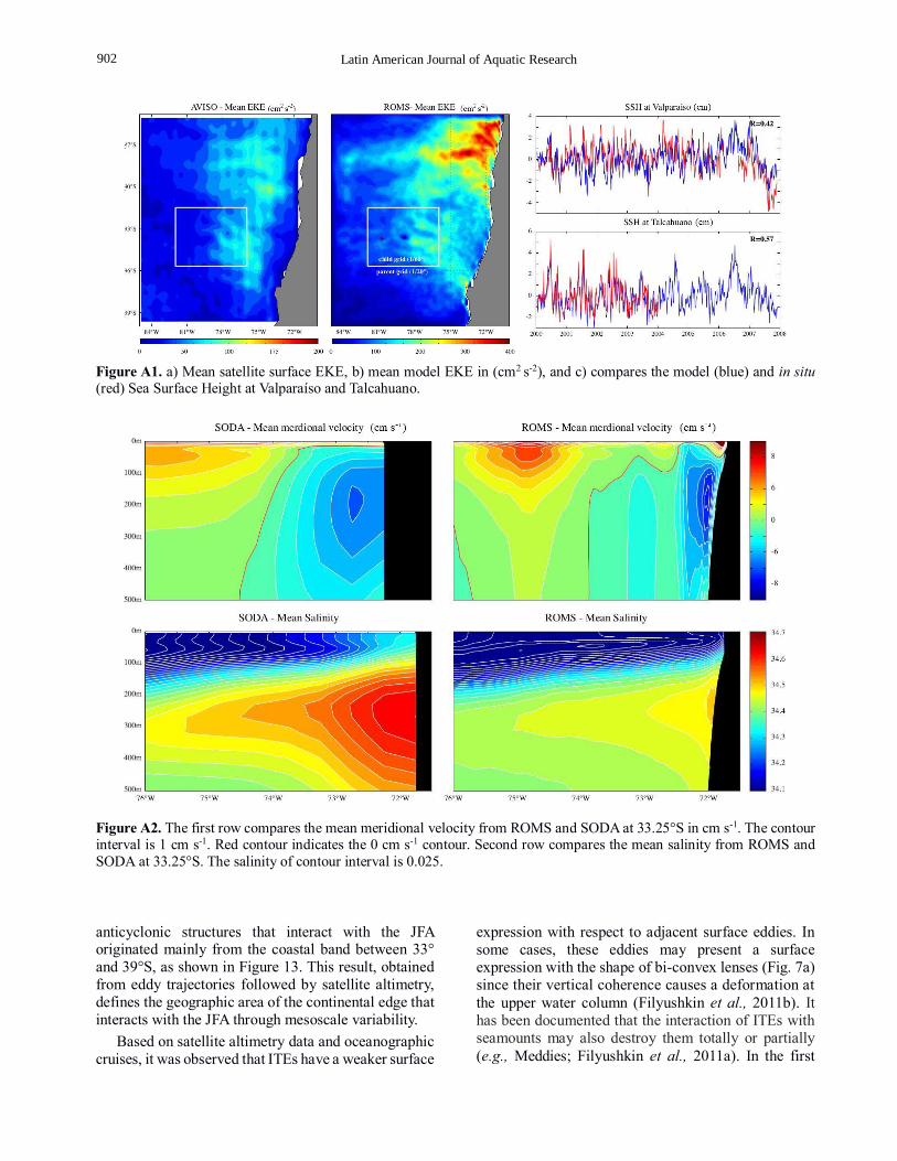
Figure A1. a) Mean satellite surface EKE, b) mean model EKE in (cm2 s-2), and c) compares the model (blue) and in situ (red) Sea Surface Height at Valparaíso and Talcahuano.

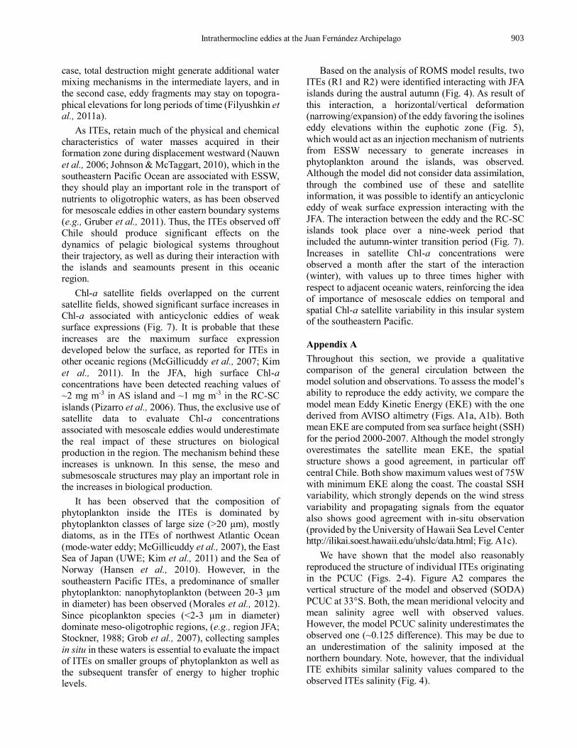
Figure A2. The first row compares the mean meridional velocity from ROMS and SODA at 33.25°S in cm s-1. The contour interval is 1 cm s-1. Red contour indicates the 0 cm s-1 contour. Second row compares the mean salinity from ROMS and

SODA at 33.25°S. The salinity of contour interval is 0.025.

anticyclonic structures that interact with the JFA originated mainly from the coastal band between 33°

and 39°S, as shown in Figure 13. This result, obtained

from eddy trajectories followed by satellite altimetry,

defines the geographic area of the continental edge that interacts with the JFA through mesoscale variability.

Based on satellite altimetry data and oceanographic

cruises, it was observed that ITEs have a weaker surface

expression with respect to adjacent surface eddies. In

some cases, these eddies may present a surface

expression with the shape of bi-convex lenses (Fig. 7a)

since their vertical coherence causes a deformation at

the upper water column (Filyushkin et al., 2011b). It has been documented that the interaction of ITEs with

seamounts may also destroy them totally or partially

(e.g., Meddies; Filyushkin et al., 2011a). In the first

902


case, total destruction might generate additional water

mixing mechanisms in the intermediate layers, and in

the second case, eddy fragments may stay on topogra-

phical elevations for long periods of time (Filyushkin et al., 2011a).

As ITEs, retain much of the physical and chemical

characteristics of water masses acquired in their

formation zone during displacement westward (Nauwn

et al., 2006; Johnson & McTaggart, 2010), which in the

southeastern Pacific Ocean are associated with ESSW,

they should play an important role in the transport of

nutrients to oligotrophic waters, as has been observed

for mesoscale eddies in other eastern boundary systems

(e.g., Gruber et al., 2011). Thus, the ITEs observed off

Chile should produce significant effects on the

dynamics of pelagic biological systems throughout

their trajectory, as well as during their interaction with

the islands and seamounts present in this oceanic

region.

Chl-a satellite fields overlapped on the current

satellite fields, showed significant surface increases in

Chl-a associated with anticyclonic eddies of weak

surface expressions (Fig. 7). It is probable that these

increases are the maximum surface expression

developed below the surface, as reported for ITEs in

other oceanic regions (McGillicuddy et al., 2007; Kim

et al., 2011). In the JFA, high surface Chl-a

concentrations have been detected reaching values of

~2 mg m-3 in AS island and ~1 mg m-3 in the RC-SC

islands (Pizarro et al., 2006). Thus, the exclusive use of

satellite data to evaluate Chl-a concentrations

associated with mesoscale eddies would underestimate

the real impact of these structures on biological

production in the region. The mechanism behind these

increases is unknown. In this sense, the meso and

submesoscale structures may play an important role in

the increases in biological production.

It has been observed that the composition of

phytoplankton inside the ITEs is dominated by

phytoplankton classes of large size (>20 μm), mostly

diatoms, as in the ITEs of northwest Atlantic Ocean

(mode-water eddy; McGillicuddy et al., 2007), the East

Sea of Japan (UWE; Kim et al., 2011) and the Sea of

Norway (Hansen et al., 2010). However, in the

southeastern Pacific ITEs, a predominance of smaller

phytoplankton: nanophytoplankton (between 20-3 μm

in diameter) has been observed (Morales et al., 2012).

Since picoplankton species (<2-3 μm in diameter)

dominate meso-oligotrophic regions, (e.g., region JFA;

Stockner, 1988; Grob et al., 2007), collecting samples

in situ in these waters is essential to evaluate the impact of ITEs on smaller groups of phytoplankton as well as

the subsequent transfer of energy to higher trophic levels.

Based on the analysis of ROMS model results, two

ITEs (R1 and R2) were identified interacting with JFA

islands during the austral autumn (Fig. 4). As result of

this interaction, a horizontal/vertical deformation

(narrowing/expansion) of the eddy favoring the isolines

eddy elevations within the euphotic zone (Fig. 5),

which would act as an injection mechanism of nutrients

from ESSW necessary to generate increases in

phytoplankton around the islands, was observed.

Although the model did not consider data assimilation,

through the combined use of these and satellite

information, it was possible to identify an anticyclonic

eddy of weak surface expression interacting with the

JFA. The interaction between the eddy and the RC-SC

islands took place over a nine-week period that

included the autumn-winter transition period (Fig. 7).

Increases in satellite Chl-a concentrations were

observed a month after the start of the interaction

(winter), with values up to three times higher with

respect to adjacent oceanic waters, reinforcing the idea

of importance of mesoscale eddies on temporal and

spatial Chl-a satellite variability in this insular system of the southeastern Pacific.

Appendix A

Throughout this section, we provide a qualitative

comparison of the general circulation between the

model solution and observations. To assess the model’s

ability to reproduce the eddy activity, we compare the

model mean Eddy Kinetic Energy (EKE) with the one

derived from AVISO altimetry (Figs. A1a, A1b). Both

mean EKE are computed from sea surface height (SSH)

for the period 2000-2007. Although the model strongly

overestimates the satellite mean EKE, the spatial

structure shows a good agreement, in particular off

central Chile. Both show maximum values west of 75W

with minimum EKE along the coast. The coastal SSH

variability, which strongly depends on the wind stress

variability and propagating signals from the equator

also shows good agreement with in-situ observation

(provided by the University of Hawaii Sea Level Center http://ilikai.soest.hawaii.edu/uhslc/data.html; Fig. A1c).

We have shown that the model also reasonably

reproduced the structure of individual ITEs originating

in the PCUC (Figs. 2-4). Figure A2 compares the

vertical structure of the model and observed (SODA)

PCUC at 33°S. Both, the mean meridional velocity and

mean salinity agree well with observed values.

However, the model PCUC salinity underestimates the

observed one (~0.125 difference). This may be due to

an underestimation of the salinity imposed at the northern boundary. Note, however, that the individual

ITE exhibits similar salinity values compared to the

observed ITEs salinity (Fig. 4).

903

http://ilikai.soest.hawaii.edu/uhslc/data.html


ACKNOWLEDGMENTS

This study was supported by the “Fondo Nacional de

Ciencia y Tecnología” (FONDECYT) Project

N°1131047 (S. Hormazábal). I. Andrade was funded by

a doctoral scholarship from the Pontificia Universidad

Católica de Valparaíso. The authors thank the Ocean

Biology Processing Group (Code 614.2) at the Goddard

Space Flight Center, Greenbelt, MD 20771, for the

production and distribution of the ocean color data. The comments of anonymous reviewers were very helpful.

REFERENCES

Alvera-Azcárate, A., A. Barth, M. Rixen & J.M. Beckers.

2005. Reconstruction of incomplete oceanographic

data sets using empirical orthogonal functions.

Application to the Adriatic Sea surface temperature.

Ocean Model., 9: 325-346.

Alvera-Azcárate, A., A. Barth, J.M. Beckers & R.H.

Weisberg. 2007. Multivariate reconstruction of missing

data in sea surface temperature, chlorophyll, and wind

satellite fields. J. Geophys. Res-Oce, 112, C03008.

doi:10.1029/2006JC003660.

Amante, C. & B.W. Eakins. 2009. ETOPO1 1 Arc-Minute

Global Relief Model: procedures, Data sources and

analysis. NOAA Technical Memorandum NESDIS

NGDC-24, 19 pp.

An, H.S., K.S. Shim & H.R. Shin. 1994. On the warm

eddies in the southwestern part of the East Sea (the

Japan Sea). J. Korean Soc. Oceanogr., 29: 152-163.

Andrade, I., S.E. Hormazábal & M.A. Correa-Ramírez.

2012. Ciclo anual de la clorofila-a satelital en el

archipiélago Juan Fernández (33°S), Chile. Lat. Am. J.

Aquat. Res., 40(3): 657-667.

Andrade, I., P. Sangrà, S.E. Hormazábal & M.A. Correa-

Ramírez. 2014. Island mass effect in the Juan

Fernández Archipelago (33°S), Southeastern Pacific.

Deep-Sea Res. I, 84: 86-99.

Aristegui, J., P. Tett, A. Hernández-Guerra, G. Basterretxea,

M.F. Montero, K Wild, P. Sangrà, S. Hernández-León,

M. Canton, J.A. García-Braun, M. Pacheco & E.D.

Barton. 1997. The influence of island-generated eddies

on chlorophyll distribution: a study of mesoscale

variation around Gran Canaria. Deep-Sea Res. I,

44(1):71–96.

Armi, L. & W. Zenk. 1984. Large lenses of highly saline

Mediterranean water. J. Phys. Oceanogr., 14: 1560-

1576.

Bakun, A. 2006. Fronts and eddies as key structures in the

habitat of marine fish larvae: opportunity, adaptive

response and competitive advantage. Sci. Mar.,

70(S2): 105-122.

Beckers, J.M. & M. Rixen. 2003. EOF calculations and

data filling from incomplete oceanographic data sets.

J. Atmos. Ocean. Technol., 20(12): 1839-1856.

Chaigneau, A., M. Le Texier, G. Eldin, C. Grados & O.

Pizarro. 2011. Vertical structure of mesoscale eddies in

the eastern South Pacific Ocean: a composite analysis from altimetry and Argo profiling floats, J. Geophys.

Res. Oceans, 116, C11025, doi:10.1029/2011JC

007134.

Chelton, D.B. & M.G. Schlax. 1996. Global observations

of oceanic Rossby waves. Science, 272: 234-238.

Chelton, D.B., M.G. Schlax, R.M. Samelson & R.A. de

Szoeke. 2007. Global observations of large ocean

eddies. Geophys. Res. Lett., 34, L15606,

doi:10.1029/2007GL030812.

Chelton, D.B., R.A. deSzoeke, M.G. Schlax, K. El Naggar

& N. Siwertz. 1998. Geographical variability of the

first-baroclinic Rossby radius of deformation. J. Phys.

Oceanogr. 28: 433-460.

Colas, F., J. McWilliams, X. Capet & J. Kurian. 2011. Heat

balance and eddies in the Peru-Chile Current System,

Clim. Dynam., 39(1): 509-529.

Correa-Ramírez, M. & S. Hormazábal. 2012. MultiTaper Method-Singular Value Decomposition (MTM-SVD):

variabilidad espacio-frecuencia de las fluctuaciones

del nivel del mar en el Pacífico suroriental. Lat. Am. J.

Aquat. Res., 40(4): 1039-1060.

Correa-Ramírez, M.A., S. Hormazábal & G. Yuras. 2007.

Mesoscale eddies and high chlorophyll concentrations off central Chile (29°S-39°S). Geophys. Res. Lett., 34,

L12604.

Correa-Ramírez, M.A., S.E. Hormazábal & C.E. Morales.

2012. Spatial patterns of annual and interannual

surface chlorophyll-a variability in the Perú-Chile

system. Prog. Oceanogr., 92-95: 8-17.

Da Silva, A.M., C.C. Young & S. Levitus. 1994. Atlas of

surface marine data 1994, Vol. 1, algorithms and

procedures, NOAA Atlas NESDIS 6, U.S. Department

of Commerce, NOAA, NESDIS, USA, 74 pp.

Debreu, L., P. Marchesiello, P. Penven & G. Cambon.

2011. Two-way nesting in split-explicit ocean models:

algorithms, implementation and validation. Ocean

Model., 49-50: 1-21.

Doty, M.S. & M. Ogury. 1956. The island mass effect. J.

Cons. Int. Explor. Mer., 22: 33-37.

Dugan, J.P., R.P. Mied, P.C. Mignerey & A.F. Schuetz. 1982. Compact, intrathermocline eddies in the

Sargasso Sea, J. Geophys. Res., 87(C1): 385-393.

Falkowski, P.G., D. Ziemann, Z. Kolber & P.K. Bienfang.

1991. Role of eddy pumping in enhancing primary

production in the ocean. Nature, 352(6330): 55-58.

904


Filyushkin, B.N., M.A. Sokolovskiy, N.G. Kozhelupova

& I.M. Vagina. 2011a. Evolution of intrathermocline eddies moving over a submarine hill. Doklady Earth

Sci., 441(2): 1757-1760.

Filyushkin, B.N., M.A. Sokolovskiy, N.G. Kozhelupova

& I.M. Vagina. 2011b. Reflection of intrathermocline

eddies on the ocean surface. Doklady Earth Sci.,

439(1): 118-121.

Garfield, N., C.A. Collins, R.G. Paquette & E. Carter.

1999. Lagrangian exploration of the California

Undercurrent, 1992-95. J. Phys. Oceanogr., 29: 560-

583.

González-Ferrán, O. 1987. Evolución geológica de las

Islas chilenas en el océano Pacífico. In: J.C. Castilla

(ed.). Islas oceánicas chilenas: conocimiento científico

y necesidades de investigación. Ediciones Universidad

Católica de Chile, Santiago, pp. 37-54.

Gordon, A.L., C.F. Giulivi, C.M. Lee, H.H. Furey, A.

Bower & L. Talley. 2002. Japan/East Sea intrather-

mocline eddies, J. Phys. Oceanogr., 32(6): 1960-1974.

Grob, C., O. Ulloa, W.K.W. Li, G. Alarcón, M. Fukasawa

& S. Watanabe. 2007. Picoplankton abundance and

biomass across the eastern south Pacific Ocean along

latitude 32.5°S. Mar. Ecol. Prog. Ser., 332: 53-62.

Gruber, N., Z. Lachkar, H. Frenzel, P. Marchesiello, M. Münnich, J.C. McWilliams, T. Nagai & G. K. Plattner.

2011. Eddy-induced reduction of biological

production in eastern boundary upwelling systems,

Nat. Geosci., 4(11): 787-792.

Hansen, C., E. Kvaleberg & A. Samuelsen. 2010.

Anticyclonic eddies in the Norwegian Sea; their generation, evolution and impact on primary

production, Deep-Sea Res. I, 57(9): 1079-1091,

doi:10.1016/j.dsr.2010.05.013.

Hormazábal, S., G. Shaffer & O. Leth. 2004. Coastal

transition zone off Chile. J. Geophys. Res., 109,

C01021, doi:10.1029/2003JC001956.

Hormazábal, S., V. Combes, C.E. Morales, M.A. Correa-

Ramírez, E. Di Lorenzo & S. Nuñez. 2013.

Intrathermocline eddies in the coastal transition zone

off central Chile (31-41°S). J. Geophys. Res. Oceans,

118: 1-11, doi:10.1002/jgrc.20337.

Isern-Fontanet, J., J. Font, E. Garcia-Ladona, M.

Emelianov, C. Millot & I. Taupier-Letage. 2004.

Spatial structure of anticyclonic eddies in the Algerian

basin (Mediterranean Sea) analyzed using the Okubo-

Weiss parameter, Deep-Sea Res. II, 51(25-26): 3009-

3028.

Johnson, G.C. & K.E. McTaggart. 2010. Equatorial

Pacific 13°C water eddies in the eastern subtropical

south Pacific Ocean. J. Phys. Oceanogr., 40(1): 226-

236, doi:10.1175/2009JPO4287.1.

Kim, D., E.J. Yang, K.H. Kim, C-W. Shin, J. Park, S. Yoo

& J-H. Hyun. 2011. Impact of an anticyclonic eddy on

the summer nutrient and chlorophyll a distributions in

the Ulleung Basin, East Sea (Japan Sea). ICES J. Mar. Sci., 69: 23-29.

Landaeta, M.F. & L.R. Castro. 2004. Zonas de

concentración de ictioplancton en el Archipiélago de

Juan Fernández, Chile. Cienc. Tecnol. Mar, 27(2): 43-

53.

Leth, O. & G. Shaffer. 2001. A numerical study of seasonal

variability in the circulation off central Chile, J.

Geophys. Res., 106: 22,229-22,248.

Marchesiello, P., J.C. McWilliams & A. Shchepetkin.

2001. Open boundary conditions for long-term

integration of regional oceanic models. Ocean Model.,

3: 1-20.

Masumoto, Y., H. Sasaki, T. Kagimoto, N. Komori, A.

Ishida, Y. Sasai, T. Miyama, T. Motoi, H. Mitsudera,

K. Takahashi, H. Sakuma & T. Yamagata. 2004. A fifty

year eddy-resolving simulation of the World Ocean-

preliminary outcomes of OFES (OGCM for the Earth

simulator). J. Earth Simul., 1: 31-52.

McGillicuddy, D., A. Robinson, D. Siegel, H. Jannasch, R.

Johnson, T. Dickey, J. McNeil, A. Michaels & A.

Knap. 1998. Influence of mesoscale eddies on new

production in the Sargasso Sea. Nature, 394: 263-266.

McGillicuddy, D.J., L.A. Anderson, N.R. Bates, T. Bibby, K.O. Buesseler, C.A. Carlson, C.S., Davis, C. Ewart,

P.G. Falkowski, S.A. Goldthwait, D.A., Hansell, W.J.

Jenkins, R. Johnson, V.K. Kosnyrev, J.R. Ledwell, Q.P.

Li, D.A. Siegel & D.K. Steinberg. 2007. Eddy/wind

interactions stimulate extraordinary mid-ocean

plankton bloom. Science, 316(5827): 1021-1026.

Mann, M.E. & J. Park. 1999. Oscillatory spatiotemporal

signal detection in climate studies: a multiple-taper

spectral domain approach. Adv. Geophys., 41: 1-131.

Morales, C.E., S. Hormazábal, M. Correa-Ramírez, O.

Pizarro, N. Silva, C. Fernández, V. Anabalón & M.L.

Torreblanca. 2012. Mesoscale variability and nutrient-phytoplankton distributions off central-southern Chile

during the upwelling season: the influence of

mesoscale eddies. Prog. Oceanogr., 104: 17-29,

doi:10.1016/j.pocean.2012.04.015.

Nauw, J.J., H.M. van Aken, J.R.E. Lutjeharms & W.P.M. de Ruijter. 2006. Intrathermocline eddies in the

southern Indian Ocean, J. Geophys. Res., 111, C03006,

doi:10.1029/2005JC002917.

Pequeño, G. & S. Sáez. 2000. Los peces litorales del

Archipiélago Juan Fernández (Chile): endemismo y

relaciones ictiogeográficas. Invest. Mar., Valparaíso, 28: 27-37.

Pingree, R.D. & B. Le Cann. 1992. Three anticyclonic

Slope Water Oceanic Eddies (SWODDIES) in the

southern bay of Biscay. Deep-Sea Res., 39: 1147-1175.

Pizarro, G., V. Montecino, R. Astoreca, G. Alarcón, G.

Yuras & L. Guzmán. 2006. Variabilidad espacial de

905


condiciones bio-ópticas de la columna de agua entre

las costas de Chile insular y continental, primavera 1999 y 2000. Cienc. Tecnol. Mar, 29(1): 45-58.

Richardson, P.L., A.S. Bower & W. Zenk. 2000. A census

of Meddies tracked by floats. Prog. Oceanogr., 45:

209-250.

Rozbaczylo, N. & J.C. Castilla. 1987. Invertebrados

marinos del Archipiélago Juan Fernández. In: J.C.

Castilla (ed.). Islas oceánicas chilenas: conocimiento

científico y necesidades de investigación. Ediciones

Unversidad Católica de Chile, Santiago, pp. 193-215.

Sasaki, H., M. Nonaka, Y. Masumoto, Y. Sasai, H. Uehara

& H. Sakuma. 2008. An eddy-resolving hindcast

simulation of the quasi-global ocean from 1950 to

2003 on the earth simulator. In: K. Hamilton & W.

Ohfuchi (eds.). High resolution numerical modelling

of the atmosphere and ocean. Springer, New York, pp.

157-185.

Sasaki, H., Y. Sasai, S. Kawahara, M. Furuichi, F. Araki,

A. Ishida, Y. Yamanaka, Y. Masumoto & H. Sakuma.

2004. A series of eddy-resolving ocean simulations in

the world ocean: OFES (OGCM for the Earth

Simulator) Project, OCEAN’04, 3, pp. 1535-1541.

Received: 10 March 2014; Accepted: 23 September 2014

Shapiro, G.I. & S.L. Meschanov. 1991. Distribution and

spreading of Red Sea Water and salt lens formation in the northwest Indian Ocean. Deep-Sea Res. I, 38: 21-

34.

Shchepetkin, A.F. & J.C. McWilliams. 2005. The regional

ocean modeling system: a split-explicit, free-surface,

topography following coordinates ocean model. Ocean

Model., 9: 347-404.

Siegel, D.A., P. Peterson, D.J. McGillicuddy, S. Maritorena

& N.B. Nelson. 2011. Bio-optical footprints created by

mesoscale eddies in the Sargasso Sea. Geophys. Res.

Lett., 38, L133608, doi:10.1029/ 2011GL047660.

Silva, N., N. Rojas & A. Fedele. 2009. Water masses in the

Humboldt current system: properties, distribution, and

the nitrate deficit as a chemical water mass tracer for

equatorial subsurface water off Chile. Deep-Sea Res.

II, 56(16): 1004-1020.

Stockner, J.G. 1988. Phototrophic picoplankton: an

overview from marine and freshwater ecosystems.

Limnol. Oceanogr., 33: 765-775.

906

Redalyc.Intrathermocline eddies at the Juan Fernández ...

Documents

Transcript of Redalyc.Intrathermocline eddies at the Juan Fernández ...