Reconstruction of time-dependent coefficients: a check of approximation schemes fornon-Markovian convolutionless dissipative generators

Bruno Bellomo,1, 2 Antonella De Pasquale,1, 3 Giulia Gualdi,1, 4 and Ugo Marzolino1, 5

1MECENAS, Universita Federico II di Napoli & Universita di Bari, Italy2CNISM and Dipartimento di Scienze Fisiche ed Astronomiche,Universita di Palermo, via Archirafi 36, 90123 Palermo, Italy

3Dipartimento di Fisica, Universita di Bari, via Amendola 173, I-70126 Bari, Italy;INFN, Sezione di Bari, I-70126 Bari, Italy

4Dipartimento di Matematica e Informatica, Universita degli Studi di Salerno,Via Ponte don Melillo, I-84084 Fisciano (SA), Italy; CNR-INFM Coherentia, Napoli,

Italy; CNISM Unita di Salerno; INFN Sezione di Napoli gruppo collegato di Salerno, Italy5Dipartimento di Fisica, Universita di Trieste, Strada Costiera 11, 34151, Trieste, Italy;

INFN, Sezione di Trieste, 34151, Trieste, Italy

We propose a procedure to fully reconstruct the time-dependent coefficients of convolutionless non-Markovian dissipative generators via a finite number of experimental measurements. By combininga tomography based approach with a proper data sampling, our proposal allows to relate the time-dependent coefficients governing the dissipative evolution of a quantum system to experimentallyaccessible quantities. The proposed scheme not only provides a way to retrieve full informationabout potentially unknown dissipative coefficients but also, most valuably, can be employed as areliable consistency test for the approximations involved in the theoretical derivation of a givennon-Markovian convolutionless master equation.

PACS numbers: 03.65.Wj, 03.65.Yz

I. INTRODUCTION

The dissipative evolution of a quantum system inter-acting with an environment represents a phenomenon ofparamount importance in quantum information scienceand beyond, as it addresses a fundamental issue in quan-tum theory. In general a complete microscopic descrip-tion of the dynamical evolution of a system coupled tothe environment (or bath) is a complex many-body prob-lem which requires the solution of a potentially infinitenumber of coupled dynamical equations. According to anopen system approach, this issue is tackled by retainingonly basic information about the environment and de-scribing the system dynamics in terms of a master equa-tion [1, 2]. The lack of a complete knowledge about thebath leads to master equations coefficients (MECs) whichmay be either unknown, or obtained from a microscop-ical derivation carried out within some approximationscheme. As a matter of fact it would then be highlyappealing to devise a procedure allowing to retrieve theMECs starting from experimentally accessible quantities.This would in fact both give access to otherwise unknownquantities and provide a strong indication about the va-lidity of the adopted theoretical framework.

So far two main dynamical regimes, Markovian andnon-Markovian, can usually be distinguished accordingto the timescale of environment dynamics (respectivelyshorter or longer than that of the system). In [3] ithas been shown that, in case of Markovian Gaussiannoise, the MECs can be retrieved by means of a finitenumber of tomographic measurements by using Gaus-sian states as a probe. Here we want to address themore involved non-Markovian case. In facts, even though

Markovian evolutions have been extensively investigated(see e.g. [1, 2, 4, 5]), in general real noisy dynamics arefar from being Markovian. Despite a growing interestin both theory and experiment [6, 7] a comprehensivetheory of non-Markovian dynamics is yet to come. Ex-act non-Markovian master equations have been derivedfor a Brownian particle linearly coupled to a harmonicoscillator bath via e.g. path integral methods [8, 9] orphase-space and Wigner function computations [10, 11].Analogous results have been obtained employing quan-tum trajectories, either exactly or in weak coupling ap-proximation [12–15]. In the framework of path integralmethods, master equations have been derived both forinitially correlated states [16, 17], and for factorized ini-tial states in the case of weak non linear interactions [18].Nevertheless, all these master equations cover only fewcases and are not simple to solve. Indeed, it would behighly desirable to find an approximation scheme fullycapturing non-Markovian features, as in general differentapproximations may lead to irreconcilable dynamics [1].

When dealing with a time-dependent generator one canface two, in principle distinct, kinds of problems. On onehand, taking for granted the functional form of the dis-sipative generator, one might be interested in retrievingthe time-independent parameters which characterize it.This issue has been tackled in [19], were it has been pre-sented a first generalization of the tomography-based ap-proach proposed in [3] to time-dependent dissipative gen-erators. There it has been shown that, under the assump-tion of Gaussian noise, the time-independent parameters(TIPs) characterizing the time-dependent MECs (whosefunctional form is previously known) as for example thesystem-bath coupling, temperature and bath frequency

arX

iv:1

007.

4537

v2 [

quan

t-ph

] 2

0 D

ec 2

010

2

cut-off, can be obtained with a finite set of measurements.On the other hand, one might be interested in the moregeneral problem of reconstructing the functional form ofthe dissipative generator itself. This might be the case ei-ther because the time-dependence of the dissipative gen-erator is completely unknown or because one wants totest the validity of the theoretical assumptions at the ba-sis of the dissipative model.

In this paper we propose an experimentally feasibleprocedure which allows the full reconstruction of thetime-dependence of convolutionless non-Markovian gen-erators. Indeed, whenever the assumption of Gaussiannoise is satisfied, by combining a tomography based ap-proach and a proper choice of data sampling, start-ing from a finite and discrete set of measurements itis possible to obtain global information about the time-dependent MECs. We envisage two main applications ofthe proposed scheme: both a full reconstruction startingfrom previously unknown MECs, and a sound, reliableand complete consistency test of the theoretical assump-tions made in deriving the dissipative generator.

The paper is organized as follows. In section II wereview the tomography based approach introduced in [3]allowing to reconstruct the first two cumulants of a Gaus-sian state at any fixed time with a finite amount of mea-surements. In section III we introduce the main lines ofour reconstruction scheme for two in principle distinctcases based on the purpose of the reconstruction and onthe available prior knowledge of the MECs. In sectionIV two different implementations, integral and differen-tial, of the reconstruction procedure are presented andtheir application is discussed. To provide an explicit ex-ample of both approaches, in section V they are appliedto the specific model of a brownian particle interactingwith an Ohmic bath of harmonic oscillators. In sectionVI we summarize and discuss our results, and finally inAppendix A we provide some more details about the sam-pling theorems involved in our reconstruction scheme.

II. THE T-C PROCEDURE

In this section we briefly review the main steps of theprocedure introduced in [3] which allows to relate theevolved first and second order cumulants of a Gaussianstate to tomographic measurements. We consider a mas-ter equation with unknown coefficients which generatesa Gaussian Shape Preserving (hereafter GSP) dissipativeevolution or, in other words, a Gaussian map. We thenfocus on the time evolution of the first and second cumu-lants of a Gaussian state, which completely determineits dynamics. Given a master equation governing theevolution of the density matrix of the system ρ(t), thedynamical equations for the first two cumulants formally

read

〈q〉t = Tr(ρ(t)q),

〈p〉t = Tr(ρ(t)p),

∆q2t = Tr(ρ(t)q2)− 〈q〉2t ,

∆p2t = Tr(ρ(t)p2)− 〈p〉2t ,

σ(q, p)t = Tr

(ρ(t)

qp+ pq

2

)− 〈q〉t〈p〉t. (1)

The explicit form of these equations depends on theadopted master equation whose coefficients, in general,are either unknown or derived by means of phenomeno-logical assumptions. Inserting into Eqs. (1) the explicitexpression of ρ(t) and then solving for the MECs, allowsto write these coefficients (or the differential equationsthey satisfy) as a function of the first two cumulantsof a Gaussian probe. Hence, by measuring these twoquantities, one can gain indirect experimental informa-tion about the MECs. To this aim, symplectic quantumtomography arises naturally as a key tool to perform therequired measurements. In particular we will use thesymplectic transform, or M2-transform [20], that findsits natural implementation in experiments with massiveparticles, as for example those to detect the longitudi-nal motion of neutrons [21] and to reconstruct the trans-verse motional states of helium atoms [22]. We also notethat the symplectic transform is equivalent to the Radontransform [23] which is experimentally implemented byhomodyne detection in the context of quantum optics[24]. We now recall a procedure introduced in [3] allow-ing to connect, at any fixed time t, tomographic measure-ments and the first two cumulants of a Gaussian probeby means of a small number of detections.

We begin by switching from the space of quantumstates, i.e. the Hilbert space, to phase-space, which canbe done by means of the Wigner map. In facts, a quan-tum state ρ(t) can be represented on phase-space in termsof its Wigner function W defined as

W (q, p, t) =1

π

∫ +∞

−∞dy exp

(i2py

)ρ(q − y, q + y, t).

(2)The Wigner function of a Gaussian state is itself a Gaus-sian function on phase space. Hence, if the dissipativeevolution is GSP, at any time the Wigner function of theevolved Gaussian state can be written as

W (q, p, t) =1

2π√

∆q2t∆p2

t − σ(q, p)2t

× exp

[− ∆q2

t (p− 〈p〉t)2 + ∆p2t (q − 〈q〉t)2

2[∆q2t∆p2

t − σ(q, p)2t ]

−2σ(q, p)t(q − 〈q〉t)(p− 〈p〉t)2[∆q2

t∆p2t − σ(q, p)2

t ]

].(3)

In general performing a tomographic map then amountsto project the above Wigner function along a line in

3

phase-space

X − µq − νp = 0, (4)

or, in other words, to compute its symplectic transform

$(X,µ, ν) = 〈δ (X − µq − νp)〉

=

∫R2

W (q, p, t)δ (X − µq − νp) dqdp.

(5)

For the case of Gaussian states, the symplectic transformis again a Gaussian function:

$ (X,µ, ν) =1

√2π√

∆q2t µ

2 + ∆p2tν

2 + 2σ(q, p)tµν

× exp

[− (X − µ〈q〉t − ν〈p〉t)2

2[∆q2t µ

2 + ∆p2tν

2 + 2σ(q, p)tµν]

], (6)

where the second cumulants always obey the constrain∆q2

t µ2 +∆p2

tν2 +2σ(q, p)tµν > 0 as a consequence of the

Schrodinger-Robertson relation [25], which represents ageneralization of the Heisenberg principle. At this pointone could wonder whether, due to experimental errors,a violation of the uncertainty principle might be ob-served. This may happen if measurements are performedon states almost saturating the inequality, i.e. on purestates. In our case measurements are performed on statesundergoing a dissipative evolution which typically are farfrom being pure hence from saturating the uncertaintyrelation. Furthermore any additional noise of statisticalorigin will have the effect of moving the reconstructedstate further away from the boundary, as noted in [26].

The symplectic transform (6) provides a relation be-tween the first and second order cumulants and the tomo-gram values along each line. In facts, performing a tomo-graphic measurement consists in choosing a pair (µ, ν),i.e. a line in phase space, and in computing $(X,µ, ν)for a given value of X. In [3] it has been shown thatby choosing the lines corresponding to position and mo-mentum probability distributions (i.e. (µ, ν) = (1, 0)and (0, 1)) then, for any fixed t, at most four pointsalong each line (i.e. tomogram) are needed to retrievethe first and second cumulant of the associated variable.Analogously, the covariance of the two variables is ob-tained by measuring at most two points along the line(µ, ν) = (1/

√2, 1/√

2). In overall, starting from a GSPmaster equation, the first and second order evolved mo-menta at time t can be obtained via a total amount ofeight or at most ten points measured in three different di-rections. In the following, we will refer to this procedureas the tomograms-cumulants (T-C) procedure.

To summarize, at each time t, the T-C procedure com-bined with Eqs. (1) provides the sought-for bridge be-tween dynamical parameters and measurable quantities.We note that, in the Markovian case, this combinationis straightforwardly performed by inverting Eqs. (1) [3].

Finally, we emphasize that even though the assumptionof Gaussian noise might be seen as an idealization, it isactually well fitted for a significant number of models[1, 2] and small deviations from Gaussianity would onlyintroduce small and controllable errors. Also, Gaussianprobes are quite straightforward to produce either with alaser or an ordinary light source (obtaining, respectively,a poissonian or a thermal distribution) [27].

III. SKETCH OF THE RECONSTRUCTION

The T-C procedure allows to gain information aboutthe unknown MECs -via experimentally accessiblequantities- locally in time. This is enough if the GSPdissipative generator is time-independent, as the infor-mation needed to fully reconstruct the unknown MECsis obtainable by performing tomographic measurementsat one arbitrary instant of time, as shown in [3]. This isno longer true when facing a time-dependent generator.In this case to fully reconstruct the unknown MECs wein principle need to gather information globally in time.Now, taking the T-C procedure as a starting point, theproblem we tackle is how to retrieve the full informationwe need by combining measurements performed on a fi-nite and discrete set of times, i.e. starting from partialinformation.

A. the dissipative generator

We focus on the reconstruction of the time-dependentMECs of the following class of master equations

dρ(t)

dt= − i

[H0, ρ(t)

]− i(λ(t) + δ)

2[q, ρ(t)p+ pρ(t)]

+i(λ(t)− δ)

2[p, ρ(t)q + qρ(t)]

−Dpp(t)

2[q, [q, ρ]]− Dqq(t)

2[p, [p, ρ(t)]]

+Dqp(t)

2([q, [p, ρ(t)]] + [p, [q, ρ(t)]]) , (7)

where the unknown MECs are λ(t), Dqq(t), Dpp(t),Dqp(t). The system Hamiltonian H is chosen to be atmost a second-order polynomial in the position and mo-mentum operators p, q [28]

H = H0 +δ

2(qp+ pq) , H0 =

1

2mp2 +

mω2

2q2, (8)

where the time dependence which may be introduced bythe Lamb shift term has been neglected. This is typi-cally justified as most of the times either the Lamb shiftis negligible or the Hamiltonian part of the dissipativegenerator reaches its asymptotic value on a much shortertimescale compared to the non unitary part [1]. In over-all, the choice of operators in Eq. (7) represents a natural

4

generalization of the GSP time-independent master equa-tion introduced in [28]. The investigation of this time-dependent class of master equations is further motivatedby the existence of a wide range of models obeying a GSPdissipative dynamics of this form [9–11, 13–17].

As a side remark we note that there may be some am-biguity in literature about the relation between time-dependent dissipative generators and Markovian/non-Markovian dynamics. In facts, some authors classify asnon-Markovian only generators containing a convolutionintegral. It has recently been proved in [29] that thesegenerators can be mapped into convolutionless ones. Thedistinctive feature of non-Markovianity becomes then thedependence of the convolutionless generator on t − t0where t0 is the initial time. According to this approacha time-dependent generator of the kind (7) could be con-sidered as Markovian. However, following a consistentpart of literature, e.g. [8, 10, 11, 13, 14, 18, 30], we willterm non-Markovian also convolutionless time-dependentgenerators as the one in Eq. (7).

B. the reconstruction scheme

Our strategy towards the reconstruction of the MECsin Eq. (7) is made up of three main steps:

1. use the T-C procedure to get indirect measure-ments of the evolved cumulants at different times;

2. use these measurements to retrieve the values ofthe MECs (or functions of them) at those timesexploiting the connection between MECs and firstcumulants of a Gaussian probe, obtained by em-ploying the dynamical equations (1);

3. starting from the obtained discrete and finite set ofvalues, reconstruct the full expression for the MECsby applying proper sampling theorems.

In particular, useful for our purposes will be the Nyquist-Shannon theorem [31, 32] and one of its more sophisti-cated generalizations involving an additive random sam-pling [31, 33, 34]. In principle we can distinguish twodifferent applications of the reconstruction procedure:check of the a priori assumed time-dependence of MECs(Case I) or complete reconstruction of MECs with no apriori assumptions (Case II).

Case I: we assume a priori a certain time dependenceof the MECs as a consequence, for example, of a micro-scopical derivation of the master equation. In this per-spective, we are interested in experimentally reconstruct-ing the MECs to check the validity of the approximationsmade. A mismatch between the assumed and the mea-sured MECs would in fact provide a strong evidence ofthe breakdown of the adopted approximation scheme. Inthis case a full knowledge of the MECs is assumed, includ-ing that of the TIPs involved, such as the bath frequencycut-off, system-bath coupling, etc. The TIPs can be ei-ther assumed or previously reconstructed [19]. In this

case, given the prior knowledge of the bandwidth associ-ated to the function to be reconstructed (i.e. the widthof its Fourier transform), the suitable sampling theoremcan be chosen accordingly. If the function is band-limitedthen to obtain an exact reconstruction it is enough toapply the simplest sampling theorem, i.e. the Nyquist-Shannon theorem (see Appendix A). The function canhence be reconstructed starting from a discrete set ofvalues spaced according to the width of its Fourier trans-form. If the bandwidth is not limited one could truncateit and still apply the same procedure, which would thenbe affected by the so-called aliasing error. To minimizeit one can perform a proper truncation. Alternatively amore general additive random sampling, that avoids thealiasing error (see Appendix A), can be employed.

Case II: here we want to fully reconstruct the MECs,or derived functions, with no previous assumption on thedynamics, i.e. the MECs are fully unknown. In general,this implies no prior knowledge of the bandwidth asso-ciated to the function to be reconstructed. In this casewe must resort to an additive random sampling (see Ap-pendix A). If on one hand this procedure involves func-tion averages with respect to the probability of draw-ing n sampling times (i.e. more involved measurements),on the other it does not require prior knowledge of thebandwidth and is an alias-free sampling. To obtain theaverages of the function we should in principle performmeasurements over a continuous interval of time, as thereconstruction is proposed with continuous random pro-cesses. In practice, every experimental apparatus em-ployed to record and process the data has a dead work-ing time, such that the random process will be discrete intime, no matter how dense, thus introducing an intrinsicsource of error in the procedure.

As a conclusive remark, we note that in both cases theset of measurements required turns out to be discretebut in principle infinite, as the reconstruction should beperformed over the whole real axis. This number can bemade finite by invoking the largely reasonable physicalcondition of a finite observation time.

IV. DIFFERENT PROCEDURES

In this section we illustrate in more detail how to im-plement the above sketched reconstruction scheme. Thestarting point are the general equations (1) and (7) whichcan be expressed in compact matrix form as

d

dtS(t) = (M − λ(t)I2)S(t), (9)

d

dtX(t) = (R− 2λ(t)I3)X(t) +D(t), (10)

where I2(3) is the 2(3)-dimensional identity matrix. Thevectors S(t) and X(t) correspond, respectively, to the

5

first and second order cumulants

S(t) =1√

√mω〈q〉t〈p〉t√mω

, X(t) =1

mω(∆q)2t

(∆p)2t

mω(σq,p)t

,(11)

and the matrices M and R contain the Hamiltonian pa-rameters

M =

(δ ω−ω −δ

), R =

2δ 0 2ω0 −2δ −2ω−ω ω 0

. (12)

Finally, D(t) is the diffusion vector

D(t) =2

mωDqq(t)Dpp(t)

mωDqp(t)

, (13)

such that the MECs to be reconstructed are λ(t) andD(t). The dynamical evolution of the first cumulants,Eq. (9), only depends on the friction coefficient λ(t)whereas that of the second cumulants, Eq. (10), dependson the whole set of MECs. At this point we can distin-guish two different approaches towards the reconstruc-tion, i.e. integral and differential.

A. Integral approach

The formal solution of Eq. (9) can be written as

Λ(t) ≡∫ t

0

dt′λ(t′) = ln

(Sj(0)

Sj(t)

), (14)

where the suffix j = 1, 2 labels the two components ofthe vector

S(t) = e−tMS(t). (15)

We note that in Eq. (14) the measurable quantities andthe unknown MEC appear on different sides. Analo-gously, we rewrite Eq. (10) as

d

dtX(t) = D(t), (16)

where

X(t) = e2Λ(t)I3e−tRX(t),

D(t) = e2Λ(t)I3e−tRD(t). (17)

Eqs. (15) and (17) are always invertible, provided one

sets the quantity√δ2 − ω2 ≡ η to the value iΩ whenever

η2 < 0 [28]. The formal solution of Eq. (16) is given by

X(t) = X(0) +∫ t

0dt′D(t′), which, using Eq. (17), can be

recast in terms of X(t) as∫ t

0

dt′e−2Λ(t,t′)I3e(t−t′)RD(t′)

= X(t)− etRe−2Λ(t)X(0); (18)

where Λ(t, t′) =∫ tt′dt′′λ(t′′). Again, considering Λ(t)

as a known quantity from Eq. (14), in Eq. (18) exper-imentally accessible quantities and MECs are groupedon different sides, respectively right and left-hand. Theright-hand sides of both equations can thus be regardedas experimental measurements of the corresponding left-hand sides. The first step is then to compute the lefthand side of Eq. (14) using the friction coefficient λ(t)provided by the assumed model. A theoretical value forΛ(t), say Λtheor(t), is obtained and its Fourier transformis performed. Once obtained the bandwidth associated toΛtheor(t) and consequently the amount of points in timerequired for the full reconstruction (according to the cho-sen sampling theorem) the following step is to evaluate

S(t) (Eq. (15)) on these points by successive applicationsof the T-C procedure. Finally, the last step is to applythe sampling theorem to the experimental data and to re-construct the left-hand side of Eq. (14), let us denote itby Λexpt(t). If the match between Λtheor(t) and Λexpt(t)is positive within the desired accuracy, one can then pro-ceed further to the reconstruction of the left-hand sideof Eq. (18) according to the same procedure. We notethat the integral approach is also feasible in case of time-dependent Hamiltonian parameters (i.e. m(t), ω(t), δ(t))as long as the generator remains GSP. In general thiskind of generators requires a numerical evaluation of theintegrals in Eqs. (9) and (10), according to which thesuitable sampling theorem must be chosen.

B. Differential approach

The T-C procedure allows to measure not only thecumulants of a given Gaussian state but also their firsttime derivatives. Indeed, by measuring each cumulantat two different times t and t + δt, its derivative can beestimated via its finite incremental ratio. For instance

d

dt∆q2

t ∼∆q2

t+δt −∆q2t

δt, (19)

where the amount of time δt is taken as the smallest timeinterval which can elapse between two different measure-ments. Once the cumulants and their derivatives at fixedtimes are given as experimental inputs, Eqs.(9) and (10)become linear algebraic equations whose unknown are theMECs. Hence from Eqs. (9) and (10) we obtain the de-

6

sired experimentally accessible estimations for the MECs

λexpt(t) ' δ +1

〈q〉t

(1

m〈p〉t −

〈q〉2t+δt − 〈q〉2tδt

)' −δ − 1

〈p〉t

(mω2〈q〉t +

〈p〉2t+δt − 〈p〉2tδt

), (20)

Dexptqq (t) ' (λ(t)− δ)∆q2

t −1

mσ(q, p)t

+∆q2

t+δt −∆q2t

2δt, (21)

Dexptpp (t) ' (λ(t) + δ)∆p2

t +mω2σ(q, p)t

+∆p2

t+δt −∆p2t

2δt, (22)

Dexptqp (t) ' m

2ω2∆q2

t −1

2m∆p2

t + λ(t)σ(q, p)t

+σ(q, p)2

t+δt − σ(q, p)2t

2δt. (23)

The number of points required to fully reconstruct theMECs depends on the sampling theorem employed. InCase I, given the prior knowledge of the bandwidth, ifthe function is band limited or it can be truncated on aneffective compact support outside of which the contribu-tions are negligible, the Nyquist-Shannon theorem canbe applied. Otherwise one must resort to the additiverandom sampling theorem, which must be in generalemployed in Case II.As the integral approach, the differential approach isalso suitable in case of time-dependent Hamiltonianparameters as long as the generator remains GSP.The Hamiltonian parameters would then be includedamong the MEPs to be reconstructed, thus raisingtheir number to seven. Since Eqs.(9) and (10) are five,two more equations would be required as for examplethose for two higher order cumulants, e.g. Tr(ρ(t)q3)and Tr(ρ(t)p3). This would not increase the numberof experimental measurements, since the higher ordermoments and cumulants of Gaussian states are com-pletely determined by the first and the second cumulants.

C. Comparison between the two approaches

Let us now briefly compare the two procedures de-scribed in this section. The differential approach requiresmore experimental measurements compared to the inte-gral approach, whereas the latter might result more in-volved from a computational point of view. For example,within the frame of Case I, the computation of the firstmember of Eq. (18) might require some numerical or ana-lytical approximations. As any kind of approximation inprinciple reduces the accuracy of the reconstruction, thedifferential approach would be a better choice. On theother hand, if the computation of the integral functionsin Eqs. (14)-(18) does not exhibit remarkable difficulties,

the integral procedure should be preferred, since it re-quires a lower number of interactions with the physicalsystem.

In Case II, the integral approach could be employed toreconstruct the left hand sides of Eqs. (14)-(18), whichare functionals of the unknown MECs. By means of timederivatives and linear operations on the reconstructedfunctions, the MECs can finally be retrieved. However,the time derivatives may amplify the error of the recon-struction. For instance, the Nyquist-Shannon theoremrequires a truncation of the Fourier’s frequencies, thus in-ducing an oscillating behavior of the reconstructed func-tions, i. e. introducing the so-called aliasing error (seeAppendix A). Even if the oscillations around the mean(true) functions are small, the time derivative may in-crease them. Hence, either one performs a better recon-struction (e.g. a larger truncation or a random additivesampling requiring a larger number of measurements) orone adopts the differential approach, thus directly recon-structing the MECs.In general, one could say that the integral procedure ismore advantageous in terms of number of measurements,but requires the ability of solving potentially involved an-alytical expressions. The differential approach, instead,is more advantageous from the point of view of versatility,as it allows to deal in a straightforward way with com-plex generators (i.e. exhibiting time-dependent Hamil-tonian parameters), at the expenses of a higher numberof measurements. Therefore, which of the two proposedapproaches proves better, strictly depends on the specificcase under investigation.

V. AN EXAMPLE

To provide an example of how to implement the pro-posed integral and differential procedures, in this sec-tion we apply both to a specific model i.e. within theperspective of Case I. As a model to be tested we con-sider a harmonic oscillator of frequency ω (our system-particle) linearly coupled to an Ohmic bath of harmonicoscillators. The TIPs of this model are the system-bathcoupling constant α, the Lorentz-Drude cut-off ωc andthe temperature T [1]. Starting from a superoperatorialversion of the Hu-Paz-Zhang master equation [8], in theweak-coupling limit (i.e. up to α2) and using the rotat-ing wave approximation (i.e. an average over the rapidlyoscillating terms), for this model a generator of the formof Eq. (7) can be obtained [30, 35]. More specifically,the Hamiltonian parameter δ is set to 0 and the MECsprovided by the model are

λtheor(t) =α2ω2

cω

ω2c + ω2

1− e−ωct

[cos(ωt) +

ωcω

sin(ωt)]

,

Dtheorqp = 0,

mω

Dtheorqq =

Dtheorpp

mω=

∆theor(t)

2, (24)

7

where at high temperature T

∆theor(t) =2α2ω2

c

ω2c + ω2

kT

×

1− e−ωct

[cos(ωt)− ω

ωcsin(ωt)

].(25)

With this choice of MECs the dissipative generator isGSP [30]. The Markovian limit is recovered when thetime dependent parameters λtheor(t) and ∆theor(t) reachtheir stationary values, i.e. at times larger than 1/ωc

λtheor(t)→ α2ω2cω

ω2c + ω2

, ∆theor(t)→ 2α2ω2c

ω2c + ω2

kT

. (26)

Usually, when studying quantum Brownian motion, oneassumes ωc/ω 1 with ωc → ∞, corresponding to anatural Markovian reservoir. In this limit, the thermal-ization time [30] is inversely proportional to the couplingstrength, while for an out-of-resonance engineered reser-voir with ωc/ω 1 (i.e. highly non Markovian), thethermalization process is slowed down.

Microscopic derivations of Master Equations usuallygive a time dependent renormalization of Hamiltonianparameters (m, ω, δ). However, they are negligible forthis benchmark model in the considered limits.

A. Integral approach

Following the steps of the integral approach we solveEq. (14) using λtheor(t) (Eq. (24)) and we get

Λtheor(t) =α2ω2

cω2

(ω2c + ω2)2

ωtω2c + ω2

ω2− 2

ωcω

+ e−ωct

[2ωcω

cos(ωt) +ω2c − ω2

ω2sin(ωt)

].

(27)

The obtained function does not belong to the functionalspace L2((R)) thus not matching the condition for theapplicability of the Nyquist-Shannon theorem (see Ap-pendix A). However, as we are interested in a finite timeinterval, we can restrict the support of Λtheor(t) to [0, t]and define:

Λtheor(t) ≡

Λtheor(t) t ∈ [0, t]

0 else. (28)

The function Λtheor(t) is in L2(R) thus can be recon-structed by the Nyquist-Shannon theorem. The discon-tinuity at t, by inducing the Gibbs phenomenon (i. e.a finite Fourier sum overshoots at the jump), might atthis point constitute a source of error. This problem canbe anyway overcome by slightly restricting the domain inwhich the reconstruction of Λtheor(t) can be trusted to[0, t − ξ] with ξ > 0. Performing the Fourier transform

ωt

(a)

0.2 0.4 0.6 0.8 1.0

0.002

0.004

0.006

0.008

Λth

eor (

t)ω

,Λex

pt(t

)ω

ωt

(b)

0.2 0.4 0.6 0.8 1.0

0.002

0.004

0.006

0.008

Λth

eor (

t)ω

,Λex

pt(t

)ω

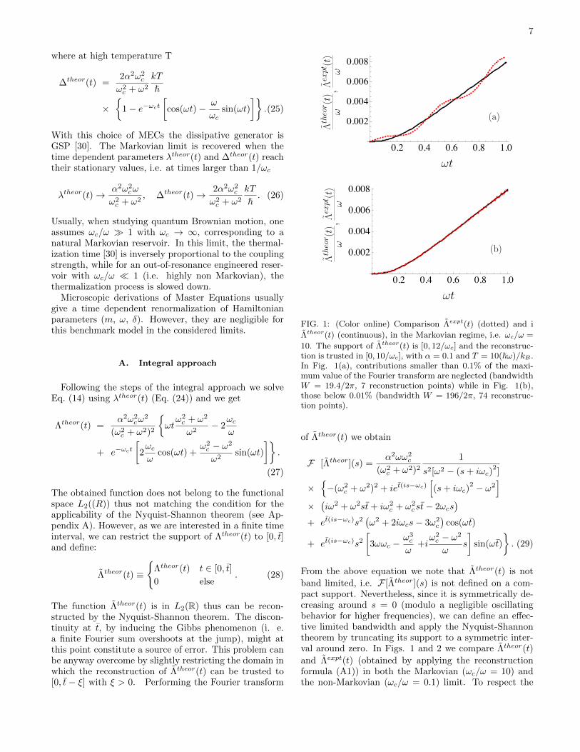
FIG. 1: (Color online) Comparison Λexpt(t) (dotted) and i

Λtheor(t) (continuous), in the Markovian regime, i.e. ωc/ω =

10. The support of Λtheor(t) is [0, 12/ωc] and the reconstruc-tion is trusted in [0, 10/ωc], with α = 0.1 and T = 10(ω)/kB .In Fig. 1(a), contributions smaller than 0.1% of the maxi-mum value of the Fourier transform are neglected (bandwidthW = 19.4/2π, 7 reconstruction points) while in Fig. 1(b),those below 0.01% (bandwidth W = 196/2π, 74 reconstruc-tion points).

of Λtheor(t) we obtain

F [Λtheor](s) =α2ωω2

c

(ω2c + ω2)2

1

s2[ω2 − (s+ iωc)2]

×−(ω2

c + ω2)2 + iet(is−ωc)[(s+ iωc)

2 − ω2]

×(iω2 + ω2st+ iω2

c + ω2cst− 2ωcs

)+ et(is−ωc)s2

(ω2 + 2iωcs− 3ω2

c

)cos(ωt)

+ et(is−ωc)s2

[3ωωc −

ω3c

ω+iω2c − ω2

ωs

]sin(ωt)

. (29)

From the above equation we note that Λtheor(t) is not

band limited, i.e. F [Λtheor](s) is not defined on a com-pact support. Nevertheless, since it is symmetrically de-creasing around s = 0 (modulo a negligible oscillatingbehavior for higher frequencies), we can define an effec-tive limited bandwidth and apply the Nyquist-Shannontheorem by truncating its support to a symmetric inter-val around zero. In Figs. 1 and 2 we compare Λtheor(t)

and Λexpt(t) (obtained by applying the reconstructionformula (A1)) in both the Markovian (ωc/ω = 10) andthe non-Markovian (ωc/ω = 0.1) limit. To respect the

8

ωt

(a)

20 40 60 80 100

0.002

0.004

0.006

0.008

0.010

Λth

eor (

t)ω

,Λex

pt(t

)ω

ωt

(b)

20 40 60 80 100

0.002

0.004

0.006

0.008

0.010

Λth

eor (

t)ω

,Λex

pt(t

)ω

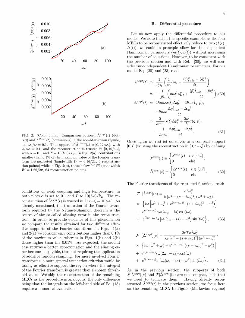
FIG. 2: (Color online) Comparison between Λexpt(t) (dot-

ted) and Λtheor(t) (continuous) in the non-Markovian regime,

i.e. ωc/ω = 0.1. The support of Λtheor(t) is [0, 12/ωc], withωc/ω = 0.1, and the reconstruction is trusted in [0, 10/ωc],with α = 0.1 and T = 10(ω)/kB . In Fig. 2(a), contributionssmaller than 0.1% of the maximum value of the Fourier trans-form are neglected (bandwidth W = 0.16/2π, 6 reconstruc-tion points) while in Fig. 2(b), those below 0.01% (bandwidthW = 1.66/2π, 64 reconstruction points).

conditions of weak coupling and high temperature, inboth plots α is set to 0.1 and T to 10(ω)/kB . The re-

construction of Λexpt(t) is trusted in [0, t−ξ = 10/ωc]. Asalready mentioned, the truncation of the Fourier trans-form required by the Nyquist-Shannon theorem is thesource of the so-called aliasing error in the reconstruc-tion. In order to provide evidence of this phenomenonwe compare the results obtained for two different effec-tive supports of the Fourier transform: in Figs. 1(a)and 2(a) we consider only contributions higher than 0.1%of the maximum value, whereas in Figs. 1(b) and 2(b)those higher than the 0.01%. As expected, the secondcase returns a better approximation and the aliasing er-ror becomes negligible, thus not requiring the applicationof additive random sampling. For more involved Fouriertransforms, a more general truncation criterion would betaking as effective support the region where the integralof the Fourier transform is greater than a chosen thresh-old value. We skip the reconstruction of the remainingMECs as the procedure is analogous, the only differencebeing that the integrals on the left-hand side of Eq. (18)require a numerical evaluation.

B. Differential procedure

Let us now apply the differential procedure to ourmodel. We note that in this specific example, as the fourMECs to be reconstructed effectively reduce to two (λ(t),∆(t)), we could in principle allow for time dependentHamiltonian parameters (m(t), ω(t)) without increasingthe number of equations. However, to be consistent withthe previous section and with Ref. [30], we will con-sider time-independent Hamiltonian parameters. For ourmodel Eqs.(20) and (23) read

λexpt(t) ' 1

〈q〉t

(1

m〈p〉t −

〈q〉2t+δt − 〈q〉2tδt

)' − 1

〈p〉t

(mω2〈q〉t +

〈p〉2t+δt − 〈p〉2tδt

),(30)

∆expt(t) ' 2mωλ(t)∆q2t − 2ωσ(q, p)t

+mω∆q2

t+δt −∆q2t

δt

' 2

mωλ(t)∆p2

t +2ω

σ(q, p)t

+1

mω∆p2

t+δt −∆p2t

δt. (31)

Once again we restrict ourselves to a compact support[0, t] (trusting the reconstruction in [0, t− ξ]) by defining

λexpt(t) ≡

λexpt(t) t ∈ [0, t]

0 else,

∆expt(t) ≡

∆expt(t) t ∈ [0, t]

0 else. (32)

The Fourier transforms of the restricted functions read:

F [λexpt](s) =α2ω2

c

k [ω2 − (s+ iωc)2] (ω2 + ω2c )·

×iω[ω2 + ω2

c + e(is−ωc)t((s+ iωc)

2 − ω2)]

+ et(is−ωc)sω(2ωc − is) cos(tω)

+ et(is−ωc)s[ωc(ωc − is)− ω2

]sin(tω)

, (33)

F [∆expt](s) =2kTα2ω2

c

sω [ω2 − (s+ iωc)2] (ω2 + ω2c )·

×iω[ω2 + ω2

c + et(is−ωc)((s+ iωc)

2 − ω2)]

+ et(is−ωc)sω(2ωc − is) cos(tω)

+ et(is−ωc)s[ωc(ωc − is)− ω2

]sin(tω)

. (34)

As in the previous section, the supports of bothF [λexpt](s) and F [∆expt](s) are not compact, such thatwe need to truncate them. Having already recon-structed Λexpt(t) in the previous section, we focus hereon the remaining MEC. In Figs. 3 (Markovian regime)

9

(a)

∆th

eor (

t)ω

,∆

expt

(t)

ω

ωt

0.2 0.4 0.6 0.8 1.0

0.05

0.10

0.15

0.20

(b)

∆th

eor (

t)ω

,∆ex

pt(t

)ω

ωt

0.2 0.4 0.6 0.8 1.0

0.05

0.10

0.15

0.20

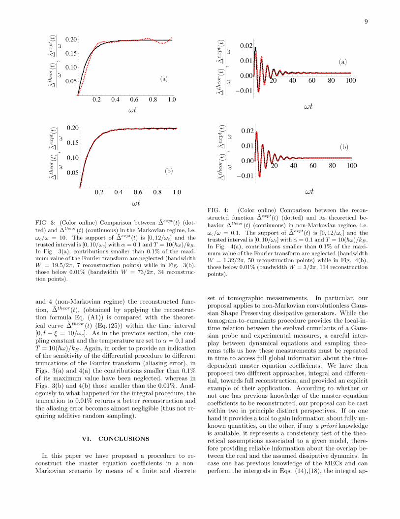
FIG. 3: (Color online) Comparison between ∆expt(t) (dot-

ted) and ∆theor(t) (continuous) in the Markovian regime, i.e.

ωc/ω = 10. The support of ∆expt(t) is [0, 12/ωc] and thetrusted interval is [0, 10/ωc] with α = 0.1 and T = 10(ω)/kB .In Fig. 3(a), contributions smaller than 0.1% of the maxi-mum value of the Fourier transform are neglected (bandwidthW = 19.5/2π, 7 reconstruction points) while in Fig. 3(b),those below 0.01% (bandwidth W = 73/2π, 34 reconstruc-tion points).

and 4 (non-Markovian regime) the reconstructed func-

tion, ∆theor(t), (obtained by applying the reconstruc-tion formula Eq. (A1)) is compared with the theoret-

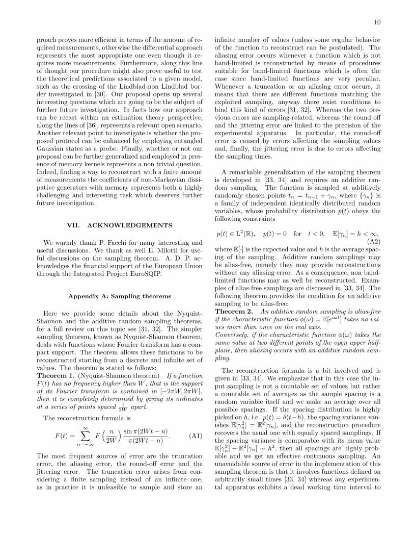
ical curve ∆theor(t) (Eq. (25)) within the time interval[0, t − ξ = 10/ωc]. As in the previous section, the cou-pling constant and the temperature are set to α = 0.1 andT = 10(ω)/kB . Again, in order to provide an indicationof the sensitivity of the differential procedure to differenttruncations of the Fourier transform (aliasing error), inFigs. 3(a) and 4(a) the contributions smaller than 0.1%of its maximum value have been neglected, whereas inFigs. 3(b) and 4(b) those smaller than the 0.01%. Anal-ogously to what happened for the integral procedure, thetruncation to 0.01% returns a better reconstruction andthe aliasing error becomes almost negligible (thus not re-quiring additive random sampling).

VI. CONCLUSIONS

In this paper we have proposed a procedure to re-construct the master equation coefficients in a non-Markovian scenario by means of a finite and discrete

(a)

∆th

eor (

t)ω

,∆ex

pt(t

)ω

ωt

20 40 60 80 1000.01

0.00

0.01

0.02

(b)

∆th

eor (

t)ω

,∆ex

pt(t

)ω

ωt

20 40 60 80 1000.01

0.00

0.01

0.02

FIG. 4: (Color online) Comparison between the recon-

structed function ∆expt(t) (dotted) and its theoretical be-

havior ∆theor(t) (continuous) in non-Markovian regime, i.e.

ωc/ω = 0.1. The support of ∆expt(t) is [0, 12/ωc] and thetrusted interval is [0, 10/ωc] with α = 0.1 and T = 10(ω)/kB .In Fig. 4(a), contributions smaller than 0.1% of the maxi-mum value of the Fourier transform are neglected (bandwidthW = 1.32/2π, 50 reconstruction points) while in Fig. 4(b),those below 0.01% (bandwidth W = 3/2π, 114 reconstructionpoints).

set of tomographic measurements. In particular, ourproposal applies to non-Markovian convolutionless Gaus-sian Shape Preserving dissipative generators. While thetomogram-to-cumulants procedure provides the local-in-time relation between the evolved cumulants of a Gaus-sian probe and experimental measures, a careful inter-play between dynamical equations and sampling theo-rems tells us how these measurements must be repeatedin time to access full global information about the time-dependent master equation coefficients. We have thenproposed two different approaches, integral and differen-tial, towards full reconstruction, and provided an explicitexample of their application. According to whether ornot one has previous knowledge of the master equationcoefficients to be reconstructed, our proposal can be castwithin two in principle distinct perspectives. If on onehand it provides a tool to gain information about fully un-known quantities, on the other, if any a priori knowledgeis available, it represents a consistency test of the theo-retical assumptions associated to a given model, there-fore providing reliable information about the overlap be-tween the real and the assumed dissipative dynamics. Incase one has previous knowledge of the MECs and canperform the intergrals in Eqs. (14),(18), the integral ap-

10

proach proves more efficient in terms of the amount of re-quired measurements, otherwise the differential approachrepresents the most appropriate one even though it re-quires more measurements. Furthermore, along this lineof thought our procedure might also prove useful to testthe theoretical predictions associated to a given model,such as the crossing of the Lindblad-non Lindblad bor-der investigated in [30]. Our proposal opens up severalinteresting questions which are going to be the subject offurther future investigation. In facts how our approachcan be recast within an estimation theory perspective,along the lines of [36], represents a relevant open scenario.Another relevant point to investigate is whether the pro-posed protocol can be enhanced by employing entangledGaussian states as a probe. Finally, whether or not ourproposal can be further generalized and employed in pres-ence of memory kernels represents a non trivial question.Indeed, finding a way to reconstruct with a finite amountof measurements the coefficients of non-Markovian dissi-pative generators with memory represents both a highlychallenging and interesting task which deserves furtherfuture investigation.

VII. ACKNOWLEDGEMENTS

We warmly thank P. Facchi for many interesting anduseful discussions. We thank as well E. Milotti for use-ful discussions on the sampling theorem. A. D. P. ac-knowledges the financial support of the European Unionthrough the Integrated Project EuroSQIP.

Appendix A: Sampling theorems

Here we provide some details about the Nyquist-Shannon and the additive random sampling theorems,for a full review on this topic see [31, 32]. The simplersampling theorem, known as Nyquist-Shannon theorem,deals with functions whose Fourier transform has a com-pact support. The theorem allows these functions to bereconstructed starting from a discrete and infinite set ofvalues. The theorem is stated as follows:Theorem 1. (Nyquist-Shannon theorem) If a functionF (t) has no frequency higher than W , that is the supportof its Fourier transform is contained in [−2πW, 2πW ],then it is completely determined by giving its ordinatesat a series of points spaced 1

2W apart.

The reconstruction formula is

F (t) =

∞∑n=−∞

F( n

2W

) sinπ(2Wt− n)

π(2Wt− n). (A1)

The most frequent sources of error are the truncationerror, the aliasing error, the round-off error and thejittering error. The truncation error arises from con-sidering a finite sampling instead of an infinite one,as in practice it is unfeasible to sample and store an

infinite number of values (unless some regular behaviorof the function to reconstruct can be postulated). Thealiasing error occurs whenever a function which is notband-limited is reconstructed by means of proceduressuitable for band-limited functions which is often thecase since band-limited functions are very peculiar.Whenever a truncation or an aliasing error occurs, itmeans that there are different functions matching theexploited sampling, anyway there exist conditions tobind this kind of errors [31, 32]. Whereas the two pre-vious errors are sampling-related, whereas the round-offand the jittering error are linked to the precision of theexperimental apparatus. In particular, the round-offerror is caused by errors affecting the sampling valuesand, finally, the jittering error is due to errors affectingthe sampling times.

A remarkable generalization of the sampling theoremis developed in [33, 34] and requires an additive ran-dom sampling. The function is sampled at additivelyrandomly chosen points tn = tn−1 + γn, where γn isa family of independent identically distributed randomvariables, whose probability distribution p(t) obeys thefollowing constraints

p(t) ∈ L2(R), p(t) = 0 for t < 0, E[γn] = h <∞,(A2)

where E[·] is the expected value and h is the average spac-ing of the sampling. Additive random samplings maybe alias-free, namely they may provide reconstructionswithout any aliasing error. As a consequence, non band-limited functions may as well be reconstructed. Exam-ples of alias-free samplings are discussed in [33, 34]. Thefollowing theorem provides the condition for an additivesampling to be alias-free:Theorem 2. An additive random sampling is alias-freeif the characteristic function φ(ω) = E[eiωt] takes no val-ues more than once on the real axis.Conversely, if the characteristic function φ(ω) takes thesame value at two different points of the open upper half-plane, then aliasing occurs with an additive random sam-pling.

The reconstruction formula is a bit involved and isgiven in [33, 34]. We emphasize that in this case the in-put sampling is not a countable set of values but rathera countable set of averages as the sample spacing is arandom variable itself and we make an average over allpossible spacings. If the spacing distribution is highlypicked on h, i.e. p(t) = δ(t−h), the spacing variance van-ishes E[γ2

n] = E2[γn], and the reconstruction procedurerecovers the usual one with equally spaced samplings. Ifthe spacing variance is comparable with its mean valueE[γ2

n] − E2[γn] ∼ h2, then all spacings are highly prob-able and we get an effective continuous sampling. Anunavoidable source of error in the implementation of thissampling theorem is that it involves functions defined onarbitrarily small times [33, 34] whereas any experimen-tal apparatus exhibits a dead working time interval to

11

record and process data. Finally we note that we wantto reconstruct functions defined only for t > 0 hence wedo not encounter any lower truncation error. The uppertruncation error can be also avoided by reconstructingslightly different functions: F (t)(1 − θ(t − t)) instead ofF (t). The differences arise from the integral transformsinvolved in the reconstruction formula, but if we are in-terested in reconstructing functions in the experimentally

accessible timescales, values greater than the threshold tof experimentally reachable times can be neglected. Thesame trick can be exploited to avoid errors due to a fi-nite input size for an additive random sampling. Indeedif the sampling probability is well localized, each pn(t)is localized as well. The probabilities pn(t) localized attimes larger than the threshold t do not contribute andthe corresponding fn vanish.

[1] F. Petruccione and H. Breuer, The Theory of Open Quan-tum Systems (Oxford University, 2002).

[2] C. W. Gardiner and P. Zoller, Quantum Noise (Springer,Berlin, 3rd ed., 2004).

[3] B. Bellomo, A. De Pasquale, G. Gualdi, and U. Mar-zolino, Phys. Rev. A 80, 052108 (2009).

[4] F. Benatti and R. Floreanini, Int. J. Mod. Phys. B 19,3063 (2005).

[5] H. Spohn, Rev. Mod. Phys. 53, 569 (1980).[6] J. J. Hope, G. M. Moy, M. J. Collett, and C. M. Savage,

Phys. Rev. A 61, 023603 (2000).[7] A. Pomyalov and D. J. Tannor, J. Chem. Phys. 123,

204111 (2005).[8] B. L. Hu, J. P. Paz, and Y. Zhang, Phys. Rev. D 45,

2843 (1992).[9] B. L. Hu and A. Matacz, Phys. Rev. D 49, 6612 (1994).

[10] F. Haake, R. Reibold, Phys. Rev. A 32, 2462 (1985).[11] J. J. Halliwell and T. Yu, Phys. Rev. D 53, 2012 (1996).[12] L. Diosi and W. T. Strunz, Phys. Lett. A 235, 569 (1997).[13] W. T. Strunz and T. Yu, Phys. Rev. A 69, 052115 (2004).[14] T. Yu, Phys. Rev. A 69, 062107 (2004).[15] A. Bassi and L. Ferialdi, Phys. Rev. Lett. 103, 050403

(2009), and in preparation.[16] R. Karrlein and H. Grabert, Phys. Rev. E 55, 153 (1997).[17] L. D. Romero and J. P. Paz, Phys. Rev. A 55, 4070

(1997).[18] B. L. Hu, J. P. Paz, and Y. Zhang, Phys. Rev. D 47,

1576 (1993).[19] B. Bellomo, A. De Pasquale, G. Gualdi, and U. Mar-

zolino, J. Phys. A 43, 395303 (2010).[20] V. I. M. O. V. Manko and G. Marmo, Phys. Scr. 62, 446

(2000).[21] G. Badurek et al., Phys. Rev. A 73, 032110 (2006).[22] C. Kurtsiefer, T. Pfau, and J. Mlynek, Nature 386, 150

(1997).[23] P. Facchi and M. Ligabo, AIP Conf. Proc. 1260, 3 (2010).[24] V. D’Auria et al., Phys. Rev. Lett. 102, 020502 (2009).[25] H. P. Robertson, Phys. Rev. 46, 794 (1934).[26] J. Rehacek et al., Phys. Rev. A 79, 032111 (2009).[27] L. Mandel and E. Wolf, Optical Coherence and Quantum

Optics (Cambridge University Press, 1995).[28] A. Sandulescu and H. Scutaru, Annals of Physics 173,

277 (1987).[29] D. Chrus’cin’ski and A. Kossakowski, Phys. Rev. Lett.

104, 070406 (2010).[30] S. Maniscalco, J. Piilo, F. Intravaia, F. Petruccione, and

A. Messina, Phys. Rev. A 70, 032113 (2004).[31] A. J. Jerri, Proceding of the IEEE 65, 1565 (1977).[32] M. Unser, Proceding of the IEEE 88, 569 (2000).[33] H. S. Shapiro and R. A. Silverman, J. Soc. Indust. Appl.

Math. 8, 225 (1960).[34] F. J. Beutler, IEEE Trans. Info. Theory IT-16, 147

(1970).[35] J. P. Paz and A. J. Roncaglia, Phys. Rev. A 79, 032102

(2009).[36] A. Monras and M. G. A. Paris, Phys. Rev. Lett. 98,

160401 (2007).