Reconstruction and update robustness of the mammalian cell cycle network
7
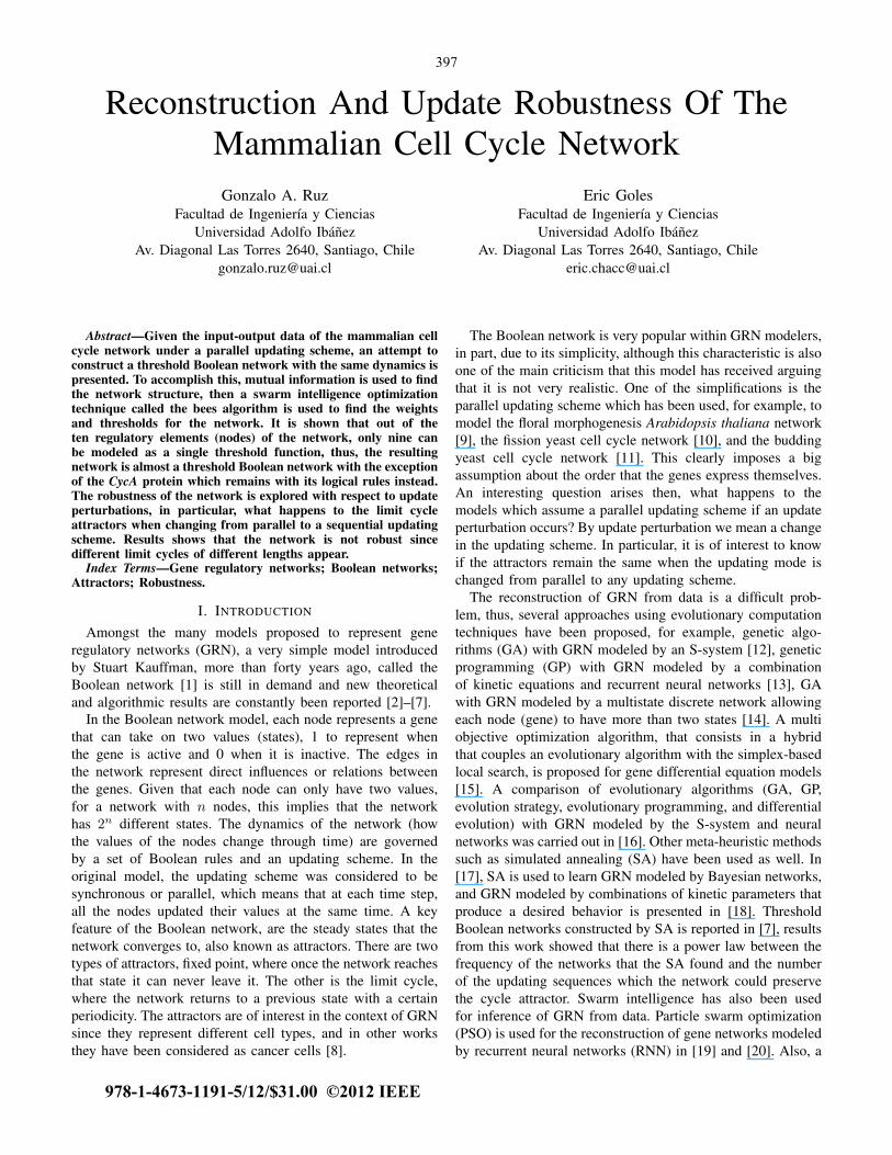
Reconstruction And Update Robustness Of The Mammalian Cell Cycle Network Gonzalo A. Ruz Facultad de Ingenier´ ıa y Ciencias Universidad Adolfo Ib´ a˜ nez Av. Diagonal Las Torres 2640, Santiago, Chile [email protected] Eric Goles Facultad de Ingenier´ ıa y Ciencias Universidad Adolfo Ib´ a˜ nez Av. Diagonal Las Torres 2640, Santiago, Chile [email protected] Abstract—Given the input-output data of the mammalian cell cycle network under a parallel updating scheme, an attempt to construct a threshold Boolean network with the same dynamics is presented. To accomplish this, mutual information is used to find the network structure, then a swarm intelligence optimization technique called the bees algorithm is used to find the weights and thresholds for the network. It is shown that out of the ten regulatory elements (nodes) of the network, only nine can be modeled as a single threshold function, thus, the resulting network is almost a threshold Boolean network with the exception of the CycA protein which remains with its logical rules instead. The robustness of the network is explored with respect to update perturbations, in particular, what happens to the limit cycle attractors when changing from parallel to a sequential updating scheme. Results shows that the network is not robust since different limit cycles of different lengths appear. Index Terms—Gene regulatory networks; Boolean networks; Attractors; Robustness. I. I NTRODUCTION Amongst the many models proposed to represent gene regulatory networks (GRN), a very simple model introduced by Stuart Kauffman, more than forty years ago, called the Boolean network [1] is still in demand and new theoretical and algorithmic results are constantly been reported [2]–[7]. In the Boolean network model, each node represents a gene that can take on two values (states), 1 to represent when the gene is active and 0 when it is inactive. The edges in the network represent direct influences or relations between the genes. Given that each node can only have two values, for a network with nodes, this implies that the network has 2 different states. The dynamics of the network (how the values of the nodes change through time) are governed by a set of Boolean rules and an updating scheme. In the original model, the updating scheme was considered to be synchronous or parallel, which means that at each time step, all the nodes updated their values at the same time. A key feature of the Boolean network, are the steady states that the network converges to, also known as attractors. There are two types of attractors, fixed point, where once the network reaches that state it can never leave it. The other is the limit cycle, where the network returns to a previous state with a certain periodicity. The attractors are of interest in the context of GRN since they represent different cell types, and in other works they have been considered as cancer cells [8]. The Boolean network is very popular within GRN modelers, in part, due to its simplicity, although this characteristic is also one of the main criticism that this model has received arguing that it is not very realistic. One of the simplifications is the parallel updating scheme which has been used, for example, to model the floral morphogenesis Arabidopsis thaliana network [9], the fission yeast cell cycle network [10], and the budding yeast cell cycle network [11]. This clearly imposes a big assumption about the order that the genes express themselves. An interesting question arises then, what happens to the models which assume a parallel updating scheme if an update perturbation occurs? By update perturbation we mean a change in the updating scheme. In particular, it is of interest to know if the attractors remain the same when the updating mode is changed from parallel to any updating scheme. The reconstruction of GRN from data is a difficult prob- lem, thus, several approaches using evolutionary computation techniques have been proposed, for example, genetic algo- rithms (GA) with GRN modeled by an S-system [12], genetic programming (GP) with GRN modeled by a combination of kinetic equations and recurrent neural networks [13], GA with GRN modeled by a multistate discrete network allowing each node (gene) to have more than two states [14]. A multi objective optimization algorithm, that consists in a hybrid that couples an evolutionary algorithm with the simplex-based local search, is proposed for gene differential equation models [15]. A comparison of evolutionary algorithms (GA, GP, evolution strategy, evolutionary programming, and differential evolution) with GRN modeled by the S-system and neural networks was carried out in [16]. Other meta-heuristic methods such as simulated annealing (SA) have been used as well. In [17], SA is used to learn GRN modeled by Bayesian networks, and GRN modeled by combinations of kinetic parameters that produce a desired behavior is presented in [18]. Threshold Boolean networks constructed by SA is reported in [7], results from this work showed that there is a power law between the frequency of the networks that the SA found and the number of the updating sequences which the network could preserve the cycle attractor. Swarm intelligence has also been used for inference of GRN from data. Particle swarm optimization (PSO) is used for the reconstruction of gene networks modeled by recurrent neural networks (RNN) in [19] and [20]. Also, a 978-1-4673-1191-5/12/$31.00 ©2012 IEEE 397
-
Upload
independent -
Category
Documents
-
view
1 -
download
0
Transcript of Reconstruction and update robustness of the mammalian cell cycle network
Reconstruction And Update Robustness Of TheMammalian Cell Cycle Network
Gonzalo A. RuzFacultad de Ingenierıa y Ciencias
Universidad Adolfo IbanezAv. Diagonal Las Torres 2640, Santiago, Chile
Eric GolesFacultad de Ingenierıa y Ciencias
Universidad Adolfo IbanezAv. Diagonal Las Torres 2640, Santiago, Chile
Abstract—Given the input-output data of the mammalian cellcycle network under a parallel updating scheme, an attempt toconstruct a threshold Boolean network with the same dynamics ispresented. To accomplish this, mutual information is used to findthe network structure, then a swarm intelligence optimizationtechnique called the bees algorithm is used to find the weightsand thresholds for the network. It is shown that out of theten regulatory elements (nodes) of the network, only nine canbe modeled as a single threshold function, thus, the resultingnetwork is almost a threshold Boolean network with the exceptionof the CycA protein which remains with its logical rules instead.The robustness of the network is explored with respect to updateperturbations, in particular, what happens to the limit cycleattractors when changing from parallel to a sequential updatingscheme. Results shows that the network is not robust sincedifferent limit cycles of different lengths appear.
Index Terms—Gene regulatory networks; Boolean networks;Attractors; Robustness.
I. INTRODUCTION
Amongst the many models proposed to represent generegulatory networks (GRN), a very simple model introducedby Stuart Kauffman, more than forty years ago, called theBoolean network [1] is still in demand and new theoreticaland algorithmic results are constantly been reported [2]–[7].
In the Boolean network model, each node represents a genethat can take on two values (states), 1 to represent whenthe gene is active and 0 when it is inactive. The edges inthe network represent direct influences or relations betweenthe genes. Given that each node can only have two values,for a network with 𝑛 nodes, this implies that the networkhas 2𝑛 different states. The dynamics of the network (howthe values of the nodes change through time) are governedby a set of Boolean rules and an updating scheme. In theoriginal model, the updating scheme was considered to besynchronous or parallel, which means that at each time step,all the nodes updated their values at the same time. A keyfeature of the Boolean network, are the steady states that thenetwork converges to, also known as attractors. There are twotypes of attractors, fixed point, where once the network reachesthat state it can never leave it. The other is the limit cycle,where the network returns to a previous state with a certainperiodicity. The attractors are of interest in the context of GRNsince they represent different cell types, and in other worksthey have been considered as cancer cells [8].
The Boolean network is very popular within GRN modelers,in part, due to its simplicity, although this characteristic is alsoone of the main criticism that this model has received arguingthat it is not very realistic. One of the simplifications is theparallel updating scheme which has been used, for example, tomodel the floral morphogenesis Arabidopsis thaliana network[9], the fission yeast cell cycle network [10], and the buddingyeast cell cycle network [11]. This clearly imposes a bigassumption about the order that the genes express themselves.An interesting question arises then, what happens to themodels which assume a parallel updating scheme if an updateperturbation occurs? By update perturbation we mean a changein the updating scheme. In particular, it is of interest to knowif the attractors remain the same when the updating mode ischanged from parallel to any updating scheme.
The reconstruction of GRN from data is a difficult prob-lem, thus, several approaches using evolutionary computationtechniques have been proposed, for example, genetic algo-rithms (GA) with GRN modeled by an S-system [12], geneticprogramming (GP) with GRN modeled by a combinationof kinetic equations and recurrent neural networks [13], GAwith GRN modeled by a multistate discrete network allowingeach node (gene) to have more than two states [14]. A multiobjective optimization algorithm, that consists in a hybridthat couples an evolutionary algorithm with the simplex-basedlocal search, is proposed for gene differential equation models[15]. A comparison of evolutionary algorithms (GA, GP,evolution strategy, evolutionary programming, and differentialevolution) with GRN modeled by the S-system and neuralnetworks was carried out in [16]. Other meta-heuristic methodssuch as simulated annealing (SA) have been used as well. In[17], SA is used to learn GRN modeled by Bayesian networks,and GRN modeled by combinations of kinetic parameters thatproduce a desired behavior is presented in [18]. ThresholdBoolean networks constructed by SA is reported in [7], resultsfrom this work showed that there is a power law between thefrequency of the networks that the SA found and the numberof the updating sequences which the network could preservethe cycle attractor. Swarm intelligence has also been usedfor inference of GRN from data. Particle swarm optimization(PSO) is used for the reconstruction of gene networks modeledby recurrent neural networks (RNN) in [19] and [20]. Also, a
978-1-4673-1191-5/12/$31.00 ©2012 IEEE
397
hybrid of differential evolution and PSO (DEPSO) for trainingRNN is investigated in [21]. Less work has been reported onthe use of ants and bees. In [22], an ant system is implementedto generate candidate network structures and in [23] the beesalgorithm is used to generate Boolean network examples tosupport a theorem presented in that work. Recently, a com-parison of the bees algorithm with SA for learning thresholdBoolean networks has been carried out in [24]. The resultsshow that the bees algorithm outperforms the SA, obtainingmore feasible solutions using less edges than the SA.
In this paper, we analyze the mammalian cell cycle logicalnetwork model presented in [25]. First, we reconstruct athreshold Boolean network model that consists in a weightmatrix and a threshold vector which is much easier to handlethan a set of logical rules per node, similar to [9]–[11], usingthe input-output data generated by the logical model [25] andan information theoretic approach combined with a swarmintelligence technique called the bees algorithm. Then, toanalyze the effects of update perturbation, we consider changesfrom parallel to sequential updates, and study the limit cycleattractors.
The rest of the paper is organized as follows. Section IIgives the background of the techniques used to conduct thisstudy. The reconstruction of the mammalian cell cycle networkis presented in section III, whereas the update perturbationstudy is carried out in section IV. The general conclusionsand future research are presented in section V.
II. BACKGROUND
A. Boolean networks
Let x be a finite set of 𝑛 variables, x = {𝑥1, . . . , 𝑥𝑛}, with𝑥𝑖 ∈ {0, 1} for 𝑖 = 1, . . . , 𝑛. A Boolean network is a pair(𝐺,𝐹 ), where 𝐺 = (V,E) is a finite directed graph; V beingthe set of 𝑛 nodes and E the set of edges. 𝐹 is a Booleanfunction, 𝐹 : {0, 1}𝑛 → {0, 1}𝑛 composed of 𝑛 local func-tions 𝑓𝑖 : {0, 1}𝑛 → {0, 1}. Furthermore, each local function𝑓𝑖 depends only on variables belonging to the neighborhood𝑉𝑖 = {𝑗 ∈ V∣(𝑗, 𝑖) ∈ E}. The indegree, 𝐾, of vertex 𝑖 is∣𝑉𝑖∣. The updating schemes are repeated periodically, and sincethe hypercube is a finite set, the dynamics of the networkconverges to attractors which are fixed points or limit cycles,defined by
∙ Fixed point: 𝑥𝑡+1𝑖 = 𝑥𝑡𝑖 for 𝑖 = {1, . . . , 𝑛}.
∙ Limit cycle: 𝑥𝑡+𝑝𝑖 = 𝑥𝑡𝑖 for 𝑖 = {1, . . . , 𝑛}.
where 𝑝 > 1 is a positive integer called the limit cycle length.The set of states that can lead the network to a specific attractoris called the basin of attraction. There are many ways ofupdating the values of a Boolean network, some examplesare [26]:
∙ Parallel or synchronous mode: where every node is up-dated at the same time.
∙ Sequential updating mode: where in every time step,every node is updated in a defined sequence.
∙ Block-sequential: the set of nodes, for a given sequence,is partitioned into blocks. The nodes in a same block
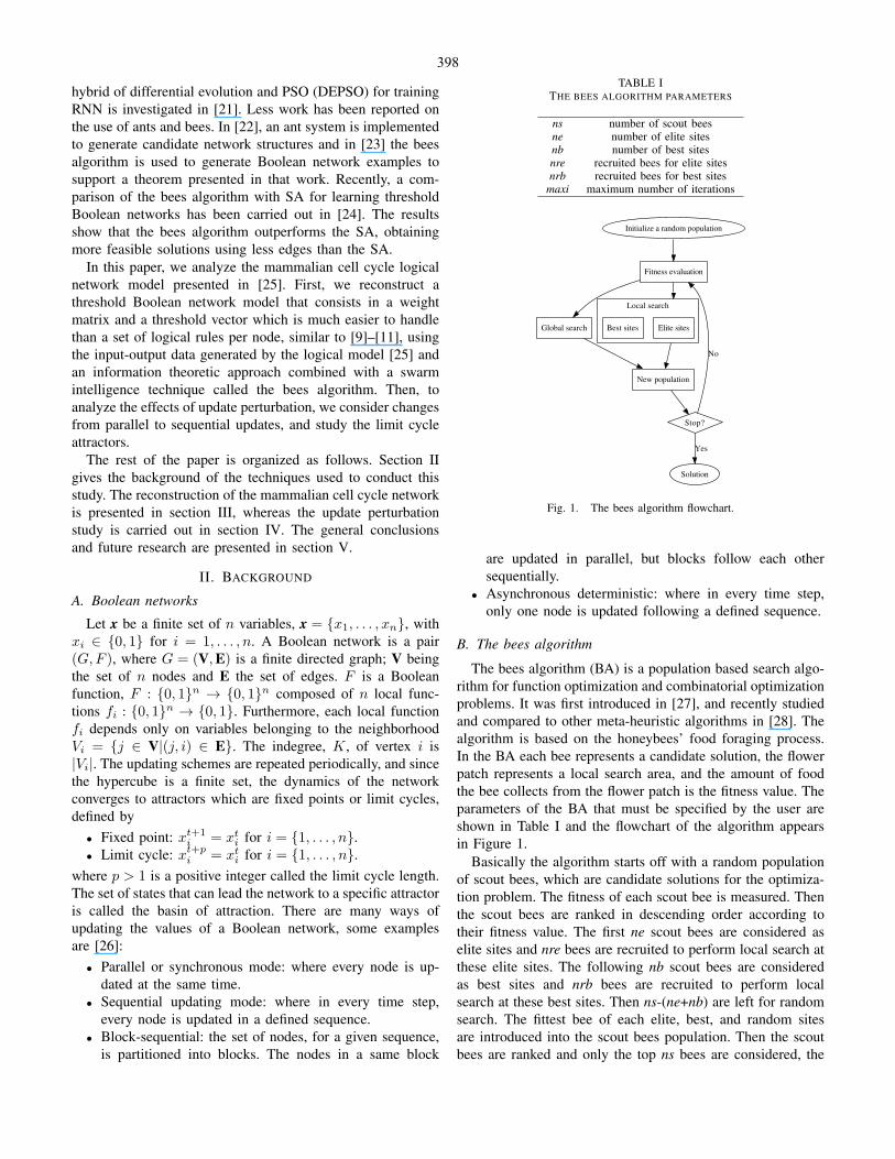
TABLE ITHE BEES ALGORITHM PARAMETERS
ns number of scout beesne number of elite sitesnb number of best sitesnre recruited bees for elite sitesnrb recruited bees for best sites
maxi maximum number of iterations
Local search
Initialize a random population
Fitness evaluation
Solution
Global search Elite sites
New population
Stop?
Best sites
Yes
No
Fig. 1. The bees algorithm flowchart.
are updated in parallel, but blocks follow each othersequentially.
∙ Asynchronous deterministic: where in every time step,only one node is updated following a defined sequence.
B. The bees algorithm
The bees algorithm (BA) is a population based search algo-rithm for function optimization and combinatorial optimizationproblems. It was first introduced in [27], and recently studiedand compared to other meta-heuristic algorithms in [28]. Thealgorithm is based on the honeybees’ food foraging process.In the BA each bee represents a candidate solution, the flowerpatch represents a local search area, and the amount of foodthe bee collects from the flower patch is the fitness value. Theparameters of the BA that must be specified by the user areshown in Table I and the flowchart of the algorithm appearsin Figure 1.
Basically the algorithm starts off with a random populationof scout bees, which are candidate solutions for the optimiza-tion problem. The fitness of each scout bee is measured. Thenthe scout bees are ranked in descending order according totheir fitness value. The first ne scout bees are considered aselite sites and nre bees are recruited to perform local search atthese elite sites. The following nb scout bees are consideredas best sites and nrb bees are recruited to perform localsearch at these best sites. Then ns-(ne+nb) are left for randomsearch. The fittest bee of each elite, best, and random sitesare introduced into the scout bees population. Then the scoutbees are ranked and only the top ns bees are considered, the
398
rest are discarded, this generates a new population. The fittestscout bee from the newly formed population is checked to seeif it satisfies the stopping criteria. If the stopping condition isnot met, then the new population is used to repeat the processof local and global search until the stopping condition is metor maxi has been reached.
III. RECONSTRUCTION OF THE MAMMALIAN CELL CYCLE
NETWORK
A differential model for the control of the mammalian cellcycle network was introduced by Novak and Tayson [29].More recently, a logical version for this model was presentedby Faure et al. [25]. In this section, a threshold Booleannetwork model will be constructed from the data generatedfrom the model in [25]. The mammalian cell cycle networkconsists of 10 genes (that code 9 proteins and 1 enzyme),therefore, there are 210 = 1024 possible states. Each stateis evaluated in the logical model, synchronously, to generatethe output of the network for the following time step. Withthis input-output data, the first step is to discover the networktopology.
A. Network structure discovery
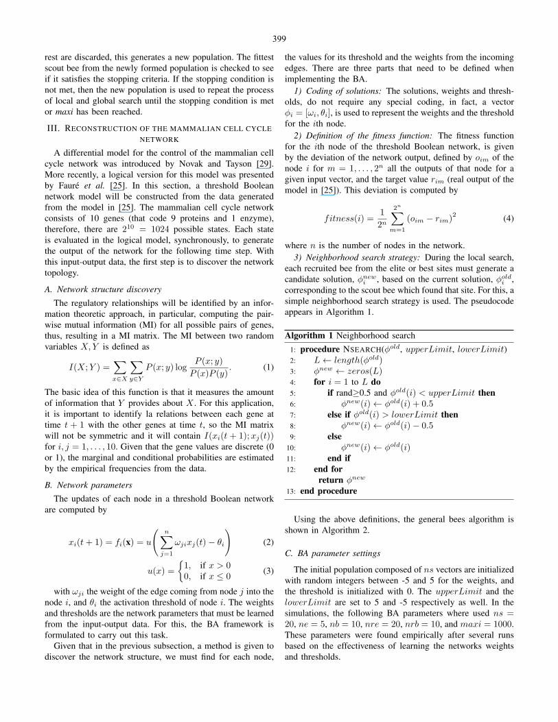
The regulatory relationships will be identified by an infor-mation theoretic approach, in particular, computing the pair-wise mutual information (MI) for all possible pairs of genes,thus, resulting in a MI matrix. The MI between two randomvariables 𝑋,𝑌 is defined as
𝐼(𝑋;𝑌 ) =∑𝑥∈𝑋
∑𝑦∈𝑌
𝑃 (𝑥; 𝑦) log𝑃 (𝑥; 𝑦)
𝑃 (𝑥)𝑃 (𝑦). (1)
The basic idea of this function is that it measures the amountof information that 𝑌 provides about 𝑋 . For this application,it is important to identify la relations between each gene attime 𝑡 + 1 with the other genes at time 𝑡, so the MI matrixwill not be symmetric and it will contain 𝐼(𝑥𝑖(𝑡 + 1);𝑥𝑗(𝑡))for 𝑖, 𝑗 = 1, . . . , 10. Given that the gene values are discrete (0or 1), the marginal and conditional probabilities are estimatedby the empirical frequencies from the data.
B. Network parameters
The updates of each node in a threshold Boolean networkare computed by
𝑥𝑖(𝑡+ 1) = 𝑓𝑖(x) = 𝑢
(𝑛∑
𝑗=1
𝜔𝑗𝑖𝑥𝑗(𝑡)− 𝜃𝑖
)(2)
𝑢(𝑥) =
{1, if 𝑥 > 00, if 𝑥 ≤ 0
(3)
with 𝜔𝑗𝑖 the weight of the edge coming from node 𝑗 into thenode 𝑖, and 𝜃𝑖 the activation threshold of node 𝑖. The weightsand thresholds are the network parameters that must be learnedfrom the input-output data. For this, the BA framework isformulated to carry out this task.
Given that in the previous subsection, a method is given todiscover the network structure, we must find for each node,
the values for its threshold and the weights from the incomingedges. There are three parts that need to be defined whenimplementing the BA.
1) Coding of solutions: The solutions, weights and thresh-olds, do not require any special coding, in fact, a vector𝜙𝑖 = [𝜔𝑖, 𝜃𝑖], is used to represent the weights and the thresholdfor the 𝑖th node.
2) Definition of the fitness function: The fitness functionfor the 𝑖th node of the threshold Boolean network, is givenby the deviation of the network output, defined by 𝑜𝑖𝑚 of thenode 𝑖 for 𝑚 = 1, . . . , 2𝑛 all the outputs of that node for agiven input vector, and the target value 𝑟𝑖𝑚 (real output of themodel in [25]). This deviation is computed by
𝑓𝑖𝑡𝑛𝑒𝑠𝑠(𝑖) =1
2𝑛
2𝑛∑𝑚=1
(𝑜𝑖𝑚 − 𝑟𝑖𝑚)2 (4)
where 𝑛 is the number of nodes in the network.3) Neighborhood search strategy: During the local search,
each recruited bee from the elite or best sites must generate acandidate solution, 𝜙𝑛𝑒𝑤𝑖 , based on the current solution, 𝜙𝑜𝑙𝑑𝑖 ,corresponding to the scout bee which found that site. For this, asimple neighborhood search strategy is used. The pseudocodeappears in Algorithm 1.
Algorithm 1 Neighborhood search
1: procedure NSEARCH(𝜙𝑜𝑙𝑑, 𝑢𝑝𝑝𝑒𝑟𝐿𝑖𝑚𝑖𝑡, 𝑙𝑜𝑤𝑒𝑟𝐿𝑖𝑚𝑖𝑡)2: 𝐿← 𝑙𝑒𝑛𝑔𝑡ℎ(𝜙𝑜𝑙𝑑)3: 𝜙𝑛𝑒𝑤 ← 𝑧𝑒𝑟𝑜𝑠(𝐿)4: for 𝑖 = 1 to 𝐿 do5: if rand≥0.5 and 𝜙𝑜𝑙𝑑(𝑖) < 𝑢𝑝𝑝𝑒𝑟𝐿𝑖𝑚𝑖𝑡 then6: 𝜙𝑛𝑒𝑤(𝑖)← 𝜙𝑜𝑙𝑑(𝑖) + 0.57: else if 𝜙𝑜𝑙𝑑(𝑖) > 𝑙𝑜𝑤𝑒𝑟𝐿𝑖𝑚𝑖𝑡 then8: 𝜙𝑛𝑒𝑤(𝑖)← 𝜙𝑜𝑙𝑑(𝑖)− 0.59: else
10: 𝜙𝑛𝑒𝑤(𝑖)← 𝜙𝑜𝑙𝑑(𝑖)11: end if12: end for
return 𝜙𝑛𝑒𝑤
13: end procedure
Using the above definitions, the general bees algorithm isshown in Algorithm 2.
C. BA parameter settings
The initial population composed of 𝑛𝑠 vectors are initializedwith random integers between -5 and 5 for the weights, andthe threshold is initialized with 0. The 𝑢𝑝𝑝𝑒𝑟𝐿𝑖𝑚𝑖𝑡 and the𝑙𝑜𝑤𝑒𝑟𝐿𝑖𝑚𝑖𝑡 are set to 5 and -5 respectively as well. In thesimulations, the following BA parameters where used 𝑛𝑠 =20, 𝑛𝑒 = 5, 𝑛𝑏 = 10, 𝑛𝑟𝑒 = 20, 𝑛𝑟𝑏 = 10, and 𝑚𝑎𝑥𝑖 = 1000.These parameters were found empirically after several runsbased on the effectiveness of learning the networks weightsand thresholds.
399
𝐼 =
⎛⎜⎜⎜⎜⎜⎜⎜⎜⎜⎜⎜⎜⎜⎜⎜⎝
𝐶𝑦𝑐𝐷(𝑡) 𝑅𝑏(𝑡) 𝐸2𝐹 (𝑡) 𝐶𝑦𝑐𝐸(𝑡) 𝐶𝑦𝑐𝐴(𝑡) 𝑝27(𝑡) 𝐶𝑑𝑐20(𝑡) 𝐶𝑑ℎ1(𝑡) 𝑈𝑏𝑐𝐻10(𝑡) 𝐶𝑦𝑐𝐵(𝑡)𝐶𝑦𝑐𝐷(𝑡 + 1) 0.6931 0 0 0 0 0 0 0 0 0𝑅𝑏(𝑡 + 1) 0.1229 0 0 0.0037 0.0037 0.0353 0 0 0 0.1229
𝐸2𝐹 (𝑡 + 1) 0 0.1518 0 0 0.0130 0.0130 0 0 0 0.1518𝐶𝑦𝑐𝐸(𝑡 + 1) 0 0.2158 0.2158 0 0 0 0 0 0 0𝐶𝑦𝑐𝐴(𝑡 + 1) 0 0.1090 0.0092 0 0.0092 0 0.1090 0.0092 0.0092 0𝑝27(𝑡 + 1) 0.0956 0 0 0.0186 0.0186 0.0186 0 0 0 0.0956
𝐶𝑑𝑐20(𝑡 + 1) 0 0 0 0 0 0 0 0 0 0.6931𝐶𝑑ℎ1(𝑡 + 1) 0 0 0 0 0.0091 0.0091 0.2903 0 0 0.0861
𝑈𝑏𝑐𝐻10(𝑡 + 1) 0 0 0 0 0.0024 0 0.0024 0.2515 0.1307 0.0024𝐶𝑦𝑐𝐵(𝑡 + 1) 0 0 0 0 0 0 0.2158 0.2158 0 0
⎞⎟⎟⎟⎟⎟⎟⎟⎟⎟⎟⎟⎟⎟⎟⎟⎠
Fig. 2. Mutual Information matrix
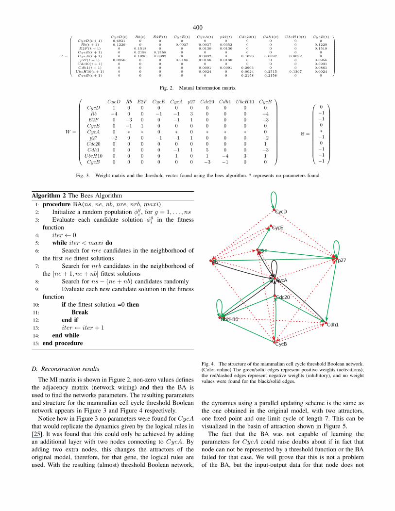
𝑊 =
⎛⎜⎜⎜⎜⎜⎜⎜⎜⎜⎜⎜⎜⎜⎜⎜⎜⎝
𝐶𝑦𝑐𝐷 𝑅𝑏 𝐸2𝐹 𝐶𝑦𝑐𝐸 𝐶𝑦𝑐𝐴 𝑝27 𝐶𝑑𝑐20 𝐶𝑑ℎ1 𝑈𝑏𝑐𝐻10 𝐶𝑦𝑐𝐵𝐶𝑦𝑐𝐷 1 0 0 0 0 0 0 0 0 0𝑅𝑏 −4 0 0 −1 −1 3 0 0 0 −4𝐸2𝐹 0 −3 0 0 −1 1 0 0 0 −3𝐶𝑦𝑐𝐸 0 −1 1 0 0 0 0 0 0 0𝐶𝑦𝑐𝐴 0 ∗ ∗ 0 ∗ 0 ∗ ∗ ∗ 0𝑝27 −2 0 0 −1 −1 1 0 0 0 −2𝐶𝑑𝑐20 0 0 0 0 0 0 0 0 0 1𝐶𝑑ℎ1 0 0 0 0 −1 1 5 0 0 −3𝑈𝑏𝑐𝐻10 0 0 0 0 1 0 1 −4 3 1𝐶𝑦𝑐𝐵 0 0 0 0 0 0 −3 −1 0 0
⎞⎟⎟⎟⎟⎟⎟⎟⎟⎟⎟⎟⎟⎟⎟⎟⎟⎠Θ =
⎛⎜⎜⎜⎜⎜⎜⎜⎜⎜⎜⎜⎜⎜⎜⎝
0−1−10∗−10−1−1−1
⎞⎟⎟⎟⎟⎟⎟⎟⎟⎟⎟⎟⎟⎟⎟⎠Fig. 3. Weight matrix and the threshold vector found using the bees algorithm. * represents no parameters found
Algorithm 2 The Bees Algorithm1: procedure BA(𝑛𝑠, 𝑛𝑒, 𝑛𝑏, 𝑛𝑟𝑒, 𝑛𝑟𝑏, 𝑚𝑎𝑥𝑖)2: Initialize a random population 𝜙𝑔𝑖 , for 𝑔 = 1, . . . , 𝑛𝑠3: Evaluate each candidate solution 𝜙𝑔𝑖 in the fitness
function4: 𝑖𝑡𝑒𝑟 ← 05: while 𝑖𝑡𝑒𝑟 < 𝑚𝑎𝑥𝑖 do6: Search for 𝑛𝑟𝑒 candidates in the neighborhood of
the first 𝑛𝑒 fittest solutions7: Search for 𝑛𝑟𝑏 candidates in the neighborhood of
the [𝑛𝑒+ 1, 𝑛𝑒+ 𝑛𝑏] fittest solutions8: Search for 𝑛𝑠− (𝑛𝑒+ 𝑛𝑏) candidates randomly9: Evaluate each new candidate solution in the fitness
function10: if the fittest solution =0 then11: Break12: end if13: 𝑖𝑡𝑒𝑟 ← 𝑖𝑡𝑒𝑟 + 114: end while15: end procedure
D. Reconstruction results
The MI matrix is shown in Figure 2, non-zero values definesthe adjacency matrix (network wiring) and then the BA isused to find the networks parameters. The resulting parametersand structure for the mammalian cell cycle threshold Booleannetwork appears in Figure 3 and Figure 4 respectively.
Notice how in Figure 3 no parameters were found for 𝐶𝑦𝑐𝐴that would replicate the dynamics given by the logical rules in[25]. It was found that this could only be achieved by addingan additional layer with two nodes connecting to 𝐶𝑦𝑐𝐴. Byadding two extra nodes, this changes the attractors of theoriginal model, therefore, for that gene, the logical rules areused. With the resulting (almost) threshold Boolean network,
CycD
Rb
E2F
CycE
CycA
p27
Cdc20
Cdh1UbcH10
CycBPajek
Fig. 4. The structure of the mammalian cell cycle threshold Boolean network.(Color online) The green/solid edges represent positive weights (activations),the red/dashed edges represent negative weights (inhibitory), and no weightvalues were found for the black/solid edges.
the dynamics using a parallel updating scheme is the same asthe one obtained in the original model, with two attractors,one fixed point and one limit cycle of length 7. This can bevisualized in the basin of attraction shown in Figure 5.
The fact that the BA was not capable of learning theparameters for 𝐶𝑦𝑐𝐴 could raise doubts about if in fact thatnode can not be represented by a threshold function or the BAfailed for that case. We will prove that this is not a problemof the BA, but the input-output data for that node does not
400
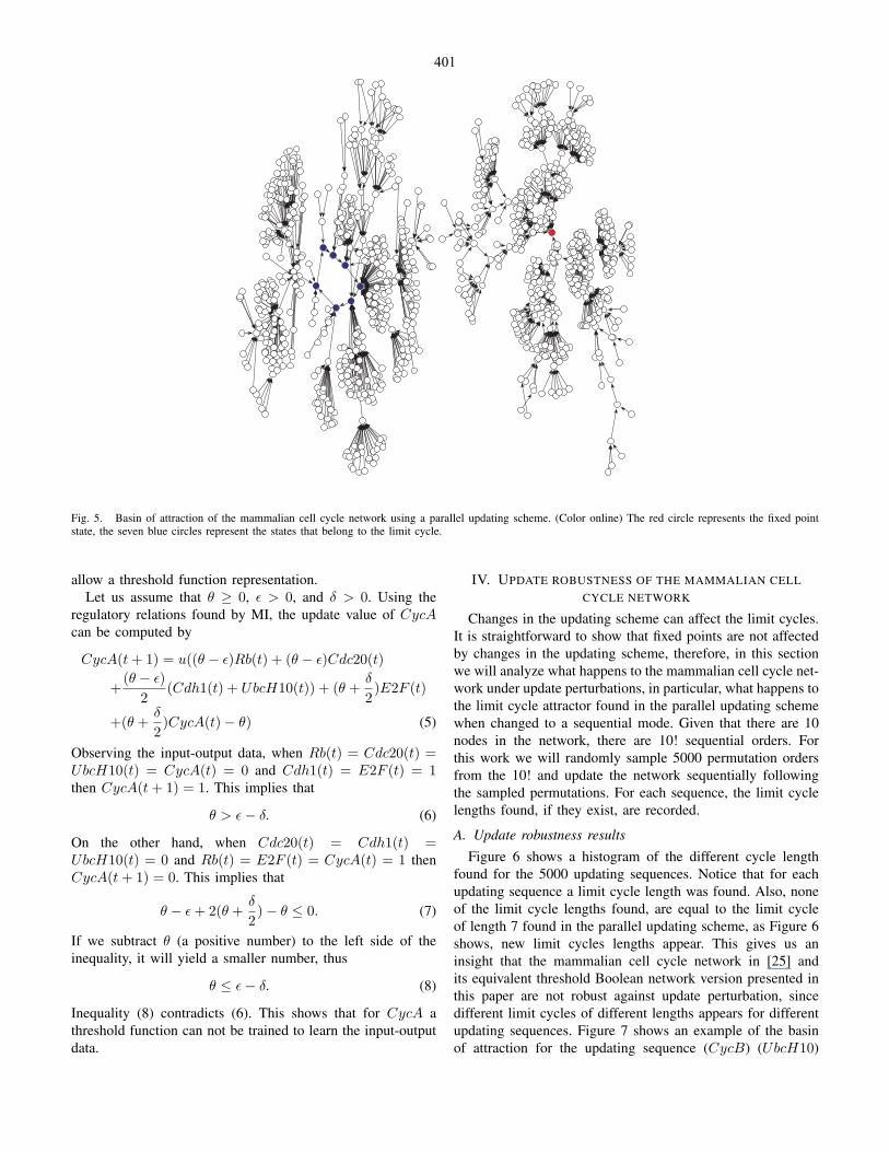
Pajek
Fig. 5. Basin of attraction of the mammalian cell cycle network using a parallel updating scheme. (Color online) The red circle represents the fixed pointstate, the seven blue circles represent the states that belong to the limit cycle.
allow a threshold function representation.Let us assume that 𝜃 ≥ 0, 𝜖 > 0, and 𝛿 > 0. Using the
regulatory relations found by MI, the update value of 𝐶𝑦𝑐𝐴can be computed by
𝐶𝑦𝑐𝐴(𝑡+ 1) = 𝑢((𝜃 − 𝜖)𝑅𝑏(𝑡) + (𝜃 − 𝜖)𝐶𝑑𝑐20(𝑡)
+(𝜃 − 𝜖)
2(𝐶𝑑ℎ1(𝑡) + 𝑈𝑏𝑐𝐻10(𝑡)) + (𝜃 +
𝛿
2)𝐸2𝐹 (𝑡)
+(𝜃 +𝛿
2)𝐶𝑦𝑐𝐴(𝑡)− 𝜃) (5)
Observing the input-output data, when 𝑅𝑏(𝑡) = 𝐶𝑑𝑐20(𝑡) =𝑈𝑏𝑐𝐻10(𝑡) = 𝐶𝑦𝑐𝐴(𝑡) = 0 and 𝐶𝑑ℎ1(𝑡) = 𝐸2𝐹 (𝑡) = 1then 𝐶𝑦𝑐𝐴(𝑡+ 1) = 1. This implies that
𝜃 > 𝜖− 𝛿. (6)
On the other hand, when 𝐶𝑑𝑐20(𝑡) = 𝐶𝑑ℎ1(𝑡) =𝑈𝑏𝑐𝐻10(𝑡) = 0 and 𝑅𝑏(𝑡) = 𝐸2𝐹 (𝑡) = 𝐶𝑦𝑐𝐴(𝑡) = 1 then𝐶𝑦𝑐𝐴(𝑡+ 1) = 0. This implies that
𝜃 − 𝜖+ 2(𝜃 +𝛿
2)− 𝜃 ≤ 0. (7)
If we subtract 𝜃 (a positive number) to the left side of theinequality, it will yield a smaller number, thus
𝜃 ≤ 𝜖− 𝛿. (8)
Inequality (8) contradicts (6). This shows that for 𝐶𝑦𝑐𝐴 athreshold function can not be trained to learn the input-outputdata.
IV. UPDATE ROBUSTNESS OF THE MAMMALIAN CELL
CYCLE NETWORK
Changes in the updating scheme can affect the limit cycles.It is straightforward to show that fixed points are not affectedby changes in the updating scheme, therefore, in this sectionwe will analyze what happens to the mammalian cell cycle net-work under update perturbations, in particular, what happens tothe limit cycle attractor found in the parallel updating schemewhen changed to a sequential mode. Given that there are 10nodes in the network, there are 10! sequential orders. Forthis work we will randomly sample 5000 permutation ordersfrom the 10! and update the network sequentially followingthe sampled permutations. For each sequence, the limit cyclelengths found, if they exist, are recorded.
A. Update robustness results
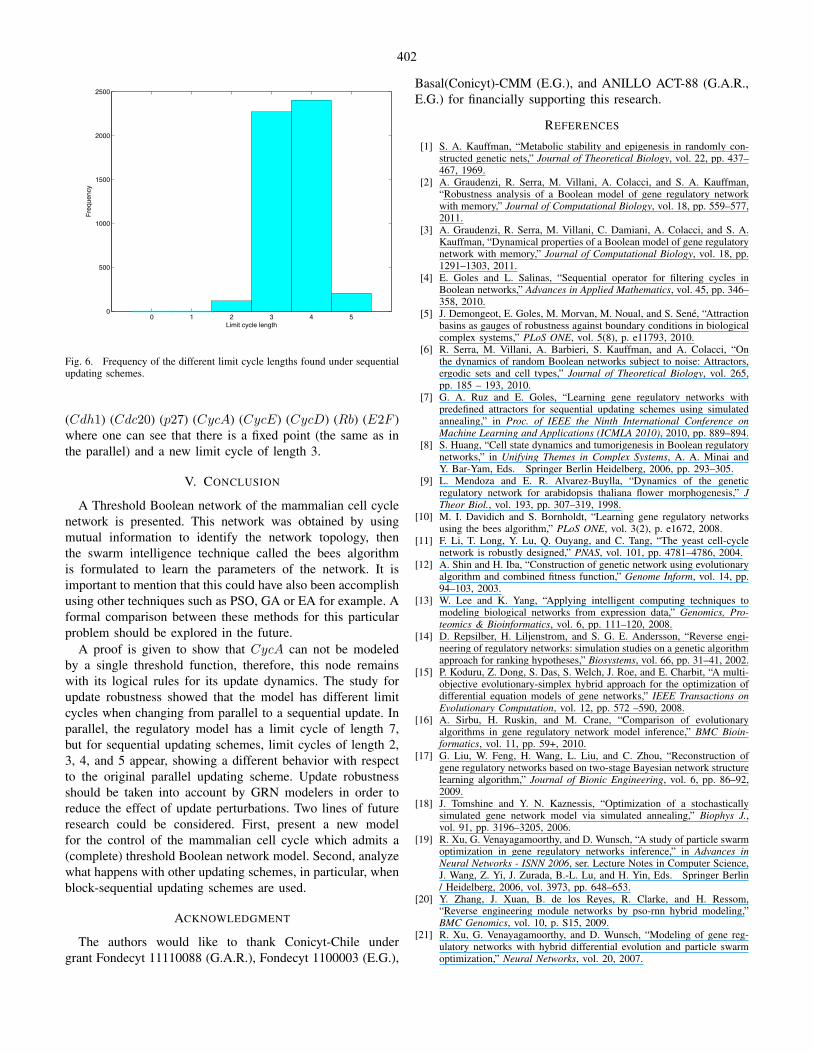
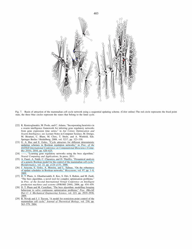
Figure 6 shows a histogram of the different cycle lengthfound for the 5000 updating sequences. Notice that for eachupdating sequence a limit cycle length was found. Also, noneof the limit cycle lengths found, are equal to the limit cycleof length 7 found in the parallel updating scheme, as Figure 6shows, new limit cycles lengths appear. This gives us aninsight that the mammalian cell cycle network in [25] andits equivalent threshold Boolean network version presented inthis paper are not robust against update perturbation, sincedifferent limit cycles of different lengths appears for differentupdating sequences. Figure 7 shows an example of the basinof attraction for the updating sequence (𝐶𝑦𝑐𝐵) (𝑈𝑏𝑐𝐻10)
401
0 1 2 3 4 50
500
1000
1500
2000
2500
Limit cycle length
Fre
quen
cy
Fig. 6. Frequency of the different limit cycle lengths found under sequentialupdating schemes.
(𝐶𝑑ℎ1) (𝐶𝑑𝑐20) (𝑝27) (𝐶𝑦𝑐𝐴) (𝐶𝑦𝑐𝐸) (𝐶𝑦𝑐𝐷) (𝑅𝑏) (𝐸2𝐹 )where one can see that there is a fixed point (the same as inthe parallel) and a new limit cycle of length 3.
V. CONCLUSION
A Threshold Boolean network of the mammalian cell cyclenetwork is presented. This network was obtained by usingmutual information to identify the network topology, thenthe swarm intelligence technique called the bees algorithmis formulated to learn the parameters of the network. It isimportant to mention that this could have also been accomplishusing other techniques such as PSO, GA or EA for example. Aformal comparison between these methods for this particularproblem should be explored in the future.
A proof is given to show that 𝐶𝑦𝑐𝐴 can not be modeledby a single threshold function, therefore, this node remainswith its logical rules for its update dynamics. The study forupdate robustness showed that the model has different limitcycles when changing from parallel to a sequential update. Inparallel, the regulatory model has a limit cycle of length 7,but for sequential updating schemes, limit cycles of length 2,3, 4, and 5 appear, showing a different behavior with respectto the original parallel updating scheme. Update robustnessshould be taken into account by GRN modelers in order toreduce the effect of update perturbations. Two lines of futureresearch could be considered. First, present a new modelfor the control of the mammalian cell cycle which admits a(complete) threshold Boolean network model. Second, analyzewhat happens with other updating schemes, in particular, whenblock-sequential updating schemes are used.
ACKNOWLEDGMENT
The authors would like to thank Conicyt-Chile undergrant Fondecyt 11110088 (G.A.R.), Fondecyt 1100003 (E.G.),
Basal(Conicyt)-CMM (E.G.), and ANILLO ACT-88 (G.A.R.,E.G.) for financially supporting this research.
REFERENCES
[1] S. A. Kauffman, “Metabolic stability and epigenesis in randomly con-structed genetic nets,” Journal of Theoretical Biology, vol. 22, pp. 437–467, 1969.
[2] A. Graudenzi, R. Serra, M. Villani, A. Colacci, and S. A. Kauffman,“Robustness analysis of a Boolean model of gene regulatory networkwith memory,” Journal of Computational Biology, vol. 18, pp. 559–577,2011.
[3] A. Graudenzi, R. Serra, M. Villani, C. Damiani, A. Colacci, and S. A.Kauffman, “Dynamical properties of a Boolean model of gene regulatorynetwork with memory,” Journal of Computational Biology, vol. 18, pp.1291–1303, 2011.
[4] E. Goles and L. Salinas, “Sequential operator for filtering cycles inBoolean networks,” Advances in Applied Mathematics, vol. 45, pp. 346–358, 2010.
[5] J. Demongeot, E. Goles, M. Morvan, M. Noual, and S. Sene, “Attractionbasins as gauges of robustness against boundary conditions in biologicalcomplex systems,” PLoS ONE, vol. 5(8), p. e11793, 2010.
[6] R. Serra, M. Villani, A. Barbieri, S. Kauffman, and A. Colacci, “Onthe dynamics of random Boolean networks subject to noise: Attractors,ergodic sets and cell types,” Journal of Theoretical Biology, vol. 265,pp. 185 – 193, 2010.
[7] G. A. Ruz and E. Goles, “Learning gene regulatory networks withpredefined attractors for sequential updating schemes using simulatedannealing,” in Proc. of IEEE the Ninth International Conference onMachine Learning and Applications (ICMLA 2010), 2010, pp. 889–894.
[8] S. Huang, “Cell state dynamics and tumorigenesis in Boolean regulatorynetworks,” in Unifying Themes in Complex Systems, A. A. Minai andY. Bar-Yam, Eds. Springer Berlin Heidelberg, 2006, pp. 293–305.
[9] L. Mendoza and E. R. Alvarez-Buylla, “Dynamics of the geneticregulatory network for arabidopsis thaliana flower morphogenesis,” JTheor Biol., vol. 193, pp. 307–319, 1998.
[10] M. I. Davidich and S. Bornholdt, “Learning gene regulatory networksusing the bees algorithm,” PLoS ONE, vol. 3(2), p. e1672, 2008.
[11] F. Li, T. Long, Y. Lu, Q. Ouyang, and C. Tang, “The yeast cell-cyclenetwork is robustly designed,” PNAS, vol. 101, pp. 4781–4786, 2004.
[12] A. Shin and H. Iba, “Construction of genetic network using evolutionaryalgorithm and combined fitness function,” Genome Inform, vol. 14, pp.94–103, 2003.
[13] W. Lee and K. Yang, “Applying intelligent computing techniques tomodeling biological networks from expression data,” Genomics, Pro-teomics & Bioinformatics, vol. 6, pp. 111–120, 2008.
[14] D. Repsilber, H. Liljenstrom, and S. G. E. Andersson, “Reverse engi-neering of regulatory networks: simulation studies on a genetic algorithmapproach for ranking hypotheses,” Biosystems, vol. 66, pp. 31–41, 2002.
[15] P. Koduru, Z. Dong, S. Das, S. Welch, J. Roe, and E. Charbit, “A multi-objective evolutionary-simplex hybrid approach for the optimization ofdifferential equation models of gene networks,” IEEE Transactions onEvolutionary Computation, vol. 12, pp. 572 –590, 2008.
[16] A. Sirbu, H. Ruskin, and M. Crane, “Comparison of evolutionaryalgorithms in gene regulatory network model inference,” BMC Bioin-formatics, vol. 11, pp. 59+, 2010.
[17] G. Liu, W. Feng, H. Wang, L. Liu, and C. Zhou, “Reconstruction ofgene regulatory networks based on two-stage Bayesian network structurelearning algorithm,” Journal of Bionic Engineering, vol. 6, pp. 86–92,2009.
[18] J. Tomshine and Y. N. Kaznessis, “Optimization of a stochasticallysimulated gene network model via simulated annealing,” Biophys J.,vol. 91, pp. 3196–3205, 2006.
[19] R. Xu, G. Venayagamoorthy, and D. Wunsch, “A study of particle swarmoptimization in gene regulatory networks inference,” in Advances inNeural Networks - ISNN 2006, ser. Lecture Notes in Computer Science,J. Wang, Z. Yi, J. Zurada, B.-L. Lu, and H. Yin, Eds. Springer Berlin/ Heidelberg, 2006, vol. 3973, pp. 648–653.
[20] Y. Zhang, J. Xuan, B. de los Reyes, R. Clarke, and H. Ressom,“Reverse engineering module networks by pso-rnn hybrid modeling,”BMC Genomics, vol. 10, p. S15, 2009.
[21] R. Xu, G. Venayagamoorthy, and D. Wunsch, “Modeling of gene reg-ulatory networks with hybrid differential evolution and particle swarmoptimization,” Neural Networks, vol. 20, 2007.
402
Pajek
Fig. 7. Basin of attraction of the mammalian cell cycle network using a sequential updating scheme. (Color online) The red circle represents the fixed pointstate, the three blue circles represent the states that belong to the limit cycle.
[22] K. Kentzoglanakis, M. Poole, and C. Adams, “Incorporating heuristics ina swarm intelligence framework for inferring gene regulatory networksfrom gene expression time series,” in Ant Colony Optimization andSwarm Intelligence, ser. Lecture Notes in Computer Science, M. Dorigo,M. Birattari, C. Blum, M. Clerc, T. Sttzle, and A. Winfield, Eds.Springer Berlin / Heidelberg, 2008, vol. 5217, pp. 323–330.
[23] G. A. Ruz and E. Goles, “Cycle attractors for different deterministicupdating schemes in Boolean regulation networks,” in Proc. of theIASTED International Conference on Computational Bioscience (Comp-Bio 2010), 2010, pp. 620–625.
[24] ——, “Learning gene regulatory networks using the bees algorithm,”Neural Computing and Applications, In press, 2011.
[25] A. Faure, A. Naldi, C. Chaouiya, and D. Thieffry, “Dynamical analysisof a generic Boolean model for the control of the mammalian cell cycle,”Bioinformatics, vol. 22, pp. e124–e131, 2006.
[26] J. Aracena, E. Goles, A. Moreira, and L. Salinas, “On the robustnessof update schedules in Boolean networks,” Biosystems, vol. 97, pp. 1–8,2009.
[27] D. T. Pham, A. Ghanbarzadeh, E. Koc, S. Otri, S. Rahim, and M. Zaidi,“The bees algorithm, a novel tool for complex optimisation problems,”in Proc. of the Second International Virtual Conference on Intelligentproduction machines and systems (IPROMS 2006), 2006, pp. 454–459.
[28] D. T. Pham and M. Castellani, “The bees algorithm: modelling foragingbehaviour to solve continuous optimization problems,” Proc. IMechEPart C: J. Mechanical Engineering Science, vol. 223, pp. 2919–2938,2009.
[29] B. Novak and J. J. Tayson, “A model for restriction point control of themammalian cell cycle,” Journal of Theoretical Biology, vol. 230, pp.563–579, 2004.
403