NASA Conference Publication 2327Part 2

Recent Experiencesin Multidisciplinary

Analysis andOptimization

Proceedings of a symposium held at

NASA Langley Research Center

Hampton, Virginia

April 24-26, 1984

J

NIL_A

NASA Conference Publication 2327Part 2

Recent Experiencesin Multidisciplinary

Analysis andOptimization

Compiled byJaroslaw Sobieski

Langley Research Center

Proceedings of a symposium held at

NASA Langley Research Center

Hampton, Virginia

April 24-26, 1984

National Aeronautics

and Space Administration

Scientific and Technical

Information Branch

1984

PREFACE

This conference publication contains the papers presented at the NASA Symposiumon Recent Experiences in Multidisciplinary Analysis and Optimization, held at NASALangley Research Center, Hampton, Virginia, April 24-26, 1984. The purposes of thesymposium were to exchange information about the status of the application of optim-ization and associated analyses in industry or research laboratories to real lifeproblems, and to examine the directions of future developments.

Within the broad statement of the symposium's purposes, information exchangehas encompassed the following:

Examples of successful applications

"Attempt and failure" examples, particularly to describe the reasons for failureand lessons learned

Identification of potential applications and benefits, even though no attemptto apply optimization may have been made as yet

Synergistic effects of optimized interaction and trade-offs occurring among twoor more engineering disciplines (e.g., structural engineering and aerodynamics)and/or subsystems in a system (e.g., propulsion and airframe in aircraft)

Traditional organization of a design process as a vehicle for or an impedimentto the progress in the design methodology

Computer technology in the context of the foregoing

This information exchange has covered aerospace and other industries as well as uni-versities and government agencies.

The goal of the meeting was to reach a better understanding of the extent towhich optimization and the associated analyses are being used, development directions,the future potential, and actions that ought to be taken to realize the potentialsooner. That goal was attained and the symposium showed through both the diversityand quality of papers and the active participation of the attendees that the activi-ties in the subject area are vigorous beyond the initial expectations. There was aconsensus that multidisciplinary analysis and optimization have an important potentialas aids to human intellect in the design process, and that cooperation of industry,academia, and government, under NASA leadership, is needed to realize that potential.

pRECEDING PAGE BLANK NOT FILMED

iii

CONTENTS

PREFACE ..................................... iii

Part I*

SESSION 1: INTRODUCTION AND GENERAL CONSIDERATIONSCo-Chairmen: L. A. McCullers and J. Sobieski

STRUCTURAL SYNTHESIS - PRECURSOR AND CATALYST ..................L. A. Schmit

OPTIMIZATION IN THE SYSTEMS ENGINEERING PROCESS ................. 19Loren A. Lemmerman

PRACTICAL CONSIDERATIONS IN AEROELASTIC DESIGN ................. 35Bruce A. Rommel and Alan J. Dodd

FLUTTER OPTIMIZATION IN FIGHTER AIRCRAFT DESIGN ................. 47William E. Triplett

APPLICATION OF THE GENERALIZED REDUCED GRADIENT METHOD TO CONCEPTUALAIRCRAFT DESIGN . ............................... 65

Gary A. Gabriele

EXPERIENCES PERFORMING CONCEPTUAL DESIGN OPTIMIZATION OF TRANSPORTAIRCRAFT ................................... 87

P. Douglas Arbuckle and Steven M. Sliwa

THE ROLE OF OPTIMIZATION IN STRUCTURAL MODEL REFINEMENT ............. 103L. L. Lehman

PIAS, A PROGRAM FOR AN ITERATIVE AEROELASTIC SOLUTION .............. 111Marjorie E. Manro

SESSION 2: OPTIMIZATION IN VARIOUS INDUSTRIESChairman: W. J. Stroud

OPTIMIZATION PROCESS IN HELICOPTER DESIGN .................... 127

A. H. Logan and D. Banerjee

ROLE OF OPTIMIZATION IN INTERDISCIPLINARY ANALYSES OF NAVALSTRUCTURES ................................... 139

S. K. Dhir and M. M. Hurwitz

APPLICATION OF OPTIMIZATION TECHNIQUES TO VEHICLE DESIGN -A REVIEW ................................... 147

B. Prasad and C. L. Magee

STRUCTURAL OPTIMIZATION IN AUTOMOTIVE DESIGN .................. 173J. A. Bennett and M, E. Botkin

*Part 1 is presented under separate cover.

17

pp.F.cEDtNG PAGE BLANK NOT FILMED

TRADEOFF METHODS IN MULTIOBJECTIVE INSENSITIVE DESIGN OFAIRPLANE CONTROL SYSTEMS ........................... 189

Albert A. Schy and Daniel P. Giesy

SESSION 3A: APPLICATIONS 1Chairman: J. H. Starnes, Jr.

STAEBL -- STRUCTURAL TAILORING OF ENGINE BLADES (PHASE II) ........... 205M. S. Hirschbein and K. W. Brown

OPTIMIZATION OF CASCADE BLADE MISTUNING UNDER FLUTTER AND FORCEDRESPONSE CONSTRAINTS ............................. 219

Durbha V. Murthy and Raphael T. Haftka

SIZING-STIFFENED COMPOSITE PANELS LOADED IN THE POSTBUCKLING RANGE ....... 235S. B. Biggers and J. N. Dickson

OPTIMAL REDESIGN STUDY OF THE HARM WING ..................... 251S. C. Mclntosh, Jr., and M. E. Weynand

COMPOSITE MATERIAL DESIGN, ANALYSIS, AND PROCESSING OF SPACE MOTORNOZZLE COMPONENTS ............................... 265

Edward L. Stanton

SESSION 3B: APPLICATIONS 2Chairman: I. Abel

A NONLINEAR PROGRAMMINGMETHOD FOR SYSTEM DESIGN WITH RESULTS THATHAVE BEEN IMPLEMENTED ............................. 267

Frank Hauser

APPLICATION OF OPTIMIZATION TECHNIQUES TO THE DESIGN OF A FLUTTERSUPPRESSION CONTROL LAW FOR THE DAST ARW-2 .................. 279

William A. Adams, Jr., and Sherwood H. Tiffany

APPLICATION OF CONMIN TO WING DESIGN OPTIMIZATION WITH VORTEX FLOWEFFECT ................ .................... 297

C. Edward Lan

CALCULATED EFFECTS OF VARYING REYNOLDS NUMBER AND DYNAMIC PRESSURE ONFLEXIBLE WINGS AT TRANSONIC SPEEDS ...................... 309

Richard L. Campbell

INFLUENCE OF ANALYSIS AND DESIGN MODELS ON MINIMUM WEIGHT DESIGN ........ 329M. Salama, R. K. Ramanathan, L. A. Schmit, and I. S. Sarma

SESSSION 4: METHODS AND TOOLS 1Co-Chairmen: R. T. Haftka and H. Miura

MULTIDISClPLINARY SYSTEMS OPTIMIZATION BY LINEAR DECOMPOSITION ......... 343J. Sobieski

vi

STRUCTURALSENSITIVITYANALYSIS: METHODS,APPLICATIONS,ANDNEEDS................................... 367

HowardM. Adelman, Raphael T. Haftka, Charles J. Camarda,and Joanne L. Walsh

SENSITIVITYANALYSISIN COMPUTATIONALAERODYNAMICS............... 385DeanR.Bristow

AIRCRAFTCONFIGURATIONOPTIMIZATIONINCLUDINGOPTIMIZEDFLIGHTPROFILES................................ 395

L. A. McCullers

THEADSGENERAL-PURPOSEOPTIMIZATIONPROGRAM.................. 413G. N. Vanderplaats

SHAPEDESIGNSENSITIVITYANALYSISOFBUILT-UPSTRUCTURES............ 423KyungK. Choi

MULTIDISCIPLINARYOPTIMIZATIONAPPLIEDTOA TRANSPORTAIRCRAFT ......... 439Gary L. Giles and G. A. Wrenn

SOMEEXPERIENCESIN AIRCRAFTAEROELASTICDESIGNUSINGPRELIMINARYAEROELASTICDESIGNOFSTRUCTURES(PADS).................... 455

Nick A. Radovcich

DESIGNENHANCEMENTTOOLSIN MSC/NASTRAN..................... 505D. V. Wallerstein

PROGRESSREPORTONTHE"AUTOMATEDSTRENGTH-AEROELASTICDESIGNOFAEROSPACESTRUCTURES"PROGRAM....................... 527

E. H. Johnsonand V. B. Venkayya

Part 2

SESSION 5A: ROTORCRAFT APPLICATIONSCo-Chairmen: C. E. Hammond and R. J. Huston

OVERVIEW: APPLICATIONS OF NUMERICAL OPTIMIZATION METHODS TOHELICOPTER DESIGN PROBLEMS .......................... 539

H. Miura

APPLICATION OF MODERNSTRUCURAL OPTIMIZATION TO VIBRATION REDUCTIONIN ROTORCRAFT ................................. 553

P. P. Friedmann

HELICOPTER ROTOR BLADE AERODYNAMIC OPTIMIZATION BY MATHEMATICALPROGRAMING .................................. 567

Joanne L. Walsh, Gene J. Bingham, and Michael F. Riley

REGRESSION ANALYSIS AS A DESIGN OPTIMIZATION TOOL ................ 579Richmond Perley

vii

A ROTOR OPTIMIZATION USING REGRESSION ANALYSIS ................. 595N. Giansante

OPTIMIZATION OF HELICOPTER ROTOR BLADE DESIGN FOR MINIMUMVIBRATION ................................... 609

M. W. Davis

APPLICATION OF NUMERICAL OPTIMIZATION TO ROTOR AERODYNAMIC DESIGN ........ 627

W. A. Pleasants III and T. J. Wiggins

AEROELASTIC/AERODYNAMIC OPTIMIZATION OF HIGH SPEED HELICOPTER/COMPOUNDROTOR ................................ 643

L. R. Sutton and R. L. Bennett

THE STRUCTURAL OPTIMIZATION OF A SPREADER BAR FOR TWIN LIFTHELICOPTER OPERATIONS ............................. 663

Alan Dobyns

MULTIOBJECTIVE OPTIMIZATION TECHNIQUES FOR STRUCTURAL DESIGN .......... 675S, S. Rao

SESSION 5B: SPACE APPLICATIONSChairman: A. W. Wilhite

IDEAS, A MULTIDISClPLINARY COMPUTER-AIDED CONCEPTUAL DESIGN SYSTEMFOR SPACECRAFT ................................ 683

Melvin J. Ferebee, Jr.

AVID II, A MULTIDISClPLINARY COMPUTER AIDED CONCEPTUAL DESIGN SYSTEMFOR LAUNCH VEHICLES AND ORBITAL TRANSFER VEHICLES t

A. W. Wilhite

MICROCOMPUTER DESIGN AND ANALYSIS OF THE CABLE CATENARY LARGESPACE ANTENNA SYSTEM ............................. 705

W. Akle

DESIGN OPTIMIZATION OF THE 34-METER DSN-NCP ANTENNAS .............. 719Roy Levy

POST AND A RANDOM-WALK SEARCH MODE ....................... 735James A Martin

COMPONENTTESTING FOR DYNAMIC MODEL VERIFICATION ................ 759T. K. Hasselman and Jon D. Chrostowski

DUAL STRUCTURAL-CONTROL OPTIMIZATION OF LARGE SPACE STRUCTURES ......... 775Achille Messac and James Turner

STRUCTURAL OPTIMIZATION WITH CONSTRAINTS ON TRANSIENTS RESPONSE ......... 803Robert Riess

tPaper not available for publication.

viii

OPTIMIZATION APPLICATIONS IN AIRCRAFT ENGINE DESIGN AND TEST .........T. K. Pratt

ON OPTIMAL DESIGN FOR THE BLADE-ROOT/HUB INTERFACE IN JET ENGINES .......Noboru Kikuchi and John E. Taylor

SESSION 6: METHODS AND TOOLS 2Co-Chairmen: H. M. Adelman and G. L. Giles

PROBLEMS IN LARGE-SCALE STRUCTURAL OPTIMIZATION ................

Jasbir S. Arora and Ashok D. Belegundu

STRUCTURAL OPTIMIZATION OF LARGE OCEAN-GOING STRUCTURES ............

Owen F. Hughes

FUNDAMENTAL DIFFERENCES BETWEEN OPTIMIZATION CODE TEST PROBLEMS ANDENGINEERING APPLICATIONS ..........................

E. D. Eason

A CONCEPTUAL BASIS FOR THE DESIGN OF DAMAGE-TOLERANT STRUCTURALSYSTEMS ...................................

Farrokh Mistree, Jon A. Shupe, and Owen F. Hughes

COMMENTS ON GUST RESPONSE CONSTRAINED OPTIMIZATION ..............Prabhat Hajela

APPLYING OPTIMIZATION SOFTWARE LIBRARIES TO ENGINEERING PROBLEMS .......M. J. Healy

OPTDES.BYU: AN INTERACTIVE OPTIMIZATION PACKAGE WITH 2D/3D GRAPHICS .....R. J. Balling, A. R. Parkinson, and J. C. Free

ON THE UTILIZATION OF ENGINEERING KNOWLEDGEIN DESIGN OPTIMIZATION ......Panos Papalambros

COMPUTER AIDED ANALYSIS AND OPTIMIZATION OF MECHANICAL SYSTEMDYNAMICS ..................................

E. J. Haug

SHAPE OPTIMIZATION INCLUDING FINITE ELEMENT GRID ADAPTATION ..........Noboru Kikuchi and J. E. Taylor

MULTIDISClPLINARY APPROACH TO THE DESIGN OF HIGH PRESSURE OXYGENSYSTEMS ...................................

R. L. Johnston

815

833

847

873

891

907

943

957

979

991

1007

1027

1037

ix

OVERVIEW: APPLICATIONS OF NUMERICAL OPTIMIZATION METHODSTO HELICOPTER DESIGN PROBLEMS

H. MiuraNASA Ames Research Center

Moffett Field, California

539

INTRODUCTION

The term "optimization" covers wide spectrum of technology, but this presenta-

tion is ]imited to the applications of numerical optimization methods (in other

words, mathematical programming or multi-variable search methods) as applied to

helicopter design problems. The potential benefits of this technology were recog-

nized as early as ten years ago, but as can be clearly seen in the table shown below,

serious effort to exploit its capabilities started only very recently. It is inter-

esting to note that the helicopter industry started incorporating this technology

much faster than the fixed wing industry. The current active interest of the

helicopter industry may be accurately reflected in the organization of a specialsession at the 1983 AHS Forum (ref. i). This situation can probably be attributed to

the existence of many difficult and urgent problems associated with helicopter

design. Also, the relatively small and flexible organizational structure of heli-

copter manufacturers might be a contributing factor. A great deal of research and

development effort is still required to ship numerical optimization methods out of

R&D departments into production design divisions. However, design optimizationmethods will be considered increasingly important to win basic research contracts,

and even to win major military aircraft design contracts in the near future.

One commonly expressed criticism of using numerical optimization in helicopter

design problems is the adequacy of analysis techniques. For example, it is importantto design a rotor system that applies minimum vibratory forces and moments to the

airframe, but prediction of dynamic airloads for a given rotor system for anyspecified flight condition is still an active research subject. Under such circum-

stances, we often have to face R&D resource allocation problems. In my opinion, itis important to have a system that can carry out design optimization based on the

best available analysis or test data. Such a system will provide a framework to

accommodate new technology developments by replacing outdated modules with new

modules. Recent developments in computer engineering provide opportunities to build

such an adaptive program system that will be allowed to grow with new technology

developments. The benefits of multi-disciplinary analysis and design will be

captured readily if the framework to integrate necessary modules is available. Also

it should be recognized that the contributions of any analysis tools or sophisticated

tests are enhanced if there are mechanisms to promptly reflect results in aircraft

design. Human engineers have been the only link between analysis and design capa-

bilities in the past, but design engineers in the helicopter industry may be able to

use numerical design optimization as a convenient practical tool in the near future.

Year

197071727374

7576777879

1980

81828384

ConceptualPrelimi nary

Design2

StructuralDesign

6

7, 8

910

11, 12, 1314

AerodynamicAcoustic

Design

15, 16

17

Rotor

SystemDesign

18

19

20, 21, 2223, 24, 25

26, 27

Flight Control ITrajectory SystemDesign Design

28

29

3O31

540

CONCEPTUAL AND PRELIMINARY DESIGN OPTIMIZATION

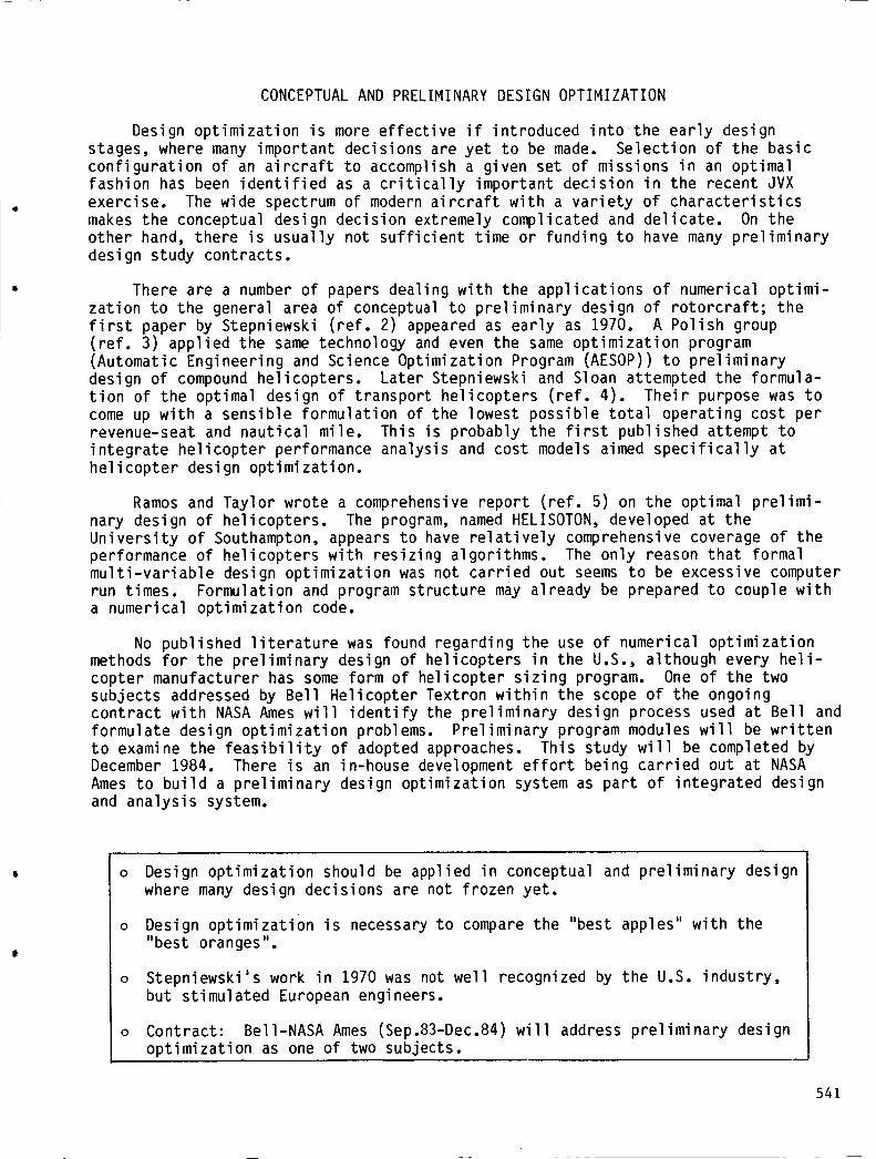
Design optimization is more effective if introduced intothe early designstages, where many important decisions are yet to be made. Selection of the basicconfiguration of an aircraft to accomplish a given set of missions in an optimalfashion has been identified as a critically important decision in the recent JVXexercise. The wide spectrum of modern aircraft with a variety of characteristicsmakes the conceptual design decision extremely complicated and delicate. On theother hand, there is usually not sufficient time or funding to have many preliminarydesign study contracts.

There are a number of papers dealing with the applications of numerical optimi-zation to the general area of conceptual to preliminary design of rotorcraft; thefirst paper by Stepniewski (ref. 2) appeared as early as 1970. A Polish group(ref. 3) applied the same technology and even the same optimization program(Automatic Engineering and Science Optimization Program (AESOP)) to preliminarydesign of compound helicopters. Later Stepniewski and Sloan attempted the formula-tion of the optimal design of transport helicopters (ref. 4). Their purpose was tocome up with a sensible formulation of the lowest possible total operating cost perrevenue-seat and nautical mile. This is probably the first published attempt tointegrate helicopter performance analysis and cost models aimed specifically athelicopter design optimization.

Ramos and Taylor wrote a comprehensive report (ref. 5) on the optimal prelimi-nary design of helicopters. The program, named HELISOTON, developed at theUniversity of Southampton, appears to have relatively comprehensive coverage of theperformance of helicopters with resizing algorithms. The only reason that formalmulti-variable design optimization was not carried out seems to be excessive computerrun times. Formulation and program structure may already be prepared to couple witha numerical optimization code.

No published literature was found regarding the use of numerical optimizationmethods for the preliminary design of helicopters in the U.S., although every heli-copter manufacturer has some form of helicopter sizing program. One of the twosubjects addressed by Bell Helicopter Textron within the scope of the ongoingcontract with NASA Ames will identify the preliminary design process used at Bell andformulate design optimization problems. Preliminary program modules will be writtento examine the feasibility of adopted approaches. This study will be completed byDecember 1984. There is an in-house development effort being carried out at NASAAmes to build a preliminary design optimization system as part of integrated designand analysis system.

o Design optimization should be applied in conceptual and preliminary designwhere many design decisions are not frozen yet.

o Design optimization is necessary to compare the "best apples" with the"best oranges".

o Stepniewski's work in 1970 was not well recognized by the U.S. industry,but stimulated European engineers.

o Contract: Bell-NASA Ames (Sep.83-Dec.84) will address preliminary designoptimization as one of two subjects.

541

STRUCTURAL DESIGN OPTIMIZATION

Reflecting current interests and needs for controlling vibration of helicopters,all the papers reviewed here addressed structural modification to control steadystate vibration levels excited by periodic forces or moments. Typically thesestudies aim at cockpit vibration reduction caused by main rotor vibratory excitationforces and moments. Done et al. applied the Vincent circle method (refs. 7, II,and 12), presenting the feasibility of this method to design optimization. Hansonand Calapodas compared, in references 9 and I0, the Vincent circle method with thestrain energy method proposed by Sciarra (ref. 6). Their conclusions were that thestrain energy method was better for stiffness modification, although it did notprovide any data for mass tuning and absorber design/positioning. Finite matrixperturbation techniques were also applied (refs. 13 and 14) to this class of problemswith reasonable success. Applications of formal optimization methods were not foundin literature. Disjoint feasible design space reported by Johnson (ref. 8) andrecently by Mills-Currah and Schmit (ref. 32) for undamped structures has not yetbeen noticed by the helicopter industry. A finite element modelling exercise programsponsored by NASA Langley Research Center will address the airframe design problem,aiming at vibration prediction and control, and may generate a broad technical data-base and provide adequate guidance for the future development of practical tools.However, helicopter vibration problems are extremely complex aeroelastic phenomenathat should involve main rotor dynamics, rotor/airframe coupling, and aerodynamicinterference, and therefore must be considered as multi-disciplinary problems.

Structural weight reduction is probably more important for helicopters than forfixed wing aircraft; hence there must be a number of applications carried out inindustry, but no formal documentation was found. The critical problem until now hasbeen lack of appropriate software. The implementation of sensitivity analysis inMSC-NASTRAN and the development of CASADAS by Northrop under an AFWAL contract willprovide desperately needed tools for structural weight reduction with static anddynamic constraints.

There is a strong trend toward the extensive use of modern composite materialsfor the primary and secondary load-carrying structures of helicopters. Automateddesign technology such as that represented by the PASCO program (ref. 33) will beuseful but has not penetrated the helicopter industry yet, probably because of thelack of experience and confidence at this time in using such a tool in the practicaldesign environment. Enormously challenging design optimization problems also existin the design of solid three-dimensional composite structures; for example, rotor hubcomponents and power train mechanical parts. These areas remain virtually untouched.

o Airframe design optimization studies focused mostly on control of vibrationexcited by main rotor vibratory forces and moments.

Vincent circle method, strain energy method, matrix perturbation

o General structural optimization codes are emerging.MSC-NASTRAN sensitivity analysis capabilityCASADAS

o Composite structural design will need numerical design optimization.

o A Langley program to develop national capability to analyze vibration aspart of helicopter structural design may include structural optimizatio_in 86-88.

542

AERODYNAMIC AND ACOUSTIC DESIGN OPTIMIZATION

Reduction of helicopter noise level is, just like vibration control, anextremely important and urgent problem that the helicopter industry is facingtoday. We have just started understanding the primary generation mechanisms ofhelicopter noise. The real challenges are to design low noise helicopters withoutdegrading the aerodynamic performance of the aircraft, or even to aim at its simul-taneous improvement. Analyses of aerodynamic responses and noise characteristics ofthe main rotor blades, especially in the important transonic regime, are stillresearch subjects. Although some computer codes have become available recently,these codes require a great deal of numerical data processing effort. Therefore,simple coupling with numerical optimization codes will not be productive at thistime, even on the fastest computers available. It is believed that the innovativeuse of approximation concepts will be instrumental in obtaining design tools that canbe used in the practical environment.

In the past, attempts were made to transfer technology developed for fixed wingairfoil optimization to rotary wing design problems (refs. 15 and 16). The resultsare encouraging in general, but a great deal of advanced research (theoretical,computational and experimental) will be required for the development of a maturetechnology base and design tools.

Significant research efforts are expended at NASA Ames to integrate currentlyavailable best-analysis techniques with a numerical optimization code. Some pre-liminary results associated with this effort were presented at the AHS Forum byTauber (ref. 17).

o Computational fluid dynamics technology coupled with numerical optimizationwill become a practical design tool. Research will be needed to integrateanalysis capabilities into numerical optimization to reduce the overallcomputation effort.

Optimization of airfoil of rotor blades has been studied using CFD and mathprogramming methods. One of the advantages recognized over the traditionalmethod is the capability to take multiple conditions simultaneously.

Numerical optimization will become useful to design low noise rotor blades.Providing theoretically optimum design based on the best analysis

availableReduction of test time and cost

543

MAIN ROTOR DESIGN OPTIMIZATION

The application of numerical optimization to rotor blade design problems waspresented by Bielawa (ref. 18) in 1971. He solved blade weight minimization problemsunder a constraint on the first aeroelastic mode damped frequency. The study waspreliminary in nature and the optimization technique used might be classified as oneof the optimality criteria approaches. However, his formulation of the rotor designproblem was in the general standard form that could be used with any of today'sgeneral mathematical programming codes. Stepniewski's paper (ref. 2) was referencedin an extensive review by Huber (ref. 19). Despite excellent pioneering work byBielawa, there were no significant publications in the next ten years in this area.But in 1982, Bennett (ref. 20) presented an epoch making paper at the AHS Forum inAnaheim. He gave several rotor design problems formulated in standard mathematicalprogramming forms, and solved them by coupling analysis codes with a general purposeoptimization code, OPT. This paper appears to have had a significant effect on thehelicopter technical community regarding applicability of numerical optimizationmethods. At the same AHS Forum, Taylor (ref. 21) presented an interesting paperaimed at blade design modification for vibratory root force reduction, although hisredesign algorithm was not an automated numerical search method.

In 1982-1983, two reports were written by Mclntosh under two separate contractswith the U.S. Army (AVRADCOM). Reference 22 describes a bearingless rotor flexbeamshape designed to minimize various combinations of bending and centrifugal stressesfor a given oscillatory excitation force distribution. Reference 23 presented anambitious effort to couple a linear rotor airframe coupled vibration analysis code,QVR, with the general optimization code CONMIN to reduce a measure of the fuselagevibration by modifying the rotor system design parameters. Both of the studiesreported by Mclntosh were preliminary and warranted further investigation, althoughsome of the results looked encouraging.

There are at least three government supported research activities in this area.This reflects the current interests and importance of rotor design problems. Two ofthem are reported in this session (refs. 26 and 27) and the other is described inreferences 24 and 25. Although it is not explicitly stated, ongoing rotor systemstudy projects such as ITR or FRR programs will use design optimization methods atvarious levels of the design effort.

0 Interests in the U.S. revived in 1982, more than ten years after the first

paper was published. Bennett's work on rotor structural design optimizationwas a significant step.

Current interest in design of low vibration rotor systems. There are anumber of areas in which analysis capabilities must be developed or improvedto obtain modules that are usable in the design process with sufficientconfidence.

Unsteady air load prediction capabilityDynamic stall modelsAdequacy of rotor design procedures

Three government supported research activities:

NASA Langley - Univ. of Washington/Univ. of Southern Illinois

U.S. Army ATL - Bell Helicopter Textron

NASA Ames - Univ. of California, Los Angeles

544

FLIGHT PATH OPTIMIZATION

This problem is obviously not a helicopter design problem. It addresses thedetermination of an optimal flight condition path to accomplish a specified missionwith a given helicopter, payload and weather conditions. The objective can beminimum fuel, minimum cost, minimum time, obstacle clearance or statistical surviva-bility. Traditionally, this type of problem was solved using optimal control theory,which seeks solutions in the form of time dependent control inputs (refs. 28 to 30).However, assuming that missions can be broken into a relatively small number ofsegments and that flight conditions are kept constant in each segment, this problemmay be cast into a standard form to be solved by nonlinear programming methods.

Recent trends in microcomputer technology indicate rapid growth in the capa-bilities of on-board, portable or even hand-held computers. The U.S. Army has aproject to use an HP-41 hand-held calculator for flight planning and on-board flightmanagement to reduce operational cost, improve operational safety and reduce pilotworkload. If sufficient computer capabilities are available, optimization of theparameters displayed to pilots will be possible. A futuristic version of thispicture is to work with an autopilot system to reduce the pilot workload in therelatively trivial mission segments. A preliminary study of this problem, especiallyfrom the viewpoint of the application of numerical optimization methods, will becarried out by Bell Helicopter under a contract with NASA Ames. An ongoing in-housestudy to generate or store necessary aircraft performance data with minimum CPU powerand memory requirement is planned to be integrated into the program that will bedeveloped by Bell under the contract.

o Optimization of flight trajectory plan has been exercised for fixed wingairplanes, but not a great deal has been done for helicopters.

o Techniques used in the past were dynamic programming and optimal controltheory, not static numerical optimization methods.

Computerization will be necessary to reduce the pilot workload, especiallyfor military helicopters.

Army program to use HP-41 for flight management of UH-IH

Feasibility of applying numerical optimization methods will be studied byBell Helicopter under the contract with NASA Ames.

Development of sensible analytical models and their sensitivity to resultsRequirements for the on-board computersEvaluation of practical pay-offs

545

CONTROL SYSTEM DESIGN OPTIMIZATION

Multi-variable function minimization methods have been used in the design oflinear control systems for some time. For example, minimization of a quadratic meritfunction of state variables has been commonly used to obtain closed loop gainschedule for linearized models. If properly coupled with rotor dynamics, controlsystem design optimization may take aircraft performance and handling quality con-straints into account. In fact, in reference 3 aircraft handling quality constraintswere considered in the scope of preliminary design. The addition of control systemdesign variables should be straightforward, even though such tasks will not besimple.

Vibration reduction by applying higher harmonic blade pitch variation has beenstudied extensively using optimal estimation and control theory. However, Jacob andLehmann (ref. 31) presented an interesting concept to transform the dynamic bladepitch control scheduling problem into non-time-dependent discrete variables. Theidea was to expand the pitch angle distribution of the blade with the weighted sum ofTschebysheff polynomials (spanwise) and Fourier series (azimuthwise). Coefficientsof the product terms in this summation were design variables to be modified by anoptimization program to reduce the vibratory hub load amplitudes. The mathematicalmodel used in this study was probably over-simplified, but it showed the feasibilityof using this concept as an alternative approach to optimal control techniques. Notethat coefficients may be computed at a certain number of discrete trim conditions anda numerical interpolation scheme can then be implemented. Compared to the approachesusing optimal estimation and control techniques, this 'static' control schedulingcannot respond to unexpected loads such as gust induced airload disturbances.

Control system design optimization coupled with aircraft performance andhandling quality analysis models will be useful.

Higher harmonic blade pitch variation scheduling for vibratory loadreduction can be formulated in a 'static' numerical optimization problem.However, it will be necessary to obtain pitch variation scheduling for eachflight condition. Also this static scheduling approach cannot respond toexternal disturbances.

546

IMPORTANCE OF APPROXIMATION CONCEPTS

Helicopter response analyses are difficult and many of them can be very expen-sive. For example, straightforward coupling of a numerical optimization code with atransonic aerodynamic analysis code for optimal design of blade tip geometry is notcurrently feasible for this reason. Rotor performance analysis, acoustic noise esti-mation or rotor system aeroelastic stability analysis could be quite expensive ifrepeated many times. Structural optimization technology developed in the early 1970s(ref. 34) provides valuable clues to overcoming the economic barrier mentioned above.The key idea is to make full use of approximations to reduce the amount of data pro-cessing. Except for the evaluation of the final design, accurate response analysesare not necessarily required; instead, we need only enough information to guide thedesign to a nearly optimal and practical design point. One of the most importantconcepts is to build explicit approximate expressions for all functions that arelikely to affect the design modification process.

For structural design, the Taylor series expansions of displacements and stresseswith respect to reciprocals of sizing variables have been found to be effective.Complete analysis is carried out only when it becomes necessary to update the Taylorseries expansion coefficients. Vanderplaats, in reference 35, introduced a procedureto gradually build second order approximations of all the functions while the designis being improved. The advantage of this scheme is that all the analysis results inthe past can contribute to improve the quality of the approximation models. In otherwords, the accuracy of the model keeps improving as the design approaches an optimum.An innovative application of this concept was presented in reference 36, in which thesystem responses were evaluated by tests, not computer runs. This idea should behelpful in planning tests in helicopter research and development.

An alternative idea is to distribute trial analysis points within the limiteddesign subspace and evaluate all the functions at those discrete points. Then,approximate interpolation functions are constructed by means of regression analysesif a sufficient amount of data is available, or by means of certain estimation tech-niques if the amount of data points is not enough. In certain cases, additional dataacquisition by complete analyses or tests may be performed. This scheme will beuseful to obtain a global picture within the design space of interest, but should beused with caution due to the nature of approximate functions. If the number ofdesign variables increases, applications of this approach will be increasingly diffi-cult. Also, all the analysis effort on the designs that grossly violate constraintsmay be wasted without contributing to the design process.

There are various intermediate approaches to compromise between the twostrategies mentioned above. In any case, the generation of appropriate explicitapproximate functions is the critically important technique necessary to makeuse of the results of sophisticated advanced analysis tools in the design process.

o Helicopter analyses are very complicated. Aerodynamics and acoustic analysisrequire especially large amount of computation. Introduction of approximationwill be essential.

Approximation concepts developed for structural optimization will beapplicable to helicopter problems. In addition, various variations ofapproximation techniques are not available. Innovative use of availabletechniques will be helpful.

547

SUMMARY

There are a number of helicopter design problems that are well suited to appli-cations of numerical design optimization techniques. Adequate implementation of thistechnology will provide high pay-offs. There are a number of numerical optimizationprograms available, and there are many excellent response/performance analysisprograms developed or being developed. But integration of these programs in a formthat is usable in the design phase should be recognized as important. It is alsonecessary to attract the attention of engineers engaged in the development ofanalysis capabilities and to make them aware that analysis capabilities are much morepowerful if integrated into design oriented codes. Frequently, the shortcomings ofanalysis capabilities are revealed by coupling them with an optimization code.

Most of the published work has addressed problems in preliminary system design,rotor system/blade design or airframe design. Very few published results were foundin acoustics, aerodynamics and control system design. Currently major efforts arefocused on vibration reduction, and aerodynamics/acoustics applications appear to begrowing fast. The development of a computer program system to integrate the multipledisciplines required in helicopter design with numerical optimization technique isneeded. The size of the helicopter industry is small compared to that of the fixedwing airplane industry; therefore it is necessary to look for help and to worktogether with other industries for the development of commonly usable engineeringdevelopments.

Activities in Britain, Germany and Poland are identified, but no publishedresults from France, Italy, the USSR or Japan were found.

o Helicopter design can make use of numerical optimization methods. Highpayoff will be expected if a system that integrates multi-disciplinaryanalysis capabilities with numerical optimization is to be created.

Development of advanced analysis programs that provide useful designoriented data should be recognized as an important mechanism for integrationwith numerical optimization.

Approximation concepts will be the critical item in this integrationeffort.

The U.S. helicopter industry became aware of the potential of this tech-nology in the last 2-3 years. Activities in Britain, Germany and Polandare observed. The U.S. helicopter industry can take advantage of thedevelopments made by other industries within the U.S.

548

REFERENCES

1. Optimal Design. Proc. of the AHS39th Annual Forum, St. Louis, MO,May 1983.

2. Stepniewski, W. Z., and Kalmback, C. F., Jr., Multi-Variable Search and ItsApplication to Aircraft Design Optimization. Aeronautical Journal, RoyalAeronautical Society, Vol. 74, No. 713, May1970, pp. 419-432.

3. Szumanski, K., Optimization of the Rotor-Wing System from Helicopter PerformancePoint of View. CASPaper No. 76-37, The Tenth Congress of the InternationalCouncil of the Aeronautical Sciences, Ottawa, Canada, Oct. 1976.

4. Stepniewski, W. Z., SomeThoughts on Design Optimization of Transport

Helicopters. Vertica, Vol. 6, 1982, pp. 1-17.

5. Ramos, O. R., and Taylor, P., "Helicopter Design Synthesis. 7th European

Rotorcraft and Powered Lift Aircraft Forum, Garmish-Partenkirchen, West Germany,Sept. 1981.

6. Sciarra, J. J., Use of the Finite Element Damped Forced Response Strain Energy

Distribution for Vibration Reduction. Boeing Vertol Company Report

No. D21-10819-1 for U.S. Army Research Office, Durham, N.C., July 1974.

7. Done, G. T. S., and Hughes, A. D., Reducing Vibration by Structural

Modification. Vertica, Vol. 1, 1976, pp. 31-38.

8. Johnson, E. J., Disjoint Design Spaces in the Optimization of HarmonicallyExcited Structures. AIAA Journal, Vol. 14, No. 2, Feb. 1976, pp. 259-261.

9. Hanson, H. W., and Calapodas, N. J., Evaluation of Practical Aspects of Vibration

Reduction Using Structural Optimization Techniques. AHS 35th Annual Forum,

Washington, D.C., May 1979.

10. Hanson, H. W., Investigation of Vibration Reduction Through Structural

Optimization. USAAVRADCOM-TR-80-D-13, 1980.

11. Done, G. T. S., and Rangacharyulu, M. A. V., Use of Optimization in Helicopter

Vibration Control by Structural Modification. Journal of Sound and Vibration,

Vol. 74, Feb. 1981.

12. Done, G. T. S., Use of Optimization in Helicopter Vibration Control by Structural

Modification. AHS Northeast Region National Specialists' Meeting on Helicopter

Vibration. Hartford, CT, Nov. 1981.

13. King, S. P., Assessment of the Dynamic Response of Structures When Modified by

the Addition of Mass, Stiffness or Dynamic Absorbers. AHS Northeast Region

National Specialists' Meeting on Helicopter Vibration, Hartford, CT, Nov. 1981.

14. Kitis, L., Pilkey, W. D., and Wang, B. P., Optimal Passive Frequency Response

Control of Helicopters by Added Structures. AIAA paper no. N83-27976, backup

document for a Synoptic in Journal of Aircraft, Sept. 1983.

15. Hicks, R. M., and McCroskey, W. J., An Experimental Evaluation of a Helicopter

Rotor Section Designed by Numerical Optimization. NASA TM-78622, Mar. 1980.

549

16. Tauber, M. E., and Hicks, R. M., Computerized Three-Dimensional AerodynamicDesign of a Lifting Rotor Blade. AHS 36th Annual Forum, Washington, D.C., May1980.

17. Tauber, M. E., Computerized Aerodynamic Design of a Transonically 'Quiet'Blade. AHS 40th Annual Forum, Crystal City, VA, May 1984.

18. Bielawa, R. L., Techniques for Stability Analysis and Design Optimization withDynamic Constraints on Nonconservative Linear Systems. 17th AIAA/ASMEStructures, Structural Dynamics and Materials Conference, Anaheim, CA, May 1971.

19. Huber, H., Parametric Trends and Optimization: Preliminary Selection ofConfiguration: Prototype Design and Manufacturing. AGARD HelicopterAerodynamics and Dynamics, AGARD-LS-63, March 1973.

20. Bennett, R. L., Applications of Optimization Methods to Rotor Design Problems.AHS 38th Annual Forum, Anaheim, CA, May 1982. Also in Vertica, Vol. 7, No. 3,1983.

21. Taylor, R. B., Helicopter Vibration Reduction by Rotor Blade Modal Shaping. AHS38th Annual Forum, Anaheim, CA, May 1982.

22. Mclntosh, S. C., A Feasibility Study of Bearingless Rotor Flexbeam Optimization.Nielsen Engineering and Research Report TR-243, Aug. 1982.

23. Mclntosh, S. C., A Study of Optimization as a Means to Reduce RotorcraftVibrations. Nielsen Engineering and Research Report TR-293, Feb. 1983.

24. Ko, T., Design of Helicopter Rotor Blades for Optimum Dynamic Characteristics.D.Sc. Thesis, Washington Univ., St. Louis, MO, 1984.

25. Peters, D. A., Ko, T., Korn, A. E., and Rossow, M. P., Design of Helicopter RotorBlades for Desired Placement of Natural Frequencies. Proceedings of the 39thAnnual Forum of the American Helicopter Society, 1983, pp. 674-689.

26. Friedmann, P. P., Application of Modern Structural Optimization to VibrationReduction in Rotorcraft. Recent Experiences in Multidisciplinary Analysis andOptimization, NASA CP-2327, Part 2, 1984, pp. 553-566.

27. Sutton, L. R., and Bennett, R. L., Aeroelastic/Aerodynamic Optimization ofHigh Speed Helicopter/Compound Rotor. Recent Experiences in MultidisciplinaryAnalysis and Optimization, NASA CP-2327, Part 2, 1984, pp. 643-662.

28. Schmitz, F. H., A Simple, Near-Optimal Takeoff Control Policy for a HeavilyLoaded Helicopter From a Restricted Area. AIAA Mechanics and Control of FlightConference, Anaheim, CA, Aug. 1974.

29. Johnson, W., Helicopter Optimal Descent and Landing After Power Loss. NASATM X-73244, May 1977.

30. Slater, G. L., and Erzberger, H., Optimal Short-Range Trajectories forHelicopters. NASA TM-84303, Dec. 1982.

31. Jacob, H. G., and Lehmann, G., Optimization of Blade Pitch Angle for HigherHarmonic Rotor Control. Vertica, Vol. 7, No. 3, 1983, pp. 271-286.

55O

32. Mills-Curran, J., and Schmit, L. A., Structural Optimization with DynamicBehavior Constraints. AIAA/ASME/ASCE/AHS24th SDMConference, Lake Tahoe, NV,May 1983.

33. Anderson, M. S., and Stroud, W. J., General Panel Sizing Computer Codeand ItsApplication to Composite Structural Panels. AIAA Journal, Vol. 17, Aug. 1979,pp. 892-897.

34. Schmit, L. A., and Miura, H., Approximation Concepts for Efficient StructuralSynthesis. NASACR-2552,Mar. 1976.

35. Vanderplaats, G. N., Approximate Concepts for Numerical Airfoil Optimization.NASATP-1370, Mar. 1979.

36. Garberoglio, J. E., Song, J. 0., and Boudreaux, W. L., Optimization of CompressorVane and Bleed Setting. ASMEpaper no. 82-GT-81, Proc. 27th International GasTurbine Conference and Exhibit, London, April 1982.

551

N87-11752

APPLICATION OF MODERN STRUCTURAL OPTIMIZATION

TO VIBRATION REDUCTION IN ROTORCRAFT

P.P. Friedmann

University of California

Los Angeles, California

PRECEDING PAGE BLANK NOT FILMED

553

/ .

SCHEMATIC REPRESENTATION OF FOUR BLADED HELICOPTER

ROTOR USED IN VIBRATION REDUCTION STUDY

The helicopter rotor model used in the study consists of a four bladed hinge-

less rotor attached to a fuselage as shown below. The helicopter is assumed to be

in trimmed forward flight. Each blade is assumed to have flap, lag, and torsional

degrees of freedom. The fuselage degrees of freedom are not included in the

analysis. Thus the aeroelastic stability and response analysis upon which this

study is based is an isolated blade analysis. The helicopter rotor vibration re-

duction problem expressed as a general class of structural synthesis problems can

be stated in the following form:\

_q(5) _0 ; q = I,......,Q _(i)

D (L) < D. < D (U) ; i = l,...,ndvi i i

and J(D) + min

where gq (D) is the qth constraint function in terms of the vector of design variables

D, Di is the i th desi_gn variable, superscripts L and U denote lower and upper bounds,respectively, and J(D) is the objective function in terms of the design variables.

For additional details see Refs. 1 and 2. Preassigned parameters are the blade pre-

cone, the blade chord 2b and the blade cross sectional aerodynamic center offset from

the elastic axis, xA.

TAI L ROTO R

TORSION

ROLL

FUSELAGE

554

Figure 1

TYPICALBLADECROSSSECTIONANDDESIGNVARIABLES

A typical cross section of the rotor blade is shown in the figure below. Thefree vibration modeshapes and frequencies are obtained from a finite elementanalysis using seven spanwise stations. The design variables are the breadth bs,the height hs and the thicknesses tb and th of the thin rectangular box sectionrepresenting the structural memberat each spanwise station. Elastic propertiesof the blade and bending torsion as well as the structural mass properties areexpressed in terms of these design variables. The nonstructural mass of the bladeis assumedto consist of two parts. The first portion is the nonstructural skin andhoneycombcore surrounding the structural cell which provides the appropriateaerodynamic shape. The second contribution to the nonstructural mass is representedby m in the figure below, which is a counter weight used as a tuning device for

ns .controlllng blade frequency placement and mode shape pattern. The nonstructural

masses mns at three outboards stations of the blade are also used as design

variables, while the offsets xm from the elastic axis are given parameters. The

presence of the nonstructural mass introduces an offset between the cross sectional

center of mass and the elastic axis. The average value of this offset is given by

f7x m dxm ns

os

XIA V =

/omdx m dxms

os

Z o

LEADING EDGE n_ |

ToN,NGWE,GHT\ I

Yo 4--

_t b

2b

m/ E.A..A,o." G --

Figure 2

555

BEHAVIORCONSTRAINTSANDOBJECTIVEFUNCTION

The two types of behavior constraints in this optimization study are frequencyconstraints and constraints on the aeroelastic stability margins in hover. Thefrequency constraints consist of the mathematical requirement that the fundamentalrotating frequencies of the blade in flap, lag and torsion should be within certainspecified upper and lower bounds. The higher frequencies are constrained so as toavoid four-per-revolution resonances. The aeroelastic constraints are the aero-elastic stability margins in hover which are assumedto be an adequate measureofstability for soft-in-plane hingeless blades. The objective function to be minimizedis a mathematical expression representing the maximumpeak-to-peak value of theoscillatory vertical hub shears or the oscillatory hu_brolling momentsdue to flap-wise bending. Thus the objective functions are: J(D) = Pzlmax for hub shears andJ(D)= mxlma_ for hub rolling moments. The blade root shears in the rotating systemare obtainea by integrating the distributed blade loads over the blade. The bladeroot momentsare obtained by calculating the integrated bending momentsdue to thedistributed loads, which consist of aerodynamic, inertia and damping loads. Thetotal forces and momentsacting at the rotor hub are obtained by resolving the ro-tating forces and momentsin the nonrotating frame, as shownin the figure below,and summingover all four blades. In this process only the fourth harmonic remainsthe first order dominant contribution.

V

z, _x

b

z I,_lz

i_ Y ey

_ L Yl" ely

~ I ",_x\_ PZ _ My.x,I<\\\-

RETREATING l __ Y ADVANCING

SIDE " X _ Px SIDE

"x'l̂^

xl, elx x, e x

Figure 3

556

BASICORGANIZATIONANDSOLUTIONOFTHEOPTIMIZATIONPROBLEM

This study uses the SUMToptimizer based on the extended interior penaltyfunction and a modified Newton's method implemented in a computer program calledNEWSUMT.The optimization design process organization for the present study, usingapproximation concepts, is illustrated in the figure below. This process consistsof the following steps. ÷

(i) An initial trial design Do is chosen by selecting the values of bs, hs, th,tb and mnsat the various spanwise stations.

(2) The uncoupled rotating modesand frequencies of the blade are obtained usinga finite element model. Explicit first order and second order Taylor seriesapproximations to the frequency constraints are calculated in closed form.

(3) The aeroelastic stability in hover, the response in forward flight, and thevertical hub shears and moment(which constitute the objective function tobe minimized) are calculated using the analysis given in Refs 3 and 4. Thegradient information for the explicit approximation of the objectivefunction is also calculated by finite differences.

(4) The mathematical programmingproblem represented by Eq(i) is replaced by anapproximate problem where the constraints gq(D)and the objective functionJ(D) are expressed by explicit Taylor series approximations. The approxi-mate problem is solved by the NEWSUMToptimizer to obtain an improved design.

(5) The entire optimization process is repeated with the improved design as astarting point until the sequenceof vectors D converges to a solution D*where all inequality constraints are satisfied and J(D*) is at least a localminimum.

READTBAL°ESG (INITIAL DESIGN D0) J

'II VIBRATION ANALYSIS ___ GENERATE FREQUENCY(GFEM-6 ELEMENTS) CONSTRAINTS

1GALERKIN METHOD CONSTRAINTS IN

(2 MODE SLN.) HOVER

AEROELASTIC ANALYSIS ___ GENERATE OBJECTIVE

IN FORWARD FLIGHT BY FUNCTION

GLOBAL GALERKIN (HUB SHEARS AND/OR

METHOD (2 MODE SLN.) HUB MOMENTS)

GENERATE APPROXIMATE

PROBLEM

CONSTRAINTS

OBJECTIVEFUNCTION

J(D)=J(D0) +(D-DO)T1"-'_--i +V=(D-DO)TL_J 16-%>

_NEWSUMT OPTIMIZER_

Figure 4

557

RESULTSFORSOFT-IN-PLANECONFIGURATIONNO. 1

Configuration No. 1 is an initial design consisting of a uniform hingelessblade with properties resembling those of the MBB105 rotor blade, which is oneof the best hingeless rotors in production. Thus an improvement on this designis indicative of the benefits due to using modern structural optimization forvibration reduction in forward flight. The detailed properties of this blade canbe found in Refs. 1 and 2. The properties given here are useful for a betterphysical understanding of the blade configuration:

_FI = 1.094; _LI = 0.710; _TI = 4.896; y = 5.5; _ = 0.07; a = 27

nb = 4; b = 0.0275; _ = 425 RPM;mns= 0; CW = 0.005

The objective function used is the value of the four-per-revolution hub shears at_=0.30 in trimmed level flight. Twostages of optimization were performed for thisconfiguration. The cross sectional dimensions corresponding to the improved designsD1 and D2 obtained after the first and second stage of the optimization aregraphically illustrated in the figure below. The design variables used were thebreadths bs and the thicknesses t h at seven spanwise stations of the blade. Toreduce somewhatthe numberof design variables, the ratios hs/b s = AR andtb/t h = ARt were treated as preassigned parameters. This approach is commonlydenoted as design variable linking (Refs. 5 and 6) in structural optimization.The first stage of optimization results in a 15.9% reduction in the peak-to-peakvertical hub shears and the second stage of optimization yields an additionalreduction of 1.03%. The maximumvalue of the hub shears remains almost unchanged.

i

=-

6.0

4.0

2,0

m D O

---<>--- 01

D 2

I I I I i0.0

0.0 0.17 0.33 0.50 0.67 0.83

SPAN

1.0

0.3

0,2-- Do

D1

o.1 /_

00 I J

0.0 0.17 0,33 0.50 0.67 0.83 1,0

SPAN

¢Jz

i

.="

Figure 5

2.0

1,0

0,0

Do

D 1

D2

- -_3,- --.-.C,-- ---_,-- ---,C_

0.0

I I I I

0.17 0.33 0.50 0.67

SPAN

I

0.83 1.0

558

RESULTSFORSOFT-IN-PLANECONFIGURATIONNO. 2

The results obtained for the previous configuration indicate that most changesin cross sectional dimensions, dictated by the optimization procedure, occur in theblade tip region. Since such changes can be easily introduced by considering non-structural tuning masses, the effects of these masseswere examined by using aslightly different initial design, denoted configuration No. 2. This initial designis characterized by the following fundamental frequencies: _FI = 1.125; _LI = 0.732and gTl = 3.176. The nonstructural tuning mass is distributed only at the threeoutboard segments of the blade, thus in this case there are a total Of 17 designvariables. Results for three different cases after one stage of optimization arepresented in the first table below. Improved design D1 is for configuration 2 with-out the nonstructural mass. The second case, where the nonstructural massesarelocated at the leading edge, is denoted by D2. The third case where the nonstruc-tural massesare located on the elastic axis, which coincides with the line ofaerodynamic centers, is denoted by D3. The results obtained indicate that the bestchoice for the location of the nonstructural mass is along the elastic axis, be-cause it produces substantial reductions in oscillatory vertical hub shears with-out increasing hub rolling momentsand without reducing the aeroelastic stabilitymargins. The second table given below shows the rotating frequencies in flap, lagand torsion for designs DI, D2 and D3 comparedto the initial design Do.

VALUES

Pzl _ PTP

_21b M

Mxl_ PTP

_21b M

14 D.V.

mns = 0

(D0-D1)%

D O

17 D.V.

mns, L.E.

(D0-D2)%

D O

17 D.V.

mns,E.A.

(D0-D3)%

D O

40.69% 20.17% 29.04%

24.32% 22.73% 16.09%

18.33% -5.83% 13.33%

39.07% 14.89% 54.84%

FREQ. D O

OJT2

14 D.V.

D 1

mRS = 0

17 D.V.

D 2

mns, L.E.

17 D.V.

D 3

mns,EA

UPPER

BOUND

(U)

LOWER

BOUND

_(L)

_F1 1.125 1.171 1.129 1.145 1.15 1.05

_F2 3.408 3.336 3.387 3.338 -- --

_L1 0.732 0.886 0.748 0.801 0.90 0.55

_L2 4.483 4.588 4.518 4.523 -- --

_T1 3.176 3.642 3.101 3.499 6.0 2.5

9.099 9.087 8.247 9.167 -- --

Figure 6

559

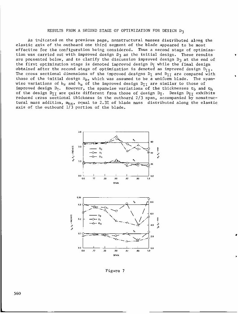
RESULTSFROMA SECONDSTAGEOFOPTIMIZATIONFORDESIGND3

As indicated on the previous page, nonstructural massesdistributed along theelastic axis of the outboard one third segment of the blade appeared to be mosteffective for the configuration being considered. Thus a second stage of optimiza-tion was carried out with improved design D3 as the initial design. These resultsare presented below, and to clarify the discussion improved design D3 at the end ofthe first optimization stage is denoted improved design DI while the final designobtained after the second stage of optimization is denoted as improved design DII.The cross sectional dimensions of the improved designs DI and DII are comparedwiththose of the initial design Do, which was assumedto be a uniform blade. The span-wise variations of bs and hs of the improved design DII are similar to those ofimproved design DI. However, the spanwise variations of the thicknesses tb and t hof the design DII are quite different from those of design DI. Design DII exhibitsreduced cross sectional thickness in the outboard 2/3 span, accompaniedby nonstruc-tural mass addition, mns, equal to 2.3% of blade mass distributed along the elasticaxis of the outboard 1/3 portion of the blade.

=-

=-

3.0

2.0

1.0

'_ _"_ bs - 60

__.--z-_---_-__' \. "_ A

D I 40

DII

0.0 I I I t I 0.0

0.0 .17 .33 .50 .67 .83 1.0

SPAN

EE

.="

J:

J=

0.35

0.3

0.2

0.1

0.0

0.0

_,.. / _ tb so

m DO "_

DII " " 4.

th

..--y-_-_--_. __O_..._.r _. _ 20-.--....,_.... __._..."_"

I I I I I o.o

.17 .33 .50 .67 .83 1.0

SPAN

Figure 7

560

ADDITIONALRESULTSFROMA SECONDSTAGEOFOPTIMIZATIONFORDESIGND3

The objective function used in the optimization was the value of the linearpeak-to-peak vertical hub shears at H = 0.30. In the tables presented below thereductions in vertical hub shears and rolling momentsat _ = 0.30 after twostages of optimization are presented. The terms linear and nonlinear in the tablesrefer to the inclusion of geometrically nonlinear effects due to moderate bladedeflections in the aeroelastic response calculation from which the hub shears androlling momentare obtained. In the nonlinear case the geometrical nonlinearitiesare included while in the linear case they are not. For design DII , the linearpeak-to-peak vertical hub shear was reduced by 37.9% and the nonlinear hub shear wasreduced by 35.9%. The corresponding reductions in the hub rolling momentswere24.17%and 25.2%, respectively. An interesting byproduct of the optimization isa reduction of total blade masswhich is shownat the bottom of the last table.In design DI only 0.2% of the blade massis added as nonstructural mass, whereasfor design DII 2.3% of the blade mass is added as nonstructural mass in the samelocations. Design Di produced a 8.7% reduction in total blade masswhile designDI_ resulted in a 19.7% reduction in total blade mass. An examination of the twoidesigns reveals that the reduction in blade mass at the outboard segments of the

blade is considerably higher than the reduction experienced by the inboard segments.

This indicates that one should be careful about violating constraints associated

with energy storage in the rotor, which can be important for autorotation.

A,

_Z --

VALUES

INITIAL

DESIGN D O

IMPROVED

DESIGN DII

REDUCTION

(Do-DII) %

DO

PEAK-

TO- 0.0575 0.0357 37.91%

LINEAR PEAK

MAXIMUM 0.2323 0.1787 23.07%

PEAK-

NON- TO- 0.0602 0.0386 35,88%

LINEAR PEAK

MAXIMUM 0.2363 0.1819 23.02%

PEAK-

TO- 0.0120 0.0091 24.17%

PEAK

MAXIMUM 0.1940 0,1331 31.39%

PEAK-

TO- 0.0119 0.0089 25.21%

PEAK

MAXIMUM 0.0946 0.1338 31.24%

z_

=_ N LINEAR

,,g%.J _

o z NON-_" _ LINEAR

_Z

oz

BLADE

MASS

REDUCTION

1st STAGE

8.7%

2nd STAGE

19.7%

Figure 8

561

VERTICALHUBSHEARSANDROLLINGMOMENTSFORDESIGNDII AS A FUNCTIONOF

As mentioned before, the objective function used in the optimization procedureis the linear expression of the hub shears at _ = 0.30. Therefore it is importantto examine the variation of the vertical hub shears and hub rolling momentsoverthe whole range of advance ratios o<_<0.30 considered. The figures below depictboth the variations of the peak-to-peak and the maximumvalues of the four-per-revvertical hub shears and hub rolling moments for the range of advance ratios.0<_<0.30. Furthermore, for the sake of completeness both the linear and the non-linear versions of these quantities are plotted. These results demonstrate thatfor the soft-in-plane configurations studied in this paper the choice of linearvertical hub shears at one particular moderately high advance ratio (_ = 0.30) asthe objective function is sufficient to guarantee a similar amount of reductionin the oscillatory vertical hub shears at the intermediate advance ratios.This statement is also supported by the behavior of the hub rolling moments, alsoshownbelow, which shows that improved design DII exhibits a consistent reductionin hub rolling momentscomparedto design Do over the whole range of advance ratiosconsidered. Additional results (Ref. 2) not presented here indicate similarreductions in root torsional moments. However in-plane hub shears experience onlya relatively minor reduction.

>

0.3

0.2

0.1

0.0

0.0

0.015

>_ 0.010

o

o.oos

0.00.0

NONLINEAR

O DO

z_ DII

I I I

0.1 0.2 0.3

NONLINEAR

O DO

0.1 O.2 O.3

0.4

0.4

Figure 9

0.6

0.4

0.2

NONLINEAR

O D O

DII

0.06

uJ

>_0.04

j,0.02

o.

0.0 I I I

0.0 0,1 0.2 0.3

0.00.0

O D O

I I J

0.4

0.1 0,2 0,3 0,4

562

CONCLUSIONSANDONGOINGEXTENSIONOFTHIS RESEARCH

The results described in the previous pages have indicated that by applyingmodernstructural optimization to the design of soft-in-plane hingeless rotors,vibratory hub shears in forward flight can be reduced by 15-40%. This reduction isachieved by relatively small modifications of the original design, which yieldoptimal frequency placement in flap, lag and torsion. It is also interesting tonote that as a byproduct of optimization, the optimized blade configuration isbetween 9-20%lighter than the initial uniform blade. This result is obtainedwithout using blade weight as the objective function in the optimization process.It is remarkable that these results are consistent with the needs expressed byBlackwell (Ref. 7) in a recent paper which advocates the need for designing bladesin such a manner as to reduce vibrations in helicopters. In his excellent paperBlackwell provides practical physical insight by considering the sensitivity ofblade vibrations to useful blade design parameters such as tip sweep, camber,blade mass and stiffness distribution, chordwise blade center of gravity offset fromthe aerodynamic center, chordwise center of gravity offset from the elastic axis,blade twist, and use of composite materials for tailoring of the vibrationalcharacteristics. Our current research is aimed at incorporating someof theseeffects in a structural optimization process based on the blade model shownbelow.The important effects incorporated are the swept tip and improved unsteady aero-dynamic modeling of the excitation. These two ingredients were selected because theswept tip is a powerful means for both modifying the vibratory response as well asoptimizing the aerodynamic and acoustic performance of the rotor. Similarly, vibra-tory loads are strongly dependent on improved capability for modeling the unsteadyaerodynamic environment.

INBOARD SEGMENT

PITCH CHANGE BEARING _ //

OUTBOARD SEGM_

SWASH PLATE

ROTOR HUB

PITCH LINK

Figure i0

563

OTHERASPECTS,LOCALFUSELAGEVIBRATIONREDUCTIONBY STRUCTURALMODIFICATION

The optimum blade design problem discussed previously attempts to reduce heli-copter vibrations by reducing the source of the vibratory excitation, namely thevibratory loads applied at the hub, as indicated in the figure below. During thedesign cycle of the helicopter the need for local vibration reduction at specificlocations in the fuselage or tail boom frequently arises. Various methods for localvibration reduction have been developed, such as vibration isolation devicesvibration absorbers and the use of local structural modification, which has beenintroduced by Done in Ref. 8. Whenusing the method of local structural modificationthe fuselage is represented by a number of easily identifiable substructures asshownbelow. A knownexcitation at the hub is assumed, and the sensitivity of theresponse at the pilot seat location (for example) is examinedas a result of intro-ducing a local structural modification consisting of either a change in massat apoint or a change in stiffness between two points (as represented by a spring),where these two quantities are assumedto be continuously varied. Using the frequen-cy response matrix of a dampedlinear system, the sensitivity of the response at thepilot seat location to modifications in each substructure is tabulated and the bestcandidate for modification is selected by a visual inspection of the results. SinceDone's work a numberof researchers have applied various variants of this approachto vibration reduction in the helicopter fuselage (Refs. 9-12). However it shouldbe noted that the methodhas not been coupled with an optimization approach based onthe mathematical programmingapproach. It appears that this problem is quite suit-able for treatment by multilevel decomposition along the lines indicated in Ref. 13,and in addition to constraints on vibration levels, other constraints can also beenforced on the substructure level.

XCITATION

Figure 11

564

AN

ARt

CW

Ib

os

mns

Mxl

nb

Pzl

Px,Py,P z

R

W

Y

U

_FI,_LI,_T1

_Fi,_Li,_Ti

SYMBOLS

= hs/b s

= tb/t h

= semi-chord nondimensionalized with respect to R

= weight coefficient = W/_2R 4

= blade flapping inertia

= length of elastic part of blade

= length defining outboard station where outboard blade segment starts

= nonstructural mass per unit length of the blade used as a tuning

weight

= hub rolling moment

= number of blades

= vertical hub shears

= distributed loading vectors per unit length of blade

= radius of the blade

= weight of the helicopter

= Lock number

= blade solidity ratio

= advance ratio

= speed of rotation (RPM)

= rotating uncoupled fundamental frequency of the blade in flap, lag

and torsion, respectively, nondimensionalized w.r.t.

= rotating uncoupled ith fundamental frequency of the blade in flap,

lag and torsion respectively, nondimensionalized w.r.t.

565

.

REFERENCES

Friedmann, P.P. and Shanthakumaran, P., "Aeroelastic Tailoring of Rotor Blades

for Vibration Reduction in Forward Flight", AIAA Paper 83-0916-CP, Proceedings

of AIAA/ASME/ASCE/AHS 24th Structures, Structural Dynamics and Materials

Conference, Lake Tahoe, NV, May 2-4, 1983, pp. 344-359.

1 Friedmann, P.P. and Shathakumaran, P., "Optimum Design of Rotor Blades for

Vibration Reduction in Forward Flight", Proceedings of the 39th Annual Forum

of the American Helicopter Society, St. Louis, MO, May 9-11, 1983, pp. 656-673.

. Shamie, J. and Friedmann, P., "Effects of Moderate Deflections on the Aero-

elastic Stability of a Rotor Blade in Forward Flight", Paper No. 24, Pro-

ceedings of the Third European Rotorcraft and Powered Lift Aircraft Forum,

Aix-en-Provence, France, 1977.

1 Friedmann, P.P. and Kottapalli, S.B.R., "Coupled Flap-Lag-Torsional Dynamics of

Hingeless Rotor Blades in Forward Flight", Journal of the American Helicopter

Society, Vol. 27, No. 4, pp. 28-36, October 1982.

5. Schmit, L.A. and Miura, H., "Approximation Concepts for Efficient Structural

Synthesis", NASA CR-2552, March 1976.

. Schmit, L.A., "Structural Optimization, Some Key Ideas and Insights", Interna-

tional Symposium on Optimum Structural Design, University of Arizona, Tucson,

October 1981.

7. Blackwell, R.H., "Blade Design for Reduced Helicopter Vibration", Journal of

the American Helicopter Society, Vol. 28, No. 3, July 1983, pp. 33-41.

8. Done, G.T.S., "Reducing Vibration by Structural Modification", Vertica, Vol. i,

No. i, 1976, pp.31-38.

. Hanson, H.W. and Calapodas, N.J., "Evaluation of the Practical Aspects of

Vibration Reduction Using Structural Optimization Techniques", Journal of the

American Helicopter Society, Vol. 25, No. 3, July 1980, pp. 37-45.

I0. Bartlett, F.D., "Flight Vibration Optimization Via Conformal Mapping", Journal

of the American Helicopter Society, Vol. 28, No. i, January 1983, pp. 49-55.

11. King, S.P., " The Modal Approach to Structural Modification", Journal of the

American Helicopter Society, Vol. 28, No. 2, April 1983, pp. 30-36.

12. Wang, B.P., Kitis, L., Pilkey, W.D. and Palazollo, A.B., "Helicopter Vibration

Reduction by Local Structural Modification", Journal of the American Heli-

copter Society, Vol. 27, No. 3, July 1982, pp. 43-47.

13. Sobieszczanki-Sobieski, J., James, B. and Dovit, A., "Structural Optimization

by Multilevel Decomposition", AIAA Paper 83-0832, Proceedings of 24th AIAA/

ASME/ASCE/AHS Structures, Structural Dynamics and Materials Conference,

May 2-4, 1983, pp. 124-143.

ACKNOWLEDGEMENT

A part of this research was funded by NASA Langley Research Center under NSG 1578.

This research is currently funded by NASA Ames Research Center under NAG 2-226.

566

N87-11753

HELICOPTER ROTOR BLADE AERODYNAMIC OPTIMIZATION

BY MATHEMATICAL PROGRAMING

Joanne L. WalshNASA Langley Research Center

Hampton, Virginia

Gene J. BinghamNASA Langley Research Center

Structures LaboratoryU.S. Army Research Technology Laboratories (AVSCOM)

Hampton, Virginia

and

Michael F. RileyKentron International, Inc.

Hampton, Virginia

567

INTRODUCTION

One of the goals in helicopter design is to improve hover and forward flightperformance. A way of achieving this goal is through the use of advanced(nonrectangular) rotor blades. Work in this area at the Army StructuresLaboratory (AVSCOM) located at the Langley Research Center is reported inreference i. The design goal is to reduce hover horsepower without degradingforward flight performance. Designs are generated by determining the influencesof rotor blade design variables (twist, percent taper, taper ratio, and solidity)on rotor performance and by adjusting these design variables to obtain desiredperformance. In reference I, an analytical procedure is described for evaluatingthe influences of the design variables on rotor performance. That procedure,referred to herein as the conventional approach, combines momentum and bladeelement theories (ref. 2) for the hover analysis and the Rotorcraft FlightSimulation Computer Program, C-81, (ref. 3) for the forward flight analysis.Advanced blades designed using the conventional approach have been evaluated intests in the Langley 4 x 7 meter wind tunnel; for example, performancepredictions have been verified for the UH-I baseline and advanced rotor blades(ref. 4).

Although the conventional approach has produced blade designs exhibiting improvedperformance, it is a tedious and time-consuming procedure. A researchertypically spends several weeks manipulating the rotor blade design variablesbefore reaching a final blade configuration. Using this approach, the researchermust have significant experience and data at hand. Any lack of experience anddata tends to increase the design time.

To avoid the tedious and time-consuming aspects of the conventional approacI_,mathematical programing techniques are being applied. Mathematical programinghas been used previously (refs. 5-8) to optimize helicopter rotor blades forvarious constraints, usually for improved aeroelastic behavior. The present workaddresses the rotor aerodynamic design and consists of coupling the hover andforward flight analysis programs with a general-purpose mathematical programingprocedure CONMIN (ref. 9). This mathematical programing design approachsystematically searches for a blade design which minimizes hover horsepower whileassuring satisfactory forward flight performance. This effort has been ongoingfor about a year and has reached a stage where satisfactory designs are providedby the procedure. The purpose of this paper is to describe how the mathematicalprograming approach was used to design an advanced rotor blade for arepresentative army helicopter, and to compare the resulting design and effortwith the design and effort for the conventional approach.

568

ORffiWAL PAGE 1%

IMPROVED PERFORMANCE OF PO(JR QUALm

Researchers a t t h e Langley Research Center a r e u s i n g exper imenta l and a n a l y t i c a l techniques t o improve r o t o r b lade performance i n bo th hover and fo rward f l i g h t . I n genera l , t h e blades on e x i s t i n g h e l i c o p t e r s have a r e c t a n g u l a r planform. Researchers have found t h a t they can improve h e l i c o p t e r performance, i.e., lower t h e r e q u i r e d horsepower, by t a p e r i n g the r o t o r blades. F i g u r e 1 shows horsepower r e q u i r e d versus v e l o c i t y p l o t s f o r three d i f f e r e n t advanced ( tapered) blades. I n each case, t h e advanced b lade requ i res l e s s horsepower than t h e b a s e l i n e ( r e c t a n g u l a r ) blade. advanced b lades f o r t h e t h r e e h e l i c o p t e r s (UH-1, UH-60, and AH-64) shown i n t h e t h r e e p l o t s were ob ta ined u s i n g t h e analyses of references 2 and 3. base1 i ne and advanced blades have been e v a l uated exper imenta l l y a t Langley, t h e UH-1, UH-60, and AH-64 f o r hover and the UH-1 and AH-64 f o r fo rward f l i g h t . I n a l l cases, t h e a n a l y t i c a l performance p r e d i c t i o n s agree w e l l w i t h t h e exper imenta l r e s u l t s .

The performance p r e d i c t i o n s f o r bo th t h e b a s e l i n e and

Both t h e

iAMALYslB Figure 1

569

• _ '_ ROTOR BLADE AERODYNAMIC DESIGN

The key aspects of the aerodynamic rotor blade design problem are illustrated in

figure 2. The design objective (goal) is to reduce the hover horsepower while

not degrading forward-flight performance. This reduction in horsepower is to beachieved for a helicopter with a specified design gross weight operating at a

specified altitude and temperature. In this study, forward-flight performance isdefined in terms of three requirements (constraints). First, the horsepower

required, hpr, for forward flight at a specified maximum (or design) horizontal

velocity, VH, must be less than the available horsepower, hpa. Second, the

helicopter must be able to sustain a pullup maneuver, i.e., the aircraft must

operate trimmed at a gross weight equal to a specified load factor multiplied by

the design gross weight at a second specified horizontal velocity, V_f, less

than VH. Third, the airfoil sections distributed along the rotor blade must

operate at section drag coefficients (or pitching moment coefficients) less than

a specified value (to avoid excessive helicopter vibration and control loads).

Two analysis computer programs are used to predict performance. The hover

analysis combines momentum and blade element theories (ref. 2). The Rotorcraft

Flight Simulation Computer Program, C-81, is used for forward flight. Only the

quasi-static trim option is used from C-81. The analyses use experimentally

derived 2-D airfoil data tables (provided by the designer) and segment the bladeinto 20 radial stations. The designer can assign one of five airfoil shapes ateach station. The choice of airfoil remains fixed throughout the analyses.

Performance predictions from both analyses have been verified experimentally.

The quantities which are varied in order to improve performance are taper ratio,

percent taper, twist, and solidity.

GOAL -REDUCE HOVER HORSEPOWER

DESIGN REQUIREMENTS- FORWARD FLIGHT PERFORMANCE

< AT SPECIFIED V H AND GROSS WEIGHT• hp r = hPa

• SUSTAIN PULL-UP MANEUVER

• AVOID AIRFOIL SECTION STALL

ANALYSIS TOOLS - HOVER (MOMENTUM AND BLADE ELEMENTTHEORIES)

FORWARD FLIGHT (C-81)

• 2-D AIRFOIL DATA• UP TO .5 DIFFERENTAIRFOIL SHAPES

• ANALYSES VERIFIED EXPERIMENTALLY

DESIGN VARIABLES - MAXIMUM TWIST, PERCENTTAPER, TAPER RATIO,AND SOLIDITY

Figure 2

570

ROTOR BLADE DESIGN VARIABLES

The design variables (percent taper, taper ratio, solidity, and twist) areillustrated in figure 3. The percent taper (also known as point of taperinitiation), r/R, defines the relative radial location r at which taper begins.The blade is rectangular up to this point and then is tapered to the tip. Ablade with zero percent taper is rectangular. The taper ratio is cr/c _ wherec r is the chord at the point of taper initiation and c t is the tip chord. Ablade with a taper ratio of 1.0 is rectangular. The blade solidity, _, is theratio of the sum of the blade areas to the rotor disk area, _R2, where R is theblade radius. In the present work, the design variable which defines solidityis the chord c r. The dashed-line blade in figure 3 represents a blade withincreased solidity over the solid-line blade. Twist, indicated in the lowerportion of the figure, is varied linearly from the root to the tip. The twistdesign variable is the maximum twist indicated by Tmax.

_°1_.._ 702> °1

I R

PERCENT TAPER r/R

TAPER RATIO Cr/C t

SOLIDITY

TWIST

Ano = n =no. OF BLADES

7TR2 '

Ir_I_-A = BLADE AREA

Z_n 4

Cr-__

"rmax _/_

Figure 3

571

CONVENTIONAL APPROACH

The conventional rotor blade design approach is a two-step method as indicated infigure 4. Only a cursory description will be given here. A more detailedexplanation can be found in reference I. The rotor blade is designed first forhover using the analysis based on reference 2. The designer changes the valuesof taper ratio and percent taper to reduce hover ho'rsepower. Then he changes thevalue of twist and repeats the above process. He continues to manipulate thesethree design variables until he arrives at the rotor blade configuration with thelowest hover horsepower. Next, he compromises this best hover design to meetforward flight requirements. He does this by varying the fourth design variable,solidity, as well as the original design variables. Solidity is primarilyinfluenced by design requirements on the pullup maneuver and airfoil stall. Thesolidity must be adequate for the pullup maneuver. Greater solidity is generallyrequired to meet the forward-flight design constraints but it compromises thebest hover design by increasing the horsepower.

Using the conventional approach, the designer is actively involved inmanipulating the design variables and deciding on design changes. He must relyon his previous experience and intuition. He is the communications link betweenthe hover and forward flight analyses. This approach involves parametric studiesand extensive cross-plots and is very time consuming. A typical design requires4-6 weeks.

572

METHOD

• DESIGN FOR HOVER ONLY. REDUCE HOVER HORSEPOWER BY

CONSIDERING INFLUENCES OF

• TAPER RATIO AND PERCENT TAPER

• TWIST

• COMPROMISE "BEST HOVER" DESIGN TO MEET FORWARD FLIGHT

REQUIREMENTS

< AT V H AND DESIGN GW• hp r = hPa

• SUSTAIN PULLUP MANEUVER

• AVOID AIRFOIL STALL

DESIGNER ACTIVELY INVOLVED

• DATA BASE

• PREVIOUS EXPERIENCE

IFORWARD FLIGHT_ HOVERPERFORMANCE ANALYSI S

T IME-CONSUMI NG

• PARAMETRIC STUDIES, CROSS PLOTS• REQUIRES 4-6 WEEKS TOTAL DESIGNER TIME

Figure 4

MATHEMATICALPROGRAMINGAPPROACH

The mathematical programing approach is illustrated in figure 5. This approachuses the same rotor performance analyses discussed previously but, in addition,

couples an optimizer to the analyses. When the designer uses mathematical

programing methods, he must define the problem in terms of an objective function

(the quantity to be minimized), a set of design variables (the quantities which

are changed in order to minimize the objective function), and a set of

constraints (requirements which must be satisfied). Once the designer has

defined the problem in these terms, which is no easy task, he is not as actively

involved in manipulating the design variables. Instead, the optimizer takes over

the role of manipulating the design variables to arrive at the best blade

design. With the mathematical programing approach, changes in the design

variables simultaneously affect both the hover analysis and the forward flight

performance analysis.

The optimizer used in this study is CONMIN (ref. 9) which is a well-established,

general-purpose optimization program. CONMIN requires the use of gradients which

in this application are determined by finite differences calculated internally byCONMIN.

• METHOD

• COUPLE OPTIMIZER (CONMIN) TO ANALYSIS TOOLS

• DEFI NE

• OBJECTIVE FUNCTION

• DESIGN VARIABLES

• CONSTRAINTS

DESIGNER NOT AS ACTIVELY INVOLVED

1.ovE I_ANALYSI S

FORWARDFLIGHT

PERFORMANCE

__OPTIMIZER I(CONMIN) I

SIMULTANEOUSLYCONSIDERS INFLUENCESOF TWIST, PERCENTTAPER,TAPER RATIO, AND SOLIDITY ON BOTH HOVER AND FORWARD FLIGHTPERFORMANCE

Figure 5

573

FORMULATION OF OPTIMIZATION PROBLEM BY MATHEMATICAL PROGRAMING

The mathematical programing formulation of the rotor blade design problem is

shown in figure 6. The objective function is the required hover horsepower. The

design variables are twist, percent taper, taper ratio, and solidity. The chord

cr controls solidity. The forward flight requirements translate into 14constraints and are obtained from the C-81 program. By CONMIN sign convention a

constraint, gi, is satisfied if it is negative or zero and violated if it is

positive.

The first constraint (eq. (1)) is that horsepower required for forward flight at

the design gross weight and the specified horizontal velocity VH not exceed thehorsepower available. The second constraint on pullup maneuver is more difficult

to translate into a mathematical programing context. The constraint on pullup

maneuver is implemented by determining from C-81 whether or not the helicopter

can trim at a gross weight equal to a load factor multiplied by the design gross

weight at a specified velocity VAf. Since experience indicates that the fail-ure of the helicopter to trim is an indication that the solidity is too small,

the trim contraint, gi, is formulated as shown in equation (2). The constraint

is set equal to -0.5 (satisfied) if trim occurs and equal to 10 - 0.5c r (notsatisfied) if trim does not occur. The final design requirement on airfoil stalltranslates easily into mathematical programing language as shown in equation

(3). This constraint is to impose restraints on the airfoil section drag

coefficient, CD. This requirement translates into 12 constraints since the

CD'S are evaluated every 30 degrees around the azimuth. An alternative (notyet implemented) would be to express the constraint in terms of the pitching

moment coefficient, Cm, which is more consistent with aeroelastic designrequirements.

• OBJECTIVE FUNCTION: HOVER HORSEPOWER

• DESIGN VARIABLES: TWIST, PERCENT TAPER, TAPER RATIO, SOLIDITY

< O SATISFIED, gi > 0 VIOLATED)CONSTRAINTS: (gi =

• HORSEPOWER REQUIRED

gl = hPr lhPa -i(1)

• PULL-UP MANEUVER

l-O.5, IF TRIMMED

g2 = _.10.-0.5c r, IF NOT TRIMMED

(2)

• AIRFOIL SECTION STALL

-1,gk CDICDm_x

12 AZIMUTHAL LOCATIONS

Figure 6

(3)

574

COMPARISON OF RESULTS FOR ADVANCED ROTOR BLADE

Rotor blade designs obtained using both the conventional and mathematicalprograming approaches are shown for a representative army helicopter (fig. 7).The goal is to find the blade design which has the lowest hover horsepower fora four-bladed helicopter with a design gross weight of 15,000 pounds and a hori-zontal velocity of 160 knots. The selected pullup maneuver requires a load factorof 1.33 (or 20,000 pounds) at a velocity of I00 knots. Both approaches startedfrom a rectangular blade which has a twist of -9.0 degrees and a solidity of0.09285. Both designs are substantial improvements over the rectangular blade.The overall designs are very similar with slight variations in the details. Thereis a significant difference in the total design time. Results obtained usingthe mathematical programing approach took 2 days. Those obtained using the con-ventional approach took 5 weeks.

DESIGN GROSS WEIGHT = 15,000 Ib

HORIZONTAL VELOCITY = 160 knots

LOAD FACTOR = 1.33 (20000 Ib)AT VLF = I00 knots

BASELI NE

(RECTANGULAR) CONVENTIONAL*

MATHEMATI CAL

PROGRAMING*

HOVER HORSEPOWER 1672 hp 1558 hp 1555 hp

TWI ST -9 ° -12 ° -I0. 6°

PERCENT TAPER 0 .80 .85

TAPER RATIO 1.0 3.0 3.1

SOL I D I TY (aT) .093 .098 .092

(Cr.) (1.75ft) (2.23 ft) (2.0ft)

DESIGN TIME 5 WEEKS 2 DAYS

*BOTH APPROACHES STARTED FROM BASELINE (RECTANGULAR) DESIGN

Figure 7

575

OBSERVATIONS ON DEVELOPMENT OF THE MATHEMATICAL PROGRAMING SYSTEM

In development of the mathematical programing system, communication played amajor role. The participants had to bridge their knowledge gap between the

rotorcraft aerodynamics and optimization disciplines. For example, the rotor

blade designer had to explain helicopter aerodynamic terminology, while the

optimization specialist had to explain mathematical programing terminology. Once

they had exchanged jargon, they could begin the problem definition. The rotorblade designer had to explain the overall design problem - what he wanted to do,

what analysis methods he used, and what trade-offs he considered. Some design

requirements were easy to translate into mathematical programing terms. Others,such as the pullup manuever, were very difficult to translate. Early discussions

revealed most of the information, but some of the intuitive reasoning used in theconventional approach was slow to surface. In fact some of the intuitive

reasoning is still surfacing. Practical design limits which are almost implicit

in the conventional approach need to be made explicit in the mathematical

programing approach. For example, the solidity was originally controlled by achord multiplication factor which was allowed to vary within wide limits.

However, in one extreme case this resulted in a blade design which wasexcessively wide and impractical to use on a helicopter. The rotor blade

designer would intuitively disregard such a design, but the optimization process

as formulated did not. A subsequent reformulation of the solidity designvariable with appropriate limits eliminated this design. (See fig. 8.)

BASIC COMMUNICATION

• JARGON EXCHANGE

• PROBLEM DEFINITION

FINDING OUT HOW CONVENTIONAL DESIGNER APPROACHES THE PROBLEM

• ANALYSIS METHODS

• TRADE-OFFS

A LOT OF TALKING REQUIRED

• EARLY DISCUSSIONS REVEALED MOST OF THE INFORMATION

• INTUITIVE REASONING MORE DIFFICULT TO SURFACE

Figure 8

576

PLANS

We plan to continue developing and improving the mathematical programing

approach (fig. 9). Plans are to replace the drag coeffient in the airfoil

section stall constraint (eq. 3, fig. 6) by the pitching moment coeffient to be

consistent with aeroelastic design requirements. Plans include improving thetrim constraint (eq. 2, fig. 6), a continuous trim constraint being evaluated

speeds up convergence. Plans also include applying the mathematical programing

approach to different helicopter configurations. We are also looking at ways to

speed up clock turnaround time. This includes speeding up computation time by

design variable scaling. We are presently limited to overnight turnaround

because of the memory requirements for the C-81 program, which, even though it is

overlaid, requires almost the entire memory of a CYBER 173 computer. We are

looking at extracting only those subroutines needed for the quasi-static trim

analysis. We also plan to use airfoils as design variables. Eventually, we plan

to add static (loads) and dynamic (vibrations) structural constraints.

• CHANGE CD TO CM IN AIRFOIL SECTION STALL CONSTRAINTS

• IMPROVE TRIM (pullup maneuver) CONSTRAINT

• APPLY TO DIFFERENT HELICOPTER CONFIGURATIONS

• SPEED UP COMPUTERTIME

• AIRFOILS AS DESIGN VARIABLES

• INCLUDE STATIC AND DYNAMIC STRUCTURAL CONSTRAINTS

Figure 9

577

CONCLUDINGREMARKS

Formal mathematical programing has been applied to the aerodynamic rotor bladedesign process. The approach is to couple hover and forward flight analysisprograms with the general-purpose optimization program CONMINto determine theblade taper ratio, percent taper, twist distribution, and solidity which minimizethe horsepower required at hover while meeting constraints on forward flightperformance. Designs obtained using this approach for the blade of arepresentative army helicopter comparewell with those obtained using aconventional approach involving personnel-intensive parametric studies. Resultsfrom the present method can be obtained in 2 days as comparedto 5 weeks requiredby the conventional procedure. Also the systematic manipulation of the designvariables by the optimization procedure minimizes the need for the researcher tohave a vast body of past experience and data in determining the influence of adesign change on the performance. Plans are to continue evaluation of the methodfor additional rotor blade configurations and refine the procedure.

REFERENCES

.

.

.

.

.

.

.

.

.

578

Bingham, Gene J.: The Aerodynamic Influences of Rotor Blade Taper, Twist,Airfoils, and Solidity on Hover and Forward Flight Performance. 37thAnnual Forum of the American Helicopter Society, New Orleans, Louisiana,May 1981.

Gessow, Alfred; and Myers, Garry C., Jr.: Aerodynamics of the Helicopters.Frederick Unger Publishing Company, New York, 1952.

Van Gaasbeck, J. R.: Rotorcraft Flight Simulation, Computer Program C-81.USARTL-TR-77-54B, 1979.

Berry, John D.: Quarter Scale Testing of an Advanced Rotor System for theUH-I Helicopter. 37th Annual Forum of the American Helicopter Society, NewOrleans, Louisiana, May 1981.

Kitis, L.; Pilkey, W. D.; and Wang, B. P.:Modification by Added Passive Structures.November 1983.

Optimal Frequency ResponseJ. of Aircraft, Vol. 20, No. 11,

Peters, D. A.; Ko, T.; and Ross.w, M. P.: Design of Helicopter Rotor Bladesfor Desired Placement of Natural Frequencies. 39th Annual Forum of theAmerican Helicopter Society, St. Louis, MO, May 1983.

Friedmann, P. P.; and Shanthakumaran, P.: Aeroelastic Tailoring of RotorBlades for Vibration Reduction in Forward Flight. AIAA/ASME/ASCE/AHS 24thStructures, Structural Dynamics and Materials Conference, May 2-4, 1983,Lake Tahoe, Nevada.

Bennett, R. L.: Application of Optimization Methods to Rotor DesignProblems. Vertica, Vol. 7, No. 3, pp 201-208, 1983.

Vanderplaats, G. N.: CONMIN - A Fortran Program for Constrained FunctionMinimization - User's Manual. NASA TM X-62282, August 1973.

N87-11754

REGRESSION ANALYSIS

AS A DESIGN OPTIMIZATION TOOL

Richmond Perley

Kaman Aerospace Corporation

Bloomfield, Connecticut

579

SUMMARY

This presentation is organized in four parts. First is a discussion of thegeneralized design problem and how it differs from a detailed, final design problem.The optimization process and a role for regression analysis are addressed. This isfollowed by the performance index, or objective function, and basic search strategyused.

The discussion of program implementation includes a description of someof theauxiliary outputs available. Finally, someconclusions are given about the value ofregression analysis as a design optimization tool.

1. GENERALIZED DESIGN PROBLEM

A. OPTIMIZATION LOOP

B. OPTIMIZATION LOOP CONSIDERATIONS

C. REGRESSION ANALYSIS CONSIDERATIONS

D. COMPUTATIONAL REQUIREMENTS - A FIGURE OF MERIT

2. PERFORMANCE INDEX (OBJECTIVE FUNCTION)

A. PERFORMANCE INDEX EQUATIONS

B. BASIC SEARCH STRATEGY

3. PROGRAM IMPLEMENTATION

A. SENSITIVITIES

B. TRADEOFF STUDY

C. CONTOUR PLOTS

4. VALUE OF REGRESSION ANALYSIS

58O

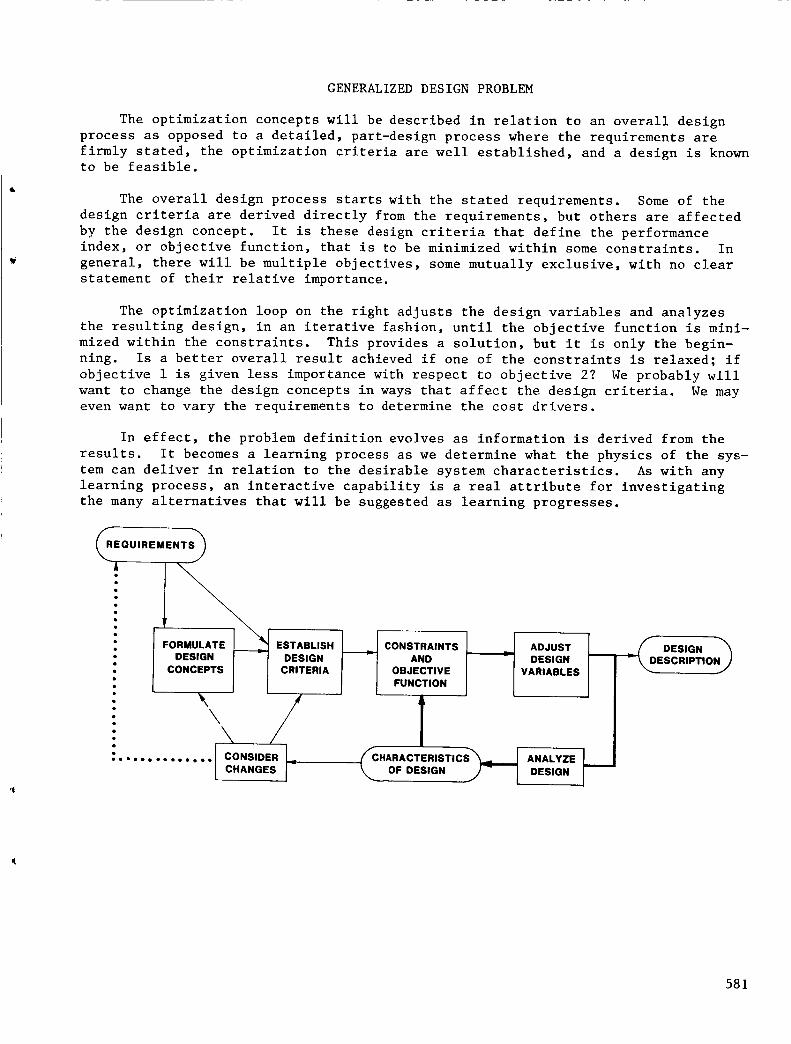
GENERALIZED DESIGN PROBLEM

The optimization concepts will be described in relation to an overall design

process as opposed to a detailed, part-design process where the requirements are

firmly stated, the optimization criteria are well established, and a design is knownto be feasible.

The overall design process starts with the stated requirements. Some of the

design criteria are derived directly from the requirements, but others are affected

by the design concept. It is these design criteria that define the performance

index, or objective function, that is to be minimized within some constraints. In

general, there will be multiple objectives, some mutually exclusive, with no clear

statement of their relative importance.

The optimization loop on the right adjusts the design variables and analyzes

the resulting design, in an iterative fashion, until the objective function is mini-

mized within the constraints. This provides a solution, but it is only the begin-

ning. Is a better overall result achieved if one of the constraints is relaxed; if

objective i is given less importance with respect to objective 2? We probably will

want to change the design concepts in ways that affect the design criteria. We may

even want to vary the requirements to determine the cost drivers.

In effect, the problem definition evolves as information is derived from the

results. It becomes a learning process as we determine what the physics of the sys-

tem can deliver in relation to the desirable system characteristics. As with any

learning process, an interactive capability is a real attribute for investigating

the many alternatives that will be suggested as learning progresses.

__EQUIREMENTS_

' !• [ -

•. , //: \: ',,

• 1: ............. CONSIDER L

CHANGES 1-

ESTABLISH_CONSTRAINTSDEsIGNANDCRITERIA OBJECTIVE

FUNCTION ADJUST

DESIGNVARIABLES

T_CHARACTERISTICS_I _ ANALYZE

OFD_SIGNJ- LDESIGN

__D DESIGN "_

ESCRPTONJ

581

OPTIMIZATION LOOP

The optimization loop involves two functions. The optimizer contains the stra-

tegies for adjusting the design variables until the objective function is minimized.

The analyzer determines the characteristics of the design from the values of the

design variables.

The analyzer used is always a compromise between accuracy, or representative-

ness, and ease of use and computational requirements. The physical processes to be

analyzed are often extremely complex and do not have direct solutions. Large matrix

inversions, finite difference methods, and the iterative solutions of aeroelastic

problems are a few examples. One approach to this compromise is to partition the

analyzer into recurring and non-recurring portions, i.e., a portion that is a func-

tion of the design variables and a portion that is not.

Since most design optimization problems are non-linear, several iterations of

the optimization loop are required to reach a solution for one set of initial

values. Depending on the degree of non-linearity, there may be several minima and

the solution found often depends on the starting point. Therefore, the process must

be started from a number of points distributed throughout the design space in order

to find the "global" minimum. This is further reason for minimizing computational

requirements.

CONSTRAINTS

AND

OBJECTIVE

FUNCTION

HARACTERISTICS _, <

OF DESIGN J

I_ITIAL VALUE_

GRADIENT

DATA

I ANALYZER

582

OPTIMIZATIONLOOPCONSIDERATIONS

The efficacy of the optimizer is a function of the types and quality of infor-mation available from the analyzer. With first gradients, it can estimate direc-tions in which to move. With second gradients, it can estimate how far to movealong each axis of the design space. If gradient information is obtained from theanalyzer through first and second differences, the convergence-limit "noise" of iter-ative solutions and the resolution-limit "noise" of matrix inversions can producelarge errors in the first gradients and make the second gradients almost unusable.The analytical solutions to manyof the physical processes of interest in designoptimization do not provide direct calculation of gradients.

O FIRST GRADIENT

o SECOND GRADIENT (HESSIAN)

o FIRST AND SECOND DIFFERENCES

- CONVERGENCE "NOISE"

- RESOLUTION "NOISE"

583

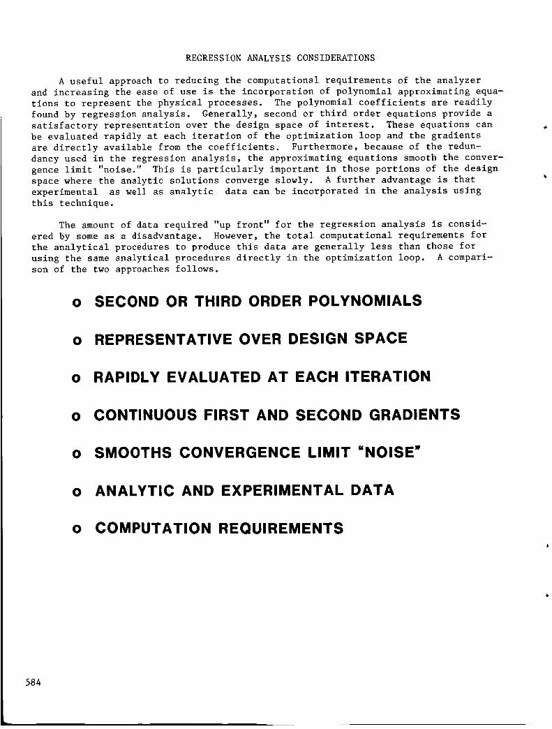
REGRESSIONANALYSISCONSIDERATIONS

A useful approach to reducing the computational requirements of the analyzerand increasing the ease of use is the incorporation of polynomial approximating equa-tions to represent the physical processes. The polynomial coefficients are readilyfound by regression analysis. Generally, second or third order equations provide asatisfactory representation over the design space of interest. These equations canbe evaluated rapidly at each iteration of the optimization loop and the gradientsare directly available from the coefficients. Furthermore, because of the redun-dancy used in the regression analysis, the approximating equations smooth the conver-gence limit "noise." This is particularly important in those portions of the designspace where the analytic solutions converge slowly. A further advantage is thatexperimental as well as analytic data can be incorporated in the analysis usingthis technique.

The amount of data required "up front" for the regression analysis is consid-ered by someas a disadvantage. However, the total computational requirements forthe analytical procedures to produce this data are generally less than those forusing the sameanalytical procedures directly in the optimization loop. A compari-son of the two approaches follows.

O SECOND OR THIRD ORDER POLYNOMIALS

O REPRESENTATIVE OVER DESIGN SPACE

O RAPIDLY EVALUATED AT EACH ITERATION

O CONTINUOUS FIRST AND SECOND GRADIENTS

O SMOOTHS CONVERGENCE LIMIT "NOISE"

o ANALYTIC AND EXPERIMENTAL DATA

o COMPUTATION REQUIREMENTS

584

COMPUTATIONALREQUIREMENTS- A FIGUREOFMERIT

The computational requirement for each data point required by the regressionanalysis is the sameas the requirement for each call to the analytical procedurewhen it is used directly by the optimizer. Therefore, a figure of merit thatreflects the computational advantage of the regression equations is the ratio of thenumberof calls to the analyzer by the optimizer to the number of data pointsrequired by the regression analysis.

Our experience shows that the numberof data points required for the regressionanalysis lies somewherebetween the numberof terms in a full cubic and three timesthe numberof terms in a full quadratic equation. These are shownas the upper andlower bounds as the numberof design variables, N, becomeslarge.

The numberof optimizer calls to the analyzer depends on a number of factors onwhich there is no universal agreement; however, upper and lower values for each aresuggested. The numberof starts/problem depends on the number of minima and is cer-tainly conservative since the design space has 2N ""corners. The number of problemsrefers to the number of times the problem statement is changed, as discussed pre-viously. The value of K depends on the newnessof the design problem and the inter-ests of the designer, but is certainly greater than unity.

It can be seen that the ratio is always greater than I, a regression advantage,unless direct use is at its lower value; regression is at its upper bound; and thenumber of design variables, N, is greater than 15 times K. The expected ratio isabout 10 times K. While the regression requirements may approach those of directuse, having once prepared the equations, the computational requirements of optimiza-tion are reduced to the point where an interactive process becomesa reality.

DIRECT USE BY ANALYZER

UPPER LOWER FACTOR

10 (N+ 3) -_- (N +3) CALLS/START

FIGURE OF MERIT =

(DIRECT USE)

(REGRESSION ANALYSIS)

REGRESSION ANALYSIS

UPPER

N 8 Nit 1 _ N_ + +--+1_

itN 3

G

3 N 2

2

LOWER

$ (--_-+ -_ + 1) ----

N

NK

10 NSK

60 K

20 NK

K

s N2X

1SK

N

6K

S

STARTS/PROBLEM

NO. OF PROBLEM8

PRODUCT

GEOMETRIC

MEAN = 10 K

585

PERFORMANCEINDEX(OBJECTIVEFUNCTION)

A weighted sumof squares of the dependent variables is the form selected forthe performance index, or objective function, because of its flexibility. Evenwithsingle objectives, it is usually the magnitude that is to be minimized, as opposedto a minimization in the algebraic sense. Multiple objectives are ideally combinedon a sum-of-squares basis since often they are mutually exclusive and the user'svalue function is generally elliptic. Vibration is one of the key items consideredin helicopter design. The quantity to be minimized is the vector sumof the realand imaginary componentsof the hub forces and momentsas they are transmittedthroughout the airframe, as well as the vibratory stresses in the rotor blades them-selves. Tradeoffs amongthe importance of the various objectives and vibrationlevels at various points in the airframe can be readily accomplished by varying theweighting factors. Constraints can also be accommodatedas penalty functions byintroducing bias levels.

O WEIGHTED SUM OF SQUARES

O SINGLE OBJECTIVE

o MULTIPLE OBJECTIVES

o VIBRATION

o TRADEOFFS

o CONSTRAINTS

586

PERFORMANCEINDEXEQUATIONS

The form of the performance index to be minimized, PI, is shown. The weightingfactors, Wh, and bias levels, Bh, are provided as real time user inputs so that

tradeoffs can be conducted in an interactive mode. The dependent variables Yh arecalculated from the polynomial approximating equations. The first and second grad-ients with respect to each of the design variables are calculated directly from thecoefficients of the approximating equations. Quantities to be maximized are given anegative weighting factor.

Constraints are accommodatedas penalty functions by setting the bias value,Bh, equal to the constraint value. It is usually necessary to start with a smallweighting factor and then increase it to moveas close to the constraint value asdesired. For "greater than" or "less than" constraints, Wh is zero when the con-straint is not violated and positive or negative, as appropriate, when it is vio-lated.

PI = _ Wh (Yh - Bh)2h

GRADIENTS

Wh, Bh = USERINPUTS

Yh = f (Xl' x2' " Xn)

aYhVPI (f) = axfapI= 2 h_Wh (Yh - Bh) axf

a2pI _ [ a2YhV2pI Cf'g) = aXg axf 2 Z wh CYh - Bh) ax axfh g aY h aY h ]+ aXg'aXf

587

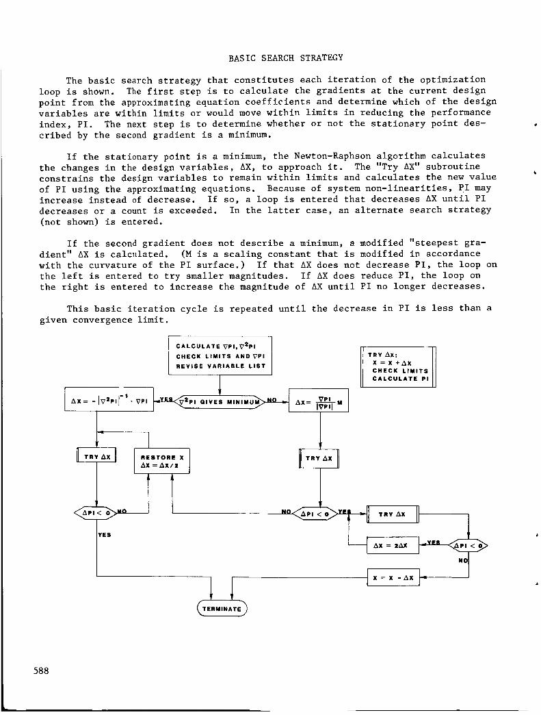
BASICSEARCHSTRATEGY

The basic search strategy that constitutes each iteration of the optimizationloop is shown. The first step is to calculate the gradients at the current designpoint from the approximating equation coefficients and determine which of the designvariables are within limits or would movewithin limits in reducing the performanceindex, PI. The next step is to determine whether or not the stationary point des-cribed by the second gradient is a minimum.

If the stationary point is a minimum, the Newton-Raphsonalgorithm calculatesthe changes in the design variables, AX, to approach it. The "Try AX" subroutineconstrains the design variables to remain within limits and calculates the new valueof PI using the approximating equations. Becauseof system non-linearities, PI mayincrease instead of decrease. If so, a loop is entered that decreases AX until PIdecreases or a count is exceeded. In the latter case, an alternate search strategy(not shown) is entered.

If the second gradient does not describe a minimum, a modified "steepest gra-dient" AX is calculated. (M is a scaling constant that is modified in accordancewith the curvature of the PI surface.) If that AXdoes not decrease PI, the loop onthe left is entered to try smaller magnitudes. If AXdoes reduce PI, the loop onthe right is entered to increase the magnitude of AXuntil PI no longer decreases.

This basic iteration cycle is repeated until the decrease in PI is less than agiven convergence limit.

CALCULATE VPI, _2pI

CHECK LIMITS AND VPI

REVISE VARIABLE LIST

- 1- 1_r

I rR .T°R,

YES

TRY _X:

X=X+AX

CHECK LIMITS

CALCULATE PI

NO_ TRY AX

i .....X = -X - AX _

588

PROGRAMIMPLEMENTATION

The concepts just described have been implemented on a DEC20time-sharing sys-tem in BASIC. The user calls the file that contains the approximating equation coef-ficients for the problem of interest and goes to work. Commandsare used to initi-ate the manyoptions and capabilities available in the program. Wehave applied itto a numberof design problems, one of which will be described in another presenta-tion. Performance has been good. In one problem involving seven design variablesand seven dependent variables, the average amount of CPUtime to find a minimumofthe performance index from any start point was under four seconds.

Several kinds of output are available to help the user gain insight into therelationships involved in the problems. Sensitivities, tradeoffs, and contour plotsare but three examples. The latter two are practical because of the rapidity withwhich the conditions at any design point can be calculated using the approximatingequations.

o DEC20 TIME SHARE - BASIC

0 INTERACTIVE PROCESSING

o 4 SECONDS OF CPU PER SEARCH

o AUXILIARY CAPABILITIES

- SENSITIVITIES

- TRADEOFFS

- CONTOUR PLOTS

589

SENSITIVITIES

This shows a table of the first derivatives of each of the dependent variables,downthe left (rotor power, maximumand minimumangle of attack, blade bendingmoment, hub shear force and pitching moment, and control load), with respect to eachof the design variables, across the top (blade bending frequency and mode, torsionmode, retention frequency, sweepangle, blade twist, and torsion frequency). Thefirst and Secondderivatives of the performance index at any design point and forany set of weighting factors can also be tabulated.

DESIGN VARIABLES

BF BMD TMD RF SWP TWST TF

HP 0.103 -0.007 0.274 -0.010 0.010 0.248 -0.119

U)W,.Jm,<mm

E<

I-ZWaZWn_Wa

AMAX 0.013 -0.029 -0.029 0.031 0.214 -0.478 0.466

AMIN 0.370 0.207 -0.514 0.000 -1.334 1.431 -1.321

BBM -2.424 -0.012 0.387 3.694 0.483 0.156 -1.047

THS 0.278 0.993 -0.002 2.323 1.428 -0.341 -0.115

PM -6.739 1.601 1.346 2.587 0.181 -0.339 2.046

PHL 0.468 0.000 -0.258 -0.095 6.672 -0.583 -0.518

590

TRADEOFF STUDY

An example of a tradeoff study is a rotor design problem that was concerned

with vibration. The optimization process was started with all weighting factors

except those on vibration terms equal to zero. A minimum was found where the vibra-

tion level was only 1.4% of the baseline value. However, the pitch horn load was

2.4 times the baseline value and was considered too high. The weighting factor on

pitch horn load was then increased and optimization was repeated. By doing this a

number of times, the curve below was generated. The double circle denotes the ini-

tial design point and the weighting factor is given at each optimization point.

This shows that pitch horn load can be decreased below the baseline value while

still retaining a vibration level of less than 9%. CPU time was not measured, but

the total time was less than ten minutes.

2.5

2.0

a<0 1.5.J

--I

0n-l--z0 1.0(.1

.5

0

2 4

O4

14 16

591

CONTOUR PLOTS

Contour plots can be generated that show any dependent variable or the perfor-

mance index with any set of weighting factors as a function of any two of the design

variables. This example is from the seven-variable rotor design problem and shows

vibration level. It helps to explain some of the multiple minima that were found.

There is a saddle point near the center and a ridge that goes from top to bottom.

If the optimization process is started anywhere to the left of that ridge, it goes

to the minimum at the lower left. Otherwise, it goes to the minimum near the right

center.

-30

-ZO ._ /o_'0

-..., 80

,ix \-. \

%

' [ 1_0 : , , , ,

1.04 1.06 l.O_ l.lO I.IZ 1.13

VIBRATION ( PERCENT OF BASELINE)

592

VALUE OF REGRESSION ANALYSIS

Our experience to date has convinced us of the value of regression analysis in

the design optimization process. One obvious advantage is the broadening of the

choice of search strategies made possible by the simple approximating equations and

their derivatives. The search strategy just described is by no means the best that

can be achieved, but it has proven its worth.

The relative ease of doing tradeoffs among the design criteria means that

answers will be found to questions that would be ignored in a more complex world.

And some of those answers will be worthwhile.

Perhaps the greatest benefit is the interactive learning that can now take

place. Answers lead to more questions, their answers, and then more questions.

However, if it takes a day, or even a few hours, for an answer to come back, the

whole thought process may be lost. The history of engineering design activities is

full of examples of the benefits of an interactive process vs a batch process, not

simply in reducing the cost of the design process, but in improving the quality of

the resulting design.

O CHOICE OF SEARCH STRATEGIES

o TRADEOFF STUDIES

o INTERACTIVE LEARNING

593

Ns÷:11 5 5

A ROTOR OPTIMIZATION USING

REGRESSION ANALYSIS

N. Giansante

Kaman Aerospace Corporation

Bloomfield, Connecticut

PRECEDING PAGE BLANK NOT FILMED

595

KAMAN REGRESSION, OPTIMIZATION, AND SENSITIVITY PROCEDURE

The design and development of present helicopter rotors is subject to the many

design variables and their interactions that affect rotor operation. Until recently,

selection of rotor design variables to achieve specified rotor operational qualities

has been a costly, time consuming, repetitive task. For the past several years,

Kaman Aerospace Corporation has successfully applied multiple linear regression anal-

ysis, coupled with optimization and sensitivity procedures, in the analytical design

of rotor systems. Figure I presents the basic steps in the regression, optimization,

and sensitivity analyses used at Kaman Aerospace Corporation.

DENTIFY DESIGN PARAMETERS_ //_-STABLISH OPTiMiZATION_

TO BE VARIED / | CRITERIA: )

(ANALYTICAL OR TEST) J _,,_IMITS/MAXIMUM/MINIMU_

( PARAMETERS / I I OPTIMIZE COST FUNCTION I

TO BE CONTRO_ _,PERFORMANCE INDEX)J

_X PtREISMIEG:TPLARDAEMs_TERMSEVIHA)_/O" ' 1 t_,_PERFORMANCE INDEX'-_DETERMINE SENSITIVITY OF

i \ ....(AN GENERATE DATA BASE "_

ALYTICAL OR EXPERIMENTAl//

Figure i

596

ROTOR DESIGN OPTIMIZATION FOR PERFORMANCE

The problem which was analyzed was a rotor design optimization for performance.

The helicopter configuration studied was an RSRA type airframe with the rotor char-

acteristics listed in Figure 2. The optimization problem, as presented in Figure 2,

was to minimize the rotor power required at hover while maintaining a maximum speed

of 160 knots and a maneuver capability of 1.5g at 120 knots with an installed power

of 1740 HP.

PROBLEM:

MINIMIZE POWER REQUIRED AT HOVER

MAINTAIN VMA X OF 160 KNOTS

MANEUVER CAPABILITY 1.5g AT 120 KNOTS

INSTALLED POWER OF 1740 HP

CONFIGURATION: RSRA AIRFRAME

GROSS WEIGHT 18400 LB

ROTOR RADIUS 27 FT

ROTOR RPM 256

BLADE CHORD 25.5 IN.

Figure 2

597

BASIC PROCEDURE

The basic procedure for the regression, optimization, and sensitivity analysis

is shown in Figure 3. The analysis starts with the selection and allowable ranges

of design variables. A general form of the approximating equations is established,

followed by a design of experiments to select vectors of design variables for entry

into the aeroelastic loads analyses. At each flight condition the aeroelastic anal-

ysis is used to develop a data base of rotor operational qualities as a function of

the design variables. Using the data base, the multiple linear regression equations

for horsepower are developed and used subsequently in Kaman's optimization program,

KAOPT, and in the sensitivity study. The analysis technique is not limited to the

use of the optimization program, KAOPT. Any suitable optimization program may be

used in the analysis.

I SELECT 1DESIGN VARIABLES

I ESTABLISH FORM OF 1HP REGRESSION EQUATION

1I ESIGN OF EXPERIMENTS I

AEROELASTIC LOAOSANALYSIS - C81

DEVELOPREGRESSION EQUATION

FOR HORSEPOWER

NO

I OPTIMIZATION 1

ADD TERMS TO HPREGRESSION

EQUATION

I SENSITIVITY I

Figure 3

598

PERFORMANCE OPTIMIZATION DESIGN VARIABLES

The design variables and the levels of these variables used in developing the

multiple linear regression equations for rotor horsepower are presented in Figure 4.

The range of variables was selected to encompass all realistic rotor designs. Exper-

ience in optimizing other flight conditions, or reasonably close design variations

of the rotor, or availability of experimental data may aid in estimating the range

of variables within which the optimum is likely to occur.

DESIGN

VARIABLES

LEVELS

OF DESIGN

VARIABLES

SWEEP ANGLE* 20 °, 0 °, -20 °, -30 o

BUILT-IN TWIST -8 °, - 12 °, - 14 °, - 16 o

TAPER RATIO 1.1:1, 2:1, 3:1

PERCENT TIP TAPER 15%, 25%, 50%

* SWEEP ANGLE + = FORWARD

Figure 4

599

FORMOFREGRESSIONEQUATIONFORPERFORMANCEOPTIMIZATION

The general form of the horsepower equation used for performance optimizationis given in Figure 5. The equation is second order in the design variables and con-tains first order interactions amongthe design variables. Experience has shownthat this form of analytical model is capable of accurately predicting rotor horse-power.

HP = a 0 + a 1 x 1 + a 2 x 2 + a 3 x 3 + a 4 x 4

+ a x11

2 2 2 21 + a22 x2 + a33 x3 + a44 x4

+ a12 x I x 2 + a13 x I x 3 + a14 x I x 4

+ a23 x 2 x 3 + a24 x 2 x 4 + a34 x 3 x 4

n n n-I n

HP = a 0 + [ al" Xl" + _ aii x2+i 7. 7. aij x.i x.j

i=l i=l I=l j=I+l

x I = SWEEP ANGLE

x 2 = BUILT-IN TWIST

x 3 = TAPER RATIO

x 4 = PERCENT TIP TAPER

DESIGN VARIABLES

Figure 5

6OO

DESIGN OF EXPERIMENTS -

MATRIX OF CONDITIONS FOR PERFORMANCE ANALYSIS

A design of experiments was developed to select vectors of design variables

from the total design space to be used in the aeroelastic loads analysis. A data

base of rotor operational qualities was established using the matrix of conditions

shown in Figure 6. The data points were selected randomly and were carefully

screened from a statistical viewpoint. Thus, the chance of accounting for the

effects of each of the variables was maximized over the design space within the

number of analytical cases run in the aeroelastic loads program.

x I EEp

X2 TWIST

II

0

o 16

0 "I- Ik

m I-

MI

Ik

4

e_ qf

20 ° 0 ° _20 ° -30 °

_0o1_10ol _!2o1_16 ° -3 o -10 ° -12 o -16 ° .S o -10 ° -12 ° -16 ° -S ° _10 ° -12o 16°

14 6 2 S 30

19 22 28 32 2

21 11 3

26 15 36

18 23 31 13

8 29 33

7 5 4 9 1

20 27 12

24 34

10

35

Figure 6

601

COEFFICIENTSFORHORSEPOWERREGRESSIONEQUATIONS

Using a stepwise multiple linear regression analysis, the approximating equa-tions for rotor horsepower were developed for each flight condition. The coeffi-cients of the horsepower equations are given in Figure 7. Also shownare the Multi-ple Correlation Coefficient (M.C.C) and the Standard Error of the Estimate (S.E.E.)for each flight condition. The M.C.C. and the S.E.E. are statistical measuresofthe fit of the regression equations within the domain of the data.

COEFFICIENT VARIABLE HOVER

ao

a 1 S

a 2 T

a 3 TR

a 4 %T2

all S

a22 T 2

a33 TR 2

a44 %T 2

a12 S,T

a13 S,TR

a14 S,%T

a23 T,TR

a24 T,%T

a34 TR,%T

:: M.C.C.

*::S. E. E.

1975.08

12.13

- 77.59

- 0.067

19.43

1.26

- 7.00

-106.88

.987

11.7

80 KNOTS ]60 KNOTS

1038.84

18.89

-27.60

-11.32

- 0.04

0.74

5.45

62.81

.01

- .29

-38.14

.982

4.7

2054.88

- 1.31

44.88

-27.88

- 0.08

2.078

140.25

- 0.I0

.61

- 1.84

9.12

.978

9.1

* M.C.C. - Multiple Correlation Coefficient

**S.E.E. - Standard Error of the Estimate

Figure 7

602

HORSEPOWER COMPARISON - REGRESSION EQUATIONS AND C81

In order to evaluate the predictive capability of the regression equations,

several cases were run on the aeroelastic loads program, C81, using combinations of

design variables not used in developing the original data base. Figure 8 presents

the results of these additional cases compared to results obtained using the regres-

sion equation. The correlation between the two sets of data is excellent, giving

confidence in the predictive capability of the analytical model over the total

design space.

x I

SWEEP TWIST RATIO TAPER

- 20 ° - 13° 2.5:1

- 30° - 9° 2.5:1

- 30° - 13° 2.5:1

- 20 ° - 9° 2.5:1

20 ° - 13° 2.5:1

20° - 9° 2.5:1

- 30° - 13° 1.5:1

- 30° - 9° 1.5:1

- 20° - 13° 1.5:1

- 20° - 9° 1,5:1

20° - 9° 1.5:1

20° - 13° 1.5:1

x2 x3 x4

BUILTIN TAPER % TIP REGRESSION

(HP)

30% 1753.65

30% 1712.66

30% 1711.29

30% 1750.94

30% 1761.53

30% 1742.53

30% 1715.24

30% 1723.97

30% 1757.60

30% 1762,26

30% 1753.85

30% 1765.49

V = 160 KNOTS V = 80 KNOTS V = 0 KNOTS

CBI REGRESSION C81 REGRESSION C81(HP) (HP) (HP) (HP) (HP)

1776.25

1715.82

1714.56

1752.02

1768.76

174B.47

1715.92

1724.64

1776.04

1760,44

1755.93

1767.46

849.69

838.76

830.20

857.88

854.52

861.22

843.64

853.37

863.13

872.50

875.84

867.96

853.12

839.81

829.73

861.98

852.32

862.08

839.34

848.83

865.69

875.68

875.93

865.14

1624.21

1643.57

1590.81

1676.96

1624.21

1676.96

1639.15

1686.86

1672.55

1720.26

1720.26

1672.55

1618.44

1629.31

1581.85

1678.20

1618.01

1677.67

1616.54

1662.44

1662.93

1720.64

1719.92

1662.34

Figure 8

603

MINIMUM HOVER POWER WITH CONSTRAINTS

Results of the optimization process are shown in Figure 9. The equations for

horsepower, developed by the regression analysis, were used in the optimization pro-

gram, KAOPT, to derive an optimum rotor based on minimum hover horsepower as a cri-

terion, with horsepower constraints at flight speeds of 120 and 160 knots and a l.Sg

maneuver capability at 120 knots.

Two local minima were found, depending upon the value of sweep used to start

the solution. This result emphasizes the need to start the solution at several

points in the design space to achieve the optimum design.

The horsepower obtained from the regression equations for each of the flight

conditions for the two local minima is shown in Figure 9. Also shown, in parenthe-

ses, is the horsepower obtained for the two local minima using the C81 aeroelastic

loads analysis. The correlation between the two sets of horsepower is excellent.

LOCAL MINIMA

POINT 1 POINT 2

SWEEP -30 ° +20 °

TWIST - 15.8 - 10.4

TAPER 3:1 3:1

PERCENT TAPER 50% 44%

HORSEPOWER

CONDITION KAOPT C81 KAOPT C81

HOVER 1501 (1509) 1616 (1601)

120 KNOTS 1613 (1626) 1684 (1688)

160 KNOTS 1740 (1744) 1740 (1744)

Figure 9

604

ALTERNATE DESIGNS

The original regression equations for horsepower and the optimization program,

KAOPT, were used to extend the problem and determine the power required at hover if

the design constraints are altered to minimize power at 120 knots or 160 knots, or

minimize installed power, respectively. The power requirements for the alternate

designs are compared to the baseline design in Figure i0. The original regression

equations were used, but the objective functions and constraints were altered for

each of the minimizations. The use of regression equations accommodates easily and

efficiently the multiplicity of conditions required in a rotor design optimizationstudy.

HOVER 120 KNOTS 160 KNOTS

BASELINE 1501 1 6 1 3 1740

MINIMUM AT HOVER 1498 1615 1744

MINIMUM AT 120 1573 1508 1809

MINIMUM AT 160 1576 1735 1698

MINIMUM INSTALLED 1559 1698 1698

Figure i0

605

SENSITIVITY- HORSEPOWERVERSUSTWISTAT 160 KNOTS

Oneof the primary advantages of using regression analysis is that the resultingapproximation equations can be used rapidly and efficiently to perform sensitivitystudies. An exampleof the results of such a study is shown in Figure ii. Horse-power is presented as a function of taper ratio and twist for two combinations ofsweepand percent tip taper. Plots of this type, which can be obtained readily fromthe approximating equations, provide an understanding of the effects the independentvariables have on rotor performance.

SWEEP= 20° FWD1880 - TIP TAPER = 25%

1860

1840

1820

1800 TAPER1780 RATIO

"" 1.1

1760 2.0

3.01740

1720

1700-16 -14 -12 -10 -8

BUILT-IN TWIST, DEG.

Figure ii

1880 - SWEEP = 30° AFTTIP TAPER = 50%

1860

1840

1820

18000

_. 17800

1760

1740__ 2"0

1720 3.0

1700-16 -14 -12 -10 -8

BUILT-IN TWIST, DEG.

TAPERRATIO

1.1

606

@

CONCLUSIONS

Approximating equations can be developed rapidly for a multiplicity of objec-

tive and constraint functions and optimizations can be performed in a rapid andcost effective manner.

The number and/or range of design variables can be increased by expanding the

data base and developing approximating functions to reflect the expanded design

space.

The order of the approximating equations can be expanded easily to improve cor-

relation between analyzer results and the approximating equations.

Gradients of the approximating equations can be calculated easily and these

gradients are smooth functions reducing the risk of numerical problems in the

optimization.

The use of approximating functions allows the problem to be started easily and

rapidly from various initial designs to enhance the probability of finding a

global optimum.

The approximating equations are independent of the analysis or optimizationcodes used.

The approximating equations can be developed using analytical or experimentaldata.

Sensitivity and tradeoff studies can be accomplished at minimal cost.

607

N87-11756

OPTIMIZATION OF HELICOPTER ROTOR BLADE

DESIGN FOR MINIMUM VIBRATION

M. W. Davis

United Technologies Research Center

East Hartford, Connecticut

PRECEDING PAGE BLANK NOT FILMED

609

INTRODUCTION

The optimization approach discussed herein is part of an ongoing effort

to develop a general automated procedure for rotor blade design. This proce-

dure can be used to determine the necessary geometric, structural, and

material properties of a rotor system to achieve desired design objectives

relating to vibration, stress, and aerodynamic performance. This paper con-

centrates on the approach used for helicopter vibration. Based on analytical

studies performed at the United Technologies Research Center (UTRC), a simpli-

fied vibration analysis has been developed to be used in conjunction with a

forced response analysis in the optimization process. This simplified analy-

sis improves the efficiency of the design process significantly. Results of

applying this approach to the design of an existing rotor blade model will be

presented.

610

ROTOR BLADE DESIGN OPTIMIZATION APPROACH

As shown in Figure I, the approach for rotor blade design has been

formulated as several separate component optimization problems concerned with

areas such as vibration, stress, and aerodynamic performance. Appropriate

constraint functions are formulated to account for the influence of design

changes in areas other than those of primary concern for a given problem.

After gaining experience with each component problem, the goal is to develop a

completely integrated approach to optimize on several design considerations

simultaneously. Based on experience with the individual optimization

problems, it will be possible to better formulate an integrated and efficient

overall approach. Furthermore, experience will be gained as to the design

variables having the largest impact on each individual problem, the tradeoffs

to be expected between various design considerations, and the capability to

meet specified design criteria for a given problem.

• Develop generic procedure applicable to alldesign considerations

Aerodynamic performance

StressesVibration

I Systemt;v

• 0 mode_____l

(Demgn parameters) Con*r,,llerl Z (Design considerations)

opt,m_zer

Figure I

611

GENERALDESIGNPARAMETERSANDCONSIDERATIONS

Figure 2 showspotential design parameters that might be used for one ofthe three componentoptimization problems shownin the previous figure. Theseinclude blade geometrical properties, primarily associated with aerodynamicperformance; material properties, generally associated with blade stress; andstructural properties, associated with vibration and stresses. Figure 2 alsoshowsgeneral considerations that must be accounted for in the overall designproblem and therefore in each of the componentproblems. Depending on theproblem being studied, these considerations may be used as objective functionsto be optimized by appropriate selection of the design variables, asconstraint functions to be satisfied, or as parameters to be monitored duringthe design sequence. In this paper, the vibration problem is of primary im-portance, and the design parameters used are mass and bending stiffnesses atradial stations along the blade.

• Typical parameters • Typical considerations

• Rotor radius • Hover figure of merit

• Chord • Cruise efficiency

• Twist • Rotor flap inertia

• Airfoil • Blade weight

• Sweep • Vibrations

• Modal frequencies • Fatigue stresses

• Mode shapes • Steady stresses• Mass

• El

• GJ

• CG axis

• Elastic axis

• Elastic limit

• Endurance limit

• Materials

Figure 2

612

APPROACHFORVIBRATION

Figure 3 outlines the approach to be used for helicopter vibration. Inorder to achieve the computer efficiency required of any useful designoptimization tool, a simplified vibration analysis is used to develop thevibration parameters or criteria to be optimized. While the automated closed-loop design procedure can be formulated by using a forced response aeroelasticrotor analysis, the proposed optimization procedure uses a simplified analysisbased on modal characteristics of the blade for the primary or inner loop.Since modal analyses are on the order of twenty times faster than forcedresponse analyses, the potential savings in time is significant for the manyiterations that may be required by any constrained optimization program. Theforced response analysis G400 (Ref. i) is then used to verify the vibrationcharacteristics of the newblade design in the outer optimization loop, whereclosed-loop optimization can also be performed.

Forced Modifiedresponseanalysis design

I Preliminarydesign I ; -_' T \ I Simplified

I vibration

Constlrained i I analysis

°ppt:°igZ:_°ni_ • Simplified approach

• Develop vibration parameters(Z) with

simplified vibration analysis

• Optimize vibration parameters with

automated procedure

• Verify new blade design with forced

response analysis

Figure 3

613

SIMPLIFIED ANALYSIS FOR VIBRATION

The simplified vibration analysis is based on the assumption that

appropriate modal parameters can be defined that indirectly relate vibration

characteristics to changes in blade design. Traditionally, frequency place-

ment has been used to minimize vibration response. In recent studies at the

United Technologies Research Center (UTRC) (Refs. 2 and 3), shaping of blade

modes has also been shown to be important, and associated parameters have been

identified as indicators of rotor blade sensitivity to vibratory airloads. In

particular, it has been predicted that vibration can be reduced by minimizing

certain weighted modal integrals. This is presented conceptually in Figure 4,

where modal shaping is used to orthogonalize the Nth mode shape relative to

the airloading distribution. In the simplified approach used for vibration,

polynomial approximations to the airload distribution are used as weightings

in the modal integrals. Mode shaping is accomplished by driving these

generalized airloads to zero to desensitize the blade to vibratory airloading.

In general, quadratic and/or cubic weighting terms are used to approximate

airload distributions encountered in high speed flight conditions.

MODAL SHAPING DESIGN CONCEPT

f

'_" _"s'_ M°de _)N" "- shape

_N dF

Generalizedairload

• Desensitize blade to vibratory airloadsby shaping of critical modes:

Generalized dF /_airload =/_)N d-x dx _, _.. XJdx _ ONj

Figure 4

614

AUTOMATED DESIGN PROCEDURE USING THE SIMPLIFIED ANALYSIS

Figure 5 shows a more detailed schematic of the inner optimization loop

shown in Figure 3. A blade eigensolution analysis (E159) is used to calculate

blade frequencies and mode shapes for a given set of design variables. This

information and the assumed airload distributions are used to calculate the

appropriate modal integrals and the difference between the actual and optimum

modal frequencies. Frequency placement and modal shaping are accomplished by

simultaneously driving these parameters to zero via minimization of a quad-

ratic performance index that consists of the weighted sum of the squares of

each vibration parameter. The weighting matrix W Z is used to reflect the

relative importance of each vibration parameter. The constrained optimization

program used for the results presented in this paper is COPES/CONMIN (Refs. 4

and 5), which is based on the Method of Feasible Directions (Ref. 6). This

program minimizes the performance index in an iterative manner. At each step,

it attempts to satisfy all specified constraints, which may be either explicit

or implicit functions of the design variables. As shown by the dashed line in

Figure 5, blade frequencies and modal integrals can also be included as

constraints rather than added to the performance index. Based on gradient and

functional information for the objective and constraint functions, COPES/

CONMIN calculates necessary changes in the design variables to further reduce

the performance index at the current iteration. The necessary gradients are

calculated by finite differences.

i . Natural frequencyDesegn parameters(0 ) _ analysis:

(mass, stiffness...) r-_ frequencies (ca) "---]

' i andmodesh. es,+,/.,e/ + ', +

Constraine,4 I I Design I I Vibration..;..;..;__.:'_'_1_ I constraints I_ e parameters (Z),,,,,,,,,,,LUL,U,, (stresses, rotor . • jprogram _--_ .... r'-- (ca ca.,},/_ _.. X dx

I I ,ner.a,..._ | _ N j

t iPer'°rm'°cenOex' IZ T W z Z I<

Figure 5

615

SAMPLE6 X 30 DESIGNPROBLEM

Figure 6 showsthe design variables to be used and the vibrationparameters to be considered for reducing vibration by the approach outlinedabove. The problem is based on an articulated rotor operating at a steady 160

kt flight condition. Thirty (30) design variables are used in the frequency

placement and modal shaping of three selected modes. The design variables

consist of the flatwise and edgewise bending stiffnesses and the mass at each

of ten (I0) spanwise blade stations. An optimum frequency and modal integral

are specified for each mode to give a total of six (6) vibration parameters to

be driven to zero. The forced response analysis G400 has been used to

identify the key modes and the associated frequency placement and modal shap-

ing criteria for the articulated rotor investigated. The three modes selected

are the first and second elastic flatwise modes and the first elastic edgewise

mode. Recent analytical studies at UTRC have shown these modes to be of par-

ticular importance for this articulated rotor (Ref. 3). Although torsion

frequencies and mode shapes are also important, no active frequency placement

or modal shaping of torsional modes are attempted in this preliminary study.

The modal integral used for each mode includes a cubic weighting function of

the blade spanwise location (x) to approximate the airloading for this high

speed flight condition.

Articulated rotor

160 kt

• 6 vibration design considerations

Frequencies Modal integrals

_IF f_PIF x 3dx

OJ2F f_2F X 3dx

OJIE _IE X 3dx

• 30 spanwise design variables

• 10 masses

• 10 flatwise stiffnesses

• 10 edgewise stiffnesses

Figure 6

616

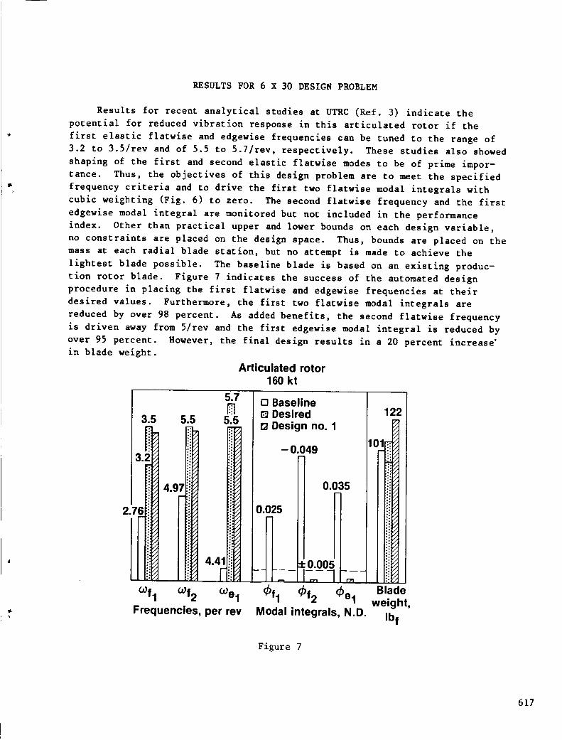
RESULTS FOR 6 X 30 DESIGN PROBLEM

Results for recent analytical studies at UTRC (Ref. 3) indicate the

potential for reduced vibration response in this articulated rotor if the

first elastic flatwise and edgewise frequencies can be tuned to the range of

3.2 to 3.5/rev and of 5.5 to 5.7/rev, respectively. These studies also showed

shaping of the first and second elastic flatwise modes to be of prime impor-

tance. Thus, the objectives of this design problem are to meet the specified

frequency criteria and to drive the first two flatwise modal integrals with

cubic weighting (Fig. 6) to zero. The second flatwise frequency and the first

edgewise modal integral are monitored but not included in the performance

index. Other than practical upper and lower bounds on each design variable,

no constraints are placed on the design space. Thus, bounds are placed on the

mass at each radial blade station, but no attempt is made to achieve the

lightest blade possible. The baseline blade is based on an existing produc-

tion rotor blade. Figure 7 indicates the success of the automated design

procedure in placing the first flatwise and edgewise frequencies at their

desired values. Furthermore, the first two flatwise modal integrals are

reduced by over 98 percent. As added benefits, the second flatwise frequency

is driven away from 5/rev and the first edgewise modal integral is reduced by

over 95 percent. However, the final design results in a 20 percent increase"

in blade weight.

3.5

,

2.7l

Articulated rotor160 kt

°Jf I

5.5

4.9

c°f 2

5.7N

5.5

4.

toe I

Frequencies, per rev

E! BaselineI_ Desired

[3 Design no. 1

- 0.049

J-_ 1+0.005

_fl _)f2 (_el

Modal integrals, N.D.

122

1(

Blad(

weight,

Ibf

Figure 7

617

RESULTSOFBLADEWEIGHTMINIMIZATION

While the first design case demonstrates the capability to achieve

significant changes in blade modal properties, the final blade weight is too

high. Therefore, the automated designer is used to redesign the blade to

minimize weight while maintaining essentially the same modal properties shown

in Figure 7. In this design problem, blade weight is added to the performance

index used above. Furthermore, constraints of ±0.005 are applied to the first

two flatwise modal integrals to ensure that the minimum values shown in Figure

7 are maintained. Note that this constraint corresponds to the dashed line

shown in Figure 7. Design No. I, achieved above, is used as the preliminary

design for optimization. As shown in Figure 8, the automated designer met all

the specified criteria on the primary vibration parameters while reducing the

blade weight of Design No. 2 to 104 ib, which is only 3 percent heavier than

the baseline blade. Once again, appropriate lower bounds have been placed on

the mass design variables. These results are achieved in one computer run,

which requires only 11.5 CPU minutes on a UNIVAC II00 machine.

Articulated rotor160 kt

Baseline

Design no. 1

Design no. 2

Desired

Wlf C_le _)lf _2f Blade weight

2.76

3.44

3.40

3.2- 3.5

4.41

5.51

5.78

5.5 -- 5.7

0.0253

0.0009

0.0050

0.0 ±0.005

-0.0489

-0.0025

-0.0029

0.0 ±0.005

101

122

104

Figure 8

618

MODIFIED MASS DISTRIBUTION FOR 6 X 30 DESIGN PROBLEM

Figure 9 shows the final mass distribution for Design No. 2, which was

used for the results presented above. Also shown in this figure is the

distribution for the baseline production blade. The cross-hatched region

represents blade root end hardware which has not been modified. While the

blade weights for both the production blade and Design No. 2 are about the

same, the mass distributions are significantly different. The automated

designer has shifted almost 15 ib from mid-span to the outer 25 percent of

the blade. This is required to achieve the substantial increase specified in

the first flatwise natural frequency. As an added benefit, the increased mass

outboard also improves rotor auto-rotation characteristics.

1.0

Baseline (101 Ib)

Design no. 2 (104 Ib)

0.6

dmi

dx0.4

(Iblin.)

O.8-

r/A

•//1

r/A

./..I

r/A

r / .,'_

r/A

./.,I

F /A r"--

0.2 . / __._._r"----a_._jf ti

./-4

O0 0 100 150I I

200 250

Spanwise location (in.)

Figure 9

619

MODIFIEDEDGEWISESTIFFNESSFOR6 X 30 PROBLEM

Figure I0 comparesthe final edgewise stiffness along the blade span forDesign No. 2 to that of the baseline production helicopter. The cross-hatchedregion represents the invariant root end hardware. As indicated, about a 40percent increase in edgewise stiffness across most of the blade span is

required to achieve the high frequency specified for the first elastic

edgewise mode. Although not shown, changes made by the automated designer in

flatwise stiffness along the blade span are insignificant, since flatwise

frequency and mode shape requirements are accomplished through changes in the

spanwise mass distribution.

350

---%_____j'--"]

Baseline (101 Ib)

Design no. 2 (104 Ib)

Eledge

300

250

200

150

100x 10 -s

(Ib.in. 2)

5O

00

I

tJ

C_

fjJ

!

B B

50 100

I

1

I 1 I

150 200 250

Spanwise location (in.)

Figure i0

620

PREDICTED VIBRATORY HUB LOADS

Figure 11 compares the vibratory hub loads (fixed system) predicted by

the forced response analysis G400 for the baseline blade and for Design No. 2.

The two inplane shears have been reduced by over 65 percent and the vertical

shear by 20 percent. The vibratory hub moments are shown only for reference,

since the hub moments make an insignificant contribution to fuselage vibration

for this articulated rotor. Since the two inplane shears have been previously

identified as primary contributors to fuselage vibration in this rotorcraft

(Ref. 3), the particular frequencies and modal integrals shown in Figure 6

were selected to reduce the response of these two components.

2OO

41rev 160hub loads,

Ib. or ft-lb"120

8O

4O

0

Articulated rotor160 kt

113 Scal

111Fx Fy

Long LatFz Mx My Mz

Vert Roll Pitch Yaw

I_1 Baseline (101 Ib)

BB Design no. 2 (104 Ib)

Shears Moments

Figure ii

621

PREDICTED FUSELAGE VIBRATIONS

Figure 12 shows the predicted 4/rev vibrations in the cockpit and cabin

for the baseline design and Design No. 2. As a result of frequence placement

and modal shaping to reduce the inplane and vertical hub shears, reductions in

vibration on the order of 50 percent have been achieved at all components

except pilot seat vertical. The low baseline value of this component has been

maintained.

Articulated rotor160 kt

1.0

0.8

0.6

41 revvibration

(g's) 0.4

0.2

0

Baseline (101 Ib)

Design no. 2 (104 Ib)

Pilot Copilot

Fwd Aftvert vert

Cabin

Figure 12

622

PREDICTED VIBRATORY STRESSES

Figure 13 shows the blade spanwise I/2 peak-to-peak vibratory stresses

predicted for both the baseline and Design No. 2. Significant reductions in

flatwise and edgewise bending stresses and in torsional stress have been

achieved all along the blade span. Reductions of nearly 50 percent have been

achieved at all the critical stress areas (outboard flatwise, midspan

edgewise, and inboard torsional) despite the lack of stress constraints and

stress terms in the performance index. This indicates that reductions can be

achieved in both fuselage vibration and blade stresses when blade frequencies

and mode shapes are appropriately tailored.

1/2 6

Peak-

to-peak 4blade

stresses, 2Articulated rotor 160 kt ksi

Baseline (101 Ib) 0

Design No. 2 (104 Ib) 25

| Torsion _ 20

to-peak 10

blade 5

stresses, 0 I I I I I "_J 0ksi0 20 40 60 80 100 0 20 40 60 80 100

r/R r/R

Figure 13

623

CONCLUDING REMARKS

This paper has outlined a simplified approach for minimizing vibration in

a rotorcraft. Rather than using a forced response analysis for the bulk of

the design optimization process, a modal analysis has been used to calculate

key vibration parameters that have been identified as being indicative of

blade sensitivity to vibratory airloading. These parameters are based on

blade modal frequencies and generalized airload integrals. By driving these

modal parameters to zero, it is possible to place frequencies and to tailor

mode shapes for reduced vibration in the fuselage. The forced response aero-

elastic analysis G400 has been used to identify the key modes and associated

frequency placement and modal shaping criteria for the articulated rotor in-

vestigated. The forced response analysis has also been used to verify the

vibration characteristics of new blade designs. This approach of using both

modal and forced response analyses for the optimization of blade structural

properties has predicted reductions in fuselage vibration on the order of 50

percent in a computationally efficient manner. An added benefit of appro-

priate modal tailoring is the reduction of blade stresses along the entire

blade span. The results of applying this approach indicate that blade modal

properties can be changed to achieve significant improvements in both fuselage

vibration and blade stress. Furthermore, these changes in modal properties

can be achieved with practical blade designs and without significant weight

penalties. While these preliminary results are not yet substantiated by

experiment, they demonstrate the application of optimization techniques to

existing methodology. Optimization studies will be continued and expanded to

include aerodynamic considerations in the design process.

624

lo

o

,

Do

o

REFERENCES

Bielawa, R. L.: Aeorelastic Analysis for Helicopter Rotors with Blade

Appended Pendulum Absorbers - Program User's Manual. NASA CR-165896,

June 1982.

Taylor, R. B.: Helicopter Vibration Reduction by Rotor Blade Modal

Shaping. Presented at the 38th Annual Forum of the American Helicopter

Society, Anaheim CA, May 4-7, 1982.

Taylor, R. B.: Helicopter Rotor Blade Design for Minimum Vibration. UTRC

Report R83-915783-27, United Technology Research Center, December 1983.

Madsen, L. E.; and G. N. Vanderplaats: Copes--A Fortran Control Program

for Engineering Synthesis. Naval Postgraduate School, Report No.

NPS69-81-003, March 1982.

Vanderplaats, G. N.: Conmin--A Fortran Program for Constrained Function

Minimization; User's Manual. NASA TM X-62282, August 1982.

Vanderplaats, G. N.; and F. Moses: Structural Optimization by Methods of

Feasible Directions. Computers and Structures, Vol. 3, 1973, pp. 739-755.

625

N87-11757

APPLICATION OF NUMERICAL OPTIMIZATION

TO ROTOR AERODYNAMIC DESIGN

W. A. Pleasants III and T. J. Wiggins

Applied Technology Laboratory

Ft. Eustis, Virginia

PRE_'Ot'NG PAGE BLANK NOT FILMED

627

ADVANCEDDESIGNREQUIREMENTS

The concept formulation for the Army family of light rotorcraft (LHX) hasresulted in greatly increased demandsfor accurate projections of rotary wing tech-nology to support independent government preliminary design trade-off studies. Theconcept formulation process is presented in detail in reference I. Figure I showsthe diversity of requirements which must be addressed in rotor design for LHX.This paper will present the experience gained in the implementation and applicationof existing optimization and analysis methods to rotor aerodynamic design. Theobjective of the optimization effort was to obtain major reductions in the calendartime and man-hours required to predict advanced rotor performance for the multipledesign points of advancedArmy aircraft concepts. While typical results of optimi-zation will be presented, the paper will concentrate on program structure andapproach, analysis and optimization problems, and areas requiring additionaleffort.

• INCREASED SPEED

• HIGH ALTITUDE, HOT DAY ENVIRONMENT

• EXTENDED RANGE

• AIR-TO-AIR COMBAT

• COMMONALtTY OF DYNAMIC COMPONE]'qTS

Figure i

628

PROGRAMSTRUCTUREANDAPPROACH

Figure 2 illustrates the basic program structure obtained by combining theFRANOP/CONMINoptimization codes of references 2 and 3 with the Bell HelicopterA7906 hover code of reference 4 and the forward-flight code of reference 5. Apreliminary design level weights analysis and simple representation of engine per-formance were added to allow evaluation of rotor design on the total helicopterdesign. Modular design of the computer program was an important consideration indeveloping the optimization code. Experience was first gained with the optimizerusing simple, low cost analysis methods. As simple analysis methods were replacedwith the more complex methods, the range of design variables, constraints, andobjective function was expandedand considerations for overall aircraft designwere added. The ability to easily add to or modify the objective functions,constraints, or even the. baslc analysis was of critical importance in responding torapidly changing design requirements. In addition, the modular structure willallow the future use of alternate optimization codes with minimal impact on the

remainder of the code. No attempt to use approximate analysis or other approaches

for increased efficiency was attempted as computer costs were a secondary concern

to manpower available to implement the analysis.

FRANOPNASA LARC

ANALYSISHOVER,FORWARDFLIGHT,WEIGHTS

OPTIMIZATIONCONk41N

NASA TM X-62282I PLOT/PRINT

Figure 2

m

629

THEOPTIMIZATIONPROBLEM

In general, the optimization problem maybe given as:

F(X) + min

subject to

gj(X) < 0 1 < j < m

where X is a vector of design variables, F(X) is an objective function to be mini-

mized, and g(X) are constraint equations. In addition, CONMIN allows side

constraints, or upper and lower limits, to be imposed on the design variables. The

typical design problem has a well-defined design requirement which leads to an

optimium design. The Army concept formulation process requires an optimization

process which is responsive to rapidly changing and widely varying design require-

ments. Figure 3 shows the options now available for design variables, objective

functions and constraints. Objective functions, design variables, and constraints

may be selected in any meaningful combination. While some design variables are

obviously redundant, care must also be exercised in selection of design variables

so that they are compatible with the problem. Selection of design variables to

which the objective function is insensitive can result in large amounts of computer

time expended for very little benefit.

F(x)_ MI_MUM

SDRKCT TO Gj (x)< 0 1<_<m

DESIGNVARIABLES

• Ul',rr...ARTWIST• RADIUS• TIP SPEED• EQUIVALENTCHORD• UNE.ARTAPERRATIO• RADIALSTATIONAT WHICHTAPERBEGINS• LOCALTWIST• LOCAL CHORD• LOCALARFOIL

OBJECTIVEFUNCTION• ENQNE _ZE

• JC_ WEIGHT• F'L,NtWI_IC;-IT

CONSTRAINTS

• STALLCRITE_• ENQNESIZE

Figure 3

630

PROGRAM CONTROL

The Framework for Analysis and Optimization Problems (FRANOP) computer code

provides the general purpose framework used in implementing the optimization

problem described here. The primary functions of FRANOP are tabulated in figure 4.

From the viewpoint of a user who is interested in using existing optimization

methods to provide better and faster solutions to existing design problems, FRANOP

has several features worthy of note. First, the ability to conduct single point

analysis was found to be highly useful in the implementation of analysis additions

and/or modifications. The ability to conduct sensitivity analysis was found to be

useful in defining the exact behavior of the objective function problem areas for

the optimizer. Finally, it was found in most cases that the output of the opti-

mizer alone was inadequate to fully understand the design process. FRANOP can be

easily modified to provide for tabulation of any desired output from the analysis.

This output provides an excellent compromise between "being buried in paper" and

operating with a t'black box" for which the user has only the input and final

answers.

FRAMEWORK FOR ANALYSIS ANDOPTIMIZATION PROBLEMS

(FRANOP)

• SINGLEPOINT ANALYSIS

• SENSmVITY ANALYSIS

• OPTIMIZATION

• TABULATION& OUTPUTOF DATA

Figure 4

631

ANALYS IS

The functions of the analysis section of the optimization program are shown

in figure 5. In developing the analysis section of the optimization program,

two constraints were imposed. First, the optimization program would use

existing rotor performance methods with minimum changes. Second, the interface

between the optimization routines and performance methods would have maximum

flexibility in selection of design variables, design conditions, objective

functions, and constraints. This flexibility was found to be necessary to

investigate widely varying design requirements, but it places a greater require-

ment on the user to select reasonable design variables and objective functions.

Selection of design variables which have minimal impact on the objective func-

tion or which result in unrealistic designs can waste large amounts of computer

time.

OPTIMIZATION ANALYSIS FUNCTIONS

• INTERFACEBETWEENOPTIMIZERAND PE_NCE METHODS

• ONE TIME PERFORMANCEMETHOD INPUT

• DESIGN VARIABLE SELECTION

• OB.ECTIVE FUNCTIONAND CONSTRAINTDEFINITION

• SELECTION AND I.I_ALUAllON OF DESIGN CONDmONS(HOVER,CRUISE,MANEUVER)

Figure 5

632

PERFORMANCEMETHODS

The major characteristics of the performance methods selected are showninfigure 6. Thesemethods are generally well correlated for existing and developmen-tal rotor designs and flight conditions. Availability of program documentation,ease of modification and integration _Ith the optimizer correlation data base, andsensitivity to the desired design variables were the primary factors in selectingthe analysis methods. For example, representation of the rotor wake in hover isnecessary to obtain realistic sensitivities of performance to nonlinear twist.Also, rotor design is a compromisebetweena numberof possible design conditionsand can strongly drive other areas of the rotorcraft design. Preliminary designlevel weights prediction and engine representation were incorporated to allow bestoverall system design as opposed to optimum isolated rotor design for a singlepoint.

A7906 HOVERANALYSIS

• UFTING SURFACEANALYSIS

• CIRCULATIONCOUPLEDWAKE

• VERTICALDRAGCALCULATIONOPTION

• WELL CORRELATED

ROTORFORWARDFLIGHTANALYSLS

• STRIP ANALYSISMETHOD

• RIGIDBLADE

• TRIM UFT ANDDRAG

• ROTORWAKENOT DIRECTLYINCLUDED

• CORRELATEDFOR CRUISEAND MANEUVER

WEIGHTS/_IALYSIS

• PARAMETRICPREUMINARYDESIGNLEVEL

• ROTOR,ENGINE,DRIVE SYS1ZM,FLIGHTCONTROLSAND FUEL SYSTEM

ENGINECHARACTERISIlCS

• POWERANDFUEL FLOW

Figure 6

633

ANALYSISPROBLEMS

The major problems encountered in implementation of the analysis portion of the

optimization code were the failure of the performance methods to converge near the

boundaries of the rotor operational envelope shown in figure 7 and the fact that

for some combinations of design variables, there will be no answer and the analysis

methods will diverge. Considerable effort was devoted to providing more efficient

and stable rotor trlm methods. It was also found necessary to deal with occasional

near failures of the analysis to converge. In those cases the analysis was close

to trlm but had the potential to distort partial derivatives. A much less obvious

problem with the analysis methods was that the optimization could lead to designs

well outside the correlation base of the performance methods. In thls case, the

user must then carefully consider the validity and level of confidence in the opti-

mization results.

OCO

(D

ROTOR THRUST LIMIT

L._ LOWER STALL BOUNDARY

I l I I I I

SPEED

Figure 7

634

OPTIMIZATION PROBLEMS

Figure 8 summarizes the major problem areas with the optimizer from the

viewpoint of the user. Scaling of design variables and/or finite difference objec-

tive function gradients was generally necessary for efficient optimization. It was

necessary to modify the optimizer to increase flexibility in dealing with scaling.

The objective functions used in this effort exhibited widely varying sensitivity to

the design variables. Near an optimum the objective function often had a wide

region of the design space where little change took place. It was often desirable

to conduct sensitivity analysis to illustrate the overall behavior of the objec-

tive function. Optimizer output was generally adequate to monitor the overall

optimization process but was not adequate to monitor the overall design process.

Iteration histories of key analysis outputs during the optimization process were a

major help in eliminating the feeling that the user is dependent on a "black box."

Finally, finite difference derivatives must be taken with increments in design

variables sufficiently large to insure that partial derivatives are outside the

"noise" level of the analysis. Optimization program defaults were found to yield

unsatisfactory finite difference derivatives in many cases.

• SCAUNG

• LACK OF FLEXIBILITY

, SENSrnVITYOF OBJECTIVEFUNCTIONS TO DESIGNVARIABLES

• OUTPUT

• RNITEDIFFERENCEDERIVATIVES

Figure 8

635

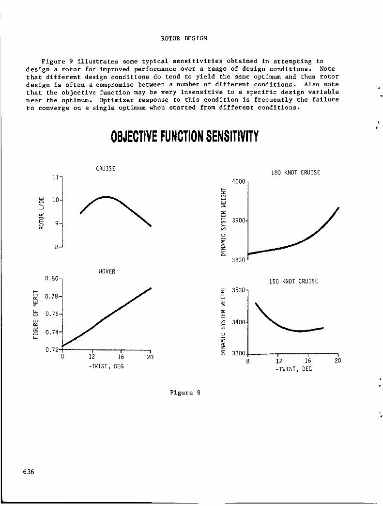
ROTORDESIGN

Figure 9 illustrates sometypical sensitivities obtained in attempting todesign a rotor for improved performance over a range of design conditions. Notethat different design conditions do tend to yield the same optimum and thus rotor

design is often a compromise between a number of different conditions. Also note

that the objective function may be very insensitive to a specific design variable

near the optimum. Optimizer response to this condition is frequently the failure

to converge on a single optimum when started from different conditions.

OBJECTIVEFUNCTIONSENSITIVITY

11-

'" 10-

__1

0F--o 9

0.80-

I---

H 078-e_

o 0.76-L_

_ 0.74-i,

0.728

CRUISE

HOVER

I I I

12 16 20

-TWIST, DEG

Figure 9

4000-

3900-

3800

F...- 3500-

i,i

,,=,3400-

(._)

Z>-,-, 3300

180 KNOT CRUISE

150 KNOT CRUISE

i i !12 16 20

-TWIST, DEG

636

HOVEROPTIMIZATION

Figure i0 shows the results of two hover optlmizations. Figure 10a illustratesa nonlinear twist optimization based on the UH-60 rotor chord, radius, and air-

foils. Starting from a -i0 ° linear twist, the optimizer produced a nonlinear twist

characteristic of the UH-60, but with improved performance. Additional effort

would be required to determine if the analysis results were valid and the rotor

could be built. Note that highly nonlinear behavior of the rotor twist was repre-

sented with a relatively small number of design variables. This was accomplished

through the use of a combination of linear and nonlinear interpolation methods

which reduce the required number of design variables from fifteen to six. This

approach was also used to reduce the number of design variables required to repre-

sent airfoil distributions and chord as a function of radius. Figure 10b illustrates

a second hover optimization. Note that if the objective function is insensitive to

a particular design variable, the optimizer used tends to leave it at the initial

value.

HOVER DESIGN

(/3I,=JL.aJn,'

,9,a

i--

-lO -

INITIAL CONDITION

HOVER PERFORMANCECASE FIGURE OF MERITOPTIMUM 0.795INITIAL COND. 0.708UH-60 0.784

FINAL OPTIMUM

I0.4.

I0.6

RADIAL STATION,X/R

I-

D.8

(a)

Figure i0

637

HOVEROPTIMIZATION

VARIABLE INITIAL FINALTWIST -17.0 -25.0TAPER 0.760 0.507

NOTE: TWIST LOWERLIMIT IS -25 DEG

0.12 ,

(..)

I--

-' 0.i0

l,(:C

0.08 l l _ i0.2 0.4 0.6 0.8 1

RADIAL STATION, X/R

.(b)

Figure 10

2800.N

Z

..2700"

0

2600"

0

2500I I I t

0 1 2 3 4

ITERATION

638

SUSTAINED MANEUVER

Figure II shows the results of a rotor design optimized for a 1.5 g sustained

load factor maneuver. A total of eleven design variables were used together with a

rotor stall criteria constraint. The optimizer revealed a minimum in two to three

iterations, as was typically the case. The initial condition was chosen to be near

or to violate the stall criteria constraint. Note that the optimizer moved chord,tip speed, and airfoil thickness (t/c) in a direction which would increase the lift

capability of the rotor.

VARIABLE INITIAL FINALRADIUS 26.8 27.0TWIST -18.0 -21.1TIP SPEED 725. 735.CHORD 1.74 1.77

0.105-

i

oioo/_- LFINAL

t

o0.0.5._,,q

0.090........... --_--

O.08b__-" , ,, ,_ , , ,,, ,0.2.2 0.4 0.6 0.8 I

RADIAL STATION, X/R

4600-

I---

w

4400._r

F--

>-

_ 4200-

.°

Z0

_4000.(,_)

_3800.

0

3600

I

i I !

0 I 2 3

ITERATION

I

4

Figure ii

639

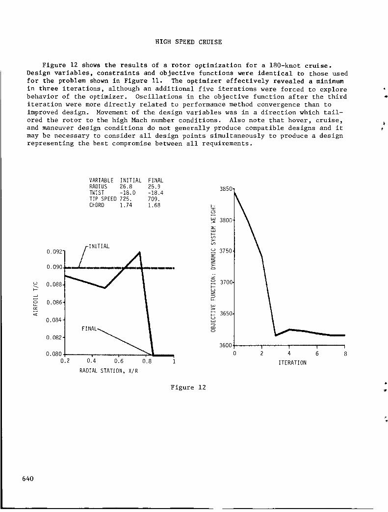
HIGH SPEED CRUISE

Figure 12 shows the results of a rotor optimization for a 180-knot cruise.

Design variables, constraints and objective functions were identical to those used

for the problem shown in Figure Ii. The optimizer effectively revealed a minimum

in three iterations, although an additional five iterations were forced to explore

behavior of the optimizer. Oscillations in the objective function after the third

iteration were more directly related to performance method convergence than to

improved design. Movement of the design variables was in a direction which tail-

ored the rotor to the high Mach number conditions. Also note that hover, cruise,

and maneuver design conditions do not generally produce compatible designs and it

may be necessary to consider all design points simultaneously to produce a design

representing the best compromise between all requirements.

VARIABLE INITIAL FINALRADIUS 26.8 25.9TWIST -18.0 -18.4TIP SPEED 725. 709.CHORD 1.74 1.68

INITIAL0,092 A

o

o.o8o_0.2 0.4 0.6 0.8 1

RADIAL STATION, X/R

Figure 12

I

38o0

F-

3750

.°

o 3700

z

_ 3650,

0

3600i 1 I

2 4 6

ITERATION

640

CONCLUSIONS

Based on initial results obtained from the performance optimization codediscussed in this paper, a numberof observations can be maderegarding the utilityof optimization codes in supporting design of rotors for improved performance.

i. The primary objective of improving the productivity and responsiveness ofcurrent design methods can be met.

2. The use of optimization allows the designer to consider a wider range ofdesign variables in a greatly compressedtime period.

3. Optimization requires the user to carefully define his problem to avoid

unproductive use of computer resources.

4. Optimization will increase the burden on the analyst to validate designs

and to improve the accuracy of analysis methods.

5. Direct calculation of finite difference derivatives by the optimizer was

not prohibitive for this application but was expensive. Approximate analysis in

some form would be considered to improve program response time.

6. Program development is not complete and will continue to evolve to

integrate new analysis methods, design problems, and alternate optimizer options.

REFERENCES

l.

.

.

.

.

Singley, G. T. III, "Army Light Family of Rotorcraft (LHX) Concept

Formulation," AIAA-83-2552, October 1983.

"FRANOPP - Framework for Analysis and Optimization Problems - User's Manual,"

NASA CR-165653, 1981.

Vanderplaats, G. N., "CONMIN - A Fortran Program for Constrained Function

Minimization, Users Manual," NASA TM X-62282, 1973.

Kocurek, J. David, et al, "Hover Performance Methodology at Bell Helicopter

Textron," Presented at the 36th Annual Forum of the American Helicopter

Society, Washington, D.C., May 1980.

Groff, T.E., "Vehicle Rotor Program," Vitro Laboratories, Silver Springs, MD,May, 1968.

641

N87:11758

AEROELASTIC/AERODYNAMIC OPTIMIZATION

OF

HIGH SPEED HELICOPTER/COMPOUND ROTOR

L. R. Sutton

Applied Technology Laboratory

U.S. Army Research and Technology Lab (AVSCOM)

Fort Eustis, VA

and

R. L. Bennett

Bell Helicopter Textron Inc.

Fort Worth, TX

PRECEDING PAGE BLANK NOT FILMED

643

HELICOPTER FUSELAGE VIBRATION PROBLEM

The helicopter fuselage vibration problem is one of the major

challenges facing the helicopter industry. Excessive vibration can

have an adverse effect on crew and passenger comfort as well as

limiting the component's service life. In order for a single analysis

to predict correctly the fuselage environment, it must be multi-

disciplinary to cover the rotor aerodynamics, rotor dynamics, fuselage

dynamics, and flight mechanics of the helicopter.

IMPACT LOADS, FLEXIBLE BLADES

_ COUPLED MODES

FLEXIBLE SWASHPLATE- -Jl__--.__/_/_ FLEXIBLE LINKAGES

BLACK BOXESSTRUCTURALMODES

Figure 1

644

EFFECTS OF FUSELAGEVIBRATIONS

Reducing the fuselage vibrations has been a continuing goalof the helicopter technical community. The fuselage vibrationlevel has a direct impact on the fiscal, physical, and psycholog-ical acceptance of the helicopter. Being able to eliminate orsignificantly reduce (without cost, weight, or complexity pen-alties) fuselage vibrations would enhance the acceptance of thenext generation helicopters.

• COMPONENT FATIGUE

• CREW AND PASSENGERCOMFORT

• PERFORMANCELIMITATIONS

• WEAPON DELIVERY ACCURACY

Figure 2

645

SOURCEOF EXTERNALAIR LOADS

For the typical helicopter configuration, the relative wind

produced by the helicopter's forward velocity is parallel to the

plane of the rotor. For the airplane propellor, the flow is per-

pendicular to the rotor plane. The parallel flow affects the

relative wind velocity components perpendicular to and along the

leading edge of the blade. The harmonic variation in the flow is

the primary source of the oscillatory aerodynamic forces acting

on the rotor blade.

_r +V ,,.f£t

FORWARDSPEED

(Vl

Figure 3

646

SOURCE OF PERIODIC AIR LOADS

The simple harmonic variation in flow perpendicular to the

leading edge has the same frequency as the rotation speed of the

rotor. However, this periodic flow variation produces periodic

aerodynamic forces at integer multiples of the rotation speed.

_0.

AI_

Figure 4

647

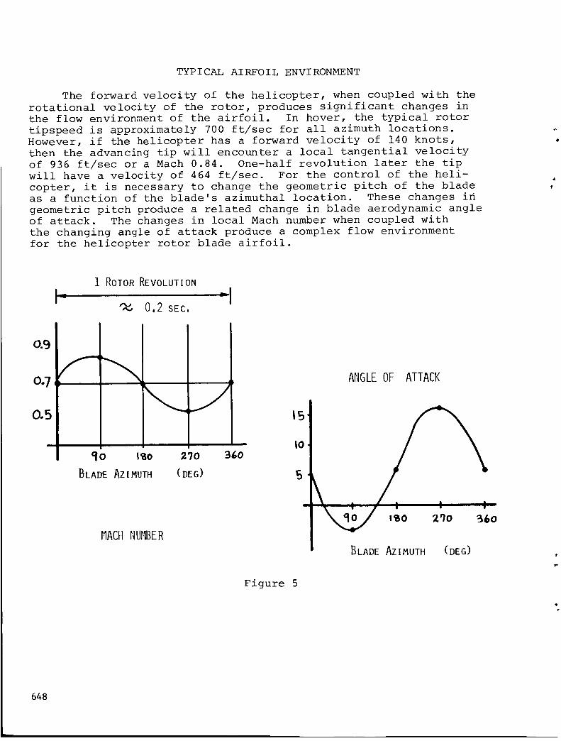
TYPICAL AIRFOIL ENVIRONMENT

The forward velocity of the helicopter, when coupled with therotational velocity of the rotor, produces significant changes inthe flow environment of the airfoil. In hover, the typical rotortipspeed is approximately 700 ft/sec for all azimuth locations.However, if the helicopter has a forward velocity of 140 knots,then the advancing tip will encounter a local tangential velocityof 936 ft/sec or a Mach 0.84. One-half revolution later the tipwill have a velocity of 464 ft/sec. For the control of the heli-copter, it is necessary to change the geometric pitch of the bladeas a function of the blade's azimuthal location. These changes ingeometric pitch produce a related change in blade aerodynamic angleof attack. The changes in local Mach number when coupled with

the changing angle of attack produce a complex flow environment

for the helicopter rotor blade airfoil.

o.9

0.7

0.5

1 ROTOR REVOLUTION

'- :II-"",,.,0,2 SEC,

qO I_O

BLADE AZIMUTH

2'10

(DEG)

B6o

t,IACHNUI.]BER

ANGLEOF ATTACK

15

i, :,oBLADE AZIMUTH (DEG)

Figure 5

648

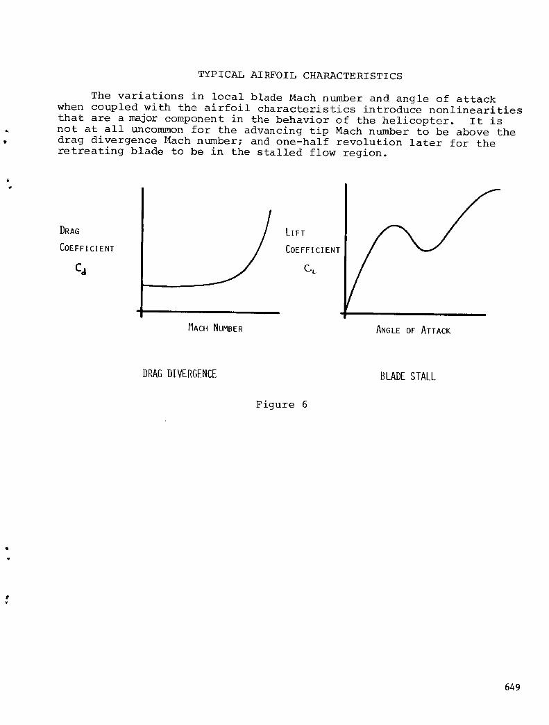
TYPICAL AIRFOIL CHARACTERISTICS

The variations in local blade Mach number and angle of attackwhen coupled with the airfoil characteristics introduce nonlinearitiesthat are a m_or component in the behavior of the helicopter. It isnot at all uncommon for the advancing tip Mach number to be above thedrag divergence Mach number; and one-half revolution later for theretreating blade to be in the stalled flow region.

DRAG

COEFFICIENT

Cd

LIFT

COEFF ICIENT

C-,L

MACH NUMBER ANGLE OF ATTACK

DRAG DIVERGENCE BLADESTALL

Figure 6

649

ROTORDYNAMICS

The dynamic behavior of the rotor blade is influenced by thecentrifugal force field as it combines with the elastic deflections(i,n the plane of rotation, out of the plane of rotation, and elastictorsion). The centrifugal force at the hub can be an order of magni-tude greater than the gross weight of the helicopter. Finite elementtechniques are used to calculate the coupled natural frequencies as afunction of the blades built in geometric twist, collective pitch, androtation speed. The centrifugal force has more influence on theout of plane modes than on the inplane modes. Coupled modes are cal-culated for various combination boundary conditions at the interfacebetween the blade and the mast.

I

CENTRIFUGALFORCE

COUPLEDELASTICDEFLECTIONS

IN THE PLANE OF ROTATION

OUT OF THE PLANE OF ROTATION

TORSION

TENSIONBENT ANALYSIS

Figure 7

650

ROTORBLADEFREQUENCY

The aeroelastic response of the helicopter rotor blade isgoverned by the separation of the aerodynamic forcing functionfrequencies (at integer multiples of the rotation speed) fromthe coupled natural frequencies. The "fan plot" shows thisrelationship in addition to identifying the nominal operatingRPMband for the rotor. Depending on the number of blades andthe blade boundary conditions at the hub, certain modes respondonly at selected forcing function frequencies.

FREQUENCY

OPERATING RPM

BAND

/

ROTOR SPEED

/AERODYNAMIC

FORCING

FUNCTION

FREQUENCY

Figure 8

651

ROTORFORCESTRANSMITTEDTO FUSELAGE

The large oscillatory aerodynamic forces acting on the bladesare summed together at the top of the mast to form the forces andmoments that are transferred to the fuselage. The unique propertyof this summing action is that the forces and moments transferredfrom the rotor to the fuselage occur at frequencies formed by multi-plying the number of blades and the rotor speed. Thus a two-bladedrotor turning at 300 rpm (5 Hz) will excite the fuselage at i0 Hz,20 Hz, 30 Hz, etc. while a four-bladed rotor would excite thefuselage at 20 Hz, 40 Hz, etc.

F_

\ F_

b'- NUMBER OF BLADES

oo

% : Z _._'"C.bn± +¢%)

--_ ,,F. ,:,c,,s,,_(:,_b-O.*+ ¢,,_,)

Itl

_y : _ a,,_,_,(nb_.',.+ q',,b)r):!

Figure 9

652

FUSELAGEDYNAMICS

The forces and moments transferred from the rotor to the fuselageoccur at frequencies near the natural frequencies of the elastic fuse-lage. This proximity has given rise to various vibration attenuationdevices that are often added to the helicopter after the design iscomplete. These after-the-fact additions are expensive in terms ofcost and weight.

Mode

(I)-(6)

Natural Fresuency

Rigid Body Modes, 0 Hz

Frequency Scale

0 Hz

Excitation Frequenc[

(7) Pylon Lateral Rocking Mode, 3.44 HZ

(8) Pylon Fore-and-Aft Rocking Mode, 5.68 HZ

(9) Pylon Vertical Nodal Beam Mode, 7.35 HZ

(10) Nodal Beam Rolling Mode, I0.17 HZI0 Hz

One-Per-Rev, 4.6 Hz

Two-Per-Rev, 9.2 Hz

(11) M/R Mast Fore-and-Aft Bending Mode, 15.02 HZ 15 Hz

(12) M/R Mast Lateral Bending Mode, 18.26 Hz Four-Per-Rev, 18.4 Hz

20 Hz

Figure I0

653

ANALYTICAL MODEL

The analytical model used during the helicopter rotor designmust contain very detailed mathematical representations of thedynamic and aerodynamic components. For the airfoils, aerodynamiccharacteristics tabular data tables are used to store the lift, drag,and pitching moments as a function of Mach number and angle ofattack. The Mach number range must go from 0.0 to 1.0, and theangle of attack table must contain entries from -180 degrees to+180 degrees. The rotor and fuselage dynamic model is based on themodal method of structural analysis. The flight mechanics modelcontains i0 rigid body degrees of freedom--six for the fuselage andtwo angles to locate the tip path plane for two rotors. Numericalintegration is used to obtain the aeroelastic response of the coupledrotor/fuselage system.

ROTORAERO 20 RADIAL SEGMENTS

TABULAR DATA FOR CL(a,M),CD(O,M), C m(a,M)

ROTOR DYNAMICS FINITE ELEMENTI MODAL REPRESENTATION

TENSION BEAM ANALYS I S

FUSELAGEDYNAMICS FINITE ELEMENTI MODAL REPRESENTATION

FLIGHT MECHANICS 10 RIGID BODY DEGREESOF FREEDOM

AEROELASTIC ANALYSIS TIME HISTORY INTEGRATION OF

COUPLED ROTOR I FUSELAGE

MODAL EQUATIONS

Figure Ii

654

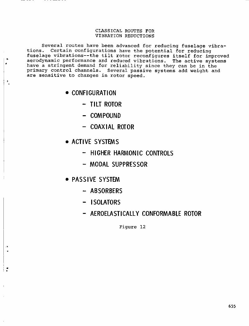
0

CLASSICAL ROUTES FOR

VIBRATION REDUCTIONS

Several routes have been advanced for reducing fuselage vibra-

tions. Certain configurations have the potential for reducing

fuselage vibrations--the tilt rotor reconfigures itself for improved

aerodynamic performance and reduced vibrations. The active systems

have a stringent demand for reliability since they can be in the

primary control channels. Several passive systems add weight and

are sensitive to changes in rotor speed.

• CONFIGURATION

- TILT ROTOR

- COMPOUND

- COAXIAL ROTOR

• ACTIVE SYSTEMS

- HIGHER HARMONIC CONTROLS

- MODAL SUPPRESSOR

• PASSIVE SYSTEM

- ABSORBERS

- ISOLATORS

- AEROELASTICALLY CONFORMABLEROTOR

Figure 12

.%

655

PROGRAMOBJECTIVES

In October of 1983, the Applied Technology Laboratory ofthe U.S. Army Research and Technology Lab awarded Bell HelicopterTextron Inc. a contract to demonstrate the feasibility and assessthe impact of using optimization in the rotor design process.Particular emphasis will be placed on designing rotors forminimum fuselage vibrations. The resulting computer programwill have to incorporate state-of-the-art technology modulesand an efficient nonlinear programming algorithm.

DEMONSTRATETHE FEASIBILITY

&

ASSESS THE IMPACT OF

USING OPTIMIZATION

IN THE

ROTOR DESIGN PROCESS

Figure 13

656

PROGRAMPHASES

The three year program is divided into four phases. BellHelicopter has recently completed the first phase which is thedevelopment of the approach for the Rotor Design OptimizationComputer Program (RDOCP). In addition to merely developinganother computer program, the RDOCPwill be used to designfully optimized rotors and a resulting rotor design will betested in the Transonic Dynamics Tunnel at NASA Langley.

IQ DEVELOPMENTAPPROACH

T_o DESIGN AND DEVELOPMENTOF DESI GN

OPTIMIZATION METHOD

1m_ o USE OF PROGRAM

EXPERIMENTAL VERIFICATIONS

Figure 14

657

DEVELOPMENTOF APPROACH

In the development of the approach, the first task was toexamine, in detail, the current rotor design process used at BellHelicopter Textron. The examination was conducted without regardfor analytical methods or computer programs, but rather to identifythe flow of information in the design process. The results ofthe examination were converted to the standard nonlinear program-ming problem by stating the key design variables (blade mass andstiffness distribution, etc.) and £he major aerodynamic, dynamic,

and handling qualities constraints. These led to the definitions

of the approach and the required software.

TASKS

• EXAMINATION OF CURRENT ROTOR DESIGN PROCESS

• FORMALIZATION OF ROTOR DESIGN OPTIMIZATION ANALYSIS

• DEFINITION OF APPROACH FOR THE ROTOR DESIGN

OPTIMIZATION COMPUTER PROGRAM (RDOCP)

• DEFINITION OF REQUIRED SOFTWARE

• SUMMARY BRIEFING

Figure 15

658

REQUIREMENTS FOR THE ROTOR DESIGN

OPTIMIZATION ANALYSIS

Since the design of a rotor system is a multidisciplinary task,

the first requirement for RDOCP is generally in terms of technical

modules. It must be able to calculate the externally applied rotor

airloads as well as the resulting forced response of the coupled

rotor fuselage system. Finally the program must be very carefully

developed in terms of user considerations if it is to receive wide-

spread acceptance.

• GENERALITY

• FUSELAGE FORCED RESPONSE

• ROTOR EXCITATION

• ROTOR RESPONSE

• USER CONSIDERATIONS

Figure 16

659

ENGINEERING MODULES

RDOCPis being structured to permit the independent variablesfrom the NLP to be used by the rotor modal analysis and/or theforced response analysis. Fuselage modal data from a finite elementanalysis will be used to represent the fuselage dynamic properties;however the fuselage modal analysis will not be included within theoptimization process. Results passed to the sensitivity analysiswill be used to reduce the computer demands.

i

ENGINEERINGOUTPUT

SENSITIVITYANALYSIS

ROTORMODALANALYSIS

INDEPENDENTVARIABLES

Ip,

FUSELAGEFORCED MODALRESPONSE

ANALYSIS

ENGINEERINGOUTPUT

Figure 17

660

MODULES FOR RDOCP

The Rotor Design Optimization Computer Program will contain

three major modules. The executive module will serve as the inter-

face between the user and the technical modules. The technical

modules will be existing validated engineering analyses. The

Rotorcraft Flight Simulation Program C81 will be used to calculate

the forced response. Rotor modal data required during the optimi-

zation process will be generated by the Myklestad analysis. RDOCP

will not contain a specific NLP but will be sufficiently general so

that it can be combined with any NLP.

• EXECUTIVE ROUTINE

• TECHNICAL MODULES

- ROTORMODAL ANALYSIS

- FUSELAGE MODAL ANALYSIS

- COUPLED ROTOR I FUSELAGE FORCED

RESPONSE ANALYSI S

• NONLINEAR PROGRAMMING ALGORITHM

Figure 18

661

EXECUTIVE ROUTINE

Bell Helicopter Textron must develop an executive routine forRDOCPto serve as the interface between the engineering user andthe technical modules. The executive must accept a wide range ofobjective function formulations, constraints and bounds. In addi-tion, it must control the flow of data between the technical modules.

• STATEMENTOF ENGINEERING PROBLEM 8

• ROTORMODAL ANALYSIS INFORMATION

• FUSELAGEMODAL ANALYSIS INFORMATION

• FORCEDRESPONSEANALYSIS INFORMATION

• NLP DATA

• DIAGNOSTIC OUTPUT CONTROL

Figure 19

662

THE STRUCTURAL OPTIMIZATION OF A SPREADER BARFOR TWIN LIFT HELICOPTER OPERATIONS

Alan DobynsSikorsky Aircraft

Stratford, Connecti cut

663

TWIN LIFT SPREADER BAR OPTIMIZATION STUDY

An optimization study has been performed to develop a minimum weight spreaderbar to allow two helicopters to lift the same payload. With this arrangement,the maximum payload that can be lifted is almost doubled without the expenseof designing and building a new helicopter. The concept has had some limiteduse by civil helicopter operators using small helicopters and has been demon-strated in large scale by two CH-54's which successfully lifted a total loadof 20 tons (see figure).

To this point, rather heavy available beams or tower structures have been usedfor the spreader bar. Since the weight of the bar not only detracts from pay-load but also adds to the logistics problem, there are more than the usual in-centives to minimize weight. Since the design requirement is for classic beamcolumn with uniform side loads resulting from bar weight and aerodynamic drag,the design problem is particularly amenable to optimization.

A study has been performed at Sikorsky to establish the minimum weight for aspreader bar sized to carry a load equal to the capacity of two Army BLACKHAWK helicopters. Toward this end, a computer program was written to analyzethe spreader bar deflections and stresses and coupled to the NASA developedCONMIN optimization routines.

664

SPREADER BAR GEOMETRY

The payload (WI) is suspended below the spreader bar by cables (called thebridle) so that the-axial load in the bar is easily calculate_ from the cable geo-metry. A maximum cant angle of the vertical cables (_) of 15 _ was used in thestudy.

a

PA _'--P A

H

@ 2g X 1,5 SAFETY FACTOR

PA = 3.WLL + 3 W_= TAN a4H 2

...,dr

WL

L r

665

LOADS ON SPREADER BAR

The spreader bar is loaded by an axial load due to the cable angles, by dragloads due to rotor downwash and bar forward velocity and by maneuvering load

factors on the bar weight.

DRAG LOAD DU E TO ROTOR DOWNWASH

AND FORWARD VELOCITY

pA._._ _ x_ _ PA

LOAD

2g X BAR WEIGHT

666

BEAM COLUMNANALYSIS

The combined normal and axial loads make the spreader bar truss a beamcolumn. The bending moment and normal deflection are magnified in a beamcolumn so that as the axial load approaches the critical column buckling load,the moment and deflection approach infinity. The equations for deflectionand moment for a uniform beam column are shown below.

BEAM WITH COMBINED NORMAL AND AXIAL LOADS

L)• MMAX =q j2 (1-SEC

• i = ,J"_'lP

5qL4 1• _ = 384 E'-"_• ('i- P/PcR)

• UNIFORM BEAMS ONLY

667

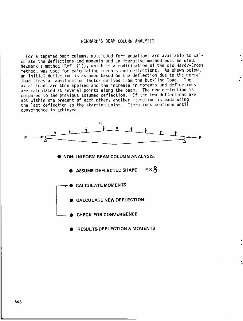
NEWMARK'SBEAMCOLUMNANALYSIS

For a tapered beamcolumn, no closed-form equations are available to cal-culate the deflections and momentsand an iterative method must be used.Newmark'smethod (Ref. (I)), which is a modification of the old Hardy-Crossmethod, was used for calculating momentsand deflections. As shownbelow,an initial deflection is assumedbased on the deflection due to the normalload times a magnification factor derived from the buckling load. Theaxial loads are then applied and the increase in momentsand deflectionsare calculated at several points along the beam. The new deflection iscomparedto the previous assumeddeflection. If the two deflections arenot within one precent of each other, another iteration is madeusingthe last deflection as the starting point. Iterations continue untilconvergence is achieved.

• NON-UNIFORM BEAM COLUMN ANALYSIS.

• ASSUME DEFLECTED SHAPE .... P X

--.---_• CALCULATE MOMENTS

• CALCULATE NEW DEFLECTION

• CHECK FOR CONVERGENCE

• RESULTS-DEFLECTION & MOMENTS

668

TRUSSDESIGNCONSTRAINTS

Strength constaints considered in the truss optimization included over-all column buckling, cap stress, cap crippling or local buckling, andcap buckling as a column between bays. The overall column buckling con-straint can never becomecritical becauseas a result of the beamcolumneffects the bending momentappraochesinfinity as the axial load nearsthe column buckling load. Constraints were placed on the D/_ and L/pratios for the cap, cross and diagonal membersso that the final designwould not be susceptible to ground handling damage. A constraint wasalso placed on the maximumcenter deflection, mainly to keep the trussfrom becoming too flexible, which could result in vibration problems.

MY• CAP STRESS- 0' = _ + P/AI

• CAP CRIPPLING- LOCAL BUCKLING

• CAP BUCKLING BETWEEN BAYS

• CENTER DEFLECTION - (_/L< .00166

• CAP AND DIAGONAL D/'T < 50

• CAP AND DIAGONAL L/p <60

• COLUMN BUCKLING

669

TYPESOFTRUSSANALYZED

For the optimization study, both constant taper and uniform center sectiontrusses were studied with both triangular and square cross sections. Design var-iables considered in the optimization were center and end width; cap, cross, anddiagonal thickness and diameter; and diagonal angle. The NASAAmesdevelopedCONMINoptimization subroutines (Ref. (2)) were used to find the optimum design,along with the NASALangley developed FRANOPPcontrol and plotting routines (Ref.(3)). CONMINuses a feasible direction optimization method based on Zoutendijk'smethod to solve a constrained optimization problem. CONMINis easy to use and hasproved to be very well suited to structural optimization problems. FRANOPPwasused as a control program to allow contour plotting of the design variables versuscontraint or objective function values. This allows the analyst to view the designspace and gain insight into the problem being optimized.

CONSTANT TAPER

UNIFORM CENTER SECTION

! !SQUARE CROSSSECTION

TRIANGULARCROSSSECTION

670

BLACKHAWKSPREADERBAR

A uniform triangular spreader bar optimized for the BLACKHAWKhelicopterweighed 770 lb. The design consisted of aluminum angles for the cap membersand aluminum tubes for the cross and diagonal members. A tapered truss was usedas the initial design but the program consistantly removedthe taper, resultingin the uniform truss shown. The programwas also run with constraints on thecenter and end widths to force the program to produce a tapered truss, whichresulted in heavier designs than the uniform truss shownbelow.

A .,q.., 2024-T3 TUBE

_ 2023-T3 ANGLE

w= 2.7'

105'

2024-T3 TU BE

i

r

WT. = 770 LBS.

671

BAR ASPECT RATIO STUDY

A study was performed to find the optimum bar length to width ratio byconstraining the truss width at center span and allowing the program to opti-mize the end width. For L/W ratios less than 36, tapered trusses resulted,while L/W ratios greater than 36 resulted in uniform trusses.

.2O

,15

WT.10

W L

,05

/1 < > L = 105'

w-,-I F,,- I-- L ,,_ H=91"W L = 16,000

.._ I I I I I I

0 10 20 30 40 50 60

L/W

672

CONTOUR PLOT OF DESIGN SPACE

A contour plot of the effect of varying cap thickness (variable No. I) andcap diameter (variable No. 3) on the cap buckling constraint (constraint No. 3)is shown below. The FRANOPP control program allows plotting of any one or twovariables against the objective function or any constraint, which is very use-ful in gaining insight about the design space. While the example shown below isrelatively linear, a more highly non-linear problem would be difficult to under-stand from simply examining the series of designs produced by CONMIN. Severalplots of the design space are worth a thousand numbers, to paraphrase the popularsaying.

673

CONCLUSIONS

An optimization study has been conducted to design a minimumweight spread-er bar to lift a payload with two helicopters. The spreader bar, which is loadedas a beam-column,was optimized using the CONMINoptimization subroutines to ob-tain a minimumweight design for the given constraints. A uniform, triangulartruss structure was found to be the minimumweight design for this application.

REFERENCES

l •

•

o

Timoshenko, S.P., Gere, G.N., "Theory of Elastic Stability", McGrawHill, New York, 1961.

Vanderplaats, G.N., "CONMIN: A Fortran Program for Constrained FunctionMinimization: User's Manual", NASA TM X-62282, August 1973.

Riley, K.M., "FRANOP - Framework for Analysis and Optimization Problems -User's Guide", NASA CR-165653, January 1981.

674

N87-11760

MULTIOBJECTIVE OPTIMIZATION TECHNIQUES FOR STRUCTURAL DESIGN

S. S. Rao

San Diego State University

San Diego, CA

675

INTRODUCTION

The multiobjective programming techniques are important in the design ofcomplex structural systems whose quality depends generally on a numberof differentand often conflicting objective functions which cannot be combined into a singledesign objective. The applicability of multiobjective optimization techniques isstudied with reference to simple design problems. Specifically, the parameteroptimization of a cantilever beamwith a tip mass and a three-degree-of-freedomvibration isolation system and the trajectory optimization of a cantilever beamare considered. The solutions of these multicriteria design problems are attemptedby using global criterion, utility function, gametheory, goal programming, goalattainment, boundedobjective function, and lexicographic methods. It has beenobserved that the gametheory approach required the maximumcomputational effort,but it yielded better optimum solutions with proper balance of the various objec-tive functions in all the cases.

PROBLEMSTATEMENT

Single objective optimization problem:

Minimize f (_)

subject to

gj(_) < 0 , j = l, 2, ..., m

where

-9-

X =

'xllx2[

Multiobjective optimization problem:

Minimize f (X)

subject to

gj(X) < 0 , j = i, 2, ..., m

with

f(X) = { fl(X) f2(X) ... fk(_)} T

676

BRIEFOUTLINEOFTECHNIQUES

All the multiobjective optimization techniques considered in this work makeuse of a single objective optimization routine. In the global criterion method, apreselected global criterion, constructed in terms of the various objectivefunctions, is minimized. The utility function method tries to maximize thecombinedor overall utility function. The gametheory approach is similar tofinding the equilibrium state whenseveral players, having different goals, try tofind their optimal strategies simultaneously. The goal programmingprocedureinvolves the minimization of the deviations from preset goals for the variousobjective functions. The goal attainment method is similar to the goal programmingmethod except that certain weights are also associated with different objectives.In the boundedobjective function method, an objective function is minimized byplacing bounds on the remaining objective functions. The lexicographic methodminimizes the objective functions sequentially starting from the most importantone.

677

GAMETHEORYAPPROACH

In this method, each objective function is associated with a player whotries to minimize his own objective. All the players are assumedto be equallyintelligent and the problem can be solved either as a non-cooperative or as acooperative game(fig. i). The cooperative gametheory is used in the presentwork. In this figure, N denotes the Nash equilibrium point in a non-cooperativegameand the arc ABrepresents the set of pareto-optimal points. Along the arc AB,the contours of f. and f^ meet tangentially and our interest is to pick one pointI gon AB using somesupercrlterion.

x2

3>(2)

x 2

x_I)

Strategy of

Strategy of player 1

player 2 /I

I

I

01f2 increases

fl increases

/

Figure i

x I

678

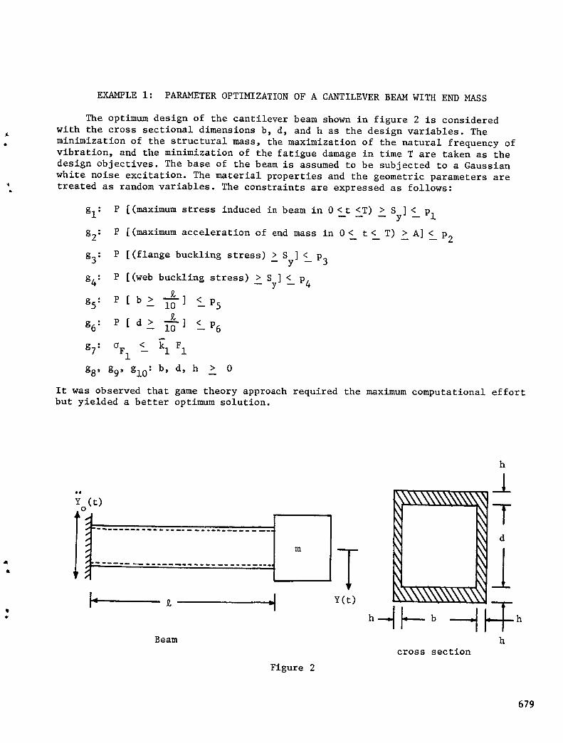
EXAMPLEi: PARAMETEROPTIMIZATIONOFA CANTILEVERBEAMWITHENDMASS

The optimum design of the cantilever beamshownin figure 2 is consideredwith the cross sectional dimensions b, d, and h as the design variables. Theminimization of the structural mass, the maximization of the natural frequency ofvibration, and the minimization of the fatigue damagein time T are taken as thedesign objectives. The base of the beamis assumedto be subjected to a Gaussianwhite noise excitation. The material properties and the geometric parameters aretreated as randomvariables. The constraints are expressed as follows:

gl: P [(maximumstress induced in beamin 0 <t <T) > S ] < Pl-- y --

g2: P [(maximum acceleration of end mass in 0<_ t<_ T) _ A] < P2

g3: P [(flange buckling stress) > S ] < P3

g4: P [(web buckling stress) _ Sy] <_ P4

g5: P [ b > _] <--P5

g6 P [ d > _] < P6

g7: < E1 FI_F I --

g8' g9' glO: b, d, h _ 0

It was observed that game theory approach required the maximum computational effort

but yielded a better optimum solution.

oe

Y (t)0

i_ _

Beam

m

Figure 2

7Y(t)

__cross section

h

1

d

1h

679

EXAMPLE 2: PARAMETER OPTIMIZATION OF A VIBRATION ISOLATION SYSTEM

In the three-degree-of-freedom vibration isolation system shown in figure 3.

z (t) represents the base excitation. The equations of motion are given byO

[m] (t) + [c] (t) + [k] _(t) = _ z (t) + c z (t)0 0 0 0

These equations can be solved for _(t) for any specified z (t) and the initial

conditions. The sp_ing stiffnesses and the damping constants are taken as design

variables so that-_ -X = {k 1 c 1 k 2 c 2 k 3 c3 }_T. Two objective functions areconsidered as

fl(_ ) = ofT [ Zo(t ) _ z3(t ) ]2 dt = integrated value of square of relativedisplacement

T

f2(_ ) = f [ k3(z 2 _ z3 ) + c3(z 2 _ z3 ) ]2 dt = integrated value of square0 of force transmitted to

main mass

Upper and lower bounds are placed on the design variables during the solution

process. As in the case of example l. here also the game theory approach yielded

a more balanced optimum solution but involved more computational effort.

z3(t)

ossI lJk3 I _ c3 z2(t)

!['iJ

Base, _ I ,3

z (t)0

Base disturbance

Isolation system

Figure 3

680

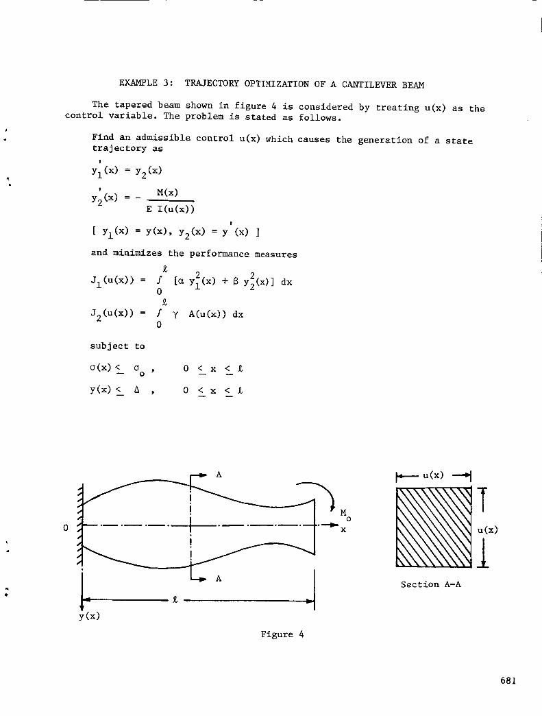
r

EXAMPLE 3: TRAJECTORY OPTIMIZATION OF A CANTILEVER BEAM

The tapered beam shown in figure 4 is considered by treating u(x) as the

control variable. The problem is stated as follows.

Find an admissible control u(x) which causes the generation of a state

trajectory as

!

YI(X) = Y2(x)

' M(x)Y2(X) = _

E l(u(x))

!

[ YI(X) = y(x), Y2(x) = y (x) ]

and minimizes the performance measures

2 2

Jl(U(X)) = f [_ Yl(X) + _ Y2(X)] dx0

J2(u(x)) = f y A(u(x)) dx0

subject to

o(x)< o , 0 < x <-- 0 -- --

y(x) < A , 0 < x <

A

M o

0 x

y(x)

Figure 4

u(x)

u(x)

1Section A-A

681

CONCLUSIONS

The present study reveals that several multiobjective optimization techni-ques can be used for the optimal design of structures. The quality of the finalsolution dependson the method used for solution. The gametheory approachappears to be promising, but morework is to be done in improving the methodfrom the point of view of computational efficiency. It will be worthwhile toconduct a comparative study of the various multiobjective optimization techniquesin the context of more complex structural design problems.

AbC.l

[c]d

f

f..3f

F.3

gjh

J.1

k

k.1

k 1

[k]

m

m.1

M(x)[m]n

Pi

P[..]

SY

t

T

u(x)

x i

X

zi(t)

Zo(t)

_,B,Y

A

SYMBOLS AND ABBREVIATIONS

specified accelerationwidth of beam

damping constant of i th damper

damping matrix

depth of beam

objective function

j th objective function

vector of objective functions

j th normalized objective function

j th inequality constraint

wall thickness

i th performance measure

number of objective functions

stiffness of i th spring

constant

stiffness matrix

length of beam

number of constraints; mass

value of i th mass

bending moment

mass matrix

number of design variables

specified probability

probability of occurrence of the event [..]

yield stress

time

duration of load application; transpose when used as a superscriptcontrol variable

i th design variable

vector of design variables

displacement of i th mass

base displacement

constants

stress

permissible deflection

682

N87-11761

IDEAS, A MULTIDISCIPLINARY COMPUTER-AIDED CONCEPTUAL

DESIGN SYSTEM FOR SPACECRAFT

i

Melvin J. Ferebee, Jr.

NASA Langley Research Center

Hampton, Virginia

683

INTRODUCTION

During the conceptual development of advanced aerospace vehicles, many

compromises must be considered to balance economy and performance of the total

system. Subsystem tradeoffs may need to be made in order to satisfy system-

sensitive attributes. Due to the increasingly complex nature of aerospace

systems, these trade studies have become more difficult and time-consuming to

complete and involve interactions of ever-larger numbers of subsystems,

components, and performance parameters. The current advances of computer-

aided synthesis, modeling and analysis techniques have greatly helped in the

evaluation of competing design concepts.

Langley Research Center's Space Systems Division is currently engaged in

trade studies for a variety of systems which include advanced ground-launched

space transportation systems, space-based orbital transfer vehicles, large

space antenna concepts and space stations. The need for engineering analysis

tools to aid in the rapid synthesis and evaluation of spacecraft has led to

the development of the Interactive Design and Evaluation of Advanced

Spacecraft (IDEAS) computer-aided design system. The IDEAS system has been

used to perform trade studies of competing technologies and requirements in

order to pinpoint possible beneficial areas for research and development.

This paper is intended to present IDEAS as a multidisciplinary tool for

the analysis of advanced space systems. The capabilities of IDEAS are

highlighted by results from previous studies. These capabilities range from

model generation and structural and thermal analysis to subsystem synthesis

and performance analysis.

684

IDEASFUNCTIONALDESCRIPTION

The Interactive Design and Evaluation of AdvancedSpacecraft (IDEAS)Computer-Aided Design and Analysis Systemfunctional methodology is showninFigure i. It consists of 40 program modules linked together by an efficientdata managementsystem. The system is divided into two distinct disciplines:interactive graphics and interactive computing. The interactive graphics arethe graphical representations of concept models and data on the interactiveterminal, and the interactive computing of the actual multidisciplinary analysisprograms available to the user. The design process begins with the creationof a three-dimensional geometry model for concept visualization and verification.An analysis model must then be created for input into the analysis programs.The models could be finite-element, finite-difference, or other mathematicalrepresentations of the system. Massproperties are generated also for inputinto analysis programs. The spacecraft subsystems are synthesized for a totalsystems concept definition. The model can then be analyzed using various toolsunder the IDEASsystem.

SPACECRAFT

SYSTEMS

\ ANALYSIS

Flgure I. Spacecraft Computer-Aided Design

685

GEOMETRY MODELING

An important step in the initial modeling of a space system concept is the visualization of the proposed system to be modeled. Figure 2 shows some initial versions of space station concepts. generated using a solid modeling geometry generator under development at NASA. Through the use of various primitive geometric entities, such as cylinders, cones, rectangles, and volumes of revolution, combined with rotation, translation and boolean operations, an analyst can model a concept in order to determine form-and-fit criterion, concept feasibility, and functionality. time and effort due to the fact that there are no analytical models created. Through the use of more powerful commercial geometry display software, such as MOVIE.BW, the models could be placed into realistic views, such as in orbit, there could be a light source representative of the Sun, shadows could be cast onto the model, and shadow information could be extracted for use in thermal analysis,

The geometry models were

By refining the concept at the geometry level, one may save

, .

* 4

I .

Figure 2. Space Station Concepts

686

STRUCTURE SYNTHESIZATION

The approach in IDEAS is to use strict mathematical relations to

automatically generate a flnlte-element model of the repeating structural

members in complex truss-like structures (for any user-specified size; shape,

and lattice density). The interconnecting truss hardware masses and sizes are

computed as a function of the structural member diameter and their masses

distributed at appropriate nodal points in the truss flnite-element model.

Additional structural appendages are then added to the truss using the

appendage synthesizer programs. Figure 3 shows the lattlce-type structures

currently being supported with a structure synthesizer. In general, the

synthesizers create and output the masses of the structural components, the

masses of the reflective mesh systems in the case of antenna design, and the

mass of the total system. Also, the center of gravity and mass moment of

inertia tensors are computed. Appendage synthesizers are used to design and

add structural appendages to a repeated structural system. The process

results in an updated structural model and updated mass/inertia properties for

the entire spacecraft. The elements used in the design of the structural

members are a mass-efflclent Isogrld, a relatively stiff triangular strut,

tension cables, and three- and four-noded elements (Ref. 1).

HOOP AND

COLUMN

RADIAL RIB I

Figure 3. Antenna Structural Concepts

687

DRAGAREACOMPUTATIONS

Another labor-saving feature incorporated into the IDEASsystem is theautomated computation of effective drag areas for lattice structures both withand without a porous mesh, and the generation of an aerodynamic drag areamodel for rlgid-body controllability analyses. In single discipline analyses,the structural analyst may have no need for these areas and the aerodynamlcistis sometimes faced with the task of generating these data for variousstructural elements and orientations from design drawings. The atmosphericdrag area approximation approach is illustrated in Figure 4. Each node, whichconsists of the intersection of several membersat various orientations, isreduced from the finite-element model to an equivalent solid structural areanormal to the spacecraft velocity vector. The blockage effects of upstreamareas on downstreamareas are factored in the solution. Also, in the case of

a porous mesh, the effects of a variable transmissibility mesh can be

superimposed onto the solution. Solid areas of external supporting subsytems,

such as solar arrays, are included (Ref. 2).

_----.v_'_-_ A3' B3 1-COMPLETE BLOCKAGENO BLOCKAGE - \

_____--,,A6,_. --.._5' _5__ -- _-71---J,_7"LI I

____.._-...__-_ARTIAL BLOCKAGE-____.............V _-- I'_B --

ANGLE Vm/Vo_ _..-------"-I Vm = MEAN MOLECULAR SPEEDv

Vo = SIC VELOCITY IN ORBIT

EACH NODE POINT REDUCED TO EQUIVALENT CIRCULAR AREA

EACH AREA HAS A BLOCKAGE FACTOR, B (= I IF SOLID)

MASKING AREAS REDUCED IN PROPORTION TO DOWNSTREAM DISTANCE

DRAG IS FUNCTION OF MASKED AREA TIMES BLOCKAGE FACTOR

Figure 4. Drag Area Computation

688

FINITE-ELEMENT MODELING OF DEPLOYING STRUCTURES

Limited research effort has been devoted to the important areas of

deployment, kinematic, and kinetic analyses of large space systems. The

spacecraft undergoes large changes in inertia (see Fig. 5) and center of

gravity locations that may affect spacecraft stability and influence rigid-

body control design. The capability to generate finite-element models of

these structures as they undergo deployment is a prerequisite to conducting

stability and stress analyses. The application of mathematical synthesization

techniques to describe the deploying structure offers a rapid, effective

means for generating the needed finite-element models at any stage of

deployment (Ref. 3).

MASS =2900kg

MAST FULLY 0%

DEPLOYED "_,#" DEPLOYED

HOOP STOWED Ix= i. 7x10 6 kg-m 2 Ix= 2. Oxl0 6 kg-m 2

Ix= I. 6x10 6 kg-m 2 I z= 2. Ix10 5 kg-m 2

Iz:3X10 3 kg-m 2 Iz=8. 3xi0 5 kg-m 2

Figure 5. IDEAS Deployment Analysis Module

689

RIGID-BODYCONTROLLABILTYANALYSIS

The Rigid-Body Control Dynamics (RCD)module calculates the on-orbitenvironmental forces and maneuver forces, and their corresponding torques onthe spacecraft at user-specified circular orbital altitudes, spacecraft orienta-tion, and mission duration. It then determines momentumstorage and desaturationrequirements, control system sizing criteria, and propellant requirements forstationkeeping, altitude control, and user-specified maneuvers. The principalfeatures of RCDare shownin Figure 6. The total torque and force time hist-ories are analyzed to determine cyclic momentumfor momentumexchange systemsizing and desaturation requirements. Momentumdesaturation requirementsare met using reaction control system (RCS)thrusters. RCSrequirements forstationkeeping are also determined (Ref. 2).

INPUT"

SLEW REQT L__._

CYCLIC MOMENTUM I _

ENVIRONMENT 1 ORBITTORQUEAND FORCE

ATMOS DRAG

GRAV GRADOTHER

MOMENTUMEXCHANGE

SYSTEMSIZING

ENVIRONMENT

ANALYS IS

----,-PREDESIGN DATA

MOMENTUMDESATURATION

ORBIT/STATION KEEPING

REACTION THRUSTERSONLY ACS

PROPULSION

> SYSTEM

REQU IREMENTS

Figure 6. Rigid-Body Control Dynamics Module (RCD)

690

ALTERNATE CONFIGURATION ANALYSIS OF A MANNED

ORBITING SPACE STATION

ORIGINAL PAGE ISOF POOR QUALITY

A primary criterion for evaluating space station concepts is the on-orblt

controllability of the space station itself. Due to the modular design of all

space station concepts, the controllability of the station will vary during

its evolutionary buildup phase. This is because the center of pressure,

center of mass, moments and products of inertia, and aerodynamic drag areas

are continuously changing. Research is under way to determine the force,

torque and controller torque for several generic space station configurations.

Time histories such as those in Figure 7 are used to size control moment

gyroscopes and propellant storage facilities on the station. The forces

are caused by three factors: aerodynamic drag, gravity gradient, and solar

pressure. These histories are also used to determine the relative merits

of various configurations flying at various orientations.

T

S

-1

|

-13

W

-17

o 40 80 120 160 200 240 280 3QO 3_)

PEWEES

ENVIRONIvF_.HTAL FORCES vs. TRUE ANOMALY

-21

-26

Jl

i, i r I i , r r I

40 SO 1=0 teO 2OO 240 2eo 320 3eO

OEQREES

ENVIRONMENTAL TOF_UES vs. TRUE ANOMALy

POP

2e

22

_ '°e

STREAMLINE "1" CONFIGURATION

ALTITUDE 270 N mi

ORIENTATION EARTH

INCLINATION 28 degrees

BETA ANGLE 0 degrees

RESUPPLY INTERVAL 90 days

CREW SIZE 4 men

1

E_RC_UeNTAL co_mo_ _CULAR I

rORCES To_ou[s To_c_(s _o_uu

:o.............. ii_Ro z -0 _Ro z -O z -O <>

-®$_ v m s_ Y msoL_ z - @ scc_ z -@

cc_ x - •

Gel Y - •GeT z

40 80 120 leo 2_0 24O 280 S.*O am)

OEGmEE$

CONTROL TORQUES vs. TRUE ANOMALY

-to

-12

-14o 4o eo 12o leo 2_o 24o _eo _o _eo

DEGREES

ANGULAR MOMENTUM REQUIREMENTS vs. TRUE ANOMALY

Flgure 7. Controllability Analysis of Manned Space Statlon Conflguration

691

, INTERACTIVE THERMAL ANALYSIS

The finite-element model files can be transferred automatically to the

Thermal Analyzer Program in order to calculate the transient temperature

response for each structural member at a given position in the spacecraft

orbit. Heat sources are solar radiation, Earth albedo, and Earth thermal

radiation. The balance between absorption of energy from the elements out

into deep space is used to determine the transient thermal response. Earth

shadowing is included. Three major assumptions are made in this type of

analysis. First, each element is considered to be an isothermal element.

Secondly, the radiation exchanges between structural members are neglected due

to small radiation view factors. Finally, structural member-to-member

shadowing is neglected. Input into this module consists of the model

geometry, thermal characteristics of all materials used in the structure and

the position in the orbit where the thermal analysis begins and ends. Output

yields elemental temperatures and heating rate time histories shown in

Figure 8 (Refs. 4 and 5).

2000,- ELEMENTNO. 625

1500 __3_

HEATINGRATE,

W/m2 IOOO

5OO

HOOPHEATING

O SOLARANDEARTHALBEDO

EARTHTHERMAL

t I I I I0.50 0.75 I.OO 1.25 1.50 1.75

TIME, hr

I0 0.25

Figure 8. Hoop Column Antenna Heating Rates

692

THERMALANALYSISOFLATTICESTRUCTUREDSPACECRAFT

Selection of materials for use in the various concepts is an extremelyimportant criterion in concept selection. Thermally induced loads areimportant contributors to the structural soundness of any concept. Analyseshave been performed in order to determine the feasibility of two candidatematerials for lattice-structured spacecraft. Figure 9 shows orbitaltemperature ranges for both aluminumand graphite epoxy as used in lattice-type structures designed to perform in equatorial orbits. In this case,aluminum membersare colder throughout the orbit due to low absorptivity toemissivity ratio when comparedto the absorptivity to emissivity ratio ofgraphite epoxy. In the Earth's shadow,the graphite epoxy exhibits fastercooling due to low thermal inertia. Using results such as these, it can be

determined just what materials can be used for various missions (Ref. 5).

ECLIPTIC PLANE ORBIT, 1000km ALTITUDE

_ a= 916

300_ _E =.80

a = .42

TEMPERATURE, E = .84

K 200

'_TEADY STATE _'_'-v i i MAXIMUM MESH

"-AI TEMPS''INSHADOW) qI'_'SHADOWINGII00-

. EARTH .11 1

SHADOW I ' '

I I I II I I I0 I 2 3 4 5 6 7

ORBIT ANGLE, rad

Figure 9. Orbital Temperature Ranges

693

STATICSTRUCTURALLOADINGANALYSIS

A static loading analysis of a concept consists of two parts. First, acomputation of all the environmental and spacecraft-induced loads must beperformed. The loading sources are from thermal loading, gravity gradientloading, atmospheric drag, static thrust, and in the case of tension/compres-sion structures, loads induced by structure pretension. With the loads identi-fied, a static, linear stuctural analysis can be executed in order to obtainstresses and deflections. The second half of the analysis consists of graph-ically presenting the stress data in the form of applied axial loads. Withthis information, the analyst can interactively redesign specific elementsthat are identified as having potential stress problems. Figure i0 showshistograms of element loads experienced in a tetrahedral truss antenna dishstructure. The top graphs represent the numberof elements experiencing arange of both tensile and compressive loads due to all environmental effects.The bottom graphs represent the loads experienced by thermal effects only.

400 - 320

300-

NUMBER OFMEMBERS 200-

100 -

0-625 -375 -125

CONVEX SURFACEMEMBERS

125

240

160

8o

,o375 625 -625 -375 -125

MEMBER LOADS, newtons

+ TENSION- COMPRESS ION

DIAGONAL

il

125 375 625

400

3OO

NUMBER OF 200MEMBERS

CONVEX SURFACE

MEMBERS

./.

///

o-625 -375 -125

v/v//////

,//

y///,

y/v/

125

DIAGONALMEMBERS

320

240 _ _/Vv

"/A

///

V//

v/

i0 r/,<, Y/

3/5 625-625-5/5-125 125

MEMBER LOADS, newtons

+TENSION

- COMPRESSION

i

375 625

Figure I0. Microwave Radiometer Spacecraft Structural Member Loads

694

SURFACEACCURACYCOMPUTATIONSON ANTENNA CONCEPTS

An important criterion in the analysis of large aperature space antennas

is the performance of the antenna reflective surface. The reflective surface,

mesh-like in composition, is usually fastened onto the antenna structure;

therefore, structural deflections will tend to affect the surface roughness of

the mesh. The surface accuracy module is designed to determine the rms

surface roughness, defocus information and boresight offset information by

utilizing the results of the static structural analysis in terms of nodal

deflections. The surface roughness is determined and is just a parameter

measuring the degree of roughness. It does not account for the errors in

manufacturing and costing considerations. (See fig. ii.)

.15

SURFACE

rms, cm

.10

IV

#"L G'R'/EPPOLAR ORBIT- EDGE ON HEATING

EARTH

SHADOW

ECLIPTICORBIT

V

GR/EP ECLIPTIC ORBI

I I I I1 2 3 4

ORBIT ANGLE, rad

MAXIMUMMESH

SHADOWING

6 7

Figure ii. Surface Distortion Variations

695

DYNAMICSTRUCTURALANALYSIS

In the determination of the flexible body controllability, the naturalfrequencies of the structure must be determined. The finite-element model

used throughout IDEAS can now be input into the structural analysis program

for a linear dynamic analysis. Figure 12 shows one mode of vibration for the

contiguous box truss structure used for Earth sciences missions and its

correlation with an independent analysis using the NASTRAN structural

analyzer. A design criterion for this type of structure was to increase the

frequency of the first mode of vibration of the offset feed mast in order to

match the frequency of the first mode of vibration of the reflective dlsh

structure. These mode shapes and frequencies are also used in the dynamic

response analysis of these types of structures (Ref. 6).

L,

_WX

_X_XXXXX,XX

XXX×

[,'i _ i

_,% __

.....iiiI

FREQUENCY L436 Hz FREQUENCY L 124 Hz

IDEAS-Generated NASTRAN-Ge ne ra ted

Figure 12. Vibrational Mode

696

DYNAMIC RESPONSE ANALYSIS OF LARGE SPACE ANTENNA

The dynamic response and structural loading of individual concepts of

large space antenna are compared to reveal the relative merits and

deficiencies of each system. Recommendations for system improvement can be

made based on information obtained from this analysis. The nodal deflection

responses of the individual concepts, such as those in Figure 13, illustrate

the flexible nature of large structures. Utilizing natural frequency infor-

mation extracted in the dynamic structural analysis, a concept can be subjected

to proposed operational environments and the effects on structural displacement

and member structural loads can be examined. The operational environments are

modeled through the use of reaction control jets imparting an impulse of a

specific magnitude and duration. Also, structural damping coefficients are

taken into account In the analysis. The results of the analysis consist of

excited modes, changes in structural surface roughness and nodal excursion(Ref. 7).

AP

F(t)-..__

3001se_ c t-200

1 sec

0

300 U

_- TIME

(sec)

X10-3

0,4

0.2

®DISPLACEMENT

(M)

0.0

-0.2

-0.4

0 50 100 150 200 250

TIME

Figure 13. Box Truss Feed Mast Nodal Deflection Response

697

SUBSYSTEMSYNTHESIS

In addition to candidate system tradeoffs, the individual subsystemsmustbe synthesized and their performance evaluated. The SubsystemSynthesis modelallows a user to input mission parameters and payload support criteria inorder to generate seven subsystemsand their individual performance require-ments. The functional methodology is shownin Figure 14. The subsystemsare synthesized by selecting individual subsystem componentparts from anequipment database• This database, consisting of some2500 componentparts,is sectioned into five subsystems: stabilization and control, propulsion,data processing and instrumentation, communications, and electrical powersubsystems. The structural and thermal subsystems are not created through theuse of database entries because the shape, size, volume, and powerrequirements of the total systems are unknownuntil the other five systems aredefined. Output is in the fo_ of total system and subsystem performancedata and an assembly listing of all componentsselected from the database(Ref. 7).

MISSIONOATA

STABILITY TI STAB|LITY _• CONIROt. & CONTROLOESIC,_ - I ComuuMO, OATA

PI_CESS ING •S_.LEC11Oi II_OI_JLSION & I_S |NSTI_IMENTAT I0N

FACTORS _QU,RIE.N,S RE(]U IRIF.I,_NTS

SELECTIONFACIOI_S

'_ THERMALACT IVE/PASSD_. CONTROLeJrLECT ION - iFACTORS

C0i'_IUNICAT ION _.

co_^No !UI_I./OOt#_|NKORI|TTWq[,_PH[I_It|S _ 01_^ pflOCESS[MG /

_rLIECT|0N FACT%AN0 • OATA [-"

*lSCZENCe I[Eou,peeN'rj

ORBIT IrIq4EIqlERIS/0CCULTATION TIME

ENERGY SOUSE SELECTION FACTOI_

MEICHT, VOLUME S_LECTION CRIT(RIA

PO_ERREQUIflEIqENTS

I__1_.POME R I

•SOURCES i

- [ DISTRIBUT ION_.

vE iCa.,ISV0LLJ_

vE !GMlDIMENSIONSINTERT [A

STRUCTURES ,'

HECHAN I SMS, '

• "SPAC ECR AI: T

.'" SIZINC

Figure 14. Spacecraft Subsystem Design

698

ENVIRONMENTAL CONTROL AND LIFE SUPPORT SYSTEM (ECLSS)

COMPUTER-AIDED TECHNOLOGY ASSESSMENT PROGRAM

In the case of manned space flight, the ECLSS system candidates must be

modeled and evaluated. The ECLSS Technology Assessment Program (Fig. 15)

receives three forms of inputs: mission requirements and consumption rates,

the candidate subsystems to be evaluated, and the criterion to which the

evaluation is to be based. Mission inputs include mission duration, resupply

interval, and crew size. Consumption rates include metabolic rates, water

usage rates, and waste production rates. Various options are available in each

of the ECLSS subsystems. For instance, air revitalization can be achieved

through either stored gas or water electrolysis. Other methods of air

revitalization could be used in conjunction with other subsystem options in

order to determine overall ECLSS system performance. The output yields three

results. First, the resupply and consumables requirements are determined.

Second, overall ECLSS system performance is quantified and finally, the llfe

cycle costs for all candidate systems are computed (Ref. 8).

MISSION OPTIONS

• CREWSIZE, N _ j

• MISSION DURATION, M

• RESUPPLY INTERVAl., R 02 !

• EVA R[SUPPLY, RE /.B$.

RESUPPL y16XI03

R'leO

Figure 15. Environmental Control and Life Support System (ECLSS) Computer-Aided

Technology Assessment Program

699

PROPOSED DEVELOPMENTS FOR IDEAS

IDEAS, as it now stands, is a system designed to provide a user with a

good first-order analysis of a multiplicity of candidate designs in rapid

fashion. It is recognized that IDEAS can be further improved with the itemslisted in Figure 16. Near-term developments include the vibration and dynamic

loading analysis capabilities, kinematic and kinetic analysis capabilities,

thermal analysis of structures including radiation view factors and thermalinterelement conduction, and the analysis of the performance of thermal

radiator (heat pipe) systems. Far-term improvements for IDEAS as well as for

computer-alded design will include the constant maintenance of the spacecraft

subsystem database, the incorporation of second-order analysis capabilities in

structural analysis, thermal analysis and flexible-body controls, thesimulation/emulatlon of spacecraft subsystems, and the cost/rellabillty/rlsk

analysis capability of the various space systems.

STRUCTURAL DYNAMICS

• Improve and Refine Vibration and Dynamic Loading Analyses

DEPLOYMENT ANALYSIS

• Improve Kinetic and Kinematic Analyses

THERMAL ANALYSIS

• Include Interelement Shadowing and Conduction, RadiationView Factors and Area Structures

• Heat Pipe Performance

SUBSYSTEM ANALYSIS

• Update Subsystem Data Base

• Incorporate ECLSS Design Algorithms into Subsystem SynthesisModule

ADDITIONAL ANALYSES

• Second-Order Analysis in Following Areas:-- Structural Analysis-- Thermal Analysis-- Controls

• Cost/Reliability/Risk Analysis• Subsystem Simulation/Emulation

Figure 16. Proposed Developments for IDEAS

700

OPTIMIZATION ISSUES IN MULTIDISCIPLINARY INTERACTIVE DESIGN

In this type of design process, one finds many needs for the optimization

of the space system design. In the area of rigid-body controllability, the

determination of a concept's natural orientation in flight (that is, the

principal axis of inertia is aligned with the local vertical of the spacecraft)

will aid in the determination of the desired orientation of the spacecraft as

well as where the thrusters can be placed. Also, in thermal analysis of

these structures, the worst-case altitude for thermal distortion in usually

determined by trial and error. Research is required in this area in order

to more accurately predict the points in orbit where thermal effects on a

structure are at a maximum. Finally, the environmental control/life support

subsystem performance algorithms should be incorporated into the subsystem

synthesis program so that a total systems concept could be synthesized andoptimized. (See fig. 17.)

SPACECRAFT CONTROLLABILITY

• Preferred Orientation

Determination of Attitude Minimizing Control Torques

THERMAL ANALYSIS

• Determination of Worst Case Attitude for Max. Stress,Max. Distortion

SUBSYSTEM PERFORMANCE

• Incorporation of ECLSS Algorithms into Subsystem

Performance Module

Figure 17. Optimization Issues

701

ORIGHVAL PAGS i3 CONCLUDING REMARKS OF POOR Q U A W

The I n t e r a c t i v e Design and Evaluat ion of Advanced Spacecraf t computer- a ided design and ana lys i s system is a m u l t i d i s c i p l i n a r y t o o l f o r use i n t h e eva lua t ion of competing concepts of advanced space systems on a conceptual l e v e l . F igure 18 shows the c a p a b i l i t i e s of t he system. A use r can i n t e r a c t i v e l y c r e a t e a model, a s s ign mass / ine r t i a p rope r t i e s , synthes ize t h e corresponding subsystems and perform s t r u c t u r a l , thermal, and environmental ana lyses rap id ly . The t i m e t o perform a complete systems a n a l y s i s u s u a l l y r e q u i r e s 1 man-month. Because of t he r a p i d i t y of t he d e s i g d e v a l u a t i o n process , many concepts can be evaluated. The c a p a b i l i t i e s of the system have been demonstrated with r e s u l t s of s t u d i e s performed on l a r g e space antennae and manned space s t a t ions . Optimization i s s u e s have been i d e n t i f i e d and p l ans f o r updating the system have been recommended.

A

C

b b

4

?

Figure 18. IDEAS C a p a b i l i t i e s

702

REFERENCES

I. Garrett, L. B.: Mathematical Synthesization of ComplexStructures.Computer-AidedGeometryModeling, NASACP-2272, 1984, p.389.

2. Garrett, L. B.: Interactive Design and Analysis of Future LargeSpacecraft Concepts. NASATP-1937, December1981.

w Garrett, L. B. and Ferebee, M. J., Jr.: Comparative Analysis of Large

Antenna Spacecraft Using the IDEAS System. AIAA Paper No. 83-0798-CP,

May 1983.

o Wright, R. L. and DeRyder D. D.: Orbital Thermal Analysis of Lattice

Structured Spacecraft Using Color Video Display Techniques. NASA

TM-85640, June 1983.

5. Garrett, L. B.: Thermal Modeling and Analysis of Structurally Complex

Spacecraft Using the IDEAS System. AIAA Paper No. 83-1459, June 1983.

. Wright, R. L., DeRyder, D. D., Ferebee, M. J., Jr., and Smith J. C.:

Interactive Analysis of a Large Aperature Earth Observations

Satellite. SAWE Paper No. 1556, May 1983.

o Ferebee, M. J., Jr., Garrett, L. B., and Farmer, J. T.:

Systems Analysis of a Land Mobile Satellite System.

No. 83-0219, January 1983.

Interactive

AIAA Paper

. Hall, J. B., Sage, K. H., and Pickett, S. J.,: Manned Space Station

Environmental Control and Life Support System (ECLSS) Computer-Aided

Technology Assessment Program. Presented at the Fourteenth Annual

Intersociety Conference on Environmental Systems (ICES), San Diego,

California, July 16-18, 1984.

703

MICROCOMPUTERDESIGNANDANALYSISOFTHECABLECATENARYLARGESPACEANTENNASYSTEM

W. AKLETRW

REDONDOBEACH,CALIFORNIA

PflEC;EDIB_ PAGE BLANK NOT FIL:K_

7O5

SYSTEM ENGINEERING AT THE CROSSROAD

For those of us who experienced the challenge of opening space to the post-Apollo

overspecialization, the 1980's promise a return to a more personal involvement in the

systems we are creating. The personal computer is offering us, individually, an

almost unlimited engineering data base, computing power, and availability. It is now

practical to generate integrated solutions to preliminary, system level multidisci-

plinary problems with a small engineering team.

This paper describes one attempt to meet this challenge in the area of Inte-

grated System Design of Large Spacecraft (ISDLS).

UP TO THE DESIGN

1950's ENGINEER

AS A 'HERO'

1970's AGE OFSPECIALIZATION

1984 ENGINEERING

IN TRANSITION

1990'$

• SLIDE RULES AND FAST AIRPLANES

• ONE-MAN DESIGNS

• FORTRAN/NASTRAN

• MOON LANDING

• MASS ENGINEERING AND SPECIALIZATION

I• OPERATIONAL STS I

I• 3RD GENERATION PERSONAL COMPUTERS

THE'COMPLEAT'

SYSTEM

ENGINEER?

• INTERACTIVE CREATIVITY:

INTUITION FOLLOWED BY PROOF

706

Figure1

DEVELOPMENT OF SYSTEM DESIGN ANALYSIS CAPABILITY

As part of its productivity effort, TRW provided personal computers (PC) to

its system engineers as they became available. This encouraged learning of personal

programming and PC.

Since the early 1970's, NASA LaRC had been developing the "dream" program to

integrate total preliminary spacecraft system design. One program, Large Advanced

Space Systems (LASS), based on mainframe computers, was highly successful in many

applications. Some of the LASS capability was implemented in 1983 on the TRW time-

share system.

The convergence of a) LASS methodology, b) the emerging familiarity with PC's,

and c) availability of low cost, 32 bit scientific PC's has led TRW system engineers

to start developing the PC-based Integrated System Design of Large Spacecraft

(ISDLS).

Plan - Integrated System Designof Large Spacecraft

• GETTING FAMILIAR

- DISSEMINATION OF 1ST GENERATION PC's

• TRANSFER OF NASA LaRC "LASS' PROGRAM

-- MAINFRAME APPLICATION

• CABLE-CATENARY ANTENNA (CCA) ANALYSIS (LADSGN)*

- SCIENTIFIC PC (32 BIT, 750 Kb RAM)

82 83 84 85

• FINITE ELEMENT PC ANALYSIS CAPABILITY

• INTEGRATED CCA ANALYSIS, (ISDLS)

• OTHER LARGE SPACECRAFT

• ORBITAL MECHANICS/DISTURBANCES,

AND SUBSYSTEMS SIZING

*LADSGN: LARGE ANTENNAS DESIGN

i

Figure2707

THIRD GENERATION SCIENTIFIC PC

The shift from mainframe implementation of "LASS" to implementing Large

Antenna Design (LADSGN) occurred when we became aware of the capacity of the latestPC's.

As an example, in our work we are using the Hewlett-Packard Series 200 (HP9816).

Its use was promted by the fact that it was accessible _nd had capacity well in

excess of our predicted needs. Compared to timeshare programming methodology, the

results were almost instantaneous, allowing fast familiarization, debugging and

program build-up.

One drawback is that the disk operating system and the powerful HPL language

are not transportable. For wide personal use, a simple language, such as BASIC,

though slower may be more universal.

!

• PERSONAL CONTROL ,"Fp

• SPEED(32 BIT MICRO PROCESSORS)

• CAPACITY(3/4 Mb RAM; 15 Mb DISC)

• COST(LESS THAN $8K)

- USER IS THE PROGRAMMERRAPID CHANGES AND UPDATES

- EXTENSIVE LOOPING AND SIMPLECONVERGENCE ANALYSIS

- ALLOWSEXTENSIVEPROGRAMOVERHEAD FOR EASIER

MAINTENANCE: PROMPTS,ANNOTATIONS...

- DEDICATED PC CAN FOLLOW THEJOB FOR COLLOCA3rlONS

Figure3708

DATA BASE - CORE OF INTEGRATED SYSTEM ANALYSIS

The system design engineer generating PC programs to solve unique problems

is doing the peripheral technical work required by ISDLS. With the advent of large

capacity PC's it is natural to want to couple some of these programs together.

The key to achieving "linkage" between various programs is a common data base.

The ISDLS program follows this simple technique. Because a large memory storagecapability is available, there is no need to cut corners in data base allocations.

What is required is to make such an allocation, with room for growth.

Once this data base is identified, productive work can start with one program,and expand as time and demands dictate.

An added advantage is the ability to make rapid changes to the conceptual

design modeling and analysis.

-- . • JI MODEL,NGT._I .I CREAT,NGT.EL ',II CONC P OATABASE

I GENERATING THE JTRADES

_1___ MODIF' THE UNDERSTA_NDING OFCONCEPT SENSITIVE ISSUES

LRESOURCE['rlME

IMITED _LUTIONJ

SUPPORTPROGRAMS

UPDATETHE jlANALYSIS J

J

Figure 4

709

THECABLECATENARYANTENNA(CCA)LARGE ANTENNA DESIGN (LADSGN) PROGRAM

The CCA has been under development by TRW since the late 1960's. It is adaptable

to very large diameters (over i000 ft) while still remaining compatible with an STS

system launch. The figure shows a i0 ft working model of the CCA.

Its main elements are:

- 8 radial deployable booms

- A deployable hub and a feed support mast

- Balanced (front and back) radial and circumferential catenary cabling

(this concept has no interfering cabling in the antenna's operational field)

- Drop lines to maintain the catenaries' front and back shades

- An RF reflecting mesh supported on the front catenaries

Also shown is a typical satellite configuration in which subsystem buses and solar

array are integrated.

Y

CABLE C_ E_A R Y A N _"_'_INA_- I (]-_.F-60TSCA-LE'-M 0 D EL

ADDED RADIAL ICABLES IF UPPERREQUIRED "_"_ _ CATENARY

.--_'_ II_ CABLE 181 J/\\\U ,M,,.--,,°,.

AIN BU

\ \ \ \ VI _ II \\ I MAIN SOLAR

CATENARY TO SCALE TIP BEAMS (16)

LOWER CATENARY

,,_CABLE (8)

DROP LINES

HUB MAST

_-J_'AF T BUS

TYPICAL SATELLITE CONFIGURATION - CABLE CATENARY ANTENNA

710

Figure5

STS COMPATIBILITY IS INTEGRATED INTO THE LADSGN PROGRAM

As an example of the integrated system level analysis capability of LADSGN,

physical constraints stowage analysis is performed within the program.

Allocations may be made in the LADSGN internal default parameters (IDP) for

the following:

- STS lift capability

- OTV weight and length as a function of spacecraft weight

- Space allowance for STS CCTV, EVA, and spacecraft buses

LADSGN attempts to maintain CCA weight, length, and diameter within these

limits.

OTV:

EVA:

CCTV:

Orbital Transfer Vehicle

Extra Vehicular Activity

Closed Circuit TV

CableCatenary Antenna SpacecraftStowage Concept in the STS

FEED BOOM (8) CCTVMAST / EVA --"

g. A A co,._

/"'MAIN _,.i- IISOLAR

\ \ARRAYc2iJMAIN BUS--

STS CARGO BAY

, - SPACECRAFT_CCA _'i_ CENTAUR=- G' 29.1 FEET _ I

.....i,, -MESH MANAGEMENT

FEED/RADIATOR

1-t/ 111BUS MAST

Figure 6

711

PROGRAM STRUCTURE

Several features are built in LADSGN to make it "friendly" to the user-

programmer.

Use of Internal Default Parameters (IDP) achieves one of the program goals:

i. Inputs are reduced to the major trade variables.

2. Specialized parameters (material properties, mesh design, ...) are

preset. They can be modified easily if so desired.

To be easily reprogrammable, each analytical step is self contained; the

equations and IDP's are written in "English." Optimization is achieved by looping

through the steps. This technique requires more program lines but is easily under-

stood by a non-programmer.

INTERNAL DEFAULT MAJOR

INPUTS PARAMETERS (IDP) CONVERGENCE LOOPS OUTPUT

• ANTENNA TYPE

• DIAMETER

• F/D RATIO

• RF FREQUENCY

• SURFACE ACCURACY

• 1ST DYNAMIC MODE

• POINTING

• OPTIMIZE

LENGTH OR WEIGHT

• ANTENNA

MIN NUMBER OF GORES

CABLING SIZE AND

LOADS, MESH SIZINGAND LOADS

• STRUCTURES

MATERIALS PROPERTIES

TUBING MIN t, D, D/t

COLUMN L/P RANGE

• MECHANICAL

STOWAGE PARAMETER,

PRELOADS

• BOOMS MAST

- LONGERON BUCKLING

CRIPPLING

- MAST BUCKLING

- STOWED LENGTH

- STOWED WEIGHT

• FEED/HUB MAST

(REPEAT ABOVE)

• DATA STORAGE

-- INPUTS

- MASS PROPERTIES

• PRINTOUT

• GRAPHICS

TIME TO PERFORM:

• LESS THAN 5 SEC • PRINTOUT 1MIN

• GRAPHICS 5 MIN

(PROGRAM LADSGN: 37 K BYTES, 869 LINES).

712

Figure 7

LADSGN PROGRAM LOGIC

LADSGN logicdisgramalso illustrates the extensive use of loops and analysis

modules.

For the CCA the total analysis is first done for the boom masts and then

repeated for the feed-hub mast.

After convergence is achieved, full mass properties are derived and all data

is stored in the common data base.

A detailed printout and graphics plot complete the output.

I MA,.M''UI

÷

L

MASS-PROPIERTIE$ IMODULE

_1 (_l.°.-*-'°' Ir

I "_ R"D'R"'R"T'A-1" ____O,."ICOEmDE

(_ PL: LORCEflOR LOAD iNPUTS

(_ PM: MAST LOADS

÷: ARtADUBT0'L I

(1) FC: STRESS DUE TO PL'Pm I

FA: ALLOWABLE STRE_ J

I 0S: LORGERO' DiAM'TER

DUE TO COLUMN STABILITY

+*'S: WALL THIO(('RF'S_" ALt(Ds x ")

I __CCR: LOCAL WALL ORtlq_.lNgYES

• J MAST-I_DTH • MAST-WIDTH x 1.K _

÷

I FORM: MASTCOLUMRALLQWABLE ] _

II LM_M"T_TOW"_'_T'I

YES

_ MASTWEIGHT '_

I t ', _, * PUINTO UT DESIGN DATA• CREATE I_RMARENT DATA FILE (DISC)

• DRAW ANTENNA CONFIGURATION

Figure 8

713

LADSGN PRINTOUT

The printout provides all the design and analysis data required to detail

"draft" the structure as well as carry the analysis to other programs.

Critical design conditions and weights are identified to sensitize the user

to the configuration "drivers."

ORIGIRAt PAGEOF PO_R QUALITY

09:3t_5B 20 Oc_ t983

"LADSGN" PROGRAM _Wade AKLE _ VERSION I.l

S_I_ CABLE-CATENARY ANTENNA SIZING ANALYSIS $_$_I

ANTENNA DIAMETER (Ft)= i00

FOCAL LENGTH/DIAMETER (F/D) = .6

OPERATING RF FREQUENCY (GHz)= 2SURFACE ACCURACY (WAVELENGTH/MAX ERROR)= t6

MAIN ELEMENT STRUCTURAL RESPONSE (HZ)I .1

OPERATING RF WAVELENGTH (Ft) = .S

NUMBER OF GORES = I4

OFF-POINTING ANGLE FROM NADIR (DeR) = S

MASTS SIZED TO OPTIMIZE WEIGHT, WITHIN HAX ALLOWED WIDTH

===== FEED MAST DESIGN DATA OUTPUT_

HAST DESIGNED BY LONGERON BUCKLING DUE TO GENERAL

COMPRESSIVE HAST LOADS (Lb) = I700

MATERIAL ALLOWABLE STRESS IS CRITICAL!

MAST DEPLOYED LENGTH (F_)= 67MAST STOWED'LENGTH (Ft)= 2.6

MAST BAY WIDTH=BAY HEIGHT (Ft) = INUMBER OF BAYS = 67

LOHGERON DIAMETER (Ft)= .0289

LONGERON THICKNESS(FI)= .00140

CANISTER WEIGHT (Lb)= 19.0

LONGERON WEIGHT (Lb)= IS,4

BATTENS WEIGHT (Lb)= 7.7

DIAGONALS WEIGHT (Lb)= 4.4

/OINTS WEIGHT (Lb)= 22.1

MECHANISM WEIGHT (Lb)= 12.0

-========= TOTAL MAST WEIGHT (Lb)= 80

S_i CABLE-CATENARY ANTENNA MASS PROPERTIES _t$_$

ANTENNA MESH MESH WEIGHT (Lb)= 19

RADIAL CATENARIES WEIGHT = $_CIRCUMFERENTIAL CATENARIES = 2

TIP MASTS WEIGHT = SiMECHANISMS WEIGHT = 7

...........................................

TOTAL ANTENNA WEIGHT (Lb) = 664.

ANTENNA GG FROM PARABOLA APPEX (Ft) = ÷7.O

ANTENNA INERTIA (PERPENDICULAR TO AXIS) (Lb-Ft^2)=÷6.OIE÷OS

ANTENNA INERTIA (PARALLEL TO AXIS) (Lb-Ft'2)=+7.27E÷OS

ANTENNA CROSS INERTIA (Lb-Ft'2)=+O.OOE÷O0

OFF-POINTING ANGLE FROM NADIR (Des) = 8.0

===== CATENARY BOOM-MAST DESIGN DATA OUTPUT=

MAST DESIGNED BY LONGERON BUCKLING DUE TO GENERAL

COMPRESSIVE MAST LOADS (Lb)= 1269

MATERIAL ALLOWABLE STRESS IS CRITZCALf

MAST DEPLOYED LENGTH (F_)= SO

MAST STOWED LENGTH (Ft) = 1.9

MAST BAY WIDTH=DAY HEIGHT (Ft)= INUMBER OF BAYS SO

LOHGERON DIAMETER (F_) = .02S1

LONGERON THICKNESS(F_) = .D0239

CANISTER WEIGHT (Lb) = 19.0

LOHGERON WEIGHT (Lb) = 4.B

BATTENS WEIGHT (Lb) = 2.4

DIAGONALS WEIGHT (Lb) = 2.S

/OINTS WEIGHT (Lb) = IS.S

MECHANISM WEIGHT (Lb)= 12.0

========== TOTAL MAST WEIGHT (Lb) = $7

714

Figure 9

LADSGN INTEGRATED GRAPHICS OUTPUT

Graphics output summarizes the results and provides for an accurate drawing

of the specified antenna.

ORIGINAL PAGE IS

OF POOR QUALITY

CableCatenaryAntennaDesignOutput

RF FREQUENCY (Ghz) = 2 IF/D ................. .6

NRTURRL FREQUENCY (Hz) = .I RNTENNR NE!GHT (Lb)= 664

WRVELENGTH/MRX ERROR = 16 LIl__?ll_ _--_ (/_I-F;^I)_::::_ :_55

/_ 14 GORES; 8 BOOMS CG @ Z- 2.{9

+× /7 _ -- --

I/ I_"°° '"'_< i

V"" I / I! \\\-. / { 1i7_'×'._, "', '_. / _ i " {

•\ / /It "_X_.-/ o , ik:/

•_/. / it ',,_' I/i/ I-_.._..t._.j _ _,.L_I:iSGN-2.1p W. AKLE, ._9:37:432i_ Qc'_ 1983

Figure10

715

CCA TRADES USING 'LADSGN'

The power of interactive personal programs resides in their ability to produce

system trades over a wide range of selected parameters.

In a matter of a couple of hours, many types of system trades can be generated.

The PC usefulness resides not only in the amount of data generated, but more

meaningfully, in sensitizing the user to the critical elements of his design (and

his program).

12

8

4

._o0 ... S!STE_"_

2

o i I I I200 300 400 500 600

CENTAUR-G'OTHER SYSTEMS

+ ASE ALLOWANCE

APPROXIMATEANTENNA

ALLOWANCE

DIAMETER (METERS)

t3!I( MO,A; ,o-o4 l _z"o / _f iPRA)

0.06 0.07 0.09 0.11 4 5 6 7 0.4 0.5 0.6

fn (Hz) MAST WIDTH (F/D)(FEET)

6O

50

i

40

z 30

a

1o

(0.5 Hz; F/D " 0.4) J

I I I2OO 4O0 6OO

DIAMETER (METERS)

OT'V

+

CCTV CARGO BAYUTILIZATION

EVA

, SPACECRAFT

FEED & MAIN BUS

MAX ALLOWABLE

FOR ANTENNA

STRUCTURAL

SYSTEM

716

Figure 11

THE NEXT STEP

In 1984, the plan is to expand the LADSGN cable catenary antenna by integrat-

ing three features:

- Finite element capability to provide stress and model data

- Spacecraft subsystems sizing as a function of orbit, pointing, and

RF power requirements (an extensive data base and individual

programs exist, and will be integrated)

- Integration of available PC-based orbital transfers and perturbation

programs.

As LADSGN expands it will become the basis for ISDLS.

Integrated System Design of Large Spacecraft

ISLDS

• LADSGN I

I • FINITE ELEMENT ANALYSIS • STRESSES [• MODAL RESPONSE

I • SPACECRAFT SUBSYSTEMS J

• ORBITAL LOADS • GG I• SOLAR

T ACS WT

SiC WT

ACS

T ARRAY

wTSIZE'_'PRF POWER

POWER

TYPICAL APPLICATIONS:

• MOBIL SAT

• DIRECT VOICE BROADCAST

• ANTENNA FLIGHT EXPERIMENT

• VLBI

Figure 12

717

BIBLIOGRAPHY

i. Garrett, L. Bernard: Interactive Design and Analysis of Future Large Space-

craft Concepts. NASA TP-1937, 1981.

718

N$7:11763

DESIGN OPTIMIZATION OF THE 34-METER DSN-NCP ANTENNAS

Roy Levy

Jet Propulsion Laboratory

Pasadena, California

719

NEW34-METERANTENNASTRUCTURECONFIGURATION

The new NASADeepSpaceNetwork (DSN) 34-m-diameter azimuth-elevation (Az-EI)antenna structure (fig. i) is an exampleof an essentially computer-automated design.In addition to pivotal computer Lagrange multiplier design optimization software,muchof the associated pre- and post-processing was also performed by computer.

The construction of one of these antennas at Goldstone, California, is welladvanced and will be completed this summer. A second installation is in progress inAustralia. Both antennas will be used primarily for spacecraft tracking and willoperate in the 8.5-GHz, 3.5-cm (l.4-in.) wavelength microwave frequency.

The alidade rotates in azimuth on a wheel-and-track horizontal bearing. Itsupports the elevation bearings and the drives of a tipping structure that rotatesin elevation. The tipping structure contains the microwave-reflecting surfacepanels, a backup structure to which the panels connect, an elevation wheel that holdsthe backup structure, a feed cone, and a subreflector-supporting quadripod. Thesurface panels, subreflector, and feed cone are the essential microwave componentsand the purpose of the remaining structures is to support, steer, and hold thesethree components in precise alignment. Wewill consider here only the design of thebackup and elevation wheel portions of the tipping structure, which are by far themost complex structural components.

L_

E

Reflec

SurfacePanels

Feed

Cone*

Structure*

Elevation*

Drive

I_ Elevation Bearing

Subreflectm

'Quadripod*

Alidade

*Tipping Structure

Figure i

720

BACKUP STRUCTURE FRAMING

The backup structural framing is shown in fig. 2. It is highly modular and

consists of 24 main radial rib trusses, 24 secondary radial rib trusses, 12

circumferential hoop trusses, and some added bracing.

The surface panels, which are parasitic and support only their own weight and

local tributary surface loads, are attached at four corners by adjustable connectors

to the top nodes of the rib trusses. The backup structure is supported by the

elevation wheel at eight attachment points.

Elevation-- --Axis

Connections(8)To Elevation /,_

SecondaryWheel _Z_]_//'_'_e,_"_#'o/A_.. Truss\Below . \

(a) Surface Nodes

45 ° Sector

Main Rib Truss

(b) RepetitiveSector

ConnectionTo ElevationWheel

Figure 2

721

ELEVATION WHEEL

The elevation wheel in fig. 3 provides the eight-point support for the backup

structure. Its essential features, in addition to providing the eight attachment

points, are the large radius elevation bull gear, which is driven by a pinion from

the alidade; the elevation tie box beam, which spans between elevation bearings; and

the counterweight, which balances the eccentricity of the weight with respect to theelevation axis.

Backup StructureConnections (8)

Elevation Axis Box Beam

Plan View Below

Backup Structure

Figure 3

722

ANTENNADESIGNPROBLEM

Figure 4 showshow the traditional formulation of the optimization problem isspecifically applied to the design of the tipping structure. The constraints arebased on microwave performance requirements and these tend to be so restrictivethat constraints on memberstresses only occasionally influence membersize selec-tion. Consequently it is both efficient and adequate to treat stress as a sideconstraint by meansof a fully stressed design algorithm.

The microwave pathlength and pointing errors will be discussed subsequently.The best-fit surface is an alternative parabolold found from least-squares analysiswhich minimizes the residual meansquare pathlength error. The rigging angle(ref. i) is the elevation angle at which the surface panels are field-adjusted to anear-perfect configuration. The antenna structure is presumedto be in perfectalignment at the rigging angle.

• Objective: Minimize structure weight

• Primary constraints:

• Root mean square microwave pathlength error (from best-fit surface)

• Boresight pointing error

• Secondary constraints:

• Stress, buckling, commercially available structural shapes,design variable groups

• Loading conditions

• Gravity (horizon to zenith elevation change in gravity

vector-w.r.t, rigging angle)

• Wind (variable antenna elevations, wind azimuths)

Figure 4

723

MICROWAVE PATHLENGTH ERROR

The geometric ray tracing on fig. 5 illustrates the pathlength-error-type

constraint. The pathlength is the distance from the aperture plane to the surface

and then, after reflection, from the surface to the focal point. The error is the

difference between the pathlength of an ideal ray reflected from a perfect surface

and the pathlength of a ray reflected from a deformed surface. It can be shown (ref.

2) that half the pathlength error at any point is the projection of the deformation

vector on the surface normal times the direction cosine with respect to the focal

axis. In practice the perfect surface reference for the pathlength error is actually

an alternative paraboloid that is least-squares best fit to the deformed surface.

The best fitting parabola is defined by up to six parameters, e.g., the three

translations in the directions of Cartesian axes, a change in focal length, and the

two rotations about the axes in the plane parallel to the aperture plane.

Z Normal To Surface

Symmetrical

Focal Point

Vertex

AperturePlane

Deflected Surface

do

CG

Paraboloidal Surface

x2 + y2- 4fz = 0

_y

X

Half path length error

R = (BCP - ADP)/2 =

R -_7 z dn

(EC + CD)

2

Figure 5

724

BORESIGHT POINTING ERROR

Five independent structure compliance terms are entailed in the computation

(ref. 3) of the pointing error in conjunction with microwave optics parameters. The

compliances are identified on fig. 6. The lateral vertex shift and paraboloid axisrotation terms are associated with the best fitting surface. These two terms and the

subreflector lateral translation usually tend to dominate the error calculation.

Z

Focus

OriginalSurface

Subreflector

Feed ConePhase

Five ComponentsOf Antenna

Pointing Error

Figure 6

Best FittingSurface

A L -Best Fit Paraboloid Lateral Vertex Shiftp -Best Fit Paraboloid Axis Rotation

A S -Subreflector Lateral Translation

C -Feed Cone Lateral Translation

S -Subreflector Rotation

725

CONSTRAINTS

Figure 7 outlines how the pathlength or pointing error constraints are

formulated using the familiar virtual work expression. The design variables are

actually groups of bar or plate elements assembled so that all members of the same

group are required to have the same area (for bar groups) or thickness (for plate

groups). One type of virtual loading is constructed for pathlength error constraints

(ref. I) and another related type is constructed for pointing error constraints

(ref. 3). Both of these depend upon the deviations from the best fitting paraboloid.

The gravity virtual loading also incorporates the difference in loading from the

rigging angle to the extreme operating elevation angles. The constraint ratio

defined in this figure is a convenient measure of how well the design satisfies a

particular constraint. Ratios less than unity indicate a satisfied constraint and

those greater indicate violations.

• Virtual work formulation for primary constraints

• The virtual work of the i th bar for the j th constraint is:

Cij = Sir Uik Li

Ai EiSir = Stress resultant for real load rUik = Stress resultant for virtual load k

The virtual load is a specially constructed vector for each pathlength orpointing constraint

Li, Ai, Ec = Length, Area, Young's Modulus

Cj = Actual value of j th constraint (pathlength or pointing)= Sum of virtual work of individual members

Thus Cj = _-i Cij• Constraint equation

Gj = Cj - Cj* _< 0.0• Constraint ratio

cjDj = _<1.0

Cj*

Cj* = Prespecified upper limit constraint

Figure 7

726

DESIGNPROCEDURE

Figure 8 refers to the familiar optimality criteria design method (ref. 4) inconjunction with Lagrange multipliers (ref. 5). Details of specific formulationsused for the present project are given in ref. 6. A variation here is the memberselection from discrete tables of commercially available structural shapes. Minimummembersizes are established for each bar design variable to be the smallestcommercial size to meet tension or buckling stress requirements (ref. 7). However,in the optimality criteria design for performance constraints, a continuous spectrumof available sizes is assumed. The final membersize selection uses the larger ofeither the nearest commercially available member size or the minimum size. Plate

member thicknesses can also be selected from a list of commercially available

thicknesses. We have compared designs derived this way with designs that assumed a

completely continuous available size spectrum and found the differences to be of no

practical significance.

• Find the Lagrange multipliers lj for j= 1,...,M from the solution ofsimultaneous nonlinear equations:

_j Gj=0; lj>0

Optimality criteria provides the design variables as

Sir Uik

Ai2 = _- _.j Ei

Design variable selection is also subject to side constraints:

Tension and buckling stress allowables for all real loads

Move limits

Specified maximum, minimum sizes

Linking groups

Exclusion from redesign

Discrete set of commercially available structural shapes

Figure 8

727

COMMERCIAL SHAPE TABLE

An excerpt from one of the commercial shape tables used in antenna design is

shown in fig. 9. The first three columns of the table describe the shape, the area,

and the radius of gyration. The remaining columns contain allowable compressive

loads for various span lengths. A minimum shape is obtained by proceeding down the

column of the first shorter span length until a shape with a load capacity larger

than required is found. The buckling formula with the actual span is used to test

the capacity of this shape. If the capacity is inadequate, the next lower shape is

tested. Because the rows of the table are arranged in order of increasing area, this

procedure reveals the lightest shape to sustain the load. A number of tables can be

specified for the computer program and the selection of designated design variables

can be directed to specific tables. There is an option to omit reference to any

table, which allows a continuous size selection for that design variable.

NO. HANDBOOK SHAPE AREA RAD

1]PSQTU-I.0Yl. OX. OE5 .304 .370

2}SQTU-1.25X DOX.120 .542 .465

3} SQTJ-I.5It 1.5X.12 .660 .560

4| SQTLI-I.5XI.5*.18 .950 .540

5}SQTU-2.0X 2.0X.Zq 1.000 .750

6}SQ IU-2.5X2.5 X.12 1.1_0 .970

7) SQTU-2,0X2,0X,1 a P 1.270 .720

8}SQTU'3.0X3.OXo12 32.5[z.35o 1.15o] _. _c.9

9}SQTU-2.0X2.0X.25 20.911.59o .69o] -= ':e-z

]tO).SQTJ-2.5(2.SW.19] 36.5]1-67o .95o] _. 5c.o

11}SQTU-3.5X3.5X.12

12)SQTU-4.0X4.0XoI2

13)SQTU-3.0X3.0X.19

14}SQTU-2o5X2.5X.25

15}SQTU-3.5X3.5X,l_

1.7qO 1.370 5_,.8

1.820 1.570 56.0

2.020 1.130 61.2

2.150 .920 64.2

2,390 1.340 7.'3.0

****t,LOAD TABLE_

SPAN

25. 50. 75.

7.9 4.8 .0

14.9 11.6 6.0

IR.7 15.6 10.5

26.B 22.0 14.1

29.3 26.1 22.3

3_.2 31.5 28.5

37.1 32.8 27.7

LV_Vl_lJ

_ n [__v

52.0 49.0

53.6 51.0

57.3 52.9

58.9 52.7

69.3 65.1

P = 33.0 k

ENGTHS100. 125. 150.

• 0 .0 .0

.0 .0 .0

5.9 .0 .0

7.9 .0 .0

16.1 10,3 7.1

25.0 19.6 13.6

18.8 12.1 .0

32.2 28.6 22.7

21.7 13.9 .0

36.1 27.6 19.2

45.6 41.8 37.8

48.1 45.0 41.6

47.9 42.3 32.B

45.6 33.3 23.1

60._ 55.3 49.7

Figure 9

728

TIPPING STRUCTURE DESIGN FLOW

Figure i0 shows the flow of the engineering problem from model generation

through design to detailing. Because our windloadlng specifications impose hurricane

wind speeds for survival and lower speeds for meeting performance constraints, the

higher speed loading is used for design and the allowable performance constraint is

increased accordingly. However, as a design simplification, wind and gravity

loadings are treated independently so that the minimum sizes found by the computer

program are not necessarily adequate. Consequently a post-processor program is used

to make the appropriate combinations of the stress resultants for gravity, wind,

snow, or ice loadings and to verify or adjust the final design using the same member

resistance criteria specifications as the design program. If this process or other

changes made by the engineering review are considered to be sufficiently extensive,

a return could be made to the design program for another analysis.

Backup StructureModel Generator

Ad Hoc Data

Generation

- Quadripod

- Feed Cone

- Elevation Wheel

- Subreflector

r

Wind LoadingGenerator

Nodal Wavefront

Resequencer

v

Design

OptimizationSoftware

I"

II

_.1

Post Processor

Safety Design Check

Additional

Loading Combinations

- t_ __ EngineeringReview

Design Drawings AFigure i0

729

TIPPINGSTRUCTURECOMPUTERMODEL

Until recently the problem size statistics for the 34-m antenna tippingstructure shownin fig. ii represented the largest problem processed by our designsoftware. However, a current project which is to extend the three 64-mDSNantennasto 70 m exceeds all of these sizes.

The constraints shownhere are actually more restrictive than those used fordesign of the 34-m antennas under construction, and are from a recent investigationfor enhancementof performance at shorter microwave wavelengths. The nine perform-ance constraints shownin the table were selected for this design as those mostlikely to becomecontrolling. The gravity loading constraints are for the worstcondition, which occurs at either zenith or horizon antenna elevations. Gravityerrors becomesignificantly lower at elevations close to the rigging angle. Therigging angle selection here is automated to make the pathlength errors equal atzenith and horizon. Another choice for rigging angle would be to minimize theweighted average pathlength error over the elevation range of a known trajectoryspacecraft mission (ref. 8).

• Problem size

Nodes

Degrees of freedom (dof)

Matrix wavefront, dof

1145 Rod members 3900

3400 Plates 90

220 Design variables 190

Performance constraints

Condition

Gravity-Worst Case: Horizon to Zenith30 MPH Wind

JY

1/2 PathlengthRMS, Ins

0.0065

Elevation Yaw

0 120

60 180

90 90

90 180

0.0130

0.0130

0.0130

None

PointingArc Secs

75.0

30.0

30.0

30.0

30.0

Stress and buckling constraints

1) 70 MPH wind at any orientation

2) 100 MPH wind at zenith elevation, any azimuth

Figure ii

730

CONSTRAINT RATIO DESIGN HISTORY

The six cycles of constraint ratio histories shown on fig. 12 are actually six

cycles of analysis and five of design. The initial design, except for a few

improving changes in topology and arrangement, is essentially the design previously

selected for the new antennas. Therefore, the starting point is a reasonably good

one because it is a previously optimized basis. However, because of the desire for

performance improvement, none of the constraints was satisfied at the beginning.

Had the starting design been a more primitive one, the initial constraint ratios

would have been even larger and the improvement from first to last cycles might have

appeared more pronounced. The windloading pathlength and pointing constraint ratios

both progress relatively smoothly to their final values of unity or less. The

gravity constraint ratios progress more erratically; the pathlength error constraint,

after a rapid improvement at Cycle 3, makes a violating side step at cycle four and

from then on is well-behaved; the pointing error constraint is significantly violated

at Cycle 2, but then becomes benign.

1.5C

1.01]O_

0.50

Pathlength Errors

l I i f

-/ ..........................

"Oe°°e'" V

I I [ I2 3 4 5

Design Cycle

Pointing Errors

I I i I

_ oee_°eeeo •

I J I f2 3 4 5

Design Cycle

1.50

1.00

0.50

Gravity

(90/180)

(90/90)

............... (0/120)

(60/180)

Wind (Elevation/Azimuth)

Figure 12

731

COMPUTER DESIGN SUMMARY

The progress of the structure weight, shown on fig. 13, could be responsible forsome of the erratic gravity constraint behavior. The weight does not stabilize until

Cycle 4 and this could affect the gravity constraint because the design algorithms

always assume that the external loading is invariant from one cycle to the next.Even when the total weight does not change between adjacent cycles, the gravity

design could be affected because of changes in the distribution of weight. The

weight graph shown indicates a successful design because the final weight is about

the same as the starting one and all nine initially violating constraint ratios have

become feasible by the last cycle.

The run time breakdown tabulation on this figure shows how little the

requirement for design optimization in each cycle adds to the time for traditional

computer analysis. Nevertheless, design optimization in itself calls for multiple

analysis cycles. The fact that only 2% of the cycle time is used for the actual

design algorithm reflects the inherent efficiency of the optimality criteria method.

The 24% of the cycle time used to process the virtual loadings represents anadditional computer effort that is associated with the requirement for design and

with the antenna formulation. Furthermore, any other design method not based upon avirtual work formulation could require at least the equivalent effort to establish

sensitivity coefficients for the design variables.

• Weight and controllingconstraint ratio

1.50

rZ¢

ii

_ 1.00

g,

Run time breakdown

Matrix Decomposition

Load-displacementAnalysis

Stress Analysis

Pathlength,PointingError Analysis

Analysis Subtotal

Pathlength andPointing ErrorVirtual LoadProcessing

Design(LagrangeMultipliers,OptimalityCriteria)

DesignSubtotal

*UNIVAC.1100/81 Total

(a) _T / STRUCTURE WEIGHT

_,%C0 N_R _ (NORMALIZED)

I L i

4 5Design Cycle

Cpu Secs*/Cycle209

40

5

4

258

83

7

9O

348

Percent

6O

12

1

1

74

24

2

26

100

Figure 13

732

SUMMARY

The summary shown in fig. 14 is almost self-explanatory. Reflective symmetry,

proposed in the last item, could provide a significant reduction of the computer

effort. Almost all Az-EI antennas have a vertical plane of symmetry and a

half-structure model would be adequate to design for gravity loadings and all wind

loadings with 0 (or 180) deg wind azimuth. Although the analysis for winds from the

side could be synthesized by first decomposing these loads and then processing

independent half-structure models with appropriate displacement boundary constraints,

this in itself is not sufficient for design. The methods of reflective symmetry make

it possible to use a half-structure model both for analysis and design. The approach

currently under development is to automate matrix decomposition with symmetric and

anti-symmetric boundary constraints, to operate on decomposed loading vectors, and

to synthesize the virtual work of the un-modelled "phantom" half-structure. Although

two stiffness matrix decompositions are required, each should require much less thanthe time for the full structure stiffness matrix. Our current 70-m antenna extension

project model has over 6000 degrees of freedom in the half structure. Even with the

most modern and largest capacity computer hardware, the time and cost to process

several design cycles with a stiffness matrix of about 12,000 degrees of freedom

with a wavefront of about 500 make the savings through reflective symmetry andthe half-structure model seem attractive.

Large antenna structure automated design satisfies pathlength andpointing error constraints

• Simultaneous design treats a spectrum of gravity and wind Ioadings

• Members chosen from commercial shape tables satisfy:

• Performance constraints at operational conditions

• Stress and buckling requirements at extremeenvironmental conditions

Per cycle computer time for design is a modest fraction of the time foranalysis. Therefore a complete design can take less than 10 times the

time for conventional single analysis cycle

For a future reduction of computer effort

• Use the principles of reflective symmetry and load decompositionon a half-structure model

Figure 14

733

l.

o

.

o

.

.

1

1

REFERENCES

Levy, R., and Melosh, R.J., "Computer Design of Antenna Reflectors," Journal

of the Structural Division, Proc. ASCE 99(ST-II), Proc. Paper 10178,

pp. 2269-2285, November 1973.

Utku, S., and Barondess, S.M., "Computation of Weighted Root-Mean-Square of

Pathlength Changes Caused by the Deformation and Imperfections of Rotational

Parabololdal Antennas," Technical Memorandum 33-118, Jet Propulsion

Laboratory, Pasadena, Calif., March 1963.

Levy, R., "Optimization of Antenna Structure Design," Eighth Conference

Electronic Computation (ASCE), Houston, Texas, February 1983.

Berke, L., and Khot, N., "Use of Optimality Criteria Methods for Large Scale

Systems," AGARD Lecture Series No. 70, On Structural Optimization,Hampton, Va., pp. 1-29, October 1974.

Khot, N., Berke, L., and Venkayya, V., "Comparison of Optimality Criteria

Algorithms for Minimum Weight Design of Structures," AIAA Journal, Vol. 17,

No. 2, pp. 182-190.

Levy, R., and Parzynski, W., "Optimality Criteria Solution Strategies in

Multiple Constraint Design Optimization," AIAA Journal Vol. 20, No. 5,pp. 708-715.

"Guide for Design of Steel Transmission Towers," ASCE Manual and Report on

Engineering Practice, No. 52, 1971.

Levy, R., "Antenna Bias Rigging for Performance Objective," IEEE Mechanical

Engineering in Radar Symposium, Wash. D.C., Nov. 8-10, 1977.

734

N87:11764

POST AND A RANDOM-WALK SEARCH MODE

James A. Martin

NASA Langley Research Center

Hampton, Virginia

735

TOPICS

Multidisciplinary analysis often requires optimization of nonlinear systems thatare subject to constraints. Trajectory optimization is one example of thissituation. The Programto Optimize Simulated Trajectories (POST)(ref. i) has beenused successfully for a numberof problems. The purpose of this report is todescribe POSTand a new optimization approach that has been incorporated into it.

Typical uses of POST will also be illustrated. The projected-gradient approach to

optimization is the preferred option in POST and will be discussed. A new approach

to optlmizatiion, the random-walk approach, will be described, and results with the

random-walk approach will be presented.

• TYPICAL USES OF POST

• PROJECTED-GRADIENTAPPROACH TO OPTIMIZATION

• RANDOM WALK APPROACH TO OPTIMIZATION

• RANDOM-WALK RESULTS

736

ORIGINAL PAGE OF POOR QUALW

CONFIGURATION FOR ENTRY TRAJECTORIES

The configuration illustrated was developed for advanced Earth-to-orbit studies and has been used for assessing entry trajectories (ref. 2). The configuration is typical of a control-configured vehicle. Rather than provide aerodynamic surfaces

provide a high degree of control authority, and artificial stability augmentation is used.

Y large enough for aerodynamic stability, smaller aerodynamic surfaces are designed to

. I

7 37

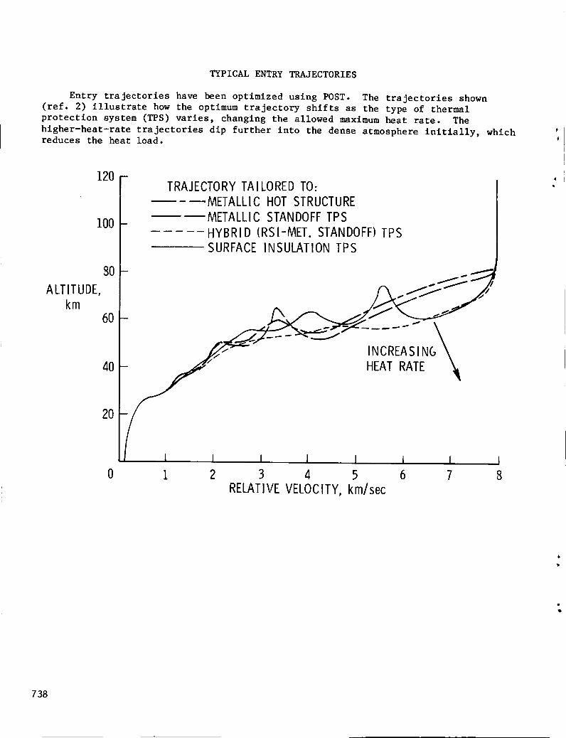
TYPICAL ENTRY TRAJECTORIES

Entry trajectories have been optimized using POST. The trajectories shown

(ref. 2) illustrate how the optimum trajectory shifts as the type of thermal

protection system (TPS) varies, changing the allowed maximum heat rate. The

hlgher-heat-rate trajectories dip further into the dense atmosphere initially, which

reduces the heat load.

120 -

I00

8O

ALTITUDE,km

6O

4O

2O

0

TRAJECTORY TAILORED TO:

METALLIC HOT STRUCTURE

METALLIC STANDOFF TPS

HYBRID (RSI-MET. STANDOFF) TPS

SURFACE INSULATION TPS

- .-. .....c..._._ "_/

,.CREAS,.C.\

[ I I I I l I

1 2 3 4 5 6 7

RELATIVE VELOCITY, km/sec

t8

'1iI

738

EFFECT OF TURBULENCE ON ENTRY HEATING

The trajectories shown (ref. 2) illustrate how the entry trajectory must be

tailored to the condition of the boundary layer. If there is only laminar heating,

the heat rate is quite low. If transition is allowed and turbulent heating exists,

the heating rate is very high unless the trajectory is tailored to account for the

different heating.

500 -

400 -

HEAT 300RATE,

kW/m 22OO

I00

0

IIIIIiiII

IIII

I "

/I I l_,.

500 I000 1500 2000

ENTRY TIME, sec

TRANSITION NOT ALLOWED, LAMINAR HEATING TAILOREDTRANSITION ALLOWED, LAMINAR HEATING TAILORED

TRANSITION ALLOWED,TURBULENT HEATING TAILORED

1 I

2500 3000

739

ORIGtNAL PAGE IS OF POOR QUALrrV

LIFI'OFF OF ADVANCED EARTH-TO-ORBIT VEHICLE

Ascent t r a j e c t o r i e s f o r advanced Earth- to-orbi t veh ic l e s have been optimized wi th POST. Single-stage veh ic l e s , such as the one shown ( r e f . 3 ) , have been studied, as w e l l as s taged systems. been considered. i n s e r t i o n o r b i t and c o n s t r a i n t s on acce le ra t ion , normal fo rce , and dynamic pressure.

Hor izonta l takeoff and a i r b r e a t h i n g concepts have a l s o The ascent t r a j e c t o r i e s o f t en inc lude t a r g e t t i n g t o a p a r t i c u l a r *

b

t

7 40

APPROACH FOR ROCKET ENGINE OPTIMIZATION

In a recent study to select optimum rocket engine chamber pressure and expansion

ratio (ref. 4), POST was used together wlth rocket engine design programs and vehicle

design and sizing programs. Although the trajectory was optimized internally, the

rocket engine chamber pressure and expansion ratio could only be optimizedparametrically.

SELECTROCKET ENGINECHAMBER PRESSURE

AND

EXPANSION RATIOS

CALCULATEROCKET ENGINE

CHARACTERI STICSl_

_

TRAJECTORY

r

J DESIGNVEHICLE

SELECTBEST ROCKETENGINECHAMBER PRESSUREAND

EXPANSION RATIO

OPTIMIZETRAJECTORY

SIZEVEHICLE

741

ROCKETENGINEOPTIMIZATION

Results of the parametric optimization of the rocket engine chamberpressure andexpansion ratio are shown(ref. 4). If vehicle dry mass is the parameter to beminimized, the optimumrocket engine would have a chamberpressure of 24.1MPA and anexpansion ratio of 60. The parametric results also provide vehicle gross massandinputs for cost estimating so that the optimumengine could be selected on a costbasis.

114 -

Si NGLE-STAGE-TO-OR BIT VEHI CLE

VEHI CLE

DRY

MASS,

Mg

110

106

102

ROCKET ENGINE

CHAMBER PRESSURE. MPa

1772 jK]

I I I I I

30 40 50 60 70

ROCKET ENGINE EXPANS ION RATIO

742

HYSAMCONFIGURATION DEVELOPMENT

A program has been under way to develop a hypersonic surface-to-air missile

(HYSAM). Some of the configuration development work that has taken place isillustrated (ref. 5).

• STABILITY AND

CONTROL OPTIONS

_ • SHOCK TRAP/

.j NOSE CAMBER_ _ BYPASS DUCT7 PARAMETR ICS_ "__/ _ __'_ • SCOOP INLET/ jr, INLET FLOW- _ __Lh_

! / su wY \

/ / f INLETTESTAsRTING "_ _ 1983 _

_, AERODYNAMIC TESTS _

1 f- ATM=4AND6 ONe/

STRUCTURAL OPTION

'li_ "/JM S--T:U AC__R;L,SOPT.

_ _._ MARTIN/MARQUARDT /

_ MISSILE DESIGN AND [PERFORMANCE STUDIES _.

1980 FOR NAVSEA _ CONFIGURATION

_- _ ALTERNATIVES

743

HYSAM TRAJECTORY FOR FLEET DEFENSE

A typical HYSAM trajectory (ref. 5) is shown.

considerably different from Earth-to-orbit vehicle

used successfully in both applications.

The HYSAM trajectories are

trajectories, but POST has been

(SCRAM JET ENGI NE-HYDROCAR BON FUEL-150 in. M I SSI LE)

22 in. x 22 in.

SHIPBOARD 80

ALTITUDElOO 000 ft

9/_BEGIN CRUISE, M= 6

4/5 POWER

/.MISSILE = 1162 IbWARHEAD - 200 Ib

-. I

I BURNOUTI t = 574 secIIIII¢:_ POWER-OFF

STAGE, M = 4. 2LAUNCH WT = 3308 Ib

I I I I _ I I

RANGE

744

.. i

ORIGtNAL PAGE IS OF POOR Q U A W

SPACE SHUTTLE ORBITER WITH TIP-FIN CONTROLLERS

The control-configured-vehicle approach appears to be useful for advanced Earth-to-orbit vehic les . to invest igate using t i p f ins in place of the center vert ica l t a i l on the Space Shuttle orbiter ( re f . 6 ) .

To help develop the technology, a program has been under way

745

RESPONSE OF SHUTTLE

As part of the investigation of the Space Shuttle Orbiter with tip fins, the

slx-degree-of-freedom version of POST was used to study the response of the orbiter

along various trajectories. This figure (ref. 6) is for the existing Shuttle orbiter

and shows the response to a 50 ft/sec head wind for a Mach number of 4.0 to

touchdown.

60

@'@c' 30

deg 0

-30

-605

13,deg 0

-5I00

5SB 'deg 50020

5r, deg 0

-20

MACH 4.0 TO TOUCHDOWN50 ft/sec HEAD WIND

r, @@

c

I I I

I I

I I I I I I0 100 200 300 400 500 600

TIME, sec

746

RESPONSE OF SHUTTLE WITH TIP FINS

The figure is different from the previous figure only in that the Shuttle has

tip fins instead of the central vertical fin (ref. 6). The differences in response

are used to evaluate the merits of the configuration change. Changes in the guidance

system logic have also been evaluated.

60

30¢' ¢c'

deg 0

-30

-605

13,deg 0

-5

6O

5tf, deg 0

-60

MACH 4. 0 TOTOUCHDOWN_ 50 ft/sec HEAD Wl ND

-!/\2--1

YI I I I I

me

¢C

B

m

I I I I I

0 100 200 300 400 500

TIME, sec

I

600

747

PROJECTED-GRADIENT OPTIMIZATION

This figure illustrates the projected gradient approach to optimization (ref.

i), which is the preferred option. The problem is to find the point with the highest

optimization level subject to the constraint boundary. A feasible region is defined,

within which the constraint errors are small enough that the trajectory can be

considered meaningful. An initial guess or nominal solution may be outside the

feasible region, as illustrated. In this case, the scheme tries to satisfy the

constraints or target in a manner that changes the independent variables a minimum

amount. Once targetted, the scheme tries to increase the optimization level along

the constraint boundary. Because of nonlinearities, the direction of search leaves

the constraint boundary so that a retargetting phase takes place based on the

gradient information at the beginning of the optimization phase.

INDEPENDENTVARIABLE

2

OPTIMIZATION

LEVELS

2

I

INAL

\FEASIBLE \REGION

CONSTRAINT

BOUNDARY

\

INDEPENDENTVAR IABLE I

748

OPTIMIZATION STEP SIZE

The step size must be selected for the optimization phase of the projected-

gradient scheme. The actual optimization level may continue to increase for very

large steps, but the constraint errors would probably be unacceptable. The approach

used by POST is to estimate what the optimization level will be after retargetting.

The step size is then selected to maximize the retargetted optimization level.

OPTIMI ZATIONLEVEL

SELECTEDSTEP SI ZE

ACTUAL

I

t I ESTIMATEI

WITHI, RETARGETTINGIII

I

IIIIII

STEPSIZE

749

RANDOM WALK OPTIMIZATION

Although the projected-gradlent approach has been used very successfully in

POST, occasional problems occur. For example, a trajectory might crash or otherwise

fall to reach a normal termination. For these infrequent but important cases, an

approach has been incorporated into POST which is almost foolproof in the sense that

if a nominal trajectory can be improved it will be.

This figure illustrates the random-walk approach to optimization. A penaltyfunction is constructed from the optimization index and the sum of the constraint

errors squared. The random-walk approach is to vary one independent variable at a

time. If an improvement in the penalty function level occurs, the new point is used

for the search in the next direction.

INDEPENDENT

VARIABLE2

OPTIMI ZATION

LEVELS

2

1

PENALTY FUNCTION LEVELS

NAL

CONSTRAINT BOUNI_

INDEPENDENTVAR IABLE 1

75O

RANDOM-WALKSTEPSIZE

The random-walk step size starts with a small value. If a step is successful,

the next step is larger. Once a step is unsuccessful, the scheme moves to the

next independent variable. When the scheme returns to the first independent

variable, the step direction is reversed and the step size is reduced.

PENALTYFUNCTION

_-, NOMINAL

_-STEP I STEP 5

__ _TEP2

EFFECTOF _

INDEPENDENT r"x_LSTEP3

VARIABLE2 _S_P4I,(SELECTED)

STEP N+I STEPN

INDEPENDENTVAR IABLE 1

751

RANDOM-WALKLOGIC

The logic for the random-walk schemeis mostly fairly straightforward. Thefirst independent variable is perturbed a small amount. If the penalty function isreduced, the perturbation size is increased and another step is taken. Whenthe stepfails to reduce the penalty function, the step size is reduced and the sign isreversed. The next independent variable is then perturbed.

The increase or decrease of the perturbation magnitude is controlled by aperturbation multiplier for each independent variable. The perturbation multiplieris initially set at 5.0 so that the steps initially grow by more than two orders ofmagnitude in three steps. Since the initial perturbation is often several orders ofmagnitude smaller than the changeneeded to find the solution, such large changes areuseful. Each time the direction of search in an independent variable changes sign,the perturbation multiple is reduced by raising it to the 0.7 power. This methodallows closer examination of the region near the optimum, yet large steps can stillbe taken whenneeded.

--I PERTURBATI ON S IZEINCREASE

I SELECT I NDEPENDENTIVARIABLE I

+

TRAJECTORY

I_ES NO_ DECREASE PERTURBATION ISIZE AND CHANGE SIGN

DECREASE PERTURBATIONMULTIPLE

VINCREMENT INDEPENDENT L-

VARIABLE I

752

INITIAL OPTIMIZATION RESULTS

Typical results of a case in which the random-walk method was used are shown.

The projected gradient method was used first. The first 12 trajectories were

required to get the gradient. The next six trajectories were attempts to target the

errors, and all six crashed. Each time a trial step crashes, the step size is

reduced by an order of magnitude. In this case, with a reduction of five orders of

magnitude in the step size and the crash of the sixth trajectory, the selected search

direction is apparently not a good choice.

The random-walk method was used when it became obvious that the projected

gradient method was having trouble. After seven trajectories with steps in the first

independent variable, the penalty function was reduced by about one third.

Perturbations in independent variables 2, 3, and 4 were not helpful. Six

trajectories with independent variable 5 perturbed reduced the penalty function

dramatically.

4000

3000

PENALTY 2000FUNCTION

1000

0

",T'""'",,'_..._

LTARGETTINGI

TRIALSTEPS

(CRASHES)

ASCENTTRAJECTORY2-STAGE VEHICLE

HOR17ONTALTAKEOFFI

oo • • 1

I

PROJECTED:

GRADIENT

110

1

3 5• ° ° °° ° ° • o 5

124

' -'-RANDOMI WALKII

II I20 30

TRAJECTORYNUMBER

•

_5

INDEPENDENTVARIABLE

NUMBER

66 6• 7 778"'r'-.... 4

40 50

753

FINALOPTIMIZATIONRESULTS

This figure showsthe continuation of the case shownin the previous figure.The penalty function scale is expanded, and only the best of each four trajectoriesis shown. The random-walkmethod was used for about 300 trajectories, and someimprovement was still being found.

The projected-gradient methodwas used at the end. Twoiterations quicklyreduced the errors to acceptable levels, and further optimization iterations madeimprovements that are not evident with the scale of the figure. Actually, theprojected-gradlent method probably could have been used successfully muchsooner andwould have solved the problem more efficiently.

PENALTY

FUNCTION

80-

40-

0-

-40-

-80 -

-1200

ASCENTTRAJECTORY2-STAGE VEHICLE

HORIZONTAL TAKEOFF

°°°°°Ooo Oo Oo

• • Ooo

°° °

°°°°OOoo °

ooooooo

°°°O°°°O°OOoooooe °

8OI I

160 240TRAJECTORYNUMBER

RANDOMWALK

Oo o

°°°°°°OOoooo

4_o.

I320

---_PROJECTEDGRADIENT

II o00

J ooo ooooo0

I

I n400

754

RANDOM-WALKRESULTS

Another exampleof use of the random-walkmethod is shownin this figure•Independent variable 6 provides someinsight into the random-walk results.Trajectories 7 through i0 were improvedminimally by perturbations of independentvariable 6, and trajectory ii resulted in a large increase in the penalty function•Trajectory 39 was a perturbation of independent variable 6 in the negative directionwhich did not reduce the penalty function. Trajectories 77 through 81 again resultedin minimal improvements in the penalty function followed by a large increase ontrajectory 82. Cases llke this indicate a strong nonlinearity. Up to a certainpoint, there is little effect of changing independent variable 6, but beyond thatpoint the results are significantly affected• This kind of behavior can lead toproblems for gradient methods if the gradient is calculated where the slope isshallow and steps are taken beyond the point where the change is significant. In therandom-walk approach, there is not muchimprovement from independent variable 6, butthe nonlinearity does not cause the methodto fail. Changesin independent variablesII and 2 provide most of the improvement.

ENTRYTRAJECTORYMINIMUM TIME

5600 - 65 $11 $6

4800

PENALTY 4000FUNCTION

32OO

".o° •°°e•° ,•,

• II _ INDEPENDENTVARIABLENUMBER

I°••,•o••ee e .2

2

I

i2O

.2

4 5 1 5 1 3e,e•eo'e°e•_•• ee•oee.o• •eeeeeeooee••.eee•eeele• ••e••.o.ee,eee.ee• e•ee•e

2400 I I I I I0 40 60 80 100 120

TRAJECTORYNUMBER

755

CONCLUSIONS

Experience with POSTat a numberof organizations around the country indicatesthat it is an excellent program for trajectory optimization problems. Also, theprojected-gradlent schemeused in POSTcan be used for problems other than trajectory

problems which require optimization of non-linear systems subject to constraints.

Despite the usefulness of the projected-gradient scheme in most problems, there are

occasional situations when using it will be difficult. For these situations, a

random-walk approach has been developed which offers a nearly foolproof solution to

most difficulties that might be encountered.

• POST IS RECOMMENDEDFOR TRAJECTORYOPTIMIZATION PROBLEMS

• THE PROJECTED-GRADIENTSCHEME IN POST IS RECOMMENDEDFOR

ALL NON-LINEAR OPTIMIZATION, NOT JUST TRAJECTORIES

• THE RANDOM-WALK APPROACH OFFERSA NEARLY FOOLPROOFSOLUTION TO MOST DIFFICULTIES ENCOUNTEREDBY THEPROJECTED-GRADlENT SCHEME

756

I •

e

•

.

e

•

References

Brauer, G. L.; Cornick, D. E.; and Stevenson, R.: Capabilities and

Applications of the Program to Optimize Simulated Trajectories. NASACR-2770, Feb. 1977.

Wurster, K. E.: An Assessment of the Impact of Transition on Advanced

Winged Entry Vehicle Thermal Protection System Mass. AIAA Paper No.

81-1090, presented at the AIAA 16th Thermophyslcs Conference, Palo Alto,CA, June 23-25, 1981.

Calouri, V. A.; Conrad, R. J.; Jenkins, J. C.: Technology Requirements for

Future Earth-to-Geosynchronous Orbit Transportation Systems. NASACR-3265, April 1980.

Martin, J. A.: Hydrocarbon Rocket Engines for Earth-to-Orbit Vehicles.

Journal of Spacecraft and Rockets, Vol. 20, No. 3, May-June 1983, pp.249-256.

Hunt, J. L.; et al: Design and Performance Sensitivities of a Dual-Mode

Scramjet Missile with Otto Fuel, Silane, and RJ-5 Pilots• Presented at

the 1983 JANNAF Propulsion Meeting, Monterey, CA, February 14-18, 1983.

Powell, R. W.; and Freeman, Delma C., Jr.: Evaluation of the AerodynamicControl of the Space Shuttle Orbiter with Tip-Fin Controllers. AIAA

Paper No. 84-0488, presented at the AIAA 22nd Aerospace Sciences Meeting,Reno, NV, January 9-12, 1984.

ACKNOWLEDGEMENTS

Examples presented were provided by James L. Hunt, J. Chris Naftel, Richard W.Powell, Kathryn E. Wurster. Their cooperation is appreciated.

757

v • 6 " "N87-117 5

COMPONENT TESTING

FOR DYNAMIC MODEL VERIFICATION

T.K. Hasselman and Jon D. Chrostowski

Engineering Mechanics Associates, Inc.

Palos Verdes Estates, California

PRECEDING PAGE BLANK NOT FIL_F._

759

DYNAMIC MODEL VERIFICATION

Dynamic model verification is the process whereby an analytical model of

a dynamic system is compared with experimental data, adjusted if necessary to

bring it into agreement with the data, and then qualified for future use in

predicting system response in a different dynamic environment. There are

various ways to conduct model verification. The approach taken here employs

Bayesian statistical parameter estimation. Unlike "curve fitting," whose ob-

jective is to minimize the difference between some analytical function and a

given quantity of test data (or "curve"), Bayesian estimation attempts also to

minimize the difference between the parameter values of that function (the

model) and their initial estimates, in a least squares sense. The objectives

of dynamic model verification, therefore, are to produce a model which (i) is

in agreement with test data, (2) will assist in the interpretation of test

data, (3) can be used to help verify a design, (4) will reliably predict

performance, and (5) in the case of space structures, will facilitate dynamic

control. (See fig. i.)

NO

HARDWARE I

NO

Q0

W

l,,-wl

W

Figure i

OBJECTIVES

e MATCH ANALYSIS AND TEST

e INTERPRET DATA

e VERIFY DESIGN

@ PREDICT PERFORMANCE

- IMPEDANCE

- DISPLACEMENT

- LOADS

- FATIGUE

- ETC.

• FACILITATE CONTROL

760

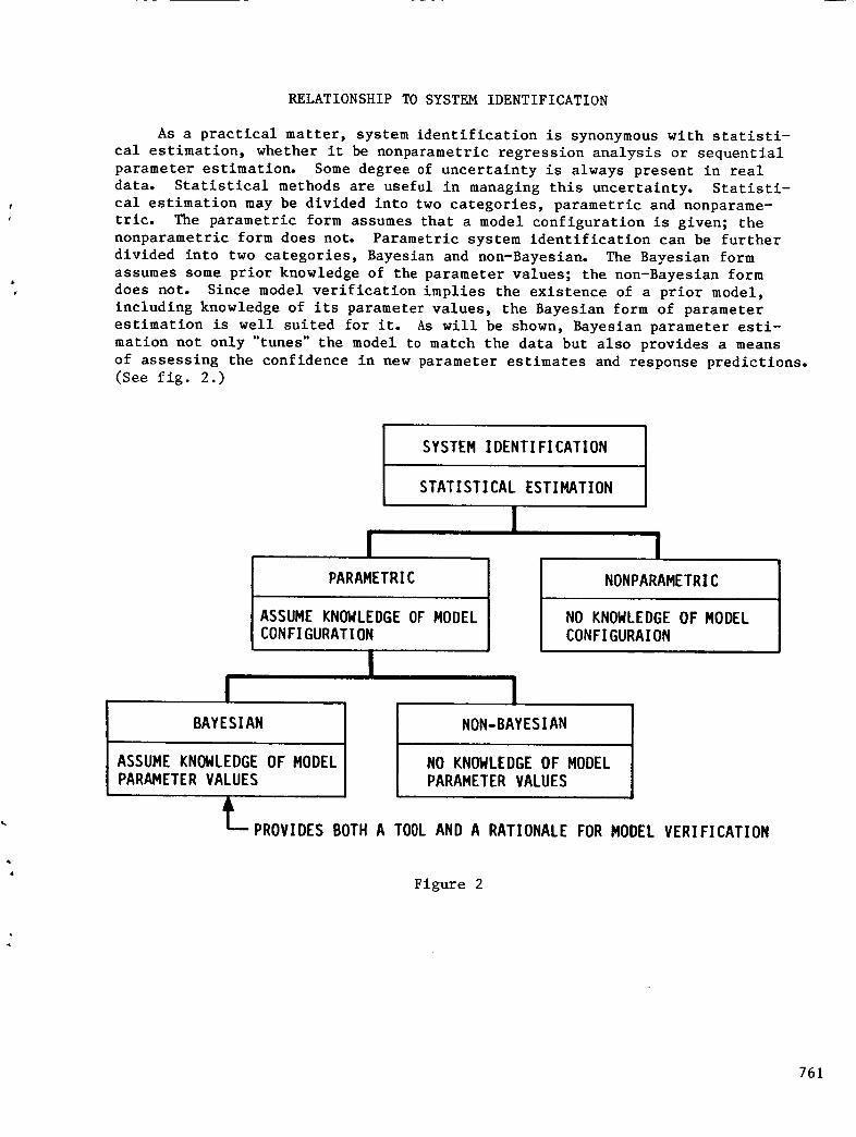
RELATIONSHIPTOSYSTEMIDENTIFICATION

As a practical matter, system identification is synonymouswith statisti-cal estimation, whether it be nonparametric regression analysis or sequentialparameter estimation. Somedegree of uncertainty is always present in realdata. Statistical methods are useful in managing this uncertainty. Statisti-cal estimation maybe divided into two categories, parametric and nonparame-tric. The parametric form assumesthat a model configuration is given; thenonparametric form does not. Parametric system identification can be furtherdivided into two categories, Bayesian and non-Bayesian. The Bayesian formassumessomeprior knowledge of the parameter values; the non-Bayeslan formdoes not. Since model verification implies the existence of a prior model,including knowledge of its parameter values, the Bayesian form of parameterestimation is well suited for it. As will be shown, Bayesian parameter esti-mation not only "tunes" the model to match the data but also provides a meansof assessing the confidence in new parameter estimates and response predictions.(See fig. 2.)

SYSTEM IDENTIFICATION

STATISTICAL ESTIMATION

lI I

PARAMETRIC

ASSUME KNOWLEDGE OF MODEL

CONFIGURATION

BAYESIAN

ASSUME KNOWLEDGE OF MODEL

PARAMETER VALUES

NON-BAYESIAN

L

NO KNOWLEDGE OF MODEL

PARAMETER VALUES

NONPARAMETRIC

NO KNOWLEDGE OF MODEL

CONFIGURAION

PROVIDES BOTH A TOOL AND A RATIONALE FOR MODEL VERIFICATION

Figure 2

761

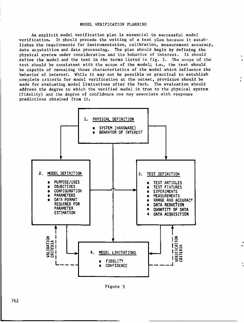
MODELVERIFICATIONPLANNING

An explicit model verification plan is essential to successful modelverification. It should precede the writing of a test plan because it estab-lishes the requirements for instrumentation, calibration, measurementaccuracy,data acquisition and data processing. The plan should begin by defining thephysical system under consideration and its behavior of interest. It shoulddefine the model and the test in the terms listed in fig. 3. The scope of the

test should be consistent with the scope of the model; i.e., the test should

be capable of revealing those characteristics of the model which influence the

behavior of interest. While it may not be possible or practical to establish

complete criteria for model verification at the outset, provision should be

made for evaluating model limitations after the fact. The evaluation should

address the degree to which the verified model is true to the physical system

(fidelity) and the degree of confidence one may associate with response

predictions obtained from it.

1. PHYSICAL DEFINITION

• SYSTEM (HARDWARE)• BEHAVIOR OF INTEREST

'V

2. MODEL DEFINITION

e PURPOSE/USES• OBJECTIVES

• CONFIGURATION

• PARAMETERS• DATA FORMAT

REQUIRED FORPARAMETERESTIMATION

o_ IL<'_'l

--,.., I

="JI

Li_ _ i

4. MODEL LIMITATIONS

• FIDELITY

• CONFIDENCE

P

3. TEST DEFINITION

• TEST ARTICLES

e TEST FIXTURES• EXPERIMENTS

• MEASUREMENTS

• RANGE AND ACCURACT

• DATA REDUCTION

• QUANTITY OF DATA

e DATA ACQUISITION

I,.-=&,iJ,-4 I.-,

.J

Figure 3

762

STRATEGYCONSIDERATIONS

Whena dynamic model must replicate the behavior of a complex physicalsystem responding to various sources of excitation, a strategy will be neededto carry out the model verification. The military principle of "divide andconquer" is helpful in formulating sucha strategy. Componenttesting offersone avenue of simplification. Direct measurement (e.g. of mass or stiffness)is always preferable to indirect parameter estimation, and should be employedwherever possible. Software capabilities and computational limitations dic-tate the primary constraints on parameter estimation, as indicated in fig. 4.Grouping and sequencing procedures maybe employed to achieve successful modelverification within these constraints.

COMPONENT TESTING

• DIRECT MEASUREMENT

• PARAMETER ESTIMATION

SOFTWARE CAPABILITY

• MODELING CAPABILITY

• NUMBER OF PARAMETERS ESTIMATED

• TYPE OF DATA INPUT

• NUMBER OF DATA POINTS PROCESSED

COMPUTATIONAL LIMITATIONS

• RESPONSE/PARAMETER SENSITIVITY

• NUMERICAL CONDITIONING

• COMPUTATION EFFORT AND COST

Figure 4

GROUPING

• MODEL PARAMETER SUBSETS

• TEST DATA SUBSETS

SEQUENCING

• BY COMPONENTS

• BY MODEL PARAMETER SUBSETS

• BY MEASUREMENT CHANNELS

• BY FREQUENCY BANDS

763

RECENTEXPERIENCEVIBRATIONTESTINGOFA CANTELEVERBEAMWITHDISCRETEDAMPER

The foregoing principles of model verification planning and strategydevelopment are currently being applied to a structure which resembles acantilever beam, with discrete damping and stiffness elements attached to itsfree end (fig. 5). The beamis nearly axi-symmetric and exhibits closely spacedpairs of modesperpendicular to its axis. It is suspendedvertically with adouble compoundpendulumdampernear its lower end. The damperconsists of apendulous weight immersedin silicone damping fluid. The mathematical model iscomprised of two components: a modal representation of the beam itself,extracted from a 500 degree-of-freedom finite element model, and a lumped-massmodel of the damper. Testing consisted of single-point random vibration, fromwhich complex frequency response and coherence functions were obtained atseveral stations along the beam.

li/_X"Clk _ _MI4\\

u..I

c_o

w

FREQ.

LOADCELL

ISHAKER _'/#A "',y/Axyla,,yAvl

DATAACQUIS.SYSTEM "-"

I

I CANTILEVERBEAM

DISPL

PROBE

---t

----t

MODE

#2

PENDULUMI

, DAMPER ASSEMBLYi

Figure 5

\

\

/

MODE #l

764

COMPONENT TESTING OF DISCRETE DAMPER

One of the objectives of this model verification effort was to determine

the damping characteristics of the discrete damper itself. Anticipating that

it might be difficult to extract this information from vibration testing of

the complete beam assembly, available data from earlier component tests per-

formed on the damper alone were processed. The component vibration tests

consisted of rigidly securing the damper housing to a carriage that was free to

move back and forth on rails. Broad-band random excitation was applied to the

carriage by a shaker, and the resulting acceleration of the carriage was

measured. Load cells in the clamps securing the damper housing measured the

force applied to the housing. The data were Fourier analyzed to obtain the

complex frequency response of force divided by acceleration, i.e. an effective

mass. The pendulum damper was modeled with two degrees of freedom, as shown

in fig. 6.

HE]GHTASSEMBLY_

SIL|CONEFLUID

7

:::::::::::::::

0

HOUSING

TOP

LOADCELL

BOTTOM

LOADCELL

SUPPORT

SHAKER

8

x IHOI.

NE]GHT

ASSEMBLY_ _.DAMPER

e

DAMPER

BASE

INPUT

Figure 6

765

COMPARISONOFPREDICTEDANDMEASUREDRESPONSE- DISCRETEDAMPER

Initial estimates of the damping constants for the pendulumdamper wereinferred from "snap-back" tests on the beamassembly. These estimates provedto be grossly in error as evidenced by the comparison of "prior model" and"test data" response shown below. A modified version of the MOVERcomputerprogram (ref. i) was then used to estimate lateral and rotational dampingcoefficients CL and CR, an equivalent representation of the two dashpots shownin the preceding figure. A subsequent attempt was madeto estimate a possiblerotational stiffness, KR, which might arise from fluid sloshing at the fre-quency of the secondpendulummode. No significant estimate of KR wasobtained; however, the estimated values of CL and CR were approximately thesame in both cases. These estimates produced the response curve labeled"revised model" in fig. 7. It matched the data points quite well.

i0°

1o-I

10 -2

REVISESMODEL

w_

N

,d

% TEST DA"A

%

•• _ d_.'•• "I _ O _I |

f" _w" i

J IPRIORMODEL

I0FREQUENCY

Figure 7

I00

766

PARAMETER ESTIMATES - DISCRETE DAMPER

A summary of the parameter estimates for CL, CR and KR is shown in fig. 8.The prior estimates are shown along with the revised estimates. In addition

to each set of estimates, the standard deviations and correlation matrix of

each estimate are shown. Standard deviations of the initial estimates were

assumed to be arbitrarily large, with no correlation. Standard deviations of

the revised estimates indicate the statistical significance of those estimates.

Of the three, only CL was estimated with a satisfactory degree of confidence.

The estimated values of CL and CR resulted in the first mode of the damper

being overcrltically damped (approximately 400% of the critical damping) and

the second mode having about 50% of critical damping. The revised estimate of

KR was rejected in favor of the prior estimate, KR=O.

PRIOR

PARAMETER ESTIMATED STANDARD CORRELATION

SYMBOL VALUE DEVIATION MATRIX

CL .140 31.6 ].0 .0 .0

CR .140 31.6 l.O .0

KR .0 S.16 l.0

REVISED

CL 3.787 .444 l.O .406 .]7]

CR .537 .800 l.O .069

KR .492 2.914 l.O

Figure 8

767

COMPARISONOF PREDICTEDANDMEASUREDRESPONSE- BEAM ASSEMBLY

The estimates of CL and CR obtained from the foregoing component test and

parameter estimation were then used in a model of the beam assembly to gener-

ate a frequency response function representing displacement response at the

lower end of the beam divided by the force input measured by the load cell(fig. 5). The discrete damper model was coupled to the modal model of the beam,

wherein each mode was nominally assumed to have 0.5% damping (one-half Of one

percent). The corresponding results labeled "prior model" are shown in fig. 9

in comparison with data points actually used in subsequent parameter estimation.

A total of 24 mass, stiffness and damping parameters was estimated in three groups,

each associated with a pair of orthogonal modes perpendicular to the beam axis.

Data from three distinct frequency bands were used in the estimation, which pro-

duced the results labeled "revised model" in the figure. As can be seen, the

revised model fits the data reasonably well except in the vicinity of the third

resonance. This is where the effect of a poor estimate of CR for the pendulum

damper would be expected to appear. Efforts are continuing to improve upon thisestimate.

i,i

__J

100

10-I

10 -2

-3I0

_I PRIOR MODEL

/_REVISED MODEL

...y,,'

I

I0

It

100

FREQUENCY

Figure 9

768

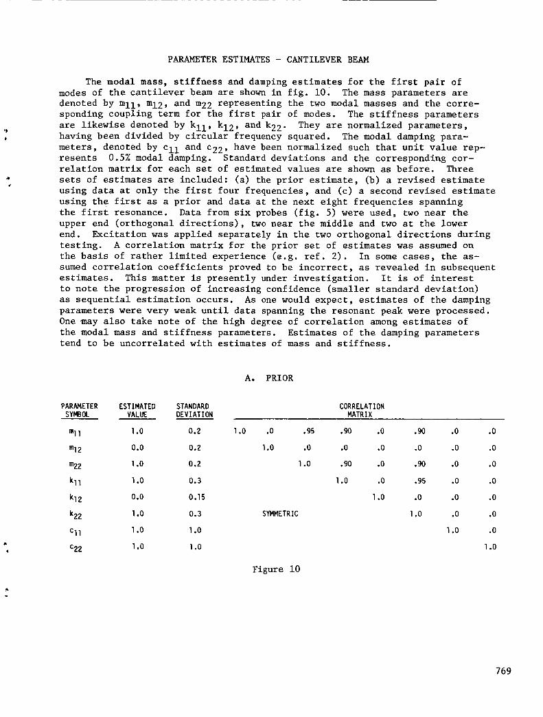
PARAMETERESTIMATES- CANTILEVERBEAM

The modal mass, stiffness and dampingestimates for the first pair ofmodesof the cantilever beamare shownin fig. i0. The mass parameters aredenoted by mll , m12, and m22representing the two modal massesand the corre-sponding coupling term for the first pair of modes. The stiffness parametersare likewise denoted by kll, k12, and k22. They are normalized parameters,having been divided by circular frequency squared. The modal damping para-meters, denoted by Cll and c22, have been normalized such that unit value rep-resents 0.5%modal damping. Standard deviations and the corresponding cor-relation matrix for each set of estimated values are shownas before. Threesets of estimates are included: (a) the prior estimate, (b) a revised estimateusing data at only the first four frequencies, and (c) a second revised estimateusing the first as a prior and data at the next eight frequencies spanningthe first resonance. Data from six probes (fig. 5) were used, two near theupper end (orthogonal directions), two near the middle and two at the lower

end. Excitation was applied separately in the two orthogonal directions during

testing. A correlation matrix for the prior set of estimates was assumed on

the basis of rather limited experience (e.g. ref. 2). In some cases, the as-

sumed correlation coefficients proved to be incorrect, as revealed in subsequent

estimates. This matter is presently under investigation. It is of interest

to note the progression of increasing confidence (smaller standard deviation)

as sequential estimation occurs. As one would expect, estimates of the damping

parameters were very weak until data spanning the resonant peak were processed.

One may also take note of the high degree of correlation among estimates of

the modal mass and stiffness parameters. Estimates of the damping parameters

tend to be uncorrelated with estimates of mass and stiffness.

A. PRIOR

PARAMETER ESTIMATED STANDARD CORRELATIONSYMBOL VALUE DEVIATION MATRIX

m]l 1.0 0.2 l.O .0 .95 .90 .0 .90 .0 .0

m]2 0.0 0.2 l.O .0 .0 .0 .0 .0 .0

m22 |.0 0.2 l.O .90 .O .90 .0 .0

kll l.O 0.3 ].0 .O .95 .0 .0

kl2 O.O 0.15 l.O .0 .0 .O

k22 ].O 0.3 SYMMETRIC l.O .O .O

Cl] l.O l.O l.O .0

c22 l.O l.O l.O

Figure i0

769

B. REVISED (i)

PARAMETER

SYMBOL

m]]

ml2

m22

kll

kl2

k22

Cll

c22

ESTIMATED

VALUE

1.150

.000

1.141

.973

.016

.986

.858

1.735

STANDARDDEVIATION

.045

.046

.054

.043

.030

.046

.574

.668

l.O -.234 .2]3

] .0 .166

].0

SYMMETRIC

CORRELATIONMATRIX

•504

-.134

.411

l.O

-.240

.609

-.204

-.788

l.O

-.041

.I07

•009

-.796

.768

1.0

-.011

-.O03

-.035

-.077

•066

.066

1.0

.004

.004

.011

.022

-.018

-.022

-.442

1.0

C. REVISED (2)

PARAMETERSYMBOL

mll

m12

m22

kll

kl2

k22

Cll

c22

ESTIMATEDVALUE

1.150

-.002

1.117

.990

-.171

.951

2.248

2.456

STANDARDDEVIATION

.025

.016

.028

.021

.013

.024

.I02

.144

l.O

CORRELATIONMATRIX

-.860 -.872 .992 -.852 -.854 -.]44 -.398

].0 .849 -.859 .992 .836 -.]45 .368

].0 -.878 .85l .989 -.092 .304

].0 -.86] -.874 .149 -.496

1.0 .851 -.]53 .329

SYMMETRIC 1.0 -.|22 .265

1.0 -.509

l.O

77O

Figure i0

(continued)

EVALUATION OF RESULTS

The progress of a model verification effort must be continuously moni-

tored to assure acceptable results. Quantities available for critical evalua-

tion include the items listed in fig. ii. Experience has shown that if an

incorrect model is being used in the parameter estimation, the estimates may

not converge, or they may converge to unreasonable values. Both the parameter

values themselves and the corresponding eigenvalues and eigenvectors (for a

linear model) should be recorded during the iterative process of parameter

estimation. This record often provides insight to problems (e.g. failure to

converge) which arise. The statistical significance of parameter estimates

should be evaluated before accepting the results. If a partial set of

parameter estimates from one estimation is used in a subsequent estimation

involving different parameters, the estimates of the partial set should be

uncorrelated from the remainder of that set. When evaluating predicted re-

sponse, one should consider the confidence limits on predicted response, in

addition to how well it matches a particular set of data.

PARAMETER ESTIMATES

NUMERICAL CONVERGENCE OF PARAMETER ESTIMATES

REASONABLENESS OF PARAMETER ESTIMATES

REASONABLENESS OF CORRESPONDING EIGENVALUES AND EIGENVECTORS

STATISTICAL SIGNIFICANCE OF PARAMETER ESTIMATES

CORRELATION AMONG PARAMETER ESTIMATES

PREDICTED RESPONSE

• RMS ERROR BETWEEN PREDICTED AND MEASURED RESPONSE

• CONFIDENCE LIMITS ON PREDICTED RESPONSE

Figure ii

771

CONCLUSIONS

Dynamic model verification is a multi-discipllned task involving analysis,

testing, parameter estimation, and most importantly, an overall plan which

coordinates these efforts. Parameter estimation (or system identification, as

some would call it) is only a part of the process. Bayesian parameter estima-

tion, however, is a valuable tool, greatly facilitating the "marriage" of

analytical and experimental data bases. (See fig. 12.)

Model verification is not an easy task. Ironically, while Bayesian

estimation adds a new dimension of capability for accomplishing this task, it

seems at times to make it even more difficult. But that is only because it

reveals weaknesses in the model or the data which might otherwise escape

unnoticed. In a very important sense, it holds the analyst more accountable

by demanding a higher degree of model fidelity to the physical system, andmeasurable confidence in the final results.

DYNAMIC MODEL VERIFICATION SHOULD INCLUDE THE FOLLOWING ELEMENTS:

.

.

.

AN INITIAL PLAN WHICH COORDINATES MODELING, TESTING AND SUBSEQUENT PARAMETERESTIMATION IN SUCH A WAY THAT SUFFICENT DATA ARE OBTAINED TO ESTIMATETHE DESIRED MODEL PARAMETERS.

A STRATEGY FOR PARAMETER ESTIMATION THAT ENABLES MODELS OF COMPLEX SYSTEMS

TO BE VERIFIED WITHIN THE LIMITATIONS OF AVAILABLE SOFTWARE AND NUMERICALCOMPUTATION.

A FINAL EVALUATION OF MODEL LIMITATIONS, BASED ON THE RESULTS OF PARAMETER

ESTIMATIO_ AND INHERENT LIMITATIONS OF ANALYSIS AND TEST WHICH ARE OTHERWISEKNOWN.

Figure 12

772

io

o

REFERENCES

Chrostowski, J.D., Evensen, D.A., and Hasselman, T.K., "Model

Verification of Mixed Dynamic Systems," ASME Journal of Mechanical

Design, Vol. i00, April 1978.

Hasselman, T.K., "Structural Uncertainty in Dynamic Analysis," Paper

811049, Transactions of the Society of Automotive Engineers, 1982.

773

w •

DUAL STRUCTURAL-CONTROL OPTIMIZATION OF

LARGE SPACE STRUCTURES

Achille Messac and James Turner

The Charles Stark Draper Laboratory, Inc.

Cambridge, Massachusetts

PRECEDING PAGE BLANK NOT FILM_

775

Abs tract

This paper proposes a new approach for solving dual structural-

control optimization problems for high-order flexible space structures

where reduced-order structural models are employed. For a given initial

structural design, a quadratic control cost is minimized subject to a

constant-mass constraint. The sensitivity of the optimal control cost

with respect to the structural design variables is then determined and

used to obtain successive structural redesigns using a constrained

gradient optimization algorithm. This process is repeated until the

constrained control cost sensitivity becomes negligible. A numerical

example is presented which demonstrates that this new approach effective-

ly addresses the problem of dual optimization for potentially very high-

order structures.

776

q

f

I Introduction

One important variable which determines the cost of transporting

a payload to orbit is its total mass. Consequently, at the structural

design stage, a strong effort is made to optimize the structure for the

mission at hand. Minimum mass and maximum structural eigenvalues consti-

tute the two most frequently used structural optimization criteria

(Refs. I-7). The resulting structure is generally highly flexible and

often requires active control (Refs. 8-12). As a result, subsequent to

the structural design, the control engineer attempts to determine the

optimal control strategy necessary to accomplish the mission.

Traditionally, the problems of optimal structural design and

optimal control design are solved with little or no interaction. As a

result, the "global design" is not optimal. In an effort to overcome

this situation, we present in this paper a new method for simultaneously

optimizing the structural and control design. A key feature of the pro-

posed method is the use of a reduced-order model for the equations of

motion. A numerical solution for the problem of optimal spacecraft slew-

ing maneuvers of a structurally optimal spacecraft is presented.

This dual optimization problem has previously been considered by

Hale (Refs. 13, 14) for problems involving simple structures. The main

difficulty encountered in the formulation of Hale's algorithm is the

relatively high order of the resulting non-linear two-point boundary

value problem (TPBVP) which must be solved at each stage of the iterative

redesign procedure; indeed the order of the resulting system is more than

four times the order of the mass or stiffness matrix. Moreover, the

777

problems associated with handling high dimensional systems are the primary

reason for the relatively limited scope of the applications of the dif-

ferent methods proposed to date.

The new approach we present in this paper follows a drastically

different path in the derivation of the necessary conditions for the

joint structural-control optimization. The problem is formulated in

modal rather than physical space. As a result, the order of the TPBVP

is dictated no longer by the complexity of the structure (order of the

mass and stiffness matrices) but rather by the number of structural

modes which participate in the dynamic excitation of the spacecraft. In

most practical applications, the total number of such modes rarely

exceeds a dozen.

Specifically, we seek the optimal structural design that enables

the slewing maneuver and vibration suppression of the spacecraft to be

performed optimally while keeping the total mass constant. The appro-

priate techniques for obtaining an optimal minimum-mass structure are

considered in another paper (Ref. 15).

II Generic Problem Statement

We wish to determine the structural design that minimizes the fol-

lowing peformance index

I x_ S(d)xf÷ I tf uTRu]dt (I)J = _ _ J [xTQ(d)x+o

subject to a linear time-invariant equation

x(t) = A(d)x(t) + B(d)u(t) (2)

where the total mass m T and initial state xo are given. In the above

equation d is the design variable vector, tf and xf are the final

time and final state respectively, x(t) is The state vector, u(t) is the

778

control force vector, S and Q are real positive semi-definite matrices, R

is a real positive definite matrix, and S, Q, and R are defined in

Appendix A.

To obtain Eq. (2) we first derive the appropriate set of governing

second-order ordinary differential equations of the form

M(d)_(t) + K(d)w(t) = E(d)u(t) (3)

where M(d) and K(d) represent the (N x N) symmetric mass and stiffness

matrices, w(t) is a generalized coordinate vector for the elastic and

rigid-body motions, and E(d) is an (N x Nc) control influence matrix which

determines the point of application of the generalized control forces

numbering N c. Equation (3) is transformed to modal coordinates by

carrying out an eigenvalue analysis and normalizing the modes _ such that

_TM_ = I and _TK_ = A. By retaining only those modes - numbering

N m < N - which significantly participate in the dynamic response of the

structure, a reduced-order state space model of the form of Eq. (2) is

obtained by defining

0 -A I

A = (4)

I 0

(5)

T Tx : {iT } (6,

where A and B are of order (2N m x 2N m) and (2N m x N c) respective-

ly, _ is a vector of modal coordinates, and I is an identity matrix.

779

III Optimization Problem Solution

A. Optimal Control Design

The necessary conditions for an optimal control solution can be

can be shown to satisfy (Ref. 9)

x= D (7)

and

u = -R -I BTI

where X is the costate vector,

D

I -I BT 1

A -BR

-Q -A T

and the boundary conditions are

l(tf) = Sx(tf)(9)

x_t'-) = xo o

(10)

Through some simple manipulations it can be shown that

X(0) = Hxo

(11)

780

where

S

-1

-H A H B(12)

and

HA = -S_21 + _22(13)

H B = -S_11 + _12(14)

with _ defined as

Dtf= e

2m

_I I

'{'21

2m

12

v/22

} 2m

} 2m

(15)

Moreover, from Ref. 11, it can be shown that the cost of Eq. (1) ¢an be

written as

J(d) = ! xTH(d)x (16)2 o o

B. Iterative Structural Redesigns

So far, we have determined the optimal control cost associated

with a given set of design variables d. We now present the numerical

scheme which is used to minimize the control cost by iteratively refin-

ing d.

781

We first express the constant mass requirement as pTd = mT,

where d is the design variable vector, mT the given total mass, and p avector of structural parameters. More specifically, in terms of changes

in the design variables Ad, the constant massconstraint follows as

pTAd = 0 ( 17 )

In order to establish a constrained optimization algorithm

which takes into account Eq. (17), we first determine the normalized

_J _Jgradient vector s =-_/li-_ll (Appendix B) where li*ll denotes the Eu-

ii II

clidian norm (see Figure I). We subsequently make use of the Orthogonal

Projection Theorem (Ref. 16) which states that the projection of the vec-

tor e onto the surface of constant mass represents the direction of great-

est decrease in J which also satisfies Eq. (17). As a result, the desired

change in the design variable vector, to within a multiplicative constant

c, becomes

I 1_d = c e ePT P (18)

P P

The performance index partial derivatives are listed in Appendix B.

From a geometrical point of view, the above equation clearly

states that when _Tp = llell ollpll, the gradient vector e is orthogonal

to the constant-mass-constraint plane and Ad = 0; thus no further improve-

ment can be made and a minimum has been reached (see Figure 1 ). On the

other hand, when eTp = 0, the gradient vector lies in the constant mass

plane and Eq. (18) requires Ad = c_; thus great improvement can be made.

In order to monitor progress towards the optimum dual design, the

following convergence parameter is defined:

782

which is equal to 0 for the worst possible design and I for the optimal

design where I*I denotes absolute value.

The constant c in Eq. (18) can be chosen in the beginning of the

optimization process such that a given small fraction of the total design

massis displaced. Examination of Eq. (18) reveals the desirable property

that the norm of Ad decreases monotonically as the optimal design is being

approached. Oncec is chosen, the following step sizes are then automat-ically determined. The dually optimal design is reached when the para-

meter 8 satisfies the inequality 11-81 < el, where eI is user speci-fied.

IV Illustrative Example

A. Structural Model

The example problem analyzed in this paper consists of a linear

structure which has the following characteristics (see Figure 2):

• 20 extensional finite elements of equal length

• 21 nodal displacements which coincide with the lumped masses

• uniform mass density p = 100 kg/m 3

• uniform Young's modulus E = 800 N/m 2

• equal initial cross-sectional areas which constitute the design

parameters (see Fig. 2)

• length £ = 3m

• a control force applied to the left-most structural node

(see Figure 2).

783

This structure has been selected because it offers two desirable

features. First, in order to verify the ability of the proposed approach

to optimize higher order structures through reduced-order modelling, it

was deemednecessary to analyze a structure which is composedof more than

15 elements. (Clearly this objective has been met.) Second, the structure

is simple enoughto allow physical interpretation of the results.

B. Optimal vs. Non-Optimal Dynamic Response

In the control problem considered here, it is desired to perform a

rest-to-rest maneuver where the rigid body modal displacement takes on the

initial value of 30.0 and the final value of 0.0 in 2 seconds (Figure 3).

As shown in Figure 3, the optimal control performance is greatly improved

through successive iterative structural redesigns, where the "optimal"

control design of the initial structure is contrasted to that of the

final - optimal - structure. There are two salient features of the dynam-

ic response. First, the peak values of these time-varying quantities are

significantly higher in the case of the non-optimal structural design. In

particular, the optimal design requires a peak control force 3.4 times

lower, and the resulting elastic deflection is 3.07 and 4.96 times lower

for the first and second mode, respectively. Second, the optimal dynamic

responses are typically smoother in the case of the optimal structural

design.

C. Control Cost Decrease

As previously stated, each step of the redesign process is respons-

ible for a decremental change in the control cost J at each redesign

stage. Figure 4 clearly depicts the expected monotonic decrease in J:

83% from the initial to final structural design in 45 iterations. Clear-

ly, this represents a dramatic decrease in the optimal cost. At a value

784

of the convergence parameter 8 of 0.95, the optimal design was considered

reached, in order to prevent the last design variable from vanishing. It

is anticipated that further gains in system performance can be achieved

by: i) allowing the total mass to be a design variable; ii) allowing the

elements of the control weighting matrices S, Q, and R to be design vari-

ables (Appendix A); and iii) allowing the sensor and actuator locations to

be design variables. However, these extensions are not considered here.

D. Consequences of Mode Shape Derivatives

Often, in structural analyses involving the variations of eigen-

values and eigenvectors, the structural designer only accounts for the

changes in the eigenvalues. While in many cases such action is accept-

able, in many others the omission of the eigenvector sensitivities leads

to erroneous results. Unfortunately, the problem dealt with in this paper

belongs to the latter class of problems. To see this we refer to Figure

5, where we observe that the first eigenvalues which participate in the

dynamic response increase (see Figure 6). Furthermore, we make the

important observation that the eigenvector nodal displacements which are

close to the point of application of the force decrease, while the others

increase. (We recall that the force vector is applied to the left; see

Figure 2.) Physically, the smaller nodal displacement at the force

application point leads to reduced structural excitation (Ref. 15).

We finally note that the effect of the mode shape sensitivity is

contained in the control influence coefficient matrix B (see Eq. (5)), and

thus conclude that the eigenvalue derivative alone will not capture the

ingredients neccesary for convergence toward the global optimum.

The basic algorithm is formulated in Figure 7.

785

V Conclusion

In this paper we present an approach for solving a dual structural-

control problem which involves high-order structures through a reduced-

order model. The validity of the theory developed is demonstrated by

using a structural model of 20 finite elements. The significant findings

of this paper are: i) the use of reduced-order models has a tremendous

impact on the computer time required in the optimization process and may

be necessary in the optimization of high-order structures; ii) the imple-

mentation of a constant mass optimization leads to a dramatic decrease in

the control cost; iii) the use of mode shape derivatives is required for

convergence towards the global optimum; and iv) the use of the eigenvalue

and eigenvector extrapolation formulas of Appendix B makes the reduced-

order model formulation a practical numerical technique (indeed, the exact

eigen solution was computed only three times during the optimization

process).

786

P

JOPTIMAL DESIGN

\

\

.__ \ . INTERMEDIATE DESIGN

/ x _ I \ DECREASING

/ .___ _osT \

Ad = C G pr p

Figure I. Gradient vector with respect to the constant-mass

plane.

787

°"'_-I I

INITIAL DESIGN

.....!._........J............J

u(t)

FINAL DESIGN

• BOTH DESIGNS HAVE EQUAL TOTAL MASS

• u(t) = CONTROL FORCE

Figure 2. Initial vs. final structural design.

788

o'"I "%

\O.Of _.

0.0 TIME (s) 2.0

8.6

Q_o_:!_2o

<

-8.60.0

I/ \

/ \I \

I' \

\ /k /

_\ i I

TIME (s) 2.0

6.8

O

,-,2oZ_O--

-6,80.0

lI _ t-\/ \ /' \

_: \ / \

,, / \ I

\ / \ I\ ....I _ /

\ I

TIME (s) 2.0

1,7

LUO.n"

oo0

__×zo

-1.7

AI

/

/ __ • ,\ r

#[/#

0.0 TIME (s) 2.0

0.0

O

a__uJ

>

-24.00.0

I '\ / '\ /

"\....,, II _ "\k i

! _ \ .;

TIME Is) 2.0

20.0

_a o._o,u. tu

>

-31.00.0

\ / \/ ,,-/ "--_I \.

[ \/

i /I _

t '

'' \/t /

_'d/ X t

TIME (s) 2.0

42.0 ....,/ \ / \( \ # \

',,'_ # '_. I \

O-- I / \ / ',

:_ I , P., ,_ \ ,-_-6 l _/ _ /" \- l

S _, r,_,, ', , \ - iiI"J' , , ',/'1/ \ i

-._0t ',/ /0.0 TIME Is) 2.0

OPTIMAL CONTROL DESIGN OF

INITIAL NON-OPTIMAL STRUCTURE

OPTIMAL CONTROL DESIGN OF

FINAL OPTIMAL STRUCTURE

Figure 3. Optimal control design of initial vs. final (optimal)

structural design.

789

Jo = INITIAL COST

J = INTERMEDIATE COST

J/Jo

0.17

ITERATION NUMBER

IItI

45

Figure 4. Monotonic decrease of optimal control cost during

the "dual" optimization process.

790

;_ = 8.8

;k.f = 16.6

FIRST MODE

;_0 = 34.8

= 47.9

SECOND MODE

;_0 = 77.5

X,f "= 93.5

THIRD MODE

;"0 = 135.0 _

;kf = 152,0

..,,,,_..._ _-._..:.____-_ ==-_- ...... . i

FOURTH MODE

INITIAL STRUCTURAL MODE SHAPE

FINAL OPTIMAL MODE SHAPE

;k0 = INITIALEIGENVALUES(rad/s) 2

Xf - FINAL EIGENVALUES (rad/s) 2

The modes are normalized such that _TM_ = I.

Figure 5. Initial vs. final eigenstructure.

791

Structural Spectrum (rad) 2s

Mode # Initial Optimal

I

2

3

4

5

6

7

8

9

10

11

1213

14

15

16

17

18

19

20

21

0.0

8.8

34.877.5

135.0

208.0

293.0

388.0491.0

600.0711.0

822.0

931.0

1034.0

1129.0

1214.0

1286.0

1345.0

1387.01413.0

1422.0

0.0

16.6

47.9

93.5

152.0

223.0

306.0

398.0

498.0

603.0

711.0818.0

923.0

1023.0

1115.0

1198.0

1269.0

1328.0

1374.0

1405.0

1422.0

Structural Designs

InitialDesign

Par. #

t

2

3

45

6

7

8

9

10

11

12

13

14

15

1617

18

19

20

O. 1451

O. 1451

O. 1451

O. 1451

O. 1451

0.1451

O. 1451

O. 1451

O. 1451

O. 1451

O. 1451O. 1451

O. t451O. 1451

O. 1451

O. 145 t

O. 1451

O. t451

O. 1451

O. 1451

Opt ima 1

O. 4O5

0.363

0.326

0.291

0.2580.227

O. 198

0.17t

O. 146

O. 122

O. 101

0.082

0.065

0.050

O. 037

0.026

0.017

0.010

O. 005

0.002

Figure 6. Structural

parameters

design.

spectrum and structural design

for the initial and final (optimal)

792

INPUT p,d,Xo,61,62,STRUCTURAL CONFIGURATION

S-Q-R RELATED CONSTANTS

i=O, imax

I co_uT_.,_,¢,X

II•_ COMPUTE A,B,J(d), '_d ' EQS. (4,5,18, A)

_ YES

NO

COMPUTE Ad-- C (3_- _ P EQ. 18

_q_ STOP. "_(OPTIMAL DESIGN)/]

I UPDATE d, M, K

a_ aX IEXTRAPOLATE¢,/_, USING Bd 'Bd

COMPUTETt" ={'f r [_sT M _]/n } }

_1 i=i+t _

YES

_r

_ COMPUTE EXACT_,X I

I

Figure 7. Differential correction algorithm.

793

REFERENCES

I •

2e

31

4•

5•

6•

7e

8•

9•

10.

11.

12.

Pierson, B.L., "A Survey of Optimal Structural Design Under Dynamic

Constraints," International Journal For Numerical Methods in

Engineering, Vol. 4, pp. 491-499, 1972.

Sheu, C.Y., and W. Prager, "Recent Developments in Optimal

Structural Design," Applied Mechanics, Rev. 21, pp. 985-992, 1968.

Turner, M.J., "Design of Minimum-Mass Structures With Specified

Natural Frequencies," AIAA Journal, 5, pp. 406-412, 1967.

McIntosh, S.C., and F.E. Eastep, "Design of Minimum-Mass Structure

With Specified Stiffness Properties," Vol. 6, No. 5, AIAA Journal,

pp. 962-964, 1968.

Bellagamba, L., and T.Y. Yang, "Minimum-Mass Truss Structure With

Constraints on Fundamental Natural Frequency," Vol. 19, No. 11, AIAA

Journal, pp. 1452-1458 (AIAA 81-4295)•

Carmichael, D.G., "Structural Modelling and Optimization," Ellis

Horwood, Ltd., Halsted Press: a division of John Wiley & Sons, 1981.

Morris, A.J., Editor, "Foundations of Structural Optimization: A

Unified Approach," John Wiley & Sons, Ltd., 1982.

Turner, J.D., and H.M. Chun, "Optimal Feedback Control of a Flexible

Spacecraft During a Large Angle Rotational Maneuver," presented as

Paper No. 82-1589 at the AIAA Guidance and Control Conference, San

Diego, CA, August 9-12, 1982.

Turner, J.D., and H.M. Chun, "Optimal Distributed Control of a

Flexible Spacecraft Using Control Rate Penalties in the Controller

Design," presented as Paper No. 82-1438 at the AIAA Guidance and

Control Conference, San Diego, CA, August 9-12, 1982.

Kirk, D.E., "Optimal Control Theory, An Introduction,"

Prentice-Hall, Inc., 1970.

Kwakernaak, H., and R. Sivan, "Linear Optimal Control Systems," John

Wiley & Sons, Inc., 1972.

Meirovitch, L., and H. Oz, "Modal-Space Control of Distributed

Gyroscopic Systems," Journal of Guidance and Control, Vol. 3, No. 2,

pp. 140-150, 1980.

794

13.

14.

15.

16.

17.

18.

19.

Hale, A.L., R.J° Lisowski, and W.E. Dahl, "Optimizing Both the

Structure and the Control of Maneuvering Flexible Spacecraft,"

presented as Paper No. 83-377 at the AAS/AIAA Astrodynamics

Specialist Conference, Lake Placid, NY, August 22-25, 1983.

Hale, A.L., and R.J. Lisowski, "Optimal Simultaneous Structural and

Control Design of Maneuvering Flexible Spacecraft," presented at the

Fourth VPI & SU/AIAA Symposium on Dynamics and Control of Large

Space Structures, Blacksburg, VA, June 6-8, 1983.

Messac, A., J. Turner, "Optimal Minimum-Mass Structural-Control

Design of Large Space Structures," AIAA Specialist Dynamics

Conference, Palm Springs, CA, May 17 & 18, 1984.

Brogan, B.R., "Modern Control Theory," Quantum Publishers, Inc.,

1974.

Brewer, W.J., "Kronecker Products and Matrix Calculus in System

Theory," IEEE Transactions on Circuits, Vol. CAS-25, No. 9, pp.

772-781, September 1978.

Fox, R.L., and M.P. Kapoor, "Rate of Change of Eigenvalues and

Eigenvectors," AIAA Journal, Vol. 6, No. 12, PP. 2426-2429, December

1968.

Nelson, B.R., "Simplified Calculation of Eigenvector Derivatives,"

AIAA Journal, Vol. 14, No. 9, pp. 1201-1205, September 1976.

795

APPENDIXA

CONTROLPENALTYMATRICESS, Q, ANDR

The matrices S, Q, and R define the weights imposed on the final

state, the intermediate states, and the control, respectively (see Eq.(I)).

Motivated by the desire to minimize the sumof the square of the

physical nodal displacements and velocities, we write

T Tw w = (_n) (_n)

nT[_T_]n CA-l)

where modal truncation has already taken place, w is defined by Eq. (3),

and

•T" _T[_T_]_ CA-2)W W

We further let

and recall that

T {_T nT} CA-3)X = _,

796

As a result, the form of the matrix Q which has resulted in

desirable dynamic responses is given by

Q (A-4)

where

]ij

01[0]ij

for any i or j = I (rigid-body velocity)

for any i or j > I (flexible-body velocity)

[02]ij

l [o]i j0-01 [@]ij

for any i or j = I (rigid-body displacement)

for any i or j greater than 2 (flexible-body

displacement)

and [*]ij denotes the ij-th element of "*". The matrix S was chosen to

be equal to 10 9 times the matrix Q. Finally, the control penalty

matrix has one entry equal to 0.5.

q

797

APPENDIX B

PERFORMANCE INDEX GRADIENT

The partial derivatives of J(d) in Eq. (16) with respect to the

i-th design variable follow as

_J/_d. = (I/2)xT (_H/_di ) x 0l

(B-l)

where

_H/_d i = HA I(_HA/_di)HAIHB - HA1 (_HB/_d i) (B-2)

_HA/_d i = -(8S/8di)_21 - S(_21/Sdi) + _22/_di (B-3)

_HB/_d i = -(_S/_di)_11 - S(_11/_d i) + _12/_di (B-4)

The partial derivatives for the state transition matrix of Eq.

(15) with respect to the i-th design variable can be expressed as

(Ref. 17)

IF

_)_I _gd, = e S1

0e-rO[_r/_di ]er_do (B-5)

2 Nm

7_I 2 / 'gdiI

_22/_di

2 Nm

} 2 Nm

} 2Nm

798

where

and

3(Atf)/3d.

- 3 (Qtf )/ 8d i

l

-3(BR- IBTtf)/_d i

-_(ATtf)/8d i

(B-6)

F = Dtf

0 - 3A/3d i 1

3A/Bd. : (B-7)

z 0 0

8B/Bd.1

(B-8)

It is understood that the chain rule is to be applied to produce

the appropriate expressions in Eqs. (B-6) and (B-8).

The structural eigenvalue and eigenvector partials required in

Eqs. (B-6 - B-8) follow as (Ref. 18)

B lj / 3d i = -':"JeT[BKIBd.-lz j(SMlSdi)]%

n

_j/Sd i = _ _k + aj%k=1

kej

(B-9)

(B-10)

799

ar

_T [8K/adi__(aM/adi)] _k/(Xk_lr ) , r # k

_T [aM/ad iJ _r/2 , r = kr

(B-II)

Since the calculation of the structural eigen solution and associ-

ated partials is costly, we use the following analytic continuation for-

mulas for extrapolating these important qualities.

n

Xj (d+Ad) = X (d) + _ (alj/adi)Ad.J j=1 3

(B-12)

n

, (d+Ad) _ _.(d) + _ (a_j/ad i)_dj--3 j =I

(B-13)

where _d is the current differential correction vector for the design

variables. The partial derivatives of _ and _j are then produced by

substituting the results of Eqs. (B-12) and (B-13) into Eqs. (B-9) through

(B-II). In order to monitor the validity of the first-order extrapolation

formulas above we test the following inequality:

TRACE (_TM_)/N m - II= I < e2

> e2

use Eqs. (B-12) and (B-13)

compute the exact solution

for _ and

where e2 is user specified.

STATE TRANSITION MATRIX SENSITIVITY CALUCLATION

To efficiently compute the state transition matrix partial deri-

vatives of Eq. (B-5), we first express the matrix F = Dtf in terms of

the following right and left eigenvector description:

800

FR = R>, FTL = L7, LTR = I

F = R YL T

(B-14)

where R and L denote the right and left modal matrices, respectively,

leading to

F_ eY_LTe = R (B-15)

-ro -Y%Te = Re (B-16)

Introducing the expressions above into Eq. (B-5) we find

ST/Sd. = ReFH. L T1 l

(B-17)

where

I

H. = ] e-Y_G, eY_d_1 i

0(B-18)

G. = LT( SF/Sd. )R1 l

(B-19)

The pq-th term of Eq. (B-18) can further be written as

1 (yq-yp) (_

[H --J [%] e do0

or, upon carrying out the integral above analytically we find

(B-20)

801

LGi Ce I_/_ _p_ q _ p

[Hi]pq = I (B-21)[G i ]pq ' q = p

The important feature of the calculation above is that one set of

right and left eigenvectors produces the sensitivity partials for all the

design variables.

802

N87-11767

STRUCTURAL OPTIMIZATION WITH CONSTRAINTS

ON TRANSIENTS RESPONSE

Robert Reiss

Howard University

Washington, D.C. 20059

803

BACKGROUND

An exceptionally elegant method for structural optimization with constraintson the static response has been presented by Shield and Prager (ref. i). Theirderivation of the optimality condition was facilitated by a reformulation of thestructural elasticity equations in terms of what was then a new variational prin-ciple, the principle of stationary mutual potential energy. Their optimality condi-tion relates the design variable to an appropriately defined "mutual strain energy."An alternative but related approach, based upon the principle of stationary mutualcomplementary energy, was presented by N.C. Huang (ref. 2).

The simplicity of these principles lies in the facts that the energy function-als are stationary at the solution to the field equations and that their stationaryvalue is proportional to the quantity to be optimized.

804

PRINCIPLE OF STATIONARY MUTUAL POTENTIAL ENERGY

The mutual potential energy functional _ is expressed in Eq. (i) for a beam

in flexure. Here u and E are deflections, p(x) and p(x) are distributed loads, and

S(x) is the bending stiffness. The displacements N and N are required only to be

kinematically admissible. Under these conditions, _ is stationary over all admissi-

ble u and _ if and only if u and _ are the true deflections under p and _, re-spectively.

If p is a unit point load centered at x=y, then the stationary value of _ is

proportional to u(y). The stationary condition for u over all admissible designs

S is, therefore, also the stationary condition for _.

_{u,u;S}= 1 f u"Su" dx

if - -- _ (p u + p u)dx

_ = 0 _ field equations

(z)

_qb = O, p = _(x-y) _ u(y) = -2qb

_S u = 0 _ _S _ = 0

805

PRINCIPLE OF STATIONARY MUTUAL COMPLEMENTARY ENERGY

The mutual complementary_energy _ is defined in Eq.(2) for a beam with bending

stiffness S(x). Here, M and M are bending moments statically admissible with the

loads p and _, respectively. The principle of stationary mutual complementary

energy states that _ is stationary if and only if M and M are the true bending

moments corresponding to the loads p and _.

Again, if p is a unit concentrated force acting at x=y, then the stationary

value of _ is 1/2 u(y). Once again, therefore, the condition that u(y) is

stationary over all designs S is also the stationary condition for

{M, M; S} = 12 f S-I M _ dx

= 0 _ field equations

(2)

m

_ = 0, p = 6(x-y) -----> u(y) = 2_

6S u = 0_6S_ = 0

8O6

A STATIONARYFUNCTIONALOFDISPLACEMENTS

The energy-like functional (3) is written specifically for a vibrating rodfixed at x=0 and acted upon by tip forces F(t) and F(t). Here, u and _ are therespective kinematically admissible axial displacements, S(x) is the cross-sectionalarea, u' and _ are, respectively, the spatial and temporal derivatives of the axialdisplacement, and c is the wave speed of propagation. The symbol * denotes theconvolution integral in time.

If the rod is initially at rest, then ¢ is stationary if and only if u andare the actual_displacements induced by the tip forces F and F, respectively.

Furthermore, if F is the unit impulse force, then the stationary value of thefunctional ¢ is proportional to the tip displacement u(L,t).

It should be observed that for the special case u = _, ¢ reduces to Gurtin'sfunctional (ref. 3) which is the transient counterpart to the principle ofstationary potential energy.

f f2¢ = S u' , u' dx + c-2 S u * _ dx

- F(t) * u(L,t) - F(t) * u(L,t) (3)

6¢ = 0 _ field equations

6¢ = 0, F (t) = _(t) _ u(L,t) = - 2¢

6sU(L,t ) = 0 _ _S¢ = 0

807

A STATIONARYFUNCTIONALOFSTRESSES

Analogous to the mutual complementary energy functional, _ (Eq. (4)) is alsoa functional of the generalized stresses, which are, for rods, the axial forcesN and N. Unlike the foregoing, however, these generalized stresses are not requiredto meet any field equations of constraint; they must only be compatible with thestatic boundary conditions, that is, N(L,t) = F(t) and N(L,t) = F(t). It may easilybe shownthat _ is stationary if and only if N and N are the true axial forcesdue to the tip forces F and F, respectively.

Moreover, if F is the unit impulse force, then the stationary value of _ isexactly half of the tip displacement u(L,t).

s-l{ 2 N' N } dx2_= cg,N' +N, (4)

g(t) -- t

_ = 0 _ field equations

_ = 0, F (t) = _(t) _ u(L,t) = 2_

_S u(L,t) = 0 _ _S_ = 0

8O8

DESIGN DERIVATIVE OF THE RESPONSE: APPLICATION OF VARIATIONAL

PRINCIPLES

Since the stationary value of the functionals @ and _ is proportional to the

response u, the variation _Su induced by the small design change 6S is obtained by

treating @ and _ as explicit functionals of the axial stiffness S. The power of

this formulation is that the implicit dependence of the functionals on S through the

kinematic arguments (Eq. (3)) or static arguments (Eq. (4)) is necessarily ignored.

In Eq.(5), u is the axial response due to a unit impulse force applied to the

tip of the rod. Likewise, in Eq.(6), N is the axial force due to the same impulsive

force. Equations (5) and (6) provide alternative explicit representations for the

variation of the response in terms of the variation in axial stiffness.

6Su = - 2 6s@(U,u;S)

f ""- { u',u' + c-2u*u } 6Sdx

6sU = 2 _s_(N,_;S)

(5)

= -fs -2 { c2g,N',N ' + N*N } 6Sdx (6)

809

DESIGNDERIVATIVEOFTHERESPONSE:APPLICATIONOFGREEN'SFUNCTIONAL

To the extent that Green's function is stiffness dependent, it is a functionalof the design. In what follows, G(x,y,t;S) is the response of a bar with axialstiffness S(x) to a unit impulse force 6(t) applied at the location x=y. Assumingthe bar is initially at rest, G satisfies Eq. (7a) and boundary conditions (7b).The displacement u(y,t), due to a driving force F(t) applied to the tip of the rod,is given by Eq. (8).

It is evident, upon taking the variation of u with respect to the stiffness(Eq. (9)), that _Su is knownif 6sG is known. The latter can be explicitly found byconvoluting the variation of the field equation (7a) with G and integrating the re-sult by parts over the entire beam. The result, which is expressed in (i0), is sub-stituted into (9) to obtain (ii). Apart from notational differences, Eqs. (ii) and(5) are identical.

g, (SG')' - c-2SG = - g_(x-y) (7a)

G(0,y,t;S) = 0

S(L)G'(L,y,t;S) = 0(7b)

u(y,t) = F , G(L,y,t;S) (8)

_sU(y,t) = F * 6sG(L,y,t;S) (9)

_G(y,Z) = -I{G'(x,z,t;S)*G'(x,y,t;S) +

+ c-2G(x,z,t;S),G(x,y,t;S)}_S(x)dx (i0)

_u = -/ [G'* u' + c-2G* u] _Sdx(Ii)

810

OPTIMALITY CRITERION

Now that the response variation is known explicitly in terms of the design

variable (Eq. (ii)), it is a straightforward matter to develop conditions of

optimality. For example, if T is the time at the maximum tip deflection, then

the necessary condition for the tip deflection u(L,T) to be a minimum for a

specified total mass (12) is given by (13). Similarly, if the mean square tip

deflection during the time internal 0 < t < T is identified as the cost function-

al (14), then the optimality condition is given by equation (15). The constants

and _ appearing in (13) and (15), respectively, are Lagrange multipliers which

are determined from the specified total mass condition.

It is obvious that finding an exact solution to the optimality condition

(13) and field equations for the transient response of a rod initially at rest

to a tip force F(t) is extremely difficult. However, for the special case of an

instantaneously applied constant force (16), it can be shown that the optimum

design is a uniform one, which incidentally is also the optimum design for the

corresponding static problem.

f

6 J S(x)dx = 0(12)

c-2 G(x,e,r) , u(x,T) + G'(x,L,T) , u'(x,T) = _ (13)

T

f u2(L,t)dt = 00

(14)

T

f u(L,t){c -2 G(x,L,t) , u(x,t) + G'(x,L,t),0

u'(x,t)}dt =

F(t) = 0 t < 0

= F t > 0

(15)

(16)

811

ABSTRACTLINEARSTRUCTURALDYNAMICS

Let u,o and c denote, respectively, the displacement, generalized stress andgeneralized strain of a rod, beam, frame, plate or shell structure. Then the fieldequations can be symbolically written in the form (17). Here T and T* are adjointlinear operators, E_) a linear stiffness operator and M(S) a linear mass operator.Adjoined to (17) are mixed boundary conditions (18), where B, B*, y and y* areappropriately defined linear operators. Specific examplesas well as a detaileddiscussion of these operators can be found in Refs. 4 and 5. In (18), _i and_2 are complementarysubsets of the boundary of the structure.

It can be shownthat the design derivative _Su is given by (19) where (-,.)denotes the bilinear form which is an L2 inner product in the spatial variable anda convolution integral in time. Also, G is the Green's function for the structure.Equation (19) maybe used as the starting point in the development of optimalityconditions for transient problems.

TN --

E¢=o

T*o + M6" = p

strain - displacement

stress - strain

equation of motion

(17)

Byu = g on _fll x [o,_)

B*y*ETu = h on _f12 x [o,=)

DE_Su = - (T u, _-_ _S T G)

_M _)- , -ff

(18)

(19)

812

REFERENCES

i. Shield, R.T.; and Prager, W.: Optimal Structural Design for Given Deflection.ZAMP,vol. 21, 1970, pp. 513-523.

2. Huang, N.C.: On the Principle of Stationary Mutual ComplementaryEnergy andIts Applications to Structural Design. ZAMP,vol. 22, 1971, pp. 608-620.

3. Gurtin, M.E.: Variational Principles for Linear Elastodynamics. Archive,Rational Mechanics and Analysis, vol. 16, 1964, pp. 34-50.

4. Oden, J.T. ; and Reddy, J.N.: Variational Methods in Theoretical Mechanics.Springer-Verlag, Berlin, 1976.

5. Reiss, R.: and Haug, E.J.: ExtremumPrinciples for Linear Initial-ValueProblems of Mathematical Physics. Int. J. Engrg. Sci., vol. 16, 1978, pp.231-250.

813

N87-I1768

OPTIMIZATION APPLICATIONS IN AIRCRAFT ENGINE DESIGN AND TEST

T. K. PrattPratt & Whitney Engineering Division

United Technologies CorporationE. Hartford, CT 06108

PRECEDLNG PAGE BLANK NOT FILM_,T.£)

815

i:

OPTIMIZATION APPLICATIONS SUPPORT MANY MULTIDISCIPLINARYPROJECTS THROUGHOUT UTC

As shown in Figure 1, optimization projects have been undertaken throughout UTCfor many years. The first major effort at Pratt & Whitney Engineering Division -Connecticut Operations (PWEDCO) has been the ongoing STAEBL (Structural TAiloringof E_ngine BL___ades)program, sponsored by NASA since 1980 [I, 27. Phase l_emonstratedthe structural optimization of two fan blades of advanced construction for minimumweight and cost. Among the multidisciplinary spin-offs from the STAEBL program arethe structural optimization of compressor blades, rotor cases and shafts, and theaerodynamic optimization of compressor blades. As a result of interdivisionalsymposia, joint optimization efforts such as the aerodynamic optimization of turbo-prop blades at Hamilton Standard (HSD), helicopter rotor blades at United Tech-nologies Research Center (UTRC), and flexbeams and twin lift spreader bars atSikorsky were supported at other UTC divisions.

Optimization techniques have also been applied to the interactive evaluation oftest data. Real-time compressor vane optimization programs were developed for rigtesting at Pratt & Whitney Engineering Division - Florida Operations (PWEDFO) [3],and later applied to both engine and rig testing at PWEDCO.

Current and projected efforts include the STAT (Structural Tailoring of AdvancedT__urboprops) program sponsored by NASA, preliminary engine design_ and the optTmiza-tion of manufacturing facilities.

PW/ED-FLORIDA HAMILTONSTANDARD

VANEOPTIMIZATION (1979)

DISK SYNTHESIS(1980)

RESEARCHCENTER

HELICOPTERROTORBLADE (1982)

PW/ED-CONNECTICUT

COMPRESSOR BLADE (PILOT) (1975)

STAEBL: ADV. FAN BLADES (1980)

COMP. BLADE STRUCTURAL (1982)

ROTOR CASE STIFFENER (1982)

STAEBL ADD-ON (1982)

ENGINE VANE OPTIMIZATION (1983)

COMP, BLADE AERODYNAMICS (1983)

ROTOR SHAFT (1983)

STAT: ADV, TURBOPROPS (1984)

PREL, ENG. DESIGN (FUTURE)

MANUFACT, FACILITY (FUTURE)

STAT: ADVANCED

TURBOPROPS (1984)

SIKORSKY

HELICOPTERFLEXBEAM (1982)

HELICOPTERTWIN LIFT

SPREADER BAR (1982)

Figure 1

816

OPTIMIZATIONMETHODSINCREASEENGINEERINGSOPHISTICATIONANDEFFICIENCY

Productivity and efficiency are of paramount importance in today's increasinglycompetitive engineering and manufacturing environments. With the advent of wordprocessors, personal computers, and electronic networking, many repetitive engineer-ing office and clerical tasks are being automated. In an analogous fashion manydifficult but repetitive engineering design, testing, and analytical tasks are alsobeing automated and optimized using commercially available hardware and softwareprograms. In addition to increasing efficiency, optimization programs are especiallyuseful for design improvement since more design variables, trade-off studies, andsophisticated analyses can be incorporated into the design process.

The automation of these engineering procedures has been madepossible by thewidespread use of CAD(ComputerAided Design) techniques in which the computer pro-vides rapid analyses of proposed-design-sand the design engineer makes the trade-offdecisions. As shownin Figure 2, a logical extension of CADis fully automateddesign in which the computer also makes the design decisions. In automated optimaldesign, the task is twofold: first, find a feasible design, and second, determine anoptimal design. With computer power improving every year, it is now possible to usethese automated optimization procedures to produce correct designs the first time.

OPTIMIZATION METHODS

ENGINEERING DESIGN, TEST, ANALYSIS

OFFICE AUTOMATION,WORD PROC,,PC'S

ENGINEERING OFFICE, CLERICAL TASKS

OPTIMIZATION CAN BE THOUGHT OF AS "DESIGN IMPROVEMENT":

CAD * AUTOMATED DESIGN * AUTOMATED OPTIMAL DESIGN

IDEALLY, OPTIMIZATION TECHNIQUES SHOULD AUTOMATICALLY BE

PART OF ENGINEERING DESIGN, TESTING, AND ANALYTICAL PROCEDURES

Figure 2

817

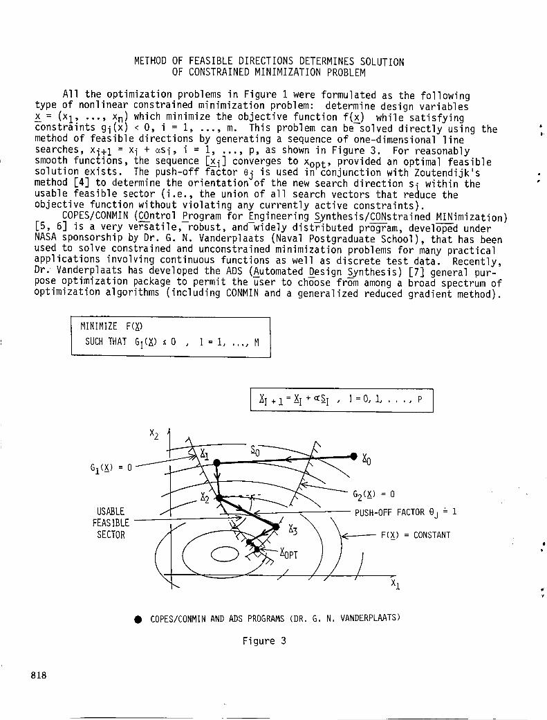
METHOD OF FEASIBLE DIRECTIONS DETERMINES SOLUTIONOF CONSTRAINED MINIMIZATION PROBLEM

All the optimization problems in Figure I were formulated as the followingtype of nonlinear constrained minimization problem: determine design variables

= (Xl' ""' _I which minimize the objective function f(x) while satisfyingconstraints gi < O, i = I, ..., m. This problem can be--solved directly using themethod of feasible directions by generating a sequence of one-dimensional linesearches, xi+ 1 = x i + _si, i = i, ..., p, as shown in Figure 3. For reasonablysmooth functions, the sequence [xi] converges to XODt, provided an optimal feasiblesolution exists. The push-off factor ej is used in'conjunction with Zoutendijk'smethod [4] to determine the orientation of the new search direction si within theusable feasible sector (i.e., the union of all search vectors that reduce theobjective function without violating any currently active constraints).

COPES/CONMIN (COntrol Program for Engineering Synthesis/CONstrained MINimization)[5, 6] is a very vers---atile, robust, and-widely dis_ibuted program, developed underNASA sponsorship by Dr. G. N. Vanderplaats (Naval Postgraduate School), that has beenused to solve constrained and unconstrained minimization problems for many practicalapplications involving continuous functions as well as discrete test data. Recently,Dr. Vanderplaats has developed the ADS (Automated Design Synthesis) [7] general pur-pose optimization package to permit the u--ser to choose fro-m among a broad spectrum ofoptimization algorithms (including CONMIN and a generalized reduced gradient method).

MINIMIZE F(X)

SUCH THAT GI(X) _ 0 , I : 1, ....M

I XI+I=XI+<S I , I=O, 1, .... P

qq_ _--"_)PT/ / /x ](Z

• COPES/CONMINAND ADS PROGRAMS (DR. G. N, VANDERPLAATS)

Figure 3

818

STAEBL PROGRAM DEMONSTRATEDON TWO ADVANCEDFAN BLADES

The optimal design of shroud!ess fan blades represented a significant applica-tion of optimization methods to a complex engineering design problem at Pratt &Whitney. Although the blade design process had been previously automated, it wasstill necessary for an engineer to remain in the design loop in order to make changesto the design variables before re-running the vibration, stress, flutter, and foreignobject damage (FOD) programs. Because of the complex nature of blade resonances dueto engine order excitation levels, it was generally sufficient to determine a feasi-ble blade, one that was usually not optimized for weight or cost. On occasion it wasnecessary to accept blades with resonance margin violations (i.e., critical frequen-cies within the operating range) if it appeared that additional experience-basedhand iterations would not produce a feasible design.

In STAEBL, two fan blades of advanced internal construction (shown in Figure 4)were optimized for direct operating cost (a weighted sum of relative engine weight,manufacturing cost and maintenance cost) while satisfying constraints on resonance,flutter, root stress, FOD, etc. The design variables for both blades includedthickness-to-chord ratios, root chord, and composite material thicknesses, as well asfiber orientation angles for the superhybrid composite blade, and location and sizeof the cavity for the hollow blade.

• DESIGN VARIABLES:

RAD I AL

DIRECTION

F I BER

ORIENTATION

SUPERHYBRID COMPOSITE

, FAN BLADE ,_=_.._._(T/B)5_

,_'_-----(T/B)4_

(-----_(T/B)3_

ROOT / _:'-_(T/B)2_

<_____(T/B)I _

TITANIUM SURFACEBORON/ALUMINUM _)

FILLER (BRAPHITE/EPOXY)"_)/

HOLLOW FAN BLADE

ROOT CHORD

_TITANIUM SKIN

• ()BJECTIVE FUNCTION: DIRECT OPERATINGCOST

• CONSTRAINTS: RESONANCE MARGIN, FLUTTER, F,O,D,, ROOT STRESS

Figure 4

819

TAILORING OF EXTERNAL GEOMETRY AND INTERNALCONSTRUCTION REDUCED WEIGHT AND COST

The structural optimization problems for the superhybrid composite and hollowfan blades were of moderate size, with II and 13 design variables, respectively;each had 68 constraints. The reference blade was a 19.2 Ib hollow shroudless fanblade developed for the E3 (Energy Efficient Engine) project sponsored by NASA. Theinitial design for each probTem was-similar to the reference blade. As shown inFigure 5, significant weight decreases were obtained for both optimized blades byreducing root chord, introducing composite materials, and, for the hollow blade,enlarging and extending the cavity.

Using the COPES/CONMIN program, the optimization procedure for each blade con-verged after 13-15 iterations, or roughly i hour CPU time on an IBM 3081 computer.Each final blade configuration was limited by several active constraints thatrestricted further design improvement. These optimal feasible designs also werere-analyzed using a refined finite element program. Correction factors based uponany discrepancies were applied to the constraints, and each blade was thenre-optimized. This procedure converged for the superhybrid composite blade, but noconvergence was obtained for the hollow blade because of incompatibilities betweenthe approximate and refined analyses.

In Phase II of the STAEBL program, a NASTRAN-compatible 2-D finite element platevibration model and an approximate large deflection local FOD model replaced I-Dbeam analyses in order to obtain closer agreement between the approximate andrefined analyses.

SUPERHYBRIDCOMPOSITE

I

t J

-- INITIAL*

...... FINAL

HOLLOW

r ,11

'IIItl

L.E. T.E.

WEIGHT(LB)

ROOTCHORD (IN)% BO/AL

% G/E

INITIAL* FINAL

19.2 12,19,1 8,3

83.5

- 16,5

WEIGHT(LB)ROOTCHORD(IN)

TI SKIN(IN)BO/TI INLAY(IN)

INITIAL* FINAL

19.2 9.3

9.1 7,5O,12 O.03

- 0.06

* REFERENCE:NASAE3 FAN BLADE

Figure 5

820

SCALED GRADIENTS ELIMINATE CONVERGENCE PROBLEMS

Proper scaling of design variables is important in many engineering optimizationapplications. Ideally, the independent variables should be balanced so that the com-ponents of the gradient of the objective function with respect to the design vari-ables are all within roughly the same order of magnitude. If the design surfaces arestretched in the direction of one or more design variables, as illustrated inFigure 6a, then gradient-based methods using steepest descent or conjugate gradientalgorithms can easily be biased in favor of the design variables with the largestgradient components. If certain design variables are ignored during the search, thenthe methods can converge prematurely to non-optimal solutions, as indicated inFigure 6a. For properly balanced cases, as in Figure 6b, it is expected that nearlyall design variables will be changed during each iteration.

For most problems, scaling is successfully achieved by dividing each designvariable by its initial value, i.e., _i = xi/x'i O, i = I, ..., n. This normalizationcan be updated with current values every 1-5 iterations, especially if there havebeen significant changes among the design variables.

I _I= xI/x_ " (_F/_ _ i) = X_ (_F/_X I) , I=1 ..... N

F(X)

t

F([)

/ XOPT

\

\ \

\ \\

\

""4 \

-_OPT

_NSCALED: SEARCH MAY TERMINATE B)

PREMATURELY

Figure 6

A)SCALED: ALL RELEVANT DESIGN VARIABLES

CHANGE ALONG EACH SEARCH DIRECTION

821

COMPONENTSOF SCALED GRADIENT ARE ALL WITHIN SAMEORDER OF MAGNITUDE FOR HOLLOW FAN BLADE

In several applications (e.g., blade structural, blade aerodynamic, and rotorshaft optimization), improper scaling produced misleading results. For example,when no scaling was used in the STAEBL hollow fan blade analysis, droot (the distanceof the hollow section from the root) was virtually unchanged from its initial valueafter 13 iterations. Subsequent analysis confirmed, however, that a larger hollowsection would both substantially reduce weight and not violate any constraints. Acheck of the objective function gradient in Figure 7 revealed the problem. Thegradient component associated with tTi (the titanium skin thickness) was two ordersof magnitude larger than the component associated with droot. As a result most ofthe optimization program effort was focused on optimizing tTi, to the neglect of

droot.When this problem was scaled, however, by dividing each design variable by its

value on the previous iteration, all objective function gradient components were with-in the same order of magnitude. All design variables changed during each line search.Consequently, after 9 iterations, droot had been reduced from 9.0 in. to 4.88 in.,and the program converged. Since 3 constraints were active, the final design waseasily confirmed to be an optimal feasible point.

I TM COMPONENT OF GRADIENT

INITIAL OF OB4ECTI_E FUNCTION

DESIGN VALUE UNSCALED _xfi _ SCALED -@_-i_fVARIABLE (INCHES)

XI = TROOT 0.875 0,460 0,403"

X2 : TTI P 0,334 0.140 0,047

x3 = DROOT 9,650 0,027] TWO 0,260

ORDERS

x4 = TTI 0,120 2,700J OF MAGN, 0,324

SAME

ORDER

• UNSCALED:

• SCALED:

AFTER13 ITERATIONS,DROOT UNCHANGEDAND PROGRAMDID NOTCONVERGE,

AFTER9 ITERATIONS,DROOT REDUCEDTO 4,88 IN, AND PROGRAMCONVERGED,

Figure 7

822

CONSTRAINT THICKNESS AND PUSH-OFF FACTOR USESIMULTANEOUSLY ACTIVE CONSTRAINTS TO ELIMINATE ZIGZAGGING

From a theoretical standpoint, most optimization strategies and programs willobtain optimal feasible solutions for a wide variety of problems. For largeindustrial applications, where CPU time is important and function calls are expensive,the superior program is one that obtains a solution in the fewest number of functionevaluations. In addition, the program should be robust enough to recognize andrecover from such convergence problems as zigzagging (i.e., bouncing between alter-nately active constraints), and skidding (i.e., re-encountering the same activeconstraint on successive iterations).

The COPES/CONMIN program has several adjustable parameters that can be finetuned for individual problems and are effective in accelerating convergence. Thepush-off factor ej determines the rebound angle within the usable feasible sector

and ranges from aggressive directions nearly tangent to active constraints (e_ _ O)to cautious directions nearly tangent to level surfaces of the objective function

_¢ >> 1). The intermediate value ej = I nearly "bisects" the usable feasible sector.nearly linear problems, aggressive values of ej will reduce the objective func-

tion most rapidly, but may also encounter skidding. Overly cautious values of ej canlead to zigzagging and larger CPU times.

Another parameter, CT, the constraint thickness parameter, performs several tasksto reduce CPU time. First, by adding constraint thickness, the program can comeclose to a constraint rather than waste time determining its position exactly. Inaddition, zigzagging can be avoided as shown in Figure 8. If two alternately activeconstraints become simultaneously active because of their increased thickness, thena new search direction will proceed down the "trough" formed by these constraintsand obtain a substantial reduction in the objective function.

CONSTRAINTS1 AND2SIMULTANEOUSLYACTIVE

X3

ACTIVE

_CONSTRAINT

GI(X) : 0

X1 G2(X) : 0

ICTI

Figure 8

823

PROPER SELECTION OF CONSTRAINT THICKNESS AND PUSH-OFF FACTORACCELERATES CONVERGENCE FOR DISK OPTIMIZATION

Compressor disks are among the most critical components of an aircraft engine;the failure and rupture of a disk can lead to serious containment problems for theengine case. In order to provide a large margin of safety, disks are designed to bestrong and durable, with special resistance to high cycle fatigue. On the other hand,any reduction in disk weight permits a reduction in related components and can pro-vide significant savings in overall engine weight. In a joint effort between PWEDFO[8] and PWEDCO, an optimization program was developed to design minimum weight disksthat satisfy constraints on profile geometry, stress, burst margin, etc.

As shown in Figure 9, the initial disk configuration was chosen to be unrealis-tically bulky to insure feasibility of the initial design, in order to accelerateconvergence. The performance of the optimization procedure was significantly affectedby the choice of search parameters. For a push-off factor o] = 0.3, zigzagging betweenconstraints 5 and 7 (which both measured slopes along the di_k profile) was evidentduring iterations 4-18. At iteration 19, both of these constraints were simultane-ously active, and a large decrease was obtained for the objective function. Conver-

gence was not achieved until 61 iterations. When a more aggressive value _ = 0.iwas taken, zigzagging was minimized, and convergence was achieved in only itera-

iooi

tions.

"I-

L_

CO

..J

,....-4

CD

0

_--

ILl

ILlr_

9O

8O

7O

°°10

_CONSTRAINTS 5 AND

7

YACTIVECONSTRAINTS5 AND 7

, SIMULTANEOUSLYACTIVE

oo,

_ . --,--Sj = 0,1

10 20 30 40 50 60

BLADED DISK SEGMENT

INY[iAL FINAL

ITERATIONNUMBER

Figure 9

824

AUTOMATED TESTING PROCEDURE FOR VANE OPTIMIZATION

Engine and rig testing is a time-consuming and expensive process. For example,high by-pass ratio turbofans running at full power can consume several thousandgallons of fuel per hour. It is an inexact science, dependent upon events such asweather, instrumentation, and mechanical failures over which there is little or nocontrol. The rewards, however, are substantial, e.g. an improvement of only 0.1%in TSFC (Thrust Specific Fuel Consumption) can provide significant yearly savings inairline fTeet fuel costs - -

Variable compressor vanes can be adjusted to improve TSFC (or alternatively,compressor or turbine efficiencies) at various power settings. As shown inFigure I0, a compressor generally has 3-5 variable vanes which can be moved indi-vidually during the test. Standard analytical techniques have been previouslyapplied. For example, the vane angles can be set sequentially from the rear to thefront of the engine. This technique, however, does not model interactive effects,especially the strong coupling between the first (inlet guide vane) and last vanes.Statistical tests (e.g., partial or full factorial) have also been utilized. Thedisadvantage of this approach is that the settings must be established prior to test,and unnecessary data may be collected in regions far from optimal vane settings.

The approximate optimization option [9] in COPES/CONMIN can be used to analyzetest data. By using it interactively in real time during a test, the vane settingprocedure can be automated using a directed search. Another advantage is that sideconstraints can be imposed for maximum and minimum vane angles, and behavior con-straints can be imposed for minimum compressor and turbine efficiencies, maximumcorrected fuel flow, etc.

PERFORMANCESOF ADVANCED ENGINES AND RIGS OPTIMIZED IN A TEST CELL BY VARYING VANE.

SETTINGS

USED APPROXIMATEOPTIMIZATIONOPTIONOF COPES/CONMINTO PREDICT TEST VANE SETTINGS

INTERACTIVELYIN REAL TIME

Figure 10

825

OPTIMUM VANE SETTINGS CORRESPOND TO CONSTRAINEDMINIMUM OF QUADRATIC FIT THROUGH TEST DATA

The solution procedure can be illustrated graphically for 2 unknown vane anglesas follows. Suppose TSFC and efficiency values are known for several different vanesettings. After a smooth surface is fit through these points, the COPES/CONMIN pro-gram can easily determine the constrained minimum point, as shown in Figure ii. Theengine or rig is then run with vane angles set at these new predicted optimum set-tings, another TSFC point is appended to the data, and a new optimum is determinedfrom a surface fit to these new data. When two successive optima agree within anaccepted tolerance level, the iterative procedure has converged. The order of thesurface fit is either linear or quadratic, depending upon the number of data pointsthat are available. If there are more data points than unknown coefficients for thesurface fit, then a least squares fit, with recent data points weighted moreheavily than previous points, is used to approximate the data.

The approximate optimization procedure is usually successful whenever analyticalfunctions and test data can be approximated locally by linear or quadratic functions.It is especially effective when there is a relatively small number (<8) of designvariables. Another advantage is that the approximate method usually requires farfewer function calls than the "exact" method.

A starting procedure is normally used to generate the first few points. Forvane optimization, an initial approximation to the gradient is usually obtained byincrementing, in turn, each vane angle from the nominal settings. During the optimi-zation, move limits restrict the search to a neighborhood of the previous optimum, asshown in Figure 11. As more data points are determined, the move limits areincreased. For sequential unconstrained linear optimization, it is imperative tohave move limits; otherwise the search would be unbounded. In this case, the nextoptimum is usually located at one of the "corners" of the "search rectangle"

TSFC

I

I

MIN V2 , MAX V2 V2

- - -i "- .... _ .............. 7-" -

11 I ........ 1 1

i I I- I /

;-" __ ,," z_-- PREVIOUSOPTIMUMi I i_ - /

// // /

= --_ PREDICTEDOPTIMUM

MAX VI/- - -:? ......... --.__

V1 MOVELIMITS

Figure 11

826

APPROXIMATEOPTIMIZATIONANALYSESBECOMEINCREASINGLYACCURATEAS HIGHORDERTERMSADDED

The objective function and constraints associated with the test data are approxi-mated with truncated Taylor series. For example, a quadratic approximation for theobjective function about the nominal design _ is given by

f(x) _ f(_Xo) + vf(_Xo).(x-_Xo)+ ½ (x-_xo)T.__H(_xo)-(x-X_o) (12.1)

where componentsof the gradient vector and Hessian matrix (assumedsymmetric),respectively, are given by

[vf] i = @f/axi i = I, ..., n

[H=]ij = @2f/axi_xj i,j = 1, ..., n

(12.2)

(12.3)

The number of unknowns in (12.1) is 1 + n + n (n+1)/2, or 1 + 2n if only thediagonal terms in the Hessian matrix are used. As more data points become available,the approximations shown in Figure 12 for the optimization problem progress fromlinear to leading order quadratic (diagonal Hessian terms) to the full quadraticexpansion (including all cross product terms). For vane optimization problems, thediagonal Hessian approximation usually includes sufficient curvature effects in orderto determine an optimum.

Accuracy of the approximate optimization method is dependent upon the nonsingu-larity of the matrix used to calculate the unknown coefficients in the Taylor series(12.1). During engine and rig tests at PWEDCO, the condition number of this coeffi-cient matrix is monitored continuously to insure the integrity of the calculations.

• OBJECTIVE FUNCTION AND CONSTRAINTS FIT BY LINEAR AND QUADRATIC POLYNOMIALS

(TRUNCATED TAYLOR SERIES):

f(x) & f(.xo) + vf(xO) , (x-_) + ½ (_--Xo)TH(_O)'(x-._.O)

X2

r

X1A). LINEARTERMSONLY

X2 X2

B), SOMEQUADRATICTERMS

Figure 12

xlC),QUADRATICTERMS

827

AUTOMATEDVANEOPTIMIZATIONTESTPROGRAMFORADVANCEDCOMMERCIALENGINEREDUCEDTSFC3.4% AT LOWPOWER

Results of an actual test in which 5 vane angle settings were determined inorder to minimize TSFCat low power for an advanced commercial engine are showninFigure 13. The first 5 test points were used to calculate the finite differenceapproximation to the gradient. The next 3 points each produced significant reduc-tions in TSFC. After the lOth test point, the diagonal terms of the Hessian wereavailable, and testing was completed soon thereafter with a substantial net TSFCimprovementof 3.4%. Since nearly every data point showedmarked improvementoverits predecessor during the optimization portion of the test, there was muchpositivefeedback and reinforcement amongthe test engineers, test stand operators, andanalytical support staff. In addition, the optimization procedure predicted pointsvery rapidly in an interactive mode. Since it takes 3-5 minutes for engine perform-ance parameters to stabilize whenever new vane settings are made, there is evenample time to run alternate analyses.

As in any real time testing environment a lack of repeatability and a varietyof experimental errors adversely affected the optimization procedure. For example,there were dead-bandand hysteresis errors in the real time stator control mechanismthat actually set the vane angles. Instrumentation errors were especially signifi-cant at cruise powersettings, since the engine was well-balanced and TSFCwasrelatively insensitive to small changes in vane settings. Numerical convergence ofthe optimization schemeis rare in these tests. The iterations are usuallyterminated when there is a consensus amongtest and analytical personnel that anyrelative improvement in results would be below the threshold of experimental error.

124!.cz)

:. 112 :

m 2

o __- 100IM

,,, -a_ 88

i I\

\

--_ _ -3,4]: '--

76 88 100 112 124

PERCENTDESIGNTHRUST

GRADI ENT

%z_TS_C1 CALCULATION

0 -_6 ' 8 ' 'TEST

-2 _NUMBER

-4OPTIMIZATION

:)UANE OPTIMIZATION ATTEMPTS(_NOMINAL _HE$ BASELINE

• CONVERGENCEPROBLEMSDUETO EXPERI[IE[ITALERRORS

Figure 13

828

AUTOMATED COMPRESSORBLADE DESIGN SYSTEM OPTIMIZESAERODYNAMICS

In designing compressor blades at PWEDCO, separate analyses are generally runby the Aerodynamics Group (who desire thin, streamlined, high-performing shapes) andthe Structures Group (who desire strong, durable shapes). There is, however, anoverall iterative loop between the groups as new designs are analyzed separately andpassed back and forth until an acceptable compromise is reached. Most of the struc-tural analysis programs for blade design (e.g., vibration, stress, foreign objectdamage, etc.) have long been linked together into an automated design system. As aresult of the STAEBL program, the structural optimization of blade design is nowbecoming more and more commonplace. Similarly, the aerodynamic blade design pro-grams have also been unified into an automated system, and a preliminary attempt hasbeen made to optimize the process. As shown in Figure 14, several geometric designvariables are determined in order to minimize loss at the aerodynamic design pointwhile satisfying restrictions on the location of the flow separation point at variouspower settings.

As in the compressor blade structural optimization, this aerodynamic optimiza-tion procedure will perform the arduous, repetitive tasks associated with designingoptimal feasible blades. Since this process must be repeated several times for eachnew build during the ongoing development of a new compressor, an automated optimiza-tion program will give the aerodynamicist more time to analyze results and investi-gate innovative designs.

• GEOMETRICDESIGN VARIABLES:

|.|le L | I I r I !

I.tH

O.$H

Io|It

|,4g|

I,_|$

Q.$

-o.., -o.moo . '. " '. '. '. ,.zo,Q $ , |lid t 4,0 0 ¢|| I |0| | t|_

OBJECTIVEFUNCTION: MINIMIZE LOSSAT AERODYNAMICDESIGN POINT

CONSTRAINTS: LOCATION OF FLOW SEPARATIONPOINT FOR VARIOUS POWER SETTINGS

Figure 14

829

APPROXIMATE OPTIMIZATION TECHNIQUES CAN BE USED TO REDUCE COST ANDINVENTORY FOR MANUFACTURING FACILITY

Another new area at Pratt & Whitney for the application of optimization methodsis in the Manufacturing Division. Recently much attention has been focused upon thetremendous cost and inventories associated with production processes. In an attemptto reduce end product costs, much effort will be expended over the next few years inorder to modernize and streamline manufacturing operations. Many analytical tech-niques developed previously for engineering applications can now be adapted tomanufacturing applications.

A pilot effort is currently under way to optimize performance and minimize totalcost associated with a small prototype manufacturing facility, shown in Figure 15,that is dedicated to the production of sets of similar types of parts. Programs suchas GPSS (General Purpose Simulation S_ystem) [i0] are available for simulating theoperation of such a facili-ty. By including different types of machines, machineoperators, tasks, part numbers, lot sizes, and queues, a GPSS simulation can sequencethrough a time history of events during a production cycle.

A representative optimization problem would be to determine the proper lot sizesfor part groups to minimize the total cost (e.g., capital equipment, personnel, set-up, and holding costs) and work-in-process while still meeting production scheduleand not exceeding machine capacity. An optimization program such as COPES/CONMIN orADS can be coupled with GPSS in order to determine the optimal configuration of thefacility. Because GPSS is not written in FORTRAN and uses integer design variables,however, the approximate optimization option of COPES/CONMINwill probably be usedin an iterative manner to analyze discrete sets of previously generated data.

• DESIGNVARIABLES:

MCH#I

,iARTNUMBER ,,/QUEUE

o oMCH#2 MCH#3 MCH#4 9 L!]

MCHM5r-"-_

o o o ? 141.L._.I

? 10MCHW9 MCH#8 HCH#? MCH#6

TIME:58:48

/ OPERATION

• OPERATORIN USE

o OPERATORSTANDBY

• OBJECTIVEFUNCTION:MINIMIZETOTALCOST,WORK-IN-PROCESS

• CONSTRAINTS:PRODUCTIONSCHEDULE,MACHINECAPACITY

Figure 15

830

CONCLUSIONS

Starting with the NASA-sponsored STAEBL program, optimization methods basedprimarily upon the versatile program COPES/CONMIN have been introduced over thepast few years to a broad spectrum of engineering problems in structural optimiza-tion, engine design, engine test, and more recently, manufacturing processes. Byautomating design and testing processes, many repetitive and costly trade-offstudies have been replaced by optimization procedures. Rather than takingengineers and designers "out of the loop," optimization has, in fact, put them morein control by providing sophisticated search techniques. The ultimate decisionwhether to accept or reject an optimal feasible design still rests with the analyst.Feedback obtained from this decision process has been invaluable since it can beincorporated into the optimization procedure to make it "more intelligent." Onseveral occasions, optimization procedures have produced novel designs, such as thenonsymmetric placement of rotor case stiffener rings, not anticipated by engineeringdesigners. In another case, a particularly difficult resonance constraint could notbe satisfied using hand iterations for a compressor blade; when the STAEBL programwas applied to the problem, a feasible solution was obtained in just two iterations.

Finally, the multidisciplinary nature of optimization has fostered applicationsin many diverse areas throughout Pratt & Whitney and UTC in general. Initialreluctance on behalf of some groups has usually been overcome by a few demonstrationcases, using programs with which they are familiar. Educational courses and symposiahave also been very useful in exchanging ideas about this emerging and importantdiscipline in the workplace. (See fig. 16.)

• EFFICIENT OPTIMIZATION METHODSARE INCREASINGLY BEING APPLIED TO PROBLEMS IN

ENGINEERING DESIGN AND TESTING.

• STRUCTURAL OPTIMIZATION CAN PROVIDE ACCEPTABLE DESIGNS EVEN IF STANDARD

ENGINEERING DESIGN METHODSAND INTUITION FAIL.

• THERE IS SUBSTANTIAL AND GROWING INTEREST IN SHARING THE RESULTS AND BENEFITS

OF THIS TECHNOLOGY THROUGHOUT UTC,

Figure 16

%

831

,

1

.

o

5.

.

1

.

.

I0.

REFERENCES

Platt, C.E., T.K. Pratt, and K.W. Brown, "Structural Tailoring of EngineBlades (STAEBL)," NASA CR-167949, 1982.

Brown, K.W., T.K. Pratt, and C.C. Chamis, "Structural Tailoring of EngineBlades (STAEBL)," Proc. AIAA/ASME/ASCE/AHS 24th Structures, StructuralDynamics, and Materials Conference, Lake Tahoe, Nevada, May 1982, pp. 79-88.

Garberoglio, J.E., J.O. Song, W.E. Boudreaux, "Optimization of Compressor Vaneand Bleed Settings," ASME Paper 82-GT-81, ASME Gas Turbine Conference, London,England, April 1982.

Zoutendijk, C.G., Methods of Feasible Directions, Elsevier, Amsterdam, 1960.

Madsen, L.E., and G.N. Vanderplaats, "COPES - A FORTRAN Control Program forEngineering Synthesis," NPS 69-81-003, Naval Postgraduate School, Monterey, CA,March 1982.

Vanderplaats, G.N., "CONMIN - A FORTRAN Program for Constrained FunctionMinimization: User's Manual," NASA TM X-62282, August 1973.

Vanderplaats, G.N., K. Sugimoto, and C.M. Sprague, "ADS-l: A New General PurposeOptimization Program," AIAA/ASME/ASCE/AHS 24th Structures, Structural Dynamics,and Materials Conference, Lake Tahoe, Nevada, May 1982, pp. 117-123.

Song, J.O., and R.E. Lee, "Application of Optimization to Aircraft Engine DiskSynthesis," Proc. International Symposium on Optimum Structural Design,University of Arizona, Tucson, Arizona, Oct. 1981.

Vanderplaats, G.N., "Efficient Algorithm for Numerical Airfoil Optimization,"AIAA Journal of Aircraft, Vol. 16, No. 12, Dec. 1979, pp. 842-847.

Henriksen, J.O., and R.C. Crain, "GPSS-H User's Manual," 2nd Ed., WolverineSoftware Corp., 1983.

832

N87"11769

ON OPTIMAL DESIGN FOR THE BLADE-ROOT/HUB

INTERFACE IN JET ENGINES t

Noboru Kikuchi and John E. Taylor

The University of Michigan

Ann Arbor, Michigan

tThe work described herein was supported via NASA Grant NAG3-388.

833

OPTIMAL DESIGN FOR THE BLADE-ROOT/HUB INTERFACE

Figure 1 shows two major problems identified with the design of the blade-root/

hub interface. The first is the so-called friction contact problem which has two

special features: unilateral contact and Coulomb_s friction. One of the difficulties

in this problem is that the portions of contact and sticking/sliding surfaces are not

known a priori.

The second is the shape optimization problem which is characterized either by

the minimization of the maximum contact pressure or by the minimization of the equiv-

alent stress on the boundary. Design variables are the shapes of the blade-root and

the hub. It is noted that friction contact and shape optimization problems are

strongly coupled in the present design problem.

BLADE-ROOT/HUBINTERFACE

OPTIMAL DESIGN PROBLEM

ICONTACTPROBLEMS

* UNILATERALCONTACT PROBLEM

(CONTACT/SEPARATION)

* COULOMB'SFRICTIONPROBLEM

(STICKING/SLIDING)

SHAPE OPTIMIZATION

* MINIMIZE THE MAXIMUM CONTACT

PRESSURE

* MINIMIZE THE EQUIVALENT

STRESS

I.FINITE ELEMENT GRID OPTIMIZATION

Figure 1

834

UNILATERALCONTACTPROBLEMS

If the initial gap between two elastic bodies is given by g0(s) and therelative displacement of two bodies is denoted by _R(S), the kinematic contactcondition along a possible contact surface (which should contain the true contactsurface) is expressed by _R'_ -gb _ 0 (shownin Fig. 2) where N is the unit vectorinward normal to the "master" surface F This meansthat the~relative normal dis-placement UR.N cannot exceed the initi_l gap go of two surfaces. The correspondingstress condltion is given by p _ 0, where p is the contact pressure normal to thesurface. Since unilateral contact is considered, p cannot be positive. Theswitching condition of these is represented by P(UR._ - go) = 0. That is, if twobodies separate, then p=0 while UR._ - go < 0. On the other hand, p < 0 and_R'_ - go = 0 if the two bodies are in contact.

°Figure 2

835

COULOMB'S FRICTION PROBLEMS

Figure 3 shows Coulomb's friction law which can be idealized by a spring-

slider model. Since the work done by the friction stresses due to Coulomb's

friction law yields a non-differentiable functional fF(-_p) Ivn_IdF where _ is the

coefficient of friction and I_TI is the magnitude of the rel_ive tangential

displacement, this has to be a_roximated by a differentiable one

fF(-_p)_(VRT)dF using a nonlinear function _c and a parameter _ such that

_e(VRT ) ÷ IVRT I as e ÷ O;

FRICTIONSTRESSES

APPROXIMATIONOF COULOMB'S

SPRING-SLIDERMODEL FRICTIONLAW

Figure 3

836

FORMULATIONFORCONTACTGAPDESIGNPROBLEM

Weconsider the contact between two elastic bodies as represented in Figure 2,including an account of friction and slip as indicated in Figure 3. The designproblem calls for the determination of optimal gap go, where go represents theinitial (before loading) gap between the bodies. The design is to be determinedaccording to a criterion on the contact pressure p, namely to minimize the maximumpressure:

Min [ max -p]go x _ F

C

This is interpreted into the form:

subject to:

(equilibrium problem statement)

_'_- go ! °

p<0

p(_.N-go) = O; fFC

Min (B)

go

subject to:

-p-B < 0

p<O;

f_gij (u) ij (v-u)d_ fFc

g0dF - G ! 0

fF godF - G <. 0C

p (v- u). NdI"

(P1)

(P2)

+ fr - _P(IVTI - [UTl)dFc

ff_f. (v-u)dfl - fFF t. (v-u)dr > 0 V v

fF (q-P)(_'_-go)dF L 0 V q s.t. q ! 0c

In this virtual displacement statement of the equilibrium problem, u represents the

actual displacement field while v symbolizes any displacement within the admissible

set. The optimal solution, say p*,g_ ,u*, must satisfy the following necessary con-

ditions associated with problem (P2) (FCD identifies intervals where g_ # go):

p = - B on FCD

-p > - $ on (Pc FCD)

fF g0dF - G = 0C

p(u.N-go) = 0 on r C

837

SHAPEOPTIMIZATION

Another shapedesign problem, shownin Figure 4, involves rather large scaleshape modification in order to reduce the maximumvalues of local criteria such asvon Mises' equivalent stress, the maximumshear stress, or the maximumprincipalstress. The optimal design problem is then represented by:

min [ max [f(u) I]F saF

subject to equilibrium equations and the gap constraint, where f(u) is a local cri-

terion evaluated at the solution u. It is noted that this problem strongly depends

on the design of gap of two bodies. Indeed, if the contact pressure generates large

bending moment, any kind of local criterion Jramatically increases at the valley ofblade-roots.

SHAPEDESIGNPROBLEMWITH RESPECTTO

LOCALDESIGNCRITERIASUCHAS

* YON MISES'EQUIVALENTSTRESS

* THE MAXIMUMSHEARSTRESS

* PRINCIPALSTRESSES

Figure 4

838

FINITE ELEMENT DISCRETIZATION AND GRID OPTIMIZATION

To analyze the design problems described above, finite element approximations

are introduced. An important fact is that the final (optimal) shape by the optimal

design problem is affected by the quality of finite element approximations. Almost

all optimiality criteria are represented by the stress tensor which is not approxi-

mated well by finite element methods. To overcome this difficulty the present

study introduces the finite element grid optimization algorithm. An example ofthis application is shown in Figure 5.

__.z__ .... lOa

]-- 2a ...I

lTHIN PLATE WITH CRACK

10..

0co

J

grid:

improved+ in itial

CRACK TIP

STRESS DISTRIBUTION

Figure 5

' OPTIMALFINITE ELEMENT1.0GRID

839

IMPLEMENTATION

Using optimality criterion methods, we shall solve the shape design problem ofthe blade-root/hub interface. Figure 6 shows a flow chart of the algorithm appliedin the present study. For a given shape of blade-root valley, the optimal designproblem for the initial gap between two bodies is solved. After determining thegap, the valley shape is now subject to design to reduce the maximumvalue of alocal criterion with a fixed gap. Since the gap design problem is not independentof_the shape of the valley part of blade-roots, we have to iterate the above pro-cedure until both design changes becomesufficiently small.

I GIVE AN INITIALGAP GO I

SOLVE THE GAP DESIGN PROBLEM WITHOUTCHANGING

SHAPE OF VALLEY

* FRICTIONCONTACTPROBLEMSARE

SOLVED

SOLVE THE DESIGN PROBLEMOF VALLEY SHAPE

FOR A GIVEN GAP

* FRICTIONCONTACT PROBLEMSARE

SOLVED

Figure 6

840

EXAMPLESFRICTIONCONTACTPROBLEMS

Figure 7 shows an exampleof friction contact problems solved by the penalty-regularity method. The unilateral contact condition _R'_ - go 2 0 is resolved bythe exterior penalty method. In this case if c is the penalty parameter and is asufficiently small number, then the boundary condition on a possible contact surfacebecomesPc = - (_R'_ - g0)+/c where Pc is an approximation of the contact pressureand a function h* meansh if h > 0 and zero if h < 0. The boundary condition in thetangential direction due to Coulomb's friction l_w is reguIarized by a differentia-ble one using an approximation of the absolute function. That is, a differentiablefunction _c is introduced to have a smooth friction law. This method is called theregularity method. Convergenceof an iterative method to solve the system of non-linear equations obtained by a finite element approximation, is achieved withinseven to ten iterations.

t I

SMALL AMOUNT OF HORIZONTAL

II

LARGE AMOUNTOF HORIZONIAL

FORCE

Figure 7

.....__.....f_102

! / _P"0o_ ,, \

-2.5 -].. 25

CONTACT PRESSURE AND

FRICTION STRESSES

841

EXAMPLESSHAPEOPTIMIZATION

Figure 8 showsan example of shape optimization problems. A thin linearlyelastic plate is under a tension field, and the upper surface of the plate is de-signed to reduce the value of the maximumshear stress under the constraint on thevolume of the plate. The design on the left hand side is obtained without using thefinite element grid optimization routine and a smoothing schemeof the design sur-face. The design on the right hand side is obtained using these additional capa-bilities. The results showthat the grid optimization and the smoothing schemearevery helpful to obtain a smooth design.

No Design is Assumed

In this part.

_ACE Applied Tensiofl Force

• Isotropic I_• Homogenuous Elastic Material

• Linear No desig

assumed

WITHOUT GRID OPTIMIZATION

J r

p i

.----.......

Figure 8

WITH GRID OPTIMIZATION

842

THE BLADE-ROOT/HUB

EXAMPLE DESIGN OF INTERFACE

Figure 9 shows a model prob]em of a design of the blade-root/hub interface.

Design of shape is combined with the algorithm for solving friction contact prob-

lems, although the grid optimization routine is not interfaced in the presentexample.

ORIGINAL AND DEFORMED SYSTEM

3000 rpz

Total 10 Iterations

132 elez. 158 nodes

EX 8. TURBINE

45 DEG.

ROUNDED CORNER

(a)Figure 9

843

STRRINENERGY

3000 rp=

Total 10 Iterations

132 elem. 158 nodes

CONTOUR= 15664.4

CONTOUR= 20885.8

CONTOUR= 26107.2

L,U=I =urn = _ I_o,u

EX 8. TURBINE

45 DEG.

ROUNDEDCORNER

(b)

,(, \

(c)

EQUTVRLENT STRESS

3000 rp=

Tota/ 10 Iterations

132 elem. 158 nodes

CONTOUR= 515428.4

CONTOUR= 686571.3

CONTOUR= 85-/714.1

J ROUNDED CORNER

Figure 9.- Continued.

844

MAX SHEAR STRESS

',," ",.\\'"...",I""c.. ....-..'.\\\,,I x.,

\ \ \ ', f ....,,,"// I\ ",, .\ \ '," / f\ "/-"" \ k ".

3000 rpz

Total 10 Iterations

132 elez. 158 nodes

EX 8. TURBINE

45 DEG.

ROUNDED CORNER

(d)

"-A.

T/" ,11" x ÷

_ X _ x 4"

3000 rp=

Total 10 Iterations

132 elel. 158 nodes

EX 8. TURBINE

45 DEG.

ROUNDED CORNER

(e)

Figure 9.- Concluded.

845

FURTHERDEVELOPMENT

Wehave analyzed the optimal shape design problem of blade-root/hub interfaceby dividing the original problem into several parts for the friction contact andshape optimization problems. Furthermore, the finite element grid design problemis also defined in order to improve the quality of approximations. The futurestudies are to makeuse of combinations of these segments. Especially, combinationof the shape and gap design problems is the next subject to be studied. After this,the grid optimization routine must be interfaced into the meansfor solution (seeFigure lO).

ACKNOWLEDGEMENTS

The present work is performed jointly with Dr. A. R. Diaz (responsible for

developments in the grid optimization scheme), Mr. T. Ting, and Mr. K. Y. Chung

(performed programming and obtained results for the sample problems_. The authors

express their appreciation to them.

I SHAPEDESIGN_.

I GAP DESIGN ,I_ OPTIMALDESIGN_ INTERFAcEOFBLADE-ROOT/HUBI GRIDDESIGN

Figure I0

846

N87-11770

PROBLEMS IN LARGE-SCALE STRUCTURAL OPTIMIZATION

Jasbir S. Arora

University of Iowa

Iowa City, Iowa

and

Ashok D. Belegundu

GMI Engineering & Management Institute

Flint, Michigan

847

#

I. INTRODUCTION

During the year 1979, it was observed that the methods of structural

optimization were not being utilized in the industry as extensively as expected.

About 20 years of extensive research on methods of structural optimization had

been conducted by that time. Several researchers had demonstrated applications of

optimization methods on various classes of problems. It was disappointing to find

that the general engineering design community was not taking advantage of the

advanced technology. Therefore, it was decided to determine reasons for this lack

of interest. The first observation was that some designers had tried optimization

methodology without success. There was a general feeling in the community that

optimization methods could be used only by the experts. The second serious problem

was that general purpose software that could handle each designer's cost and

constraint functions was not available for the solution of engineering design

problems. A major reason was that it was not known which method would be most

suitable for engineering design applications. Therefore, there was a need to

conduct a comprehensive study to evaluate various available methods with a

particular regard to their suitability for structural design optimization

problems. Such a study was started in 1979 and completed by the middle of 1982.

Results of this study are presented in this paper. Throughout the paper,

reference is made to structural optimization problems. However, the discussion is

applicable to the design of mechanical as well as other complex engineering systems.

It is somewhat satisfying to see the use of optimization methodology being

accelerated in the recent past. For example, some real world applications of

optimization methods were presented at the recent Euromech Colloquium [I], 18th

Midwestern Mechanics Conference [2], International Symposium on Optimum Structural

Design [3], and the llth IFIP Conference on System Modelling and Optimization [4].

More effort is beginning to be spent on software development. For example, the

incorporation of design sensitivity analysis into MSC/NASTRAN [5], IDESIGN program

[6], OPT package [711, and many other special purpose programs [8-12] have been

developed in the recent past. However, substantial effort needs to be expended in

these areas to fully realize the potential of optimization methods.

In this paper, a general design optimization model for large complex systems

is defined. Major features of the model that challenge various optimization

algorithms are discussed. Requirements of a model optimization algorithm are

identified. Objectives of the study of various algorithms are defined and a basis

for conducting such a study is developed. Primal as well as transformation

methods are analytically studied and a unified viewpoint of various methods is

presented. Several numerical examples are solved using different methods to study

their performance. Conclusions drawn from the study are presented and

discussed. Areas of future research in nonlinear programming as well as

structural optimization are identified and discussed.

2. DESIGN OPTIMIZATION MODEL FOR LARGE SYSTEMS

In this section, a general design optimization model and its features are

presented and discussed.

848

2.1 Desisn Optimization Model

Let beR n be a vector of design parameters. Then a general design

optimization problem is defined as follows:

min f(b); beS (2.1)

where the constraint set S is a subsect of Rn defined as

S = {b: gi(b) = O, i = 1 to m'; gi(b) _ 0, i = (m' + i) to m}(2.2)

It is assumed that the functions f(b) and gi(b) are at least continuouslydifferentiable. In appearance, the model defined in Eqs. (2.1) and (2.2) is

identical to the standard nonlinear programming problem. However, there is one

very important difference. The difference is that some of the functions f(b) and

gi(b) are implicit functions of design variables b. That is, the explicit form ofthese functions in terms of the design variables is not known. The functions can

usually be evaluated only after a large, complex analysis problem has been solved.

There are several classes of engineering design problems that can be

represented [13] by the model defined in Eqs. (2.1) and (2.2). For example,

minimum weight structural design problems with stress, displacement, buckling

load, natural frequency, and other constraints under static as well as dynamic

loads; mechanical system design optimization; fail-safe optimal structural design

problems; kinematic synthesis; and optimal design of large systems with

substructures can be represented by the model. In addition, there are many problems

of optimal shape design of systems or subsystems that are represented by the model.

With the above definition of the design optimization model, we are in a

position to define what is meant by large-scale optimization problems. Of course,the obvious definition is that the numbers of design variables and/or constraints

are large. Typically, n > 25 and/or m > 100. However, in engineering design, the

problem can be classified as a large-scale problem even if n and m are not very

large. The reason for this is that the analysis model can be so large that it can

take hours of CPU time on a fast computer to calculate functions and their

gradients. This is true for problems that require large dimensional finite

element models to accurately predict response of the system. For transient

dynamic response problems, even smaller-degree-of-freedom models can consume a

large amount of CPU time. Therefore, we will classify any engineering design prob-

lem to be of large scale if n _ 25 and/or m _ I00, or if it has implicit func-

tions that require a large amount of CPU time to compute function values.

2.2 Major Difficulties

The most prominent difficulty with problems of engineering design is the

implicit nature of the functions. As noted, evaluation of the functions can

require an enormous amount of computational effort. In addition, the evaluation of

gradients of such functions requires not only additional computational effort, but

also computer programming effort. For each class of problems, special programs

must be developed to evaluate functions and their gradients. These programs can

be very large, needing advanced database management and software development

concepts. Depending on the type of problem, this process may require several man-

years of effort.

849

Another difficulty with problems of engineering design is that, in general,the problem cannot be shownto be convex. In fact, engineering design problemsare characterized by the presence of multiple local minima. This meansthatseveral starting designs must be tried and the problem optimized each time in thehope of obtaining a better design. This can be a tedious and time-consumingprocess.

Software for design optimization is either not available or tedious touse. Most of the existing programs are not interactive. They do not allow anyuser control over the iterative process. Graphics capability is almost unheard ofin design optimization software. In addition, manyof the programs have no provenglobal convergenceproperties. In this regard, it must be observed that theengineering design community has not developed algorithms and software based onstrict global convergence theory. Global convergence is an indication of thereliability and robustness of an algorithm. Use of globally convergent algorithmsin engineering design will require less adjustment of various parameters andconsequently, less expertise in optimization theory on the part of the generaluser. More attention should be paid to this aspect in engineering design appli-cations.

3. MODEL DESIGN OPTIMIZATION ALGORITHM

In this section, we describe a model algorithm for engineering design

optimization. We must strive to develop such an algorithm in the future. Most

existing algorithms can be described by the following iterative prescription:

b(k+l) = b(k) + _p(k); k = O, I, 2, ... (3.1)

where k is the iteration number, p(k) is a direction of desirable move in the

design space, _ is a step length along the direction p(k), and b _0) is an initialdesign estimate.

An obvious requirement of an algorithm for large scale optimization is that

it must be efficient. Efficiency of an algorithm can be improved in two ways:

(i) by reducing the total number of iterations, and (ii) by reducing the computing

time per iteration. With regard to reducing the total number of iterations, itis desirable for an algorithm to have a superlinear or quadratic rate of

convergence. Many methods incorporate quasi-Newton updates for Hessian matrix of

the Lagrangian function into their algorithm to achieve a superlinear rate of

convergence. The basic idea here is that with the curvature information for the

Lagrange function incorporated into an algorithm, a better direction of design

improvement is obtained, thus accelerating the rate of convergence.

With regard to reducing computing time per iteration, calculations for p(k)

and _ should be as efficient as possible. Efficiency of calculations for the

direction vector p(k) in engineering design applications can be substantially

improved if active set strategies are used in an algorithm. The reason for this

is that with active set strategies, gradients of only a subset of the constraints

are needed. This results in significant savings because of the implicit nature of

the functions. Note, however, that use of an active set strategy should not de-

stroy any global convergence properties that the algorithm may have.

850

Another very important calculation at each design iteration is to determinethe step size Manymethods calculate step size by minimizing a descentfunction along_the direction p(k). The descent function is usually constructedusing the functions of the problem. To find _k' therefore, a search must beperformed along the direction p , which requires an evaluation of functions.Since manyfunctions are implicit in engineering design, an evaluation of the exact_k can require an enormousamount of calculations. Thus, approximate strategiesmust be developed to calculate the step length, or perhaps the use of a descentfunction and the associated line search should be avoided altogether.

The problem of determination of a step length, however, is more involved thanit appears. It turns out that global convergence of an algorithm is assuredthrough the requirement that a descent function must reduce in value at eachiteration. This is assured by calculating the proper step length. Since globalconvergence is a 'must' for an algorithm that has to be applied to problems ofengineering design, it does not seempossible to avoid a one-dimensional search forcomputing the step length.

The algorithm to be used in engineering design environment must treat thegeneral optimization problem defined in Eqs. (2.1) and (2.2). In other words,equality constraints must also be treated. No assumptions regarding the form of thefunctions of the problem (i.e., linear, posinomial, separable) should be made.

Finally, the user should not be required to select too manyparameters relatedto the optimization algorithm. The general user is usually not an expert in optimi-zation theory, so he will not know how to select the parameters. In addition,he cannot be expected to fix any failures of the algorithm. Therefore, a goodalgorithm should be self correcting. If failure does occur, the user should begiven some indication of where the trouble mayhave occurred and how to fix it.In summary, then, the model algorithm must be generally applicable, efficient,globally convergent, and easy to use, and must incorporate active set strategy.

4. PURPOSE OF THE STUDY

A natural question now arises: which of the existing methods is/are most

suitable for solving (2.1)? Unfortunately, very few comparative studies have been

done in optimal design of structural systems. The emphasis has been on studying

one particular method by solving a variety of problems without considering how it

compares with other existing methods. As a result, we now have several algorithms

whose relative performance is not properly understood.

A few studies have been conducted in the field of mathematical programming

(MP). However, it may not be possible to correlate the performance of an algorithm

on MP problems with its performance on structural optimization problems. The reason

is that the MP problems do not possess many of the difficulties present in the

structural problem. The first comprehensive study in the field of mathematical

programming was conducted by Colville [14]. Since then, other comparative studies

have been conducted by Stocker [15], Himmelblau [16], Biggs [17], Schittkowski

[18], Miele et al. [19], and a few others. The study of Sandgren and Ragsdell

[20] is based on a solution of some problems in engineering design. However, the

851

problems chosen are of the MPtype: explicit functions, small dimension (n + m51 + bounds). Problems with multiple local minima are not considered.

In structural optimization, far less information is available on the relativemerits of algorithms. De Silva and Grant [21] have comparedpenalty functiontechniques by solving a planar truss problem. Their study, however, consideredonly Sequential Unconstrained Minimization Techniques (SUMT's). Carpenter andSmith [22] have also studied SUMT'sfor solving structural design problems. Theiremphasis is on studying the unconstrained minimization algorithms used in SUMT'sand comparing the use of finite difference versus analytical computation ofgradients. In the second study by Carpenter and Smith [23], which is fairly com-prehehsive, the method of sequential linear programming, a feasible directionsmethod, and SUMT'sare considered. Trusses and plates are used as test problems.The main conclusion reached by these authors is that the sequential linear program-ming method is more efficient that both the SUMT'sand the method of feasibledirections. However, this conclusion is questionable because the gradient of thepenalty function in SUMT'sis computed inefficiently [22] and not by the efficienttechnique recommendedby Belegundu and Arora [24]. Use of the technique in Ref.22 will makeSUMT'smore competitive in the study. Furthermore, multipliermethods are not included in that study.

The present study differs from previous studies because the difficultiesposed by problem (2.1) are addressed, a numberof recently developed algorithmsare included, both theoretical as well as numerical aspects are considered, andsomerelatively large scale problems are solved. Aims of the study are toidentify strengths and weaknessesof a method and to develop a unified viewpointfor the NLPmethods.

5. ANALYTICAL EVALUATION OF NONLINEAR PROGRAMMING METHODS

In Section 3, essential features that an algorithm should possess for

structural optimization were presented. In this section, we will examine how ex-

isting methods measure up to the stated requirements. Specifically, the following

basis is used to study each method. (I) The presence of implicit functions makes

problem (2.1) different from an MP problem. It is therefore examined whether a

given method is especially suited for handling such implicit functions. (2) The

geometrical significance of the direction vector p(k) in Eq. (3.1) is studied to

bring out similarities and differences between methods. (3) The global convergenceproperties of a method are studied. (4) It is examined whether the method uses

an active set strategy. Further, it is determined whether any global convergence

properties that the method possesses are valid with the use of an active set

strategy. (5) It is examined whether the method uses the W matrix (which is a

positive definite approximation to the Hessian of the Lagrangian function), or

if not, whether it is possible to incorporate this matrix into the method. Use

of such a method leads to superlinear convergence.

Various gradient-based NLP methods can be grouped under primal methods and

transformation methods. By a primal method of solution, we mean a method that

works directly on the original problem given in (2.1). In primal methods, the

direction vector p(k) at the kth iteration is determined by an expression of theform

852

w(k)p (k) = _N0 + _ _iNi (5.1)

where _0 and _i are scalars (Lagrange multipliers), NO and Ni are gradients of thecost and constraint functions, respectively, matrix W(k) was defined earlier, andI k is the active constraint set. It is evident from (5.1) that computing p(k)requires computing the gradient vectors N I of individual functions that are in the

set Ik .

Transformation methods are based on solving (2.1) by reformulating it as a

sequence of unconstrained minimizations. In this c_s of methods, the design isupdated during an unconstrained minimization, and p--- is obtained by an

expression of the form

w(k)p (k) = - v_T(b(k),8 (k)) (5.2)

where W (k) is a known matrix and 8(k) is a vector of known parameters. In (5.2),

even though _ depends on the functions gi for ielk, computing V_ does not requirecomputing the gradients NI of individual constraint functions. This is desirable

for structural optimization problems and is discussed in more detail in Refs. 24

and 25. As a result, we conclude that transformation methods possess a special

structure to handle implicit functions and primal methods do not. Therefore, the

classification into primal and transformation methods is intimately related to the

structure of the structural optimization problem.

5.1 Primal Methods

Recursive QP Methods

Recursive quadratic programming (RQP) methods have been recently developed

[26-34]. They are gaining popularity due to their strong convergence

characteristics. The basic idea behind RQP methods is to develop Newton-like

algorithms for constrained optimization. This results in the iterative solution

of the QP:

sin NOTp + 1/2pTwp

.T

s.t. NI P + gi = 0, iel I (5.3).T

and NIP + gi 4 0, iel 2

where W, NO , N i, and gi are all evaluated at b(k), and I1 and 12 are active sets

associated with the equality and inequality constraints, respectively. Once p is

obtained from (5.3), a step length is estimated along p by minimizing a descentfunction.

A relatively straightforward calculation shows [34] that the solution p of

(5.3) can be expressed as

i 2p = - p + p (5.4)

where pl is a vector obtained by projecting2the cost gradient into the tangent

hyperplane to the active constraints, and p is a vector normal to this 1 21 2 n o

hyperplane. The p and p directio s are sh wn in Fig. i. The vectorslP and pare orthogonal (relative to the W matrix). From Fig. i, we see that -p is a cost

853

reduction step while p2 is a constraint correction step. Thus, the p-vector inRQPmethods tries to achieve a simultaneous reduction in cost and constraintviolations. So far, two globally convergent RQPalgorithms have been developed.Oneis by Hart [29] in 1977 and the other by Pshenichny [30] in 1978.

Han's Algorithm: No active set strategy is used [29]. The QP in (5.3) solved ateach iteration includes all m constraints of the original problem. This is needed

to ensure that p is a continuous function of the design variable. The fact is

used to prove global convergence of the algorithm. The algorithm is unsuitable

for structural optimization due to the enormous computation involved. However,

Han obtains super_inear convergence by taking W to be a positive definite

approximation to V=L, where L is the Lagrangian function. Powell [32], who has

implemented a modified form of Han's algorithm, has generated W using a quasi-

Newton update.

Pshenichny's Algorithm: Global convergence has been proved using an active set

strategy [30]. This algorithm has been successfully used for structural design

problems [34]. Pshenichny, however, ignores the possibility of using second order

information in the W-matrix. He takes W as an identity matrix. We can therefore

accelerate Pshenichny's method by taking W to be a positive definite approximationto V-L.

RQP methods possess a common drawback. The step length a is determined by

minimizing a descent function of the form B(b) = f(b) + rF(b), where F(b) is some

penalty function that measures the amount of infeasibility of design b. The

difficulty is that the scalar r tends to become large during the iterative

process. This results in small step size because of greater emphasis on constraint

feasibility.

Gradient Projection Methods

The gradient projection method was first developed by Rosen [35] in 1961.

Feasible directions methods that were developed earlier (in 1960 [36]) involved

_N o

b(k P

Figure i. pl and p2 Vectors

854

solving an LP or QPsubproblem at each iteration. However, if the cost offunction and gradient evaluations wassmall compared to that of solving a linearprogram, then feasible direction methods could becomeexpensive to use. Rosenwasthus motivated to develop a method in which the direction vector could beobtained in a closed form rather than by solving an LP or QPsubproblem. Thus, incontrast with feasible directions methods, the gradient projection method uses adirection vector which is not the best but is mucheasier to compute. It was notedin Section 2 that function and gradient evaluations in structural optimization areenormously expensive. Becauseof this, it is better to solve a relativelyinexpensive LP or QPsubproblem and obtain the best possible improvement indesign, rather than implement the gradient projection philosophy.

An analysis of the gradient projection methods helps to view the method inte_ms of the pl and p2 steps discussed in connection with RQPmethods. First, a_pl step is taken from a feasible design b(k). Let a be the step size in this

direction. Then, a new design b(k, i) = b(k) a pl is obtained, which is in

general infeasible (Fig. 2). Now, a sequence of p2 steps, or 'correction' steps,is taken to obtain a new feasible design, b(k+l).

Because of Sudden changes in the active set, the gradient projection method has

not been proved to be globally convergent. Further, modifying the method to make

it globally convergent would destroy the basic simplicity of the method. Another

disadvantage is that it is difficult to maintai_,d_cent. T_s, it may happen

thatuponreturningto thefeasibleregion,flb > flb J). hiscase,asmaller step _ has to be chosen from the previous feasible design b(k), and the

correction procedure has to be re-initiated. This 'orthogonal iteration' can be

quite expensive. Moreover, the correction procedure needs special care to ensure

that a solution exists. Final_y, though a W-matrix can be incorporated into themethod in calculating pl and p_, it is computationally difficult to maintain

quasi-Newton updates because of the complicated logic involved.

Reduced Gradient Methods

Reduced gradient methods are based on the simple variable elimination

technique developed by Wolfe [37] in 1967. The idea is to use the constraints

satisfied at equality at the current point to eliminate some of the variables.

The problem then becomes unconstrained in the remaining variables.

"_0P

%

Figure 2. Gradient Projection Method

855

There is, however, someconfusion in both the mathematical programmingliterature as well as the structural optimization literature on the relativemerits and demerits of the reduced gradient methods. For example, the reducedgradient method has been declared superior to the gradient projection method[20,38], whereas these two methods are considered to be essentially the sameinRef. 39. The confusion arises whenstudying reduced gradient methods in thecontext of solving inequality constrained problems. Someresearchers convert theinequality constrained problem to an equality constrained one by adding nonnega-tive slack variables, while others adopt an active-set strategy. It turns outthat if an active-set strategy is used, the reduced gradient method becomeses-sentially the sameas the gradient projection method. On the other hand, if theinequality constrained problem is converted to an equality constrained problem,then the reduced gradient method behaves quite differently from the gradientprojection method. In this case, the reduced gradient method is more efficientthan the gradient projection method and can also be shownto be globallyconvergent (unlike the gradient projection method). Unfortunately, the inequalityconstrained problem in structural optimization has to be solved using an active-set strategy. The reason for this is that the addition of slack variables toconvert inequalities in equalities implies that all constraints are active andhence have to be differentiated. This is ruled out in large-scale structuraloptimization becauseof enormouscomputation and storage of information involved.Therefore, when solving structural optimization problems we need not differentiatebetween gradient projection and reduced gradient methods.

Method of Bard and Greenstadt

Though this method assumes convexity of the problem (which cannot be assumed

for the structural problem) it is briefly examined here because it casts furtherlight on the p_ and p directions discussed earlier.

It was noted that the direction p (Fig. i) tries to reduce both cost and

constraint violation. There is thus no single-purpose goal for selecting step

size along p. Bard an_ Green_tadt [40] were therefore motivated to decompose pinto two directions; s and s_ maximizes the Lagrangian. They then consider an

algorithm in which these steps are taken alternately. The attraction of this

algorithm is that in making each step, the aim of either minimizing or maximizing

the Lagrangian is well defined. As a result, step s_ze selection along each step

is notle difficulty. It turns out that the sI and s_ directions are identical tothe -p and p directions discussed earlier.

We therefore see that the pl and p2 steps form the backbone of the primal

methods discussed above. The aims of these different methods are shown in

Fig. 3. The geometrical similarity between these methods is tied into common

difficulties with step size selection, maintaining descent and global convergence.

Feasible Directions Methods

The idea behind these methods is to move from one feasible design to an

improved feasible design. This is in contrast to the 'exterior point' methods

studied above which iterate through the infeasible region. Feasible directions

methods solve an LP or QP subproblem which yields an 'improving feasibledirection' d. The vector d satisfies the conditions NOTd < 0 and NiTd < 0

for ieI k. Such a direction d is shown in Fig. 4. The solution of the LP or QP

856

subproblem to determine d also involves certain user-supplied parameters,el, called the 'push-off' factors (Fig. 4). The greater the value of ei, thegreater the direction is pushed awayfrom the ith constraint boundary into thefeasible region.

Evidently, the direction vector use_ in feasible directions methods isconceptually different from the p and p directions of earlier methods. Somefeasible directions methods are proved to be globally convergent and also use anactive set strategy. Zoutendijk's E_erturbation algorithm [36] and an algorithmby Polak [41,42] are in this category. On the other hand, Topkis and Vienott'salgorithm [43] is globally convergent but does not use an active set, which makesit inapplicable to structural design problems.

Theoretically, therefore, feasible directions methods are quite attractive.Computationally, however, there are certain major difficulties. First, aconstrained line search has to be performed. Second, it is clear that a good

b °): STARTING DESIGN

./ ._.._ _-METHOD OF BARD

_ AND GREENSTADT

GRADIENT

PROJECTION"%"_,_._ fRQP METHODSAND REDUCED t v _,,t,.t,.t,.t,.t,.t@_.,-,

GRADIENT (_ ._

MET_ _'_ Lb.: SOLUTION _

FEASIBLE REGION

Figure 3. The Aims of Different Methods

: PUSH-OFF

OR

DIRECTION

FEASIBLE REGION

Figure 4. Feasible Direction

857

choice of push-off factors e. at a current design b(k) requires information aboutithe curvature of the constralnt functions. Since the curvature is different atdifferent points, no initial choice of e. can, in general, be madeto obtain rapidconvergence. Note that if 0. are too sm_ll, then the design iterations constantlyhit the constraint boundary,!slowing downconvergence. Onemaypossibly infer fromthis that feasible directions methods will work best in an interactive mode.

In existing feasible directions methods, no curvature information is used,and hence only linear convergence can be expected. In defining the QPsubproblem,a normalization constraint of the form I/2dTd _ i is used. It is suggestedinstead to use the constraint

I/2dTwd < I (5.5)

where W is the usual quasi-Newton approximation to V2L. Use of curvatureinformation in W can be expected to accelerate convergence, and perhaps alleviatethe difficulty in choosing appropriate values for the push-off factors. This, atany rate, needs to be investigated.

Sequential LP Methods

In these methods, an LP subproblem is obtained by linearizing the cost and

constraint functions about the current design and imposing a linear step size

constraint. The LP subproblem at each iteration is

T

min N ° p

.T

s.t. N1 P + gi = 0, i_l I (5.6)T

NI P + gi ( 0, ieI 2

and [Pjl • _j, J = 1 to n

where p is the direction vector, 11 and 12 are active sets associated with the

equality and inequality constraints, respectively, and _= are move limits input bythe user. These methods are known to researchers in str6ctural optimization, but

are not used by researchers in mathematical programming.

Major difficulties with this type of method are listed below.

(i) The step size constraint [Pjl _ _, J = I, ..., n, causes difficulty inidentifying a descent function. The descen_ function used in RQP methods does not

serve as a descent function in (5,6), as may be verified. Abscence of a descent

function makes it difficult to estimate step size and to prove global convergence.

(2) Referring to Fig. 5, we notice that if _. in (5.6) are chosen too small,

then no solution may exist for the subproblem. OnJthe other hand, if _= is large,

then p may become large. A step size control along p then becomes necessary.

Unfortunately, this is difficult in view of (I) above.

These difficulties and the fact that only linear convergence is possible

(since no curvature information is involved) make sequential LP methods inferior

compared to RQP methods. The reason is that function and gradient calculations

858

require much more computation than solving an LP or QP subproblem in structural

optimization. Thus, one may as well solve a QP instead of an LP and use a method

that is superlinearly and globally convergent.

Other Primal Methods

We will briefly comment on other primal methods. Optimality criteria methods

have been used for structural optimization [44,45]. These methods are based on

iterative techniques for solving the nonlinear set of necessary conditions. A

major difficulty with the methods is that a descent towards the optimum can not be

maintained. Therefore global convergence of the methods can not be proved.

There are other projection methods that have been developed in the MP

literature [46]. These are iterative techniques based on a combination of active

set selection and projection concepts. The techniques have not been used for

structural optimization.

There are other methods that involve solving a sequence of nonlinear

subproblems [47]. The subproblem has a nonlinear objective function (the

Lagrangian) and linear constraint approximations. Such methods are not suitable

for structural optimization because (i) they are not globally convergent, and (ii)they require more computational effort.

5.2 Transformation Methods

The term 'transformation method' is used to describe any method that solves

the constrained optimization problem by transforming it into one or more

unconstrained optimization problems. Transformation methods include exterior and

interior penalty function methods as well as augmented Lagrangian or multipliermethods.

Many of the constraint functions in optimal structural design are implicit

functions of design variables. This implicit nature of the constraint functions

makes it expensive to calculate their gradients. Transformation methods

essentially collapse all constraints of the design problem into one equivalent

functional constraint [48] which serves as a penalty term for the transformation

methods. This is in contrast to primal methods, as discussed in Section 5.1.

There are three classes of transformation methods that have usually been

discussed in the literature: the penalty function (exterior), the barrier (or

interior penalty) function, and the multiplier (augmented Lagrangian) methods.

_ gi(b)=O

FEASIBLE REGION

Figure 5. No Solution Exists to LP Problem

859

The penalty and barrier methods have been referred to as Sequential UnconstrainedMinimization Techniques (SUMT's) by Fiacco and McCormick [49].

All transformation methods convert the constrained problem (2.1) into anunconstrained problem for the 'transformation function'

_(b,r) = f(b) + P(g(b),r) (5.7)

where r, is a vector of controlling parameters and P is a real-valued functionwhose action of imposing the penalty is controlled by r. The local minimumof _(b,r) at the kth iteration is denoted by b" ". The idea of transformationmethods is very attractive because efficient unconstrained algorithms (e.g.,Davidon-Fletcher-Powell method) [38] can be used to completely solve the con-strained problem. It is shownthat the idea of transformation methods is alsovery attractive for design problems in which implicit constraints must be treated.

SUrF's

The most popular penalty function is the quadratic function given bym' m

+ ]2P(g(b),r) = r [ [gi(b)] 2 + r _ [gi(b) (5.8)i=l i=m '+I

+where r is a scalar parameter and g.(b) = max(0,gi(b)). The inverse and logibarrier functions are also quite popular [49]. The barrier methods, however, are

not applicable to problems,having no_linear equality constraints. It can be shownthat as r(k) ÷ =, b (k) ÷ b , where b is a solution of the constrained problem.

SUMT's possess a number of undesirable properties. The weaknesses are most

serious when r is large. When r is large, the penalty and barrier functions tend

to be ill-behaved near the boundary of the constraint set where the _imum points

usually lie. There is also the problem of selecting the sequence {r_=_}. Thechoice of r(I) and the rate at which r(k) tends to infinity can seriously affect

the computational effort to find a solution. Furthermore, the Hessian matrix of

the unconstrained function becomes ill-continued as r ÷ _ [38]. In spite of these

difficulties, these methods have been used quite extensively for structural

optimization. For barrier methods, Schmit and co-workers [50] and Haftka and co-

workers [51] have used certain 'extended-barrier functions' which are free from

weaknesses possessed by conventional barrier methods.

l_ItIp ller Methods

The multiplier methods have been developed in the recent literature to

alleviate some of the difficulties with SUMT's. In multiplier methods, there is

no need for the controlling parameters r to go to infinity. As a result, the

transformation function _ has good conditioning with no singularities.

Furthermore, multiplier methods (like SUMT's) are globally convergent and have

been proved to possess faster rates of convergence than SUMT's [52].

In multiplier methods, the penalty function is given as

I m' +_ m[ +8i)+]2jP(gCb),r,O) = _ [ r i[gi(b) + 0 ]2 1i= 1 i ri[(gi(b)i=m '+I (5.9)

where O. and r. > 0 are parameters associated with the ith constraint. The

Lagrang_ multiplier Vi associated with the ith constraint is given by Vi = ri0i"

860

If 8. = 0 and r i = r then (5.9) reduces to the well-known quadratic loss function• 1

glven in (5.8) where convergence can be forced by letting r ÷ _. However, the

objective of multiplier method is to keep each r i finite. Furthermore, if b(8) is

obtained by minimizing _(g(b)r,8), then the aim Of choosing @i is such that

gi(b(8))_0 for l<i_m' and max(-Si,gi(b(8))+O for m'+l(i(m(5.10)

Powell [53] and Hestenes [54] have independently suggested a modified Newton

formula for changing e i to satisfy (5.10). This method is especially attractive

for large scale problems because of its simplicity. A second-order Newton method

can also be used for changing 8i. The idea behind selecting r i is to make sure

that the constraint violations are improved. This is done by suitably increasing

the values of r i. Details regarding changes in e i and r i are given in Ref. 25.

The increases in parameters r i are especially significant because they lead to

a practical method for enforcing global convergence. This fact is borne out by

test results.

The geometrical significance of multiplier methods can be best understood by

the following result derived by Powell [53]. He showed that minimizing

_(b,r,8) to obtain b(8) is equivalent to solving the problem

min f(b)

s.t. gi(b) -- gi(b(8)), i = 1 to m' (5.11)

and gi(b) ( max (-8i, gi(b(8))), i = (m' + i) to m

From (5.11), the aim of changing 8 in (5.10) also becomes clear. The iterative

process is shown in Fig. 6.

The problem associated with step size calculations in primal methods to

force convergence is not present in transformation methods. Transformation

methods are more reliable as a result, and numerical results confirm this fact.

In multiplier methods, the strategy for increasing r i to ensure a monotonic

reduction in the convergence parameter turns out to be an outstanding feature.

b(k)STARTING c_ /

DESIGN FOR_

MINIMIZATION _ b (k),

oF/ gi(b)=MAX [gi(b(/_(k)))-8(k)]

I

Figure 6. Direction Vector in Multiplier Methods

861

It has been shown [55] that Newton's formula to change 8 leads to an

arbitrarily fast rate of linear convergence by making ri sufficiently large.

Furthermore, the second-order formula to change 8 leads to a superlinear rate of

convergence. However, transformation methods require a series of unconstrained

minimizations, which is quite expensive. This latter fact also raises a question

about the level of approximation that needs to be maintained for each

minimization.

Both SUMT's and multiplier methods use active set strategies. In penalty

methods based on (5.8), an inequality constraint gi < 0 need not be considered for

evaluating _ or V_. Similarly in multiplier methods, there is no need to consider

an inequality constraint gi for which gi + 8i < 0.

More details about the methods can be found in Refs. 24, 46, and 56.

o _RJMERICAL EVALUATION OF PROMISING NLP ALGORITHMS

FOR LARGE SCALE STRUCTURAL OPTIMIZATION

6.1 Test Problems

Most of the test problems are obtained from structural optimization

literature. The twelve test problems include design of plane trusses as well as

plane frames. In these problems, the cost function to be minimized is the weight

of the structure. The constraints correspond to limits on stresses, displacements,

and lowest natural frequency. The stress constraints are obtained from the

AISC specifications [57]. Also, different cross-sectional shapes are used. Thus,

the problems have a variety of cost and constraint functions. The problems are of

different sizes; the number of design variables ranges from 3 to 47 and the

number of constraints ranges from 3 to 252. A list of the test problems together

with the number of design variables and constraints for each problem is given in

Table I. Detailed data and figures can be found in Refs. 46 and 58.

Table I. PROBLEMS IN STUDY

NO. PROBLEM DESCRIPTION n m

1 ROSEN-SUZUKI (ref. 59) 4 3

2 SPRING 3 7

3 3-BAR TRUSS 3 19

4 IO-BAR TRUSS-CASE IA I0 28

5 10-BAR TRUSS-CASE IB I0 28

6 IO-BAR TRUSS-CASE 2A 20 38

7 IO-BAR TRUSS-CASE 2B 20 39

8 I-BAY, 2-STORY FRAME-CASE 1A 16 84

9 I-BAY, 2-STORY FRAME-CASE IB 16 85

i0 47-BAR TRUSS 47 134

II 2-BAY, 6-STORY FRAME 36 252

12 200-BAR TRUSS 29 116

6.2 Evaluation Criteria

The choice of criteria to be used for evaluating codes based on their

performance on test problems is a difficult issue. One approach that has been

862

used in the past is to solve a variety of test problems and then simply present

summary statistics. In recent years, other approaches have been developed in

mathematical programming [18,20,60,61]. Minkoff's paper [61] presents an

excellent discussion of the considerations involved in developing evaluationcriteria.

Unfortunately, the criteria that have been developed in mathematical

programming cannot be directly used in structural optimization because of certain

complications in the latter class of problems. One reason is that often the

optimum solution b* cannot be precisely calculated. A second complication in

structural optimization is that, for some large scale problems, it is generally notpossible to run a program to "completion" because of the excessive amount of

computing costs as well as the difficulty of obtaining an optimum. One approach

that may be followed is to run each code for a fixed amount of time and then

compare the final solutions. Another complication in comparing codes is the presence

of a large number of local minima in structural problems. For example, a code

which is highly sensitive to local minima will converge to the local minima nearest

a starting design. In spite of such difficulties, it may be possible to combine

various reliability measures such as accuracy, efficiency, global convergence,

finding a global minimum, into one single criterion. However, there is an arbi-

trary aspect to combining these criteria.

The evaluation criteria that have been used in the present work to analyzetest results are as follows:

(I) Accuracy: The value of the cost function at the final design (which is

required to be feasible) is compared. This criterion has been chosen because it

is of great significance to the designer.

(2) Reliability: A reliable code is expected to give a feasible solution.

The solution need not be an exact optimum. For example, a code may give accurate

solutions for some problems but may fail to give feasible solutions on others.

Such a code is labelled unreliable.

(3) Efficiency: Total computing time is used as a measure of the efficiencyof a code.

The three criteria above are not combined in any manner. Thus, no effort is

made to identify the "best" code. A code is simply labelled as accurate,

reliable, and/or efficient. It is up to the reader to judge the best method based

on his or her viewpoint.

Every optimization algorithm has a set of parameters that have to be selected

before execution. In this work, an effort has been made to select near-optimum

values for these parameters to compare different methods at their "best." Colville

[14] has also used this approach. One drawback of this approach is that it depends

on the familiarity the testers have with the codes. Furthermore, all gradient

calculations have been done analytically. Finally, the convergence criterion of

the desired solution has been set between 1% and 0.1% for most problems. The con-

vergence criterion is measured differently in some codes, but is generally a reflec-

tion of the accuracy with which the Kuhn-Tucker conditions are satisfied. It is

well known that no optimization code exists today that can obtain more accurate

solutions for most structural problems with reasonable computational effort. More-

over, in design practice, a tolerance of 1% or less is entirely satisfactory.

Therefore, variations of the convergence criteria (for each problem) have not been

carried out in this study.

863

6.3 Codes of Study

The codes that are described below are based on the theory and algorithms

presented earlier. These codes are run on a set of test problems and the results

are discussed in the next section. Each code is given a name and these names are

used in all discussions.

(1) CONMIM: This code has been developed by Vanderplaats and is based on a fea-

sible directions method. References 62 and 63 may be consulted for further details.

(2) OPTDYN: This code has been developed by Bhatti and Polak [43] and is based

on the feasible directions method.

(3) LINRM: This code has been developed by the authors and is based on the

recursive quadratic programming method of Pshenichny [30,34].

(4) GRP-UI: This code has been developed by the authors [64]. It is based on a

gradient projection algorithm and usually requires modification of the step size

parameter after a few iterations.

(5) SUMT: This code has been programmed by the authors and is based on the

exterior quadratic penalty function.

(6) M-3: This is a multiplier code developed by the authors and is based on

Powell's algorithm [25,56].

(7) M-4: This is a multiplier code developed by the authors. M-4 differs from M-

3 in the way in which the Lagrange multipliers are updated [25,56].

(8) M-5: This is a multiplier code developed by the authors and is based on

Fletcher's algorithm [25,56].

The first four codes are based on the primal methods and the last four are

based on the transformation methods.

6.4 Results

Each of the eight codes in Section 6.3 is used to solve the twelve problems

in Table i (except for OPTDYN, which is not run on the last three problems in Table

1 because of computer storage restrictions). For each run, iteration histories of

the cost function, constraint violations, and convergence parameter are recorded.

Also, total computing time, number of function and gradient evaluations, optimum

cost, and description of active constraints at the optimum are noted. The list of

active constraints is useful in examining whether different codes converged to

different local minima. The detailed information can be found in Ref. 46. Here,

summary results and a few detailed results are presented to substantiate theconclusions.

First, let us discuss the accuracy as measured by the cost function value at

the final design of each code. Table 2 presents the optimum (final) cost for each

problem and code. It is clearly evident that OPTDYN is the most inaccurate, and

performance on problems 7, 8 and 9 is 'unacceptable'. The second thing we notice

is that the final costs obtained from LINRM are consistently higher than for the

other codes, except for problem Ii (2-bay, 6-story frame). CONMIN, GRP-UI, SUMT,

864

M-3, M-4 and M-5 have very nearly the sameaccuracy for problems 1 to i0. GRP-UIand SUMTare inaccurate on problem Ii, and CONMINis inaccurate on problem 12(200-bar truss). Therefore, the main conclusions regarding accuracy are thatOPTDYNis the most inaccurate, LINRMis inaccurate, and the rest are comparable.

Consider now Tables 3, 4 and 5 which maybe used to examine efficiency. InTable 3, computing times for problems i-3 are not given because the numberoffunction and gradient evaluations (FE and GE) is more significant because of thesmall size of the problems. Note that total computing time is used to measure theinefficiency of a code. However, FE and GEcounts are also provided. It is evi-dent that CONMINand GRP-UIare the most efficient. The four transformation codes,on the other hand, are the most inefficient. LINRMand OPTDYNfall in between.

Table 2. COMPARISONOFOPTIMUMCOSTFUNCTIONVALUES

NO. CONMIN OPTDYN LINRM GRP-UI SUMT M-3 M-4 M-5

1 56.15 56.01 56.0 56.0 56.0 56.0 56.0 56.02 FALLS .01543 .01543 FALLS .01470 .01273 .01272 .012833 21.05 20.54 20.54 20.54 20.53 20.53 20.53 20.544 5563 5472 6429 5727 5932 5719 11280 57255 5607 5711 6965 5810 5921 6072 6011 61736 4793 9436 6151 5077 5070 4898 5057 52117 4982 15570 5907 5350 4774 4978 4988 48768 6529 13220 8122 6646 6464 6460 6493 65119 7333 25771 8122 7302 7300 7316 8493 7593

I0 3723 --- 4307 3779 3784 3880 3775 3740II FALLS --- 22832 35380 34072 26616 FALLS 2444512 348000 --- 33315 FALLS 27564 266600 266654 26262

Table 3. COMPARISONOFCOMPUTINGTIME (SEC)

NO. CONMIN OPTDYN LIN_ GRP-UI SUMT M-3 M-4 M-5

4 10.7 37.2 7.1 24.7 65.0 106.0 71.4 46.25 7.3 43.0 11.0 23.2 66.0 109.0 52.1 61.06 12.9 41.0 17.7 17.4 86.0 76.0 68.0 89.07 23.0 95.0 42.9 26.2 I01.0 289.0 143.0 146.08 20.7 88.0 81.0 29.5 95.0 148.0 182.0 139.09 51.0 185.0 81.0 41.8 148.0 221.0 431.0 207.0

I0 45.5 --- 77.0 31.5 150.0 159.0 186.0 186.011 FALLS --- 330.0 148.0 248.0 230.0 FALLS 301.012 333.0 --- 1582.0 FAILS 1400.0 1524.0 1543.0 1556.0

It may also be noted that SUMTis as efficient as the multiplier methods forstructural optimization problems. OnMPproblems, however, it is well knownthatSUMTis significantly less efficient comparedto multiplier methods. This is alsonoticed for problem 1 in the present study. Weconclude that SUMTis not asinefficient (compared to multiplier methods) on structural problems as on MPproblems.

865

As for reliability (measured by the ability of a code to obtain a feasibledesign), we see that CONMINfails on problems 2 and 11, and GRP-UIfails onproblems 2 and 12. Amongtransformation methods, M-4 fails in problem 11. LINRM,SUMT,M-3 and M-5 are reliable.

6.5 Discussion of Results

The analytical study presented earlier helps to explain results obtained in

Section 6.4. First, note that transformation codes are slower (in computing time)

than primal codes. This is primarily due to the unconstrained minimizations.

Primal methods work with direct approximations to the functions and are conse-

quently faster.

Second, the most efficient codes, CONMIN and GRP-UI, are also the most unreli-

able. LINRM, SUMT, M-3 and M-5 are the most reliable but are far less efficient.

It is interesting to note that LINRM, SUMT, M-3 and M-5 are all proved to be glob-

ally convergent in theory (convergent from any starting design), whereas CONMIN and

GRP-UI are not. Thus, we see that the globally convergent algorithms have proved to

be more reliable. However, they are not very efficient. Upon further consider-

Table 4. COMPARISON OF FUNCTION EVALUATIONS

NO. CONMIN OPTDYN LINRM GRP-UI SUMT M-3 M-4 M-5

1 40 506 91 45 191 67 72 64

2 -- 522 188 -- 1604 I010 1605 1605

3 46 400 56 45 85 68 72 71

4 132 716 39 50 1200 2000 1218 854

5 95 722 i01 50 1200 2000 800 1488

6 162 425 201 40 1320 1093 929 1200

7 152 323 201 40 551 1645 832 842

8 151 453 213 65 567 880 971 926

9 187 335 213 80 367 547 1189 556

i0 129 -- 201 20 526 651 600 600

Ii .... 750 70 600 572 -- 495

12 139 -- 601 -- 600 750 750 750

Table 5. COMPARISON OF GRADIENT EVALUATIONS

NO. CONMIN OPTDYN LINRM GRP-UI SUMT M-3 M-4 M-5

1 13 144 19 45 130 51 54 52

2 -- 115 50 -- 1192 1805 2365 2691

3 14 201 26 45 65 59 66 64

4 45 95 20 50 1168 1979 1214 796

5 22 95 50 50 1185 1997 798 593

6 39 97 i00 40 938 932 864 1179

7 37 95 i00 40 493 1601 693 613

8 37 88 i00 65 454 681 816 572

9 46 92 100 80 268 394 730 361

I0 30 -- I00 20 286 141 387 398

II -- -- 154 70 120 216 -- 307

12 46 -- 200 -- 301 441 456 435

866

ation, this is not surprising, because in globally convergent algorithms, the

step size is determined to reduce the value of a descent function [56]. It leads

to a conservative choice of step size and slows down the rate of convergence.

This probably means that no code can be both efficient and reliable at the same

time. Hybrid codes are therefore suggested in which we first use an efficient

code and then switch over to a reliable code [56].

In Section 6.4, it was noticed that LINRM is less accurat@ than the other

codes (except OPTDYN). This is clearly evident from Table 3. This is interesting

because the convergence parameter in LINRM is close to zero for all the

problems. This indicates that the Kuhn-Tucker necessary conditions [38] are

satisfied. Since LINRM is based on a descent algorithm, it is reasonable to

assume that a local minimum is obtained. Upon closer examination of the results,

it is noticed that the step size used in LINRM is considerably smaller than in

other codes. This is primarily because the scalar r becomes too large (see

Section 5.2 on RQP methods). Because of this, LINRM is more sensitive to local

minima than other codes. It simply converges to a local minimum nearest the starting

design, which may be far from the global minimum. This is shown conceptually in

Fig. 7 in reference to an unconstrained minimization problem. In Fig. 7, a code

that is initiated from b (0) will generally miss the local minimum b* and converge

to b**, unless it takes extremely small steps. The reliability of LINRM to converge

to a local minimum makes it a good code. However, its maximum potential lies in

hybrid methods. In such methods, a large-step algorithm is first used to "jump"

over some of the nearest local minima. Then a switch is made to LINRM.

7. PROBLEHS NEEDING ATTENTION

Considering analytical as well as numerical aspects, we conclude that global

convergence is expensive to enforce. However, globally convergent algorithms are

(b}

I i

I I i

i i i

b(°)b* b**

>b

Figure 7. Step Size and Sensitivity to Local Minimum

867

reliable and therefore extremely attractive in the general design environment.

Our goal should then be to make globally convergent algorithms more efficient.

In particular, better descent functions in RQP methods and use of approximations

(while maintaining convergence) in transformation methods should be investigated.

Second-order information in Pshenichny's RQP algorithm and feasible directions

methods must be incorporated. Further, the level of approximation at each uncon-

strained minimization in transformation methods needs further attention.

The difficulty in achieving both efficiency and reliability motivates the use

of hybrid methods. We may first run a large-step algorithm to bring the design

near an optimum in relatively few iterations. A switch can then be made to a reli-

able algorithm for terminal convergence. Also, initial use of large-step codes

will prevent the design from converging to a poor local minimum far off from the

global minimum.

Finally, there are ways in which a study of this nature can be improved.

Specifically, use of a larger number of codes representing each method, wider

variety of test problems (mixed element problems, dynamic problems) and different

starting points• The evaluation criteria for engineering design problems can alsobe refined•

REFERENCES

I •

•

•

.

.

.

o

So

Eschenauer, H. and Olhoff, N. (Eds.), Optimization Methods in Structural

Design, Proceedings of the Euromech Colloquium 164, University of Siegen,

FRG, October 12-14, 1982.

Arora, J.S., Benedict, R.L., Liu, Y.K. and Patel, V.C. (Eds.), Developments in

Mechanics, Vol. 12, Proceedings of the 18th Midwestern Mechanics Conference,

The University of Iowa, Iowa City, Iowa, May 16-18, 1983.

Gallagher, R.H., et al (Eds.), Proceedings of the International Symposium on

Optimum Structural Design, University of Arizona, Tucson, AZ, Oct. 19-22, 1981.

Thoft-Christensen, P. (Ed.), System Modelling and Optimization, Abstracts of

the 11th Conference, International Federation for Information Processing,

Technical University of Denmark, Copenhagen, Denmark, July 25-29, 1983.

Lahey, R.S., "Implementing Design Sensitivity Analysis in MSC/NASTRAN,"

Developments in Mechanics 12, Proceedings of the 18th Midwestern Mechanics

Conference, The University of Iowa, Iowa City, Iowa, May 16-18, 1983.

Arora, J.S. and Liu, W.B., "Interactive DesignkOptimization of Systems:

IDESIGN User's Manual", Department of Civil Engineering, The University of

Iowa, Iowa City, Iowa, March 1983.

Ragsdell, K.M., OPT Package, Design Optimization Laboratory, University of

Arizona, Tucson, AZ, 1976.

Fleury, C. Ramanathan, R.K., Salana, M., and Schmit, L.A., Jr., "ACCESS

Computer Program for Synthesis of Large Structural Systems", Proceedings of

the International Symposium on OptimUm Structural Design, University of

Arizona, Tucson, AZ, October 1981.

868

.

I0.

ii.

12.

13.

14.

15.

18.

19.

20.

21.

22.

Sobieski, J., "From Black-Box to a Programming System: Remarks on

Implementation and Application of Optimization Methods", Proceedings of the

NATO Advanced Studies Institute on Structural Optimization, Sart-Tilman,Belgium, 1980.

Bennett, J.A. and Nelson, M.R., "An Optimization Capability for Automotive

Structures", SAE Transactions, Vol. 88, 1979, pp. 3236-3243.

Nguyen, D.T., Arora, J.S. and Belegundu, A.D., "Design Optimization Codes for

Structures: DOCS Computer Program", J. of Aircraft, Vol. 20, No, 9, September1983, pp. 817-824.

Haftka, R.T. and Prasad, B., "Programs for Analysis and Resizing of Complex

Structures (PARS)", Computers and Structures, Vol. I0, Nos. I and 2, March

1979, pp. 323-330.

Haug, E.J. and Arora, J.S., Applied Optimal Design: Mechanical and Structural

Systems, Wiley-Interscience, New York, 1979.

Colville, A.R., "A Comparative Study of Nonlinear Programming Codes", Tech.

Rep. No. 320-2949, IBM New York Scientific Center, June 1968.

"AStocker, D.C., Comparative Study of Nonlinear Programming Codes", M.S

Thesis, The University of Texas, Austin, Texas, 1969.

Himmelblau, D.M., Applied Nonlinear ProgramminG, McGraw-Hill, New York, 1972.

Biggs, M.C., "Constrained Minimization Using Recursive, Equality Quadratic

Programming", in Numerical Methods for Nonlinear Optimization, F.A. Lootsma

(Ed.), Academic Press, London, 1972.

Schittkowski, K., "A Numerical Comparison of 13 Nonlinear Programming Codes

With Randomly Generated Test Problems", in Numerical Optimization of Dynamic

Systems, L.C.W. Dixon and G.P. Szego (Eds.), North-Holland Publishing Co.,1980.

Miele, A., Tietze, J.L. and Levy, A.V., "Comparison of Several Gradient

Algorithms for Mathematical Programming Problems", Aero-Astronautics ReportNo. 94, Rice University, 1972.

Sandgren, E. and Ragsdell, K.M., "The Utility of Nonlinear Programming

Algorithms: A Comparative Study - Parts I and II", Journal of Mechanical

Design, Vol. 102, July 1980, pp. 540-552.

DeSilva, B.M.E. and Grant, G.N.C., "Comparison of Some Penalty Function Based

Optimization Procedures for the Synthesis of a Planar Truss", International

Journal for Numerical Methods in Engineering, Vol. 7, No. 2, 1973, pp. 155-173.

Carpenter, W.C. and Smith, E.A., "Computational Efficiency in Structural

Optimization", Engineering Optimization, 1975, Vol. I, pp. 169-188.

869

23.

24.

25.

26.

27.

28.

29.

30.

31.

32.

33.

34.

35.

Carpenter, W.C. and Smith, E.A., "Computational Efficiency of NonlinearProgrammingMethods on a Class of Structural Problems", International Journal

for Numerical Methods in Engineering, Vol. 11, 1977, pp. 1203-1223.

Belegundu, A.D. and Arora, J.S., "Potential of Transformation Methods in

Optimal Design", AIAA Journal, Vol. 19, No. i0, pp. 1372-1374, 1981.

Belegundu, A.D. and Arora, J.S., "A Computational Study of Transformation

Methods for Optimal Design", AIAA Journal, Vol. 22, No. 4, pp. 535-542, 1984.

Han, S.P., "Superlinearly Convergent Variable Metric Methods for General

Nonlinear Programming", Mathematical Programming, Vol. 11, 1976, pp. 263-282.

Polak, E. and Tits, A.L., "A Recursive Quadratic Programming Algorithm for

Semi-Infinite Optimization Problems", Memorandum No. UCB/ERLM80/50, Electronic

Research Laboratory, The University of California, Berkeley, September 1980.

Powell, M.J.D., "The Convergence of Variable Metric Methods for Nonlinearly

Constrained Optimization Calculations", in Nonlinear Programming 3, O.L.

Mangasarian, R.R. Meyer and S.M. Robinson, (Eds.), Academic Press, 1978, pp.27-63.

Han, S.P., "A Globally Convergent Method for Nonlinear Programming", Journal

Optimization Theory Applications, Vol. 22, 1977, pp. 297-309.

Pshenichny, B.N. and Danilin, Y.M., Numerical Methods in Extremal Problems,

Mir Publishers, Moscow, 1978.

Wilson, R.B., "A Simple Algorithm for Concave Programming", Ph.D.

Dissertation, Graduate School of Business Administration, Harvard University,

Boston, 1963.

Powell, M.J.D., "A Fast Algorithm for Nonlinearly Constrained Optimization

Calculations", presented at the 1977 Dundee Conference on Numerical Analysis.

Chao, N., Fenves, S.J. and Westerberg, A.W., "Application of a Reduced

Quadratic Programming Technique to Optimal Structural Design", Proceedings of

the International Symposium on Optimum Structural Design, held at The

University of Arizona, Tuscon, Arizona, October 19-22, 1981.

Belegundu, A.D. and Arora, J.S., "A Recursive Quadratic Programming Method

with Active Set Strategy for Structural Optimization", International Journal

for Numerical Methods in Engineering, Vol. 20, pp. 803-816, 1984.

Rosen, J.B., "The Gradient Projection Method for Nonlinear Programming, Part

II. Nonlinear Constraints", Journal of the Society for Industrial and Appl.

Math, Vol. 9, 1961, pp. 514-532.

Zoutendijk, G., Methods of Feasible Directions, Elsevier, Amsterdam, 1960.

Wolfe, P., "Methods of Nonlinear Programming", Chapter 6 of Nonlinear

Programming, J. Abadie, (Ed.), North-Holland Publishing Company, Amsterdam,1970.

87O

38. Luengerger, D.G., Introduction to Linear and Nonlinear Programming, Addison-

Wesley Publishing Co., Reading, Massachusetts, 1973.

39. Sargeant, R.W.H., "Numerical Methods for Constrained Optimization", P.E. Gill

and W. Murray (Eds.), Academic Press, 1974.

40. Bard, Y. and Greenstadt, J.L., "A Modified Newton Method for Optimization with

Equality Constraints", in Optimization, R. Fletcher, (Ed.), Academic Press,London and New York, 1969.

41. Gonzaga, G., Polak, E., and Trahan, R., "An Improved Algorithm for Problems

with Functional Inequality Constraints", Memorandum No. UCB/ERLM 78/56,

Electronics Research Laboratory, University of California, Berkeley, Sep-tember 1977.

42. Bhatti, M.A., Polak, E. and Pister, K.S., "OPTDYN - A General Purpose

Optimization Program for Problems With or Without Dynamic Constraints", Rep.No. UCB/EERC-79/16, University of California, Berkeley, July 1979.

43. Topkis, D.M. and Vienott, A.F., Jr., "On the Convergence of Some Feasible

Direction Algorithms for Nonlinear Programming", J. SIAM Control 5, 2, May1967, pp. 268-279.

44. Dobbs, M.W. and Nelson, R.B., "Application of Optimality Criteria to Automated

Structural Design", AIAA Journal, 14, 10, October 1976, pp. 1436-1443.

45. Khot, N.S., Berke, L. and Venkayya, V.B., "Comparison of Optimality Criteria

Algorithms for Minimum Weight Design of Structures", presented at the

AIAA/ASME/SAE 19th Structures_ Structural Dynamics and Materials Conference,

Bethesda, MD, April 1978, pp. 37-46.

46. Belegundu, A.D. and Arora, J.S., "A Study of Mathematical Programming Methods

for Structural Optimization", Technical Report No. CAD-SS-82.5, Division of

Materials Engineering, The University of Iowa, Iowa City, Iowa, August 1982.

47. Rosen, J.B. and Kreuser, J., "A Gradient Projection Algorithm for Nonlinear

Constraints", in Numerical Methods for Nonlinear Optimization, F.A. Lootsma

(Ed.), Academic Press, London, 1972, pp. 297-300.

48. Arora, J.S., Haug, E.J. and Rajan, S.D., "Efficient Constraint Treatment in

Structural Optimization", Paper 80-501, ASCE National Convention, Hollywood,Florida, October 1980.

49. Fiacco, A.V. and McCormick, G.P., "Nonlinear Pro_rammin$: Sequential

Unconstrained Minimization Techniques", John Wiley and Sons, Inc., 1968.

50. Cassis, J.H. and Schmit, L.A., "On Implementation of the Extended Interior

Penalty Function", Int. J. for Numerical Methods in Engineering, Vol. I0,1976, pp. 3-23.

51. Prasad, B. and Haftka, R.T., "A Cubic Extended Interior Panalty Function for

Structural Optimization", Int. J. for Numerical Methods in Engineering, Vol.

14, No. 9, 1979, pp. 1107-1126.

871

52.

53.

54.

55.

56.

57.

58.

59.

60.

61.

62.

63.

64.

Bertsekas, D.P., "Multiplier Methods: A Survey", Automatica, vol. 12, 1976,

pp. 133-145.

Powell, M.J.D., "A Method for Nonlinear Constraints in Minimization Problems",

in Optimization, R. Fletcher (Ed.), Chapter 19, Academic Press, London and New

York, 1969.

Hestenes, M.R., "Multiplier and Gradient Methods", J. Opt. Theory.Appl±, 4,

1969, pp. 303-320.

Fletcher, R., "An Ideal Penalty Function for Constrained Optimization", J.

Inst. Maths. Applics., 15, 1975, pp. 319-342.

Belegundu, A.D. and Arora, J.S., "A Study of Mathematical Programming Methods

for Structural Optimization - Part I: Theory", Accepted by International

Journal for Numerical Methods in Engineering, 1983.

American Institute of Steel Construction, Manual of Steel Construction,

Seventh Edition, 1973.

Belegundu, A.D. and Arora, J.S., "A Study of Mathematical Programming Methods

for Structural Optimization - Part II: Numerical Results", Accepted by

International Journal for Numerical Methods in Engineering, 1984.

Rosen, J.B. and Suzuki, S., "Construction of Nonlinear Programming Test

Problem", Communications of Association for Computing Machinery, Vol. 8,

p. 113, 1965.

Miele, A., Gonzalez, S. and Wu, A.K., On Testing Algorithms for Mathematical

Programming Problems, Aero-Astronautics Report No. 134, Rice University, 1976.

Minkoff, M., "Methods for Evaluating Nonlinear Programming Software", in

Nonlinear Programming 4, O.L. Mangasarian, R.R. Meyer, and S.M. Robinson(Eds.), Academic Press, 1981.

Vanderplaats, G.N. and Moses, F., "Structural Optimization by Methods of

Feasible Directions", Computers and Structures, Vol. 3, 1973, pp. 739-755.

Vanderplaats, G.N., CONMIN - A Fortran Program for Constrained Function

Minimization User's Manual, NASA TM X-62282, August 1973.

Arora, J.S. and Sohoni, V.N., "A General Purpose Nonlinear Programming Code

GRP Projection Method", Technical Report No. 41, College of Engineering,

University of Iowa, Iowa City, Iowa, June 1978.

ACKNOWLEDGEMENT

This research is supported

by the NSF Grant CEE 82-13851

872

N 7-11771

STRUCTURAL OPTIMIZATION OF

LARGE 0CEAN-GOING STRUCTURES

Owen F. Hughes

Naval Architecture Department

University of New South Wales

Sydney, Australia

873

Introduction

Ocean-going vehicles and platforms are among the largest structures in the

world and are subjected to relatively harsh conditions of motions and loads. Some of

them, such as semi-submersible platforms, are a relatively new type of structure and

hence there is no formal, well evolved and established structural design code as

there is for more traditional structures.

These structures are costly and, because of the smaller waterplane area

compared to a ship, they are much more weight sensitive, especially if they utilize

vertically tensioned mooring for better seakeeping. Hence there is a paramount need

to reduce both cost and weight and to achieve an optimum tradeoff between them, while at

the same time providing the required degree of reliability, damage tolerance and

maintainability. The structural design of warships is even more complex, involving

tradeoffs in the structure's vertical center of gravity as well as in weight and

cost. In the past the only way of coping with such challenging structural design

tasks was to develop a design code for each particular type of structure. But the

availability of computers and the methods of structural analysis and structural

optimization that computers have made possible have provided the opportunity to

develop more rationally or scientifically based methods of design - in essence,

design from first principles. This requires not only the coupling of finite element

analysis and optimization, but also the synthesis of these with limit state analysis,

reliability and damage tolerance. The earliest and strongest efforts to achieve this

have occurred in the field of aircraft and aerospace structures, and much progresshas been made.

More recently, efforts have also been made to develop a design method of

this type for ships and other ocean structures (ref. I). One of the many advantages

of a rationally based design method is versatility; it can be used for structures

that have widely differing purposes, measures of merit, shapes and sizes - which is,

of course, the raison d'etre of this conference. Hence the purpose of this paper is

to describe a rationally based design method that has been developed within the field

of ocean structures, in order that persons dealing with other types of structure can

judge whether and to what extent its various features may be useful for those other

types. Also, even though some features may not be applicable they might stimulatesome useful ideas.

Basic Design Method

In any large structure it is possible to distinguish three levels of

structural design. Concept design deals with the topology and overall geometry of

the structure; preliminary design establishes the structural dimensions of all

principal structural members; and detail design is concerned with local aspects such

as joints, openings, and reinforcements. Overall structural geometry is generally

determined by overall design requirements rather than by structural requirements,

while detail design is largely guided and constrained by fabrication methods and

requirements. Also, since local structural details are numerous and basically

874

similar amongvarious structures they lend themselves to standardization and todesign from handbooks and structural codes. Thus, it is in preliminary design thatthe structural designer has the largest numberof significant decisions and options,and the greatest scope for optimizing the structure so that it best fulfils theobjectives and satisfies all of the various constraints and requirements. Thereforethe design method described herein is for preliminary design only.

Fig. 1 shows the methodology and the seven essential aspects of rationallybased preliminary structural design. Of course the steps could be further subdividedand/or grouped differently, but the basic schemeis applicable to nearly allstructures, and all seven aspects are essential for true rationally based design.But it is also necessary that they be balanced and integrated. "Balanced" meansthateach aspect should be developed to the level of detail and capability that isappropriate for preliminary design; no moreand no less. Somespecial care isrequired to achieve this balance. For example, one of the great advantages of thefinite element method is its ability to portray local stress concentrations by usinga fine mesh. But preliminary design deals only with principal membersand it has tomodel the entire structure; hence a fine mesh representation, although appealingbecause it gives more complete information (and also "looks better" graphically) isnot appropriate for this phase of design. The basic problem is a lack of corres-pondencebetween the analysis variables (element thicknesses) and the designvariables (web heights, flange widths, stiffener sizes and spacings, in addition tothicknesses).

A mismatch can also occur in the choice of the optimization method. Forexample, most penalty function and gradient methods are best suited for finding a"field optimum", as occurs when there are only a few constraints and all are non-linear. But for each principal memberin a large structure there are dozens ofconstraints, and the above methods becometoo slow. Moreover, they also becomeinappropriate because all of these constraints overlap and partly eclipse each other,and the optimum invariably lies at an intersection of constraints rather than in a"hollow" formed by one or two constraints.

In addition to being balanced (dealing with the sameinformation) thevarious aspects must also share that information easily and efficiently. Therefore,the computer program that implements the design method must have a well organized andwell documenteddatabase.

Although the basic method of Fig. 1 applies to nearly all structures, thefirst 3 aspects will differ in content for different types of structure because theloads, the types of principal members,and the possible limit states of those memberswill all be different. Hence for maximumversatility these aspects of the programshould be modular, to permit their adaptation or substitution.

875

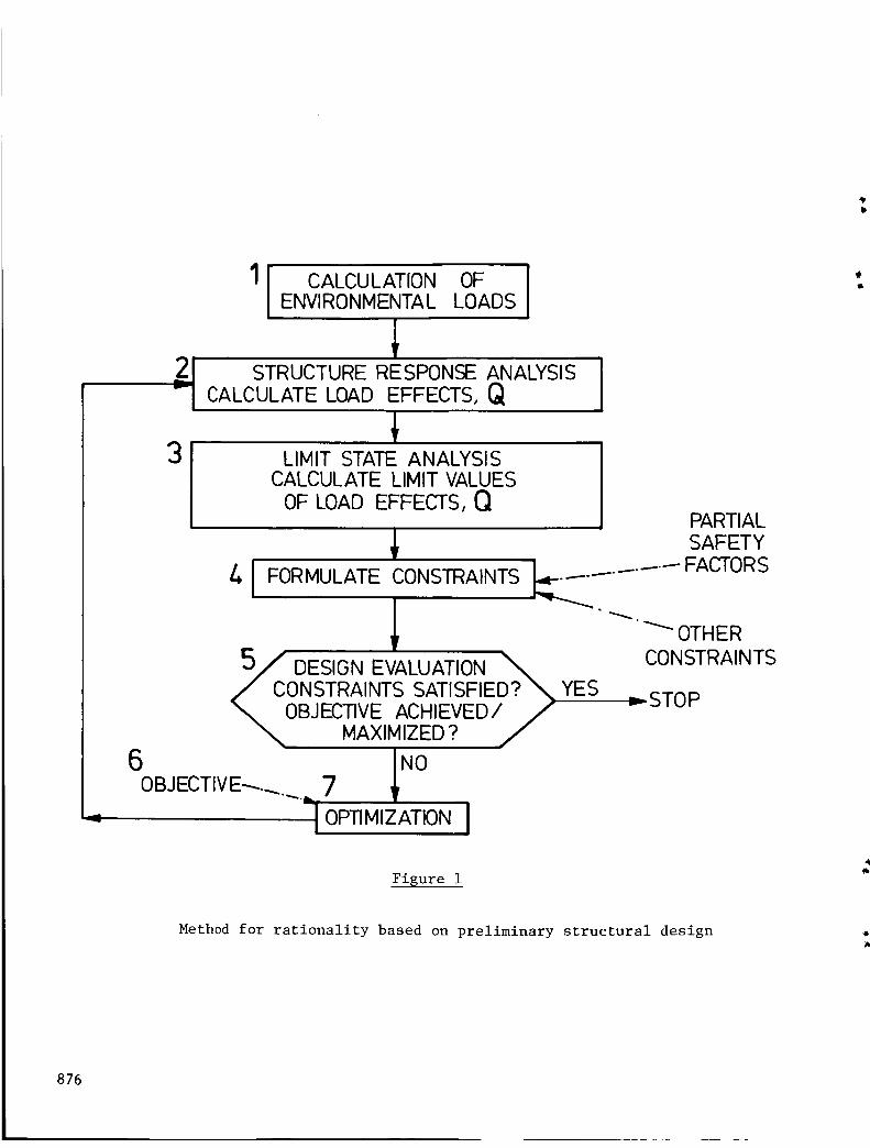
3

II CALCULATIONOF IENVIRONMENTAL LOADS

_21 STRUCTURE RESPONSE ANALYSIS

-I CALCULATE LOAD EFFECTS, Q

LIMIT STATE ANALYSISCALCULATE LIMITVALUES

OF LOAD EFFECTS, Q

FORMULATE CONSTRAINTS

_ DESIGN EVALUATION

ONSTRAINTS SATISFIED? _ YESOBJECTIVE ACHIEVED//

MAXIMIZED ?

6 _NOOBJECTIVE_._......_ 7IOPTIMIZATION I

PARTIALSAFETY

I__T ...... FACTORS

OTHER

CONSTRAINTS

,._STOP

Fisure 1

Method for rationality based on preliminary structural design

876

The method of Fig. 1 has been implemented in a computer program known as

MAESTRO*. The program is modular, corresponding to the boxes shown in the figure,

and the response analysis has been further subdivided to permit substructuring. A

common database is used for storing and sharing information among the modules. These

features have helped to make the program versatile. For example, as shown in refs.

2, 3 and 4, MAESTRO has been applied successfully to a box girder bridge, to

commercial ships and to warships, even though these three classes of structure have

totally different purposes (and measures of merit) and substantial differences in

loads, in the proportions, complexity and stiffness of the structure, in operating

requirements and in many other aspects. A design study involving a semi-submersible

platform will be published in the near future. As noted earlier, the basic method-

ology applies to an even wider variety of structures, such as road and rail vehicles

and aircraft. For these further applications the program would, of course, require

some modification, but because of its modular structure it is definitely capable ofsuch adaptation and extension.

The remainder of this paper consists of a brief description of how the

basic aspects of Fig. 1 have been implemented in MAESTRO. The seventh aspect -

optimization - is not discussed here because it is covered fully in the paper by

Mistree, Shupe and Hughes (ref. 5). The paper concludes with a brief summary of the

use of MAESTRO for the structural optimization of a 96000 ton tanker.

i. Calculation of External Loads

Because of the new and rather unusual geometry of semi-submersibles and

other ocean platforms there are no empirically derived and time-tested expressions

for design loads as there are for ships, bridges and aircraft. Therefore during the

past ten years or so several computer programs have been developed for calculatingthese loads from first principles, most often by means of source distributions.

Some examples are SPLASHD, WAMLOS, AQWA and MATTHEW. In the development of MAESTRO

the intention has been to eventually interface one of these with the MAESTRO load

module. Therefore the latter is largely passive, accepting whatever loads the

designer inputs (as obtained from the empirical expressions and methods). The only

loads that are calculated and applied automatically are the hydrostatic loads due to

immersion, as in a ship's hull.

2. Response Analysis

The method for the response analysis is, of course, the finite element

method. For a ship the overall structure is essentially a box girder (the "hull

girder") and it is possible to begin the analysis with a segment of the hull girder.

But for structures of more complex topology, such as ocean platforms, the response

analysis must deal with the complete structure. To attempt to begin at any lower

level would introduce unacceptable levels of uncertainty in relation to boundaryconditions - both loads and restraints.

* M_ethod for _Analysis, E_valuation and STRuctural Optimization

877

In MAESTROthe structural modeling is divided into three levels: modules,strakes and principal members,as shownin Fig. 2. A module is any structure, or

portion of structure, consisting of frames and plating and having one direction or

axis (regarded as "lengthwise") along which the transverse frames are evenly spaced

and are orthogonal to that axis. In a very general sense a module is "tubular", but

it need not be prismatic and the cross section may be of any shape whatever, open or

closed. In Fig. 2 the drilling tower, deck, column segments and pontoon are all

modules. Other examples are segments of a ship hull (Fig. 3) or aircraft fuselage

or wing (Fig. 4).

As shown in Fig. 2 a strake is a lengthwise row of stiffened panels and

frame segments and, optionally, a girder along either edge. Each strake can have

linear taper and/or twist along its length, and hence the overall module can have a

pronounced change in its cross sectional shape; it need not be prismatic. A strake

can be either flat or cylindrical, and the panel stiffeners can be either longi-

tudinal or transverse.

/ / ' STRAKMEODULE

PRINCIPAL

_/

MEMBERS

= ELEMENTS

Figure 2

Subdivision of structure

878

NOTE:

NULL MODULE

This figure is an example of a MAESTRO-produced deflection plot, using the

hidden line removal option and a deflection exaggeration factor of 50.

Figure 3

MAESTRO model of a bulk carrier (i module)

"\

Figure 4

MAESTRO model of a 737 wing (4 modules)

879

As mentioned earlier, preliminary structural design is not concerned withlocal details but rather with the dimensions of the principal members. In order tohave a balance and a good interface between the response analysis and the optimi-zation, the finite elements in MAESTROcorrespond precisely to the principal members.The elements are therefore relatively large; e.g. a complete panel from one deck toanother and from one frame to the next, as shownin Fig. 5, or a correspondingsegment of a transverse frame or longitudinal girder. Figure 6 shows the subdivisioninto elements for a typical semi-submersible platform.

_^. STIFFENED PILLAR -" F"-'--_

DOUBLE WALL /__//

ELEMENT _ ""-" /

TRANSVERSE SUPERELEMENT

_y (ANY COMB. OF BARS, BEAMS,TRIANGLES g QUADRILATERALS)

USED FOR BULKHEADS,DEEP WEBS, ETC.

Figure 5

Typical elements in MAESTRO

Figure 6

MAESTRO model of a semi-submersible platform (12 modules)

88O

The elements in MAESTRO have been carefully defined in order to provide the

degree of accuracy that is required (and no more). For example the beam element

accounts for the effects of transverse shear, end rigidity due to brackets, and

elastic angular deformation of joints; also it can represent either an ordinary beam

or a beam attached to plating, with the plating acting as a flange. For large

brackets, bulkheads, and other principal members of nonstandard geometry the element

representing the member is constructed as a "superelement"; i.e. it is built up ofsmaller elements and then static condensation is used to eliminate all internal

nodes, keeping only those that are needed for attachment to other principal members.

Figure 7 illustrates this for a large bracket.

d

\

(a) Transverse webbracket

NEUTRAL AXIS OF ADJACENT

HYBRID BEAM ELEMENT

FLANGE VSB

NODES ELEMENTS

,./_""" _ ELEMENTS

THESE NODES CONNECTWITH PLATE ELEMENTS =

-..... I /i\

\ N-Z-

/NEUTRAL AXIS OF ADJACENT

HYBRID BEAM ELEMENT

(b) Superelement model of bracket

INEUTRAL

AXIS STIFFENED PANEL

S

NEUTRAL AXIS

FLANGE NODE

(c) Superelement after

reduction

Figure 7

Reduction of superelement

881

Figure 8 shows the design variahles in a typical strake. These values are

constant over the length of the strake. If the strake is nonprismatic (tapered and/

or twisted) the values will be determined by the combination or "envelope" of lowest

safety margins over the length of the strake. If it is desired to have a change in

a design variable within a module length (e.g. a change of plate thickness) then two

(or more) in-line strakes are used instead of one.

/

Girder "

Frame •

Figure 8

Example of a strake, showing design variables

882

Through the use of strakes, a module can contain any number of lengthwise

webs, bulkheads, floors, decks, etc. Through the use of superelements a module may

also contain any number of transverse brackets, webs, diaphragms and bulkheads.

Openings are created by deleting elements; openings smaller than a panel element are

ignored. Fig. 9 illustrates how strakes, superelements and modules can be combined

to represent quite complex structures, in this case a naval frigate.

Figure 9

MAESTRO model of a frigate (5 modules)

883

3. Limit State Analysis

A limit state is any undesirable condition that a structure might possibly

reach, and the limit values, QL, are the values of the load effects Q at which that

condition would be reached. There are two types of limit state analyses, corres-

ponding to the two levels of limit states: those involving only individual members

(strake level) and those involving several members (module level). Fig. i0 shows an

example of the latter: collapse of the transverse framing of a tanker. For this

limit state MAESTRO uses a simplified (and conservative) form of plastic frame

analysis.

For the member limit states MAESTRO contains a library of subroutines, each

of which calculates the limit values _L for a particular mode of failure, using

approximate engineering algorithms appropriate to each mode. The limit state library

currently contains algorithms for 33 member limit states: 12 for a stiffened panel,

6 for a girder segment and 15 for a transverse frame segment. The theory underlying

the algorithms is presented fully in ref. I. The limit state library is modular,

allowing the addition of new subroutines to deal with new limit states, as might

arise from different geometry (e.g. sandwich panels) or new materials (e.g. fiber-

reinforced plastics). In most cases the limit states are a nonlinear function of the

design variables Z; let us denote this nonlinear dependency as QL(X). The variousalgorithms deal with the nonlinearity algebraically, in a "strength of materials"

fashion; nonlinear finite element analysis would be computationally prohibitive

because of the large number of members and load combinations.

Io HULL MODULE

I.E. MULTI- MEMBER

FAILURE

FAILURE

MUST ACCOUNT FOR:

• INTERACTIONS BETWEEN MEMBERS

_L INSTABILITY• COMBINED FAILURE MODES YIELD

Figure i0 Example of failure at module level

884

Besides structural failure, there are other ways in which a member or a

module can become unfit, especially the latter. For example, there may be limits on

the overall deflection of a module, as occurs in a wing. Fatigue is a cumulative

phenomenon that imposes a limit on the magnitude of the cyclic stress in the upper

and lower "flanges" of the module when it flexes as a beam, as shown in Fig. ii for a

ship. In both cases the load effect Q(X) (deflection, module flexural stress) is a

function of the design variables of all of the members, not just one, and the limit

value QL(X) does not coincide with any single physical event.

4. Formulation of Constraints

(a) Reliability-based Strength Constraints

Having calculated both the load effects Q and the limit values QL(X ) inall of the members and for all loadcases, the program then formulates the constraints.These are of the form

YoQ(X)< QL(X)

in which the parentheses indicate functional dependence, which is often nonlinear.

The total safety factor Y0 is a product of various partial safety factors whichaccount for

(i)

(i) the degree of seriousness of the limit state

(2) the probability of the relevant loads

(3) the degree of uncertainty in the associated load effects

(4) the degree of uncertainty in the associated limit values

In MAESTRO the partial safety factors are part of the input data, and the actual

values are obtained from an appropriate reliability-based code, as already exist for

many classes of structure and are being developed for others.

Figure ii Limit state for fatigue (allowable cyclic

stress for a given design load)

885

(b) Other (Non-strength-related) Constraints

As illustrated in Fig. 12, besides the strength constraints there are many

others arising from functional, local and fabrication requirements. These differ

widely from one structure to the next, and the MAESTRO program allows the designer to

specify any number of them, of any type and in any combination, either for individual

strakes or for an entire module. In the tanker example to be presented subsequently,

there were approximately 550 strength-related constraints and about 450 other

constraints, giving a total of about i000 constraints.

5. Evaluation of Current Design

In each cycle of the overall design process of Fig. i, the formulation of

the strength-related constraints involves a thorough search for the lowest margin for

each of the 33 limit states in each strake; i.e. the largest difference between the

left and right hand sides of eq. (i). Within each strake the calculations are

repeated bay by bay, and for each loadcase in turn, and a complete record is kept of

the values of the lowest margins, the corresponding location and loadcase, and the

values of the relevant load effects. If requested, the program prints this

information in an orderly tabular format, in various optional levels of detail. Thus

as the optimization proceeds the designer can monitor the process as closely as he

wishes. This feature also means that MAESTRO can be used for the comprehensive

evaluation of a given design or of an existing structure - perhaps after some damage

or some modification, either real or projected.

OTHER CONSTRAINTS ( BESIDES SAFETY )

E.G.

• FUNCTIONAL CONSTRAINT ON _q__[__.I

WEB HEIGHT FOR

CLEARANCE _--~50

• LOCAL E.G LOCAL BUCKLING _sI_

OF STIFF'R. WEB tw

~200 hs< 30tw [

CUTOUTS, ATTACHMENTS, ETC.

• FABRICATION EGhs< 0.6hf

~ 200

h I

SAFETY 550OTHER /.50

1000 CONSTRAINTS

(1080 FOR SEG. BALLAST TANKER)

Figure 12

Other (non-strength-related) constraints

886

6. Measure of Merit

In MAESTRO the measure of merit may be any function of the design

variables - linear or nonlinear, single or multiple. For example, it may be any

desired combination of weight, cost and vertical center of gravity (VCG). This

particular combination is illustrated in Fig. 13. The curved surface represents the

combined and net effect of all of the constraints. It is actually an irregular

surface - it is the outer envelope of all of the many individual constraints, each of

which is itself a surface consisting of the lowest possible combinations of weight,

VCG, and cost which just satisfy the requirements of that particular constraint. In

different regions of the design space different constraints are the outermost or

"active" constraints. Any point in the design space that does not penetrate below

this surface is a feasible design (.such as point A) and any point actually on the

surface is an optimum design (point B). The surface indicates what sort of tradeoffs

are available to the designer.

For example, the weight would be lower in a more intricate - and costlier -

design (point C) but the extent to which this option is followed may depend on the

ratio between the weight savings and the extra cost. Because of its flexibility in

regard to measures of merit, the program can be used for a wide variety of tradeoff

studies. As mentioned earlier the optimization aspects of the program are covered inref. 5.

OUTER ENVELOPE

OF CONSTRAINTSURFACES

WEIGHT

_VCG

SLOPE =

WEIGHT SAVED

EXTRA COST

Figure 13

Multiobjective optimization

COST

887

Example

By way of example, this section briefly summarizes the results of an

optimum design of a 96000 ton tanker, on the basis of least life-cycle cost. Details

are given in ref. 3. Because one of the main purposes of this study was to assess

the economic benefits of rationally based design, all of the design specifications

(principal dimensions, geometry, loads, etc.) were the same as for an actual, rule-

based, manually produced design. As explained in ref. 3 special steps were taken to

avoid any bias in favour of MAESTRO and to remove the rather uncertain question of

corrosion allowance from the comparison. In rationally based design there is a clear

distinction between steel that is required for adequate strength and steel that is

provided in order to allow for corrosion. MAESTRO provides only the former; the

latter must be added on after the optimization.

The transverse section of the basis ship is shown in Fig. 14. For the

three cargo tank lengths which comprised the MAESTRO structural model the cost of the

basis design was 9708 cost units, and the structural weight (which is automatically

calculated by MAESTRO) was 8050 tons. As mentioned earlier, the initial scantlings

for MAESTRO are completely arbitrary and so in this case, in order to provide a

direct and graphic comparison between the rule-based design and the MAESTRO design,

the scantlings of the former were used as the initial scantlings for MAESTRO.

I I I I I I i

-I F

"-I f"

-l F

-7

"-I

--I

--1

--1 r"

--I T-

---1 F

--I

--]

__T T 1- T T 1- T _

I I i I I I I I I I I 1 I

q

/T T T VTT TT TT TTT

Fisure 14

Basis ship: 96000 dwt tanker

888

The performance of MAESTRO is shown in Fig. 15. The solution for the

optimum design required 12 design cycles, which took about 12 minutes of computer

time on an IBM 370/158. The total computing (cpu) cost was about $130. The result-

ing optimum design had a total life-cycle savings (in which increased revenue from

weight savings is converted to and subtracted from initial cost) of 8477 cost units,

which is a 13% improvement on the basis or current practice design. The savings in

initial cost was 6%, which for a tanker of this size represents a savings of the

order of one million dollars.

The figure also shows two other optimization runs starting with very

different initial values of the design variables: one in which they are all 3 times

the basis ship values and another in which they are all 1/3 of the basis values. In

both cases the program converged to the same optimum solution as before, thus demon-

strating that it does not require good - or even feasible - initial values, and also

showing that it achieves a global optimum.

x11/QZ

I-

00

26000-- _VERY LARGE (3X)

_..i INITIAL SCANTLINGS

\\/ \

\14000 \

\\\

12000 -\

, \ jBASIC (CURRENT PRACTICE) DESIGN

10000-__ (8708 COST UNITS)

8000 -

FINAL MAESTRO DESIGN, .VERY SMALL (+3) (8477 COST UNITS)

6000- //INITIAL SCANTLINGS

4000-

2OOO

/

I I I I I I i I i I l I

1 2 3 4 5 6 7 8 9 10 11 12

DESIGN CYCLE

Figure 15

Results of tanker optimization

889

Effect of Using Standard Sections

The foregoing savings will be decreased slightly by the need to use

standard plate thicknesses and standard rolled sections for the stiffeners. MAESTRO

deliberately treats these design variables, and also the stiffener spacing, as

continuous variables in order to avoid the enormous computation and complexity of

discrete variable optimization. This also has the advantage of allowing the designer

himself to decide these questions, and to do so after he has seen what the idealized

optimum is. This is very helpful information and with it he can make a betterdecision as to how much standardization he wants. The standard sizes do not all have

to be the next larger size; it is usually sufficient to choose the nearest size,

unless this would mean decreasing all of the scantlings in a particular stiffened

panel. After inserting standard sizes wherever he wishes, the designer then runs

MAESTRO for one more cycle with all of these design variables fixed (a standard

feature on MAESTRO). The program then automatically adjusts all other scantlings

to obtain the new (and final) optimum design which has all of the standard sizes

and still satisfies all of the constraints. By observing the new optimum cost the

designer can immediately see how far from the idealized optimum his selection of

standard sizes has taken him. In most cases the departure is small. For example, in

the tanker the insertion of standard sections reduced the life-cycle savings from 13%

to 11% compared to the rule-based design, which still represents a substantial

savings. Moreover this guarantees that the 6% savings in initial cost is a real

savings, being based on realistic limitations to standard sections.

References

.

2.

.

.

.

O.F. Hughes, Ship Structural Design, Wiley-lnterscience, 1983.

O.F. Hughes, F. Mistree, and J. Davies, "Automated Limit State Design of Steel

Structures", Proceedings of the Sixth Australasian Conference on the Mechanics

of Structures and Materials, Christchurch, August 1977, pp. 98-106.

D. Liu, O.F. Hughes, and J.E. Mahowald, "Applications of a Computer-Aided,

Optimal Preliminary Ship Structural Design Method", Trans. SNAME, Society of

Naval Architects and Engineers, 1981.

O.F. Hughes, "A Method for Nonlinear Optimum Design of Large Structures, and

Applications to Naval Ship Design", Int. Symp. on Optimum Structural Design,

Univ. of Arizona, Tucson, Oct. 1981.

F. Mistree, J.A. Shupe, and O.F. Hughes, "A Conceptual Basis for the Design of

Damage Tolerant Structural Systems", Recent Experiences in Multidisciplinary

Analysis and Optimization, NASA CP-2327, Part 2, 1984, pp. 907-942.

890

Ns÷- lvve

FUNDAMENTAL DIFFERENCES BETWEEN OPTIMIZATION CODE TEST PROBLEMSAND ENGINEERING APPLICATIONS

E° D. EasonFailure Analysis Associates

Palo Alto, California

891

INTRODUCTION

There are manystudies in the literature comparing the performance ofnonlinear programming codes applied to a wide variety of problems [I-9].Several of these comparison studies have been conducted with real or realisticengineering problems [i-8]. In addition, there is a growing body of litera-ture regarding the methodology of conducting comparative tests and the validi-ty of comparative results [8,11-18]. An entire conference was devoted to thistopic in 1981 [18]. A key result from all of the nonlinear optimization codecomparison literature is that the relative performance of codes is highlydependent on the specific problem. Thus, if the typical engineering problemdiffers substantially from the type of problems that have been used for com-paring optimization codes, it would not be surprising if the relative perfor-mance of codes on engineering problems did not agree with the published com-parative results. The purpose of the present paper is to suggest that thereis at least one fundamental difference between the problems used for testingoptimization codes and the problems that engineers often need to solve; inparticular, the level of precision that can be practically achieved in thenumerical evaluation of the objective function, derivatives, andconstraints. This difference affects the performance of optimization codes,as illustrated below by two examples.

All nonlinear constrained optimization problems can be put in the form:

minimize f(x)

subject to g(x) _ 0 (I)h(x) = 0

where the functions f, g, and h are generally nonlinear, x is a vector ofvariables, and g and h are generally vector functions. Within this frameworkone can define two general classes of nonlinear constrained minimizationproblems.

Class One functions f, g, and h can be evaluated toany desired precision except as limited by the wordlength or precision of the computer.

Class Two functions f, g, and h cannot be evaluatedto a level of precision comparable to the wordlength or precision of the computer, generally foreconomic reasons.

In the typical Class One problem, f, g, and h are analytic functions.

Examples of Class Two problems are cases where f, g, or h are the result of

Monte Carlo simulation, solution of ordinary or partial differential equations

(e.g. finite element analysis), numerical integration, solution of nonlinear

algebraic equations, or any other iterative algorithm.

It should be apparent that many engineering problems fall into thesecond class, where the cost of refining the analysis beyond a few significant

892

digits would be prohibitive. Often convergence to within 10% in the basic

analysis that evaluates f, g, or h is considered acceptable for engineering

purposes, and this single-digit precision may be greater than the accuracy ofmodeling the real situation. A prime example is optimization requiring finite

element analysis.

In the following figures the type of problem used in various code

comparison studies is identified. Two limited-precision problems are present-ed and solved by two optimization codes over a range of precision in evaluat-

ing f and/or g. The first problem is typical of Monte Carlo simulationmodels, or analyses that are sensitive to rounding or truncation error. The

functions contain a random noise component that may vary from one evaluation

to the next. The second problem is typical of numerical integration, includ-

ing ordinary differential equation initial value problems. The precision (and

evaluation cost) can be varied by changing the integration step size.

893

ANALYSIS OF PROBLEMS GIVEN IN SELECTED SOURCES

Table 1 categorizes the test problems used in selected comparison

studies. The vast majority are Class One problems where the function andconstraints can be evaluated to arbitrarily high precision. Some problems

have some of the features of Class Two problems in that they arose from engi-

neering applications and they are not analytically differentiable, but they

are not strictly Class Two because there are no precision limits. Only three

problems are clearly in the Class Two category where the function or con-

straints can only be evaluated to limited precision. All of these involve

solution of an ordinary differential equation. This can only be accomplished

to relatively low precision if that evaluation is to be repeated many times.

Two of the three Class Two problems and three of the ten problems with someClass 2 features were not used for ranking in these comparison studies because

few codes could solve them. In summary, most test problems are Class One, and

of those problems that are Class Two (or that have some features of ClassTwo), a significant fraction cannot be used for ranking because few optimiza-

tion codes could solve them. This is evidence that the performance of optimi-

zation codes on the difficult Class Two problems is unknown.

SOME FEATURESSOURCE CLASS1 OF CLASS 2 CLASS2

(NUMBER) (PROBLEM ID) (PROBLEM ID)

COLVILLE (1) 6

EASON & FENTON (2) 8

HIMMELBLAU (5) 32

SANDGREN (6) 19

SCHITTKOWSKI (9) 185

C6,C8

C6",E9"_E 11, E 12

C6,C8,H14

C6,C8,E9",E 11,E 12,$25-$27,$30"

D

E 13"(ODE)

H13(ODE)

E 13",S28"(0DE)

250 PROBLEMS 10 PROBLEMS 3 PROBLEMS

• Not used for ranking due to poor performance by most codes.

Table 1

894

EXAMPLEOFA CLASSTWOPROBLEMINVOLVINGRANDOMNOISE

Problem 1 is a simple Type 2 test problem. The lack of precision inthe evaluation of f and one of the constraint functions comes from additiverandom noise that is normally distributed with a mean of zero and standarddeviation S. Such a situation may arise when the function and/or constraintare evaluated by Monte Carlo simulation, or when compoundedround-off errorstrongly influences the calculated value of a function or constraint. Eachtime the optimizer asks for a new value of f and g, the value is slightlydifferent for the samex because of the randomnoise component. By adjustingthe standard deviation it is possible investigate a range of noise-to-signalratios for the function f and the constraint g. (See fig. I.)

PROBLEM 1 (RANDOM NOISE)

MIN f(X)--SIN(XI/2)'COS X2+Pl

SUBJECT TO

X ->01

X2>-O

271"- X 1-X2+ P2 >- 0

WHERE

/31 AND P2 ARE NORMALLY-DISTRIBUTED RANDOM

NUMBERS WITH MEAN /,(,=0 AND STANDARD DEVIATION

O= S (INPUT)

S -NOISE/SIGNAL FOR f

S1(2"/i')- NOISE/SIGNAL FOR g

FEASIBLE STARTING POINT: X 1-4.0, X 2--.2

Figure 1

895

CONTOUR PLOT FOR PROBLEM 1 RANDOM NOISE

Figure 2 is a contour plot for Problem 1. The objective function is aperiodic array of hills and valleys. The nominal position of the functionalconstraint cuts through the feasible minimum, The random noise causes thefunctional constraint to vary right and left and the function value to vary inand out of the plane of the paper.

27[

7F

0

0

0

0.3

1.0

Figure 2

y

x I

27F

Start _(4,0.2)

896

SOLUTIONSTORANDOMNOISEPROBLEM

Figure 3 gives the solutions by two optimization codes to Problem 1with a range of noise-to-signal ratios in both constraint and objective func-tion. The numbers on the figure are the number of function evaluations toreach the corresponding relative error shownon the top scale. There are somecases (at large ratios of objective function noise-to-signal) where neithercode was able to solve the problem. However, in most cases the PATPENcode, asimple Hooke & Jeeves direct search strategy [19], was able to solve theproblem in 120 to 200 function evaluations. The PCONcode, which is a Powellcode with SUMT-typeconstraints [20], was very unsuccessful on this problem.PCONwas able to solve only 3 of 23 cases to the samegeneral level of erroras PATPEN. In two other cases the level of error was approximately an orderof magnitude greater wizh PCONthan PATPEN. In all cases PCONrequired morefunction evaluations, sometimes substantially more, than PATPEN. The PATPENcode was well-behaved; at termination the relative error from the true solu-tion is comparable to the noise-to-signal ratio.

RELATIVE FUNCTION ERROR,%(OPEN SYMBOL ERROR l Ox GREATER)

uJ"E3

,_1n

OI-

u.Io9

OZ

I-,.Z

IZI-

Z0¢D

I.L00I--

mr

0.01

I0 I'I_ 176

0.1 1.O

, , I lll_il_1781 , i I llli_ I167236

• PCON

• PATPEN

• NEITHER CODE SOLVED

•177

•177

•151

:1_139706I I I IIIII I 1 t I I IIII

1.0

10

I I_llV_

I

E163

190396

E"180

_4214i

10

1.0'I

I

0.1

1503

0.010.01

•151

160718

•177

• 149

0.1

•144'

•14_

v13

146•

I I I I 1

RATIO OF FUNCTION NOISE TO AMPLITUDE, %

Figure 3

897

PROBLEM2 OPTIMUMGEARRATIOS

The second problem is a simulation by numerical integration of vehicleacceleration from five to one hundred miles per hour. The gear ratios are tobe optimized to the torque-speed curve of the engine such that the time of theacceleration event is minimized. The expressions for the problem are givenin figure 4 and the torque-speed curve is shownin figure 5. This problem is asimplified version of Problem E-13, which was one of the test problems inearlier studies (see Table 1). The objective function (time) cannot beevaluated more accurately than the time increment used in the numerical inte-gration. There is a direct trade-off between the amount of computer effortspent in the numerical integration and the amount spent in the numericaloptimization. The objective function is calculated from a discontinuousexpression for acceleration that corresponds to the abrupt change from posi-tive to negative acceleration (wind resistance) during shifts.

PROBLEM 2 (GEAR RATIO)

MIN f(X)=T, WHERE

1 _0TCON1 ACC dt=95 MPH

ACC =(X i) (TORQUE) - (FORCE)(RAD)]

RAD ....(Xi)2 (El) *Vl

-(FORCE)(RAD)2/VI

DURING

ACCELERATION

DURING

SHIFTING

SUBJECT TO

20>-Xl>_X2>-X

X1>-15

3->X4->X5-- 2

FEASIBLE STARTING POINT: X 1 = 15, X2= 9.05, X3= 6.14,

X4- 4.55, X5= 3.61

Figure 4

898

ENGINECHARACTERISTICCURVEFORPROBLEM2

Figure 5 corresponds to the engine torque-speed curve in the accelera-tion problem. The dashed line is the maximumallowable engine speed, at whicha shift must occur.

140

120

100

I,--LI.

I

J 80

0n-OF- 60

40

2O

00 1000

I I I I I I I I2000 3000 4000 5000

ENGINE SPEED, RPM

|

6000

Figure 5

899

COMPARISON OF OPTIMAL GEAR RATIO SOLUTIONS

Table 2 shows solutions to Problem 2 at three precision levels (numeri-cal integration time steps). The same two optimization codes are used as in

Problem 1, and in some cases multiple runs are shown The x= are the gearratios, f is the total elapsed time in seconds (to be'minimized), and #FE is

the number of function evaluations required for the solution.

At the lowest precision level the PATPEN code finds as good a solutionas the PCON code in far fewer function evaluations. The x= solutions are

slightly different between the two codes, but the objective _unction is the

same. This is indicative of the discreteness in the objective function, which

can only take values at 0.1 sec steps. At the finer integration step (0.01

sec) PATPEN is still superior, requiring far fewer function evaluations to

reach the improved function value of 38.53. However, at this integration

precision PCON is capable of finding a slightly better solution, albeit with

more than ten times as many function evaluations. At the finest integrationstep PCON finds a significantly better solution than PATPEN in about the same

number of function evaluations, indicating that the more sophisticated codeperforms better when the function can be evaluated accurately. However, note

that each function evaluation takes a hundred times more computation at the

0.001 sec time step compared to the 0.1 sec time step. Consequently, 330

function evaluations at 0.001 time step are as expensive as 33,000 function

evaluations at 0.1 time step. Overall, the least-cost solution is to use theless sophisticated code and the larger integration step.

INTEGRATIONSTEP

0.1

0.01

0.001

PATPEN

PCON

PATPEN

PCON

PATPEN

PCON

Xl X 2 X 3 X 4 X 5

18.2 10.0 7.8 5.8 3.8

16.5 11.7 8.3 5.8 3.8

17.7 13.0 9.3 6.2 3.8

19.7 13.1 8.6 5.8 3.8

19.6 12.0 8.0 5.8 3.8

19.4 13.9 9.0 5.9 3.8

20.0 12.4 8.5 5.8 3.8

19.8 12.7 8.7 5.8 3.8

f ÷FE

38.7 58

38.7 485

38.7 1186

38.53 84

38.53 509

38.51 935

38.659 258

38.501 330

TABLE 2

900

DISCUSSIONOFPERFORMANCEDIFFERENCES

In the random noise Problem 1, the objective function value at x_ canbe either larger or smaller than the value at x2 depending on f. and p. (see

1 1

Figure 6). If the difference fl - f2 is small compared to the Pi' an optimi-zation code may be totally confused by the random nature of the apparent

gradient. Algorithms such as PCON that base their line search step length and

direction on apparent gradients or an assumed quadratic functional form may

take large steps in totally wrong directions because of the random component

in the function. Less sophisticated algorithms such as Hooke & Jeeves [19] orNelder & Mead simplex [21] have predetermined, relatively small search step

lengths, so they do not go far in wrong directions.

An additional performance difference arises from the stopping

criterion. More sophisticated codes often test for zero gradients or numeri-cal satisfaction of Kuhn-Tucker conditions. In the presence of random noise,

these conditions are unlikely to be satisfied to normal tolerance levels

except by random chance, so the codes would be expected to "dither" unproduc-tively about the minimum point. The direct search codes terminate when a

better point cannot be found by reducing the step length below some minimum.

Thus they seize on a low function value and quickly terminate because no

smaller f + p is likely in the immediate vicinity. One would expect such acode to return a final f + p that is about one standard deviation below opti-

mum f, and this is observed. In Figure 3, for example, the error in the

PATPEN solution [final(f + p) - fo]/fo is slightly below the true noise-to-

amplitude ratio P/fo' where subscript o refers to the true optimum.

Problem 1 schematic

• ._<

f+p

Actual gradient

_/ _/Apparent gradient

°°,°°_"°

x 1 x2

Figure 6

901

PERFORMANCEDIFFERENCES

In Problem 2, the principal difficulty is the discrete-valued objectivefunction, conceptually shown for two variables in Figure 7. The minimumheight difference between adjacent regions is the integration time step (0.1to 0.001), but within each region the objective function is flat for a rangein each of the variables. In the test problem it would be easy to eliminatethe most obvious source of discreteness by interpolating final time at 100mph; however, there may be other sources of discreteness in real simulationmodels.

On a stepwise flat objective function, codes that estimate local gra-dients are likely to terminate prematurely. Assumptions of quadratic form inline search strategies are also likely to be unproductive unless the minimumstep length can be forced to be greater than the average size of the discrete-valued region. Direct search strategies have less problem because the stepsize typically starts large and reduces whenno further progress occurs. Suchcodes will automatically terminate when their step size is reduced below thesize of the discrete region.

Problem 2 schematic

11

Figure 7

A

x2

902

I.

.

.

.

.

.

.

CONCLUSIONS

Two classes of optimization problem have been defined. Class One functions

and constraints can be evaluated to a high precision that depends

primarily on the word length of the computer. Class Two functions and/orconstraints can only be evaluated to a moderate or a low level of preci-

sion for economic or modeling reasons, regardless of the computer wordlength.

Optimization codes have not been adequately tested on Class Two

problems. Where those problems have been used, many codes have beenunsuccessful.

There are very few Class Two test problems in the literature, while there

are literally hundreds of Class One test problems.

The relative performance of two codes may be markedly different for Class

One and Class Two problems. Based on the limited sample of two problemsand two codes, less sophisticated direct search type codes may be less

likely to be confused or to waste many function evaluations on Class Two

problems. Of course, the less sophiticated codes may be unable to solveproblems with many variables.

The analysis accuracy and minimization performance are related in a com-

plex way that probably varies from code to code. On a problem where the

analysis precision was varied over a range, the simple Hooke and Jeevescode was more efficient at low precision while the Powell code was more

efficient at high precision.

These results are tentative and should be confirmed by generation of many

more Class Two test problems and comparisons of optimization codes ofinterest to engineers.

The results suggest that a great deal more testing effort should be

expended to ensure that codes being developed now do not degrade signifi-cantly in the presence of low accuracy, Type 2 Problem functions.

903

REFERENCES

i. Colville, A. R., "A Comparative Study on Nonlinear Programming Codes," IBMNew York Scientific Center Report No. 320-2949, June 1968, summarized in

Proceedings of the Princeton Symposium on Mathematical Programming, Kuhn,H. W., ed., Princeton, NJ, 1970, pp. 487-501.

. Eason, E. D. and Fenton, R. G., "Testing and Evaluation of Numerical

Methods for Design Optimization," University of Toronto Report UTME-TP7204, September 1972.

o Eason, E. D. and Fenton, R. G., "A Comparison of Numerical Optimization

Methods for Engineering Design," Journal of Engineering for Industry,Trans. ASME Series B, Vol. 96, No. 1, February 1974, pp. 191-196.

4. Stocker, D. C., A Comparative Study of Nonlinear Programming Codes, MSThesis, University of Texas at Austin, 1969.

5. Himmelblau, D. M., Applied Nonlinear Programming, McGraw-Hill, New York,1972.

6. Sandgren, E., The Utility of Nonlinear Programming Algorithms, Ph.D.Thesis, Purdue University, 1977.

o Sandgren, E., and Ragsdell, K. M., "The Utility of Nonlinear ProgrammingAlgorithms: A Comparative Study- Parts I and II," ASME Journal of Mechani-

cal Design, Vol. 102, No. 3, July 1980, pp. 540-551.

8. Sandgren, E., "A Statistical Review of the Sandgren-Ragsdell Comparative

Study," Evaluatin_ Mathematical Programming Techniques, Lecture Note #199,Springer-VerIag, 1982, pp. 72-90.

go Schittkowski, K., Nonlinear Programmin_ Codes - Information, Tests Per-formance, Lecture Notes in Economics and Mathematical Systems, No_ 183,

Springer-Verlag, New York, 1980.

10. Eason, E. D., "Validity of Colville's Time Standardization for Comparing

Optimization Codes," ASME Paper No. 77-DET-116, September 1977.

11. Dembo, R. S. and Mulvey, J. M., "On the Analysis and Comparison of Mathe-

matical Programming Algorithms and Software," Proceedings of the Bicenten-

nial Conference on Mathematical Programming, Gaithersberg, Maryland, 1976.

12. Hillstrom, K. E., "A Simulation Test Approach to the Evaluation and Com-

parison of Unconstrained Nonlinear Optimization Algorithms," ArgonneNational Laboratories Report No. ANL-76-20, 1976.

13. Nazareth, L. and Schlick, F., "The Evaluation of Unconstrained Optimiza-

tion Routines," Proceedings of the Bicentennial Conference on Mathematical

Programming, Gaithersberg, Maryland, December 1976.

14. Crowder, H. P., Dembo, R. S., and Mulvey, J. M., "Reporting Computational

Experiments in Mathematical Programming," Mathematical Programming, Vol.15, #3, November 1978, pp. 316-329.

904

15. Miele, A. and Gonzalez, S., "On the Comparative Evaluation of Algorithmsfor Mathematical ProgrammingProblems," presented at Nonlinear ProgrammingSymposium- 3, Madison, Wisconsin, July 1977.

16. Eason, E. D., "Evidence of FundamentalDifficulties in Nonlinear Optimiza-tion Code Comparisons," Evaluating Mathematical Pro_rammin_ Techniques,Lecture Note #199, Springer-Verlag, 1982, pp. 60-71.

17. Hoffman, K. L. and Jackson, R. H. F., "In Pursuit of a Methodology for

Testing Mathematical Programming Software," Evaluating MathematicalProgramming Techniques, Lecture Note #199, Springer-Verlag, 1982, pp. 60-71.

18. Mulvey, j. M. (ed), Evaluating Mathematical Programming Techniques, (Pro-ceedings of Conference at Boulder, Colorado, 1981), Lecture Note #199,

Spri nger-Verlag, 1982.

19. Hooke, R. and Jeeves, T. A., "'Direct Search' Solution of Numerical and

Statistical Problems," Journal of the ACM, Vol. 8, No. 2, April 1961, pp.212-229.

20. Powell, M. J. D., "An Efficient Method for Finding the Minimum of a Func-

tion of Several Variables Without Calculating Derivatives," ComputerJournal, Vol. 7, No. 4, 1964, pp. 155-162.

21. Nelder, J. A. and Mead, R., "Simplex Method for Function Minimization,"

Computer Journal, Vol. 7, No. 4, January 1965, pp. 308-313.

905

N8 -11773

A CONCEPTUAL BASIS FOR THE DESIGN OF DAMAGE-TOLERANT STRUCTURAL SYSTEMS

Farrokh Mistree

Associate Professor

Department of Mechanical Engineering

University of Houston

Houston, Texas

Jon A. ShupeResearch Assistant

Department of Mechanical Engineering

University of Houston

Houston, Texas

Owen F. HughesProfessor

Department of Naval Architecture

University of New South Wales

Sydney, Australia

PRECEDING PAGE BLANK NOT FILMED

C" 5-" 907

A CONCEPTUAL BASIS FOR THE DESIGN OF DAMAGE-TOLERANT STRUCTURAL SYSTEMS

ABSTRACT

We define damage-tolerant structural systems as those systems which not only

have adequate intact strength to withstand initial failure but also adequate

residual strength to minimize the possibility of, and hence the consequences of,

further failure. The incorporation of damage tolerance cannot be done in total

isolation of the function being required of the system and the costs associated

with obtaining improved damage tolerance. Our approach, therefore, is to

formulate multiple-objective, multi-level decision support problems the solutions

of which represent a compromise between higher costs and higher damage

tolerance. Multiple-objective decision support problems are easily solved in the

linear domain. Our fomulations, however, include both linear and nonlinear

constraints and goals, which in the past, have not been considered due to the

resulting complexity. In this paper we

present a complete discussion and description of decision support

problems, including coupled DSPs and multi-level DSPs with examples

provide a general formulation of a design decision support problem which

provides a basis for the inclusion of damage-tolerant considerations in

structural design

identify what further research needs to be done in order to obtain infor-

mation that is required but not known for solving problems using these

models

identify what needs to be done to implement this prototype method in

practice

I. INTRODUCTION AND BACKGROUND

In the past, there have been many approaches to structural design. Most

approaches have been based on deterministic, "rule of thumb" formulas that

resulted in overweight, over-strengthened structures. These methods were

appropriate when there were no advanced analysis techniques and structure cost was

a small fraction of the total cost of the project. Now, however, as structures

get larger (witness several plans for steel structures in over one thousand feet

of water) and computers and programs allow more complex analysis of structures,

there is a need for a rational approach (as opposed to an ad hoc, random approach)

that promotes optimal structural design.

Hughes et al. (1,2) have proposed a method for the design of semi-monocoque

structures. The method is summarized in Figure i. The method begins with the

input of loads and other pertinent data about the structural system. An

appropriate finite-element module is used to analyze the structure and output the

demand on the subsystems. A limit analysis is performed on the structural system

to determine if it has the capability to withstand the demands placed upon it.

Appropriate constraints are then formulated and the structural system is

optimized. At this point the subsystem design cycle is entered. Here, for each

subsystem in turn, a limit analysis is performed, constraints are formulated, and

an optimal subsystem design is derived. This cycle continues until all subsystems

have been optimized. If convergence has not been reached the process continues in

the system design cycle.

908

There are several assumptions in this design method. It is assumed that the

geometry and structural materials have been previously defined and that the loads

on the structure are known. Also, a "design-oriented" type of finite-element

analysis for semi-monocoque structures, together with the theory and methods for

the limit analysis of both the overall structure and the various substructures, is

presented in (2). Thus, these items will not be discussed in this paper. The

main topics for discussion are

- development of a methodology that handles multiple levels of

optimization

- formulation of the optimization problems for the structural

system and each of its subsystems

This will permit a designer to obtain a superior design which, ideally, will

represent the best compromise between the various (and conflicting) objectives.

2. MULTI-LEVEL SYSTEM DECISION SUPPORT PROBLEMS (DSP)

Engineering systems, such as structures, are generally too complex to be

handled in their entirety. This necessitates design of the overall system by

first decomposing the system into subsystems. If the system is then designed in

parts (sequentially), there is no guarantee that an overall optimal design will be

reached. Thus, it becomes necessary to develop a methodology for the optimization

of a multi-level system. The multi-level system is described as a system that

contains more than one level of interaction between the system and its sub-

systems. The design of such a system is based on the formulation and solution of

a series of problems involving decisions to be made by the designer. In this

paper, the information necessary to enable a designer to formulate these decisions

as Decision Support Problems (DSP) is presented. Solution of the DSPs will result

in superior (or optimal) solutions. These DSPs are capable of handling multi-

objective problems that contain both "hard" and "soft" information.

In this section the structure of a multi-level DSP is presented. The

characteristics of Damage-Tolerant Design (DTD) are presented in Section 3. A

discussion of the compromise DSP and how it is formulated is given in Section 4.

Also presented are two generic DSP formulations for damage- tolerant design.

Section 5 contains two case studies. The first is an example of the use of multi-

level DSPs in ship design. The second case study is a coupled DSP that combines

the selection of a structural material with structural design optimization.

2.1 Structure of a Multi-Level DSP

An engineering system can be represented hierarchically as in Figure 2. The

hierarchical nature of system design facilitates the identification of complexity

and the inter-relationships among various levels and subsystems. The relations

and bonds of a hierarchical system are essential for the visualization of the

system. A practical example of parent system-subsystem relationship is shown in

Figure 2. A ship hull module (or compartment) is subdivided into subsystems

called strakes. In turn each strake can be considered to be made up of subsystems

such as platesp stiffeners, girders, and frames. It is important to note that all

of the subsystems are integral parts of the parent system (hull module). This

means that changes in one subsystem affect the parent system and other subsystems,

as shown by the circle intersections. Thus no subsystem can be considered inisolation from the rest.

909

At each level of the hierarchical structure, for each subsystem, the designprocess involves a set of decisions which are qualified by the followingassertions (3):

Design is a series of decisions.

- Somedecisions can be madeconcurrently.- Somedecisions must be madesequentially.

Design involves multi-level decision making.

- Interaction between the various levels of subsystems exists. Thisinteraction maybe only one way or both ways.

- Interaction between the subsystems at the same level of the sameparentor of different parents also exists. This interaction can be one wayor both ways.

2.2 Types of Decision Support Problems (4)

In design, there are basically three ways to derive the answers to problems

encountered. They are analysis, synthesis, and heuristic thinking. These may seem

to be widely divergent but it is possible to integrate all three in the form of

structured decision support problems. A structuring of information for the DSP is

necessary to make a good decision. Since there are different types of decisions

to be made, different categories of DSP exist.

They are

- Selection

- Compromise

- Coupled Selection and Compromise

Selection DSPs are appropriate for problems that involve the choice of an

alternative from among several. The choice is made based on ratings given to

multiple attributes and their relative importance. Compromise DSPs involve the

optimization of an alternative by changing design variables optimally. Compromise

is discussed further in Section 4. A coupled DSP involves the solution of a

selection and a compromise DSP simultaneously. An example of a coupled problem is

given in Section 5.

3. DISCUSSION OF GENERAL DAMAGE-TOLERANT DESIGN (DTD)

Since the compromise decision support problem is capable of handling multi-

goal problems, it is an important tool for the design of structural systems. This

stems from the fact that, in structural systems, there are always at least two

important objectives that must be met to achieve a superior design. The first

objective is economic efficiency and the second is technical efficiency. Several

criteria can be used as measures of efficiency. Weight, for example, may be an

indirect measure of both economic and technical efficiency. Reliability,

stiffness, and strength are all measures of technical efficiency. Cost is a direct

measure of economic efficiency and an indirect measure of technical efficiency.

Therefore, there are at least two goals or objectives that must be defined and

used in the design of a structure.

910

Damage-tolerant structures have _twokinds of strength: intact strength andresidual strength (5). Intact strength represents the amount by which the workingload of the structure can be exceeded before it fails. Residual strengthrepresents the strength remaining in a structure once a vital component has beenrendered ineffective. A damage-tolerant structure will thus resist initialfailure (due to intact strength) and will also resist further failure afterinitial failure (due to residual strength). Thus, intact and residual strengthsare measures of technical efficiency. Also, since a failure due to residualstrength would result in complete loss of the structure and thus a large financialloss, it can be said that residual strength is an indirect measure of economicefficiency. Since it may be desirable to minimize weight in a damage-tolerantstructure, we have a second indirect measure of economic efficiency. Therefore,ideally, a damage-tolerant design (DTD) represents an optimal balance between thegoals of technical efficiency and the goals of economic efficiency.

4. COMPROMISE DSP: DEFINITIONS AND TERMINOLOGY

The basic approach to the solution of a structural optimization problem is to

formulate the design problem as a compromise DSP and to solve it using

optimization techniques. These optimization techniques must allow the designer to

find the values of the design variables that simultaneously satisfy the

requirements on the system's capability and to achieve desired goals as far as

possible. The goals can be conflicting and of different dimensions. To formulate

the compromise DSP, the techniques of goal programming are used. A program

capable of solving the DSP has been implemented at the University of Houston

called SLIP2. The details of this program can be found in Mistree et al. (6).

The next step is to describe how these compromise problems can be

formulated. First, it is important to know the components that make up theproblem. They are given by Kupparaju and Mistree (7) as

- Variables - system variables

- deviation variables

- Constraints - system constraints

- goal constraints

- Bounds - on system variables- on deviation variables

- Objective - in terms of deviation variables

A generic word formulation of the compromise problem follows:

GIVEN

- A structure with given geometry and materials

- The requirements that need to be satisfied by the design for feasibility

- The goals of the design; these need to be achieved as far as possible

FIND

- The values of the system variables

- The values of the deviation variables (which indicate the extent to which

the goals are achieved)

911

SATISFY

- System constraints: must be satisfied for feasibility

- Goal constraints: to be achieved as far as possible

- Bounds

- Lower and upper bounds on the system variables

- Lower and upper bounds on the deviation variables

MINIMIZE

- The difference between the required and the estimated performance of the

design

4.1 System Variables and System Constraints

The generic word problem for compromise is explained with reference to Figure

3.

System variables

System constraints

X_ = (Xl,X2,X3...,Xn)

C./D.(X) _ R. andi i -- I

Ci(X)/Di(X) _ R°

System descriptors are either fixed by the specifications provided or are

variable as to the need of the design. The descriptors, as the name implies,

describe the state of a system completely. Since some of the descriptors are

fixed parameters and do not change during the course of the design, the state of

the system is dependent entirely upon a set of variable descriptors termed system

variables. In general, a set of "n" design variables is represented by X. These

variables may be continuous, Boolean (l=true, 0=false), or a combination of the

two, an example of which will be shown later. Syste_ variables are, by their

nature, independent of the other descriptors and can be changed as required by the

designer to alter the state of a system.

A system constraint is a constraint placed on the design that has to be

satisfied for feasibility of the design. Mathematically, system constraints are

functions of the system variables only. They are rigid and no violations are

allowed. They relate the demands placed on the system D(X) to the capability of

the system C or C(X) to meet the demand.

Now a tie-in to damage tolerance can be made. There are four categories of

system constraints: catastrophic, non-catastrophic, operational, and proportion-

ality. Catastrophic constraints deal with complete system failure, whereas non-

catastrophic constraints deal with local or limited failures that could (but not

necessarily) lead to complete failure. Operational constraints keep the system

within bounds to ensure its operability and proportionality constraints ensure

that system components can be fabricated. In generic form, for the i-th mode of

failure the system constraint is

912

c./ D.(X) _ R. or C_ (X)/ D. (X) _ R.I 1 -- 1 i -- I - l

The difference between the two lies in the fact that the capability can be either

a constant C i (such as yield stress) or can be a function of the design

variables Ci (X) (such as the critical buckling stress). For the purposes of

damage tolerance, the ratio of a structure's strength capability to the demand (or

stresses) placed upon it will be referred to as the intact strength factor Bi.

Thus, the ratio of the system capability to the demand on the system will always

be constrained to be not less than a minimum safety factor R i for the i-th mode

of failure. In reality, these factors are the product of several partial safety

factors, which are specified by safety authorities such as AISC, and which have

been obtained on the basis of providing a satisfactory reliability level. These

system constraints do not prevent the capability/demand ratio from being very

large. When this happens, the design is technically, but not economically,

efficient. Prevention of large ratios is the responsibility of the goal

constraints as will be shown later.

4.2 Deviation Variables and Coal Constraints

Deviation variables include dl which is the underachievement of the i-th goal,

and d_ which is the overachievement of the i-th goal.

Coal constraints are

number of goals

(i/m

m

I C. (X)/D. (X))/S + d -d I = i; m represents thei= 1 i i

B + d2 + =max/Bmin - d2 1

Coal constraints represent the aspiration levels of a designer for the

design. They are always expressed as equalities and relate the goals of the

designer to the actual achievement of the design. It is possible that the

designer's goals are inordinately high or the system constraints are much too

restrictive to attain the aspired levels of achievement. The deviation variables

d_ and dE are used to allow the designer a certain degree of latitude in making

decisions. A particular goal may either be overachieved (d_ >0, dT=0) ori i

underachieved (d7 >0, d_=0). The two deviation variables associated with eachI 1

goal therefore relate the actual performance of the design to the desired level of

performance. If there are two or more goals it is imperative that the goals are

made dimensionless with all the deviation variables varying between a fixed range

(e.g. 0 to I, 0 to I0, etc.). In order to achieve this it may be necessary to

scale the goal (e.g. divide the function by a suitable constant). For example

Coal Function

Expected Value of Function÷+ d-dl = 0

913

To particularize the goal constraints to the damagetolerant case, first, letS represent a desired value for the capability/demand ratio for the structure. IfS is always greater then min(Ci (X)/Di(X)) (or Bmin, for short), then it is desir-able for the feasible design to satisfy the following constraints:

- the average intact strength should be as close to S as possible, i. e.,

m

(1/m i_ 1 C.l (X)/D._t (X))/_ S +d I- - dI÷

- the difference between the highest and lowest intact strength factors, i.e.,

B = max(C. (X)/D. (X)) and B = min(C. (X)/D. (X)), for i=l,2,...,m,max i - i - min i - _ -

should be as small as possible, i.e.,

B /B. + d2 - d2=lmax mln

These constraints ensure that the intact strength factor B for the "average"failure mode is as close to S as possible and that the spread of B is as small as

possible. Note that the system constraints maintain a minimum safety factor R

for each mode of failure, while the first goal constraint uses a target safetyfactor S that the average of the intact strengths is made to meet.

4.3 Bounds

It is necessary to place bounds on both the system variables (X) and the

deviation variables (d-, d+), i.e.,

L<X<U

0 _< d- _< I for all ii

÷

0 _< d. < i for all ii

These specific limits are placed on the magnitude of each of the variables.

Each variable is associated with a lower and upper bound as a result of the

limited capability of the system or based on the designer's judgment. If there

are two or more goal constraints, it is imperative that all the deviation

variables are dimensionless (or are of the same dimension) and it is desirable

that they vary between a fixed range (e.g. 0 to i). The bounds demarcate the

region in which a search is to be made for a feasible solution.

914

4.40b)ective Function

The objective function is to minimize Z(d-, d+).

The designer sets an aspiration level for each of the goals. It may be

impossible to obtain a design that is up to the standards aspired to. Hence, a

compromise solution has to be accepted by the designer. It is desirable, however,

to obtain a design whose performance matches the aspirations as closely as

possible. This is the objective of a compromise DSP solution. The difference

between the goals and achievement is expressed by a co_mbin_tion of the appropriatedeviation variables Z(d-, d+). The magnitude of Z(d , d ) is an indication of

the extent to which specific goals are achieved. All the goals may not be equally

important to the designer. Goal programming formulations are classified either as

Archimedian or preemptive based on the manner in which importance is assigned to

the deviation variables. The objective or achievement function in Archimedian

goal programming is

+ -- ÷

Z(d_ d+) = Pl d_ + P2 dl + "'" +P2m-i dm+P2m dm

where the weights PI' P2' ... reflect the desire to achieve one goal, more than

the others. In Archimedian goal programming the weights Piare such that

2m

Pi = 1i=l

The values of these weights are often based on estimates and designer

preferences. It may be difficult to come up with truly credible weights that

attach more importance to one goal than the other. This often requires more

information than the designer may have at hand at the time; therefore, the

Archimedian may not be the best method to use. A method for determining the

weights is given in Riggs (8).

In preemptive goal programming, this uncertainty is circumvented by rank

ordering the goals. Goals are ranked lexicographically and a more important goal

is to be satisfied as much as possible before other goals are considered. The

achievement function, for instance, may look like

÷

where Pl is much larger than P2 which is much larger than P3 and so on. The

deviatiori variable d. has to be-minimized preemptively before d I is consideredand so forth. The prlorztzes represent rank, i.e., by how much one goal is

preferred to another. No conclusions can be drawn with respect to the amount by

which one goal is preferred or is more important than another. This approach is

more suitable when there is less information available.

4.5 Generic Formulation of the Compromise DSP

Using the foregoing discussion as a basis, a generic compromise DSP can be

created. The solution of such a DSP will represent a superior design. This

915

design will represent a compromisebetween technical and economic efficiency, i.e.the intact strength of the intact structure and cost. The mathematicalformulation of the compromise DSPwhich includes intact strength considerationsfor an intact structure follows.

GIVEN

D = demand on system

C = capability of system

R?l' Ri = safety factor for i-th failure mode, (superscript c indicates

catastrophic as opposed to non-catastrophic failure)

Sc, S = target factor of safety

m = number of catastrophic failure modes

n = number of non-catastrophic failure modes

= operational functions

= minimum profitable operational levels

= fabrication functions (e.g., Xi/Xj)

= minimum proportional sizes

= system design variables

d = deviation variables

= lower bounds on system variables

= upper bounds on system variables

B = reserve strength factor

V = total weight of system

VE = expected value of the weight

K = cost of system

KE = expected value of the cost

Z = objective function

916

FIND

The values of the design variables Xm

÷

The values of the deviation variables d , d

SATISFY

System Constraints

- Catastrophic Failure Constraints

C.(X)/D.(X) _ R_ i= 1,2,...,mI -- 1 --

- Non-catastrophic Failure Constraints

Cj (X)/Dj(X) Z R; j = 1,2,...,n

- Operational Constraints

- Fabrication Constraints

Bounds on System Variables

L<X_< U

Goal Constraints (dimensionless)

- Catastrophic Failure Goals

(i/m

m

z

i=lC. (X)/D.(X))/S c + d_ +I - i- - dl = i

Bc /B c + d2 +max min - d2 = 1

- Non-catastrophic Failure Goals

n +

(1/n r C_(X)/D3 (X))/S + d_o - d 3 = ij=l - J -

B / B. + d4 - d4 = imax mln

917

- Weight

v<_ >iv+ =o- Cost

x>i2 + : o

Bounds on Deviation Variables

0 < d- < i and 0 _< dl+ < 1 for i=l,2,...,m.i i

MINIMIZE

Z(d7 d+) = Pldl + P2 dl + P3d2 +'''+ Plld6 +PI2 d6

with

Pi >> Pj >> Pk (Preemptive). The symbol >> indicated preference.

or

12

l p. = 1 (Archimedian)

i=l i

4.6 Generic Formulation of a Coupled Selection-Compromise DSP

As mentioned before_ the compromise DSP can contain system variables that are

real, Boolean, or a mixture of the two. The advantage of this lies in the fact

that a coupled problem can be formulated and solved. A coupled problem is one

that combines selection (a choice made from several alternatives by considering

various attributes) and compromise. One example of a coupled problem is the

inclusion of the selection of the construction material (thus establishing

important material constants, such as yield strength) in the damage-tolerant

design (DTD) compromise DSP. The formulation follows.

GIVEN

D = demand on system

C = capability of system

R?i' R.I = safety factor for i-th failure mode, (superscript c indicates

catastrophic as opposed to non-catastrophic failure)

918

sC_ S = target factors of safety

m = number of catastrophic failure modes

n = number of non-catastrophic failure modes

0 = operational functionsm

M = minimum profitable operational levels

F = fabrication functions

T = minimum proportional sizes

X = system design variables

a = number of alternative materials

b = number of attributes for material selection

Y = alternative variables (Boolean)

Yi = I material is selected

= 0 material is not selected

Rij = normalized rating (i-th alternative, j-th attribute)

lj = relative importance of attribute j (normalized)

d = deviation variables for compromise

D = deviation variables for selection

L = lower bounds on system variables

U = upper bounds on system variables

V = total weight of system

V E = expected value of the weight

K = cost of system

KE = expected value of the cost

Z = objective function

919

FIND

The value of the alternative variables (selection) Y

The values of the system (compromise) design variables

The values of the deviation variables D-,__ , d ,dD+ - +

SATISFY

Selection System Constraints - (Only one alternative is chosen.)

a

Z Y, = 1

i=l l

Selection Goal Constraints - (Merit of each alternative should be as close to

unity as possible.)

b

Z

j=l

(I. R..) Y, + D7 - D_ = i; there will be 'a' such constraintsj lj i l i

Compromise System Constraints

- Catastrophic Failure Constraints

C. (X)/D, (X) _ R?; i = 1,2...,mi -- i - I

- Non-catastrophic Failure Constraints

C.(X)/D°(X) k R,; j = 1,2...,nj - 3 - 3

- Operational Constraints

0 (x) >_M

920

- Fabrication Constraints

F(X) _ T

Bounds on System Variables

L<X<U

Goal Constraints - (Dimensionless)

- Catastrophic Failure Goals

(llm

m

C. (X)/D. (X))/S c + d[ +i=l i - I - - dl = i

Bc /B c + d2 +max min - d2 = I

-Non-catastrophic Failure Goals

(I/n

n

r. C. (X)/D. (X))/S + d3 + =j=l J - J - - d3 1

B /B. +d 4 d4=lmax mzn

- Weight

4-

V(X)/V E + d5 - d5 = 0

- Cost

4-

K(X)IK E + d6 - d6 = 0

Bounds on Deviation Variables

0 _ D_, D_ _ I; for i=1,2,..., a1 1

0 _ d_, d+1"<- i; for i=1,2,..., b

921

MINIMIZE

.

selection problem involves three different steels with different properties.

problem is a simple one but serves to illustrate the principles involved.

Z = P1 (_ _+) + P2 (d_ d +)

where

PI >> P2 where >> symbolizes preference

Such a coupled problem has been solved and the results are given in Section

The structural system is a three-bar truss with two loading modes. The

The

4.7 Solution Algorithm

The compromise DSP for practical structures will always have

a mix of linear and non-linear constraint functions

some mix of equality and inequality constraints

multiple objectives which may also be some mix of linear and non-linearfunctions.

This constrained multi-objective compromise DSP can be solved by the SLIP2

algorithm (6). This program has been extensively used (1,9,10,11) to design

comprehensive structural systems. Its cost effectiveness has been documented in

(1,12); for 22 variables, 91 constraints (29 non-linear), and 2 goals, SLIP2 used 13

seconds Of CPU time on a Honeywell 6600 computer. Recently it has been used by

Lyon (13), who has correctly shown the role of preemptive and Archimedian

formulations, using SLIP2 in the design of large systems (in his case, the preli-

minary design of ships). Ittimakin (14) has implemented the SLIP2 algorithm in

BASIC on an Apple ll/plus microcomputer. He has shown that the algorithm can be

used to solve not only DSPs but also to solve traditional linear programming and

network problems, algebraic equations (any mix of linear and non-linear equations),

and curve-fitting problems.

5. EXAMPLES

Two examples are presented in this section as verification of the efficacy of

the design approach that has been presented in this paper. The first example is a

descriptive example embodying existing software and design thought; the second

example contains a math formulation that covers a more specific, albeit

pathological problem. Together, they demonstrate the more important principles

covered by the design method that has been described here.

The first example is based on work modified from Hughes (2). The example

that has been drawn forth and applied to large problems serves t_ illustrate theconcept of multi-level DSPs as discussed in Section 2. There are some differences

in terminology between Example 1 and those of this paper. The reason for this is

that the terminology in this paper has been kept general in order that problems

from other disciplines can be handled. However, since the first example

922

specifically handles ship structure design, the terminology has been adapted tothat use in ship structures. For example, the terms "catastrophic" and "non-catastrophic" have been used to define two categories of failure modes. Theequivalent terms in this case study are "collapse" and "unserviceability." Also,the term "strake" is used instead of "subsystem." However, the formulation of thecompromiseDSPsfollows the sameformat presented in Section 4.

The second case illustrates the coupled problem presented in Section 4.6.This problem is formulated to select one of three materials and to optimize theweight and strength of a three-bar truss. The specific math formulation isderived from a word problem to demonstrate the solution of what might be seen asan open-ended problem.

5.1 Example i: Limit States Levels and Type,s

In a structure there are many types of limit states and man_ way_ of categor-

izing them. First, there are substructure limit states that involve only one

substructure and overall limit states that involve more than one substructure

and which therefore cannot be dealt with at the substructure level. In a semi-

monocoque structure there are two main types of overall collapse: longitudinal

collapse which occurs when the overall longitudinal bending moment M exceeds the

limit value M I , and transverse collapse which occurs when the transverse framinghas sufferedUL_ufficient individual failures (e.g., plastic hinge, flexural-

torsional buckling) to form an overall failure mechanism. Fatigue failure

normally corresponds to the substructure level, but for structures in which the

overall loading is cyclic (ship hulls, aircraft, etc.) it can also constitute an

overall limit state. In this case, the limit can be expressed in terms of a

minimum required section modulus ZR such that the cyclic stresses are kept

within acceptable limits, as determined by Miner's Rule or another method of

fatigue analysis.

In addition to the collapse limit states, there are various other ways inwhich a structure or substructure can become unsuitable or "unserviceable." For

example, there are often limits on structural flexibility arising from aeroelastic

or hydroelastic considerations (such as flutter) or from vibration or other

dynamic response. In a semi-monocoque structure, these limits can be expressed in

terms of a minimum required value of cross sectional moment of inertia IR.

5.2 Example I: Optimization of Ship Structures

In even a medium-size structure there are typically I00 to 200 design

variables, and a nonlinear optimization problem of this size involves far too much

computation to be solved as a single problem, Therefore one of the prerequisites

for rationally based structural design is a method or strategy for subdividing the

overall problem while still retaining true overall optimization and the capability

of dealing with overall constraints. In this section, a brief outline of a dual-

level strategy which meets these requirements is presented.

5.2.1 Subdivision of the overall optimization problem

The subdivision of the overall optimization problem is based on the concept

of a substructure, which is a region of structure in which a sufficient number of

923

the scantlings (dimensions) are linked, either by fixed structural geometry or byexplicit constraints linking two or more scantlings, such that the region forms alogical entry from an optimization point of view. The characteristics which mostclearly make a region suitable as a substructure are geometric uniformity andidentical, repetitive structural members. Such characteristics are frequentlyimposed on portions of structure in order to simplify the design and to therebygain increased economyand efficiency in nearly all aspects of the structure's

existence. Any such uniformity provides an opportunity for reducing the amount of

computation, and the choice of substructures should reflect and take full

advantage of uniformity.

Figure 4 shows the most common type of substructure for a semi-monocoque

hull. For simplicity, it will be called a "strake." It consists of a

longitudinal row of panels, transverse frame segments, and if applicable,

longitudinal girder segments. In most ships, these members are uniform and

repetitive in the longitudinal direction over quite large distances. Local

changes in geometry are disregarded because they are dealt with in detail

design. Whatever the length of the uniformity, that is the length of the

substructure. This reduces the number of design variables. In Figure 4, the

strake substructure has 12 design variables: four for the stiffened panel, four

for the frame segments, and four for the girder segment.

Substructures also reduce the number of limit values that have to be

calculated because identical members all have the same value. Hence, there is

just one constraint for each mode of member failure, and to formulate each

constraint it is necessary only to scan for and utilize the largest value of each

relevant load effect.

5.2.2 Design variables of the overall optimization problem

A parent system design variable is any mathematical combination or function

of subsystem design variables which plays the role of an independent variable in

an overall limit state. There are two different groups of parent system design

variables, one for hull girder collapse and one for constraints relating to hull

girder section properties Z and I.

The first group of parent system design variables consists of those member

limit values which are involved in the collapse of the hull girder, either

longitudinal or transverse. These will be denoted as QL,hg. For longitudinalcollapse, the number of panels varies, depending on the structural geometry of the

collapse may be expressed symbolically in the form

Mult (QL,hg) e Ys,o M

in which Ys,o is the partial safety factor for overall collapse.

Transverse overall collapse involves a number of different loads, some of

which are independent. Hence, the load is not a simple scalar quantity as is hull

girder bending moment; rather it is a set or group of individual loads which we

shall denote as F. The symbol _d represents the set of design loads; for those

loads which are random, a characteristic value or design extreme value is u_ed. The

magnitude of each vector is characterized by its norm, which we denote as F

924

= FTF

The transverse ultimate strength of the ship F , is the set values of F which.-- BL

cause collapse of the transverse framing. Since _here are several load vectors

_ult is always taken as the worst of these, that is, the particular combinationand sequence which causes collapse for the smallest value of F.

In terms of QL,hg the constraint against transverse collapse is

ult (QL,hg) k Ys,oFd

in which the parentheses signify the functional dependence of the overall ultimate

strength on QL,hg, the member limit values that are involved in the collapse, andindicate that these latter values are the "design variables" in the overall level

of optimization.

In the overall limit states relating to hull girder fatigue and flexibility

the hull girder section modulus Z and moment of inertia I take the place of the

load effects. These geometric quantities can be expressed in terms of the cross-

sectional areas of the substructures which comprise the ship's cross section.

Therefore these areas are treated as parent system design variables, represented

by A, and the constraints relating to hull girder fatigue and flexibility arethen functions of these variables, which are few in number, rather than as a

function of the many independent design variables. In symbolic form theseconstraints are

ZB (_) k ZB, R

ZD (_) a ZD, R

I (A) k IR

in which subscripts B and D stand for bottom and deck respectively,

signifies the required minimum value of Z and I.

and R

The use of subsystems and overall design variables makes it possible to

divide the system design problem into several smaller problems, one for each of

the substructures and one for the overall structure. In each substructure problem

the design variables are the structural dimensions, denoted as X. In the overall

problem the design variables are _L,hg and A. Using the generic compromise DSP

developed in Section 4.5, we now formulate the compromise DSP for the overall

structure (parent system) and other compromise DSPs for the substructures. The

parent system is coupled by multilevel goal constraints. These constraints are a

function of the cross section area variable (deck or bottom) and the pertinent

values of the subsystem dimension variables. Similar constraints are given in the

subsystem model. A multiplier is used with the parent system values A B and AD tb

model the fractional portion of the parent system that the subsystem represents.

925

926

5.2.3 Parent system: compromise DSP

The compromise DSP formulation follows:

M = longitudinal bending moment

Mul t = ultimate longitudinal bending moment

y = partial safety factor for overall collapseS_O

Fd = set of design loads

Ful t = loads that would cause transverse collapse

u = working stressW

Z = hull girder section modulus

I = moment of inertia

KG = distance of the vertical center of gravity from the keel

(lowermost point of the ship structure)

IT = transverse moment of inertia of the hull compartment

n = percentage area represented by a particular subsystem

FIND-- SD - section modulus of the deck

SB - section modulus of the bottom

AD - section area of the deck

AB - section area of the bottom

_L - member limit values

-- ÷

, e - parent system deviation variables

SATISFY

Parent System Constraints

Collapse

- Longitudinal Collapse

Mul t (Qe,hg)/M Z Ys,o

CIVEN

- Transverse Collapse

Fult (_L,hg) /Fd a Ys,o

- Hull Girder Bending Stress

fI(SD,AD) _ °Wldec k

f2 (SB,AB) _ °Wlbottom

- Hull Girder Fatigue

ZB (AB) _ ZB, R

ZD (AD) _ ZD, R

Unserviceability

- Hull Girder Rigidity

I (A) _ IR

Bounds on Parent System Variables

_A _ _ _ _A

_ -<s<-u sL S -

Goal Constraints (Dimensionless)

- Vertical Center of Gravity

-- ÷

f3(SD,AD,SB,AB)/KG + e I -e I = 1

- Moment of Inertia

-- ÷

f4(AD,AB)/IT+ e 2- e 2 = I

927

- Weight

fs(AD,AB)/VE + e3 - e3 : 0

- Cost

f6 (AD' AB)/KE + e4 - e: = 0

- Multilevel constraints

f7 (nAD'_'_) + e_ - e_ = 1

f8 (nAB'P'S) + e_ - e_ = i

Bounds on Deviation Variables

- +

0 < e. < i; 0 _< e. < 1 for i=1,2,3,4,5,6i I

MINIMIZE

Z=P1(el+el)+P2(e2+e2)+P3e3+P4e4*P5( +

5.2.4 Strake (subsystem) compromise: with plate and stiffeners only

The strake compromise formulation follows:

GIVEN

FIND

As in the generic compromise DSP (Section 4.5)

P- plat'_ d'impn_{nn_ (t'hir, kn_aq, l_ncrt-h _'i¢'lt'h _}- ................. . ................ 0-°. :, ....... .

- stiffener dimensions (height, web thickness, width of flange, thickness

of flange)

d_ d+- deviation variables

SATISFY

Strake Constraints

Panel Collapse

928

- Stiffener Failure

c

C 1 (s)/D 1 (s) _> R 1

- Combined Buckling

C2(P,s)/D2(P,s) > Rc.... -- 2

- Membrane Yield

c

C3(P) /D3(_P) >_ R3

- Stiffener Buckling

c

C4(s) /D 4 (_s) >_ R4

Panel Unserviceability

- Yield in Tension in Stiffener Flange

C5 (_) /D 5 ({) _ R I

- Yield in Tension in Plating

C6(_) /D6 (P) a R2

- Yield in Compression in Stiffener Flange

C7 (_) /D 7 (_) _ R3

- Yield in Compression in Plating

C8 (_) /D8 (P) a R4

- Plate Bending

C9 (P, s) / D 9 (P, s) a R 5

929

- Local Buckling

CI0(_) / DI0(_) _ R6

Bounds on Strake Variables

_Lp_<P _<Up

L < s<U--S -S

Goal Constraints (Dimensionless)

- Collapse Goals

4

(¼ Z C. (P, s)/D. (P,s))/S c + d-i=1 I - - i - - l

Bc /B c d7 - d+ = 1max min + 2

- Unserviceability

6

(1/6 r C. (P,s) / C (P,s))/S+d 7j=l 3 -- j --

- d 3 = 1

• +d - = 1Bmax / Bm, n

- Weight

v <__,__>iv_+_7- _+5=o

- Cost

<_P,__>/_'+_{- <_ : o- Multilevel Constraints

4-

fl(nAD,P,s) + d 7 - d 7 = i

4-

f2(nAB,P,s) + d8 - d8 = 1

930

Boundson Deviation Variables

MINIMIZE

0 <_ d? <_ i; 0 <_ d+ -< 1i i

; i = l, 2, ..., 8

Z = Pl(dl + dI) + P2 (d2 + d2 ) + P3 ( + "'"

This model only includes plates and stiffeners.

girders and/or frames is possible and requires only

appropriate system variables and associated constraints.

However, inclusion of

the addition of the

5.2.4 Integration of compromise DSPs in the design cycle

In Section i, Figure 1 was presented as a flow chart of a systematic approach

to structural design. Figure 5 is now presented to show how the math models in

this section fit into the overall scheme.

The design cycle remains the same. The additions worthy of attention are in

the constraint formulation boxes. As shown, the constraint categories are now

known. The same goes for the hull subsystem. Thus, the formulations given in

this section fit into the design method and thus are not isolated problems.

5.3 Example 2: A Coupled Decision Support Problem

The usefulness of the generic coupled problem will be illustrated by treating

a simple three-member indeterminate structure involving two distinct loadconditions and the selection of a structural material from among three

alternatives.

5.3.1 Problem situation

Given a three-bar truss with geometry as shown in Figure 6, the system para-

meters are

H = i0 in

B1 = 135 o

82 = 90 o

83 = 45 o

931

Oli = 20,000 (I_ A2

AI 2AIA 2 + /2 AI2 )

o21 =

20,000 /2 A I

2A 1A 2 + /2 A21

o31 =

20,000 A 2

22A 1 A2 + /2 A 1

The material alternatives are malleable cast iron, gray cast iron, and steel.

Their properties are given in Table I. The cross-sectional areas of the three

members should be sized so as to prevent failure and yet yield a low-weight

design.

Alternative

Malleable 5400

Cast Iron

Gray 4500Cast Iron

Steel 240000

Attributes

Allowable

Stresses (psi)

Corrosion Resistance

(Relative Rank)

4

3

Elastic Moduli

XI06 (psi)

25

13

30

Cost

$1cu. ft

i00.0

ii0.0

150.0

TABLE 1 - MATERIAL ALTERNATIVES

5.3.2 Word problem for the three-bar truss

The word problem for the three-bar truss is as follows:

GIVEN

The system configuration shown in Figure 6

The equations relating applied forces to resulting stresses

That two distinct load conditions are present

Member 2 is always in tension

Members 1 and 3 may be in tension or compression depending on theload

The material alternatives are malleable cast iron, gray cast iron, andsteel

Material properties are given in Table 1

FIND

- The most appropriate material from among three alternatives- Cross-sectional area of members i and 3

- Cross-sectional area of member 2

932

SATISFY

SELECTION

i. Only one material can be chosen

2. The relative merits should be as close to unity as possible

COMPROMISE

System constraints

o

4.

5.

The tensile stress in member 1 is not to exceed the permissible stress

level

The tensile stress in member 2 is not to exceed the permissible stress

level

The compressive stress in member 3 is not to exceed the permissible

stress level

Goal constraints

o

7.

8.

The weight of the entire structure is to be kept as close to zero as

possible (i.e., minimize weight)

The material used in constructing member 1 is to be used as efficiently

as possible

The material used in constructing member 2 is to be used as efficiently

as possible

Bounds: System variables

9. The areas of members are non-negative

i0. The areas of members are less than a designer-specified value

Bounds: Deviation variables

ii. The values of the normalized deviation variables are non-negative

12. The values of the normalized deviation variables are less than unity

MINIMIZE

The overachievement of the weight goal first and then the deviation from

the most efficient utilization of the material

933

5.3.3 Math formulation

The math formulation is as follows:

GIVEN

As in the word problem

FIND

X 1 [ in 2] - cross sectional area of AI, A 3

X 2 [in 2] - cross sectional area of A2

, d+ compromise deviation variables

YI' Y2' Y3 - material selection variables (Boolean)

D' D÷ - selection deviation variables

SATISFY

SELECTION

i. System Constraints

Y1 + Y2 + Y3 = 1

2. Goal Constraints

÷

(Ii RII + 12 RI2 + 13 RI3 + 14 RI4) Y1 + D1 - D1 = 1

(Ii R21 + 12 R22 + 13 R23 + 14 R24) Y2 + D2 - D_ = 1

(I÷

1 R31 + 12 R32 + 13 R33 + 14 R34) Y3 + D3 - D3 = 1

COMPROMISE

System Constraints

3. Stress in member 1

Oll- (5400 Y1 + 4500 Y2 + 24000 Y3 ) N 0

934

4. Stress in member2

- (5400 Y1 + 4500 Y2 + 24000Y3)_ _ 0°21

5. Stress in member 3

- (5400 Y1 + 4500 Y2 + 24000 Y3)(0.75) _ 0_ _3 _

Goal Constraints (Dimensionless)

6. Weight

+

(0.276 Y1 + 0.276 Y2 + 0.283 Y3 ) H (2/2A I + A2)/4.0 + d_ - d I = 0

7. Utilization of member 1

(5400Y 1 + 4500Y 2 + 24000 Y3 )

°II

8. Utilization of member 2

(5400Y I + 4500Y 2 + 24000Y 3)

°21

Bounds on System Variables

9. XI, X 2 _ 0

2

i0. XI, X 2 _< 4 in

Bounds on Deviation Variables

ii. 0 < d < 1 ; 0 < d+ _< 1

12. 0 < D- <_ i; 0 _<D+ <_ 1

MINIMIZE

÷Z = PI (D1 + D1 + D2 + D2 +

+ d3 + d 3)+ P2(dl + dl) + P3(d2 + d2 + +

PI >> P2 >> P3

935

5.3.4 Solution

The solution obtained from using SLIP2(6) on an AS/9000N computer is:

YI = 0.0

Y2 = 0.0

Y3=I.0

2

Xl=0.56in

2

X 2 = 0.51 in

The material selected is steel (Y_ =i. 0). Member 2 has a cross-sectional area of

0.51 in. sq. while members I and 3_have cross-sectional areas of 0.56 in. sq. The

active constraint is the tension on member i. The tension constraint on member 2

and the compression constraint on member 3 are well within their limits.

This type of problem would be useful in any design where selection of

material and optimized weight and strength are critical, e.g., for space

structures.

6. A PROTOTYPE SYSTEM: FUTURE RESEARCH AND DEVELOPMENT

In the first section of this paper a design method based on current tech-

nology was described. In this section future developments and research will be

outlined that will lend support in creating a viable design system for the design

of structural systems. Further research is required in several areas.

- Further investigation of the character of the system design problem is

needed. This includes the development of constraints for various

classes of problems.

- Establishment of values for the target factors of safety that are

reliability based is required. (The AISC has released a

reliability based code within the past year.)

- Formulation and solution of multiple-level DSPs should be further

explored and expanded.

- Further research is required to determine the effective use of sensi-

tivity analysis and the impact of soft information on the design

of structural systems.

- The feasibility of employing expert systems to aid a designer in

structural design should be investigated. The application Of

expert systems to constraint banks (compilations of appropriate

constraints based on different structural failure theories) will

be shown by Shupe, J. A. and Mistree, F., University of Houston,

(work in progress).

936

- In this paper, the compromise DSP for intact strength has beenpresented. More work needs to be done to develop the compromiseDSP for coupled intact and residual strength. One approach hasbeen presented by Mistree (5).

It may be appropriate at this stage to identify an overall strategy which issuitable for system design. There are two possible approaches to design synthesisthat could allow one to take advantage of the different analysis (or failure)theories. One strategy is to develop multiple failure analysis modules usingdifferent theories of failure (plasticity, fatigue, reliability, etc.). Thesystem would feature a controller which would use the appropriate module anddirect the flow of information between the different modules. This concept isillustrated in Figure 7. As can be seen, the controller interacts with thedifferent failure analyses modules and the of the parent system.

The second approach for design synthesis that could be developed is a singlesynthesis model that can accommodatethe various analysis modules directly, and itis presented in Figure 8. This synthesis model should be able to accommodatedifferent failure modes. This model is similar to the multi-level DSP modelpresented earlier. The important feature here is that the synthesis model is anadaptive one. Thus the samesynthesis model is capable of synthesizing the impactof different modesof failure. The second approach is favored by the authors.

ACKNOWLEDGEMENTS

The financial contributions of NL Technology Systems - I_ towards the

establishment of a research program to improve the effectiveness of designers

operating in a computer-assisted environment are gratefully acknowledged. The

technical contribution of Mr. N. Kuppuraju, a graduate student at the University

of Houston, in Section 4 is gratefully acknowledged.

REFERENCES

. O. F. Hughes, F. Mistree, V. Zanic, "A Practical Method for the Rational

Design of Ship Structures", Journal of Ship Research, Vol. 26, No. 2, June

1980, pp. 101-113.

. O. F. Hughes, Ship Structural Design: A Rationally-Based, Computer-Aided,

Optimization Approach, Wiley & Sons, 1983.

. N. Kuppuraju, "Computer Based Design-Synthesis An Approach to Problem

Solving", M. S. Thesis, Department of Mechanical Engineering, University of

Houston, May 1984.

. F. Mistree, D. Muster, "Design Harmonization: A Computer-based Approach for

Design in the Systems Age", Optimization in Computer-aided Design, (ed. J. S.

Get.), North-Holland, 1984.

. F. Mistree, "Design of Damage Tolerant Structural Systems", Engineering

Optimization, Vol. 6, 1983, pp. 141-144.

937

o

o

o

9.

I0.

II.

12.

13.

14.

F. Mistree, O. F. Hughes, H. B. Phuoc, "An Optimization Method for the Design

of Large, Highly Constrained Complex Systems", Engineering Optimization, Vol.

5, No. 3, 1981, pp.179-197.

N. Kuppuraju, F. Mistree, "Compromise - An Effective Approach to Solve Multi-

objective Structural Design Problems", Paper Submitted to Computers and

Structures, 1984.

J. S. Riggs, Engineering Economy, McGraw-Hill, 1977.

O. F. Hughes, " A Method for Nonlinear Optimum Design of Large Structures and

Applications to Naval Ship Design," Intl. Symp. on Opt. Struc. Des.,

University of Arizona, Tucson, Section 10, Oct. 1981, p. 5.

J. D. Davis, O. F. Hughes, F. Mistree, "Automated Limit State Design of Steel

Structures," Proceedings, 6th Australasian Conference on Mechanics of

Structures and Materials, Christchurch, New Zealand, Aug. 1977, pp. 98-106.

D. Lin, O. F. Hughes, J. Mahowald, "Applications of a Computer-Aided, Optimal

Preliminary Ship Structural Design Method," Transactions SNAME, 1981.

F. Mistree, T. D. Lyon, J. A. Shupe, "Design of Damage Tolerant Offshore

Structures", Proceedings MTS-IEEE Oceans 82, 20-24 Sept, 1982, pp. 1201-

1206.

T. D. Lyon, "An Advanced Computer-based Method for the Design of Engineering

Systems", M. S. Thesis, Department of Mechanical Engineering, University of

Houston, February 1983.

P. Ittimakin, "Design of Advanced Engineering Systems Using a Micro

Computer", M. S. Thesis, Department of Mechanical Engineering, University of

Houston, May 1984.

938

ORIGINAL PAGE IS

OF POGR QUALITY

Figure

Figure

LOADS AND OTHER DESIGN DATA I

FINITE- ELEMENT ANALYSISOF STRUCTURAL SYSTEM

iLIMIT ANALYSIS OF

STRUCTURAL SYSTEM

iIFO_ATECONST_,NTSi

iST_U<_SYSTEMOFT,MIZATIONI

jST_U_AI_Ys_sO_H

i_TR SD--YST__O.T_I_SI

ISO_STRT_O,T_M,_ATIOHI1

iYES

t ,

_s

TOPTIMUM t DESIGN

i.- Structural Design Cycle.

u

(aird._

\Stiffener!

_.l

\ / _-\

_)."<<t_'-----"L--\'\\.S'r'*"IP,at.Hull Module _ Straka ___plst'_e_.

--.--.t Plat. /---._._

me-

Hierarchical Levels

Parent System

(") Subsystem

f'_ Component (Sub-Subsystems)

Interacttona

Shared variables between subsystems

_--_ Shared varisblea between subsystem and parent system

Shared variables between components

_]]]] Shared variables between component and subsystem

Hierarchical Nature of a Structural System.

939

ill

(win Z

i=1

ILl

_C

n-

Z

(/)UJ

C3

f

(Ci/D i ) )IS ÷ d_-dl÷= 1 Brnax/B rain+ d2-d2=l

GOAL 1 _ _)GOAL 2

_._,_o '_, '__,-,I "_oI

• d--F "--t.,._e\\ "._o

S/I, ,, ,,p_-._\ x.<o.

/Iil DE_#'_.ACE Illill !",';i'__

__' X2 ->L 2

"1"

ARROWS INDICATE

DIRECTION OF

FEASIBILITY

Figure 3.-

•_) X 1 _> L 1

0

GOAL CONSTRAINTS

SYSTEM CONSTRAINTS AND BOUNDS

Typical Design Space:

X_ _< Ul <----

DESIGN VARIABLE X 1

Two-Variable Compromise DSP.

- _'-.J .," i

./'_./j _." 1 ..... - I

IIALL __// I ,' _, -- ''_

/ ,'/ (. i / II #

_/P_££V_ ..... i I r ./ iI_TRAKE

G I RDER

Figure 4.- Strake Subsystem.

940

JLOADSAND OTHER DESIGN DAT_

FORMULATE CONSTAINTS I._____.._._.T

Longitudinal Collapse

Transverse Collapse

Hull Girder Collapse

Hull Girder Fatigue

Hull Girder Rigidity

STRUCT_ALSYSTEM OPTIMIZATION ISolve for optimum

z arent s stem variables

P [

_Dul

_J J LIMIT ANALYSIS OF IJ STRUCTURAL SUBSYSTEM

_L______FORMULATE SUBSYSTEM CONSTRAINTS

Collapse

Serviceability

Fabrication

Operational

Goals

SUBSYSTEM OPTIMIZATION m

Solve for optimum

d_ensions of curren=

subsystem

<All Subsystems Done?_ NO

Y,S--

NO _'OPTINIR'I' DESIGN

Figure 5.- Multi-Level System Design.

Y

H=IO "

45'

4 5"

P_=20 kips P.=20 kidsz

Figure 6.- Three-Bar Truss.

941

FAILURE THEORY i

CONTROLLER I,IODULE

FAILURE THEORY 3

!-_ I ._-_,

I" \ iii \ (I'-'_" _\

_"_ FAILURETHEORYZ l'_1111111I_ !IIIIIIl_;, _,.-. I.--.: _I '_ ___

,

I I\ /

Figure 7.- Parent System/Controller/Analysis Modules.

l _, x \

:_,' _'-_. _il"___ _.,,_..,.;_- (_._'"-7

i°

_o

3.

The parent system isdefined in terms of

subsystems A- E.

Two pairs of _ub_ystemshave shared variables.

(B and C; D and E)

Subsystem A has variables

that are independent from

the other subsystems.

Figure 8.- Parent System and Analysis Modules.

942

N87-11774

COMMENTS ON GUST RESPONSE CONSTRAINED OPTIMIZATION

Prabhat HajelaDepartment of Engineering Sciences

University of FloridaGainesvil le, Florida

943

ABSTRACT

Recent research pertaining to optimum structural design with probabilisticconstraints is reviewed. The limitations and complexities introduced in the designas a result of the transition from deterministic to probabilistic constraints areunderscored. A concise development of the theoretical aspects of optimum design ofaircraft structures subjected to random wind loads is presented and suggestions forfuture research are offered. An emphasis is placed on the incorporation of recentdevelopments in fracture mechanics in the design constraints,

INTRODUCTION

An overwhelming majority of recent developments in optimum structural designhave dealt primarily with the minimum weight design of a statically loadedstructure. Structural design with constraints on the dynamic responsecharacteristics introduces an additional degree of complexity and has been thesubject of recent research. A random vibration environment necessitates areformulation of the optimization problem and presents significant new problems thatare the subject of this paper.

Optimum design of structural systems with random parameters and probabilisticconstraints is a physically realistic problem. Ground excitation during anearthquake or unsteady wind shears are examples of random loads. A similarsituation exists for an airplane flying into patches of storm or nonstormturbulence, There are two levels of difficulty that can be identified in this

problem:

(a) A systematic description of the random loads and the choice of astatistical process that would allow the computation of the dynamicresponse parameters of interest

(b) The interpretation of these parameters for the optimum design problem(this would include the formulation of constraints that would minimize theconservativeness in the design but would still be computationally viable)

A considerable body of literature exists in the civil engineering disciplinethat deals specifically with the description of random loads. A power spectraldensity description is perhaps the most common approach to the problem wherein thefrequency spectrum of ground motion or air pressure distribution is specified.Reference i reviews the subject in some detail. There were considerably fewerpublications pertaining to probabilistic or reliability based optimum design.References 2-4 are indicative of attempts at optimization in a nondeterministicenvironment for simplistic structural configurations.

The primary focus of the present paper is to review the state-of-art approachesfor probabilistic design in aerospace applications. Research efforts in this areaare typified by References 5-8. The deficient areas are defined and new methodologypresently under study is outlined. The numerical results obtained under this studywill be presented in a separate publication.

944

AIR TURBULENCE MODELS

Measurements of various air turbulence samples indicate both a time and aspatial variation. A rapid penetration of the gust field justifies assumption offreezing the gust in time (ref. 9). This assumption would be invalid in rotorcraftapplications and for air vehicles that have a significant hover mode. In mostresponse calculations, the spatial variation of the gust field along a spanwisedirection is neglected and only a variation in the flight direction is taken intoconsideration. This one-dimensional model (fig. l) needs to be reassessed forlight, high aspect ratio airplanes.

Computation of the system response in the frequency domain is more elegant thanthe time domain solution and is therefore emphasized in this paper. Following thisapproach a turbulence field is typically characterized by the gust velocity powerspectral density (PSD) distribution shown in figure 2.

FLIGHT DIRECTION

SPANWISE

D IRECT ION

Figure 1.- One-dimensional turbulence model.

I0.0

_(k)

10 -3

10 -6

O.

i I i Ji .0 I0.0 i00.0 I000.0

k

Figure 2.- von Karman power spectra.

945

The power spectral density function is representative of the variation of the meansquare values of the gust velocities with frequency and is established on the basisof a stationary, isotropic, homogeneous,one-dimensional gust field characterized bya Gaussian probability distribution. The power spectral density distribution forthe gust intensity is used in conjunction with the response admittance functions tocomputethe linear response of the system to the gust loading (Figure 3). The vonKarmanspectra given by

@(_) = o2LII

1 + 8 (1.339L_)2T

[l + (1.339LR) 2]l]/6

provides a good fit to recorded turbulence data. Here, o is the rms turbulence

intensity and 'L' is the "scale of turbulence" which is representative of a spatial

distance over which no correlation exists in the gust intensities. Flight

measurements indicate some disagreement with the stationarity assumption. This lack

of agreement is in the higher turbulence load levels where the computed responseunderestimates the actual response. This suggests a modification in the Gaussianmodel for turbulence.

X

Figure 3.- Linear response analysis in the frequency domain.

946

GUST RESPONSE ANALYSIS

A modal response approach is customarily preferred for the dynamic analysis oflarge structural systems. A finite number of elastic modes and dominant rigid bodymodes are used to model the structural deformations. In terms of the displacementvector w, the system equations of motion are written as

(-m 2 [M] + [K] - [A]){w} = {G}

where [M] and [K] are the mass and stiffness matrices, [A] iS the matrix of loadsdue to oscillation at frequency m, and {G} is the force coefficient array per unitgust velocity. The displacements {w} can be represented approximately by thesuperposition of the characteristic modes:

{w}= [,] {q}

where [@] is the matrix of 'm' normalized eigenmodes and {q} is an m-dimensionalvector of modal participation factors. The system equation is rewritten as

2Here mm

(-m2[l] + ['-mm2] - [A]) {q} = {_}

is the m-th natural frequency and arrays [A] and {G} are defined as

[A] : [_]T [A][_]

{{_}: [,IT{G}

The above set of simultaneous algebraic equations is solved for a range of reducedfrequencies of interest. The forces and the stresses are computed in terms of thedisplacements.

947

THE STRUCTURAL OPTIMIZATION PROBLEM

Structural optimization problem in a stochastic environment must account for

the random variation in design parameters in addition to the random dynamic loads.

The problem formulation is stated as

Minimize

Subject to

F(a)k

P[ U {Ri(_(a,t)) • ri} ] _ [pf]i=1

a<t<b

Rj(a) < rj

di L < di < diU

Here F(d) is typically the structural weight, a is the vector of design variables

and _ is the time varying dynamic response. R_ is the response function with a

deterministic or random bound specified by ri,land [pf] represents the upper bound

on the probability of failure. The design variables have prescribed lower and upperbounds.

In the event that Ri(@ (d,t)) is a stationary random process, the constraintcan be rewritten in a deterministic, time independent manner (ref. 10).

P[k k

U {Ri(w(a,t)) • ri} ] : _ qi(_) < (pf)i=1 i=l

a<t<b

where, for R and r both conforming to a normal distribution and exhibitingstatistical independence,

® 212duq(_)_ i f e-U2

vL_ "r - UR/,I_r2__+ (_R

where the _'s and _'s denote the mean and rms values, respectively. The solution to

the ensuing deterministic problem can be approached by any standard nonlinear

programming strategy. While this approach may perform well for simplistic

situations involving single response quantities, gust response design poses

significant new problems. The power spectral density approach used in aircraft gust

design leads to the rms values of individual loads such as shear, bending moment andtorsion at various points within the structure. However, the statistical nature of

these loads conceals information regarding their combination characteristic (sign

and magnitude), which is very important from the standpoint of design. A constantprobability of combination criterion has been suggested to circumvent this

948

problem. The normal probability distribution density function (fig. 4) for twovariables, x and y, is given as

1 exp[- 1 x-ijx 2: 2 [CT)

p(x,y)2 OxOy 2(I xy) x

-2Pxy (x_) y-_y y-_y 2+ 11This equation represents ellipses in planes parallel to the x-y plane and the

infinite load combinations on the boundary of the ellipse have an equal probabilityof occurrence. The shape and orientation of the ellipse depend upon the mean and

mean square values of x and y and on a quantity p_y, referred to as the correlationcoefficient. In an attempt to define a finite number of dominant load combinations,

Stauffer and Hoblitt (ref. 7) propose a technique to circumscribe the ellipse by anoctagon (fig. 5) and use the eight vertices of the octagon as critical load

combinations in the structural design. This procedure would be intractable if a

higher number of equally probable loads were to be combined.

P (M,V)

BENDING MOMENT

M

V

/ FORCE

Figure 4.- Probability density.

949

SHEAR

FORCE

BENDING MOMENT

Figure 5.- Equal probability of load combination.

Gross and Sobieski (ref. 6) suggest an alternate procedure which would be applicableto a general multivariate normal density distribution. This approach discretizesthe equal probability curve/hypersurface into a finite number of design-load-combination conditions. In an optimization framework this would translate into avery large number of constraints, a situation that is countered by recourse to the"cumulative constraint" idea which permits folding these constraints into a singlerepresentative measure.

In both these strategies the correlation coefficient Pxy plays a key role.This quantity in defined as follows

_ i f @w(m) [Hx(m) * Hv(m) + Hv(m) * H,(m)]

Pxy ,_xAy, o real Jreal ^imag Yima g

d_

where @ (m) is the gust power spectral density; H_ and H,, are the frequency response• W ^ 3

functlons for the load quantities x and y; Ax and A, are the ratios of the designrms loads ox and Oy to the design rms gust intensify Ow, respectively. The valueof Pxv varies between +I and -I with ± I representing complete statisticaldependence and a value of 0 representing complete statistical independence. Sincethis quantity varies with the change in the stiffness and mass distribution, it isimperative to define approximations to this coefficient which would becomputationally less cumbersome.

950

DIRECT APPROACH

The approach presently under study computes the power spectral density for acombined stress function and constrains the rms values of this function byprescribed bounds. Consider a combined stress constraint of the form

R(ax,ay,Txy) < Ral I

where R is a stress interaction curve and is constrained by an upper bound Ral I Bythe methods of an earlier section, the generalized force vector can be written as

{F} : ([A] 2[.]){w} + {G}

The quantities and Tx are functions of the shear V, torque T, bendingaX,.a lay properties MP.moment M, and the materl

The constraint can be expressed as

R(V,T,M,MP) < Rall

Furthermore, the forces and moments can be expressed in terms of the force vector

{F} through a transfer matrix based on the structural geometry:

{V} = [TI]{F }

{M} = [T2]{F }

{T} = [T3]{F }

The admittance for the composite response function R, denoted here as HR, canbe computed over a range of frequencies of interest and the rms response valdeevaluated as

2o R = f

0

IHR 12 @w (m) d,.

It is obvious that the procedure requires considerable numerical resources andan important emphasis in the ongoing study would be to establish guidelines tominimize this investment.

951

RELIABILITY CONSTRAINTS IN PROBABILISTIC DESIGN

In a stochastic excitation environment, there are two logical failure criteria

of comparable significance:

(I) Single excursion failure which corresponds to an overstress in any one

cycle of loading

(2) Fatigue failure that results from a gradual degradation in the

structural strength due to cyclic loading

Johnson (ref. 11) formulates constraints for a response function x(t) that isstationary and has a Gaussian distribution. An assumption that large values of x(t)

arrive independently leads to a Poisson probability function for the number of

times n that a large magnitude X is exceeded in time t. If Ts denotes the desired

life for the structure and Xs is the specified value that the response cannotexceed, the constraint to guard against a single excursion failure is written as

gs,e

T

= l - s _'_ exp (- Xs2/2(_x]_ • 0_I _X

For a fatigue failure analysis, the classical Palmgren-Miner theory provides an

estimate of the rate of fatigue damage and the constraint is formulated as

(_;_Lf b-2 b-I (___gfof : 1 _c (2)'T _x r ) • 0

Here, Lf is the desired fatigue life; _x and a. are the rms value of the responseand the response rate and b and c are constant_ obtained from an empirical relation

N(x) - c bX

where N(x) is the number of cycles to failure at stress level x. The above formu-

lation is based on an analysis in the frequency domain and is applicable to response

functions taken one at a time or to a combined response function°

952

RELIABILITY CONSTRAINTS FROMTHE FRACTURE MECHANICS STANDPOINT

Reference 12 presents a comprehensive discussion on recent advances in fracture

mechanics. Empirical relationships express the degradation in the material in terms

of fault or crack propagation rates and provide better estimates of the useful life

of the structure than the Palmgren-Miner theory. Incorporation of these ideas in

the design constraints is a principal focus of the ongoing study. Consider the

cracked specimen shown in figure 6. The differences between various cracked

components is expressed in terms of a stress intensity factor, k. This factor

describes the stress field around a crack tip and is functionally dependent on the

stress o and the crack geometry denoted by 'a'. There is a critical stress intensity

constant kc for a given material. For the crack shown in Fig. 6, this functionalrelationship can be expressed in terms of the range of stress intensity factor Ak

and the range of stress variation A_:

ak = ao _a

The factor I/2 changes as the crack size increases in comparison to the

characteristic width of the specimen.

o-

Figure 6.- Cracked material specimen.

953

The crack propogation rate per cycle of load is given as

d__a=dn cAkb

where c and b are constants dependent on the material of the specimen. For a value

of b = 2 (steel) one can write an expression for the crack size after t flight hoursas

a(t) : a0 eC_A_2Not

where N^u is.the number of gust loads per flight hour; (Aa)2 is :he mean square valueof a Gausslan response function a. The Griffith Irwin equation- indicates theresidual strength in a material with crack size 'a' in terms of the critical stress

intensity constant kc:

The time to reach a critical crack size ac is obtained as*_

1 ac

- In a-otc c_A2No

At tf flight hours after tc, the crack size is

af = aceC_Aa2Notf

and the residual strength at this time is obtained as

Rf= Rc ec_A_ Notf

* Equation is valid for determinate structures only and modifications are necessaryfor redundant structures.

**Note that ac generally corresponds to the material ultimate strength, Rc

954

Design constraints can thus be formulated to require t c to be greater than aspecified time Tc

Tc c_A2Ngl _=Ia c o

ao

Another constraint could be formulated that required the residual strength to be

above a certain bound (Rf/Rc • KI), Tf flight hours after the critical crack size isreached. Such a constraint-woula be I_rescribed from a maintenance schedule:

Tf c_A_2N o • 0g2 -l

InK1

SUMMARY

The major finding of the present survey can be outlined as follows.

(a) The frequency domain analysis provides an elegant solution strategLv to

the gust response problem. However, the lack of agreement in measured

data with assumptions such as stationarity, normality and the one-dimensional variation in gust velocity dictate the need for

reassessing the turbulence modeling.

(b) The phase information regarding load combinations is suppressed in a

frequency domain solution. This is problematic when combined stressconstraints are prescribed in the design. Strategies to circumvent

these problems are stated.

(c) The definition of realistic constraints for the optimum design is

addressed from the standpoint of recent developments in fracturemechanics.

ACKNOWLEDGEMENTS

The author would like to thank Mr. Bruce Ainbinder for his assistance in this

study.

REFERENCES

I. Gould, P. L.; Abu-Sitta, S. H.: Dynamic Response of Structures to Wind and

Earthquake Loading. John Wiley and Sons, 1980.

2. Nigam, N. C.; Narayanan, S.: Structural Optimization in Aseismic Design. 5th

World Conference on Earthquake Engineering, Rome, June 1973, Paper No. 374.

3. Rao, S. S.: Reliability-Based Optimization Under Random Vibration

Environment. Computers and Structures, Vol. 14, pp 345-355, 1981.

955

. Kato, B.; Nakamura, V.; Anraku, H.: Optimum Earthquake Design of ShearBuildings. ASCE Journal of the Engineering Mechanics Division, Vol. 98, No.EM4, Aug 1972, pp 891-910.

o Gross, D. W.: A Multi-Disciplinary Approach to Structural Design for StochasticLoads. Presented at the 17th AIAA Aerospace Sciences Meeting, New Orleans,1979.

. Gross, D. W.; Sobieski, J. E.: Application to Aircraft Design of NonlinearOptimization Methods which Include Probabilistic Constraints. Presented at the18th AIAA Aerospace Sciences Meeting, San Diego, 1980.

7. Stauffer, W. A.; Hoblitt, F. M.: Loads Determination in the Design of the L-

lOll. Journal of Aircraft, Vol. I0, No. 8, August 1973, pp. 459-467.

8. Pratt, K. G.: Performance and Dynamics of Aerospace Vehicles, NASA SP-258,1971.

9. Turner, E. W.: An Exposition on Aircraft Response to Atmospheric Turbulence

Using Power Spectral Density Analysis Techniques. AFFDL-TR-76-162, 1977.

10. Nigam, N. C.: Structural Optimization in Random Vibration Envirnonment. AIAA

Journal, Vol. I0, No. 4, April 1972, pp. 551-553.

11. Johnson, E. H.: Optimization of Structures Undergoing Harmonic or StochasticExcitation. Stanford University, SUDAAR No. 501, 1976.

12. Hertzberg, R.W.: Deformation and Fracture Mechanics of EngineeringMaterials. John Wiley and Sons, 1976.

956

N87111775

APPLYING OPTIMIZATIONSOFTWARELIBRARIES TOENGINEERING PROBLEMS

M. J. HealyBoeing Computer Services Company

Seattle, Washington

957

NONLINEAR PROGRAMMING

The nonlinear programming applications encountered in a large aerospace com-pany are a real challenge to those who provide mathematical software libraries andconsultation services. Typical applications include preliminary design studies,data fitting and filtering, jet engine simulations, control system analysis, andtrajectory optimization and optimal control. Problem sizes range from single-variable unconstrained minimization to constrained problems with highly nonlinearfunctions and hundreds of variables. Most of the applications can be posed asnonlinearly constrained minimization problems.

Sample Applications

DATA FITTING/APPROXIMATION

DIGITAL FILTERING

FLIGHT MANAGEMENT CO#_UTER SYSTEMS

PRELIMINARY DESIGN

STRUCTURAL OPT IMIZATION

TRAJECTORY OPTIMIZATION

Minimization (Maximization)

minimize f(x) (minimize -f(x))

subject to

cilx) : o

ci(x) _ 0

and

(i = I, ..., me),

(i : me+l, ..., m),

zj _ xj _ uj (j = I, ...,n).

Figure 1

958

ORIGINAL PAGE PSOF POOR QUALITY

PRELIMINARY DESIGN

Preliminary design problems typically have several performance indices withup to 30 independent variables. The independent variables might represent, forexample, overall airframe and engine design parameters such as wing aspect ratioand engine cycle pressure ratio. Evaluating the performance indices at differentcombinations of values for these variables allows a design concept to be explored.The optimization method drives the independent variables to a mlnimum or max-mum of a selected performance index subject to performance level constraints onthe others. Varying the constraint levels an increment at a time and solving fora new optimum at each increment allow a "frontier" of non-dominated designs to beexplored.

PERFORMANCE

INDEX

flDOMINATED

DESIGNS

NON-DOMINATED

I I DESIGNS

I t I Ii i II I I, t ,I I I Ic I c 2 ck

PERFORMANCE INDEX f2

MINIMIZE fl(x)

SUBJECT TO

f2(x) _ ci

Figure 2

959

PERFORMANCE SIMULATION PROBLEMS

A major problem with this type of analysis is that the performance indexvalues are usually output from a complex performance simulation which was origi-nally programmed to do analyses at a fixed design point. When evaluated over arange of design points, the performance functions are computationally expensive toevaluate and contain discontinuities. Sometimes, the computational process is un-stable when design points are varied and the resulting performance surfaces inmulti-dimensional space contain a significant noise component. Many compromisesin performance evaluation may have to be made to allow modern, fast-convergingoptimization methods to be used.

ENGINE DESIGN BPR, CPR, ETC. MISSION DESCRIPTION

ENGINE

PROGRAM

UNINSTALLED ENGIN_PERFORMANCE FN,Wo,ETC.

ALT. DIST

AIRPLANE

PERFORMANCE

PROGRAM

AIRFRAME DESCRIPTION

INLET/EXHAUST

NOZZLE PERFORMANCE

Figure 3

MISSION PERFORMANCERANGE,ETC.AIRPLANE SIZE,WTINSTALLED ENGINEPERFORMANCE

960

TRAJECTORY OPTIMIZATION

Trajectory optimization problems are being reformulated as nonlinear program-ming problems in different ways. An infinite-dimensional problem must be refor-mulated as a finite-dimensional one, so some form of discretization or approxima-tion is involved. A recent method is to express each state and control variableas a linear combination of B-splines and find optimal values for the coefficients.The resulting nonlinear programming problem may have hundreds of variables andconstraints.

A major problem with this type of approach is insuring that nonlinear pro-gramming solutions correspond to optimal trajectories - some solutions may be ex-traneous local minima. Another problem is the numerical conditioning of theJacobian matrix of the constraints in certain parameter subspaces.

minimize fo(xP,tp)

subject to

f(x i, i ,t i) : 0

(i : 1, ..., p)

i n

xk = T.j=l

Xk,j Bj(ti)

Figure 4

961

OPTIMIZATION ON FLIGHT COMPUTERS

Flight management algorithms include in-flight optimal control, an attempt todo optimization in real time. The optimal solutions, usually obtained in a sin-gle-variable minimization, may control the flight directly (e. g., via the throt-tle) or serve as an informational aid to the pilot.

A common difficulty is the small word length and limited arithmetic capabili-ties of many flight computers (e. g., a 16-bit word length). Even a single-vari-able problem may be hard to solve, since the large roundoff error level leads to"choppy" curves with many false local minima.

TRUECURVE "_

A !

INTERVAL OF I I iUNCERTAINTY _ I I I -e----

I • I

_"_.COMPUTERARITHMETIC

MINIMUM

Figure 5

962

ILL-CONDITIONED PROBLEMS

lll-conditioned problems are common in nonlinear programming. The objectivefunction curvature around an optimum may be sensitive to variations in certaindirections in the space of independent variables but relatively insensitive inother directions. Or, two or more important constraints may be redundant or near-ly so. In either case, small errors in satisfying the exact conditions for find-ing a solution (e. g., in satisfying constraints) can cause a large uncertainty inlocating an optimum. This can make a problem appear to have many local optimawhen in fact a single solution exists, lll-conditioning has a direct impact onthe iterative process of finding a solution, since the iteration matrices involvedare essentially singular. A simple method such as steepest descent, which doesnot use matrices directly, will require a prohibitive number of iterations to con-verge.

X2

• MINIMUM

STEEPEST DESCENT

(MAJOR ITERATION POINTS)

L__._

X1

Figure 6

963

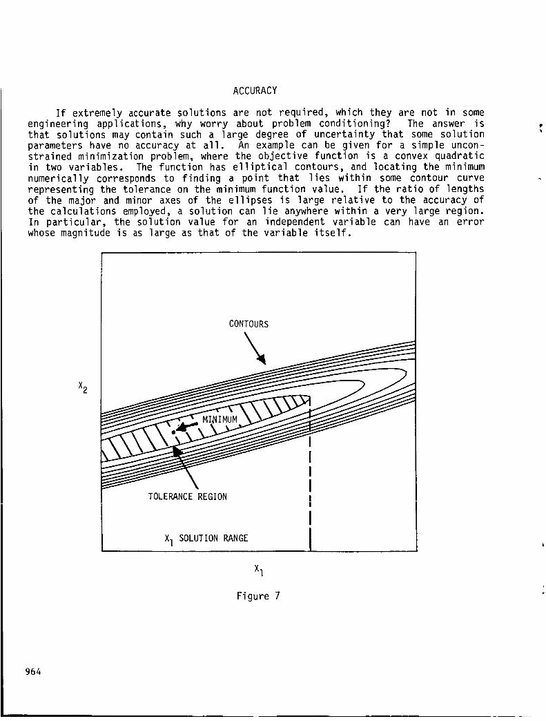
ACCURACY

If extremely accurate solutions are not required, which they are not in someengineering applications, why worry about problem conditioning? The answer isthat solutions may contain such a large degree of uncertainty that some solutionparameters have no accuracy at all. An example can be given for a simple uncon-strained minimization problem, where the objective function is a convex quadraticin two variables. The function has elliptical contours, and locating the minimumnumerically corresponds to finding a point that lies within some contour curverepresenting the tolerance on the minimumfunction value. If the ratio of lengthsof the major and minor axes of the ellipses is large relative to the accuracy ofthe calculations employed, a solution can lie anywhere within a very large region.In particular, the solution value for an independent variable can have an errorwhosemagnitude is as large as that of the variable itself.

CONTOURS

X2

!

I

X1 SOLUTION RANGE i

X1

Figure 7

964

PORTABILITY AND THE MACHINE ENVIRONMENT

Added to the numerical difficulties of the applications is the great varietyof host computer systems served by a single software library operating in a largecompany. At one time, a mathematical subroutine could be entered into a librarysystem which was expected to serve only a single type mainframe. Now, host envi-ronments range over several types of mainframe and also minis, micros (e. g.,flight computers), and supercomputers.

For efficiency, the codes included in a modern library must be portable andwell-equipped for maintenance. Source code comments and usage documentation mayreceive almost as much attention in code development as the numerical method it-self. A typical software library is programmed mostly in portable Fortran, with acore of subroutines which have portable usage but different code on each system.These core subroutines serve to interface the library with a specific machine en-vironment, for example, by specifying the local single precision accuracy.

i

DOCUMENTATION

_ PORTABLE_

COREWq"

SUBROUTINE

LIBRARY

i] l ,IFLOATING POINT

WORDS

fl iINTEGER

WORDS

_,e, ETC.

LOCALVALUES

MACHINE/SYSTEM

ENVIRONMENT

Figure 8

965

A BRIEF HISTORY

Fast-converging methods embodied in numerically stable codes have proved tobe the key to success in overcoming many of the difficulties in nonlinear pro-gramming. The earliest fast method was Newton's method. However, steepest de-scent or some "direct search" method was often used due to the instability ofNewton's method and to the fact that it requires second derivatives for solving aminimization problem. Quasi-Newton methods, requiring only first derivatives,were developed in the 1960's. However, early methods of this type were unstableand often slow to converge. Conjugate gradient methods, also developed in the1960's, were fast on certain types of problems but were often as slow as steepestdescent. Techniques for handling constraints, such as penalty functions and gra-dient projection, had similar problems.

Stabilized Newton and quasi-Newton methods appeared on early optimizationsoftware libraries beginning in about 1971. These methods were soon coupled tonew gradient projection techniques, yielding efficient codes for linearly con-strained problems. More recently, sparse matrix techniques and projectedLangrangian methods have extended the range of efficient codes to large-scale andnonlinearly-constrained optimization.

pre-1959

Minimization

Newton

Steepest descentDirect search methods

Constraints

Penalty function

Simplex method for Linear Programming

1959 - 1969

Minimization

Nonlinear simplex search method

Quasi-Newton methods (Davidon, 1959 - Fletcher/Powell, 1963) (refs. I, 2)

Conjugate gradient minimization (Fletcher/Reeves, 1964) (ref. 3)

Sequential polynomial line search

Early trust region methods (Levenberg, 1944 - Marquardt, 1963) (refs. 4, 5)

Constraints

Projected/reduced gradient methods (Rosen, 1960 - Wolfe, 1962) (refs. 6, 7)

Generalized reduced gradient method (Abadie and Carpentier, 1969) (ref. 8)

1970 - present

Minimization

Stabilized Newton/quasi-Newton methods

BFGS update (1970) (ref. 10)

Modified Cholesky Factorization (Gill/Murray, 1971 - 1974) (ref. 11, 12)

Trust region methods

Constraints

Modern projected/reduced gradient methods

Active set strategies, Lagrange multiplier estimates (1971 - 1974) (ref. 13)

Null-space/range-space decomposition (1974 - 1976) (ref. 14)

Projected Lagrangian methods (refs. 15-17)

Sequential quadratic programming

Figure 9

966

OPTIMIZATION CATEGORIES AND METHODS

Contemporary optimization methods were developed within an orderly problemclassification scheme. Problems are classified in categories based on theirstructure (e. g., nonlinear least squares) and the computational resources avail-able for solving the problem (e. g., whether or not partial derivatives of theproblem functions can be calculated analytically). This scheme reflects currentknowledge of the most effective methods for the different categories of smooth ordifferentiable optimization and also linear programming.

For some categories, no overall method can be recommended. For example, whenthe problem functions or their derivatives are discontinuous, the problem must becarefully analyzed, and solution methods often rely heavily on problem-specificheuristics. In many cases, it is best to reformulate the problem. The situationfor discontinuous optimization is reminiscent of the old days of smooth optimiza-tion.

Are Yes [Consultation ]

Discontinuous _I Required IFunctions

nvolved?

NoLinear ! Yes =ICommercial

IProgramming? v I LP SolversI.................................................. N_o _ ............................................

Smooth Nonlinear Optimization ] Squares?Least ]

i N° Yes I

No /Nonlinear t Yes No I Linear Least Ye__ 1System --

_[ tSquares?

No I Are Yes

--t Constraints _

Present?

S ){ NLI

Figure 10

967

NONLINEAR SYSTEMS AND NONLINEAR LEAST SQUARES

Because of its fast convergence, Newton's method is the basis for most smoothnonlinear optimization algorithms, including nonlinear system solvers and nonlin-ear least squares. However, the method is not robust and the required derivatives(including second derivatives for minimization problems) are not always available.Powell's hybrid method and the Levenberg-Marquardt method are two forms of trustregion or restricted-step methods which modify Newton's method to obtain robustsolution algorithms. They also eliminate the need for second derivatives in non-linear least squares problems. Quasi-Newton and finite-difference approximationsmake up for the missing first derivatives and usually maintain fast convergence.Some problems, however, do require more specialized methods in order for fast so-lutions to be obtained.

No

Overdetermined?

-- Matrix Available?

Yes

Is a Least SquaresSolution

Acceptable?

Yes

No

Hybrid method

with quasi-Newton Jacobian

Hybrid method

with user-suppliedJacobian

ConsultationRequired 1

No

Levenberg-Marquardt

with

finite-difference

Jacobian

l_ Ln_ Jo_vuJal= tMatrix Available?

Figure 11

Yes

Levenberg-

Marquardtwith

user-suppliedJacobian

968

UNCONSTRAINED MINIMIZATION

Although most optimization problems have constraints, it is worthwhileto study the modern methods for unconstrained minimization because they are incor-porated in contemporary methods for constrained problems. This is especially trueof the Newton, quasi-Newton, and single variable methods. If the problem has

fewer than, say, 200 variables (depending on computer resources available),Newton-type methods are preferable. However, they require the storage and use ofa search matrix whose size is roughly the square of the problem size. Conjugategradient methods are much less efficient but use no matrices.

For single-variable problems, safeguarded polynomial search methods minimizea sequence of approximating polynomials within bounds. Recent bounding strategieshave been developed to maintain the fast convergence of the polynomial search.

Are

ConstraintsPresent?

N°1Single

Variable?

No

Yes

No Is the First |

-- Derivative [--

i Available?

Safeguarded I

quadraticpolynomials

No

AreDerivativesAvailable?

I quasi-Newton _ Are Second

method with Derivativesfinite-difference Available?

derivatives

quasi-Newton I

method with

user-suppliedderivatives

Large-Scale IProblem?

modifiedNewtonmethod

Yes

No

conjugate

gradient method

with finite-I difference

[ derivatives

AreDerivatives

Available?

Yes

1Safeguarded

cubicpolynomials

Yes

conlugategradient

method with

user-suppliedderivatives

Figure 12

969

PROJECTED GRADIENTS AND REDUCED GRADIENTS

Modern constrained methods use a projection strategy coupled with a Newton-type minimization method. During the iterative process, the search steps of theunconstrained method are essentially projected into a linear subspace defined bythe currently active constraints, i. e., those that would be violated in an uncon-strained search. Lagrange multiplier approximations are used in deciding when todrop a constraint from the active set.

For linear constraints, projection methods maintain feasibility after firstlocating a feasible point. Projection methods for nonlinear constraints use lin-ear approximations but take account of the constraint nonlinearities by addingLangrangian and penalty function terms to the original objective function. Themethods for nonlinear constraints are often referred to as projected Lagrangianmethods.

xi -I

STEP i

x i

PROJECTION STEP i+l

\

UNCONSTRAINEDMINIMUM

Figure 13

970

LINEAR LEAST SQUARES

Linear least squares problems can be solved using standard numerical linearalgebra techniques if there are no constraints. If there are constraints, aniterative method must be used. The problem then is a special type of quadraticprogram, or minimization of a quadratic function (in this case, an L2-norm) sub-ject to linear equations and inequalities. Most quadratic programming methods areprojected gradient methods. However, specialized methods have been developed forthe particular case of the minimum-norm problem.

No

_r

Linear JAlgebra

(LINPACK)

No

Are YesConstraints

Present?

Linear t Yes-- Constraints?

Figure 14

Minimum norm Iwith projected

gradients

971

GENERALCONSTRAINEDMINIMIZATION

The distinction between linear and nonlinear constraints has long been funda-mental to optimization methods. Only recently have reliable, fast-convergingmethods evolved for nonlinear constraints, and as mentioned before they use a formof projection, a strategy which has always been used for linear constraints. Thenull-space method refers to a particularly efficient form of projection, for whichgood codes have recently becomeavailable.

The development of sparse matrix techniques has added a new category of opti-mization problems which can be solved efficiently. This refers to large-scalenonlinear problems, which often have thousands of variables.

No

IIs the Objective

FunctionQuadratic?

No _ YesLargeScale?

Yes

1No

Large-scaleProjected

LagrangianMethodNo Simple

Bounds

i Only?

_o_ Linear L-_Constraints? ----I .................

Null-spaceQuadratic

ProgrammingMethod

÷Simply-bounded

Null-spaceQuadratic

Minimization

Quadratic ProgrammingL .................................... a

SequentialQuadratic

Programming/Projected

LagrangianMethod

Linear _Yes -1Constraints?

Large-scaleReducedGradientMethod

Figure 15

972

CONCLUSION

Highly complex optimization problems with many variables were formulated inthe early days of computing. At the time, many problems had to be reformulated or

bypassed entirely, and solution methods often relied on problem-specificstrategies. Problems with more than ten variables usually went unsolved.

Modern optimization software libraries represent a complete change in this

situation. Adances in optimality and convergence theory and in numericalanalysis, especially linear algebra, have made possible codes that are both fast

and robust. Advances in mathematical software techniques encourage the packaging

of software for implementation in a great variety of computing environments. A

major challenge in optimization software at present is in increasing user

awareness of these developments and expanding the scope of future applications.

AVAILABILITY

TO

USER

APPLICATIONSMODERN

OPTIMIZATION

LIBRARIES

DEVELOPMENT

• OPTIMALITY/CONVERGENCETHEORY

• NUMERICALANALYSIS

Figure 16

973

SYMBOLS AND ABBREVIATIONS

ALT

BPR

Bj(t i )

CPR

ci(x)

DIST

f(x)

fl,f2

fo(xP,tp)

f(xi,_i,_i,ti)

Fn

i,j,k

.Qj

m

m e

n

P

Ps

t i

tP

Altitude

Bypass ratio

B-spline function evaluated at point t i

Cycle pressure ratio

Constraint function i evaluated at point x

Distance

Objective function evaluated at point x

Performance indices - used as either objective or constaint func-

tions

Objective function for B-spline formulation

problem

Constraint function for B-spline formulation of trajectory

problem; expresses system dynamics at point i

Net thrust

Indices

Lower bound on independent variable j

Number of constraints

Number of equality constraints

Number of variables in Figure 1, number of test points in Figure 4

Number of B-spline evaluation points

Specific excess power

The i-th B-spline point

Final time

of trajectory

974

U °

3

WT

X °

3

x p

ixk

Xk,j• •

RI,k.1

E

Upper bound on independent variable j

Airplane weight

Independent variable j

Final time vector of trajectory variables

Trajectory variable k evaluated at B-spline point i

The j-th B-spline coefficient of trajectory variable

Trajectory time derivatives evaluated at B-spline point

Summation

k

i

975

.

.

,

.

.

.

,

.

,

10.

II.

12.

13.

14.

15.

REFERENCES

David,n, W.: Variable Metric Methods for Minimization. AEC Research andDevelopment Rep. ANL-5590, Argonne Natl. Labs., 1959.

Fletcher, R.; and Powell, M.J.D.: A Rapidly Convergent Descent Method forMinimization. Computer J., vol. 6, 1963, pp. 163-168.

Fletcher, R.; and Reeves, C.M.: Function Minimization by Conjugate Gradient.Computer J., vol. 7, 1964, pp. 149-154.

Levenberg, K.: A Method for the Solution of Certain Problems in Least Squares.Quart. Appl. Math., vol. 2, 1944, pp.164-168.

Marquardt, D.: An Algorithm for Least Squares Estimation of Nonlinear Para-meters. SIAM J. Appl. Math., vol. 11, 1963, pp. 431-441.

Rosen, J.B.: The Gradient Projection Method for Nonlinear Programming. Part I:Linear Constraints. SIAM J. Appl. Math., vol. 8, 1960, pp. 181-217.

Wolfe, P.: Recent Developments in Nonlinear Programming. Rand. Corp. Rep.R-4OI-PR, 1962.

Abadie, J.; and Carpentier, J.: Generalization of the Wolfe Reduced GradientMethod to the Case of Nonlinear Constraints. Optimization, edited by R.Fletcher, Academic Press, 1969, pp. 37-49.

Fiacco, A.V.: and McCormick, G.P.: Nonlinear Programming: Sequential Uncon-strained Minimization Techniques. John Wiley and Sons, NY, 1968.

Broyden, C.G.: The Convergence of a Class of Double-Rank Minimization Algorithms.J. Inst. Math. Applic., vol. 6, pp. 76-90, 1970.

Gill, P.E.; and Murray, W.: Quasi-Newton Methods for Unconstrained Optimization.J. Inst. Math. Applic., vol. 9, pp. 91-108, 1972.

Gill. P.E.; and Murray, W.: Quasi-Newton Methods for Linearly ConstrainedOptimization. Chapter 3. Numerical Methods for Constrained Optimization,Academic Press, 1974.

Gill, P.E.; and Murray, W.: Quasi-Newton Methods for Linearly Constrained Opti-mization. Natl. Phys. Labs. Rep. NAC 32, Teddington, Middlesex, UK, 1973.

Gill, P.E.; and Murray, W.: Newton-Type Methods for Linearly Constrained Opti-mization. Chapter 2. Numerical Methods for Constrained Optimization, AcademicPress, 1974.

Murray, W.; and Wright, M.H.: Computation of the Search Direction in ConstrainedOptimization Algorithms. Algorithms for Constrained Minimization of SmoothNonlinear Functions, A.G. Buckley and J.-L. Goffin, eds., Math. Proj. Study 16,Mathematical Programming S.c., pp. 62-83, 1982.

16. Murtagh, B.A.; and Saunders, M.A.: A Projected Lagrangian Algorithm and Its

976

im

17.

Implementation for Sparse Nonlinear Constraints. Algorithms for Constrained

Minimization of Smooth Nonlinear Functions, A.G. Buckley and J.-L. Goffin,

eds., Math. Proj. Study 16, Mathematical Programming Soc., 1982.

Powell, M.J.D.: A Fast Algorithm for Nonlinearly Constrained Optimization Cal-

culations. Rep. DAMTP 77-NA 2, Univ. Cambridge, UK, 1977.

977

N87-11776

OPTDES.BYU: AN INTERACTIVE OPTIMIZATION

PACKAGE WITH 2D/3D GRAPHICS

R. J. Bailing

A. R. Parkinson

J. C. Free

Brigham Young University

Provo, Utah

PRECEDING PAGE BLANK NOT F_

979

I. INTRODUCTION

The OPTDES.BYU package was developed to assist the engineer in obtaining

efficient designs. In particular, the package helps the engineer to perform the

following fundamental tasks in the design process:

(I) Interfacing with existing analysis software

(2) Defining and redefining the design problem

(3) Searching for improved designs

(4) Interpreting results from the design process

II. INTERFACING WITH ANALYSIS

The OPTDES package obtains results from analysis for a particular application by

calling the user-supplied subroutine:

SUBROUTINE ANFUNC (NAV, NAF, AV, IAF, AF)

AV(NAV) = given "analysis variables"

AF(NAF) = returned "analysis functions"

IAF(NAF) = given flags indicating which analysis

functions need to be computed

Analysis variables may potentially become design variables, and analysis functions

may potentially become design functions (objective, constraints) when the design

problem is later defined.

In addition to the ANFUNC subroutine the user must supply the file "ANLIZ AV"

which contains the initial values of the analysis variables as well as optional

character descriptions by which the analysis variables will be referred in the OPTDES

software. Character descriptions for the analysis functions may also be supplied in

an optional "ANLIZ AF" file:

ANLIZ AV FILE ANLIZ AF FILE

-30.0, x-coor node 1

30.0, x-coor node 2

35.0, y-coor node 3

2.0, diameter tube 1

2.0, diameter tube 2

0.3, thickness tube 1

0.3, thickness tube 2

weightstress tube 1

stress tube 2

buck stress tube i

buck stress tube 2

x-defl node 3

y-defl node 3

The user may supply an optional subroutine ANGRAD which returns values for

analytical derivatives of specified analysis functions with respect to specified

analysis variables. In the absence of a user-supplied ANGRAD subroutine such

derivatives are approximated by finite differences in OPTDES. Optional subroutines

named ANPREP, ANPOST, and ANITER may be supplied for interfacing to analysis pre,

post, and intermediate processing, respectively. Such processing is defined to be

computing which is independent from the derivation of analysis functions from

analysis variables. These subroutines may call processing software directly or just

store/restore data to/from files for stand-alone processing software.

980

A general method for interfacing any existing stand-alone analysis package toOPTDESwill now be sketched. Analysis packages typically contain "READ"and "WRITE"statements throughout. When linked with optimization, this input/output must beperformed only once and eliminated thereafter in the several calls to analysis. TheOPTDESpackage contains a set of "RI" and "R2" subroutines. Calls to the "RI"subroutines should be inserted into the analysis source code following all "READ"and"WRITE"statements. Whenthe stand alone analysis package is then executed, the"ANLIZAV°' and "ANLIZ AF" files are automatically generated along with a binary filecontaining local analysis input. The stand alone analysis program is then changed toa subroutine, the calls to "RI" subroutines are replaced by calls to corresponding"R2" subroutines, and all "READ"and "WRITE" statements are deleted. The ANFUNCsubroutine to be linked with OPTDESsimply calls this new analysis subroutine. AnANPREPsubroutine is also linked with OPTDESwhich calls the subroutine "R2PREP"which restores the local analysis input from the binary file.

/ stand-alone I

np=t--I a.alysis /--o_tp_t--_l_ i lo_all/ (calls R1 subs)I/ \

store store

I irestore restore

ANPREP

R2PREP

OPTDESAV

AF Isubroutine I

_- analysis

(calls R2 subs)

(no read/wrlte)

981

After the user-supplied subroutines and files have been created, they may belinked to the OPTDES"DEBUG"module for testing. This module allows one tointeractively perform analysis, derivative analysis, and processing:

ENTERINGDEBUG

>deb> help"dis av,af 1-2 5"

"set av I-2 5"

"fun af I-2 5""gra af i-2 5"

"ite""pos""bat""qui"

display listed analysis variables or functions(default = all)set values for listed analysis variables (default =all)compute listed analysis functions (default = all)compute gradients of listed analysis functions(default = all)analysis intermediate processanalysis post-processswitch to batch modeexit program

III. DEFINING THE DESIGN PROBLEM: SETUP

The SETUP module in OPTDES provides a means for interactively defining or

redefining an optimization problem. Design variables and design functions

(objective, inequality constraints, equality constraints) may be added with thecommands shown below:

>set > add dv

<mapped analysis variable number (def=l)> 3

<minimum value (def=-1.00)> 10

<maximum value (def=1.00)> 40

>set > add df

<mapped analysis function number (def=l) > 2

<type: objective(=l), inequality(=2), equality(=3)

<less than(=1) or greater than(=2) (def=1)>

<reference value (def=0.00) > i00

(def=1) > 2

It is also possible to add "fancy" design variables which allows one to map several

analysis variables to the same design variable, or which allow one to add a group of

design variables having the same minimum and maximum bounds with one command. Fancy

design functions may be added in like manner.

982

The analysis variables, analysis functions, design variables, or design func-tions may be displayed in the SETUPmodule. The following is an example:

>set> dis dvd.v.# scaled a.v.# unscaled minimum maximum description

1 0.667 3 35.0 I0.0 40.0 y-coor node 3

2 -0.500 4 2.00 1.0 5.0 diameter tube 1

5 2.00 diameter tube 2

>set > dis df

d.f.# a.f.# ty reference _ description

1 2 it i00.000 50.000 stress tube 1

2 1 mn 80.000 30.000 weight

3 4 it 0.250 0.100 y-defl node 3

Several commands are available for redefining a design problem. One can delete

design variables or functions. One can rescale design variables or functions. It is

also possible to relatively rescale all design variables with a single "zoom"

command. The values of design variables and unmapped analysis variables may be

manually changed. A very useful command is available for changing the status of

design functions (i.e. objective to inequality constraint, inequality constraint to

equality constraint, etc).

After a design problem has been defined (or redefined), it should he stored to a

file. Similarly, a previously defined problem may be restored from a file. The

store and restore commands allow the user to specify the file name.

At this point it is useful to comment on the "DIALOGUE" file in OPTDES. All

terminal input and output from the interactive modules in OPTDES is automatically

echoed to a file named "DIALOGUE" for the user's record.

The Bureau of Reclamation used the OPTDES package in the planning stages for a

billion-dollar water project in central Utah. They found the interactive capability

for defining and redefining design problems to be valuable as the following comments

suggest:

"The most important use of the computer model was the ability to

explore a lot of alternatives, to do the 'what ifs'. With OPTDES.BYU it

was possible to respond to such questions fairly quickly."

983

IV. SEARCHING FOR IMPROVED DESIGNS : OPTMIZ

The OPTMIZ module allows one to interactively search for improved designs.

Three general techniques are available for doing this. The first technique is brute

force trial-and-error. This is accomplished by manually setting values of design

variables which automatically initiates a call to analysis:

>opt> set dv 2 6-8 14

<scaled values given (def='°n")?>

<dv# 2: unscaled value (def=-33.0)> -35

<dv# 6: unscaled value (def=lg0.0)> 187

<dv# 7: unscaled value (def= 73.0)> 80

<dv# 8: unscaled value (def= 70.0)> 60

<dv# 14: unscaled value (def = 4.00)> 2

The second technique is to run a formal optimization algorithm. The software

currently contains four fundamentally different nonlinear constrained optimization

algorithms, namely: generalized reduced gradient, sequential linear programming,

method of multipliers, and feasible directions. Algorithms are easily added to the

software, and work is currently under way to add a sequential quadratic programming

algorithm. A command is given to select an algorithm followed by a command to run a

specified number of iterations where an iteration is defined as the generation of a

new design. After the specified number of iterations has been completed (assuming

the algorithm's convergence criteria were not satisfied) any OPTMIZ command may be

given (such as run more iterations, select a new algorithm, display variables, etc).

One may also make variations in the selected algorithm by changing algorithm

parameters with a command.

The third technique for searching consists of geometric ideas. A gridding

command allows one to create a uniform mesh in design space or any of its subspaces.

Analysis is automatically performed at each mesh point and the best design among

these points is found. A line command causes analysis to be performed at uniformly

spaced points along a line in a specified direction from the current design in design

space. The direction may be specified directly, taken as the direction of steepest

descent, or taken as a combination of the objective and active constraint

gradients. The use of grid and line searching is illustrated as follows:

984

> opt > grid

<number of dimensions (def=2)>

<same spacing all dimensions (def="y")?>

<dim# I: design variable number (def=l)>

<dim# I: number of mesh points (clef=2)> 10

<dim# 1: backward distance (def=2.0)>

<dim# i: forward distance (def=2.0)>

<dim# 2: design variable number (def=2)>

FINISHED-- best design was 66 iterations ago

> opt > line

<direction: input (=i), steepest(=2), gradient(=3) (def=1)> 2

<starting distance (def=0.00)>

<ending distance (clef=2.35)>

<number of points (def=2)> i0

FINISHED-- best design was 3 iterations ago

Print flags may be set to regulate the amount of printout which occurs at eachnew design (or iteration):

> opt> change print<print out optimization indicators (def="n")? >y<print out analysis counters (def="n")?> y<print out design variables (def="n")?><print out design functions (def="n")?>

ITERATION-- : 1step size objective max ineq max equ

1.59 -1.22 -1.39 0.

anal-calls anal-evals grad-calls grad-evals

2 8 0 0

As new designs are generated at each iteration, the values of design variables,

design functions, analysis variables, and analysis functions are written to a

direct-access binary file with the same name as the problem definition file followed

by "_H '°. This permits the designer to backtrack as well as recover from program

crashes. The following commands enable one to access this file:

>opt> dis iter

<starting iteration (def=0)>

<ending iteration (def=107)>

iter#

0

1

3

103

104

107

algorithm typefirst iteration

trial and error

grid searchingbacktrack to iteration 36

generalized reduced gradient

sequential linear programming

>opt > set iter

<iteration (def=107)> 103

> opt > purge

<first iteration deleted (def=0)>

<first iteration retained (def=108)>

For large design problems, a semi-interactive mode is possible. The batch

command causes OPTDES input to be taken from a specified file rather than from the

terminal. For example, the contents of the file might be the commands: grg, run,

20, quit. This would cause 20 iterations of the grg algorithm to be performed in

batch mode. The user could then leave the terminal and return later to restore the

results and continue.

985

The optional user-supplied analysis subroutines may be activated in the OPTMIZmodule. Specifically, commandsare available to cause gradients to be computedbythe ANGRADsubroutine, to set the regularity at which the ANITERsubroutine is calledand to execute the ANPOSTsubroutine. The ANPREPsubroutine is always executed atthe top of the program.

V. INTERPRETING RESULTS : GRAPH

Graphics are used to interpret results. The GRAPH module allows one to

interactively generate history and sensitivity plots on the terminal screen or on a

plotter or other hard copy device. The user must supply move and draw subroutines

for the particular graphics device if the available move and draw subroutines

(Tektronix Plot-10) do not work. Example plots are shown below and on the next page.

1 .500

OPTDES .8YU DESIGN

I

EVOLUTION

I I

1 .000

0.500

0.000

m

-0.500 --m

-l.O00

-!o500

-2.000I I2

1 1 , 1

I I I4 6

ITERATION

I = OBJECTIVE

2 = MAX INEQUALITY3 = STEP LENGTH

J

I

u

m

m

m

, ]8

986

%.

120

100

80

60

40

20

OPTOES.BYU AMOUNT OF ANALYSIS

I i i i i J 4

I I I I2 4 6

ITERATION

l = FUNCTION CALLS :2 = FUNCTION EVALS

OPTDES.BYU ONE-DIMENSIONAL GRID

]4°'°°°_' ' ' ' I ' ' ' ' I I ' ' ' I ' ' ' ' I ' I ' ''- _=l 30.000

S ZT XR 120.000 -Z_ES ZS 110.000

z

x

Z

80.000 --C_

Z

70.000

F60.000

K 100.000SI

90.000

50"00£0.000 15.000 20.000 25.000 30.000

HEIGHT IN35.000

987

Twoand three dimensional images of design space (or subspace) may be produced.OPTDES creates input files for the high-performance graphics package MOVIE.BYU.Infeasible regions are clipped away. Objective function values may be depicted bycontours and/or color. In a two-dimensional image, the objective value may also bedisplayed by warping the plane in the third dimension. It is also possible to cutthe 3-dimensional feasible region apart with planes and explode the resulting pieces.Data for these images is generated by the gridding commandin the OPTMIZmodule. Ofcourse if the design space is of dimension higher than 3, the non-displayeddimensions are held constant. Someexamples follow.

I

988

I

\

\

\

989

VI. PROGRAMMING STANDARDS

Strict programming standards were enforced during the development of the OPTDES

package. Standard FORTRAN-77 was the language that was used. All arrays are allo-

cated dynamically. Changing storage size simply requires changing the dimension of

the integer, real, and/or character vector at the top of the program. Only a handful

of common blocks are used. The source code is structured. The only statement

labels used are for FORMAT statements. All input is screened to prevent unnecessary

program aborts. File handling is performed in one central subroutine.

990

Ns÷: 1_777 ,

ON THE UTILIZATION OF ENGINEERING

KNOWLEDGE IN DESIGN OPTI_IIZATION

Panos Papalambros

Department of Mechanical Engineering

and Applied Mechanics

The University of _.lichigan

991

INTRODUCTION

A long-standing difficulty in the use of formal optimization techniques in

design is the often nonmathematical form in which design knowledge is available.

In general, engineering knowledge incorporated in a design optimization problem has

the form of a mathematical model, such as a nonlinear programming one. The solution

to the problem is provided by an optimization technique which operates on the model

exclusively. Typically the solution technique is iterative in nature.

Thus, knowledge which has not been included in the analytical model cannot be

used. _reover, knowledge (possibly mathematical in nature) which is not compatible

in form with the iterative structure of optimization algorithms cannot be used in an

automated way, although the designer/analyst may use that knowledge implicitly in a

heuristic way. For any real design problem, it is evident that additional knowledge

is available, which however cannot be modelled easily or properly. Typical examples

are manufacturing considerations in structural design which are usually expressed as

simple upper and lower bounds on the design variables and subtly called "technologi-

cal constraints."

In this article, some current research work conducted at the University of

_chigan is described to illustrate efforts for incorporating knowledge in optimiza-

tion in a nontraditional way. Much of this research is yet unpublished.

The incorporation of available knowledge in a logic structure is examined in two

circumstances. The first examines the possibility of introducing global design

information in a local active set strategy implemented during the iterations of

projection-type algorithms for nonlinearly constrained problems (ref. i). The

technique used combines global and local monotonicity analysis of the objective and

constraint functions (refs. 2 and 3). The second examines a knowledge-based program

which aids the user to create configurations that are most desirable from the manu-

facturing assembly viewpoint. The data bank used is the classification scheme

suggested by Boothroyd (ref. 4). The important aspect of this program is that it is

an aid for synthesis intended for use in the design concept phase in a way similar

to the so-called "idea-triggers" in creativity-enhancement techniques like brain-

storming. The idea generation, however, is not random but it is driven by the goal

of achieving the best acceptable configuration.

992

LOCALMONOTONICITYANALYSIS

For problems of this form, minimize f(x) subject to g(x) i 0 and h(x) = 0with x as a vector in a n-dimensional real space; the question of which constraintsgi are active is important mathematically, but more so in the design context, sincethe active constraints represent critical design requirements. An active set strat-egy selects active constraints at each iteration based on local information. Thereare different stategies to do that. Oneof them is based on local monotonicity,i.e., the signs of the partial derivatives of the functions with respect to thedesign variables. The program ACCME(Automated C_onstraint C_riticality by M_onotonicityE_valuations) outlined in figure 1 implements such a strategy, in conjunction with areduced-gradient type of search. The partial derivatives are calculated in thetangent space of the subspace of active inequality and equality constraints (con-strained derivatives).

I Stop

, IDo one-dimensional I

minimization of ob-

jective function be-_

tween current and

new point

[Deactlvate con-

straints with non-

preservingmonotonicities

_IC ..... t point ]_

I Find partial (trained) derivatives I....for objective and constraint functions

_ Optimum? I

INoiApplyfirst....tooicityrolel

I Move in

_ NO J direction _:s:e:tew II Are any constraints active? _point

l'e II Find dominant constraint I

I Apply second monotonicity rule ]

Are objective function monotonicities preserved? I

Yes

Yes [Ar_ constraint functions monotonicities preserved? I NO

Deactivate con-

straints with nD_-

preserving mono-tonicities

I I YesAre any constraints active? |

JI So1 ........ t system of_ ]

active constraints for

new point Find dominant constraint

Figure 1

993

MONOTONICITYANDDOMINANCERULES

The following two monotonicity rules can be proved (even when nondifferentiablefunctions are involved).

Rule i: If the objective function is monotonic with respect to (wrt) a particularvariable in the neighborhood of a local minimum, then there exists at least oneactive constraint with opposite monotonicity wrt that variable in that neighborhood.Rule 2: If the objective function is stationary wrt a particular variable in theneighborhood of a local minimum, then either all constraints containing that variableare inactive, or there exist at least two active constraints having opposite mono-tonicities wrt that variable in that neighborhood.

Whenmore than one candidate active constraint exists, then a dominance strategyis employed to select the constraint which is most likely active. In ACCMEthis isdone by selecting the minimumor maximumdistance d_=xi-gi(xi)/[_g_(xi)/_xi) ] for allappropriate j, depending on whether the gj's are loSally _ncreasin_ or decreasingwrt xi, as shownschematically in figure 2.

f

3 X

3

la] Constraint02 is dominant

f

IXi 1 3 2 Xi

Ibl Constraint gl is dominant

Figure 2

994

A LOCAL STRATEGY EXAMPLE

A two-dimensional example representing the design of a helical compression

spring is shown in figure 3, together with the iteration path followed by ACCME.

The corner solution is identified after three iterations. In the first one, g7 is

put in the active set; in the second, g7 is dropped and gl is brought in; in the

third, gl is retained and g3 is added. There are now zero degrees of freedom, the

Karush-Kuhn-Tucker conditions are satisfied and the algorithm terminates.

C

2o

15

lO

6,

' gs

o ,oo4 .o5

\ / I / __

.11_ /' _,</iy

,l___'_l lii/

II_ _II // 7

// /

i 1•075 .1 .12 .25 d

Figure 3

995

A LOCAL/GLOBAL STRATEGY EXAMPLE

The monotonicity and dominance rules can be applied globally if the m6notoni-

city properties are globally established. This was in fact the way the o_iginal

theory was developed. These global results can be derived analytically, often with-out too much effort. The global rules can be used in an overriding mode to influ-

nece the decision making at each iteration. A separate subroutine containing the

global rules is included in ACCME and called upon in the active set decisions. Notethat the form of the logic allows the introduction of any global rules, not just

those derived from monotonicity arguments. An example involving an explosively

actuated cylinder is shown in figures 4, 5 and 6. The global rules were derived

independently in ref. 5. Figures 5 and 6 are the output from ACCME.

X 3

X 1 X2

X 1 = UNSWEPT CYLINDER LENGTH, IN

X 2 = WORKING STORE OF PISTON, IN

X 3 = OUTSIDE DIAMETER OF CYLINDER, IN

X4 = INITIAL PRESSURE OF COMBUSTION, KPSI

X_ = PISTON DIAMETER, INb

Figure 4

996

oF pOeR QUALn '

>>>>>Automated Constraint Criticality by Monotonicity Evaluations<<<<<

s.,I_.¢,=***¢s¢.8¢_sITERATION NO.( 1)=**=*=s.scs_*_¢,*¢ss

Current point:

Values of design variables:x{ I)= 0.20000

x( 2)- 1.5000

x( 3)- 0.80000

x( 4)- 10.000

x( 5)- 0.32000

Value of objective function:f- 1.7000

Values of constraints:

g( _)--0.20000

g( 2)- -1.5000

g( 3)--0.80000

g( 4)- -10.000

g( 5)--0.32000

g( 6)--0.20000

g( 7)- -26.426

g( 8)- 104.2S

g( 9)- -17.857

g(_0)--0.48000

g(I_)--0.30000

THIS POINT IS INFEASIBLE!!!

Monotonicity and dominance analysis:

For this point, based on first monotonicity rule,

one of the following constraints wrt x( 1)may be active:

g(7)

9(7)

NOTE: A: any p¢int, based on first monotonicity rule,wrt x( 1)constraint g( 7) is GLOBALLY active.

For this point,based on second monotonicity rule,

one of the following constraints wrt s( 4) may be active:

_(8)

g(9)

For this point, wrt x( 4)constraint g( 8)may be dominant.

Decisions taken for this iteration:

>>>>>AT THIS ITERAT_0N,BASED ON FIRST MONOTONICITY RULE,

>>>>>WRT x( I)CONSTRAINT g( 7)IS ACTed.

>>>>>AT THIS ITERAT;ON,BASED ON SECOND MONOTONICITY RULE,

>>>>>WRT x( 4)CONSTRAINT g( 8)IS ACTIVE..

*,=s*,*=**_*,Jsts**-ITERATION NO.( 2)*ttcs*=s$¢_¢*scss**s

Current point:

Values of design variables:

x( I)- 0.1640gE-01

x( 2)- 1.5000

x( 3)- 0.80000

x( 4)- 8.7038

x( 5)- 0.32000

Value of objective function:

f- 1.5164

Values of constraints:

g( 1)--0.164098-01

g( 2)- -1.5000

g( 3)--0.80000

g( 4)- -8.7038

g( 5)--0.3200C

g( 6)--0.20000

g( 7)- 0.27780£-0-

g( B)= 0.56B438-)3

g( 9)- -20.943

g[IG)--0.48000

g(11)--0.48359

Monotonicity and dominance analysis:

For this point, based on first monoto_icity rule,

one of the following constraints wrt x( 8)may be active:

g(1)

g(5)

g(9)

For this point, wrt x( 5)c0nscraint g( 1)may be dominant.

Monotonicicy of active constraints are preserved.

Dez!sions taken for this iteration:

>>>>>AT THIS ITERATION,BASED ON FIRST MONOTONICITT RULE,

>>>>>WRT x( 5)CONSTRAINT g( l)_S ACTIVE.

>>>>>FROM ITERATION( I):WRT s( I)CONSTRAINT g( ?)IS AL_TIVE.

>>>>>FROM ITERATION( I):WRT x( 4)CONSTRAINT g( 8)IS ACTIVE.

Figure 5

997

998

=,,,,=,,,,*===,===,,ITERATION NO.( 3),,=*,,==,,,$,,*=,,=$

Current point:

values of design variables:

x( I)=-0.47003E-23

x( 2)- 1.5000

x( 3)= 0.80000

x( 4)= 8.8405

x( 5)= 0.31752

Value of objective function:

f- 1.5000Values of constraints:

g( I)= 0.47003E-23

g( 2)= -1.5000

g( 3)=-0.80000

g( 4)= -8.8405

g( 5)=-0.31752

g( 6)--0.20000

g( 7)= 0.81819E-11

g( 8)= C.19423E-0_

g( 9)= -20.680

g(I0)=-0.48248

g(11)=-0.50000

Monotonioity and dominance analysis:

For this point, based on first monotonicity rule,

one of the following constraints wrt =( 2)mBy be active:

g(2)g(5)g(9)For this point, wrt x( 2)constraint g( 9)may be dominant.

For this point,based on second monotonicity rule,

one of the following constraints wrt x(3) may be active:

g(6)

NOTE: At any point, based on second monotonicity rule,

constraints g(6) and g(9) MUST be simultanously active.

Decisions taken for this iteration:

>>>>>AT THIS ITERATION,BASED ON FIRST MONOTONICITY RULE,

>>>>>WRT x( 2)CONSTRAINT g( 9)IS ACTIVE.

>>>>>AT THIS ITERATION,BASED ON SECOND MONOTONICITY RULE,

>>>>>WRT x( 3)CONSTRAINT g( 6)IS ACTIVE.

,>,>,FROM ITERATION( I):WRT x( I)CONSTRAINT g( 7)IS ACTIVE.

,>>>,FROM ITERATION( I):WRT x( 4)CONSTRAINT g( 8)IS ACTIVE.

,>>>>FROM ITERATION( 2):WRT x( 5)CONSTRAINT g( 1)IS ACTIVE.

**,,*,=,=*=,,,,=,,=,ITERATION NO.( 4)=*=*=*,,,=,,=,=$=,=,

Current point:

Values of design variables:

x( i)= 0.23799E-23

x( 2)= 1.0777

x( 3)= 1.0000

x( 4)= 19.900

x( 5)= 0,21163

Value of objective function:f= 1.0777

Values of constraints:

g( I)=-0.23799E-23

a( 2)= -1.0777

g( 3)= -1.0000

g( 4)= -19.900

g( 5)--0.21163g( 6)= c.og( 7)=-0.39790E-:_

g( 8)=-C.I:369E-:_g( 9)=-C.355_7E-14

g(10,=-C.7883-

g(11)=-0.9_22£

Decisions taken for this iteration:

>>>>,FROM ITERATION( I):WRT x( I)CONSTRAINT g( 7)IS ACTIVE.

,,,>>FROM ITERATION( I):WRT x( 4)CONSTRAINT g( 8)IS ACTIVE.

>>,>,FROM ITERATION( 2):WRT x( 5)CONSTRAINT g( I)IS ACTIVE.

,,,>>FROM ITERATION( 3):WRT x( 2)CONSTRAINT g( 9)IS ACTIVE.

,,>>,FROM ITERATION( 3):WRT x( 3)CONSTRAINT g( 6)IS ACTIVE.

*TERM:NATION CRITERION MET, KARUSH-KUMN-TUCKER CONDITIONS SATISFIED,

Figure 6

A PRODUCTION SYSTE_I WITH GLOBAL RULES

Looking at the utilization of global rules only, without local monotonicity

analysis, one can create an optimization procedure that includes problem-dependent

knowledge supplied by the user. The general form of such a procedure is shown infigure 7.

RETRIEVE PROBL_! DEPENDENT RULES

RELATED TO CONSTRAINT ACTIVITY

AND OPTI_LL PROPERTIES TO CREATE

THE KNOWLEDGE BASE

t,EVALUATE THE STATE AT CURRENTPOINT, INCLUDING FEASIBILITY AND

CONSTRAINT ACTIVITY

K-K-T CONDITIONS SATISFIED? YES

I NO

SEARCH APPLICABLE RULES IN _{E

KNOWLEDGE BASE TO UPDATE THE

ACTIVE CONSTRAINT SET

I SOLVE EQUALITY CONSTRAINED PROBLEMUSING UNCONSTRAINED METHOD AND

APPLYING CONSTRAINED DERIVATIVES

(FOR SEVERAL SPECIAL CASES)

STOPPING CRITERION OTHER THAN

K-K-T CONDITIONS SATISFIED?

Figure 7

999

PRODUCTION RULES TYPES

Following the original way that global monotonicity analysis was implemented,

a set of rule types can be identified as the first few elements of the production

system. In figure 8, seven different rules are listed pertaining to constraint

activity and possible properties of the optimum. It should be noted that any number

of rule types can be included as more knowledge types are identified as important

in the entire process. This of course presumes types requiring knowledge attainable

prior to complete solution.

Provide model Information type by type to aid the solution process

Type i. The following Inequality constraints are always active:

t.

Type 2. one or more constraints wtthln each of the following groups must be active:

<start with number of constraints In each group>

Type 3, If A<X(I)<B. then G(K) Is active <or Inactive with K as a minus Interger>:

Type 4, If G(1) active, then one or more constraints within the following group must be active:

<following I ts the number of constraints tn each group>

Type 5. If A<X(I)<B. then G(K) Is dominant to a group of G(J)S:<following I.K ts the number of constraints In each group>

Type 6, If G(I) active, then G(d) reckJndent and_ vise versa:

Type 7. If X(I) In (A.B). then X{l) In RANOOM(C.O):

Figure 8

1000

RULE-BASED DECISIONS

The user provides the available knowledge for a specific problem, according to

the different rule types. In figure 9, the input knowledge for a simple example is

shown in the top half. The rules are connected so that several decisions can be

reached. These are shown in the bottom half of figure 9. Note that most of these

decisions are in fact global conclusions.

**** Summary of the problem-dependent knowledge provided by the USer ****

Type I: 3 rules

Constraint G( l) Is always active

Constraint G( 3} Is always activeConstraint G(6) Is always active

Type 2: I rules

One or more of the following constraints must be active: G(5), G(8)

Type 3: I rules

If X(2) In (O.3OOOOOE+OI,O. IOOOOOE#O2), then G(5) Is active

Type 4: I rulesIf G( 1) tS active.

Type 6: I rulesIf G(4) tS acttve.

Type 7: I rules

If X(3) Is In (O.O

then one or more of the following constraints must be active: G( 4)

then G(S) Is redundant

.O.28OOOOE+Ot). then It Is moved to (O.2805OOE+Ot.O.3OOOOOE*O3)

Using Type I rules,

constraint G( 1) isconstraint G(3) isconstraint G(6) ts

Ustng Type 2 rules.constraint G(8) IS

Using Type 3 rules.constraint G(5) is

Ustng Type 4 rules.constraint G(4) ts

added to the active set

added to the active setadded to the active set

added to the active set

added to the active set

added to the active setConstraint G(5) ts deleted from the active set

(This deletion Is caused by applying Type 6 rules)

Using Type T rules.X( 3) Is changed to 0.196552E*03

The rule search of the current Iteration Is finished. The current active set contains0 equality constraints:

5 inequality constraints:G(t). G(3), G(6), G(8). G(4)

5 constraints

Figure 9

1001

DESIGN DATA FOR AUTOMATED ASSEMBLY

The data collected and organized by Boothroyd is the only quantified measure

of how good a design may be from the assembly viewpoint. A typical data structurefrom ref. 4 is shown in figure I0. Two main performance criteria, orienting effici-

ency (OE) and relative feeder cost (FC), must be established based on geometric

characteristics codified in the form of indices. The goal is to maximize OE and

minimize FC. The charts, or interactive program versions of them, are used to ana L

lyse existing design and/or assist in redesign.

AUTOMATIC HANDLING -- DATA FOR ROTATIONAL PARTS

(first digit 0, 1 or 2)

KEY: OE FC

digit 1 0.15 1.5

2 0.45 1.5

0

5 'glcE

part is ALPHA

symmetric

(see note ]t

0

0.7 1

iO 0.7 1

O.g 1

part can be fed in a slot 0,4 1supported by large end or

protruding flange with 0.3 1

center of mass below sup O.g 1porting surfaces

BETA symmetric steps or 0.4 1

external surfaces 2 O. 3 1

15 _ (see note 3)= _ 0.75 1

= on both 0.5 1

= _ side and"_ end 3 0.21

o=! surface)s) 0.85 1

._ BETAsymmetric on side 0.5 I

-_ _ grooves surface 4 0. l 1

i! holes Or onlyrecesses 0.85 1

(see note 3)

_ 0.5 I"7- on end

"_ surface(s) 5 0.2 1

'_ _ only 0.6 1

_._ BETA symmetric hidden

features with no cor-

respondi_ ex_rl 6

features (see note 4) 0.6 1

BETA asymmetric

features on side or

end surface(s)

slightly asymmetric

or small features;

amount ot asymmetry or 8feature size less than

0/10 and L/tO

part is not BETA symmetric Icede the main feature or

features requiring orientation about the principal axis)

BETA asymmetric projections, BETA asymmetric grooves or _._=_o _ - =steps, or chamfers flats (can be seen in silhouette) o _ p _(can be seen in silhouette) _ = _ _-=_

through through groove _ -_ o ._

on both groove can be seen in E _ -_ _ o

on side on end side and or fiat side view m _ _ _ ._

surface surface(s) end can be -->"_ o .I::_only only surface(s) seen in an end on side _ _ _ _

end view surface surface = = _ _ =

2 3 4 5 6 7 8

0.3 l 0.5 1 0.3 1 0.35 I 0.2 I 0.5 I

0.15 1 0.2 I 0.15 1 0.2 l 0.2 l 0.2 I

0.45 1 O.g 2 0.45 i 0.g I O.g 2 0.g 2

-MANUAL HANDLING REQUIRED-

Irel, 41

Figure I0

1002

BINARYTREEDECISIONAID

From a practical viewpoint, it is best to guide the designer in the initialdevelopment phase towards meeting the goals, rather than redesign. This can beachieved by interacting with a program that makesoptimal suggestions - a situationdifferent from the expert system configuration. A natural logic for this program,based on the original format of the data, is a binary tree structure (fig. ii).This attempts to suggest first general configuration decisions and then more specificones.

¥p_rt ls N.PIM sy_eulc

(_ ,lo,,, I)

V&UE OF

OIGIT 2 • 0

Figure II

1003

SERIALDECISIONREPRESENTATION

The binary-tree structure has certain flaws, in spite of its intuitive appeal.By attempting to assign digit values one by one, it may arrive at configurationsworse than actually possible, because the actual chart data are not perfectlystructured along the diagonal (fig. i0). If the binary tree structure is used,additional searches will be required to guarantee optimal configuration. Instead,a serial representation can be used where decisions are based on examining all bestpossibilities by attempting to assign several digits at once, e.g. a single tripletvalue for the first three digits to give OEand FC values. This structure is shownin figure 12. It represents a heuristic search appropriate for small data bases,but is it compatible with the way the designer should be aided naturally.

LONG CYLII_)EI_

, I"°° _OUP _ ° °

DISCS

Figure 12

1004

ORIGINAL PAGE IS

OF POOR QUALITY

AN EXAMPLE DESIGN

An example of a typical interaction for the first three digit assignment and

final design results is shown in figure 13. Note that the program makes just opti-

mal recommendations. The designer is forced to conceptualize the design and examine

different possibilities as suggested.

IZI ASSIGN DIGITS 1,2,3 FOR ROTATIOHAL PART ZZ_

EATTENPTING TO ASSIGNOE - e.De FC • 1.eel

IT IS RECOflNEHDED THAT ...(1,2) LOHG CYLINDERS L/D ) 1.5

IS THIS POSSIBLE ? ...Y

IT IS RECOflMENDED THAT ...(2,e) ALPHA SYN.

OR

(2,1) NOT ALPHA SYfl., SLOT FED UITH C.fl. BELOU SUPPORTING S'FACESIS THIS POSSIBLE? ...Y

IT IS RECORMENDED THAT ...(3,e) BETA SYN.

OR

(3,5) BETA ASYH. THRU GROOVE OR FLAT SEEN IN END UIEUIS THIS POSSIBLE ? ...Y

ZZZ OPTINAL PARAMETERS ASSIGNED ZZ_

ZZZX_ZZ_ZZXZZ_ZZZ_ZZZIIZ_ZZRESULTS OF SEARCH

OE - e.De FC • l.ee

PLEASE 1HPUT THE SPECIFIC 1,2,3 BOOTHROYD DIGITSYOU PICKED, IN THAT ORDER AS INTEGERS ...e,e,e

ZZZZZZZZZZZISZ$$$ISZ_Z_ZZ

RESULTS OF DESIGH STUDY

ZZZZZ_ZZZZ_Z_ZSZSZZZZ$

--- ROTATIONAL PART ---

RAXIRUR PART DIREHSION • 2s.ee flA.REQUIRED RATE OF ASSEflDLY • 6e.ee PARTS/fllNHUHBER OF SINULTAHEOUS OPERATIONS • 2

FlUE DIGIT AUTONATIC HANDLING CODE -2eeee

ORIENTING EFFICIENCY 'OE' • e.geRELATIVE FEEDER COST CR • FC + DC • 1.eeRAXINUN BASIC FEED RATE Ffl • 54.ee PARTS/fllNDIFFICULTY RATING FOR RUTORATIC HANDLING DF • 1.11COST OF AUTONRTIC HAHDLIHG PER PART CF - e.e3 z DF •

TUO DIGIT AUTONATIC INSERTION CODE •38

RELATIVE MORKHEAD COST UC - e.seDIFFICULTY RATING FOR AUTORATIC INSERTION DI • e.seCOST OF AUTONATIC INSERTION PER PART CI - e.es = VI -

OPERATION COST - e.16 CENTS

Figure 13

e.e3 CENTS

e.e5 CENTS

1005

ACKNOWLEDGMENTS

The work described in this article has been supported by NSF Grants CME 80-

06687 and MEA 83-00158 and also by the IBM Corporation Contract "Optimal Design for

Robotic Assembly" at the University of _chigan. This support is gratefully

acknowledged. The program ACC_ was developed by S. Azarm, the production rules

program by H.L. Li and the assembly consultant program by M. Jakiela with the aid

of A.G. Ulsoy.

I.

.

.

.

.

REFERENCES

Azarm, S.; Papalambros, P.: A Case for a Knowledge-Based Active Set Strategy.

ASME Paper No. 83-DET-38, September 1983.

Azarm, S.; Papalambros, P.: An Automated Procedure for Local Monotonicity

Analysis. ASME Paper No. 83-DET-48, September 1983.

Azarm, S.: Local Monotonicity in Optimal Design. Ph.D. Dissertation, Dept of

Mechanical Engineering and Applied Mechanics, The University of Michigan, Ann

Arbor, 1984.

Boothroyd, G.; and Dewhurst, P.: Design for Assembly-A Designer's Handbook.

The IIn_v_rsity of Massachusetts at _herst, !98!_

Papalambros, P; Wilde, D.J.: Regional Monotonicity in Optimum Design. Trans.

ASME, J. of Mechanical Design, Vol. 102, No. 3, 1980, pp. 497-500.

1006

N87-11778

COMPUTER AIDED ANALYSIS AND OPTIMIZATION

OF

MECHANICAL SYSTEM DYNAMICS

E. J. Haug

Center for Computer Aided Design

The University of Iowa

Iowa City, Iowa

1007

The field of mechanical system dynamics has traditionally been focused on

rigid body linkages and machines that consist of a few interconnected bodies.

Significant developments have occurred that allow expansion of the capability in

computer aided analysis of mechanisms and machines. A two week Advanced Study

Institute, sponsored by NAT0, NSF, and the Army Research Office in August 1983,

focused on this area. Presentations by leaders in the field from North America

and Europe highlighted gains that are bringing the technology of machine dynamics

closer to the status of better developed fields such as finite element structural

analysis.

The purpose of this paper is to outline a computational approach to spatial

dynamics of mechanical systems that substantially enlarges the scope of

consideration to include flexible bodies, feedback control, hydraulics, and

related Interdisciplinary effects. Design sensitivity analysis and optimization

is the ultimate goal. The approach to computer generation and solution of the

system dynamic equations and graphical methods for creating animations as output

is outlined in this paper, with references given for more detail.

DYNAMICSOF

LARGESCALE, CONSTRAINED,MECHANICALSYSTEMS

* SPATIAL DYNAMICS OF RIGID AND FLEXIBLE BODY SYSTEMS

* INTERDISCIPLINARY EFFECTS (CONTROLS, HYDRAULICS,

IMPACT,,,,)

* COMPUTER GENERATION AND SOLUTION OF

EQUATIONS OF MOTION

* ANIMATED GRAPHICS OUTPUT

* DESIGN SENSITIVITY ANALYSIS

I008

A building block approach is employed to allow for a general formulation and

creation of a modular code to which new capabilities and special purpose models

can be attached as they are developed and needed. The basic building blocks

available to the user are bodies (either rigid or flexible) that represent

individual components within the system, a library of kinematic joints that

connect components in the system, force elements that can be used to represent the

effect of nonlinear springs, dampers, and actuators, and complete

interdisciplinary modules that may represent subsystems, control systems, or

hydraulic subsystems.

Once the user has specified the structure of the system and its

innerconnection using standard components, the equations of motion are

automatically formulated and integrated to predict dynamic performance of the

system. Graphic computation of hidden line removal is then carried out to create

display instructions that are presented at a higher frame rate, creating an

animated graphic output.

BUILDINGBLOCKS

* BODIES

* KINEMAT!C JOINTS

* SPRING-DAMPER-ACTUATORS

1009

Individual bodies used in modelling a mechanical system are located in a

global XYZ coordinate system, using Cartesian coordinates of the origin of a body

fixed _-n-_ coordinate system and Euler parameters [I] to orient the body.

The _-n-_ coordinate system may be viewed as the front, side, and top views of the

component on a drafting board. $peclal points that are needed to locate joints

between bodies and points of force application are defined in the natural draftingboard coordinates system.

Modal deformation coordinates, including both vibration modes and static

correction modes that are calculated with standard finite _lement computer

programs, are employed to represent elastic deformation of the body [2].

INDIVIDUAl.BODY

7,Q

T ) Oi

/>Y

EULER PARAMETER

ORIENTATION COORDINATES

MODAL DEFORMATION

COORDINATES

' vibration modes

' static correction modes

1010

The method used in the DADS formulation for orienting bodies in space employs

Euler parameter generalized coordinates that have been used extensively in

astronomy to overcome essential singularity characteristics that are associated

with more conventional orientation variables such as Euler angles [I]. Euler's

theorem states that if a pair of coordinate systems have their origin in common,

then there exists a unit vector u about which one coordinate system can be rotated

by an angle X to bring it into coincidence wlth the other coordinate system.

Defining the vector e to be the unit vector u times the sine of half the angle of

rotation and a scalar variable e0 to be the cosine of half that angle, one can

define a four-vector _ of Euler parameters the sum of the squares of whose

components is one, to uniquely orient a coordinate system in space. The

mathematical properties of Euler parameters are discussed in Ref. I.

EULER PARAMETERS

X

!; I Z

e _ u sin x

- - 2

e - cos ×0 -

\ U .,-_

,.,_._/.>_,,_I' P = [eo, e, e, e3iTz/ - _i - 1 2

-yo"

2 2 2 2e +e +e +e0 1 2 3

=1

I011

A library of kinematic joints is provided to allow the engineer to connect

mechanical components of the system. The library of standard joints listed on the

left contains the most common kinematic connections between mechanical components

that are used in mechanical design. In addition to the standard joint types,

composite joints are used to represent bodies with small mass and higher pairjoints are admitted.

SPHERICAL

UNIVERSAL

REVOLUTE

TRANSLATIONAL

CYLINDRICAL

SCREW

KINEMATIC JOINTS

COMPOSITE

SPHERICAL-SPHERICAL

REVOLUTE-REVOLUTE

REVOLUTE-TRANSLATIONAL

CAM

SLOT

GEAR

1012

To illustrate the approach for user deflnlt_on of kinematic joints, consider

first the spherical (ball and socket) joint. The mathematical definition of a

spherical joint is simply that the center of the ball on body j and the center of

socket on body i must be in common. The vector equation that defines this

condition is shown. Notice that this equation involves the generallzed Icoordinates of each of the two bodies and the coordinates of vectors s' and s 'j

that define the location of the joint on each of the two bodies in th_elr

undeformed drafting board coordinate system. Thus, the user must supply only thedesignation of the pair of bodies connected and the three coordinates of the

attachment point on each of the bodies. The DADS code automatically constructsthe equations of constraint [3].

• °

7

0

_ri _rj

/×

>Yi i i J

r +AS' - F

J-As'

J=0

1013

As a second example, the universal joint shown is specified by constructing

the spherical equations for point P, which is c_mmon to both of the bodies, andwriting the condition that the vectors__ and__ J are orthogonol; i.e., their

scalar product is zero. To specify a universal joint, the user is required only

to locate the center of the cross (point P) on each of the two bodies that are

connected and a second point on the cross on each of the two bodies.

UNIVERSAL JOINT

P

i Jg.g :0

1014

A third kinematic joint that is commonly used in machines is the rotational

or revolute Joint, which allows rotation about a specified axis on each of two

bodies, but no relative translation along that common llne. To specify this

Joint, a point P at the center of the bearing must be common to the two bodies,h_nce it must satisfy the spherical Joint equations. In addition, vectors g and

K3 on each of the two bodies, which are to coincide with the axis of relative

rotation, must remain parallel; i.e., their vector product must be zero.

Revolute Joint

1015

Having defined the kinematics of a mechanical system, it remains to prescribe

forces acting on the system. Externally applied forces are defined by their point

of application and direction and are automatically included in the system

generalized force. Two force elements that are commonly applied between bodiesare shown here. The translational sprlng-damper-actuator is a general nonlinear

force element that applies equal and opposite forces on attachment points Pi and

Pi' along the llne between these two points. The damping coefficient c, spring

r_te k, and actuator force a may be specified as nonlinear functionsof £ or %, specified by input data.

Similarly, a torsional spring-damper-actuator is allowed around each revolute

joint, providing torque action and reaction on the connected bodies.

TRANSLATIONALSPRING-DAMPER-ACTUATOR ROTATIONALSPRING-DAMPER-ACTUATOR

REVOLUTE

JOINT

C

1016

Having specified all the kinematic joints, a nonlinear system of algebraicconstraint equations is automatically assembled [3]. Similarly, once the massmiand matrix of momentsand products of inertia I i are specified for the ith body,the equations of motion are automatically assembled and constraints are accountedfor using the Lagrange multiplier %. The result is a mixed system of differentialand algebraic equations of motion.

A generalized coordinate partitioning algorithm [4,5] is used to

automatically identify an independent set of generalized coordinates and a

standard numerical integration algorithm is employed to systematically solve the

system of equations.

DIFFERENTIAL-ALGEBRAIC

EQUATIONS OF MOTION

Composite algebraic constraint equations

i 1 2 2 n n)r ,p ,r ,p ,...,r ,p : 0

Differential equations of motion

i..i "[ im r +@._, =f

r

Ti i i-i

4B I B PT i

+_ x=b

P

T• i i .i i

+ 8B I B P

I017

Interdisciplinary effects are treated in the formulation using the same

approach as outlined for defining characteristics of mechanical components.

Flexible bodies are represented by vibration and static correction mode

deformation coordinates [2]. Preprocessing with a finite element code is employed

to create the reduced mass and stiffness characteristics of each flexible body,

which are subsequently read into the DADS code to characterize deformation and its

full nonlinear coupling with the gross motion variables.

Feedback control and hydraulic subsystems [6,7] are modelled using a library

of components that are defined in a state input-force output module whose

governing equations are fully coupled with the dynamic system equations.

Intermittent motion is defined through an impact event in which generalized

momentum balance is used to prescribe velocity discontinuity due to impact and

continues the integration [8].

INTERDISCIPLINARY EFFECTS

FEEDBACK CONTROL AND HYDRAULICS

' library of components

' state variable input

' force output

' fully coupled

INTERMITTENT MOTION

' impact event times

' generalized momentum balance

' velocity discontinuity

1018

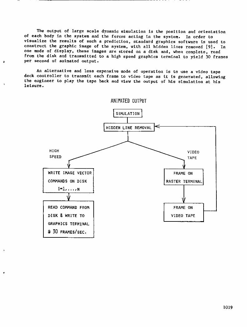
The output of large scale dynamic simulation is the position and orientation

of each body in the system and the forces acting in the system. In order to

visualize the results of such a prediction, standard graphics software is used to

construct the graphic image of the system, with all hidden lines removed [9]. In

one mode of display, these images are stored on a disk and, when complete, read

from the disk and transmitted to a high speed graphics terminal to yield 30 framesper second of animated output.

An alternative and less expensive mode of operation is to use a video tape

deck controller to transmit each frame to video tape as it is generated, allowing

the engineer to play the tape back and view the output of his simulation at hisleisure.

ANIMATEDOUTPUT

I SIMULATION I

HIGH

SPEED

WRITE IMAGE VECTOR

COMMANDS ON DISK

I=I,,,,,N

READ COMMAND FROM

DISK & WRITE TO

GRAPHICS TERH|NAL

@ 30 FRAMES/SEC,

I HIDDEN LINE REMOVAL i_

TAPE

RASTER TERMINAL

FRAME ON

VIDEO TAPE

1019

As a large-scale example of use of the software, a tractor-trailer vehicle

with load-leveling tandem axles was modelled and propelled along a road with an

angled ditch that served to induce roll dynamics. As indicated schematically, the

kinematics of vehicle and axle movement was modelled using spherical, revolute,

and translational joints. Translational spring-dampers were used to represent

flexibility and damping characteristics of suspension springs and shock

absorbers. Hysteresis loops were included in the springs to account for

substantial friction losses that occur in heavy leaf springs of vehicles.

MODELING WITH DADS

RVLT

__ @ TRAILER

@ G R'OUN O

TRACTOR-TRAILER MODEL

0

1020

The sequence of snapshots shown illustrates the prediction of position of the

vehicle during various phases of crossing the ditch. In this case, a severe roll

motion of the trailer is predicted, which cannot be compensated for by the

suspension of the tractor. The alternative to graphics is digital printout, which

locates all the bodies in space. This is clearly not as attractive as the graphics

display of predictions. With graphics, and in fact animation at 30 frames per

second, the analyst can obtain a clear physical understanding of how the vehicle

performs and perhaps why difficulties arise.

I

z

×_1_y

I

---q

I

1021

A second example, illustrated in the figure, involves the prediction of

structural collapse [10] during automobile impact with an obstacle. Collapse of

the structure is modelled, employing the DADS code to represent kinematics of the

collapse mechanism and plastic hinge data to represent structural collapse

characteristics. As indicated by the sequence of snapshots, the nature of

collapse of the structure during an oblique impact is predicted in a form that

assists in visualization of the collapse mechanism. The code also predicts

acceleration of the passenger compartment, which provides information on severity

of the crash event on passengers.

z

x_-Y

z

Zxt_"Y

Z

/-Y

/::!//ii_l,,:;ii!t",\\k

z

xi--,,z

xl-Y

1022

Design sensitivity analysis has been implemented in the DADS software [II] to

predict the change in state due to a change in design parameters, denoted here as

a vector b. The governing equations for design sensitivity are derived by direct

differentiation of the system constraint equations and equations of motion to

obtain the matrix equations for derivatives of dynamic response with respect to

design. These equations are integrated to calculate the derivative of state with

respect to design, which is then made available for predicting the effect of a

design perturbation on dynamic performance. Note that both the equations of

motion and the direct sensitivity equations are integrated forward in time,

comprising a rather large system of equations that are automatically integrated bythe code.

DIRECTDESIGNSENSITIVITY

Equations of Motion

¢(q) = 0

.°

Mq + oT% = Q + Rq

Direct Sensitivity Equaticns;

Cqqb + Ob = 0

Mqb + %)bqb - Qqqh - Rqqb... = Qb + "''

1023

An alternate method of design sensitivity analysis [II] with attractiveefficiency characteristics has been implemented using an adjoint variabletechnique that wasborrowed from the control and structural fields. Using thistechnique, a set of adjoint equations, shownat the bottom of the chart, areintegrated backward in time after the dynamic simulation is completed. Uponcompletion of this integration, the derivative of a general response measure iscalculated, as shownby the last equation on the chart. This method has theattractive feature that only two integrations are required to obtain sensitivityresults. It does, however, require that dynamic information predicted during theforward sweepbe stored and recalled for use in forming and integrating theadjoint equations backward in time.

ADJOINT DESIGN SENSITIVITY

Response Measure

= g(q(r),q(T),b) + fTf(q,q,_,b)dt

0

integ.Adjolnt Equations (0 < T)

T

q = f_

"" _T fTM_ + _ + ... = + ...q q

7

d_ f" TQbd-_ = gb + [fb + + "'']0

1024

As a simple illustration of design sensitivity analysis, the sllder-crankmechanismshownwas analyzed with dimensions bI and b2 of the coupler llnk asdesign variables. The graph shownat the bottom of the chart plots the predictedvariation in acceleration of the slider and the change in acceleration that wasobtained by perturbing the design and reanalyzlng. As indicated, the sensitivityprediction and reanalysis result coincide, indicating that accurate designsensitivity can be achieved. A functional _0 shownon the chart was used tocalculate performance design sensitivity associated with these designparameters. As indicated, the changedue to perturbation and change predicted bydesign sensitivity agree to the third place of numerical accuracy. Designsensitivity results of this kind have been used in design optimization [Ii] toindicate feasibility of use of this formulation of the equations of dynamics anddesign sensitivity in performance optimization.

ti

0.2

---_ 0.2

I.°° L.75

.50

N0o .25

0.00"X

<_

:X

oO

-.50

-.750.(

L T rl

o I L°'!

0.49

b o.25]_b = [-,,l-Ij T x lO-3

l 2

_o=_0 (X4-?.O) dt

A o=-o.o,84, o=-O.O8,2

i l • .... i

.I .2 .3 .4

V,!

.5 .6 ._' 1.0

1025

REFERENCES

I. Wittenburg, J., Dynamics of Systems of Rigid Bodies, Teubner, Stuttgart, 1977.

2. Yoo, W. S. and Haug, E. J., "Large Displacement Dynamics of Machines with

Flexible Components," Journal of Structural Mechanics, to appear, 1984.

. Haug, E. J., Nikravesh, P. E., Sohonl, V. N., and Wehage, R. A., "Computer

Aided Analysis of Large-scale, Constrained, Mechanical Systems," Proceedings,

Fourth International Symposium on Large Engineering Systems, Calgary, Alberta,Canada, June 1982.

. Wehage, R. A. and Haug, E. J., "Generalized Coordinate Partitioning for

Dimension Reduction in Analysis of Constrained DynamlcSystems," Journal of

Mechanical Design, Vol. 104, No. I, 1982.

. Mani, N. K. and Haug, E. J., Singular Value Decomposition for Analysis and

Optimization of Mechanical System Dynamics, Technical Report, Center for

Computer Aided Design, The University of Iowa, July 1984.

. Vanderploeg, M. and Lance, G. M., "Controlled Dynamic System Modelling,"

Computer Aided Analysis and Optimization of Mechanical System Dynamics, (ed.E. J. Haug), Springer Verlag, Heidelberg, 1984.

. Lance, G. M., Liang, C. G., McCleary, M. A., and Mousseau, C. W., Simulation

of Integrated Vehicular Systems, Part I, Technical Report, Center for Computer

Aided Design, The University of Iowa, January 1984.

.

o

Wehage, R. A. and Haug, E. J., "Dynamic Analysis of Mechanical Systems with

Intermittent Motion," Journal of Mechanical Design, Vol. 104, No. 3, 1982.

Nikravesh, P. E., "Application of Animated Graphics in Large Scale Mechanical

System Dynamics," Computer Aided Analysis and Optimization of Mechanical

System Dynamics (ed. E. J. Haug), Springer Verlag, Heidelberg, 1984.

I0. Nikravesh, P. E. and Chung, I. S., "Structural Collapse and Vehicular Crash

Simulation Using a Plastic Hinge Technique," Journal of Structural Mechanics,Vol. 12, No. 3, 1984.

ii. Haug, E. J., Manl, N. K., and Krishnaswaml, P., "Design Sensitivity Analysis

and Optimization of Dynamically Driven Systems," Computer Aided Analysis and

Optimization of Mechanical System Dynamics (ed. E. J. Haug), Springer Verlag,Heidelberg, 1984.

1026

N87-I1779

SHAPE OPTIMIZATION

INCLUDING FINITE ELEMENT GRID ADAPTATION

Noboru Kikuchi

and

J. E. Taylor

The University of Michigan

Ann Arbor, l_l

1027

OBJECTIVES

The prediction of optimal shape design for structures depends on having a suf-ficient level of precision in the computation of structural response. These require-ments become critical in situations where the region to be designed includes stressconcentrations or unilateral contact surfaces, for example. In the approach toshape optimization discussed in this paper, a meansto obtain grid adaptation isincorporated into the finite element procedures. This facility makes it possibleto maintain a level of quality in the computational estimate of response that issurely adequate for the shape design problem.

FINITE ELEMENT I

SOLUTIONPROCEDUREI

/GRID ADAPTATION SHAPE DESIGN I

L(Using Optimality Criteria) l I (Using Optimality Criterion)

1028

A SHAPEOPTIMIZATIONPROBLEM

Weconsider the design of a plane, elastic disc for minimumvolumes, asindicated in the figure. Tractions and displacements are prescribed over res-pective portions of the boundary. The shape design is expressed by functionR(@)over the specified interval A < _ <_B. The yon Mises equivalent stressmust satisfy the performance constraint _ < o on the design boundary; o is

-- . axa given bound value. The domain of the disc i_a_aken to be slmply connecte_, and

a ray from the origin intersects the_boundary only once (i.e., the domain is star-

shaped). We note that _ may exceed _ on the boundary outside the design intervalor in the domain of the disc. max

MIN VOLUME

SUBJECT TO

* EQUIL. EQUATIONS

* BOUNDARY CONDITIONS

* LOCAL CRITERION

_ -_MAX IN A__@_CB

VOLUME = (CONSTANT THICKNESS)*(AREA)

AREA =B I R(E)) R (JRd(_ + A0A 0

DOMAIN = SINGLY CONNECTED AND STAR SHAPED

R(E)) = THE DESIGN VARIABLE ON AN INTERVAL (A,B)

_ SURFACE

1029

OPTIMALITYCRITERIONFORSHAPEDESIGN

A variational interpretation of the nonlinear programmingproblem (_)to the necessary conditions:

%_>0; _(R(0),e) - _max--<0; %[_(R(0),e) - _max]-= 0

leads

A

fba R6Rd0- fba % _lr=R(0)d0 = 0

A

Here _ symbolizes the variation of _ with respect to R within the requirements of

the equilibrium boundary value_problem statement. An interpretation of these equa-

tions provides that k ¢ 0 and _ = _ along the design boundary for the optimalmax

shape. This suggests an iterative approacn for the determination of optimal design

R(@) according to the relationship:

ARmax

R(K÷I) = R(K) _ _ _ (_(K) _ Smax)max

Superscript K represents iterate number, AR equals the 'maximum design change'max I

per iterate step, and B is a normalization sca±e factor with magnitude on the order

of unity.

1030

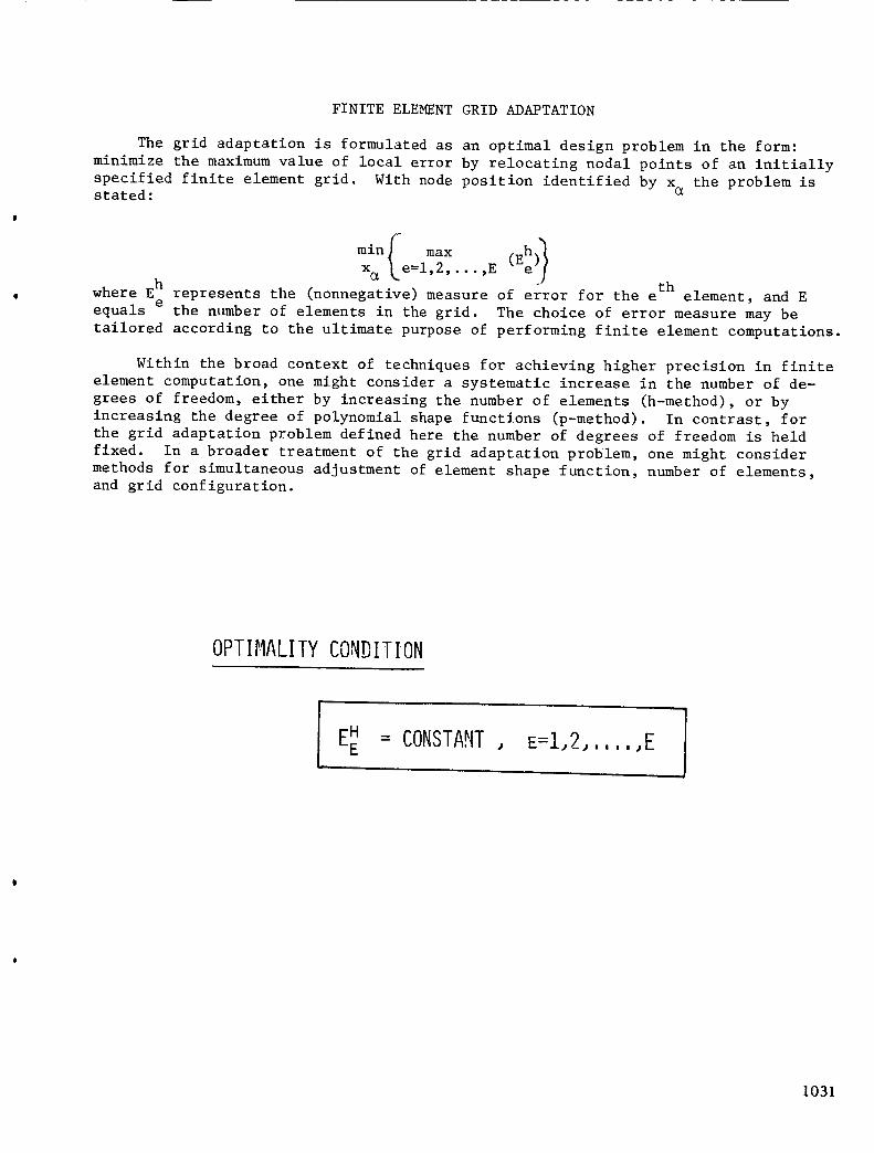
FINITE ELEMENT GRID ADAPTATION

The grid adaptation is formulated as an optimal design problem in the form:

minimize the maximum value of local error by relocating nodal points of an initially

specified finite element grid. With node position identified by x the problem isstated:

minI maxx _e=l,2,...,Eth

where Eh represents the (nonnegative) measure of error for the e element, and E

equals e the number of elements in the grid. The choice of error measure may be

tailored according to the ultimate purpose of performing finite element computations.

Within the broad context of techniques for achieving higher precision in finite

element computation, one might consider a systematic increase in the number of de-

grees of freedom, either by increasing the number of elements (h-method), or by

increasing the degree of polynomial shape functions (p-method). In contrast, for

the grid adaptation problem defined here the number of degrees of freedom is held

fixed. In a broader treatment of the grid adaptation problem, one might consider

methods for simultaneous adjustment of element shape function, number of elements,

and grid configuration.

OPTIMALITYCONDITION

EH = CONSTA T, E=I,2,,,,,,E

1031

MEASUREOFLOCALERROR

To help explain the definition of error indicator Eh for the grid adaptationeproblem, we consider as an example problem the simple interpolation using a piece-wise linear polynomial for function f(x) in the interval (a,b). Let the intervalbe decomposedinto segments

= (x ,XE+I) , e=l,2, . .. ,E, Xl=_e e

and x^=b. Then the following relationship between interpolant fl(x) and the func-tion _(x) holds:

max I f (x)-fl (x) I < h maxx_ -- ex_

e e

Idf/dx I

In other words, the interpolation error in element _ is bounded by the product ofelement size h and the maximum absolute value in _ e of the derivative df/dx.

Following thiseidea, the error indicator Eh for theefinite element mesh is defined

as the maximum of the difference between e the value _h of computed equivalent

stress in _ and the values _ h for elements adjacent e to _ (see Figure

below), e em e

ERROR INDICATORS

H

EH = MAX O'EM - O- H

M=I,. ,.JME

_ = THE EQUIVALENTSTRESS OF I_E

H =O'EM THE EQUIVALENT STRESS OF i'VEM

H E = THE TOTAL NUMBER OF ADJACENT ELEMENTS

1032

RELOCATIONMETHODS

There are infinitely manyways to relocate nodes. Here we shall use theschemedescribed below. The idea of the relocation schemeis that if the valueof error indicator is large, the size of the element must be reduced. Althoughthe relocation schemetends not to provide nonconvex four-node elements, it ispossible to generate non-convex elements. Thus, at each step of node relocationprocess, we have to check whether or not non-convex elements are generated. Itis also noted that the nodes on the outside boundary do not have complete freedomto be relocated, since these nodes must lie on the specified boundary.

In order to determine whether or not the new location of nodes improves qualityof approximations, the quantity QI is introduced, which is the ratio of the maximumvalue vs. the average value of error indicators. If QI is close to the value ofunity, the grid is close to the optimum. Similarly, if the quantities QI ,• . ee=l,...,E, are defined as the ratio of the maximumvalue of error indlcators vs.error indicator E in each finite element, the portion where the approximation is

e

"poor" can be easlly identified. Indeed, if QI is large, then the quality of the

computational result for the e th element is poo_.th0n the other hand, if QI is• eclose to the value of unity, the quality of the e element is, relatlvely speaking,good.

NODE RELOCATION METHODS

E N E N

X_ = _ XNI(E_HI/AEI) / I=_ EH/El AEI

EH = ERROR INDICATORI

AE : AREA OF ELEMENTI

=

XNI COORDINATES OF THE CENTROID

QUALITY INDEX

Q I.= MAX EH / EH' AV

EHv = THE AVERAGE ERROR INDICATOR

1033

EXAMPLE-GRID OPTIMIZATION

The figure shows an example of application of the grid optimization. A thin

linearly elastic plate is subject to both horizontal and downward vertical forces

through a flat rigid punch. Because of the horizontal force, the stress distribu-

tion is not symmetric while the stress becomes infinity at both edges of a rigid

punch. If a uniform grid is used to analyze this problem, singular behavior or

of the stress cannot be simulated well. However, the grid optimization algorithm

provides at least improved grids which are capable of simulating singular behavior

rather realistically.

APPLIED FORCE

RIGID FLAT PUNCH

"UNIFORM" INITIAL GRID

* AFTER FOUR ITERATIONS

L

_m

J

OPTIMAL GRID

Lu , , , _

-2.

)-

.8. °

-10.

SINGULARITIES AT PUNCHEDGES ARE RECREATED BYTHE OPTIMAL GRID

! 4.0

grid:

improved+ initial

STRESS DISTRIBUTION INY-DIRECTION

1034

EXAMPLE-SHAPE OPTIMIZATION

The figure shows an application of both shape and grid optimization algorithms.

It is an interesting observation that both shape and grid optimization problems

possess a similar optimality criterion. Indeed, the "fully" stressed condition

°_ = _max must be reached if any design restrictions are not imposed for shape opti-mlzaumon. On the other hand, the equal distribution of errors Eh = constant must

• .ebe realized at the optimal finite element grid. Both optlmizatlon problems thus

have very similar nature, especially so far as numerical algorithms are concerned.

Implementation is as follows. At the first several iterations of shape optimization

we would not apply any grid optimization algorithm, since the design change is

substantial at the beginning stage of the shape design iteration process, using

the optimality criterion method. After the design change becomes moderate, the

grid design by relocation of nodes becomes active. Since the design change is

small, grid modification should not have too large an effect on the shape design.

Examples show that this method is effective.

No DESIGN

WITHOU._______TTH.__E_EGRID OPTIMIZATION

_ _ DESIGN SURFACE TENSION

_''- _ IS OSCILLATED FORCE

__" .'_'I"-'l'_...... IDESIGN SURFACE /I I I

- 1 I

[ ,, Ib ,1 [

No DESIGN

II WITH THE GRID OPTIMIZATION

___ _> BETTER

I IK No DESIGN_I I_'_--.__ DESIGN SURFACE

#### $4 s#@ #s IJ

_---'v/_FFECT OF THE GRID OPTIMIZATION

1035

CONCLUSION

A provision for grid adaptation is incorporated into computational proceduresfor the prediction of optimal structural shape. The inclusion of such meanstoimprove the quality of computational results from finite element analysis facilitatessolution for shape optimization, particularly in situations where local variationswould have a strong effect on shape.

Acknowledgements

The authors express their gratitude to Dr. A. R. Diaz for his efforts on the

developments of codes for shape and grid optimization. The developments reports

in this paper were supported by the National Science Foundation under Grant CEE8118158.

1036

m

N87-I1780

MULTIDISCIPLINARY APPROACH TO THE

DESIGN OF HIGH PRESSURE OXYGEN SYSTEMS

R. L. Johnston

Lyndon B. Johnson Space Center

Houston, Texas

1037

PROBLEM

Muchof the design, manufacture, inspection, test, and operation of current highpressure oxygen componentsand systems has been driven by weight, cost, func-tional, and schedule requirements. As a result, little coordination has beenexpendedon design for safe operation. While the numberof oxygen related fireshas not been large, their cost, including program losses and delays, has been verylarge. Most of these failures need not have occurred.

1038

BACKGROUND

The incidents listed are examples of preventable fires. The Apollo 13 fire was

caused by improper operating procedures during the prelaunch period. The failure

was facilitated by a design that permitted the tank heaters to be electrically

overloaded. The cost of this failure exceeded $I00,000,000 when the loss of mis-sion is considered. Good fortune prevented the loss of three astronauts.

The oxygen flow control valve test failure occurred because possible internalparticle impact ignition mechanisms were not understood or considered in the

design. Material selection could also have been better in that materials less

susceptible to ignition (Inconel, Monel, etc.) could have been selected.

The extravehicular mobility unit fire was caused by failure to carefully consider

possible internal ignition mechanisms in the design. Ignitable materials (alum-

inum, stainless steel) were used to reduce weight. Testing was largely performed

with inert gases; hence little opportunity to detect incompatibility of the designwith high pressure existed. The cost of this incident exceeded $30,000,000.

SHUTTLE OXYGENFLOW CONTROL

VALVE

EXTRAVEHICULARMOBILITY UNIT

APOLLO 13 -- IN-FLIGHT FIRE IN A CRYOGENIC OXYGENPRESSURE VESSEL RESULTED IN VESSEL RUP-TURE AND CAUSED ABORT OF A LUNARLANDING MISSION. FIRE CAUSED BY IMPROPERGROUND OPERATION AND PERMISSIVE DESIGN

-- TESTS RESULTED IN IGNITION OF THE VALVEAND COMPLETE DESTRUCTION OF THE COM-PONENT. MATERIAL SELECTION WAS POOR.SEVERAL IGNITION MECHANISMS WERE NOTCONSIDERED

-- FIRE DESTROYED A TEST UNIT AND SPACESUIT AND SERIOUSLY INJURED A TECHNICIAN.ACCEPTANCE AND QUALIFICATION TESTSWERE CONDUCTED USING NITROGEN. DESIGNENCOURAGED INTERNAL GENERATION OFCONTAMINATION

1039

DISCIPLINE BIASES

The solution to the problem of fires in high pressure oxygen systems clearly

requires a multidisciplinary approach extending through the life of the system.

Major improvements over current designs (circa 1970's) can be made in material

_election and in design. However, these two disciplines cannot solve the total

problem. Continuing concern and determination to respect the operating limits and

conditions, as well as the exercise of care in the manufacturing and inspection

phases, are required in component production if safe operation is to be achieved.

DESIGN m PRIMARILY CONCERNED WITH FUNCTIONALREQUIREMENTS

MATERIALS m PRIMARILY CONCERNED WITH MECHANICALPROPERTIES, WEIGHT, AND EASE OF MANU-FACTURING

MANUFACTURING _ PRIMARILY CONCERNED WITH MINIMIZINGMANUFACTURING PROBLEMS

OUALITY -- PRIMARILY CONCERNED WITH CONFORMANCETO DRAWING AND PROCESS SPECIFICATIONS

CLEANING _ PRIMARILY CONCERNED WITH INITIAL CON-TAMINATION

TEST m PRIMARILY CONCERNED WITH FUNCTIONALBEHAVIOR. TESTS CONDUCTED WITH BENIGNFLUIDS TO MINIMIZE FACILITY AND TEST COSTS

OPERATION _ PRIMARILY CONCERNED WITH WORKINGCONDITION OF THE SYSTEM AND WITHPREVENTION OF LAUNCH DELAY

1040

POTENTIALIGNITIONSOURCES

The list of potential ignition sources, while not exhaustive, illustrates both thecomplexity and the subtle nature of prevention of fires by concentration on elim-ination of ignition sources only. The designer must be aware of the possibleignition mechanismsthat could be included in his design and prevent the inclusionof as manyas possible. However, elimination of the total list is probably notpossible.

ELECTRICAL FAILURE

PARTICLE IMPACT

CONTAMINATION

PNEUMATIC SHOCK

ADIABATICCOMPRESSION

FRETTING ORGALLING

HELMHOLTZRESONANCE

FRICTIONALHEATING

STATIC DISCHARGE

-- INSULATION LOSS OR FAILURE

m ENERGETIC IMPACT CAUSED BY PARTICLESACCELERATED TO SONIC VELOCITIES

-- IMPROPER CLEANING OR INTERNAL GENER-ATION AND COLLECTION

RAPID VALVE OPENING ACROSS LARGE PRES-SURE DIFFERENCES

INADEQUATE DISSIPATION OF HEAT GENER-ATED BY PRESSURE INCREASES

GENERATION OF LOCALIZED HIGH TEMPER-ATURES BY RUBBING OR PRESSURE WELDING

GENERATION OF HIGH TEMPERATURES BYRESONATING GAS COLUMNS IN BLINDPASSAGES

GENERATION OF HIGH TEMPERATURES BYRAPID GAS FLOW PAST THIN SECTIONS

GENERATION OF STATIC ARCS BY RAPID GASFLOW OVER INSULATING MATERIALS

i041

EXAMPLEOFA DESIGNRELATEDHAZARD

By transfering the shut-off function to the lowest level pressure regulator, rapidpneumatic surges can be prevented. This type of design does require that the low

pressure regulator be capable of withstanding full system pressure in the event

that a failed-open condition occurs in the intermediate regulator. Some weight

may be added to the component by this design approach, but the advantage of this

type of design in reducing surge i_nition of internal contaminations appears to be

well worth while.

WITH FAST OPENINGSHUTOFF VALVE

(a)

7000 PSI

0 PSI

PSI

BEFORE AFTERVALVE VALVE

OPENING OPENING

PSi

7000 PSi

200 PSI

4 PSI

WITH SHUTOFF FUNCTIONIN REGULATOR

(a)

Sl 7000 PSI

200 PSI 200 PSI

_OPSI 4_PSI

BEFORE AFTERVALVE VALVE

OPENING OPENING

1042

EXAMPLEOFMATERIALSELECTIONRELATEDHAZARD

The use of materials with large heats of combustion can result in rapid firepropagation rather than self-extlnguishment. The probability of impact ignition

is also increased. The use of such materials for weight savings or ease of manu-

facturing reasons can be easily offset by the cost of recovering from a singleincident.

PHYSICAL PROPERTIES OF TYPICAL OXYGEN

SYSTEM METALLIC MATERIALS

Material

Impact IgnitionUltimate Tensile Max. Use Heat of Sensitivity Pressure

Density, Strength Temp., Combustion, Threshold

Ib/In3 (kg/m3) 1000 Ib/In2 (MN/m 2) °F (K) Btu/Ib (MJ/kg) Ib/In2 (N/m 2)

Aluminumalloys

StainlessSteel

Inconel 718

Monel 400

0.10 (2800) 40 (276) 350 (450) 130 000 (302) 1050 (?.24)

0.28 (7800) 140 (965) 950 (783) 33 500 (77.8) 1050 (7.24)

0.30 (8300) 180 (1240) 1200 (922) 15 100 (35.1) 8000 (55.2)

0.31 (8600) 145 (1000) 1000 (811) 14 200 (33.1) 8000 (55.2)

1043

EXAMPLEOFMANUFACTURINGTECHNIOUERELATEDHAZARD

The elimination of "feather edges" by careful manufacturing and inspection canremove one source of internally generated contamination. Even if the thin edgedoes not separate and becomecontamination, it could be ignited by friction inhigh flow regions if the heat dissipation paths are small.

Numerous other manufacturing related ignition sensitive conditions and techniques

for their elimination are discussed in reference 1.

(A) -FEATHEREDEDGE

HERED EDGE

THROUGH

(c)

__ATHERED EDGE

AVOIDED BY STOPPINGSHORT

1044

EXAMPLE OF A 0UALITY RELATED HAZARD

The overdrill condition (which actually occurred in manned maneuvering unit

hardware) can result in ignition caused by several different mechanisms. It can

act as a debris or contamination trap, it can resonate producing high temperature,

high temperatures can he produced by system actuation due to adiabatic compres-

sion, or the thin section may he torn free to become a high velocity particle upon

exposure to repeated penumatic impact. One of these mechanisms probably initiatedthe EMU fire.

X-ray inspection conducted by an inspector trained to recognize such conditions

would serve to reduce ignition probabilities. The use of a clear plastic tooling

"proof block" to permit visualization of such conditions is also highly desirable

(if not mandatory) for parts with complex internal flow paths.

1045

EXAMPLE OF CONTAMINATION RELATED HAZARD

The assembly of previously cleaned and particle free parts can generate internal

contamination which may not be removed by subsequent cleaning. The condition may

be reduced or eliminated by clever design. Careful selection of the level of

assembly prior to intermediate or final cleaning may also help.

G E N E R A T E S _/'/_.._._ _//_,_

/ / //t_/,_L_',__" / / _/, '// / / /1. I/ /THREADSENGAGEu_-_-'_ / / /

V/// 7//;FLOW STREAM

POOR GOOD

1046

EXAMPLEOFA TESTRELATEDHAZARD

Most extravehicular mobility unit qualification testing and all individual unitacceptance testing was conducted using nitrogen. As a result, the first exposureto oxygen for the unit involved in the fires was with technicians in close proxim-ity. The fire occurred on the 19th actuation of the oxygen control valve during abench test of the system. Had oxygenbeen used more extensively in acceptancetesting, the fire would have occurred in a remotely operated hazardous test area.

Post-manufacturing acceptance testing and most qualification testing should beconducted with oxygen. While somefires maybe delayed until a substantial periodof operation has passed, some"infant mortality" cases maybe prevented fromreaching the user. All acceptance testing and qualification testing should beconsidered hazardous and should be conducted remotely in facilities designed forthis purpose.

• QUALIFICATION AND ACCEPTANCE TESTSCONDUCTED WITH NITROGEN

• OXYGEN NOT USED TO REDUCE TEST COMPLEXITYAND TO AVOID REQUIREMENTS FOR HAZARDOUSTEST AREA

• FIRST EXPOSURES TO OXYGEN OCCURRED WITHTECHNICIANS PRESENT

• FIRE OCCURRED ON 19TH ACTUATION OF SYSTEMUSING OXYGEN

1047

EXAMPLE OF AN OPERATIONALLY RELATED HAZARD

The invention of ad hoc procedures to work around an equipment problem can lead to

more problems than it solves. If fully coordinated review cannot be obtained,

then such procedures should not be attempted.

m

r-

2_ 1._._,,_" " _ TOHEATERTOFAN

EVENT SEQUENCE

• INSTALLATION OF INCORRECT THERMOSTATICSWITCHES

• DAMAGE TO CAPACITANCE GAGING PROBE

• FAILURE OF APPROVED DETANKINGPROCEDURES

• INVENTION OF NEW WORK-AROUNDPROCEDURES

• DAMAGE TO HEATER INSULATION

• IN FLIGHT FIRE

_ i'_""_ TEMPERATURE

ENSOR

_PROBE II _ ELEMENT

u_60 /--TIu _ FAN

_- _.:_?,u,,_ ,PPER,,LLTUHE

/-- ELECTRICAL

CONDUIT.,,.. / /"-- FLUIDTEMPERATURE

IVENTAND _ SENSORFEEDLINES _ _ SHEATHIFORCLARIT,)__..l_ TEMPER

LOWER__ RE.ORFILLTUBE_ / _ / _ DEN$1T

I _ / I_ ttl _ _ WIRESl

/ 7""_ _ _, HEATERDENSITY (1L I I _ I '_',,J)SENSOR, _ _ _ _ REAINNER _ I; _, I I TErnTUNE--'---\ \ ."II_,"_'-./ SEN

DENSITY .r Trl

PROSE'--"

SHEATHEDTEMPERATURESENSORWIRES(2)

DENSITYPROBEWIRES121ANO

ATERWIRES16)

HEATERTEMPERATURESENSOR

ASSEMBLY

1048

OBSERVATIONS AND CONCLUSIONS

o Every facet of design, manufacturing, inspection, test and operation must

cooperate to prevent high pressure oxygen fires

o The information and skills exist which, if applied, can reduce both the number

and magnitude of high pressure oxygen fires

REFERENCE

i. Bond, A.C., et al.: Design Guide for High Pressure Oxygen Systems, NASA

RP-III3, 1983.

1049

1. Report No. 2. Government Acc_ion No.

NASA CP-2327, Part 2

4. Title and Subtitle

RECENT EXPERIENCES IN MULTIDISCIPLINARY ANALYSIS AND

OPTIMIZATION

7. Author(s)

Jaroslaw Sobieski, Compiler

9. Performing Organization Name and Addre_

NASA Langley Research Center

Hampton, Virginia 23665

12. S_nsoring Agency Name and Address

National Aeronautics and Space Administration

Washington, DC 20546

3. Recipient's Catalog No.

5. Report Date

September 1984

6. Performing Organization Code

505-33-53-12

8. Performing Organization Report No.

L-15830

10. Work Unit No.

11. Contract or Grant No.

13. Type of Report and Period Covered

Conference Publication

14. Sponsoring Agency Code

15. Supplementary Notes

16. Abstract

This conference publication contains the papers presented at the NASA Symposium onRecent Experiences in Multidisciplinary Analysis'and Optimization, held at NASA

Langley Research Center, Hampton, Virginia, April 24-26, 1984. The purposes of the

symposium were to exchange information about the status of the application of optimi-zation and the associated analyses in industry or research laboratories to real life

problems, and to examine the directions of future developments. Within the broadstatement of the symposium's purpose, information exchange has encompassed examples of

successful application; identification of potential applications and benefits, even

though no attempt to apply optimization may have been made as yet; synergistic effects

of optimized interaction and trade-offs occurring among two or more engineering dis-

ciplines (e.g., structural engineering and aerodynamics) and/or subsystems in a sys-

tem (e.g., propulsion and airframe in aircraft); and computer technology in the con-

text of the foregoing. This information exchange has covered aerospace and other

industries as well as universities and government agencies.

The goal of the meeting was to reach a better understanding of the extent to which

optimization and the associated analyses are being used, development directions, the

future potential, and actions that ought to be taken to realize the potential sooner.

That goal was attained and there was a consensus that multidisciplinary analysis and

optimization have an important potential as aids to human intellect in the design

process, and that the cooperation of industry, academia, and government, under NASA

leadership, is needed to realize that potential.

17. Key Words (Sugg_ted by Author(s))

OptimizationSynthesisSystemsSensitivityComputers

19. Security Cla_if. (of this report)

Unclassified

18. Distribution Statement

20. Security Classif. (of this page)

Unclassified

21. No. of Pages

51922. Price

NASA-Langley, 1984