Multidisciplinary Design of Aeronautical Composite Cycle ...

TECHNISCHE UNIVERSITÄT MÜNCHENFakultät für Maschinenwesen

Lehrstuhl für Luftfahrtsysteme

Multidisciplinary Design ofAeronautical

Composite Cycle Engines

Sascha Kaiser

Vollständiger Abdruck der von der Fakultät für Maschinenwesen der TechnischenUniversität München zur Erlangung des akademischen Grades eines

Doktor-Ingenieurs (Dr.-Ing.)

genehmigten Dissertation.

Vorsitzender: Prof. Dr.-Ing. Volker Gümmer

Prüfer der Dissertation: 1. Prof. Dr.-Ing. Mirko Hornung

2. Adjunct Prof. Dr. Anders LundbladhChalmers University of Technology, Gothenburg, Sweden

Die Dissertation wurde am 28.02.2019 bei der Technischen Universität Müncheneingereicht und durch die Fakultät für Maschinenwesen am 28.10.2019 angenommen.

i

Acknowledgement

We set out to achieve the lowest sfc in the world, regardless of weight and bulk;so far we’ve achieved the weight and the bulk.

– Frank Owner about the Bristol Proteus turboprop engine

This thesis is the result of six years of work. It would not have been possible without thesupport from many people, who cannot be counted or named individually. To some of themI want to convey my gratitude on this page. First, I want to thank my thesis supervisorProf. Mirko Hornung and my second examiner Prof. Anders Lundbladh for their continuoussupport throughout the thesis in guiding the research topics into the right direction andasking the right questions at the right time.

Most of the work has been conducted at the research institute Bauhaus Luftfahrt e.V., where amotivating and liberal working environment allowed me to explore many different perspectivesof my work before converging on the research question. I want to thank my dear colleagues,who held up the good spirit at all times, and fostered a supportive research environment. Inparticular, I want to thank Oliver Schmitz and Clement Pornet, who accompanied my earlyyears in research, Patrick Vratny, Michael Schmidt, Ulrich Kling, Philipp Heinemann andAnne Schuster, who became outstanding friends, and the core propulsion group around ArneSeitz and Markus Nickl.

During my work, I could rely on profound and thought provoking feedback from colleaguesin industry. Stefan Donnerhack was a strong promoter of my work, and enabled researchpartnerships that will most likely persist beyond this thesis. Hermann Klingels is the ingeni-ous inventor behind the concept with a matchless intuition for engineering solutions. JensTrübenbach and Alyssa Butler accompanied the finishing.

Last but not least, I could not have accomplished such an enduring task without a solid basis.My family and my parents gave me their absolute support and backing, and never missed toput a smile on my face, when I needed it. Thank you Sonja, Sophie and Alexander.

Sascha Kaiser

Munich, 29th January 2020

ii Preamble

The method development for this thesis was partially conducted in the projects LEMCOTEC(Low Emissions Core-Engine Technologies) and ULTIMATE (Ultra Low emission TechnologyInnovations for Mid-century Aircraft Turbine Engines). LEMCOTEC was co-funded by theEuropean Commission within the Seventh Framework Programme (2007-2013) under theGrant Agreement n° 283216. ULTIMATE received funding from the European Union’s Ho-rizon 2020 research and innovation programme under grant agreement n° 633436.

iii

Abstract

The efficiency of aero engines improved with every new generation. Improvements of turbocomponents, as well as increase of overall pressure ratio and combustor temperatures raisedthermal efficiency, while higher bypass ratio fans raised propulsive efficiency. With the new-est generation of turbofans, the improvement potential of the Joule-/Brayton-cycle and thepropulsive efficiency approach technically viable limits. At the same time, ambitious emis-sion reduction targets require further leaps in engine efficiency. The Composite Cycle Engineconcept introduced in this thesis is a candidate for a step change in core engine architectures.

The concept introduces a piston engine to the high-pressure part of a turbofan core engine,where it drives a high pressure compressor. Piston engines burn fuel at constant volume,which brings along a free pressure rise. They enable higher cycle temperatures and pressuresdue to instationary operation. The created efficiency improvement comes at the price of higherweight, size and pressure oscillations. This thesis answers the question, if the resulting fuelburn improvement can achieve future emission reduction targets with detailed multidiscip-linary component modelling. The piston engine is simulated with a 0D time-resolved model.Engine weight and size are estimated on component-level to generate physically adequateresults for comparison with a turbofan. A sophisticated 2-zone NOx emissions model wasdeveloped to evaluate compliance with projected certification targets.

The appraisal of the technical viability was supported by detailed preliminary, conceptualdesign of the core engine. Particularly piston engine features were specified such as oper-ating mode, layout, lubrication, cooling and coupling to turbo components. The choice ofcomponent limits was supported by data from production piston engines from all fields ofapplications.

The concept was evaluated on a short-to-medium range aircraft platform with a year 2035technological level. The engine was evaluated against a projected geared turbofan. With afour-stroke piston engine, overall efficiency can be increased by 12.3 %. Mission fuel burnreduces only by 5.7 % as engine mass increases significantly from 3 502 kg to 5 962 kg. NOxemissions triple. Using a two-stroke piston engine almost allows to meet fuel burn reductiontargets for the year 2035 with a further 1.1 % improvement due to lower engine weight,although efficiency is worse. The additional use of an intercooler can alleviate thermal andNOx problems, but does not provide better efficiency or engine mass. A more advancedfree-piston engine concept could considerably improve engine efficiency and mass. The mainchallenges identified are high mechanical and thermal loads on the piston engines.

v

Contents

Vorwort i

Abstract iii

List of Figures xii

List of Tables xiv

Nomenclature xv

1 Introduction 1

2 The Composite Cycle Engine Concept 3

2.1 Thermodynamic Benefits of Composite Cycle Engines . . . . . . . . . . . . . 3

2.2 Piston Engines in Aviation . . . . . . . . . . . . . . . . . . . . . . . . . . . . . 6

2.3 Experience and Research on the Composite Cycle Engine Architecture . . . . 11

2.4 Alternative Cycles and Closed Volume Combustion Concepts . . . . . . . . . 15

3 Methods 19

3.1 Fluid Properties . . . . . . . . . . . . . . . . . . . . . . . . . . . . . . . . . . 19

3.2 Propulsion System Simulation . . . . . . . . . . . . . . . . . . . . . . . . . . . 23

3.3 Piston System Simulation . . . . . . . . . . . . . . . . . . . . . . . . . . . . . 29

3.3.1 Heat Losses . . . . . . . . . . . . . . . . . . . . . . . . . . . . . . . . . 34

3.3.2 Numerical Integration . . . . . . . . . . . . . . . . . . . . . . . . . . . 36

3.3.3 Implementation into Engine Simulation Environment . . . . . . . . . . 37

3.3.4 Validation . . . . . . . . . . . . . . . . . . . . . . . . . . . . . . . . . . 39

3.3.5 Mechanical Losses . . . . . . . . . . . . . . . . . . . . . . . . . . . . . 42

3.4 Heat Exchanger Modelling . . . . . . . . . . . . . . . . . . . . . . . . . . . . . 45

vi Contents

3.5 Flow Path Generation . . . . . . . . . . . . . . . . . . . . . . . . . . . . . . . 47

3.6 Mass Estimation . . . . . . . . . . . . . . . . . . . . . . . . . . . . . . . . . . 48

3.7 Aircraft Level Assessment . . . . . . . . . . . . . . . . . . . . . . . . . . . . . 53

3.8 Instationary Operation . . . . . . . . . . . . . . . . . . . . . . . . . . . . . . . 54

3.8.1 Impact of Pulsating Flow on Turbo Components . . . . . . . . . . . . 54

3.8.2 Mechanical Oscillation . . . . . . . . . . . . . . . . . . . . . . . . . . . 56

3.9 Emissions . . . . . . . . . . . . . . . . . . . . . . . . . . . . . . . . . . . . . . 57

3.9.1 CO2 Emissions . . . . . . . . . . . . . . . . . . . . . . . . . . . . . . . 57

3.9.2 NOx Emissions . . . . . . . . . . . . . . . . . . . . . . . . . . . . . . . 58

3.9.3 Noise Emissions . . . . . . . . . . . . . . . . . . . . . . . . . . . . . . 67

3.9.4 Other Emissions and Interference between Emission Targets . . . . . . 68

4 Conceptual Design of Composite Cycle Engines 71

4.1 Evaluation Platform . . . . . . . . . . . . . . . . . . . . . . . . . . . . . . . . 71

4.2 Overall Engine Design . . . . . . . . . . . . . . . . . . . . . . . . . . . . . . . 77

4.3 Piston Engine Design . . . . . . . . . . . . . . . . . . . . . . . . . . . . . . . . 81

4.4 Synergistic Technologies . . . . . . . . . . . . . . . . . . . . . . . . . . . . . . 87

5 Results of Selected Composite Cycle Engine Concepts 91

5.1 Baseline Four-Stroke Engine Concept . . . . . . . . . . . . . . . . . . . . . . . 91

5.1.1 Flow Path and Mass . . . . . . . . . . . . . . . . . . . . . . . . . . . . 95

5.1.2 Fuel Burn . . . . . . . . . . . . . . . . . . . . . . . . . . . . . . . . . . 98

5.1.3 Part-Load Behaviour . . . . . . . . . . . . . . . . . . . . . . . . . . . . 99

5.1.4 NOx Emissions . . . . . . . . . . . . . . . . . . . . . . . . . . . . . . . 100

5.1.5 Technology Sensitivity Study . . . . . . . . . . . . . . . . . . . . . . . 101

5.2 Alternative Piston Engine Concepts . . . . . . . . . . . . . . . . . . . . . . . 102

5.2.1 Two-Stroke Piston Engine . . . . . . . . . . . . . . . . . . . . . . . . . 102

5.2.2 Intercooled Composite Cycle Engine . . . . . . . . . . . . . . . . . . . 105

5.2.3 Free-Piston Engine . . . . . . . . . . . . . . . . . . . . . . . . . . . . . 108

5.2.4 Summary . . . . . . . . . . . . . . . . . . . . . . . . . . . . . . . . . . 111

5.3 Technology Road Mapping . . . . . . . . . . . . . . . . . . . . . . . . . . . . . 116

6 Conclusion and Outlook 119

Bibliography 123

Contents vii

A Appendix 143

A.1 Turbo Component Setup . . . . . . . . . . . . . . . . . . . . . . . . . . . . . . 143

A.2 Validation 2-Stroke Engine Neural Network . . . . . . . . . . . . . . . . . . . 144

A.3 Supplementary figures . . . . . . . . . . . . . . . . . . . . . . . . . . . . . . . 145

A.4 Supplementary Data . . . . . . . . . . . . . . . . . . . . . . . . . . . . . . . . 147

ix

List of Figures

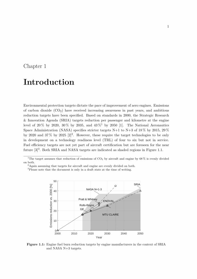
1.1 Engine fuel burn reduction targets by engine manufacturers in the context ofSRIA and NASA N+3 targets. . . . . . . . . . . . . . . . . . . . . . . . . . . 1

2.1 Temperature 𝑇 over specific entropy 𝑠 diagram of the Composite Cycle incontrast to the Joule-/Brayton-cycle at ToC conditions (adapted from [17]).Station nomenclature according to Figure 3.2. Station 41 after addition ofturbine stator cooling air, station 44 after turbine work extraction. . . . . . . 4

2.2 Options for CCE turbofan architectures with fan shaft driven by (a) the pistonengine, (b) the turbine, and (c) a compound of both. . . . . . . . . . . . . . . 5

2.3 IFSD rates of piston engines in contrast to large commercial aircraft regulationsand turbo engines. . . . . . . . . . . . . . . . . . . . . . . . . . . . . . . . . . 8

2.4 Inflation-adjusted fuel price over time [40]. . . . . . . . . . . . . . . . . . . . . 10

2.5 Brake specific fuel consumption BSFC of piston engines over time. . . . . . . 11

2.6 General arrangements of (a) the Wright R-3350 TC [50], and (b,c) the NapierNomad E.145 [24]. . . . . . . . . . . . . . . . . . . . . . . . . . . . . . . . . . 13

2.7 Wankel-type rotary engine (a) rotor and (b) casing [62], and (c) cross-sectionalschematic drawing [63]. . . . . . . . . . . . . . . . . . . . . . . . . . . . . . . 15

2.8 Schematic illustration of (a) a pulsed detonation engine [75], and (b) a waverotor engine [76]. . . . . . . . . . . . . . . . . . . . . . . . . . . . . . . . . . . 17

3.1 Combustion temperature in dependence of FAR and pressure 𝑝 for combustorentry temperature 𝑇3 = 1 000 K. . . . . . . . . . . . . . . . . . . . . . . . . . . 21

3.2 CCE schematic general arrangement with station nomenclature (top), and withrespective simulation sequence within APSS (bottom). . . . . . . . . . . . . . 24

3.3 Component map of a low pressure ratio outer fan with efficiency iso-contoursand typical design and off-design operating points. . . . . . . . . . . . . . . . 28

3.4 Single-zone cylinder control volume with relevant mass, energy and enthalpyflows. . . . . . . . . . . . . . . . . . . . . . . . . . . . . . . . . . . . . . . . . 29

3.5 Synthetic valve lift characteristic over non-dimensional opening time. . . . . . 31

x List of Figures

3.6 Comparison between scavenging efficiency 𝜂𝑠 over delivery ratio of differentscavenging models against uni-flow, loop and cross scavenging [106]. . . . . . 32

3.7 Normalised rates of heat release d𝑄fuel (top) and their cumulative rates (bot-tom) for variations of the Wiebe parameters 𝑤𝑎 (left) and 𝑤𝑚 (right). . . . . 33

3.8 Compressibility factor 𝑍 for various pressures and temperatures for FAR = 0as provided in literature and interpolation used here. . . . . . . . . . . . . . . 34

3.9 Impact of real gas correction for typical CCE piston engine TO conditions. . 35

3.10 (a) Simplified piston geometry used here in contrast to (b) a real high-performancepiston [118]. . . . . . . . . . . . . . . . . . . . . . . . . . . . . . . . . . . . . . 36

3.11 Cylinder pressure 𝑝 over relative volume 𝑉 diagram contrasting cycles withsurrogate solution and adapted valve timing and combustion parameters forTO conditions. . . . . . . . . . . . . . . . . . . . . . . . . . . . . . . . . . . . 39

3.12 Cylinder pressure 𝑝 over relative volume 𝑉 diagram contrasting cycles withsurrogate solution and adapted valve timing and combustion parameters forcruise conditions. . . . . . . . . . . . . . . . . . . . . . . . . . . . . . . . . . . 40

3.13 Crank-angle resolved temperature 𝑇 and pressure 𝑝 of published data [123]against the piston engine simulation program. . . . . . . . . . . . . . . . . . . 42

3.14 Stacked contributions to FMEP by various components over engine speed fortypical TO conditions. . . . . . . . . . . . . . . . . . . . . . . . . . . . . . . . 44

3.15 (a) Schematic of an intercooled recuperated engine, and (b) MTU profile tubeheat exchanger [130]. . . . . . . . . . . . . . . . . . . . . . . . . . . . . . . . . 45

3.16 Important geometric ratios on (a) turbo components, and (b) ducts. . . . . . 47

3.17 Flow path visualisation (blue solid lines) over a PW1100G general arrangementdrawing [132]. . . . . . . . . . . . . . . . . . . . . . . . . . . . . . . . . . . . . 48

3.18 Cross-section of a high-performance piston [134] with derived basic geometricrelations for other piston components. . . . . . . . . . . . . . . . . . . . . . . 49

3.19 Fan mass estimates [138] and regression (solid line). . . . . . . . . . . . . . . 49

3.20 Iso-contours of change in fuel burn depending on TSFC and total engine mass𝑚PPS on a year 2035 short-to-mid range aircraft. Red lines indicate engine-related emission reduction targets. . . . . . . . . . . . . . . . . . . . . . . . . 54

3.21 Schematic illustration of the two engine mountings [155]. . . . . . . . . . . . . 56

3.22 Limits of NOx emissions in the LTO cycle with future SRIA reduction targets,and some current in-service and projected aircraft engines. . . . . . . . . . . . 58

3.23 Schematic illustration of the relations of the zones of the 2-zone model [105]. 60

3.24 Qualitative scope of (a) temperature and (b) mass in both zones of the 2-zone-model in contrast to mean values. . . . . . . . . . . . . . . . . . . . . . . . . . 63

3.25 Creation of NO over crank angle in contrast to equilibrium NO concentration. 64

List of Figures xi

3.26 Simulated NOx emissions in contrast to published data from piston engines. . 65

3.27 Plot of combustion temperature over fuel-air-ratio for assessment of equivalentcombustor inlet temperature 𝑇 *

3 . . . . . . . . . . . . . . . . . . . . . . . . . . 67

4.1 Turbine cooling air distribution on cascades for given material temperaturesfor the year 2015 engine. . . . . . . . . . . . . . . . . . . . . . . . . . . . . . . 73

4.2 Evaluation logic for assessing the year 2035 GTF. . . . . . . . . . . . . . . . . 75

4.3 Changes in fuel burn and sizing thrust 𝐹N for a year 2015 and year 2035 GTFs. 75

4.4 Comparison between engine general arrangement drawings for (bottom) apresent and (top) a year 2035 technological standard. . . . . . . . . . . . . . . 76

4.5 Schematic of the investigated CCE engine architecture. . . . . . . . . . . . . . 78

4.6 Schematics of gearing options with (a-c) planetary gearbox, and (d) a two-stagespur gear transmission. . . . . . . . . . . . . . . . . . . . . . . . . . . . . . . . 80

4.7 (a) Parametric study of gearbox geometric properties, and (b) gearing nomen-clature. . . . . . . . . . . . . . . . . . . . . . . . . . . . . . . . . . . . . . . . 80

4.8 Geometric compression ratio CR over mean piston velocity 𝑣mean categorisedby engine fuel. . . . . . . . . . . . . . . . . . . . . . . . . . . . . . . . . . . . 82

4.9 Pressure over volume diagram for a four-stroke engine with no pressure rise(left), a pressure ratio of 1.5 (middle), and operating as a gas generator (right). 83

4.10 (a) Options for valve drive trains, and (b) comparison of wet and dry cylinderliner cooling. . . . . . . . . . . . . . . . . . . . . . . . . . . . . . . . . . . . . 84

4.11 Free double piston arrangement with the engine on the centre line and pistoncompressors around the piston using the engine power [241]. . . . . . . . . . . 87

4.12 (a) Options for including intercoolers into the CCE baseline (top left). Optionsfor recuperators (b) with different working fluids, and in (c) different locations. 88

4.13 Temperature 𝑇 over specific entropy 𝑠 diagram of the baseline CCE cycle [81].Station nomenclature according to Figure 3.2. Stations 31-34 piston engineinternal, instationary states. Station 41 after addition of turbine stator coolingair, station 44 after turbine work extraction in equivalent single stage turbinemodel [102]. . . . . . . . . . . . . . . . . . . . . . . . . . . . . . . . . . . . . . 89

5.1 Temperature 𝑇 over specific entropy 𝑠 diagram of CCE against GTF at ToCconditions. Station nomenclature according to Figure 3.2. Station 41 afteraddition of turbine stator cooling air, station 43 after turbine work extraction,and station 44 after addition of rotor cooling air in equivalent single stageturbine model [102]. . . . . . . . . . . . . . . . . . . . . . . . . . . . . . . . . 94

5.2 Power and heat balance for the core engine under TO conditions. . . . . . . . 96

xii List of Figures

5.3 (a) General arrangement of the baseline CCE (top) drawn against the referenceGTF (bottom). (b) Cross-sectional view through the piston engine (top) withpiston engine gearbox (bottom). . . . . . . . . . . . . . . . . . . . . . . . . . 97

5.4 Changes in fuel burn and sizing thrust 𝐹𝑁 for baseline CCE. . . . . . . . . . 98

5.5 CCE part power characteristics (a) TSFC, and (b) change in TSFC againstGTF and fuel ratio burned in the piston engine. . . . . . . . . . . . . . . . . . 99

5.6 Comparison between four-stroke and two-stroke CCE in a temperature 𝑇 overspecific entropy 𝑠 diagram at ToC conditions. . . . . . . . . . . . . . . . . . . 104

5.7 General arrangement of the baseline four-stroke CCE (top) drawn against two-stroke CCE (bottom). . . . . . . . . . . . . . . . . . . . . . . . . . . . . . . . 104

5.8 General arrangement of the intercooled two-stroke CCE (top) drawn againsta two-stroke CCE (bottom). . . . . . . . . . . . . . . . . . . . . . . . . . . . . 107

5.9 Temperature 𝑇 over specific entropy 𝑠 diagram of CCE with and withoutintercooler at ToC conditions. . . . . . . . . . . . . . . . . . . . . . . . . . . . 107

5.10 General arrangement of the free-piston CCE (top) drawn against two-strokeCCE (bottom). . . . . . . . . . . . . . . . . . . . . . . . . . . . . . . . . . . . 110

5.11 Power and heat balance of the high pressure spool of the free-piston engine. . 110

5.12 Changes in fuel burn and sizing thrust 𝐹𝑁 for the CCE concepts and GTFengines. . . . . . . . . . . . . . . . . . . . . . . . . . . . . . . . . . . . . . . . 112

5.13 Changes in fuel burn FB, TSFC (left), PPS mass 𝑚PPS and bore (right) of theinvestigated CCE concepts when varying number of cylinders. . . . . . . . . . 112

5.14 CCE NOx emission levels in LTO cycle with respect to emission reductiontargets. . . . . . . . . . . . . . . . . . . . . . . . . . . . . . . . . . . . . . . . 113

5.15 Displacement volume specific power over mean effective pressure 𝑝mean cat-egorised by engine application. . . . . . . . . . . . . . . . . . . . . . . . . . . 114

5.16 Displacement volume specific engine mass over power specific engine masscategorised by engine application. . . . . . . . . . . . . . . . . . . . . . . . . . 115

5.17 CCE TRL maturation road map. . . . . . . . . . . . . . . . . . . . . . . . . . 117

A.1 Verifications of the calculation of the equilibrium constant 𝐾𝑐 exemplary forReaction (3.116). . . . . . . . . . . . . . . . . . . . . . . . . . . . . . . . . . . 145

A.2 Verifications of the equilibrium concentrations of the species of the OHC-System over temperature against published data [172]. . . . . . . . . . . . . . 145

A.3 Power per volume flow over power per area. . . . . . . . . . . . . . . . . . . . 146

xiii

List of Tables

3.1 Thermodynamic properties tables specifying inputs with ranges. . . . . . . . 21

3.2 Standard design iteration scheme for a GTF. . . . . . . . . . . . . . . . . . . 26

3.3 Standard off-design iteration scheme for a GTF. . . . . . . . . . . . . . . . . 28

3.4 Input parameters for the four-stroke piston engine surrogate artificial neuralnetwork with ranges and output parameters. . . . . . . . . . . . . . . . . . . 37

3.5 Adaptation of valve timings and combustion parameters for TO conditions tomeet piston engine specified performance. . . . . . . . . . . . . . . . . . . . . 40

3.6 Adaptation of valve timings and combustion parameters for cruise conditionsto meet piston engine specified performance. . . . . . . . . . . . . . . . . . . . 41

3.7 Input parameters for the piston engine validation and comparison betweenoutputs in reference and simulation. . . . . . . . . . . . . . . . . . . . . . . . 41

3.8 Pressure losses in heat exchanger. . . . . . . . . . . . . . . . . . . . . . . . . . 45

3.9 Summary of geometric properties of turbo components. . . . . . . . . . . . . 47

3.10 Structure of engine masses and validation values. . . . . . . . . . . . . . . . . 52

3.11 Diesel engines and references used for the validation of the NOx simulationmodel, completeness of simulation data, and simulation error. . . . . . . . . . 65

4.1 Assumptions for reference GTF ToC design point with a year 2035 technolo-gical standard. . . . . . . . . . . . . . . . . . . . . . . . . . . . . . . . . . . . 74

4.2 Specifications for main operating points for reference GTF design with a year2035 technological standard on a year 2035 airframe. . . . . . . . . . . . . . . 76

4.3 NOx emission estimates for LTO cycle and cruise. . . . . . . . . . . . . . . . . 77

5.1 Assumptions for CCE design point performance. . . . . . . . . . . . . . . . . 92

5.2 Efficiency corrections for CCE simulation. . . . . . . . . . . . . . . . . . . . . 93

5.3 Baseline CCE cycle properties. . . . . . . . . . . . . . . . . . . . . . . . . . . 94

5.4 Piston engine limit properties. Operating point TO if not specified otherwise. 95

xiv List of Tables

5.5 Mass breakdown of CCE against GTF. . . . . . . . . . . . . . . . . . . . . . . 96

5.6 Aircraft level metrics with baseline CCE. . . . . . . . . . . . . . . . . . . . . 98

5.7 CCE NOx emission estimates in LTO cycle and cruise. . . . . . . . . . . . . . 100

5.8 CCE sensitivities of technology assumptions on TSFC, power plant systemmass 𝑚PPS and fuel burn FB in order of highest fuel burn improvement potential.102

5.9 Two-stroke CCE cycle properties. . . . . . . . . . . . . . . . . . . . . . . . . . 103

5.10 CCE two-stroke NOx emission estimates in LTO cycle and cruise. . . . . . . . 105

5.11 Main cycle characteristics of a CCE with intercooler. . . . . . . . . . . . . . . 106

5.12 Intercooled CCE NOx emission estimates in LTO cycle and cruise. . . . . . . 108

5.13 Parameter assumptions for FP engine. . . . . . . . . . . . . . . . . . . . . . . 108

5.14 Main cycle characteristics of a CCE with free piston. . . . . . . . . . . . . . . 109

5.15 Free-piston CCE NOx emission estimates in LTO cycle and cruise. . . . . . . 111

A.1 Input parameters for the two-stroke piston engine surrogate artificial neuralnetwork with ranges and output parameters. . . . . . . . . . . . . . . . . . . 144

A.2 Structure of engine weights and validation values for 2-stroke CCE. . . . . . . 147

A.3 Structure of engine weights and validation values for intercooled 2-stroke CCE. 148

A.4 Structure of engine weights and validation values for free-piston CCE. . . . . 148

A.5 Station report for four-stroke CCE. . . . . . . . . . . . . . . . . . . . . . . . . 149

A.6 Station report for two-stroke CCE. . . . . . . . . . . . . . . . . . . . . . . . . 150

A.7 Station report for intercooled two-stroke CCE. . . . . . . . . . . . . . . . . . 151

A.8 Station report for free-piston CCE. . . . . . . . . . . . . . . . . . . . . . . . . 152

A.9 Comparison of results of piston engine surrogate artificial neural network withsimulation model of four-stroke CCE. . . . . . . . . . . . . . . . . . . . . . . . 153

A.10 Comparison of results of piston engine surrogate artificial neural network withsimulation model of two-stroke CCE. . . . . . . . . . . . . . . . . . . . . . . . 154

A.11 Comparison of results of piston engine surrogate artificial neural network withsimulation model of intercooled two-stroke CCE. . . . . . . . . . . . . . . . . 155

A.12 Comparison of results of piston engine surrogate artificial neural network withsimulation model of free-piston CCE. . . . . . . . . . . . . . . . . . . . . . . . 156

xv

Nomenclature

List of Latin Symbols

𝐴 m2 Area𝑎𝑖 – NASA CEA polynomial coefficients𝐴* K Initial temperature difference in the two-zone modelAR – Aspect Ratio𝑏𝑖 – NASA CEA polynomial coefficientsBMEP Pa Brake Mean Effective PressureBPR – Bypass RatioBSFC g/kW h Brake Specific Fuel Consumption𝑐 – Correction or calibration factor𝐶 W/K Heat capacity rate𝑐𝐴 – Calibration factor for initial temperature difference 𝐴*

𝑐D – Nozzle discharge coefficient𝑐𝐹 𝐺 – Nozzle thrust coefficient𝑐𝑝 J/(kg K) Specific heat at constant pressure𝐶∘

𝑝 J/(mol K) Specific molar heat at constant pressureCR – Geometric Compression Ratio𝑐𝑠 – NOx proportionality factor𝑑 m Diameter𝐷𝑝 g Pollutant emitted in LTO cycleEINOx gNOx/kgfuel Emission Index NOxEOC ° End of CombustionEVC ° Exhaust Valve ClosingEVO ° Exhaust Valve Opening𝑓 Hz Pulsation frequency𝐹 N Thrust (force)FAR – Fuel-Air-RatioFB kg Mission fuel burnFF – Flow FunctionFHV J/kg Fuel Heating Value (lower)FL 100 ft Flight Level (pressure altitude)

xvi Nomenclature

FMEP Pa Friction Mean Effective Pressure𝐺 J/kg Gibbs energyGR – Gap Ratioℎ J/kg Specific enthalpyΔ𝑓𝐻

∘298 J/mol Molar enthalpy at 298 K

𝐻∘ J/mol Specific molar enthalpyHTR – Hub-to-Tip RatioIMEP Pa Indicated Mean Effective PressureIVC ° Intake Valve ClosingIVO ° Intake Valve Opening𝑘 W/(m2 K) Thermal conductivity𝐾𝑐 – Equilibrium constant𝑘𝑓 (m3/(mol s))𝑛 Forward reaction coefficient𝑘𝑟 (m3/(mol s))𝑛 Reverse reaction coefficient𝑙 m Length𝑀 – Mach number𝑚 kg Mass𝑀 kg/mol Molar mass�� kg/s Mass flow rateMTOW kg Maximum Take-Off Weight𝑛 Hz Spool speed𝑛 – NumberNTU – Number of Transfer UnitsOEW kg Operating Empty WeightOPR – Overall Pressure Ratio𝑃 W Power𝑝 Pa Total pressure𝑝peak Pa Piston engine peak pressurePPR – Peak Pressure Ratio�� W Heat flow rate𝑞 – Ratio𝑄 J Heat𝑅 J/(kg K) Specific gas constant𝑟 m Radius𝑅𝑚 J/(mol K) Universal gas constantRNI – Reynolds Number Index𝑠 J/(kg K) Specific entropy𝑠 m StrokeΔ𝑓𝑆

∘298 J/(mol K) Molar entropy at 298 K

𝑆∘ J/(mol K) Specific molar entropySM – Surge Margin𝑠NOx gNOx/kgfuel NOx severity parameterSOC ° Start of Combustion

Nomenclature xvii

𝑡 s Time𝑇 K Total temperatureTR – Taper RatioTSFC kg/(N s) Thrust Specific Fuel Consumption𝑈 J Inner energy𝑢 J/kg Specific inner energy𝑣 m/s Velocity𝑉 m3 Volume𝑣mean m/s Mean piston velocity𝑣tip m/s Fan tip speed𝑊 J Work𝑤𝑎 – Wiebe parameter𝑤𝑚 – Wiebe parameterWAR – Water-Air-RatioWP J/kg Work Potential𝑦 – Non-dimensional time of heat release𝑍 – Compressibility factor

List of Greek Symbols

𝛼 W/(m2 K) Heat transfer coefficient𝛽 – Auxiliary parameter in component maps𝜖 – Heat exchanger effectiveness𝜂 – Efficiency𝜂air – Air efficiency𝜂core – Core efficiency𝜂is – Isentropic efficiency𝜂o – Overall efficiency𝜂p – Propulsive efficiency𝜂pol – Polytropic efficiency𝜂s – Scavenging efficiency𝜂th – Thermal efficiency𝜂tr – Transmission efficiency𝛾 – Heat capacity ratio𝜆 – Delivery ratio𝜆0 – Initial air ratio in combustion zone of the two-zone model𝜆𝑠 – Connecting rod ratio𝜇 Pa s Dynamic viscosity𝜈 – Mole number𝜑 ° Crankshaft angle𝜑 – Air number𝛱 – Pressure ratio

xviii Nomenclature

𝜓 – Load coefficient𝛹 – Entropy function𝜌 kg/m3 Density

List of Subscripts

0 Ambient Conditions1 Component inlet2 Component exitcold Heat exchanger cold sidec Combustioncool Cooling aircorr Correcteddes Design moded DisplacementG Grosshot Heat exchanger hot sideid Ideal

is Isentropici Inner (fan)M Materialm MeanN Neto Outer (fan)s Staticst Stream Tube0–9 Station nomenclature (see

Figure 3.2)std Standardc Cooling

List of Acronyms

ACC Active Clearance ControlAE All-ElectricCCE Composite Cycle EngineCEA Chemical Equilibrium with ApplicationsCLAIRE CLean AIR EngineCO Carbon MonoxideCO2 Carbon DioxideCR CruiseEGR Exhaust Gas RecirculationETOPS Extended OperationsFDGS Fan Drive Gear SystemFP Free PistonGTF Geared TurbofanHALE High Altitude Long EnduranceHPC High-Pressure CompressorHPT High-Pressure TurbineIC IntercoolerIFSD In-flight ShutdownIPC Intermediate-Pressure CompressorIRA Intercooled Recuperated Aero engine

Nomenclature xix

ISA International Standard AtmosphereLDI Lean Direct InjectionLPS Low-Pressure SpoolLPT Low-Pressure TurbineLTO Landing and Take-offNO Nitrogen oxideNOx Nitrogen oxides, mainly nitric oxide (NO) and nitrogen dioxide (NO2)OH HydroxidePC Piston CompressorPE Piston EnginePPS Power Plant SystemSCR Selective Catalytic ReductionSLS Sea Level StaticSoA State of the ArtSRIA Strategic Research & Innovation AgendaTBC Thermal Barrier CoatingTBO Time Between OverhaulTCDS Type-Certificate Data SheetTDC Top Dead CentreTiAl Titanium AluminideTO Take-OffToC Top of ClimbTRL Technology Readiness LevelUDF Unducted FanUHC Unburned Hydrocarbons

List of Organisations and Software

ACARE Advisory Council for Aviation Research and Innovation in EuropeAPD Pacelab APD, PACE GmbHAPSS Aircraft Propulsion System SynthesisATAG Air Transport Action GroupBHL Bauhaus Luftfahrt e.V.CAEP Committee on Aviation Environmental ProtectionCLEEN Continuous Lower Energy, Emissions and NoiseEASA European Aviation Safety AgencyEC European CommissionENOVAL Engine Module ValidatorsERAST Environmental Research Aircraft and Sensor TechnologyGasTurb GasTurb®, GasTurb GmbHIATA International Air Transport AssociationICAO International Civil Aviation Organization

xx Nomenclature

LEMCOTEC Low-Emissions Core-Engine TechnologiesMATLAB MATLAB® R2017b, The MathWorks inc.NASA National Aeronautics Space AdministrationULTIMATE Ultra Low emission Technology Innovations for Mid- century Aircraft Tur-

bine Engines

1

Chapter 1

Introduction

Environmental protection targets dictate the pace of improvement of aero engines. Emissionsof carbon dioxide (CO2) have received increasing awareness in past years, and ambitiousreduction targets have been specified. Based on standards in 2000, the Strategic Research& Innovation Agenda (SRIA) targets reduction per passenger and kilometre at the enginelevel of 20 % by 2020, 30 % by 2035, and 43 %1 by 2050 [1]. The National AeronauticsSpace Administration (NASA) specifies stricter targets N+1 to N+3 of 18 % by 2015, 29 %by 2020 and 37 % by 2025 [2]2. However, these require the target technologies to be onlyin development on a technology readiness level (TRL) of four to six but not in service.Fuel efficiency targets are not yet part of aircraft certification but are foreseen for the nearfuture [3]3. Both SRIA and NASA targets are indicated as shaded regions in Figure 1.1.

1The target assumes that reduction of emissions of CO2 by aircraft and engine by 68 % is evenly dividedon both.

2Again assuming that targets for aircraft and engine are evenly divided on both.3Please note that the document is only in a draft state at the time of writing.

2000 2010 2020 2030 2040 2050

Year

0

10

20

30

40

50

Em

issi

ons

redu

ctio

n vs

. 200

0 [%

]

NASA N+1-3

SRIA

MTU CLAIRE

Pratt & Whitney

Rolls-Royce

GE

ENOVAL

Figure 1.1: Engine fuel burn reduction targets by engine manufacturers in the context of SRIAand NASA N+3 targets.

2 1 Introduction

Comparing the afore-mentioned targets to the goals of aero engine concepts foreseen byimportant manufacturers shows a discrepancy. An improvement of 15 % was achieved bymodern turbofan engines [4, 5]. Beyond that point, e.g. MTU’s CLean AIR Engine (CLAIRE)agenda foresees a next-generation geared turbofan (GTF) by the year 2030 with a further10 % improvement [6–8]. A third CLAIRE concept aims to feature an advanced cycle beyondthe Joule-/Brayton-cycle. Pratt & Whitney foresees a further, more ambitious 10 % to 15 %improvement by 2025 [2, 9]. For a third generation GTF, a generic cost improvement by 45 %is envisaged, which embraces fuel burn, maintenance and manufacturing cost. Rolls-Royceforesees the three-spool turbofan ADVANCE with an improvement of 20 % by 2020, and thegeared UltraFan with variable pitch fan with 25 % improvement by 2025 [10, 11]. From GEAviation, no engine agenda goes beyond the GE9X [12]. The European research programmeENOVAL found a similar mid-term improvement target of 26 % by 2025 [13, 14].

The projected improvements are on a good trajectory to achieve SRIA 2020 targets, butno improvements beyond 25 % to 30 % are foreseen on a Joule-/Brayton-cycle based engine.Therefore, a novel cycle is required in the mid future. The Composite Cycle Engine (CCE)is presented in this thesis as a candidate concept, which combines advantages of turbofanand piston engines. The concept introduces a piston engine on the high-pressure part of aturbofan core. The combustion in piston engines is partially isochoric, and thereby providespressure rise without the cost of shaft power. Due to an instationary operating principle,much higher combustion temperatures and pressures can be sustained. Thus, the CCE hassignificant thermal efficiency improvement potential over turbofan engines. This thesis seeksto answers the question:

Can the Composite Cycle Engine achieve future emission reduction targets underconsideration of weight penalties and conceptual design constraints on a short-to-medium range aircraft?

The target of this thesis is to identify the true fuel burn improvement of the concept asoptimising thermal efficiency only is misleading. An application-oriented conceptual designidentifies the key technologies, which are required to implement the cycle. Multidisciplinarymethods for meaningful benchmarking of novel engine concepts and detailed evaluation aredeveloped. Engine weight is estimated from the bottom up to capture relevant design andsizing effects. Efficiency and weight are used to evaluate mission fuel burn. This translatesinto fuel cost and CO2 emissions as a metric for environmental footprint. Flow path layoutand engine sizing determine the mechanical feasibility of the concept. Detailed conceptualdesign of the CCE, and in particular its piston engine are presented. Multiple operatingpoints are used to size the engine and evaluate performance. The impact at the aircraftlevel is quantified. A sophisticated model for estimation of NOx emissions in piston engineand combustor is used to assess applicability to certification scenarios. In addition to thesequantitative measures, further disciplines – such as mechanical oscillations or emissions ofnoise, soot and water vapour – are discussed qualitatively. The presented methods are appliedto designs with four-stroke and two-stroke engines, as well as in combination with intercoolers,and with an advanced free-piston engine.

3

Chapter 2

The Composite Cycle Engine Concept

The integrated assembly of at least two heat engine cycles featuring independent compression,heat source and expansion operating on the same working fluid is denoted as Composite CycleEngine1 [16]. The first complete cycle is the Joule-/Brayton-cycle, which is conventionallyused in turbofan engines. It consists of turbo compression, isobaric combustion and turboexpansion. In the concept investigated in this thesis, the second cycle entirely takes place ina piston engine. The term was established in the scope of the LEMCOTEC project [16]. Itwas sought in distinction to the well-established term Compound Engine, which denotes anengine that uses at least two different principles of power extraction – usually a piston enginefollowed by a turbine – that contribute to shaft power working on the same fluid.

In this chapter, the benefits of a CCE over the turbofan are discussed for application in acivil transport category aircraft mission. The challenges introduced by the piston engine arediscussed by means of built engines. Related studies with composite and compound enginedesigns are then reviewed to summarize previous findings in the field.

2.1 Thermodynamic Benefits of Composite Cycle Engines

The CCE concept allows for increased thermal efficiency. It improves the thermodynamiccycle by putting a topping cycle upon the Joule-/Brayton-cycle as shown in the temperature 𝑇over specific entropy 𝑠 diagram in Figure 2.1 (p. 4). The higher peak pressure and temperatureis the first main thermodynamic benefit of the Composite Cycle. This is enabled by theinstationary operation of the piston engine, which reduces the mean thermal load of thematerial to a technically feasible level. The second main benefit is the (partially) isochoriccombustion. This leads to a pressure rise that is achieved by heat addition rather than shaftpower as in a turbo compressor. This effectively reduces the required compression power for

1Note that the term Composite Cycle was rarely used before in the context of variable cycle engines (alsoaugmented cycle and convertible cycle). These engines can alter the cycle during operation to achieve optimalbehaviour under highly varied operating conditions. It is often used to switch from turbofan characteristics insubsonic operation to turbojet characteristics during supersonic operation. One example is GE’s CompositeCycle Engine [15, p. 13-7, Fig-2], which was designed for supersonic operation up to and above Mach numbersof 3.0, and could switch to a pure turbojet mode above M = 2.0.

4 2 The Composite Cycle Engine Concept

0 200 400 600 800 1000 1200

Specific entropy s [J/kg]

200

400

600

800

1000

1200

1400

1600T

empe

ratu

re T

[K]

2

3

441

4445

5

2

25

3

31

32

33

34 35

441

4445

5

2

3

441

4445

5

2

25

3

31

32

33

34 35

441

4445

5

Turbofan: T4 = 1600 K, OPR = 50

CCE: T4 = 1400 K, OPR = 35

Isobaric lines

Figure 2.1: Temperature 𝑇 over specific entropy 𝑠 diagram of the Composite Cycle in contrastto the Joule-/Brayton-cycle at ToC conditions (adapted from [17]). Station nomen-clature according to Figure 3.2. Station 41 after addition of turbine stator coolingair, station 44 after turbine work extraction.

a given target pressure at the beginning of the expansion process. A minor benefit comesfrom the more efficient compression and expansion process within the piston engine. Thereasons are avoidance of tip losses, lower fluidic frictional losses due to much less requiredwetted area for achieving high pressure, and partially intercooled compression through wallheat losses.

The thermal efficiency in the modern turbofans based on the Joule-/Brayton-cycle approachestechnologically viable limits. Further improvements of the cycle are increasingly difficult toachieve and the required leaps in efficiency to achieve emission reduction targets appearunlikely. Current engines can achieve 15 % to 16 % mission fuel burn reductions comparedto the year 2000 technological standards [4, 5]. Turbofan engines for the near-to-mid futureare projected to achieve 19 % to 26 % shown in Chapter 1 [13, 14, 18]. No significant furtherimprovement potential beyond that point is foreseen.

The SRIA CO2 reduction target on the propulsion system level is −30 % [1] by 2035 and −43 %CO2 by 2050. To achieve these targets while ignoring aircraft level cascading effects, overallengine efficiency 𝜂o in an engine for a short-to-medium range aircraft would need to increasefrom 31 % in 2000 [19] to 44 % and 54 %, respectively. Assuming a long-term improvementof propulsive efficiency 𝜂p to 85 %, thermal efficiency of 52 % and 64 %, respectively, wouldbe required.

Modern aero engines achieve a thermal efficiency of approximately 46 % [17]. A study coveringchanges in OPR and combustor exit temperature 𝑇4 for generic top of climb conditions(𝑀0.80, FL350, ISA) shows that with further optimisation of the main cycle parameters, an

2.1 Thermodynamic Benefits of Composite Cycle Engines 5

(a) (b) (c)

Figure 2.2: Options for CCE turbofan architectures with fan shaft driven by (a) the pistonengine, (b) the turbine, and (c) a compound of both.

improvement to 48 % is possible by 2035 at higher OPR and slightly lower 𝑇4 [17]. To reachthe efficiency improvement targets, turbo component losses would need to reduce furtherby 40 % and OPR to increase to 60 to reach 2035 targets. To achieve 2050 targets withthe Joule-/Brayton-cycle, turbo components need 100 % component efficiency and an OPRof 120. These numbers assume that engine mass and relative turbine cooling air do notincrease.

Several physical limitations impede the achievement of these improvements: first, higherOPR results in smaller volume flow at the high-pressure compressor (HPC) exit, leading toreduced blade height. As the gap between blade and casing cannot be reduced arbitrarilyto maintain a margin for transient operation, tip leakage grows, and compressor efficiencyreduces [20]. Second, the combustor exit temperature 𝑇3 increases with OPR, which requiresheavier and more expensive materials in the last HPC stages. It incurs higher engine cost dueto added turbo component stages and more complex component technology. Raising 𝑇3 and𝑇4 leads to a considerable increase in turbine cooling flow and required cooling effectivenessfor a given permissible blade material temperature. Piston engines in the high-pressure partof the core are a solution to the OPR ceiling of turbo engines.

The power provided by the piston engine can be either used for core compression or for thefan. The resulting fundamental architectural options are shown in Figure 2.2. In option (a),the piston engine drives the fan, while a turbine runs the core compression. In Option (b),the piston power is used for compression of the core flow. Option (c) is a combination of both,where the piston engine provides a share of the total shaft power. The number of turboshaftsis arbitrary.

Thermodynamically, none of the options is inherently better than another. As long as grosspower provided by piston engine and turbine are unchanged, their assignment to individualshafts does not alter the overall balance of fuel flows and net shaft power. Therefore, othercriteria may favour one of the concepts. In a previous qualitative assessment of these archi-tectures, the turbine driven shaft in option (b) was shown to be most suitable for a turbofanarrangement [16]. Geometric restrictions in connecting the piston engine to a power sink arelow. Mechanical loads are smallest by avoiding couplings between turbo and piston shafts.If the piston engine drives the fan alone as in option (a), it needs to be considerably largerto provide enough power than in the other two options. Therefore, only option (b) is furtherinvestigated in this thesis.


Compared to turbo engines, piston engines have several drawbacks. They have high mech-anical losses, if they are connected to a crankshaft. These can be of the order of 5 % to 10 %.The operation is intermittent, which leads to lower utilisation of the displacement volume itoccupies, higher bulk size, and engine mass. The practical implications are discussed in thenext section.

2.2 Piston Engines in Aviation

The history of controlled, powered, heavier-than-air flight started in 1901 with piston en-gines [21]. Two years later, the Wright brothers performed their first flight tests with a4-cylinder water-cooled piston engine with a power of 12 kW [22]. Langley experimentedwith unpiloted aeroplanes with a five-cylinder radial engine that had a power of 2.4 kW anda mass of 3.2 kg [22]. It had one of the lowest ever achieved displacement volume-specificmasses of 4.2 kg/L. Even earlier applications of piston engines in aeronautics go back to 1872in dirigible balloon flights [22]. From that point on, piston engines grew larger in size, power,and number of pistons.

The technological zenith of piston engines was in the 1940s. The highest number of pistonswas in the Wright R-2160 Tornado with 42 cylinders and six rows of radial engines in sevenbanks. The engine had to be cooled by water, as cooling air in the first rows would haveheated up to such a degree that cooling was insufficient in the rear rows. It had a shaftpower of 1 750 kW. The most powerful planned aeronautical piston engine was the Rolls-Royce Crecy. The Crecy’s twelve cylinders delivered a shaft power of 3 100 kW [23]. It usedsuper-charging and an exhaust power turbine for power augmentation. Its specific mass was0.40 kg/kW based on take-off power. It was developed over five years until 1945 but was neverflight tested. The Napier Sabre with 24 cylinders in an H-arrangement had a shaft power of2 240 kW, the most powerful non-radial aeronautical piston engine to date [24]. The largestsingle piston displacement volume was achieved on the Charomskiy ACh-30 with a bore of0.18 m and a stroke of 0.20 m [25]. It was a turbocharged V-12 engine for long-range aircraft.

With the advent of reliable and powerful turbo engines, large aeronautical piston enginesabruptly ceased to persist in development. The de Havilland Ghost turbojet entered serviceon the Comet in 1949, the Rolls-Royce Dart turboprop on the Vickers Viscount in 1953,and the Allison T-56 turboprop engine in 1955. The first turboprop engines had a specificconsumption of 320 g/kW h (0.52 lb/hp h), which was 40 % higher than comparable pistonengines at the time such as the Wright R-3350 turbo-compound [26]. Thermal efficiencylevels similar to the last large piston-based aero engines were reached only recently in 2009with the Europrop TP400 engine [27]. The reasons why turbo engines were commercially moreviable at the time are important for understanding the main drawbacks of piston engines. Ifthese issues are solved, piston engines can be a competitive alternative in the future.

Size and Weight: The Allison T-56 turboprop specific mass of 0.25 kg/kW – three timeslower than that of comparable in-service piston engines such as the Wright R-3350turbo-compound with 0.74 kg/kW, or the non-compounded Wright R-3350 R-18 with

2.2 Piston Engines in Aviation 7

0.80 kg/kW. The bulk volume of the Wright was 32 % larger than the Allison’s, andthe diameter was more than double with 1.42 m.

To make a like-for-like comparison, the Piper PA-46 aircraft will be featured on thenext pages. It entered service in 1983 and can be equipped with either the LycomingTIO-540 piston engine (aircraft sales name Piper Malibu or Piper M350, [28]) or thePT6A turboprop engine (aircraft sales name Piper Meridian or Piper M500, [29]). Bothengines were developed in the late 1950s. While the Lycoming has a specific mass of1.0 kg/kW, the PT6A denotes 0.30 kg/kW at maximum power2. Despite lower enginemass and larger tank capacity, the PT6A equipped Piper has a 340 nmi shorter missionrange due to 35 % higher specific fuel consumption. The aircraft with piston enginewould have further saving potential when sizing the aircraft for the same mission range.Despite higher maximum take-off weight (MTOW) of the piston-powered aircraft, thepayload with full fuel is 5 % smaller. Therefore, a novel engine concept with pistonengines must achieve lower engine mass and bulk size. Otherwise, the engine could betoo heavy or large for under-wing installation and lead to cuts in payload.

Reliability and Maintenance: A common perception about piston engines is that theyhave relatively low reliability and short maintenance intervals. An important measureto quantify reliability is the in-flight shutdown (IFSD) rate, expressing the number ofin-flight shutdowns per flight hour. A low IFSD on an aircraft-engine combination isrequired to receive extended operations (ETOPS) certification. This permits an airlineto fly for extended time spans with one engine on a twin-engine aircraft in case of anIFSD [30, 31]. For example, ETOPS 120 allows an aircraft to fly for two hours on oneengine to the closest airport at any given time during a mission. To get ETOPS 120certification, an IFSD rate of less than 5 × 10−5/h must be proven on an engine type inoperation. For ETOPS 180, less than 2 × 10−5/h is required. This was later translatedinto a dual engine failure probability of less than 0.3 × 10−8/h [32]. For more than 180minutes, a rate lower than 1 × 10−5/h is required. Achieving ETOPS is necessary tocross oceans on a shorter or direct route.

Some reference numbers comparing IFSD rates are shown in Figure 2.3 (p. 8). TheICAO fleet average of piston engines in 1953 was 35 × 10−5/h. The Wright R-1820,which was used on the DC-3, had already achieved 9 × 10−5/h [33]. General aviationpiston engines of the 1960s were still more reliable with rates of 4.6 × 10−5/h on single-engine aircraft and 2.3 × 10−5/h on twin-engine aircraft [34]. The latter were almostreliable enough to achieve ETOPS 180. Of the engine-related accidents, 51 % could beattributed to pilot error, for example inadequate pre-flight planning or the misman-agement of fuel. In 10 % of the cases, improper maintenance, servicing and inspectioncould be attributed to the accident. These errors can be avoided in commercial avi-ation, meaning that ETOPS certifiable reliability levels appear feasible. Early largeturbofans demonstrated similar IFSD rates of 40 × 10−5/h [35]. Modern large turbofanengines averaged a rate of 1 × 10−5/h in 2003 [31], and can be as low as 0.1 × 10−5/hfor individual engine models.

2The engine has a rated power of 630 kW, but it is derated to 370 kW in the Piper PA-46.


Figure 2.3: IFSD rates of piston engines in contrast to large commercial aircraft regulationsand turbo engines.

A study investigating accidents on rotorcraft over three decades showed similar prob-ability for engine-related accidents on piston and turbine single-engine vehicles around30 % [36]. The rate of engine-related accidents was also similar with about 20 acci-dents per 1 000 registered rotorcraft. They highlighted, however, that helicopters witha single-turbine engine are safer than with a single-piston engine, when consideringhigher utilisation rates for single-turbine rotorcraft. The comparability was limited astypical usage and pilot experience differed significantly between both categories, and asmost accidents could be attributed to human error.

Comparing the Piper PA-46 aircraft engines, time between overhaul (TBO) of theLycoming engine is 2 000 h, and that of the PT6A is 3 600 h. The difference between thetwo is less than a factor of two. Moreover, the aircraft with PT6A engine is 900 000 $(73 %) more expensive, partially due to a considerably higher engine price tag. Ifpiston engines were built with the same level of manufacturing cost and thus technicalsophistication, the TBOs can be expected to converge. Engine overhaul cost per flighthour for the PT6A is three times higher than that of the Lycoming piston engine,despite higher TBO.

Low flight altitude and speed: Naturally aspirated piston engines have a significant powerlapse in altitude. Power decreases with air density, as engine speed cannot be increaseddue to mechanical constraints. Transport category aircraft with piston engines fromthe 1940s and 1950s had a cruise altitude of 15 000 ft (5 000 m). This is insufficient toensure over-the-weather flight. So, piston engine powered aircraft were susceptible tobad weather, leading to diverted and cancelled flights. Only over-sizing of the piston

2.2 Piston Engines in Aviation 9

engine could have alleviated the problem for naturally aspirated piston engines. Oneway to cope with the restricted power supply at altitude was a reduction of airspeed.With turboprop engines in connection with pressurised cabins, cruise altitude could beincreased to over 20 000 ft (6 000 m) with the Rolls-Royce Dart powered Vickers Vis-count [37] as turbo engines can process higher volume flows. Later with turbojets likethe de Havilland Ghost, altitudes over 30 000 ft (9 000 m) were feasible.

Turbocharged piston engines alleviate the problem of the constant displacement volumeby increasing air density before induction [38]. The turbo-supercharged Wright R-3350TC for the Lockheed Super Constellation, and the turbo-supercharged Wright R-2800Double Wasp for the DC-6 both reached a flight altitude of 23 000 ft (7 000 m). Thesuper-charged Junkers Jumo 207 with a charging pressure of 3 bar was operated ataltitudes over 40 000 ft (12 200 m) [23].

Looking at the Piper PA-46, the turbocharged Lycoming powered M350 has a cruisealtitude of 25 000 ft (7 600 m) and an airspeed of 213 kts (110 m/s). In contrast, thePT6A powered M500 has a cruise altitude of 30 000 ft (9 100 m) and an airspeed of260 kts (134 m/s). The Lycoming is charged with a boost of 1.2 bar, which almostremedies the differences in flight speed and altitude. Turbocharging therefore removesthe lack of power in altitude.

Fuel price: The fuel price was at an inflation-adjusted all-time low in the 1950s and -60sas shown in Figure 2.4 (p. 10). Consequently, the incentive for operators to use fuel-efficient engines was relatively low. While it is hardly conceivable that operators todaywould use an engine with 40 % higher specific consumption, it was viable at that time.The advantages of turbo engines mentioned above could outshine their lower efficiency.Today, fuel price has a large share of the operating cost of an aircraft. It is about athird of the direct operating cost on a short-to-medium range aircraft and more than40 % on a long-range aircraft [39].

The advancement of progressive engine technology is subject to many unknowns andvery costly. Market boundary conditions dictate the likelihood of success for novel tech-nologies. A famous example is the open rotor research conducted mainly during the1980s. The open rotor engines GE Unducted Fan (UDF) [41] and PW/Allison 578-DXwere flight-tested in 1987 and 1989. Thus, they reached TRL 6. At the same time, theinflation-adjusted fuel price declined to a 15-year low. The open rotor concept devel-opment was consequently cancelled in 1989 [41], when McDonnell Douglas decided toequip the MD-90 with V2500 turbofans rather than open rotor engines. The low fuelprice was one of the reasons for this decision [42]. In the 2000s, research and develop-ment recommenced with the Clean Sky research engines SAGE 1 by Rolls-Royce andSAGE 2 by SNECMA [43], or by GE in the CLEEN program [41]. Coincidentally, thefuel price increased considerably during that time. The current fuel price is lower thanin the 2000s but still at a relatively high level, which may incentivise the developmentand use of fuel-efficient engines.


1860 1880 1900 1920 1940 1960 1980 2000 2020 2040

Year

0

50

100

150In

flatio

n ad

just

ed o

il pr

ice

[$]

Allison T-56

de Havilland Ghost

Rolls-Royce Dart

GE UDF

PW/Allison 578-DX

SafranOpen Rotor

Figure 2.4: Inflation-adjusted fuel price over time [40].

After piston engines were supplanted by turbo engines in large aeronautical applications,the development of aeronautical piston engines came to a halt. Piston engines that werefurther used in general aviation were designs from the 1960s such as the afore-mentionedLycoming TIO-540-AE2A. Only in recent years, the development of novel small-scale designscommenced. Thielert developed the TAE 125 engine, now under the names CD135 and CD155by Technify Motors, running on kerosene with a specific consumption as low as 214 g/kW h(0.352 lb/hp h). Austro Engines also develops new aeronautical piston engines running onkerosene. In the European Commission (EC) funded Clean Sky programme, Austro Enginesdeveloped the AE440 V-8 diesel engine for helicopter application with a specific dry mass ofonly 0.6 kg/kW [44].

Piston engine efficiency has clearly improved over the past century. The trend of brake specificfuel consumption (BSFC), i.e. referring to shaft power, over time is illustrated in Figure 2.5(p. 11). Modern marine piston engines achieve a specific consumption of about 180 g/kW h(0.296 lb/hp h) and down to 166 g/kW h (0.273 lb/hp h) at full power in the MAN S90ME-C9two-stroke diesel engine [45]. Still, it is difficult to predict what efficiencies large aeronauticalpiston engines could achieve with technological progress since engines in other applicationsare subject to different design goals. The lowest BSFC from all engines reviewed in thisthesis is achieved by the projected turbo-compound high altitude long endurance (HALE)engine ERAST TE95-627 [46] with 148 g/kW h (0.243 lb/hp h). In comparison, the CCEtechnological target for the pure piston engine appears rather modest with about 350 g/kW h.However, this figure only refers to the piston engine itself. Since it is highly charged, the cyclestarts at a high temperature and pressure level. The pressure ratio over the piston engineis, therefore, small and the isolated cycle efficiency relatively low, while overall core engine

2.3 Experience and Research on the Composite Cycle Engine Architecture 11

1880 1900 1920 1940 1960 1980 2000 2020 2040 2060

Year

100

150

200

250

300

350

400

450

500

550B

rake

Spe

cific

Fue

l Con

sum

ptio

n B

SF

C [g

/kW

h]

Piston enginealone

CCEcore

Allison T-56

RR AE2100

TP400

AircraftAutomotiveMarineRace CarAuxiliaryOther or n/a

Figure 2.5: Brake specific fuel consumption BSFC of piston engines over time.

efficiency is better than in a naturally aspirated piston engine. The entire CCE core enginewould achieve a BSFC3 around 175 g/kW h.

With current technological advances in motor engineering and research, the past flaws ofpiston engines can be overcome. Lower reliability and higher maintenance efforts have beenshown to be manageable. The inflation-adjusted fuel price is on a high level today. Thefindings from this section highlight that a CCE should deviate from past aeronautical pistonengines in two main points: First, a turbine should serve as the main power source to leverageits outstanding power-to-mass ratio and to reduce the required shaft power from the pistonengine. Second, the piston engine should be highly turbocharged to reduce its size and massfor a given power. This also eliminates limitation of flight altitude and speed.

2.3 Experience and Research on the Composite Cycle EngineArchitecture

Examples of research and application of the CCE and the turbo-compound principle showcasethe benefits of the combination of piston and turbomachinery. Per definition, the CCE andturbo-compound architectures only differ in the existence of a second combustor. In practicalapplications, however, most turbo-compounds used the piston engine as the main powerprovider, while the CCE uses the piston engine only to put the highly efficient topping cycleinto effect.

3This is a synthetic number for a turbofan as a fraction of the fan power is used to pressurise the core.This fraction has been deducted from the shaft power here.


In a turbo-compound, a turbine is added to the piston engine for power augmentation. Itoperates on the piston exhaust pressure and remaining heat. This leads to lower fuel con-sumption and higher specific power [47]. Turbo-compounding famously appeared in operationin the 1950s with the Wright R-3350 TC [48] and as a concept in the Napier Nomad E.145 [24,49]. Their general arrangements are depicted in Figure 2.6 (p. 13). In both engines, the pis-ton engine provides the main share of the shaft power, and is only supported by a turbinedriven by the exhaust gas from the piston engine. Both engines feature a turbo compressorthat charges the piston engine. In the Wright R-3350 TC, the turbo compressor is coupledwith the piston shaft and works as a supercharger. The compressor achieves a manifold pres-sure of 1.3 bar. The blow-down turbine recovers the kinetic energy of the exhaust flow andcontributes about 15 % of the shaft power.

In case of the Napier Nomad E.145, the compressor is coupled to the turbine. Only thenet power of both is transmitted to the piston shaft via an infinitely variable gear displayedin the top right of Figure 2.6 (p. 13)(b). The gear moderates speeds between the turbine-compressor assembly and the piston engine. The speed on the turbo shaft can then be chosenfreely during operation in part load. The turbo shaft contributes about 13 % of the net shaftpower after deduction of compressor power. The turbine alone provides about the sameamount of power as the piston engine. The Napier Nomad E.145 boosts the pressure beforethe piston engine to 6 bar. The pressure ratio increases in altitude to obtain enough enginepower. Its efficiency is unmatched by turboprop engines until today. Both engines improveefficiency over pure piston engines considerably.

The term composite engine appeared in advertisements for the previously mentioned NapierNomad E.145 engine [51]. It was then used to promote its composition of “half diesel” and“half gas turbine”. Its architecture is a typical turbo-compound. Its predecessor, the NapierNomad E.125 prototype, was developed in 1945 and is a CCE according to the definition usedhere [49]. The E.125 features an axial compressor driven by a turbine followed by a radialcompressor driven by a piston engine. It has two separate shafts. On the first, the pistonengine drives a radial compressor. On the second, the turbine drives the axial compressor.Both shafts contribute their excess power to independent, counter-rotating propellers. Anauxiliary constant pressure combustor after the piston engine is used for power augmentationin high power conditions, such as take-off. The peak pressure of 138 bar achieved by thepiston engine exceeds the pressures achieved by any turbo engine.

An application area of highly charged piston engines are HALE platforms. These use pistonengines because they make better use of the available oxygen in the air [52, 53]. A turbo enginerequires four times as much air mass flow rate as a spark ignition engine for a given power.Moreover, the low BSFC of turbocharged piston engines is almost independent from altitude.When the piston engine inlet conditions are kept constant to sea level ambient pressure,the charging pressure ratio can be increased to 125 at a flight altitude of 100 kft [52]. Theextremely high pressure ratio raises the thermal efficiency potential by 25 % to 40 %, whichis counteracted by increasing losses in the compression and intercooling system. ProjectedBSFC in such a turbo-compound application can be as low as 175 g/kW h (0.29 lb/hp h)[52].

2.3 Experience and Research on the Composite Cycle Engine Architecture 13

(a)

(b)

(c)

Figure 2.6: General arrangements of (a) the Wright R-3350 TC [50], and (b,c) the Napier NomadE.145 [24].


The Grob G 850 Strato 2C high altitude platform used an off-the-shelf Continental piston en-gine as its core and sole power provider. It was charged with a three-spool turbo compressionsystem. Thus, it flew up to 60 kft, the highest altitude ever flown by a piston engine. It wascapable of flying up to 78 kft [54]. In the NASA research programme Environmental ResearchAircraft and Sensor Technology (ERAST), many propulsion options for a HALE platform forflight altitudes up to 100 kft were investigated on paper [46, 55]. At peak altitude, the turbopressure ratio is between 85 and 95. Similar to the Strato 2C engine, they envisaged a three-spool turbocharger system with three intercoolers. They also investigated turbo-compoundarrangements with turbine contributions up to 24 % of the shaft power. The lowest projectedBSFC of 157 g/kW h (0.26 lb/hp h) was estimated on a turbo-compound two-stroke dieselengine.

Compound and CCE concepts were also subject in many research publications, which in-vestigated the viability under various operating scenarios or for special applications. In the1980s, NASA investigated concepts for turbo-compound and highly turbocharged piston en-gines for helicopter application with a power of 750 kW [23]. They drew the conclusionthat turbocharged piston engines would not be competitive with respect to mass. Thus,turbo-compounding would be required. Two-stroke engines were found to be favourable overfour-stroke engines due to lower mass, despite slightly lower efficiency. A pressure ratio beforethe piston engine above 10.0 could help to reduce piston engine mass. A cooler before thepiston engine was suggested to reduce the thermal load on the piston engine and increaseengine life at the cost of 6 % BSFC. A specific mass of 0.26 kg/kW was projected. Theturbine would provide a net contribution of 24 % of the total shaft power at full load. Fuelconsumption would reduce by 31 % at 20 % higher engine mass compared to a gas turbine.

A turbo-compound concept for utility vehicles was designed and tested by the Cummins En-gine Company in the 1970s and early 1980s [56, 57]. They achieved a fuel burn improvementof 20 % over a conventional utility diesel engine. Like the NASA concept, a power turbinewas used to augment piston engine power, and a separate turbocharger was employed. Afterextensive testing, normal wear was observed on the piston engine.

Another study with a turbo-compound engine concept raised mean effective pressure 𝑝meanof a marine diesel from 22 bar to up to 80 bar to increase power from a given displacementvolume [58]. Power quadrupled with small improvements in efficiency. Heat losses tripled, andpeak pressure increased to 720 bar. When restricting peak pressure to 250 bar, power couldstill be 2.5 times higher. The approach was then transferred to an aeronautical one-shaft CCEconcept [59]. A charge pressure ratio of 9.1 and a pressure ratio across the four-stroke pistonengine of about 2.0 was specified. Depending on piston engine mass, a fuel burn improvementof 8 % to 12 % could be achieved on a short-to-medium range aircraft. A different study foran aeronautical CCE in the 500 kN thrust class found a potentially very high mass up to 30 t.However, mass could reduce considerably, if small trades in efficiency were made [60].

2.4 Alternative Cycles and Closed Volume Combustion Concepts 15

(a) (b) (c)

Figure 2.7: Wankel-type rotary engine (a) rotor and (b) casing [62], and (c) cross-sectionalschematic drawing [63].

2.4 Alternative Cycles and Closed Volume Combustion Con-cepts

Other approaches were pursued to achieve higher power densities with closed volume combus-tion. The rotary engine is a closed volume combustion engine that directly produces torquealong the engine axis. Thus, no conversion of linear into revolutionary motion is needed. TheWankel-type rotary engine is the most popular concept of this engine class. It is constitutedby a disk that rotates eccentrically around the engine shaft. The most renowned configur-ation with three chambers is depicted in Figure 2.7. The volume covered by the movementof the rotor constitutes the engine displacement volume, and the perimeter is enclosed bythe casing. This type of engine can rotate around another shaft. Therefore, it can be builtaround the low-pressure spool of a two-spool turbofan and be placed co-axially to the turbocomponents. This allows for a very compact flow path layout [61].

As a further benefit, rotary engine concepts typically feature lower specific mass of 0.4 kg/kWto 0.5 kg/kW [64, 65] than crankshaft bound piston engines that typically have a mass that ishigher than 1 kg/kW. This is a result of the engine layout, which features three chambers and,hence, performs three cycles simultaneously. The engine has a four-stroke characteristic withall connected benefits. Particularly, the scavenging behaviour of such an engine is superior tothat of a two-stroke engine [66]. Mean and peak cycle temperatures are lower, and inlet andoutlet pressure are decoupled since both valves are opened separately. Thus, it is possible toprovide a pressure boost at the cost of reduced shaft power. Mechanical engine oscillationsare much lower than in piston engines and only of second order.

The rotary engine has some drawbacks. The feasible geometric compression ratio of theengine is limited by the envelope covered by the rotor and typically lower than in pistonengines. The chamber geometry results in a very slim volume during combustion [65], as canbe seen at the bottom of Figure 2.7(c). This leads to delayed, and sometimes incompletecombustion, as well as high soot production. The rate of heat release can be expected to be


lower than in piston engines. The rotor or casing geometry can be compromised to achieve amore suitable geometry for combustion, such as a pocket in the rotor or a pilot combustionchamber. These measures result in an even lower geometric compression ratio.

The heat release always occurs at the same location of the casing, exposing it to high thermalload. In contrast, hot surfaces in piston engines are exposed to cool air during the scavengingstroke. Another technical challenge is the sealing of the engine since the edges separating thechambers move relative to the steady casing. This leads to leakage between the chambers andrestricts the permissible peak pressure in the cycle. Current research projects have achievedup to 100 bar [64, 65], which is still comparably low. Both leakage and the low peak pressureare the main sources for inferior performance compared to piston engines [67, 68].

The rotary engine concept will not be investigated further in this thesis. It may be viable incases where small packaging is required, flow path layout with piston engines would be toocomplicated, piston engine oscillations are excessive, or to make use of the four-stroke en-gine characteristics, such as in gas generator operation. Former examinations of this conceptshowed a thrust specific fuel consumption (TSFC) improvement of 14 % with an increase inmass of 5 % [69] against a turbofan of similar technological level. A different study predicted4.5 % improvement with an increase in mass of 31 % [70]. The configuration that leads aturboshaft through the rotary engine axis is geometrically challenging and may lead to largeand heavy disks [70]. Studies comparing rotary engines with piston engines in aeronauticalapplications show a competitive BSFC with 20 % lower specific mass [62]. The company Li-quidPiston investigates an inverted rotary engine design with improved combustion chambergeometry and static seals. They have only presented a 2.4 kW demonstrator so far, but predicta relative increase in efficiency of the order of 10 % over conventional piston engines [71].

Many other concepts with isochoric combustion have been proposed. Pulsed detonation asshown in Figure 2.8 (p. 17)(a) is achieved by detonating a fuel-air mixture in tubes [72].The detonation wave then travels downstream with high pressure spikes to a turbine. Thisleads to highly unsteady operating conditions in the high-pressure turbine (HPT) with anorder of magnitude pressure oscillation. This results in highly varying incidence angles on theturbine rotor blades and severe penalties on HPT efficiency. Equivalent steady state valuescan be as low as 27 % [73], or at best 70 % at low utilisation of the combustor tubes [74]. Theimprovements through isochoric combustion could be vitiated by the degradation of turbineefficiency [75]. Turbine film cooling is difficult to achieve as the cooling flow could reverseduring pressure spikes. To avoid this, cooling air pressure could be increased to the pressurespike level, or internal blade cooling could be used.

The wave rotor as shown in Figure 2.8 (p. 17)(b) uses complex shock systems to achieveisochoric combustion [76, 77]. It delivers a comparatively steady mass flow, but wall cooling,and particularly off-design performance are critical issues when the finely concerted shocksystem falls out of synchronisation. Moreover, thermal expansion of the rotor and sealing ofthe rotor surfaces is technically not mastered [78]. Therefore, only special purpose conceptsenvisage a wave rotor for future applications.

In conclusion, other isochoric combustion technologies currently fall behind the maturity ofpiston engines and suffer from major challenges that have not been solved to date. Therefore,

2.4 Alternative Cycles and Closed Volume Combustion Concepts 17

(a) (b)

Figure 2.8: Schematic illustration of (a) a pulsed detonation engine [75], and (b) a wave rotorengine [76].

they will not be considered in this thesis. As an option, the secondary combustion chamber inthe CCE concept could be either of these technologies. This promises only small improvementas most of the fuel is burnt in the piston engine during the mission fuel burn relevant cruisephase. The additional complexity does not appear to be justified.

Many other candidate technologies for future aero engines are being investigated, and noclear favourite has emerged, yet. For example, electrification of the propulsive drive train hasreceived increasing attention. The first major variants are parallel-hybrid electric architec-tures that provide a part of the source energy as electrical energy stored in batteries aboardthe aircraft. Battery energy density limits the achievement of significant reductions in fueland energy consumption. For applicability in passenger aircraft, a minimum a system energydensity of 1 000 W h/kg has been identified in past studies for beneficial application in short-to-medium range passenger aircraft [19, 79–81]. Benefits can be realised on design rangesup to 1 000 nmi [19]. The introduction of 50 % electrification could potentially reduce fuelburn by 14 %, while total energy consumption would increase by 7 % [80]. Current batterytechnology achieves system energy density of 200 to 250 W h/kg on cell level [82], and it isnot clear whether the required improvements can be achieved in batteries fulfilling the safetyand reusability requirements for commercial aviation. Including overall CO2 emissions withelectricity production and a projected energy mix, viable mission ranges with net savingsare further reduced [19]. Also, hybrid-electric concepts require major changes in the airportinfrastructure. In conclusion, this technology is not a competitor for civil passenger transportclass aircraft.

In contrast, the CCE concept uses drop-in fuels. It is compatible with a potential future shiftto biofuels or hydrogen. The outer engine mould line remains the same, and the conceptdoes not require additional components outside of the engine, such as electrical systems.The interface between aircraft and engine does not alter except for the required adaptionto increased engine weight. Thus, the aircraft architecture can be retained, just like thetraditional aircraft and engine design process. No complicated interactions between aircraftand engine manufacturers are required. Lastly, the components foreseen in the CCE are wellknown and at respectively high TRL. Hence, the technology and development risk is lowerthan with unproven technologies.

19

Chapter 3

Methods

This chapter introduces methods for multidisciplinary design of CCEs. First, methods forperformance simulation of turbo and piston engines are presented. Their outcomes are usedfor the estimation of flow path and mass. Then, metrics for impact at the aircraft levelwill be shown. Next, effects due to instationary operation of the piston engine are assessed.Finally, emissions of CO2, NOx, noise and others are discussed. In this chapter, representativeoperating conditions from the CCE simulations presented later in this thesis (Chapter 5) areused to illustrate the impact of assumptions made.

3.1 Fluid Properties

The simulation of thermodynamic cycles requires the knowledge of fluid properties everytime changes to the fluid state occur. In gas turbine engines, wide ranges of pressuresand temperatures are covered. Consequently, the assumption of ideal gas properties, i.e.constant specific heat capacity 𝑐𝑝, and heat capacity ratio 𝛾 causes errors, which are too largefor accurate calculation of central performance metrics such as thermal efficiency 𝜂th [83].Therefore, half-ideal gas properties are used within the scope of this thesis, where the gasproperties are dependent on temperature 𝑇 but not pressure 𝑝. The introduced error byneglecting the impact of pressure is small for the range of pressures observed in a gas turbineengine1. The additional computational effort was avoided in this manner.

The fluid properties were obtained with the NASA Chemical Equilibrium with Applications(CEA) database [84, 85]. It contains coefficients 𝑎𝑖 for polynomial representation of the fluidproperties for all relevant species, e.g. N2 and O2, as shown for specific molar heat capacity𝐶∘

𝑝 in Eq. (3.1) [86]. The polynomials are specified for ranges from 200 K to 1 000 K, and from1 000 K to 6 000 K. The polynomials for the enthalpy are obtained by integration according toEq. (3.2) and Eq. (3.3), with the molar enthalpy Δ𝑓𝐻

∘298 and the molar entropy Δ𝑓𝑆

∘298 of the

formation at 298.15 K. For each temperature range, seven coefficients 𝑎𝑖 and two integrationconstants 𝑏𝑖 are provided in tables.

1The difference in specific heat capacity 𝑐𝑝 between 1 bar and 100 bar is 0.3 % at 1 800 K, and 0.01 % at1 500 K. The integral error in a Joule-/Brayton-cycle is negligible.

20 3 Methods

𝐶∘𝑝

𝑅𝑚= 𝑎1𝑇 2 + 𝑎2

𝑇+ 𝑎3 + 𝑎4𝑇 + 𝑎5𝑇

2 + 𝑎6𝑇3 + 𝑎7𝑇

4 (3.1)

𝐻∘

𝑅𝑚= 𝛥𝑓𝐻

∘298

𝑅𝑚+∫ 𝑇

298.15 K

𝐶∘𝑝

𝑅𝑚d𝑇

= −𝑎1𝑇

+ 𝑎2 ln𝑇 + 𝑎3𝑇 + 𝑎4𝑇 2

2 + 𝑎5𝑇 3

3 + 𝑎6𝑇 4

4 + 𝑎7𝑇 5

5 + 𝑏1 (3.2)

𝑆∘

𝑅𝑚= 𝛥𝑓𝑆

∘298

𝑅𝑚+∫ 𝑇

298.15 K

𝐶∘𝑝

𝑅𝑚𝑇d𝑇

= − 𝑎12𝑇 2 − 𝑎2

𝑇+ 𝑎3 ln𝑇 + 𝑎4𝑇 + 𝑎5𝑇 2

2 + 𝑎6𝑇 3

3 + 𝑎7𝑇 4

4 + 𝑏2 (3.3)

The properties of mixtures of species are calculated by summation of the individual propertiesweighted by their molar fraction. Air is modelled as a composition of 78.0840 % of nitrogen(N2), 20.9476 % of oxygen (O2), 0.9365 % of argon (Ar), and 0.0319 % of CO2. Further speciesare neglected. The (mass) specific properties are then obtained by division through themolar mass 𝑀 of the species, e.g. 𝑐𝑝 = 𝐶∘

𝑝/𝑀 . Since pressure dependency is not considered,all properties were evaluated at a pressure of 100 bar in accordance with the commercialgas turbine simulation environment GasTurb®. High pressure turns down the amount ofdissociation and, thus, reduces non-linearity at high temperatures. Neglecting dissociationmay result in a slight over-prediction of engine performance as molecules may not recombineduring expansion in a real engine. The effect of excitation of vibrational modes in moleculesat high temperatures is retained.

Combustion is modelled for kerosene, specifically Jet-A1 fuel, at a fuel temperature of298 K [87]. In the NASA CEA, Jet-A1 fuel is chemically represented as hydrocarbon with themolecular formula C12H23. The ideal reaction with air (neglecting Ar and CO2) in depend-ence of the air number 𝜑 is given in Reaction (3.4). The resulting stoichiometric fuel-air-ratiois FARst = 0.0682 (𝜑 = 1, air-fuel-ratio = 14.67). In the CEA database, a fuel heating valueFHV of 43.031 MJ/kg is specified. The value used in this thesis is the Jet-A1 certificationminimum FHV of 42.80 MJ/kg [88]. FAR is corrected accordingly in the engine simulation.

𝜑 C12H23 + 17.75 O2 + 3.7738 · 17.75 N2

−→ 12𝜑 CO2 + 11.5𝜑 H2O + 17.75(1 − 𝜑) O2 + 66.9852 N2 (3.4)

The combustion of kerosene adds an additional dimension to the fluid properties. Theproducts of combustion in the gas, H2O and CO2 need to be considered. Particularly athigh temperatures, by-products such as carbon monoxide (CO) and hydroxide (OH) formdue to incomplete combustion and dissociation. Here, equilibrium composition is assumedat all conditions. This assumption neglects the incomplete recombination of combustionproducts such as CO and OH, after they were created at high temperatures. This simplifica-tion is accepted to reduce computational effort. Otherwise, the chemical composition of the

3.1 Fluid Properties 21

0 0.02 0.04 0.06 0.08

Fuel-Air Ratio [-]

1000

1500

2000

2500

3000

Com

bust

ion

Tem

pera

ture

[K]

with FHVCombustion tables:1 bar10 bar100 bar

Figure 3.1: Combustion temperature in dependence of FAR and pressure 𝑝 for combustor entrytemperature 𝑇3 = 1 000 K.

gas would need to be modelled and traced throughout the engine, and their properties wouldneed to be recalculated at each station. During combustion, dissociation of molecules plays animportant role. Therefore, the combustion pressure 𝑝 is an additional parameter that is usedfor calculating combustion composition and its final temperature. Combustion temperaturedeviates at high FAR as illustrated in Figure 3.1. Lower pressure leads to more dissociation,and consequently lower combustion temperatures. In contrast, the ideal calculation withoutdissociation is indicated as a solid line. Beyond stoichiometric FAR, the calculation withoutdissociation becomes erroneous.

The gas properties are pre-calculated and implemented in the engine simulation as griddedtabulated data. The input ranges are summarised in Table 3.1. The properties are obtainedwith a multidimensional spline interpolation function, which is computationally efficient ongridded data. Entropy is interpolated logarithmically in temperature, because the physicalrelation between both is logarithmic.

Table 3.1: Thermodynamic properties tables specifying inputs with ranges.

Input Unit Range Step sizeTemperature K 200 - 4 000 100*

FAR – 0.00 - 0.10 0.01Pressure (combustion only) bar 0.1 - 1 000 ·

√10

Output UnitSpecific entropy 𝑠 J/(kg K)Specific enthalpy ℎ J/(kg K)Heat capacity ratio 𝛾 –Specific heat capacity 𝑐𝑝 J/(kg K)Molar mass 𝑀 kg/mol* 50 K between 200 K and 400 K.

22 3 Methods

Other gas properties are calculated from the tabulated ones according to Equations (3.5)-(3.8). The specific gas constant 𝑅 is obtained via the molar mass 𝑀 and the universal gasconstant 𝑅𝑚 [84]. The entropy function 𝛹 is useful for numerical computation of compres-sion and expansion processes. Other important properties – such as the heat capacity ratio 𝛾or inner energy 𝑢 – are calculated in dependence of these properties according to the funda-mental thermodynamic relations [89]. The work potential WP is the extractable specific workwhen expanding a fluid from a given state with temperature 𝑇1 and pressure 𝑝1 to ambientconditions 𝑝0.

𝑅 = 𝑅𝑚

𝑀with 𝑅𝑚 = 8.31451 J

mol K (3.5)

𝛹 = 𝑠

𝑅− ln

(𝑝

𝑝std

)(3.6)

WP = ℎ1 − ℎ0,is = ℎ(𝑇1) − ℎ(𝑇 (𝛹0,is)) (3.7)

with 𝛹0,is = 𝛹1 − ln(𝑝1𝑝0

)(3.8)

The corrected mass flow rate ��corr given in Eq. (3.9) is used in component maps for off-design(see Section 3.2), and for flow path generation. Most importantly, the cross-sectional area𝐴 scales linearly with ��corr for a given Mach number 𝑀 [83]. The standard corrected massflow rate ��corr,std given in Eq. (3.11) fulfils the same purpose with the benefit of having theunit kg/s. The standard corrected spool speed 𝑛corr,std, and the Reynolds number index RNIwith the dynamic viscosity 𝜇 are used for loss-scaling in off-design, which will be describedin the following section.

��corr = ��

√𝑇 ·𝑅𝑝

(3.9)

𝐴 = ��corr · 𝑓(𝑀) (3.10)

��corr,std = ��

√𝑇

𝑇std𝑅

𝑅std𝑝

𝑝std

(3.11)

𝑛corr,std = 𝑛√𝑇

𝑇std𝑅

𝑅std

(3.12)

RNI =𝑝

𝑝std𝜇

𝜇(𝑇std)√𝑇

𝑇std𝑅

𝑅std

(3.13)

The standard conditions are specified as:

𝑝std = 101 325 Pa 𝑇std = 288.15 K 𝑅std = 287.05 Jkg K (3.14)

3.2 Propulsion System Simulation 23

All properties displayed in this thesis are total states, if not denoted otherwise. Static condi-tions are indicated by a lower case "s" subscript. Static states are obtained in dependence ofthe flow Mach number 𝑀 . Since the initial static temperature 𝑇s in Eq. (3.15) is unknown,the static state needs to be found by iteration until the condition in Eq. (3.18) is satisfied.The other static parameters can be calculated directly henceforth.

𝑎 =√𝛾𝑅𝑇s (3.15)

𝑣 = 𝑀 · 𝑎 (3.16)ℎs = ℎ− 𝑣2 (3.17)

ℎ(𝑇s) = ℎs (3.18)

3.2 Propulsion System Simulation

The propulsion system was simulated using the Bauhaus Luftfahrt (BHL) in-house simulationenvironment Aircraft Propulsion System Synthesis (APSS) [90]. It is a component-based,modular program written in MATLAB® [91]. Its detail level and fidelity are similar toGasTurb® [92, 93]. APSS allows to set up and modify arbitrary engine architectures, whichis necessary for the appropriate implementation of piston components into the engine. Theprincipal structure of the engine simulation environment has been described in numeroustheses [94–98] and books [83, 99, 100]. Therefore, only the fundamental architecture of APSSis described here. Generally, components are described with subscript "1" for inlet conditionsand subscript "2" for outlet conditions in deviation to the station nomenclature of an aeroengine, which is introduced later.

The engine is simulated in the sequence the air passes through the engine as illustrated inFigure 3.2 (p. 24). The atmosphere is the international standard atmosphere (ISA) withrespective temperature deviations Δ𝑇ISA [101]. The intake features an intake pressure loss.The fan is the first compressor stage. A compression process with a given pressure ratio𝛱 is expressed by means of the entropy functions 𝛹 according to equation Eq. (3.19) withpolytropic efficiency 𝜂pol. The temperature after compression 𝑇2 needs to satisfy Eq. (3.20).The solution can be found by iteration. The required power 𝑃 for a given mass flow rate �� isa result. The fan additionally splits the flow into bypass and core stream based on the bypassratio (BPR). The following intermediate-pressure compressor (IPC) and HPC are simulatedaccordingly.

𝛹2 = 𝛹1 + ln(𝛱)𝜂pol

(3.19)

𝛹(𝑇2) = 𝛹2 (3.20)𝑃 = ��1 · (ℎ(𝑇2) − ℎ(𝑇1)) (3.21)

24 3 Methods

IntakeAmbience Fan

Bypass

IPC HPC Combustor LPTPiston Engine

Core Nozzle

Bypass Nozzle

Ambience

Intercooler

HP SpoolLP SpoolGearbox

Control volumeMain flowSplitter Bypass/CoreMechanicalHeatSecondary Air System

0 1 2 21

18

25

13 16

3 35 4 5 86

Bypass

Figure 3.2: CCE schematic general arrangement with station nomenclature (top), and withrespective simulation sequence within APSS (bottom).

In the combustor, the required FAR is calculated to match the prescribed exit temperature.The turbine satisfies the power requirement 𝑃req of compressors and potential power off-takes with given isentropic efficiency 𝜂is. The turbine pressure ratio 𝛱 is an outcome of theresulting temperature 𝑇2 according to Eq. (3.23). An equivalent single-stage turbine coolingmodel considers the impact of cooling with mass flow ��1,cool and temperature 𝑇1,cool [102].A part of the cooling air is introduced in the nozzle guide vane (NGV) with the share 𝑞NGV,and perfectly mixed with the main mass flow ��1,main according to Eq. (3.24) and Eq. (3.25).It fully contributes to the work extraction in the rotor. The remainder of the cooling airis introduced after the rotor and does not produce useful work. If the single-stage coolingmodel is applied to a multi-stage turbine, the rotor inlet temperature does not match theactual temperature. Relations for cooling air amount calculation need to account for that.

ℎ2 =ℎ1 − 𝑃req

��1

𝜂is(3.22)

𝛱 = exp (𝛹(𝑇2) − 𝛹(𝑇1)) (3.23)��1 = ��1,main + 𝑞NGV · ��1,cool (3.24)

ℎ1 = ��1,main · ℎ1,main + 𝑞NGV · ��1,cool · ℎ1,cool��1

(3.25)

The gross thrust 𝐹G created in the nozzle is obtained through isentropic expansion to ambientconditions, indicated with subscript "0". The nozzle exit velocity 𝑣2 is obtained throughEq. (3.27). If it is supersonic, the velocity is limited2 to the speed of sound 𝑎2, and the

2Theoretically, the flow could be over-expanded to supersonic velocities with a convergent-divergent nozzle.The increase in thrust is, however, marginal for low supersonic speeds 𝑀 < 2 as present in turbofan engines [83].


Mach number to 𝑀2 = 1. In that case, the static nozzle exit pressure 𝑝2,s is recalculatedaccordingly. The pressure thrust obtained in that case is additionally dependent on the nozzleexit area 𝐴2. The nozzle discharge 𝑐D describes the effectively used cross-sectional area ofthe nozzle, and the thrust coefficient 𝑐𝐹 𝐺 the actual thrust received from the ideal thrust asa fraction is lost due to a non-uniform exit velocity profile.

𝛹2,s,id = 𝛹1 − ln(𝑝1𝑝0,s

)(3.26)

𝑣2,id =√

2 · (ℎ1 − ℎ2,s) (3.27)

𝑣2 =

⎧⎨⎩𝑣2,id 𝑀2 < 1𝑎2 𝑀2 = 1

(3.28)

𝐹G = 𝑐𝐹 𝐺 · ��2 · 𝑣2⏟ ⏞ momentum thrust

+𝐴2 · (𝑝2,s − 𝑝0,s)⏟ ⏞ pressure thrust

(3.29)

𝐴2 = ��2𝜌2𝑣2𝑐D

(3.30)

Additional components in the engine simulation environment of the CCE architecture are thepiston engine, described in Section 3.3, and heat exchangers, described in Section 3.4.

Engine integrated metrics are calculated subsequently. From this point, the engine stationnomenclature as depicted in Figure 3.2 (top) is used. The numbering is in accordance withGasTurb [92]. A state-of-the-art (SoA) two-spool GTF architecture, as used in the Pratt& Whitney PW1100G engine, is used throughout the thesis as a baseline platform. Manyprojected future engines are geared turbofans [11, 13, 18]. Here, a high-speed low-pressureturbine (LPT) drives a high-speed IPC, and through a gearbox a slowly turning fan. Thisdecouples the fan tip speed 𝑣tip from the turbomachinery on the low-pressure spool. Thisallows for lower stage counts in the LPT, higher fan efficiency and lower fan noise emissions.The HPC is driven by the HPT.

The net thrust 𝐹N is calculated according to Eq. (3.31) in dependence of the flight speed𝑣0. Eq. (3.32) shows the calculation of TSFC. Overall engine efficiency 𝜂o can be split intopropulsive efficiency 𝜂p, transmission efficiency 𝜂tr, and core efficiency 𝜂core according to Eqs.(3.33) to (3.35). The core work potential WPcore is defined as the work potential in the LPTafter the required power for inner fan and IPC have been subtracted. The product of coreand transmission efficiency is thermal efficiency 𝜂th.

26 3 Methods

𝐹N = 𝐹G,core + 𝐹G,bypass − ��2 · 𝑣0 (3.31)

TSFC = ��fuel𝐹N

(3.32)

𝜂core = 𝑃core𝑃fuel

=��core · (WPcore − 1

2𝑣20)

��fuel · FHV (3.33)

𝜂tr = 𝑃kinetic𝑃core

=12(��9𝑣2

9 + ��19𝑣219 − ��2𝑣2

0)

��core · (WPcore − 12𝑣

20)

(3.34)

𝜂p = 𝑃propulsive𝑃kinetic

= 𝐹N · 𝑣012(��9𝑣2

9 + ��19𝑣219 − ��2𝑣2

0) (3.35)

𝜂o = 𝜂core · 𝜂tr · 𝜂p = 𝑣0TSFC · FHV (3.36)

A typical engine setup specifies several parameters, which are outputs of the engine simula-tion, such as engine thrust 𝐹N,st. These need to be adjusted by iteration. A typical iterationscheme is shown in Table 3.2. Thrust and fan tip diameter 𝑑2,tip are adjusted via intake massflow rate and outer fan pressure ratio 𝛱2,o. Losses inside the stream tube are accounted forby correcting the net thrust calculated. All thrusts quoted in this thesis denote stream tubethrust. Outer nacelle losses are accounted for in the scope of the aircraft.

Table 3.2: Standard design iteration scheme for a GTF.

Input variable TargetStandard corrected fan mass flow ��2,corr,std Fan diameter 𝑑2,tipOuter fan pressure ratio 𝛱2,o Stream tube thrust 𝐹N,stInner fan pressure ratio 𝛱2,i Fan work split Δℎ𝑜/𝑖

IPC pressure ratio 𝛱IPC Overall pressure ratio OPRBypass ratio BPR Ideal nozzle velocity ratio (𝑣19/𝑣9)idIPC tip speed 𝑣IPC,tip IPC speed 𝑛IPC = LP spool speed 𝑛LP

Other engine performance parameters are defined according to best practice rules within thisthesis. The ratio of exhaust jet velocities of bypass to core 𝑣19/𝑣9 was optimised for efficiency.The optimum ratio is approximated with Eq. (3.37), based on bypass duct and turbine exitduct pressure ratios 𝛱13−16 and 𝛱5−6, as well as their respective isentropic efficiencies 𝜂is,fan,oand 𝜂is,LPT [83]. The fan tip speed is estimated in dependence of its pressure ratio 𝛱fan,o [99].The specific work of the inner fan 𝛥ℎi reduces with BPR [99]. For the CCE design point,additionally the fan load coefficient 𝜓 is kept constant to the GTF to ensure aerodynamicsimilarity. It is defined according to Eq. (3.38) with the outer fan specific work 𝛥ℎo andmean speed of the outer fan 𝑣m,o.


𝑣19𝑣9

= 𝛱13−16𝛱5−6

· 𝜂is,fan · 𝜂is,LPT (3.37)

𝜓 = 2𝛥ℎo𝑣2

m,o(3.38)

To simulate off-design behaviour of the turbomachinery, component maps are used. In off-design, pressure ratio 𝛱 and component efficiency are calculated in dependence of standardcorrected mass flow ��corr,std and spool speed 𝑛corr,std. Turbo compressor maps additionallyspecify the surge line (SL), which may not be exceeded. The surge margin SM in thisthesis is defined according to Eq. (3.39). It relates to the surge pressure ratio 𝛱SL at givencorrected mass flow rate. During the design point calculation, component maps are scaledto the specified design point pressure ratio, mass flow rate and efficiency. This approachassumes that turbo components of different stage count, loading, and technological standardfeature similar off-design behaviour. Therefore, it is important to choose a component mapthat is close to the desired application in terms of pressure ratio and stage count to avoidsignificant deviations. The commercial software GasTurb® offers a comprehensive collectionof component maps in a standardised format [103]. Sizing effects are considered through theRNI as defined in Eq. (3.13).

SM = 𝛱SL −𝛱

𝛱 − 1

��corr.=𝑐𝑡.

(3.39)

Figure 3.3 (p. 28) shows a typical component map with design and off-design points. Theauxiliary parameter 𝛽 is used to parameterise the map. It lies between 0.0 and 1.0, where𝛽 = 0.0 is in proximity of the choke line, and 𝛽 = 1.0 in proximity of the surge line. Thecorrected spool speed 𝑛corr,std and the 𝛽 value need to be found by iteration to satisfy powerequilibrium on the spools and respective inlet mass flow rate. A standard iteration schemein off-design is shown in Table 3.3 (p. 28). The combustor exit temperature 𝑇4 is the onlyfreely selectable parameter, typically used to achieve a required thrust 𝐹N,st.

The simulation environment has been validated against GasTurb® for a GTF model for designand off-design conditions. The difference in all important overall engine performance metricswas less than 0.2 %. The main difference is the interpolation scheme of the thermodynamicdata. GasTurb uses only linear interpolation as opposed to spline interpolation in APSS,which leads to minor differences particularly at low temperatures, as present in the bypassstream. Another minor difference is the calculation of FAR after combustion, where GasTurbemploys additional empirical calibration factors.

28 3 Methods

100 200 300 400 500 600

Std. corr. mass flow rate mstd,corr

[kg/s]

1

1.1

1.2

1.3

1.4

1.5

1.6

1.7

Pre

ssur

e ra

tio

[-]

0.71 0.740.74

0.77

0.77

0.770.

77

0.77

0.770.8

0.8

0.8

0.8

0.8

0.8

0.8 0.830.83

0.83

0.83

0.83

0.83

0.83 0.860.86

0.86

0.86

0.86

0.86

0.86

0.86

0.89

0.89

0.89

0.89

0.89

0.89

0.92

0.92

0.92

0.92

0.92

0.94

0.94

0.3

0.5

0.7

0.80.85

0.9

0.95

1

1.05

1.1N

red = ct.

is = ct.

= ct.ToC (design)TOCruiseSurge line

Figure 3.3: Component map of a low pressure ratio outer fan with efficiency iso-contours andtypical design and off-design operating points.

Table 3.3: Standard off-design iteration scheme for a GTF.

Input variable Target𝛽fan,o Bypass nozzle mass flow rate ��bypass𝛽fan,i Core nozzle mass flow rate ��core𝛽IPC Mass flow rate in IPC component map ��21𝛽HPC Mass flow rate in HPC component map ��25𝛽HPT Mass flow rate in HPT component map ��41𝛽LPT Mass flow rate in LPT component map ��45HP spool speed 𝑛HP HP spool power equilibriumLP spool speed 𝑛LP LP spool power equilibriumStd. corrected fan mass flow ��2,corr,std Combined fan component map mass flows ��2Combustor exit temperature 𝑇4 Stream tube thrust 𝐹N,st

3.3 Piston System Simulation 29

m, u, V

Qfuelmfuelm1

H1 H2

m2

Qwall,top

Qwall,side

QpistonW

Mass flowEnergy flowEnthalpy flowControl volume

Figure 3.4: Single-zone cylinder control volume with relevant mass, energy and enthalpy flows.

3.3 Piston System Simulation

A common simple model for simulation of a piston engine cycle is the representation with aSeiliger cycle. It consists of polytropic compression, isochoric combustion, isobaric combus-tion and polytropic expansion. This model is too simplistic to achieve the desired accuracyin this thesis. It was shown to have major deviations from the more-detailed 0-dimensionalmodel in terms of efficiency, shaft power and peak temperatures [17]. The main reasons arethat the Seiliger cycle does not resolve the scavenging process and the superposition of heataddition and piston expansion. Moreover, wall heat losses are neglected.

Therefore, a 0-dimensional approach, also known as Single-zone cylinder model, is pursued inthis thesis. It resolves time but not the cylinder volume [104]. The model is a thermodynamicview of the cylinder volume as a single control volume with all relevant mass, energy andenthalpy flows as illustrated in Figure 3.4. The state of the cylinder volume is expressed byits temperature 𝑇 , the working fluid mass 𝑚, and the current Volume 𝑉 in dependency ofthe crankshaft angle 𝜑.

𝑝 = 𝑚𝑅𝑇

𝑉(3.40)

𝑉 (𝜑) = 𝜋

4 · 𝑑2𝑠 ·( 1

CR − 1 + 12

(1 − cos𝜑+ 𝜆𝑠

4 (1 − cos(2𝜑))))

(3.41)

𝑡 = 𝜑

360∘2𝑠

𝑣mean(3.42)

The cylinder pressure 𝑝 results directly from cylinder volume 𝑉 and the equation of state(3.40). The volume 𝑉 depends on the piston bore 𝑑, stroke 𝑠, connecting rod ratio 𝜆𝑠 =𝑠/(2 · 𝑙con rod), and geometric compression ratio CR. The latter is defined as the ratio of

30 3 Methods

maximum to minimum cylinder volume. The relation between simulation time 𝑡 and thecrankshaft angle 𝜑 is given by Eq. (3.42) with the mean piston velocity 𝑣mean.

The mass flow balance is shown in Eq. (3.43) with the differential mass flow rate d𝑚1 throughthe intake and d𝑚2 through the exhaust. The mass flow rate calculated with Eq. (3.44)depends on the effective valve area 𝐴valve,eff , the fluid conditions of the mass flow source,and the flow function FF according to Eq. (3.45) [105]. The pressure ratio 𝛱 across thevalve is limited to the critical pressure ratio, where 𝑀 = 1 is reached. Depending on thepressure conditions, reverse flow through inlet or outlet valve may occur. In any case, thefluid properties of the source need to be supplied to the equations. If reverse flow through theinlet occurs, the exhaust gas is assumed to be re-ingested completely before fresh air enters.

d𝑚d𝜑 = d𝑚1

d𝜑 + d𝑚2d𝜑 + d𝑚fuel

d𝜑 (3.43)

d𝑚valved𝜑 = 𝐴valve,eff ·

√2𝑅𝑇

· 𝑝 · FF (3.44)

FF =√

𝛾

𝛾 − 1 ·(𝛱

2𝛾 −𝛱

𝛾+1𝛾

)(3.45)

𝛱 = min(𝑝2𝑝1

;( 2𝛾 + 1

) 𝛾𝛾−1)

(3.46)

The effective valve area is phase resolved to represent valve opening characteristics accordingto Eq. (3.47). The valve lift 𝑙valve is provided with a synthetic opening function displayed inEq. (3.50) and Figure 3.5 (p. 31). The opening function assumes that full valve lift is obtainedafter 25 % of the total opening time between exhaust valve opening (EVO) and exhaust valveclosing (EVC). The attainable opening characteristics depend on the actuation mechanism,which will be discussed in Section 4.3.

𝐴valve,eff = 𝑛valve · 𝑐D · 𝜋𝑑2valve · 𝑙valve(𝜑) (3.47)

𝑑valve = 0.75 · (√

2 − 1) · 𝑑 (3.48)

𝑙valve(𝜑) = 𝑙valve,max ·

⎧⎪⎪⎪⎨⎪⎪⎪⎩12

(1 − cos

(𝜋·𝑓(𝜑)

0.25

))𝑓(𝜑) < 0.25

1 0.25 < 𝑓(𝜑) < 0.7512

(1 − cos

(𝜋·(1−𝑓(𝜑))

0.25

))0.75 < 𝑓(𝜑)

(3.49)

with 𝑓(𝜑) = 𝜑− EVOEVC − EVO (3.50)

During scavenging, perfect mixing with the contents of the cylinder is assumed. This as-sumption is conservative, if scavenging is effective, i.e. most of the gas from the last cycleis exhausted and little mixing with fresh air takes place. For example, uni-flow scavengedtwo-stroke engines achieve a scavenging efficiency 𝜂𝑠, which is equivalent to a perfect dis-


0 0.25 0.5 0.75 1

Non-dimensional opening time f( ) [-]

-1

-0.5

0

Rel

ativ

e va

lve

lift l

()

[-]

Figure 3.5: Synthetic valve lift characteristic over non-dimensional opening time.

placement of 60 % to 70 % as illustrated in Figure 3.6 (p. 32) [106]. Scavenging efficiencydenotes the ratio of fresh air to total air in the cylinder according to Eq. (3.51), and deliveryratio 𝜆 the ratio of inducted air to cylinder mass. For scavenging with two valves located atthe piston head corresponding to loop scavenging, the perfect mixing model is approximatelyaccurate [106, 107]. If scavenging effectiveness was improved, lower cycle temperatures couldbe achieved. This would enable better utilisation of the piston volume and lower heat losses.Thus, uni-flow scavenging leads to lighter and more efficient engines [23]. Another importantmetric is the air efficiency 𝜂air according to Eq. (3.52). It denotes the ratio of processedmass per cycle and swept volume. A high 𝜂air indicates a high mass flow rate that can beprocessed in relation to the swept mass. It is usually close to one in a four-stroke engine. Ina two-stroke engine, it strongly depends on the pressure difference between inlet and outlet,and can exceed one, if high amounts of air are passed directly from inlet to exhaust duringscavenging.

𝜂s = 𝑚cylinder,fresh𝑚cylinder

(3.51)

𝜂air = 𝑚cycle𝑚swept

= 𝑚cycle𝑉𝑑 · 𝜌

(3.52)

The rate of heat release is prescribed by the empirical Wiebe3 function in Eq. (3.53) withthe two Wiebe parameters 𝑤𝑎 and 𝑤𝑚 [108, 109]. In the simulation, addition of fuel 𝑚fueland heat release 𝑄fuel are assumed to concur. The function provides a synthetic rate of heatrelease, which includes the superimposed effects of the rate of fuel injection, fuel evaporationand combustion. Novel developments like arbitrary injection profiles or multiple injectionsthrough electro-magnetic actuation cannot be mapped with the Wiebe function. They maybe represented through double-Wiebe functions or polynomial surrogate functions [110]. Thecombustion time 𝑡c from start of combustion (SOC) to end of combustion (EOC) is expressedwith the non-dimensional time of heat release 𝑦 according to Eq. (3.54). In the originalformulation, the parameter 𝑤𝑎 = 6.908 was chosen to represent a combustion efficiency 𝜂c of

3Depending on the transcription sometimes spelled "Vibe".

32 3 Methods

0.4 0.6 0.8 1 1.2 1.4 1.6 1.8 2Delivery ratio [-]

0

0.2

0.4

0.6

0.8

1

1.2

Sca

veng

ing

effic

ienc

y s [-

]

Perfect displacement70 % perfect displacementPerfect mixing

Figure 3.6: Comparison between scavenging efficiency 𝜂𝑠 over delivery ratio of different scaven-ging models against uni-flow, loop and cross scavenging [106].

99.9 %. Eq. (3.53) has been modified to always yield complete combustion, while combustionefficiency 𝜂c is supplied as an additional parameter in Eq. (3.55). The impact of the Wiebeparameters on the rate of heat release is illustrated in Figure 3.7 (p. 33).

d𝑄fueld𝜑 = d𝑡

d𝜑 · 𝑄fuel,tot1 − e−𝑤𝑎

· 𝑤𝑎 · (𝑤𝑚 + 1) · 𝑦𝑤𝑚

𝑡c· exp

(−𝑤𝑎 · 𝑦𝑤𝑚+1

)(3.53)

𝑦 = 𝑡− 𝑡SOC𝑡c

(3.54)

d𝑚fueld𝜑 = d𝑄fuel

d𝜑 · 1FHV · 𝜂c

(3.55)

The energy balance of all energy and enthalpy flows shown in Figure 3.4 is summarised inEq. (3.56). The change in total inner energy 𝑈 is used to determine the change in specificinner energy 𝑢 over crank angle 𝜑. The released work 𝑊 is determined according to Eq. (3.57).Calculation of heat loss 𝑄 is described in Subsection 3.3.1.

d𝑈d𝜑 = 𝑚

d𝑢d𝜑 + 𝑢

d𝑚d𝜑 = 𝑐𝑝,1

d𝑚1d𝜑 + 𝑐𝑝,2

d𝑚2d𝜑 + d𝑊

d𝜑 + d𝑄d𝜑 + d𝑄fuel

d𝜑 (3.56)

d𝑊d𝜑 = −𝑝d𝑉

d𝜑 (3.57)

The ideal gas model neglects the finite displacement of molecules as well as the attractiveforces between the molecules [111]. Thus, the pressure obtained with the ideal gas law islower than the real pressure, except for temperatures below 250 K and low pressures. Theeffect is alleviated at higher temperatures due to the reduced density for a given pressure.This effect can be expressed with the compressibility factor 𝑍. It denotes the ratio of the real


0 0.5 10

1

2

3

4N

orm

. dQ

fuel

[-]

0 0.5 1

Norm. comb. duration y [-]

0

0.2

0.4

0.6

0.8

1

Nor

m. c

um. d

Qfu

el [-

]

wm

= 0.5

wa = 10

wa = 7

wa = 5

0 0.5 10

1

2

3

4

0 0.5 1

Norm. comb. duration y [-]

0

0.2

0.4

0.6

0.8

1

wa = 7

wm

= 0.2

wm

= 0.5

wm

= 1.0

Figure 3.7: Normalised rates of heat release d𝑄fuel (top) and their cumulative rates (bottom)for variations of the Wiebe parameters 𝑤𝑎 (left) and 𝑤𝑚 (right).

gas pressure 𝑝real to the pressure obtained via the ideal gas law 𝑝ideal according to Eq. (3.58).Tabulated data for 𝑍 in dependency of temperature, pressure and FAR is used here [111,112]. It does not cover the full range of temperatures and pressures required. Therefore, thisdata was blended with other data for clean air at low temperatures down to 200 K [113] asdisplayed in Figure 3.8 (p. 34).

𝑝real = 𝑍 · 𝑝ideal = 𝑍 · 𝑚𝑅𝑇𝑉

(3.58)

The compressibility correction is particularly important at high pressure conditions with morethan 100 bar. Therefore, it was only used to investigate the piston engine simulation programfor impact on peak pressure and shaft power. For example, at a peak pressure of 250 bar andtemperature of 2 500 K, 𝑍 = 1.037 leads to a deviation in peak pressure of 9.3 bar, or 3.7 %4.Considering real gas properties leads to higher peak pressures and, thus, higher shaft power.

To evaluate the impact of real gas on the engine simulation, a cycle representative of CCEtake-off (TO) operating conditions was used. Using real gas, peak pressure 𝑝peak increasesby 3.7 %, while shaft power increases by 1.6 %. Peak temperature and mass flow rate aremostly unaffected. To retain the specified peak pressure and shaft power, compression ratio

4In contrast, for a gas turbine combustor exhaust operating at 60 bar and 2 000 K, an error of only 0.5 bar,or 0.7 %, would result.

34 3 Methods

500 1000 1500 2000 2500 3000

Temperature [K]

0.95

1

1.05

1.1

1.15

1.2

1.25

Com

pre

ssib

ility

Facto

r [-

]

p = 1 bar

p = 50 bar

p = 150 bar

p = 270 bar

p = 400 bar

Perry, 2008

Wolgast, 2014

Interpolated

(all for FAR = 0)

Figure 3.8: Compressibility factor 𝑍 for various pressures and temperatures for FAR = 0 asprovided in literature and interpolation used here.

CR and injected fuel were adapted. The impact on the cycle is shown in Figure 3.9 (p. 35).Geometric compression ratio was reduced from 6.39 to 6.15 in order to stay below 250 bar. Netfuel flow reduces by 0.2 % to achieve the same shaft power. Hence, a small net improvementis obtained through real gas properties. This impact will be considered later in the engineefficiency calculation via a fuel flow correction factor.

3.3.1 Heat Losses

Heat losses are caused by a temperature gradient between fluid in the cylinder and the cylinderwall, and by radiation of the hot combustion gases to the wall. Accurate representation of allphysical effects requires knowledge of the time- and space-resolved flow field, and the stateof soot particles, which have an impact on the amount of radiation. Since most of theseparameters are unknown in a 0-dimensional simulation model, a semi-empirical model forthe heat transfer coefficient 𝛼 according to Woschni is used [104, 114, 115]. The numbers inEq. (3.59) need to be supplied in SI units, except for the pressure 𝑝, which needs to be suppliedin units of bar. Further relevant parameters are the swirl velocity 𝑣𝑢, the displacement volume𝑉d, the reference fluid properties after EVC 𝑇ref , 𝑝ref and 𝑉ref , and motoring pressure 𝑝0. Thelatter is obtained, when no fuel is injected. It is estimated by assuming isentropic compressionand expansion after EVC.


0.15 0.2 0.25 0.3

Rel. Piston Volume [-]

140

160

180

200

220

240

260

280

300P

isto

n pr

essu

re [b

ar]

ppeak = 250 bar

No real gasReal gasReal gas, adapted CR

Figure 3.9: Impact of real gas correction for typical CCE piston engine TO conditions.

𝛼 = 130 Wm2 K

· 𝑑−0.2 · 𝑝0.8 · 𝑇−0.53 · 𝐶0.8 (3.59)

𝐶 = 𝑘1 · (2.280 · 𝑣mean + 0.308 · 𝑣𝑢) + 𝐶2𝑉d𝑇ref

𝑝ref𝑉ref· (𝑝− 𝑝0) (3.60)

with 𝑘1 =

⎧⎨⎩1.0 Intake valve closed7.0 Intake valve open

(3.61)

𝐶2 = max(3.24 × 10−3; 2.3 × 10−5 · (𝑇wall,i − 600 K) + 5 × 10−3

)(3.62)

d𝑄d𝜑 = 𝛼 ·𝐴wall,𝑖 · (𝑇 − 𝑇wall,𝑖) · d𝑡

d𝜑 (3.63)

The factor 𝑘1 in Eq. (3.60) corrects heat transfer during induction of fresh air, where consid-erable turbulence is created, according to Eq. (3.61) [110]. The second correction term 𝐶2according to Eq. (3.62) comes into action, when wall temperatures are higher than 520 K.The temperature boundary layer is then thinner, and combustion takes place closer to thewall [116].

The wall is divided into cylinder head, cylinder and piston. Each wall’s temperature 𝑇wall,𝑖 isprescribed in the model. The cylinder needs to be cooled according to the obtained heat flow.The respective wall areas 𝐴wall,𝑖 are simplified to circles for cylinder head and piston surface,and a cylinder shell for the cylinder wall, as illustrated in Figure 3.10 (p. 36). In contrastto the real piston geometry, the heat flow into the piston is underestimated, because the realsurface is larger. On the other hand, heat flow into the cylinder is overestimated, because thecylinder wall is almost entirely covered by the piston at top dead centre (TDC). Furthermore,constant wall temperatures are implied. The real cylinder temperature decreases continuously

36 3 Methods

(a) (b)

Figure 3.10: (a) Simplified piston geometry used here in contrast to (b) a real high-performancepiston [118].

from top to bottom [117]. To take these effects into account, the cylinder wall area at TDC isattributed to cylinder head and piston to equal shares. The actual cylinder wall temperatureneeds to be considered for piston lubrication. The lubricant is typically injected at the toppiston ring.

3.3.2 Numerical Integration

The numerical integration of the derivatives shown before in the crank angle domain resultsin the calculation of a full engine cycle. The integration is initiated at the crankshaft angle,when all valves are closed, because the fluid state can be best estimated at this point. Itis assumed to be equal to the intake conditions. Many derivatives are zero at this point,since no mass exchange or heat release takes place. The simulation needs to run severaltimes until start and end conditions match. At this point the simulation has converged. Thisprocess typically requires 10 to 20 iterations. Then, time-averaged performance metrics suchas power, heat flow, fuel flow, and air mass flow can be calculated. Only these will be usedin the engine simulation.

The integration is performed with an ordinary differential equation (ODE) solver. In this case,the Adams-Bashforth-Moulton Predict-Evaluate-Correct-Evaluate (PECE) solver is used,which is implemented in MATLAB as the ode113 solver [119]. The step size is adaptiveto resolve sudden changes in derivatives finely, but advance quickly when the derivativesare relatively steady. Also, the solver uses a number of previous results for more accurateprediction to reduce the number of simulation steps. This is particularly useful for such acomputationally expensive problem. To further reduce computational time, corrections offluid conditions and particularly FAR are employed after each simulation cycle.


3.3.3 Implementation into Engine Simulation Environment

The integral results are used within the engine simulation environment APSS described inSection 3.2. Since the computational time of a single piston engine simulation run is about30 s, and the piston engine is run hundreds of times during a single engine calculation untilall iteration targets have been obtained, a surrogate model of the piston simulation wasused. Artificial neural networks allow mapping a multi-dimensional input space to a multi-dimensional output space with arbitrary relations between the parameters. A work flow asdescribed in [120] was used to create artificial neural networks from pre-calculated enginesimulations with the input variables specified in Table 3.4. A total of 9 000 simulations wererun for each of the two engines, which were distributed across the input space with Latinhypercube sampling [121].

Table 3.4: Input parameters for the four-stroke piston engine surrogate artificial neural networkwith ranges and output parameters.

Input Unit RangeIntake temperature 𝑇1 K 300 – 1 200Intake pressure 𝑝1 kPa 200 – 7 000Piston bore 𝑑 m 0.08 – 0.30Piston pressure ratio 𝛱 – 0.70 – 3.00Geometric compression ratio CR – 4 – 18Mean piston velocity 𝑣mean m/s 5 – 25Valve lift 𝑙valve m 0.010 – 0.040Fuel-air-ratio FAR2 at EVO – 0.010 – 0.080Cylinder wall temperature K 400 – 1 000

Output Unit Mean rel. error [%]Exhaust temperature 𝑇2 K 0.04Shaft power 𝑃 W 0.37Heat loss �� W 0.60Mass flow rate ��1 kg/s 0.24Exhaust fuel air ratio FAR – 0.01Peak pressure 𝑝peak Pa 0.04

Several neural network layer set-ups were evaluated for creation of the neural networks. Upto three layers were used with varying total number of neurons and varying distribution ofneurons across the layers. 85 % of the simulations were used for neural network training.Further 10 % were used for validation to verify that the network actually improves and doesnot over-fit the training points. The remaining 5 % of simulations were used for independenttesting of the neural network quality5.

The results are shown in the bottom half of Table 3.4. The best network quality, i.e. thelowest error was achieved with three neural network layers with 75, 50 and 25 neurons in

5This is recommended practice in addition to the validation points, since the latter have an impact on thenetwork training process.

38 3 Methods

the first, second and third layer, respectively. The mean errors are generally below 1 %. Thelargest errors can be observed with engine power 𝑃 and heat loss ��. Exhaust temperature,peak pressure and FAR can be predicted particularly well. Neural networks for a two-strokeengine were similarly created and results are reported in Table A.1 (p. 144). The inputparameter ranges were narrowed down as experience from the four-stroke engine for requiredranges was available. The resulting mean errors are lower than 0.1 %.

A major drawback of the chosen implementation with a surrogate model is the fixed set-up.Only the parameters that were selected during the model creation process can be changedafter the surrogate model was created. This is a compromise between reduced model resol-ution and effort for creating a model. In case of the piston engine, some parameters thatcould be used for off-design variability are kept fixed within the neural networks. Namely,this concerns the heat release characteristics, which are expressed with four variables: startand end of combustion, as well as two Wiebe parameters 𝑤𝑎 and 𝑤𝑚. The four valve timingsfor intake and exhaust opening and closing are fixed, which may however be flexible whenusing adaptable cam shafts. In total, the parametric space of the neural networks wouldhave needed to be increased from currently 9 to 17 parameters. In consequence, the requirednumber of simulations would have been much higher with a lower expected neural networkquality.

As a solution, the geometric compression ratio CR was used as a surrogate to the above-mentioned parameters in off-design. Lowering CR leads to lower shaft power and lowerpeak pressure 𝑝peak, which is preferable under TO conditions to reduce peak pressure. Anactual mechanical implementation for changing CR has not been considered to be viable foraero engines6. The same effect is achieved by retarding heat release, or by closing valveslater and, thus, lowering the effective CR. Both measures are in use in production engines,with electronically controlled injectors and additional kinematics on the cam shaft for valveactuation.

To verify that CR can indeed be used as a surrogate, typical operating points were simulatedwith both conditions: first with modified CR and then with design CR but adapted valveand combustion timings. As boundary conditions, the same mass flow rate ��1, peak pressure𝑝peak and engine power 𝑃 should be achieved. An optimiser was used that could freely varythe timing parameters for minimum fuel flow.

First, TO conditions were simulated. In the surrogate model, CR was reduced from a designvalue of 9.6 to 6.4. The reduction leads to lower peak pressures and allows to stay below thelimit of 250 bar during multi-point engine design. When changing CR back to the design pointvalue, peak pressure increases to 360 bar as shown in Figure 3.11 (p. 39). Adapted timingsreduce peak pressure below the 250 bar limit with two measures: first, the heat release isdelayed beyond TDC. Thus, the peak pressure is not increased through combustion beyondthe pressure, which is achieved via pure compression during the compression stroke. Second,

6Note that former engine concepts investigated the feasibility of variable compression ratios. Two notablesolutions are an additional kinematics on the crankshaft, which is very complex, or the displacement of thecasing like the Saab tilting monohead, which is easier to achieve [122]. Other solutions are hydraulic pistons,eccentricities on bearings, and transformable dead volumes in cylinder or cylinder head.


0 0.2 0.4 0.6 0.8 1


0

50

100

150

200

250

300

350

400P

isto

n pr

essu

re [b

ar]

ppeak = 250 bar

Take-Off CRDesign CRAdapted Valves and Combustion

Figure 3.11: Cylinder pressure 𝑝 over relative volume 𝑉 diagram contrasting cycles with sur-rogate solution and adapted valve timing and combustion parameters for TO con-ditions.

intake and exhaust closing are retarded to reduce the effective CR of the engine. The areaenclosed by the cycle is evidently similar to the cycle with the lower CR but shifted to theleft, i.e. to lower effective volumes.

The other performance characteristics are met as summarised in Table 3.5 (p. 40). The resultsshow that the adapted timings can save 0.7 % fuel in the piston engine. These savings werenot considered in the later simulations, since the valve timings possibly cannot be adapted asflexibly as required to achieve the saving. A fuel flow neutral adaptation with the suggestedmeasures appears feasible.

Then, cruise was investigated. Here, CR changes in the opposite direction to 18.0 in thesurrogate model. When using design CR, peak pressure reduces from 166 bar to 109 barand shaft power accordingly. Hence, opposing adaptation of valve timings and combustionparameters is required as shown in Figure 3.12 (p. 40) and Table 3.6 (p. 41). Valves need toclose earlier, and combustion completes earlier to achieve almost the same peak pressure. Theresults show that fuel flow with the adaptations is 0.4 % higher. This effect is incorporatedinto the engine simulations. A surrogate change of CR beyond 18.0 cannot be representedby changes in valve and combustion characteristics and, consequently, would require higherpenalties on piston engine fuel flow.

3.3.4 Validation

The piston simulation program was validated against publicly available crank-shaft resolvedperformance data from a two-stroke piston engine simulation program [123, 124]. The main

40 3 Methods

Table 3.5: Adaptation of valve timings and combustion parameters for TO conditions to meetpiston engine specified performance.

Parameter Unit Surrogate AdaptedWiebe parameter 𝑤𝑎 – 6.91 6.80Wiebe parameter 𝑤𝑚 – 1.40 1.80Start of combustion ° -5 1End of combustion ° 45 52Inlet valve opening ° 120 89Inlet valve closing ° 265 299Exhaust valve opening ° 95 94Exhaust valve closing ° 285 281Trapped FAR – 0.0496 0.0550

OutputMass flow rate kg/s 1.914 1.914Shaft power 𝑃 kW 537.0 536.3Peak pressure 𝑝peak bar 248.8 247.8Fuel flow g/s 46.1 45.7

0 0.2 0.4 0.6 0.8 1


0

50

100

150

200

Pis

ton

pres

sure

[bar

]

Cruise CRDesign CRAdapted Valves and Combustion

Figure 3.12: Cylinder pressure 𝑝 over relative volume 𝑉 diagram contrasting cycles with sur-rogate solution and adapted valve timing and combustion parameters for cruiseconditions.


Table 3.6: Adaptation of valve timings and combustion parameters for cruise conditions to meetpiston engine specified performance.

Parameter Unit Surrogate AdaptedWiebe parameter 𝑤𝑎 – 6.91 7.07Wiebe parameter 𝑤𝑚 – 1.40 1.93Start of combustion ° −5 0End of combustion ° 45 28Inlet valve opening ° 120 125Inlet valve closing ° 265 227Exhaust valve opening ° 95 111Exhaust valve closing ° 285 246Trapped fuel-air-ratio – 0.0680 0.0537

OutputMass flow rate kg/s 0.387 0.328Shaft power 𝑃 kW 186.8 186.8Peak pressure 𝑝peak bar 166.1 164.9Fuel flow g/s 11.99 12.04

engine set-up specifications and time-averaged results are displayed in Table 3.7. The mainperformance indicators mass flow rates ��1 and ��2 as well as indicated power 𝑃 are met withan error of less than 0.1 %. Other important metrics display a maximum error of up to 0.7 %.

Table 3.7: Input parameters for the piston engine validation and comparison between outputsin reference and simulation.

Input parameter Unit ValueIntake temperature 𝑇1 K 492Intake pressure 𝑝1 kPa 1 034Piston bore 𝑑 m 0.079Piston pressure drop 𝑝1 − 𝑝2 kPa 86.2Geometric compression ratio CR – 9.2Mean piston velocity 𝑣mean m/s 15.2Cylinder wall temperature K 811

Output parameter Unit Reference [123] Simulation Error [%]Air mass flow rate ��1 g/s 148.42 148.45 0.0Fuel mass flow rate ��fuel g/s 5.080 5.081 0.0Exhaust temperature 𝑇2 K 1 143.1 1 151.0 0.7Indicated power 𝑃 kW 80.57 80.65 0.1Heat loss ��loss W 17.48 17.59 0.7Peak pressure 𝑝peak MPa 19.14 19.23 0.4Peak temperature 𝑇peak K 2 536.4 2 524.9 −0.5

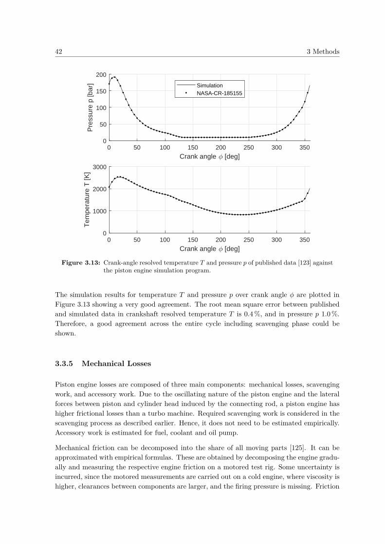
42 3 Methods

0 50 100 150 200 250 300 350

Crank angle [deg]

0

50

100

150

200

Pre

ssur

e p

[bar

] SimulationNASA-CR-185155

0 50 100 150 200 250 300 350

Crank angle [deg]

0

1000

2000

3000

Tem

pera

ture

T [K

]

Figure 3.13: Crank-angle resolved temperature 𝑇 and pressure 𝑝 of published data [123] againstthe piston engine simulation program.

The simulation results for temperature 𝑇 and pressure 𝑝 over crank angle 𝜑 are plotted inFigure 3.13 showing a very good agreement. The root mean square error between publishedand simulated data in crankshaft resolved temperature 𝑇 is 0.4 %, and in pressure 𝑝 1.0 %.Therefore, a good agreement across the entire cycle including scavenging phase could beshown.

3.3.5 Mechanical Losses

Piston engine losses are composed of three main components: mechanical losses, scavengingwork, and accessory work. Due to the oscillating nature of the piston engine and the lateralforces between piston and cylinder head induced by the connecting rod, a piston engine hashigher frictional losses than a turbo machine. Required scavenging work is considered in thescavenging process as described earlier. Hence, it does not need to be estimated empirically.Accessory work is estimated for fuel, coolant and oil pump.

Mechanical friction can be decomposed into the share of all moving parts [125]. It can beapproximated with empirical formulas. These are obtained by decomposing the engine gradu-ally and measuring the respective engine friction on a motored test rig. Some uncertainty isincurred, since the motored measurements are carried out on a cold engine, where viscosity ishigher, clearances between components are larger, and the firing pressure is missing. Friction


is typically expressed as friction mean effective pressure (FMEP), which is the normalisedfriction power 𝑃f according to Eq. (3.64).

FMEP = 2 · 𝑃f𝑉𝑑 · 𝑛

(3.64)

In this thesis, semi-empirical relations from literature are used [125–128], which cover thedominant physical dependencies of mechanical friction. Friction related to the crankshaft con-sists of bearing friction FMEPbear,main in Eq. (3.65) and seal friction FMEPseal in Eq. (3.66).Bearing friction depends on the number of bearings 𝑛b, the rotational speed 𝑛 in units ofrpm, the bearing diameter 𝑑b, the bearing length 𝑙b, the number of cylinders per crankshaft𝑛c. The crankshaft FMEP is then obtained with the proportionality constants 𝑐b and 𝑐s.The bearing dimensions 𝑑b and 𝑙b can be estimated according to Eq. (3.67) [127].

FMEPbear,crank = 𝑐b · 𝑛b · 𝑛0.6 · 𝑑3b · 𝑙b

𝑛c · 𝑑2 · 𝑠(3.65)

FMEPseal = 𝑐s · 𝑑b𝑛c · 𝑑2 · 𝑠

(3.66)

with 𝑐b = 0.202 kPa min0.6

mm 𝑐s = 9.36 × 104 kPa mm2

𝑑b = 0.62 · 𝑏 𝑙b = 0.40 · 𝑏 (3.67)

Piston friction consists of skirt friction, ring friction and gas friction. The latter is caused bythe gas pressure during fired operation. It depends on piston intake pressure 𝑝1 and ambientpressure 𝑝0. The connecting rod bearing dimensions 𝑑b,cr and 𝑙b,cr can be estimated accordingto Eq. (3.72) [127].

FMEPskirt = 𝑐ps · 𝑣mean𝑏

(3.68)

FMEPrings = 𝑐pr ·(

1 + 1 000𝑛

) 1𝑏2 (3.69)

FMEPgas = 𝑐g · 𝑝1𝑝0

·(0.088 · CR + 0.182 · CR1.33−2·𝐾·𝑣mean

)(3.70)

FMEPbear,conrod = 𝑐bc ·𝑛𝑏 · 𝑛 · 𝑑3

b,cr · 𝑙b,cr

𝑛𝑐 · 𝑑2 · 𝑠(3.71)

with 𝑐ps = 0.294 kPa s 𝑐pr = 4.06 × 104 kPa mm2

𝑐g = 6.89 kPa s 𝐾 = 0.0238 smin 𝑐bc = 3.03 × 10−4 kPa min

mm𝑑b,cr = 0.57 · 𝑏 𝑙b,cr = 0.39 · 𝑏 (3.72)

Valvetrain friction consists of camshaft, seal, and valve friction including hydrodynamic andmixed oscillating friction. The relations for valve friction are for flat follower valves and single

44 3 Methods

500 1000 1500 2000 2500 3000 3500

Engine speed [rpm]

0

0.5

1

1.5

2

2.5

FM

EP

[bar

]

Crankshaft

Piston

Valves

Accessories

Fuel pump

Figure 3.14: Stacked contributions to FMEP by various components over engine speed for typ-ical TO conditions.

overhead cams. The relations use the number of camshaft bearings 𝑛𝑐𝑠, the total number ofvalves 𝑛𝑣, and the valve lift 𝑙valve. The dynamic viscosity 𝜇 is assumed to be 10 mPa s likeSAE 10W-30 oil at 90 ∘C [125].

FMEPcamshaft = 𝑐c · 𝑛0.6 · 𝑛𝑐𝑠

𝑛𝑐𝑏2𝑠(3.73)

FMEPseal,camshaft = 1.2 kPa (3.74)

FMEPvalve = 𝑐ff ·(

2 + 105 + 𝜇𝑁

)· 𝑛𝑣

𝑛𝑐𝑠(3.75)

FMEPvalve,osc,hydro = 𝑐oh · 𝑙1.5valve𝑛

0.5𝑛𝑣

𝑏 · 𝑠 · 𝑛𝑐(3.76)

FMEPvalve,osc,mixed = 𝑐om ·(

2 + 105 + 𝜇𝑁

)· 𝑙valve · 𝑛𝑣

𝑛𝑐𝑠(3.77)

with 𝑐c = 6 720 kPa mm3 min0.6 𝑐ff = 200 kPamm

𝑐oh = 0.50 kPa (mm min)0.5 𝑐om = 10.7 kPa

The accessory work includes the fuel feed pump, the common rail pump, the lubrication pumpand the cooling pump. The power required for the fuel pumps was estimated with Eq. (3.78)based on volume flow �� and pressure increment Δ𝑝 [129]. The common rail pressure here is2 500 bar. The work of oil and coolant pump was estimated with Equations (3.79) and (3.80).The resulting loss composition for typical CCE TO conditions and different rotational speedsis illustrated in Figure 3.14. As can be seen, the fuel pump constitutes a major share ofthe losses. The injection pressure should, therefore, be chosen as low as possible, whilemaintaining good combustion efficiency and low smoke numbers.

3.4 Heat Exchanger Modelling 45

(a) (b)

Figure 3.15: (a) Schematic of an intercooled recuperated engine, and (b) MTU profile tube heatexchanger [130].

𝑃access = �� · Δ𝑝 = ��

𝜌· Δ𝑝 (3.78)

FMEPoil = 1.28 kPa + 0.0079 kPa min ·𝑁 − 8.4 × 10−7 kPa min2 ·𝑁2 (3.79)FMEPcoolant = 0.13 kPa + 0.002 kPa min ·𝑁 + 3 × 10−7 kPa min2 ·𝑁2 (3.80)

3.4 Heat Exchanger Modelling

Heat exchangers can be used inside a CCE architecture for intercooling, for dissipation ofpiston engine heat losses, and for recuperation. Heat exchangers add mass, bulk and pressurelosses to the engine, which need to be compensated by improving engine efficiency or byreducing overall engine mass. In this thesis, specifications of heat exchangers as used in theEU-funded Horizon 2020 project Ultra Low emission Technology Innovations for Mid- centuryAircraft Turbine Engines (ULTIMATE) are applied [81]. The assumed pressure losses aresummarised in Table 3.8. For the ducts, a higher loss for recuperators is assumed, becausethe ducting length and number of bends are notably higher as illustrated in Figure 3.15(a).

Table 3.8: Pressure losses in heat exchanger.

Location Pressure loss [%]Hot side 6.0Cold side 5.7Intercooler duct 1.0Recuperator duct 2.0

An important design parameter of heat exchanges is the heat exchanger effectiveness 𝜖, whichdescribes the ratio of transferred heat 𝑄 to maximum transferable heat 𝑄max. 𝜖 is definedaccording to Eq. (3.81). In this thesis, the heat capacity rates on hot side and cold side,𝐶hot and 𝐶cold, are assumed to be equal to achieve minimum heat exchanger losses [131]. Inthat case, the equation for heat exchanger effectiveness simplifies to a ratio of temperature

46 3 Methods

differences according to Eq. (3.82). Other ratios may be beneficial to optimise on overallengine level or when available space is constrained.

𝜖 = 𝑄

𝑄max(3.81)

= 𝑇1,hot − 𝑇2,hot𝑇1,hot − 𝑇1,cold

, if 𝐶hot = 𝐶cold (3.82)

𝐶 = 𝑐𝑝 · �� (3.83)

Two strategies for increasing 𝜖 are possible: Either the heat exchanger size is increased,while the pressure losses are kept constant, or pressure losses are increased – for example byincreasing flow velocity or by using turbulators – to keep heat exchanger size constant. In thisthesis, the first approach is pursued, since pressure losses are typically more dominant thanheat exchanger mass with respect to fuel burn. Heat exchanger size is assumed to scale withnumber of transfer units NTU according to Eq. (3.84), with the heat transfer coefficient 𝑘 andthe heat exchange area 𝐴. The relation in Eq. (3.85) is derived from a cross-flow lancet heatexchanger for engine application [99] as illustrated in Figure 3.15(b). With a fully resolvedheat exchanger model, other optima may be found.

NTU = 𝑘 ·𝐴𝐶

(3.84)

= 0.9 · 𝜖0.882 − 𝜖

(3.85)

Heat exchanger mass was assumed to be proportional to NTU, in accordance with [99]. Theequations for matrix and ducting mass are summarised in Equations (3.86) to (3.89) forintercooler (IC) and recuperators (REC) [81].

𝑚mat,IC = 3.2 s · ��IC · 𝜖

0.882 − 𝜖(3.86)

𝑚mat,REC = 9.0 s · ��IC · 𝜖

0.882 − 𝜖(3.87)

𝑚duct,IC = 0.2 ·𝑚mat,REC(𝜖 = 0.75) (3.88)𝑚duct,REC = 0.8 ·𝑚mat,REC(𝜖 = 0.75) (3.89)

For off-design, the heat exchanger effectiveness is assumed to increase linearly with reductionin mass flow according to Eq. (3.90) [92], because the lower mass flow still has the samesurface area for heat exchange. The pressure loss was assumed to scale with the square ofthe corrected mass flow on both sides.

3.5 Flow Path Generation 47

(a) (b)

Figure 3.16: Important geometric ratios on (a) turbo components, and (b) ducts.

Table 3.9: Summary of geometric properties of turbo components.

Component AR1 AR2 GR1 GR1 TR1 TR2 HTR1 HTR2 𝑀1 𝑀2

Fan 2.6 – 0.25 – 0.88 – 0.30 – 0.68 0.48IPC 3.0 1.9 0.30 0.30 0.75 0.85 0.65 0.73 0.33 0.25HPC 3.1 1.5 0.30 0.30 0.50 0.90 0.49 0.90 0.27 0.12HPT 2.0 1.8 0.40 0.40 0.90 0.75 0.79 0.76 0.07 0.32LPT 2.5 2.5 0.35 0.35 0.90 0.80 0.74 0.60 0.15 0.45

𝜖 = 1 − ��

��des· (1 − 𝜖des) (3.90)

Δ𝑝 = 1 −��2

corr,std��2

corr,std,des· (1 − Δ𝑝des) (3.91)

3.5 Flow Path Generation

The generation of the flow path layout is a prerequisite for estimating engine size and todetermine, whether all components foreseen can be placed into the core cowling. The sizesare additionally used in this thesis for component mass estimations.

Turbo component cross-sectional areas are obtained via Eq. (3.10) with prescribed typicalaxial Mach numbers 𝑀 [95]. Turbo component sizes were generated on a stage resolved levelwith typical hub-to-tip ratios HTR, gap ratios GR, aspect ratios AR, and taper ratios TR asillustrated in Figure 3.16(a). The values were derived from a PW1100G general arrangementdrawing [132] in conjunction with an approximate performance simulation of the engine. Theresults are summarised in Table 3.9. Axial flow Mach numbers 𝑀 were determined with theflow path cross-sections and mass flow rates from the engine simulation. Radial compressorgeometry is based on empirical relations [133].

Duct geometry was derived from general arrangement drawings of contemporary aero engines.Its axial length 𝑙d was correlated with the relative mean radius reduction as illustrated in

48 3 Methods

-0.5 0 0.5 1 1.5 2 2.5 3 3.50

0.2

0.4

0.6

0.8

1

1.2

Figure 3.17: Flow path visualisation (blue solid lines) over a PW1100G general arrangementdrawing [132].

Figure 3.16(b). The regressions are separated for compressor intake duct in Eq. (3.92) andducts between turbo components in Eq. (3.93). The bypass nozzle is assumed to have anopening angle of 12°, and the core nozzle of 20°.

𝑙d,compressor intake𝑟1,m

= 3.3 − 3.0 · 𝑟2,m𝑟1,m

(3.92)

𝑙d,inter turbo𝑟1,m

= 1.79 − 1.64 · min(𝑟2,m𝑟1,m

; 𝑟1,m𝑟2,m

)(3.93)

(3.94)

The general arrangement is then obtained by sequential positioning of all components. Theirboundary coordinates are propagated to the adjacent component. An overlay of the resultover the PW1100G engine general arrangement in Figure 3.17 shows the validity of theapproach.

Piston engine dimensions were obtained in a bottom-up manner as well [129]. Piston, cylinderhead, cylinder liner and casing sizes were approximated based on high-performance motors,mainly from [134]. The relevant set-up and dimensions are illustrated in Figure 3.18 (p. 49)based on piston bore 𝑑. Cylinder liner thickness is proportional to piston power, with areference nominal power of 520 kW.

3.6 Mass Estimation

For engine mass estimation, many semi-empirical approaches are available [135–137]. Thedisadvantage of such approaches is that they are based on established engine architectures.The CCE architecture is significantly different from a turbofan architecture. Therefore, acomponent-based bottom-up approach was pursued. This ensures that conceptual decisionsare represented physically correct in the engine mass.

3.6 Mass Estimation 49

Figure 3.18: Cross-section of a high-performance piston [134] with derived basic geometric re-lations for other piston components.

1 1.5 2 2.5 3 3.5

Fan diameter [m]

0

500

1000

1500

2000

2500

3000

Fan

wei

ght [

kg]

Data points from [Greitzer, 2010]

Fit R2 = 0.97

Figure 3.19: Fan mass estimates [138] and regression (solid line).

Fan mass is estimated based on fan diameter. A regression on existing mass estimationsfrom [138] is shown in Eq. (3.95) and Figure 3.19. The data points feature both titaniumand composite material fans.

Fan drive gear system (FDGS) mass is evaluated as a function of gear ratio and torque [139,140]. Eq. (3.96) uses the power on the low-pressure spool (LPS) during TO conditions, therotational speeds 𝑛1 of LPS and 𝑛2 of the fan. A refined mass estimation can be achievedwith a component build-up method [141], but was not used here.

50 3 Methods

𝑚fan = 196 kg · 𝑑2.06fan (3.95)

𝑚GB = −16.98 kg + 0.01715 kg ·(𝑃GB𝑛2

)0.75·(𝑛1𝑛2

)0.15(3.96)

The masses of the turbo components, i.e. compressors and turbines, are estimated via thevolume of their flow paths. Their volume is assumed to be proportional to their mass. Thevolume is obtained via triangulation of the flow path coordinates, which were calculated asdescribed in Section 3.5. The volume is then multiplied with the density of the material of therespective stage. For compressors, titanium alloy is assumed with a density of 4 450 kg/m3

and a cut-off temperature of 650 K at TO conditions [142]. Beyond that temperature, nickelalloy with a density of 7 900 kg/m3 is used. Nickel alloy is used in the turbines, too. In theLPT, titanium aluminide (TiAl) with a density of 3 900 kg/m3 is used below 1 000 K.

The obtained turbo component mass needs to be adapted for stage solidity, disks, and casings.The final form of the turbo component mass estimation is shown in Eq. (3.97) with thecalibration constant 𝑐. High pressure components exhibit a higher volume-specific mass thanlow pressure components due to higher stage aspect ratios, higher disk masses, and sturdiercasings. Turbines have a higher volume-specific mass than compressors due to higher stagesolidity and heavier disks. In consequence, the calibration constants shown in Eq. (3.98) weredetermined. Additionally, the area-averaged mean circumferential speed 𝑣𝑚 was taken intoconsideration [143]. The exponent 𝑒 is 0.5 for compressors and 0.6 for turbines. Shaft massesare included in the turbines.

𝑚 = 𝑐 · 𝜌 · 𝑉 ·(

𝑣𝑚

350 m/s

)𝑒

(3.97)

𝑐IPC = 0.35 𝑐HPC = 1.0 𝑐HPT = 1.4 𝑐LPT = 0.8 (3.98)

Combustion chamber mass is proportional to mean combustor diameter 𝑑m according toEq. (3.99) [143]. Accessories – such as engine anti-icing, fire extinguishing, aircraft/engineinterface, and ventilation – and the accessory gearbox with starter, generator and hydraulicpumps are scaled linearly to ToC sizing thrust 𝐹N,ToC as suggested by [143]. Residual enginemasses for systems (electrical, oil, air, etc.) and dressings (sensors, fuel heat exchanger,fairings, mountings, etc.) are assumed to contribute a fixed share of 15 % of the engine massas suggested by [143], and based on empirical data of modern turbofan engines [144].

3.6 Mass Estimation 51

𝑚combustor = 196 kgm2 · 𝑑2

m (3.99)

with 𝑑m = 12 (𝑑m,HPC,2 + 𝑑m,HPT,1) (3.100)

𝑚accessories = 5 kgkN · 𝐹N,ToC (3.101)

𝑚residual = 0.15 ·𝑚engine (3.102)

Nacelle mass is modelled according to semi-empirical relations based on wetted area withnacelle length 𝑙Nacelle and diameter 𝑑Nacelle shown in Eq. (3.103) [145]. The dimensions werecorrelated from general arrangement drawings of contemporary aero engines. A correctionfactor of 0.70 was applied to adapt for high BPR engines. While reference [145] suggestsdoubling wetted area, only the single wetted area was considered as thrust reverser masswas modelled separately. The latter scales linearly with TO thrust 𝐹N,TO based on datafrom [144]. Masses of core cowling, bypass nozzle and core nozzle are estimated in accordancewith Eq. (3.103) with the respective dimensions but without the correction factor 0.70.

𝑚Nacelle = 0.70 ·24.88 kgm2 · 𝑙Nacelle · 𝜋𝑑Nacelle (3.103)

with 𝑑Nacelle = 1.056 𝑑fan + 0.41 m (3.104)and 𝑙Nacelle = 1.7 · 𝑑fan (3.105)

𝑚thrust rev = 3.37 kgkN · 𝐹N,TO (3.106)

The complete structure of the engine and power plant system (PPS) mass estimation issummarised in Table 3.10 (p. 52) based on the suggested breakdown in [144]. The methodwas validated with a simulation model of the PW1100G engine. The result was comparedto the type-certificate data sheet (TCDS) engine mass [146]. Pylon mass is included in theaircraft control balance.

The mass estimation of the piston system is crucial for the accurate evaluation of the CCEconcept, since the added mass constitutes one of its main drawbacks. One option is to use atop-down approach based on empirical data collected from series, experimental and conceptpiston engines. Valuable approximations for piston system mass can be derived from thedata and the dominating parameters can be identified [23, 129]. As a major drawback of thisapproach, the masses are specified for entire engine systems, including accessories for water,fuel and oil, gearing, output shaft with flange, and potentially a turbocharger. Therefore,top-down mass estimations tend to overestimate the base piston system mass. Moreover, theestimation for piston systems with very different operating conditions requires extrapolationfrom available data, which incurs further uncertainty. Sensitivities for individual mass itemswould not be physically appropriate.

52 3 Methods

Table 3.10: Structure of engine masses and validation values.

Component Method PW1100Gmodel [kg]

TCDS[kg]

Fan, incl. fan cas-ing and intermediatecasing

Regression on data [138] de-pendent on fan diameter

851

FDGS, incl. lubrica-tion system

Relation [140] dependent ontorque and gear ratio

309

Turbo components Based on volume and speed- IPC 140- HPC 266- HPT 178- LPT 492

Combustor Regression on data [144] 77Systems & Dressings 15 % of engine mass 431Accessories Prop. to ToC thrust 132Engine Sum of above 2 875 2 858

(-0.6 %)

Nacelle, incl. in-take, external fair-ings, acoustic linings

Prop. to wetted area [145] 498

Thrust reverser Prop. to TO thrust 496Core cowl Prop. to wetted area [145] 64Bypass nozzle Prop. to wetted area [145] 86Core nozzle Prop. to wetted area [145] 19PPS Engine mass + sum of above 4 038

Therefore, a component-based bottom-up mass modelling was pursued. The mass-drivingcomponents were modelled, in particular cylinder liner, cylinder head, casing, piston, con-necting rod, crankshaft and valvetrain. The piston is divided into piston head with a solidityof 80 % and the skirt with a solidity of 30 % as indicated in Figure 3.18. Piston bore andstroke are equal. The connecting rod between piston and crankshaft is 1.7 times as long asthe stroke, based on best practice [147]. Connecting rod cross-sectional area is sized to receivethe peak load with a safety factor of 3.0. The crankshaft has a baseline diameter of 0.19 m,and is scaled with torque 𝑇 1/3. Mass of the above-mentioned parts is obtained via theirvolume and an assumed material. Most piston parts (cylinder liner and head, connectingrod, crankshaft, camshaft) are steel-based alloys with a density of 7 730 kg/m3. The pistonsare assumed to be made of TiAl, which has appealing properties for reciprocating parts witha low density of 3 900 kg/m3, high-temperature capability and good oxidation resistance [148,149]. The use of TiAl for valves, connecting rods and piston pins has been successfully tested,but it was not used for pistons before. It is used in the aeronautical industry for light-weighthigh-temperature parts, in particular LPTs. The motor block is assumed to be made from

3.7 Aircraft Level Assessment 53

magnesium alloy due to its low density of 1 800 kg/m3. Magnesium alloys for casings areproven technology in the automotive industry and in aviation [150].

The valves are actuated with camshafts with an assumed shaft diameter of 50 mm. Massesof bearings, injectors, and common rail fuel pump are estimated by scaling masses of knowncomponents with diameter or power. Masses of other minor items such as crankshaft casingand back plate, valves, ducts and piston rings are not specifically modelled and consideredto be included in the overall piston engine mass. The results from the bottom-up estimationwere developed and verified in a master’s thesis [129]. They showed very good agreementwith estimations from a top-down approach based on empirical data, which by itself had amean error of 10 % with an empirical database.

3.7 Aircraft Level Assessment

Novel engine concepts have three major impacts at the aircraft level. First, an improvementin engine efficiency reduces required fuel aboard the aircraft for a given mission. As a result,MTOW reduces, and wing area and aircraft structural mass can be reduced at constantwing loading. Second, additional PPS mass requires more thrust as well as a sturdier pylonand wing structure [17] with similar cascading effects mentioned above. Third, a larger fandiameter increases nacelle drag and possibly landing gear weight to maintain a given groundclearance. The last impact is not relevant in this thesis, because fan diameter is kept constant.The fan diameter was optimised for the application, and no major deviation due to the CCEis expected. Thus, simulation complexity was reduced.

To take full account of these cascading effects, a fully resizable short-to-medium range aircraft(180 passengers, design range 2 850 nmi) is used. The aircraft was sized in the commercialaircraft design platform Pacelab APD [151]. The aircraft represents a technological standardof an entry into service year 2035. The aircraft subsystem architecture is all-electric (AE),i.e. all aircraft subsystems are driven electrically, and no bleed off-takes are taken from theengine. The customer bleed, particularly cabin air and anti-icing, are provided externallywith auxiliary compressors and electric heating. This requires a higher, mission averagedpower off-take of 184 kW per engine.

The resulting impact at the aircraft level was evaluated for mission fuel burn, operatingempty weight (OEW) and MTOW for several combinations of engine TSFC improvementand change in PPS mass. The results are provided in the simulation environment as griddeddata and spline interpolation is used to get the aircraft impact. At each mission point, therequired thrust in all simulated mission points can be obtained. Trade factors (sometimesreferred to as exchange factors) can be used to map changes in TSFC and PPS mass 𝑚PPS onchanges in mission fuel burn (FB). The change in 𝑚PPS is nearly linear in fuel burn as shownin past studies [152]. Thus, a linearised trade factor can be used as shown in Eq. (3.107). ForTSFC, a parabolic relation can be used as shown in Eq. (3.108). Cascading effects abate withincreasing improvements, since the mass share of fuel in the aircraft reduces progressively.The linearised equations show the trade between PPS weight and TSFC. An improvement in

54 3 Methods

10 11 12 13 14 15 16

Cruise TSFC [g/kN/s]

3000

4000

5000

6000T

otal

eng

ine

mas

s [k

g]

-0.35

-0.3

-0.25

-0.2

-0.15

-0.1

-0.05 0

0.050.1

22

23

23

24

24

25

25

26

27 SR

IA 2035

SR

IA 2050

SRIA

2020

Fuel Burn vs Y2015Sizing Thrust F

N [kN]

Y2015 Ref. GTF

Figure 3.20: Iso-contours of change in fuel burn depending on TSFC and total engine mass𝑚PPS on a year 2035 short-to-mid range aircraft. Red lines indicate engine-relatedemission reduction targets.

TSFC by 1 % allows a 290 kg higher PPS mass for equal fuel burn. A linearisation of relativechange in sizing thrust is displayed in Eq. (3.110).

ΔFB𝑚,PPS = 1 %201 kg · Δ𝑚PPS = 0.498 %

100 kg · Δ𝑚PPS (3.107)

ΔFBTSFC = 1.443 · ΔTSFC + 0.930 · ΔTSFC2 (3.108)ΔFB = (1 + ΔFB𝑚,PPS) · (1 + ΔFBTSFC) − 1 (3.109)

Δ𝐹N,ToC = 0.425 · ΔTSFC + 0.490 %100 kg · Δ𝑚PPS (3.110)

The resulting iso-contour plots on the tabulated data are illustrated in Figure 3.207. Theengine-related SRIA 2020 goals are achieved with a moderate TSFC improvement by 3.6 %against the present technological standard, if engine mass remains constant. The SRIA 2035targets require a weight-neutral TSFC improvement by 13.3 %. Achieving SRIA 2050 targetsrequires a very significant, weight-neutral leap by 27.0 %.

3.8 Instationary Operation

3.8.1 Impact of Pulsating Flow on Turbo Components

The instationary operation of piston engines imposes pulsating flow conditions on the adjacentturbo components. The IPC is subject to pulsating outlet conditions, and the HPT topulsating inlet conditions. The secondary combustor operation may be impaired by pulsatingflow conditions, affecting fuel atomisation. This could potentially lead to thermo-acousticvibrations through resonant response of the heat release rate.

7The power plant mass is reduced compared to the PW1100G model mass presented in Section 3.6 as theadvanced aircraft platform requires less sizing thrust

3.8 Instationary Operation 55

Investigations of the impact of pulsating flow on turbine efficiency revealed a dependencyon pulsation frequency 𝑓pulse and amplitude Δ𝑝/𝑝 [153]. Higher amplitudes lead to an al-most linear increase in losses. For a pulsation frequency of 2 500 Hz in a two-stage turbine,isentropic efficiency drops by 0.33 % for an amplitude of 2.5 % of the total pressure, and upto 1.05 % for an amplitude of 7.5 %. The pulsation frequency in the CCE is of the order of500 Hz. Higher frequency increases losses in an almost linear relation as the pressure gradientincreases for a given amplitude. The losses mainly occur in the first stage of the turbine.After the first stage, oscillation amplitude is reduced to a third. For simplification, it isassumed that the entire loss is created in the first stage. The concluding relation used withinthis thesis is shown in Eq. (3.111).

For the IPC, pulsating exit conditions impair efficiency and blade vibrations [154]. Again,both amplitude and frequency were found to play an important role in the magnitude ofefficiency losses. The relation with respect to amplitude is approximated as a quadraticfunction as shown in Eq. (3.112) with 𝑅2 = 0.998. An amplitude of 20 % of the total pressure𝑝 results in a 6 % efficiency loss in the last stage, when the pulsation frequency is much largerthan the blade passing frequency. When blade passing frequency in the compressor is similarto the pulsation frequency 𝑓 losses are minimal with a loss of 4 % per 20 % amplitude.

Δ𝜂is,HPT = 13.4 % · Δ𝑝𝑝

· 2𝑛stages

· 𝑓pulse2 500 Hz (3.111)

Δ𝜂is,IPC = 150 % ·(Δ𝑝𝑝

)2· 1𝑛stages

(3.112)

Buffering volumes before and after the piston engine are foreseen to reduce the oscillationsseen by the turbo components, and thus efficiency losses. The buffering volumes are sizedto keep the loss in the full component below 0.05 % and, thus, negligible. Reducing thepulsations helps to prevent high cycle fatigue in the blade roots due to vibrations [154].Additional volumes that contribute to buffering – such as ducting, the combustor and itsannulus – may further reduce the oscillations seen by the turbo components, but they areneglected for sizing.

The volume is approximated with simple estimations. The pistons on one shaft are as-sumed to be equally phase shifted. The resulting pulsation frequency 𝑓pulse is calculated withEq. (3.113). It is assumed that the mass change peak-to-peak in the buffering volume 2 · Δ𝑚is equal to the mass inducted during one cycle according to Eq. (3.114). This is a conser-vative assumption, since valve opening times overlap, which leads to lower mass oscillations.Buffering volume 𝑉buff is then derived according to the ideal gas law with Eq. (3.115), wherethe permissible pressure oscillation Δ𝑝 was determined with Eq. (3.111) or Eq. (3.112).

56 3 Methods

Figure 3.21: Schematic illustration of the two engine mountings [155].

𝑓pulse = 𝑛cyl · 𝑓2 (3.113)

Δ𝑚 = ��

2 · 𝑛cyl · 𝑓(3.114)

𝑉buff = Δ𝑚𝑅𝑇2Δ𝑝 (3.115)

3.8.2 Mechanical Oscillation

Mechanical oscillations in piston engines are a result of their oscillatory mode of operation.Here, only a first consideration of the dynamic loads imposed by pistons and connecting rodsis presented, in order to judge the extent of forces and moments within the piston engineassembly.

The engine mounting is illustrated in Figure 3.21. The front mount takes the axial loads– mainly the thrust – of the engine. The rear mount carries transversal forces and torque.Other moments are carried by both mounts [155]. In some engines the thrust loads aretransferred directly to the rear mount via thrust links, when space is confined. The forwardengine mount is then attached to the fan casing. The piston engine should be mounted closeto the forward mount to reduce the impact on the remaining engine. Otherwise, detrimentaleffects on tip clearances and surge margins may occur.

In the concept used in this thesis, which will be presented later in greater detail, two V-typepiston engines are used, which are arranged around the engine axes. The piston enginesare synchronised through gearing, which allows balancing forces between both engines. Itis assumed that the piston engines are mounted to a separate, rigid frame, so all forces andmoments can be first equalised between the two engines. This frame is then connected to theengine mounting, which receives the remaining forces. One engine is installed on the top ofthe core engine with hanging pistons. The other engine is mounted on the bottom with its

3.9 Emissions 57

pistons facing upwards. This mirrored arrangement allows always having two pistons movingin exactly opposing direction. Thus, all net forces are balanced. This does not balance allmoments created by pistons, however. On the crankshaft, for each rod bearing journal acounterweight can be applied to reduce the net force of the moving piston. Additionally,two balance weights on front and rear of the shaft can be applied to counteract momentscreated by shaft, con rod and pistons. Their masses and eccentricities are two degrees offreedom for balancing. The remaining third moment can be fully extinguished with furthermeans such as balance shafts or moment balancing gears [147]. Generally, more pistons makebalancing easier. On a V10-engine for example, all forces and moments of first order can beequalised and the second order moment is small [156]. Therefore, mechanical oscillations arenot further evaluated. The potentially required added mass and space may, however, implydetrimental impact on fuel burn of unknown magnitude. Also, it may be required to balanceeach piston engine separately, if the frame cannot be built rigidly enough with reasonableeffort.

3.9 Emissions

Aircraft emissions regulations are a major driver for technological developments. CO2 andNOx emissions will be quantified as they are important for fuel saving evaluation and forcertification. Apart from these, noise and other emissions, and how they may change incontrast to a turbofan are discussed in this chapter qualitatively.

3.9.1 CO2 Emissions

Assuming usage of kerosene as fuel, CO2 emissions are directly proportional to fuel burn asshown in Reaction (3.4). The assessment of fuel burn is described in Section 3.7. Emissionsof CO2 are regulated due to their radiative forcing impact on climate warming. AviationCO2 accounted for a total of 2 % of the total anthropogenic emissions in 1992, about 2.5 %in 2005 [157], and is projected to increase to at least 3 % by 2050 [158]. It is predicted toincrease by a factor of 2.4 to 3.6 compared to the year 2005 [157]. The SRIA specifies targetsof -36 %, -51 % and -68 % for the years 2020, 2035 and 2050 respectively against year 2000certification standard per passenger and kilometre on aircraft level (not including air trafficmanagement, infrastructure and operational improvements). For the propulsion system only,targets of -20 %, -30 % and -43 %8 are targeted. Global aviation CO2 emissions are subject tothe Air Transport Action Group (ATAG) goals [159]. These foresee a carbon-neutral growthfrom 2020 onwards, and a 50 % reduction by 2050 compared with year 2005 global emissionsfrom aviation. These targets should be achieved by improvements in technology and air trafficmanagement, but also market-based measures such as carbon off-setting and biofuels. TheATAG goals are not further discussed in this thesis, as market trends are out of the scope.

8Assuming equal split between airframe and propulsion system.

58 3 Methods

10 20 30 40 50 60 70 80 90

OPR [-]

0

20

40

60

80

100

120

140

160

NO

x Em

issi

on L

evel

Dp [g

/kN

]

LEMCOTEC RTFLEMCOTEC MOR

LEMCOTEC LTF

CFM56-5C4

PW1133GLEAP-1A35

GE90-94B

GEnx-1B76

V2533-A5Trent XWB-97

CAEP/6SRIA 2020 (CAEP/6 - 60%)SRIA 2035 (CAEP/6 - 65%)SRIA 2050 (CAEP/6 - 75%)(all for T

SLS > 89 kN)

Figure 3.22: Limits of NOx emissions in the LTO cycle with future SRIA reduction targets,and some current in-service and projected aircraft engines.

3.9.2 NOx Emissions

Nitrogen oxide (NO) and nitrogen dioxide (NO2) are environmentally harmful trace gases [158].They impair local air quality around airports. They lead to respiratory disorders. Moreover,NOx promotes ground-level ozone, which is a pulmonary irritant [160]. Aviation can contrib-ute as much as 5 % of the NOx in proximity of large airports [161]. Hence, they are subjectto emission reduction agendas. Altitude NOx has an impact on radiative forcing indirectlyvia other species as described in Section 3.9.4.

The SRIA [1] specifies targets of -60 %, -65 % and -75 % for the years 2020, 2035 and 2050 re-spectively in the landing and take-off (LTO) cycle against the year 2008 certification standardper kg of fuel burnt (CAEP/6, [162]). The targets are shown in Figure 3.22 with relevant ref-erence engines. They are dependent on engine thrust and OPR, where higher thrust-specificNOx emissions in the LTO cycle are permitted if OPR is increased. This promotes higherefficiency engines by allowing for a trade-off between CO2 and NOx emissions.

This target is supported by shortfall of emissions during taxiing through emission-free taxiingby the year 2050, which may be achieved by infrastructure measures such as electric towingvehicles or with electric taxiing with the fan as proposed by [152]. Moreover, high altitudeNOx has an impact on ozone chemistry, leading to increased ozone production. Targetsof -80 %, -84 % and -90 % for the years 2020, 2035 and 2050 respectively during cruise perpassenger kilometre against a year 2000 technological standard have been specified9. Globalin-flight NOx emissions on international flights are expected to increase by a factor between2.2 and 3.0 from 2010 to 2040 [161]. A similar relative increase in LTO cycle emissions ispredicted.

9This translates into -75 %, -77 % and -78 % per kilogram fuel burnt, respectively, assuming the targetedimprovements in combined engine and airframe efficiency will be met. In consequence, cruise emission indexNOx (EINOx) is allowed to stay almost constant from 2020 onwards.

3.9 Emissions 59

For the estimation of NOx emissions in conventional gas turbine engines, well established semi-empirical relations are available. The CCE concept requires additional effort: In the pistonengine, the gas turbine relations cannot be used, because the process is highly instationary.While peak temperatures and pressures are higher than in a gas turbine combustor, residencetimes at these conditions are much shorter. In the secondary combustor, these relations needto be corrected for the reduced oxygen content due to the preceding piston engine. SuitableNOx emissions models for both are presented in the following.

Piston Engine

Several chemical pathways exist to form NO from the contents of the combustion gases. Themost commonly considered and predominant pathway is the Zeldovich mechanism, whichresults in the creation of Thermal NO. It consists of Reactions (3.116)-(3.118). In conventionaldiesel engines, it generates approximately 95 % of NOx [163].

N2 + O𝑘1� NO + N (3.116)

N + O2𝑘2� NO + O (3.117)

N + OH𝑘3� NO + H (3.118)

Under fuel rich conditions with relevant amounts of CH in the flame, the prompt NO mech-anism is important. The two dominant pathways are the Fenimore pathway in Reaction(3.119) and the Moskaleva in Reaction (3.120) [164, 165]. Under high pressure conditions,the N2O mechanism becomes important as shown in Reaction (3.121) and (3.122). Since thefirst reaction requires a third arbitrary agent M, the reaction rates grow faster than thoseof other pathways at high density. A fourth, more recently discovered pathway is the NNHmechanism shown in Reaction (3.123) [166]. It requires three agents for the initial reactionbut is not very well understood, yet. A fifth source is fuel NO, which is created, when thefuel contains nitrogen. In kerosene, nitrogen concentrations are negligible [164].

N2 + CH → HCN + N → . . . → NO (3.119)N2 + CH → NCN + H → . . . → NO (3.120)

N2 + H + M → N2O + M (3.121)N2O + O → 2NO (3.122)

N2 + H + M → NNH + M → . . . → NO (3.123)

In this thesis, only the Zeldovich pathway is considered. The prompt NO pathway is notrelevant, since fuel rich conditions are avoided for fuel efficiency. Because most publicationsfor simulation only consider this pathway, a calibration to these simulation results is most

60 3 Methods

Figure 3.23: Schematic illustration of the relations of the zones of the 2-zone model [105].

accurate. Further pathways are implicitly included in this way. This approach introduces asystematic error, when other NOx creation pathways grow more than the Zeldovich mech-anism in the CCE operating conditions in comparison to the reference conditions used formodel calibration. This could be the case for the N2O and NNH pathways, since they becomerelevant under high pressure conditions.

NOx generation is highly dependent on fluid state. Therefore, it is time- and space-dependentin the piston engine. Time-resolved mean cylinder temperature and pressure are availablefrom the 0D simulation model presented in Section 3.3. NOx is produced in the combustionzones in the cylinder, where the temperatures are highest. The NOx generation is assumed tobe fully decoupled from combustion [167], i.e. the chemical reactions of the NOx generationprocess occur after the combustion reactions are complete. This assumption is justified asthe combustion reactions are fast enough and, hence, the combustion reaction zone and timeis small in relation to the NOx generating process. It allows to execute the performancesimulation first, and run the NOx simulation subsequently.

The simplest model with a spatial resolution is the 2-zone model [105, 168, 169]. Here, thefluid is divided into a fresh air zone and a zone that contains the fluid after combustion tookplace. A third, non-resolved zone is the flame front, which is assumed to be negligibly small.The relation of the zones is displayed in Figure 3.23.

NOx is assumed to be produced only in the combustion zone, Zone 2. Its generation issimulated with reaction kinetics, i.e. with the chemical non-equilibrium generation rates [170].The reaction rate for NO according to Reactions (3.116)-(3.118) is shown in Equation (3.124).The reaction rate is dependent on the reactant concentrations, and the reaction rates for theforward reaction 𝑘f and the reverse reaction 𝑘r. The reaction rates can be obtained fromrespective databases. In this thesis, the rates have been obtained from CHEMKIN 3.0 [171],and are displayed in Equations (3.125)-(3.127) for the Zeldovich mechanism.

3.9 Emissions 61

d[NO]d𝑡 = 𝑘1,f [N2][O] − 𝑘1,r[NO][N] (3.124)

+𝑘2,f [N][O2] − 𝑘2,r[NO][O]+𝑘3,f [N][OH] − 𝑘3,r[NO][H]

𝑘1,r = 2.70 × 107 m3

mol s · exp(

−355 cal/mol𝑅𝑚𝑇

)(3.125)

𝑘2,f = 9.00 × 103 m3

mol s · 𝑇 · exp(

−6 500 cal/mol𝑅𝑚𝑇

)(3.126)

𝑘3,f = 3.36 × 107 m3

mol s · exp(

−385 cal/mol𝑅𝑚𝑇

)(3.127)

They typically follow the form of the Arrhenius equation 𝐴 · exp (−𝐸0/(𝑅𝑚𝑇 )), where 𝐴 isa constant, 𝐸0 is the reaction’s activation energy, 𝑅𝑚 = 1.987 cal/mol/K is the universal gasconstant and 𝑇 the reaction temperature [170]. Hence, reaction rates increase exponentiallywith temperature and quadratically with pressure, since concentration increases with density.This shows why NOx is generated particularly at high temperatures and pressures. Thecorresponding reaction coefficients 𝑘1,f , 𝑘2,r and 𝑘3,r are not specified in CHEMKIN 3.0 [171],but can be obtained via the equilibrium constant 𝐾𝑐 with

𝐾𝑐 = 𝑘f𝑘r

(3.128)

𝐾𝑐 expresses the ratio of concentrations of reactants and products [171], at which forwardand reverse reactions are in equilibrium:

𝐾𝑐 = 𝐾 ·(𝑝std𝑅𝑚𝑇

)Δ𝜈

(3.129)

with 𝐾 = exp(𝑛species∑

𝑖

𝐺std,i

)(3.130)

and 𝐺std,𝑖 = 𝜈𝑖 · (𝑆std,𝑖 −𝐻std,𝑖) (3.131)

and Δ𝜈 =𝑛species∑

𝑖

𝜈𝑖 (3.132)

Here, the standard molar entropy 𝑆std,𝑖 and the standard molar enthalpy 𝐻std,𝑖 can be ob-tained with the NASA nine-term polynomials for the respective temperature 𝑇 for arbitraryspecies as described in Section 3.1. These are used to calculate the standard molar Gibbsenergy 𝐺std,𝑖. The mole number 𝜈 indicates the number of the species in the reaction, withreactants being negative and products being positive. The change in mole number Δ𝜈 is thesum of all mole numbers. Δ𝜈 is positive for reactions with a growing number of molecules.A reaction with Δ𝜈 = 0 is independent from pressure. As can be seen, 𝐾𝑐 can be calculatedwithout the knowledge of the reaction coefficients 𝑘. The correct calculation of the equilib-

62 3 Methods

rium constant has been verified with published data of both forward and reverse reactioncoefficients. An example is shown in Figure A.1 (p. 145) in Appendix A.3.

For calculation of the NOx generation rates, the concentrations of species N, O and OH mustbe known in zone 2. To this end, the OHC-System can be employed according to Eq. (3.133)-(3.137) [105]. These reactions are fast enough in comparison to the Zeldovich mechanism,so that they can always be assumed to be in equilibrium in zone 2. This is referred to asquasi-steady state approximation [164].

H2 � 2H (3.133)O2 � 2O (3.134)

H2O �12H2 + OH (3.135)

H2O �12O2 + H2 (3.136)

CO2 � CO + 12O2 (3.137)

Additionally, the three atomic balances for C, O and H must be satisfied, giving a total ofeight conditions. This allows to solve for the concentrations of the eight species CO2, H2O,CO, OH, H2, H, O2, and O. The implementation of the model has been validated againstother publications [115, 172]10. The validation quality of the implemented model is illustratedin Figure A.2 (p. 145) in Appendix A.3.

The simulation starts when valves close. It integrates the NOx generation in time accordingto Eq. (3.124). No distinction between the two zones is made until combustion starts. Thisprovides the initial conditions. At that point, zone 2 is initiated. The air ratio 𝜆0 is definedaccording to Eq. (3.138), and held constant in zone 2. Thus, the mass in zone 2 𝑚2 can becalculated with Eq. (3.139). Therefore, 𝑚2 is prescribed by the rate of heat release accordingto the Wiebe function as given in Eq. (3.53). The difference between the fuel mass 𝑚f andthe initial fuel mass 𝑚f,0 constitutes the injected fuel. The residual fuel from the previouscycle remains evenly distributed over both zones with fuel-air ratio FAR1.

𝜆0 = FARstoichFAR2

(3.138)

𝑚2 = (1 + 1FAR2 − FAR1

) · (𝑚f −𝑚f,0) (3.139)

The initial temperature difference between both zones 𝐴* is an empirical value specific to anengine. Due to lack of comparable engines for calibration of 𝐴*, the value is defined relative tothe increase in temperature due to combustion with air ratio 𝜆0 at SOC as in Eq. (3.140). The

10As a caveat, the concentrations of atomic nitrogen N displayed in [115] are two orders of magnitude toolow.

3.9 Emissions 63

200 250 300 350 400 450 500

Crank angle [deg]

0

1000

2000

3000

Tem

pera

ture

T [K

]

SOC

TZone 2

TZone 1

Tmean

(a)

200 250 300 350 400 450 500

Crank angle [deg]

0

0.005

0.01

0.015

0.02

Mas

s m

[kg]

SOC

mZone 2

mZone 1

m

(b)

Figure 3.24: Qualitative scope of (a) temperature and (b) mass in both zones of the 2-zone-model in contrast to mean values.

flame temperature 𝑇fl is estimated by assuming a stoichiometric gas composition. The phase-resolved temperature difference between both zones is then adapted empirically according toEq. (3.141). In this equation, the pressure of the motored engine 𝑝0 is calculated by assumingisentropic compression and expansion according to the prescribed cylinder volume 𝑉 (𝜑). Thetemperature difference is assumed to level out until EVO. With the temperature differenceprescribed, the actual temperatures 𝑇1 and 𝑇2 are calculated with the conditions of equalpressure 𝑝 in both zones and the volume of both zones 𝑉1 and 𝑉2 being equal to the cylindervolume according to the ideal gas equation.

𝐴* = 𝑐𝐴 · (𝑇fl − 𝑇SOC) (3.140)𝑇2(𝜑) − 𝑇1(𝜑) = 𝐵(𝜑) ·𝐴* with (3.141)

𝐵(𝜑) = 1 −

𝜑∫𝜑SOC

(𝑝(𝜑) − 𝑝0(𝜑))𝑚2(𝜑) d𝜑

𝜑EVO∫𝜑SOC

(𝑝(𝜑) − 𝑝0(𝜑))𝑚2(𝜑) d𝜑

The resulting conditions in both zones are displayed in Figure 3.24 for typical TO conditions,i.e. with highest cylinder temperatures. Until SOC, the entire control volume is only one zone.Thus, the temperature in the fresh air zone 1 is equal to the mean temperature, because thecombustion zone contains no mass. The mean temperature approaches 𝑇2 during combustion,while the temperature difference between both zones reduces and eventually becomes zero,when the exhaust valves open. The mass 𝑚2 is zero at start of combustion and increases untilend of combustion. Some air always remains in zone 1 depending on FAR. Coincidentally,the mass in zone 1 and zone 2 is almost equal in the plot displayed in Figure 3.24(b).

As can be seen, the mean temperature barely reaches 2 200 K. The creation of NO reachesnotable orders of magnitude only above this temperature. The simulated NO creation forthe example is depicted in Figure 3.25 (p. 64). The temperature 𝑇2 starts a at much highervalue, resulting in high NO creation rates. This underlines the importance of resolving thecombustion zone. After the peak temperature is reached, the equilibrium NO concentration

64 3 Methods

360 380 400 420 440 460 480 500 520

Crank angle [deg]

0

1000

2000

3000

4000

NO

mol

e fr

actio

n [p

pm]

-4000

-2000

0

2000

4000

6000

8000

10000

12000

Cha

nge

in N

O m

ole

frac

. dN

O/d

t [pp

m]

SOC

NO fractionNO equilibrium frac.dNO/dt

Figure 3.25: Creation of NO over crank angle in contrast to equilibrium NO concentration.

gets below the actual NO concentration and reverse reaction occurs for a short period. At thispoint, however, the reaction coefficients are much smaller than during creation. Thus, onlya small fraction of the created NO is reduced. After 𝑇2 falls below approximately 2 200 K,equilibrium concentration further declines, but the reaction is virtually frozen.

After the verification of sub-models of the NOx generation simulation, in particular thereaction kinetics and the OHC-System, the integrated model has been verified by comparingsimulation results to published data. Since performance data are required for simulatingNOx emissions in the two-zone model, only sources that provide enough detail about engineperformance were considered. A major challenge was the accurate reproduction of the engineperformance simulation, because the simulation model requires a total of 20 parameters, suchas boundary conditions, geometry, valve timings and rate of heat release. Where available,the time-resolved rate of heat release was replicated by adapting the Wiebe parameters witha least squares solver. As can be seen in Table 3.11 (p. 65), for none of the engines all requireddata for reproduction of the engine performance were available. Some of the published datawere contradictory. Missing and inconsistent data were supplemented with best practicevalues or – where available – were matched to integral performance metrics, such as power,mass flow, fuel flow and peak pressure.

Then, the two engine calibration parameters for the NOx simulation model 𝑐𝐴 and 𝜆0 werecalibrated to the design point of the piston engine, to yield similar NOx emissions as published.Part-load NOx emissions were then simulated with a fixed setup. A mean error across theentire range of operating conditions of 11.9 % against experimental data and 7.4 % againstsimulated data was determined. Individual results for all five engines are shown in Figure 3.26(p. 65). The trends in part load are well replicated in general. The methodology tends toslightly over-predict NOx emissions at full load and slightly under-predict in lower part load.The characteristic shown in sub-figure (a) deviates considerably from the simulation. Themain cause here might be the change in rate of heat release going into part load. The chosencalibration parameters 𝑐𝐴 and 𝜆0 with mean simulation errors are shown in Table 3.11 (p. 65).

3.9 Emissions 65

Table 3.11: Diesel engines and references used for the validation of the NOx simulation model,completeness of simulation data, and simulation error.

Engine &References St

roke

Bou

ndar

yC

ondi

tion

s

Val

veT

imin

gs

Per

form

ance

Hea

tR

elea

se

𝜆0 𝑐𝐴Error

Exp. Sim.Mercedes-Benz OM355 [173–176] 4 – x x x 1.01 0.90 24.1 % –Natur. asp. diesel engine [177–179] 4 – x d d 1.03 0.90 8.0 % 6.9 %Large-scale generator [180] 2 x x x – 1.05 0.90 5.4 % 5.7 %MAN B&W L70MC [181, 182] 2 x – x – 1.15 0.90 11.3 % –MAN B&W 4T50ME [183–186] 2 i – x x 1.15 0.90 10.9 % 9.5 %Mean 11.9 % 7.4 %x – full availability of data; d – only design point; i – incomplete

0 2 4 6

Fuel flow [g/s]

5

10

15

NO

x [g

NO

x/kW

h]

(a) Mercedes-Benz OM355

5 6 7 8 9

IMEP [bar]

500

1000

1500

NO

x [p

pm]

(b) Natur. asp. diesel engine

40 60 80 100 120

Load [%]

1200

1400

1600

1800

2000

NO

x [p

pm]

(c) Large-scale generator

20 40 60 80 100

Load [%]

12

14

16

18

20

NO

x [g

NO

x/kW

h]

(d) MAN B&W L70MC

20 40 60 80 100

Load [%]

2

4

6

8

NO

x [g

/s] Published experimental

single data pointsPublished simulatedSimulation model

(e) MAN B&W 4T50ME

Figure 3.26: Simulated NOx emissions in contrast to published data from piston engines.

66 3 Methods

The parameter 𝑐𝐴 = 0.90 can be kept constant across all engines. For two-stroke engines,𝜆0 is in the range between 1.05 and 1.15. For four-stroke engines, a smaller range between1.01 and 1.03 was found. The main reason for the difference between the two engine typesmay be the residual gas in the two-stroke engine, modifying the combustion chemistry. Theranges identified during the verification will be used for simulation in this thesis. A meanerror of 10 % will be added on top as uncertainty in accordance with the mean simulationerror shown in Table 3.11.

Higher fidelity NOx simulation methods resolve the combustion space into more than twozones in multi-zone models [187], or use computational fluid dynamics (CFD). More chemicalreaction pathways may be considered at the expense of computational effort. This is typicallydone to investigate the impact of alternative NOx generation pathways. The split of NOand NO2 is not resolved here, because NO2 is generated equivalently from NO accordingto Reactions (3.142)-(3.144) [188]. Therefore, the creation of NO2 does not alter the NOxconcentration.

NO + O3 → NO2 + O2 (3.142)2NO + O2 → 2NO2 (3.143)

NO + O � NO2 + ℎ𝜈 (3.144)

Gas Turbine Combustion Chamber

For conventional gas turbine engines semi-empirical relations are used for estimation of NOxemissions. These require at least the inlet conditions 𝑇3 and 𝑝3. As displayed in Eq. (3.145)and used in the gas turbine simulation environment GasTurb [92], the NOx severity parameter𝑠NOx grows exponentially with the combustor inlet temperature 𝑇3 and less than linearlywith pressure 𝑝3. According to [189], EINOx scales linearly with 𝑠NOx with a proportionalityfactor 𝑐𝑠. A factor 𝑐𝑠 = 12.4 was calculated for near-future projected lean direct injection(LDI) combustion chambers [18].

𝑠NOx =(

𝑝32 965 kPa

)0.4· exp

(𝑇3 − 826 K

194 K + 6.29 − 100 · WAR53.2

)(3.145)

EINOx = 𝑐𝑠 · 𝑠NOx (3.146)

EINOx = (8.4 + 0.0209 · 𝑒0.0082𝑇3) · 𝑒19(WAR−0.006344) ·(Δ𝑇combustor

300 K

)0(3.147)

Although the relation was calibrated to modern combustor technological levels, the sensit-ivities were first derived for rich-burn quick-quench lean-burn (RQL) combustors and mightnot represent accurate trends. In general, relations are only accurate within the range of inlettemperatures and pressures, for which data was available. The combustor exit temperaturesand inlet pressures are relatively low in the CCE concept similar to past combustors, but

3.9 Emissions 67

0 FAR3 FAR4 FARst

Fuel-Air-Ratio [-]

T3*

T3

T4

Tfl

Tem

pera

ture

[K]

Figure 3.27: Plot of combustion temperature over fuel-air-ratio for assessment of equivalentcombustor inlet temperature 𝑇 *

3 .

the inlet temperature is very high and the oxygen content lower than in fresh air. Flametemperature 𝑇 fl, combustor exit temperature 𝑇4, and water-air-ratio may be considered inaddition [190]. A more recent semi-empirical relation displayed in Eq. (3.147) takes accountof the temperature increase in the combustion chamber on top [191]. The last exponent wasspecified as zero in the publication but may be used to calibrate results to advanced techno-logical levels. In this thesis, the first presented relation will be used as the author has goodconfidence in it and experience with using it.

The inlet air into the combustion chamber needs to account for the conditions coming from thepiston engine. Since available oxygen is lower, the resulting flame temperature 𝑇fl is lower, too.To incorporate this effect, an equivalent combustor inlet temperature 𝑇 *

3 is calculated, whichyields the same flame temperature with fresh air. The principle is illustrated in Figure 3.27.For given combustor inlet conditions 𝑇3 and FAR3, the equivalent inlet temperature for cleanair is calculated.

NOx is present at combustor inlet from the piston engine. Depending on fluid conditions,equilibrium NOx may be lower than actual NOx, which would result in a reverse reaction.The extent of reverse reaction is difficult to estimate as residence times in the combustor areunknown. If temperatures are too low, the reaction rates will be very small. Hence, theremay be only a narrow temperature range, which will result in significant reverse reaction.In the GT-24 and GT-26 gas turbines with sequential combustion by Alstom, very low NOxemissions in the secondary combustor were presented [192]. Under highly consumed oxygenconditions with NOx in the inlet of the secondary combustor, a consumption of NOx ispossible through reverse reaction [193].

3.9.3 Noise Emissions

Noise is harmful to residents close to airports. It is targeted to be reduced by 11 dB by 2035,and 15 dB by 2050 against the year 2000 technological standard for the entire aircraft. In

68 3 Methods

the CCE concept, a new noise source is introduced with the piston engine. The literature onpiston engine noise is, however, inconclusive.

The two dominant frequencies introduced are the piston revolution speed with about 50 Hzand the aerodynamic pulsation before and after the piston engine with about 250 Hz, which isof the order of the LPT revolution speed. The human perceived noise, the so-called A-weightednoise, is 30 dB and 9 dB lower at these frequencies, respectively, than at best perception at1 000 Hz [194]. Atmospheric attenuation for these frequencies is negligible. The piston enginesource noise is attenuated through the turbo components. Experimental measurements withheat exchangers placed in the exhaust flow path, which can be expected to impose a similareffect as turbomachinery, showed an attenuation by 4 dB on turbine noise due to a mufflingeffect [195]. Studies with early piston engines with propellers claimed that piston enginecombustion noise is masked by propeller noise, and is effectively attenuated with mufflers.Almost no combustion noise radiates from the piston engine, since the cylinder is closedduring combustion. Piston and cylinder are stiff enough to confine the noise inside the pistonengine [196].

Notable examples for comparison between turbo and piston engines are the Piper PA-46M350 and M500 as discussed in Section 2.2. Both are very similar aircraft with almost equalMTOW. The M350 has a Lycoming TIO-540 turbo-charged piston engine, while the M500has a Pratt & Whitney PT6A-42A turboprop engine. Since airframe noise can be expected tobe very similar, certification noise differences can be accounted to the engine. With 83.1 dB,the M350 is considerably louder than the M500 with 72.0 dB TO certification noise [197]. Thefirst was, however certified with an 80 in. three-bladed propeller, the second with a larger,four-bladed 82.5 in. propeller. So, the off-set may at least be partially caused by the propeller.Today’s aero piston engines are noisier due to air cooling and poor exhaust muffling [198].

Quantitative estimates of piston engine source noise are difficult to obtain. The changeof other main engine noise sources can be evaluated according to empirical relations [199].Impact on noise generation of turbo components arises through change in fan rotational speed,and due to changes in jet mass flows and velocities. The sizing thrust likely increases for anaircraft with CCE because of higher engine mass. Bypass jet noise would then increase dueto higher excess velocity. Fan noise would increase because the required fan speed is higherfor a given load coefficient. Core jet noise would reduce due to lower core mass flow rate.

3.9.4 Other Emissions and Interference between Emission Targets

Other aviation-related emissions and their impact are mentioned in the following. The emis-sions are not quantified here, but potential changes due to the CCE architecture will beoutlined.

• Soot is created during combustion in fuel rich conditions. When oxygen is missingfor complete combination with the hydrocarbons locally, solid carbon particles form.These will create visible smoke from the engine exhaust, which must be omitted on theground for reasons of environmental perception. The radiative forcing by soot directly is

3.9 Emissions 69

small [158]. In high altitudes, soot serves as condensation nucleus for water vapour and,hence, fosters cloud formation. Thus, soot emissions in cruise have a significant impacton radiative forcing [200]. In the CCE concept, increased soot production may occurin the piston engine due to non-uniform combustion. Quantification of soot productionrequires precise knowledge of the spray break-up and combustion process, which isnot available in the required detail at this point. Oxidation of soot may occur withinthe piston engine at high temperatures or in the secondary combustor. A maximumpermissible FAR = 0.055 at exhaust valve opening is used in this thesis to avoid notablesoot production.

• Water vapour has a radiative forcing impact, just like contrails and cirrus clouds thatresult from these emissions [158]. Clouds in lower altitudes tend to cool the earth byreflecting more irradiated sunlight than rejecting heat to the earth, while the oppositeis true for high altitude clouds in the troposphere and lower stratosphere [158, 201].Therefore, water vapour released in aircraft cruising altitudes has a climate warmingeffect. Water vapour is created during combustion of fuel according to Reaction (3.4).Hence, water vapour will be reduced proportionately to the reduction in fuel burn. Theimpact on contrails is more difficult to project, since it is amongst others dependent onexhaust conditions, flight altitude, and soot.

• Ozone has a radiative forcing effect, too. It is created through NOx chemistry, i.e.reduced NOx emissions will reduce ozone creation. Increased ozone concentration inthe upper troposphere reduces ultraviolet radiation on the earth’s surface. On thenorthern hemisphere, ultraviolet irradiation is projected to be reduced by 1.3 % in 2050due to aviation emissions.

• Methane has a strong radiative forcing effect in high altitudes. Aircraft engines fuelledby kerosene do not emit methane, but the NOx emitted by them decreases methaneconcentration. The mitigating effect on radiative forcing has a similar magnitude as theeffect by ozone production [158]. Recent research indicates that the impact additionalozone on radiative forcing is about 1.6 times as high as that of methane reduction [157,202]. The reduction of methane has a much longer lasting impact of the order of 20 to50 years.

• Carbon monoxide acts as a respiratory poison and has, therefore, negative effectson local air quality around airports [203]. CO is created in piston engines mainly infuel rich conditions. Since the concept laid out in this thesis operates only in fuellean conditions, no significant increase in CO emissions is expected. Due to highlynon-uniform conditions during combustion, this assumption needs to be verified.

• Unburned hydrocarbons (UHC) impair local air quality. UHC emissions in theCCE are assumed to be generally on a low level, since UHC from the piston engine canstill be oxidised in the secondary combustor. Since the secondary combustor runs veryfuel lean, it might be prone to incomplete combustion as well.

70 3 Methods

The radiative forcing impact of water vapour, contrails and cirrus clouds is greater than theimpact of CO2 by a factor of one to three. Since both are reduced likewise by reducing fuelburn, no additional optimisation target is required.

Emission reduction targets interfere with each other. A typical example is the trade-offbetween CO2 and NOx emissions. Gas turbine engines typically improve cycle efficiency, whenOPR is increased. However, NOx emissions increase with OPR as well. This is reflected in theICAO NOx certifications limits, which permit higher NOx emissions in engines with higherOPR [162]. Modern LDI combustors may not feature such characteristics [204]. Anothertypical trade-off is between noise and fuel burn [205]. For example, a larger fan may resultin reduced fan speed with lower noise, but higher mass and nacelle drag, and thus fuel burn.In open rotor design, the GE36 nominally achieved CAEP/4 noise compliance by sacrificing5 % cruise efficiency over the GE UDF demonstrator [41].

71

Chapter 4

Conceptual Design ofComposite Cycle Engine

In this chapter, an evaluation platform is presented, which is a GTF extrapolated to a possibleyear 2035 technological standard. At this time, a CCE engine could enter service. Conceptualdesign options for the CCE and the piston engine specifically are presented in Sections 4.2and 4.3. Annexed technologies, which can enhance the potential of the CCE are presented inSection 4.4. A set of technologies that promises the best potential for application in a CCEbased on the evaluation platform is selected and investigated in Chapter 5.

4.1 Evaluation Platform

The primary figure of merit for evaluating and selecting CCE architectures in this thesis ismission fuel burn, or CO2 as discussed in Sections 3.7 and 3.9.1. Fuel burn is an importantmetric for airlines when selecting engines, as it directly relates to fuel cost. It includesthe effects of improved efficiency and heavier engines. A further future driver for fuel burnoptimisation is planned environmental certification limit on CO2 emissions [206]. Not allenvironmental effects are covered by fuel burn, however, as pointed out in Section 3.9.4.

With current legislation, only a minor financial incentive is provided for reduction of otheremissions. Optimising for NOx emissions will be important, if environmental charges at air-ports are significant. As a current example, however, Heathrow airport charges 20.15 $ [207]1

per kg of NOx. For a turnaround with an A320neo with PW1127G-JM engines, this resultsin charges of 130.73 $ [208]. In total, only approximately 3 % of the landing charges are forNOx emissions [209]. Therefore, no significant monetary incentive is applied today for redu-cing LTO NOx emissions beyond the certification limit. Noise emissions are mainly drivenby airframe, fan noise and jet noise. Core noise is a minor contributor and thus optimisationtarget, as long as noise regulations are met.

An engine with a year 2015 technological standard on a short-to-medium range aircraft is thebase platform [17]. The evaluation platform was then obtained by implementing expected

1Calculated with the closing exchange rate of 1.306 $/£ on 07/10/2017.

72 4 Conceptual Design of Composite Cycle Engines

technological improvements until the year 2035 time frame. The airframe represents a year2035 technological standard for both the reference engine and the investigated CCEs, toeliminate changes in fuel burn due to airframe improvements. Thus, specified changes infuel burn represent isolated engine level improvements. Multiple operating points are usedfor engine design: The aerodynamic engine sizing point is ToC, because the maximum flowcapacity of the turbo components is reached here for low specific thrust engines [95]. At TOconditions, the turbine cooling air mass flow and mass-relevant parameters are calculated. Inthe CCE piston engine, peak pressure 𝑝peak reaches its limit. Lastly, cruise (CR) conditionsare simulated for TSFC calculation, which feeds into mission fuel burn2. Sea level static(SLS) conditions are simulated for NOx emissions in the LTO cycle. Here, no power off-takeis used in accordance with regulations [162].

The turbine cooling system is laid out to provide enough cooling for each turbine stageto sustain a prescribed material temperature 𝑇M. The ratio of turbine cooling air massflow ��cool to hot gas mass flow ��gas is estimated according to Eq. (4.1) with the coolingtechnology parameter 𝑐cool. The cooling effectiveness 𝜂cool is defined according to Eq. (4.3).A maximum permissible material temperature of 1 350 K for stators and 1 250 K for rotorshas been assumed [210] for the SoA engine. The effect of cooling is resolved down to cascadelevel [102]. Sealing air of 3 % of ��25 per stage in the turbine is always ensured and includedin the turbine cooling air amount, but it is not part of the cooling mass flow in Eq. (4.1).Below a cut-off temperature of 1 250 K, neither cooling nor sealing air is used. The sealingair amount is linearly reduced down from 1 300 K for convergence reasons. In the LPT, nocooling is foreseen as the entry temperature is low enough. In reality, small amounts ofcooling and sealing air are still required, which is neglected here.

��cool��gas

= 𝑐cool𝜂cool

1 − 𝜂cool(4.1)

with 𝑐cool = 0.052 (4.2)

𝜂cool = 𝑇gas − 𝑇M𝑇gas − 𝑇cool

(4.3)

A cooling technology parameter of 𝑐cool = 0.052 provides total turbine cooling air of ap-proximately 25 % of the core mass flow ��25 for the year 2015 engine [99, p. 255 ff.]. Thedistribution of cooling air on the cascades is illustrated in Figure 4.1 (p. 73). About 16 % ofthe core mass flow ��25 are used in the first stage and 9 % in the second stage. For the year2035 engine technological level, an increase in permissible material temperature of 50 K is as-sumed [211]. This could be achieved through improved materials or thermal barrier coatings(TBCs).

2Mission fuel burn is an integral value taking account of fuel flows in along the entire mission including TOand climb. Since, however, about 90 % of the mission fuel is burnt during cruise in a short-to-medium rangemission (excluding taxiing and descent), this thesis assumes that cruise is representative for mission fuel burnestimation.

4.1 Evaluation Platform 73

T4 = 1919 K

Tc = 907 K

wc/w25 = 6.6%

wc/w25 = 9.0%

wc/w25 = 3.8%

wc/w25 = 5.7%

TM = 1350 K

c = 56.2%1250 K63.5%

1350 K32.5%

1250 K45.7%

Figure 4.1: Turbine cooling air distribution on cascades for given material temperatures for theyear 2015 engine.

Size effects on HPC efficiency were analysed. Tip losses in the compressor stages becomesignificant below a reduced corrected mass flow rate ��red,corr of 4.5 kg/s due to tip clearancesand surface finishes [212]. Although the last HPC stages have a reduced corrected mass flowrate of 1.4 kg/s, the logarithmic mean mass flow rate of the HPC is 6.3 kg/s, i.e. higher thanthe threshold. Therefore, the impact on component efficiency has been considered negligible.In the CCE, corrected mass flow rates are generally higher than in a GTF due to lower OPR.

For the year 2035 evaluation platform, an evolutionary improvement of the year 2015 baselineGTF has been assumed using technologies being researched at a low TRL level [213, 214] andby extrapolating mid-term projections by engine manufacturers [2, 10, 14, 215, 216]. Theimprovements are assumed to be achieved on the component level without break-throughtechnologies. The chosen technological assumptions are summarised in Table 4.1 (p. 74).Mainly, turbo component efficiencies are improved by 1 % through measures like improvedaerodynamic design, and active clearance control (ACC) [217] or other active control. HPTefficiency receives a larger improvement to account for reduced turbine cooling air losses, whilethe LPT receives a smaller increment, since it is already at a high level. Combustor pressureloss includes annular and dump diffuser losses, and reduces due to use of LDI technology.Auxiliary technologies such as variable pitch fans or variable area nozzles may be required toachieve satisfactory off-design behaviour. They are not further reflected in the fan componentmap or weight modelling. Design OPR is increased to 50 as the optimum shifts due to highercomponent efficiencies [17]. Component mass savings through technologies, such as blisks,are assumed to cancel with added mass required for measures for efficiency improvement,such as lower aspect ratio blades or ACC. Thus, the weight calibration factors presented inEq. (3.98) were kept constant.


Table 4.1: Assumptions for reference GTF ToC design point with a year 2035 technologicalstandard.

Performance Parameter Unit Value Δ vs. 2015Polytropic outer fan efficiency % 92.5 +1.0Polytropic inner fan efficiency % 90.0 +1.0Polytropic IPC efficiency % 91.0 +1.0Polytropic HPC efficiency % 91.0 +1.0Isentropic HPT efficiency % 92.0 +1.5Isentropic LPT efficiency % 94.0 +0.5Intake pressure loss % 0.3 –Compressor intake, inter compressor, andturbine exhaust duct pressure loss

% 1.0 –

Combustor pressure loss % 4.0 −1.0Combustion efficiency % 99.99 +0.09Cooling technology factor 𝑐cool – 0.0468 −10 %Shaft and planetary gearbox losses (each) % 1.0 –Bypass duct pressure loss % 1.0 –Core thrust coefficient 𝑐𝐹 𝐺 – 0.980 –Bypass thrust coefficient 𝑐𝐹 𝐺 – 0.993 –Nozzle discharge coefficients 𝑐D – 0.995 –

Component Limits ValueIPC tip speed m/s 410 –HPC tip speed m/s 450 –Max. IPC stage pressure ratio 𝛱st – 1.45 –Max. HPC stage pressure ratio 𝛱st – 1.40 –Max. mean HPT load coefficient 𝜓st,m – 3.8 –Max. mean LPT load coefficient 𝜓st,m – 2.5 –

The evaluation logic is displayed in Figure 4.2 (p. 75)(a), showing the individual contributionsgoing from the year 2000 to the year 2035 reference architecture. The year 2015 GTF engineoffers a 16 % fuel burn improvement on the year 2000 aircraft platform [4, 5]. It uses aconventional customer bleed for anti-ice and cabin of 5 g/s per passenger, totalling 0.45 kg/sper engine. The mission averaged power off-take is 67 kW.

Then, the aircraft platform is switched over to the year 2035 technological level. Fuel burnincreases by 1.1 % at the aircraft level through the change to an AE subsystem architec-ture with higher power off-takes of a mission-averaged 184 kW. All sub-systems are drivenelectrically including environmental control system for cabin air, and anti-icing. Hence, nocustomer bleed is taken from the engine. The detriment is here accounted to the engine.

Moving the technological level then to the expected year 2035 standard, TSFC reduces by6.5 %, and PPS mass from 3 951 kg to 3 530 kg. In total, fuel burn reduces by 10.3 %. Thus,fuel burn improvement due to the engine is 23.8 % against the year 2000. This is insufficientto meet SRIA 2035 targets as shown in Figure 4.3 (p. 75).

4.1 Evaluation Platform 75

0.7

0.8

0.9

1

Rel

. Fue

l Bur

n [-

]Y2000 turbofan

SoA GTF

SoA GTF withY2035 off-takes

Y2035 GTF

Y2000 aircraft platform Y2035 aircraft platform

SRIA 2020

SRIA 2035

Figure 4.2: Evaluation logic for assessing the year 2035 GTF.

10 11 12 13 14 15 16


3000

4000

5000

6000

Tot

al e

ngin

e m

ass

[kg]

-0.35

-0.3

-0.25

-0.2

-0.15

-0.1

-0.05 0

0.050.1

22

23

23

24

24

25

25

26

27 SR

IA 2035

SR

IA 2050

SRIA

2020


N [kN]

Y2015 Ref. GTFY2015 Ref. GTF AEY2035 Reference GTF

Figure 4.3: Changes in fuel burn and sizing thrust 𝐹N for a year 2015 and year 2035 GTFs.

The resulting aircraft thrust requirements and engine efficiencies are displayed with otherperformance metrics in Table 4.2 (p. 76). The ToC Mach number is higher than cruise toprovide thrust margin in design. The actual mission is flown with a lower Mach number.The fan diameter is 1.98 m and will be kept fixed for all following studies. The diameter wasoptimised for the year 2035 GTF platform. Small deviations from the optimum may originatefrom different bypass ratios and, hence, transmission efficiencies, as well as reduced requiredsizing thrust. Bypass ratio increases from 12.1 (ToC) to 14.4, due to improved technology,reduced thrust requirement, and reduced turbine cooling air demand of 21.3 %. The engineis visualised in Figure 4.4 (p. 76). The decrease in core mass flow leads to smaller turbocomponents. As a result, the engine is 0.17 m shorter.

NOx emissions were simulated according to Section 3.9.2 in the LTO cycle and for cruiseconditions, to evaluate in-flight emissions. The results are summarised in Table 4.3 (p. 77).The 7 % idle point could not be simulated, because it was beyond the limits of the componentmaps and did not converge. Idle emissions of SoA engines (LEAP-1A35A, GEnx-1B76,PW1133G-JM, and Trent XWB-84) were averaged [208], resulting in 13.7 % of the LTOemissions. Simulated total LTO emissions were corrected accordingly. The SRIA 2035 NOxemission target can be met clearly. The level is almost sufficient to meet SRIA 2050 targets(20.6 g/kN). The cruise emissions are 36 % below year 2000, which was simulated to be


Table 4.2: Specifications for main operating points for reference GTF design with a year 2035technological standard on a year 2035 airframe.

Operating Point Unit ToC CR TOAltitude m 10 668 11 278 0Mach number – 0.78 0.76 0.20Δ𝑇ISA K 10 10 10Streamtube Thrust kN 23.75 18.49 102.9

TSFC g/kN/s 13.96 13.90 8.63𝑇3 K 835 799 917𝑇4 K 1 767 1 681 1 928OPR – 50.0 45.4 42.8BPR – 14.4 15.0 14.7

-1 -0.5 0 0.5 1 1.5 2 2.5 3

-1

-0.5

0

0.5

1

0.17 m shorter

Figure 4.4: Comparison between engine general arrangement drawings for (bottom) a presentand (top) a year 2035 technological standard.

4.2 Overall Engine Design 77

3.67 g/s. This clearly misses the SRIA target of reduction by 84 %. This result may be takencautiously, since the semi-empirical relations were derived for SLS conditions and may beinaccurate in cruise.

Table 4.3: NOx emission estimates for LTO cycle and cruise.

Operating Point Unit SLS Cruise100 % 85 % 30 % 7 %

EINOx g/kgfuel 21.2 16.2 3.7 – 9.1Fuel flow kg/s 0.816 0.666 0.216 – 0.260Time s 42 132 240 – –Emission 𝐷𝑝 g 726.3 1 422.6 194.5 372.0* 2.36 g/sTotal 𝐷𝑝 g 2 715.4 –𝐷𝑝/𝐹N,SLS g/kN 21.5 –CAEP/6−65 % g/kN 28.8 –*estimated 13.7 % of total 𝐷𝑝

4.2 Overall Engine Design

In this section, design options for features of the CCE architecture are discussed. All tech-nological assumptions of the reference GTF platform are retained for the CCE. Designcharacteristics of the piston engine are discussed in the next Section 4.3.

Market segment: The choice of the optimum market segment for CCEs is not obvious. En-gines for short-range aircraft have a higher potential efficiency improvement over turbofans,because of smaller core sizes. This leads to significant tip-losses in HPC and HPT, limitingoptimum OPR. In CCEs, tip losses are less pronounced in the turbo compressors due to muchlower turbo pressure ratio. Clearances in pistons are much lower than in turbomachinery.Therefore, the peak pressure ratio in the CCEs is not restricted by core size as in turbofan en-gines. This leads to a higher improvement potential through CCEs. A slow aircraft equippedwith propellers would give even higher improvements as less thrust is required and, hence, theweight penalty by pistons is lower. On the other side, the cascading benefits on fuel burn dueto improved efficiency are higher on a long-range aircraft. The ratio of fuel to total aircraftweight is particularly high here. Moreover, additional engine weight has a lower penalty dueto high aerodynamic efficiency of the aircraft. These effects favour application to long-rangeaircraft, even though the efficiency potential is smaller, because turbofan engines have higherOPR and overall efficiency.

In this thesis, an engine for short-to-medium range aircraft will be investigated. The largemarket volume of this segment justifies higher development costs for such a new technology,as in the past the power gearbox for the GTF. The amount of publicly available data for thissegment facilitates a more accurate and reliable assessment. General trends are nonethelessapplicable to all market segments. This is particularly true, since the piston engine can be


Fan IPC HPC

PistonEngine

Gearbox

Gearbox LPTCombustor

One turbo shaft layout

2 V-typefour-stroke engines

axial-radialarrangement LDI

combustor

Figure 4.5: Schematic of the investigated CCE engine architecture.

sized in power simply by changing the number of pistons, making it applicable across enginefamilies.

Engine architecture: The basic engine architecture is illustrated in Figure 4.5. The turbocomponents are arranged on a single shaft, including fan, IPC and LPT. No HPT is used.In previous investigations, the IPC was on a separate shaft driven by the HPT [16], but theload on the HPT was low. Thus, the power extraction can be combined into a single turbinefor lower part count, complexity and overall engine length. Fan and IPC speed are decoupledvia the gearbox in any case. Analysis of off-design behaviour confirmed that the operationalrequirements can be met with just one turboshaft as will be shown later. Transient analysishas not been carried out to prove that rapid acceleration is feasible within operability margins.

The piston banks are arranged around the core as two V-type engines. With the cylinderhead accessories, i.e. valves, valvetrain and ducting, it was not possible to fit three V-typeengines into the cross-section of the core. The top engine is hanging. A dry sump lubricatingsystem is foreseen to prevent ingestion of large amounts of oil into the piston engine. Earlierinverted piston engines with hanging cylinders and wet sump, such as the Daimler-Benz DB605, experienced this problem. In a dry sump lubrication, oil is actively removed from thecrank casing [129, 147].

Intake and exhaust valves of the piston engine are far away from the engine centreline andclose to the core cowling. Hence, the core air needs to be guided outwards. The space enclosedby the two V-engines in the chosen configuration is insufficient to contain a compressor. As aspace-saving solution, an axial-radial compressor connected to the piston engine was selected.The radial compressor guides air outwards to the intake valves. The axial length of the turbocomponent is reduced, limiting overall engine length. Other options not considered here couldbe to move the piston engine outward radially to create enough space for an axial compressor,at the price of extending the core cowl and potentially increasing bypass duct pressure losses.

Coupling between piston engine and HPC: The piston engine has a large speed mis-match to the turbo components. While the piston engine rotates with 3 200 rpm in designpoint (limited by the maximum permissible mean piston velocity 𝑣mean) the HPC rotates with

4.2 Overall Engine Design 79

14 000 rpm at typical compressor tip speeds. Hence, a gearing is required between turbo com-ponents and piston engine. To achieve the required transmission ratio of approximately 4.5, acouple of engineering solutions can be conceived. A bevel gear can achieve large transmissionratios on a small space. This solution was disregarded here as it has higher transmissionlosses than a spur gear, is difficult to manufacture with helical gearing, and has high axialreactive loads [218].

A single spur gear stage is not feasible, since the transmission ratio would require a large gearto be on the piston engine. The resulting gears on the piston engine would block wide parts ofthe bypass cross-section. Other possible gearing options are illustrated in Figure 4.6 (p. 80).Options (a) to (c) involve planetary (epicyclic) gearboxes, which offer an even and balancedload distribution across the gears as is used on the PW-1000G engine. Option (d) uses atwo-stage transmission to cope with the geometric constraints created by the core cowling.Geometry and individual transmission ratios were estimated to identify the best solution.

In option (a), the sun gear of the planetary gearbox drives the HPC. The piston enginedrives the ring gear directly through a spur gear on the outer side. This set-up results in anadditional transmission ratio of 0.43 from spur gear to ring gear due to geometrical constraintsby the core cowling. This leads to a very high transmission ratio on the planetary gearboxof 10.4. Geometrically, this can be only realised with two gears on the planet carrier, whichcontradicts the target of even load distribution across the planet gears. Option (b), therefore,drives the ring gear indirectly with a transmission ratio of 1.0 from piston engine to ring gear.Although this enables a planetary gearbox with a transmission ratio of 4.5 with four to fivegears on the planet carrier, the piston engine spur gear now violates the core cowling. Inoption (c), the piston engine drives the planet carrier instead, again with a transmission ratioof 1.0. As an advantage, the transmission ratio can be realised more easily with five to sixgears on the planet carrier, but the violation of the core cowling persists. If the piston enginegear size was reduced to a permissible level, the gear ratio on the planetary gear would againbe very high.

As planetary gearboxes were not viable, a two-stage spur gear shown as option (d) wasselected. It transmits the piston engine power in a compact arrangement without violatingthe core cowling. The distribution of the transmission ratio can be freely chosen to optimisefor size or losses, while obeying geometrical constraints. Here, the overall size of the gearswas minimised as objective. As constraints, the core cowling radius of 0.60 m should notbe violated, and the gears should not become too small. The lower limit is given by thetorque transmitted and the space required for the low-pressure spool, going through the gearconnected to the radial compressor. The parametric space and the selected configuration aredisplayed in Figure 4.7 (p. 80)(a). The respective gear labelling is displayed in Figure 4.7(p. 80)(b). As can be seen, the transmission ratio should be performed completely on stage2, to minimise the size of gears on stage 1. The size of gear 21 is limited by the minimumrequired diameter of gear 22 to transmit the applied torque. For gear 12, a minimum radiusof 100 mm was specified to provide space for the low-pressure spool. The study suggests thathigher transmission ratios on stage 2 with transmission ratios below 1 would result in evensmaller gears on stage 1, but higher losses can be expected.


PPEplanetarygearbox

qN=0.43qN=10.4

(a)

PPE

qN=1.0qN=4.5

(b)

PPE

qN=1.0qN=4.5

(c)

PPE

qN=1.0..4.5qN=1.0..4.5

(d)

Figure 4.6: Schematics of gearing options with (a-c) planetary gearbox, and (d) a two-stagespur gear transmission.

0.6 0.7 0.8 0.9 1

Relative radius of gear G21

[-]

0.7

0.75

0.8

0.85

0.9

0.95

1

Rel

ativ

e ge

ar r

atio

G21

/G22

[-] 0.1

0.105

0.1050.11

0.110.115

0.1150.12

0.145

0.14

5

0.15

0.15

0.155

0.15

5

0.16

0.16

0.165

0.16

5

0.170.

17

0.175

0.17

5

Gea

r 22

too

smal

l

Gear 1

2 to

o sm

all

Radius gear 11 [m]Radius gear 21 [m]Design point

(a)

0 0.1

Length [m]

0

0.1

0.2

0.3

0.4

0.5

Rad

ius

[m]

G22

G21

G12

G11

(b)

Figure 4.7: (a) Parametric study of gearbox geometric properties, and (b) gearing nomenclature.

4.3 Piston Engine Design 81

A coupling of piston engine directly to the fan would be desirable since the rotational speedof both is similar. The mechanical connection of both is, however, complicated by the IPCand the planetary gearbox between both. A complex gearing and transmission system withimplied losses and weight would be required. Moreover, additional losses and distortions in thecompressor intake duct would result from potentially bulky fairings around the transmission.Start-up and off-design behaviour might be another issue.

Combustor: The inlet temperature of the secondary combustor is very high. Thus, auto-ignition of the fuel may be possible without complicated nozzle design, as demonstrated in thestationary gas turbines GT-24 and GT-26 by Alstom [219, 220]. These achieve autoignitionin the second combustor at inlet temperatures of 1 270 K with very low NOx emissions [192].This concept of flameless combustion is suggested for the CCE. With this concept, the flametemperature is highly reduced and NOx formation almost entirely suppressed [221]. Flamelesscombustion is feasible above inlet temperatures of 1 100 K, even with highly reduced oxygencontent or exhaust gas recirculation [221].

4.3 Piston Engine Design

The technical feasibility of a CCE concept is tightly coupled to its conceptual design. Itemsof these will be discussed in the following, and the choice used within this thesis will bemotivated. The characteristics of alternative design options are reviewed and compared tothe design chosen. Mechanical limits of piston engines restrict the operational performancethat can be achieved, when optimising the cycle. A reasonable choice for those limits is,therefore, important in assessing the potentials of the CCE architecture. No similar pistonengine application is available today, which can be used to derive these limits. Recent studiesdealt with the application of piston engines for large transport category aircraft [129, 222].

Empirical data of built engines can support the choice of specified performance characteristicsof piston engines. A database with 300 piston engines was established. Publicly availabledata sources [22, 46, 147, 223–232], technical publications, type certificate data sheets andproduct data sheets were used. The sources range over applications in aviation (170 engines),automotive (70), marine (20), utility vehicles, race cars and auxiliary units. They coverdisplacement volumes from 0.1 L to 30 m3, powers from 1 kW to 90 MW, and engine massesfrom 3 kg to 2 000 t. In the following charts, the ranges of the envisaged CCE piston engines,which will be presented in Chapter 5, are indicated for reference. The numbers from thedatabase have limited significance as in most of these applications the design goals weredifferent from an aeronautical engine. Engine cost was more important and weight lessimportant.

Peak pressure: The peak pressure in the piston engine defines the peak mechanical loadson piston and cylinder material. Values range from 200 bar to 250 bar in high demand ap-plications [233], and up to 365 bar in experimental engines [134, 233]. Therefore, a mid-termlimit of 250 bar and a long-term limit of 300 bar appear feasible.


4 6 8 10 12 14 16 18 20 22

Mean piston velocity vmean

[m/s]

4

6

8

10

12

14

16

18

20

22

24

Com

pres

sion

rat

io C

R [-

]

CCE

AvGasDieselGasoline

Figure 4.8: Geometric compression ratio CR over mean piston velocity 𝑣mean categorised byengine fuel.

Mean piston velocity: It represents mechanical stress on piston and liner through acceler-ation and lateral forces. Empirical values are shown in Figure 4.8 against compression ratioCR categorised by fuel type. The 𝑣mean of most diesel engines is limited to 14 m/s. In thisthesis, a maximum 𝑣mean of 18 m/s is assumed to be feasible. The only diesel engines in thedatabase achieving such high velocities were the Junkers Jumo opposing piston engines [223],and the projected HALE piston engines from the ERAST programme [46]. Therefore, thepiston velocity can be considered an ambitious technological target.

Geometric compression ratio: It dictates the obtained pressure at TDC. The CR ofengines running on gasoline is limited to about 10. Above this value, knock initiates withuncontrolled, premature detonations. Diesel engines attain much higher CR up to 24, sincefuel is only added to the air when combustion initiates. Higher values of CR would lead toexcessive peak pressures. In this thesis, CR is selected so that a peak pressure of 250 bar isnever exceeded. The resulting CR of 6 to 12 is low compared to other diesel engines due tothe high charging.

Operational mode: Two-stroke and four-stroke operation is possible. The advantage oftwo-stroke operation is that every stroke performs work, suggesting higher power-to-weightratios. Four stroke operation, on the other hand, offers almost perfect scavenging, reducingmean fluid temperature in the piston and providing predictable fluid conditions. Their valvetimings enable better utilisation of the displacement volume, while in a two-stroke enginevalves can be open up to 50 % of the stroke, which reduces effective compression ratio andutilisation of the displacement volume. As a result, the displacement-specific power can bealmost equal in both operating modes [66]. Considering the reduced mean fluid temperature


0 0.5 1

Rel. cylinder volume [-]

0

50

100

150

200

250

Pre

ssur

e [b

ar]

= 1

pin = pex

IMEP = 48.2 bar

th = 32.3 %

WP = 0.0 %

w = 1.13 kg/s

0 0.5 1


0

50

100

150

200

250

= 1.5

pin

pex

IMEP = 32.1 bar

th = 23.6 %

WP = 12.2 %

w = 1.03 kg/s

0 0.5 1


0

50

100

150

200

250

= 2.95

pin

pex

IMEP = 0.0 bar

th = 0.0 %

WP = 34.1 %

w = 0.77 kg/s

Figure 4.9: Pressure over volume diagram for a four-stroke engine with no pressure rise (left),a pressure ratio of 1.5 (middle), and operating as a gas generator (right).

as well as the resulting reduced heat losses and material strain, a four-stroke piston engine ischosen as a baseline for the CCE.

A special characteristic of the four-stroke engine is the chronological separation of inlet andoutlet valve opening. This allows for independent inlet and outlet pressure levels and, hence,a pressure rise across the piston engine. Previous studies showed that a pressure rise acrossthe piston engine with a pressure ratio of 1.5 to 1.6 can improve overall engine efficiency [59].A comparison between constant pressure and a pressure ratio of 1.5 across the piston engineis shown in Figure 4.9. A further benefit of this mode of operation is the reduction of netshaft power, reducing the weight of power transmission devices such as shafts, bearings andgears. Instead, more work potential is generated by the engine. As can be seen, the sumof thermal efficiency and work potential is indeed greater than the thermal efficiency of theengine creating only shaft power. Secondary air circumventing the piston engine, such asturbine cooling air, needs to be pressurised elsewhere. In this thesis, a small, auxiliary radialcompressor is foreseen. A piston compressor may also be a viable option for small secondaryairflows. Possibly, not all the turbine cooling air needs to be pressurised, if the availablepressure level is sufficiently high for later turbine stages.

The exhaust pressure level could be increased to the point where no net shaft power isprovided at all as illustrated on the right graph of Figure 4.9. In that case, the piston engineoperates as a gas generator and provides work potential only. This operating mode leads toequal areas in the 𝑝-𝑉 -diagram during work and scavenging strokes. Thus, no consumer of thepiston engine power, i.e. turbo or piston compressor, is required, reducing engine complexity.As a drawback, the required piston displacement volume is higher since mass flow is morethan 30 % lower, and hence no reduction in engine weight can be expected. This concept isnot further investigated in this thesis.

In a previous study of CCE concepts comparing operating modes, two-stroke engines yieldedinferior results compared to four-stroke engines [66]. For this thesis, valve timings and scav-enging pressure difference of the two-stroke engine have been optimised for the applicationcase. Thus, scavenging efficiency significantly improves from 50 % [66] to 80 % to 90 %. Asa result, the piston engine can be utilised to a higher degree while reducing bore, and hencepiston engine mass. In the previous study, arbitrary cylinder wall temperatures were permit-


Overhead cam rocker (OHC) Direct

Pushrod/Overhead valve

(a)

Engine block CoolantLiner

dry liner wet liner

(b)

Figure 4.10: (a) Options for valve drive trains, and (b) comparison of wet and dry cylinder linercooling.

ted, while it is now restricted to 500 K. This warrants a review of the original findings, andtwo-stroke operation will be benchmarked against four-stroke operation in Chapter 5.

Stroke: The engine stroke has an impact on engine size, weight, and mechanical loads. Ashorter stroke leads to smaller engines but higher accelerations of the piston and reactiveforces on the drive train for a given mean piston velocity 𝑣mean. For this reason, large marinepiston engines have stroke-to-bore ratios up to 5.0, while high-speed piston engines such asin racing cars have ratios as low as 0.4 [234]. In this thesis, a stroke equal to the bore, alsoreferred to as square stroke, is chosen as used in most automotive engines. It serves as a goodcompromise between size and weight on the one hand, and mechanical loads on the otherhand.

Valves: The valves are actuated by overhead camshaft driven as shown in the top left ofFigure 4.10(a). More weight- and space-saving options would be hydraulically driven valvesas used in large diesel and race car engines, or electro-mechanically, electro-hydraulically, orelectro-pneumatically driven valves as in the FreeValve concept by Koenigsegg [235]. Furtheradvantages of these types are fully variable opening timings and characteristics, which can betailored to off-design conditions. The timings can be optimised for performance, fuel burn,or other emissions. Such actuators open and close valves faster, improving scavenging andengine efficiency. These effects are not included in the simulation. Pushrod actuation, alsocalled overhead valves, as seen in historic piston engines can save space in the cylinder head.They are not used here due to poor dynamic behaviour and higher weight.

The cylinder head is assumed to house two intake and two exhaust valves with equal dia-meter3. The valve diameter 𝑑valve is assumed to be 75 % of the maximum feasible diameterin accordance with real engine designs [125].

3Some piston engines features larger intake than exhaust valves. During the exhaust stroke the air is pushedout, which leads to higher pressure ratios and, thus, higher mass flows for a given valve area. Moreover, thespeed of sound is higher in the exhaust flow. In this manner, scavenging losses can be minimised. This measureis neglected in this thesis.


The temperature capabilities of valves and outlet duct limit the permissible piston engineexhaust temperature. In a 1980s NASA study, a temperature of 1 230 K was specified forrated power at sea level, standard day, and 1 370 K under hot and high conditions [23]. Sincenickel-based valves are limited to about 1 300 K, advanced valve technology such as ceramicvalves may be required to achieve the specified limit for TO and climb [236, 237]. A limittemperature of 1 350 K appears feasible for TO conditions.

Fuel injection: Fuel injection options are pre-mixing with induced ignition and direct in-jection with auto-ignition. The first is used in the Otto-cycle. Through pre-mixing, higherutilisation of oxygen in the combustion air can be achieved and a rapid rate of heat releasewith a high ratio of isochoric combustion. Pre-mixing is limited to the auto-ignition tem-perature of the fuel-air mixture. If it is reached before TDC, combustion starts too earlywith adverse effects on engine efficiency and mechanical integrity. This phenomenon is knownas knock [125]. This limits the permissible CR in Otto engines to approximately 12 [104].The auto-ignition temperature for kerosene is about 500 K [88]. The envisaged cycles for theCCE have higher charging temperatures of the order of 700 K to 800 K under TO conditions.Therefore, only direct injection is viable with main disadvantages of lower oxygen utilisationand inhomogeneous combustion leading to soot and NOx emissions.

The minimum permissible air number 𝜆 to stay below the soot limit is in the range of 1.2 to1.4 [107, 238], i.e. FAR below 0.055. High charging pressures increase the tendency towardssoot production [107]. Good fuel atomisation is, therefore, mandatory for avoiding soot. Acommon rail injection system was chosen with 2 500 bar [147], which is at the top end of therange.

Lubrication: All surfaces with relative movement to each other require lubrication to avoidmetal-to-metal contact. This particularly concerns contact between piston and liner. Thestability limits of the lubricating fluid restrict the permissible cylinder liner temperature atTDC position of the top piston ring. Oil decomposes, if the liner is too hot. Lubricatingoil is used up to about 500 K [126]. Therefore, cylinder liner temperature was limited to500 K. The piston and cylinder head can bear higher temperatures, because the surfacesexposed to the combustion gases do not need to be lubricated. Steel pistons can achieve peaktemperatures up to 740 K. Temperatures of 600 K were assumed here in accordance withother applications [118]. Higher temperatures were avoided to prevent a mismatch betweenthermal expansion of piston and liner, with resulting thermal stresses or leakage, and adverseeffects on injector lifetime.

A ceramic coating can be used to protect the metal surfaces from high temperatures, similarto TBCs on turbine blades. Expected benefits are lower heat transfer during scavenging,resulting in higher volumetric efficiency, and thus higher torque [239]. Heat losses at highertemperatures during combustion might be reduced. Contradictory results from other studiesclaim, however, that higher wall temperatures lead to a smaller thermal boundary layerat the wall resulting in combustion closer to the wall with the consequence of higher heattransfer [116] during combustion. This results in the opposite of what is aspired. Therefore,no ceramic coating of piston and cylinder surfaces is foreseen.


Cooling: The piston engine is actively cooled to maintain the required material temperat-ures. All components are assumed to be oil cooled as water is temperature limited due toboiling4. The piston is cooled to about 50 % via oil cooling, about 30 % are transmitted tothe cylinder liner via the piston rings, and the remaining 20 % to the connecting rod andthe surrounding on the bottom of the piston [118]. About 2 g/s of oil per kW of power isrequired. The cylinder is cooled with a wet liner as depicted in Figure 4.10(b). The coolantis in direct contact with the liner and absorbs heat directly, but is more difficult to seal.

Free-piston concepts: The baseline piston engine for this thesis has a conventional crank-shaft binding. Unconventional piston implementations feature appealing properties for aeroengine applications [240]. One such solution is the free-piston engine. Its piston has no axialkinematic restrictions, and is controlled only by fluid forces. A solution particularly suitableas an aeronautical engine was proposed in a patent by Klingels [241] as illustrated in Fig-ure 4.11 (p. 87). Here, the power produced by the engine is directly transferred to a pistoncompressor.

Omitting the crankshaft reduces weight and size of the engine and enables free placementwithin the core cowling. Lateral forces between piston and cylinder are eliminated. Therefore,the lubrication only needs to bear the piston weight and mechanical losses reduce [242]. Thiscould allow lubricating the piston with pressurised air instead of oil [243]. In turn, thiseliminates wall temperature restrictions. If the walls are hotter, the piston engine can becooled with core air instead of bypass air, retaining the piston engine heat losses within thecore engine and raising thermal efficiency. If no oil is used for lubrication, uni-flow scavengingcan be used, because no oil is ingested during scavenging. Scavenging efficiency improves and,thus, other cycle parameters during operation. Since mechanical loads on the piston are lowerin this setup, higher mean piston velocities are feasible. NOx generation could reduce throughlower residence times in the piston and quick piston acceleration after fuel injection [242].The compression ratio is variable in such an engine, which enables higher part-load efficiency.

The operational principle works best with a two-stroke operating characteristic. A four-strokecharacteristic could be realised with additional effort. For example, four separate cylinderscould be connected via a coupling rod. The rod would need to be in the centre of the com-bustion chamber in case of a single coupling rod. This infers combustion chamber geometryand challenging coupling rod operating conditions. An alternative usage of the free-pistonexcess power is the generation of electrical power, e.g. for hybrid electric propulsion [244].In Section 5.2.3, a two-stroke free-piston engine will be used to illustrate a further leap inimprovement potential of the CCE.

Free-piston engines generally suffer from difficult engine control and high cycle to cycle vari-ations [242]. Small variations in stroke amplify to large variations in compression pressure,which can be as high as 15 % [242]. Engine control can be improved with an opposed pistondesign, which also mitigates vibrations, but a piston synchronisation link is required. Viableoperating frequencies of a free-piston engine are limited, which can lead to unsatisfactoryoperating characteristics in part load. The simulation of free-piston engines is more difficult

4A water pressure of about 5 bar shifts the boiling point to 420 K. Depressurisation of the cooling circuitwould then result in breakdown of engine cooling.

4.4 Synergistic Technologies 87

Figure 4.11: Free double piston arrangement with the engine on the centre line and pistoncompressors around the piston using the engine power [241].

as the piston kinematics are not prescribed but a result of the relationship between powersource and sink.

4.4 Synergistic Technologies

The combination of the CCE concept with other radical engine component technologies isviable, if further significant improvements in engine efficiency or reductions in engine masscan be expected. Since engine complexity already increases considerably through the pistonengine, marginal improvements are unlikely to justify additional components. Core enginesize can become critical, if further bulky components are added. Options for synergisticcomponents are discussed in the following.

Heat exchangers are featured in many novel concepts with the target of improving engineefficiency by utilising waste heat. For example, the intercooled recuperated aero engine (IRA)concept promises a TSFC improvement of 8 % against a GTF of same technological level [130].In the CCE, heat exchangers could serve two purposes: As intercoolers, they could reducethermal load in the piston engine and save weight by increasing fluid density. As recuperators,they could recover waste heat from the exhaust to increase thermal efficiency, or core specificwork to reduce core size.

Multiple combinations with the CCE can be envisaged for such configurations as displayedin Figure 4.12 (p. 88). These were assessed with simplified thermodynamic evaluations [81].Parametric studies varying 𝑇4 and OPR were performed to evaluate TSFC, engine massand fuel burn on a long-range aircraft. They demonstrated the fundamental improvementpotential of the CCE cycle.

In the baseline three-shaft CCE architecture used for these studies, the LPT drives the fan,and HPT drives the IPC. The high-pressure core of the engine is composed of a pistoncompressor (PC) driven by a piston engine (PE). Optimum operating conditions are OPR =


(a)turbine cooling bleed piston engine bypass

(b)

(c)

Figure 4.12: (a) Options for including intercoolers into the CCE baseline (top left). Optionsfor recuperators (b) with different working fluids, and in (c) different locations.

33 and 𝑇4 = 1 400 K. This leads to 16 % fuel burn improvement over a reference GTF,although engine mass increases by 20 %.

For intercooling, two options were evaluated, as shown in Figure 4.12(a). First, the intercooler(IC) could be placed between IPC and PC. This reduces required compression work andsignificantly reduces thermal load in the PE. Second, the IC could be placed directly in frontof the piston engine, to further reduce its thermal load. However, no benefit in reducingcompression work would be obtained, and heat would be rejected at high pressure, which isdetrimental to thermal efficiency.

The studies showed that the first option for an intercooled CCE has a fuel burn improvementpotential of 1 % to 2 % against the baseline. While TSFC remains almost constant, pistonmass decreases notably. Piston size and cost reduce, but the intercooler is added. OptimumOPR is considerably higher than in the baseline, enabled through reduced temperatures afterthe compression process. Optimum 𝑇4 is slightly higher. The optimum IC effectiveness 𝜖 wasfound between 50 % to 70 %. Higher 𝜖 leads to further mass savings, but TSFC progress-ively deteriorates. In conclusion, the intercooler introduces beneficial features to the CCEand offers further modest fuel burn improvements. Therefore, an intercooled CCE will beinvestigated in Chapter 5.

For recuperation, the IRA-equivalent configuration is shown in Figure 4.12(b) and (c), inthe respective left configurations. There, the flow before the secondary combustor wouldbe diverted to the engine exhaust to recover waste heat. The fundamental issue with thisconfiguration is the inept temperature condition as illustrated in Figure 4.13 (p. 89). In thebaseline cycle, the temperature before the combustor 𝑇35 is about 600 K higher than theengine exhaust 𝑇5. Generally, CCE cycles tend to have low exhaust temperatures.

4.4 Synergistic Technologies 89

Figure 4.13: Temperature 𝑇 over specific entropy 𝑠 diagram of the baseline CCE cycle [81]. Sta-tion nomenclature according to Figure 3.2. Stations 31-34 piston engine internal,instationary states. Station 41 after addition of turbine stator cooling air, station44 after turbine work extraction in equivalent single stage turbine model [102].

To create a viable temperature difference, the baseline cycle conditions could be modified, byboth decreasing 𝑇35, and increasing 𝑇5. To get meaningful heat flows in the correct direction,a temperature difference of at least 200 K was assumed to be required. To achieve this, 𝑇4would need to be increased to over 2 000 K at an OPR of 20. This would reduce TSFC of thebase cycle by 20 %. This efficiency gap cannot be closed by the savings through recuperation.

Therefore, other options were investigated, involving both other recuperating mass flowsand recuperator locations. Figure 4.12(b) shows the option to use the turbine cooling bleed(middle) for recuperation. Although this considerably increases required turbine cooling air,it helps to reduce temperature gradients in the turbine blades. The other option uses aseparate small bleed of the order of 10 % of the core mass flow (Figure 4.12(b), right). Theadvantage of both options is that they recuperate to only a small mass flow, reducing theweight and size of the heat exchanger matrix. The coolant temperature 𝑇3 is lower, becauseit is extracted before the piston engine.

Another measure is to relocate the recuperator between HPT and LPT (Figure 4.12(c),middle), to utilise the higher temperature 𝑇45. As a major drawback, LPT work potentialreduces. A further option would be to introduce a third combustor between HPT and LPTto increase 𝑇5. Here, heat is added at relatively low pressure, reducing thermal efficiency.

All options were combined amongst each other and numerically investigated, with a total of18 recuperated configurations. These offered at best marginal improvements over the baselineCCE [81]. Despite existing optimisation potentials on heat exchanger level, major technicaluncertainty exists about the heat exchangers. They would need to operate at highly elevatedtemperatures of 1 400 K, and weight and pressure loss would need to be reduced considerably,to obtain a relevant cycle improvement. Therefore, recuperation is not further regarded in


this thesis. If the piston compressor was exchanged with a turbo compressor in these studies,similar general deltas and results could be expected. An additional gearbox would be required,the compression efficiency would decrease, but engine weight would reduce.

These findings should be revisited, if novel technologies improved the viability of heat ex-changers. Heat exchanger designs need to be compact with small pressure losses. An enablingtechnology for these requirements may be the use of secondary fluid heat exchangers, possiblyoperating with liquid metals. These could reduce pressure losses on the gas side [245].

Bottoming cycles are another approach to utilise waste heat potential. Typically, they usea closed Rankine cycle that operates on an organic fluid or CO2. The bottoming cycle canonly contribute power based on the heat available in the exhaust. The required two heatexchangers and the turbine consume considerable space and weight. As a result, fuel burnimprovement potential is only 1 % to 2 % [246, 247] in a turbofan architecture. In the CCEconcept, this share is more restricted due to lower exhaust temperature and core mass flow.Therefore, bottoming cycles were omitted as annexed technology. It could be combined intothe concept synergistically, when the technology further matures.

91

Chapter 5

Results of Selected Composite CycleEngines Concepts

This chapter demonstrates the capabilities of the methods presented in Chapter 3 on anengine with the conceptual design characteristics discussed in Chapter 4. Several potentialimplementations of the CCE are presented and benchmarked against a year 2035 GTF andagainst SRIA 2035 emission reduction targets. Sensitivity studies for crucial technologyparameters indicate the robustness of the results. Finally, a technology roadmap shows thepotential way forward.

The studies are performed for a short-to-medium range aircraft and an engine with a year 2035technology standard as described in Section 3.7 and Section 4.1. The baseline CCE illustratesa possible engineering solution for the implementation of the cycle with technology that isas conventional as possible. Solutions in the following Section 5.2 with a two-stroke engine,an intercooler, and a free-piston illustrate further development and improvement potentials.The studies include multi-point design in ToC, TO, and CR conditions. Changes in TSFCand engine mass are used to evaluate fuel burn improvement. NOx emissions are separatelyevaluated for the LTO cycle and cruise conditions.

5.1 Baseline Four-Stroke Engine Concept

The baseline CCE features a four-stroke piston engine driving an axial-radial compressor. Asingle turbine drives the fan and the IPC. The engine is first scrutinised for optimum operat-ing conditions. Therefore, the available design parameters are varied and their impact on fuelburn and component operating limits is evaluated. Engine specifications complementary tothe GTF are summarised in Table 5.1 (p. 92). HPC efficiency is assumed to be 2 % worse toaccount for inferior efficiency of axial-radial compressors compared to an axial compressor inthis component size. The load coefficient of the radial compressor stage of 1.8 leads to a ToCpressure ratio between 2.5 and 3.0, depending on OPR. Axial stages are added to achievehigher pressure ratios. Piston system transmission efficiency was evaluated according to Sec-tion 3.3.5 for all operating points. Piston engine mechanical losses are assumed to reduce by

92 5 Results of Selected Composite Cycle Engine Concepts

20 % compared to the model due to improved surface quality and lubrication technology. The2-stage high pressure spool gearbox was assumed to lose further 0.5 % of transmitted powerper stage. Pressure losses of 1 % in intake and exhaust duct respectively appear justified asflow speeds are low in the buffering volume and the distributing pipes. The power off-take isextracted from the high pressure spool as in the GTF.

Table 5.1: Assumptions for CCE design point performance.

Performance Parameter Unit ValuePolytropic axial-radial HPC efficiency % 89.0Auxiliary compressor efficiency % 85.0Piston system transmission losses rel. to model in Section 3.3.5 % −20.0HP spool gearbox transmission efficiency % 99.0Piston intake and exhaust duct pressure loss (each) % 1.0

Component LimitsHPC tip speed m/s 500HPC radial stage load coefficient 𝜓st,tip – 1.8Piston engine peak pressure 𝑝peak bar 250Piston engine exhaust temperature 𝑇35 K 1 350Piston bore m 0.17Compressor surge margin SM % 15.0

The limit of radial compressor tip speed at impeller outlet was set to 500 m/s. The maximumpermissible piston engine exhaust temperature is limited to 1 350 K by the capabilities ofoutlet duct and valves. For compressor surge margin, a limit of 15 % was specified. Thepiston bore was limited to 0.17 m to fit the piston engine assembly into the core cowling.Larger bores would lead to major interference with the core cowling at both crankshaftcasing and valvetrain.

Modelling of piston components and interaction with turbo components requires several cor-rections on efficiency. These are summarised in Table 5.2 (p. 93). These were applied to theengine simulation with fuel flow correction factors. Real gas effects lead to 0.2 % lower pistonengine fuel flow as shown in Section 3.3. The use of compression ratio as a surrogate foradapted valve timings and combustion parameters requires an increase in piston engine fuelflow of 0.4 % in cruise as described in Section 3.3.2. The stages of HPC and LPT adjacent tothe piston engine are subject to pulsation according to Section 3.8.1. The buffering volumesare respectively sized to ensure that efficiency losses are negligible.

The piston engine introduces many new design and off-design parameters, which need tosatisfy many constraints. To handle the simulation complexity, a gradient-based optimiser1

was used, which obeys the equality and non-equality constraints discussed before. Fuel burn isthe minimisation objective. Since the solver is gradient based, it may not surmount obstaclessuch as changes in stage count, and could converge to a local optimum depending on thestarting solution.

1The MATLAB built-in solver fmincon was used.

5.1 Baseline Four-Stroke Engine Concept 93

Table 5.2: Efficiency corrections for CCE simulation.

Parameter ValueReal gas correction on piston engine fuel flow −0.2 %Surrogate model correction on piston engine fuel flow in cruise +0.4 %Pulsation correction on HPC efficiency <0.05 %Pulsation correction on LPT efficiency <0.05 %

To ensure that a global optimum is found, global search algorithms were used. Geneticalgorithms randomly permute the solution variables and combine the best solutions to findnew optima2. Furthermore, global search algorithms, which are supplied with start solutionsrandomised around a previously found local optimum were used3. Subsequently, again agradient-based optimiser finds the local optimum from the best newly generated solutions.Eventually, the global optimum is assumed to be the best local optimum found. This approachshowed that the global solvers found the same optimum as the gradient-based solver before.

The resulting baseline CCE engine cycle properties found by the optimisation procedure aresummarised in Table 5.3 (p. 94). The TO combustor outlet temperature 𝑇4 = 1397 K andOPR = 29 are much lower than in the reference GTF with 𝑇4 = 1928 K and OPR = 43.The peak pressure ratio (PPR) is, however, much higher with 241. Moving 𝑇4 to lowervalues implies a higher share of fuel burned in the piston engine, which leads to betterengine efficiency. The optimum OPR is constrained by permissible peak pressure and exhausttemperature of the piston engine. In ToC and CR, small fractions of the core flow (5 % and2 % respectively) circumvent the piston engine. Piston engine pressure ratio is between 1.17and 1.31 . The value is lower than the optimum found by previous authors in the range of1.5 to 1.6 [59]. This may be a result of the much higher charging. Cruise TSFC is 12.3 %lower than that of the GTF. The turbine cooling air ratio reduces from 21.3 % to 3.9 % ofthe core mass flow ��25, due to low 𝑇3 and 𝑇4.

The temperature over specific entropy diagram of the CCE cycle is shown in Figure 5.1 (p. 94)for ToC conditions. The lower OPR and 𝑇4 are clearly visible. The piston cycle on top ofthe Joule-/Brayton-cycle reaches higher pressures and temperatures than the reference GTFcycle. The compression process in the piston starts at a higher temperature than 𝑇3 due tomixing of residual gas and fresh air. Compression in the piston appears to have a polytropicefficiency higher than 100 % as specific entropy decreases. This is a result of heat rejectionfrom the cylinder walls, leading to intercooled compression. It causes a decrease in entropyduring expansion. Note that the isobaric lines are displayed for clean air without combustionproducts. Thus, peak pressure is indeed higher than indicated by the graph.

Piston engine-related parameters and important figures of merit are summarised in Table 5.4(p. 95). The highly charged piston engine leads to a volume specific power in the rangeof charged automotive engines, and high net indicated mean effective pressure (IMEP) of43 bar with scavenging work already subtracted. The compression ratio CR is lower than

2The MATLAB built-in solver ga (for genetic algorithm) was used.3The MATLAB built-in solvers GlobalSearch and MultiStart were used.


Table 5.3: Baseline CCE cycle properties.

Operating Point Unit ToC TO CRStreamtube Thrust kN 25.36 109.88 19.97𝑇3 K 709 767 667𝑇35 K 1 221 1 350 1 100𝑇4 K 1 226 1 397 1 152TSFC g/kN/s 12.51 7.59 12.19OPR – 32.9 29.1 30.1PPR – 406 241 389BPR – 18.1 18.8 18.7

Peak pressure bar 144 250 123IPC pressure ratio – 3.0 3.4 3.0HPC pressure ratio – 7.2 6.2 7.1Piston engine pressure ratio – 1.309 1.175 1.215Trapped FAR – 0.030 0.030 0.025Piston engine circumv. fraction % 5.4 0.0 1.7Piston engine power MW 4.59 9.91 3.50Piston engine heat loss MW 1.89 4.13 1.39Piston engine transmission eff. % 92.3 94.9 91.5

0 200 400 600 800 1000 1200 1400


200

400

600

800

1000

1200

1400

1600

1800

2000

2200

Tem

pera

ture

T [K

]

2

2122

2425

3

4

4445

56

41

43

0.2 bar

1.0 bar

3.2 bar

10.0 bar

31.6 bar100.0 bar

2

2122

25

354

56

3

41

43

GTFCCE 4-strokePiston engine

Figure 5.1: Temperature 𝑇 over specific entropy 𝑠 diagram of CCE against GTF at ToC con-ditions. Station nomenclature according to Figure 3.2. Station 41 after addition ofturbine stator cooling air, station 43 after turbine work extraction, and station 44after addition of rotor cooling air in equivalent single stage turbine model [102].


in automotive Otto engines, to stay below the peak pressure limit. The piston engine hasa volume specific mass of 22.4 kg/L. The value is close to the value extrapolated for pistonengines with contemporary manufacturing technology of 20 kg/L specified by [59], while atraditional design of historic large aero piston engines would yield specific masses up to37 kg/L. The piston area load is twice as high as in automotive engines, which indicates achallenge for piston design.

Table 5.4: Piston engine limit properties. Operating point TO if not specified otherwise.

Parameter Unit ValuePiston bore m 0.169Number of pistons – 24Displacement volume L 91.2Piston area load W/mm2 18.4Net IMEP bar 42.6CR – 7.3Max. 𝑣mean (ToC) m/s 18.0Max. engine speed (ToC) rpm 3 192Volume specific mass kg/L 22.4Volume specific power kW/L 108.7

A power and heat balance for the core engine is prepared in Figure 5.2 (p. 96). On thelow-pressure spool, the majority of power is consumed by the fan. Losses are a small fractionof the shaft power. On the high pressure spool, losses, off-takes and power for compressionof secondary air flows constitute 7.5 % of the piston engine power. Auxiliary power forcompression of piston engine circumventing air is not required under TO conditions as all airpasses the piston engine. Mechanical losses and piston engine heat losses sum up to 4.4 MW.They are dissipated with 34.8 kg/s of bypass air. These are mixed downstream with theremaining bypass air before the bypass nozzle.

5.1.1 Flow Path and Mass

The flow path of the CCE is shown in contrast to the reference GTF in Figure 5.3 (p. 97)(a).The CCE is 1.38 m longer than the GTF, mainly due to the large piston engine. Reducedturbo component sizes, lower core mass flow rate and lower stage counts due to reducedturbo pressure ratio can only partially compensate for this. The dashed circles indicatebuffering volumes. The second buffering volume collecting the piston engine exhaust flow isarranged around the engine centreline enclosed by the piston engines and cut by line A–A.Both buffering volumes fit well into the available headspace.

Figure 5.3 (p. 97)(b) displays the cross-sectional view through the piston engine with thearrangement inside the core cowling (two outer dotted lines). The core cowling has a smallinterference towards the rear of the piston engine. Only a small fraction of the circumferenceis affected. At the cylinder head, enough space is available for the valvetrain. Betweencylinder walls and core cowling, some space is remaining, which could be used for piston


Fan-19.35

Gearbox-0.20

IPC-4.12

LP Spool-0.24

LPT23.91

LP Spool

Power [MW]

HPC-9.17

POfftake

-0.18Turbine CA

-0.05PE circ.

-0.00Accessories

-0.25Gearbox

-0.09PE losses

-0.16

PPE

9.91

HP Spool

Power [MW]

Qdiss.

0.26

Qloss

4.13

Bypass cooler

Heat [MW]Bypass cooler air mass flow: 34.8 kg/s

T1 = 335.6 K T2 = 460.1 K

Figure 5.2: Power and heat balance for the core engine under TO conditions.

engine cooling. The piston banks have an opening angle of 110°. The two inner dashed linesindicate the contour of the exhaust buffering volume at maximum extent.

The component mass breakdown is summarised in Table 5.5. Total turbo component masses(excluding fan) decrease considerably by 195 kg, or 24 %, in total. This compensates only asmall fraction of the piston system mass of 2 208 kg including piston engine gearbox. In total,engine mass doubles, and PPS mass increases by 2 432 kg (69 %).

Table 5.5: Mass breakdown of CCE against GTF.

Component GTF [kg] CCE [kg] Δ [%]Fan 782.3 786.1 0.5FDGS 278.2 292.3 5.1IPC 101.2 74.0 -26.9HPC 177.0 174.3 -1.5Combustor 56.4 41.9 -25.6HPT 115.2 – -100.0LPT 363.7 328.1 -9.8Piston engine gearbox – 168.8 –Piston engine – 2 039.3 –Systems & dressings 351.6 711.5 102.3Accessories 118.7 126.8 6.8Engine 2 344.3 4 743.2 102.3

Nacelle 464.5 464.5 0.0Thrust reverser 416.1 444.3 6.8Core cowl 153.2 151.5 -1.1Bypass nozzle 119.7 136.6 14.1Core nozzle 32.4 21.7 -33.1PPS 3 530.2 5 961.8 68.9


-1 0 1 2 3 4

-1

-0.5

0

0.5

1

1.38 m longer

A

A

B

B

(a)

-0.6 -0.4 -0.2 0 0.2 0.4 0.6

-0.6

-0.4

-0.2

0

0.2

0.4

0.6 A--A

B--B

(b)

Figure 5.3: (a) General arrangement of the baseline CCE (top) drawn against the referenceGTF (bottom). (b) Cross-sectional view through the piston engine (top) with pistonengine gearbox (bottom).


10 11 12 13 14 15 16


3000

4000

5000

6000

Tot

al e

ngin

e m

ass

[kg]

-0.35

-0.3

-0.25

-0.2

-0.15

-0.1

-0.05 0

0.050.1

22

23

23

24

24

25

25

26

27

SR

IA 2035

SR

IA 2050

SRIA

2020


N [kN]

Y2015 Ref. GTFY2015 Ref. GTF AEY2035 Reference GTFBaseline CCE

Figure 5.4: Changes in fuel burn and sizing thrust 𝐹𝑁 for baseline CCE.

5.1.2 Fuel Burn

The locale of the baseline CCE is illustrated in Figure 5.4, and important aircraft level metricsare summarised in Table 5.6. The baseline CCE misses the year 2035 emission reductionstarget by 1.9 %. The fuel burn improvement due to improved engine efficiency is largelyconsumed by increased engine mass4. As a result, the improvement over the GTF of similartechnology level is significant but condensed to 5.7 %.

This underlines the importance of achieving low piston engine mass. Nevertheless, air-craft structural weight (OEW without engines) increases only by 1.9 %, which implies minorchanges in aircraft design and manufacturing cost. MTOW is 6.4 % higher, incurring higherlanding fees. The sizing thrust in ToC is higher than the year 2015 level.

Table 5.6: Aircraft level metrics with baseline CCE.

Parameter Unit ValueΔFB vs. Y2000 % -28.1ΔFB vs. Y2035 % -5.7ΔFB vs. Y2035 due to TSFC % -14.7ΔFB vs. Y2035 due to mass % 11.7OEW w/o engines t 32.3MTOW t 76.8

The optimum number of 24 pistons was found by altering their number by multiples of 4,to change the number by one on each piston bank. More pistons lead to decreased overallengine mass as piston engine mass scales favourably with a smaller bore. However, TSFCincreases as piston heat loss rises with the surface-to-volume ratio of the pistons. The overallengine is 16 cm longer. Detailed results are shown in contrast to the other CCEs investigatedin Section 5.2.4. Increasing the number of pistons to 28 increases fuel burn by 1.2 % due to

4Adding the deltas of changes due to TSFC and mass delivers a smaller improvement of 3.0 % as opposedto the specified 5.7 %. The difference has two reasons: First, the relative changes need to be multiplied ratherthan added. Second, the cascading effects of TSFC are greater at the true (higher) mass.


0.4 0.5 0.6 0.7 0.8 0.9 1 1.1 1.2

Rel. thrust FN

/FN,typ. cruise

[-]

12

13

14

15

16

17

TS

FC

[g/k

N/s

]

CCEGTFCCE typ. cruiseGTF typ. cruise

(a)

0.4 0.5 0.6 0.7 0.8 0.9 1 1.1 1.2

Rel. thrust FN

/FN,typ. cruise

[-]

0.75

0.8

0.85

0.9

0.95

1

1.05

See

lege

nd

Rel. TSFC vs. GTFShare of fuel burned in PE

(b)

Figure 5.5: CCE part power characteristics (a) TSFC, and (b) change in TSFC against GTFand fuel ratio burned in the piston engine.

1.1 % inferior TSFC. PPS mass reduces by 0.8 %, piston engine mass by 1.5 %. Reducing thenumber of pistons to 20 increases TSFC by 3.0 % as the piston engine bore is now limited andthe fuel split is shifted towards the secondary combustor. Although engine mass decreasesby 4.0 %, fuel burn increases by 2.8 %.

5.1.3 Part-Load Behaviour

This section shows how the CCE behaves in off-design under part-load conditions. Cruiseconditions are chosen, because part-load behaviour is important considering performance onoff-design aircraft missions, and in particular shorter missions or missions with less than max-imum permissible payload. Short-to-medium aircraft are typically utilised on much shortermission ranges than the design range of about 3 000 nmi. More than 79 % of the missions areless than 1 000 nmi [39].

The part power TSFC curve is displayed in Figure 5.5(a). The curve is visibly flatter than thatof the GTF because of many degrees of freedom, which can be used in part load for efficiencyoptimisation. As displayed in Figure 5.5(b), the advantage against the GTF increases towardslower thrusts, up to 20 % at a relative mechanical spool speed 𝑁L,mech,rel of 0.78 at 47 % of thetypical cruise thrust. Thus, the fuel burn advantage on off-design short-range missions withlower fuel load and payload may be higher than on the design mission. Moreover, short-rangemissions are typically flown on lower altitude and at lower cruise speed, which would furtherfavour the CCE. The economically optimal cruise speed and altitude will be lower than witha turbofan. The higher MTOW has a detrimental impact, though. The ratio of fuel burnedshifts towards the more efficient piston engine in lower part load. The secondary combustoris deactivated below 𝑁L,mech,rel = 0.90 at 82 % of typical cruise thrust. The TSFC is almostconstant down to this thrust, while it already increases steeply in the GTF at this point.


5.1.4 NOx Emissions

NOx emissions were simulated in the LTO cycle and for typical cruise conditions. The LTOcycle consists of four operating points that represent the typical emission footprint for a singlerotation of an aircraft. These have a rated thrust of 100 % for 42 s to represent TO, 85 % for132 s to represent climb, 30 % for 4 min to represent approach, and 7 % for 26 min to representtaxiing and ground idle. All points are simulated at SLS conditions without power off-takesor customer bleeds at ISA conditions in accordance with certification requirements.

The NOx emission results are summarised in Table 5.7. In total, emissions are 3.2 timesas high as those of the GTF in the LTO cycle. The main reason is the significantly higherEINOx in the piston engine, which is 3.6 times as high as in the GTF under 100 % conditions.More than 99 % of NOx is created in the piston engine. Notably, the emission index of thepiston engine only declines in the approach rating. The cruise emissions are 8 times as high.EINOx is on a similarly high level as the 100 % SLS point despite lower peak pressures andtemperatures due to a higher CR. As a result, high pressures and combustion temperaturesappear earlier at TDC, leading to a shift in NOx production towards start of combustion.

Table 5.7: CCE NOx emission estimates in LTO cycle and cruise.

Operating Point Unit SLS Cruise100 % 85 % 30 %

PE EINOx g/kgfuel 75.7 ±14 71.2 ±13 44.9 ±8𝑑 80.5 ±12PE fuel flow kg/s 0.648 0.451 0.120𝑑 0.232Combustor EINOx g/kgfuel 0.8 0.8 0.3𝑑 0.3Combustor fuel flow kg/s 0.138 0.194 0.099𝑑 0.014Total 𝐷𝑝 g 8 826𝑎 ±18% 18.7 g/s ±15%Δ𝐷𝑝 vs. GTF % +225 +691𝐷𝑝/𝐹N,SLS g/kN 65 ±12 –CAEP/6−65 % g/kN 20𝑏 / 150𝑐 –𝑎 incl. estimated 13.7 % of total 𝐷𝑝 for 7 % thrust point.𝑏 based on OPR = 27.9𝑐 based on peak pressure ratio 𝑝peak/𝑝2 = 247.5𝑑 extrapolated from 60 % thrust

The degrees of freedom available for operating the CCE can be used to minimise NOx emis-sions in the LTO cycle. The cycle can be tailored for high local air quality on the ground, andfor high efficiency in-flight. With this optimisation, NOx emissions can be reduced comparedto typical operating conditions used for TO by 10 % under TO conditions, and by increas-ingly more for low power conditions. These measures are included in the table. Optimisingfor minimum NOx essentially minimises piston engine fuel flow to shift it to the secondarycombustor. The reduction potential is limited by off-design component limits and turbinecooling capabilities. This strategy is not desirable in cruise as a shift of fuel flow to thesecondary combustor would impair efficiency.


Depending on the choice of the certification reference pressure ratio, the limit is significantlyexceeded by a factor of 3.2 when using OPR, or easily met with a margin of 57 % when usingPPR, being defined as the ratio of peak pressure 𝑝peak and 𝑝2. A reference pressure ratio of100 would be required to stay within the year 2035 limit. This highlights the importance ofdefining an appropriate reference pressure ratio for engine certification. It should account forthe improved efficiency of CCE and permit higher emission levels than GTF engines but stillpose a challenge for engine designers.

Measures for NOx reduction in piston engines can be used to reduce the emission levels. Theuse of ammonia (NH3) for selective catalytic reduction (SCR) appears only feasible for theLTO cycle, since 5 % to 10 % NH3 of the fuel flow rate are required for effective reduction.For an entire mission, it would require substantial additional tanks in the aircraft. Catalyticsurfaces in the engine exhaust may be necessary.

Another option is to inject water into the piston engine [248]. Multiple options are availableto achieve this: First, a fuel-water emulsion dispenses with the need for multiple tanks. Withthis measure, NOx can be reduced by up to 50 %. However, problems with corrosion and ratedpower may occur. Second, water may be injected into the cylinder via a separate injector.The amount of water injection can be tailored to the operating point. Third, water can befumigated before the piston engine. As with SCR, the problem with this technique lies inthe large amounts of water of the order of 10 % to 20 % of the fuel flow rate. As positive sideeffects, rated power increases and thermal load decreases.

The secondary combustor is a further option to reduce NOx. The secondary combustorwould need to be operated in an appropriate temperature window to achieve this. Reductionof piston engine NOx could be achieved through exhaust gas recirculation (EGR). A higherfraction of residual gas in the piston engine reduces flame temperature and, thus, NOx creationrates. This could be achieved through internal EGR. By tailoring valve timings, the amountof residual gas could be increased. In two-stroke engines, this can also be achieved by reducingthe scavenging pressure ratio. EGR decreases engine power, however.

5.1.5 Technology Sensitivity Study

Many assumptions made in this thesis are uncertain to a degree. Some limits could be ex-ceeded with high-end development, manufacturing and material technology, while others maynot be reached considering the operating environment and the required component lifetimes.Therefore, a sensitivity study shows the impact of the most critical technology assumptionsmade. This reveals the most important technology parameters, which require attention dur-ing development, or can otherwise pose a show-stopper, if they cannot be achieved. Thechanges performed were chosen to represent a bandwidth, which appears to be reasonablywithin the true technology level that can be expected at entry into service time frame.

Individual sensitivities are displayed in Table 5.8 (p. 102). The table shows the reference valueused in all studies and the high-end value. The changes in TSFC, power plant system mass𝑚PPS and fuel burn FB are respectively evaluated. For example, if the piston peak pressure𝑝peak could reach 300 bar instead of 250 bar under TO conditions, fuel burn can improve by


1.7 %, because TSFC improves considerably. Engine mass increases by 1.1 %, because somepiston component masses scale with peak pressure.

Table 5.8: CCE sensitivities of technology assumptions on TSFC, power plant system mass𝑚PPS and fuel burn FB in order of highest fuel burn improvement potential.

Parameter Unit Ref. High ΔTSFC [%] Δ𝑚PPS [%] ΔFB [%]Piston peak pressure 𝑝peak bar 250 300 -1.6 1.1 -1.7Mean piston velocity 𝑣mean m/s 18 20 -1.0 -1.4 -1.6Piston exhaust temp. 𝑇35 K 1 350 1 400 -0.7 -0.2 -0.9PE mechanical losses % - -2 -0.7 -0.3 -0.9Liner temperature K 500 600 -0.6 1.5 -0.5

Increasing 𝑣mean improves both TSFC and power plant system mass, because the availabledisplacement volume of the piston engine can be utilised to a higher degree. Therefore,increasing 𝑣mean is very desirable, and yields the same order of fuel burn improvement asincreasing peak pressure. Increasing piston exhaust temperature 𝑇35 and reducing pistonengine mechanical losses by 2 % (abs.) both yield almost one percent improvement, mainlythrough improvement of TSFC. Increasing liner temperature – despite reducing piston engineheat losses – is the least effective measure, because the mean temperature of the fluid inthe piston increases and, therefore, the volumetric efficiency of the piston goes down. Theresulting increase in required displacement volume and power plant mass consumes a largepart of the efficiency improvement.

Superimposing the effects of all high-end parameter, the fuel burn improvement of the CCEcould be doubled from 5.7 % to 10.9 %. Vice versa, the fuel burn improvement in the baselineCCE could be entirely consumed, if all nominal values were instead surpassed in the oppositedirection. This underlines the importance of conceptual design and reasonable componentlimits beyond just the improvements by the cycle.

5.2 Alternative Piston Engine Concepts

In this section, alternative CCE concepts are investigated, which alleviate major drawbacksof the baseline but may incur higher complexity or use components, which are currently at alow TRL. The potential of these concepts is shown here to highlight the further developmentpotential of CCEs.

5.2.1 Two-Stroke Piston Engine

The two-stroke engine requires a pressure drop from intake to exhaust in contrast to the four-stroke engine. The pressure drop Δ𝑝 is specified as a ratio of the absolute intake pressure 𝑝1,and is freely varied by the optimiser. While higher Δ𝑝 improves scavenging and lowers meanpiston temperature, it also infers higher losses. The trapped fuel-air-ratio FAR in a two-strokeengine is typically higher than in a four-stroke engine due to inferior scavenging. While a

5.2 Alternative Piston Engine Concepts 103

four-stroke engine cycle starts with almost fresh air, a two-stroke engine has considerableamounts of residual gas from the previous cycle. To release the same amount of heat, thefinal trapped FAR is higher. It is bounded by the soot limit set to FAR = 0.055.

The optimum number of pistons reduces from 24 in the four-stroke engine to 16 as the massflow rate per displacement volume increases. The fuel burn optimal results are summarised inTable 5.9. The two-stroke engine is less efficient, because of imperfect scavenging. Althoughcycle temperature is higher, exhaust temperature can be handled, because fresh air directlypasses through the cylinder during the scavenging process. OPR increases from 29 to 39.The scavenging pressure drop across the piston engine is about 3 %.

Table 5.9: Two-stroke CCE cycle properties.


Peak pressure bar 250 250 175IPC pressure ratio – 12.9 15.5 12.1HPC pressure ratio – 2.9 2.2 2.9Piston engine pressure ratio – 0.968 0.972 0.968Trapped FAR – 0.055 0.055 0.055Piston engine circumv. fraction % 0.0 0.0 0.0Piston engine power MW 4.34 7.79 3.55Piston engine heat loss MW 1.28 2.27 1.05Piston engine transmission eff. % 92.6 94.4 91.8

The two-stroke CCE burns about 90 % of the total fuel in the piston engine. The cycles arecompared in Figure 5.6 (p. 104). The higher OPR is apparent and mean piston cycle temper-ature is 370 K higher. Incomplete scavenging shifts the piston cycle to higher temperatures.Despite higher temperature, the heat losses of the piston engine reduce by 45 % in TO due tolower pistons surface area. Since the two-stroke engines process higher mass flow rates, thecore flow increases, and core specific work reduces. 𝑇4 is similar to the 4-stroke CCE. Thepeak pressure in cruise is higher with 175 bar compared to 123 bar.

A comparison between the general arrangement of two-stroke and four-stroke CCE is shownin Figure 5.7 (p. 104). The engine is 0.76 m shorter. In addition to the reduced numberof pistons, bore reduces from 0.17 m to 0.12 m. The engine has a 3.7 % higher TSFC, butis 23.2 % lighter. Driven by the marked mass reduction, fuel burn reduces by 1.1 %. Mass


0 200 400 600 800 1000 1200


500

1000

1500

2000

2500

Tem

pera

ture

T [K

]

221

2225

354

56

3

41

43

0.2 bar

1.0 bar

3.2 bar

10.0 bar

31.6 bar

100.0 bar

2

2122

25

354

56

3

41

43

CCE 4-strokePiston engineCCE 2-strokePiston engine

Figure 5.6: Comparison between four-stroke and two-stroke CCE in a temperature 𝑇 over spe-cific entropy 𝑠 diagram at ToC conditions.

-1 0 1 2 3 4 5

-1

-0.5

0

0.5

1

0.76 m shorter

Figure 5.7: General arrangement of the baseline four-stroke CCE (top) drawn against two-strokeCCE (bottom).

breakdown is presented in Appendix A.4 in Table A.2 (p. 147). Results for variation incylinder numbers are presented later in Section 5.2.4. A lower number of pistons offersslightly better TSFC, but higher engine mass. The net fuel burn would be 0.1 % worse.

NOx emissions of the two-stroke piston engine are shown in Table 5.10 (p. 105). The thrust-specific LTO emissions are 50 % higher than in the four-stroke engine. Two changes can beidentified: First, EINOx is twice as high due to higher cycle temperatures induced by inferiorscavenging in two-stroke engines. Second, the two-stroke CCE burns less fuel in SLS in the


piston engine compared to the four-stroke engine. As a result, the certification limit for theyear 2035 can only be met when using a reference pressure ratio over 160. In cruise, EINOxand total emissions are twice as high as in the four-stroke engine and 16 times as high asin the GTF. Measures for active NOx reduction such as water injection would probably beneeded to be implemented.

Table 5.10: CCE two-stroke NOx emission estimates in LTO cycle and cruise.


PE EINOx g/kgfuel 141.9 ±44 139.3 ±41 35.1 ±5𝑑 159.6 ±45PE fuel flow kg/s 0.534 0.369 0.114𝑑 0.237Combustor EINOx g/kgfuel 5.6 4.4 0.0𝑑 1.4Combustor fuel flow kg/s 0.244 0.282 0.042𝑑 0.006Total 𝐷𝑝 g 12 907𝑎 ±29% 37.8 g/s ±28%Δ𝐷𝑝 vs. GTF % +375 +1 502𝐷𝑝/𝐹N,SLS g/kN 100 ±29 –CAEP/6−65 % g/kN 26𝑏 / 150𝑐 –𝑎 incl. estimated 13.7 % of total 𝐷𝑝 for 7 % thrust point.𝑏 based on OPR = 37.0𝑐 based on peak pressure ratio 𝑝peak/𝑝2 = 247.5𝑑 extrapolated from 45 % thrust

The two-stroke CCE configuration with 16 cylinders is used as a reference for comparisonwith the following two concepts. In addition to the reduced fuel burn and highly reducedengine mass, the two-stroke engine is conceptually simpler, since no auxiliary compressor forpressurisation of turbine cooling air and the flow circumventing the piston engine is required.The resulting sizing thrust of 24.2 kN is still higher than the reference GTF (23.7 kN), butaircraft structural mass, i.e. OEW without engines, is only 0.5 % higher.

5.2.2 Intercooled Composite Cycle Engine

An intercooler is used to reduce required power for compression in the HPC and thermal loadin the piston engine. Main intercooler specifications were shown in Table 3.8 in Section 3.4.Intercooler mass including ducting mass estimation was presented in this section in Eq. (3.86)and Eq. (3.88). The intercooler effectiveness 𝜖IC constitutes an additional optimisation para-meter. As start value, 60 % effectiveness was chosen in accordance with previous results [81,249] that found the optimum to be in the range of 50 % to 70 %. Higher intercooler effective-ness tends to bring only minor improvements, which are then consumed by intercooler mass.The optimum design 𝜖IC is 61 % in the CCE, which is in the range identified in previousstudies.

The fuel burn optimal engine has 12 cylinders. Results of it are summarised in Table 5.11(p. 106). The intercooler reduces the power required for compression on the HPC. As a result,the split of compression shifts from low-pressure to high-pressure spool, and piston engine


size does not reduce. Thus, PPS mass is almost equal to the uncooled two-stroke CCE. Massbreakdown is presented in Appendix A.4 in Table A.3 (p. 148). The secondary combustorexit temperature 𝑇4 is as low as in the four-stroke and two-stroke engines presented before.The turbine cooling air ratio is 3.7 %, which mainly consists of sealing flow (3.0 %) for thefirst stage. The following stages are uncooled.

The temperature over entropy diagram is shown in Figure 5.9 (p. 107). The piston engineinlet temperature 𝑇3 is up to 250 K lower, leading to a lower cycle temperature inside thecylinder. Thus, heat losses of the piston engine reduce by 10 % to 20 %.

Table 5.11: Main cycle characteristics of a CCE with intercooler.

Operating Point Unit ToC TO CRStreamtube Thrust kN 24.24 105.02 19.01𝑇3 K 647 633 595𝑇35 K 1 032 1 208 975𝑇4 K 1 228 1 406 1 148TSFC g/kN/s 12.88 8.00 12.69OPR – 37.7 33.4 34.5PPR – 693 241 511BPR – 18.0 18.4 18.5

Peak pressure bar 246 250 162IPC pressure ratio – 4.8 5.8 4.7HPC pressure ratio – 7.5 5.4 6.9Piston engine pressure ratio – 0.976 0.981 0.976Trapped FAR – 0.055 0.055 0.050Piston engine circumv. fraction % 0.0 0.0 0.0Piston engine power MW 4.15 7.70 3.11Piston engine heat loss MW 1.12 1.86 0.82Piston engine transmission eff. % 92.6 94.8 91.7Intercooler effectiveness 𝜖 – 0.61 0.71 0.63

The general arrangement is shown in Figure 5.8 (p. 107). Intercooler size was approximatedwith a specific matrix density of 1 600 kg/m3 [99] for a lancet type heat exchanger, and anassumed 50 % void space. Engine length increases by 0.68 m, leading to a length betweenuncooled two-stroke and four-stroke engine. Compacter heat exchanger configurations couldreduce intercooler length and potentially also mass [250–252]. TSFC and fuel burn are 0.4 %worse than in the two-stroke engine. The results from these studies confirm earlier find-ings [81, 249] that intercooled CCEs do not improve cycle efficiency.

NOx emissions in the intercooled CCE are almost as low as in the four-stroke CCE, and28 % lower than in the uncooled two-stroke engine. The results are summarised in Table 5.12(p. 108). The mean predicted emissions in the LTO cycle are 3.3 times as high as in the GTF.The LTO emissions are within the limit when applying a reference pressure ratio of 110 foremission regulation. During cruise, emission levels are ten times as high as in the GTF but35 % lower than in the uncooled two-stroke CCE.


-1 0 1 2 3 4 5

-1

-0.5

0

0.5

1

0.68 m longer

Figure 5.8: General arrangement of the intercooled two-stroke CCE (top) drawn against a two-stroke CCE (bottom).

0 200 400 600 800 1000 1200


500

1000

1500

2000

2500

Tem

pera

ture

T [K

]

2

2122

25

354

56

3

41

43

0.2 bar

1.0 bar

3.2 bar

10.0 bar

31.6 bar

100.0 bar

221

22

24

25

35

4

56

3

41

43

CCE 2-strokePiston engineCCE IC 2-strokePiston engine

Figure 5.9: Temperature 𝑇 over specific entropy 𝑠 diagram of CCE with and without intercoolerat ToC conditions.


Table 5.12: Intercooled CCE NOx emission estimates in LTO cycle and cruise.



5.2.3 Free-Piston Engine

A free piston (FP) engine concept as described in Section 4.3 was simulated. The conceptwas originally proposed by Klingels as a free double piston [241], and transfers the power bythe piston engine directly to a piston compressor. Pressurised air lubrication and higher walltemperatures are assumed, since lateral forces are small. Heat losses are partially dissipatedto the core flow. A heat exchange effectiveness 𝜖 from cooling fins to the core flow of 50 % isassumed. Mechanical losses of 0.5 % are assumed as lateral forces are small, and no crankshaftis used. The power off-take is, therefore, taken from the low-pressure spool. It increases by60 kW to cater for fuel pump, lubrication and valve actuation. This is the approximatetime-averaged value across the mission. The assumptions are summarised in Table 5.13.

Table 5.13: Parameter assumptions for FP engine.

Parameter Unit Baseline FPMean piston velocity m/s 18.0 24.0Cylinder wall temperature K 500 up to 1 000PE transmission efficiency % 93.0 99.5Power off-take kW 184 244Heat sink – bypass core and bypassPiston operating mode – 2- and 4-stroke only 2-stroke

Piston compressor CR – n/a 24.0

The compression side of the piston system is represented with neural networks like the pistonengines with equal modelling detail level as described in Section 3.3. Note that changing CRin off-design is possible in free-piston engines, since stroke is not prescribed by a crankshaft.This is an additional degree of freedom for off-design optimisation. The compressor CR


should be chosen as high as possible, to minimise dead volume losses. A mechanically feasiblecompression ratio of 24 was chosen. In past application, CR up to 50 were reported, whichdeclined in part load [253]. The piston compressor uses passively actuated valves, driven onlyby the pressure difference. Hence, no camshaft is required for these.

The fuel burn optimal number of pistons is 12, i.e. six free-piston units with two enginecylinders each. Performance characteristics of the free-piston engine are shown in Table 5.14.The combustor exit temperature 𝑇4 is further reduced by about 90 K compared to the two-stroke engine. As a result, TSFC is 6 % better. OPR is lower with 28 instead of 39. Lowerengine inlet temperature 𝑇3 and higher purging pressures ratios reduce heat loss by 20 % to30 % from the intercooled two-stroke CCE. Due to the low TO 𝑇4, an uncooled turbine isfeasible.

Table 5.14: Main cycle characteristics of a CCE with free piston.


Peak pressure bar 157 250 125IPC pressure ratio – 7.6 7.0 6.9Piston compressor pressure ratio – 3.8 3.8 3.8Piston engine pressure ratio – 0.956 0.964 0.952Trapped FAR – 0.041 0.055 0.038Piston engine circumv. fraction % 5.9 8.4 4.9Piston engine power MW 3.50 9.17 2.82Piston engine heat loss MW 0.63 1.58 0.43Piston engine transmission eff. % 99.5 99.5 99.5

The general arrangement of the CCE with free pistons is shown in Figure 5.10 (p. 110). Theentire high-pressure assembly is notably smaller. The six free-piston devices still occupy alarge fraction of the core space. The core engine is 0.67 m shorter than the two-stroke CCE,and even slightly shorter than the GTF due to elimination of the high pressure spool. PPSmass is 14 % lower than the two-stroke CCE. The free pistons including the compressor as-sembly alone are 23 % lighter than the two-stroke piston engine. Mass breakdown is presentedin Appendix A.4 in Table A.4 (p. 148). Fuel burn reduces by 9.6 %. The resulting aircraft islighter than with a GTF (MTOW −2.6 %).

The power and heat balance of the CCE in TO and cruise is shown in Figure 5.11 (p. 110).Under TO conditions, the amount of heat to be dissipated is 3.7 times as high as in cruise.In cruise, about 20 % of the heat is cooled with piston engine circumventing air from the core


-1 0 1 2 3 4

-1

-0.5

0

0.5

1

0.67 m shorter

Figure 5.10: General arrangement of the free-piston CCE (top) drawn against two-stroke CCE(bottom).

HPC-9.13

Friction-0.05

Piston engine9.17

HP Spool

Power [MW]

1.34Heat [MW]

0.28Heat [MW]

Bypass mass flow: 9.0 kg/sT1 = 332.9 K T2 = 479.3 K

PE circumv. mass flow: 2.8 kg/sT1 = 819.2 K T2 = 908.4 K

PE mass flow: 30.5 kg/s

(a) TO

HPC-2.81

Friction-0.01

Piston engine2.82

HP Spool

Power [MW]

0.35Heat [MW]

0.09Heat [MW]

Bypass mass flow: 3.2 kg/sT1 = 281.0 K T2 = 389.1 K

PE circumv. mass flow: 0.6 kg/sT1 = 706.0 K T2 = 853.0 K

PE mass flow: 11.3 kg/s

(b) Cruise

Figure 5.11: Power and heat balance of the high pressure spool of the free-piston engine.

mass flow. Thus, almost 100 kW of heat is kept in the core engine cycle, reducing requiredfuel flow in the secondary combustor. This amounts to 1 % of the heat from combustion offuel.

NOx emissions of the free-piston CCE are 9 % lower than those of the two-stroke CCE,but 40 % higher than the four-stroke. The results are summarised in Table 5.15 (p. 111).Certification limits would be met when using a reference pressure ratio of 140. Emissions incruise are 35 % lower than in the uncooled two-stroke CCE.

Besides the challenges with free-piston control mentioned in Section 4.3, some additionalchallenges become obvious. It needs to be proven that gas lubrication can be sustained underall operating conditions and manoeuvring loads. A dual piston cooling system – by the bypasscooler and the core air flow circumventing the piston engine – needs to be implemented. Thus,a free-piston CCE may be considered as a further development step with a later entry intoservice (EIS) year 2050.


Table 5.15: Free-piston CCE NOx emission estimates in LTO cycle and cruise.



5.2.4 Summary

The fuel burn reduction potential of all investigated CCE concepts is summarised in Fig-ure 5.12 (p. 112). The four-stroke CCE has the smallest improvement potential of all con-cepts. It almost achieves SRIA 2035 targets. The significant engine efficiency improvementis spoiled by high engine mass. A two-stroke piston engine notably reduces piston enginemass, but TSFC is higher due to inferior scavenging. The remaining benefit is a 1.1 % fuelburn improvement over the four-stroke engine. The remaining gap of 1.1 % to SRIA 2035targets could be closed with further improvements in propulsive efficiency. Intercooling leadsto lower cycle temperatures, but engine mass is virtually equal, while TSFC increases. Netfuel burn increases by 0.4 %. Using a free-piston engine provides another step improvementin engine mass and TSFC, improving fuel burn substantially by 9.6 % over the two-strokeengine. Thus, the SRIA 2035 targets could be met, but the gap towards SRIA 2050 targetsis still large.

Full station reports of all investigated engines can be found in Appendix A.4 in Tables A.5to A.8. The quality of the simulation results with the surrogate model neural network wascontrolled by comparing the results with the original simulation model. The results aresummarised in Tables A.9 to A.12. The deviation for the four-stroke piston engine neuralnetwork are mostly below 0.25 %. Only the power at altitude is over-predicted by about1 %. The deviations for the two-stroke neural network are generally below 0.06 % and oftenbelow 0.02 %. The quality is highly improved compared to the four-stroke engine as thenetworks were generated for a smaller parametric space. This shows that neural networkscan successfully be used as surrogate models for piston engine simulation to cut computationaltime.


10 11 12 13 14 15 16


3000

4000

5000

6000

Tot

al e

ngin

e m

ass

[kg]

-0.35

-0.3

-0.25

-0.2

-0.15

-0.1

-0.05 0

0.050.1

22

23

24

24

25

25

26

27 SR

IA 2035

SR

IA 2050

SRIA

2020


N [kN]

Y2015 Ref. GTFY2015 Ref. GTF AEY2035 Reference GTFCCE 2-strokeCCE 4-strokeCCE intercooled 2-strokeCCE free piston 2-stroke

Figure 5.12: Changes in fuel burn and sizing thrust 𝐹𝑁 for the CCE concepts and GTF engines.

8 12 16 20 24 28

Number of pistons [-]

-16

-14

-12

-10

-8

-6

-4

-2

Cha

nge

rel.

to Y

2035

GT

F [%

]

8 12 16 20 24 28

Number of pistons [-]

3500

4000

4500

5000

5500

6000

mP

PS

[kg]

0.11

0.13

0.15

0.17

0.19

Bor

e [m

]

Limit

4-stroke2-stroke2-stroke ICFree PistonSelected

FB TSFC

mPPS

Bore

Figure 5.13: Changes in fuel burn FB, TSFC (left), PPS mass 𝑚PPS and bore (right) of theinvestigated CCE concepts when varying number of cylinders.

The comparison of all concepts with a variation of the number of pistons is displayed inFigure 5.13. Changes in TSFC and fuel burn are displayed in the left graph. The four-strokeengine’s improvement in TSFC has a very large penalty due to engine mass compared to theother concepts. The fuel burn improvement of the free-piston CCE is higher than the TSFCimprovement due to cascading effects on aircraft level. On the right chart, engine mass andbore are displayed. The two-stroke and the intercooled version have a very similar weight.In the lines of the four-stroke CCE and the free-piston CCE, a kink appears where the borehits the limit of 0.17 m. Smaller kinks in the lines can originate from discrete steps in stagecounts or stage material choice.

The estimated NOx emissions for the four concepts are illustrated in Figure 5.14 (p. 113)against SRIA targets. Uncertainty due to the emission modelling methods as well as the


0 50 100 150 200 250

OPR [-]

0

20

40

60

80

100

120

NO

x Em

issi

on L

evel

Dp [g

/kN

]

PW1133G

V2533-A5

Y2035 GTF

CCE 4S

CCE 2S

CCE IC

Free piston CCE

CAEP/6SRIA 2020 (CAEP/6 - 60%)SRIA 2035 (CAEP/6 - 65%)SRIA 2050 (CAEP/6 - 75%)(all for T

SLS > 89 kN)

Certificationuncertainty

Simulationuncertainty

Figure 5.14: CCE NOx emission levels in LTO cycle with respect to emission reduction targets.

applicable certification pressure ratio is displayed. Using steady turbo pressure ratio corres-ponds to the left end of the area, while using peak pressure ratio corresponds to the rightend. The turbo pressure ratio is lower than the OPR of the GTF.

The four-stroke CCE achieves the lowest emissions 𝐷𝑝. It is, however, about three times ashigh as the year 2035 GTF, and about 50 % higher than that of the SoA GTF. A referencepressure ratio of about 100 would need to be applied to comply with SRIA 2035 targets.The intercooled and the free-piston CCE follow with higher emission levels. To complywith SRIA 2035 certification targets, reference pressure ratios of 110 and 140 would needto be applied. The uncooled two-stroke engine has the highest emissions and would requirea reference pressure ratio of 160. Considering that the current certification permits higherNOx emissions in more efficient engines, the use of turbo pressure ratio as reference appearsinappropriate. Using the mean pressure in the piston for reference pressure ratio calculationwould provide challenging yet realistic NOx emission targets.

High charging is required in the CCE concept to achieve small enough piston engines. Thisleads to high mean effective pressures 𝑝mean in the range of 25 bar to 40 bar as shown inFigure 5.15 (p. 114). Within the database of built piston engines introduced in Section 4.3,only race cars achieve 𝑝mean above 30 bar. Top fuel engines used in drag racing go beyond100 bar. Marine diesel engines have a charging boost of about 5 bar and achieve 𝑝mean ofabout 25 bar in four-stroke engines and 20 bar in two-stroke engines.

The required 𝑝mean is achieved with much higher charging than usual in piston engine ap-plications, which typically top out at a pressure ratio of approximately 5.0 achieved in asingle stage radial compressor. The challenge lies in sustaining the mean effective pressureat high reliability and lifetimes. The power per displacement volume 𝑃/𝑉d exhibits a similar


1 10 100

Mean effective pressure pmean

[bar]

1

10

100

1000

Dis

plac

emen

t spe

cific

pow

er P

/Vd [k

W/L

]

CCEpiston enginemax cont.

AircraftAutomotiveMarineRace CarAuxiliaryUtil.Veh.Other or n/a

Figure 5.15: Displacement volume specific power over mean effective pressure 𝑝mean categorisedby engine application.

result due to charging. Marine piston engines fall short of other engines due to very lowrotational speeds 𝑛 despite high 𝑝mean. The aeronautical piston engines coming closest to thespecified target are the rotary engine SuperTec KKM 504d [254] and the modern diesel engineDieselJet CR 2.0 16V [255] both having a 𝑝mean of about 20 bar. This shows that modernaeronautical piston engine designs clearly outperform historical piston engines, which had a𝑝mean of about 10 bar.

A similar trend can be read from Figure A.3 (p. 146) (see Appendix A.4) that shows powerper volume flow over power per piston area. The power per volume flow expresses theutilisation of the available displacement volume 𝑉d and rotational speed 𝑛. The CCE pistonengine achieves values of the order of turbo-charged race cars. The resulting power per pistonarea is 1.5 to 3 times as high as values achieved today in marine long-stroke diesel enginesat 1 kW/cm2. This limit has been highlighted by another study about CCEs [256]. If thespecified target cannot be achieved, more pistons with higher displacement volume and enginemass are required with adverse effects on fuel burn. To date, only race car engines in thedatabase achieve such values. Consequently, piston durability at such high loads is a criticaltechnological target.

The piston engine mass 𝑚 is a pivotal factor in the benchmarking of the CCE. To comparethe results with piston masses from the database meaningfully5, they are displayed relativeto maximum continuous power 𝑃 and displacement volume 𝑉d, respectively, in Figure 5.16(p. 115). Aeronautical piston engines achieve a volume-specific mass about a full order ofmagnitude lower than automotive or marine engines. This shows the potential of light-

5Note that the numbers are subject to uncertainty as some components are not always included in the massbalance, such as gearings or coolers for manifold air, coolant and lubricant.


0.1 1 10 100

Power specific mass m/P [kg/kW]

10

100

Vol

ume

spec

ific

mas

s m

/Vd [k

g/L]

CCEpiston engine

max cont.


Figure 5.16: Displacement volume specific engine mass over power specific engine mass categor-ised by engine application.

weight piston engine designs. Even race car engines have higher volume-specific masses.However, race car engines achieve the lowest power-specific mass, followed by automotiveand aeronautical engines, which have similar values.

The piston engine in the CCE has a power-specific mass of the order of race car engines of0.15 kg/kW to 0.25 kg/kW with respect to estimated continuous power6. Quoted CCE pistonengine mass here is systematically lower as it refers to the pure piston engine, while the massesin the database refer to full engine masses, including turbochargers, gears, and auxiliariessuch as fuel and coolant pumps. The aeronautical engine with the closest power-specificmass is the turbo-compound Rolls-Royce Crecy with 0.40 kg/kW [23]. The high chargingpressure in the CCE concept must not lead to an over-proportionate increase in mass. Thevolume-specific mass of 20 kg/L to 30 kg/L is not very ambitious when comparing to the bulkof aeronautical engines, but it needs to be maintained at much higher 𝑝mean.

To conclude, some performance parameters of the CCE piston engine are beyond typicalvalues that can be found in series piston engines. This is a result of a lack of comparablepiston engine designs rather than proof that the applied loads are too high. In some respects,such as volume-specific mass, they are modest. The simultaneous achievement of high powerdensity, relatively light-weight design, and a high lifetime appears to be most critical.

6Continuous power was estimated to be 83 % of the TO power derived on database values. The ratioof brake to indicated mean effective pressure was set to 0.95, to account for the piston engine mechanicalefficiency.


5.3 Technology Road Mapping

Technological maturity is typically expressed with technology readiness level (TRL) [257].The typical time to maturity for engine technology being at TRL 2 today is in the range of10 to 20 years [214]. The CCE can be expected at the top end of the range as the involvedcomplexity is high. The systems used in the CCE concept are of high TRL today and widelyused in the aeronautical, automotive, marine, locomotive and energy industries. The mainchallenges lie in the simultaneous realisation of assumed component limits and the systemintegration of turbo and piston components.

For the CCE components, the piston system is the most challenging part of the power plant.The assumed technical parameters are in the range of today’s feasibility when looking atmean piston velocity, peak pressure, wall temperatures and compression ratio. These needto be realised on a light-weight design at high loads. It needs to sustain the conditionsfor the typical operating cycles until overhaul of the order of 10 000 h to be competitive withturbofan engines. With regards to liner life of at least 10 000 h, the mean piston speed appearsfeasible with current technology level and a liner temperature of 500 K [23]. Higher pistonspeeds reduce liner life exponentially. The flameless combustor operates under pulsation withvitiated air, and higher inlet temperatures. Main challenges here are combustion stabilityand combustor cooling. For the adjacent turbo components, i.e. IPC exit and HPT inlet,the oscillating boundary conditions may impair surge margin or efficiency. The presentedsimple approximations suggest that no significant penalty may be expected. Higher fidelityinvestigations with circumferential resolution of the boundary conditions need to verify this.The piston cooling system’s heat sink needs to handle megawatts compared to hundreds ofkilowatts today for planetary gearbox cooling.

A TRL maturation road map is presented in Figure 5.17 (p. 117). The current TRL of theCCE is 2, with the concept and the application being formulated. Further development stepsshould include:

• TRL 2: Estimate manufacturing and maintenance cost to evaluate commercial viability.

• TRL 3: Elaborate critical piston engine characteristics. Prove operation of turboma-chinery with pulsating boundary conditions with satisfactory efficiency and mechanicaldurability on lab scale. Detail piston engine design with components and subsystemswith high-fidelity analytical methods with emphasis on structures, thermals, dynamicbehaviour, and light-weight design. Test a scaled, charged single cylinder piston engineon lab scale to verify performance predictions and viability of component limits.

• TRL 4: Operate a scaled core engine with a small number of pistons coupled to a scaledHPC to validate integrated operational behaviour. Operate power turbine downstreamof core engine to validate high-level requirements. Run fully designed engine with sub-systems on lab scale. Validate complete piston cooling system with piston as heat sourceand bypass as heat sink. Show endurance capabilities. Validate combustor stability andcooling.

5.3 Technology Road Mapping 117

2020 2025 2030 2035 2040 2045 2050

Cost

Pulsation

Charged PE

Analytical PE design

Scaled core engine

PE lab scale

PE cooling

Combustor

FP engine

Full scale core

FP full scale core

Prototype

FP prototype

Flight test

FP flight test

Regional EIS

Long Range EISTRL

2

3

4

5

6

7

8

Figure 5.17: CCE TRL maturation road map.

• TRL 5: Validate a full-scale core with relevant operating conditions. Demonstratepredicted performance in a lab environment. Show operability with interaction of pistonengine, buffering volume, combustion chamber and turbomachinery with respect topulsation, vibration and transient behaviour. Demonstrate appropriate sizing of mountsfor dynamic loads.

• TRL 6: Build and test full engine prototype for ground testing and autonomous op-eration of the full assembly. Demonstrate endurance and achievement of performancetargets.

• TRL 7: In-flight testing of a prototype for flight envelope validation of engine.

From a technology maturation perspective, a regional or short-range application would permitto implement the piston engine on a less demanding and less costly platform. Since smallturbofan engines operate on comparably low pressure ratios and turbo component efficiencies,the improvement potential through piston engines is still given. Entry into service on aregional platform in 2035 could later be followed by a long-range application. From a marketsegment perspective, the characteristics of the CCE favour a long-range application as theCCE has higher fuel burn improvement potential here. The cascading effects for efficiencyare higher, while the penalties for engine mass are lower. Moreover, fuel cost forms a highershare of the cash operating cost on long-range applications.

FP development would need to start 10 to 15 years later to achieve an EIS year 2050. Ad-ditional research on low TRL is required to gain a better understanding of specific technicalissues. Engine development and validation is certainly the greatest challenge in this concept.


Free-piston control and operation must be ensured in every point of the operating envelope.Air lubrication is a critical technology that is mandatory to fully utilise the benefits of afree-piston engine. The dual piston cooling system with air cooling to the core and liquidcooling to the bypass needs to be developed. Full engine prototyping and flight testing shouldbe less complicated with the experience from the previous CCEs.

To conclude, the technical complexity of the integrated system suggests a higher than averagebut not excessive time to maturity. Therefore, an EIS may be realised around the year 2035,provided a high market incentive (mainly a high share of fuel in the cash operating costs)and support by policymakers. Engine manufacturers need to gather the know-how for design,operability, manufacture and certification.

119

Chapter 6

Conclusion and Outlook

Conclusion

This thesis presented methods for comprehensive analysis of a promising aero-engine thatis based on the Joule-/Brayton-cycle and uses a closed volume topping cycle to improvethermal efficiency: the Composite Cycle Engine. The presented concept comprises a con-ventional turbofan architecture that has a piston engine operating in its high-pressure core.Piston engine performance modelling and integration into a comprehensive aero-engine sim-ulation environment were shown. The Composite Cycle Engine architecture induces majorchanges to the core engine, which cannot be benchmarked by thermal efficiency only. There-fore, detailed methods for engine mass, size and NOx emissions were presented. These wereapplied in the most important engine operating points at top of climb for sizing, take-off formaximum mechanical limits, and cruise for efficiency. The methods enable a comprehensive,multidisciplinary assessment of the proposed engine architecture with respect to its viabilityto meet the challenging future efficiency targets.

The herein conducted studies showed that the Composite Cycle Engine concept does notinherently achieve double-digit fuel burn improvement over a turbofan of similar technologylevel. Although thermal efficiency is higher, the added mass of the piston engine needs tobe compensated for. Therefore, conceptual design options for engine architecture and pistondesign characteristics were presented, discussed and evaluated. The final engine architecturewas selected based on the most promising technical viability. It features a piston enginedriving an axial-radial compressor on the high-pressure spool, and a single turbine drivingintermediate pressure compressor and fan on the low-pressure spool. A secondary combustorbefore the turbine augments core engine power. The piston engine is arranged in two V-motors around the engine rotational axis. It is connected to the high pressure compressorvia a two-stage spur gear.

The chosen engine design was then evaluated on a short-to-medium range aircraft platformfor overall efficiency, size, mass, fuel burn and NOx emissions against a projected year 2035geared turbofan engine. A four-stroke 24-cylinder piston engine was shown to improve specificfuel consumption by 12.3 %. While engine mass increases by 68.9 %, fuel burn still improves

120 6 Conclusion and Outlook

by 5.7 %. The overall pressure ratio is 29 and combustor exit temperature is 1397 K at take-off conditions. Most fuel is burned in the piston engine, leading to high thermal efficiency.The efficiency improvement against a turbofan increases in part load to 20 %. Hence, theeconomically optimum cruise speed and altitude will be lower than with a turbofan. Atechnology sensitivity study revealed that the expected bandwidth of critical technologyassumptions is of the order of the predicted fuel burn improvement. NOx emissions are3 times as high as in the turbofan and 50 % higher than the level of 2015. Mitigation ofpressure oscillations to a negligible level is possible with buffering volumes.

Compared to the four-stroke engines, using two-stroke engines with 16 cylinders leads toa reduction of efficiency by 3.7 %, but a mass saving by 23.2 %, resulting in another 1.1 %fuel burn improvement. Overall pressure ratio is higher in this engine, and combustor exittemperature is on a similar level. The temperatures within the piston are higher resultingin 50 % higher NOx emissions. As mitigation, an intercooler between the turbo compressorscould reduce emissions almost to the level of the four-stroke engine. However, this comes atthe cost of higher specific fuel consumption and 0.8 % higher fuel burn. Both engines missthe year 2035 carbon dioxide (CO2) reduction targets, but could close the gap with minorimprovements in propulsive efficiency, e.g. by usng a larger fan. As a technologically advanced but more challenging option, a free-piston gasgenerator was shown to decrease both specific fuel consumption and engine mass beyond thelevel of the two-stroke engine. Fuel burn improves by 9.6 %, allowing to exceed the year 2035efficiency targets. NOx emissions are 9 % lower than in the two-stroke engine.

Outlook

The innovation of a new technology relies on three factors according to design innovation [258]:

Technical feasibility — Business viability — Human desirability

All three must be present to facilitate innovation. This thesis mainly answered questionsabout the first part – if a Composite Cycle Engine can be built with today’s knowledge anddesign methods. Business viability is partially addressed by assessing fuel burn and mass,which indicate the impact on operating and manufacturing cost. The impact on the airlinesbusiness model was not discussed in this thesis. It would be less prone to fuel price fluctuationsbut might require a more resilient network to cater for more frequent maintenance. Air-framers would need to design for higher engine and lower fuel mass. Engine manufacturerswould need to handle a high development risk. The third point, human desirability, addressesnot only a potentially lower ticket price but also perceived passenger comfort and trust in theengine. The perceived environmental impact could be vital. Lower emissions in CO2 may beappealing, but emissions in NOx or noise should receive appropriate attention.

Independent from its architecture, the piston engine offers considerable room for explorationand potential improvement. One option was shown with the free-piston design. Many otherswere not scrutinised, such as opposing piston engines, radial engines, or swash plates. Para-meters chosen fixed within this thesis could be altered and optimised, such as valve timings

121

and kinematics, heat release characteristics, and piston kinematics. For example, variablecompression ratio may improve efficiency in cruise, while reducing peak pressures duringtake-off. Another architectural option is the use of piston compressors on the high-pressurespool coupled to the piston engine. Although piston mass and size increase tremendously,lower gearing losses and higher compression efficiency could eventually result in lower fuelburn.

The presented set of methods allows implementation and investigation of such configurations.A major improvement potential lies in the improved utilisation of the piston engine heat losses.A concept that would utilise these within the core engine cycle, could replenish a major shareof the order of 5 % to 10 % of the fuel heat and improve engine efficiency by the same amount.One way to achieve this was shown with the free-piston engine. Another way could be theuse of a secondary heat pump cycle. This cycle could elevate the temperature level of thepiston engine cooling fluid to a level that would enable heat dissipation to the core fluid.

The chosen piston engine specifications are ambitious but have the potential to be exceededin a high-end aeronautical application. To identify if margins are available, the followingdisciplines need to be detailed and investigated: structural design of crankshaft, piston, andcylinder, masses, materials, life estimation with realistic load collectives, lubrication, valveactuation, and piston cooling. The entirety of these disciplines determines whether singlecomponent limits specified in this thesis are viable. Particularly the high piston area specificpower appears critical.

On engine integrated level, dynamic loads, vibrations, noise, and engine accessories need tobe detailed further. Turbo components need to be shown to operate under mechanical andaerodynamic oscillations without impairments to efficiency, surge margin, and componentlife. The foreseen buffering volumes need to mitigate temporal and spatial oscillations forthe engine. Elaboration of the secondary air system needs to prove that all components canbe cooled appropriately, specifically the secondary combustor with high entry temperatures.This combustor needs to be shown to operate under lean conditions with vitiated air.

123

Bibliography

[1] Strategic Research & Innovation Agenda – Volume 1. Tech. rep. Advisory Council forAviation Research and Innovation in Europe (ACARE), Sept. 2012.

[2] Christopher Hughes, Dale Van Zante and James Heidmann. “Aircraft Engine Tech-nology for Green Aviation to Reduce Fuel Burn”. In: 3rd AIAA Atmospheric SpaceEnvironments Conference. Honolulu, Hawaii: American Institute of Aeronautics andAstronautics, June 2011. doi: 10.2514/6.2011-3531.

[3] International Standards and Recommended Practices - Annex 16 - Environmental Pro-tection - Volume III - CO2 Certification Requirement. Draft International Standard.International Civil Aviation Organization (ICAO), 2014.

[4] Pratt & Whitney – PurePower – Family of Engines. Brochure. East Hartford, Con-necticut: Pratt & Whitney, 2015. url: http://newsroom.pw.utc.com/download/PurePowerFamily-S16154.pdf.

[5] LEAP – The Power of the Future. Brochure. Cincinnati, Ohio: CFM International,2017. url: https://www.cfmaeroengines.com/wp-content/uploads/2017/09/Brochure_LEAPfiches_2017.pdf.

[6] Silke Hansen. “Saving fuel is in - Sustainability in aviation: an overview”. In: AERORE-PORT. Ed. by Eckhard Zanger. 02I16. Munich, Germany: MTU Aero Engines, 2016,pp. 22–23.

[7] J. Sieber. Triebwerkstechnologien für den zukünftigen Luftverkehr. Presentation. Wash-ington, D.C.: MTU Aero Engines, June 2010.

[8] R. Martens. Das Technologieprogramm CLAIRE der MTU Aero Engines. Presenta-tion. MTU Aero Engines, July 2007.

[9] A. Epstein. Engines for Green Aviation’s Future. Presentation. Salzburg, Austria:Pratt & Whitney, Oct. 2010.

[10] F. Haselbach, A. Newby and R. Parker. “Concepts & Technologies for the Next Gener-ation of Large Civil Aircraft Engines”. In: 29th Congress of the International Councilof the Aeronautical Sciences. St. Petersburg, Russia, Sept. 2014.

[11] Rob Mitchell and Mike Whitehead. “The Rolls-Royce UltraFan Engine® – Deliveringthe Next Generation of Aerospace Propulsion System”. In: 23rd International Sym-posium of Air Breathing Engines. ISABE-2017-22511. Manchester, UK, Sept. 2017.

https://doi.org/10.2514/6.2011-3531

http://newsroom.pw.utc.com/download/PurePowerFamily-S16154.pdf

http://newsroom.pw.utc.com/download/PurePowerFamily-S16154.pdf

https://www.cfmaeroengines.com/wp-content/uploads/2017/09/Brochure_LEAPfiches_2017.pdf

https://www.cfmaeroengines.com/wp-content/uploads/2017/09/Brochure_LEAPfiches_2017.pdf

124 Bibliography

[12] David Joyce. GE Investor Meeting at the Paris Air Show. Presentation. Paris, France:GE Aviation, June 2017.

[13] Jörg Sieber and Edgar Merkl. “Low Pressure System Technologies for Ultra HighBypass Ratio Engines”. In: 23rd International Symposium of Air Breathing Engines.ISABE-2017-21392. Manchester, UK, Sept. 2017.

[14] Jörg Sieber. “European Technology Programs for Eco-Efficient Ducted Turbofans”. In:22nd International Symposium of Air Breathing Engines. ISABE-2015-20029. Phoenix,Arizona, Sept. 2015.

[15] J. E. Johnson. “Advanced Aero-Engine Concepts and Controls”. In: AGARD Con-ference Proceedings 572. Advisory Group for Aerospace Research and Development.Hull, Canada: North Atlantic Treaty Organization, June 1996.

[16] Sascha Kaiser et al. “Composite Cycle Engine Concept with Hectopressure Ratio”. In:Journal of Propulsion and Power 32.6 (2016), pp. 1413–1421. doi: 10.2514/1.B35976.

[17] Sascha Kaiser et al. “Unified Thermodynamic Evaluation of Radical Aero EngineCycles”. In: Proceedings of the ASME Turbo Expo 2016. GT2016-56313. Seoul, SouthKorea, June 2016. doi: 10.1115/GT2016-56313.

[18] Ralf von der Bank et al. “Advances in Ultra-High Pressure Ratio Core-Engines”. In:65. Deutscher Luft- und Raumfahrtkongress. DLRK2016-420006. Sept. 2016.

[19] Oliver Schmitz. “Methodical Assessment of Electric Propulsion Systems for TransportCategory Aircraft”. Dissertation. Munich, Germany: TU Munich, 2016.

[20] Konstantinos G. Kyprianidis and Andrew M. Rolt. “On the Optimization of a GearedFan Intercooled Core Engine Design”. In: Journal of Engineering for Gas Turbinesand Power 137.4 (2015). doi: 10.1115/1.4028544.

[21] A Flying Machine that Flies a Little. News Paper Article Friday Evening, July 26,1901. Minneapolis, Minnesota: The Minneapolis Journal, July 1901.

[22] C. F. Taylor. “Aircraft Propulsion – A Review of the Evolution of Aircraft PistonEngines”. In: Smithsonian Annals of Flight. Vol. 1. 4. Washington: Smithsonian Insti-tution – National Air and Space Museum, 1971.

[23] J. Castor, J. Martin and C. Bradley. Compound Cycle Engine for Helicopter Ap-plication. Tech. rep. NASA CR-180824. Phoenix, Arizona: Garrett Turbine EngineCompany, Sept. 1987.

[24] H. Sammons and E. Chatterton. Napier Nomad Aircraft Diesel Engine. SAE TechnicalPaper 550239. SAE International, 1955. doi: 10.4271/550239.

[25] Victor Kotelnikov. Russian Piston Aero Engines. The Crowood Press, 2005. isbn:9781861267023.

[26] Paul H. Wilkinson. Aircraft Engines of the World 1966/67. Washington, D.C.: PaulH. Wilkinson, 1967.

[27] M. Daly. Jane’s Aero Engines 2013/2014. Coulsdon, England, U.K: Jane’s InformationGroup, 2013.

https://doi.org/10.2514/1.B35976

https://doi.org/10.1115/GT2016-56313

https://doi.org/10.1115/1.4028544

https://doi.org/10.4271/550239

Bibliography 125

[28] M350 – Specifications – Pricing. Brochure. Vero Beach, Florida: Piper Aircraft, Inc.,2018.

[29] Introducing the 2018 M500. Brochure. Vero Beach, Florida: Piper Aircraft, Inc., 2018.

[30] Getting to Grips with ETOPS. Tech. rep. Blagnac Cedex, France: Airbus S.A.S., Oct.1998.

[31] C. Ekstrand and M. Pandey. “New ETOPS Regulations”. In: Boeing Aero. Ed. by S.Szehner. 22. Seattle, Washington: The Boeing Company, Apr. 2003, pp. 3–11.

[32] CAP 513 – Extended Range Twin Operations (ETOPS). Tech. rep. Cheltenham, UK:Civil Aviation Authority – Safety Regulation Group, Oct. 2002.

[33] H. Soekkha. Aviation Safety: Human Factors, System Engineering, Flight Operations,Economics, Strategies & Management. Rotterdam, The Netherlands: CRC Press, 1997.isbn: 9067642584.

[34] Accidents Involving Engine Failure/Malfunction US General Aviation. Special StudyNTSB-AAS-72-10. Washington, D.C.: National Transportation Safety Board, Nov.1972.

[35] Supplementary Techniques – Handling Engine Malfunctions. Flight Operations Brief-ing Notes. Blagnac Cedex, France: Airbus S.A.S., Dec. 2006.

[36] Franklin D. Harris, Eugene F. Kasper and Laura E. Iseler. U.S. Civil Rotorcraft Ac-cidents, 1963 Through 1997. Tech. rep. NASA TM-2000-209597. Moffett Field, Cali-fornia: NASA Ames Research Center, Dec. 2000.

[37] Bill Gunston, ed. The Illustrated Encyclopedia of Propeller Airliners. 1st. London,UK: Phoebus Publishing, 1980.

[38] R. Singh, G. Amayugo and F. Noppel. “Innovation in Aeronautics”. In: ed. by T.Young and M. Hirst. 1st. Oxford, UK: Woodhead Publishing, 2012. Chap. Jet EngineDesign Drivers: Past, Present and Future, pp. 56–82. isbn: 978-0-85709-609-8.

[39] M. Schmidt. “Ground-Operational Assessment of Novel Aircraft Cabin Configura-tions”. Dissertation. Munich, Germany: TU Munich, 2018.

[40] BP Statistical Review of World Energy. Tech. rep. 67. Sunbury on Thames, Middlesex:BP plc, June 2018.

[41] S. Arif Khalid et al. FAA CLEEN Program - Open Rotor Engine Aeroacoustic Tech-nology Final Report. Research rep. DOT/FAA/AEE/2014-03. Evendale, OH: GeneralElectric, May 2013.

[42] Whatever happened to propfans? news article. Flight International, June 2007. url:https : / / www . flightglobal . com / news / articles / whatever - happened - to -propfans-214520/.

[43] Jean-François Brouckaert et al. “Clean Sky research and demonstration programmesfor next-generation aircraft engines”. In: The Aeronautical Journal 122.1254 (July2018), pp. 1163–1175. doi: 10.1017/aer.2018.37.

https://www.flightglobal.com/news/articles/whatever-happened-to-propfans-214520/

https://www.flightglobal.com/news/articles/whatever-happened-to-propfans-214520/

https://doi.org/10.1017/aer.2018.37

126 Bibliography

[44] Skyline – Show Time: Demonstrators in the Sky. Brochure 15. Brussels, Belgium:Clean Sky Joined Undertaking, Mar. 2015.

[45] MAN B&W S90ME-C9.2-TII. Project Guide. Copenhagen, Denmark: MAN Diesel &Turbo, Mar. 2012.

[46] J. Bettner, C. Blandford and B. Rezy. Propulsion System Assessment for Very HighAltitude UAV Under ERAST. Tech. rep. NASA CR-195469. Indianapolis, Indiana:Allison Engine Company, May 1995.

[47] Habib Aghaali and Hans-Erik Ångström. “A Review of Turbocompounding as a WasteHeat Recovery System for Internal Combustion Engines”. In: Renewable and Sustain-able Energy Reviews 49 (Sept. 2015), pp. 813–824. doi: 10.1016/j.rser.2015.04.144.

[48] Facts about the Wright Turbo Compound. Tech. rep. Wood-Ridge, New Jersey: Curtiss-Wright Corporation, Wright Aeronautical Division, Oct. 1956.

[49] M. A. Smith. “Napier Nomad – An Engine of Outstanding Efficiency”. In: Flightand Aircraft Engineer. Vol. 65. 2362. London, UK: Flight International, Apr. 1954,pp. 543–551.

[50] Larry Dwyer. Wright R-3350. Oct. 2013. url: http://www.aviation-history.com/engines/r3350.htm.

[51] Napier & Son Limited. “Napier Nomad – The World’s Finest Composite AircraftEngine”. In: Flight and Aircraft Engineer. Vol. 60. 2227. London, UK, Sept. 1951,p. 9.

[52] R. E. Wilkinson and R. B. Benway. “Liquid Cooled Turbocharged Propulsion Systemfor HALE Application”. In: Volume 2: Aircraft Engine; Marine; Microturbines andSmall Turbomachinery. ASME, June 1991. doi: 10.1115/91-gt-399.

[53] Luca Piancastelli et al. “High Altitude Operations with Piston Engines Power PlantDesign Optimization, Turbo-Charging, Turbo Matching, Efficiency and Serial Ar-rangement Optimization”. In: ARPN Journal of Engineering and Applied Sciences11.7 (Apr. 2016), pp. 4333–4345. issn: 1819-6608.

[54] Andrzej Jeziorski. “High and Dry – The German Government’s Unexpected With-drawal of Funding Could Kill a Unique High-Altitude Aircraft”. In: Flight Interna-tional. Vol. 149. 4508. Sutton, UK: Reed Business Publishing, Jan. 1996, pp. 66–67.

[55] D. Bents et al. Propulsion Selection for 85kft Remotely Piloted Atmospheric ScienceAircraft. Tech. rep. NASA TM-107302. Cleveland, Ohio: Lewis Research Center, July1996.

[56] M. Brands, J. Werner and J. Hohne. Vehicle Testing of Cummins TurbocompoundDiesel Engine. Tech. rep. NASA CR-159840. Columbus, Indiana: Cummins EngineCompany, June 1980.

[57] J. Hoehne and J. Werner. The Cummins Advanced Turbocompound Diesel Engine Eval-uation. Tech. rep. NASA CR-168042. Columbus, Indiana: Cummins Engine Company,Dec. 1982.

https://doi.org/10.1016/j.rser.2015.04.144

https://doi.org/10.1016/j.rser.2015.04.144

http://www.aviation-history.com/engines/r3350.htm

http://www.aviation-history.com/engines/r3350.htm

https://doi.org/10.1115/91-gt-399

Bibliography 127

[58] P. Eilts. “Investigation of Engine Processes with Extreme Pressures and Turbocom-pounding”. In: SAE Technical Paper Series. 2016-01-0567. SAE International, Apr.2016. doi: 10.4271/2016-01-0567.

[59] P. Eilts and J. Friedrichs. “Investigation of a Diesel Engine for Aircraft Application”.In: 53rd AIAA/SAE/ASEE Joint Propulsion Conference. Atlanta, GA: American In-stitute of Aeronautics and Astronautics, July 2017. doi: 10.2514/6.2017-4792.

[60] Felix Klein and Stephan Staudacher. “Plausibility Study of Hecto Pressure Ratio Con-cepts in Large Civil Aero Engines”. In: ASME Turbo Expo 2017: TurbomachineryTechnical Conference and Exposition – Volume 1: Aircraft Engine; Fans and Blowers;Marine; Honors and Awards. ASME, June 2017. doi: 10.1115/gt2017-64214.

[61] John Whurr. Aircraft Compound Cycle Propulsion Engine. U.S. pat. US patent 5,692,372.London, England, Dec. 1997.

[62] P. Meng, W. Hady and R. Barrows. An Overview of the NASA Rotary Engine ResearchProgram. Tech. rep. NASA TM-83699. Cleveland, Ohio: Nasa Lewis Research Center,Aug. 1984.

[63] C. Vilmann. Deformation Analysis of Rotary Combustion Engine Housings. Tech. rep.NASA-CR-188187. Houghton, Michigan: Michigan Technological University, 1991.

[64] Ritsuharu Shimizu et al. “Mazda 4-Rotor Rotary Engine for the Le Mans 24-HourEndurance Race”. In: SAE Technical Paper Series. 920309. SAE International, Feb.1992. doi: 10.4271/920309.

[65] H. P. Berg et al. “Turbowankel-Triebwerks-Familien - Neuartige Antriebskonzepte fuerdie Allgemeine Luftfahrt der Zukunft”. In: Deutscher Luft- und Raumfahrtkongress2015. Rostock, Germany, Sept. 2015.

[66] M. Nickl and S. Kaiser. “Evaluation of Piston Engine Modes and Configurations inComposite Cycle Engine Architectures”. In: 6th CEAS Conference. 867. Bucharest,Romania, Oct. 2017.

[67] M. Picard, T. Tian and T. Nishino. “Predicting Gas Leakage in the Rotary Engine– Part I: Apex and Corner Seals”. In: Journal of Engineering for Gas Turbines andPower 138 (June 2016), pp. 062503-1–8. doi: 10.1115/1.4031873.

[68] M. Picard, T. Tian and T. Nishino. “Predicting Gas Leakage in the Rotary Engine –Part II: Side Seals and Summary”. In: Journal of Engineering for Gas Turbines andPower 138 (June 2016), pp. 062503-1–8. doi: 10.1115/1.4031874.

[69] John Whurr. “Otto Cycle Core Turbofan Concepts”. MA thesis. Cranfield University,Mar. 1995.

[70] Markus Nickl et al. “Performance Modeling of a Composite Cycle Engine with RotaryEngine”. In: Deutscher Luft- und Raumfahrtkongress 2016. Braunschweig, Germany,Sept. 2016.

[71] Daniele Littera et al. “Development of the XMv3 High Efficiency Cycloidal Engine”.In: JSAE/SAE 2015 Small Engine Technologies Conference & Exhibition. 2015.

https://doi.org/10.4271/2016-01-0567

https://doi.org/10.2514/6.2017-4792

https://doi.org/10.1115/gt2017-64214

https://doi.org/10.4271/920309

https://doi.org/10.1115/1.4031873

https://doi.org/10.1115/1.4031874

128 Bibliography

[72] G. D. Roy et al. “Pulse Detonation Propulsion: Challenges, Current Status and Fu-ture Perspective”. In: Progress in Energy and Combustion Science 30.6 (Jan. 2004),pp. 545–672. doi: 10.1016/j.pecs.2004.05.001.

[73] Dale Van Zante, Edmane Envia and Mark G. Turner. The Attenuation of a DetonationWave by an Aircraft Engine Axial Turbine Stage. Tech. rep. NASA TM-2007-214972.Cleveland, Ohio: Nasa Glenn Research Center, Sept. 2007.

[74] C. Xisto et al. “The Efficiency of a Pulsed Detonation Combustor-Axial Turbine In-tegration”. In: Aerospace Science and Technology (2018).

[75] C. Xisto et al. “Analytical Model for the Performance Estimation of Pre-Cooled PulseDetonation Turbofan Engines”. In: ASME Turbo Expo 2017. GT2017-63776. Char-lotte, NC: ASME, June 2017. doi: 10.1115/GT2017-63776.

[76] Scott M. Jones and Gerard E. Welch. Performance Benefits for Wave Rotor-ToppedGas Turbine Engines. Tech. rep. NASA TM X-2406. Cleveland, Ohio: University ofToledo, Dec. 1996.

[77] Gerard E. Welch et al. Wave-Rotor-Enhanced Gas Turbine Engine Demonstrator.Tech. rep. NASA TM-1999-209459. Cleveland, Ohio: Nasa Glenn Research Center,Oct. 1999.

[78] P. Akbari, R. Nalim and N. Mueller. “A Review of Wave Rotor Technology and Ap-plications”. In: Journal of Engineering for Gas Turbines and Power 128.4 (Jan. 2006),pp. 717–735. doi: 10.1115/1.2204628.

[79] Patrick C. Vratny. “Conceptual Design Methods of Electric Power Architectures forHybrid Energy Aircraft”. Dissertation. Munich, Germany: TU Munich, 2019.

[80] Clement Pornet. “Conceptual Design Methods for Sizing and Performance of Hybrid-Electric Transport Aircraft”. Dissertation. Munich, Germany: TU Munich, Apr. 2018.

[81] Sascha Kaiser et al. “Investigations of the Synergy of Composite Cycle and IntercooledRecuperation”. In: The Aeronautical Journal 122.1252 (June 2018), pp. 869–888. doi:10.1017/aer.2018.46.

[82] B. Ketterer et al. Lithium-Ion Batteries State of the Art and Application Potentialin Hybrid-, Plug-In Hybrid- and Electric Vehicles. Tech. rep. FZKA 7503. Karlsruhe,Germany: Institut für Materialforschung I, Oct. 2009.

[83] Nicholas Cumpsty. Jet Propulsion - A Simple Guide to the Aerodynamic and Ther-modynamic Design and Performance of Jet Engines. 1st. Cambridge, UK: CambridgeUniversity Press, Cambridge, UK, 2003.

[84] Gordon. Computer Program for Calculation of Complex Chemical Equilibrium Com-positions and Applications - P1 - Analysis. Tech. rep. RP-1311. NASA, 1994.

[85] Bonnie J. McBride and Sanford Gordon. Computer Program for Calculation of Com-plex Chemical Equilibrium Compositions and Applications - II. User Manual and Pro-gram Description. Tech. rep. RP-1311. Cleveland, Ohio: NASA, 1996.

https://doi.org/10.1016/j.pecs.2004.05.001

https://doi.org/10.1115/GT2017-63776

https://doi.org/10.1115/1.2204628

https://doi.org/10.1017/aer.2018.46

Bibliography 129

[86] Alexander Burcat and Branko Ruscic. Third Millennium Ideal Gas and condensedPhase Thermochemical Database for Combustion with Updates from Active Thermo-chemical Tables. Tech. rep. ANL-05/20. Argonne, Illinois: Technion – Israel Instituteof Technology, Sept. 2005.

[87] Carmen M. Gracia-Salcedo, Theodore A. Brabbs and Bonnie J. McBride. ExperimentalVerification of the Thermodynamic Properties for a Jet-A Fuel. Tech. rep. NASA TR-101475. Cincinnati, Ohio: NASA Lewis Research Center, 1988.

[88] Handbook of Aviation Fuel Properties. Tech. rep. Coordinating Research Council, Inc.,1983.

[89] Desmond E. Winterbone. Advanced Thermodynamics for Engineers. 1st. Arnold Lon-don, 1997.

[90] S. Kaiser. Introduction to Aircraft Propulsion System Simulation (APSS). InternalReport IB-16001. Munich, Germany: Bauhaus Luftfahrt e.V., Aug. 2016.

[91] MATLAB R2017b. Comp. software. Natick, Massachusetts: The MathWorks, Inc.,2017.

[92] Joachim Kurzke. GasTurb 12 – Design and Off-Design Performance of Gas Turbines.GasTurb GmbH. 2013.

[93] Joachim Kurzke. GasTurb Details 6 – An Utility for GasTurb. GasTurb GmbH. Aachen,Germany, 2015.

[94] P. Pilidis. “Digital Simulation of Gas Turbine Performance”. PhD thesis. Glasgow,UK: University of Glasgow, Nov. 1983.

[95] Reinhold Schaber. “Numerische Auslegung und Simulation von Gasturbinen”. Disser-tation. Munich, Germany: TU Munich, 2000.

[96] T. Grönstedt. “Development of Methods for Analysis and Optimization of Complex JetEngine Systems”. PhD thesis. Göteborg, Sweden: Chalmers University of Technology,2000.

[97] V. A. Pachidis. “Gas Turbine Advanced Performance Simulation”. PhD thesis. Cran-field, UK: Cranfield University, Jan. 2006.

[98] K. G. Kyprianidis. “Multi-Disciplinary Conceptual Design of Future Jet Engine Sys-tems”. PhD thesis. Cranfield, UK: Cranfield University, Apr. 2010.

[99] H. Grieb. Projektierung von Turboflugtriebwerken. 1st. Basel, Switzerland: SpringerBasel AG, 2004. doi: 10.1007/978-3-0348-7938-5.

[100] Philip P. Walsh and Paul Fletcher, eds. Gas Turbine Performance. 2nd. Oxford, UK:Blackwell Science Ltd, Mar. 2004. doi: 10.1002/9780470774533.

[101] Manual of the ICAO Standard Atmosphere – extended to 80 kilometres. Tech. rep. Doc7488. International Civil Aviation Organization (ICAO), 1993.

[102] J. Kurzke. “Performance Modelling Methodology – Efficiency Definitions for CooledSingle and Multistage Turbines”. In: ASME Turbo Expo 2002. 2002-GT-30497. Ams-terdam, Netherlands, June 2002. doi: 10.1115/GT2002-30497.

https://doi.org/10.1007/978-3-0348-7938-5

https://doi.org/10.1002/9780470774533

https://doi.org/10.1115/GT2002-30497

130 Bibliography

[103] Joachim Kurzke. Compressor and Turbine Maps for Gas Turbine Performance Com-puter Programs – Issue 3. GasTurb GmbH. 2013.

[104] Günter P. Merker and Rüdiger Teichmann, eds. Grundlagen Verbrennungsmotoren– Funktionsweise, Simulation, Messtechnik. 7th. Springer Vieweg, Wiesbaden, 2014.isbn: 978-3-658-03195-4. doi: 10.1007/978-3-658-03195-4.

[105] Günter P. Merker et al. Simulating Combustion. 2nd. Springer-Verlag Berlin Heidel-berg, 2006. doi: 10.1007/3-540-30626-9.

[106] G. Merker and M. Gerstle. Evaluation on Two Stroke Engines Scavenging Models.SAE Technical Paper 970358. SAE International, 1997. doi: 10.4271/970358.

[107] Alfred Urlaub. Verbrennungsmotoren. 2nd. Springer-Verlag Berlin Heidelberg, 1995.doi: 10.1007/978-3-642-79114-7.

[108] I. I. Wiebe. Brennverlauf und Kreisprozess von Verbrennungsmotoren. VEB VerlagTechnik Berlin, 1970.

[109] J. I. Ghojel. “Review of the development and applications of the Wiebe function: Atribute to the contribution of Ivan Wiebe to engine research”. In: International Journalof Engine Research 11.4 (2010), pp. 297–312. doi: 10.1243/14680874JER06510.

[110] Michael Gerstle. “Simulation des instationaeren Betriebsverhaltens hochaufgeladenerVier- und Zweitakt-Dieselmotoren”. Dissertation. Universität Hannover, 1999.

[111] Eike Jens Wolgast. “Ein Beitrag zur Prozessrechnung an Verbrennungsmotoren unterBeruecksichtigung der realen Gaseigenschaften”. Dissertation. Helmut-Schmidt-Universität/ Universität der Bundeswehr Hamburg, 2014.

[112] F. Zacharias. “Analytische Darstellung der thermodynamischen Eigenschaften vonVerbrennungsgasen”. Dissertation. TU Berlin, 1966.

[113] Don W. Green and Robert H. Perry, eds. Perry’s Chemical Engineers’ Handbook. 8th.McGraw-Hill New York, 2008.

[114] G. Woschni. “Die Berechnung der Wandverluste und der thermischen Belastung derBauteile von Dieselmotoren”. In: MTZ – Motortechnische Zeitschrift. Vol. 31. 12. Stut-tgart, Germany: Vieweg Verlag, 1970.

[115] Rudolf Pischinger, Manfred Klell and Theodor Sams. Thermodynamik der Verbren-nungskraftmaschine. 3rd. Springer-Verlag Wien, 2009. doi: 10.1007/978- 3- 211-99277-7.

[116] G. Woschni and W. Spindler. “Heat Transfer With Insulated Combustion ChamberWalls and Its Influence on the Performance of Diesel Engines”. In: Journal of Engin-eering for Gas Turbines and Power 110.3 (1988). doi: 10.1115/1.3240146.

[117] Gerhard Woschni, Benedikt Klaus and Klaus Zeilinger. “Untersuchung des Wärmetrans-portes zwischen Kolben, Kolbenringen und Zylinderbüchse”. In: MTZ – Motortechnis-che Zeitschrift. Vol. 59. 9. Springer Fachmedien Wiesbaden, 1998, pp. 556–563. doi:10.1007/bf03251379.

https://doi.org/10.1007/978-3-658-03195-4

https://doi.org/10.1007/3-540-30626-9

https://doi.org/10.4271/970358

https://doi.org/10.1007/978-3-642-79114-7

https://doi.org/10.1243/14680874JER06510

https://doi.org/10.1007/978-3-211-99277-7

https://doi.org/10.1007/978-3-211-99277-7

https://doi.org/10.1115/1.3240146

https://doi.org/10.1007/bf03251379

Bibliography 131

[118] Mahle GmbH, ed. Pistons and Engine Testing. 1st. Wiesbaden, Germany: Vieweg+TeubnerVerlag, 2012. doi: 10.1007/978-3-8348-8662-0.

[119] Lawrence F. Shampine and Mark W. Reichelt. “The MATLAB ODE Suite”. In: SIAMJournal on Scientific Computing 18.1 (1997), pp. 1–18. doi: 10.1137/S1064827594276424.

[120] Arne Seitz. “Advanced Methods for Propulsion System Integration in Aircraft Con-ceptual Design”. Dissertation. München: TU Munich, 2012.

[121] M. D. McKay, R. J. Beckman and W. J. Conover. “A Comparison of Three Methodsfor Selecting Values of Input Variables in the Analysis of Output from a ComputerCode”. In: Technometrics 21.2 (May 1979), pp. 239–245. doi: 10.2307/1268522.

[122] B. Manescu, I. Dragomir and N. Stanescu. A Background of Variable CompressionRatio Engines. Scientific Bulletin. Apr. 2016.

[123] Jon H. VanGerpen. A Two-Stroke Diesel Engine Simulation Program. Tech. rep.NASA CR-185155. Ames, Iowa: Iowa State University, Feb. 1990.

[124] Jon H. VanGerpen. Simulation of a Combined-Cycle Engine. Tech. rep. NASA CR-188232. Ames, Iowa: Iowa State University, June 1991.

[125] Colin R. Ferguson and Allan T. Kirkpatrick. Internal Combustion Engines – AppliedThermosciences. 3rd. Chichester, UK: John Wiley & Sons, 2016.

[126] John B. Heywood. Internal Combustion Engine Fundamentals. 1st. New York: McGraw-Hill, Inc., 1988.

[127] K. Patton, R. Nitschke and J. Heywood. Evaluation on Two Stroke Engines ScavengingModels. SAE Technical Paper 890836. SAE International, 1989. doi: 10.4271/890836.

[128] Daniel Sandoval. “An Improved Friction Model for Spark Ignition Engines”. Bachelor’sThesis. Massachusetts Institute of Technology, May 2002.

[129] Paul Keller. “Piston Engine Conceptualization for Composite Cycle Engines”. MAthesis. TU Munich, May 2017.

[130] S. Boggia and K. Rüd. “Intercooled Recuperated Gas Turbine Engine Concept”. In:41st AIAA/ASME/SAE/ASEE Joint Propulsion Conference & Exhibit. AIAA 2005-4192. Tucson, Arizona: American Institute of Aeronautics and Astronautics, July 2005.doi: 10.2514/6.2005-4192.

[131] J. E. Hesselgreaves, Richard Law and David Reay. Compact Heat Exchangers. 2nd.Oxford, UK: Butterworth-Heinemann, 2016.

[132] G. R. Kappler and S. Staudacher. “Gewichtsstudie zu Niederdrucksystemen modernerTurbofan-Triebwerke”. In: Deutscher Luft- und Raumfahrtkongress. München, Sept.2012.

[133] H. Grieb. Verdichter für Turbo-Flugtriebwerke. 1st. Basel, Switzerland: Springer BerlinHeidelberg, 2009. doi: 10.1007/978-3-540-34374-5.

[134] S. G. Schneider. “Mechanische und thermische Beanspruchung in Großdieselmotorenbei extrem hohen Mitteldrücken”. Dissertation. München: TU Munich, 2012.

https://doi.org/10.1007/978-3-8348-8662-0

https://doi.org/10.1137/S1064827594276424

https://doi.org/10.2307/1268522

https://doi.org/10.4271/890836

https://doi.org/10.2514/6.2005-4192

https://doi.org/10.1007/978-3-540-34374-5

132 Bibliography

[135] B. H. Oman. Vehicle Design Evaluation Program. Tech. rep. NASA CR-145070. Hamp-ton, Virginia: NASA Langley Research Center, Jan. 1977.

[136] Pasquale M. Sforza. Commercial Airplane Design Principles. 1st. Oxford, UK: Butterworth-Heinemann, 2015.

[137] R. J. Pera et al. Vehicle Design Evaluation ProgramA Method to Estimate Weight andDimensions of Aircraft Gas Turbine Engines. Tech. rep. NASA CR-135170. Seattle,Washington: Boeing Military Airplane Development, May 1977.

[138] E. M. Greitzer. Volume 2: Appendices – Design Methodologies for Aerodynamics,Structures, Weight, and Thermodynamic Cycles. Tech. rep. NASA/CR–2010-216794/VOL2.Cambridge, Massachusetts: The MIT, Aurora Flight Sciences, and Pratt&WhitneyTeam, Dec. 2010.

[139] C. N. Reynolds. Advanced Prop-Fan Engine Technology (APET) Single- and Counter-Rotation Gearbox-Pitch Change Mechanism. Tech. rep. CR-168114. East Hartford,Connecticut: NASA Lewis Research Center, July 1985.

[140] Eric S. Hendricks and Michael T. Tong. Performance and Weight Estimates for an Ad-vanced Open Rotor Core-Engines. Tech. rep. TM-2012-217710. Cleveland, OH: NASAGlenn Research Center, Sept. 2012.

[141] A. Stroh, G. Wortmann and A. Seitz. “Conceptual Sizing Methods for Power Gear-boxes in Future Gas Turbine Engines”. In: Deutscher Luft- und Raumfahrtkongress2017. 450100. Munich, Germany, Sept. 2017.

[142] K. Steffens and H. Wilhelm. Werkstoffe, Oberflächentechnik und Fertigungsverfahrenfuer die nächste Generation von Flugtriebwerken. Tech. rep. NASA CR-189171. Toledo,Ohio: MTU Aero Engines, July 2001.

[143] D. A. Sagerser, S. Lieblein and R. P. Krebs. Empirical Expressions for EstimatingLength and Weight of Axial-Flow Components of VTOL Powerplants. Tech. rep. Mu-nich, Germany: NASA Lewis Research Center, 1971.

[144] Luftfahrttechnisches Handbuch. IABG mbH. Ottobrunn, Germany, 2015. url: www.lth-online.de.

[145] A. J. B. Jackson. “Optimisation of Aero and Industrial Gas Turbine Design for theEnvironment”. PhD thesis. Cranfield University, 2009.

[146] European Aviation Safety Agency (EASA). Type-Certificate Data Sheet for PW1100G-JM Series Engines. No. IM.E.093. Nov. 2015.

[147] R. van Basshuysen and F. Schäfer, eds. Handbuch Verbrennungsmotor. 7th. SpringerVieweg, Wiesbaden, 2015. isbn: 978-3-658-04677-4. doi: 10.1007/978-3-658-04678-1.

[148] Hartmut Baur et al. “𝛾-TiAl for Aeroengine and Automotive Applications”. In: Inter-metallics and Superalloys. Wiley-VCH Verlag GmbH & Co. KGaA, Apr. 2006, pp. 384–390. doi: 10.1002/3527607285.ch65.

www.lth-online.de

www.lth-online.de

https://doi.org/10.1007/978-3-658-04678-1

https://doi.org/10.1007/978-3-658-04678-1

https://doi.org/10.1002/3527607285.ch65

Bibliography 133

[149] Anil K. Sachdev et al. “Titanium for Automotive Applications: Challenges and Op-portunities in Materials and Processing”. In: JOM 64.5 (Apr. 2012), pp. 553–565. doi:10.1007/s11837-012-0310-8.

[150] Mustafa Kemal Kulekci. “Magnesium and its Alloys Applications in Automotive In-dustry”. In: The International Journal of Advanced Manufacturing Technology 39.9-10(Nov. 2007), pp. 851–865. doi: 10.1007/s00170-007-1279-2.

[151] Pacelab Engineering Workbench 5.1.1. Comp. software. Berlin, Germany: PacelabGmbH, 2012.

[152] Philipp Heinemann et al. “Advanced Tube and Wing Aircraft for Year 2050 Time-frame”. In: 55th AIAA Aerospace Sciences Meeting. AIAA 2017-1390. Grapevine,Texas, Jan. 2017. doi: 10.2514/6.2017-1390.

[153] F. Bakhtiari and H.-P. Schiffer. “Numerical Approach to the Modelling of Transi-ent Interaction of Prospective Combustor Concepts and Conventional High PressureTurbines”. In: Deutscher Luft- und Raumfahrtkongress. Berlin, Sept. 2017.

[154] V. Bicalho Civinelli de Almeida and D. Peitsch. “Aeroelastic Assessment of a HighlyLoaded High Pressure Compressor Exposed to Pressure Gain Combustion Disturb-ances”. In: Journal of the Global Power and Propulsion Society 2 (Oct. 2018), F72OUU.doi: 10.22261/jgpps.f72ouu.

[155] Andreas Linke-Diesinger. Systeme von Turbofan-Triebwerken. 1st. Hamburg, Ger-many: Springer Berlin Heidelberg, 2014. doi: 10.1007/978-3-662-44570-9.

[156] Eduard Köhler and Rudolf Flierl. Verbrennungsmotoren. Vieweg+Teubner Verlag,2011. doi: 10.1007/978-3-8348-8309-4.

[157] David S. Lee et al. “Aviation and Global Climate Change in the 21st Century”. In:Atmospheric Environment 43.22-23 (July 2009), pp. 3520–3537. doi: 10.1016/j.atmosenv.2009.04.024.

[158] Joyce E. Penner et al. Aviation and the Global Atmosphere – Summary for PolicyMakers. Tech. rep. Intergovernmental Panel on Climate Change (IPCC), 1999.

[159] The Right Flightpath to Reduce Aviation Emissions. Brochure. Durban, South Africa:Air Transport Action Group (ATAG), Nov. 2011.

[160] Michael Kenney et al. Aviation Emissions and Air Quality Handbook – Version 3Update 1. Tech. rep. Federal Aviation Administration – Office of Environment andEnergy, Jan. 2015.

[161] ICAO Environmental Report 2016 – Aviation and Climate Change. Tech. rep. Inter-national Civil Aviation Organization (ICAO), 2016.

[162] International Standards and Recommended Practices - Annex 16 - Environmental Pro-tection - Volume II - Aircraft Engine Emissions. International Standard. InternationalCivil Aviation Organization (ICAO), 2008.

[163] A. N. Hayhurst and I. M. Vince. “Nitric oxide formation from N2 in flames: Theimportance of "prompt" NO”. In: Progress in Energy and Combustion Science 6.1(1980), pp. 35–51. doi: 10.1016/0360-1285(80)90014-3.

https://doi.org/10.1007/s11837-012-0310-8

https://doi.org/10.1007/s00170-007-1279-2

https://doi.org/10.2514/6.2017-1390

https://doi.org/10.22261/jgpps.f72ouu

https://doi.org/10.1007/978-3-662-44570-9

https://doi.org/10.1007/978-3-8348-8309-4

https://doi.org/10.1016/j.atmosenv.2009.04.024


https://doi.org/10.1016/0360-1285(80)90014-3

134 Bibliography

[164] J. Warnatz, Ulrich Maas and Robert W. Dibble. Combustion. Springer-Verlag BerlinHeidelberg, 2006. doi: 10.1007/978-3-540-45363-5.

[165] Elke Goos et al. “Prompt NO Formation in Flames: The Influence of NCN Thermo-chemistry”. In: Proceedings of the Combustion Institute. Vol. 34. 1. 2013, pp. 657–666.doi: 10.1016/j.proci.2012.06.128.

[166] Joseph W. Bozzelli and Anthony M. Dean. “O + NNH: A possible new route forNOx formation in flames”. In: International Journal of Chemical Kinetics 27.11 (Nov.1995), pp. 1097–1109. doi: 10.1002/kin.550271107.

[167] Matthew Blake Thames. “Experimentation and Modeling of Formation in a SmallTurbo-Charged Diesel Engine”. MA thesis. Auburn University, May 2013.

[168] Günter P. Merker, Bernd Hohlbaum and Martin Rauscher. “Two-Zone Model for Cal-culation of Nitrogen-Oxide Formation in Direct-Injection Diesel Engines”. In: Inter-national Off-Highway & Powerplant Congress & Exposition. SAE International, Sept.1993. doi: 10.4271/932454.

[169] Günter Heider, Gerhard Woschni and Klaus Zeilinger. “2-Zonen Rechenmodell zurVorausrechnung der NO-Emission von Dieselmotoren”. In: MTZ - MotortechnischeZeitschrift. Vol. 59. 11. Vieweg Verlag, 1998, pp. 770–775. doi: 10.1007/BF03226479.

[170] Tamas Turanyi and Alison S. Tomlin. Analysis of Kinetic Reaction Mechanisms. 1st.Springer-Verlag Berlin Heidelberg, 2014. doi: 10.1007/978-3-662-44562-4.

[171] Robert J. Kee et al. CHEMKIN-III - A FORTRAN Chemical Kinetics Package for theAnalysis of Gas-Phase Chemical and Plasma Kinetics. Tech. rep. UC-405. Livermore,CA: Sandia National Laboratories, May 1996.

[172] Daniel Sabathil. “Beitrag zur NOx - Simulation eines Beitrag zur NOx-Simulationeines Ottomotors im Instationärbetrieb”. Dissertation. TU Darmstadt, 2010.

[173] J. Mohammadhassani et al. “Prediction of NOx Emissions from a Direct InjectionDiesel Engine Using Artificial Neural Network”. In: Modelling and Simulation in En-gineering 2012 (2012), pp. 1–8. doi: 10.1155/2012/830365.

[174] Amin Maghbouli et al. “A Multi-Dimensional CFD-Chemical Kinetics Approach inDetection and Reduction of Knocking Combustion in Diesel-Natural Gas Dual-FuelEngines Using Local Heat Release Analysis”. In: SAE International Journal of Engines6.2 (Apr. 2013), pp. 777–787. doi: 10.4271/2013-01-0865.

[175] Seyed Mohammad Mousavi et al. “A numerical investigation on combustion and emis-sion characteristics of a dual fuel engine at part load condition”. In: Fuel 166 (Feb.2016), pp. 309–319. doi: 10.1016/j.fuel.2015.10.052.

[176] S. Jafarmadar and M. Khanbabazadeh. “A Full-Cycle 3 Dimensional Numerical Sim-ulation of a Direct Injection Diesel Engine”. In: International Journal of AutomotiveEngineering 3.2 (2013).

https://doi.org/10.1007/978-3-540-45363-5

https://doi.org/10.1016/j.proci.2012.06.128

https://doi.org/10.1002/kin.550271107

https://doi.org/10.4271/932454

https://doi.org/10.1007/BF03226479

https://doi.org/10.1007/978-3-662-44562-4

https://doi.org/10.1155/2012/830365

https://doi.org/10.4271/2013-01-0865

https://doi.org/10.1016/j.fuel.2015.10.052

Bibliography 135

[177] C. D. Rakopoulos, D. C. Rakopoulos and D. C. Kyritsis. “Development and validationof a comprehensive two-zone model for combustion and emissions formation in a DIdiesel engine”. In: International Journal of Energy Research 27.14 (2003), pp. 1221–1249. doi: 10.1002/er.939.

[178] C. D. Rakopoulos et al. “Validation and sensitivity analysis of a two zone Dieselengine model for combustion and emissions prediction”. In: Energy Conversion andManagement 45.9-10 (June 2004), pp. 1471–1495. doi: 10.1016/j.enconman.2003.09.012.

[179] C. D. Rakopoulos, K. A. Antonopoulos and D. C. Rakopoulos. “Development andapplication of multi-zone model for combustion and pollutants formation in directinjection diesel engine running with vegetable oil or its bio-diesel”. In: Energy Conver-sion and Management 48.7 (July 2007), pp. 1881–1901. doi: 10.1016/j.enconman.2007.01.026.

[180] Vasilios T. Lamaris et al. “Development and Validation of a Multi-Zone Combus-tion Model for Predicting Performance Characteristics and NOx Emissions in LargeScale Two-Stroke Diesel Engines”. In: Volume 3: Combustion Science and Engineering.ASME, 2009. doi: 10.1115/imece2009-11382.

[181] Laurie Goldsworthy. “Reduced Kinetics Schemes for Oxides of Nitrogen Emissionsfrom a Slow-Speed Marine Diesel Engine”. In: Energy & Fuels 17.2 (Mar. 2003),pp. 450–456. doi: 10.1021/ef020172c.

[182] L. Goldsworthy. “Real time model for oxides of nitrogen emissions from a slow speedmarine diesel”. In: Journal of Marine Engineering & Technology 2.1 (2003), pp. 3–12.doi: 10.1080/20464177.2003.11020166.

[183] A. Andreasen and S. Mayer. “Modelling of the Oxidation of Fuel Sulfur in Low SpeedTwo-Stroke Diesel Engines”. In: CIMAC Congress 2010. 39. International Council onCombusiton Engines. Bergen, Norway, June 2010.

[184] A. Andreasen and K. Nyggard. Water-in-Fuel Emulsion as Marine Engine Fuel forReduced NOx and Particulate Emissions. Tech. rep. Environmental Project No. 13802011. Danish Environmental Protection Agency, 2011.

[185] Fabio Scappin et al. “Validation of a zero-dimensional model for prediction of NOxand engine performance for electronically controlled marine two-stroke diesel engines”.In: Applied Thermal Engineering 37 (May 2012), pp. 344–352. doi: 10 . 1016 / j .applthermaleng.2011.11.047.

[186] Spiridon I. Raptotasios et al. “Application of a multi-zone combustion model to in-vestigate the NOx reduction potential of two-stroke marine diesel engines using EGR”.In: Applied Energy 157 (Nov. 2015), pp. 814–823. doi: 10.1016/j.apenergy.2014.12.041.

[187] Petra Andersson. “Models for Predicting the NOx Exhaust Pollutants in a DieselEngine”. MA thesis. Department of Physics Lund, 1989.

https://doi.org/10.1002/er.939

https://doi.org/10.1016/j.enconman.2003.09.012




https://doi.org/10.1115/imece2009-11382

https://doi.org/10.1021/ef020172c

https://doi.org/10.1080/20464177.2003.11020166

https://doi.org/10.1016/j.applthermaleng.2011.11.047


https://doi.org/10.1016/j.apenergy.2014.12.041


136 Bibliography

[188] Irvin Glassman, Richard A. Yetter and Nick G. Glumac. Combustion. 5th. AcademicPress, 2014.

[189] National Research Council. Aeronautical Technologies for the Twenty-First Century.National Academy Press, 1992. doi: 10.17226/2035.

[190] Stephen P. Lukachko and Ian A. Waitz. “Effects of Engine Aging on Aircraft NOxEmissions”. In: ASME 1997 International Gas Turbine and Aeroengine Congress andExhibition. Orlando, Florida, USA, 1997. doi: 10.1115/97-GT-386.

[191] Konstantinos G. Kyprianidis and Devaiah Nalianda abd Erik Dahlquist. “A NOxEmissions Correlation for Modern RQL Combustors”. In: Energy Procedia 75 (2015),pp. 2323–2330. doi: 10.1016/j.egypro.2015.07.433.

[192] Daniel Guyot, Gabrielle Tea and Christoph Appel. “Low NOx Lean Premix ReheatCombustion in Alstom GT24 Gas Turbines”. In: Journal of Engineering for Gas Tur-bines and Power 138.5 (2016). doi: 10.1115/1.4031543.

[193] Felix Guethe, Marta de la Cruz García and Andre Burdet. “Flue Gas Recirculation inGas Turbine: Investigation of Combustion Reactivity and NOX Emission”. In: ASMETurbo Expo 2009: Power for Land, Sea, and Air. GT2009-59221. 2009, pp. 179–191.doi: 10.1115/GT2009-59221.

[194] Gerhard Müller and Michael Möser, eds. Handbook of Engineering Acoustics. 1st. Mu-nich, Germany: Springer Berlin Heidelberg, 2013. doi: 10.1007/978-3-540-69460-1.

[195] C. Salpingidou et al. “Conceptual design study of a geared turbofan and an openrotor aero engine with intercooled recuperated core”. In: Proceedings of the Institu-tion of Mechanical Engineers, Part G: Journal of Aerospace Engineering (Apr. 2018),p. 095441001877088. doi: 10.1177/0954410018770883.

[196] H. Hubbard. Aeroacoustics of Flight Vehicles – Volume 1: Noise Sources. Tech. rep.NASA RP-1258. Hampton, Virginia: NASA Langley Research Center, Aug. 1991.

[197] European Aviation Safety Agency (EASA). Light propeller driven aeroplanes noisedatabase – Issue 29. Jan. 2018. url: https://www.easa.europa.eu/easa-and-you/environment/easa-certification-noise-levels.

[198] J. Ivosevic, I. Mihalincic and T. Bucak. “Noise Analysis of a Twin Piston Engine Air-craft”. In: Congress on Sound and Vibration. Ljubljana, Slovenia: European AcousticsAssociation, Sept. 2010.

[199] E. Bertsch. Noise Prediction within Conceptual Aircraft Design. Research rep. Forschungs-bericht 2013-20. Braunschweig, Germany: Deutsches Zentrum für Luft- und Raumfahrte.V., 2013.

[200] Ulrike Burkhardt, Lisa Bock and Andreas Bier. “Mitigating the Contrail Cirrus Cli-mate Impact by Reducing Aircraft Soot Number Emissions”. In: npj Climate andAtmospheric Science 1.1 (Oct. 2018). doi: 10.1038/s41612-018-0046-4.

https://doi.org/10.17226/2035

https://doi.org/10.1115/97-GT-386

https://doi.org/10.1016/j.egypro.2015.07.433

https://doi.org/10.1115/1.4031543

https://doi.org/10.1115/GT2009-59221

https://doi.org/10.1007/978-3-540-69460-1

https://doi.org/10.1177/0954410018770883

https://www.easa.europa.eu/easa-and-you/environment/easa-certification-noise-levels

https://www.easa.europa.eu/easa-and-you/environment/easa-certification-noise-levels

https://doi.org/10.1038/s41612-018-0046-4

Bibliography 137

[201] O. Boucher et al. “Clouds and Aerosols”. In: Climate Change 2013: The PhysicalScience Basis. Contribution of Working Group I to the Fifth Assessment Report of theIntergovernmental Panel on Climate Change. Cambridge, United Kingdom and NewYork, NY, USA: Cambridge University Press, 2013. Chap. Clouds and Aerosols.

[202] D. S. Lee et al. “Transport impacts on atmosphere and climate: Aviation”. In: Atmo-spheric Environment 44.37 (Dec. 2010), pp. 4678–4734. doi: 10.1016/j.atmosenv.2009.06.005.

[203] Airport Air Quality Manual. Tech. rep. Doc 9889. International Civil Aviation Organ-ization (ICAO), 2011.

[204] Konstantinos G. Kyprianidis and Erik Dahlquist. “On the trade-off between aviationNOx and energy efficiency”. In: Journal of Applied Energy 185.2 (2017), pp. 1506–1516. doi: 10.1016/j.apenergy.2015.12.055.

[205] A. Seitz, D. Schmitt and S. Donnerhack. “Emission comparison of turbofan and openrotor engines under special consideration of aircraft and mission design aspects”.In: The Aeronautical Journal 115.1168 (June 2011), pp. 351–360. doi: 10 . 1017 /s000192400000587x.

[206] International Civil Aviation Organization’s CO2 Certification Requirement for NewAircraft. Tech. rep. International Council on Clean Transportation (ICCT), Aug. 2013.

[207] Conditions of Use including Airport Charges from 1 January 2017. Brochure. Houn-slow, Middlesex: Heathrow Airport Limited, Oct. 2016.

[208] ICAO Committee on Aviation Environmental Protection (CAEP). ICAO Aircraft En-gine Emissions Databank – version 23b. Apr. 2017. url: https://www.easa.europa.eu/easa-and-you/environment/icao-aircraft-engine-emissions-databank.

[209] Matt Gorman and Rick Norman. Applying Environment & Sustainability to AirportCharges. Presentation. Jan. 2015.

[210] Alexios Alexiou et al. “Performance Modelling of an Ultra-High Bypass Ratio GearedTurbofan”. In: 23rd International Symposium of Air Breathing Engines. ISABE-2017-22512. Manchester, UK, Sept. 2017.

[211] Uwe Schulz et al. “Some Recent Trends in Research and Technology of AdvancedThermal Barrier Coatings”. In: Aerospace Science and Technology 7.1 (2003), pp. 73–80. doi: 10.1016/S1270-9638(02)00003-2.

[212] A. J. Glassman. Users Manual for Updated Computer Code for Axial-Flow CompressorConceptual Design. Tech. rep. NASA TM-107193. Cleveland, Ohio: Nasa Lewis Re-search Center, June 1992.

[213] Technology Roadmap – Technical Annex. Research rep. 3rd Edition. IATA, in collab-oration with Georgia Institute of Technology, June 2009.

[214] Technology Roadmap 2013 – 4th Edition. Tech. rep. International Air Transport As-sociation (IATA), June 2013.




https://doi.org/10.1017/s000192400000587x

https://doi.org/10.1017/s000192400000587x

https://www.easa.europa.eu/easa-and-you/environment/icao-aircraft-engine-emissions-databank

https://www.easa.europa.eu/easa-and-you/environment/icao-aircraft-engine-emissions-databank

https://doi.org/10.1016/S1270-9638(02)00003-2

138 Bibliography

[215] Ralf von der Bank et al. “LEMCOTEC – Improving the Core-Engine Thermal Effi-ciency”. In: ASME Turbo Expo 2014. GT2014-25040. Düsseldorf, Germany, June 2014.doi: 10.1115/GT2014-25040.

[216] MTU Aero Engines AG. High-tech made by MTU. Brochure. Munich, Germany, May2017.

[217] C. Mercer, W. Haller and M. Tong. “Adaptive Engine Technologies for Aviation CO2Emissions Reduction”. In: 42nd AIAA/ASME/SAE/ASEE Joint Propulsion Confer-ence & Exhibit. AIAA 2005-4192. Sacramento, California: American Institute of Aero-nautics and Astronautics, July 2006. doi: 10.2514/6.2006-5105.

[218] Karl-Heinrich Grote and Jörg Feldhusen, eds. Dubbel. 24th. Springer Berlin Heidelberg,2014. doi: 10.1007/978-3-642-38891-0.

[219] Felix Güthe, Jaan Hellat and Peter Flohr. “The Reheat Concept: The Proven Pathwayto Ultralow Emissions and High Efficiency and Flexibility”. In: Journal of Engineeringfor Gas Turbines and Power 131.2 (2009). doi: 10.1115/1.2836613.

[220] A. Ciani et al. “Full-Scale Atmospheric Tests of Sequential Combustion”. In: ASMETurbo Expo 2010: Power for Land, Sea, and Air. GT2010-22891. Glasgow, UK, June2010. doi: 10.1115/GT2010-22891.

[221] J. A. Wünning and J. G. Wünning. “Flameless Oxidation to Reduce Thermal NO-Formation”. In: Progress in Energy and Combustion Science 23.1 (1997), pp. 81–94.doi: 10.1016/S0360-1285(97)00006-3.

[222] Daniel Diez Alvarez. “Development of a Free-Piston Model for the Automated Prelim-inary Design of New Type Aero-Engines in the Development Environment Pacelab”.Bachelor’s Thesis. Universität Stuttgart, Nov. 2016.

[223] Stefan Ittner. Dieselmotoren für die Luftfahrt – Innovation und Tradition im Junkers-Flugmotorenbau bis 1933. 1st. Oberhaching, Germany: Aviatic Verlag, 1996.

[224] Hermann Hiereth and Peter Prenninger. Aufladung der Verbrennungskraftmaschine.1st. Vienna, Austria: Springer Vienna, 2003. doi: 10.1007/978-3-7091-0650-1.

[225] E. Bach and P. Pfeiffer. Leistungssteigerung von Verbrennungsmotoren. Lehrbrief V7.Dresden, Germany: Hochschule für Technik und Wirtschaft Dresden (FH), 2002.

[226] Paul H. Wilkinson. Aircraft Engines of the World 1944. New York: Paul H. Wilkinson,1944.

[227] Klaus L. Schulte. Gegenkolbenflugdiesel – Zurück in die Zukunft. e-Journ Nr. Tt-08.K.L.S. Publishing, 2008.

[228] European Aviation Safety Agency (EASA). Type-Certificate Data Sheet for L 2400series engines. TCDS EASA.E.084. Aug. 2006.

[229] “British Power Units - Principal Data of Current Aircraft Gas Turbines and PistonEnignes”. In: Flight and Aircraft Engineer. Ed. by C. M. Poulsen. Vol. 70. 2019. Lon-don, UK, Sept. 1947, pp. 250–251.

https://doi.org/10.1115/GT2014-25040

https://doi.org/10.2514/6.2006-5105

https://doi.org/10.1007/978-3-642-38891-0

https://doi.org/10.1115/1.2836613

https://doi.org/10.1115/GT2010-22891

https://doi.org/10.1016/S0360-1285(97)00006-3

https://doi.org/10.1007/978-3-7091-0650-1

Bibliography 139

[230] K. von Gersdorff, H. Schubert and S. Ebert. Die deutsche Luftfahrt - Flugmotoren undStrahltriebwerke. 4th. Bonn, Germany: Bernard & Graefe, 2007.

[231] G. Hack. Der schnelle Diesel – Alles über Diesel-Autos. Stuttgart, Germany: Motor-buch Verlag, 1985. isbn: 3613010488.

[232] A. Brouwers. 150 and 300 kW Lightweight Diesel Aircraft Engine Design Study. Tech.rep. NASA CR-3260. Muskegon, Michigan: Teledyne Continental Motors, 1980.

[233] Sebastian B. Pflaum. “Entwicklung und Untersuchung eines Brennverfahrens fuerNiedrigstemissionen bei Dieselmotoren”. Dissertation. TU Munich, 2011.

[234] M. Theissen et al. “10 Years of BMW F1 Engines”. In: 31. Internationales WienerMotorensymposium 2010. Austrian Society of Automotive engineers. Wien, Apr. 2010.

[235] Robin Hamberg. “Optimization of FreeValve’s Fully Variable Valve Control Systemfor a Four-Cylinder Engine”. MA thesis. Stockholm, Sweden: KTH Royal Institute ofTechnology, May 2017.

[236] N. K. Raghuwanshi, A. Pandey and R. K. Mandloi. “Failure Analysis of Internal Com-bustion Engien Valves: A Review”. In: International Journal of Innovative Researchin Science, Engineering and Technology 1.2 (Dec. 2012), pp. 173–181. issn: 2319-8753.

[237] Klaus Mollenhauer and Helmut Tschöke. Handbook of Diesel Engines. 1st ed. Berlin:Springer Berlin Heidelberg, 2010. doi: 10.1007/978-3-540-89083-6.

[238] Klaus Schreiner. Basiswissen Verbrennungsmotor. 2nd. Springer Fachmedien Wies-baden, 2015. doi: 10.1007/978-3-658-06187-6.

[239] D. N. Assanis. “The Effect of Thin Ceramic Coatings on Petrol Engine Performanceand Emissions”. In: International Journal of Vehicle Design 13.4 (1992), pp. 378–387.doi: 10.1504/IJVD.1992.061733.

[240] Stefan Zima. Ungewöhnliche Motoren. 1st. Munich, Germany: Vogel CommunicationsGroup, 2005.

[241] Hermann Klingels. Wärmekraftmaschine mit Freikolbenverdichter. DE patent 10 2012206 123 A1. London, England, Oct. 2013.

[242] R. Mikalsen and A. P. Roskilly. “A Review of Free-Piston Engine History and Applic-ations”. In: Applied Thermal Engineering 27.14-15 (Oct. 2007), pp. 2339–2352. doi:10.1016/j.applthermaleng.2007.03.015.

[243] E. M. Khaimovich. Hydraulic Control of Machine Tools. Oxford, UK: Pergamon Press,1965.

[244] Un-Jae Seo et al. “Design considerations of a linear generator for a range extenderapplication”. In: Archives of Electrical Engineering 64.4 (Dec. 2015), pp. 581–592.doi: 10.1515/aee-2015-0043.

[245] C. Salpingidou et al. “Investigation and Assessment of the Performance of Various Re-cuperative Cycles based on the Intercooled Recuperation Concept”. In: ASME TurboExpo 2018. GT2018-76778. Oslo, Norway, June 2018.

https://doi.org/10.1007/978-3-540-89083-6

https://doi.org/10.1007/978-3-658-06187-6

https://doi.org/10.1504/IJVD.1992.061733


https://doi.org/10.1515/aee-2015-0043

140 Bibliography

[246] Khaled Zarati, Samer Maalouf and Askin Isikveren. “Investigations of SynergisticCombination of the Composite Cycle and Intercooled Recuperation”. In: 23rd Inter-national Symposium of Air Breathing Engines. ISABE-2017-21345. Manchester, UK,Sept. 2017.

[247] F. Jacob et al. “Performance of a Supercritical CO2 Bottoming Cycle for Aero Ap-plications”. In: Applied Sciences 7.3 (Mar. 2017), p. 255. doi: 10.3390/app7030255.

[248] A. A. Iyer et al. “Experimental Study on the Effect of Water Injection in an InternalCombustion Engine”. In: IOSR Journal of Mechanical and Civil Engineering 17.10(Mar. 2017), pp. 58–64. doi: 10.9790/1684-17010055864.

[249] S. Kaiser et al. “A Composite Cycle Engine Concept for Year 2050”. In: 31st Congressof the International Council of the Aeronautical Sciences. Belo Horizonte, Brazil, Sept.2018.

[250] Xin Zhao et al. “Experimental Validation of the Aerodynamic Characteristics of anAero-engine Intercooler”. In: Journal of Engineering for Gas Turbines and Power139.5 (Nov. 2016), p. 051201. doi: 10.1115/1.4034964.

[251] Zinon Vlahostergios et al. “Efforts to Improve Aero Engine Performance Throughthe Optimal Design of Heat Recuperation Systems Targeting Fuel Consumption andPollutant Emissions Reduction”. In: 12th European Conference on TurbomachineryFluid Dynamics and hermodynamics. European Turbomachinery Society, 2017. doi:10.29008/etc2017-356.

[252] Pok-Wang Kwan et al. “Minimising Loss in a Heat Exchanger Installation for an In-tercooled Turbofan Engine”. In: Volume 1: Aircraft Engine; Ceramics; Coal, Biomassand Alternative Fuels; Wind Turbine Technology. ASME, 2011. doi: 10.1115/gt2011-45814.

[253] C. A. Amann. “Evaluating Alternative Internal Combustion Engines: 1950–1975”.In: Journal of Engineering for Gas Turbines and Power 121.3 (1999), p. 540. doi:10.1115/1.2818506.

[254] Dieselmotor - KKM 500d. Product data sheet. Cottbus, Germany: Wankel SuperTecGmbH, 2016.

[255] European Aviation Safety Agency (EASA). Type-Certificate Data Sheet for DIES-ELJET TDA CR. TCDS EASA.E.079. Mar. 2016.

[256] Dimitrios Chatzianagnostou and Stephan Staudacher. “Comparison of Piston ConceptDesign Solutions for Composite Cycle Engines – Part I: Similarity Considerations”.In: Journal of Engineering for Gas Turbines and Power 140.9 (June 2018), p. 091702.doi: 10.1115/1.4039704.

[257] Technology Readiness Assessment Guide. Guide DOE G 413.3-4A. Washington, D.C.:U.S. Department of Energy, Sept. 2011.

[258] Tim Brown. Change by Design. Harper Collins Publ. USA, 2011. isbn: 9780061766084.

https://doi.org/10.3390/app7030255

https://doi.org/10.9790/1684-17010055864

https://doi.org/10.1115/1.4034964

https://doi.org/10.29008/etc2017-356

https://doi.org/10.1115/gt2011-45814

https://doi.org/10.1115/gt2011-45814

https://doi.org/10.1115/1.2818506

https://doi.org/10.1115/1.4039704

Bibliography 141

[259] R. Plencner. Plotting Component Maps in the Navy/NASA Engine Program (NNEP)–A Method and Its Usage. Tech. rep. NASA TM-101433. Cleveland, Ohio: Lewis Re-search Center, Jan. 1989.

[260] R. Stabe, W. Whitneyu and T. Moffitt. Performance of a High-Work Low AspectRatio Turbine Tested with a Realistic Inlet Radial Temperature Profile. Tech. rep.NASA TM-83655. Cleveland, Ohio: Lewis Research Center, June 1984.

[261] G. K. Serovy. Compressor and Turbine Prediction System Development – Lessonsfrom Thirty Years of History. Tech. rep. AGARD LS-83. AGARD, 1976.

143

Appendix A

Appendix

A.1 Turbo Component Setup

The following list summarises the used component maps with their references and their useddesign points for map scaling. The component maps in machine readable format are takenfrom the GasTurb Map Collection 3 [103].

Fan: Fan with pressure ratio 1.5 ; Rel. speed 1.0; 𝛽 = 0.5 [87]Fan core with pressure ratio 1.44; Rel. speed 1.0; 𝛽 = 0.5 [87]

IPC: Compressor with pressure ratio 7.8 [259]; Rel. speed 1.0; 𝛽 = 0.5

HPC: Compressor with pressure ratio 7.8 (same as IPC) [259]; Rel. speed 1.0; 𝛽 = 0.5

Radial Compressor: Single stage radial compressor with pressure ratio 4.0; Rel. speed 1.0;𝛽 = 0.5

HPT: Single stage turbine with design pressure ratio 2.3 [260]; Rel. speed 1.0; 𝛽 = 0.5

LPT: 2-stage turbine with design pressure ratio 2.4 [261]; Rel. speed 1.0; 𝛽 = 0.5

144 A Appendix

A.2 Validation 2-Stroke Engine Neural Network

Table A.1: Input parameters for the two-stroke piston engine surrogate artificial neural networkwith ranges and output parameters.

Input Unit RangeIntake temperature 𝑇1 K 500 – 900Intake pressure 𝑝1 kPa 400 – 4 500Piston bore 𝑑 m 0.10 – 0.20Piston pressure ratio 𝛱 – 0.95 – 0.998Geometric compression ratio CR – 5 – 20Mean piston velocity 𝑣mean m/s 10 – 25Valve lift 𝑙valve m 0.030 – 0.030Fuel-air-ratio FAR2 at EVO – 0.020 – 0.060Cylinder wall temperature K 450 – 1 050

Output Unit Mean rel. error [%]Exhaust temperature 𝑇2 K 0.01Shaft power 𝑃 W 0.10Heat loss ��loss W 0.04Mass flow rate ��1 kg/s 0.03Exhaust fuel air ratio FAR – 0.01Peak pressure 𝑝peak Pa 0.05

A.3 Supplementary figures 145

A.3 Supplementary figures

0 1000 2000 3000

Temperature [K]

10-60

10-40

10-20

100

1020

Coe

ffici

ents

[m3 /m

ol; -

]

GRI-MECH published

k1,f

k1,r

Kc

Figure A.1: Verifications of the calculation of the equilibrium constant 𝐾𝑐 exemplary for Reac-tion (3.116).

1000 1500 2000 2500 3000

Temperature [K]

-6

-5

-4

-3

-2

-1

0

Com

mon

loga

rithm

of m

ole

frac

tion

[-] Sabathil, 2010, Fig. 4.4

Reaction Kinetic Model:[H2O], [CO2], [CO], [O2], [H2]

[N2], [NO], [N]

[OH], [H], [O]

Figure A.2: Verifications of the equilibrium concentrations of the species of the OHC-Systemover temperature against published data [172].

146 A Appendix

102 103 104 105

Power per piston area P/A [kW/m2]

102

103

104

Pow

er p

er v

olum

e flo

w P

/(V

d f)

[kW

s/L]

CCEpiston enginemax cont.


Figure A.3: Power per volume flow over power per area.

A.4 Supplementary Data 147

A.4 Supplementary Data

Table A.2: Structure of engine weights and validation values for 2-stroke CCE.

Component GTF [kg] CCE [kg] Δ [%]Fan 782.3 779.8 -0.3fan drive gear system (FDGS) 278.2 277.6 -0.2IPC 101.2 144.4 42.7HPC 177.0 78.7 -55.5Combustor 56.4 42.9 -23.8HPT 115.2 – -100.0LPT 363.7 479.1 31.7Piston engine gearbox – 115.0 –Piston engine – 883.7 –Systems & dressings 351.6 515.7 46.6Accessories 118.7 121.0 1.9Engine 2 344.3 3 437.9 46.6

Nacelle 464.5 464.5 0.0Thrust reverser 416.1 424.2 1.9Core cowl 153.2 152.3 -0.6Bypass nozzle 119.7 75.5 -36.9Core nozzle 32.4 26.4 -18.6power plant system (PPS) 3 530.2 4 580.7 29.8

148 A Appendix

Table A.3: Structure of engine weights and validation values for intercooled 2-stroke CCE.

Component GTF [kg] CCE [kg] Δ [%]Fan 782.3 780.0 -0.3FDGS 278.2 283.6 1.9IPC 101.2 101.0 -0.2HPC 177.0 62.1 -64.9Combustor 56.4 36.9 -34.6HPT 115.2 – -100.0LPT 363.7 303.1 -16.7Piston engine gearbox – 134.3 –Piston engine – 931.2 –Systems & dressings 351.6 518.4 47.4Accessories 118.7 121.2 2.1Engine 2 344.3 3 455.9 47.4

Nacelle 464.5 464.5 0.0Thrust reverser 416.1 424.7 2.1Core cowl 153.2 147.3 -3.9Bypass nozzle 119.7 71.6 -40.2Core nozzle 32.4 21.6 -33.5PPS 3 530.2 4 585.5 29.9

Table A.4: Structure of engine weights and validation values for free-piston CCE.

Component GTF [kg] CCE [kg] Δ [%]Fan 782.3 778.6 -0.5FDGS 278.2 274.9 -1.2IPC 101.2 123.5 22.1HPC 177.0 – -100.0Combustor 56.4 67.6 20.0HPT 115.2 – -100.0LPT 363.7 383.6 5.5Free-Piston engine – 678.0 –Systems & dressings 351.6 427.4 21.5Accessories 118.7 115.8 -2.5Engine 2 344.3 2 849.5 21.5

Nacelle 464.5 464.5 0.0Thrust reverser 416.1 405.7 -2.5Core cowl 153.2 150.0 -2.1Bypass nozzle 119.7 26.2 -78.1Core nozzle 32.4 25.1 -22.4PPS 3 530.2 3 921.0 11.1

A.4

Supplementary

Data

149Table A.5: Station report for four-stroke CCE.

Top of climb Take-off Cruise

𝑚 𝑇 𝑝 𝑚R,std 𝑚 𝑇 𝑝 𝑚R,std 𝑚 𝑇 𝑝 𝑚R,stdStation kg/s K kPa kg/s kg/s K kPa kg/s kg/s K kPa kg/s

2 226.41 256.72 35.54 609.34 562.48 300.53 103.88 560.33 197.05 252.90 31.67 590.6313 214.56 290.56 53.50 408.07 534.03 335.63 150.38 388.34 187.04 283.05 45.93 408.9616 214.56 300.38 52.66 421.54 534.03 343.79 148.35 398.42 187.04 291.51 45.22 421.5521 11.85 274.00 43.58 26.86 28.45 317.90 124.73 24.28 10.01 268.69 38.36 25.5225 11.85 386.40 128.50 10.82 28.45 460.95 426.43 8.55 10.01 377.58 114.11 10.173 11.85 708.82 912.02 2.06 28.45 766.56 2615.70 1.80 10.01 666.78 799.33 1.9335 11.71 1221.09 1170.14 2.09 28.16 1349.97 3020.83 2.04 9.85 1100.26 953.68 2.054 11.71 1225.78 1123.33 2.18 28.20 1397.35 2904.97 2.17 9.87 1152.24 917.07 2.1841 12.11 1211.92 1123.33 2.24 29.16 1379.58 2904.97 2.23 10.20 1138.65 917.07 2.2443 12.11 573.54 41.11 42.12 29.16 697.42 129.23 35.57 10.20 536.54 34.14 41.335 12.17 574.43 41.11 42.35 29.29 697.90 129.23 35.74 10.25 537.32 34.14 41.556 12.17 574.43 40.70 42.78 29.29 697.90 128.31 36.00 10.25 537.32 33.81 41.95

150A

Appendix

Table A.6: Station report for two-stroke CCE.



2 226.41 256.72 35.54 609.34 556.94 300.53 103.88 554.81 196.77 252.90 31.67 589.7813 209.97 288.88 52.49 405.86 517.65 333.79 147.50 382.72 182.86 281.52 45.11 405.9516 209.97 296.46 51.73 417.18 517.65 338.98 145.72 390.40 182.86 288.80 44.46 417.1921 16.44 275.27 44.04 36.96 39.28 319.00 126.12 33.21 13.91 269.83 38.80 35.1425 16.44 601.48 562.02 4.28 39.28 710.67 1943.86 3.22 13.91 576.66 465.60 4.283 16.44 817.87 1634.66 1.72 39.28 876.92 4219.85 1.65 13.91 783.35 1339.76 1.7335 16.03 1129.03 1551.29 2.07 38.42 1349.99 4022.92 2.09 13.56 1115.74 1269.98 2.134 16.07 1212.39 1489.24 2.24 38.48 1405.81 3858.56 2.23 13.57 1134.53 1216.33 2.2441 16.66 1199.12 1489.24 2.31 39.91 1388.25 3858.56 2.30 14.08 1122.64 1216.33 2.3143 16.66 529.32 42.20 54.23 39.91 657.29 131.30 46.51 14.08 493.18 34.95 53.395 16.75 530.81 42.20 54.59 40.11 658.41 131.30 46.79 14.15 494.69 34.95 53.756 16.75 530.81 41.78 55.14 40.11 658.41 130.34 47.14 14.15 494.69 34.61 54.27

A.4

Supplementary

Data

151

Table A.7: Station report for intercooled two-stroke CCE.



2 226.41 256.72 35.54 609.34 555.95 300.53 103.88 553.83 197.06 252.90 31.67 590.6613 214.48 288.43 52.22 416.40 527.32 333.68 147.19 390.63 186.96 281.04 44.86 417.0816 214.48 300.48 51.33 432.35 527.32 345.73 145.06 403.47 186.96 291.95 44.10 432.3621 11.93 272.96 42.87 27.45 28.63 316.73 123.17 24.69 10.10 267.70 37.82 26.0725 11.93 349.81 189.38 7.03 28.63 392.48 677.22 5.00 10.10 337.50 166.04 6.673 11.93 646.86 1400.76 1.29 28.63 633.16 3608.30 1.19 10.10 595.16 1143.22 1.2935 11.73 1031.71 1339.52 1.68 28.24 1208.09 3472.62 1.69 9.92 974.51 1093.96 1.694 11.80 1227.73 1285.93 1.92 28.42 1406.29 3332.40 1.91 9.97 1147.87 1049.70 1.9241 12.19 1210.74 1285.93 1.97 29.36 1384.12 3332.40 1.96 10.30 1131.60 1049.70 1.9743 12.19 555.45 41.26 41.57 29.36 680.06 129.70 35.23 10.30 516.23 34.23 40.795 12.24 555.83 41.26 41.76 29.48 679.87 129.70 35.37 10.34 516.55 34.23 40.986 12.24 555.83 40.85 42.18 29.48 679.87 128.77 35.63 10.34 516.55 33.90 41.38

152A

Appendix

Table A.8: Station report for free-piston CCE.



2 226.41 256.72 35.54 609.34 549.71 300.53 103.88 547.61 197.17 252.90 31.67 590.9813 212.28 288.23 52.10 412.94 516.38 332.85 145.95 385.30 185.25 280.99 44.83 413.4516 212.28 290.79 51.49 419.63 516.38 335.43 144.50 390.68 185.25 282.88 44.32 419.6421 14.13 273.92 43.57 32.03 33.32 317.41 124.11 28.56 11.92 268.66 38.35 30.4025 14.13 506.06 326.82 5.80 33.32 565.22 859.96 5.50 11.92 482.73 263.17 5.943 14.13 737.85 1244.02 1.84 33.32 818.94 3276.71 1.74 11.92 705.68 1001.23 1.8935 14.35 1052.41 1149.77 2.42 34.06 1315.95 2874.86 2.57 12.09 1010.64 939.34 2.444 14.41 1212.88 1103.78 2.71 34.06 1319.66 2745.24 2.69 12.14 1139.15 900.92 2.7141 14.41 1212.88 1103.78 2.71 34.06 1319.66 2745.24 2.69 12.14 1139.15 900.92 2.7143 14.41 568.01 39.88 51.41 34.06 659.64 125.20 41.70 12.14 531.89 33.27 50.235 14.41 568.01 39.88 51.41 34.06 659.64 125.20 41.70 12.14 531.89 33.27 50.236 14.41 568.01 39.48 51.93 34.06 659.64 124.38 41.98 12.14 531.89 32.95 50.71


Table A.9: Comparison of results of piston engine surrogate artificial neural network with sim-ulation model of four-stroke CCE.

Parameter Unit Neural Network Simulation Delta [%]Top of climbMass flow kg/s 0.448 0.447 0.12Exhaust temperature K 1248.2 1248.1 0.01Trapped FAR - 0.030 0.030 -0.21Power kW 191.2 189.9 0.68Heat loss kW -79.0 -78.9 0.03Peak pressure bar 144.3 144.2 0.07

Take-offMass flow kg/s 1.140 1.138 0.14Exhaust temperature K 1350.0 1350.3 -0.02Trapped FAR - 0.030 0.030 -0.22Power kW 413.0 413.3 -0.05Heat loss kW -172.0 -172.1 -0.05Peak pressure bar 250.0 250.1 -0.06

CruiseMass flow kg/s 0.394 0.394 -0.07Exhaust temperature K 1107.2 1107.0 0.02Trapped FAR - 0.025 0.025 -0.22Power kW 146.0 144.2 1.27Heat loss kW -58.1 -58.0 0.04Peak pressure bar 123.2 123.0 0.11

154 A Appendix

Table A.10: Comparison of results of piston engine surrogate artificial neural network withsimulation model of two-stroke CCE.

Parameter Unit Neural Network Simulation Delta [%]Top of climbMass flow kg/s 0.985 0.985 -0.00Exhaust temperature K 1129.0 1129.1 -0.00Trapped FAR - 0.017 0.017 0.00Power kW 271.0 270.9 0.02Heat loss kW -79.9 -79.9 0.02Peak pressure bar 250.0 249.9 0.02

Take-offMass flow kg/s 2.353 2.353 -0.01Exhaust temperature K 1350.0 1350.4 -0.03Trapped FAR - 0.020 0.020 -0.05Power kW 486.6 486.8 -0.04Heat loss kW -141.7 -141.8 -0.04Peak pressure bar 250.0 249.9 0.06

CruiseMass flow kg/s 0.833 0.833 -0.00Exhaust temperature K 1115.7 1115.8 -0.00Trapped FAR - 0.018 0.018 0.00Power kW 222.0 222.0 0.01Heat loss kW -65.3 -65.3 0.01Peak pressure bar 174.6 174.6 0.00


Table A.11: Comparison of results of piston engine surrogate artificial neural network withsimulation model of intercooled two-stroke CCE.

Parameter Unit Neural Network Simulation Delta [%]Top of climbMass flow kg/s 0.957 0.957 -0.01Exhaust temperature K 1031.8 1031.8 -0.00Trapped FAR - 0.022 0.022 0.00Power kW 345.6 345.5 0.00Heat loss kW -93.6 -93.6 0.00Peak pressure bar 246.3 246.2 0.01

Take-offMass flow kg/s 2.297 2.297 -0.00Exhaust temperature K 1208.1 1208.1 0.00Trapped FAR - 0.025 0.025 0.01Power kW 642.0 641.9 0.01Heat loss kW -155.0 -155.0 -0.00Peak pressure bar 250.0 249.9 0.03

CruiseMass flow kg/s 0.810 0.810 -0.00Exhaust temperature K 974.5 974.5 0.00Trapped FAR - 0.020 0.020 0.00Power kW 259.1 259.1 -0.03Heat loss kW -68.1 -68.1 0.00Peak pressure bar 161.8 161.7 0.03

156 A Appendix

Table A.12: Comparison of results of piston engine surrogate artificial neural network withsimulation model of free-piston CCE.

Parameter Unit Neural Network Simulation Delta [%]Top of climbMass flow kg/s 1.108 1.108 -0.00Exhaust temperature K 1064.4 1064.4 -0.00Trapped FAR - 0.017 0.017 0.00Power kW 291.8 291.8 -0.00Heat loss kW -52.4 -52.4 -0.00Peak pressure bar 156.5 156.5 -0.01

Take-offMass flow kg/s 2.543 2.543 -0.00Exhaust temperature K 1350.0 1350.0 0.00Trapped FAR - 0.024 0.024 0.01Power kW 764.4 764.4 -0.01Heat loss kW -131.3 -131.3 0.01Peak pressure bar 250.0 250.0 -0.01

CruiseMass flow kg/s 0.945 0.945 -0.00Exhaust temperature K 1018.3 1018.4 -0.00Trapped FAR - 0.015 0.015 0.00Power kW 235.4 235.4 -0.01Heat loss kW -36.1 -36.1 -0.02Peak pressure bar 124.6 124.6 0.01

Multidisciplinary Design of Aeronautical Composite Cycle ...

Documents

Transcript of Multidisciplinary Design of Aeronautical Composite Cycle ...