Recent developments in CANDECOMP/PARAFAC algorithms:

a critical review

Nicolaas (Klaas) M. Fabera, Rasmus Brob,*, Philip K. Hopkec

aDepartment of Production and Control Systems, ATO, P.O. Box 17, 6700 AA Wageningen, The NetherlandsbFood Technology, Royal Veterinary and Agricultural University, Rolighedsvej 30, 1958 Frederiksberg C, Denmark

cDepartment of Chemical Engineering, Clarkson University, Potsdam, NY 13699-5705, USA

Received 30 November 2001; received in revised form 16 August 2002; accepted 25 August 2002

Abstract

Several recently proposed algorithms for fitting the PARAFAC model are investigated and compared to more established

alternatives. Alternating least squares (ALS), direct trilinear decomposition (DTLD), alternating trilinear decomposition

(ATLD), self-weighted alternating trilinear decomposition (SWATLD), pseudo alternating least squares (PALS), alternating

coupled vectors resolution (ACOVER), alternating slice-wise diagonalization (ASD) and alternating coupled matrices

resolution (ACOMAR) are compared on both simulated and real data. For the recent algorithms, only unconstrained three-way

models can be fitted. In contrast, for example, ALS allows modeling of higher-order data, as well as incorporating constraints

on the parameters and handling of missing data. Nevertheless, for three-way data, the newer algorithms are interesting

alternatives. It is found that the ALS estimated models are generally of a better quality than any of the alternatives even when

overfactoring the model, but it is also found that ALS is significantly slower. Based on the results (in particular the poor

performance of DTLD), it is advised that (a slightly modified) ASD may be a good alternative to ALS when a faster algorithm is

desired.

D 2002 Elsevier Science B.V. All rights reserved.

Keywords: Trilinear; Overfactoring; Algorithm comparison; Speed

1. Introduction

The parallel factor analysis model (PARAFAC) is

being increasingly used in chemometrics [1–7]. PAR-

AFAC is used for curve-resolution and also for

quantitative analysis under the name second-order

calibration. Second-order calibration is often per-

formed using the algorithm generalized rank annihi-

lation method (GRAM) for fitting the PARAFAC

model [8–12].

In recent years, several new algorithms for fitting

PARAFAC models have appeared in the literature.

Even though many of them have been developed

partly by the same researchers, they have not been

compared with the prior algorithms. Consequently, an

overview of the relative merits of these new algo-

rithms is lacking, which is highly undesirable. In this

paper, an extensive comparison is made leading to

suggestions as to which algorithms to use in practical

analysis.

0169-7439/02/$ - see front matter D 2002 Elsevier Science B.V. All rights reserved.

PII: S0169 -7439 (02 )00089 -8

* Corresponding author.

E-mail address: rb@kvl.dk (R. Bro).

www.elsevier.com/locate/chemometrics

Chemometrics and Intelligent Laboratory Systems 65 (2003) 119–137

The remainder of the paper is organized as fol-

lows. First, the PARAFAC model is shortly described

and some essential aspects of the algorithms are

provided. No detailed description of the algorithms

will be given in this paper because these are available

in the literature. Considerable attention, however, will

be paid to misunderstandings that are used as a basis

for some of the algorithms. A detailed study on

simulated data is then conducted and the results of

this study are compared to applications on two

measured data sets. The focus in the comparison is

on the quality of the solution in terms of estimated

parameters, in terms of quantitative calibration results

and in terms of robustness against over-factoring the

model.

2. Theory

2.1. The CANDECOMP/PARAFAC trilinear model

The PARAFAC model was developed in 1970. It

was suggested independently by Carroll and Chang

[13] under the name CANDECOMP (canonical

decomposition) and by Harshman [14] under the

name PARAFAC (parallel factor analysis). In the

following, the model will be termed PARAFAC as

is common in the chemometric literature. The PAR-

AFAC model has gained increasing attention in che-

mometrics due to (i) its structural resemblance with

many physical models of common instrumental data

and (ii) its uniqueness properties which imply that

often data following the PARAFAC model can be

uniquely decomposed into individual contributions

[15–17]. This means that, e.g., overlapping peaks in

chromatographic data with spectral detection can be

resolved mathematically and that fluorescence excita-

tion–emission measurements of mixtures of fluoro-

phores can be separated into contributions from

individual fluorophores.

Although higher-order models exist, only the three-

way model and algorithms will be described in the

following. A three-way F-component PARAFAC

model of a three-way array R(I� J�K) is given as

rijk ¼XFf¼1

xif yjf zkf þ eijk ð1Þ

where rijk is an element of R, xif is the fth loading of

the ith entity in the first mode and yjf and zkf are

defined likewise. The residual variation is held in eijk.

Associated with the structure of the model as given

above is a loss function defining how to determine the

parameters in the model. In this paper, only the least

squares fitting of the PARAFAC model is discussed as

well as some alternative less well-defined estimation

principles. However, it is also possible to find the

parameters of the model in other ways such as through

a weighted least squares principle [18,19]. Although

such alternative loss functions are interesting from an

application point of view, these will not be discussed

here. The main focus is on the least squares fitting and

suggested alternatives. In the following, the term

model will be used both for the algebraic expression

similar to Eq. (1) and also for any specifically fitted

model with its associated parameters. The distinction

between these two different usages of the term will

not be made explicit.

There are different ways of writing the PARAFAC

model and in order to facilitate the discussion of the

algorithms, several of these are discussed. For details

on the properties of the PARAFAC model and its

applications in chemistry, the reader is referred to the

literature [14,20,21].

The PARAFAC model can be written in terms of

frontal slices. Let Rk be the I� J matrix obtained from

R by fixing the third mode at the value k. Hence, this

matrix contains the elements rijk, i = 1,. . .,I; j= 1,. . .,J[22–26]. It is possible to write the PARAFAC model

in terms of its frontal slices as

Rk ¼ XDkYT þ Ek ; k ¼ 1; . . . ;K ð2Þ

where X(I�F) is the first mode loading matrix with

typical elements xif, Y( J�F) is the second mode

loading matrix with elements yjf. Let the third mode

loading matrix be Z(K�F) with typical elements zkf.

Then the matrix Dk is a diagonal matrix, which

contains the kth row of Z on its diagonal. The matrix

Ek holds the residual variation of Rk.

Another notation for the PARAFAC model follows

from rearranging the three-way data into a matrix; so-

called unfolding or matricization [27]. The three-way

N.M. Faber et al. / Chemometrics and Intelligent Laboratory Systems 65 (2003) 119–137120

array is represented by an I� JK matrix R, which is

defined as

R ¼ ½R1;R2; . . . ;RK � ð3Þ

and the PARAFAC model then follows as

R ¼ XðZOYÞT þ E ð4Þ

where O is the so-called Khatri-Rao product equal to

a column-wise Kronecker product [21,28]. This re-

presentation is not very illuminating at first sight, but

it enables specifying the model in ordinary matrix

algebra and also provides a good starting point for

describing certain algorithms quite compactly.

2.2. Decomposition methods

There are many published algorithms for fitting the

PARAFAC models and it is difficult to gain an over-

view of their relative performances. In the following,

some of these algorithms are described and compared.

Of the described algorithms, only one algorithm

(alternating least squares) handles higher-order arrays,

constrained models and weighted least squares loss

functions. However, the focus is on three-way uncon-

strained algorithms, so these properties are not treated

further here. In the following sections, each algorithm

will be shortly discussed in order to set the stage for

the comparison of the algorithms.

2.2.1. Alternating least squares

The first algorithms for fitting the PARAFAC

model were least squares algorithms based on the

principle of ALS-alternating least squares [13,14] and

in fact, the alternating least squares has been the most

frequently used algorithm to date. The principle

behind alternating least squares is to separate the

optimization problem into conditional subproblems

and solve these in a least squares sense through simple

established numerical methods. For PARAFAC, the

use of Eq. (4) suggests a straightforward way to

implement an ALS algorithm. The PARAFAC model

can also be expressed as in Eq. (4) for the data

matricized in the second and third mode. Let Rx be

the I� JK matricized array as in Eq. (4) and define

Ry( J� IK) and Rz(K� IJ) similarly as the arrays

matricized in the second and third mode, respectively.

Then the PARAFAC model can be equivalently writ-

ten as

Rx ¼ XðZOYÞT þ Ex ð5ÞRy ¼ YðZOXÞT þ Ey ð6Þ

Rz ¼ ZðYOXÞT þ Ez ð7Þ

A simple updating for X follows by assuming Y and Z

fixed in Eq. (5). Then the least squares optimal X

given Y and Z can be found as

X ¼ RxððZOYÞTÞþ ð8Þ

where the superscript + indicates the Moore–Penrose

inverse. An ALS algorithm follows as shown in

Table 1.

The initialization (step 1) and convergence (step 5)

settings will be described later. The ALS algorithm

consists of three least squares steps, each providing a

better estimate of one set of loadings and the overall

algorithm, will therefore improve the least squares fit

of the model to the data. If the algorithm converges to

the global minimum, the least squares model is found.

The problem of assessing whether this global mini-

mum is found is interesting in itself but not treated in

this paper. Usually, a line-search is added to the

iterative scheme to speed up convergence [29].

2.2.2. Direct trilinear decomposition

Direct trilinear decomposition (DTLD) is based on

solving the well-known GRAM eigenvalue problem.

GRAM is applicable when there are only two slices

(usually samples) in one mode. In GRAM, the load-

ings in two of the modes are found directly from the

two slices of the array. These loadings are found by

first calculating an orthogonal basis for the subspace

in each of the modes. Subsequently, transformation

matrices are found that transform these bases into the

estimated pure components. Depending on how the

Table 1

PARAFAC-ALS algorithm

PARAFAC-ALS for given three-way array R and for given number

of components F

(1) Initialize Y and Z

(2) X =Rx((ZOY)T)+

(3) Y=Ry((ZOX)T)+

(4) Z=Rx((YOX)T)+

(5) Continue from step 2 until convergence

N.M. Faber et al. / Chemometrics and Intelligent Laboratory Systems 65 (2003) 119–137 121

subspaces are found, the GRAM solution can be

shown to provide a least squares solution to a so-

called Tucker model. The practical implication of this

is that the GRAM method does possess certain well-

defined properties with respect to fit, but these proper-

ties are not in terms of the PARAFAC model itself.

Therefore, the adequacy of the approximation

depends on how well the Tucker model is in accord-

ance with the PARAFAC model, which basically

means that the systematic variation should be close

to the trilinear model presented in Eq. (1). In situa-

tions where this is not the case, the GRAM solution is

expected to deviate substantially from the least

squares PARAFAC solution.

In DTLD, the GRAM method is extended to data

with more than two slices by generating two pseudo-

slices as differently weighted averages of all the

slices. From the two pseudo-slices, the loadings in

two modes are found using GRAM. The loadings in

the last mode can be found using Eqs. (5), (6) or (7)

depending on which mode was used for generating the

pseudo-slabs. Thus, apart from choosing the number

of components, DTLD also requires a choice to be

made as to which mode is used for generating the

pseudo-slabs. Usually, the sample mode is chosen

when such exists, but the choice is not always

obvious. Algorithmic details and alternatives can be

found in several papers [9,11,30–33,12].

2.2.3. Alternating trilinear decomposition

Recently, several new algorithms have been pro-

posed in the literature. Alternating Trilinear Decom-

position (ATLD) is one of those [34]. ATLD is based

on the formulation of PARAFAC in Eq. (2). As for the

matricized version of PARAFAC, this slice-wise rep-

resentation can be expressed with respect to any of the

three modes as

Rk ¼ XDkYT þ Ek ; k ¼ 1; . . . ;K ð9Þ

Ri ¼ YDiZT þ Ei; i ¼ 1; . . . ; I ð10Þ

Rj ¼ XDjZT þ Ej; j ¼ 1; . . . ; J ð11Þ

In e.g. Eq. (10), the model is expressed in terms of

vertical slices of size ( J�K) and the matrix Di is to be

interpreted as an operator onX extracting the ith row of

X to its diagonal. Eq. (11) is defined likewise with Dj

holding the jth row of Y on its diagonal. Considering,

for example, Eq. (9), Wu et al. [34] propose to update Z

by replacing the kth row of Z with the diagonal of

XþRkðYTÞþ: ð12ÞRunning through all k’s (1,. . .,K) the whole

matrix Z is updated. Similar updates can be devised

for the first and second mode loadings and an

algorithm similar to ALS (Table 1) can then be

made. The authors claim that the use of a pseudo-

inverse helps avoiding the appearance of different

numerical problems, but this is not usually the case.

The claimed superiority of the algorithm is not

related to the use of the pseudo-inverse. The differ-

ence between a least squares algorithm and ATLD

arises because the update in Eq. (12) is not a least

squares update of the rows of Z. The outcome of Eq.

(12) is a matrix of size F�F where F is the number

of components. If and only if this matrix is diagonal,

then updating the kth row of Z with the diagonal part

will provide a least squares update. However, in

general, the matrix will not be diagonal and there-

fore, the update of Z using only the diagonal part

will have no obvious optimality properties. Subse-

quently updating X and Y in a similar fashion means

that the overall algorithm has no well-defined opti-

mization goal and in fact, will not necessarily con-

verge and may end up in different solutions if started

from different initial values. Regardless of the ill-

defined properties of the ATLD algorithm, it is

claimed to be less sensitive than ALS to over-

factoring. By less sensitive, the authors mean that

even though overfactored, the model will produce a

solution similar to the one obtained when correctly

factored (plus additional components). It is important

to stress that, if this is happens, then the smaller

(than ALS) sensitivity can only occur by deviating

from a least squares fit. Whether this is appropriate

in a specific application is questionable but outside

the scope of this paper. The background for this

property when overfactoring is not obvious but it is

evidently related to the special updating used.

2.2.4. Self-weighted alternating trilinear decomposi-

tion

The self-weighted alternating trilinear decomposi-

tion (SWATLD) was suggested by Chen et al. [35,36]

and is similar to ATLD. As for ATLD, the algorithm is

N.M. Faber et al. / Chemometrics and Intelligent Laboratory Systems 65 (2003) 119–137122

based on updatingX,YandZ in turn. And as for ATLD,

none of the three different updates actually optimize the

least squares PARAFAC loss function, nor do they

optimize the same function. Hence, the algorithm does

not have any well-defined convergence properties. The

algorithm is described in the original literature.

2.2.5. Pseudo alternating least squares algorithm

The algorithm pseudo alternating least squares

algorithm (PALS) was recently suggested [37]. This

algorithm is based on an updating scheme inspired by

the update used in ATLD. Again, the algorithm alter-

nates between different loss functions, none of which

coincide with the least squares PARAFAC formula-

tion. Hence, as for ATLD, an overall objective is not

optimized. In this respect, the name PALS including

‘‘alternating least squares’’ is very misleading as, evi-

dently, the PALS does not belong to this class.

2.2.6. Alternating coupled vectors resolution

The algorithm alternating coupled vectors resolu-

tion (ACOVER) suggested by Jiang et al. [38] differs

from the above algorithms in that the components

are not estimated simultaneously but sequentially

( f = 1,. . .,F). As for the above algorithms, though,

these components are found in such a way that the

final estimates are not optimizing any overall crite-

rion. It is not clear from the original paper why the

algorithm can be expected to yield a reasonable

solution to the PARAFAC problem. For example, the

algorithm and its derivation is based on estimating a

matrix P with the property that XTP= I. However, as

the first component and first column of P are found

without considering additional components, the above

property can only be fulfilled ‘backwards’. And

indeed, in the algorithm given by the authors, the

orthogonality-criterion does not hold in practice for

the estimated parameters.

2.2.7. Alternating slice-wise diagonalization

Alternating slice-wise diagonalization (ASD) [39]

is a method which is similar to ATLD but introduces

an initial compression of the data using singular value

decomposition. Again, the algorithm suffers the same

theoretical shortcomings as the above algorithms. The

penalty term used in the algorithm, k, is set to 10� 3

although the influence of this parameter was found to

be little in practice.

2.2.8. Alternating coupled matrices resolution

The algorithm alternating coupled matrices resolu-

tion (ACOMAR) [40] is similar to ACOVER

described earlier.

2.2.9. Summary

The algorithms described above can be categorized

in several ways:

1. Least squares (ALS) versus ad hoc loss function

(new alternatives). PARAFAC-ALS aims at fitting

the PARAFAC model in the least squares sense and

GRAM fits a certain associated model in a least

squares sense. None of the remaining methods com-

pared in this paper fit the model in a least squares

sense. These algorithms are defined through a num-

ber of iterative steps, but the different steps within

each algorithm optimize different objective func-

tions. Furthermore, none of these loss functions co-

incide with the least squares PARAFAC loss. Hence,

convergence and statistical properties are not de-

fined. In fact, some of the algorithms will converge

to different end points when started from different

initial values. Although this can also happen for

ALS algorithms, this latter phenomenon is caused

by an infeasible local minimum solution whereas for

the alternative methods, this lack of convergence is

an intrinsic property.

2. Identifiability conditions. The algorithms also differ

in which PARAFAC models they can fit uniquely.

The parameters of the PARAFAC model are

uniquely determined in a wide range of situations

[17] but some algorithms are not capable of esti-

mating all the associated models. Only ALS is

capable of fitting all identified PARAFAC models

whereas the other algorithms, being to a large extent

based on pseudo-inverses of the component ma-

trices, can only fit a subset of the feasible PARAFAC

models. The specific conditions are shown in Table

2. Some of the algorithms are capable of fitting the

PARAFAC model non-uniquely when the condi-

tions in the table are not met, but this is not treated in

detail here.

3. Statistical properties. Little is known about the

statistical properties of the different algorithms. It

has been shown that ALS approaches the Cramer-

Rao lower bound for high signal-to-noise ratios

[41], whereas similar properties are unknown for

N.M. Faber et al. / Chemometrics and Intelligent Laboratory Systems 65 (2003) 119–137 123

the remaining algorithms. Their justification lies

primarily in the speed and claimed insensitivity to

overfactoring.

4. Extensions of models. As already mentioned, the

ALS algorithm is particularly useful in situations

where constraints need to be incorporated into the

model [21,42–46], where a weighted loss function

is needed [3,18,47,48], where missing data have to

be handled [21,49,50], or where higher-order

models are required [3,51,52]. None of the

alternative algorithms can handle these situations

directly although some extensions can be envi-

sioned for some of the algorithms.

2.3. Evaluation criteria

The following criteria have been used for assessing

the quality of the solutions obtained by different

algorithms.. Quality of solution in terms of mean squared error

of each component matrix upon normalizing the col-

umns of X and Y and scaling Z accordingly. For

example,

MSEx ¼

XIi¼1

XFf¼1

ðxif � xif Þ2

IFð13Þ

and likewise for the other modes. For the real data sets,

the MSEx is given in percentages relative to the ‘true’

solution, which is defined as the best-fitting solution

with the correct number of components.. Speed (CPU time) is used for the simulated study

to show the differences in speed. Similar results are

obtained for the real data but are not provided.. Lack-of-fit (LOF) of data in percentages

LOF ¼ 100

XIi¼1

XJj¼1

XKk¼1

e2ijk

XIi¼1

XJj¼1

XKk¼1

r2ijk

0BBBBB@

1CCCCCA ð14Þ

. Sensitivity to overfactoring (problem of deter-

mining the correct dimensionality). This is judged

visually as well as by monitoring how well over-

factored models match the correct solution (in terms

of MSE).. Predictive ability (RMSEC). For real data sets,

the predictive ability is also assessed based on the

known concentrations of the analytes. For each

analyte and model, the best-correlating score vector

from the PARAFAC model is used for building a

univariate regression model (no offset) for the ana-

lyte concentration. This is done as explained in seve-

ral papers on second order calibration [8,21,56,57].

The root mean square error of calibration (RMSEC)

is calculated as

RMSEC ¼

XIi¼1

ðyijk � yijkÞ2

I � 1: ð15Þ

As the regression model used for prediction is a

simple univariate model predicting analyte concentra-

tion from one score (no offset), themodel is very simple

in terms of degrees of freedom. Given the high number

of samples in the data sets, there is hence no need for

cross- or testset validation for evaluating the differ-

ences in predictive power. Cross-validation was tested

on selected calibration problems (not shown) and gave

almost the same results as those reported below.

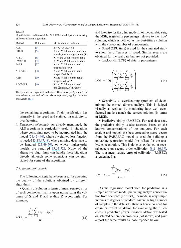
Table 2

Identifiability conditions of the PARAFAC model parameters using

different different algorithms

Method Reference Identifiability condition

ALS [14] kx + ky + kzz 2F + 2

DTLD [54] X and Y full column rank and

non-degenerate eigenvalues (Z)

ATLD [55] X, Y and Z full column rank

SWATLD [35] X, Y and Z full column rank

PALS [37] X and Y full column rank;

unspecified for Z

ACOVER [38] X and Y full column rank;

unspecified for Z

ASD [39] X and Y full column rank;

unspecified for Z

ACOMAR [40] X and Y full column rank

and Adiag(z(k))2 invertible

The symbols are explained in the text. The k-rank (kx, ky and kz) is a

term related to the rank of a matrix as explained, e.g. by Harshman

and Lundy [53].

N.M. Faber et al. / Chemometrics and Intelligent Laboratory Systems 65 (2003) 119–137124

3. Experimental

3.1. Calculations

Calculations are performed using Matlab (Math-

works, Natick, MA). The code for DTLD and ALS is

taken from the N-way Toolbox [29]. The function for

ACOVER is adapted from Jiang et al. [38]. ATLD,

ASD, ACOMAR, SWATLD and PALS are performed

using in-house functions. The following alterations

have been found to be necessary:

1. Using the general recipe outlined in Appendix A,

improved updating formulas are derived for

ACOMAR (Appendix B) and PALS (Appendix C).

2. The original implementation of ASD exhibits

severe convergence problems, which are probably

caused by the specific initialisation and a non-

convergent algorithm. The original code has been

streamlined so as to more closely follow the

original description (Appendix D). Moreover, the

current version allows one to vary the initialisation

for the X- and Y-mode loading matrices.

3. The code for ACOVER has been adapted to

harmonise with the other algorithms. Moreover,

the singular value decomposition inside the

algorithm has been replaced by a call to NIPALS

to avoid memory problems.

To enable a fair comparison for the iterative

methods, a DTLD initialisation is applied when pos-

sible (see Table 3). This is to avoid the convergence

problems that are more frequently encountered when

using a singular value decomposition-based or ran-

dom initialisation. The threshold value for the con-

vergence criterion is set to such a tight value that

decreasing it by a factor of 10 will not change the first

three decimal digits of the simulation results. The

maximum number of iterations is set sufficiently high

to allow an algorithm to converge.

The estimated models are post-processed as fol-

lows. First, the X- and Y-mode profiles are scaled to

unit norm and the X-mode profiles rescaled accord-

ingly. Second, the factors are sorted according to the

length of the Z-mode profiles.

The foremost criterion for assessing the quality of a

solution for the simulated data is the MSE with

respect to the input profiles, see Eq. (13). Correct

application of this criterion hinges on a suitable

matching of estimated and input profiles, especially

when overestimating the true number of components.

One often encounters studies where this matching is

based on (functions of) correlation coefficients, but

the resulting numbers are insensitive to scale. In the

present study, the matching is achieved by minimising

the MSE over all modes jointly, which is consistent

with the evaluation criterion Eq. (13).

A copy of the programs used is available on request.

3.2. Data

3.2.1. Simulated data

Two data sets were simulated with the property that

they span a reasonable range with respect to overlap

among the individual profiles.

3.2.1.1. Simulated data set I. The first example

results from simulating a high-performance liquid

chromatography (HPLC) system with ultraviolet

(UV) diode array detection (DAD). The X- and Y-

mode profiles are shown in Fig. 1 (I = 20 and J= 50).

The elements of the Z-mode profiles are drawn from a

Table 3

Settings for the iterative methods

Method Initialisation Convergence

criterion

Threshold Maximum number

of iterations

ALS DTLD for Y and Z fit error 10� 10 (10� 6) 10000 (2500)

ATLD DTLD for X and Y fit error 10� 6 (10� 6) 10000 (30)

SWATLD DTLD for X and Y fit error 10� 9 (10� 6) 10000 (5000)

PALS DTLD for X and Y fit error 10� 8 (10� 6) 10000 (100)

ACOVER SVD for za change in za 10� 7 (10� 5) 10000 (200)

ASD DTLD for X and Y SD loss 10� 9 (10� 10) 10000 (2000)

ACOMAR SVD for X and P=Y+ T fit error 10� 9 (10� 6) 10000 (3000)

The numbers in parentheses denote the values suggested in the literature. The symbols are explained in the text.

N.M. Faber et al. / Chemometrics and Intelligent Laboratory Systems 65 (2003) 119–137 125

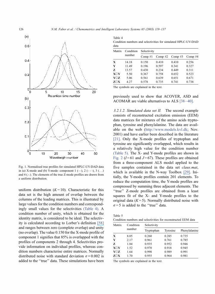
uniform distribution (K = 10). Characteristic for this

data set is the high amount of overlap between the

columns of the loading matrices. This is illustrated by

large values for the condition numbers and correspond-

ingly small values for the selectivities (Table 4). A

condition number of unity, which is obtained for the

identity matrix, is considered to be ideal. The selectiv-

ity is calculated according to Lorber’s definition [58]

and ranges between zero (complete overlap) and unity

(no overlap). The value 0.150 for the X-mode profile of

component 1 signifies that 85% is overlapped with the

profiles of components 2 through 4. Selectivities pro-

vide information on individual profiles, whereas con-

dition numbers characterise entire matrices. Normally

distributed noise with standard deviation r = 0.002 is

added to the ‘‘true’’ data. These simulations have been

previously used to show that ACOVER, ASD and

ACOMAR are viable alternatives to ALS [38–40].

3.2.1.2. Simulated data set II. The second example

consists of reconstructed excitation emission (EEM)

data matrices for mixtures of the amino acids trypto-

phan, tyrosine and phenylalanine. The data are avail-

able on the web (http://www.models.kvl.dk; Nov.

2001) and have earlier been described in the literature

[21]. Only the X-mode profiles of tryptophan and

tyrosine are significantly overlapped, which results in

a relatively high value for the condition number

(Table 5). The X- and Y-mode profiles are shown in

Fig. 2 (I = 61 and J = 67). These profiles are obtained

from a three-component ALS model applied to the

five samples contained in the data set claus.mat,

which is available in the N-way Toolbox [29]. Ini-

tially, the Y-mode profiles contain 201 elements. To

reduce the computation time, the Y-mode profiles are

compressed by summing three adjacent elements. The

‘‘true’’ Z-mode profiles are obtained from a least

squares fit of the X- and Y-mode profiles to the

original data (K = 5). Normally distributed noise with

r = 5 is added to the ‘‘true’’ data.

Table 4

Condition numbers and selectivities for simulated HPLC-UV-DAD

data

Matrix Condition Selectivity

numberComp #1 Comp #2 Comp #3 Comp #4

X 14.18 0.150 0.410 0.410 0.256

Y 11.49 0.196 0.597 0.341 0.327

Z 13.57 0.430 0.234 0.449 0.311

XOY 5.50 0.367 0.758 0.652 0.523

YOZ 5.06 0.561 0.639 0.651 0.671

ZOX 4.27 0.578 0.735 0.741 0.738

The symbols are explained in the text.

Fig. 1. Normalised true profiles for simulated HPLC-UV-DAD data

in (a) X-mode and (b) Y-mode: component 1 (—), 2 (- - -), 3 (. . .)

and 4 (.-.). The elements of the true Z-mode profiles are drawn from

a uniform distribution.

Table 5

Condition numbers and selectivities for reconstructed EEM data

Matrix Condition Selectivity

numberTryptophan Tyrosine Phenylalanine

X 8.05 0.260 0.285 0.735

Y 2.17 0.961 0.761 0.785

Z 1.84 0.935 0.952 0.946

XOY 1.52 0.970 0.918 0.945

YOZ 1.64 0.998 0.989 0.991

ZOX 1.70 0.955 0.964 0.981

The symbols are explained in the text.

N.M. Faber et al. / Chemometrics and Intelligent Laboratory Systems 65 (2003) 119–137126

3.2.2. Real data

As examples of simple fluorescence data sets, the

following two measured data sets were used. The data

sets are available from the authors on request.

3.2.2.1. Real data set I. A Perkin-Elmer LS50 B

fluorescence spectrometer was used to measure fluo-

rescence landscapes using excitation wavelengths

between 200 and 350 nm with 5 nm intervals. Fifteen

samples containing different amounts of hydroqui-

none, tryptophan, phenylalanine and DOPAwere made

in Milli-Q water from stock solutions. The emission

wavelength range was truncated to 260–390 nm in 1-

nm steps and excitationwas set to 245–305 nm in 5-nm

steps. Excitation and emission monochromator slit

widths were set to 5 nm. Scan speed was 1500 nm/

min and from each EEM, the EEM of a blank was

subtracted primarily to remove Raman scatter. The data

set was split into three replicates by leaving out

emission 260, 263, 266,. . ., in the first replicate, 261,

264,. . ., in the second and 262, 265,. . ., in the third

replicate. More details on the data can be found in the

literature [59].

3.2.2.2. Real data set II. Fifteen liquid samples

containing hydroquinone, tryptophan, tyrosine and

DOPAwere measured on a Cary Eclipse Fluorescence

Spectrophotometer using slit widths of 5 nm on both

excitation and emission. Emission ranged from 282 to

412 nm in approximately 2-nm steps and excitation

was set to 230–300 nm in 5-nm steps. Each sample

was measured six consecutive times and each of the

six sets of data was modeled independently giving six

different realizations of each model.

4. Results and discussion

4.1. Analysis of simulated data

4.1.1. Simulated data set I

First, the relative performance of the competing

methods is assessed when selecting the correct model

dimensionality. It is expected that ALS, which

involves the pseudo-inverses of Khatri-Rao products

(see Table 1), yields more stable results than the

alternatives, because they all work in one way or

another with pseudo-inverses of X and Y (DTLD,

PALS, ACOVER, ASD and ACOMAR) or X, Y and

Z (ATLD and SWATLD). This is confirmed by the

median MSE-values (Table 6). To facilitate the inter-

pretation, all numbers are normalised with respect to

the ALS results. The ALS solution is clearly superior,

while SWATLD and ASD are the best alternatives. The

results are considerably worse for DTLD, ATLD,

PALS, ACOVER and ACOMAR. The poor results

for ACOVER and ACOMAR contrast the optimistic

presentation in the original papers [38,40], where

similar simulations are performed to demonstrate the

viability of these methods. The ranking of the methods

is quite different when CPU consumption is consid-

ered (DTLD initialisation is accounted for in the CPU

consumption of ALS, ATLD, SWATLD, PALS and

Fig. 2. Normalised true profiles for simulated HPLC-UV-DAD data

in (a) X-mode and (b) Y-mode: tryptophan (—), tyrosine (- - -),

phenylalanine (. . .). The true Z-mode profiles are obtained from a

least squares fit.

N.M. Faber et al. / Chemometrics and Intelligent Laboratory Systems 65 (2003) 119–137 127

ASD). ALS is slowest while the non-iterative DTLD is

fastest, closely followed by ATLD and ASD. ALS

ranks first in terms of LOF (median value), directly

followed by a number of methods. Only ATLD seems

to be unacceptable in terms of fitting capability.

Next, the relative performance is assessed when

overestimating the correct model dimensionality by a

single component. The primary motivation for intro-

ducing the iterative alternatives is that ALS suffers

from convergence problems when too many compo-

nents are fitted to the data (‘‘overfactoring’’). One

observes a consistent deterioration of the MSE crite-

rion for all methods (Table 7), but the ranking remains

approximately the same. DTLD, PALS and ACOMAR

exhibit the largest increase of MSE. The CPU con-

sumption of DTLD, ACOVER and ASD has slightly

increased, while the remaining algorithms seem to

encounter serious problems. Especially, ALS and

PALS are extremely slow. The deterioration of LOF

is consistent with the MSE results (considerably worse

for PALS). ALS is best, followed by ASD and

SWATLD. Only ATLD and PALS are unacceptable.

4.1.2. Simulated data set II

Table 8 summarises the results obtained when

selecting the correct model dimensionality. Compar-

ing the second column of Tables 6 and 8 shows that

the alternatives generally perform better for this data

set. This can be (qualitatively) explained from the

smaller difference of condition number and selectiv-

ities calculated for the loading matrices and their

Khatri-Rao products (compare Tables 4 and 5). ALS

is best, closely followed by ASD and SWATLD. It is

remarkable that DTLD, which is by far the oldest

alternative, performs worse. DTLD is fastest, but the

gain over ACOMAR, ASD and ATLD is small. When

considering LOF, ALS ranks first, but all alternatives

seem to be acceptable in this respect.

Overfactoring leads to a consistent increase of the

MSE (Table 9). ACOVER forms an exception (1.58

versus 1.60 in Table 8), but this ‘‘improvement’’ must

be attributed to the rather limited number of runs

(100). Compared with the other methods, ACOMAR

performs considerably worse. The increase of CPU

consumption is similar as observed for the high-over-

lap data. LOF has consistently deteriorated; for ACO-

MAR it is considerably worse. Again, ALS is best,

closely followed by ASD and SWATLD. Only ACO-

MAR exhibits an unacceptable LOF.

The preceding observations can be summarised as:

1. ALS performs best in terms of quality of the so-

lution (MSE as well as fit), but is computationally

(too) demanding when overfactoring.

Table 7

Ranking of different algorithms for simulated HPLC-UV-DAD data

with F = 5 (100 runs)

Method MSEa Rank CPU (total) Rank LOFa Rank

ALS 1.09 1 15.67 7 1.01 1

DTLD 5.98 6 0.06 1 1.13 5

ATLD 5.12 5 0.69 3 3.94 7

SWATLD 1.64 2 1.69 5 1.08 3

PALS 6.04 7 24.18 8 5.61 8

ACOVER 9.34 8 1.13 4 1.17 6

ASD 2.38 3 0.24 2 1.03 2

ACOMAR 3.20 4 2.10 6 1.12 4

The results are normalised with respect to the ALS results obtained

with F = 4.a Median value.

Table 8

Ranking of different algorithms for reconstructed EEM data with

F = 3 (100 runs)

Method MSEa Rank CPU (total) Rank LOFa Rank

ALS 1.00 1 1.00 7 1.00 1

DTLD 2.97 8 0.20 1 1.08 7

ATLD 2.01 7 0.37 4 1.11 8

SWATLD 1.30 4 0.72 6 1.02 4

PALS 1.69 6 0.62 5 1.02 5

ACOVER 1.60 5 2.15 8 1.05 6

ASD 1.07 2 0.34 3 1.00 2

ACOMAR 1.12 3 0.21 2 1.00 3

The results are normalised with respect to the ALS results.a Median value.

Table 6

Ranking of different algorithms for simulated HPLC-UV-DAD data

with F = 4 (100 runs)

Method MSEa Rank CPU (total) Rank LOFa Rank

ALS 1.00 1 1.00 8 1.00 1

DTLD 4.77 6 0.05 1 1.06 4

ATLD 5.08 7 0.12 2 3.89 8

SWATLD 1.62 2 0.46 5 1.08 6

PALS 3.95 5 0.86 6 1.06 5

ACOVER 9.06 8 0.93 7 1.13 7

ASD 2.18 3 0.19 3 1.02 2

ACOMAR 2.65 4 0.40 4 1.06 3

The results are normalised with respect to the ALS results.a Median value.

N.M. Faber et al. / Chemometrics and Intelligent Laboratory Systems 65 (2003) 119–137128

2. ASD and SWATLD are the best alternatives. ASD

has an advantage over SWATLD, because it con-

verges in reasonable CPU time.

3. DTLD is fastest, but does not yield a good solution.

However, the solution may be good enough for

initialisation purposes.

ATLD, PALS, ACOVER and ACOMAR cannot be

recommended.

4.2. Analysis of real data

Each of the two real data sets consisted of several

replicate data sets. For data set I, three replicates were

made by leaving out some emissions throughout the

emission spectrum and for data set II, six replicates

were generated by measuring the samples six times.

Both data sets contained samples with differing

amounts of four analytes. Ideally, four PARAFAC

components are hence expected to be suitable. Only

the best algorithms ALS, DTLD, ASD and SWATLD

will be investigated for the analysis of the real data.

4.2.1. Real data set I

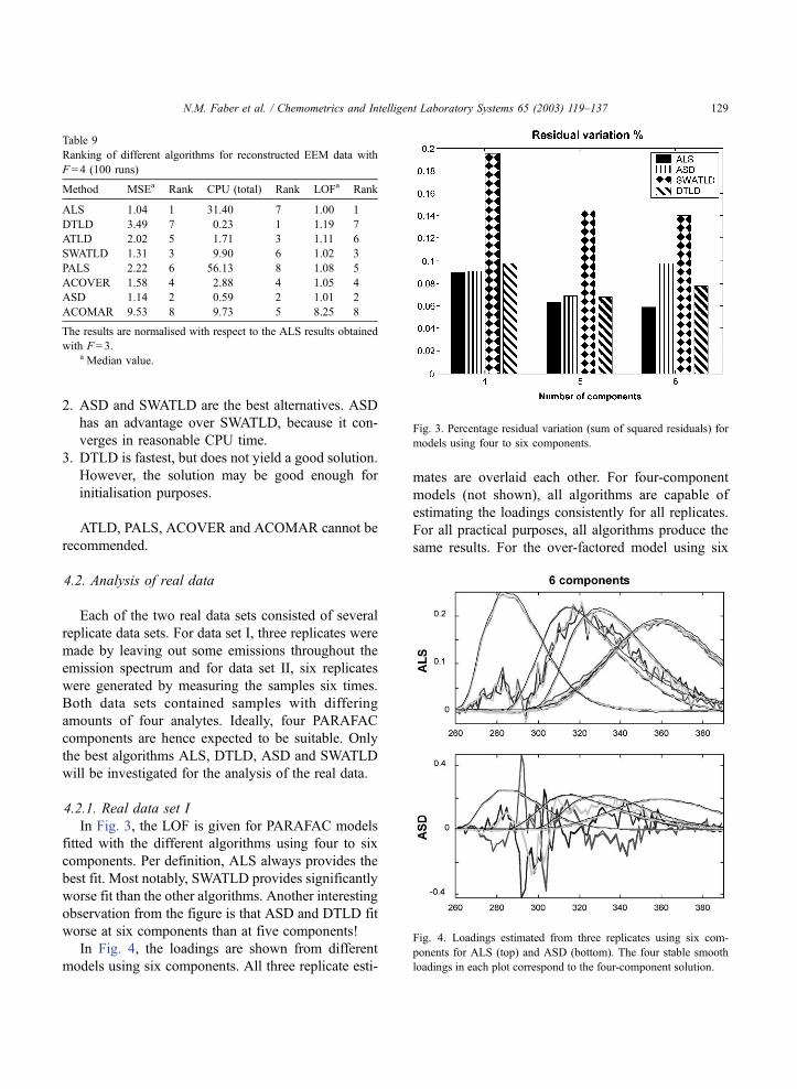
In Fig. 3, the LOF is given for PARAFAC models

fitted with the different algorithms using four to six

components. Per definition, ALS always provides the

best fit. Most notably, SWATLD provides significantly

worse fit than the other algorithms. Another interesting

observation from the figure is that ASD and DTLD fit

worse at six components than at five components!

In Fig. 4, the loadings are shown from different

models using six components. All three replicate esti-

mates are overlaid each other. For four-component

models (not shown), all algorithms are capable of

estimating the loadings consistently for all replicates.

For all practical purposes, all algorithms produce the

same results. For the over-factored model using six

Table 9

Ranking of different algorithms for reconstructed EEM data with

F = 4 (100 runs)

Method MSEa Rank CPU (total) Rank LOFa Rank

ALS 1.04 1 31.40 7 1.00 1

DTLD 3.49 7 0.23 1 1.19 7

ATLD 2.02 5 1.71 3 1.11 6

SWATLD 1.31 3 9.90 6 1.02 3

PALS 2.22 6 56.13 8 1.08 5

ACOVER 1.58 4 2.88 4 1.05 4

ASD 1.14 2 0.59 2 1.01 2

ACOMAR 9.53 8 9.73 5 8.25 8

The results are normalised with respect to the ALS results obtained

with F= 3.a Median value.

Fig. 3. Percentage residual variation (sum of squared residuals) for

models using four to six components.

Fig. 4. Loadings estimated from three replicates using six com-

ponents for ALS (top) and ASD (bottom). The four stable smooth

loadings in each plot correspond to the four-component solution.

N.M. Faber et al. / Chemometrics and Intelligent Laboratory Systems 65 (2003) 119–137 129

components it is seen that the three replicated ALS

models are very close to each other. Four of the six

components are virtually identical to the four-compo-

nent solution (minimally 99.5% agreement). For the

other algorithms, exemplified in the figure by ASD, the

four components from the four-component solution are

also found to the same extent as for ALS. However,

different auxiliary components are found for different

replicates. The six-component DTLD solution seems to

vary a bit more over replicates than for the other

algorithms also in terms of reproducing the four-com-

ponent solution.

In Fig. 5, the root mean squared error of calibration

(RMSEC) values are given for different regression mo-

dels. The regression was performed by regressing the

concentration vector of the specific analyte onto the

best correlating score vector without introducing off-

sets. The general trend is that there is little effect of

Fig. 5. RMSEC values for the four different analytes for four (left column) to six (right column) component models. For each algorithm and

number of components each bar represents the result for one of the three replicate runs. The large errors for phenylalanine are due to the higher

concentrations.

Fig. 6. Residual variation for data set II.

N.M. Faber et al. / Chemometrics and Intelligent Laboratory Systems 65 (2003) 119–137130

over-factoring even for the least squares models. A few

specific models stand out as bad, but no consistent

pattern is seen to indicate superiority of one algorithm

over the other.

4.2.2. Real data set II

For the second real data set, figures similar to

above are given. The results support that ALS does

not suffer any particular problems when over-factor-

ing compared to the alternative algorithms.

The residual variation in Fig. 6 shows that DTLD

suffers much worse fit than the other algorithms and

that the six-component DTLD model fits worse than

the five-component DTLD model.

Fig. 7 shows very much the same pattern as for real

data set I. An exception compared to data set 1 is that

DTLD fails to estimate even the four-component

solution appropriately (not shown). Also opposed to

data set 1, the auxiliary components in the six-compo-

nent ALS solutions are not similar from replicate to

replicate. In replicates 5 and 6, ALS produces less

good results than in replicates 1–4. Overall, all algo-

rithms produce results of similar quality for the six-

Fig. 8. RMSEC values for the four different analytes for four (left column) to six (right column) component models. For each algorithm and

number of components each bar represents the result for one of the six replicate runs.

Fig. 7. Loadings estimated from six replicates using six components

for ALS (top) and ASD (bottom). The results differ markedly from

replicate to replicate making interpretations difficult.

N.M. Faber et al. / Chemometrics and Intelligent Laboratory Systems 65 (2003) 119–137 131

component solution. For most replicates, the algo-

rithms are capable of estimating parameters that are

similar to the ones from the four-component model, but

for one or two replicates each algorithm fails to do so.

The quantitative results from data set II are given in

Fig. 8 and again, most algorithms perform similarly

with the exception that DTLD seems to vary more in

quality than the other algorithms.

5. Conclusions

A thorough investigation of several algorithms has

revealed a number of important aspects:

ALS does not seem to suffer as much as recently

claimed from over-factoring. DTLD, while being fast, is a surprisingly poor

method for fitting the PARAFAC model. All the recent algorithms for PARAFAC described

here suffer from lack of proper understanding of

their working. However, while none of them turn out to perform

better than ALS with respect to the quality of the

estimated model and parameters, they are frequently

much faster than ALS, especially when the model is

over-factored.

The main conclusion to draw from this investigation

is that ALS is still preferred if quality of solution is of

prime importance. When computation time is more im-

portant, however, other alternatives may be preferred.

In fact, the results may be interpreted such that ASD is a

viable alternative and especially a better alternative

thanDTLD. It is important to remind, though, that there

are other least squares fitting procedures than ALS,

some of which are much faster but have not yet been

thoroughly tested for overfactoring [46,60]. Given the

poor results of DTLD, further research and applications

may be needed for deciding on appropriate initializa-

tion of iterative algorithms in general.

Acknowledgements

R. Bro acknowledges support provided by STVF

(Danish Research Council) through project 1179, as

well as the EU-project Project GRD1-1999-10337,

NWAYQUAL.

Appendix A. Useful manipulations for deriving

updating formulas

Updating formulas for loading matrices can be

derived as follows:

1. a loss function is formulated in terms of a Fro-

benius norm,

2. the Frobenius norm is rewritten as a trace function,

3. the derivative of the trace function with respect to

the loading matrix is found,

4. the derivative is set to zero and the resulting ex-

pression is worked out.

This appendix summarises manipulations that are

useful for carrying out steps 2 and 3.

The relationship between the Frobenius norm

(square root of the sum of the squared matrix ele-

ments) and the trace function (sum of the diagonal

elements of a matrix) is given by

NAN2 ¼ TrðATAÞ ð16ÞThe following obviously holds for the trace func-

tion:

TrðATÞ ¼ TrðAÞ ð17ÞThe expression for a trace function can be rewritten

using

TrðABÞ ¼ TrðBAÞ ð18Þwhenever the product BA exists.

The following expressions hold for the derivative

of a trace function (Ref. [61], pp. 177–178):

BTrðAXÞBX

¼ AT ð19Þ

BTrðXTAXÞBX

¼ ðAþ ATÞX ð20Þ

BTrðXAXTÞBX

¼ XðAþ ATÞ ð21Þ

Appendix B. Improved updating formula for

ACOMAR estimate of Z

In the following derivation, the numbers in square

brackets preceding an expression refer to the original

work. Using Eqs. (16) and (17) and the symmetry of

N.M. Faber et al. / Chemometrics and Intelligent Laboratory Systems 65 (2003) 119–137132

Dk, the loss function with respect to the Z-mode

loadings is written as

rðZÞ ¼XKk¼1

NRkP� XDkN2

¼XKk¼1

TrðPTRTkRkP� 2PTRT

kXDk

þ DkXTXDkÞ ð22Þ

where P=Y+ T (the so-called coupled matrix of X).

Using Eqs. (19) and (20) and the symmetry of XTX

and Dk yields that

BrðZÞBDk

¼XKk¼1

ð�2XTRkPþ 2XTXDkÞ; k ¼ 1; . . . ;K

ð23ÞSetting the derivatives to zero leads to equalities

which can only hold if

zk ¼ diagðXþRkPÞ; k ¼ 1; . . . ;K ð24Þwhere zk is the kth row of Z and diag() symbolises the

diagonal of a square matrix. This rationale then implies

that taking the diagonal of the right side of Eq. (24) will

be an appropriate update. Thus, the original updating

formula is only ‘‘improved’’ in the sense that it is

consistent with the ACOMAR loss function. We have

performed calculations where Eq. (22) was replaced by

a true least squares step (see Table 1), but the quality of

the solution was not significantly affected.

Appendix C. Improved updating formulas for

PALS estimates of X, Y and Z

In the following derivation, the numbers in square

brackets preceding an expression refer to the original

work. Using Eqs. (16)–(18), the loss function with

respect to the X-mode loadings is written as

rðXÞ¼XKk¼1

NRk � XDkYTN2 þ kNRkY

þT � XDkN2

¼XKk¼1

½TrðRTkRk�2RT

kXDkYTþYDkX

TXDkYTÞ

þ kTrðYþRTkRkY

þT � 2YþRTkXDk

þ DkXTXDkÞ� ð25Þ

Using Eqs. (19) and (21) and the symmetry of Dk

YTYDk and Dk2 yields that

BrðXÞBX

¼XKk¼1

ð�2RkYDk þ 2XDkYTYDkÞ

þ kð�2RkYþTDk þ 2XD2

kÞ

¼ 2XKk¼1

ðXDkðYTYþ kIÞDkÞ

� RkðYþ kYþTÞDk ð26Þ

where I is the F�F identity matrix. It is immediate that

X¼XKk¼1

ðRkðYþkYþTÞDkÞXKk¼1

ðDkðYTYþkIÞDkÞ !�1

ð27ÞLikewise, one finds

Y ¼XKk¼1

ðRTk ðXþ kXþTÞDkÞ

�XKk¼1

ðDkðXTXþ kIÞDkÞ !�1

ð28Þ

When deriving the correct updating formula for the Z-

mode loadings, it is convenient to express the loss

function in terms of summations over the X- and Y-

mode loadings:

rðZÞ¼XIi¼1

2NRi � YDiZTN2þ kNYþRi

h� DiZ

TN2i

þXJj¼1

kNXþRTj � DjZ

TN2

¼XIi¼1

2TrðRTi Ri � 2ZDiY

TRi þ ZDiYTYDiZ

T�

þkTrðRTi Y

þTYþRi�2ZDiYþTRiþZD2

i ZTÞ

þXJj¼1

kTrðRjXþTXþRT

j �2ZDjXþRT

j þZD2j Z

TÞ

ð29ÞStarting from Eq. (29), it is straightforward to show that

Z ¼XIi¼1

RTi ð2Yþ kYþTÞDi þ k

XJj¼1

RjXþTDj

!

�XIi¼1

Dið2YTYþ kIÞDi þ kXJj¼1

D2j

!�1

ð30Þ

N.M. Faber et al. / Chemometrics and Intelligent Laboratory Systems 65 (2003) 119–137 133

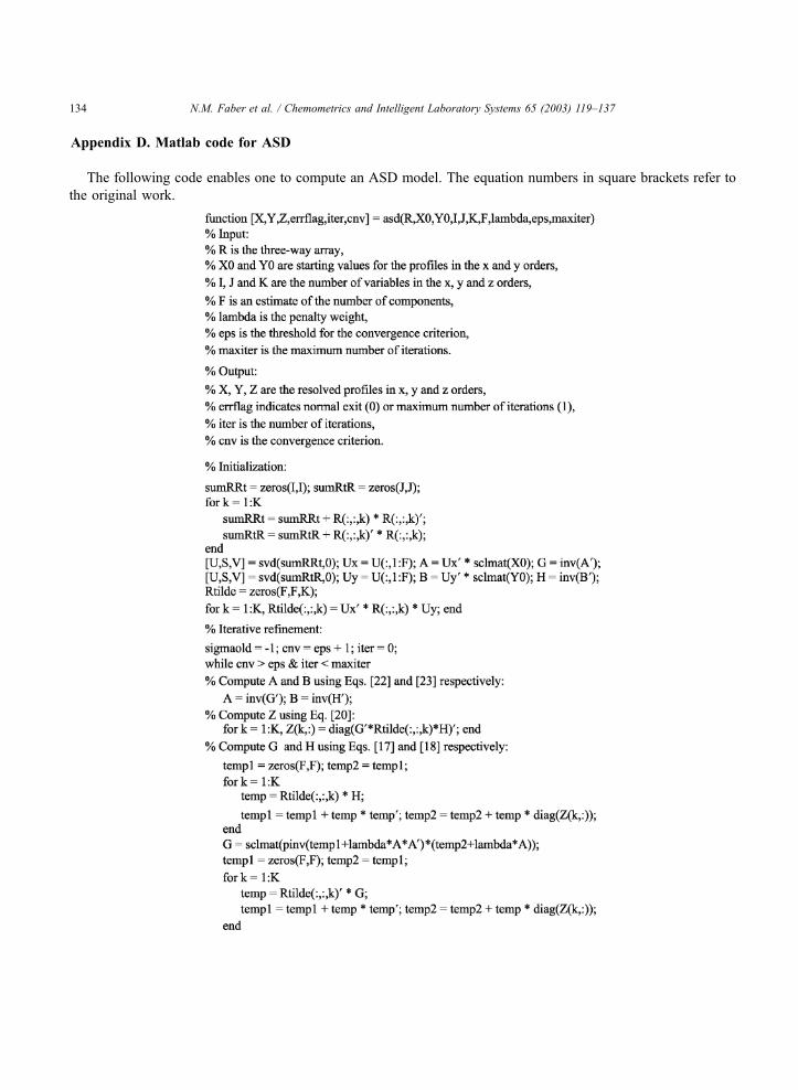
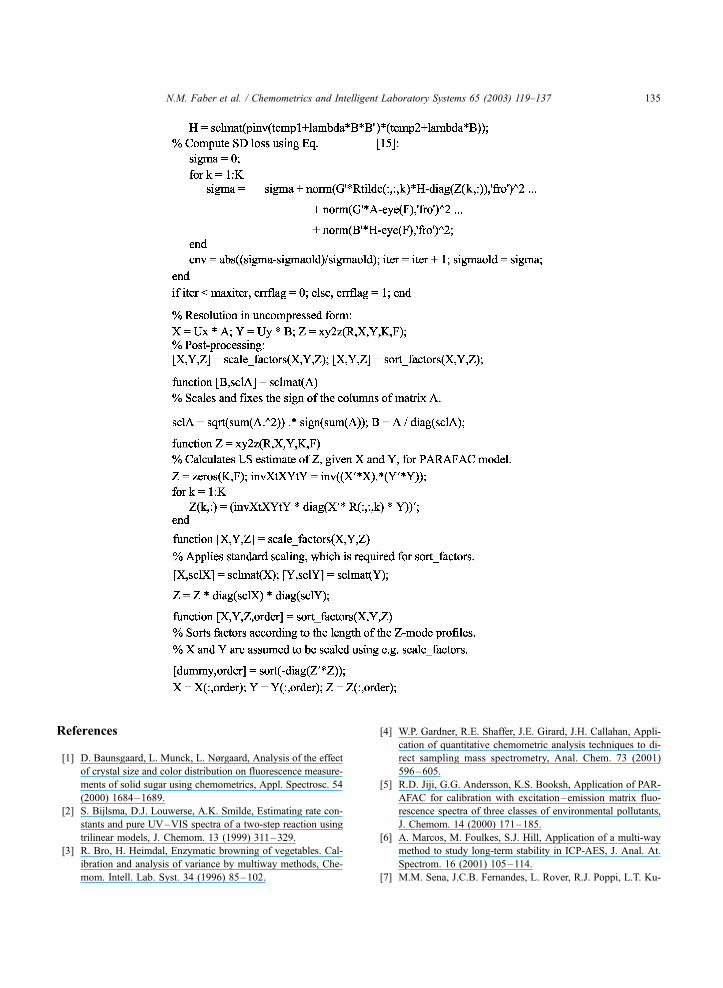
Appendix D. Matlab code for ASD

The following code enables one to compute an ASD model. The equation numbers in square brackets refer to

the original work.

N.M. Faber et al. / Chemometrics and Intelligent Laboratory Systems 65 (2003) 119–137134

References

[1] D. Baunsgaard, L. Munck, L. Nørgaard, Analysis of the effect

of crystal size and color distribution on fluorescence measure-

ments of solid sugar using chemometrics, Appl. Spectrosc. 54

(2000) 1684–1689.

[2] S. Bijlsma, D.J. Louwerse, A.K. Smilde, Estimating rate con-

stants and pure UV–VIS spectra of a two-step reaction using

trilinear models, J. Chemom. 13 (1999) 311–329.

[3] R. Bro, H. Heimdal, Enzymatic browning of vegetables. Cal-

ibration and analysis of variance by multiway methods, Che-

mom. Intell. Lab. Syst. 34 (1996) 85–102.

[4] W.P. Gardner, R.E. Shaffer, J.E. Girard, J.H. Callahan, Appli-

cation of quantitative chemometric analysis techniques to di-

rect sampling mass spectrometry, Anal. Chem. 73 (2001)

596–605.

[5] R.D. Jiji, G.G. Andersson, K.S. Booksh, Application of PAR-

AFAC for calibration with excitation–emission matrix fluo-

rescence spectra of three classes of environmental pollutants,

J. Chemom. 14 (2000) 171–185.

[6] A. Marcos, M. Foulkes, S.J. Hill, Application of a multi-way

method to study long-term stability in ICP-AES, J. Anal. At.

Spectrom. 16 (2001) 105–114.

[7] M.M. Sena, J.C.B. Fernandes, L. Rover, R.J. Poppi, L.T. Ku-

N.M. Faber et al. / Chemometrics and Intelligent Laboratory Systems 65 (2003) 119–137 135

bota, Application of two- and three-way chemometric meth-

ods in the study of acetylsalicylic acid and ascorbic acid mix-

tures using ultraviolet spectrophotometry, Anal. Chim. Acta

409 (2000) 159–170.

[8] K.S. Booksh, J.M. Henshaw, L.W. Burgess, B.R. Kowalski, A

2nd-order standard addition method with application to cali-

bration of a kinetics-spectroscopic sensor for quantitation of

trichloroethylene, J. Chemom. 9 (1995) 263–282.

[9] N.M. Faber, L.M.C. Buydens, G. Kateman, Generalized rank

annihilation method: I. Derivation of eigenvalue problems, J.

Chemom. 8 (1994) 147–154.

[10] N.M. Faber, L.M.C. Buydens, G. Kateman, Generalized rank

annihilation method: II. Bias and variance in the estimated

eigenvalues, J. Chemom. 8 (1994) 181–203.

[11] N.M. Faber, L.M.C. Buydens, G. Kateman, Generalized rank

annihilation: III. Practical implementation, J. Chemom. 8

(1994) 273–285.

[12] E. Sanchez, B.R. Kowalski, Generalized rank annihilation

factor analysis, Anal. Chem. 58 (1986) 496–499.

[13] J.D. Carroll, J. Chang, Analysis of individual differences

in multidimensional scaling via an N-way generalization

of ‘Eckart-Young’ decomposition, Psychometrika 35 (1970)

283–319.

[14] R.A. Harshman, Foundations of the PARAFAC procedure:

models and conditions for an ‘explanatory’ multi-modal factor

analysis, UCLA Work. Pap. Phon. 16 (1970) 1–84.

[15] R.A. Harshman, Determination and proof of minimum

uniqueness conditions for PARAFAC1, UCLA Work. Pap.

Phon. 22 (1972) 111–117.

[16] J.B. Kruskal, Rank, decomposition, and uniqueness for 3-way

and N-way arrays, in: R. Coppi, S. Bolasco (Eds.), Multiway

Data Analysis, Elsevier, Amsterdam, 1989, pp. 8–18.

[17] N.D. Sidiropoulos, R. Bro, On the uniqueness of multili-

near decomposition of N-way arrays, J. Chemom. 14 (2000)

229–239.

[18] R. Bro, N.D. Sidiropoulos, A.K. Smilde, Maximum likelihood

fitting using simple least squares algorithms, J. Chemom. 16

(2002) 387–400.

[19] H.A.L. Kiers, Weighted least squares fitting using ordinary

least squares algorithms, Psychometrika 62 (1997) 251–266.

[20] R. Bro, PARAFAC. Tutorial and applications, Chemom. In-

tell. Lab. Syst. 38 (1997) 149–171.

[21] R. Bro, Multi-way analysis in the food industry. Models, algo-

rithms, and applications. PhD thesis, University of Amsterdam

(NL), http://www.mli.kvl.dk/staff/foodtech/brothesis.pdf,

1998.

[22] R.A. Harshman, Substituting statistical for physical decompo-

sition: are there application for parallel factor analysis (PAR-

AFAC) in non-destructive evaluation, in: X.P.V. Malague

(Ed.), Advances in Signal Processing for Nondestructive

Evaluation of Materials, Kluwer Academic Publishing, Dor-

drecht, The Netherlands, 1994, pp. 469–483.

[23] R.A. Harshman, M.E. Lundy, The PARAFAC model for three-

way factor analysis and multidimensional scaling, in: H.G.

Law, C.W. Snyder Jr., J. Hattie, R.P. McDonald (Eds.), Re-

search Methods for Multimode Data Analysis, Praeger, New

York, 1984, pp. 122–215.

[24] S.E. Leurgans, R.T. Ross, R.B. Abel, A decomposition for

three-way arrays, Siam J. Matrix Anal. Appl. 14 (1993)

1064–1083.

[25] R.T. Ross, S.E. Leurgans, Component resolution using multi-

linear models, Methods Enzymol. 246 (1995) 679–700.

[26] C.W. Snyder, W.D. Walsh, P.R. Pamment, Three-mode

PARAFAC factor analysis in applied research, J. Appl.

Psychol. 68 (1983) 572–583.

[27] H.A.L. Kiers, Towards a standardized notation and terminol-

ogy in multiway analysis, J. Chemom. 14 (2000) 105–122.

[28] C.R. Rao, S. Mitra, Generalized Inverse of Matrices and its

Applications, Wiley, New York, 1971.

[29] C.A. Andersson, R. Bro, The N-way toolbox for MATLAB,

Chemom. Intell. Lab. Syst. 52 (2000) 1–4.

[30] N.M. Faber, On solving generalized eigenvalue problems us-

ing MATLAB, J. Chemom. 11 (1997) 87–91.

[31] M.J.P. Gerritsen, H. Tanis, B.G.M. Vandeginste, G. Kateman,

Generalized rank annihilation factor analysis, iterative target

transformation factor analysis, and residual bilinearization for

the quantitative analysis of data from liquid chromatography

with photodiode array detection, Anal. Chem. 64 (1992)

2042–2056.

[32] S. Li, J.C. Hamilton, P.J. Gemperline, Generalized rank anni-

hilation method using similarity transformations, Anal. Chem.

64 (1992) 599–607.

[33] A. Lorber, Features of quantifying composition from two-di-

mensional data array by the rank annihilation factor analysis

method, Anal. Chem. 57 (1985) 2395–2397.

[34] H.L. Wu, M. Shibukawa, K. Oguma, An alternating trilinear

decomposition algorithm with application to calibration of

HPLC-DAD for simultaneous determination of overlapped

chlorinated aromatic hydrocarbons, J. Chemom. 12 (1998)

1–26.

[35] Z.P. Chen, H.L. Wu, J.H. Jiang, Y. Li, R.Q. Yu, A novel

trilinear decomposition algorithm for second-order linear cal-

ibration, Chemom. Intell. Lab. Syst. 52 (2000) 75–86.

[36] Z.P. Chen, H.L. Wu, R.Q. Yu, On the self-weighted alternating

trilinear decomposition algorithm—the property of being in-

sensitive to excess factors used in calculation, J. Chemom. 15

(2001) 439–453.

[37] Z.P. Chen, Y. Li, R.Q. Yu, Pseudo alternating least squares

algorithm for trilinear decomposition, J. Chemom. 15 (2001)

149–167.

[38] H.L. Jiang, H.L. Wu, Y. Li, R. Yu, Alternating coupled vectors

resolution (ACOVER) method for trilinear analysis of three-

way data, J. Chemom. 13 (1999) 557–578.

[39] J.H. Jiang, H.L. Wu, Y. Li, R.Q. Yu, Three-way data resolu-

tion by alternating slice-wise diagonalization (ASD) method,

J. Chemom. 14 (2000) 15–36.

[40] Y. Li, J.H. Jiang, H.L. Wu, Z.P. Chen, R.Q. Yu, Alternating

coupled matrices resolution method for three-way arrays anal-

ysis, Chemom. Intell. Lab. Syst. 52 (2000) 33–43.

[41] X.Q. Liu, N.D. Sidiropoulos, Cramer-Rao lower bounds for

low-rank decomposition of multidimensional arrays, IEEE

Trans. Signal Process. 49 (2001) 2074–2086.

[42] R. Bro, S. de Jong, A fast non-negativity-constrained least

squares algorithm, J. Chemom. 11 (1997) 393–401.

N.M. Faber et al. / Chemometrics and Intelligent Laboratory Systems 65 (2003) 119–137136

[43] R. Bro, N.D. Sidiropoulos, Least squares algorithms under

unimodality and non-negativity constraints, J. Chemom. 12

(1998) 223–247.

[44] S.P. Gurden, J.A. Westerhuis, S. Bijlsma, A.K. Smilde, Mod-

elling of spectroscopic batch process data using grey models

to incorporate external information, J. Chemom. 15 (2001)

101–121.

[45] R.A. Harshman, W.S. De Sarbo, An application of PARAFAC

to a small sample problem, demonstrating preprocessing, or-

thogonality constraints, and split-half diagnostic techniques,

in: H.G. Law, C.W. Snyder, J.A. Hattie, R.P. McDonald

(Eds.), Research Methods for Multimode Data Analysis,

Praeger Special Studies, New York, 1984, pp. 602–642.

[46] W.P. Krijnen, J.M.F. ten Berge, A constrained PARAFAC

method for positive manifold data, Appl. Psychol. Meas. 16

(1992) 295–305.

[47] R.D. Jiji, K.S. Booksh, Mitigation of Rayleigh and Raman

spectral interferences in multiway calibration of excitation–

emission matrix fluorescence spectra, Anal. Chem. 72 (2000)

718–725.

[48] P. Paatero, A weighted non-negative least squares algorithm

for three-way ‘PARAFAC’ factor analysis, Chemom. Intell.

Lab. Syst. 38 (1997) 223–242.

[49] W.J. Heiser, P.M. Kroonenberg, Dimensionwise fitting in

PARAFAC-CANDECOMP with missing data and constrained

parameters, 1997.

[50] P. Hopke, P. Paatero, H. Jia, R.T. Ross, R.A. Harshman,

Three-way (PARAFAC) factor analysis: examination and

comparison of alternative computational methods as applied

to ill-conditioned data, Chemom. Intell. Lab. Syst. 43 (1998)

25–42.

[51] R. Bro, M. Jakobsen, Exploring complex interactions in de-

signed data using GEMANOVA. Color changes in fresh beef

during storage, J. Chemom. 16 (2002) 294–304.

[52] J. Nilsson, S. de Jong, A.K. Smilde, Multiway calibration in

3D QSAR, J. Chemom. 11 (1997) 511–524.

[53] R.A. Harshman, M.E. Lundy, Data preprocessing and the ex-

tended PARAFAC model, in: H.G. Law, C.W. Snyder Jr., J.

Hattie, R.P. McDonald (Eds.), Research Methods for Multi-

mode Data Analysis, Praeger, New York, 1984, pp. 216–284.

[54] E. Sanchez, B.R. Kowalski, Tensorial resolution: a direct tri-

linear decomposition, J. Chemom. 4 (1990) 29–45.

[55] H.L. Wu, M. Shibukawa, K. Oguma, Second-order calibration

based on alternating trilinear decomposition: a comparison

with the traditional PARAFAC algorithm, Anal. Sci. 13

(1997) 53–58.

[56] J.L. Beltran, J. Guiteras, R. Ferrer, Three-way multivariate

calibration procedures applied to high-performance liquid

chromatography coupled with fast-scanning fluorescence

spectrometry detection. Determination of polycyclic aromatic

hydrocarbons in water samples, Anal. Chem. 70 (1998)

1949–1955.

[57] M. Linder, Bilinear regression and second order calibration.

PhD thesis, Department of Mathematics, Stockholm Univer-

sity, 1998.

[58] A. Lorber, Error propagation and figures of merit for quanti-

fication by solving matrix equations, Anal. Chem. 58 (1986)

1167–1172.

[59] D. Baunsgaard, Factors Affecting 3-way Modelling (PARAF

AC) of Fluorescence Landscapes, The Royal Veterinary and

Agricultural University, Frederiksberg, Denmark, 1999.

[60] P. Paatero, The multilinear engine—a table-driven, least

squares program for solving multilinear problems, including

the N-way parallel factor analysis model, J. Comput. Graph.

Stat. 8 (1999) 854–888.

[61] J.R. Magnus, H. Neudecker, Matrix Differential Calculus with

Applications in Statistics and Econometrics, Wiley, Chiches-

ter, 1988.

N.M. Faber et al. / Chemometrics and Intelligent Laboratory Systems 65 (2003) 119–137 137