Recent Advances in Control-Oriented Modeling of Automotive Power Train Dynamics

IEEE/ASME TRANSACTIONS ON MECHATRONICS, VOL. 11, NO. 5, OCTOBER 2006 513

Recent Advances in Control-Oriented Modeling ofAutomotive Power Train Dynamics

Josko Deur, Member, IEEE, Josko Petric, Jahan Asgari, and Davor Hrovat, Senior Member, IEEE

Abstract—This paper presents a survey of the recent researchresults of the authors in the field of modeling of automotive powertrain systems and components. The goal of the research is to pro-pose simple and accurate power train models for controller designand to propose computationally efficient simulations. The mod-eling includes typical power train components such as electronicthrottle, SI engine, torque converter, planetary gear set, wet clutch,differential, half shaft, and tire. Experimental model validation re-sults are presented.

Index Terms—Control, dynamics, modeling, power train, roadvehicles.

NOMENCLATURE

a Inner clutch diameter.A0 Cross-sectional flow area of the torque con-

verter.b Outer clutch diameter.ba Equivalent half-shaft damping.bii, bit, bti, btt Damping coefficients of the second-order

torque converter model (calculated from thetorque converter static curves).

beb Equivalent damping of the engine blockmounts in the pitch direction.

f0 Steady-state functions of the torque con-verter.

F Tire force.Fapp Applied clutch force.Fz Normal force to tire.g Speed ratio of the second planetary gear.g(vr) Sliding tire friction function (friction poten-

tial function).h Manifold heat-transfer coefficient; clutch

fluid film thickness; speed ratio of the firstplanetary gear.

i Differential speed ratio.I Engine inertia.Iii, Iit, Iti, Itt Equivalent cross-coupling inertia of the

second-order torque converter model (calcu-lated from Ii,t and bii,it,ti,tt).

Ii,t,s Impeller, turbine, and stator inertia.

Manuscript received October 29, 2005; revised June 16, 2006. Recommendedby Guest Editor K. Jezernik. This work was supported in part by the Ford MotorCompany, and in part by the Ministry of Science, Education, and Sports of theRepublic of Croatia.

J. Deur and J. Petric are with the Faculty of Mechanical Engineering andNaval Architecture, University of Zagreb, Zagreb HR-10002, Croatia (e-mail:[email protected]; [email protected]).

J. Asgari and D. Hrovat are with the Ford Research and Advanced Engineer-ing, Dearborn, MI 48121 USA (e-mail: [email protected]; [email protected]).

Digital Object Identifier 10.1109/TMECH.2006.882980

ka Equivalent half-shaft stiffness.keb Equivalent stiffness of the engine block

mounts in the pitch direction.L Tire–road contact patch length.Lf Equivalent fluid inertia length of the torque

converter.M Engine torque.Mb Engine load torque.p Manifold air pressure.papp, p Applied clutch pressure(s).r Effective tire radius.R Gas constant.s Operator of the Laplace transform.Si,t,s Characteristic torque converter area con-

stants.t Time.Ta Ambient temperature; dc motor armature

time constant.T Manifold air temperature; clutch torque.Td Engine combustion delay.Tp Nondominant time constant of the second-

order torque converter model.Tr Engine runner air temperature.Tv Time constant due to the torque converter

fluid inertia effect.v Wheel center speed.vr Tire–road relative speed (slip speed).V Manifold volume.Vf Torque converter fluid velocity.Wi Throttle air-mass flow.Wo Engine port air-mass flow.z Average horizontal tire tread deflection.z Horizontal tire tread deflection.αb Half of the transmission backlash angle.ζ Bristle position inside tire–road contact

patch.θ Throttle angle.θLH Limp-home throttle position.θR Reference throttle angle.κ Ratio of the specific thermal capacities; char-

acteristic coefficient of lumped tire frictionmodel.

ν Empiric scaling factor of the clutch modelsqueeze-speed equation.

ρ Fluid density.σ0,1 Tire tread stiffness and damping coefficients.σ2 Tire–road viscous friction coefficient.τdif = 2(1 − i−1)τhs. Reactive differential torque.

1083-4435/$20.00 © 2006 IEEE

514 IEEE/ASME TRANSACTIONS ON MECHATRONICS, VOL. 11, NO. 5, OCTOBER 2006

Fig. 1. Functional diagram of the power train with automatic transmission (for the brake-on case).

τe = τi. Output engine torque (load torque).τft Turbine-side transmission friction.τfs Differential-side transmission friction.τhs Half-shaft torque.τi,t,s Impeller, turbine, and stator torque.τs Gear set output torque (differential input

torque).ϕRHS RHS term in the torque converter fluid flow

state equation.ω Engine speed; clutch relative speed (slip

speed); wheel rotational speed.ωdo Differential output speed.ωe. ωi. Engine speed.ωeb Engine block speed in the pitch direction.ωi,t,s Impeller, turbine, and stator speed.ωs Gear set output speed (differential input

speed).

I. INTRODUCTION

CONTROL-oriented power train models should be as sim-ple as possible to facilitate controller design and provide

computationally efficient simulations. At the same time, theyneed to accurately capture relevant (dominant) modes of thepower train dynamics [1]–[3].

This paper presents a survey of the authors’ recent workin this field, as an extension of the fundamental effort in [1]and [2]. The emphasis is on an analysis and on the model-ing of several, usually neglected power train dynamics effects,which include air temperature transients in the SI engine intakemanifold, electronic throttle lag, torque converter dynamics, au-tomatic transmission component friction and backlash, clutchfriction dynamics and drag, and tire friction dynamics.

II. FUNCTIONAL DESCRIPTION OF POWER TRAIN

Fig. 1 depicts the structure of the considered power train withautomatic transmission. The torque of a spark-ignition inter-nal combustion engine is controlled by an electronic throttle.The electronic throttle (or drive-by-wire system) is typically alow-power dc servo drive that positions the throttle plate, thuscontrolling the amount of air-mass flow into the engine cylin-ders.

The torque converter is a three-element hydrodynamic fluidcoupling, which provides damping of power train vibrationsand torque multiplication during the vehicle drive-away phase.It consists of the impeller (pump) that is connected to the engine,the turbine that is connected to the transmission, and the stator

(reactor) that is connected to the engine block through a one-wayclutch.

The transmission considered here is a typical four-speedfront-wheel-drive automatic transmission consisting of a pairof planetary gears. The transmission speed ratio is controlledby changing the hydraulic pressures p at different wet clutchesthat can be of a plate or a band design. The differential connectsthe gear set output shaft to the wheels, provides the gear-basedtorque multiplication, and allows each wheel to rotate at a differ-ent speed. The wheels are connected to the differential throughcompliant half shafts. The wheels and the vehicle mass are notincluded in Fig. 1, because the brake-on case is primarily consid-ered herein (relevant for transmission engagements). If needed,they can be added into the model, as shown in [1] and [2].

The engine, torque converter, gear set, and differential aremounted on the engine block, which is connected to the vehiclebody and the subframe through several compliant mounts. Fromthe standpoint of power train modeling, the relatively complexengine block dynamics may be approximately described by anequivalent inertia–spring–damper system that moves in the pitchdirection.

More detailed descriptions of the power train system and itscomponents can be found in [4].

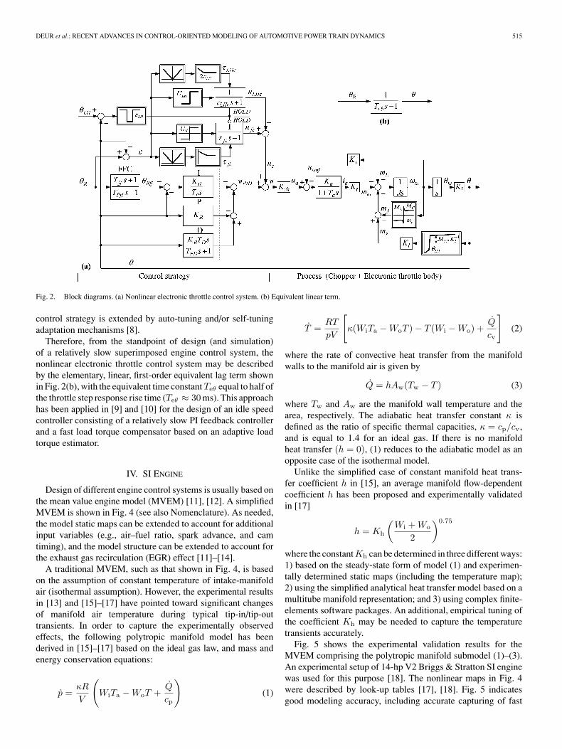
III. ELECTRONIC THROTTLE

The electronic throttle process model is given on the rightof Fig. 2(a). It consists of the dc motor and the chopper linearmodel, extended with the friction and dual return spring non-linearities mf(ω) and ms(θ), respectively. In order to capturethe experimentally observed presliding–displacement frictioneffect, a dynamic friction model has been developed and vali-dated in [5] and [6].

The throttle angle experimental response in Fig. 3(a) demon-strates that the electronic throttle can effectively be controlled bya proportional-integral-derivative (PID) controller for the large-signal operating mode [7]. However, as shown by the dashedlines in Fig. 3(b) and (c), the electronic throttle performancein the small-signal operating mode is significantly affected bythe friction and limp-home nonlinearities [6]. In order to im-prove the small-signal operating mode performance, the PIDcontroller is extended in [6] by nonlinear friction and limp-homecompensators [Fig. 2(a)]. Fig. 3 indicates that the applicationof compensators provides similar, desired control performancefor different operating modes, i.e., the highly nonlinear processbehavior is effectively linearized. This can also be achieved inthe presence of variations of process parameters (e.g., motor ar-mature resistance, battery voltage, and friction) if the nonlinear

DEUR et al.: RECENT ADVANCES IN CONTROL-ORIENTED MODELING OF AUTOMOTIVE POWER TRAIN DYNAMICS 515

Fig. 2. Block diagrams. (a) Nonlinear electronic throttle control system. (b) Equivalent linear term.

control strategy is extended by auto-tuning and/or self-tuningadaptation mechanisms [8].

Therefore, from the standpoint of design (and simulation)of a relatively slow superimposed engine control system, thenonlinear electronic throttle control system may be describedby the elementary, linear, first-order equivalent lag term shownin Fig. 2(b), with the equivalent time constant Teθ equal to half ofthe throttle step response rise time (Teθ ≈ 30 ms). This approachhas been applied in [9] and [10] for the design of an idle speedcontroller consisting of a relatively slow PI feedback controllerand a fast load torque compensator based on an adaptive loadtorque estimator.

IV. SI ENGINE

Design of different engine control systems is usually based onthe mean value engine model (MVEM) [11], [12]. A simplifiedMVEM is shown in Fig. 4 (see also Nomenclature). As needed,the model static maps can be extended to account for additionalinput variables (e.g., air–fuel ratio, spark advance, and camtiming), and the model structure can be extended to account forthe exhaust gas recirculation (EGR) effect [11]–[14].

A traditional MVEM, such as that shown in Fig. 4, is basedon the assumption of constant temperature of intake-manifoldair (isothermal assumption). However, the experimental resultsin [13] and [15]–[17] have pointed toward significant changesof manifold air temperature during typical tip-in/tip-outtransients. In order to capture the experimentally observedeffects, the following polytropic manifold model has beenderived in [15]–[17] based on the ideal gas law, and mass andenergy conservation equations:

p =κR

V

(WiTa − WoT +

Q

cp

)(1)

T =RT

pV

[κ(WiTa − WoT ) − T (Wi − Wo) +

Q

cv

](2)

where the rate of convective heat transfer from the manifoldwalls to the manifold air is given by

Q = hAw(Tw − T ) (3)

where Tw and Aw are the manifold wall temperature and thearea, respectively. The adiabatic heat transfer constant κ isdefined as the ratio of specific thermal capacities, κ = cp/cv,and is equal to 1.4 for an ideal gas. If there is no manifoldheat transfer (h = 0), (1) reduces to the adiabatic model as anopposite case of the isothermal model.

Unlike the simplified case of constant manifold heat trans-fer coefficient h in [15], an average manifold flow-dependentcoefficient h has been proposed and experimentally validatedin [17]

h = Kh

(Wi + Wo

2

)0.75

where the constant Kh can be determined in three different ways:1) based on the steady-state form of model (1) and experimen-tally determined static maps (including the temperature map);2) using the simplified analytical heat transfer model based on amultitube manifold representation; and 3) using complex finite-elements software packages. An additional, empirical tuning ofthe coefficient Kh may be needed to capture the temperaturetransients accurately.

Fig. 5 shows the experimental validation results for theMVEM comprising the polytropic manifold submodel (1)–(3).An experimental setup of 14-hp V2 Briggs & Stratton SI enginewas used for this purpose [18]. The nonlinear maps in Fig. 4were described by look-up tables [17], [18]. Fig. 5 indicatesgood modeling accuracy, including accurate capturing of fast


Fig. 3. Experimental electronic throttle responses. (a) Large-signal operatingmode. (b) Small-signal operating mode outside the limp-home region. (c) Small-signal operating mode around the limp-home region.

Fig. 4. Block diagram of the mean value engine model for isothermalmanifold.

temperature transients. The high-frequency oscillations in theexperimental responses are due to combustion pulsations (notincluded in the MVEM).

Possibly different heat transfer characteristics of plenum andrunners can be taken into account by developing a more complexpolytropic manifold model consisting of separate lumped sub-models for plenum and runners. Rewriting a pair of p–T stateequations (1) to two pairs of state equations for the plenum vol-

Fig. 5. Validation results for the two-state polytropic manifold model.

Fig. 6. Validation results for the three-state polytropic model with and withoutthe backflow effect.

ume and the equivalent runner volume (pp–Tp, pr–Tr), applyingthe obvious boundary conditions on air-mass flows, and neglect-ing the pressure drop across the manifold (pp ≈ pr) leads to asimple and computationally efficient three-state manifold modelpresented in [17]. The effect of backflow from the cylinders tothe runners can be introduced by using the simple substitutionWoTo → WoTo − WbfTbf in the three-state model equations,thus accounting for the backflow enthalpy [17]. Fig. 6 illustratesthat using the three-state model with backflow effect yields anaccurate prediction of the runner temperature response.

One of the main applications of the presented model is theestimation (and prediction) of the port air-mass flow Wo forthe purpose of air–fuel ratio feedforward control [15] and en-gine torque estimation [10]. According to the analysis of thelinearized manifold model given in [19] and [20], the pressureresponse p is 40% faster for the adiabatic than the isothermalmanifold, while the throttle flow Wi and the port flow Wo re-sponses are similar for both the models. Consequently, the tra-ditional port flow estimation and prediction algorithms basedon the isothermal model would be inaccurate for the adiabaticmanifold if the estimator utilizes the pressure measurement sig-nal, and would be rather insensitive to manifold modeling errorsif the throttle flow measurement signal is used [20].


Fig. 7. Dynamic torque converter model. (a) Block diagram. (b) Bond graph.(c) Equivalent mechanical system.

V. TORQUE CONVERTER

The torque converter is usually modeled by using thewell-known capacity factor/torque ratio versus speed ratiosteady-state curves ωi/

√τi = f1(ωt/ωi) and τt/τi = f2(ωt/ωi)

(cf. Fig. 1). These curves can be given in the form of look-uptables, or described by appropriate physical or empirical alge-braic equations [21], [22]. Such a static torque converter modelhas been proven to be adequate in the frequency range of 10–20Hz (at the idle speed region). However, the higher frequencyrange may be of interest for analyses of disturbance/vibrationdamping, and for simulation, estimation, and control of high-frequency and NVH-related power train dynamics during throt-tle steps and gear shifts. In this high-frequency range, the torqueconverter dynamics due to the fluid and stator dynamic effectsshould be considered.

A dynamic torque converter model for operations below thecoupling point (ωt/ωi <≈0.85, the stator is locked) has beenproposed in [23]. The model has been extended for operationsabove the coupling point (including the coast drive mode) in[24]. The model from [24] is shown in Fig. 7(a) and (b) in theform of a block diagram and a bond graph [25], respectively.The switching logic in Fig. 7(a) corresponds to the descriptionof the stator one-way clutch.

As a basic model simplification, it may be assumed that: 1)the stator dynamics is negligible(Is → 0, Ss ≈ 0; or operations

Fig. 8. Block diagrams of the linearized torque converter models. (a) Simpli-fied second-order model. (b) Simplified third-order model.

below the coupling point) and 2) the flow cross-coupling accel-eration terms are negligible (Si,t,s ≈ 0) [24], [26]. According tothe bond graph analysis in [24], the simplified third-order modelmay be represented by an equivalent mechanical system withimpeller and turbine inertias, two continuously variable trans-missions, and a spring-damper in-series combination [Fig. 7(c)].

If it is additionally assumed that the fluid inertia effect is neg-ligible (Lf → 0), the simple second-order model is obtained.This model is usually called the static torque converter model(see Section IV), assuming that the impeller and turbine inertiasIi and It are lumped to the “external” engine and input trans-mission inertias, respectively. The static model is defined bythe nonlinear functions f0 in Fig. 7(a) and additional nonlinearfunctions for fluid velocity V and stator speed ωs, which arerelated to the expressions ϕRHS = 0 and τs0 = 0 [26].

The second- and third-order models have been linearized andanalyzed in [26]. It has been found that the structures of thelinearized models can be significantly simplified based on as-sumptions that are valid for the particular torque converter (andapparently for other torque converters). The block diagrams ofthe simplified models are shown in Fig. 8. The second-ordermodel is of aperiodic lag type, or of integral–lag type [as shownin Fig. 8(a)] if the low-frequency aperiodic dynamics is ne-glected or if the torque converter operates above the couplingpoint. The model parameters depend on the operating point(speed ratio ωt/ωi), and they can be readily calculated fromthe inertia parameters Ii and It, and gradients of the torqueconverter static curves [26].

The third-order linearized model includes one moreparameter—the time constant Tv related to the fluid inertia ef-fect. If Tp > 2Tv, the third-order model in Fig. 8(b) may be


Fig. 9. Schematic of the wet clutch.

regarded as the second-order model in Fig. 8(a) extended withthe parasitic term 1/(Tvs + 1) in the cross-coupling paths. How-ever, if Tp < 2Tv, the emphasized resonance effect occurs, i.e.,weakly damped oscillations appear in the model response. Thisbecomes the case for operations above the coupling point [26].The resonance frequency, given in radians per second, was foundto be 0.6ωi. It should be noted that the structure of the third-order torque converter model in Fig. 8(b) corresponds to thewell-known structure of a two-mass elastic system [27]. This isnot a surprising result, taking into account the representation oftorque converter dynamics, as shown in Fig. 7(c) [24].

The linearized models have been used in [26] to plot thetorque converter frequency responses. The frequency responsesshow that the torque converter effectively attenuates the high-frequency vibrations transferred from the impeller to the turbineside, and vice versa. The fluid inertia effect increases the atten-uation capability for normalized frequencies greater than 0.8–2pulses per impeller revolution. However, the attenuation of im-peller torque-to-impeller speed and turbine torque-to-turbinespeed high-frequency vibrations is smaller than that in theconverter-less transmission, due to the effect of the decoupledimpeller and turbine inertia by means of a fluid.

VI. WET CLUTCH

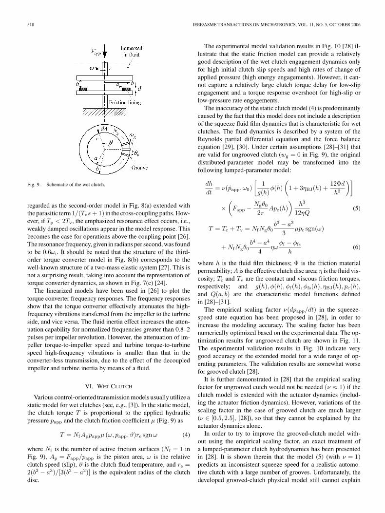
Various control-oriented transmission models usually utilize astatic model for wet clutches (see, e.g., [3]). In the static model,the clutch torque T is proportional to the applied hydraulicpressure papp and the clutch friction coefficient µ (Fig. 9) as

T = NfAppappµ (ω, papp, ϑ)re sgn ω (4)

where Nf is the number of active friction surfaces (Nf = 1 inFig. 9), Ap = Fapp/papp is the piston area, ω is the relativeclutch speed (slip), ϑ is the clutch fluid temperature, and re =2(b3 − a3)/[3(b2 − a2)] is the equivalent radius of the clutchdisc.

The experimental model validation results in Fig. 10 [28] il-lustrate that the static friction model can provide a relativelygood description of the wet clutch engagement dynamics onlyfor high initial clutch slip speeds and high rates of change ofapplied pressure (high energy engagements). However, it can-not capture a relatively large clutch torque delay for low-slipengagement and a torque response overshoot for high-slip orlow-pressure rate engagements.

The inaccuracy of the static clutch model (4) is predominantlycaused by the fact that this model does not include a descriptionof the squeeze fluid film dynamics that is characteristic for wetclutches. The fluid dynamics is described by a system of theReynolds partial differential equation and the force balanceequation [29], [30]. Under certain assumptions [28]–[31] thatare valid for ungrooved clutch (wg = 0 in Fig. 9), the originaldistributed-parameter model may be transformed into thefollowing lumped-parameter model:

dh

dt= ν(papp, ω0)

[1

g(h)φ(h)

(1 + 3ηBJ(h) +

12Φd

h3

)]

×(

Fapp − Ngθ0

2πApc(h)

)h3

12ηQ(5)

T = Tc + Tv = NfNgθ0b3 − a3

3µpc sgn(ω)

+ NfNgθ0b4 − a4

4ηω

φf − φfs

h(6)

where h is the fluid film thickness; Φ is the friction materialpermeability; A is the effective clutch disc area; η is the fluid vis-cosity; Tc and Tv are the contact and viscous friction torques,respectively; and g(h), φ(h), φf(h), φfs(h), ηBJ(h), pc(h),and Q(a, b) are the characteristic model functions definedin [28]–[31].

The empirical scaling factor ν(dpapp/dt) in the squeeze-speed state equation has been proposed in [28], in order toincrease the modeling accuracy. The scaling factor has beennumerically optimized based on the experimental data. The op-timization results for ungrooved clutch are shown in Fig. 11.The experimental validation results in Fig. 10 indicate verygood accuracy of the extended model for a wide range of op-erating parameters. The validation results are somewhat worsefor grooved clutch [28].

It is further demonstrated in [28] that the empirical scalingfactor for ungrooved cutch would not be needed (ν ≈ 1) if theclutch model is extended with the actuator dynamics (includ-ing the actuator friction dynamics). However, variations of thescaling factor in the case of grooved clutch are much larger(ν ∈ [0.5, 2.5], [28]), so that they cannot be explained by theactuator dynamics alone.

In order to try to improve the grooved-clutch model with-out using the empirical scaling factor, an exact treatment ofa lumped-parameter clutch hydrodynamics has been presentedin [28]. It is shown therein that the model (5) (with ν = 1)predicts an inconsistent squeeze speed for a realistic automo-tive clutch with a large number of grooves. Unfortunately, thedeveloped grooved-clutch physical model still cannot explain


Fig. 10. Results of the experimental validation of the static and dynamic models for ungrooved clutch. Operating parameters: initial engagement speed (slip)(r/min), pressure rise time (s), fluid temperature (◦C).

Fig. 11. Squeeze-speed scaling factor for the ungrooved clutch.

the experimentally observed pressure rate-dependence of thesqueeze speed (included in the empirical factor ν), and willrequire further studies.

VII. AUTOMATIC TRANSMISSION

Control-oriented power train models typically include onlydominant transmission dynamic modes such as gear inertia andhalf-shaft compliance, and dominant static effects such as gearratio and clutch Coulomb friction [1]–[3]. These models are usu-ally derived, analyzed, and validated for different transmissionshifts (typically for 1–2 upshift). According to the validation

results in [32], they cannot capture some important charac-teristics of the experimentally observed power train behaviorfor park/reverse and park/drive engagements. The main issuewas that the model response for the half-shaft torque includedweakly damped oscillations in the final response phase, whilethe experimental response was well damped.

In order to improve the modeling accuracy, the basic trans-mission model from [32] is extended in [33] with some of theneglected, mostly nonlinear effects such as transmission com-ponent friction and backlash, clutch drag, and engine blockdynamics.

Fig. 13 shows the bond graph of the extended model for afour-speed automatic transmission1 whose schematic is givenin Fig. 12. The core of the model is the basic gear set submodelgiven between the bonds X and Y in Fig. 13. This submodelconsists of the inertia elements I, the gear ratio transformersTF, and the clutch friction resistance elements R. One of themain advantages of the bond graph modeling method is that itis a simple and systematic way of dealing with redundant statevariables by means of applying the causality rules [25]. For theparticular case of gear set submodel, two of the possible six statevariables are redundant (the speeds ωs2 and ωr1c2). The model

1Note that the brake-on case is considered (Fig. 1). In the brake-off case,the model needs to be extended by wheel inertia–tire friction–vehicle massmodel [1], [2], [32].


Fig. 12. Schematic of the gear set.

Fig. 13. Bond graph model of automatic transmission.

state equations are [32]

A

[ωs1

ωs

]= B [ τrc τlrc τfc τbc τdc τs ]T (7)

ωt =1It

(τt − τfc − τrc − τdc) (8)

ωeb =1

Ieb0(τlrc + τbc − τe − τdiff − τeb0) (9)

where the constant-parameter matrices A and B are definedin [32], and the engine mount torque is given by

τeb0 = bebωeb + keb

∫ωebdt. (10)

The redundant states are calculated as[ωs2

ωr1c2

]=

[− 1+g

h1+g+h

h

− 1h

1+hh

] [ωs1

ωs

]. (11)

The only nonlinearity in the gear set submodel (7)–(11) relatesto the clutch friction

[τrc τlrc τfc τbc τdc] = f([ωrc ωlrc ωfc ωbc ωdc])

= f([ωt −ωs2 ωr1c2 −ωeb ωt −ωs1 ωs2 −ωeb ωt −ωr1c2]).

(12)

Fig. 14. Results of the experimental validation of the automatic transmissionmodel for park/reverse engagement.

As proposed in [32] and [34], the gear set clutch frictionmodel is based on the Karnopp friction model. The main advan-tage of this approach is a superior computing efficiency whencompared to other possible, static and dynamic friction mod-els. A disadvantage is the complexity of the model structure,but, nevertheless, the model derivation and implementation isstraightforward.

After extending the gear set–half-shaft compliance submodel,a very good agreement between simulation and experimental re-sponses has been observed (Fig. 14). The main model extensionsinclude [33] (Fig. 13) the following:

1) transmission backlash 2αb, in order to reproduce high-amplitude half-shaft torque oscillations during the clutchengagement phase (time interval [0.8, 1] in Fig. 14);

2) transmission friction τft and τfs, which damp the torqueresponse during the final engagement phase for the brake-on case;

3) Stribeck friction of the clutch model, which causes anabrupt torque growth at the end of the clutch engagementphase (at t ≈ 1.15 s);

4) clutch drag (torque at zero clutch pressure), which pro-vides prediction of initial torque offset (at t < 0.75 s), andgives consistent response in the presence of transmissionbacklash.

In order to preserve the simple control-oriented model struc-ture, the proposed extensions are given in “lumped” forms (onlya single backlash element αb and only a pair of transmissionfriction elements Rft and Rfs).

VIII. TIRE

The tire friction is traditionally modeled by utilizing a staticmodel, which can be described by brush model expressions [35]or empirical formulae (e.g., “magic” formulae [36]). The recentinterest in modeling the tire friction dynamics has been mo-tivated by the need for precise and computationally efficient


Fig. 15. Brush representation of the longitudinal tire dynamics.

simulations for high-performance vehicle dynamics systemsoperating at a wide range of vehicle speeds (including zerospeed) [37], [38]. The brush model from [37] captures im-portant aspects of the tire friction dynamics, but has a com-plex distributed-parameter form with a large number of inter-nal states. A more pragmatic tire friction modeling approachhas led to the relaxation length-based model [38], which maybe regarded as a semiempirical quasi-static lumped-parametermodel.

More recently, a brush-type longitudinal tire dynamics modelhas been developed based on the LuGre friction model [39].The model accounts for the friction effects in a more preciseway than in [37],2 and can have a one-state lumped parameterform similar to [38]. The model has been modified in [40] toobtain consistent static and dynamic model forms, and thenextended in [41] and [42] for combined longitudinal and lateralmotion including calculation of self-aligning torque [a three-dimensional (3-D) model]. The overall model developments,including validation, are presented in [43].

Fig. 15 shows the brush representation of the longitudinaltire tread dynamics. It is assumed that the tire–road contact isrealized through a lot of tiny, massless, and elastic elements(so-called bristles) attached to a circular belt [35]. The processof horizontal bristle deflection z and the related generation ofthe tire force F is described by the following equations:

∂z(ζ, t)∂t

= vr −σ0|vr|g(vr)

z − r|ω|∂z(ζ, t)∂ζ

(13)

F (t) =1L

∫ L

0

[σ0z(ζ, t) + σ1

∂z(ζ, t)∂t

+ σ2vr

]dζ (14)

where vr = rω − v is the slip speed, g(vr) is a positive general-ized Stribeck curve for the stick-slip friction, σ0 and σ1 are thehorizontal stiffness and damping coefficients of the tire tread,and σ2 is the viscous friction coefficient.

The model has the following simple analytical solution forthe steady-state conditions:

F = sgn (vr)g(vr)[1 − Z

L

(1 − e−L/Z

)]+ σ2vr,

Z =∣∣∣∣rωvr

∣∣∣∣ g(vr)σ0

. (15)

2The tire tread stress–strain curve is described in the LuGre model by anonlinear, hysteretic curve, which is more realistic than the saturated linearcurve that is commonly used in the traditional brush models.

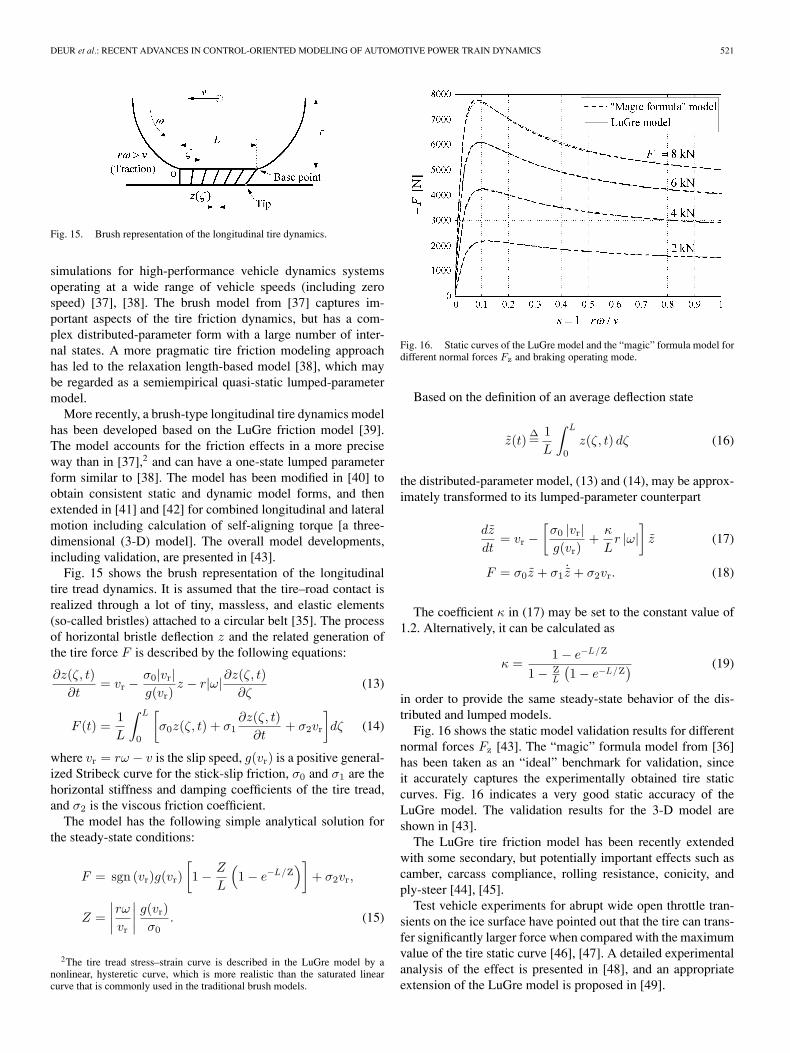
Fig. 16. Static curves of the LuGre model and the “magic” formula model fordifferent normal forces Fz and braking operating mode.

Based on the definition of an average deflection state

z(t)∆=

1L

∫ L

0

z(ζ, t) dζ (16)

the distributed-parameter model, (13) and (14), may be approx-imately transformed to its lumped-parameter counterpart

dz

dt= vr −

[σ0 |vr|g(vr)

+κ

Lr |ω|

]z (17)

F = σ0z + σ1˙z + σ2vr. (18)

The coefficient κ in (17) may be set to the constant value of1.2. Alternatively, it can be calculated as

κ =1 − e−L/Z

1 − ZL

(1 − e−L/Z

) (19)

in order to provide the same steady-state behavior of the dis-tributed and lumped models.

Fig. 16 shows the static model validation results for differentnormal forces Fz [43]. The “magic” formula model from [36]has been taken as an “ideal” benchmark for validation, sinceit accurately captures the experimentally obtained tire staticcurves. Fig. 16 indicates a very good static accuracy of theLuGre model. The validation results for the 3-D model areshown in [43].

The LuGre tire friction model has been recently extendedwith some secondary, but potentially important effects such ascamber, carcass compliance, rolling resistance, conicity, andply-steer [44], [45].

Test vehicle experiments for abrupt wide open throttle tran-sients on the ice surface have pointed out that the tire can trans-fer significantly larger force when compared with the maximumvalue of the tire static curve [46], [47]. A detailed experimentalanalysis of the effect is presented in [48], and an appropriateextension of the LuGre model is proposed in [49].


IX. CONCLUSION

The presented modeling, analysis, and validation results haveshown that some of usually neglected dynamic effects can havea significant influence on the accuracy of the automotive powertrain models for specific operating modes and modeling tasks.These effects include the following.

1) Electronic throttle delay may be described by a linear first-order lag term, provided that the control strategy effectivelylinearizes the nonlinear electronic throttle body dynamics.

2) Manifold air temperature transients affect the accuracy ofthe cylinder air charge estimation/prediction based on manifoldpressure measurement.

3) Torque converter fluid dynamics modeling is important forvibration attenuation analysis and wide frequency range simu-lations. The fluid dynamics may cause an oscillatory mode foroperations above the coupling point.

4) Wet clutch fluid dynamics significantly affects the accu-racy of clutch torque response for low-/medium-energy clutchengagements.

5) Transmission friction and backlash, low-speed clutchfriction, and clutch drag have a substantial influence on thepark/reverse and park/drive engagement modeling accuracy.

6) Tire friction dynamics modeling provides computationallyefficient simulations for a wide vehicle speed range, and in-creases the model fidelity in the high-frequency range. Using ahysteretic stress–strain curve for the tire tread, as incorporatedin the LuGre model, increases the accuracy of the tire staticcurves.

ACKNOWLEDGMENT

The authors would like to express their gratitude towardDr. B. Tobler from the Ford Research and Advanced Engi-neering for constructive and very helpful discussions, and datasupport.

REFERENCES

[1] D. Hrovat and W. E. Tobler, “Bond graph modeling of automotive powertrains,” J. Franklin Inst., vol. 328, pp. 623–662, 1991.

[2] D. Hrovat, J. Asgari, and M. G. Fodor, “Automotive mechatronics sys-tems,” in Mechatronics Systems, Techniques and Applications, C. T.Leondes, Ed. New York: Gordon and Breach, 2000, pp. 1–98.

[3] D. Cho and K. J. Hedrick, “Automotive powertrain modeling for control,”Trans. ASME, J. Dyn. Syst. Meas. Control, vol. 111, pp. 568–576, 1989.

[4] H. Heisler, Advanced Vehicle Technology, 2nd ed. Warrendale, PA: SAE,2002.

[5] D. Pavkovic, J. Deur, M. Jansz, and N. Peric. (2003). Experimental identi-fication of electronic throttle body. Presented at the 10th Eur. Conf. PowerElectron. Appl., Toulouse, France [CD-ROM].

[6] J. Deur, D. Pavkovic, N. Peric, M. Jansz, and D. Hrovat, “An electronicthrottle control strategy including compensation of friction and limp-homeeffects,” IEEE Trans. Ind. Appl., vol. 40, no. 3, pp. 821–834, May–Jun.2004.

[7] J. Deur, D. Pavkovic, N. Peric, and M. Jansz. (2002). Analysis and opti-mization of an electronic throttle for linear operating modes. Presented atthe 10th Int. Power Electron. Motion Control Conf., Dubrovnik-Cavtat,Croatia [CD-ROM].

[8] D. Pavkovic, J. Deur, M. Jansz, and N. Peric, “Adaptive control of au-tomotive electronic throttle,” Control Eng. Pract., vol. 14, pp. 121–136,2006.

[9] J. Deur, V. Ivanovic, D. Pavkovic, and M. Jansz, “Identification and speedcontrol of SI engine for idle operating mode,” SAE Paper 2004-01-0898,2004.

[10] D. Pavkovic, J. Deur, V. Ivanovic, and D. Hrovat, “SI engine load torqueestimator based on adaptive Kalman filter and its application to idle speedcontrol,” SAE Paper 2005-01-0036, 2005.

[11] B. K. Powell, “A dynamic model for automotive engine control analysis,”in Proc. 18th IEEE Conf. Decision Control, 1979, pp. 120–126.

[12] E. Hendricks, A. Chavalier, M. Jensen, S. C. Sorenson, D. Trumpy, andJ. Asik, “Modeling of the intake manifold filling dynamics,” SAE Paper960037, 1996.

[13] M. Fons, M. Muller, A. Chevalier, C. Vigild, E. Hendricks, andS. C. Sorenson, “Mean value engine modeling of an SI engine with EGR,”SAE Paper 1999-01-0909, 1999.

[14] M. Jankovic and S. W. Magner, “Cylinder air-charge estimation for ad-vanced intake valve operation in variable cam timing engines,” JSAE Rev.,vol. 22, no. 4, pp. 445–452, Oct. 2001.

[15] A. Chevalier, C. Vigild, and E. Hendricks, “Predicting the port air massflow of SI engines in air/fuel ratio control applications,” SAE Paper 2000-01-0260, 2000.

[16] D. Hrovat, “Mean value engine models,” private communication, 1989–1990.

[17] J. Deur, D. Hrovat, J. Petric, and Z. Situm. (2003). A control-orientedpolytropic model of SI engine intake manifold. Presented at the ASMEInt. Mech. Eng. Congr. Expo., Washington, DC, vol 2 [CD-ROM].

[18] J. Petric, J. Deur, D. Pavkovic, I. Mahalec, and Z. Herold, “Experimentalsetup for SI-engine modeling and control research,” Strojarstvo, vol. 46,no. 1–3, pp. 39–50, 2004.

[19] J. Deur, D. Hrovat, and J. Asgari, “Analysis of mean value engine modelwith emphasis on intake manifold thermal effects,” in Proc. IEEE Int.Conf. Control Appl., Istanbul, Turkey, 2003, vol. 1, pp. 161–166.

[20] J. Deur, S. W. Magner, M. Jankovic, and D. Hrovat. (2004). Influence of in-take manifold heat transfer effects on accuracy of SI engine air charge pre-diction, Presented at the ASME Int. Mech. Eng. Congr. Expo., Anaheim,CA, vol. 2 [CD-ROM].

[21] G. G. Lucas and A. Rayner, “Torque converter design calculations,” Au-tomob. Eng., pp. 56–60, 1970.

[22] A. Kotwicki, “Dynamic models for torque converter equipped vehicles,”SAE Paper 820393, 1982.

[23] T. Ishihara and R. Emori, “Torque converter as a vibration damper and itstransient characteristics,” SAE Paper 660368, 1966.

[24] D. Hrovat and W. E. Tobler, “Bond graph modeling and computer simula-tion of automotive torque converter,” J. Franklin Inst., vol. 319, no. 1–2,pp. 93–114, 1985.

[25] D. C. Karnopp, D. L. Margolis, and R. Rosenberg, System Dynamics—AUnified Approach. New York: Wiley, 1990.

[26] J. Deur, D. Hrovat, and J. Asgari. (2002). Analysis of torque converterdynamics. Presented at the ASME Int. Mech. Eng. Congr. Expo., NewOrleans, LA, vol. 2 [CD-ROM].

[27] J. Deur and N. Peric, “Analysis of speed control system for electricaldrives with elastic transmission,” in Proc. IEEE Int. Symp. Ind. Electron.,Bled, Slovenia, Jul.1999, vol. 3, pp. 624–630.

[28] J. Deur, J. Petric, J. Asgari, and D. Hrovat, “Modeling of wet clutchengagement including a thorough experimental validation,” SAE Paper2005-01-0877, 2005.

[29] B. Jacobson, “Engagement of oil immersed multi-disc clutches,” in Proc.ASME Int. Power Transmiss. Gearing Conf., 1992, vol. 43-2, pp. 567–574.

[30] S. Natsumeda and T. Miyoshi, “Numerical simulation of engagementof paper based wet clutch facing,” Trans. ASME, J. Tribol., vol. 116,pp. 232–237, 1994.

[31] E. J. Berger, F. Sadeghi, and C. M. Krousgrill, “Analytical and numericalmodeling of engagement of rough, permeable, grooved wet clutches,”Trans. ASME, J. Tribol., vol. 119, pp. 143–148, 1997.

[32] J. Deur, J. Asgari, D. Hrovat, and P. Kovac, “Modeling and anal-ysis of automatic transmission engagement dynamics—Linear case,”Trans. ASME., J. Dyn. Syst. Meas. Control, vol. 128, pp. 263–277, Jun.2006.

[33] J. Deur, J. Asgari, and D. Hrovat, “Modeling and analysis of automatictransmission engagement dynamics—Nonlinear case including valida-tion,” Trans. ASME, J. Dyn. Syst. Meas. Control, vol. 128, pp. 251–262,Jun. 2006.

[34] . (2003). Modeling of an automotive planetary gear set based onKarnopp model for clutch friction. Presented at the ASME Int. Mech.Eng. Congr. Expo., Washington, DC, vol. 2 [CD-ROM].

[35] H. B. Pacejka and R. S. Sharp, “Shear force development by pneumatictyres in steady state conditions: A review of modelling aspects,” VehicleSyst. Dyn., vol. 20, pp. 121–176, 1991.


[36] E. Bakker, L. Nyborg, and H. B. Pacejka, “Tyre modelling for use invehicle dynamics studies,” SAE Paper 870421, 1987.

[37] A. van Zanten, W. D. Ruf, and A. Lutz, “Measurement and simulation oftransient tire forces,” SAE Paper 890640, 1989.

[38] J. E. Bernard and C. L. Clover, “Tire modeling for low-speed and high-speed calculations,” SAE Paper 950311, 1995.

[39] C. Canudas de Wit and P. Tsiotras, “Dynamic tire friction models forvehicle traction control,” in Proc. 38th IEEE Conf. Decision Control,Phoenix, AZ, 1999, pp. 3746–3751.

[40] J. Deur, “Modeling and analysis of longitudinal tire dynamics based on theLuGre friction model,” in Proc. 3rd IFAC Workshop Advances AutomotiveControl, Karlsruhe, Germany, 2001, pp. 101–106.

[41] J. Deur, J. Asgari, and D. Hrovat. (2001). A dynamic tire friction modelfor combined longitudinal and lateral motion. Presented at the ASME Int.Mech. Eng. Congr. Expo., New York, NY, vol. 2 [CD-ROM].

[42] J. Deur. (2002). A brush-type dynamic tire friction model for non-uniformnormal pressure distribution. Presented at the 15th IFAC World Congr.,Barcelona, Spain [CD-ROM].

[43] J. Deur, J. Asgari, and D. Hrovat, “A 3D brush-type dynamic tire frictionmodel,” Vehicle Syst. Dyn., vol. 42, no. 3, pp. 133–173, 2004.

[44] J. Deur, V. Ivanovic, M. Troulis, C. Miano, D. Hrovat, and J. Asgari,“Extensions of LuGre tire friction model related to variable slip speedalong contact patch length,” in Proc. 3rd IAVSD Int. Tyre Colloq. TyreModels Vehicle Dyn. Anal., Vienna, Austria, 2004, p. 32.

[45] , “Extensions of LuGre tire friction model related to variable slipspeed along contact patch length,” Vehicle Syst. Dyn., vol. 43, pp. 508–524, 2005.

[46] J. Deur, V. Ivanovic, D. Pavkovic, D. Hrovat, J. Asgari, M. Troulis, andC. Miano, “Experimental analysis and modeling of longitudinal tire fric-tion dynamics for abrupt transients,” in Proc. 3rd IAVSD Int. Tyre Colloq.Tyre Models Vehicle Dyn. Anal., Vienna, Austria, 2004, p. 33.

[47] , “Experimental analysis and modeling of longitudinal tire frictiondynamics for abrupt transients,” Vehicle Syst. Dyn., vol. 43, pp. 525–539,2005.

[48] V. Ivanovic, J. Deur, M. Kostelac, Z. Herold, M. Troulis, C. Miano,D. Hrovat, J. Asgari, D. Higgins, J. Blackford, and V. Koutsos, “Exper-imental identification of dynamic tire friction potential on ice surfaces,”presented at the XIX IAVSD Symp., Milan, Italy, 2005.

[49] V. Ivanovic, J. Deur, J. Asgari, D. Hrovat, and O. Hofmann, “Modeling ofdynamic tire friction potential on ice surfaces,” in Proc. 2006 ASME Int.Mech. Eng. Congr. Expo., Chicago, IL, to be published.

Josko Deur (M’02) received the B.S., M.S., and thePh.D. degrees, all in electrical engineering, from theUniversity of Zagreb, Zagreb, Croatia, in 1989, 1993,and 1999, respectively.

In 1990, he joined the Faculty of Mechanical En-gineering and Naval Architecture, University of Za-greb, as an Assistant, where he has been an AssistantProfessor since 2002. In 2000, he was a PostdoctoralVisiting Scholar with the Ford Research Laboratory,Dearborn, MI, where he was engaged in research ondifferent aspects of automotive system dynamics and

control. His current research interests include modeling and control of dynamicsystems with emphasis on the automotive systems and servo drives.

Josko Petric received the B.S., M.S., and Ph.D. degrees, all in mechanical en-gineering, from the University of Zagreb, Zagreb, Croatia, in 1987, 1991, and1994, respectively.

He is currently an Associate Professor in the Faculty of Mechanical Engi-neering and Naval Architecture at the University of Zagreb. His areas of teachinginclude automatic control, mechatronics, robotics, and fluid power. His currentresearch interests include modeling and control of automotive systems.

Dr. Petric is a member of the American Society of Mechanical Engineers.

Jahan Asgari received the B.Sc. degree from California State University, Sacra-mento, in 1983, and M.S. and Ph.D. degrees from the University of California,Davis, in 1985 and 1989, respectively, all in mechanical engineering.

Currently, he is with Ford Research and Advanced Engineering, Dearborn,MI, where he is engaged in several projects on driveline, and chassis modelingand control.

Davor Hrovat (S’77–M’79–SM’91) received theB.Sc. (Dipl. Ing.) degree from the University ofZagreb, Zagreb, Croatia, in 1972, and the M.S. andPh.D. degrees from the University of California,Davis, in 1976 and 1979, respectively, all in mechan-ical engineering.

Since 1981, he has been with the Ford Researchand Advanced Engineering, Dearborn, MI, where heis currently a Corporate Technical Specialist, coor-dinating and leading research efforts on various as-pects of vehicle/power train control systems. He is

the holder of more than 50 patents.Dr. Hrovat is a Fellow of the American Society of Mechanical Engineers.

He has recently been elected to the National Academy of Engineering. He hasserved on the Editorial Boards of a number of ASME and IEEE journals, and iscurrently an Editor of the IFAC journals Control Engineering Practice, Interna-tional Journal of Vehicle Autonomous Systems, and Vehicle System Dynamics.He was the recipient of the 1996 ASME/Dynamic Systems and Control Innova-tive Practice Award and the 1999 AACC Control Engineering Practice Award.

Recent Advances in Control-Oriented Modeling of Automotive Power Train Dynamics

Documents

Transcript of Recent Advances in Control-Oriented Modeling of Automotive Power Train Dynamics