www.frontiersin.org June 2011 | Volume 5 | Article 85 | 1

Original research articlepublished: 30 June 2011

doi: 10.3389/fnins.2011.00085

Real-time position reconstruction with hippocampal place cells

Christoph Guger1*, Thomas Gener 2, Cyriel M. A. Pennartz3, Jorge R. Brotons-Mas4, Günter Edlinger1, S. Bermúdez i Badia5, Paul Verschure5, Stefan Schaffelhofer1 and Maria V. Sanchez-Vives2

1 g.tec medical engineering GmbH/Guger Technologies OG, Graz, Austria2 Institut d’Investigacions Biomediques August Pi i Sunyer, Institució Catalana de Recerca i Estudis Avançats, Barcelona, Spain3 Center for Neuroscience, University of Amsterdam, Amsterdam, Netherlands4 Instituto Cajal, Consejo Superior de Investigaciones Científicas, Madrid, Spain5 Synthetic Perceptive, Emotive and Cognitive Systems, Institució Catalana de Recerca i Estudis Avançats, Universitat Pompeu Fabra, Barcelona, Spain

Brain–computer interfaces (BCI) are using the electroencephalogram, the electrocorticogram and trains of action potentials as inputs to analyze brain activity for communication purposes and/or the control of external devices. Thus far it is not known whether a BCI system can be developed that utilizes the states of brain structures that are situated well below the cortical surface, such as the hippocampus. In order to address this question we used the activity of hippocampal place cells (PCs) to predict the position of an rodent in real-time. First, spike activity was recorded from the hippocampus during foraging and analyzed off-line to optimize the spike sorting and position reconstruction algorithm of rats. Then the spike activity was recorded and analyzed in real-time. The rat was running in a box of 80 cm × 80 cm and its locomotor movement was captured with a video tracking system. Data were acquired to calculate the rat’s trajectories and to identify place fields. Then a Bayesian classifier was trained to predict the position of the rat given its neural activity. This information was used in subsequent trials to predict the rat’s position in real-time. The real-time experiments were successfully performed and yielded an error between 12.2 and 17.4% using 5–6 neurons. It must be noted here that the encoding step was done with data recorded before the real-time experiment and comparable accuracies between off-line (mean error of 15.9% for three rats) and real-time experiments (mean error of 14.7%) were achieved. The experiment shows proof of principle that position reconstruction can be done in real-time, that PCs were stable and spike sorting was robust enough to generalize from the training run to the real-time reconstruction phase of the experiment. Real-time reconstruction may be used for a variety of purposes, including creating behavioral–neuronal feedback loops or for implementing neuroprosthetic control.

Keywords: real-time position reconstruction, place cells, firing fields, spatial navigation, hippocampus, brain–computer interface, BCI, spikes

Edited by:Eberhard E. Fetz, University of Washington, USA

Reviewed by:Sheri Mizumori, University of Washington, USASam Deadwyler, Wake Forest Medical School, USA

*Correspondence:Christoph Guger, g.tec medical engineering GmbH/Guger Technologies OG, Sierningstrasse 14, 4521 Schiedlberg, Austria.e-mail: guger@gtec.at

the cortical surface. In order to address this question we used the activity of hippocampal place cells (PCs) to predict the position of an animal (rat) in real-time.

Neural cells with spatially modulated firing have been found in almost all areas of the hippocampus and in some surround-ing areas, such as medial entorhinal cortex (Hafting et al., 2005). Hippocampal PCs may provide a representation of an animal’s position in its environment and recent data suggests also time-dependent episodic coding (Leutgeb et al., 2005; Pastalkova et al., 2008; Rennó-Costa et al., 2010). Their background firing rate is low, but when an animal enters the receptive field of the neuron, its firing rate rapidly increases (to a maximum between 5 and 30 Hz; O’Keefe and Dostrovsky, 1971). This specific location is called the place field (PF) of that particular neuron.

Animals use different cues to navigate and to build cognitive environmental representations which can be divided into idi-othetic (self-motion) and external landmarks (Knierim et al., 1998).

IntroductIonBrain–computer interfaces (BCI) are using the electroencephalo-gram (EEG), the electrocorticogram (ECoG), and trains of action potentials as inputs to analyze brain activity for communication purposes and/or the control of external devices (McFarland et al., 2008; Schalk et al., 2008; Velliste et al., 2008). The major difference between the three types of measures is their spatial resolution. In humans, scalp EEG provides a spatial resolution of several centim-eter, ECoG of several millimeter and spikes of several micrometer. EEG and ECoG based BCI systems use mostly motor imagery and evoked potentials (Wolpaw et al., 2003; McFarland et al., 2008; Guger et al., 2009; Pfurtscheller et al., 2010). BCI systems based on spikes have thus far used action potentials from the primary motor area that allow monkeys or humans to control robotic devices or computer systems (Hochberg et al., 2006; Velliste et al., 2008). Thus far it is not known whether a BCI system can be developed that utilizes the states of central brain structures located well below

Frontiers in Neuroscience | Neuroprosthetics June 2011 | Volume 5 | Article 85 | 2

Guger et al. Real-time position reconstruction

off-lIne posItIon reconstructIonFor off-line position reconstruction the following tasks have to be performed (see Figure 1):

(1) Data acquisition: first training data has to be acquired of a rat moving around in a two-dimensional space. Therefore the x- and y-positions of the rat have to be acquired with sufficient time resolution to capture the movements of the animal accurately. Implanted electrodes connected to an amplifier are used to record action potentials from the hip-pocampus together with the rat’s position information. The recording must last long enough to ensure that the rat visits each position of the arena. The tracking data must be availa-ble continuously throughout the whole recording and spike amplitudes have to be checked for artifacts.

(2) Encoding step: manual spike sorting is performed to assign to each spike a certain neuron number, to be able to distin-guish activity of different neurons and to remove noise. This results in spike templates for automatic spike sorting and allows to calculate firing rate maps in order to identify PFs of the recorded cells. The firing rate maps and tracking infor-mation are used as training data for a position reconstruc-tion algorithm.

(3) Decoding step: in this step spiking activity, recorded from a different time segment than in (2), but from the same rat and the same session, is used as input into the position recon-struction algorithm to reconstruct (decode) the trajectories of the rat’s movements occurring during the period that very same spike trains were recorded.

(4) Accuracy calculation: the reconstructed position based on spikes is compared with the animal’s real position acqui-red with the tracking system to calculate the accuracy of the procedure.

off-lIne experIments and recordIng setupFor the off-line experiments action potential data were recorded from three rats from CA1 or subiculum at IDIBAPS (Barcelona) and the Institute of Cognitive Neuroscience (University College London, UCL). Recording details are given in Table 1. The rats were chronically implanted with a microdrive and tetrodes were used for the recordings. The electrodes were connected to the record-ing system (sampling rate 48 Hz, bandpass: 300 Hz–6 kHz) via a headstage amplifier. For tracking the rat’s position, small infrared light-emitting diodes (LEDs) were attached to the rat’s head and a video camera was mounted above the experimental arena. The sampling frequency for the position-tracking signal was 48 Hz (IDIBAPS) and 46.875 Hz (UCL). Animals were food-deprived up to 80% of their original weight after which recordings com-menced. Grains of sweetened rice were thrown in the enclosed environment every 20 s at random locations within the open field, keeping the animal in continuous locomotion, thereby allowing a complete sampling of the environment. IDIBAPS rats were cared for and treated in accordance with Spanish regulatory laws (BOE 256; October 25, 1990) which comply with the EU guidelines on protection of vertebrates used for experimentation (Strasbourg March 18, 1986). The animal care facility is registered with the number B9900020 and is regulated by the Real Decreto (Español)

Rodents use landmarks to guide them to specific locations and they find the way back without landmarks by using self-motion cues known as path integration (O’Keefe and Conway, 1980; Etienne, 1992). In blind rats, Save et al. (1998) showed that self-motion (idi-othetic) information in conjunction with stimulus recognition is sufficient for normal firing of PCs. However, path integration tends to accumulate errors over time and therefore a re-calibration by fixed external landmarks is required (Poucet et al., 2003).

Both cells in the hippocampus proper (CA1) and subiculum show location related firing patterns. CA1 cells provide a spatial representation of the environment, and can even show multiple maps for one environment when environmental cues are changed (Leutgeb et al., 2005; Rennó-Costa et al., 2010). In contrast, sub-icular cells provide a representation of the geometric relationships between different locations in an environment (Sharp, 1997, 1999). Parasubicular and subicular PCs tend to show higher levels of back-ground activity and have larger PFs than hippocampal PCs (CA1; Taube, 1995).

Place cells were used to reconstruct the path of rats by inves-tigating their firing patterns (Wilson and McNaughton, 1993; Brown et al., 1998; Zhang et al., 1998; Jensen and Lisman, 2000; Barbieri et al., 2005). All of these studies used hippocampal PCs, with large numbers of simultaneously recorded neurons, in two cases using linear tracks (Zhang et al., 1998; Jensen and Lisman, 2000), in two other cases circular environments (Brown et al., 1998; Barbieri et al., 2005), and in one case in a rectangular environment (Wilson and McNaughton, 1993). In these studies the spike information and position of the rat were recorded first before position reconstruction methods were applied off-line. For reconstruction Template Matching and Bayesian methods were investigated. In general a Bayesian two-step algorithm tak-ing into account the previous position of the rat performed best and was tested by several groups (Brown et al., 1998; Zhang et al., 1998; Jensen and Lisman, 2000; Barbieri et al., 2005). Importantly, data of the same run was used for training and for testing the performance.

In this study we test whether the rat’s position can be recon-structed in real-time using training data acquired before the actual experiment. For this task it is important that all steps including data acquisition, visualization of spikes, storage, spike sorting, and position reconstruction are done in real-time without delay. In this way, PC firing can be used to provide on-line feedback to the rat to manipulate its behavior and possibly manipulate underlying cognitive processes. First we investigate three differ-ent rats foraging in a rectangular environment. For the position reconstruction a Bayesian two-step algorithm was implemented and tested to identify the important parameters of the algorithm. We tested how neurons of CA1 and neurons with larger PFs than those found in CA1, such as subicular neurons, perform in this environment. Then we implemented a spike sorting algorithm that works also in real-time with high accuracy and speed and compared it to manual and automatic spike sorting results (done off-line). Based on these results we started the real-time posi-tion reconstruction experiments with one rat to test reconstruc-tion accuracy using previously recorded training data and to test whether all analysis tasks could be performed fast enough to sup-port real-time reconstruction.

www.frontiersin.org June 2011 | Volume 5 | Article 85 | 3

Guger et al. Real-time position reconstruction

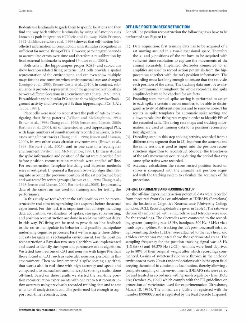
FIgure 1 | Spikes and tracking information were acquired and the first 50% of the data were used for the encoding step, the last 50% were used for the decoding. Then in the encoding step first the data were manually sorted and firing rate maps and spike templates were calculated from the spike trains. From the position-tracking data the probability distribution was calculated. In the decoding step the spikes are automatically sorted with the spike templates calculated before. Then the firing rate of each neuron was calculated and passed

together with the probability distribution of position and with the firing rate maps into the Bayesian two-step algorithm. The Bayesian two-step algorithm returns the reconstructed position and was compared to the position coming from the tracking system to calculate the overall accuracy of the reconstruction procedure. In real-time mode instead of splitting the data in 50% parts, one run was performed for the encoding and later on another run was performed for the real-time decoding step.

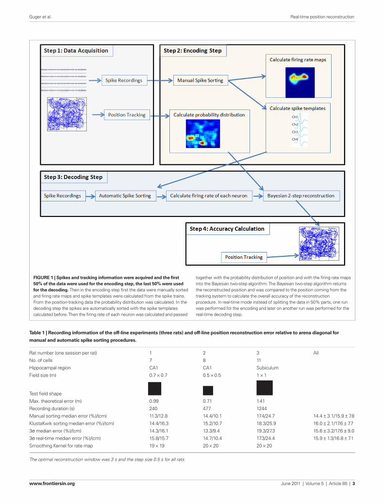
Table 1 | recording information of the off-line experiments (three rats) and off-line position reconstruction error relative to arena diagonal for

manual and automatic spike sorting procedures.

Rat number (one session per rat) 1 2 3 All

No. of cells 7 8 11

Hippocampal region CA1 CA1 Subiculum

Field size (m) 0.7 × 0.7 0.5 × 0.5 1 × 1

Test field shape

Max. theoretical error (m) 0.99 0.71 1.41

Recording duration (s) 240 477 1244

Manual sorting median error (%)/(cm) 11.3/12.8 14.4/10.1 17.4/24.7 14.4 ± 3.1/15.9 ± 7.8

KlustaKwik sorting median error (%)/(cm) 14.4/16.3 15.2/10.7 18.3/25.9 16.0 ± 2.1/17.6 ± 7.7

3σ median error (%)/(cm) 14.3/16.1 13.3/9.4 19.3/27.3 15.6 ± 3.2/17.6 ± 9.0

3σ real-time median error (%)/(cm) 15.8/15.7 14.7/10.4 17.3/24.4 15.9 ± 1.3/16.8 ± 7.1

Smoothing Kernel for rate map 19 × 19 20 × 20 20 × 20

The optimal reconstruction window was 3 s and the step size 0.5 s for all rats.

Frontiers in Neuroscience | Neuroprosthetics June 2011 | Volume 5 | Article 85 | 4

Guger et al. Real-time position reconstruction

The reconstruction algorithm can be improved off-line by tweaking several parameters: (i) length of reconstruction window: this defines the degree of averaging the spiking activity over time; (ii) step size for shifting the reconstruction window forward after each iteration, (iii) smoothing factor of PFs: firing rate and spatial occupancy distributions were smoothed using a rectangular filter. This reduced the influence of outliers on the reconstruction result. (iv) The minimum number of spikes within each reconstruction window: if this parameter is set to a value m higher than zero, the reconstruction is only performed for windows that include at least m spikes. If this condition is not fulfilled the reconstruction for this step is skipped and the position is interpolated. Setting m to a high value affects the reconstruction accuracy but also reduces the number of time points where the reconstruction can be per-formed at all. (v) The number of PCs. It is important to find a parameter combination yielding the best reconstruction result. Therefore the reconstruction accuracy was compared for differ-ent parameter combinations and the optimal was selected (length of reconstruction window: 0.5, 1–10 s in steps of 1; step size: 100, 200, 500, 1000, 2000 ms; smoothing factor: 5 × 5 to 30 × 30 in steps of 1 × 1). The datasets were divided into two equally long parts. Algorithm training (encoding) was performed on the first half of each recording session, while the remaining 50% was used for decoding (reconstruction).

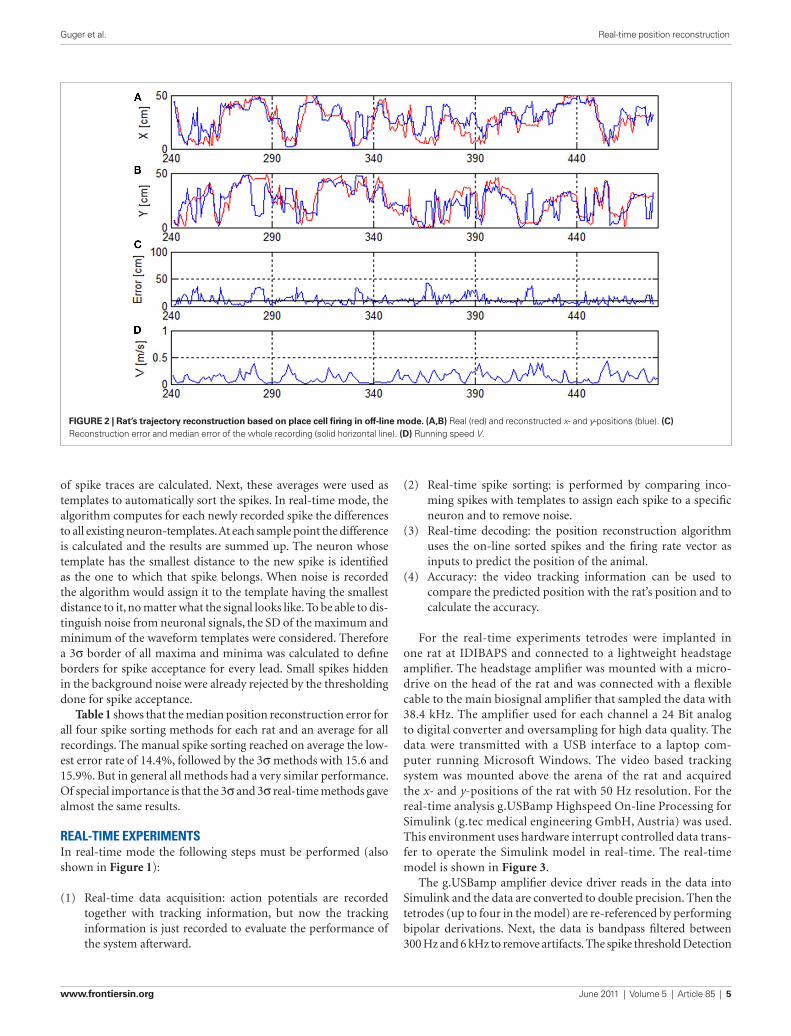
off-lIne resultsFigure 2 shows the reconstruction results computed with the Bayesian two-step algorithm for one recording (rat 2) of 477 s length. Data from seconds 0 to 240 were used to train the algo-rithm and the interval 241–477 was used to test the accuracy of the method.

To calculate the reconstruction error, the reconstructed position was compared to the position known from the position-tracking data. Figure 2 shows that the reconstructed path follows the real path for many data points of the recording. In this case the median reconstruction error was 9.4 cm or 13.3%. The graph illustrates some erratic jumps of the reconstructed path in both x- and y-coor-dinates (e.g., at seconds 280, 365, 415,…) which were mostly caused by a drop in firing rate.

Table 1 compares reconstruction performance for different spike sorting methods for all rats. Spikes were sorted (i) manually, (ii) with the KlustaKwik (Harris et al., 2000; Redish, 2008) algorithm using the energy, amplitude, and first principal component of spike waveforms, (iii) with the 3σ method and, (iv) in real-time mode with the 3σ real-time method. The 3σ method will be described below. For methods i–iii the spike sorting was performed for the first 50% of the data of a session to yield training data and for the last 50% of the session to have testing data. The firing field was calculated only from the training data and the position reconstruc-tion algorithm was trained only with the training data. For the real-time operation it is not possible to sort the spikes in advance and therefore a real-time sorting algorithm was developed. This means that only information from the training data can be used to sort the spikes of the testing data and this is tested with the method iv.

The real-time 3σ method uses the manual sorting results as input to calculate average spike waveforms for each neuron. Additionally the SD of the maximum and the minimum voltages

1201 October 1, 2005. UCL rats handling and care were conducted under Home Office licensing according to the guidelines in the Animals (Scientific Procedures) Act of 1986.

The reconstruction was tested in square arenas of different sizes. The size of the arenas leads also to the maximum theoretical posi-tion reconstruction error by calculating the diagonal distance (e.g., 70 cm*SQRT(2) = 99 cm). The recording duration was between 240–1244 s.

off-lIne posItIon reconstructIon algorIthmFirst, the recorded spike activity was used as input for the manual spike sorting procedure to separate neuronal activity picked up by the electrodes into single cell activity. To carry out the sorting between spikes, amplitudes, shapes, and timing of the spikes were compared across different electrodes. Units were only included for further analysis if no spike was present in the first millisecond of the interspike interval histogram (ISIH). In real-time mode the spike sorting must be done automati-cally. Therefore the resulting templates from the manual sorting were used to resort the spike activity to simulate the real-time procedure.

Next, firing rate maps were created based on spike and tracking information. The arena was divided into subsets of space (64 × 64) and a specific class (unique ID) was assigned to each pixel. This led to an edge length for each pixel of, e.g., 1.09 cm for rat 1. The firing rate for each class was calculated by counting the number of spikes within this location. Afterward these firing rate maps were spatially smoothed with a window of specific length (Smoothing Kernel in Table 1).

For position reconstruction the Bayesian two-step algorithm with continuity constraint was implemented (Zhang et al., 1998). The probability of being at position x, given the number of spikes n of all the cells within the time window is

P x n P x f x f xin

i

N

ii

Ni( | ) ( ) ( ) exp ( )= ⋅

⋅ − ⋅

= =

∏ ∑1 1

∆

(1)

where P(x) is the rat’s position distribution, fi (x) is the average

firing rate of cell i at position x, N is the total number of PCs, ∆ is the length of the time window. The most probable position will be regarded as the animal’s position:

ˆ arg max ( | ),x P x nx

Bayes step1− =

(2)

A continuity constraint can improve the accuracy of recon-struction by reducing sudden jumps in the reconstructed path by incorporating the reconstructed position from the preceding time step and speed information (e.g., Barbieri et al., 2005). This gives the Bayesian two-step algorithm:

P x n x P x n P x xt t t t t t t( | , ) ( | ) ( | )− −= ⋅1 1 (3)

The firing rates of all cells within a sliding time window were compared with the firing rate vectors of each pixel that were set up in the training phase. A pixel number (e.g., 8 out of 64 × 64) was returned which identified the reconstructed position. Then the time window was shifted to the next reconstruction position.

www.frontiersin.org June 2011 | Volume 5 | Article 85 | 5

Guger et al. Real-time position reconstruction

(2) Real-time spike sorting: is performed by comparing inco-ming spikes with templates to assign each spike to a specific neuron and to remove noise.

(3) Real-time decoding: the position reconstruction algorithm uses the on-line sorted spikes and the firing rate vector as inputs to predict the position of the animal.

(4) Accuracy: the video tracking information can be used to compare the predicted position with the rat’s position and to calculate the accuracy.

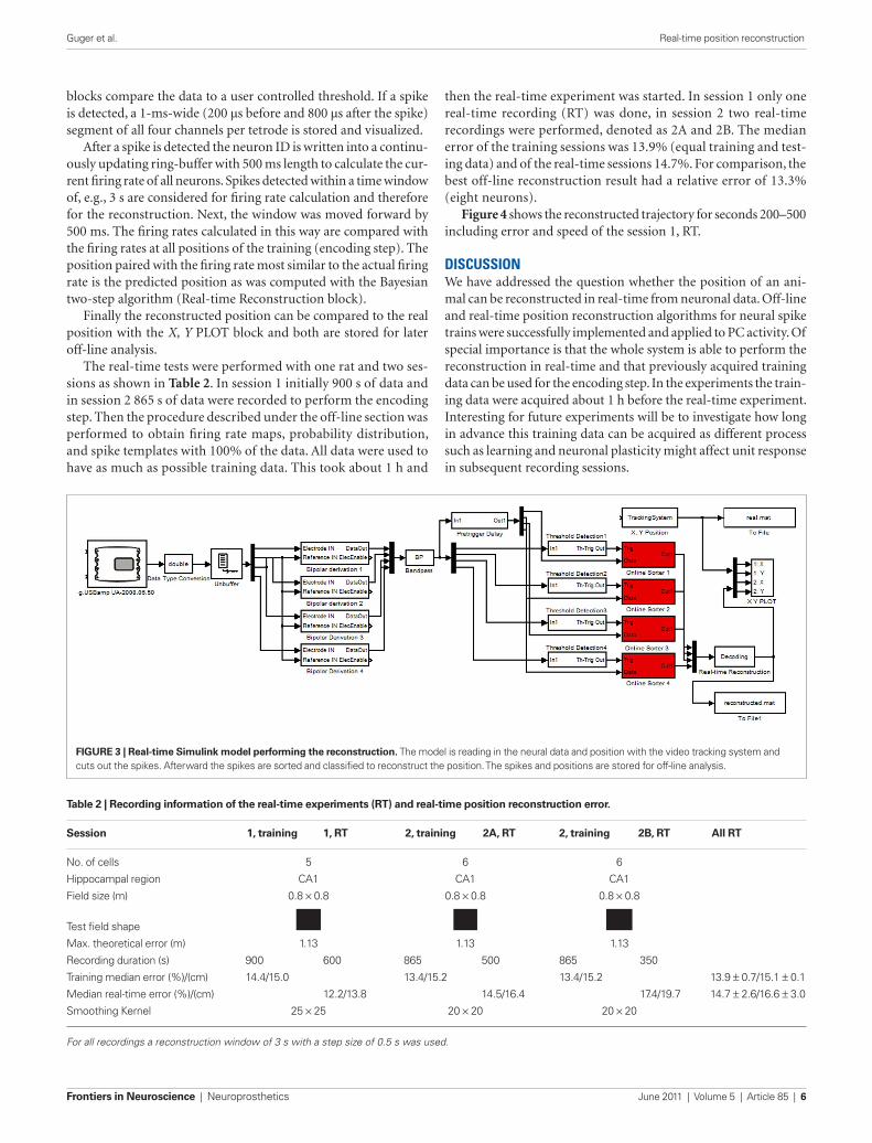
For the real-time experiments tetrodes were implanted in one rat at IDIBAPS and connected to a lightweight headstage amplifier. The headstage amplifier was mounted with a micro-drive on the head of the rat and was connected with a flexible cable to the main biosignal amplifier that sampled the data with 38.4 kHz. The amplifier used for each channel a 24 Bit analog to digital converter and oversampling for high data quality. The data were transmitted with a USB interface to a laptop com-puter running Microsoft Windows. The video based tracking system was mounted above the arena of the rat and acquired the x- and y-positions of the rat with 50 Hz resolution. For the real-time analysis g.USBamp Highspeed On-line Processing for Simulink (g.tec medical engineering GmbH, Austria) was used. This environment uses hardware interrupt controlled data trans-fer to operate the Simulink model in real-time. The real-time model is shown in Figure 3.

The g.USBamp amplifier device driver reads in the data into Simulink and the data are converted to double precision. Then the tetrodes (up to four in the model) are re-referenced by performing bipolar derivations. Next, the data is bandpass filtered between 300 Hz and 6 kHz to remove artifacts. The spike threshold Detection

of spike traces are calculated. Next, these averages were used as templates to automatically sort the spikes. In real-time mode, the algorithm computes for each newly recorded spike the differences to all existing neuron-templates. At each sample point the difference is calculated and the results are summed up. The neuron whose template has the smallest distance to the new spike is identified as the one to which that spike belongs. When noise is recorded the algorithm would assign it to the template having the smallest distance to it, no matter what the signal looks like. To be able to dis-tinguish noise from neuronal signals, the SD of the maximum and minimum of the waveform templates were considered. Therefore a 3σ border of all maxima and minima was calculated to define borders for spike acceptance for every lead. Small spikes hidden in the background noise were already rejected by the thresholding done for spike acceptance.

Table 1 shows that the median position reconstruction error for all four spike sorting methods for each rat and an average for all recordings. The manual spike sorting reached on average the low-est error rate of 14.4%, followed by the 3σ methods with 15.6 and 15.9%. But in general all methods had a very similar performance. Of special importance is that the 3σ and 3σ real-time methods gave almost the same results.

real-tIme experImentsIn real-time mode the following steps must be performed (also shown in Figure 1):

(1) Real-time data acquisition: action potentials are recorded together with tracking information, but now the tracking information is just recorded to evaluate the performance of the system afterward.

FIgure 2 | rat’s trajectory reconstruction based on place cell firing in off-line mode. (A,B) Real (red) and reconstructed x- and y-positions (blue). (C) Reconstruction error and median error of the whole recording (solid horizontal line). (D) Running speed V.

Frontiers in Neuroscience | Neuroprosthetics June 2011 | Volume 5 | Article 85 | 6

Guger et al. Real-time position reconstruction

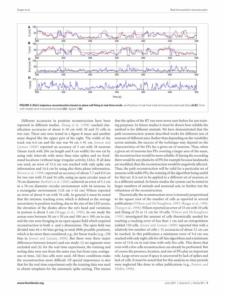
then the real-time experiment was started. In session 1 only one real-time recording (RT) was done, in session 2 two real-time recordings were performed, denoted as 2A and 2B. The median error of the training sessions was 13.9% (equal training and test-ing data) and of the real-time sessions 14.7%. For comparison, the best off-line reconstruction result had a relative error of 13.3% (eight neurons).

Figure 4 shows the reconstructed trajectory for seconds 200–500 including error and speed of the session 1, RT.

dIscussIonWe have addressed the question whether the position of an ani-mal can be reconstructed in real-time from neuronal data. Off-line and real-time position reconstruction algorithms for neural spike trains were successfully implemented and applied to PC activity. Of special importance is that the whole system is able to perform the reconstruction in real-time and that previously acquired training data can be used for the encoding step. In the experiments the train-ing data were acquired about 1 h before the real-time experiment. Interesting for future experiments will be to investigate how long in advance this training data can be acquired as different process such as learning and neuronal plasticity might affect unit response in subsequent recording sessions.

blocks compare the data to a user controlled threshold. If a spike is detected, a 1-ms-wide (200 μs before and 800 μs after the spike) segment of all four channels per tetrode is stored and visualized.

After a spike is detected the neuron ID is written into a continu-ously updating ring-buffer with 500 ms length to calculate the cur-rent firing rate of all neurons. Spikes detected within a time window of, e.g., 3 s are considered for firing rate calculation and therefore for the reconstruction. Next, the window was moved forward by 500 ms. The firing rates calculated in this way are compared with the firing rates at all positions of the training (encoding step). The position paired with the firing rate most similar to the actual firing rate is the predicted position as was computed with the Bayesian two-step algorithm (Real-time Reconstruction block).

Finally the reconstructed position can be compared to the real position with the X, Y PLOT block and both are stored for later off-line analysis.

The real-time tests were performed with one rat and two ses-sions as shown in Table 2. In session 1 initially 900 s of data and in session 2 865 s of data were recorded to perform the encoding step. Then the procedure described under the off-line section was performed to obtain firing rate maps, probability distribution, and spike templates with 100% of the data. All data were used to have as much as possible training data. This took about 1 h and

FIgure 3 | real-time Simulink model performing the reconstruction. The model is reading in the neural data and position with the video tracking system and cuts out the spikes. Afterward the spikes are sorted and classified to reconstruct the position. The spikes and positions are stored for off-line analysis.

Table 2 | recording information of the real-time experiments (rT) and real-time position reconstruction error.

Session 1, training 1, rT 2, training 2A, rT 2, training 2B, rT All rT

No. of cells 5 6 6

Hippocampal region CA1 CA1 CA1

Field size (m) 0.8 × 0.8 0.8 × 0.8 0.8 × 0.8

Test field shape

Max. theoretical error (m) 1.13 1.13 1.13

Recording duration (s) 900 600 865 500 865 350

Training median error (%)/(cm) 14.4/15.0 13.4/15.2 13.4/15.2 13.9 ± 0.7/15.1 ± 0.1

Median real-time error (%)/(cm) 12.2/13.8 14.5/16.4 17.4/19.7 14.7 ± 2.6/16.6 ± 3.0

Smoothing Kernel 25 × 25 20 × 20 20 × 20

For all recordings a reconstruction window of 3 s with a step size of 0.5 s was used.

www.frontiersin.org June 2011 | Volume 5 | Article 85 | 7

Guger et al. Real-time position reconstruction

that the spikes of the RT run were never seen before for any train-ing purposes. In future studies it must be shown how reliable the method is for different animals. We have demonstrated that the path reconstruction system described works for different sets of neurons of different sizes. Rather than depending on the variability across animals, the success of the technique may depend on the characteristics of the PFs for a given set of neurons. Thus, when a given set of neurons has PFs covering a larger area of the maze, the reconstruction would be more reliable. If during the recording there would be any plasticity of PFs for example because landmarks are modified, then the reconstruction would be negatively affected. Thus, the path reconstruction will be valid for a particular set of neurons with stable PFs, the training of the algorithm being useful for that set. It is not to be applied to a different set of neurons or to a different animal. In future studies the system can be tested in larger numbers of animals and neuronal sets, to further test the robustness of the reconstruction.

Theoretically the reconstruction error is inversely proportional to the square root of the number of cells as reported in several publications (Wilson and McNaughton, 1993; Skaggs et al., 1996; Zhang et al., 1998). Wilson reported an error of 33 cm with 10 cells and Zhang of 25 or 11 cm for 10 cells. Wilson and McNaughton (1993) investigated the amount of cells theoretically needed for reaching a tracking error of less than 1 cm and an extrapolation yielded 110 cells. Jensen and Lisman (2000) reported that with a relatively low number of cells (∼5) accuracies of about 12 cm can be reached. In this publication a minimum error of 9.4 cm was reached with only eight cells for off-line algorithms and a minimum error of 13.8 cm in real-time with only five cells. This shows that even with a few cells reconstruction can already be performed. But of course the presence, location, and size of PFs play an important role. Large errors occur if space is uncovered by lack of spikes and lack of cells. It must be noted that for this analysis no time periods were neglected like done in other publications (e.g., Fenton and Muller, 1998).

Different accuracies in position reconstruction have been reported in different studies. Zhang et al. (1998) reached clas-sification accuracies of about 4–10 cm with 30 and 25 cells in two rats. These rats were tested in a figure-8 maze and another maze shaped like the upper part of the eight. The width of the track was 6.4 cm and the size was 94 cm × 81 cm. Jensen and Lisman (2000) reported an accuracy of 3 cm with 38 neurons (linear track with 204 cm length and 8 cm width) for one rat by using only intervals with more than nine spikes and no food-stand locations (without large irregular activity, LIAs). If all data was used, an error of 15.4 cm was reached with only spike rate information and 14.4 cm by using also theta phase information. Brown et al. (1998) reported an accuracy of about 7.7 and 8.0 cm for two rats with 33 and 34 cells, using an open circular maze of 70 cm diameter. Barbieri et al. (2005) achieved an error of 5.1 cm in a 70-cm diameter circular environment with 44 neurons. In a rectangular environment (124 cm × 62 cm) Wilson reported an error of about 9 cm with 76 cells. In general it must be noted that the intrinsic tracking error, which is defined as the average uncertainty in position tracking, due to the size of the LED arrays, the elevation of the diodes above the rat’s head and variations in posture is about 5 cm (Skaggs et al., 1996). In our study the arenas were between 50 cm × 50 cm and 100 cm × 100 cm in size, and the rats were foraging in an open square field which required reconstruction in both x- and y-dimensions. The open field was divided into 64 × 64 bins giving in total 4096 possible positions, which is far more than considered, e.g., for linear tracks (e.g., 150 bins in Jensen and Lisman, 2000). But there were three major differences between Jensen’s and our study: (i) no segments were excluded and (ii) for the real-time experiment, the training and testing data were not from the same run, but from runs contigu-ous in time, (iii) less cells were used. All three conditions make the reconstruction more difficult. Of special importance is also that for the real-time experiment only the training data was used to obtain templates for the automatic spike sorting. This means

FIgure 4 | rat’s trajectory reconstruction based on place cell firing in real-time mode. x/y-Positions of real track (red) and reconstructed track [blue (A,B)]. Error with median error horizontal line [solid (C)]. Speed V (D).

Frontiers in Neuroscience | Neuroprosthetics June 2011 | Volume 5 | Article 85 | 8

Guger et al. Real-time position reconstruction

coding). We wanted to implement a system that could also be used as a real-time system and therefore spike firing from future peri-ods of time were not included in our study (see also Brown et al., 1998). This may have imposed a further limit on reconstruction quality. The step size had a minor influence on accuracy and 500 ms appeared to be optimal for the accuracy and it is also relatively short compared to a 3-s time window.

The spike sorting algorithm used in this paper requires some training data to identify spike templates for real-time sorting. A disadvantage of real-time sorting algorithms is that neurons of which waveforms are changing during recording cannot be identi-fied after the training stage (Chandra and Optican, 1997; Aksenova et al., 2003). Therefore real-time spike sorting algorithms without the need of a learning phase are developed (Rutishauser et al., 2006). This is of special importance for closed-loop experiments which adapt experimental stimuli to the neural response observed. In some previous position reconstruction papers the spike sorting was done with all the data and for the encoding and decoding steps the data were split (e.g., Brown et al., 1998). In the current paper it was important to get all of the parameters for spike sorting only from the training data to allow the sorting in real-time mode. This was realized with the 3σ method that performed comparably to well known sorting methods (manual sorting, KlustaKwik).

The position reconstruction was also possible with subicular units, but was more accurate with CA1 units which have smaller PFs (Taube, 1995; Sharp, 1997). This was of course just tested with one recording but it is interesting that subicular units contain enough information for the reconstruction. Hippocampal and subicular regions work together, possibly to provide the overall cognitive mapping abilities of the animal (Sharp, 1997). For the real-time experiments CA1 was used because of the higher accuracy achieved here but for future experiments it will be interesting to perform reconstruction using both types at the same time. More datasets will be recorded in future to compare the two regions.

Hippocampal activity is also depending on theta activity (O’Keefe and Recce, 1993). The phase of firing becomes earlier on each successive theta cycle the animals runs through its’ PF. Huxter et al. (2008) demonstrated that phase precession occurs in both lin-ear and two-dimensional environments and that position and head-ing can be predicted from neural activity at different theta phases. Heading information can be best recovered from ascending slopes of theta oscillations and position reconstruction optimally from descending slopes. Jensen and Lisman (2000) found that recon-struction is improved when phase coded and rate coded informa-tion are both considered. But this was only the case when epochs with large systematic error were excluded first. For the real-time reconstruction it is not possible to exclude epochs and therefore it was not implemented for the real-time experiments. Furthermore the optimal time window for reconstruction was around 3 s which spans several theta cycles and averages out the phase information.

Trying to reconstruct the animal’s path based on the firing of a small set of neurons is not only a technological achievement. By doing it, we try to understand how the hippocampus and the brain integrate information from PCs in order to codify position and to construct a map of space. Something that we have learnt is that a few neurons are sufficient to reconstruct with certain accuracy the trajectory of an animal. This finding suggests that there is quite

Erratic jumps in reconstruction accuracy can occur for different reasons. The firing rate is modulated by speed, and often decreases when the animal stops and receives food rewards and therefore stopping was often associated to visiting the home base or to eating (Tchernichovski et al., 1998). This increased the chance for errors and artifacts in the recorded data. There may be also biological reasons for the erratic jumps, maybe due to the rat looking around or planning the next move (Johnson et al., 2005). Jensen and Lisman (2000) have shown that by using both phase information and rate information the reconstruction error can be improved. In this case also theta cycles must be identified to investigate the firing at specific theta phases. But the improvement is reduced if large systematic error sources affect the reconstruction. Jensen and Lisman (2000) showed that erratic jumps can be reduced if the reconstruction is only performed for time windows with a minimum of spikes pre-sent. Furthermore when an animal is eating, LIA and sharp wave-ripples occur which are associated with replay and thus yields larger errors (Foster and Wilson, 2007; Lansink et al., 2009). As already mentioned in the results section, minimizing the reconstruction to points where the firing rate is above a certain threshold yielded better reconstruction results for certain segments of space. But it does not reduce the overall error rate much, because the posi-tions that have not been reconstructed have to be interpolated. This estimation leads to new reconstruction errors for the interpolated positions, and thus increases the error rate. Important to note is also that for a real-time system every single time point should be reconstructed and therefore no data were excluded.

The length of the reconstruction window defines how many spikes are used for the reconstruction and is therefore dependent on the firing rate of the neurons and the rat’s running speed. In theory the error is inversely proportional to the square root of the time window. While Zhang et al. (1998) and Brown et al. (1998) used windows of about 1 s length we found that a relative long time window of 3 s yielded the best results, which can be explained by the lower amount of cells used. Also Wilson and McNaughton (1993) showed an improved accuracy by increasing the window length from 0.1 to 4 s. Jensen and Lisman (2000) showed that even with short windows of about 100–500 ms good accuracy can be reached, but excluded epochs with less spikes. In our case, using a time window of 3 s, the time steps that contained no spikes were below 0.5% of total recording time, and therefore their influence can be neglected. It must of course be noted that a rat can run longer distances if the window length increases.

We found that the selection of the PF smoothing Kernel is of relevance for the reconstruction. Zhang et al. (1998) reported that the reconstruction was not sensitive to the spatial blurring Kernel. The difference in findings may depend on the number of simul-taneously recorded cells included: the lesser number of cells, the larger the impact each one of the PFs has on the global computa-tion. Thus, larger PFs overlap more easily with other PFs and this increases the joint firing rate and yields a lower error rate. But this advantage is counterbalanced by the fact that larger PFs hold less spatial information. In this study the optimal smoothing Kernel was calculated in the off-line procedure.

In previous studies (Zhang et al., 1998) the time window used for position reconstruction included spike information not only from the past (retrospective coding) but also from the future (prospective

www.frontiersin.org June 2011 | Volume 5 | Article 85 | 9

Guger et al. Real-time position reconstruction

cells and head direction cells. J. Neurophysiol. 80, 425–446.

Lansink, C. S., Goltstein, P. M., Lankelma, J. V., McNaughton, B. L., and Pennartz, C. M. (2009). Hippocampus leads ventral striatum in replay of place-reward information. PLoS Biol. 7, e1000173. doi: 10.1371/journal.pbio.1000173

Leutgeb, S., Leutgeb, J. K., Barnes, C. A., Moser, E. I., McNaughton, B. L., and Moser, M. B. (2005). Independent codes for spatial and episodic memory in hippocampal neuronal ensembles. Science 309, 619–623.

McFarland, D. J., Krusienski, D. J., Sarnacki, W. A., and Wolpaw, J. R. (2008). Emulation of computer mouse control with a noninvasive brain-computer interface. J. Neural Eng. 5, 101–110.

O’Keefe, J., and Conway, D. H. (1980). On the trail of the hippocampal engram. Physiol. Psychol. 8, 229–238.

O’Keefe, J., and Dostrovsky, J. (1971). The hippocampus as a spatial map. Preliminary evidence from unit activ-ity in the freely-moving rat. Brain Res. 34, 171–175.

O’Keefe, J., and Recce, M. L. (1993). Phase relationship between hippocampal place units and the EEG theta rhythm. Hippocampus 3, 317–330.

Pastalkova, E., Itskov, V., Amarasingham, A., and Buzsáki, G. (2008). Internally generated cell assembly sequences in the rat hippocampus. Science 321, 1322–1327.

Pfurtscheller, G., Allison, B. Z., Brunner, C., Bauernfeind, G., Solis-Escalante, T., Scherer, R., Zander, T. O., Mueller-Putz, G., Neuper, C., and Birbaumer, N. (2010). The Hybrid BCI. Front.

referencesAksenova, T. I., Chibirova, O. K., Dryga, O.

A., Tetko, I. V., Benabid, A. L., and Villa, A. E. (2003). An unsupervised auto-matic method for sorting neuronal spike waveforms in awake and freely moving animals. Methods 30, 178–187.

Barbieri, R., Wilson, M. A., Frank, L. M., and Brown, E. N. (2005). An analysis of hippocampal spatio-temporal repre-sentations using a Bayesian algorithm for neural spike train decoding. IEEE Trans. Neural Syst. Rehab. Eng. 13, 131–136.

Brown, E. N., Frank, L. M., Tang, D., Quirk, M. C., and Wilson, M. A. (1998). A statistical paradigm for neural spike train decoding applied to position prediction from ensemble firing pat-terns of rat hippocampal place cells. J. Neurosci. 18, 7411–7425.

Chandra, R., and Optican, L. M. (1997). Detection, classification, and super-position resolution of action poten-tials in multiunit single-channel recordings by an online real-time neural network. IEEE Trans. Biomed. Eng. 44, 403–412.

Etienne, A. S. (1992). Navigation of a small mammal by dead reckoning and local cues. Curr. Dir. Psychol. Sci. 1, 48–52.

Fenton, A., and Muller, R. (1998). Place cell discharge is extremely variable during individual passes of the rat through the firing field. Proc. Natl. Acad. Sci. U.S.A. 95, 3182–3187.

Foster, D. J., and Wilson, M. A. (2007). Hippocampal theta sequences. Hippocampus 17, 1093–1099.

Guger, C., Daban, S., Sellers, E., Holzner, C., Krausz, G., Carabalona, R., Gramatica, F., and Edlinger, G.

(2009). How many people are able to control a P300-based brain-computer interface (BCI)? Neurosci. Lett. 462, 94–98.

Hafting, T., Fyhn, M., Molden, S., Moser, M. B., and Moser, E. I. (2005). Microstructure of a spatial map in the entorhinal cortex. Nature 436, 801–806.

Harris, K. D., Henze, D. A., Csicsvari, J., Hirase, H., and Buzsáki, G. (2000). Accuracy of tetrode spike separation as determined by simultaneous intracel-lular and extracellular measurements. J. Neurophysiol. 84, 401–414.

Hochberg, L. R., Serruya, M. D., Friehs, G. M., Mukand, J. A., Saleh, M., Caplan, A. H., Branner, A., Chen, D., Penn, R. D., and Donoghue, J. P. (2006). Neuronal ensemble control of prosthetic devices by a human with tetraplegia. Nature 442, 164–171.

Huxter, J. R., Kevin Allen, T. J., and Csicsvari, J. (2008). Theta phase-specific codes for two-dimensional position, trajectory and heading in the hippocampus. Nat. Neurosci. 11, 587–594.

Jensen, O., and Lisman, J. E. (2000). Position reconstruction from an ensemble of hippocampal place cells: contribution of theta phase coding. J. Neurophysiol. 83, 2602–2609.

Johnson, A., Seeland, K., and Redish, A. D. (2005). Reconstruction of the postsubiculum head direction signal from neural ensembles. Hippocampus 15, 86–96.

Knierim, J. J., Hemant, H. S., and McNaughton, B. L. (1998). Interactions between idiothetic cues and external landmarks in the control of place

Neurosci. 4:30. doi: 10.3389/fnpro.2010.00003

Poucet, B., Lenck-Santini, P. P., Paz-Villagrán, V., and Save, E. (2003). Place cells, neocortex and spatial naviga-tion: a short review. J. Physiol. Paris 97, 537–546.

Redish, D. A. (2008). MClust Spike Sorting Toolbox. Available at: http://redish-lab.neuroscience.umn.edu/MClust/MClust.html

Rennó-Costa, C., Lisman, J., Verschure, P. (2010). The mechanism of rate remap-ping in the dentate gyrus. Neuron 68, 1051–1058.

Rutishauser, U., Schuman, E., and Mamelak, A. (2006). Online detection and sorting of extracellularly recorded action potentials in human medial temporal lobe recordings, in vivo. J. Neurosci. Methods 154, 204–224.

Save, E., Cressant, A., Thinus-Blanc, C., and Poucet, B. (1998). Spatial firing of hippocampal place cells in blind rats. J. Neurosci. 18, 1818–1826.

Schalk, G., Miller, K. J., Anderson, N. R., Wilson, J. A., Smyth, M. D., Ojemann, J. G., Moran, D. W., Wolpaw, J. R., and Leuthardt, E. C. (2008). Two-dimensional movement control using electrocorticographic signals in humans. J. Neural Eng. 5, 75–84.

Sharp, P. E. (1997). Subicular cells generate similar spatial firing patterns in two geometrically and visually distinctive environments: comparison with hip-pocampal place cells. Behav. Brain Res. 85, 71–92.

Sharp, P. E. (1999). Complimentary roles for hippocampal versus subicular/entorhinal place cells in coding place, context, and events. Hippocampus 9, 432–443.

some redundancy in the system and opens the question of why this redundancy is necessary, and what are all the different spatial and non-spatial aspects that PCs are coding. It also reveals that our system works for a stable set of PCs, while the hippocampus can deal with PFs which can be rather plastic, while the spatial representation remains stable. With the system described here, one could explore under which conditions our reconstruction algorithm could main-tain a stable path reconstruction while some landmarks, and thus some PFs, would change.

For a BCI application based on PCs it has to be assumed that a rat could be trained in a closed-loop experiment to modulate its own PC activity. In a first run the rat learns its environment and generates particular patterns of PC activity at various places in the arena. If the animal would only receive a rewarding stimulus when it visits a particular position in space where a specific PC fires, one may ask whether the activity of this PC would be enhanced. Another question is whether the rat is able to modulate PC firing voluntarily.

The system can also be seen as a verification method of the prior characterization of the environment and allows us the express stability with a certain accuracy rate. This allows of course also to

express changes of the environment to study varying environments. The spatial characterization of the environment is specific for the training arena and can therefore not be applied to unknown spatial contexts. But this is also the case for other neuroprosthetic applica-tions that must be trained, e.g., on a specific types of movement.

The closed-loop experimentation and analysis system proposed here allows to evaluate the quality of PC recordings in real-time and helps to reduce the recording time. The real-time system allows researchers on the fly to check whether the spikes are sortable and not contaminated with noise. Furthermore, it can be used to change, e.g., arena properties and or provide direct neuronal stimulation during the recording to investigate changes in PFs. As such it intro-duces a new range of closed-loop systems for the study of cognition and behavior and their neuronal substrate. Our study showed suc-cessfully that deeper brain structures can be analyzed in real-time which could be useful for future neuroprosthetic applications.

acknowledgmentsThis work was supported by the FFG, EU-IST (FP6-027731) project Presenccia, and Renachip.

Frontiers in Neuroscience | Neuroprosthetics June 2011 | Volume 5 | Article 85 | 10

Guger et al. Real-time position reconstruction

position reconstruction with hippocampal place cells. Front. Neurosci. 5:85. doi: 10.3389/fnins.2011.00085This article was submitted to Frontiers in Neuroprosthetics, a specialty of Frontiers in Neuroscience.Copyright © 2011 Guger, Gener, Pennartz, Brotons-Mas, Edlinger, Bermúdez i Badia, Verschure, Schaffelhofer and Sanchez-Vives. This is an open-access article sub-ject to a non-exclusive license between the authors and Frontiers Media SA, which per-mits use, distribution and reproduction in other forums, provided the original authors and source are credited and other Frontiers conditions are complied with.

framework with application to hip-pocampal place cells. J. Neurophysiol. 79, 1017–1044.

Conflict of Interest Statement: The authors declare that the research was con-ducted in the absence of any commercial or financial relationships that could be construed as a potential conflict of interest.

Received: 10 February 2010; accepted: 10 June 2011; published online: 30 June 2011.Citation: Guger C, Gener T, Pennartz CMA, Brotons-Mas JR, Edlinger G, Bermúdez i Badia S, Verschure P, Schaffelhofer S and Sanchez-Vives MV (2011) Real-time

thetic arm for self-feeding. Nature 453, 1098–1101.

Wilson, M. A., and McNaughton, B. L. (1993). Dynamics of the hippocampal ensemble code for space. Science 261, 1055–1058.

Wolpaw, J. R., McFarland, D. J., Vaughan, T. M., and Schalk, G. (2003). The Wadsworth Center brain-computer interface (BCI) research and devel-opment program. IEEE Trans. Neural Syst. Rehabil. Eng. 11, 204–207.

Zhang, K., Ginzburg, I., McNaughton, B. L., and Sejnowski, T. J. (1998). Interpreting neuronal population activity by reconstruction: unified

Skaggs, W. E., McNaughton, B. L., Wilson, M. A., and Barnes, C. A. (1996). Theta phase precession in hippocampal neuronal populations and the com-pression of temporal sequences. Hippocampus 6, 149–172.

Taube, J. S. (1995). Place cells recorded in the parasubiculum of freely moving rats. Hippocampus 5, 569–583.

Tchernichovski, O., Benjamini, Y., and Golani, I. (1998). The dynamics of long-term exploration in the rat. Biol. Cybern. 78, 423–432.

Velliste, M., Perel, S., Spalding, M. C., Whitford, A. S., and Schwartz, A. B. (2008). Cortical control of a pros-