This is the author’s version of a work that was submitted/accepted for pub-lication in the following source:

Larue, Gregoire S., Rakotonirainy, Andry, & Pettitt, Anthony N. (2011)Real-time evaluation of driver’s alertness on highways. In Pratelli, A &Brebbia, C A (Eds.) Urban Transport XVII, Wessex Institute of TechnologyPress, Pisa.

This file was downloaded from: http://eprints.qut.edu.au/41996/

c© Copyright 2011 [please consult the authors]

Notice: Changes introduced as a result of publishing processes such ascopy-editing and formatting may not be reflected in this document. For adefinitive version of this work, please refer to the published source:

http://dx.doi.org/10.2495/UT110471

Real-time evaluation of driver’s alertness onhighways

G.S. Larue, A. Rakotonirainy, A.N. PettittCentre for Accident Research and Road Safety - Queensland (Brisbane,Australia)

Abstract

Suburbanisation has been internationally a major phenomenon in the last decades.Suburb-to-suburb routes are nowadays the most widespread road journeys; andthis resulted in an increment of distances travelled, particularly on faster suburbanhighways. The design of highways tends to over-simplify thedriving task and thiscan result in decreased alertness. Driving behaviour is consequently impaired anddrivers are then more likely to be involved in road crashes. This is particularly dan-gerous on highways where the speed limit is high. While effective countermeasuresto this decrement in alertness do not currently exist, the development of in-vehiclesensors opens avenues for monitoring driving behaviour in real-time. The aim ofthis study is to evaluate in real-time the level of alertnessof the driver through sur-rogate measures that can be collected from in-vehicle sensors. Slow EEG activityis used as a reference to evaluate driver’s alertness. Data are collected in a drivingsimulator instrumented with an eye tracking system, a heartrate monitor and anelectrodermal activity device (N=25 participants). Four different types of highways(driving scenario of 40 minutes each) are implemented through the variation of theroad design (amount of curves and hills) and the roadside environment (amount ofbuildings and traffic). We show with Neural Networks that reduced alertness canbe detected in real-time with an accuracy of 92% using lane positioning, steeringwheel movement, head rotation, blink frequency, heart ratevariability and skinconductance level. Such results show that it is possible to assess driver’s alertnesswith surrogate measures. Such methodology could be used to warn drivers of theiralertness level through the development of an in-vehicle device monitoring in real-time drivers’ behaviour on highways, and therefore it couldresult in improved roadsafety.Keywords: Driving impairment, Alertness, Neural Networks, Simulated driving,

Real-time assessment

1 Introduction

Most metropolitan cities in the world have experienced rapid suburbanisation overthe past few decades. This phenomenon has not brought peopleand jobs closerto each other due to diffuse commuting patterns [1]. Often people are not able tolive close to where they work because of a lack of affordable housing in manymetropolitan areas. Internationally, average trip lengths have increased dramati-cally in the last 20 years and this increase has been linked tothe growing use ofthe car [2]. This led to transport networks developments andincrements in com-muting distances. For instance work trip distance has sharply increased while themean daily commuting time per capita has shown only a slight growth [3]. Moreand more people residing in the suburban areas are using faster modes, and thesuburbanisation of houses and workplaces is the outcome of the increasing use offaster suburban routes instead of slow urban routes [4]. Thesuburb-to-suburb jour-ney to work is by far the most widespread. Such journey is madefrom an outlyingresidential area to a nearby suburban employment centre, crossing or not sometowns [2].

Australian cities, with the exception of central Sydney, have been planned accord-ing to the good urban planning practices of the 19th and 20th centuries. To a largeextent endemic congestion has not been a major factor as it isin other developedcountries. Australian cities continue to grow, space beingnot a problem, and spa-tial separation increases at metropolitan, regional and national levels [5]. Disjunc-tion between home and work location increases and communities are increasinglyfragmented and connected by highways [6].

The design of highways tends to over-simplify the driving task. On such roads,driving is mainly a lane-keeping task. A lane keeping task isnot cognitively stim-ulating and can cause the driver to suffer from an alertness decrement after lessthan 20 minutes [7]. Driving behaviour is consequently impaired and drivers arethen more likely to be involved in road crashes due to potentially slow reactiontimes or lack of reaction to unpredictable events. This is particularly dangerous onhighways where the speed limit is high. This draws inattention to the most impor-tant contributor (27%) to fatal and hospitalisation crashes in 2003 in Queensland,Australia (Queensland Transport, 2005). While effective countermeasures to thisdecrement in alertness do not currently exist, the development of in-vehicle sen-sors opens avenues for monitoring driving behaviour and reduction in alertness inreal-time.

The aim of this study is to evaluate in real-time the level of alertness of the driveron different types of Australian highways through surrogate measures that can becollected from in-vehicle sensors. This study focuses on two factors that decreasealertness: (i) the road design and (ii ) the roadside environment. Slow EEG activityis used as a reference to evaluate driver’s alertness. Alertness decrement is detectedin real-time using surrogate measures related to the driving performance. Data arecollected in a driving simulator instrumented with an eye tracking system, a heart

rate monitor and an electrodermal activity device (N=25 participants). Four dif-ferent types of highways (driving scenario of 40 minutes each) are implementedthrough the variation of the road design (amount of curves and hills) and the road-side environment (amount of buildings and traffic).

This paper will first introduce the background of the research, and then providea description of the experimental design. Then the results of the evaluation of thedriver’s alertness on the different highways will be presented. The last part of thispaper will discuss the implications of the results of the this analysis.

2 Background

2.1 Measuring alertness

The most reliable and reproducible way to measure the alertness of a driver driv-ing is to use an EEG [8, 9, 10]. EEG signals are analysed in the frequency domain,and four different bands contain the information:α, β, θ and δ. The most reli-able method to measure alertness variation is to use the following algorithm:θ+α

β.

When increasing, this ratio between slow and fast wave activities indicate a decre-ment of alertness [11, 12]. Bursts are also of interest to detect increments in bandsoccurring relatively sparsely. It can particularly be usedto detect microsleep fol-lowing alpha and theta activities [13].

An EEG device cannot be used in a vehicle for at least three reasons: (i) theinconvenience for the driver, (ii ) the prohibitive cost, and (iii ) the noise intro-duced due to electromagnetic field interferences. Nevertheless, such a device canbe used in a laboratory-based experiment so that correlation with driving perfor-mance (observed variables from the driver the car and the environment) can beisolated and investigated.

2.2 Surrogate measures

Surrogate measures correlated to the alertness level during this study have beeninvestigated in [14]. They are summarised here:

• ECG (heart rate, inter-beat intervals, heart rate variability)• Eye activity (blink frequency, eye closure)• Head rotation (toward the side)• Electrodermal activity (Skin conductance Level SCL, Non specific fluctua-

tion rate, rise-time and half-recovery time)• Simulator data (lane lateral shift variability, speed variability, steering wheel

variability, time to lane crossing)

2.3 Evaluation of alertness using Neural Networks

Neural networks are composed of a network of simple processing elements calledneurons, which can exhibit complex global behaviour, determined by the connec-tions between the processing elements and element parameters. An elementary

neuron computes an output from the inputs as follows: first each input (here theobservations such as reaction times) is weighted appropriately, then the sum of theweighted inputs and a bias form the input to a transfer function f which providesthe output (here the accuracy) [15].

NNs are capable of approximating any function with a finite number of discon-tinuities. Training the neural network consists of adjusting the values of the con-nections (weights) between elements. This permits the modelling of the complexrelationship between the relevant measurementsObst (inputs) and the alertnessAlertt (output) at timet. Particularly, multilayer feedforward networks can modelsuch complex, non-linear relationships and when properly trained, provide reason-able answers when presented with totally new inputs. In sucha network, inputs areprocessed through successive layers of neurons, the information moving in onlyone direction, forward, from the input nodes (taking the variables of the problemas inputs), through the hidden nodes (if any) and to the output node (whose out-puts should be as close as possible to the observed outputs, using the MSE as a costfunction), without any cycles or loops in the network. Thesenetworks are trainedby backpropagation, which is a gradient descent algorithm in which the networkweights are moved along the negative of the gradient of the performance function[16].

3 Methods

3.1 Participants

A stratified random sampling approach was used to obtain a representative pop-ulation of licensed drivers (for at least two years), regular drivers from differentage groups (as per categories used in road safety i.e. 18-24,25-59 and 60+). The60+ category was not targeted in this study due to vision impairments and possiblecircadian and cognitive functioning changes related to ageing [17].

Twenty-five subjects aged between 18 and 49 (mean age = 29.1 years, SD =8.3) volunteered for this study. Thirty participants were expected to drive in thisexperiment but five subjects were removed from the sample dueto motion sicknesswhich occurred during training on the driving simulator.

Young drivers were recruited from Queensland University ofTechnology (QUT).Other participants were selected from staff at QUT and the general community.Participants had their licence for a minimum of two years anddrove a minimum ofthree days per week similar to previous research [18]. All subjects provided writtenconsent for this study which was approved by QUT ethics committee. Participantswere paid AUS $80 for completing the four driving sessions; students undertakingthe first year psychology subject received course credit fortheir participation.

3.2 Experimental design

Both road design and roadside environment of the highway were varied in thisexperiment. The combination of low and high variability of both parameters resulted

in four different scenarios (see Table 1). Scenario 1 is characterised by low roaddesign variability and a low roadside variability. Roadside variability is changedto high for scenario 2, while road design variability is increased for scenario 3.Scenario 4 is done with both road design and roadside variability high.

Table 1: The four experiment scenarios

roadside variability

low high

road design variability low scenario 1 scenario 2

high scenario 3 scenario 4

In each experiment, the participants were asked to drive andfollow road rulesfor approximately 40 minutes. Each participant is tested oneach scenario (repeatedmeasures design) in the following conditions:

• driving consists of following a lane (no itinerary involved) at constant speed(60 kilometres per hour), without having to stop the car (no red traffic lightsor other stops) or to press the brakes frequently (no T intersections or per-pendicular turns)

• no manual gear changes were required• no use of indicators was required• low traffic conditions (no congestion).

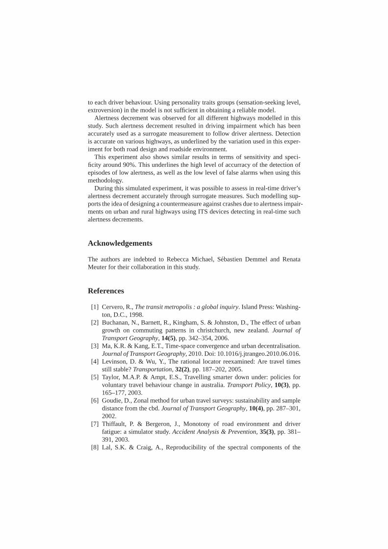
Road geometry is varied through the curvature of the road as well as its altitude.In the road design with low variability, the road is essentially straight or with littlecurves and flat. In the road design with high variability, theroad is a sequence ofsmall straight sections, significant curves and hills.

The roadside environment is varied in terms of scenery (low versus high vari-ability). Low roadside variability is composed of a desert-like scenery with bushesalong the road with periodic traffic occurring in the oncoming lane only. This mod-els an Australian rural highway. High roadside variabilityis composed of variousbuildings, roadside barriers, overhanging lights, overpasses and trees/foliage withtraffic surrounding the vehicle (no congestion and no requirements to overtake).This represents Australian urban highways.

3.3 Experimental conditions

Participants were tested individually in a quiet room in four sessions lasting approx-imately one hour per session. Each participant drives in oneof the four scenarios(randomly assigned) in the simulator once a week for four weeks at a fixed testingtime. Testing times are scheduled at 9am, 11am, 1pm and 3pm. Each participantchooses a testing time for which they feel they are the most alert.

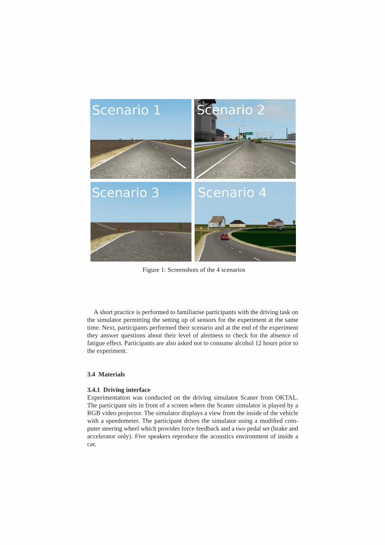
Figure 1: Screenshots of the 4 scenarios

A short practice is performed to familiarise participants with the driving task onthe simulator permitting the setting up of sensors for the experiment at the sametime. Next, participants performed their scenario and at the end of the experimentthey answer questions about their level of alertness to check for the absence offatigue effect. Participants are also asked not to consume alcohol 12 hours prior tothe experiment.

3.4 Materials

3.4.1 Driving interfaceExperimentation was conducted on the driving simulator Scaner from OKTAL.The participant sits in front of a screen where the Scaner simulator is played by aRGB video projector. The simulator displays a view from the inside of the vehiclewith a speedometer. The participant drives the simulator using a modified com-puter steering wheel which provides force feedback and a twopedal set (brake andaccelerator only). Five speakers reproduce the acoustics environment of inside acar.

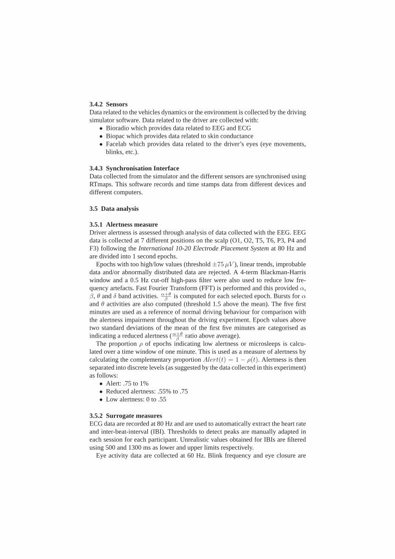
3.4.2 SensorsData related to the vehicles dynamics or the environment is collected by the drivingsimulator software. Data related to the driver are collected with:

• Bioradio which provides data related to EEG and ECG• Biopac which provides data related to skin conductance• Facelab which provides data related to the driver’s eyes (eye movements,

blinks, etc.).

3.4.3 Synchronisation InterfaceData collected from the simulator and the different sensorsare synchronised usingRTmaps. This software records and time stamps data from different devices anddifferent computers.

3.5 Data analysis

3.5.1 Alertness measureDriver alertness is assessed through analysis of data collected with the EEG. EEGdata is collected at 7 different positions on the scalp (O1, O2, T5, T6, P3, P4 andF3) following theInternational 10-20 Electrode Placement Systemat 80 Hz andare divided into 1 second epochs.

Epochs with too high/low values (threshold±75µV ), linear trends, improbabledata and/or abnormally distributed data are rejected. A 4-term Blackman-Harriswindow and a 0.5 Hz cut-off high-pass filter were also used to reduce low fre-quency artefacts. Fast Fourier Transform (FFT) is performed and this providedα,β, θ andδ band activities.α+θ

βis computed for each selected epoch. Bursts forα

andθ activities are also computed (threshold 1.5 above the mean). The five firstminutes are used as a reference of normal driving behaviour for comparison withthe alertness impairment throughout the driving experiment. Epoch values abovetwo standard deviations of the mean of the first five minutes are categorised asindicating a reduced alertness (α+θ

βratio above average).

The proportionρ of epochs indicating low alertness or microsleeps is calcu-lated over a time window of one minute. This is used as a measure of alertness bycalculating the complementary proportionAlert(t) = 1 − ρ(t). Alertness is thenseparated into discrete levels (as suggested by the data collected in this experiment)as follows:

• Alert: .75 to 1%• Reduced alertness: .55% to .75• Low alertness: 0 to .55

3.5.2 Surrogate measuresECG data are recorded at 80 Hz and are used to automatically extract the heart rateand inter-beat-interval (IBI). Thresholds to detect peaksare manually adapted ineach session for each participant. Unrealistic values obtained for IBIs are filteredusing 500 and 1300 ms as lower and upper limits respectively.

Eye activity data are collected at 60 Hz. Blink frequency andeye closure are

extracted by Facelab. This device also furnishes data aboutthe driver head move-ments, in particular the rotation of the head to the side.

Electrodermal activity is collected at 1 Hz. Skin conductance level and non-specific fluctuation rates, rise-time and half-recovery time are extracted. A thresh-old of 0.02µS is used to find non-specific responses.Car and environment variables are obtained from the simulator. Data collectedfrom the simulator is sampled at 20 Hz. Lane lateral shift variability, speed vari-ability, steering wheel movement variability and Time to Lane Crossing (TLC)were used in this analysis. Only straight sections of road were used to computethese metrics.These variables are normalised for each participant using the five first minutes ofdriving for each of the four sessions. Due to the high number of surrogate mea-surements, a Principal Component Analysis (PCA) is performed to reduce thenumber of inputs to the mathematical model. PCA extracts relevant informationfrom complex datasets and reduces possible correlated variables into a smallernumber of uncorrelated variables called principal components. Principal compo-nents are ordered as a function of their explanation of data variability [19]. Onlycomponents explaining more than 5% of the variance in the data are selected aspredictors for the neural networks.

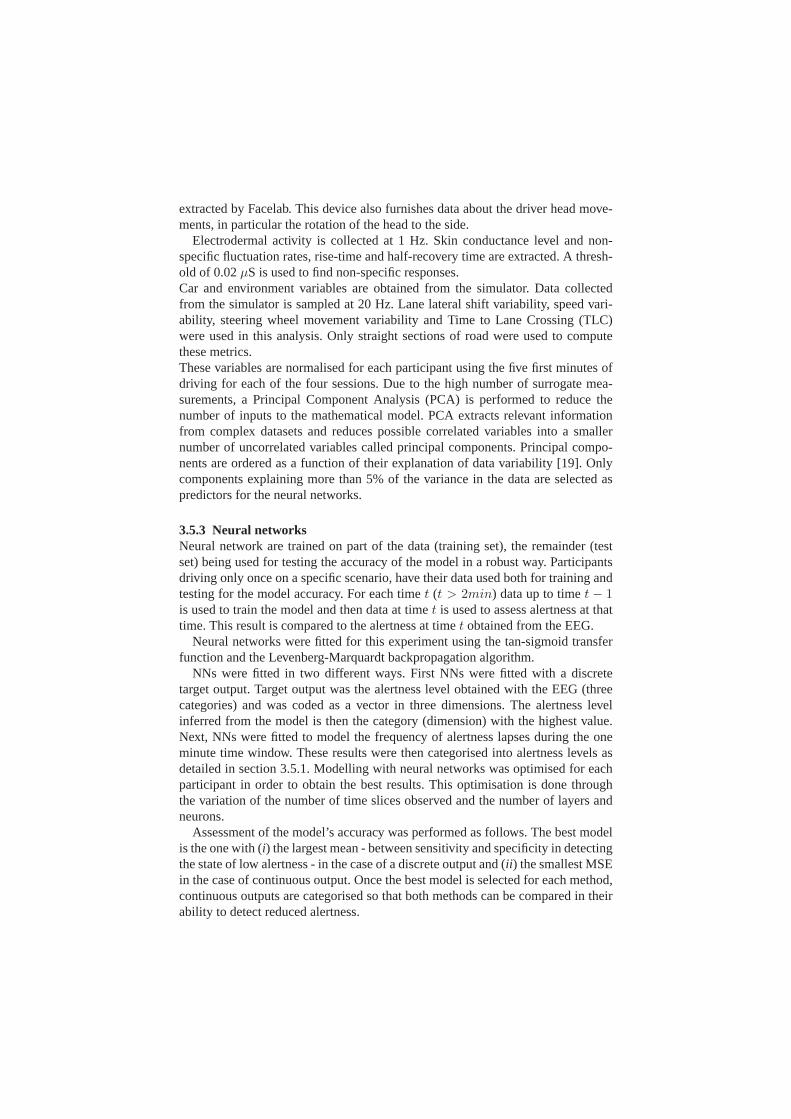
3.5.3 Neural networksNeural network are trained on part of the data (training set), the remainder (testset) being used for testing the accuracy of the model in a robust way. Participantsdriving only once on a specific scenario, have their data usedboth for training andtesting for the model accuracy. For each timet (t > 2min) data up to timet − 1is used to train the model and then data at timet is used to assess alertness at thattime. This result is compared to the alertness at timet obtained from the EEG.

Neural networks were fitted for this experiment using the tan-sigmoid transferfunction and the Levenberg-Marquardt backpropagation algorithm.

NNs were fitted in two different ways. First NNs were fitted with a discretetarget output. Target output was the alertness level obtained with the EEG (threecategories) and was coded as a vector in three dimensions. The alertness levelinferred from the model is then the category (dimension) with the highest value.Next, NNs were fitted to model the frequency of alertness lapses during the oneminute time window. These results were then categorised into alertness levels asdetailed in section 3.5.1. Modelling with neural networks was optimised for eachparticipant in order to obtain the best results. This optimisation is done throughthe variation of the number of time slices observed and the number of layers andneurons.

Assessment of the model’s accuracy was performed as follows. The best modelis the one with (i) the largest mean - between sensitivity and specificity in detectingthe state of low alertness - in the case of a discrete output and (ii ) the smallest MSEin the case of continuous output. Once the best model is selected for each method,continuous outputs are categorised so that both methods canbe compared in theirability to detect reduced alertness.

4 Results

Principal Component Analysis resulted in the identification of six componentsexplaining more than 5% of the variance.PCA1 is mainly composed of the skinconductance level.PCA2 can be reduced to blink frequency.PCA3 is a combina-tion of skin conductance measures (SCR rise-time and SCR half-recovery time).PCA4 is the result of a selection of ECG metrics whilePCA5 combines drivingperformance (lane keeping, steering wheel movement) to skin conductance mea-sures (NSF rate and SCR rise-time). FinallyPCA6 is largely composed of thehead rotation.

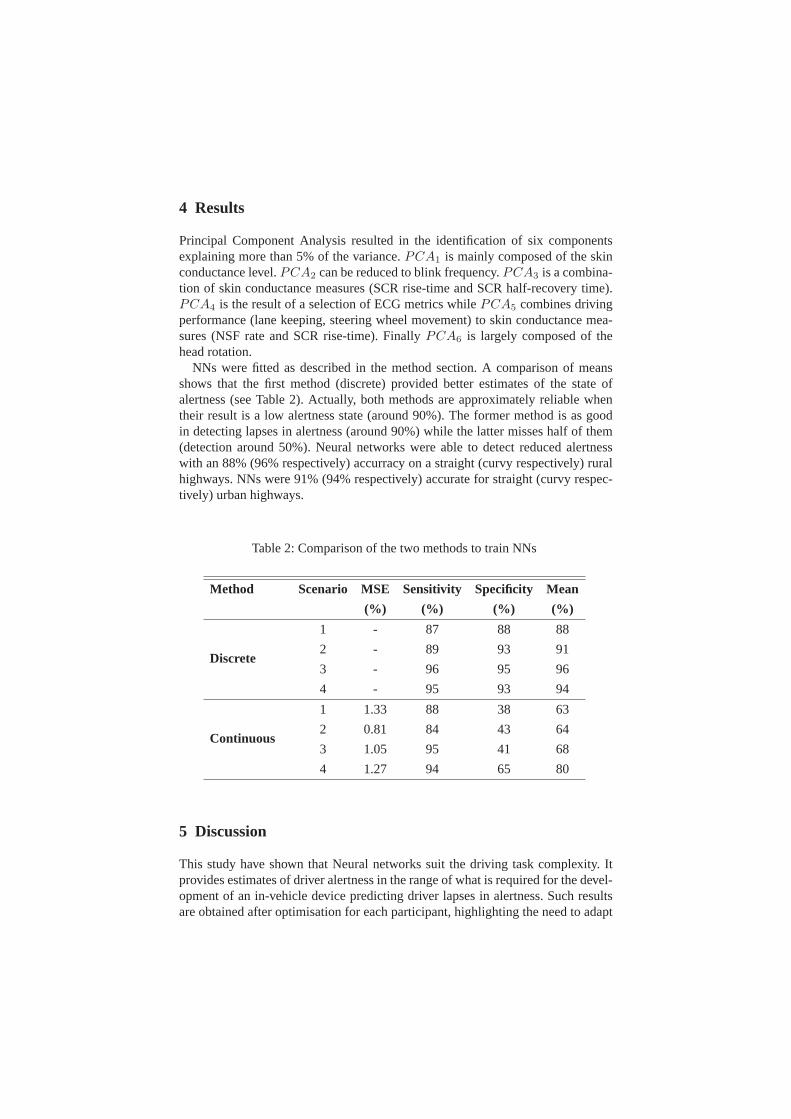
NNs were fitted as described in the method section. A comparison of meansshows that the first method (discrete) provided better estimates of the state ofalertness (see Table 2). Actually, both methods are approximately reliable whentheir result is a low alertness state (around 90%). The former method is as goodin detecting lapses in alertness (around 90%) while the latter misses half of them(detection around 50%). Neural networks were able to detectreduced alertnesswith an 88% (96% respectively) accurracy on a straight (curvy respectively) ruralhighways. NNs were 91% (94% respectively) accurate for straight (curvy respec-tively) urban highways.

Table 2: Comparison of the two methods to train NNs

Method Scenario MSE Sensitivity Specificity Mean

(%) (%) (%) (%)

Discrete

1 - 87 88 88

2 - 89 93 91

3 - 96 95 96

4 - 95 93 94

Continuous

1 1.33 88 38 63

2 0.81 84 43 64

3 1.05 95 41 68

4 1.27 94 65 80

5 Discussion

This study have shown that Neural networks suit the driving task complexity. Itprovides estimates of driver alertness in the range of what is required for the devel-opment of an in-vehicle device predicting driver lapses in alertness. Such resultsare obtained after optimisation for each participant, highlighting the need to adapt

to each driver behaviour. Using personality traits groups (sensation-seeking level,extroversion) in the model is not sufficient in obtaining a reliable model.

Alertness decrement was observed for all different highways modelled in thisstudy. Such alertness decrement resulted in driving impairment which has beenaccurately used as a surrogate measurement to follow driveralertness. Detectionis accurate on various highways, as underlined by the variation used in this exper-iment for both road design and roadside environment.

This experiment also shows similar results in terms of sensitivity and speci-ficity around 90%. This underlines the high level of accurracy of the detection ofepisodes of low alertness, as well as the low level of false alarms when using thismethodology.

During this simulated experiment, it was possible to assessin real-time driver’salertness decrement accurately through surrogate measures. Such modelling sup-ports the idea of designing a countermeasure against crashes due to alertness impair-ments on urban and rural highways using ITS devices detecting in real-time suchalertness decrements.

Acknowledgements

The authors are indebted to Rebecca Michael, Sebastien Demmel and RenataMeuter for their collaboration in this study.

References

[1] Cervero, R.,The transit metropolis : a global inquiry. Island Press: Washing-ton, D.C., 1998.

[2] Buchanan, N., Barnett, R., Kingham, S. & Johnston, D., The effect of urbangrowth on commuting patterns in christchurch, new zealand.Journal ofTransport Geography, 14(5), pp. 342–354, 2006.

[3] Ma, K.R. & Kang, E.T., Time-space convergence and urban decentralisation.Journal of Transport Geography, 2010. Doi: 10.1016/j.jtrangeo.2010.06.016.

[4] Levinson, D. & Wu, Y., The rational locator reexamined: Are travel timesstill stable?Transportation, 32(2), pp. 187–202, 2005.

[5] Taylor, M.A.P. & Ampt, E.S., Travelling smarter down under: policies forvoluntary travel behaviour change in australia.Transport Policy, 10(3), pp.165–177, 2003.

[6] Goudie, D., Zonal method for urban travel surveys: sustainability and sampledistance from the cbd.Journal of Transport Geography, 10(4), pp. 287–301,2002.

[7] Thiffault, P. & Bergeron, J., Monotony of road environment and driverfatigue: a simulator study.Accident Analysis & Prevention, 35(3), pp. 381–391, 2003.

[8] Lal, S.K. & Craig, A., Reproducibility of the spectral components of the

electroencephalogram during driver fatigue.International Journal of Psy-chophysiology, 55(2), pp. 137–143, 2005.

[9] Pollock, V.E., Schneider, L.S. & Lyness, S.A., Reliability of topographicquantitative EEG amplitude in healthy late-middle-aged and elderly subjects.Electroencephalography and Clinical Neurophysiology, 79(1), pp. 20–26,1991.

[10] Tomarken, A.J., Davidson, R.J., Wheeler, R.E. & Kinney,L., Psychometricproperties of resting anterior EEG asymmetry: Temporal stability and inter-nal consistency.Psychophysiology, 29(5), pp. 576–592, 1992.

[11] Lal, S.K.L., Craig, A., Boord, P., Kirkup, L. & Nguyen, H., Developmentof an algorithm for an EEG-based driver fatigue countermeasure.Journal ofSafety Research, 34(3), pp. 321–328, 2003.

[12] Bastien, C.H., Ladouceur, C. & Campbell, K.B., EEG characteristics priorto and following the evoked K-Complex.Canadian Journal of ExperimentalPsychology, 54(4), pp. 255–265, 2000.

[13] Eoh, H.J., Chung, M.K. & Kim, S.H., Electroencephalographic study ofdrowsiness in simulated driving with sleep deprivation.International Jour-nal of Industrial Ergonomics, 35(4), pp. 307–320, 2005.

[14] Larue, G.S., Rakotonirainy, A. & Pettitt, A.N., Driving performance onmonotonous roads.20th Canadian Multidisciplinary Road Safety Confer-ence, Niagara Falls, Canada, 2010.

[15] Russell, S. & Norvig, P.,Artificial Intelligence - A Modern Approach. Pren-tice Hall series in artificial intelligence, Pearson Education, 2nd edition,2003.

[16] Rumelhart, D.E., Hinton, G.E. & Williams, R.J., Learning representations byback-propagating errors.Nature, 323(6088), pp. 533–536, 1986.

[17] Blatter, K. & Cajochen, C., Circadian rhythms in cognitive performance:Methodological constraints, protocols, theoretical underpinnings.Physiology& Behavior, 90(2-3), pp. 196–208, 2007.

[18] Campagne, A., Pebayle, T. & Muzet, A., Oculomotor changes due to roadevents during prolonged monotonous simulated driving.Biological Psychol-ogy, 68(3), pp. 353–368, 2005.

[19] Shaw, P.J.A.,Multivariate Statistics for the Environmental Sciences, 2003.