“Re-discovering” an old material, Polyaniline, for modern ...
267
Scuola di Dottorato in Scienze e Tecnologie Chimiche Corso di Dottorato in Chimica Industriale – XXVI Ciclo Settore scientifico disciplinare: CHIM/03 “Re-discovering” an old material, Polyaniline, for modern applications Tutor: Prof. Laura Prati Co-tutor: Dott.ssa Cristina Della Pina Coordinatore: Prof. Dominique Roberto Tesi di Dottorato di: Ermelinda FALLETTA Matr. N˚ R09061 A.A. 2012-2013
-
Upload
khangminh22 -
Category
Documents
-
view
0 -
download
0
Transcript of “Re-discovering” an old material, Polyaniline, for modern ...
Scuola di Dottorato in Scienze e Tecnologie Chimiche
Corso di Dottorato in Chimica Industriale – XXVI Ciclo
Settore scientifico disciplinare: CHIM/03
“Re-discovering” an old material, Polyaniline,
for modern applications
Tutor: Prof. Laura Prati
Co-tutor: Dott.ssa Cristina Della Pina
Coordinatore: Prof. Dominique Roberto
Tesi di Dottorato di:
Ermelinda FALLETTA Matr. N˚ R09061
A.A. 2012-2013

i
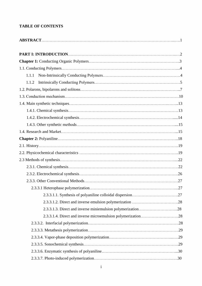
TABLE OF CONTENTS
ABSTRACT……………………………………………………………………………………...….1
PART I: INTRODUCTION……………………………………………………………………..…2
Chapter 1: Conducting Organic Polymers………………………………………………………….3
1.1. Conducting Polymers…………………………………………………………………………....4
1.1.1 Non-Intrinsically Conducting Polymers…………………………………………………4
1.1.2 Intrinsically Conducting Polymers………………………………………………………5
1.2. Polarons, bipolarons and solitons………………………………………………………………..7
1.3. Conduction mechanism…………………………………………………………………………10
1.4. Main synthetic techniques……………………………………………………………….……..13
1.4.1. Chemical synthesis………………………………………………………………………13
1.4.2. Electrochemical synthesis…………………………………………………………….....14
1.4.3. Other synthetic methods………………………………………………………………....15
1.4. Research and Market…………………………………………………………………………...15
Chapter 2: Polyaniline……………………………………………………………………………..18
2.1. History………………………………………………………………………………………….19
2.2. Physicochemical characteristics ……………………………………………………………….19
2.3 Methods of synthesis…………………………………………………………………………....22
2.3.1. Chemical synthesis………………………………………………………………………22
2.3.2. Electrochemical synthesis……………………………………………………………….26
2.3.3. Other Conventional Methods……………………………………………………………27
2.3.3.1 Heterophase polymerization………………………………………………………...27
2.3.3.1.1. Synthesis of polyaniline colloidal dispersion…………………………….27
2.3.3.1.2. Direct and inverse emulsion polymerization …………………………….28
2.3.3.1.3. Direct and inverse miniemulsion polymerization………………………..28
2.3.3.1.4. Direct and inverse microemulsion polymerization……………………….28
2.3.3.2. Interfacial polymerization………………………………………………………….28
2.3.3.3. Metathesis polymerization………………………………………………………….29
2.3.3.4. Vapor-phase deposition polymerization………………………………………...….29
2.3.3.5. Sonochemical synthesis…………………………………………………………….29
2.3.3.6. Enzymatic synthesis of polyaniline………………………………………………...30
2.3.3.7. Photo-induced polymerization………………………………………………….….30

ii
2.3.3.8. Plasma polymerization……………………………………………………………..30
2.4. Conductivity……………………………………………………………………………...…….30
2.4.1. Effect of doping………………………………………………………………………….31
2.4.2. Effect of moisture………………………………………………………………………..32
2.4.3.Effect of crystallinity……………………………………………………………………..33
2.4.4. Effect of molecular weight………………………………………………………………34
2.4.5. Conduction mechanism………………………………………………………………….34
2.5. Techniques of characterization…………………………………………………………………36
2.5.1. FT-IR spectroscopy…………………………………………………………………...…36
2.5.2. UV-vis spectroscopy…………………………………………………………………….38
2.5.3. XRPD diffraction………………………………………………………………………..41
2.5.4. Cyclic voltammetry………………………………………………………...……………46
2.5.5. Conductivity measurements……………………………………………………………..51
Chapter 3: One dimensional polyaniline…………………………………………………………..52
3.1. Importance of one-dimensional polyaniline………………………………………………...….53
3.2. Synthetic methods…………………………………………………………..………………….53
3.2.1. Hard template synthesis…………………………………………...………………….54
3.2.2. Soft template synthesis……………………………………………………………….54
3.2.3. Combined soft and hard template synthesis………………………………………….55
3.2.4. No-template synthesis…………………………………………..…………………….55
3.2.4.1. Radiolytic synthesis………………………………………..……………….55
3.2.4.2. Rapid mixing reaction………………………………………………………56
3.3. Properties……………………………………………………………………………….56
Chapter 4: Composite materials……………………………………………………………………58
4.1. PANI/insulating polymers……………………………………………………………………...59
4.1.1. Techniques of preparation of PANI blends…………………………………………..59
4.1.1.1. Synthetic methods to prepare PANI blends and composites………………60
4.1.1.2. Blending methods…………………………………………………………..62
4.1.2. Physicochemical properties…………………………………………………………..63
4.1.3. PANI nanofibers by electrospinning technique………………………………...…….65
4.2. PANI/ferrites nanocomposites………………………………………………………………….67
4.2.1. Iron oxides nanoparticles……………………………………………………………..67
4.2.2 Techniques of preparation of PANI/ferrites…………………………………………..70
Chapter 5: Applications……………………………………………………………………………72
iii
5.1. EMI (ElectroMagnetic Interference) shielding applications…………………………………...73
5.1.1. Signal transmission…………………………………………………………………...74
5.1.2. Electromagnetic interference (EMI)………………………………………………….75
5.1.3. EMI shielding………………………………………………………………………...76
5.1.4. Materials for EMI shielding…………………………………………………………..77
5.1.4.1. Metals used in EMI shielding………………………………………………77
5.1.4.2. Composite materials in EMI shielding……………………………………..78
5.1.4.3. Intrinsically conducting polymers in EMI shielding……………………….79
5.2. Biomedical applications………………………………………………………………………..81
5.2.1. Biomolecular sensing…………………………………………………………………81
5.2.2. Biomolecular actuators……………………………………………………………….83
5.2.3. Tissue engineering……………………………………………………………………84
5.2.4. Drug delivery systems………………………………………………………………..86
5.3. Sensors applications…………………………………………………………………………....87
5.3.1. Sensors based on transduction………………………………………………………..87
5.3.1.1. Potentiometric sensors……………………………………………………...87
5.3.1.2. Amperometric sensors……………………………………………………...87
5.3.1.3. Piezoeletric sensors…………………………………………………………88
5.3.1.4. Calorimetric/thermal sensors……………………………………………….88
5.3.1.5. Optical sensors……………………………………………………………...89
5.3.1.6. Pressure sensors…………………………………………………………….89
5.3.1.6.1. High pressure sensors……………………………………………..91
5.3.1.6.2. Low pressure (touch) sensors……………………………………..92
5.3.2. Sensors based on application mode…………………………………………………..94
5.3.2.1. Chemical sensors…………………………………………………………...94
5.3.2.2. Ion-selective sensors………………………………………………………..95
5.3.2.3. pH sensors…………………………………………………………………..96
5.3.2.4. Humidity sensors…………………………………………………………...96
5.4. Other applications………………………………………………………………………………97
PART II: EXPERIMENTAL PART……………………………………………………………..98
Chapter 6: Synthetic methods………………………………………………………………...……99
6.1. PANI preparation.……………………………………………………………………………..100
6.1.1. PANI preparation from aniline monomer…………………………………………...100

iv
6.1.2. PANI preparation from N-(4-amonophenyl)aniline (aniline dimer)………………..100
6.1.3. PANI preparation from aniline dimer using O2 as the oxidant……………………...100
6.1.4. 4-Oxo-4-(4-(phenylamino)phenylamino)butanoic acid (Aniline dimer-COOH,
ADCOOH) preparation……………………………………………………..……….101
6.2. PANI modification……………………………………………………………………………101
6.2.1. PANI deprotonation (dedoping).……………………………………………………101
6.2.2. PANI reprotonation (redoping) with inorganic acids……………………………….101
6.2.3. PANI reprotonation (redoping) with organic acids…………………………………102
6.2.4. PANI reduction (synthesis of Leucoemeraldine)…………………………………...102
6.3. Metal oxides nanoparticles preparation……………………………………………………….102
6.3.1 Fe3O4 nanoparticles (NPs) preparation………………………………………………103
6.3.1.1. Fe3O4 nanoparticles (NPs) preparation by co-precipitation method………103
6.3.1.2. Preparation of Fe3O4 nanoparticles (NPs) with a mean diameter of 2.3 nm
(MNP_3) by Metal Vapour Synthesis (MVS) technique………………….103
6.3.1.3. Fe3O4 nanoparticles (NPs) preparation by solvothermal method…………104
6.3.1.3.1. Preparation of Fe3O4 NPs with a mean diameter of 10.0 nm
(MNP_2)… ……………………………………………………..104
6.3.1.3.2. Preparation of Fe3O4 NPs with a mean diameter of 27.0 nm
(MNP_1)…………………….……….…………….....................104
6.3.2. Preparation of Fe3O4 nanoparticles capped with aniline dimer–COOH…………….104
6.3.2.1. One-step preparation of Fe3O4 nanoparticles capped with aniline dimer
COOH………………………………………………………………..........104
6.3.2.2. Two-step preparation of Fe3O4 nanoparticles capped with aniline dimer
COOH……………………………………………………..........................105
6.3.3. MFe2O4 (M= Co, Ni, Mn, Cu, Zn and Mg) and FeCr2O4 nanoparticles preparation by
co-precipitation method…………………………………………………..................105
6.4. PANI/MFe2O4 (M= Fe, Co, Ni, Mn, Cu, Zn and Mg) and PANI/FeCr2O4 composites
preparation……………………………………………………………………………………105
6.4.1. PANI/MFe2O4 composites preparation using H2O2 as the oxidant…………………106
6.4.2. PANI/MFe2O4 composites preparation using O2 as the oxidant……………………106
6.5. PANI nanofibers preparation by electrospinning technique………………………………….106
6.5.1. Spun solutions preparation………………………………………………………….106
Chapter 7: Characterization techniques…………………………………………………………..108
7.1. Spectroscopic techniques……………………………………………………………………...109

v
7.1.1. Fourier Transform Infrared (FT-IR) spectroscopy………………………………….109
7.1.2. Ultraviolet-visible (UV-vis) spectroscopy…………………………………………..109
7.1.3. Atomic Absorption spectroscopy (AAS)……………………………………………109
7.2. Thermogravimetric technique………………………………………………………………...110
7.3. Mass spectrometry…………………………………………………………………………….110
7.4. NMR spectroscopy……………………………………………………………………………110
7.5. X-Rays powder diffraction …………………………………………………………………...110
7.6. Microscopic techniques……………………………………………………………………….110
7.6.1. Transmission Electron Microscopy (TEM)………………………………………....110
7.6.2. Scanning Electron Microscopy (SEM)……………………………………………...111
7.7. Electrical resistivity measurements…………………………………………………………...111
7.8. Magnetic measurements………………………………………………………………………111
7.9. Wave guide dielectric characterization………………………………………………………..111
7.10. Electrospinning process……………………………………………………………………...112
7.11. Direct an direct citocompatibility tests of PANI nanofibers on a SH-SY5Y human cell
line…………………………………………………………………………………………...112
7.12. Measurements of electrical conductivity as a function of force……………………………..115
7.13. Piezoresistive measurements………………………………………………………………...115
PART III: RISULTS AND DISCUSSION…………………………………………….………..116
Chapter 8: Synthesis and characterization of PANI/metal oxide nanocomposites……………….117
8.1. New clean one-pot synthesis of polyaniline/Fe3O4 nanocomposites with magnetic and
conductive behaviour…………………………………………………………………………118
8.1.1.Catalytic polymerization………………………………………………….………….119
8.1.2. Spectroscopic characterization……………………………………………………...122
8.1.3. Morphological characterization………………………………………………….….124
8.1.4. Mechanism of nanorods formation………………………………………………….126
8.1.5. Thermogravimetric analyses……………………………………………………..….127
8.1.6. Magnetic measurements………………………………………………………….....127
8.1.7.Conductivity measurements………………………………………………………….132
8.2. The effect of nanoparticle size on the synthesis and properties of PANI/Fe3O4
nanocomposites……………………………………………………………………………...134
8.2.1.Catalytic polymerization…………………………………………………………….134
8.2.2. Morphological characterization……………………………………………….…….138
vi
8.2.3. Magnetic measurements…………………………………………………………….142
8.3. Synthesis and characterization of PANI/MFe2O4 composites: the role of the bivalent
metal (M)……………… ……………………………………………………………………145
8.3.1.Catalytic polymerization using CoFe2O4 NPs as the catalysts………………………146
8.3.2. Morphological and spectroscopic characterization………………………………....148
8.3.3. Magnetic measurements…………………………………………………………….152
8.3.4.Catalytic polymerization using MFe2O4 NPs as the catalysts (M= Mn, Co, Ni, Cu, Zn,
Mg) and characterization…………………………………………………………….154
8.4. Electromagnetic characterization……………………………………………………………..160
8.5. Microwave absorption properties……………………………………………………………..162
8.6. Towards well-dispersed PANI–Fe3O4 nanomaterials………………………………………...166
8.6.1. ADCOOH characterization………………………………………………………….167
8.6.2. ADCOOH/Fe3O4 NPs composites prepared by a one-pot method and their
characterization……………………………………………………………………...169
8.6.3. ADCOOH/Fe3O4 NPs composites prepared by a two-step method and their
characterization……………………………………………………………………...172
8.6.4. Synthesis of PANI/Fe3O4 composites using ADCOOH/Fe3O4 NPs precursors prepared
by a two-step method………………………………………………………………..173
Chapter 9: Improvements in the preparation of polyaniline nanofibers by electrospinning technique
and their biocompatibility. Towards pure electrospun polyaniline…………………..175
9.1. PANI/PEO nanofibers: effect of different raw sources………………………………………177
9.1.1. Morphological characterization……………………………………………………..177
9.1.2. Spectroscopic characterization……………………………………………………...181
9.1.3. Conductivity measurements…………………………………………………………184
9.1.4. Tests of cytocompatibility…………………………………………………………..187
9.2. PANI/PMMA nanofibers: effect of washing………………………………………………….189
9.2.1. Morphological characterization……………………………………………………..189
9.2.2. Spectroscopic characterization……………………………………………………...195
9.2.3. Tests of cytocompatibility…………………………………………………………..196
Chapter 10: Piezoresistive properties of polyaniline: towards low cost force and strain
sensors……………………………………………………………………………….198
10.1. Electromechanical characterization of PANI under high loading…………………………..199
10.1.1. Electromechanical response………………………………………………………..200
10.1.2. Diffractometric characterization…………………………………………………...202

vii
10.1.3. Electrical conductivity……………………………………………………………..202
10.1.4. Piezoresistive effect………………………………………………………………..203
10.2. Electromechanical characterization of PANI under low loading……………………………206
10.3. Piezoresistive effect in polyaniline. The effect of different raw materials and doping
agents………………………………………………………………………………………...209
10.3.1. Electrical conductivity……………………………………………………………..213
10.3.2. Morphological characterization……………………………………………………214
10.3.3. Electromechanical response………………………………………………………..217
10.3.4. Piezoresistive effect………………………………………………………………..219
PART IV: CONCLUSIONS……………………………………………………………………..226
REFERENCES…………………………………………………………………………………...230

1
Abstract
The chemical industry of the forthcoming years will be shaped by a number of emerging global
megatrends strictly related to the growth and aging of the world population (nine billion people in
2050). This will result in demand of innovative materials able to solve new needs in different fields:
health, communication, energy, environmental sustainability, etc. In this diversified context,
conducting organic polymers (COPs) are expected to play an important role thanks to their
polyhedric properties. Among them, polyaniline is one of the more investigated COPs owing to its
peculiar properties which make it a potential substitute of conventional materials in different fields
(electronics, fenestration, textile industry, sensors and many others).
However, to date many aspects related to its synthesis and application are still open. Scope of the
present work is to provide alternative eco-friendly methods to the traditional synthetic routes
towards PANI-based materials and enlarge their present applications in view of the novel
requirements. This study has been organized in three main sections. In the first section a new green
protocol will be present to prepare PANI/metal oxides nanocomposites, innovative materials in the
field of EMI shielding. For the first time the double role of magnetic nanoparticles, as catalysts of
the reaction and magnetic fillers of the final products, will be illustrated.
Conducting/magnetic materials are particularly tempting for their ability to reduce the
electromagnetic interferences (EMI) originated by the increasing use of electronic devices and
telecommunication equipment. Preliminary results in terms of their microwave absorbing properties
will be shown.
The possibility to improve the health and quality of life for millions of people worldwide is, in fact,
the overall goal of tissue engineering. Nanostructured PANI in form of fibers or wires could find
application as novel conductive scaffolds in neuronal or cardiac stimulations. In the second section,
the possibility to produce highly pure polyaniline nanofibers by electrospinning technique will be
showed. These materials, characterized by high values of conductivity and cytocompatibility, could
represent an alternative to traditional solutions for cardiac and neuronal stimulation.
Regarding the third section of the work, the amazing piezoresistive properties of PANI, especially
in form of film, will be for the first time herein presented. Herein, the extraordinary high GF values
of PANI-based films (more than 10 times higher than those of commercial piezoresistors) will be
reported. The mechanical monitoring in large and small scale (buildings/touch-technology) needs of
highly sensitive stress/strains sensors and PANI-based materials are particularly promising in this
sector. All these characteristics contribute to make PANI and its composites innovative materials
which could offer new solutions for many challenges of the future.

2
PART I: INTRODUCTION

3
Chapter 1: Conducting Organic Polymers

4
1.1. Conducting polymers
1.1.1. Non-Intrinsically Conducting Polymers
Most of the polymers manufactured today are insulators. When they are synthesized from olefins, as
ethylene, propylene or higher ones, their backbone is made of carbon-carbon single bonds,
otherwise they are made of repetitive ester, ether or amidic bonds. As there is no possibility for a
charge to move along a conjugated -bond path, these polymers show high resistivity, hence very
low conductivity. The only possibility to make a conductive material is to add a second component
for example metal powder or carbon black.[1] Recently, many publications show that CNTs (carbon
nanotubes) are one of the best fillers (Figure 1.1). In fact, adding only 2-3 % weight of single
walled carbon nanotubes (SWNT) to a polymer can improve its conductivity by several orders of
magnitude (Figure 1.2). [2, 3]
Figure 1.1.: articles and patents on carbon nanotubes (CNT) and CNT composites per year.
Figure 1.2.: conductivity of CNT composites as a function of its mass fraction.

5
1.1.2. Intrinsically Conducting Polymers
Since the discovery of the highly conducting polyacetylene (PA) in 1977,[4] the scientific
community has focused its efforts on the study and optimization of a new class of materials:
conductive organic polymers (COPs).
Among these innovative materials, called also “synthetic metals”, polyaniline (PANI), polypyrrole
(PPy) and polythiophene (PTh) are still the most studied for their peculiar characteristics, as good
conductivity and high environmental stability,[5] that make them particularly attractive for
applications in many fields (photovoltaic devices,[6] batteries,[7] electrodes,[8] sensors,[9] and
many others).
The simplest conducting polymer is polyacetylene. Figures 1.3. a and b show its structural isomers.
In 1958 the Italian Giulio Natta (Figure 1.4.) prepared polyacetylene with high cristallinity using a mixture
of Al(CH2CH3)3 and Ti(OC4H9)4 as the initiator.[10]
However, the limited physicochemical characteristics of the product led to a loss of interest from
the scientific community for many years.
At the beginning of 1970, the Japanese chemical Hideki Shirakawa (Figure 1.5. c) found a useful
way to control the ratio of the two isomers during the synthesis of PA. The synthetic method
applied was based on the use of the same Ziegler-Natta catalyst used from Natta. However, by
Figure 1.3.: a) trans-PA and b) cis-PA
Figure 1.4.: Giulio Natta
a b
6
acting on the reaction conditions, especially temperature and catalyst amount, Shirakawa obtained a
silvery film of pure trans-PA and a coppery film of pure cis-PA.
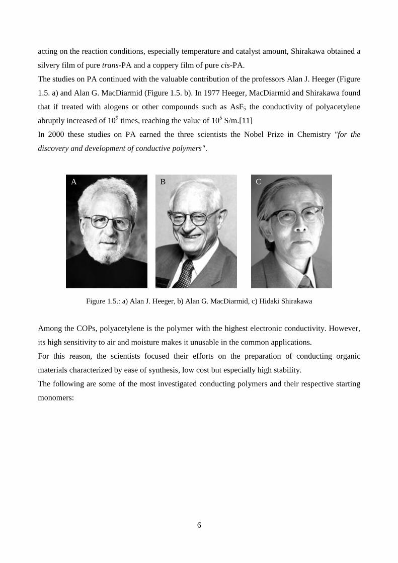
The studies on PA continued with the valuable contribution of the professors Alan J. Heeger (Figure
1.5. a) and Alan G. MacDiarmid (Figure 1.5. b). In 1977 Heeger, MacDiarmid and Shirakawa found
that if treated with alogens or other compounds such as AsF5 the conductivity of polyacetylene
abruptly increased of 109 times, reaching the value of 10
5 S/m.[11]
In 2000 these studies on PA earned the three scientists the Nobel Prize in Chemistry "for the
discovery and development of conductive polymers".
Among the COPs, polyacetylene is the polymer with the highest electronic conductivity. However,
its high sensitivity to air and moisture makes it unusable in the common applications.
For this reason, the scientists focused their efforts on the preparation of conducting organic
materials characterized by ease of synthesis, low cost but especially high stability.
The following are some of the most investigated conducting polymers and their respective starting
monomers:
Figure 1.5.: a) Alan J. Heeger, b) Alan G. MacDiarmid, c) Hidaki Shirakawa
A B C

7
1)
2)
3)
1.2. Polarons, bipolarons and solitons
In the COPs the equilibrium geometry in the ionized state is different from this in the ground state.
[12-14]
Figure 1.7. reports the energies involved in the ionization process of a molecule.
Figure 1.6.: 1a) aniline, 1b) polyaniline, 2a) pyrrole, 2b) polypyrrole, 3a) thiophene, 3b) polythiophene
a b
a b
a b
Figure 1.7.: a) Energies involved in a ionization process of a molecule, b) schematic illustration of the
one-electron Energy levels for a molecule in its ground state and its first ionization state.
Ground state First ionization
state
a b

8
Following the scheme reported in Figure 1.7., when a molecule is excited it passes from the ground
state to the first ionization state. The energy involved in this process is EI1. However, it is possible
that in the ground state the geometry of the molecule is distorted and the molecule adopts the
equilibrium geometry of the ionization state. This produces a distortion energy (Edis in Figure 1.7.
a).
As shown in Figure 1.7. b, this distortion causes an upward shift of the highest occupied molecular
orbital (HOMO) and a downward shift of the lowest unoccupied molecular orbital (LUMO).
As it can be inferred from Figure 1.7. a, the geometry relaxation in the ionized state is favoured
when EI1- EI2 >> Edis, that is when the reduction ∆ (Figure 1.7. b) upon distortion is larger than Edis
required to make the distortion.
In all materials, including polymers, an ionization process produces a hole in the valence band
corresponding to a positive charge. For most of the solids this process doesn’t cause lattice
distortion. Moreover, the positive charge is completely delocalized and makes these materials
conductive.
However, as reported above, in a conducting organic polymeric chain during the ionization process
the localization of the charge is energetically favoured, because producing around the charge a local
distortion (relaxation) of the lattice. This process causes the presence of localized electronic states.
For example, during an oxidation process an electron is removed from the chain, causing a lowering
of the ionization energy of ∆. If ∆ is larger than Edis necessary to distort the lattice locally around
the charge, this localization process is favourable. This produces a polaron, that in chemistry is a
radical anion (spin ½) associated with a lattice distortion.
When a second electron is subtracted from the chain, it can be removed from the polaron, producing
a bipolar, o from another point of the chain, producing two polarons.
A bipolaron can be defined as a pair of like charges (dication or dianion) associated with a local
lattice distortion.
The formation of the bipolaron is more favoured than that of two polarons, because the energy
gained due to the local lattice deformation is larger than Coulomb repulsion between the two
charges of same sign that are in the same location.[15]
Polaronic and bipolaronic states can be produced in polymers that have not degenerate ground
states. Most of the conducting organic polymers present these conditions, because their resonant
structures are not isoelectronic.
In the case of trans-polyacetylene the configuration of the ground state is degenerate, because the
interchange of the single and double bounds doesn’t involve energy variations. This means that two

9
geometric structures have the same energy. (Figure 1.8. A). The transition from a phase to another
is described from the parameter:
u= dC=C- dC-C
where dC=C and dC-C are the distance of the double and single bonds respectively.
A B
As a result of this degeneracy, when a bipolaron is formed in a trans-polyacetylene the two charges
can be separated (Figure 1.8. B) forming two single charges, named solitons. This process of charge
separation is favourable because doesn’t increase the distortion energy of the system. In fact, the
geometric structure that appears between the two charges has the same energy as the geometric
structure on the other sides of the charges. The soliton corresponds to a zero value of u (Figure 1.8.
A). Solitons are defects of conjugation that sign the transition from one phase to another, as
reported in Figure 1.8. A.
In the case of trans-PA a neutral soliton occurs when a chain contains an odd number of conjugated
carbons, a radical (Figure 1.9.).
Figure 1.8.: A) Trans-polyacetylene phases and their energetic diagrams, B) illustration of the formation of two
charged solitons on a chain of trans-polyacetylene

10
In a long chain, the spin density in a neutral soliton is not localized on a carbon atom but
delocalized on several carbons.[16-18]
The energy level associated to a neutral soliton is occupied only by n electron (Figure 1.9. A); as a
result its spin is ½ and zero charge. On the contrary, positive and negative solitons (Figures 1.9. B
and C) have zero spin values but are positively or negatively charged. When subjected to an electric
field, charged solitons can move longitudinally along the polymeric chain thus generating current
transport.
1.3. Conduction mechanism
Generally, the backbone of the common polymers mainly consists of σ bands and the hybridization
of each atom of carbon is sp3. The high energy gap (Egap > 6 eV) between the bonding band (σ) and
antibonding band (σ*) makes these materials insulating.
Differently, in the COPs the backbone consists of atoms of carbon hybridized sp2, that form three σ
bonds, and a pz orbital that allows a π overlapping with the pz orbital of the adjacent carbon.
The presence along the backbone of these conjugated double bonds, π delocalized system, is
responsible for the electronic properties of the conducting polymers.
The presence of these conjugated double bonds produces two bands, that similarly to the metals can
be called “valence band” and “conduction band” (Scheme 1.1.).[12]
A B C
Figure 1.9.: Band structure for a trans-PA chain containing a A) neutral soliton, B) positively charged soliton,
C) negatively charged soliton

11
Roughly, as for the inorganic materials also for the organic polymers the band model can be applied
to explain their conductivity.
In COPs the electric conductivity is due to the low value of the Egap ( 1- 4 eV), that allows the
electrons in the valence band (π) to access the conduction band (π*).[13]
Figure 1.9. reports a comparison between the conductivity of COPs and those of other common
materials.
In the inorganic semiconductor the removal or addition of electrons can be realized in different
ways, for example by photoexcitation or by the introduction of impurities (dopants).
Scheme1.1.: Energy variation vs number of double bonds
Π
Π*
Figure 1.9.: Comparison between the conductivity of COPs and those of other common materials

12
If the impurity provides an electron to the conduction band (CB), the doping process is called n-
type doping. On the contrary, if the impurity subtracts an electron to the valence band (VB),
producing a hole, the doping process is called p-type doping (Figure 1.10.). Electrons and holes are
the charge carriers responsible to the electric conductivity of these materials.
However, this model doesn’t explain why in the COPs the conductivity is associated with unpaired
electrons but rather with spinless charge carriers.
Starting from the band model, it is possible to define two quantities: the ionization energy (IE) and
the electronic affinity (EA).
The ionization energy is the energy required to remove an electron from the valence band.
The electron affinity is the energy required to capture an electron in the conduction band.
Generally, conducting organic polymers are characterized by small IE and large EA, that easily
allow to oxidize (n-type doping) or reduce (p-type doping) the system.[14]
Since the inorganic semiconductors are strict, they maintain their structure also the addition of
removal of electrons.
Conducting organic polymers, instead, are characterized by low coordination and high flexibility
and ability to structural distortions. For these reasons, the removal or introduction of charges cause
a distortion (relaxation) around them. This kind of distortions are energetically favoured because
they allow the stabilization of the charges.
The distortion of the backbone, due to the addition or removal of electrons, can lead to excited
states, called solitons, polarons and bipolarons, that are defects responsible for the electronic
conductions. Three methods were used to generate additional solitons: chemical doping,
photogeneration and charge injection. An electron will be accepted by the dopant anion to form a
Figure 1.10.: n-doping and p-doping in the inorganic semiconductors.

13
carbocation (positive charge) and a free radical during the chemical doping (oxidation) of the
polymer chain, known to organic chemists as radical cation or polaron to physicists.
Both the soliton and polaron can be neutral or charged (positively or negatively) as shown in Figure
1.11.
1.4. Main synthetic techniques
Typically COPs are prepare by traditional polymerization reactions, such as condensation and
addition reactions. However, more accurately the synthetic methods of COPs can be categorized in
three main groups: chemical, electrochemical and photochemical syntheses.[20]
1.4.1. Chemical synthesis
Among all the synthetic methods developed to produce COPs, the oldest and still the most popular
route for the preparation of these materials in bulk is the chemical oxidative polymerization
reaction. This approach remains the most used and also investigated especially for large scale
production level. Stoichiometric oxidants, such as KMnO4, K2Cr2O7, (NH4)2S2O8 but also metals in
high oxidation state,[21-24] are used at low pH values. Even though chemical synthesis is the most
applied in academic and industrial fields, the control of the morphology and conductive
characteristics of the products is harder than in the case of electrochemical approach. In fact, small
changes of some parameters (such as temperature, concentration, etc…) cause big changes in the
characteristics of the products. Moreover, the large production of waste, such as MnO2, (NH4)2SO4
and so on, makes this approach unsustainable in terms of environmental impact.
In the last years, alternative catalytic processes have been developed in order to reduce the
production of waste and provide cleaner products. In this context the use of catalysts, in form of
Figure 1.11.: defects in conducting organic polymers. a) neutral soliton, b) positive soliton, c) negative
soliton, d) positive polaron, e) negative polaron, f) positive bipolaron, g) negative bipolaron
a b c
d e
f g

14
salts of metals or nanopaticles, [25-30] or sonication [31-34] allow to speed up the polymerization
reactions working in cleaner and mild conditions.
1.4.2. Electrochemical synthesis
Unlike chemical syntheses, electrochemical approach allows to control accurately morphology and
conductive behaviour of COPs. It is particularly effective in the preparation of COPs in form of film
and allows to tune easily the final thickness. Different techniques can be used including
potentiostatic (constant potential), galvanostatic (constant current) and potentiodynamic (potential
scanning, i.e. cyclic voltammetry) methods.[35] In this kind of reaction the choice of the solvent
and electrolyte is crucial, because they have to be stable at the oxidation potential.
Electrochemical syntheses occur through addition polymerization reactions. They are oxidative
processes and are characterized by three steps:
1) initiation step: radical monomer is produced by electrochemical oxidation;
2) chain propagation: radical reacts with a non-radical to produce a new radical species;
3) chain termination: two radicals react each other to create a non-radical species.
The electropolymerization mechanism is still a research topic of relevant interest. In this context,
the contrasting interpretation of pyrrole polymerization is emblematic.
As an example the electropolymerization of pyrrole is reported below.[36]
Pioneering investigations of Funt and Diaz,[37, 38] then confirmed by Waltman and Bargon,[39,
40] have proposed that pyrrole activation occurs through electron transfer from the monomer
forming a radical cation-rich solution near the electrode in several steps.
Step 1
In the first step pyrrole monomer (Py) is oxidized at the surface of the electrode producing cation
radical (Py+
) stabilized by resonance by the mechanism reported in Scheme 1.2.
NH
NH
N+
HN
+
H
Scheme 1.2. Cation radical formation
Step 2
Thanks to their reactivity Py+
species can react each other by coupling reaction producing dimeric
cationic species, which can lose protons forming neutral dimers (Scheme 1.3.).
+
= Py+
-e
-

15
N+
HN
+
H
+
N+
H
N+H
NH
NH
Scheme 1.3. chain propagation
Step 3
Also dimeric species can be oxidized to produce cation radicals. Moreover, since the unpaired
electron is now delocalized over two rings, the potential oxidation of dimer is lower than that of
corresponding monomer and it can be oxidized more easily producing trimeric cations and then
neutral trimers.
Step 4
The chain propagation continues producing long polymers. It stops when two radicals react each
other to create a non-radical species.
Pletcher and co-workers have suggested another mechanism in which the cation radical, formed by
the loss of an electron, reacts directly with a neutral molecule giving a cation dimer [41]. The cation
dimer then loses a second electron and 2 protons, thus forming the neutral dimer.
1.4.3. Other synthetic methods
In addition to two main synthetic methods reported above (chemical and electrochemical
syntheses), many others have been investigated. In general, the necessity of developing new
synthetic strategies is related to the possibility to obtain COPs in precise nano-sized forms, such as
nanofibers, nanospheres, nanorods, etc.
Solide-state polymerization, microwave-assisted polymerization, UV light-assisted polymerization,
plasma-induced polymerization and vapor phase polymerization are good examples of alternative
approaches.[42]
1.5. Research and Market
From their discovery to date the scientific interest in the conducting organic polymers has grown up
exponentially, as confirmed by the graph reported in Figure 1.12., which shows the number of
publication per years for polyaniline.
-2H+

16
According to a recent market research report,[43] the total market for conducting organic polymers
is expected to reach $3.4 billion by 2017.
Factors driving market of COPs are lightweight, easy fabrication, low cost and high resistance to
heat that make them particularly appealing in many fields, such as electronic devices, EMI
(ElectroMagnetic Interference) shielding, biomedicine, and so on. Cost is another important factor
influencing the electro-active polymers market growth.
North America dominate the market for COPs. In fact, as reported in Figure 1.13, it held a 65%
share of the global COPs product market, followed by Europe with a 22% share in 2011.
Recently, DuPont has signed an agreement with Ormecon Chemie of Ammersbek, Germany to
commercialize their Ormecon's polyaniline-based products including anticorrosion coatings and
printed circuit board, a market of $9-15 billion.
Figure 1.12.: number of publications per year for polyaniline
Figure 1.13.: Global production market for COPs in 2011

17
The US market for conductive polymers is forecast to reach 240.5 thousand tons by the year 2015.
Conductive polymers could, in the long-term, be an alternative to silicon. Opportunities exist in
display materials, chip packaging, plastic transistors, sensors, and ultracapacitors,.
However, intrinsically conducting polymers (COPs in the Figure 1.14.) production is currently
small in the overall conducting polymer (CPs in Figure 1.14.) market but it is the fastest growing
market in future. At present it accounts for only 12% of the total conducting polymer market, but
this share is estimated to increase to 20% by 2017.
In any case, conductive organic polymers represent the largest submarket of the overall electro-
active polymers market with an expected $2.6 billion by 2017, at a CAGR (Compound Annual
Growth Rate) of 6.1% from 2012 to 2017.
Figure 1.14.: Global market for conducting polymers in 2011. CPs= conducting polymers, COPs=
intrinsically conducting organic polymers, IDPs= Inherently dissipative polymers

18
Chapter 2: Polyaniline

19
2.1. History
Polyaniline (PANI) has the longest history among the intrinsically conducting polymers. It is one of
the oldest artificial conducting polymers and its high electrical conductivity among organic
compounds has attracted continuing attention.
The aniline monomer was isolated as early as 1826 when crystalline salts of aniline sulfuric and
phosphoric acid were observed from the pyrolytic distillation of indigo.[44]
Although the exact date of the first reported polyaniline is unclear, aniline was oxidized
early as 1834 [45] and 1840,[46] when pure aniline (observed as a colorless oil) was obtained from
indigo and oxidized with chromic acid.
Observed as a black precipitate, “aniline black”, in an organic form as part of melanin, a type of
organic polymer, in 1934, polyaniline has been reported since 1860,[47] and some of the first
accurate researches on the subject was made by Green and Woodhead.[48-50]
The terms “emeraldine” and “nigraniline” for different redox forms of aniline black, were
introduced more recently (about second half of the 19th
century)[51] and defined at the beginning of
the 20th century, alongwith other redox forms such as leucoemeraldine, protoemeraldine and
pernigraniline, as linear N–C4 coupled aniline octamers with different oxidation state, i.e., different
number of N-phenyl-benzoquinonediimine and 4-aminodiphenylamine moieties in the
backbone.[50, 52] The interest in polyaniline rose up after the demonstration by MacDiarmid that,
after acidic doping, it becomes a conductor, with conductivity up to 3 S/cm.[53]
2.2. Physicochemical characteristics
Polyaniline is composed of aniline repeat units connected to form a backbone. The existence of a
nitrogen atom lying between phenyl rings allows the formation of different oxidation states that can
affect its physical properties.
Although leucoemeraldine, emeraldine and pernigraniline are the three most common forms, many
other intermediate forms are available, depending on the degree of oxidation of the units (Figure
2.1).
N N N N N N N NH2
H H H H H H H
N N N N N N N NH
H H H H H H
a) Leucoemeraldine
b) Protoemeraldine

20
N N N N N N N NH
H H H H
N N N N N N N NH
N N N N N N N NH
Some properties and characteristics of polyaniline are strictly correlated to its oxidation state.
Leucoemeraldine (Figure 2.1. a) is an amorphous material, whose colour ranges from pale brown to
white. This material, characterized by a high melting point, is insoluble in all solvents. In moist air
it is slowly oxidized to protoemeraldine (Figure 2.1. b), more rapidly if heated.
Protoemeraldine form is characterized by a violet colour and is soluble in acetic acid. If protonated
it forms yellowish-green salts.
Emeraldine (Figure 2.1. c) is the half-oxidized form. It’s partially soluble in pyridine, N, N-dimethyl
formamide and N-methylpyrrolidinone producing blue coloured solution. In the presence of organic
or inorganic acids it forms a salt green coloured called emeraldine salt, which is the unique
electrically conducting form of polyaniline.
In its base form nigraniline (Figure 2.1. d) it is stable and forms dark bluet coloured solutions in
acetic acid, formic acid and pyridine. If heated in an acidic solution it forms green coloured salts
because of its reduction to emeraldine.
In base and salt form pernigraniline (Figure 2.1. e) is not stable. In bases and acids it decomposes
quickly to forms in lower oxidation state.
It is well known that polyaniline has switching, optical, conductive and solubility properties that
distinguish it from other conducting polymers.[54, 55]
The ability to switch from one form to another and the optical properties of PANI are interlinked
and influence each other directly. PANI is a mixed oxidation state polymer, ranging from the most
reduced leucoemerladine form, which is yellow in colour, to the half oxidized emerladine which is
green, and the violet fully oxidized pernigraniline[33] as illustrated in Figure 2.1. The
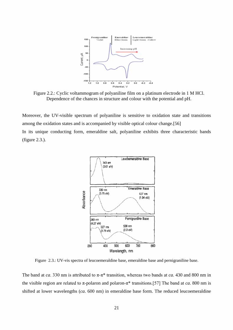
electrochemical switching of polyaniline among the oxidation states can be readily monitored by
cyclic voltammetry as illustrated in Figure 2.2.
c) Emeraldine
d) Nigraniline
e) Pernigraniline
Figure 2.1.: Polyaniline in different oxidation states
21
Moreover, the UV-visible spectrum of polyaniline is sensitive to oxidation state and transitions
among the oxidation states and is accompanied by visible optical colour change.[56]
In its unique conducting form, emeraldine salt, polyaniline exhibits three characteristic bands
(figure 2.3.).
Figure 2.3.: UV-vis spectra of leucoemeraldine base, emeraldine base and pernigraniline base.
The band at ca. 330 nm is attributed to π-π* transition, whereas two bands at ca. 430 and 800 nm in
the visible region are related to π-polaron and polaron-π* transitions.[57] The band at ca. 800 nm is
shifted at lower wavelengths (ca. 600 nm) in emeraldine base form. The reduced leucoemeraldine
Figure 2.2.: Cyclic voltammogram of polyaniline film on a platinum electrode in 1 M HCl.
Dependence of the chances in structure and colour with the potential and pH.
22
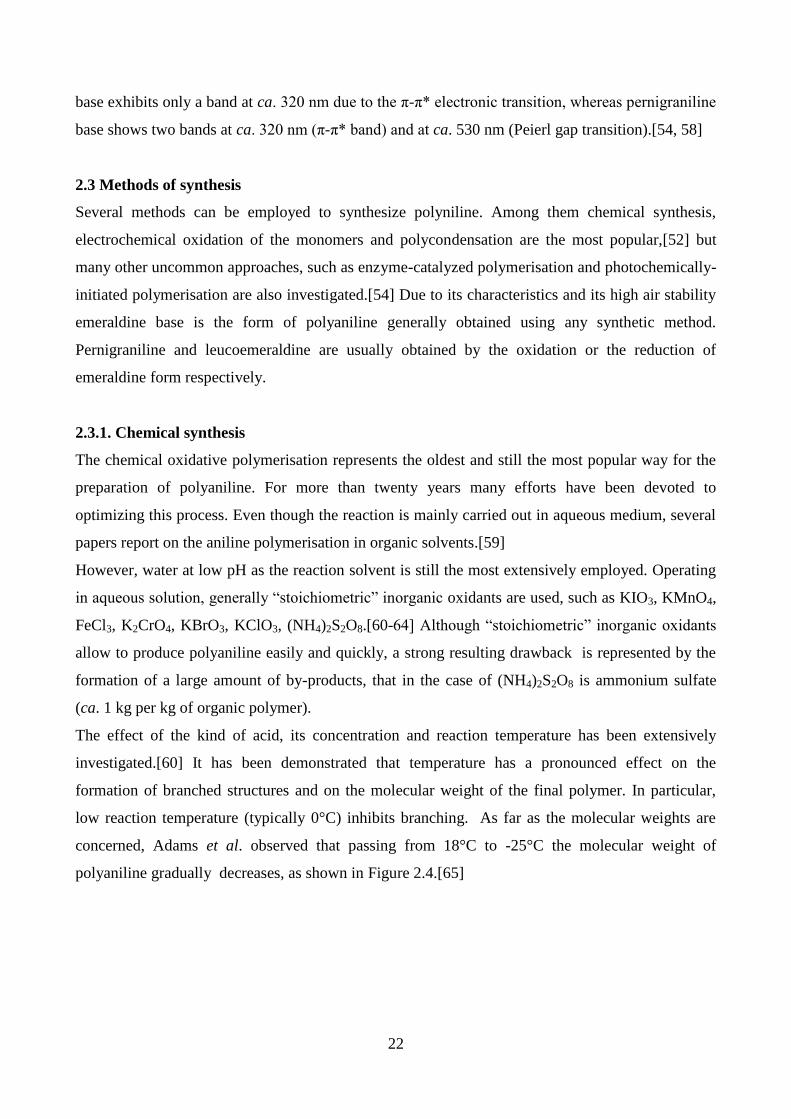
base exhibits only a band at ca. 320 nm due to the π-π* electronic transition, whereas pernigraniline
base shows two bands at ca. 320 nm (π-π* band) and at ca. 530 nm (Peierl gap transition).[54, 58]
2.3 Methods of synthesis
Several methods can be employed to synthesize polyniline. Among them chemical synthesis,
electrochemical oxidation of the monomers and polycondensation are the most popular,[52] but
many other uncommon approaches, such as enzyme-catalyzed polymerisation and photochemically-
initiated polymerisation are also investigated.[54] Due to its characteristics and its high air stability
emeraldine base is the form of polyaniline generally obtained using any synthetic method.
Pernigraniline and leucoemeraldine are usually obtained by the oxidation or the reduction of
emeraldine form respectively.
2.3.1. Chemical synthesis
The chemical oxidative polymerisation represents the oldest and still the most popular way for the
preparation of polyaniline. For more than twenty years many efforts have been devoted to
optimizing this process. Even though the reaction is mainly carried out in aqueous medium, several
papers report on the aniline polymerisation in organic solvents.[59]
However, water at low pH as the reaction solvent is still the most extensively employed. Operating
in aqueous solution, generally “stoichiometric” inorganic oxidants are used, such as KIO3, KMnO4,
FeCl3, K2CrO4, KBrO3, KClO3, (NH4)2S2O8.[60-64] Although “stoichiometric” inorganic oxidants
allow to produce polyaniline easily and quickly, a strong resulting drawback is represented by the
formation of a large amount of by-products, that in the case of (NH4)2S2O8 is ammonium sulfate
(ca. 1 kg per kg of organic polymer).
The effect of the kind of acid, its concentration and reaction temperature has been extensively
investigated.[60] It has been demonstrated that temperature has a pronounced effect on the
formation of branched structures and on the molecular weight of the final polymer. In particular,
low reaction temperature (typically 0°C) inhibits branching. As far as the molecular weights are
concerned, Adams et al. observed that passing from 18°C to -25°C the molecular weight of
polyaniline gradually decreases, as shown in Figure 2.4.[65]

23
Figure 2.4.: Dependence of Mw from the temperature
However, below this temperature the molecular weight of PANI falls back.[65]
Chemical oxidative polymerization of aniline using HCl and (NH4)2S2O8 can be described by the
following chemical equation (Equation 2.1.):
4x(C6H7N·HCl) + 5x(NH4)2S2O8 (C24H18N4·2HCl)x + 5x(NH4)2SO4 +2xHCl + 5x(H2SO4)
(Eq. 2.1.)
As it is possible to observe using a chemical approach PANI is obtained in form of emeraldine salt.
Starting from this reaction several modifications of the oxidative polymerization of aniline have
been proposed.
In this context, an interesting alternative is represented by the interfacial polymerization or
emulsion polymerization. By this approach aniline and, if required, a surfactant are dissolved in an
organic solvent, whereas the oxidizing agent is in the aqueous phase. The polymerization reaction
carries out at the interfacial region.[66]
A modern approach to large scale PANI production suggests the use of more environmentally
friendly oxidants, such as molecular oxygen or hydrogen peroxide.[64, 67-74] This new “green”
approach would open the way to novel applications.
In fact, especially for specific applications, such as medical and biomedical ones, high purity
materials are required.
From a thermodynamic point of view, the reagent H2O2 is advantaged owing to its higher redox
potential (1.77V vs SCE), which is enough for initiating and sustaining aniline polymerization.
Moreover, the formation of H2O as the only reduction product greatly simplifies post-treatments
and recycling. Often the oxidation by dioxygen and hydrogen peroxide is a slow process which can
be accelerated by the use of a catalyst.[26-30, 70] A big help derives by the use of ultrasound

24
irradiation.[74] Many catalysts have been studied for promoting the oxidative polymerization of
aniline. Among them soluble metal ions in high oxidation states or more complex heterogeneous
systems have been employed.[21-31, 61-64]
As reported by Wei et al., the difficult step in aniline polymerization is the oxidation of the
monomer to form dimeric species, that can then quickly oxidized to PANI, thanks to their lower
oxidation potential.[76-79]
This means that starting from the preformed aniline dimer, N-4-aminophenylaniline, the oxidative
polymerization can carry out more easily. Copper, copper salts, gold nanoparticles and nanosized
ferrites have shown an high catalytic activity in this reaction.[26, 30, 80]
Although PANI is prepared from more than one hundred year, to date the mechanism of formation
is not clear. The informations that we have essentially come from electrochemical experiments. For
this reason it’s assumed that chemical and electrochemical reaction mechanisms for PANI
preparation are similar.
In 1960s Mohilner et al. [81] and Bacon and Adams[82] proposed a mechanism for the anodic
oxidation of aniline to PANI in acidic media. as the first step in both chemical and electrochemical
oxidative polymerization of aniline, authors suggested the formation of cation radical, called
anilinium cation (Figure 2.5.)
NH2
Figure 2.5.: anilinium cation
It’s formation is strictly related to the pH of the solution.
The “head-to-tail” and “tail-to-tail” free-radical recombinations of aniline cation radicals lead to the
formation of several dimeric species (Fig. 2.6.):

25
NH NH2
N N
NH2NH2
A preliminary computational investigation of the reaction between aniline cation radical and aniline
indicates that the formation of ADPA is predominant.[83]
However, the dimeric species produced during the oxidative polymerization of aniline in acidic
solutions, as well as the mechanism of their formation, are still controversial.
The PANI chain-growth mechanism was investigated many times in the past and it is still open to
discussion.[77, 84-89]
In 1990s Gospodinova and Terlemezyan reported a redox process between the growing chain in
protonated pernigraniline form (oxidant) and aniline monomers (reductant) in acidic media (pH <
2).[84] Monomer units are gradually added to the chain reaching the emeraldine oxidation state.
To date this mechanism is still accepted, though with some modifications. Moreover, they
suggested that during the growth of the chain the primary oxidant (an oxidizing specie, such as
KMnO4 or (NH4)2S2O8 in the chemical polymerization and anode in the electrochemical reaction)
prefers to oxidize leucoemeraldine, proto-emeraldine, and emeraldine-like oligomers rather than
aniline monomers, whereas aniline monomer is oxidized by the growing nigraniline/pernigraniline-
PANI chain rather than to form new reactive species.
More in detail, during the propagation phase redox reactions among nigraniline/pernigraniline-like
oligomers and aniline monomers were considered as single-electron transfer reactions leading to the
formation of oligomeric cation radicals and aniline cation radicals which further undergo free-
radical recombination reactions.[85, 86, 89]
It was observed that pH value of reaction medium influences branching phenomena. High levels of
acidity cause branching of PANI chains.[85, 86, 89]
In the Scheme 2.1 is reported the whole mechanism of PANI formation.
p-amminodifenilammina
(ADPA )
trans-azobenzene
benzidine Figure 2.6.: Dimeric species by aniline oxidation reaction
26
NH2 NH2
.+2 2
N+
N+
H
H
H
NH
NH2
.++NH2
.+NH
N+
N+
HH
H
H
H
NH
NH
NH2
NH
N+
N+
H
H
H
PANI (Emeraldine)
Ox
+ anilineRedox process (pH < 2)
- 2H+
Ox
Ox
+ aniline
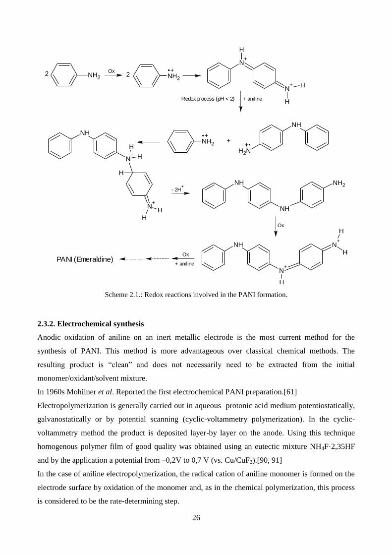
Scheme 2.1.: Redox reactions involved in the PANI formation.
2.3.2. Electrochemical synthesis
Anodic oxidation of aniline on an inert metallic electrode is the most current method for the
synthesis of PANI. This method is more advantageous over classical chemical methods. The
resulting product is “clean” and does not necessarily need to be extracted from the initial
monomer/oxidant/solvent mixture.
In 1960s Mohilner et al. Reported the first electrochemical PANI preparation.[61]
Electropolymerization is generally carried out in aqueous protonic acid medium potentiostatically,
galvanostatically or by potential scanning (cyclic-voltammetry polymerization). In the cyclic-
voltammetry method the product is deposited layer-by layer on the anode. Using this technique
homogenous polymer film of good quality was obtained using an eutectic mixture NH4F·2,35HF
and by the application a potential from –0,2V to 0,7 V (vs. Cu/CuF2).[90, 91]
In the case of aniline electropolymerization, the radical cation of aniline monomer is formed on the
electrode surface by oxidation of the monomer and, as in the chemical polymerization, this process
is considered to be the rate-determining step.

27
Unfortunately, using this approach only small quantities of PANI can be produced (comparing to
chemical polymerization). This limitation reduce the possibility to scale-up the production of
polyaniline by electrochemical synthesis.
2.3.3. Other conventional methods
In addition to these well-established methods, many others have been developed. Some of these are
modifications of the chemical and electrochemical syntheses discussed above, but many other use
different approaches.
2.3.3.1. Heterophase polymerization
This method produces polyaniline of high quality. In particular, it allows to tune very accurately
chemical-physical properties of the final product from a small to a large volume scale.[92-98]
The heterophase polymerization technique includes different methods of polymerization such as
precipitation, suspension, microsuspension, emulsion, miniemulsion, microemulsion, dispersion,
reverse micelle and inverse polymerizations.
In some of these cases (suspension, microsuspension, miniemulsion and microemulsion
polymerization methods) because of its low miscibility in aqueous solution monomer forms
spherical droplets whose size is controlled by a proper choice of the dispersing technique (such as
stirring, ultrasonic treatment or homogenization). The addition of a stabilizer guarantees their
stabilization in water. The size of the droplets varies, according to the polymerization method, in the
following order: suspension >microsuspension >miniemulsion >microemulsion.
The polymerization reaction takes place inside the monomer droplets.
The emulsions are divided into two types: “direct”, oil in water (o/w); and inverse, water in oil
w/o). The selection depends on the chosen emulsifier, the water to oil ratio, and the temperature
of the polymerization. The microemulsion again is subdivided into general microemulsion and
miniemulsion depending upon the droplet size and stability and the amount of surfactant used.
2.3.3.1.1. Synthesis of polyaniline colloidal dispersion
This method is also known as dispersion polymerization.[99, 100] In this approach a water soluble
polymer, used as a steric stabilizer (i. e. poly(N-vinylpyrrolidone) (PVP)), is added to the solution,
causing the formation of PANI in colloidal form. Typically, the average size of the colloidal PANI
particles, obtained by using this synthetic method, range from a few tens to hundreds nanometers
and the shape of the particles may be spherical, globular, granular, cylindrical or branched dendritic
structures.[101, 102]

28
2.3.3.1.2. Direct and inverse emulsion polymerization
Aniline monomer is solubilized in an acidic aqueous solution containing the oxidizing specie. a
nonpolar or weakly polar solvent (i. e. xylene, chloroform or toluene) is added forming an uniform
emulsion.[103] By using this method (direct emulsion), at the end of the reaction PANI salt has to
be purified by all other by-products present in the emulsion. Generally, the product is isolated by
destabilizing the emulsion through the addition of acetone and washed several times.
In the inverse emulsion polymerization process an organic emulsion of aniline monomer solubilized
in a nonpolar organic solvent (i. e. chloroform, isooctane, toluene or in a mixture of solvents) is
added to an aqueous solution. An oil-soluble initiator, such as ammonium persulfate, benzoyl
peroxide, and so on, starts the polymerization. During the course of the reaction, PANI remains as a
soluble component in the organic phase. At the end of polymerization the organic phase is separated
and washed repeatedly with distilled water. Acetone or other suitable solvent are used to break the
emulsion and precipitate the PANI salt.[104, 105]
2.3.3.1.3. Direct and inverse miniemulsion polymerization
A miniemulsion is defined as a submicron (50-500 nm) dispersion of organic materials (oils) in
water. Typically this system contains oil, water, surfactant and a co-surfactant, that usually is a low
molecular weight compound poorly soluble in water but a highly soluble in monomer. These co-
surfactants retard the outward diffusion of the monomer from droplets and form an intermolecular
complex at the oil–water interface, thereby creating a low interfacial tension and a high resistance to
droplet coalescence. For these two reasons, emulsion droplets become quite small and stable.[106,
107]
2.3.3.1.4. Direct and inverse microemulsion polymerization
A microemulsion is defined as a micro-heterogeneous system characterized by a large interfacial
area and low viscous. As in the miniemulsion process, also in this case the system typically contains
oil, water, surfactant and a co-surfactant. Playing with the kind and amount of components of the
mixture, inverse microemulsion polymerization allow to prepare polymeric nanoparticles, hollow
nanospheres and nanotubes.[108, 109]
2.3.3.2. Interfacial polymerization
This technique is particular useful to produce PANI in nanofiber form.[110] In a typical reaction
ane oxidizing agent (ammonium persulfate, hydrogen peroxide and so on) and, if necessary, a
polymerization catalyst are in the aqueous phase, whereas aniline monomer and in some case

29
surfactant in the organic phase. The polymerization reaction takes place at the interfaces of two
immiscible solvents. Various products ranging from a one-dimensional radially aligned nanofiber to
a spherical shaped PANI with a narrow size distribution can be obtained, setting very carefully
some reaction parameters, such as temperature, concentrations of reactants, stirring speed, etc.[111,
112]
2.3.3.3. Metathesis polymerization
Metathesis polymerization is an curious method that allows to produce PANI without employing
aniline monomer in the reaction mixture. In fact, heating p-dichlorobenzene at 220°C for 12 h in the
presence of sodium amide in an organic medium (i. e. benzene) PANI is produced along with
sodium chloride and ammonia.[113]
2.3.3.4. Vapor-phase deposition polymerization
This innovative technique allows to prepare PANI thin films growing directly on a substrate by
polymerizing aniline monomer in a vapor-phase.[114-116] In a typical example an alcoholic
solution containing the oxidizing agent (i. e. FeCl3) and the acid dopant (i. e. camphor sulfonic acid)
is coated on a clean polymeric substrate film, such as polyethylene terephthalate (PET), polyimide
(PI), polyvinyl chloride (PVC), polystyrene (PS), and so on by dip or spin coating and then dried.
Exposing the dry film to aniline vapours in a closed reaction chamber, a polymerization reaction
takes place on the preformed film. At the end of the reaction a thin PANI film is produced on the
substrate.
2.3.3.5. Sonochemical synthesis
Sonochemical method is a quite new technology that finds many applications in chemical syntheses.
It’s known that when an ultrasonic wave passes through a liquid medium a large amount of
microbubbles are produced. They grow and collapse in a very short time (about a few
microseconds) and this effect is called ultrasonic cavitation. It can generated local temperatures as
high as 5000 K and pressures as high as 500 atm, with heating and cooling rates greater than 109
K/s.[117] Therefore, sonochemical synthesis is extensively applied in dispersion, emulsifying,
crushing and particle activation. Jing et al. synthesized PANI nanofibers with high polymer yields
using this technique.[118, 119]

30
2.3.3.6. Enzymatic synthesis of polyaniline
Horseradish peroxidase (HRP) and soybean peroxidase (SBP) are oxidoreductase enzymes able to
oxidize aromatic amines, including polyaniline, in the presence of hydrogen peroxide.[120-122]
The possibility to use an enzyme in combination with a “green” oxidant, such as hydrogen
peroxide, makes this method particularly attracting. Unlike chemical oxidation, in enzymatic
catalyzed polymerization, the oxidation rate is mainly dependent on the amount and activity of the
enzyme. Although during enzymatic oxidation, no inorganic by-products are generated, the recycle
of the enzyme at the end of the reaction and its stability in the reaction conditions are the biggest
drawbacks of this method.
2.3.3.7. Photo-induced polymerization
The photo-induced polymerization of aniline involves the photo-excitation of aniline monomer to
obtain the corresponding polymer. Wang et al. synthesized PANI by using a Nd:YAG laser to
irradiate an Au electrode in a solution containing aniline under an applied external bias.[123] The
morphology of the polymer produced is strictly dependent on the excitation wavelength. In fact, a
more globular morphology is observed for the UV synthesis, whereas a more fibrillar morphology
is detected for the visible light synthesis.[124, 125]
2.3.3.8. Plasma polymerization
Plasma polymerization (or glow discharge polymerization) uses plasma sources to generate a gas
discharge that provides energy to activate or fragment aniline monomer in order to initiate the
polymerization reaction. Polymers formed by this technique are generally highly branched and
highly cross-linked, and adhere very well to solid surfaces. The biggest advantage to this process is
that polymers can be directly attached to a desired surface while the chains are growing, which
reduces steps necessary for other coating processes such as grafting. Moreover, it is a solvent-free
process and a pinhole-free coating can be obtained.[126, 127]
2.4. Conductivity
Emeraldine salt is the only conductive form of polyaniline. Its conductivity is related to many
factors, such as the redox and acid-base properties of the polymer, its degree of crystallinity,
presence of branching, morphology, mode of synthesis and so on. As mentioned before (chapter 1,
p. 9-12) the transition from insulating to conductive state in polyaniline is due to the oxidation
process and to the creation on the polymer's backbone of cation radicals, either polarons or
bipolarons.

31
2.4.1. Effect of doping
Pioneering investigations of MacDiarmid et al. demonstrated that the degree of protonation of
chemically synthesized polyaniline (emeraldine oxidation state) is a function of pH solution. They
observed that that the protonation degree decreased from about 50% at pH 0 to less than 10% at pH
3. Because the decreasing in protonation between pH 2 and 3 was sharp, they suggested that high
degrees of protonation are a prerequisite for high conductivity values.[128]
However, this assumption is true for vacuum-dried PANI, but in wet conditions the results can be
different.
In general, the protonation of PANI helps to form a polaron structure, where a current is carried by
the holes. When the PANI is in a perfect EB form (50% oxidized with alternative quinoid and
benzenoid rings), 50% doping will result in the protonation of the entire quinoid ring. This will lead
to the formation of perfect polaron leading to a high achievable conductivity. Therefore, from an
initial zero level of doping, with the increase in the degree of doping the conductivity is increased
due to the formation of increasingly more polaron. Furthermore, with the increase in the degree of
doping beyond 50%, the decreased conductivity may be due to the formation of bipolarons.[129,
130]
Catedral et al. investigated the effect of the kind of dopant on the conductivity (Figure 2.7), finding
that HClO4-doped sample gave the highest conductivity (109.04 S/cm), which is 2x10⁵ times
greater than that of the undoped sample, while HI-doped PANI showed the lowest conductivity
(0.02 S/cm).[131]
Figure 2.7.: Scaled plots of current density versus electric field for PAni-ES with different dopants
showing the slopes as the conductivity in S/cm. Data from Catedral et al.[131]
Authors fitted conductivity values versus computed HOMO-LUMO energy gap data. They found an
inverse correlation, as shown in the Figure 2.8.
32
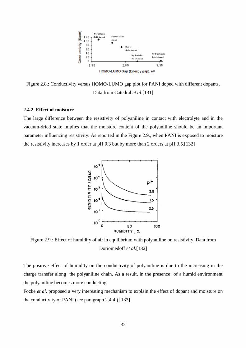
Figure 2.8.: Conductivity versus HOMO-LUMO gap plot for PANI doped with different dopants.
Data from Catedral et al.[131]
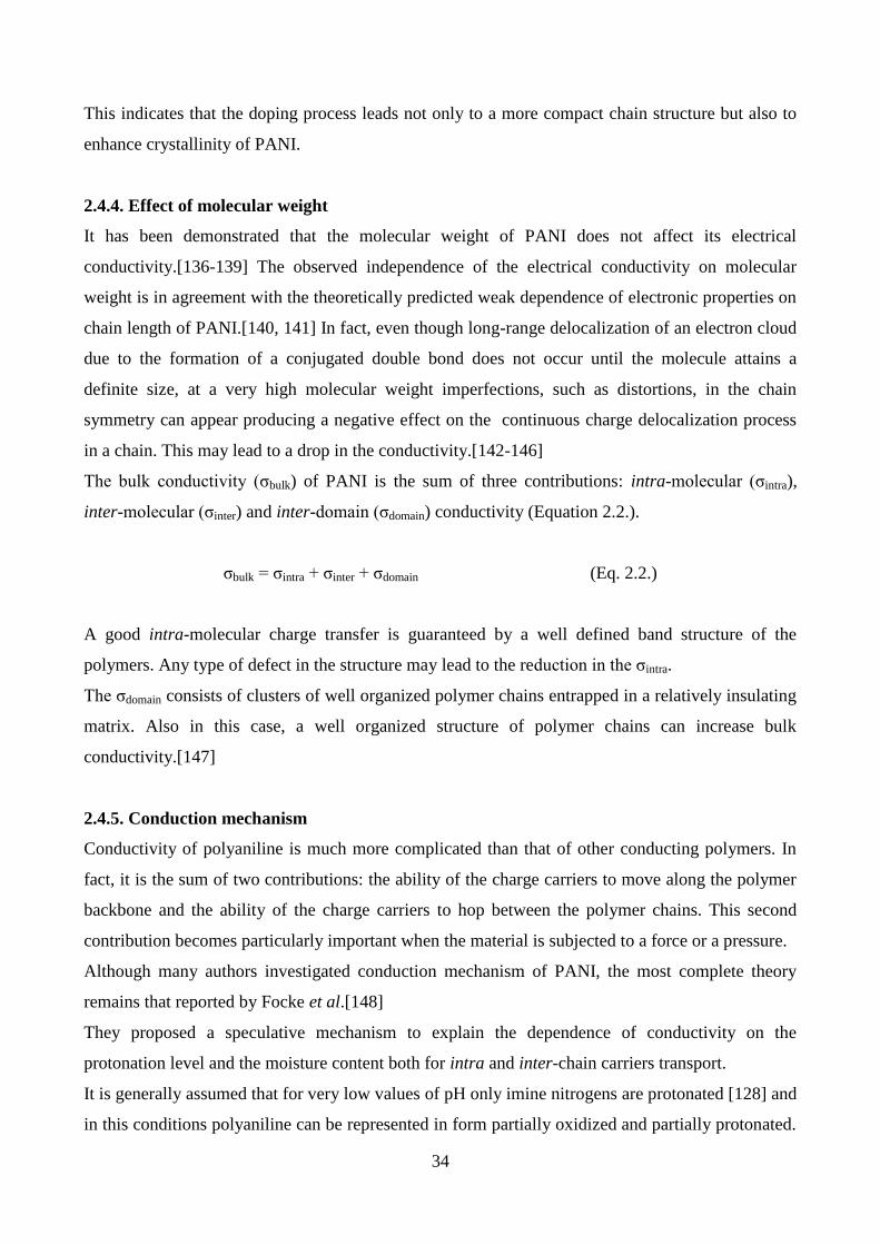
2.4.2. Effect of moisture
The large difference between the resistivity of polyaniline in contact with electrolyte and in the
vacuum-dried state implies that the moisture content of the polyaniline should be an important
parameter influencing resistivity. As reported in the Figure 2.9., when PANI is exposed to moisture
the resistivity increases by 1 order at pH 0.3 but by more than 2 orders at pH 3.5.[132]
Figure 2.9.: Effect of humidity of air in equilibrium with polyaniline on resistivity. Data from
Doriomedoff et al.[132]
The positive effect of humidity on the conductivity of polyaniline is due to the increasing in the
charge transfer along the polyaniline chain. As a result, in the presence of a humid environment
the polyaniline becomes more conducting.
Focke et al. proposed a very interesting mechanism to explain the effect of dopant and moisture on
the conductivity of PANI (see paragraph 2.4.4.).[133]

33
2.4.3.Effect of crystallinity
The electrical properties of polyaniline are strongly influenced by the chains structure. It has been
observed that with the increase in crystallinity the conductivity is increased, because the structure
becomes more organized.
In fact, it is known that the inter-chain electron mobility in a given polymer is significantly
increased with ordered solid state structure, such as crystalline domains.[133]
As reported in the previous paragraph (2.4.1.), high level of conductivity in PANI can be obtained
by doping polymer with aqueous HCl. Moreover, each conducting polymer particle can be
considered as a conducting crystal grain. Particles can polymerize in various sized spaces displaying
different crystallinities.
Therefore, the size of crystal grain and the degree of crystallinity dramatically affect the
conductivity.
X-Ray diffraction is used to investigate the chain ordering and crystallinity in polymeric materials.
In general, no distinctive crystal structure is observed in undoped PANI. In this case an amorphous
peak appears at a 2 of ~ 20° (Figure 2.10 a). Studying the morphology of conducting polymer,
Warren et al. found that the ratio of half-width to height (HW/H) of the X-ray diffraction peak
reflects ordering in the polymer backbone. At small HW/H value corresponds high crystalline
order.[134] After doping, a small sharp peak appears in 2 of ~ 9.0°, which can be attributed to the
crystallinity, and the peak at 2 of ~ 20° is shifted to higher angle , corresponding to a decreased d-
spacing between polymer backbones (Figure 2.10 b).[135]
Figure 2.10.: XRPD patterns of undoped (a) and doped (b) PANI.
a b
Crystalline peak
34
This indicates that the doping process leads not only to a more compact chain structure but also to
enhance crystallinity of PANI.
2.4.4. Effect of molecular weight
It has been demonstrated that the molecular weight of PANI does not affect its electrical
conductivity.[136-139] The observed independence of the electrical conductivity on molecular
weight is in agreement with the theoretically predicted weak dependence of electronic properties on
chain length of PANI.[140, 141] In fact, even though long-range delocalization of an electron cloud
due to the formation of a conjugated double bond does not occur until the molecule attains a
definite size, at a very high molecular weight imperfections, such as distortions, in the chain
symmetry can appear producing a negative effect on the continuous charge delocalization process
in a chain. This may lead to a drop in the conductivity.[142-146]
The bulk conductivity (σbulk) of PANI is the sum of three contributions: intra-molecular (σintra),
inter-molecular (σinter) and inter-domain (σdomain) conductivity (Equation 2.2.).
σbulk = σintra + σinter + σdomain (Eq. 2.2.)
A good intra-molecular charge transfer is guaranteed by a well defined band structure of the
polymers. Any type of defect in the structure may lead to the reduction in the σintra.
The σdomain consists of clusters of well organized polymer chains entrapped in a relatively insulating
matrix. Also in this case, a well organized structure of polymer chains can increase bulk
conductivity.[147]
2.4.5. Conduction mechanism
Conductivity of polyaniline is much more complicated than that of other conducting polymers. In
fact, it is the sum of two contributions: the ability of the charge carriers to move along the polymer
backbone and the ability of the charge carriers to hop between the polymer chains. This second
contribution becomes particularly important when the material is subjected to a force or a pressure.
Although many authors investigated conduction mechanism of PANI, the most complete theory
remains that reported by Focke et al.[148]
They proposed a speculative mechanism to explain the dependence of conductivity on the
protonation level and the moisture content both for intra and inter-chain carriers transport.
It is generally assumed that for very low values of pH only imine nitrogens are protonated [128] and
in this conditions polyaniline can be represented in form partially oxidized and partially protonated.
35
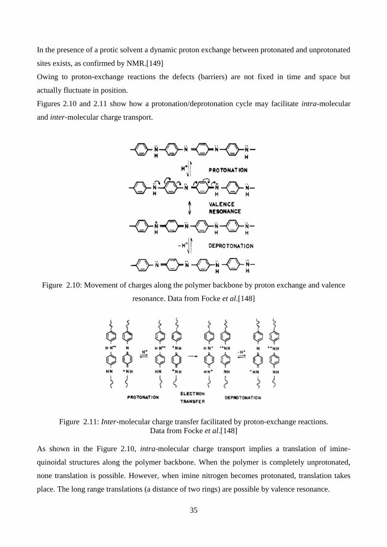
In the presence of a protic solvent a dynamic proton exchange between protonated and unprotonated
sites exists, as confirmed by NMR.[149]
Owing to proton-exchange reactions the defects (barriers) are not fixed in time and space but
actually fluctuate in position.
Figures 2.10 and 2.11 show how a protonation/deprotonation cycle may facilitate intra-molecular
and inter-molecular charge transport.
Figure 2.10: Movement of charges along the polymer backbone by proton exchange and valence
resonance. Data from Focke et al.[148]
Figure 2.11: Inter-molecular charge transfer facilitated by proton-exchange reactions.
Data from Focke et al.[148]
As shown in the Figure 2.10, intra-molecular charge transport implies a translation of imine-
quinoidal structures along the polymer backbone. When the polymer is completely unprotonated,
none translation is possible. However, when imine nitrogen becomes protonated, translation takes
place. The long range translations (a distance of two rings) are possible by valence resonance.

36
However, any deprotonated imine nitrogen or protonated amine nitrogen will act as a barrier for
translation along the polymer backbone. It follows that considerable mobility along the polymer
chain is possible on protonation of only one of the imine nitrogens of the quinoidal structures.
Inter-chain transport is different. In fact, a double protonation is required. The first protonation is
crucial because it allows the formation of radical cations. For this second type of transport authors
proposed a coupling of electronic and ionic transport which increases as the degree of protonation
of the imine nitrogens decreases. The dependence of the proton exchange on the presence of a
source of protons explains the high increase in conductivity observed when dry PANI is exposed to
humidity (Paragraph 2.4.2.). In fact, water molecules may aid in proton transport between chains by
formation of hydronium ions.
2.5. Techniques of characterization
Among all techniques that can be used to characterize polyaniline, FT-IR and UV-vis
spectroscopies, cyclic voltammetry and conductivity measurements are the most useful.
In fact, since its low solubility in common solvents, techniques as NMR aren’t powerful
instruments.
2.5.1. FT-IR spectroscopy
FT-IR spectroscopy is probably the most useful technique to characterize polyaniline. One of the
most important data that could be obtained, even at a first glance, is the oxidation degree of the
polymer. Figures 2.12 (A-C) show characteristic Fourier-transform IR spectra of leucoemeraldine,
emeradine and pernigraniline respectively.

37
Figure 2.12: FT-IR spectra of leucoemeraldine (A), emeraldine (B) and pernigraniline (C)
The Fourier-transform IR spectrum of emeraldine (Figure 2.12 B) shows a characteristic band at
1570 cm-1
, assigned to the C=C stretching of the quinoid rings (N=Q=N) and two peaks at 1498 cm-
1 and 1484 cm
-1, assigned to the C=C stretching vibration mode for the benzenoid rings (N-B-N).
The peaks at 1311 cm-1
and 1246 cm-1
are related to the C-N and C=N stretching modes and those
at 1027 cm-1
and 889 cm-1
to the in-plane and out-of-plane bending of C-N. The peaks at 754 cm-1
and 692 cm-1
correspond at deformation vibration modes for the aromatic rings, while the peak at
573 cm-1
is characteristic for the 1, 4 di-substituted benzene.[150] The ratio between the two bands
at 1498 cm-1
and 1484 cm-1
is diagnostic to estimate the ratio between quinoid and aromatic groups
and consequently the oxidation degree of the polymer. In fact, when polyaniline is in its totally
reduced form (leucoemeraldine), this ratio is minor than one. In fact, leucoemeraldine is
characterized by amino-benzenoid units. In its emeraldine form polyaniline contains about the same
amount of amino-benzenoid and imino-quinoid units. For this reason, as reported in the Figure 2.12
B, for polyaniline in its emeraldine form is about 1. When polyaniline is in its totally oxidized form
(pernigraniline) only imino-quinoid units are present in the backbone and the ratio is higher than 1.
It is interesting to note the effect of the conjugation of the polymer on the spectrum, i.e. the broad
band from 2000 cm-1
to 4000 cm-1
, that covers half the instrumental range. It arises from the
overlapping of many vibrational modes, especially the ones of NH and phenilene diamine groups.
Moreover, some of the aminic nitrogen becomes protoned upon addition of an acid, thus becoming
vastly hydrogen bonded and thus widening the band at high wavenumbers.[150]
Wavenumber (cm-1)
B
C
A

38
2.5.2. UV-vis spectroscopy
One of the major limitations of conducting polymers, in particular polyaniline and polypyrrole, is
that they are characterized by a very low solubility. In particular polyaniline is poorly soluble in a
few solvents, as pyrrolidones and amides. A typyical UV-Vis specimen is prepared dissolving a
minimal amount of PANI in 2-pyrrolidone or N,N-dimethylformamide obtaining a blue to green
solution. The typical spectrum of polyaniline is reported in Figures 2.3. and 2.13.
Figure 2.13. Change in the UV-Vis spectrum during the oxidation of leucoemeraldine to emeradine
base with oxygen in N-methylpyrrolydinone. Data from Kang et al., ref. 151.
The band at 320 nm corresponds to the * transition of the benzenoid rings. The peak at 410
nm corresponds to the polarone-bipolarone transition and the broad peak at 800 nm to the *
transition of the imine-quinoid group. UV-vis spectroscopy allows to investigate how spectrum of
polyaniline varies when leucoemeraldine is oxidized to emeraldine (Figure 2.13.). In fact, the peak
at 800 nm increases with the oxidation of the polymer.[151] By the use of this technique is possible
also to investigate the behaviour leucoemeraldine and emeraldine when an acid as HClO4 is added
into the organic solution in air and in N2. Recording spectra at different times it has been observed
that leucoemeraldine and emeraldine in their protonated forms are metastable in N-
methylpyrrolydinone.
In fact, Figure 2.14a shows that the aminic nitrogen atoms of leucoemeraldine are deprotoned and
oxidised by the atmospheric oxygen at the same time, with an increment of the 650 nm band. This
does not happen when the specimen is kept under nitrogen. Figure 2.14.c shows how the aminic
groups of leucoemeraldine are deprotonated but not oxidised when no oxidant is present.
Emeraldine shows a different behaviour. In fact, in air (Figure 2.14.b) PANI undergoes
deprotonation without any further oxidation. However, in the absence of any oxidant the oxidation
state decreases as the deprotonation goes on.[151]
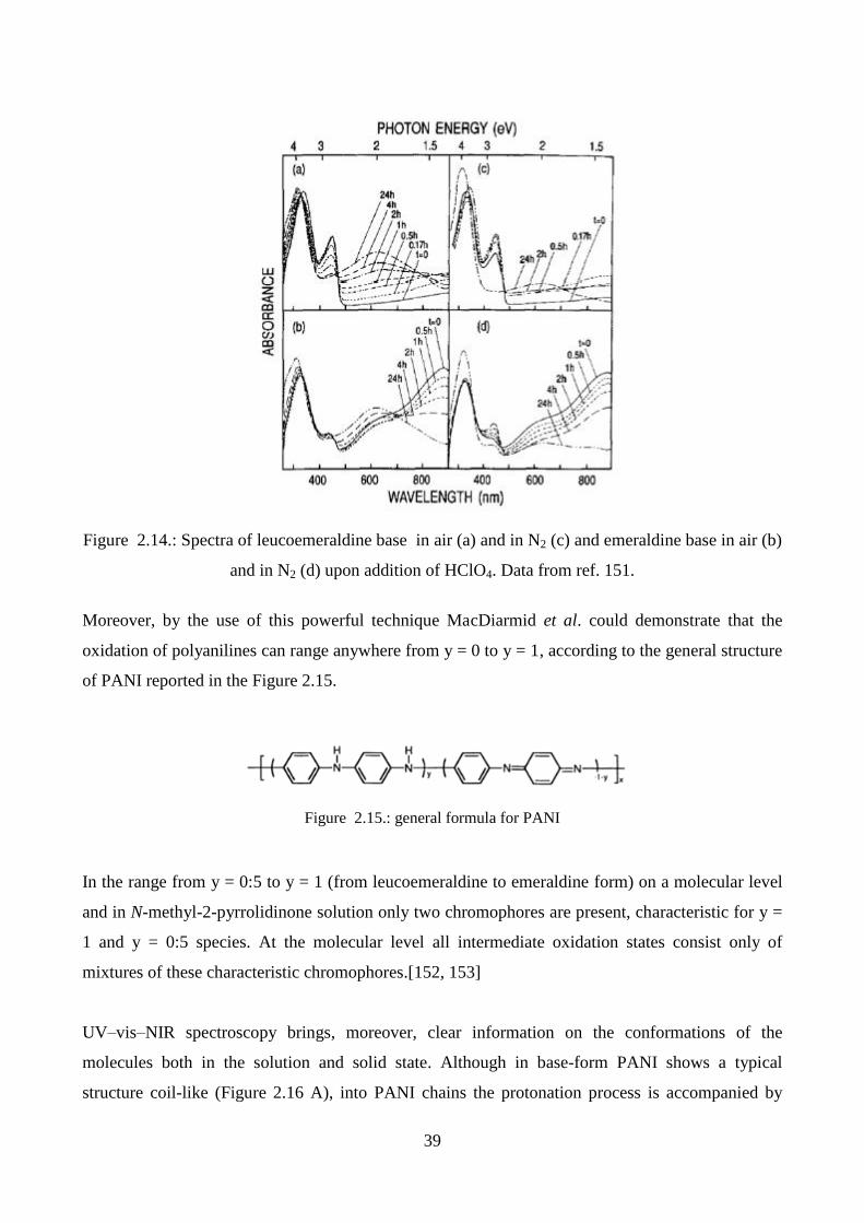
39
Figure 2.14.: Spectra of leucoemeraldine base in air (a) and in N2 (c) and emeraldine base in air (b)
and in N2 (d) upon addition of HClO4. Data from ref. 151.
Moreover, by the use of this powerful technique MacDiarmid et al. could demonstrate that the
oxidation of polyanilines can range anywhere from y = 0 to y = 1, according to the general structure
of PANI reported in the Figure 2.15.
Figure 2.15.: general formula for PANI
In the range from y = 0:5 to y = 1 (from leucoemeraldine to emeraldine form) on a molecular level
and in N-methyl-2-pyrrolidinone solution only two chromophores are present, characteristic for y =
1 and y = 0:5 species. At the molecular level all intermediate oxidation states consist only of
mixtures of these characteristic chromophores.[152, 153]
UV–vis–NIR spectroscopy brings, moreover, clear information on the conformations of the
molecules both in the solution and solid state. Although in base-form PANI shows a typical
structure coil-like (Figure 2.16 A), into PANI chains the protonation process is accompanied by

40
creation of positive charges on the nitrogen atoms that, because their repulsions, can cause
straightening of the chain (structure rod-like, Figure 2.16 B).
Figure 2.16.: Coil-like (A) and rod-like conformations of PANI. Data from ref. 155.
This is extremely beneficial for delocalization of the electrons (charges) along the chain, and
creation energetically most favourable polaronic structure. The polymer conformation can be
strongly influenced by a dopant, as well as a solvent used during the sample preparation. For
example, bulky anionic dopants cannot quickly diffuse in between the chains following the
delocalizing positive charges; in this case the chain expansion will be hindered.[154] Xia et al.
investigated the effect of solvent in the conformation of PANI-HCSA (camphorsulfonic acid)
demonstrating that coil-like conformation is predominant in m-cresol, p-cresol, 2-chlorophenol, 2-
fluorophenol and 3-ethylphenol, whereas rod-like conformation in chloroform, NMP (N-
methylpyrolidinone), DMF (N, N-dimethylformamide), and benzyl alcohol.[155]
The conformation of polyaniline chains can be determined on the basis of its UV–vis–NIR spectra,
as reported in the Figure 2.17.
A B

41
The band extending from 800 nm toward the near infrared region, shown in Figure 2.17. a, is called
free-carrier tail and is characteristic for PANI in rod-like conformation highly conductive.
Otherwise, when protonated PANI is in coil-like conformation this effect disappear (Figure 2.17. b).
2.5.3. XRPD diffraction
X-Ray Powder Diffraction (XRPD) is one of the most important analysis used to investigate the
structure of a solid. In fact, several information are contained in an XRPD spectrum. These include:
lattice constants, existing of different phases and, through the application of the Scherrer equation
(Equation 2.3.), average crystallite size.
where τ is the mean size of the ordered (crystalline) domains, K is a dimensionless shape factor,
with a value close to unity. The shape factor has a typical value of about 0.9, but varies with the
actual shape of the crystallite; λ is the X-ray wavelength, β is the line broadening at half the
maximum intensity (FWHM) in radians and θ is the Bragg angle.
In the last thirty years the intense study of many researchers clarified the structure of
polyaniline.[156-158] However, the structural characteristics were investigated more in detail by
Pouget et al. [159, 160] They reported two distinct classes of emeraldine characterized by two
different structures.
Figure 2.17.: UV-vis spectra of (a) protonated PANI in rod-like conformation and (b) protonated PANI in
coil-like conformation and (c) base emeraldine. Data from ref. 154.
Eq. 2.3.

42
For this kind of investigation emeraldine was prepared by two different methods. Class I meraldine
was prepared by chemical synthesis or by electrochemical deposition obtaining ES-I in powder or
film form respectively. These materials were converted in emeraldine base (EB-I) in alkaline
conditions. By another approach EB in powder form was dissolved in N-methyl-2-pyrrolidone
(NMP) and then directly casted on substrates producing EB-II films. Alternatively, EB-I could be
converted to EB-II by washing with tetrahydrofurane (THF), then with NMP, and then vacuum
dried. Protonation was accomplished through treatment with aqueous HCl of pH varying from 4 to
0. As reported in the Figure 2. 18., ES-I a new crystalline structure appears, which grows in
intensity with lattice parameters varying as the protonation level is increased.
Figure 2.18.:XRPD patterns of emeraldine base (EB-I, a), and emeraldine salt (ES-I, b). Data from
ref. 160.
Class I emeraldine is that for which the base form is essentially amorphous EB-I and the HCl salt
exhibits ES-I structure. In general, class I materials form when the polymer is obtained from
solution in protonated form.
In Figure 2.19. is reported the increase in crystallinity from EB-I to ES-I upon gradual protonation.
a
b

43
Figure 2.19.: XRPD spectra of PANI increasing the protonation level from EB-I to ES-I. Data from ref. 159.
EB-I is characterized by an amorphous structure. The d spacings measured from ES-I “low-
temperature” powder are reported in Table 2.1. and the evolution of some d spacings with the
[Cl]/[N] ratio is shown on Figure 2.19.
Table 2.1.: Emeraldine “Low-Temperature" HCl salt ES-I ([Cl]/[N] 0.5): d= Spacing, L= Domain
Length and hkl= Pseudoorthorhombic Indexation. Data from ref. 159.
Comparing Figure 2.18. with 2.20., a markedly different diffraction pattern for EB-II is shown.
pro
tonat
ion
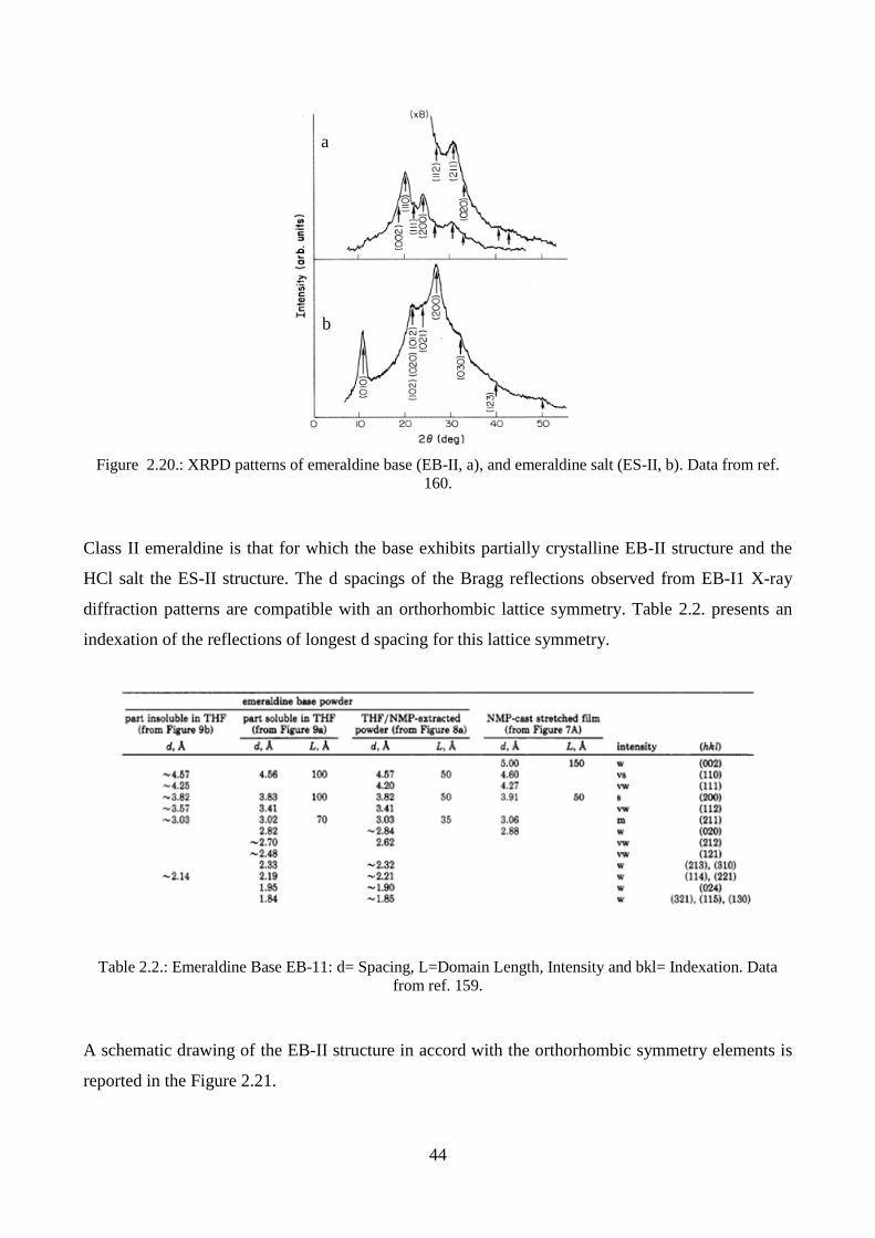
44
Figure 2.20.: XRPD patterns of emeraldine base (EB-II, a), and emeraldine salt (ES-II, b). Data from ref.
160.
Class II emeraldine is that for which the base exhibits partially crystalline EB-II structure and the
HCl salt the ES-II structure. The d spacings of the Bragg reflections observed from EB-I1 X-ray
diffraction patterns are compatible with an orthorhombic lattice symmetry. Table 2.2. presents an
indexation of the reflections of longest d spacing for this lattice symmetry.
Table 2.2.: Emeraldine Base EB-11: d= Spacing, L=Domain Length, Intensity and bkl= Indexation. Data
from ref. 159.
A schematic drawing of the EB-II structure in accord with the orthorhombic symmetry elements is
reported in the Figure 2.21.
a
b

45
Figure 2.21.: Projection along the chain axis and side view of the average structure of (A) the
polyaniline chain and (B) EB-II. The dashed line represents a chain a/2 below or above the plane of
the paper. Data from ref. 159.
Figure 2.22.shows a schematic drawing of the ES-II structure.
Figure 2.22.: Projection along the chain axis and side view of the two orthorhombic structures
considered for ES-II. Data from ref. 159.
According to the data reported in the Table 2.1., Figure 2.23 shows a schematic drawing of ES-I
structure.
Figure 2.23.: Projection along the chain axis and side view of ES-I. Data from ref. 159.
All these differences in structure have subtle effects on the electronic properties of doped
polyaniline. Judging by the similarity of the Debye-Schemer patterns, polyaniline prepared as salt
and redoped with other anions such as ClO4- or HSO4
- adopts structures similar to the ES-I
structure. Authors noted also that the details of the crystal structure are dependent upon counterion
used during the process of protonation.
A B
A B

46
2.5.4. Cyclic voltammetry
Figure 2.24. shows typical cyclic voltammograms (CVs) of PANI/HClO4 films, recorded at
different sweep rate (from 10 to 200 mV s−1
), in an aqueous solution of HClO4 1 M.[161]
Figure 2.24.: Cyclic voltammograms of PANI-HClO4 film, recorded at different sweep rate (from 10 to 200
mV s−1), in an aqueous solution of HClO4 1 M. Data from ref. 161.
There are three redox pairs, with oxidation peaks at 0.125 V (A), 0.5 V (B) and 0.7 V/SCE (C). For
the first redox pair AA’, the increase of the sweep rate does not influence the position of the two
peak potentials. Instead, for the third redox pair CC’, the anodic and cathodic peak potential are
shifted towards lower potential, by increasing the sweep rate. Also, the peak potential separation
increases from 30 mV (V D10 mV s−1
) up to 40 mV (V D200 mV s−1
). The second redox pair BB’ is
almost undistinguishable at low sweep rate (V D10 mV s−1
), but gradually increases with it.
According to the literature, the oxidation peaks A and C correspond to the changes in the oxidation
state of the PANI films. Snauwaert et al.[162] have evidenced, by X-ray photoelectron
spectroscopy, that the ratio between the amine and imine content is function of the electrochemical
potential. At 0.15 V/SCE the imine concentration is about 25% (protoemeraldine) and gradually
increases to 50% (emeraldine) at 0.6 V/SCE and then up to 80% (nigraniline) at 0.8 V/SCE. The
amine concentration is higher at low potential (75% at 0.15 V/SCE) and decreases to 20%, at 0.8
V/SCE.
So, the first peak A corresponds to the first step of oxidation of neutral PANI, and the third peak C

47
corresponds to the further oxidation of PANI, from emeraldine to nigraniline. The middle pairBB0
has been attributed either to the presence of ortho-coupled polymers [163] or to the degradation of
PANI (soluble species such as benzoquinone and hydroquinone).[164]
In Figure 2.25. are shown voltammograms of PANI in 1 M trichloroacetic acid, recorded at
different sweep rates, from 10 to 200 mV s−1
.
Figure 2.25.: Cyclic voltammograms of PANI-C2HCl3O2 film, recorded at different sweep rate
(from 10 to 200 mV s−1
), in an aqueous solution of C2HCl3O2 1 M. Data from ref. 161.
The first oxidation peak (A) appears at about 0.18 V/SCE and the third oxidation peak (C) appears
at about 0.55 V/SCE. The middle peak B is not distinct on the oxidation wave, only on the
reduction wave (B’). For the first redox pairAA0, the increase of the sweep rate shifts the position
of the two peak potentials towards higher potentials. The third redox pair CC’ is characterized by a
constant value for the anodic peak potential and by a gradually shift of the cathodic peak potential
towards lower potentials, with the sweep rate. The third peak C exhibits a very broad oxidation
wave comparing with the first peak, A. This indicates that the charge transfer takes place more
difficult for the second step of oxidation of PANI than for the first step of oxidation.
Figure 2.26. shows CVs of PANI in chloroacetic acid 1M, recorded at different sweep rates.
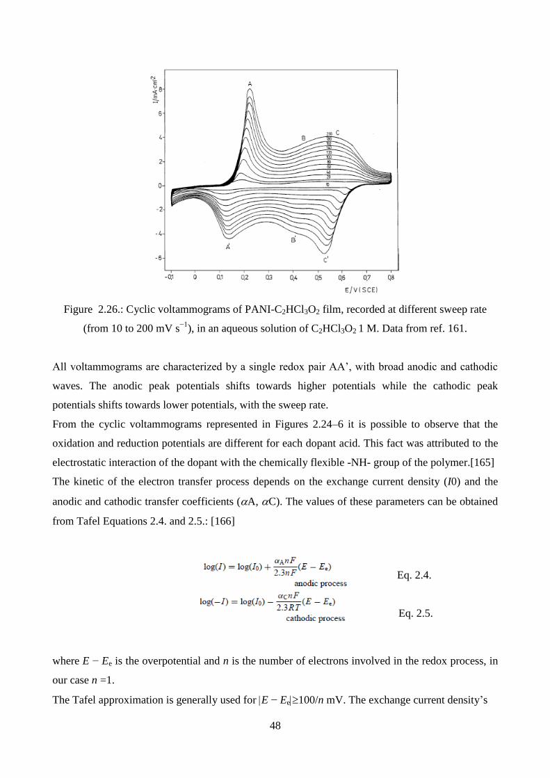
48
Figure 2.26.: Cyclic voltammograms of PANI-C2HCl3O2 film, recorded at different sweep rate
(from 10 to 200 mV s−1
), in an aqueous solution of C2HCl3O2 1 M. Data from ref. 161.
All voltammograms are characterized by a single redox pair AA’, with broad anodic and cathodic
waves. The anodic peak potentials shifts towards higher potentials while the cathodic peak
potentials shifts towards lower potentials, with the sweep rate.
From the cyclic voltammograms represented in Figures 2.24–6 it is possible to observe that the
oxidation and reduction potentials are different for each dopant acid. This fact was attributed to the
electrostatic interaction of the dopant with the chemically flexible -NH- group of the polymer.[165]
The kinetic of the electron transfer process depends on the exchange current density (I0) and the
anodic and cathodic transfer coefficients (A, C). The values of these parameters can be obtained
from Tafel Equations 2.4. and 2.5.: [166]
where E − Ee is the overpotential and n is the number of electrons involved in the redox process, in
our case n =1.
The Tafel approximation is generally used for E − Ee100/n mV. The exchange current density’s
Eq. 2.4.
Eq. 2.5.
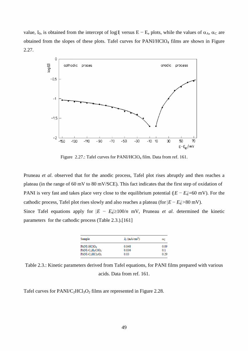
49
value, I0, is obtained from the intercept of logI versus E − Ee plots, while the values of A, C are
obtained from the slopes of these plots. Tafel curves for PANI/HClO4 films are shown in Figure
2.27.
Figure 2.27.: Tafel curves for PANI/HClO4 film. Data from ref. 161.
Pruneau et al. observed that for the anodic process, Tafel plot rises abruptly and then reaches a
plateau (in the range of 60 mV to 80 mV/SCE). This fact indicates that the first step of oxidation of
PANI is very fast and takes place very close to the equilibrium potential (E − Ee=60 mV). For the
cathodic process, Tafel plot rises slowly and also reaches a plateau (for E − Ee>80 mV).
Since Tafel equations apply for E − Ee100/n mV, Pruneau et al. determined the kinetic
parameters for the cathodic process (Table 2.3.).[161]
Table 2.3.: Kinetic parameters derived from Tafel equations, for PANI films prepared with various
acids. Data from ref. 161.
Tafel curves for PANI/C2HCl3O2 films are represented in Figure 2.28.

50
Figure 2.28.: Tafel curves for PANI/C2HCl3O2 film. Data from ref. 161.
They are similar with those show in Figure 2.27., for PANI/HClO4. The anodic plot rises abruptly
(in the range of 20 to 90 mV/SCE) while the cathodic plot rises slowly. So, the first step of
oxidation of PANI/C2HCl3O2 also takes place very quickly. The kinetic parameters obtained for the
cathodic process are listed in Table 2.3.
Tafel curves for PANI/C2H3ClO2 (Figure 2.29.) are different comparing with those represented in
Figures 2.27. and 2.28.
Figure 2.29.: Tafel curves for PANI/C2H3ClO2 film. Data from ref. 161.
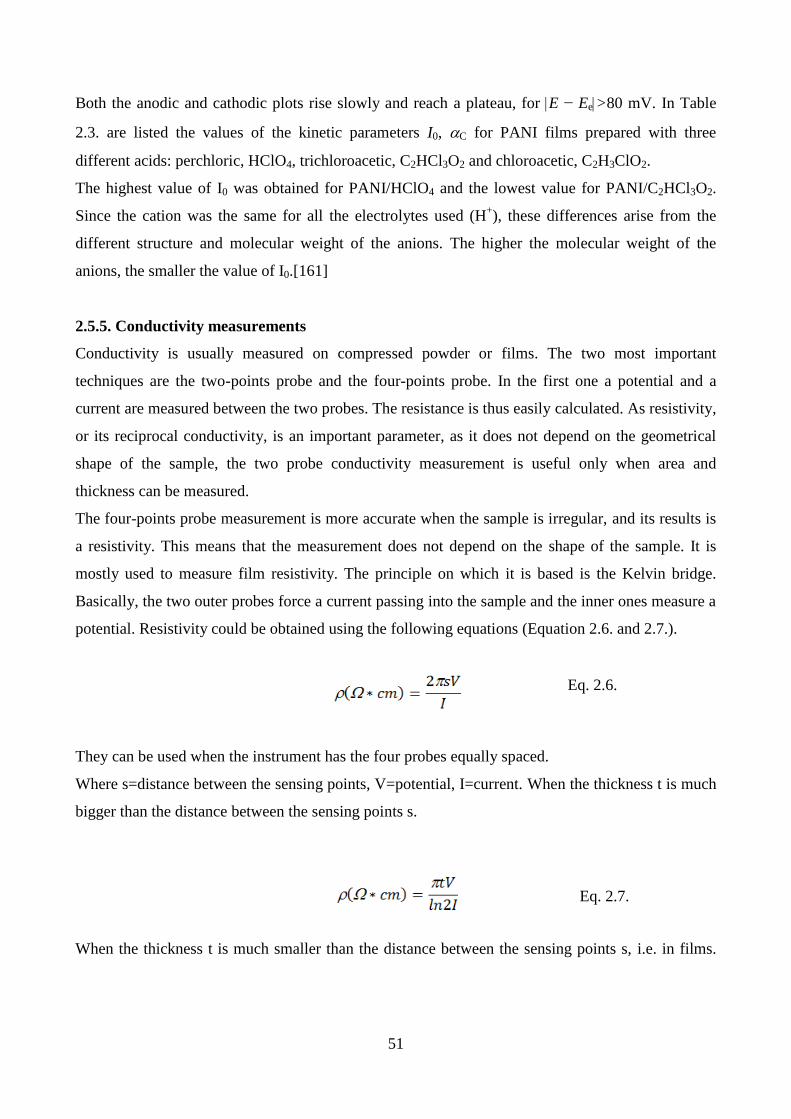
51
Both the anodic and cathodic plots rise slowly and reach a plateau, for E − Ee>80 mV. In Table
2.3. are listed the values of the kinetic parameters I0, C for PANI films prepared with three
different acids: perchloric, HClO4, trichloroacetic, C2HCl3O2 and chloroacetic, C2H3ClO2.
The highest value of I0 was obtained for PANI/HClO4 and the lowest value for PANI/C2HCl3O2.
Since the cation was the same for all the electrolytes used (H+), these differences arise from the
different structure and molecular weight of the anions. The higher the molecular weight of the
anions, the smaller the value of I0.[161]
2.5.5. Conductivity measurements
Conductivity is usually measured on compressed powder or films. The two most important
techniques are the two-points probe and the four-points probe. In the first one a potential and a
current are measured between the two probes. The resistance is thus easily calculated. As resistivity,
or its reciprocal conductivity, is an important parameter, as it does not depend on the geometrical
shape of the sample, the two probe conductivity measurement is useful only when area and
thickness can be measured.
The four-points probe measurement is more accurate when the sample is irregular, and its results is
a resistivity. This means that the measurement does not depend on the shape of the sample. It is
mostly used to measure film resistivity. The principle on which it is based is the Kelvin bridge.
Basically, the two outer probes force a current passing into the sample and the inner ones measure a
potential. Resistivity could be obtained using the following equations (Equation 2.6. and 2.7.).
They can be used when the instrument has the four probes equally spaced.
Where s=distance between the sensing points, V=potential, I=current. When the thickness t is much
bigger than the distance between the sensing points s.
When the thickness t is much smaller than the distance between the sensing points s, i.e. in films.
Eq. 2.6.
Eq. 2.7.
52
Chapter 3: One dimensional polyaniline
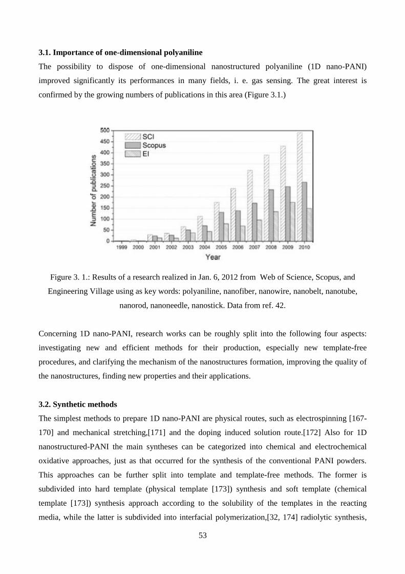
53
3.1. Importance of one-dimensional polyaniline
The possibility to dispose of one-dimensional nanostructured polyaniline (1D nano-PANI)
improved significantly its performances in many fields, i. e. gas sensing. The great interest is
confirmed by the growing numbers of publications in this area (Figure 3.1.)
Figure 3. 1.: Results of a research realized in Jan. 6, 2012 from Web of Science, Scopus, and
Engineering Village using as key words: polyaniline, nanofiber, nanowire, nanobelt, nanotube,
nanorod, nanoneedle, nanostick. Data from ref. 42.
Concerning 1D nano-PANI, research works can be roughly split into the following four aspects:
investigating new and efficient methods for their production, especially new template-free
procedures, and clarifying the mechanism of the nanostructures formation, improving the quality of
the nanostructures, finding new properties and their applications.
3.2. Synthetic methods
The simplest methods to prepare 1D nano-PANI are physical routes, such as electrospinning [167-
170] and mechanical stretching,[171] and the doping induced solution route.[172] Also for 1D
nanostructured-PANI the main syntheses can be categorized into chemical and electrochemical
oxidative approaches, just as that occurred for the synthesis of the conventional PANI powders.
This approaches can be further split into template and template-free methods. The former is
subdivided into hard template (physical template [173]) synthesis and soft template (chemical
template [173]) synthesis approach according to the solubility of the templates in the reacting
media, while the latter is subdivided into interfacial polymerization,[32, 174] radiolytic synthesis,

54
[175] rapid mixing reaction method,[176] and sonochemical synthesis.[118, 119] Here the main
synthetic approaches will be discussed: hard template synthesis, soft template synthesis, combined
soft and hard template synthesis and no-template synthesis.
3.2.1. Hard template synthesis
Martin et al. proposed for the first time the hard template synthesis to prepare conducting organic
polymers, such as polyaniline and polypyrrole.[177-181] 1D nanostructured-materials with
controllable diameter, length and orientation can be synthesized in the pores, channels of hard
templates such as membranes,[179-181] zeolites,[182] anodic aluminum oxide (AAO),[183–185]
and so on. Hexagonal channels of mesoporous aluminosilicate can be used as templates to prepare
PANI filaments with diameters of 3 nm.[182] Although this technique is attracting and elegant, the
removal of the template at the end of the reaction is the biggest drawback. In fact, it is tedious and
can compromise th morphology of the product. Typically, the polymerization reaction takes place in
the channels of template after addition of stoichiometric oxidants at a mixture of monomer and
template. However, in addition to the chemical oxidative polymerization, PANI nanofibers,
nanotubules and nanoribbons can be also prepared by electrochemical oxidative polymerization
using PTM (track-etched membrane),[186] AAO [184] and nanochannels [187] as hard templates.
Using this technique Cao et al. prepared PANI nanotubules encapsulated nickel nanowires using
alumina membrane as the hard-template.[188]
3.2.2. Soft template synthesis
The soft template synthesis method, always called the template-free method [189–192] or self-
assembly method [193] in the literatures in that no hard templates is used, entails synthesizing
PANI, as well as polypyrrole,[190,194] in the presence of structure-directing molecules such as
surfactants,[195, 196] deoxyribonucleic acid (DNA),[197,198] polyelectrolytes,[199] thiolated
cyclodextrins,[200] sulfonated porphyrin,[201] liquid crystalline,[202] and ethanol,[203, 204]
which act as templates for the production of one-dimensional nanomaterials. The surfactants are
often complex acids with bulky side groups, such as the naphthalenesulfonic acid (NSA),[191, 205,
206] camphorsulfonic acid (CSA),[207-210] azobenzenesulfonic acid (ABSA),[211] chiral 2-
pyrrolidone-5-carboxylic acid (PCA),[212] 4-(3-(4-((4-
nitrophenyl)azo)phenyloxy)propyl)aminobenzene sulfonic acid (C3-ABSA),[213] 2-acrylamido-2-
methyl-1-propanesulfonic acid (AMPSA),[214] 5-aminonaphthalene-2-sulfonic acid (ANSA),[192]
etc. The polyelectrolytes include poly(acrylic acid), poly(styrenesulphonic acid), etc.[199, 215]
Compared to the hard template method, this approach is simpler and cheaper because the use of soft
55
templates omits the tedious post-synthesis process. The formation of the one-dimensional nano-
structured PANI depended on the reaction conditions, such as the concentration of aniline, the
molar ratio of aniline to oxidant or the soft template. Hypotheses were proposed for the formation
mechanisms of the nanostructures, although not confirmed. Because of the hydrophobic property of
aniline and the hydrophilic property of the surfactants, the latter form nano- or microstructured
precursors by self-assembling processes.[205, 211, 216, 217] The precursors play a template role in
forming of the 1D nano-PANI.[185, 189, 193, 218, 219] The diameters and lengths of the one-
dimensional nano-structured polymer are strictly related to many factors, such as the soft templates,
molar ratio of surfactant to aniline, reacting temperature and time and other synthetic conditions.
3.2.3. Combined soft and hard template synthesis
Qiu et al. proposed a new technique that combines soft and hard template to produce highly
oriented PANI nanostructures.[213] Typically, aniline and a surfactant (soft template) are dissolved
in deionized water to form a homogenous emulsion and ultrasonicated. Afterwards the hard
template is added in the emulsion and ultrasonicated for another while. Then, a stoichiometric
oxidant is added rapidly into the solution and the polymerization takes place.
By the use of this technique well-oriented PANI nanotubes and nanofibers are produced within the
pores of the hard template. In the absence of templates, both soft and hard, neither nanofibers nor
nanotubes are obtained. This indicates that both the soft and hard template affected the formation of
the nanofibers or nanotubes.
3.2.4. No-template synthesis
This method allows to synthesize one-dimensional nano-structured PANI without any templates,
hard or soft. Interfacial polymerization, radiolytic synthesis, rapid mixing reaction, sonochemical
synthesis, electrochemical approach are good examples of no-template synthesis of 1D nano-PANI.
Interfacial polymerization, sonochemical synthesis and electrochemical approach were already
discussed in the paragraph 2.3.3.2., 2.3.3.5. and 2.3.2. respectively. Below radiolytic synthesis and
rapid mixing reaction will be treated in more detail.
3.2.4.1. Radiolytic synthesis
In this method, an acidic aqueous solution of aniline and a stoichiometric oxidant is irradiated with
gamma rays without any template.[175] Setting accurately some parameters, such as concentration
of reagents, is possible to produce nanofibers or rod-like structures. Although no complete
explanation for the formation mechanism of the nanofibers was provided up to date, however, the
56
authors concluded that PANI self-assembled when the polymerization is carried out with gamma
irradiation. PANI nanofibers decorated with metal nanoparticles were also prepared with the same
gamma irradiation procedure.[175] At the same time, thin films of PANI nanofibers were
synthesized by the same group by ultraviolet irradiation of a spin coated mixture of aniline nitric
acid and APS on the surface of a siliconwafer.[220] The nanofibers demonstrate typical diameters
of 20–150 nm and lengths of microns.
3.2.4.2. Rapid mixing reaction
Mixing rapidly aniline with a solution of a stoichiometric oxidant, rather than the conventional slow
addition of the solution of oxidant to that of aniline, PANI nanofibers with comparable shapes and
sizes to those of interfacial polymerization method are obtained, rendering this method the simplest
one in producing PANI nanofibers.[176] Owing to the even distribution of aniline and APS
molecules in the solution, all the initiator molecules were consumed rapidly after the start of the
polymerization and the secondary growth of PANI was suppressed, resulting in exclusive
nanofibers in the product. The growth of the PANI nanofibers was related with the polarity of the
solvents.
For example, in aqueous systems, pure nanofibers were produced, while in ethanol and isopropanol,
mixture of short nanofibers attached with irregular particles and agglomerates of 100–300 nm
particulates were obtained, respectively. However, according to Zhang et al., [193] the formation of
nano-structured PANI, which was synthesized in presence of H3PO4 without any other template,
soft or hard, was expected to originate from the micelles formed by anilinium cations, which acted
as the templates in forming the nanostructures. Chiou and Epstein [221, 222] prepared PANI
nanofibers by dilute polymerization, in which a small portion of acid solution containing aniline
was carefully transferred to the solution of APS in acid and then leave the mixture to react without
any disturbance. The diameters of the fibers can be roughly tuned by appropriate selection of the
acids. The formation of the nanofibers was, as explained, owing to the reduced numbers of
nucleation sites on the surface of the nanofibers in a dilute condition, which allowed PANI to grow
directionally, differing from that of the competition between the directional growth and the
formation of additional nucleation centers in the case of high aniline concentration, which resulted
irregular PANI product.
3.3. Properties
Conductivity measurement of the hard-template synthesized PANI nanotubules [186, 223] showed
that the conductivities decreased with the increasing of the diameters, and finally reaches the
57
conductivity of the conventional PANI powder. This was resulted from the decreasing proportion of
the highly ordered layer in the materials with increasing of diameters and from the higher
conductivity of the highly ordered layer than that of the disordered inner part of the
fibers/tubes.[224] The analogous conductivity decrease was also observed for electrochemically
template-synthesized PANI nanoribbons.[187]
The four-probe conductivity of the PANI pellet consisting of both granular particles and
nanofibers,[109] or the PANI nanofibers pellet [225, 196, 226] was similar to their counterpart
synthesized by the conventional procedure, and was affected by the doping acid and doping degree,
and so on. The directly measured electrical conductivity of a single PANI nanotube, which was
synthesized by the soft template method, is ca.30 S/cm,[208, 209] far more higher than the 10−2
S/cm order of magnitude [208, 209, 211] for the nanotube pellet due to the large intertubular contact
resistance.[208, 209] Brunauer–Emmett–Teller (BET) surface area of the PANI nanofibers
decreased with increasing of the fiber diameters.[33] For example, BET surface area of dedoped
PANI nanofibers with diameters of 30, 50, and 120 nm are 54.6, 49.3, and 37.2 m2/g, respectively.
In addition, the BET surface area of doped PANI nanofibers was lower than that of the dedoped
ones, which is in consistent with the results of the conventional PANI.

58
Chapter 4: Composite materials

59
4.1. PANI/insulating polymers
Blends of conducting polymers with conventional insulating polymers have received great attention
over the last decade, especially in form of nanofibers and nanowires, because of their unique and
useful properties, which are important for several potential applications such as electronic devices
in optics and electronic and biomedical materials,[227-229] protective clothing,[230] filtration
media,[231] charge storage devices,[232-233] and sensors and actuators.[234-236] PANI blended
with some polymers have been employed for this purpose, including poly(ethylene oxide),[237]
nylon-6,[238] polystyrene[235, 239] and polylactic acid (PLA).[240] In particular PLA and its
copolymers are biodegradable and biocompatible, present good thermoplastic processability, and
have potential applications as commodity plastics to be used in agricultural products and disposable
materials.[241] Because of its biocompatibility, PLA is often used as the base material for implant
devices, such as suture fibers and scaffolds for tissue engineering.[242] Recently, it has been
employed in nanofiber preparation with the electrospinning technique.[243–245] Therefore, PLA is
a promising candidate for the preparation of conducting nanofibers in combination with PANI for
sensors and other applications.
4.1.1. Techniques of preparation of PANI blends
Although PANI blends are particularly attracting materials, the choice of the best method to
produce them with specified characteristics remains an unresolved problem. The problem arises
because the processing method may significantly determine the properties of the manufactured
composite materials. All the synthetic methodologies can be essentially reduced to two distinct
groups: synthetic methods based on aniline polymerization in the presence of or inside a matrix
polymer, and blending methods to mix a previously prepared PANI with a matrix polymer.
Roughly, synthetic methods include: dispersion polymerization of aniline in the presence of a
matrix polymer in a disperse or continuous phase of a dispersion, chemical in situ polymerization of
aniline in a matrix or in a solution with a matrix polymer, electrochemical polymerization of aniline
in a matrix covering an anode, polymer grafting to a PANI surface, copolymerization of aniline
with other monomers resulting in the formation of soluble aniline copolymers, which can be
considered as a composite polymer. Blending methods consist of: solution blending soluble matrix
polymers and substituted polyanilines, solution blending soluble matrix polymers and PANI doped
by functionalized protonic acids (counterion-induced processability), solution blending undoped
PANI with polymers soluble in amide or acidic solvents, dry blending followed by melt processing
(MP) (mechanical mixing of doped PANI with thermoplastic polymer, then molded in a hot press or
extruder).

60
Naturally, each of these methods has its own advantages and limitations. Specifically, the synthetic
direction is probably preferable if it is necessary to produce inexpensive conducting composites,
due to use of inexpensive aniline instead of more expensive PANI, or when there is a need to form
composites which have conductivity only in a thin surface layer. Good homogeneity and a low
percolation threshold characterize these composites. On the other hand, blending methods
sometimes seem to be more technologically desirable from the standpoint of large scale production,
particularly in the case of melt processing techniques. Blending methods will probably become very
practicable when techniques to produce inexpensive, nanosized PANI will be well developed.
4.1.1.1. Synthetic methods to prepare PANI blends and composites
PANI composites can be produced by polymerization of aniline in dispersion systems. This kind of
synthesis is carried out at low temperature by the use of a stoichiometric oxidant in the presence of
water soluble polymers (used as a surfactant) or tailor-made reactive copolymers,[246] such as
poly(2-vinylpyridine-co-p-aminostyrene),[247] PVA,[248, 249], poly(N-vinylpyrrolidone),[250,
251] PEO,[252] cellulose derivatives,[253, 254] poly(methylvinylether),[255] etc.
Other methods of chemical polymerization of aniline exist that are carried out in the presence of
polymer matrix which does not demand the presence of surfactants in the reaction mixture.
All these methods can differ for many aspects. For example, aniline can be polymerized at lower
temperatures (0–10°C), but changing the sequence of the addition of reagents to the reaction
mixture. In fact, in some cases aniline is added to an acidified solution of a matrix polymer (PVA,
chlorinated copolymer latex Haloflex) and oxidant APS, followed by precipitation and filtration of a
conducting composite [256, 257]. In another sequence, an acidified solution of the oxidant can be
added to a previously cooled solution of aniline and polymers. In particular, Gangopadhyay et
al.[258] and Stejskal et al.[251] used the last approach to prepare a PANI/PVA composite that
exhibits significant EMI shielding capacity, and potential for sensing moisture and methanol vapor
[258, 259].
Polyaniline can be produced also by chemical aniline polymerization in/on solid polymer matrix.
Unlike aniline polymerization in a solution, this method produces modified polymer matrixes with a
PANI layer at their surface or inside a thin subsurface layer. Naturally, the thickness and
conductivity of the layers depend on the method of modification and on the time of contact of the
solid matrix with the reaction medium. These methods produce composites with a wide surface
conductivity range, from semiconductor up to the conductivity of pure PANI.
61
Apparently, this method is not technological suitable for sheet materials, both because it requires
the use of polymer matrixes with a good adhesion to PANI, and because it produces pure PANI at
the matrix surface, having poor mechanical properties. At the same time, for fiber and textile
materials with a well developed reactive surface, it may lead to the production of conducting fibers
and fabrics with grafted PANI at the surface and inside of pores. This approach resulted in suitable
materials for EMI shielding, sensors, static electricity dissipation, etc.[260-262].
Two methods to obtain electrically conductive fabrics by in situ polymerization of aniline were
compared by Oh et al.[263]. These materials were prepared by immersing the Nylon 6 fabrics in
pure aniline or an aqueous hydrochloride solution of aniline followed by initiating the successive
direct polymerization in a separate bath (DPSB) or in a mixed bath (DPMB) of oxidant and dopant
solution with aniline. Polymerization of aniline on porous materials has also been used to prepare
conducting membrane materials whose permeability and other properties could be maintained by
the porosity of the final material and conducting polymer layers formed inside pores.[264, 265]
Specifically, Tishchenko et al.[264] elaborated composite systems based on a microporous
polyethylene membrane modified in situ during the oxidative polymerization of pyrrole from the
gas phase or by the polymerization of aniline in an aqueous medium. The composite membranes
displayed a low resistance in electrolyte solutions owing to the coating of polypyrrole or PANI
inside the pores. Another diffusion-oxidation method [260] is aniline (or other monomer)
polymerization in polymer matrixes impregnated with an oxidant that also allows preparation of
PANI (polypyrrole) conducting composites, but this seems not to be very practical. Specifically, it
can be realized through exposing the matrix polymer (e.g. poly(acrylamide)) impregnated with an
oxidizing agent to hydrochloric acid vapor, and then to the monomer vapor [266] or solution.[267]
By an electrochemical approach polymerization at an electrode (anode) surface coated by a non-
conducting polymer film at the aniline oxidation potential results in the formation of a
PANI/polymer composite.[268, 269] The necessary condition here is penetration (diffusion) of
aniline, solvent and electrolyte through the coating to its interface with the anode,[268] to create the
electrochemical prerequisites to oxidize molecules of aniline (in reality anilinium cations), and
growing PANI macromolecules. This condition can be realized in two ways: through pores and by
swelling the polymer coating in the reaction medium (solution), separately or in parallel, dependent
on the coating porosity and swellability. Under appropriate condition, the polymerization starts at
the interface between the anode surface and the coating,[268] and the resultant PANI grows from
this interface into the coating bulk, forming a new electrically conducting alloy film, as shown for
different matrixes in the polypyrrole case.[270–273]
62
4.1.1.2. Blending methods
The low solubility of PANI in common organic solvent is strictly related to its aromatic structure,
inter-chain hydrogen bonds and effective charge delocalization in its structure.[274] Many methods
have been developed to prepare PANI soluble in different solvents and facilitate the preparation of
PANI conducting composites with polymers soluble in the same solvents. Some of these synthetic
methods are summarized below:
1. PANI soluble in organic solvents can be prepared from aniline monomer modified with
alkyl,[275, 276] alkoxy [277] and other substituents.
2. The introduction of sulfonic groups on PANI benzene rings produces water soluble sulfonated
self-acid-doped PANI (SPAN) [278, 279] or highly sulfonated SPAN.[280]
3. Aniline can be polymerized with other monomers to form soluble aniline copolymers.[281]
4. The use of functionalized protonic acids as the dopants (e. g. CSA (canphorsulfonic acid), DBSA
(dodecylbenzenesulfonic acid), phosphoric acid diesters, etc.), increases the solubility in non-polar
or weakly polar organic solvents.[282–285]
5. The use of amide solvents such as NMP and DMF, in which PANI base is soluble.[286].
Obviously, the nature of the solvent influences the properties and ease of preparation of blends of
alkoxy substituted PANI. For example, Gonçalves et al.[287] investigated the suitability of different
solvents to prepare PU–POMA [PU= polyurethane, POMA= poly(o-methoxyaniline)] blend films
by casting, comparing DMF, NMP and m-cresol. DMF was the best solvent for two reasons:
suppressed deprotonation during the preparation of a predoped POMA solution in DMF as
compared with NMP, due to a lower basicity of DMF as against NMP; convenience in the use of
DMF owing to its lower boiling point (153°C) than NMP (202°C) or m-cresol (202°C).
Flexible conducting free standing films were obtained by Gonçalves et al. using PU–POMA
solutions in DMF at different weight ratios and their flexibility is very similar to films of pure
PU.[287]
Concerning composites of PANI with alkyl substituents, Anand et al. developed and studied soluble
POT [poly(o-toluidine)] and PMT [poly (m-toluidine)] blends with PVC (polyvinylchloride).[288]
POT doped PANI in its base forms was soluble in THF, which is also a solvent for PVC. The
authors found that POT and PMT bases produced as salts of HNO3 were the most soluble among
other bases.[288]
Sevil et al.[289] demonstrated that chlorine substituted PANI had enhanced solubility in
comparison with pure PANI. Specifically, they prepared 2-chloro-polyaniline (2-Cl-PANI) in its
non-conducting EB form, and dissolved it with PVC in THF for casting into thin composite films.

63
Chen and Hwang prepared water-soluble PVA/SPAN (self-acid-doped polyaniline) and
PVA/PAPSAH [poly(aniline-co-N-propanesulfonic acid aniline)] blends.[290] They supposed that
the strong interaction of these polyanilines with PVA through hydrogen bonding between hydroxyl
groups (of PVA) and positively charged amine and imine sites (of SPAN and PAPSAH) led to a
decrease in hydrogen bonding among PVA chains and to a partial miscibility.
By a typical amine-epoxide reaction Yamaguchi et al. produced blends of LEB (leucoemeraldine
base) with phenylglycidylether (PGE) more soluble in acetone and chloroform than LEB.[291]
More recently, Adams et al.[292, 293] developed a new acid-solution processing route for
preparation of highly conductive PANI films and fibers soluble in chloroform, diethylketone,
hexafluoro-2-propanol, m-cresol and dichloroacetic acid. It comprises the use of AMPSA as both
the protonating acid and the solvating group and dichloroacetic acid (DCAA) as the solvent.
However, also other dopants such as DEHEPSA and PMMA, in DCAA or difluorochloroacetic acid
can be used.[294, 295]
Moon and Park prepared blends of PANI with copolymeric acids such as poly(methylmethacrylate-
co-p-styrenesulfonic acid) (PMMA-co-SSA), poly(styrene-co-p-styrenesulfonic acid) (PS-co-SSA),
and poly(methylmethacrylate-co-2-acrylamido-2-methyl-1-propanesulfonic acid) (PMMA-co-
AMPSA) soluble in NMP.[296]
Among copolymers used for the preparation of PANI blends polyethylene oxide (PEO),
poly(methyl-methacrylate) (PMMA) and polystyrene (PS) are the most common. These copolymers
are particular useful to prepare nanofibers and nanowires of PANI blends by electrospining
technique, increasing the viscosity of the PANI solution.
4.1.2. Physicochemical properties
The interaction of PANI with copolymer affects not only the solubility of the blend but also other
physicochemical properties, such as thermal stability, mechanical properties and conductivity.
Generally, adding an insulating copolymer into PANI its conductivity decreases,[168] but
characteristic mechanical properties improve. Instead, thermal properties are strictly related to the
kind of copolymer used.
However, sometimes the interaction among the blend components can cause an increase of
conductivity. In fact, Jeon et al. observed that composites of PANI-DBSA/PC (PC= polycarbonate)
prepared by an inverted emulsion polymerization method show values of electrical conductivity
three times higher than pristine PANI.[297-300] FT-IR spectroscopy on the composite showed the
existence of hydrogen bonding between PANI and PC, which increased the glass transition
temperature with increasing PANI content.

64
Moreover, the comparison of DSC and conductivity data showed that the electrical conductivity
increased around the glass transition temperature. The authors explained this by the fact that the
PANI chains contacted more frequently and facilitated electron transfer through the hydrogen
bonding between PANI and PC. In addition, the tensile strength of the composite decreased with
PANI content below the percolation threshold (13 wt%) of PANI. This interaction may also be
displayed by improved thermal stability of PANI/PC blends compared to pure PANI.[301] Aside
from the physical–chemical interactions between PANI and copolymer used, the kind of dopant and
its size should affect the properties of the PANI conducting composites. A decrease of electrical
conductivity can be also due to the presence of solvent into the material. For example, cast films of
doped PANI and its blends can retain solvent. This is important, especially in the case of high
boiling solvents, which are very difficult to completely remove. In turn, this may affect several
material properties. For example, Jousseaume et al.[302] revealed a decrease of the conductivity by
electrical conductivity measurements during heating–cooling cycles, as the residual solvent (m-
cresol) and moisture evaporation of. This phenomenon was explained by the existence of a frontier
sensitive to the solvent at the periphery of conducting clusters.
Specifically, for PANI-DiOHP/PS films, the temperature dependence of conductivity before and
after the partial evaporation of the solvent was well described by a model of a tunnel effect limited
by the charging energy of conducting clusters. Changes in crystallinity, due to the presence of
copolymer host, can strongly affect other important properties, such as tenacity. For example, a
significant drop in crystallinity with increasing PANI fraction from 0 to 9 wt% was reported by
Zhang et al.[303] for PANI-CSA/PA blends. In the case of blend fibers of PANI-DBSA and
UHMW-PE (ultra high molecular weight polyethylene) prepared by Andreatta and Smith [304]
through solution blending in decalin with various ratios of PANI to UHMW-PE, the modulus and
the tenacity of the fibers ranged from 40 to 0.5 GPa, and from 2 to 0.02 GPa, respectively.
Conductivity was 3 * 10-4
S/cm for blends containing 5 wt% of PANI.
It is known that PANI doped with a binary mixture of sulfonic acids possesses peculiar
thermostability, conductivity and other characteristic features as compared to the polymer doped
separately by sulfonic acids such as DBSA, TSA (toluene-sulfonic acid) or naphtalenedisulfonic
acid.[305] Koul et al.[306] have shown enhanced electrical and optical properties, along with higher
solubility in all common organic solvents, for PANI doped with a mixture of DBSA/TSA (1:1).
Using this double doped PANI, they prepared composite films with ABS (acrylonitrile–butadiene–
styrene copolymer ) by casting from the chloroform solution. The surface resistance of these
composites changed from 300 M/cm to 1.302 k/cm, dependent on the PANI doped content and
the method of mixing the system components. The importance of physical–chemical interaction of

65
the matrix polymer and doped PANI for conducting blend properties was also demonstrated by
Wang et al.[307] for PANI/PEO blends cast from aqueous solution. They used an acidic phosphate
ester dopant prepared through reaction of POCl3 with poly(ethyleneglycol) monomethylether
(PEGME, Mw= 350). The DSC curves of the blends with different doped PANI loadings showed a
shift of the single endothermic peak (at 67°C in pure PEO) corresponding to a suppressed melting
temperature for the PEO crystallites. This effect was explained by compatibilization of the rigid
conjugated polymer with the matrix polymer, achieved due to the ability of the ester dopant to form
hydrogen bonds with PEO, reducing the interfacial energy of the two incompatible blend
components.[307] This phenomenon may be considered to be a kind of plasticizing effect caused by
the long poly(ethyleneglycol) tail of the dopant.
4.1.3. PANI nanofibers by electrospinning technique
In recent years, many processing techniques have been used to prepare polymer nanofibers. Among
them, drawing,[308] template synthesis,[309, 181] phase separation,[310] self-assembly,[311, 312]
electrospinning,[313, 314] etc. are the most investigated. The template synthesis allows to produce
nanometer tubules and fibrils of various raw materials, such as electronically conducting polymers,
metals, semiconductors and carbons. However, the removal of the template at the end of the
reaction is a big drawback, because it adds steps to the final work-up of the reaction and, moreover,
can compromise the final morphology of the products. The phase separation consists of dissolution,
gelation, extraction using a different solvent, freezing, and drying resulting in a nanoscale porous
foam. The process takes relatively long period of time to transfer the solid polymer into the nano-
porous foam. The self-assembly is a process in which individual, pre-existing components organize
themselves into desired patterns and functions. However, similarly to the phase separation the self-
assembly is time-consuming in processing continuous polymer nanofibers. All these methods are
useful in lab scale, but cannot be employed to produce nanofibers and nanowires in industrial scale.
For this purpose, electrospinning technique seems to be much more appropriate.
A schematic diagram of the electrospinning setup is shown in Figure 4.1.

66
There are basically three components to fulfill the process: a high voltage supplier, a capillary tube
with a pipette or needle of small diameter, and a metal collecting screen. In the electrospinning
process a high voltage is used to create an electrically charged jet of polymer solution or melt out of
the pipette. Before reaching the collecting screen, the solution jet evaporates or solidifies, and is
collected as an interconnected web of small fibers.[313, 314] One electrode is placed into the
spinning solution/melt and the other attached to the collector. In most cases, the collector is simply
grounded, as indicated in Figure 4.1. The electric field is subjected to the end of the capillary tube
that contains the solution fluid held by its surface tension. This induces a charge on the surface of
the liquid. Mutual charge repulsion and the contraction of the surface charges to the counter
electrode cause a force directly opposite to the surface tension.[315] As the intensity of the electric
field is increased, the hemispherical surface of the fluid at the tip of the capillary tube elongates to
form a conical shape known as the Taylor cone.[316] Further increasing the electric field, a critical
value is attained with which the repulsive electrostatic force overcomes the surface tension and the
charged jet of the fluid is ejected from the tip of the Taylor cone. The discharged polymer solution
jet undergoes an instability and elongation process, which allows the jet to become very long and
thin. Meanwhile, the solvent evaporates, leaving behind a charged polymer fiber. In the case of the
melt the discharged jet solidifies when it travels in the air.
Many parameters can influence the transformation of polymer solutions into nanofibers through
electrospinning.
These parameters include (a) the solution properties such as viscosity, elasticity, conductivity, and
surface tension, (b) governing variables such as hydrostatic pressure in the capillary tube, electric
potential at the capillary tip, and the gap (distance between the tip and the collecting screen), and (c)
ambient parameters such as solution temperature, humidity, and air velocity in the electrospinning
chamber.[317]
Figure 4.1.: Diagram of electrospinning setup.
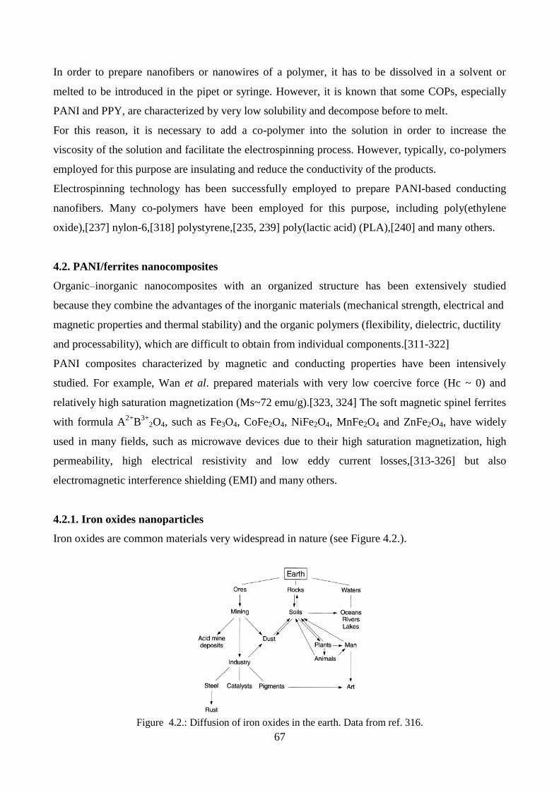
67
In order to prepare nanofibers or nanowires of a polymer, it has to be dissolved in a solvent or
melted to be introduced in the pipet or syringe. However, it is known that some COPs, especially
PANI and PPY, are characterized by very low solubility and decompose before to melt.
For this reason, it is necessary to add a co-polymer into the solution in order to increase the
viscosity of the solution and facilitate the electrospinning process. However, typically, co-polymers
employed for this purpose are insulating and reduce the conductivity of the products.
Electrospinning technology has been successfully employed to prepare PANI-based conducting
nanofibers. Many co-polymers have been employed for this purpose, including poly(ethylene
oxide),[237] nylon-6,[318] polystyrene,[235, 239] poly(lactic acid) (PLA),[240] and many others.
4.2. PANI/ferrites nanocomposites
Organic–inorganic nanocomposites with an organized structure has been extensively studied
because they combine the advantages of the inorganic materials (mechanical strength, electrical and
magnetic properties and thermal stability) and the organic polymers (flexibility, dielectric, ductility
and processability), which are difficult to obtain from individual components.[311-322]
PANI composites characterized by magnetic and conducting properties have been intensively
studied. For example, Wan et al. prepared materials with very low coercive force (Hc ~ 0) and
relatively high saturation magnetization (Ms~72 emu/g).[323, 324] The soft magnetic spinel ferrites
with formula A2+
B3+
2O4, such as Fe3O4, CoFe2O4, NiFe2O4, MnFe2O4 and ZnFe2O4, have widely
used in many fields, such as microwave devices due to their high saturation magnetization, high
permeability, high electrical resistivity and low eddy current losses,[313-326] but also
electromagnetic interference shielding (EMI) and many others.
4.2.1. Iron oxides nanoparticles
Iron oxides are common materials very widespread in nature (see Figure 4.2.).
Figure 4.2.: Diffusion of iron oxides in the earth. Data from ref. 316.

68
They are also prepared in laboratory in different sizes and morphology.
Iron oxides are composed of Fe and O and/or OH. In most of them iron is in trivalent state.
Concerning their structure, iron oxides consist of close packed arrays of anions [usually in
hexagonal (hcp) or cubic close packing (ccp)] in which the interstices are partly filled with divalent
or trivalent Fe predominately in octahedral, Fe(O,OH)6 but in some cases in tetrahedral, FeO4,
coordination. The various oxides differ in the way in which the basic structural units (octahedral or
tetrahedral) are arranged in the space.
Materials where Fe3+
is the main cationic component are called spinels. There are three main
families of ferrites: spinel ferrites, garnet ferrites and hexaferrites, that differ for properties and
characteristics.
Concerning the structure of ferrites, the oxygens form a fcc sublattice with the cations occupying 16
octahedral (B-sites) and 8 tetrahedral (A-sites) positions. The distribution of the metal ions is very
important to understand the properties of these materials.
Figure 4.3. shows the unit cell corresponding to magnetite and maghemite, typical inverse spinel
ferrites.
Oxide-hydroxides
and hydroxides
Oxides
-FeOOH (Goethite) -Fe2O3 (Hematite)
-FeOOH (Lepidocrocite) Fe3O4 (Magnetite)
β-FeOOH (Akaganéite) -Fe2O3 (Maghemite)
Fe16O16(OH)x(SO4)y nH2O (Schwertmannite) β-Fe2O3 (Maghemite)
-FeOOH ( Ferroxyhite) ε-Fe2O3 (Maghemite)
Fe5HO8 4H2O (Ferrihydrite) FeO (Wüstite)
Fe(OH)3 (Bernalite)
Fe(OH)2(Ferrous hydroxide)
Fex3+
Fe y2 + (OH)3x+2y-z(A
-); A= Cl
-, 1/2SO4
2-
(Green Rusts)
Table 4.1.: Main iron oxides present on the Earth.

69
Spinels are characterized by direct and inverse structure. More in particular, in a structure of normal
(or direct) spinels (AB2O4) divalent A(II) ions occupy the tetrahedral voids, whereas the trivalent
B(III) ions occupy the octahedral voids in the close packed arrangement of oxide ions.
A normal spinel can be represented as: (AII)tet
(BIII
)2oct
O4.
MgAl2O4 (known as spinel), Mn3O4, ZnFe2O4, FeCr2O4 (chromite) etc. are typical spinels with
direct structure.
In structures of inverse spinels (B(AB)O4) A(II) ions occupy the octahedral voids, whereas half of
B(III) ions occupy the tetrahedral voids. It can be represented as: (BIII
)tet
(AIIB
III)
octO4.
Fe3O4 (magnetite), CoFe2O4, NiFe2O4 etc. are typical spinel with inverse structure.
The above inverse spinels can also be written as:
Fe3O4 = FeIII
(FeIIFe
III)O4
CoFe2O4 = FeIII
(CoIIFe
III)O4
NiFe2O4 = FeIII
(NiIIFe
III)O
4
The number of octahedral sites occupied may be ordered or random. The random occupation leads
to defected spinels.
Nano sized particles of iron oxide have emerged as versatile materials for different applications due
to their magnetic, electronic, photonic and optical properties. The structure-function relationship of
these nanoparticles have been intensively studied because of the applications in magnetic storage,
gas sensing, biomedical, and catalysis applications.[328-332] Iron oxides nano particles have been
prepared by a variety of methods such as sonochemical reactions,[333] mechanochemical
synthesis,[334] hydrolysis, thermolysis of precursors as well as co-precipitation technique.[335]
Nano particles with a virtually near to monodisperse size distribution can be produced by thermal
decomposition of an iron-cupferron complex in octylamine.[336]
Figure 4.3.: representation of unit cell for magnetite (a) and maghmetite (b).

70
Due to their unique properties, currently these materials are particularly investigated for their
application in different areas, such as catalysis,[337] biomedicine,[338] magnetic resonance
imaging,[339] data storage [340] and many others.
4.2.2. Techniques of preparation of PANI/ferrites
Recently, thanks to their innovative properties polymeric nanocomposites have attracted a growing
attention from the international scientific community, opening new perspectives in the world of
nanotechnologies. The synthetic methods are distinguished in two types: in situ [341] and ex
situ.[342] The former method is a two steps approach. In the first step monomer is polymerized in
the presence of metallic ions. Otherwise metallic ions can be added at the end of the polymerization
reaction. In the second step metallic ions are reduced chemically, thermally or photochemically.
In the ex situ methods, instead, metal nanoparticles are first synthesized, then passivated and finally
dispersed in the liquid monomer that is polymerize to produce a solid nanocomposite.
In both cases the synthesis of the second component is done separately from the polymerization of
monomer.
Metal/polymer nanocomposite are characterized by interesting properties that make them
particularly attractive for many advanced applications (e. g., microwave absorbers, optical filters,
materials for photothermal solar collectors, material refractive index ultra high / low, materials for
magneto-optical and electro-optical, etc.).
More in particular, PANI/metal oxides nanocomposites have been prepared according to many
different methods. A template-free method was used to prepare PANI/Fe3O4 composites with a
core–shell structure.[343, 344]
The preparation of PANI-Fe3O4 nanocomposites through polymerization of aniline in the presence
of a ferrofluid has been reported.[345] PANI composites containing nanomagnets (e.g. Fe3O4, d≈14
nm) were prepared by a chemical method.[346] PANI/nano-Fe3O4 composites were prepared by the
solid-stabilized emulsion (Pickering emulsion) route.[347] PANI–Fe3O4 nanocomposites were
obtained through mechanical mixing of dodecyl benzene sulfonic acid doped (DBSA)–PANI
powder and HCl-doped PANI–Fe3O4 powder.[348] Fe3O4/PANI /DBSA with core–shell structure
were synthesized by emulsion polymerization. Aphesteguy et al. prepared PANI-Fe3O4 through
polymerization of aniline in the absence of external oxidant.[349] Mixtures of iron(II ) and iron(III )
compounds were used as oxidants to polymerize aniline to PANI and form Fe3O4 particles in a
single step. PANI has been prepared also using a mixture of FeCl2 and FeCl3 as oxidants.[350]
Composites of magnetic microtubes were obtained through in situ polymerization of aniline in the
presence of Fe3O4 NPs in the microchannels of AAO (anodi aluminium oxide) to result in tubular

71
structure of PANI/Fe3O4 nanocomposites.[351] Hsieh et al. reported the preparation of PANI/-
Fe2O3 nanocomposites by a reverse micelle process.[352] PANI nanotubes containing Fe3O4 NPs
(~10 nm in diameter) and coaxial PANI/-Fe2O3 nanofibers have been synthesized via a self-
assembly process.[353, 354] In addition to all the preparations here reported, scientific literature
contains many other examples of preparation of PANI/metal oxides composites.

72
Chapter 5: Applications

73
Conducting polymers can be applied in a wide variety of fields. The first and the most important
characteristic that makes these materials appealing is related to their electrical properties which can
be modulated varying the entity of doping. Thanks to the fact that they could be dielectrics as well
as semiconductor and conductors, they find applications in diodes, transistors, sensors, drug
delivery systems and many other electronics device. PANI can be also used as material for gas, pH
and other chemicals sensors, as a electroactive component of strain sensors, for selective permeable
membranes, for LEDs, for biomedical applications (drug delivery systems, tissue regeneration,
etc.), in antenna systems and many others.[355-360]
Even though the technology based on silicon is still more reliable, conducting polymers are being
developed as they are more lightweight, flexible and, once the technology is well established, they
will be more economic. Another important characteristic of this class of materials is that they are
particularly effective in the absorption of electromagnetic radiation in the range of microwaves. In
fact, they are being developed as new materials for the electromagnetic interference shielding
(EMI), replacing currents technology based on polymer-metal particles or polymer-carbon
composites. The upgrade that conducting polymers could add to the current technology, based on
soft iron plate or magnetic iron oxides layer, is that they can provide a significant microwave or
radio absorption, without adding much weight.
As regards polyaniline, a large number of potential applications arises from the presence of various
oxidation states, the possibility to interchange among them and, for every oxidation state, the
possibility to vary the entity of doping.
5.1. EMI (ElectroMagnetic Interference) shielding applications
The life of the modern humanity is based on the transmission of data. Many resources are invested
every year for the development of existing technology and the creation of new ones. A very big
portion of the western economy and finance relies on the possibility to transfer information over
long distances within seconds. Information and Communication Technology (ICT) plays also a very
important role in the development of large new economies, like the ones of the BRIC (Brasil,
Russia, India, China). Moreover, with the increasing pervasiveness of cell phones and wireless local
area networks, and the current push to wirelessly connect handheld computers with local and wide
area wireless networks, these devices can also interfere with medical equipment located in
hospitals, clinics and similar. For all these reasons electromagnetic interference is potentially
harmful and thus deserves a big consideration. Every year millions of devices are manufactured that
are susceptible to EMI like for example cell phones, radio, Wi-Fi apparatus, personal computers and
many more. The development of effective shields assumes therefore an enormous importance. They
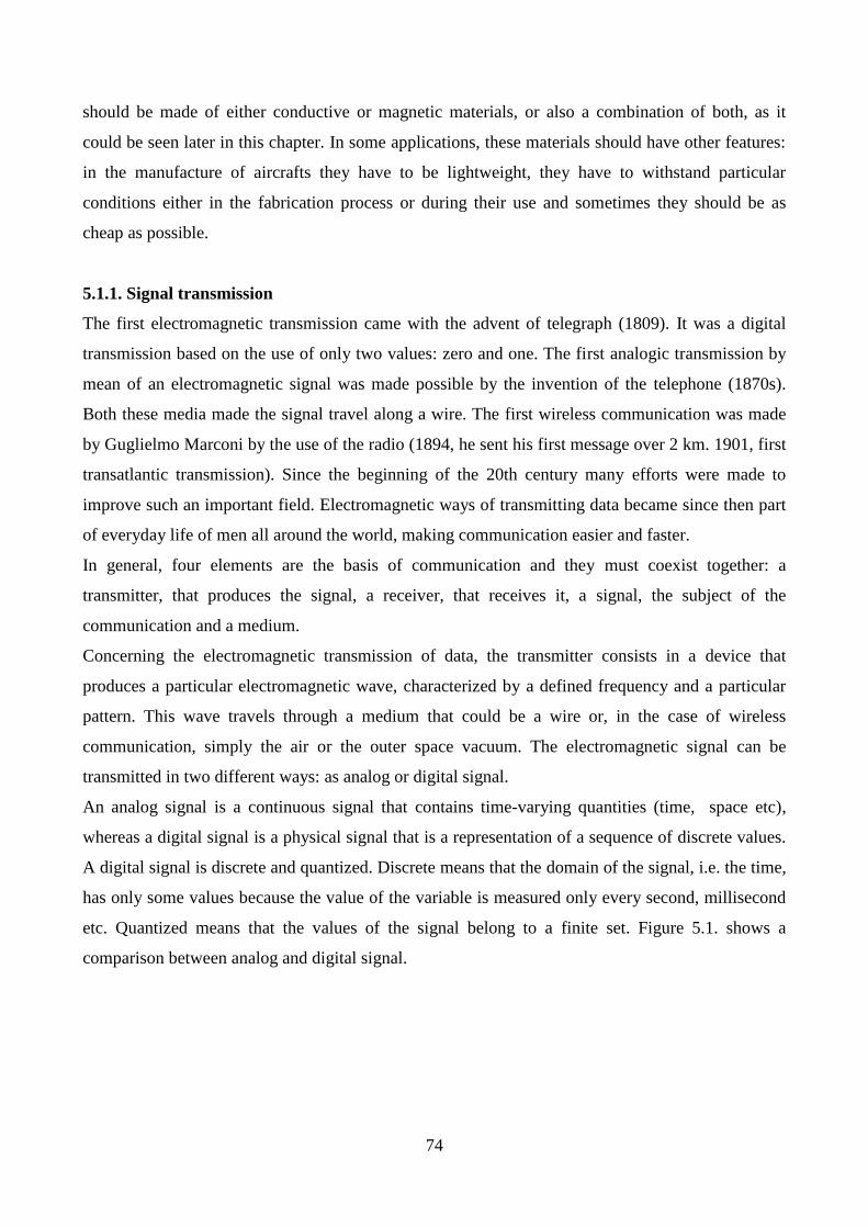
74
should be made of either conductive or magnetic materials, or also a combination of both, as it
could be seen later in this chapter. In some applications, these materials should have other features:
in the manufacture of aircrafts they have to be lightweight, they have to withstand particular
conditions either in the fabrication process or during their use and sometimes they should be as
cheap as possible.
5.1.1. Signal transmission
The first electromagnetic transmission came with the advent of telegraph (1809). It was a digital
transmission based on the use of only two values: zero and one. The first analogic transmission by
mean of an electromagnetic signal was made possible by the invention of the telephone (1870s).
Both these media made the signal travel along a wire. The first wireless communication was made
by Guglielmo Marconi by the use of the radio (1894, he sent his first message over 2 km. 1901, first
transatlantic transmission). Since the beginning of the 20th century many efforts were made to
improve such an important field. Electromagnetic ways of transmitting data became since then part
of everyday life of men all around the world, making communication easier and faster.
In general, four elements are the basis of communication and they must coexist together: a
transmitter, that produces the signal, a receiver, that receives it, a signal, the subject of the
communication and a medium.
Concerning the electromagnetic transmission of data, the transmitter consists in a device that
produces a particular electromagnetic wave, characterized by a defined frequency and a particular
pattern. This wave travels through a medium that could be a wire or, in the case of wireless
communication, simply the air or the outer space vacuum. The electromagnetic signal can be
transmitted in two different ways: as analog or digital signal.
An analog signal is a continuous signal that contains time-varying quantities (time, space etc),
whereas a digital signal is a physical signal that is a representation of a sequence of discrete values.
A digital signal is discrete and quantized. Discrete means that the domain of the signal, i.e. the time,
has only some values because the value of the variable is measured only every second, millisecond
etc. Quantized means that the values of the signal belong to a finite set. Figure 5.1. shows a
comparison between analog and digital signal.
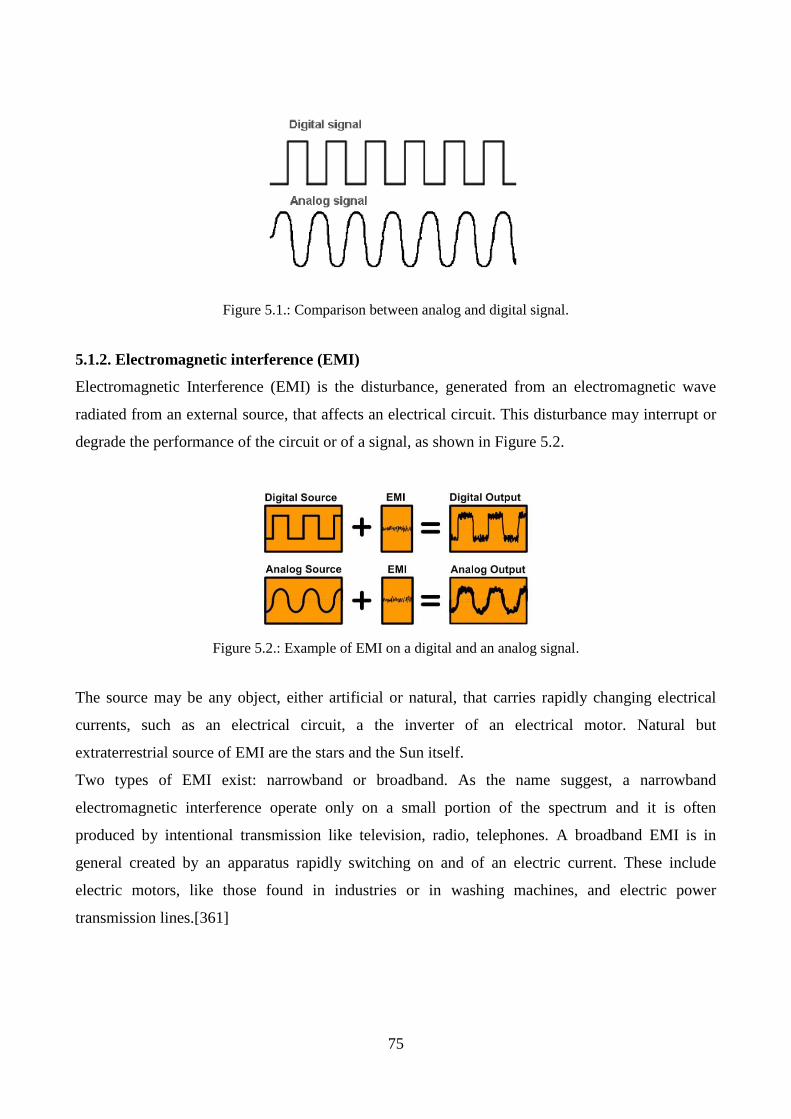
75
Figure 5.1.: Comparison between analog and digital signal.
5.1.2. Electromagnetic interference (EMI)
Electromagnetic Interference (EMI) is the disturbance, generated from an electromagnetic wave
radiated from an external source, that affects an electrical circuit. This disturbance may interrupt or
degrade the performance of the circuit or of a signal, as shown in Figure 5.2.
Figure 5.2.: Example of EMI on a digital and an analog signal.
The source may be any object, either artificial or natural, that carries rapidly changing electrical
currents, such as an electrical circuit, a the inverter of an electrical motor. Natural but
extraterrestrial source of EMI are the stars and the Sun itself.
Two types of EMI exist: narrowband or broadband. As the name suggest, a narrowband
electromagnetic interference operate only on a small portion of the spectrum and it is often
produced by intentional transmission like television, radio, telephones. A broadband EMI is in
general created by an apparatus rapidly switching on and of an electric current. These include
electric motors, like those found in industries or in washing machines, and electric power
transmission lines.[361]

76
5.1.3. EMI shielding
Two main mechanisms exist for shielding an electromagnetic interference. The first and often
primary is reflection. A fundamental characteristic that a shield should have to reflect an incoming
radiation is the presence of mobile charge carriers, as the conduction electrons in a metal. For this
reason metals are the most used materials for EMI shields and their method of shielding is based on
the reflection. However, the weight and the stiffness of these materials make them unsuitable for
application in some fields, such as aerospace industry. In this case the use of composites, made of
organic polymers filled with particles, can be a smart solution.
A second mechanism for EMI shielding is absorption. An absorption shield should have electric
and/or magnetic dipoles that interact with the electric and/or the magnetic field in the radiation. The
presence of electric dipoles is represented by the dielectric constant.
Materials with higher and tend to be a better shield.[362] There are many methods to enhanced
the magnetic permeability: reducing the number of magnetic domain walls, using small particles or
creating multilayer magnetic films.[363, 364] Absorption loss is a function of and . High values
of absorption loss are thus obtained from materials having high both the dielectric constant and the
magnetic permeability. Absorption loss and reflection loss are also a function of the electromagnetic
wave frequency: the first one increases with the frequency, the second one decreases. An important
parameter that affects the loss is the shape of the material. In the presence of a large interfacial area,
a third shielding mechanism happens, called multiple reflections. Examples of these materials are
foams or composites. The skin depth at which the field drops is defined by Equation 5.1.:
where f is the frequency of the electromagnetic wave in Hz, is the magnetic permeability in H
m-1
and is the conductivity in S m-1
.
The sum of the contributes from reflection, absorption and multiple reflection is called shielding
effectiveness (SEdB) and is expressed in decibel (Eq. 5.2.),
SEdb= A + R + B
where A is the absorption loss, R is the reflection loss and B is a term which takes into account the
loss caused by multiple-reflection inside the shield.[365, 366] A shielding effectiveness of 30dB,
corresponding to 99.9% attenuation of the EMI radiation, is considered an adequate level of
shielding for many applications.[367]
Eq. 5.1.
Eq. 5.2.

77
The mechanisms of shielding is illustrated in Figure 5.3.
Figure 5.3.: Basic shielding mechanism.
5.1.4. Materials for EMI shielding
Over the years many different materials have been developed to obtain a good shielding power.
Among them metals, conducting polymers and their composites are the most investigated.
5.1.4.1. Metals used in EMI shielding
Metals are excellent conductors of electricity and can absorb, reflect and transmit electromagnetic
interference. The ability to conduct both electricity and heat make metals particularly interesting for
many applications. These characteristics allow the use of metals as materials for EMI shielding. In
fact, high frequency electromagnetic radiation is either prevented from escaping from the
equipment or the equipment is shielded from stray radiation by metal shields and covers.[368]
The common material used for construction of enclosures for shielding is mu-metal, a high
permeability alloy composed of 14% iron, 5% copper, 1.5% chromium and 79.5% nickel. The other
metals/materials used as a shield are brass, aluminum, silver, nickel, stainless steel, metalized
plastics and conductive carbon/graphite composites. These conductive composites have certain
limitations, for example carbon/graphite suffer from brittleness, aluminum based has low impact
resistance, and stainless steel has high density. The metal shield is susceptible for corrosion, which
leads to Rusty Bolt Effect of nonlinearity to cause intermodulation problem especially in sea
environment. The use of two different metals for shield and gasket causes galvanic corrosion which
leads to nonlinearity and decrease in SE of the metallic shields.[369, 370] For shielding applications
based on reflection, the weight saving benefit of magnesium enclosures extends over the full
frequency spectrum. For shielding based on absorption, die cast enclosures of magnesium and
aluminum provide nominally equivalent shielding effectiveness on an equal weight basis. The lower
78
density of magnesium offsets the higher conductivity of the aluminum. Die cast magnesium alloy
enclosures for EMI shielding provide significant advantages over both plastic and alternative metal
housings.[371]
5.1.4.2. Composite materials in EMI shielding
Conventional plastic materials are excellent electrical insulators having resistivity in the range of
1015
–1018
cm. For EMI shielding purpose they have to be modified by metallization processes.
In particular, following methods are used for metalizing the plastic surface:[372-375]
• Foil laminates and tapes
• Ion plating
• Vacuum metallization
• Zinc flame spraying
• Zinc arc spraying
• Cathode sputtering
• Conductive paints
• Electroless plating
• Electroplating
Otherwise, plastic materials can be made conducting by incorporation of a conducting material,
such as carbon black. It is known that carbon is used as a good reinforcement material in the rubber
industry, as well as filler in wire and cable sheathing. Moreover, because of its graphitic nature,
carbon black is a semiconductor, typically the dry resistivity is in the range of 20–0.5 cm and
when used as filler in rubbers and plastics it endows the compound with antistatic/conductive
properties. Calleja et al. studied the electrical conductivity of high-density polyethylene (HDPE)—
Carbon fiber composites mixed with different concentrations of carbon black.[376] They found that
carbon fibers provide charge transport over large distances and carbon black particles improve the
inter fiber contacts. If the segmented carbon black - HDPE component lies above the percolation
threshold, carbon black particle ensure the electrical interfiber contacts acting as bridges. As a result
conductivity rises. Ramadin et al. reported the electrical properties of laminated epoxy-carbon fiber
composites.[377] The electromagnetic losses as a function of frequency and specimen spacing are
also studied. They observed optimum SE of the laminated epoxy composite (~ 62 dB) occurs at
about 30 mm specimen spacing and frequency ~ 9 GHz. Das et al. reported that the EMI shielding
characteristics of natural rubber and ethylene-vinyl acetate (EVA) filled with conductive carbon
black (Vulcan XC-72) and short carbon fiber (SCF).[378] The EVA based composites are found to
be the more effective in EMI shielding particularly when SCF is used as the conductive filler.

79
The SCF filled composites exhibit higher SE at lower filler loading compared to carbon black filled
ones. The SE of these composites is found to be higher at X-band frequency range (8–12 GHz)
compared to that at microwave frequency range (100–2000 MHz). The composites containing SCF
are technically useful materials (SE ≥ 20dB) in X-band region.
Also graphite fibers found application in the EMI shielding. In fact, Simon et al. reported that resins
containing 30% graphite fibers exhibit good shielding properties.[379] Luo and Chung reported the
electromagnetic interference shielding effect of flexible graphite.[380] The SE is exceptionally high
130 dB at 1–2 GHz higher than that of solid copper. In addition to conventional shielding
applications, flexible graphite can serve as a shielding gasket material, due to its flexibility.
The shielding effectiveness of stainless steel fibers filled thermoplastics is typically 36–42 dB. A
number of other metal fibers such as copper, brass, aluminum and iron have been reported as fillers
for EMI shielding composites, but few are used on a commercial basis. Aluminum fibers have the
advantage of low specific gravity, while copper fibers offer the highest intrinsic electrical
conductivity of any of the metals. Both these materials, however, are subject to surface oxidation
under normal environmental conditions. For the preparation of all these composites ABS
(acetylonitrile-butadiene-styrene), Nylon, PC (polycarbonate), PET (polyethylene terephthalate),
PPO (Poly(p-phenylene oxide) and PS (polystyrene) are used as polymeric matrices.
5.1.4.3. Intrinsically conducting polymers in EMI shielding
Intrinsically conducting polymers are alternative materials for EMI shielding. Among all the
conducting polymers, polyaniline and polypyrrole are mainly used for EMI shielding purposes. It is
known that one of the inherent problems of the intrinsically conductive polymers is their low
processability. In order to overcome this problem, many studies have been done. For example,
Trivedi and Dhawan proposed a method to graft conducting PANI onto glass fabric, glass wool and
nylon cloth to impart flexibility and mechanical strength to the PANI, which is otherwise powdery
and unprocessable.[381-384]
This conducting flexible surfaces are advantageous compared with the presently popular method of
preparing conductive composites by the addition of metal powder/flakes or carbon black to
conventional polymer, in which uneven mixing reduces the mechanical properties, there is often
compatibility between the filler and the polymer matrix, and there is a risk of surface corrosion;
whereas conducting PANI grafted surfaces can withstand any level of acidic fumes and high
humidity levels without any degradation. The grafted Nylon fabric affords a shielding effectiveness
of 37 dB up to 50 KHz and 30 dB up to 1000 KHz, and above this frequency a sudden fall in SE is
observed.
80
Conducting polyaniline composites are also mainly used for EMI shielding purposes. Trivedi and
Dhawan 73 prepared flexible polyaniline composites with water-soluble polymers like polyvinyl
alcohol/carboxymethyl cellulose and their derivatives.[385] Their resistivities lie in the range 60
to 1000 cm and may prove to be useful for dissipation of electrostatic discharge.
Kathirgamanathan reported that composites consisting of polyaniline coated nickel (spheres),
carbon black dispersed into copoly (ethylene-propylene) matrix show SE > 20 dB in the frequency
range of 10 KHz–100 MHz.[386] This kind of materials are suitable for most shielding applications.
Mixtures of PANI and conducting powders such as silver, graphite and carbon black resulted to be
useful for EMI shielding in the frequency range from 10 MHz to 1 GHz.[387]
Lee et al. observed that ES (emeraldine salt) without mixing of conductive powder shows SE of 17
dB, whereas composed with graphite or silver show SE of ~ 27 and ~ 46 dB respectively.[387]
It has been found that PANI-CSA (camphorsulfonic acid) cast film using m-cresol as the secondary
dopant reaches a shielding efficiency of 39 dB at 1 GHz.[388, 389]
Pant et al. synthesized ferrofluid-conducting polyaniline composites of different concentration with
a nonconducting polyvinyl alcohol matrix. They found that by increasing the ferrofluid
concentration the shielding property of the material also increases.[390]
In the scientific literature the number of papers that describe new methods to produce PANI
composites for EMI shielding is huge and scientists try to develop continuously materials that are
more efficient and performing.
In addition to polyaniline another important conducting polymer that has received much attention in
the EMI shielding is polypyrrole. However, since it is completely insoluble in any solvents and
infusible, it is mainly prepared in form of composite. For example, Trivedi and Dhawan described a
process for the polymerization of pyrrole on insulating surfaces like nylon, terylene and glass fabric
and polymer matrix like polyvinyl alcohol (PVA) by vapor phase polymerization.[391]
The electrical resistivity of these PVA/PPy composite films is in the range 200 cm to 20 K
cm. Lee and coworkers synthesized PPy and metal (Ag, Pd) compounds coated on woven
polyethylene terephthalate (PET) and nonwoven polyester (PE) fabrics by electrochemical
treatment.[392] PPy coated on PET or PE fabrics was electrochemically synthesized by using
anthraquinone-2-sulfonic acid (AQSA) as a dopant. The results show that both conducting PPy and
Ag layers contribute to the increase of EMI SE. Pomposa et al. developed intrinsically conducting
hot melt adhesives (ICHMAS) based on PPy blends for EMI shielding applications.[393] These
new materials retain the advantages of conventional hot melt adhesives (e.g., melt processibility,
quick bonding, good adhesion to a wide variety of substrates etc) having a level of electrical
conductivity appropriate to be used at room temperature as EMI shields in electronic, computing

81
and telecommunication applications (i.e., form-in-place EMI gaskets, thin film EMI shields,
isolation of internal EMI-generating circuits etc.).
5.2. Biomedical applications
After the discovery in the 1980s of their compatibility with many biological molecules, research on
conducting polymers for biomedical applications grew significantly. Studies have included:
electrical stimulation, use in cell adhesion and migration, application in DNA synthesis and protein
secretion [394–397]. Specifically, many of these studies involved nerve, bone, muscle, and cardiac
cells, which respond to electrical impulses. COPs present a number of important advantages for
biomedical applications, including biocompatibility, ability to entrap and controllably release
biological molecules (i.e., reversible doping), ability to transfer charge from a biochemical reaction,
and the potential to easily alter the electrical, chemical, physical, and other properties of the COPs
to better suit the nature of the specific application. These unique characteristics are useful in many
biomedical applications, such as biosensors, tissue-engineering scaffolds, neural probes, drug-
delivery devices, and bio-actuators. Moreover, COPs are inexpensive, easy to synthesize, and
versatile because their properties can be readily modulated by the wide range of molecules that can
be entrapped or used as dopants. In addition, COPs permit control over the level and duration of
electrical stimulation for tissue engineering applications, a limitation of electrets. COPs can also be
tailored to create substrates with high surface area, a key aspect to decreasing impedance in neural
probes.
5.2.1. Biomolecular sensing
The first biosensing device was created by integrating an enzyme into an electrode,[398] and since
that time, much progress has been made in monitoring and diagnosing metabolites (e.g., glucose,
hormones, neurotransmitters, antibodies, antigens) for clinical purposes. A biosensor is composed
of a sensing element (i.e., biomolecule) and a transducer.[399] The sensing element interacts with
the analyte of interest producing a chemical signal that is transmitted to the transducer, which
ultimately transforms the input into an electrical signal. COPs are extensively used as transducers
that integrate the signals produced by biological sensing elements such as enzymes.
Depending on how the chemical signal is sensed and transmitted, biosensors can be distinguished
in: amperometric (measures current), potentiometric (measures potential), conductometric
(measures change in conductivity), optical (measures light absorbance or emission), calorimetric
(measures change in enthalpy), and piezoelectric (measures mechanical stress). The most common
types of transducers are amperometric and potentiometric. An amperometric biosensor measures the

82
current produced when a specific product is oxidized or reduced at a constant applied
potential.[399] The COP mediates the electron transfer (e.g., via hydrogen peroxide) between an
enzyme, such as an oxidase or dehydrogenase, and the final electrode. Potentiometric biosensors
use ion-selective electrodes as physical transducers. For example, detection of urea by ureases is
performed via the production of NH3, which interacts with PPy to produce an electrical signal. This
signal could be a product of a change in pH and the subsequent ion mobility in the polymer matrix
triggered by an equilibration of the dopants with the free ions in solution.[400, 401]
However, for biosensor applications electroactive materials (COPs) have been modified, integrating
on its surface specific biological recognition components (bioactive macromolecules). Many
different techniques have been developed for the immobilization of biologically active molecules on
COPs, but in general they can distinguished in Two main classes: non-covalent and covalent
modifications. Non-covalent modifications include adsorption, physical entrapment, and affinity
binding. Covalent immobilization includes all techniques that create a covalent bond between the
conducting substrate and the biomolecule via functional moieties.[402, 403]
Physical adsorption is the simplest method of immobilization and one of the first approaches used
for biosensors. Although adsorption is simple, controlling the concentration of the immobilized
compound is difficult and immobilization is not stable because of the weak non-covalent forces
involved, which decrease the lifetime of the biosensor.[403] Another drawback is that compound
adsorption occurs as a monolayer, which limits the quantity of sensing element. An alternative to
adsorption is physical entrapment of the desired biomolecule during electropolymerization, which is
one of the most extensively used techniques. During this process monomer, dopant, and
biomolecules are mixed in a single solution used for electrochemical polymerization. This process
is usually performed under mild conditions (i.e., neutral pH, aqueous, low oxidation potentials)
without chemical reactions that could alter the activity of proteins, and only requires a single step
for both polymerization and molecule immobilization. Although entrapment is a popular
immobilization technique, it has some important limitations. For example, the hydrophobic nature
of the polymer compromises the quaternary structure of proteins, decreasing their biological
activity. To overcome this limitation, new alternatives have focused on creating more hydrophilic
polymers using modified monomers, such as pyrrole rings with long hydrophilic chains.[404, 405].
Also, entrapment methods require a high concentration of the biomolecule (~0.2–3.5 mg/mL),
which is not always available and increases the cost of the process. Finally, the entrapment
procedure diminishes the accessibility of analytes to the sensing element and thus affects affinity
complex formation (e.g., antibody–antigen, hybridization of nucleotides). As a result, other
immobilization techniques, such as affinity binding and covalent modification, have been explored

83
to overcome these limitations. Affinity binding methods are based on immobilizing molecules on
the surface of COPs via strong non-covalent interactions. An attractive alternative to affinity
binding for biomolecule attachment involves the introduction of appropriate functional groups into
COPs backbones or the surface modification of the polymers, followed by covalent bonding (i.e.,
grafting) of bioactive macromolecules to the surfaces. In comparison to adsorption, entrapment, and
affinity binding immobilization, this approach is typically more robust and stable to external
environmental factors, allows high loading, and increases biosensor lifetime; however, it is usually
more complex and sometimes requires reaction conditions not suitable for biomolecules. Compared
to the entrapment methods, surface chemical conjugation increases the accessibility of the analytes
and enhances the formation of affinity interactions. Another conjugation method is chemical
grafting after polymerization of unmodified COPs.
5.2.2. Biomolecular actuators
Bioactuators are devices that are used to create mechanical force, which in turn can be used as
artificial muscles. COP scaffold subject to an electrical stimulation shows a change in the volume.
This property can be exploited for the construction of bioactuators. Artificial muscles consist of a
three-layers system, where two outer layers are made of COP and the middle layer comprises a non-
conductive material.[406, 407] When current is applied across the two COP films, one of the films
is oxidized and the other is reduced. The oxidized film expands owing to the inflow of dopant ions,
whereas the reduced film expels the dopant ions and in the process shrinks, as shown in Scheme
5.1.
Scheme 5.1.: volume change as a consequence in an oxidation/reduction process for a bioactuator.
Anode Catode
Anion
COP

84
Ions can enter the polymer either in the oxidized state as shown in Equation (5.3.) or in the reduced
state as in Equation (5.4.):[408]
P+A
- + e
- P
0 + A
-
P+A
- + C
+ + e
- P
0 + (AC)
where P+ represents the polymer in doped oxidized state and P
0 the polymer in undoped reduced
state. P+A
- indicates that an anion A
- is incorporated in the polymer as the dopant ion and P
0(AC)
indicates that a cation is inserted during reduction. The combined effect of simultaneous expansion
and contraction is translated into a mechanical force that bends the polymer, which mimics the
effect of muscles in biological systems.[409]
5.2.3. Tissue engineering
In order to employ a material for tissue engineering applications this has to show good conductivity,
reversible oxidation, redox stability, biocompatibility, hydrophobicity (40–70°C water contact angle
promotes cell adhesion), three-dimensional geometry and surface topography. These are typical
characteristics of COPs and for this reason they are widely used in this field.
Polypyrrole was one of the first materials investigated for this purpose. Several studies have
demonstrated cell and tissue compatibility of PPy in vitro and in vivo. To date, it has been
demonstrated that PPy can be used to support cell adhesion and growth of a number of different cell
types, including endothelial cells,[396, 410, 411] rat pheochromocytoma (PC12) cells,[412, 413]
neurons and support cells (i.e., glia, fibroblasts) associated with dorsal root ganglia (DRG),[414,
415] primary neurons,[416, 417] keratinocytes,[418] and mesenchymal stem cells.[419] Besides
studies on its biocompatibility PPy doped with p-toluene sulfonate (TS) was investigated as
material for electrical stimulation of cells and it was observed that it can modulate cellular response.
Electrical stimulation of PPy in its oxidized form can also be used to modulate cell function.[413]
For example, PC12 cells seeded on electrochemically synthesized PSS (polystyrenesulphonate )-
doped PPy films having a resistivity of ~1k were found to exhibit a ~91% increase in median
neurite length when a positive potential of 100mV was passed through the PPy for 2 h.[413] These
studies demonstrate that cell growth and function can be drastically enhanced at the interface of PPy
undergoing electrical stimulation. However, the oxidation/reduction processes of the COPs can
affect the cell activities in different ways. For example, bioactive molecules can be adsorbed,
entrapped or expelled during the electrochemical processes. These phenomena can have positive or
Eq. 5.3.
Eq. 5.4.

85
negative effects on the cells depending on the type of bioactive molecule involved. Sometimes, in
fact, this approach is used to entrap biomolecules, such as adenosine 5’-triphosphate (ATP) [420–
422] and nerve growth factor (NGF) [412] in PPy and other COPs for both drug delivery and tissue
engineering applications. In addition to its surprising electrical conductivity, another important
characteristic of PPy that has be taken into account is its mechanical properties. As reported earlier,
COPs, such as PPy and PANI, are crystalline and brittle and for this reason cannot be considered
ideal candidate for tissue scaffold materials.
In order to overcome this limitation PPy was modified in form of composite (e. g., PPy/polystyrene
[423]) or by covalent modification (e. g., PPy functionalized at the position with either a methyl
ester or a carboxylic acid side chain [424]). However, polypyrrole modified with polystyrene
suffers from low biodegradability. For this reason other copolymers were investigated. Among
them polylactic acid (PLA) seems to be the most performing so PPy nanoparticle–PLA composites
were created and shown to be both degradable and conductive (resistivity ranging from 2107–15
cm).[425] Both parameters could be modulated by varying the amount of PPy in the blend.
Unlike that for PPy, the interest in PANI for this kind of applications has been slower. However,
more recently the investigations on this polymer for tissue regeneration have risen. It has been
proven that biocompatibility of PANI is specific to particular cells. Many efforts have been directed
to improve biocompatibility, conductivity, and mechanical properties of polyaniline. Most of these
strategies involve noncovalent and covalent techniques, as previously reported for PPy-based
materials. Cell biocompatibility of doped PANI (with HCl) has been observed in vitro.[426]
However, an initial lag in cell (cardiac myoblast) growth rate was found in the presence of doped
PANI. It can be attributed to the acid leaching from doped polymer in the cell medium that causes a
decrease in conductivity. For this reason other methods have been investigated to modify PANI to
render it biocompatible maintaining at the same time the desirable electroconductivity. For
example, composites of PANI-PEO-PPO (PEO= polyethylene oxide, PPO= polypropylene oxide),
where PPO is entrapped within PANI while PEO is exposed at the surface, show higher
hydrophilicity and conductivity (~0.6 S/cm).[427] Similarly, PANI–chitosan nanocomposites are
characterized by biocompatibility and good surface characteristics.[428] Moreover, PANI–gelatin
composites have been demonstrated to have good biocompatibility in vivo and enhanced
mechanical properties that allow it to be electrically spun into fibers to generate three-dimensional
scaffolds.[228] Concerning covalent modification, direct modification of the aniline monomer to
create a functional group (methyl chloride) allows to link PANI with other species, for example
aminoacids.[429] This kind of modification results in good PC12 cell attachment, proliferation, and
response to NGF.
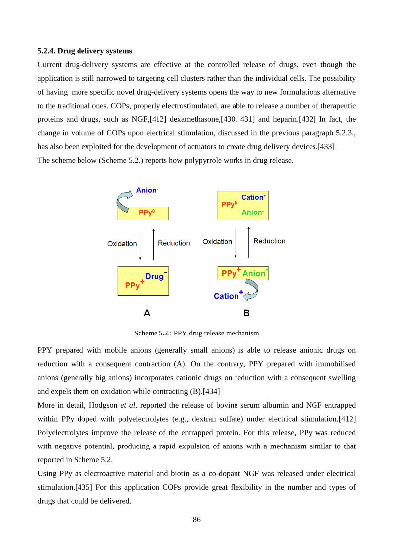
86
5.2.4. Drug delivery systems
Current drug-delivery systems are effective at the controlled release of drugs, even though the
application is still narrowed to targeting cell clusters rather than the individual cells. The possibility
of having more specific novel drug-delivery systems opens the way to new formulations alternative
to the traditional ones. COPs, properly electrostimulated, are able to release a number of therapeutic
proteins and drugs, such as NGF,[412] dexamethasone,[430, 431] and heparin.[432] In fact, the
change in volume of COPs upon electrical stimulation, discussed in the previous paragraph 5.2.3.,
has also been exploited for the development of actuators to create drug delivery devices.[433]
The scheme below (Scheme 5.2.) reports how polypyrrole works in drug release.
Scheme 5.2.: PPY drug release mechanism
PPY prepared with mobile anions (generally small anions) is able to release anionic drugs on
reduction with a consequent contraction (A). On the contrary, PPY prepared with immobilised
anions (generally big anions) incorporates cationic drugs on reduction with a consequent swelling
and expels them on oxidation while contracting (B).[434]
More in detail, Hodgson et al. reported the release of bovine serum albumin and NGF entrapped
within PPy doped with polyelectrolytes (e.g., dextran sulfate) under electrical stimulation.[412]
Polyelectrolytes improve the release of the entrapped protein. For this release, PPy was reduced
with negative potential, producing a rapid expulsion of anions with a mechanism similar to that
reported in Scheme 5.2.
Using PPy as electroactive material and biotin as a co-dopant NGF was released under electrical
stimulation.[435] For this application COPs provide great flexibility in the number and types of
drugs that could be delivered.

87
5.3. Sensors applications
Polyaniline, as well as other conducting organic polymers,[436, 437] when exposed to specific
conditions, such as acidic or basic vapors and liquids, such as HCl, ammonia gas,[438, 439] or
ammonia water,[440, 306] CO2,[441] as well as some neutral gases including chloroform,[442]
alcohols,[443] etc., changes its electrical conductivity. This modification makes it a novel
promising material for sensor applications. However, conventional PANI shows poor sensitivity
because of the poor diffusion of analyte molecules into the polymer and its composites films.[444-
446] On the contrary, one-dimensional nano-structured PANI exhibits the best performances,
thanks to its significantly enhanced exposure area and penetration depth for gas molecule.[174, 446,
447]
Sensors can be classified depending on the mode of trasduction and the kind of application.
5.3.1. Sensors based on transduction
Sensors based on transduction are called transducers. They are devices that convert a signal in
one form of energy to another form of energy. A sensor is used to detect a parameter in one form
and reports it in another form of energy, often an electrical signal.
5.3.1.1. Potentiometric sensors
Potentiometric sensors can be distinguished into symmetric and asymmetric. A potentiometric
sensor either symmetric [448] or asymmetric [449] depends on the homogeneous and heterogeneous
interface between the dipolar layers of charges. Symmetrical potentiometric sensors are classical
electrodes in which the ion-selective membrane is placed between two solutions. In an
asymmetrical ion selective electrode, one side of the membrane is in contact with a solid phase
while the other one is exposed to the measured solution. A potentiometric sensor measures the
change in potential caused by a chemical reaction that separates electric charge.
Potentiometric sensors based on the combination of electropolymerized materials and neutral
ionophores offer attractive advantages in food analysis.[450] More in detail, PANI was successfully
used in potentiometric sensors for pH measurement,[451, 452] and the determination of different
species, such as ammonia,[453] metal ions,[454–456] sulfite,[457] antioxidants and many other
compounds.[458–464].
5.3.1.2. Amperometric sensors
An amperometric sensor is a detection and quantitative measurement device in which redox events
associated with the selective recognition of an analyte of interest are processed by an

88
electrochemical transducer to produce signal in form of current, whose magnitude is proportional to
the quantity of analyte present. The recognition component of an amperometric sensor usually
consists of an electroactive redox substance (e. g., COPs) or composite of chemical or biological
origin intimately connected to the transducer's electronics. Amperometric sensors measure the
current generated at the surface of the electrode as a result of electron transfer from the
oxidation or reduction reaction of the electroactive species, typically at a constant applied potential.
Umana & Waller proposed a new amperometric sensor based on an enzyme (glucose oxidase)
immobilized on a film of PPy during the electropolymerization of the corresponding
monomer.[395] This electrode is useful to detect glucose in aqueous solutions for a period of up to
7 days.
5.3.1.3. Piezoeletric sensors
Piezoelectric sensors measure the electrical potential caused by applying a mechanical force
(pressure, acceleration, strain or force) to a piezoelectric material, that is a material that produces an
electric field when exposed to a change in dimension caused by an imposed mechanical force
(piezoelectric or generator effect) or, conversely, produces a mechanical stress when subjected to an
applied electric field (electrostrictive or motor effect). The effect of an applied pressure on the
electrical properties of conducting composites has been studied under static [465] and dynamic
[466, 467] conditions. Some materials exhibit a decrease of the electrical resistivity when a
compressive force is applied on their surface, as a result of the reduction of the inter-particulate
distance and the subsequent formation of conducting networks inside the insulating matrix.[465,
468–470] In contrast, other systems present the opposite behavior; the electrical resistivity increases
while the material is being pressed due to the disconnection of the conducting particle contacts
caused by the shear stress components and the ensuing rupture of the paths of charge carriers.[466]
These contradictory results indicate that a specific piezo-resistive response of a conducting
composite should be related to the microstructure of the material and, also, to the experimental
conditions in which the study was performed.
5.3.1.4. Calorimetric/thermal sensors
A thermistor is a type of resistor whose resistance varies significantly with temperature. This kind
of materials can be used as cheap and sensitive temperature sensors. Conducting organic polymers
in combination with enzymes have been used for this purpose.[471]

89
5.3.1.5. Optical sensors
An optical sensor is a device that converts light rays into electronic signals. More in particular, it
measures light absorbed or emitted as a consequence of a biochemical reaction. Optical sensors
have been used in new technologies for detecting small amounts of chemical, gaseous species. In
this context, polyaniline and polypyrrole have been strongly investigated thanks to their amazing
optical properties that make them powerful materials for the determination of chemicals in vapour
and liquid state. Polymer nanofibers, such as polyaniline nanofibers, with uniform diameters less
than 500 nm can be made in bulk quantities through a facile aqueous and organic interfacial
polymerization method at ambient conditions. The nanofibers have lengths varying from 500 nm to
10 μm and form interconnected networks in a thin film. Thin film nanofiber sensors can be made of
the polyaniline nanofibers having superior performance in both sensitivity and time response to a
variety of gas vapors including acids, bases, redox active vapors, alcohols and volatile organic
chemicals.[472]
5.3.1.6. Pressure sensors
A pressure sensor measures pressure, typically of gases or liquids. Pressure is an expression of the
force required to stop a fluid from expanding, and it is usually stated in terms of force per unit area.
A pressure sensor usually acts as a transducer; it generates a signal as a function of the pressure
imposed.
Pressure sensors can be used to indirectly measure other variables such as fluid/gas flow, speed,
water level, and altitude. Pressure sensors can alternatively be called pressure transducers, pressure
transmitters, pressure senders, pressure indicators and piezometers, manometers, among other
names.
Pressure sensors can vary drastically in technology, design, performance, application suitability and
cost and can be classified in terms of pressure ranges they measure, temperature ranges of
operation, and most importantly the type of pressure they measure. Pressure sensors are variously
named according to their purpose, but the same technology may be used under different names.
Generally it is possible to distinguish:
Absolute pressure sensor: it measures the pressure relative to perfect vacuum;
Gauge pressure sensor: it measures the pressure relative to atmospheric pressure. A tire pressure
gauge is an example of gauge pressure measurement; when it indicates zero, then the pressure that it
is measuring is the same as the ambient pressure.
Vacuum pressure sensor: it is a sensor that measures pressures below atmospheric pressure,
showing the difference between that low pressure and atmospheric pressure (i.e., negative gauge

90
pressure), but it may also be used to describe a sensor that measures low pressure relative to perfect
vacuum (i.e. absolute pressure).
Differential pressure sensor: it measures the difference between two pressures, one connected to
each side of the sensor. Differential pressure sensors are used to measure many properties, such as
pressure drops across oil filters or air filters, fluid levels (by comparing the pressure above and
below the liquid) or flow rates (by measuring the change in pressure across a restriction).
Technically speaking, most pressure sensors are really differential pressure sensors; for example a
gauge pressure sensor is merely a differential pressure sensor in which one side is open to the
ambient atmosphere.
Sealed pressure sensor: this sensor is similar to a gauge pressure sensor except that it measures
pressure relative to some fixed pressure rather than the ambient atmospheric pressure (which varies
according to the location and the weather).
It is important to discuss also the characteristics which are used to quantify all sensors.
Accuracy: the accuracy of a sensor relates to its ability to measure the absolute value of a specified
metric. Very accurate sensors typically require calibration to a known standard to account for drift
and changes in environmental conditions. For example, a user will typically tare a microbalance
before making a precise weight measurement. This characteristic is particularly relevant to
polyaniline sensors because the electrochemical properties of polyaniline may vary widely with
environmental characteristics such as electrolyte species/concentration and temperature, as well as
material characteristics such as oxidation state, microstructure, and molecular weight.
Precision: it is a measure of a sensor’s ability to produce the same output with identical inputs.
Precision incorporates repeatability, when multiple measurements are taken over a short period of
time, as well as reproducibility, when multiple measurements are taken over long periods of time,
by different users, with different instruments, or at different locations. The key to high
reproducibility in polyaniline sensors is to ensure that the pretreatment of the polymer is consistent,
as the equilibrium chemical state of polyaniline depends on its oxidation history.
Resolution: the resolution, also known as discrimination, of a strain sensor is defined as the smallest
deflection which produces a detectable output. While this is important characteristic in any strain
sensing device, it is generally a result of noise within all the components of a strain measuring
instrument, and not the sensing element alone. For this reason, examining resolution is not
particularly relevant to the fundamental electrochemical properties of polyaniline.
Range: the input range will dictate the operational conditions of a sensor, and the output range will
dictate the system required to interpret the signal. The input range of a polyaniline sensor is limited
by the greatest strain which can be applied to the material before inducing permanent damage or

91
deformation. The output range will influence the type of circuitry required to interpret the signal,
primarily whether amplification is necessary.
Sensitivity: it is a measure of the slope of the output with increasing input. The magnitude of the
electrical output of polyaniline will depend on how efficiently work done by stretching a
polyaniline film can be converted into electrical energy. This characteristic will dictate the viability
of polyaniline based energy harvesting devices.
Linearity: like sensitivity, linearity takes into account the slope of the output with increasing input;
however it focuses on the slope variation over the functional range of the sensor. Non-linear sensors
require more complex systems to interpret the output signal, but non-linearity can be corrected with
a calibration curve.
Hysteresis: it is the dependency of the output signal on the trajectory of the input. In a polyaniline
sensor, hysteresis may depend on input factors such as strain rate or whether applied strain is
positive or negative.
Random Error: also called noise, random error is sensor output which does not result from the input.
This type of error typically affects the resolution of a sensor; as the output signal to noise ratio
(S/N) approaches 1, it becomes difficult to distinguish the two. The time dependency of ion
diffusion into polyaniline will reduce high frequency noise produced by ambient vibrations.
Systemic Error: it is introduced through inputs which are unintentional or out of the control of the
user. These inputs can be introduced via operational/observational variation (user error), drift,
attenuation or distortion of the signal in the transmission system, or environmental changes such as
temperature variation. Systemic errors typically affect the accuracy of a sensor, and can be
corrected using compensation methods such as internal calibration standards, filtering, and
feedback. Ensuring that the test fixture is well constructed and the methodologies are consistent will
help to reduce systemic variation in polyaniline sensor output. Testing polyaniline in steady state
conditions will reduce drift.
5.3.1.6.1. High pressure sensors
The measurement of high pressure is indispensable in many fields for national economy
development and defense industry, especially in military production, research and experiment of
strategy and tactics weapon. For instance, the applications of pressure measurements such as new
materials synthesis in high pressure environment, underground nuclear weapon explosion, safety
protection in highway, underwater shock wave measurement and protection in accident collision all
call for high pressure sensors. The pressure to be measured in these applications reaches the level of
GPa or even higher. Therefore, an ultra-high pressure sensor is not only indispensable for military

92
departments but also has a bright application for civilian use in the future. The sensor should be
capable of working in harsh environments such as high pressure and high temperature, and keeping
stability and reliability. Moreover, it should meet accuracy requirements in high pressure
conditions.
Conducting organic polymers integrated with transducers have been investigated as sensor pressure.
In fact, it is known that when an external ultra-high pressure is exerted onto a polymeric substance,
the distances between the molecular chains decrease. The amount of internal defects and free
volume will decrease, and the restrictions on molecular chain motions will increase. The increase in
the molecular chain interactions will change some of the materials properties drastically. For
instance, the electrical resistivity of polymer will be affected differently by different types and sizes
of charge carriers when an external pressure exerted on the polymer increases. If the charge carriers
are particles of large sizes such as ions, the decrease in free volumes and inter-chain distances will
obstruct the mobility of ions between molecular chains. Consequently, the electrical resistivity will
increase. Conversely, if the charge carriers are small particles such as electrons, the decrease in
inter-chain distances will cause overlaps of molecular orbitals and enhance the mobility of charge
carriers between molecular chains. Thus, the electrical resistivity will decrease.[473]
Zhang et al. reported the effect of high pressure (35-140 MPa) applied on PANI pellets and
pressure time, demonstrating that increasing pressure and pressure time, conductivity value of PANI
gradually increases to a maximum value and then decreases.[474] The same behaviour was
observed from many other authors when PANI pellets were subjected to more high pressure
(GPa).[475]
More recently, Varma and Jayalekshmi investigated the performances of PANI/MWCNTs (multi-
walls carbon nanotubs) composites as pressure sensors.[476] They demonstrated the positive effect
of MWCNTs in the polymeric matrix for this kind of applications. Moreover, many authors dealt
with the effect of the variation of temperature on the conductibility.[477, 478]
Similar investigation were carried out on PPy and its composites in form of pellets and films
obtaining similar results.[479-481]
5.3.1.6.2. Low pressure (touch) sensors
Tactile sensors are basically arrays of force sensors that enable monitoring across a whole specific
surface area, and not only discrete points pressure monitoring. They are demanded in applications
where unstructured environments or uncertainty are present, like minimal invasive surgery (MIS),
robotics, rehabilitation, virtual reality, telepresence, or industrial automation.
93
Many different approaches have been proposed to fabricate these sensors, most of them are based
on piezoresistive principles [482-489] or capacitive [490-494], and a few are based on optical [495]
or piezoelectrical transduction.[496] Most of these sensors are made using technologies for micro-
electro-mechanical systems (MEMS) on silicon [483, 490, 497] or on polymers.[482, 486, 494]
These technologies are not orientated to large area devices, and many of them are proposed for
applications that demand high spatial resolution and good performance in terms of errors, like
MIS.[490] Moreover, most of these realizations have ranges in the order of hundreds of mN or even
N. Especifications for the sensors to be used in robotics depends on the especific application (for
instance fine manipulation or assistance in moving people). However, ranges in the order of tens of
Newtons per tactel are common.[498, 499] Sensors that cover larger areas and have also wider input
ranges can be obtained by arranging single force sensors on a usually flexible substrate,[484, 489,
492] but this increases costs because many instances of these force sensors are needed and because
they must be assembled on the substrate. To lower the cost of the sensor it is better to obtain the
whole array in the batch fabrication process minimizing further assembly of separate components.
The commercial capacitive sensor reported into ref. 498 is designed for manipulative tasks in
robotics and is able to cover large areas and it is stretchable, so it can be mounted on freeform
surfaces. However, signal conditioning of capacitive sensors is more complex than that for
piezoresistive sensors and most proposals for large area low cost sensors are based on piezoresistive
materials, especially to obtain smart tactile sensors with very compact electronics that can be placed
close to the raw sensor.[500-502] A new generation of large tactile sensors are being developed and
commercialized, where a piezoresistive polymer film is used,[503, 504] showing a decrease in
electrical resistance when a normal force is applied. However, their use for large surface
applications seems unlikely due to the high cost of materials used. The electroactive materials
incorporated in currently developed configurations use metallic microparticles (silver) embedded on
a polymer film, metallic central films (silver) separated by a pressurable elastomeric polymer film,
or a combination of both of them.[503, 504] In spite of the valuable advances that these
technologies show, the use of high cost materials such as silver is an important impediment since
large surface applications cannot be afforded by these types of sensors. Another large area, flexible
pressure sensor was proposed by Someya et al.[505] In this case, a pressure-sensitive flexible layer
made of polydimethylsiloxane (PDMS) containing electrically conductive graphite particles was
used. But once again, the fabrication process was complicated as well as the cost of the final device
increased by the deposition of gold layers (vacuum evaporated) and polyimide layers (cured at
180°C). The technology developed by CIDETEC [506] uses conducting polymers as electroactive
materials for construction of pressure sensors. The spincoating of flexible plastic films of

94
polyethyleneterephtalate (PET) with conductive inks obtained from conductive polymers results in
a flexible conductive film on flexible plastic substrates. The presence of a roughness at microscopic
level leads to a resistivity decrease when different pressures are applied. This new technology
shows great advantages for application on high surface area.
5.3.2. Sensors based on application mode
Depending on the use of sensors, they can also be classified into different classes. In fact, it is
possible to distinguish sensors employed to measure chemicals, such as gases or liquids, ions,
alcohols, pH and humidity.
5.3.2.1. Chemical sensors
A chemical sensor is a device that transforms a chemical information, ranging from the
concentration of a specific sample component to total composition analysis, into an analytically
useful signal. The chemical information, mentioned above, may originate from a chemical reaction
of the analyte or from a physical property of the system investigated. Chemical sensors have been
widely used in such applications as critical care, safety, industrial hygiene, process controls, product
quality controls, human comfort controls, emissions monitoring, automotive, clinical diagnostics,
home safety alarms, and, more recently, homeland security. In these applications, chemical sensors
have resulted in both economic and social benefits. An application of COPs for detection of gaseous
analytes belongs to the well developed field of chemosensor design. Gases interacting with COPs
can be divided in two main classes: gases which chemically react with COPs and gases which
physically adsorb on COPs. Chemical reactions lead to changes in the doping level of COPs and
alter therefore their physical properties like resistance or optical absorption. Electron acceptors like
NO2, I2, O3, O2 are able to oxidize partially reduced COPs and therefore increase their doping level.
To oxidize COPs, the gas should have a higher electron affinity than the COPs. NO2 was found to
increase the number of charge carriers in PANI [507] through oxidative doping with NO2− ions and
therefore decrease the resistance. Oppositely, an oxidation of nanofibers of emeraldine salt by NO2
to pernigraniline base state leads to an increase in resistance.[508] SO2 also increases the number of
charge carriers in PPY thus decreasing the resistance.[509] Electron donating gases like H2S, NH3
and N2H4 reduce and therefore dedope COPs, which leads to an increase in resistance. Ammonia
[600, 511] and H2S [512] were found to decrease the conductivity of COPs. Weak physical
interactions of non-reactive volatile organic compounds (chloroform, acetone, aliphatic alcohols,
benzene, toluene, etc.) with the polymer may lead to modification of COPs resistance. The
mechanisms were not studied in details. An adsorption of ethanol and hexanol on dipentoxy
95
substituted polyterthiophene was supposed to change the potential barrier at the boundaries between
COPs grains.[513] Resistance increases due to adsorption of chloroform, acetone, ethanol,
acetonitrile, toluene and hexane on PANI, PPY and polythiophene derivatives were explained by
COP swelling leading to a higher distance between the PANI chains [174, 514, 515] or by
modification of the dielectric constant of COPs.[516] Acetone was suggested to diffuse into the
inter-segmental spaces in the PPY matrices and thus destroying the dispersing interactions between
aromatic pyrrole rings and inducing a higher disorder.[517] For such compounds as acetone a
formation of hydrogen-bonds with PPY was also suggested. These interactions hinder electron
jumping and hence decrease the conductivity of PPY. Interaction of methanol with emeraldine salt
of PANI increases the number of charge carriers through hydrogen bonding of methanol with
reduced amine sites in the polymer. On the contrary, such interaction of methanol with emeraldine
base leads to twisting of the polymer chains, resulting in a lower mobility of the charge carriers and
an increase of the polymer resistance.[518] Interaction of short chain aliphatic alcohols with various
PANI derivatives increases the order in the polymer films which is accompanied by expansion of
polymer chains and conductivity increase.[174, 443] Adsorption of short chain aliphatic alcohols to
PANI/PSS blends is assumed to enhance the charge transfer between adjacent PANI particles by
reducing of the potential barrier for hopping/tunnelling processes, or by increasing of interchain and
interparticle charge mobility.[519] However, an adsorption of long chain aliphatic alcohols leads to
higher film resistances, in this case a prevailing effect of these non-polar compounds is their
insulating properties hindering charge transfer between polymer chains.[174, 443]
5.3.2.2. Ion-selective sensors
Generally, ion sensors have been developed taking the polymer as the conductive
system/component, or as a matrix for the conducting system. When such systems come in contact
with analytes to be sensed, some ionic exchange/interaction occurs, which in turn is transmitted as
an electronic signal for display. Ion selective electrodes (ISE) are suitable for determination of some
specific ions in a solution in the presence of other ions. The quantitative analysis of ions in
solutions by ISEs is a widely used analytical method, with which all chemists are familiar.
Commercial potentiometric devices of varying selectivity for both cations and anions are common
in most laboratories.[520] Ion sensors find wide application in medical, environmental and
industrial analysis. They are also used in measuring the hardness of water. Potentiometric ISEs for
copper ions have been prepared by screen-printing, with the screen-printing paste composed of
methyl and butyl methacrylate copolymer, copper sulphides and graphite.[521] Ion-sensitive
chemical transduction is based on ion selectivity conveyed by ionophore—ion-exchange agents,

96
charged carriers and neutral carriers—doped in polymeric membranes. In addition to organic salts,
several macrocyclics, such as antibiotics, crown ethers and calixerenes, are used as neutral carriers,
functioning by host–guest interactions.[522-525]
The polymeric membrane-based device consists of an internal electrode and reference solution, the
selective membrane across which an activity-dependent potential difference develops, and an
external reference electrode to which the membrane potential is compared in the potential
measurement. The response and selectivity of an ion-selective device depend on the composition of
the membrane. A new Ca2+
-selective polyaniline (PANI)-based membrane has been developed for
all-solid-state sensor applications.[526] The membrane is made of electrically conducting PANI
containing bis [4-(1,1,3,3-tetramethylbutyl) phenyl] phosphoric acid (DTMBP-PO4H), dioctyl
phenylphosphonate (DOPP) and cationic (tridodecylmethylammonium chloride, TDMACl) or
anionic (potassium tetrakis (4-chlorophenyl) borate, KTpClPB) as lipophilic additives. PANI is
used as the membrane matrix, which transforms the ionic response to an electronic signal. A new
potentiometric sensor electrode for sulfide based on PPY films has been introduced by Atta et
al.[527]
5.3.2.3. pH sensors
A simple and speedy device to measure the acidity and alkalinity of a fluid. A pH meter acts as a
volt meter that measures the electrical potential difference between a pH electrode and a reference
electrode and displays the result in terms of the pH value of the solution in which they are
immersed.
From many years polyaniline has been investigated as new organic material to pH measure in
aqueous solution.[528-531] Increasing pH at a given potential, polyaniline undergoes a
deprotonation process that causes a gradually decrease of conductivity of the polymeric material.
Similarly at a given pH changing potential conductivity changes. This is true for PANI but also for
polypyrrole. Thanks to these propeties, De Marcos and Woldeis developed a pH sensor based on a
film of PPy.[532] Many studies have focused on PANI.[533-536, 53]
5.3.2.4. Humidity sensors
Humidity sensors are useful for the detection of the relative humidity (RH) in various environments.
These sensors attracted a lot of attention in the medical and industrial fields. The measurement and
control of humidity are important in many areas, including industry (paper, food, electronic),
domestic environment (air conditioner), medical (respiratory equipment), etc. Polymer, polymer
composites and modified polymers with hydrophilic properties have been used in humidity sensor
97
devices. Venancio et al. described a new simple method to fabricate cheap and “throw-away”
sensors for air moisture.[537] In the first step, a 16-finger inter-digitated graphite pattern was
introduced onto a PET (polyethylene terephthalate) film or a copy paper by a specific procedure. In
the second step, either a coating of PANI nanofibers was deposited on the pattern by dipping into
the aqueous dispersion of 2-acrylamido-2-methyl-1-propane-sulfonic acid doped PANI nanofibers
or an HCl-doped PANI film by in situ deposition. Sensitivity to moisture, which is given as the
resistance change ratio of the sensors, of the sensor with PANI nanofibers (R = 93.3% ± 19%) is
much higher than the one with in situ deposited PANI film (R =5.05% ± 0.79%), which, as
explained, resulted from the higher active surface area of PANI nanofibers than the in situ deposited
PANI film. PANI nanofibers were deposited on a SAW resonator as a selective coating to enhance
the sensitivity of the humidity sensor.[538] In comparison with the uncoated oscillator, which did
not show an obvious frequency change on humidity changes, the PANI nanofiber coated one
exhibited a larger frequency shift. The sensitivity, in terms of f/f , was at least 16.8 ppm/ (%RH)−1
at room temperature, about two times higher than the best reported for SAW humidity sensors in
publications. PANI nanofiber films were fabricated onto screen printed electrodes by using the
chemical deposition method and investigated for humidity sensors.[539] At a lower relative
humidity (<50% RH), the electrical resistance of the sensor decreased with increasing humidity.
While at a higher relative humidity, the electrical resistance of the sensor increased with humidity.
The reversed behavior was attributed to the distortion of the nanostructure or change in the
oxidation state of PANI with the absorption of water molecules.
5.4. Other applications
Some other applications of COPs, like support for the lipase-mediated reaction,[540] a precursor for
nanocarbons,[541] a reducing agent for gold nanoparticles with controlled sizes,[542] materials for
batteries, catalysts, solar cells, hydrogen storage, field-effect transistors, fuel cells, etc.[543] were
also reported but are not elaborated on here.
98
PART II: EXPERIMENTAL PART

99
Chapter 6: Synthetic methods
100
6.1. PANI preparation
Polyaniline was prepared by different techniques, using H2O2 or molecular O2 as the oxidant and
aniline monomer or its dimer (N-(4-aminophenyl)aniline) as the reagent.
6.1.1. PANI preparation from aniline monomer
Synthesis of Emeraldine Salt 1 (ES1) from aniline monomer was carried out according to a method
reported in the literature.[544] In particular, aniline (5.0 g, 54.0 mmol) was dissolved in 40 mL of
HCl 5 M. The solution was stirred at low temperature (ice bath). Then, an aqueous solution of
(NH4)2S2O8 (22.0 g, 96.5 mmol in 80 ml water) was added drop by drop keeping the temperature in
the 0-5 °C range. After 6 hours the green product was filtered on a buchner funnel, washed with
water and acetone (to remove organic soluble oligomers), dried at 60°C until constant weight,
powdered with a mortar and stored for future characterization and use.
The yield was 69%.
6.1.2. PANI preparation from N-(4-amonophenyl)aniline (aniline dimer)
Emeraldine Salt 2 (ES2) was synthesized from N-(4-aminophenyl)aniline (AD) using a green
method previously developed by Della Pina et al.[36] 5.0 g (27.0 mmol) of AD were dissolved in
125 mL of HCl 1 M. After the complete dissolution of AD (ca. 30 minutes) 25 mL of an aqueous
solution of H2O2 35% (H2O2/AD molar ratio ~ 10) and 50 mg of FeCl36H2O (AD/Fe molar
ratio=150) were added under stirring. After 24 hours, a green product was filtered on a buchner
funnel, washed with water and acetone (to remove organic soluble oligomers) until clearness of the
mother liquors, dried at 60°C until constant weight, powdered with a mortar and stored for future
characterization and use.
The yield was 81%.
6.1.3. PANI preparation from N-(4-amonophenyl)aniline (aniline dimer) using O2 as the
oxidant
500 mg (2.7 mmmol) of AD were dissolved in 30 mL of water. 10 mL of HCl 1 M (AD/HCl= 1,
molar ratio) was added to the solution and the mixture was stirred for 30 minutes until complete
dissolution of AD. 5 mg of FeCl36H2O (AD/Fe molar ratio=150) were added under stirring and the
mixture was stirred under pressure of oxygen (2 bars) for 3 days at 80°C.
At the end of the reaction, mixture was cooled at room temperature and filtered on a buchner
funnel. A green product was filtered on a buchner funnel, washed with water and acetone (to
remove organic soluble oligomers) until clearness of the mother liquors, dried at 60°C until constant
101
weight, powdered with a mortar and stored for future characterization and use. The yield was 71%.
This product will be called ES2'.
6.1.4. Aniline dimer-COOH (ADCOOH) preparation
The synthesis of aniline dimer-COOH (ADCOOH) was carried out according to a method reported
in the literature.[344] N-(4-amonophenyl)aniline (0.9 g , 5.0 mmol) and succinic anhydride(0.5 g, 5
mmol) were dissolved in 30ml CH2Cl2 and stirred at room temperature for five hours. As the
reaction proceeded, a white-grey precipitate was formed. At the end of the reaction, the precipitate
was filtered on a buchner funnel, washed several times with diethyl ether until clearness of the
mother liquors, dried at 60°C until constant weight, powdered with a mortar and stored for future
characterization and use.
The yield was 90%.
6.2. PANI modification
Modifications carried out on PANI (ES1 and ES2) prepared by the methods described above were
reactions of deprotonation, reprotonation with different acid dopants and reduction.
6.2.1. PANI deprotonation (dedoping)
ES1 and ES2 were separately dispersed in a solution of NH4OH (NH4OH/ES= 2, molar ratio) for
three hours. At the end of the reaction, a dark violet precipitate was collected on a buchner funnel,
washed with water abundantly until the mother liquors were neutral, dried at 60°C until constant
weight, powdered with a mortar and stored for future characterization and use. The products
obtained by the deprotonation of ES1 and ES2 will be called emeraldine base 1 and 2 (EB1 and
EB2) respectively.
6.2.2. PANI reprotonation (redoping) with inorganic acids
500 mg of EB1 and EB2 were separately dispersed in 20mL of water. Different inorganic acids
(HCl, H2SO4 and H3PO4) were added separately (aniline/inorganic acid=2, molar ratio). After 24
hours, reprotonated PANI (ES1/HCl, ES 1/H2SO4, ES1/H3PO4, ES2/HCl, ES2/H2SO4, ES2/H3PO4)
were collected by filtration on a buchner funnel, washed with water abundantly until the mother
liquors were neutral, dried at 35°C until constant weight, powdered with a mortar and stored for
future characterization and use.
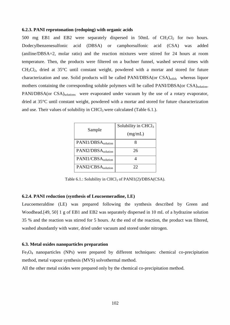
102
6.2.3. PANI reprotonation (redoping) with organic acids
500 mg EB1 and EB2 were separately dispersed in 50mL of CH2Cl2 for two hours.
Dodecylbenzenesulfonic acid (DBSA) or camphorsulfonic acid (CSA) was added
(aniline/DBSA=2, molar ratio) and the reaction mixtures were stirred for 24 hours at room
temperature. Then, the products were filtered on a buchner funnel, washed several times with
CH2Cl2, dried at 35°C until constant weight, powdered with a mortar and stored for future
characterization and use. Solid products will be called PANI/DBSA(or CSA)solid, whereas liquor
mothers containing the corresponding soluble polymers will be called PANI/DBSA(or CSA)solution.
PANI/DBSA(or CSA)solutions were evaporated under vacuum by the use of a rotary evaporator,
dried at 35°C until constant weight, powdered with a mortar and stored for future characterization
and use. Their values of solubility in CHCl3 were calculated (Table 6.1.).
Sample Solubility in CHCl3
(mg/mL)
PANI1/DBSAsolution 8
PANI2/DBSAsolution 26
PANI1/CBSAsolution 4
PANI2/CBSAsolution 22
Table 6.1.: Solubility in CHCl3 of PANI1(2)/DBSA(CSA).
6.2.4. PANI reduction (synthesis of Leucoemeradine, LE)
Leucoemeraldine (LE) was prepared following the synthesis described by Green and
Woodhead.[49, 50] 1 g of EB1 and EB2 was separately dispersed in 10 mL of a hydrazine solution
35 % and the reaction was stirred for 5 hours. At the end of the reaction, the product was filtered,
washed abundantly with water, dried under vacuum and stored under nitrogen.
6.3. Metal oxides nanoparticles preparation
Fe3O4 nanoparticles (NPs) were prepared by different techniques: chemical co-precipitation
method, metal vapour synthesis (MVS) solvothermal method.
All the other metal oxides were prepared only by the chemical co-precipitation method.

103
6.3.1. Fe3O4 nanoparticles (NPs) preparation
6.3.1.1. Fe3O4 nanoparticles (NPs) preparation by co-precipitation method
Fe3O4 NPs powder-type (Fe3O4 NPsp) were prepared according to the method of Deng et al.[545]
3.2 g of FeSO4·7H2O were dissolved in 70 mL of water in the presence of 70 mg of poly(ethylene
glycol) (PEG) under nitrogen atmosphere. 0.6 mL of H2O2 30% (w/w) (Fe: H2O2 = 3:1, molar ratio)
were slowly added and the pH was corrected to 13 by adding NaOH 8 M. The reaction mixture was
stirred at 50°C for 6 h. The black product was recovered by magnetic separation, washed several
time by water, dried in oven at 110°C overnight until constant weight, powdered with a mortar and
stored under inert atmosphere (N2) for future characterization and use.
The yield was 91%.
Fe3O4 NPs ferrofluid-type (Fe3O4 NPsff) were prepared according to the method of Xu et al.,[546]
but with some variations.
Thus, 6.0 g of FeCl3·6H2O and 2.2 g FeCl2·4H2O were dissolved in 25 mL of water and stirred in a
200 mL beaker under nitrogen atmosphere at 80°C. Then 12.5 mL of ammonia solution were
rapidly added into the solution and the mixture was kept reacting for 30 min. After adding 0.94 g of
oleic acid to the black dispersion, the stirring was maintained for other 90 min. The magnetic
powder was collected by a magnet at the bottom of the beaker, the supernatant liquid removed and
the solid residue washed several times with water. After drying overnight in air, the solid material
was transferred into 100 mL of toluene thus obtaining a stable magnetic ferrofluid solution (40%
w/w).
6.3.1.2. Preparation of Fe3O4 nanoparticles (NPs) with a mean diameter of 2.3nm (MNP_3) by
Metal Vapour Synthesis (MVS) technique
Following the metal vapour synthesis technique, 250 mg of metallic iron were evaporated in 100mL
of acetone. This solution of Fe nanoparticles was maintained under inert atmosphere (Ar) at -40°C.
Then, 1 mL of oleic acid was added and the solution was maintained at room temperature in air.
After 24 hours Fe3O4 nanoparticles were separated by centrifugation. They were re-dispersed in 75
mL of n-hexane obtaining a stable colloidal solution. The ICP analyses showed an iron content of
187.5 mg. The TEM analyses confirmed the presence of Fe3O4 nanoparticles having a mean
diameter of 2.3 nm with a distribution ranging from 1 to 4 nm.[547]

104
6.3.1.3. Fe3O4 nanoparticles (NPs) preparation by solvothermal method
6.3.1.3.1. Preparation of Fe3O4 NPs with a mean diameter of 10.0 nm (MNP_2)
In a 50 mL three-necked flask Fe(CO)5 (2.13 mmol), oleic acid (8.51 mmol) and octyl ether (12
mL) was mixed under nitrogen and magnetic stirring. The molar ratio between precursor and
surfactant was 1:4 and the precursor concentration was ca. 0.18 M. The solution was heated at
105°C for 10 minutes, then (with a rate of 3°C/min) until 285°C and kept at this temperature for
1h. After cooling at room temperature, the solution was washed with acetone and centrifuged at
6000 rpm for 10 minutes once and then 2 times with petroleum ether. Finally, NPs were dispersed
in toluene.[548]
6.3.1.3.2. Preparation of Fe3O4 NPs with a mean diameter of 27.0 nm (MNP_1)
In a 50 mL three-necked flask Fe-oleate (1.52 mmol), trioctylamine (30 mmol) and oleic acid (0.76
mmol) was mixed under nitrogen and magnetic stirring. The solution was heated until to 360°C
(3.3°C/min) and kept at this temperature for 30 min. The mixture was cooled at room temperature,
then washed with acetone and centrifuged at 6000 rpm for 10 minutes for 5 times. At the end NPs
were dispersed in toluene.[549]
6.3.2. Preparation of Fe3O4 nanoparticles capped with aniline dimer–COOH
Below different methods to prepare Fe3O4 nanoparticles capped with aniline dimer–COOH are
reported. The one-step method is taken from the scientific literature,[344] the two-step technique
represents an innovative approach.
6.3.2.1. One-step preparation of Fe3O4 nanoparticles capped with aniline dimer–COOH
The synthesis of Fe3O4NPs capped with ADCOOH (Fe3O4 NPsADCOOH) was carried out according
to a method reported in the literature.[344] FeCl2·4H2O (0.9 g) and FeCl3·6H2O (2.4 g) were
dissolved under N2 in demineralized Milli-Q water (20 ml) under vigorous stirring. The solution
was heated to 60°C and, then, 5 ml of a solution of NH4OH (28% w/w) was quickly added,
immediately followed by addition of a solution of aniline dimer–COOH (different amount of
ADCOOH in 2 ml of acetone). Mixture was stirred for 1 hour at 80°C. The reaction mixture was
then cooled slowly to room temperature. A dark powder was filtered, washed sequentially with
acetone and ethanol, dried at 60°C until constant weight, powdered with a mortar and stored for
future characterization and use.
The yield was 65%.

105
6.3.2.2. Two-step preparation of Fe3O4 nanoparticles capped with aniline dimer–COOH
1 mL of Fe3O4 NPsff prepared in section 6.3.1.1. were dried by the use of a rotary evaporator. Fe3O4
NPsff were washed several timed (ca. 10) with acetone to remove oleic acid and dried.
Meanwhile, ADCOOH was dissolved in different solvents (acetone, methanol, tetrahydrofuran and
1, 4-dioxane). The concentration of these organic solutions is reported in Table 6.2.
ADCOOH (mg) Solvent (mL) Concentration (mg/mL)
100 5 20
“ “ “
“ “ “
50 “ 10
Table 6.2.: Concentration of solutions containing ADCOOH in different solvents.
2 mL of each solution were put in contact with Fe3O4 NPsff , washed as described above, for 12
hours.
Fe3O4 NPsADCOOH were recovered by centrifugation, dried at 60°C until constant weight, powdered
with a mortar and stored for future characterization and use.
6.3.3. MFe2O4 (M= Co, Ni, Mn, Cu, Zn and Mg) nanoparticles preparation by co-precipitation
method
All the other metal oxides were prepared only as powder-type following a typical chemical co-
precipitation method. Aqueous solutions of Fe3+
0.3 M (solutions A) and M2+
0.15 M (solutions B)
were prepared dissolving the correct amounts of salts in HCl 0.4 M. 20 mL of solution A and 20 mL
of solution B were mixed together and stirred for 20 minutes at 80°C under nitrogen atmosphere.
Then, a solution of NaOH 1.5 M was quickly added until pH 13 under vigorous stirring. After 2
hours, the products were magnetically decanted, washed repeatedly with distilled water until neutral
pH, dried in oven at 110°C overnight until constant weight, powdered with a mortar and stored for
future characterization and use.
All yields were ~ 85 %.
6.4. PANI/MFe2O4 (M= Fe, Co, Ni, Mn, Cu, Zn and Mg) composites preparation
PANI/MFe2O4 were prepared by oxidative polymerization of aniline dimer, using H2O2 or
molecular O2 as the oxidants in the presence of the corresponding amount of MFe2O4.
The products obtained by these reactions will be labeled as follows: PANI/MFe2O4.
106
6.4.1. PANI/MFe2O4 composites preparation using H2O2 as the oxidant
The typical synthesis was conducted as follows: 500 mg (2.7 mmol) of AD were dispersed in 30
mL of water. 2.7 mL of HCl 1 M (AD/HCl= 1, molar ratio) were added into the solution and the
mixture was stirred for 30 minutes until complete dissolution of AD. Then, 1.2 mL of an aqueous
solution of hydrogen peroxide 35% (H2O2/AD= 5, molar ratio) were added. Finally, different
amounts of MFe2O4 (as prepared in sections 6.3.1., 6.3.2., 6.3.3.) were added into the solution.
After 24 hours, a dark product was recovered by filtration on a Buchner funnel and washed
repeatedly with water and with acetone until clearness of the mother liquors. The product was dried
in an oven at 60°C until it reaches a constant weight, powdered with a mortar and stored for future
characterization and use.
6.4.2. PANI/MFe2O4 composites preparation using O2 as the oxidant
The typical synthesis was conducted as follows: 500 mg (2,7 mmol) of AD were dispersed in 30
mL of water. 2.7 mL of HCl 1 M (AD/HCl= 1, molar ratio) was added into the solution and the
mixture was stirred for 30 minutes until complete dissolution of AD. Then, different amounts of
MFe2O4 (as prepared in sections 6.3.1., 6.3.2., 6.3.3.) were added into the solution. The dispersion
was stirred under pressure of molecular oxygen (3 bars) for 3 days at 80°C. Finally, a dark product
was filtered on a Buchner funnel, washed repeatedly with water and with acetone until clearness of
the mother liquors, dried in an oven at 60°C until it reaches a constant weight, powdered with a
mortar and stored for future characterization and use.
6.5. PANI nanofibers preparation by electrospinning technique
PANI1/DBSAsolution and PANI2/CSAsolution were used to produce PANI nanofibers by
electrospinning process.
6.5.1. Spun solutions preparation
Poly(ethylene oxide) (PEO; Mw=600000) and Poly(methy lmetacrilate) (PMMA; Mw=1000000;
350000) were used as binder (co-polymer). Concerning PANI/PEO blends, samples
(PANI1/DBSAsolution, and PANI2/CSAsolution were dissolved in CHCl3 using the values of solubility
reported in Table 6.1. The amount of PEO into the organic solutions of PANI/DBSAsolution ranged
from 0 to 1% wt with respect to the amount of PANI.
Concerning PANI/PMMA blends, PANI/DBSA was dissolved in a mixture of CHCl3:DMF 5:1w/w
maintaining a concentration of 7-8 mg/mL.
The amount of PMMA ranged from 30 to 83% wt with respect to the amount of PANI.

107
Once PEO or PMMA were added into the polymeric solution, mixture was stirred for 12 hours at
room temperature. In all cases homogeneous solutions were obtained. No phase separation was
observed before use.

108
Chapter 7: Characterization techniques

109
7.1. Spectroscopic techniques
As far as spectroscopic techniques are concerned, FT-IR, UV-vis and AAS spectroscopies were
employed, as described below.
7.1.1. Fourier Transform Infrared (FT-IR) spectroscopy
A small amount of product was mixed with KBr and finely crushed. The resulting powder was,
then, compressed in 13 mm diameter pellets with a 10 ton hydrostatic press and analysed on a Jasco
FT-IR 410 spectrometer. The range of the measurement was 500-4000 cm-1
with a resolution of 0.5
cm-1
.
7.1.2. Ultraviolet-visible (UV-vis) spectroscopy
A small amount of product was dissolved in few millimetres of solvent (generally, N, N-dimethyl
formamide or 2-pyrrolidone).
The blank, i.e. the spectrum of the solvent, was recorded before the sample in 1 cm optical path
quartz cuvette, using an HP8453 diode array UV-vis spectrophotometer. The range of the
measurement was 250-1100 nm with a resolution of 1 nm.
7.1.3. Atomic Absorption spectroscopy (AAS)
About 20 mg of product were dissolved in 5 mL of sulfonitric mixture at 80°C until dissolution.
Then, the excess of acid was evaporated and the solution was diluted with MilliPore water and
analyzed using a Perkin Elmer3100 spectrometer. Wavelengths were set as reported in Table 7.1.
Metal (nm)
Fe 248.7
Co 240.7
Ni 232.0
Cu 324.8
Zn 213.9
Mg 285.2
Mn 279.5
Table 7.1: Values of wavelength used to quantify metals in AAS.
110
The concentrations of metals into the solutions, and hence in the composite materials, were
calculated from absorbance via a linear regression on the data obtained analysing 1, 5, 7.5, 10 ppm
standard metals solutions.
7.2. Thermogravimetric technique
Thermograms of samples were carried out on a Perkin Elmer TAC 7/DX instrument. In each
experiment, a small amount of sample (about 10 mg) was put on a platinum pan and heated under
N2 in the range of 50-1000°C with a heating rate of 1°C/min.
7.3. Mass spectrometry
Liquid secondary ion spectrometry (LSIMS) was employed. Spectra were acquired on a VG
Autospec M246 double focusing mass spectrometer operating in the positive ion mode in the range
of 150-500 z/m. 3-Nitrobenzyl alcohol was used as the matrix.
7.4. NMR spectroscopy
1H NMR spectra were recorded in D2O on a Bruker 300 MHz instrument.
7.5. X-Rays powder diffraction
A small amount of product was placed in a sample quartz holder and analyzed using a Rigaku D III-
MAX horizontal scan powder diffractometer with Cu K radiation. 2 ranged from 10 to 80 with
an increment of 0.04 (2)/s.
7.6. Microscopic techniques
Morphological characterizations were carried out by TEM, SEM and STEM techniques as reported
below.
7.6.1. Transmission Electron Microscopy (TEM)
TEM images were recorded using a Zeiss LIBRA EFTEM FEG TEM, operating at 200 kV and
equipped with an in-column omega filter for energy selective imaging and diffraction.
The samples were prepared by drop drying a toluene solution in the nanoparticle samples case or an
acetonitrile dilute suspension in the case of PANI/Fe3O4 nanocomposite samples.
Size distribution of studied samples were determined by a statistical analysis processed by means of
the PEBBLES, freely available software developed in the Laboratory of Nanotechnology, ISTM-
CNR.

111
7.6.2. Scanning Electron Microscopy (SEM)
The SEM specimens were prepared by drop-casting the polymeric suspension onto an aluminium
foil and the measurements were carried out on a SEM-LEO 1430 microscope.
7.7. Electrical resistivity measurements
Electrical resistivity was measured by different techniques.
Electrochemical impedance spectroscopy (EIS): the electrical behaviour and the specific
electrical conductivity (S cm−1
) of the solid materials were obtained by measuring the resistance
R () by electrochemical impedance spectroscopy (EIS). AC-Impedance tests were performed on a
pressed pellet of polymers using an AUTOLAB PGSTAT 30 Metrohm in the frequency range from
10 mHz to 1 MHz by applying an excitation ac-voltage of 10 mV rms.
Two-wire method: the electrical resistivity of the samples was measured by the two-wire method,
where the voltage was applied and the current measured by a Keithley 487 picoammeter/voltage
source. All measurements were performed in direct current (DC) mode, at room temperature. On
each sample, two parallel rectangular gold electrodes were deposited by magnetron sputtering on
one side of the sample. Copper wires were attached to the electrodes with silver paint to ensure
good electrical contact.
7.8. Magnetic measurements
Magnetic measurements were carried out by the use of a Quantum Design MPMS XL-5 SQUID
magnetometer. Magnetization-demagnetization M–H curves have been measured after zero-field
cooling to 5 K, increasing the field up to 50 kOe, and decreasing it to −600 Oe. The temperature
dependence of the magnetization has been measured between 5 and 300 K after zero-field cooling
(ZFC) or field cooling (FC, Hcool = 100 Oe).
7.9. Wave guide dielectric characterization
In order to obtain small 2cmx2cmx0.2cm tiles of sample a mould was set-up. Materials were
prepared mixing 1 g of sample with 3 g of commercial PVAc glue (dispersion of polymer in water
ca. 50%). The viscous fluid was deposited in the mould layer by layer. Between the deposition of
one layer to another 20 minutes passed to let glue dry out. When the tile reaches the desired
thickness it was dried in an oven at 60°C for 24 h. Then, the mould was removed and tiles were
polished with sandpaper. Samples were analyzed on a Anritsu VNA (37277) Vector Network
Analyzer in the range of 18 to 26 GHz.

112
7.10. Electrospinning process
The electrospinning setup used was supplied by Linari Engineering-Pisa, Italy. The electrospinning
parameters were: temperature (21°C), injection rate (from 0.3 to 1.98 ml/h), a target-capillary
distance (12 cm) and relative humidity (RH) (<40%). Concerning the way of fiber collection a static
collector and a rotating collector (the rotation speed of the drum was 30 rpm) were used.
7.11. Indirect and direct cytocompatibility tests of PANI nanofibers on a SH-SY5Y human
cell line
Pretreatment of samples: PANI nanofibers (NFs) were cut producing small samples with areas
ranging from 4.16 to 9.67 mm2. They were stored in a refrigerator until use.
To tests indirect cytocompatibility samples of NFs were disinfected in different manners. They were
treated in ethanol 70% (v/v) for 15 min. After this time, ethanol was removed by a pipette. The
treatment was repeated maintaining PANI NFs in ethanol for 48 hours. Then, ethanol was
evaporated for 3 hours under a hood.
In another test PANI NFs were put I contact for 48 hours in PBS (phosphate buffer solution, pH
7.2-7.4) + 3% (v/v) of penicillin/streptomicyn.
Finally, they were exposed for 10 minutes under UV irradiation (253.7 nm).
Samples were prepared for SEM observation in a chemical hood.
SH-SY5Y cell line: culture conditions and medium: SH-SY5Y cells (human neuroblastoma cell
line, ATCC® CRL-2266™) were cultured at 37°C, 5% CO2, in Dulbecco’s modified Eagle’s
medium (DMEM, Gibco, Invitrogen, product code 10938) supplemented with 10% (v/v) fetal
bovine serum (FBS, Gibco, Invitrogen, product codes 26140 or 10270), 1% (v/v) L-glutamine
(Gibco, Invitrogen, product code 25030) and 1% (v/v) penicillin/streptomycin solution (Gibco,
Invitrogen, product code 15140-148). Before using, media were filtered with vacuum filter systems
(Corning, product codes 431097 or 430769).
SH-SY5Y cell line, thawing out and splitting: Cryopreserved SH-SY5Y cells were kept in
cryogenic vials in 80% (v/v) FBS, 10% (v/v) DMEM and 10% (v/v) dimethyl sulfoxide (DMSO,
Sigma, product code D8418) within a tank (Forma Scientific Inc, 8038 model) filled with liquid
nitrogen at about -190°C. After vials had been carefully opened, ice crystals were melted by gently
pipetting 1ml of culture medium (previously heated at 37°C) with a Pasteur pipette (Copan, product
code 201CS01). The suspension was transferred to a 50 ml centrifuge tube (BD Falcon, product
code 352070) containing 10 ml of medium and centrifuged (Eppendorf AG, 5415R model) at 900
rpm for 5 min. The supernatants were discarded and the pellet was suspended with 10 ml of

113
medium and placed in a 75 cm² flask (BD Falcon, product code 137787). After checking the cell
density by an inverted optical microscope (Leica, LEITZ DM IRB model), the flask was moved to
the incubator. After 80%-90% of the available surface had been colonized, the medium was
discarded by aspiration and cells were gently washed with 2 ml phosphate buffered saline (PBs,
Gibco, Invitrogen, product code 14190) to remove serum and cell debris. 1 ml of trypsin (Gibco,
Invitrogen, product code 154000) was added and the flask was moved back to the incubator for 3-5
min. After the cells had been detached, trypsin was eluted with 5 ml of medium and the suspension
was transferred to a 50 ml centrifuge tube, to be centrifuged at 900 rpm for 5 min. The supernatants
were discarded, while the cells were suspended with fresh medium and counted.
Cell counting: Fifty μl cell suspension was transferred to a 0.65 ml microcentrifuge tube (Corning,
product code 3206) and mixed with the same volume of trypan blue (Sigma, product code T8154).
Ten μl was pipetted in a haemocytometer grid (Neubauer chamber) and the viable cells were
counted.
Trypan Blue (Fig. 1A) is a commonly used dye to distinguish between viable and nonviable cells:
the first ones exclude the dye and they appear white, while the second ones absorb the dye and they
are coloured in blue (Fig. 1B). This property relies on the negative charge of the cromophore, that
may not interact with the cells unless their membrane is damaged.
Neubauer chamber (Fig. 2) is composed of two opposite identical grids, that are divided into nine
squares (each one is identified with a letter from A to I in Fig. 2). A glass is placed 0.01 mm over
the grids and the empty volume is filled with 10 μL cell suspension.
The number of white cells lying within the squares A, C, E, G and I was counted (the cells lying on
the boundaries were skipped) and the mean value was determined. Then it was multiplied by 2 (to
consider the elution with Trypan Blue) and 104
(because every square has a volume of 0.01 mm³),
that is:
Cell density (cell number/ml) = mean number of counted cells · 2 · 104 (Eq. 1).
By multiplying the cell density and the suspension volume (ml), the total number of cells
may be estimated:
Cell number = mean number of counted cells · 2 · 104 * suspension volume (Eq. 2).
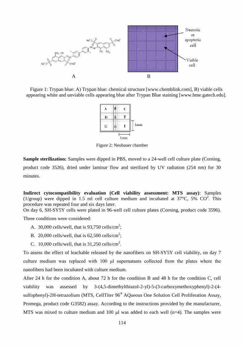
114
A B
Figure 1: Trypan blue: A) Trypan blue: chemical structure [www.chemblink.com], B) viable cells
appearing white and unviable cells appearing blue after Trypan Blue staining [www.bme.gatech.edu].
Figure 2: Neubauer chamber
Sample sterilization: Samples were dipped in PBS, moved to a 24-well cell culture plate (Corning,
product code 3526), dried under laminar flow and sterilized by UV radiation (254 nm) for 30
minutes.
Indirect cytocompatibility evaluation (Cell viability assessment: MTS assay): Samples
(1/group) were dipped in 1.5 ml cell culture medium and incubated at 37°C, 5% CO2. This
procedure was repeated four and six days later.
On day 6, SH-SY5Y cells were plated in 96-well cell culture plates (Corning, product code 3596).
Three conditions were considered:
A. 30,000 cells/well, that is 93,750 cells/cm2;
B. 20,000 cells/well, that is 62,500 cells/cm2;
C. 10,000 cells/well, that is 31,250 cells/cm2.
To assess the effect of leachable released by the nanofibers on SH-SY5Y cell viability, on day 7
culture medium was replaced with 100 μl supernatants collected from the plates where the
nanofibers had been incubated with culture medium.
After 24 h for the condition A, about 72 h for the condition B and 48 h for the condition C, cell
viability was assessed by 3-(4,5-dimethylthiazol-2-yl)-5-(3-carboxymethoxyphenyl)-2-(4-
sulfophenyl)-2H-tetrazolium (MTS, CellTiter 96®
AQueous One Solution Cell Proliferation Assay,
Promega, product code G3582) assay. According to the instructions provided by the manufacturer,
MTS was mixed to culture medium and 100 μl was added to each well (n=4). The samples were

115
incubated at 37°C for 2-4 h, then their absorbance was recorded at 490nm (Tecan
spectrophotometer, Infinite® 200 PRO model).
Results were reported as mean ± standard deviation with respect to controls cultured with fresh
medium.
7.12. Measurements of electrical conductivity as a function of force
Measurements of electrical conductivity as a function of force were carried out on pellets of PANI
having diameter of 13 mm and thickness of 1 mm. They were prepared pressing 200 mg of each
material for 30 minutes at 100 kN using a hydraulic press (Atlas Manual Hydraulic Press).
Concerning measurements at high values of force (0-100 kN), each material was tested at room
temperature. A MTS Alliance RT/100 testing machine was used. The values of force were increased
from 0 to 100 kN with a crosshead displacement of 0.07 mm/min.
Concerning measurements at low values of force (0-20 N), each material was tested at room
temperature and after a thermal treatment for 2 hours at 50 and 100°C. Each pellet was placed on
digital balance and the values of force were gradually increased and decreased by the use of a
screw.
In both cases each pellet was subjected to 3 cycles of loading and unloading and electrical
conductivities were obtained indirectly by the resistivity measures using an AMEL 338 multimeter.
7.13. Piezoresistive measurements
The piezoresistive effect was quantified by 4-point-bending tests. In those tests, the electrical
resistance changes with strain were measured. The 4-point-bending tests were performed in a
Shimadzu-AG-IS 500 N testing instrument at speeds from 0.2 to 2 mm/min and a maximum vertical
(z axis) displacement of 2 mm. Each test was composed by four cycles of deformation.
Stability tests were also performed in selected samples up to 40 cycles. The electrical resistance and
its variations during the deformation process were monitored by a digital multimeter Agilent
34401A.

116
PART III: Results and Discussion

117
Chapter 8: Synthesis and characterization of PANI/metal
oxide nanocomposites

118
As reported in Chapter 4 section 4.2., conductive polymeric compounds exhibiting outstanding
electric and magnetic properties, i. e. polymeric matrices incorporating Fe3O4 nanoparticles, are of
great interest for many applications.[550–554] In the last years, many methods have been developed
to synthesize this kind of nanocomposites. Some of them are based on the precipitation of magnetic
nanoparticles in the presence of polymer in an organic solvent, such as N-methyl pyrrolidinone
(NMP).[346] In other synthetic approaches magnetic nanoparticles (MNPs) are prepared in advance
and then added to the solution containing aniline that will be subsequently polymerized by the use
of an oxidant under acidic conditions [555] or under UV light irradiation.[556]
In this chapter a new clean one-pot synthesis of PANI/Fe3O4 composites will be presented using O2
and H2O2 as the oxidants and Fe3O4 nanoparticles as the magnetic fillers and reaction catalysts
under mild conditions. Because MNPs promoted catalytically the reaction of PANI preparation, the
effect of nanoparticle size on the synthesis and properties of PANI/Fe3O4 nanocomposites was also
deepened.
Preliminary results in terms of microwave absorbing properties will be presented.
Moreover, in order to clarify what is the catalytically active metallic center in the spinel structure,
iron(II) was substituted with another bivalent cation (Mn, Co, Ni, Cu, Zn, Mg) and the effect of
such a substitution on the catalytic performance was investigated.
Finally, an innovative synthetic approach to produce well dispersed PANI/Fe3O4 composites will
be proposed.
8.1. New clean one-pot synthesis of polyaniline/Fe3O4 nanocomposites with magnetic and
conductive behaviour
As reported by Wei et al. the most energy demanding step in the polymerization of aniline is its
oxidation to produce dimeric and trimeric species.[76, 77] Once they have been produced, they
evolve rapidly to produce oligomeric and polymeric materials. However, the redox potential of the
couple aniline/emeraldine salt is relatively high (1.46 V). This means that, accordingly, oxygen is
unable to carry out the reaction owing to its low redox potential (E°= 1.23 O2/H2O V). On the
contrary, from a thermodynamic point of view hydrogen peroxide (E°= 1.78 H2O2/H2O V) could
represent a good choice. However, owing to kinetic limitations the use of a specific catalyst is
necessary.[36] Another possibility to overcome this thermodynamic limitation consists in replacing
the starting material (aniline) with another more reactive species, such as N-(4-aminophenyl)aniline
(aniline dimer, AD). Previous investigations showed that copper powder or its salts are useful
catalysts for this reaction.[26]

119
Herein, for the first time the double role (magnetic fillers and catalysts) of both pristine and oleic-
acid-coated Fe3O4 nanoparticles in the oxidative polymerization of N-(4-aminophenyl)aniline is
reported.[80]
8.1.1. Catalytic polymerization
Tables 8.1. and 8.2. show the polymerization yields obtained by the oxidative polymerization of AD
in the presence of MNPs using molecular oxygen or hydrogen peroxides as the oxidizing agents
respectively.
AD/Fe3O4 (molar ratio)
MNPs ferrofluid-type
(MNPsff)
MNPs powder-type
(MNPsp)
Sample no. Yield (%) Sample no. Yield (%)
Without Fe3O4 NPs 1 0 2 0
681 3 2 4 9
343 5 7 6 10
228 7 10 8 14
137 9 15 10 25
50 11 46 12 48
20 13 55 14 57
10 15 60 16 62
5 17 69 18 68
Table 8. 1.: Polymerization yields for the aerobic oxidative polymerization of AD in the absence
and in the presence of MNPs. Reaction time= 3 days, reaction temperature= 80°C, pO2= 3 bar.
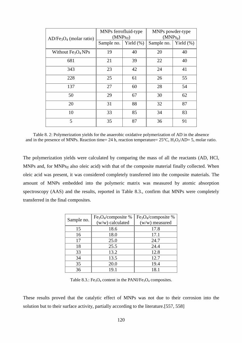
120
AD/Fe3O4 (molar ratio)
MNPs ferrofluid-type
(MNPsff)
MNPs powder-type
(MNPsp)
Sample no. Yield (%) Sample no. Yield (%)
Without Fe3O4 NPs 19 40 20 40
681 21 39 22 40
343 23 42 24 41
228 25 61 26 55
137 27 60 28 54
50 29 67 30 62
20 31 88 32 87
10 33 85 34 83
5 35 87 36 91
Table 8. 2: Polymerization yields for the anaerobic oxidative polymerization of AD in the absence
and in the presence of MNPs. Reaction time= 24 h, reaction temperature= 25°C, H2O2/AD= 5, molar ratio.
The polymerization yields were calculated by comparing the mass of all the reactants (AD, HCl,
MNPs and, for MNPsff also oleic acid) with that of the composite material finally collected. When
oleic acid was present, it was considered completely transferred into the composite materials. The
amount of MNPs embedded into the polymeric matrix was measured by atomic absorption
spectroscopy (AAS) and the results, reported in Table 8.3., confirm that MNPs were completely
transferred in the final composites.
Sample no. Fe3O4/composite %
(w/w) calculated
Fe3O4/composite %
(w/w) measured
15 18.6 17.8
16 18.0 17.1
17 25.0 24.7
18 25.5 24.4
33 13.2 12.8
34 13.5 12.7
35 20.0 19.4
36 19.1 18.1
Table 8.3.: Fe3O4 content in the PANI/Fe3O4 composites.
These results proved that the catalytic effect of MNPs was not due to their corrosion into the
solution but to their surface activity, partially according to the literature.[557, 558]
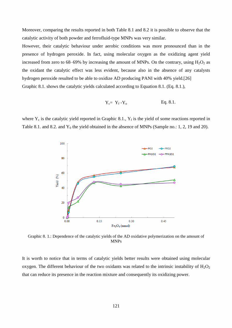
121
Moreover, comparing the results reported in both Table 8.1 and 8.2 it is possible to observe that the
catalytic activity of both powder and ferrofluid-type MNPs was very similar.
However, their catalytic behaviour under aerobic conditions was more pronounced than in the
presence of hydrogen peroxide. In fact, using molecular oxygen as the oxidizing agent yield
increased from zero to 68–69% by increasing the amount of MNPs. On the contrary, using H2O2 as
the oxidant the catalytic effect was less evident, because also in the absence of any catalysts
hydrogen peroxide resulted to be able to oxidize AD producing PANI with 40% yield.[26]
Graphic 8.1. shows the catalytic yields calculated according to Equation 8.1. (Eq. 8.1.),
Yc= Yf -Yo
where Yc is the catalytic yield reported in Graphic 8.1., Yf is the yield of some reactions reported in
Table 8.1. and 8.2. and Y0 the yield obtained in the absence of MNPs (Sample no.: 1, 2, 19 and 20).
Graphic 8. 1.: Dependence of the catalytic yields of the AD oxidative polymerization on the amount of
MNPs
It is worth to notice that in terms of catalytic yields better results were obtained using molecular
oxygen. The different behaviour of the two oxidants was related to the intrinsic instability of H2O2
that can reduce its presence in the reaction mixture and consequently its oxidizing power.
Eq. 8.1.
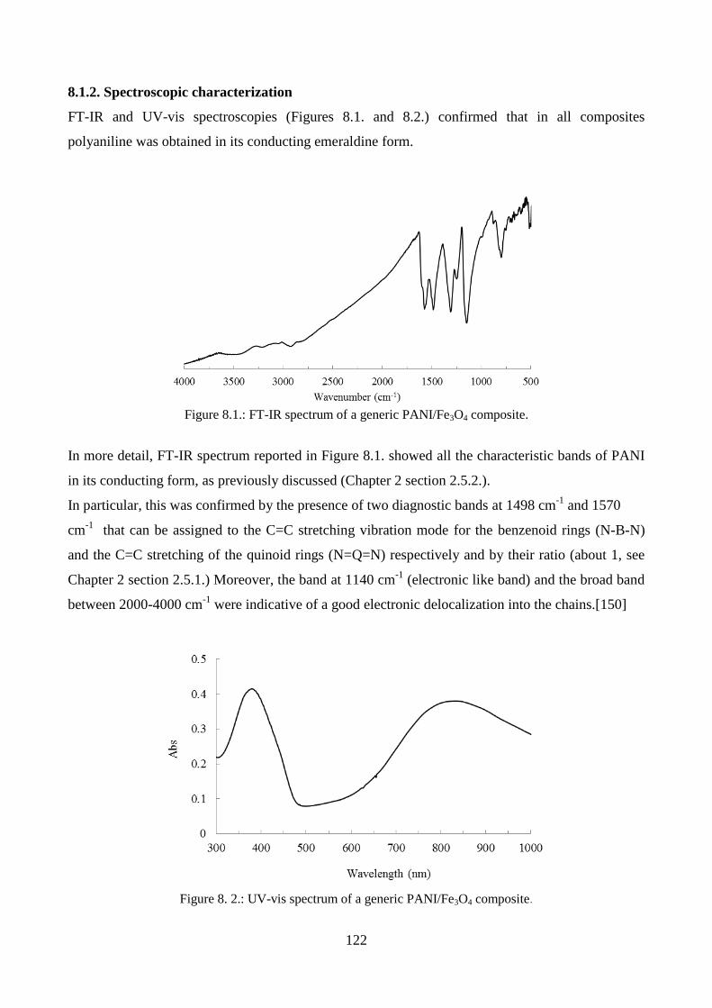
122
8.1.2. Spectroscopic characterization
FT-IR and UV-vis spectroscopies (Figures 8.1. and 8.2.) confirmed that in all composites
polyaniline was obtained in its conducting emeraldine form.
In more detail, FT-IR spectrum reported in Figure 8.1. showed all the characteristic bands of PANI
in its conducting form, as previously discussed (Chapter 2 section 2.5.2.).
In particular, this was confirmed by the presence of two diagnostic bands at 1498 cm-1
and 1570
cm-1
that can be assigned to the C=C stretching vibration mode for the benzenoid rings (N-B-N)
and the C=C stretching of the quinoid rings (N=Q=N) respectively and by their ratio (about 1, see
Chapter 2 section 2.5.1.) Moreover, the band at 1140 cm-1
(electronic like band) and the broad band
between 2000-4000 cm-1
were indicative of a good electronic delocalization into the chains.[150]
Figure 8.1.: FT-IR spectrum of a generic PANI/Fe3O4 composite.
Figure 8. 2.: UV-vis spectrum of a generic PANI/Fe3O4 composite.

123
The UV-vis spectrum showed two characteristic bands at about 300 and 849 nm, due to the -*
transition of the benzenoid ring and benzenoid/quinoid transition respectively.
The amount of MNPs into the composites was measured by atomic absorption spectroscopy, as
reported above, but also confirmed by X-ray powder diffraction analyses (Figures 8.3. A and B).
All the diffractograms clearly showed the characteristic Bragg diffraction peaks corresponding to
the Miller indices for the reflection planes (220), (311), (400), (422), (511), (440) at 2= 30.3, 35.6,
43.2, 53.6, 57.1 and 62.8 respectively for Fe3O4, while the broad peak at about 2 20 was
assigned to PANI with very low crystallinity. Moreover, these results confirmed that Fe3O4 was in
spinel phase [559, 560] and the purity of the products via the absence of other phases of iron oxide
such as maghemite or hematite. Obviously, the intensity of the diffraction peaks of MNPs in the
PANI/Fe3O4 composites (Figures 8.3. b, c, b’, c’) became stronger with increasing the nanoparticle
loadings.
Control over the dispersion of the nanoparticles in the polymer matrix is a critical point to produce
high quality composites.
However, according to the literature,[561, 562] the reduced intensity of the diffraction peaks of
PANI indicated a strong interaction between PANI backbone and MNPs and, consequently, a good
dispersion
2 theta
A B
a
b
c
a
'
b'
c
'
Figure 8.3.: A) XRPD patterns of MNPsp (a) and its composites with PANI (b= sample no. 16, c= sample no.
18), B) XRPD patterns of MNPsff (a’) and its composites with PANI (b’= sample no. 15, c’= sample no. 17)

124
The average size of nanoparticles was calculated according to the Debye-Scherrer equation (Eq.
2.2.):
where k is the shape factor, is the X-ray wavelength (0.15418 nm), is the full width at half-
height and is the Bragg angle. The results are reported in Table 8.4.
Sample Mean diameter (nm)
MNPsp 11.0
Sample no. 15 11.1
Sample no. 17 11.0
Fe3O4NPsff 11.0
Sample no. 16 13.4
Sample no. 18 13.6
Table 8.4.: Mean diameter of the MNPs calculated by the Scherrer’s equation.
8.1.3. Morphological characterization
The average size of MNPs calculated by the Debye-Scherrer equation was confirmed by TEM
characterization (Figures 8.4. A and B).
Figure 8.4.: TEM images of (A) MNPsp, (B) MNPsff.
Eq. 2.2.
A B
200
nm
200 nm

125
However, differently from the MNPsp embedded into the polymer matrix that maintained the same
size, in the composites containing MNPsff, these latter showed a larger diameter probably due to
agglomeration phenomena.
Although MNPs powder and ferrofluid-type displayed a very similar catalytic behaviour (see Tables
8.1., 8.2. and Graphic 8.1.), they influenced differently PANI/Fe3O4 composites morphology
(Figures 8.5 and 8.6.).
Figure 8.5.: TEM (A and B) and SEM (C and D) images of PANI/MNPsff composites.
Figure 8. 6.: SEM images of PANI/MNPsp composites.
A B
A B
C D

126
Figures 8.5 A-D show that PANI/MNPsff composites exhibited rod-like morphology with diameters
ranging from 30 to 110 nm. On the contrary, composites containing MNPsp presented more
irregular structures.
8.1.4. Mechanism of nanorods formation
PANI/MNPsff composites synthesis reported above can be considered as a kind of interfacial
polymerization. In fact, in this case magnetic NPs were introduced into the reaction mixture in an
organic solution. As reported in the literature,[563] interfacial polymerization is an useful template-
free synthetic approach to produce polyaniline in form of nanofibers/-wires/-rods and, in this
context, Zhang and many other authors reported the possibility to form pure PANI or PANI/Fe3O4
composites in form of nanorods and nanotubes following a self-assembly process.[193, 342]
According to the mechanism proposed by Zhang and coworkers, Scheme 8.1. reports an hypothetic
mechanism of synthesis able to justify nanorods formation by the one-pot approach reported above.
Scheme 8.1.: Hypothetic mechanism for PANI/Fe3O4NPsff nanorods formation.
More in detail, N-(4-amonophenyl)aniline is soluble in acidulated water but also in organic solvent,
as toluene. Therefore, when MNPs ferrofluid-type were added, AD partially diffused into the
organic solvent. The reaction mixture resulted in a biphasic system constituted of aqueous phase
containing the oxidant (H2O2 or O2) and part of AD molecules and an organic phase containing the
iron oxide NPs and the remaining part of AD. The reaction took place primarily at the water/toluene
interface, where the present magnetic NPs can catalyze the first step of the polymerization reaction
Fe3O4NPsff
Drop of toluene Aniline dimer
Polymer
Fe3O4NPsff in toluene

127
among the molecules present on the surface of the organic phase, thus producing nanorods through
an elongation process.
On the contrary, in the case of MNPs powder-type all the reagents were in the same phase and the
polymerization reaction took place immediately. Any control of morphology wasn’t allowed.
8.1.5. Thermogravimetric analyses
The TGA (thermogravimetric analyses) results of pure PANI and PANI/Fe3O4 composites are
reported in Figure 8.7.
The TGA curve of pure PANI (Figure 8.7. a) showed three major weight losses, the first step at
around 120°C due to the expulsion of water molecules, the second step at 230-550°C due to the loss
of dopant and the third at 600-1000°C due to the thermal decomposition of the polymer. MNPs
embedded into the polymeric matrix improved the thermal stability of PANI, probably through the
interaction between magnetic nanoparticles and PANI chains. In fact, the weight losses were much
less for the composites (Figures 8.7. b and c).
8.1.6. Magnetic measurements
The magnetization-demagnetization M–H curves of MNPs powder and ferrofluid-type, Sample no.
18, 36, 17 and 35 are presented below (Figure 8.8.). The curves were recorded at 5 K after zero field
cooling from 300 K. Magnetization M is referred to the Fe3O4 mass in each sample.
Figure 8.7.: TGA results for (a) pure PANI (Sample no. 20), (b) Sample no. 34 and (c)
Sample no. 36.
b
c
a
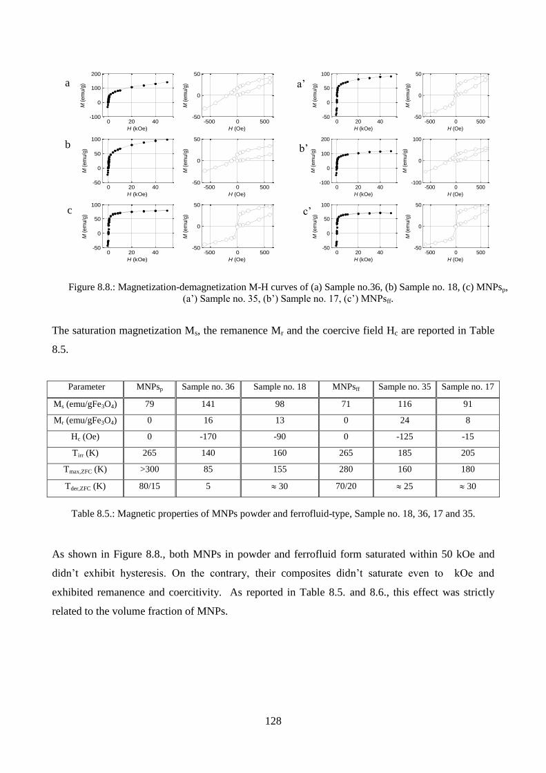
128
The saturation magnetization Ms, the remanence Mr and the coercive field Hc are reported in Table
8.5.
Parameter MNPsp Sample no. 36 Sample no. 18 MNPsff Sample no. 35 Sample no. 17
Ms (emu/gFe3O4) 79 141 98 71 116 91
Mr (emu/gFe3O4) 0 16 13 0 24 8
Hc (Oe) 0 -170 -90 0 -125 -15
Tirr (K) 265 140 160 265 185 205
Tmax,ZFC (K) >300 85 155 280 160 180
Tder,ZFC (K) 80/15 5 30 70/20 25 30
Table 8.5.: Magnetic properties of MNPs powder and ferrofluid-type, Sample no. 18, 36, 17 and 35.
As shown in Figure 8.8., both MNPs in powder and ferrofluid form saturated within 50 kOe and
didn’t exhibit hysteresis. On the contrary, their composites didn’t saturate even to kOe and
exhibited remanence and coercitivity. As reported in Table 8.5. and 8.6., this effect was strictly
related to the volume fraction of MNPs.
Figure 8.8.: Magnetization-demagnetization M-H curves of (a) Sample no.36, (b) Sample no. 18, (c) MNPsp,
(a’) Sample no. 35, (b’) Sample no. 17, (c’) MNPsff.
a a’
b
0 20 40-50
0
50
100
H (kOe)
M (
em
u/g
)
-500 0 500-50
0
50
H (Oe)
M (
em
u/g
)
0 20 40-100
0
100
200
H (kOe)
M (
em
u/g
)
-500 0 500-100
0
100
H (Oe)
M (
em
u/g
)
0 20 40-50
0
50
100
H (kOe)
M (
em
u/g
)
-500 0 500-50
0
50
H (Oe)
M (
em
u/g
)
0 20 40-100
0
100
200
H (kOe)
M (
em
u/g
)
-500 0 500-50
0
50
H (Oe)
M (
em
u/g
)0 20 40
-50
0
50
100
H (kOe)
M (
em
u/g
)
-500 0 500-50
0
50
H (Oe)
M (
em
u/g
)
0 20 40-50
0
50
100
H (kOe)
M (
em
u/g
)
-500 0 500-50
0
50
H (Oe)
M (
em
u/g
)
b’
c c’
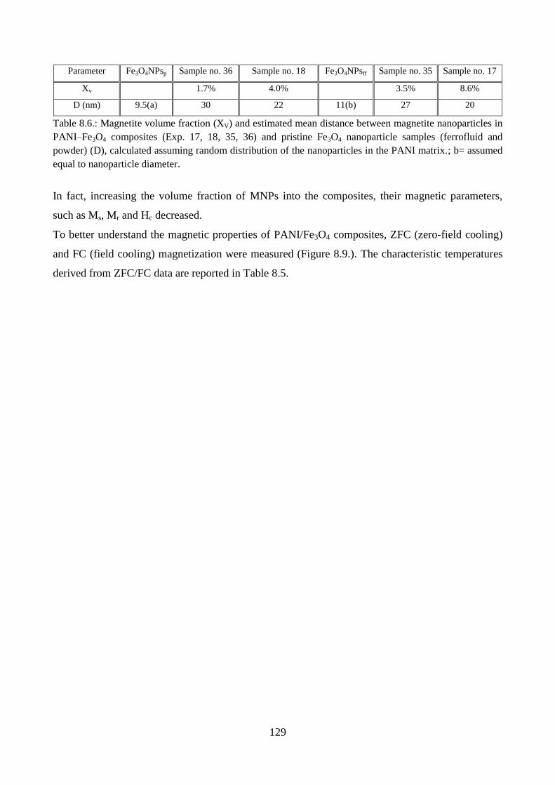
129
Parameter Fe3O4NPsp Sample no. 36 Sample no. 18 Fe3O4NPsff Sample no. 35 Sample no. 17
Xv 1.7% 4.0% 3.5% 8.6%
D (nm) 9.5(a) 30 22 11(b) 27 20
Table 8.6.: Magnetite volume fraction (XV) and estimated mean distance between magnetite nanoparticles in
PANI–Fe3O4 composites (Exp. 17, 18, 35, 36) and pristine Fe3O4 nanoparticle samples (ferrofluid and
powder) (D), calculated assuming random distribution of the nanoparticles in the PANI matrix.; b= assumed
equal to nanoparticle diameter.
In fact, increasing the volume fraction of MNPs into the composites, their magnetic parameters,
such as Ms, Mr and Hc decreased.
To better understand the magnetic properties of PANI/Fe3O4 composites, ZFC (zero-field cooling)
and FC (field cooling) magnetization were measured (Figure 8.9.). The characteristic temperatures
derived from ZFC/FC data are reported in Table 8.5.

130
The non-overlapping ZFC and FC curves indicated an irreversible behaviour at low temperature for
all the samples, probably due to the presence of anisotropic magnetic interactions (AMIs), such as
the magnetocrystalline anisotropy, surface anisotropy, inter-particle interactions, etc., which were
0 50 100 150 200 250 3000
5
10
15
T (K)
M (
em
u/g
)
0 50 100 150 200 250 3000
2
4
6
8
10
T (K)
M (
em
u/g
)
0 50 100 150 200 250 3000
5
10
15
T (K)
M (
em
u/g
)
0 50 100 150 200 250 3000
0.02
0.04
0.06
0.08
T (K)
-d(M
FC-M
ZF
C)/
dT (
em
u/g
/K)
0 50 100 150 200 250 300-0.02
0
0.02
0.04
0.06
0.08
0.1
T (K)
-d(M
FC-M
ZF
C)/
dT (
em
u/g
/K)
0 50 100 150 200 250 300-0.1
0
0.1
0.2
0.3
T (K)
-d(M
FC-M
ZF
C)/
dT (
em
u/g
/K)
a
b
c
0 50 100 150 200 250 3000
5
10
15
20
25
T (K)
M (
em
u/g
)
0 50 100 150 200 250 3000
5
10
15
20
25
T (K)
M (
em
u/g
)
0 50 100 150 200 250 3000
5
10
15
20
T (K)
M (
em
u/g
)
0 50 100 150 200 250 3000
0.02
0.04
0.06
0.08
0.1
0.12
T (K)
-d(M
FC-M
ZF
C)/
dT
(em
u/g
/K)
0 50 100 150 200 250 300-0.1
0
0.1
0.2
0.3
T (K)
-d(M
FC-M
ZF
C)/
dT
(em
u/g
/K)
0 50 100 150 200 250 300-0.05
0
0.05
0.1
0.15
0.2
T (K)
-d(M
FC-M
ZF
C)/
dT
(em
u/g
/K)
a’
b’
c’
Figure 8.9.: ZFC and FC magnetization (100 Oe) of (c) MNPs powder and (c’) ferrofluid-type, (b)
Sample no. 18, (a) 36, (b’) 17 and (a’) 35. On the left, temperature dependence of MFC (open triangles),
MZFC (open circles) and MFC−MZFC (dots). On the right, derivative −d(MFC −MZFC)/dT (dots).

131
able to block the magnetization when temperature was low. At the temperature of maximum ZFC
magnetization (Tmax,ZFC), the thermal energy was comparable to the AMIs. The difference MFC −
MZFC represents the blocking effect of the AMIs, that was parameterized by Fiorani et al. by
Tirr,[564] reported in Table 8.5. It indicates the temperature at which the value of this difference
falls to 3% of its value at 5. Above such a temperature, the thermal energy is larger than the AMIs
for most magnetic particles. As reported in Tables 8.5., Tmax,ZFC and Tirr showed that the
temperature at which the magnetic anisotropy barrier was overcome by the thermal energy was
higher for samples with larger volume fractions of Fe3O4.
The graphic of the derivative −d(MFC −MZFC)/dT reported in Figure 8.9. represents the distribution
of the energy barriers in the sample. Maxima in these plots (Tmax,der) are reported in Table 8.5.
When the volume fraction XV of magnetite was low (Sample no. 36), the barrier distribution
decreased monotonously from 5 K upwards. At medium Fe3O4 fraction, the barrier distribution was
wider and features a broad maximum at about 30 K. In nominally pure samples, the distribution was
even wider, the broad peak shifts at 80 K and another maximum was visible at about 15 K. The
interpretation of the magnetic nanoparticles behavior was complex because there are several effects
that must be taken into account.[565] Magnetic nanoparticles behave differently from the
corresponding bulk material due to finite-size effects, surface effects and inter-particle interactions.
Superparamagnetism [566] is a finite-size effect whereas a typical surface effect is that the
saturation magnetization of a nanoparticle is different from that in the bulk.[567] In the low
magnetite content Sample no. 36, where the inter-particle interactions were weaker, the
magnetization at 5 K was not saturated even at 50 kOe because of the peculiar behaviour of the
nanoparticle surface layers. AMIs are affected by all the effect types: for instance, the
magnetocrystalline anisotropy scales as the particle volume, the anisotropy of the particle surface
layers is different from the core anisotropy, and the inter-particle interactions (e.g. dipole–dipole)
introduce concentration-dependent magnetic anisotropy.
The results indicated that the magnetic behaviour of the PANI–Fe3O4 composites was strictly
related to the inter-particle interactions, according to the literature.[557, 568] The dependence of the
shape of the M–H curves and of the characteristic quantities Ms, Mr, and Hc on the Fe3O4 content
was clear evidence of the presence of strong inter-particle interactions.[569] The ZFC and FC
magnetization curves further supported this view in that the flattening of the FC curve at low T, the
higher Tmax,ZFC and Tirr,[570] and the higher peak position of the distribution of the effective
magnetic anisotropy barriers observed upon increasing the Fe3O4 volume fraction are known signs
of inter-particle interactions. When inter-particle interactions are stronger than thermal energy, they
give rise to a frozen collective state where the magnetic moments of the nanoparticles are coupled

132
to each other.[565] This coupling is an additional source of magnetic anisotropy since the
minimum-energy orientation of the individual magnetic moments depends on the spatial
distribution of the other nanoparticles. The M–H curves recorded at 5 K after zero field cooling
provided insight into such a frozen state. As already known,[567] a larger fraction of the magnetic
component led to a decrease in coercivity and to magnetic saturation at lower fields. Saturation
magnetization at low temperature larger than in the bulk was more rarely observed [571] and it
probably was a surface effect.[572]
The ZFC/FC data confirmed the importance of inter-particle interactions in PANI/Fe3O4
composites. The characteristic temperatures Tirr and Tmax,ZFC strongly depend on the Fe3O4 content
mirroring the increase in both maximum and median anisotropy barrier, respectively. The
distribution of the effective anisotropy barriers, represented by the derivative −d(MFC −MZFC)/dT,
depends on the magnetite fraction and it seemed that there are two contributions to this distribution.
The first was a broad distribution of barriers peaking at a magnetite-content-dependent temperature.
It was less important in the most dilute Sample no. 36 where it manifested just as a shoulder. Such a
contribution can be attributed to AMI barriers arising from inter-particle interactions. The other
contribution was independent on the magnetite content and peaks at about 15 K. It was clearly
visible in the most dilute sample and in the pure samples where the inter-particles barrier
contribution shifted to higher temperature. It can be attributed to a surface effect, that is, to the
formation of a frozen state within the surface layer of each nanoparticle.[564]
It was also interesting to note that the AMI barrier distributions in Samples no. 17, 18 and 35 were
more similar to each other (and more different from that of Sample no. 36) than what it can be
expected on the basis of the magnetite volume fractions. This may be an indication that at Fe3O4
volume fraction >2% some clustering of the magnetite nanoparticles in the PANI matrix occurred.
8.1.7. Conductivity measurements
Table 8.7. reports the conductivity values of Sample no. 18, 36, 17 and 35 measurements by
electrochemical impedance spectroscopy (EIS) technique.
Sample no. Thickness (mm) 0 V (S cm−1
) 0.5 V (S cm−1
) 1 V (S cm−1
)
18 0.095 2.76 10-3
6.01 10-3
5.12 10-3
36 0.100 2.50 10-3
1.62 10-3
1.48 10-3
17 0.152 2.00 10-2
2.50 10-2
5.40 10-3
35 0.121 1.60 10-2
1.60 10-2
1.60 10-3
Table 8.7.: Conductivity values of Sample no. 18, 36, 17 and 35.

133
Figures 8.10. A-D display Nyquist plots of Sample no. 18, 36, 17 and 35 and reflect the various
elements of a circuit model based on electronic conductivity.
The equivalent circuit that fits most adequately the impedance data of PANI/Fe3O4 composites
corresponds to the parallel combination of capacitance and charge transfer resistance consistent
with the conductivity of emeraldine salt. Overall resistance (Rt, intercept at low frequency)
corresponded to the bulk resistance which arose from the resistance of the combination of intra-
chain and inter-chain conductivity pathway. Series resistance (Rs, intercept at high frequency) was
instead related to the lower band gap mechanism that was ascribed to the intra-chain charge
transfer. Both were ascribed to the ability to transport charge carriers along the polymer chains. It is
noteworthy of remark that in the spectra collected for the Sample no. 17, Rs was determined by
adopting the same equivalent circuit of the other specimens. As it can be expected, with the
decrease of the fixed voltage, the charge transfer resistance value decreased gradually and the PANI
appeared to have a faster conductivity, generally related to the overcoming of band gap of intra-
chain mechanism. By comparing the different behaviours of the samples under investigation (Table
8.7.), it is noteworthy that the samples prepared by MNPs ferrofluid-type (Sample no. 17 and 35)
Figure 8.10.: Nyquist plot of the Sample no. (A) 18, (B) 36, (C) 17 and (D) 35.
0
10000
20000
30000
40000
50000
60000
70000
80000
90000
100000
0 50000 100000 150000 200000
Z' / ohm·cm2
-Z'' / o
hm
·cm
2
0V
0.5V
1V
frequency
0
5000
10000
15000
20000
25000
0 10000 20000 30000 40000 50000
Z' / ohm·cm2
-Z'' / o
hm
·cm
2
0V
0.5V
1V
frequency
0
200
400
600
800
1000
1200
0 500 1000 1500 2000 2500
Z' / ohm·cm2
-Z'' / o
hm
·cm
2
0V
0,5V
1Vfrequency
A B
C D
0
50000
100000
150000
200000
250000
0 100000 200000 300000 400000 500000
Z' / ohm·cm2
-Z'' /
oh
m·c
m2 0V
0,5V
1V
frequency
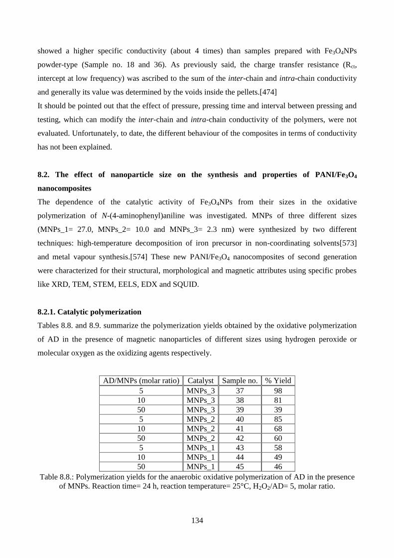
134
showed a higher specific conductivity (about 4 times) than samples prepared with Fe3O4NPs
powder-type (Sample no. 18 and 36). As previously said, the charge transfer resistance (Rct,
intercept at low frequency) was ascribed to the sum of the inter-chain and intra-chain conductivity
and generally its value was determined by the voids inside the pellets.[474]
It should be pointed out that the effect of pressure, pressing time and interval between pressing and
testing, which can modify the inter-chain and intra-chain conductivity of the polymers, were not
evaluated. Unfortunately, to date, the different behaviour of the composites in terms of conductivity
has not been explained.
8.2. The effect of nanoparticle size on the synthesis and properties of PANI/Fe3O4
nanocomposites
The dependence of the catalytic activity of Fe3O4NPs from their sizes in the oxidative
polymerization of N-(4-aminophenyl)aniline was investigated. MNPs of three different sizes
(MNPs_1= 27.0, MNPs_2= 10.0 and MNPs_3= 2.3 nm) were synthesized by two different
techniques: high-temperature decomposition of iron precursor in non-coordinating solvents[573]
and metal vapour synthesis.[574] These new PANI/Fe3O4 nanocomposites of second generation
were characterized for their structural, morphological and magnetic attributes using specific probes
like XRD, TEM, STEM, EELS, EDX and SQUID.
8.2.1. Catalytic polymerization
Tables 8.8. and 8.9. summarize the polymerization yields obtained by the oxidative polymerization
of AD in the presence of magnetic nanoparticles of different sizes using hydrogen peroxide or
molecular oxygen as the oxidizing agents respectively.
AD/MNPs (molar ratio) Catalyst Sample no. % Yield
5 MNPs_3 37 98
10 MNPs_3 38 81
50 MNPs_3 39 39
5 MNPs_2 40 85
10 MNPs_2 41 68
50 MNPs_2 42 60
5 MNPs_1 43 58
10 MNPs_1 44 49
50 MNPs_1 45 46
Table 8.8.: Polymerization yields for the anaerobic oxidative polymerization of AD in the presence
of MNPs. Reaction time= 24 h, reaction temperature= 25°C, H2O2/AD= 5, molar ratio.

135
AD/MNPs (molar ratio) Catalyst Sample no. % Yield
5 MNPs_3 46 70
10 MNPs_3 47 63
50 MNPs_3 48 54
5 MNPs_2 49 87
10 MNPs_2 50 69
50 MNPs_2 51 53
Table 8.9.: Polymerization yields for the aerobic oxidative polymerization of AD in the presence of
MNPs. Reaction time= 3 days, reaction temperature= 80°C, pO2= 3 bar.
When H2O2 was employed as the oxidant, the catalytic activity of MNPs increased with decreasing
their sizes, following the trend:
2.3 nm > 10 nm > 27.0 nm
However, this trend was not observed at higher values of AD/MNPs (molar ratio), where the
catalytic activity of smaller MNP_3 was even lower than that of the larger MNPs_1 (Table 8.8.).
Also under aerobic conditions the catalytic activity of MNPs_3 resulted to be always lower than
that of bigger ones (MNPs_2).
Such a behaviour of the smaller MNP_3 can be probably explained with an overoxidation of the
nanoparticles to Fe2O3. The absence of the bivalent metallic center (Fe2+
) on the surface of NPs
could interrupt the catalytic cycle, guaranteed by the couple Fe2+
/Fe3+
. However, at the moment,
this hypothesis has not yet been confirmed.
Similarly, as reported in Section 8.1., the amount of MNPs embedded into some PANI/Fe3O4
composite samples was measured by AAS and the results are summarized in Table 8.10.
Sample no. Catalyst Oxidant Loss of MNPs (%)
37
MNPs_3
H2O2
20
38 21
39 17
43
MNPs_1
3
44 3
45 6
46
MNPs_3 O2
21
47 20
48 54
Table 8.10.: Loss of MNPs into the PANI/Fe3O4 composites measured by AAS.

136
Under both aerobic and anaerobic conditions smaller nanoparticles (MNPs_3) showed higher
losses. Such a phenomenon confirmed that smaller NPs were more sensitive to the reaction
conditions than the bigger ones.
Unlike that for all the other MNPs, in the case of MNPs_1 a large amount of oleic acid was
employed to obtain a homogeneous organic dispersion of big nanoparticles. In order to investigate
if large quantities of oleic acid effect the catalytic activity of MNPs, a sample of MNPs_1
containing 60% of oleic acid was abundantly washed with acetone to remove any trace of
surfactant. Then, increasing amounts of oleic acid were added to MNPs and these latter were tested
in the oxidative polymerization of AD. The results, reported in Graphic 8.2., demonstrated that the
amount of oleic acid practically didn’t affect the polymerization reaction.
Graphic 8.2.: Yield % against oleic acid %. Reaction conditions: reaction time= 24 h, reaction temperature=
25°C, H2O2/AD= 5 (molar ratio), AD/MNPs= 50 (molar ratio).
All the materials were characterized by different techniques. FT-IR and UV-vis spectra resulted to
be similar to those reported in Figures 8.1. and 8.2., confirming that into the composites polyaniline
was in its conductive emeraldine form.
XRPD diffractograms of these second generation of PANI/Fe3O4 composites are reported in Figures
8.11. A-C.

137
As it is possible to observe, the presence of the inorganic magnetic component resulted evident in
the composite materials prepared with MNPs_1 and MNPs_2, whereas the absence of diffraction
peaks of magnetite in composites synthesized in the presence of MNPs_3 might be attributed to the
very small size of NPs.
Figure 8.11.: XRPD patterns of A) composites containing MNPs_1 (a= sample no.45, b= sample no. 44, c=
sample no. 43), B) composites containing MNPs_2 (a= sample no.42, b= sample no. 41, c= sample no. 40),
C) composites containing MNPs_3 (a= sample no.39, b= sample no. 38, c= sample no. 37).
A B
C
a
b
c
a
b
c
a
b
c

138
8.2.2. Morphological characterization
The PANI/Fe3O4 composites were characterized for their structural and morphological attributes
using specific probes like XRD, TEM, STEM, EELS and EDX and the results are reported below
(Figure 8.12.).
200 nm
200 nm
A
B
C D
E
F

139
100 nm
200 nm
G
H
I
J
K
L

140
100 nm
M N
O
P
Q
100 nm
141
Figure 8.12.: A) TEM image of MNP_1, B) statistical distribution of MNP_1 diameters, C) TEM image of
PANI/MNP_1 composite (Sample 43) with contrast improved by energy filtering, D) statistical analysis of
size distribution of MNP_1 inside PANI/MNP_1 composite (Sample 43), E) electron diffraction pattern of
PANI/MNP_1 composite and corresponding analysis (F), G) PANI/MNP_1 sample EFTEM (Energy Filtered
50 nm
50 nm
100 nm
R
S
T
U
V

142
TEM) image: in red is reporder the image generated only from iron, H) EELS (Electron Energy loss
Spectroscopy) spectrum of PANI/ MNP_1 sample the red arrow underlines the Fe L2,3 signal, I) TEM image
of MNP_2, J) statistical distribution of MNP_2 diameters, K) TEM image of PANI/MNP_2 composite
(Sample 40) without any energy filtering, L) statistical analysis of size distribution of MNP_2 inside
PANI/MNP_2 composite (Sample 40), M) PANI/MNP_2 sample(Sample 40) conventional TEM image,
reference image for the EFTEM (Energy Filtered TEM) image (N): in red is reporder the image generated
only from iron, O) EELS (Electron Energy loss Spectroscopy) spectrum of PANI/MNP_2 sample (Sample
40) the red arrows underline the Fe L2,3 signal, P) electron diffraction pattern of PANI/MNP_2 sample
(Sample 40) and corresponding analysis (Q), R) TEM image of MNP_3, S) statistical distribution of MNP_3
diameters, T) TEM image of PANI/MNP_3 composite (Sample 37) with contrast improved by energy
filtering, U) PANI/MNP_3 (Sample 37) STEM image, V) PANI/MNP_3 (Sample 37) Energy Dispersive X-
ray (EDX) spectrum.
To image the MNPs within the composite, and thus study their morphology and distribution, an
energy filtered TEM was used to optimize the contrast between MNPs and polymer by using
electrons with an energy loss of 30 eV, so that the polymer matrix appeared as a light gray halo
instead of being very dark as occurs in conventional ZLF (zero-loss filtered) TEM.
In all cases the morphology of magnetic NPs resulted to be unchanged during the composite
synthesis and a good dispersion within the PANI matrix was observed.
In order to verify that they didn’t suffer from a change of crystal phase and/or chemical composition
during the synthesis, several micro analytical techniques were used to examine the samples in
depth.
Electron diffraction (ED) patterns confirmed that PANI/MNP_1 and PANI/MNP_2 (Figures 8.12. E
and P) comprised magnetite MNPs with spinel structure. PANI/MNP_3 gave no detectable
diffraction probably because of ring broadening brought about by their small size. So, in this case
Scanning TEM (STEM) (Figure 8.12. U) and STEM/Energy Dispersive X-ray (EDX) spectroscopy
(Figure 8.12. V) were performed: the MNP_3 nanoparticles were distinctly visible in STEM image
and the EDX spectrum (not reported) showed the presence of Fe into the composite.
Electron Energy Loss Spectroscopy (EELS) and Energy Selected Imaging (ESI) experiments were
also performed. In the EELS spectrum of the composites (Figures 8.12. H, G, N, O), the Fe-L2,3
edge, with the typical “white lines", starting from 708 eV was clearly seen for all the three samples.
ESI images selecting the Fe-L2,3 edge energy were collected for PANI/MNP_1 and PANI/MNP_2,
instrumental resolution being too low to image the individual NPs in PANI/MNP_3.
8.2.3. Magnetic measurements
Magnetic measurements were carried out by the use of a Quantum Design MPMS XL-5 SQUID
magnetometer. The magnetic properties of PANI/MNPs nanocomposites were evaluated by
measuring the hysteresis cycle in the field-cooling condition (HysFC, Hcool = 50 kOe) and the

143
temperature dependence of the magnetization in both Zero Field Cooling (ZFC) and Field Cooling
(FC, Hcool = 10 Oe) modes. In both cases the measuring field was 10 Oe.
The saturation magnetization Ms, the remanence Mr and the coercive field Hc are reported in Table
8.11 and M-H curves are shown in Figure 8.13.
Parameter Sample no. 37 Sample no. 40 Sample no. 43
Ms (emu/g)a, b
8.9 16.6 13.8
Mr (emu/g)b 0.03 4.0 2.1
Mr/Ms 0.003 0.24 0.15
Hc (Oe) 0.08 0.45 0.60
Tirr (K) 150 110 300
Tmax,ZFC (K) 5 90 310
Tder,ZFC (K) 5 60 270
Table 8.11.: Magnetic properties of PANI/MNPs composites (Sample no. 37, 40 and 43). aMs and Mr are
referred to composite mass and at 50 kOe.
-50 -40 -30 -20 -10 0 10 20 30 40 50-10
-8
-6
-4
-2
0
2
4
6
8
10
H (kOe)
M (
em
u/g
)
-50 -40 -30 -20 -10 0 10 20 30 40 50-20
-15
-10
-5
0
5
10
15
20
H (kOe)
M (
em
u/g
)
-50 -40 -30 -20 -10 0 10 20 30 40 50-15
-10
-5
0
5
10
15
H (kOe)
M (
em
u/g
)
A B
C
Figure 8.13.: Magnetization-demagnetization M-H curves of (a) Sample no.37, (b) Sample no. 40 and (c)
sample 43.

144
As it is possible to observe, PANI/Fe3O4 composite (Sample no. 37) containing smaller magnetic
nanoparticles didn’t reach saturation even to 50 kOe, didn’t exhibit remanence and coercitivity and
didn’t show hysteresis.
As expected, the other composites (Samples no. 40 and 43) saturated within 50 kOe, exhibited
remanence and coercitivity and showed very small hysteresis that increased with the NPs sizes.
The unexpected trend observed for the Mr/Ms values, could be due to a different distribution of
inorganic nanoparticles within the polymeric matrix. In fact, in general the value of this ratio
increased with the NPs sizes.
To better understand the magnetic properties of PANI/Fe3O4 composites, ZFC (zero-field cooling)
and FC (field cooling) magnetization were measured (Figure 8.14.). The characteristic temperatures
derived from ZFC/FC data are reported in Table 8.11.
A
A’ B’
B
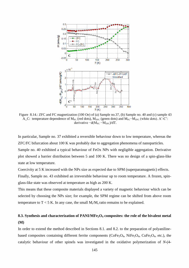
145
All composites show the magnetic behaviours expected for the corresponding magnetic NPs with
different sizes.
In particular, Sample no. 37 exhibited a reversible behaviour down to low temperature, whereas the
ZFC/FC bifurcation about 100 K was probably due to aggregation phenomena of nanoparticles.
Sample no. 40 exhibited a typical behaviour of FeOx NPs with negligible aggregation. Derivative
plot showed a barrier distribution between 5 and 100 K. There was no design of a spin-glass-like
state at low temperature.
Coercivity at 5 K increased with the NPs size as expected due to SPM (superparamagnetic) effects.
Finally, Sample no. 43 exhibited an irreversible behaviour up to room temperature. A frozen, spin-
glass-like state was observed at temperature as high as 200 K.
This means that these composite materials displayed a variety of magnetic behaviour which can be
selected by choosing the NPs size; for example, the SPM regime can be shifted from above room
temperature to T < 5 K. In any case, the small Mr/Ms ratio remains to be explained.
8.3. Synthesis and characterization of PANI/MFe2O4 composites: the role of the bivalent metal
(M)
In order to extend the method described in Sections 8.1. and 8.2. to the preparation of polyaniline-
based composites containing different ferrite components (CoFe2O4, NiFe2O4, CuFe2O4, etc.), the
catalytic behaviour of other spinels was investigated in the oxidative polymerization of N-(4-
Figure 8.14.: ZFC and FC magnetization (100 Oe) of (a) Sample no.37, (b) Sample no. 40 and (c) sample 43
A_C: temperature dependence of MFC (red dots), MZFC (green dots) and MFC−MZFC (white dots). A’-C’:
derivative −d(MFC −MZFC)/dT.
C
C’

146
aminophenyl)aniline, replacing iron(II) with another metal (Mn, Co, Ni, Cu, Zn, Mg). This
approach allowed to clarify what is the catalytically active metallic center in the spinel structure.
MFe2O4 materials (M= Co, Ni, Mn, Cu, Zn, Mg) were synthesized by chemical co-precipitation
method and PANI/MFe2O4 composites were characterized by different techniques: FT-IR, UV-vis,
XRPD, TEM and SQUID.
8.3.1. Catalytic polymerization using CoFe2O4 NPs as the catalysts
At first, Fe(II) was replaced with Co(II) and CoFe2O4NPs were produced as powder (CoMNPsp)
and ferrofluid (oleic acid-modified NPs dispersed in toluene, CoMNPsff).
Tables 8.12. and 8.13. report the results obtained in terms of yield in the oxidative polymerization
of AD using H2O2 and molecular oxygen as the oxidants.
AD/CoFe2O4 (molar ratio) CoMNPsff CoMNPsp
Sample no. Yield (%) Sample no. Yield (%)
50 52 67 55 59
10 53 75 56 70
5 54 81 57 74
Table 8.12.: Polymerization yields for the aerobic oxidative polymerization of AD in the presence
of CoMNPs. Reaction time= 3 days, reaction temperature= 80°C, pO2= 3 bar.
AD/CoFe2O4 (molar ratio) CoMNPsff CoMNPsp
Sample no. Yield (%) Sample no. Yield (%)
50 58 80 61 53
10 59 89 62 70
5 60 98 63 83
Table 8.13: Polymerization yields for the anaerobic oxidative polymerization of AD in the presence of CoMNPs. Reaction time= 24 h, reaction temperature= 25°C, H2O2/AD= 5, molar ratio.
These results showed that both CoMNPs powder- and ferrofluid-type resulted to be good candidates
as catalysts for the oxidative polymerization of AD.
However, contrary to what was observed for Fe3O4 NPs (Tables 8.1. and 8.2.), the catalytic activity
of CoMNPs was higher under aerobic conditions than in the presence of hydrogen peroxide. In fact,
as reported above (section 8.1.), hydrogen peroxide allowed to achieve polyaniline with 40% yield
after 24 h also in the absence of any catalyst. This means that the starting point “zero” was different

147
for the two oxidants. Such an effect was more evident if yields were calculated according to Eq. 8.1.
(Graphic 8.3.).
As shown in Graphic 8.3., even though in the presence of molecular oxygen both CoMNPs powder-
and ferrofluid-type exhibited similar catalytic activities, on the contrary using hydrogen peroxide
they displayed different behaviours. In particular, CoMNPsff showed higher catalytic performances
if compared to the CoMNPsp.
The different results obtained using different oxidants could be ascribed to the ability of CoMNPs to
decompose H2O2. In fact, as reported by Lahiri et al., [575], spinel ferrites (in particular, manganese
and cobalt ferrites) are active in the decomposition of H2O2. This means that the presence of
CoMNPs into the reaction mixture might limit the presence of the oxidant thus producing polymer
in low yield. However, when magnetic NPs were capped with oleic acid to give the corresponding
ferrofluid-type NPs, their catalytic activity towards H2O2 decomposition was depressed and the
polymer yield increased (Table 8.13. and Graphic 8.3.).
As reported in Section 8.1. for Fe3O4NPs, also in this case the content of inorganic component into
the final composites was determined by atomic absorption spectroscopy (AAS) and the results,
summarized in Table 8.14., confirmed that the inorganic component was totally incorporated into
the final insoluble composites maintaining a constant Fe/Co molar ratio of 2.
Graphic 8.3.: Dependence of the catalytic yields of the AD oxidative polymerization from the
amount of CoMNPs.
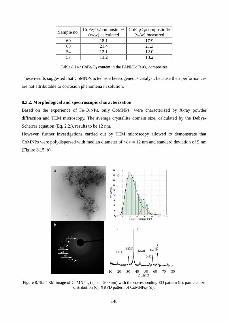
148
Sample no. CoFe2O4/composite %
(w/w) calculated
CoFe2O4/composite %
(w/w) measured
60 18.1 17.9
63 21.4 21.3
54 12.1 12.0
57 13.2 13.2
Table 8.14.: CoFe2O4 content in the PANI/CoFe2O4 composites
These results suggested that CoMNPs acted as a heterogeneous catalyst, because their performances
are not attributable to corrosion phenomena in solution.
8.3.2. Morphological and spectroscopic characterization
Based on the experience of Fe3O4NPs, only CoMNPsff were characterized by X-ray powder
diffraction and TEM microscopy. The average crystallite domain size, calculated by the Debye-
Scherrer equation (Eq. 2.2.), results to be 12 nm.
However, further investigations carried out by TEM microscopy allowed to demonstrate that
CoMNPs were polydispersed with median diameter of <d> = 12 nm and standard deviation of 5 nm
(Figure 8.15. b).
Figure 8.15.: TEM image of CoMNPsff (a, bar=200 nm) with the corresponding ED pattern (b), particle size
distribution (c), XRPD pattern of CoMNPsff (d).
{111} {220}
{311}
{222}
{440
} {422}
{511}
a
b
c
d

149
More in detail, the size histogram reported in Figure 8.15. b suggested that two different NP
populations were present, the major one (95%) with <d> = 12 nm and the minor one (5%) with <d>
= 20 nm. The spinel structure of MNPs, previously observed by the XRPD pattern (Figure 8.15. d),
was confirmed by electron diffraction (ED) pattern (Figure 8.15. b), corresponding to the bright-
field image (Figure 8.15. a).
The presence of CoMNPs into the composites, already established by AAS analyses (Table 8.14.)
was confirmed by X-ray powder diffraction, as shown in Figure 8.16.
Figure 8.16.: XRPD patterns of CoMNPsff (a) and its composites with PANI (b= sample no. 60, c= sample
no. 59)
The broad peak at around 25° can be assigned to the amorphous polymeric matrix, whereas the
other peaks can be assigned to pure cobalt ferrite phase with a cubic spinel structure, according to
the literature.[576]
Moreover, the mean diameter of CoMNPs embedded into the polymeric matrix resulted to be
unchanged (about 12 nm) if compared to that of pristine nanoparticles, as shown in Table 8.15.
Sample Mean diameter (nm)
MNPsff 12.0
Sample no. 59 12.4
Sample no. 60 12.7
Table 8.15.: Mean diameter of the CoMNPs calculated by the Scherrer’s equation
a
b
c
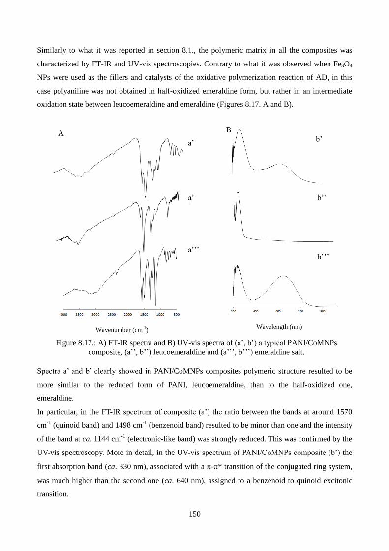
150
Similarly to what it was reported in section 8.1., the polymeric matrix in all the composites was
characterized by FT-IR and UV-vis spectroscopies. Contrary to what it was observed when Fe3O4
NPs were used as the fillers and catalysts of the oxidative polymerization reaction of AD, in this
case polyaniline was not obtained in half-oxidized emeraldine form, but rather in an intermediate
oxidation state between leucoemeraldine and emeraldine (Figures 8.17. A and B).
Spectra a’ and b’ clearly showed in PANI/CoMNPs composites polymeric structure resulted to be
more similar to the reduced form of PANI, leucoemeraldine, than to the half-oxidized one,
emeraldine.
In particular, in the FT-IR spectrum of composite (a’) the ratio between the bands at around 1570
cm-1
(quinoid band) and 1498 cm-1
(benzenoid band) resulted to be minor than one and the intensity
of the band at ca. 1144 cm-1
(electronic-like band) was strongly reduced. This was confirmed by the
UV-vis spectroscopy. More in detail, in the UV-vis spectrum of PANI/CoMNPs composite (b’) the
first absorption band (ca. 330 nm), associated with a -* transition of the conjugated ring system,
was much higher than the second one (ca. 640 nm), assigned to a benzenoid to quinoid excitonic
transition.
Figure 8.17.: A) FT-IR spectra and B) UV-vis spectra of (a’, b’) a typical PANI/CoMNPs
composite, (a’’, b’’) leucoemeraldine and (a’’’, b’’’) emeraldine salt.
Wavenumber (cm-1
)
a’
a’
’
a’’’
b’
b’’
b’’’
Wavelength (nm)
A B

151
The FT-IR and UV-vis analyses, together with the reaction yields, showed that, even though
CoMNPs exhibited catalytic activity in the oxidative polymerization of N-(4-amino phenyl)aniline,
they stopped the reaction before that polymer reached the oxidation state of emeraldine.
In order to address the oxidative polymerization reaction towards conducting emeraldine form, a co-
catalyst able to complete the oxidation process was added to the reaction mixture. Fe3+
(AD/Fe3+
=
1000 molar ratio) was chosen as the co-catalyst owing to its catalytic ability, as reported in the
literature.[36] In this case the polymeric matrix of the composites was obtained in the conductive
emeraldine form, as confirmed by FT-IR and UV-vis spectroscopies, that showed spectra similar to
those reported in Figures 8.1. and 8.2., and by conductivity measurements (Table 8.16.)
Sample (S cm-1)
Emeraldine salt 3.5 10-3
Leucoemeraldine 1.0 10-8
Sample no. 59 7.3 10-5
Sampleno. 60 4.9 10-5
PANI/CoMNPs with co-catalyst 5.5 10-3
Table 8.16.: Conductivity values of emeraldine salt, leucoemeraldine, Sample no. 59, Sample no. 60 and
PANI/CoMNPs composite prepared in the presence of Fe3+
as the co-catalyst.
As for PANI/Fe3O4 composites (Figure 8.7.), also for PANI/CoMNPs materials the positive effect
of the presence of magnetic fillers into the polymeric matrix on its thermal stability was observed
by TGA technique (Figure 8.18.).

152
Figure 8.18.: TGA results for (a) pure PANI (Sample no. 20), (b) Sample no. 62 and (c) sample no. 63.
8.3.3. Magnetic measurements
In order to define a CoFe2O4 NP single-domain structure its diameter has to be < ca. 320 nm.
Moreover, in order to reverse its magnetization by coherent rotation its diameter has to be < ca. 50
nm. XRD and TEM investigation (Fig. 8. 15) showed that individual CoMNPs reported above
showed smaller diameters than these (329 n and 50 nm). It’s well known from the literature,[577]
that the blocking diameter for CoMNPs is 9 nm at 300 K and 2 nm at 5 K. For this reason CoMNPs
and PANI/CoMNPs should exhibit a partial superparamagnetic behavior at high temperature.
However, it should be stressed that these critical diameters – especially the blocking diameters – are
valid for non-interacting NPs free from surface effects. The magnetization of CoMNPsff and
PANI/CoMNPs composites (Samples no.: 53, 54, 59 and 60) were measured either as a function of
temperature in the range 300-5 K at low field (10 Oe) in ZFC and FC mode, and as magnetization
isotherm (hysteresis loop) between ±50 kOe at 5 K after FC (+50 kOe) from 295 K.
Figure 8.19 shows the ZFC and FC magnetization curves and the main parameters are summarized
in Table 8.17.
b
c
a

153
Figure 8.19.: Magnetization of CoMNPsff and PANI/CoMNPs composites. Left: ZFC (solid circles)
and FC (hollow circles) magnetization; right: magnetization isotherms (FC hysteresis loops). A),
CoMNPsff, B) sample no. 54, C) sample no. 60, D) sample no. 53, E) sample no. 59.
Sample T0 (K)
a (K
–b) b
CoMNPsff 746±3 (3.4±0.3) 10–6
1.91±0.01
54
783±12 (9±2) 10–6
1.74±0.05
60 793±6 (12±2) 10–6
1.69±0.02
53 727±7 (2.6±0.5) 10–6
1.95±0.04
59 759±4 (9.1±0.9) 10–6
1.75±0.02 a Generalized Bloch-type law: M(T) = M(0) (1 – aT
b), T0 = a
-1/b.
Table 8.17.: Optimal parameters from fitting the FC low-field magnetization of ferrofluid-type
CoFe2O4 NPs and PANI-CoFe2O4 NP composites to the generalized Bloch-type law. a
The data showed that the samples did not reach saturation even at 50 kOe and had high coercivity.
The values of saturation magnetization (Msat) at 50 kOe are in accordance with those reported in
the literature for bulk CoFe2O4 [578].
The ZFC and FC curves of CoMNPsff overlapped in the 5-300 K range and both MZFC and MFC
increased on cooling. These curves are very similar to those observed for bulk ferrites.[578] In the
investigated temperature range, there was no evidence of superparamagnetic behavior with its
A
B
C
D
E
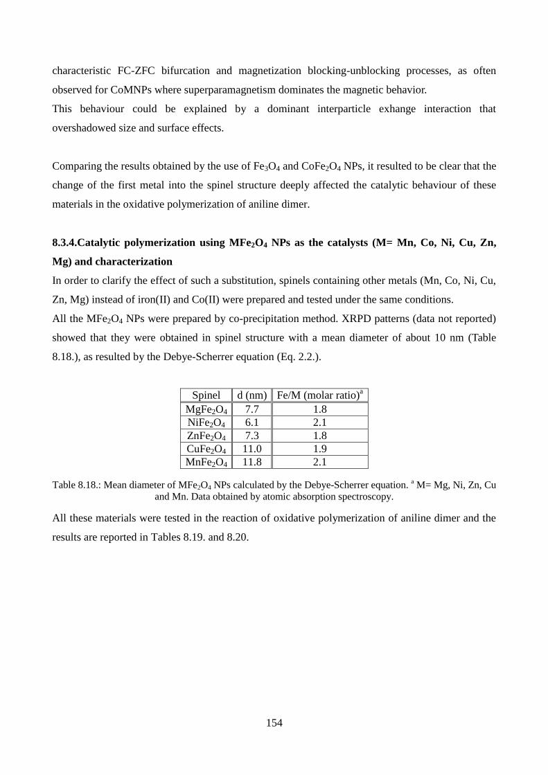
154
characteristic FC-ZFC bifurcation and magnetization blocking-unblocking processes, as often
observed for CoMNPs where superparamagnetism dominates the magnetic behavior.
This behaviour could be explained by a dominant interparticle exhange interaction that
overshadowed size and surface effects.
Comparing the results obtained by the use of Fe3O4 and CoFe2O4 NPs, it resulted to be clear that the
change of the first metal into the spinel structure deeply affected the catalytic behaviour of these
materials in the oxidative polymerization of aniline dimer.
8.3.4.Catalytic polymerization using MFe2O4 NPs as the catalysts (M= Mn, Co, Ni, Cu, Zn,
Mg) and characterization
In order to clarify the effect of such a substitution, spinels containing other metals (Mn, Co, Ni, Cu,
Zn, Mg) instead of iron(II) and Co(II) were prepared and tested under the same conditions.
All the MFe2O4 NPs were prepared by co-precipitation method. XRPD patterns (data not reported)
showed that they were obtained in spinel structure with a mean diameter of about 10 nm (Table
8.18.), as resulted by the Debye-Scherrer equation (Eq. 2.2.).
Spinel d (nm) Fe/M (molar ratio)a
MgFe2O4 7.7 1.8
NiFe2O4 6.1 2.1
ZnFe2O4 7.3 1.8
CuFe2O4 11.0 1.9
MnFe2O4 11.8 2.1
Table 8.18.: Mean diameter of MFe2O4 NPs calculated by the Debye-Scherrer equation. a M= Mg, Ni, Zn, Cu
and Mn. Data obtained by atomic absorption spectroscopy.
All these materials were tested in the reaction of oxidative polymerization of aniline dimer and the
results are reported in Tables 8.19. and 8.20.

155
Sample no. MFe2O4 AD/MFe2O4 (molar ratio) Yield %
64
NiFe2O4
5 77
65 10 64
66 50 61
67
CuFe2O4
5 86
68 10 82
69 50 81
70 ZnFe2O4 5 61
71 MgFe2O4 5 63
72 MnFe2O4 5 48
Table 8.19.: Polymerization yields for the aerobic oxidative polymerization of AD in the presence
of MFe2O4 NPs. Reaction time= 3 days, reaction temperature= 80°C, pO2= 3 bar.
Sample no. MFe2O4 AD/MFe2O4 (molar ratio) Yield %
73
NiFe2O4
5 66
74 10 43
75 50 24
76
CuFe2O4
5 63
77 10 34
78 50 28
79 ZnFe2O4 5 31
80 MnFe2O4 5 21
81 MgFe2O4 5 18
Table 8.20.: Polymerization yields for the anaerobic oxidative polymerization of AD in the presence of MFe2O4 NPs. Reaction time= 24 h, reaction temperature= 25°C, H2O2/AD= 5, molar ratio.
As reported in Tables 8.19. and 8.20., under aerobic conditions all the ferrites showed interesting
catalytic behaviours, exhibiting quite high polymerization yields (from 48 to 66%). On the contrary,
when the reaction was carried out under anaerobic conditions, using H2O2 as the oxidant, good
results in terms of yield were obtained only for NiFe2O4 and CuFe2O4 NPs.
Regarding MFe2O4, a different catalytic activity appeared when H2O2 was employed as the oxidant.
As reported in the literature and discussed above,[575] spinels resulted to be good catalysts in the
H2O2 decomposition reaction. This means that during AD oxidative polymerization part of the

156
oxidant could be subtracted to the polymerization reaction mixture, justifying the lower
polymerization yield observed under these conditions.
Graphic 8.4. summarizes the results obtained in the oxidative polymerization of AD when spinels
NPs (Fe3O4, CoFe2O4, NiFe2O4, MnFe2O4, CuFe2O4, MgFe2O4 and ZnFe2O4) were employed under
the same reaction conditions in the presence of hydrogen peroxide as the oxidant.
Graphic 8.4. Dependence of polymerization yields from the first metallic center of spinel structures.
Reaction conditions: AD/MFe2O4= 5 (molar ratio), H2O2/AD= 5 (molar ratio), temperature= 25°C, reaction
time= 24 h.
It looks clear that the catalytic effect of spinel ferrite NPs on PANI preparation was strictly related
to the first metallic center, following the trend reported below:
Fe ≥ Co > Ni ≥ Cu >> Zn > Mn ≥ Mg
The best results in terms of yield were obtained using Fe3O4, CoFe2O4, NiFe2O4 and CuFe2O4 NPs
as the reaction catalysts and magnetic fillers, whereas in all the other cases PANI was obtained in
very low yield.
In order to justify the trend observed, the results obtained in terms of yield were correlated to the
their ability to decompose H2O2 and to the inversion degree of the ferrites.
Table 8.21. reveals that the catalytic activity of the ferrites in the decomposition of H2O2 follows
the order: Mn > Co > Cu > Ni >Cd > Zn in MFe2O4.[575]
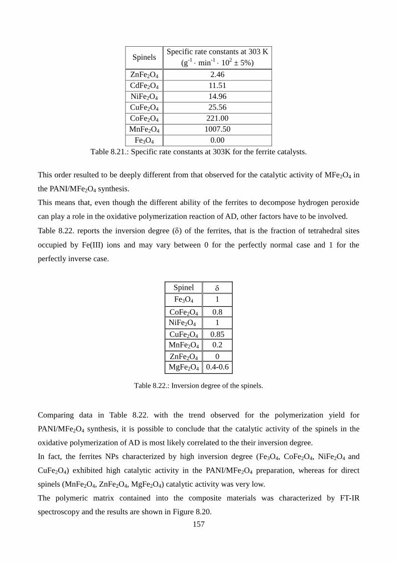
157
Spinels Specific rate constants at 303 K
(g-1
min-1
102 ± 5%)
ZnFe2O4 2.46
CdFe2O4 11.51
NiFe2O4 14.96
CuFe2O4 25.56
CoFe2O4 221.00
MnFe2O4 1007.50
Fe3O4 0.00
Table 8.21.: Specific rate constants at 303K for the ferrite catalysts.
This order resulted to be deeply different from that observed for the catalytic activity of MFe2O4 in
the PANI/MFe2O4 synthesis.
This means that, even though the different ability of the ferrites to decompose hydrogen peroxide
can play a role in the oxidative polymerization reaction of AD, other factors have to be involved.
Table 8.22. reports the inversion degree () of the ferrites, that is the fraction of tetrahedral sites
occupied by Fe(III) ions and may vary between 0 for the perfectly normal case and 1 for the
perfectly inverse case.
Spinel
Fe3O4 1
CoFe2O4 0.8
NiFe2O4 1
CuFe2O4 0.85
MnFe2O4 0.2
ZnFe2O4 0
MgFe2O4 0.4-0.6
Table 8.22.: Inversion degree of the spinels.
Comparing data in Table 8.22. with the trend observed for the polymerization yield for
PANI/MFe2O4 synthesis, it is possible to conclude that the catalytic activity of the spinels in the
oxidative polymerization of AD is most likely correlated to the their inversion degree.
In fact, the ferrites NPs characterized by high inversion degree (Fe3O4, CoFe2O4, NiFe2O4 and
CuFe2O4) exhibited high catalytic activity in the PANI/MFe2O4 preparation, whereas for direct
spinels (MnFe2O4, ZnFe2O4, MgFe2O4) catalytic activity was very low.
The polymeric matrix contained into the composite materials was characterized by FT-IR
spectroscopy and the results are shown in Figure 8.20.

158
Figure 8.20.: FT-IR spectra of (Mg) Sample no. 81, (Mn) Sample no. 80, (Zn) Sample no. 79, (Cu) Sample
no. 76, (Ni) Sample no. 73, (Co) Sample no. 63, (Fe) Sample no. 36.
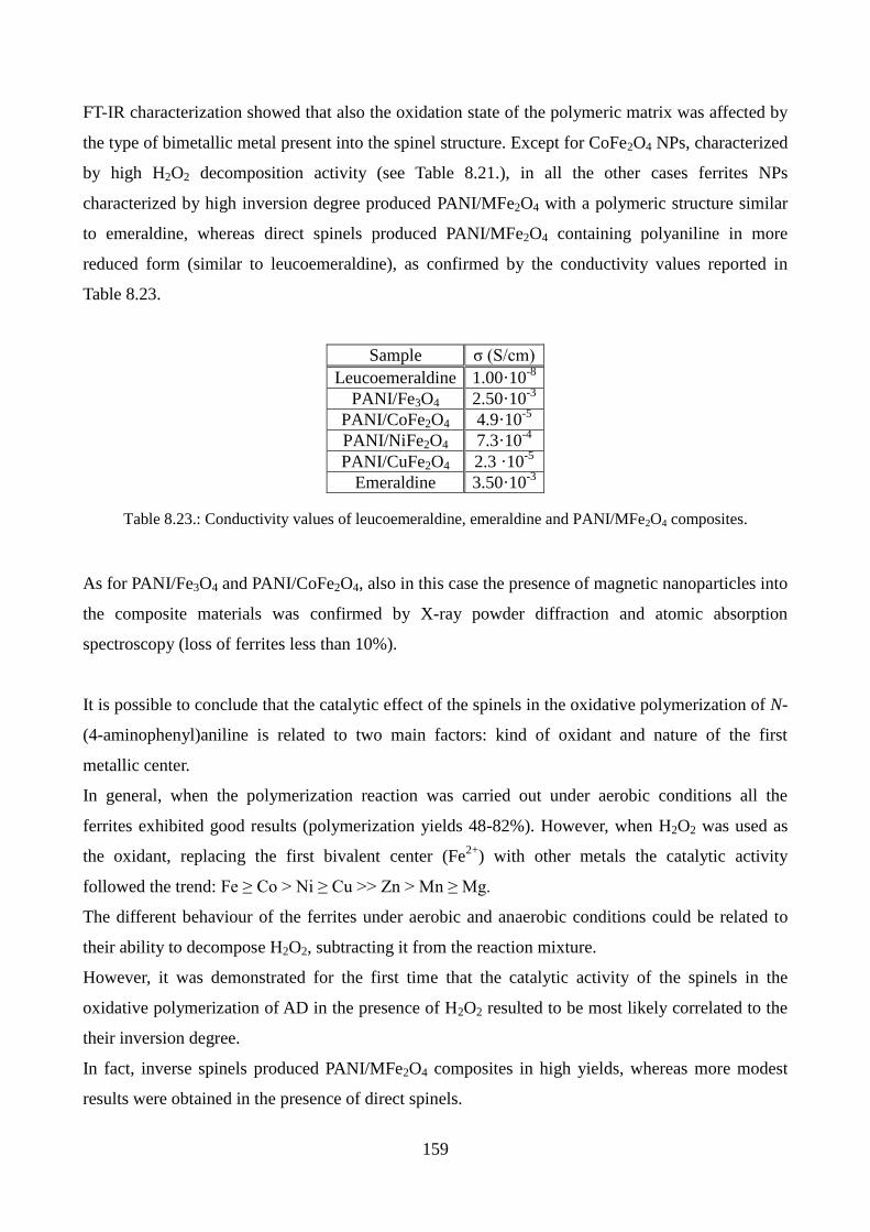
159
FT-IR characterization showed that also the oxidation state of the polymeric matrix was affected by
the type of bimetallic metal present into the spinel structure. Except for CoFe2O4 NPs, characterized
by high H2O2 decomposition activity (see Table 8.21.), in all the other cases ferrites NPs
characterized by high inversion degree produced PANI/MFe2O4 with a polymeric structure similar
to emeraldine, whereas direct spinels produced PANI/MFe2O4 containing polyaniline in more
reduced form (similar to leucoemeraldine), as confirmed by the conductivity values reported in
Table 8.23.
Sample σ (S/cm)
Leucoemeraldine 1.00·10-8
PANI/Fe3O4 2.50·10-3
PANI/CoFe2O4 4.9·10-5
PANI/NiFe2O4 7.3·10-4
PANI/CuFe2O4 2.3 ·10-5
Emeraldine 3.50·10-3
Table 8.23.: Conductivity values of leucoemeraldine, emeraldine and PANI/MFe2O4 composites.
As for PANI/Fe3O4 and PANI/CoFe2O4, also in this case the presence of magnetic nanoparticles into
the composite materials was confirmed by X-ray powder diffraction and atomic absorption
spectroscopy (loss of ferrites less than 10%).
It is possible to conclude that the catalytic effect of the spinels in the oxidative polymerization of N-
(4-aminophenyl)aniline is related to two main factors: kind of oxidant and nature of the first
metallic center.
In general, when the polymerization reaction was carried out under aerobic conditions all the
ferrites exhibited good results (polymerization yields 48-82%). However, when H2O2 was used as
the oxidant, replacing the first bivalent center (Fe2+
) with other metals the catalytic activity
followed the trend: Fe ≥ Co > Ni ≥ Cu >> Zn > Mn ≥ Mg.
The different behaviour of the ferrites under aerobic and anaerobic conditions could be related to
their ability to decompose H2O2, subtracting it from the reaction mixture.
However, it was demonstrated for the first time that the catalytic activity of the spinels in the
oxidative polymerization of AD in the presence of H2O2 resulted to be most likely correlated to the
their inversion degree.
In fact, inverse spinels produced PANI/MFe2O4 composites in high yields, whereas more modest
results were obtained in the presence of direct spinels.

160
Finally, inverse spinels led to composites containing PANI in conducting emeraldine form, whereas
when direct spinels were used as the catalysts polymeric matrix resulted to be more reduced (similar
to leucoemeraldine).
8.4. Electromagnetic characterization
Complex permittivity (ε* = ε’-i ε’’) and complex permeability (μ* = μ’ – iμ’’) were derived from
the measured scattering parameters (S11 and S21). Measurements were carried out in waveguide
WR42 between 18 and 26 GHz using an accurate deembedding procedure with calibrated standards.
Two samples were prepared by mixing a host medium (PVA, polyvinyl acetate) with a polyaniline
and PANI/Fe3O4 respectively, as described in Chapter 7, paragraph 7.9. Owing to the high amount
of material necessary to carry out these measures, PANI/Fe3O4 composite was realized by
mechanical mixing of PANI and Fe3O4 NPs (11 nm, prepared as describe in Chapter 6, paragraph
6.3.1.) maintaining a PANI/Fe3O4 ratio of 1:0.2 (w/w). The permittivity and permeability of both
PANI and PANI/Fe3O4 materials were retrieved from the measured scattering parameters by
Bruggeman’s method.[579] It is well known that real (ε’, μ’) and imaginary (ε’’, μ’’) parts of
complex permittivity and permeability characterize respectively the electric and magnetic
polarizability and the energy loss due to electric and magnetic effects.[580, 581]
Figures 8.21 show the real and imaginary part of relative permittivity and permeability for each
sample.
A

161
Figure 8.21.: Frequency dependence of real (A) and imaginary (B) part of complex
permittivity and real (C) and imaginary (D) part of complex permeability for PANI
and PANI/Fe3O4 composite
B
C
D
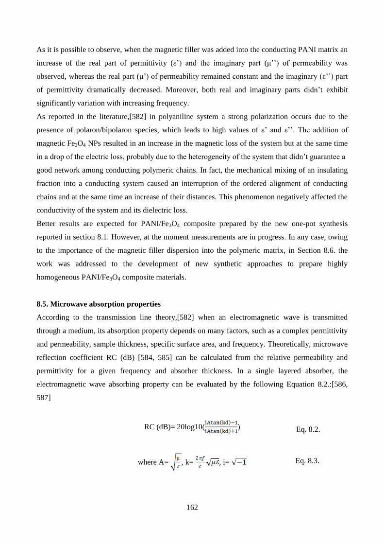
162
As it is possible to observe, when the magnetic filler was added into the conducting PANI matrix an
increase of the real part of permittivity (ε’) and the imaginary part (μ’’) of permeability was
observed, whereas the real part (μ’) of permeability remained constant and the imaginary (ε’’) part
of permittivity dramatically decreased. Moreover, both real and imaginary parts didn’t exhibit
significantly variation with increasing frequency.
As reported in the literature,[582] in polyaniline system a strong polarization occurs due to the
presence of polaron/bipolaron species, which leads to high values of ε’ and ε’’. The addition of
magnetic Fe3O4 NPs resulted in an increase in the magnetic loss of the system but at the same time
in a drop of the electric loss, probably due to the heterogeneity of the system that didn’t guarantee a
good network among conducting polymeric chains. In fact, the mechanical mixing of an insulating
fraction into a conducting system caused an interruption of the ordered alignment of conducting
chains and at the same time an increase of their distances. This phenomenon negatively affected the
conductivity of the system and its dielectric loss.
Better results are expected for PANI/Fe3O4 composite prepared by the new one-pot synthesis
reported in section 8.1. However, at the moment measurements are in progress. In any case, owing
to the importance of the magnetic filler dispersion into the polymeric matrix, in Section 8.6. the
work was addressed to the development of new synthetic approaches to prepare highly
homogeneous PANI/Fe3O4 composite materials.
8.5. Microwave absorption properties
According to the transmission line theory,[582] when an electromagnetic wave is transmitted
through a medium, its absorption property depends on many factors, such as a complex permittivity
and permeability, sample thickness, specific surface area, and frequency. Theoretically, microwave
reflection coefficient RC (dB) [584, 585] can be calculated from the relative permeability and
permittivity for a given frequency and absorber thickness. In a single layered absorber, the
electromagnetic wave absorbing property can be evaluated by the following Equation 8.2.:[586,
587]
RC (dB)= 20log10( )
where A= , k= , i=
Eq. 8.2.
Eq. 8.3.

163
In the above equations (Eq. 8.3.), µ and ε are, respectively, the complex permeability and
permittivity of the absorbing material, k is the wavenumber, f is the frequency of the incident
electromagnetic wave, c is the speed of light in vacuum and d is the thickness of the absorbing
layer.
Figures 8.22. A-C present the variation of shielding effectiveness due to reflection (SER) and
absorption (SEA) in the frequency range of 18-26 GHz for PANI and PANI/Fe3O4 samples.
B
A

164
Figure 8.22.: Frequency dependence of reflection (A and B) and transmission (C) coefficients.
PANI sample showed a higher effect on microwave absorbing properties than PANI/Fe3O4
composite, revealing at 26 GHz values of reflection and transmission coefficient of -8dB and -32dB
respectively, whereas under the same conditions PANI/Fe3O4 sample showed values of -7.5dB and -
17dB. These results were interpreted in terms of non-homogeneous distribution of Fe3O4 NPs into
the polymeric matrix that has a negative effect in the composite performance.
The calculated absorption spectra for all the samples have been compared with measured spectra
and the shapes of both experimental and theoretically calculated spectra resulted to be similar
(Figure 8.23.)
C
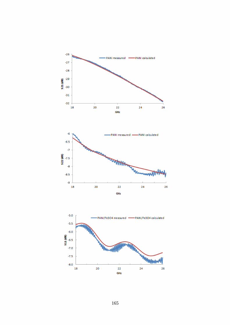
165

166
Figure 8.23.: Comparison between measured and calculated reflection and transmission
coefficients.
8.6. Towards well-dispersed PANI–Fe3O4 nanomaterials
Control over the dispersion of the magnetic NPs into the polymer matrix is critical for the magnetic
properties of composite materials and their performances.
The inability to control the particle dispersion is mostly associated with clustering, which is
influenced by particle–particle and particle–matrix interactions. Designing synthetic strategies in
which the NPs are prevented from forming larger agglomerates is important to guarantee good
properties and performances of the composite products.[588] In the scientific literature some
authors have reported a new synthetic strategy to prepare polymer/magnetic NPs composites
characterized by ordered structures, especially core shell.[589, 590] Preparing materials with highly
ordered structure reduces the risk of NP aggregation that, however, may not completely be avoided.
A possibility to overcome agglomeration phenomena is the use of ultrasonic irradiation that not only
increases the NP dispersion but also favors the formation of organized structures.[34, 343, 344, 590-
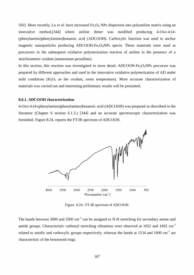
167
592]. More recently, Lu et al. have increased Fe3O4 NPs dispersion into polyaniline matrix using an
innovative method,[344] where aniline dimer was modified producing 4-Oxo-4-(4-
(phenylamino)phenylamino)butanoic acid (ADCOOH). Carboxylic function was used to anchor
magnetic nanoparticles producing ADCOOH-Fe3O4NPs specie. These materials were used as
precursors in the subsequent oxidative polymerization reaction of aniline in the presence of a
stoichiometric oxidant (ammonium persulfate).
In this section, this reaction was investigated in more detail. ADCOOH-Fe3O4NPs precursor was
prepared by different approaches and used in the innovative oxidative polymerization of AD under
mild conditions (H2O2 as the oxidant, room temperature). More accurate characterization of
materials was carried out and interesting preliminary results will be presented.
8.6.1. ADCOOH characterization
4-Oxo-4-(4-(phenylamino)phenylamino)butanoic acid (ADCOOH) was prepared as described in the
literature (Chapter 6 section 6.1.3.) [344] and an accurate spectroscopic characterization was
furnished. Figure 8.24. reports the FT-IR spectrum of ADCOOH.
Figure 8.24.: FT-IR spectrum of ADCOOH.
The bands between 3000 and 3500 cm-1
can be assigned to N-H stretching for secondary amine and
amide groups. Characteristic carbonyl stretching vibrations were observed at 1652 and 1692 cm-1
related to amidic and carboxylic groups respectively, whereas the bands at 1534 and 1600 cm-1
are
characteristic of the benzenoid rings.

168
Comparing UV-vis spectra of AD and ACOOH (Figure 8.25. a and b) a shift of the band at ca. 290
nm to higher wavelengths was observed, indicating an increase in the conjugation degree.
Figure 8.25.: UV-vis spectra of (a) AD, (b) ADCOOH and (c) succinic anhydride.
LSIMS (liquid secondary ionization mass spectroscopy) was used to determine the mass of the
product (Figure 8.26.)
The characteristic peak M+1 at 285 m/z corresponded to the mass of the expected product.
Finally, NMR spectrum (Figure 8.27.) confirmed the structure of the product obtained: 4-Oxo-4-(4-
(phenylamino)phenylamino)butanoic acid.
a
b
c
Figure 8.26.: Mass spectrum of ADCOOH.
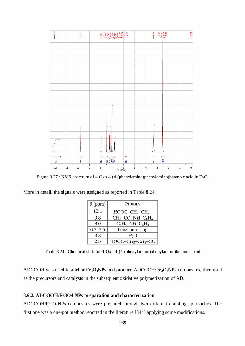
169
Figure 8.27.: NMR spectrum of 4-Oxo-4-(4-(phenylamino)phenylamino)butanoic acid in D2O.
More in detail, the signals were assigned as reported in Table 8.24.
(ppm) Protons
12.1 HOOC–CH2–CH2–
9.8 –CH2–CO–NH–C6H4–
8.0 –C6H4–NH–C6H4–
6.7–7.5 benzenoid ring
3.3 H2O
2.5 HOOC–CH2–CH2–CO
Table 8.24.: Chemical shift for 4-Oxo-4-(4-(phenylamino)phenylamino)butanoic acid
ADCOOH was used to anchor Fe3O4NPs and produce ADCOOH/Fe3O4NPs composites, then used
as the precursors and catalysts in the subsequent oxidative polymerization of AD.
8.6.2. ADCOOH/Fe3O4 NPs preparation and characterization
ADCOOH/Fe3O4NPs composites were prepared through two different coupling approaches. The
first one was a one-pot method reported in the literature [344] applying some modifications.

170
ADCOOH/Fe3O4NPs1 was prepared exactly as reported in ref. 344, adding ADCOOH to the
reaction mixture during the Fe3O4 NPs synthesis, and used as a reference sample.
Then, the reaction was repeated changing the ADCOOH/Fe ratio (% w/w) into the reaction mixture.
The results are summarized in Table 8.25.
Sample ADCOOH/Fe (% w/w) Mean diameter of NPs (nm)a
ADCOOH/Fe3O4NPs1 0.26 6.0
ADCOOH/Fe3O4NPs2 2.64 7.1
ADCOOH/Fe3O4NPs3 7.12 7.3
Table 8.25.: Different preparation for ADCOOH/Fe3O4NPs composites. Reaction conditions: [Fe]= 0.34 M.
reaction temperature= 80°C, pH= 8, reaction time= 1h. a Data obtained by XRPD patterns through the
Debye-Scherrer equation.
Figure 8.28. shows the FT-IR spectra of Fe3O4NPs, ADCOOH/Fe3O4NPs1 and
ADCOOH/Fe3O4NPs2 composites.
As it is possible to observe, the characteristic bands of ADCOOH were more evident in
ADCOOH/Fe3O4NPs2 than ADCOOH/Fe3O4NPs1 (Figure 8.28.). However, the band at 1692 cm-1
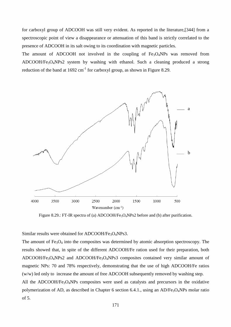
171
for carboxyl group of ADCOOH was still very evident. As reported in the literature,[344] from a
spectroscopic point of view a disappearance or attenuation of this band is strictly correlated to the
presence of ADCOOH in its salt owing to its coordination with magnetic particles.
The amount of ADCOOH not involved in the coupling of Fe3O4NPs was removed from
ADCOOH/Fe3O4NPs2 system by washing with ethanol. Such a cleaning produced a strong
reduction of the band at 1692 cm-1
for carboxyl group, as shown in Figure 8.29.
Similar results were obtained for ADCOOH/Fe3O4NPs3.
The amount of Fe3O4 into the composites was determined by atomic absorption spectroscopy. The
results showed that, in spite of the different ADCOOH/Fe ration used for their preparation, both
ADCOOH/Fe3O4NPs2 and ADCOOH/Fe3O4NPs3 composites contained very similar amount of
magnetic NPs: 70 and 78% respectively, demonstrating that the use of high ADCOOH/Fe ratios
(w/w) led only to increase the amount of free ADCOOH subsequently removed by washing step.
All the ADCOOH/Fe3O4NPs composites were used as catalysts and precursors in the oxidative
polymerization of AD, as described in Chapter 6 section 6.4.1., using an AD/Fe3O4NPs molar ratio
of 5.
Figure 8.29.: FT-IR spectra of (a) ADCOOH/Fe3O4NPs2 before and (b) after purification.
a
b

172
In all cases PANI/Fe3O4 composites were obtained with good yield (66-77%) and polymeric
component resulted to be PANI in its conducting emeraldine form, suggesting that the coating on
the inorganic nanoparticles didn’t compromise their catalytic activity.
XRPD analyses confirmed the presence of inorganic materials into the polymeric matrix.
TEM characterizations are in progress to evaluate the effect of ADCOOH coating on the dispersion
of the inorganic component into the composites.
8.6.3. ADCOOH/Fe3O4NPs composites prepared by a two-step method and their
characterization
ADCOOH/Fe3O4NPs composites were prepared by a different approach: by a two-step method.
In this case Fe3O4NPs (mean diameter = 11 nm) were prepared in advance by a chemical co-
precipitation method and then dispersed in toluene (amount Fe3O4 in toluene= 33mg/mL) using
oleic acid as the surfactant (Chapter 6 section 6.3.1.1.). 1 mL of this dispersion was dried by the
use of a rotary evaporator and Fe3O4 NPsff were washed several timed (ca. 10) with acetone to
remove oleic acid and dried.
Different samples of these NPs (30 mg) were dispersed for 12 hours in 2 mL of different organic
solution containing ADCOOH, as summarized in Table 8.26.
ADCOOH (mg) Solvent (mL) Concentration (mg/mL)
100 5 20
“ “ “
“ “ “
50 “ 10
Table 8.26.: Concentration of different organic solutions containing ADCOOH
ADCOOH/Fe3O4NPs composites were recovered by centrifugation, dried at 60°C until constant
weight, powdered with a mortar and characterized by FT-IR spectroscopy and XRPD diffraction,
whereas liquid fractions were analyzed by UV-vis spectroscopy to measure the amount of free
ADCOOH remained into the organic solution.
As it is possible to observe in Table 8.27., the percentage of ADCOOH absorbed on magnetic NPs
decreased increasing the polarity of the solvent used, expressed as dielectric constant.

173
Solvent Dielectric constant %ADCOOH absorbed (w/w)
Dioxane 2.21 61
Tetrahydrofuran
7.58 50
Acetone 20.7 39
Methanol 32.7 21
Table 8.27.: Percentage of ADCOOH absorption on NPs in different solvents.
FT-IR spectra of ADCOOH-capped NPs in different solvents are similar to those reported in Figure
8.29. b, confirming the coordination between organic and inorganic component.
8.6.4. Synthesis of PANI/Fe3O4 composites using ADCOOH/Fe3O4NPs precursors prepared by
a two-step method
All these materials were employed in the oxidative polymerization of AD as described in Chapter 6
Section 6.4.1., using an AD/Fe3O4NPs molar ratio of 5.
Also in this case PANI/Fe3O4 composites were obtained with good yield (57-71%) and polymeric
component resulted to be PANI in its conducting emeraldine form. XRPD analyses confirm the
inclusion of magnetic NPs into the polymeric matrix, whereas TEM characterization are in progress
to evaluate the presence of agglomeration phenomena.
Figure 8.30. correlates the yields obtained in the presence of different ADCOOH/Fe3O4NPs
materials with dielectric constants of solvents used to anchor magnetic NPs on ADCOOH and
percentage of ADCOOH absorbed on magnetic NPs.
Figure 8.30.: Polymerization yields, dielectric constants of solvents and percentage of ADCOOH
absorbed on magnetic NPs.

174
As it is possible to observe from Table 8.27. and Figure 8.30., the percentage of ADCOOH
anchored on Fe3O4 NPs is closely related to the dielectric constant of solvents used. Solvents
characterized by high dielectric constant caused low level of ADCOOH/Fe3O4 coupling, favoring
the presence of free ADCOOH. Magnetic NPs characterized by low anchoring level had large
surface area exposed to the reaction mixture, producing PANI/Fe3O4 composites in high yield. On
the contrary, increasing the amount of ADCOOH anchored on magnetic NPs, their surface area
exposed to the reaction mixture decreased slightly reducing their catalytic properties.
175
Chapter 9: Improvements in the preparation of polyaniline
nanofibers by electrospinning technique and their
biocompatibility. Towards pure electrospun polyaniline

176
Conducting polymers in nanostructured form, as nanofibers, nanotubes and nanowires, in particular
polyaniline, have received a great deal of attention by the scientific community for their potential
applications (electronic, magnetic, biomedical, optical fields).
Nanosized materials can be realized through many different methods and techniques.
In particular, PANI nanostructures can be synthesized through a “template synthesis” route. In this
context different templates, such as zeolite channels, track-etched polycarbonate and nanosized
alumina membrane, have been employed to direct growth of the PANI nanostructures.[21]
However, although this technique is attracting and elegant, the removal of the template at the end of
the reaction is the biggest drawback. In fact, it is tedious and can compromise the morphology of
the final products.
Recently, electrospinning has emerged as a promising technique for the production of wires and/or
fibers of polymers with diameters ranging from 10 nm to 10 µm.[591-594] Unfortunately, the poor
processability of the polyaniline in form of conducting emeraldine salt makes it difficult to be
electrospun. In addition to poor processability, another limit for the PANI electrospinning is the low
viscosity and surface tension of the polymer in organic solvents as chloroform.
As reported by Cao et al., the limitation of poor solubility can be overcome by the use of
appropriate doping agents. In fact, polyanilines doped with sulfonic acids (camphorsulfonic acid,
CSA, dodecylbenezensulfonic acids, DBSA, …) show higher processability in common
solvents.[282]
As far as the low viscosity is concerned, another polymer can be added. However, it is in general an
insulator material (polystyrene,[595] polyacrylonitrile,[596] polymethylmethacrylate
(PMMA),[597] polyvinylpyrrolidone,[598] polyethylenoxide (PEO),[599]), that can compromise
the electrical conductivity of the final product.
Mc Diarmid et al. spun big PANI fibers (ca. 1320 nm) doped with CSA blended with PEO, finding
that for high content of PANI (72% weight with respect to PEO) single fibers exhibit high value of
conductivity (33 S cm-1
) with respect to the conductivity of a pure polymer cast (10-1
S cm-1
).[167,
237]
In similar manner, many other authors produced PANI wires or fibers using different insulating co-
polymers.
However, the possibility to produce pure PANI nanofibers (PANI NFs) is very tempting. This
would allow to obtain materials characterized by very high electrical properties. Moreover, the
complete removal of co-polymer would resolve possible problems of biocompatibility for medical
and biomedical applications. It has been, in fact, recently demonstrated that pure PANI is
biocompatible and not cytotoxic.[600]

177
For this purpose, two different synthetic methods (classical approach, (NH4)2S2O8 as the oxidant,
PANI1),[544] and “green” approach (H2O2 as the oxidant,PANI2),[26] described in Chapter 6
sections 6.1.1. and 6.1.2., were followed for preparing PANI.
PEO and PMMA were chosen as the co-polymers and pure PANI NFs were produced by the use of
two strategies.
Aim of the first part of the work was to optimize the minimum amount of co-polymer necessary for
the electrospinning process in order to obtain PANI NFs as pure as possible. Moreover, the
electrospinning parameters (type of collector, distance needle-collector, speed of solution) were
varied in order to study these effects on the morphology of blended PANI NFs and on their
electronic conductivity.
Instead, in the second part, the co-polymer was removed by a washing treatment after the
electrospinning process.
9.1. PANI/PEO nanofibers: effect of different raw sources
9.1.1. Morphological characterization
Concerning PANI1/PEO blends, all the blended system solutions were homogeneous and showed
no phase separation prior to the electrospinning process. In the absence of PEO, PANI1 didn’t lead
to fibers production during the electrospinning process. However, increasing PANI1 amount the
consequent increase of viscosity of the blended solution guaranteed a more stable jet and, as a
consequence, the fiber formation.[601]
Figure 9.1 shows the correlation between the nanofibers production and PEO/PANI1 ratio (w/w).
Figure 9.1.:Correlation between the nanofibers production and PEO/PANI1 ratio (w/w).

178
Figures 9.2. A-E report SEM images at low and high magnification of the nanofibers collected from
solutions with different PEO/PANI1 and the diameters distribution using both a static (A-C) and a
rotating collector (D-E).
A1 A2
B1 B2
C1 C2
D1 D2

179
The morphological characterization shows that, increasing gradually the PANI1/PEO ratio from 1:
1 to 1: 0.1 the mean diameter of fibers is reduced by half (from 430 nm to 230 nm) and the surface
morphology becomes rougher. Moreover, the size of the fibers is affected by the method used to
collect them. In fact, the rotating collector promotes a narrow distribution of the diameters favoring
a stretching effect (Figures 9.2. D and E) with respect to the static collector (Figures 9.2. A-C).
However, when the PEO concentration is too low (PANI1/PEO 1:0.2) some defects (beads) appear
on the polymer nanofibers (Figures 9.2. D and E). Their formation is probably due to capillary
instability of jet caused by surface tension.
Figure 9.3. shows the results obtained using PANI2 in the electrospinning process changing the
PEO/PANI2 ratio (w/w).
SEM characterizations are summarized in Figure 9.4.
E1 E2
Figure 9.2.: SEM images at low and high magnification and diameters distribution for the composite
nanofibers with a PANI1:PEO ratio of : A)1:1, B)1:0.8 collected on static collector and C)1:0.8 (w/w)
D)1:0.2, E)1:0.1 (w/w) collected on rotating collector.
Figure 9.3.:Correlation between the nanofibers production and PEO/PANI1 ratio (w/w).

180
A1 A2
B2
C1 C2
D1 D2
B1

181
Also in the case of PANI2, increasing gradually the PANI2/PEO ratio from 1: 1 to 1: 0.2 the mean
diameter of fibers is reduced by half from ca. 800 to ca. 300 nm. However, in this case it is more
evident from the SEM images that coarse nanofibers are due to the agglomeration of smaller ones.
This phenomenon is more important for high values of PANI2/PEO ratio. Moreover, a large
distribution of diameters is observed, especially for the samples containing high amount of PEO
(PEO/PANI2= 1: 1, 1: 0.8 and 1: 0.6). Unlike PANI1, for PANI2 the decrease of PEO amount into
the blend doesn’t compromise dramatically the nanofibers morphology. In fact, also for very low
PEO amount nanofibers are obtained although with a higher roughness morphology.
9.1.2. Spectroscopic characterization
Figure 9.5.A shows FT-IR spectra of PANI1/PEO NFs (1:0.4, 1:1, w/w) and a sample of PANI1 not
spun, while Figure 9.5.B reports the analogous FT-IR spectra of the materials prepared by PANI2.
E1 E2
Figure 9.4.: SEM images at low and high magnification and diameters distribution for the composite
nanofibers with a PEO:PANI2 ratio (w/w) of : A)1:1, B)1:0.8, C)1:0.6, D)1:0.4 and E)1:0.2 collected on
static collector.

182
All the spectra exhibit the characteristic absorptions for the conducting doped polyaniline . The
bands at ca. 1350, 1050 and 1000 cm-1
can be assigned to the bending vibration mode of the S=O
bonds. Whereas, the bands at ca. 1570, 1490 cm-1
are assigned respectively to the C=C stretching of
the quinoid rings (N=Q=N) and to the C=C stretching vibration mode for the benzenoid rings (N-B-
N). The typical characteristic spectral peak of PEO at around 2885 cm-1
[602] is not very prominent
in the PANI1/PEO composites, probably due to its low concentration in the composites. No
significant changes in intensities and frequencies were observed for the materials collected by
rotating collector. For this reason only the FT-IR spectra of the fibers collected on the static
collector have been reported.
Figure 9.6. shows UV-visible of PANI1 not spun and PANI1/PEO NFs collected on a static
collector.
a
b
c
a
b
c
Figure 9.5.: FT-IR spectra of (A) PANI1 derivatives: a) PANI1 not spun, b) PANI1/PEO 1:0.4 spun
nanofibers (static collector), c)PANI1/PEO 1:1 spun nanofibers (static collector), (B) PANI2 derivatives: a)
PAND2 not spun, b) PAND2/PEO 1:0.4 spun nanofibers (static collector), c)PAND2/PEO 1:1 spun
nanofibers (static collector).
A B
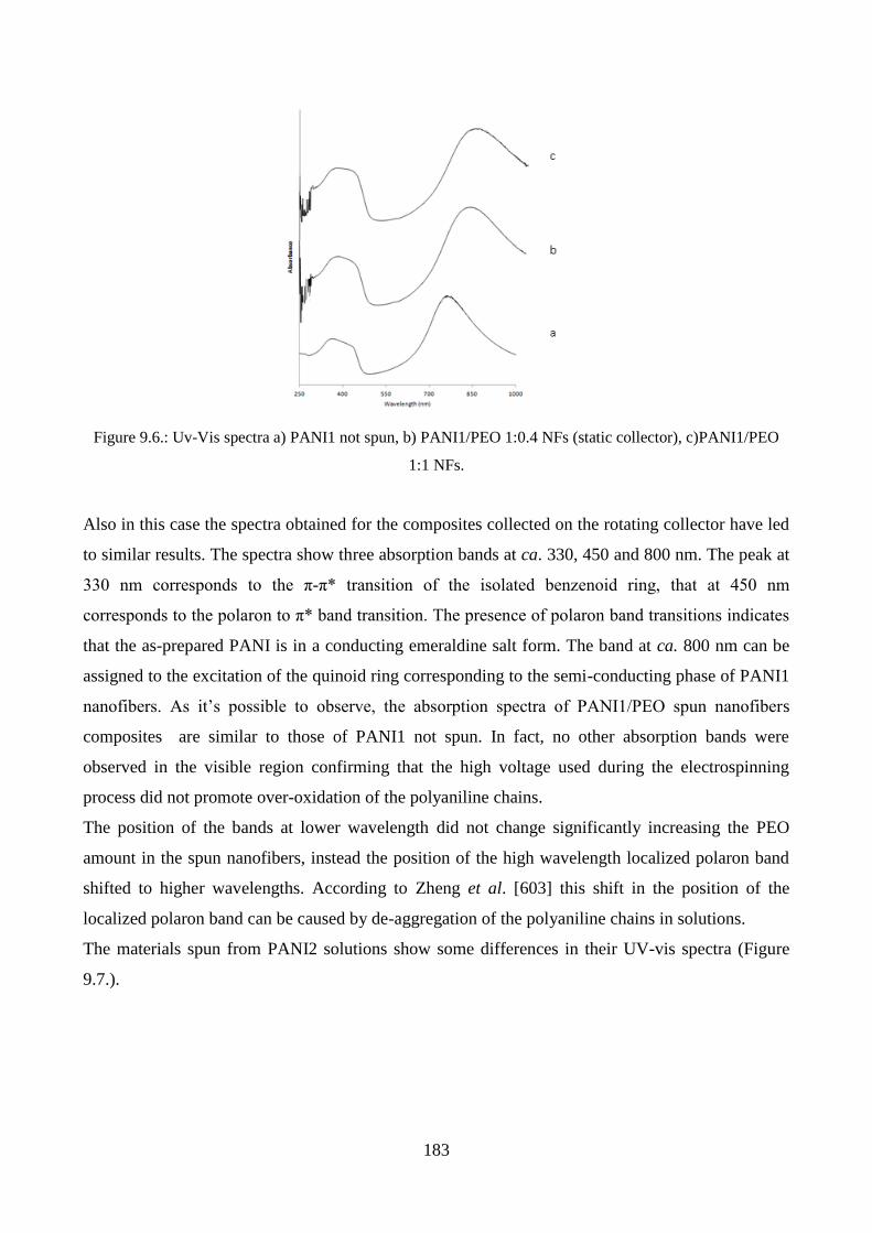
183
Figure 9.6.: Uv-Vis spectra a) PANI1 not spun, b) PANI1/PEO 1:0.4 NFs (static collector), c)PANI1/PEO
1:1 NFs.
Also in this case the spectra obtained for the composites collected on the rotating collector have led
to similar results. The spectra show three absorption bands at ca. 330, 450 and 800 nm. The peak at
330 nm corresponds to the π-π* transition of the isolated benzenoid ring, that at 450 nm
corresponds to the polaron to π* band transition. The presence of polaron band transitions indicates
that the as-prepared PANI is in a conducting emeraldine salt form. The band at ca. 800 nm can be
assigned to the excitation of the quinoid ring corresponding to the semi-conducting phase of PANI1
nanofibers. As it’s possible to observe, the absorption spectra of PANI1/PEO spun nanofibers
composites are similar to those of PANI1 not spun. In fact, no other absorption bands were
observed in the visible region confirming that the high voltage used during the electrospinning
process did not promote over-oxidation of the polyaniline chains.
The position of the bands at lower wavelength did not change significantly increasing the PEO
amount in the spun nanofibers, instead the position of the high wavelength localized polaron band
shifted to higher wavelengths. According to Zheng et al. [603] this shift in the position of the
localized polaron band can be caused by de-aggregation of the polyaniline chains in solutions.
The materials spun from PANI2 solutions show some differences in their UV-vis spectra (Figure
9.7.).

184
Figure 9.7.: Uv-Vis spectra a) PANI2 not spun, b) PANI2/PEO NFs (1:0.4), c) PANI2/PEO NFs (1:1).
In fact, the peaks at 330, 450 and 800 nm are shifted to ca. 270, 400 and 1000 nm, whereas a new
peak at ca. 550 nm appears. The presence of two peaks (450 and 550 nm) in PANI2 based
materials may arise from two types of polaron to π* band transitions, as these polyaniline
nanostructures have two types of polaron bands, resulting from two types of polyaniline chain
orientations. The significant intensity at 1000 nm can doubtlessly be attributed to the increase in the
relative mass fraction of doped-PANI.[604]
9.1.3. Conductivity measurements
The complex impedance Z= Z’- jZ’’, where Z’ and Z’’ are respectively the real and imaginary part
of the impedance, describes the dielectric response of spun nanofiber composites. The frequency
dependence of the real part of the sample impedance, which is governed by the resistance of the
material for PANI1/PEO NFs and for a sample of PANI1 not spun is showed in Figure 9.8.
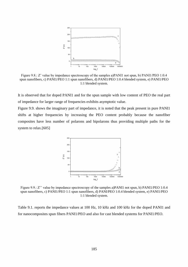
185
1 10 100 1000 10000 100000 1000000
0
50
100
150
200
250
Z' (
)
log10
f
c
b
a
Figure 9.8.: Z’ value by impedance spectroscopy of the samples a)PANI1 not spun, b) PANI1/PEO 1:0.4
spun nanofibers, c) PANI1/PEO 1:1 spun nanofibers, d) PANI1/PEO 1:0.4 blended system, e) PANI1/PEO
1:1 blended system.
It is observed that for doped PANI1 and for the spun sample with low content of PEO the real part
of impedance for larger range of frequencies exhibits asymptotic value.
Figure 9.9. shows the imaginary part of impedance, it is noted that the peak present in pure PANI1
shifts at higher frequencies by increasing the PEO content probably because the nanofiber
composites have less number of polarons and bipolarons thus providing multiple paths for the
system to relax.[605]
1 10 100 1000 10000 100000 1000000
0
50
100
150
200
250
c
b
Z''
()
log10
f
a
Figure 9.9.: Z’’ value by impedance spectroscopy of the samples a)PANI1 not spun, b) PANI1/PEO 1:0.4
spun nanofibers, c) PANI1/PEO 1:1 spun nanofibers, d) PANI/PEO 1:0.4 blended system, e) PANI1/PEO
1:1 blended system.
Table 9.1. reports the impedance values at 100 Hz, 10 kHz and 100 kHz for the doped PANI1 and
for nanocomposites spun fibers PANI1/PEO and also for cast blended systems for PANI1/PEO.

186
SAMPLE f=10Hz f=10kHz f=100KHz
Z’
[Ω]
Z”
[Ω]
[S/cm-1
]
Z’
[Ω]
Z”
[Ω]
[S/cm-1
]
Z’
[Ω]
Z”
[Ω]
[S/cm-1
]
PANI1 2.34 0.003 2.1410-2
2.36 0.09 2.1210-2
2.20 1.37 2.2710-2
PANI1/PEO
1:0.4 9.38 0.006 5.3310
-3 9.36 0.14 5.3410
-3 9.11 1.98 5.4910
-3
PANI1/PEO
1:1 172 0.11 2.9110
-4 178 0.85 2.8110
-4 184 14.5 2.7210
-4
PANI1/PEO*
1:0.4 34.08 0.019 1.4710
-3 35.11 0.37 1.4210
-3 35.3 3.99 1.4210
-3
PANI1/PEO*
1:1 201 0.22 2.4910
-4 205 0.77 2.4410
-4 204.5 14.75 2.4410
-4
PANI2/PEO
1:1 220 0.31 2.7310
-4 212 0.71 2.6310
-4 205 14.82 2.4410
-4
PANI2/PEO*
1:1 218 0.30 2.7010
-4 220 0.86 2.7310
-4 208 16.32 2.5810
-4
Table 9.1.: Complex Impedance and conductivity at selected frequencies. * No spun, blended system.
Obviously increasing the content of PEO in the nanofibers, the Z’ and Z’’ values also increase and
the correspondent conductivity values decrease. Comparing the same composite materials
(PANI1/PEO) spun with the blended sample it is possible to notice that the spun system displays a
better value of conductivity than the blended system indicating that the network of spun nanofibers
improves the conduction mechanism. The conductivity values of the spun PANI2/PEO (1:1) are
similar with respect to the analogue blended system. This result is probably due to the
morphological characteristics of spun fibers.
To better analyze the data, a Cole-Cole plot for the various nano-composites samples of
PANI1/PEO and for PANI1 is reported (Figure 9.10.).
0 50 100 150 200
0
50
100
150
200
Z''
()
Z' ()
ab
c
d e
Figure 9.10.: Cole-Cole plot for the impedance of samples : a)PANI1 not spun, b) PANI1/PEO 1:0.4 spun
nanofibers, c)PANI1/PEO 1:1 spun nanofibers, d) PANI1/PEO 1:0.4 blended system, e) PANI1/PEO 1:1
blended system.

187
The diagram, visibly asymmetric, confirms that at high frequency (greater than 100 KHz) the
behavior of the materials is more and more similar to resistive-inductive (RL) response, while at
frequencies near DC the resistive comportment is almost absolute, in dependence of the material
typology. The presence of inductive effect is more marked with increasing the presence of PEO in
the composite.
As reported in the scientific literature,[26] PANI2 is less conductive than PANI1. Such a different
behaviour is not clear but could be related to a lower value of molecular weight of PANI2 than
PANI1 or to their different degree of crystallinity (see Chapter 10, paragraph 10.1.2.).
For this reason, measurements of AC conductivity of samples resulted to be limited at low values of
frequency. DC conductivity values are summarized in Table 9.2.
SAMPLE [S/cm-1
]
PANI2* 1.1110-6
PANI2/PEO 1:0.2 7.1510-7
PANI2/PEO 1:0.4 5.0210-7
PANI2/PEO 1:0.6 4.6810-7
PANI2/PEO 1:0.8 4.5610-7
Table 9.2.: conductivity values of PANI2/PEO NFs. * No spun.
However, also in this case, the values of conductivity of PANI2-based NFs increase as the
PEO/PANI2 ratio (w/w) decreases.
9.1.4. Tests of cytocompatibility
In order to test direct and indirect PANI/PEO NFs cytocompatibility on a SH-SY5Y human cell
line, PANI1/PEO and PANI2/PEO NFs (PANI:PEO ratio 1:0.4 w/w) were sterilized under different
conditions: 15 minutes in EtOH 70%, 48 hours in PBS (phosphate buffer solution, pH 7.2-7.4) +
3% (v/v) of penicillin/streptomicyn and 10 minutes under UV irradiation (253.7 nm).
In all cases, PANI NFs suffered from degradation. Important fragmentation phenomena and
indissolubility of the samples did not allow to carry out biological tests on PANI2 NFs.
Figure 9.11. shows the degradation of PANI1 NFs after the washing treatment.

188
NFs degradation can be explained in terms of phase segregation phenomena. In fact, the
sterilization process caused the removal of the small PEO amount present into NFs. Owing to the
non-homogeneous distribution of PEO and PANI into the blend, this phenomenon dramatically
compromised the morphology of NFs.
However, despite these drawbacks, PANI1 NFs exhibited good results in terms of cell viability, as
shown in Figure 9.12.
Phase segregation phenomena observed in PANI/PEO NFs didn’t allow a thorough biological
characterization.
A1 A2
Figure 9.11.: SEM images of PANI1/PEO (1: 0.4 w/w) before (A1) and after (A2) EtOH treatment .
Figure 9.12.: Results of biocompatibility in vitro for PANI1/PEO NFs (1: 0.4 w/w): SH-SY5Y cells (human
neuroblastoma cell line) viability after 48 h of incubation at 37°C, 5% CO2.

189
9.2. PANI/PMMA nanofibers: effect of washing
In order to overcome the drawback related to the degradation of PANI/PEO NFs after sterilization
procedure, PEO was substituted with another polymer (PMMA) not soluble in water or ethanol but
able to guarantee no segregation phenomena into the PANI/PMMA blend. This new approach
allowed to spin PANI/PMMA NFs using high amount of insulating copolymer and remove it in a
second step with a specific washing treatment.
9.2.1. Morphological characterization
PANI/PMMA solutions were prepared with the same procedure as used for PANI/PEO (see Chapter
6 paragraph 6.5.1) but using the PANI/PMMA ratio (w/w) reported in Figure 9.12.
In this case, a mixture of CHCl3: DMF (dimethylformamide)= 5:1 was used as the solvent, in order
to increase PANI solubility.
Figure 9.12.:Correlation between nanofibers production and (A) PMMA/PANI1 and (B)
PMMA/PANI2 ratio (w/w).
A
B

190
As shown in Figure 9.12 A, PANI1/PMMA NFs were obtained only when high amount of
copolymer was used (PANI1: PMMA= 1:4). In fact, the low solubility of PANI1/DBSA in organic
solvent leads to PANI1/PMMA organic mixtures characterized by low viscosity, that compromises
jet stability.
On the contrary, the higher solubility of PANI2/DBSA allows to reduce the amount of copolymer
used (PANI2: PMMA= 3:1).
Starting from the results obtained whit PEO as the copolymer, all PANI/PMMA NFs were washed
for 2 minutes with 2-propanol after the electrospinning process and before the biological tests in
order to remove PMMA from PANI NFs and investigate if some morphological modifications
occur.
Figures 9.13. show the morphological characterization of PANI1/PMMA and PANI2/PMMA NFs
obtained using different PANI/PMMA ratios before (Figures 9.13. A1, A2, C1, C2, E1, E2, G1 and
G2) and after (Figures 9.13. A3, A4,C3, C4, E3, E4, G3 and G4) treatment with 2-propanol.
A1 A2
A3 A4
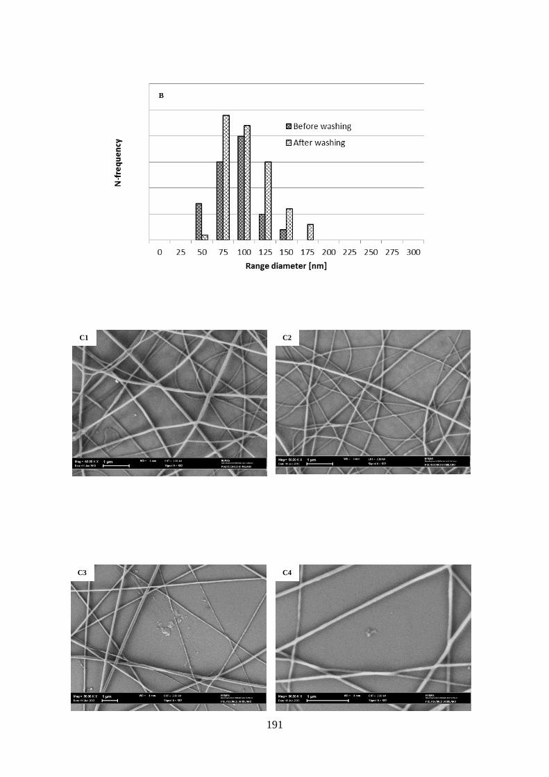
191
B
C1 C2
C3 C4
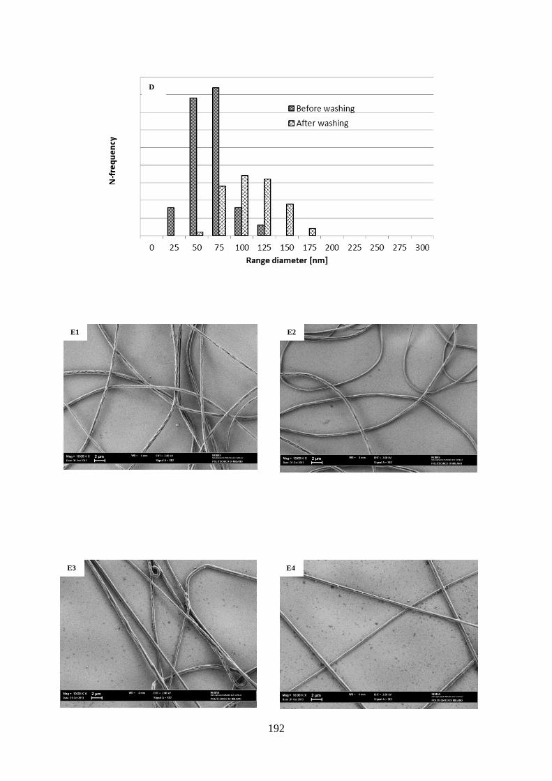
192
D
E2
E3 E4
E1

193
G1 G2
G3 G4
F
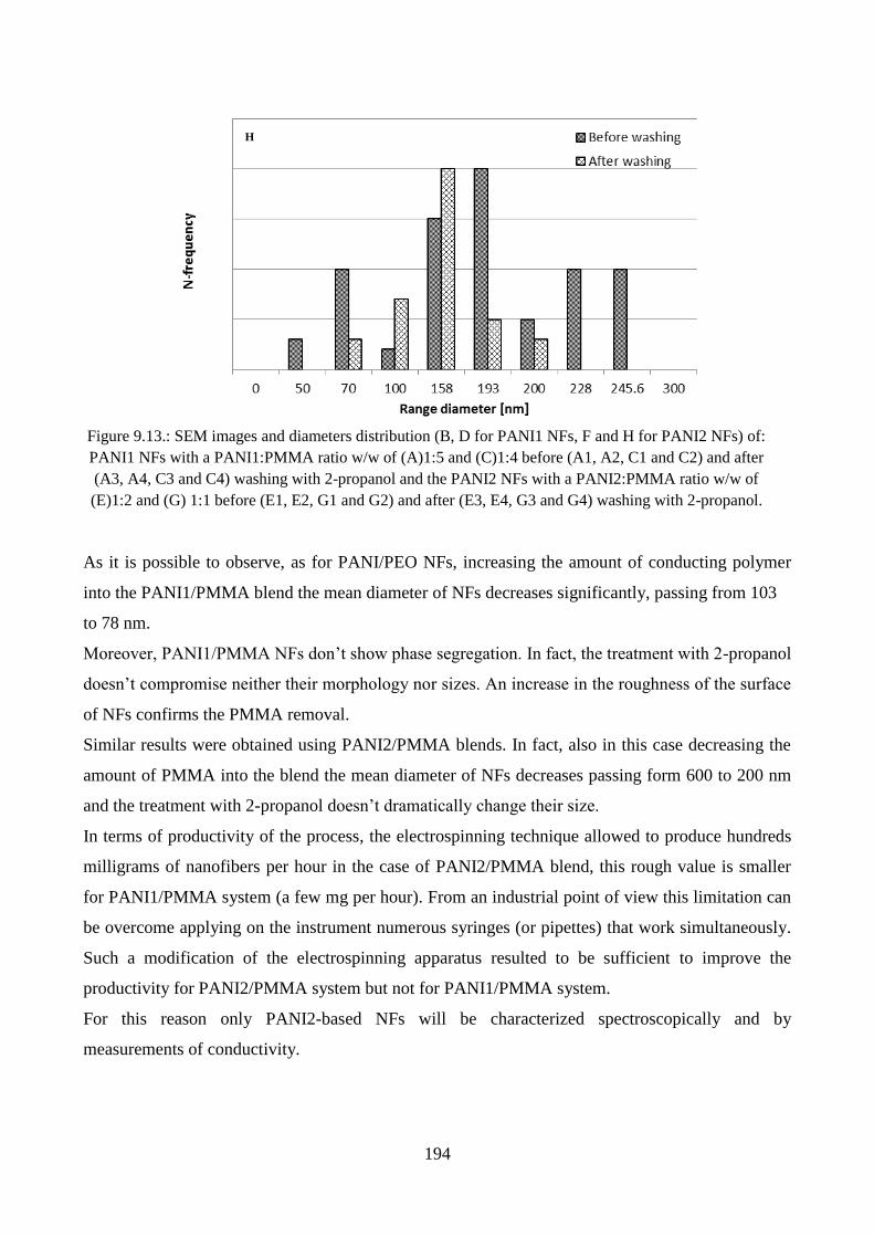
194
As it is possible to observe, as for PANI/PEO NFs, increasing the amount of conducting polymer
into the PANI1/PMMA blend the mean diameter of NFs decreases significantly, passing from 103
to 78 nm.
Moreover, PANI1/PMMA NFs don’t show phase segregation. In fact, the treatment with 2-propanol
doesn’t compromise neither their morphology nor sizes. An increase in the roughness of the surface
of NFs confirms the PMMA removal.
Similar results were obtained using PANI2/PMMA blends. In fact, also in this case decreasing the
amount of PMMA into the blend the mean diameter of NFs decreases passing form 600 to 200 nm
and the treatment with 2-propanol doesn’t dramatically change their size.
In terms of productivity of the process, the electrospinning technique allowed to produce hundreds
milligrams of nanofibers per hour in the case of PANI2/PMMA blend, this rough value is smaller
for PANI1/PMMA system (a few mg per hour). From an industrial point of view this limitation can
be overcome applying on the instrument numerous syringes (or pipettes) that work simultaneously.
Such a modification of the electrospinning apparatus resulted to be sufficient to improve the
productivity for PANI2/PMMA system but not for PANI1/PMMA system.
For this reason only PANI2-based NFs will be characterized spectroscopically and by
measurements of conductivity.
Figure 9.13.: SEM images and diameters distribution (B, D for PANI1 NFs, F and H for PANI2 NFs) of:
PANI1 NFs with a PANI1:PMMA ratio w/w of (A)1:5 and (C)1:4 before (A1, A2, C1 and C2) and after
(A3, A4, C3 and C4) washing with 2-propanol and the PANI2 NFs with a PANI2:PMMA ratio w/w of
(E)1:2 and (G) 1:1 before (E1, E2, G1 and G2) and after (E3, E4, G3 and G4) washing with 2-propanol.
H

195
9.2.2. Spectroscopic characterization
Figure 9.14. shows UV-vis and FT-IR spectra of PANI2/PMMA NFs produced using a
PANI2/PMMA ratio (w/w) of 1:2.
UV-vis spectrum shows the characteristic band of PANI in its conducting emeraldine form, even
though the band corresponding to the excitation of the quinoid ring that in protonated emeraldine is
at around 800 nm, in this case is shifted to lower wavelength (600 nm). Such a shift is characteristic
of unprotonated poyaniline.
FT-IR characterization was carried out before and after washing of the sample with 2-propanol in
order to remove the excess of PMMA. As it is possible to observe (Figures 9.14. B and C), the
A
B C
Figure 9.14.: (A) UV-vis and (B) FT-IR spectra and its magntification (C) of PANI2/PMMA NFs,
PANI2/PMMA 1:2 (w/w).

196
bands of PMMA, especially carbonylic band, are very intense and tend to cover that of PANI.
However, after the washing step, the characteristic band of polyaniline at ca.1570 and 1490 cm-1
become more evident, confirming the effectiveness of the 2-propanol treatment.
9.2.3. Tests of cytocompatibility
Indirect cytocompatibility tests were carried out on SH-SY5Y cells (human neuroblastoma cell
line).
For this scope, washed and unwashed PANI2/PMMA NFs were incubated for 1, 3 and 7 days in the
culture medium to evaluate the possible release of toxic species.
At the time points selected, the supernatants were removed and used to culture SH-SY5Y cells.
In particular, three conditions were examined:
a) 31,250 cells/cm2, 48 h of incubation with the supernatants;
c) 62,500 cells/cm2, 72 h of incubation with the supernatants;
c) 93,750 cells/cm2, 24 h of incubation with the supernatants.
As a control, SH-SY5Y cells were also cultured in fresh medium.
Then, cell viability was evaluated by MTS assay (Promega), according to the instructions provided
by the manufacturer.
For all the conditions tested, the results (Figure 9.15.) have shown that after 1 and 3 days of
exposure to the culture medium previously incubated with the NFs, SH-SY5Y cell viability was
generally comparable with controls. After 7 days of exposure, SH-SY5Y cell viability was lower
than controls for both washed and unwashed PANI2/PMMA NFs in the condition a) and only for
unwashed PANI2/PMMA NFs in the condition b), while for both NFs it was comparable with
controls under the other conditions.

197
Figure 9.15.: Cytocompatibility tests. ns = p-value > 0.05, * = p-value < 0.05, ** = p-value < 0.001,
**** = p-value < 0.0001
Even though preliminary, these results have suggested that washed PANI2/PMMA NFs might be a
better substrate for culturing SH-SY5Y cells than unwashed PANI2/PMMA NFs.
To better investigate this aspect, direct cytocompatibility tests are in progress.
In particular, SH-SY5Y cells were cultured in contact with washed and unwashed PANI2/PMMA
NFs for 24 h and 48 h and their morphology was observed by an optical and a scanning electron
microscope (SEM).
The SEM analysis is still in progress, but the preliminary investigations by the optical
microscope have shown that controls cultured in standard tissue culture plates have a more flattened
and spread morphology than the SH-SY5Y cells cultured on the NFs.

198
Chapter 10: Electromechanical properties of polyaniline:
towards low cost force and strain sensors
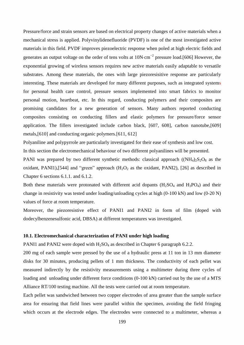
199
Pressure/force and strain sensors are based on electrical property changes of active materials when a
mechanical stress is applied. Polyvinylidenefluoride (PVDF) is one of the most investigated active
materials in this field. PVDF improves piezoelectric response when poled at high electric fields and
generates an output voltage on the order of tens volts at 10Ncm−2
pressure load.[606] However, the
exponential growing of wireless sensors requires new active materials easily adaptable to versatile
substrates. Among these materials, the ones with large piezoresisitive response are particularly
interesting. These materials are developed for many different purposes, such as integrated systems
for personal health care control, pressure sensors implemented into smart fabrics to monitor
personal motion, heartbeat, etc. In this regard, conducting polymers and their composites are
promising candidates for a new generation of sensors. Many authors reported conducting
composites consisting on conducting fillers and elastic polymers for pressure/force sensor
application. The fillers investigated include carbon black, [607, 608], carbon nanotube,[609]
metals,[610] and conducting organic polymers.[611, 612]
Polyaniline and polypyrrole are particularly investigated for their ease of synthesis and low cost.
In this section the electromechanical behaviour of two different polyanilines will be presented.
PANI was prepared by two different synthetic methods: classical approach ((NH4)2S2O8 as the
oxidant, PANI1),[544] and “green” approach (H2O2 as the oxidant, PANI2), [26] as described in
Chapter 6 sections 6.1.1. and 6.1.2.
Both these materials were protonated with different acid dopants (H2SO4 and H3PO4) and their
change in resistivity was tested under loading/unloading cycles at high (0-100 kN) and low (0-20 N)
values of force at room temperature.
Moreover, the piezoresistive effect of PANI1 and PANI2 in form of film (doped with
dodecylbenzenesulfonic acid, DBSA) at different temperatures was investigated.
10.1. Electromechanical characterization of PANI under high loading
PANI1 and PANI2 were doped with H2SO4 as described in Chapter 6 paragraph 6.2.2.
200 mg of each sample were pressed by the use of a hydraulic press at 11 ton in 13 mm diameter
disks for 30 minutes, producing pellets of 1 mm thickness. The conductivity of each pellet was
measured indirectly by the resistivity measurements using a multimeter during three cycles of
loading and unloading under different force conditions (0-100 kN) carried out by the use of a MTS
Alliance RT/100 testing machine. All the tests were carried out at room temperature.
Each pellet was sandwiched between two copper electrodes of area greater than the sample surface
area for ensuring that field lines were parallel within the specimen, avoiding the field fringing
which occurs at the electrode edges. The electrodes were connected to a multimeter, whereas a

200
cantilever allowed to measure the deformation of pellet. The experimental set-up is shown in Figure
10.1.
10.1.1. Electromechanical response
The mechanical hysteresis of PANI1 and PANI2 were characterized in stress–strain tests for three
cycles (Figure 10.2.).
Figure 10.1.: Experimental set-up for the resistivity and strain measurements under loading/unloading
cycles.
Multimeter
Cantilever
A

201
Negative values of strain at low forces can be attributed to the deformation of the circular thin
copper foils not present during the zero setting of the testing machine.
It is possible to observe that the loading/unloading curves didn’t coincide during the successive
cycles and mechanical hysteresis were evident for both materials. As shown in Figure 10.2., the
mechanical hysteresis decreased with increasing the number of cycles, suggesting a mechanical
stabilization.
During the first cycle both materials displayed an irreversible deformation and the hysteresis was
much larger than the others in both cases. This behavior could be attributed to the high stiffness of
these materials that does not allow the reversal and recovery of the initial microstructure.
It is to notice the overall small nonlinear behaviour of PANI1 for deformations up to ~0.04 mm and
a linear behaviour for deformations larger than ~0.04 mm. These two regimes can be mainly
attributed to low deformation, mainly morphological reconfigurations of the polymer pellet,
followed by a true stretching and reorientation of the polymer chains for larger deformations. On
the contrary PANI2 showed a linear and almost hysteresis-free behaviour for all the range of
deformation investigated, suggesting a higher stability of the morphology and compactness of this
polymer.
B
Figure 10.2.: Stress-strain curves under loading/unloading cycles for (A) PANI1/H2SO4 and (B)
PANI2/H2SO4. Blue line= cycle no. 1, red line= cycle no. 2 and green line= cycle no. 3.
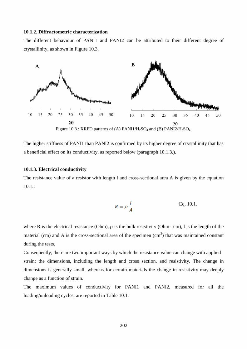
202
10.1.2. Diffractometric characterization
The different behaviour of PANI1 and PANI2 can be attributed to their different degree of
crystallinity, as shown in Figure 10.3.
The higher stiffness of PANI1 than PANI2 is confirmed by its higher degree of crystallinity that has
a beneficial effect on its conductivity, as reported below (paragraph 10.1.3.).
10.1.3. Electrical conductivity
The resistance value of a resistor with length l and cross-sectional area A is given by the equation
10.1.:
where R is the electrical resistance (Ohm), is the bulk resistivity (Ohm cm), l is the length of the
material (cm) and A is the cross-sectional area of the specimen (cm2) that was maintained constant
during the tests.
Consequently, there are two important ways by which the resistance value can change with applied
strain: the dimensions, including the length and cross section, and resistivity. The change in
dimensions is generally small, whereas for certain materials the change in resistivity may deeply
change as a function of strain.
The maximum values of conductivity for PANI1 and PANI2, measured for all the
loading/unloading cycles, are reported in Table 10.1.
A B
Figure 10.3.: XRPD patterns of (A) PANI1/H2SO4 and (B) PANI2/H2SO4.
Eq. 10.1.

203
Sample cycle1(S/cm) cycle2(S/cm) cycle3(S/cm)
PANI1 1.0110-2
1.2710-2
1.2910-2
PANI2 4.8410-5
4.7610-5
4.7810-5
Table 10.1.: Maximum value of conductivity for each cycle for PANI1 and PANI2.
As it is possible to observe, PANI2 showed maximum values of conductivity constant but much
lower than those of PANI1. The difference in conductivity can be explained in terms of different
degree of crystallinity (Figure 10.3) but also with a different molecular weight (not investigated in
this thesis). As reported in Chapter 2 paragraph 2.4., the electrical properties of polyaniline are
strongly influenced by the structure of chains. It has been observed that with the increase in
crystallinity the conductivity increased, because the structure becomes more organized.[133] In this
case the higher crystallinity of PANI1 guaranteed high values of conductivity (Table 10.1.) but at
the same time lower mechanical characteristics, as shown by stress-strain curves (Figure 10.2. A).
On the contrary, the low degree of crystallinity of PANI2 causes lower value of conductivity but
higher mechanical properties.
10.1.4. Piezoresistive effect
By strict definition, piezoresistors refer to resistors whose resistivity changes with applied strain
(more details are reported in §10.3.)
The fractional change in the electrical resistivity (DR/R0) plotted against the applied force and the
change of deformation (Dl/l0) for both PANI1 and PANI2 is reported in Figure 10.4.
A

204
As it is possible to observe from Figure 10.4., a fractional change in the electrical resistance for
both PANI1 and PANI2 was observed under uniaxial compression. This change went up to 87%
and 90% for PANI1 and PANI2 respectively when the compressive stress was in the range of 0-100
kN. The change in electrical resistance reversibly decreased upon loading and increased upon
unloading in each cycle. Moreover, it is important to notice the complete reproducibility for the
three loading and unloading processes for both materials, PANI1 and PANI2. The relationship
between change in resistance and deformation was expressed in terms of gauge factor (Equation
10.2.):
where R0 is the steady-state electrical resistance of the material without deformation (l0) and R is
the resistance change caused by the change in length (l).[607] It quantifies the magnitude of the
piezoresistivity effect.
According to the linear regression, i.e., Y = kX, the relationship between the fractional change in
electrical resistivity (DR/R0) and the deformation (Dl/l0) for both PANI1 and PANI2 is shown in
Figure 10.5.
Figure 10. 4.: Change in resistance against applied force and change of deformation for PANI1 (A) and
PANI2 (B). Blue (change of deformation), red (force), green (change of resistance)
B
Eq. 10.2.

205
The slope of the linear fit, according to Eq. 10.2. (obtained with a R-square higher than 0.90),
corresponds to the GF of the samples.
For PANI1 and PANI2 GF resulted to be 0.29 and 0.42 respectively. These values of GF are typical
of commercial stress/strain sensors (GF of 0.1-2), that only show geometric effect.
However, it is known that the piezoresistive behaviour of polyaniline is strictly related to its
mechanism of conduction, as described in Chapter 2, paragraph 2.4.
More in detail, the conductivity of PANI is the sum of two contributions: the ability of the charge
carriers to move along the polymer backbone (intra-chain mechanism) and the ability of the charge
carriers to hop between the polymer chains (inter-chain mechanism).[148] This second contribution
becomes particularly important when the material is subjected to stress/strain processes.
B
Figure 10.5.: Fractional change in electrical resistance as a function of the deformation for PANI1 (A) and
PANI2 (B).

206
During the compression (stress) processes the distance among polymeric chains is gradually
reduced, promoting the movement of charge carriers among the polymeric chains. This
phenomenon leads to a gradual decrease of resistance values and, therefore, to an increase of
conductivity of the material.
On the contrary, if the material is subjected to strain processes the consequent increased inter-
chains distance reduces the ability of charge carriers to hop among them, causing an increase of
resistance values (low conductivity).
In this context, the low values of GF obtained for both PANI1 and PANI2 in this section was
attributed to the use of the materials in form of pellet. For this reason PANI1 and PANI2 were
produced in form of film using DBSA (dodecylbenzenesulfonic acid) or CSA (camphorsulfonic
acid) as the dopant and their piezoresistive behaviour was carried out by 4-point bending tests
(Paragraph 10.3). However, similar behaviour of both PANI1 and PANI2 under these conditions
encourage a more detailed investigation of PANI2 for its application in the field of stress/strain
sensors. In fact, the higher solubility of PANI2 in common organic solvents and its lower
conductivity make it ideal for application as piezoresistor in form of thin film.
10.2. Electromechanical characterization of PANI under low loading
In the last years the application of polyaniline as new material for polymeric resistors has been
investigated only at high values of force. In this regarding, starting from the previous results
obtained under these conditions, the variation of resistivity of pellets of PANI1/ H2SO4 and PANI2/
H2SO4 was investigated also at low value of applied force (0-20 N).
It was sandwiched between two copper electrodes of area greater than the sample surface area for
ensuring that field lines were parallel within the specimen, avoiding the field fringing which occurs
at the electrode edges. The electrodes were connected to the multimeter and placed on digital
balance. Each material was tested at room temperature. The values of force were gradually
increased and decreased by the use of a screw, as shown in Figure 10.6.

207
The conductivity of each pellet was measured indirectly by the resistivity measurements using a
multimeter during the four cycles of loading and unloading under different force conditions (0-20
N).
Figure 10.7. shows that also at low value of force PANI1 and PANI2 doped with H2SO4 exhibited a
linear relationship between the resistance and the applied force during the loading and unloading
processes. However, in this case the experimental set-up used didn’t allow to measure the change of
deformation.
Figure 10.6.: Experimental set-up for the measurements of the resistivity variation during
loading/unloading cycles (0-20 N).
A

208
Also at low values of applied force both PANI and PANI2 show similar behaviour, exhibiting a
good linear relationship between resistance and force. However, because of the high values of
resistance of PANI2, this material becomes conductive at higher values of force (about 2.5 N).
The maximum values of conductivity for both PANI1 and PANI2 during different cycles are
reported in Table 10.2.
Sample cycle1(S/cm) cycle2(S/cm) cycle3(S/cm) cycle4(S/cm)
PANI1 9.8310-7
9.6610-7
8.8010-7
8.6610-7
PANI2 1.7710-8
1.7910-8
1.8110-8
1.6010-8
Table 10.2.: Maximum value of conductivity for each cycle for PANI1 and PANI2.
The values of conductivity of PANI1 are higher than those of PANI2. However, in this case the
difference is not as evident as in the measurements at high applied force (Table 10.1.).
This suggests that working at low values of force the differences in crystallinity of both materials
become less important, not compromising their values of conductivity that in this case resulted to be
more similar. Unfortunately, the impossibility to measure the deformation of pellets during
loading/unloading cycles didn’t allow to calculate the values of GF under these conditions.
Figure 10.7.: Resistance against applied force for PANI1 (A) and PANI2 (B).
B

209
10.3. Piezoresistive effect in polyaniline. The effect of different raw materials and doping
agents
Electrical strain gauges are based on the measurement of an inherent electrical property (most often
resistance) as function of an induced strain.
Piezoresistivity describes change in the electrical resistivity as function of a mechanical strain.
Piezoresistive films are used to produce macroscopic strain gauges or small devices useful as force
transducers, such as accelerometers, pressure and/or deformation sensors.
The magnitude of the piezoresistivity effect is often quantified by the gauge factor (GF) (Eq. 10.3.).
Many commercially available thin film piezoresistive strain gauges are metal foils deposited on
flexible polymer substrates. Generally, they are used to measure deformation in bridges, buildings,
machine parts, etc. However, their performances are not good for other applications, such as
measuring strain in biological tissues and large movements in robotic devices, among others, due to
their limited flexibility.[617]
An additional problem with metal film strain gauges is their delamination and the low inherent
resistivity and resistivity variation with strain.
Many approaches have been developed to obtain strain gauge resistance which is large enough to be
distinguished from lead wire resistance.
For example, metal films can be designed to have a large length/width ratio (about 500) to increase
the resistance. The metal pattern is folded back upon itself so as to take up as little space as
possible, but the size of the overall strain gauge is dictated by the required length/width ratio.
Commercial metal film strain gauges have a typical resistance of 50-100 Ohms. In this case, the
contribution of lead wire resistance to the total strain gauge resistance cannot be ignored and
introduces errors of several percent.[618]
To eliminate the effect of lead wire resistance, a multiple-terminal resistance measurement can be
employed. However, more than two leads must be connected to the device and this makes this
method more complicated for practical applications.
Another important material useful for micromachined sensors is silicon.[619, 620] However, the
use of silicon limits the choice of substrate. Moreover, owing to its low flexibility it cannot be used
for large-scale applications.
More recently polymer-based strain gauges have been suggested as a more useful flexible
substitute.[620]
In general, these materials are insulating polymers whose conductivity is increased by the
incorporation of conductive materials, generally metallic particles or carbon nanotubes. At high
enough loading the contact among conducting grains guarantees current flow.
210
The piezoresistitive effect results from the change of grains distances during compression or
expansion.[465, 618]
Some problems are associated to the use of those materials, too. For example, the particulate nature
of the films prevents small geometry patterning. Another drawback is the delamination of the
polymer from the particle surface. This phenomenon is ascribed to poor wetting and poor adhesion
of the filler to the polymer matrix. Moreover, it is difficult to obtain a uniform dispersion of
polymer and metal particles.[618]
The discovery of homogeneously flexible conductive polymers that exhibit piezoresistive properties
without embedding carbon or metal conductive fillers opened the way to a new era of strain gauges.
Strain gauges formed from piezoresistive, homogeneous conductive polymer films show several
advantages. They maintain the same advantage of the polymer composites with respect to
processing and eliminate the necessity to apply multiple-terminal resistance measurements,
essential in the case of metal strain gauges, having high resistance.
Moreover, thanks to their homogeneity, they can be produced in highly uniform films.
Intrinsically conductive polymers, such as PANI, can be used for this scope. Concerning
polyaniline, there are not enough data and investigations on its piezoresistive properties. Moreover,
these results are conflicting. Lillemose et al.[621] reported a negative GF of ~ 5 in 4-point-bending
experiments, that means an increase in conductivity for large deformations owing to the alignment
of the polymeric chains.[622] However, the 4-point-bending experiment does not provide the large
deformation needed for the alignment of polymeric chains. More recently, Pereira et al.[623]
describe the piezoresistive effect of a commercial polyaniline, prepared in form of thin film, and
report GF values from 10 to 22 for different samples.
In this work PANI1 and PANI2 were doped with organic acid, dodecylbenzenesulfonic acid
(DBSA) and camphorsulfonic acid (CSA), (see Chapter 6 section 6.2.3.) in order to be solubilized
in chloroform. Films of PANI1 and PANI2 doped with DBSA and CSA were produced by drop-
casting process using a plate of PET (polyethylene terephthalate) as support. In all the samples a
pair of gold rectangular electrodes with 6×2 mm and 1 mm apart were deposited by sputtering. On
the top of each electrode, a copper wire with 0.125 mm diameter was glued with silver ink, as
shown in Figure 10.8, and their piezoresistive effect was investigated.

211
The relationship between electrical response and mechanical solicitations was evaluated and the
values of the gauge factor were calculated.
In order to quantify the piezoresistive effect, 4-point bending tests were performed. In these tests,
the electrical resistance changes with strain were measured. Figure 10.9. shows a diagram of the 4-
point bending jig.
In 4-point-bending experiments, the strain along the longitudinal direction (εl), calculated from the
theory of pure bending of a plate, to form a cylindrical surface between the inner loading points, is
given by Equation 10.3., according with ref. 65:
Figure 10.8.: Sample of PANI for measurement of piezoresistivity.
Figure 10.9.: Diagram of the 4-point bending jig used in the present study.
Eq. 10.3.

212
where d is the distance from the neutral plane to the plane of the sample, which in this case is
approximately equal to the thickness of the substrate (1 mm), z is the vertical displacement of the
and a is the distance between the first and the second points of the 4-point bending load cell (10
mm).
The 4-point-bending tests were performed in a Shimadzu-AG-IS 500 N testing instrument at speeds
from 0.1 to 10 mm/min and a maximum vertical (z axis) displacement from 0.1 to 2.5 mm (Figure
10.10.)
A
B
Figure 10.10.: A) 1: Universal Shimadzu - AG-IS 500 N testing machine, 2: digital multimeter, 3: computer;
B) Photograph of a sample in a test deformation during 4-point-bending.

213
Each test was composed by four cycles of deformation. Stability tests were also performed in
selected samples up to 40 cycles.
10.3.1. Electrical conductivity
The d.c. electrical conductivity of the materials was calculated from the slope of I–V curves
measured with an automated Keithley 487 picoammeter/voltage source and the resistivity of the
samples () was calculated by the equation 10.1.The corresponding values of electrical conductivity
are summarized in Table 10.3. Figure 10.11. shows the I–V plots for PANI1 and PANI2 doped with
DBSA and CSA. Samples doped with DBSA were also subjected to a thermal treatment (1 hour at
70°C) in order to remove any trace of solvent (CHCl3) among the polymeric chains and remove
residual stresses in order to guarantee the mechanical stabilization.
Figure 10.11.: I–V plots for PANI1/DBSA and PANI2/DBSA at room temperature (A). PANI1/DBSA and
PANI2/DBSA after thermal treatment (1 h at 70°C) (B), PANI1/CSA (C) and PANI2/CSA (D) at room
temperature.
A B
C D

214
Sample (S/cm)* (S/cm)**
PANI1/DBSA 5.1210-6
5.8210-6
PANI2/DBSA 4.1710-9
1.8010-8
PANI1/CSA 2.1910-7
-
PANI2/CSA 1.6710-7
-
Table 10.3.: Values of conductivity of samples at room temperature (*) and after thermal treatment (1 h at
70°C) (**).
When DBSA is used as the doping agent, PANI1 exhibits higher values of electrical conductivity
than PANI2, probably due to the longer polymeric chains and higher molecular weight. Moreover,
the electrical conductivity of PANI1/DBSA does not change after thermal treatment, whereas for
PANI2/DBSA it increases 10 times, suggesting a better packing of polymeric chains.
On the contrary, concerning CSA, PANI1 and PANI2 show similar values of conductivity.
The differences observed when DBSA and CSA are employed as dopants can be attributed to the
different characteristics of these organic acids. In fact, due to its smaller counterion size CSA
guarantees stronger inter-chain interactions, that implies higher values of electrical conductivity,
more evident in PANI2 than in PANI1.
10.3.2. Morphological characterization
The morphological characterization of all the samples was carried out by SEM microscopy and the
results are shown in Figure 10.12.
A A’

215
B B’
C C’
D D’

216
E E’
F F’
G G’

217
As shown in Figure 10.12. and confirmed by the piezoresistive response (see § 10.3.4.), at room
temperature the materials prepared by PANI1 show more regular globular-like structures than
PANI2 and after a thermal treatment, when any trace of solvent and residual stresses are removed,
their morphology becomes more compact. Concerning PANI2, at room temperature the morphology
of the polymer deeply changes with the dopant used. In fact, PANI2/DBSA shows higher
uniformity than PANI2/CSA, even though lower than PANI1. Moreover, after thermal treatment the
removal of solvent leads to a porous and more compact morphology (Figure 10.12.D) that
positively affects the piezoresistive behaviour of the material (see later).
Finally, the very high irregular morphology of PANI2/CSA before and after the thermal treatment
justifies the poor piezorestive response of this material in all the conditions.
10.3.3. Electromechanical response
The mechanical properties of polyaniline (initial modulus, maximum strain and hysteresis) are key
issues for its application as piezoresistive sensors, since the mechanical properties play a critical
role in sensor response and reliability. The mechanical hysteresis is important to analyse
reproducibility of stress–strain tests in sensor applications. Good linearity of electrical resistance
depends on the mechanical properties of the material.
Figure 10.13. shows stress-strain curves for PANI1 and PANI2 doped with DBSA and CSA.
H H’
Figure 10.12.: SEM images at low and high magnification for PANI1/DBSA at room temperature (A
and A’), PANI1/DBSA after thermal treatment (B and B’), PANI2/DBSA at room temperature (C and
C’), PANI2/DBSA after thermal treatment (D and D’), PANI1/CSA at room temperature (E and E’),
PANI1/CSA after thermal treatment (F and F’), PANI2/CSA at room temperature (G and G’),
PANI2/CSA after thermal treatment (H and H’).

218
As it is possible to observe, loading and unloading curves do not coincide during successive cycles,
given evidence of a mechanical hysteresis in the material. In all cases, the mechanical hysteresis
decreases with increasing number of cycles, in particular for the first cycle, and increases for
increasing strain. Among all the samples investigated, only PANI1/CSA shows lower hysteresis,
explained with a more compact and flexible structure (Figures 10.12. E and E’), whereas PANI2
always exhibits higher hysteresis than PANI1, according with a more irregular structure (Figure
10.12. C and C’, H and H’).
It is to notice the overall small nonlinear behaviour of the samples with a linear and almost
hysteresis free behaviour for deformations up to ~0.4 mm and another linear behaviour for
deformations larger than ~0.6 mm. These two regimes can be mainly attributed to low deformation,
mainly morphological reconfigurations of the porous polymer film, followed by a true stretching
and reorientation of the polymer chains for larger deformations. The stress-strain curves of the
samples after thermal treatment do not show any modifications
A B
Figure 10.13.: Stress-strain curves of PANI1/DBSA (A),PANI2/DBSA (B), PANI1/CSA (C) and
PANI2/CSA (D).
C D
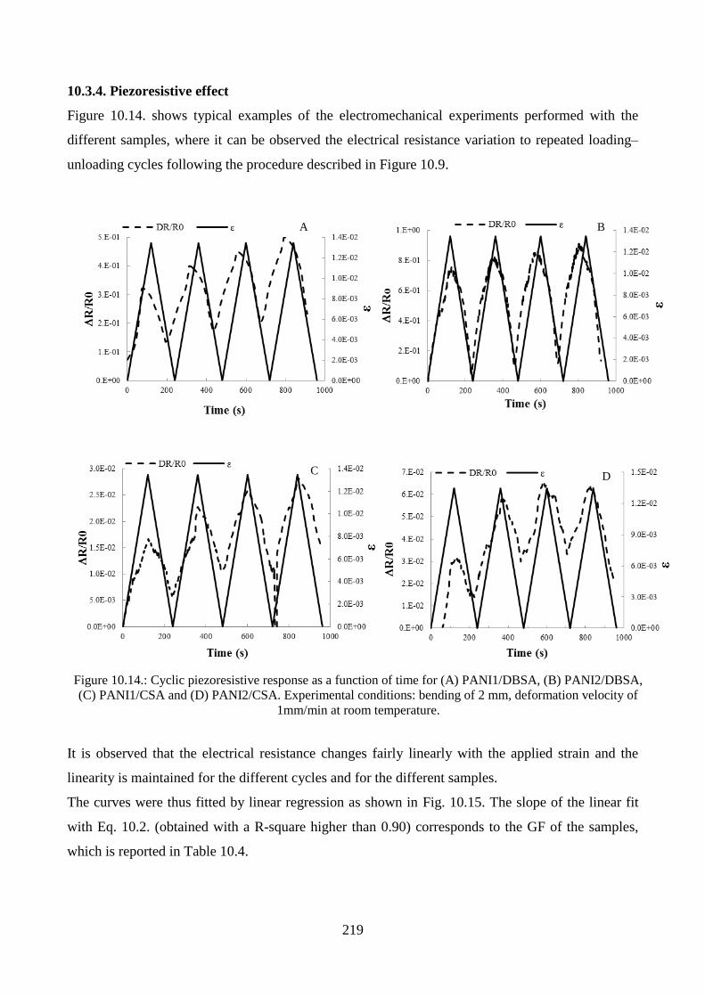
219
10.3.4. Piezoresistive effect
Figure 10.14. shows typical examples of the electromechanical experiments performed with the
different samples, where it can be observed the electrical resistance variation to repeated loading–
unloading cycles following the procedure described in Figure 10.9.
It is observed that the electrical resistance changes fairly linearly with the applied strain and the
linearity is maintained for the different cycles and for the different samples.
The curves were thus fitted by linear regression as shown in Fig. 10.15. The slope of the linear fit
with Eq. 10.2. (obtained with a R-square higher than 0.90) corresponds to the GF of the samples,
which is reported in Table 10.4.
Figure 10.14.: Cyclic piezoresistive response as a function of time for (A) PANI1/DBSA, (B) PANI2/DBSA,
(C) PANI1/CSA and (D) PANI2/CSA. Experimental conditions: bending of 2 mm, deformation velocity of
1mm/min at room temperature.
A B
C D
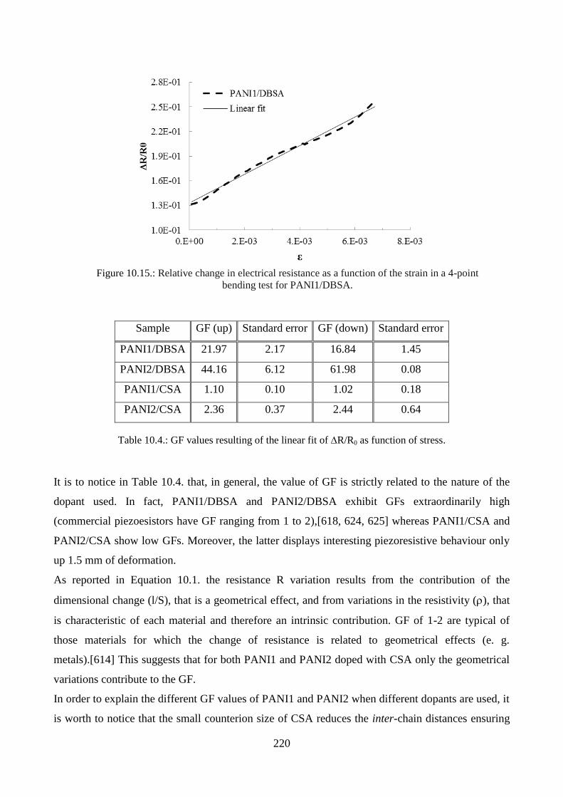
220
Sample GF (up) Standard error GF (down) Standard error
PANI1/DBSA 21.97 2.17 16.84 1.45
PANI2/DBSA 44.16 6.12 61.98 0.08
PANI1/CSA 1.10 0.10 1.02 0.18
PANI2/CSA 2.36 0.37 2.44 0.64
Table 10.4.: GF values resulting of the linear fit of R/R0 as function of stress.
It is to notice in Table 10.4. that, in general, the value of GF is strictly related to the nature of the
dopant used. In fact, PANI1/DBSA and PANI2/DBSA exhibit GFs extraordinarily high
(commercial piezoesistors have GF ranging from 1 to 2),[618, 624, 625] whereas PANI1/CSA and
PANI2/CSA show low GFs. Moreover, the latter displays interesting piezoresistive behaviour only
up 1.5 mm of deformation.
As reported in Equation 10.1. the resistance R variation results from the contribution of the
dimensional change (l/S), that is a geometrical effect, and from variations in the resistivity (), that
is characteristic of each material and therefore an intrinsic contribution. GF of 1-2 are typical of
those materials for which the change of resistance is related to geometrical effects (e. g.
metals).[614] This suggests that for both PANI1 and PANI2 doped with CSA only the geometrical
variations contribute to the GF.
In order to explain the different GF values of PANI1 and PANI2 when different dopants are used, it
is worth to notice that the small counterion size of CSA reduces the inter-chain distances ensuring
Figure 10.15.: Relative change in electrical resistance as a function of the strain in a 4-point
bending test for PANI1/DBSA.
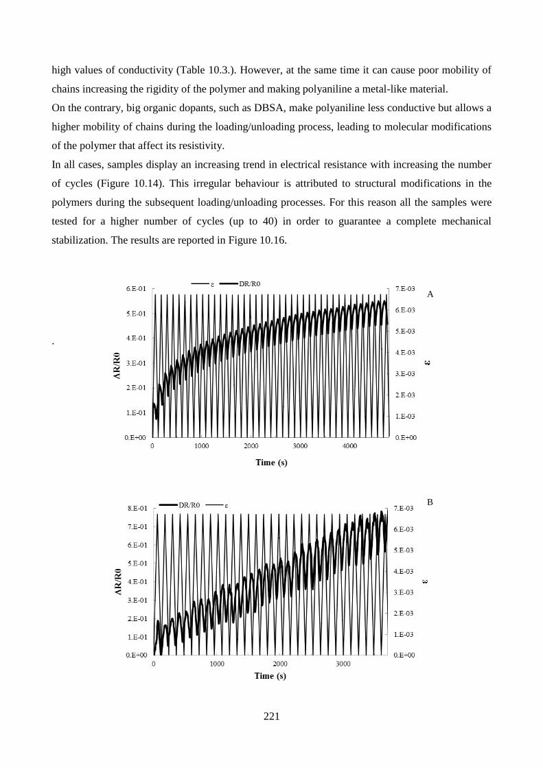
221
high values of conductivity (Table 10.3.). However, at the same time it can cause poor mobility of
chains increasing the rigidity of the polymer and making polyaniline a metal-like material.
On the contrary, big organic dopants, such as DBSA, make polyaniline less conductive but allows a
higher mobility of chains during the loading/unloading process, leading to molecular modifications
of the polymer that affect its resistivity.
In all cases, samples display an increasing trend in electrical resistance with increasing the number
of cycles (Figure 10.14). This irregular behaviour is attributed to structural modifications in the
polymers during the subsequent loading/unloading processes. For this reason all the samples were
tested for a higher number of cycles (up to 40) in order to guarantee a complete mechanical
stabilization. The results are reported in Figure 10.16.
.
A
B

222
Figure 10.16. shows that PANI1/DBSA and PANI1/CSA reach stabilization after 40 and 7 cycles
respectively, whereas PANI2/DBSA still shows a growing trend after 40 cycles and PANI2/CSA is
completely unstable. It is interesting to notice that even if the overall resistance increases in the first
cases, the resistance variation, i.e. the GF, remains practically stable over the different cycles (see
Figure 10.17.)
C
D
Figure 10.15.: Cyclic piezoresistive response as a function of time for (A) PANI1/DBSA, (B)
PANI2/DBSA, (C) PANI1/CSA and (D) PANI2/CSA. Experimental conditions: bending of 1 mm,
deformation velocity of 1mm/min at room temperature, number of cycles= 40 for A, B and D and 20
for C.
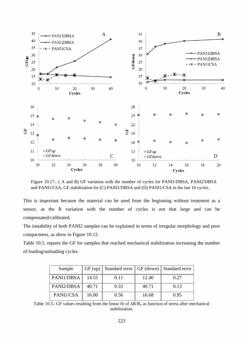
223
This is important because the material can be used from the beginning without treatment as a
sensor, as the R variation with the number of cycles is not that large and can be
compensated/calibrated.
The instability of both PANI2 samples can be explained in terms of irregular morphology and poor
compactness, as show in Figure 10.12.
Table 10.5. reports the GF for samples that reached mechanical stabilization increasing the number
of loading/unloading cycles.
Sample GF (up) Standard error GF (down) Standard error
PANI1/DBSA 14.55 0.11 12.40 0.27
PANI2/DBSA 40.71 0.33 40.71 0.13
PANI1/CSA 16.00 0.56 16.68 0.95
Table 10.5.: GF values resulting from the linear fit of R/R0 as function of stress after mechanical
stabilization.
Figure 10.17.: ( A and B) GF variation with the number of cycles for PANI1/DBSA, PANI2/DBSA
and PANI1/CSA, GF stabilization for (C) PANI1/DBSA and (D) PANI1/CSA in the last 10 cycles.
D
A B
C

224
As it is possible to observe the mechanical stabilization affects also the values of GF. In fact,
PANI1/DBSA and PANI2/DBSA maintain high GF values but lower standard errors, confirming
the stabilization of the polymers during the loading/unloading cycles, whereas PANI1/CSA under
these conditions exhibits GF very similar to that of PANI1/DBSA, suggesting a complete
modification of the original molecular structure.
In order to obtain materials stable for all the loading/unloading cycles and at the same time remove
any trace of solvent (CHCl3) that can compromise their inter-chains network, all the samples were
subjected to a thermal treatment (1 hour at 70°C) and tested again. PANI2/DBSA and PANI1/CSA
maintain the same behaviours shown at room temperature, even though the former becomes stable
more quickly (after 25 cycles). The higher stability of PANI2/DBSA can be explained by the
morphology change (Figures 10.12 D and D’). As it is possible observe, the removal of solvent
leads to a quite porous and more regular morphology that positively affects the piezoresistive
behaviour. On the contrary, also after the thermal treatment PANI2/CSA exhibits an unstable trend,
justified by the high irregular morphology of the sample before and after the thermal aging process.
Only PANI1/DBSA shows a complete stabilization and for this reason it was tested at different
velocity of deformation, as shown in Figure 10.18. and GF variation is summarized in Figure 10.19.
Figure 10.18.: Cyclic piezoresistive response as a function of time for PANI1/DBSA after thermal
treatment (1 h at 70°C). Experimental conditions: bending of 1 mm, deformation velocity of (A)
1mm/min, (B) 2 mm/min, (C) 5 mm/min and (D) 10 mm/min.
A B
C D
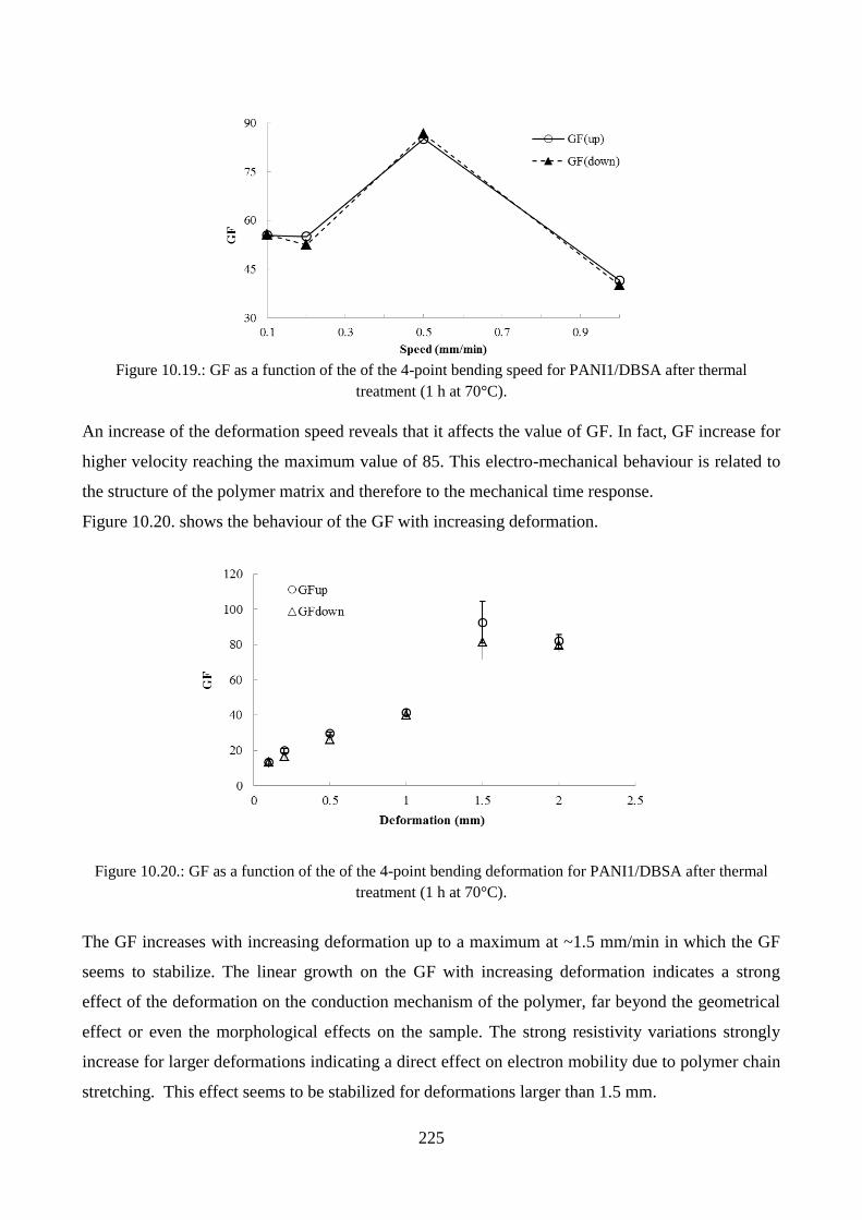
225
An increase of the deformation speed reveals that it affects the value of GF. In fact, GF increase for
higher velocity reaching the maximum value of 85. This electro-mechanical behaviour is related to
the structure of the polymer matrix and therefore to the mechanical time response.
Figure 10.20. shows the behaviour of the GF with increasing deformation.
The GF increases with increasing deformation up to a maximum at ~1.5 mm/min in which the GF
seems to stabilize. The linear growth on the GF with increasing deformation indicates a strong
effect of the deformation on the conduction mechanism of the polymer, far beyond the geometrical
effect or even the morphological effects on the sample. The strong resistivity variations strongly
increase for larger deformations indicating a direct effect on electron mobility due to polymer chain
stretching. This effect seems to be stabilized for deformations larger than 1.5 mm.
Figure 10.19.: GF as a function of the of the 4-point bending speed for PANI1/DBSA after thermal
treatment (1 h at 70°C).
Figure 10.20.: GF as a function of the of the 4-point bending deformation for PANI1/DBSA after thermal
treatment (1 h at 70°C).

226
PART IV: Conclusions
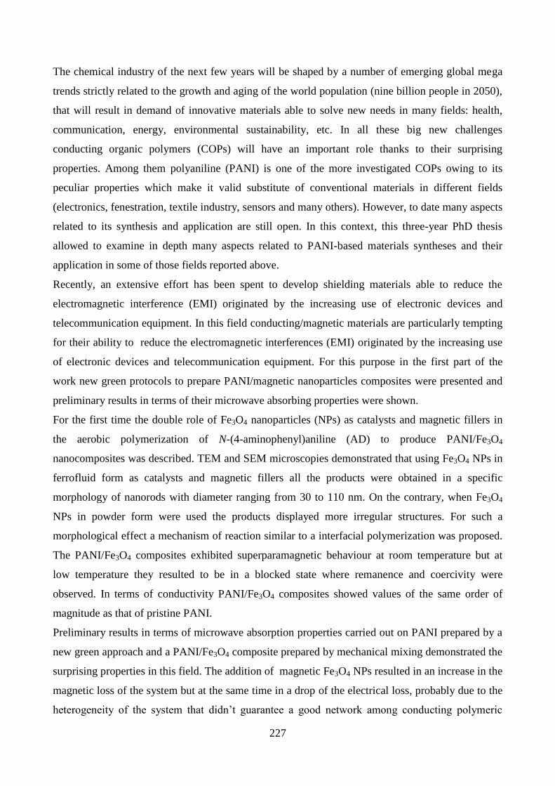
227
The chemical industry of the next few years will be shaped by a number of emerging global mega
trends strictly related to the growth and aging of the world population (nine billion people in 2050),
that will result in demand of innovative materials able to solve new needs in many fields: health,
communication, energy, environmental sustainability, etc. In all these big new challenges
conducting organic polymers (COPs) will have an important role thanks to their surprising
properties. Among them polyaniline (PANI) is one of the more investigated COPs owing to its
peculiar properties which make it valid substitute of conventional materials in different fields
(electronics, fenestration, textile industry, sensors and many others). However, to date many aspects
related to its synthesis and application are still open. In this context, this three-year PhD thesis
allowed to examine in depth many aspects related to PANI-based materials syntheses and their
application in some of those fields reported above.
Recently, an extensive effort has been spent to develop shielding materials able to reduce the
electromagnetic interference (EMI) originated by the increasing use of electronic devices and
telecommunication equipment. In this field conducting/magnetic materials are particularly tempting
for their ability to reduce the electromagnetic interferences (EMI) originated by the increasing use
of electronic devices and telecommunication equipment. For this purpose in the first part of the
work new green protocols to prepare PANI/magnetic nanoparticles composites were presented and
preliminary results in terms of their microwave absorbing properties were shown.
For the first time the double role of Fe3O4 nanoparticles (NPs) as catalysts and magnetic fillers in
the aerobic polymerization of N-(4-aminophenyl)aniline (AD) to produce PANI/Fe3O4
nanocomposites was described. TEM and SEM microscopies demonstrated that using Fe3O4 NPs in
ferrofluid form as catalysts and magnetic fillers all the products were obtained in a specific
morphology of nanorods with diameter ranging from 30 to 110 nm. On the contrary, when Fe3O4
NPs in powder form were used the products displayed more irregular structures. For such a
morphological effect a mechanism of reaction similar to a interfacial polymerization was proposed.
The PANI/Fe3O4 composites exhibited superparamagnetic behaviour at room temperature but at
low temperature they resulted to be in a blocked state where remanence and coercivity were
observed. In terms of conductivity PANI/Fe3O4 composites showed values of the same order of
magnitude as that of pristine PANI.
Preliminary results in terms of microwave absorption properties carried out on PANI prepared by a
new green approach and a PANI/Fe3O4 composite prepared by mechanical mixing demonstrated the
surprising properties in this field. The addition of magnetic Fe3O4 NPs resulted in an increase in the
magnetic loss of the system but at the same time in a drop of the electrical loss, probably due to the
heterogeneity of the system that didn’t guarantee a good network among conducting polymeric

228
chains. The best results are expected for PANI/Fe3O4 composite prepared by the new catalytic
approach reported in this thesis.
The dependence of the catalytic activity of Fe3O4NPs from their sizes in the oxidative
polymerization of N-(4-aminophenyl)aniline was also investigated and it was demonstrated that the
catalytic effect of magnetic nanoparticles increased as their size decreased. Fe3O4NPs didn’t
undergo chemical or crystallographic change during the polymerization reaction and resulted to be
almost uniformly dispersed in the polymer matrix guaranteeing a good homogeneity of the
magnetic properties within the sample. Moreover, PANI/Fe3O4 nanocomposites showed tunable
magnetic properties as a function of the magnetic NPs size.
In order to clarify what was the catalytically active metallic center in the spinel structure of
magnetite, Fe(II) was substituted with another metal (Mn, Co, Ni, Cu, Zn, Mg) and the effect of
such a substitution on the catalytic performance was investigated.
It was observed that the catalytic effect of the spinels in the oxidative polymerization of N-(4-
aminophenyl)aniline was related to two main factors: kind of oxidant and nature of the first metallic
center. In general, when the polymerization reaction was carried out under aerobic conditions all the
ferrites exhibited good results in terms of polymerization yield. However, when H2O2 was used as
the oxidant, replacing the first bivalent center (Fe2+
) with other metals the catalytic activity
followed the trend: Fe ≥ Co > Ni ≥ Cu >> Zn > Mn ≥ Mg.
The different behaviour of the ferrites under aerobic and anaerobic conditions could be related to
their ability to decompose H2O2, subtracting it from the reaction mixture.
However, it was demonstrated for the first time that the catalytic activity of the spinels in the
oxidative polymerization of AD in the presence of H2O2 resulted to be most likely correlated to the
their inversion degree. In fact, inverse spinels produced PANI/MFe2O4 composites in high yields
and led to composites containing PANI in conducting emeraldine form, whereas more modest
results were obtained in the presence of direct spinels producing more reduced polymeric matrix
(similar to leucoemeraldine).
In the second part of this thesis interesting results in the preparation of highly pure polyaniline
nanofibers (NFs) by the electrospinning technique were presented. These nanostructured materials
showed high values of conductivity and good cytocompatibility. Highly pure PANI NFs were
produced by two strategies: reducing as much as possible the co-polymer amount (polyethylene
oxide, PEO) within the PANI/insulating blend used to spun NFs or removing the co-polymer
(polymethylmetacrylate, PMMA) after the electrospinning process by a washing step. Moreover, in
the first case two different kinds of collector were used (static and rotating) and the effect on the
morphology of blended PANI/PEO NFs was investigated.

229
It was observed a decrease of the fiber size and an increase of the conductivity values by reducing
PEO amount. Moreover, the use of a rotating collector had a stretching effect on the nanofibers,
promoting a narrow distribution of diameters. However, the sterilization treatment carried out on
PANI NFs before to test their cytocompatibility resulted to affect negatively their morphology. This
phenomenon was explained in terms of phase segregation. In fact, owing to the non-homogeneous
distribution of PEO and PANI into the blend, the sterilization process caused the removal of a small
co-polymer amount present into the NFs thus dramatically compromising their morphology.
Substituting PEO with another co-polymer (PMMA), not soluble in water or ethanol but able to
guarantee no segregation phenomena, it was possible to spun PANI/PMMA NFs using a high
amount of the insulating copolymer and remove it in a second step with a specific washing
treatment: 2 minutes in 2-propanol. After the washing step PANI NFs didn’t change size and
morphology. Their cytocompatibility was tested on SH-SY5Y cells (human neuroblastoma cell
line). Preliminary results suggested that washed PANI/PMMA NFs result to be a better substrate for
culturing SH-SY5Y cells than unwashed PANI/PMMA NFs. To better investigate this aspect, direct
cytocompatibility tests are in progress
The mechanical monitoring in large and small scale (buildings/touch-technology) needs of highly
sensitive stress/strains sensors and in the third part the amazing piezoelectric properties of PANI
film will be for the first time presented.
In the first part of this section the electromechanical characterization of PANI pellets doped with
H2SO4 was carried out under high and low force loading. The variation of resistance with the
deformation was expressed in terms of gauge factor, GF, and resulted to be similar to that of
commercial stress/strain sensors (0.1-2), whose change in resistance is strictly related to geometrical
factors.
However, at molecular level the conductivity of PANI is the sum of two contributions: the ability of
the charge carriers to move along the polymer backbone (intra-chain mechanism) and the ability of
the charge carriers to hop between the polymer chains (inter-chain mechanism). This second
contribution is particularly important when the material is subjected to stress/strain processes. In
order to emphasize this second contribution and increase the intrinsic piezoresistive effect PANI
was produced in film form and tested in strain/stress tests. The extraordinary high GF values
obtained under specific conditions (more than 10 times higher than those of commercial strain
gauges) open the way to innovative applications of polyaniline in the world of low cost stress/strain
sensors.

230
References
[1] L. Rupprecht, Conductive polymers and plastics in industrial applications, William Andrew
(1999);
[2] M. Bryning, M. Islam, J. Kikkawa, A. Yodh, Advanced Materials, 17 (2005) 1186-1191;
[3] R. Ramasubramaniam, J. Chen, H. Liu, Applied Physics Letters, 83 (2003) 2928-2930;
[4] C. K. Chiang, C. R. Fincher, Jr. Y. W. Park, A. J. Heeger, H. Shirakawa, E. J. Louis, S. C. Gau,
A. G. MacDiarmid, Physical Review Letters, 39 (1977) 1098-1107;
[5] T. A. Skotheim, R. L. Elsenbaumer, J. R. Reynolds, Handbook of Conducting Polymers;
[6] D. Verma, D. Dutta, Journal of Physics: Condensed Matter, 19 (2007) 186212-186217;
[7] H. Karami, M. F. Mousavi, M. Shamsipur, Journal of Power Sources, 117 (2003) 255-259;
[8] M. M. Gvozdenović, B. Z. Jugović, T. L. Trišović, J. S. Stevanović, B. N. Grgur, Materials
Chemistry and Physics, 125 (3) (2011) 601-605;
[9] D. N. Huyen, N. T. Tung, N. D. Thien, L. H. Thanh, Sensor, 11 (2011) 1924-1931;
[10] G. Natta, G. Mazzanti, P. Corraddini, Atti della Accademia Nazionale dei Lincei. Rendiconti
Classe di Scienze Fisiche, Matematiche e Naturali, 25 (1958) 3;
[11] H. Shirakawa, E. J. Luis, A. G. MacDiarmid, C. K. Chiang, A. J. Heeger, Journal of the
Chemical Society, Chemical Communications, (1977) 578-580;
[12] G. Zerbi, La Chimica e l’Industria, 73 (1991) 355;
[13] P. Chandrasekhar, Conducting Polymers, Fundamentals and Applications, Kluwer Academic
Publishers (1999);
[14] J. L. Bredas, G. B. Street, Accounts of Chemical Research, 18 (1985) 309-315;
[15] P. W. Anderson, Physical Review Letters, 34 (1975) 953-955;
[16] W. P. Su, J. R. Schrieffer, A. J. Heeger, Physical Review Letters, 42 (1979) 1698-1701;
[17] D. S. Boudreaux, R. R. Chance, J. L. Brédas, R. Silbey, Physical Review B: Condensed
Matter, 28 (1983) 6927-6936;
[18] H. Thomann, L. R. Dalton, Y. Tomkiewicz, N. S. Shiren, T. C. Clarke, Physical Review
Letters, 50 (1983) 533-536;
[19] S. Roth, Introduction To The Physics Of Conducting Polymers. Mater. Sci. Forum, 21 (1987)
1–12;
[20] M. S. Dresslhaus, G. Dresselhaus, A. Jorio, A. G. Souza Filho, R. Saito, Carbon, 40 (2002)
2043-2061;
[21] K. Mallick, M. J. Witcomb, A. Dinsmore, M. S. Scurrell, Langmuir, 21 (2005) 7964-7967;
[22] Y. Wang, Z. Liu, B. Han, Z. Sun, Y. Huang, G. Yang, Langmuir, 21 (2005) 833-836;

231
[23] Z. Sun, Y. Geng, J. Li, X. Wang, X. Jing, F. Wang, Journal of Applied Polymer Science, 72
(1999) 1077-1084;
[24] T. K. Sarma, D. Chowdhury, A. Paul, A. Chattopadhyay, Chemical Communications, (2002)
1048-1049;
[25] N. Toshima, S. Hara, Progress in Polymer Science, 20 (1995) 155-183;
[26] Z. Chen, C. Della Pina, E. Falletta, M. Rossi, Journal of Catalysis, 267 (2009) 93-96;
[27] C. Della Pina, E. Falletta, M. Lo Faro, M. Pasta, M. Rossi, Gold Bulletin, 42 (2009) 27-33;
[28] Z. Chen, C. Della Pina, E. Falletta, M. Lo Faro, M. Pasta, M. Rossi, N. Santo, Journal of
Catalysis, 259 (2008) 1-4;
[29] H.V.R. Dias, R. M. G. Rajapakse, D. M. M. Krishantha, M. Fianchini, X. Wang, R. L.
Elsenbaumer, Journal of Material Chemistry, 17 (2007) 1762-1768;
[30] H. V. R. Dias, X. Wang, R. M. G. Rajapakse, R. L. Elsenbaumer, Chemical Communications,
(2006) 976-978;
[31] H. Liu, X. B. Hu, J. Y. Wang, R. I. Boughton, Macromolecules, 35 (2002) 9414-9419;
[32] J. Huang, S. Virji, B. H. Weiller, R. B. Kaner, Journal of American Chemical Society, 125
(2003) 314-315;
[33] J. Huang, R. B. Kaner, Journal of American Chemical Society, 126 (2004) 851-855;
[34] X. Lu, H. Mao, D. Chao, W. Zhang, Y. Wei, Macromolecular Chemistry and Physics, 207
(2006) 2142–2152;
[35] K. Doblhofer, K. Rajeshwar, T. A. Skotheim, R. L. Elsenbaumer, J. R. Reynolds (Eds.),
Handbook of Conducting Polymers, 2nd ed., Marcel Dekker, (1998) 531;
[36] C. Della Pina, E. Falletta, M. Rossi, Catalysis Today 160 (2011) 11–27;
[37] B. L. Funt, A. F. Diaz, Organic Electrochemistry: an Introduction and a Guide, Marcel
Dekker, (1991) 1337;
[38] E. M. Genies, G. Bidan, A. F. Diaz, Journal of Electroanalytical Chemistry, 149 (1983) 101;
[39] R. J. Waltman, J. Bargon, Canadian Journal of Chemistry, 64 (1986) 76-95;
[40] R. J. Waltman, J. Bargon, Tetrahedron, 40 (1984) 3963-3970;
[41] S. Asavapiriyanont, G. K. Chandler, G. A. Gunawardena, D. Pletcher, Journal of
Electroanalytical Chemistry, 177 (1984) 229-244;
[42] J. Wang, D. Zhang, Advances in Polymer Technology, 32 (S1) (2013) E323–E368;
[43] www.marketsandmarkets.com;
[44] O. Unverdorben, Annual Physical Chemistry, 8 (1826) 397;
[45] F. F. Runge, Annual Physical Chemistry, 31 (1834) 513;

232
[46] J. Frtzche, Journal fur Praktische Chemie, 20 (1840) 454;
[47] A. G. MacDiarmid, A. J. Epstein, Faraday Discussions, 88 (1989) 317-332;
[48] H. Letheby, Journal of Chemical Society, 15 (1862) 161-163;
[49] A. Green, A. Woodhead, Journal of Chemical Society Transactions, 101 (1912) 1117-1123;
[50] A. Green, A. Woodhead, Journal of Chemical Society Transactions, 97 (1910) 2388-2403;
[51] E. Noelting, Scientific and Industrial History of Aniline Black, WM. J. Matheson& Co, (1889);
[52] R. Willstätter, C. W. Moore, Berichte der Deutschen Chemischen Gesellschaft, 40 (1907)
2665;
[53] J. Chiang, A. MacDiarmid, Synthetic Metals, 13 (1986) 193-205;
[54] G. G. Wallace, G. M. Spinks, P. R. Teasdale, Conductive Electroactive Polymers, CRC Press,
London (2002);
[55] G. G. Wallace, G. M. Spinks, L. A. P. Kane-Maguire, P. R. Teasdale, Conductive
Electroactive Polymers: Intelligent Polymer Systems, CRC Press, London(2009);
[56] J. E. de Albuquerque, L. H. C. Mattoso, R. M. Faria, J. G. Masters, A. G MacDiarmid,
Synthetic Metals, 146 (2004) 1-10;
[57] Y. Xia, J. M. Wiesinger, A. G. MacDiarmid, A. J. Epstein, Chemistry of Materials, 7 (1995)
443-445;
[58] W. S. Huang, A. G. MacDiarmid, Polymer, 34 ( 1993) 1833-1845;
[59] A. Boyle, J. P. Penneau, E. Genies, C. Riekiel, Journal of Polymer Science, Part B: Polymer
Physics, 30 (1992) 265-274;
[60] J. Chiang, A. MacDiarmid, Synthetic Metals, 13 (1986) 193-205;
[61] K. Mallick, M. J. Witcomb, A. Dinsmore, M. S. Scurrell, Langmuir, 21 (2005) 7964-7967;
[62] Y. Wang, Z. Liu, B. Han, Z. Sun, Y. Huang, G. Yang, Langmuir, 21 (2005) 833-836;
[63] Z. Sun, Y. Geng, J. Li, X. Wang, X. Jing, F. Wang, Journal of Applied Polymer Science, 72
(1999) 1077-1084;
[64] T. K. Sarma, D. Chowdhury, A. Paul, A. Chattopadhyay, Chemical Communications, (2002)
1048-1049;
[65] P. N Adams, P. J.Laughlin, A. P. Monkman, A. M. Kenwright, Polymer, 37 (1996) 3411-3417;
[66] J.E. Österholm, Y.Cao, F.L. Klavetter, P.Smith, Synth. Met. 55 (1993) 1034.
[67] S. Trakhtenberg, Y. Hangun-Balkir, J. C. Warner, F. F. Bruno, J. Kumar, R. Nagarajan, L. A.
Samuelson, Journal of the American Chemical Society, 127 (2005) 9100-9104;.
[68] W. Liu, A. Anagnostopoulos, F. F. Bruno, K. Senekal, J. Kumar, S. Tripathy, L. Samuelson,
Synthetic Metals, 101 (1999) 738-741;

233
[69] N. Bicak, B. Karagoz, Journal of Polymer Science Part A: Polymer Chemistry, 44 (2006)
6025-6031;
[70] N. Toshima, S. Hara, Progress in Polymer Science, 20 (1995) 155-183;
[71] S. E. Bourdo, B. C. Berry, T. Viswanathan, Journal of Applied Polymer Science, 98 (2005) 29-
33;
[72] W. Liu, A. L. Cholli, R. Nagarajan, J. Kumar, S. Tripathy, F. F. Bruno, L. Samuelson, Journal
of the American Chemical Society, 121 (1999) 11345-11355;
[73] W. Liu, J. Kumar, S. Tripathym, J. Senecal, L. Samuelson, Journal of the American Chemical
Society, 121 (1999) 71-78;
[74] D. K. Moon, K. Osokada, T. Maruyama, T. Yamamoto, Macromolecular Chemistry and
Physics, 193 (1992) 17231728;
[75] M. Sivakumar, A. Gedanken, Synthetic Metals, 148 (2005) 301-306;
[76] Y. Wei, G. W. Jang, Ch. Ch. Chan, K. F. Hsuen, R. Hariharan, S. A. Patel, C. K. Whitecar,
Journal of Physical Chemistry, 94 (1990) 7716-7721;
[77] Y. Wei, X. Tang, Y. Sun, W. W. Focke, Journal of Polymer Science Part A: Polymer
Chemistry, 27 (1989) 2385-2396;
[78] Y. Wei, R. Hariharan, S. A. Patel, Macromolecules, 23 (1990) 758-764;
[79] Y. Wei, K. F. Hsueh, G. W. Jang, Polymer, 35 (1994) 3572-3575;
[80] C. Della Pina, M. Rossi, A. M. Ferretti, A. Ponti, M. Lo Faro, E. Falletta, Synthetic Metals,
162 (2012) 2250-2258;
[81] D. M. Mohilner, R. N. Adams, W. J. Argersinger Jr., Journal of the American Chemical
Society, 84 (1962) 3618-3622;
[82] J. Bacon, R. N. Adams, Journal of the American Chemical Society, 90 (1968) 6596-6599;
[83] G. Ćirić-Marjanović, unpublished results.
[84] N. Gospodinova, L. Terlemezyan, Progress in Polymer Science, 23 (1998) 1443-1484;
[85] G. Ćirić-Marjanović, M. Trchová, J. Stejskal, Collection of Czechoslovak Chemical
Communications, 71 (2006) 1407-1426;
[86] G. Ćirić-Marjanović, E.N. Konyushenko, M. Trchová, J. Stejskal, Synthetic Metals, 158
(2008) 200-211;
[87] N. Gospodinova, L. Terlemezyan, P. Mokreva, K. Kossev, Polymer, 34 (1993) 2434-2437;
[88] Y. Ding, A. B. Padias, H. K. Hall Jr., Journal of Polymer Science Part A: Polymer Chemistry,
37 (1999) 2569-2579;
[89] R. Madathil, S. Ponrathnam, H. J. Byrne, Polymer, 45 (2004) 5465-5471;
[90] E. M. Genies, C. Tsintavis, Journal of Electroanalytical Chemistry, 195 (1985) 109-128;

234
[91] E. M. Genies, M. Łapkowski, Journal of Electroanalytical Chemistry, 236 (1987) 199-208;
[92] G. Vidotto, A. Crosato-Arnaldi, G. Talamini, Macromolecular Chemistry and Physics, 122
(1969) 91–104;
[93] M. Carenza, G. Palma, European Polymer Journal, 21 (1985) 41–47;
[94] A. Guyot, Salamone JC, Editor-in-Chief. Polymeric materials encyclopedia, Boca Raton: CRC
Press, 9 (1996) 7228–7237;
[95] H. D. H. Stover, Salamone JC, Editor-in-Chief. Polymeric materials encyclopedia, Boca
Raton: CRC Press, 9 (1996) 7237–7238;
[96] E. A.Gruike, Kroschwitz JI. Executive editor., Encyclopedia of polymer science and
engineering, NewYork: John Wiley & Sons, 16 2nd Ed. (1989) 443–473;
[97] H. Bieringer, K. Flatau, D. Reese, Angewandte Makromolekulare Chemie, 123 (1984) 307–
334;
[98] H. G. Yuan, G. Kalfas, W. H. Ray, Journal of Macromolecular Science - Reviews in
Macromolecular Chemistry & Physics, 31 (1991) 215–299;
[99] K. E. J. Barrett, Dispersion polymerization in organic media, London: John Wiley & Sons,
(1975);
[100] S. Palaniappan, M. Sairam, Journal of Applied Polymer Science, 108 (2008) 825–32;
[101] J. Stejskal, Journal of Polymer Materials, 18 (2001) 225–258;
[102] J. Stejskal, Dendrimers, assemblies, nanocomposites, Arshady R, Guyot A, Editors, London,
Citus Books (2002) 195–281;
[103] V. R. Gowariker, N. V. Viswanathan, J. Sreedhar, Polymer Science, New Delhi, India, New
Age International (P) Limited (1996) 73;
[104] F. Yan, G. Xue, Journal of Material Chemistry, 9 (1999) 3035–3039;
[105] E. Ruckenstein, Y. Sun, Synthetic Metals, 74 (1995) 107–113;
[106] H. Huang, H. Zhang, J. Li, S. Cheng, F. Hu, B. Tan, Journal of Applied Polymer Science, 68
(1998) 2029–2039;
[107] H. Huang, H. Zhang, Z. Ai, J. Li, S. Cheng, F. Hu, Z. Ai, B. Tan, S. Cheng, J. Li, Journal of
Applied Polymer Science, 73 (1999) 315–322;
[108] E. Marie, R. Rothe, M. Antonietti, K. Landfester, Macromolecules, 36 (2003) 3967–3973;
[109] J. Li, K. Fang, H. Qiu, S. Li, W. Mao, Q. Wu, Synthetic Metals, 145 (2004) 191–194;
[110] S. Ding, H. Mao, W. J. Zhang, Applied Polymer Science, 109 (2008) 2842–2847;
[111] P. Dallas, D. Stamopoulos, N. Boukos, V. Tzitzios, D. Niarchos, D. Petridis, Polymer, 48
(2007) 3162–3169;
[112] J. Chen, D. Chao, X. Lu, W. Zhang, Materials Letters, 61 (2007) 1419–1423;

235
[113] Q. Guo, C. Yi, L. Zhu, Q. Yang, Y. Xie, Polymer, 46 (2005) 3185–3189;
[114] J. Y. Kim, E. Y. Kim, Y. S. Won, H. S. Lee, K. S. Suh, Synthetic Metals, 139 (2003) 485–
489;
[115] J. Y. Kim, S. J. Kwon, S. W. Han, Y. K. Min, Japanese Journal of Applied Physcs, 43 (2004)
5660–5664;
[116] J. Y. Kim, J. H. Lee, S. J. Kwon, Synthetic Metals, 157 (2007) 336–342;
[117] K. S. Suslick, Science, 1990, 3, 1439-1445;
[118] X. L. Jing, Y. Y. Wang, D. Wu, L. She, Y. Guo, Journal of Polymer Science Part
A: Polymer Chemistry, 44 (2006) 1014–1019;
[119] X. Jing, Y. Wang, D. Wu, J. P. Qiang, Ultrasonic Sonochemistry, 14 (2007) 75–80;
[120] S. Kobayashi, H. Uyama, S. Kimura, Chemical Review, 101 (2001) 3793–3818;
[121] E. Arias-Marin, J. Romero, A. S. Ledezma-Perez, S. Kniajansky, Polymer Bulletin, 37
(1996) 581–587;
[122] L. Mejias, M. H. Reihmann, S. Sepulveda-Boza, H. Ritter, Macromolecular Bioscience, 2
(2002) 24–32;
[123] N. Kobayashi, K. Teshima, R. Hirohashi, Journal of Material Chemistry, 8 (1998) 497–506;
[124] R. A. Barros, W. M. Azevedo, F. M. Aguiar, Materials Characterization, 50 (2003) 131–134;
[125] P. K. Khanna, N. Singh, S. Charan, A. K. Viswanath, Materials Chemisty and Physics, 92
(2005) 214–219;
[126] C. Nastase, F. Nastase, A. Dumitru, M. Ionescu, I. Stamatin, Composites Part A: Appl ied
Science and Manufacturing, 36 (2005) 481–485;
[127] F. Nastase, I. Stamatin, C. Nastase, D. Mihaiescu, A. Moldovan, Progress in Solid State
Chemistry, 34 (2006) 191–199;
[128] A. G. MacDiarmid, J. C. Chiang, A. F. Richter, N. L. D. Somasiri, Conducting Polymers,
Alcacer, L., Ed.; Reidel: Dordrecht, The Netherlands (1986);
[129] E. R. Holland, S. J. Pomfret, P. N. Adams, L. Abell, A. P. Monkmann, Synthetic Metals, 84
(1997) 777–778;
[130] P. Kiattibutr, L. Tarachiwin, L. Ruangchuay, A. Sirivat, J..Schwank, Reactive and Functional
Polymers, 53 (2002) 29–37;
[131] M. D. Catedral, A. K. G. Tapia, R. V. Sarmago, J. P. Tamayo, E. J. del Rosario, Science
Diliman, 16/2 (2004) 41-46;
[132] M. Doriomedoff, F. Hautiere-Cristofini, R. De Surville, M. Jozefowicz, L.T. Yu, R .Buvet,
Journal de Chimie Physique et de Physico-Chimie Biologique, 68 (1971) 1063;
236
[133] Q. Zhou, J. Wang, Y. Ma, C. Cong, F. Wang, Colloid & Polymer Science, 285 (2007) 405–
411;
[134] Y. Wei, G. W. Jang, K. F. Hsueh, E. M. Scherr, A. G. MacDiarmid, A. J. Epstein, Polymer,
33 (1992) 314–322;
[135] H. Farrokhzad, T. Van Gerven, B. Van der Bruggen, European Polymer Journal, in press;
[136] A.G. MacDiarmid, A. J. Epstein, Materials Research Society Symposium Proceedings, 247
(1992) 565-576;
[137] A. Ohtani, M. Abe, M. Ezoe, T. Doi, T. Miyata, A. Miyake, Synthetic Metals, 55-57 (1993)
3696-3701;
[138] P. N. Adams, P. J. Laughlin, A. P. Monkman, A. M. Kenwright, Polymer, 37 (1996) 3411-
3417;
[139] P. N. Adams, P. J. Laughlin, A. P. Monkman, Synthetic Metals, 76 (1996) 157-160;
[140] P. G. de Gennes, Comptes rendus de l'Académie des Sciences Paris, 2/302 (1986) 1;
[141] D. S. Pearson, P. A. Pincus, G. W. Heffner, S. M. Dahman, Macromolecules, 26 (1993)
1570-1575;
[142] S. Bhadra, N. K. Singha, D. Khastgir, Synthetic Metals, 156 (2006) 1148–1154;
[143] S. Bhadra, S. Chattopadhyay, N. K. Singha, D. Khastgir, Journal of Polymer Science Part B:
Polymer Physics, 45 (2007) 246–259;
[144] S. Bhadra, N. K. Singha, D. Khastgir, Polymer International, 56 (2007) 919–927;
[145] S. Bhadra, N. K. Singha, D. Khastgir, Journal of Applied Polymer Science, 104 (2007) 1900–
1904;
[146] S. Bhadra, D. Khastgir, Polymer Degradation and Stability, 92 (2007) 1824–1832;
[147] A. Wolter, P. Rannou, J. P. Travers, B. Gilles, D..Djurado, Physical Review B, 58 (1998)
7637–7647.;
[148] W. W. Focke, G. E. Wnek, Y. Wei, Journal of Physical Chemistry, 91/22 (1987) 5813-5818;
[149] M. Nechtstein, C. Santier, Journal de Physique, 47 (1986) 935-937;
[150] S. Quillard, G. Louarn, S. Lefrant, A. G. MacDiarmid, Physical Review B, 50 (1994) 12496-
12508;
[151] E. Kang, K. Neoh, T. Tan, S. Khor, K. Tan, Macromolecules, 23 (1990) 2918-2926;
[152] A. G. MacDiarmid, A. Epstein, Faraday Discussions of the Chemical Society, 88 (1989) 317-
332;
[153] A. G. MacDiarmid, A. J. Epstein, Science and Applications of Conducting Polymers, W.R.
Salaneck, D.T. Clark, and E.J. Samuelson, Eds. Adam Hilger, Bristol, UK, (1991) 117-127;
[154] J. Laska, Journal of Molecular Structure, 701 (2004) 13-18;
237
[155] Y. Xis, J. M. Wiesinger, A. G. MacDiarmid, Polymer, 7 (1995) 443-445;
[156] R. H. Baughman, J. F. Wolf, H. Eckhardt, W. Shacklette, Synthetic Metals, 25 (1988) 121-
137;
[157] W. Fosong, T. Jinsong, W. Lixiang, Z. Hongfang, M. Zhishen, Molecular Crystals and
Liquid Crystals, 160 (1988) 175-184;
[158] Y. B. Moon, Y. Cao, P. Smith, A. J. Heeger, Polymer Communications, 30 (1989) 196-199;
[159] J. P. Pouget, M. E. Jdzefowiczt, A. J. Epstein, X. Tang, A. G. MacDiarmid, Macromolecules,
24 (1991) 779-789;
[160] M. E. Jbzefowicz, R. Laversanne, H. H. S. Javadi, A. J. Epstein, J. P. Pouget, X. Tang, A. G.
MacDiarmid, Physical Review B, 39 (1989) 12958-12961;
[161] S. Pruneanu, E. Veress, I. Marian, L. Oniciu, Journal of Material Science, 34 (1999) 2733–
2739;
[162] P . Snauwaert, R. Lazzaroni, J . Riga, J . Verbist, D. Gonbeau, Electronic Properties of
Conjugated polymers III, Springer Series in Solid State Sciences, edited by H. Kuzmany, M.
Mehring and S. Roth, Springer, Berlin, 91 (1989) 301–304;
[163] R. L. Hand, R. F . Nelson, Journal of the American Chemical Society, 96 (1974) 850-860;
[164] V. B. Shim, M. S. Won, S . M. Park, Journal of the Electrochemical Society, 137 (1990) 538-
544;
[165] D. C. Trivedi, S . K. Dhawan, Synthetic Metals, 58 (1993) 309-324;
[166] R. Greef, R. Peat, L. M. Peter, D. Pletcher, J. Robinson, Instrumental Methods in
Electrochemistry, Ellis Horwood, Chichester, (1980) 25;
[167] A.G. MacDiarmid, W.E. Jones Jr., I. D. Norris, J. Gao, A. T. Johnson Jr.,N. J. Pinto, J. Hone,
B. Han, F. K. Ko, H. Okuzaki, M. Llaguno, Synthetic Metals, 119 (2001) 27–30;
[168] N. J. Pinto, A. T. Johnson Jr., A. G. MacDiarmid, C. H. Mueller, N. Theofylaktos, D. C.
Robinson, F. A. Miranda, Applied Physics Letters, 83 (2003) 4244–4246;
[169] Y. X. Zhou, M. Freitag, J. Hone, C. Staii, N. J. Pinto, A. T. Johnson Jr., A. G. MacDiarmid,
Applied Physics Letters, 83 (2003) 3800–3802;
[170] P. K. Kahol, N. J. Pinto, Synthetic Metals, 140 (2004) 269–272;
[171] H. X. He, C. Z. Li, N. J. Tao, Applied Physics Letters, 78 (2001) 811–813;
[172] C. He, Y. W. Tan, Y. F. Li, Journal of Applied Polymer Science, 87 (2003) 1537–1540;
[173] X. Y. Zhang, R. Chan-Yu-King, A. Jose, S. K. Manohar, Synthetic Metals, 145 (2004) 23–29;
[174] S. Virji, J. X. Huang, R. B. Kaner, B. H. Weiller, Nano Letters, 4 (2004) 491–496;
[175] S. K. Pillalamarri, F. D. Blum, A. T. Tokuhiro, J. G. Story, M. F. Bertino, Chemistry of
Materials, 17 (2005) 227–229;
238
[176] J. X. Huang, R. B. Kaner, Angewandte Chemie International Edition, 43 (2004) 5817–5821;
[177] C. R. Martin, L. S. Van Dyke, Z. Cai, W. Liang, Journal of the American Chemical Society,
112 (1990) 8976–8977;
[178] R. M. Penner, C. R. Martin, Journal of the Electrochemical Society, 133 (1986) 2206–2207;
[179] C. R. Martin, Science, 266 (1994) 1961–1966;
[180] C. R. Martin, Accounts of Chemical Research, 28 (1995) 61–68;
[181] C. R. Martin, Chemistry of Materials, 8 (1996) 1739–1746;
[182] C. G. Wu, T. Bein, Science, 264 (1994) 1757–1759;
[183] C. W. Wang, Z. Wang, M. K. Li, H. L. Li, Chemical Physics Letters, 341 (2001) 431–434;
[184] Z. Wang, M. A. Chen, H. L. Li, Materials Science and Engineering A, 328 (2002) 33–38;
[185] S. M. Yang, K. H. Chen, Y. F. Yang, Synthetic Metals, 152 (2005) 65–68;
[186] M. Delvaux, J. Duchet, P. Y. Stavaux, R. Legras, S. Demoustier-Champagne, Synthetic
Metals, 113 (2000) 275–280;
[187] C. Y. Peng, A. K. Kalkan, S. J. Fonash, B. Gu, A. Sen, Nano Letters, 5 (2005) 439–444;
[188] H. Cao, C. Tie, Z. Xu, J. Hong, H. Sang, Applied Physics Letters, 78 (2001) 1592–1594;
[189] H. J. Qiu, M. X. Wan, B. Matthews, L. M. Dai, Macromolecules, 34 (2001) 675–677;
[190] J. Liu, M. X. Wan, Journal of Materials Chemistry, 11 (2001) 404–407;
[191] Y. Z. Long, Z. J. Chen, P. Zheng, N. L. Wang, Z. M. Zhang, M. X. Wan, Journal of Applied
Physics, 93 (2003) 2962–2965;
[192] Z. X. Wei, M. X. Wan, Journal of Applied Polymer Science, 87 (2003) 1297–1301;
[193] Z. M. Zhang, Z. X. Wei, M. X. Wan, Macromolecules, 35 (2002) 5937–5942;
[194] Y. S. Yang, J. Liu, M. X. Wan, Nanotechnology, 13 (2002) 771–773;
[195] A. D. W. Carswell, E. A. O’Rear, B. P. Grady, Journal of the American Chemical Society,
125 (2003) 14793–14800;
[196] X. Y. Zhang, S. K. Manohar, Chemical Communications, (2004) 2360–2361;
[197] P. Nickels,W. U. Dittmer, S. Beyer, J. P.Kotthaus, F. C. Simmel, Nanotechnology, 15 (2004)
1524–1529;
[198] Y. F. Ma, J. M. Zhang, G. J. Zhang, H. X. He, Journal of the American Chemical Society,
126 (2004) 7097–7101;
[199] J. M. Liu, S. C. Yang, Journal of the Chemical Society, Chemical Communications, (1991)
1529–1531;
[200] S. J. Choi, S. M. Park, Advanced Materials, 12 (2000) 1547–1549;
[201] T. Hatano, M. Takeuchi, A. Ikeda, S. Shinkai, Chemistry Letters, 32 (2003) 314–315;

239
[202] L. M. Huang, Z. B. Wang, H. T. Wang, X. L. Cheng, A. Mitra, Y. X. Yan, Journal of
Material Chemistry, 12 (2002) 388–391;
[203] J. Kan, R. Lv, S. Zhang, Synthetic Metals, 145 (2004) 37–42;
[204] J. Q. Kan, S. L. Zhang, G. L. Jing, Journal of Applied Polymer Science, 99 (2006) 1848–
1853;
[205] M. X. Wan, J. C. Li, Journal of Polymer Science Part A: Polymer Chemistry, 38 (2000)
2359–2364;
[206] Y. Z. Long, Z. J. Chen, N. L. Wang, Z. M. Zhang, M. X. Wan, Physica B: Condensed Matter,
325 (2003) 208–213;
[207] L. J. Zhang, M. X. Wan, Nanotechnology, 13 (2002) 750–755;
[208] Y. Z. Long, L. J. Zhang, Y. J. Ma, Z. J. Chen, N. L. Wang, Z. Zhang, M. X. Wan,
Macromolecular Rapid Communications, 24 (2003) 938–942;
[209] Y. Z. Long, J. L. Luo, J. Xu, Z. J. Chen, L. J. Zhang, J. C. Li, M. X. Wan, Journal of Physics:
Condensed Matter, 16 (2004) 1123–1130;
[210] Y. Z. Long, Z. J. Chen, N. L. Wang, Y. J. Ma, Z. Zhang, L. J. Zhang, M. X. Wan, Applied
Physics Letters, 83 (2003) 1863–1865;
[211] K. Huang, M. X. Wan, Chemistry of Materials, 14 (2002) 3486–3492;
[212] Y. S. Yang, M. X. Wan, Journal of Materials Chemistry, 12 (2002) 897–901;
[213] H. J. Qiu, J. Zhai, S. H. Li, L. Jiang, M. X. Wan, Advanced Functional Materials, 13 (2003)
925–928;
[214] N. J. Pinto, P. L. Carrión, A. M. Ayala, M. Ortiz-Marciales, Synthetic Metals, 148 (2005)
271–274;
[215] J. H. Hwang, S. C. Yang, Synthetic Metals, 29 (1989) 271–276;
[216] Z. M. Zhang, Z. X. Wei, L. J. Zhang, W. X. Wan, Acta Materialia, 53 (2005) 1373–1379;
[217] J. Huang, M. X. Wan, Journal of Polymer Science Part A: Polymer Chemistry, 37 (1999)
151–157;
[218] U. Beginn, Advanced Materials, 10 (1998) 1391–1394;
[219] M. Bockstaller, W. Köhler, G. Wegner, D. Vlassopoulos, G. Fytas, Macromolecules, 33
(2000) 3951–3953;
[220] L. K. Werake, J. G. Story, M. F. Bertino, S. K. Pillalamarri, F. D. Blum, Nanotechnology, 16
(2005) 2833–2837;
[221] N. R. Chiou, A. J. Epstein, Advanced Materials, 73 (2005) 1679–1683;
[222] N. R. Chiou, A. J. Epstein, Synthetic Metals, 153 (2005) 69–72;
[223] R. V. Parthasarathy, C. R. Martin, Chemistry of Materials, 6 (1994) 1627–1632;
240
[224] J. P. Spatz, B. Lorenz, K. Weishaupt, H. D. Hochheimer, Physical Review B, 50 (1994)
14888–14892;
[225] X. Y. Zhang, W. J. Goux, S. K. Manohar, Journal of the America Chemical Society, 126
(2004) 4502–4503;
[226] W. G. Li, H. L. Wang, Journal of the American Chemical Society, 126 (2004) 2278–2279;
[227] M. H. Yun, N. V. Myung, R. P. Vasquez, C. S. Lee, E. Menke, R. M. Penner, Nano Letters,
4 (2004) 419-422;
[228] M. Li, Y. Guo, Y. Wei, A. G. MacDiarmid, P. Y. Lelkes, Biomaterials, 27 (2006) 2705-2715;
[229] G. E. Wnek, M. E. Carr, D. G. Simpson, G. I. Bowlin, Nano Letters, 3 (2003) 213-216;
[230] H. Schreuder-Gibson, P. Gibson, K. Senecal, M. Sennett, J. Walker, W. Yeomans, D. Ziegler,
P. P. Tsai, Journal of Advanced Materials, 34 (2002) 44-55;
[231] P. Gibson, H. S. Gibson, D. Rivin, Colloids and Surfaces A, 2001, 187, 469-481;
[232] C. Kim, K. S. Yang, Applied Physics Letters, 83 (2003) 1216-1218;
[233] S. W. Choi, S. M. Jo, W. S. Lee, Y. R. Kim, Advanced Materials, 15 (2003) 2027-2032;
[234] H. Liu, J. Kameoka, D. A. Czaplewski, H. G. Craighead, Nano Letters, 4 (2004) 671-675;
[235] D. Aussawasathien, J. H. Dong, L. Dai, Synthetic Metals, 154 (2005) 37-40;
[236] K. M. Manesh, A. I. Gopalan, K. P. Lee, P. Santhosh, K. D. Song, D. D. Lee, IEEE
Transactions on Nanotechnology, 6 (2007) 513-518;
[237] I. D. Norris, M. M. Shaker, F. K. Ko, A. G. MacDiarmid, Synthetic Metals, 114 (2000) 109-
114;
[238] K. H. Hong, T. J. Kang, Journal of Applied Polymer Science, 99 (2006) 1277-1286;
[239] M. Wei, B. W. Kang, C. M. Sung, J. Mead, Macromolecular Materials and Engineering,
2006, 291, 1307-1314;
[240] P. H. S. Picciani, E. S. Medeiros, Z. Pan, W. J. Orts, L. H. C. Mattoso, B. G. Soares, Journal
of Applied Polymer Science, 112 (2009) 744–753;
[241] B. Gupta, N. Revagade, J. Hilborn, Progress in Polymer Science, 32 (2007) 455-482;
[242] R. Langer, J. P. Vacanti, Tissue Engineering Science, 260 (1993) 920-926;
[243] X. Zong, K. Kim, D. Fang, S. Ran, B. S. Hsiao, B. Chu, Polymer, 43 (2002) 4403-4412;
[244] H. Hou, Z. Jun, A. Reuning, A. Schaper, J. H. Wendorff, A. Greiner, Macromolecules, 35
(2002) 2429-2431;
[245] Z. Jun, H. Hou, A. Schaper, J. H. Wendorff, A. Greiner, e-Polymers, 9 (2003)1-9;

241
[246] S. P. Armes, Current Opinion in Colloid & Interface Science, 1/2 (1996) 214–220;
[247] S. P. Armes, M. J. Aldissi, Journal of the Chemical Society, Chemical Communications, 2
(1989) 88–89;
[248] S. P. Armes, M. J. Aldissi, M. Hawley, J. G. Beery, S. Gottesfeld, Langmuir, 7/7 (1991)
1447–1452;
[249] N. Gospodinova, P. Mokreva, L. Terlemezyan, Journal of the Chemical Society, Chemical
Communications, 13 (1992) 923–924;
[250] H. Eisazadeh, G. Spinks, G. G. Wallace, Polymer International, 37/2 ((1995) 87–91;
[251] J. Stejskal, P. Kratochvil, M. Helmstedt, Langmuir, 12/14 (1996) 3389–3392;
[252] B. Vincent, J. Waterson, Journal of the Chemical Society, Chemical Communications,
1990;9:683–4.
[253] J. Stejskal, M. Špirkova, A. Riede, M. Helmstedt, P. Mokreva, J. Prokeš, Polymer, 40/10
(1999) 2487–2492;
[254] D. Chattopadhyay, M. Chakraborty, B. M. Mandal, Polymer International, 50/5 (2001) 538–
544;
[255] P. B. Banerjee, M. L. Digar, S. N. Bhattacharyya, B. M. Mandal, European Polymer Journal,
30/4 (1994) 499–501;
[256] P. Beadle, S. P. Armes, S. Gottesfeld, C. Mombourquette, R. Houlton, W. D. Andrews, S. F.
Agnew, Macromolecules, 25/9 (1992) 2526–2530;
[257] M.Morita, Journal of Polymer Science: Polymer Physics, 32/2 (1994) 231–242;
[258] R. Gangopadhyay, A. De, G. Ghosh, Synthetic Metals, 123/1 (2001) 21–31;
[259] K. Ogura, T. Saino, M. Nakayama, H. Shiigi, Journal of Materials Chemistry, 7/7 (1997)
2363–2366;
[260] A. Malinauskas, Polymer, 4/9 (2001) 3957–3972;
[261] R. Anbarasan, J. Jayaseharan, M Sudha, J. L. Devi, P. V. Nirmala, A. J. Gopalan, Applied
Polymer Science, 2001;81(2):468–78;
[262] R. Anbarasan, T. Vasudevan, A. Gopalan, Journal of Materials Science, 35/3 (2000) 617–25;
[263] K. W. Oh, K. H. Hong, S. H. Kim, Journal of Applied Polymer Science, 74/8 (1999) 2094–
2101;
[264] G. A. Tishchenko, J. Dybal, J. Stejskal, V. Kudela, M. Bleha, E. Y. Rosova, G. K.
Elyashevich, Journal of Membrane Science, 196 (2002) 279–287;
[265] G. K. Elyashevich, L. Terlemezyan, I. S. Kuryndin, V. K. Lavrentyeva, P. Mokreva, E. Y.
Rosova, Y. N. Sazanov ,Thermochima Acta, 374/1 (2001) 23–30;
242
[266] B. Das, S. Kar, S. Chakraborty, D. Chakraborty, S. Gangopadhyay, Journal of Applied
Polymer Science, 69/5 (1998) 841–844;
[267] M. Chakraborty, D. C. Mukherjee, B. M. Mandal, Synthetic Metals, 98/3 (1999) 193–200;
[268] J. Anand, S. Palaniappan, D .N. Sathyanarayana, Progress in Polymer Science, 23/6 (1998)
993–1018;
[269] T. Fukunada, K. Fuse, K. Kobayashi, Japan Patent, 62-139896 (1987);
[270] O. Niwa, T. Tamamura, Journal of Chemical Society, Chemical Communications, 13 (1984)
817–818;
[271] M. A. De Paoli, R. J. Waltman, A. F. Diaz, J. Bargon, Journal of Chemical Society, Chemical
Communications, 15 (1984) 1015–1016;
[272] M. G. Han, S. S. Im, Polymer, 42/17 (2001) 7449–7454;
[273] T. Jeevananda, Siddaramaiah, European Polymer Journal, 39/3 (2003) 569–578;
[274] T. Vikki, L. O. Pietilä, H. Österholm, L. Ahjopalo, A. Takala, A. Toivo, K. Levon, P.
Passiniemi, O. Ikkala, Macromolecules, 29/8 (1996) 2945–2953;
[275] Y. Wei, W. W. Focke, G. E. Wnek, A. Ray, A. G..MacDiarmid, Journal of Physical
Chemistry, 93 (1989) 495–499;
[276] M. Leclerc, J. Guay, L. H. Dao, Macromolecules, 22/2 (1989) 649–653;
[277] D. Macinnes, B. L. Funt, Synthetic Metals, 25/3 (1988) 235–242;
[278] J. Yue, A. J. Epstein, A. G. MacDiarmid, Molecular Crystals and Liquid Crystals, 189 (1990)
255–261;
[279] J. Yue, Z. H. Wang, K. R. Cromack, A. J. Epstein, A. G. MacDiarmid, Journal of the
American Chemical Society, 113/7 (1991) 2665–2671;
[280] X. L. Wei, Y. Z. Wang, S. M. Long, C. Bobeczko, A. J..Epstein, Journal of the American
Chemical Society, 118/11 (1996) 2545–2555;
[281] X. G. Li, M. R. Huang, L. H. Zhu, Y. L. Yang, Journal of Applied Polymer Science, 82/4
(2001) 790–798.;
[282] Y. Cao, P. Smith, A. J. Heeger, Synthetic Metals, 48/1 (1992) 91–97;
[283] A. J. Heeger, Synthetic Metals, 57/1 (1993) 3471–3482;
[284] A. Pron, J. E. Österholm, P. Smith, A. J. Heeger, J. Laska, M. Zagorska, Synthetic Metals,
57/1 (1993) 3520–3525;
[285] Y. Cao, P. Smith, A. J. Heeger, Synthetic Metals, 57/1 (1993) 3514–3519;
[286] M. Angelopoulos, C. E. Asturias, S. P. Ermer, E. Ray, E. M. Scherr, A. G. MacDiarmid, M.
A. Akhtar, Z. Kiss, A. J. Epstein, Molecular Crystals and Liquid Crystals, 160 (1988) 151–
163;
243
[287] D. Gonçalves, A. Waddon, F. E. Karasz, L. Akcelrud, Synthetic Metals, 74/3 (1995) 197–
199;
[288] J. Anand, S. Palaniappan, Siddaramaiah, P. Srinivasan, D. N. Sathyanarayana, European
Polymer Journal, 35/3 (1999) 499–507;
[289] U. A. Sevil, O. Guven, Ö. Birer, S. Süzer, Synthetic Metals, 110/3 (2000) 175–179;
[290] S. A. Chen, G. W. Hwang, Polymer, 38/13 (1997) 3333–3346;
[291] I. Yamaguchi, T. Yasuda, T. Yamamoto, Journal of Polymer Science, Polymer Chemistry,
39/18 (2001) 3137–3143;
[292] P. N. Adams, P. Devasagayam, S. J. Pomfret, L. Abell, A. P. Monkman, Journal of Physics:
Condensed Matter, 10/37 (1998) 8293–8303;
[293] S. J. Pomfret, P. N. Adams, N. P. Comfort, A. P. Monkman, Synthetic Metals, 101/1-3 (1999)
724–725;
[294] T. E. Olinga, J. Fraysse, J. P. Travers, A. Dufresne, A. Pron, Macromolecules, 33/6 (2000)
2107–2113;
[295] J. Fraysse, J. Planés, A. Dufresne, A. Guermache, Macromolecules, 34/23 (2001) 8143–8148;
[296] H. S. Moon, J. K. Park, Journal of Polymer Science, Polymer Chemistry, 36/9 (1998) 1431–
1439;
[297] S. Yang, E. Ruckenstein, Synthetic Metals, 59/1 (1993) 1–12;
[298] E. Ruckenstein, S. Yang, Synthetic Metals, 53/3 (1993) 283–292;
[299] E. Ruckenstein, Y. Sun, Synthetic Metals, 74/2 (1995) 107–113;
[300] Y. Sun, E. Ruckenstein, Synthetic Metals, 74/2 (1995) 145–150;
[301] T. Jeevananda, Siddaramaiah, V. Annadurai, R. Somashekar, Journal of Applied Polymer
Science, 82/2 (2001) 383–388;
[302] V. Jousseaume, M. Morsli, A. Bonnet, Journal of Applied Physics, 84 (2002) 1848–1855;
[303] Q. Zhang, X. Wang, Y. Geng, D. Chen, X. Jing, Journal of Polymer Science, Polymer
Physics, 40/22 (2002) 2531–2538;
[304] A. Andreatta, P. Smith, Synthetic Metals, 55/2-3 (1993) 1017–1022;
[305] L. W. Shacklette, G. G. Miller, R. L. Elsenbaumer, C. C. Han, B. M. Webling, B. Wessling,
US Patent 5,281,363 (1994);
[306] S. Koul, R. Chandra, S. K. Dhawan, Sensors and Actuator B, 75/3 (2001) 151–159;
[307] Y. Wang, X. Wang, J. Li, H. Zhang, Z. Mo, X. Jing, F..Wang, Journal of Polymer Science,
Polymer Physics, 40 (2002) 605–612;
[308] T. Ondarcuhu, C. Joachim, Europhysics Letters, 42/2 (1998) 215–220;

244
[309] L. Feng, S. Li, H. Li, J. Zhai, Y. Song, L. Jiang, Angewandte Chemie International Edition,
41/7 (2002) 1221–1223;
[310] P. X. Ma, R. Zhang, Journal of Biomedical Materials Research, 46 (1999) 60–72;
[311] G. J. Liu, J. F. Ding, L. J. Qiao, A. Guo, B. P. Dymov, J. T. Gleeson, Chemistry: A European
Journal, 5 (1999)2740–2749;
[312] G. M. Whitesides, B. Grzybowski, Science, 295 (2002) 2418–2421;
[313] J. M. Deitzel, J. Kleinmeyer, J. K. Hirvonen, N. C. Beck Tan, Polymer, 42 (2001) 8163–
8170;
[314] H. Fong, D. H. Reneker, Electrospinning and formation of nanofibers, Salem DR editor,
Structure formation in polymeric fibers, Munich: Hanser, (2001) 225–246;
[315] X. Fang, D. H. Reneker, Journal of Macromolecular Science: Physics, B36 (1997) 169–173;
[316] G. I. Taylor, Electrically driven jets, Proc R Soc London, Ser A, 313 (1969) 453–475;
[317] J. Doshi, D. H. Reneker, Journal of Electrostatics, 35/2-3 (1995) 151–160;
[318] K. H. Hong, T. J. Kang, Journal of Applied Polymer Science, 99 (2006) 1277-1286;
[319] A. Lagashetty, A. Venkataraman, Resonance, (2005) 49-60;
[320] M. D. Ventra, S. Evoy, J. R. Heflin‚ Introduction to Nanoscale Science and Technology,
Kluwer Academic Publishers, (2004);
[321] S. Aoshima , F. R. Costa , L. J. Fetters , G. Heinrich , S. Kanaoka, A. Radulescu , D. Richter ,
M. Saphiannikova, U. Wagenknecht, Advances in Polymer Science, Springer-Verlag Berlin
Heidelberg, 210 (2008);
[322] J. Jiang, L. Li, M. Zhu, Reactive & Functional Polymers, 68 (2008) 57–62;
[323] M. Wan, J. Fan, Polymer Science Part A: Polymer Chemistry, 36 (1998) 2749-2755;
[324] Y. I. Kim, D. Kim, C. Lee, Physica B, 337 (2003) 42–51;
[325] Y. Qu, H. Yang, N. Yang, Y. Fan, H. Zhu, G. Zou, Materials Letters, 60 (2006) 3548–3552;
[326] M. P. Gonzalez-Sandoval, A. M. Beesley, M. M. Yoshida, L. F. Cobas, J. A. M. Aquino,
Journal of Alloys and Compounds, 369 (2004) 190–194;
[327] R. M. Cornell, U. Schwertmann, The Iron Oxides: Structure, Properties, Reactions,
Occurences and Uses, Wiley-VCH Verlag GmbH & Co. KGaA, Weinheim, ISBN: 3-527-
30274-3, (2003);
[328] Z. Jing, Y. Wang, S. Wu, Sensors and Actuators B: Chemical, 113/1 (2006) 177-181;
[329] Y. Gao, Y. Bao, M. Beerman, A. Yasuhara, D. Shindo, M. K. Krishman, Applied Physics
Letters, 84 (2004) 3361-3363;
[330] A. K. Gupta , M. Gupta, Biomaterials, 26/18 ( 2005) 3995-4021;
[331] D. K. Bora, P. Deb, Nanoscale Research Letters, 4 (2009)138–143;

245
[332] Q. Liu, Z. Cui, Z. Ma, S. Bian, W. Song, L. Wan, Nanotechnology, 18 (2007) 385605-
385610;
[333] M. A. Willard, L. K. Kurihara, E. E. Carpenter, S. Calvin, V. G. Harris, International
Materials Reviews, 49 (2004) 125-170;
[334] C. Jovalekic, M. Zdujic, A. Radakovic, M. Mitric, Materials Letters, 24 (1995) 365-368;
[335] S. Lee, J. Jeong, S. Shin, J. Kim, J. Kim, Journal of Magnetism and Magnetic Materials, 282
(2004) 147-150;
[336] J. Rockenberger, E. C. Scher, A. P. Alivisatos, Journal of the American Chemical Society,
121 (1999) 11595-11596;
[337] H. Lu, W. Schmidt, N. Matoussevitch, H. Bönnemann, B. Spliethoff, B. Tesche, E. Bill, W.
Kiefer, F. Schüth, Angewandte Chemie International Edition, 43/3 (2004) 4304-4306;
[338] A. K. Gupta, M. Gupta, Biomaterials, 26/18 (2005) 3995-4021;
[339] S. Mornet, S. Vasseur, F. Grasset, P. Verveka, G. Goglio, A. Demourgues, J. Portier, E.
Pollert, E. Duguet, Progress in Solid State Chemistry, 34 (2006) 237-247;
[340] T. Hyeon, Chemical Communications, (2003) 927-934;
[341] J. J. Watkins, T. J. McCarthy, Chemistry of Materials, 7/11 (1995) 1991-1994;
[342] Z. Zhang, M. Wan, Y. Wei, Nanotechnology, 16 (2005) 2827-2832;
[343] Y. Long, Z. Chen, J. L. Duvail, Z. Zhang, M. Wan, Physica B, 370 (2005) 121-130;
[344] X. Lu, Y. Yu, L. Chen, H. Mao, H. Gao, J. Wang, W. Zhang, Y. Wei, Nanotechnology, 16
(2005) 1660-1665;
[345] M. Kryszewski, J. K. Jeszka, Synthetic Metals, 94 (1998) 99–104;
[346] M. X. Wan, W. Zhou, J. C. Li, Synthetic Metals, 78 (1996) 27–31;
[347] Q. Xiao, X. Tan, L. Ji, J. Xue, Synthetic Metals, 157 (2007) 784-791;
[348] W. Xue, K. Fang, H. Qiu, J. Li, W. Mao, Synthetic Metals, 156 (2006) 506–509
[349] J. C. Aphesteguy, P. G. Bercoff, S. E. Jacobo, Physica B, 398 (2007) 200–203;
[350] G. Liu, M. S. Freund, Macromolecules, 30 (1997) 5660–5665;
[351] S. Xiong, Q. Wang, Y. Chen, Journal of Applied Polymer Science, 111 (2009) 963–969;
[352] T. H. Hsieh, K. S. Ho, C. H. Huang, Y. Z. Wang , Z. L. Chen, Synthetic Metals, 156 (2006)
1355–1361;
[353] Z. M. Zhang, M. X. Wan, Synthetic Metals, 132 (2003) 205–212;
[354] Z. M. Zhang, M. X. Wan, Y. Wei, Nanotechnology, 16 (2005) 2827–2832;
[355] C. Cui, Y. Huang, J. Lee, US Patent 5,451,526;
[356] M. Hirata, R. Yosomiya, S. Takenishi, US Patent 5,252,292;
[357] F. Yamagishi, C. Van Ast, L. Miller, US Patent 5,331,287;

246
[358] R. Yodice, R. Gapinski, US Patent 4,791,374;
[359] A. Epstein, J. Yue, US Patent 5,208,301;
[360] M. Wrighton, H. White Jr, G. Kittlesen, US Patent 5,034,192;
[361] J. Lai, X. Huang, S. Chen, T. Nehl, Industry Applications IEEE Transactions, 40 (2004) 178-
185;
[362] V. Sadchikov, Z. Prudnikova, Steel in Translation, (1997) 66-69;
[363] W. Biter, P. Jamnicky, W. Coburn, International sample electronics conference, (1994) 234;
[364] C. Grimes, Proceedings IEEE Aerospace Applications Conference, (1994) 211-221;
[365] S. A. Schelkunoff, Electromagnetic Waves, D. Van Nostrand, Princeton, NJ, (1943);
[366] R. B. Schulz, V. C. Plantz, D. R. Brush, IEEE Transactions on Electromagnetic
Compatibility, 30/3 (1988) 187-201;
[367] S. Yang, K. Lozano, A. Lomeli, H. D. Foltz, R. Jones, Composites: Part A, 36 (2005) 691-
697;
[368] D. M. Bigg, E. J. Bradbury, Conducting Polymers, Ed. R. B. Seymour,. Plenum press: New
York, (1981) 23;
[369] A. C. Niranjanappa, R. Biliya, D. C. Trivedi, Seminar on State of the Art in EMI—EMC and
Future Trends; India, (1996);
[370] E. J. Carlson, Materials Performance, 29 (1990) 76-80;
[371] EMI Shielding—NDC Quality Magnesium Castings, www.northerndiecast.com;
[372] J. C. Huang, Advances Polymer Technology, 14 (1995) 137-150;
[373] J. R. Ellis, Handbook of Conducting Polymers, Ed. T.A. Skotheim, Marcel Dekker, New
York, 1 (1986) 501;
[374] N. V. Mandich, Plating and Surface Finishing, 81 (1994) 60-63;
[375] M. Stefecka, M. Kando, H. Matsuo, Y. Nakashima, M. Koyanagi, T. Kamiya, M. Cernak,
Journal Materials Science, 39 (2004) 2215-2217;
[376] B. F. J. Calleja, R. K. Bayer, T. A. Ezquerra, Journal of Materials Science, 33/23 (1998)
1411;
[377] Y. Ramadin, S. A. Jawad, S. M. Musameh, M. Ahmad, A. M. Zihlif, A. Paesano, E.
Martuscelli, G. Ragosta, Polymer International, 34 (1994) 145-150;
[378] N. C. Das, D. Khastgir, T. K. Chaki, A. Chakraborty, Composites Part A:Applied Science and
Manufacturing, 31 (2000) 1069-1081;
[379] R. M. Simon, Conducting Polymers, Ed. R. B. Seymour, Plenum press, New York, (1981)
49;
[380] X. Luo, D. D. L. Chung, Carbon, 34 (1996) 1293-1294;
247
[381] D. C. Trivedi, S. K. Dhawan, Journal of Materials Chemistry, 2 (1992) 1091-1096;
[382] D. C. Trivedi, S. K. Dhawan, Polymer Science Contemporary Themes, Ed. S. Sivaram, Tata
McGraw-Hill, New Delhi, 2 (1991) 746;
[383] S. K. Dhawan, D. C. Trivedi, Electromagnetic Compatibility Journal, 4 (1991) 1-4;
[384] D. C. Trivedi, S. K. Dhawan, Polymers for Advanced Technologies, 4 (1993) 335-340;
[385] D. C. Trivedi, S. K. Dhawan, Frontiers of Polymer Research, Eds. J. K. Nigam, P. N. Prasad,
Plenum, New York, (1992) 419;
[386] P. Kathirgamanathan, Journal of Materials Chemistry, 3 (1993) 259-262;
[387] C. Y. Lee, H. G. Song, K. S. Jang, E. J. Oh, A. J. Epstein, J. Loo, Synthetic Metals, 102
(1999) 1346-1349;
[388] T. Makela, S. Pienimaa, T. Taka, S. Jussila, H. Isotalo, Synthetic Metals, 85 (1997) 1335-
1336;
[389] T. Makela, J. Sten, A. Hujanen, H. Isotala, Synthetic Metals, 101 (1999) 707;
[390] R. P. Pant, S. K. Dhawan, N. D. Kataria, D. K. Suri, Journal of Magnetism and Magnetic
Materials, 252 (2002) 16-19;
[391] D. C. Trivedi, S. K. Dhawan, Bulletin of Materials Science, 16 (1993) 371-380;
[392] K. Hong, C. Y. Lee, C. K. Jeong, J. H. Sim, K. Kim, J. Joo, M. S. Kim, J. Y. Lee, S. H.
Jeong, S. W. Byun, Current Applied Physics, 1 (2001) 439-442;
[393] J. A. Pomposa, J. Rodriguez, H. Grande, Synthetic Metals, 104 (1999) 107-111;
[394] N. C. Foulds, C. R.Lowe, Journal of the Chemical Society, Faraday Transations, 82 (1986)
1259–1264;
[395] M. Umana, J. Waller, Analytical Chemistry, 58 (1986) 2979–2983;
[396] J. Y. Wong, R. Langer, D. E. Ingber, Proceedings of the National Academy of Sciences USA,
91 (1994) 3201–3204;
[397] G. Shi, M. Rouabhia, Z. Wang, L. H. Dao, Z..Zhang, Biomaterials, 25 (2004) 2477–2488;
[398] L. C. Clark, C. Lyons, Annals of the New York Academy of Sciences, 102 (1962) 29–45;
[399] M. Gerard, A. Chaubey, B. D. Malhotra, Biosensors and Bioelectronics, 17 (2002) 345–359;
[400] P. C. Pandey, A. P. Mishra, Analyst, 113 (1988) 329–331;
[401] A. Gambhir, M. Gerard, A. Mulchandani, B. D. Malhotra, Applied Biochemistry and
Biotechnology, 96 (2001) 249–257;
[402] B. D Malhotra, A. Chaubey, S. P. Singh, Analytica Chimica Acta, 578 (2006) 59–74;
[403] T. Ahuja, I. A. Mir, D. Kumar, Rajesh, Biomaterials, 28 (2007) 791–805;
[404] C. Mousty, B. Galland, S. Cosnier, Electroanalysis, 13 (2001) 186–190;

248
[405] S. Fabiano, C. Tran-Minh, B. Piro, L. A. Dang, M. C. Pham, O. Vittori, Materials Science
and Engineering C, 21 (2002) 61–67;
[406] T. F. Otero, J. M. Sansihena, Bioelectrochemistry and Bioenergetics, 42 (1997) 117–122;
[407] T. F. Otero, M. T. Cortes, Sensors and Actuators B, 96 (2003) 152–156;
[408] E. Smela, Advanced Materials, 15 (2003) 481–494;
[409] M. R. Gandhi, P. Murray, G. M. Spinks, G. G. Wallace, Synthetic Metals, 73 (1995) 247–
256;
[410] B. Garner, A. Georgevich, A. J. Hodgson, L. Liu, G. G. Wallace, Journal of Biomedical
Materials Research, 44 (1999) 121–129;
[411] B. Garner, A. J. Hodgson, G. G. Wallace, P. A. Underwood, Journal of Materials Science:
Materials in Medicine, 10 (1999) 19–27;
[412] A. J. Hodgson, M. J. John, T. Campbell, A. Georgevich, S. Woodhouse, T. Aoki,
Proceedings in SPIE International Society of Optical Engineering, 2716 (1996) 164–176;
[413] C. E. Schmidt, V. R. Shastri, J. P. Vacanti, R. Langer, Proceedings of the National Academy
of Sciences USA, 94 (1997) 8948–8953;
[414] X. Wang, X. Gu, C. Yuan, S. Chen, P. Zhang, T. Zhang, J. Yao, F. Chen, G. Chen, Journal of
Biomedical Materials Research, 68A (2004) 411–422;
[415] H. K. Song, B. Toste, K. Ahmann, D. Hoffman-Kim, G. T. R. Palmore, Biomaterials, 27
(2006) 473–484;
[416] W. R. Stauffer, X. T. Cui, Biomaterials, 27 (2006) 2405–2413;
[417] N. Gomez, J. Y. Lee, J. D. Nickels, C. E. Schmidt, Advanced Functional Materials, 17
(2007) 1645–1653;
[418] D. D. Ateh, P. Vadgama, H. A. Navsaria, Tissue Engineering, 12 (2006) 645–655;
[419] H. Castano, E. A. O’Rear, P. S. McFetridge, V. I. Sikavitsas, Macromolecular Bioscience, 4
(2004) 785–794;
[420] A. Boyle, E. Geniès, M. Fouletier, Journal of Electroanalytical Chemistry, 279 (1990) 179–
86;
[421] M. Pyo, G. Maeder, R. T. Kennedy, J. R. Reynolds, Journal of Electroanalytical Chemistry,
368 (1994) 329–332;
[422] M. Pyo, J. R. Reynolds, Journal of Materials Chemistry, 8 (1996) 128–133;
[423] E. Hakansson, A. Kaynak, T. Lin, S. Nahavandi, T. Jones, E. Hu, Synthetic Metals, 144
(2004) 21–28;
[424] A. N. Zelikin, D. M. Lynn, J. Farhadi, I. Martin, V. Shastri, R. Langer, Angewandte Chemie
International Edition, 41 (2002) 141–145;
249
[425] G. Shi, M. Rouabhia, Z. Wang, L. H. Dao, Z. Zhang, Biomaterials, 25 (2004) 2477–2488;
[426] P. R. Bidez, S. Li, A. G. MacDiarmid, E. C. Venancio, Y. Wei, P. I. Lelkes, Journal of
Biomaterials Science: Polymer Edition, 17 (2006) 199–212;
[427] Z. F. Li, E. Ruckenstein, Journal of Colloid and Interface Science, 264 (2003) 370–377;
[428] D. Cheng, H. Xia, H. S. Chan, Journal of Nanoscience and Nanotechnology, 5 (2005) 466–
473;
[429] E. Guterman, S. Cheng, K. Palouian, P. Bidez, P. Lelkes, Y. Wei, Polymer Preprints,
American Chemical Society, Division of Polymer Chemistry, 43 (2002) 766–767;
[430] R. Wadhwa, C. F. Lagenaur, X. T. Cui, Journal of Controlled Release, 110 (2006) 531–541;
[431] M. R. Abidian, D. H. Kim, D. C. Martin, Advanced Materials, 18 (2006) 405–409;
[432] Y. Li, K. G. Neoh, E. T. Kang, Journal of Biomedical Materials Research Part A, 73A
(2005) 171–181;
[433] L. Kulinsky, H. Xu, H. K. A. Tsai, M. Madou, Proceedings in SPIE International Society of
Optical Engineering, (2006) 6173;
[434] D. Svirskin, J. Travas-Sejdic, A. Rodgers, S . Garg, Journal of Controlled Release, 146
(2010) 6-15;
[435] P. M. George, D. A. LaVan, J. A. Burdick, C. Y. Chen, E. Liang, R. Langer, Advanced
Materials, 18 (2006) 577–581;
[436] F. Selampinar, L. Toppare, U. Akbulut, T. Yalcin, S. Suzer, Synthetic Metals, 68 (1995) 109–
116;
[437] J. E. G. De Souza, B. B. Neto, F. L. Dos Santos, C. P. DeMelo, M. S. Santos, T. B. Ludermir,
Synthetic Metals, 102 (1999) 1296–1298;
[438] M. Hirata, L. Sun, Sensors and Actuators A, 40 (1994) 159–163;
[439] K. H. Hong, K. W. Oh, T. J. Kang, Journal of Applied Polymer Science, 92 (2004) 37–42;
[440] S. K. Dhawan, D. Kumar, M. K. Ram, S. Chandra, D. C. Trivedi, Sensors and Actuators B,
40 (1997) 99–103;
[441] S. Takeda, Thin Solid Films, 343–344 (1999) 313–316;
[442] S. Sharma, C. Nirkhe, S. Pethkar, A. A. Athawale, Sensors and Actuators B, 85 (2002) 131–
136;
[443] A. A. Athawale, M. V. Kulkarni, Sensors and Actuators B, 67 (2000) 173–177;
[444] G. E. Collins, L. J. Buckley, Synthetic Metals, 78 (1996) 93–101;
[445] C. P. De Melo, C. G. Dos Santos, A. M. S. Silva, F. Dos Santos, J. E. G. De Souza,
Molecular Crystals and Liquid Crystals Science and Technology: Section A, 374 (2002) 543–
548;

250
[446] J. X. Huang, S. Virji, B. H. Weiller, R. B. Kaner, Chemistry: A European Journal, 10 (2004)
1314–1319;
[447] G. F. Li, C. Martinez, J. Janata, J. A. Smith, M. Josowicz, S. Semancik, Electrochemical and
Solid-State Letters, 7 (2004) H44–H47;
[448] M. R. Ganjali, P. Norouzi, M. Rezapour, Encyclopedia of Sensors, Potentiometric Ion
Sensors, American Scientific Publisher (ASP), Los Angeles, 8 (2006) 197-288;
[449] F. Faridbod, M. R. Ganjali, R. Dinarvand, P. Norouzi, S. Riahi, Sensors, 8 (2008) 1645-1703;
[450] M. Tudorache, C. Bala, Analytical and Bioanalytical Chemistry, 388 (2007) 565-578;
[451] J. Bobacka, A. Ivaska, A. Lewenstam, Electroanalysis, 5–6 (2003) 366-374;
[452] T. Lindfors, A. Ivaska, Journal of Electroanalytical Chemistry, 531 (2002) 43-52;
[453] M. Kaempgen, S. Roth, Journal of Electroanalytical Chemistry, 586 (2006) 72-76;
[454] K. Crowley, E. O. Malley, A. Morrin, M. R. Smyth, A. J. Killard, Analyst, 133 (2008) 391-
399;
[455] A. Michalska, M. Wojciechowski, W. Jedral, E. Bulska, K. Maksymiuk, Journal of Solid-
State Electrochemistry, 13 (2009) 99-106;
[456] G. A. Evtugyn, I. I. Stoikov, S. V. Belyakova, E. E. Stoikova, R. V. Shamagsumova, A. Yu.
Zhukov, I. S. Antipin, H. C. Budnikov, Talanta, 2008, 76, 441-447;
[457] T. Lindfors, A. Ivaska, Analytica Chimica Acta, 2000, 404, 111-119;
[458] S. de Marcos, N. Alcubierre, J. Galbán, J. R. Castillo, Analytica Chimica Acta, 502 (2004) 7-
13;
[459] L. Zhang, C. Zhang, J. Lian, Biosensors in Bioelectronics, 24 (2008) 690-695;
[460] N. M. Kocherginsky, Z. Wang, Journal of Electroanalytical Chemistry, 611 (2007) 162-168;
[461] S. Ivanov, V. Tsakova, V. M. Mirsky, Electrochemistry Communications, 2006, 8, 643-646;
[462] M. Ates, A. S. Sarac, Progress in Organic Coatings, 66 (2009) 337-358;
[463] V. V. Abalyaeva, O. N. Efimov, Russian Journal of Electrochemistry, 2005, 41, 1180-1184;
[464] J. M. Gutiérrez, L. Moreno-Barón, M. I. Pividori, S. Alegret, M. del Valle, Microchimica
Acta, 169 (2010) 261-268;
[465] S. Radhakrishnan, B. Kar Swarnendu, Sensors and Actuators A: Physical, 120 (2005) 474-
481;
[466] J. Vilčáková, M. Paligová , M. Omastová, P. Sáha, O. Quadrat, Synthetic Metals, 146 (2004)
121-126;
[467] M. Pelíšková, J. Vilčáková, M. Omastová, P. Sáha, C. Li, O. Quadrat, Smart Materials and
Structures, 14 (2005) 949-952;
[468] A. Allaoui, S. V. Hoa, P. Evesque, J. B. Bai, Scripta Materialia, 61 (2009) 628-631;

251
[469] N. D. Alexopoulos, C. Bartholome, P. Poulin, Z. Marioli-Riga, Composites Science and
Technology, 70/12 (2010) 1733-1741;
[470] N. D. Alexopoulos, C. Bartholome, P. Poulin, Z. Marioli-Riga, Composites Science and
Technology, 70/2 (2010) 260-271;
[471] K. Mosbach, B. Danielsson, Analytical Chemistry, 53 (1981) 83A-94A;
[472] B. H. Weiller, S. Virji, R. B. Kaner, J. Huang, US8012326 B2;
[473] S. J. Cui, D. P. Xu, W. H. Su, F. S. Wang, S. L. Wang, Chinese Journal of High Pressure
Physics, 1 (1987) 71-75;
[474] D. Zhang, Polymer Testing, 26 (2007) 9-13;
[475] ] Z. X. Bao, C. X. Liu, N. J. Pinto, Synthetic Metals, 87 (1997) 147–150;
[476] S. J. Varma, S. Jayalekshmi, Journal of Applied Polymer Science, 117 (2010) 138-142;
[477] Z. X. Bao, C. X. Liu, N. J. Pinto, Synthetic Metals, 87 (1997) 147-150;
[478] J. Prokes, M. Varga, I. Křivka, A. Rudajevová, J. Stejskal, Journal of Materials Chemistry,
21 (2011) 5038-5045;
[479] J. Mikat, I. Orgzall, H. D. Hochheimer, Physical Review B, 65 (2002) 174202;
[480] J. Mikat, I. Orgzall, B. Lorenz, S. Sapp, C. R. Martin, J. L. Burris, H. D. Hochheimer,
Physica B: Condensed Matter, 265/1–4 (1999) 154–159;
[481] I. Orgzall, B. Lorenz, S. T. Ting, P.-H Hor, V. Menon, C. R. Martin, H. D. Hochheimer,
Physical Review B, 54 (1996) 16654–16658;
[482] J. Engel, N. Chen, C. Tucker, C. Liu, S. H. Kim, D. Jones, Proceedings of the IEEE Sensors,
Exco, Daegu, Korea, Oct 2006, 563–566;
[483] B. J. Kane, M. R. Cutkosky, G. T. A. Kovacs, Journal of Microelectromechanical Systems,
9/4 (2000) 425–434;
[484] T. Mei, W. J. Li, Y. Ge, Y. Chen, L. Ni, M. H. Chan, Sensors and Actuators, 80 (2000) 155–
162;
[485] T. Lomas, A. Tuantranont, V. M. Bright, NSTI Nanotechnology Conference, (2004);
[486] K. Kim, K. R. Lee, D. S. Lee, N. Cho, W. H. Kim, K. Park, H. Park, Y. Kim, Y. Park, J. Kim,
Journal of Physics, Conference Series, 34 (2006) 399–403;
[487] A. Wisitsoraat, V. Patthanasetakul, T. Lomas, A. Tuantranont, Sensors and Actuators A, 139
(2007) 17–22;
[488] J. H. Shan, T. Mei, L. Sun, D. Y. Kong, Z. Y. Zhang, L. Ni, M. Meng, J. R. Chu, Proceedings
of the IEEE/RSJ International conference on intelligent robots and systems, (2005) 1818–1823;
[489] K. Nakamura, T. Toriyama, S. Sugiyama, IEE Journal of Transactions on Electrical and
Electronic Engineering, 5 (2010) 157–163;

252
[490] T. Salo, T. Vancura, O. Brand, H. Baltes (2003), IEEE MEMS, Micro Electro Mechanical
Systems, Kyoto, Japan, (2003) 590–593;
[491] M. Leineweber, G. Pelz, M. Schmidt, H. Kappert, G. Zimmer, Sensors and Actuators, 84
(2000) 236–245;
[492] U. Paschen, M. Leineweber, J. Arnelung, M. Schmidt, G. Zammer, Sensors and Actuators, 68
(1998) 294–298;
[493] B. L. Gray, R. S. Fearing, IEEE International conference robotics and automation, (1996);
[494] H. K. Lee, S. I. Chang, E. Yoon, Proceedings of the 19th International conference on micro
electro mechanical systems MEMS2006, Istambul, Turkey, (2006) 606–609;
[495] G. Hellard, R. A. Russell, Proceedings of the Australasian conference on robotics and
automation 2006, Auckland, New Zealand, (2006);
[496] R. S. Dahiya, M. Valle, G. Metta, L. Lorenzelli, 14th
IEEE International conference on
electronics, circuits and systems (ICECS), (2007) 1075–1078;
[497] T. Lomas, A. Tuantranont, V. M. Bright, NSTI Nanotechnology conference, (2004);
[498] http://pressureprofile.com/products-robotouch
[499] http://www.shadowrobot.com
[500] K. Weiss, H. Wörn, IEEE International conference on manipulation and grasping IMG,
Genua, Italy (2004);
[501] G. Cannata, M. Maggliali, Proceedings of the 2006 IEEE International conference on
multisensor fusion and integration for intelligent systems, (2006) 160–166;
[502] M. Shimojo, A. Namiki, M. Ishikawa, R. Makino, K. Mabuchi, IEEE Sensors Journal, 4/5
(2004) 589–596;
[503] http://www.tekscan.com
[504] http://www. peratech.com
[505] T. Someya, T. Sekitani, S. Iba, Y. Kato, H. Kawaguchi, T. Sakurai, Proceedings of the
National Academy of Sciences USA, 101/27 (2004) 9966–9970;
[506] E. Ochoteco, J. A. Pomposo, T. Sikora, F. Vidal, F. Martinez, G. Obieta, H. Grande,
Microsystem Technologies, 14/8 (2008) 1089–1097;
[507] D. Xie, Y. Jiang, W. Pan, D. Li, Z. Wu, Y. Li, Sensors and Actuators B: Chemical, 81 (2002)
158-164;
[508] X. B. Yan, Z. J. Han, Y. Yang, B. K. Tay, Sensor and Actuators B: Chemical, 123 (2007)
107-113;
[509] W. Prissanaroon, L. Ruangchuay, A. Sirivat, J. Schwank, Synthetic Metals, 114 (2000) 65-72;
[510] F. Mohammad, Journal of Physics D: Applied Physics, 31 (1998) 951-959;

253
[511] Y. Sakurai, H. S. Jung, T. Shimanouchi, T. Inoguchi, S. Morita, R. Kuboi, K. Natsukawa,
Sensors and Actuators B: Chemical, 83 (2002) 270-275;
[512] T. Hanawa, S. Kuwabata, H. Hashimoto, H. Yoneyama, Synthetic Metals, 30 (1989) 173-181;
[513] L. Torsi, M. C. Tanese, N. Cioffi, M. Gallazzi, L. Sabbatini, P. G. Zambonin, Sensors and
Actuators B: Chemical, 98 (2004) 204-207;
[514] J. Reemts, J. Parisi, D. Schlettwein, Thin Solid Films, 466, (2004) 320-325;
[515] B. Li, S. Santhanam, L. Schultz, M. Jeffries-EL, M. C. Iovu, G. Sauve, J. Cooper, R. Zhang,
J. C. Revelli, A. G. Kusne, Sensors and Actuators B, 123 (2007) 651-660;
[516] B. Vercelli, S. Zecchin, N. Comisso, G. Zotti, A. Berlin, E. Dalcanale, L. B. Groenendaal,
Chemistry of Materials, 14 (2002) 4768-4774;
[517] L. Ruangchuay, A. Sirivat, J. Schwank, Synthetic Metals, 140 (2004) 15-21;
[518] C. K. Tan, D. J. Blackwood, Sensors and Actuators B: Chemical, 71 (2000) 184-191;
[519] E. Segal, R. Tchoudakov, M. Narkis, A. Siegmann, W. Yen, Sensors and Actuators B:
Chemical, 104 (2005) 140-150;
[520] A. J. Cunningham, Introduction to bioanalytical sensors, New York, Wiley, (1998) 112;
[521] S. Achmatowicz, M. Jakubowska, E. Zwierkowska, R. Koncki, L. Tymecki, Proceedings
XXIV International Microelectronics and Packaging Society (IMAPS), Poland Conference,
Rytro (2000);
[522] A. Cadogan, Z. Gao, A. Lewenstam, A. Iraska, D. Diamond, Analytical Chemistry, 64 (1992)
2496–2501;
[523] M. Careri, A. Casnati, A. Guarinoni, R. Mangia, G. Mori, A. Pochini, R. Ungaro, Analytical
Chemistry, 65 (1993) 3156–3160;
[524] K. Suzuki, K. Watanabe, Y. Matsumoto, M. Kobayashi, S. Sato, D. Siswanta, H. Hisamoto,
Analytical Chemistry, 67 (1995) 324–334;
[525] Y. Tsujimura, M. Yokoyama, K. Kimura, Analytical Chemistry, 67 (1995) 2401–2404;
[526] T. Lindfors, A. Ivaska, Analytica Chimica Acta, 437 (2001) 171–183;
[527] F. A. Nada, A. Galal, H. B. Mark Jr., T. Yu, P. L. Bishop, Talanta, 47 (1998) 987–999;
[528] Q. J. Wang, X. J. Zhang, C. G. Zhang, X. Y. Zhu, Chemical journal of Chinese Universities,
18 (1997) 226-228;
[529] C. A. Lindino, L. O. S. Bulhoes, Analytica Chimica Acta, 334 (1996) 317-322;
[530] D. T. MacQuade, A. E. Pullen, T. M. Swagen, Chemical Reviews, 100 (2000) 2537-2574;
[531] A. A. Karyakin, M. Vuki, L. V. Lukachova, E. E. Karyakina, A. V. Orlov, G. P. Karpachova,
J. Wang, Analytical Chemistry, 71 (1999) 2534-2540;
[532] S. De Marcos, O. S. Wolbeis, Analytica Chemica Acta, 334 (1996) 149-153;

254
[533] Z. Ge, C. W. Brown, L. Sun, S. C. Yang, Analytica Chimica Acta, 65 (1993) 2335-2338;
[534] E. Pringsheim, E. Terpetschning, O. S. Wolbeis, Analytica Chimica Acta, 357 (1997) 247-
252;
[535] U. W. Grummt, A. Pron, M. Zagorska, S. Lefrant, Analytica Chimica Acta, 357 (1997) 253-
259;
[536] Z. Jin, Y. Su, Y. Duan, Sensors and Actuators B: Chemical, 71 (2000) 118-122;
[537] E. C. Venancio, L. H. C. Mattoso, P. S. D. Herrmann, A. G. Mac Diarmid, Sensors and
Actuator B: Chemical, 130 (2008) 723–729;
[538] T. T. Wu, Y. Y. Chen, T. H. Chou, Journal of Physics D: Applied Physics, 41 (2008)
085101;
[539] F. W. Zeng, X. X. Liu, D. Diamond, K. T. Lau, Sensors and Actuator B: Chemical, 143
(2010) 530–534;
[540] G. Lee, H. Joo, J. Lee, Journal of Molecular Catalysis B: Enzymatic, 54/3-4 (2008) 116–121;
[541] M. Kyotani, H. Goto, K. Suda, T. Nagai, Y. Matsui, K. Akagi, Journal of Nanoscience and
Nanotechnology, 8/4 (2008) 1999–2004;
[542] A. Janosevic, G. C. Marjanovic, B. Marjanovic, M. Trchová, J. Stejskal, Materials Letters,
64/21 (2010) 2337–2340;
[543] J. Wang, D. Zhang, Advances in Polymer Technology, 32/S1 (2013) E323–E368;
[544] J. C. Chang, A. G. MacDiarmid, Synthetic Metals, 13 (1986) 193-205;
[545] J. G. Deng, C. L. He, Y. X. Peng, J. H. Wang, X. P. Long, P. Li, Synthetic Metals, 139 (2003)
295–301;
[546] J. H. Xu, L. Cui, N. Tong, H. Gu, Journal of the American Chemical Society, 128 (2006)
15582–15583;
[547] G. Vitulli, C. Evangelisti, A. M. Caporusso, P. Pertici, N. Panziera, S. Bertozzi, P. Salvadori,
Metal Nanoclusters in Catalysis and Materials Science: The Issue of Size Control, Edited by B.
Corain, G. Schmid, N. Toshima, (2008) 437-452;
[548] T. Hyeon, S. S. Lee, J. Park, Y. Chung, H. B. Na, Journal of the American Chemical Society,
123 (2001) 12798-12801;
[549] J. Park, K. An, Y. Hwang, J. G. Park, H. J. Noh, J. Y. Kim, J. H. Park, N. M. Hwang, T.
Hyeon, Nature Materials, 3 Dec (2004) 891-895;
[550] N. Guskos, E. A. Anagnostakis, V. Likodimos, T. Bodziony, J. Typek, M. Maryniak, U.
Narkiewicz, I. Kucharewicz, S. Waplak, Journal of Applied Physics, 97 (2005) 024304;
[551] K. Suri, S. Annapoorni, R.P. Tandon, N.C. Mehra, Synthetic Metals, 126 (2002) 137–142;
[552] X. Yang, L. Xu, N. S. Choon, C. S. O. Hardy, Nanotechnology, 14 (2003) 624–629;

255
[553] D. G. Shchukin, I. L. Radtchenko, G. B. Sukhorukov, Materials Letters, 57 (2002) 1743–
1747;
[554] M. Wang, W. Li, Journal of Polymer Science, 35 (1997) 2129–2136;
[555] H. Xia, D. Cheng, C. Xiao, H. S. O. Chan, Journal of Materials Chemistry, 15 (2005) 4161–
4166;
[556] A. C. V. Araújo, R. J. de Oliveira, J. S. Alves, A. R. Rodrigues, F. L. A. Machado, F. A. O.
Cabral, W. M. de Azevedo, Synthetic Metals, 160 (2010) 685–690;
[557] C. Yang, J. Du, Q. Peng, R. Qiao, W. Chen, C. Xu, Z. Shuai, M. Gao, Journal of Physical
Chemistry B, 113 (2009) 5052–5058;
[558] L. Gao, J. Zhuang, L. Nie, J. Zhang, N. Gu, T. Wang, J. Feng, D. Yang, S. Perrett, X. Yan,
Nature Nanotechnology, 2 (2007) 577–583;
[559] J. Zhang, J. Chen, Z. Wang, Materials Letters, 61 (2007) 1629-1632;
[560] J. Sun, S. Zhou, P. Hou, Y. Yang, J. Weng, X. Li, M. Li, Journal of Biomedical Materials
Research Part A, 80A (2007) 333-341;
[561] G. Qiu, Q. Wang, M. Nie, Journal of Applied Polymer Science, 102 (2006) 2107-2111;
[562] H. Gu, Y. Huang, X. Zhang, Q. Wang, J. Zhu, L. Shao, N. Haldolaarachchige, D. P. Young,
S. Wei, Z. Guo, Polymer, 53 (2012) 801-809;
[563] S. Xing, H. Zheng, G. Zhao, Synthetic Metals, 158 (2008) 59–63;
[564] L. Del Bianco, D. Fiorani, A. M. Testa, E. Bonetti, L. Savini, S. Signoretti, Physical Review
B, 66 (174418) (2002) 1–11;
[565] X. Batlle, A. Labarta, Journal of Physics D: Applied Physics, 35 (2002) R15–R42;
[566] S. Bedanta, W. Kleemann, Journal of Physics D: Applied Physics, 42/013001 (2009) 1–28;
[567] L. Del Bianco, A. Hernando, D. Fiorani, Surface Effects in Magnetic Nanoparticles, Springer,
New York, (2005) 217–238;
[568] Z. Liu, J. Wang, D. H. Xie, G. Chen, Small, 4 (2008) 462–466;
[569] D. Farrell, Y. Cheng, R. W. McCallum, M. Sachan, S. A. Majetich, Journal of Physical
Chemistry B, 109 (2005) 13409–13419;
[570] G. C. Papaefthymiou, E. Devlin, A. Simopoulos, D. K. Yi, S. N. Riduan, S. S. Lee, J. Y.
Ying, Physical Review B, 80 (2009) 024406;
[571] V. Calero-Diaz del Castillo, C. Rinaldi, IEEE Transactions on Magnetics, 46 (2010) 852–
859;
[572] E. De Biasi, C. A. Ramos, R. D. Zysler, H. Romero, Physical Review B, 65 (2002) 144416;
[573] J. Park, K. An, Y Hwang, J. G. Park, H. J. Noh, J. Y. Kim, J. H. Park, N. M. Hwang, T.
Hyeon, Nature Materials, 3 (2004) 891-895;
256
[574] G. Vitulli, C. Evangelisti, A. M. Caporusso, P. Pertici, N. Panziera, S. Bertozzi, P. Salvadori,
Metal Nanoclusters in Catalysis and Materials Science: The Issue of Size Control, Edited by B.
Corain, G. Schmid, N. Toshima, (2008) 437-452;
[575] P. Lahiri, S. Sengupta, Canadian Journal of Chemistry, 69 (1991) 33-36;
[576] H. Wang, J. Huang, L. Ding, C. Wang, Y. Han, Journal of Wuhan University of Technology-
Materials Science Edition, 26 (2011) 257-261;
[577] J. M. D. Coey, Magnetism and Magnetic Materials, CUP, Cambridge (2009);
[578] J. Smit, H. Wijn, Ferrites, Philips, (1959);
[579] K. Karkkainen, A. Shivole, K. Nikoskinen, “Analysis of a Three-Dimensional Dielectric
Mixture with Finite Difference Method”, IEEE Trans. Geoscience and Remote Sensing, Vol.
39, No. 5, May 2001, pp. 1013-1018.
[580] K. Singh, A. Ohlan, A.K. Bakhshi, S.K. Dhawan, Materials Chemistry and Physics 119
(2010) 201–207;
[581] C. Hou, T. Li, T. Zhao, W. Zhang, Y. Cheng, Materials & Design 33 (2012) 413–418
[582] Y. Yao, H. Jiang, J. Wu, D. Gu, L. Shen, Procedia Engineering 27 (2012) 664–670
[583] E. Michielssen, J.-M. Sajer, S. Ranjithan, R. Mittra, IEEE Transactions on Microwave
Theory and Techniques 41 (1993) 024–1031.
[584] D. Micheli, C. Apollo, R. Pastore, M. Marchetti, Composites Science and Technology 70
(2010) 400–409.
[585] D. Micheli, C. Apollo, R. Pastore, R. Bueno Morles, S. Laurenzi, M. Marchetti, Acta
Astronautica 69 (2011) 747–757
[586] C. A.Balanis, Advanced Engineering Electromagnetics, New York, John Wiley and Sons;
(1989);
[587] S.W. Phang, R. Daik, M.H. Abdullah, Thin Solid Films, 477 (2005) 125–130.
[588] J. Gass, P. Poddar, J. Almand, S. Srinath, H. Srikanth, Advanced Functional Materials, 16
(2006) 71–75;
[589] J. Deng, X. Ding, W. Zhang, Y. Peng, J. Wang, X. Long, P. Li, A. S. C. Chan, Polymer, 43
(2002) 2179-2184;
[590] X. Lu, H. Mao, D. Chao, W. Zhang, Y. Wei, Journal of Solid State Chemistry, 179 (2006)
2609-2615;
[591] H. Xia, Q. Wang, Chemistry of Materials, 14 (2002) 2158-2165;
[592] J. H. Yu, G. C. Rutledge, Electrospinning, in Encyclopedia of Polymer Science and
Technology, Online Edition, John Wiley & Sons, New Jersey, (2007);
[593] D. Li, Y. Xia, Advanced Materials, 16/14 (2004) 1151-1170;

257
[594] Y. Zhu, J. Zhang, Y. Zheng, Z. Huang, L. Feng, L. Jiang, Advanced Functional Materials,16
(2006) 568-574;
[595] W. Pan, Q. Zhang, Y. Chen, Optoelectronics And Advanced Materials – Rapid
Communications, 4/12 (2010) 2118-2122;
[596] J. B. Veluru, K. K. Satheesh, D.C. Trivedi, M. V. Ramakrishna, T. N.Srinivasan, Journal of
Engineered Fibers and Fabrics, 2/2 (2007) 25-31;
[597] A. Bishop, P. Gouma, Reviews on Advanced Materials Science, 10 (2005) 209-214;
[598] P. Frontera, C. Busacca, P. Antonucci, M. Lo Faro, E. Falletta, C. Della Pina, M. Rossi,
American Institute of Physics Conference Proceedings, 1459 (2012) 253-255;
[599] P. Humpolicek, V. Kasparkova, P. Saha, J. Stejskal, Synthetic Metals, 162 (2012) 722– 727;
[600] W. K. Son, J. H. Youk, T. S. Lee, W. H. Park, Polymer, 45 (2004) 2959-2966;
[601] http://www.sigmaaldrich.com/spectra/ftir/FTIR002642.PDF;
[602] W. Zheng, Y. Min, A. G. MacDiarmid, M. Angelopoulos, Y. H. Liao, A. J. Epstein, Synthetic
Metals, 84 (1997) 109-110;
[603] B. K. Kuila, M. Stamm, Journal of Material Chemistry, 20 (2010) 6086-6094;
[604] N. J. Pinto, A. A. Acosta, G. P. Sinha, F. M. Aliev, Synthetic Metals, 113 (2000) 77-81;
[605] A. V. Shirinov,W. K. Schomburg, Sensors and Actuator A: Physical; 142 (2008) 48-55;
[606] A. E. Job, F. A. Oliveira, N. Alves, J. A. Giacometti, L. H. C. Mattoso, Synthetic Metals,
135–136 (2003) 99-100;
[607] M. Knite, V. Teteris, A. Kiploka, J. Kaupuzs, Sensors and Actuators A: Physical, 110 (2004)
142-149;
[608] G. T. Pham, Y. B. Park, Z. Liang, C. Zhang, B. Wang, Composites Part B: Engineering, 39
(2008) 209-216;
[609] G. Carotenuto, B. Martorana, G. LaPeruta, A. Longo, P. Perlo, L. Nicolais, Sensors and
Actuators A: Physical, 132 (2006) 541-546;
[610] M. N. Kalasad, M. A. Gadyal, R. K. Hiremath, I. Mohamed Ikram, B. G. Mulimani, I. M.
Khazi, S. K. Anantha Krishnan, M. K. Rabinal, Composites Science and Technology, 68 (2008)
1787-1793;
[611] F. Cataldo, P. Maltese, Polymers for Advanced Technology, 12 (2001) 293-299;
[612] M. V Andrés, K. W. H Foulds, M. J Tudor, Sensor and Actuators, 15 (1988) 417-426;
[613] P. Lorenzini, J. M Dusseau, J. L Robert, V. Mosser, S. Contreras, Sensors and Actuators A:
Physical, 33 (1992) 53-56;
[614] E. Defaÿ, C. Millon, C. Malhaire, D. Barbier, Sensors and Actuators A: Physical, 99 (2002)
64-67;

258
[615] A. Ettouhami, N. Zahid, M. Elbelkacemi, Comptes Rendus Mecanique, 332 (2004) 141-146;
[616] S. Beeby, G. Ensell, M. Kraft, N. White, MEMS mechanical sensors, Boston, Artech House,
(2004);
[617] S. Yang, N. Lu, Sensors, 13 (2013) 8577-8594;
[618] R. E. Giedd, Y. Wang, M. G. Moss, J. Kaufmann, T. L. Brewer, US Patent 5,505,093 (1996);
[619] A. Alloui, S. V. Hoa, P. Evesque, J. B. Bai, Scripta Materialia, 61 (2009) 628-631;
[620] C. X. Liu, J. W. Choi, Nanomaterials, 2 (2012) 329-347;
[621] M. Lillemose, M. Spieser, N. O. Christiansen, A. Christiansen, A. Boisen, Microelectronic
Engineering, 85 (2008) 969-971;
[622] R. P. McCall, E. M. Scherr, A. G. MacDiarmid, A. J. Epstein, Physical Review B, 50 (1994)
5094-5100;
[623] J. N. Pereira, P. Vieira, A. Ferreira, A. J. Paleo, J. G. Rocha, S. Lanceros-Méndez, Journal of
Polymer Research, 19 (2012) 9815-9821;
[624] http://uk.rs-online.com/web/p/strain-gauges/0632168/;
[625] V. Correia, C. Caparros, C. Casellas, L. Francesch, J. G. Rocha, S. Lanceros-Mendez, Smart
Materials and Structures, 22/10 (2013) 105028.