Range-Based Localization in Mobile Sensor Networks

Range-Based Localization in Mobile SensorNetworks

Bram Dil1, Stefan Dulman2, and Paul Havinga1,2

1 Embedded Systems, University of Twente, The Netherlands2 Ambient Systems, The Netherlands

[email protected], [email protected],[email protected]

Abstract. Localization schemes for wireless sensor networks can beclassified as range-based or range-free. They differ in the informationused for localization. Range-based methods use range measurements,while range-free techniques only use the content of the messages. None ofthe existing algorithms evaluate both types of information. Most of thelocalization schemes do not consider mobility. In this paper, a SequentialMonte Carlo Localization Method is introduced that uses both types ofinformation as well as mobility to obtain accurate position estimations,even when high range measurement errors are present in the network andunpredictable movements of the nodes occur. We test our algorithm invarious environmental settings and compare it to other known localiza-tion algorithms. The simulations show that our algorithm outperformsthese known range-oriented and range-free algorithms for both static anddynamic networks. Localization improvements range from 12% to 49% ina wide range of conditions.

1 Introduction

A wireless sensor network is a network where small sensors with limited hard-ware capabilities communicate wirelessly with each other. First all nodes areplaced in a random matter (like dropping them from an airplane). “When thenodes are dropped”, they are capable of communicating with each other within acertain communication radius. The network can be considered as an undirectedgraph using its connectivity and range measurement information. When certaininformation is propagated through the network, nodes can be located by usingthat information.

Wireless sensor networks hold the promise of many new applications in thearea of monitoring and control. Examples include target tracking, intrusion de-tection, wildlife habitat monitoring, climate control, and disaster management([3]). Localization of the nodes is one of the main issues in a wireless sensornetwork. While many algorithms have been proposed to estimate the position ofthe nodes, there is still no algorithm that performs best in all networks.

As range measurements between nodes contain some error, the nodes’ loca-tions can only be estimated. This is called “the range error” problem ([2]). Node

K. Romer, H. Karl, and F. Mattern (Eds.): EWSN 2006, LNCS 3868, pp. 164–179, 2006.c© Springer-Verlag Berlin Heidelberg 2006

Range-Based Localization in Mobile Sensor Networks 165

localization algorithms dependent on range measurements are sensitive to rangeerrors. While range-free algorithms overcome this problem, they perform badlyin irregular networks ([3], [4]). Several studies have been performed to minimizethe impact of these range measurement errors. These studies estimate a node’sposition by giving a certain weight to each measurement or estimated node’slocation. These weights are then used to compute a least square solution byusing an Iterative Weighted Least Square Method (IWLSM) ([2], [7], [19]).

In general, localization algorithms follow the following scheme ([3]): anchor-unknown distance determination, deriving a node’s position given the anchordistances, and then refinement of the position estimates. Because mobile sensornetworks are changing fast as time progresses, not much effort has been investedin researching the refinement phase. However, this phase can be successfullyapplied to static networks ([1], [2]).

Most of the current proposed localization algorithms apply an IterativeWeighted Least Square Method ([1], [2], [6], [7], [18], [19]). They differ in deter-mination of the anchor-unknown distances and in weights used in the IWLSM.

Improved MDS-MAP ([5]) uses a different technique: Multi-Dimensional Scal-ing (MDS). This method uses all available local information around a node andcomputes a local map for each node. By merging these local maps and knownanchor positions, a global map can be computed. With this global map avail-able, the nodes can estimate their position. This centralized localization tech-nique uses a lot of communication and is therefore not applicable in mobilesensor networks. In this study, we compare our algorithm with an IWLSM, us-ing the same weights as our localization scheme. These weights are based onstandard and available knowledge of the accuracy of the range measurementhardware.

In addition, we compare our algorithm with the following range-free algo-rithms: DV-hop ([18]) and an SMCL method ([13]). With increasing range mea-surement error, the positioning error increases of the range-based algorithms. Wemade a comparison with range-free algorithms when high range measurementerrors are present in the network.

Our algorithm adapts a Monte Carlo Localization (MCL) method, which hasbeen successfully implemented in robotics localization ([11], [12]) and range-freelocalization in a mobile wireless sensor networks ([13]). Our Monte Carlo Local-ization algorithm combines range-free and range-based information to improveits performance. It uses the range-free information to increase its robustness evenwhen high range measurement errors are present in the network. In addition, itimproves the localization accuracy and lowers the computational costs by us-ing the range measurements. In addition, we use the mobility in the network toincrease accuracy.

This paper is organized as follows: After the problem formulation in Section 2,Section 3 describes a known Sequential Monte Carlo Localization solution in arange-free mobile wireless sensor network. In section 4, we introduce our newalgorithm that uses all of the range-free information described in Section 3.Section 5 presents the simulation reports and comparisons with other localization

166 B. Dil, S. Dulman, P. Havinga

algorithms. In Section 6, we analyze the results of our algorithm and comparethem with the results of other localization algorithms. Section 7 summarizes theconclusions.

2 Problem Formulation

In a mobile sensor network, we assume that the time is divided into fixed constanttime units. In a time unit, the node moves away from its previous location to itscurrent location. When a time unit has elapsed, the localization algorithm has tolocate the unknowns with the information available. Our algorithm is interestedin estimating the filtering distribution of a node when range measurements areavailable in the network. The Sequential Monte Carlo approach provides simula-tion based solutions to estimate the posterior distribution of nonlinear discretetime dynamic models ([9]).

We formulate the mobile localization problem in a state space form as follows:Let t be the discrete time given in time units; lt is the position distribution of anode given at time t; ot represents the observations of a node received from theanchors between time t − 1 and t. We are interested in estimating recursivelyin time the so-called filtering distribution: P (lt|o0:t). The filtering distributionis represented by N weighted samples which are updated every time unit, usingan importance function. The performance of the Sequential Monte Carlo Local-ization algorithm is highly dependent on this latter distribution function. In theideal case samples are drawn from the posterior distribution: P (l0:t|o0:t), butmost of the time it is impossible to sample directly from the posterior distribu-tion. The general Sequential Monte Carlo method looks like ([15]):

P (l0:t|o0:t) = P (l0|o0)t∏

k=1

P (lk|l0:(k−1), o0:k) (1)

Different importance functions have been proposed through the years, which aremost of the time special cases of this general algorithm ([15]). An overview ofSequential Monte Carlo methods can be found in ([15]).

3 Known SMCL Solution

A Sequential Monte Carlo Localization algorithm for mobile wireless networksis described in [13]. In this article no range measurements are present so theobservations of the node (ot) only consists of anchor positions. Connectivity con-straints are constructed from these anchor positions. They use a prior importancefunction ([17]), which implies that the importance function draws samples with-out any knowledge of the observations. They use the following recursive function:

P (lt|o0:t) = P (l0)t∏

k=1

P (lk|lk−1) (2)

w(i)t = w

(i)t−1P (ot|l(i)t ) (3)


Their algorithm is divided into three phases which are described in the nextthree subparagraphs. In the last subparagraph we discuss the observations andextensions.

3.1 Prediction Phase

In the prediction phase the samples are drawn from the previous predictions:P (lt|lt−1). The algorithm assumes that nodes know their maximum speed Vmax.Given a previous position lt−1 and speed constraint Vmax, possible predictedpositions by lt−1 are within a circular region with origin lt−1 and radius Vmax.This gives the following constraint:

P (lt|lt−1) =

{1

πV 2max

if d(lt, lt−1) ≤ Vmax,

0 otherwise.(4)

Here d(lt, lt−1) is the distance between the current prediction lt and the previousprediction lt−1. Our algorithm also uses this speed constraint (Section 4.2).

3.2 Filtering Phase

In the filtering phase the predictions that do not lie within the connectivityconstraints are filtered (Equation 3: P (ot|li)). Because the transmission range ismodelled as a perfect circle and only two-hop away information is available, thefollowing condition holds:

filter(p) = ∀a ∈ S, d(p, a) ≤ tr ∩ ∀b ∈ T, tr ≤ d(p, b) ≤ 2tr (5)

Here is p the prediction; S is the set of one-hop away anchors, T is the setof two-hop away anchors; tr is the transmission range and d(p, a) is the dis-tance between prediction p and anchor a. Because P (ot|li) (Equation 3) canonly be 1 or 0, the weights associated with the predictions are also 1 (valid) or0 (invalid). Our algorithm uses an extended version of this filtering condition(Section 4.2).

3.3 Re-sampling

After one prediction and filtering step, the number of valid predictions is ofvariable size. To keep the number of valid predictions of constant size, the processof predicting and filtering is repeated until N valid samples are drawn. Thesimulations proved that N = 50 was sufficient ([13]). The final position estimateis the mean of the predictions.

3.4 Observations and Extensions

In the first time unit, no previous predictions are available (P (l0)). In [13],these previous predictions are placed randomly in the possible area. Placingthe previous predictions randomly gives poor results in the first few time units.


We propose that if no previous predictions are available, the algorithm makespredictions based upon the first connectivity constraint received: P (l1|o(1)

1 ). Thisproposal, shortly mentioned in [13], not only improves the results in the first fewtime units but also decreases the “initialization phase” time. We then use thefollowing recursive function:

P (lt|o0:t) = P (l1|o(1)1 )

t∏

k=2

P (lk|lk−1) (6)

The importance function draws predictions based only on previous predictions.This means that if the constraints based upon connectivity and previous predic-tions are tight, many predictions have to be made to come to N valid predictions.It is even possible that this algorithm cannot make any valid predictions. Thatis why we use a looping limit that limits the number of times the process ofpredicting and filtering is done. When the looping limit is reached and no validpredictions are made, the algorithm makes predictions as if it had no previouspredictions.

4 SMCL and Range Measurements

In this section, we discuss the case when range measurements are present in thenetwork. When we include the range measurements into the recursive SequentialMonte Carlo computation, we obtain the following filtering distribution:

P (lt|occ,0:t, orm,0:t) (7)

Here occ,0:t are the connectivity constraints andorm,0:tare the rangemeasurements.We made an approximation of the optimal solution ([10]) by dividing the

optimal solution into several suboptimal solutions as the optimal solution cannotbe evaluated directly. We propose the following new recursive computation:

P (lt|occ,0:t, orm,0:t) ≈∑

o(i)rm,1∈orm,1

P (l1|occ,1, o(i)rm,1)

t∏

k=2

∑

o(i)rm,k∈orm,k

P (lk|lk−1, occ,k, o(i)rm,k) (8)

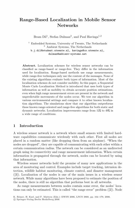
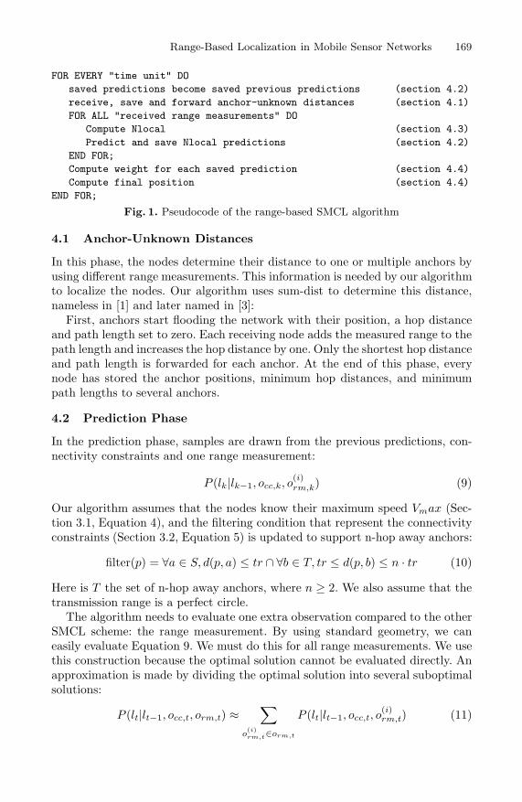
Figure 1 shows an overview in pseudocode of the algorithm. The nodes locallyuse this algorithm to estimate their positions with the received information ofthe anchors. The different phases of the algorithm are discussed in the followingsubsections.


FOR EVERY "time unit" DOsaved predictions become saved previous predictions (section 4.2)receive, save and forward anchor-unknown distances (section 4.1)FOR ALL "received range measurements" DO

Compute Nlocal (section 4.3)Predict and save Nlocal predictions (section 4.2)

END FOR;Compute weight for each saved prediction (section 4.4)Compute final position (section 4.4)

END FOR;

Fig. 1. Pseudocode of the range-based SMCL algorithm

4.1 Anchor-Unknown Distances

In this phase, the nodes determine their distance to one or multiple anchors byusing different range measurements. This information is needed by our algorithmto localize the nodes. Our algorithm uses sum-dist to determine this distance,nameless in [1] and later named in [3]:

First, anchors start flooding the network with their position, a hop distanceand path length set to zero. Each receiving node adds the measured range to thepath length and increases the hop distance by one. Only the shortest hop distanceand path length is forwarded for each anchor. At the end of this phase, everynode has stored the anchor positions, minimum hop distances, and minimumpath lengths to several anchors.

4.2 Prediction Phase

In the prediction phase, samples are drawn from the previous predictions, con-nectivity constraints and one range measurement:

P (lk|lk−1, occ,k, o(i)rm,k) (9)

Our algorithm assumes that the nodes know their maximum speed Vmax (Sec-tion 3.1, Equation 4), and the filtering condition that represent the connectivityconstraints (Section 3.2, Equation 5) is updated to support n-hop away anchors:

filter(p) = ∀a ∈ S, d(p, a) ≤ tr ∩ ∀b ∈ T, tr ≤ d(p, b) ≤ n · tr (10)

Here is T the set of n-hop away anchors, where n ≥ 2. We also assume that thetransmission range is a perfect circle.

The algorithm needs to evaluate one extra observation compared to the otherSMCL scheme: the range measurement. By using standard geometry, we caneasily evaluate Equation 9. We must do this for all range measurements. We usethis construction because the optimal solution cannot be evaluated directly. Anapproximation is made by dividing the optimal solution into several suboptimalsolutions:

P (lt|lt−1, occ,t, orm,t) ≈∑

o(i)rm,t∈orm,t

P (lt|lt−1, occ,t, o(i)rm,t) (11)


In this case, every range measurement can be seen as a sampling function, notconsidering the other range measurements. Given range measurement rm to an-chor position a, the predictions according to the range measurement are some-where located at the edge of the circle with origin a and radius rm. This givesthe following constraint:

P (lt|orm) =

{1 if d(lt, a) = rm,

0 otherwise.(12)

Note that after the prediction phase we only have valid predictions, so we donot need a filtering phase.

4.3 Weights and Sample Size

Our algorithm uses a constant number of predictions: N . This is done to keepthe computational costs at a low and constant level. In the prediction phase,the sampling of the predictions is divided into several sampling functions bythe range measurements. So every sampling function samples a portion of Npredictions: Nlocal. The size of Nlocal depends on the precision of the rangemeasurement, formulated as: 1

σ2rm

. σ2rm stands for the variance of the range mea-

surement. This variance is based on the hop distance associated with the rangemeasurement. Every range measurement consists of “hop count” independentrange measurements. We use an approximation made in [19]:

σ2rm,i ≈ i · σ2

rm,1 (13)

Here i stands for the number of hops. Our algorithm uses this approximationto compute the ratio between the precisions of the various range measurements.This ratio is used to compute the size of Nlocal, and is later used to computethe final position estimation. Note that this ratio can be calculated only usingthe “hop count” because we assume that the nodes have the same distancemeasurement hardware (σ2

rm,1 is a constant).

4.4 Computing the Final Position Estimation

In this phase, the algorithm uses the predictions, made in the prediction phase,to compute its position estimation. With the available range measurements andassociated weights (Equation 13), a weight is estimated for each prediction. Letp1. . . pi be all predictions with locations x1, y1. . . xi, yi. Let A1. . .Aj be all knownanchor positions with associated range measurements R1. . . Rj to the specificnode. The weights of the predictions are computed by the summed squarederror multiplied by the appropriate range measurement weights:

σ2pi

=j∑

k=1

1σ2

rm,k

(d(pi, Ak) − Rk

)2(14)

1σ2

rm,k

stands for the precision estimate of range measurement Rk. We take the

summed square error as an estimate of the variance of prediction pi: σ2pi

. Using


this estimate, the precision of prediction pi is 1σ2

pi

. If we have N predictions then

the optimal position (x, y) is where:∑N

i=11

σ2pi

((xi−x)2+(yi−y)2

)is minimized.

This weighted least square solution can be computed with an iterative weightedleast square method. It can also be computed with a weighted mean method.The weighted mean method uses less computation power and is therefore a goodreplacement:

x =1

∑Ni=1 σ−2

pi

·N∑

i=1

σ−2pi

· xi

y =1

∑Ni=1 σ−2

pi

·N∑

i=1

σ−2pi

· yi

(15)

This algorithm uses the ratio between the weights to compute the weighted leastsquare solution.

4.5 Observations

It is possible that no valid predictions can be made. In this case, the algorithmmakes predictions as if it had no previous predictions. When the range measure-ments are really bad, it is even possible that our algorithm cannot make anyvalid predictions with no speed constraints. In that case, the recursive functionproposed in Section 3.4 is used (Equation 6).

A range measurement that does not satisfy its own connectivity constraintchanges its value to the nearest number that satisfies this constraint. This in-creases the performance of the algorithm in several ways:

- More predictions can be made, giving a better representation of the positiondistribution.

- Peaks in the range measurements have less influence on the final positionestimation.

5 Simulations

In this section, we analyze our algorithm by running several simulations usingMatLab. In these simulations, we test our algorithm with different values foralgorithm-specific parameters and under various environmental settings. In ad-dition, we compare our results to other localization techniques: these are theIWLSM, the range-free MCL scheme ([13]) and DV-HOP ([18]). We analyzethe results of the localization schemes by looking at the mean error versus thecommunication costs.

5.1 General Simulation Set-Up

Except when stated otherwise, we use the same general set-up for all simulations.The sensor nodes are uniformly placed within a 1x1 units2 area and a transmis-sion range tr of 0.125 units is used. For simplicity, the transmission range issimulated as a perfect circle and messages are always received correctly.


The parameters we vary are:

- The number of predictions drawn by the sampling function. In general, weuse a number of 50 samples.

- The number of nodes placed within the area. In general, we use a numberof 180 nodes. The node density (average number of 1-hop away nodes) isdetermined by simulation. The general set-up has a node density of: 13.9.

- The number of anchors placed within the area. In general, we use a numberof 20 anchors. The anchor density (average number of 1-hop away anchors) isdetermined by simulation. The general set-up has an anchor density of: 1.3.

- The speed of the nodes, which we choose randomly from [0, V max]. Thenodes’ speed is given as a ratio of the transmission range. In general, we usea speed of [0, 1].

- The Time-To-Live (TTL) of the messages. This value indicates the numberof times a message is forwarded. We keep the communication costs per al-gorithm the same with this parameter, so the performance of the differentalgorithms are determined by the localization error. DV-Hop isn’t affected bythe TTL and has different communication costs than the other algorithms.In general, we use a TTL of 4 for every algorithm.

- The range measurement errors, which we simulate by a Gaussian distributionwith the real distance as the mean. The standard deviation of the erroris represented as a ratio of the real range. In general, we use a standarddeviation of 0.2 ([7]). This value is based on the picoradio ([8]) that usesReceived Signal Strength Indication (RSSI) for range measurements.

- We tested each simulation setup for 50 runs, each consisting of 50 time units.

We adopt a modified ([13]) random waypoint mobility model ([16]) for the nodes.With this model, a node randomly chooses its destination. After arriving at itsdestination, the node chooses a new destination. Furthermore, the speed of thenodes are changed and randomly chosen from [0, V max] after each time unitand when the nodes arrive at their destinations. We use this model to maintainan average speed. Before localization, we run the modified random waypointmobility model for several time units to maintain the distribution created bythis mobility model.

We use the following settings for the other localization schemes:

- The extensions proposed in this article (Section 3.4 and Equation 6) areused for the range-free SMCL scheme ([13]). We also need another update tosupport different values of TTL (Section 4.2, Equation 10). We use a loopinglimit of 10 and a sample size of 50, which should be enough according to [13].

- The IWLSM uses the same weights and range measurement values as ouralgorithm.

- We use the DV-hop localization scheme as proposed in ([18]).

5.2 Accuracy

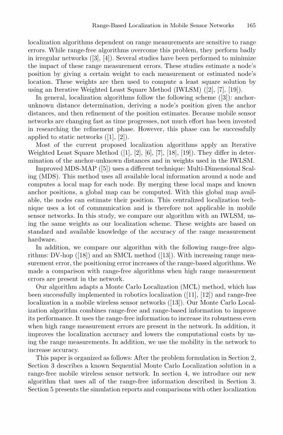
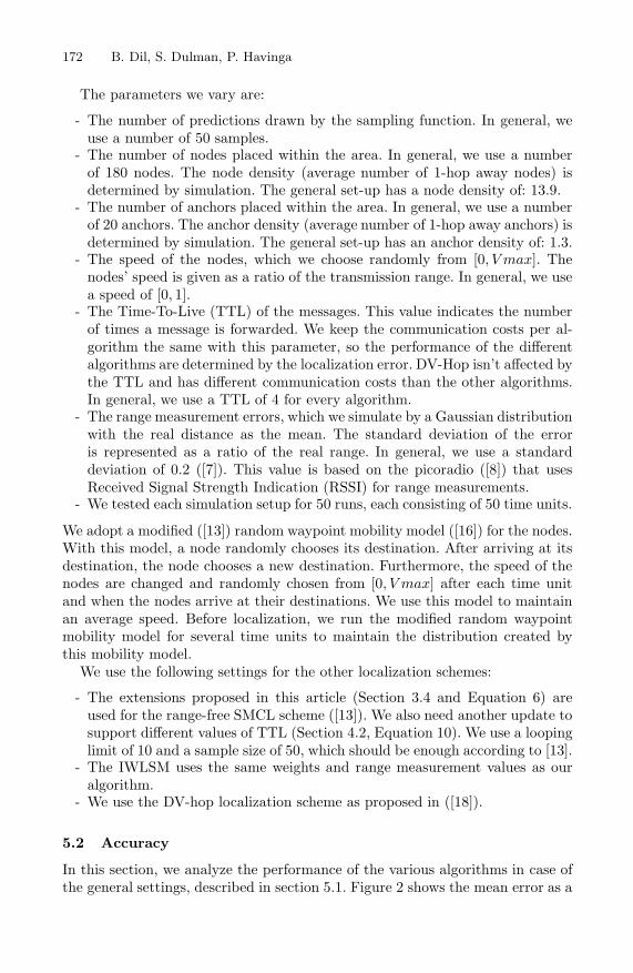
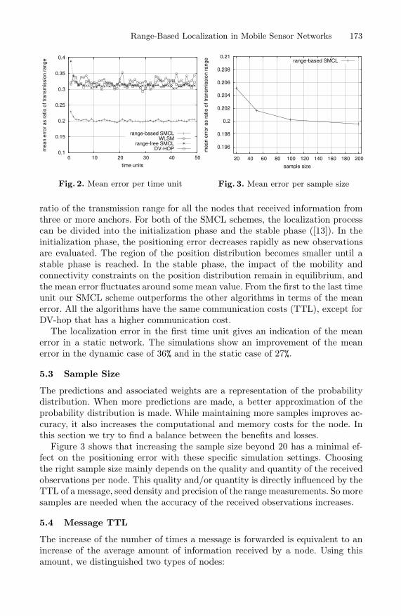
In this section, we analyze the performance of the various algorithms in case ofthe general settings, described in section 5.1. Figure 2 shows the mean error as a


0.1

0.15

0.2

0.25

0.3

0.35

0.4

0 10 20 30 40 50

me

an

err

or

as r

atio

of

tra

nsm

issio

n r

an

ge

time units

range-based SMCLWLSM

range-free SMCLDV-HOP

Fig. 2. Mean error per time unit

0.196

0.198

0.2

0.202

0.204

0.206

0.208

0.21

20 40 60 80 100 120 140 160 180 200

me

an

err

or

as r

atio

of

tra

nsm

issio

n r

an

ge

sample size

range-based SMCL

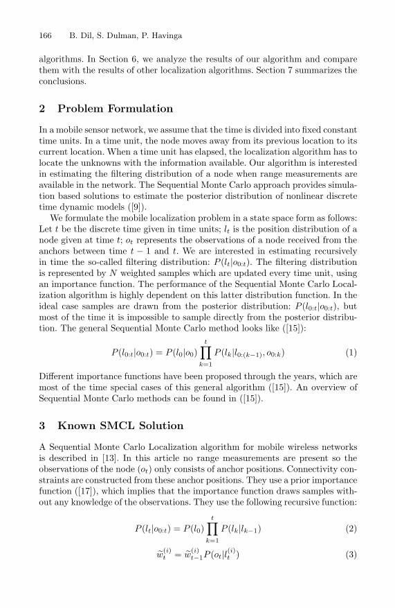
Fig. 3. Mean error per sample size

ratio of the transmission range for all the nodes that received information fromthree or more anchors. For both of the SMCL schemes, the localization processcan be divided into the initialization phase and the stable phase ([13]). In theinitialization phase, the positioning error decreases rapidly as new observationsare evaluated. The region of the position distribution becomes smaller until astable phase is reached. In the stable phase, the impact of the mobility andconnectivity constraints on the position distribution remain in equilibrium, andthe mean error fluctuates around some mean value. From the first to the last timeunit our SMCL scheme outperforms the other algorithms in terms of the meanerror. All the algorithms have the same communication costs (TTL), except forDV-hop that has a higher communication cost.

The localization error in the first time unit gives an indication of the meanerror in a static network. The simulations show an improvement of the meanerror in the dynamic case of 36% and in the static case of 27%.

5.3 Sample Size

The predictions and associated weights are a representation of the probabilitydistribution. When more predictions are made, a better approximation of theprobability distribution is made. While maintaining more samples improves ac-curacy, it also increases the computational and memory costs for the node. Inthis section we try to find a balance between the benefits and losses.

Figure 3 shows that increasing the sample size beyond 20 has a minimal ef-fect on the positioning error with these specific simulation settings. Choosingthe right sample size mainly depends on the quality and quantity of the receivedobservations per node. This quality and/or quantity is directly influenced by theTTL of a message, seed density and precision of the range measurements. So moresamples are needed when the accuracy of the received observations increases.

5.4 Message TTL

The increase of the number of times a message is forwarded is equivalent to anincrease of the average amount of information received by a node. Using thisamount, we distinguished two types of nodes:


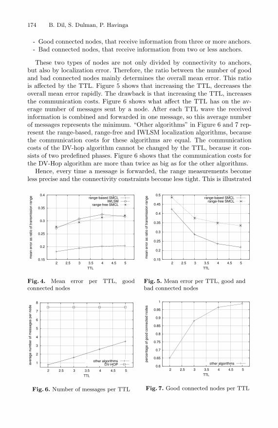
- Good connected nodes, that receive information from three or more anchors.- Bad connected nodes, that receive information from two or less anchors.

These two types of nodes are not only divided by connectivity to anchors,but also by localization error. Therefore, the ratio between the number of goodand bad connected nodes mainly determines the overall mean error. This ratiois affected by the TTL. Figure 5 shows that increasing the TTL, decreases theoverall mean error rapidly. The drawback is that increasing the TTL, increasesthe communication costs. Figure 6 shows what affect the TTL has on the av-erage number of messages sent by a node. After each TTL wave the receivedinformation is combined and forwarded in one message, so this average numberof messages represents the minimum. “Other algorithms” in Figure 6 and 7 rep-resent the range-based, range-free and IWLSM localization algorithms, becausethe communication costs for these algorithms are equal. The communicationcosts of the DV-hop algorithm cannot be changed by the TTL, because it con-sists of two predefined phases. Figure 6 shows that the communication costs forthe DV-Hop algorithm are more than twice as big as for the other algorithms.

Hence, every time a message is forwarded, the range measurements becomeless precise and the connectivity constraints become less tight. This is illustrated

0.15

0.2

0.25

0.3

0.35

0.4

2 2.5 3 3.5 4 4.5 5

me

an

err

or

as r

atio

of

tra

nsm

issio

n r

an

ge

TTL

range-based SMCLIWLSM

range-free SMCL

Fig. 4. Mean error per TTL, goodconnected nodes

0.15

0.2

0.25

0.3

0.35

0.4

0.45

0.5

2 2.5 3 3.5 4 4.5 5

me

an

err

or

as r

atio

of

tra

nsm

issio

n r

an

ge

TTL

range-based SMCLrange-free SMCL

Fig. 5. Mean error per TTL, good andbad connected nodes

1

2

3

4

5

6

7

8

2 2.5 3 3.5 4 4.5 5

ave

rag

e n

um

be

r o

f m

essa

ge

s p

er

no

de

TTL

other algorithmsDV-HOP

Fig. 6. Number of messages per TTL

0.6

0.65

0.7

0.75

0.8

0.85

0.9

0.95

1

2 2.5 3 3.5 4 4.5 5

pe

rce

nta

ge

of

go

od

co

nn

ecte

d n

od

es

TTL

other algorithms

Fig. 7. Good connected nodes per TTL


by Figure 4, which shows a decrease of accuracy of good connected nodes with in-creasing TTL. Figure 4 also shows that this decrease of accuracy with increasingTTL is minimal.

The bad connected nodes have a dramatically high mean error comparedto the good connected nodes. So including the position estimates of the badconnected nodes is questionable. When these position estimates are not included,the chosen TTL for a mobile wireless sensor network mainly depends on thedesired localization coverage. Figure 7 shows the increase of good connectednodes when the TTL increases.

Therefor, in this paper we use the good connected nodes for the determinationof the mean error.

5.5 Anchor Density

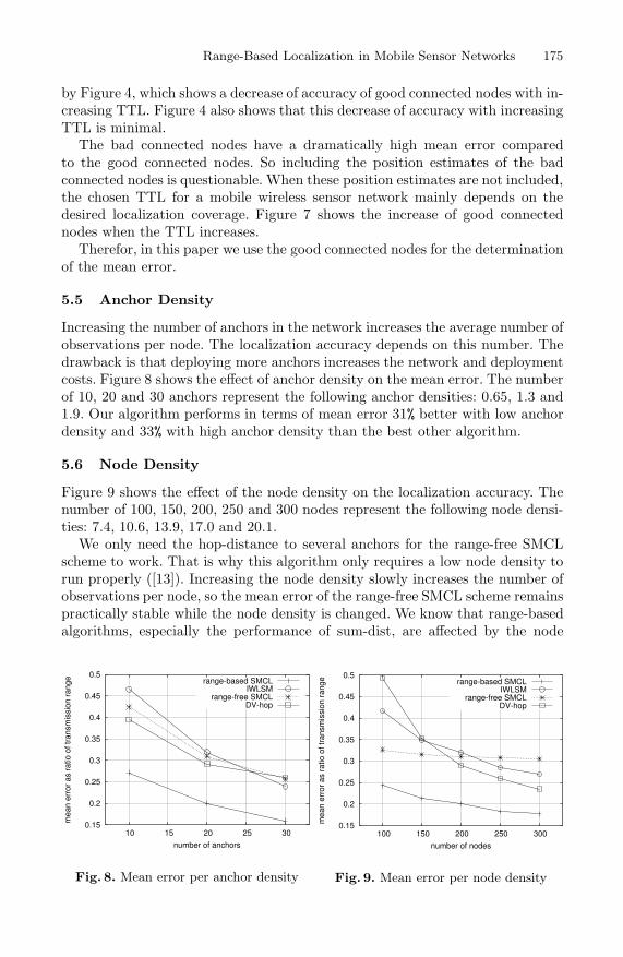
Increasing the number of anchors in the network increases the average number ofobservations per node. The localization accuracy depends on this number. Thedrawback is that deploying more anchors increases the network and deploymentcosts. Figure 8 shows the effect of anchor density on the mean error. The numberof 10, 20 and 30 anchors represent the following anchor densities: 0.65, 1.3 and1.9. Our algorithm performs in terms of mean error 31% better with low anchordensity and 33% with high anchor density than the best other algorithm.

5.6 Node Density

Figure 9 shows the effect of the node density on the localization accuracy. Thenumber of 100, 150, 200, 250 and 300 nodes represent the following node densi-ties: 7.4, 10.6, 13.9, 17.0 and 20.1.

We only need the hop-distance to several anchors for the range-free SMCLscheme to work. That is why this algorithm only requires a low node density torun properly ([13]). Increasing the node density slowly increases the number ofobservations per node, so the mean error of the range-free SMCL scheme remainspractically stable while the node density is changed. We know that range-basedalgorithms, especially the performance of sum-dist, are affected by the node

0.15

0.2

0.25

0.3

0.35

0.4

0.45

0.5

10 15 20 25 30

me

an

err

or

as r

atio

of

tra

nsm

issio

n r

an

ge

number of anchors


range-free SMCLDV-hop

Fig. 8. Mean error per anchor density

0.15

0.2

0.25

0.3

0.35

0.4

0.45

0.5

100 150 200 250 300

me

an

err

or

as r

atio

of

tra

nsm

issio

n r

an

ge

number of nodes



Fig. 9. Mean error per node density


density ([3]). Increasing the node density leads to straighter paths between thenodes and anchors, so that the shortest path becomes a better approximation ofthe real distance. When the real distances are better approximated, the range-based algorithms perform better.

Figure 9 shows an improvement of the mean error of 25% with low node densityand 25% with high node density than the best other algorithm compared withour algorithm.

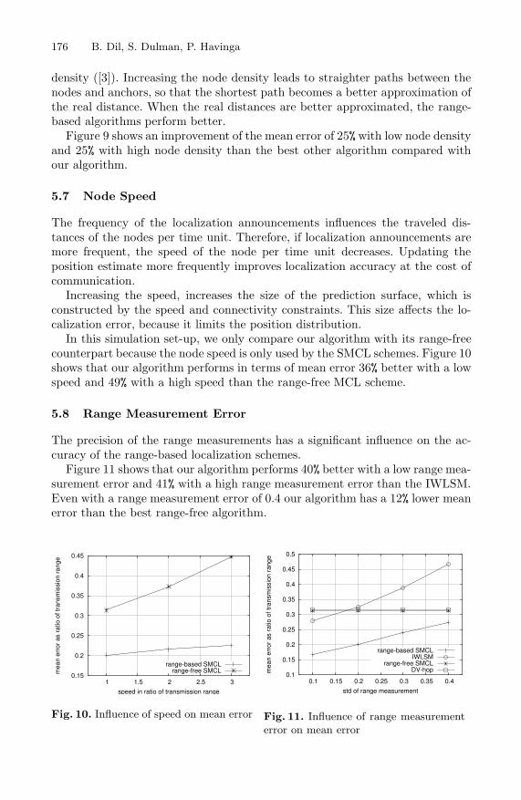
5.7 Node Speed

The frequency of the localization announcements influences the traveled dis-tances of the nodes per time unit. Therefore, if localization announcements aremore frequent, the speed of the node per time unit decreases. Updating theposition estimate more frequently improves localization accuracy at the cost ofcommunication.

Increasing the speed, increases the size of the prediction surface, which isconstructed by the speed and connectivity constraints. This size affects the lo-calization error, because it limits the position distribution.

In this simulation set-up, we only compare our algorithm with its range-freecounterpart because the node speed is only used by the SMCL schemes. Figure 10shows that our algorithm performs in terms of mean error 36% better with a lowspeed and 49% with a high speed than the range-free MCL scheme.

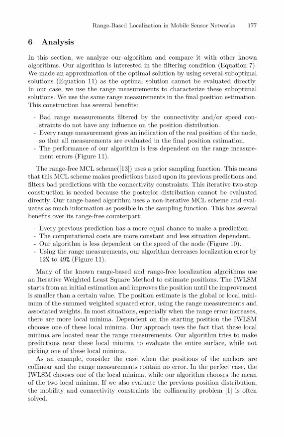
5.8 Range Measurement Error

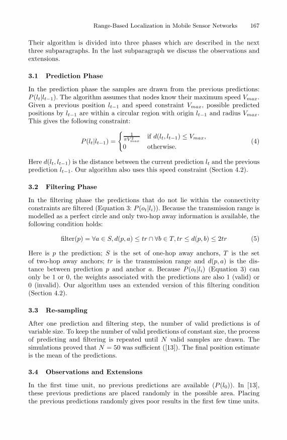
The precision of the range measurements has a significant influence on the ac-curacy of the range-based localization schemes.

Figure 11 shows that our algorithm performs 40% better with a low range mea-surement error and 41% with a high range measurement error than the IWLSM.Even with a range measurement error of 0.4 our algorithm has a 12% lower meanerror than the best range-free algorithm.

0.15

0.2

0.25

0.3

0.35

0.4

0.45

1 1.5 2 2.5 3

mean e

rror

as r

atio o

f tr

ansm

issio

n r

ange

speed in ratio of transmission range

range-based SMCLrange-free SMCL

Fig. 10. Influence of speed on mean error

0.1

0.15

0.2

0.25

0.3

0.35

0.4

0.45

0.5

0.1 0.15 0.2 0.25 0.3 0.35 0.4

me

an

err

or

as r

atio

of

tra

nsm

issio

n r

an

ge

std of range measurement



Fig. 11. Influence of range measurementerror on mean error


6 Analysis

In this section, we analyze our algorithm and compare it with other knownalgorithms. Our algorithm is interested in the filtering condition (Equation 7).We made an approximation of the optimal solution by using several suboptimalsolutions (Equation 11) as the optimal solution cannot be evaluated directly.In our case, we use the range measurements to characterize these suboptimalsolutions. We use the same range measurements in the final position estimation.This construction has several benefits:

- Bad range measurements filtered by the connectivity and/or speed con-straints do not have any influence on the position distribution.

- Every range measurement gives an indication of the real position of the node,so that all measurements are evaluated in the final position estimation.

- The performance of our algorithm is less dependent on the range measure-ment errors (Figure 11).

The range-free MCL scheme([13]) uses a prior sampling function. This meansthat this MCL scheme makes predictions based upon its previous predictions andfilters bad predictions with the connectivity constraints. This iterative two-stepconstruction is needed because the posterior distribution cannot be evaluateddirectly. Our range-based algorithm uses a non-iterative MCL scheme and eval-uates as much information as possible in the sampling function. This has severalbenefits over its range-free counterpart:

- Every previous prediction has a more equal chance to make a prediction.- The computational costs are more constant and less situation dependent.- Our algorithm is less dependent on the speed of the node (Figure 10).- Using the range measurements, our algorithm decreases localization error by

12% to 49% (Figure 11).

Many of the known range-based and range-free localization algorithms usean Iterative Weighted Least Square Method to estimate positions. The IWLSMstarts from an initial estimation and improves the position until the improvementis smaller than a certain value. The position estimate is the global or local mini-mum of the summed weighted squared error, using the range measurements andassociated weights. In most situations, especially when the range error increases,there are more local minima. Dependent on the starting position the IWLSMchooses one of these local minima. Our approach uses the fact that these localminima are located near the range measurements. Our algorithm tries to makepredictions near these local minima to evaluate the entire surface, while notpicking one of these local minima.

As an example, consider the case when the positions of the anchors arecollinear and the range measurements contain no error. In the perfect case, theIWLSM chooses one of the local minima, while our algorithm chooses the meanof the two local minima. If we also evaluate the previous position distribution,the mobility and connectivity constraints the collinearity problem [1] is oftensolved.


In this paper, the communication costs for the different algorithms are equal,except for the DV-hop algorithm that uses much more communication (Figure 6).

7 Conclusions

In this paper, we proposed a non-iterative MCL scheme that uses all informa-tion to improve localization accuracy and robustness. This information consistsof range measurements, connectivity constraints, and mobility information. Sim-ulations show that our algorithm decreases the localization error by 12% to 49%in static and dynamic networks under a wide range of conditions, even whenthe node and network resources are limited. Future work aims at testing ouralgorithm in other mobility models and real life settings.

References

1. A. Savvides, H. Park and M. Srivastava: The Bits and Flops of the N-Hop Multi-lateration Primitive for Node Localization Problems. In First ACM InternationalWorkshop on Wireless Sensor Networks and Application, Atlanta, GA, September2002.

2. C. Savarese, J. Rabay and K. Langendoen: Robust Positioning Algorithms for Dis-tributed Ad-Hoc Wireless Sensor Networks. USENIX Technical Annual Conference,Monterey, CA, June 2002.

3. Koen Langendoen and Niels Reijers: Distributed localization in wireless sensornetworks: A quantitative comparison. In Computer Networks (Elsevier), specialissue on Wireless Sensor Networks, 2003.

4. Y. Shang, W. Ruml, Y. Zhang and M. Fromherz: Localization From Mere Connec-tivity. MobiHoc’03, Annapolis, Maryland, June 2003.

5. Yi Shang and Wheeler Ruml: Improved MDS-based localization. In Infocom 20046. L.Evers,W.Bach, D.Dam,M.Jonker, H.Scholten, and P.Havinga: An iterative qual-

ity based localization algorithm for adhoc networks. In Department of ComputerScience, University of Twente, 2002.

7. L.Evers, S.Dulman, P.Havinga: A distributed precision based localization algorithmfor ad-hoc networks. Proceedings of Pervasive Computing (PERVASIVE 2004).

8. Jan Beutel: Geolocation in a picoradio environment. In MS Thesis, ETH Zurich,Electronics Lab, 1999.

9. J.E.Handschin: Monte Carlo Techniques for Prediction and Filtering of Non-LinearStochastic Processes. Automatica 6. pp. 555-563. 1970.

10. V.S.Zaritskii, V.S.Svetnik, L.I.Shimelevich: Monte Carlo technique in problems ofoptimal data processing. Automation and Remote Control 12: 95-103. 1974.

11. F.Dellaert, D.Fox, W.Burgard, S.Thrun: Monte Carlo Localization for MobileRobots. IEEE International Conference on Robotics and Automation (ICRA). May1999.

12. S.Thrun, D.Fox, W.Burgard, F.Dellaert: Robust Monte Carlo Localization for Mo-bile Robots. Artificial Intelligence Journal. 2001.

13. L.Hu, D.Evans: Localization for Mobile Sensor Networks. Tenth Annual Interna-tional Conference on Mobile Computing and Networking (MobiCom 2004), USA.2004.


14. A.Kong, J.S.Liu, W.H.Wong: Sequential Imputations and Bayesian Missing DataProblems. Journal of the American Statistical Association. Volume 89, pp. 278-288.1994.

15. A.Doucet, S.Godsill, C.Andrieu: On Sequential Monte Carlo Sampling Methodsfor Bayesian Filtering. Statistics and Computing. Volum 10, pp. 197-208. 2000.

16. T.Camp, J.Boleng, V.Davies: A survey of Mobility Models for Ad Hoc NetworksResearch. Wireless Communications and Mobile Computing. Volume 2, Number5. 2002.

17. H.Tanizaki, R.S.Mariano: Nonlinear and non-Gaussian statespace modeling withMonte-Carlo simulations. Journal of Econometrics 83: 263-290. 1998.

18. D.Niculescu, B.Nath: Ad hoc positioning systems. In: IEEE Globecom 2001, SanAntonio. 2001.

19. S.Dulman, P.Havinga: Statistically enhanced localization schemes for randomlydeployed wireless sensor networks. DEST International Workshop on Signal Pro-cessing for Sensor Networks, Australia. 2004.

Range-Based Localization in Mobile Sensor Networks

Documents

Transcript of Range-Based Localization in Mobile Sensor Networks