Randomized Response, Statistical DisclosureControl and Misclassification: a Review

Ardo van den HoutPeter G.M. van der Heijden

Utrecht University, Faculty of Social SciencesDept. of Methodology and StatisticsHeidelberglaan 2, 3584 CS Utrecht

The Netherlands

Abstract

This paper discusses analysis of categorical data which have beenmisclassified and where misclassification probabilities are known. Fieldswhere this kind of misclassification occurs are randomized response,statistical disclosure control, and classification with known sensitivityand specificity. Estimates of true frequencies are given, and adjust-ments to the odds ratio are discussed. Moment estimates and maxi-mum likelihood estimates are compared and it is proved that they arethe same in the interior of the parameter space. Since moment esti-mators are regularly outside the parameter space, special attention ispaid to the possibility of boundary solutions. An example is given.

Keywords: contingency table, EM algorithm, misclassification, oddsratio, randomized response, sensitivity, specificity, statistical disclo-sure control.

1 Introduction

When scores on categorical variables are observed, there is a possibility ofmisclassification. By a categorial variable we mean a stochastic variable

1

which range consists of a limited number of discrete values called the cat-egories. Misclassification occurs when the observed category is i while thetrue category is j, i 6= j. This paper discusses analysis of categorical datasubject to misclassification with known misclassification probabilities.

There are four fields in statistics where the misclassification probabilitiesare known. The first is randomized response (RR). RR is an interview tech-nique which can be used when sensitive questions have to be asked. Warner(1965) introduced this technique and we use a simple form of the method asan introductory example. Let the sensitive question be ‘Have you ever usedillegal drugs?’ The interviewer asks the respondent to roll a dice and to keepthe outcome hidden. If the outcome is 1,2,3 or 4 the respondent is asked toanswer question Q, if the outcome is 5 or 6 he is asked to answer Qc, where

Q = ‘Have you ever used illegal drugs?’

Qc = ‘Have you never used illegal drugs?’

The interviewer does not know which question is answered and observes only‘yes’ or ‘no’. The respondent answers Q with probability p = 2/3 and answersQc with probability 1− p. Let π be the unknown probability of observing ayes-response to Q. The probability of a yes-response is λ = pπ+(1−p)(1−π).So, with the observed proportion as an estimate λ of λ, we can estimate πby

π =λ− (1− p)

2p− 1. (1)

The main idea behind RR is that perturbation by the misclassificationdesign (in this case the dice) protects the privacy of the respondent and thatinsight in the misclassification design (in this case the knowledge of the valueof p) can be used to analyse the observed data.

It is possible to create RR settings in which questions are asked to getinformation on a variable with K > 2 categories (Chaudhuri and Mukerjee,1988, Chapter 3). We restrict ourselves in this paper to those RR designs ofthe form

λ = Pπ, (2)

where λ = (λ1, ..., λK)t is a vector denoting the probabilities of the ob-served responses with categories 1, ..., K, π = (π1, ..., πK)t is the vector ofthe probabilities of the true responses and P is the K ×K transition matrixof conditional misclassification probabilities pij, with

pij = IP (category i is observed| true category is j).

2

Note that this means that the columns of P add up to 1. In the Warnermodel above we have λ = (λ1, 1− λ1)

t,

P =

(p 1− p

1− p p

),

and π = (π1, 1− π1)t . Further background and more complex randomized

response schemes can be found in Fox and Tracy (1986) and Chaudhuri andMukerjee (1988).

The second field where the misclassification probabilities are known isthe post randomisation method (PRAM), see Kooiman, Willenborg andGouweleeuw (1997). The idea of PRAM is to misclassify the values of cat-egorical variables after the data have been collected in order to protect theprivacy of the respondents by preventing disclosure of their identities. PRAMcan be seen as applying RR after the data have been collected. More infor-mation about PRAM and a comparison with RR is given in Section 2.

The third field is statistics in medicine and epidemiology. In these disci-plines, the probability to be correctly classified as a case given that one is acase is called the sensitivity, and the probability to be correctly classified asa non-case given that one is a non-case is called the specificity. In medicine,research concerning the situation with known sensitivity and specificity ispresented in Chen (1989) and Greenland (1980, 1988). In epidemiology, seeMagder and Hughes (1997) and Copeland et al. (1977).

The fourth field is the part of statistical astronomy that discusses rectifi-cation and deconvolution problems. Lucy (1974), for instance, considers theestimation of a frequency distribution where observations might be misclas-sified and where the misclassification probabilities are presumed known.

To present RR and PRAM as misclassification seems to be a logical ap-proach, but a note must be made on this usage. Misclassification is a wellknown concept within the analysis of categorical data and different methodsto deal with this kind of perturbation have been proposed, see the reviewpaper by Kuha and Skinner (1997), but the situation in which misclassifica-tion probabilities are known does not often occur. In most situations, theseprobabilities have to be estimated which makes analyses of misclassified datamore complex.

The focus of this paper is on RR and PRAM. The discussion is about theanalysis of the misclassified data, not about the choice of the misclassificationprobabilities. The central problem is: given the data subject to misclassifica-

3

tion and given the transition matrix, how should we adjust standard analysisof frequency tables in order to get valid results?

Special attention is given to the possibility of boundary solutions. By aboundary solution we mean an estimated value of the parameter which lieson the boundary of the parameter space. For instance, in formula (1) theunbiased moment estimate of π is given. It is possible that this estimate isnegative and makes no sense. In this case the moment estimate differs fromthe maximum likelihood estimate which is zero and therefore lies on theboundary of the parameter space. (This was already noted by, for instance,Singh, 1976.)

The possibility that the moment estimator yields estimates outside theparameter space is an awkward property, since standard analyses as, e.g.,univariate probabilities and the odds ratio, are in that case useless. However,negative estimates are likely to occur when RR used. Typically, RR is appliedwhen sensitive characteristics are investigated and often sensitivity goes handin hand with rareness. Therefore, some of the true frequencies in a samplemay be low and when these frequencies are unbiasedly estimated, randomerror can easily cause negative estimates. The example discussed in Section7 illustrates this situation. Regarding PRAM the same problem can occur,see Section 2.

This analysis of misclassified data has also been discussed by other au-thors, see the references above. Our present aim is to bring together thedifferent fields of misclassification, compare the different methods, and pro-pose methods to deal with boundary solutions. Noticeably lacking in someliterature is a discussion of the properties of proposed estimators such as un-biasedness and maximum likelihood. Where appropriate, we try to fill thisgap.

Section 2 provides more information about PRAM. A comparison withRR is made. Section 3 discusses the moment estimator of the true fre-quency table, i.e., the not-observed frequencies of the correctly classifiedscores. Point estimates and estimations of covariances are presented. In Sec-tion 4 we consider the maximum likelihood estimation of the true frequencytable. Again point estimation and variances are discussed, this time usingthe EM algorithm. Section 5 relates the moment estimator to the maximumlikelihood estimator. In Section 6 we consider the estimation of the odds ra-tio. In Section 7 an example is given with RR data stemming from researchinto violating regulations of social benefit. Section 8 evaluates the resultsand concludes.

4

2 Protecting Privacy

The post randomisation method (PRAM) was introduced by Kooiman etal.(1997) as a method for statistical disclosure control of microdata files. Amicrodata file is a data matrix where each row, called a record, corresponds toone respondent and where the columns correspond to the variables. Statisti-cal disclosure control (SDC) aims at safeguarding the identity of respondents.Because of the privacy protection, data producers, such as national statisticalinstitutes, are able to pass on data to a third party.

PRAM can be applied to variables in the microdata file that are cate-gorical and identifying. Identifying variables are variables that can be usedto re-identify individuals represented in the data. The perturbation of theseidentifiers makes re-identification of individuals less likely. The PRAM pro-cedure yields a new microdata file in which the scores on certain categoricalvariables in the original file may be misclassified into different scores ac-cording to a given probability mechanism. In this way PRAM introducesuncertainty in the data: the user of the data can not be sure that the infor-mation in the file is original or perturbed due to PRAM. In other words, therandomness of the procedure implies that matching a record in the perturbedfile to a record of a known individual in the population could, with a highprobability, be a mismatch.

An important aspect of PRAM is that the recipient of the perturbed datais informed about the misclassification probabilities. Using these probabili-ties he can adjust his analysis and take into account the extra uncertaintycaused by applying PRAM.

As with RR, the misclassification scheme is given by means of a K ×Ktransition matrix P of conditional probabilities pij, with

pij = IP (category i is released|true category is j).

Since national statistical institutes, which are the typical users of SDC meth-ods, prefer model free approaches to their data, PRAM is presented in theform

IE[T ∗|T ] = PT, (3)

where T ∗ is the vector of perturbed frequencies and T is the vector of thetrue frequencies. So instead of using probabilities as in (2), frequencies areused in (3) to avoid commitment to a specific parametric model.

PRAM is currently under study and is by far not the only way to protectmicrodata against disclosure (see, e.g., Willenborg and De Waal, 2001). Two

5

common methods used by national statistical institutes are global recodingand local suppression. Global recoding means that the number of categoriesis reduced by pooling, so that the new categories include more respondentsthan the original categories. This can be necessary when a category in theoriginal file contains just a few respondents. For example, in microdata filewhere the variable profession has just one respondent with the value ‘mayor’,we can make a new variable ‘working for the government’ and include in thiscategory not only the mayor, but also the people in the original file who havegovernmental jobs. The identity of the mayor is then protected not only bythe number of people in the survey with governmental jobs, but also by thenumber of people in the population with governmental jobs.

Local suppression means protecting identities by making data missing.In the example above, the identity of the mayor can be protected by makingthe value ‘mayor’ of the variable profession missing.

When microdata are processed by using recoding or suppression, there isalways loss of information. This is inevitable: losing information is intrinsicto SDC. Likewise, there will be loss of information when data are protectedby applying PRAM.

PRAM is not meant to replace existing SDC techniques. Using the tran-sition matrix with the misclassification probabilities to take into account theperturbation due to PRAM, requires extra effort and becomes of course morecomplex when the research questions become more complex. This may notbe acceptable to all researchers. Nevertheless, existing SDC methods are alsonot without problems. Especially global recoding can destroy detail that isneeded in the analysis. For instance, when a researcher has specific ques-tions regarding teenagers becoming 18 years old, it is possible that the datahe wants to use is globally recoded before it is released. It is possible thatthe variable age is recoded from year of birth to age categories going from 0to 5, 5 to 10, 10 to 15 , 15 to 20, etcetera. In that case the researcher haslost his object of research.

PRAM can be seen as a SDC method which can deal with specific requestsconcerning released data (such as in the foregoing paragraph) or with datawhich are difficult to protect using current SDC methods (meaning the lossof information is too large). PRAM can of course also be used in combinationwith other SDC methods. Further information about PRAM can be found inGouweleeuw, Kooiman, Willenborg and De Wolf (1998) and Van den Hout(1999).

The two basic research questions concering PRAM are (i) how to choose

6

the misclassification probabilities in order to make the released microdatasafe, and (ii) how should statistical analysis be adjusted in order to takeinto account the misclassification probabilities? As already stated in theintroduction, this paper concerns (ii). Our general objective is not only topresent user-friendly methods in order to make PRAM more user-friendly,but also to show that results in more than one field in statistics can be usedto deal with data perturbed by PRAM. Regarding (i), see Willenborg (2000)and Willenborg and De Waal (2001), Chapter 5.

Comparing (2) with (3), it can be seen that RR and PRAM are mathe-matically equivalent. Therefore, PRAM is presented in this paper as a specialform of RR. In fact, the idea of PRAM dates back from Warner (1971), theoriginator of RR, who mentions the possibilities of the RR procedure to pro-tect data after they have been collected. PRAM can be seen as applyingRR after the data have been collected. Rosenberg (1979, 1980) elaboratesthe Warner idea and calls it ARRC: additive RR contamination. PRAMturns out to be the same as ARRC. Rosenberg discusses multivariate anal-ysis of data protected by ARRC: multivariate categorical linear models andthe chi-square test for contingency tables, in particular.

In the remainder of this section we make some comparisons betweenPRAM and RR. Since the methods serve different purposes, important dif-ferences may occur in practice. First, PRAM will be typically applied tothose variables which may give rise to the disclosure of the identity of a re-spondent, i.e., covariates as, e.g., gender, age and race. RR, on the otherhand, will be typically applied to response variables, since the identifyingcovariates are obvious from the interview situation. Secondly, the usefulnessof the observed response in the RR setting is dependent on the cooperation ofthe respondent, whereas applying PRAM is completely mechanic. AlthoughRR may be of help in eliciting sensitive information, the method is not apanacea, see Van der Heijden et al. (2000). The third important differenceconcerns the choice of the transition matrix. When using RR the matrix isdetermined before the data are collected, but in the case of PRAM the ma-trix can be determined conditionally on the original data. This means thatthe extent of randomness in applying PRAM can be controlled better thanin the RR setting, see Willenborg (2000).

PRAM is similar to RR regarding the possibility of boundary solutions,see Section 1. PRAM is typically used when there are respondents in thesample with rare combinations of scores. Therefore, some of the true frequen-cies in a sample may be low and when PRAM has been applied and these

7

frequencies are unbiasedly estimated, random error can easily cause nega-tive estimates. So, also regarding PRAM, methods to deal with boundarysolutions are important.

3 Moment Estimator

This section generalizes (1) in order to obtain a moment estimator of the truecontingency table. A contingency table is a table with the sample frequenciesof categorical variables. For example, the 2-dimensional contingency table oftwo binary variables has four cells, each of which contains the frequency ofa compounded class of the two variables. Section 3.1 presents the momentestimator for a m-dimensional table (m > 1). In Section 3.2 formulas tocompute covariances are presented.

3.1 Point Estimation

If P in (2) is non-singular and we have an unbiased point estimate λ of λ,we can estimate π by the unbiased moment estimator

π = P−1λ, (4)

see, Chaudhuri and Mukerjee (1988), and Kuha and Skinner (1997).In practice, assuming that P in (2) is non-singular does not impose much

restriction on the choice of the misclassification design. P−1 exists whenthe diagonal of P dominates, i.e., pii > 1/2 for i ∈ 1, ..., K, and this isreasonable since these probabilities are the probabilities that the classificationis correct.

In this paper we assume that the true response is multinomially dis-tributed with parameter vector π. The moment estimator (4) is not a maxi-mum likelihood estimator since it is possible that for some i ∈ 1, ..., K, πi

is outside the parameter space (0,1).In Section 1, we have considered the misclassification of one variable.

The generalization to a m-dimensional contingency table with m > 1 isstraightforward when we have the following independence property betweeneach possible pair (A,B) of the m variables:

IP (A∗ = i, B∗ = k|A = j, B = l) = IP (A∗ = i|A = j)IP (B∗ = k|B = l). (5)

8

Regarding RR, this property means, that the misclassification design is inde-pendently applied to the different respondents and, when more than one ques-tion is asked, the design is independently applied to the different questions.So, in other words, answers from other respondents or to other questionsdo not influence the misclassification design in the RR survey. RegardingPRAM, this property means that the misclassification design is indepen-dently applied to the different records and independently to the differentvariables.

In this situation we structure the m-dimensional contingency table as an1-dimensional table of the compounded variable. For instance, when we havethree binary variables, we get an 1-dimensional table with rows indexed by111, 112, 121, 122, 211, 212, 221, 222. (The last index changes first.) Dueto property (5) it is easy to create the transition matrix of the compoundedvariable using the transition matrices of the underlying separate variables.Given the observed compounded variable and its transition matrix we canuse the moment estimator as described above.

To give an example, assume we have an observed cross-tabulation of themisclassified variables A, and B, where row variable A has K categories andtransition matrix PA, and column variable B has S categories and transitionmatrix PB. (When one of the variables is not misclassified, we simply takethe identity matrix as the transition matrix.) Together A and B can beconsidered as one compounded variable with KS categories. When property(5) is satisfied we can use the Kronecker product, denoted by ⊗, to computethe KS ×KS transition matrix P as follows:

P = PB ⊗ PA =

pB11PA pB

12PA · · · pB1SPA

.... . . . . .

...pB

S1PA · · · · · · pBSSPA

,

where each pBijPA for i, j ∈ 1, ..., S, is itself a K ×K matrix.

3.2 Covariances

Since the observed response is multinomially distributed with parameter vec-tor λ, the covariance matrix of (4) is given by

V (π) = P−1V (λ)(P−1

)t

= n−1P−1(Diag(λ)− λλt

) (P−1

)t, (6)

9

where Diag(λ) denotes the diagonal matrix with the elements of λ on thediagonal. The covariance matrix (6) can be unbiasedly estimated by

V (π) = (n− 1)−1P−1(Diag(λ)− λλ

t) (

P−1)t

, (7)

see Chaudhuri and Mukerjee (1988, Section 3.3).As stated before, national statistical institutes prefer a model free ap-

proach. Consequently, Kooiman et al. (1997) present only the extra variancedue to applying PRAM, and do not assume a multinomial distribution. Thevariance given by Kooiman et al. (1997) can be related to (6) in the followingway. Chaudhuri and Mukerjee (1988, Section 3.3) present a partition of (6)in two terms, where the first denotes the variance due to the multinomialscheme and the second represents the variance due to the perturbation:

V (π) = Σ1 + Σ2, (8)

where

Σ1 =1

n

(Diag(π)− ππt

)

and

Σ2 =1

nP−1

(Diag(λ)− PDiag(π)P t

) (P−1

)t.

Analysing Σ2 it turns out that it is the same as the variance due to PRAMgiven in Kooiman et al. (1997), as was to be expected, see Appendix A.

4 Maximum Likelihood Estimator

As already noted in Sections 1 and 2, it is possible that the moment esti-mator yields estimates outside the parameter space when the estimator isapplied to RR data or PRAM data. Negative estimates of frequencies areawkward, since they do not make sense. Furthermore, when there are morethan two categories and the frequency of one of them is estimated by a neg-ative number, it is unclear how the moment estimate must be adjusted inorder to obtain a solution in the parameter space. This is a reason to lookfor a maximum likelihood estimate (MLE). Another reason to use MLEs isthat in general, unbiasedness is not preserved when functions of unbiasedestimates are considered. Maximum likelihood properties on the other hand,are in general preserved (see Mood, Graybill and Boes, 1985).

10

This section discusses first the estimation of the MLE of the true contin-gency table using the EM algorithm and, secondly, in 4.2, the covariances ofthis estimate.

4.1 Point Estimation

The expectation-maximization (EM) algorithm (Dempster, Laird and Rubin,1977) can be used as an iterative scheme to compute MLEs when data areincomplete, i.e., when some observations are missing. The EM algorithmis in that case an alternative to maximizing the likelihood function usingmethods as, e.g., the Newton Raphson method. Two appealing properties ofthe EM algorithm relative to Newton-Raphson are its numerical stablity and,given that the complete data problem is a standard one, the use of standardsoftware for complete data analysis within the steps of the algorithm. Theseproperties can make the algorithm quite user-friendly. More background andrecent developments can be found in McLachlan and Krishnan (1997).

We will now see how the EM algorithm can be used in a misclassificationsetting, see also Bourke and Moran (1988), Chen (1989), and Kuha andSkinner (1997). For ease of exposition we consider the 2×1 frequency tableof a binary variable A. As stated before, we assume multinomial sampling.

When the variable is subject to misclassification, say with given transitionmatrix P = (pij), we do not observe values of A, but instead we observe valuesof a perturbed A, say A∗.

Let A∗ be tabulated inA∗ 1 n∗1

2 n∗2n

where n∗i for i = 1, 2 is the observed number of values i of A∗ and n∗1+n∗2 =n is fixed. Let π = IP (A = 1) and λ = IP (A∗ = 1). When transitionprobabilities are given, we know λ = p11π+p12(1−π). So, ignoring constants,the observed data log likelihood is given by

log l∗(π) = n∗1 log λ + n∗2 log(1− λ)

= n∗1 log (p11π + p12(1− π)) + n∗2 log (p21π + p22(1− π)) . (9)

The aim is to maximize log l∗(π) for π ∈ (0, 1).In this simple case of a 2×1 frequency table, the maximization of log l∗(π)

is no problem. By computing the analytic solution to the root of the first

11

derivative, we can locate the maximum. Nevertheless, in the case of a K×1frequency table, finding the analytic solution can be quite tiresome and weprefer an iterative method. The 2×1 table will serve as an example.

To explain the use of the EM algorithm, we can translate the problemof maximizing (9) into an incomplete-data problem. We associate with eachobserved value of A∗ its not-observed non-perturbed value of A. Togetherthese pairs form an incomplete-data file with size n. (In the framework ofRubin (1976): the missing data are missing at random, since they are missingby design.) When we tabulate this incomplete-data file we get

A1 2

A∗ 1 n11 n12 n∗12 n21 n22 n∗2

n1 n2 n

(10)

where for i, j ∈ 1, 2, nij is the frequency of the combination A∗ = i andA = j . Only the marginals n∗1 and n∗2 are observed.

When we would have observed the complete data, i.e., nij for i, j ∈ 1, 2,we would only have to consider the bottom marginal of (10) and the complete-data log likelihood function of π would be given by

log l(π) = n1 log π + n2 log(1− π), (11)

from which the maximum likelihood estimate π = n1/n follows almost im-mediately.

The idea of the EM algorithm is to maximize the incomplete-data likeli-hood by iteratively maximizing the expected value of the complete-data loglikelihood (11), where the expectation is taken over the distribution of thecomplete-data given the observed data and the current fit of π at iteration p,denoted by π(p). That is, in each iteration we look for the π which maximizesthe function

Q(π, π(p)

)= IE

[log l(π)|n∗1, n∗2, π(p)

]. (12)

In the EM algorithm it is not necessary to specify the correspondingrepresentation of the incomplete-data likelihood in terms of the complete-data likelihood (McLachlan and Krishnan, 1997, Section 1.5.1). In otherwords, we do not need (9), the function which plays the role of the incomplete-data likelihood, but we can work with (11) instead.

12

Since (11) is linear with respect to ni, we can rewrite (12) by replacingthe unknown ni’s in (11) by the expected values of ni’s given the observedn∗i ’s and π(p). Furthermore, since n = n∗1 + n∗2, and n is known, n∗2 does notcontain extra information. Therefore, (12) is equal to:

Q(π, π(p)

)= IE

[N1|n∗1, π(p)

]log π + IE

[N2|n∗1, π(p)

]log(1− π), (13)

where N1 and N2 are the stochastic variables with values n1 and n2, and, ofcourse, N1 + N2 = n.

The EM algorithm consists in each iteration of two steps: the E-step andthe M-step. In this situation the E-step consist of estimating IE

[N1|n∗1, π(p)

].

We assume that (n11, n12, n21, n22) are values of the stochastic variables (N11,N12, N21, N22) which are multinomially distributed with parameters (n, π11,π12, π21, π22). A property of the multinomial distribution is that the condi-tional distribution of (Ni1, Ni2) given ni+ = n∗i is again multinomial withparameters (n∗i , πi1/πi+, πi2/πi+), for i ∈ 1, 2. So we have

IE [Nij|n∗1, π11, π12, π21, π22] = n∗iπij

πi+

.

And consequently

IE [N1|n∗1, π11, π12, π21, π22] =π11

π1+

n∗1 +π21

π2+

n∗2. (14)

See also Schafer (1997, Section 3.2.2.).In order to use the updates π(p) of π = IP (A = 1) and the fixed misclas-

sification probabilities we note that

πi1 = IP (A∗ = i, A = 1) = IP (A∗ = i|A = 1)IP (A = 1). (15)

and

πi+ = IP (A∗ = i) =2∑

k=1

IP (A∗ = i|A = k)IP (A = k). (16)

Next, we use (14), (15) and (16) to estimate IE[N1|n∗1, π(p)

]by

n(p)1 =

2∑

i=1

pi1π(p)

pi1π(p) + pi2 (1− π(p))n∗i ,

which ends the E-step.

13

The M-step gives an update for π, which is the value of π that maximizes(13), using the current estimate of IE

[N1|n∗1, π(p)

], which also provides an

estimate of IE[N2|n∗1, π(p)

]= n− IE

[N1|n∗1, π(p)

]. Maximizing is easy due to

the correspondence between the standard form of (11) and the form of (13):

π(p+1) = n(p)1 /n.

The EM algorithm is started with an initial value π(0). The followingcan be stated regarding the choice of the initial value and convergence of thealgorithm. When there is a unique maximum in the interior of the param-eter space, the EM algorithm will find it, see the convergence theorems ofthe algorithm as discussed in McLachlan and Krishnan (1997, Section 3.4).Furthermore, as will be explained in Section 5, in the RR/PRAM setting,the incomplete-data likelihood is from a regular exponential family and istherefore strictly concave, so finding the maximum should not pose any dif-ficulties when the starting point is chosen in the interior of the parameterspace and the maximum is also achieved in the interior.

In general, let A have K categories and for i, j ∈ 1, 2, ..., K: let πj =IP (A = j), let nij denote the cell frequencies in the K ×K table of A∗ andA, let nj denote the frequencies in the K × 1 table of A, and let n∗i denotethe frequencies in the observed K × 1 table of A∗. The observed data loglikelihood is given by

log l∗(π) =K∑

i=1

n∗i log λi + C (17)

where λi =∑K

k=1 pikπk and C is a constant.The EM algorithm in this situation and presented as such in Kuha and

Skinner (1997) is

Initial values: π(0)j =

n∗jn

E-step: n(p)ij =

pijπ(p)j∑K

k=1 pikπ(p)k

n∗i

n(p)j =

K∑

i=1

n(p)ij

M-step: π(p+1)j =

n(p)j

n.

14

Note that π(p)j < 0 is not possible for j ∈ 1, 2, ..., K.

This section discussed the misclassification of one variable, but as shownin section 3, the generalization to a m-dimensional contingency table withm > 1 is straightforward when we have property (5) for each possible pair ofthe m variables. In that case we create a compounded variable, put togetherthe transition matrix of this variable and use the EM algorithm as describedabove.

4.2 Covariances

Consider the general case where A has K categories and the observed data loglikelihood is given by (17). Assuming that the MLE of π lies in the interiorof the parameter space, we can use the information matrix to estimate theasymptotic covariance matrix of the parameters. Using πK = 1−∑K−1

i=1 πi, weobtain for k, l ∈ 1, ..., K − 1 the kl-component of the information matrix:

− ∂

∂πk∂πl

log l∗(π) =K∑

i=1

n∗iλ2

i

(pil − piK)(pik − piK). (18)

Incorporating the estimate λi = n∗i /n in (18) we get an approximation of theinformation matrix where for k, l ∈ 1, ..., K − 1 the kl-component is givenby

K∑

i=1

n

λi

(pik − piK)(pil − piK), (19)

see Bourke and Moran (1988). The inverse of this approximation can be usedas an estimator of the asymptotic covariance matrix.

When the MLE of π is on the boundary of the parameter space, using theinformation matrix is not appropriate and we suggest to use the bootstrappercentile method to estimate a 95% confidence interval (regarding the boot-strap, see Efron and Tibshirani, 1993). The bootstrap scheme we propose isthe following. We draw B bootstrap samples from a multinomial distribu-

tion with parameter vector λ =(λ1, ..., λK

)tand estimate for each bootstrap

replication the corresponding parameter π∗ = (π∗1, ..., π∗K) of the multinomial

distribution of the true table. The resulting B bootstrap estimates π∗i aresorted for each i ∈ 1, .., K from small to large and the confidence intervalfor each πi is constructed by deleting 5% of the sorted values: 2.5% of thesmallest estimates and 2.5% of the largest.

15

Note that this scheme incorporates the double stochastistic scheme of theRR setting: the variance due to the multinomial distribution and the extravariance due to applying RR. A disadvantage of the bootstrap in this settingis that computations can take some time since the bootstrap is combinedwith the EM algorithm.

5 The MLE compared to the moment esti-

mate

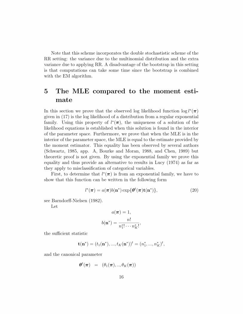
In this section we prove that the observed log likelihood function log l∗(π)given in (17) is the log likelihood of a distribution from a regular exponentialfamily. Using this property of l∗(π), the uniqueness of a solution of thelikelihood equations is established when this solution is found in the interiorof the parameter space. Furthermore, we prove that when the MLE is in theinterior of the parameter space, the MLE is equal to the estimate provided bythe moment estimator. This equality has been observed by several authors(Schwartz, 1985, app. A, Bourke and Moran, 1988, and Chen, 1989) buttheoretic proof is not given. By using the exponential family we prove thisequality and thus provide an alternative to results in Lucy (1974) as far asthey apply to misclassification of categorical variables.

First, to determine that l∗(π) is from an exponential family, we have toshow that this function can be written in the following form

l∗(π) = a(π)b(n∗) expθt(π)t(n∗), (20)

see Barndorff-Nielsen (1982).Let

a(π) = 1,

b(n∗) =n!

n∗1! · · ·n∗K !,

the sufficient statistic

t(n∗) = (t1(n∗), ..., tK(n∗))t = (n∗1, ..., n

∗K)t,

and the canonical parameter

θt(π) = (θ1(π), .., θK(π))

16

= (log λ1, ..., log λK)

= (logK∑

j=1

p1jπj, ..., logK∑

j=1

pKjπj).

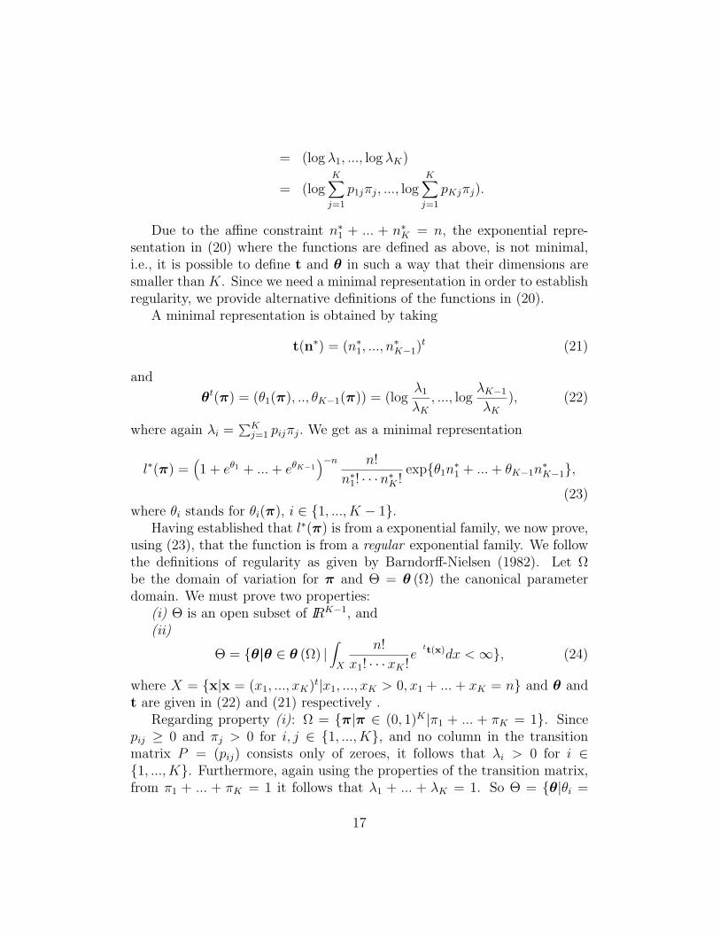
Due to the affine constraint n∗1 + ... + n∗K = n, the exponential repre-sentation in (20) where the functions are defined as above, is not minimal,i.e., it is possible to define t and θ in such a way that their dimensions aresmaller than K. Since we need a minimal representation in order to establishregularity, we provide alternative definitions of the functions in (20).

A minimal representation is obtained by taking

t(n∗) = (n∗1, ..., n∗K−1)

t (21)

and

θt(π) = (θ1(π), .., θK−1(π)) = (logλ1

λK

, ..., logλK−1

λK

), (22)

where again λi =∑K

j=1 pijπj. We get as a minimal representation

l∗(π) =(1 + eθ1 + ... + eθK−1

)−n n!

n∗1! · · ·n∗K !expθ1n

∗1 + ... + θK−1n

∗K−1,

(23)where θi stands for θi(π), i ∈ 1, ..., K − 1.

Having established that l∗(π) is from a exponential family, we now prove,using (23), that the function is from a regular exponential family. We followthe definitions of regularity as given by Barndorff-Nielsen (1982). Let Ωbe the domain of variation for π and Θ = θ (Ω) the canonical parameterdomain. We must prove two properties:

(i) Θ is an open subset of IRK−1, and(ii)

Θ = θ|θ ∈ θ (Ω) |∫

X

n!

x1! · · ·xK !e

tt(x)dx < ∞, (24)

where X = x|x = (x1, ..., xK)t|x1, ..., xK > 0, x1 + ... + xK = n and θ andt are given in (22) and (21) respectively .

Regarding property (i): Ω = π|π ∈ (0, 1)K |π1 + ... + πK = 1. Sincepij ≥ 0 and πj > 0 for i, j ∈ 1, ..., K, and no column in the transitionmatrix P = (pij) consists only of zeroes, it follows that λi > 0 for i ∈1, ..., K. Furthermore, again using the properties of the transition matrix,from π1 + ... + πK = 1 it follows that λ1 + ... + λK = 1. So Θ = θ|θi =

17

log λiλ−1K |λ1+ ...+λK = 1, λi > 0. For each r = (r1, ..., rK−1) ∈ IRK−1, there

is a choice for λ1, ..., λK such that λ1 + ...+λK = 1, λi > 0 for i ∈ 1, ..., K,and log λiλ

−1K = ri for i ∈ 1, ..., K − 1. So property (i) is satisfied by the

equality Θ = IRK−1.Regarding property (ii):

∫

X

n!

x1! · · · xK !e

tt(x)dx ≤ n!∫

X

(λ1

λK

)x1

· · ·(

λK−1

λK

)xK−1

dx

= n!∫

Xλx1

1 · · ·λxKK

1

λnK

dx

≤ n!∫

X

(1

λK

)n

dx < ∞,

for every λK ∈ (0, 1) and n = x1 + ...+xK . This means that (24) is satisfied.Having shown that the observed data log likelihood l∗(π) is from a regular

exponential family, we can use the powerful theory that exists for this family.A property that is of practical use is that the maximum of the observed datalikelihood is unique when found in the interior of the parameter space, sincethe likelihood is strictly concave (Barndorff-Nielsen, 1982). This justifies theuse of the maximum found by the EM algorithm in Section 4.1.

A second property concerns the comparison of the MLE and the estimateprovided by the moment estimator. The two estimates are equal when bothare in the interior of the parameter space. The equality can be proved asfollows. We continue to use the minimal representation as given in (23) whereθ is the canonical parameter and where a(π) is given by

a(π) =(1 + eθ1 + ... + eθK−1

)−n,

When log l∗(π) is maximized, we solve the likelihood equations

∂

∂θlog l∗(π) = 0.

That is∂

∂θ(θtt(n∗)) =

∂

∂θ(− log a(π)). (25)

We have∂

∂θ(θtt(n∗)) = (n∗1, ..., n

∗K−1)

t (26)

18

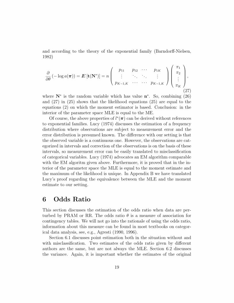
and according to the theory of the exponential family (Barndorff-Nielsen,1982)

∂

∂θ(− log a(π)) = IE [t(N∗)] = n

p11 p12 · · · p1K...

. . . . . ....

pK−1,K · · · · · · pK−1,K

π1

π2...

πK

,

(27)where N∗ is the random variable which has value n∗. So, combining (26)and (27) in (25) shows that the likelihood equations (25) are equal to theequations (2) on which the moment estimator is based. Conclusion: in theinterior of the parameter space MLE is equal to the ME.

Of course, the above properties of l∗(π) can be derived without referencesto exponential families. Lucy (1974) discusses the estimation of a frequencydistribution where observations are subject to measurement error and theerror distribution is presumed known. The difference with our setting is thatthe observed variable is a continuous one. However, the observations are cat-egorized in intervals and correction of the observations is on the basis of theseintervals, so measurement error can be easily translated to misclassificationof categorical variables. Lucy (1974) advocates an EM algorithm comparablewith the EM algoritm given above. Furthermore, it is proved that in the in-terior of the parameter space the MLE is equal to the moment estimate andthe maximum of the likelihood is unique. In Appendix B we have translatedLucy’s proof regarding the equivalence between the MLE and the momentestimate to our setting.

6 Odds Ratio

This section discusses the estimation of the odds ratio when data are per-turbed by PRAM or RR. The odds ratio θ is a measure of association forcontingency tables. We will not go into the rationale of using the odds ratio,information about this measure can be found in most textbooks on categor-ical data analysis, see, e.g., Agresti (1990, 1996).

Section 6.1 discusses point estimation both in the situation without andwith misclassification. Two estimates of the odds ratio given by differentauthors are the same, but are not always the MLE. Section 6.2 discussesthe variance. Again, it is important whether the estimates of the original

19

frequencies are in the interior of the parameter space or not.

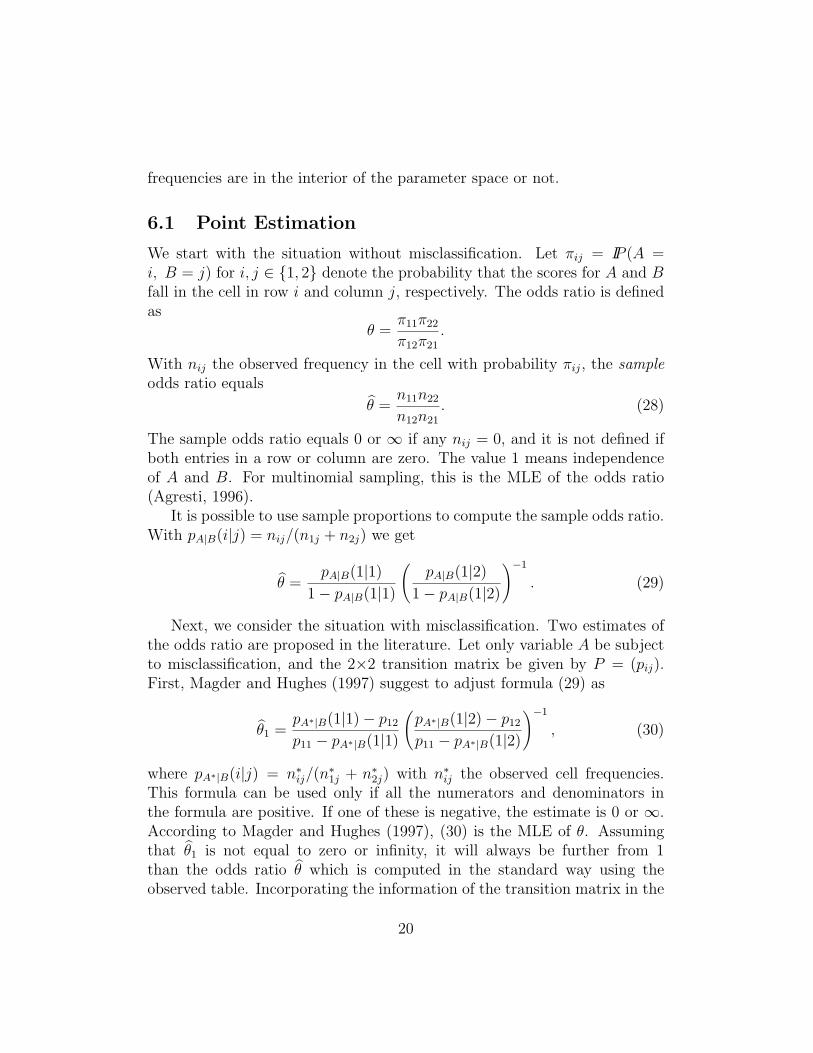
6.1 Point Estimation

We start with the situation without misclassification. Let πij = IP (A =i, B = j) for i, j ∈ 1, 2 denote the probability that the scores for A and Bfall in the cell in row i and column j, respectively. The odds ratio is definedas

θ =π11π22

π12π21

.

With nij the observed frequency in the cell with probability πij, the sampleodds ratio equals

θ =n11n22

n12n21

. (28)

The sample odds ratio equals 0 or ∞ if any nij = 0, and it is not defined ifboth entries in a row or column are zero. The value 1 means independenceof A and B. For multinomial sampling, this is the MLE of the odds ratio(Agresti, 1996).

It is possible to use sample proportions to compute the sample odds ratio.With pA|B(i|j) = nij/(n1j + n2j) we get

θ =pA|B(1|1)

1− pA|B(1|1)

(pA|B(1|2)

1− pA|B(1|2)

)−1

. (29)

Next, we consider the situation with misclassification. Two estimates ofthe odds ratio are proposed in the literature. Let only variable A be subjectto misclassification, and the 2×2 transition matrix be given by P = (pij).First, Magder and Hughes (1997) suggest to adjust formula (29) as

θ1 =pA∗|B(1|1)− p12

p11 − pA∗|B(1|1)

(pA∗|B(1|2)− p12

p11 − pA∗|B(1|2)

)−1

, (30)

where pA∗|B(i|j) = n∗ij/(n∗1j + n∗2j) with n∗ij the observed cell frequencies.

This formula can be used only if all the numerators and denominators inthe formula are positive. If one of these is negative, the estimate is 0 or ∞.According to Magder and Hughes (1997), (30) is the MLE of θ. Assumingthat θ1 is not equal to zero or infinity, it will always be further from 1than the odds ratio θ which is computed in the standard way using theobserved table. Incorporating the information of the transition matrix in the

20

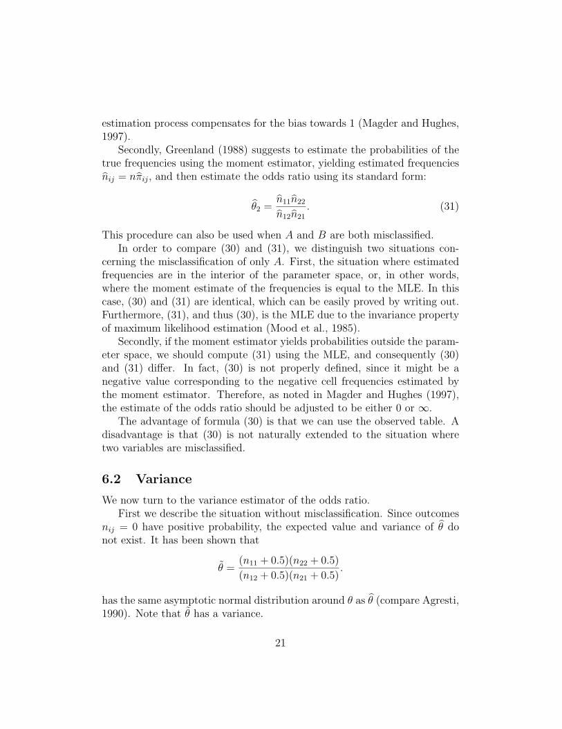
estimation process compensates for the bias towards 1 (Magder and Hughes,1997).

Secondly, Greenland (1988) suggests to estimate the probabilities of thetrue frequencies using the moment estimator, yielding estimated frequenciesnij = nπij, and then estimate the odds ratio using its standard form:

θ2 =n11n22

n12n21

. (31)

This procedure can also be used when A and B are both misclassified.In order to compare (30) and (31), we distinguish two situations con-

cerning the misclassification of only A. First, the situation where estimatedfrequencies are in the interior of the parameter space, or, in other words,where the moment estimate of the frequencies is equal to the MLE. In thiscase, (30) and (31) are identical, which can be easily proved by writing out.Furthermore, (31), and thus (30), is the MLE due to the invariance propertyof maximum likelihood estimation (Mood et al., 1985).

Secondly, if the moment estimator yields probabilities outside the param-eter space, we should compute (31) using the MLE, and consequently (30)and (31) differ. In fact, (30) is not properly defined, since it might be anegative value corresponding to the negative cell frequencies estimated bythe moment estimator. Therefore, as noted in Magder and Hughes (1997),the estimate of the odds ratio should be adjusted to be either 0 or ∞.

The advantage of formula (30) is that we can use the observed table. Adisadvantage is that (30) is not naturally extended to the situation wheretwo variables are misclassified.

6.2 Variance

We now turn to the variance estimator of the odds ratio.First we describe the situation without misclassification. Since outcomes

nij = 0 have positive probability, the expected value and variance of θ donot exist. It has been shown that

θ =(n11 + 0.5)(n22 + 0.5)

(n12 + 0.5)(n21 + 0.5).

has the same asymptotic normal distribution around θ as θ (compare Agresti,1990). Note that θ has a variance.

21

The close relation between θ and θ is the reason we will discuss asymptoticstandard error (ASE) of log θ, although it is not mathematically sound to doso.

There are at least two methods available to estimate the ASE of log θ.The first method is using the delta method. The estimated ASE is then givenby

ASE(log θ) =(

1

n11

+1

n12

+1

n21

+1

n22

)1/2

,

see Agresti (1990, Sections 3.4 and 12.1).The second method to estimate the ASE in the situation without mis-

classification is to use the bootstrap. For instance, we can use the bootstrappercentile method to estimate a 95% confidence interval. When we assumethe multinomial distribution, we take the vector of observed cell proportionsas MLE of the cell probabilities. With this MLE we simulate a large num-ber of multinomial tables and each time compute the odds ratio. Then weestimate a 95% confidence interval is the same way as described in Section4.2.

Next, we consider the situation with misclassification. Along the line ofthe two methods described above, we discuss two methods to estimate thevariance of the estimate of the odds ratio. First, when the moment estimatoris used, the delta-method can be applied to determine the variance of thelog odds ratio. Greenland (1988) shows how this can be done when thetransition matrix is estimated with known variances. Our situation is easier,since the transition matrix is given. We use the multivariate delta method(Bishop, Fienberg and Holland, 1975, Section 14.6.3). The random vectoris π = (π11, π12, π21, π22)

t with 4 × 4 asymptotic covariance-variance matrixV (π), see Section 3. We take the function f to be

f(π) = log(

π11π22

π12π21

),

which has a derivative at π ∈ (0, 1)4. The delta method provides the asymp-totic variance Vf for f(π):

Vf = (Df)tV (π)Df,

where Df is the gradient vector of f at π and V (π) is given by (6).The problem with this method is that it makes use of the moment esti-

mator which only makes sense when this estimator yields a solution in the

22

interior of the parameter space. A second way to estimate the variance isusing the bootstrap method and can also be applied in combination with theEM algorithm. Since the table provided by the algorithm is an estimate, weshould take into account the variance of this estimate when estimating thevariance of the estimate of the odds ratio. This motivates the following pro-cedure. (i) We assume that the observed table is multinomially distributedand we draw a large number of samples from this distribution. Let B bethe number of samples. (ii) For each of the B samples we estimate the truetable using the EM algorithm and furthermore we estimate the odds ratio.This results in the numbers θ∗1, .., θ

∗B. We then use the bootstrap percentile

method, see Section 4.2, to estimate from θ∗1, .., θ∗B a 95% confidence interval.

7 An Example

This section illustrates the foregoing by estimating tables of true frequencieson the basis of data collected using RR. Also, in Section 7.2, an estimate ofthe odds ratio will be discussed. The example makes clear that boundarysolutions can occur when RR is applied and that we need to apply methodssuch as the EM algorithm and the bootstrap.

7.1 Frequencies

The RR data we want to analyse stem from a research into violating reg-ulations of social benefit (Van Gils, Van der Heijden and Rosebeek, 2001).Sensitive items were binary: respondents were asked whether or not theyviolated certain regulations.

The research used the RR procedure introduced by Kuk (1990) wherethe misclassification design is constructed by using stacks of cards. Since theitems in the present research were binary, two stacks of cards were used. Inthe right stack the proportion of red cards was 8/10, and in the left stack itwas 2/10. The respondent was asked to draw one card from each stack. Thenthe sensitive question was asked, and when the answer to it was ‘yes’, therespondent should name the color of the card of the right stack, and whenthe answer was ‘no’, the respondent should name the color of the card of theleft stack.

We associate violations with the color red. In this way the probability tobe correctly classified is 8/10 both for respondents who violated regulations

23

and for those who did not. The transition matrix is therefore given by

P =

(8/10 2/102/10 8/10

), (32)

We discuss observed frequencies of red or black regarding two questions,Q1 and Q2, which were asked using this RR procedure. Both questionsconcern the period in which the respondent received a benefit. In translation,question Q1: Did you turn down a job offer, or did you endanger on purposean offer to get a job? And Q2: Was the number of job applications less thanrequired? In our discussion, we deal first with the frequencies of the separatequestions, and secondly, we take them together, meaning that we tabulate thefrequencies of the four possible profiles: red-red, red-black, black-red, black-black, and we want to know the true frequencies of the profiles violation-violation, violation-no violation, no violation-violation and no violation-noviolation.

We assume that the data are multinomially distributed, so the correspon-dence between the probabilities and the frequencies is direct, given n = 412,the size of the data set. Univariate observed frequencies are

Q1 red 120black 292

andQ2 red 171

black 241

The moment estimate of the true frequencies is equal to the MLE sincethe solution is in the interior of the parameter space:

Q1 violation 62.67no violation 349.33

andQ2 violation 147.67

no violation 264.33

Since we have for each respondent the answers to both RR questions,we can tabulate the frequencies of the 4 possible response profiles, see table1. Using the Kronecker product to determine the 4 × 4 transition matrix,see Section 3.1, the moment estimate yields a negative cell entry, see table2. The MLE can be computed by using the EM algorithm as described inSection 4.1 and is given by table 3.

There is a discrepancy which shows up in this example. From table 3, wecan deduce estimated univariate frequencies of answers to Q1 and Q2. Theseestimates, which are based on the MLE of the true multivariate frequenciesare different from the univariate moment estimates which are also MLE’s.Differences however are small.

24

Q2

red blackQ1 red 68 52 120

black 103 189 292171 241 412

Table 1: Response Profiles

Q2

violation no violationQ1 violation 73.00 -10.33 62.67

no violation 74.67 274.66 349.33147.67 264.33 412

Table 2: Moment Estimate

Next, we turn to the estimation of variance. First, the univariate case,where we only discuss question Q1. The estimated probability of violation isπ=62.67/412=0.152. The estimated standard error of π can be computed byusing (7) and is estimated to be 0.037. The bootstrap scheme as explainedin Section 4.2 can also be used. With B = 500 we compute the bootstrapstandard error of π from the sample covariance matrix of the bootstrap es-timates π∗1, ..., π

∗B This procedure yields the same estimate of the standard

error as above.Secondly, we compute the variance of the four estimated probabilities

concerning profiles of violation. From table 3 we obtain π = (π1, ..., π4)t

= (0.17, 0.00, 0.19, 0.64)t. Since the MLE is on the boundary of the parame-ter space, estimating a 95% confidence interval is more useful than estimatingstandard errors. We use the bootstrap percentile method as explained in Sec-tion 4.2. Using B = 500 we obtain the four intervals [0.10,0.22], [0.00,0.04],[0.12,0.28], and [0.56,0.72], for π = (π1, ..., π4)

t

7.2 Odds Ratio

To determine whether the items corresponding to Q1 and Q2 are associated,we want to know the odds ratio. The starting point is the 2× 2 contingencytable of observed answers to Q1 and Q2, given by table 1. Without anyadjustment, the estimated odds ratio is (68 · 189)/(103 · 52) = 2.40.

25

Q2

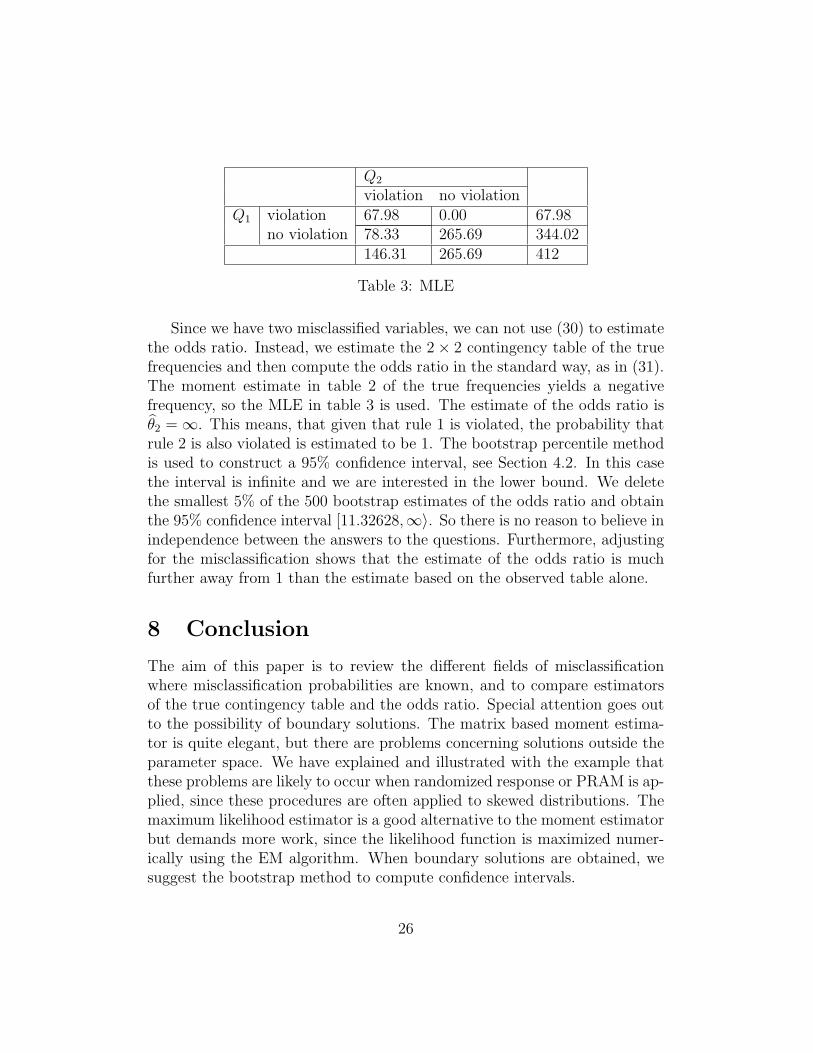
violation no violationQ1 violation 67.98 0.00 67.98

no violation 78.33 265.69 344.02146.31 265.69 412

Table 3: MLE

Since we have two misclassified variables, we can not use (30) to estimatethe odds ratio. Instead, we estimate the 2× 2 contingency table of the truefrequencies and then compute the odds ratio in the standard way, as in (31).The moment estimate in table 2 of the true frequencies yields a negativefrequency, so the MLE in table 3 is used. The estimate of the odds ratio isθ2 = ∞. This means, that given that rule 1 is violated, the probability thatrule 2 is also violated is estimated to be 1. The bootstrap percentile methodis used to construct a 95% confidence interval, see Section 4.2. In this casethe interval is infinite and we are interested in the lower bound. We deletethe smallest 5% of the 500 bootstrap estimates of the odds ratio and obtainthe 95% confidence interval [11.32628,∞〉. So there is no reason to believe inindependence between the answers to the questions. Furthermore, adjustingfor the misclassification shows that the estimate of the odds ratio is muchfurther away from 1 than the estimate based on the observed table alone.

8 Conclusion

The aim of this paper is to review the different fields of misclassificationwhere misclassification probabilities are known, and to compare estimatorsof the true contingency table and the odds ratio. Special attention goes outto the possibility of boundary solutions. The matrix based moment estima-tor is quite elegant, but there are problems concerning solutions outside theparameter space. We have explained and illustrated with the example thatthese problems are likely to occur when randomized response or PRAM is ap-plied, since these procedures are often applied to skewed distributions. Themaximum likelihood estimator is a good alternative to the moment estimatorbut demands more work, since the likelihood function is maximized numer-ically using the EM algorithm. When boundary solutions are obtained, wesuggest the bootstrap method to compute confidence intervals.

26

The proof of the equality of the moment estimate and the maximumlikelihood estimate, when these estimates are in the interior of the parameterspace, is interesting because it establishes theoretically what was conjecturedby others on the basis of numerical output.

Regarding PRAM, the results are useful in the sense that they showthat frequency analysis with the released data is possible and that there isongoing research in the field of RR and misclassification which deals with theproblems that are encountered. This is important concerning the acceptanceof PRAM as a SDC method.

Regarding RR, the example illustrates that a boundary solution may beencountered in practice. This possibility was also noted by others but is, asfar as we know, not investigated in the multivariate situation with attentionto the estimation of standard errors.

References

Agresti, A. (1990), Categorical Data Analysis, New York: Wiley.

Agresti, A. (1996), An Introduction to Categorical Data Analysis, New York:Wiley.

Barndorff-Nielsen, O. (1982) Exponential Families, Encyclopedia of Statis-tical Sciences, Ed. S. Kotz and N.L. Norman, New York: Wiley.

Bishop, Y.M.M., Fienberg, S.E., and Holland, P.W. (1975), Discrete Mul-tivariate Analysis, Cambridge: MIT Press.

Bourke, P.D. and Moran, M.A. (1988) Estimating Proportions From Ran-domized Response Data Using the EM Algorithm, J. Am. Stat. Assoc,83, pp 964-968

Chaudhuri, A., and Mukerjee, R. (1988), Randomized Response: Theoryand Techniques, New York: Marcel Dekker.

Chen, T.T. (1989) A Review of Methods for Misclassified Categorical Datain Epidemiology, Stat. Med., 8, pp 1095-1106.

Copeland, K.T., Checkoway, H., McMichael, A. J., and Holbrook, R. H.(1977) Bias Due to Misclassification in the Estimation of Relative Risk,Am. J. Epidemiol., 105, pp 488-495.

27

Dempster, A. P., Laird, N.M. and Rubin, D.B. (1977) Maximum Likelihoodfrom Incomplete Data via the EM algorithm, J. R. Stat. Soc., 39, pp1-38.

Efron, B, and Tibshirani, R.J (1993) An Introduction to the Bootstrap, NewYork: Chapman and Hall.

Fox, J.A., and Tracy, P.E. (1986) Randomized Response: A method forSensitive Surveys, Newbury Park: Sage.

Gouweleeuw, J.M., Kooiman, P., Willenborg, L.C.R.J., and De Wolf, P.-P.(1998) Post Randomisation for Statistical Disclosure Control: Theoryand Implementation, J. Off. Stat., 14, pp 463-478.

Greenland, S. (1980), The Effect of Misclassification in the Presence ofCovariates, Am. J. Epidemiol., 112, pp 564-569.

Greenland, S. (1988), Variance Estimation for Epidemiologic Effect Esti-mates under Misclassification, Stat. Med., 7, pp 745-757.

Kooiman, P., Willenborg, L.C.R.J., and Gouweleeuw, J.M. (1997), PRAM:a Method for Dislosure Limitation of Microdata, Research paper no.9705, Voorburg/Heerlen: Statistics Netherlands.

Kuha, J., and Skinner, C. (1997) Categorical Data Analysis and Misclassi-fication, Survey Measurement and Process Quality, Ed. L. Lyberg etal., New York: Wiley.

Kuk, A.Y.C. (1990) Asking Sensitive Questions Indirectly. Biometrika., 77,pp 436-438.

Lucy, L.B. (1974) An Iterative Technique for the Rectification of ObservedDistributions, Astron. J., 79, pp 745-754.

Magder, L. S., and Hughes, J. P. (1997) Logistic Regression When theOutcome Is Measured with Uncertainty, Am. J. Epidemiol., 146, pp.195-203.

McLachlan, G. F., and Krishnan, T. (1997) The EM Algorithm and Exten-sions, New York: Wiley.

28

Mood, A.M., Graybill, F.A., and Boes, D.C. (1985) Introduction to thetheory of Statistics, Auckland: McGraw-Hill.

Rice, J.A. (1995) Mathematical Statistics and Data Analysis, Belmont: DuxburyPress.

Rosenberg, M.J. (1979) Multivariate Analysis by a Randomized ResponseTechnique for Statistical Disclosure Control, Ph.D. Dissertation, Uni-versity of Michigan.

Rosenberg, M.J. (1980) Categorical Data Analysis by a Randomized Re-sponse Technique for Statistical Disclosure Control, Proceedings of theSurvey Research Section, American Statistical Association.

Rubin, D.B. (1976) Inference and Missing Data, Biometrika, 63,581-592.

Schafer J.L.(1997) Analysis of Incomplete Multivariate Data, London: Chap-man and Hall.

Schwartz, J.E. (1985) The Neglected Problem of Measurement Error inCategorical Data, Soc. Meth. Research, 13, pp 435-466.

Singh, J (1976) A Note on RR Techniques, Proc. ASA. Soc. Statist. Sec.,772.

Van Gils, G., Van der Heijden,P.G.M., and Rosebeek, A. (2001). Onderzoeknaar regelovertreding. Resultaten ABW, WAO en WW. Amsterdam:NIPO. (In Dutch)

Van den Hout, A.D.L. (1999) The Analysis of Data Perturbed by PRAM,Delft: Delft University Press.

Van der Heijden, P.G.M., Van Gils, G., Bouts, J., and Hox, J.J. (2000) AComparison of Randomized Response, Computer-Assisted Self-Interview,and Face-to-Face Direct Questioning, Soc. Meth. Research, 28, pp 505-537.

Warner, S.L. (1965) Randomized Response: a Survey Technique for Elimi-nating Answer Bias, J. Am. Stat. Assoc., 60, pp 63-69.

Warner, S.L. (1971) The Linear Randomized Response Model, J. Am. Stat.Assoc., 66, pp 884-888.

29

Willenborg, L. (2000) Optimality Models for PRAM, in Proceedings in Com-putational Statistics, Ed. J.G. Bethlehem and P.G.M. van der Heijden,pp 505-510, Heidelberg: Physica-Verlag.

Willenborg, L., and De Waal, T. (2001) Elements of Statistical DisclosureControl, New York: Springer.

Appendix A

As stated in Section 3.2, V (π) can be partitioned as

V (π) = Σ1 + Σ2, (33)

where

Σ1 =1

n

(Diag(π)− ππt

)

and

Σ2 =1

nP−1

(Diag(λ)− PDiag(π)P t

) (P−1

)t. (34)

To understand (33):

Σ1 + Σ2 =1

n

(Diag(π)− ππt + P−1Diag(λ)

(P−1

)t −Diag(π))

=1

n

(P−1Diag(λ)

(P−1

)t − ππt)

=1

nP−1

(Diag(λ)− PππtP t

) (P−1

)t

=1

nP−1

(Diag(λ)− λλt

) (P−1

)t

= V (π)

The variance due to PRAM as given in Kooiman et al. (1997) equals

V(T |T

)= P−1V (T ∗|T )

(P−1

)t

= P−1

K∑

j=1

T (j)Vj

(P−1

)t(35)

where for j ∈ 1, ..., K, T (j) is the true frequency of category j, and Vj isthe K × K covariance matrix of two observed categories h and i given thetrue category j:

30

Vj(h, i) =

pij(1− pij) if h = i

−phjpij if h 6= i, for h, i ∈ 1, ..., K, (36)

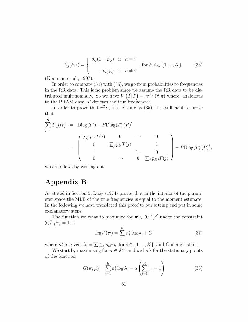
(Kooiman et al., 1997).In order to compare (34) with (35), we go from probabilities to frequencies

in the RR data. This is no problem since we assume the RR data to be dis-tributed multinomially. So we have V

(T |T

)= n2V (π|π) where, analogous

to the PRAM data, T denotes the true frequencies.In order to prove that n2Σ2 is the same as (35), it is sufficient to prove

thatK∑

j=1

T (j)Vj = Diag(T ∗)− PDiag(T ) (P )t

=

∑j p1jT (j) 0 · · · 0

0∑

j p2jT (j)...

.... . . 0

0 · · · 0∑

j pKjT (j)

− PDiag(T ) (P )t ,

which follows by writing out.

Appendix B

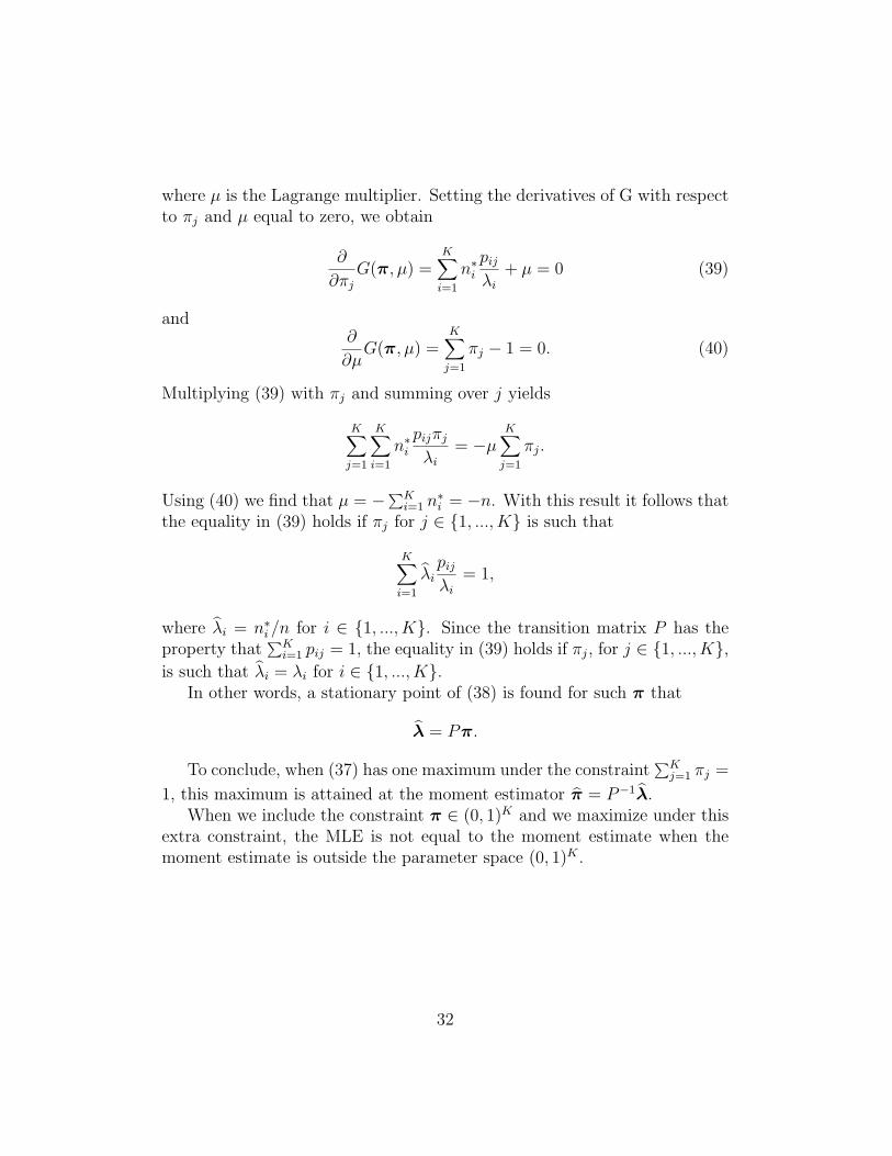
As stated in Section 5, Lucy (1974) proves that in the interior of the param-eter space the MLE of the true frequencies is equal to the moment estimate.In the following we have translated this proof to our setting and put in someexplanatory steps.

The function we want to maximize for π ∈ (0, 1)K under the constraint∑Kj=1 πj = 1, is

log l∗(π) =K∑

i=1

n∗i log λi + C (37)

where n∗i is given, λi =∑K

k=1 pikπk, for i ∈ 1, ..., K, and C is a constant.We start by maximizing for π ∈ IRK and we look for the stationary points

of the function

G(π, µ) =K∑

i=1

n∗i log λi − µ

K∑

j=1

πj − 1

(38)

31

where µ is the Lagrange multiplier. Setting the derivatives of G with respectto πj and µ equal to zero, we obtain

∂

∂πj

G(π, µ) =K∑

i=1

n∗ipij

λi

+ µ = 0 (39)

and∂

∂µG(π, µ) =

K∑

j=1

πj − 1 = 0. (40)

Multiplying (39) with πj and summing over j yields

K∑

j=1

K∑

i=1

n∗ipijπj

λi

= −µK∑

j=1

πj.

Using (40) we find that µ = −∑Ki=1 n∗i = −n. With this result it follows that

the equality in (39) holds if πj for j ∈ 1, ..., K is such that

K∑

i=1

λipij

λi

= 1,

where λi = n∗i /n for i ∈ 1, ..., K. Since the transition matrix P has theproperty that

∑Ki=1 pij = 1, the equality in (39) holds if πj, for j ∈ 1, ..., K,

is such that λi = λi for i ∈ 1, ..., K.In other words, a stationary point of (38) is found for such π that

λ = Pπ.

To conclude, when (37) has one maximum under the constraint∑K

j=1 πj =

1, this maximum is attained at the moment estimator π = P−1λ.When we include the constraint π ∈ (0, 1)K and we maximize under this

extra constraint, the MLE is not equal to the moment estimate when themoment estimate is outside the parameter space (0, 1)K .

32