Procedia Computer Science 59 ( 2015 ) 142 – 151

1877-0509 © 2015 The Authors. Published by Elsevier B.V. This is an open access article under the CC BY-NC-ND license (http://creativecommons.org/licenses/by-nc-nd/4.0/).Peer-review under responsibility of organizing committee of the International Conference on Computer Science and Computational Intelligence (ICCSCI 2015)doi: 10.1016/j.procs.2015.07.528

ScienceDirectAvailable online at www.sciencedirect.com

International Conference on Computer Science and Computational Intelligence (ICCSCI 2015)

Rainfall Monthly Prediction Based on Artificial Neural Network: A Case Study in Tenggarong Station, East Kalimantan -

Indonesia Mislana*, Haviluddinb*, Sigit Hardwinartoc, Sumaryonod, Marlon Aipassae

a,bFaculty of Mathematics and Natural Science, UNMUL Indonesia c,d,eFaculty of Forestry, UNMUL Indonesia

Abstract

The accuracy of forecasting rainfall is very important due to the current world climate change. Afterwards, to get an accurate forecasting of rainfall, this paper applied an Artificial Neural Network (ANN) with the Backpropagation Neural Network (BPNN) algorithm. In this experiment, the rainfall data were tested using two-hidden layers of BPNN architectures with three different epochs which were [2-50-10-1, epoch 500]; [2-50-20-1, with epochs 1000 and 1500]. The mean square error (MSE) is employed to measure the performance of the classification task. The experimental results showed that the architecture [2-50-20-1, epoch 1000] produced a good result with the value of MSE was 0.00096341. Furthermore, BPNN algorithm has provided a good model to predict rainfall in Tenggarong, East Kalimantan - Indonesia. © 2015 The Authors. Published by Elsevier B.V. Peer-review under responsibility of organizing committee of the International Conference on Computer Science and Computational Intelligence (ICCSCI 2015).

Keywords: ANN, BPNN, rainfall, MSE

1. Introduction

The rainfall forecast information is an essential requirement to support water resources management especially when it is related to climate change in tropical regions such as in Indonesia. Nowadays, climate change affects the

* Corresponding author. Tel.: +6281331112002; +6281347011790

E-mail address: haviluddin@unmul.ac.id; airmasadepan@yahoo.co.id

© 2015 The Authors. Published by Elsevier B.V. This is an open access article under the CC BY-NC-ND license (http://creativecommons.org/licenses/by-nc-nd/4.0/).Peer-review under responsibility of organizing committee of the International Conference on Computer Science and Computational Intelligence (ICCSCI 2015)

143 Mislan et al. / Procedia Computer Science 59 ( 2015 ) 142 – 151

pattern of rainfall. The impact of these effects includes extreme occurrence of flooding and droughts [1-3]. Furthermore, the prediction of rainfall with good and accurate method is indispensable in order to anticipate the impact [4-7].

Therefore, in order to produce efficient accurate results of forecasting rainfall and weather, a few methods have been developed. Among them, a statistical model has been widely used to make forecasts of rainfall. This model works by lowering the equation of the data itself (data driven) such as a simple method regression analysis (SRA), decomposition, exponential smoothing method (ES) and autoregressive integrated moving average (ARIMA). Several studies have indicated that they are still inaccurate methods to forecast rainfall and weather because weather data are non-linear [8, 9]. However, in some cases, rainfall prediction statistical method is also able to produce good and accurate predictions [10].

Along with the development of computing technology, many researchers are trying to make predictions using the ANN method in the field of hydrology. Abhishek, K. et al, have conducted research with ANN rainfall prediction in Udupi district of Karnataka, India. Another researchers also have predicted the data series of rainfall for 30 years (1977-2006) at the station of Nagpur, India. The results of this research has revealed that by using a backpropagatin neural network (BPNN), accurate prediction could be obtained [11, 12]. A combination of several ANN algorithms that was designed to predict monthly rainfall in the period of 1949 – 2011, from 24 stations Liuzhou, China, also showed accurate prediction results. The used research method was a hybrid between the ANN algorithm particle swarm optimization (PSO) and genetic algorithm (GA), called HPSOGA. The results of this research confirmed that the ANN has been very effective in making predictions of monthly rainfall in the city of Guangxi, the southwest of China [13].

Therefore, this paper will apply one of the ANN models, namely BPNN, in order to predict the rainfall which has a data type of non-linear in Tenggarong, East Kalimantan, Indonesia. The second part of this paper describes the architecture of BPNN models while time series predictor is discussed in the next part. Section 4 presents the analysis and discussion of the findings. Finally, conclusions are summarized in the last section.

2. Research Method and Process

2.1. The Artificial Neural Network

The ANN is an engineering concept of knowledge in the field of artificial intelligence designed by adopting the human nervous system. Wherein, the main processing of the human nervous system is composed of the brain nerve cells as the basic unit of information processing. In the concept of ANN, the basic unit of information processing are called neurons which serves process information in parallel and immediately. Furthermore, the process of training the ANN has many types and uses, including Perceptron, Backpropagation, Self-Organizing Map (SOM), and Delta [9, 10]. Therefore, this study proposes BPNN algorithm to predict rainfall data by studying and analyzing the patterns non-linear of the past data in order to obtain more accurate prediction results with minimum error. Furthermore, BPNN is briefly described.

2.2. The Backpropagation Neural Network

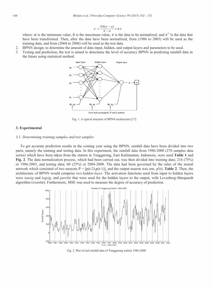
One of the ANN algorithms called BPNN is a supervised learning method. The BPNN was first introduced by Paul Werbos in 1974, then popularized by Rumelhart and McCelland in 1986. In general, the BPNN works by forwarding the output layer to the input layer in changing the weights [14-16]. Furthermore, ANN works like humans in which learning is performed through examples and exercises in each layer of ANN. The layer in BPNN consists of three parts, namely input layer, hidden layer and output layer, Fig. 1.

In general, the steps to build the BPNN algorithm for the prediction of rainfall data were adopted from previous research (Haviluddin & Alfred. R.) which is outlined [16]: 1. Data Normalization and separation; secondary data rainfall of the year 1986 - 2008 will be normalized using an

asymptotic function called sigmoid function in order to get the value of rainfall data in smaller intervals which are [0.1 0.8] using the following equation,

144 Mislan et al. / Procedia Computer Science 59 ( 2015 ) 142 – 151

where; is the minimum value, is the maximum value, is the data to be normalized, and 'is the data that have been transformed. Then, after the data have been normalized, from (1986 to 2003) will be used as the training data, and from (2004 to 2008) will be used as the test data.

2. BPNN design; to determine the amount of data input, hidden, and output layers and parameters to be used. 3. Testing and prediction; the test is aimed to determine the level of accuracy BPNN in predicting rainfall data in

the future using statistical method.

Fig. 1. A typical structure of BPNN architecture [17]

3. Experimental

3.1. Determining training samples and test samples

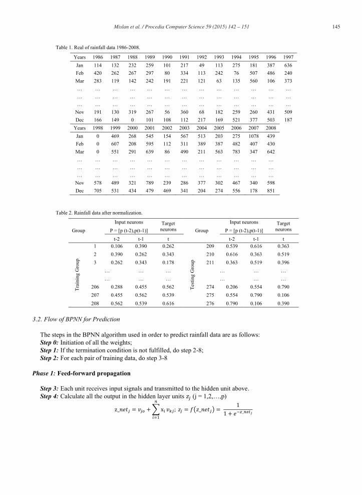
To get accurate prediction results in the coming year using the BPNN, rainfall data have been divided into two parts, namely the training and testing data. In this experiment, the rainfall data from 1986-2008 (276 samples data series) which have been taken from the station in Tenggarong, East Kalimantan, Indonesia, were used Table 1 and Fig. 2. The data normalization process, which had been carried out, was then divided into training data; 216 (75%) or 1986-2003, and testing data; 60 (25%) or 2004-2008. The data had been governed by the rules of the neural network which consisted of two neurons P = [p(t-2),p(t-1)], and the output neuron was one, p'(t), Table 2. Then, the architecture of BPNN would comprise two-hidden-layer. The activation functions used from input to hidden layers were tansig and logsig, and purelin that were used for the hidden layers to the output, with Levenberg-Marquardt algorithm (trainlm). Furthermore, MSE was used to measure the degree of accuracy of prediction.

Fig. 2. Plot of real rainfall data of Tenggarong station 1986-2008

145 Mislan et al. / Procedia Computer Science 59 ( 2015 ) 142 – 151

Table 1. Real of rainfall data 1986-2008.

Years 1986 1987 1988 1989 1990 1991 1992 1993 1994 1995 1996 1997 Jan 114 132 232 259 101 217 49 113 275 181 387 636 Feb 420 262 267 297 80 334 113 242 76 507 486 240 Mar 283 119 142 242 191 221 121 63 135 560 106 373 … … … … … … … … … … … … … … … … … … … … … … … … … … … … … … … … … … … … … … …

Nov 191 130 319 267 56 360 68 182 259 260 431 509 Dec 166 149 0 101 108 112 217 169 521 377 503 187

Years 1998 1999 2000 2001 2002 2003 2004 2005 2006 2007 2008 Jan 0 469 268 545 154 567 513 203 275 1078 439 Feb 0 607 208 595 112 311 389 387 482 407 430 Mar 0 551 291 639 86 490 211 563 783 347 642 … … … … … … … … … … … … … … … … … … … … … … … … … … … … … … … … … … … …

Nov 578 489 321 789 239 286 377 302 467 340 598 Dec 705 531 434 479 469 341 204 274 556 178 851

Table 2. Rainfall data after normalization.

Group Input neurons Target

neurons Group Input neurons Target

neurons P = [p (t-2),p(t-1)] P = [p (t-2),p(t-1)] t-2 t-1 t t-2 t-1 t

Trai

ning

Gro

up

1 0.106 0.390 0.262

Testi

ng G

roup

209 0.539 0.616 0.363 2 0.390 0.262 0.343 210 0.616 0.363 0.519 3 0.262 0.343 0.178 211 0.363 0.519 0.396

… … … … … … … … … … … …

206 0.288 0.455 0.562 274 0.206 0.554 0.790 207 0.455 0.562 0.539 275 0.554 0.790 0.106 208 0.562 0.539 0.616 276 0.790 0.106 0.390

3.2. Flow of BPNN for Prediction

The steps in the BPNN algorithm used in order to predict rainfall data are as follows: Step 0: Initiation of all the weights; Step 1: If the termination condition is not fulfilled, do step 2-8; Step 2: For each pair of training data, do step 3-8

Phase 1: Feed-forward propagation

Step 3: Each unit receives input signals and transmitted to the hidden unit above. Step 4: Calculate all the output in the hidden layer units (j = 1,2,…,p)

146 Mislan et al. / Procedia Computer Science 59 ( 2015 ) 142 – 151

Step 5: Calculate all the network output in unit output (k = 1,2,…,m)

Phase 2: Back-forward

Step 6: Calculate factor output unit based on unit output error (k = 1,2,…,m) k = (tk – yk)f’(y-netk) = (tk -yk)yk(1-yk)

tk = output target; = output unit that will be used in the layer underneath the weight change Calculate weight change wkj, with the learning rate α ( wji = α k zj, k = 1,2,…,m; j = 0,1,…,p)

Step 7: Calculate factor unit hidden layer based on the error in each hidden layer unit zj (j = 1,2,…,p)

Factor hidden layer unit [ j = _netj f’ (z_netj) = _netj zj (1-zj)] Calculate weight change rate vji [ vji = α k zj, k = 1,2,…,p; j = 0,1,…,n]

Phase 3: Weight modification

Step 8: Calculate the weight of all the changes that led to the output unit wkj(new) = wkj(old) + wji; (k = 1,2,…,p; j = 0,1,…,n)

Weight changes that led to the hidden layer units [vkj(new) = vkj(old) + vji; (j = 1,2,…,p; w = 0,1,…,n)]

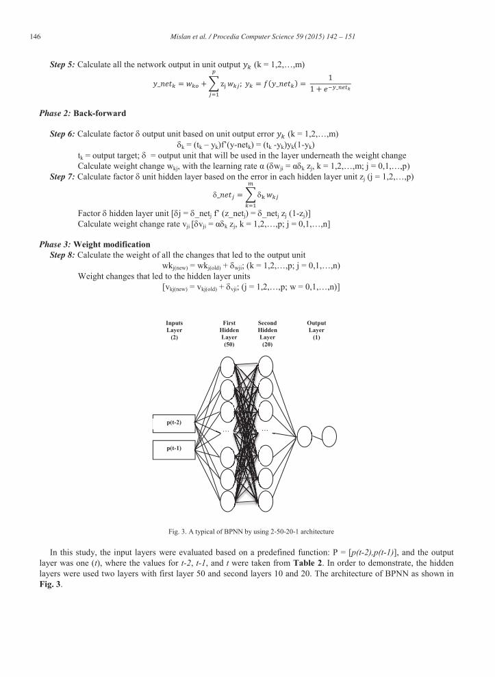
Fig. 3. A typical of BPNN by using 2-50-20-1 architecture In this study, the input layers were evaluated based on a predefined function: P = [p(t-2),p(t-1)], and the output

layer was one (t), where the values for t-2, t-1, and t were taken from Table 2. In order to demonstrate, the hidden layers were used two layers with first layer 50 and second layers 10 and 20. The architecture of BPNN as shown in Fig. 3.

p(t-2)

p(t-1)

Inputs Layer

(2)

First Hidden Layer (50)

Output Layer

(1)

Second Hidden Layer (20)

… …

147 Mislan et al. / Procedia Computer Science 59 ( 2015 ) 142 – 151

4. Results and Discussions

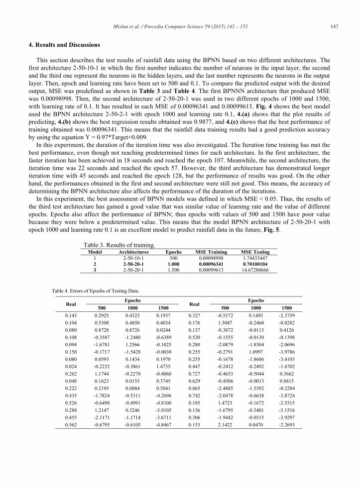
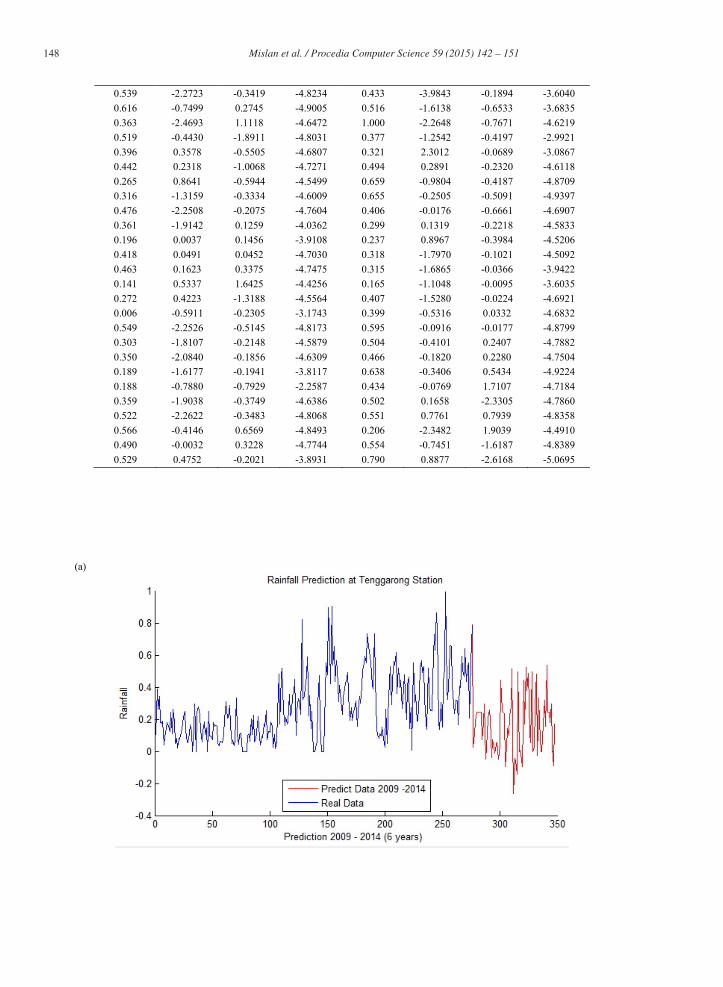
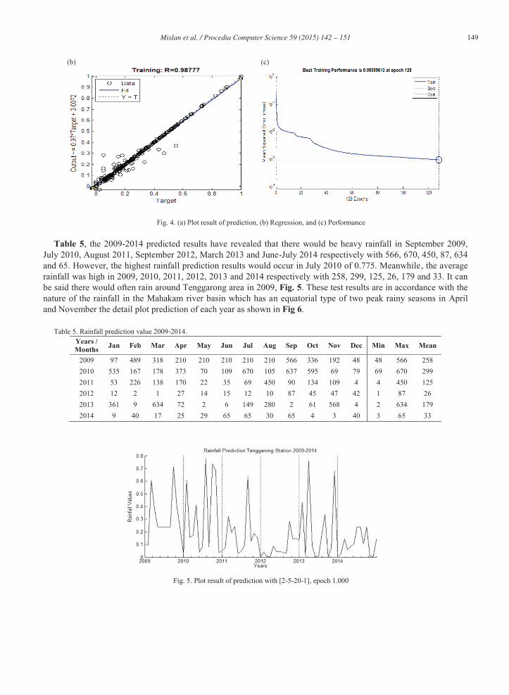
This section describes the test results of rainfall data using the BPNN based on two different architectures. The first architecture 2-50-10-1 in which the first number indicates the number of neurons in the input layer, the second and the third one represent the neurons in the hidden layers, and the last number represents the neurons in the output layer. Then, epoch and learning rate have been set to 500 and 0.1. To compare the predicted output with the desired output, MSE was predefined as shown in Table 3 and Table 4. The first BPNNN architecture that produced MSE was 0.00098998. Then, the second architecture of 2-50-20-1 was used in two different epochs of 1000 and 1500, with learning rate of 0.1. It has resulted in each MSE of 0.00096341 and 0.00099613. Fig. 4 shows the best model used the BPNN architecture 2-50-2-1 with epoch 1000 and learning rate 0.1, 4.(a) shows that the plot results of predicting, 4.(b) shows the best regression results obtained was 0.9877, and 4.(c) shows that the best performance of training obtained was 0.00096341. This means that the rainfall data training results had a good prediction accuracy by using the equation Y = 0.97*Target+0.009.

In this experiment, the duration of the iteration time was also investigated. The Iteration time training has met the best performance, even though not reaching predetermined times for each architecture. In the first architecture, the faster iteration has been achieved in 18 seconds and reached the epoch 107. Meanwhile, the second architecture, the iteration time was 22 seconds and reached the epoch 57. However, the third architecture has demonstrated longer iteration time with 45 seconds and reached the epoch 128, but the performance of results was good. On the other hand, the performances obtained in the first and second architecture were still not good. This means, the accuracy of determining the BPNN architecture also affects the performance of the duration of the iterations.

In this experiment, the best assessment of BPNN models was defined in which MSE < 0.05. Thus, the results of the third test architecture has gained a good value that was similar value of learning rate and the value of different epochs. Epochs also affect the performance of BPNN; thus epochs with values of 500 and 1500 have poor value because they were below a predetermined value. This means that the model BPNN architecture of 2-50-20-1 with epoch 1000 and learning rate 0.1 is an excellent model to predict rainfall data in the future, Fig. 5.

Table 3. Results of training.

Model Architectures Epochs MSE Training MSE Testing 1 2-50-10-1 500 0.00098998 1.74433447 2 2-50-20-1 1.000 0.00096341 0.70100104 3 2-50-20-1 1.500 0.00099613 14.67280666

Table 4. Errors of Epochs of Testing Data.

Real Epochs

Real Epochs

500 1000 1500 500 1000 1500 0.143 0.2925 0.4323 0.1937 0.327 -0.5572 0.1493 -2.3759 0.104 0.5308 0.4850 0.4034 0.176 1.5047 -0.2460 -0.0282 0.080 0.8728 0.8726 0.0244 0.137 -0.3872 -0.0113 0.4126 0.108 -0.3587 -1.2480 -0.6389 0.520 -0.1555 -0.0130 -0.1398 0.094 -1.6781 1.2566 -0.1025 0.280 -2.0879 -1.8304 -2.0696 0.150 -0.1717 -1.5428 -0.0030 0.255 -0.2791 1.0997 -3.9786 0.080 0.0593 0.1434 0.1970 0.255 -0.1678 -1.8606 -3.4103 0.024 -0.2232 -0.3861 1.4735 0.447 -0.2412 -0.2492 -1.6702 0.262 1.1744 -0.2270 -0.4060 0.727 -0.4653 -0.5044 0.3662 0.048 0.1623 0.0155 0.3745 0.629 -0.4506 -0.0013 0.8815 0.222 0.2195 0.0884 0.5041 0.865 -2.4885 -1.5392 -0.2284 0.435 -1.7824 -0.5311 -4.2696 0.742 -2.0478 -0.6638 -3.8724 0.526 -0.6498 -0.4991 -4.8100 0.185 1.4723 -0.1672 -2.5315 0.288 1.2147 0.3246 -3.9105 0.136 -1.6795 -0.3401 -3.1516 0.455 -2.1171 -1.1714 -3.6711 0.306 -1.9442 -0.0515 -3.9297 0.562 -0.6795 -0.6105 -4.8467 0.153 2.1422 0.0470 -2.2693

148 Mislan et al. / Procedia Computer Science 59 ( 2015 ) 142 – 151

0.539 -2.2723 -0.3419 -4.8234 0.433 -3.9843 -0.1894 -3.6040 0.616 -0.7499 0.2745 -4.9005 0.516 -1.6138 -0.6533 -3.6835 0.363 -2.4693 1.1118 -4.6472 1.000 -2.2648 -0.7671 -4.6219 0.519 -0.4430 -1.8911 -4.8031 0.377 -1.2542 -0.4197 -2.9921 0.396 0.3578 -0.5505 -4.6807 0.321 2.3012 -0.0689 -3.0867 0.442 0.2318 -1.0068 -4.7271 0.494 0.2891 -0.2320 -4.6118 0.265 0.8641 -0.5944 -4.5499 0.659 -0.9804 -0.4187 -4.8709 0.316 -1.3159 -0.3334 -4.6009 0.655 -0.2505 -0.5091 -4.9397 0.476 -2.2508 -0.2075 -4.7604 0.406 -0.0176 -0.6661 -4.6907 0.361 -1.9142 0.1259 -4.0362 0.299 0.1319 -0.2218 -4.5833 0.196 0.0037 0.1456 -3.9108 0.237 0.8967 -0.3984 -4.5206 0.418 0.0491 0.0452 -4.7030 0.318 -1.7970 -0.1021 -4.5092 0.463 0.1623 0.3375 -4.7475 0.315 -1.6865 -0.0366 -3.9422 0.141 0.5337 1.6425 -4.4256 0.165 -1.1048 -0.0095 -3.6035 0.272 0.4223 -1.3188 -4.5564 0.407 -1.5280 -0.0224 -4.6921 0.006 -0.5911 -0.2305 -3.1743 0.399 -0.5316 0.0332 -4.6832 0.549 -2.2526 -0.5145 -4.8173 0.595 -0.0916 -0.0177 -4.8799 0.303 -1.8107 -0.2148 -4.5879 0.504 -0.4101 0.2407 -4.7882 0.350 -2.0840 -0.1856 -4.6309 0.466 -0.1820 0.2280 -4.7504 0.189 -1.6177 -0.1941 -3.8117 0.638 -0.3406 0.5434 -4.9224 0.188 -0.7880 -0.7929 -2.2587 0.434 -0.0769 1.7107 -4.7184 0.359 -1.9038 -0.3749 -4.6386 0.502 0.1658 -2.3305 -4.7860 0.522 -2.2622 -0.3483 -4.8068 0.551 0.7761 0.7939 -4.8358 0.566 -0.4146 0.6569 -4.8493 0.206 -2.3482 1.9039 -4.4910 0.490 -0.0032 0.3228 -4.7744 0.554 -0.7451 -1.6187 -4.8389 0.529 0.4752 -0.2021 -3.8931 0.790 0.8877 -2.6168 -5.0695

(a)

149 Mislan et al. / Procedia Computer Science 59 ( 2015 ) 142 – 151

(b)

(c)

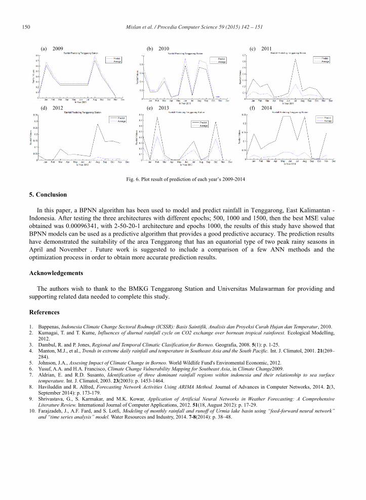
Fig. 4. (a) Plot result of prediction, (b) Regression, and (c) Performance Table 5, the 2009-2014 predicted results have revealed that there would be heavy rainfall in September 2009,

July 2010, August 2011, September 2012, March 2013 and June-July 2014 respectively with 566, 670, 450, 87, 634 and 65. However, the highest rainfall prediction results would occur in July 2010 of 0.775. Meanwhile, the average rainfall was high in 2009, 2010, 2011, 2012, 2013 and 2014 respectively with 258, 299, 125, 26, 179 and 33. It can be said there would often rain around Tenggarong area in 2009, Fig. 5. These test results are in accordance with the nature of the rainfall in the Mahakam river basin which has an equatorial type of two peak rainy seasons in April and November the detail plot prediction of each year as shown in Fig 6.

Table 5. Rainfall prediction value 2009-2014.

Years / Months Jan Feb Mar Apr May Jun Jul Aug Sep Oct Nov Dec Min Max Mean

2009 97 489 318 210 210 210 210 210 566 336 192 48 48 566 258 2010 535 167 178 373 70 109 670 105 637 595 69 79 69 670 299 2011 53 226 138 170 22 35 69 450 90 134 109 4 4 450 125 2012 12 2 1 27 14 15 12 10 87 45 47 42 1 87 26 2013 361 9 634 72 2 6 149 280 2 61 568 4 2 634 179 2014 9 40 17 25 29 65 65 30 65 4 3 40 3 65 33

Fig. 5. Plot result of prediction with [2-5-20-1], epoch 1.000

150 Mislan et al. / Procedia Computer Science 59 ( 2015 ) 142 – 151

(a) 2009

(b) 2010

(c) 2011

(d) 2012

(e) 2013

(f) 2014

Fig. 6. Plot result of prediction of each year’s 2009-2014

5. Conclusion

In this paper, a BPNN algorithm has been used to model and predict rainfall in Tenggarong, East Kalimantan - Indonesia. After testing the three architectures with different epochs; 500, 1000 and 1500, then the best MSE value obtained was 0.00096341, with 2-50-20-1 architecture and epochs 1000, the results of this study have showed that BPNN models can be used as a predictive algorithm that provides a good predictive accuracy. The prediction results have demonstrated the suitability of the area Tenggarong that has an equatorial type of two peak rainy seasons in April and November . Future work is suggested to include a comparison of a few ANN methods and the optimization process in order to obtain more accurate prediction results.

Acknowledgements

The authors wish to thank to the BMKG Tenggarong Station and Universitas Mulawarman for providing and supporting related data needed to complete this study.

References

1. Bappenas, Indonesia Climate Change Sectoral Rodmap (ICSSR): Basis Saintifik, Analisis dan Proyeksi Curah Hujan dan Temperatur, 2010. 2. Kumagai, T. and T. Kume, Influences of diurnal rainfall cycle on CO2 exchange over bornean tropical rainforest. Ecological Modelling,

2012. 3. Dambul, R. and P. Jones, Regional and Temporal Climatic Clasification for Borneo. Geografia, 2008. 5(1): p. 1-25. 4. Manton, M.J., et al., Trends in extreme daily rainfall and temperature in Southeast Asia and the South Pacific. Int. J. Climatol, 2001. 21(269–

284). 5. Johnson, J.A., Assesing Impact of Climate Change in Borneo. World Wildlife Fund's Enviromental Economic, 2012. 6. Yusuf, A.A. and H.A. Francisco, Climate Change Vulnerability Mapping for Southeast Asia, in Climate Change2009. 7. Aldrian, E. and R.D. Susanto, Identification of three dominant rainfall regions within indonesia and their relationship to sea surface

temperature. Int. J. Climatol, 2003. 23(2003): p. 1453-1464. 8. Haviluddin and R. Alfred, Forecasting Network Activities Using ARIMA Method. Journal of Advances in Computer Networks, 2014. 2(3,

September 2014): p. 173-179. 9. Shrivastava, G., S. Karmakar, and M.K. Kowar, Application of Artificial Neural Networks in Weather Forecasting: A Comprehensive

Literature Review. International Journal of Computer Applications, 2012. 51(18, August 2012): p. 17-29. 10. Farajzadeh, J., A.F. Fard, and S. Lotfi, Modeling of monthly rainfall and runoff of Urmia lake basin using “feed-forward neural network”

and “time series analysis” model. Water Resources and Industry, 2014. 7-8(2014): p. 38–48.

151 Mislan et al. / Procedia Computer Science 59 ( 2015 ) 142 – 151

11. Abhishek, K., et al., A Rainfall Prediction Model using Artificial Neural Network. 2012 IEEE Control and System Graduate Research Colloquium (ICSGRC 2012), 2012.

12. Charaniya, N.A. and S.V. Dudul, Design of Neural Network Models for Daily Rainfall Prediction. International Journal of Computer Applications, 2013. 61(14, January 2013): p. 23-26.

13. Wu, J., J. Long, and M. Liu, Evolving RBF neural networks for rainfall prediction using hybrid particle swarm optimization and genetic algorithm. Neurocomputing, 2015. 148(2015): p. 136–142.

14. Basheer, I.A. and M. Hajmeer, Artificial neural networks: fundamentals, computing, design, and application. Journal of Microbiological Methods, 2000. 43(2000): p. 3-31.

15. Sermpinis, G., et al., Forecasting and trading the EUR/USD exchange rate with stochastic Neural Network combination and time-varying leverage. Decision Support Systems, 2012. 54(2012): p. 316–329.

16. Haviluddin and R. Alfred, Daily Network Traffic Prediction Based on Backpropagation Neural Network. Australian Journal of Basic and Applied Sciences, 2014. 8(24)(Special 2014): p. 164-169.

17. Chen, G., et al., The genetic algorithm based back propagation neural network for MMP prediction in CO2-EOR process. Fuel, 2014. 126(2014): p. 202–212.