Rrs

LD

a

A

R

R

6

A

P

K

H

M

I

K

A

E

1

Ta

I

0d

e c o l o g i c a l m o d e l l i n g 2 0 2 ( 2 0 0 7 ) 333–344

avai lab le at www.sc iencedi rec t .com

journa l homepage: www.e lsev ier .com/ locate /eco lmodel

adio-tracking squirrels: Performance of homeange density and linkage estimators withmall range and sample size

uc A. Wauters, Damiano G. Preatoni ∗, Ambrogio Molinari, Guido Tosiepartment of Environment, Health and Safety, University of Insubria, Varese, Via J.H. Dunant 3, I-21100 Varese, Italy

r t i c l e i n f o

rticle history:

eceived 21 November 2005

eceived in revised form

October 2006

ccepted 2 November 2006

ublished on line 11 December 2006

eywords:

ome range estimator reliability

inimum convex polygons

ncremental cluster-analysis

ernel density estimators

djusted smoothing factor

urasian red squirrel

a b s t r a c t

Studies that use radio-tracking to reveal social structure and habitat use in populations

of small and medium-sized mammals face a trade-off between number of location data (n)

and monitoring of many individuals, to maximize efficiency. We simulated these conditions

using location data from 30 radio-collared red squirrels, subsampled at different percent-

ages of total number of locations and tested the performance of four home range estimators.

Two linkage estimators, the minimum convex polygon (MCP), and the incremental cluster-

analysis polygon (ICP) and two probability density estimators, the fixed kernel density

estimation with reference smoothing factor (KDE with href), and with least squares cross-

validation to calculate smoothing factor (KDE LSCV with hlscv). KDE produced the largest

home range estimates, MCP and KDE LSCV intermediate estimates, and ICP the smallest

ones. Differences between estimators were larger at smaller n, but consistent throughout

the entire range of locations (16–74) in our data set. Although KDE is widely used and LSCV is

widely recommended to calculate bandwidth, our results confirmed that the value of h has

a considerable influence on the home range estimate and varied more strongly when sam-

ple size (n) decreased. Our models showed that overestimation with KDE could be avoided

by applying the average ratio of hlscv/href (in our case 0.75) as a multiplier of href and use

this recalculated bandwidth to produce more reliable home range and core area estimates

(KDEadj). MCP and KDE had lower variability than KDE LSCV and ICP. Stability improved with

sample size and tended towards an asymptote at more than 60 locations for MCP and KDE.

We conclude that high variation in ICP and KDE LSCV at small n limits their applicability

to few situations (n > 70, landscapes with distinct habitat patches where ranges consists of

several, separated cores). We recommend use of both MCP and KDEadj for home range size

and KDEadj for core area size and propose to estimate a ‘best core area’ based on 85% MCP

when a home range is mononuclear and 85% ICP when it is multinuclear.

increasing. In particular, research focuses on space use (posi-

. Introduction

he use of radio-telemetry in research on vertebrates to studyvariety of fundamental ecological processes is continuously

∗ Corresponding author. Present address: Dipartimento Ambiente-Salu-21100 Varese (VA), Italy. Tel.: +39 0332 421 538; fax: +39 0332 421446.

E-mail address: prea@uninsubria.it (D.G. Preatoni).304-3800/$ – see front matter © 2006 Elsevier B.V. All rights reserved.oi:10.1016/j.ecolmodel.2006.11.001

© 2006 Elsevier B.V. All rights reserved.

te-Sicurezza, Universita dell’ Insubria, Varese, Via J.H. Dunant 3,

tion, size and utilization of home ranges, e.g. Wauters et al.,2005), dispersal behaviour and distances (Larsen and Boutin,1994; Byrom and Krebs, 1999), movements in or along contrast-

i n g

track Ltd., Wareham, Dorset, UK) and a hand-held GPS (Garmin

334 e c o l o g i c a l m o d e l l

ing habitats (in landscape fragmentation studies, e.g. Selonenand Hanski, 2003; Desrochers et al., 2003) and habitat use andselection (Aebischer et al., 1993; Leban et al., 2001). Concomi-tantly with improved radio-telemetry techniques, increasinglysophisticated methods to estimate home ranges have beendeveloped. One of the most widely used is the kernel den-sity estimation (KDE). KDE creates contours of intensity ofutilization (isopleths) by calculating the mean influence ofdata points at grid intersections (Worton, 1989). Each isoplethcontains a fixed percentage of the utilization density, that cor-responds with the amount of time the animal spends in thearea comprised by that contour (Hemson et al., 2005). AlthoughKDE has been widely considered as the most reliable con-touring method applied in ecological studies (Powell, 2000;Kernohan et al., 2001), it is very sensitive to the smoothing fac-tor, h, the distance over which a data point influences the gridintersections (Worton, 1989; Kernohan et al., 2001; Hemson etal., 2005). Large values of h produce larger and less detailedhome range estimates, while small values of h undersmooththe outer density isopleths (100%, 95% contours) and may cre-ate discontinuous islands of utilization, but reveal more ofthe internal structure (intensively used core areas, Silverman,1986; Worton, 1989). The two preferred methods of calculatingh in KDE are the reference smoothing factor (href) and the least-squares cross-validation (LSCV): choice of method affects thevalue of h and thus the estimated shape and size of the homerange (Worton, 1989; Seaman and Powell, 1996; Hemson et al.,2005).

In a recent paper, Hemson et al. (2005) critically analysethe accuracy of KDE home range estimates using least-squarescross-validation (LSCV). Using subsamples, drawn at differenttime-intervals, of real data from four global positioning sys-tem (GPS)-collared lions Panthera leo, they showed that LSCVproduced variable results and a 7% failure rate for home rangeestimates using fewer than 100 locations, and even a 61% fail-ure rate when more than 100 locations were used (Hemson etal., 2005). Their findings were in contrast with previous stud-ies that recommended LSCV as the best available method tocalculate h, while concluding that href oversmoothes, henceoverestimates home range size (Worton, 1989; Seaman andPowell, 1996; Powell, 2000). However, in contrast with theapproach by Hemson et al. (2005), these tests have been basedon computer simulation of animal locations and not on fielddata. Based on their own work and on similar simulationsusing real GPS data from moose Alces alces (Girard et al., 2002),Hemson et al. (2005) conclude that variation at small samplesizes and failure at large sample sizes of LSCV – related to bio-logically relevant patterns of space use, such as intensive useof core areas and territorial behaviour – limits the applicabilityof KDE based on LSCV and casts doubt on the reliability andcomparability of the method as a home range estimator.

However, the use of GPS-collars, thus the availability oflarge amounts of location data gathered at fixed time-intervalsover long periods, is still limited to large mammals and birds,and to marine animals such as sea-turtles and fish (e.g. Merrillet al., 1998; Galanti et al., 2000; Le Boeuf et al., 2000; Block

et al., 2001; Rodgers, 2001; Girard et al., 2002; Hemson etal., 2005; Jonsen et al., 2006). The majority of radio-trackingstudies on small to medium-sized mammals typically collectsmall amounts of fixes (<50) per animal, but often monitor

2 0 2 ( 2 0 0 7 ) 333–344

a much larger number of individuals than with (expensive)GPS-collars. These studies rely on location estimates derivedfrom triangulation or homing-in to the radio-signal and subse-quent mapping of locations using a handheld GPS or detailedmaps of the study-area, rather than on satellite-based GPSpositions (e.g. White and Garrott, 1990; Wauters and Dhondt,1992; Garton et al., 2001; Wauters et al., 2005). Moreover, inher-ent to most studies that use radio-tracking for studying spaceand habitat use of individuals in one or more populations, arethe constraints related to sample size, both in terms of numberof radio-tagged animals and number of locations per animal(Kenward, 1987; White and Garrott, 1990; Kernohan et al.,2001). In the latter case, attention must be paid to determinethe appropriate sampling interval (time between consecutivefixes) to avoid, or reduce, autocorrelation in location data (e.g.Swihart and Slade, 1985).

Here, we extended on the tests presented by Hemson etal. (2005) using location data from a small mammal species,the red squirrel Sciurus vulgaris, on a scale very different fromthat of large carnivores or herbivores. This species has a spac-ing pattern that is similar to many small and medium-sizedmammals (Wauters and Dhondt, 1992). Red squirrels typicallyhave partly overlapping, food-based home ranges of relativelysmall size, but home range size, and the size of core areas,can vary greatly among habitats (2–5 ha in high-quality mixedbroadleaf-conifer woodlands, 20–35 ha in subalpine coniferforests) and between years (10–30 ha in years following a richtree seed–crop, 80–110 ha the year following seed–crop fail-ure) (Wauters and Dhondt, 1992; Lurz et al., 2000; Wauters etal., 2001, 2005). Hence, compared to lions or moose, squirrelshave small home ranges and range estimates are calculatedusing relatively few locations, allowing us to explore effectsof scale (animal size, home range size) and sampling inten-sity on home range size and stability in more detail. We alsoextend tests to two other home range estimators: incrementalhierarchical cluster analysis using the cumulative utiliza-tion distribution (ICP), and minimum convex polygons withmononuclear core area (MCP, Kenward, 1987; Kenward andHodder, 1996).

2. Methods

2.1. Home range data

Between May 2002 and October 2004, we trapped and radio-collared 30 red squirrels with adjustable necklace transmitters(PD-2C transmitters, Holohil Systems Ltd., Carp, Ontario,Canada or TW-4 transmitters, Biotrack Ltd., Wareham, Dorset,UK) in two mixed montane conifer forests (Cedrasco, n = 19squirrels, Oga, n = 11 squirrels) in the Lombardy Alps, N. Italy(Wauters et al., 2004; Trizio et al., 2005). We estimated loca-tions (hereinafter called fixes) to the nearest 10 m × 10 m byhoming-in to the radio-signal (Wauters and Dhondt, 1992;Wauters et al., 2001) using a Telonics TR-4 receiver with adirectional three-element Yagi antenna (150–152 MHz, Bio-

GPS-II plus). We monitored all squirrels for 5–6 months(May–October) taking one or two fixes per day (one duringmorning activity bout, the second in the afternoon when

g 2 0 2 ( 2 0 0 7 ) 333–344 335

t1tataoeshgeuna

ttsrupchsuno2twareHf

a(nwtsbadofi1umdu

2

Fiut

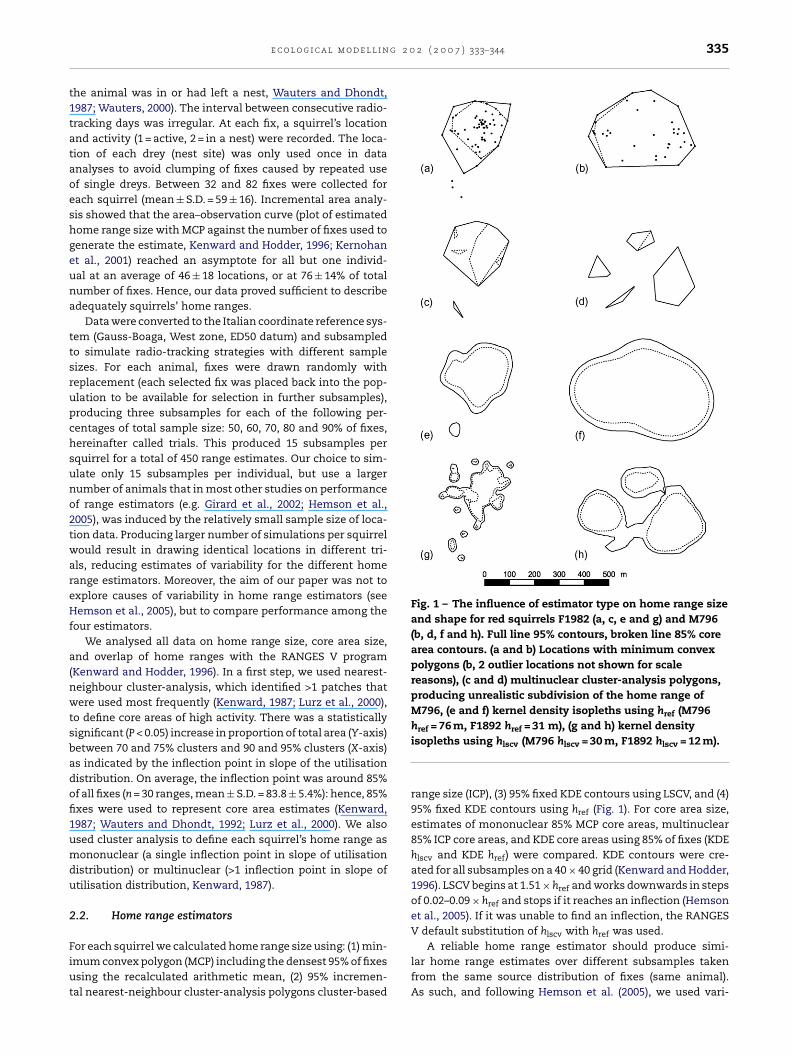
Fig. 1 – The influence of estimator type on home range sizeand shape for red squirrels F1982 (a, c, e and g) and M796(b, d, f and h). Full line 95% contours, broken line 85% corearea contours. (a and b) Locations with minimum convexpolygons (b, 2 outlier locations not shown for scalereasons), (c and d) multinuclear cluster-analysis polygons,producing unrealistic subdivision of the home range ofM796, (e and f) kernel density isopleths using href (M796

e c o l o g i c a l m o d e l l i n

he animal was in or had left a nest, Wauters and Dhondt,987; Wauters, 2000). The interval between consecutive radio-racking days was irregular. At each fix, a squirrel’s locationnd activity (1 = active, 2 = in a nest) were recorded. The loca-ion of each drey (nest site) was only used once in datanalyses to avoid clumping of fixes caused by repeated usef single dreys. Between 32 and 82 fixes were collected forach squirrel (mean ± S.D. = 59 ± 16). Incremental area analy-is showed that the area–observation curve (plot of estimatedome range size with MCP against the number of fixes used toenerate the estimate, Kenward and Hodder, 1996; Kernohant al., 2001) reached an asymptote for all but one individ-al at an average of 46 ± 18 locations, or at 76 ± 14% of totalumber of fixes. Hence, our data proved sufficient to describedequately squirrels’ home ranges.

Data were converted to the Italian coordinate reference sys-em (Gauss-Boaga, West zone, ED50 datum) and subsampledo simulate radio-tracking strategies with different sampleizes. For each animal, fixes were drawn randomly witheplacement (each selected fix was placed back into the pop-lation to be available for selection in further subsamples),roducing three subsamples for each of the following per-entages of total sample size: 50, 60, 70, 80 and 90% of fixes,ereinafter called trials. This produced 15 subsamples perquirrel for a total of 450 range estimates. Our choice to sim-late only 15 subsamples per individual, but use a largerumber of animals that in most other studies on performancef range estimators (e.g. Girard et al., 2002; Hemson et al.,005), was induced by the relatively small sample size of loca-ion data. Producing larger number of simulations per squirrelould result in drawing identical locations in different tri-ls, reducing estimates of variability for the different homeange estimators. Moreover, the aim of our paper was not toxplore causes of variability in home range estimators (seeemson et al., 2005), but to compare performance among the

our estimators.We analysed all data on home range size, core area size,

nd overlap of home ranges with the RANGES V programKenward and Hodder, 1996). In a first step, we used nearest-eighbour cluster-analysis, which identified >1 patches thatere used most frequently (Kenward, 1987; Lurz et al., 2000),

o define core areas of high activity. There was a statisticallyignificant (P < 0.05) increase in proportion of total area (Y-axis)etween 70 and 75% clusters and 90 and 95% clusters (X-axis)s indicated by the inflection point in slope of the utilisationistribution. On average, the inflection point was around 85%f all fixes (n = 30 ranges, mean ± S.D. = 83.8 ± 5.4%): hence, 85%xes were used to represent core area estimates (Kenward,987; Wauters and Dhondt, 1992; Lurz et al., 2000). We alsosed cluster analysis to define each squirrel’s home range asononuclear (a single inflection point in slope of utilisation

istribution) or multinuclear (>1 inflection point in slope oftilisation distribution, Kenward, 1987).

.2. Home range estimators

or each squirrel we calculated home range size using: (1) min-mum convex polygon (MCP) including the densest 95% of fixessing the recalculated arithmetic mean, (2) 95% incremen-al nearest-neighbour cluster-analysis polygons cluster-based

href = 76 m, F1892 href = 31 m), (g and h) kernel densityisopleths using hlscv (M796 hlscv = 30 m, F1892 hlscv = 12 m).

range size (ICP), (3) 95% fixed KDE contours using LSCV, and (4)95% fixed KDE contours using href (Fig. 1). For core area size,estimates of mononuclear 85% MCP core areas, multinuclear85% ICP core areas, and KDE core areas using 85% of fixes (KDEhlscv and KDE href) were compared. KDE contours were cre-ated for all subsamples on a 40 × 40 grid (Kenward and Hodder,1996). LSCV begins at 1.51 × href and works downwards in stepsof 0.02–0.09 × href and stops if it reaches an inflection (Hemsonet al., 2005). If it was unable to find an inflection, the RANGESV default substitution of hlscv with href was used.

A reliable home range estimator should produce simi-lar home range estimates over different subsamples takenfrom the same source distribution of fixes (same animal).As such, and following Hemson et al. (2005), we used vari-

336 e c o l o g i c a l m o d e l l i n g 2 0 2 ( 2 0 0 7 ) 333–344

Table 1 – Descriptive statistics of the home range (95% contours) and core area (85% contours) estimators

Parameter MCP ICP KDE KDE LSCV

Home range size (ha) mean ± S.D.(min–max)

7.24 ± 5.76 (0.80–28.71) 5.54 ± 5.01 (0.80–26.15) 10.49 ± 9.10 (1.39–43.15) 7.17 ± 5.41 (0.97–27.62)

Core area size (ha) mean ± S.D.(min–max)

4.70 ± 3.24 (0.39–15.37) 2.67 ± 2.26 (0.35–12.27) 6.72 ± 5.47 (0.72–26.74) 4.94 ± 3.64 (0.66–18.01)

Coefficient of variation (%CV)home ranges

11.0 ± 8.4 (0.3–49.4) 22.4 ± 18.9 (0.1–106) 12.8 ± 10.7 (0.6–74.5) 20.0 ± 17.4 (0.7–102)

Coefficient of variation (%CV) coreareas

12.2 ± 9.2 (0.3–43.7) 27.9 ± 19.8 (0.1–93.8) 14.0 ± 10 (0.2–62.2) 18.6 ± 15.8 (0.6–89.5)

Correlation coefficients, rn, home range size −0.10 NS −0.01 NS −0.13 NS −0.09 NSn, core area size −0.09 NS −0.02 NS −0.14 NS −0.11 NSn, %CV home ranges −0.42** −0.56** −0.40** −0.38**n, %CV core areas −0.46** −0.42** −0.46** −0.36**

Means and %CV are from three subsamples per trial (n = 5 trials) for all squirrels (n = 30, total sample size n = 150). Over all subsamples, the. = 42 ±.05), *

number of fixes (sample size) varied between 16 and 74 (mean ± S.Dfixes) and the various range-size estimators; NS, not significant (P > 0

ation (expressed as %CV) of home range estimates amongsubsamples as an index of home range estimator perfor-mance. We assessed stability of home range estimates withoverlap analysis in RANGES V (Kenward and Hodder, 1996).The percentage of overlap of each range among subsampleswith the same percentage of fixes was calculated. If all homerange estimates were identical, all values would be 100%: themean and standard deviation of values (% overlap) per ani-mal and sample-size combination were used as indices forstability.

2.3. Statistical analysis

We used linear mixed models to investigate the effects ofsample size (number of fixes), type of home range estima-tor (MCP, ICP, KDE and KDE LSCV) and the type by samplesize interaction on: (1) variation in home range size, (2)variation in core area size, (3) coefficients of variation (perfor-mance) of home range estimators, (4) coefficient of variationof core area estimators, and (5) arcsine transformed valuesof proportion home range overlap. Because multiple range-estimates of each individual squirrel were used in the varioustrials, this mixed model was adjusted for repeated mea-sures of individual in subsample (SAS PROC MIXED, Verbekeand Molenberghs, 2000). Compound symmetry gave the bestfit (Schwarz’s Bayesian Information Criterion, smallest BICvalue) for the correlation structure of the residual correlationmatrix. Degrees of freedom and standard errors of F-and t-tests were obtained using Kenward–Rogers method (Verbekeand Molenberghs, 2000). Interpretation of pairwise differencesbetween estimators were based on least squares means. Withhome range size or core area size as dependent variable, a sig-nificant type effect indicated that the various estimators gavedifferent results for range size, a significant effect of samplesize indicated that range size changed with sample size, and

a significant interaction that the range size–sample size rela-tionship differed among estimators. With %CV as dependentvariable, a significant type effect indicated that performancediffered among estimators, an effect of sample size that per-

14). Pearson’s r for correlations between sample size (n, number ofP < 0.01, **P < 0.001 (for r = 0.31, P = 0.0001).

formance changed with number of fixes, while a significantinteraction suggested that the sample size–performance rela-tionship differed among estimators.

All tests of significance are two-tailed and the significancelevel was set at 0.05. Unless otherwise indicated values arepresented in the text as mean ± S.D.

3. Results

Variation in home range size among individuals was large(Table 1) due to biological variation in space use between thesexes, among years and habitats. The largest ranges wereabout 30 times bigger than the smallest. This allowed us to testthe robustness of the different home range estimators over awide size-range. Sample size was not significantly correlatedwith any of the estimators of home range and core area size(Table 1, Fig. 2a and b). In contrast, the coefficient of varia-tion of each estimator was reduced with increasing samplesize (Table 1, Fig. 3a and b). Home range and core area size-values calculated with the different estimators were stronglycorrelated (n = 150, r between 0.81 and 0.97, all P < 0.0001). Alsopercentage variation in the different home range and core areaestimators over the three subsamples were significantly cor-related. The poorest agreement was between MCP and KDELSCV methods (r = 0.20, P = 0.014), the best between MCP andKDE (r = 0.63, P < 0.0001).

3.1. Effects of smoothing factor and sample size onKernel density estimators

For kernel home range estimators, the average value ofthe smoothing factor href was 51 ± 25 m (range 17–131 m),and mean variation (%CV) within individuals and trials was7.1 ± 6.9% (range 0–40%). When using LSCV the smoothing fac-tor decreased (h mean ± S.D. = 36 ± 15 m, range 11–81 m).

lscv

On average hlscv was 0.75 ± 0.24 times href (range 0.22–1.30)and pair-wise differences were highly significant (href − hlscv,paired t-test t148 = 11.0, P < 0.0001). Variation (%CV) within indi-viduals and trials was significantly higher than with href (hlscv

e c o l o g i c a l m o d e l l i n g 2 0 2 ( 2 0 0 7 ) 333–344 337

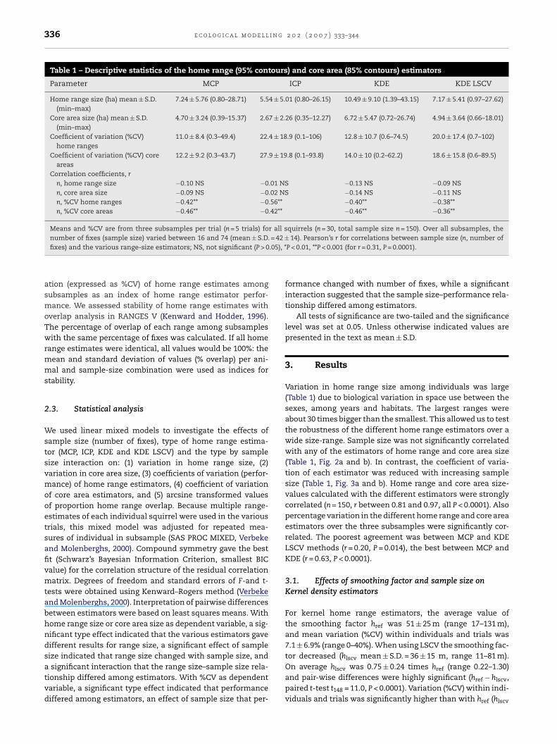
Fig. 2 – Mean values per trial of (a) home range size and (b) core area size of individual red squirrels (n = 150 trials), producedby each of the four estimators, against sample size. (c and d) Trend lines of linear regressions of home range and core areasize on sample size shown separately: Home ranges, MCP = 8.98–0.04×; ICP = 5.69–0.004×; KDE = 14.09–0.09×; KDELSCV = 8.53–0.03×; core areas, 85%MCP = 5.57–0.02×; 85%ICP = 2.83–0.004×; 85%KDE = 9.05–0.06×; 85%KDEL

1rscs

tnPtPevmf

fiAwhwoiP

SCV = 6.07–0.03×. All R2 between <0.001 and 0.02.

8.2 ± 14.6, range 1–85%, difference href − hlscv = −11.2 ± 15.3%,ange from −78 to +24%, paired t-test t148 = −8.95, P < 0.0001). Inome cases, KDE LSCV produced biologically unrealistic rangeontours: this was the case when values of hlscv were verymall and difference with href large (see Fig. 1g, for example).

Both average href over trials and its coefficient of varia-ion decreased with increasing sample size (correlation withumber of fixes, href r = −0.27, P = 0.0009, %CV href r = −0.40,< 0.0001). There was no relation between values of href and

heir coefficient of variation among subsamples (r = −0.02,= 0.83). The value of href has a significant influence onstimated range size by KDE (r = 0.87, P < 0.0001) and higherariation in href produced more variation among KDE esti-ates (CV KDE − CV href r = 0.67, P < 0.0001). This was also true

or core areas.In only 2 out of 450 range estimates (0.4%), LSCV failed to

nd an appropriate value of h and hlscv was replaced with href.lso the value of hlscv and its coefficient of variation decreasedith increasing sample size (correlation with number of fixes,

= −0.27, P = 0.0008, %CV h r = −0.21, P = 0.008). There

lscv lscv

as no relation between values of hlscv and their coefficientf variation (r = −0.02, P = 0.77). The value of hlscv has a signif-

cant influence on estimated range size by KDE LSCV (r = 0.81,< 0.0001) and higher variation in hlscv produced more vari-

ation among KDE LSCV estimates (CV KDE LSCV − CV hlscv

r = 0.81, P < 0.0001). This was also true for core areas.

3.2. Estimator type and range size

KDE produced consistently larger home ranges than MCPand KDE LSCV that produced similar sizes (Table 2). Homerange size with ICP was significantly smaller than withall other estimators (Table 2). For 85% core area size, dif-ferences between estimators were similar. The effect ofsample size on home range size also differed among estima-tors (Table 2). Home range size changed less with numberof fixes for ICP than for MCP and KDE LSCV (differencesbetween slopes ± S.E., ICP-MCP = 0.04 ± 0.01, P = 0.003, ICP-KDE LSCV = 0.03 ± 0.02, P = 0.06, MCP-KDE LSCV = −0.01 ± 0.01,P = 0.50), while KDE home ranges decreased most stronglywith number of fixes (Fig. 2c, all P < 0.05). For core areas, rela-tionships between number of fixes and core area size didnot differ significantly for MCP and ICP (differences betweenslopes ± S.E. = 0.02 ± 0.01, P = 0.06) and for MCP and KDE LSCV

(0.01 ± 0.01, P = 0.49, Fig. 2d).

Classification of home ranges as mono- or multinuclearchanged with method. Using the incremental utilisation dis-tribution in cluster-analysis, 19 squirrels had mononuclear

338 e c o l o g i c a l m o d e l l i n g 2 0 2 ( 2 0 0 7 ) 333–344

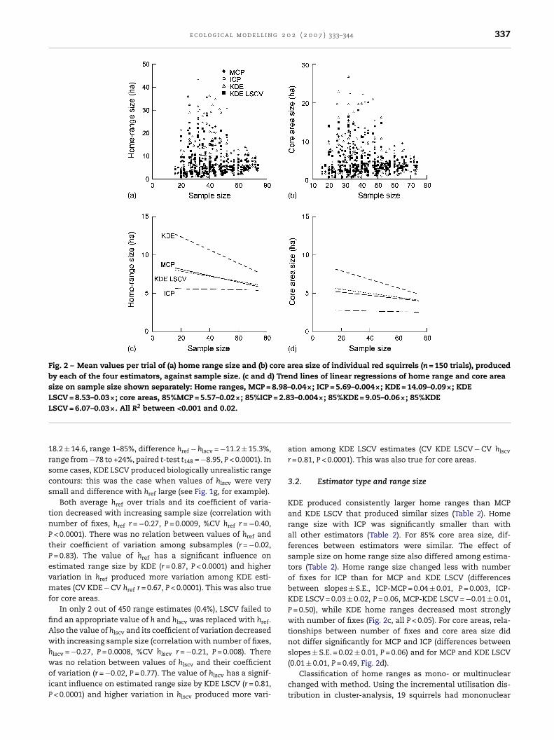
Fig. 3 – Plots of coefficient of variation in (a) home range and (b) core area against sample size, for each of the fourestimators. (c and d) Trend lines of logaritmic regression models of %CV in home range and core area against sample size.Home ranges: Ln MCP = 3.21–0.026×, R2 = 0.19, Ln ICP = 3.21–0.026×, R2 = 0.31, Ln KDE = 3.31–0.027×, R2 = 0.17, Ln KDE

.029

.023

LSCV = 3.79–0.027×, R2 = 0.20, core areas: Ln 85%MCP = 3.40–0Ln 85%KDE = 3.40–0.025×, R2 = 0.19, Ln 85%KDE LSCV = 3.55–0

and 11 multinuclear ranges. With ICP, only three out of 30red squirrels (10%) had mononuclear 85% core areas, against24 (80%) with KDE and 16 (53%) with KDE LSCV. Also averagenumber of nuclei within the 85% core area differed among

Table 2 – Generalised mixed models testing effects of estimatoron home range and core area size, and on coefficient of variatioindex of performance

Model parameters Home range size Core a

Estimator type F3, 563 = 29.8; P < 0.0001 F3, 563 = 34.6Sample size F1, 576 = 7.75; P = 0.006 F1, 576 = 5.04Type* sample size F3, 563 = 5.54; P = 0.0009 F3, 563 = 4.84R2 GLM-model 0.08 0.14%Variance among individuals

with repeated measures 85% �2 = 982.2; P < 0.0001 81% �2 = 82

Estimate ± S.E. Estimate

Slope sample size (b) 0.04 ± 0.02* 0.02 ± 0MCP-ICPa 3.29 ± 0.55*** 2.74 ± 0MCP-KDEa −5.12 ± 0.82*** −3.48 ± 0MCP-KDE LSCVa 0.44 ± 0.58 NS −0.50 ± 0ICP-KDEa −8.41 ± 1.06*** −6.22 ± 0ICP-KDE LSCVa −2.85 ± 0.68*** −3.24 ± 0KDE-KDE LSCVa 5.56 ± 0.98*** 2.98 ± 0

a Significance of differences of least squares means (LSMD) was tested by t

×, R2 = 0.21, Ln 85%ICP = 4.03–0.024×, R2 = 0.15,×, R2 = 0.14.

estimators (mean ± S.D., ICP 3.3 ± 1.4, range 1–6, KDE 1.2 ± 0.5,range 1–3, KDE LSCV 2.5 ± 2.9, range 1–12). Considering the for-mation of many small cores (>5) around single locations orgroups of 2–3 locations as biologically unrealistic, least square

type, sample size (number of fixes) and their interactionn (%CV) of home range and core area estimates as an

rea size %CV home ranges %CV core areas

; P < 0.0001 F3, 563 = 21.7; P < 0.0001 F3, 561 = 14.9; P < 0.0001; P = 0.025 F1, 198 = 99.9; P < 0.0001 F1, 213 = 96.8; P < 0.0001; P = 0.003 F3, 563 = 9.78; P < 0.0001 F3, 561 = 3.05; P = 0.028

0.30 0.30

5.2; P < 0.0001 8% �2 = 20.4; P < 0.0001 10% �2 = 23.9; P < 0.0001

± S.E. Estimate ± S.E. Estimate ± S.E.

.01 NS −0.49 ± 0.08*** −0.47 ± 0.08***

.40*** −32.09 ± 4.30*** −27.60 ± 4.79***

.59*** −4.07 ± 2.83 NS −3.38 ± 2.76 NS

.40 NS −18.27 ± 4.17*** −10.63 ± 4.01 **

.75*** 28.02 ± 4.53*** 24.23 ± 5.03***

.40*** 13.82 ± 5.39 ** 16.98 ± 5.24**

.56*** −14.20 ± 4.48** −7.25 ± 4.13 NS

-test with d.f. = 267; NS, not significant, *P < 0.05, **P < 0.01, ***P < 0.001.

g 2 0 2 ( 2 0 0 7 ) 333–344 339

cwttuK

3

FaarMngmfinaeifienPwtrKa

3

Ohe(s(InItP(Mtr(tPK1

adbo

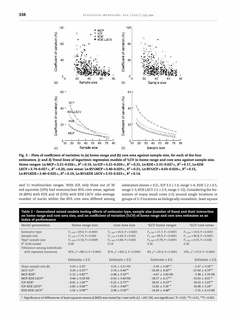
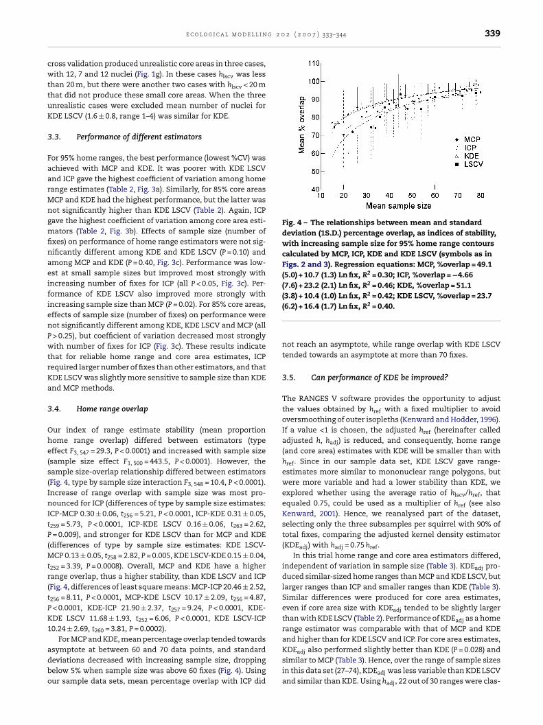
Fig. 4 – The relationships between mean and standarddeviation (1S.D.) percentage overlap, as indices of stability,with increasing sample size for 95% home range contourscalculated by MCP, ICP, KDE and KDE LSCV (symbols as inFigs. 2 and 3). Regression equations: MCP, %overlap = 49.1(5.0) + 10.7 (1.3) Ln fix, R2 = 0.30; ICP, %overlap = −4.66(7.6) + 23.2 (2.1) Ln fix, R2 = 0.46; KDE, %overlap = 51.1(3.8) + 10.4 (1.0) Ln fix, R2 = 0.42; KDE LSCV, %overlap = 23.7

e c o l o g i c a l m o d e l l i n

ross validation produced unrealistic core areas in three cases,ith 12, 7 and 12 nuclei (Fig. 1g). In these cases hlscv was less

han 20 m, but there were another two cases with hlscv < 20 mhat did not produce these small core areas. When the threenrealistic cases were excluded mean number of nuclei forDE LSCV (1.6 ± 0.8, range 1–4) was similar for KDE.

.3. Performance of different estimators

or 95% home ranges, the best performance (lowest %CV) waschieved with MCP and KDE. It was poorer with KDE LSCVnd ICP gave the highest coefficient of variation among homeange estimates (Table 2, Fig. 3a). Similarly, for 85% core areasCP and KDE had the highest performance, but the latter wasot significantly higher than KDE LSCV (Table 2). Again, ICPave the highest coefficient of variation among core area esti-ators (Table 2, Fig. 3b). Effects of sample size (number of

xes) on performance of home range estimators were not sig-ificantly different among KDE and KDE LSCV (P = 0.10) andmong MCP and KDE (P = 0.40, Fig. 3c). Performance was low-st at small sample sizes but improved most strongly withncreasing number of fixes for ICP (all P < 0.05, Fig. 3c). Per-ormance of KDE LSCV also improved more strongly withncreasing sample size than MCP (P = 0.02). For 85% core areas,ffects of sample size (number of fixes) on performance wereot significantly different among KDE, KDE LSCV and MCP (all> 0.25), but coefficient of variation decreased most stronglyith number of fixes for ICP (Fig. 3c). These results indicate

hat for reliable home range and core area estimates, ICPequired larger number of fixes than other estimators, and thatDE LSCV was slightly more sensitive to sample size than KDEnd MCP methods.

.4. Home range overlap

ur index of range estimate stability (mean proportionome range overlap) differed between estimators (typeffect F3, 547 = 29.3, P < 0.0001) and increased with sample sizesample size effect F1, 500 = 443.5, P < 0.0001). However, theample size-overlap relationship differed between estimatorsFig. 4, type by sample size interaction F3, 548 = 10.4, P < 0.0001).ncrease of range overlap with sample size was most pro-ounced for ICP (differences of type by sample size estimates:

CP-MCP 0.30 ± 0.06, t256 = 5.21, P < 0.0001, ICP-KDE 0.31 ± 0.05,

259 = 5.73, P < 0.0001, ICP-KDE LSCV 0.16 ± 0.06, t263 = 2.62,= 0.009), and stronger for KDE LSCV than for MCP and KDE

differences of type by sample size estimates: KDE LSCV-CP 0.13 ± 0.05, t258 = 2.82, P = 0.005, KDE LSCV-KDE 0.15 ± 0.04,

252 = 3.39, P = 0.0008). Overall, MCP and KDE have a higherange overlap, thus a higher stability, than KDE LSCV and ICPFig. 4, differences of least square means: MCP-ICP 20.46 ± 2.52,

256 = 8.11, P < 0.0001, MCP-KDE LSCV 10.17 ± 2.09, t256 = 4.87,< 0.0001, KDE-ICP 21.90 ± 2.37, t257 = 9.24, P < 0.0001, KDE-DE LSCV 11.68 ± 1.93, t252 = 6.06, P < 0.0001, KDE LSCV-ICP0.24 ± 2.69, t260 = 3.81, P = 0.0002).

For MCP and KDE, mean percentage overlap tended towards

symptote at between 60 and 70 data points, and standardeviations decreased with increasing sample size, droppingelow 5% when sample size was above 60 fixes (Fig. 4). Usingur sample data sets, mean percentage overlap with ICP did

(6.2) + 16.4 (1.7) Ln fix, R2 = 0.40.

not reach an asymptote, while range overlap with KDE LSCVtended towards an asymptote at more than 70 fixes.

3.5. Can performance of KDE be improved?

The RANGES V software provides the opportunity to adjustthe values obtained by href with a fixed multiplier to avoidoversmoothing of outer isopleths (Kenward and Hodder, 1996).If a value <1 is chosen, the adjusted href (hereinafter calledadjusted h, hadj) is reduced, and consequently, home range(and core area) estimates with KDE will be smaller than withhref. Since in our sample data set, KDE LSCV gave range-estimates more similar to mononuclear range polygons, butwere more variable and had a lower stability than KDE, weexplored whether using the average ratio of hlscv/href, thatequaled 0.75, could be used as a multiplier of href (see alsoKenward, 2001). Hence, we reanalysed part of the dataset,selecting only the three subsamples per squirrel with 90% oftotal fixes, comparing the adjusted kernel density estimator(KDEadj) with hadj = 0.75 href.

In this trial home range and core area estimators differed,independent of variation in sample size (Table 3). KDEadj pro-duced similar-sized home ranges than MCP and KDE LSCV, butlarger ranges than ICP and smaller ranges than KDE (Table 3).Similar differences were produced for core area estimates,even if core area size with KDEadj tended to be slightly largerthan with KDE LSCV (Table 2). Performance of KDEadj as a homerange estimator was comparable with that of MCP and KDEand higher than for KDE LSCV and ICP. For core area estimates,

KDEadj also performed slightly better than KDE (P = 0.028) andsimilar to MCP (Table 3). Hence, over the range of sample sizesin this data set (27–74), KDEadj was less variable than KDE LSCVand similar than KDE. Using hadj, 22 out of 30 ranges were clas-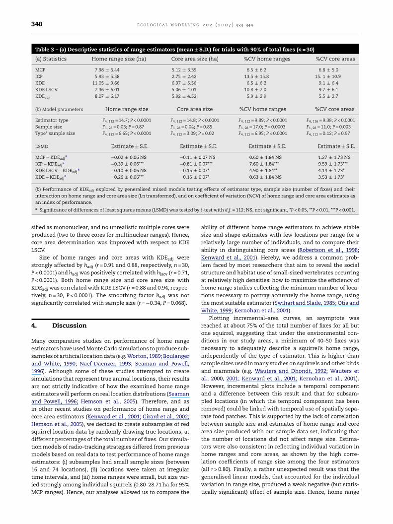

340 e c o l o g i c a l m o d e l l i n g 2 0 2 ( 2 0 0 7 ) 333–344

Table 3 – (a) Descriptive statistics of range estimators (mean ± S.D.) for trials with 90% of total fixes (n = 30)

(a) Statistics Home range size (ha) Core area size (ha) %CV home ranges %CV core areas

MCP 7.98 ± 6.44 5.12 ± 3.39 6.5 ± 6.2 6.8 ± 5.0ICP 5.93 ± 5.58 2.75 ± 2.42 13.5 ± 15.8 15. 1 ± 10.9KDE 11.05 ± 9.66 6.97 ± 5.56 6.5 ± 6.2 9.1 ± 6.4KDE LSCV 7.36 ± 6.01 5.06 ± 4.01 10.8 ± 7.0 9.7 ± 6.1KDEadj 8.07 ± 6.17 5.92 ± 4.52 5.9 ± 2.9 5.5 ± 2.7

(b) Model parameters Home range size Core area size %CV home ranges %CV core areas

Estimator type F4, 112 = 14.7; P < 0.0001 F4, 112 = 14.8; P < 0.0001 F4, 112 = 9.89; P < 0.0001 F4, 116 = 9.38; P < 0.0001Sample size F1, 28 = 0.03; P = 0.87 F1, 28 = 0.04; P = 0.85 F1, 28 = 17.0; P = 0.0003 F1, 28 = 11.0; P = 0.003Type* sample size F4, 112 = 6.65; P < 0.0001 F4, 112 = 3.09; P = 0.02 F4, 112 = 6.95; P < 0.0001 F4, 112 = 0.12; P = 0.97

LSMD Estimate ± S.E. Estimate ± S.E. Estimate ± S.E. Estimate ± S.E.

MCP − KDEadja −0.02 ± 0.06 NS −0.11 ± 0.07 NS 0.60 ± 1.84 NS 1.27 ± 1.73 NS

ICP − KDEadja −0.39 ± 0.06*** −0.81 ± 0.07*** 7.60 ± 1.84*** 9.59 ± 1.73***

KDE LSCV − KDEadja −0.10 ± 0.06 NS −0.15 ± 0.07* 4.90 ± 1.84** 4.14 ± 1.73*

KDE − KDEadja 0.26 ± 0.06*** 0.15 ± 0.07* 0.63 ± 1.84 NS 3.53 ± 1.73*

(b) Performance of KDEadj explored by generalised mixed models testing effects of estimator type, sample size (number of fixes) and theirn coe

d by t

interaction on home range and core area size (Ln transformed), and oan index of performance.a Significance of differences of least squares means (LSMD) was teste

sified as mononuclear, and no unrealistic multiple cores wereproduced (two to three cores for multinuclear ranges). Hence,core area determination was improved with respect to KDELSCV.

Size of home ranges and core areas with KDEadj werestrongly affected by hadj (r = 0.91 and 0.88, respectively, n = 30,P < 0.0001) and hadj was positively correlated with hlscv (r = 0.71,P < 0.0001). Both home range size and core area size withKDEadj was correlated with KDE LSCV (r = 0.88 and 0.94, respec-tively, n = 30, P < 0.0001). The smoothing factor hadj was notsignificantly correlated with sample size (r = −0.34, P = 0.068).

4. Discussion

Many comparative studies on performance of home rangeestimators have used Monte Carlo simulations to produce sub-samples of artificial location data (e.g. Worton, 1989; Boulangerand White, 1990; Naef-Daenzer, 1993; Seaman and Powell,1996). Although some of these studies attempted to createsimulations that represent true animal locations, their resultsare not strictly indicative of how the examined home rangeestimators will perform on real location distributions (Seamanand Powell, 1996; Hemson et al., 2005). Therefore, and asin other recent studies on performance of home range andcore area estimators (Kenward et al., 2001; Girard et al., 2002;Hemson et al., 2005), we decided to create subsamples of redsquirrel location data by randomly drawing true locations, atdifferent percentages of the total number of fixes. Our simula-tion models of radio-tracking strategies differed from previousmodels based on real data to test performance of home rangeestimators: (i) subsamples had small sample sizes (between

16 and 74 locations), (ii) locations were taken at irregulartime intervals, and (iii) home ranges were small, but size var-ied strongly among individual squirrels (0.80–28.71 ha for 95%MCP ranges). Hence, our analyses allowed us to compare the

fficient of variation (%CV) of home range and core area estimates as

-test with d.f. = 112; NS, not significant, *P < 0.05, **P < 0.01, ***P < 0.001.

ability of different home range estimators to achieve stablesize and shape estimates with few locations per range for arelatively large number of individuals, and to compare theirability in distinguishing core areas (Robertson et al., 1998;Kenward et al., 2001). Hereby, we address a common prob-lem faced by most researchers that aim to reveal the socialstructure and habitat use of small-sized vertebrates occurringat relatively high densities: how to maximize the efficiency ofhome range studies collecting the minimum number of loca-tions necessary to portray accurately the home range, usingthe most suitable estimator (Swihart and Slade, 1985; Otis andWhite, 1999; Kernohan et al., 2001).

Plotting incremental–area curves, an asymptote wasreached at about 75% of the total number of fixes for all butone squirrel, suggesting that under the environmental con-ditions in our study areas, a minimum of 40–50 fixes wasnecessary to adequately describe a squirrel’s home range,independently of the type of estimator. This is higher thansample sizes used in many studies on squirrels and other birdsand mammals (e.g. Wauters and Dhondt, 1992; Wauters etal., 2000, 2001; Kenward et al., 2001; Kernohan et al., 2001).However, incremental plots include a temporal componentand a difference between this result and that for subsam-pled locations (in which the temporal component has beenremoved) could be linked with temporal use of spatially sepa-rate food patches. This is supported by the lack of correlationbetween sample size and estimates of home range and corearea size produced with our sample data set, indicating thatthe number of locations did not affect range size. Estima-tors were also consistent in reflecting individual variation inhome ranges and core areas, as shown by the high corre-lation coefficients of range size among the four estimators

(all r > 0.80). Finally, a rather unexpected result was that thegeneralised linear models, that accounted for the individualvariation in range size, produced a weak negative (but statis-tically significant) effect of sample size. Hence, home range

g 2 0

absFrttMfihro

shcmktuefmoc8vmpKL(hisoawtrht

(inuots(dtLTaostl

e c o l o g i c a l m o d e l l i n

nd core area size tended to decrease with increasing num-er of fixes which is opposite to what would be expected ifmall sample sizes is predicted to underestimate range size.or KDE and KDE LSCV this could be explained by a negativeelationship between sample size and the value of, respec-ively, href and hlscv, that affect the size comprised withinhe KDE and KDE LSCV isopleths. However, also 95 and 85%CP ranges slightly decreased with increasing number of

xes (Fig. 2c and d). This might be an artifact of some largeome ranges of squirrels in the Cedrasco area, with poor foodesources, that were estimated with relatively small numberf fixes.

Within the range of animal locations in our sample dataet, the kernel method with reference bandwidth (KDE with

ref) and minimum convex polygons (MCP) had the lowestoefficient of variation among subsamples, thus produced theost reliable estimates of real home ranges. Both methods are

nown to be sensitive to outliers, which often are locationsaken during excursions away from the area most intensivelysed by the focal animal (e.g. Kenward et al., 2001; Kernohant al., 2001; Wauters et al., 2005). Our analyses excluded atorehand such (rare) excursions by using 95% contours for esti-

ating home range size (see Fig. 1a). However, KDE tended toverestimate home range size, as well as core area size, asompared with other methods and mean 95% range-size and5% core area size by MCP or KDE with least squares crossalidation (KDE LSCV) were only about 70% of the sizes esti-ated by KDE (see Table 1 and Fig. 2c and d). This confirms

revious tests using simulated locations which agreed thatDE using href produces larger values of bandwith than KDESCV using hlscv and as such oversmoothes range contourse.g. Seaman and Powell, 1996; Powell, 2000). In our data set

lscv was on average 0.75 × href (range 0.22–1.30) and withinndividual squirrels, for a given percentage of fixes, href wasignificantly larger than hlscv. In only few cases, the multiplierf href to obtain hlscv was larger than 1. Moreover, our analyseslso confirmed that the size of both 95 and 85% range contoursere strongly correlated with the bandwith value, but this was

rue for KDE as well as for KDE LSCV. Thus, as predicted theo-etically (Silverman, 1986; Worton, 1989), values of bandwidthaffected values of home range and core area size with the

wo kernel density estimators.An interesting difference with the study by Hemson et al.

2005) on lions is the much lower failure rate of LSCV. Thiss likely due to a combination of factors: (i) our sample sizesever exceeded 100 locations, and for several lions LSCV fail-re rate increased with n > 100, (ii) since we used a nest-sitenly once, squirrels did not have many locations very closeogether (taking account of scale), while recurrent use of denites by some lions resulted in many concentrated locations,iii) squirrels do not patrol range boundaries, while lions mighto so, creating more heterogeneous spacing patterns of loca-ions in lions than in squirrels (Wauters and Dhondt, 1992;urz et al., 2000; Wauters et al., 2001, 2005; Hemson et al., 2005).his contrast in performance of KDE LSCV strengthens therguments made by Hemson et al. (2005) that the suitability

f this estimator depends on the spacing pattern of the studypecies and therefore has limited value when researchers aimo compare home range sizes over species, populations and/orandscapes.

2 ( 2 0 0 7 ) 333–344 341

An essential issue in our models with KDE is the approachto reduce oversmoothing with kernel density estimators with-out increasing variability. Our models testing the use of anadjusted bandwith showed that oversmoothing with KDEusing href can be largely avoided applying the average ratioof hlscv on href, in our case 0.75, as a multiplier of href and usethe resulting value of hadj as bandwith. This will eliminate themore extreme bandwidth-values produced by hlscv which pro-duced the smallest (e.g. F1892, Fig. 1) and largest ranges withKDE LSCV and caused the higher coefficient of variation, thuslower performance, in KDE LSCV than in KDE range estimates.In our trial, KDEadj produced similar home range and core areasize estimates as MCP and significantly smaller ones than KDE,while its variability was comparable with MCP and KDE, thetwo most stable estimators, and better than KDE LSCV and ICP.Such an adjusted KDE estimator with hadj = 0.70 href was usedon red squirrels by Wauters et al. (2005) and resulted in com-parable home range size estimates as with MCP, but larger coreareas than with a nearest neighbor linkage estimator. More-over, used as dependent variable in models exploring variationin home range size it produced similar results as models usingMCP (Wauters et al., 2005). Therefore, we conclude that usingKDEadj with hadj calculated from the average hlscv/href ratio is avalid alternative that reduces problems inherent to both KDEand KDE LSCV.

Which method best described the internal structure? Anal-ysis of similarity and stability both confirm that MCP was areliable method to estimate 95% home range contours, but,inherent to its linkage technique of locations based on theirdistance from a single center, it can only produce mononuclearcore areas (Kenward, 1987; Kenward and Hodder, 1996). Such aspace-use pattern is, however, not realistic, since several of thered squirrels used in our data set and many other vertebratespecies use several activity nuclei within their home range(e.g. Kenward, 1987; White and Garrott, 1990; Seaman andPowell, 1996; Lurz et al., 2000; Kenward et al., 2001; Kernohanet al., 2001). The second linkage method we tested, ICP, did pro-duce multinuclear core areas. The major problem with ICP wasits tendency to create several distinct polygons that overlapwith small clusters (small areas with few locations), therebyproducing biologically unrealistic space-use patterns withinthe home range and, consequently, strongly underestimating95% home range size and core area size. Potential solutionsfor this inherent problem with ICP-based ranges are to firstexclude outlying locations and then to define a multinuclearoutlier-exclusive range core (OEC), using concave polygons toform the clusters (Kenward et al., 2001). Another factor thatmight improve performance of ICP as a home range estima-tor is sample size: our analysis indicated that both similarityand stability improved more strongly with increasing samplesize than with the other estimators. Similarity in range sizereached similar levels as with MCP and KDE at between 60 and70 fixes for 95% contours, but for 85 core areas ICP continuedto perform less well even at the maximum sample size (n = 74)within our data set. Mean and standard deviation of percent-age overlap, as indices of stability, also strongly increased with

sample size. Mean% overlap was over 90% and similar to thatfor MCP and KDE when about 70 or more fixes were used.Thus, with larger sample sizes (>70 fixes), ICP can be a reli-able home range estimator, particularly when home ranges

i n g

342 e c o l o g i c a l m o d e l l

are effectively multinuclear. Future studies, comparing vari-ous ICP methods, should explore whether the use of concaverather than convex polygons to produce clusters can eliminatethe problem of underestimating core area size (e.g. Kenwardet al., 2001).

An alternative solution has been proposed and applied byWauters et al. (2005). They first determined whether a squir-rel’s home range was mononuclear or multinuclear basedon the inflection point(s) of the utilisation distribution pro-duced with incremental cluster-analysis. If a home rangewas defined as mononuclear, the 85% MCP with recalculatedarithmetic mean was used as core area estimator, when itwas multinuclear, the 85% ICP was the core area estimator.Wauters et al. (2005) called this the ‘best core area’ and foundthat best core area and 85% ICP were strongly correlated (n = 73,r = 0.92, P < 0.0001), and that multivariate models with best corearea as the dependent variable revealed ecologically signifi-cant differences in core area size related to food availabilityand internal range structure.

With our data set, each of the four estimators revealed dif-ficulties in producing reliable core areas. For example, KDEproduced a single (mononuclear) core area for F1892, that cor-responded with the 85% MCP (see Fig. 1a and e). However, thesame squirrel had a multinuclear range with ICP, consistingof one large and three very small cores (Fig. 1c), while withKDE LSCV both the 95% home range and 85% core area con-sisted of one large and many small nuclei (Fig. 1g). For M796,in contrast, locations were widely dispersed in small clusters,nevertheless KDE produced a single core area (Fig. 1b and f).In this case, ICP and KDE LSCV corresponded well, producingmultinuclear core areas with three nuclei each (Fig. 1d and h).Thus, KDE and MCP produced the most realistic and most sim-ilar range estimates for F1892, while KDE LSCV was the bestestimator for M796. We argue that these examples are repre-sentative of most problems linked to home range estimatorsbased on sample sizes of less than 70 locations taken fromsmall animals with relatively small ranges.

5. Conclusions

In general, home range models using the fixed KDE didnot adjust the standard smoothing factor href, nor did theyexplore whether adjustements of href would have improvedestimates of home range or core area size (Kernohan et al.,2001; Rodriguez-Robles, 2003; Wronski, 2005). Here, we havedemonstrated that the problems of oversmoothing with KDEusing href can be largely avoided applying the average ratioof hlscv on href (here 0.75) as a multiplier of href and use theresulting value of hadj as bandwith. Our simulations, based onour analyses of similarity (coefficient of variation) and stabil-ity (mean% overlap) in relation to sample size, also showedthat the various home range estimators tended to convergeat >60 locations for 95% home ranges. Reliable estimates ofhome range size with MCP and KDEadj can be based on about50 locations (CV 10% or less, mean overlap 90%). However, for

reliable core area estimates with KDEadj, radio-tracking shouldproduce around 60–70 locations per animal over the period(season and year) space (or habitat) use is studied. Theseanalyses should lead researchers to increase the number of

2 0 2 ( 2 0 0 7 ) 333–344

locations (sample size) to those used in most previous radio-tracking studies on squirrels and other small mammals (e.g.Kenward, 1987; Wauters and Dhondt, 1992; Lurz et al., 2000;Kenward et al., 2001; Wauters et al., 2001, 2005).

In general, our analysis confirm the problems raised bystatisticians (e.g. Jones et al., 1996) and revealed by Hemsonet al. (2005), using true GPS-based radio-locations, concerningthe use of LSCV for data-based bandwidth selection for kerneldensity estimators. Although improved methods for optimiz-ing bandwidth have been proposed (e.g. ‘solve-the-equation’plug-in bandwidth selector, Sheather and Jones, 1991; Joneset al., 1996), these are not yet readily available to ecologistsusing software packages for estimating home ranges. Recentlydeveloped alternatives, such as fractal-based spatial analysisof movement paths (Hagen et al., 2001), or space use analy-sis based on mechanistic home range models derived fromunderlying descriptions of individual movement behaviour(Moorcroft et al., 1999, 2006; Mitchell and Powell, 2004) shouldbe considered as valid alternatives to traditional ‘descriptive’estimators. However, modellers must be careful when apply-ing the latter technique, since it builds on a priori knowledge ofsocial behaviour (interactions) among neighbouring individ-uals, or on the assumption that home ranges (or territories)are structured primarily by the fitness-driven need for effi-cient accumulation of resources required for survival andreproduction (Mitchell and Powell, 2004). In the latter case,distribution and quality of patches with primary resources,resource use and depletion over time, and travelling costs areimportant model-input variables that must be well known forthe species considered (Mitchell and Powell, 2004). For manyspecies the knowledge of these ecological parameters maynot be sufficiently detailed to construct deterministic mod-els and recent papers have used large, social mammals (e.g.coyotes, Moorcroft et al., 1999, 2006) or only created sim-ulated home ranges in simulated landscapes (Mitchell andPowell, 2004). Another alternative approach is based on ran-dom diffusion models of animal movements when individualsare sampled frequently so that successive observations aredependent (Blackwell, 1997). However, these models incorpo-rate a finite number of behavioural (or physiological) statesand a set of diffusion rules, describing the movements while ina given state; the latter based on assumptions on the species’behaviour (Blackwell, 1997). Although the model proposed byBlackwell (1997) and applied to wood mice (Apodemus sylvati-cus) can reveal different movement behaviours and internalstructure (multi-nuclear core areas) of home ranges, they donot give estimates of range size, making it impossible tocompare spacing patterns with results from previous studies.Therefore, we feel that both random diffusion and determin-istic models should also present the ‘traditional’ home range(and core area) estimates, to allow modellers and ecologists tocompare ‘basic’ data on range size with the underlying spaceuse patterns.

Finally, a different adaptation than ours of the kernelestimator has been proposed recently to avoid biased esti-mates of the kernel utilization distribution if data contain

periods of frequent observations with temporally more iso-lated and independent observations: in other words to takeaccount issues of autocorrelation (Katajisto and Moilanen,2006). The so-called time kernel method and its spatiotem-

g 2 0

potauiottlotrmddet

A

AfpoVCNRWwdIS

r

A

B

B

B

B

D

G

e c o l o g i c a l m o d e l l i n

oral extension account for temporal and spatial aggregationf observations (fixes) and gives less weight to those fixeshat are both temporally and spatially aggregated (Katajistond Moilanen, 2006). This time kernel model can become veryseful for researchers that monitor their animals at irregular

ntervals and/or combine different observation techniques. Inur case, however, a sound tracking protocol, collecting loca-ions with regular time intervals and over a relatively longime period (see methods) prevents problems with autocorre-ation at the start. Although we have focused on red squirrels,ur modelling framework is applicable to analyse spacing pat-erns of small and medium-sized mammals. We recommendesearchers to use both MCP and KDEadj as home range esti-

ators, and KDEadj with a ‘best core area’ linkage estimator foretermining core areas. These estimators can then be used asependent variables in multivariate models that explore theffects of ecologically relevant parameters than are predictedo influence the species’ space and/or habitat use pattern.

cknowledgements

ndy South, Peter Lurz and an anonymous referee gave use-ul comments to improve the manuscript. This study wasart of the ASPER project (Alpine Squirrel Population Ecol-gy Research), funded by the Parco Regionale delle Orobiealtellinesi and the province of Sondrio (Servizio Agricoltura,accia e Pesca, Settore Risorse Ambientali) to Istituto OikosGO, Milan, and by grant no. 6997-01 from the Committee foresearch and Exploration of the National Geographic Society,ashington, DC, USA, to L.A.W. Additional financial supportas given by MIUR (Ministero dell’Istruzione, dell’Universita eella Ricerca), project COFIN 2003, number 2003053710-006 to

nsubria University, and logistic support was provided by thetelvio National Park.

e f e r e n c e s

ebischer, N.J., Robertson, P.A., Kenward, R.E., 1993.Compositional Analysis of habitat use from animalradio-tracking data. Ecology 74, 1313–1325.

lackwell, P.G., 1997. Random diffusion models for animalmovement. Ecol. Model. 100, 87–102.

lock, B.A., Dewar, H., Blackwell, S.B., Williams, T.D., Price, E.D.,Farewell, C.J., Boustany, A., Teo, S.L.H., Seitz, A., Walli, A.,Fudge, D., 2001. Migratory movements, depth preferences, andthermal biology of Atlantic bluefin tuna. Science 293,1310–1314.

oulanger, J.G., White, G.C., 1990. A comparison of home rangeestimators using Monte Carlo simulation. J. Wildl. Manage. 54,310–315.

yrom, A.E., Krebs, C.J., 1999. Natal dispersal of juvenile arcticground squirrels in the boreal forest. Can. J. Zool. Rev. Can.Zool. 77, 1048–1059.

esrochers, A., Hanski, I.K., Selonen, V., 2003. Siberian flyingsquirrel responses to high-and low-contrast forest edges.

Landsc. Ecol. 18, 543–552.

alanti, V., Tosi, G., Rossi, R., Foley, C., 2000. The use of GPSradio-collars to track elephants (Loxodonta africana) in theTarangire National park (Tanzania). Hystrix, It. J. Mamm. 11,27–37.

2 ( 2 0 0 7 ) 333–344 343

Garton, E.O., Wisdom, M.J., Leban, F.A., Johnson, B.K., 2001.Experimental design for radiotelemetry studies. In:Millspaugh, J.J., Marzluff, J.M. (Eds.), Radio-tracking andAnimal Populations. Academic Press, San Diego, CA, USA, pp.14–42.

Girard, I., Quellet, J.P., Courtois, R., Dussault, C., Breton, L., 2002.Effects of sampling effort based on GPS telemetry onhome-range size estimations. J. Wildl. Manage. 66,1290–1300.

Hagen, C.A., Kenkel, N.C., Walker, D.J., Baydack, R.K., Braun, C.E.,2001. Fractal-based spatial analysis of radiotelemetry data. In:Millspaugh, J.J., Marzluff, J.M. (Eds.), Radio Tracking andAnimal Populations. Academic Press, San Diego, pp. 167–187.

Hemson, G., Johnson, P., South, A., Kenward, R.E., Ripley, R.,MacDonald, D., 2005. Are kernels the mustard? Data fromglobal positioning system (GPS) collars suggests problems forkernel home-range analyses with least-squarescross-validation. J. Anim. Ecol. 74, 455–463.

Jones, M.C., Marron, J.S., Sheather, S.J., 1996. A brief survey ofbandwidth selection for density estimation. J. Am. Stat. Assoc.91, 401–407.

Jonsen, I.D., Myers, R.A., James, M.J., 2006. Robust hierarchicalstate-space models reveal diel variation in travel rates ofmigrating leatherback turtles. J. Anim. Ecol. 75, 1046–1057.

Katajisto, J., Moilanen, A., 2006. Kernel-based home rangemethod for data with irregular sampling intervals. Ecol.Model. 194, 405–413.

Kenward, R.E., 1987. Wildlife Radio Tagging, Equipment, FieldTechniques and Data Analysis. Academic Press, London, 222pp.

Kenward, R.E., 2001. A Manual for Wildlife Radio Tagging.Academic Press, London, 311 pp.

Kenward, R.E., Hodder, K.H., 1996. RANGES V. An Analysis Systemfor Biological Location Data. ITE, Wareham, 66 pp.

Kenward, R.E., Clarke, R.T., Hodder, K.H., Walls, S.S., 2001. Densityand linkage estimators of home range, nearest-neighborclustering defines multinuclear cores. Ecology 82, 1905–1920.

Kernohan, B.J., Gitzen, R.A., Millspaugh, J.J., 2001. Analysis ofanimal space use and movements. In: Millspaugh, J.J.,Marzluff, J.M. (Eds.), Radio Tracking and Animal Populations.Academic Press, San Diego, pp. 125–166.

Larsen, K.W., Boutin, S., 1994. Movements, survival, andsettlement of red squirrel (Tamiasciurus hudsonicus) offspring.Ecology 75, 214–223.

Le Boeuf, B.J., Crocker, D.E., Costa, D.P., Blackwell, S.B., Webb, P.M.,Houser, D.S., 2000. Foraging ecology of northern elephantseals. Ecol. Monogr. 70, 353–382.

Leban, F.A., Wisdom, M.J., Garton, E.O., Johnson, B.K., Kie, J.G.,2001. Effect of sample size on the performance of resourceselection analyses. In: Millspaugh, J.J., Marzluff, J.M. (Eds.),Radio Tracking and Animal Populations. Academic Press, SanDiego, pp. 291–307.

Lurz, P.W.W., Garson, P.J., Wauters, L.A., 2000. Effects of temporaland spatial variations in food supply on the space andhabitat use of red squirrels (Sciurus vulgaris L.). J. Zool. 251,167–178.

Merrill, S.B., Adams, L.G., Nelson, M.E., Mech, L.D., 1998. Testingreleasable GPS radiocollars on wolves and white-tailed deer.Wildl. Soc. Bull. 26, 830–835.

Mitchell, M.S., Powell, R.A., 2004. A mechanistic home rangemodel for optimal use of spatially distributed resources. Ecol.Model. 177, 209–232.

Moorcroft, P.R., Lewis, M.A., Crabtree, R.L., 1999. Home rangeanalysis using a mechanistic home range model. Ecology 80,1656–1665.

Moorcroft, P.R., Lewis, M.A., Crabtree, R.L., 2006. Mechanistichome range models capture spatial patterns and dynamics ofcoyote territories in Yellowstone. Proc. R. Soc., Lond. B. 273,1651–1659.

i n g

344 e c o l o g i c a l m o d e l l

Naef-Daenzer, B., 1993. A new transmitter for small animals andenhanced methods of home-range analysis. J. Wildl. Manage.57, 680–689.

Otis, D.L., White, G.C., 1999. Autocorrelation of location estimatesand the analysis of radiotracking data. J. Wildl. Manage. 63,1039–1044.

Powell, R.A., 2000. Animal home ranges and territories and homerange estimators. In: Boitani, L., Fuller, T.K. (Eds.), ResearchTechniques in Animal Ecology, Controversies andConsequences. Columbia University, New York, pp. 65–110.

Robertson, P.A., Aebischer, N.J., Kenward, R.E., Hanski, I.K.,Williams, N.P., 1998. Simulation and jack-knifing assessmentof home-range indices based on underlying trajectories. J.Appl. Ecol. 35, 928–940.

Rodgers, A.R., 2001. Recent telemetry technology. In: Millspaugh,J.J., Marzluff, J.M. (Eds.), Radio Tracking and AnimalPopulations. Academic Press, San Diego, pp. 82–121.

Rodriguez-Robles, J.A., 2003. Home ranges of gopher snakes(Pituophis catenifer Colubridae) in central California. Copeia 2,391–396.

Seaman, D.E., Powell, R.A., 1996. An evaluation of the accuracy ofkernel density estimators for home range analysis. Ecology77, 2075–2085.

Selonen, V., Hanski, I.K., 2003. Movements of the flying squirrelPteromys volans in corridors and in matrix habitat. Ecography26, 641–651.

Sheather, S.J., Jones, M.C., 1991. A reliable data-based bandwidthselection method for kernel density estimation. J. R. Stat. Soc.Ser. B-Stat. Methodol. 53, 683–690.

Silverman, B.W., 1986. Density Estimation for Statistics and DataAnalysis. Chapman and Hall, London, 176 pp.

Swihart, R.K., Slade, N.A., 1985. Testing for independence ofobservations in animal movements. Ecology 66, 1176–1184.

Trizio, I., Crestanello, B., Galbusera, P., Wauters, L.A., Tosi, G.,Matthysen, E., Hauffe, H.C., 2005. Geographical distance andphysical barriers shape the genetic structure of Eurasian red

2 0 2 ( 2 0 0 7 ) 333–344

squirrels (Sciurus vulgaris) in the Italian Alps. Mol. Ecol. 14,469–481.

Verbeke, G., Molenberghs, G., 2000. Linear mixed models forlongitudinal data. In: Springer Series in Statistics.Springer-Verlag, New York, 608 pp.

Wauters, L.A., 2000. Squirrels—medium-sized Granivores inwoodland habitats. In: Halle, S., Stenseth, N.C. (Eds.), ActivityPatterns in Small Mammals: A Comparative EcologicalApproach. Ecological Studies, vol. 141. Springer-Verlag,Heidelberg, pp. 131–143.

Wauters, L., Dhondt, A.A., 1987. Activity budget and foragingbehaviour of the red squirrel (Sciurus vulgaris, Linnaeus 1758)in a coniferous habitat. Z. Saugetierk. 52, 341–352.

Wauters, L.A., Dhondt, A.A., 1992. Spacing behaviour of the redsquirrel, Sciurus vulgaris, variation between habitats and thesexes. Anim. Behav. 43, 297–311.

Wauters, L.A., Lurz, P.W.W., Gurnell, J., 2000. The effects ofinterspecific competition by grey squirrels (Sciurus carolinensis)on the space use and population dynamics of red squirrels (S.vulgaris) in conifer plantations. Ecol. Res. 15, 271–284.

Wauters, L.A., Gurnell, J., Preatoni, D., Tosi, G., 2001. Effects ofspatial variation in food availability on spacing behaviour anddemography of Eurasian red squirrels. Ecography 24, 525–538.

Wauters, L.A., Zaninetti, M., Tosi, G., Bertolino, S., 2004. Iscoat-clour polymorphism in Eurasian red squirrels (Sciurusvulgaris L.) adaptive? Mammalia 68, 37–48.

Wauters, L.A., Bertolino, S., Adamo, M., Van Dongen, S., Tosi, G.,2005. Food shortage disrupts social organization, the case ofred squirrels in conifer forests. Evol. Ecol. 19, 375–404.

White, G.C., Garrott, R.A., 1990. Analysis of WildlifeRadio-Tracking Data. Academic Press, San Diego, 383 pp.

Worton, B.J., 1989. Kernel methods for estimating the utilisationdistribution in home-range studies. Ecology 70, 164–168.

Wronski, T., 2005. Home-range overlap and spatial organizationas indicators for territoriality among male bushbuck(Tragelaphus scriptus). J. Zool. 266, 227–235.