Racial Disparities in the Health Effects from AirPollution: Evidence from Ports

Kenneth Gillingham and Pei Huang∗

March 15, 2022

Abstract

This study examines the uneven effects of air pollution from maritime ports onphysical and mental health across racial groups. We exploit quasi-random variation invessels in port from weather events far out in the ocean to estimate how port trafficinfluences air pollution and human health. We find that one additional vessel in a portover a year leads to 3.1 hospital visits per thousand Black residents within 25 miles ofthe port and only 1.1 per thousand for whites. We assess a port-related environmentalregulation and show that the policy can help alleviate racial inequalities in healthoutcomes.Keywords: air pollution, health, environmental justice, quasi-experiment, instrumentalvariables, regression discontinuity design.JEL codes: D63, I14, Q51, Q53, Q58, R41

∗Gillingham: Yale University and NBER, kenneth.gillingham@yale.edu; Huang: ZEW, pei.huang@zew.de.The authors gratefully acknowledge the constructive feedback from Janet Currie, Matt Kotchen, RobertMendelsohn, Kyle Meng, Marten Ovaere, Stephanie Weber, Richard Woodward, and the participants at manyconferences and seminars, including the 8th IZA Workshop on Environment, Health and Labor Markets,the ASSA Annual Meeting, and the AERE Summer Conference. This publication was developed underAssistance Agreement No. RD835871 awarded by the US Environmental Protection Agency (EPA) to YaleUniversity. It has not been formally reviewed by EPA. The views expressed in this document are solely thoseof the authors and do not necessarily reflect those of the Agency. EPA does not endorse any products orcommercial services mentioned in this publication.

1

1 IntroductionAir pollution is well known to negatively affect human health, most notably by contributingto respiratory and cardiovascular illnesses. More perniciously, the health effects are oftenunevenly distributed across the population, with some groups facing higher pollutionexposures (e.g., Currie, 2011; Colmer et al., 2020; Currie et al., 2020) and worse healthoutcomes (e.g., Chay and Greenstone, 2003b; Currie and Walker, 2011; Deschênes et al.,2017). There are rising concerns about environmental justice in the United States due tothese disproportionate exposures and health outcomes. Indeed, a key plank of PresidentJoseph Biden’s campaign platform involved improving environmental and health outcomesfor communities of color.1

This paper examines racial inequity in health outcomes due to air pollution around amajor point source of air pollution: maritime ports.2 It also explores the sources of this in-equity, which could include differences in pollution exposure as well as differing responsesto such exposure. Port facilities are especially important to study not only because theyproduce substantial pollution but also because they tend to be located in highly populatedand low-income areas. Around 39 million people live within close proximity to ports in theUnited States (EPA, 2016), and many are people of color (Houston et al., 2008). For example,Long Beach, California, has one of the largest ports in the country and is 70% non-white.In standard port activities, marine ships, trucks, and cargo-handling equipment often burnhighly polluting fossil fuels, such as bunker fuel and diesel fuel. Yet emissions from portactivities tend to be poorly regulated in most of the United States, and congestion in portsis as great as it has ever beendue to theCOVID-19pandemic-related supply chain challenges.

In this study, we estimate the contemporaneous effects of port activity-related airpollution on physical and mental health, focusing on racial disparities in health outcomes.The analysis consists of three steps. We first leverage quasi-experimental variation fromdistant oceanic events several days prior that exogenously shift the vessel tonnage or countsin port to identify the causal impact of port traffic on air pollution. The intuition forour identification strategy is that lagged distant storms far out in the ocean will changethe path of ships and delay arrivals into port but do not otherwise affect the weather ornon-port-related economic activity in areas surrounding the ports.

In the second step, we estimate the causal effect of daily pollution concentrations onhospital visits in port areas using quasi-random variation from the vessel tonnage in ports(as predicted by distant oceanic storms several days prior) and local wind conditions. Our

1See https://joebiden.com/climate-communities-of-color/.2Throughout the rest of the paper, we use the term “ports” to refer to oceanic maritime port facilities. We

do not consider inland river or lake ports.

2

results indicate that the health impact on the Black population is three times the impact onthe white population (the impact on Hispanics tends to fall in between). We finally usea regression discontinuity design and dynamic simulation to analyze a regulation thatreduces fossil fuel use in ports to show how policy can substantially reduce inequality inhealth outcomes.

We find several compelling results. First, we show that additional tonnage or vessels inport increases pollution concentrations for major air pollutants within a 25-mile radiusof the 27 largest ports in the United States. For example, adding one more vessel inport increases fine particulate matter (PM2.5) concentrations by 0.53 �g/m3, or about 5%on average. Second, we show that air pollution is responsible for hospital visits relatedto respiratory, heart, and psychiatric problems near ports, and the Black population isdisproportionately impacted. We find that one additional average-tonnage vessel in a portover a year leads to 3.1 hospital visits per thousand Black residents within 25 miles of amajor port in California and only 1.1 hospital visits per thousand whites. We also provideevidence showing differences in pollution exposure as well as differences in the responseto exposure, indicating that the inequity in hospital admissions likely comes about fromboth sources. Our results further show that a policy in California to reduce fossil fuel usein ports significantly reduces pollutant concentrations, disproportionately benefiting theBlack population. The reduced pollution leads to 5.1 avoided hospital visits per thousandBlack residents per year and 2.1 avoided hospital visits per thousand white residents.

This paper makes several important contributions to the literature. The paper con-tributes to the economic literature on environmental inequalities by demonstrating how amajor point source of pollution leads to unequal health outcomes for minority populationsand how policy can ameliorate this inequality. This relates to the literature documentinghow low-income, minority groups are more likely than other groups to live adjacent toenvironmental risks, such as Superfund hazardous waste sites (Currie, 2011) and powerplants (Davis, 2011). In addition, an emerging body of economic literature shows het-erogeneity in the average effects of air pollution exposure on health across races (e.g.,Chay and Greenstone, 2003b; Currie and Walker, 2011; Knittel et al., 2016; Alexander andCurrie, 2017), age categories (e.g., Schlenker and Walker, 2016; Deschênes et al., 2017;Halliday et al., 2019), or locations (e.g., Jayachandran, 2009). To our knowledge, ourpaper is the first to examine inequality due to emissions from a highly relevant setting forenvironmental justice: port facilities. Further, we are the first to explore the mechanismsbehind the inequality in our setting, enriching our knowledge of the drivers of unequalhealth outcomes across racial groups.

Our paper also contributes to the growing literature identifying the relationship be-

3

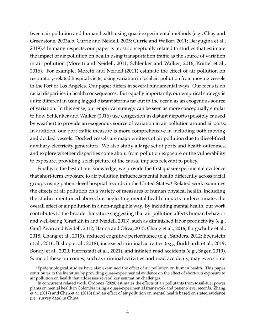
tween air pollution and human health using quasi-experimental methods (e.g., Chay andGreenstone, 2003a,b; Currie and Neidell, 2005; Currie and Walker, 2011; Deryugina et al.,2019).3 In many respects, our paper is most conceptually related to studies that estimatethe impact of air pollution on health using transportation traffic as the source of variationin air pollution (Moretti and Neidell, 2011; Schlenker and Walker, 2016; Knittel et al.,2016). For example, Moretti and Neidell (2011) estimate the effect of air pollution onrespiratory-related hospital visits, using variation in local air pollution frommoving vesselsin the Port of Los Angeles. Our paper differs in several fundamental ways. Our focus is onracial disparities in health consequences. But equally importantly, our empirical strategy isquite different in using lagged distant storms far out in the ocean as an exogenous sourceof variation. In this sense, our empirical strategy can be seen as more conceptually similarto how Schlenker and Walker (2016) use congestion in distant airports (possibly causedby weather) to provide an exogenous source of variation in air pollution around airports.In addition, our port traffic measure is more comprehensive in including both movingand docked vessels. Docked vessels are major emitters of air pollution due to diesel-firedauxiliary electricity generators. We also study a large set of ports and health outcomes,and explore whether disparities come about from pollution exposure or the vulnerabilityto exposure, providing a rich picture of the causal impacts relevant to policy.

Finally, to the best of our knowledge, we provide the first quasi-experimental evidencethat short-term exposure to air pollution influences mental health differently across racialgroups using patient-level hospital records in the United States.4 Related work examinesthe effects of air pollution on a variety of measures of human physical health, includingthe studies mentioned above, but neglecting mental health impacts underestimates theoverall effect of air pollution in a non-negligible way. By including mental health, our workcontributes to the broader literature suggesting that air pollution affects human behaviorand well-being (Graff Zivin and Neidell, 2013), such as diminished labor productivity (e.g.,Graff Zivin and Neidell, 2012; Hanna and Oliva, 2015; Chang et al., 2016; Borgschulte et al.,2018; Chang et al., 2019), reduced cognitive performance (e.g., Sanders, 2012; Ebensteinet al., 2016; Bishop et al., 2018), increased criminal activities (e.g., Burkhardt et al., 2019;Bondy et al., 2020; Herrnstadt et al., 2021), and inflated road accidents (e.g., Sager, 2019).Some of these outcomes, such as criminal activities and road accidents, may even come

3Epidemiological studies have also examined the effect of air pollution on human health. This papercontributes to the literature by providing quasi-experimental evidence on the effect of short-run exposure toair pollution on health that addresses several key estimation challenges.

4In concurrent related work, Ordonez (2020) estimates the effects of air pollutants from fossil-fuel powerplants on mental health in Colombia using a quasi-experimental framework and patient-level records. Zhanget al. (2017) and Chen et al. (2018) find an effect of air pollution on mental health based on stated evidence(i.e., survey data) in China.

4

about partly due to the impact of air pollution on mental health.The paper proceeds as follows. Section 2 provides a brief background on port pollution

and human health. Section 3 describes our data and descriptive statistics. Section 4discusses our empirical strategies and identification. Section 5 presents the main empiricalresults. Section 6 discusses implications for policy, and Section 7 concludes.

2 Background

2.1 Air Pollution in PortsPorts serve as a primary conduit for global trade and play a significant role in the localeconomies for many coastal cities (EPA, 2017). The Organisation for Economic Co-operationand Development (OECD) projects that global marine freight will more than quadruple by2050, and this expansion is expected to increase port activities further.5 Docked vessels inports can be one of the dirtiest emitters in terms of local air pollutants, as they often operateauxiliary engines to generate onboard electricity by burning bunker fuel and diesel (Wanet al., 2016). Other diesel-powered activities in ports, such as cargo handling equipment,automated guided vehicles, and short-haul trucks, also emit a substantial amount of airpollution (Agrawal et al., 2009). Hence, ports can be one of the largest contributors to airpollution in surrounding regions.6 It is notable that approximately 30% of counties in theUnited States that are currently out of compliance or previously failed to meet the NationalAmbient Air Quality Standards (NAAQS) either include or are adjacent to major ports (seeFigure B.1).7

Most ports are located in urban areas with high population density (e.g., Los Angelesand New York), often surrounded by low-income, minority neighborhoods. For example,around 40% of zip codes within a 25-mile radius of the major ports in California aredesignated as “disadvantaged” communities, with concentrations of people that are oflow income, color, high unemployment, and/or low levels of educational attainment.8These low-income households and people of color living or working in port areas can

5See https://www.itf-oecd.org/sites/default/files/docs/2015-01-27-outlook2015.pdf.6See https://www.latimes.com/california/story/2020-01-03/port-ships-are-becoming-la-worst-

polluters-regulators-plug-in.7The National Ambient Air Quality Standards are specified under the Clean Air Act in the United States,

which determines maximum allowable concentrations of criteria air pollutants that have been proved to beharmful to human health.

8Disadvantaged communities in California are often disproportionately impacted by environmentalhazards. They are determined based on Senate Bill 535 (SB 535). The bill requires a proportion of the revenuefrom the Cap-and-Trade program auction to be allocated to projects that benefit disadvantaged communities.The designation of disadvantaged communities uses the CalEnviroScreen tool, a scoring system with severalfactors: pollution burden and socioeconomic characteristics.

5

be significantly impacted by air pollution (Houston et al., 2014). Many studies haveconsistently documented differences in air pollution exposure across socioeconomic groups(see recent reviews in Mohai et al., 2009; Banzhaf et al., 2019a,b; Hsiang et al., 2019), andports are likely one contributing factor for these differences.

2.2 Air Pollution and HealthAir pollution is well known to be detrimental to human health (Dockery et al., 1993).Breathing in polluted air can affect lung development and cause respiratory diseases(Dockery and Pope III, 1994), such as asthma and chronic obstructive pulmonary disease(DeVries et al., 2017;Wang et al., 2019). Epidemiologists have also established an associationbetween air pollution and cardiovascular disease (Seaton et al., 1995), including impairingblood vessel function (Riggs et al., 2020), speeding up artery calcification (Keller et al.,2018), and increasing risk of hemorrhagic stroke (Sun et al., 2019). Moreover, studies haveshown an association between air pollution and breast and lung cancer (Cheng et al., 2020).

A growing number of economic studies use quasi-experimental methods to estimatethe causal effects of air pollution exposure on human health, using health metrics suchas infant mortality and birth outcomes (e.g., Chay and Greenstone, 2003b; Currie andNeidell, 2005; Currie et al., 2009; Currie and Walker, 2011; Sanders and Stoecker, 2015;Arceo et al., 2016; Alexander and Schwandt, 2019), adult mortality (e.g., Deryugina et al.,2019; Anderson, 2020), respiratory problems (e.g., Moretti and Neidell, 2011; Schlenkerand Walker, 2016), and cardiovascular diseases (e.g., Schlenker and Walker, 2016; Hallidayet al., 2019). While the focus of much of the literature has been on physical health, there isgrowing epidemiological work showing an association between air pollution and mentalhealth (e.g., Sass et al., 2017; Kim et al., 2018; Brokamp et al., 2019).

Air pollution could adversely affect mental health through several channels. Airpollution can lead to neuroinflammation and oxidative stress linked to anxiety, depression,and cognitive dysfunction (Sørensen et al., 2003; Salim et al., 2011). In addition, people tendto reduce outdoor activities due to pollution, which may induce mental disorders throughpathways such as vitamin D deficiency from limited access to sunlight (Anglin et al., 2013),reduced exercise (Suija et al., 2013), restricted access to green space (Cohen-Cline et al.,2015), and less social support (George et al., 1989). Moreover, some studies suggest thatworsened physical health caused by air pollution exposure may also lead to fear and stress,which increases anxiety and other mental illnesses (Scott et al., 2007).

6

3 Data and Descriptive StatisticsThis paper compiles a comprehensive data set from multiple sources on port traffic, airpollution, health, local weather, and major oceanic storms.

3.1 Port TrafficWe obtain port data from the US Army Corps of Engineers (USACE) for 2001–2016. Thedata contain dates on which ships enter and exit from ports, including container ships,bulk carriers, tanker ships, and passenger ships. We match the entrance and clearancerecords for each vessel visit based on vessel names or identity numbers, from which we canapproximate the number of days a vessel is at berth in a port.9 For each date in a port, wethen calculate gross vessel tonnage and the number of vessels, which serve as the core porttraffic measures for this study. Since different vessel types have different sizes and weights,the calculated gross vessel tonnage variable represents vessel heterogeneity to some extent.

One minor weakness of these data is that USACE mainly tracks waterborne transporta-tion originating from or heading to foreign ports and does not have complete coverageof ships traveling between domestic ports. According to the Bureau of TransportationStatistics, foreign waterborne freight accounts for 85–90% of total shipping tonnage inmaritime ports in the United States.10 Hence, the USACE data should be a reasonablerepresentation of total vessel tonnage in the included ports in this study, even if it missesa small fraction of the tonnage. This minor caveat about our data is analogous to one inSchlenker and Walker (2016), where the data set they use for airport traffic only accountsfor major domestic airline passenger travel.

Table A.1 contains the summary statistics of daily vessel tonnage and counts. In ourfinal data set, we focus on the 27 major maritime ports in the United States, six of whichare in California.11

3.2 Air PollutionWe obtain daily air pollution concentration data from US Environmental Protection Agency(EPA)AirQuality System (AQS) for five local air pollutants, carbonmonoxide (CO), nitrogendioxide (NO2), ozone (O3), PM2.5, and sulfur dioxide (SO2), for 2001–2016. The data contain

9The data contain some unmatched vessel entrance or clearance records. We treat these entries as a singleday in port since most vessels in the data sample enter and exit from ports on the same day.

10This estimate is obtained from https://www.bts.gov/content/us-waterborne-freight.11The six major California ports are the Ports of Long Beach, Los Angeles, Oakland, San Diego, Hueneme,

and San Francisco.

7

dailymaxima andmeans of pollution concentrations at the pollutionmonitoring site level.12Due to advancements in remote sensing technology and machine learning models,

researchers are now able to predict granular air pollution concentrations by integratingsatellite imagery, chemical transport models, pollution monitor data, land cover, andmeteorological data. We obtain daily zip code-level satellite-based PM2.5 projection datafrom Reid et al. (2021), primarily used for robustness checks. The data set includes threeprojections using various machine learning algorithms: the Ranger algorithm, the extremegradient boosting tree algorithm, and the generalized linear model that combines theresults from the previous two algorithms. We select the data from the third method.

3.3 HealthWe obtain patient-level administrative data from the California Office of Statewide HealthPlanning and Development for 2010–2016. These include three types of data: PatientDischarge Data (PDD), Emergency Department Data (EDD), and Ambulatory SurgeryCenter Data (ASCD). The PDD consists of overnight stays from all California hospitals.The EDD and ASCD keep track of patients who had single-day emergency treatmentin an Emergency Room or licensed freestanding Ambulatory Surgery Centers. Any pa-tient initially logged in the EDD/ASCD that is subsequently admitted to a hospital forovernight stays is dropped in the EDD/ASCD and then added to the PDD to eliminatedouble-counting and ensure consistency.

These three data sets provide dates for hospital visits, the zip codes of home addresses,demographics (age, sex, and race), one principal diagnosis, and up to 24 secondarydiagnoses. In our primary specification, we pool the three data sets and count the dailynumber of hospital visits at each zip code for patients who had either a principal orsecondary diagnosis related to the health problems examined in this paper.13 We thenmerge in population data from the 2010 US Census.14 We next calculate the daily hospitalvisit rate at the zip code level, indicating the number of hospital visits per million residentsper day. We focus on hospital visits of six categories of illnesses: respiratory (asthma, acuteupper respiratory, all respiratory), mental (anxiety, all psychiatric), and heart-related. We

12The EPA AQS reports various daily means with different time windows that air passes through themonitoring device before it is analyzed. For example, for CO at certain monitoring sites, there are one-hourand eight-hour run daily averages. We take averages for each monitor and day.

13We conduct several robustness checks by exploring only principal diagnoses and each of the three datasets separately.

14US Census data is based on the zip code tabulation area (ZCTA), so we merge in based on the ZCTA.We exclude the ZCTAs with fewer than 5,000 residents (or those with fewer than 1,000 residents in eachsocioeconomic group for heterogeneity analysis), which only accounts for 2%of the total California population.For the remainder of the paper, we refer to ‘zip codes’ for simplicity.

8

also include two diseases for placebo checks: arterial embolism (i.e., stuck blood clots) andappendicitis.15 Figure B.2 illustrates that our sample includes large sections of the largesturban areas in California.

3.4 WeatherWe acquire weather data from the National Oceanic and Atmospheric Administration(NOAA) Integrated Surface Database for 2001–2016. We construct daily measures ofweather variables from hourly readings at the weather station level. These variables includedew point, minimum and maximum temperatures, precipitation, wind speed, and winddirection. The minimum and maximum temperatures are the lowest and highest hourlyreadings in a day, and the daily precipitation is the summation of hourly records.16 Wethen calculate daily means for dew point temperature, wind speed, and wind direction.The wind direction blowing north is normalized to zero, and it increases up to 360 degreesclockwise.

3.5 Tropical CyclonesTropical cyclones are rapidly rotating storms that originate in the tropical oceans. Thoseoccurring in the northeastern Pacific Ocean or the Atlantic Ocean are called hurricanes,while those in the northwestern Pacific Ocean are called typhoons. We obtained data onthe 578 tropical cyclones near the United States from 2001-2016 from the NOAA NationalHurricane Center. The data track dates, times, center locations, maximum wind, centralpressure, and wind radii of historical cyclones every six hours in the Northeast andNorth-central Pacific Ocean and the Atlantic Ocean.

Figure 1(a) shows all hurricanes that occurred in 2016 and the locations of the 27 majorports in the United States. The figure shows that cyclones can strike ports, which maydirectly impact local weather and air pollution. Our primary results only use data whencyclones are at least 500 miles away from the 27 major ports. We chose 500 miles becausecyclones are documented to have a typical radius in the range of 125–310 miles, so we canbe assured that the ports are well outside the scope of the cyclones included in our study.17

15The administrative data sets adopt what are called ‘ICD codes’ to record diagnoses. In October 2015, thecodes were upgraded from ICD-9-CM codes to the ICD-10-CM codes. Table A.2 presents the ICD codes forthis study. The codes that fall into the psychiatric categories follow Brokamp et al. (2019) by excluding thoseassociated with suicides. The table also presents the corresponding Medicare Severity Diagnosis RelatedGroup (MS-DRG) codes for calculating the medical costs of illnesses from the Medicare data.

16For missing hourly precipitation readings, we assume they are the same as the most recent availablereading.

17See https://public.wmo.int/en/our-mandate/focus-areas/natural-hazards-and-disaster-risk-reduction/tropical-cyclones.

9

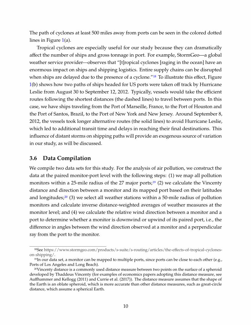
The path of cyclones at least 500 miles away from ports can be seen in the colored dottedlines in Figure 1(a).

Tropical cyclones are especially useful for our study because they can dramaticallyaffect the number of ships and gross tonnage in port. For example, StormGeo—a globalweather service provider—observes that “[t]ropical cyclones [raging in the ocean] have anenormous impact on ships and shipping logistics. Entire supply chains can be disruptedwhen ships are delayed due to the presence of a cyclone.”18 To illustrate this effect, Figure1(b) shows how two paths of ships headed for US ports were taken off track by HurricaneLeslie from August 30 to September 12, 2012. Typically, vessels would take the efficientroutes following the shortest distances (the dashed lines) to travel between ports. In thiscase, we have ships traveling from the Port of Marseille, France, to the Port of Houston andthe Port of Santos, Brazil, to the Port of New York and New Jersey. Around September 8,2012, the vessels took longer alternative routes (the solid lines) to avoid Hurricane Leslie,which led to additional transit time and delays in reaching their final destinations. Thisinfluence of distant storms on shipping paths will provide an exogenous source of variationin our study, as will be discussed.

3.6 Data CompilationWe compile two data sets for this study. For the analysis of air pollution, we construct thedata at the paired monitor-port level with the following steps: (1) we map all pollutionmonitors within a 25-mile radius of the 27 major ports;19 (2) we calculate the Vincentydistance and direction between a monitor and its mapped port based on their latitudesand longitudes;20 (3) we select all weather stations within a 50-mile radius of pollutionmonitors and calculate inverse distance-weighted averages of weather measures at themonitor level; and (4) we calculate the relative wind direction between a monitor and aport to determine whether a monitor is downwind or upwind of its paired port, i.e., thedifference in angles between the wind direction observed at a monitor and a perpendicularray from the port to the monitor.

18See https://www.stormgeo.com/products/s-suite/s-routing/articles/the-effects-of-tropical-cyclones-on-shipping/.

19In our data set, a monitor can be mapped to multiple ports, since ports can be close to each other (e.g.,Ports of Los Angeles and Long Beach).

20Vincenty distance is a commonly used distance measure between two points on the surface of a spheroiddeveloped by Thaddeus Vincenty (for examples of economics papers adopting this distance measure, seeAuffhammer and Kellogg (2011) and Currie et al. (2017)). The distance measure assumes that the shape ofthe Earth is an oblate spheroid, which is more accurate than other distance measures, such as great-circledistance, which assume a spherical Earth.

10

For our analysis of health impacts, we construct the data at the paired zip code-port levelwith similar steps: (1) we select all zip codes within a 25-mile radius of the six major portsin California; (2) we calculate the Vincenty distance between a paired zip code and port; (3)we calculate the zip code-level pollution measures by taking inverse distance-weightedaverages of the monitor-level data within 25 miles of zip code centroids; (4) we calculatezip code-level weather measures by selecting all weather stations within 50 miles of zipcode centroids and take inverse distance-weighted averages.

Table 1 contains the summary statistics for themain variables in this study, with hospitalvisit rates broken down by race. Tables A.3–A.7 present the supplementary summarystatistics of pollution and hospital visit rates for various slices of the data.

3.7 Descriptive Statistics on Racial DisparitiesBefore diving into the empirical modeling, we present descriptive statistics on racial dis-parities in pollution exposure and hospital visits near ports in California. Following Currieet al. (2020), we primarily focus on comparing non-Hispanic white and Black populations.The Hispanic ethnic identity is often described as more fluid over time than non-Hispanicwhite or Black groups, which may introduce measurement errors in comparing Hispanicsand non-Hispanics (Liebler et al., 2017). However, for the interested reader, we also presentsome descriptive statistics for Hispanics in Figure B.3.

Figure 2(a) shows distributions of the Black andwhite populations residing in Californiaport areas by distance to their nearest mapped ports. We observe that the Black populationtends to live closer to ports, while the white population is more uniformly distributed,suggesting that ports may disproportionately impact Blacks simply due to differences inexposure to air pollution.

Figure 2(b) presents distributions of populations for the two racial groups by percentileof mean PM2.5 exposure at the zip code level over 2010–2016. We see that Blacks live inareas that are exposed to higher pollution concentrations than whites. As further evidence,Table A.8 presents the average pollution exposure for Blacks and whites in port areas,weighted by the population of each race at the zip code level.21 The evidence indicatesthat Blacks face substantially higher exposure to air pollution in areas around ports thanwhites.

21This analysis focuses on differences in exposure across zip codes and ignores any within-zip codedifferences in exposure, so it may slightly underestimate disparities in pollution exposure. That said, thisapproach is standard in the literature (see a review of this approach in Banzhaf et al. (2019b)). Figures B.4 andB.5 further illustrate the locations of PM2.5 monitors and ports, computed average pollution concentrations,and race-specific population shares at the zip code level surrounding two major urban areas in California.

11

Next, we examine the racial gaps in health outcomes. Figure 3 plots probability densityfunctions of annual hospital visit rates for the Black and white populations for zip codeswithin 0–12.5 miles to ports and zip codes within 12.5–25 miles to ports. In both panels,the distributions for the Black population lie to the right of the distributions for whites.The gaps in mean hospital visit rates between Blacks and whites become slightly widercloser to ports. Further, Figure B.6 shows that annual air pollution exposure for individualsvisiting hospitals is notably higher for Blacks thanwhites. These figures provide descriptiveevidence of racial disparities in pollution exposure and health outcomes in port areas.

4 Empirical Strategy

4.1 Effect of Vessels in Ports on Air PollutionWe begin our analysis by estimating the effect of port traffic on daily air pollutionconcentrations. Our empirical specification is as follows:

%8?C = �+?C + X8C� + �C + �8? + 48?C , (1)

where %8?C refers to local air pollutant concentrations at monitor 8 that is mapped to port ?on day C. The variable +?C is either the gross vessel tonnage or the number of vessels inport. The set of variables X8C includes weather controls consisting of maximum, minimum,and dew point temperatures; precipitation; wind speed; and relative wind direction (indi-cating whether a monitor is downwind or upwind of the mapped port). X8C also includesquadratic terms for each of the weather controls (except for the relative wind direction). Weincorporate temporal fixed effects �C that consist of county-by-year, month, day-of-week,and holiday fixed effects.22 Since there may be unobserved time-invariant effects, we furtherincludemonitor-port fixed effects �8? . 48?C is the error term. The parameter of interest, �, canbe interpreted as the effect of port traffic on local air pollutant concentrations for a given day.

There are several potential concerns in estimating equation (1) using ordinary leastsquares (OLS) that may lead to biased estimates of �. One concern is that there may be somemeasurement error in the port traffic measures because we observe vessels originatingfrom or heading to foreign ports (85-90% of tonnage), so we miss some vessels in ouranalysis. A second concern is the possibility of omitted variables, such as unobservedeconomic or weather factors that affect port traffic and local air pollution.

22The holidays include NewYear, Martin Luther King Jr. Day, Presidents Day, Memorial Day, IndependenceDay, Labor Day, Columbus Day, Veterans Day, Thanksgiving, and Christmas, as well as the three-day priorand post the holiday.

12

To address these concerns, our empirical approach leverages quasi-random variationfromdistant tropical cyclones several days prior to the day under consideration. Specifically,we instrument for +?C using the existence of lagged tropical cyclones far out in the ocean.As mentioned above, these cyclones often disrupt travel for marine vessels, delaying theirarrival into ports, leading to fewer ships and less tonnage in ports several days later (recallFigure 1). The first stage relies on this disruptive impact on shipping.

To be precise, the first stage of our instrumental variables approach is:

+?C = )�C−< +W8?C� + &8?C , (2)

where )�C−< is an indicator variable equal to one if there are one or more tropical cyclonesfar out in the ocean (i.e., at least 500 miles away from ports) on day C − <. We use aseven-day lag (< = 7) in our primary specification, but we run robustness checks withdifferent lags. A cyclone can last anywhere from a few days to weeks. Thus, to create thislagged variable, we first identify the days when there are one or more cyclones that areat least 500 miles away from ports, and then take the seven-day lag.23 The variable W8?C

includes the exogenous variables defined in equation (1): weather controls, temporal fixedeffects, and monitor-port fixed effects.

To be a valid instrument, )�C−< must satisfy the exclusion restriction, i.e., it is uncorre-lated with the error term 48?C in equation (1).24 A direct threat to the exclusion restrictionwould be if the tropical cyclones hit the ports several days later, directly affecting pollution.We avoid this concern by removing the observations for the days when cyclones appearwithin a 200-mile radius of ports. We also remove observations two days prior and after thecyclones are within a 200-mile radius. Further, we perform a robustness check removingall observations within 21 days after a cyclone is last within 200 miles of ports in case ittakes ports weeks to recover after a storm.

Another concern could be that lagged distant cyclones not only impact vessel tonnageor counts in ports but also substantially influence the composition of vessels, which may,in turn, affect air pollution in ports. Figure B.7 shows that lagged tropical cyclones far outin the ocean do not appear to have any notable effect on the composition of vessel types inports. In addition, when a storm is slated to arrive at a port, vessels tend to depart earlier toavoid or weather the storm at sea and avoid potential collisions, so later departures shouldnot be a threat to identification.

23The choice of seven days is motivated both because it is a week after the storm was out at sea and becausewe observe a drop in vessel tonnage in ports seven days later.

24We expect lagged distant tropical cyclones always to reduce the number of vessels and gross tonnage inports, so the monotonicity condition should hold.

13

Amoremodest threat could be if lagged tropical cyclones far out in the ocean sufficientlyimpact meteorological patterns that they indirectly affect current-day weather in the ports.We explore this by dividing the sample into month-days when )�C−7 = 1 and thosewhen it is zero. Figure 4 shows distributions of the six weather variables across the twosubsamples.25 The distributions between the two grouped samples are almost identical,confirming that the weather in the ports is no different when there are tropical cyclones inthe distant ocean seven days prior than when there are not.26

Thus, for there to be remaining identification concerns, there would have to be someother localized source of air pollution that happens to be correlated with distant stormsseven days earlier. This seems unlikely to us. But we will also perform a placebo test and aset of robustness checks to further support the instrument’s validity.

4.2 Effect of Air Pollution on HealthTo estimate the relationship between air pollution and health outcomes in port areas, wespecify the following linear regression model for the overall population and separately forBlacks and whites:

H8?C = �%8?C + X8C� + �C + �8? + 48?C , (3)

where H8?C is the hospital visit rate (i.e., hospital visits per million residents) associatedwith an illness in zip code 8 that is mapped to port ? on day C. The variable %8?C is the airpollutant concentration. We run the regression separately for each of four pollutants—CO,NO2, PM2.5, and SO2—that are shown to be detrimental to human health.27 Because thesepollutants have different scales, we standardize them by their sample means and standarddeviations to facilitate comparisons. In an extension in Section 5.4, we also considerincluding sets of these pollutants that might be co-emitted. The remaining variablesare similar to those specified in equation (1), where X8C is a set of weather controls (notincluding wind variables). �C is the set of temporal fixed effects. �8? denotes zip code-portfixed effects, which are especially useful for controlling for time-invariant factors thataffect health and pollution levels (e.g., poor households with lower baseline health havepreviously sorted into in polluted areas). The coefficient of interest � indicates the effect ofa one-unit increase in air pollution concentrations on the daily hospital visit rate associated

25Because the number of observations in the two subsamples is different, we randomly draw a subset ofobservations in the second subsample, so the number of observations is the same between the samples, butstatistical tests of differences in means are no different if we use the each of the full subsamples.

26To provide further evidence, Table A.9 presents the standardized mean differences, variance ratio, andKolmogorov-Smirnov statistics for the weather variables.

27In this choice of pollutants to study, we follow the existing evidence of the health effects of common airpollutants (e.g., Dominici et al., 2006; Bell et al., 2008; Brokamp et al., 2019).

14

with an illness.However, estimating equation (3) using OLSmay still lead to a biased estimate of �. One

potential concern is that exposure to air pollution is not randomly assigned to residents,and thus people with preferences for better air quality may adjust their daily activitiesbased on pollution forecasts. Another potential concern is that there may be measurementerrors in pollution exposure. Our pollution measures at the zip code level may deviatefrom residents’ actual exposure since we do not observe their exact home addresses, andpeople are also unlikely to be stationary all the time. In addition, there may be time-varyingomitted variables correlated with both air pollution and health.

To address these concerns, we employ an over-identified instrumental variables ap-proach (Knittel et al., 2016; Schlenker and Walker, 2016; Deryugina et al., 2019), where thefirst-stage regression is specified as:

%8?C = 1+̂?C + 2,(8C +7∑B=1

3B,�B8C + 4+̂?C ×,(8C +

7∑B=1

5B+̂?C ×,�B8C+

7∑B=1

6B,(8C ×,�B8C +

7∑B=1

7B+̂?C ×,(8C ×,�B8C +W8?C� + &8?C .

(4)

In this equation,,(8C represents wind speed. ,�B8C is an indicator variable for wind

direction, which is equal to one if the daily mean wind direction in zip code 8 falls in each45-degree interval [45s, 45s+45), where B ∈ {1, ..., 7} is the interval.28 The variable +̂?C is thefitted vessel tonnage in port ? on day C, which is obtained using the following regression:

+?C =∑?

�?1? × )�C−< + �?C , (5)

where )�C−< is the tropical cyclone indicator variable. The variable 1? is an indicator forport ?, which allows the effect of the instrument to vary across locations.

The intuition for the identification in this empirical strategy is that we are isolating andleveraging the variation in vessel tonnage that comes about because of distant tropicalcyclones several days prior.29 This approach avoids using any variation in vessel ton-nage related to factors that may also influence hospital visit rates. For example, people

28We exclude the interval [0, 45) in regressions as the base, and no observations fall in the interval [315,360) in our data set, so this interval is also excluded. W8?C includes the same weather controls (except forwind direction and wind speed) and fixed effects as in equation (2).

29Wooldridge (2002, p. 117) discusses the assumptions for using fitted variables as instruments, whichrequires the exogenous regressors for generating fitted instruments to be orthogonal with the error term inthe main estimation equation, i.e., equation (3). See Dahl and Lochner (2012) and Schlenker and Walker(2016) for recent papers using fitted variables as instruments.

15

may observe or possess information about port traffic and adjust their activities andpollution exposure accordingly. For there to be a remaining identification concern, onemust believe that tropical cyclones in the distant ocean several days prior influence hospi-tal visits in areas around ports through a channel outside of port traffic. This seems unlikely.

Our specification also includes local wind direction and wind speed in the set ofinstruments, which adds statistical power because local wind affects the spatial distributionof air pollutants. A large body of meteorological literature has shown that wind directionand speed are strong predictors of local pollutant concentrations (e.g., Chaloulakou et al.,2003; Kukkonen et al., 2005; Karner et al., 2010). Based on this scientific evidence, a growingnumber of studies in the economics literature exploit variation in local wind as the driverfor air pollution (e.g., Moeltner et al., 2013; Schlenker and Walker, 2016; Keiser et al., 2018;Deryugina et al., 2019; Bondy et al., 2020; Anderson, 2020; Herrnstadt et al., 2021).

5 Results

5.1 Effect of Vessels in Port on Air PollutionWe begin our analysis by demonstrating a causal relationship between port traffic andair pollution. We estimate the model given in equation (1) using two-stage least squares,with the existence of distant tropical cyclones seven days prior as the instrument. Weperform this estimation using all 27 major ports in the United States. The standard errorsare two-way clustered by monitor-port and day.30

In the first stage, we estimate equation (2). We find a strong first-stage relationship,consistent with lagged distant tropical cyclones affecting vessel tonnage and the numberof vessels. The first-stage F-statistics reported in Panel A of Table 2 range from 13 to35.31 These are well above standard thresholds for weak instruments to be a concern(e.g., Andrews et al. (2019) suggest that instruments are weak below a threshold of ten).The point estimates shown in Table A.10 are all significant, indicating that the existenceof lagged distant tropical cyclones results in 20,000 metric ton (Mt) less tonnage (or 0.5fewer vessels) in ports per day.32 We also present two tests for weak instruments, theAnderson-Rubin Wald statistic and the related Stock and Wright (2000) LM S statistic. Thenull hypothesis of the two tests is that the coefficient of the endogenous variable is equal to

30We cluster by monitor-port because we exploit the relative wind direction between a port and monitor,and a monitor can be mapped to multiple ports.

31All first-stage F statistics reported in this paper are cluster-robust Kleibergen-Paap Wald F statistics(Kleibergen and Paap, 2006), which are much smaller than the standard Cragg-Donald Wald F statisticsassuming i.i.d. errors (not reported in the paper) (Cragg and Donald, 1993).

32The specifications are the same across the columns. The number of observations differs across columnsdue to the minor differences in data availability for each pollutant.

16

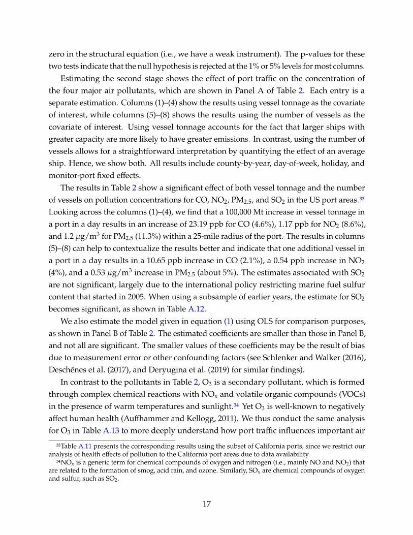
zero in the structural equation (i.e., we have a weak instrument). The p-values for thesetwo tests indicate that the null hypothesis is rejected at the 1% or 5% levels formost columns.

Estimating the second stage shows the effect of port traffic on the concentration ofthe four major air pollutants, which are shown in Panel A of Table 2. Each entry is aseparate estimation. Columns (1)–(4) show the results using vessel tonnage as the covariateof interest, while columns (5)–(8) shows the results using the number of vessels as thecovariate of interest. Using vessel tonnage accounts for the fact that larger ships withgreater capacity are more likely to have greater emissions. In contrast, using the number ofvessels allows for a straightforward interpretation by quantifying the effect of an averageship. Hence, we show both. All results include county-by-year, day-of-week, holiday, andmonitor-port fixed effects.

The results in Table 2 show a significant effect of both vessel tonnage and the numberof vessels on pollution concentrations for CO, NO2, PM2.5, and SO2 in the US port areas.33Looking across the columns (1)–(4), we find that a 100,000 Mt increase in vessel tonnage ina port in a day results in an increase of 23.19 ppb for CO (4.6%), 1.17 ppb for NO2 (8.6%),and 1.2 �g/m3 for PM2.5 (11.3%) within a 25-mile radius of the port. The results in columns(5)–(8) can help to contextualize the results better and indicate that one additional vessel ina port in a day results in a 10.65 ppb increase in CO (2.1%), a 0.54 ppb increase in NO2

(4%), and a 0.53 �g/m3 increase in PM2.5 (about 5%). The estimates associated with SO2

are not significant, largely due to the international policy restricting marine fuel sulfurcontent that started in 2005. When using a subsample of earlier years, the estimate for SO2

becomes significant, as shown in Table A.12.We also estimate the model given in equation (1) using OLS for comparison purposes,

as shown in Panel B of Table 2. The estimated coefficients are smaller than those in Panel B,and not all are significant. The smaller values of these coefficients may be the result of biasdue to measurement error or other confounding factors (see Schlenker and Walker (2016),Deschênes et al. (2017), and Deryugina et al. (2019) for similar findings).

In contrast to the pollutants in Table 2, O3 is a secondary pollutant, which is formedthrough complex chemical reactions with NOx and volatile organic compounds (VOCs)in the presence of warm temperatures and sunlight.34 Yet O3 is well-known to negativelyaffect human health (Auffhammer and Kellogg, 2011). We thus conduct the same analysisfor O3 in Table A.13 to more deeply understand how port traffic influences important air

33Table A.11 presents the corresponding results using the subset of California ports, since we restrict ouranalysis of health effects of pollution to the California port areas due to data availability.

34NOx is a generic term for chemical compounds of oxygen and nitrogen (i.e., mainly NO and NO2) thatare related to the formation of smog, acid rain, and ozone. Similarly, SOx are chemical compounds of oxygenand sulfur, such as SO2.

17

pollutants. The estimates are negative but insignificant. This may be driven by increases inNOx from port traffic (shown in Table 2), which can also interact with existing O3 in the airand in some cases actually reduce the total O3 concentrations (Sillman, 1999; Seinfeld andPandis, 2016; He et al., 2020).35 In the remainder of the paper, we focus on the four criteriaair pollutants (CO, NO2, PM2.5, and SO2), noting that they can all affect human health viachannels separate from O3.

The increase in pollution from added port traffic can be interpreted as the combinedeffect from the direct emissions from the additional vessels in port and the indirectemissions due to the complementary activities associated with handling goods from theship. For example, cargo handling equipment and short-haul trucks are often poweredwith diesel fuel and can be expected to add to the emissions from the ship itself. While thereare no other estimates exactly like ours in the literature, the US Environmental ProtectionAgency estimates that emissions associated with marine traffic account for 7–61% of NOx

and SOx in certain port areas (EPA, 2003). In a rough calculation, our estimates suggestthat marine shipping in the 27 major ports in the United States contributes 36% of NO2

within a 25-mile radius (see Appendix C.1).

5.2 Racial Disparities in the Effects of Air Pollution on HealthWe now turn to the effects of air pollution on health outcomes—and how they differ by race.We estimate the model given in equation (3) separately for the overall population, Blacks,and whites using two-stage least squares, where we instrument for air pollution using thefitted vessel tonnage and local wind conditions.36 We perform this estimation using thedata from California to leverage our hospital admissions data. The pollutant concentrationsare standardized by their sample mean and standard deviation. The standard errors forthe health analysis are clustered by zip code-port and day.

Table 3 presents the results of the second stage of the instrumental variables estimation,showing the effect of increased air pollutant concentrations on hospital visits per millionresidents for respiratory, heart, and psychiatric problems. Panel A shows the results for theoverall population within 25 miles of port facilities, while Panels B and C show the resultsfor Blacks and whites, respectively.37 Each estimate represents an individual regression.

35This finding is different from Moretti and Neidell (2011), where port traffic results in an increase inO3 concentrations in the port areas of Los Angeles. This discrepancy may be due to different studiedlocations. Auffhammer and Kellogg (2011) show that southern California, including Los Angeles, tends to beVOC-limited for O3 formation (the opposite is NOx-limited), where the NOx concentrations are relativelyhigh, and increases in NOx emissions may not change O3 concentrations. Our study covers a larger set ofport locations that likely consists of both NOx-limited and VOC-limited areas.

36We obtain fitted vessel tonnage from equation (5) using all 27 US ports from 2001 to 2016.37Tables A.14–A.16 also present more details behind the compiled Table 3, including adjusted R2 and the

18

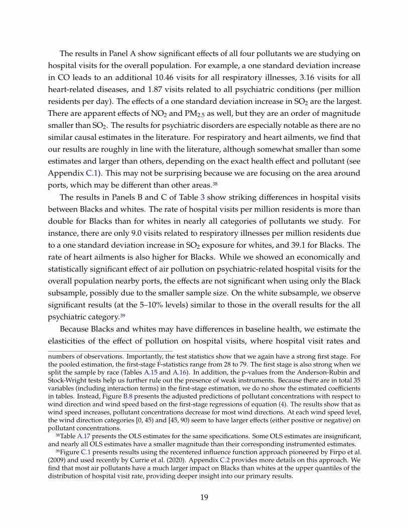
The results in Panel A show significant effects of all four pollutants we are studying onhospital visits for the overall population. For example, a one standard deviation increasein CO leads to an additional 10.46 visits for all respiratory illnesses, 3.16 visits for allheart-related diseases, and 1.87 visits related to all psychiatric conditions (per millionresidents per day). The effects of a one standard deviation increase in SO2 are the largest.There are apparent effects of NO2 and PM2.5 as well, but they are an order of magnitudesmaller than SO2. The results for psychiatric disorders are especially notable as there are nosimilar causal estimates in the literature. For respiratory and heart ailments, we find thatour results are roughly in line with the literature, although somewhat smaller than someestimates and larger than others, depending on the exact health effect and pollutant (seeAppendix C.1). This may not be surprising because we are focusing on the area aroundports, which may be different than other areas.38

The results in Panels B and C of Table 3 show striking differences in hospital visitsbetween Blacks and whites. The rate of hospital visits per million residents is more thandouble for Blacks than for whites in nearly all categories of pollutants we study. Forinstance, there are only 9.0 visits related to respiratory illnesses per million residents dueto a one standard deviation increase in SO2 exposure for whites, and 39.1 for Blacks. Therate of heart ailments is also higher for Blacks. While we showed an economically andstatistically significant effect of air pollution on psychiatric-related hospital visits for theoverall population nearby ports, the effects are not significant when using only the Blacksubsample, possibly due to the smaller sample size. On the white subsample, we observesignificant results (at the 5–10% levels) similar to those in the overall results for the allpsychiatric category.39

Because Blacks and whites may have differences in baseline health, we estimate theelasticities of the effect of pollution on hospital visits, where hospital visit rates and

numbers of observations. Importantly, the test statistics show that we again have a strong first stage. Forthe pooled estimation, the first-stage F-statistics range from 28 to 79. The first stage is also strong when wesplit the sample by race (Tables A.15 and A.16). In addition, the p-values from the Anderson-Rubin andStock-Wright tests help us further rule out the presence of weak instruments. Because there are in total 35variables (including interaction terms) in the first-stage estimation, we do no show the estimated coefficientsin tables. Instead, Figure B.8 presents the adjusted predictions of pollutant concentrations with respect towind direction and wind speed based on the first-stage regressions of equation (4). The results show that aswind speed increases, pollutant concentrations decrease for most wind directions. At each wind speed level,the wind direction categories [0, 45) and [45, 90) seem to have larger effects (either positive or negative) onpollutant concentrations.

38Table A.17 presents the OLS estimates for the same specifications. Some OLS estimates are insignificant,and nearly all OLS estimates have a smaller magnitude than their corresponding instrumented estimates.

39Figure C.1 presents results using the recentered influence function approach pioneered by Firpo et al.(2009) and used recently by Currie et al. (2020). Appendix C.2 provides more details on this approach. Wefind that most air pollutants have a much larger impact on Blacks than whites at the upper quantiles of thedistribution of hospital visit rate, providing deeper insight into our primary results.

19

pollution measures are scaled by the inverse hyperbolic sine (IHS) transformation. TheIHS transformation has a similar interpretation as a logarithmic transformation, but zerosare defined. The estimates can be interpreted as percentage changes in the hospital visitrate due to a one percent increase in pollutant concentrations. Table A.18 shows that mostelasticities associated with respiratory and heart illnesses are statistically significant andmost estimates are greater for Blacks than whites, especially for upper respiratory ailments.

A natural question is whether there is a statistically significant difference between Blacksand whites. We perform a statistical test to examine the equality of the estimates acrossBlacks and whites.40 The test results in Table A.19 show that the differences between Blacksand whites are positive for all ailments and significant for respiratory ailments, indicatingthat respiratory issues are the underlying driver of the racial disparities. We also estimate(3) using differences in hospital visit rates between Blacks and whites as the dependent vari-able, restricting the data to zip codes with hospital visits for both Blacks and whites (TableA.20). We again observe that the differences in respiratory issues are positive and significant.

While the focus of this paper is the racial gap between Blacks and whites, we alsoestimate the effects of air pollution on hospital visits for Hispanics, which are shown inTable A.21. When compared to the results in Table 3, Hispanics have higher hospital visitrates associated with respiratory ailments than whites but lower rates than Blacks. We alsoobserve significant estimates associated with psychiatric illnesses for Hispanics.41

When interpreting these estimates, it is also important to keep in mind several crucialpoints. The estimated health effects may not be entirely attributable to a single pollutantsince some pollutants may be co-emitted with others. In an extension, we also estimate thejoint effects of certain pollutants on hospital visit rates, presented in the next subsection.Another crucial point is that some people who are ill may choose not to visit hospitals dueto restricted access to medical resources or the opportunity costs of spending time in ahospital. Some hospital visits may also be pre-scheduled. These are common caveats inthe literature using hospital visit data.

Another important point is that these estimates of health effects focus on the con-temporaneous effects of air pollution on health. There may also be longer-term effects,including cumulative effects or symptoms that arise a few days later. Thus, we estimateour model using different time windows up to 28 days following a pollution exposure for

40The approach uses the following Z test: / =�1−�F√

(��21+(��2

F

, where �1 and �F are point estimates for Blacks

and whites, and (��1 and (��F are the associated standard errors.41We also explore heterogeneous effects of air pollution by age and sex. Table A.22 shows that there are

larger effects on children for respiratory illnesses and larger effects on the elderly for psychiatric and heartmaladies. Table A.23 shows little difference in the effect between males and females.

20

the overall population, Blacks, and whites.42 Figures B.9–B.11 illustrate that the estimatesgradually increase with the length of the time window for respiratory illnesses, suggestingcumulative health effects of air pollution. For psychiatric and heart illnesses, the effect ofair pollution appears to be flat and even decreasing for Blacks and whites after 21 days.

To provide further context, we calculate the effects of one additional average-tonnagevessel in a port over a year on air pollution-induced annual hospital visits and hospitalmedical costs, as shown in Table 4.43 Panel A shows the results of annual hospital visits forresidents living within 25 miles of a major port facility. For Blacks, one additional vessel inport results in 2,500 respiratory hospital visits, 520 heart-related visits, and 98 psychiatricvisits (per million residents in a year in California). This amounts to 3.1 additional hospitalvisits per thousand Black residents in a year. For whites, one additional vessel in portresults in 570 respiratory hospital visits, 300 heart-related visits, and 210 psychiatric visits(per million residents in a year). This adds up to 1.1 additional hospital visits per thousandwhite residents in a year, only about one-third of the visits for Black residents.

Panel B of Table 4 calculates the cost of these additional hospital visits. For thiscalculation, we use the 2017 inpatient discharge data from the Centers for Medicare andMedicaid Services (CMS).44 The results of the calculation show that one more average-tonnage vessel in port over a year leads to $28 in medical costs per capita for Black residentsand $10 for white residents.

5.3 Evidence on the Mechanisms Behind the Racial DisparitiesThese findings show clear racial disparities in the health effects of air pollution in portareas. A natural question that arises is whether these disparities are due to Blacks livingin more polluted areas or Blacks having greater vulnerability to air pollution exposure(Hsiang et al., 2019). The evidence presented in Section 3.7 clearly shows that the Blackpopulation tends to have greater exposure to pollution than the white population. In the

42These estimations include the commensurate number of leading weather controls.43We calculate the results in the following steps: (1) calculate pollution concentration changes for the

studied pollutants due to one more vessel in ports (i.e., a 589,000 Mt increase in vessel tonnage) based onthe estimates in Panel A of Table 2; (2) calculate changes in annual hospital visits due to the changes instandardized concentrations of CO, NO2, PM2.5, and SO2 based on the estimates in Table 3; (3) select thelargest values across the air pollutants for each illness category. We also estimate the reduced form resultsfor the relationship between vessel tonnage and health outcomes in Section C.3.

44The Medicare data provide national average inpatient payments and total discharges for each diagnosis,which is categorized by theMS-DRG code (see https://www.cms.gov/Research-Statistics-Data-and-Systems/Statistics-Trends-and-Reports/Medicare-Provider-Charge-Data/Inpatient2017). We use the web service(http://icd10cmcode.com) based on CMS’s ICD-10 MS-DRG Conversion Project to convert the ICD-10diagnosis codes to the MS-DRG codes. The mapped MS-DRG codes for the studied primary illness groupsare presented in Table A.2. We calculate the average medical costs for each of the illness groups, weighted bythe total number of discharges.

21

population of hospital patients, Blacks are from zip codes that also face higher pollutionexposure. This underscores that differences in exposure are at least part of the story.

To explore whether Blacks have higher marginal damages in response to the samepollutant exposures than whites (i.e., are more vulnerable to exposure), we group zip codessurrounding the California ports by their average daily PM2.5 pollution levels. Specifically,we focus on the zip codes with available hospital visit data for Blacks andwhites and dividethem into eight groups by pollution percentile. We assume that zip codes in each percentilegroup have similar pollution exposure levels. We cannot entirely rule out differences ofexposure to air pollution within zip code groups, but we see households of different raceswell distributed across zip codes around ports and zip codes are fairly small areas in cities,so we expect that differences in pollutant concentrations within zip code groups to besmall. The intuition for this analysis is that given the same pollution exposures, differentcausal effects of pollution on hospital visit rates across racial groups suggest that factorsother than pollution play a role.

We estimate equations (3)–(5) for each group of zip codes. Figure 5 illustrates that thefour pollutants have larger effects on hospital visit rates (related to respiratory, heart, andpsychiatric) for Blacks than whites across percentiles. These results suggest that Blacks facehigher damages from air pollution exposure than whites even if exposure is held roughlyconstant, i.e., Blacks are more vulnerable to pollution exposure than whites.

The difference in vulnerability may come about due to a wide range of determinantsthat differ across races, such as baseline health, income, avoidance behavior, defensiveinvestments, or other socioeconomic characteristics. We explore this by collecting healthand economic characteristics data for areas surrounding the major ports in Californiaand compare them for Blacks and whites. Figure C.2(a) shows that Blacks have worsehealth conditions (e.g., smoking rate, obesity rate, no exercising rate, and poor or fairgeneral health rate) than whites, implying reduced baseline health for Blacks. In addition,Figure C.2(b) indicates that Blacks also have worse socioeconomic status than whites, withhigher poverty rates, reduced health insurance coverage, lower income per capita, andlower levels of education, which may make them more vulnerable to health risks frompollution exposure. Figure C.2(c) further shows that the selected economic characteristicsare correlated with the Black-white health gap in port areas. The detailed analysis and datasources are presented in Section C.4. While these results on the differences in vulnerablilityare illuminating, we should be cautious about interpreting the differences in socioeconomicstatus and behavioral patterns as causal drivers for the disparities in the causal effects ofair pollution across races that we clearly observe in our setting.

22

5.4 Placebo Tests, Extensions, and Robustness ChecksIn this section, we conduct two placebo tests and a set of extensions and robustness checksto support our identification and highlight the channels driving our results.

Placebo Tests. In the first placebo test, we consider the possibility that lagged distanttropical cyclones might affect air pollution through channels other than port traffic that stillhave effects days later. Should this be the case, it would imply that our instrument directlyaffects air pollution through a channel outside of port traffic. To test this possibility, weexamine air pollutant concentrations in areas far from ports (e.g., 75–100miles) but similarlydistant from the tropical cyclones as the ports. We regress air pollution concentrations inthese “control” areas far from the ports on the lagged distant tropical cyclone instrument.Table 5 shows that the coefficients from this estimation are quite small relative to theirsample means and are not significant for any of the pollutants, in clear contrast to ourresults in Table 2. This finding supports our argument that lagged distant tropical cyclonesare unlikely to have a lingering effect on weather patterns and air pollution throughchannels other than port traffic.

In our second placebo test, we consider the possibility that some other factor relating toport traffic may be influencing hospital admissions besides air pollution. If this were thecase, one would expect hospital admissions for other illnesses that are clearly unrelated topollution exposure also to increase with port traffic. For example, arterial embolisms andappendicitis are all maladies that are highly unlikely to relate to air pollution exposure.Table A.24 estimates the same specifications for the overall population as in Panel A ofTable 3 for these prognoses. All of the coefficients are small and not significant at even the5% level. This result supports our contention that air pollution is actually the cause of thehealth impacts we estimate.

Extensions and Robustness Checks. Table A.25 presents a set of robustness checks thatuse slightly different model specifications of the effect of vessels in port on pollutantconcentrations. Panels A–C show that temporal fixed effects and weather controls areimportant for identification. Panel D shows that the results with fewer weather controlsare reasonably close to the primary specification, suggesting that the results are not verysensitive to the exact specification of weather controls. Panel E presents the results ofpollution monitors within 12.5 miles of the major ports rather than 25 miles. The resultsare reasonably close to the baseline estimates.

We also run robustness checks relating to the exact definition of our lagged distanttropical cyclone instrument. In the primary specification presented above, we used a

23

dummy variable for the existence seven days prior of tropical cyclones that are at least 500miles away from ports (and we exclude any observations where a cyclone is within 200miles within a two-day window). Table A.26 presents a variety of the robustness checksrelating to the instrument. These include using an 800-mile threshold to exclude cycloneobservations to further reduce the likelihood of tropical cyclones influencing air pollutiondirectly, using different numbers of days for the lag instead of seven days, using multiplelags as instruments, using limited information maximum likelihood (LIML) to address anychance of a weak instrument, and using the count of cyclones rather than a dummy for theexistence of tropical cyclones. The results are reasonably close to the primary results inTable 2 for all specifications.45

We construct pollution measures in our primary analysis by taking inverse distanceweight averages of monitor level data. There are not monitors in every zip code, soone concern might be measurement error in pollution exposures due to the interpolatedpollution measures. There is no obvious reason why this would be a problem for racialdisparities, but for good measure, we conduct a robustness check by replacing the monitordata with zip code-level satellite-based measures for PM2.5 concentrations from Reid et al.(2021). Table A.28 shows that the results are close to the primary results shown in Table3.46 We also conduct a robustness check for Figure 5 using the satellite-based pollutionmeasures. The estimates, presented in Figure B.12, are again close to the primary results.

Another important analysis, which also sheds light on the drivers of our results, is toexamine the joint effects of air pollutants on health outcomes. Our primary specificationsexamine each air pollutant separately, as is common in the literature. However, air pol-lutants may be co-emitted and co-transported, so some of the coefficients for individualpollutants may include the effects of multiple pollutants. Identifying joint effects is oftenmore challenging due to the need to instrument for more than one variable, but it ispossible. Local wind can impact the spatial dispersion of pollutants differently, and higherwind speeds may even influence the need for ship engine thrust and the rate of pollutantemissions. Thus, wind direction and wind speed continue to be useful instruments,providing a sufficient number of instruments. We focus on the joint effects of CO, NO2, andSO2 that are directly emitted from engine combustion in ports. Because NO2 and SO2 are

45In addition, we run two specifications including all of the removed observations due to the tropicalcyclones being close (e.g., within a 200-mile radius) to the ports and excluding 21 days of observations aftercyclones near ports. The second specification reduces the concern about the lingering effects of severe stormsstriking port areas. Table A.27 shows that the estimates remain significant and are quite similar to ourprimary results.

46We conduct another analysis by stratifying zip codes with similar distances to their nearest pollutionmonitors. We then run the baseline regressions. Figure B.13 shows clear racial disparities across the zip codegroups.

24

precursors to PM2.5 with an conversion rate of several percent per hour (Luria et al., 2001;Lin and Cheng, 2007), it is difficult to differentiate the effects between PM2.5, NO2, and SO2

(Deryugina et al., 2019). We use the sample of zip code-port-days where measurements forCO, NO2, and SO2 are all available.

Table A.29 presents the results of the joint estimations.47 For the joint effects of COand NO2 on respiratory ailments (column (1)), the estimates associated with CO aresignificantly positive, and the estimates associated with NO2 are negative and insignificantfor the overall population. The negative sign is consistent with findings on near-sourceatmospheric chemistry, indicating that an increase in NO2 may decrease O3 concentrationsin certain settings (Sillman, 1999; Seinfeld and Pandis, 2016). It is also consistent withresults in Schlenker and Walker (2016). The coefficients for whites mirror those for theentire population, while for Blacks we find a positive coefficient.

The coefficients on CO in column (2) of Table A.29 are significant for the overall pop-ulation and the white subsample. For Blacks, SO2 appears to be the driver for healthoutcomes. Blacks tend to live closer to ports and thus are more likely to be exposed toemissions from fossil fuels with high sulfur content (Wan et al., 2016). We see similarresults when examining the combination of CO, NO2, and SO2 in column (3), with SO2

having the strongest effect of increasing hospital visits, and with NO2 having a negativecoefficient for all three groups (at the 1% significance level for the overall population, 10%significance level for whites, and insignificant for Blacks). The remaining columns showfewer significant results, but the explanations are likely similar. These results underscorethe complexity of joint estimation of co-pollutants.48

In another robustness check, we explore whether additional road congestion due tomore port activity may be causing some of our health effects findings rather than airpollution. When there are more vessels in ports and greater tonnage being transferred,one would expect there to be more truck traffic. Our primary findings include the effect ofadditional air pollution from increased truck traffic. Still, one might be concerned thatsome of the estimates—such as those relating to mental health—could be influenced byadditional road congestion. Thus, we bring in vehicle detection data from the CaliforniaDepartment of Transportation Performance Measurement System, which contains daily

47While some first-stage F statistics (i.e., the cluster-robust Kleibergen-Paap Wald F statistics) are below thethreshold of ten, the Anderson-Rubin and Stock-Wright LM S statistics suggest that weak instruments shouldnot be a concern. The standard Cragg-Donald Wald F statistics are also larger than ten (not reported). Forjoint estimations, we only report the results for the overall categories of respiratory, heart, and psychiatricillnesses.

48We also jointly estimate the model only using zip codes closer to ports, finding mostly larger estimates(see columns (1)–(3) in Table A.30).

25

highway traffic data at the ‘vehicle detection station’ level for 2010–2016.49 For each hour ofthe day, these data include average daily delays (measured in vehicle hours spent to pass afreeway segment) at various threshold speeds (i.e., 35, 40, 45, 50, 55, and 60 miles per hour)for each station.

Our analysis selects all of the stations located within 10 miles of the six major portsin California, and we include the station-days with at least 40% of observations. Wethen regress traffic delay measures at the various threshold speeds on the fitted vesseltonnage or the fitted vessel count. Table A.31 presents these results, which show nosignificant coefficients across panels and columns, despite very large samples. We takethis as suggestive evidence that our instrument—vessels in ports predicted by distant andlagged cyclones—is unlikely to substantially influence road congestion, indicating that airpollution is much more likely to be the channel through which our results occur.

We also consider whether wind may affect hospital visits through factors other than airpollution. Strong winds may lead to fewer outdoor activities, thus reducing exposure toair pollutants. We run a robustness check excluding days with wind speeds greater than3.3 meters per second, with this threshold chosen because it is the upper end of the “lightbreeze” designation under the Beaufort Wind Scale. The results are reasonably robust tothe exclusion of intense windy days (see Table A.32).

Oneminor concern is that our racial disparity findings are due to greater direct exposureto pollution at ports by Blacks if a higher percentage of dock workers are Black. However,the total number of workers in ports is small relative to the population living in theneighborhoods surrounding ports. For example, there are 12,938 employees in port andharbor operations in the US in 2021, which is only about 0.03% of the total 39 millionpopulation residing in port areas.50 Moreover, 71% of port workers are men, while we findeffects on women as well (Table A.33).51

For additional reference, Table A.34 shows the effect of air pollution on total hospitalvisits from any cause for the overall population, Blacks, and whites. These include theillnesses examined in this study and all others recorded in the hospital visit data set. Wesee that all estimates are statistically significant and larger than those in Table 3. Whilerespiratory and cardiovascular hospital visits are known to be the main ailments caused byair pollution, this robustness check suggests that other, non-standard health outcomes arealso likely to increase with pollution exposure.

49The data are obtained from http://pems.dot.ca.gov.50See https://www.ibisworld.com/industry-statistics/employment/port-harbor-operations-united-

states/.51See https://www.bls.gov/cps/cpsaat18.htm.

26

Finally, we run a set of further robustness checks. We calculate hospital visit ratesbased only on principal diagnoses rather than the combination of principal and secondarydiagnoses. The results (Table A.35) are similar to our baseline results, although the effectsare a bit smaller. We estimate the model separately for each of the three hospital visit datasets we pool for our health results. Tables A.36–A.38 illustrate that we still find significanthealth effects (and racial disparities) from air pollution, and emergency room visits loggedin the Emergency Department Data seem the main driver, although again the effects aresmaller, as would be expected. We run our primary specification using LIML instead oftwo-stage least squares (Table A.39) and again find very similar results.

6 Policy ImplicationsOur results showing racial disparities in the effects of port pollution on health outcomesraise the question of whether policy can help alleviate the disparities. Policy coulddirectly reduce exposures by cutting emissions or address the drivers of the racial gap inthe air pollution response functions. However, policy has largely focused on reducingexposures. One example is a regulation in California to reduce emissions from portfacilities by reducing fossil-fuel usage in ports, perhaps most importantly by electrifyingmajor port activities. We employ a regression discontinuity design (RDD) to find the causaleffect of this policy. Then we use a dynamic simulation to explore whether generatingadditional electricity to power docked ships produces sufficient emissions to offset thehealth improvements from reduced ship emissions.

6.1 Brief Background on Port-related PoliciesTo date, several policies have been implemented to regulate emissions from marine ships.Perhaps the most prominent policy, the MARPOL Annex VI Protocol by InternationalMaritime Organization, adopted in 1997, regulates sulfur content in marine fossil fuelsto limit emissions of NOx, SOx, PM, and VOCs in the ocean.52 More recently, attentionhas turned to replace fossil fuels altogether by electrifying port activities. This couldinclude allowing docked vessels to turn off their auxiliary electricity-generating engines andinstead use onshore electricity from the grid. Other port activities could also be electrified.53

52See http://www.imo.org/en/OurWork/Environment/PollutionPrevention/AirPollution/Pages/Air-Pollution.aspx.

53At the national level, United States has implemented several programs to reduce emissions from otherport facilities, including the Ports Initiative, EPA’s Diesel Emissions Reduction Act (DERA) grant program,Department of Transportation’s Transportation Investment Generating Economic Recovery (TIGER) andCongestion Mitigation and Air Quality Improvement (CMAQ) programs, and the Department of Energy’sClean Cities program (EPA, 2016).

27

California has the strongest regulations on port emissions in the United States. Thecenterpiece policy is the “Ocean-Going Vessel At-Berth Regulation,” which was adoptedin December 2007. This regulation limited air pollutant emissions from container ships,passenger ships, and refrigerated cargo ships at the six major California ports.54 Thereare two compliance options: use onshore electricity when docked or find an equivalentemission reduction through alternative fuels or emission control equipment. Beginning onJanuary 1, 2010, vessel operators were required to reduce at-berth emissions of NOx andPM by 10%, and since then the policy has been tightened further.55 Our analysis focuseson the first phase of the regulation beginning on January 1, 2010.

6.2 Effect of California’s Regulation on Air Pollutant ConcentrationsEmpirical Strategy. Our empirical strategy relies on the sharp discontinuity in how portactivities were fueled on January 1, 2010. Onshore electricity and cleaner fossil fuels aremore expensive than conventional fuels, and thus there was no incentive for ship operatorsand port operators to comply before this date (EPA, 2017). It is very likely that some ofthe at-berth charging infrastructure was already installed prior to this date, but it was notbeing used until ports were required to comply.

Our regression discontinuity design follows a model specification similar in principle toseveral recent studies (e.g., Davis, 2008; Auffhammer and Kellogg, 2011; Chen andWhalley,2012; Anderson, 2014; Bento et al., 2014):

%8?C = �%>;82HC + 5 (�0C4C) + �+?C +W8C� + �C + �8? + 48?C . (6)

The dependent variable %8?C is the log of the concentration of a local air pollutant inmonitor 8 that is mapped to port ? on day C. %>;82HC is a dummy variable that is equal toone when the policy is in effect on day C and zero otherwise. The expression 5 (�0C4C) is aflexible function of the date. The dates are normalized to be zero at the first date of thepolicy; hence, the coefficient � represents the treatment effect of the policy. The variable+?Cis the log vessel tonnage in port instrumented using our lagged distant tropical cyclonesinstrument.56 We also include the same weather controls (W8C) and fixed effects (�C and�8?) as in equation (1).

54See https://ww2.arb.ca.gov/resources/documents/berth-faqs.55For instance, beginning on January 1 2014, at least 50% of a fleet’s visits must use onshore electricity each

quarter of a year and auxiliary engine power generation must be reduced by 50%.56We include the instrumented vessel tonnage because it controls for possible abrupt changes in the

number of vessels visiting ports that might occur if there is an avoidance response of vessels to the policyimplementation (Klotz and Berazneva, 2021).

28

The flexible function of the date is crucial for identification, as it controls for potentialendogeneity from time as the running variable (Imbens and Lemieux, 2008). We specify5 (�0C4C) with two terms: �0C4C and %>;82HC × �0C4C . Thus, our final specification is alocal linear regression discontinuity design, following Anderson (2014):

%8?C = �%>;82HC + �1�0C4C + �2%>;82HC × �0C4C + �+?C +W8C� + �C + �8? + 48?C . (7)

We estimate this equation using an augmented local linear approach to increase thepower of estimation, following Hausman and Rapson (2018). The approach consists of twosteps. We first use the full data sample to regress pollution measures on the exogenousvariables (e.g., weather controls, instrumented log vessel tonnage, and fixed effects). Wethen regress the residuals obtained from the first step on the local linear terms (i.e., %>;82HC ,�0C4C , and %>;82HC × �0C4C) within a narrow bandwidth of dates. We specify a uniformkernel (Imbens and Lemieux, 2008; Anderson, 2014) and choose a bandwidth of 60 dayson each side of the policy threshold in the primary specification. We also run robustnesschecks with different bandwidths. This procedure removes the necessity of using a globalpolynomial and the associated overfitting concerns (Hausman and Rapson, 2018).

Results. Following the augmented local linear approach, we first obtain the residualsby regressing air pollution measures on all exogenous regressors specified in equation (7)using the full data sample (2001–2016) across the six major California ports. Figure 6 plotsdaily average residuals for NO2 with a shorter time window around the first policy date(normalized to be zero). Each point is an average of residuals across all monitor-port pairs.We see clear downward breaks of linear trends occurring at the first date of the Californiaat-berth regulation, suggesting that the regulation results in lower concentrations of NO2

in port areas (there are similar declines for most other pollutants but without significance).Table 6 presents the regression results, where each column reports results from a

separate regression for a pollutant. The estimates in the first row indicate the effect ofthe regulation. Consistent with Figure 6, the coefficient for NO2 is significant at the 5%level, as shown in columns (2). The regulation leads to a decrease in average pollutionconcentrations by 26% for NO2. There also appear to be reductions in CO emissions, butthe coefficient is not significant at the 5% level.57

57We conduct bootstrap inference to test the estimates associated with the policy variable, following the fastwild cluster bootstrap algorithm in Roodman et al. (2019). For each regression, we obtain 10,000 bootstrapdraws with replacement clustered by monitor-port and day, which is comparable to the primary specificationwith clustering by monitor-port and day. Figure B.14 presents the bootstrap 95% confidence intervals, whichare fairly close to the primary specification results.

29

We next calculate the avoided annual hospital visits and hospital-related medical costsper capita by race due to the California regulation.58 Table 7 shows that the regulationavoids 5.5 hospital visits per thousand Black residents per year associated with psychiatric,respiratory, and heart-related illnesses. It also leads to 2.1 avoided hospital visits perthousand white residents per year. The avoided medical costs per capita per year for Blackresidents come out to $48, which is much larger than the $19 for whites. These resultshighlight how the policy alleviated the Black-white gaps in air pollution-induced hospitalvisits around ports.

Simple calculations suggest that the benefits of avoiding adverse health outcomes fromthis policy outweigh the costs. The California Air Resources Board estimates that theannual regulatory costs for affected businesses and port authorities due to the Ocean-Going Vessel At-Berth Regulation vary from $36 million to $167 million in 2017 USD.59 Ourestimates suggest that the first phase of the policy saves $302million/year inmedical costs.60

We also run two placebo tests for the RDD analysis. The first testmoves the discontinuityfrom the actual date of policy implementation to a different date: either January 1, 2009,or January 1, 2011. If seasonal effects drive our results, the coefficients would be similarto our primary results. The second placebo test examines regions further away from theports to confirm that something else statewide was not affecting air pollution on January 1,2010. We use the data from air pollution monitors 75–100 miles from the California ports.Table A.40 shows the results of these placebo tests. The coefficients tend to be insignificantand generally close to zero, providing further evidence supporting our identification.

The results from varying the bandwidth are shown in Figure B.15, and indicate that theexact choice of bandwidth makes little difference to our estimates. We also specify a ‘donut’model in which a certain number of days are removed on either side of the policy threshold(Barreca et al., 2011). This specification addresses a potential concern about short-termavoidance behaviors by vessels in response to the policy (Hausman and Rapson, 2018).Figure B.16 presents the results with various donut periods, showing that the results donot deviate substantially from our primary estimates.

58We calculate the results with the following steps: (1) calculate absolute pollution concentration changesbased on the estimates in Table 6; (2) calculate changes in annual hospital visits due to the changes in CO,NO2, PM2.5, and SO2 concentrations based on the estimates in Table 3; (3) for each illness category, select thelargest values across the air pollutants (to avoid double-counting due to the possibility of joint emissions).Note that these results do not account for any increases in emissions from the power sector.

59See https://ww3.arb.ca.gov/regact/2007/shorepwr07/tsd.pdf.60Table 7 presents that the California at-berth regulation results in $20 savings per capita for illnesses

related to respiratory, heart, and psychiatric illnesses. There are 15.08 million residents living within 25 milesof the major ports in California. The medical costs of $302 million are the multiplication of $20 and 15.08million.

30

6.3 Dynamic SimulationIf the California regulation reduced fossil fuel use in ports but increased fossil fuel usefrom electricity generation, it is possible that the pollution was just shifted from oneplace to another. To explore this possibility, we use a dynamic simulation of the entireenergy system in the United States. Specifically, we implement a reference case scenariobased on the US Energy Information Administration (EIA) Annual Energy Outlook anda scenario that gradually shifts at-berth energy consumption from fossil fuel-poweredauxiliary engines to electricity across all ports in the United States. Then we examinedhow electricity generation and emissions change.

To perform this exercise, we use the National Energy Modeling System (NEMS) runon a Yale server.61 This model is a general equilibrium model that includes all majorenergy markets and explicitly depicts major energy supply sectors (coal, natural gas,oil), demand sectors (residential, industrial, commercial, and transportation), conversionsectors (electricity and liquid fuels), macroeconomic activities, and international energymarkets (EIA, 2009). It has an electricity dispatch model with geographic disaggregationbased on the actual fleet of generating plants in the United States. Besides producingwell-respected government forecasts, it has been used for decades by researchers toanalyze energy markets (e.g., Palmer et al., 2010; Auffhammer and Sanstad, 2011; Wilk-erson et al., 2013; Gillingham and Huang, 2019, 2020). It is especially useful for ourresearch question in that it contains a detailed link between energy consumption in portsand electricity generation. Appendix D contains details on themodel and the two scenarios.

Figure B.17 presents the simulation modeling results for CO, NOx, PM2.5, and SO2

emissions from vessels and electricity generation in the United States for the referencecase and the policy scenario.62 Notably, the reduction in emissions from marine vessels issubstantial, while the increase in emissions from electricity generation is extremely small.The reason for this result is simple: the power sector uses much cleaner energy sourceson average (i.e., natural gas and renewables) and is adopting technologies to mitigateemissions over time. Line losses are modeled and make a negligible impact. While everysimulation model should be viewed as an informed approximation and should not betaken as a causal estimate, this finding from the simulation modeling suggests that thelocalized air pollution benefits in reducing racial disparities from port emission regulationsare very likely to outweigh any negative effects of additional air pollution from increased

61The model we use is identical to EIA’s NEMS with minor configuration adjustments to enable us to run iton a Yale server.

62Table A.41 presents the associated fossil fuel and electricity consumptions by marine vessels across thescenarios.

31

electricity generation. The result is likely to be even stronger in California, which has anespecially clean electricity grid.

7 ConclusionsThis paper establishes a set of causal relationships from port traffic to air pollution andracial disparities in health outcomes across racial groups. We use a quasi-experiment,where port traffic is influenced by lagged distant tropical cyclones, to ascertain the effect ofport traffic on local air pollution and hospital visits. To the best of our knowledge, we arethe first to investigate how a highly emitting point source—port facilities—can influenceracial disparities in health and how policy can improve distributional outcomes.

Our results show that adding another vessel or increasing the overall vessel tonnage inports will increase air pollution concentrations in the areas surrounding the ports. Thisleads to increased hospital visits for respiratory, heart-related, and psychiatric ailmentsthat disproportionately affect Black residents. One additional vessel in port over a yearleads to 3.1 additional hospital visits per thousand Black residents per year and 1.1 visitsper thousand whites. We provide new evidence on mechanisms: the two racial groups arenot only receiving different pollution exposures, but appear to have differing responses toexposure. Policy to reduce emissions from ships at berth may help reduce the disparities,and we show that a major California regulation disproportionately benefits Black residents.This California regulation reduces hospital visits by 5.5 per thousand Blacks per year and2.1 per thousand whites.

The findings of this study lay the groundwork for further research uncovering racialdisparities in air pollution in a variety of settings with highly polluting point sources,informingdiscussions about environmental justice, andprovidingguidance topolicymakersaiming to improve public health and reduce inequality.

ReferencesAgrawal, H., Eden, R., Zhang, X., Fine, P. M., Katzenstein, A., Miller, J. W., Ospital, J., Teffera,S., and Cocker, D. R. (2009). Primary particulate matter from ocean-going engines in theSouthern California Air Basin. Environmental Science & Technology, 43(14):5398–5402.

Alexander, D. and Currie, J. (2017). Is it who you are or where you live? Residentialsegregation and racial gaps in childhood asthma. Journal of Health Economics, 55:186–200.

Alexander, D. and Schwandt, H. (2019). The Impact of Car Pollution on Infant and ChildHealth: Evidence from Emissions Cheating.

32

Anderson, M. L. (2014). Subways, strikes, and slowdowns: The impact of public transit ontraffic congestion. American Economic Review, 104(9):2763–2796.

Anderson, M. L. (2020). As the Wind Blows: The Effects of Long-Term Exposure to AirPollution on Mortality. Journal of the European Economic Association, 18(4):1886–1927.

Andrews, I., Stock, J. H., and Sun, L. (2019). Weak Instruments in Instrumental VariablesRegression: Theory and Practice. Annual Review of Economics, 11(1):727–753.

Anglin, R. E., Samaan, Z., Walter, S. D., and Sarah, D. M. (2013). Vitamin D deficiency anddepression in adults: Systematic review and meta-analysis. British Journal of Psychiatry,202(2):100–107.

Arceo, E., Hanna, R., and Oliva, P. (2016). Does the Effect of Pollution on Infant MortalityDiffer Between Developing and Developed Countries? Evidence from Mexico City. TheEconomic Journal, 126(591):257–280.

Auffhammer, M. and Kellogg, R. (2011). Clearing the air? the effects of gasoline contentregulation on air quality. American Economic Review, 101(6):2687–2722.

Auffhammer, M. and Sanstad, A. H. (2011). Energy efficiency in the residential andcommercial sectors. RFF Backgrounder.

Banzhaf, H. S., Ma, L., and Timmins, C. (2019a). Environmental Justice: EstablishingCausal Relationships. Annual Review of Resource Economics, 11:377–398.

Banzhaf, H. S., Ma, L., and Timmins, C. (2019b). Environmental justice: The economics ofrace, place, and pollution. Journal of Economic Perspectives, 33(1):185–208.

Barreca, A. I., Guldi, M., Lindo, J. M., and Waddell, G. R. (2011). Saving babies? Revisitingthe effect of very lowbirthweight classification.Quarterly Journal of Economics, 126(4):2117–2123.

Bell, M. L., Ebisu, K., Peng, R. D., Walker, J., Samet, J. M., Zeger, S. L., and Dominici, F.(2008). Seasonal and regional short-term effects of fine particles on hospital admissionsin 202 US counties, 1999-2005. American Journal of Epidemiology, 168(11):1301–10.

Bento, A. M., Kaffine, D. T., Roth, K., and Zaragoza-Watkins, M. (2014). The effectsof regulation in the presence of multiple unpriced externalities: Evidence from thetransportation sector. American Economic Journal: Economic Policy, 6(3):1–29.

33

Bishop, K., Ketcham, J., and Kuminoff, N. (2018). Hazed and Confused: The Effect of AirPollution on Dementia.

Bondy, M., Roth, S., and Sager, L. (2020). Crime Is in the Air: The ContemporaneousRelationship between Air Pollution and Crime. Journal of the Association of Environmentaland Resource Economists, 7(3):555–585.

Borgschulte, M., Molitor, D., and Zou, E. Y. (2018). Air Pollution and the Labor Market:Evidence fromWildfire Smoke.

Brokamp, C., Strawn, J. R., Beck, A. F., and Ryan, P. (2019). Pediatric Psychiatric Emer-gency Department Utilization and Fine Particulate Matter: A Case-Crossover Study.Environmental Health Perspectives, 127(9):097006.

Burkhardt, J., Bayham, J., Wilson, A., Carter, E., Berman, J. D., O’Dell, K., Ford, B., Fischer,E. V., and Pierce, J. R. (2019). The effect of pollution on crime: Evidence from dataon particulate matter and ozone. Journal of Environmental Economics and Management,98:102267.

Chaloulakou, A., Kassomenos, P., Spyrellis, N., Demokritou, P., and Koutrakis, P. (2003).Measurements of PM10 and PM2.5 particle concentrations in Athens, Greece. AtmosphericEnvironment, 37(5):649–660.

Chang, T. Y., Graff Zivin, J., Gross, T., and Neidell, M. (2016). Particulate pollution and theproductivity of pear packers. American Economic Journal: Economic Policy, 8(3):141–169.

Chang, T. Y., Graff Zivin, J., Gross, T., and Neidell, M. (2019). The Effect of Pollution onWorker Productivity: Evidence from Call Center Workers in China. American EconomicJournal: Applied Economics, 11(1):151–172.

Chay, K. Y. and Greenstone, M. (2003a). Air Quality, Infant Mortality, and the Clean AirAct of 1970.

Chay, K. Y. and Greenstone, M. (2003b). The impact of air pollution on infant mortality:evidence from geographic variation in pollution shocks induced by a recession. QuarterlyJournal of Economics, 118(3):1121–1167.

Chen, S., Oliva, P., and Zhang, P. (2018). Air Pollution and Mental Health: Evidence fromChina.

Chen, Y. and Whalley, A. (2012). Green infrastructure: The effects of urban rail transit onair quality. American Economic Journal: Economic Policy, 4(1):58–97.

34

Cheng, I., Tseng, C., Wu, J., Yang, J., Conroy, S. M., Shariff-Marco, S., Li, L., Hertz, A.,Gomez, S. L., Le Marchand, L., Whittemore, A. S., Stram, D. O., Ritz, B., and Wu, A. H.(2020). Association between ambient air pollution and breast cancer risk: Themultiethniccohort study. International Journal of Cancer, 146(3):699–711.

Cohen-Cline, H., Turkheimer, E., and Duncan, G. E. (2015). Access to green space, physicalactivity and mental health: A twin study. Journal of Epidemiology and Community Health,69(6):523–529.

Colmer, J., Hardman, I., Shimshack, J. P., and Voorheis, J. (2020). Disparities in PM 2.5 airpollution in the United States. Science, 369(6503):575–578.

Cragg, J. G. andDonald, S. G. (1993). Testing Identifiability and Specification in InstrumentalVariable Models. Econometric Theory, 9(2):222–240.

Currie, J. (2011). Inequalities at birth: Some causes and consequences. American EconomicReview: Papers & Proceedings, 101(3):1–22.

Currie, J., Greenstone, M., and Meckel, K. (2017). Hydraulic fracturing and infant health:New evidence from Pennsylvania. Science Advances, 3(12):e1603021.

Currie, J. and Neidell, M. (2005). Air pollution and infant health: What can we learn fromClaifornia’s recent experience. Quarterly Journal of Economics, 120(3):1003–1030.

Currie, J., Neidell, M., and Schmieder, J. F. (2009). Air pollution and infant health: Lessonsfrom New Jersey. Journal of Health Economics, 28(3):688–703.

Currie, J., Voorheis, J., and Walker, W. R. (2020). What Caused Racial Disparities inParticulate Exposure to Fall? New Evidence from the Clean Air Act and Satellite-BasedMeasures of Air Quality.

Currie, J. and Walker, W. R. (2011). Traffic congestion and infant health: Evidence fromE-Zpass. American Economic Journal: Applied Economics, 3(1):65–90.

Dahl, G. B. and Lochner, L. (2012). The Impact of Family Income on Child Achievement:Evidence from the Earned Income. American Economic Review, 102(5):1927–1956.

Davis, L. W. (2008). The effect of driving restrictions on air quality in Mexico City. Journalof Political Economy, 116(1):38–81.

Davis, L. W. (2011). The Effect of Power Plants on Local Housing Values and Rents. Reviewof Economics and Statistics, 93(4):1391–1402.

35

Deryugina, T., Heutel, G., Miller, N. H., Molitor, D., and Reif, J. (2019). The Mortality andMedical Costs of Air Pollution: Evidence from Changes in Wind Direction. AmericanEconomic Review, 109(12):4178–4219.

Deschênes, O., Greenstone, M., and Shapiro, J. S. (2017). Defensive Investments and theDemand for Air Quality: Evidence from the NOx Budget Program. American EconomicReview, 107(10):2958–2989.

DeVries, R., Kriebel, D., and Sama, S. (2017). Outdoor Air Pollution and COPD-RelatedEmergency Department Visits, Hospital Admissions, and Mortality: A Meta-Analysis.COPD: Journal of Chronic Obstructive Pulmonary Disease, 14(1):113–121.

Dockery, D. W. and Pope III, C. A. (1994). Acute Respiratory Effects of Particulate AirPollution. Annual Review of Public Health, 15(1):107–132.

Dockery, D. W., Pope III, C. A., Xu, X., Spengler, J. D., Ware, J. H., Fay, M. E., Ferris, B. G.,and Speizer, F. E. (1993). An Association between Air Pollution and Mortality in Six U.S.Cities. New England Journal of Medicine, 329(24):1753–1759.

Dominici, F., Peng, R. D., Bell, M. L., Pham, L., McDermott, A., Zeger, S. L., and Samet,J. M. (2006). Fine particulate air pollution and hospital admission for cardiovascular andrespiratory diseases. JAMA, 295(10):1127–34.

Ebenstein, A., Lavy, V., and Roth, S. (2016). The Long-Run Economic Consequences ofHigh-Stakes Examinations: Evidence from Transitory Variation in Pollution. AmericanEconomic Journal: Applied Economics, 8(4):36–65.

EIA (2009). The National Energy Modeling System: An Overview 2009. Technical report,United State Energy Information Administration, Washington, DC.

EPA (2003). Control of Emissions From NewMarine Compression-Ignition Engines at orAbove 30 Liters Per Cylinder. Technical report, United States Environmental ProtectionAgency, Washington, DC.

EPA (2016). National Port Strategy Assessment: Reducing Air Pollution and GreenhouseGses atU.S. Ports. Technical report, Office of TransportationAirQuality, EPA,Washington,DC.

EPA (2017). Shore Power Technology Assessment at U.S. Ports. Technical report, Offce ofTransportation and Air Quality, EPA, Washington, DC.

36

Firpo, S., Fortin, N. M., and Lemieux, T. (2009). Unconditional Quantile Regressions.Econometrica, 77(3):953–973.

George, L. K., Blazer, D. G., Hughes, D. C., and Fowler, N. (1989). Social support and theoutcome of major depression. British Journal of Psychiatry, 154(APR.):478–485.

Gillingham, K. and Huang, P. (2019). Is abundant natural gas a bridge to a low-carbonfuture or a dead-end? Energy Journal, 40(2):1–26.

Gillingham, K. and Huang, P. (2020). Long-Run Environmental and Economic Impacts ofElectrifyingWaterborne Shipping in the United States. Environmental Science & Technology,54(16):9824–9833.

Graff Zivin, J. and Neidell, M. (2012). The Impact of Pollution on Worker Productivity.American Economic Review, 102(7):3652–3673.

Graff Zivin, J. and Neidell, M. (2013). Environment, Health, and Human Capital. Journal ofEconomic Literature, 51(3):689–730.

Halliday, T. J., Lynham, J., and De Paula, A. (2019). Vog: Using Volcanic Eruptions toEstimate the Health Costs of Particulates. Economic Journal, 129(620):1782–1816.

Hanna, R. and Oliva, P. (2015). The effect of pollution on labor supply: Evidence from anatural experiment in Mexico City. Journal of Public Economics, 122:68–79.

Hausman, C. and Rapson, D. S. (2018). Regression discontinuity in time: Considerationsfor empirical applications. Annual Review of Resource Economics, 10(1).

He, G., Pan, Y., and Tanaka, T. (2020). The short-term impacts of COVID-19 lockdown onurban air pollution in China. Nature Sustainability, 3(12):1005–1011.

Herrnstadt, E., Heyes, A., Muehlegger, E., and Saberian, S. (2021). Air Pollution andCriminal Activity: Microgeographic Evidence from Chicago. American Economic Journal:Applied Economics.

Houston, D., Krudysz, M., and Winer, A. (2008). Diesel Truck Traffic in Low-Income andMinority Communities Adjacent to Ports: Environmental Justice Implications of Near-Roadway Land Use Conflicts. Transportation Research Record: Journal of the TransportationResearch Board, 2067(1):38–46.

37

Houston, D., Li, W., and Wu, J. (2014). Disparities in exposure to automobile and trucktraffic and vehicle emissions near the Los Angeles-long beach port complex. AmericanJournal of Public Health, 104(1):156–164.

Hsiang, S., Oliva, P., and Walker, W. R. (2019). The Distribution of Environmental Damages.Review of Environmental Economics and Policy, 13(1):83–103.

Imbens, G. W. and Lemieux, T. (2008). Regression discontinuity designs: A guide topractice. Journal of Econometrics, 142(2):615–635.

Jayachandran, S. (2009). Air quality and early-life mortality: Evidence from Indonesia’swildfires. Journal of Human Resources, 44(4):916–954.

Karner, A. A., Eisinger, D. S., and Niemeier, D. A. (2010). Near-roadway air quality:Synthesizing the findings from real-world data. Environmental Science & Technology,44(14):5334–5344.

Keiser, D. A., Lade, G. E., and Rudik, I. (2018). Air pollution and visitation at U.S. nationalparks. Science Advances, 4(7).

Keller, J. P., Larson, T. V., Austin, E., Barr, R. G., Sheppard, L. E., Vedal, S., Kaufman, J. D.,and Szpiro, A. A. (2018). Pollutant composition modification of the effect of air pollutionon progression of coronary artery calcium. Environmental Epidemiology, 2(3):e024.

Kim, S. H., Shin, S. D., Song, K. J., Ro, Y. S., Kong, S. Y., Kim, J., Ko, S. Y., and Lee, S. Y. (2018).Association between ambient PM2.5 and emergency department visits for psychiatricemergency diseases. American Journal of Emergency Medicine.

Kleibergen, F. and Paap, R. (2006). Generalized reduced rank tests using the singular valuedecomposition. Journal of Econometrics, 133(1):97–126.

Klotz, R. and Berazneva, J. (2021). Correlated Pollutants, Avoidance, and Local Environ-mental Policy.

Knittel, C. R., Miller, D. L., and Sanders, N. J. (2016). Caution, drivers! children present:Traffic, pollution, and infant health. Review of Economics and Statistics, 98(2):350–366.

Kukkonen, J., Pohjola, M., Sokhi, R. S., Luhana, L., Kitwiroon, N., Fragkou, L., Rantamäki,M., Berge, E., Ødegaard, V., Slørdal, L. H., Denby, B., and Finardi, S. (2005). Analysis andevaluation of selected local-scale PM10 air pollution episodes in four European cities:Helsinki, London, Milan and Oslo. Atmospheric Environment, 39:2759–2773.

38

Liebler, C. A., Porter, S. R., Fernandez, L. E., Noon, J. M., and Ennis, S. R. (2017). America’sChurning Races: Race and Ethnicity Response Changes Between Census 2000 and the2010 Census. Demography, 54(1):259–284.

Lin, Y. C. and Cheng, M. T. (2007). Evaluation of formation rates of NO2 to gaseous andparticulate nitrate in the urban atmosphere. Atmospheric Environment, 41(9):1903–1910.

Luria, M., Imhoff, R. E., Valente, R. J., Parkhurst, W. J., and Tanner, R. L. (2001). Rates ofconversion of sulfur dioxide to sulfate in a scrubbed power plant plume. Journal of theAir & Waste Management Association, 51(10):1408–13.

Moeltner, K., Kim, M. K., Zhu, E., and Yang, W. (2013). Wildfire smoke and healthimpacts: A closer look at fire attributes and their marginal effects. Journal of EnvironmentalEconomics and Management, 66(3):476–496.

Mohai, P., Pellow, D., and Roberts, J. T. (2009). Environmental justice. Annual Review ofEnvironment and Resources, 34:405–430.

Moretti, E. and Neidell, M. (2011). Pollution, health, and avoidance behavior: evidencefrom the Ports of Los Angeles. Journal of Human Resources, 46(1):154–175.

Ordonez, P. (2020). Power Plants, Air Pollution, and Health in Colombia.

Palmer, K. L., Sweeney, R., and Allaire, M. (2010). Modeling policies to promote renewableand low-carbon sources of electricity.

Reid, C. E., Considine, E. M., Maestas, M. M., and Li, G. (2021). Daily PM2.5 concentrationestimates by county, ZIP code, and census tract in 11 western states 2008–2018. ScientificData, 8(1):1–15.

Riggs, D. W., Zafar, N., Krishnasamy, S., Yeager, R., Rai, S. N., Bhatnagar, A., and O’Toole,T. E. (2020). Exposure to airborne fine particulate matter is associated with impairedendothelial function and biomarkers of oxidative stress and inflammation. EnvironmentalResearch, 180.

Roodman, D., Nielsen, M. Ø., MacKinnon, J. G., and Webb, M. D. (2019). Fast and wild:Bootstrap inference in Stata using boottest. The Stata Journal, 19(1):4–60.

Sager, L. (2019). Estimating the effect of air pollution on road safety using atmospherictemperature inversions. Journal of Environmental Economics and Management, 98:102250.

39

Salim, S., Asghar, M., Taneja, M., Hovatta, I., Chugh, G., Vollert, C., and Vu, A. (2011).Potential contribution of oxidative stress and inflammation to anxiety and hypertension.Brain Research, 1404:63–71.

Sanders, N. J. (2012). What Doesn’t Kill You Makes You Weaker: Prenatal PollutionExposure and Educational Outcomes. Journal of Human Resources, 47(3):826–850.

Sanders, N. J. and Stoecker, C. (2015). Where have all the young men gone? Using sexratios to measure fetal death rates. Journal of Health Economics, 41:30–45.

Sass, V., Kravitz-Wirtz, N., Karceski, S. M., Hajat, A., Crowder, K., and Takeuchi, D. (2017).The effects of air pollution on individual psychological distress. Health & Place, 48:72–79.

Schlenker, W. and Walker, W. R. (2016). Airports, air pollution, and contemporaneoushealth. Review of Economic Studies, 83(2):768–809.

Scott, K. M., Von Korff, M., Ormel, J., Zhang, M. y., Bruffaerts, R., Alonso, J., Kessler,R. C., Tachimori, H., Karam, E., Levinson, D., Bromet, E. J., Posada-Villa, J., Gasquet, I.,Angermeyer, M. C., Borges, G., de Girolamo, G., Herman, A., and Haro, J. M. (2007).Mental disorders among adults with asthma: results from the World Mental HealthSurvey. General Hospital Psychiatry, 29(2):123–133.

Seaton, A., Godden, D., MacNee, W., and Donaldson, K. (1995). Particulate air pollutionand acute health effects. The Lancet, 345(8943):176–178.

Seinfeld, J. H. and Pandis, S. N. (2016). Atmospheric Chemistry and Physics: From Air Pollutionto Climate Change, 3rd Edition. John Wiley & Sons, 3rd editio edition.

Sillman, S. (1999). The relation between ozone, NO(x) and hydrocarbons in urban andpolluted rural environments. Atmospheric Environment, 33(12):1821–1845.

Sørensen, M., Daneshvar, B., Hansen, M., Dragsted, L. O., Hertel, O., Knudsen, L., andLoft, S. (2003). Personal PM2.5 exposure and markers of oxidative stress in blood.Environmental Health Perspectives, 111(2):161–166.

Stock, J. H. and Wright, J. H. (2000). GMM with weak identification. Econometrica,68(5):1055–1096.

Suija, K., Timonen, M., Suviola, M., Jokelainen, J., Järvelin, M.-R., and Tammelin, T. (2013).The association between physical fitness and depressive symptoms among young adults:results of the Northern Finland 1966 birth cohort study. BMC Public Health, 13(1):535.

40

Sun, S., Stewart, J. D., Eliot, M. N., Yanosky, J. D., Liao, D., Tinker, L. F., Eaton, C. B., Whitsel,E. A., and Wellenius, G. A. (2019). Short-term exposure to air pollution and incidence ofstroke in the Women’s Health Initiative. Environment International, 132.

Wan, Z., Zhu, M., Chen, S., and Sperling, D. (2016). Pollution: Three steps to a greenshipping industry. Nature, 530(7590):275–277.

Wang, M., Aaron, C. P., Madrigano, J., Hoffman, E. A., Angelini, E., Yang, J., Laine, A.,Vetterli, T. M., Kinney, P. L., Sampson, P. D., Sheppard, L. E., Szpiro, A. A., Adar, S. D.,Kirwa, K., Smith, B., Lederer, D. J., Diez-Roux, A. V., Vedal, S., Kaufman, J. D., andBarr, R. G. (2019). Association between long-term exposure to ambient air pollution andchange in quantitatively assessed emphysema and lung function. JAMA, 322(6):546–556.

Wilkerson, J. T., Cullenward, D., Davidian, D., and Weyant, J. P. (2013). End use technologychoice in the National Energy Modeling System (NEMS): An analysis of the residentialand commercial building sectors. Energy Economics, 40:773–784.

Wooldridge, J. M. (2002). Econometric Analysis of Cross Section and Panel Data. MIT Press,Cambridge, MA.

Zhang, X., Zhang, X., and Chen, X. (2017). Happiness in the air: How does a dirty skyaffect mental health and subjective well-being? Journal of Environmental Economics andManagement, 85:81–94.

41

Tables and Figures

Table 1: Summary statistics of main variables

Within 25 Miles of US Ports Within 25 Miles of CA PortsMean SD Min Max Mean SD Min Max

Panel A: Port

Tonnage (100,000 Mt) 4.25 4.00 0.00 49.30 5.89 4.83 0.00 26.07Vessel Counts 14.84 14.12 0.00 157.00 10.23 7.59 0.00 43.00

Panel B: Pollution

COMean (ppb) 499.42 398.92 0.00 45666.67 408.82 217.71 0.00 14840.56NO2 Mean (ppb) 13.64 10.21 0.00 99.12 14.88 8.49 0.29 56.77PM2.5 Mean (�g/m3) 10.66 6.94 0.00 239.20 10.33 5.35 0.00 60.70SO2 Mean (ppb) 2.12 3.20 0.00 121.48 0.63 0.48 0.00 8.22

Panel C: Hospital visits per million residents – Overall population

Asthma . . . . 67.85 64.69 0.00 3572.04Upper Respiratory . . . . 42.71 50.36 0.00 3912.23All Respiratory . . . . 227.03 147.87 0.00 12791.29All Heart . . . . 140.05 92.80 0.00 1339.42Anxiety . . . . 45.28 47.06 0.00 743.83All Psychiatric . . . . 137.57 107.62 0.00 2231.48

Panel D: Hospital visits per million residents – Black

Asthma . . . . 203.80 292.77 0.00 5771.08Upper Respiratory . . . . 94.15 201.07 0.00 4488.62All Respiratory . . . . 527.54 549.55 0.00 16992.63All Heart . . . . 240.74 316.69 0.00 4664.18Anxiety . . . . 65.60 165.94 0.00 2991.03All Psychiatric . . . . 273.04 398.59 0.00 6511.63

Panel E: Hospital visits per million residents – White

Asthma . . . . 81.04 139.02 0.00 4248.09Upper Respiratory . . . . 34.86 94.74 0.00 3992.02All Respiratory . . . . 294.03 324.38 0.00 9398.50All Heart . . . . 231.28 244.23 0.00 4436.56Anxiety . . . . 74.68 129.58 0.00 2851.71All Psychiatric . . . . 247.73 316.29 0.00 8458.65

Notes: This table presents summary statistics of the main variables, including mean, standard deviation,minimum, and maximum. The variables are split into three panels, i.e., port, pollution, and health. Thedata are obtained from the US Army Corps of Engineers, the US EPA Air Quality System, and the Office ofStatewide Health Planning and Development of California.

42

Table 2: Effect of vessels in ports on air pollutant concentrations in the United States

Dependent variable: pollutant concentration

CO NO2 PM2.5 SO2 CO NO2 PM2.5 SO2

(1) (2) (3) (4) (5) (6) (7) (8)

Panel A: IV estimates

Vessel Tonnage 23.19∗ 1.17∗∗∗ 1.20∗∗ 0.15(13.58) (0.34) (0.55) (0.12)

Vessel Counts 10.65∗ 0.54∗∗∗ 0.53∗∗ 0.07(6.44) (0.17) (0.26) (0.06)

1st-Stage F Stat. 26.79 35.27 21.95 25.52 17.18 21.37 13.13 15.22Adjusted R2 0.53 0.72 0.31 0.43 0.53 0.70 0.29 0.43Observations 524,197 604,632 428,220 484,745 524,197 604,632 428,220 484,745

Panel B: OLS estimates

Vessel Tonnage −1.01 0.05∗∗∗ 0.05∗∗∗ −0.002(0.71) (0.02) (0.02) (0.01)

Vessel Counts −0.08 0.01∗∗ 0.03∗∗∗ −0.001(0.28) (0.01) (0.01) (0.003)

Adjusted R2 0.55 0.76 0.40 0.44 0.55 0.76 0.40 0.44Observations 524,197 604,632 428,220 484,745 524,197 604,632 428,220 484,745

Notes: Panel A presents the IV estimates of the effect of port traffic on pollutant concentrations within a25-mile radius of ports in the United States, while Panel B presents the corresponding OLS estimates. Eachentry presents an individual regression on a local air pollutant. In Panel A, the endogenous variables, vesseltonnage and vessel counts, are instrumented by an indicator of seven-day lagged cyclones at least 500-miledistant from ports. All regressions include weather controls, such as the quadratics of maximum, minimum,and dew point temperature, precipitation, wind speed, and relative wind direction between a monitor-portpair. All regressions also include county-by-year, month, day-of-week, holiday, and monitor-port fixedeffects. An observation is a monitor-port-day. Standard errors are clustered by monitor-port pair and day.Significance levels are indicated by *** 1%, ** 5%, and * 10%.

43

Table 3: Effect of air pollution on hospitalization rates in California port areas, instrumentalvariable estimation

Dependent variable: hospital visits/million residents

Respiratory Heart Psychiatric

Upper All All AllAsthma Respiratory Respiratory Heart Anxiety Psychiatric

(1) (2) (3) (4) (5) (6)

Panel A: Overall population

CO (ppb) 2.79∗∗∗ 3.09∗∗∗ 10.46∗∗∗ 3.16∗∗∗ 0.69∗∗ 1.87∗∗∗(0.41) (0.64) (1.74) (0.63) (0.27) (0.65)

NO2 (ppb) 2.39∗∗∗ 2.91∗∗∗ 8.79∗∗∗ 3.09∗∗∗ 0.71∗∗∗ 1.94∗∗∗(0.38) (0.61) (1.61) (0.58) (0.25) (0.61)

PM2.5 (�g/m3) 1.84∗∗∗ 2.21∗∗∗ 6.73∗∗∗ 2.19∗∗∗ 0.50∗∗ 1.33∗∗∗(0.32) (0.51) (1.37) (0.49) (0.21) (0.50)

SO2 (ppb) 3.28∗∗∗ 4.68∗∗∗ 13.13∗∗∗ 4.40∗∗∗ 1.19∗∗∗ 3.08∗∗∗(0.63) (0.97) (2.57) (0.93) (0.40) (0.96)

Panel B: Black

CO (ppb) 7.81∗∗∗ 5.38∗∗∗ 20.44∗∗∗ 5.74∗∗∗ 0.92 −0.04(1.63) (1.43) (4.04) (1.79) (0.81) (1.88)

NO2 (ppb) 7.18∗∗∗ 8.77∗∗∗ 23.32∗∗∗ 5.95∗∗∗ 1.23 0.66(1.68) (1.48) (4.23) (1.85) (0.85) (1.96)

PM2.5 (�g/m3) 5.66∗∗∗ 6.28∗∗∗ 18.00∗∗∗ 3.77∗∗∗ 0.38 −0.53(1.28) (1.13) (3.29) (1.41) (0.60) (1.45)

SO2 (ppb) 10.87∗∗∗ 16.35∗∗∗ 39.10∗∗∗ 8.23∗∗∗ 1.93 1.54(2.54) (2.41) (6.65) (2.88) (1.35) (3.07)

Panel C: White

CO (ppb) 2.41∗∗∗ 2.10∗∗∗ 9.55∗∗∗ 4.02∗∗∗ 0.11 2.38∗(0.51) (0.41) (1.56) (1.16) (0.54) (1.25)

NO2 (ppb) 1.78∗∗∗ 1.80∗∗∗ 6.84∗∗∗ 3.51∗∗∗ 0.22 2.32∗∗(0.46) (0.40) (1.42) (1.01) (0.48) (1.12)

PM2.5 (�g/m3) 1.53∗∗∗ 1.51∗∗∗ 5.55∗∗∗ 2.78∗∗∗ 0.16 1.82∗(0.41) (0.35) (1.29) (0.91) (0.43) (0.99)

SO2 (ppb) 2.05∗∗∗ 2.63∗∗∗ 8.98∗∗∗ 4.64∗∗∗ 0.35 3.35∗∗(0.69) (0.58) (2.10) (1.49) (0.70) (1.63)

Notes: This table presents the instrumental variable estimation of the effect of air pollution on contemporaneoushospital visit rate for the overall population, Blacks, and whites. Each entry presents an individual regression ofan air pollutant on an illness category. Pollution concentrations are standardized to their means and standarddeviations, and they are instrumented by fitted vessel tonnage in ports, wind direction, wind speed, and theirinteractions. All regressions include weather controls, such as the quadratics of maximum, minimum, and dewpoint temperature, and precipitation. All regressions also include county-by-year, month, day-of-week, holiday,and zip code-port pair fixed effects. An observation is a zip code-port-day. Standard errors are clustered by zipcode-port pair and day. The first-stage F statistics range from 28 to 79 for Panel A, from 21 to 61 for Panel B, andfrom 27 to 83 for Panel C. Estimates are weighted by the zip code-specific population. Significance levels areindicated by *** 1%, ** 5%, and * 10%.

44

Table 4: Effect of one additional vessel in a port over an entire year on hospital visits andmedical costs in California

AllRespiratory

AllHeart

AllPsychiatric

(1) (2) (3)

Panel A: Hospital visits per million residents

Black 2,500 520 98White 570 300 210Overall Population 840 280 200

Panel B: Medical costs per capita (2017 USD)

Black 22 5 1White 5 3 2Overall Population 7 3 2

Notes: Panel A presents the back-of-the-envelope calculations of the effect of one additional vessel in port onannual hospital visits, based on the instrumental variable estimates in Tables 2 and 3. Panel B presents the medicalcosts associated with the hospital visits in Panel A based on the payment data from the Centers for Medicare andMedicaid Services. The average medical costs are $8,917 for psychiatric illnesses, $8,715 for respiratory illnesses,and $9,679 for heart-related illnesses. Based on the US 2010 Decennial Census, the total population residing inthe zip codes within 25 miles of California’s major ports is 15.08 million, where 1.12 million are Black, and 5.07million are white. All numbers are rounded to two significant figures.

Table 5: Placebo test on the effect of the cyclone instrument on air pollutant concentrationsin distant areas

Dependent variable: pollutant concentration

CO NO2 PM2.5 SO2

(1) (2) (3) (4)Tropical Cyclone 15.67 0.01 −0.19 0.004

(10.28) (0.06) (0.12) (0.03)

Adjusted R2 0.54 0.72 0.33 0.48Observations 82,278 135,801 98,568 70,950

Notes: This table presents the placebo test on regressing the instrumental variable of seven-day lagged cy-clones that are at least 500-mile distant from ports on air pollutant concentrations in certain areas that are farfrom ports (i.e., 75–100 miles from major US ports). Each column presents an individual regression on a localair pollutant. All regressions include weather controls, such as quadratics of maximum, minimum, and dewpoint temperatures, precipitation, wind speed, and wind direction. All regressions also include county-by-year,month, day-of-week, holiday, and pollution monitor fixed effects. An observation is a monitor-day. Standarderrors are clustered by pollution monitor and day. Significance levels are indicated by *** 1%, ** 5%, and * 10%.

45

Table 6: Effect of California Ocean-Going Vessel At-Berth Regulation on air pollution, RDDestimation

Dependent variable: residual of log pollution concentration

CO NO2 PM2.5 SO2

(1) (2) (3) (4)CA Regulation × Date −0.01∗∗ −0.004 −0.01∗∗ −0.005

(0.003) (0.002) (0.004) (0.01)CA Regulation −0.13∗ −0.26∗∗ 0.14 −0.23

(0.07) (0.11) (0.11) (0.21)Date 0.005∗∗ 0.01∗∗ 0.003 0.01∗∗

(0.002) (0.002) (0.003) (0.004)Pre-policy Mean 620.35 18.40 14.70 1.83Observations 4,677 5,082 2,698 2,934

Notes: This table presents the second-stage augmented local linear RDD estimation of the effect of theCalifornia at-berth regulation on air pollutant concentrations. The second-stage RDD dependent variable istaken from the residuals by regressing log pollution concentrations on weather controls (i.e., the quadraticsof maximum, minimum, and dew point temperature, precipitation, wind speed, and relative wind directionbetween a monitor-port pair), fixed effects (i.e., county-by-year, month, day-of-week, holiday, and port-monitor pair), and log vessel tonnage (instrumented by seven-day lagged and 500-mile distant cyclonesfrom ports). The local linear bandwidth is specified as 60 days on both sides of the policy threshold. Anobservation is a monitor-port-day. Standard errors are clustered by monitor-port pair and normalized day.Significance levels are indicated by *** 1%, ** 5%, and * 10%.

Table 7: Effect of California Ocean-Going Vessel At-Berth Regulation on annual hospitalvisits and medical costs

AllRespiratory

AllHeart

AllPsychiatric

(1) (2) (3)

Panel A: Hospital visits per million residents

Black -4,300 -980 -170White -1,100 -580 -380Overall Population -1,400 -510 -340

Panel B: Medical costs per capita (2017 USD)

Black -37 -9 -2White -10 -6 -3Overall Population -12 -5 -3

Notes: Panel A presents the back-of-the-envelope calculations of the effect of the California at-berth regulationon annual hospital visits based on the estimates in Tables 3 and 6. Panel B presents the medical costs associatedwith the hospital visits in Panel A based on the payment data from Centers for Medicare and Medicaid Services.The average medical costs are $8,917 for psychiatric illnesses, $8,715 for respiratory illnesses, and $9,679 forheart-related illnesses. Based on the US 2010 Decennial Census, total population residing in the zip codes within25 miles of the major ports in California is 15.08 million, in which 1.12 million are Black and 5.07 million arewhite. All numbers are rounded to two significant figures.

46

(a)

Shipping Route

Distorted Normal

Cyclone Track

Hurricane Leslie (2012)

(b)

Figure 1: (a) Locations of major ports and tracks of tropical cyclones. (b) Illustrativeshipping routes and a tropical cyclone track.

Notes: Panel (a) plots the locations ofmajor ports (red diamonds) in the United States and the tracks of tropicalcyclones (colored dots) in the Northeast and North Central Pacific Ocean and the Atlantic Ocean in 2016. Thegray× dots indicate the cyclone observations within 500miles of ports or on land. Panel (b) plots two shippingroutes to US ports and the track of Hurricane Leslie in 2012. The solid lines indicate the distorted routesin response to the cyclone, while the dashed lines represent the normal routes. The grey dots and roundrepresent Hurricane Leslie. The hurricane data are obtained from the NOAA National Hurricane Center,and the shipping routes are approximated based on data from the online tool: https://www.shipmap.org.

47

0.00

0.05

0.10

0.15

5 10 15 20 25Distance to Port (Miles)

Pop

ulat

ion

Sha

re

(a)

0.00

0.05

0.10

0.15

0.20

25 50 75 100Pollution Percentile

Black

White

(b)

Figure 2: (a) Distribution of population by distance to major California ports. (b) Distribu-tion of the population in California port areas by percentile of PM2.5 concentration.

Notes: Panel (a) plots population distribution in the California port areas by the distance between censustract and port, separately for non-Hispanic Black and white populations. We obtain population data at thecensus tract level and assign a distance between a census tract to its nearest mapped port to all race-specificpopulations within the census tract. Panel (b) plots population distribution in the California port areas bypercentile of PM2.5 concentration, separately for non-Hispanic Black and white population. Larger pollutionpercentiles represent higher pollution exposures. The data are acquired from the US 2010 Decennial Censusand US EPA Air Quality System.

0−12.5 Miles to Ports 12.5−25 Miles to Ports

0 300 600 900 0 300 600 900

0.000

0.002

0.004

0.006

Annual hospital visit rate (Hospital Visits per 1,000 Residents)

Den

sity

Black

White

Figure 3: Distribution of annual hospital visit rates in California port areas.

Notes: This figure plots the distribution density of annual hospital visit rates separately for non-HispanicBlack and white population in the areas within 0–12.5 miles from ports and 12.5–25 miles from ports inCalifornia. The hospital visit rate is calculated as the annual total hospital visits related to psychiatric,respiratory, and heart-related illnesses in each zip code for 2010–2016. The dashed lines represent samplemeans. The gap between the dashed lines in the left panel is 88, while the gap in the right panel is 75. Weexclude the zip codes having less than 1,000 race-specific populations in our analysis. The data are obtainedfrom the Office of Statewide Health Planning and Development of California.

48

Min Temperature (C) Precipitation (mm) Dew Point Temperature (C)

Wind Speed (m/s) Wind Direction (degree) Max Temperature (C)

−10 0 10 20 30 0 10 20 30 40 50 −20 −10 0 10 20 30

0 5 10 15 0 100 200 300 −10 0 10 20 30 40

0.00

0.02

0.04

0.06

0.08

0.000

0.025

0.050

0.075

0.100

0.000

0.002

0.004

0.006

0

1

2

3

0.0

0.1

0.2

0.3

0.4

0.00

0.02

0.04

0.06

0.08

Den

sity

Existence of seven−daylagged cyclones

Yes No

Figure 4: Distribution of local weather in port areas.

Notes: This figure presents the density of weather measures in the US port areas, separately for themonth-days when there exist seven-day lagged and 500-mile distant tropical cyclones in the ocean and thesame month-days when there are no such cyclones. The dashed lines represent the means of the distributions.We do not plot the observations with precipitation greater than 50. The data are obtained from the NOAAIntegrated Surface Database.

49

PM2.5 SO2

CO NO2

20 40 60 80 100 20 40 60 80 100

0

40

80

0

40

80

Pollution Percentile

Effe

ct o

f pol

lutio

n on

hos

pita

l vis

it ra

te

Black

White

Figure 5: Effects of pollution on hospital visit rates by pollution percentile.

Notes: This figure plots effects of pollution on total hospital visit rates (related to respiratory, heart, andpsychiatric illnesses) in eight PM2.5 pollution percentile groups. Pollution concentrations in regressionsare from the EPA monitoring data, standardized to their means and standard deviations, and they areinstrumented by fitted vessel tonnage in ports, wind direction, wind speed, and their interactions. Error barscorrespond to 95% confidence intervals, where standard errors from regressions are clustered by port-zipcode and day. An observation is a zip code-port-day.

50

−0.5

0.0

0.5

1.0

−60 −30 0 30 60Normalized Day

Res

idua

ls fo

r N

O2

Figure 6: Residuals of NO2 concentrations for the RDD analysis.

Notes: This figure plots daily average residuals across all monitor-port pairs for NO2. The grey solid linesare linear fitted lines of the residuals. The policy date is normalized to be zero, indicated by the verticaldotted lines. A few extreme values are not shown in the figure.

51

A Supplementary Tables (For Online Publication)

Table A.1: Summary statistics of the major ports in United States

Vessel Tonnage (100,000 Mt) Vessel CountsMean SD Min Max Mean SD Min Max

Houston, TX 12.4 3.4 1.34 35.9 53.9 12.2 8.00 157.0Long Beach, CA 9.8 3.4 0.00 24.7 18.7 5.8 0.00 55.0New York, NY and NJ 8.2 2.8 0.41 49.3 21.0 7.2 1.00 142.0Los Angeles, CA 7.4 3.0 0.00 26.1 15.3 5.6 0.00 49.0South Louisiana, LA, Port of 7.2 2.7 0.98 17.9 22.7 7.2 4.00 51.0New Orleans, LA 4.9 1.5 0.29 11.7 19.4 5.7 2.00 46.0Baltimore, MD 4.9 2.1 0.09 15.6 12.9 4.3 1.00 50.0Savannah, GA 3.9 1.7 0.00 12.1 10.5 3.5 0.00 29.0Oakland, CA 3.7 1.9 0.00 23.5 6.9 3.5 0.00 53.0Seattle, WA 3.5 1.5 0.24 10.6 24.4 5.1 1.00 46.0Miami, FL 3.5 1.9 0.11 10.7 24.4 7.2 5.00 57.0Port Everglades, FL 3.3 2.2 0.04 14.4 17.7 4.4 4.00 40.0Charleston, SC 3.2 1.2 0.00 9.1 8.4 2.9 0.00 26.0Tacoma, WA 2.9 1.5 0.04 13.7 14.4 4.5 1.00 34.0Beaumont, TX 2.7 1.2 0.00 7.7 7.3 2.9 0.00 20.0Mobile, AL 2.7 1.0 0.06 7.2 12.2 3.9 1.00 31.0Jacksonville, FL 2.2 1.0 0.00 7.6 8.1 3.0 0.00 23.0Portland, OR 1.8 1.0 0.00 7.0 7.7 3.9 0.00 29.0Tampa, FL 1.6 0.8 0.00 6.1 7.6 3.3 0.00 30.0Philadelphia, PA 1.6 1.0 0.00 6.2 3.7 2.1 0.00 21.0Baton Rouge, LA 1.5 0.8 0.00 6.1 5.3 2.5 0.00 17.0Galveston, TX 1.5 1.0 0.00 7.1 10.9 4.7 0.00 31.0Lake Charles, LA 1.4 0.7 0.00 4.3 7.7 3.4 0.00 23.0San Diego, CA 0.8 0.7 0.00 6.0 4.3 2.4 0.00 15.0Port Hueneme, CA 0.5 0.4 0.00 2.4 1.7 1.3 0.00 6.0Palm Beach, FL 0.3 0.2 0.00 3.0 6.2 3.3 0.00 19.0San Francisco, CA 0.3 0.5 0.00 3.9 0.7 1.1 0.00 11.0

Notes: This table presents the summary statistics of daily vessel tonnage and daily mean vessel countsfor the 27 major ports in the United States. The data are obtained from the US Army Corps of Engineers.

52

Table A.2: ICD-9-CM, ICD-10-CM, and MS-DRG codes

ICD-9 Code ICD-10 Code MS-DRG Code

Panel A: Respiratory

Asthma 493 J45 202, 203Upper Respiratory 460-465 J00-J06 011-013, 152, 153

All Respiratory 460-519 J00-J99011-013, 152-156, 177-182,186-206, 793, 865, 866,919-921, 928, 929, 951

Panel B: Heart

All Heart 410-429 I20-I52175, 176, 222-227, 280-285,288-293, 296-298, 302, 303,306-311, 314-316, 793

Panel C: Psychiatric

Anxiety 300.0, 300.2 F40, F41 880, 882

All Psychiatric

300.0, 300.2, 296.0,296.4-296.9, 309.0,309.2-309.4, 295, 308.9,309.8, 314.0, 314.2, 314.9,312.0-312.2, 312.8, 312.9,313.8, 299.0, 299.8, 312.3,307.9, 311, 296.2, 296.3,296.8, 296.9, 298.0, 300.4,625.4, 301.10, 301.12,301.13, 301.0, 301.3,301.4, 301.6-301.9, 301.50,301.59

F43.2, F43.8, F43.9, F20,F22-F25, F28, F29, F43.0,F43.1, F90, F91, F84.0,F84.5, F84.8, F63, F32,F33, F34.0, F34,1, F60

880-886

Panel D: Placebo

Arterial Embolism 444 I74 .Appendicitis 540-543 K35-K38 .

Notes: Table presents the ICD-9-CM, and ICD-10-CM codes for counting hospital visits for the illnessgroups examined in the paper and the corresponding MS-DRG code for calculating average medicalcosts for each illness group. The codes include the ranges of themselves and any subcategories. We donot calculate medical costs for the placebo diseases.

53

Table A.3: Supplementary summary statistics of variables

Within 25 Miles of US Ports Within 25 Miles of CA PortsMean SD Min Max Mean SD Min Max

Panel A: Pollution

COMax (ppb) 839.9 730.3 0.0 49000.0 921.1 854.2 0.0 49000.0NO2 Max (ppb) 25.7 15.9 0.0 417.0 29.1 17.0 0.0 270.0PM2.5 Max (�g/m3) 11.7 7.5 0.0 265.9 13.5 8.5 0.0 239.2SO2 Max (ppb) 5.5 9.5 0.0 462.1 3.0 3.4 0.0 144.2O3 Mean (ppb) 26.6 11.6 0.0 100.7 25.5 11.2 0.0 84.8O3 Max (ppb) 37.0 14.5 0.0 144.0 35.7 13.2 0.0 114.0

Panel B: Hospital visits per million residents – Placebo illnesses

Arterial Embolism . . . . 0.7 5.2 0.0 297.5Appendicitis . . . . 4.0 12.7 0.0 431.8

Notes: This table presents supplementary summary statistics for pollution and placebo illness variables,including mean, standard deviation, minimum, and maximum. The data are obtained from the USEPA Air Quality System and the Office of Statewide Health Planning and Development of California.

Table A.4: Summary statistics of hospital visit rate for Hispanics

Mean SD Min MaxAsthma 53.5 101.1 0.0 2806.4Upper Respiratory 51.3 93.0 0.0 3089.1All Respiratory 184.7 211.2 0.0 8917.6All Heart 71.1 118.6 0.0 2900.7Anxiety 36.5 83.2 0.0 1870.9All Psychiatric 96.6 162.1 0.0 3663.0

Notes: This table presents summary statistics of hospital visit rates (i.e., hospital visits per mil-lion residents) for Hispanics, including mean, standard deviation, minimum, and maximum.The data are obtained Office of Statewide Health Planning and Development of California.

54

Table A.5: Summary statistics of hospital visit rate by age group

Mean SD Min Max

Panel A: Ages 5 and under

Asthma 75.4 189.3 0.0 4635.0Upper Respiratory 251.5 364.6 0.0 5867.6All Respiratory 491.3 597.6 0.0 11973.7All Heart 8.0 60.9 0.0 1988.1Anxiety 0.6 16.8 0.0 983.3All Psychiatric 5.3 49.7 0.0 2320.2

Panel B: Ages between 5 and 19

Asthma 58.0 118.7 0.0 4779.8Upper Respiratory 50.8 110.1 0.0 4490.2All Respiratory 150.2 223.4 0.0 13035.9All Heart 4.6 33.3 0.0 1938.0Anxiety 13.0 56.5 0.0 1938.0All Psychiatric 53.5 131.0 0.0 3876.0

Panel C: Ages between 20 and 64

Asthma 59.8 72.8 0.0 3310.1Upper Respiratory 24.6 43.2 0.0 4280.3All Respiratory 159.2 144.5 0.0 13640.0All Heart 70.8 74.1 0.0 1416.4Anxiety 50.1 60.3 0.0 1045.2All Psychiatric 147.3 133.3 0.0 2351.7

Panel D: Ages 65 and above

Asthma 123.2 202.7 0.0 3791.5Upper Respiratory 18.7 77.2 0.0 2521.0All Respiratory 577.3 490.6 0.0 11764.7All Heart 776.8 527.7 0.0 7582.9Anxiety 94.9 174.5 0.0 3731.3All Psychiatric 282.9 344.1 0.0 6529.9

Notes: This table presents summary statistics of hospital visit rates (i.e., hospital visits per millionresidents) by age group, including mean, standard deviation, minimum, and maximum. The dataare obtained Office of Statewide Health Planning and Development of California.

55

Table A.6: Summary statistics of hospital visit rate by sex group

Mean SD Min Max

Panel A: Female

Asthma 81.4 92.7 0.0 3621.2Upper Respiratory 45.1 66.0 0.0 4782.7All Respiratory 243.3 190.9 0.0 14006.6All Heart 129.3 112.1 0.0 1642.6Anxiety 57.6 71.8 0.0 1314.1All Psychiatric 160.6 147.7 0.0 2956.6

Panel B: Male

Asthma 54.2 72.3 0.0 3523.3Upper Respiratory 40.5 61.1 0.0 3252.3All Respiratory 210.9 168.5 0.0 11518.4All Heart 151.4 129.0 0.0 2088.6Anxiety 32.7 53.8 0.0 1135.1All Psychiatric 113.7 125.4 0.0 2684.0

Notes: This table presents summary statistics of hospital visit rates (i.e., hospital visits per millionresidents) by sex group, including mean, standard deviation, minimum, and maximum. The dataare obtained Office of Statewide Health Planning and Development of California.

56

Table A.7: Summary statistics of hospital visit rate by data specification

Overall Population Black WhiteMean SD Min Max Mean SD Min Max Mean SD Min Max

Panel A: Principal Diagnosis

All Respiratory 88.6 77.6 0.0 6089.5 200.8 299.9 0.0 8496.3 95.4 161.5 0.0 5639.1All Heart 32.1 38.5 0.0 729.0 51.5 140.6 0.0 2952.8 51.1 105.1 0.0 3439.4All Psychiatric 29.4 40.7 0.0 999.3 75.9 191.5 0.0 3787.9 52.0 139.3 0.0 5639.1

Panel B: Patient Discharge Data (PDD)

All Respiratory 79.6 67.7 0.0 2652.1 160.9 281.1 0.0 5703.4 130.7 205.5 0.0 5988.0All Heart 77.5 62.0 0.0 1231.4 135.8 232.8 0.0 4296.5 130.0 183.4 0.0 4261.4All Psychiatric 59.5 61.1 0.0 1142.0 112.8 240.8 0.0 5581.4 118.0 205.9 0.0 6578.9

Panel C: Emergency Department Data (EDD)

All Respiratory 130.4 115.2 0.0 12519.1 345.4 441.7 0.0 16672.0 137.4 209.6 0.0 7518.8All Heart 46.2 50.0 0.0 791.5 89.9 187.6 0.0 3738.3 73.6 121.9 0.0 3759.4All Psychiatric 68.5 71.8 0.0 1190.1 150.7 287.2 0.0 5401.2 112.7 198.7 0.0 6986.0

Panel D: Ambulatory Surgery Center Data (ASCD)

All Respiratory 17.0 31.1 0.0 785.2 21.2 99.6 0.0 3738.3 25.9 73.5 0.0 2851.7All Heart 16.4 29.7 0.0 691.9 15.0 77.1 0.0 1994.0 27.7 72.4 0.0 1996.0All Psychiatric 9.6 23.7 0.0 691.9 9.5 69.3 0.0 2952.8 17.0 61.9 0.0 2991.8

Notes: Table presents summary statistics of hospital visit rate in various data specifications, includingmean, standard deviation, minimum, and maximum. Panels A–C show statistics for different OSHPDdata sets. Panel D presents the statistics by only counting principal diagnoses (i.e., secondary diagnosesare excluded). The data are obtained Office of Statewide Health Planning and Development of California.

Table A.8: Average pollution exposure weighted by Black and white population in portareas

Black White

CO (ppb) 423.12 406.95NO2 (ppb) 15.25 13.68PM2.5 (�g/m3) 10.55 10.03SO2 (ppb) 0.63 0.60

Notes: This table presents average pollution exposure for Blacks andwhites for 2010–2016, weighted by the zip code-level Black and whitepopulation. The population data are obtained fromUS 2010 DecennialCensus. The pollution data are from the US EPA Air Quality System.

57

Table A.9: Balance statistics for weather variables in port areas

StandardizedMean Differences

VarianceRatio

Kolmogorov-SmirnovStatistics

Wind Speed (m/s) -0.005 1.068 0.016Wind Direction (degree) -0.009 1.041 0.013Max Temperature (C) 0.006 0.989 0.009Min Temperature (C) -0.005 1.000 0.008Precipitation (mm) -0.011 1.068 0.009Dew Point Temperature (C) -0.015 0.991 0.014

Notes: This table presents the balance statistics of weather variables in the US port areas, separately for themonth-days when there exist seven-day lagged and 500-mile distant tropical cyclones in the ocean and thesame month-days when there are no such cyclones. Balanced sub-samples indicate that standardized meandifferences are close to zero, variance ratios are close to one, and Kolmogorov-Smirnov (KS) statistics are closeto zero. The data are obtained from the NOAA Integrated Surface Database.

Table A.10: First-stage relationship between tropical cyclones and port traffic

Dependent variable: port trafficVessel Tonnage Vessel Counts

(1) (2) (3) (4) (5) (6) (7) (8)Tropical Cyclone −0.24∗∗∗ −0.22∗∗∗ −0.22∗∗∗ −0.20∗∗∗ −0.53∗∗∗ −0.47∗∗∗ −0.48∗∗∗ −0.44∗∗∗

(0.05) (0.04) (0.05) (0.04) (0.13) (0.10) (0.13) (0.11)AR stat. p-val 0.070 0.000 0.019 0.219 0.070 0.000 0.019 0.219SW S stat. p-val 0.060 0.000 0.017 0.164 0.060 0.000 0.017 0.164Observations 524,197 604,632 428,220 484,745 524,197 604,632 428,220 484,745

Notes: This table presents the first-stage results for the instrumental variable estimation in Panel A of Table2. Each entry corresponds to an individual regression. The instrument is an indicator of seven-day laggedand 500-mile distant cyclones in the ocean. All regressions include weather controls, such as the quadratics ofmaximum temperature, minimum temperature, dew point temperature, precipitation, wind speed, and relativewind direction between a monitor-port pair. All regressions also include county-by-year, month, day-of-week,holiday, and monitor-port pair fixed effects. An observation is a monitor-port-day. Standard errors are clusteredby monitor-port pair and day. AR refers to Anderson-Rubin Wald statistic and SW refers to the Stock andWright LM S statistic. Significance levels are indicated by *** 1%, ** 5%, and * 10%.

58

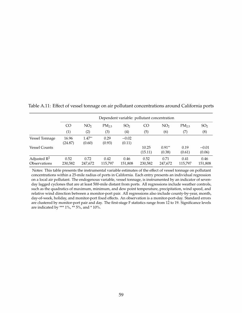
Table A.11: Effect of vessel tonnage on air pollutant concentrations around California ports

Dependent variable: pollutant concentration

CO NO2 PM2.5 SO2 CO NO2 PM2.5 SO2

(1) (2) (3) (4) (5) (6) (7) (8)Vessel Tonnage 16.96 1.47∗∗ 0.29 −0.02

(24.87) (0.60) (0.93) (0.11)Vessel Counts 10.25 0.91∗∗ 0.19 −0.01

(15.11) (0.38) (0.61) (0.06)

Adjusted R2 0.52 0.72 0.42 0.46 0.52 0.71 0.41 0.46Observations 230,582 247,672 115,797 151,808 230,582 247,672 115,797 151,808

Notes: This table presents the instrumental variable estimates of the effect of vessel tonnage on pollutantconcentrations within a 25-mile radius of ports in California. Each entry presents an individual regressionon a local air pollutant. The endogenous variable, vessel tonnage, is instrumented by an indicator of seven-day lagged cyclones that are at least 500-mile distant from ports. All regressions include weather controls,such as the quadratics of maximum, minimum, and dew point temperature, precipitation, wind speed, andrelative wind direction between a monitor-port pair. All regressions also include county-by-year, month,day-of-week, holiday, and monitor-port fixed effects. An observation is a monitor-port-day. Standard errorsare clustered by monitor-port pair and day. The first-stage F statistics range from 12 to 19. Significance levelsare indicated by *** 1%, ** 5%, and * 10%.

59

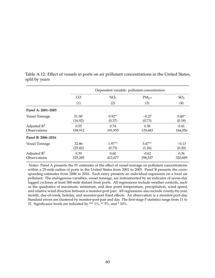
Table A.12: Effect of vessels in ports on air pollutant concentrations in the United States,split by years

Dependent variable: pollutant concentration

CO NO2 PM2.5 SO2

(1) (2) (3) (4)

Panel A: 2001–2005

Vessel Tonnage 31.38∗ 0.92∗∗ −0.27 0.40∗∗(16.92) (0.37) (0.73) (0.18)

Adjusted R2 0.55 0.74 0.38 0.41Observations 198,912 191,955 129,683 164,056

Panel B: 2006–2016

Vessel Tonnage 32.86 1.97∗∗∗ 3.47∗∗∗ −0.13(25.82) (0.73) (1.26) (0.20)

Adjusted R2 0.39 0.60 -0.62 0.36Observations 325,285 412,677 298,537 320,689

Notes: Panel A presents the IV estimates of the effect of vessel tonnage on pollutant concentrationswithin a 25-mile radius of ports in the United States from 2001 to 2005. Panel B presents the corre-sponding estimates from 2006 to 2016. Each entry presents an individual regression on a local airpollutant. The endogenous variables, vessel tonnage, are instrumented by an indicator of seven-daylagged cyclones at least 500-mile distant from ports. All regressions include weather controls, suchas the quadratics of maximum, minimum, and dew point temperature, precipitation, wind speed,and relative wind direction between a monitor-port pair. All regressions also include county-by-year,month, day-of-week, holiday, and monitor-port fixed effects. An observation is a monitor-port-day.Standard errors are clustered by monitor-port pair and day. The first-stage F statistics range from 11 to21. Significance levels are indicated by *** 1%, ** 5%, and * 10%.

60

Table A.13: 2SLS estimation of the effect of vessels in port on ozone pollution

Dependent variable: pollutant concentration

(1) (2)Vessel Tonnage −1.19

(0.78)Vessel Counts −0.55

(0.38)1st-Stage F Stat. 36.10 19.60Adjusted R2 0.38 0.37Observations 848,889 848,889

Notes: Panel A presents the OLS estimates of the effect of port traffic on O3 concentrations within a 25-mileradius of ports in the United States. Panel B presents the IV estimates of the effect of port traffic on O3 concen-trations within a 25-mile radius of ports in the United States. Each entry presents an individual regression on alocal air pollutant. The endogenous variables, vessel tonnage and the number of vessels, are instrumented byan indicator of seven-day lagged cyclones that are at least 500-mile distant from ports. All regressions includeweather controls, such as the quadratics of maximum, minimum, and dew point temperature, precipitation,wind speed, and relative wind direction between a monitor-port pair. All regressions also include county-by-year, month, day-of-week, holiday, and monitor-port fixed effects. An observation is a monitor-port-day.Standard errors are clustered by monitor-port pair and day. The first-stage F statistics for column (1) is 36 andfor column (2) is 20. Significance levels are indicated by *** 1%, ** 5%, and * 10%.

61

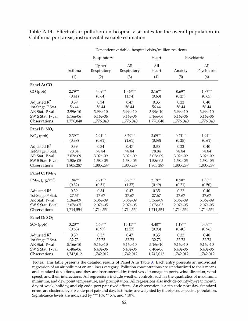
Table A.14: Effect of air pollution on hospital visit rates for the overall population inCalifornia port areas, instrumental variable estimation

Dependent variable: hospital visits/million residents

Respiratory Heart Psychiatric

Upper All All AllAsthma Respiratory Respiratory Heart Anxiety Psychiatric

(1) (2) (3) (4) (5) (6)

Panel A: CO

CO (ppb) 2.79∗∗∗ 3.09∗∗∗ 10.46∗∗∗ 3.16∗∗∗ 0.69∗∗ 1.87∗∗∗(0.41) (0.64) (1.74) (0.63) (0.27) (0.65)

Adjusted R2 0.39 0.34 0.47 0.35 0.22 0.401st-Stage F Stat. 56.44 56.44 56.44 56.44 56.44 56.44AR Stat. P-val 3.99e-10 3.99e-10 3.99e-10 3.99e-10 3.99e-10 3.99e-10SW S Stat. P-val 5.16e-06 5.16e-06 5.16e-06 5.16e-06 5.16e-06 5.16e-06Observations 1,776,040 1,776,040 1,776,040 1,776,040 1,776,040 1,776,040

Panel B: NO2

NO2 (ppb) 2.39∗∗∗ 2.91∗∗∗ 8.79∗∗∗ 3.09∗∗∗ 0.71∗∗∗ 1.94∗∗∗(0.38) (0.61) (1.61) (0.58) (0.25) (0.61)

Adjusted R2 0.39 0.34 0.47 0.35 0.22 0.401st-Stage F Stat. 78.84 78.84 78.84 78.84 78.84 78.84AR Stat. P-val 3.02e-09 3.02e-09 3.02e-09 3.02e-09 3.02e-09 3.02e-09SW S Stat. P-val 1.58e-05 1.58e-05 1.58e-05 1.58e-05 1.58e-05 1.58e-05Observations 1,805,287 1,805,287 1,805,287 1,805,287 1,805,287 1,805,287

Panel C: PM2.5

PM2.5 (�g/m3) 1.84∗∗∗ 2.21∗∗∗ 6.73∗∗∗ 2.19∗∗∗ 0.50∗∗ 1.33∗∗∗(0.32) (0.51) (1.37) (0.49) (0.21) (0.50)

Adjusted R2 0.39 0.34 0.47 0.35 0.22 0.401st-Stage F Stat. 27.67 27.67 27.67 27.67 27.67 27.67AR Stat. P-val 5.36e-09 5.36e-09 5.36e-09 5.36e-09 5.36e-09 5.36e-09SW S Stat. P-val 2.07e-05 2.07e-05 2.07e-05 2.07e-05 2.07e-05 2.07e-05Observations 1,714,554 1,714,554 1,714,554 1,714,554 1,714,554 1,714,554

Panel D: SO2

SO2 (ppb) 3.28∗∗∗ 4.68∗∗∗ 13.13∗∗∗ 4.40∗∗∗ 1.19∗∗∗ 3.08∗∗∗(0.63) (0.97) (2.57) (0.93) (0.40) (0.96)

Adjusted R2 0.39 0.33 0.47 0.35 0.22 0.401st-Stage F Stat. 32.73 32.73 32.73 32.73 32.73 32.73AR Stat. P-val 5.16e-10 5.16e-10 5.16e-10 5.16e-10 5.16e-10 5.16e-10SW S Stat. P-val 6.40e-06 6.40e-06 6.40e-06 6.40e-06 6.40e-06 6.40e-06Observations 1,742,012 1,742,012 1,742,012 1,742,012 1,742,012 1,742,012

Notes: This table presents the detailed results of Panel A in Table 3. Each entry presents an individualregression of an air pollutant on an illness category. Pollution concentrations are standardized to their meansand standard deviations, and they are instrumented by fitted vessel tonnage in ports, wind direction, windspeed, and their interactions. All regressions include weather controls, such as the quadratics of maximum,minimum, and dew point temperature, and precipitation. All regressions also include county-by-year, month,day-of-week, holiday, and zip code-port pair fixed effects. An observation is a zip code-port-day. Standarderrors are clustered by zip code-port pair and day. Estimates are weighted by the zip code-specific population.Significance levels are indicated by *** 1%, ** 5%, and * 10%.

62

Table A.15: Effect of air pollution on hospital visit rates for Blacks in California port areas,instrumental variable estimation

Dependent variable: hospital visits/million residents

Respiratory Heart Psychiatric

Upper All All AllAsthma Respiratory Respiratory Heart Anxiety Psychiatric

(1) (2) (3) (4) (5) (6)

Panel A: CO

CO (ppb) 7.81∗∗∗ 5.38∗∗∗ 20.44∗∗∗ 5.74∗∗∗ 0.92 −0.04(1.63) (1.43) (4.04) (1.79) (0.81) (1.88)

Adjusted R2 0.17 0.10 0.23 0.13 0.05 0.191st-Stage F Stat. 46.35 46.35 46.35 46.35 46.35 46.35AR Stat. P-val 0 0 0 0 0 0SW S Stat. P-val 0.000361 0.000361 0.000361 0.000361 0.000361 0.000361Observations 877,072 877,072 877,072 877,072 877,072 877,072

Panel B: NO2

NO2 (ppb) 7.18∗∗∗ 8.77∗∗∗ 23.32∗∗∗ 5.95∗∗∗ 1.23 0.66(1.68) (1.48) (4.23) (1.85) (0.85) (1.96)

Adjusted R2 0.17 0.10 0.23 0.13 0.05 0.191st-Stage F Stat. 61.44 61.44 61.44 61.44 61.44 61.44AR Stat. P-val 0 0 0 0 0 0SW S Stat. P-val 0.000338 0.000338 0.000338 0.000338 0.000338 0.000338Observations 887,300 887,300 887,300 887,300 887,300 887,300

Panel C: PM2.5

PM2.5 (�g/m3) 5.66∗∗∗ 6.28∗∗∗ 18.00∗∗∗ 3.77∗∗∗ 0.38 −0.53(1.28) (1.13) (3.29) (1.41) (0.60) (1.45)

Adjusted R2 0.17 0.10 0.23 0.13 0.05 0.191st-Stage F Stat. 23.52 23.52 23.52 23.52 23.52 23.52AR Stat. P-val 3.32e-10 3.32e-10 3.32e-10 3.32e-10 3.32e-10 3.32e-10SW S Stat. P-val 0.000549 0.000549 0.000549 0.000549 0.000549 0.000549Observations 846,980 846,980 846,980 846,980 846,980 846,980

Panel D: SO2

SO2 (ppb) 10.87∗∗∗ 16.35∗∗∗ 39.10∗∗∗ 8.23∗∗∗ 1.93 1.54(2.54) (2.41) (6.65) (2.88) (1.35) (3.07)

Adjusted R2 0.17 0.10 0.23 0.13 0.05 0.191st-Stage F Stat. 21.09 21.09 21.09 21.09 21.09 21.09AR Stat. P-val 0 0 0 0 0 0SW S Stat. P-val 0.000292 0.000292 0.000292 0.000292 0.000292 0.000292Observations 871,296 871,296 871,296 871,296 871,296 871,296

Notes: This table presents the detailed results of Panel B in Table 3. Each entry presents an individual regression of anair pollutant on an illness category. Pollution concentrations are standardized to their means and standard deviations,and they are instrumented by fitted vessel tonnage in ports, wind direction, wind speed, and their interactions. Allregressions include weather controls, such as the quadratics of maximum, minimum, and dew point temperature, andprecipitation. All regressions also include county-by-year, month, day-of-week, holiday, and zip code-port pair fixedeffects. An observation is a zip code-port-day. Standard errors are clustered by zip code-port pair and day. Estimatesare weighted by the zip code-specific population. Significance levels are indicated by *** 1%, ** 5%, and * 10%.

63

Table A.16: Effect of air pollution on hospital visit rates for whites in California port areas,instrumental variable estimation

Dependent variable: hospital visits/million residents

Respiratory Heart Psychiatric

Upper All All AllAsthma Respiratory Respiratory Heart Anxiety Psychiatric

(1) (2) (3) (4) (5) (6)

Panel A: CO

CO (ppb) 2.41∗∗∗ 2.10∗∗∗ 9.55∗∗∗ 4.02∗∗∗ 0.11 2.38∗(0.51) (0.41) (1.56) (1.16) (0.54) (1.25)

Adjusted R2 0.17 0.09 0.34 0.28 0.15 0.321st-Stage F Stat. 58.31 58.31 58.31 58.31 58.31 58.31AR Stat. P-val 8.13e-10 8.13e-10 8.13e-10 8.13e-10 8.13e-10 8.13e-10SW S Stat. P-val 8.72e-06 8.72e-06 8.72e-06 8.72e-06 8.72e-06 8.72e-06Observations 1,650,747 1,650,747 1,650,747 1,650,747 1,650,747 1,650,747

Panel B: NO2

NO2 (ppb) 1.78∗∗∗ 1.80∗∗∗ 6.84∗∗∗ 3.51∗∗∗ 0.22 2.32∗∗(0.46) (0.40) (1.42) (1.01) (0.48) (1.12)

Adjusted R2 0.17 0.09 0.34 0.28 0.15 0.321st-Stage F Stat. 83.18 83.18 83.18 83.18 83.18 83.18AR Stat. P-val 1.84e-08 1.84e-08 1.84e-08 1.84e-08 1.84e-08 1.84e-08SW S Stat. P-val 2.95e-05 2.95e-05 2.95e-05 2.95e-05 2.95e-05 2.95e-05Observations 1,679,994 1,679,994 1,679,994 1,679,994 1,679,994 1,679,994

Panel C: PM2.5

PM2.5 (�g/m3) 1.53∗∗∗ 1.51∗∗∗ 5.55∗∗∗ 2.78∗∗∗ 0.16 1.82∗(0.41) (0.35) (1.29) (0.91) (0.43) (0.99)

Adjusted R2 0.17 0.09 0.34 0.28 0.15 0.321st-Stage F Stat. 27.30 27.30 27.30 27.30 27.30 27.30AR Stat. P-val 2.31e-08 2.31e-08 2.31e-08 2.31e-08 2.31e-08 2.31e-08SW S Stat. P-val 4.14e-05 4.14e-05 4.14e-05 4.14e-05 4.14e-05 4.14e-05Observations 1,598,695 1,598,695 1,598,695 1,598,695 1,598,695 1,598,695

Panel D: SO2

SO2 (ppb) 2.05∗∗∗ 2.63∗∗∗ 8.98∗∗∗ 4.64∗∗∗ 0.35 3.35∗∗(0.69) (0.58) (2.10) (1.49) (0.70) (1.63)

Adjusted R2 0.17 0.09 0.33 0.28 0.15 0.321st-Stage F Stat. 38.52 38.52 38.52 38.52 38.52 38.52AR Stat. P-val 9.80e-10 9.80e-10 9.80e-10 9.80e-10 9.80e-10 9.80e-10SW S Stat. P-val 8.90e-06 8.90e-06 8.90e-06 8.90e-06 8.90e-06 8.90e-06Observations 1,616,890 1,616,890 1,616,890 1,616,890 1,616,890 1,616,890

Notes: This table presents the detailed results of Panel C in Table 3. Each entry presents an individual regression of anair pollutant on an illness category. Pollution concentrations are standardized to their means and standard deviations,and they are instrumented by fitted vessel tonnage in ports, wind direction, wind speed, and their interactions. Allregressions include weather controls, such as the quadratics of maximum, minimum, and dew point temperature, andprecipitation. All regressions also include county-by-year, month, day-of-week, holiday, and zip code-port pair fixedeffects. An observation is a zip code-port-day. Standard errors are clustered by zip code-port pair and day. Estimates areweighted by the zip code-specific population. Significance levels are indicated by *** 1%, ** 5%, and * 10%.

64

Table A.17: OLS estimates of the effect of air pollution on hospital visit rates in Californiaport areas

Dependent variable: hospital visits/million residents

Respiratory Heart Psychiatric

Upper All All AllAsthma Respiratory Respiratory Heart Anxiety Psychiatric

(1) (2) (3) (4) (5) (6)

Panel A: Overall population

CO (ppb) 0.63∗∗∗ 0.24 2.06∗∗∗ 1.20∗∗∗ 0.09 0.25(0.19) (0.23) (0.76) (0.30) (0.09) (0.23)

NO2 (ppb) 1.36∗∗∗ −0.11 3.94∗∗∗ 3.18∗∗∗ 0.66∗∗∗ 2.05∗∗∗(0.24) (0.37) (0.98) (0.44) (0.16) (0.44)

PM2.5 (�g/m3) 0.49∗∗∗ 0.32∗ 1.39∗∗∗ −0.07 0.06 0.07(0.12) (0.18) (0.50) (0.24) (0.09) (0.23)

SO2 (ppb) 0.47∗∗∗ −0.43∗∗∗ −0.55 0.35∗∗ 0.09 0.27(0.13) (0.16) (0.45) (0.17) (0.08) (0.19)

Panel B: Black

CO (ppb) 2.41∗∗∗ −0.17 5.00∗∗∗ 2.59∗∗∗ 0.58∗∗ 1.52∗∗(0.70) (0.54) (1.72) (0.74) (0.28) (0.74)

NO2 (ppb) 4.13∗∗∗ 0.65 11.12∗∗∗ 5.06∗∗∗ 1.50∗∗∗ 4.20∗∗∗(1.02) (0.91) (2.65) (1.11) (0.43) (1.16)

PM2.5 (�g/m3) 1.70∗∗∗ −0.08 2.33∗ 0.34 0.28 0.01(0.54) (0.45) (1.35) (0.59) (0.22) (0.58)

SO2 (ppb) 2.63∗∗∗ −0.10 2.36 0.81 −0.03 0.64(0.70) (0.56) (1.64) (0.59) (0.26) (0.67)

Panel C: White

CO (ppb) 0.74∗∗∗ −0.08 2.55∗∗∗ 2.17∗∗∗ 0.19 0.64(0.23) (0.13) (0.77) (0.50) (0.17) (0.43)

NO2 (ppb) 2.09∗∗∗ −0.30 6.87∗∗∗ 6.51∗∗∗ 1.50∗∗∗ 4.84∗∗∗(0.29) (0.23) (0.90) (0.72) (0.28) (0.73)

PM2.5 (�g/m3) 0.31∗∗ 0.02 0.68 −0.17 0.01 0.14(0.15) (0.11) (0.44) (0.38) (0.16) (0.38)

SO2 (ppb) 0.49∗∗∗ −0.29∗∗∗ −0.09 0.53∗ −0.12 0.02(0.15) (0.10) (0.38) (0.31) (0.15) (0.33)

Notes: This table presents the OLS estimation of the effect of air pollution on hospital visit rates for the overallpopulation, Blacks, and whites. Each entry presents an individual regression of an air pollutant on an illnesscategory. Pollution concentrations are standardized to their means and standard deviations. All regressionsinclude weather controls, such as the quadratics of maximum temperature, minimum temperature, dew pointtemperature, precipitation, wind speed, and relative wind direction between a zip code-port pair. All regressionsalso include county-by-year, month, day-of-week, holiday, and zip code-port pair fixed effects. An observation is azip code-port-day. Standard errors are clustered by zip code-port pair and day. Estimates are weighted by the zipcode-specific population. Significance levels are indicated by *** 1%, ** 5%, and * 10%.

65

Table A.18: Elasticities of the effect of pollution on hospital visit rates for Blacks and whitesin California port areas

Dependent variable: IHS transformation of hospital visit rates

Respiratory Heart Psychiatric

Upper All All AllAsthma Respiratory Respiratory Heart Anxiety Psychiatric

(1) (2) (3) (4) (5) (6)

Panel A: Black

CO (ppb) 0.103∗∗∗ 0.224∗∗∗ 0.091∗∗∗ 0.124∗∗∗ 0.068 −0.003(0.038) (0.058) (0.026) (0.036) (0.054) (0.042)

NO2 (ppb) 0.016 0.189∗∗∗ 0.038∗ 0.063∗∗ 0.051 0.002(0.027) (0.040) (0.021) (0.027) (0.039) (0.030)

PM2.5 (�g/m3) 0.051∗ 0.174∗∗∗ 0.059∗∗∗ 0.064∗∗ 0.032 −0.015(0.027) (0.041) (0.020) (0.026) (0.038) (0.030)

SO2 (ppb) 0.185∗∗ 0.531∗∗∗ 0.184∗∗∗ 0.248∗∗∗ 0.209∗ 0.010(0.075) (0.112) (0.054) (0.075) (0.113) (0.082)

Panel B: White

CO (ppb) 0.125∗∗∗ 0.141∗∗∗ 0.083∗∗∗ 0.084∗∗∗ 0.005 0.056∗(0.033) (0.037) (0.023) (0.024) (0.035) (0.028)

NO2 (ppb) 0.037∗ 0.112∗∗∗ 0.039∗∗ 0.049∗∗∗ 0.017 0.034∗(0.021) (0.027) (0.015) (0.015) (0.023) (0.018)

PM2.5 (�g/m3) 0.056∗∗ 0.111∗∗∗ 0.043∗∗ 0.058∗∗∗ 0.021 0.044∗∗(0.024) (0.030) (0.017) (0.017) (0.025) (0.020)

SO2 (ppb) 0.191∗∗∗ 0.281∗∗∗ 0.145∗∗∗ 0.153∗∗∗ 0.021 0.099∗(0.063) (0.074) (0.045) (0.044) (0.065) (0.052)

Notes: This table presents the instrumental variable estimation of elasticities of the effect of pollution on hos-pital visit rates for Blacks and whites in California port areas. Each entry presents an individual regression ofan air pollutant on an illness category. The dependent variables and pollution measures are IHS transformed.The instruments include fitted vessel tonnage in ports, wind direction, wind speed, and their interactions. Allregressions include weather controls, such as the quadratics of maximum, minimum, and dew point temperature,and precipitation. All regressions also include county-by-year, month, day-of-week, holiday, and zip code-port pairfixed effects. An observation is a zip code-port-day. Standard errors are clustered by zip code-port pair and day.The first-stage F statistics range from 20 to 91 for Panel A and from 31 to 103 for Panel B. Estimates are weighted bythe zip code-specific population. Significance levels are indicated by *** 1%, ** 5%, and * 10%.

66

Table A.19: Test for differences of hospital visit rates of Blacks and whites in Californiaport areas

Respiratory Heart Psychiatric

Asthma UpperRespiratory

AllRespiratory

AllHeart Anxiety All

Psychiatric(1) (2) (3) (4) (5) (6)

CO (ppb) 5.40∗∗∗ 3.29∗∗ 10.88∗∗ 1.73 0.81 -2.43[3.15] [2.21] [2.51] [0.81] [0.83] [-1.08]

NO2 (ppb) 5.41∗∗∗ 6.97∗∗∗ 16.48∗∗∗ 2.44 1.01 -1.66[3.10] [4.55] [3.69] [1.16] [1.04] [-0.73]

PM2.5 (�g/m3) 4.13∗∗∗ 4.77∗∗∗ 12.45∗∗∗ 0.98 0.22 -2.35[3.08] [4.04] [3.52] [0.58] [0.29] [-1.34]

SO2 (ppb) 8.83∗∗∗ 13.72∗∗∗ 30.12∗∗∗ 3.59 1.58 -1.81[3.35] [5.53] [4.32] [1.11] [1.04] [-0.52]

Notes: This table presents the statistical tests for the equality of regression coefficients for Blacks and whites in Panels Band C in Table 3. Pollution concentrations are standardized to their means and standard deviations. Each entry presentsan individual test. The numbers in square brackets are Z-scores. Significance levels are indicated by *** 1%, ** 5%, and *10%.

Table A.20: Effect of air pollution on differences of hospital visit rates between Blacks andwhites in California port areas, instrumental variable estimation

Dependent variable: hospital visit rate for Blacks – hospital visit rate for whites

Respiratory Heart Psychiatric

Upper All All AllAsthma Respiratory Respiratory Heart Anxiety Psychiatric

(1) (2) (3) (4) (5) (6)CO (ppb) 6.75∗∗∗ 5.65∗∗∗ 11.50∗∗ −0.93 −0.26 −6.20

(2.47) (1.83) (5.09) (3.09) (1.88) (4.01)NO2 (ppb) 6.62∗∗∗ 9.13∗∗∗ 17.65∗∗∗ −0.85 −0.52 −5.14

(2.34) (1.71) (4.90) (2.85) (1.74) (3.67)PM2.5 (�g/m3) 5.31∗∗∗ 6.76∗∗∗ 14.03∗∗∗ −1.31 −0.39 −4.62

(1.93) (1.45) (4.13) (2.29) (1.40) (3.08)SO2 (ppb) 10.01∗∗∗ 14.72∗∗∗ 29.78∗∗∗ 0.18 −0.55 −5.72

(3.26) (2.53) (7.07) (4.00) (2.31) (4.78)

Notes: This table presents the effects of pollution on the differences of hospital visit rates between Blacks and whites.Each entry presents an individual regression of an air pollutant on an illness category. Pollution concentrations arestandardized to their means and standard deviations, and they are instrumented by fitted vessel tonnage in ports,wind direction, wind speed, and their interactions. All regressions include weather controls, such as the quadraticsof maximum, minimum, and dew point temperature, and precipitation. All regressions also include county-by-year,month, day-of-week, holiday, and zip code-port pair fixed effects. An observation is a zip code-port-day. Standarderrors are clustered by zip code-port pair and day. Estimates are weighted by the zip code-specific population. Thefirst-stage F statistics range from 26 to 72. Significance levels are indicated by *** 1%, ** 5%, and * 10%.

67

Table A.21: Effect of air pollution on hospital visit rates for Hispanics in California portareas

Dependent variable: hospital visits/million residents

Respiratory Heart Psychiatric

Upper All All AllAsthma Respiratory Respiratory Heart Anxiety Psychiatric

(1) (2) (3) (4) (5) (6)CO (ppb) 2.21∗∗∗ 3.76∗∗∗ 10.29∗∗∗ 0.79 1.40∗∗∗ 2.71∗∗∗

(0.55) (0.82) (1.98) (0.66) (0.42) (0.86)NO2 (ppb) 2.18∗∗∗ 4.16∗∗∗ 9.92∗∗∗ 0.96 1.15∗∗∗ 2.59∗∗∗

(0.50) (0.78) (1.82) (0.60) (0.38) (0.78)PM2.5 (�g/m3) 1.37∗∗∗ 3.15∗∗∗ 6.97∗∗∗ 0.26 1.05∗∗∗ 1.91∗∗∗

(0.41) (0.65) (1.52) (0.48) (0.31) (0.65)SO2 (ppb) 3.07∗∗∗ 7.00∗∗∗ 15.53∗∗∗ 1.47 1.84∗∗∗ 4.33∗∗∗

(0.85) (1.25) (2.90) (0.95) (0.62) (1.31)

Notes: This table presents the instrumental variable estimation of the effect of air pollution on hospital visit ratesfor the Hispanic population. Each entry presents an individual regression of an air pollutant on an illness category.Pollution concentrations are standardized to their means and standard deviations, and they are instrumented byfitted vessel tonnage in ports, wind direction, wind speed, and their interactions. All regressions include weathercontrols, such as the quadratics of maximum temperature, minimum temperature, dew point temperature, andprecipitation. All regressions also include county-by-year, month, day-of-week, holiday, and zip code-port pairfixed effects. An observation is a zip code-port-day. Standard errors are clustered by zip code-port pair andday. Estimates are weighted by the zip code-specific population. The first-stage F statistics range from 28 to 79.Significance levels are indicated by *** 1%, ** 5%, and * 10%.

68

Table A.22: Effect of air pollution on hospital visit rates in California port areas by age

Dependent variable: hospital visits/million residents in each age group

Respiratory Heart Psychiatric

Upper All All AllAsthma Respiratory Respiratory Heart Anxiety Psychiatric

(1) (2) (3) (4) (5) (6)

Panel A: Ages 5 and under

CO (ppb) 2.97∗∗ 13.63∗∗∗ 22.97∗∗∗ 0.46∗ 0.12 0.92∗∗∗(1.27) (4.46) (8.62) (0.27) (0.09) (0.23)

NO2 (ppb) 3.16∗∗∗ 14.05∗∗∗ 20.00∗∗ 0.50∗ 0.10 0.76∗∗∗(1.21) (4.20) (8.07) (0.27) (0.08) (0.21)

PM2.5 (�g/m3) 2.27∗∗ 9.23∗∗∗ 12.52∗ 0.27 0.08 0.72∗∗∗(0.96) (3.36) (6.53) (0.20) (0.06) (0.17)

SO2 (ppb) 4.13∗∗ 21.71∗∗∗ 27.81∗∗ 0.72∗ 0.16 1.07∗∗∗(2.07) (6.93) (13.25) (0.44) (0.14) (0.36)

Panel B: Ages between 5 and 19

CO (ppb) 2.41∗∗∗ 3.59∗∗∗ 7.78∗∗∗ 0.14 −0.10 0.46(0.71) (1.08) (2.30) (0.11) (0.20) (0.55)

NO2 (ppb) 2.47∗∗∗ 3.46∗∗∗ 6.67∗∗∗ 0.18∗ −0.03 0.82(0.67) (1.03) (2.17) (0.11) (0.19) (0.52)

PM2.5 (�g/m3) 1.90∗∗∗ 2.75∗∗∗ 5.37∗∗∗ 0.09 0.05 0.67(0.54) (0.86) (1.79) (0.09) (0.15) (0.42)

SO2 (ppb) 3.52∗∗∗ 6.67∗∗∗ 11.35∗∗∗ 0.23 −0.07 1.55∗(1.13) (1.67) (3.51) (0.18) (0.31) (0.85)

Panel C: Ages between 20 and 64

CO (ppb) 2.42∗∗∗ 1.92∗∗∗ 8.19∗∗∗ 1.42∗∗∗ 0.93∗∗∗ 1.44∗(0.41) (0.36) (1.24) (0.42) (0.34) (0.74)

NO2 (ppb) 1.94∗∗∗ 2.20∗∗∗ 7.35∗∗∗ 1.26∗∗∗ 0.91∗∗∗ 1.50∗∗(0.37) (0.34) (1.13) (0.39) (0.32) (0.69)

PM2.5 (�g/m3) 1.50∗∗∗ 1.75∗∗∗ 5.76∗∗∗ 0.82∗∗∗ 0.66∗∗ 0.97∗(0.31) (0.29) (0.98) (0.32) (0.26) (0.57)

SO2 (ppb) 2.72∗∗∗ 3.72∗∗∗ 11.36∗∗∗ 1.80∗∗∗ 1.49∗∗∗ 2.37∗∗(0.61) (0.56) (1.87) (0.61) (0.50) (1.10)

Panel D: Ages 65 and above

CO (ppb) 4.31∗∗∗ 0.50 15.80∗∗∗ 17.87∗∗∗ 0.67 5.90∗∗∗(1.08) (0.51) (4.02) (3.96) (0.96) (2.11)

NO2 (ppb) 4.02∗∗∗ 0.93∗∗ 14.51∗∗∗ 17.01∗∗∗ 0.86 5.94∗∗∗(0.99) (0.45) (3.57) (3.57) (0.86) (1.89)

PM2.5 (�g/m3) 2.98∗∗∗ 0.56 11.04∗∗∗ 12.53∗∗∗ 0.40 4.13∗∗∗(0.83) (0.38) (3.10) (3.06) (0.71) (1.58)

SO2 (ppb) 5.86∗∗∗ 1.60∗∗ 20.75∗∗∗ 22.63∗∗∗ 1.69 9.33∗∗∗(1.56) (0.70) (5.39) (5.52) (1.28) (2.90)

Notes: This table presents the instrumental variable estimation of the effect of air pollution on hospital visitrates by age. Each entry presents an individual regression of an air pollutant on an illness category. Pollutionconcentrations are standardized to their means and standard deviations, and they are instrumented by fitted vesseltonnage in ports, wind direction, wind speed, and their interactions. All regressions include weather controls, suchas the quadratics of maximum temperature, minimum temperature, dew point temperature, and precipitation.All regressions also include county-by-year, month, day-of-week, holiday, and zip code-port pair fixed effects. Anobservation is a zip code-port-day. Standard errors are clustered by zip code-port pair and day. Estimates areweighted by the zip code-specific population. The first-stage F statistics range from 27 to 79. Significance levels areindicated by *** 1%, ** 5%, and * 10%.

69

Table A.23: Effect of air pollution on hospital visit rates in California port areas by sex

Dependent variable: hospital visits/million residents in each sex group

Respiratory Heart Psychiatric

Upper All All AllAsthma Respiratory Respiratory Heart Anxiety Psychiatric

(1) (2) (3) (4) (5) (6)

Panel A: Male

CO (ppb) 2.20∗∗∗ 2.58∗∗∗ 9.09∗∗∗ 2.77∗∗∗ 0.64∗∗∗ 1.72∗∗∗(0.40) (0.63) (1.64) (0.76) (0.23) (0.61)

NO2 (ppb) 1.85∗∗∗ 2.35∗∗∗ 7.56∗∗∗ 2.80∗∗∗ 0.59∗∗∗ 1.85∗∗∗(0.37) (0.59) (1.53) (0.70) (0.22) (0.57)

PM2.5 (�g/m3) 1.43∗∗∗ 1.81∗∗∗ 5.76∗∗∗ 1.78∗∗∗ 0.43∗∗ 1.18∗∗(0.31) (0.49) (1.30) (0.57) (0.18) (0.47)

SO2 (ppb) 2.36∗∗∗ 3.75∗∗∗ 11.14∗∗∗ 3.66∗∗∗ 1.00∗∗∗ 2.79∗∗∗(0.62) (0.93) (2.42) (1.12) (0.34) (0.91)

Panel B: Female

CO (ppb) 3.37∗∗∗ 3.58∗∗∗ 11.79∗∗∗ 3.52∗∗∗ 0.76∗ 2.02∗∗(0.52) (0.71) (1.93) (0.63) (0.40) (0.85)

NO2 (ppb) 2.91∗∗∗ 3.45∗∗∗ 9.98∗∗∗ 3.37∗∗∗ 0.84∗∗ 2.04∗∗(0.49) (0.67) (1.80) (0.59) (0.37) (0.80)

PM2.5 (�g/m3) 2.24∗∗∗ 2.59∗∗∗ 7.68∗∗∗ 2.59∗∗∗ 0.58∗ 1.50∗∗(0.40) (0.56) (1.52) (0.50) (0.30) (0.65)

SO2 (ppb) 4.19∗∗∗ 5.59∗∗∗ 15.07∗∗∗ 5.10∗∗∗ 1.39∗∗ 3.40∗∗∗(0.80) (1.09) (2.89) (0.95) (0.59) (1.26)

Notes: This table presents the instrumental variable estimation of the effect of air pollution on hospital visitrates by sex. Each entry presents an individual regression of an air pollutant on an illness category. Pollutionconcentrations are standardized to their means and standard deviations, and they are instrumented by fittedvessel tonnage in ports, wind direction, wind speed, and their interactions. All regressions include weathercontrols, such as the quadratics of maximum temperature, minimum temperature, dew point temperature, andprecipitation. All regressions also include county-by-year, month, day-of-week, holiday, and zip code-port pairfixed effects. An observation is a zip code-port-day. Standard errors are clustered by zip code-port pair andday. Estimates are weighted by the zip code-specific population. The first-stage F statistics range from 28 to 79.Significance levels are indicated by *** 1%, ** 5%, and * 10%.

70

Table A.24: Effect of air pollution on hospital visit rates of placebo illnesses for the overallpopulation in California port areas, instrumental variable estimation

Dependent variable: hospital visits/million residents

ArterialAppendicitis Embolism

(1) (2)

Panel A: CO

CO (ppb) 0.09 0.03(0.06) (0.02)

Adjusted R2 0.01 0.00Observations 1,776,040 1,776,040

Panel B: NO2

NO2 (ppb) 0.08 0.02(0.05) (0.02)

Adjusted R2 0.01 0.00Observations 1,805,287 1,805,287

Panel C: PM2.5

PM2.5 (�g/m3) 0.07 0.02(0.04) (0.02)

Adjusted R2 0.01 0.00Observations 1,714,554 1,714,554

Panel D: SO2

SO2 (ppb) 0.14∗ 0.03(0.08) (0.03)

Adjusted R2 0.01 0.00Observations 1,742,012 1,742,012

Notes: This table presents the instrumental variable estimation of the effect of air pollution on hospital visitrates for placebo illnesses. Each entry presents an individual regression of an air pollutant on an illness category.Pollution concentrations are standardized to their means and standard deviations, and they are instrumentedby fitted vessel tonnage in ports, wind direction, wind speed, and their interactions. All regressions includeweather controls, such as the quadratics of maximum temperature, minimum temperature, dew point tem-perature, and precipitation. All regressions also include county-by-year, month, day-of-week, holiday, andzip code-port pair fixed effects. An observation is a zip code-port-day. Standard errors are clustered by zipcode-port pair and day. Estimates are weighted by the zip code-specific population. The first-stage F statisticsrange from 28 to 79. Significance levels are indicated by *** 1%, ** 5%, and * 10%.

71

Table A.25: Robustness check for the effect of vessel tonnage in port on air pollution,various model specifications

Dependent variable: pollutant concentration

CO NO2 PM2.5 SO2

(1) (2) (3) (4)

Panel A: No weather controls and temporal fixed effects

Vessel Tonnage 2,358.96 120.54 4.13 37.07(3,618.78) (263.04) (3.11) (110.60)

Adjusted R2 -167.74 -649.67 -1.34 -514.91Observations 524,197 604,632 428,220 484,745

Panel B: No weather controls

Vessel Tonnage 16.76 0.57 1.15∗ 0.17(16.01) (0.43) (0.66) (0.13)

Adjusted R2 0.45 0.61 0.13 0.39Observations 524,197 604,632 428,220 484,745

Panel C: No temporal fixed effects

Vessel Tonnage 233.52∗∗∗ 9.84∗∗ 8.16∗∗∗ 0.94(88.98) (4.44) (2.21) (0.73)

Adjusted R2 -1.34 -3.79 -5.23 -0.09Observations 524,197 604,632 428,220 484,745

Panel D: No quadratic weather terms

Vessel Tonnage 18.06 0.98∗∗∗ 0.93∗ 0.05(13.53) (0.33) (0.56) (0.12)

Adjusted R2 0.53 0.72 0.29 0.42Observations 524,197 604,632 428,220 484,745

Panel E: Monitors within 12.5 miles of ports

Vessel Tonnage 28.21∗ 1.04∗∗∗ 1.33∗∗ 0.23(14.67) (0.39) (0.57) (0.17)

Adjusted R2 0.59 0.73 0.29 0.39Observations 263,877 282,449 232,277 279,891

Notes: This table presents the robustness check results for Table 2 with various model specifications. Eachpanel presents regressions using an alternative model specification. Log vessel tonnage is instrumented byan indicator of seven-day lagged and 500-mile distant cyclones from ports. All regressions include weathercontrols, such as the quadratics of maximum temperature, minimum temperature, dew point temperature,precipitation, wind speed, and relative wind direction between a monitor-port pair. All regressions alsoinclude county-by-year, month, day-of-week, holiday, and monitor-port pair fixed effects. Standard errorsare clustered by monitor-port pair and day. The first-stage F statistics for Panel A is 0.1–3, for Panel B is21–35, for Panel C is 6–16, for Panel D is 22–36, and for Panel E is 20–25. Significance levels are indicated by*** 1%, ** 5%, and * 10%.

72

Table A.26: Robustness check for the effect of vessel tonnage in port on air pollution,various instrumental variable specifications

Dependent variable: pollutant concentration

CO NO2 PM2.5 SO2

(1) (2) (3) (4)

Panel A: Exclude cyclones within 800 miles of ports

Vessel Tonnage 18.24 0.90∗∗∗ 0.84∗ 0.06(11.80) (0.31) (0.51) (0.12)

Adjusted R2 0.54 0.73 0.35 0.44Observations 524,197 604,632 428,220 484,745

Panel B: Six-day lagged cyclones

Vessel Tonnage 16.90 1.25∗∗∗ 0.97∗ 0.16(13.49) (0.36) (0.57) (0.12)

Adjusted R2 0.54 0.71 0.34 0.43Observations 524,197 604,632 428,220 484,745

Panel C: Eight-day lagged cyclones

Vessel Tonnage 27.75∗∗ 0.95∗∗∗ 0.95 0.08(13.49) (0.34) (0.59) (0.12)

Adjusted R2 0.53 0.73 0.34 0.44Observations 524,197 604,632 428,220 484,745

Panel D: Six-, seven-, and eight-day lagged cyclones (2SLS)

Vessel Tonnage 22.93∗ 1.12∗∗∗ 1.07∗∗ 0.12(12.39) (0.32) (0.50) (0.11)

Adjusted R2 0.53 0.72 0.33 0.43Observations 524,197 604,632 428,220 484,745

Panel E: Six-, seven-, and eight-day lagged cyclones (LIML)

Vessel Tonnage 23.08∗ 1.13∗∗∗ 1.09∗∗ 0.12(12.53) (0.33) (0.52) (0.11)

Adjusted R2 0.53 0.72 0.32 0.43Observations 524,197 604,632 428,220 484,745

Panel F: Cyclone counts

Vessel Tonnage −9.15 0.55∗∗ 1.22∗∗ −0.03(10.92) (0.27) (0.48) (0.09)

Adjusted R2 0.55 0.75 0.30 0.44Observations 524,197 604,632 428,220 484,745

Notes: This table presents the results of robustness check for Table 2 with various instrumental variablespecifications. Each panel presents regressions using an alternative instrumental variable specification. Allregressions include weather controls, such as the quadratics of maximum temperature, minimum tempera-ture, dew point temperature, precipitation, wind speed, and relative wind direction between a monitor-portpair. All regressions also include county-by-year, month, day-of-week, holiday, and monitor-port pair fixedeffects. Standard errors are clustered by monitor-port pair and day. The first-stage F statistics for Panel A is24–31, for Panel B is 21–33, for Panel C is 18–31, for Panel D is 8–12, and for Panel F is 29–41. Significancelevels are indicated by *** 1%, ** 5%, and * 10%.

73

Table A.27: Robustness check for the effect of vessel tonnage in port on air pollution,including and excluding different sets of observations where cyclones are close to ports

Dependent variable: pollutant concentration

CO NO2 PM2.5 SO2

(1) (2) (3) (4)

Panel A: Including 2 days before and after cyclones near ports

Vessel Tonnage 20.32 1.11∗∗∗ 1.17∗∗ 0.15(13.61) (0.34) (0.57) (0.12)

Adjusted R2 0.54 0.72 0.31 0.43Observations 529,953 611,553 433,831 491,725

Panel B: Excluding 21 days after cyclones near ports

Vessel Tonnage 22.62 1.20∗∗∗ 1.54∗∗ 0.12(13.87) (0.35) (0.59) (0.12)

Adjusted R2 0.54 0.71 0.25 0.44Observations 508,766 586,027 412,972 465,777

Notes: Panel A presents the instrumental variable estimation of the effect of vessel tonnage in ports onair pollution, where we include the dates when there exist tropical cyclones near ports (e.g., within the200-mile radius of ports) and two days before and after the events. Panel B presents the instrumentalvariable estimation of the effect of vessel tonnage in ports on air pollution, where we exclude 21 days aftertropical cyclones near ports (e.g., within the 200-mile radius of ports). Each column presents an individualregression on a local air pollutant. Log of vessel tonnage is instrumented by an indicator of seven-day laggedand 500-mile distant cyclones from ports. All regressions include weather controls, such as the quadraticsof maximum temperature, minimum temperature, dew point temperature, precipitation, wind speed, andrelative wind direction between a monitor-port pair. All regressions also include county-by-year, month,day-of-week, holiday, and monitor-port pair fixed effects. Standard errors are clustered by monitor-port pairand day. The first-stage F statistics for Panel A is 21–35 and for Panel B is 21–34. Significance levels areindicated by *** 1%, ** 5%, and * 10%.

74

Table A.28: Effect of air pollution on hospital visit rates in California port areas, satellite-based projected data

Dependent variable: hospital visits/million residents

Respiratory Heart Psychiatric

Upper All All AllAsthma Respiratory Respiratory Heart Anxiety Psychiatric

(1) (2) (3) (4) (5) (6)

Panel A: Overall population

PM2.5 (�g/m3) 1.82∗∗∗ 2.41∗∗∗ 7.05∗∗∗ 2.38∗∗∗ 0.51∗∗ 1.42∗∗∗(0.32) (0.51) (1.38) (0.50) (0.22) (0.52)

Adjusted R2 0.39 0.33 0.47 0.35 0.22 0.40Observations 1,799,639 1,799,639 1,799,639 1,799,639 1,799,639 1,799,639

Panel B: Black

PM2.5 (�g/m3) 5.45∗∗∗ 5.81∗∗∗ 16.72∗∗∗ 4.33∗∗∗ 0.63 −0.10(1.30) (1.09) (3.25) (1.45) (0.63) (1.50)

Adjusted R2 0.17 0.10 0.23 0.13 0.05 0.19Observations 884,524 884,524 884,524 884,524 884,524 884,524

Panel C: White

PM2.5 (�g/m3) 1.40∗∗∗ 1.53∗∗∗ 5.54∗∗∗ 2.82∗∗∗ 0.10 1.77∗(0.40) (0.34) (1.24) (0.89) (0.43) (0.98)

Adjusted R2 0.17 0.09 0.33 0.28 0.15 0.32Observations 1,674,738 1,674,738 1,674,738 1,674,738 1,674,738 1,674,738

Notes: This table presents the instrumental variable estimation of the effect of PM2.5 on hospital visit rates for theoverall population, Blacks, and whites. PM2.5 measures are satellite-based projections, which are standardized by thesample mean and standard deviation. Each entry presents an individual regression of an air pollutant on an illnesscategory. Pollution measures are instrumented by fitted vessel tonnage in ports, wind direction, wind speed, and theirinteractions. All regressions include weather controls, such as the quadratics of maximum temperature, minimumtemperature, dew point temperature, and precipitation. All regressions also include county-by-year, month, day-of-week, holiday, and zip code-port pair fixed effects. An observation is a zip code-port-day. Standard errors are clusteredby zip code-port pair and day. Estimates are weighted by the zip code-specific population. The first-stage F statisticsrange from 32 to 45. Significance levels are indicated by *** 1%, ** 5%, and * 10%.

75

Table A.29: Effect of air pollution on hospital visit rates in California port areas – jointestimation with zip codes within a 25-mile radius from ports

Dependent variable: hospital visits/million residents

All Respiratory All Heart All Psychiatric

(1) (2) (3) (4) (5) (6) (7) (8) (9)

Panel A: Overall population

CO (ppb) 15.34∗∗∗ 9.70∗∗∗ 21.16∗∗∗ 0.59 2.05∗∗ −0.17 −0.51 0.31 −0.08(5.22) (3.03) (5.97) (1.59) (1.00) (1.80) (1.73) (1.08) (1.99)

NO2 (ppb) −5.02 −22.14∗∗∗ 2.64∗ 4.30 2.44 0.75(4.97) (8.49) (1.51) (2.84) (1.70) (3.23)

SO2 (ppb) 0.99 18.29∗∗ 1.83 −1.53 2.70∗ 2.11(4.37) (7.27) (1.40) (2.59) (1.55) (2.91)

1st-Stage F Stat. 23.16 9.46 5.77 23.16 9.46 5.77 23.16 9.46 5.77AR Stat. P-val 3.99e-10 5.16e-10 5.16e-10 3.99e-10 5.16e-10 5.16e-10 3.99e-10 5.16e-10 5.16e-10SW S Stat. P-val 5.16e-06 6.40e-06 6.40e-06 5.16e-06 6.40e-06 6.40e-06 5.16e-06 6.40e-06 6.40e-06Observations 1,776,040 1,742,012 1,742,012 1,776,040 1,742,012 1,742,012 1,776,040 1,742,012 1,742,012

Panel B: Black

CO (ppb) −8.67 −1.08 7.69 2.65 3.89 3.26 −4.95 −3.00 −4.53(13.01) (7.08) (14.61) (4.95) (2.89) (5.31) (5.61) (3.16) (6.33)

NO2 (ppb) 32.05∗∗ −16.77 3.40 1.19 5.41 2.91(13.72) (21.64) (5.20) (8.23) (5.90) (10.12)

SO2 (ppb) 40.46∗∗∗ 52.79∗∗∗ 3.33 2.45 5.33 3.20(11.54) (17.62) (4.64) (7.32) (5.20) (8.89)

1st-Stage F Stat. 15.41 9.86 5.43 15.41 9.86 5.43 15.41 9.86 5.43AR Stat. P-val 0 0 0 0 0 0 0 0 0SW S Stat. P-val 0.000361 0.000292 0.000292 0.000361 0.000292 0.000292 0.000361 0.000292 0.000292Observations 877,072 871,296 871,296 877,072 871,296 871,296 877,072 871,296 871,296

Panel C: White

CO (ppb) 17.02∗∗∗ 12.49∗∗∗ 20.30∗∗∗ 3.03 3.27∗ 1.40 0.23 0.86 −0.11(4.35) (2.69) (5.16) (2.76) (1.83) (3.41) (2.94) (1.91) (3.70)

NO2 (ppb) −7.48∗ −14.74∗ 0.99 3.54 2.15 1.84(4.03) (7.83) (2.49) (5.53) (2.74) (6.07)

SO2 (ppb) −4.59 6.20 1.09 −1.50 2.42 1.07(3.39) (6.39) (2.21) (4.71) (2.33) (4.98)

1st-Stage F Stat. 24.35 9.62 3.89 24.35 9.62 3.89 24.35 9.62 3.89AR Stat. P-val 8.13e-10 9.80e-10 9.80e-10 8.13e-10 9.80e-10 9.80e-10 8.13e-10 9.80e-10 9.80e-10SW S Stat. P-val 8.72e-06 8.90e-06 8.90e-06 8.72e-06 8.90e-06 8.90e-06 8.72e-06 8.90e-06 8.90e-06Observations 1,650,747 1,616,890 1,616,890 1,650,747 1,616,890 1,616,890 1,650,747 1,616,890 1,616,890

Notes: This table presents the instrumental variable estimation of the effect of air pollution on hospital visit rate withina 25-mile radius of CA ports, jointly estimated for multiple air pollutants. Each column in a panel presents an individualregression on a set of pollutants. Pollution concentrations are standardized to their means and standard deviations,and they are instrumented by fitted vessel tonnage in ports, wind direction, wind speed, and their interactions. Allregressions include weather controls and their quadratic terms, such as the quadratics of maximum temperature,minimum temperature, dew point temperature, and precipitation. All regressions also include county-by-year, month,day-of-week, holiday, and zip code-port pair fixed effects. An observation is a zip code-port-day. Standard errors areclustered by zip code-port pair and day. Estimates are weighted by the zip code-specific population. Significance levelsare indicated by *** 1%, ** 5%, and * 10%.

76

Table A.30: Effect of air pollution on hospital visit rates in California port areas – jointestimation with zip codes within a 15-mile radius from ports

Dependent variable: hospital visits/million residents

All Respiratory All Heart All Psychiatric

(1) (2) (3) (4) (5) (6) (7) (8) (9)

Panel A: Overall population

CO (ppb) 21.36∗∗∗ 14.32∗∗∗ 24.64∗∗∗ 1.72 2.27∗∗ 0.69 −0.83 0.26 −0.63(5.42) (3.31) (6.14) (1.53) (1.03) (1.81) (1.68) (1.17) (1.89)

NO2 (ppb) −10.97∗∗ −23.31∗∗ 0.98 3.58 3.78∗∗ 2.01(5.29) (9.29) (1.52) (3.27) (1.69) (3.46)

SO2 (ppb) −5.36 12.78∗ 0.33 −2.45 3.66∗∗ 2.09(4.25) (7.20) (1.30) (2.76) (1.45) (2.93)

Observations 866,835 859,168 859,168 866,835 859,168 859,168 866,835 859,168 859,168

Panel B: Black

CO (ppb) 9.65 11.09 24.71 1.12 2.41 0.87 −8.60 −5.20 −4.61(13.19) (7.57) (15.60) (5.36) (3.28) (5.72) (5.77) (3.66) (6.63)

NO2 (ppb) 17.70 −28.60 3.18 3.23 11.80∗∗ −1.25(14.16) (24.96) (5.70) (9.48) (5.90) (11.15)

SO2 (ppb) 24.70∗∗ 45.54∗∗ 2.48 0.13 12.19∗∗ 13.10(11.01) (18.59) (4.68) (7.70) (5.05) (9.46)

Observations 562,552 557,677 557,677 562,552 557,677 557,677 562,552 557,677 557,677

Panel C: White

CO (ppb) 23.97∗∗∗ 15.59∗∗∗ 26.54∗∗∗ 6.73∗∗ 5.52∗∗∗ 3.29 2.64 3.09 0.13(5.08) (3.32) (5.77) (3.06) (2.13) (3.69) (3.27) (2.27) (3.82)

NO2 (ppb) −14.92∗∗∗ −23.78∗∗∗ −3.45 4.83 1.06 6.43(4.51) (9.01) (2.69) (6.43) (3.09) (6.99)

SO2 (ppb) −9.28∗∗ 8.92 −3.60 −7.30 0.46 −4.46(3.65) (7.41) (2.31) (5.45) (2.57) (5.80)

Observations 802,910 795,414 795,414 802,910 795,414 795,414 802,910 795,414 795,414

Notes: This table presents the instrumental variable estimation of the effect of air pollution on hospital visit rate within a15-mile radius of CA ports, jointly estimated for multiple air pollutants. Each column in a panel presents an individualregression on a set of pollutants. Pollution concentrations are standardized to their means and standard deviations, andthey are instrumented by fitted vessel tonnage in ports, wind direction, wind speed, and their interactions. All regres-sions include weather controls and their quadratic terms, such as the quadratics of maximum temperature, minimumtemperature, dew point temperature, and precipitation. All regressions also include county-by-year, month, day-of-week,holiday, and zip code-port pair fixed effects. An observation is a zip code-port-day. Standard errors are clustered by zipcode-port pair and day. Estimates are weighted by the zip code-specific population. Significance levels are indicated by*** 1%, ** 5%, and * 10%.

77

Table A.31: Effect of fitted vessel tonnage on highway congestion in California port areas

Dependent variable: traffic delay with respect to threshold speed

35 mph 40 mph 45 mph 50 mph 55 mph 60 mph(1) (2) (3) (4) (5) (6)

Panel A: Vessel tonnage

Fitted Vessel Tonnage 7.49 8.78 9.97 10.92 11.69 12.43(5.86) (6.73) (7.57) (8.43) (9.36) (10.33)

Adjusted R2 0.33 0.35 0.37 0.39 0.42 0.44Observations 2,625,756 2,625,756 2,625,756 2,625,756 2,625,756 2,625,756

Panel B: Vessel counts

Fitted Vessel Counts 4.84 5.67 6.44 7.06 7.55 8.03(3.79) (4.35) (4.89) (5.45) (6.04) (6.67)

Adjusted R2 0.33 0.35 0.37 0.39 0.42 0.44Observations 2,625,756 2,625,756 2,625,756 2,625,756 2,625,756 2,625,756

Notes: This table presents the OLS estimation for the effect of fitted vessel tonnage and counts on highwaycongestion in California’s port areas. The fitted values are obtained from regressing log vessel tonnage or vesselcounts on the instrument of seven-day lagged and 500-mile distant cyclones from ports. The dependent variableis measured as average delays to a threshold speed. Each column presents a regression of threshold speed. Allregressions include weather controls (i.e., the quadratics of maximum temperature, minimum temperature, dewpoint temperature, precipitation, and wind direction) and fixed effects (i.e., county-by-year, month, day-of-week,holiday, freeway, and VDS-port). An observation is a VDS-port-day. Standard errors are clustered by VDS-portand day. Significance levels are indicated by *** 1%, ** 5%, and * 10%.

78

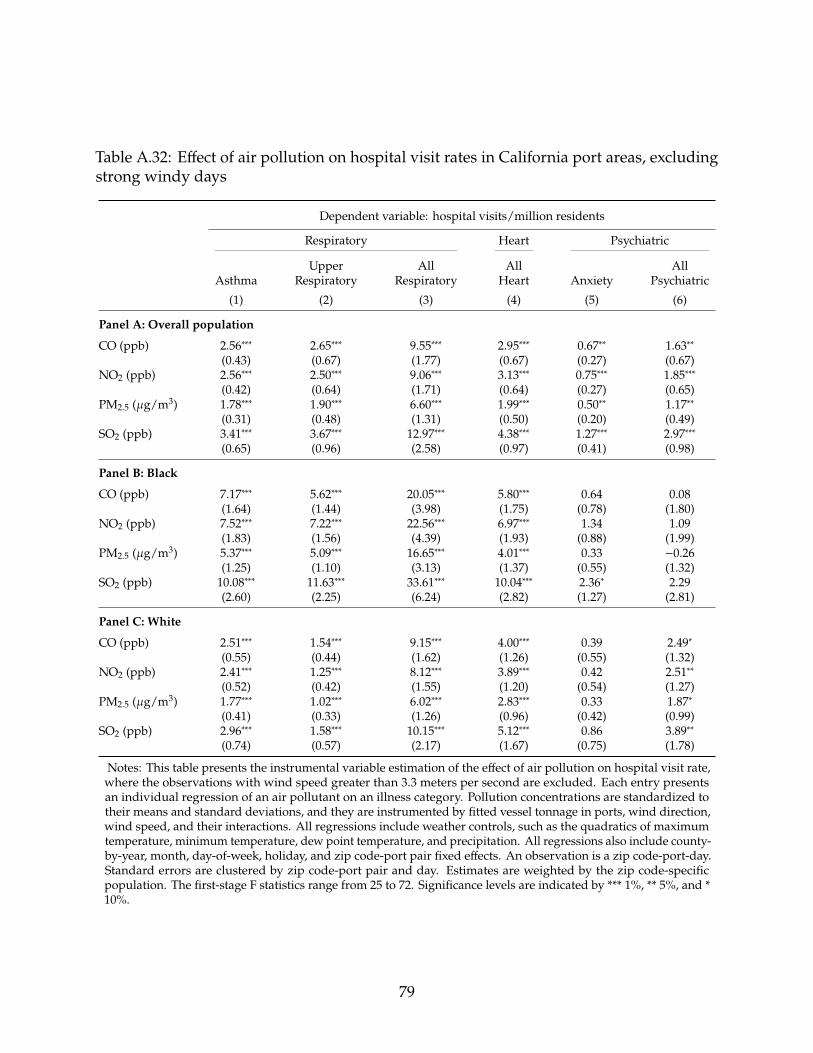
Table A.32: Effect of air pollution on hospital visit rates in California port areas, excludingstrong windy days

Dependent variable: hospital visits/million residents

Respiratory Heart Psychiatric

Upper All All AllAsthma Respiratory Respiratory Heart Anxiety Psychiatric

(1) (2) (3) (4) (5) (6)

Panel A: Overall population

CO (ppb) 2.56∗∗∗ 2.65∗∗∗ 9.55∗∗∗ 2.95∗∗∗ 0.67∗∗ 1.63∗∗(0.43) (0.67) (1.77) (0.67) (0.27) (0.67)

NO2 (ppb) 2.56∗∗∗ 2.50∗∗∗ 9.06∗∗∗ 3.13∗∗∗ 0.75∗∗∗ 1.85∗∗∗(0.42) (0.64) (1.71) (0.64) (0.27) (0.65)

PM2.5 (�g/m3) 1.78∗∗∗ 1.90∗∗∗ 6.60∗∗∗ 1.99∗∗∗ 0.50∗∗ 1.17∗∗(0.31) (0.48) (1.31) (0.50) (0.20) (0.49)

SO2 (ppb) 3.41∗∗∗ 3.67∗∗∗ 12.97∗∗∗ 4.38∗∗∗ 1.27∗∗∗ 2.97∗∗∗(0.65) (0.96) (2.58) (0.97) (0.41) (0.98)

Panel B: Black

CO (ppb) 7.17∗∗∗ 5.62∗∗∗ 20.05∗∗∗ 5.80∗∗∗ 0.64 0.08(1.64) (1.44) (3.98) (1.75) (0.78) (1.80)

NO2 (ppb) 7.52∗∗∗ 7.22∗∗∗ 22.56∗∗∗ 6.97∗∗∗ 1.34 1.09(1.83) (1.56) (4.39) (1.93) (0.88) (1.99)

PM2.5 (�g/m3) 5.37∗∗∗ 5.09∗∗∗ 16.65∗∗∗ 4.01∗∗∗ 0.33 −0.26(1.25) (1.10) (3.13) (1.37) (0.55) (1.32)

SO2 (ppb) 10.08∗∗∗ 11.63∗∗∗ 33.61∗∗∗ 10.04∗∗∗ 2.36∗ 2.29(2.60) (2.25) (6.24) (2.82) (1.27) (2.81)

Panel C: White

CO (ppb) 2.51∗∗∗ 1.54∗∗∗ 9.15∗∗∗ 4.00∗∗∗ 0.39 2.49∗(0.55) (0.44) (1.62) (1.26) (0.55) (1.32)

NO2 (ppb) 2.41∗∗∗ 1.25∗∗∗ 8.12∗∗∗ 3.89∗∗∗ 0.42 2.51∗∗(0.52) (0.42) (1.55) (1.20) (0.54) (1.27)

PM2.5 (�g/m3) 1.77∗∗∗ 1.02∗∗∗ 6.02∗∗∗ 2.83∗∗∗ 0.33 1.87∗(0.41) (0.33) (1.26) (0.96) (0.42) (0.99)

SO2 (ppb) 2.96∗∗∗ 1.58∗∗∗ 10.15∗∗∗ 5.12∗∗∗ 0.86 3.89∗∗(0.74) (0.57) (2.17) (1.67) (0.75) (1.78)

Notes: This table presents the instrumental variable estimation of the effect of air pollution on hospital visit rate,where the observations with wind speed greater than 3.3 meters per second are excluded. Each entry presentsan individual regression of an air pollutant on an illness category. Pollution concentrations are standardized totheir means and standard deviations, and they are instrumented by fitted vessel tonnage in ports, wind direction,wind speed, and their interactions. All regressions include weather controls, such as the quadratics of maximumtemperature, minimum temperature, dew point temperature, and precipitation. All regressions also include county-by-year, month, day-of-week, holiday, and zip code-port pair fixed effects. An observation is a zip code-port-day.Standard errors are clustered by zip code-port pair and day. Estimates are weighted by the zip code-specificpopulation. The first-stage F statistics range from 25 to 72. Significance levels are indicated by *** 1%, ** 5%, and *10%.

79

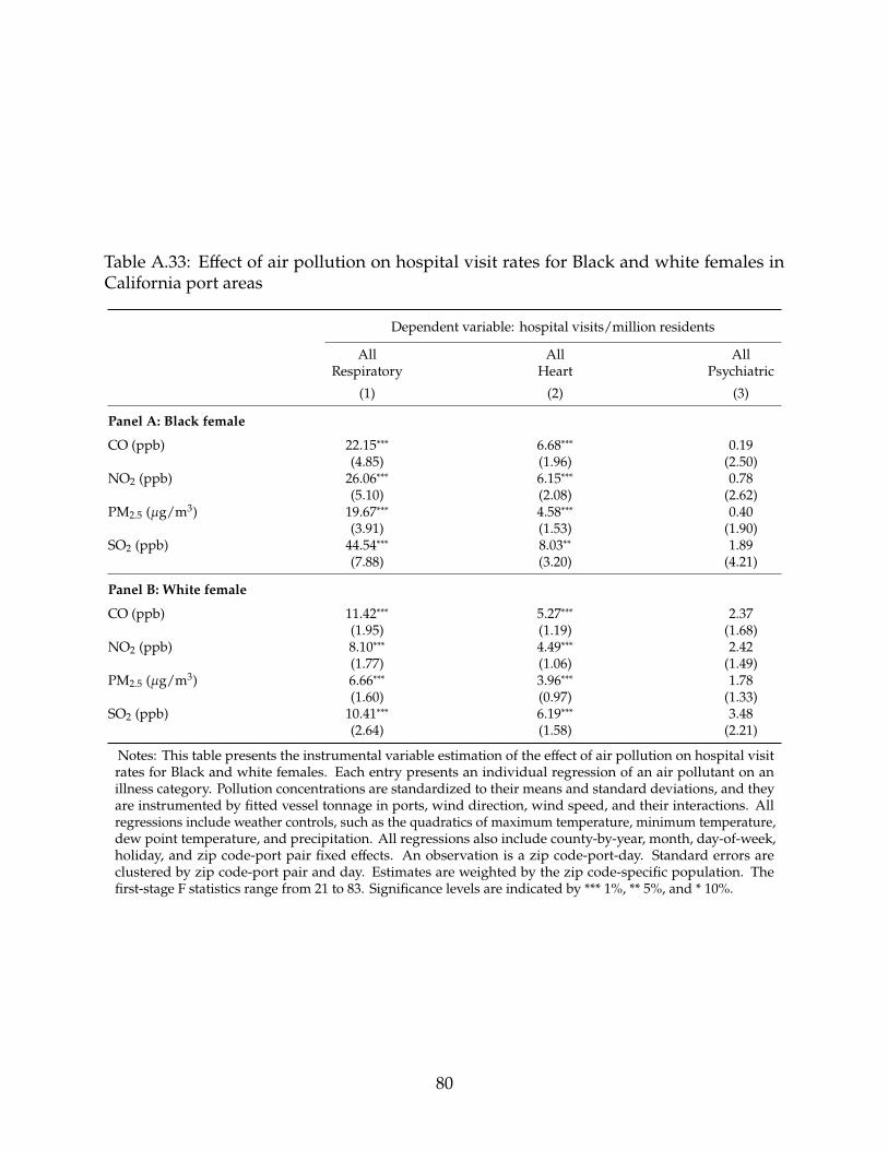
Table A.33: Effect of air pollution on hospital visit rates for Black and white females inCalifornia port areas

Dependent variable: hospital visits/million residents

All All AllRespiratory Heart Psychiatric

(1) (2) (3)

Panel A: Black female

CO (ppb) 22.15∗∗∗ 6.68∗∗∗ 0.19(4.85) (1.96) (2.50)

NO2 (ppb) 26.06∗∗∗ 6.15∗∗∗ 0.78(5.10) (2.08) (2.62)

PM2.5 (�g/m3) 19.67∗∗∗ 4.58∗∗∗ 0.40(3.91) (1.53) (1.90)

SO2 (ppb) 44.54∗∗∗ 8.03∗∗ 1.89(7.88) (3.20) (4.21)

Panel B: White female

CO (ppb) 11.42∗∗∗ 5.27∗∗∗ 2.37(1.95) (1.19) (1.68)

NO2 (ppb) 8.10∗∗∗ 4.49∗∗∗ 2.42(1.77) (1.06) (1.49)

PM2.5 (�g/m3) 6.66∗∗∗ 3.96∗∗∗ 1.78(1.60) (0.97) (1.33)

SO2 (ppb) 10.41∗∗∗ 6.19∗∗∗ 3.48(2.64) (1.58) (2.21)

Notes: This table presents the instrumental variable estimation of the effect of air pollution on hospital visitrates for Black and white females. Each entry presents an individual regression of an air pollutant on anillness category. Pollution concentrations are standardized to their means and standard deviations, and theyare instrumented by fitted vessel tonnage in ports, wind direction, wind speed, and their interactions. Allregressions include weather controls, such as the quadratics of maximum temperature, minimum temperature,dew point temperature, and precipitation. All regressions also include county-by-year, month, day-of-week,holiday, and zip code-port pair fixed effects. An observation is a zip code-port-day. Standard errors areclustered by zip code-port pair and day. Estimates are weighted by the zip code-specific population. Thefirst-stage F statistics range from 21 to 83. Significance levels are indicated by *** 1%, ** 5%, and * 10%.

80

Table A.34: Effect of air pollution on all-cause total hospital visit rates in California portareas

Dependent variable: hospital visits/million residents

OverallPopulation Black White

(1) (2) (3)

Panel A: CO

CO (ppb) 19.02∗∗∗ 41.56∗∗∗ 12.29∗∗∗(4.01) (8.65) (4.76)

Adjusted R2 0.69 0.47 0.60Observations 1,776,040 877,072 1,650,747

Panel B: NO2

NO2 (ppb) 17.31∗∗∗ 41.77∗∗∗ 10.91∗∗(3.69) (8.92) (4.23)

Adjusted R2 0.69 0.47 0.60Observations 1,805,287 887,300 1,679,994

Panel C: PM2.5

PM2.5 (�g/m3) 13.41∗∗∗ 30.08∗∗∗ 9.02∗∗(3.11) (6.90) (3.85)

Adjusted R2 0.69 0.47 0.60Observations 1,714,554 846,980 1,598,695

Panel D: SO2

SO2 (ppb) 26.07∗∗∗ 57.42∗∗∗ 15.97∗∗∗(5.69) (13.61) (6.05)

Adjusted R2 0.69 0.47 0.60Observations 1,742,012 871,296 1,616,890

Notes: This table presents the instrumental variable estimation of the effect of air pollution on all-causetotal hospital visit rates for the overall population, Blacks, and whites. Each entry presents an individualregression of an air pollutant on an illness category. Pollution concentrations are standardized to their meansand standard deviations, and they are instrumented by fitted vessel tonnage in ports, wind direction, windspeed, and their interactions. All regressions include weather controls, such as the quadratics of maximumtemperature, minimum temperature, dew point temperature, and precipitation. All regressions also includecounty-by-year, month, day-of-week, holiday, and zip code-port pair fixed effects. An observation is a zipcode-port-day. Standard errors are clustered by zip code-port pair and day. Estimates are weighted by the zipcode-specific population. The first-stage F statistics range from 21 to 83. Significance levels are indicated by*** 1%, ** 5%, and * 10%.

81

Table A.35: Effect of air pollution on hospital visit rates in California port areas, principaldiagnoses

Dependent variable: hospital visits/million residents

All All AllRespiratory Heart Psychiatric

(1) (2) (3)

Panel A: Overall population

CO (ppb) 6.05∗∗∗ 0.72∗∗∗ 0.32(1.24) (0.22) (0.20)

NO2 (ppb) 4.91∗∗∗ 0.63∗∗∗ 0.40∗∗(1.16) (0.20) (0.18)

PM2.5 (�g/m3) 3.70∗∗∗ 0.51∗∗∗ 0.27∗(0.97) (0.16) (0.15)

SO2 (ppb) 7.43∗∗∗ 0.83∗∗ 0.64∗∗(1.81) (0.32) (0.29)

Panel B: Black

CO (ppb) 10.83∗∗∗ 1.05 −0.40(2.47) (0.69) (0.81)

NO2 (ppb) 13.38∗∗∗ 0.84 −0.15(2.55) (0.71) (0.82)

PM2.5 (�g/m3) 10.02∗∗∗ 0.84 −0.38(1.94) (0.53) (0.61)

SO2 (ppb) 22.65∗∗∗ 0.85 0.29(4.05) (1.10) (1.24)

Panel C: White

CO (ppb) 4.72∗∗∗ 0.85∗ 0.65∗(0.97) (0.43) (0.36)

NO2 (ppb) 3.19∗∗∗ 0.72∗ 0.72∗∗(0.89) (0.38) (0.31)

PM2.5 (�g/m3) 2.43∗∗∗ 0.66∗ 0.61∗∗(0.80) (0.34) (0.28)

SO2 (ppb) 4.23∗∗∗ 0.89 1.06∗∗(1.30) (0.57) (0.47)

Notes: This table presents the instrumental variable estimation of the effect of air pollution on hospital visitrates for the overall population, Blacks, and whites, where hospital visit rates are calculated only using princi-pal diagnoses. Each entry presents an individual regression of an air pollutant on an illness category. Pollutionconcentrations are standardized to their means and standard deviations, and they are instrumented by fittedvessel tonnage in ports, wind direction, wind speed, and their interactions. All regressions include weathercontrols, such as the quadratics of maximum temperature, minimum temperature, dew point temperature, andprecipitation. All regressions also include county-by-year, month, day-of-week, holiday, and zip code-port pairfixed effects. An observation is a zip code-port-day. Standard errors are clustered by zip code-port pair andday. Estimates are weighted by the zip code-specific population. The first-stage F statistics range from 21 to 83.Significance levels are indicated by *** 1%, ** 5%, and * 10%.

82

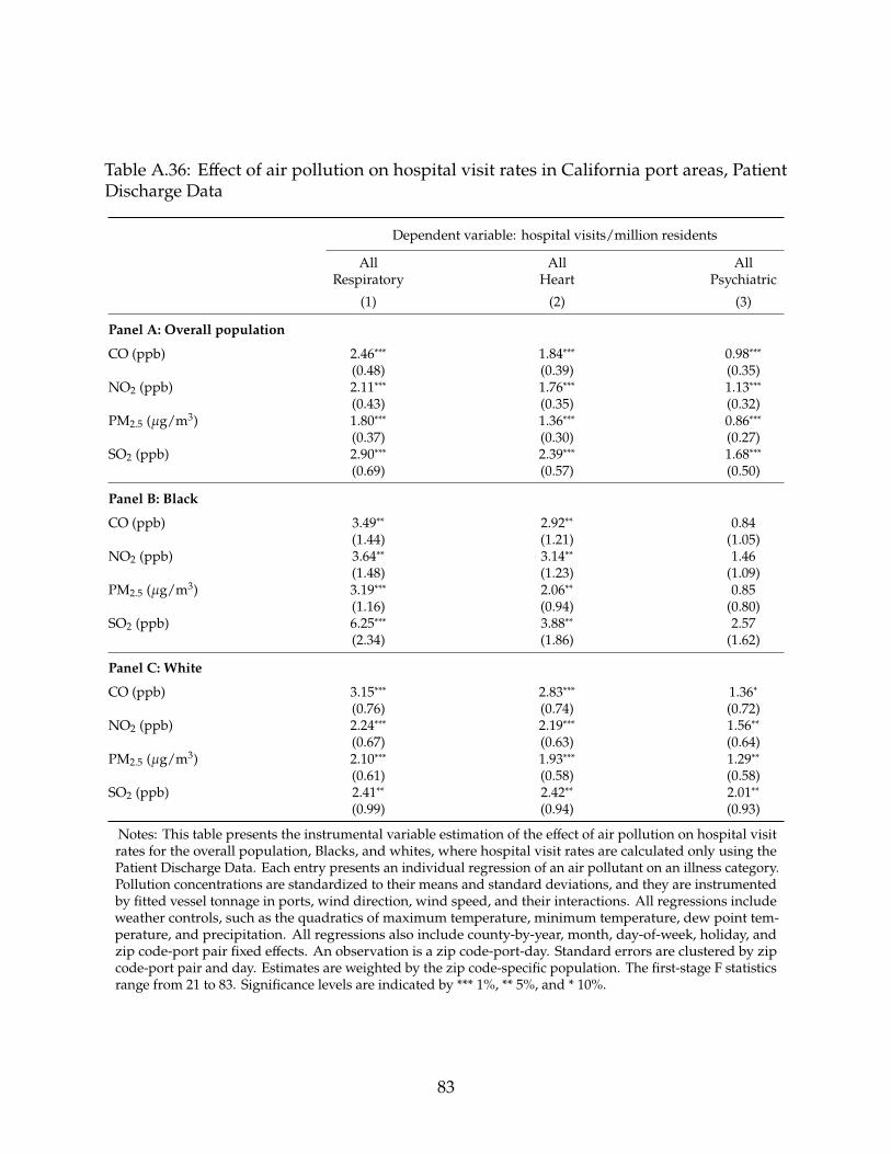
Table A.36: Effect of air pollution on hospital visit rates in California port areas, PatientDischarge Data

Dependent variable: hospital visits/million residents

All All AllRespiratory Heart Psychiatric

(1) (2) (3)

Panel A: Overall population

CO (ppb) 2.46∗∗∗ 1.84∗∗∗ 0.98∗∗∗(0.48) (0.39) (0.35)

NO2 (ppb) 2.11∗∗∗ 1.76∗∗∗ 1.13∗∗∗(0.43) (0.35) (0.32)

PM2.5 (�g/m3) 1.80∗∗∗ 1.36∗∗∗ 0.86∗∗∗(0.37) (0.30) (0.27)

SO2 (ppb) 2.90∗∗∗ 2.39∗∗∗ 1.68∗∗∗(0.69) (0.57) (0.50)

Panel B: Black

CO (ppb) 3.49∗∗ 2.92∗∗ 0.84(1.44) (1.21) (1.05)

NO2 (ppb) 3.64∗∗ 3.14∗∗ 1.46(1.48) (1.23) (1.09)

PM2.5 (�g/m3) 3.19∗∗∗ 2.06∗∗ 0.85(1.16) (0.94) (0.80)

SO2 (ppb) 6.25∗∗∗ 3.88∗∗ 2.57(2.34) (1.86) (1.62)

Panel C: White

CO (ppb) 3.15∗∗∗ 2.83∗∗∗ 1.36∗(0.76) (0.74) (0.72)

NO2 (ppb) 2.24∗∗∗ 2.19∗∗∗ 1.56∗∗(0.67) (0.63) (0.64)

PM2.5 (�g/m3) 2.10∗∗∗ 1.93∗∗∗ 1.29∗∗(0.61) (0.58) (0.58)

SO2 (ppb) 2.41∗∗ 2.42∗∗ 2.01∗∗(0.99) (0.94) (0.93)

Notes: This table presents the instrumental variable estimation of the effect of air pollution on hospital visitrates for the overall population, Blacks, and whites, where hospital visit rates are calculated only using thePatient Discharge Data. Each entry presents an individual regression of an air pollutant on an illness category.Pollution concentrations are standardized to their means and standard deviations, and they are instrumentedby fitted vessel tonnage in ports, wind direction, wind speed, and their interactions. All regressions includeweather controls, such as the quadratics of maximum temperature, minimum temperature, dew point tem-perature, and precipitation. All regressions also include county-by-year, month, day-of-week, holiday, andzip code-port pair fixed effects. An observation is a zip code-port-day. Standard errors are clustered by zipcode-port pair and day. Estimates are weighted by the zip code-specific population. The first-stage F statisticsrange from 21 to 83. Significance levels are indicated by *** 1%, ** 5%, and * 10%.

83

Table A.37: Effect of air pollution on hospital visit rates in California port areas, EmergencyDepartment Data

Dependent variable: hospital visits/million residents

All All AllRespiratory Heart Psychiatric

(1) (2) (3)

Panel A: Overall population

CO (ppb) 8.05∗∗∗ 1.12∗∗∗ 0.78∗∗(1.49) (0.23) (0.36)

NO2 (ppb) 6.86∗∗∗ 1.18∗∗∗ 0.77∗∗(1.40) (0.22) (0.34)

PM2.5 (�g/m3) 5.02∗∗∗ 0.74∗∗∗ 0.42(1.16) (0.18) (0.28)

SO2 (ppb) 10.57∗∗∗ 1.89∗∗∗ 1.35∗∗(2.23) (0.36) (0.56)

Panel B: Black

CO (ppb) 17.27∗∗∗ 2.42∗∗ −0.90(3.35) (0.99) (1.32)

NO2 (ppb) 20.20∗∗∗ 2.46∗∗ −0.90(3.52) (1.03) (1.39)

PM2.5 (�g/m3) 15.19∗∗∗ 1.42∗ −1.38(2.69) (0.76) (1.04)

SO2 (ppb) 33.69∗∗∗ 3.86∗∗ −1.12(5.55) (1.64) (2.25)

Panel C: White

CO (ppb) 6.67∗∗∗ 1.29∗∗∗ 1.27∗(1.14) (0.47) (0.73)

NO2 (ppb) 4.89∗∗∗ 1.36∗∗∗ 1.11∗(1.03) (0.41) (0.63)

PM2.5 (�g/m3) 3.71∗∗∗ 1.00∗∗∗ 0.81(0.90) (0.37) (0.56)

SO2 (ppb) 6.81∗∗∗ 2.24∗∗∗ 1.83∗∗(1.51) (0.62) (0.93)

Notes: This table presents the instrumental variable estimation of the effect of air pollution on hospital visitrates for the overall population, Blacks, and whites, where hospital visit rates are calculated only using theEmergency Department Data. Each entry presents an individual regression of an air pollutant on an illnesscategory. Pollution concentrations are standardized to their means and standard deviations, and they areinstrumented by fitted vessel tonnage in ports, wind direction, wind speed, and their interactions. All regres-sions include weather controls, such as the quadratics of maximum temperature, minimum temperature, dewpoint temperature, and precipitation. All regressions also include county-by-year, month, day-of-week, holiday,and zip code-port pair fixed effects. An observation is a zip code-port-day. Standard errors are clustered by zipcode-port pair and day. Estimates are weighted by the zip code-specific population. The first-stage F statisticsrange from 21 to 83. Significance levels are indicated by *** 1%, ** 5%, and * 10%.

84

Table A.38: Effect of air pollution on hospital visit rates in California port areas, AmbulatorySurgery Center Data

Dependent variable: hospital visits/million residents

All All AllRespiratory Heart Psychiatric

(1) (2) (3)

Panel A: Overall population

CO (ppb) −0.05 0.19 0.11(0.28) (0.26) (0.19)

NO2 (ppb) −0.18 0.15 0.03(0.26) (0.23) (0.18)

PM2.5 (�g/m3) −0.09 0.09 0.05(0.21) (0.19) (0.14)

SO2 (ppb) −0.33 0.12 0.05(0.41) (0.37) (0.28)

Panel B: Black

CO (ppb) −0.32 0.40 0.01(0.57) (0.39) (0.41)

NO2 (ppb) −0.52 0.35 0.10(0.58) (0.42) (0.39)

PM2.5 (�g/m3) −0.38 0.29 −0.003(0.42) (0.30) (0.31)

SO2 (ppb) −0.85 0.50 0.10(0.86) (0.63) (0.63)

Panel C: White

CO (ppb) −0.27 −0.11 −0.25(0.44) (0.50) (0.37)

NO2 (ppb) −0.29 −0.03 −0.35(0.40) (0.44) (0.33)

PM2.5 (�g/m3) −0.26 −0.14 −0.29(0.35) (0.39) (0.29)

SO2 (ppb) −0.24 −0.02 −0.49(0.58) (0.62) (0.49)

Notes: This table presents the instrumental variable estimation of the effect of air pollution on hospital visitrates for the overall population, Blacks, and whites, where hospital visit rates are calculated only using theAmbulatory Surgery Center Data. Each entry presents an individual regression of an air pollutant on anillness category. Pollution concentrations are standardized to their means and standard deviations, and theyare instrumented by fitted vessel tonnage in ports, wind direction, wind speed, and their interactions. Allregressions include weather controls, such as the quadratics of maximum temperature, minimum temperature,dew point temperature, and precipitation. All regressions also include county-by-year, month, day-of-week,holiday, and zip code-port pair fixed effects. An observation is a zip code-port-day. Standard errors areclustered by zip code-port pair and day. Estimates are weighted by the zip code-specific population. Thefirst-stage F statistics range from 21 to 83. Significance levels are indicated by *** 1%, ** 5%, and * 10%.

85

Table A.39: LIML estimation of the effect of air pollution on hospital visit rates for theoverall population in California port areas

Dependent variable: hospital visits/million residents

Respiratory Heart Psychiatric

Upper All All AllAsthma Respiratory Respiratory Heart Anxiety Psychiatric

(1) (2) (3) (4) (5) (6)

Panel A: CO

CO (ppb) 2.44∗∗∗ 2.66∗∗∗ 9.09∗∗∗ 3.09∗∗∗ 0.51∗ 1.81∗∗(0.41) (0.58) (1.61) (0.68) (0.31) (0.73)

Adjusted R2 0.33 0.29 0.42 0.31 0.17 0.36Observations 1,776,040 1,776,040 1,776,040 1,776,040 1,776,040 1,776,040

Panel B: NO2

NO2 (ppb) 1.99∗∗∗ 2.58∗∗∗ 7.50∗∗∗ 3.01∗∗∗ 0.57∗∗ 1.94∗∗∗(0.38) (0.55) (1.49) (0.62) (0.28) (0.67)

Adjusted R2 0.33 0.29 0.42 0.31 0.17 0.36Observations 1,805,287 1,805,287 1,805,287 1,805,287 1,805,287 1,805,287

Panel C: PM2.5

PM2.5 (�g/m3) 1.49∗∗∗ 1.98∗∗∗ 5.64∗∗∗ 2.11∗∗∗ 0.41∗ 1.33∗∗(0.33) (0.47) (1.29) (0.53) (0.23) (0.56)

Adjusted R2 0.33 0.29 0.42 0.31 0.18 0.36Observations 1,714,554 1,714,554 1,714,554 1,714,554 1,714,554 1,714,554

Panel D: SO2

SO2 (ppb) 2.45∗∗∗ 4.09∗∗∗ 10.74∗∗∗ 4.10∗∗∗ 0.95∗∗ 2.86∗∗∗(0.61) (0.86) (2.33) (0.97) (0.43) (1.03)

Adjusted R2 0.33 0.28 0.42 0.31 0.17 0.36Observations 1,742,012 1,742,012 1,742,012 1,742,012 1,742,012 1,742,012

Notes: This table presents the LIML instrumental variable estimation of the effect of air pollution on hospital visitrates for the overall population. Each entry presents an individual regression of an air pollutant on an illness category.Pollution concentrations are standardized to their means and standard deviations, and they are instrumented by fittedvessel tonnage in ports, wind direction, wind speed, and their interactions. All regressions include weather controls,such as the quadratics of maximum temperature, minimum temperature, dew point temperature, and precipitation. Allregressions also include county-by-year, month, day-of-week, holiday, and zip code-port pair fixed effects. An observa-tion is a zip code-port-day. Standard errors are clustered by zip code-port pair and day. Estimates are unweighted.Significance levels are indicated by *** 1%, ** 5%, and * 10%.

86

Table A.40: Placebo tests for the effect of California Ocean-Going Vessel At-Berth Regulationon air pollution

Dependent variable: residual of log pollution concentration

CO NO2 PM2.5 SO2

(1) (2) (3) (4)

Panel A: One year before the policy

CA Regulation 0.03 0.02 0.07 −0.005(0.08) (0.08) (0.13) (0.13)

Date 0.0001 −0.001 0.002 −0.001(0.002) (0.002) (0.003) (0.003)

CA Regulation × Date 0.002 0.001 −0.01∗∗ 0.01(0.002) (0.002) (0.004) (0.004)

Pre-policy Mean 642.22 18.71 15.01 1.89Observations 4,745 5,055 1,913 3,129

Panel B: One year after the policy

CA Regulation 0.15 0.10 0.07 −0.01(0.10) (0.09) (0.11) (0.27)

Date −0.003 0.0003 0.001 0.003(0.002) (0.002) (0.002) (0.004)

CA Regulation × Date 0.001 −0.0003 −0.004 −0.002(0.002) (0.003) (0.003) (0.01)

Pre-policy Mean 599.15 18.01 14.03 1.74Observations 4,828 5,166 2,673 3,359

Panel C: Neighboring areas

CA Regulation 0.27 0.13∗ −0.23∗ 0.15∗(0.16) (0.06) (0.11) (0.06)

Date 0.001 −0.001 0.004∗ 0.01(0.003) (0.001) (0.002) (0.01)

CA Regulation × Date −0.01 −0.001 −0.01∗ −0.01(0.004) (0.002) (0.004) (0.02)

Pre-policy Mean 406.79 11.37 11.28 1.31Observations 1,591 3,195 1,364 509

Notes: This table presents the placebo tests for RDD estimation of the effect of the California at-berth reg-ulation on local air pollution. The second-stage RDD dependent variable is taken from the residuals byregressing log pollution concentrations on weather controls (i.e., the quadratics of maximum temperature,minimum temperature, dew point temperature, precipitation, wind speed, and relative wind direction be-tween a monitor-port pair), fixed effects (i.e., county-by-year, month, day-of-week, holiday, and port-monitorpair), and log vessel tonnage (instrumented by seven-day lagged and 500-mile distant cyclones from ports).The local linear bandwidth is specified as 60 days on both sides of the policy threshold. Panel A shows theresults of specifying placebo policy dates one year before the actual policy date. Panel B shows the results ofspecifying placebo policy dates one year after the actual policy date. Panel C shows the results by assigningthe policy date to neighboring areas located 75 to 100 miles from ports. An observation is a monitor-port-day.Standard errors are clustered by monitor-port pair and normalized day. Significance levels are indicated by*** 1%, ** 5%, and * 10%.

87

Table A.41: Projected energy consumption by marine vessels in the United States

Fossil Fuel Electricity

Reference Shore Power Reference Shore Power

2017 0.78 0.78 0.00 0.002020 0.77 0.72 0.01 0.052025 0.81 0.64 0.01 0.182030 0.85 0.66 0.01 0.192035 0.90 0.70 0.01 0.222040 0.93 0.72 0.01 0.222045 0.97 0.74 0.01 0.242050 1.01 0.77 0.01 0.25

Notes: This table presents projected marine vessel energy consumption simulated in Yale-NEMS. Theunit is quadrillion Btu. The data include electricity and fossil fuel consumption for the reference caseand the shore power scenario.

88

B Supplementary Figures (For Online Publication)

0.0

0.1

0.2

2010 2012 2014 2016 2018Year

Cou

nty

shar

e

Figure B.1: Share of nonattainment counties adjacent to the major ports in the UnitedStates.

Notes: The figure plots the share of nonattainment counties that fail to meet the National Ambient AirQuality Standards and locate within a 50-mile radius of the major ports in the United States. The standardsinclude Carbon Monoxide (1971), Nitrogen Dioxide (1971), 8-Hour Ozone (2008, 2015), PM10 (1987), PM2.5(1997, 2006, 2012), Sulfur Dioxide (1971, 2010). The data are obtained from US EPA NAAQS Greenbook.

89

Figure B.2: Locations of zip codes near the major California ports.

Notes: This figure plots the locations of zip codes that are within 25 miles of the major ports in California,shown in blue areas. According to the US 2010 Decennial Census, around 47 percent of the population inCalifornia resides in the blue areas.

0.00

0.05

0.10

0.15

5 10 15 20 25Distance to Port (Miles)

Pop

ulat

ion

Sha

re

(a)

0.00

0.05

0.10

0.15

0.20

25 50 75 100Pollution Percentile

(b)

Figure B.3: (a) Distribution of Hispanic population by distance to major California ports.(b) Distribution of the Hispanic population in California port areas by percentile of PM2.5concentration.

Notes: Panel (a) plots population distribution in the California port areas by the distance between censustract and port for the Hispanic population. We obtain the population data at the census tract level andassign a distance between a census tract to its nearest mapped port to the population within the censustract. Panel (b) plots population distribution in the California port areas by percentile of PM2.5 concentration.Larger pollution percentiles represent higher pollution exposures. The data are obtained from the US 2010Decennial Census and US EPA Air Quality System.

90

Long Beach, CA

Los Angeles, CAPM2.5Level

10.511.011.512.0

A

Long Beach, CA

Los Angeles, CA

BlackShare (%)

020406080

B

Long Beach, CA

Los Angeles, CAWhiteShare (%)

255075

C

Figure B.4: Average PM2.5 concentrations, Black population shares, and white populationshares in zip codes near ports in Los Angeles, California.

Notes: Panel A presents the daily average PM2.5 concentrations at the zip code level based on the EPAmonitoring data within 25 miles from the two major ports near Los Angeles, California. Panel B shows thepercentage of Black population in a zip code for the same area, while Panel C shows the percentage of whitepopulation. The blue crosses in the panels represent the location of PM2.5 monitor sites with available data.The red stars indicate the Ports of Los Angeles and Long Beach. The pollution data are obtained from the USEPA Air Quality System. The population data are acquired from the US 2010 Decennial Census.

Oakland, CA

San Francisco, CA

PM2.5Level

8.08.59.09.5

A

Oakland, CA

San Francisco, CABlackShare (%)

01020304050

B

Oakland, CA

San Francisco, CA

WhiteShare (%)

255075

C

Figure B.5: Average PM2.5 concentrations, Black population shares, and white populationshares in zip codes near ports in San Francisco, California.

Notes: Panel A presents the daily average PM2.5 concentrations at the zip code level based on the EPAmonitoring data within 25 miles from the two major ports near San Francisco, California. Panel B shows thepercentage of Black population in a zip code for the same area, while Panel C shows the percentage of whitepopulation. The blue crosses in the panels represent the location of PM2.5 monitor sites with available data.The red stars indicate the Ports of San Francisco and Oakland. The pollution data are obtained from the USEPA Air Quality System. The population data are acquired from the US 2010 Decennial Census.

91

NO

2 (pp

b)S

O2 (

ppb)

CO

(ppb

)P

M2.

5 (µg

m3 )

2010 2012 2014 2016 2010 2012 2014 2016

14

15

16

0.5

0.6

0.7

0.8

0.9

400

410

420

430

440

9.5

10.0

10.5

Year

Black

White

Figure B.6: Annual air pollution exposure for individuals visiting hospitals by race.

Notes: This figure plots the annual averages of baseline pollution exposure separately for non-Hispanic Blackand white patients in the areas within 25 miles from ports in California. The patients visit hospitals due topsychiatric, respiratory, and heart-related illnesses during 2010–2016. The pollution data are obtained fromthe US EPA Air Quality System, and the hospital visit data are obtained Office of Statewide Health Planningand Development of California.

92

0

20

40

60

Cargo

Tank

er Tug

Barge

/Sco

w

Tank

Bar

geOth

er

Vessel Type

Ave

rage

Per

cent

age

Seven−daylagged cyclones

No

Yes

Figure B.7: Average daily share of vessel type in ports.

Notes: This figure presents the average daily share of vessel types in major 27 US ports, separately for thedays when there exist seven-day lagged and 500-mile distant tropical cyclones in the ocean and the dayswhen there are no such cyclones. The error bars indicate standard deviations. The data are obtained fromthe US Army Corps of Engineers.

93

PM2.5 SO2

CO NO2

0.0 2.5 5.0 7.5 10.0 12.5 0.0 2.5 5.0 7.5 10.0 12.5

−20

−15

−10

−5

0

5

−15

−10

−5

0

5

−20

−10

0

−30

−20

−10

0

10

Wind Speed (m/s)

Pre

dict

ed P

ollu

tant

Con

cent

ratio

ns WindDirection

[0, 45)

[45, 90)

[90, 135)

[135, 180)

[180, 225)

[225, 270)

[270, 315)

Figure B.8: First-stage results of adjusted predictions of pollutant concentrations withrespect to wind direction and wind speed.

Notes: This figure presents the adjusted predictions of pollutant concentrations generated by the first-stageregressions, i.e., equation (4) of 2SLS. We allow the wind direction and wind speed variables to vary, whilekeeping other non-focal variables constant. Specifically, we evaluate pollutant concentrations at the locationof Port of Long Beach and zip code 90062 for the year 2015, with the projected vessel tonnage as 4.56, dewpoint temperature as 4.56, precipitation as 0.42, maximum temperature as 21.63, minimum temperature as12.83, month as July, day-of-week as Friday, and non-holiday days. The wind direction blowing north isnormalized to zero, and it increases up to 360 degrees clockwise.

94

All Respiratory All Heart All Psychiatric

CO

NO

2P

M2.5

SO

2

1 3 5 9 14 21 28 1 3 5 9 14 21 28 1 3 5 9 14 21 28

0

50

100

150

200

0

50

100

150

200

0

50

100

150

0

100

200

300

Time Window Following Exposure (day)

Est

imat

ed C

oeffi

cien

ts

Figure B.9: Effect of air pollution on hospital visit rate for the overall population withdifferent time windows following pollution exposure in California port areas.

Notes: This figure plots IV estimates of equation (3) with different time windows following pollutionexposure. Estimates are shown for time windows of one day, three days, five days, nine days, 14 days, 21days, and 28 days. The dependent variable is the sum of hospital visits over the number of time windows permillion residents, indicated on the x-axis. The one-day window estimates are also reported in columns (3),(4), and (7) in Panel A of Table 3. The pollution measures are instrumented by fitted vessel tonnage in ports,wind direction, wind speed, and interactions. All regressions include a set of weather controls, such as thequadratics of maximum, minimum, and dew point temperatures, precipitation, and their leads up to thetime window. All regressions also include county-by-year, month, day-of-week, holiday, and zip code-portpair fixed effects. An observation is a zip code-port-day. Standard errors are clustered by zip code-port pairand day. Estimates are weighted by zip code-specific population. The error bars represent 95% confidenceintervals.

95

All Respiratory All Heart All Psychiatric

CO

NO

2P

M2.5

SO

2

1 3 5 9 14 21 28 1 3 5 9 14 21 28 1 3 5 9 14 21 28

−100

0

100

200

300

−100

0

100

200

300

400

0

100

200

300

0

200

400

600

800

Time Window Following Exposure (day)

Est

imat

ed C

oeffi

cien

ts

Figure B.10: Effect of air pollution on hospital visit rate for Blacks with different timewindows following pollution exposure in California port areas.

Notes: This figure plots IV estimates of equation (3) with different time windows following pollutionexposure. Estimates are shown for time windows of one day, three days, five days, nine days, 14 days, 21days, and 28 days. The dependent variable is the sum of hospital visits over the number of time windows permillion residents, indicated on the x-axis. The one-day window estimates are also reported in columns (3),(4), and (7) in Panel B of Table 3. The pollution measures are instrumented by fitted vessel tonnage in ports,wind direction, wind speed, and interactions. All regressions include a set of weather controls, such as thequadratics of maximum, minimum, and dew point temperatures, precipitation, and their leads up to thetime window. All regressions also include county-by-year, month, day-of-week, holiday, and zip code-portpair fixed effects. An observation is a zip code-port-day. Standard errors are clustered by zip code-port pairand day. Estimates are weighted by zip code-specific population. The error bars represent 95% confidenceintervals.

96

All Respiratory All Heart All Psychiatric

CO

NO

2P

M2.5

SO

2

1 3 5 9 14 21 28 1 3 5 9 14 21 28 1 3 5 9 14 21 28

0

50

100

150

200

0

50

100

0

40

80

0

50

100

150

Time Window Following Exposure (day)

Est

imat

ed C

oeffi

cien

ts

Figure B.11: Effect of air pollution on hospital visit rate for whites with different timewindows following pollution exposure in California port areas.

Notes: This figure plots IV estimates of equation (3) with different time windows following pollutionexposure. Estimates are shown for time windows of one day, three days, five days, nine days, 14 days, 21days, and 28 days. The dependent variable is the sum of hospital visits over the number of time windows permillion residents, indicated on the x-axis. The one-day window estimates are also reported in columns (3),(4), and (7) in Panel C of Table 3. The pollution measures are instrumented by fitted vessel tonnage in ports,wind direction, wind speed, and interactions. All regressions include a set of weather controls, such as thequadratics of maximum, minimum, and dew point temperatures, precipitation, and their leads up to thetime window. All regressions also include county-by-year, month, day-of-week, holiday, and zip code-portpair fixed effects. An observation is a zip code-port-day. Standard errors are clustered by zip code-port pairand day. Estimates are weighted by zip code-specific population. The error bars represent 95% confidenceintervals.

97

0

50

20 40 60 80 100Pollution Percentile

Effe

ct o

f PM

2.5

on h

ospi

tal v

isit

rate

Black

White

Figure B.12: Effects of PM2.5 on hospital visit rates by pollution percentile using satellite-based pollution measures.

Notes: This figure plots the effects of PM2.5 pollution on total hospital visit rates (related to respiratory, heart,and psychiatric illnesses) in eight pollution percentile groups. The PM2.5 pollution measures are basedon satellite-based pollution data. Pollution concentrations in regressions are standardized to their meansand standard deviations, and they are instrumented by fitted vessel tonnage in ports, wind direction, windspeed, and their interactions. Error bars correspond to 95% confidence intervals, where standard errors fromregressions are clustered by port-zip code and day. An observation is a zip code-port-day.

98

PM2.5 SO2

CO NO2

5 10 15 20 5 10 15 20

−100

0

100

−100

0

100

Distance to nearest monitor (mile)

Effe

ct o

f pol

lutio

n on

hos

pita

l vis

it ra

te

Black

White

Figure B.13: Effects of pollution on hospital visit rates by distance to nearest pollutionmonitors.

Notes: This figure plots effects of pollution on total hospital visit rates (related to respiratory, heart, andpsychiatric illnesses) for zip codes by distance to nearest pollution monitors. Pollution concentrations inregressions are standardized to their means and standard deviations, and they are instrumented by fittedvessel tonnage in ports, wind direction, wind speed, and their interactions. Error bars correspond to 95%confidence intervals, where standard errors from regressions are clustered by port-zip code and day. Anobservation is a zip code-port-day. Missing values indicate that there are monitors within such distance tozip codes.

99

−50

−25

0

25

CO NO2 PM2.5 SO2

Effe

ct o

f CA

Reg

ulat

ion

on p

ollu

tant

Con

cent

ratio

ns (

%)

Baseline

Bootstrap

Figure B.14: Cluster bootstrap inference for the effect of California Ocean-Going VesselAt-Berth Regulation on air pollutant concentrations.

Notes: The figure plots the the local linear RDD point estimates and 95% confidence intervals from thebaseline regression (shown in Table 6) and a wild cluster bootstrap algorithm.

100

PM2.5 SO2

CO NO2

50 55 60 65 70 50 55 60 65 70

−0.75

−0.50

−0.25

0.00

0.25

−0.75

−0.50

−0.25

0.00

0.25

Bandwidth

Est

imat

ed C

oeffi

cien

ts

Figure B.15: Robustness check for the effect of California Ocean-Going Vessel At-BerthRegulation on air pollutant concentrations with varying RDD bandwidths.

Notes: The figure plots the local linear RDD point estimates and 95% confidence intervals with varyingbandwidths (i.e., 55–75 days on both sides of the policy threshold). The baseline bandwidth is 65 days, asindicated by the red dots.

101

PM2.5 SO2

CO NO2

0 2 4 6 0 2 4 6

−0.75

−0.50

−0.25

0.00

0.25

−0.75

−0.50

−0.25

0.00

0.25

Donut Days

Est

imat

ed C

oeffi

cien

ts

Figure B.16: Robustness check for the effect of California Ocean-Going Vessel At-BerthRegulation on air pollutant concentrations with varying RDD “donut” periods.

Notes: The figure plots the local linear RDD point estimates and 95% confidence intervals with varying“donut” periods (i.e., removing 0–7 days of observations on both sides of the policy threshold). The baseline“donut” period is 0 day, as indicated by the red dots.

102

PM2.5 SO2

CO NOx

2020 2030 2040 2050 2020 2030 2040 2050

2020 2030 2040 2050 2020 2030 2040 2050

1.00

1.25

1.50

1.75

0.6

0.8

1.0

1.2

0.2

0.4

0.6

0.100

0.125

0.150

Year

Em

issi

ons

(mill

ion

met

ric to

n)

Scenario Reference Shore Power

Source Marine Vessels Electricity Generation

Figure B.17: Projected emissions of local air pollutants from marine vessels and electricitygeneration in the United States.

Notes: This figure plots local air pollutant emissions from marine vessels and power plants in the UnitedStates under the reference and shore power scenarios, projected in Yale-NEMS. The projection starts from2017 indicated by the gray dotted lines.

103

C Supplementary Analysis (For Online Publication)

C.1 Results ComparisonThis appendix presents supplementary analyses for the main text. We first present com-parisons of our baseline estimates to the existing evidence in the literature. We thenprovide additional evidence on how pollution affects different unconditional quantiles ofhospital visit distributions for Blacks and whites. In the third part, we show the estimatesof the reduced-form relationship between vessels in ports and human health. Lastly, wepresent the analysis of the relationship between Black-white health gap and socioeconomiccharacteristics.

Effect of vessels in ports on air pollution. We first compare our instrumented estimates(focusing on the effects of vessel tonnage) in Table 2 to the existing evidence on thecontributions of seaports to local air pollution. We are not aware of any other study thatexplores this question in the literature; however, some government reports and onlinearticles address the relationship between port and local air pollution. For example, US EPAestimates that ocean-going vessels contribute to 7% of NOx emissions in Ports of BatonRouge/New Orleans and up to 61% in the Santa Barbara areas (EPA, 2003). In addition,another evidence states that marine shipping in ports accounts for as much as half SOx

emissions in major port cities, such as Los Angeles.1Our estimates show that a 100,000 Mt vessel tonnage increase in port leads to a 1.17 ppb

increase in NO2 concentrations. The summary statistics in Table 1 show that on averagethere is 425,000 Mt vessel tonnage in a port in a day. This tonnage results in about a 5 ppbincrease in NO2 concentrations in port areas in the US, a 36% increase of the daily meanconcentration. This result is within the range of previously cited sources.

We also compare our estimates to the NAAQS to examine whether pollution from portsis likely to lead to nonattainment status.2 The current one-hour standard for CO is that thepollution concentration cannot exceed 35,000 ppb more than once per year. Our resultsshow that one average-sized vessel (29,000 Mt) in a port results in a 6.64 ppb increase inCO pollution.3 Combining this 6.64 ppb increase with the average daily maximum of CO(shown in Table A.3), the estimated resulting concentration is 846.54 ppb (6.64 + 839.9),which is far below the EPA standard. Similarly, the resulting pollution concentrations

1See https://www.ft.com/content/31d0e224-dde8-11e8-9f04-38d397e6661c.2The details of the standards for pollutants considered harmful to public health and the environment are

available at https://www.epa.gov/criteria-air-pollutants/naaqs-table.3The 6.64 ppb increase is calculated from 0.29×23.19 based on the estimates in Table 2 and summary

statistics reported in Table 1.

104

for NO2 and SO2 due to average gross vessel tonnage in ports are also below the EPA’sone-hour standards.4

EPA has established a 24-hour standard for PM2.5 at 35 micrograms per cubic meter(�g/m3). Adding the increase in PM2.5 concentrations 0.35 �g/m3 (0.29×1.20) (owing toan average-sized vessel in a port) to the daily 24-hour average (10.66 �g/m3) results ina concentration of 11 �g/m3, which is around 31% of the EPA standard. Note that thecalculations presented above are based on the summary averages across all ports. Someareas on certain days may still exceed the EPA standards due to increased vessel counts inports.

Effect of air pollution on health. Since there is a large body of economics and epidemio-logical literature examining the effect of air pollution on health, it is natural to compare ourestimates in Panel A of Table 3 to the literature. Compared to Schlenker and Walker (2016),our estimates associated with the effect of CO on respiratory and heart hospital visits arerelatively larger. For example, we find that a one ppb increase in CO concentration leads toa 0.02% increase in all respiratory hospital visits, while Schlenker and Walker (2016) find a0.037% increase.5 The discrepancy in results may be driven by different studied locations.Other epidemiological studies show the effect of a one ppb increase in CO pollution onrespiratory hospital visits in a range of 0.001–0.008% (e.g., Hwang and Chan, 2002; Peelet al., 2005; Stieb et al., 2009), which are smaller than our estimates.

For heart-related illness, we find that a one �g/m3 increase in PM2.5 concentrationleads to a 0.3% increase of hospital visits, which is higher than the estimates 0.13–0.15%in the epidemiology literature (e.g., Dominici et al., 2006; Bell et al., 2008). Two recentepidemiology studies find evidence that a 0.11% increase in psychiatric hospital visitsis attributed to a one �g/m3 increase in PM2.5 concentration, which is fairly close to ourestimate, 0.09%.

C.2 RIF-Quantile Effect of Air Pollution on HealthWe provide additional evidence on how pollution affects different unconditional quantilesof the hospital visit distributions for Blacks and whites using the unconditional quantileregression method introduced by Firpo et al. (2009). This method involves calculating there-centered influence function (RIF) for the outcome variable (e.g., hospital visit rates) at acertain quantile and replace the dependent variable in equation (3) with the calculated RIF.The RIF for hospital visit H at the =th quantile @= is calculated as RIF(H, @=) = @=+ =−1{H≤@=}

5H(@=) ,

4The one-hour standards for NO2 and SO2 are 100 parts per billion (ppb) and 75 ppb, respectively.5This calculation requires converting standardized estimates to the level before standardization.

105

where 5H(@=) is the density function of H at quantile @= . In practice, we calculate 19 RIFstatistics, starting from the 5th quantile to the 95th quantile of the hospital visit ratedistribution for each subsample of Blacks and whites. In total, we fit 38 RIF-quantileregressions for each of the four studied air pollutants. Because pollution is endogenous,we adopt a control-function approach, where we include the residuals from the first-stageregression equation (4) into the regression equation of interest (3). One caveat of thisRIF-quantile analysis using the control-function approach is that we should interpret thestandard errors carefully because there may exist sampling error in the first-stage residuals.

The regression estimates illustrate how the effect of pollution on hospital visit ratesdirectly transforms to the unconditional distribution of hospital visit rates. Figure C.1presents the RIF-quantile regression estimates by race and pollutant, suggesting that at theupper quantiles of the hospital visit rate distribution, air pollution has larger impacts onBlacks compared to whites.

106

PM2.5 SO2

CO NO2

0 25 50 75 100 0 25 50 75 100

0 25 50 75 100 0 25 50 75 100

0

40

80

120

0

50

100

150

200

0

25

50

75

0

20

40

60

80

hospital visit rate Percentile

RIF

/qua

ntile

Effe

ct

Black

White

Figure C.1: RIF-quantile effects of pollution on hospital visit rates by race.

Notes: This figure plots the estimates from 38 individual regressions of equation (3) for each air pollutant,with 19 regressions for each race. The dependent variable is the RIF statistics of total hospital visit rateassociated with respiratory, heart, and psychiatric ailments for a given quantile. The pollution measuresare instrumented by fitted vessel tonnage in ports, wind direction, wind speed, and interactions. Allregressions include a set of weather controls, such as the quadratics of maximum, minimum, and dew pointtemperatures and precipitation. All regressions also include county-by-year, month, day-of-week, holiday,and zip code-port pair fixed effects. Standard errors are clustered by zip code-port pair and day. Estimatesare weighted by zip code-specific population. The error bars represent 95% confidence intervals.

C.3 Reduced-form Relationship between Vessels in Ports and HealthThis section examines the reduced-form relationship between the number of vessels inports and human health. We estimate the regression model in equations (1) and (2) byspecifying the dependent variable as hospital visit rate across illness categories. We usethe ten-day lagged cyclones that are 500 miles distant from ports as the instrumental vari-able in our baseline specification.6 Since the instrumental variable specification is similarto the one used in themain text, we do not present the results for instrument validity checks.

6We use the ten-day lagged cyclones here instead of the seven-day lagged ones in the main text becausethe ten-day lagged cyclones show a stronger correlation in the first stage.

107

Table C.1 presents the first-stage relationship between the cyclone instrument and vesseltonnage in ports across samples. The point estimate is statistically significant, suggestingthe cyclone instrument leads to a 3–4% reduction in vessel tonnage in ports. The first-stageF statistics are in a range of 22–23, which are above the threshold of ten, suggesting noevidence of weak instruments.

Table C.1: First-stage results of the effect of tropical cyclones on vessel tonnage

Dependent variable: vessel tonnage

Overall Black White

(1) (2) (3)

Tropical Cyclone −0.38∗∗∗ −0.39∗∗∗ −0.31∗∗∗

(0.08) (0.08) (0.07)

First-stage F Stat. 22.04 21.89 22.54Adjusted R2 0.74 0.73 0.78Observations 1,805,287 887,300 1,679,994

Notes: This table presents the first-stage results of the instrumental variable estimation in Table C.2. Theinstrument is a dummy of ten-day lagged and 500-mile distant cyclones from ports. All regressions include aset of weather controls, such as the quadratics of maximum, minimum, and dew point temperatures, precipi-tation, wind speed, and relative wind direction between a zip code-port pair. All regressions also includecounty-by-year, month, day-of-week, holiday, and zip code-port pair fixed effects. Standard errors are clus-tered by zip code-port pair and day. Estimates are weighted by zip code-specific population. Significancelevels are indicated by *** 1%, ** 5%, and * 10%.

Table C.2 presents the instrumental variable estimation for the effect of vessel tonnageon hospital visits across seven illness categories. Most estimates associated with respiratoryillnesses shown in columns (1)–(3) are statistically significant. They show that a 100,000 Mtincrease in gross vessel tonnage in a port results in an additional 15.19 hospital visits permillion residents related to all respiratory illnesses for the overall population, 35.59 hospitalvisits per million Black population, and 10.33 hospital visits per million white population.These results provide additional evidence that vessels in ports can contribute to racialdisparities in respiratory-related health outcomes. However, the estimates associated withpsychiatric and heart illnesses have surprising signs, and they are either statistically signifi-cant at the 5–10% level or insignificant. We do not see strong results related to psychiatricand heart illnesses, probably because the composition of air pollutants co-emitted fromvessels together may not cause mental and heart illnesses.

108

Table C.2: Effect of vessel tonnage on contemporaneous hospital visit rate in Californiaport areas, instrumental variable estimation

Dependent variable: hospital visits/million residentsRespiratory Heart Psychiatric

Upper All All AllAsthma Respiratory Respiratory Heart Anxiety Psychiatric

(1) (2) (3) (4) (5) (6)

Panel A: Overall population

Vessel Tonnage 1.82∗∗ 5.41∗∗∗ 15.19∗∗∗ −0.30 −1.10∗ −2.91∗(0.80) (1.38) (3.74) (1.40) (0.60) (1.56)

Adjusted R2 0.38 0.26 0.40 0.35 0.21 0.39Observations 1,805,287 1,805,287 1,805,287 1,805,287 1,805,287 1,805,287

Panel B: Black

Vessel Tonnage 7.08∗∗ 9.79∗∗∗ 35.59∗∗∗ −0.80 −2.07 −9.34∗∗(3.51) (3.02) (10.97) (3.41) (1.40) (4.10)

Adjusted R2 0.16 0.08 0.19 0.13 0.05 0.18Observations 887,300 887,300 887,300 887,300 887,300 887,300

Panel C: White

Vessel Tonnage 1.24 2.34∗∗∗ 10.33∗∗∗ −0.61 −1.43 −4.22(1.12) (0.83) (3.41) (2.82) (1.22) (3.06)

Adjusted R2 0.17 0.09 0.32 0.28 0.15 0.32Observations 1,679,994 1,679,994 1,679,994 1,679,994 1,679,994 1,679,994

Notes: This table presents the instrumental variable estimation of the effect of vessel tonnage on the contem-poraneous hospital visit rate. Each column presents an individual regression on an illness category. Theendogenous variable, log of vessel tonnage, is instrumented by the dummy of ten-day lagged and 500-miledistant cyclones from ports. All regressions include a set of weather controls, such as the quadratics ofmaximum, minimum, and dew point temperatures, precipitation, wind speed, and relative wind directionbetween a zip code-port pair. All regressions also include county-by-year, month, day-of-week, holiday, andzip code-port pair fixed effects. Standard errors are clustered by zip code-port pair and day. Estimates areweighted by the zip code-specific population. Significance levels are indicated by *** 1%, ** 5%, and * 10%.

Tables C.3 shows the OLS estimates for the effect of vessel tonnage on hospital visits.The estimates for respiratory illnesses become insignificant for the Black population. Theyare also much smaller than the corresponding instrumental variable estimates, suggestingpotential bias. The OLS estimates associated with psychiatric and heart illnesses arepositive, but they are with small magnitudes.

109

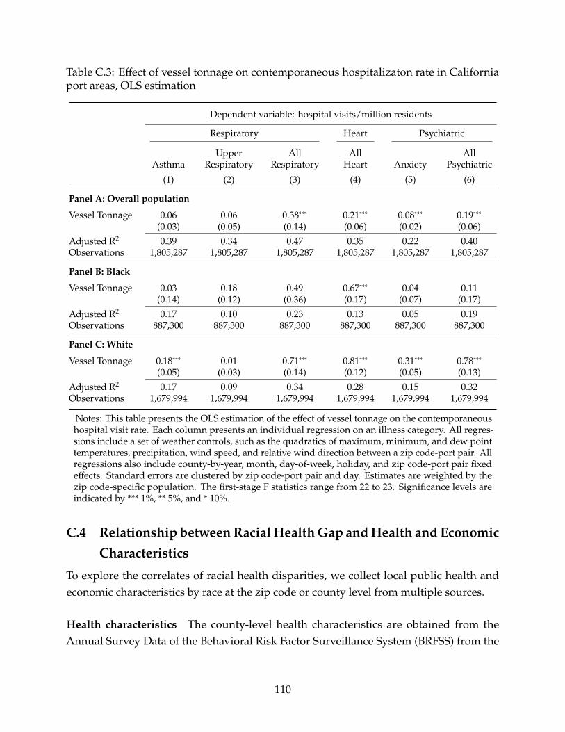
Table C.3: Effect of vessel tonnage on contemporaneous hospitalizaton rate in Californiaport areas, OLS estimation

Dependent variable: hospital visits/million residents

Respiratory Heart Psychiatric

Upper All All AllAsthma Respiratory Respiratory Heart Anxiety Psychiatric

(1) (2) (3) (4) (5) (6)

Panel A: Overall population

Vessel Tonnage 0.06 0.06 0.38∗∗∗ 0.21∗∗∗ 0.08∗∗∗ 0.19∗∗∗(0.03) (0.05) (0.14) (0.06) (0.02) (0.06)

Adjusted R2 0.39 0.34 0.47 0.35 0.22 0.40Observations 1,805,287 1,805,287 1,805,287 1,805,287 1,805,287 1,805,287

Panel B: Black

Vessel Tonnage 0.03 0.18 0.49 0.67∗∗∗ 0.04 0.11(0.14) (0.12) (0.36) (0.17) (0.07) (0.17)

Adjusted R2 0.17 0.10 0.23 0.13 0.05 0.19Observations 887,300 887,300 887,300 887,300 887,300 887,300

Panel C: White

Vessel Tonnage 0.18∗∗∗ 0.01 0.71∗∗∗ 0.81∗∗∗ 0.31∗∗∗ 0.78∗∗∗(0.05) (0.03) (0.14) (0.12) (0.05) (0.13)

Adjusted R2 0.17 0.09 0.34 0.28 0.15 0.32Observations 1,679,994 1,679,994 1,679,994 1,679,994 1,679,994 1,679,994

Notes: This table presents the OLS estimation of the effect of vessel tonnage on the contemporaneoushospital visit rate. Each column presents an individual regression on an illness category. All regres-sions include a set of weather controls, such as the quadratics of maximum, minimum, and dew pointtemperatures, precipitation, wind speed, and relative wind direction between a zip code-port pair. Allregressions also include county-by-year, month, day-of-week, holiday, and zip code-port pair fixedeffects. Standard errors are clustered by zip code-port pair and day. Estimates are weighted by thezip code-specific population. The first-stage F statistics range from 22 to 23. Significance levels areindicated by *** 1%, ** 5%, and * 10%.

C.4 Relationship betweenRacial HealthGap andHealth and EconomicCharacteristics

To explore the correlates of racial health disparities, we collect local public health andeconomic characteristics by race at the zip code or county level from multiple sources.

Health characteristics The county-level health characteristics are obtained from theAnnual Survey Data of the Behavioral Risk Factor Surveillance System (BRFSS) from the

110

Centers for Disease Control and Prevention.7 BRFSS is a survey that collects informationon chronic health conditions and health behaviors, conducted every year via telephoneacross the US We collect data for the period 2003–2012, where county-level responses areavailable. We focus on the counties where the zip codes within 25 miles of the majorCalifornia ports are located. An observation in the final dataset is county-year.

We calculate the race-specific smoking rate in each county as the share of surveyrespondents who report smoking “every day” or “some days” to the total number ofrespondents in the race group. We calculate the poor or fair health status rate as the percentof respondents who report their general health as “poor” or “fair.” We also calculate theobesity rate in each county as the share of survey respondents who have a body massindex 30 or above. Lastly, we calculate the no exercise rate in each county as the share ofrespondents who did not participate in exercises other than regular jobs during the pastmonth. We then plot the distributions of each calculated health characteristic separatelyfor Blacks and whites, as shown in Figure C.2(a). The results demonstrate that Blackstend to haveworse health conditions thanwhites, implyingworse baseline health for Blacks.

Economic characteristics We obtain zip code-level economic characteristics data fromthe American Community Survey (ACS) 5-Year Data from US Census Bureau for the period2012–2016.8 An observation in the final dataset is zip code-year.

The race-specific poverty rate characteristic in each zip code is calculated as the percentof the population who have income in the past 12 months below the poverty level to thetotal population of the race group. We calculate the no health insurance rate as the shareof the population who do not have health insurance coverage. We measure income as percapita inflation-adjusted to the data year dollar. We calculate the bachelor’s degree rate asthe percent of the population who have a bachelor’s degree or above.

Similarly, we plot the distributions of each calculated economic characteristic separatelyfor Blacks and whites. Figure C.2(b) shows that Blacks have worse socioeconomic statusthan whites, which may make them more vulnerable to deal with health risks frompollution exposure.

We also estimate the correlations between the Black-white health gap and the consideredeconomic characteristics by running the following regression:

H8C = -18C + -F8C + 48C ,

7Data were downloaded from https://www.cdc.gov/brfss/annual_data/annual_data.htm (December26, 2021).

8We use the R package “tidycensus” to get access to the data.

111

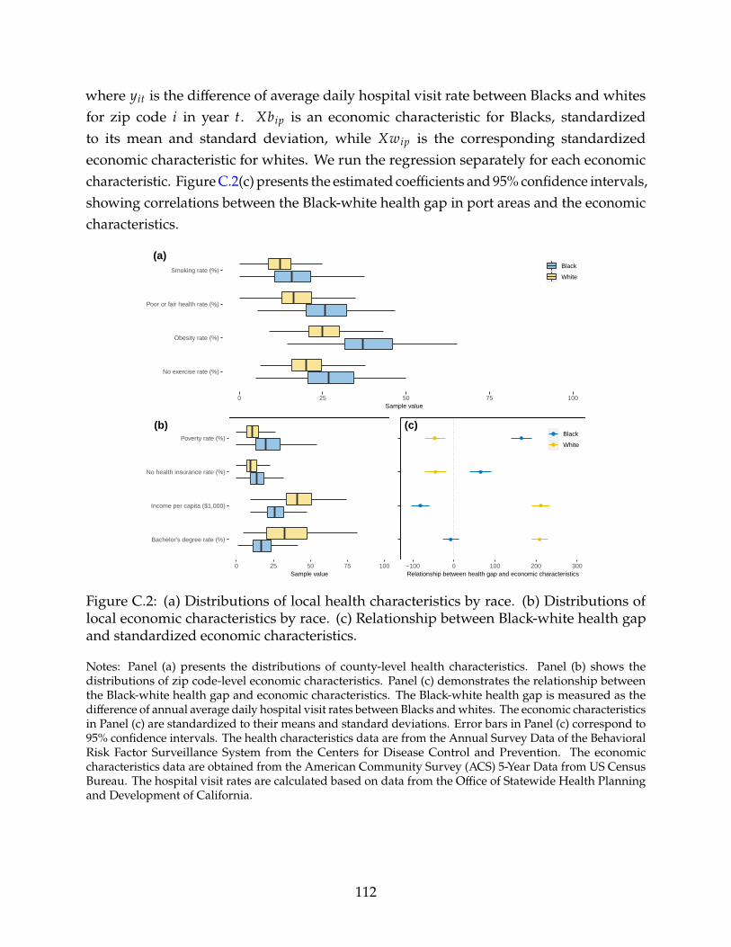
where H8C is the difference of average daily hospital visit rate between Blacks and whitesfor zip code 8 in year C. -18? is an economic characteristic for Blacks, standardizedto its mean and standard deviation, while -F8? is the corresponding standardizedeconomic characteristic for whites. We run the regression separately for each economiccharacteristic. FigureC.2(c) presents the estimated coefficients and 95% confidence intervals,showing correlations between the Black-white health gap in port areas and the economiccharacteristics.

No exercise rate (%)

Obesity rate (%)

Poor or fair health rate (%)

Smoking rate (%)

0 25 50 75 100Sample value

Black

White

(a)

Bachelor's degree rate (%)

Income per capita ($1,000)

No health insurance rate (%)

Poverty rate (%)

0 25 50 75 100Sample value

(b)

−100 0 100 200 300Relationship between health gap and economic characteristics

Black

White

(c)

Figure C.2: (a) Distributions of local health characteristics by race. (b) Distributions oflocal economic characteristics by race. (c) Relationship between Black-white health gapand standardized economic characteristics.

Notes: Panel (a) presents the distributions of county-level health characteristics. Panel (b) shows thedistributions of zip code-level economic characteristics. Panel (c) demonstrates the relationship betweenthe Black-white health gap and economic characteristics. The Black-white health gap is measured as thedifference of annual average daily hospital visit rates between Blacks andwhites. The economic characteristicsin Panel (c) are standardized to their means and standard deviations. Error bars in Panel (c) correspond to95% confidence intervals. The health characteristics data are from the Annual Survey Data of the BehavioralRisk Factor Surveillance System from the Centers for Disease Control and Prevention. The economiccharacteristics data are obtained from the American Community Survey (ACS) 5-Year Data from US CensusBureau. The hospital visit rates are calculated based on data from the Office of Statewide Health Planningand Development of California.

112

D National Energy Modeling System (For Online Publica-tion)

The National Energy Modeling System (NEMS) is an integrated energy-economy modelingsystem developed by EIA. A 2017 version of NEMS is currently hosted on a server at YaleUniversity, and we call it Yale-NEMS at EIA’s request. Yale-NEMS comprises 13 modulescomprehensively modeling major energy supply sectors, conversion sectors, demandmarkets, macroeconomics, and international energy markets. The model simulates energymarkets out to 2050 subject to a comprehensive set of constraints, such as economics, tech-nological advancement, demographics, resource availability, and behavior assumptions.The model also includes current energy and environmental policies at the state and federallevels, while it does not consider any proposed rule-makings. Model projections includeenergy consumption, production, trade, prices, and emissions.

Since we are particularly interested in the effects of shore-side energy consumptionand its interaction with the power sector, this appendix discusses how Yale-NEMS modelsmarine fuel consumption and electricity generation. The description of other modules isavailable at EIA (2009). We first introduce the reference case of Yale-NEMS, which we useas the baseline for our analysis.

D.1 Annual Energy OutlookWe take Annual Energy Outlook (AEO) 2017 as the reference case. AEO 2017 is a reg-ular update of the US energy market outlook, released in early 2017 by EIA. The seriesof AEOs have been widely referenced for decision makings by government agencies,academia, and private sectors for decades. AEO 2017 projects a time path of key USenergy market indicators from present to 2050 EIA (2017a). Comparing to previous annualoutlooks, AEO 2017 includes two reference projections, one including the Clean PowerPlan (CPP) and the other excluding it. Because the CPP is much less stringent than its origi-nal form, in this study, we use AEO 2017without the Clean Power Plan as the reference case.

While AEO 2017 is a few years old, electricity generation in the United States has onlybecome cleaner since 2017. Thus, if our simulation results are biased in any direction, theywould be biased towards overestimating the air pollution from electricity consumption. Thissuggests that using AEO 2021 would only strengthen our results that the California portelectrification regulation reduced air pollution emissions on net.

113

D.2 Marine Energy ConsumptionIn Yale-NEMS, the transportation demand module projects transit and auxiliary fuelconsumption by marine vessels, within the US Emission Control Area—the areas within200 nautical miles of the US coast and outside ECA EIA (2016).

Yale-NEMS models the marine fuel consumption by vessel type (tanker, container,gas (LPG/LNG), roll-on/roll-off, bulk, and general cargo) within the ECA in three steps,as is discussed in great detail in EIA (2016). First, the model estimates the total energyconsumption in a base year (2013) based on historical data. From the base year, the modelthen determines the projections of energy demand in future years by several factors: fleetturnover rate—representing the rate of new vessels entering a fleet moving through ECA,marine fuel efficiency improvement, and industrial output—accounting for economicgrowth. Third, the model splits total energy consumption into four fuel types, includingdistillate oil, residual oil, CNG, and LNG, based on fuel price changes using a logit modelspecification.

EIA’s NEMS does not explicitly model port-side electricity consumption and we addthis feature to Yale-NEMS. First, we obtain historical data on vessel visits connected toonshore electricity and compare them to the total number of visits, which provides usthe approximate percentage of energy consumption from electricity by year and region.For future years, we assume the same proportion of using electricity from 2016. We alsoincorporate the California Ocean-Going Vessel At-Berth Regulation (see Section 6.1 fordetails). Second, since we know the total fossil fuel consumption in ECA, we calculatethe total electricity consumption based on the calculated percentages, constituting thereference shore-side electricity consumption in the model. Third, we subtract the newlyadded marine electricity demand from the total commercial electricity demand. Thus thetotal electricity demand across sectors is still comparable to the AEO 2017 base projections.Fourth, we calculate the reference emissions from vessels by applying the emission factorsby engine type (transit and auxiliary) and fuel type to total fuel consumption.

D.3 Electricity GenerationThe Electricity Market Module (EMM) in Yale-NEMS explicitly models the US electricitymarket and its interaction with other energy markets EIA (2017b). The module is at theNorth American Electric Reliability Corporation (NERC) region level. In each modelingyear, other interrelated modules pass critical parameters to the EMM, including electricitydemand from the four end-use demand modules (commercial, industrial, residential, andtransportation demand), input fuel prices from the fuel supply modules (coal, natural gas,

114

and fuel oils), and macroeconomic expectations from the macroeconomic module. TheEMM then makes production decisions by choosing a fuel mix to generate electricity tomeet demand cost-efficiently with perfect foresight.

The outputs from the EMM include electricity quantities and prices, input fuel consump-tion, emissions, and capital investment for additional capacity, which are then all returnedto the related modules. Several factors determine the total emissions from generatingelectricity, including emission factors across energy types and mitigation technologies. Themodel iterates until market equilibrium achieves. The electricity consumption from ports islinked to EMM.When there is electricity incurred by vessels, the demand is received by theEMM, and then the EMM generates electricity to meet such demand most economically.

Yale-NEMS only reports emissions of SO2 and NOx from the power sector. To evaluatePM2.5, we use an approximation approach similar to Gillingham and Huang (2019, 2020).First, we calculate the base year (2014) PM2.5 emissions from power plants based on theEPA 2014 National Emissions Inventory (NEI) data and obtain the energy consumptionfrom Yale-NEMS in the same year. Second, we extrapolate the emissions after 2014 as aconstant proportion of energy consumption.

D.4 Shore Power ScenarioWe construct a shore power scenario, in which all US ports implement shore power forauxiliary engines of vessels. Specifically, we allow auxiliary fuels (e.g., distillate oil, residualoil, and natural gas) consumed by vessels to be gradually replaced by electricity generatedby power plants from 2020 to 2025, and after 2025 all auxiliary engines are powered byelectricity. The fuel switch follows the following linear adjustment:

@ 5 ,C =

(1 − C − 2019

2025 − 2019

)@05 ,C,

@4 ,C =C − 2019

2025 − 2019

∑5

@05 ,C,

where @05 ,C

represents the consumption of auxiliary fuel 5 by vessels in ports in year C(C < 2025) in the reference case and @ 5 ,C is the adjusted fuel consumption in the ShorePower scenario. @4 ,C is electricity consumption by vessels in ports switched from fossilfuels. From the year 2025 onwards, fossil fuels consumed by auxiliary engines are entirelyreplaced with electricity, as represented in the following:

115

@ 5 ,C = 0,

@4 ,C =∑5

@05 ,C.

We run the reference case and the Shore Power scenario individually in Yale-NEMS.We then compare the emissions results between the two cases, and the differences indicatethe effect of implementing shore power in ports.

References for AppendicesBell, M. L., Ebisu, K., Peng, R. D., Walker, J., Samet, J. M., Zeger, S. L., and Dominici, F.(2008). Seasonal and regional short-term effects of fine particles on hospital admissionsin 202 US counties, 1999-2005. American Journal of Epidemiology, 168(11):1301–10.

Dominici, F., Peng, R. D., Bell, M. L., Pham, L., McDermott, A., Zeger, S. L., and Samet,J. M. (2006). Fine particulate air pollution and hospital admission for cardiovascular andrespiratory diseases. JAMA, 295(10):1127–34.

EIA (2009). The National Energy Modeling System: An Overview 2009. Technical report,United State Energy Information Administration, Washington, DC.

EIA (2016). Transportation Sector Demand Module of the National Energy ModelingSystem: Model Documentation. Technical report, United States Energy InformationAdministration, Washington, DC.

EIA (2017a). Annual Energy Outlook 2017. Technical report, U.S. Energy InformationAdministration, Washington, DC.

EIA (2017b). Electricity Market Module of the National Energy Modeling System: ModelDocumentation. Technical report, United States Energy Information Administration,Washington, DC.

EPA (2003). Control of Emissions From NewMarine Compression-Ignition Engines at orAbove 30 Liters Per Cylinder. Technical report, United States Environmental ProtectionAgency, Washington, DC.

Firpo, S., Fortin, N. M., and Lemieux, T. (2009). Unconditional Quantile Regressions.Econometrica, 77(3):953–973.

116

Gillingham, K. and Huang, P. (2019). Is abundant natural gas a bridge to a low-carbonfuture or a dead-end? Energy Journal, 40(2):1–26.

Gillingham, K. and Huang, P. (2020). Long-Run Environmental and Economic Impacts ofElectrifyingWaterborne Shipping in the United States. Environmental Science & Technology,54(16):9824–9833.

Hwang, J. S. and Chan, G. C. (2002). Effects of air pollution on daily clinic visits for lowerrespiratory tract illness. American Journal of Epidemiology, 155(1):1–10.

Peel, J. L., Tolbert, P. E., Klein, M., Metzger, K. B., Flanders,W. D., Todd, K., Mulholland, J. A.,Ryan, P. B., and Frumkin, H. (2005). Ambient air pollution and respiratory emergencydepartment visits. Epidemiology, 16(2):164–174.

Schlenker, W. and Walker, W. R. (2016). Airports, air pollution, and contemporaneoushealth. Review of Economic Studies, 83(2):768–809.

Stieb, D. M., Szyszkowicz, M., Rowe, B. H., and Leech, J. A. (2009). Air pollution andemergency department visits for cardiac and respiratory conditions: a multi-city time-series analysis. Environmental Health, 8:25.

117