Quasi-diabatic representations of adiabatic potential energy surfaces coupled by conical...

THE JOURNAL OF CHEMICAL PHYSICS 137, 22A511 (2012)

Quasi-diabatic representations of adiabatic potential energy surfacescoupled by conical intersections including bond breaking: A more generalconstruction procedure and an analysis of the diabatic representation

Xiaolei Zhua) and David R. Yarkonyb)

Department of Chemistry, Johns Hopkins University, Baltimore, Maryland 21218, USA

(Received 14 May 2012; accepted 25 June 2012; published online 27 July 2012)

The analytic representation of adiabatic potential energy surfaces and their nonadiabatic interactionsis a key component of accurate, fully quantum mechanical descriptions of nonadiabatic dynamics.In this work, we describe extensions of a promising method for representing the nuclear coordinatedependence of the energies, energy gradients, and derivative couplings of Nstate adiabatic electronicstates coupled by conical intersections. The description is based on a vibronic coupling model and candescribe multichannel dissociation. An important feature of this approach is that it incorporates infor-mation about the geometry dependent interstate derivative couplings into the fitting procedure so thatthe resulting representation is quantifiably quasi diabatic and quasi diabatic in a least squares sense.The reported extensions improve both the rate of convergence and the converged results and willpermit the optimization of nonlinear parameters including those parameters that govern the place-ment of the functions used to describe multichannel dissociation. Numerical results for a coupledquasi-diabatic state representation of the photodissociation process NH3+hv → NH2+H illustratethe potential of the improved algorithm. A second focus in this numerical example is the quasi-diabatic character of the representation which is described and analyzed. Special attention is paidto the immediate vicinity of the conical intersection seam. © 2012 American Institute of Physics.[http://dx.doi.org/10.1063/1.4734315]

I. INTRODUCTION

For the foreseeable future, accurate fully quantum me-chanical simulations of electronically nonadiabatic processesinvolving conical intersections will require analytic represen-tations of the requisite electronic structure data,1 energies,energy gradients and derivative couplings in the adiabaticrepresentation, or the Hamiltonian matrix elements in the di-abatic representation. The need to accurately sample initialdistributions means that even more approximate dynamicalapproaches such as trajectory surface hopping,2 which can beused with electronic structure data determined “on the fly” or“directly” as needed,3, 4 can also benefit from analytic repre-sentations of electronic structure data. A principal advantageof analytic representations is that they can employ much moreaccurate wave functions than are currently practical in directdynamics. Unfortunately the representation of adiabatic po-tential energy surfaces coupled by conical intersections ob-tained by ab initio methods is a challenging problem. Thechallenge is particularly daunting when chemical bonds arebroken and the molecule dissociates.

The existence of conical intersections, with their singularderivative couplings in the adiabatic basis motivates the useof a quasi-diabatic state representation of the adiabatic states.The advantages of a diabatic representation are two fold. Arigorous diabatic representation solves the problem of thesingular derivative couplings by requiring that the derivative

a)Electronic mail: [email protected])Electronic mail: [email protected].

coupling in the diabatic representation vanish globally (seeSec. III). The vanishing of the derivative coupling also sim-plifies the form the nuclear Schrödinger equation.5 Unfortu-nately, the attribute quasi used above, which we shall omitbelow except as needed for emphasis, indicates that for poly-atomic molecules rigorous diabatic bases do not exist.5–7

The determination of a quasi-diabatic representation ofcoupled adiabatic states data has long been a problem ofconsiderable interest in computational nonadiabatic chem-istry. For a synopsis of much of this work prior to 2008, seeRef. 8. The determination of a diabatic representation com-bines a method for constructing the diabatic state data fromthe adiabatic state data with a method for fitting or repre-senting the diabatic state data. The type of ab initio dataused to define the diabatic basis, some combination of en-ergies, energy gradients and derivative couplings, is also anissue. Approaches to this problem include (i) the fourfoldway diabatization,9, 10 accompanied by fitting the resulting di-abatic matrix elements;11 (ii) diabatization by ansatz whichfits the adiabatic energies using a matrix of smoothly varyingfunctions;12, 13 (iii) Shepard interpolation of a diabatic repre-sentation based on energy gradients, derivative couplings, andtheir derivatives;14–16 (iv) diabatizations based on the regu-larized representation17, 18 followed by fitting the diabatic en-ergies; (v) double many body expansions;19–22 (vi) the gen-eralized adiabatic angle method;8 (vii) methods based onpolyspherical coordinates and dynamical symmetry groups,1

and (viii) methods based on molecular properties.23, 24

Recently we have introduced an approach based ona vibronic coupling model25 that uses ab initio energies,

0021-9606/2012/137(22)/22A511/13/$30.00 © 2012 American Institute of Physics137, 22A511-1

This article is copyrighted as indicated in the article. Reuse of AIP content is subject to the terms at: http://scitation.aip.org/termsconditions. Downloaded to IP:69.137.46.163 On: Sun, 15 Dec 2013 07:49:47

http://dx.doi.org/10.1063/1.4734315

http://dx.doi.org/10.1063/1.4734315

http://dx.doi.org/10.1063/1.4734315

http://dx.doi.org/10.1063/1.4734315

22A511-2 X. Zhu and D. R. Yarkony J. Chem. Phys. 137, 22A511 (2012)

energy gradients and derivative couplings to determine the di-abatic representation.26–28 This approach has several featuresto its merit. It uses overcomplete sets of coordinates (see alsoRef. 22) and is therefore not tied to a specific coordinate rep-resentation. Indeed, in a future work, we will show how acombination of natural internal coordinates29 and the expo-nential coordinates used here can be used to describe bondbreaking in molecules where one or more fragments remainintact. Although most of the ab initio data are described ina least squares sense, the ability to designate some points asnodes, points where the ab initio data are exactly reproduced,allows for a flexible combination of least squares fitting andinterpolation. The use of functions localized in distinct re-gions of nuclear coordinate space, facilitates the descriptionof multichannel processes.22 The incorporation of interstatederivative coupling information into the fitting procedure re-sults in a representation which is quantifiably diabatic and di-abatic in a least squares sense. The use of derivative couplingdata and intersection adapted coordinates30 enables a continu-ous and accurate description of a seam of conical intersectionand its local topography. The numerical example used in thiswork28 accurately describes 24 points of conical intersectionon a two state seam. Although currently limited to two stateseams of conical intersection, the approach developed herecan be readily extended handle seams of conical intersectionof three states.

In this work, we introduce an enhanced algorithm whichimproves both convergence and the converged result of thefitting procedure and will enable optimization of nonlinearparameters. In light of our earlier comments concerning di-abatic representations, we will also investigate, from a com-putational perspective, the diabatic representation producedby this procedure, demonstrating in particular, its ability toaccurately describe the immediate vicinity of a conical inter-section.

The nonadiabatic photodissociation of ammonia,

NH3(X, v) → NH3(A, v′) → NH2(X, A) + H, (1)

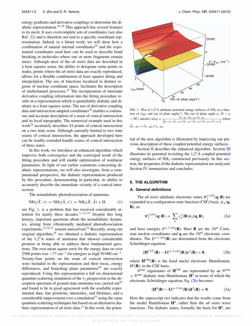
see Fig. 1, is a problem that has received considerable at-tention for nearly three decades.11, 31–55 Despite this longhistory, important questions about the nonadiabatic dynam-ics, arising from vibrationally mediated photodissociationexperiments,35, 56, 57 remain unresolved.54 Recently, using ouroriginal algorithm,28 we obtained a diabatic representationof the 1,21A states of ammonia that showed considerablepromise in being able to address these fundamental ques-tions. The root mean square error for the energy data on over2500 points was ∼77 cm−1 for energies as high 50 000 cm−1.Twenty-four points on the seam of conical intersectionwere included in the representation and their locus, energydifferences, and branching plane parameters58 are exactlyreproduced. Using this representation a full six dimensionalquantum scattering simulation of the v2 progression in the ab-sorption spectrum of ground state ammonia was carried out59

and found to be in good agreement with the available exper-imental data, line positions, intensities, and lifetimes, and aconsiderable improvement over a simulation53 using the samequantum scattering techniques but based on an alternative dia-batic representation of ab initio data.11 In this work, the poten-

FIG. 1. Plot of 1,21A adiabatic potential energy surfaces of NH3 as a func-tion of rNH1 and out of plane angle(˚). The out of plane angle ϕ, (0 < ϕ

< 90˚) satisfies sin ϕ = dN−H1×dN−H2 ·dN−H3!!!dN−H1×dN−H2+dN−H2×dN−H3+dN−H3×dN−H1

!!!where

dN−Hn = rN−Hn/rN−Hn.

tial of the new algorithm is illustrated by improving our pre-vious description of these coupled potential energy surfaces.

Section II describes the enhanced algorithm. Section IIIillustrates its potential revisiting the 1,21A coupled potentialenergy surfaces of NH3 constructed previously. In this sec-tion, the properties of the diabatic representation are analyzed.Section IV summarizes and concludes.

II. THE ALGORITHM

A. General definitions

The ab initio adiabatic electronic states "a,(ab)J (q; R) are

expanded in a configuration state function (CSF) basis, ψα(q;R), as

"a,(ab)J (q; R) =

"

α

cJα (R)ψα(q; R), (2a)

and have energies Ea, J, (ab)(R). Here R are the 3Nat Carte-sian nuclear coordinates and q are the 3Nel electronic coor-dinates. The Ea, J, (ab)(R) are determined from the electronicSchrödinger equation,

[HCSF (R) − IEa,J,(ab)(R)]cJ (R) = 0, (2b)

where HCSF(R) is the fixed nuclei electronic Hamiltonian,He(R), in the CSF basis.

Nstate eigenstates of HCSF are represented by an Nstate

× Nstate diabatic state Hamiltonian, Hd in terms of which theelectronic Schrödinger equation, Eq. (2b) becomes

[Hd(R) − IEa,J,(m)(R)]dJ (R) = 0. (3a)

Here the superscript (m) indicates that the results come fromthe model Hamiltonian Hd, rather than the ab initio wavefunctions. The diabatic states, formally the basis for Hd, are



constructed from adiabatic states,

!du (q; R) =

N state∑

J=1

!a,(ab)J (q; R)(d−1)Ju (R)

=N state∑

J=1

!a,(ab)J (q; R)du

J (R). (3b)

As discussed in Ref. 28, Hd is expanded in terms of basismatrices, Bu,v, as

Hd (R) =Nc∑

n=1

Vnp(n)(R)Bu(n),v(n), (4)

where Bu,v is an Nstate × Nstate symmetric matrix with a 1 inthe (u,v) and (v,u) elements and the remaining elements 0. Forexample, for Nstate = 2 there are three basis matrices,

B1,1 =(

1 00 0

)B1,2 =

(0 11 0

)and B2,2 =

(0 00 1

).

The Nc unknown coefficients of combination, the Vn, 1≤ n ≤ Nc, are denoted the linear parameters. The advantageof Hd in the form of Eq. (4), is that it makes the lineardependence of Hd on the Vj explicit and easy to work with.The geometry dependence of Hd is contained in the polyno-mials p(n)(R), symmetry adapted linear combinations of basicmonomials, gl(R). The gl(R) currently in use are described inAppendix A. As explained in Ref. 28, p(n)(R)= Pu(n)gl(n)(R), where Pu(n) is the appropriate grouptheoretical projection operator. The nonlinear parametersare contained in the p(n) and are denoted collectively asγ i, 1 ≤ i ≤ Nnl. The nonlinear parameters are described inAppendix A.

B. Defining equations

We now turn to the equations defining the linear and non-linear parameters. The Vj and γ i are chosen so that the differ-ences between the Hd determined, and ab initio determined,energies, energy gradients, and derivative couplings (actu-ally the interstate coupling vector which is approximatelythe derivative coupling times the energy difference) are min-imized on a set of nuclear configurations, Rn, 1 ≤ n ≤ Npoint,

in a prescribed manner. The following definitions will allowus to succinctly express the conditions:

LI,I,(x)0 (Rn) ≡ Ea,I,(x)(Rn), (5a)

LI,I,(x)j (Rn) ≡ ∇jE

a,I,(x)(Rn), (5b)

LI,J,(x)j (Rn) ≡ h

I,J,(x)j (Rn), (5c)

where ha,I,J,(x)j is a component of the interstate coupling vec-

tor ha,I,J,(x) defined by

ha,I,J,(m)(R) = dI (R)†∇Hd (R)dJ (R) (5d)

and

ha,I,J,(ab)(R) = cI (R)†∇HCSF (R)cJ (R)

≈ fa,I,J,(ab)(R)[Ea,J,(ab)(R) − Ea,J,(ab)(R)],

(5e)

where fa, I, J, (ab) is the ab initio derivative coupling vector.From Eq. (3a), its derivative and Eq. (4), Eqs. (5a)–(5c) be-come, for x = m,

LI,J,(m)j (Rn) =

Nc∑

l=1

VlWn,I,J,j ;I ≡ (WV)k = L(m)k , (6a)

where

Wn,I,J,j ;l = dI†(Rn)Bu(l),v(l)dJ (Rn)[∇jp(l)(Rn)], (6b)

and ∇0 means do nothing. In Eq. (6a) and below is convenientto re-index the four indices (n,I,J,j) by k so that L

I,J,(x)j (Rn),

is replaced by L(x)k , and Wn,I,J,j ;l by Wk,l for 1 ≤ k ≤ Neq.

In Eq. (6b) at each Rn, the ∇ j denote the derivatives with re-spect to a local, nonredundant coordinate system. The choiceof local coordinates is arbitrary and different coordinatescan be used for different points. This flexibility is a key as-pect of the algorithm. It is also important to emphasize thatEq. (6a) is exact even though the dJ depend on R. Finally, forclarity, note that Eqs. (6a) and (6b) illustrate two of the differ-ent lengths of matrix-vector products used in this work, withEq. (6a) using length Nc and Eq. (6b) using length Nstate.

We would like to require L(ab)k = L(m)

k for all k, but thatis not possible since Neq ≫ (Nc + Nnl). Instead we requireL(ab)

j = L(m)j for 1 ≤ j ≤ Nlsq be solved in a least squares

sense and the remaining Nex = Neq−Nlsq equations, that isL(ab)

j = L(m)j for Nlsq < j ≤ Neq, be solved exactly. Nuclear

configurations whose ab initio data fall into the second cate-gory will be referred to as nodes. The desired solution is ob-tained with the help of the Lagrangian,

#(V, γ ,λ) = 12

Nlsq∑

j=1

[L

(m)j − L

(ab)j

]2

+Neq∑

j=Nlsq+1

λj−Nlsq

[L

(m)j − L

(ab)j

]+ t

2V†V,

(7)

where the λj are the Lagrange multipliers. The origin of thefinal term in Eq. (7), a damping term, is explained below. Re-quiring GV

i = ∂#∂Vi

= 0, for 1 ≤ i ≤ Nc; Gλi = ∂#

∂λi= 0, for 1

≤ i ≤ Nex; and Gγj = ∂#

∂γj= 0 for 1 ≤ j≤ Nnl, gives through

second order in displacements, the standard Newton-Raphsonequations,

⎛

⎜⎝#V,V #V,λ #V,γ

#V,λ 0 #λ,γ

#γ ,V #γ ,λ #γ ,γ

⎞

⎟⎠

0

⎛

⎜⎝δVδλ

δγ

⎞

⎟⎠ = −

⎛

⎜⎝GV

Gλ

Gγ

⎞

⎟⎠

0

. (8)

Here #V,Vi,j = ∂2#

∂Vi∂Vj, #V,λ

i,j = ∂2#∂Vi∂λj

, and etc.; V = V0 + δV,

λ = λ0 + δλ, and γ = γ 0 + δγ ; and the superscript 0, whichwe will suppress when no confusion will result, indicates that



the quantities are evaluated at the current, as opposed to thedisplaced, “point.” The gradients are given by

!GV

Gλ

"

=!

Wlsq†Wlsq + tI Wex†

Wex 0

"!Vλ

"

−!

Wlsq†L(ab),lsq

L(ab),ex

"

+!

GV

0

"

(9a)

and

Gγj =

#L(m),lsq − L(ab),lsq$† ∂Wlsq

∂γj

V + λ† ∂Wex

∂γj

V, (9b)

where

GVj = V† ∂(Wlsq)†

∂Vj

(L(m),lsq − L(ab),lsq ) + V† ∂(Wex)†

∂Vj

λ.

(10)In Eqs. (9a) and (10), we have partitioned the exact and leastsquares equations writing

L(ab) =!

L(ab),lsq

L(ab),ex

"

and W =!

Wlsq

Wex

"

, (11)

where L(ab),lsq (Wlsq) is a vector (matrix) of length (size) Nlsq

(NlsqxNc) and L(ab),ex (Wex) is a vector (matrix) of length(size) Nex (NexxNc). Note that W has an explicit γ -dependencethrough the p(n) and an implicit γ -dependence through the dJ,that is,

∂Wn,I,J,j ;l

∂γk

= dI †(Rn)Bu(l),v(l)dJ (Rn)

%∂

∂γk

∇jp(l)(Rn)

&

+'

∂dI †(Rn)

∂γk

Bu(l),v(l)dJ (Rn)

+ dI †(Rn)Bu(l),v(l) ∂dJ (Rn)

∂γk

&[∇jp

(l)(Rn)].

(12a)

whereas, from Eqs. (6a) and (6b), W, has only an implicit V-dependence through the dJ, that is,

∂Wn,I,J,j ;l

∂Vk

='

∂dI †(Rn)

∂Vk

Bu(l),v(l)dJ (Rn)

+ dI †(Rn)Bu(l),v(l) ∂dJ (Rn)

∂Vk

&[∇jp

(l)(Rn)].

(12b)

Here and below we suppress the superscripts ex and lsq whenno confusion will result. The evaluation of ∂2$

∂zi∂zjis discussed

in Appendix B. The appearance of terms like ∂dI† (Rn)∂Vk

, mightappear to preclude accurate description of the immediatevicinity of a conical intersection. However, we show in Ap-

pendix C, where the evaluation of ∂dI† (Rn)∂γk

and ∂dI† (Rn)∂Vk

is dis-cussed, that this is emphatically not the case, although it is byno means a trivial matter. Finally, note that GV contains onlyterms that arise from the implicit V-dependence of W.

C. Original algorithm

There are several ways to use these results to obtain a vi-able Hd. Our previous work28, 60 has been restricted to the de-termination of the linear parameters, the Vi, with the γ j fixed,using

!Wlsq†

Wlsq + tI Wex†

Wex 0

" !Vλ

"

=!

Wlsq†L(ab),lsq

L(ab),ex

"

,

(13)which is obtained from Eq. (9a), by neglecting GV , whichas we note in Appendix B is expected to be small whenan approximate solution has been achieved. While an ap-proximation to the more complete Newton-Raphson result inEq. (8), Eq. (13) is comparatively straightforward to formulateand solve. The V obtained from this system of linear equa-tions reproduce well, the ab initio data.28, 60, 61 These equa-tions must be solved iteratively since the dJ(Rn) are requiredto determine the Vi and conversely. The final term in Eq. (7),the damping or flattening term, where t > 0, is included sincesome linear combinations of the Vn may not be well-definedby the available ab initio data, that is the matrix Wlsq†

Wlsq

is rank deficient. Since t is small and positive, ∼10−5 ≥ t≥ 10−8, this term tends to drive ill-defined linear combina-tions of Vi toward 0. In this way its inclusion avoids patho-logical behavior in the fits, with a relatively small cost in thequality of fit.

D. Newton-Raphson equations

We now turn to the use of the Newton-Raphson equa-

tions. Given the occurrence of ∂dI† (Rn)∂Vk

and the importance ofconical intersections the full Newton-Raphson equations mustbe used with some care. Appendixes B–D address many tech-nical issues in this regard.

1. Linear terms, V

In general, Eq. (13) converges rapidly to a unique solu-tion as long as Nc is relatively small. However for more elab-orate representations, larger Nc, the V determined from thisequation provide a minimum in the root mean square energyerror, with a modest residual gradient.59 In this work, to gobeyond Eq. (13), we introduce an economical approximationto the full second order procedure for the linear terms

(M)0

!δVδλ

"

= −!

GV

Gλ

"

0

, (14)

where

M =!

#V,V #V,λ

#λ,V 0

"

. (15)

The approximate Hessian is discussed in Appendixes Band C. The solution to Eq. (14) is discussed in Appendix D.



2. Nonlinear terms, γ

Finally we turn to the issue of optimizing the nonlin-ear parameters, parameters whose principal purpose, see Ap-pendix A, is to distribute the basic monomials, gl(R), through-out coordinate space. This is accomplished using the fullNewton-Raphson equations, Eqs. (8). Again the approximateHessian is described in Appendixes B and C. Here it is onlyimportant to emphasize the need to have good starting valuesfor the linear parameters before the nonlinear terms are opti-mized.

III. COMPUTATIONAL RESULTS

The coupled adiabatic potential energy surfaces consid-ered in this study describe the 1,21A states of NH3. The sub-space of the full 6-dimensional nuclear coordinate space de-scribed by Hd is relevant to the well studied photodissociationreaction given in (1). This reflects the fact that the preponder-ance of the Rn used to define Hd were obtained from nona-diabatic surface hopping trajectories with initial conditionsappropriate for reaction (1). A three dimensional plot of theadiabatic potential energy surfaces for the 1,21A states evinc-ing the ground state minimum, the minimum and saddle pointon the 21A potential energy surface, and the minimum energypoint of conical intersection, is provided in Fig. 1. Althoughat first glance this might appear to be a relatively straight-forward computational problem, that turns out not to be thecase. The Hd must accurately describe: (i) an extended 4 di-mensional seam of conical intersection, for which points wellremoved from the minimum energy crossing point are acces-sible and likely to be relevant to the nonadiabatic photodisso-ciation; (ii) a highly anharmonic minimum for the A state witha low barrier separating the region of the minimum from thatof the seam of conical intersections; and (iii) a ground statepotential energy surface that must be well described over anenergy range of ∼6 eV while insuring that the representationis sufficiently diabatic to be suitable for quantum dynamics.

Previously we have constructed, using Eq. (13), an Hd

intended for use in describing reaction (1).28 The electronicstructure description of the 1,21A states of NH3, multirefer-ence configuration interaction wave functions comprised ofover 30 × 106 CSFs and the form of Hd, which consistedof over 9000 linear terms defined by a total of over 27 000energies, energy gradients, and derivative couplings, is pre-sented in Ref. 28. This Hd was shown to provide and excel-lent representation of the ab inito data from which it wasconstructed.28 The utility of Hd for describing reaction (1)was tested by a fully quantum mechanical, 6 dimensional sim-ulation of the v2 progression in the A ← X absorption spec-trum of NH3, including the line positions, intensities and linewidths. Although this spectrum had proven difficult to simu-late previously,53 excellent agreement with the experimentalresults was found.59

In this work our goals are two-fold: (i) to establish theutility of the Newton-Raphson approach in Eq. (14) in sys-tems with conical intersections and determine the potentialbenefits compared to the use of Eq. (13) and (ii) to assess andillustrate the diabaticity of the derived diabatic representation.

A. Derivative couplings

As noted previously the goal of the transformation to di-abatic states is to minimize the derivative coupling in the dia-batic representation, ⟨!d

α (q; R)|∇k!dβ (q; R)⟩q, which is eval-

uated in terms of the residual derivative coupling as follows.Using the definition the adiabatic derivative coupling

fa,I,J,(ab)k (R) ≡

!!

a,(ab)I (q; R)|∇k!

a,(ab)J (q; R)

"q (16)

from Eqs. (3a) and (3b) and their derivatives, we obtain

fa,I,J,(ab)k (R) =

Nstate#

α=1

dIα(R)∇kdJ

α (R)

+Nstate#

α,β=1

dIα (R)

!!d

α (q; R)|∇k!dβ (q; R)

"qdJ

β (R)

(17)

≈ dI (R)†(∇kHd )dJ (R)Ea,J,(m)(R) − Ea,I,(m)(R)

≡ fa,I,J,(m)k (R). (18)

The approximate equality in Eq. (18) comes from ne-glecting the second term in Eq. (17), the derivative couplingdue to the quasi-diabatic states !d

u . The use of Eq. (3b)to define the quasi-diabatic states guarantees that, in princi-ple, the diabatic states can reproduce the adiabatic energies.The question is how diabatic is the transformation. This isdetermined from Eqs. (17) and (18), from which for 1 ≤ I< J ≤ Nstate, the residual derivative coupling, δf a,I,J

k (R)≡ f

a,I,J,(ab)k (R) − f

a,I,J,(m)k (R) is related to the quasi-diabatic

state coupling, ⟨!dα (q; R)|∇k!

dβ (q; R)⟩qby the following sys-

tem of linear equations:

δf a,I,Jk (R) =

#

1≤α<β≤Nstate

[dIα(R)dJ

β (R)

− dIβ (R)dJ

α (R)]!!d

α (q; R)|∇k!dβ (q; R)

"q. (19)

For the Nstate = 2 case considered here, Eq. (19) reduces tothe appealing result:

δf a,I,Jk (R) =

!!d

I (q; R)|∇k!dJ (q; R)

"q . (20)

Thus, the magnitude ∥δfa,I,J(R)∥ is a direct measure ofthe quality of the quasi-diabatic representation. For a rigorousdiabatic basis, δfa,I,J(R), would vanish globally. As noted inthe Introduction this is not possible here.

Two comments concerning the derivative coupling are inorder. The ab initio determined derivative couplings cannotbe described exactly in the current approach since the nonre-movable part of the derivative coupling cannot be describedby a square truncated representation such as the one we use.6

This contribution becomes part of the residual coupling. Aswe will see below, this contribution is small compared to theremovable part, where the energy separation of the adiabaticstates is small. When the energy separation is large, althoughthe residual coupling is an appreciable fraction of the actualcoupling, neither is significant. In dissociation channels wherethe total derivative coupling can become small, care must be



taken to avoid including the nonremovable part.28 The sec-ond point concerns the fact that the derivative couplings de-termined from Hd are necessarily due to internal coordinatesonly. However the ab initio determined derivative couplingsinclude contributions from overall rotations and translations.These contributions, are not a problem, in principle, since theycan be represented as electronic matrix elements of the form⟨!a,(ab)

I |Oel|!a,(ab)J ⟩, where Oel is the total electronic gradi-

ent or total orbital angular momentum operator.62 One mustonly be careful to remove these contributions from fa.I.J,(ab)(R)prior to the fitting.

B. Newton-Raphson equations

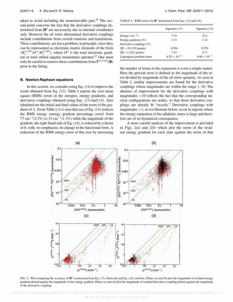
In this section, we consider using Eq. (14) to improve theresult obtained from Eq. (13). Table I reports the root meansquare (RMS) errors in the energies, energy gradients, andderivative couplings obtained using Eqs. (13) and (14). Alsotabulated are the initial and final values of the norm of the gra-dient of ". From Table I, it is seen that use of Eq. (14) reducesthe RMS energy (energy gradient percentage error) from77 cm−1(2.3%) to 33 cm−1(1.1%) while the magnitude of thegradient, the right-hand side of Eq. (14), is reduced by a factorof 8, with, we emphasize, no change in the functional form. Areduction of the RMS energy error of this size by increasing

TABLE I. RMS errors for Hd determined from Eqs. (13) and (14).

Equation (13) Equation (14)

Energy (cm−1) 77.0 33.2Energy gradients (%) 2.33 1.14Derivative couplings (%)∥f∥ >10 (192 points) 0.594 0.570∥f∥ >1 (612 points) 7.43 4.71Lagrangian gradient norm 4.29 × 10−2 6.04 × 10−3

the number of terms in the expansion is a not a simple matter.Here the percent error is defined as the magnitude of the er-ror divided by magnitude of the ab initio quantity. As seen inTable I, similar improvements are found for the derivativecouplings whose magnitudes are within the range 1–10. Theabsence of improvement for the derivative couplings withmagnitudes >10 reflects the fact that the corresponding nu-clear configurations are nodes, so that these derivative cou-plings are already fit “exactly.” Derivative couplings withmagnitudes <1, as we illustrate below, occur in regions wherethe energy separation of the adiabatic states is large and there-fore are of no dynamical consequence.

A more careful analysis of the improvement is providedin Figs. 2(a) and 2(b) which plot the norm of the resid-ual energy gradient for each state against the norm of that

FIG. 2. Plot comparing the accuracy of Hd constructed from Eq. (13), black dot and Eq. (14), red dots. Plates (a) and (b) plot the magnitude of residual energygradient plotted against the magnitude of the energy gradient. Plates (c) and (d) plot the magnitude of residual derivative coupling plotted against the magnitudeof the derivative coupling.



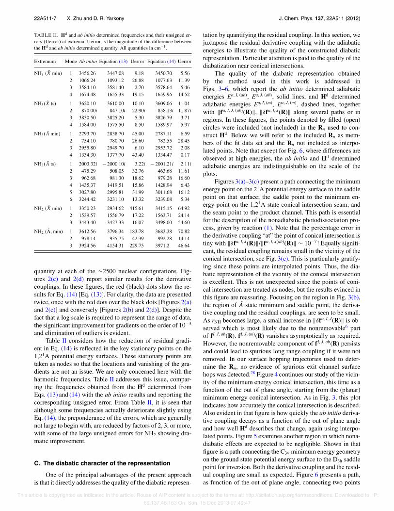
TABLE II. Hd and ab initio determined frequencies and their unsigned er-rors (Uerror) at extrema. Uerror is the magnitude of the difference betweenthe Hd and ab initio determined quantity. All quantities in cm−1.

Extremum Mode Ab initio Equation (13) Uerror Equation (14) Uerror

NH3 (X min) 1 3456.26 3447.08 9.18 3450.70 5.562 1066.24 1093.12 26.88 1077.63 11.393 3584.10 3581.40 2.70 3578.64 5.464 1674.48 1655.33 19.15 1659.96 14.52

NH3(X ts) 1 3620.10 3610.00 10.10 3609.06 11.042 870.00i 847.10i 22.90i 858.13i 11.87i3 3830.50 3825.20 5.30 3826.79 3.714 1584.00 1575.50 8.50 1589.97 5.97

NH3(A min) 1 2793.70 2838.70 45.00 2787.11 6.592 754.10 780.70 26.60 782.55 28.453 2955.80 2949.70 6.10 2953.72 2.084 1334.30 1377.70 43.40 1334.47 0.17

NH3(A ts) 1 2003.32i − 2000.10i 3.22i − 2001.21i 2.11i2 475.29 508.05 32.76 463.68 11.613 962.68 981.30 18.62 979.28 16.604 1435.37 1419.51 15.86 1428.94 6.435 3027.80 2995.81 31.99 3011.68 16.126 3244.42 3231.10 13.32 3239.08 5.34

NH2 (X min) 1 3350.23 2934.62 415.61 3415.15 64.922 1539.57 1556.79 17.22 1563.71 24.143 3443.40 3427.33 16.07 3498.00 54.60

NH2 (A, min) 1 3612.56 3796.34 183.78 3683.38 70.822 978.14 935.75 42.39 992.28 14.143 3924.56 4154.31 229.75 3971.2 46.64

quantity at each of the ∼2500 nuclear configurations. Fig-ures 2(c) and 2(d) report similar results for the derivativecouplings. In these figures, the red (black) dots show the re-sults for Eq. (14) [Eq. (13)]. For clarity, the data are presentedtwice, once with the red dots over the black dots [Figures 2(a)and 2(c)] and conversely [Figures 2(b) and 2(d)]. Despite thefact that a log scale is required to represent the range of data,the significant improvement for gradients on the order of 10−3

and elimination of outliers is evident.Table II considers how the reduction of residual gradi-

ent in Eq. (14) is reflected in the key stationary points on the1,21A potential energy surfaces. These stationary points aretaken as nodes so that the locations and vanishing of the gra-dients are not an issue. We are only concerned here with theharmonic frequencies. Table II addresses this issue, compar-ing the frequencies obtained from the Hd determined fromEqs. (13) and (14) with the ab initio results and reporting thecorresponding unsigned error. From Table II, it is seen thatalthough some frequencies actually deteriorate slightly usingEq. (14), the preponderance of the errors, which are generallynot large to begin with, are reduced by factors of 2, 3, or more,with some of the large unsigned errors for NH2 showing dra-matic improvement.

C. The diabatic character of the representation

One of the principal advantages of the present approachis that it directly addresses the quality of the diabatic represen-

tation by quantifying the residual coupling. In this section, wejuxtapose the residual derivative coupling with the adiabaticenergies to illustrate the quality of the constructed diabaticrepresentation. Particular attention is paid to the quality of thediabatization near conical intersections.

The quality of the diabatic representation obtainedby the method used in this work is addressed inFigs. 3–6, which report the ab initio determined adiabaticenergies Ea, I, (ab), Ea, J, (ab), solid lines, and Hd determinedadiabatic energies Ea, I, (m), Ea, J, (m), dashed lines, togetherwith ∥fa, I, J, (ab)(R)∥, ∥δfa, I, J(R)∥ along several paths or inregions. In these figures, the points denoted by filled (open)circles were included (not included) in the Rn used to con-struct Hd. Below we will refer to the included Rn as mem-bers of the fit data set and the Rn not included as interpo-lated points. Note that except for Fig. 6, where differences areobserved at high energies, the ab initio and Hd determinedadiabatic energies are indistinguishable on the scale of theplots.

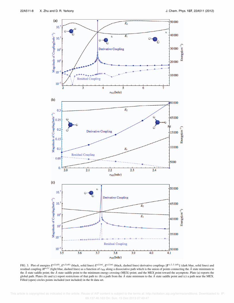
Figures 3(a)–3(c) present a path connecting the minimumenergy point on the 21A potential energy surface to the saddlepoint on that surface; the saddle point to the minimum en-ergy point on the 1,21A state conical intersection seam; andthe seam point to the product channel. This path is essentialfor the description of the nonadiabatic photodissociation pro-cess, given by reaction (1). Note that the percentage error inthe derivative coupling “at” the point of conical intersection istiny with ∥δfa, I, J(R)∥/∥fa, I, J(ab)(R)∥ ∼ 10−7! Equally signifi-cant, the residual coupling remains small in the vicinity of theconical intersection, see Fig. 3(c). This is particularly gratify-ing since these points are interpolated points. Thus, the dia-batic representation of the vicinity of the conical intersectionis excellent. This is not unexpected since the points of coni-cal intersection are treated as nodes, but the results evinced inthis figure are reassuring. Focusing on the region in Fig. 3(b),the region of A state minimum and saddle point, the deriva-tive coupling and the residual couplings, are seen to be small.As rNH becomes large, a small increase in ∥δfa, I, J(R)∥ is ob-served which is most likely due to the nonremovable6 partof fI, J, ab(R). fI, J, (m)(R) vanishes asymptotically as required.However, the nonremovable component of fI, J, ab(R) persistsand could lead to spurious long range coupling if it were notremoved. In our surface hopping trajectories used to deter-mine the Rn, no evidence of spurious exit channel surfacehops was detected.28 Figure 4 continues our study of the vicin-ity of the minimum energy conical intersection, this time as afunction of the out of plane angle, starting from the (planar)minimum energy conical intersection. As in Fig. 3, this plotindicates how accurately the conical intersection is described.Also evident in that figure is how quickly the ab initio deriva-tive coupling decays as a function of the out of plane angleand how well Hd describes that change, again using interpo-lated points. Figure 5 examines another region in which nona-diabatic effects are expected to be negligible. Shown in thatfigure is a path connecting the C3v minimum energy geometryon the ground state potential energy surface to the D3h saddlepoint for inversion. Both the derivative coupling and the resid-ual coupling are small as expected. Figure 6 presents a path,as function of the out of plane angle, connecting two points



FIG. 3. Plot of energies Ea,I,(ab), Ea,J,(ab) (black, solid lines) Ea,I,(m), Ea,J,(m) (black, dashed lines) derivative couplings ∥f a, I, J, (ab)∥ (dark blue, solid lines) andresidual coupling δf a,I,J (light blue, dashed lines) as a function of rNH along a dissociative path which is the union of points connecting the A state minimum tothe A state saddle point; the A state saddle point to the minimum energy crossing (MEX) point; and the MEX point toward the asymptote. Plate (a) reports theglobal path. Plates (b) and (c) report restrictions of that path to: (b) a path from the A state minimum to the A state saddle point and (c) a path near the MEX.Filled (open) circles points included (not included) in the fit data set.



FIG. 4. Plot of energies Ea,I,(ab), Ea,J,(ab) (black, solid lines) Ea,I,(m), Ea,J,(m)

(black dashed lines), derivative couplings ∥f a,I,J,(ab)∥ (dark blue, solid line)and residual coupling ∥δf a,I, J∥ (light blue, dashed line) along a path centeredat the minimum energy conical intersection as a function as a function of theout of plane angle. Filled (open) circles are points included (not included) inthe fit data set.

on the seam of conical intersections in distinctly differentregions of nuclear coordinate space. The small residual cou-plings, obtained with interpolated points, in the vicinity of twodistinct conical intersections is quite gratifying. These resultsillustrate the fact that the behavior of the derivative couplingsnear the minimum energy conical intersection considered inFigs. 3 and 4 is typical of points on the seam of coni-cal intersection defined by Hd. Taken together the results inthese figures strongly support the quasi- diabatic characterof Hd.

Figure 7 presents a more global picture of the quasi-diabatic representation plotting Hd

1,1, Hd2,2, and Hd

1,2. It is in-teresting to observe how the region of the saddle point on the21A state, a strongly avoided intersection of the 21A and 31Astates, is reproduced by a single diabatic state. Although thescale is necessarily large for Hd

1,1 and Hd2,2, their smoothness

is evident.


(black dashed lines), derivative couplings ∥f a,I,J,(ab)∥ (dark blue, solid line)and residual coupling ∥δf a,I,J∥ (light blue, dashed lines) as a function of theout of plane angle from the planar saddle point on the 11A potential energysurface to the ground state minimum. Filled circles are points included in thefit data set.


(black dashed lines), derivative couplings ∥f a,I,J,(ab)∥ (dark blue, solid line)and residual coupling ∥δf a,I,J∥ (light blue dashed lines) along a path start-ing from the MEX to a distinct local minimum energy conical intersection,MEX-L with a significantly different molecular structure. Filled (open) cir-cles points included (not included) in the fit data set. The path is predomi-nately along the out-of-plane angle, along which direction the diabatic statesare coupled. Note that by moving along the mirror image of this path one canachieve a full rotation and return to the MEX.

FIG. 7. Diabatic representation as a function of rNH and out-of-plane angle:Plate (a)Hd

1,1 and Hd2,2 and Plate (b) Hd

1,2.



IV. SUMMARY AND CONCLUSIONS

In this work, an approximate Newton-Raphson procedureis introduced which leads to a more precise quasi-diabatic rep-resentation of adiabatic potential energy surfaces coupled byconical intersections. The quasi-diabatic representation usespolynomials with flexible origins to improve the descrip-tion locally. The Newton-Rapshon procedure will enable opti-mization of these origins. The properties of the derived quasi-diabatic representation are studied.

ACKNOWLEDGMENTS

This work was supported by National Science Founda-tion (NSF) Grant No. CHE-1010644 to D.R.Y.

APPENDIX A: MONOMIAL FUNCTIONS

As discussed in previous work,26, 28 the gl are constructedfrom four basic functions of the internal coordinates, wi:

• Exponential functions63 w1(ri,j ) = e−s1(ri,j −r(a(i,j ))i,j ),

(A1a)

• Gaussian functions w2(ri,j ) = e−s2(ri,j −r(b(i,j ))i,j )2

,

(A1b)

• Reciprocal functions63 w3(ri,j )

= e−s3(ri,j −rc(i,j ))i,j )/(ri,j + r

(d(i,j ))i,j ), (A1c)

• Dot-Cross product functions14 wi,j,k,l4

= ri,j × ri,k · ri,l/|ri,j ri,kri,lri,krj,lrk,l|α. (A1d)

Gaussian functions are centered on specific origins andtheir values can be made to vanish quickly when steppingaway from those origins. They are local basis functions thatserve to describe the region near their origin. The origins, con-sequently, are key nonlinear parameters.

The gl(R) are constructed as products of the w and havethe following monomial form:

gl(R)=3!

m=1

!

1≤i≤j≤Nat

"wm(ri,j )

#α(l)m,i,j

!

(i,j,k,m)

"w

(i,j,k,m)4

#β(l)i,j,k,m

(A2)for 1 ≤ l ≤ Ng. Note in Eq. (A2), (l) is a label, not an exponent,but α

(l)m,i,j and β

(l)i,j,k,m are exponents. Here (i,j,k,m), again a

label not an exponent, denotes the allowed combinations offour atoms. The order of the monomial gl, o(l), is given by

o(l) =$

m,i<j

α(l)m,i,j +

$

i,j,k,m

β(l)i,j,k,m. (A3)

The choice of α(l)m,i,j and β

(l)i,j,k,m, which are introduced in

Eq. (A2), is in principle arbitrary. Increases in α(n)m,i,j and β

(n)i,j,k,l

are used to reduce the error in the representation of the adia-batic data, at the expense of a larger Ng. In previous work, the

nonlinear parameters sj, α, r(a(i,j ))i,j , r (b(i,j ))

i,j , r (c(i,j ))i,j , and r

(d(i,j ))i,j

were determined by trial and error in the range sj > 0, r (xi,j )i,j >

0, and α >1/2. The approach introduced here will be used, infuture work, to determine optimal values of these quantities.

APPENDIX B: SECOND DERIVATIVES

Through straightforward but tedious algebra the first andsecond derivatives with respect to Vj, λj, and γ j can be de-termined by differentiating Eq. (7). For the gradients, we find

∂&

∂x= [L(m),lsq − L(ab),lsq ]†

∂L(m),lsq

∂x

+[L(m),ex − L(ab),ex]†∂λ

∂x+ ∂(L(m),ex)†

∂xλ + tV† ∂V

∂x

(B1)

and then for the second derivatives

∂2&

∂x∂y= ∂L(m),lsq†

∂y

∂L(m),lsq

∂x+ [L(m),lsq − L(ab),lsq ]†

× ∂2L(m),lsq

∂x∂y+ ∂L(m),ex†

∂x

∂λ

∂y+ ∂L(m),ex†

∂y

∂λ

∂x

+ [L(m),ex − L(ab),ex]†∂2λ

∂x∂y+ ∂2L(m),ex†

∂x∂yλ

+ tV† ∂2V∂x∂y

+ t∂V†

∂y

∂V∂x

= ∂L(m),lsq†

∂y

∂L(m),lsq

∂x+ ∂L(m),ex†

∂x

∂λ

∂y

+ ∂L(m),ex†

∂y

∂λ

∂x+ ∂2L(m),ex†

∂x∂yλ + t

∂V†

∂y

∂V∂x

+ [L(m),lsq − L(ab),lsq ]†∂2L(m),lsq

∂x∂y, (B2)

where differentiating the second equality in Eq. (6a) gives

∂L(m)

∂x= ∂W

∂xV + W

∂V∂x

, (B3a)

∂2L(m)

∂x∂y= ∂2W

∂x∂yV + ∂ W

∂y

∂V∂x

+ ∂W∂x

∂V∂y

+ W∂2V∂x∂y

,

(B3b)Here x,y ∈ (Vi, λj , γk). Using the generic results inEq. (B2) and (B3a)–(B3b) and the fact that

∂L(m)k

∂λi

= 0, (B4)

we obtain the following Hessian matrix elements

∂2&

∂λi∂λj

= 0, (B5a)

∂2&

∂Vi∂λj

=∂L(m),ex†

j

∂Vi

, (B5b)



∂2"

∂γi∂λj

=∂L(m),ex†

j

∂γi

, (B5c)

∂2"

∂Vi∂Vj

= ∂L(m),lsq†

∂Vj

∂L(m),lsq

∂Vi

+ [L(m),lsq − L(ab),lsq ]†

× ∂2L(m),lsq

∂Vi∂Vj

+ ∂2L(m),ex†

∂Vi∂Vj

λ + tδij , (B5d)

∂2"

∂Vi∂γj

= ∂L(m),lsq†

∂γj

∂L(m),lsq

∂Vi

+ [L(m),lsq − L(ab),lsq]†

× ∂2L(m),lsq

∂Vi∂γj

+ ∂2L(m),ex†

∂Vi∂γj

λ, (B5e)

∂2"

∂γi∂γj

= ∂L(m),lsq†

∂γj

∂L(m),lsq

∂Vi

+[L(m),lsq − L(ab),lsq ]†∂2L(m),lsq

∂γi∂γj

+ ∂2L(m),ex†

∂γi∂γj

λ,

(B5f)

where the intermediate quantities are evaluated using

∂L(m)k

∂Vi

=!

∂W∂Vi

V"

k

+ Wk,i , (B6a)

∂L(m)k

∂γi

=!

∂W∂γi

V"

k

. (B6b)

Our working approximation is that we can ignore ∂2L(m)k

∂x∂yterms

because they are multiplied by [L(m), lsq − L(ab), lsq] or λ,which are small quantities if the fit is qualitatively correct.Thus, the working approximation for the Hessian is givenby Eqs. (B5a)–(B5c) and the following approximations toEqs. (B5d)–(B5f),

∂2"

∂Vi∂Vj

≈ ∂L(m),lsq†

∂Vj

∂L(m),lsq

∂Vi

+ tδij , (B7a)

∂2"

∂Vi∂γj

≈ ∂L(m),lsq†

∂γj

∂L(m),lsq

∂Vi

, (B7b)

∂2"

∂γi∂γj

≈ ∂L(m),lsq†

∂γj

∂L(m),lsq

∂γi

. (B7c)

APPENDIX C: EVALUATION OF ∂dI (Rn)∂zk

Since W is given by Wn,I,J,j ;l = dI†(Rn)Bu(l),v(l)

dJ (Rn)[∇jp(l)(Rn)], its derivative with respect to the param-

eter zk requires ∂dI (Rn)∂zk

. This is obtained from the derivative ofEq. (3a) as follows:

dI (R)†#

∂

∂zk

Hd (R)$

dJ (R)

= (Ea,J,(m)(R) − Ea,I,(m)(R))dI (R)†∂

∂zk

dJ (R), (C1)

so

∂dI (R)∂zk

=Nstate%

K =I

dK (R)dK (R)†[ ∂

∂zkHd (R)]dI (R)

(Ea,I,(m)(R) − Ea,K,(m)(R)),

(C2a)or

∂dI (R)†

∂zk

dK (R) =dK (R)†[ ∂

∂zkHd (R)]dI (R)

(Ea,I,(m)(R) − Ea,K,(m)(R)). (C2b)

This is valid provided we are not near a conical intersectionwhere Ea,I,(m)(R) = Ea,K,(m)(R).

At a conical intersection of states I and J, it might ap-pear that ∂dI (R)†

∂zkdJ(R) is not well-defined but this is not the

case. The desired derivative is obtained from the derivative ofthe orthogonality constraint,64 which requires that at a coni-cal intersection dI are chosen so that the g and h vectors areorthogonal, that is, g · h = 0, where

2gk ≡ LI,I,(m)k − L

J,J,(m)k and hk ≡ L

I,J,(m)k . (C3)

The derivative of g · h = 0 is obtained as follows:

∂h∂zk

= ∂(dI )†

∂zk

(∇HddJ )+(dI )†∂(∇Hd )

∂zk

(dJ ) + (dI )†∇Hd ∂dJ

∂zk

= ∂(dI )†

∂zk

(dJ )LJ,J,(m) +%

K =I,J

∂(dI )†

∂zk

(dK )LK,J,(m)

+ (dI )†∂(∇Hd )

∂zk

(dJ ) + LI,I,(m)(dI )†∂dJ

∂zk

+%

K =I,J

(dK )†∂(dJ )∂zk

LK,I,(m)

= [LI,I,(m) − LJ,J,(m)](dI )†∂dJ

∂zk

+ (dI )†∂(∇Hd )

∂zk

(dJ )

+%

K =I,J

∂(dI )†

∂zk

(dK )LK,J,(m)+%

K =I,J


LK,I,(m)k

= 2[g](dI )†∂dJ

∂zk

+ (dI )†∂(∇Hd )

∂zk

(dJ )

+%

K =I,J

∂(dI )†

∂zk

(dK )LK,J,(m)+%

K =I,J


LK,I,(m).

(C4)

Similarly

∂g∂zk

=#−2h

∂(dJ )†

∂zk

&dI

'$

+%

K =I,J

#∂(dI )†

∂zk

dK LK,I,(m) − ∂(dJ )†

∂zk

(dK )LK,J,(m)$

+12

#(dI )†

∂(∇Hd )∂zk

(dI ) − (dJ )†∂(∇Hd )

∂zk

dJ )$

. (C5)



Using Eqs. (C4) and (C5), we construct

g · ∂

∂zk

h + h · ∂

∂zk

g = 0, (C6)

which gives the desired equation for (dI )† ∂dJ

∂zk:

0 = 2[∥g∥2 − ∥h∥2](dI )†∂dJ

∂zk

+ g ·

⎡

⎣(dI )†∂(∇Hd )

∂zk

(dJ )

+∑

K =I,J

∂(dI )†

∂zk

(dK )LK,J,(m)+∑

K =I,J


LK,I,(m)

⎤

⎦

+ h ·

⎡

⎣12

(dI + dJ )†∂(∇Hd )

∂zk

(dI − dJ )

+∑

K =I,J

∂(dI )†

∂zk

(dK )LK,I,(m)−∑

K =I,J


LK,J,(m)

⎤

⎦ .

(C7)

Note that when Nstate is greater than 2, Eq. (C7) includesterms (dI )† ∂dK

∂zkwhich are obtained from Eq. (C2b). For clarity

we note that, from Eq. (C3), in Eq. (C7) the dot products, hand g refer to the coordinates components, that is, the gradientcomponents of ∇Hd or the vector components of LK,J,(m),which come from ∇Hd via Eq. (6b).

APPENDIX D: FORMULATION AND SOLUTIONOF EQ. (14)

In this section, we explain how terms included in Eq. (14)are assembled and the equation subsequently solved. FromEq. (B3a), we see that the quantity required for Eq. (14) thatis not already available from Eq. (13) is

∂Wxn,I,J,j ;l

∂Vk, x = lsq or ex.

From Eq. (12b),∂Wx

n,I,J,j ;l

∂Vkis given by (where the superscript x

is omitted as irrelevant)

∂Wn,I,J,j ;l

∂Vk

=∑

K

[∂dI †

(Rn)∂Vk

dK (Rn)dK (Rn)†Bu(l),v(l)dJ (Rn)

+ dI †(Rn)Bu(l),v(l)dK (Rn)dK (Rn)†

∂dJ (Rn)∂Vk

]

× [∇jp(l)(Rn)]=

∑

K

[∂dI †

(Rn)∂Vk

dK (Rn)

×Wn,K,J,j ;l+Wn,I,K,j ;ldK (Rn)†∂dJ (Rn)

∂Vk

]

,

(D1)

with ∂(dI )∂Vk

†dJ given by either Eq. (C2b) or (C7) depending on

the size of Ea,I,(m)(R) − Ea.J.(m)(R).The approximate Hessian described in Appendix B

when used in Eq. (14) gives an extension of the standardGauss-Newton method to problems with constraints, beingequivalent to the Gauss-Newton method when no exact

equations are present. It is well known that, unlike theNewton-Raphson method, the Gauss-Newton method isnot guaranteed to be locally convergent. Even thought theconvergence of the Gauss-Newton method can approachquadratic when the approximate Hessian is well conditioned,such a favorable situation has never been observed in thepresent work. Divergence has been observed when during thefitting procedure Hd exhibits qualitative changes.

On the other hand, the original method [Eq. (13)] hasshown a tendency to enter small scale oscillations, but be-have more stably when the step sizes are large. This is caused

by the fact that the ∂(dI )∂Vk

†dJ described by Eq. (C2b) can take

large values when states are energetically close but not yet de-generate enough to use intersection adapted coordinates andEq. (C7). For this reason, Eq. (13) is used at the start of the fit-ting procedure and Eq. (14) used when the coefficients ceaseto change dramatically.

Even in this situation, however, the fitting procedure isnot guaranteed to converge and can be subject to the samedivergence problem of the Gauss-Newton method. Two tech-niques, damping and line search, both routinely used forGauss-Newton and Newton-Raphson methods, are applied tocounter such problems.

In damping a diagonal shift is added to the approximateHessian, so that Eq. (B7a) becomes

∂2"

∂Vi∂Vj

≈ ∂L(m),lsq†

∂Vj

∂L(m),lsq

∂Vi

+ (t + t)δij . (D2)

t is an arbitrary non-negative number. When no exact equa-tions are present, the method becomes equivalent to theLevenberg-Marquardt algorithm,65 which is the algorithmused in most nonlinear least squares fitting programs. The sizeof the damping parameter t can be adjusted dynamically dur-ing the fitting procedure. Note that t appears only on the left-hand side of the equation while t appears on both sides. Asa result, unlike the flattening term t, t does not affect the fi-nal converged result. Instead, t can be properly described as adamping parameter that only affects the rate of convergence.This method is intermediate between a Newton type methodand a gradient descent method, which balances the stability ofgradient descent and rapid convergence of Newton-type meth-ods. The parameter is chosen in the range of 10−3 and 10−7

depending on the stability of the convergence procedure.In the line search approach, the program steps along the

direction pointed by the solution vector of Eq. (14) and lo-cates the point where the norm of the gradient of Lagrangianreaches a minimum. This point is taken as the starting pointfor the next iteration. The line search technique ensures thatthe gradient of the Lagrangian will always decrease and thusis immune to oscillations. However, the line search can betrapped in a very shallow local minimum. It is therefore onlyused when approaching final convergence.

As in the Gauss-Newton method, because the Hessianmatrix is approximate, when the damping term is absent con-vergence is not guaranteed and in general will not be reached.When a large enough damping term is present, the methodhas a guaranteed linear convergence. The linear convergencecan be extremely slow when the Hessian is ill-conditioned.



However, the quality of the fit will cease to change signifi-cantly when this situation occurs and we therefore terminatethe procedure at this point.

Finally note that while the line search guarantees thenorm of the gradient decreases, it does not guarantee theconstraints be exactly satisfied until the final convergence isreached. We therefore monitor the exact equations and willonly terminate the procedure when that part error becomessufficiently small. We are presently studying the relation be-tween the residual norm of the gradient of the Lagrangian andthe quality of the fit.

1B. Lasorne, M. A. Robb, H.-D. Meyer, and F. Gatti, Chem. Phys. 377, 30(2010).

2J. C. Tully, J. Chem. Phys. 93, 1061 (1990).3M. Ben-Nun and T. J. Martinez, J. Phys. Chem. A 104, 5161 (2000).4G. A. Worth, M. A. Robb, and B. Lasorne, Mol. Phys. 106, 2077 (2008).5M. Baer, Chem. Phys. 15, 49 (1976).6C. A. Mead and D. G. Truhlar, J. Chem. Phys. 77, 6090 (1982).7M. Baer, Phys. Rep. 358, 75 (2002).8V. C. Mota and A. J. C. Varandas, J. Phys. Chem. A 112, 3768 (2008).9H. Nakamura and D. G. Truhlar, J. Chem. Phys. 117, 5576 (2002).

10H. Nakamura and D. G. Truhlar, J. Chem. Phys. 118, 6816 (2003).11Z. H. Li, R. Valero, and D. G. Truhlar, Theor. Chem. Acc. 118, 9 (2007).12W. Eisfeld and A. Viel, J. Chem. Phys. 122, 204317 (2005).13A. Viel and W. Eisfeld, J. Chem. Phys. 120, 4603 (2004).14O. Godsi, C. R. Evenhuis, and M. A. Collins, J. Chem. Phys. 125, 104105

(2006).15C. R. Evenhuis and M. A. Collins, J. Chem. Phys. 121, 2515 (2004).16C. Evenhuis and T. J. Martínez, J. Chem. Phys. 135, 224110 (2011).17H. Köppel, J. Gronki, and S. Mahapatra, J. Chem. Phys. 115, 2377 (2001).18H. Köppel and B. Schubert, Mol. Phys. 104, 1069 (2006).19T. C. Thompson, G. Izmirlian, S. J. Lemon, D. G. Truhlar, and C. A. Mead,

J. Chem. Phys. 82, 5597 (1985).20A. J. C. Varandas, F. B. Brown, C. A. Mead, D. G. Truhlar, and N. C. Blais,

J. Chem. Phys. 86, 6258 (1987).21E. Martínez-Núñez and A. J. C. Varandas, J. Phys. Chem. A 105, 5923

(2001).22L. A. Poveda, M. Biczysko, and A. J. C. Varandas, J. Chem. Phys. 131,

044309 (2009).23A. Macías and A. Riera, J. Phys. B. 11, L489 (1978).24A. J. Dobbyn and P. J. Knowles, Mol. Phys. 91, 1107 (1997).25H. Köppel, W. Domcke, and L. S. Cederbaum, in Conical Intersections,

edited by W. Domcke, D. R. Yarkony, and H. Köppel (World Scientific,New Jersey, 2004), Vol. 15, p. 323.

26X. Zhu and D. R. Yarkony, J. Chem. Phys. 132, 104101 (2010).27X. Zhu and D. R. Yarkony, Mol. Phys. 108(19), 2611 (2010).28X. Zhu and D. R. Yarkony, J. Chem. Phys. 136, 174110 (2012).29G. Fogarasi, X. Zhou, P. W. Taylor, and P. Pulay, J. Am. Chem. Soc. 114,

8191 (1992).30G. J. Atchity, S. S. Xantheas, and K. Ruedenberg, J. Chem. Phys. 95, 1862

(1991).

31V. Vaida, W. Hess, and J. L. Roebber, J. Phys. Chem. 88, 3397 (1984).32A. D. Walsh and P. A. Warsop, Trans. Faraday Soc. 57, 345 (1961).33P. Rosmus, P. Botschwina, H.-J. Werner, V. Vaida, P. C. Engelking, and M.

I. McCarthy, J. Chem. Phys. 86, 6677 (1987).34M. I. McCarthy, P. Rosmus, H.-J. Werner, P. Botschwina, and V. Vaida,

J. Chem. Phys. 86, 6693 (1987).35A. Bach, J. M. Hutchison, R. J. Holiday, and F. F. Crim, J. Chem. Phys.

116, 9315 (2002).36S. L. Tang and D. G. Imre, Chem. Phys. Lett. 144, 6 (1988).37S. A. Henck, M. A. Mason, W.-B. Yan, K. K. Lehmann, and S. L. Coy,

J. Chem. Phys. 102, 4783 (1995).38J. Biesner, L. Schnieder, G. Ahlers, X. Xie, K. H. Welge, M. N. R. Ashfold,

and R. N. Dixon, J. Chem. Phys. 88, 3607 (1988).39J. Biesner, L. Schneider, G. Ahlers, X. Xie, K. H. Welge, M. N. R. Ashfold,

and R. N. Dixon, J. Chem. Phys. 91, 2901 (1989).40E. L. Woodbridge, M. N. R. Ashfold, and S. R. Leone, J. Chem. Phys. 94,

4195 (1991).41D. H. Mordaunt, M. N. R. Ashfold, and R. N. Dixon, J. Chem. Phys. 104,

6472 (1996).42D. H. Mordaunt, M. N. R. Ashfold, and R. N. Dixon, J. Chem. Phys. 104,

6460 (1996).43D. H. Mordaunt, M. N. R. Ashfold, R. N. Dixon, P. Löffler, L. Schneider,

and K. H. Welge, J. Chem. Phys. 108, 519 (1998).44R. A. Loomis and M. I. Lester, Annu. Rev. Phys. Chem. 48, 643 (1997).45J. P. Reid, R. A. Loomis, and S. R. Leone, J. Chem. Phys. 112, 3181

(2000).46J. P. Reid, R. A. Loomis, and S. R. Leone, Chem. Phys. Lett. 324, 240

(2000).47J. P. Reid, R. A. Loomis, and S. R. Leone, J. Phys. Chem. A 104, 10139

(2000).48K. L. Wells, G. Perriam, and V. G. Stavros, J. Chem. Phys. 130, 074308

(2009).49R. N. Dixon, Chem. Phys. Lett. 147, 377 (1988).50R. N. Dixon, Mol. Phys. 88, 949 (1996).51R. N. Dixon and T. W. R. Hancock, J. Phys. Chem. A 101, 7567 (1997).52D. Bonhommeau and D. G. Truhlar, J. Chem. Phys. 129, 014302 (2008).53W. Lai, S. Y. Lin, D. Xie, and H. Guo, J. Chem. Phys. 129, 154311 (2008).54D. Bonhommeau, R. Valero, D. G. Truhlar, and A. W. Jasper, J. Chem.

Phys. 130, 234303 (2009).55W. Lai, S. Y. Lin, D. Xie, and H. Guo, J. Phys. Chem. A 114, 3121 (2010).56A. Bach, J. M. Hutchison, R. J. Holiday, and F. F. Crim, J. Chem. Phys.

118, 7144 (2003).57M. L. Hause, Y. H. Yoon, and F. F. Crim, J. Chem. Phys. 125, 174309

(2006).58D. R. Yarkony, Acc. Chem. Res. 31, 511 (1998).59X. Zhu, J. Ma, D. R. Yarkony, and H. Guo, J. Chem. Phys. 136, 234301

(2012).60J. J. Dillon, D. R. Yarkony, and M. S. Schuurman, J. Chem. Phys. 134,

044101 (2011).61B. N. Papas, M. S. Schuurman, and D. R. Yarkony, J. Chem. Phys. 129,

124104 (2008).62D. R. Yarkony, J. Chem. Phys. 90, 1657 (1989).63B. J. Braams and J. M. Bowman, Int. Rev. Phys. Chem. 28, 577 (2009).64D. R. Yarkony, J. Chem. Phys. 112, 2111 (2000).65D. Marquardt, SIAM J. Appl. Math. 11, 431 (1963).


http://dx.doi.org/10.1016/j.chemphys.2010.08.011

http://dx.doi.org/10.1063/1.459170

http://dx.doi.org/10.1021/jp994174i

http://dx.doi.org/10.1080/00268970802172503

http://dx.doi.org/10.1016/0301-0104(76)89006-4

http://dx.doi.org/10.1063/1.443853

http://dx.doi.org/10.1016/S0370-1573(01)00052-7

http://dx.doi.org/10.1021/jp710610d

http://dx.doi.org/10.1063/1.1500734

http://dx.doi.org/10.1063/1.1540622

http://dx.doi.org/10.1007/s00214-006-0237-7

http://dx.doi.org/10.1063/1.1904594

http://dx.doi.org/10.1063/1.1646371

http://dx.doi.org/10.1063/1.2338912

http://dx.doi.org/10.1063/1.1770756

http://dx.doi.org/10.1063/1.3660686

http://dx.doi.org/10.1063/1.1383986

http://dx.doi.org/10.1080/00268970500417937

http://dx.doi.org/10.1063/1.448594

http://dx.doi.org/10.1063/1.452463

http://dx.doi.org/10.1021/jp0101460

http://dx.doi.org/10.1063/1.3176512

http://dx.doi.org/10.1088/0022-3700/11/16/003

http://dx.doi.org/10.1080/002689797170842

http://dx.doi.org/10.1063/1.3324982

http://dx.doi.org/10.1080/00268976.2010.515258

http://dx.doi.org/10.1063/1.4704789

http://dx.doi.org/10.1021/ja00047a032

http://dx.doi.org/10.1063/1.461036

http://dx.doi.org/10.1021/j150660a006

http://dx.doi.org/10.1039/tf9615700345

http://dx.doi.org/10.1063/1.452416

http://dx.doi.org/10.1063/1.452417

http://dx.doi.org/10.1063/1.1471908

http://dx.doi.org/10.1016/0009-2614(88)87080-5

http://dx.doi.org/10.1063/1.469526

http://dx.doi.org/10.1063/1.453910

http://dx.doi.org/10.1063/1.457644

http://dx.doi.org/10.1063/1.460653

http://dx.doi.org/10.1063/1.471368

http://dx.doi.org/10.1063/1.471367

http://dx.doi.org/10.1063/1.475415

http://dx.doi.org/10.1146/annurev.physchem.48.1.643

http://dx.doi.org/10.1063/1.480902

http://dx.doi.org/10.1016/S0009-2614(00)00605-9

http://dx.doi.org/10.1021/jp001065r

http://dx.doi.org/10.1063/1.3072763

http://dx.doi.org/10.1016/0009-2614(88)80252-5

http://dx.doi.org/10.1080/00268979609484484

http://dx.doi.org/10.1021/jp964045r

http://dx.doi.org/10.1063/1.2943213

http://dx.doi.org/10.1063/1.2996357

http://dx.doi.org/10.1063/1.3132222

http://dx.doi.org/10.1063/1.3132222

http://dx.doi.org/10.1021/jp908688a

http://dx.doi.org/10.1063/1.1561619

http://dx.doi.org/10.1063/1.2363192

http://dx.doi.org/10.1021/ar970113w

http://dx.doi.org/10.1063/1.4725496

http://dx.doi.org/10.1063/1.3523344

http://dx.doi.org/10.1063/1.2978389

http://dx.doi.org/10.1063/1.456059

http://dx.doi.org/10.1080/01442350903234923

http://dx.doi.org/10.1063/1.480779

http://dx.doi.org/10.1137/0111030

Copyright and Permission Notice:

Reprinted with permission from J. Chem. Phys. 137, 22A511 (2012),

Copyright 2012, AIP Publishing LLC. This article may be downloaded for

personal use only. Any other use requires prior permission of the author and

the AIP Publishing LLC

Quasi-diabatic representations of adiabatic potential energy surfaces coupled by conical...

Documents

Transcript of Quasi-diabatic representations of adiabatic potential energy surfaces coupled by conical...