
Quarterly Bulletin 3/2002 - Swiss National Bank (SNB)
80
Quarterly Bulletin September 2002 3
-
Upload
khangminh22 -
Category
Documents
-
view
0 -
download
0
Transcript of Quarterly Bulletin 3/2002 - Swiss National Bank (SNB)

Quarterly BulletinSe
ptem
ber
2002
3

Swiss National BankQuarterly Bulletin
September 3/2002 Volume 20


Table of Contents
14 Overview15 Übersicht16 Sommaire17 Sommario
18 Monetary policy assessment
12 Economic and monetary developments in Switzerland13 1 International environment13 1.1 Economic development 15 1.2 Monetary development 16 1.3 Economic outlook
17 2 Monetary development17 2.1 Interest rates20 2.2 Exchange rate21 2.3 Monetary aggregates23 2.4 Loans and capital market borrowing
25 3 Aggregate demand and output25 3.1 GDP and industrial output27 3.2 Foreign trade and current account30 3.3 Investment31 3.4 Consumption32 3.5 Capacity utilisation32 3.6 GDP forecasts for 2002 and 2003
33 4 Labour market33 4.1 Employment34 4.2 Unemployment
35 5 Prices35 5.1 Consumer prices36 5.2 Core inflation37 5.3 Prices of total supply
38 6 Inflation prospects38 6.1 International price development38 6.2 Price development in Switzerland39 6.3 Inflation prospects for 2002–2004
40 7 Economic situation from the vantage point of the SNB’s bank offices40 7.1 Production41 7.2 Components of demand41 7.3 Labour market41 7.4 Prices and margins
42 How accurate are GDP forecasts? An empirical study for SwitzerlandEveline Ruoss and Marcel Savioz
64 The International Monetary Fund as International Lender of Last ResortUmberto Schwarz
74 Chronicle of monetary events

SNB 4 Quarterly Bulletin 3/2002
Overview
Monetary policy assessment (p. 8)On 19 September 2002, at its quarterly assess-
ment of the situation, the Swiss National Bank de-cided to leave the target range for the three-monthLibor rate unchanged at 0.25%–1.25%. For the timebeing, the three-month Libor is to be kept in the mid-dle of the target range. Monetary policy was lastadjusted on 26 July 2002, when the target range waslowered by 0.5 percentage points.
Economic and monetary developments (p. 12)The economic pick-up that had started to take
hold in many OECD countries at the beginning of 2002continued in the last few months, albeit at a modestpace. In the second quarter, real gross domestic prod-uct (GDP) rose both in the US and in the euro areaand Japan compared with the previous period, withEurope and Japan benefiting from higher demandfrom the US and the Asian region. Domestic demand,however, remained feeble. In particular, there was nosign yet of a turnaround in investment.
In the second quarter 2002, the Swiss economywas not able to overcome the stagnation persistingsince mid-2001. Real GDP rose only negligibly quar-ter-on-quarter and fell 0.4% short of the correspond-ing year-earlier level. In the industrial sector, theemerging economic recovery ground to a halt, andbusiness prospects in the export sector were againjudged less favourably. Employment declined oncemore, with jobless figures reaching 2.8% by July.Annual inflation measured by the consumer priceindex receded by 0.1 percentage points to 0.5%between May and August. The prices of importedconsumer goods still fell short of the correspondingyear-earlier level, while the upward pressure onprices for domestic goods eased somewhat.
The Swiss franc tended to firm between May andAugust. To counter a tightening of monetary condi-tions, the National Bank lowered the target range forthe three-month Libor rate by half a percentage pointto 0.25%–1.25% on 26 July. Subsequently, short-term interest rates declined markedly. In the courseof international interest rate movements, long-terminterest rates also fell, albeit to a lesser extent thanin the money market. In August, the yield on ten-yearConfederation bonds amounted to 3.2% comparedwith 3.5% in May.
How accurate are GDP forecasts – a survey forSwitzerland (p. 42)In this paper, the quality of forecasts for annual
growth of real GDP for Switzerland is examined. Thesurvey covers GDP forecasts drawn up by 14 differentinstitutes between 1981 and 2000. As many forecastsas possible published by the institutes during theyear for the current calendar year, the following yearand the year after are included. The results show thatthe forecasts made during the year for the currentyear, or in autumn for the following year are informa-tive and clearly surpass naive forecasting procedures.Moreover, these forecasts meet optimality standards:they are not distorted, not correlated and efficient.They may be described as weakly rational. At the sametime, however, the study makes it clear that forecasterrors increase considerably with the forecastinghorizon. Forecasts over a time period of more than 18 months no longer shed any light on the futurecourse of the economy and do not meet optimalitystandards. These results are in keeping with the expe-rience gained in other countries.
The International Monetary Fund as lender oflast resort (p. 64)Ten years ago, Switzerland became a member of
the International Monetary Fund (IMF). During theseten years, the IMF underwent profound changes,which are primarily reflected in the massive expan-sion of its credit business. In the process, the natureof the IMF also changed in that it became a kind ofinternational lender of last resort. As a result, theIMF saw itself increasingly confronted with the prob-lem of moral hazard. The paper shows that the IMFintroduced or devised numerous measures to limitthis risk. One of the chief measures is the participa-tion of the private sector in solving debt crises. Thiscan be achieved by means of joint clauses or a mech-anism for the restructuring of sovereign debt.

SNB 5 Quarterly Bulletin 3/2002
Übersicht
Geldpolitische Lagebeurteilung (S. 8)Die Schweizerische Nationalbank beschloss an
der vierteljährlichen Lagebeurteilung vom 19. Sep-tember 2002 das Zielband für den Dreimonats-Liborunverändert bei 0,25%–1,25% zu belassen. Der Drei-monats-Libor soll bis auf weiteres im mittleren Bereichdes Zielbandes gehalten werden. Die letzte Anpas-sung der Geldpolitik war am 26. Juli 2002 erfolgt, alsdas Zielband um 0,5 Prozentpunkte gesenkt wordenwar.
Wirtschafts- und Währungslage (S. 12)Die konjunkturelle Belebung, die sich Anfang
2002 in vielen Ländern der OECD abzuzeichnen be-gann, setzte sich in den letzten Monaten verhaltenfort. Das reale Bruttoinlandprodukt erhöhte sich imzweiten Quartal sowohl in den USA als auch im Euro-Gebiet und in Japan gegenüber der Vorperiode, wobeiEuropa und Japan von einer steigenden Nachfrageaus den USA und aus dem asiatischen Raum profitier-ten. Die Binnennachfrage blieb dagegen schwach.Noch keine Trendwende zeichnete sich insbesonderebei den Investitionen ab.
Die schweizerische Wirtschaft vermochte sichim zweiten Quartal nicht von der seit Mitte 2001anhaltenden Stagnation zu lösen. Das reale Bruttoin-landprodukt wuchs gegenüber der Vorperiode nurgeringfügig und lag 0,4% unter dem entsprechendenVorjahresstand. In der Industrie kam die sich anbah-nende konjunkturelle Erholung ins Stocken und dieGeschäftsaussichten wurden im Exportsektor wiederzurückhaltender eingeschätzt. Die Beschäftigung bil-dete sich nochmals zurück und die Arbeitslosenquotestieg bis Juli auf 2,8%. Die am Konsumentenpreis-index gemessene Jahresteuerung sank von Mai bisAugust um 0,1 Prozentpunkte auf 0,5%. Die Preiseimportierter Konsumgüter lagen weiterhin unter dementsprechenden Vorjahresstand, während sich dieTeuerung bei den inländischen Gütern leicht ver-ringerte.
Der Franken tendierte von Mai bis August höher.Um einer Verschärfung der monetären Rahmenbedin-gungen entgegenzuwirken, senkte die Nationalbankam 26. Juli das Zielband für den Dreimonats-Libor umeinen halben Prozentpunkt auf 0,25%–1,25%. In derFolge bildeten sich die kurzfristigen Zinssätze deut-lich zurück. Im Zuge der internationalen Zinsbewe-gung gaben auch die langfristigen Zinssätze nach,wenn auch weniger stark als am Geldmarkt. Im Augustbetrug die Rendite zehnjähriger Bundesobligationen3,2%, gegenüber 3,5% im Mai.
Wie gut sind BIP-Prognosen – EineUntersuchung für die Schweiz (S. 42)In diesem Aufsatz wird die Qualität der Prog-
nosen für das jährliche Wachstum des realen Bruttoinlandprodukts für die Schweiz untersucht.Berücksichtigt werden BIP-Prognosen, die von 14 verschiedenen Instituten in den Jahren 1981 bis2000 erstellt wurden. Dabei werden möglichst allePrognosen einbezogen, welche die Institute währendeines Jahres für das laufende, das nächste und dasübernächste Kalenderjahr veröffentlichten. Die Ergeb-nisse zeigen, dass die Prognosen, die unter dem Jahrfür das laufende oder im Herbst für das nächste Jahrgemacht werden, informativ sind und naive Progno-severfahren klar übertreffen. Auch genügen diesePrognosen den Optimalitätseigenschaften: sie sindunverzerrt, nicht korreliert und effizient. Sie könnenals schwach rational bezeichnet werden. Gleichzeitigmacht die Untersuchung aber klar, dass die Prognose-fehler mit dem Prognosehorizont stark zunehmen.Prognosen über einen Zeithorizont von mehr als 18 Monaten sagen über den künftigen Konjunktur-verlauf nichts mehr aus und genügen auch nicht denOptimalitätseigenschaften. Diese Ergebnisse stim-men mit ausländischen Erfahrungen überein.
Der Internationale Währungsfonds als inter-nationaler Lender of Last Resort (S. 64)Vor zehn Jahren trat die Schweiz dem Interna-
tionalen Währungsfonds (IWF) bei. In diesen zehnJahren durchlief der IWF tiefgreifende Veränderun-gen, die sich insbesondere in der massiven Auswei-tung seiner Kredittätigkeit widerspiegeln. Damit wan-delte sich auch die Natur des IWF, der zu einer Artinternationalem Lender of Last Resort wurde. AlsFolge davon sah sich der Währungsfonds vermehrtmit dem Problem des Moral Hazards konfrontiert.Dieser Aufsatz zeigt, dass der IWF viele Massnahmenergriff oder konzipierte, um dieses Risiko zu begren-zen. Zu den wichtigsten Massnahmen gehört insbe-sondere die Beteiligung des Privatsektors bei derLösung von Schuldenkrisen. Diese kann mit der Hilfevon Kollektivklauseln oder einem Mechanismus zurRestrukturierung souveräner Schulden erreicht wer-den.

SNB 6 Quarterly Bulletin 3/2002
Sommaire
Appréciation de la situation économique etmonétaire (p. 8)Lors de l’analyse trimestrielle de la situation du
19 septembre 2002, la Banque nationale suisse adécidé de laisser inchangée à 0,25%–1,25% la margede fluctuation du Libor à trois mois et de maintenir,jusqu’à nouvel avis, le Libor à trois mois dans la zonemédiane de cette marge. La dernière adaptation de lapolitique monétaire remonte au 26 juillet 2002; lamarge de fluctuation avait alors été abaissée d’undemi-point.
Situation économique et monétaire (p. 12)La reprise que la conjoncture avait commencé à
marquer dans de nombreux pays de l’OCDE, au débutde 2002, s’est poursuivie ces derniers mois, mais à unrythme modéré. Du premier au deuxième trimestre, leproduit intérieur brut réel a augmenté aux Etats-Unis, mais aussi dans la zone euro et au Japon;l’Europe et le Japon ont bénéficié notamment d’unedemande accrue en provenance des Etats-Unis et dela zone asiatique. La demande intérieure est restéecependant faible. Ainsi, aucun retournement de ten-dance n’était perceptible, en particulier du côté desinvestissements.
Au deuxième trimestre, l’économie suisse n’estpas parvenue à sortir de la phase de stagnation qui lacaractérise depuis le milieu de 2001. Le produit inté-rieur brut réel a augmenté légèrement par rapport aupremier trimestre, mais diminué de 0,4% en compa-raison annuelle. La reprise de la conjoncture, quis’était amorcée dans l’industrie, a tourné court, et lesecteur de l’exportation s’est de nouveau montré plusréservé en ce qui concerne l’évolution future de lademande. L’emploi a encore reculé, et le taux de chô-mage a augmenté, passant à 2,8% en juillet. Le tauxannuel de renchérissement, mesuré à l’indice des prixà la consommation, a fléchi de 0,1 point entre mai etaoût pour s’établir à 0,5%. Les prix des biens deconsommation importés ont continué à se replier enun an, tandis que le renchérissement des biens d’ori-gine suisse a marqué une légère baisse.
Entre mai et août, le franc a eu tendance à serevaloriser. Pour éviter un durcissement des condi-tions-cadres sur le plan monétaire, la Banque natio-nale a abaissé d’un demi-point, le 26 juillet, la margede fluctuation du Libor à trois mois, marge qui a ainsipassé à 0,25%–1,25%. Les taux d’intérêt à courtterme ont ensuite nettement fléchi. Dans le sillage de la tendance observée sur le plan international, les
taux d’intérêt à long terme ont eux aussi diminué,mais pas autant que les rémunérations servies sur lemarché monétaire. Le rendement des obligations àdix ans de la Confédération s’établissait à 3,2% enaoût, contre 3,5% en mai.
La fiabilité des prévisions du PIB – Etude empirique pour la Suisse (p. 42)L’étude porte sur la fiabilité des prévisions de
croissance annuelle du produit intérieur brut réel dela Suisse. L’analyse se fonde sur les prévisions du PIB,établies entre 1981 et 2000, par quatorze instituts.Elle tient compte autant que possible de toutes les prévisions que ces instituts ont publiées dansl’année, pour l’année en cours, l’année suivante etl’année d’après. Les résultats montrent que les pré-visions faites dans l’année, pour l’année en cours, eten automne, pour l’année suivante, sont instructiveset l’emportent nettement sur des procédés dits naïfsde prévision. Elles satisfont également aux condi-tions d’optimalité: elles sont en effet exemptes debiais et de corrélation, mais efficientes. Elles peuventêtre considérées comme faiblement rationnelles.L’examen révèle en outre que les erreurs de prévisionaugmentent fortement avec l’horizon de prévision.Des prévisions qui portent sur un horizon dépassant18 mois ne sont plus instructives et ne satisfont plusaux conditions d’optimalité. Les résultats de cetexamen sont en harmonie avec ceux obtenus pourd’autres pays.
Le Fonds monétaire international comme prê-teur international de dernier ressort (p. 64)La Suisse a adhéré, il y a dix ans, au Fonds
monétaire international (FMI). Durant cette période,cette institution a connu de profonds changements,le plus important étant l’accroissement du volumedes crédits accordés. La nature du Fonds s’est elleaussi modifiée: il est devenu en quelque sorte un prêteur international de dernier ressort («lender oflast resort»). Par conséquent, il s’est vu confrontédavantage au problème du risque moral. Cette étudemontre que nombre de mesures qui ont été adoptéesou échafaudées par le FMI durant cette période l’ont été afin de limiter ce risque. Parmi ces mesuresfigure notamment la participation du secteur privé à la résolution des crises. Elle peut être obtenue àl’aide de clauses d’action collective ou d’un méca-nisme de restructuration de la dette souveraine.

SNB 7 Quarterly Bulletin 3/2002
Sommario
Valutazione della situazione monetaria (p. 8)Il 19 settembre 2002, in occasione della valu-
tazione trimestrale, la Banca nazionale svizzera hadeciso di lasciare inalterato allo 0,25%–1,25% ilmargine di oscillazione del Libor a tre mesi. Fino anuovo avviso, l’istituto di emissione intende mante-nere il Libor a tre mesi nella zona centrale di questafascia. L’ultimo adeguamento di politica monetariarisale al 26 luglio 2002; in quell’occasione la Bancanazionale aveva ridotto la fascia di fluttuazione di0,5 punti percentuali.
Situazione economica e monetaria (p. 12)La ripresa economica delineatasi in diversi Paesi
dell’OCSE all’inizio del 2002 è proseguita nel corsodegli ultimi mesi, ma ad un ritmo moderato. Nelsecondo trimestre dell’anno, il prodotto internolordo reale è aumentato tanto negli Stati Unitiquanto nell’area dell’euro e in Giappone. Europa eGiappone hanno tratto profitto della crescentedomanda proveniente dagli Stati Uniti e dalla regioneasiatica. La domanda interna, invece, è rimasta de-bole. In particolare gli investimenti non hannosegnalato alcuna inversione di tendenza.
In Svizzera l’attività produttiva è risultata sta-gnante anche nel secondo trimestre. Il prodotto inter-no lordo reale è aumentato solo leggermente sul tri-mestre precedente, mentre si è contratto dello 0,4%rispetto all’anno precedente. La ripresa congiuntu-rale che sembrava delinearsi nell’industria si è arre-stata e le prospettive d’affari nel settore delle espor-tazioni sono state giudicate con minore ottimismo. Ilcalo dell’occupazione è proseguito ed il tasso didisoccupazione è salito al 2,8% in luglio. Da maggioad agosto, il rincaro annuale, misurato attraversol’indice nazionale dei prezzi al consumo, si è ridottodi 0,1 punti percentuali scendendo all’0,5%. I prezzidei beni di consumo importati sono nuovamenterisultati inferiori all’anno precedente, mentre il rin-caro dei beni domestici si è leggermente ridotto.
Da maggio ad agosto, il corso del franco sviz-zero si è rafforzato. Per evitare di esporre l’econo-mia a condizioni monetarie quadro più restrittive, il26 maggio la Banca nazionale ha ridotto di mezzopunto percentuale il margine d’oscillazione del Libora tre mesi, portandolo allo 0,25%–1,25%. I tassid’interesse a breve sono perciò nettamente calati.Sulla scia dell’evoluzione internazionale si sonoridotti, seppure in minor misura, anche i tassi a lungotermine. Il rendimento delle obbligazioni a dieci annidella Confederazione è sceso dal 3,5% in maggio al3,2% in agosto.
La qualità delle previsioni del PIL – Un’analisi per la Svizzera (p. 42)Il contributo analizza il grado di affidabilità
delle previsioni di crescita annuale del prodottointerno lordo reale per la Svizzera. La ricerca si basasulle previsioni di 14 istituti pubblicate tra il 1981 e il2000. Nella misura del possibile, sono state prese inconsiderazione tutte le previsioni pubblicate da unistituto nel corso dell’anno per l’anno stesso e perl’anno successivo. I risultati indicano che le previ-sioni relative all’anno in corso o che sono pubblicatein autunno per l’anno successivo sono informative edecisamente superiori alle previsioni ottenute conmetodi di previsione naive. Tali previsioni soddisfanoinoltre le proprietà di ottimalità: sono prive di bias,non correlate ed efficienti. Si possono quindi definirecome razionali in senso debole. La ricerca mette tut-tavia in evidenza che l’errore di previsione aumentafortemente con l’orizzonte previsivo. Le previsioniriferite ad un periodo superiore a diciotto mesi nonsono più in grado di fornire informazioni utili sull’an-damento congiunturale e non presentano più le pro-prietà di ottimalità. Questi risultati confermano leconclusioni di analoghe ricerche per l’estero.
Il Fondo monetario internazionale comelender of last resort (p. 64)Da dieci anni, la Svizzera è membro del Fondo
monetario internazionale (FMI). In questo decennioil FMI ha conosciuto cambiamenti profondi, che sisono manifestati soprattutto in una notevole espan-sione della sua attività creditizia. È quindi cambiatala natura stessa del FMI, trasformandosi, si può dire,in un lender of last resort a livello internazionale. Diconseguenza il FMI si è trovato sempre più esposto alproblema di moral hazard. Quest’articolo dimostrache il FMI ha preso o ideato diversi provvedimenti alloscopo di limitare tale rischio. Una delle misure piùimportanti è la partecipazione del settore privato allarisoluzione delle crisi d’indebitamento. Essa puòessere ottenuta ricorrendo a clausole collettive o ameccanismi di ristrutturazione del debito sovrano.

SNB 8 Quarterly Bulletin 3/2002
Monetary policy assessment

SNB 9 Quarterly Bulletin 3/2002
Press release on the quarterlyassessment of the situation of 19 September 2002
Unchanged monetary policy – target range for the three-month Libor rateremains at 0.25%–1.25%The National Bank has decided to leave the tar-
get range for the three-month Libor rate unchangedat 0.25%–1.25%. For the time being, the three-month Libor is to be kept in the middle of the targetrange. The National Bank last adjusted its monetarypolicy on 26 July 2002, when it lowered the targetrange by 50 basis points. In so doing, it reacted tothe sluggish pace of the economic recovery inSwitzerland, which already became apparent at thattime, as well as to the Swiss franc’s renewed upwardtrend. The National Bank took advantage of the lee-way afforded by the favourable price development.Since March 2001, the National Bank has eased itsmonetary policy substantially, lowering the targetrange for the three-month Libor by a total of 2.75percentage points. The anticipated recovery of theglobal economy is taking hold only gradually and aperceptible upswing is not expected until the springof 2003. This will also have an impact on the eco-nomic development in our country. The NationalBank, therefore, will continue its relaxed monetarystance. Price stability is not threatened.
The Swiss economy’s performance was belowthe National Bank’s expectations during the first half-year of 2002. Business activity continues to sufferfrom the difficult economic climate worldwide andthe strong Swiss franc. In the second quarter 2002,real GDP was slightly below last year's level, but didnot contract again compared with the previous quar-ter. Unemployment registered another slight in-crease.
Private and government consumption remain themost important pillars of the economy. The decline in capital spending accelerated again during the pre-vious quarters, while construction investment sawstagnating figures. By contrast, both exports andimports picked up in the second quarter 2002 vis-à-vis the previous quarter. The development of ordersreceived, however, does not yet point to a sustainedrecovery of exports.
Annual inflation measured by the national -consumer price index (CPI) increased from 0.4% inJanuary to 1.1% in April. It subsequently receded and hit a low point of –0.1% in July 2002. In August,it climbed to 0.5%. The negative inflation rate in July is mainly attributable to a change in data collec-tion on clearance sales prices for clothing. Irrespec-tive of this special effect, inflationary pressureremains low, which is again due largely to lowerprices for imported goods. Inflation in the domesticgoods sector always exceeded the one-percent markthis year. Core inflation, computed by the NationalBank as the trimmed mean, likewise amounts toapproximately 1%. Consequently, the modest infla-tion is not a sign of a deflationary development inSwitzerland.
The National Bank views the prospects for theglobal economy more cautiously than it did only threemonths ago. Economic growth in the US is unlikely topick up speed before the spring of 2003; after that itshould gradually regain its potential. The same ap-plies to the European economy.
According to the National Bank’s assessment, theSwiss economy will see only moderate growth ratesuntil mid-2003. After that, the economy is set torebound. Private and government consumption areexpected to continue to underpin economic activity.What the economy needs to recover, however, is forexports to pick up. Such an increase strongly dependson the development of the global economy, particu-larly on the demand for capital goods. With risingexports, equipment investment in Switzerland is alsolikely to go up again. Based on the recently revised fig-ures from the system of national accounts, the Natio-nal Bank now expects that on average real GDP willalmost stagnate in 2002. Growth will probably resumein 2003. Unemployment will rise further this year.
As a result of the delayed economic reboundinflation is likely to remain low during the next quar-ters and is not expected to rise again until 2004.
Reacting to the strong franc and the lacklustreeconomy, the National Bank has made significantinterest rate cuts, thereby considerably relaxing themonetary conditions. For the time being, it will main-tain its expansionary monetary course so as to sup-port the economic rebound and to keep Swiss francinvestments a fairly unattractive option. Low interestrates and the relatively significant growth of themonetary aggregates do not jeopardise price stabili-ty under the current circumstances. The NationalBank considers the present level of the three-monthLibor appropriate.

SNB 10 Quarterly Bulletin 3/2002
There are still considerable uncertainties in thecurrent climate, however. Should the global economyslide into another recession or the Swiss franc expe-rience another upward trend – especially vis-à-vis theeuro – economic recovery in Switzerland might be atrisk again. The National Bank will step in quicklyshould circumstances change.
Press release for 26 July 2002
Economic recovery slower than expected –dissatisfaction with the exchange rate The Swiss National Bank will lower the target
range for the three-month Libor rate with immediateeffect by 0.5 percentage points to 0.25%–1.25%. Forthe time being, it intends to keep the three-monthLibor rate in the middle of the new target range. Byfurther loosening the monetary reins, the NationalBank reacts to increasing signs from Switzerland andabroad pointing to a delay in economic recovery andslower-than-anticipated economic growth in 2002. Itnow forecasts the average growth rate for real GDP tofall considerably short of 1% in 2002. Moreover, thefurther real appreciation of the Swiss franc has led toa tightening of monetary conditions which is clearlyundesirable under the current circumstances. Therenewed easing of monetary policy will not jeopardiseprice stability in the short and medium term.
The strengthening of the Swiss franc reflectsthe sustained economic and political uncertainties,which led to a loss in confidence also on the interna-tional stock markets. The turbulence in the stockmarkets could, however, turn into a risk factor shouldit persist contrary to expectations. The National Bankwill continue to follow the development of the econ-omy very closely.

SNB 11 Quarterly Bulletin 3/2002

SNB 12 Quarterly Bulletin 3/2002
Economic and monetary developments in Switzerland
Report to the attention of the Governing Board with a view to its quarterlyassessment of the situation and to the attention of the Bank Council
The report was passed on 19 September 2002. Data which became available at la later date has been included whenever possible. Quarter-on-quartercomparisons are always based on seasonally-adjusted data.

SNB 13 Quarterly Bulletin 3/2002
1 International environment
1.1 Economic development
The economic pick-up that had started to takehold in many OECD countries since the beginning of2002 continued in the last few months, albeit at amodest pace. In the second quarter, real grossdomestic product (GDP) rose in the US, the euro areaand Japan compared with the previous period, withEurope and Japan benefiting from higher demandfrom the US and the Asian region. Domestic demand,however, remained feeble. In particular, there was nosign yet of a turnaround in investment.
In the second half of the year, the economies inmost countries are likely to rebound only slightly. Thelarge-scale stock market losses incurred around mid-year, which followed in the wake of a series of finan-cial scandals, placed an additional burden on theeconomy. They dented, inter alia, consumer confi-dence, limited companies’ financing possibilities anddetrimentally affected the financial sector. The pre-requisites for an economic recovery remain intact,however. The central banks continued to pursue anexpansionary monetary policy course and the avail-able leading indicators did not signal a renewed eco-nomic downturn.
Slackening growth in the USIn the US, real GDP increased at an annualised
rate of 1.1% in the second quarter vis-à-vis the pre-vious period, as against 5.0% in the first quarter. GDPwas thus up 2.1% from a year previously. Growth was
driven by private consumer spending and stockpilingas well as, to a lesser degree, by government con-sumption. Exports picked up momentum as the dollarslid, but foreign trade made an overall negative con-tribution to growth due to the steep rise in imports.Whereas corporate investment in construction drop-ped sharply, private residential construction andequipment investment picked up steam.
In the third quarter, the economy is likely torevive only moderately. Manufacturing output in theprocessing industry remained almost at the previousperiod’s level. According to the latest surveys, pri-vate consumption suffered from the consequences ofthe stock market slump and the gloomier situation onthe labour market. The unemployment rate edgeddown to 5.8%, still remaining one percentage pointabove the previous year’s level. Corporate investmentactivity remained muted amid the uncertain outlookand the stagnating order intake. Exports, by con-trast, continued to expand.
Slump persisting in the EUIn the euro area, real GDP rose at an annualised
rate of 1.4% in the second quarter, i.e. at the samepace as in the previous period. It was thus up 0.6%from a year earlier. Whereas exports gained momen-tum and private and government consumption ex-panded slightly, investment dropped sharply again.Of the three large industrial countries in the EU zone,France recorded slightly above-average growth alsoin the second quarter, while the German and Italianeconomies developed at a subdued pace, as was alsothe case for most smaller countries.
1998 1999 2000 2001 2002
0
1
2
3
4
5
6
United States Graph 1.1Year-on-year change
%Real GDPConsumer prices
1998 1999 2000 2001 2002
–2
–1
0
1
2
3
4
5
6
Japan Graph 1.2Year-on-year change
%Real GDPConsumer prices
Source: BISSource: Bank for International Settlements (BIS)

SNB 14 Quarterly Bulletin 3/2002
Real growth in the euro area is likely to remainsluggish in the second half of the year as well. Manu-facturing output in the processing industry fell inJuly after having edged up slightly in the secondquarter. The latest surveys suggest that sentimentamong producers and consumers deteriorated. Whileunemployment rose from 8.1% in January to 8.3% in July, private consumption picked up significantly;the appreciation of the euro against the dollar tendsto put a brake on export activity.
Compared with the euro area, the British econ-omy performed better in the second quarter. RealGDP rose at an annualised rate of 2.3%, as against0.6% in the previous period. Growth was driven byexports and private consumption. At around mid-year, though, signs of a renewed slowdown in growthemerged in the UK as well.
Slight recovery in JapanThe economic picture for Japan brightened in
the second quarter. Real GDP increased at an annu-alised rate of 2.6% after having stagnated in theprevious period and having declined significantly in2001. Vigorous export activity, stimulated by thedepreciation of the yen in 2001, mainly contributedto this rebound. Private and government consump-tion, by contrast, rose modestly. Investment con-tracted again, yet not by as much as in the previousperiods.
The Japanese economy is likely to exhibit weakgrowth in the second half of the year. A sustainedrecovery of domestic demand is still not to be ex-pected; domestic demand is, among other factors,affected by the deterioration in the labour market.The unemployment rate stood at 5.5% in July, com-pared with 5.0% a year earlier. Moreover, the appre-ciation of the yen in the second quarter is likely toput a strain on the export sector.
Situation in Latin America deterioratedSeveral Latin American countries were hit by
crises in the first half of 2002. In Argentina, theeconomy collapsed and inflation soared. Negotia-tions with the International Monetary Fund (IMF) ona new economic programme and loan package failed.In the second quarter, the crisis spilled over toUruguay, where the banking system ran into liquidityproblems after Argentine and, subsequently, Uru-guayan account holders started to withdraw theirdeposits. In June and August, the internationalfinancial institutions provided Uruguay with exten-sive funds to prop up its banking system. In Brazil,too, economic woes multiplied. Growing uncertaintyabout the outcome of the presidential election inOctober led to a second-quarter increase in the riskpremium on Brazilian government bonds, and theBrazilian currency plunged. In order to stabilise thesituation and to counteract the growing loss of con-fidence on the part of creditors and investors, theIMF approved a USD 30 billion stand-by credit forBrazil at the beginning of September.
1998 1999 2000 2001 2002
0
1
2
3
4
5
6
Euro area Graph 1.3Year-on-year change
%Real GDPConsumer prices
1998 1999 2000 2001 2002
0
1
2
3
4
5
6
Switzerland Graph 1.4Year-on-year change
%Real GDPConsumer prices
Source: BIS Sources: Swiss Federal Statistical Office (SFSO)State Secretariat for Economic Affairs (seco)

SNB 15 Quarterly Bulletin 3/2002
1.2 Monetary development
Stable pricesIn the OECD area (not including high-inflation
countries), consumer prices held steady on averagebetween May and July after having increased in thefirst four months of the year mainly on the back ofhigher energy prices. Between May and July, energyprices rose only slightly, whereas food prices fellsomewhat and the other prices were flat. Averageannual inflation in the OECD countries was 1.4% in July.
In the US and the UK, the annual inflation ratemeasured by consumer prices remained unchanged at1.3% and 1.2% respectively in the second quarter. InJuly, it rose slightly to 1.5% in the US and edgeddown to 1.0% in the UK. In the euro area, inflation(harmonised price index) receded from 2.6% in thefirst quarter to 2.1% in the second quarter andslipped further to 1.9% in July.
In Japan, deflation seems to be subsidingslowly. In July, consumer prices fell 0.8% short of the year-earlier level, compared with a decline of0.9% in the second quarter and 1.4% in the first.
No change in key interest ratesThe central banks of the major industrial coun-
tries left their key interest rates unchanged in thethird quarter as well after having reduced them sig-nificantly in 2001. The Fed’s targeted call money ratestill stood at 1.75%, the minimum offered rate forrefinancing transactions (repo rates) of the ECB at3.25% and the repo rate of the Bank of England at4.0%. The call money rate of the Bank of Japan per-sisted at 0.0%. By steering this monetary policycourse, the central banks took account of the lowinflationary threats and the relentlessly lacklustreeconomy. Some smaller industrial countries, how-ever, such as Canada and Norway, lifted their keyinterest rates slightly.
Lower long-term interest ratesLong-term interest rates slipped during the
second quarter, following a first-quarter rise. In theUS, the yield on ten-year government bonds sank by0.6 percentage points to 4.7% between March andJuly. During the same period, the euro area regis-tered a decline of 0.3 percentage points; in July, ten-year government bonds yielded 5.0%. In the UK, theten-year yield on government bonds rose to 5.2% upto May and subsequently slipped to 5.0% in July; inJapan, it stood at 1.3%, 0.2 percentage points belowthe February figure.

SNB 16 Quarterly Bulletin 3/2002
1.3 Economic outlook
As a result of the increased uncertainty aboutthe onset and the magnitude of the economic recov-ery, most forecasting institutions downgraded theirgrowth expectations for real GDP. In September, theconsensus forecast1 for the US was 2.4% for 2002 and3.1% for 2003, i.e. 0.3 and 0.5 percentage pointsrespectively below the June forecast. Forecasts forthe euro area were also lowered, yet not by as much.
Real GDP is projected to grow by 1.0% in 2002 and by 2.3% in the next year (June forecast: 1.3% and2.7% respectively). The forecast for the UK wasrevised slightly downward to 1.6% and 2.6% respec-tively. In September, the consensus participants weremore pessimistic in their outlook for Japan, too. For2002, they expect real GDP to contract by 0.8%, asagainst 0.5% projected three months earlier. Theforecast for 2003 is still 1.0%.
2 Real GDP, change from previ-ous year in percent3 Consumer prices (Consensus)and consumption deflator (OECD),change from previous year in per-cent
1 Consensus forecasts aremonthly surveys conductedamong approximately 200 leading companies and economicresearch institutes in roughly 20 countries, covering predictionsfor the development of GDP,prices, interest rates and otherrelevant economic indicators.
The results are published by Con-sensus Economics Inc., London.
4 Inflation EU: euro area5 OECD: not including high-inflation countriesSources: OECD: Economic OutlookJune 2002; Consensus: September Survey
Economic growth2 Inflation3, 4, 5
OECD Consensus OECD Consensus
2002 2003 2002 2003 2002 2003 2002 2003
European Union 1.5 2.8 1.0 2.3 2.1 2.0 2.1 1.8
Germany 0.7 2.5 0.5 1.9 1.4 1.6 1.4 1.4
France 1.4 3.0 1.2 2.4 1.5 1.4 1.8 1.5
United Kingdom 1.9 2.8 1.6 2.6 2.3 2.3 2.1 2.3
Italy 1.5 2.8 0.7 2.3 2.5 2.1 2.3 1.9
United States 2.5 3.5 2.4 3.1 1.4 1.8 1.6 2.3
Japan –0.7 0.3 –0.8 1.0 –1.6 –1.7 –1.0 –0.7
Switzerland 1.0 2.3 0.6 1.8 0.6 0.7 0.7 1.0
OECD 1.8 3.0 – – 1.3 1.4 – –
Forecasts Table 1

SNB 17 Quarterly Bulletin 3/2002
Since the major foreign central banks kept theirkey interest rates steady from May to August 2002,money market rates abroad with a three-month matu-rity remained approximately at their level of early May(cf. graph 2.3). As a consequence, the interest rategaps between US dollar and euro investments, on theone hand, and Swiss franc investments, on the other,continued to widen. US dollar interest rates exceededSwiss interest rates by 99 basis points on average inAugust (May: 63 basis points); euro interest rateswere 256 basis points higher than the Swiss ones(May: 219 basis points). The differential to the lowerJapanese money market rate narrowed from 120 basispoints in May to 72 basis points in August.
Long-term yields also on the declineLong-term yields decreased as well. Measured
by the estimated yield on a synthetic federal discountbond with a residual maturity of ten years, theyreceded from 3.48% in May to 3.18% in August (cf.graph 2.2). The decline was, however, less pro-nounced than that on the money market. The timepremium thus increased appreciably. Measured by the difference between the yield on a ten-year dis-count bond and the yield on a three-month moneymarket debt register claim, the time premium rosefrom 2.33 percentage points in May to 2.61 percent-age points in August.
Although inflation rates persisted at over 2%and short-term interest rates in the euro area re-mained unchanged, yields on European governmentbonds with a maturity of ten years fell by just as muchas the corresponding yields on Confederation bonds(cf. graph 2.4). The differential between Europeanand Swiss long-term interest rates amounted to 1.55 percentage points in August. Yields on US gov-ernment bonds exhibited the steepest decline. Thedifferential to long-term Swiss interest rates shrankfrom 1.68 percentage points in May to 1.08 percent-age points in August. Even nominal yields of compa-rable Japanese bonds, which were already at anextremely low level, dropped somewhat. The differ-ence between Swiss and Japanese government bondsamounted to 1.93 percentage points in August.
2 Monetary development
The Swiss franc firmed from May to August2002. In order to counter the tightening of monetaryconditions and so as not to jeopardise the economicrecovery, the Swiss National Bank lowered the inter-est rate target range for the three-month Libor rateby 0.5 percentage points on 26 July for the secondtime this year. Monetary conditions in Switzerlandhave thus eased somewhat overall.
The lower money market rates were mirrored inthe accelerated growth of the money stock M3. Theinterest rate-induced switching of term deposits tomore liquid forms of investment is most clearlyreflected in the expansion of the money stocks M1and M2. The volume of domestic loans shrank slightly,however. Stock markets suffered drastic losses.
2.1 Interest rates
Further fall in money market ratesOn 2 May 2002, the National Bank lowered the
interest rate target range for three-month Swissfranc investments on the London interbank market(Libor) by 50 basis points. On 26 July it reduced thetarget range for its key interest rate by another 50 basis points to 0.25%–1.25%. Since the three-month Libor had fluctuated within the lower half ofthe old target range before it was cut, the actualreduction only amounted to roughly 25 basis points.In August, the three-month Libor hovered slightlyabove the 0.75% mid-point of the new target range.Repo rates declined from 0.93% before the interestrate reduction to 0.57% at the end of August.
The call money rate and the issuing yield of fed-eral money market debt register claims developedparallel to the key rate (cf. graph 2.1). Since May, thecall money rate has fallen short of the three-monthLibor rate by 18 basis points on average, the issuingyield of federal money market debt register claims by27 basis points.

1998 1999 2000 2001 2002
0
2
4
6
8
Interest rates abroad Graph 2.3Three-month Libor
%USD DEM EUR CHF
1998 1999 2000 2001 2002
0
2
4
6
8
Interest rates abroad Graph 2.4Long-term government paper
%US Germany Euro area Switzerland
Graph 2.2: Confederation bonds:until the end of 2000, averageyield calculated by maturity: as of 2001, spot interest rate of 10-year discount bonds.Money market debt registerclaims: yield at auction. If several auctions per month: the last of the month.Source: SNB
SNB 18 Quarterly Bulletin 3/2002
1998 1999 2000 2001January February March April May June July August
2002
0
2
4
6
Confederation bonds Federal money market debt register claims (3 months) Interest rate differential
%
Bond yield and interest rate structure Graph 2.2Monthly averages and daily values
Graphs 2.1 and 2.3: Source: SNB
1998 1999 2000 2001January February March April May June July August
2002
0
2
4
6
Three-month Libor Call money rate Target range
%
Money market rates Graph 2.1Monthly averages and daily values
Graph 2.4: US: yield on 10-yearUS treasury paper, secondarymarket. Germany: current yield onquoted 10-year German Federalsecurities. Switzerland: Confeder-ation bonds; see graph 2.2.Source: BIS

SNB 19 Quarterly Bulletin 3/2002
Banks’ interest rates declinedThe yield on medium-term notes of commercial
banks generally follows the long-term yield of primeborrowers with a time lag of about one month. Thisalso proved true from May to August 2002. After ini-tially persisting at the level of early April (3.19%),the yield on medium-term notes of the cantonalbanks declined to 2.72% by the beginning of August.The interest rate on savings deposits at cantonalbanks remained virtually steady. At the beginning ofAugust, it stood at 1.2%. Even though the refinanc-ing basis was favourable thanks to the markeddecline in money market rates, the banks left theirterms for old and new mortgage loans unchangeduntil the end of July. It was not before August thatseveral banks lowered their mortgage loan rates.
Major corrections on the stock exchangesIn June and July 2002, stock exchanges around
the world suffered falls in equity prices to an extentlast seen after the attacks in the US on 11 September2001. These losses were partly offset in August. Stockindices in August fell short of their end-2001 read-ings: the Swiss indices by 16.5% (SMI) and 19.0%(SPI), the European STOXX50 by 24.6% and the DowJones by 13.0%.
The latest stock market losses are primarily dueto dwindling investor confidence. The confidence cri-sis was, in particular, deepened by several high-pro-file bankruptcies, such as the one of the energy giantEnron and the media group WorldCom, as well as bythe ongoing discussion about the role of auditors inconnection with accounting irregularities. The USCongress consequently toughened punishments forbalance sheet fraud. Simultaneously, the US Securi-ties and Exchange Commission (SEC) drastically stiff-ened regulations on the disclosure duties of listedcompanies.

SNB 20 Quarterly Bulletin 3/2002
2.2 Exchange rate
US dollar stabilisingFrom May to mid-July 2002, the US dollar re-
mained soft against the major currencies, continuinga phase that had started in February. During thismore than five-month period, the US dollar lost up to11% vis-à-vis the pound sterling and up to 15% vis-à-vis the euro. For a short period of time, the eurowas above parity. It was last traded at such a highprice in February 2000. Against the yen, the US dollarlost up to 13%. The Japanese currency climbed to itshighest level against the US currency since February2001.
In mid-July 2002, the downward slide of thegreenback was halted. It subsequently gained someground. Vis-à-vis the euro, it firmed by 3% until theend of August. The appreciation against the yen andthe pound sterling was slightly weaker (1.7%).
Stable Swiss francAveraged over May to August, the euro ex-
change rate in Swiss francs remained relatively sta-ble. By reducing the interest rate target range on 26 July, the National Bank succeeded in easing theupward pressure on the Swiss franc, which hadbecome manifest in July. At the end of August, theeuro was quoted at Sfr 1.47.
The Swiss franc, however, further strengthenedagainst the US dollar from May to July, reaching alevel last recorded three and a half years ago. Thegreenback subsequently gained 3.5% and was quotedat Sfr 1.49 at the end of August 2002.
The real export-weighted external value of theSwiss franc rose by 2.0% in the first eight months ofthe year. The Swiss franc gained 9.7% against NorthAmerica, 4.1% against Asia and 5.9% against Aus-tralia. It remained comparatively stable vis-à-vis theEuropean countries (0.5%).
1998 1999 2000 2001 2002
1.1
1.2
1.3
1.4
1.5
1.6
1.7
1.8
1.1
1.2
1.3
1.4
1.5
1.6
1.7
1.8
Exchange rates Graph 2.6Foreign exchange rates in CHF
CHF/USD CHF/100 JPYUSD JPY
1998 1999 2000 2001 2002
110
115
120
125
Real exchange rate indices Graph 2.7Index of CHF exchange rates, Nov. 1977 = 100
Export-weighted Euro area
Graphs 2.5, 2.6 and 2.7:Source: SNB
1998 1999 2000 2001 2002
1.50
1.55
1.60
1.65
1.70
1.75
2.2
2.3
2.4
2.5
2.6
2.7
Exchange rates Graph 2.5Foreign exchange rates in CHF
CHF/EUR CHF/GBPEUR GBP

SNB 21 Quarterly Bulletin 3/2002
2.3 Monetary aggregates
Monetary base developing slowly but surelyThe seasonally-adjusted monetary base, which
consists of banknote circulation and the banks’ sightdeposits with the National Bank, remained virtuallysteady since the beginning of the year. As the mone-tary base expanded significantly in the second half of2001, it exceeded its year-earlier level by far. Com-pared with the year-back month, the seasonally-adjusted monetary base grew by 5.6% in July.
The seasonally-adjusted banknote circulation,which accounts for approximately 90% of the mone-tary base, amounted to Sfr 34,935 million on averagein the second quarter. This corresponds to a 1.8%decrease (annualised 7.0%) compared with the pre-vious quarter. However, it is still 7.3% higher than ayear earlier. The fall in banknote circulation from theprevious quarter is largely due to a decline in largeand medium denominations. Yet 1000-franc notesstill make a considerable contribution to year-on-year growth in banknote circulation compared withthe previous year.
As usual, the seasonally-adjusted sight depositsexhibited much heavier fluctuations than banknotecirculation. Their average level of Sfr 3,175 millionsince the beginning of the year was largely equal tothat recorded in the year-earlier period. Second-quarter demand for sight deposits was up by 6.6%(annualised 28.9%) from the previous quarter.
Significant growth of money stock M3The broadly defined monetary aggregates M1,
M2 and M3 continued to show very mixed develop-ment. The steadily declining money market ratesincreasingly prompted investors to switch from termdeposits to more liquid forms of investment. Termdeposits were thus 11.9% lower in July than a yearpreviously. At the same time, transaction accountsexpanded by 7.5% and currency in circulation by3.3%. Sight deposits staged an especially vigorousincrease of 15.6%. Overall, the money stock M1 was10.9% higher in July than a year ago.
The money stock M2, which additionally includessavings deposits, also rose steeply, by 11.3% in Julycompared with the year-earlier month. The moneystock M3 rose by 5.7% in the year to July. This is thehighest year-on-year growth rate since May 1997.
1998 1999 2000 2001 2002
–4
–2
0
2
4
6
8
10
12
14
28
30
32
34
36
38
40
42
44
46
Monetary base Graph 2.8Seasonally-adjusted
% CHF bnYear-on-year changeActual
1998 1999 2000 2001 2002
–2
0
2
4
6
8
10
12
14
16
430
440
450
460
470
480
490
500
510
520
Money stock M3 Graph 2.9Seasonally-adjusted
% CHF bnYear-on-year changeActual
Graphs 2.8 and 2.9:Source: SNB

SNB 22 Quarterly Bulletin 3/2002
2000 2001 2001 2002
Q2p Q3p Q4p Q1p Q2p Junep Julyp Augustp
Currency in circulation 2.4 5.2 3.8 5.8 9.8 10.6 7.0 6.4 3.3 4.0
Sight deposits –4.6 –1.5 –2.1 –0.9 1.4 3.3 5.6 9.5 15.6 16.4
Transaction accounts 0.4 –0.6 –1.7 0.2 3.2 4.5 5.8 7.0 7.5 9.5
M1 –1.9 –0.2 –1.1 0.5 3.3 4.9 5.9 8.2 10.8 12.0
Savings deposits –9.0 –5.8 –7.5 –5.4 –0.6 4.4 9.1 10.1 11.9 13.4
M2 –5.3 –2.8 –4.1 –2.3 1.5 4.6 7.4 9.1 11.3 12.6
Term deposits 17.9 27.4 33.9 24.3 17.9 –0.1 –9.0 –11.3 –11.9 –16.3
M3 –1.8 2.8 2.7 2.9 4.8 3.6 3.5 4.3 5.7 5.8
Broadly defined monetary aggregates and their components5 Table 3
1 In billions of Swiss francs;average of monthly values;monthly values are averages ofdaily values2 From previous year in percent3 MB = monetary base = bank-note circulation + sight depositaccounts
4 SAMB = seasonally-adjustedmonetary base = monetary basedivided by the corresponding sea-sonal factors
5 Definition 1995, change fromprevious year in percentp Provisional
2000 2001 2001 2002
Q2 Q3 Q4 Q1 Q2 June July August
Banknote circulation1 31.6 33.0 32.5 32.7 34.6 35.9 34.9 34.5 34.7 34.4
Change2 2.4 4.7 3.9 5.5 8.7 10.8 7.3 5.9 5.9 5.3
Sight deposit accounts1 3.2 3.3 3.3 3.4 3.3 3.1 3.3 3.4 3.1 3.3
Change2 –12.0 0.2 0.4 4.9 6.0 0.1 –0.3 7.4 4.9 –2.3
MB1,3 34.8 36.3 35.8 36.1 37.8 39.0 38.1 37.9 37.8 37.7
SAMB1,4 34.8 36.3 35.9 36.7 37.5 38.7 38.2 38.1 38.1 38.4
Change2 1.1 4.1 3.5 5.4 8.4 10.3 6.5 5.8 5.6 4.6
Monetary base and its components Table 2

SNB 23 Quarterly Bulletin 3/2002
2.4 Loans and capital marketborrowingDomestic loans declinedDomestic loans comprise loans by the banks to
borrowers resident in Switzerland or the Principalityof Liechtenstein. They include unsecured customerclaims, secured customer claims and mortgageclaims. At 76%, mortgage claims account for thelargest part of domestic loans in terms of volume.Mortgage claims plus secured customer claims makeup the secured domestic loans. A breakdown by indi-vidual components shows that unsecured customerclaims shrank by approximately 17% since peaking inApril 2001. The decline in June 2002 was 15% in ayear-on-year comparison. This decline reflects thepersisting uncertainties surrounding the futuredevelopment of the economy and the situation on thefinancial markets. For the first time this year, securedcustomer claims have also contracted. In June, theydropped by 5.5% year-on-year. Mortgage claims,however, which are the best secured loan component,expanded further.
While mortgage claims continued to increase,the other loan categories shrank markedly. On bal-ance, domestic loans declined in June 2002, albeitonly slightly, compared with the previous year.
Booming bond issuesIn the second quarter 2002, issuing activity
in the Swiss capital market was, as in the previousquarter, characterised by the comparatively strongpresence of foreign borrowers. Their gross issuance,though, at Sfr 11 billion, fell short of the peakreached in the first quarter (Sfr 14.4 billion). Roughlyhalf of these issues were accounted for by tranches ofissuing programmes. Redemptions were relatively lowagain. This resulted in Sfr 6.7 billion in net borrowingon the capital market by foreign borrowers, anamount that has only rarely been topped in recentyears. Issuance by Swiss borrowers was, once more,slightly higher than in the previous quarter. Issues bythe Confederation again accounted for more than halfof the total issuing volume. Redemptions were rela-tively low as no Confederation bonds were due or paidback early. Net borrowing on the capital market bySwiss bond issuers reached Sfr 5.3 billion, one of thehighest levels in recent years.
Issuing activity in the stock market ground to anear standstill. The value of the issues fell nearly Sfr 1 billion short of the amount of redemptions,which were roughly at the same level as in the pre-vious quarters.
1998 1999 2000 2001 2002
–10
0
10
20
30
Annual rates of change: secured and unsecured loans Graph 2.10
%Unsecured Secured

SNB 24 Quarterly Bulletin 3/2002
Capital marked borrowing in billions if Swiss francs Table 4
2000 2001 2001 2002
Q2 Q3 Q4 Q1 Q2
Bonds and shares, total
Price of issue1 79.5 73.4 14.2 18.7 21.6 24.0 20.5
Conversions/Redemptions 53.6 60.4 11.8 18.1 14.6 13.7 9.4
Net borrowing 25.8 13.0 2.3 0.6 7.0 10.3 11.1
Swiss bonds
Price of issue1 37.1 27.0 5.6 7.9 4.7 8.0 9.2
Conversions/Redemptions 23.0 21.1 4.5 4.8 4.5 6.9 4.0
Net borrowing 14.1 5.9 1.1 3.1 0.2 1.1 5.3
Swiss shares
Price of issue1 8.9 12.3 1.4 0.6 9.4 1.5 0.2
Redemptions 5.7 7.3 0.5 5.4 0.4 0.8 0.9
Net borrowing 3.2 5.0 0.9 –4.8 8.9 0.7 –0.8
Foreign bonds2
Price of issue1 33.5 34.0 7.1 10.2 7.5 14.4 11.1
Redemptions 25.0 32.0 6.8 7.9 9.6 5.9 4.4
Net borrowing3 8.5 2.1 0.3 2.3 –2.1 8.5 6.7
1 By date of payment2 Without foreign-currencybonds3 Without conversions

SNB 25 Quarterly Bulletin 3/2002
3 Aggregate demand and output
3.1 GDP and industrial outputDelayed economic recoveryIn the second quarter 2002, the Swiss economy
was not yet able to overcome the recessionary trendspersisting since mid-2001. Real GDP rose only mod-estly quarter-on-quarter and fell 0.4% short of thecorresponding year-earlier level. Private and govern-ment consumption as well as construction investmentadded some positive momentum. Equipment invest-ment, by contrast, tumbled again compared with theprevious period; as a consequence, domestic finaldemand shrank further. Conversely, goods exportswere higher and inventories increased again. Withimports also rising at an accelerated pace, however,GDP was only slightly higher.
Weaker GDP growth in 2001According to a first estimate by the Swiss Feder-
al Statistical Office (SFSO), real GDP rose by 0.9% in2001. The economy thus grew 0.4 percentage pointsmore slowly than anticipated by the State Secretariatfor Economic Affairs (seco). Subsequently, the secoadjusted its quarterly estimate to that of the SFSO.The new growth curve for real GDP points slightlydownwards from the second quarter 2001 until thefirst quarter 2002, as compared with the previousperiod. The correction in construction investmentwas especially pronounced (cf. section 3.3). Yet pri-vate consumption, too, exhibited less robust devel-opment than initially assumed. The first GDP estimateof the SFSO is always revised in the following year.
2000 2001 2002 2002
Q2 Q3 Q4 Q1 Q2
Private consumption 1.1 1.1 1.2 0.9 1.0 1.0 0.3
Govt. and social insurance consumption 0.2 0.4 0.1 0.3 0.4 0.1 0.7
Investment in fixed assets 1.5 –1.4 –0.6 –2.0 –3.0 –1.8 –2.2
Construction investment 0.3 –0.6 –0.6 –0.8 –0.7 0.0 0.2
Equipment investment 1.2 –0.8 0.0 –1.1 –2.3 –1.7 –2.4
Domestic final demand 2.9 0.1 0.7 –0.7 –1.6 –0.7 –1.3
Inventories –0.3 0.7 0.3 2.3 0.0 0.8 1.1
Exports, total 4.3 0.0 0.9 –1.2 –1.6 –3.3 –0.4
Aggregate demand 6.9 0.7 1.9 0.4 –3.3 –3.2 –0.6
Imports, total –3.7 0.1 0.5 0.1 –3.3 –2.5 –0.2
GDP 3.2 0.9 1.5 0.3 0.0 –0.7 –0.4
GDP and its components Table 5At prices of 1990; percentage-point contributionto year-on-year change in GDP
Sources: SFSO, seco

SNB 26 Quarterly Bulletin 3/2002
Industrial activity still weakThe economic revival in the industrial sector,
which had been observed in the first few months ofthe year, began to stall in the second quarter.According to the surveys conducted by the SwissInstitute for Business Cycle Research at the SwissFederal Institute of Technology (KOF/FIT), businessactivity in industry was sluggish from May to July. The synthetic index of industrial activity persisted atan unsatisfactory level, and output continued todecrease slightly.
All in all, the picture for domestic market-orient-ed companies was somewhat brighter than that forthe export sector. Both orders received from Switzer-land and the order backlog stabilised compared withthe first quarter, and finished goods inventories werefurther reduced.
In the export sector, however, orders receivedwere still on a slight decrease. Since output wasincreased from the first quarter, finished goodsinventories could not be reduced any further andwere increasingly being assessed as too high again.
More cautious expectationsThe business outlook also deteriorated some-
what from May to July, but the mood remained opti-mistic overall. After expectations had brightenedconsiderably in the first few months of 2002, theexport industry, in particular, again gave a more cau-tious assessment of the development of demand inthe short and medium term. Accordingly, it cut backsomewhat its production plans and the planned pur-chases of primary products. In the domestic sector,however, the leading indicators improved steadilyuntil July, although not as substantially as at thebeginning of the year.
1998 1999 2000 2001 2002
–30
–20
–10
0
10
20
30
Industrial activity Graph 3.2Smoothed, by export shares
Balance0–33% 66–100% Total
1998 1999 2000 2001 2002
–6
0
6
12
Industrial output Graph 3.3
%Year-on-year change
Graph 3.1:Annualised estimate for the quarterSource: seco
Graph 3.3: Source: SFSO
Graph 3.2: The synthetic index ofindustrial activity consists of theresults of the following four ques-tions: orders received and outputcompared with the correspondingyear-earlier month, as well asevaluation of the order backlogand of the finished goods inven-tories.Source: Swiss Institute for Busi-ness Cycle Research at the FederalInstitute of Technology (KIF/FIT)
1998 1999 2000 2001 2002
0
2
4
6
8
320
330
340
350
360
GDP Graph 3.1Smoothed, at prices of 1990
CHF bn %Year-on-year changeActual

SNB 27 Quarterly Bulletin 3/2002
3.2 Foreign trade and current account
Slightly stronger exportsSwiss exports of goods in the second quarter
were, for the first time again, slightly higher than ayear previously (0.4%), following three straightquarters of considerable declines. They picked upsteam compared with the previous period as well.Positive momentum was created, in particular, bygrowing demand from the US, the emergingeconomies of Asia and some EU countries.
Exports of consumer goods exhibited the steep-est rise, with demand for pharmaceutical productsand clothing developing at an above-average pace.Shipments of raw materials and semi-manufactures,too, surpassed their year-back level for the first timein three quarters (1.3%). Exports of capital goods,
however, continued to fall, yet at a much slower rate(–5.1%). While exports of the machinery and elec-tronics industry dropped once more, deliveries of pre-cision instruments, in particular, expanded.
Mixed demand from the EUOverall, (nominal) exports to the EU countries
again declined slightly in the second quarter, falling2.0% below the previous year’s level. Compared withthe previous period, however, the downward trendeased. Whereas exports to Germany and Britain weresignificantly lower than a year earlier (–9.4% and –7.7% respectively), exports to France climbed againfor the first time following three declining quarters(9.0%). Exports to Italy also advanced further(3.4%).
2000 2001 2001 2002
Q2 Q3 Q4 Q1 Q2
Total 7.0 –0.4 1.4 –0.4 –8.4 –6.2 –0.6
Raw materials and semi-manufactures 8.1 –1.2 4.5 –4.0 –10.1 –9.2 –2.6
Energy sources –0.8 9.3 13.2 1.4 10.4 11.9 0.0
Capital goods 8.5 –5.8 –6.5 –5.3 –16.2 –14.0 –8.4
Consumer goods 5.8 3.3 4.5 5.6 –3.1 –0.3 6.6
Import prices 6.0 1.6 5.1 –0.2 –1.2 –3.1 –3.5
Real imports by use1 Table 7Change from previous year in percent
2000 2001 2001 2002
Q2 Q3 Q4 Q1 Q2
Total 7.1 2.1 3.8 –1.4 –1.6 –5.6 0.4
Raw materials and semi-manufactures 9.6 –1.5 –0.8 –4.6 –7.3 –7.7 1.3
Capital goods 9.9 0.2 3.1 –3.4 –7.8 –12.5 –5.1
Consumer goods 2.4 6.7 8.2 3.2 8.8 2.0 4.3
Export prices 3.3 2.0 4.5 2.0 –0.8 –0.1 –0.6
Real exports by use1 Table 6Change from previous year in percent
1 Without precious metals, pre-cious stones and gems as well asobjets d’art and antiques (total 1).Source: Swiss General Directorateof Customs

SNB 28 Quarterly Bulletin 3/2002
Demand stimuli from the US, Asia andEastern EuropeThe most significant positive demand stimuli
came from the US, the emerging economies of Asiaand from Eastern Europe. Exports to the US toppedthe year-earlier level by 4.1% after three quarters ofsometimes steep falls. The Asian emerging economieshad a 5.1% higher demand for Swiss goods. Whiledemand from China and the Central European coun-tries also exhibited positive development, exports toJapan plummeted once more (–16.7%).
No clear turnaround yetReal exports continued to rise in July compared
with the previous month. Given the fragile globaleconomic situation, which is mirrored in the unsatis-factory development of orders received in the Swissexport industry, a renewed setback cannot, however,be ruled out.
Imports back at year-earlier levelReal imports of goods were considerably higher
in the second quarter compared with the previousperiod. At 0.6%, the corresponding year-back levelwas only slightly missed, following a decline of –6.2%in the first quarter.
Second-quarter imports of capital goods were,for the fifth time in a row, below the previous year’slevel (–8.4%); however, the rate of decline deceler-ated compared with the previous quarters. The sameholds true for imports of raw materials and semi-manufactures, which fell by 2.6% from the previousyear. Imports of consumer goods regained consider-able ground (6.6%) for the first time since the end of2001. Imports of pharmaceutical products exhibitedespecially vigorous growth, but there were still nosigns of a turnaround in consumer durables.
Graph 3.5: Without preciousmetals, precious stones and gemsas well as objets d’art andantiques (total 1).Source: Swiss General Directorateof Customs
1998 1999 2000 2001 2002
–10
0
10
20
30
Exports by trading partners Graph 3.5Year-on-year change
%European industrial countries Non-European industrial countries Emerging economies Developing countries
Graph 3.4: Annualised estimatefor the quarter, incl. preciousmetals, precious stones and gemsas well as objets d’art andantiques (total 2).Source: seco
1998 1999 2000 2001 2002
–5
0
5
10
15
20
25
120
130
140
150
160
170
180
Exports Graph 3.4Smoothed, at prices of 1990
CHF bn %Year-on-year changeActual

SNB 29 Quarterly Bulletin 3/2002
20001 20012 20012 20023
Q2 Q3 Q4 Q1 Q2
Goods –4.2 –4.6 –1.2 –0.7 0.9 0.1 0.7
Special trade –2.1 1.7 0.2 0.1 1.6 0.9 1.5
Services 25.6 24.2 6.0 5.7 5.3 7.9 5.0
Tourism 2.4 2.0 0.0 0.4 0.0 1.3 –0.2
Labour income and investment income 35.7 21.4 5.9 3.1 7.0 5.0 5.5
Investment income 43.5 30.0 8.0 5.3 9.2 7.3 7.8
Current transfers –4.9 –6.9 –1.3 –2.2 –2.2 –2.2 –1.5
Total current account 52.2 34.1 9.4 5.9 11.0 10.8 9.7
Current account Balances in billions of Swiss francs Table 8
1 Revised2 Provisional3 Estimates
Lower export and import prices – higherterms of tradeIn the second quarter, export prices, measured
by average prices, fell by 0.6% year-on-year afterhaving edged 0.2% lower in the first quarter. Importprices fell substantially more (–3.5%), with thedecline in the prices of capital goods and energysources being particularly pronounced. Overall, therelationship between export and import prices (termsof trade) improved by 2.9% (first quarter: 3.0%)within a year.
Current account surplus widened againIn the second quarter, nominal imports again
weakened much more significantly, by 4.0%, thannominal exports, which virtually stagnated year-on-year (–0.2%; special trade, not working-day ad-justed). The trade balance closed with a surplus of Sfr 1.5 billion, following a small positive balance inthe previous year. Total goods trade, which alsoincludes trade in electrical energy, and imports andexports of precious metals, precious stones, gems,etc., recorded a surplus (Sfr 0.7 billion), following adeficit a year earlier.
The surplus from services shrank by Sfr 1 billionyear-on-year to Sfr 5 billion. Receipts from tourismand the banks’ income from financial services againreceded considerably. Receipts from internationaltransportation and the insurance companies’ earn-ings from services dropped as well. The surplus fromlabour income and investment income amounted toSfr 5.5 billion, slightly less than in the second quar-ter 2001. This decline was due to lower net earningsfrom portfolio investment and direct investment.
Compared with the corresponding year-back quar-ter, the current account surplus rose by Sfr 0.3 billionto Sfr 9.7 billion in the second quarter. The share innominal GDP was 9.1%, as against 9% in the year-earlier quarter.

Graphs 3.6 and 3.7:Annualised estimate for thequarterSource: seco
SNB 30 Quarterly Bulletin 3/2002
1998 1999 2000 2001 2002
–10
–5
0
5
10
40
41
42
43
44
Construction investment Graph 3.6Smoothed, at prices of 1990
CHF bnYear-on-year changeActual
%
1998 1999 2000 2001 2002
–15
–10
–5
0
5
10
15
30
35
40
45
50
55
60
Equipment investment Graph 3.7Smoothed, at prices of 1990
CHF bn %Year-on-year changeActual
3.3 Investment
Investment activity remained subdued in thesecond quarter. This was especially true for equip-ment investment, which plummeted again. Construc-tion investment, by contrast, continued to showmuted growth. Overall, investment in fixed assets fell8.7% below the previous year’s level.
Slight increase in construction investmentConstruction investment expanded slightly in
the second quarter compared with the previous pe-riod and exceeded the year-earlier level by 1.7%.According to the quarterly construction survey byKOF/FIT, the majority of building contractors stillconsidered business to be difficult. Whereas thesituation in foundation engineering was again judgedmore pessimistically, signs of a stabilisation in build-ing engineering emerged. This is also reflected by thenumber of newly built apartments, which was up 3%in the second quarter compared with the previousyear.
Stagnation in the second half of 2002In the second half of 2002, construction invest-
ment in general is not likely to provide any stimuli.Residential construction will probably perform best.In the first half of 2002, the number of building per-mits issued for new apartments was nearly 5% higherthan a year earlier. Figures published by Wüest&Part-ner on the development of supply and prices point toa consistently strong excess demand for residentialspace. Residential construction is also underpinned
by the low mortgage rates and falling constructioncosts. In April, prices for residential constructionwere 0.2% lower than a year ago; the previous surveyof October 2001 had reported a 1.9% increase. Asregards industrial construction, there are no signs ofimprovement yet. The excess supply of office andcommercial space rose steeply in the second quarter,which means that projects will generally be post-poned or trimmed down for some time to come. Con-struction volume in foundation engineering, which isstrongly influenced by the large infrastructure pro-jects, is likely to develop more or less as in the previ-ous year, thus not generating any stimuli for growth.
Construction investment 2001The system of national accounts for 2001, pub-
lished by the SFSO in September, showed significantlyrevised figures for real construction investment,which dropped by 4.8% after the quarterly GDP esti-mate had suggested a 1.3% increase. The cleardecline is attributable to the development of invest-ment in foundation engineering, which dwindled by11% after several large private and public infrastruc-ture projects had entered into their finishing stagesin 2001. Investment in building construction slippedby approximately 3% in real terms, mainly due tosharply declining investment in residential construc-tion. It should be noted that the figures on construc-tion investment are based on the provisional datapublished in July 2002 and will most probably have tobe revised next year.

SNB 31 Quarterly Bulletin 3/2002
1998 1999 2000 2001 2002
0
1
2
3
4
5
185
190
195
200
205
210
Private consumption Graph 3.8Smoothed, at prices of 1990
CHF bn %Year-on-year changeActual
Annualised estimate for the quarterSource: seco
Steep fall in equipment investmentSecond-quarter equipment investment plum-
meted again compared with the previous period,falling almost 18% short of the year-earlier level.This development was reflected both in decliningimports of capital goods and in dwindling sales ofSwiss capital goods (Swissmem survey).
No turnaround in sight yetGiven the unsatisfactory business situation in
industry and the gloomy earnings reports, a turn-around in equipment investment is unlikely in theshort term. Although domestic orders received in theSwiss machinery, electronics and metal industry sta-bilised in the second quarter and the downtrend inseasonally and trend-adjusted imports of capitalgoods slowed, an increase in equipment investment isto be expected only once the economic climate hasimproved substantially.
3.4 Consumption
Weaker growth in private consumptionPrivate consumer spending was up 1% in the
second quarter from the previous period (annualisedrate). It thus remained on its moderate growth pathwhich, according to the revised figures, started inthe third quarter 2001. In a year-on-year comparison,private consumption grew by 0.5%, as against 1.6%in the first quarter.
The indicators suggest that demand for con-sumer goods as well as for services rose at a muchslower pace than a year earlier. From April to June,real turnover in the retail industry, on average, fell0.4% short of its corresponding year-back level afterhaving expanded by 2.8% in the first quarter. Thenumber of newly registered motor cars was 7.6%down from the previous year’s level, and the numberof domestic overnight stays in hotels diminished by2.0% (first quarter: –2.0% and –9.3% respectively).
Consumer sentiment gloomyThe consumer confidence index compiled at the
beginning of July fell from the previous survey inApril, from –9 points down to –18 points. It thusagain hit the level it had reached in October 2001 inthe aftermath of the terrorist attacks of 11 Septem-ber. Households judged especially the developmentof the economy and the financial situation in the pasttwelve months to be significantly less favourablethan in their previous assessment. Future economicprospects and job security were also deemed to beconsiderably worse than in the previous survey threemonths ago.
According to the retail trade survey by KOF/FIT,business activity deteriorated clearly since April andwas only barely satisfactory in July. Despite this dis-appointing development, the retail trade industryremains optimistic about the prospects for the com-ing three months. The hotel and restaurant industry,however, anticipates shrinking demand.

SNB 32 Quarterly Bulletin 3/2002
3.5 Capacity utilisation
The rate of utilisation of the production factorsin a national economy is of considerable significancefor assessing inflation and deflation risks. This ratemay be estimated on the basis of two indicators, theoutput gap and the utilisation of technical capacitiesin industry. The (positive or negative) output gapmeasures the deviation of actual real GDP from theproduction potential, which must be estimated em-pirically. Capacity utilisation in industry is computedbased on business surveys of the average utilisationof production units.
Negative output gap widensSince the beginning of 2001 business activity
has been waning; this was reflected in the develop-ment of the output gap. Since real GDP grew at aslower pace than the production potential, the out-put gap narrowed continuously from a slightly posi-tive value in the fourth quarter 2000 (0.6%) to–1.8% in the second quarter.
Slightly rising capacity utilisation in industryBy contrast, capacity utilisation in industry
according to the KOF/FIT survey rose slightly in thesecond quarter. The value adjusted for seasonal andrandom factors amounted to 80.6% compared with80.3% in the previous period. It thus continued tofall distinctly short of the long-term average of 84%.Moreover, a growing number of enterprises regardedproduction capacities as too high. A lack of demandwas still listed as the chief obstacle to production.
3.6 GDP forecasts for 2002 and 2003
The National Bank expects real GDP to comeclose to stagnation in 2002 after still having forecastan increase of 1% in June. On the whole, negligiblestimuli only are likely to emanate from domesticdemand in the second half-year. Given the weak eco-nomic growth in major markets, exports, too, willhardly stage a recovery.
A number of institutions and banks also revisedtheir economic forecasts for 2002 downward in thethird quarter. On average, in September they expect-ed a rise in real GDP of 0.8% following projectedgrowth of 1.2% in June. The forecast of the BusinessEconomists’ Consensus (BEC)1 for GDP growthamounted to 0.3% at the end of September. It thuswas 0.9 percentage points lower than in the previoussurvey in June.
The forecasts for 2003 also underwent a down-ward adjustment. The institutions and banks nowexpect the Swiss economy to grow by 1.8%, following2.2% in June 2002. The forecast of the BEC amount-ed to 1.5% (June: 2.1%).
1998 1999 2000 2001 2002
–3
–2
–1
0
1
80
82
84
86
88
Capacity utilisation Graph 3.9
%Output gap Utilisation rate (rhs)
%
Sources: SNB, KOF 1 A total of 20 economists frombanks, companies and economicresearch institutes participated inthe quarterly Business Econo-mists’ Consensus (BEC) at the endof September 2002. It is con-ducted and analysed by the Eco-nomics and Treasury Section ofZürcher Kantonalbank on behalfof Business Economists.

SNB 33 Quarterly Bulletin 3/2002
2000 2001 2001 2002
Q2 Q3 Q4 Q1 Q2 July August
Full- and part-time employed1 2.2 1.1 1.0 1.1 0.4 –0.3 –0.3 – –
Full-time employed1 1.0 0.7 0.7 0.5 0.0 –1.0 –1.3 – –
Unemployment rate2, 3 2.0 1.9 1.7 1.7 2.1 2.6 2.5 2.6 2.7
Unemployed3 72.0 67.2 61.1 61.1 77.3 93.5 91.2 93.0 96.4
Jobseekers3 124.6 109.4 103.2 100.8 119.9 139.8 139.7 142.3 145.2
Persons on short working hours3 0.7 2.4 0.8 1.5 6.6 13.6 11.6 3.5 –
Registered vacancies3 13.5 12.4 13.9 11.4 10.6 10.5 10.3 9.6 8.9
Labour market Figures not seasonally-adjusted Table 9
1 Change from previous year inpercent2 Registered unemployed inpercent of the economically activepopulation according to the 1990national census (working popula-tion: 3,621,716 persons)
3 In thousands; yearly andquarterly values are averages ofmonthly valuesSources: SFSO, seco
4 Labour market
4.1 Employment
Declining employmentEmployment declined for the third time in suc-
cession in the second quarter. Compared with theprevious period, it diminished by 0.4%, falling shortof the corresponding year-earlier level by 0.3%. Thedecline affected full-time employment only, whichdropped by 0.5% from the first-quarter level and by1.3% year-on-year. By contrast, the number of per-sons working between 50% and 89% increased by0.7% and 3.9% respectively. The figures for part-time employment of less than 50% remained un-changed.
Staff was reduced mainly in the industrial andconstruction sectors. The number of employed per-sons diminished in these two sectors by 0.7% eachcompared with the previous period and fell 2% and2.5% respectively year-on-year. Jobs were cut inpractically all sectors. In the service sector, employ-ment declined by 0.1%, still exceeding the previousyear’s level by 0.4%. Jobs were shed mainly in trade,the hotel and restaurant industry, in insurance andservices for enterprises.
Weaker demand for labourSluggish economic development also affected
the assessment of staff capacities. According to thequarterly survey in the industrial sector by KOF/FIT,enterprises continued to consider their workforces tobe excessive. The same applied to an even greaterextent to the construction sector. The employmentforecasts by the SFSO deteriorated further in thesecond quarter, with the service sector also beingaffected, notably banks and insurance companies.
Following a temporary rise in March and April,the Manpower Index, which measures the space occu-pied by job advertisements in Swiss newspapers,declined again until July. The vacancies index calcu-lated by the SFSO based on a survey also continued torecede in the second quarter.
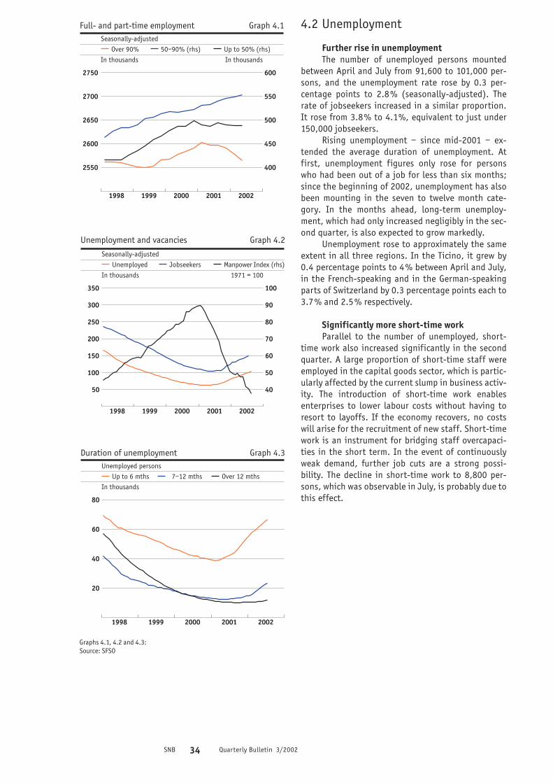
SNB 34 Quarterly Bulletin 3/2002
4.2 Unemployment
Further rise in unemploymentThe number of unemployed persons mounted
between April and July from 91,600 to 101,000 per-sons, and the unemployment rate rose by 0.3 per-centage points to 2.8% (seasonally-adjusted). Therate of jobseekers increased in a similar proportion.It rose from 3.8% to 4.1%, equivalent to just under150,000 jobseekers.
Rising unemployment – since mid-2001 – ex-tended the average duration of unemployment. Atfirst, unemployment figures only rose for personswho had been out of a job for less than six months;since the beginning of 2002, unemployment has alsobeen mounting in the seven to twelve month cate-gory. In the months ahead, long-term unemploy-ment, which had only increased negligibly in the sec-ond quarter, is also expected to grow markedly.
Unemployment rose to approximately the sameextent in all three regions. In the Ticino, it grew by0.4 percentage points to 4% between April and July,in the French-speaking and in the German-speakingparts of Switzerland by 0.3 percentage points each to3.7% and 2.5% respectively.
Significantly more short-time workParallel to the number of unemployed, short-
time work also increased significantly in the secondquarter. A large proportion of short-time staff wereemployed in the capital goods sector, which is partic-ularly affected by the current slump in business activ-ity. The introduction of short-time work enablesenterprises to lower labour costs without having toresort to layoffs. If the economy recovers, no costswill arise for the recruitment of new staff. Short-timework is an instrument for bridging staff overcapaci-ties in the short term. In the event of continuouslyweak demand, further job cuts are a strong possi-bility. The decline in short-time work to 8,800 per-sons, which was observable in July, is probably due tothis effect.
1998 1999 2000 2001 2002
2550
2600
2650
2700
2750
400
450
500
550
600
Full- and part-time employment Graph 4.1Seasonally-adjusted
In thousands In thousandsOver 90% 50–90% (rhs) Up to 50% (rhs)
1998 1999 2000 2001 2002
50
100
150
200
250
300
350
40
50
60
70
80
90
100
Seasonally-adjusted
In thousands 1971 = 100Unemployed Jobseekers Manpower Index (rhs)
Unemployment and vacancies Graph 4.2
1998 1999 2000 2001 2002
20
40
60
80
Duration of unemployment Graph 4.3Unemployed persons
In thousandsUp to 6 mths 7–12 mths Over 12 mths
Graphs 4.1, 4.2 and 4.3:Source: SFSO

SNB 35 Quarterly Bulletin 3/2002
5 Prices
5.1 Consumer pricesAnnual inflation measured by the national con-
sumer price index fell from 0.6% to 0.5% betweenMay and August. The general trend towards a slow-down in price rises thus continued. In July, the con-sumer price index was 0.1% below the year-earlierlevel. The main reason for this temporary decline inthe index was the data on clearance sales prices inthe category “clothing and footwear”, which hadbeen collected a month earlier than formerly. With-out this special effect, annual inflation would haveamounted to 0.5%. Inflationary pressure on domes-tic goods and services eased further due to persis-tently sluggish business activity, and inflation-damp-ening effects continued to emanate from importedconsumer goods.
Further decline in domestic inflationIn domestic consumer goods, annual inflation
diminished by 0.3 percentage points to 1.3% in June,an unchanged level in July and August. The declinewas particularly pronounced in domestic goods.Annual inflation in this category had still amountedto 1.8% in January and dropped to 0.7% by August.By contrast, price pressure in the service sector onlyeased marginally. In August, the rent index exceededthe corresponding previous year’s level by 0.8%, fol-lowing 0.9% in the previous survey in May. Annualinflation in other private services, which account forapproximately half of the basket of services, declinedby 0.3 percentage points to 1.8% between May andAugust. Price increases for public services stabilisedat 1.6%.
Accelerated price decline on imported goods After the price-curbing effect of imported con-
sumer goods had virtually petered out in April (–0.7%), the index of imported goods again remainedwell below the year-earlier level from May onwards. InAugust, a year-on-year decline of 2.0% was recorded.A contributing factor continued to be price reduc-tions for oil products, which in August fell short ofthe previous year’s level by 7.8%. The higher externalvalue of the Swiss franc also continued to keep the lidon prices.
2001 2001 2002
Q4 Q1 Q2 May June July August
National consumer price index total 1.0 0.4 0.6 0.7 0.6 0.3 –0.1 0.5
Domestic goods and services 1.7 1.8 1.8 1.5 1.6 1.3 1.3 1.3
Goods 1.5 1.5 1.8 1.2 1.4 0.6 0.5 0.7
Services 1.8 1.9 1.7 1.6 1.6 1.6 1.5 1.4
Private services without rents 1.5 1.9 2.0 2.0 2.1 2.0 1.8 1.8
Rents 2.8 2.2 1.6 1.1 0.9 0.9 0.9 0.8
Public services 0.5 1.1 1.3 1.6 1.6 1.6 1.6 1.6
Imported goods and services –1.2 –3.5 –3.0 –1.8 –2.0 –2.6 –3.9 –2.0
Without oil products –0.4 –0.7 –1.8 –0.1 –0.3 –0.7 –3.0 –0.9
Oil products –4.7 –16.0 –9.7 –10.2 –10.4 –12.9 –8.5 –7.8
Breakdown of the national consumer price index Table 10Change in percent
Sources: SFSO, SNB

SNB 36 Quarterly Bulletin 3/2002
... and of the SFSOThe two core inflation rates calculated by the
SFSO always exclude the same goods from the com-modities basket. In the case of core inflation 1, theseare foodstuffs, beverages, tobacco, seasonal prod-ucts, energy and fuel. Core inflation 2 also excludesproducts with administered prices. Compared withMay, the two core inflation rates declined by 0.2 per-centage points each and amounted to 0.7% and0.6% respectively in August.
5.2 Core inflation
Slightly lower core inflation of the SNBSince inflation measured by the national con-
sumer price index is subject to numerous short-termeffects that tend to obscure the view on the generalprice trend, the National Bank computes a core infla-tion rate. This core inflation rate excludes, in anyperiod, those 15% of goods with the highest annualinflation rate and the 15% of goods with the lowestannual inflation rate from the commodities basket ofthe consumer price index. In June, core inflation ofthe National Bank dropped by 0.2 percentage pointsto 0.9%, where it remained in July and August. Thisdecline reflects the cyclically-induced lower infla-tionary pressure. The fact that core inflation exceedsinflation as measured by the national index shows,moreover, that the inflation-dampening special fac-tors carry more weight than inflationary influences.
1998 1999 2000 2001 2002
–2
0
2
4
6
Consumer prices Graph 5.1Year-on-year change
%Total Goods Services
1998 1999 2000 2001 2002
–2
0
2
4
6
Consumer prices Graph 5.2Year-on-year change
%Total Domestic goods Imported goods
Graphs 5.1, 5.2:Sources: SFSO

SNB 37 Quarterly Bulletin 3/2002
prices for consumer goods and capital goods toppedthe previous year’s level (1.1% and 0.5% respec-tively). For the first time in two years, the price indexfor raw materials surpassed the year-earlier level(+2.0%). While the prices of goods produced inSwitzerland for the domestic market fell by 0.6%compared with the previous year, export goodsbecame cheaper by 0.4%.
In August, the index figure for imported goodswas 3.3% lower than a year earlier. Prices continuedtheir downward trend in all four categories of goods.This trend was particularly pronounced in the case ofraw materials and semi-manufactures (–6.1% and–3.6% respectively). Consumer goods and capitalgoods did not become cheaper to the same extent(–3.0% and –2.2% respectively).
5.3 Prices of total supply
Stabilisation of prices of total supplyThe price index of total supply (producer and
import prices) again dropped slightly between Mayand August after the decline in March and April hadcome to a standstill. This was attributable to import-ed goods, which became cheaper – not least due tothe firming of the Swiss franc. The price level forgoods manufactured in Switzerland remained stable.Thus, as hitherto, no inflationary stimuli for thedownstream consumer level emanate from producerand import prices.
In August, producer prices fell 0.6% short ofthe previous year’s level. This decline was due to pricecuts for semi-manufactures (–1.8%). By contrast,
1998 1999 2000 2001 2002
0.0
0.5
1.0
1.5
2.0
2.5
Core inflation Graph 5.3Year-on-year change
%Consumer prices Core inflation (SNB)
1998 1999 2000 2001 2002
–6
–4
–2
0
2
4
6
8
10
Prices of total supply Graph 5.4Veränderung gegenüber Vorjahr
%Total Producer prices Import prices
Sources: SFSO, SNB Source: SFSO

SNB 38 Quarterly Bulletin 3/2002
6 Inflation prospects
6.1 International price development
Inflation-dampening effects from abroadFears concerning an imminent US attack on Iraq
and possible delivery bottlenecks pushed up the oilprice per barrel of Brent crude oil from approximately23 dollars to at times just under 29 dollars betweenJune and mid-September. The higher prices, however,were offset by the US dollar’s depreciation vis-à-visthe Swiss franc. Expressed in Swiss francs, the pricefor crude oil was even somewhat below the previousyear’s level. The situation on the crude oil market isnot expected to ease in the coming months. In addi-tion to the continuing political tension, the seasonal-ly induced higher demand for oil also stands in theway of a price decline. As a result of the weak growthof the global economy, inflationary pressure on otherimport goods is likely to remain insignificant, how-ever – a development which is further reinforced bythe stronger Swiss franc. Contrary to our assessmentin June, we now expect that the price index forimported consumer goods will be slightly below thecorresponding year-earlier level by the end of theyear.
6.2 Price development in Switzerland
Hardly any cyclical inflationary stimuliAs a result of the weak economy, domestic infla-
tion on the consumer level has eased considerablysince the beginning of the year. An appreciable eco-nomic upturn is unlikely in the short term. The situa-tion on the labour market, in particular, will probablyonly improve during the course of 2003 so that costpressure from the wage front is not expected tointensify for the time being. Furthermore, producerand import prices – which can be considered as ameasure for the price development of intermediateservices – are not expected to produce any inflation-ary stimuli. Together with a continually highly com-petitive market, there will therefore still be little lee-way for price increases.
Rents slightly higherRents for apartments account for roughly 20%
of the basket of goods that make up the consumerprice index. Therefore, the future development ofsuch rents is of particular importance for assessinginflationary prospects. Contrary to our expectations,the August survey revealed a drop in annual rentincreases from 0.9% to 0.8%. Apartments are likelyto remain in tight supply in the short term, whichmeans that landlords can raise the rent for a new ten-ant or when an apartment is rented for the first time.We therefore expect apartment rents to go up some-what in the months ahead. The lowering of mortgagerates in August is expected to be passed on to thetenants next spring and will therefore cushion rentincreases.
SNB 39 Quarterly Bulletin 3/2002
6.3 Inflation forecast for 2002–2004
At its quarterly assessment of the situation on19 September 2002, the National Bank left the targetrange for the three-month Libor rate unchanged at0.25%–1.25%, after having last lowered it by half apercentage point on 26 July 2002.
The National Bank views the prospects for theglobal economy less optimistically than at the lastquarterly assessment of the situation on 11 June2002. Economic growth both in the US and in Europeis unlikely to pick up speed before the spring of 2003and regain its potential. For this reason, the econom-ic upswing is taking hold only gradually in Switzer-land as well. According to the National Bank’s assess-ment, the Swiss economy will see only moderategrowth rates until mid-2003. The negative output gapwill thus remain for some time.
As a result of the delayed economic rebound inSwitzerland, the National Bank expects inflation tobe lower during the next quarters than it had antici-pated at the quarterly assessment in June. Low inter-est rates and the relatively significant growth ofmonetary aggregates do not jeopardise price stabili-ty under the current circumstances.

SNB 40 Quarterly Bulletin 3/2002
7 Economic situation from thevantage point of the SNB’s bankofficesThe bank offices of the National Bank are con-
stantly in touch with a large number of enterprisesfrom various sectors of the economy. Their reports,which contain the subjective evaluations of theenterprises, are an important additional source ofinformation for assessing the economic situation. Inthe following, the results of the talks held from Mayto August on the current and future economic situa-tion are summarised.
7.1 ProductionMost companies hardly saw any improvement in
business from April to August. Business was unsatis-factory not only in the industrial sector, but manycompanies in the services sector were faced with thesame situation. The flat economic development madefor considerably stiffer competition in almost all sec-tors and put pressure on margins. Overall, a cyclicalupturn is no longer expected this year.
IndustryDifferent industrial sectors exhibited a more
mixed development during the last months than atthe beginning of the year. The same applies to devel-opment within the same sector. While individual sec-tors – depending on their markets – experienced acertain recovery in demand, the situation in otherareas and markets hardly changed. Many companiesin the pharmaceutical and foodstuffs sectors, whichare resistant to cyclical fluctuations, as well as sup-pliers of niche products, continued to achieve goodresults. However, most producers of capital goodsand upstream goods (paper, metal and plastics indus-try, sub-suppliers to the construction industry),reported a continued fall in turnover and fewerorders. Suppliers of near-consumer products (tex-tiles, watches, furniture) increasingly suffered fromrather weak demand as well.
ServicesBusiness deteriorated in many areas of the ser-
vices sector. The hotel and restaurant industry andretail trade felt the subdued consumer sentiment.Sluggish sales of goods also had a negative impact ontransport companies and logistics service providers.In the area of services provided for the business sec-tor (consulting firms, the printing industry), thecompanies’ cost-cutting measures left their mark,and in the financial sector, asset management feltthe effects of the sombre mood in the equities mar-kets.
Tourist industryThe tourist industry had a disappointing sum-
mer season and hoteliers were pessimistic about thesecond half of the year. The fact that there were fewerforeign guests from Germany, the US and Japan wasparticularly troubling. In addition to weaker demandfrom abroad, currency-related losses in revenueadded to the strain. Many areas also saw the numberof their Swiss guests dwindle so that the number ofovernight stays was down in almost all regions andcategories. Profiting from Expo.02, the Three LakesRegions was an exception.
ConstructionThe mood in the construction sector was sub-
dued overall, and the clear differences betweenregions and sectors, which had been observable forquite some time, remained. In some regions positivesigns came from residential construction, and a num-ber of construction companies benefited from largeinfrastructure projects. It appears that constructionactivity has stabilised on a lower level overall. Theconstruction sector again reported insufficientdemand and considers the price level to be too low.

SNB 41 Quarterly Bulletin 3/2002
7.2 Components of demand
Private consumptionAfter turnover of consumer goods had still reg-
istered increases up to the second quarter, the salesvolume went down appreciably in the summermonths. In particular, consumers showed consider-ably more restraint and were more price-consciouswhen purchasing clothing, furniture and electronicsarticles. Sales of luxury items fell off sharply, notleast because foreign guests stayed away. Foodstuffs,pharmaceutical products and everyday goods, an areawhich had still exhibited satisfactory development,also showed a certain downward trend from Juneonward.
Equipment investmentMany companies were not able to fully utilise
their available capacities. Investment was scaledback rigorously as a result. Only investment projectsfor replacing old machinery and equipment were car-ried out.
Exports of goodsThere were some bright spots in the export area.
Several sectors reported a slightly stronger demandfrom abroad. These sectors included producers fromthe pharmaceutical and foodstuffs industry as well ascompanies from the chemical industry and suppliersfor the European automobile industry. While someprecision instruments producers reported an increasein their turnover, only a few companies in themachinery industry were able to boost sales. Busi-ness of export-oriented companies was largely deter-mined by their markets. While sales to the US, Asia(except Japan) and to Eastern Europe trendedupward, sales to the big EU countries – Germany inparticular – showed a disappointing development.
7.3 Labour market
During the summer months, many companieswere forced to cut costs in order to prevent a furtherdeterioration of their earnings situation. A wave ofrestructuring led to staff reductions, and short-timework was on the rise. Given the contraction in out-put, personnel resources were still deemed to be toohigh in many areas. Companies in the capital goodssector were most affected. The few sectors which stillcreated new jobs reported wage claims to be clearlylower.
7.4 Prices and margins
Eroding margins were of major concern in mostcompanies. On the one hand, competition – and thusthe price war – became stiffer as a result of the weakdemand. The stronger franc, on the other hand, ledto lower revenue in most export-driven companies.

How accurate are GDP forecasts?An empirical study for Switzerland
by Eveline Ruoss, Economic Analysis, and Marcel Savioz, Research, Swiss National Bank, Zurich
The authors would like to thank Reto Vögeli for his assistance in collating thedata, and the forecasting institutes for helping to complete the data. They are grateful for comments by Marlene Amstad, Franziska Bignasca, Aline Chabloz, Enzo Rossi and Mathias Zurlinden.
SNB 42 Quarterly Bulletin 3/2002

SNB 43 Quarterly Bulletin 3/2002
Despite their significance, economic forecastsdo not have a very good reputation. The media fre-quently run reports on forecasts that have provedcompletely wrong. However, like weather forecasts,economic forecasts should not be condemned alto-gether simply because some have proved unreliable.It is surely preferable to form an opinion by lookingat their accuracy over a relatively long period.
The first study of this type for Switzerland wascarried about by Wasserfallen (1992). He showed thatthe forecasts for real gross domestic product (GDP)produced by nine selected forecasting institutestended to slightly underestimate the real growthrates achieved between 1974 and 1991. He alsoshowed that although the direction of changes in GDP was predicted correctly, the forecasts tended tooverestimate the scale of such changes. The resultsindicated that there was very little difference in theaccuracy of the forecasts made by the nine forecast-ing institutes. However, in view of the small sample,no significance test was carried out.
It is now ten years since this paper was pub-lished. Since then, there has been an increase in boththe number of institutes producing regular forecastsand the frequency with which forecasts are issued. It therefore seems to make sense to examine thisincreased body of data on Swiss economic forecast-ing. The aim of this paper is to show what can beexpected of economic forecasting. However, we donot intend to instigate a contest between the fore-casting institutes. For this reason, the results arepublished without direct reference to the institutes.
In this paper we examine forecasts for annualgrowth in real GDP in Switzerland. We look at theforecasts made by 14 different organisations andinstitutes between 1981 and 2000. Unlike Wasserfal-len (1992) and many surveys carried out for othercountries (e.g. Öller and Barot, 2000), our study isnot confined to the forecasts generated in theautumn for the following calendar year. As far as pos-sible, we include all forecasts made by the institutesduring the year for the current, following and next-but-one calendar year.
The paper is structured as follows. Section 1outlines the data. In Section 2 charts and descriptivestatistics are used to discuss the size of the forecasterrors and whether the forecasts are unbiased andefficient. The third and fourth sections investigatewhether the impressions gained from the charts anddescriptive statistics are corroborated by economet-ric tests and whether the forecasts of the institutesare better than forecasts based on simple naive me-thods. In Section 5 we consider whether forecasterrors would be lower if the estimates published bythe Swiss Federal Statistical Office (SFSO) were takenas the outcome instead of the GDP growth data pub-lished by the State Secretariat for Economic Affairs(seco), which are released earlier. Section 6 containsa summary of our findings and conclusions.1
1 cf. Hendry and Ericsson(2001) for an introduction to interpreting and evaluatingforecasts.

SNB 44 Quarterly Bulletin 3/2002
1 Data
1.1 Forecasts
This paper examines the forecasts for the per-centage annual change in real GDP made by 14 dif-ferent institutes, banks and organisations (referredto throughout as institutes). Alongside the FederalCommission for Economic Policy (KfK) and the SwissNational Bank (SNB), they include a number of com-mercial banks (CS, SBC, the old and the new UBS,and ZKB), international organisations (IMF, OECD)and various research institutes with organisationalor personnel links to universities (BAK, CREA, KOF,MAT, SGZZ). Our sample thus includes all instituteswhich to our knowledge have published regular eco-nomic forecasts for Switzerland in recent years.
Table 1 gives the names and abbreviations ofthe 14 institutes in our sample. It also shows thestart of the data series at each institute. The longestdata series (KfK) goes back to 1971. Our evaluation isconfined to the period 1981–2000 for two reasons:Firstly, the data set for the period before 1981 is rel-atively small because only a few institutes generatedforecasts and some of these were for GNP rather thanGDP. Secondly, the Swiss Confederation started topublish quarterly figures for real GDP in 1981. Thisgreatly improved the information on real GDP during
the year and probably influenced the quality of fore-casting. Forecasts made since 1981 should thereforeexhibit different statistical characteristics from thosepublished before 1981.
The forecasts in our data set can be classifiedaccording to the month in which they were publishedand the period to which they refer. With reference tothe forecasting horizon, we make a distinctionbetween forecasts for (i) the current calendar year,(ii) the following calendar year and (iii) the next-but-one calendar year. The date when the forecasts weremade is classified on the basis of the months (i)November, December and January, (ii) August, Sep-tember and October, (iii) May, June and July and (iv)February, March and April. Aggregation over three-month periods mitigates the problem that with someinstitutes it is not always possible to determineexactly when a particular forecast was made.
Our classification gives 12 different forecastinghorizons. h represents the number of months fromthe middle month in the three-month period in whichthe forecast was generated to the end of the calendaryear to which it refers. The horizons h = 0 to h = 9thus refer to forecasts for the current calendar year. h = 0 comprises forecasts made in November, Decem-ber and (in some cases) January for the calendar yearthat is about to end/has just ended. h = 12 to h = 21refer to forecasts for the next calendar year while
1 Vor 1997: SchweizerischeKreditanstalt (SKA).
2 Forecasts prior to 1980:Working Group for EconomicForecasts. From 1981: EconomicForecasting Subcommittee of the KfK.
3 Merged with SBC in Decem-ber 1997 to form the new UBS.
4 Former Union Bank ofSwitzerland
Abbreviation Name Year when forecastingof real GDP growth commenced
BAK BAK Basel Economics Ltd. 1983
CREA Institute of Applied Macroeconomics, School of Higher Business Studies at the University of Lausanne 1977
CS1 Credit Suisse 1994
IMF International Monetary Fund, Washington 1995
KfK Commission for Economic Policy, Berne 19712
KOF Centre for the Research of Economic Activity at the Federal Institute of Technology in Zurich 1976
MAT Aurelio Mattei, University of Lausanne 1977
OECD Organisation for Economic Cooperation and Development, Paris 1981
UBS3 Union Bank of Switzerland, Zurich 1982
SBC3 Swiss Bank Corporation, Basel 1981
SGZZ Center for Futures Research, St. Gallen 1976
SNB Swiss National Bank 1977
UBS UBS4 1998
ZKB Zürcher Kantonalbank 1994
Forecasting institutes Table 1

SNB 45 Quarterly Bulletin 3/2002
h = 24 to h = 33 refer to forecasts for the next-but-one calendar year. h = 33 thus denotes the two-yearforecasts produced in February, March and April, forinstance forecasts made in March 1998 for the year2000.
Table 2 shows the number of observations foreach forecasting horizon and institute. The samplecomprises a total of 766 observations. As the tableshows, only a few institutes, i.e. KOF, KfK, the OECDand SBC (UBS “new” from 1998) generated 20 fore-casts with the same forecasting horizon in the twenty-year period 1981–2000. This was principally becausesome of the institutes altered the timing of forecastspublished during this time or did not make forecastsfor some periods.
Almost all of the 766 forecasts were published.The sources are shown in the appendix. The excep-tions are some of the forecasts by the SNB, which aretaken from internal documents, specifically the mon-
etary policy reports for the coming year elaboratedeach autumn between 1974 and 1999. Unlike the cor-responding press releases, these documents in mostcases contain precise forecasting data. Where a fig-ure is qualified as “nearly” we deduct 0.25 percent-age points. Similarly, we add 0.25 percentage pointsto those figures qualified with “at least”. In fourcases, only qualitative data were available on futureeconomic trends, so that for those years a forecastfigure for the SNB is missing.
Despite the gaps in our data set, our chartanalysis and descriptive statistics provide an initialpicture of the accuracy of the forecasts. By contrast,the gaps detract from the econometric tests outlinedin section 3. Consequently, these are confined toinstitutes for which we have complete data series,thus enabling us to use standard econometric tests toassess the accuracy of the forecasts.
1 From 1993 including thespring forecasts by the SwissConfederation’s Expert Group for Economic Forecasting
2 UBS and SBC merged inDecember 1997 to form the newUBS.
Date of forecast Time BAK CREA CS IMF KfK1 KOF MAT OECD UBS2 SBC2 SGZZ SNB UBS ZKB Totalhori- ofzon obser-
vations
Forecast for the current calendar yearNovember to January h=0 6 5 20 20 16 17 3 2 89August to October h=3 17 13 7 6 20 19 3 7 92May to July h=6 4 1 1 20 9 1 2 6 44February to April h=9 13 13 6 6 8 19 10 17 3 6 101
Forecast for the following calendar yearNovember to January h=12 5 7 20 20 19 16 16 14 3 6 126August to October h=15 16 12 6 5 20 16 2 6 83May to July h=18 3 1 19 5 2 5 35February to April h=21 13 12 4 5 8 18 10 5 2 4 81
Forecast for the next-but-one calendar yearNovember to January h=24 4 8 12 11 5 2 4 46August to October h=27 15 11 14 1 1 42May to July h=30 2 1 1 4February to April h=33 13 10 23Total 111 94 23 22 57 91 20 90 63 75 36 14 23 47 766
Overview of forecasts by time horizon and institutes 1981–2000 Table 2

SNB 46 Quarterly Bulletin 3/2002
1.2 Outcomes
To assess the quality of the forecasts, they arecompared with the actual GDP figures. Since GDP isnormally revised several times, it is necessary todecide which figure to take as the outcome. Follow-ing the literature, we use the first available estimatefor real GDP growth. In our case, this is the annualaverage calculated by the State Secretariat for Eco-nomic Affairs (seco) in March of each year on thebasis of its quarterly estimates.2
The period 1981–2000 contains two businesscycles. It thus includes both recessions and upswings,making it suitable for judging the accuracy of eco-nomic forecasts. On the basis of the seco data, annualaverage growth in real GDP was 1.4%. In six years,real GDP declined. The sharpest decline was 1.3% in1982. The highest growth rate was 3.4% in 2000. Themedian is 1.95%, which is well above the averagegrowth rate. This shows that the distribution of therates of change in GDP in the period 1981–2000 is notsymmetrical; downtrends (negative growth rates)have a greater impact than high growth rates. Thestandard deviation (SD), i.e. the square root of thesquared deviations from the mean outcome, is 1.548.We use this figure as a benchmark.
2 From 1981–1986 the quar-terly GDP estimates were carriedout be the Swiss FederalStatistical Office (SFSO), whichis part of the Federal Depart-ment of Home Affairs. In 1987this task was entrusted to the Federal Office for EconomicQuestions within the Federal
Department of Economic Affairs.Since 1999 the quarterly esti-mates for GDP have been calcu-lated by the State Secretariat forEconomic Affairs (seco).
2 How accurate are GDP forecasts?
2.1 Chart analysis
Figures 1 and 2 provide an initial insight intothe quality of the forecasts. Fig. 1 shows the resultsfor horizons h = 0 to h = 9, while the results for hori-zons h = 12 to h = 21 are shown in Fig. 2. The left-hand column in each chart contains four scatter dia-grams while the right-hand column contains fourtime series plots. The curves show the GDP growthrates forecasts by the various institutes against theactual values (blue line). The deviations between theactual GDP growth rates and the forecasts indicatethe development of forecast errors over time.
In the scatter diagrams, the x-axis representsactual GDP growth and the y-axis forecasts of GDPgrowth. Forecast errors, which are defined as the dif-ference between the actual and forecast growth rate,correspond to the horizontal distance from a point tothe 45° line. The closer the plots are to the 45° line,the more accurate the forecasts. The four squaresindicated with Roman numerals show whether thedirection of the GDP trend was forecast accurately. If the points are in squares I or III, a rise or decline in real GDP was anticipated correctly. By contrast, ifthe points are in squares II or IV, the institutes pre-dicted the wrong direction, i.e. a rise rather thandecline in GDP (square IV) or a fall rather than a rise(square II).
How accurate are the forecasts? Fig. 1 showsthat the accuracy of the 89 h0-forecasts included inour evaluation is good. The projections generated inNovember to January for the current/last calendaryear are close to the 45° line. The wrong directionwas only forecast in one case, with a rise rather thana decline in GDP being anticipated. The forecasts forh = 3, i.e. forecasts made between August and Octo-ber, are also close to the 45° line. By contrast, theforecasts for h = 9 (February to April) are a good dealless reliable. They scatter widely and in about a fifthof cases a rise in real GDP was indicated, when theactual trend was a decline.

SNB 47 Quarterly Bulletin 3/2002
Actual and forecast GDP growth rate for the current calendar year Figure 1
–4
–3
–2
–1
0
1
2
3
4
–4 –3 –2 –1 0 1 2 3 4 %
November to January (h=0)
August to October (h=3)
May to July (h=6)
February to April (h=9)
%Fo
reca
st G
DP g
row
th r
ate
Actual GDP growth rate
–2
–1
0
1
2
3
4
–2 –1 0 1 2 3 4
–2
–1
0
1
2
3
4
–2 –1 0 1 2 3 4
–2
–1
0
1
2
3
4
–2 –1 0 1 2 3 4
IV I
III II
45o–4
–3
–2
–1
0
1
2
3
4%
82 84 86 88 90 92 94 96 98 00 %
Actual GDP growth
– Institutes’ forecasts
–2
–1
0
1
2
3
4
82 84 86 88 90 92 94 96 98 00
–2
–1
0
1
2
3
4
82 84 86 88 90 92 94 96 98 00
–2
–1
0
1
2
3
4
82 84 86 88 90 92 94 96 98 00

SNB 48 Quarterly Bulletin 3/2002
Actual and forecast GDP growth rate for the following calendar year Figure 2
November to January (h=12)
August to October (h=15)
May to July (h=18)
February to April (h=21)
%
%
Fore
cast
GDP
gro
wth
rat
e
Actual GDP growth rate
IV I
III II
45o
% Actual GDP growth
– Instituts’ forecasts
–3
–2
–1
0
1
2
3
4
–3 –2 –1 0 1 2 3 4
–2
–1
0
1
2
3
4
–2 –1 0 1 2 3 4
–2
–1
0
1
2
3
4
–2 –1 0 1 2 3 4
–2
–1
0
1
2
3
4
–2 –1 0 1 2 3 4
–3
–2
–1
0
1
2
3
4
82 84 86 88 90 92 94 96 98 00 %
–2
–1
0
1
2
3
4
82 84 86 88 90 92 94 96 98 00
–2
–1
0
1
2
3
4
82 84 86 88 90 92 94 96 98 00
–2
–1
0
1
2
3
4
82 84 86 88 90 92 94 96 98 00

SNB 49 Quarterly Bulletin 3/2002
Two other observations can be made on thebasis of the scatter diagrams in Fig. 1. Firstly, there isno indication that the forecasts are systematicallydistorted to the left or right of the 45° line. In otherwords, the forecasts are neither too high nor too lowon average. They are thus unbiased. Secondly, thecharts indicate that as from h = 9 the slope of thescatter plot is no longer around the 45° line buttends to be flatter. In other words, GDP forecaststend to underestimate the trend in upward phasesand overestimate it in periods of negative growth.From this we conclude that the higher the absoluteforecast change, the higher the forecast error, i.e.the horizontal distance from the 45° line. They thusseem to correlate with the absolute forecast figures.This suggests that some information available to theinstitutes (including the correlation between theforecast and the forecast error) is not utilised in theforecasting process, resulting in informational inef-ficiency. Informational inefficiency is suspected forhorizons h = 9 as well as for h = 12 and h = 15 in Fig. 2 because the slope of the scatter plotseems to be flatter than 45°.
The h12 forecasts in Fig. 2 contain 126 observa-tions and represent the highest number of observa-tions of all 12 time horizons. These are forecasts pub-lished between November and January for the comingyear. Although they scatter substantially, there isstill a positive correlation between the forecast andactual values. This recedes in the subsequent charts.For the h15, h18 and h21 forecasts there is hardly anypositive correlation between forecast and actual GDP.The same applies to the predictions for h24 to h33,which are not shown here. They form a horizontalband in the upper two squares of the scatter dia-grams. In other words, they only change slightly.They thus possibly provide information on theexpected trend or potential growth, but no longergive any information on the future business cycle.
2.2 Descriptive statistics: ME, MAE, RMSE and Theil’s U Forecast errors can be quantified in various ways.
Table 3 shows six common statistics for the time hori-zons h = 0 to h = 33. Note that for some horizons onlya small number of observations are available (cf.Table 2).
The Mean Error (ME) shows whether the fore-casts are too high or too low on average and thusindicates whether they are biased. In the forecastsfor the current year (h = 0,3,6,9) the mean error isclose to zero. It is also close to zero for h = 12, whereWasserfallen (1992) identifies a slightly positiveforecast error. The mean errors increase substantiallywith the forecasting horizon. For the longest horizon(h = 33), it is 1.3 percentage points, which is onlyslightly lower than the average actual GDP growthrate. Moreover, from h = 15 the mean error is consis-tently negative, i.e. the actual growth rate is alwaysoverestimated. This is mainly because the extremelynegative forecast errors are higher than the extre-mely positive errors from this horizon onwards (seeMIN and MAX).
The Mean Absolute Error (MAE), i.e. the meanabsolute difference between actual and forecastgrowth, is a yardstick of the accuracy of the forecasts.It rises significantly with the forecasting horizon.

SNB 50 Quarterly Bulletin 3/2002
The picture is similar for the Root Mean SquaredError (RMSE). This commonly used statistical measuregives major errors a higher weighting than minorones, thus taking account of the fact that the mainaim of forecasting is to avoid large errors. The RMSEalso rises with the forecasting period. While it is be-low 1 for forecasts for the current year (h = 0,3,6,9),from h = 18 it exceeds the standard deviation foractual GDP (1.55).
Another descriptive statistic shown in Table 3 isthe inequality coefficient of Theil. In analogy withWinker (2002, p. 257), we define it as RMSE dividedby the standard deviation of the actual real GDP. If Uis less than 1, this means the forecast error is smallerthan the standard deviation, i.e. the average varia-tion of the actual values. In this case the forecastersscore better than an alternative forecasting methodwhich uses the 1981–2000 average of the actual GDPgrowth rates as a forecast. The results show that forforecasts for the current year (h = 0,3,6,9) the valuefor U is well below 1. Similarly, forecasts for the nextcalendar year generated between August and January(h = 12,15) are more accurate than the average forthe actual GDP growth rate. That changes from h = 18,where U is greater than 1. As the charts show, thelong-term forecasts are virtually meaningless asregards future business cycles.3
Forecast error: Actual valueminus predicted value. A plussign indicates an under-estimate while a minus signindicates an overestimate.
Mean (ME), minimum (MIN) andmaximum (MAX) forecast error
RMSE: Root Mean Squared Error
Theil’s U: RMSE divided by thestandard deviation (SD) of theactual values
3 This comparison is notentirely fair because it assumes aknowledge of the average GDPgrowth rate for 1981–2000. Later on we use a comparisonbased only on information thatwas actually available to theinstitutes when they made theirforecasts.
ME MIN MAX MAE RMSE Theil’s U
Forecasts for the current calendar yearh=0 0.110 –0.8 2.1 0.340 0.480 0.31
h=3 0.020 –1.7 1.6 0.446 0.575 0.37
h=6 0.039 –1.7 2.2 0.632 0.803 0.52
h=9 –0.112 –2.2 2.2 0.805 0.989 0.64
Forecasts for the following calendar yearh=12 0.034 –2.5 2.5 0.988 1.175 0.76
h=15 –0.286 –3.5 2.4 1.175 1.462 0.94
h=18 –0.514 –3.8 1.7 1.306 1.635 1.06
h=21 –0.583 –4.1 3.1 1.439 1.790 1.16
Forecasts for the next-but-one calendar yearh=24 –0.572 –4.0 2.1 1.393 1.730 1.12
h=27 –0.721 –4.1 2.0 1.607 1.919 1.24
h=30 –0.250 –4.3 1.6 1.900 2.393 1.55
h=33 –1.322 –3.7 1.5 1.670 2.069 1.34
Forecast error 1981–2000 Table 3

SNB 51 Quarterly Bulletin 3/2002
3 Optimality conditions of theforecastsIn both the chart analysis and the descriptive
statistics, there is a risk that random patterns may beinterpreted as systematic patterns. Econometric testscan be used to minimise this risk.
This section looks at three necessary conditionsrequired for optimal forecasting. Firstly, forecastsshould be unbiased (Section 3.1). Secondly, thereshould be no autocorrelation between forecast errors(Section 3.2). Thirdly, forecasts should be efficient,i.e. forecast errors should not correlate with informa-tion that was generally available at the time when theforecast was made (Section 3.3).4
The tests are only carried out for institutes thatmade at least 18 forecasts for a given horizon. We cal-culate the results for each institute individually toavoid statistical problems arising from a possible het-erogeneity of the forecasts.5 Due to lack of data, onlyforecasts for the current year (h = 0,3,6,9) and thefollowing year (h = 12,15,18,21) are tested.
Econometric tests generally give reliableresults, even for small samples, if the forecast errorsare normally distributed. Consequently, the normalityof the distribution was tested first. These tests didnot give any indication that the hypothesis of normaldistribution of forecast errors should be rejected.6
These findings also provide scope to calculate confi-dence intervals for various forecasting horizons. Themethod is outlined on page 62.
3.1 Are the forecasts biased?
We start by looking at whether the forecasts arebiased, i.e. whether they are systematically too highor too low. A biased forecast is suboptimal because itcan be corrected and thus improved on the basis ofthe bias recognised from past forecasts.
Unbiasedness is often tested using the Theil-Mincer-Zarnowitz equation. This is a regression of theactual values on a constant and the forecast values.In the following we test whether the intercept isequal to zero and the slope is equal to one. Holdenand Peel (1990) pointed out that this null hypothesisis merely sufficient but not necessary for unbiased-ness. Following their suggestion, we only run aregression of the forecast error eth on the constant(cf. Clements and Hendry (1998), p.57.):
(1) eth = α + εt
If the constant α deviates significantly fromzero, the hypothesis that the forecast is unbiased isrejected. It should be noted that the ordinary leastsquares method gives consistent results, but that thestandard error is biased if there is autocorrelation inthe residuals. For reasons outlined in the next sec-tion, autocorrelation of the first order has to beassumed for the forecasts for the following calendaryear. In these cases, the standard errors were cor-rected using the method of Brown and Maital (1981).
Table 4a summarises the results of 15 regres-sions. The estimated values for the constant α areshown in column 2 with the standard error in brack-ets. In only one case is the null hypothesis rejected atthe usual significance levels. In the other cases,there was no reason to assume that the constant isnot zero. The results therefore show that the forecasterrors can be considered unbiased, fulfilling the firstcondition for optimal forecasting.
4 Here we follow Granger andNewbold (1973), who recom-mend that the optimality of fore-casts should be based on ananalysis of forecast errors ratherthan a regression of the actualvalues on the predicted values.Cf. Clements and Hendry (1998,p. 56).
5 We will be utilising the panel structure of the data in a separate study.
6 The normal distribution ofthe forecast error was testedusing the Jarque-Bera statistics.These tests show a normaldistribution for most forecastinghorizons. Moreover, the usualtests show that the forecasterrors are stationary.

SNB 52 Quarterly Bulletin 3/2002
α was estimated by the leastsquares method, whereby thestandard error was calculatedusing the Brown and Maitalmethod (1981). The LM-test forautocorrelation is the Breusch-Godfrey test. The start values forthe test equation, i.e. thelagged right-hand variables outside the sample, were set atzero.
a) Standard error estimatedusing the Brown and Maitalmethod (1981) with a lag of thefirst order b) The residuals lagged by oneperiod are omitted from theBreusch-Godfrey test equation.
c) Newey-West HAC standarderror with truncation after thesecond lag d) The data for 1981 aremissing.e) The data for 1981 and 1982are missing.
***, **, *: Significance level1%, 5%, 10%
Bias Autocorrelationα P LM(3), LM(2) p-value
1 2 3 4 5
h=0 0.180 0.040** 3.888 0.274(3 institutes) (0.082)
0.103 0.397 8.554 0.036**(0.118c)
0.045 0.649 1.450 0.694(0.097)
h=3 0.080 0.527 6.018 0.111(2 institutes) (0.124)
0.074d 0.728 3.250 0.355(0.209)
h=6 –0.035 0.856 4.591 0.204(1 institute) (0.191)
h=9 –0.179d 0.370 2.163 0.539(2 institutes) (0.194)
0.242d 0.306 0.603 0.896(0.230)
h=12 0.160 0.625 0.450b 0.778(4 institutes) (0.327a)
0.025 0.931 0.369b 0.831(0.289a)
–0.184d 0.635 0.598b 0.741(0.388a)
0.083e 0.805 0.014b 0.993(0.337a)
h=15 –0.265 0.439 0.156b 0.925(1 institute) (0.343a)
h=18 –0.658d 0.207 0.754b 0.686(1 institute) (0.522a)
h=21 –0.400e 0.459 1.664b 0.435(1 institute) (0.540a)
Optimality tests 1 – Unbiasedness of forecasts Table 4a

SNB 53 Quarterly Bulletin 3/2002
3.2 Are the forecast errorsautocorrelated?The second condition for an optimal forecast
requires that, for the forecasts of the current year,the forecast errors should not be autocorrelated.Autocorrelation would occur if, for example, a nega-tive forecast error (overestimate) was always fol-lowed by a positive forecast error (underestimate)and vice versa. Such forecasts are sub-optimalbecause they can be corrected and thus improved onthe basis of the observed pattern of forecast errorsand the observed autocorrelation of the forecasterrors.
Autocorrelation of forecast errors should bejudged differently if the forecasting horizons overlap.Let us take as an example the forecasts generated inMay, June and July for the following calendar year (h = 18): both the forecast errors of the forecast gener-ated in June 2000 for 2001 and of the forecasts made inJune 2001 for 2002 are likely to have been affected bythe terrorist attacks in the USA on 11 September 2001.As a result, it is probable that both forecasts overesti-mate GDP growth. What has been illustrated with theexample of 11 September is naturally repeated year foryear. In other words, autocorrelation is to be expectedfor all forecasts for time horizons of a year or more(h = 12,15,18, 21) because the overlapping forecastingperiod contains common events (innovations). How-ever, in such cases, the autocorrelation should only berelated to the previous year’s errors (autocorrelation ofthe first order), not to the forecast errors made two ormore years before.
To test for autocorrelation of forecast errors, wecan use the results shown in Table 4a. Since the residu-als from equation (1) represent the forecast erroradjusted for the mean value, testing for autocorrela-tion of the residuals is equivalent to testing for auto-correlation of forecast errors. Column 4 shows theresults of the Lagrange Multiplier Test (LM) afterBreusch-Godfrey. The p-value in column 5 shows theprobability of the LM-statistics, assuming that there isno autocorrelation of the residuals (h= 0,3,6,9) or thatonly autocorrelation of the first order is identified (h =12,15,18,21).7 The results show that – with oneexception – the p-values are over 5%. From this weconclude that there is no autocorrelation of the fore-cast errors that would contradict the optimality of theforecasts.
3.3 Informational efficiency of theforecastsEfficiency is the third requirement for optimal
forecasts. A forecast is efficient if it uses all informa-tion available at the time when it is made. Tests forinformational efficiency therefore look at whetherthe forecast errors correlate with information knownat the time when the forecast was made (orthogonal-ity tests). They are based on a regression of the fore-cast error on variables that could be observed whenthe forecast was made:
(2) eth = α + �xt–i + εt �i=1 h = 0,3,6,9i=2 h = 12,15,18,21.
eth represents the forecast error in calendar year t andxt–i an information variable (or a vector of informa-tion variables). The information variable has a lag ofone period if the forecast error refers to forecasts forthe current calendar year (h = 0,3,6,9), and a lag oftwo periods if the error refers to forecasts for the fol-lowing calendar year (h= 12,15,18, 21). This guaran-tees that only information available when the fore-cast was made is used as right-hand variables. Thecoefficient (or a vector of coefficients) � is zero if the forecast error does not correlate with the variablext–i. By contrast, if � is not zero, xt–i correlates withthe forecast error and the forecast is not efficient rel-ative to the information set to which the variable xt–ibelongs. Again, the error term of the regressions forthe following year (h =12,15,18,21) may be autocorre-lated.
Was efficient use made of the informationused for producing the forecast?In the simplest efficiency test the information
variable xt–i is the observed value for the series beingpredicted. In this case, the variable xt–i is the lastactual real GDP growth rate. If there is no autocorre-lation with the forecast errors and they do not corre-late with the GDP growth rate, the forecasts are saidto show weak informational efficiency.
We refrain from reporting the detailed results ofthis orthogonality test. The hypothesis � = 0 cannotbe rejected in any of the regressions and, therefore,the forecast errors are not correlated with the GDPgrowth rate. Taking into account the results outlinedin section 3.2 (no autocorrelation), it can be assumedthat the forecasts are weakly informational efficient.
7 For (h = 12,15,18,21) theBreusch-Godfrey test is modi-fied: the residuals for a one-period lag are omitted from thetest regression. The results of the Q test (not shown) corre-spond to the results of theBreusch-Godfrey test.

SNB 54 Quarterly Bulletin 3/2002
Tests for stronger informational efficiency canbe carried out by extending the set of information. Bytaking the forecast itself as the variable xt–i, it is pos-sible to check whether the forecasting institute madeefficient use of the information available when theforecast was produced. If �≠ 0, the forecaster did notmake efficient use of the information underlying theforecast. If � > 0, the change in GDP was systemati-cally underestimated; if � is between –1 and 0 thechange in GDP was systematically overestimated.8
This test can be illustrated with help of thecharts. If � ≠ 0, the plots in the scatter diagrams inFigs. 1 and 2 are not along the 45° line. If � > 0 (or–1< �< 0), the line through the scatter plot is flatter(steeper) than the 45° line. By contrast, if �< –1, theslope in the scatter plot is negative, indicating thatthe institutes did not manage to forecast whetherGDP would grow or contract in the calendar year towhich the forecast refers. In this case, while positive(negative) GDP growth rates were predicted, theactual growth rates were negative (positive).
Orthogonality test Autocorrelation� p-value LM(3), LM(2) p-value
1 2 3 4 5
h=0 –0.070 0.181 3.095 0.377(3 institutes) (0.051)
–0.018 0.810 8.645 0.034**(0.073c)
–0.072 0.331 2.694 0.441(0.072)
h=3 –0.036 0.681 6.104 0.107(2 institutes) (0.087c)
–0.271d 0.195 3.293 0.349(0.201)
h=6 0.201 0.274 4.793 0.188(1 institute) (0.178)
h=9 0.228d 0.214 0.963 0.810(2 institutes) (0.177)
0.075d 0.725 0.512 0.916(0.211)
h=12 0.029 0.860 0.486b 0.784(4 institutes) (0.165a)
–0.218 0.200 0.635b 0.728(0.170a)
0.375d 0.288 0.553b 0.758(0.353a)
0.575e 0.039** 0.453b 0.798(0.279a)
h=15 –0.090 0.807 0.154b 0.926(1 institute) (0.370a)
h=18 –3.217d 0.000*** 0.912b 0.634(1 institute) (0.792a)
h=21 –1.430e 0.092* 0.184b 0.912(1 institute) (0.850a)
Optimality tests 2 – Informational efficiency regarding the institutes’ own forecast Table 4b
� was estimated by the leastsquares method, whereby thestandard error was calculatedusing the Brown and Maitalmethod (1981). The LM-test forautocorrelation is the Breusch-Godfrey test. The start values forthe test equation, i.e. thelagged right-hand variablesoutside the sample, were set at zero.
a) Standard error estimatedusing the Brown and Maitalmethod (1981) with a lag of thefirst orderb) The residuals lagged by oneperiod are omitted from theBreusch-Godfrey test equation.
c) Newey-West HAC standarderror with truncation after thesecond lag d) The data for 1981 are missing.e) The data for 1981 and 1982are missing. ***, **, *: Significance level1%, 5%, 10%
8 This only applies forunbiased forecasts.

SNB 55 Quarterly Bulletin 3/2002
The results of this orthogonality test are shownin Table 4b. The structure of this table is similar toTable 4a: the standard error for time horizons from h =12 given in brackets is calculated according toBrown and Maital (1981). The third column gives thep-value while the fourth and fifth columns give theresults of an autocorrelation test for the residuals,which can be used to test whether the standard errorswere calculated correctly.
Up to h =18, � does not normally deviate signif-icantly from zero. It is true that from h = 6 there is atrend towards positive � coefficients, indicating acertain “inertia” in the forecasts. However, since theaccuracy of the estimates declines (increasing stan-dard error), in all cases except one the hypothesis �= 0 cannot be rejected.9 To sum up, the forecasts upto h=15 show weak informational efficiency and arealso efficient in a stronger sense as they make opti-mal use of the information used to produce the fore-casts. This is not true for h =18 and h = 21. In the caseof h =18, � is even significantly below –1, so theinstitutes did not manage to forecast recessions overthis forecast horizon.
Are the forecasts strongly informationalefficient? Informational efficiency is strongest when all
publicly available information is utilised efficiently.To show that the forecasts are not efficient in thissense, it is sufficient to find information that wasgenerally available to the institutes and that corre-lates with the forecast error. Such a result would beinteresting as it would show how forecasting could beimproved. However, a result indicating that no corre-sponding variables could be found is not very mean-ingful. Only if all available data had been taken intoaccount – and that is an impossible task – would it bepossible to conclude that the forecasts are stronglyinformational efficient.10
In this section, we show that information existswhich could be used to improve forecasting – namely,forecasts from other institutes. Assuming informa-tional efficiency, the forecast errors of one instituteshould not correlate with the forecasts of another. Ifthere is a correlation, the institute has not suffi-ciently analysed the forecasts made by the otherinstitute. There are either shortcomings in “forecast-ing technology” or the institute has overlooked thefact that the other institute utilises data which itignores or does not pay sufficient attention to.
To test this, the forecasts made by other insti-tutes are taken as the xt–i variable in Equation 2. Tomake sure that this information was available whenthe forecast was made, we only use forecasts made inthe previous three-month period. For instance, totest the informational efficiency of forecasts for h = 0a regression of the corresponding forecast errors onthe forecasts for h = 3 is performed.
Table 4c summarises the results. Columns 2-7are headed by the six institutes whose forecasts areused as the variable. The results show that the fore-casts made by one institute correlate in one case,while those of another correlate three times. The sec-ond institute is the OECD, which possibly has betterinformation on the international economic situationthan the other institutes. In any case, the resultsshown in this table indicate that the forecasts are notstrongly informational efficient.
In the literature, forecasts that are both unbi-ased and show strong informational efficiency aredescribed as strongly rational. As this section shows,there is information which is not utilised, so the fore-casts are not strongly rational. As set out in Section3.1, the forecasts for the current and following calen-dar year are nevertheless unbiased and thus weaklyrational.11
9 This contradicts Wasserfallen(1992, p. 300). For h=12Wasserfallen assumed that theactual change in GDP was over-estimated.
10 In the literature, stronginformational efficiency isgenerally referred to simply asinformational efficiency.
11 Alternative terminologyrefers to unbiasedness and weakinformational efficiency as weak rationality (see e.g.Kirchgässner, 1993). Theforecasts are weakly rational in this sense, too.
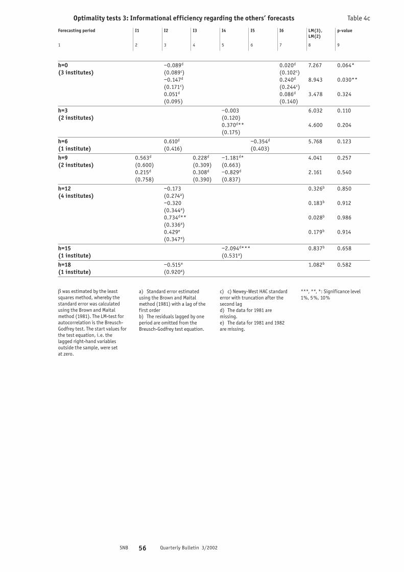
SNB 56 Quarterly Bulletin 3/2002
� was estimated by the leastsquares method, whereby thestandard error was calculatedusing the Brown and Maitalmethod (1981). The LM-test forautocorrelation is the Breusch-Godfrey test. The start values forthe test equation, i.e. thelagged right-hand variablesoutside the sample, were set at zero.
a) Standard error estimatedusing the Brown and Maitalmethod (1981) with a lag of thefirst order b) The residuals lagged by oneperiod are omitted from theBreusch-Godfrey test equation.
c) c) Newey-West HAC standarderror with truncation after thesecond lag d) The data for 1981 aremissing.e) The data for 1981 and 1982are missing.
***, **, *: Significance level1%, 5%, 10%
Forecasting period I1 I2 I3 I4 I5 I6 LM(3), p-valueLM(2)
1 2 3 4 5 6 7 8 9
h=0 –0.089d 0.020d 7.267 0.064*(3 institutes) (0.089c) (0.102c)
–0.147d 0.240d 8.943 0.030**(0.171c) (0.244c)0.051d 0.086d 3.478 0.324(0.095) (0.140)
h=3 –0.003 6.032 0.110(2 institutes) (0.120)
0.370d** 4.600 0.204(0.175)
h=6 0.610d –0.354d 5.768 0.123(1 institute) (0.416) (0.403)
h=9 0.563d 0.228d –1.181d* 4.041 0.257(2 institutes) (0.600) (0.309) (0.663)
0.215d 0.308d –0.829d 2.161 0.540(0.758) (0.390) (0.837)
h=12 –0.173 0.326b 0.850(4 institutes) (0.274a)
–0.320 0.183b 0.912(0.344a)0.734d** 0.028b 0.986(0.336a)0.429e 0.179b 0.914(0.347a)
h=15 –2.094d*** 0.837b 0.658(1 institute) (0.531a)
h=18 –0.515e 1.082b 0.582(1 institute) (0.920a)
Optimality tests 3: Informational efficiency regarding the others’ forecasts Table 4c

SNB 57 Quarterly Bulletin 3/2002
4 Comparison with naive forecasts
In the previous sections, we saw that forecastsup to h = 18 satisfy the optimality criteria for fore-casts. The question now is whether such forecasts aresuperior to naive forecasts. We define naive forecastsas simple forecasting methods requiring very littleeffort.
A first naive method, which we call naive fore-cast 1, takes the average GDP growth in the past 20 years as a forecast. For 2000 this naive forecast is thus the average GDP growth rate for 1980–1999.12
A second naive method called naive forecast 2 uses the last actual GDP growth rate as a fore-cast. Naive forecast 2 for 2000 thus corresponds tothe actual growth rate in 1999.
Table 5a compares the RMSE of the two naiveforecasting methods with the RMSE of the forecastsgenerated by the institutes. This comparison is basedon four different time horizons. We assume that thetwo naive forecasts are published in March, as soonas the average GDP growth rate for the previous yearis known. Hence, some of the h = 9 and h = 21 fore-casts generated by the institutes in February to Aprilwere made before the GDP growth rate is publishedand are thus not based on the same information asthe naive forecasts. By contrast, for the forecastsmade between May and July for h = 6 and h = 18 thefirst GDP estimate was already available as theseforecasts were made up to three months after thenaive forecasts.
The results show that the forecasts made by theinstitutes for the current calendar year (h = 6 and h = 9) have far lower forecast errors than the twonaive forecasts. Looking at the forecasts for the fol-lowing calendar year, the quality of the forecasts forh = 18 is roughly the same as for naive forecast 1,while the forecasts for h = 21 are inferior to naiveforecast 1. Moreover, both forecasts made by theinstitutes for the following year (h =18 and h =21) arebetter than the naive forecast 2.
12 For the effective values prior to 1981 we have to use thefirst data issued by the SFSO.
All institutesFigures in square brackets:RMSE/SD (Theil’s U)
RMSE 1981–2000
Forecasting period All institutes Naive Forecast 1: Naive Forecast 2:Average growth rate Last actual
growth rate
h=6 0.803 1.534 1.618[0.519] [0.991] [1.045]
h=9 0.989 1.534 1.618[0.639] [0.991] [1.045]
h=18 1.635 1.564 2.263[1.056] [1.011] [1.527]
h=21 1.790 1.564 2.263[1.156] [1.011] [1.527]
Comparison with naive forecasting methods Table 5a

SNB 58 Quarterly Bulletin 3/2002
In a next step the Diebold and Mariano test(1995) is used to check the statistical significance ofthe results. The hypothesis tested is that the MeanSquared Error (MSE) is the same for the naive fore-casts and the forecasts of the institutes. We still as-sume a squared loss function with positive and nega-tive errors of the same magnitude leading to equallyhigh losses and above-average weighting of largeforecast errors. For the institutes’ forecasts, we takethe forecasting series of a forecaster with a largenumber of observations in the relevant period.
The results are shown in Table 5b. This tableshows the difference between the MSE for the naiveforecasts and the forecasts made by the institutes forh = 0 to h = 21. From this it is evident that the fore-casts generated by an institute for h = 0 to h = 12 issignificantly better than the two naive forecastingmethods. The null hypothesis, which postulates thatthere is no difference, is consistently rejected at the5% significance level and in most cases at the 1%significance level as well. Moreover, the forecastsgenerated by an institute for h =15 and h =18 are bet-ter than naive forecasts 2. In all other cases, the dif-ference is not statistically significant. In otherwords, the forecasts made by the institutes are sta-tistically not significantly worse than the two naiveforecasts.13
13 In a few cases, autocorrela-tion was observed so the Newey-West correction was used.Estimation with ARMA residualsgives similar results.
The forecasts made by the insti-tutes are represented by theforecasting series of an institutewith a large number of observa-tions in the relevant period.
Standard error calculated usingthe Newey-West method***, **, *: Significance level1%, 5%, 10%a) 1982–2000, 19 forecastsb) 1983–2000, 18 forecasts
Institutes’ forecasts Institutes’ forecasts versus naive forecast versus naive forecast 1 2
Forecasts for the current calendar year h=0 2.192*** 2.457***
(0.299) (0.659)
h=3 2.053*** 2.318***(0.263) (0.699)
h=6 1.660*** 1.925**(0.272) (0.740)
h=9a 1.742*** 1.713**(0.337) (0.631)
Forecasts for the following calendar yearh=12 1.069** 4.207**
(0.411) (1.734)
h=15 0.527 3.665**(0.518) (1.536)
h=18a –0.701 2.590*(0.849) (1.273)
h=21b –0.330 1.703(0.767) (1.179)
Loss differentials between naive forecasts and institutes’ forecasts 1981–2000 Table 5b

SNB 59 Quarterly Bulletin 3/2002
14 See Granger (1996), p. 463 and 464.
All institutesThe second column contains data from Table 3 for comparisonpurposes.
5 Forecast errors versus revision of GDPThe last question we wish to look at in this study
is the impact of revisions of the actual values on fore-cast errors. Actual GDP figures are revised severaltimes and occasionally completely reworked as aresult of major changes in the calculation method ofthe national accounts. So far in this paper, we haveused the first GDP estimate for the previous year pub-lished by the seco in March as the actual value.
Following publication of the first estimate bythe seco, the SFSO publishes its own figures on realGDP and its components in the third quarter. Thesefigures are based on a larger data set. The seco thenadjusts its data in line with this figure. We start bylooking at whether the forecast errors made by theinstitutes in our sample would be lower if we took theSFSO figure rather than the seco figure as our out-come.
Table 6 shows the forecast errors for the in-stitutes for h= 0 to h = 21 measured by the RMSE. This shows that for the shorter time horizons(h= 0,3,6,9,12) the RMSE is lower relative to the secodata than the SFSO data. For h =15,18,21 the oppo-site is the case, but the RMSE for these horizons areroughly of the same magnitude as the standard de-viation of real GDP (1.55) regardless whether they arecalculated with the seco or the SFSO data. For theseforecasting horizons the forecasts are thus virtuallymeaningless in both cases.
How should these results be interpreted? Klein(1981) pointed out that revision represents the “lim-its of forecasting”. He argues that if the data arerevised by around 10% the mean error cannot be lessthan 10%14 because genuine revision errors should bynature be unforecastable.
RMSE RMSErelative to the actual value of the seco relative to the actual value of the SFSO
Forecasts for the current calendar yearh=0 0.480 0.642
h=3 0.575 0.662
h=6 0.803 0.843
h=9 0.989 1.051
Forecasts for the following yearh=12 1.175 1.215
h=15 1.462 1.417
h=18 1.635 1.530
h=21 1.790 1.666
Institutes’ forecasts versus the seco and SFSO actual values 1981–2000 Table 6

SNB 60 Quarterly Bulletin 3/2002
Knowledge of the size of the revision of GDPforecasts can therefore provide an indication of howfar removed the forecasts are from the “limits offorecasting”. We define the revision errors as the dif-ference between the SFSO data and the annual GDPgrowth rate published by seco. In 1981–2000 theaverage revision error was 0.075 percentage pointsand was thus almost unbiased on average. However,individual revisions were between –0.9 and 1.0 per-centage points. The average absolute revision errorwas 0.385, which was a quarter of the average realGDP growth rate. The RMSE is 0.489, which is about a third of the standard deviation in the real GDPgrowth rate.
In Table 6 the forecast error for h= 0 relative toseco is 0.480 and the forecast error for h= 3 is 0.575.That is close to the limit of forecasting. This resultindicates that the forecasts can only be improved ifthe responsible statistical agencies succeed in reduc-ing the revision error. As we have shown, from h =18the forecasts are no longer informative. However, ifrevision errors were reduced by – for example – half,our rule of thumb for the confidence interval (seepage 62) indicates that this limit could be extendedby one quarter to h =21.
The final question is whether the seco estimatesmeet the optimality criteria. To test this we use thesame method as for the forecasts made by the insti-tutes.
Table 7 summarises the results. A regression ofthe revision error on a constant shows that the con-stant does not differ significantly from zero (column2). In other words, the GDP data published by theseco are unbiased. Further, a LM-test does not indi-cate any autocorrelation of the revision errors. Thethird column shows that the revision errors cannot bepredicted on the basis of the seco figure. The initialGDP estimate thus is weakly informational efficientcompared with the annual SFSO estimate. A strongertest is to run a regression of the revision error on theinstitutes’ forecasts that were available at the timewhen the first estimate was made. A link between thefirst GDP estimate and the autumn forecast of oneinstitute can be identified, but only at the 10% sig-nificance level. This means that the first seco esti-mate of GDP growth ignores information that is con-tained in the forecasts made by this institute. Theinformational efficiency of the initial GDP figure isthus not strong.
Unbiasedness; Weak informational Informational efficiencya
autocorrelation efficiency
Constant 0.075 0.201 0.311(0.111) (0.149) (0.266)
GDP growth –0.090(0.072)
h=0 0.108(0.570)
h=0 –0.288(0.448)
h=0 –0.686(0.425)
h=3 0.749*(0.395)
h=3 –0.032(0.210)
LM(3) 5.356 3.233 2.256
p-value 0.147 0.357 0.521
Optimality criteria for the first GDP estimate (seco) 1981–2000 Table 7
The forecasts made by the insti-tutes are represented by theforecasting series of an institutewith a large number of observa-tions in the relevant period.a) The forecast for 1981 ismissing. ***, **, *: significance level 1%, 5%, 10%

SNB 61 Quarterly Bulletin 3/2002
6 Summary and conclusions
This paper examines the accuracy of Swiss GDPforecasts on the basis of 766 observations by 14 dif-ferent institutes.
The results show that the forecasts made duringthe year for the current year or in the autumn for thefollowing year are both informative and clearly betterthan naive forecasting methods. However, even theforecasts made at year-end for the current year stillhave an average forecast error of about 0.5 percent-age points, which is roughly equivalent to the revi-sion error.
Our study also shows that the forecast errorincreases sharply as the time horizon increases. Forforecasts made between May and July for the follow-ing year (h = 18), the forecast error is roughly equi-valent to the standard deviation of the actual GDPgrowth rates. Forecasts for even longer horizons nolonger provide any meaningful information about thefuture business cycle. At best they may provide anindication of the potential growth of the Swiss econ-omy. Our findings do not change significantly if theSFSO data are taken as the outcome instead of theseco data.
These somewhat disappointing findings do notonly apply to Swiss forecasts. Studies of forecastingin other countries come to similar conclusions. In anextensive survey of the accuracy of European growthforecasts generated in the autumn for the followingyear, Öller and Barot (2000) reported forecast errorsof a similar order of magnitude. Like us, in a study ofthree leading British forecasting institutes Mills andPepper (1999) came to the conclusion that as from h = 18 forecasts are not a useful tool for assessingbusiness cycle.15
It is good to know that for the forecasting hori-zons where they are informative, the Swiss GDP fore-casts meet the usual optimality criteria for forecasts.The forecasts are unbiased, so they can be describedas weakly rational. Similarly, efficient use is made ofthe information included in the time series beingforecast. The forecasts for the current year and thefollowing year thus are weakly informational efficient.They are also efficient in terms of the set of informa-tion used to generate the forecast. However, SwissGDP forecasts in our sample do not pass the moststringent test – i.e. the test of strong informationalefficiency – because, in some cases, forecast errorscorrelate with the forecasts of other institutes.
15 Mills and Pepper, 1999, p. 247:“It is found that forecasts are notof much use at horizons greaterthan 18 months (that is, 6 monthsbefore the year being forecast).”
All in all, our results highlight the considerableuncertainty associated with future GDP and the busi-ness cycle. This is important for decision-makersbecause it is a warning that they should not allowthemselves to be lulled into false security.
Given that forecasts are informative at shortforecasting horizons only, the forecasting institutesfor their part should regularly review and rapidlyadapt their forecasts in the light of new information.In recent years, there has been a clear trend to pro-duce several forecasts a year, which is desirable fromthe users’ viewpoint. For the forecasters, it would behelpful if statistical data on Swiss economic activitywere published quickly and – if possible – monthly.

SNB 62 Quarterly Bulletin 3/2002
A rule of thumb for confidenceintervals
Assuming a normal distribution of the forecasterrors, 50% of forecast errors are between +/–0.675standard deviations and 80% are between +/–1.28standard deviations. From this, a simple rule ofthumb for conveying the uncertainty related to fore-casts can be derived.
The starting point is an equation that approxi-mates the root mean squared error (RMSE) as a linearfunction of the forecasting horizon h. Using the datafrom Table 3 we obtain the following:
1) RMSE = 0.45+0.06*h
where h is the number of months from the timewhen the forecast is made to the end of the year forwhich the forecast is made. The equation shows thatthe RMSE based on the average historical results forall the institutes in 1981–2000 increases by about0.18 percentage points per quarter. In the forecastsfor h = 6 the standard error is 0.81, while in the fore-casts for h =12 it is 1.17. In the forecasts for h =18 itis 1.5 and thus roughly equivalent to the standarddeviation of real GDP.16
16 For unbiased forecasts, RMSE corresponds to thestandard error.
In the next step, the standard error for the vari-ous horizons can be used to calculate confidence inter-vals. For this we follow the proposal made by Granger(1996) and give the 50% confidence interval in addi-tion to the 80% confidence interval. For a forecast of2% for h = 6 there is a 50% probability that the actualvalue will be between 1.5% and 2.5% and an 80%probability that it will be between 1% and 3%.
50% CI: 2±0.675*0.81≈2±0.5580% CI: 2±1.28*0.81≈2±1
For a forecast of 2% for h =12 there is a 50%probability that the actual value will be between 1.2%and 2.8% and an 80% probability that it will bebetween 0.5% and 3.5%.
50% CI: 2±0.675*1.17 ≈2±0.7980% CI: 2±1.28*1.17 ≈2±1.5
This rule of thumb for the confidence interval offorecast error can be used to produce FAN-chartsbased on historical experience. These could help toimprove interpretation of forecasts on the basis ofthe forecasting horizon and give an indication of therisks involved in the forecast.

SNB 63 Quarterly Bulletin 3/2002
Sources
The forecasts made by the institutes in our sam-ple were taken from the following publications:
BAK: CH-Plus, quarterly; CREA: Analyses etPrévisions, autumn and spring; CS: 1987–1996: “bul-letin” der SKA, monthly, 1997–2000: “Bulletin” derCS, monthly; IMF: World Economic Outlook, autumnand spring; KfK: Mitteilungen der Kommission fürKonjunkturfragen, supplement to December editionof “Die Volkswirtschaft”, 1993–2000 (spring fore-casts): Confederation’s Expert Group for EconomicForecasting, seco; KOF: monthly as well as half-yearlyreports, autumn and spring; MAT: Prévisions éco-nométriques, annual; OECD: Economic Outlook, Juneand December; UBS “old”: 1976–1986: “Wirtschafts-Notizen”, monthly, 1987–1997: “InternationalerKonjunkturausblick”, quarterly; SBC: “Der Monat”;SGZZ: “Lagebeurteilung der Bauwirtschaft”, annually;SNB: Vorschläge für die Geldpolitik im Jahre 19xx,annually, unpublished; UBS “new”: “Outlook Schweiz”,quarterly; ZKB: “Konjunkturbarometer”, monthly.
The actual values for the percentage annualchange in real GDP were taken from the followingpublications:
Annual average on the basis of the quarterlydata: 1981–1989: “Wirtschaftsspiegel”, no. 3 (March),Swiss Federal Statistical Office , 1990–2000: Statisti-cal Monthly Bulletin of the Swiss National Bank, no. 3(March)
Annual estimate of the Swiss Federal StatisticalOffice: Swiss Statistical Year Books, volumes1982–2001
Literature
Brown, W.B. and Maital, S.M. 1981. What DoEconomists Know? An Empirical Study of Experts’Expectations. Econometrica 49: 491–504.
Clements, M.P. and Hendry, D.F. 1998. Forecast-ing economic time series. Cambridge: Cambridge Uni-versity Press.
Diebold, F.X. and Mariano, R. 1995. ComparingPredictive Accuracy. Journal of Business and EconomicStatistics 13: 253–265.
Granger, C.W.J. 1996. Can We Improve the Per-ceived Quality of Economic Forecasts? Journal ofApplied Econometrics 11: 455–473.
Granger, C.W.J. and Newbold, P. 1973. SomeComments on the Evaluation of Economic Forecasts.Applied Economics 5: 35–47.
Hendry, D.F. and Ericsson, N.R., eds. 2001.Understanding Economic Forecasts. The MIT Press.
Holden, K. and Peel, D.A. 1990. On Testing forUnbiasedness and Efficiency of Forecasts. ManchesterSchool 58: 120–127.
Kirchgässner, G. 1993. Testing Weak Rationalityof Forecasts with Different Time Horizons. Journal ofForecasting 12: 541–558.
Klein, L.R. 1981. Econometric Models and Guidesfor Decision Making. New York: Free Press.
Mills, T.C. and Pepper, G.T. 1999. Assessing theForecasters: An Analysis of the Forecasting Records ofthe Treasury, the London Business School and theNational Institution. International Journal of Fore-casting 15: 247–257.
Newey, W.K. and West, K.D. 1987. A Simple, Pos-itive Semi-Definite, Heteroskedasticity and Autocor-relation Consistent Covariance Matrix. Econometrica55: 703–708.
Öller, L.-E. and Barot, B. 2000. The Accuracy ofEuropean Growth and Inflation Forecasts. Interna-tional Journal of Forecasting 16: 293–315.
Steckler, H.O. 2002. The Rationality and Effi-ciency of Individuals’ Forecasts. In A Companion toEconomic Forecasting, M.C. Clements and D.F. Hendry(eds.), 222–240. Oxford: Blackwell.
Wasserfallen, W. 1992. Konjunkturprognosen inder Schweiz. Finanzmarkt und Portfolio Management3: 296–302.
Winker, P. 2002. Vektor Autoregressive Modelle.In Finanzmarkt-Ökonometrie, M. Schröder (ed.),213–262. Stuttgart: Schäffer-Poeschel Verlag.

SNB 64 Quarterly Bulletin 3/2002
The International Monetary Fund as International Lender of Last Resort
by Umberto Schwarz, Bretton Woods Institutions, Swiss National Bank, Zurich

SNB 65 Quarterly Bulletin 3/2002
1 Introduction
Switzerland has been a member of the Interna-tional Monetary Fund (IMF) for ten years now. Thisprovides a suitable occasion to review the pastdecade. It has been a period of far-reaching changefor the IMF. First, the IMF has deepened its involve-ment in the poorest countries of the world. Second,since the mid-1990s, it has been lending on a fargreater scale than in the previous two decades. Theresult has been to widen the IMF’s field of compe-tence. It has become, as it were, an internationallender of last resort. This, in turn, has led to anincrease in moral hazard in particular. In otherwords, international creditors and borrowing coun-tries have modified their behaviour by taking morerisk. The aim of this paper is to show that the pur-pose of many of the measures adopted by the IMF in the past ten years has been to reduce this moralhazard.
In the 1990s, and especially in the second halfof the decade, the level of financial assistanceapproved by the IMF rose rapidly. As of 30 April 2002,the total amounted to 87 billion Special DrawingRights (SDRs), the equivalent of approximately CHF174 billion. In 1994, before the financial crisis inMexico, the total was just SDR 8 billion. Two yearslater, as that crisis peaked, the figure had risen toSDR 28 billion. Since 1998, total committed amountshas risen steadily in the face of a series of crises inAsia, Russia, Brazil, Argentina and Turkey.1
This expansion in credit was possible becausethe resources available to the IMF were increased.These consist of the IMF’s capital and lines of creditthat it can draw upon. In 1999, the IMF’s capital wasraised from SDR 146 billion to SDR 212 billion. How-ever, this capital is not entirely available. The IMFmay draw only on the quotas of countries withoutbalance of payments difficulties. The credit linesavailable to the IMF were doubled from SDR 17 billionto SDR 34 billion in 1998.2
This expansion in credit was also made possibleby changes in the principles governing the IMF’slending policy. They were triggered by the Mexicanfinancial crisis of 1995 and the Korean crisis of 1997.After the Mexican crisis, the IMF adopted a policyallowing a quick and massive intervention in case acrisis erupted (Emergency Financing Mechanism).This policy was reinforced during the Korean crisis, atwhich time a new facility was created, the Supple-mental Reserve Facility. This facility does not functionlike the traditional ones. IMF loans usually serve to
catalyze a flow of private funds. They are not intend-ed to fill in a significant part of the external financ-ing gap. Accordingly, loans may be quite modest. Themoney is paid in tranches, depending on whether cer-tain targets in the economic adjustment programmehave been reached. By contrast, loans granted underthe new facility are treated differently: the amountsof the loans are large and most of them are releasedimmediately.
The increase in the financial resources of theIMF and the change in the principles governing itslending policy meet a need that has emerged as inter-national capital flows have swelled. Althoughincreased liberalization of capital movements hasimproved the distribution of financial resources, atthe same time it has weakened the internationalfinancial system. Capital account crises can be fierceand assume enormous proportions, particularly ifaccompanied by the withdrawal of short-term funds.
There are many reasons why capital may bewithdrawn or loans not rolled over, but the conse-quences are the same: the debtor country is unable toobtain any more funds from private sources. In thesecircumstances the debtor may apply to the IMF. TheIMF finds itself in the role of a lender of last resort,which is the only institution able or willing to provideliquidity after all other sources of finance have driedup. In the same way in which the lender of last resortat the national level – usually the central bank –offers support to commercial banks facing large with-drawals of deposits, the IMF can provide assistance toa country facing an outflow of capital. Stanley Fischerin particular, the then First Deputy Managing Directorof the IMF, supported this view, with some reserva-tions however (Fischer, 1999). Reservations can beexplained by the fact that the IMF has limited re-sources. Unlike a central bank, the IMF cannot createmoney. The amount of credit it can offer is limited bythe resources at its disposal. Consequently, the IMF isa special kind of lender of last resort.
1 Cf. IMF, Annual Report. 2 There are two types of creditline: the General Arrangementsto Borrow (GAB) totalling SDR 17billion and the New Arrange-ments to Borrow (NAB) totallingSDR 34 billion. The NAB includethe GAB. The GAB are financedby the most important industri-alised countries (Belgium, Cana-
da, France, Germany, Italy, theNetherlands, Sweden, Switzer-land, the United States and theUnited Kingdom). The NAB arefinanced by these 11 countriesplus several other industrialisedand emerging market countries(Australia, Austria, Denmark,Finland, Hong Kong, Korea,
Kuwait, Luxembourg, Malaysia,Norway, Saudi Arabia, Singa-pore, Spain and Thailand). (Inthe case of Switzerland, as inGermany, Sweden and HongKong, the central bank acts asthe participating institution.)

SNB 66 Quarterly Bulletin 3/2002
The function of lender of last resort entails ben-efits, but its economic cost in the form of greatermoral hazard is high. Moral hazard is the conse-quence of each and every insurance policy. Such acontract reduces the incentive to take steps to avoidsituations that inevitably result in insurance claims.The easier it is to claim insurance benefits, the morerisky the behaviour. Similarly, a national lender oflast resort also provides a form of insurance: on theone hand, banks adopt riskier lending policies, whichincreases the probability that the lender of last resortwill have to take action, and on the other handdepositors, i.e. banks’ creditors, pay less attention tobanks’ risk quality.
The IMF faces the same problem at the interna-tional level. As lender of last resort, the guaranteethat it implicitly provides for its members may inducethem to neglect the risks attendant on running upexcessive debts. On the other hand, it gives the cred-itors of the indebted countries a certain guaranteethat even in the event of financial difficulties theywill still get their money back. The consequence is anincrease in international financial instability, andgreater demand for the services of the internationallender of last resort.
There is, however, a fundamental distinctionbetween the insurance provided by the IMF and astandard insurance contract. Under the latter, theinsurer transfers money to the insured to cover theloss. Once the transfer is completed, the insured isreleased from any further obligations. In the case ofthe IMF, the procedure after the first step is differ-ent. As described above, in the event of a loss (pay-ment difficulty) there is first a transfer of moneyfrom the insurer (IMF) to the insured (debtor coun-try). But the process does not end there. The trans-ferred resources are not left in the hands of thedebtor country: they enable it to service its debts,and thus pass to the creditor without delay. Nor is thedebtor country released from all further obligations:it has to repay its debt to the IMF at a later date. Inother words, the assistance provided by the IMF in itsfunction as lender of last resort accrues not to thedebtor country, but to its creditors.
The repayment of loans is linked to economicadjustments that involve a slowdown in growth whichcould at times be considerable. This does not affectall social strata equally. The cause of the excessiveindebtedness may lie in the fact that the socialgroups responsible for the indebtedness are not iden-tical with those that have to bear the costs of theeconomic adjustment associated with repaying thedebt. Thus, drawing on the insurance offered by theIMF in the end means transferring money from thepopulation of the debtor country to its creditors.Accordingly, this benefit does not involve the trans-fer of resources of the insurer (which is financed bythe taxpayers of the rich countries) to the debtorcountry (Jeanne and Zettelmeyer, 2001).
Up to now, the debtor countries, with a fewexceptions, have always repaid their debts to the IMF.This will not necessarily always be the case, however.If debtor countries were to stop repayments, the tax-payers of those countries that finance the IMF wouldhave to shoulder the resulting losses. This aspectmust also be considered in any assessment of themoral hazard induced by the IMF.

SNB 67 Quarterly Bulletin 3/2002
2 Recent IMF measures to deal withmoral hazardRecently, the IMF has launched a number of ini-
tiatives closely resembling certain measures thatnational lenders of last resort and national monetaryauthorities have taken to directly and indirectlycounter moral hazard. The number and diversity ofthe measures demonstrates that there is no simplesolution to the problem of moral hazard.3 This is truenot only at the national, but also at the internationallevel.
The high price of the Supplemental ReserveFacility provides little deterrenceThe classic solution for reducing moral hazard
is to charge a high rate of interest for a last-resortcredit. Thornton and Bagehot outlined this solutionat the national level in the 19th century. Raising theprice of a last-resort credit has the effect of curbingdemand for the services of the lender of last resort,and hence of reducing moral hazard.
The IMF has created a facility that follows thisprinciple, the Supplemental Reserve Facility, whichoffers loans at a high rate of interest. Although theIMF has made use of this facility, the demand forcredit has not decreased. There are three reasons forthis. First, the relatively strict conditions of the facil-ity do not apply to all last-resort credits. Second,even in the case of loans on these conditions, the dis-advantage in the form of higher credit costs is still farless serious than the negative consequences of nocredit supply at all. Third, the deterrent effect on thedemand for credit is also moderated by the fact thatin the past the IMF has in certain circumstancesapproved the conversion of loans initially granted ata high rate of interest into loans at normal rates ofinterest. This has occurred when the debtor has notbeen able to pay back the first loan within the pre-scribed time limit. It is thus clear why the creation ofthis new, high-interest facility has hardly weakeneddemand for last-resort loans.
Constructive ambiguity is attractive, but unsuitableTo reduce moral hazard, the lender of last resort
can leave the private sector in the dark about itsintentions, i.e. not indicate whether it really is pre-pared to intervene in a crisis. Creditors faced with apotential loss will be more careful about extendingloans. On the one hand, this strategy is ambiguous,as it is based on uncertainty about the actions of thelender of last resort; but on the other hand it is alsoconstructive, because it reduces the probability thatthe lender of last resort will have to intervene.
The principles that the IMF applies at present todecide whether it will provide assistance in a crisisare based on constructive ambiguity. In this regard,two principles that the International Monetary andFinance Committee adopted at Prague in September2000 are relevant:1. official financing is limited;2. IMF lending will depend on the chances of a coun-
try regaining access to the capital markets: if theprospects are good, an extraordinary loan is justi-fied.
These two principles are the concrete expres-sion of constructive ambiguity. According to the firstprinciple, the IMF reaffirms its intention of makingonly modest contributions to help overcome possiblebalance of payments difficulties. The second princi-ple, on the other hand, weakens this statement byallowing exceptions, without however going intogreater detail about the circumstances that apply tosuch exceptional cases. Obviously, the appraisal ofwhether the prospects of regaining access to capitalmarkets are good or not offers wide scope for inter-pretation.
3 Freixas et al. (1999) discussin detail the various measuresadopted by national lenders oflast resort to reduce moral haz-ard.

SNB 68 Quarterly Bulletin 3/2002
The most serious weakness in a policy of con-structive ambiguity is its lack of credibility. It is timeinconsistent. Whereas ex ante the IMF can leave mar-ket participants in the dark about whether it will helpa debtor country in difficulties, such an attitude isnot optimal ex post. If the international communitydoes not want to accept the risk of a systemic crisis,it will support a debtor country in difficulties. How-ever, it should be mentioned at this point that in tworecent cases the IMF declined financial support for animportant member: Russia (1998) and Argentina(from the end of 2001). It cannot be said with cer-tainty whether these two cases are sufficient confir-mation that the IMF has been successful with its pol-icy of constructive ambiguity or whether – in thesetwo cases – no systemic risk actually existed underthe conditions prevailing.
A policy of constructive ambiguity has a seconddisadvantage. It discriminates against small debtorcountries, for they are not regarded as importantenough to trigger a systemic crisis.
Contingent Credit Line is hardly credibleIn addition, the IMF has created a Contingent
Credit Line facility which allows member countriesthat fulfil certain conditions to obtain loans as need-ed on terms that are more favourable than those ofthe Supplemental Reserve Facility. Up to now, nocountry has applied for this facility. This is not sur-prising. A country that applies for it must fear that itwill be seen as sending out a warning signal to themarket, resulting in higher capital costs and possiblyless access to capital. In the same vein, the IMF can-not reserve its resources solely for those countriesthat fulfil certain conditions – as proposed, forinstance, in the report of the International FinancialInstitution Advisory Commission chaired by A.H.Meltzer (2000). This solution, too, is time inconsis-tent: it would not be optimal to refuse assistance to acountry in danger of triggering systemic risk on thepretext that the country failed to fulfil certain condi-tions.
Prevention and transparency are necessary,but insufficientFurthermore, the IMF has passed a package of
measures intended to indirectly reduce moral hazard.For this purpose, it has considerably expanded itsinstruments of crisis prevention in recent years. Ithas developed a novel concept for analysing thefinancial sector that complements its traditionalmacroeconomic analyses. In addition, it has adoptedmore transparent methods of presenting the resultsof its analyses. As regards the financial sector analy-sis, the preventive measures have been implementedin three steps. In the first stage, the IMF or anotherspecialised institution draws up a standard or a codeagainst which the practices applied can be mea-sured.4 Then, the IMF assesses these practices andtheir observance in member countries at regularintervals. The assessments are carried out in a Finan-cial Sector Assessment Program (FSAP). The IMF prac-tices meta-prevention: it does not supervise itself,but makes recommendations to the supervisoryauthorities. Finally, the recommendations drawn upon the basis of this assessment are published in areport (Financial Sector Stability Assessment). Thepublication of the assessment results on the state ofan economy and its financial system is intended tostrengthen market discipline by inducing financialmarket actors to withdraw from countries with anexcessive risk. The resulting transparency makes itpossible to differentiate between good and bad risks.
Since the beginning of 2002, the IMF has alsobeen assessing global financial stability at quarterlyintervals (Global Financial Stability Report). Thesereports expand and replace the annual report ondevelopments in international capital markets andalso complement the semi-annual report on theglobal economy (World Economic Outlook).
Developments in the field of financial sectoranalysis show that the IMF has changed its tradition-al methods of work, which were concerned solely withsurveillance of monetary and fiscal policies. Thisapproach was suitable so long as countries’ biggestbalance of payments problem was due to imbalancesin the current account, caused by monetary or fiscaldisequilibrium. But now that balance of paymentsproblems go beyond just the current account, thisapproach is inadequate (Chang and Velasco, 2001;Diamond and Rajan, 2001).
4 At present, the most impor-tant standards and codes coverthe following areas: monetaryand financial policy transpa-rency, fiscal transparency, datadissemination, banking super-
vision, insurance supervision,securities regulation, paymentssystems, corporate governance,accounting, auditing, insolvencyand creditor rights.

SNB 69 Quarterly Bulletin 3/2002
Preventive measures must be taken to identifysituations that could cause balance of paymentsproblems in good time. If a recommendation by theIMF triggers corrective measures, there is less likeli-hood that it will have to intervene as lender of lastresort. This also indirectly reduces moral hazard.Besides this advantage, though, prevention has onegreat weakness. Each financial crisis has its peculiarcharacteristics. If these were always caused by a lim-ited and known number of factors, it would beenough to establish the absence of these factors tocompletely exclude the emergence of a crisis. But thisis not the case, because each crisis differs from everyother. Consequently, even the most ingenious systemof prevention would not be able to recognise allcrises.
The objective of greater transparency is toenable market forces to exercise their discipliningfunction better and to sanction bad debtors byrestricting credit before a situation becomes utterlyhopeless. Transparency alone, however, will notachieve this goal. As they know that there is an insti-tution prepared to act as a lender of last resort, pri-vate creditors see no reason to cut off credit to baddebtors. Withdrawal simply means lower earnings,because bad debtors pay a higher rate of interestthan lower-risk debtors.
3 Involving the private sector
Involving the private sector in crisis manage-ment also indirectly reduces moral hazard. The objec-tive is to convince creditors to extend payment dead-lines or to waive part of the debt – in other words, toagree to a debt restructuring. Just as large IMF loanscreate moral hazard, so the involvement of privatecreditors diminishes this risk, because it reduces theinvolvement of the IMF. In these cases the privatecreditors themselves – and not the IMF – provideadditional liquidity or, if necessary, waive part of the debt.
Unilateral suspension of debt service repay-ments also results in private sector involvement, butthis amounts to coercion and provides only a costly,temporary breathing space: the sovereign debtor iscut off from the rest of the world, without any effecton its outstanding debts. Such an emergency mea-sure goes beyond the scope of this paper.5 If thissolution is rejected, and assuming that the IMF nei-ther can nor will stand by idly, the remaining choiceis between the two alternatives mentioned above: the IMF assists countries in financial difficulties, or it convinces private creditors to step in. Whereas the first scenario creates moral hazard, the seconddoes not.
The main difficulty in involving the private sec-tor is the free-rider problem. As a group, creditors arenaturally interested in agreeing to debt restructuringso as to avoid a default. But at the same time, it isalso in the interest of each individual creditor that allthe other creditors (but not he himself) shouldapprove a debt restructuring: the more creditorsrenounce part of their claims, the higher the part ofthe claims available to the free rider. The conse-quence is that no creditor is prepared to agree to adebt restructuring. To overcome this hurdle it is nec-essary to convince all creditors that none of them canride for free, unless the other creditors are preparedto continue without him. It must be made clear tothem that absolutely nothing will happen if each actson his own. Hence, the creditors’ action must ofnecessity be coordinated. Each creditor must be surethat all the others are pulling in the same direction.
5 Suspension of debt servicerepayments by a private debtorleads to the opening of bank-ruptcy proceedings, possiblyresulting in the liquidation ofthe debtor’s assets and in thecreditor receiving only a pro ratashare of the existing net assets.
However, this procedure is notpossible in the case of a sover-eign debtor, as no mechanismexists for opening bankruptcyproceedings against a sovereigndebtor.

SNB 70 Quarterly Bulletin 3/2002
The greater the number of creditors involved,the more difficult coordination is. There are morebondholders than banks that can extend loans.Therefore it is more difficult to gather bondholdersaround one table or bring them together for a tele-conference. Moreover, unlike banks, bondholders areusually unknown to the debtors. Furthermore, themore liquid the debt instruments are, the more com-plex the coordination. In a liquid market, creditorsthat do not want to participate in a debt restructur-ing can easily dispose of their securities.6 Finally,coordination is also complicated if creditors have anincreased awareness of the risks involved and statetheir loans in the balance sheet at market valuerather than at face value. Provision against loansreduces the loss suffered in the event of debt restruc-turing. This weakens the negotiating position of theother creditors and diminishes the chances of suc-cessful coordination.
The involvement of the private sector can beachieved either through ad hoc procedures orthrough a sovereign debt restructuring mechanism.
Ad hoc proceduresThe ad hoc coordination procedures currently
applied or proposed depend mainly on the type ofdebt instrument involved. In the case of medium- andlong-term bank loans, the leading creditor banksknown as the London Club exercise the coordinationfunction. They negotiate a debt restructuring agree-ment with the debtor, and then circulate it among theother creditor banks. The experience of the 1980sshows that it is not always easy to convince the othercreditor banks to underwrite this agreement.Restructuring of short-term bank loans is much moreseldom. In the case of Korea, the banks reached aconsensus in 1998 under which each undertook notto reduce its credit line if all the other banks agreedto do the same. To ensure that the banks really didobserve this agreement, the Federal Reserve (the UScentral bank) assumed responsibility for coordina-tion. It organised teleconferences between the cen-tral banks of the countries whose banks had grantedKorea loans. Each central bank then informed thebanks in its country of the other banks’ credit lines.In 2001, the IMF tried to set up a similar mechanismfor Turkey, but in vain. The exchange of informationdid not prevent banks from reducing their commit-ments. With hindsight, it is less surprising that thecoordination attempt for Turkey failed than that thecoordination for Korea succeeded.
In the 19th and the first half of the 20th centu-ry, bondholders’ committees assumed responsibilityfor rescheduling claims arising from bonds. Theirsolutions were similar to those for restructuringdebts owed to banks. The committee of creditorsappointed representatives who were entrusted withnegotiating the debt restructuring. Given the largenumber of creditors, the process was very laboriousand could take years. The debt restructuring negotia-tions in the inter-war period bear witness to this(Eichengreen and Portes, 1989).
Throughout the second half of the 20th centuryand until a few years ago, no bond debts at all wererestructured. Bondholders’ committees disbanded oneafter the other. Recently, the IMF has come out infavour of reintroducing these committees. As an alter-native to forming committees, bond agreements couldcontain clauses that overcome the problem of coordi-nating numerous anonymous creditors. One type ofclause would be needed to facilitate the appointmentof representatives to negotiate the conditions ofrestructuring. A second type of clause would be need-ed to prevent a minority of creditors from blocking arestructuring agreement. Accordingly, these clauseswould have to make it possible for the majority of cred-itors to accept a restructuring agreement negotiatedby their representatives. The introduction of collectiveaction clauses in the bond agreements of sovereigndebtors was first proposed in 1996 by the Group of Tenafter the Mexican financial crisis (Group of Ten, 1996).7
6 Securities of debtors infinancial difficulties are some-times bought by a particularcategory of investors. This grouphas specialised in buyingsecurities whose market value is
far below the nominal value(vulture funds). Their objective isto receive the full sum owed.These buyers add considerably tothe complexity of restructuring.
7 Bonds with clauses that fulfila similar function existed earlier(British style bonds). However,the practical significance ofthese clauses is unclear. Pakistan,which in 1999 rescheduledbonds issued under English law,
did not make use of these bondclauses. Should this be seen as reluctance on the part ofPakistan, or are the clausesinadequate? This question can-not be answered unequivocally.

SNB 71 Quarterly Bulletin 3/2002
The main difficulty with both approaches – com-mittees and clauses – is that they are not appliedautomatically. Neither debtors nor creditors can becompelled to use them. Creditors need to make adeliberate decision to form committees or to incorpo-rate such clauses in bond contracts. Committees areformed or clauses introduced only if the creditors areinterested in doing so – i.e. if they do not reduce theavailability of credit from the IMF. As this is preciselywhat the IMF is trying to achieve, there is no incen-tive for the creditors to act. In other words, the pri-vate sector, expecting that the IMF will not run therisk of a systemic crisis, is not prepared to adopt mea-sures that would facilitate its involvement in solvingcrises. The private sector expects that in the absenceof such measures there is a greater likelihood that theIMF will intervene. Even if creditors agree one day toonly issue bonds that incorporate such clauses, bonddebt existing at that time, which did not contain suchclauses, would still have to be taken into account.Even if this problem were completely solved, otherdebt instruments that did not contain such clausesmight still cause difficulties. It thus remains uncer-tain whether the private sector will participate in solv-ing crises through ad hoc approaches in general andmore specifically through collective action clauses.
Sovereign debt restructuring mechanismAn alternative to these ad hoc approaches is to
create a sovereign debt restructuring mechanism(SDRM) capable of coordinating the intervention ofprivate creditors in crises. Krueger (2001 and 2002)has outlined the goals for such a mechanism: 1. to allow for a temporary stay on creditor litigation
after a suspension of payments but before arestructuring agreement is reached;
2. to enable a qualified majority of creditors to bind adissenting minority to the terms of a restructuringagreement;
3. to facilitate the provision of new money from pri-vate creditors during the period of the stay;
4. to protect creditor interests by giving them as-surances that the debtor country will pursue eco-nomic policies enabling it to resume repayments offoreign debts and that it will negotiate the restruc-turing of these debts in good faith.
Such a mechanism at the international levelcorresponds to the procedures applied at the nation-al level to bankrupt companies in the private sectoror entities in the public sector (municipalities). Theobjectives of such proceedings are preventing over-hasty sales of assets and, as a counterweight, estab-lishing an environment in which the debtor’s activi-ties can be monitored. With one exception, theaforementioned goals are identical with the econom-ic objectives that should ideally be applied in privatebankruptcy proceedings, as described by Hart (1995).An efficient procedure has to maximise the value ofthe assets, primarily by preventing a precipitate saleof assets by rash creditors, and at the same time cre-ate conditions that facilitate a possible restructuringof the illiquid or insolvent company. This goal is for-mulated in the first and second points of the listabove. An efficient procedure must ensure that theranking of the debtors is maintained. This concern isaddressed in the third point. Finally, the proceduremust make it possible to mete out appropriate penal-ties to those responsible for the bankruptcy. Thisfinal condition is not fulfilled.
The creation of such a mechanism faces seriousobstacles. There are two main difficulties. First, theconditions for dealing with the bankruptcy of a sover-eign debtor have to enjoy global recognition. Inother words, the procedure must be accepted by alljurisdictions. If this is not the case, bonds will simplybe issued in countries that do not recognise theseconditions. The same applies to bank debts which willbe reported in the financial statements of companiesdomiciled in these countries. Second, this frameworkmust ensure that the debtor does indeed pursue eco-nomic policies that put it in a position to resumerepayment of foreign debt. In addition, the debtormust negotiate debt restructuring in good faith. Inthe case of violations it must be possible to applysanctions. Because the debtor is a sovereign state,and the government bears responsibility for financialdifficulties, it is not easy to find a solution that takesthis criterion into account.
SNB 72 Quarterly Bulletin 3/2002
The implementation of this mechanism facestwo further difficulties. It will be necessary to deter-mine the institution – IMF, debtors or creditors – thatcan take the first step toward restructuring withinthis formal framework. In practice, such a procedurewould only be opened if the IMF restricted access toits resources. Therefore, the determining factors fortapping IMF resources must receive particular atten-tion. Second, an authority should be appointed tomediate in possible conflicts among the creditors orbetween debtors and creditors.
The question of creating a mechanism to dealwith the bankruptcy of a sovereign debtor was raisedafter the Mexican crisis. At the time, the idea wasrejected for various reasons (Group of Ten, 1996). Itwas thought that negotiations would be very difficultand time-consuming, because the goals and the phi-losophy of bankruptcy procedures vary considerablyfrom country to country. The authorities responsiblefor economic policy cannot be supervised or replacedlike the managers of a private company in domesticbankruptcy proceedings. It was thought that litigiouscreditors would not be a serious problem for the sov-ereign debtor and it would therefore not be necessaryto protect the latter. Finally, it was also assumed thatseveral of the objectives of such a mechanism couldbe achieved with more informal methods. Althoughthe first two theses have proved to be correct, thelast two have turned out to be wrong. Litigious credi-tors that went to court were able, for instance, toprevent Peru from normalising its relations with morecooperative creditors. The Asian financial crisis andin particular the way in which the IMF has dealt withthe most recent crises in Argentina (up until autumn2001) and Turkey have demonstrated the limits ofcurrent informal methods.
The difficulties described here must not betaken as an excuse to drop the idea of creating a sov-ereign debt restructuring mechanism. Talking openlyabout these difficulties rather constitutes a call toovercome them. Despite these difficulties, such amechanism offers a sensible solution to the problemof creditor coordination. Coordination is necessary to ensure the participation of the private sector incrisis management, a participation that in turn isnecessary to reduce the moral hazard caused by largeIMF loans.8
8 Simply restricting IMF loanswithout a sovereign debtrestructuring mechanism resultseither in activation of ad hocprocedures or in a unilateralsuspension of debt servicing.Given the limited efficiency
of these two methods, the IMFmakes more resources availablethan necessary. The reduction of IMF loans goes hand in handwith a sovereign debt restructur-ing mechanism.

SNB 73 Quarterly Bulletin 3/2002
4 Concluding remarks
At the end of the 1990s, the IMF redefined itsrole. It increasingly acquired the characteristics of aninternational lender of last resort. The existence oflast-resort lending has helped to weaken perceptionsof the risk associated with international financing. Tocounter this increase in moral hazard, the IMF adopt-ed a number of initiatives. It created a credit facilitythat allows it to extend large loans at a higher rate ofinterest. It has explicitly restricted access to officialfinancing, while simultaneously reserving for itselfthe right to depart from this policy in exceptional cir-cumstances. Furthermore, it has expanded its role incrisis prevention by widening its field of activity inthe financial sector and giving greater transparencyto the results of its analyses. However, it is evidentthat these measures or statements of intent do notgo far enough in diminishing moral hazard. Rather,the way to achieve this goal appears to include pri-vate sector involvement, despite the difficultiesinvolved in realising it.
At present, the international community andthe IMF in particular are examining the questions ofcollective action clauses for sovereign bonds and asovereign debt restructuring mechanism. Work is pro-ceeding in both directions, and mainly for two rea-sons. First, there are too many difficulties that affectboth strategies for either of them to be abandoned atthis stage. Second, discussions on various levelsabout which strategy to choose revealed sharp differ-ences of opinion among creditor countries, betweenthe private sector and the public sector in the credi-tor countries, and between debtor countries andcreditor countries. In view of these differences ofopinion, the private sector is focusing on collectiveaction clauses for sovereign bonds, while the IMF –without thereby neglecting the study of modalities ofits involvement in the introduction of such clauses –is intensively studying a sovereign debt restructuringmechanism.
Bibliography
Chang, R. and Velasco, A. 2001. A Model ofFinancial Crises in Emerging Markets. Quarterly Jour-nal of Economics 116: 489–517.
Diamond, D.W. and Rajan, R.G. 2001. Banks,short-term debt and financial crises: theory, policyimplications and applications. Carnegie-RochesterConference Series on Public Policy 54: 37–71.
Eichengreen, B. and Portes, R. 1989. After theDeluge: Default, Negotiation, and Readjustment dur-ing the Interwar Years. In B. Eichengreen and P.H.Lindert (eds.), The International Debt Crisis in Histori-cal Perspective, Cambridge: MIT Press.
Fischer, S. 1999. On the Need for an Interna-tional Lender of Last Resort, revised versions of apaper delivered to a joint luncheon of the AmericanEconomic Association and the American FinanceAssociation, New York. http://www.imf.org/exter-nal/np/speeches/1999/010399.htm.
Freixas, X., Giannini C., Hogarth G. and SoussaF. 1999. Lender of last resort: a review of the litera-ture. Bank of England Financial Stability Review 7:151–167.
Group of Ten. 1996. The Resolution of SovereignLiquidity Crises. A Report to the Ministers and Gover-nors prepared under the auspices of the Deputies.Basel: Bank for International Settlements and Wash-ington D.C.: International Monetary Fund.
Hart, O. 1995. Firms, Contracts and FinancialStructure. Oxford: Clarendon Press.
International Financial Institution AdvisoryCommission. 2000. Report. Commission under thechairmanship of Meltzer, A.H.
International Monetary Fund. Annual Report,various years.
Jeanne, O. and Zettelmeyer, J. 2001. Interna-tional bailouts, moral hazard and conditionality. Eco-nomic Policy, A European Forum 33: 409–432.
Krueger, A. 2001. International Financial Archi-tecture for 2002: A New Approach to Sovereign DebtRestructuring. Paper delivered on the occasion of the National Economists’ Club Annual Members’ Din-ner of the American Enterprise Institute, WashingtonD.C. http://www.imf.org/external/np/speeches/2001/112601.htm
Krueger, A. 2002. A New Approach to SovereignDebt Restructuring. Washington D.C.: InternationalMonetary Fund.

SNB 74 Quarterly Bulletin 3/2002
Chronicle of monetary events

SNB 75 Quarterly Bulletin 3/2002
Lowering of the target range for thethree-month Libor rate
On 26 July 2002, the Swiss National Bank low-ered the target range for the three-month Libor rateby half a percentage point to 0.25%–1.25%. By eas-ing the monetary reins, the National Bank reacted tothe delayed economic recovery and the further realappreciation of the Swiss franc.
Target range for the three-month Liborrate left unchanged
At its quarterly assessment of the situation on19 September 2002, the National Bank decided toleave the target range for the three-month Libor rateat 0.25%–1.25%.

Published bySwiss National BankEconomic DivisionBörsenstrasse 15P.O. BoxCH-8022 Zurich
DesignWeiersmüller Bosshard Grüninger WBG, Zurich
CompositionVisiolink AG, Zurich
CopyrightReproduction permitted with reference to sourceSpecimen copies requested