Quantum chromodynamics and other field theories on the light ...

Physics Reports 301 (1998) 299—486

Quantum chromodynamics and other field theorieson the light cone

Stanley J. Brodsky!, Hans-Christian Pauli", Stephen S. Pinsky#

! Stanford Linear Accelerator Center, Stanford University, Stanford, CA 94309, USA" Max-Planck-Institut fu( r Kernphysik, D-69029 Heidelberg, Germany

# Ohio State University, Columbus, OH 43210, USA

Received October 1997; editor: R. Petronzio

Contents

1. Introduction 3022. Hamiltonian dynamics 307

2.1. Abelian gauge theory: quantumelectrodynamics 308

2.2. Non-abelian gauge theory:Quantum chromodynamics 311

2.3. Parametrization of space—time 3132.4. Forms of Hamiltonian dynamics 3152.5. Parametrizations of the front form 3172.6. The Poincare symmetries in the front

form 3192.7. The equations of motion and the

energy—momentum tensor 3222.8. The interactions as operators acting in

Fock space 3273. Bound states on the light cone 329

3.1. The hadronic eigenvalue problem 3303.2. The use of light-cone wavefunctions 3343.3. Perturbation theory in the front form 3363.4. Example 1: The qqN -scattering amplitude 3383.5. Example 2: Perturbative mass

renormalization in QED (KS) 3413.6. Example 3: The anomalous magnetic

moment 3453.7. (1#1)-dimensional: Schwinger model

(LB) 3493.8. (3#1)-dimensional: Yukawa model 352

4. Discretized light-cone quantization 3584.1. Why discretized momenta? 360

4.2. Quantum chromodynamics in 1#1dimensions (KS) 362

4.3. The Hamiltonian operator in 3#1dimensions (BL) 366

4.4. The Hamiltonian matrix and itsregularization 376

4.5. Further evaluation of the Hamiltonianmatrix elements 381

4.6. Retrieving the continuum formulation 3814.7. Effective interactions in 3#1 dimensions 3854.8. Quantum electrodynamics in 3#1

dimensions 3894.9. The Coulomb interaction in the front form 393

5. The impact on hadronic physics 3955.1. Light-cone methods in QCD 3955.2. Moments of nucleons and nuclei in the

light-cone formalism 4025.3. Applications to nuclear systems 4075.4. Exclusive nuclear processes 4095.5. Conclusions 411

6. Exclusive processes and light-conewavefunctions 4126.1. Is PQCD factorization applicable to

exclusive processes? 4146.2. Light-cone quantization and heavy

particle decays 4156.3. Exclusive weak decays of heavy hadrons 4166.4. Can light-cone wavefunctions be

measured? 418

0370-1573/98/$19.00 Copyright ( 1998 Elsevier Science B.V. All rights reservedPII S 0 3 7 0 - 1 5 7 3 ( 9 7 ) 0 0 0 8 9 - 6

QUANTUM CHROMODYNAMICSAND OTHER FIELD THEORIES

ON THE LIGHT CONE

Stanley J. BRODSKY!, Hans-Christian PAULI", Stephen S. PINSKY#

! Stanford Linear Accelerator Center, Stanford University, Stanford, CA 94309, USA" Max-Planck-Institut fu( r Kernphysik, D-69029 Heidelberg, Germany

# Ohio State University, Columbus, OH 43210, USA

AMSTERDAM — LAUSANNE — NEW YORK — OXFORD — SHANNON — TOKYO

7. The light-cone vacuum 4197.1. Constrained zero modes 4197.2. Physical picture and classification of zero

modes 4297.3. Dynamical zero modes 434

8. Non-perturbative regularization andrenormalization 4368.1. Tamm—Dancoff Integral equations 4378.2. Wilson renormalization and confinement 442

9. Chiral symmetry breaking 4469.1. Current algebra 447

9.2. Flavor symmetries 4509.3. Quantum chromodynamics 4539.4. Physical multiplets 454

10. The prospects and challenges 456Appendix A. General conventions 460Appendix B. The Lepage—Brodsky convention

(LB) 462Appendix C. The Kogut—Soper convention (KS) 463Appendix D. Comparing BD- with LB-spinors 465Appendix E. The Dirac—Bergmann method 466References 476

Abstract

In recent years light-cone quantization of quantum field theory has emerged as a promising method for solvingproblems in the strong coupling regime. The approach has a number of unique features that make it particularlyappealing, most notably, the ground state of the free theory is also a ground state of the full theory. We discuss thelight-cone quantization of gauge theories from two perspectives: as a calculational tool for representing hadrons as QCDbound states of relativistic quarks and gluons, and also as a novel method for simulating quantum field theory ona computer. The light-cone Fock state expansion of wavefunctions provides a precise definition of the parton model anda general calculus for hadronic matrix elements. We present several new applications of light-cone Fock methods,including calculations of exclusive weak decays of heavy hadrons, and intrinsic heavy-quark contributions to structurefunctions. A general non-perturbative method for numerically solving quantum field theories, “discretized light-conequantization”, is outlined and applied to several gauge theories. This method is invariant under the large class oflight-cone Lorentz transformations, and it can be formulated such that ultraviolet regularization is independent of themomentum space discretization. Both the bound-state spectrum and the corresponding relativistic light-cone wavefunc-tions can be obtained by matrix diagonalization and related techniques. We also discuss the construction of thelight-cone Fock basis, the structure of the light-cone vacuum, and outline the renormalization techniques required forsolving gauge theories within the Hamiltonian formalism on the light cone. ( 1998 Elsevier Science B.V. All rightsreserved.

PACS: 11.10.Ef; 11.15.Tk; 12.38.Lg; 12.40.Yx

S.J. Brodsky et al. / Physics Reports 301 (1998) 299—486 301

1. Introduction

One of the outstanding central problems in particle physics is the determination of the structureof hadrons such as the proton and neutron in terms of their fundamental quark and gluon degreesof freedom. Over the past 20 years, two fundamentally different pictures of hadronic matter havedeveloped. One, the constituent quark model (CQM) [469], or the quark parton model [144,145],is closely related to experimental observation. The other, quantum chromodynamics (QCD) isbased on a covariant non-abelian quantum field theory. The front form of QCD [172] appears tobe the only hope of reconciling these two. This elegant approach to quantum field theory isa Hamiltonian gauge-fixed formulation that avoids many of the most difficult problems in theequal-time formulation of the theory. The idea of deriving a front form constituent quark modelfrom QCD actually dates from the early 1970s, and there is a rich literature on the subject[74,119,135,30,6,120,304,305,332,350,87,88,235—237]. The main thrust of this review will be todiscuss the complexities that are unique to this formulation of QCD, and other quantum fieldtheories, in varying degrees of detail. The goal is to present a self-consistent framework rather thantrying to cover the subject exhaustively. We will attempt to present sufficient background materialto allow the reader to see some of the advantages and complexities of light-front field theory. Wewill, however, not undertake to review all of the successes or applications of this approach. Alongthe way we clarify some obscure or little-known aspects, and offer some recent results.

The light-cone wavefunctions encode the hadronic properties in terms of their quark and gluondegrees of freedom, and thus all hadronic properties can be derived from them. In the CQM,hadrons are relativistic bound states of a few confined quark and gluon quanta. The momentumdistributions of quarks making up the nucleons in the CQM are well-determined experimentallyfrom deep inelastic lepton scattering measurements, but there has been relatively little progress incomputing the basic wavefunctions of hadrons from first principles. The bound-state structure ofhadrons plays a critical role in virtually every area of particle physics phenomenology. Forexample, in the case of the nucleon form factors and open charm photoproduction the crosssections depend not only on the nature of the quark currents, but also on the coupling of the quarksto the initial and final hadronic states. Exclusive decay processes will be studied intensively atB-meson factories. They depend not only on the underlying weak transitions between the quarkflavors, but also the wavefunctions which describe how B-mesons and light hadrons are assembledin terms of their quark and gluon constituents. Unlike the leading twist structure functionsmeasured in deep inelastic scattering, such exclusive channels are sensitive to the structure of thehadrons at the amplitude level and to the coherence between the contributions of the various quarkcurrents and multi-parton amplitudes. In electro-weak theory, the central unknown required forreliable calculations of weak decay amplitudes are the hadronic matrix elements. The coefficientfunctions in the operator product expansion needed to compute many types of experimentalquantities are essentially unknown and can only be estimated at this point. The calculation of formfactors and exclusive scattering processes, in general, depend in detail on the basic amplitudestructure of the scattering hadrons in a general Lorentz frame. Even the calculation of the magneticmoment of a proton requires wavefunctions in a boosted frame. One thus needs a practicalcomputational method for QCD which not only determines its spectrum, but which can providealso the non-perturbative hadronic matrix elements needed for general calculations in hadronphysics.

302 S.J. Brodsky et al. / Physics Reports 301 (1998) 299—486

An intuitive approach for solving relativistic bound-state problems would be to solve thegauge-fixed Hamiltonian eigenvalue problem. The natural gauge for light-cone Hamiltoniantheories is the light-cone gauge A`"0. In this physical gauge the gluons have only two physicaltransverse degrees of freedom. One imagines that there is an expansion in multi-particle occupationnumber Fock states. The solution of this problem is clearly a formidable task, and if successful,would allow one to calculate the structure of hadrons in terms of their fundamental degrees offreedom. But even in the case of the simpler abelian quantum theory of electrodynamics very littleis known about the nature of the bound-state solutions in the strong-coupling domain. In thenon-abelian quantum theory of chromodynamics, a calculation of bound-state structure has todeal with many difficult aspects of the theory simultaneously: confinement, vacuum structure,spontaneous breaking of chiral symmetry (for massless quarks), and describing a relativisticmany-body system with unbounded particle number. The analytic problem of describing QCDbound states is compounded not only by the physics of confinement, but also by the fact that thewavefunction of a composite of relativistic constituents has to describe systems of an arbitrary numberof quanta with arbitrary momenta and helicities. The conventional Fock state expansion based onequal-time quantization becomes quickly intractable because of the complexity of the vacuum ina relativistic quantum field theory. Furthermore, boosting such a wavefunction from the hadron’s restframe to a moving frame is as complex a problem as solving the bound-state problem itself. In moderntextbooks on quantum field theory [242,342], one therefore hardly finds any trace of a Hamiltonian.This reflects the contemporary conviction that the concept of a Hamiltonian is old-fashioned andlittered with all kinds of almost intractable difficulties. The presence of the square root operator in theequal-time Hamiltonian approach presents severe mathematical difficulties. Even if these problemscould be solved, the eigensolution is only determined in its rest system as noted above.

Actually, the action and the Hamiltonian principle in some sense are complementary, and bothhave their own virtues. In solvable models they can be translated into each other. In the absence ofsuch, it depends on the kind of problem one is interested in: The action method is particularlysuited for calculating cross sections, while the Hamiltonian method is more suited for calculatingbound states. Considering composite systems, systems of many constituent particles subject to theirown interactions, the Hamiltonian approach seems to be indispensable in describing the connec-tions between the constituent quark model, deep inelastic scattering, exclusive process, etc. In theCQM, one always describes mesons as made of a quark and an anti-quark, and baryons as made ofthree quarks (or three anti-quarks). These constituents are bound by some phenomenologicalpotential which is tuned to account for the hadron’s properties such as masses, decay rates ormagnetic moments. The CQM does not display any visible manifestation of spontaneous chiralsymmetry breaking; actually, it totally prohibits such a symmetry since the constituent masses arelarge on a hadronic scale, typically of the order of one-half of a meson mass or one-third ofa baryon mass. Standard values are 330 MeV for the up- and down-quark, and 490 MeV for thestrange-quark, very far from the “current” masses of a few (tens) MeV. Even the ratio of the up- ordown-quark masses to the strange-quark mass is vastly different in the two pictures. If oneattempted to incorporate a bound gluon into the model, one would have to assign to it a mass atleast of the order of magnitude of the quark mass, in order to limit its impact on the classificationscheme. But a gluon mass violates the gauge invariance of QCD.

Fortunately, “light-cone quantization”, which can be formulated independent of the Lorentzframe, offers an elegant avenue of escape. The square root operator does not appear, and the


vacuum structure is relatively simple. There is no spontaneous creation of massive fermions in thelight-cone quantized vacuum. There are, in fact, many reasons to quantize relativistic field theoriesat fixed light-cone time. Dirac [123], in 1949, showed that in this so-called “front form” ofHamiltonian dynamics, a maximum number of Poincare generators become independent of theinteraction, including certain Lorentz boosts. In fact, unlike the traditional equal-time Hamil-tonian formalism, quantization on a plane tangential to the light cone (“null plane”) can beformulated without reference to a specific Lorentz frame. One can construct an operator whoseeigenvalues are the invariant mass squared M2. The eigenvectors describe bound states of arbitraryfour-momentum and invariant mass M and allow the computation of scattering amplitudes andother dynamical quantities. The most remarkable feature of this approach, however, is theapparent simplicity of the light-cone vacuum. In many theories the vacuum state of the freeHamiltonian is also an eigenstate of the total light-cone Hamiltonian. The Fock expansionconstructed on this vacuum state provides a complete relativistic many-particle basis for diagonal-izing the full theory. The simplicity of the light-cone Fock representation as compared to that inequal-time quantization is directly linked to the fact that the physical vacuum state has a muchsimpler structure on the light cone because the Fock vacuum is an exact eigenstate of the fullHamiltonian. This follows from the fact that the total light-cone momentum P`'0 and it isconserved. This means that all constituents in a physical eigenstate are directly related to that state,and not to disconnected vacuum fluctuations.

In the Tamm—Dancoff method (TDA) and sometimes also in the method of discretized light-conequantization (DLCQ), one approximates the field theory by truncating the Fock space. Based onthe success of the constituent quark models, the assumption is that a few excitations describe theessential physics and that adding more Fock space excitations only refines the initial approxima-tion. Wilson [455,456] has stressed the point that the success of the Feynman parton modelprovides hope for the eventual success of the front-form methods.

One of the most important tasks in hadron physics is to calculate the spectrum and thewavefunctions of physical particles from a covariant theory, as mentioned. The method of“discretized light-cone quantization” has precisely this goal. Since its first formulation [354,355]many problems have been resolved but some remain open. To date, DLCQ has proved to be one ofthe most powerful tools available for solving bound-state problems in quantum field theory[363,68].

Let us review briefly the difficulties. As with conventional non-relativistic many-body theory onestarts out with a Hamiltonian. The kinetic energy is a one-body operator and thus simple. Thepotential energy is at least a two-body operator and thus complicated. One has solved the problemif one has found one or several eigenvalues and eigenfunctions of the Hamiltonian equation. Onecan always expand the eigenstates in terms of products of single-particle states. These single-particle wavefunctions are solutions of an arbitrary “single-particle Hamiltonian”. In the Hamil-tonian matrix for a two-body interaction most of the matrix elements vanish, since a two-bodyHamiltonian changes the state of up to two particles. The structure of the Hamiltonian is that oneof a finite penta-diagonal block matrix. The dimension within a block, however, is infinite to startwith. It is made finite by an artificial cut-off, for example on the single-particle quantum numbers.A finite matrix, however, can be diagonalized on a computer: the problem becomes ‘approximatelysoluble’. Of course, at the end, one must verify that the physical results are (more or less) insensitiveto the cut-off(s) and other formal parameters. Early calculations [353], where this procedure was


actually carried out in one space dimension, showed rapid converge to the exact eigenvalues. Themethod was successful in generating the exact eigenvalues and eigenfunctions for up to 30 particles.From these early calculations it was clear that discretized plane waves are a manifestly useful toolfor many-body problems. In this review we will display the extension of this method (DLCQ) tovarious quantum field theories [137—140,227,228,258,259,261,264,354,355,358,422,29,272,359—361,392,393].

The first studies of model field theories had disregarded the so-called ‘zero modes’, the space-like constant field components defined in a finite spatial volume (discretization) and quantizedat equal light-cone time. But subsequent studies have shown that they can support certain kindsof vacuum structure. The long range phenomena of spontaneous symmetry breaking[206—208,33,382,223,389] as well as the topological structure [259,261] can in fact be reproducedwhen they are included carefully. The phenomena are realized in quite different ways. For example,spontaneous breaking of Z

2symmetry (/P!/) in the /4-theory in 1#1 dimension occurs via

a constrained zero mode of the scalar field [33]. There the zero mode satisfies a nonlinear constraintequation that relates it to the dynamical modes in the problem. At the critical coupling a bifurca-tion of the solution occurs [209,210,389,33]. In formulating the theory, one must choose one ofthem. This choice is analogous to what in the conventional language we would call the choice ofvacuum state. These solutions lead to new operators in the Hamiltonian which break theZ

2symmetry at and beyond the critical coupling. The various solutions contain c-number pieces

which produce the possible vacuum expectation values of /. The properties of the strong-couplingphase transition in this model are reproduced, including its second-order nature and a reasonablevalue for the critical coupling [33,382]. One should emphasize that solving the constraint equa-tions really amounts to determining the Hamiltonian (P~) and possibly other Poincare generators,while the wavefunction of the vacuum remains simple. In general, P~ becomes very complicatedwhen the constraint zero modes are included, and this in some sense is the price to pay to havea formulation with a simple vacuum, combined with possibly finite vacuum expectation values.Alternatively, it should be possible to think of discretization as a cutoff which removes states with0(p`(n/¸, and the zero mode contributions to the Hamiltonian as effective interactions thatrestore the discarded physics. In the light-front power counting a la Wilson it is clear that there willbe a huge number of allowed operators.

Quite separately, Kalloniatis et al. [259] have shown that also a dynamical zero mode arises ina pure SU(2) Yang—Mills theory in 1#1 dimensions. A complete fixing of the gauge leaves thetheory with one degree of freedom, the zero mode of the vector potential A`. The theory hasa discrete spectrum of zero-P` states corresponding to modes of the flux loop around the finitespace. Only one state has a zero eigenvalue of the energy P~, and is the true ground state of thetheory. The non-zero eigenvalues are proportional to the length of the spatial box, consistent withthe flux loop picture. This is a direct result of the topology of the space. Since the theory consideredthere was a purely topological field theory, the exact solution was identical to that in theconventional equal-time approach on the analogous spatial topology [217].

Much of the work so far performed has been for theories in 1#1 dimensions. For these theoriesthere is much success to report. Numerical solutions have been obtained for a variety of gaugetheories including U(1) and SU(N) for N"1,2,3 and 4 [228,227,229,230,272]; Yukawa [182]; andto some extent /4 [203,204]. A considerable amount of analysis of /4 [203,204,206—210,214] hasbeen performed and a fairly complete discussion of the Schwinger model has been presented


[137—139,326,210,214,296]. The long-standing problem in reaching high numerical accuracy to-wards the massless limit has been resolved recently [438].

The extension of this program to physical theories in 3#1 dimensions is a formidablecomputational task because of the much larger number of degrees of freedom. The amount of workis therefore understandably smaller; however, progress is being made. Analyses of the spectrumand light-cone wavefunctions of positronium in QED

3`1have been made by Tang et al. [422]

and Krautgartner et al. [279]. Numerical studies on positronium have provided the Bohr, thefine, and the hyperfine structure with very good accuracy [429]. Currently, Hiller et al. [222]are pursuing a non-perturbative calculation of the lepton anomalous moment in QED usingthe DLCQ method. Burkardt [79] and, more recently, van de Sande and Dalley [79,437,439,116]have solved gauge theories with transverse dimensions by combining a transverse lattice methodwith DLCQ, taking up an old suggestion of Bardeen and Pearson [17,18]. Also of interest isrecent work of Hollenberg and Witte [225], who have shown how Lanczos tri-diagonalizationcan be combined with a plaquette expansion to obtain an analytic extrapolation of a physicalsystem to infinite volume. The major problem one faces here is a reasonable definition of aneffective interaction including the many-body amplitudes [357,361]. There has been considerablework focusing on the truncations required to reduce the space of states to a manageable level[363,367,368,456]. The natural language for this discussion is that of the renormalizationgroup, with the goal being to understand the kinds of effective interactions that occur whenstates are removed, either by cutoffs of some kind or by an explicit Tamm—Dancoff truncation.Solutions of the resulting effective Hamiltonian can then be obtained by various means, forexample using DLCQ or basis function techniques. Some calculations of the spectrum of heavyquarkonia in this approach have recently been reported [48]. Formal work on renormalization in3#1 dimensions [339] has yielded some positive results but many questions remain. Morerecently, DLCQ has been applied to new variants of QCD

1`1with quarks in the adjoint

representation, thus obtaining color-singlet eigenstates analogous to gluonium states [121,360,437].

The physical nature of the light-cone Fock representation has important consequences for thedescription of hadronic states. As to be discussed in greater detail in Sections 3 and 5, one cancompute electromagnetic and weak form factors rather directly from an overlap of light-conewavefunctions t

n(x

i, k

Mi, j

i) [131,299,418]. Form factors are generally constructed from hadronic

matrix elements of the current SpD jk(0)Dp#qT. In the interaction picture one can identify the fullyinteracting Heisenberg current Jk with the free current jk at the space—time point xk "0.Calculating matrix elements of the current j`"j0#j3 in a frame with q`"0, only diagonalmatrix elements in particle number n@"n are needed. In contrast, in the equal-time theory onemust also consider off-diagonal matrix elements and fluctuations due to particle creation andannihilation in the vacuum. In the non-relativistic limit one can make contact with the usualformulas for form factors in Schrodinger many-body theory.

In the case of inclusive reactions, the hadron and nuclear structure functions are the probabilitydistributions constructed from integrals and sums over the absolute squares Dt

nD2. In the far

off-shell domain of large parton virtuality, one can use perturbative QCD to derive the asymptoticfall-off of the Fock amplitudes, which then in turn leads to the QCD evolution equations fordistribution amplitudes and structure functions. More generally, one can prove factorizationtheorems for exclusive and inclusive reactions which separate the hard and soft momentum transfer


regimes, thus obtaining rigorous predictions for the leading power behavior contributions to largemomentum transfer cross sections. One can also compute the far off-shell amplitudes within thelight-cone wavefunctions where heavy quark pairs appear in the Fock states. Such states persistover a time qKP`/M2 until they are materialized in the hadron collisions. As we shall discuss inSection 6, this leads to a number of novel effects in the hadroproduction of heavy quark hadronicstates [67].

A number of properties of the light-cone wavefunctions of the hadrons are known from bothphenomenology and the basic properties of QCD. For example, the endpoint behavior of light-cone wave and structure functions can be determined from perturbative arguments and Reggearguments. Applications are presented in Ref. [70]. There are also correspondence principles. Forexample, for heavy quarks in the non-relativistic limit, the light-cone formalism reduces toconventional many-body Schrodinger theory. On the other hand, we can also build effectivethree-quark models which encode the static properties of relativistic baryons. The properties ofsuch wavefunctions are discussed in Section 5.

We will review the properties of vector and axial vector non-singlet charges and compare thespace—time with their light-cone realization. We will show that the space—time and light-cone axialcurrents are distinct; this remark is at the root of the difference between the chiral properties ofQCD in the two forms. We show for the free quark model that the front form is chirally symmetricin the SU(3) limit, whether the common mass is zero or not. In QCD chiral symmetry is brokenboth explicitly and dynamically. This is reflected on the light-cone by the fact that the axial-chargesare not conserved even in the chiral limit. Vector and axial-vector charges annihilate the Fockspace vacuum and so are bona fide operators. They form an SU(3)?SU(3) algebra and conservethe number of quarks and anti-quarks separately when acting on a hadron state. Hence, theyclassify hadrons, on the basis of their valence structure, into multiplets which are not massdegenerate. This classification however turns out to be phenomenologically deficient. The remedyof this situation is unitary transformation between the charges and the physical generators of theclassifying SU(3)?SU(3) algebra.

Although we are still far from solving QCD explicitly, it now is the right time to givea presentation of the light-cone activities to a larger community. The front form can contribute tothe physical insight and interpretation of experimental results. We therefore will combine a certainamount of pedagogical presentation of canonical field theory with the rather abstract andtheoretical questions of most recent advances. The present attempt can neither be exhaustive norcomplete, but we have in mind that we ultimately have to deal with the true physical questions ofexperiment.

We will use two different metrics in this review. The literature is about evenly split in their use.We have, for the most part, used the metric that was used in the original work being reviewed. Welabel them the LB convention and the KS convention and discuss them in more detail in Section 2and the appendix.

2. Hamiltonian dynamics

What is a Hamiltonian? Dirac [125] defines the Hamiltonian H as that operator whose action onthe state vector DtT of a physical system has the same effect as taking the partial derivative with


respect to time t, i.e.

HDtT"i /tDtT . (2.1)

Its expectation value is a constant of the motion, referred to shortly as the “energy” of the system.We will not consider pathological constructs where a Hamiltonian depends explicitly on time. Theconcept of an energy has developed over many centuries and applies irrespective of whether onedeals with the motion of a non-relativistic particle in classical mechanics or with a non-relativisticwavefunction in the Schrodinger equation, and it generalizes almost unchanged to a relativistic andcovariant field theory. The Hamiltonian operator P

0is a constant of the motion which acts as the

displacement operator in time x0,t,

P0Dx0T"i /x0Dx0T . (2.2)

This definition applies also in the front form, where the “Hamiltonian” operator P`

is a constant ofthe motion whose action on the state vector,

P`

Dx`T"i /x`Dx`T , (2.3)

has the same effect as the partial with respect to “light-cone time” x`,(t#z). In this section weelaborate on these concepts and operational definitions to some detail for a relativistic theory,focusing on covariant gauge field theories. For the most part the LB convention is used howevermany of the results are convention independent.

2.1. Abelian gauge theory: Quantum electrodynamics

The prototype of a field theory is Faraday’s and Maxwell’s electrodynamics [323], which isgauge invariant as first pointed by Weyl [449].

The non-trivial set of Maxwells equations has the four components

kFkl"gJl. (2.4)

The six components of the electric and magnetic fields are collected into the antisymmetricelectromagnetic field tensor Fkl,kAl!lAk and expressed in terms of the vector potentialsAk describing vector bosons with a strictly vanishing mass. Each component is a real-valuedoperator function of the three space coordinates xk"(x, y, z) and of the time x0"t. Thespace—time coordinates are arranged into the vector xk labeled by the ¸orentz indices(i, j, k, l"0, 1, 2, 3). The Lorentz indices are lowered by the metric tensor gkl and raised bygkl with gikgkj"dji. These and other conventions are collected in Appendix A. The couplingconstant g is related to the dimensionless fine structure constant by

a"g2/4p+c . (2.5)

The antisymmetry of Fkl implies a vanishing four-divergence of the current Jl(x), i.e.

kJk"0 . (2.6)

In the equation of motion, the time derivatives of the vector potentials are expressed as functionalsof the fields and their space-like derivatives, which in the present case are of second order in the


time, like 00Ak"f [Al, Jk]. The Dirac equations

(ickk!m)W"gckAkW , (2.7)

for given values of the vector potentials Ak, define the time derivatives of the four complex-valuedspinor components Wa(x) and their adjoints WM a(x)"Wsb(x)(c0)ba, and thus of the currentJl,WM clW"WM aclabWb. The mass of the fermion is denoted by m, the four Dirac matrices byck"(ck)ab. The Dirac indices a or b enumerate the components from 1 to 4, doubly occurringindices are implicitly summed over without reference to their lowering or raising.

The combined set of the Maxwell and Dirac equations is closed. The combined set of the 12coupled differential equations in 3#1 space—time dimensions is called quantum electrodynamics(QED).

The trajectories of physical particles extremalize the action. Similarly, the equations of motion ina field theory like Eqs. (2.4) and (2.7) extremalize the action density, usually referred to as the¸agrangian L. The Lagrangian of quantum electrodynamics (QED)

L"!14FklFkl#1

2[WM (ickDk!m)W#h.c.] , (2.8)

with the covariant derivative Dk"k!igAk, is a local and hermitean operator, classically a realfunction of space—time xk. This almost empirical fact can be cast into the familiar and canonicalcalculus of variation as displayed in many text books [39,242], whose essentials shall be recalledbriefly.

The Lagrangian for QED is a functional of the 12 components Wa(x), WM a(x), Ak(x) and theirspace—time derivatives. Denoting them collectively by /

r(x) and k/r

(x) one has thusL"L[/

r, k/r

]. Crucial is that L depends on space—time only through the fields. Independentvariation of the action with respect to /

rand k/r

,

d(Pdx0 dx1 dx2 dx3 L(x)"0 , (2.9)

results in the 12 equations of motion, the Euler equations

inir!dL/d/

r"0 with ni

r[/],dL/d(i/r

) , (2.10)

for r"1,2,2, 12. The generalized momentum fields nir[/] are introduced here for convenience and

later use, with the argument [/] usually suppressed except when useful to emphasize the field inquestion. The Euler equations symbolize the most compact form of equations of motion. Indeed,the variation with respect to the vector potentials

dL/d(iAj),nji[A]"!Fij and dL/dAj,gJj"gWM cjW (2.11)

yields straightforwardly the Maxwell equations (2.4), and varying with respect to the spinors

nia[t],dL

d(iWa)"

i2WM bciba ,

dLdWa

"!

i2

kWM bckba#gWM bckbaAk!mWM a (2.12)

and its adjoints give the Dirac equations (2.7).The canonical formalism is particularly suited for discussing the symmetries of a field theory.

According to a theorem of Noether [242,346] every continuous symmetry of the Lagrangian isassociated with a four-current whose four-divergence vanishes. This in turn implies a conserved


charge as a constant of motion. Integrating the current Jk in Eq. (2.6) over a three-dimensionalsurface of a hypersphere, embedded in four-dimensional space—time, generates a conserved charge.The surface element duj and the (finite) volume X are defined most conveniently in terms of thetotally antisymmetric tensor ejklo (e

0123"1):

duj"13!

ejklo dxk dxl dxo , X"Pdu0"Pdx1 dx2 dx3 , (2.13)

respectively. Integrating Eq. (2.6) over the hyper-surface specified by x0"const. then reads

x0 PX

dx1 dx2 dx3 J0(x)#PX

dx1 dx2 dx3 C

x1J1(x)#

x2

J2(x)#

x3J3(x)D"0 . (2.14)

The terms in the square bracket reduce to surface terms which vanish if the boundary conditionsare carefully defined. Under that proviso the charge

Q"Pdu0

J0(x)"PX

dx1 dx2 dx3 J0(x0, x1, x2, x3) (2.15)

is independent of time x0 and a constant of the motion.Since L is frame-independent, there must be ten conserved four-currents. Here they are

j¹jl"0 jJj,kl"0 , (2.16)

where the energy—momentum ¹jl and the boost-angular-momentum stress tensor Jj,kl are respect-ively,

¹jl"njrl/

r!gjkL , Jj,kl"xk¹jl!xl¹jk#nj

rRklrs

/s. (2.17)

As a consequence the Lorentz group has ten “conserved charges”, the ten constants of the motion

Pl"PX

du0(n0

rl/

r!g0kL) ,

(2.18)

Mkl"PX

du0(xk¹0l!xl¹0k#n0

rRkl

rs/

s(x)) ,

the 4 components of energy—momentum and the 6 boost-angular momenta, respectively. The first twoterms in Mkl correspond to the orbital and the last term to the spin part of angular momentum.The spin part R is either

Rklab"14

[ck, cl]ab or Rklop"gkoglp!gkpglo , (2.19)

depending on whether /rrefers to spinor or to vector fields, respectively. In the latter case, we

substitute njrPnoj"dL/d(jAo) and /

sPAp. Inserting Eqs. (2.11) and (2.12) one gets for gauge

theory the familiar expressions [39]

Jj,kl"xk¹jl!xl¹jk#18iWM (cj[ck, cl]#[cl, ck]cj)W#AkFjl!AlFjk . (2.20)

The symmetries will be discussed further in Section 2.6.In deriving the energy—momentum stress tensor one might overlook that nj

r[/] does not

necessarily commute with k/r. As a rule, one therefore should symmetrize in the boson and


anti-symmetrize in the fermion fields, i.e.

njr[/]k/

rP1

2(nj

r[/]k/

r#k/

rnjr[/]) ,

njr[t]kt

rP1

2(nj

r[t]kt

r!kt

rnjr[t]) , (2.21)

respectively, but this will be done only implicitly.The Lagrangian L is invariant under local gauge transformations, in general described by

a unitary and space—time-dependent matrix operator º~1(x)"ºs(x). In QED, the dimension ofthis matrix is 1 with the most general form º(x)"e~*gK(x). Its elements form the abelian groupº(1), hence abelian gauge theory. If one substitutes the spinor and vector fields in Fkl and WM aDkWbaccording to

WI a"ºWa , AI k"ºAkºs#(i/g)(kº)ºs , (2.22)

one verifies their invariance under this transformation, as well as that of the whole Lagrangian. TheNoether current associated with this symmetry is the Jk of Eq. (2.11).

A straightforward application of the variational principle, Eqs. (2.11) and (2.12), does not yieldimmediately manifestly gauge invariant expressions. Rather one gets

¹kl"FkilAi#12[WM icklW#h.c.]!gklL . (2.23)

However, using the Maxwell equations one derives the identity

FkilAi"FkiFli#gJkAl#i(FkiAl) . (2.24)

Inserting that into the former gives

¹kl"FkiF li #12[iWM ckDlW#h.c.]!gklL#i(FkiAl) . (2.25)

All explicit gauge dependence resides in the last term in the form of a four-divergence. One can thuswrite

¹kl"FkiF li #12[iWM ckDlW#h.c.]!gklL , (2.26)

which together with energy—momentum

Pl"PX

du0(F0iF li!g0lL#1

2[iWM c0DlW#h.c.]) (2.27)

is manifestly gauge-invariant.

2.2. Non-abelian gauge theory: Quantum chromodynamics

For the gauge group SU(3), one replaces each local gauge field Ak(x) by the 3]3 matrix Ak(x),

AkP(Ak)cc{"

12 A

1J3Ak

8#Ak

3Ak

1!iAk

2Ak

4!iAk

5Ak

1#iAk

21J3

Ak8!Ak

3Ak

6!iAk

7Ak

4#iAk

5Ak

6#iAk

7! 2J3

Ak8B . (2.28)

This way one moves from quantum electrodynamics to quantum chromodynamics with the eightreal-valued color vector potentials Ak

aenumerated by the gluon index a"1,2, 8. These matrices


are all hermitean and traceless since the trace can always be absorbed into an abelian U(1) gaugetheory. They belong thus to the class of special unitary 3]3 matrices SU(3). In order to make senseof expressions like WM AkW the quark fields W(x) must carry a color index c"1,2,3 which are usuallysuppressed as are the Dirac indices in the color triplet spinor W

c,a(x).More generally for SU(N), the vector potentials Ak are hermitian and traceless N]N matrices.

All such matrices can be parametrized Ak,¹acc{

Aka. The color index c (or c@) runs now from 1 to n

c,

and correspondingly the gluon index a (or r, s, t) from 1 to n2c!1. Both are implicitly summed, with

no distinction of lowering or raising them. The color matrices ¹acc{

obey

[¹r, ¹s]cc{"if rsa¹a

cc{, Tr(¹r¹s)"1

2dsr. (2.29)

The structure constants f rst are tabulated in the literature [242,342,343] for SU(3). For SU(2) theyare the totally antisymmetric tensor e

rst, since ¹a"1

2pa with pa being the Pauli matrices. For SU(3),

the ¹a are related to the Gell—Mann matrices ja by ¹a"12ja. The gauge-invariant Lagrangian

density for QCD or SU(N) is

L"!12Tr(FklFkl)#1

2[WM (ickDk!m)W#h.c.]

"!14Fkl

aFakl#1

2[WM (ickDk!m)W#h.c.], (2.30)

in analogy to Eq. (2.8). The unfamiliar factor of 2 is because of the trace convention in Eq. (2.29).The mass matrix m"md

cc{is diagonal in color space. The matrix notation is particularly suited for

establishing gauge invariance according to Eq. (2.22) with the unitary operators U now beingN]N matrices, hence non-abelian gauge theory. The latter fact generates an extra term in thecolor-electro-magnetic fields

Fkl,kAl!lAk#ig[Ak, Al] ,

or

Fkla,kAl

a!lAk

a!gf arsAk

rAl

s, (2.31)

but such that Fkl remains antisymmetric in the Lorentz indices. The covariant derivative matrixfinally is Dk

cc{"d

cc{k#igAk

cc{. The variational derivatives are now

dL/d(iArj)"!Fijr

, dL/dArj"!gJjr

with Jjr"WM cj¹aW#f arsFji

rAsi , (2.32)

in analogy to Eq. (2.11), and yield the color-Maxwell equations

kFkl"gJ l with J l"WM cl¹aW¹a#(1/i)[Fli, Ai] . (2.33)

The color-Maxwell current is conserved,

kJk"0 . (2.34)

Note that the color-fermion current jka"WM cl¹aW is not trivially conserved. The variational

derivatives with respect to the spinor fields like Eq. (2.12) give correspondingly the color-Diracequations

(ickDk!m)W"0 . (2.35)


Everything proceeds in analogy with QED. The color-Maxwell equations allow for the identity

Fkia

lAai"Fkia

Fli,a#gJkaAl

a#gf arsFki

aAl

rAsi#i(Fki

aAl

a) . (2.36)

The energy—momentum stress tensor becomes

¹kl"2Tr(FkiF li )#12[iWM ckDlW#h.c.]!gklL!2i Tr(FkiAl) . (2.37)

Leaving out the four divergence, ¹kl is manifestly gauge-invariant,

¹kl"2Tr(FkiF li )#12[iWM ckDlW#h.c.]!gklL (2.38)

as are the generalized momenta [245]

Pl"PX

du0(2Tr(F0iF li )!g0lL#1

2[iWM c0DlW#h.c.]) . (2.39)

Note that all this holds for SU(N), in fact it holds for d#1 dimensions.

2.3. Parametrization of space—time

Let us review some aspects of canonical field theory. The Lagrangian determines both theequations of motion and the constants of motion. The equations of motion are differentialequations. Solving differential equations one must give initial data. On a hypersphere in four-space,characterized by a fixed initial “time” x0"0, one assumes to know all necessary field components/r(x0

0, x

1). The goal is then to generate the fields for all space—time by means of the differential

equations of motion.Equivalently, one can propagate the initial configurations forward or backward in time with the

Hamiltonian. In a classical field theory, particularly one in which every field /rhas a conjugate

momentum nr[/],n0

r[/], see Eq. (2.10), one gets from the constant of motion P

0to the

Hamiltonian P0by substituting the velocity fields L

0/rwith the canonically conjugate momenta n

r,

thus P0"P

0[/, n]. Equations of motion are then given in terms of the classical Poisson brackets

[186],

0/

r"MP

0, /

rN#-

, 0nr"MP

0, n

rN#-

. (2.40)

They are discussed in greater details in Appendix E. Following Dirac [125—127], the transition toan operator formalism like quantum mechanics is consistently achieved by replacing the classicalPoisson brackets of two functions A and B by the “quantum Poisson brackets”, the commutatorsof two operators A and B

MA, BN#-P(1/i+)[A, B]

x0/y0, (2.41)

and correspondingly by the anti-commutator for two fermionic fields. Particularly, one substitutesthe basic Poisson bracket

M/r(x), n

s(y)N

#-"d

rsd(3)(x

1!y

1) (2.42)

by the basic commutator

(1/i+)[/r(x), n

s(y)]

x0/y0"d

rsd(3)(x

1!y

1) . (2.43)


The time derivatives of the operator fields are then given by the Heisenberg equations, seeEq. (2.57).

In gauge theory like QED and QCD, one cannot proceed so straightforwardly as in the abovecanonical procedure, for two reasons: (1) Not all of the fields have a conjugate momentum, that isnot all of them are independent; (2) Gauge theory has redundant degrees of freedom. There areplenty of conventions how one can ‘fix the gauge’. It suffices to say for the moment that ‘canonicalquantization’ applies only for the independent fields. In Appendix E we will review the Dirac—Bergman procedure for handling dependent degrees of freedom, or for ‘quantizing underconstraint’.

Thus far time t and space x1

was treated as if they were completely separate issues. But ina covariant theory, time and space are only different aspects of four-dimensional space—time. Onecan however generalize the concepts of space and of time in an operational sense. One can define‘space’ as that hypersphere in four-space on which one chooses the initial field configurations inaccord with microcausality. The remaining, the fourth coordinate can be thought of being kind ofnormal to the hypersphere and understood as ‘time’. Below we shall speak of space-like andtime-like coordinates, correspondingly.

These concepts can be grasped more formally by conveniently introducing generalized coordi-nates xJ l. Starting from a baseline parametrization of space—time like the above xk [39] with a givenmetric tensor gkl whose elements are all zero except g00"1, g11"!1, g22"!1, andg33"!1, one parametrizes space—time by a certain functional relation

xJ l"xJ l(xk) . (2.44)

The freedom in choosing xJ l(xk) is restricted only by the condition that the inverse xk(xJ l) exists aswell. The transformation conserves the arc length; thus (ds)2"gkldxkdxl"gJ ijdxJ idxJ j. The metrictensors for the two parametrizations are then related by

gJ ij"(xk/xJ i)gkl(xl/xJ j) . (2.45)

The two four-volume elements are related by the Jacobian J(xJ )"Ex/xJ E, particularly d4x"J(xJ )d4xJ . We shall keep track of the Jacobian only implicitly. The three-volume element du

0is

treated correspondingly.All the above considerations must be independent of this reparametrization. The fundamental

expressions like the Lagrangian can be expressed in terms of either x or xJ . There is however onesubtle point. By matter of convenience, one defines the hypersphere as that locus in four-space onwhich one sets the “initial conditions” at the same “initial time”, or on which one “quantizes” thesystem correspondingly in a quantum theory. The hypersphere is thus defined as that locus infour-space with the same value of the “time-like” coordinate xJ 0, i.e. xJ 0(x0, x

1)"const. Correspond-

ingly, the remaining coordinates are called ‘space-like’ and denoted by the spatial three-vectorxJN "(xJ 1, xJ 2, xJ 3). Because of the (in general) more complicated metric, cuts through the four-spacecharacterized by xJ 0"const are quite different from those with xJ

0"const. In generalized coordi-

nates the covariant and contravariant indices can have rather different interpretation, and onemust be careful with the lowering and rising of the Lorentz indices. For example, only

0"/xJ 0 is

a ‘time derivative’ and only P0

a “Hamiltonian”, as opposed to 0 and P0 which in general arecompletely different objects. The actual choice of xJ (x) is a matter of preference and convenience.


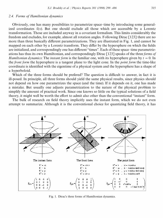
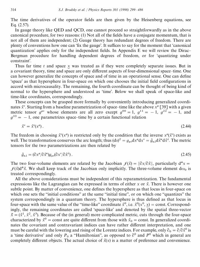
Fig. 1. Dirac’s three forms of Hamiltonian dynamics.

2.4. Forms of Hamiltonian dynamics

Obviously, one has many possibilities to parametrize space—time by introducing some general-ized coordinates xJ (x). But one should exclude all those which are accessible by a Lorentztransformation. Those are included anyway in a covariant formalism. This limits considerably thefreedom and excludes, for example, almost all rotation angles. Following Dirac [123] there are nomore than three basically different parametrizations. They are illustrated in Fig. 1, and cannot bemapped on each other by a Lorentz transform. They differ by the hypersphere on which the fieldsare initialized, and correspondingly one has different “times”. Each of these space—time parametriz-ations has thus its own Hamiltonian, and correspondingly Dirac [123] speaks of the three forms ofHamiltonian dynamics: The instant form is the familiar one, with its hypersphere given by t"0. Inthe front form the hypersphere is a tangent plane to the light cone. In the point form the time-likecoordinate is identified with the eigentime of a physical system and the hypersphere has a shape ofa hyperboloid.

Which of the three forms should be prefered? The question is difficult to answer, in fact it isill-posed. In principle, all three forms should yield the same physical results, since physics shouldnot depend on how one parametrizes the space (and the time). If it depends on it, one has madea mistake. But usually one adjusts parametrization to the nature of the physical problem tosimplify the amount of practical work. Since one knows so little on the typical solutions of a fieldtheory, it might well be worth the effort to admit also other than the conventional “instant” form.

The bulk of research on field theory implicitly uses the instant form, which we do not evenattempt to summarize. Although it is the conventional choice for quantizing field theory, it has


many practical disadvantages. For example, given the wavefunctions of an n-electron atom at aninitial time t"0, t

n(x

*, t"0), one can use the Hamiltonian H to evolve t

n(x

*, t) to later times t.

However, an experiment which specifies the initial wavefunction would require the simultaneousmeasurement of the positions of all of the bounded electrons. In contrast, determining the initialwavefunction at fixed light-cone time q"0 only requires an experiment which scatters oneplane-wave laser beam, since the signal reaching each of the n electrons, along the light front, at thesame light-cone time q"t

i#z

i/c.

A reasonable choice of xJ (x) is restricted by microcausality: a light signal emitted from any pointon the hypersphere must not cross the hypersphere. This holds for the instant or for the point form,but the front form seems to be in trouble. The light cone corresponds to light emitted from theorigin and touches the front form hypersphere at (x, y)"(0, 0). A signal carrying actually informa-tion moves with the group velocity always smaller than the phase velocity c. Thus, if noinformation is carried by the signal, points on the light cone are unable to communicate. Onlywhen solving problems in one-space and one-time dimension, the front form initializes fields onlyon the characteristic. Whether this generates problems for pathological cases like massless bosons(or fermions) is still under debate.

Comparatively little work is done in the point form [154,192,405]. Stech and collaborators [192]have investigated the free particle, by analyzing the Klein—Gordon and the Dirac equation. As itturns out, the orthonormal functions spanning the Hilbert space for these cases are rather difficultto work with. Their addition theorems are certainly more complicated than the simple plane-wavestates applicable in the instant or the front form.

The front form has a number of advantages which we will review in this article. Dirac’s legacyhad been forgotten and re-invented several times, thus the approach carries names as different asinfinite-momentum frame, null-plane quantization, light-cone quantization, or most unnecessarilylight-front quantization. In the essence these are the same.

The infinite-momentum frame first appeared in the work of Fubini and Furlan [153] inconnection with current algebra as the limit of a reference frame moving with almost the speed oflight. Weinberg [448] asked whether this limit might be more generally useful. He considered theinfinite-momentum limit of the old-fashioned perturbation diagrams for scalar meson theories andshowed that the vacuum structure of these theories simplified in this limit. Later Susskind[414,415] showed that the infinities which occur among the generators of the Poincare group whenthey are boosted to a fast-moving reference frame can be scaled or subtracted out consistently. Theresult is essentially a change of the variables. Susskind used the new variables to draw attention tothe (two-dimensional) Galilean subgroup of the Poincare group. He pointed out that the simplifiedvacuum structure and the non-relativistic kinematics of theories at infinite momentum might offerpotential-theoretic intuition in relativistic quantum mechanics. Bardakci and Halpern [16] furtheranalyzed the structure of the theories at infinite momentum. They viewed the infinite-momentumlimit as a change of variables from the laboratory time t and space coordinate z to a new “time”q"(t#z)/J2 and a new “space” f"(t!z)/J2. Chang and Ma [92] considered the Feynmandiagrams for a /3-theory and quantum electrodynamics from this point of view and where able todemonstrate the advantage of their approach in several illustrative calculations. Kogut and Soper[274] have examined the formal foundations of quantum electrodynamics in the infinite-mo-mentum frame, and interpret the infinite-momentum limit as the change of variables thus avoidinglimiting procedures. The time-ordered perturbation series of the S-matrix is due to them, see also


[40,41,406,274,275]. Drell et al. [130—133] have recognized that the formalism could serve as kindof natural tool for formulating the quark-parton model.

Independent of and almost simultaneous with the infinite-momentum frame is the work on nullplane quantization by Leutwyler [302,303], Klauder et al. [273], and by Rohrlich [390]. Inparticular, they have investigated the stability of the so-called “little group” among the Poincaregenerators [304—307]. Leutwyler recognized the utility of defining quark wavefunctions to give anunambiguous meaning to concepts used in the parton model.

The later developments using the infinite-momentum frame have displayed that the naming issomewhat unfortunate since the total momentum is finite and since the front form needs noparticular Lorentz frame. Rather it is frame-independent and covariant. ¸ight-Cone Quantizationseemed to be more appropriate. Casher [91] gave the first construction of the light-cone Hamil-tonian for non-Abelian gauge theory and gave an overview of important considerations inlight-cone quantization. Chang et al. [93—96] demonstrated the equivalence of light-cone quantiz-ation with standard covariant Feynman analysis. Brodsky et al. [53] calculated one-loop radiativecorrections and demonstrated renormalizability. Light-cone Fock methods were used by Lepageand Brodsky in the analysis of exclusive processes in QCD [297—300,62,345]. In all of this workthere was no citation of Dirac’s work. It did reappear first in the work of Pauli and Brodsky[354,355], who explicitly diagonalize a light-cone Hamiltonian by the method of discretizedlight-cone quantization, see also Section 4. Light-front quantization appeared first in the work ofHarindranath and Vary [203,204] adopting the above concepts without change. Frankeand collaborators [14,146—148,385], Karmanov [267,268], and Pervushin [369] have also doneimportant work on light-cone quantization. Comprehensive reviews can be found in[300,62,66,250,72,185,80].

2.5. Parametrizations of the front form

If one were free to parametrize the front form, one would choose it most naturally as a realrotation of the coordinate system, with an angle u"p/4. The “time-like” coordinate would then bex`"xJ 0 and the “space-like” coordinate x~"xJ 3, or collectively

Ax`

x~B"1

J2 A1 !1

1 1B Ax0

x3B , gab"A0 1

1 0B . (2.46)

The metric tensor gkl obviously transforms according to Eq. (2.45), and the Jacobian for thistransformation is unity.

But this has not what has been done, starting way back with Bardakci and Halpern [16] andcontinuing with Kogut and Soper [274]. Their definition corresponds to a rotation of thecoordinate system by u"!p/4 and an reflection of x~. The Kogut—Soper convention (KS) [274]is thus:

Ax`

x~B"1

J2 A1 1

1 !1B Ax0

x3B , gab"A0 1

1 0B . (2.47)

see also Appendix C. It is often convenient to distinguish longitudinal Lorentz indices a orb (#,!) from the transversal ones i or j (1,2), and to introduce transversal vectors by


xM"(x1, x2). The KS-convention is particularly suited for theoretical work, since the raising and

lowering of the Lorentz indices is simple. With the totally antisymmetric symbol

e``12

"1 , thus e`12~

"1 , (2.48)

the volume integral becomes

Pdu`"Pdx~ d2x

M"Pdx

`d2x

M. (2.49)

One should emphasize that `"~ is a time-like derivative /x`"/x

~as opposed to

~"`, which is a space-like derivative /x~"/x

`. Correspondingly, P

`"P~ is the

Hamiltonian which propagates in the light-cone time x`, while P~"P` is the longitudinal

space-like momentum.In much of the practical work, however, one is bothered with the J2’s scattered all over the

place. At the expense of having various factors of 2, this is avoided in the Lepage—Brodsky (LB)convention [299]:

Ax`

x~B"A1 1

1 !1BAx0

x3B thus gab"A0 2

2 0B , gab"A0 1

212

0B , (2.50)

see also Appendix B. Here, `"1

2~ is a time-like and

~"1

2` a space-like derivative. The

Hamiltonian is P`"1

2P~, and P

~"1

2P` is the longitudinal momentum. With the totally

antisymmetric symbol

e``12

"1 e`12~

"12

, (2.51)

the volume integral becomes

Pdu`"

12Pdx~d2x

M"Pdx

`d2x

M. (2.52)

We will use both the LB-convention and the KS-convention in this review, and indicate in eachsection which convention we are using.

The transition from the instant form to the front form is quite simple: In all the equations foundin Sections 2.1 and 2.2 one has to substitute the “0” by the “#” and the “3” by the “!”. Take asan example the QED four-momentum in Eq. (2.27) to get

Pl"PX

du0AF0iFil#

14g0lFijFij#

12[iWM c0DlW#h.c.]B ,

(2.53)

Pl"PX

du`AF`iFil#

14g`l FijFij#

12[iWM c`DlW#h.c.]B ,

also in KS-convention. The instant and the front form look thus almost identical. However,after having worked out the Lorentz algebra, the expressions for the instant and front-form


Hamiltonians are drastically different:

P0"

12PX

du0(E2#B2)#

12PX

du0[iWM c`D

0W#h.c.] ,

(2.54)

P`"

12PX

du`

(E2,#B2

,)#

12PX

du`

[iWM c`D`W#h.c.] ,

for the instant and the front-form energy, respectively. In the former one has to deal with all threecomponents of the electric and the magnetic field, in the latter only with two of them, namelywith the longitudinal components E

,"1

2F`~"E

zand B

,"F12"B

z. Correspondingly,

energy—momentum for non-abelian gauge theory is

Pl"PX

du0(F0i

aFail#1

4g0lFij

aFaij#1

2[iWM c0¹aDalW#h.c.]) ,

(2.55)

Pl"PX

du`(F`i

aFail#1

4g`l Fij

aFaij#1

2[iWM c`¹aDalW#h.c.]) .

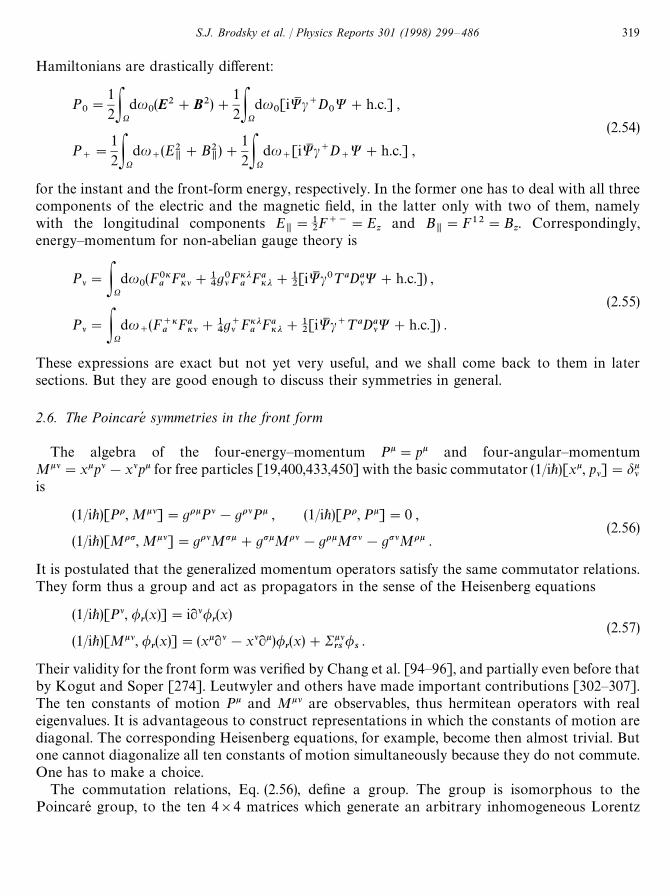
These expressions are exact but not yet very useful, and we shall come back to them in latersections. But they are good enough to discuss their symmetries in general.

2.6. The Poincare symmetries in the front form

The algebra of the four-energy—momentum Pk"pk and four-angular—momentumMkl"xkpl!xlpk for free particles [19,400,433,450] with the basic commutator (1/i+)[xk, pl]"dklis

(1/i+)[Po, Mkl]"gokPl!golPk , (1/i+)[Po, Pk]"0 ,(2.56)

(1/i+)[Mop, Mkl]"golMpk#gpkMol!gokMpl!gplMok .

It is postulated that the generalized momentum operators satisfy the same commutator relations.They form thus a group and act as propagators in the sense of the Heisenberg equations

(1/i+)[Pl, /r(x)]"il/

r(x)

(2.57)(1/i+)[Mkl, /

r(x)]"(xkl!xlk)/

r(x)#Rkl

rs/

s.

Their validity for the front form was verified by Chang et al. [94—96], and partially even before thatby Kogut and Soper [274]. Leutwyler and others have made important contributions [302—307].The ten constants of motion Pk and Mkl are observables, thus hermitean operators with realeigenvalues. It is advantageous to construct representations in which the constants of motion arediagonal. The corresponding Heisenberg equations, for example, become then almost trivial. Butone cannot diagonalize all ten constants of motion simultaneously because they do not commute.One has to make a choice.

The commutation relations, Eq. (2.56), define a group. The group is isomorphous to thePoincare group, to the ten 4]4 matrices which generate an arbitrary inhomogeneous Lorentz


transformation. The question of how many and which operators can be diagonalized simulta-neously turns out to be identical to the problem of classifying all irreducible unitary transforma-tions of the Poincare group. According to Dirac [123] one cannot find more than seven mutuallycommuting operators.

It is convenient to discuss the structure of the Poincare group [400,433] in terms of thePauli—Lubansky vector »i,eijklPjMkl, with eijkl being the totally antisymmetric symbol in4 dimensions. » is orthogonal to the generalized momenta, Pk»k"0, and obeys the algebra

(1/i+)[»i, Pk]"0 , (1/i+)[»i, Mkl]"gil»k!gik»l , (1/i+)[»i, »j]"eijkl»kPl . (2.58)

The two group invariants are the operator for the invariant mass-squared M2"PkPk and theoperator for intrinsic spin-squared »2"»k»k. They are Lorentz scalars and commute with allgenerators Pk and Mkl, as well as with all »k. A convenient choice of the six mutually commutingoperators is therefore for the front form:

(1) the invariant mass squared, M2"PkPk,(2—4) the three space-like momenta, P` and P

M,

(5) the total spin squared, S2"»k»k,(6) one component of », say »`, called S

z.

There are other equivalent choices. In constructing a representation which diagonalizes simulta-neously the six mutually commuting operators one can proceed consecutively, in principle, bydiagonalizing one after the other. At the end, one will have realized the old dream of Wigner [450]and of Dirac [123] to classify physical systems with the quantum numbers of the irreduciblerepresentations of the Poincare group.

Inspecting the definition of boost-angular-momentum Mkl in Eq. (2.18) one identifies whichcomponents are dependent on the interaction and which are not. Dirac [123,126] calls themcomplicated and simple, or dynamic and kinematic, or Hamiltonians and momenta, respectively.In the instant form, the three components of the boost vector K

i"M

i0are dynamic, and the three

components of angular momentum J*"e

ijkM

jkare kinematic. The cyclic symbol e

ijkis 1, if the

space-like indices ijk are in cyclic order, and zero otherwise.As noted already by Dirac [123], the front form is special in having four kinematic components

of Mkl (M`~

, M12

, M1~

, M2~

) and only two dynamic ones (M`1

and M`2

). One checks thisdirectly from the defining equation (2.18). Kogut and Soper [274] discuss and interpret them interms of the above boosts and angular momenta. They introduce the transversal vector B

Mwith

components

BM1

"M`1

"(1/J2)(K1#J

2) , B

M2"M

`2"(1/J2)(K

2!J

1) . (2.59)

In the front form they are kinematic and boost the system in x- and y-direction, respectively. Thekinematic operators

M12"J

3, M

`~"K

3(2.60)

rotate the system in the x—y plane and boost it in the longitudinal direction, respectively. In thefront form one deals thus with seven mutually commuting operators [123]

M`~

, BM

and all Pk , (2.61)


instead of the six in the instant form. The remaining two Poincare generators are combined intoa transversal angular—momentum vector S

Mwith

SM1

"M1~

"(1/J2)(K1!J

2) , S

M2"M

2~"(1/J2)(K

2#J

1) . (2.62)

They are both dynamical, but commute with each other and M2. They are thus members ofa dynamical subgroup [274], whose relevance has yet to be exploited.

Thus, one can diagonalize the light-cone energy P~ within a Fock basis where the constituentshave fixed total P` and P

M. For convenience, we shall define a “light-cone Hamiltonian” as the

operator

HLC"PkPk"P~P`!P2

M, (2.63)

so that its eigenvalues correspond to the invariant mass spectrum Miof the theory. The boost

invariance of the eigensolutions of HLC

reflects the fact that the boost operators K3

and BM

arekinematical. In fact, one can boost the system to an “intrinsic frame” in which the transversalmomentum vanishes

PM"0 thus H

LC"P~P` . (2.64)

In this frame, the longitudinal component of the Pauli—Lubansky vector reduces to the longitudi-nal angular momentum J

3" J

z, which allows for considerable reduction of the numerical work

[429]. The transformation to an arbitrary frame with finite values of PM

is then trivially performed.The above symmetries imply the very important aspect of the front form that both the

Hamiltonian and all amplitudes obtained in light-cone perturbation theory (graph by graph!) aremanifestly invariant under a large class of Lorentz transformations:

(1) boosts along the 3-direction: and p`PC,p`, p

MPp

M,

pMp~PC~1

,p~

(2) transverse boosts: p`Pp`, pMPp

M#p`C

M,

p~Pp~#2pM)C

M#p`C2

M(3) rotations in the x—y plane: p`Pp`, p2

MPp2

M.

All of these hold for every single-particle momentum pk, and for any set of dimensionlessc-numbers C

,and C

M. It is these invariances which also lead to the frame independence of the Fock

state wave functions.If a theory is rotational invariant, then each eigenstate of the Hamiltonian which describes

a state of non-zero mass can be classified in its rest frame by its spin eigenvalues

J2DP0"M, P"0T"s(s#1)DP0"M, P"0T ,(2.65)

JzDP0"M, P"0T"s

zDP0"M, P"0T .

This procedure is more complicated in the front form since the angular momentum operator doesnot commute with the invariant mass-squared operator M2. Nevertheless, Hornbostel [228—230]constructs light-cone operators

J2"J23#J2

M, with J

3"J

3#e

ijB

MiPMj

/P`,(2.66)

JMk"(1/M)e

kl(S

MlP`!BMlP~!K

3P

Ml#J3elmPMm

) ,


which, in principle, could be applied to an eigenstate DP`, PMT to obtain the rest frame spin

quantum numbers. This is straightforward for J3since it is kinematical; in fact,J

3"J

3in a frame

with PM"0

M. However, J

Mis dynamical and depends on the interactions. Thus, it is generally

difficult to explicitly compute the total spin of a state using light-cone quantization. Some of theaspects have been discussed by Coester [106] and collaborators [105,102]. A practical and simpleway has been applied by Trittmann [429]. Diagonalizing the light-cone Hamiltonian in theintrinsic frame for J

zO0, he can ask for J

.!9, the maximum eigenvalue of J

zwithin a numerically

degenerate multiplet of mass-squared eigenvalues. The total ‘spin J’ is then determined byJ"2J

.!9#1, as to be discussed in Section 4. But more work on this question is certainly

necessary, as well as on the discrete symmetries like parity and time reversal and their quantumnumbers for a particular state, see also Hornbostel [228—230]. One needs the appropriate languagefor dealing with spin in highly relativistic systems.

2.7. The equations of motion and the energy—momentum tensor

Energy—momentum for gauge theory had been given in Eq. (2.55). They contain time derivativesof the fields which can be eliminated using the equations of motion.

¹he color-Maxwell equations are given in Eq. (2.33). They are four (sets of) equations fordetermining the four (sets of) functions Ak

a. One of the equations of motion is removed by fixing the

gauge and we choose the light-cone gauge [22]

A`a"0 . (2.67)

Two of the equations of motion express the time derivatives of the two transversal componentsAaM

in terms of the other fields. Since the front-form momenta in Eq. (2.55) do not depend on them,we discard them here. The fourth is the analogue of the Coulomb equation or of the Gauss’ law inthe instant form, particularly kFk`

a"gJ`

a. In the light-cone gauge the color-Maxwell charge

density J`a

is independent of the vector potentials, and the Coulomb equation reduces to

!`—A~a!`

iAi

Ma"gJ`

a. (2.68)

This equation involves only (light-cone) space derivatives. Therefore, it can be satisfied only, if oneof the components is a functional of the others. There are subtleties involved in actually doing this,in particular one has to cope with the ‘zero mode problem’, see for example [358]. Disregardingthis here, one inverts the equation by

Aa`"AI a

`#(g/(i`)2)J`

a. (2.69)

For the free case (g"0), A~ reduces to AI ~. Following Lepage and Brodsky [299], one can collectall components which survive the limit gP0 into the ‘free solution’ AI k

a, defined by

AI a`"!(1/`)

iAi

Ma, thus AI k

a"(0, A

Ma, AI `

a) . (2.70)

Its four-divergence vanishes by construction and the Lorentz condition kAI ka"0 is satisfied as anoperator. As a consequence, AI k

ais purely transverse. The inverse space derivatives (i`)~1 and

(i`)~2 are actually Green’s functions. Since they depend only on x~, they are comparativelysimple, much simpler than in the instant form where (e2)~1 depends on all three space-likecoordinates.


¹he color-Dirac equations are defined in Eq. (2.35) and are used here to express the timederivatives

`W as function of the other fields. After multiplication with b"c0 they read explicitly

(ic0c`¹aDa`#ic0c~¹aDa

~#iai

M¹aDa

Mi)W"mbW , (2.71)

with the usual ak"c0ck, k"1,2,3. In order to isolate the time derivative one introduces theprojectors K

B"KB and projected spinors W

B"WB by

KB"1

2(1$a3) , W

B"K

BW . (2.72)

Note that the raising or lowering of the projector labels $ is irrelevant. The c0cB are obviouslyrelated to the KB, but differently in the KS- and LB-convention

c0cB"2KBLB"J2KB

KS. (2.73)

Multiplying the color-Dirac equation once with K` and once with K~, one obtains a coupled set ofspinor equations

2i`

W`"(mb!iai

M¹aDa

Mi)W

~#2gAa

`¹aW

`,

(2.74)2i

~W

~"(mb!iai

M¹aDa

Mi)W

`#2gAa

~¹aW

~.

Only the first of them involves a time derivative. The second is a constraint, similar to the above inthe Coulomb equation. With the same proviso in mind, one defines

W~"(1/2i

~)(mb!iai

M¹aDa

Mi)W

`. (2.75)

Substituting this into the former, the time derivative is

2i`

W`"2gAa

`¹aW

`#(mb!iaj

M¹aDa

Mj)(1/2i

~)(mb!iai

M¹aDa

Mi)W

`. (2.76)

Finally, in analogy to the color-Maxwell case, one can conveniently introduce the free spinorsWI "WI

`#WI

~by

WI "W`#(mb!iai

Mi)(1/2i

~)W

`. (2.77)

Contrary to the full spinor see, for example, Eq. (2.75), WI is independent of the interaction. To getthe corresponding relations for the KS-convention, one substitutes the “2” by “J2” in accord withEq. (2.73).

The front-form Hamiltonian according to Eq. (2.55) is

P`"PX

duÀFìFi`#

14Fij

aFaij#

12[iWM c`¹aDa

`W#h.c.]B . (2.78)

Expressing it as a functional of the fields will finally lead to Eq. (2.89) below, but despite thestraightforward calculation we display explicitly the intermediate steps. Consider first the energydensity of the color-electro-magnetic fields 1

4FijFij#FìFi`. Conveniently defining the abbrevi-

ations

Bkla"f abcAk

bAl

c, sk

a"f abckAl

bAcl , (2.79)


the field tensors in Eq. (2.31) are rewritten as Fkla"kAl

a!lAk

a!gBkl

aand typical tensor

contractions become

12Fkl

aFakl"kAl

akAal!kAl

alAak#2sk

aAak#1

2g2Bkl

aBakl . (2.80)

Using FaiFai"2FìFì, the color-electro-magnetic energy density

14FijFij#FìFi`"1

4FijFij!1

2FiaFia"1

4FiiFii!1

4FiaFia"1

4FijF

ij!1

4FabFab (2.81)

separates completely into a longitudinal (a, b) and a transversal contribution (i, j) [358]; see alsoEq. (2.54). Substituting A

`by Eq. (2.69), the color-electric and color-magnetic parts become

14FabFba"1

2À

`À

`"1

2g2J`(1/(i`)2)J`#1

2(

iAi

M)2#gJÀI

`,

(2.82)14FijF

ij"1

4g2BijB

ij!1

2(

iAi

M)2#siA

i#1

2Aj(i

i)A

j,

respectively. The role of the different terms will be discussed below. The color-quark energy densityis evaluated in the LB-convention. With iWM c`Da

`¹aW"iWsc0c`Da

`¹aW and the projectors of

Eq. (2.72) one gets first iWM c`Da`¹aW"iJ2Ws

`Da

`¹aW

`. Direct substitution of the time deriva-

tives in Eq. (2.76) then gives

iWM c`Da`¹aW"WI s

`(mb!iaj

MDa

Mj¹a)(1/J2i

~) (mb!iai

MDb

Mi¹b)W

`. (2.83)

Isolating the interaction in the covariant derivatives i¹aDak"ik!g¹aAak produces

iWM c`Da`¹aW"gWI s

àjMAa

Mj¹aWI

~#gWI s

~ajMAa

Mj¹aWI

`

#(g2/J2)Ws`

ajMAa

Mj¹a

1i

~

aiMAb

Mi¹bW

`

#(1/J2)Ws`(mb!iaj

MMj

) (1/i~

) (mb!iaiMMi

)W`

. (2.84)

Introducing jI ka

as the color-fermion part of the total current JI ka, that is

jI la(x)"WIM cl¹aWI with JI l

a(x)"jI l

a(x)#sJ l

a(x) , (2.85)

one notes that Jà"JI `

awhen comparing with the defining equation (2.77). For the transversal

parts holds obviously

jI iMa"WI sai

M¹aWI "WI s

àiM¹aWI

~#WI s

~aiM¹aWI

`. (2.86)

With c`c`"0 one finds

WIM ckAI kc`clAI lWI "WIM ciMAI

Mic`ci

MAI

MiWI "WI sai

MAI

Mic`c0aj

MAI

MjWI

"J2WI s`

aiMAI

MiaiMAI

MiWI

`, (2.87)

see also [300]. The covariant time derivative of the dynamic spinors Wa is therefore

iWM c`Da`¹aW"gjI i

MAI

Mi#1

2g2WIM ckAI k(c`/i`)clAI lWI #1

2WIM c`((m2!+ 2

M)/i`)WI (2.88)


in terms of the fields AI k and WI a. One finds the same expression in LB-convention. Since it isa hermitean operator, one can add Eqs. (2.82) and (2.88) to finally get the front-form Hamiltonianas a sum of five terms,

P`"

12Pdx

`d2x

MAWI M c`m2#(i+

M)2

i`WI #AI k

a(i+

M)2AI akB#gPdx

`d2x

MJI kaAI ak

#

g2

4 Pdx`

d2xM

BI kla

BI akl#g2

2 Pdx`d2x

MJI à

1(i`)2

JI à

#

g2

2 Pdx`

d2xM

WIM ck¹aAI akcì`

(cl¹bAI blWI ) . (2.89)

Only the first term survives the limit gP0, hence P~PPI ~, referred to as the free part of theHamiltonian. For completeness, the space-like components of energy—momentum as given inEq. (2.55) become

Pk"Pdx

`d2x

M(FìFik#iWM c`¹aDa

kW)

"Pdx`

d2xM(WIM cì

kWI #AI k

a`

kAI ak) for k"1, 2,! . (2.90)

Inserting the free solutions as given below in Eq. (2.100), one gets for PI k"(P`, PM, PI ~)

PI k" +j,c,f Pdp`d2p

Mpk(aJ s(q)aJ (q)#bI s(q)bI (q)#dI s(q)dI (q)) , (2.91)

in line with expectation: In momentum representation the momenta PI k are diagonal operators.Terms depending on the coupling constant are interactions and in general are non-diagonaloperators in Fock space.

Eqs. (2.89) and (2.90) are quite generally applicable:

f They hold both in the Kogut—Soper and Lepage—Brodsky convention.f They hold for arbitrary non-abelian gauge theory SU(N).f They hold therefore also for QCD (N"3) and are manifestly invariant under color rotations.f They hold for abelian gauge theory (QED), formally by replacing the color matrices¹a

c,c{with the

unit matrix and by setting to zero the structure constants f abc, thus Bkl"0 and sk"0.f They hold for 1 time dimension and arbitrary d#1 space dimensions, with i"1,2,d. Only

what has to be adjusted is the volume integral :dx`

d2xM.

f They thus hold also for the popular toy models in 1#1 dimensions.f Last but not least, they hold for the ‘dimensionally reduced models’ of gauge theory, formally by

setting the transversal derivatives of the free fields to zero, that is ³MWI a"0 and ³

MAI k"0.

Most remarkable, however, is that the relativistic Hamiltonian in Eq. (2.89) is additive [274] in the“kinetic” and the “potential” energy, very much like a non-relativistic Hamiltonian

H"¹#º . (2.92)


In this respect, the front form is distinctly different from the conventional instant form. WithH,P

`the kinetic energy

¹"PI`"

12Pdx

`d2x

MAWIM c`m2#(i+

M)2

i`WI #AI k

a(i+

M)2AI akB (2.93)

is the only term surviving the limit gP0 in Eq. (2.89). The potential energy º is correspondinglythe sum of the four terms

º"»#¼1#¼

2#¼

3. (2.94)

Each of them has a different origin and interpretation. The vertex interaction

»"gPdx`

d2xM

JI kaAI ak (2.95)

is the light-cone analogue of the JkAk-structures known from covariant theories, particularlyelectrodynamics. It generates three-point vertices describing bremsstrahlung and pair creation.However, since JI k contains also the pure gluon part sJ k, it includes the three-point-gluon vertices aswell. The four-point-gluon interactions

¼1"

g2

2 Pdx`

d2xM

BI kla

BI akl (2.96)

describe the four-point-gluon vertices. They are typical for non-abelian gauge theory and comeonly from the color-magnetic fields in Eq. (2.82). The instantaneous—gluon interaction

¼2"

g2

2 Pdx`

d2xM

JI à

1(i`)2

JI à

(2.97)

is the light-cone analogue of the Coulomb energy, having the same structure (density-propagator-density) and the same origin, namely Gauss’ equation (2.69). ¼

3describes quark—quark,

gluon—gluon, and quark—gluon instantaneous-gluon interactions. The last term, finally, is theinstantaneous-fermion interaction

¼3"

g2

2 Pdx`

d2xMWI M ck¹aAI ak

cì`

(cl¹bAI blWI ) . (2.98)

It originates from the light-cone specific decomposition of Dirac’s equation (2.74) and has nocounterpart in conventional theories. The present formalism is however more symmetric: Theinstantaneous gluons and the instantaneous fermions are partners. This has some interestingconsequences, as we shall see below. Actually, the instantaneous interactions were seen first byKogut and Soper [274] in the time-dependent analysis of the scattering amplitude as remnants ofchoosing the light-cone gauge.

One should carefully distinguish the above front-form Hamiltonian H from the light-coneHamiltonian H

LC, defined in Eqs. (2.63) and (2.64) as the operator of invariant mass-squared. The

former is the time-like component of a four-vector and therefore frame-dependent. The latter isa Lorentz scalar and therefore independent of the frame. The former is covariant, the latterinvariant under Lorentz transformations, particularly under boosts. The two are related to each


other by multiplying H with a number, the eigenvalue of 2P`:

HLC"2P`H . (2.99)

The above discussion and interpretation of H applies therefore also to HLC

. Note that matrixelements of the “Hamiltonian” have the dimension SenergyT2.

2.8. The interactions as operators acting in Fock space

In Section 2.7 the energy—momentum four-vector Pk was expressed in terms of the free fields.One inserts them into the expressions for the interactions and integrates over configuration space.The free fields are

WI acf(x)"+j P

dp`d2pM

J2p`(2p)3(bI (q)ua(p, j)e~*px#dI s(q)va(p, j)e`*px) ,

(2.100)

AI ak(x)"+j P

dp`d2pM

J2p`(2p)3(aJ (q)ek(p, j)e~*px#aJ s(q)e*k (p, j)e`*px) ,

where the properties of the ua, va and ek are given in the appendices and where

[aJ (q), aJ s(q@)]"MbI (q), bI s(q@)N"MdI (q), dI s(q@)N"d(p`!p`@)d(2)(pM!p@

M)dj@j dc@

cdf@f

. (2.101)

Doing that in detail is quite laborious. We therefore restrict ourselves here to a few instructiveexamples, the vertex interaction », the instantaneous-gluon interaction ¼

2and the instan-

taneous-fermion interaction ¼3.

According to Eq. (2.95) the fermionic contribution to the vertex interaction is

»f"gPdx

`d2x

MjI kaAI ak"gPdx

`d2x

MWIM (x)ck¹aWI (x)AI ak(x)K

x`/0

"

g

J(2p)3+

j1,j2,j3

+c1,c2,a3

Pdp`

1d2p

M1J2p`

1Pdp`

2d2p

M2J2p`

2Pdp`

3d2p

M3J2p`

3Pdx

`d2x

M(2p)3

[(bI s(q1)uN a(p1

, j1)e`*p1x

#dI (q1)vN a(p1

, j1)e~*p1x)¹a3

c1,c2ckab(dI s(q2)vb(p2

, j2)e`*p2x#bI (q

2)ub(p2, j2)e~*p2x)]

](aJ s(q3)e*k (p

3, j

3)e`*p3x#aJ (q

3)ek(p3

, j3)e~*p3x) . (2.102)

The integration over configuration space produces essentially Dirac delta—functions in the singleparticle momenta, which reflect momentum conservation:

Pdx

`2p

e*x`(+jp`j)"dA+

j

p`j B , P

d2xM

(2p)3e~*xM(+jpMj)"d(2)A+

j

pMjB . (2.103)

Note that the sum of these single-particle momenta is essentially the sum of the particle momentaminus the sum of the hole momenta. Consequently, if a particular term has only creation or onlydestruction operators as in

bs(q1)ds(q

2)as(q

3)d(p`

1#p`

2#p`

3)K0 ,


its contribution vanishes since the light-cone longitudinal momenta p` are all positive and cannotadd to zero. The case that they are exactly equal to zero is excluded by the regularizationprocedures discussed below in Section 4. As a consequence, all energy diagrams which generate thevacuum fluctuations in the usual formulation of quantum field theory are absent from the outset inthe front form.

The purely fermionic part of the instantaneous-gluon interaction given by Eq. (2.97) becomes,respectively,

¼2,f

"

g2

2 Pdx`

d2xM

jIà

1(i`)2

jIà"

g2

2 Pdx`

d2xM

WIM (x)c`¹aWI (x)1

(i`)2WIM (x)c`¹aWI (x)D

x`/0.

¼2,f

"

g2

2(2p)3+jj

+c1,c2,c3,c4

Pdp`

1d2p

M1J2p`

1Pdp`

2d2p

M2J2p`

2Pdp`

3d2p

M3J2p`

3Pdp`

4d2p

M4J2p`

4

]Pdx

`d2x

M(2p)3

[(bI s(q1)uN a(p1,j1)e`*p1x#dI (q

1)vN a(p1, j1)e~*p1x)¹a

c1,c2

]càb(dI s(q2)va(p2,j2)e`*p2x#bI (q2)ua(p2

, j2)e~*p2x)]

]1

(i`)2[(bI s(q

3)uN a(p3, j3)e`*p3x#dI (q

3)vN a(p3,j3

)e~*p3x)¹ac3,c4

]càb(dI s(q4)vb(p4, j4)e`*p4x#bI (q

4)ub(p4

, j4)e~*p4x)] . (2.104)

By the same reason as discussed above, there will be no contributions from terms with onlycreation or only destruction operators. The instantaneous-fermion interaction, finally, becomesaccording to Eq. (2.98),

¼3"

g2

2 Pdx`

d2xM

WI M ck¹aAI akcìL`

(cv¹bAI bvWI )

"

g2

2(2p)3+jj

+c1,a2,a3,c4

Pdp`

1d2p

M1J2p`

1Pdp`

2d2p

M2J2p`

2Pdp`

3d2p

M3J2p`

3Pdp`

4d2p

M4J2p`

4

]Pdx

`d2x

M(2p)3

[(bI s(q1)uN (p

1, j

1)e`*p1x#dI (q

1)vN (p

1, j

1)e~*p1x)¹a2

c1,c

]ck(aJ s(q2)e*k (p2

, j2)e`*p2x#aJ (q

2)ek(p2

, j2)e~*p2x)

]1

i`(aJ s(q

3)e*l (p3, j3)e`*p3x#aJ (q

3)el(p3, j3)e~*p3x)¹a3

c,c4

]cl(dI s(q4)v(p

4, j

4)e`*p4x#bI (q

4)u(p

4, j

4)e~*p4x)] . (2.105)

Each of the instantaneous interactions types has primarily 24!2"14 individual contributions,which will not be enumerated in all detail. In Section 4 complete tables of all interactions will betabulated in their final normal ordered form, that is with all creation operators are to the left of thedestruction operators. All instantaneous interactions like those shown above are four-pointinteractions and the creation and destruction operators appear in a natural order. According toWick’s theorem this “time-ordered” product equals to the normal ordered product plus the sum of


all possible pairwise contractions. The fully contracted interactions are simple c-numbers whichcan be omitted due to vacuum renormalization. The one-pair contracted operators, however,cannot be thrown away and typically have a structure like

I(q)bI s(q)bI (q) . (2.106)

Due to the properties of the spinors and polarization functions ua, va and ek they become diagonaloperators in momentum space. The coefficients I(q) are kind of mass terms and have been labeledas “self-induced inertias” [354]. Even if they formally diverge, they are part of the operatorstructure of field theory, and therefore should not be discarded but need careful regularization. InSection 4 they will be tabulated as well.

3. Bound states on the light cone

In principle, the problem of computing for quantum chromodynamics the spectrum and thecorresponding wavefunctions can be reduced to diagonalizing the light-cone Hamiltonian. Anyhadronic state must be an eigenstate of the light-cone Hamiltonian, thus a bound state of mass M,which satisfies (M2!H

LC)DMT"0. Projecting the Hamiltonian eigenvalue equation onto the

various Fock states SqqN D, SqqN gD2 results in an infinite number of coupled integral eigenvalueequations. Solving these equations is equivalent to solving the field theory. The light-cone Fockbasis is a very physical tool for discussing these theories because the vacuum state is simple and thewavefunctions can be written in terms of relative coordinates which are frame-independent. Interms of the Fock-space wavefunction, one can give exact expressions for the form factors andstructure functions of physical states. As an example we evaluate these expressions with a pertur-bative wavefunction for the electron and calculate the anomalous magnetic moment of the electron.

In order to lay down the groundwork for upcoming non-perturbative studies, it is indispensableto gain control over the perturbative treatment. We devote therefore a section to the perturbativetreatment of quantum electrodynamics and gauge theory on the light cone. Light-cone perturba-tion theory is really Hamiltonian perturbation theory, and we give the complete set of rules whichare the analogues of the Feynman rules. We shall demonstrate in a selected example, that one getsthe same covariant and gauge-invariant scattering amplitude as in Feynman theory. We also shalldiscuss one-loop renormalization of QED in the Hamiltonian formalism.

Quantization is done in the light-cone gauge, and the light-cone time-ordered perturbationtheory is developed in the null-plane Hamiltonian formalism. For gauge-invariant quantities, thisis very loosely equivalent to the use of Feynman diagrams together with an integration over p~ byresidues [426,427]. The one-loop renormalization of QED quantized on the null plane looks verydifferent from the standard treatment. In addition to not being manifestly covariant, x`-orderedperturbation theory is fraught with singularities, even at tree level. The origin of these unusual,“spurious”, infrared divergences is not a mystery. Consider, for example, a free particle whosetransverse momentum p

M" (p1, p2) is fixed, and whose third component p3 is cut at some

momentum K. Using the mass-shell relation, p~"(m2#p2M)/2p`, one sees that p` has a lower

bound proportional to K~1. Hence, the light-cone spurious infrared divergences are simplya manifestation of space—time ultraviolet divergences. A great deal of work is continuing on how totreat these divergences in a self-consistent manner [456]. Bona fide infrared divergences are of


course also present, and can be taken care of as usual by giving the photon a small mass, consistentwith light-cone quantization [406].

As a matter of practical experience, and quite opposed to the instant form of the Hamiltonianapproach, one gets reasonable results even if the infinite number of integral is equations truncated.The Schwinger model is particularly illustrative because in the instant form this bound state hasa very complicated structure in terms of Fock states while in the front form the bound state consistsof a single electron—positron pair. One might hope that a similar simplification occurs in QCD. TheYukawa model is treated here in Tamm—Dancoff truncation in 3#1 dimensions [182,373,374].This model is particularly important because it features a number of the renormalization problemsinherent to the front form, and it motivates the approach of Wilson to be discussed later.

3.1. The hadronic eigenvalue problem

The first step is to find a language in which one can represent hadrons in terms of relativisticconfined quarks and gluons. The Bethe—Salpeter formalism [37,312] has been the central methodfor analyzing hydrogenic atoms in QED, providing a completely covariant procedure for obtainingbound-state solutions. However, calculations using this method are extremely complex and appearto be intractable much beyond the ladder approximation. It also appears impractical to extend thismethod to systems with more than a few constituent particles. A review can be found in Ref. [312].

An intuitive approach for solving relativistic bound-state problems would be to solve theHamiltonian eigenvalue problem

HDWT"JM2#P2DWT (3.1)

for the particle’s mass, M, and wavefunction, DWT. Here, one imagines that DWT is an expansion inmulti-particle occupation number Fock states, and that the operators H and P are second-quantized Heisenberg operators. Unfortunately, this method, as described by Tamm and Dancoff[117,421], is complicated by its non-covariant structure and the necessity to first understand itscomplicated vacuum eigensolution over all space and time. The presence of the square-rootoperator also presents severe mathematical difficulties. Even if these problems could be solved, theeigensolution is only determined in its rest system (P"0); determining the boosted wavefunction isas complicated as diagonalizing H itself.

In principle, the front-form approach works in the same way. One aims at solving the Hamil-tonian eigenvalue problem

HDWT"M2#P2

M2P`

DWT , (3.2)

which for several reasons is easier: Contrary to Pzthe operator P` is positive, having only positive

eigenvalues. The square-root operator is absent, and the boost operators are kinematic, seeSection 2.6. As discussed there, in both the instant and the front form, the eigenfunctions can belabeled with six numbers, the six eigenvalues of the invariant mass M, of the three space-likemomenta P`, P

M, and of the generalized total spin-squared S2 and its longitudinal projection S

z,

that is

DWT"DW; M, P`, PM, S2, S

z; hT . (3.3)


In addition, the eigenfunction is labeled by quantum numbers like charge, parity, or baryonnumber which specify a particular hadron h. The ket DWT can be calculated in terms of a completeset of functions DkT or Dk

nT,

Pd[k] DkT SkD"+nPd[k

n] Dk

nT Sk

nD"1 . (3.4)

The transformation between the complete set of eigenstates DWT and the complete set of basis statesDk

nT are then Sk

nDWT. The projections of DWT on Dk

nT are usually called the wavefunctions

Wn@h(M,P`,PM,S2,Sz)

(k),SknDWT . (3.5)

Since the values of (M, P`, PM, S2, S

z) are obvious in the context of a concrete case, we convene to

drop reference to them and write simply

DWT"+nPd[k

n] Dk

nTW

n@h(k),+

nPd[k

n] Dk

nT Sk

nDW; M, P` P

M, S2, S

z; hT . (3.6)

One constructs the complete basis of Fock states DknT in the usual way by applying products of

free-field creation operators to the vacuum state D0T:

n"0: D0T,

n"1: DqqN : kì, k

Mi, j

iT " bs(q

1)ds(q

2) D0T,

n"2: DqqN g: kì, k

Mi, j

iT " bs(q

1)ds(q

2)as(q

3) D0T,

n"3: Dgg: kì, k

Mi, j

iT " as(q

1)as(q

2) D0T,

F F F F D0T .

(3.7)

The operators bs(q), ds(q) and as(q) create bare leptons (electrons or quarks), bare antileptons(positrons or antiquarks) and bare vector bosons (photons or gluons). In the above notation, oneexplicitly keeps track of only the three continuous momenta k`

iand k

Miand of the discrete helicities

ji. The various Fock-space classes are conveniently labeled with a running index n. Each Fock state

DknT"Dn : k`

i, k

Mi, j

iT is an eigenstate of P` and P

M. The eigenvalues are

PM"+

ion

kMi

, P`"+ion

kì

with kì'0 . (3.8)

The vacuum has eigenvalue 0, i.e. PMD0T"0 and P`D0T"0.

The restriction k`'0 for massive quanta is a key difference between light-cone quantizationand ordinary equal-time quantization. In equal-time quantization, the state of a parton is specifiedby its ordinary three-momentum k"(k

x, k

y, k

z). Since each component of k can be either positive

or negative, there exist zero total momentum Fock states of arbitrary particle number, and thesewill mix with the zero-particle state to build up the ground state, the physical vacuum. However, inlight-cone quantization each of the particles forming a zero-momentum state must have vanish-ingly small k`. The free or Fock-space vacuum D0T is then an exact eigenstate of the full front-formHamiltonian H, in stark contrast to the quantization at equal usual time. However, as we shall seelater, the vacuum in QCD is undoubtedly more complicated due to the possibility of color-singlet


states with P`"0 built on zero-mode massless gluon quanta [189], but as discussed in Section 7,the physical vacuum is still far simpler than is usual.

Since k`i'0 and P`'0, one can define boost-invariant longitudinal momentum fractions

xi"

k`i

P`with 0(x

i(1 , (3.9)

and adjust the notation. All particles in a Fock state DknT"Dn : x

i, k

Mi, j

iT have then four-

momentum

kki,(k`, k

M, k~)

i"Axi

P`, kMi

,m2

i#k2

MixiP` B for i"1,2,N

n, (3.10)

and are “on shell”, (kk kk)*"m2*. Also the Fock state is “on shell” since one can interpret

ANn

+i/1

k~i BP`!P2

M"

Nn

+i/1A(k

Mi#x

iPM)2#m2

ix B!P2

M"

Nn

+i/1A

k2M#m2

x Bi

(3.11)

as its free invariant mass squared MI 2"PI kPI k. There is some confusion over the terms “on-shell”and “off-shell” in the literature [367]. The single-particle states are on-shell, as mentioned, butthe Fock states k

nare off the energy shell since MI in general is different from the bound-state

mass M which appears in Eq. (3.2). In the intrinsic frame (PM"0), the values of x

*and k

Miare

constrained by

Nn

+i/1

xi"1,

Nn

+i/1

kMi"0 , (3.12)

because of Eq. (3.8). The phase-space differential d[kn] depends on how one normalizes the

single-particle states. In the convention where commutators are normalized to a Dirac d-function,the phase-space integration is

Pd[kn]2" +

jionP[dx

id2k

Mi]2, with

(3.13)

[dxid2k

Mi]"dA1!

Nn

+j/1

xjBd(2)A

Nn

+j/1

kMjBdx

12dx

Nnd2k

M12d2k

MNn.

¹he additional Dirac d-functions account for the constraints (3.12). The eigenvalue equation (3.2)therefore stands for an infinite set of coupled integral equations

+n{P[dk@

n{] Sn : x

i, k

Mi, j

iDHDn@ : x@

i, k@

Mi,j@

iTW

n{@h(x@

i, k@

Mi, j@

i)"

M2#P2M

2P`W

n@h(x

i, k

M, j

i) (3.14)

for n"1,2,R. The major difficulty is not primarily the large number of coupled integralequations, but rather that the above equations are ill-defined for very large values of the transversalmomenta (“ultraviolet singularities”) and for values of the longitudinal momenta close to theendpoints x&0 or x&1 (“endpoint singularities”). One often has to introduce cut-offs K, toregulate the theory in some convenient way, and subsequently to renormalize it at a particular


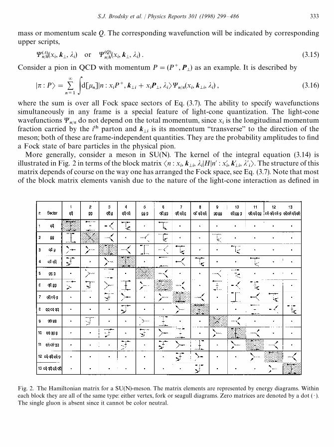
Fig. 2. The Hamiltonian matrix for a SU(N)-meson. The matrix elements are represented by energy diagrams. Withineach block they are all of the same type: either vertex, fork or seagull diagrams. Zero matrices are denoted by a dot ( ) ).The single gluon is absent since it cannot be color neutral.

mass or momentum scale Q. The corresponding wavefunction will be indicated by correspondingupper scripts,

W(K)n@h

(xi, k

M, j

i) or W(Q)

n@h(x

i, k

M, j

i) . (3.15)

Consider a pion in QCD with momentum P"(P`, PM) as an example. It is described by

Dn : PT"=+n/1Pd[k

n]Dn : x

iP`, k

Mi#x

iPM, j

iTW

n@n(xi, k

Mi, j

i) , (3.16)

where the sum is over all Fock space sectors of Eq. (3.7). The ability to specify wavefunctionssimultaneously in any frame is a special feature of light-cone quantization. The light-conewavefunctions W

n@n do not depend on the total momentum, since xiis the longitudinal momentum

fraction carried by the i5) parton and kMi

is its momentum “transverse” to the direction of themeson; both of these are frame-independent quantities. They are the probability amplitudes to finda Fock state of bare particles in the physical pion.

More generally, consider a meson in SU(N). The kernel of the integral equation (3.14) isillustrated in Fig. 2 in terms of the block matrix Sn : x

i, k

Mi, j

iDHDn@ : x@

i, k@

Mi, j@

iT. The structure of this

matrix depends of course on the way one has arranged the Fock space, see Eq. (3.7). Note that mostof the block matrix elements vanish due to the nature of the light-cone interaction as defined in


Eq. (2.94). The vertex interaction in Eq. (2.95) changes the particle number by one, whilethe instantaneous interactions in Eqs. (2.96), (2.97) and (2.98) change the particle number only upto two.

3.2. The use of light-cone wavefunctions

The infinite set of integral equations (3.14) is difficult if not impossible to solve. But given thelight-cone wavefunctions W

n@h(x

i, k

Mi, j

i), one can compute any hadronic quantity by convolution

with the appropriate quark and gluon matrix elements. In many cases of practical interest it sufficesto know less information than the complete wavefunction. As an example consider

Ga@h

(x,Q)"+nPd[k

n]DW(Q)

n@h(x

i, k

Mi, j

i)D2+

i

d(x!xi) . (3.17)

Ga@h

is a function of one variable, characteristic for a particular hadron, and depends parametricallyon the typical scale Q. It gives the probability to find in that hadron a particle with longitudinalmomentum fraction x, irrespective of the particle type, and irrespective of its spin, color, flavor ortransversal momentum k

M. Because of wavefunction normalization the integrated probability is

normalized to one.One can ask also for conditional probabilities, for example, for the probability to find a quark of

a particular flavor f and its momentum fraction x, but again irrespective of the other quantumnumbers. Thus,

Gf@h

(x; Q)"+nPd[k

n]DW(Q)

n@h(x

i, k

Mi, j

i)D2+

i

d(x!xi)d

i,f. (3.18)

The conditional probability is not normalized, even if one sums over all flavors. Such probabilityfunctions can be measured. For exclusive cross sections, one often needs only the probabilityamplitudes of the valence part

Uf@h

(x; Q)"+nPd[k

n]W(Q)

n@h(x

i, k

Mi, j

i)+i

d(x!xi)d

i,fdn,7!-%/#%

H(k2Mi4Q2) . (3.19)

Here, the transverse momenta are integrated up to momentum transfer Q2.The leading-twist structure functions measured in deep-inelastic lepton scattering are immedi-

ately related to the above light-cone probability distributions by

2MF1(x, Q)"

F2(x, Q)x

++f

e2fG

f@p(x, Q) . (3.20)

This follows from the observation that deep-inelastic lepton scattering in the Bjorken-scalinglimit occurs if x

bjmatches the light-cone fraction of the struck quark with charge e

f. However, the

light cone wavefunctions contain much more information for the final state of deep-inelasticscattering, such as the multi-parton distributions, spin and flavor correlations, and the spectator jetcomposition.

One of the most remarkable simplicities of the light-cone formalism is that one can write downthe exact expressions for the electro-magnetic form factors. In the interaction picture, one can


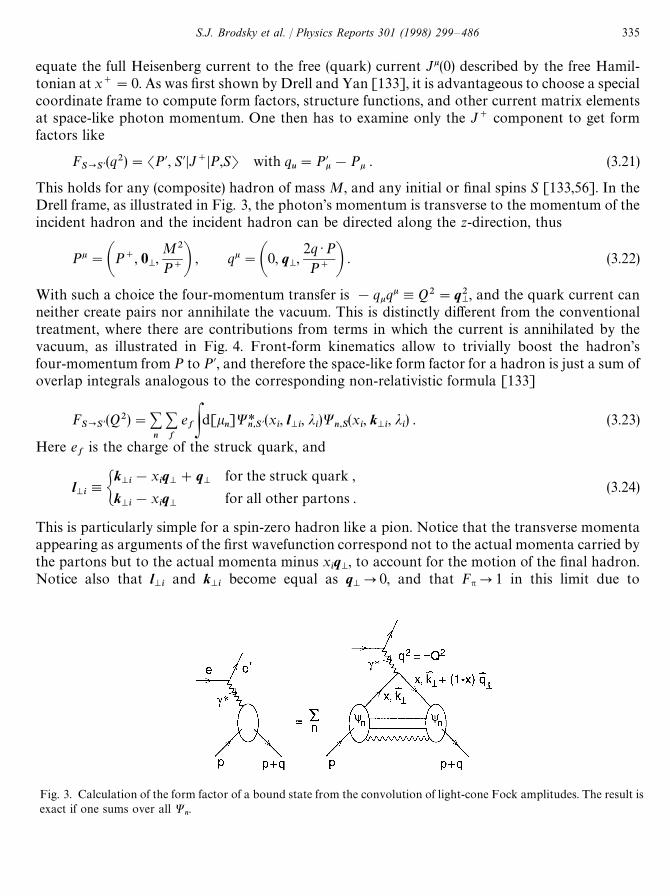
Fig. 3. Calculation of the form factor of a bound state from the convolution of light-cone Fock amplitudes. The result isexact if one sums over all W

n.

equate the full Heisenberg current to the free (quark) current Jk(0) described by the free Hamil-tonian at x`"0. As was first shown by Drell and Yan [133], it is advantageous to choose a specialcoordinate frame to compute form factors, structure functions, and other current matrix elementsat space-like photon momentum. One then has to examine only the J` component to get formfactors like

FS?S{

(q2)"SP@, S@DJ`DP,ST with qu"P@k!Pk . (3.21)

This holds for any (composite) hadron of mass M, and any initial or final spins S [133,56]. In theDrell frame, as illustrated in Fig. 3, the photon’s momentum is transverse to the momentum of theincident hadron and the incident hadron can be directed along the z-direction, thus

Pk"AP`, 0M,M2

P`B , qk"A0, qM,2q )PP` B . (3.22)

With such a choice the four-momentum transfer is !qkqk,Q2"q2M, and the quark current can

neither create pairs nor annihilate the vacuum. This is distinctly different from the conventionaltreatment, where there are contributions from terms in which the current is annihilated by thevacuum, as illustrated in Fig. 4. Front-form kinematics allow to trivially boost the hadron’sfour-momentum from P to P@, and therefore the space-like form factor for a hadron is just a sum ofoverlap integrals analogous to the corresponding non-relativistic formula [133]

FS?S{

(Q2)"+n

+f

efPd[k

n]W*

n,S{(x

i, l

Mi, j

i)W

n,S(x

i, k

Mi, j

i) . (3.23)

Here ef

is the charge of the struck quark, and

lMi,G

kMi!x

iqM#q

Mfor the struck quark ,

kMi!x

iqM

for all other partons .(3.24)

This is particularly simple for a spin-zero hadron like a pion. Notice that the transverse momentaappearing as arguments of the first wavefunction correspond not to the actual momenta carried bythe partons but to the actual momenta minus x

iqM, to account for the motion of the final hadron.

Notice also that lMi

and kMi

become equal as qMP0, and that F

pP1 in this limit due to


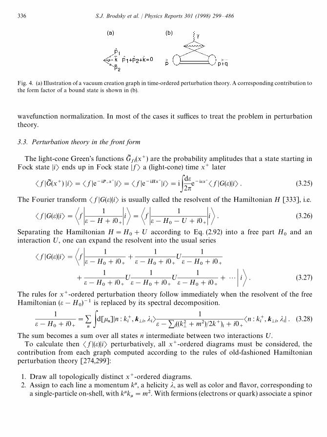
Fig. 4. (a) Illustration of a vacuum creation graph in time-ordered perturbation theory. A corresponding contribution tothe form factor of a bound state is shown in (b).

wavefunction normalization. In most of the cases it suffices to treat the problem in perturbationtheory.

3.3. Perturbation theory in the front form

The light-cone Green’s functions GIfi(x`) are the probability amplitudes that a state starting in

Fock state DiT ends up in Fock state D fT a (light-cone) time x` later

S f DGI (x`) DiT"S f De~*P`x`DiT"S f De~*Hx`DiT"iPde2n

e~*ex`S f DG(e)DiT . (3.25)

The Fourier transform S f DG(e)DiT is usually called the resolvent of the Hamiltonian H [333], i.e.

S f DG(e)DiT"Tf K1

e!H#i0`KiU"Tf K

1e!H

0!º#i0

`KiU . (3.26)

Separating the Hamiltonian H"H0#º according to Eq. (2.92) into a free part H

0and an

interaction º, one can expand the resolvent into the usual series

S f DG(e)DiT"Tf K1

e!H0#i0

`

#

1e!H

0#i0

`

º

1e!H

0#i0

`

#

1e!H

0#i0

`

º

1e!H

0#i0

`

º

1e!H

0#i0

`

#2K iU . (3.27)

The rules for x`-ordered perturbation theory follow immediately when the resolvent of the freeHamiltonian (e!H

0)~1 is replaced by its spectral decomposition.

1e!H

0#i0

`

"+nPd[k

n]Dn : k`

i, k

Mi, j

iT

1e!+

i((k2

M#m2)/2k`)

i#i0

`

Sn : k`i

, kMi

, jiD . (3.28)

The sum becomes a sum over all states n intermediate between two interactions º.To calculate then S f D(e)DiT perturbatively, all x`-ordered diagrams must be considered, the

contribution from each graph computed according to the rules of old-fashioned Hamiltonianperturbation theory [274,299]:

1. Draw all topologically distinct x`-ordered diagrams.2. Assign to each line a momentum kk, a helicity j, as well as color and flavor, corresponding to

a single-particle on-shell, with kkkk"m2. With fermions (electrons or quark) associate a spinor


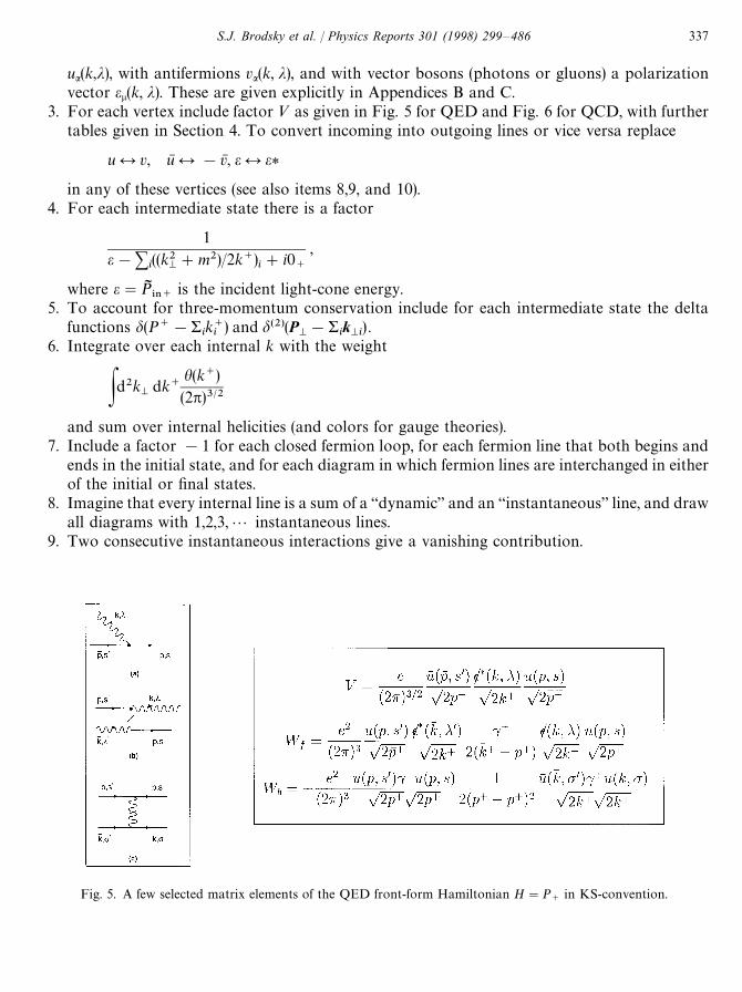
Fig. 5. A few selected matrix elements of the QED front-form Hamiltonian H"P`

in KS-convention.

ua(k,j), with antifermions va(k, j), and with vector bosons (photons or gluons) a polarizationvector e

l(k, j). These are given explicitly in Appendices B and C.

3. For each vertex include factor » as given in Fig. 5 for QED and Fig. 6 for QCD, with furthertables given in Section 4. To convert incoming into outgoing lines or vice versa replace

u % v, uN % !vN , e % e*

in any of these vertices (see also items 8,9, and 10).4. For each intermediate state there is a factor

1e!+

i((k2

M#m2)/2k`)

i#i0

`

,

where e"PI*/`

is the incident light-cone energy.5. To account for three-momentum conservation include for each intermediate state the delta

functions d(P`!&ik`i

) and d(2)(PM!&

ikMi

) .6. Integrate over each internal k with the weight

Pd2kM

dk`h(k`)(2p)3@2

and sum over internal helicities (and colors for gauge theories).7. Include a factor !1 for each closed fermion loop, for each fermion line that both begins and

ends in the initial state, and for each diagram in which fermion lines are interchanged in eitherof the initial or final states.

8. Imagine that every internal line is a sum of a “dynamic” and an “instantaneous” line, and drawall diagrams with 1,2,3,2 instantaneous lines.

9. Two consecutive instantaneous interactions give a vanishing contribution.


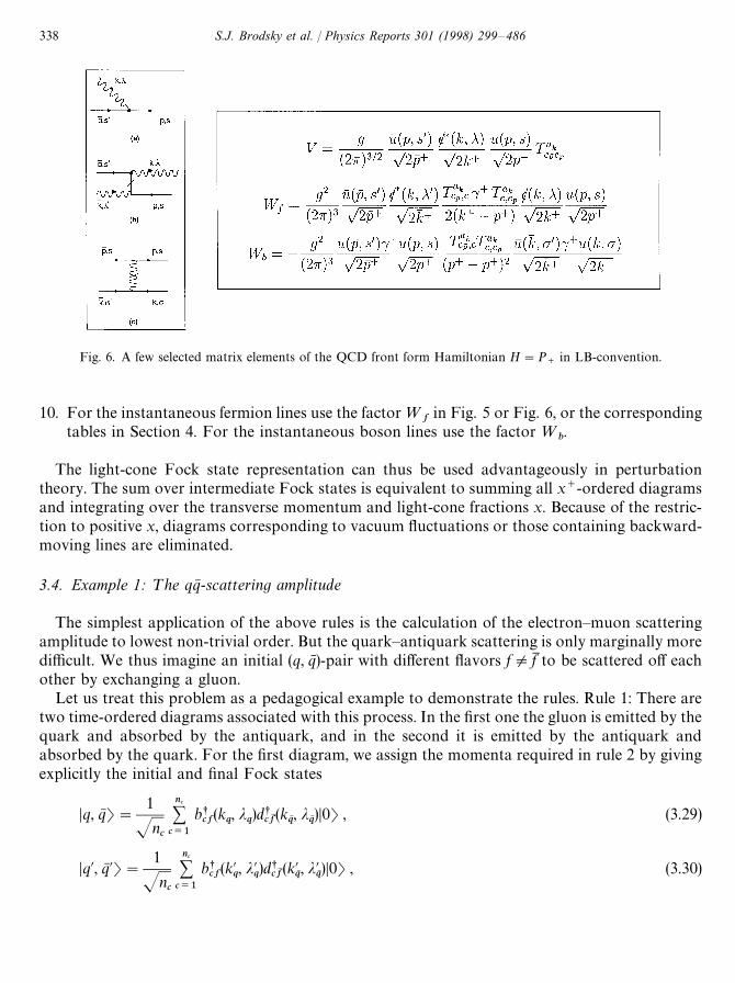
Fig. 6. A few selected matrix elements of the QCD front form Hamiltonian H"P`

in LB-convention.

10. For the instantaneous fermion lines use the factor ¼f

in Fig. 5 or Fig. 6, or the correspondingtables in Section 4. For the instantaneous boson lines use the factor ¼

b.

The light-cone Fock state representation can thus be used advantageously in perturbationtheory. The sum over intermediate Fock states is equivalent to summing all x`-ordered diagramsand integrating over the transverse momentum and light-cone fractions x. Because of the restric-tion to positive x, diagrams corresponding to vacuum fluctuations or those containing backward-moving lines are eliminated.

3.4. Example 1: ¹he qqN -scattering amplitude

The simplest application of the above rules is the calculation of the electron—muon scatteringamplitude to lowest non-trivial order. But the quark—antiquark scattering is only marginally moredifficult. We thus imagine an initial (q, qN )-pair with different flavors fOfM to be scattered off eachother by exchanging a gluon.

Let us treat this problem as a pedagogical example to demonstrate the rules. Rule 1: There aretwo time-ordered diagrams associated with this process. In the first one the gluon is emitted by thequark and absorbed by the antiquark, and in the second it is emitted by the antiquark andabsorbed by the quark. For the first diagram, we assign the momenta required in rule 2 by givingexplicitly the initial and final Fock states

Dq, qN T"1

Jnc

nc

+c/1

bscf

(kq, j

q)ds

cfM(k

qN, j

qN)D0T , (3.29)

Dq@, qN @T"1

Jnc

nc+c/1

bscf

(k@q, j@

q)ds

cfM(k@

qN, j@

qN)D0T , (3.30)


respectively. Note that both states are invariant under SU(nc). The usual color singlets of QCD are

obtained by setting nc"3. The intermediate state

Dq@, qN , gT"S2

n2c!1

nc

+c/1

nc+

c{/1

n2c~1+a/1

¹ac,c{

bscfM

(k@q, j@

q)ds

cfM {(k

qN, j

qN)as

a(k

g, j

g)D0T , (3.31)

has “a gluon in flight”. Under that impact, the quark has changed its momentum (and spin), whilethe antiquark as a spectator is still in its initial state. At the second vertex, the gluon in flight isabsorbed by the antiquark, the latter acquiring its final values (k@

qN, j@

qN). Since the gluons longitudinal

momentum is positive, the diagram allows only for k@q`(k`

q. Rule 3 requires at each vertex the

factors

Sq, qN D»Dq@, qN , gT"g

(2p)3@2Sn2c!12n

c

[uN (kq, j

q)ckek(kg, jg)u(k@

q, j@

q)]

J2k`qJ2k`

gJ2k@`

q

, (3.32)

Sq@, qN , gD»Dq@, qN @T"g

(2p)3@2Sn2c!12n

c

[uN (kqN, j

qN)cle*l (kg, jg)u(k@

qN,j@

qN)]

J2k`qN

J2k`g

J2k@qN`

, (3.33)

respectively. If one works with color neutral Fock states, all color structure reduces to an overallfactor C, with C2"(n2

c!1)/2n

c. This factor is the only difference between QCD and QED for this

example. For QCD C2"43

and for QED C2"1. Rule 4 requires the energy denominator 1/*E.With the initial energy

e"PI`"1

2PI ~"(k

q#k

qN)`"1

2(k

q#k

qN)~,

the energy denominator

2*E"(kq#k

qN)~!(k

g#k@

q#k

qN)~"!Q2/k`

g(3.34)

can be expressed in terms of the Feynman four-momentum transfers

Q2"k`g(k

g#k@

q!k

q)~, QM 2"k`

g(k

g#k

qN!k@

qN)~. (3.35)

Rule 5 requires two Dirac-delta functions, one at each vertex, to account for conservation ofthree-momentum. One of them is removed by the requirement of rule 6, namely to integrate over allintermediate internal momenta and the other remains in the final equation (3.43). The momentumof the exchanged gluon is thus fixed by the external legs of the graph. Rule 6 requires that one sumsover the gluon helicities. The polarization sum gives

dkl(kg),+

jg

ek(kg, j

g) e*l (kg

, jg)"!gkl#(k

g,kgl#kg,lgk)/ki

ggi , (3.36)

see Appendix B. The null vector gk has the components [299]

gk"(g`, gM, g~)"(0, 0

M, 2) , (3.37)


and thus the properties g2,gkgk"0 and kg"k`. In light-cone gauge, we find for the g-dependent terms

A+jg

Sq, qN D»Dq@, qN , gTSq@, qN , gD»Dq@, qN @TBg"

(gC)2(2p)3

12k`

g(k

gg)

]G[uN (q)ckkk

gu(q@)]

J4k`qk@q`

[uN (qN )clglu(qN @)]J4k`

qNk@qN`

#

[uN (q)cugku(q@)]

J4k`q

k@q`

[uN (qN )clklgu(qN @)]

J4k`qN

k@qN` H . (3.38)

Next, we introduce four-vectors like lkq"(k

g#k

q!k@

q)k. Since its three-components vanish by

momentum conservation, lkq

must be proportional to the null vector gk. With Eq. (3.35) one gets

lkq"(k

g#k

q!k@

q)k"(Q2/2k`

g)gk, lk

qN"(k

g#k@

qN!k

qN)k"(QM 2/2k`

g)gk . (3.39)

The well-known property of the Dirac spinors, (kq!k@

q)k[uN (k

q, j

q)cku(k@

q, j@

q)]"0, yields then

[uN (q)ckkkgu(q@)]"[uN (q)ckgku(q@)]Q2/2k`

g"[uN (q)cù(q@)]Q2/2k`

g,

and Eq. (3.38) becomes

A+jg

Sq, qN D»Dq@, qN , gTSq@, qN , gD»Dq@, qN @TBg"(gC)2(2p)3

Q2

2(k`g

)3[uN (q)cù(q@)]

J4k`q

k@q`

[uN (qN )cù(qN @)]J4k`

qNk@qN`

. (3.40)

Including the gkl contribution, the diagram of second order in » gives thus

»

1PI

`!H

0

»"

g2C2

(2p)3[uN (k

q, j

q)cku(k@

q, j@

q)]

J4k`q

k@q`

1Q2

[uN (kqN, j

qN)cku(k@

qN, j@

qN)]

J4k`qNk@qN`

!

g2C2

(2p)3[uN (k

q, j

q)cù(k@

q, j@

q)]

J4k`q

k@q`

1(k`

g)2

[uN (kqN, j

qN)cù(k@

qN, j@

qN)]

J4k`qN

k@qN`

, (3.41)

up to the delta functions, and a step function H(k@q`4k`

q), which truncates the final momenta k@`.

Evaluating the second time ordered diagram, one gets the same result up to the step functionH(k@

q`5k`

q). Using

H(k@q`4k`

q)#H(k@

q`5k`

q)"1 ,

the final sum of all time-ordered diagrams to order g2 is Eq. (3.41). One proceeds with rule 8, byincluding consecutively the instantaneous lines. In the present case, there is only one. From Fig. 5we find

Sq, qN D¼bDq@, qN @T"

g2C2

(2p)3[uN (k

q, j

q)cù(k@

q, j@

q)]

J4k`q

k@q`

1(k`

q!k@

q`)2

[uN (kqN, j

qN)cù(k@

qN, j@

qN)]

J4k`qN

k@qN`

. (3.42)

Finally, adding up all contributions up to order g2, the qqN -scattering amplitude becomes

¼#»

1PI

`!H

0

»"

(gC)2(2p)3

(!1)(k

q!k@

qN)2

[uN (kq, j

q)cku(k@

q, j@

q)][uN (k

qN, j

qN)cku(k@

qN, j@

qN)]

]1

Jk`q

k`qNk@q`k@

qN`

d(P`!P@`)d(2)(PM!P @

M) . (3.43)


Fig. 7. One loop self-energy correction for the electron. Time flows upward in these diagrams.

The instantaneous diagram ¼ is thus cancelled exactly against a corresponding term in thediagram of second order in the vertex interaction ». Their sum gives the correct second-orderresult.

3.5. Example 2: Perturbative mass renormalization in QED (KS)

As an example for light-cone perturbation theory we follow here the work of Mustaki et al.[339,372] to calculate the second-order mass renormalization of the electron and the renormaliz-ation constants Z

2and Z

3in the KS convention.

Since all particles are on-shell in light-cone time-ordered perturbation theory, the electronwavefunction renormalization Z

2must be obtained separately from the mass renormalization dm.

At order e2, one finds three contributions. First, the perturbation expansion

¹"¼#»(1/(p`!H

0))» (3.44)

yields a second-order contribution in », as shown in Fig. 7a. The initial (or final) electron fourmomentum is denoted by

pk"(p`, pM, (p2

M#m2)/2p`) . (3.45)

Second and finally, one has first-order contributions from ¼f

and ¼g, corresponding to Fig. 7b

and Fig. 7c. In the literature [354,422,66] these two-point vertices have been called “seagulls” or“self-induced inertias”.

One has to calculate the transition matrix amplitude ¹pp

ds,p"Sp, sD¹Dp, pT between a free

electron states with momentum and spin (p, s) and one with momentum and spin (p, p). The


normalization of states as in Eq. (3.3) was thus far

Sp@, s@Dp, sT"d(p`!p@`)d2 (pM!p@

M)d

s,s{, (3.46)

but for an invariant normalization it is better to use SpJ , sD,J2p`Sp, sD. Then one finds,

2mdmdsp,¹

pJ pJ"2p`¹

ppNdmd

sp"(p`/m)¹pp

. (3.47)

The other momenta appearing in Fig. 7a are

k"(k`, kM, k2

M/2k`) , (3.48)

k@"Ap`!k`,(p

M!k

M)2#m2

2(p`!k`), p

M!k

MB . (3.49)

Using the above rules to calculate ¹pp

, one obtains for the contribution from Fig. 7a,

dmadsp"e2

1m

+j,s{ P

d2kM

(4p)3Pp`

0

dk`[uN (p,p)e. *(k, j)u(k@, s@)][uN (k@, s@)e. (k, j)u(p, s)]

k`(p`!k`)(p~!k~!k@~). (3.50)

It can be shown that

[uN (p, p)ck(k. @#m)clu(p, s)]dkl(k)"4dspCA

2p`

k`#

k`

p`!k`B(p ) k)!m2D , (3.51)

which leads to the expression given below for dma. For Fig. 7b, one gets, using the rule for the

instantaneous fermion,

dmb"e2

p`

2m+j P

d2kM

(2p)3P`=

0

dkùN (p, s)e. *(k, j)cè. (k, j)u(p, p)

2p`2k`2(p`!k`)

"e2p`

2mPd2k

M(2p)3P

`=

0

dk`

k`(p`!k`). (3.52)

For Fig. 7c one finds,

dmc"

e2p`

2m+sPd2k

M(2p)3P

`=

0

dk`

2k`

uN (p, s)c`

J2p` Cu(k, s)uN (k, s)2(p`!k`)2

!

v(k, s)vN (k, s)2(p`#k`)2D

cù(p, p)

J2p`

"

e2p`

2m Pd2k

M(2p)3CP

`=

0

dk`

(p`!k`)2!P

`=

0

dk`

(p`#k`)2D . (3.53)

These integrals have potential singularities at k`"0 and k`"p`, as well as an ultra-violetdivergence in k

M. To regularize them, we introduce in a first step small cut-offs a and b:

a(k`(p`!b , (3.54)


and get rid of the pole at k`"p` in dmb

and dmcby a principal value prescription. One then

obtains

dma"

e22mP

d2kM

(2p)3 CPp`

0

dk`

k`

m2

p ) k!2A

p`

a!1B!lnA

p`

b BD ,

dmb"

e22mP

d2kM

(2p)3lnA

p`

a B , (3.55)

dmc"

e2mP

d2kM

(2p)3 Ap`

a!1B ,

where

p ) k"m2(k`)2#(p`)2k2

M2p`k`

. (3.56)

Adding these three contributions yields

dm"

e22mP

d2kM

(2p)3 CPp`

0

dk`

k`

m2

p ) k#lnA

baBD . (3.57)

Note the cancelation of the most singular infrared divergence.To complete the calculation, we present two possible regularization procedures:1. ¹ransverse dimensional regularization. The dimension of transverse space, d, is continued from

its physical value of 2 to 2#e and all integrals are replaced by

Pd2kMP(k2)ePddk

M, (3.58)

using e"1!d/2 as a small quantity. One thus gets

(k2)ePddkM(k2

M)a"0 for a50,

(k2)ePddkM

1k2M#M2

"Ak2

M2Be pe

,

(3.59)

(k2)ePddkM

1(k2

M#M2)2

"Ak2

M2Be pM2

,

(k2)ePddkM

k2M

k2M#M2

"!Ak2

M2Be pM2

e.

In this method, a and b in Eq. (3.57) are treated as constants. Dimensional regularization gives zerofor the logarithmic term, and for the remainder

dm"

e2m(2p)3P

1

0

dxPd2k

Mk2M#m2x2

, (3.60)


with x,(k`/p`), the above integral yields

dm"e2m/8p2e (3.61)

as the final result.2. Cut-offs. In this method [299,422,66], one restricts the momenta of any intermediate Fock

state by means of the invariant condition

PI 2"+iAm2#k2

Mx B

i

4K2 , (3.62)

where PI is the free total four-momentum of the intermediate state, and where K is a large cut-off.Furthermore, one assumes that all transverse momenta are smaller than a certain cut-off K

M, with

KM@K . (3.63)

In the case of Fig. 5a, Eq. (3.62) reads

k2M

k`#

(pM!k

M)2#m2

p`!k`(K@ with K@,

K2#p2M

p`. (3.64)

Hence

a"k2M

K@, b"

(pM!k

M)2#m2

K@N

ba"

(pM!k

M)2#m2

k2M

. (3.65)

In Ref. [339] it is shown that

Pd2kM

lnAbaB"Pd2k

M Pp`

0

dk`

p`

m2

p ) k. (3.66)

Now

dm"

e22mP

d2kM

(2p)3Pp`

0

dk`m2

p ) kA1

p`#

1k`B . (3.67)

Upon integration, and dropping the finite part, one finds

dm"(3e2m/16p2)ln(K2M/m2) , (3.68)

which is of the same form as the standard result [39]. Since dm is not by itself a measurablequantity, there is no contradiction in finding different results. Note that the seagulls are necessaryfor obtaining the conventional result.

Finally, the wavefunction renormalization Z2, at order e2, is given by

1!Z2"+@

m

DSpD»DmTD2(p

`!PI

`,m)2

, (3.69)


where PI`,m

is the free total energy of the intermediate state m. Note that this expression is the sameas one of the contributions to dm, except that here the denominator is squared. One has thus

(1!Z2)d

sp"e2p`P

d2kM

(4p)3Pp`

0

dk`

k`(p`!k`)uN (p,p)ck(cak@a#m)clu(p,s)dkl(k)

(p~!k~!k@~)2

"

e2dsp

(2p)3P1

0

dxPd2k

Mk2M#m2x2C

2(1!x)k2M

x(k2M#m2x2)

#xD , (3.70)

which is the same result as that obtained by Kogut and Soper [274]. Naturally, this integral is bothinfrared and ultraviolet divergent. Using the above rules, one gets

Z2(p`)"1#

e28p2eC

32!2 lnA

p`

a BD#e2

(2p)2lnA

p`

a BC1!2 lnAkmB!lnA

p`

a BD , (3.71)

where k2 is the scale introduced by dimensional regularization. Note that Z2

has an unusualdependence on the longitudinal momentum, not found in the conventional instant form. But thismay vary with the choice of regularization. A similar p` dependence was found for scalar QED byThorn [426,427].

In Ref. [339,340] the full renormalization of front-form QED was carried out to the one-looplevel. Electron and photon mass corrections were evaluated, as well as the wavefunction renormal-ization constants Z

2and Z

3, and the vertex correction Z

1. One feature that distinguishes the

front-form from the instant-form results is that the ultraviolet-divergent parts of Z1

and Z2

exhibitmomentum dependence. For physical quantities such as the renormalized charge e

R, this mo-

mentum dependence cancels due to the Ward identity Z1(p`,p@`)"JZ

2(p`)Z

2(p@`). On the other

hand, momentum-dependent renormalization constants imply non-local counter terms. Given thatthe tree-level Hamiltonian is non-local in x~, it is actually not surprising to find counter termsexhibiting non-locality. As mentioned in Ref. [456], the power counting works differently here inthe front than in the instant form. This is already indicated by the presence of four-pointinteractions in the Hamiltonian. The momentum dependence in Z

1and Z

2is another manifesta-

tion of unusual power counting laws. It will be interesting to apply them systematically in the caseof QED. Power counting alone does not provide information about cancelation of divergencesbetween diagrams. It is therefore important to gain more insight into the mechanism of cancelationin cases where one does expect this to occur as in the calculation of the electron mass shift.

3.6. Example 3: ¹he anomalous magnetic moment

The anomalous magnetic moment of the electron had been calculated in the front form byBrodsky et al. [53], using the method of alternating denominators. Its calculation is a transparentexample of calculating electro-magnetic form factors for both elementary and composite systems[41,56] as presented in Section 3.2 and for applying light-cone perturbation theory. Langnau andBurkardt [76,77,291,292] have calculated the anomalous magnetic moment at very strong coup-ling, by combining this method with discretized light-cone quantization, see below. We chooselight-cone coordinates corresponding to the Drell frame, Eq. (3.14), and denote as in the precedingsection the electron’s four-momentum and spin with (p, s). In line with Eq. (3.21), the Dirac and


Pauli form factors can be identified from the spin-conserving and spin-flip current matrix elements:

M`"Tp#q,CK

J`(0)p` Kp,CU"2F

1(q2) , (3.72)

M`¬"Tp#q,CK

J`(0)p` Kp,BU"!2(q

1!iq

2)F

2(q2)

2M, (3.73)

where C corresponds to positive spin projection sz"#1

2along the z-axis. The mass of the

composite system M is of course the physical mass m of the lepton. The interaction of the currentJ`(0) conserves the helicity of the struck constituent fermion (uN j{c`uj)/k`

"2djj{. Thus, one hasfrom Eqs. (3.23), (3.72) and (3.73)

F1(q2)"

12M`

"+

j

ejP[dk

n]t*n

p`q,(x, k

M, j)t(n)

p,(x, k

M, j) , (3.74)

!Aq1!iq

22M BF2

(q2)"12M`

¬"+

j

ejP[dk

n]t*n

p`q,(x, k

M, j)t(n)

p,¬(x, k

M, j) . (3.75)

In this notation, the summation over all contributing Fock states (n) and helicities (j) is assumed,and the reference to single-particle states i in the Fock states is suppressed. Momentum conserva-tion is used to eliminate the explicit reference to the momentum of the struck lepton in Eq. (3.24).Finally, the leptons wavefunction directed along the final direction p#q in the current matrixelement is denoted as

t(n)p`q,sz

(x, kM, j)"W

n@e(p`q,s2,sz)(x

i, k

Mi, j

i) .

One recalls that F1(q2) evaluated in the limit q2P0 with F

1P1 is equivalent to wavefunction

normalization

P[dk]t*p

tp"1, P[dk]t*

p¬tp¬"1 . (3.76)

The anomalous moment a"F2(0)/F

1(0) can be determined from the coefficient linear in q

1!iq

2from t*

p`qin Eq. (3.75). Since according to Eq. (3.24)

q

M

t*p`q

,!+iEj

xi

k

Mi

t*p`q

, (3.77)

one can, after integration by parts, write explicitly

aM

"!+j

ejP[dk

n]+iEj

t*p

xiA

k

1

#

ik

2Bi

tp¬

. (3.78)

The anomalous moment can thus be expressed in terms of a local matrix element at zeromomentum transfer (see also with Section 5 below). It should be emphasized that Eq. (3.78) isexact, valid for the anomalous element of actually any spin-1

2-system.


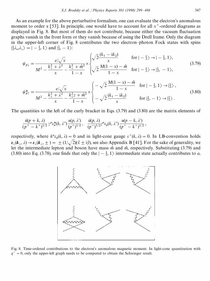
Fig. 8. Time-ordered contributions to the electron’s anomalous magnetic moment. In light-cone quantization withq`"0, only the upper-left graph needs to be computed to obtain the Schwinger result.

As an example for the above perturbative formalism, one can evaluate the electron’s anomalousmoment to order a [53]. In principle, one would have to account for all x`-ordered diagrams asdisplayed in Fig. 8. But most of them do not contribute, because either the vacuum fluctuationgraphs vanish in the front form or they vanish because of using the Drell frame. Only the diagramin the upper-left corner of Fig. 8 contributes the two electron—photon Fock states with spinsD12j%,jcT"D!1

2, 1T and D1

2,!1T:

tp¬"

e/Jx

M2!k2M#j2

x!

k2M#mL 2

1!x

]GJ2

(k1!ik

2)

xfor D!1

2TPD!1

2, 1T,

J2M(1!x)!mL

1!xfor D!1

2TPD1

2, !1T,

(3.79)

t*p"

e/Jx

M2!k2M#j2

x!

k2Mz#mL 21!x

]G!J2

M(1!x)!mL1!x

for D!12, 1TPD1

2T ,

!J2(k

1!ik

2)

xfor D1

2,!1TPD1

2T .

(3.80)

The quantities to the left of the curly bracket in Eqs. (3.79) and (3.80) are the matrix elements of

uN (p#k, j)(p`!k`)1@2

cke*k (k, jA)u(p, j@)(p`)1@2

,uN (p, j)(p`)1@2

ckek(k, jA)u(p!k, j@)

(p`!k`)1@2,

respectively, where kkek(k, j)"0 and in light-cone gauge e`(k, j)"0. In LB-convention holdseM(k

M, j)Pe

M(k

M,$)"$(1/J2)(xL $iyL ), see also Appendix B [41]. For the sake of generality, we

let the intermediate lepton and boson have mass mL and mJ , respectively. Substituting (3.79) and(3.80) into Eq. (3.78), one finds that only the D!1

2, 1T intermediate state actually contributes to a,


since terms which involve differentiation of the denominator of tp¬

cancel. One thus gets [56]

a"4Me2Pd2k

M16p3P

1

0

dx[mL !(1!x)M]/x(1!x)

[M2!(k2M#mL 2)/(1!x)!(k2

M#mJ 2)/x]2

,

"

apP

1

0

dxM[mL !M(1!x)]x(1!x)

mL 2x#mJ 2(1!x)!M2x(1!x), (3.81)

which, in the case of QED (mL "M, mJ "0) gives the Schwinger result a"a/2p [53]. As comparedto Schwinger the above is an almost trivial calculation.

The general result Eq. (3.78) can also be written in matrix form

a2M

"!+j

ejP[dx d2k

M]t*S

M)L

Mt , (3.82)

where SM

is the spin operator for the total system and LM

is the generator of “Galilean” transverseboosts [41] on the light cone, i.e. S

M)L

M"(S

`¸

~#S

~¸

`)/2 where S

B"(S

1$iS

2) is the

spin-ladder operator and

¸B"+

iEj

xiA

k

i

G

ik

2iB (3.83)

(summed over spectators) in the analog of the angular momentum operator r]p. Eq. (3.78) canalso be written simply as an expectation value in impact space.

The results given in Eqs. (3.74), (3.75) and (3.78) may also be convenient for calculating theanomalous moments and form factors of hadrons in quantum chromodynamics directly fromthe quark and gluon wavefunctions t(x, k

M, j). These wavefunctions can also be used to calculate

the structure functions and distribution amplitudes which control large momentum transferinclusive and exclusive processes. The charge radius of a composite system can also be written inthe form of a local, forward matrix element:

F1(q2)

q2 Kq2/0

"!+j

ejP[dx d2k

M]t*

p,A+iEj

xi

k

MiB

2tp,

. (3.84)

We thus find that, in general, any Fock state DnT which couples to both t*

and t¬

will givea contribution to the anomalous moment. Notice that because of rotational symmetry in the xL - andyL -direction, the contribution to a"F

2(0) in Eq. (3.78) always involves the form (a, b"1,2, n)

M+iEj

t*xi

k

Mi

t¬&kMo(ka

M) kb

M) , (3.85)

compared to the integral (3.76) for wavefunction normalization which has terms of order

t*t

&ka

M) kb

Mo(ka

M) kb

M) , k2o(ka

M) kb

M) . (3.86)

Here o is a rotationally invariant function of the transverse momenta and k is a constant withdimensions of mass. Thus, by order of magnitude

a"O(kM/(k2#Sk2MT)) (3.87)


summed and weighted over the Fock states. In the case of a renormalizable theory, the onlyparameters k with the dimension of mass are fermion masses. In super-renormalizable theories,k can be proportional to a coupling constant g with dimension of mass.

In the case where all the mass-scale parameters of the composite state are of the same order ofmagnitude, we obtain a"O(MR) as in Eq. (3.13), where R"Sk2

MT~1@2 is the characteristic size of

the Fock state. On the other hand, in theories where k2@Sk2MT, we obtain the quadratic relation

a"O(kMR2). Thus, composite models for leptons can avoid conflict with the high-precision QEDmeasurements in several ways.

f There can be strong cancelations between the contribution of different Fock states.f The parameter k can be minimized. For example, in a renormalizable theory this can be

accomplished by having the bound state of light fermions and heavy bosons. Since k5M, wethen have a5O(M2R2).

f If the parameter k is of the same order as the other mass scales in the composite state, then wehave a linear condition a"O(MR).

3.7. (1#1)-dimensional: Schwinger model (¸B)

Quantum electrodynamics in one-space and one-time dimension (QED1`1

) with masslesscharged fermions is known as the Schwinger model. It is one of the very few models of fieldtheory which can be solved analytically [311,401,402,108—110]. The charged particles areconfined because the Coulomb interaction in one-space dimension is linear in the relativedistance, and there is only one physical particle, a massive neutral scalar particle withno self-interactions. The Fock-space content of the physical states depends crucially on thecoordinate system and on the gauge. It is only in the front form that a simple constituentpicture emerges [34,326,317]. It is the best example of the type of simplification that peoplehope will occur for QCD in physical space—time. Recent studies of similar model withmassive fermion and for non-abelian theory where the fermion is in the fundamental andadjoint representation show however that many properties are unique to the Schwinger model[193,347].

The Schwinger model in Hamiltonian front-form field theory was studied first by Bergknoff [34].The description here follows him closely, as well as Perry’s recent lectures [367]. There is anextensive literature on this subject: DLCQ [137,460], lattice gauge theory [113], light-frontintegral equations [315], and light-front Tamm-Dancoff approaches [338] have used the model fortesting the various methods.

Bergknoff showed that the physical boson in the Schwinger model in light-cone gauge is a pureelectron—positron state. This is an amazing result in a strong-coupling theory of massless bareparticles, and it illustrates how a constituent picture may arise in QCD. The kinetic energy vanishesin the massless limit, and the potential energy is minimized by a wavefunction that is flat inmomentum space. One might expect that since a linear potential produces a state that is aslocalized as possible in position space.

Consider first the massive Schwinger model. The finite fermion mass m is a parameter to be set tozero, later. The Lagrangian for the theory takes the same form as the QED Lagrangian, Eq. (2.8).Again one works in the light-cone gauge A`"0, and uses the same projection operators K

Bas in


Section 2. The analogue of Eq. (2.74) becomes now simply

i~t`"!imt

~#eA~t

`, i`t

~"imt

~. (3.88)

The equation for t`

involves the light-front time derivative ~, so t`

is a dynamical degree offreedom that must be quantized. On the other hand, the equation for t

~involves only spatial

derivatives, so t~

is a constrained degree of freedom that should be eliminated in favor of t`.

Formally,

t~"(m/`)t

`. (3.89)

It is necessary to specify boundary condition in order to invert the operator `. If we had notchosen a finite mass for the fermions then both t

`and t

~would be independent degrees of

freedom and we would have to specify initial conditions for both. Furthermore, in the front form, ithas only been possible to calculate the condensate S0DttM D0T for the Schwinger model by identifyingit as the coefficient of the linear term in the mass expansion of matrix element of the currents [34].Due to the gauge, one component is fixed to A`"0, but the other component A~ of the gaugefield is also a constrained degree of freedom. It can be formally eliminated by the light-coneanalogue of Gauss’s law:

A~"!(4e/(`)2)ts`

t`

. (3.90)

One is left with a single dynamical degree of freedom, t`, which is canonically quantized at x`"0,

Mt`(x~),ts

`(y~)N"K

`d(x~!y~) (3.91)

similar to what was done in QED. The field operator at x`"0, expanded in terms of the freeparticle creation and annihilation operators, takes the very simple form

t`

(x~)"Pk`;0

dk`

4p[b

ke~*k >x#ds

ke*k >x] with Md

k,ds

pN"Mb

k,bs

pN"4pd(k`!p`) . (3.92)

The canonical Hamiltonian H"P`"1

2P~ is divided into the three parts,

H"H0#H@

0#»@ . (3.93)

These Fock-space operators are obtained by inserting the free fields in Eq. (3.92) into the canonicalexpressions in Eq. (2.89). The free part of the Hamiltonian becomes

H0"P

k;0

dk8pA

m2

k B(bskbk#ds

kdk) . (3.94)

H@0

is the one-body operator which is obtained by normal ordering the interaction, i.e.

H@0"

e24pP

k;0

dk4pP

p;0

dp A1

(k!p)2!

1(k#p)2B (bs

kbk#ds

kdk) . (3.95)

The divergent momentum integral is regulated by the momentum cut-off, Dk!pD'e. One finds

H@0"

e22pP

dk4p A

1e!

1k#O(e)B(bs

kbk#ds

kdk) . (3.96)


The normal-ordered interaction is

»@"4pe2Pdk

14p

2

dk4

4pd(k

1#k

2!k

3!k

4)G

2(k

1!k

3)2

bs1ds2d4b3

#

2(k

1#k

2)2

bs1ds2d3b4!

1(k

1!k

3)2

(bs1bs2b3b4#ds

1ds2d3d4)#2H . (3.97)

The interactions that involve the creation or annihilation of electron—positron pairs are notdisplayed. The first term in »@ is the electron—positron interaction. The longitudinal momentumcut-off requires Dk

1!k

3D'e and leads to the potential

v(x~)"4q1q2P

=

~=

dk4p

h(DkD!e)e~*kx~@2"q1q2C

2pe

!Dx~D#O(e)D . (3.98)

This potential contains a linear Coulomb potential that we expect in two dimensions, but it alsocontains a divergent constant, being negative for unlike charges and positive for like charges.

In charge neutral states the infinite constant in »@ is exactly canceled by the divergent “mass”term in H@

0. This Hamiltonian assigns an infinite energy to states with net charge, and a finite

energy as, eP0, to charge zero states. This does not imply that charged particles are confined, butthat the linear potential prevents charged particles from moving to arbitrarily large separationexcept as charge-neutral states.

One should emphasize that even though the interaction between charges is long-ranged, thereare no van der Waals forces in 1#1 dimensions. It is a simple geometrical calculation to show thatall long-range forces between two neutral states cancel exactly. This does not happen in higherdimensions, and if we use long-range two-body operators to implement confinement we must alsofind many-body operators that cancel the strong long-range van der Waals interactions.

Given the complete Hamiltonian in normal-ordered form we can study bound states. A powerfultool for getting started is the variational wavefunction. In this case, one can begin with a state thatcontains a single electron—positron pair

DW(P)T"PP

0

dp4p

/(p)bspdsP~p

D0T . (3.99)

The normalization of this state is SW(P@)DW(P)T"4pPd(P@!P). The expectation value of theone-body operators in the Hamiltonian is

SWDH0#H@

0DWT"

12PP

dk4p C

m2!e2/pk

#

m2!e2/pP!k

#

2e2pe DD/(k)D2 , (3.100)

and the expectation value of the normal-ordered interaction is

SWD»@DWT"!

e2PP

@dk1

4pdk

24p Cg

1(k

1!k

2)2#

1P2D/*(k

1)/(k

2) . (3.101)

The prime on the last integral indicates that the range of integration in which Dk1!k

2D(e must

be removed. By expanding the integrand about k1"k

2, one can easily confirm that the 1/e

divergences cancel.


The easiest case to study is the massless Schwinger model. With m"0, the energy is minimizedwhen

/(k)"J4p . (3.102)

The invariant-mass squared, M2"2PH, becomes then finally

M2"e2/p . (3.103)

This type of simple analysis can be used to show that this electron—positron state is actually theexact ground state of the theory with momentum P, and that bound states do not interact with oneanother [367].

It is intriguing that for massless fermions, the massive bound state is a simple bound state of anelectron and a positron when the theory is formulated in the front form using the light-cone gauge.This is not true in other gauges and coordinate systems. This happens because the charges screenone another perfectly, and this may be the way a constituent picture emerge in QCD. On the otherhand there are many differences between two and four dimensions. In two dimensions, for example,the coupling has the dimension of mass making it natural for the bound state mass to beproportional to coupling in the massless limit. On the other hand, in four dimensions the couplingis dimensionless and the bound states in a four-dimensional massless theory must acquire amass through dimensional transmutations. A simple model of how this might happen is discussedin the renormalization of the Yukawa model and in some simple models in the section on re-normalization.

3.8. (3#1 )-dimensional: ½ukawa model

Our ultimate aim is to study the bound-state problem in QCD. However light-front QCD isplagued with divergences arising from both small longitudinal momentum and large transversemomentum. To gain experience with the novel renormalization programs that this requires, it isuseful to study a simpler model. The two-fermion bound-state problem in the 3#1 light-frontYukawa model has many of the non-perturbative problems of QCD while still being tractable inthe Tamm—Dancoff approximation. This section follows closely the work in Refs. [182,373,374].The problems that were encountered in this calculation are typical of any (3#1)-dimensionalnon-perturbative calculation and laid the basis for Wilson’s current light-front program[451,452,456,364—366] which will be briefly discussed in the section on renormalization.

The light-front Tamm—Dancoff method (LFTD) is Tamm—Dancoff truncation of the Fock spacein light-front quantum field theory and was proposed [363,422] to overcome some of the problemsin the equal-time Tamm—Dancoff method [68]. In this approach, one introduces a longitudinalmomentum cut-off e to remove all the troublesome vacuum diagrams. The bare vacuum state isthen an eigenstate of the Hamiltonian. One can also introduce a transverse momentum cut-off K toregulate ultraviolet divergences. Of course, the particle truncation and momentum cut-offs spoilLorentz symmetries. In a properly renormalized theory, one has to remove the cut-off dependencefrom the observables and recover the lost Lorentz symmetries. One has avoided the originalvacuum problem but now the construction of a properly renormalized Hamiltonian is a nontrivialproblem. In particular, the light-front Tamm—Dancoff approximation breaks rotational invariancewith respect to the two transverse directions. This is visible in the spectrum which does not exhibit


the degeneracy associated with the total angular momentum multiplets. It is seen that renormaliz-ation has sufficient flexibility to restore the degeneracy.

Retaining only two-fermion and two-fermion, one-boson states one obtains a two-fermionbound-state problem in the lowest-order Tamm—Dancoff truncation. This is accomplished byeliminating the three-body-sector algebraically which leaves an integral equation for the two-bodystate. This bound state equation has both divergent self-energy and divergent one-boson exchangecontributions. In the renormalization of the one-boson exchange divergences the self-energycorrections are ignored. Related work can be found in Refs. [176,279,459].

Different counter terms are introduced to renormalize the divergences associated with one-boson exchange. The basis for these counter terms is easily understood, and uses a momentumspace slicing called the high—low analysis. It was introduced by Wilson [454] and is discussed indetail for a simple one-dimensional model in the section on renormalization.

To remove the self-energy divergences one first introduces a sector-dependent mass counter termwhich removes the quadratic divergence. The remaining logarithmic divergence is removed bya redefinition of the coupling constant. Here one faces the well-known problem of triviality: Fora fixed renormalized coupling the bare coupling becomes imaginary beyond a certain ultravioletcut-off. This was probably seen first in the Lee model [293] and then in meson—nucleon scatteringusing the equal-time Tamm—Dancoff method [114].

The canonical light-front Hamiltonian for the (3#1)-dimensional Yukawa model is given by

P~"

12Pdx~ d2x

M[2its

~`t

~#m2

B/2#

M/ )

M/] . (3.104)

The equations of motion are used to express t~

in terms of t`

, i.e.

t~"(1/i`)[ia

M)

M#b(m

F#g/)]t

`. (3.105)

For simplicity, the two fermions are taken to be of different flavors, one denoted by bp and the otherby Bp. We divide the Hamiltonian P~ into P~

&3%%and P~

*/5, where

P~&3%%

"P[d3k]m2

B#k2

k`as(k)a(k)#+

p P[d3k]m2

F#k2

k`[bsp(k)bp(k)#Bsp(k)Bp(k)] , (3.106)

P~*/5"g +

p1,p2P[d3k

1]P[d3k

2]P[d3k

3]2(2p)3d3(k

1!k

2!k

3)

][(bsp1(k

1)bp2

(k2)#Bsp1

(k1)Bp2

(k2))a(k

3)uN p1

(k1)up2

(k2)#(bsp2

(k2)bp1

(k1)

#Bsp2(k

2)Bp1

(k1))as(k

3)uN p2

(k2)up1

(k1)] . (3.107)

Note that the instantaneous interaction was dropped from P~*/5

for simplicity. The fermion number2 state that is an eigenstate of P~ with momentum P and helicity p is denoted as DW(P, p)T. Thewavefunction is normalized in the truncated Fock space, with

SW(P@, p@)DW(P, p)T"2(2p)3P`d3(P!P@)dpp{ .


In the lowest-order Tamm—Dancoff truncation one has

DW(P, p)T" +p1p2P[d3k

1]P[d3k

2]U

2(P, pDk

1p1, k

2p2)bsp1

(k1)Bsp2

(k2)D0T

# +p1p2P[d3k

1]P[d3k

2]P[d3k

3]U

3(P, pDk

1p1, k

2p2, k

3)bsp1

(k1)Bsp2

(k2)as(k

3)D0T ,

where U2is the two-particle and U

3the three-particle amplitude, and where D0T is the vacuum state.

For notational convenience, one introduces the amplitudes W2

and W3

by

U2(P, pDk

1p1, k

2p2)"2(2p)3P`d3(P!k

1!k

2)Jx

1x2Wp1p2

2(i

1x1, i

2x2) , (3.108)

U3(P, pDk

1p1, k

2p2, k

3)"2(2p)3P`d3(P!Rk

i)Jx

1x2x3Wp1p2

3(i

1x1, i

2x2, i

3x3) . (3.109)

As usual, the intrinsic variables are xiand i

i"j

Mi:

kki"Axi

P`, jMi

,j2Mi#m2

xiP` B ,

with +ixi"1 and +

ijMi"0. By projecting the eigenvalue equation

(P`P~!P2M)DWT"M2DWT (3.110)

onto a set of free Fock states, one obtains two coupled integral equations:

CM2!m2

F#(i

1)2

x1

!

m2F#(i

1)2

x2

DWp1p22

(i1, x

1)

"

g2(2p)3

+s1P

dy1

d2q1

J(x1!y

1)x

1y1

Ws1,p23

(q1, y

1; i

2, x

2)uN p1

(i1, x

1)u

s1(q

1, y

1)

#

g2(2p)3

+s2P

dy2

d2q2

J(x2!y

2)x

2y2

Wp1s23

(i1, x

1; q

2, y

2)uN p2

(i2,x

2)u

s2(q

2, y

2) (3.111)

and

CM2!m2

F#(i

1)2

x1

!

m2F#(i

2)2

x2

!

m2B#(i

1#i

2)2

x3

DWp1p23

(i1, x

1; i

2, x

2)

"g+s1

Ws1p22

(!i2, x

1#x

3)

Jx3x1(x

1#x

3)

uN p1(i

1, x

1)u

s1(!i

2, x

1#x

3)

#g+s2

Wp1s22

(i1, x

1)

Jx3x2(x

3#x

2)uN p2

(i2, x

2)u

s2(!i

1, x

2#x

3) . (3.112)


After eliminating W3

one ends up with an integral equation for W2

and the eigenvalue M2:

M2Wp1p22

(i, x)"Am2

F#i2

x(1!x)#[SE]BWp1p2

2(i, x)

#

a4p2

+s1,s2Pdy d2q K(i, x; q,y; u)p1p2§s1s2

Ws1s22

(q,y) #counterterms , (3.113)

where a"g2/4p is the fine structure constant. The absorption of the boson on the same fermiongives rise to the self-energy term [SE], the one by the other fermion generates an effectiveinteraction, or the boson-exchange kernel K,

K(i, x; q, y; u)p1p2§ s1s2"

[uN (i, x; p1)u(q, y; s

1)][uN (!i, 1!x; p

2)u(!q, 1!y; s

2)]

(a#2(i ) q))Jx(1!x)y(1!y), (3.114)

with

a"Dx!yDGu!

12C

m2F#k2

x(1!x)#

m2F#q2

y(1!y)DH!m2B#2m2

F

!

m2F#k2

2 Cyx#

1!y1!xD!

m2F#q2

2 Cxy#

1!x1!yD , (3.115)

with k"DiD and u,M2. Possible counter terms will be discussed below.Since p"C,B one faces thus 4]4"16 coupled integral equations in the three variables x and j

M.

But the problem is simplified considerably by exploiting the rotational symmetry around the z-axis.Let us demonstrate that shortly. By Fourier transforming over the angle /, one introduces firststates U with good total spin-projection S

z"p

1#p

2,m,

Wp1p22

(i, x)"+m

e*m(

J2pUp1p2

(k, x; m) (3.116)

and uses that second to redefine the kernel:

»(k, x, m; q, y, m@; M2)p1p2§s1s2"P

d/ d/@2p

e~*m(e*m{({K(k, /, x; q, /@, y; M2)p1p2§s1s2. (3.117)

The /-integrals can be done analytically. Now, recall that neither Sz

nor ¸z

is conserved; onlyJz"S

z#¸

zis a good quantum number. In the two-particle sector of spin-1

2particles the spin

projections are limited to DSzD41, and thus, for J

;given, one has to consider only the four

amplitudes U

(k, x; Jz!1), U

¬(k, x; J

z), U

¬(k, x; J

z), and U

¬¬(k, x; J

z#1). Rotational symmetry

allows thus to reduce the number of coupled equations from 16 to 4, and the number of integrationvariables from 3 to 2. Finally, one always can add and subtract the states, introducing

UBt(k, x)"(1/J2)(U

(k, x; J

z!1)$U

¬¬(k, x; J

z#1)) ,

(3.118)UB

s(k, x)"(1/J2) (U

¬(k, x; J

z)$U

¬(k, x; J

z)) .


The integral equations couple the sets (t~, s`) and (t`, s~). For Jz"0, the “singlet” and the

“triplet” states uncouple completely, and one has to solve only two pairs of two coupled integralequations. In a way, these reductions are quite natural and straightforward, and have been appliedindependently also by Krautgartner et al. [279] and most recently by Trittmann and Pauli [429].

Next, let us discuss the structure of the integrand in Eq. (3.113) and analyze eventual divergences.Restrict first to J

z"0, and consider [uN (x, i; p

1)u(y, q; s

1)] for large q, taken from the tables in

Section 4. They are such that the kernel K becomes independent of DqD in the limit DqDPR. Thus,unless U vanishes faster than DqD~2, the q-integral potentially diverges. In fact, introducing anultraviolet cut-off K to regularize the DqD-dependence, the integrals involving the singlet wavefunc-tions UB

4diverge logarithmically with K. In the J

z"1 sector one must solve a system of four

coupled integral equations. One finds that the kernel »,¬¬

approaches the same limit !f (x, y) asq becomes large relative to k. All other kernels fall off faster with q. For higher values of J

z, the

integrand converges since the wavefunctions fall-off faster than DqD~2. Counter terms are thereforeneeded only for J

z"0 and J

z"$1. These boson-exchange counter terms have no analogue in

equal-time perturbation theory, and will be discussed below.These integral equations are solved numerically, using Gauss—Legendre quadratures to evaluate

the q and y integrals. Note that the eigenvalue M2 appears on both the left- and right-hand side ofthe integral equation. One handles this by choosing some “starting point” value u on the r.h.s. Bysolving the resulting matrix eigenvalue problem one obtains the eigenvalue M2(u). Taking that asthe new starting point value, one iterates the procedure until M2(u)"u is numerically fulfilledsufficiently well.

For the parameter values 14a42 and 24mF/m

B44 one finds only two stable bound states,

one for each DJzD41. In the corresponding wavefunctions, one observes a dominance of the

spin-zero configuration Sz"0. The admixture from higher values of ¸

zincreases gradually with

increasing a, but the predominance of ¸z"0 persists also when counter terms are included in the

calculation. With the above parameter choice no bound states have been found numerically forJz'1. They start to appear only when a is significantly increased.The above bound-state equations are regularized. How are they renormalized? In the section on

renormalization, below, we shall show in simple one-dimensional models that it is possible to addcounter terms to the integral equation of this type that completely remove all the cut-offdependence from both the wavefunctions and the bound-state spectrum. In these one-dimensionalmodels the finite part of the counter term contains an arbitrary dimensionful scale k and anassociated arbitrary constant. In two-dimensional models the arbitrary constant becomes anarbitrary function. The analysis presented here is based on the methods used in the one-dimen-sional models. It is convenient to subdivide the study of these counter terms into two categories.One is called the asymptotic counter terms, and the other is called the perturbative counter terms.

Studies of the simple models and the general power counting arguments show that integralequations should be supplemented by a counter term of the form,

G(K)Pq dq dy F(x, y)/(q, y) . (3.119)

For the Yukawa model one has not been able to solve for G(K) F(x, y) exactly such that itremoves all that cut-off dependence. One can, however, estimate G(K) F(x, y) perturbatively. The


lowest-order perturbative counter terms, those of order a2, correspond to the box graphs in theintegral equation. They are thus called the “box counter terms” (BCT). Applying it to the Yukawamodel, one finds that the integral equation should be modified according to

»(k, x; q, y; u)P»(k, x; q, y; u)!»BCT(x, y) . (3.120)

»BCT(x, y) contains an undetermined parameter ‘C’. Redoing the bound-state mass calculationswith this counter term one finds that the cut-off independence of the solutions is greatly reduced.Thus, one has an (almost) finite calculation involving arbitrary parameters, C for each sector.Adjusting the C’s allows us to move eigenvalues around only in a limited way. It is possiblehowever to make the J

z"1 state degenerate with either of the two J

z"0 states. The splitting

among the two Jz"0 states remains small.

One can also eliminate divergences non-perturbatively by subtracting the large transversemomentum limit of the kernel. We call this type of counter term as the asymptotic counter term. Inthe Yukawa model one is only able to employ such counter terms in the J

z"0 sector. One then has

»(k, x; q, y; M2)s`,s`P»(k, x; q, y; M2)s`,s`#f (x, y) , (3.121)

»(k, x; q, y; M2)s~,s~P»(k, x; q, y; M2)s~,s~!f (x, y) . (3.122)

One can find an extra interaction allowed by power counting in the LC-Hamiltonian that wouldgive rise to more terms. One finds that with the asymptotic counter term the cut-off dependence hasbeen eliminated for the (t!, s#) states and improved for the (t#, s!) states. We also find thatthis counter term modifies the large k behavior of the amplitudes U(k, x) making them fall off fasterthan before.

The asymptotic counter term, as it stands, does not include any arbitrary constants that can betuned to renormalize the theory to some experimental input. This differs from the case with the boxcounter term where such a constant appeared. One may, however, add an adjustable piece which ingeneral involves an arbitrary function of longitudinal momenta. This is motivated by the simplemodels discussed in the section on renormalization. One replaces

f (x, y)Pf (x, y)!Gk/(1#16Gkln(K/k)) (3.123)

Gk and the scale k are not independent. A change in k can be compensated by adjusting Gk suchthat (1/G

l)!1

6ln(k)"constant. This ‘constant’ is arbitrary and plays the role of the constant “C”

in the box counter term. One finds that by adjusting the constant a much wider range of possibleeigenvalues can be covered, compared to the situation with the box counter term.

Consider now the effects of the self-energy term [SE]. Note that in the bound state problem theself-energy is a function of the bound state energy M2. The most severe ultraviolet divergence in[SE]

(M2)is a quadratical divergence. One eliminates this divergence by subtracting at the threshold

M2"M20,(m2

F#k2)/(x(1!x))

[SE](M2)

P[SE](M2)

![SE](M2

0),g2(M2!M2

0)p

(M2). (3.124)

p(M2)

is still logarithmically divergent. The remaining logarithmically divergent piece correspondsto wavefunction renormalization of the two fermion lines. One finds

p-0'$*7.1!35

"A[SE]M2 B

-0'$*7.

,!¼(K) (3.125)


One can absorb this divergence into a new definition of the coupling constant. After the subtraction(but ignoring all “boson-exchange” counter terms) the integral equation becomes

(M2!M20)Wp1p2

2(k, x)"

a4p2

[BE]#a

4p2(M2!M2

0)p

(M20)Wp1p2

2(k, x) , (3.126)

where [BE] stands for the term with the kernel K. After rearranging the terms one finds, with allspin indices suppressed,

(M2!M20)C1#

a4p2

¼(K)DW"

a4p2

[BE]#a

4p2(M2!M2

0)(p#¼(K))W . (3.127)

The r.h.s. is now finite. One must still deal with the divergent piece ¼ on the l.h.s. of the equation.Define

aR"a/(1#(a/4p2)¼(K)) . (3.128)

Then one can trade a K-dependent bare coupling a in favor of a finite renormalized coupling aR.

One has

(M2!M20)W"

aR/4p2

1!aR/4p2(p

(M2)#¼(K))

[BE] . (3.129)

One sees that the form of the equation is identical to what was solved earlier (where all counterterms were ignored) with a replaced by a

R/[1!a

R/4p2(p#¼)]. One should note that p is

a function of x and k, and therefore effectively changes the kernel. In lowest-order Tamm—Dancoffthe divergent parts of [SE] can hence be absorbed into a renormalized mass and coupling. It ishowever not clear whether this method will work in higher orders.

Inverting the equation for aR

one has

a(K)"aR/(1!(a

R/4p2)¼(K)) . (3.130)

One sees that for every value of aR

other than aR"0 there will be a cut-off K at which the

denominator vanishes and a becomes infinite. This is just a manifestation of “triviality” in thismodel. The only way the theory can be sensible for arbitrarily large cut-off KPR, is when a

RP0.

In practice, this means that for fixed cut-off there will be an upper bound on aR.

4. Discretized light-cone quantization

Constructing even the lowest state, the “vacuum”, of a quantum field theory has been sonotoriously difficult that the conventional Hamiltonian approach was given up altogether long agoin the 1950s, in favor of action-oriented approaches. It was overlooked that Dirac’s “front form ofHamiltonian dynamics” [123] might have less severe problems. Of course, the action and theHamiltonian forms of dynamics are equivalent to each other. The action is more suitable forderiving cross sections, the Hamiltonian more convenient when considering the structure of boundstates in atoms, nuclei, and hadrons. In fact, in the front form with periodic boundary conditionsone can combine the aspects of a simple vacuum [448] and a careful treatment of the infrared


degrees of freedom. This method is called “discretized light-cone quantization” (DLCQ) [354] andhas three important aspects:

1. the theory is formulated in a Hamiltonian approach;2. calculations are done in momentum representation;3. quantization is done at equal light-cone rather than at equal usual time.

As a method, “discretized light-cone quantization” has the ambitious goal to calculate the spectraand wavefunctions of physical hadrons from a covariant gauge field theory. In fact, in 1#1dimensions this method provides the first total solutions to non-trivial quantum field theories. In3#1 dimensions, the conversion of this non-perturbative method into a reliable tool for hadronicphysics is beset with many difficulties [185]. Their resolution will continue to take time. Since itsfirst formulation [354,355] many problems have been resolved but many remain, as we shall see.Many of these challenges are actually not peculiar to the front form but appear also in conven-tional Hamiltonian dynamics. For example, the renormalization program for a quantum fieldtheory has been formulated thus far only in order-by-order perturbation theory. Little work hasbeen done on formulating a non-perturbative Hamiltonian renormalization [363,456].

At the beginning, one should emphasize a rather important aspect of periodic boundaryconditions: all charges are strictly conserved. Every local Lagrangian field theory has vanishingfour-divergences of some “currents” of the form kJk"0. Written out explicitly this reads

`J`#

~J~"0 . (4.1)

The restriction to 1#1 dimensions suffices for the argument. The case of 3#1 dimensions isa simple generalization. The “charge” is defined by

Q(x`),P`L

~L

dx~ J`(x`, x~). (4.2)

Conservation is proven by integrating Eq. (4.1),

(d/dx`)Q(x`)"0 , (4.3)

provided that the terms from the boundaries vanish, i.e.

J`(x`, ¸)!J`(x`,!¸)"0 . (4.4)

This is precisely the condition for periodic boundary conditions. If one does not use periodicboundary conditions, then one has to ensure that all fields tend to vanish “sufficiently fast” at theboundaries. To guarantee the latter is much more difficult than taking the limit ¸PR at the endof a calculation. Examples of conserved four-currents are the components of the energy—momentum stress tensor with kHkl"0, the conserved “charges” being the four components of theenergy—momentum four-vector Pl.

Discretized light-cone quantization applied to abelian and non-abelian quantum field theoriesfaces a number of problems only part of which have been resolved by recent work. Here is a ratherincomplete list:

1. Is the front form of Hamiltonian dynamics equivalent to the instant form? Does one get thesame results in both approaches? Except for a class of problems involving massless left-handed


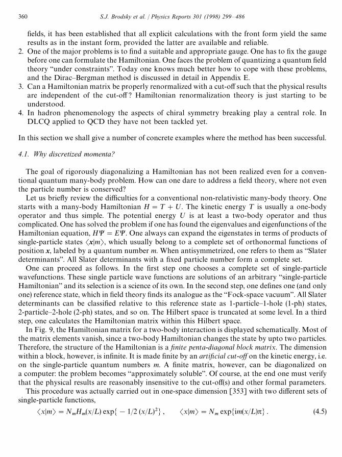
fields, it has been established that all explicit calculations with the front form yield the sameresults as in the instant form, provided the latter are available and reliable.

2. One of the major problems is to find a suitable and appropriate gauge. One has to fix the gaugebefore one can formulate the Hamiltonian. One faces the problem of quantizing a quantum fieldtheory “under constraints”. Today one knows much better how to cope with these problems,and the Dirac—Bergman method is discussed in detail in Appendix E.

3. Can a Hamiltonian matrix be properly renormalized with a cut-off such that the physical resultsare independent of the cut-off ? Hamiltonian renormalization theory is just starting to beunderstood.

4. In hadron phenomenology the aspects of chiral symmetry breaking play a central role. InDLCQ applied to QCD they have not been tackled yet.

In this section we shall give a number of concrete examples where the method has been successful.

4.1. Why discretized momenta?

The goal of rigorously diagonalizing a Hamiltonian has not been realized even for a conven-tional quantum many-body problem. How can one dare to address a field theory, where not eventhe particle number is conserved?

Let us briefly review the difficulties for a conventional non-relativistic many-body theory. Onestarts with a many-body Hamiltonian H"¹#º. The kinetic energy ¹ is usually a one-bodyoperator and thus simple. The potential energy º is at least a two-body operator and thuscomplicated. One has solved the problem if one has found the eigenvalues and eigenfunctions of theHamiltonian equation, HW"EW. One always can expand the eigenstates in terms of products ofsingle-particle states SxDmT, which usually belong to a complete set of orthonormal functions ofposition x, labeled by a quantum number m. When antisymmetrized, one refers to them as “Slaterdeterminants”. All Slater determinants with a fixed particle number form a complete set.

One can proceed as follows. In the first step one chooses a complete set of single-particlewavefunctions. These single particle wave functions are solutions of an arbitrary “single-particleHamiltonian” and its selection is a science of its own. In the second step, one defines one (and onlyone) reference state, which in field theory finds its analogue as the “Fock-space vacuum”. All Slaterdeterminants can be classified relative to this reference state as 1-particle—1-hole (1-ph) states,2-particle—2-hole (2-ph) states, and so on. The Hilbert space is truncated at some level. In a thirdstep, one calculates the Hamiltonian matrix within this Hilbert space.

In Fig. 9, the Hamiltonian matrix for a two-body interaction is displayed schematically. Most ofthe matrix elements vanish, since a two-body Hamiltonian changes the state by upto two particles.Therefore, the structure of the Hamiltonian is a finite penta-diagonal block matrix. The dimensionwithin a block, however, is infinite. It is made finite by an artificial cut-off on the kinetic energy, i.e.on the single-particle quantum numbers m. A finite matrix, however, can be diagonalized ona computer: the problem becomes “approximately soluble”. Of course, at the end one must verifythat the physical results are reasonably insensitive to the cut-off(s) and other formal parameters.

This procedure was actually carried out in one-space dimension [353] with two different sets ofsingle-particle functions,

SxDmT"NmH

m(x/¸) expM!1/2 (x/¸)2N , SxDmT"N

mexpMim(x/¸)pN . (4.5)


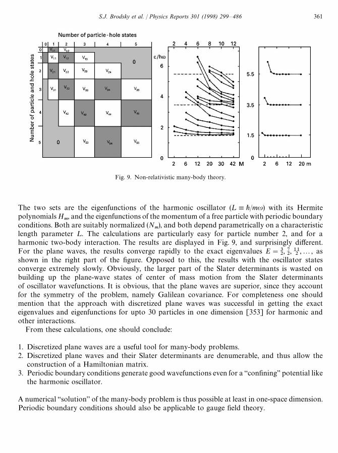
Fig. 9. Non-relativistic many-body theory.

The two sets are the eigenfunctions of the harmonic oscillator (¸,+/mu) with its Hermitepolynomials H

m, and the eigenfunctions of the momentum of a free particle with periodic boundary

conditions. Both are suitably normalized (Nm), and both depend parametrically on a characteristic

length parameter ¸. The calculations are particularly easy for particle number 2, and for aharmonic two-body interaction. The results are displayed in Fig. 9, and surprisingly different.For the plane waves, the results converge rapidly to the exact eigenvalues E"3

2, 72, 11

2,2, as

shown in the right part of the figure. Opposed to this, the results with the oscillator statesconverge extremely slowly. Obviously, the larger part of the Slater determinants is wasted onbuilding up the plane-wave states of center of mass motion from the Slater determinantsof oscillator wavefunctions. It is obvious, that the plane waves are superior, since they accountfor the symmetry of the problem, namely Galilean covariance. For completeness one shouldmention that the approach with discretized plane waves was successful in getting the exacteigenvalues and eigenfunctions for upto 30 particles in one dimension [353] for harmonic andother interactions.

From these calculations, one should conclude:

1. Discretized plane waves are a useful tool for many-body problems.2. Discretized plane waves and their Slater determinants are denumerable, and thus allow the

construction of a Hamiltonian matrix.3. Periodic boundary conditions generate good wavefunctions even for a “confining” potential like

the harmonic oscillator.

A numerical “solution” of the many-body problem is thus possible at least in one-space dimension.Periodic boundary conditions should also be applicable to gauge field theory.


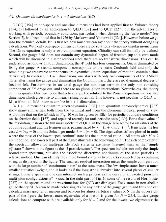
4.2. Quantum chromodynamics in 1#1 dimensions (KS)

DLCQ [354] in one-space and one-time dimensions had been applied first to Yukawa theory[354,355] followed by an application to QED [137] and to QCD [227], but the advantages ofworking with periodic boundary conditions, particularly when discussing the “zero modes” (seeSection 7), had been noted first in 1976 by Maskawa and Yamawaki [324]. However, before we gointo the technical details, let us first see how much we can say about the theory without doing anycalculations. With only one-space dimension there are no rotations — hence no angular momentum.The Dirac equation is only a two-component equation. Chirality can still formally be defined.Second, the gauge field does not contain any dynamical degree of freedom (up to a zero modewhich will be discussed in a later section) since there are no transverse dimensions. This can beunderstood as follows. In four dimensions, the Ak field has four components. One is eliminated byfixing the gauge. A second component corresponds to the static Coulomb field and only theremaining two transverse components are dynamical (their “equations of motion” contain a timederivative). In contrast, in 1#1 dimensions, one starts with only two components of the Ak-field.Thus, after fixing the gauge and eliminating the Coulomb part, there are no dynamical degrees offreedom left. Furthermore, in an axial gauge the nonlinear term in the only non-vanishingcomponent of Fkl drops out, and there are no gluon—gluon interactions. Nevertheless, the theoryconfines quarks. One way to see that is to analyze the solution to the Poisson equation in one-spacedimension which gives rise to a linearly rising potential. This however is not peculiar to QCD

1`1.

Most if not all field theories confine in 1#1 dimensions.In 1#1 dimensions quantum electrodynamics [137] and quantum chromodynamics [227]

show many similarities, both from the technical and from the phenomenological point of view.A plot like that on the left side in Fig. 10 was first given by Eller for periodic boundary conditionson the fermion fields [137], and repeated recently for anti-periodic ones [139]. For a fixed value ofthe resolution, it shows the full mass spectrum of QED in the charge zero sector for all values of thecoupling constant and the fermion mass, parametrized by j"(1#p(m/g)2)~1@2. It includes the freecase j"0 (g"0) and the Schwinger model j"1 (m"0). The eigenvalues M

iare plotted in units

where the mass of the lowest “positronium” state has the numerical value 1. All states with M'2are unbound. The lower left part of the figure illustrates the following point. The rich complexity ofthe spectrum allows for multi-particle Fock states at the same invariant mass as the “simpleqqN -states” shown in the figure as the “2 particle sector”. The spectrum includes not only the simplebound-state spectrum, but also the associated discretized continuum of the same particles inrelative motion. One can identify the simple bound states as two quarks connected by a confiningstring as displayed in the figure. The smallest residual interaction mixes the simple configurationwith the large number of “continuum states” at the same mass. The few simple states have a muchsmaller statistical weight, and it looks as if the long string “breaks” into several pieces of smallerstrings. Loosely speaking one can interpret such a process as the decay of an excited pion intomulti-pion configurations p*Pppp. In the right part of Fig. 10 some of the results of Hornbostel[227] on the spectrum and the wavefunctions for QCD are displayed. Fock states in non-abeliangauge theory SU(N) can be made color singlets for any order of the gauge group and thus one cancalculate mass spectra for mesons and baryons for almost arbitrary values of N. In the upper rightpart of the figure the lowest mass eigenvalue of a meson is given for N"2,3,4. Lattice gaugecalculations to compare with are available only for N"2 and for the lowest two eigenstates; the


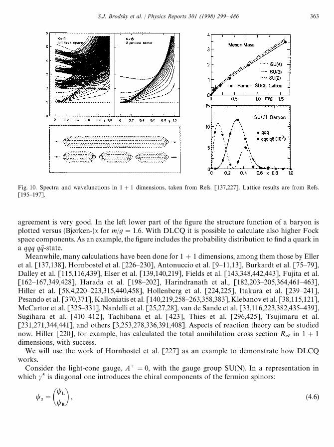
Fig. 10. Spectra and wavefunctions in 1#1 dimensions, taken from Refs. [137,227]. Lattice results are from Refs.[195—197].

agreement is very good. In the left lower part of the figure the structure function of a baryon isplotted versus (Bj+rken-)x for m/g"1.6. With DLCQ it is possible to calculate also higher Fockspace components. As an example, the figure includes the probability distribution to find a quark ina qqq qqN -state.

Meanwhile, many calculations have been done for 1#1 dimensions, among them those by Elleret al. [137,138], Hornbostel et al. [226—230], Antonuccio et al. [9—11,13], Burkardt et al. [75—79],Dalley et al. [115,116,439], Elser et al. [139,140,219], Fields et al. [143,348,442,443], Fujita et al.[162—167,349,428], Harada et al. [198—202], Harindranath et al., [182,203—205,364,461—463],Hiller et al. [58,4,220—223,315,440,458], Hollenberg et al. [224,225], Itakura et al. [239—241],Pesando et al. [370,371], Kalloniatis et al. [140,219,258—263,358,383],Klebanov et al. [38,115,121],McCartor et al. [325—331], Nardelli et al. [25,27,28], van de Sande et al. [33,116,223,382,435—439],Sugihara et al. [410—412], Tachibana et al. [423], Thies et al. [296,425], Tsujimaru et al.[231,271,344,441], and others [3,253,278,336,391,408]. Aspects of reaction theory can be studiednow. Hiller [220], for example, has calculated the total annihilation cross section R

eeNin 1#1

dimensions, with success.We will use the work of Hornbostel et al. [227] as an example to demonstrate how DLCQ

works.Consider the light-cone gauge, A`"0, with the gauge group SU(N). In a representation in

which c5 is diagonal one introduces the chiral components of the fermion spinors:

ta"At

Lt

RB , (4.6)


The usual group generators for SU(N) are the ¹a"12ja. In a box with length 2¸ one finds

tL(x)"!

im4 P

`L

~L

dy~e(x~!y~)tR(x`,y~) , (4.7)

A~a(x)"!

g2P

`L

~L

dy~Dx~!y~DtsR¹at

R(x`,y~) . (4.8)

The light-cone momentum and light-cone energy operators are

P`"P`L

~L

dx~tsR~

tR

, (4.9)

P~"!

im2

4 P`L

~L

dx~P`L

~L

dy~tsR(x~)e(x~!y~)t

R(y~)

!

g2

2 P`L

~L

dx~P`L

~L

dy~tsR¹at

R(x~)Dx~!y~Dts

R¹at

R(y~) , (4.10)

respectively. Here, t is subject to the canonical anti-commutation relations. For example, foranti-periodic boundary conditions one can expand

tR(x~)

c"

1

J2¸

=+

n/12,32,2

(bn,c

e~* nnx~@L#dsn,c

e* nnx~@L) , (4.11)

where

Mbsn,c1

, bm,c2

N"Mdsn,c1

, dm,c2

N"dc1,c2

dn,m

, (4.12)

with all other anticommutators vanishing. Inserting this expansion into the expressions for P`,Eq. (4.9), one thus finds

P`"A2p¸ B

=+

n/12,32,2

n(bsn,c

bn,c#ds

n,cdn,c

) . (4.13)

Similarly, one finds for P~ of Eq. (4.10)

P~"A¸

2pB(H0#») , (4.14)

where

H0"

=+

n/12,

32,2

m2

n(bs

n,cbn,c#ds

n,cdn,c

) (4.15)

is the free kinetic term, and the interaction term » is given by

»"

g2

p=+

k/~=

ja(k)1k2

ja(!k) , (4.16)


where

ja(k)"¹ac1,c2

=+

n/~=

(H(n)bsn,c1

#H(!n)dn,c1

)(H(n!k)bn~k,c2

#H(k!n)dsk~n,c2

) . (4.17)

Since we will restrict ourselves to the color singlet sector, there is no problem from k"0 inEq. (4.16), since ja(0)"0 acting on color singlet states. Normal ordering the interaction (4.16) givesa diagonal operator piece

»":»:#g2C

Fp

=+

n/12,

32,2

Inn

(bsn,c

bn,c#ds

n,cdn,c

) , (4.18)

with the “self-induced inertia”

In"!

12n

#

n`1@2+

m/1

1m2

. (4.19)

The color factor is CF"(N2!1)/2N. The explicit form of the normal ordered piece :»: can be

found in Ref. [227] or in the explicit tables below in this section. It is very important to keep theself-induced inertias from the normal ordering, because they are needed to cancel the infraredsingularity in the interaction term in the continuum limit. Already classically, the self energy of oneingle quark is infrared divergent because its color electric field extends to infinity. The sameinfrared singularity (with opposite sign) appears in the interaction term. They cancel for colorsinglet states, because there the color electric field is nonzero only inside the hadron. Since thehadron has a finite size, the resulting total color electric field energy must be infrared finite.

The next step is to actually solve the equations of motions in the discretized space. Typically oneproceeds as follows: Since P` and P~ commute they can be diagonalized simultaneously. Actually,in the momentum representation, P` is already diagonal, with eigenvalues proportional to 2p/¸.Therefore, the harmonic resolution K [137],

K"(¸/2p)P` , (4.20)

determines the size of the Fock space and thus the dimension of the Hamiltonian matrix, whichsimplifies the calculations considerably. For a given K"1, 2, 3,2, there are only a finite numberof Fock states due to the positivity condition on the light-cone momenta. One selects now onevalue for K and constructs all color singlet states. In the next step one can either diagonalize H inthe full space of states with momentum K (DLCQ approximation) or in a subspace of that space(for example with a Tamm—Dancoff approximation). The eigenvalue E

i(K) corresponds to invari-

ant masses

M2i(K),2P`

iP~

i"KE

i(K) , (4.21)

where we indicated the parametric dependence of the eigenvalues on K.Notice that the length ¸ drops out in the invariant mass, and that one gets a spectrum for any

value of K. Most recent developments in string theory, the so-called ‘M(atrix)-theory’ [416],emphasizes this aspect, but for the present one should consider the solutions to be physical only inthe continuum limit KPR.

Of course there are limitations on the size of matrices that one can diagonalize (although theLanczos algorithm allows quite impressive sizes [220]). Therefore what one typically does is to


repeat the calculations for increasing values of K and to extrapolate observables to KPR. Thefirst QCD

2calculations in that direction were performed in Refs. [227,75]. In these pioneering

works it was shown that the numerics actually converged rather quickly (except for very smallquark masses, where ground state mesons and ground state baryons become massless) since thelowest Fock component dominates these hadrons (typically less than 1% of the momentum iscarried by the sea component). The suppression of the higher particle Fock states is presumablyspecial to super-renormalizable theories where the couplings which change particle number aresuppressed as g2/M2. Due to these fortunate circumstances a variety of phenomena could beinvestigated. For example, Hornbostel studied hadron masses and structure functions for variousN which showed very simple scaling behavior with N. A correspondence with the analytic work ofEinhorn [136] for meson form factors in QCD

1`1was also established. Ref. [75] focused more on

nuclear phenomena. There it was shown that two nucleons in QCD1`1

with two colors and twoflavors form a loosely bound state — the “deuteron”. Since the calculation was based entirely onquark degrees of freedom it was possible to study binding effects on the nuclear structure function(“EMC-effect”). Other applications include a study of “Pauli-blocking” in QCD

1`1. Since quarks

are fermions, one would expect that sea quarks which have the same flavor as the majority of thevalence quarks (the up quarks in a proton) are suppressed compared to those which have theminority flavor (the down quarks in a proton) — at least if isospin breaking effects are small.However, an explicit calculation shows that the opposite is true in QCD

2! This so called “anti

Pauli-blocking” has been investigated in Refs. [76,77], where one can also find an intuitiveexplanation.

4.3. The Hamiltonian operator in 3#1 dimensions (B¸)

Periodic boundary conditions on L can be realized by periodic boundary conditions on thevector potentials Ak and anti-periodic boundary conditions on the spinor fields, since L is bilinearin the Wa. In momentum representation one expands these fields into plane wave states e~*pkxk, andsatisfies the boundary conditions by discretized momenta

p~"G

n¸

n with n"12,32,2,R for fermions ,

n¸

n with n"1,2,2,R for bosons ,(4.22)

pM"

n¸

M

nM

with nx, n

y"0, $1, $2,2,$R for both .

As an expense, one has to introduce two artificial length parameters, ¸ and ¸M. They also define

the normalization volume X,2¸(2¸M)2.

More explicitly, the free fields are expanded as

WI a(x)"1

JX+q

1

Jp`(b

qua(p, j)e~*px#ds

qva(p, j)e*px) ,

(4.23)

AI k(x)"1

JX+q

1

Jp`(a

qek(p, j)e~*px#as

qe*k (p, j)e*px) ,


particularly for the two transverse vector potentials AI i,AI iM

(i"1, 2). The light-cone gauge andthe light-cone Gauss equation, i.e. A`"0 and A~"(2g/(i`)2), J`!(2/(i`))i

jAj

M, respectively,

complete the specification of the vector potentials Ak. The subtlety of the missing zero-mode n"0in the expansion of the AI

Mwill be discussed below. Each denumerable single-particle state “q” is

specified by at least six quantum numbers, i.e.

q"Mq D k`, kMx

, kMy

, j, c, f N"Mq D n, nx, n

y, j, c, f N . (4.24)

The quantum numbers denote the three discrete momenta n, nx, n

y, the two helicities j"(C, B),

the color index c"1, 2,2, NC, and the flavor index f"1, 2,2, N

F. For a gluon state, the color

index is replaced by the glue index a"1, 2,2, N2C!1 and the flavor index is absent. Correspond-

ingly, for QED the color- and flavor index are absent. The creation and destruction operators likeasq

and aq

create and destroy single-particle states q, and obey (anti-) commutation relations like

[aq, as

q{]"Mb

q, bs

q{N"Md

q, ds

q{N"d

q,q{. (4.25)

The Kronecker symbol is unity only if all six quantum numbers coincide. The spinors ua and va, andthe transverse polarization vectors e

Mare the usual ones, and can be found in Ref. [66] and in the

appendix.Finally, after inserting all fields in terms of the expansions in Eq. (4.23), one performs the

space-like integrations and ends up with the light-cone energy—momenta Pl"Pl(a

q, as

q, b

q, bs

q, d

q, ds

q) as operators acting in Fock space. The space-like components of Pl are

simple and diagonal, and its time—time-like component is complicated and off-diagonal. ItsLorentz-invariant contraction

HLC,PlPl"P`P~!P2

M(4.26)

is then also off-diagonal. For simplicity, it is referred to as the light-cone Hamiltonian HLC

, and oftenabbreviated as H"H

LC. It carries the dimension of an invariant mass squared. In a frame in which

PM"0, it reduces to H"P`P~. It is useful to give its general structure in terms of Fock-space

operators.

4.3.1. A typical term of the Hamiltonian: Pure gauge theoryAs an example consider a typical term in the Hamiltonian, the pure gauge contribution ¼

1as

defined in Eq. (2.96), i.e.

P~pg"

g2

4 Pdx~d2xM

BI aklBI kla .

Inserting the free field solutions AI kafrom Eq. (4.23), one deals with 24"16 terms. The various terms

can be classified according to their operator structure and belong to one of the six classes.

aq1

aq2

aq3

aq4

, asq4

asq3

asq2

asq1

,

asq1

aq2

aq3

aq4

, asq4

asq3

asq2

aq1

,

asq1

asq2

aq3

aq4

, asq4

asq3

aq2

aq1

.

In the first step, we pick out only those terms with one creation and three destruction operators.Integration over the space-like coordinates produces a product of three Kronecker delta functions


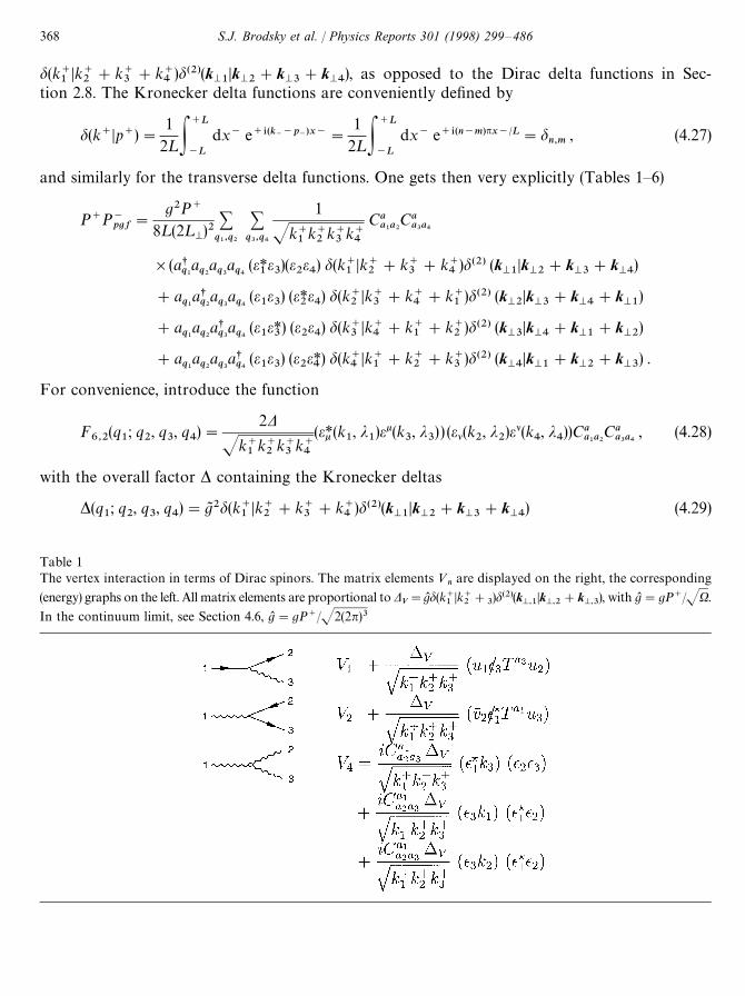
Table 1The vertex interaction in terms of Dirac spinors. The matrix elements »

nare displayed on the right, the corresponding

(energy) graphs on the left. All matrix elements are proportional to DV"gL d(k`

1Dk`

2#

3)d(2)(k

M,1Dk

M,2#k

M,3), with gL"gP`/JX.

In the continuum limit, see Section 4.6, gL "gP`/J2(2n)3

d(k`1

Dk`2#k`

3#k`

4)d(2)(k

M1Dk

M2#k

M3#k

M4), as opposed to the Dirac delta functions in Sec-

tion 2.8. The Kronecker delta functions are conveniently defined by

d(k`Dp`)"1

2¸P`L

~L

dx~ e`*(k~~p~)x~"

12¸P

`L

~L

dx~ e`*(n~m)px~@L"dn,m

, (4.27)

and similarly for the transverse delta functions. One gets then very explicitly (Tables 1—6)

P`P~pgf

"

g2P`

8¸(2¸M)2

+q1,q2

+q3,q4

1

Jk`1k`2

k`3

k`4

Caa1a2

Caa3a4

](asq1aq2aq3aq4

(e*1e3)(e

2e4) d(k`

1Dk`

2#k`

3#k`

4)d(2) (k

M1Dk

M2#k

M3#k

M4)

#aq1asq2aq3aq4

(e1e3) (e*

2e4) d(k`

2Dk`

3#k`

4#k`

1)d(2) (k

M2Dk

M3#k

M4#k

M1)

#aq1aq2asq3aq4

(e1e*3) (e

2e4) d(k`

3Dk`

4#k`

1#k`

2)d(2) (k

M3Dk

M4#k

M1#k

M2)

#aq1aq2aq3asq4

(e1e3) (e

2e*4) d(k`

4Dk`

1#k`

2#k`

3)d(2) (k

M4Dk

M1#k

M2#k

M3) .

For convenience, introduce the function

F6,2

(q1; q

2, q

3, q

4)"

2D

Jk`1

k`2

k`3k`4

(e*k (k1, j

1)ek(k

3, j

3) ) (el(k2, j2)el(k4, j4))Ca

a1a2Ca

a3a4, (4.28)

with the overall factor * containing the Kronecker deltas

*(q1; q

2, q

3, q

4)"gJ 2d(k`

1Dk`

2#k`

3#k`

4)d(2)(k

M1Dk

M2#k

M3#k

M4) (4.29)


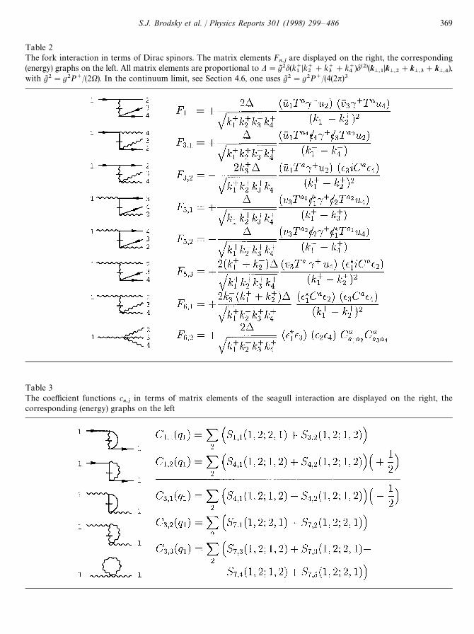
Table 2The fork interaction in terms of Dirac spinors. The matrix elements F

n,jare displayed on the right, the corresponding

(energy) graphs on the left. All matrix elements are proportional to D"gJ 2d(k`1Dk`

2#k`

3#k`

4)d(2)(k

M,1Dk

M,2#k

M,3#k

M,4),

with gJ 2"g2P`/(2X). In the continuum limit, see Section 4.6, one uses gJ 2"g2P`/(4(2n)3

Table 3The coefficient functions c

n,jin terms of matrix elements of the seagull interaction are displayed on the right, the

corresponding (energy) graphs on the left


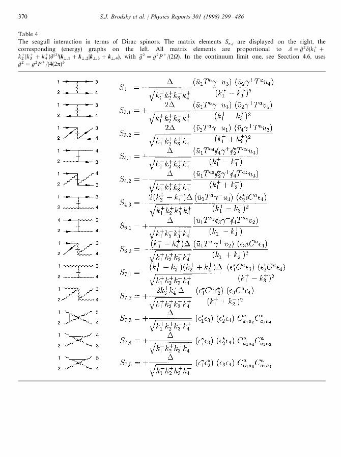
Table 4The seagull interaction in terms of Dirac spinors. The matrix elements S

n,jare displayed on the right, the

corresponding (energy) graphs on the left. All matrix elements are proportional to D"gJ 2d(k`1#

k`2Dk`

3#k`

4)d(2)(k

M,1#k

M,2Dk

M,3#k

M,4), with gJ 2"g2P`/(2X). In the continuum limit one, see Secction 4.6, uses

gJ 2"g2P`/(4(2p)3


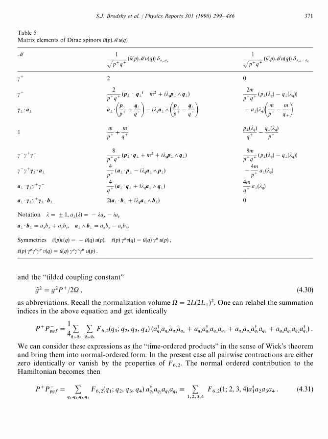
Table 5Matrix elements of Dirac spinors uN (p)Mu(q)

M 1

Jp`q`(uN (p)Mu(q)) djp,jq

1

Jp`q`(uN (p)Mu(q)) djp,~jq

c` 2 0

c~2

p`q`(p

M) q

Mg m2#ij

qpM'q

M)

2m

p`q`(p

M(j

q)!q

M(j

q))

cM) a

MaM)A

pM

p`#

qM

q`B!ijqaM'A

pM

p`!

qM

q`B !aM(j

q)A

m

p`!

m

q`B

1m

p`#

m

q`

pM(j

q)

q`!

qM(j

q)

p`

c~c`c~8

p`q`(p

M) q

M#m2#ij

qpM'q

M)

8m

p`q`(p

M(j

q)!q

M(j

q))

c~c`cM) a

M

4

p`(a

M) p

M!ij

qaM'p

M) !

4m

p`aM(j

q)

aM) c

Mc`c~

4

q`(a

M) q

M#ij

qaM'q

M)

4m

q`aM(j

q)

aM) c

Mc`c

M) b

M2(a

M) b

M#ij

qaM'b

M) 0

Notation j"$1, aM(j)"!ja

x!ia

y

aM) b

M"a

xbx#a

yby, a

M'b

M"a

xby!a

ybx.

Symmetries vN (p)v(q)"!uN (q) u(p), vN (p) ckv(q)"uN (q) ck u(p) ,

vN (p) ckclco v(q)"uN (q) coclck u(p) .

and the “tilded coupling constant”

gJ 2"g2P`/2X , (4.30)

as abbreviations. Recall the normalization volume X"2¸(2¸M)2. One can relabel the summation

indices in the above equation and get identically

P`P~pgf

"

14

+q1,q2

+q3,q4

F6,2

(q1; q

2, q

3, q

4) (as

q1aq2aq3aq4#a

q2asq1aq4aq3#a

q3aq4asq1aq2#a

q4aq3aq2asq1) .

We can consider these expressions as the “time-ordered products” in the sense of Wick’s theoremand bring them into normal-ordered form. In the present case all pairwise contractions are eitherzero identically or vanish by the properties of F

6,2. The normal ordered contribution to the

Hamiltonian becomes then

P`P~pgf

" +q1,q2,q3,q4

F6,2

(q1; q

2, q

3, q

4) as

q1aq2aq3aq4, +

1,2,3,4

F6,2

(1; 2, 3, 4)as1a2a3a4

. (4.31)


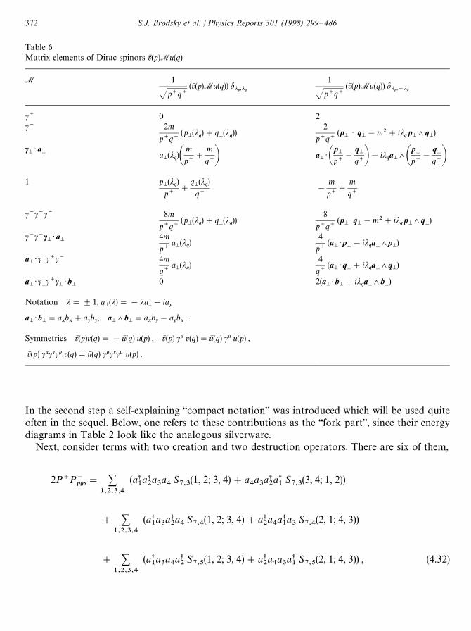
Table 6Matrix elements of Dirac spinors vN (p)Mu(q)

M 1

Jp`q`(vN (p)Mu(q)) djp,jq

1

Jp`q`(vN (p)Mu(q)) djp,~jq

c` 0 2c~ 2m

p`q`(p

M(j

q)#q

M(j

q))

2

p`q`(p

M) q

M!m2#ij

qpM'q

M)

cM) a

M aM(j

q)A

m

p`#

m

q`B aM)A

pM

p`#

qM

q`B!ijqaM'A

pM

p`!

qM

q`B1 p

M(j

q)

p`#

qM(j

q)

q`!

m

p`#

m

q`

c~c`c~ 8m

p`q`(p

M(j

q)#q

M(j

q))

8

p`q`(p

M) q

M!m2#ij

qpM'q

M)

c~c`cM) a

M4m

p`aM(j

q)

4

p`(a

M) p

M!ij

qaM'p

M)

aM) c

Mc`c~ 4m

q`aM(j

q)

4

q`(a

M) q

M#ij

qaM'q

M)

aM) c

Mc`c

M) b

M0 2(a

M) b

M#ij

qaM'b

M)

Notation j"$1, aM(j)"!ja

x!ia

y

aM) b

M"a

xbx#a

yby, a

M'b

M"a

xby!a

ybx.

Symmetries vN (p)v(q)"!uN (q) u(p) , vN (p) ck v(q)"uN (q) ck u(p) ,

vN (p) ckclco v(q)"uN (q) coclck u(p) .

In the second step a self-explaining “compact notation” was introduced which will be used quiteoften in the sequel. Below, one refers to these contributions as the “fork part”, since their energydiagrams in Table 2 look like the analogous silverware.

Next, consider terms with two creation and two destruction operators. There are six of them,

2P`P~pgs

" +1,2,3,4

(as1as2a3a4

S7,3

(1, 2; 3, 4)#a4a3as2as1

S7,3

(3, 4; 1, 2))

# +1,2,3,4

(as1a3as2a4

S7,4

(1, 2; 3, 4)#as2a4as1a3

S7,4

(2, 1; 4, 3))

# +1,2,3,4

(as1a3a4as2

S7,5

(1, 2; 3, 4)#as2a4a3as1

S7,5

(2, 1; 4, 3)) , (4.32)


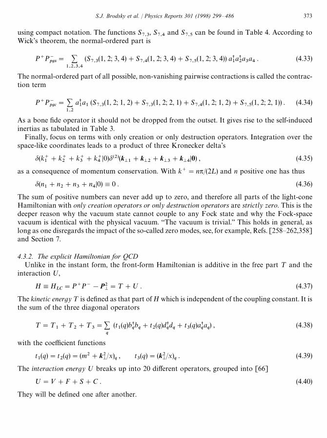
using compact notation. The functions S7,3

, S7,4

and S7,5

can be found in Table 4. According toWick’s theorem, the normal-ordered part is

P`P~pgs

" +1,2,3,4

(S7,3

(1, 2; 3, 4)#S7,4

(1, 2; 3, 4)#S7,5

(1, 2; 3, 4)) as1as2a3a4

. (4.33)

The normal-ordered part of all possible, non-vanishing pairwise contractions is called the contrac-tion term

P`P~pgc

"+1,2

as1a1

(S7,3

(1, 2; 1, 2)#S7,3

(1, 2; 2, 1)#S7,4

(1, 2; 1, 2)#S7,5

(1, 2; 2, 1)) . (4.34)

As a bone fide operator it should not be dropped from the outset. It gives rise to the self-inducedinertias as tabulated in Table 3.

Finally, focus on terms with only creation or only destruction operators. Integration over thespace-like coordinates leads to a product of three Kronecker delta’s

d(k`1#k`

2#k`

3#k`

4D0)d(2)(k

M1#k

M2#k

M3#k

M4D0) , (4.35)

as a consequence of momentum conservation. With k`"np/(2¸) and n positive one has thus

d(n1#n

2#n

3#n

4D0),0 . (4.36)

The sum of positive numbers can never add up to zero, and therefore all parts of the light-coneHamiltonian with only creation operators or only destruction operators are strictly zero. This is thedeeper reason why the vacuum state cannot couple to any Fock state and why the Fock-spacevacuum is identical with the physical vacuum. “The vacuum is trivial.” This holds in general, aslong as one disregards the impact of the so-called zero modes, see, for example, Refs. [258—262,358]and Section 7.

4.3.2. The explicit Hamiltonian for QCDUnlike in the instant form, the front-form Hamiltonian is additive in the free part ¹ and the

interaction º,

H,HLC"P`P~!P2

M"¹#º . (4.37)

The kinetic energy ¹ is defined as that part of H which is independent of the coupling constant. It isthe sum of the three diagonal operators

¹"¹1#¹

2#¹

3"+

q

(t1(q)bs

qbq#t

2(q)ds

qdq#t

3(q)as

qaq) , (4.38)

with the coefficient functions

t1(q)"t

2(q)"(m2#k2

M/x)

q, t

3(q)"(k2

M/x)

q. (4.39)

The interaction energy º breaks up into 20 different operators, grouped into [66]

º"»#F#S#C . (4.40)

They will be defined one after another.


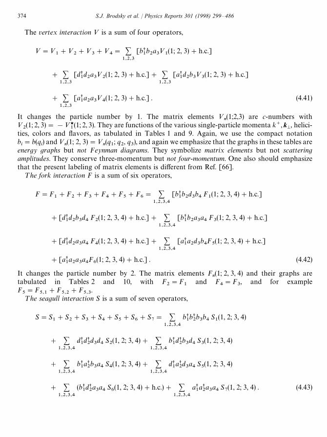
The vertex interaction » is a sum of four operators,

»"»1#»

2#»

3#»

4" +

1,2,3

[bs1b2a3»

1(1; 2, 3)#h.c.]

# +1,2,3

[ds1d2a3»

2(1; 2, 3)#h.c.]# +

1,2,3

[as1d2b3»

3(1; 2, 3)#h.c.]

# +1,2,3

[as1a2a3»

4(1; 2, 3)#h.c.] . (4.41)

It changes the particle number by 1. The matrix elements »n(1;2,3) are c-numbers with

»2(1; 2, 3)"!»

w

1(1; 2, 3). They are functions of the various single-particle momenta k`, k

M, helici-

ties, colors and flavors, as tabulated in Tables 1 and 9. Again, we use the compact notationbi"b(q

i) and »

n(1; 2, 3)"»

n(q

1; q

2, q

3), and again we emphasize that the graphs in these tables are

energy graphs but not Feynman diagrams. They symbolize matrix elements but not scatteringamplitudes. They conserve three-momentum but not four-momentum. One also should emphasizethat the present labeling of matrix elements is different from Ref. [66].

¹he fork interaction F is a sum of six operators,

F"F1#F

2#F

3#F

4#F

5#F

6" +

1,2,3,4

[bs1b2d3b4

F1(1; 2, 3, 4)#h.c.]

#[ds1d2b3d4

F2(1; 2, 3, 4)#h.c.]# +

1,2,3,4

[bs1b2a3a4

F3(1; 2, 3, 4)#h.c.]

#[ds1d2a3a4

F4(1; 2, 3, 4)#h.c.]# +

1,2,3,4

[as1a2d3b4F

5(1; 2, 3, 4)#h.c.]

#[as1a2a3a4F6(1; 2, 3, 4)#h.c.] . (4.42)

It changes the particle number by 2. The matrix elements Fn(1; 2, 3, 4) and their graphs are

tabulated in Tables 2 and 10, with F2"F

1and F

4"F

3, and for example

F5"F

5,1#F

5,2#F

5,3.

¹he seagull interaction S is a sum of seven operators,

S"S1#S

2#S

3#S

4#S

5#S

6#S

7" +

1,2,3,4

bs1bs2b3b4

S1(1, 2; 3, 4)

# +1,2,3,4

ds1ds2d3d4

S2(1, 2; 3, 4)# +

1,2,3,4

bs1ds2b3d4

S3(1, 2; 3, 4)

# +1,2,3,4

bs1as2b3a4

S4(1, 2; 3, 4)# +

1,2,3,4

ds1as2d3a4

S5(1, 2; 3, 4)

# +1,2,3,4

(bs1ds2a3a4

S6(1, 2; 3, 4)#h.c.)# +

1,2,3,4

as1as2a3a4

S7(1, 2; 3, 4) . (4.43)


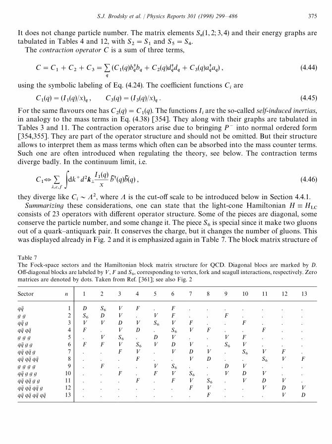
Table 7The Fock-space sectors and the Hamiltonian block matrix structure for QCD. Diagonal blocs are marked by D.Off-diagonal blocks are labeled by », F and S

6, corresponding to vertex, fork and seagull interactions, respectively. Zero

matrices are denoted by dots. Taken from Ref. [361]; see also Fig. 2

Sector n 1 2 3 4 5 6 7 8 9 10 11 12 13

qqN 1 D S6

» F . F . . . . . . .g g 2 S

6D » . » F . . F . . . .

qqN g 3 » » D » S6

» F . . F . . .qqN qqN 4 F . » D . S

6» F . . F . .

g g g 5 . » S6

. D » . . » F . . .qqN g g 6 F F » S

6» D » . S

6» . . .

qqN qqN g 7 . . F » . » D » . S6

» F .qqN qqN qqN 8 . . . F . . » D . . S

6» F

g g g g 9 . F . . » S6

. . D » . . .qqN g g g 10 . . F . F » S

6. » D » . .

qqN qqN g g 11 . . . F . F » S6

. » D » .qqN qqN qqN g 12 . . . . . . F » . . » D »

qqN qqN qqN qqN 13 . . . . . . . F . . . » D

It does not change particle number. The matrix elements Sn(1, 2; 3, 4) and their energy graphs are

tabulated in Tables 4 and 12, with S2"S

1and S

5"S

4.

The contraction operator C is a sum of three terms,

C"C1#C

2#C

3"+

q

(C1(q)bs

qbq#C

2(q)ds

qdq#C

3(q)as

qaq) , (4.44)

using the symbolic labeling of Eq. (4.24). The coefficient functions Ciare

C1(q)"(I

1(q)/x)

q, C

3(q)"(I

3(q)/x)

q. (4.45)

For the same flavours one has C2(q)"C

1(q). The functions I

iare the so-called self-induced inertias,

in analogy to the mass terms in Eq. (4.38) [354]. They along with their graphs are tabulated inTables 3 and 11. The contraction operators arise due to bringing P~ into normal ordered form[354,355]. They are part of the operator structure and should not be omitted. But their structureallows to interpret them as mass terms which often can be absorbed into the mass counter terms.Such one are often introduced when regulating the theory, see below. The contraction termsdiverge badly. In the continuum limit, i.e.

C1Q +

j,c,f Pdk`d2kM

I1(q)x

bI s(q)bI (q) , (4.46)

they diverge like Ci&K2, where K is the cut-off scale to be introduced below in Section 4.4.1.

Summarizing these considerations, one can state that the light-cone Hamiltonian H,HLC

consists of 23 operators with different operator structure. Some of the pieces are diagonal, someconserve the particle number, and some change it. The piece S

6is special since it make two gluons

out of a quark—antiquark pair. It conserves the charge, but it changes the number of gluons. Thiswas displayed already in Fig. 2 and it is emphasized again in Table 7. The block matrix structure of


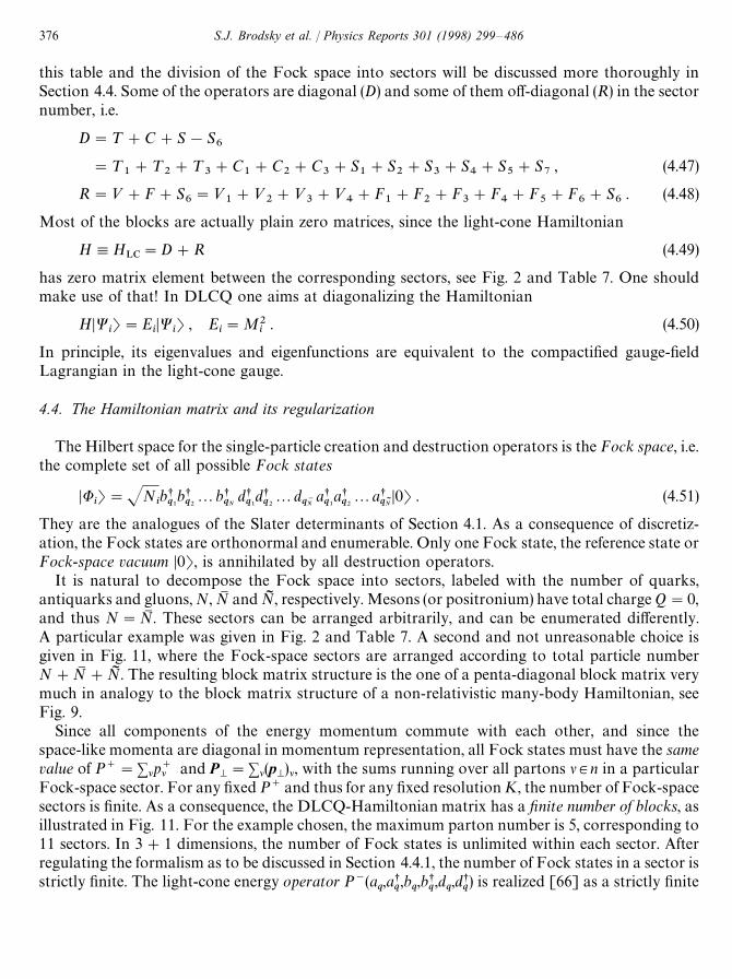
this table and the division of the Fock space into sectors will be discussed more thoroughly inSection 4.4. Some of the operators are diagonal (D) and some of them off-diagonal (R) in the sectornumber, i.e.

D"¹#C#S!S6

"¹1#¹

2#¹

3#C

1#C

2#C

3#S

1#S

2#S

3#S

4#S

5#S

7, (4.47)

R"»#F#S6"»

1#»

2#»

3#»

4#F

1#F

2#F

3#F

4#F

5#F

6#S

6. (4.48)

Most of the blocks are actually plain zero matrices, since the light-cone Hamiltonian

H,HLC"D#R (4.49)

has zero matrix element between the corresponding sectors, see Fig. 2 and Table 7. One shouldmake use of that! In DLCQ one aims at diagonalizing the Hamiltonian

HDWiT"E

iDW

iT , E

i"M2

i. (4.50)

In principle, its eigenvalues and eigenfunctions are equivalent to the compactified gauge-fieldLagrangian in the light-cone gauge.

4.4. The Hamiltonian matrix and its regularization

The Hilbert space for the single-particle creation and destruction operators is the Fock space, i.e.the complete set of all possible Fock states

DUiT"JN

ibsq1bsq22

bsqN

dsq1dsq22d

qNMasq1asq22

asqNI

D0T . (4.51)

They are the analogues of the Slater determinants of Section 4.1. As a consequence of discretiz-ation, the Fock states are orthonormal and enumerable. Only one Fock state, the reference state orFock-space vacuum D0T, is annihilated by all destruction operators.

It is natural to decompose the Fock space into sectors, labeled with the number of quarks,antiquarks and gluons, N, NM and NI , respectively. Mesons (or positronium) have total charge Q"0,and thus N"NM . These sectors can be arranged arbitrarily, and can be enumerated differently.A particular example was given in Fig. 2 and Table 7. A second and not unreasonable choice isgiven in Fig. 11, where the Fock-space sectors are arranged according to total particle numberN#NM #NI . The resulting block matrix structure is the one of a penta-diagonal block matrix verymuch in analogy to the block matrix structure of a non-relativistic many-body Hamiltonian, seeFig. 9.

Since all components of the energy momentum commute with each other, and since thespace-like momenta are diagonal in momentum representation, all Fock states must have the samevalue of P`"+lp`l and P

M"+l(pM

)l, with the sums running over all partons l3n in a particularFock-space sector. For any fixed P` and thus for any fixed resolution K, the number of Fock-spacesectors is finite. As a consequence, the DLCQ-Hamiltonian matrix has a finite number of blocks, asillustrated in Fig. 11. For the example chosen, the maximum parton number is 5, corresponding to11 sectors. In 3#1 dimensions, the number of Fock states is unlimited within each sector. Afterregulating the formalism as to be discussed in Section 4.4.1, the number of Fock states in a sector isstrictly finite. The light-cone energy operator P~(a

q,as

q,b

q,bs

q,d

q,ds

q) is realized [66] as a strictly finite


Fig. 11. The Hamiltonian matrix for a meson. Allowing for a maximum parton number 5, the Fock space can be dividedinto 11 sectors. Each sector contains enumerably many Fock states. Matrix elements are represented by “energy”diagrams which are characteristic for each block. Blocks with no diagrams are zero matrices. Note that the figure mixesaspects of QCD where the single gluon is absent and of QED which has no three-photon vertices.

Heisenberg matrix with strictly finite matrix elements. From a technical point of view this is simplerthan the complicated integral equations discussed in Section 3.

4.4.1. Fock-space regularizationIn an arbitrary frame, each particle is on its mass-shell p2"m2. Its four-momentum is

pk"(p`, pM, p~) with p~"(m2#p2

M)/p`. For the free theory (g"0), the total four-momentum is

Pk&3%%

"+lpkl where the index l runs over all particles in a particular Fock-space sectorDU

nT"SnDU

nT. The components of the free four-momentum are

Pk&3%%

"+l|n

(pk)l . (4.52)

Note that the spatial components are Pk"Pk&3%%

. As usual, one introduces intrinsic momenta x andkM

by

xl"p`lP`

, (pM)l"(k

M)l#xlPM

. (4.53)


The spatial components of Eq. (4.52) become then the constraints

+l

xl"1 , +l

(kM)l"0 , (4.54)

while the free invariant mass of a Fock state becomes

M2&3%%

"Pk&3%%

P&3%%,k"A+

l|n(pk)lBA+

l|n(pk)lB (4.55)

and, therefore,

M2&3%%

"+l|n A

m2#k2M

x Bl . (4.56)

The free invariant mass squared has a minimum with respect to kM

and x, at kM"0 and at

(xl).*/"ml/+

l|nml , (4.57)

respectively, and has the value

MM 2&3%%

,minA+l|n A

m2#k2M

x BlBKA+l|n

mlB2

. (4.58)

In the continuum limit the equality is strict. Physically, this corresponds to having all constituentsat the same rapidity. The minimal mass-squared is frozen-in and cannot be shared by the particlesoff-shell. The available mass-squared M2

&3%%!MM 2

&3%%is therefore the physically meaningful quantity.

The available mass-squared M2&3%%

!MM 2&3%%

plays the same role in DLCQ as the kinetic energy¹ in non-relativistic quantum mechanics, see also Section 4.1. The analogy can be used to regulatethe Fock space: A Fock state is admitted only when its “off-shell” kinetic energy is below a certaincut-off, i.e.

+l|n A

m2#k2M

x Bl!MM 2&3%%

4K2 . (4.59)

Except for the term MM 2&3%%

, this dynamic regularization scheme is nothing but the Brodsky—Lepageregularization [62,53,299,300]. It also defines a factorization scheme for hard scattering processesin perturbative QCD. Since only Lorentz scalars appear, this regularization is Lorentz but notnecessarily gauge-invariant. The constant K has the dimension of a SmassT and is at our disposal.Other cut-offs have also been proposed [363,456]. It is self-understood that the cut-off scale can bemade sector dependent. DLCQ has an option for having as many “sector-dependent regularizationparameters” as might be convenient. As a result of Fock-space regularization the Fock space andtherefore the dimension of the Hamiltonian matrix is strictly finite.

4.4.2. Vertex regularizationFock-space regularization turns out to be insufficient when dealing with products of operators

like »». More specifically, sums over intermediate states diverge badly for almost all matrixelements S1D»»D4T"+

2,3S1D»D2, 3TS2, 3D»D4T. One must introduce additional regularization


schemes, which is not always easy. One possible choice is to regulate the interaction on the operatorlevel, for example by multiplying each matrix element in Eq. (4.41) with a cut-off function H. Forthe vertex interaction one can thus define

»n(q

1; q

2, q

3)N»M

n(q

1; q

2, q

3)"»

n(q

1; q

2, q

3) H

V(q

1; q

2, q

3),

with

HV(q

1; q

2, q

3)"H

Q(q

1; q

2) H

M(q

2, q

3) . (4.60)

The two-step functions are

HQ(q

1; q

2)"G

1 if [(p1!p

2)2!(m

1!m

2)2]4K2 ,

0 otherwise,(4.61)

HM

(q1; q

2)"G

1 if [(p1#p

2)2!(m

1#m

2)2]4K2 ,

0 otherwise.(4.62)

The single-particle momenta piare those associated with the state q

i, see above. H

Qis a measure for

the momentum transfer and HM

a measure for the off-shell mass induced across the vertex. Thescale parameter K may be (or may not be) the same as in Section 4.4.1. This vertex regularizationrealizes what has been referred to by Lepage as a local regulator as opposed to the globalFock-space regulator in Eq. (4.59). It is generalizable to forks and seagulls and reads there

Fn(q

1; q

2, q

3, q

4)NFM

n(q

1; q

2, q

3)"F

n(q

1; q

2, q

3, q

4) H

F(q

1; q

2, q

3, q

4) ,

with

HF(q

1; q

2, q

3, q

4)"H

Q(q

1; q

2) H

M(q

3, q

4) ,

Sn(q

1, q

2; q

3, q

4)NSM

n(q

1, q

2; q

3, q

4)"S

n(q

1, q

2; q

3, q

4) H

S(q

1, q

2; q

3, q

4) , (4.63)

with

HS(q

1, q

2; q

3, q

4)"H

Q(q

1; q

2) H

Q(q

3, q

4)H

M(q

3, q

4) . (4.64)

It regulates automatically the contractions, i.e. the regulated expressions in Eq. (4.34) becomefinite

P`P~pgc

"+1,2

as1a1(SM

7,3(1, 2; 1, 2)#SM

7,3(1, 2; 2, 1)#SM

7,4(1, 2; 1, 2)#SM

7,5(1, 2; 2, 1)) . (4.65)

Note that vertex regularization is frame-independent.

4.4.3. RenormalizationRenormalization is simple in principle: The eigenvalues may not depend on the regulator scale(s)

K. Thus, if the eigenvalue equation is

H(K)DWiT"E

i(K)DW

iT , E

i"M2

i(4.66)

one must require that

dEi(K)/dK"0 for all i , (4.67)


up to terms of order 1/K. To require this is easier than to find a practical realization. As a matter offact, it has not been found yet, irrespective of whether one deals with the compactified or thecontinuum theory, see Section 8.

4.4.4. The key challenge in DLCQIn principle, one can proceed for 3#1 dimensions like in Section 4.2 for 1#1 dimensions: One

selects a particular value of the harmonic resolution K and the cut-off K, and diagonalizes thefinite-dimensional Hamiltonian matrix by numerical methods.

If this is all so simple, why has the problem not been solved a long time ago? What is the keyproblem?

The bottle neck of any field theoretic Hamiltonian approach in physical space—time is that thedimension of the Hamiltonian matrix increases exponentially fast with K, and that one may notsimply truncate the Fock-space at pleasure, because of gauge invariance. Let us consider theconcrete example of harmonic resolution K"5, as illustrated in Fig. 2 and Table 7. Suppose, theregularization procedure allows for 10 discrete momentum states in each direction. A single particlehas about 103 degrees of freedom. A Fock-space sector with n particles has then roughly 10n~1different Fock states. The qqN -sector has thus about 103 Fock states. Sector 13 in Fig. 2 with its8 particles has thus about 1021 Fock states. Chemists are able to handle matrices with some 107dimensions, but 1021 dimensions exceed the calculational capacity of any computer in theforeseeable future. The problem is a grave one, in particular since one has to diagonalize theHamiltonian for KPR.

For physical space—time one is thus thrown back to the same (insoluble?) problem as inconventional many-body physics as displayed in Fig. 9. One has to diagonalize finite matrices withexponentially large dimensions (typically'106). In fact, in quantum field theory the problem isworse since particle number is not conserved. Even advanced numerical methods or the methods ofmodern quantum chemistry are apparently insufficient for the task. One needs to develop effectiveinteractions which act in smaller matrix spaces and still are related to the full interaction. In a way,deriving an effective interaction can be understood as the aim to reduce the dimension of a matrixin a diagonalization problem from 1021 to 103!

In the present we shall mention three perhaps promising developments, namely theTamm—Dancoff approach, the similarity scheme and the Hamiltonian flow equations, but forphysical space—time, the final break-through has not been achieved, yet.

1. The effective interaction a la Tamm [421] and Dancoff [117] can be generalized by the method ofiterated resolvents [188,357,361,362] to avoid the most brutal violations of gauge invariance.Because of this, Wolfgang Pauli is reported to have called the Tamm—Dancoff approach “the moststupid idea I have ever seen”. This approach will be presented more thoroughly in Section 4.7.

2. The similarity scheme of G"azek and Wilson [184,185,456] will be discussed in Section 8.3. The Hamiltonian flow equations have been proposed recently by Wegner [188,447]. In view of

recent work by Lenz and Wegner on the particle—phonon model in solid state theory [294] theyseem to be rather promising. Wegner has found and applied a unitary transformation º(l) to anarbitrary matrix as given for example in Table 8, such that º(l) depends on a continuousparameter l. It has the property that

d/dl Tr(R(l)R(l))(0 , (4.68)


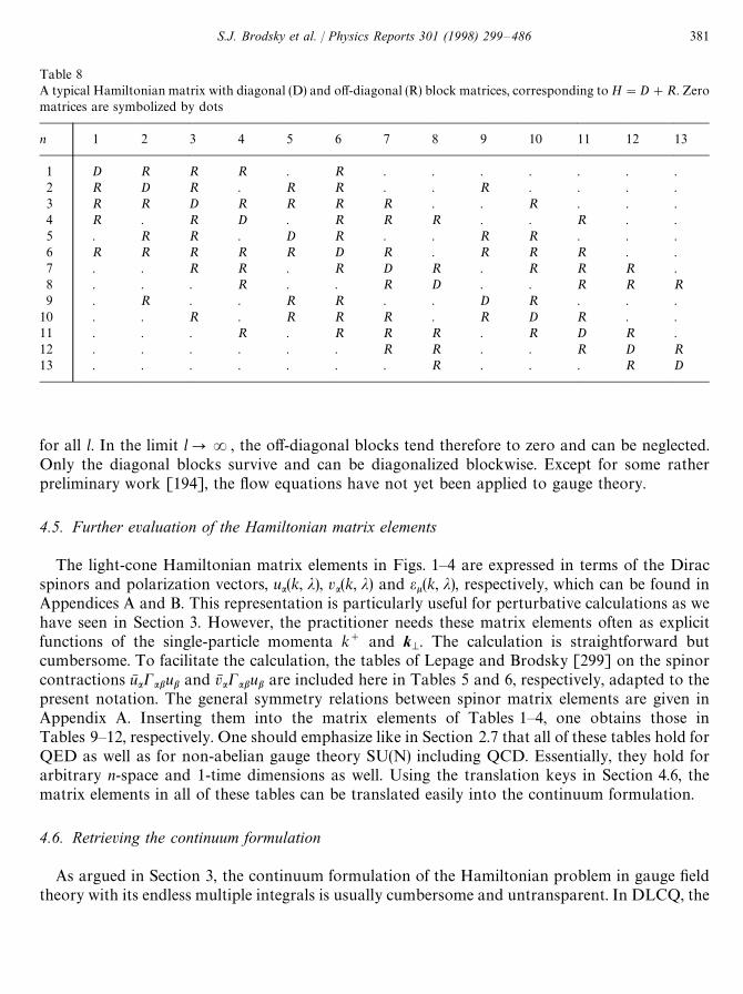
Table 8A typical Hamiltonian matrix with diagonal (D) and off-diagonal (R) block matrices, corresponding to H"D#R. Zeromatrices are symbolized by dots

n 1 2 3 4 5 6 7 8 9 10 11 12 13

1 D R R R . R . . . . . . .2 R D R . R R . . R . . . .3 R R D R R R R . . R . . .4 R . R D . R R R . . R . .5 . R R . D R . . R R . . .6 R R R R R D R . R R R . .7 . . R R . R D R . R R R .8 . . . R . . R D . . R R R9 . R . . R R . . D R . . .

10 . . R . R R R . R D R . .11 . . . R . R R R . R D R .12 . . . . . . R R . . R D R13 . . . . . . . R . . . R D

for all l. In the limit lPR, the off-diagonal blocks tend therefore to zero and can be neglected.Only the diagonal blocks survive and can be diagonalized blockwise. Except for some ratherpreliminary work [194], the flow equations have not yet been applied to gauge theory.

4.5. Further evaluation of the Hamiltonian matrix elements

The light-cone Hamiltonian matrix elements in Figs. 1—4 are expressed in terms of the Diracspinors and polarization vectors, ua(k, j), va(k, j) and ek(k, j), respectively, which can be found inAppendices A and B. This representation is particularly useful for perturbative calculations as wehave seen in Section 3. However, the practitioner needs these matrix elements often as explicitfunctions of the single-particle momenta k` and k

M. The calculation is straightforward but

cumbersome. To facilitate the calculation, the tables of Lepage and Brodsky [299] on the spinorcontractions uN aCabub and vN aCabub are included here in Tables 5 and 6, respectively, adapted to thepresent notation. The general symmetry relations between spinor matrix elements are given inAppendix A. Inserting them into the matrix elements of Tables 1—4, one obtains those inTables 9—12, respectively. One should emphasize like in Section 2.7 that all of these tables hold forQED as well as for non-abelian gauge theory SU(N) including QCD. Essentially, they hold forarbitrary n-space and 1-time dimensions as well. Using the translation keys in Section 4.6, thematrix elements in all of these tables can be translated easily into the continuum formulation.

4.6. Retrieving the continuum formulation

As argued in Section 3, the continuum formulation of the Hamiltonian problem in gauge fieldtheory with its endless multiple integrals is usually cumbersome and untransparent. In DLCQ, the


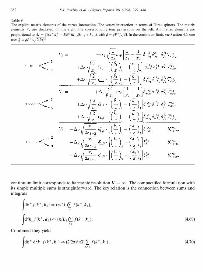
Table 9The explicit matrix elements of the vertex interaction. The vertex interaction in terms of Dirac spinors. The matrixelements »

nare displayed on the right, the corresponding (energy) graphs on the left. All matrix elements are

proportional to DV"gL d(k`

1Dk`

2#3)d(2)(k

M,1Dk

M,2#k

M,3), with gL "gP`/JX. In the continuum limit, see Section 4.6, one

uses gL "gP`/J2(2n)3

continuum limit corresponds to harmonic resolution KPR. The compactified formulation withits simple multiple sums is straightforward. The key relation is the connection between sums andintegrals

Pdk` f (k`, kM) Q (p/2¸)+

n

f (k`, kM),

Pd2kM

f (k`, kM) Q (p/¸

M)+nM

f (k`, kM) . (4.69)

Combined they yield

Pdk` d2kM

f (k`, kM) Q (2(2p)3/X) +

n,nM

f (k`, kM) . (4.70)


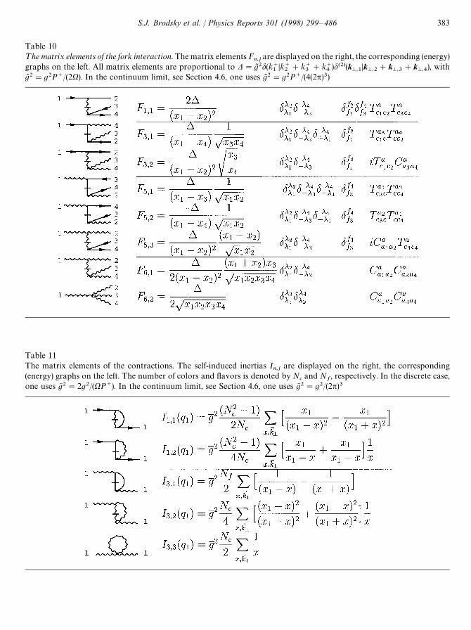
Table 10¹he matrix elements of the fork interaction. The matrix elements F

n,jare displayed on the right, the corresponding (energy)

graphs on the left. All matrix elements are proportional to D"gJ 2d(k`1Dk`

2#k`

3#k`

4)d(2)(k

M,1Dk

M,2#k

M,3#k

M,4), with

gJ 2"g2P`/(2X). In the continuum limit, see Section 4.6, one uses gJ 2"g2P`/(4(2p)3)

Table 11The matrix elements of the contractions. The self-induced inertias I


(energy) graphs on the left. The number of colors and flavors is denoted by Ncand N

f, respectively. In the discrete case,

one uses gN 2"2g2/(XP`). In the continuum limit, see Section 4.6, one uses gN 2"g2/(2p)3


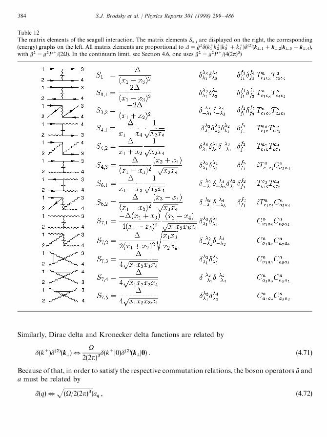
Table 12The matrix elements of the seagull interaction. The matrix elements S


(energy) graphs on the left. All matrix elements are proportional to D"gJ 2d(k`1k`2Dk`

3#k`

4)d(2)(k

M,1#k

M,2Dk

M,3#k

M,4),

with gJ 2"g2P`/(2X). In the continuum limit, see Section 4.6, one uses gJ 2"g2P`/(4(2p)3)

Similarly, Dirac delta and Kronecker delta functions are related by

d(k`)d(2)(kM) Q

X2(2p)3

d(k`D0)d(2)(kMD0) . (4.71)

Because of that, in order to satisfy the respective commutation relations, the boson operators aJ anda must be related by

aJ (q) Q J(X/2(2n)3)aq, (4.72)


and correspondingly for fermion operators. The commutation relations, Eq. (4.25), become then,for example,

[aq, as

q{] Q [aJ (q

1), aJ s(q

2)]"d

a1,a2dj1,j2

d(k`1!k`

2)d(2)(k

M1!k

M2) . (4.73)

Substituting Eqs. (4.70), (4.71) and (4.72) into Eq. (4.31), for example, one gets straightforwardly

P`P~pg"Pdk`

1d2k

M1Pdk`2d2k

M2Pdk`3

d2kM3Pdk`

4d2k

M4

] +a1,a2,a3,a4

+j1,j2,j3,j4

F6,2

(q1; q

2,q

3, q

4)aJ (q

1)saJ (q

2)aJ (q

3)aJ (q

4) . (4.74)

This appears to be a clumsy expression as compared to Eq. (4.31). The physics is the same in bothof them. The matrix element F

6,2is defined formally like in Eq. (4.28), except for the Dirac delta

functions, i.e.

D(q1; q

2, q

3, q

4)"(g2P`/4(2p)3)d(k`

1!k`

2!k`

3!k`

4)d(2)(k

M1!k

M2!k

M3!k

M4) . (4.75)

Of course, one has formally to replace sums by integrals, Kronecker delta by Dirac delta functions,and single-particle operators by their tilded versions. But as a net effect and in practice, onereplaces

gJ 2"g2P`/2X by gJ 2"g2P`/4(2p)3 (4.76)

in order to convert the discretized expressions in Tables 1—4 and Tables 9—12 to the continuumlimit. See also the captions to the tables.

The DLCQ method can be considered a general framework for solving problems such asrelativistic many-body theories or approximate models. The general procedure is:

1. Phrase your physics problem in a compactified version like DLCQ.2. Apply your approximation and simplifications.3. Derive your final result.4. At the end of calculation convert expressions back to the continuum formulation.

This procedure was applied in Section 4.8.

4.7. Effective interactions in 3#1 dimensions

Instead of an infinite set of coupled integral equations like in Eq. (3.14), the eigenvalue equationH

LCDWT"M2DWT leads in DLCQ to a strictly finite set of coupled matrix equations

N+j/1

SiDHD jT S jDWT"ESnDWT for all i"1, 2,2, N . (4.77)

The rows and columns of the block matrices SiDHD jT are denumerated by the sector numbersi, j"1, 2,2, N, in accord with the Fock-space sectors in Fig. 2 or Fig. 11. Each sector containsmany individual Fock states with different values of x, p

Mand j, but due to Fock-space regulariz-

ation (K), their number is finite.


Effective interactions are a well known tool in many-body physics [337]. In field theory themethod is known as the Tamm—Dancoff approach. It was applied first by Tamm [421] and byDancoff [117] to Yukawa theory for describing the nucleon—nucleon interaction. For the frontform, a considerable amount of work has been done thus far, for instance by Tang et al. [422],Burkardt et al. [80—84], Fuda et al. [155—161], G"azek et al. [182,456], Gubankova et al. [194],Hamer et al. [420], Heinzl et al. [211—215], Hiller et al. [458], Hollenberg et al. [224], Jones et al.[255,256], Kaluza et al. [264], Kalloniatis et al. [260,386], Krautgartner et al. [279], Prokhatilov etal. [14], Trittmann et al. [429—431], Wort [459], Zhang et al. [461—466], and others[49,134,191,233,251,252,270,285], but the subject continues to be a challenge for QCD. In particu-lar one faces the problem of non-perturbative renormalization but with recent progress in Refs.[8,2,85,464], particularly see the work of Bakker et al. [306,310,399], Bassetto et al. [5,23—26],Brisudova et al. [48—50], as will be discussed in Section 8.

Let us review in short the general procedure [337] on which the Tamm—Dancoff approach[117,421] is based. The rows and columns of any Hamiltonian matrix can always be split into twoparts. One speaks of the P-space and of the rest, the Q-space Q,1!P. The division is arbitrary,but for being specific let us identify first the P-space with the qqN -space:

P"D1TS1D , Q"

N+j/2

D jTS jD . (4.78)

Eq. (4.77) can then be rewritten conveniently as a 2]2 block matrix

ASPDHDPT SPDHDQT

SQDHDPT SQDHDQTB ASPDWT

SQDWTB"EASPDWT

SQDWTB , (4.79)

or explicitly

SPDHDPT SPDWT#SPDHDQT SQDWT"E SPDWT , (4.80)

SQDHDPT SPDWT#SQDHDQT SQDWT"E SQDWT . (4.81)

Rewriting the second equation as

SQDE!HDQT SQDWT"SQDHDPT SPDWT , (4.82)

one observes that the quadratic matrix SQDE!HDQT could be inverted to express the Q-spacewavefunction SQDWT in terms of the P-space wavefunction SPDWT. But the eigenvalue E isunknown at this point. To avoid this, one solves first another problem: One introduces the startingpoint energy u as a redundant parameter at disposal, and defines the Q-space resolvent as theinverse of the block matrix SQDu!HDQT,

GQ(u)"1/SQDu!HDQT . (4.83)

In line with Eq. (4.82) one thus defines

SQDWT,SQDW(u)T"GQ(u)SQDHDPTSPDWT , (4.84)

and inserts it into Eq. (4.81). This yields an eigenvalue equation

H%&&

(u)DPTSPDWk(u)T"E

k(u)DW

k(u)T , (4.85)


which defines unambiguously the effective interaction

SPDH%&&

(u)DPT"SPDHDPT#SPDHDQTGQ(u)SQDHDPT . (4.86)

Both of them act only in the usually much smaller model space, the P-space. The effectiveinteraction is thus well defined: It is the original block matrix SPDHDPT plus a part where the systemis scattered virtually into the Q-space, propagating there by impact of the true interaction, andfinally is scattered back into the P-space: SPDHDQTG

Q(u)SQDHDPT. Every numerical value of

u defines a different Hamiltonian and a different spectrum. Varying u one generates a set of energyfunctions E

k(u). Whenever one finds a solution to the fixed-point equation [352,467]

Ek(u)"u , (4.87)

one has found one of the true eigenvalues and eigenfunctions of H, by construction.It looks therefore as if one has mapped a difficult problem, the diagonalization of a large matrix

(1021) onto a simpler problem, the diagonalization of a much smaller matrix in the model space(103). But this is only true in a restricted sense. One has to invert a matrix. The numerical inversionof a matrix takes about the same effort as its diagonalization. In addition, one has to vary u andsolve the fixed-point equation (4.87). The numerical work is thus rather larger than smaller ascompared to a direct diagonalization. But the procedure is exact in principle. In particular, one canfind all eigenvalues of the full Hamiltonian H, irrespective of how small one chooses the P-space.Explicit examples for that can be found in Refs. [352,361,467].

The key problem is how to get (SQDu!HDQT)~1, the inversion of the Hamiltonian matrix in theQ-sector, as required by Eq. (4.83). Once this is achieved, for example by an approximation (seebelow), the sparseness of the Hamiltonian matrix can be made use of rather effectively: Onlycomparatively few block matrices SPDHDQT differ from being strict zero matrices, see Fig. 2 orFig. 11.

In fact, the sparseness of the Hamiltonian matrix can be made use of even more effectively byintroducing more than two projectors, as done in the method of iterated resolvents [357,361,362].One easily recognizes that Eqs. (4.79), (4.80), (4.81), (4.82), (4.83), (4.84), (4.85) and (4.86) can beinterpreted as the reduction of the block matrix dimension from 2 to 1. But there is no need toidentify the P-space with the lowest sector. One can also choose the Q-space identical to the lastsector and identify the P-space with the rest, P"1!Q:

P"

n+j/1

D jTS jD with 14n4N , Q,1!P . (4.88)

The same steps as above then reduce the block matrix dimension from N to N!1. The effectiveinteraction acts in the now smaller space of N!1 sectors. This procedure can be repeated until onearrives at a block matrix dimension 1 where the procedure stops: The effective interaction in theFock-space sector with only one quark and one antiquark is defined again unambiguously. Moreexplicitly, suppose that in the course of this reduction one has arrived at block matrix dimension n.Denote the corresponding effective interaction H

n(u). The eigenvalue problem corresponding to

Eq. (4.77) then reads

n+j/1

SiDHn(u)D jTS jDW(u)T"E(u)SiDW(u)T for i"1, 2,2, n . (4.89)


Observe that i and j refer here to sector numbers. Since one has started from the full Hamiltonian inthe last sector, one has to convene that H

N"H. Now, in analogy with Eqs. (4.83) and (4.84), define

the resolvent of the effective sector Hamiltonian Hn(u) by

Gn(u)"

1SnDu!H

n(u)DnT

, (4.90)

SnDW(u)"Gn(u)

n~1+j/1

SnDHn(u)D jTS jDW(u)T , (4.91)

respectively. The effective interaction in the (n!1)-space then becomes [357]

Hn~1

(u)"Hn(u)#H

n(u)G

n(u)H

n(u) (4.92)

for every block matrix element SiDHn~1

(u)D jT. To obtain the corresponding eigenvalue equationone substitutes n by n!1 everywhere in Eq. (4.89). Everything proceeds as above, including thefixed point equation E(u)"u. But one has achieved much more: Eq. (4.92) is a recursion relationwhich holds for all 1(n(N! Notice that this so-called method of iterated resolvents requires onlythe inversion of the effective sector Hamiltonians SnDH

nDnT. On a computer, this is an easier

problem than the inversion of the full Q-space matrix as in Eq. (4.83). Moreover, one can now makeuse of all zero block matrices in the Hamiltonian, as worked out in Ref. [361].

The Tamm—Dancoff approach (TDA) as used in the literature, however, does not follow literallythe outline given in Eqs. (4.78), (4.79), (4.80), (4.81), (4.82), (4.83), (4.84), (4.85) and (4.86), rather onesubstitutes the “energy denominator” in Eq. (4.83) according to

1SQDu!¹!ºDQT

"

1SQD¹*!¹!dº(u)DQT

N

1SQD¹*!¹DQT

, (4.93)

with

dº(u)"u!¹*!º .

Here, ¹* is not an operator but a c-number, denoting the mean kinetic energy in the P-space[117,421]. In fact, the two resolvents

GQ(u)"

1SQD¹*!¹!dº(u)DQT

, G0"

1SQD¹*!¹DQT

(4.94)

are identically related by

GQ(u)"G

0#G

0dº(u)G

Q(u) (4.95)

or by the infinite series of perturbation theory

GQ(u)"G

0#G

0dº(u)G

0#G

0dº(u)G

0dº(u)G

0# ) ) ) . (4.96)

The idea is that the operator dº(u) in some sense is small, or at least that its mean value in theQ-space is close to zero, Sdº(u)T+0. In such a case it is justified to restrict to the very first term inthe expansion, G

Q(u)"G

0, as usually done in TDA. Notice that the diagonal kinetic energy

¹*!¹ can be inverted trivially to get the resolvent G0.


4.8. Quantum electrodynamics in 3#1 dimensions

Tang et al. [422] gave the first application to DLCQ to QED3`1

at strong coupling, followedlater by Kaluza et al. [264]. Both works addressed the positronium eigenvalue spectrum as a test ofthe method. In either case the Fock space was truncated to include only the qqN and qqN g states. Theso-truncated DLCQ-matrix was diagonalized numerically, with rather slow convergence of theresults. Omitting the one-photon state g, they have excluded the impact of annihilation. Therefore,rather than “positronium”, one should call such models “muonium with equal masses”. Langnauand Burkardt have calculated the anomalous magnetic moment of the electron for very strongcoupling [76,77,291,292]. Krautgartner et al. [279,265] proceeded in a more general way by usingthe effective interaction of the Tamm—Dancoff approach. A detailed analysis of the Coulombsingularity and its impact on numerical calculations in momentum representation has led them todevelop a Coulomb counter-term technology, which did improve the rate of numerical conver-gence significantly. It was then possible to reproduce quantitatively the Bohr aspects of thespectrum, as well as the fine and hyperfine structure.

One should emphasize that the aim of calculating the positronium spectrum by a Hamiltonianeigenvalue equation is by no means a trivial problem. In the instant form, for example, thehyperfine interaction is so singular, that thus far the Hamiltonian eigenvalue equation has not beensolved. The hyperfine corrections have only been calculated in the lowest non-trivial orders ofperturbation theory, see Ref. [44]. One also should note that the usual problems in configurationspace associated with recoil and reduced mass, are simply absent in momentum representation.

Although the Tamm—Dancoff approach was originally applied in the instant form [117,421], onecan translate it easily into the front form, as we have discussed above. The approximation ofEqs. (4.93) and (4.86) give G

Q(u)+G

0, and thus the virtual scattering into the Q-space produces an

additional P-space interaction, the one-photon exchange interaction »G0». Its two time orderings

are given diagrammatically in Fig. 12. The original P-space interaction is the kinetic energy, ofcourse, plus the seagull interaction. Of the latter, we keep here only the instantaneous-photonexchange and denote it as ¼, which is represented by the first graph in Fig. 12. Without theannihilation terms, the effective Hamiltonian is thus

H%&&"¹#¼#»G

0»"¹#º

%&&. (4.97)

The only difference is that the unperturbed energy has to be replaced by the mean kinetic energy ¹*as introduced in Eq. (4.93), which in light-cone quantization is given by

¹*"12A

m2q#k2

Mx

#

m2qN#k2

M1!x

#

m2q#k@2

Mx@

#

m2qN#k@2

M1!x@ B . (4.98)

The same “trick” was applied by Tamm and by Dancoff in their original work [117,421]. Incorrespondence to Eq. (3.34), the energy denominator in the intermediate state of the Q-space

¹*!¹"!Q2/Dx!x@D (4.99)

can now be expressed in terms of Q, of the average four-momentum transfer along the electron andthe positron line, i.e.

Q2"!12((k

q!k@

q)2#(k

qN!k@

qN)2) . (4.100)


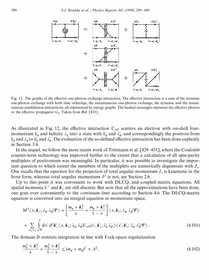
Fig. 12. The graphs of the effective one-photon exchange interaction. The effective interaction is a sum of the dynamicone-photon exchange with both time orderings, the instantaneous one-photon exchange, the dynamic and the instan-taneous annihilation interactions, all represented by energy graphs. The hashed rectangles represent the effective photonor the effective propagator G

0. Taken from Ref. [431].

As illustrated in Fig. 12, the effective interaction º%&&

scatters an electron with on-shell four-momentum k

qand helicity j

qinto a state with k@

qand j@

q, and correspondingly the positron from

kqNand j

qNto k@

qNand j@

qN. The evaluation of the so-defined effective interaction has been done explicitly

in Section 3.4.In the sequel, we follow the more recent work of Trittmann et al. [429—431], where the Coulomb

counter-term technology was improved further to the extent that a calculation of all spin-paritymultiplets of positronium was meaningful. In particular, it was possible to investigate the impor-tant question to which extent the members of the multiplets are numerically degenerate with J

z.

One recalls that the operator for the projection of total angular momentum Jzis kinematic in the

front form, whereas total angular momentum J2 is not, see Section 2.6.Up to this point it was convenient to work with DLCQ, and coupled matrix equations. All

spatial momenta k` and kM

are still discrete. But now that all the approximations have been done,one goes over conveniently to the continuum limit according to Section 4.6. The DLCQ-matrixequation is converted into an integral equation in momentum space,

M2Sx, kM; j

q, j

qNDWT"C

mq#k2

Mx

#

mqN#k2

M1!x D Sx, k

M; j

q, j

qNDWT

# +j@

q,j@qN PDdx@ d2k@

MSx, k

M; j

q, j

qNDº

%&&Dx@, k@

M; j@

qj@qN,TSx@, k@

M; j@

q, j@

qNDWT . (4.101)

The domain D restricts integration in line with Fock-space regularization

m2q#k2

Mx

#

m2qN#k2

M1!x

4(mq#m

qN)2#K2. (4.102)


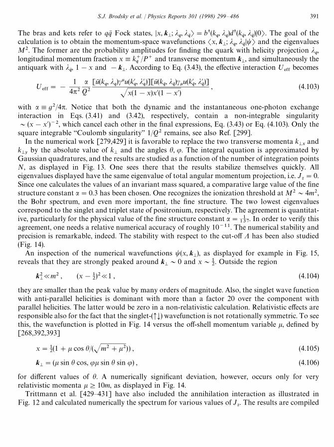
The bras and kets refer to qqN Fock states, Dx, kM; j

q, j

qNT"bs(k

q, j

q)ds(k

qN, j

qN)D0T. The goal of the

calculation is to obtain the momentum-space wavefunctions Sx, kM; j

q, j

qNDtT and the eigenvalues

M2. The former are the probability amplitudes for finding the quark with helicity projection jq,

longitudinal momentum fraction x,k`q/P` and transverse momentum k

M, and simultaneously the

antiquark with jqN, 1!x and !k

M. According to Eq. (3.43), the effective interaction º

%&&becomes

º%&&"!

14p2

aQ2

[uN (kq, j

q)cku(k@

q, j@

q)][uN (k

qN, j

qN)cku(k@

qN, j@

qN)]

Jx(1!x)x@(1!x@), (4.103)

with a,g2/4p. Notice that both the dynamic and the instantaneous one-photon exchangeinteraction in Eqs. (3.41) and (3.42), respectively, contain a non-integrable singularity&(x!x@)~2, which cancel each other in the final expressions, Eq. (3.43) or Eq. (4.103). Only thesquare integrable “Coulomb singularity” 1/Q2 remains, see also Ref. [299].

In the numerical work [279,429] it is favorable to replace the two transverse momenta kMx

andkMy

by the absolute value of kM

and the angles h, u. The integral equation is approximated byGaussian quadratures, and the results are studied as a function of the number of integration pointsN, as displayed in Fig. 13. One sees there that the results stabilize themselves quickly. Alleigenvalues displayed have the same eigenvalue of total angular momentum projection, i.e. J

z"0.

Since one calculates the values of an invariant mass squared, a comparative large value of the finestructure constant a"0.3 has been chosen. One recognizes the ionization threshold at M2&4m2,the Bohr spectrum, and even more important, the fine structure. The two lowest eigenvaluescorrespond to the singlet and triplet state of positronium, respectively. The agreement is quantitat-ive, particularly for the physical value of the fine structure constant a" 1

137. In order to verify this

agreement, one needs a relative numerical accuracy of roughly 10~11. The numerical stability andprecision is remarkable, indeed. The stability with respect to the cut-off K has been also studied(Fig. 14).

An inspection of the numerical wavefunctions t(x, kM), as displayed for example in Fig. 15,

reveals that they are strongly peaked around kM&0 and x&1

2. Outside the region

k2M@m2 , (x!1

2)2@1 , (4.104)

they are smaller than the peak value by many orders of magnitude. Also, the singlet wave functionwith anti-parallel helicities is dominant with more than a factor 20 over the component withparallel helicities. The latter would be zero in a non-relativistic calculation. Relativistic effects areresponsible also for the fact that the singlet-(CB) wavefunction is not rotationally symmetric. To seethis, the wavefunction is plotted in Fig. 14 versus the off-shell momentum variable k, defined by[268,392,393]

x"12(1#k cos h/(Jm2#k2) ) , (4.105)

kM"(k sin h cos, uk sin h sin u) , (4.106)

for different values of h. A numerically significant deviation, however, occurs only for veryrelativistic momenta k510m, as displayed in Fig. 14.

Trittmann et al. [429—431] have also included the annihilation interaction as illustrated inFig. 12 and calculated numerically the spectrum for various values of J

z. The results are compiled


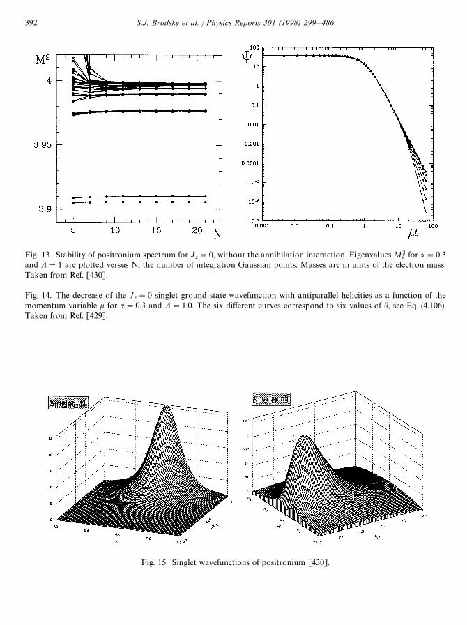
Fig. 13. Stability of positronium spectrum for Jz"0, without the annihilation interaction. Eigenvalues M2

ifor a"0.3

and K"1 are plotted versus N, the number of integration Gaussian points. Masses are in units of the electron mass.Taken from Ref. [430].

Fig. 14. The decrease of the Jz"0 singlet ground-state wavefunction with antiparallel helicities as a function of the

momentum variable k for a"0.3 and K"1.0. The six different curves correspond to six values of h, see Eq. (4.106).Taken from Ref. [429].

Fig. 15. Singlet wavefunctions of positronium [430].


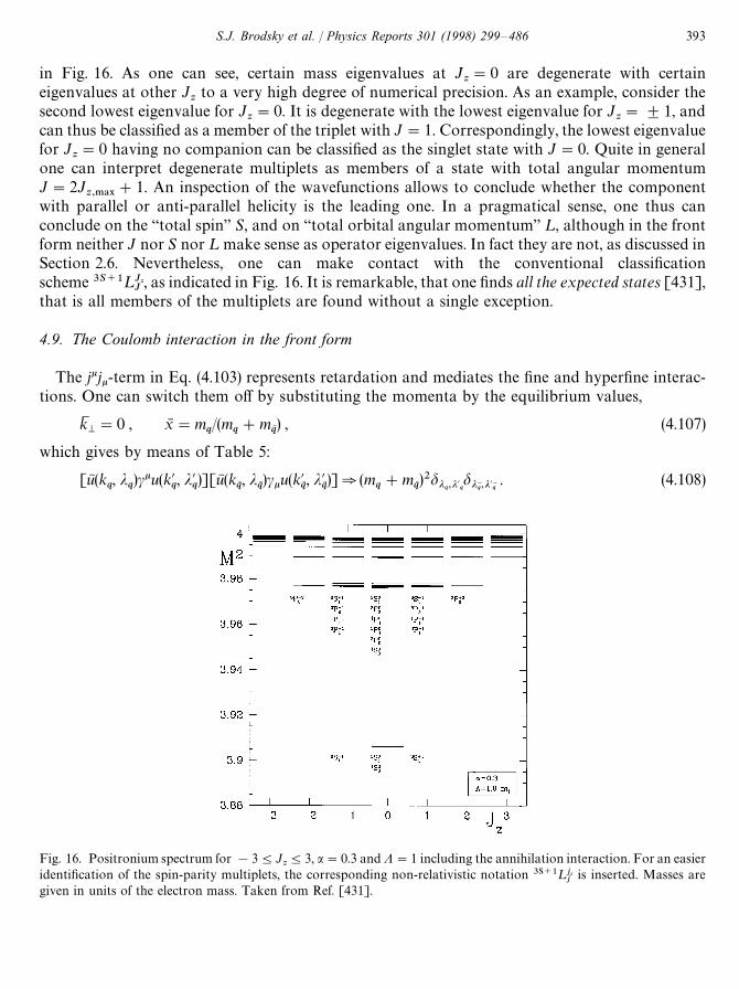
Fig. 16. Positronium spectrum for !34Jz43, a"0.3 and K"1 including the annihilation interaction. For an easier

identification of the spin-parity multiplets, the corresponding non-relativistic notation 3S`1¸jzj

is inserted. Masses aregiven in units of the electron mass. Taken from Ref. [431].

in Fig. 16. As one can see, certain mass eigenvalues at Jz"0 are degenerate with certain

eigenvalues at other Jzto a very high degree of numerical precision. As an example, consider the

second lowest eigenvalue for Jz"0. It is degenerate with the lowest eigenvalue for J

z"$1, and

can thus be classified as a member of the triplet with J"1. Correspondingly, the lowest eigenvaluefor J

z"0 having no companion can be classified as the singlet state with J"0. Quite in general

one can interpret degenerate multiplets as members of a state with total angular momentumJ"2J

z,.!9#1. An inspection of the wavefunctions allows to conclude whether the component

with parallel or anti-parallel helicity is the leading one. In a pragmatical sense, one thus canconclude on the “total spin” S, and on “total orbital angular momentum” ¸, although in the frontform neither J nor S nor ¸ make sense as operator eigenvalues. In fact they are not, as discussed inSection 2.6. Nevertheless, one can make contact with the conventional classificationscheme 3S`1¸Jz

J, as indicated in Fig. 16. It is remarkable, that one finds all the expected states [431],

that is all members of the multiplets are found without a single exception.

4.9. The Coulomb interaction in the front form

The jkjk-term in Eq. (4.103) represents retardation and mediates the fine and hyperfine interac-tions. One can switch them off by substituting the momenta by the equilibrium values,

kMM"0 , xN "m

q/(m

q#m

qN) , (4.107)

which gives by means of Table 5:

[uN (kq, j

q)cku(k@

q, j@

q)][uN (k

qN, j

qN)cku(k@

qN, j@

qN)]N(m

q#m

qN)2djq,j@

qdjqN ,j@

qN. (4.108)


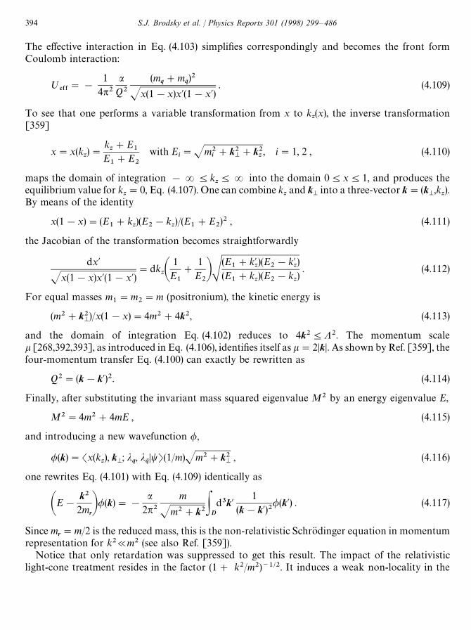
The effective interaction in Eq. (4.103) simplifies correspondingly and becomes the front formCoulomb interaction:

º%&&"!

14p2

aQ2

(mq#m

qN)2

Jx(1!x)x@(1!x@). (4.109)

To see that one performs a variable transformation from x to kz(x), the inverse transformation

[359]

x"x(kz)"

kz#E

1E1#E

2

with Ei"Jm2

i#k2

M#k2

z, i"1, 2 , (4.110)

maps the domain of integration !R4kz4R into the domain 04x41, and produces the

equilibrium value for kz"0, Eq. (4.107). One can combine k

zand k

Minto a three-vector k"(k

M,k

z).

By means of the identity

x(1!x)"(E1#k

z)(E

2!k

z)/(E

1#E

2)2 , (4.111)

the Jacobian of the transformation becomes straightforwardly

dx@

Jx(1!x)x@(1!x@)"dk

zA1E

1

#

1E

2BS

(E1#k@

z)(E

2!k@

z)

(E1#k

z)(E

2!k

z). (4.112)

For equal masses m1"m

2"m (positronium), the kinetic energy is

(m2#k2M)/x(1!x)"4m2#4k2, (4.113)

and the domain of integration Eq. (4.102) reduces to 4k24K2. The momentum scalek [268,392,393], as introduced in Eq. (4.106), identifies itself as k"2DkD. As shown by Ref. [359], thefour-momentum transfer Eq. (4.100) can exactly be rewritten as

Q2"(k!k@)2. (4.114)

Finally, after substituting the invariant mass squared eigenvalue M2 by an energy eigenvalue E,

M2"4m2#4mE , (4.115)

and introducing a new wavefunction /,

/(k)"Sx(kz), k

M; j

q, j

qNDtT(1/m)Jm2#k2

M, (4.116)

one rewrites Eq. (4.101) with Eq. (4.109) identically as

AE!

k2

2mrB/(k)"!

a2p2

m

Jm2#k2PDd3k@1

(k!k@)2/(k@) . (4.117)

Since mr"m/2 is the reduced mass, this is the non-relativistic Schrodinger equation in momentum

representation for k2@m2 (see also Ref. [359]).Notice that only retardation was suppressed to get this result. The impact of the relativistic

light-cone treatment resides in the factor (1# k2/m2)~1@2. It induces a weak non-locality in the


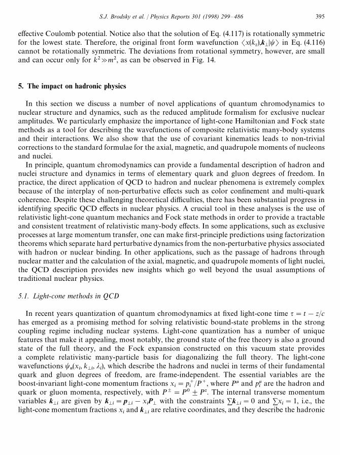
effective Coulomb potential. Notice also that the solution of Eq. (4.117) is rotationally symmetricfor the lowest state. Therefore, the original front form wavefunction Sx(k

z),k

MDtT in Eq. (4.116)

cannot be rotationally symmetric. The deviations from rotational symmetry, however, are smalland can occur only for k2Am2, as can be observed in Fig. 14.

5. The impact on hadronic physics

In this section we discuss a number of novel applications of quantum chromodynamics tonuclear structure and dynamics, such as the reduced amplitude formalism for exclusive nuclearamplitudes. We particularly emphasize the importance of light-cone Hamiltonian and Fock statemethods as a tool for describing the wavefunctions of composite relativistic many-body systemsand their interactions. We also show that the use of covariant kinematics leads to non-trivialcorrections to the standard formulae for the axial, magnetic, and quadrupole moments of nucleonsand nuclei.

In principle, quantum chromodynamics can provide a fundamental description of hadron andnuclei structure and dynamics in terms of elementary quark and gluon degrees of freedom. Inpractice, the direct application of QCD to hadron and nuclear phenomena is extremely complexbecause of the interplay of non-perturbative effects such as color confinement and multi-quarkcoherence. Despite these challenging theoretical difficulties, there has been substantial progress inidentifying specific QCD effects in nuclear physics. A crucial tool in these analyses is the use ofrelativistic light-cone quantum mechanics and Fock state methods in order to provide a tractableand consistent treatment of relativistic many-body effects. In some applications, such as exclusiveprocesses at large momentum transfer, one can make first-principle predictions using factorizationtheorems which separate hard perturbative dynamics from the non-perturbative physics associatedwith hadron or nuclear binding. In other applications, such as the passage of hadrons throughnuclear matter and the calculation of the axial, magnetic, and quadrupole moments of light nuclei,the QCD description provides new insights which go well beyond the usual assumptions oftraditional nuclear physics.

5.1. Light-cone methods in QCD

In recent years quantization of quantum chromodynamics at fixed light-cone time q"t!z/chas emerged as a promising method for solving relativistic bound-state problems in the strongcoupling regime including nuclear systems. Light-cone quantization has a number of uniquefeatures that make it appealing, most notably, the ground state of the free theory is also a groundstate of the full theory, and the Fock expansion constructed on this vacuum state providesa complete relativistic many-particle basis for diagonalizing the full theory. The light-conewavefunctions t

n(x

i, k

Mi, j

i), which describe the hadrons and nuclei in terms of their fundamental

quark and gluon degrees of freedom, are frame-independent. The essential variables are theboost-invariant light-cone momentum fractions x

i"p`

i/P`, where Pk and pk

iare the hadron and

quark or gluon momenta, respectively, with PB"P0$Pz. The internal transverse momentumvariables k

Miare given by k

Mi"p

Mi!x

iPM

with the constraints +kMi"0 and +x

i"1, i.e., the

light-cone momentum fractions xiand k

Miare relative coordinates, and they describe the hadronic


system independent of its total four momentum pk. The entire spectrum of hadrons and nuclei andtheir scattering states is given by the set of eigenstates of the light-cone Hamiltonian H

LCof QCD.

The Heisenberg problem takes the form

HLC

DWT"M2DWT . (5.1)

For example, each hadron has the eigenfunction DWHT of HQCD

LCwith eigenvalue M2"M2

H. If we

could solve the light-cone Heisenberg problem for the proton in QCD, we could then expand itseigenstate on the complete set of quark and gluon eigensolutions DnT"DuudT, DuudgT,2 of the freeHamiltonian H0

LCwith the same global quantum numbers:

DWpT"+

n

DnTtn(x

i, k

Mi, j

i) . (5.2)

The tn(n"3, 4,2) are first-quantized amplitudes analogous to the Schrodinger wave function,

but it is Lorentz-frame-independent. Particle number is generally not conserved in a relativisticquantum field theory. Thus, each eigenstate is represented as a sum over Fock states of arbitraryparticle number and in QCD each hadron is expanded as second-quantized sums over fluctuationsof color-singlet quark and gluon states of different momenta and number. The coefficients of thesefluctuations are the light-cone wavefunctions t

n(x

i, k

Mi, j

i). The invariant mass M of the partons in

a given Fock state can be written in the elegant form M2"+3i/1

(k2Mi#m2)/x

i. The dominant

configurations in the wavefunction are generally those with minimum values of M2. Note thatexcept for the case m

i"0 and k

Mi"0, the limit x

iP0 is an ultraviolet limit; i.e. it corresponds to

particles moving with infinite momentum in the negative z direction: kziP!k0

iP!R .

In the case of QCD in one-space and one-time dimensions, the application of discretizedlight-cone quantization [66], see Section 4, provides complete solutions of the theory, including theentire spectrum of mesons, baryons, and nuclei, and their wavefunctions [227]. In the DLCQmethod, one simply diagonalizes the light-cone Hamiltonian for QCD on a discretized Fock statebasis. The DLCQ solutions can be obtained for arbitrary parameters including the number offlavors and colors and quark masses. More recently, DLCQ has been applied to new variants ofQCD(1#1) with quarks in the adjoint representation, thus obtaining color-singlet eigenstatesanalogous to gluonium states [115].

The DLCQ method becomes much more numerically intense when applied to physical theoriesin 3#1 dimensions; however, progress is being made. An analysis of the spectrum and light-conewavefunctions of positronium in QED(3#1) is given in Ref. [279]. Currently, Hiller et al. [222]are pursuing a non-perturbative calculation of the lepton anomalous moment in QED using thismethod. Burkardt has recently solved scalar theories with transverse dimensions by combininga Monte Carlo lattice method with DLCQ [79].

Given the light-cone wavefunctions, tn@H

(xi, k

Mi, j

i), one can compute virtually any hadronic

quantity by convolution with the appropriate quark and gluon matrix elements. For example, theleading-twist structure functions measured in deep inelastic lepton scattering are immediatelyrelated to the light-cone probability distributions:

2MF1(x, Q)"

F2(x, Q)x

++a

e2aG

a@p(x, Q) , (5.3)


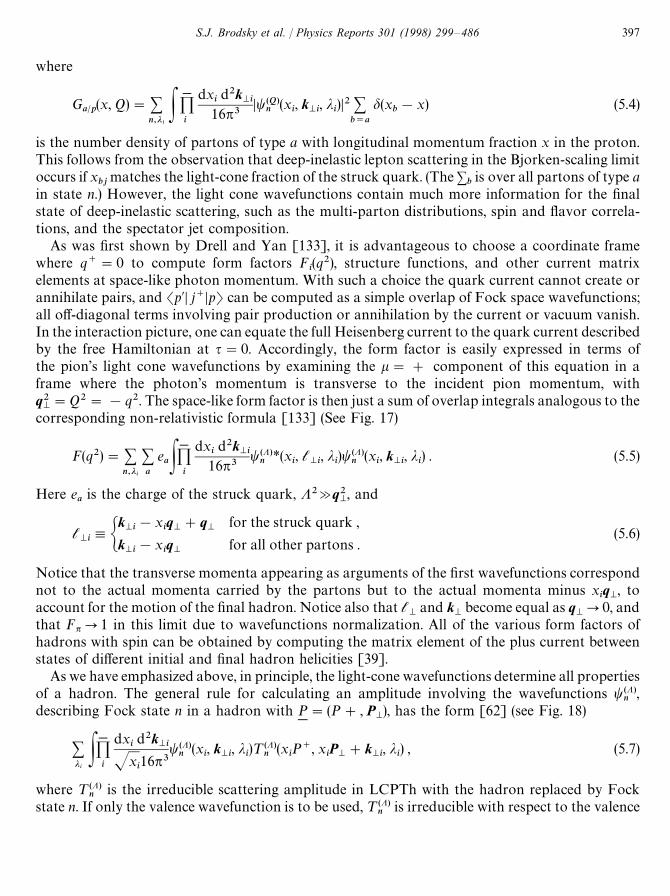
where

Ga@p

(x, Q)"+n,jiP<1

i

dxid2k

Mi16p3

Dt(Q)n

(xi, k

Mi, j

i)D2 +

b/a

d(xb!x) (5.4)

is the number density of partons of type a with longitudinal momentum fraction x in the proton.This follows from the observation that deep-inelastic lepton scattering in the Bjorken-scaling limitoccurs if x

bjmatches the light-cone fraction of the struck quark. (The +

bis over all partons of type a

in state n.) However, the light cone wavefunctions contain much more information for the finalstate of deep-inelastic scattering, such as the multi-parton distributions, spin and flavor correla-tions, and the spectator jet composition.

As was first shown by Drell and Yan [133], it is advantageous to choose a coordinate framewhere q`"0 to compute form factors F

i(q2), structure functions, and other current matrix

elements at space-like photon momentum. With such a choice the quark current cannot create orannihilate pairs, and Sp@D j`DpT can be computed as a simple overlap of Fock space wavefunctions;all off-diagonal terms involving pair production or annihilation by the current or vacuum vanish.In the interaction picture, one can equate the full Heisenberg current to the quark current describedby the free Hamiltonian at q"0. Accordingly, the form factor is easily expressed in terms ofthe pion’s light cone wavefunctions by examining the k"# component of this equation in aframe where the photon’s momentum is transverse to the incident pion momentum, withq2M"Q2"!q2. The space-like form factor is then just a sum of overlap integrals analogous to the

corresponding non-relativistic formula [133] (See Fig. 17)

F(q2)"+n,ji

+a

eaP<1

i

dxid2k

Mi16p3

t(K)*n

(xi, l

Mi, j

i)t(K)

n(x

i, k

Mi, j

i) . (5.5)

Here eais the charge of the struck quark, K2Aq2

M, and

lMi,G

kMi!x

iqM#q

Mfor the struck quark ,

kMi!x

iqM

for all other partons .(5.6)

Notice that the transverse momenta appearing as arguments of the first wavefunctions correspondnot to the actual momenta carried by the partons but to the actual momenta minus x

iqM, to

account for the motion of the final hadron. Notice also that lM

and kM

become equal as qMP0, and

that FnP1 in this limit due to wavefunctions normalization. All of the various form factors ofhadrons with spin can be obtained by computing the matrix element of the plus current betweenstates of different initial and final hadron helicities [39].

As we have emphasized above, in principle, the light-cone wavefunctions determine all propertiesof a hadron. The general rule for calculating an amplitude involving the wavefunctions t(K)

n,

describing Fock state n in a hadron with P"(P#, PM), has the form [62] (see Fig. 18)

+jiP<1

i

dxid2k

MiJx

i16p3

t(K)n

(xi, k

Mi, j

i)¹(K)

n(x

iP`, x

iPM#k

Mi, j

i) , (5.7)

where ¹(K)n

is the irreducible scattering amplitude in LCPTh with the hadron replaced by Fockstate n. If only the valence wavefunction is to be used, ¹(K)

nis irreducible with respect to the valence


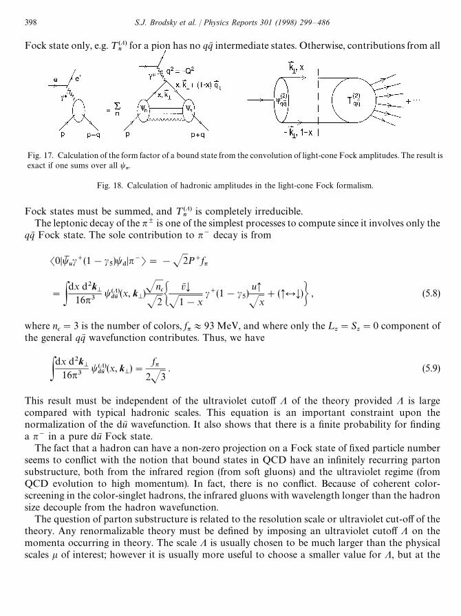
Fig. 17. Calculation of the form factor of a bound state from the convolution of light-cone Fock amplitudes. The result isexact if one sums over all t

n.

Fig. 18. Calculation of hadronic amplitudes in the light-cone Fock formalism.

Fock state only, e.g. ¹(K)n

for a pion has no qqN intermediate states. Otherwise, contributions from all

Fock states must be summed, and ¹(K)n

is completely irreducible.The leptonic decay of the nB is one of the simplest processes to compute since it involves only the

qqN Fock state. The sole contribution to n~ decay is from

S0DtMuc`(1!c

5)t

$Dn~T"!J2P`fn

"Pdx d2k

M16p3

t(K)duN

(x, kM)Jn

cJ2G

vN BJ1!x

c`(1!c5)uCJx

#(C%B)H , (5.8)

where nc"3 is the number of colors, fn+93 MeV, and where only the ¸

z"S

z"0 component of

the general qqN wavefunction contributes. Thus, we have

Pdx d2k

M16p3

t(K)duN

(x, kM)"

fn2J3

. (5.9)

This result must be independent of the ultraviolet cutoff K of the theory provided K is largecompared with typical hadronic scales. This equation is an important constraint upon thenormalization of the duN wavefunction. It also shows that there is a finite probability for findinga n~ in a pure duN Fock state.

The fact that a hadron can have a non-zero projection on a Fock state of fixed particle numberseems to conflict with the notion that bound states in QCD have an infinitely recurring partonsubstructure, both from the infrared region (from soft gluons) and the ultraviolet regime (fromQCD evolution to high momentum). In fact, there is no conflict. Because of coherent color-screening in the color-singlet hadrons, the infrared gluons with wavelength longer than the hadronsize decouple from the hadron wavefunction.

The question of parton substructure is related to the resolution scale or ultraviolet cut-off of thetheory. Any renormalizable theory must be defined by imposing an ultraviolet cutoff K on themomenta occurring in theory. The scale K is usually chosen to be much larger than the physicalscales k of interest; however it is usually more useful to choose a smaller value for K, but at the


expense of introducing new higher-twist terms in an effective Lagrangian: [301]

L(K)"L(K)0

(as(K), m(K))#

N+n/1

(1/K)ndL(K)n

(as(K), m(K))#O(1/K)N`1 , (5.10)

where

L(K)0"!1

4F(K)

aklF(K)akln

#tM (K)[iD. (K)!m(K)]t(K) . (5.11)

The neglected physics of parton momenta and substructure beyond the cutoff scale has the effect ofrenormalizing the values of the input coupling constant g(K2) and the input mass parameter m(K2)of the quark partons in the Lagrangian.

One clearly should choose K large enough to avoid large contributions from the higher-twistterms in the effective Lagrangian, but small enough so that the Fock space domain is minimized.Thus, if K is chosen of order 5—10 times the typical QCD momentum scale, then it is reasonable tohope that the mass, magnetic moment and other low momentum properties of the hadron could bewell-described on a Fock basis of limited size. Furthermore, by iterating the equations of motion,one can construct a relativistic Schrodinger equation with an effective potential acting on thevalence lowest-particle number state wavefunction [297,298]. Such a picture would explain theapparent success of constituent quark models for explaining the hadronic spectrum and low-energyproperties of hadron.

It should be emphasized that infinitely growing parton content of hadrons due to the evolutionof the deep inelastic structure functions at increasing momentum transfer, is associated with therenormalization group substructure of the quarks themselves, rather than the “intrinsic” structureof the bound state wavefunction [63,65]. The fact that the light-cone kinetic energy S(k2

M#m2)/xT

of the constituents in the bound state is bounded by K2 excludes singular behavior of the Fockwavefunctions at xP0. There are several examples where the light-cone Fock structure of thebound-state solutions is known. In the case of the super-renormalizable gauge theory, QED(1#1),the probability of having non-valence states in the light-cone expansion of the lowest lying mesonand baryon eigenstates to be less than 10~3, even at very strong coupling [227]. In the case ofQED(3#1), the lowest state of positronium can be well described on a light-cone basis with two tofour particles, Deè~T, Deè~cT, Deè~ccT, and Deè~eè~T; in particular, the description of theLambshift in positronium requires the coupling of the system to light-cone Fock states with twophotons “in flight” in light-cone gauge. The ultraviolet cut-off scale K only needs to be taken largecompared to the electron mass. On the other hand, a charged particle such as the electron does nothave a finite Fock decomposition, unless one imposes an artificial infrared cut-off.

We thus expect that a limited light-cone Fock basis should be sufficient to represent boundcolor-singlet states of heavy quarks in QCD(3#1) because of the coherent color cancelations andthe suppressed amplitude for transversely polarized gluon emission by heavy quarks. However, thedescription of light hadrons is undoubtedly much more complex due to the likely influence of chiralsymmetry breaking and zero-mode gluons in the light-cone vacuum. We return to this problem later.

Even without solving the QCD light-cone equations of motion, we can anticipate some generalfeatures of the behavior of the light-cone wavefunctions. Each Fock component describes a systemof free particles with kinematic invariant mass squared:

M2"n+i

(k2Mi#m2

i)/x

i. (5.12)


On general dynamical grounds, we can expect that states with very high M2 are suppressed inphysical hadrons, with the highest mass configurations computable from perturbative consider-ations. We also note that ln x

i"ln(k0#kz)

i/(P0#Pz)"y

i!y

Pis the rapidity difference between

the constituent with light-cone fraction xiand the rapidity of the hadron itself. Since correlations

between particles rarely extend over two units of rapidity in hadron physics, this argues thatconstituents which are correlated with the hadron’s quantum numbers are primarily found withx'0.2.

The limit xP0 is normally an ultraviolet limit in a light-cone wavefunction. Recall, that in anyLorentz frame, the light-cone fraction is x"k`/p`"(k0#kz)/(P0#Pz). Thus in a frame wherethe bound state is moving infinitely fast in the positive z direction (“the infinite momentum frame”),the light-cone fraction becomes the momentum fraction xPkz/pz. However, in the rest frameP"0, x"(k0#kz)/M. Thus, xP0 generally implies very large constituent momentumkzP!k0P!R in the rest frame; it is excluded by the ultraviolet regulation of the theory— unless the particle has strictly zero mass and transverse momentum.

If a particle has non-relativistic momentum in the bound state, then we can identifykz&xM!m. This correspondence is useful when one matches physics at the relativistic/non-relativistic interface. In fact, any non-relativistic solution to the Schrodinger equation can beimmediately written in light-cone form by identifying the two forms of coordinates. For example,the Schrodinger solution for particles bound in a harmonic oscillator potential can be taken asa model for the light-cone wavefunction for quarks in a confining linear potential [299]:

t(xi, k

Mi)"A exp(!bM2)"exp!Ab

n+i

k2Mi#m2

ixiB . (5.13)

This form exhibits the strong fall-off at large relative transverse momentum and at the xP0 andxP1 endpoints expected for soft non-perturbative solutions in QCD. The perturbative correctionsdue to hard gluon exchange give amplitudes suppressed only by power laws and thus willeventually dominate wave function behavior over the soft contributions in these regions. Thisansatz is the central assumption required to derive dimensional counting perturbative QCDpredictions for exclusive processes at large momentum transfer and the xP1 behavior of deep-inelastic structure functions. A review is given in Ref. [62]. A model for the polarized andunpolarized gluon distributions in the proton which takes into account both perturbative QCDconstraints at large x and coherent cancelations at low x and small transverse momentum is givenin Refs. [63,65].

The light-cone approach to QCD has immediate application to nuclear systems: The formalismprovides a covariant many-body description of nuclear systems formally similar to non-relativisticmany-body theory.

One can derive rigorous predictions for the leading power-law fall-off of nuclear amplitudes,including the nucleon—nucleon potential, the deuteron form factor, and the distributions ofnucleons within nuclei at large momentum fraction. For example, the leading electro-magneticform factor of the deuteron falls as F

d(Q2)"f (a

s(Q2))/(Q2)5, where, asymptotically,

f (as(Q2))Ja

s(Q2)5`c. The leading anomalous dimension c is computed in Ref. [59].

In general, the six-quark Fock state of the deuteron is a mixture of five different color-singletstates. The dominant color configuration of the six quarks corresponds to the usual proton—neutron bound state. However, as Q2 increases, the deuteron form factor becomes sensitive to


deuteron wavefunction configurations where all six quarks overlap within an impact separationbMi(O(1/Q). In the asymptotic domain, all five Fock color-singlet components acquire equalweight; i.e., the deuteron wavefunction becomes 80% “hidden color” at short distances. Thederivation of the evolution equation for the deuteron distribution amplitude is given in Refs.[59,249].

QCD predicts that Fock components of a hadron with a small color dipole moment can passthrough nuclear matter without interactions [36,60]; see also [334]. Thus, in the case of largemomentum transfer reactions where only small-size valence Fock state configurations enter thehard scattering amplitude, both the initial and final state interactions of the hadron states becomenegligible. There is now evidence for QCD “color transparency” in exclusive virtual photono production for both nuclear coherent and incoherent reactions in the E665 experiment atFermilab [141], as well as the original measurement at BNL in quasi-elastic pp scattering in nuclei[216]. The recent NE18 measurement of quasielastic electron—proton scattering at SLAC findsresults which do not clearly distinguish between conventional Glauber theory predictions andPQCD color transparency [320].

In contrast to color transparency, Fock states with large-scale color configurations stronglyinteract with high particle number production [42].

The traditional nuclear physics assumption that the nuclear form factor factorizes in the formFA(Q2)"+

NF

N(Q2)F"0$:

N@A(Q2), where F

N(Q2) is the on-shell nucleon form factor is in general

incorrect. The struck nucleon is necessarily off-shell, since it must transmit momentum to align thespectator nucleons along the direction of the recoiling nucleus.

Nuclear form factors and scattering amplitudes can be factored in the form given by the reducedamplitude formalism [55], which follows from the cluster decomposition of the nucleus in the limitof zero nuclear binding. The reduced form factor formalism takes into account the fact that eachnucleon in an exclusive nuclear transition typically absorbs momentum Q

NKQ/N. Tests of this

formalism are discussed in a later section.The use of covariant kinematics leads to a number of striking conclusions for the electromag-

netic and weak moments of nucleons and nuclei. For example, magnetic moments cannot bewritten as the naive sum k"+k

iof the magnetic moments of the constituents, except in the

non-relativistic limit where the radius of the bound state is much larger than its Compton scale:R

AM

AA1. The deuteron quadrupole moment is in general non-zero even if the nucleon—nucleon

bound state has no D-wave component [58]. Such effects are due to the fact that even “static”moments have to be computed as transitions between states of different momentumpk and pk#qk with qkP0. Thus, one must construct current matrix elements between boosted states.The Wigner boost generates non-trivial corrections to the current interactions of bound systems [51].

One can also use light-cone methods to show that the proton’s magnetic moment kp

and itsaxial-vector coupling g

Ahave a relationship independent of the assumed form of the light-cone

wave function [71]. At the physical value of the proton radius computed from the slope of theDirac form factor, R

1"0.76 fm, one obtains the experimental values for both k

pand g

A; the

helicity carried by the valence u and d quarks are each reduced by a factor K0.75 relative to theirnon-relativistic values. At infinitely small radius R

pM

pP0, k

pbecomes equal to the Dirac mo-

ment, as demanded by the Drell—Hearn—Gerasimov sum rule [174,129]. Another surprising fact isthat as R

1P0, the constituent quark helicities become completely disoriented and g

AP0. We

discuss these features in more detail in the following section.


In the case of the deuteron, both the quadrupole and magnetic moments become equal to that ofan elementary vector boson in the Standard Model in the limit M

dR

dP0. The three form factors of

the deuteron have the same ratio as that of the ¼ boson in the Standard Model [58].The basic amplitude controlling the nuclear force, the nucleon—nucleon scattering amplitude can

be systematically analyzed in QCD in terms of basic quark and gluon scattering subprocesses. Thehigh momentum transfer behavior of the amplitude from dimensional counting is M

pp?ppK

fpp?pp

(t/s)/t4 at fixed center of mass angle. A review is given in Ref. [62]. The fundamentalsubprocesses, including pinch contributions [289], can be classified as arising from both quarkinterchange and gluon exchange contributions. In the case of meson—nucleon scattering, the quarkexchange graphs [43] can explain virtually all of the observed features of large momentum transferfixed CM angle scattering distributions and ratios [90]. The connection between Regge behaviorand fixed angle scattering in perturbative QCD for quark exchange reactions is discussed in Ref.[69]. Sotiropoulos and Sterman [407] have shown how one can consistently interpolate from fixedangle scaling behavior to the 1/t8 scaling behavior of the elastic cross section in the sA!t, large!t regime.

One of the most striking anomalies in elastic proton—proton scattering is the large spincorrelation A

NNobserved at large angles [280]. At JsK5 GeV, the rate for scattering with

incident proton spins parallel and normal to the scattering plane is four times larger than scatteringwith anti-parallel polarization. This phenomena in elastic pp scattering can be explained as theeffect due to the onset of charm production in the intermediate state at this energy [61]. Theintermediate state DuuduudccN T has odd intrinsic parity and couples to the J"S"1 initial state,thus strongly enhancing scattering when the incident projectile and target protons have their spinsparallel and normal to the scattering plane.

The simplest form of the nuclear force is the interaction between two heavy quarkonium states,such as the ¶(bbM ) and the J/t(ccN ). Since there are no valence quarks in common, the dominantcolor-singlet interaction arises simply from the exchange of two or more gluons, the analog of thevan der Waals molecular force in QED. In principle, one could measure the interactions of suchsystems by producing pairs of quarkonia in high energy hadron collisions. The same fundamentalQCD van der Waals potential also dominates the interactions of heavy quarkonia with ordinaryhadrons and nuclei. As shown in Ref. [313], the small size of the QQM bound state relative to themuch larger hadron sizes allows a systematic expansion of the gluonic potential using the operatorproduct potential. The matrix elements of multigluon exchange in the quarkonium state can becomputed from non-relativistic heavy quark theory. The coupling of the scalar part of theinteraction to large-size hadrons is rigorously normalized to the mass of the state via the traceanomaly. This attractive potential dominates the interactions at low relative velocity. In this way,one establishes that the nuclear force between heavy quarkonia and ordinary nuclei is attractiveand sufficiently strong to produce nuclear-bound quarkonium [64].

5.2. Moments of nucleons and nuclei in the light-cone formalism

Let us consider an effective three-quark light-cone Fock description of the nucleon in whichadditional degrees of freedom (including zero modes) are parameterized in an effective potential.After truncation, one could in principle obtain the mass M and light-cone wavefunction of the


three-quark bound states by solving the Hamiltonian eigenvalue problem. It is reasonable toassume that adding more quark and gluonic excitations will only refine this initial approximation[363]. In such a theory the constituent quarks will also acquire effective masses and form factors.However, even without explicit solutions, one knows that the helicity and flavor structure of thebaryon eigenfunctions will reflect the assumed global SU(6) symmetry and Lorentz invariance ofthe theory. Since we do not have an explicit representation for the effective potential in thelight-cone Hamiltonian H%&&%#5*7%

LCfor three-quarks, we shall proceed by making an ansatz for the

momentum space structure of the wavefunction W. As we will show below, for a given size of theproton, the predictions and interrelations between observables at Q2"0, such as the protonmagnetic moment k

pand its axial coupling g

A, turn out to be essentially independent of the shape

of the wavefunction [71].The light-cone model given in Refs. [395—397] provides a framework for representing the general

structure of the effective three-quark wavefunctions for baryons. The wavefunction ( is con-structed as the product of a momentum wavefunction, which is spherically symmetric and invariantunder permutations, and a spin—isospin wavefunction, which is uniquely determined by SU(6)-symmetry requirements. A Wigner—Melosh [450,332] rotation is applied to the spinors, so that thewavefunction of the proton is an eigenfunction of J and J

zin its rest frame [105,68]. To represent

the range of uncertainty in the possible form of the momentum wave function, we shall choose twosimple functions of the invariant mass M of the quarks:

tHO

(M2)"NHO

exp(!M2/2b2) , tP08%3

(M2)"NP08%3

(1#M2/b2)~p , (5.14)

where b sets the characteristic internal momentum scale. Perturbative QCD predicts a nominalpower-law fall off at large k

Mcorresponding to p"3.5 [299,395—398]. The Melosh rotation insures

that the nucleon has j"12

in its rest system. It has the matrix representation [332]

RM(x

i, k

Mi, m)"

m#xiM!ir ) (n]k

i)

J(m#xiM)2#k2

Mi

(5.15)

with n"(0, 0, 1), and it becomes the unit matrix if the quarks are collinear RM

(xi, 0, m)"1. Thus,

the internal transverse momentum dependence of the light-cone wavefunctions also affects itshelicity structure [51].

The Dirac and Pauli form factors F1(Q2) and F

2(Q2) of the nucleons are given by the spin-

conserving and the spin-flip vector current J`V

matrix elements (Q2"!q2) [61]

F1(Q2)"Sp#q,CDJ`

VDp,CT , (5.16)

(Q1!iQ

2)F

2(Q2)"!2MSp#q,CDJ`

VDp,BT . (5.17)

We can then calculate the anomalous magnetic moment a"limQ2?0

F2(Q2). [The total proton

magnetic moment is kp"(e/2M)(1#a

p).] The same parameters as in Ref. [396] are chosen;

namely m"0.263 GeV (0.26 GeV) for the up- and down-quark masses, and b"0.607 GeV(0.55 GeV) for t

P08%3(t

HO) and p"3.5. The quark currents are taken as elementary currents with

Dirac moments eq/2m

q. All of the baryon moments are well-fit if one takes the strange quark mass

as 0.38 GeV. With the above values, the proton magnetic moment is 2.81 nuclear magnetons, theneutron magnetic moment is !1.66 nuclear magnetons. (The neutron value can be improved by


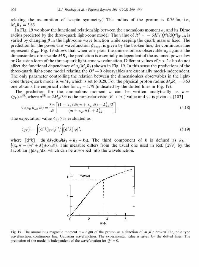
Fig. 19. The anomalous magnetic moment a"F2(0) of the proton as a function of M

pR

1: broken line, pole type

wavefunction; continuous line, Gaussian wavefunction. The experimental value is given by the dotted lines. Theprediction of the model is independent of the wavefunction for Q2"0.

relaxing the assumption of isospin symmetry.) The radius of the proton is 0.76 fm, i.e.,M

pR

1"3.63.

In Fig. 19 we show the functional relationship between the anomalous moment apand its Dirac

radius predicted by the three-quark light-cone model. The value of R21"!6dF

1(Q2)/dQ2D

Q2/0is

varied by changing b in the light-cone wave function while keeping the quark mass m fixed. Theprediction for the power-law wavefunction t

P08%3is given by the broken line; the continuous line

represents tHO

. Fig. 19 shows that when one plots the dimensionless observable ap

against thedimensionless observable MR

1the prediction is essentially independent of the assumed power-law

or Gaussian form of the three-quark light-cone wavefunction. Different values of p'2 also do notaffect the functional dependence of a

p(M

pR

1) shown in Fig. 19. In this sense the predictions of the

three-quark light-cone model relating the Q2P0 observables are essentially model-independent.The only parameter controlling the relation between the dimensionless observables in the light-cone three-quark model is m/M

pwhich is set to 0.28. For the physical proton radius M

pR

1"3.63

one obtains the empirical value for ap"1.79 (indicated by the dotted lines in Fig. 19).

The prediction for the anomalous moment a can be written analytically as a"Sc

VTaNR, where aNR"2M

p/3m is the non-relativistic (RPR) value and c

Vis given as [103]

cV(x

i, k

Mi, m)"

3mM C

(1!x3)M(m#x

3M)!k2

M3/2

(m#x3M)2#k2

M3D . (5.18)

The expectation value ScVT is evaluated as

ScVT"P[d3k]c

VDtD2/P[d3k]DtD2, (5.19)

where [d3k]"dk1dk

2dk

3d(k

1#k

2#k

3). The third component of k is defined as k

3i"

12(x

iM!(m2#k2

Mi)/x

iM). This measure differs from the usual one used in Ref. [299] by the

Jacobian <dk3i/dx

iwhich can be absorbed into the wavefunction.


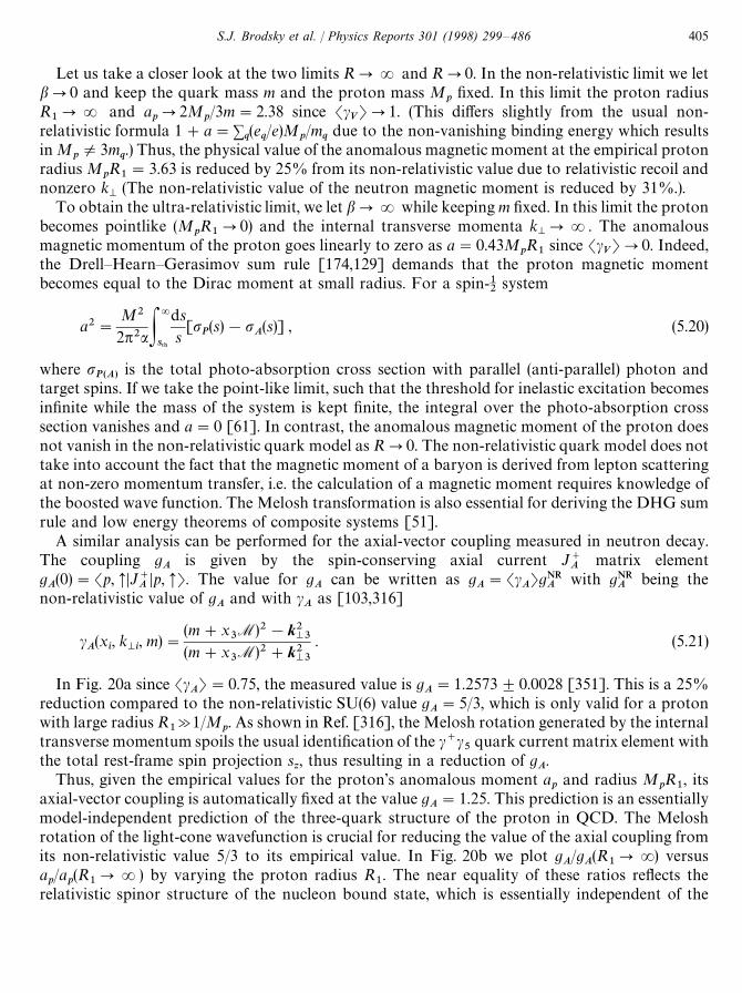
Let us take a closer look at the two limits RPR and RP0. In the non-relativistic limit we letbP0 and keep the quark mass m and the proton mass M

pfixed. In this limit the proton radius

R1PR and a

pP2M

p/3m"2.38 since Sc

VTP1. (This differs slightly from the usual non-

relativistic formula 1#a"+q(e

q/e)M

p/m

qdue to the non-vanishing binding energy which results

in MpO3m

q.) Thus, the physical value of the anomalous magnetic moment at the empirical proton

radius MpR

1"3.63 is reduced by 25% from its non-relativistic value due to relativistic recoil and

nonzero kM

(The non-relativistic value of the neutron magnetic moment is reduced by 31%.).To obtain the ultra-relativistic limit, we let bPR while keeping m fixed. In this limit the proton

becomes pointlike (MpR

1P0) and the internal transverse momenta k

MPR. The anomalous

magnetic momentum of the proton goes linearly to zero as a"0.43MpR

1since Sc

VTP0. Indeed,

the Drell—Hearn—Gerasimov sum rule [174,129] demands that the proton magnetic momentbecomes equal to the Dirac moment at small radius. For a spin-1

2system

a2"M2

2p2aP=

s5)

dss[p

P(s)!p

A(s)] , (5.20)

where pP(A)

is the total photo-absorption cross section with parallel (anti-parallel) photon andtarget spins. If we take the point-like limit, such that the threshold for inelastic excitation becomesinfinite while the mass of the system is kept finite, the integral over the photo-absorption crosssection vanishes and a"0 [61]. In contrast, the anomalous magnetic moment of the proton doesnot vanish in the non-relativistic quark model as RP0. The non-relativistic quark model does nottake into account the fact that the magnetic moment of a baryon is derived from lepton scatteringat non-zero momentum transfer, i.e. the calculation of a magnetic moment requires knowledge ofthe boosted wave function. The Melosh transformation is also essential for deriving the DHG sumrule and low energy theorems of composite systems [51].

A similar analysis can be performed for the axial-vector coupling measured in neutron decay.The coupling g

Ais given by the spin-conserving axial current J`

Amatrix element

gA(0)"Sp, CDJ`

ADp, CT. The value for g

Acan be written as g

A"Sc

ATgNR

Awith gNR

Abeing the

non-relativistic value of gA

and with cA

as [103,316]

cA(x

i, k

Mi, m)"

(m#x3M)2!k2

M3(m#x

3M)2#k2

M3

. (5.21)

In Fig. 20a since ScAT"0.75, the measured value is g

A"1.2573$0.0028 [351]. This is a 25%

reduction compared to the non-relativistic SU(6) value gA"5/3, which is only valid for a proton

with large radius R1A1/M

p. As shown in Ref. [316], the Melosh rotation generated by the internal

transverse momentum spoils the usual identification of the c`c5

quark current matrix element withthe total rest-frame spin projection s

z, thus resulting in a reduction of g

A.

Thus, given the empirical values for the proton’s anomalous moment ap

and radius MpR

1, its

axial-vector coupling is automatically fixed at the value gA"1.25. This prediction is an essentially

model-independent prediction of the three-quark structure of the proton in QCD. The Meloshrotation of the light-cone wavefunction is crucial for reducing the value of the axial coupling fromits non-relativistic value 5/3 to its empirical value. In Fig. 20b we plot g

A/g

A(R

1PR) versus

ap/a

p(R

1PR) by varying the proton radius R

1. The near equality of these ratios reflects the

relativistic spinor structure of the nucleon bound state, which is essentially independent of the


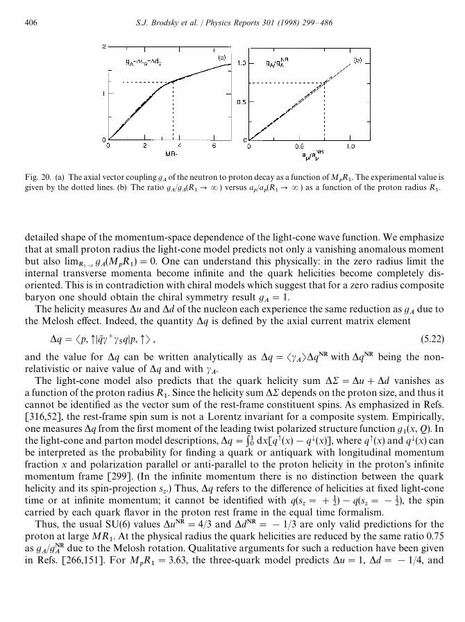
Fig. 20. (a) The axial vector coupling gA

of the neutron to proton decay as a function of MpR

1. The experimental value is

given by the dotted lines. (b) The ratio gA/g

A(R

1PR) versus a

p/a

p(R

1PR) as a function of the proton radius R

1.

detailed shape of the momentum-space dependence of the light-cone wave function. We emphasizethat at small proton radius the light-cone model predicts not only a vanishing anomalous momentbut also lim

R1?0gA(M

pR

1)"0. One can understand this physically: in the zero radius limit the

internal transverse momenta become infinite and the quark helicities become completely dis-oriented. This is in contradiction with chiral models which suggest that for a zero radius compositebaryon one should obtain the chiral symmetry result g

A"1.

The helicity measures *u and *d of the nucleon each experience the same reduction as gA

due tothe Melosh effect. Indeed, the quantity *q is defined by the axial current matrix element

*q"Sp, CDqN c`c5qDp, CT , (5.22)

and the value for *q can be written analytically as *q"ScAT*qNR with *qNR being the non-

relativistic or naive value of *q and with cA.

The light-cone model also predicts that the quark helicity sum *R"*u#*d vanishes asa function of the proton radius R

1. Since the helicity sum *R depends on the proton size, and thus it

cannot be identified as the vector sum of the rest-frame constituent spins. As emphasized in Refs.[316,52], the rest-frame spin sum is not a Lorentz invariant for a composite system. Empirically,one measures *q from the first moment of the leading twist polarized structure function g

1(x, Q). In

the light-cone and parton model descriptions, *q":10

dx[q(x)!q¬(x)], where q(x) and q¬(x) canbe interpreted as the probability for finding a quark or antiquark with longitudinal momentumfraction x and polarization parallel or anti-parallel to the proton helicity in the proton’s infinitemomentum frame [299]. (In the infinite momentum there is no distinction between the quarkhelicity and its spin-projection s

z.) Thus, *q refers to the difference of helicities at fixed light-cone

time or at infinite momentum; it cannot be identified with q(sz"#1

2)!q(s

z"!1

2), the spin

carried by each quark flavor in the proton rest frame in the equal time formalism.Thus, the usual SU(6) values *uNR"4/3 and *dNR"!1/3 are only valid predictions for the

proton at large MR1. At the physical radius the quark helicities are reduced by the same ratio 0.75

as gA/gNR

Adue to the Melosh rotation. Qualitative arguments for such a reduction have been given

in Refs. [266,151]. For MpR

1"3.63, the three-quark model predicts *u"1, *d"!1/4, and


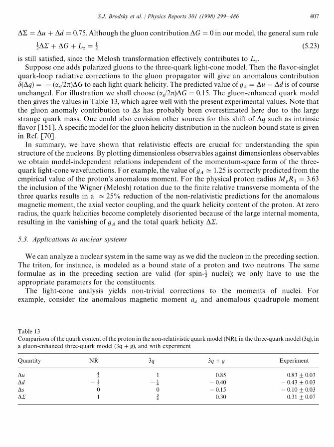
Table 13Comparison of the quark content of the proton in the non-relativistic quark model (NR), in the three-quark model (3q), ina gluon-enhanced three-quark model (3q#g), and with experiment

Quantity NR 3q 3q#g Experiment

*u 43

1 0.85 0.83$0.03*d !1

3!1

4!0.40 !0.43$0.03

*s 0 0 !0.15 !0.10$0.03*R 1 3

40.30 0.31$0.07

*&"*u#*d"0.75. Although the gluon contribution *G"0 in our model, the general sum rule

12*R#*G#¸

z"1

2(5.23)

is still satisfied, since the Melosh transformation effectively contributes to ¸z.

Suppose one adds polarized gluons to the three-quark light-cone model. Then the flavor-singletquark-loop radiative corrections to the gluon propagator will give an anomalous contributiond(*q)"!(a

s/2p)*G to each light quark helicity. The predicted value of g

A"*u!*d is of course

unchanged. For illustration we shall choose (as/2p)*G"0.15. The gluon-enhanced quark model

then gives the values in Table 13, which agree well with the present experimental values. Note thatthe gluon anomaly contribution to *s has probably been overestimated here due to the largestrange quark mass. One could also envision other sources for this shift of *q such as intrinsicflavor [151]. A specific model for the gluon helicity distribution in the nucleon bound state is givenin Ref. [70].

In summary, we have shown that relativistic effects are crucial for understanding the spinstructure of the nucleons. By plotting dimensionless observables against dimensionless observableswe obtain model-independent relations independent of the momentum-space form of the three-quark light-cone wavefunctions. For example, the value of g

AK1.25 is correctly predicted from the

empirical value of the proton’s anomalous moment. For the physical proton radius MpR

1"3.63

the inclusion of the Wigner (Melosh) rotation due to the finite relative transverse momenta of thethree quarks results in a K25% reduction of the non-relativistic predictions for the anomalousmagnetic moment, the axial vector coupling, and the quark helicity content of the proton. At zeroradius, the quark helicities become completely disoriented because of the large internal momenta,resulting in the vanishing of g

Aand the total quark helicity *R.

5.3. Applications to nuclear systems

We can analyze a nuclear system in the same way as we did the nucleon in the preceding section.The triton, for instance, is modeled as a bound state of a proton and two neutrons. The sameformulae as in the preceding section are valid (for spin-1

2nuclei); we only have to use the

appropriate parameters for the constituents.The light-cone analysis yields non-trivial corrections to the moments of nuclei. For

example, consider the anomalous magnetic moment ad

and anomalous quadrupole moment


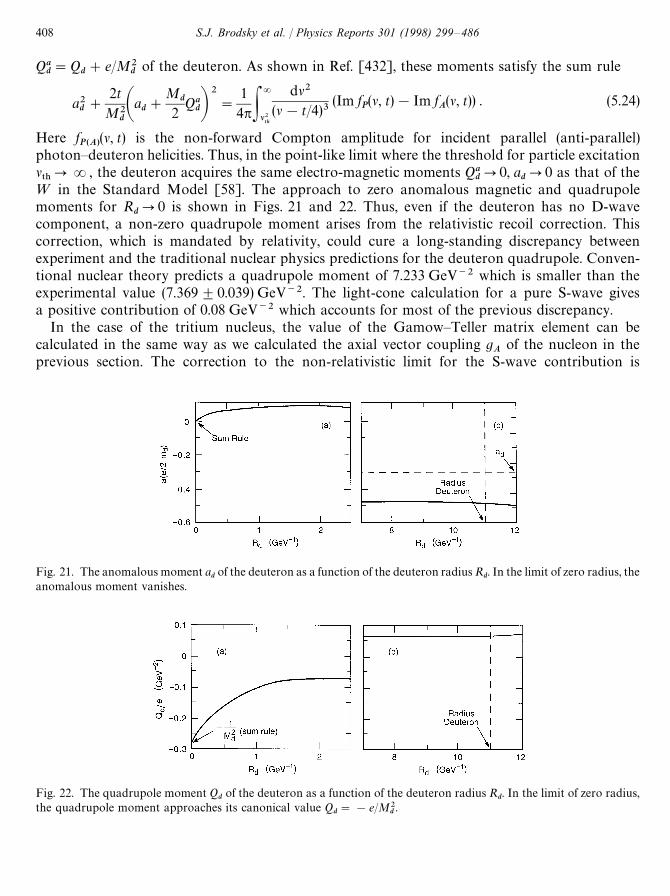
Fig. 22. The quadrupole moment Qdof the deuteron as a function of the deuteron radius R

d. In the limit of zero radius,

the quadrupole moment approaches its canonical value Qd"!e/M2

d.

Fig. 21. The anomalous moment adof the deuteron as a function of the deuteron radius R

d. In the limit of zero radius, the

anomalous moment vanishes.

Qad"Q

d#e/M2

dof the deuteron. As shown in Ref. [432], these moments satisfy the sum rule

a2d#

2tM2

dAad#

Md

2Qa

dB2"

14pP

=

l2th

dl2(l!t/4)3

(Im fP(l, t)!Im f

A(l, t)) . (5.24)

Here fP(A)

(l, t) is the non-forward Compton amplitude for incident parallel (anti-parallel)photon—deuteron helicities. Thus, in the point-like limit where the threshold for particle excitationl5)PR, the deuteron acquires the same electro-magnetic moments Qa

dP0, a

dP0 as that of the

¼ in the Standard Model [58]. The approach to zero anomalous magnetic and quadrupolemoments for R

dP0 is shown in Figs. 21 and 22. Thus, even if the deuteron has no D-wave

component, a non-zero quadrupole moment arises from the relativistic recoil correction. Thiscorrection, which is mandated by relativity, could cure a long-standing discrepancy betweenexperiment and the traditional nuclear physics predictions for the deuteron quadrupole. Conven-tional nuclear theory predicts a quadrupole moment of 7.233 GeV~2 which is smaller than theexperimental value (7.369$0.039) GeV~2. The light-cone calculation for a pure S-wave givesa positive contribution of 0.08 GeV~2 which accounts for most of the previous discrepancy.

In the case of the tritium nucleus, the value of the Gamow—Teller matrix element can becalculated in the same way as we calculated the axial vector coupling g

Aof the nucleon in the

previous section. The correction to the non-relativistic limit for the S-wave contribution is


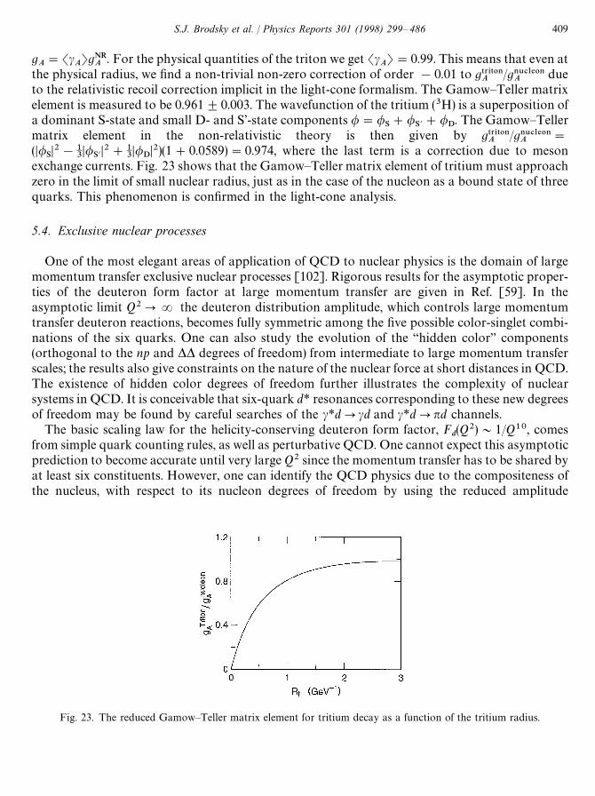
Fig. 23. The reduced Gamow—Teller matrix element for tritium decay as a function of the tritium radius.

gA"Sc

ATgNR

A. For the physical quantities of the triton we get Sc

AT"0.99. This means that even at

the physical radius, we find a non-trivial non-zero correction of order !0.01 to g53*50/A

/g/6#-%0/A

dueto the relativistic recoil correction implicit in the light-cone formalism. The Gamow—Teller matrixelement is measured to be 0.961$0.003. The wavefunction of the tritium (3H) is a superposition ofa dominant S-state and small D- and S’-state components /"/

S#/

S{#/

D. The Gamow—Teller

matrix element in the non-relativistic theory is then given by g53*50/A

/g/6#-%0/A

"

(D/SD2!1

3D/

S{D2#1

3D/

DD2)(1#0.0589)"0.974, where the last term is a correction due to meson

exchange currents. Fig. 23 shows that the Gamow—Teller matrix element of tritium must approachzero in the limit of small nuclear radius, just as in the case of the nucleon as a bound state of threequarks. This phenomenon is confirmed in the light-cone analysis.

5.4. Exclusive nuclear processes

One of the most elegant areas of application of QCD to nuclear physics is the domain of largemomentum transfer exclusive nuclear processes [102]. Rigorous results for the asymptotic proper-ties of the deuteron form factor at large momentum transfer are given in Ref. [59]. In theasymptotic limit Q2PR the deuteron distribution amplitude, which controls large momentumtransfer deuteron reactions, becomes fully symmetric among the five possible color-singlet combi-nations of the six quarks. One can also study the evolution of the “hidden color” components(orthogonal to the np and ** degrees of freedom) from intermediate to large momentum transferscales; the results also give constraints on the nature of the nuclear force at short distances in QCD.The existence of hidden color degrees of freedom further illustrates the complexity of nuclearsystems in QCD. It is conceivable that six-quark d* resonances corresponding to these new degreesof freedom may be found by careful searches of the c*dPcd and c*dPnd channels.

The basic scaling law for the helicity-conserving deuteron form factor, Fd(Q2)&1/Q10, comes

from simple quark counting rules, as well as perturbative QCD. One cannot expect this asymptoticprediction to become accurate until very large Q2 since the momentum transfer has to be shared byat least six constituents. However, one can identify the QCD physics due to the compositeness ofthe nucleus, with respect to its nucleon degrees of freedom by using the reduced amplitude


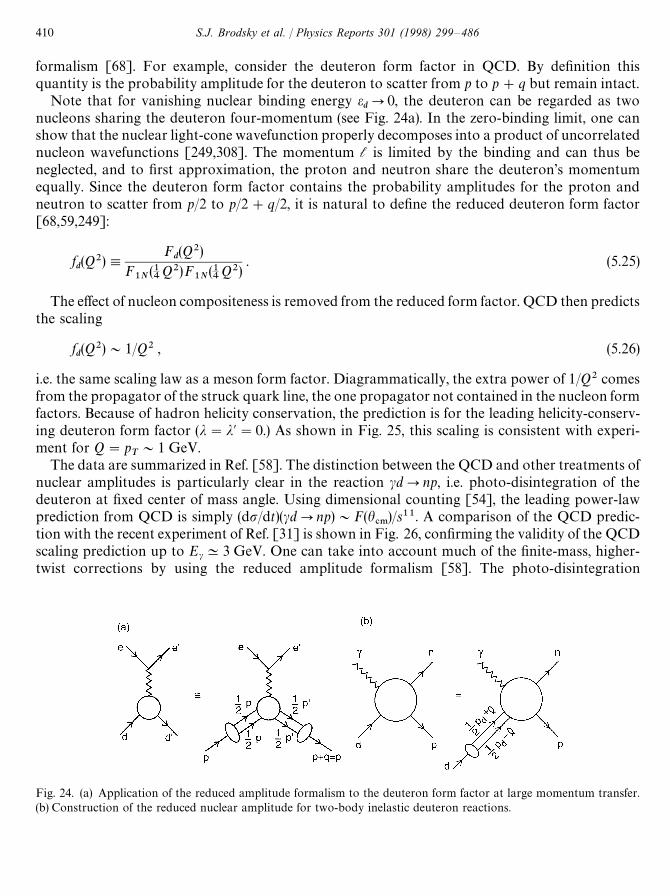
Fig. 24. (a) Application of the reduced amplitude formalism to the deuteron form factor at large momentum transfer.(b) Construction of the reduced nuclear amplitude for two-body inelastic deuteron reactions.

formalism [68]. For example, consider the deuteron form factor in QCD. By definition thisquantity is the probability amplitude for the deuteron to scatter from p to p#q but remain intact.

Note that for vanishing nuclear binding energy edP0, the deuteron can be regarded as two

nucleons sharing the deuteron four-momentum (see Fig. 24a). In the zero-binding limit, one canshow that the nuclear light-cone wavefunction properly decomposes into a product of uncorrelatednucleon wavefunctions [249,308]. The momentum l is limited by the binding and can thus beneglected, and to first approximation, the proton and neutron share the deuteron’s momentumequally. Since the deuteron form factor contains the probability amplitudes for the proton andneutron to scatter from p/2 to p/2#q/2, it is natural to define the reduced deuteron form factor[68,59,249]:

fd(Q2),

Fd(Q2)

F1N

(14Q2)F

1N(14Q2)

. (5.25)

The effect of nucleon compositeness is removed from the reduced form factor. QCD then predictsthe scaling

fd(Q2)&1/Q2 , (5.26)

i.e. the same scaling law as a meson form factor. Diagrammatically, the extra power of 1/Q2 comesfrom the propagator of the struck quark line, the one propagator not contained in the nucleon formfactors. Because of hadron helicity conservation, the prediction is for the leading helicity-conserv-ing deuteron form factor (j"j@"0.) As shown in Fig. 25, this scaling is consistent with experi-ment for Q"p

T&1 GeV.

The data are summarized in Ref. [58]. The distinction between the QCD and other treatments ofnuclear amplitudes is particularly clear in the reaction cdPnp, i.e. photo-disintegration of thedeuteron at fixed center of mass angle. Using dimensional counting [54], the leading power-lawprediction from QCD is simply (dp/dt)(cdPnp)&F(h

#.)/s11. A comparison of the QCD predic-

tion with the recent experiment of Ref. [31] is shown in Fig. 26, confirming the validity of the QCDscaling prediction up to EcK3 GeV. One can take into account much of the finite-mass, higher-twist corrections by using the reduced amplitude formalism [58]. The photo-disintegration


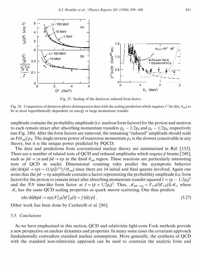
Fig. 25. Scaling of the deuteron reduced form factor.

Fig. 26. Comparison of deuteron photo-disintegration data with the scaling prediction which requires s11dp/dt(s, h#.

) tobe at most logarithmically dependent on energy at large momentum transfer.

amplitude contains the probability amplitude (i.e. nucleon form factors) for the proton and neutronto each remain intact after absorbing momentum transfers p

p!1/2p

dand p

n!1/2p

d, respectively

(see Fig. 24b). After the form factors are removed, the remaining “reduced” amplitude should scaleas F(h

#.)/p

T. The single inverse power of transverse momentum p

Tis the slowest conceivable in any

theory, but it is the unique power predicted by PQCD.The data and predictions from conventional nuclear theory are summarized in Ref. [133].

There are a number of related tests of QCD and reduced amplitudes which require pN beams [249],such as pN dPcn and pN dPnp in the fixed h

#.region. These reactions are particularly interesting

tests of QCD in nuclei. Dimensional counting rules predict the asymptotic behavior(dp/dt)(pN dPnp)&(1/(p2

T)12) f (h

#.) since there are 14 initial and final quanta involved. Again one

notes that the pN dPnp amplitude contains a factor representing the probability amplitude (i.e. formfactor) for the proton to remain intact after absorbing momentum transfer squared tL"(p!1/2p

d)2

and the NM N time-like form factor at sL"(pN #1/2pd)2. Thus, M

pN d?np&F1N

(tL )F1N

(sL )Mr, where

Mrhas the same QCD scaling properties as quark meson scattering. One thus predicts

(dp/dX)(pN dPnp)/F21N

(tK )F21N

(sL )&f (X)/p2T

. (5.27)

Other work has been done by Cardarelli et al. [86].

5.5. Conclusions

As we have emphasized in this section, QCD and relativistic light-cone Fock methods providea new perspective on nuclear dynamics and properties. In many some cases the covariant approachfundamentally contradicts standard nuclear assumptions. More generally, the synthesis of QCDwith the standard non-relativistic approach can be used to constrain the analytic form and


unknown parameters in the conventional theory, as in Bohr’s correspondence principle. Forexample, the reduced amplitude formalism and PQCD scaling laws provide analytic constraints onthe nuclear amplitudes and potentials at short distances and large momentum transfers.

6. Exclusive processes and light-cone wavefunctions

One of the major advantages of the light-cone formalism is that many properties of largemomentum transfer exclusive reactions can be calculated without explicit knowledge of the form ofthe non-perturbative light-cone wavefunctions. The main ingredients of this analysis are asymp-totic freedom, and the power-law scaling relations and quark helicity conservation rules ofperturbative QCD. For example, consider the light-cone expression (5.5) for a meson form factor athigh momentum transfer Q2. If the internal momentum transfer is large then one can iterate thegluon-exchange term in the effective potential for the light-cone wavefunctions. The result is thatthe hadron form factors can be written in a factorized form as a convolution of quark “distributionamplitudes” /(x

i,Q), one for each hadron involved in the amplitude, with a hard-scatterig ampli-

tude ¹H

[297—299]. The pion’s electro-magnetic form factor, for example, can be written as

Fn(Q2)"P1

0

dxP1

0

dy /*n(y, Q)¹

H(x, y, Q)/n(x, Q)(1#O(1/Q)) . (6.1)

Here ¹H

is the scattering amplitude for the form factor but with the pions replaced by collinear qqNpairs, i.e. the pions are replaced by their valence partons. We can also regard ¹

Has the free particle

matrix element of the order 1/q2 term in the effective Lagrangian for c*qqN PqqN .The process-independent distribution amplitude [297—299] /n(x, Q) is the probability amplitude

for finding the qqN pair in the pion with xq"x and x

qN"1!x. It is directly related to the light-cone

valence wavefunction:

/n(x, Q)"Pd2k

M16p3

t(Q)qqN @n(x, k

M) (6.2)

"P`n Pdz~4n

e*xP`pz~@2 S0DtM (0)c`c

52J2n

c

t(z)DnT(Q)z`/z

M/0. (6.3)

The kM

integration in Eq. (6.2) is cut off by the ultraviolet cutoff K"Q implicit in the wavefunction; thus only Fock states with invariant mass squared M2(Q2 contribute. We will returnlater to the discussion of ultraviolet regularization in the light-cone formalism.

It is important to note that the distribution amplitude is gauge-invariant. In gauges other thanlight-cone gauge, a path-ordered “string operator” P exp(:1

0ds ig A(sz) ) z) must be included be-

tween the tM and t. The line integral vanishes in light-cone gauge because A ) z"A`z~/2"0 andso the factor can be omitted in that gauge. This (non-perturbative) definition of / uniquely fixes thedefinition of ¹

Hwhich must itself then be gauge-invariant.

The above result is in the form of a factorization theorem; all of the non-perturbative dynamics isfactorized into the non-perturbative distribution amplitudes, which sums all internal momentumtransfers up to the scale Q2. On the other hand, all momentum transfers higher than Q2 appear in¹

H, which, because of asymptotic freedom, can be computed perturbatively in powers of the QCD

running coupling constant as(Q2).


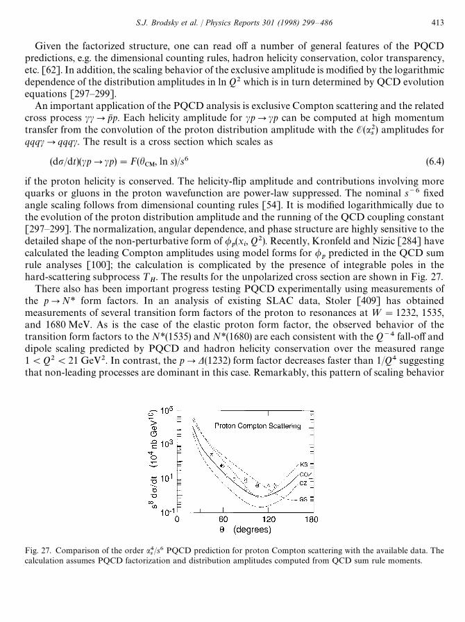
Fig. 27. Comparison of the order a4s/s6 PQCD prediction for proton Compton scattering with the available data. The

calculation assumes PQCD factorization and distribution amplitudes computed from QCD sum rule moments.

Given the factorized structure, one can read off a number of general features of the PQCDpredictions, e.g. the dimensional counting rules, hadron helicity conservation, color transparency,etc. [62]. In addition, the scaling behavior of the exclusive amplitude is modified by the logarithmicdependence of the distribution amplitudes in ln Q2 which is in turn determined by QCD evolutionequations [297—299].

An important application of the PQCD analysis is exclusive Compton scattering and the relatedcross process ccPpN p. Each helicity amplitude for cpPcp can be computed at high momentumtransfer from the convolution of the proton distribution amplitude with the O(a2

s) amplitudes for

qqqcPqqqc. The result is a cross section which scales as

(dp/dt)(cpPcp)"F(hCM

, ln s)/s6 (6.4)

if the proton helicity is conserved. The helicity-flip amplitude and contributions involving morequarks or gluons in the proton wavefunction are power-law suppressed. The nominal s~6 fixedangle scaling follows from dimensional counting rules [54]. It is modified logarithmically due tothe evolution of the proton distribution amplitude and the running of the QCD coupling constant[297—299]. The normalization, angular dependence, and phase structure are highly sensitive to thedetailed shape of the non-perturbative form of /

p(x

i, Q2). Recently, Kronfeld and Nizic [284] have

calculated the leading Compton amplitudes using model forms for /p

predicted in the QCD sumrule analyses [100]; the calculation is complicated by the presence of integrable poles in thehard-scattering subprocess ¹

H. The results for the unpolarized cross section are shown in Fig. 27.

There also has been important progress testing PQCD experimentally using measurements ofthe pPN* form factors. In an analysis of existing SLAC data, Stoler [409] has obtainedmeasurements of several transition form factors of the proton to resonances at ¼"1232, 1535,and 1680 MeV. As is the case of the elastic proton form factor, the observed behavior of thetransition form factors to the N*(1535) and N*(1680) are each consistent with the Q~4 fall-off anddipole scaling predicted by PQCD and hadron helicity conservation over the measured range1(Q2(21 GeV2. In contrast, the pPD(1232) form factor decreases faster than 1/Q4 suggestingthat non-leading processes are dominant in this case. Remarkably, this pattern of scaling behavior


is what is expected from PQCD and the QCD sum rule analyses [100], since, unlike the case of theproton and its other resonances, the distribution amplitude /

N*(x

1, x

2, x

3, Q) of the D resonance is

predicted to be nearly symmetric in the xi, and a symmetric distribution leads to a strong

cancelation [89] of the leading helicity-conserving terms in the matrix elements of the hardscattering amplitude for qqqPc*qqq.

These comparisons of the proton form factor and Compton scattering predictions with experi-ment are very encouraging, showing agreement in both the fixed-angle scaling behavior predictedby PQCD and the normalization predicted by QCD sum rule forms for the proton distributionamplitude. Assuming one can trust the validity of the leading order analysis, a systematic series ofpolarized target and beam Compton scattering measurements on proton and neutron targets andthe corresponding two-photon reactions ccPppN will strongly constrain a fundamental quantity inQCD, the nucleon distribution amplitude /(x

i, Q2). It is thus imperative for theorists to develop

methods to calculate the shape and normalization of the non-perturbative distribution amplitudesfrom first principles in QCD.

6.1. Is PQCD factorization applicable to exclusive processes?

One of the concerns in the derivation of the PQCD results for exclusive amplitudes is whetherthe momentum transfer carried by the exchanged gluons in the hard scattering amplitude ¹

His

sufficiently large to allow a safe application of perturbation theory [238]. The problem appears tobe especially serious if one assumes a form for the hadron distribution amplitudes /

H(x

i, Q2) which

has strong support at the endpoints, as in the QCD sum rule model forms suggested by Chernyakand Zhitnitskii and others [100,468].

This problem has now been clarified by two groups: Gari et al. [170] in the case of baryon formfactors, and Mankiewicz and Szczepaniak [419], for the case of meson form factors. Each of theseauthors has pointed out that the assumed non-perturbative input for the distribution amplitudesmust vanish strongly in the endpoint region; otherwise, there is a double-counting problem formomentum transfers occurring in the hard scattering amplitude and the distribution amplitudes.Once one enforces this constraint, (e.g. by using exponentially suppressed wavefunctions [299]) onthe basis functions used to represent the QCD moments, or uses a sufficiently large number ofpolynomial basis functions, the resulting distribution amplitudes do not allow significant contribu-tion to the high Q2 form factors to come from soft gluon exchange region. The comparison of thePQCD predictions with experiment thus becomes phenomenologically and analytically consistent.An analysis of exclusive reactions on the effective Lagrangian method is also consistent with thisapproach. In addition, as discussed by Botts [47], potentially soft contributions to large anglehadron—hadron scattering reactions from Landshoff pinch contributions [289] are strongly sup-pressed by Sudakov form factor effects.

The empirical successes of the PQCD approach, together with the evidence for color transpar-ency in quasi-elastic pp scattering [62] gives strong support for the validity of PQCD factorizationfor exclusive processes at moderate momentum transfer. It seems difficult to understand thispattern of form factor behavior if it is due to simple convolutions of soft wavefunctions. Thus, itshould be possible to use these processes to empirically constrain the form of the hadrondistribution amplitudes, and thus confront non-perturbative QCD in detail. For recent work, seeRefs. [7,122,254,334].


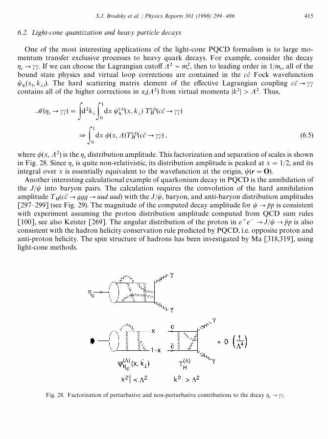
Fig. 28. Factorization of perturbative and non-perturbative contributions to the decay gcPcc.

6.2. Light-cone quantization and heavy particle decays

One of the most interesting applications of the light-cone PQCD formalism is to large mo-mentum transfer exclusive processes to heavy quark decays. For example, consider the decaygcPcc. If we can choose the Lagrangian cutoff K2&m2

c, then to leading order in 1/m

c, all of the

bound state physics and virtual loop corrections are contained in the ccN Fock wavefunctiontgc

(xi, k

Mi). The hard scattering matrix element of the effective Lagrangian coupling ccNPcc

contains all of the higher corrections in as(K2) from virtual momenta Dk2D'K2. Thus,

M(gcPcc)"Pd2k

MP1

0

dx t(K)gc (x, kM) ¹(K)

H(ccNPcc)

NP1

0

dx /(x, K)¹(K)H

(ccNPcc) , (6.5)

where /(x, K2) is the gcdistribution amplitude. This factorization and separation of scales is shown

in Fig. 28. Since gcis quite non-relativistic, its distribution amplitude is peaked at x"1/2, and its

integral over x is essentially equivalent to the wavefunction at the origin, t(r"O).Another interesting calculational example of quarkonium decay in PQCD is the annihilation of

the J/t into baryon pairs. The calculation requires the convolution of the hard annihilationamplitude ¹

H(ccNPgggPuud uud) with the J/t, baryon, and anti-baryon distribution amplitudes

[297—299] (see Fig. 29). The magnitude of the computed decay amplitude for tPpN p is consistentwith experiment assuming the proton distribution amplitude computed from QCD sum rules[100], see also Keister [269]. The angular distribution of the proton in e`e~PJ/tPpN p is alsoconsistent with the hadron helicity conservation rule predicted by PQCD, i.e. opposite proton andanti-proton helicity. The spin structure of hadrons has been investigated by Ma [318,319], usinglight-cone methods.


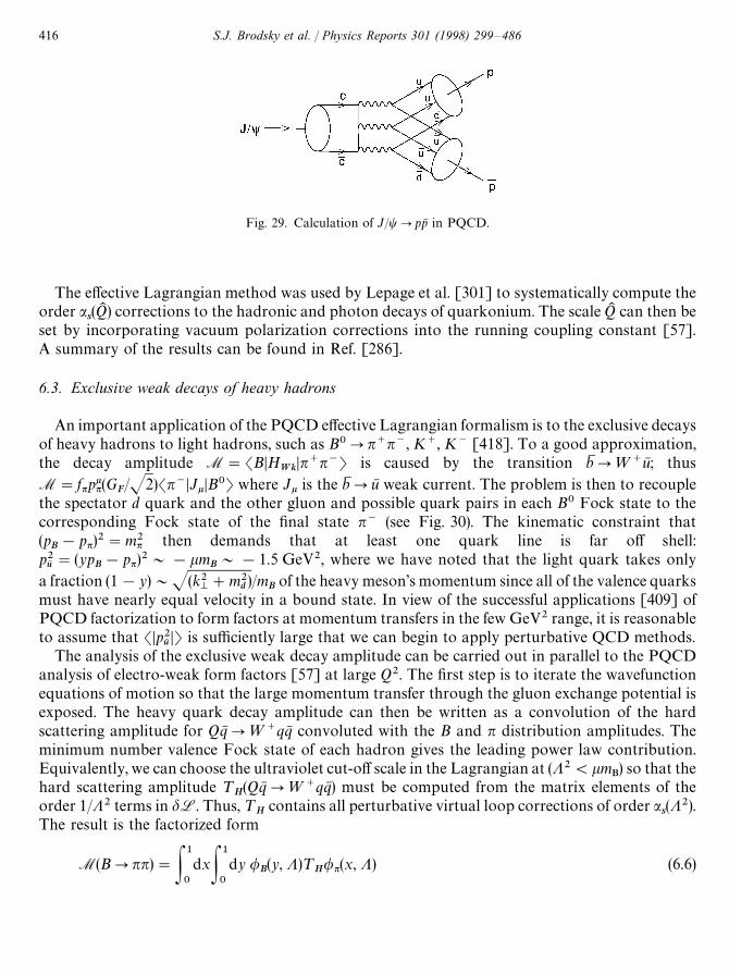
Fig. 29. Calculation of J/tPppN in PQCD.

The effective Lagrangian method was used by Lepage et al. [301] to systematically compute theorder a

s(QK ) corrections to the hadronic and photon decays of quarkonium. The scale QK can then be

set by incorporating vacuum polarization corrections into the running coupling constant [57].A summary of the results can be found in Ref. [286].

6.3. Exclusive weak decays of heavy hadrons

An important application of the PQCD effective Lagrangian formalism is to the exclusive decaysof heavy hadrons to light hadrons, such as B0Pn`n~, K`, K~ [418]. To a good approximation,the decay amplitude M"SBDH

WkDn`n~T is caused by the transition bM P¼`uN ; thus

M"fnpkn(GF/J2)Sn~DJkDB0T where Jk is the bM PuN weak current. The problem is then to recouple

the spectator d quark and the other gluon and possible quark pairs in each B0 Fock state to thecorresponding Fock state of the final state n~ (see Fig. 30). The kinematic constraint that(p

B!pn)2"m2n then demands that at least one quark line is far off shell:

p2uN"(yp

B!pn)2&!km

B&!1.5 GeV2, where we have noted that the light quark takes only

a fraction (1!y)&J(k2M#m2

d)/m

Bof the heavy meson’s momentum since all of the valence quarks

must have nearly equal velocity in a bound state. In view of the successful applications [409] ofPQCD factorization to form factors at momentum transfers in the few GeV2 range, it is reasonableto assume that SDp2

uNDT is sufficiently large that we can begin to apply perturbative QCD methods.

The analysis of the exclusive weak decay amplitude can be carried out in parallel to the PQCDanalysis of electro-weak form factors [57] at large Q2. The first step is to iterate the wavefunctionequations of motion so that the large momentum transfer through the gluon exchange potential isexposed. The heavy quark decay amplitude can then be written as a convolution of the hardscattering amplitude for QqN P¼`qqN convoluted with the B and n distribution amplitudes. Theminimum number valence Fock state of each hadron gives the leading power law contribution.Equivalently, we can choose the ultraviolet cut-off scale in the Lagrangian at (K2(km

B) so that the

hard scattering amplitude ¹H(QqN P¼`qqN ) must be computed from the matrix elements of the

order 1/K2 terms in dL. Thus, ¹H

contains all perturbative virtual loop corrections of order as(K2).

The result is the factorized form

M(BPnn)"P1

0

dxP1

0

dy /B(y, K)¹

H/n(x, K) (6.6)


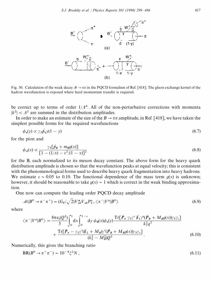
Fig. 30. Calculation of the weak decay BPnn in the PQCD formalism of Ref. [418]. The gluon exchange kernel of thehadron wavefunction is exposed where hard momentum transfer is required.

be correct up to terms of order 1/K4. All of the non-perturbative corrections with momentaDk2D(K2 are summed in the distribution amplitudes.

In order to make an estimate of the size of the BPnn amplitude, in Ref. [418], we have taken thesimplest possible forms for the required wavefunctions

/n(y)Jc5p. ny(1!y) (6.7)

for the pion and

/B(x)Jc5[p.

B#m

Bg(x)]

[1!(1/x)!e2/(1!x)]2(6.8)

for the B, each normalized to its meson decay constant. The above form for the heavy quarkdistribution amplitude is chosen so that the wavefunction peaks at equal velocity; this is consistentwith the phenomenological forms used to describe heavy quark fragmentation into heavy hadrons.We estimate e&0.05 to 0.10. The functional dependence of the mass term g(x) is unknown;however, it should be reasonable to take g(x)&1 which is correct in the weak binding approxima-tion.

One now can compute the leading order PQCD decay amplitude

M(B0Pn~n`)"(GF/J2)»*

ud»

ubPkn`Sn~D»kDB0T (6.9)

where

Sn~D»kDB0T"8pa

s(Q2)3 P

1

0

dxP1~e

0

dy /B(x)/n(y)

Tr[P. n~c5cl k.1ck(P.

B#M

Bg(x))c

5cl]

k21q2

#

Tr[P. n!c5cl(k.

2#M

B)cl(P.

B#M

Bg(x))c

5cl]

(k22!M2

B)Q2

. (6.10)

Numerically, this gives the branching ratio

BR(B0Pn`n~)&10~8m2N , (6.11)


where m"10D»ub/»

cbD is probably less than unity, and N has strong dependence on the value of

g: N"180 for g"1 and N"5.8 for g"1/2. The present experimental limit [21] is

BR(B0Pn`n~)(3]10~4 . (6.12)

A similar PQCD analysis can be applied to other two-body decays of the B; the ratios of the widthswill not be so sensitive to the form of the distribution amplitude, allowing tests of the flavorsymmetries of the weak interaction. Semi-leptonic decay rates can be calculated[99,128,187,246,404], and the construction of the heavy quark wavefunctions [101,465], can behelpful for that.

6.4. Can light-cone wavefunctions be measured?

Essential information on the shape and form of the valence light-cone wavefunctions can beobtained empirically through measurements of exclusive processes at large momentum transfer. Inthe case of the pion, data for the scaling and magnitude of the photon transition form factor Fcn0(q2)suggest that the distribution amplitude of the pion /n(x, Q) is close in form to the asymptotic form/=n (x)"J3fn(1!x), the solution to the evolution equation for the pion at infinite resolutionQPR, [299]. Note that the pion distribution amplitude is constrained by nPkl decay,

P1

0

dx /n(x, Q)"fn/2J3 . (6.13)

The proton distribution amplitude as determined by the proton form factor at large momentumtransfer, and Compton scattering is apparently highly asymmetric as suggested by QCD sum rulesand SU(6) flavor-spin symmetry.

The most direct way to measure the hadron distribution wavefunction is through the diffractivedissociation of a high energy hadron to jets or nuclei, e.g. nAPJet#Jet#A@, where the final-statenucleus remains intact [36,149]. The incoming hadron is a sum over all of its H0

LCfluctuations.

When the pion fluctuates into a qqN state with small impact separation b0M(1/Q), its color interactions

are minimal the “color transparency” property of QCD [60]. Thus, this fluctuation will interactcoherently throughout the nucleus without initial or final state absorption corrections. The result isthat the pion is coherently materialized into two jets of mass M| with minimal momentum transferto the nucleus

DQL"

M|!pq|n2E

L

. (6.14)

Thus, the jets carry nearly all of the momentum of the pion. The forward amplitude atQ

M, Q

L@R~1n is linear in the number of nucleons. The total rate integrated over the forward

diffraction peak is thus proportional to A2/[email protected] most remarkable feature of the diffractive nAPJet#Jet#X reactions is its potential to

measure the shape of the pion wavefunction. The partition of jet longitudinal momentum gives thex-distribution; the relative transverse momentum distribution provides the k

M-distribution of

tqqN @n(x, k

M). Such measurements are now being carried out by the E791 collaboration at Fermilab.


In principle, such experiments can be carried out with a photon beam, which should confirm thex2#(1!x) cPqqN distribution of the basic photon wavefunction. Measurements ofpAPJet p#Jet A could, in principle, provide a direct measurement of the proton distributionamplitude /

p(x

i; Q).

7. The light-cone vacuum

The unique features of “front form” or light-cone quantized field theory [123] provide a powerfultool for the study of QCD. Of primary importance in this approach is the existence of a vacuumstate that is the ground state of the full theory. The existence of this state gives a firm basis for theinvestigation of many of the complexities that must exist in QCD. In this picture the rich structureof vacuum is transferred to the zero modes of the theory. Within this context the long-rangephysical phenomena of spontaneous symmetry breaking [206—208] [33,382,223,389,375,376] aswell as the topological structure of the theory [259,377,378,383,384,261] can be associated with thezero mode(s) of the fields in a quantum field theory defined in a finite spatial volume and quantizedat equal light-cone time [299].

7.1. Constrained zero modes

As mentioned previously, the light-front vacuum state is simple; it contains no particles ina massive theory. In other words, the Fock space vacuum is the physical vacuum. However, onecommonly associates important long-range properties of a field theory with the vacuum: spontan-eous symmetry breaking, the Goldstone pion, and color confinement. How do these complicatedphenomena manifest themselves in light-front field theory?

If one cannot associate long-range phenomena with the vacuum state itself, then the onlyalternative is the zero momentum components or “zero modes” of the field (long range % zeromomentum). In some cases, the zero mode operator is not an independent degree of freedom butobeys a constraint equation. Consequently, it is a complicated operator-valued function of all theother modes of the field. Zero modes of this type have been investigated first by Maskawa andYamawaki as early as in 1976 [324].

This problem has recently been attacked from several directions. The question of whetherboundary conditions can be consistently defined in light-front quantization has been discussed byMcCartor and Robertson [325—331,388], and by Lenz [295,296]. They have shown that formassive theories the energy and momentum derived from light-front quantization are conservedand are equivalent to the energy and momentum one would normally write down in an equal-timetheory. In the analyses of Lenz et al. [295,296] and Hornbostel [230] one traces the fate of theequal-time vacuum in the limit P3PR and equivalently in the limit hPp/2 when rotating theevolution parameter q"x0 cos h#x3 sin h from the instant parametrization to the front par-ametrization. Heinzl and Werner et al. [206—210,214] considered /4 theory in (1#1) dimensions andattempted to solve the zero mode constraint equation by truncating the equation to one particle.Other authors [203,204,389] find that, for theories allowing spontaneous symmetry breaking, thereis a degeneracy of light-front vacua and the true vacuum state can differ from the perturbativevacuum through the addition of zero mode quanta. In addition to these approaches there


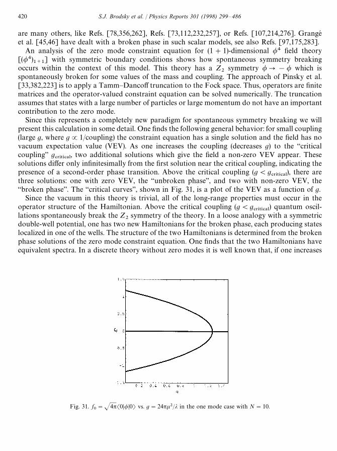
Fig. 31. f0"J4pS0D/D0T vs. g"24pk2/j in the one mode case with N"10.

are many others, like Refs. [78,356,262], Refs. [73,112,232,257], or Refs. [107,214,276]. Grangeet al. [45,46] have dealt with a broken phase in such scalar models, see also Refs. [97,175,283].

An analysis of the zero mode constraint equation for (1#1)-dimensional /4 field theory[(/4)

1`1] with symmetric boundary conditions shows how spontaneous symmetry breaking

occurs within the context of this model. This theory has a Z2

symmetry /P!/ which isspontaneously broken for some values of the mass and coupling. The approach of Pinsky et al.[33,382,223] is to apply a Tamm—Dancoff truncation to the Fock space. Thus, operators are finitematrices and the operator-valued constraint equation can be solved numerically. The truncationassumes that states with a large number of particles or large momentum do not have an importantcontribution to the zero mode.

Since this represents a completely new paradigm for spontaneous symmetry breaking we willpresent this calculation in some detail. One finds the following general behavior: for small coupling(large g, where gJ1/coupling) the constraint equation has a single solution and the field has novacuum expectation value (VEV). As one increases the coupling (decreases g) to the “criticalcoupling” g

#3*5*#!-, two additional solutions which give the field a non-zero VEV appear. These

solutions differ only infinitesimally from the first solution near the critical coupling, indicating thepresence of a second-order phase transition. Above the critical coupling (g(g

#3*5*#!-), there are

three solutions: one with zero VEV, the “unbroken phase”, and two with non-zero VEV, the“broken phase”. The “critical curves”, shown in Fig. 31, is a plot of the VEV as a function of g.

Since the vacuum in this theory is trivial, all of the long-range properties must occur in theoperator structure of the Hamiltonian. Above the critical coupling (g(g

#3*5*#!-) quantum oscil-

lations spontaneously break the Z2

symmetry of the theory. In a loose analogy with a symmetricdouble-well potential, one has two new Hamiltonians for the broken phase, each producing stateslocalized in one of the wells. The structure of the two Hamiltonians is determined from the brokenphase solutions of the zero mode constraint equation. One finds that the two Hamiltonians haveequivalent spectra. In a discrete theory without zero modes it is well known that, if one increases


the coupling sufficiently, quantum correction will generate tachyons causing the theory to breakdown near the critical coupling. Here the zero mode generates new interactions that preventtachyons from developing. In effect what happens is that, while quantum corrections attempt todrive the mass negative, they also change the vacuum energy through the zero mode and the masseigenvalue can never catch the vacuum eigenvalue. Thus, tachyons never appear in the spectra.

In the weak coupling limit (g large) the solution to the constraint equation can be obtained inperturbation theory. This solution does not break the Z

2symmetry and is believed to simply insert

the missing zero momentum contributions into internal propagators. This must happen if light-front perturbation theory is to agree with equal-time perturbation theory [94—96].

Another way to investigate the zero mode is to study the spectrum of the field operator /. Hereone finds a picture that agrees with the symmetric double-well potential analogy. In the brokenphase, the field is localized in one of the minima of the potential and there is tunneling to the otherminimum.

7.1.1. Canonical quantizationFor a classical field the (/4)

1`1Lagrange density is

¸"`/

~/!1

2k2/2!(j/4!)/4. (7.1)

One puts the system in a box of length d and imposes periodic boundary conditions. Then

/(x)"(1/Jd)+n

qn(x`)e*k`nx~, (7.2)

where k`n"2pn/d and summations run over all integers unless otherwise noted.

It is convenient to define the integral :dx~ /(x)n!(zero modes)"Rn. In terms of the modes of

the field it has the form,

Rn"

1n!

+i1,i2,2,inE0

qi1

qi22

qin

di1`i2` > > >`in,0

. (7.3)

Then the canonical Hamiltonian is

P~"

k2q20

2#k2R

2#

jq40

4!d#

jq20R

22!d

#

jq0R

3d

#

jR4

d. (7.4)

Following the Dirac—Bergman prescription, described in Appendix E, one identifies firstclassconstraints which define the conjugate momenta

0"pn!ik`

nq~n

, (7.5)

where

[qm, p

n]"1

2dn,m

, m, nO0. (7.6)

The secondary constraint is [457],

0"k2q0#

jq30

3!d#

jq0R

2d

#

jR3

d, (7.7)


which determines the zero mode q0. This result can also be obtained by integrating the equations of

motion.To quantize the system one replaces the classical fields with the corresponding field operators,

and the Dirac bracket by i times a commutator. One must choose a regularization and anoperator-ordering prescription in order to make the system well-defined.

One begins by defining creation and annihilation operators ask

and ak,

qk"S

d4nDkD

ak, a

k"as

~k, kO0 , (7.8)

which satisfy the usual commutation relations

[ak, a

l]"0 , [as

k, as

l]"0 , [a

k, as

l]"d

k,l, k,l'0 . (7.9)

Likewise, one defines the zero mode operator

q0"J(d/4p)a

0. (7.10)

In the quantum case, one normal orders the operator Rn.

General arguments suggest that the Hamiltonian should be symmetric ordered [32]. However, itis not clear how one should treat the zero mode since it is not a dynamical field. As an ansatz onetreats a

0as an ordinary field operator when symmetric ordering the Hamiltonian. The tadpoles are

removed from the symmetric ordered Hamiltonian by normal ordering the terms having no zeromode factors and by subtracting

32a20

+nE0

1DnD

. (7.11)

In addition, one subtracts a constant so that the VEV of H is zero. Note that this renormalizationprescription is equivalent to a conventional mass renormalization and does not introduce any newoperators into the Hamiltonian. The constraint equation for the zero mode can be obtained bytaking a derivative of P~ with respect to a

0. One finds

0"ga0#a3

0# +

nE0

1DnD Aa0ana~n

#ana~n

a0#a

na0a~n

!

3a0

2 B#6R3

, (7.12)

where g"24pk2/j. It is clear from the general structure of Eq. (7.12) that a0

as a function of theother modes is not necessarily odd under the transform a

kP!a

k, (kO0) associated with the

Z2

symmetry of the system. Consequently, the zero mode can induce Z2

symmetry breaking in theHamiltonian.

In order to render the problem tractable, we impose a Tamm—Dancoff truncation on the Fockspace. One defines M to be the number of non-zero modes and N to be the maximum number ofallowed particles. Thus, each state in the truncated Fock space can be represented by a vector oflength S"(M#N)!/(M!N!) and operators can be represented by S]S matrices. One can definethe usual Fock space basis, Dn

1, n

2,2, n

MT where n

1#n

2#2#n

M4N. In matrix form, a

0is

real and symmetric. Moreover, it is block diagonal in states of equal P` eigenvalue.


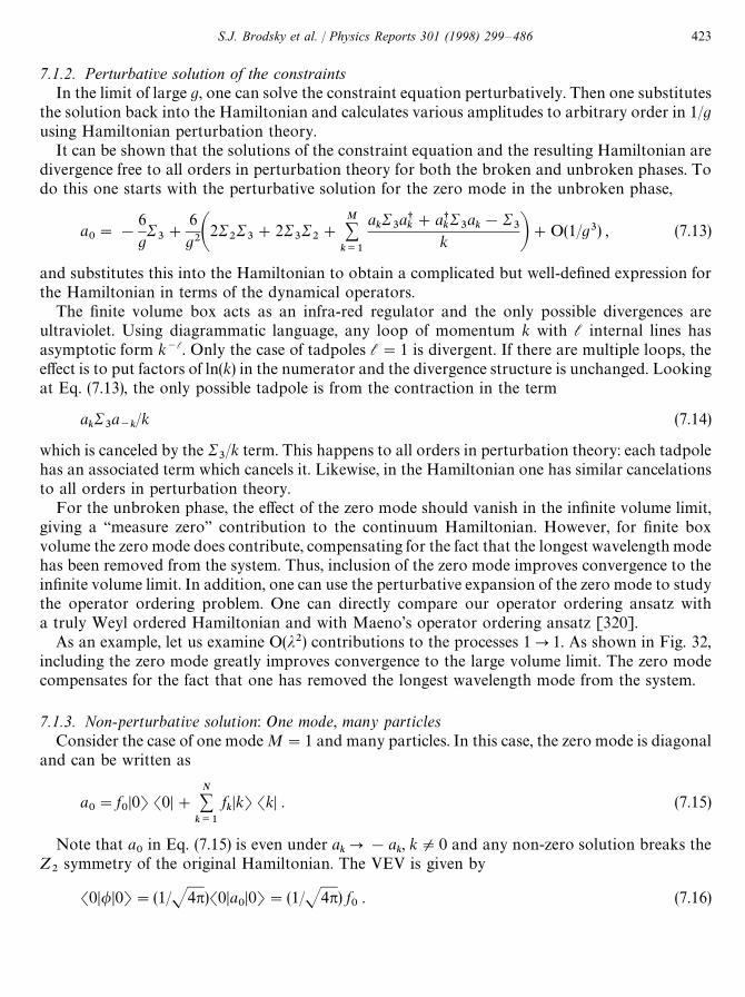
7.1.2. Perturbative solution of the constraintsIn the limit of large g, one can solve the constraint equation perturbatively. Then one substitutes

the solution back into the Hamiltonian and calculates various amplitudes to arbitrary order in 1/gusing Hamiltonian perturbation theory.

It can be shown that the solutions of the constraint equation and the resulting Hamiltonian aredivergence free to all orders in perturbation theory for both the broken and unbroken phases. Todo this one starts with the perturbative solution for the zero mode in the unbroken phase,

a0"!

6gR

3#

6g2A2R

2R

3#2R

3R

2#

M+k/1

akR

3ask#as

kR3ak!R

3k B#O(1/g3) , (7.13)

and substitutes this into the Hamiltonian to obtain a complicated but well-defined expression forthe Hamiltonian in terms of the dynamical operators.

The finite volume box acts as an infra-red regulator and the only possible divergences areultraviolet. Using diagrammatic language, any loop of momentum k with l internal lines hasasymptotic form k~l. Only the case of tadpoles l"1 is divergent. If there are multiple loops, theeffect is to put factors of ln(k) in the numerator and the divergence structure is unchanged. Lookingat Eq. (7.13), the only possible tadpole is from the contraction in the term

akR

3a~k

/k (7.14)

which is canceled by the R3/k term. This happens to all orders in perturbation theory: each tadpole

has an associated term which cancels it. Likewise, in the Hamiltonian one has similar cancelationsto all orders in perturbation theory.

For the unbroken phase, the effect of the zero mode should vanish in the infinite volume limit,giving a “measure zero” contribution to the continuum Hamiltonian. However, for finite boxvolume the zero mode does contribute, compensating for the fact that the longest wavelength modehas been removed from the system. Thus, inclusion of the zero mode improves convergence to theinfinite volume limit. In addition, one can use the perturbative expansion of the zero mode to studythe operator ordering problem. One can directly compare our operator ordering ansatz witha truly Weyl ordered Hamiltonian and with Maeno’s operator ordering ansatz [320].

As an example, let us examine O(j2) contributions to the processes 1P1. As shown in Fig. 32,including the zero mode greatly improves convergence to the large volume limit. The zero modecompensates for the fact that one has removed the longest wavelength mode from the system.

7.1.3. Non-perturbative solution: One mode, many particlesConsider the case of one mode M"1 and many particles. In this case, the zero mode is diagonal

and can be written as

a0"f

0D0T S0D#

N+k/1

fkDkT SkD . (7.15)

Note that a0

in Eq. (7.15) is even under akP!a

k, kO0 and any non-zero solution breaks the

Z2

symmetry of the original Hamiltonian. The VEV is given by

S0D/D0T"(1/J4p)S0Da0D0T"(1/J4p) f

0. (7.16)


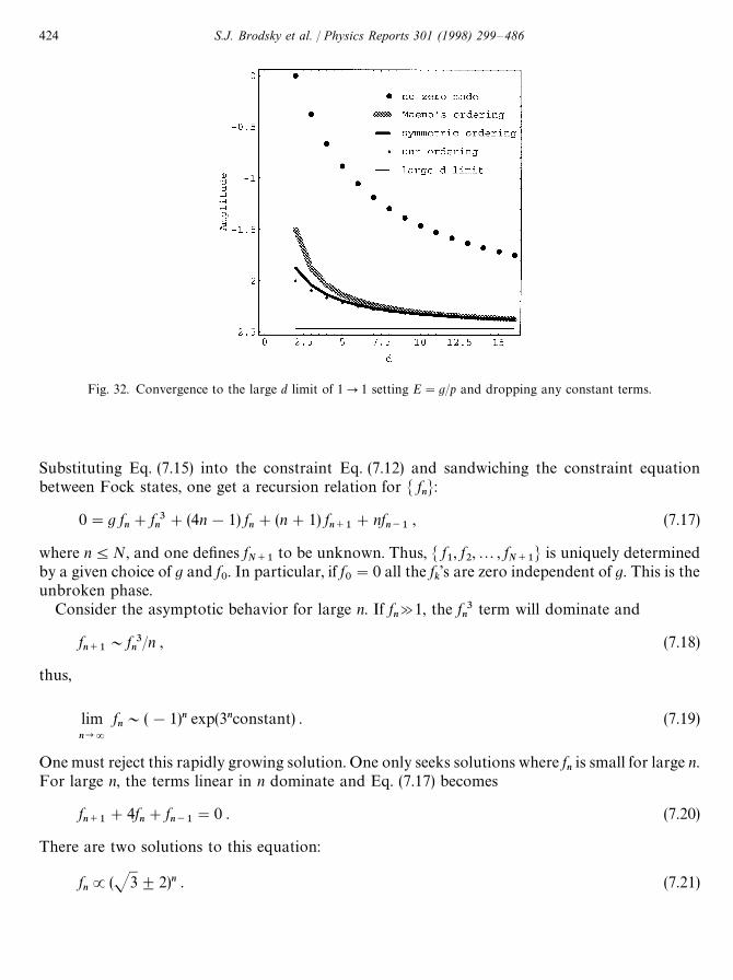
Fig. 32. Convergence to the large d limit of 1P1 setting E"g/p and dropping any constant terms.

Substituting Eq. (7.15) into the constraint Eq. (7.12) and sandwiching the constraint equationbetween Fock states, one get a recursion relation for M f

nN:

0"g fn#f 3

n#(4n!1) f

n#(n#1) f

n`1#nf

n~1, (7.17)

where n4N, and one defines fN`1

to be unknown. Thus, M f1, f

2,2, f

N`1N is uniquely determined

by a given choice of g and f0. In particular, if f

0"0 all the f

k’s are zero independent of g. This is the

unbroken phase.Consider the asymptotic behavior for large n. If f

nA1, the f 3

nterm will dominate and

fn`1

&f 3n

/n , (7.18)

thus,

limn?=

fn&(!1)n exp(3nconstant) . (7.19)

One must reject this rapidly growing solution. One only seeks solutions where fnis small for large n.

For large n, the terms linear in n dominate and Eq. (7.17) becomes

fn`1

#4fn#f

n~1"0 . (7.20)

There are two solutions to this equation:

fnJ(J3$2)n . (7.21)


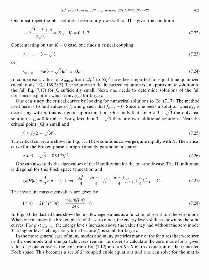
One must reject the plus solution because it grows with n. This gives the condition

!

J3!3#g

2J3"K , K"0, 1, 22 (7.22)

Concentrating on the K"0 case, one finds a critical coupling

g#3*5*#!-

"3!J3 (7.23)

or

j#3*5*#!-

"4p(3#J3)k2+60k2 . (7.24)

In comparison, values of j#3*5*#!-

from 22k2 to 55k2 have been reported for equal-time quantizedcalculations [93,1,168,282]. The solution to the linearized equation is an approximate solution tothe full Eq. (7.17) for f

0sufficiently small. Next, one needs to determine solutions of the full

non-linear equation which converge for large n.One can study the critical curves by looking for numerical solutions to Eq. (7.17). The method

used here is to find values of f0

and g such that fN`1

"0. Since one seeks a solution where fn

isdecreasing with n, this is a good approximation. One finds that for g'3!J3 the only realsolution is f

n"0 for all n. For g less than 3!J3 there are two additional solutions. Near the

critical point D f0D is small and

fn+f

0(2!J3)n . (7.25)

The critical curves are shown in Fig. 31. These solutions converge quite rapidly with N. The criticalcurve for the broken phase is approximately parabolic in shape:

g+3!J3!0.9177f 20

. (7.26)

One can also study the eigenvalues of the Hamiltonian for the one-mode case. The Hamiltonianis diagonal for this Fock space truncation and

SnDHDnT"32

n(n!1)#ng!f 4n4!

2n#14

f 2n#

n#14

f 2n`1

#

n4

f 2n~1

!C . (7.27)

The invariant mass eigenvalues are given by

P2DnT"2P`P~DnT"njSnDHDnT

24pDnT . (7.28)

In Fig. 33 the dashed lines show the first few eigenvalues as a function of g without the zero mode.When one includes the broken phase of the zero mode, the energy levels shift as shown by the solidcurves. For g(g

#3*5*#!-the energy levels increase above the value they had without the zero mode.

The higher levels change very little because fn

is small for large n.In the more general case of many modes and many particles many of the features that were seen

in the one-mode and one-particle cases remain. In order to calculate the zero mode for a givenvalue of g one converts the constraint Eq. (7.12) into an S]S matrix equation in the truncatedFock space. This becomes a set of S2 coupled cubic equations and one can solve for the matrix


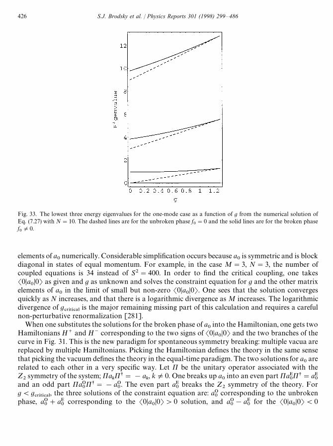
Fig. 33. The lowest three energy eigenvalues for the one-mode case as a function of g from the numerical solution ofEq. (7.27) with N"10. The dashed lines are for the unbroken phase f

0"0 and the solid lines are for the broken phase

f0O0.

elements of a0numerically. Considerable simplification occurs because a

0is symmetric and is block

diagonal in states of equal momentum. For example, in the case M"3, N"3, the number ofcoupled equations is 34 instead of S2"400. In order to find the critical coupling, one takesS0Da

0D0T as given and g as unknown and solves the constraint equation for g and the other matrix

elements of a0

in the limit of small but non-zero S0Da0D0T. One sees that the solution converges

quickly as N increases, and that there is a logarithmic divergence as M increases. The logarithmicdivergence of g

#3*5*#!-is the major remaining missing part of this calculation and requires a careful

non-perturbative renormalization [281].When one substitutes the solutions for the broken phase of a

0into the Hamiltonian, one gets two

Hamiltonians H` and H~ corresponding to the two signs of S0Da0D0T and the two branches of the

curve in Fig. 31. This is the new paradigm for spontaneous symmetry breaking: multiple vacua arereplaced by multiple Hamiltonians. Picking the Hamiltonian defines the theory in the same sensethat picking the vacuum defines the theory in the equal-time paradigm. The two solutions for a

0are

related to each other in a very specific way. Let P be the unitary operator associated with theZ

2symmetry of the system; Pa

kPs"!a

k, kO0. One breaks up a

0into an even part PaE

0Ps"aE

0and an odd part PaO

0Ps"!aO

0. The even part aE

0breaks the Z

2symmetry of the theory. For

g(g#3*5*#!-

, the three solutions of the constraint equation are: aO0

corresponding to the unbrokenphase, aO

0#aE

0corresponding to the S0Da

0D0T'0 solution, and aO

0!aE

0for the S0Da

0D0T(0


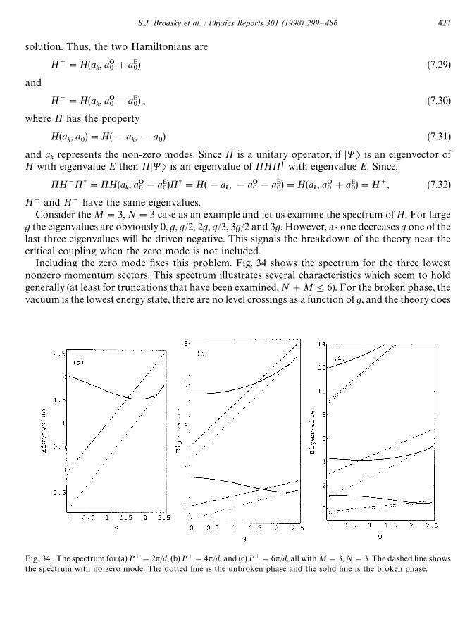
Fig. 34. The spectrum for (a) P`"2p/d, (b) P`"4p/d, and (c) P`"6p/d, all with M"3, N"3. The dashed line showsthe spectrum with no zero mode. The dotted line is the unbroken phase and the solid line is the broken phase.

solution. Thus, the two Hamiltonians are

H`"H(ak, aO

0#aE

0) (7.29)

and

H~"H(ak, aO

0!aE

0) , (7.30)

where H has the property

H(ak, a

0)"H(!a

k, !a

0) (7.31)

and ak

represents the non-zero modes. Since P is a unitary operator, if DWT is an eigenvector ofH with eigenvalue E then PDWT is an eigenvalue of PHPs with eigenvalue E. Since,

PH~Ps"PH(ak, aO

0!aE

0)Ps"H(!a

k, !aO

0!aE

0)"H(a

k, aO

0#aE

0)"H`, (7.32)

H` and H~ have the same eigenvalues.Consider the M"3, N"3 case as an example and let us examine the spectrum of H. For large

g the eigenvalues are obviously 0, g, g/2, 2g, g/3, 3g/2 and 3g. However, as one decreases g one of thelast three eigenvalues will be driven negative. This signals the breakdown of the theory near thecritical coupling when the zero mode is not included.

Including the zero mode fixes this problem. Fig. 34 shows the spectrum for the three lowestnonzero momentum sectors. This spectrum illustrates several characteristics which seem to holdgenerally (at least for truncations that have been examined, N#M46). For the broken phase, thevacuum is the lowest energy state, there are no level crossings as a function of g, and the theory does


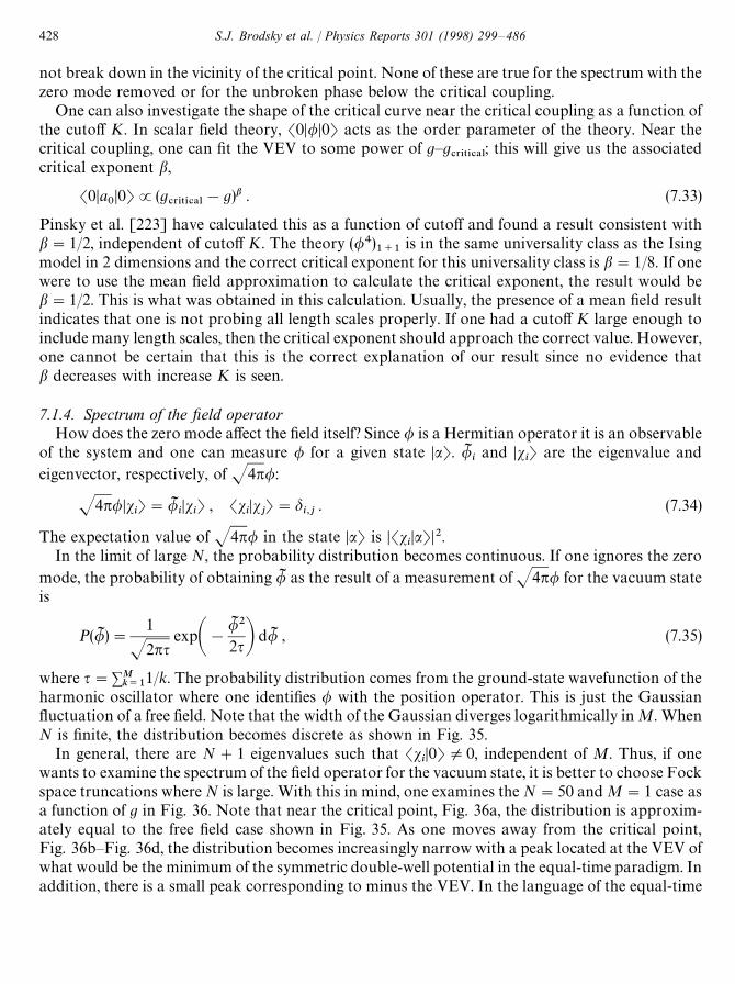
not break down in the vicinity of the critical point. None of these are true for the spectrum with thezero mode removed or for the unbroken phase below the critical coupling.

One can also investigate the shape of the critical curve near the critical coupling as a function ofthe cutoff K. In scalar field theory, S0D/D0T acts as the order parameter of the theory. Near thecritical coupling, one can fit the VEV to some power of g—g

#3*5*#!-; this will give us the associated

critical exponent b,

S0Da0D0TJ(g

#3*5*#!-!g)b . (7.33)

Pinsky et al. [223] have calculated this as a function of cutoff and found a result consistent withb"1/2, independent of cutoff K. The theory (/4)

1`1is in the same universality class as the Ising

model in 2 dimensions and the correct critical exponent for this universality class is b"1/8. If onewere to use the mean field approximation to calculate the critical exponent, the result would beb"1/2. This is what was obtained in this calculation. Usually, the presence of a mean field resultindicates that one is not probing all length scales properly. If one had a cutoff K large enough toinclude many length scales, then the critical exponent should approach the correct value. However,one cannot be certain that this is the correct explanation of our result since no evidence thatb decreases with increase K is seen.

7.1.4. Spectrum of the field operatorHow does the zero mode affect the field itself? Since / is a Hermitian operator it is an observable

of the system and one can measure / for a given state DaT. /Iiand Ds

iT are the eigenvalue and

eigenvector, respectively, of J4p/:

J4p/DsiT"/I

iDs

iT , Ss

iDs

jT"d

i,j. (7.34)

The expectation value of J4p/ in the state DaT is DSsiDaTD2.

In the limit of large N, the probability distribution becomes continuous. If one ignores the zeromode, the probability of obtaining /I as the result of a measurement of J4p/ for the vacuum stateis

P(/I )"1

J2pqexpA!

/I 22qB d/I , (7.35)

where q"+Mk/1

1/k. The probability distribution comes from the ground-state wavefunction of theharmonic oscillator where one identifies / with the position operator. This is just the Gaussianfluctuation of a free field. Note that the width of the Gaussian diverges logarithmically in M. WhenN is finite, the distribution becomes discrete as shown in Fig. 35.

In general, there are N#1 eigenvalues such that SsiD0TO0, independent of M. Thus, if one

wants to examine the spectrum of the field operator for the vacuum state, it is better to choose Fockspace truncations where N is large. With this in mind, one examines the N"50 and M"1 case asa function of g in Fig. 36. Note that near the critical point, Fig. 36a, the distribution is approxim-ately equal to the free field case shown in Fig. 35. As one moves away from the critical point,Fig. 36b—Fig. 36d, the distribution becomes increasingly narrow with a peak located at the VEV ofwhat would be the minimum of the symmetric double-well potential in the equal-time paradigm. Inaddition, there is a small peak corresponding to minus the VEV. In the language of the equal-time


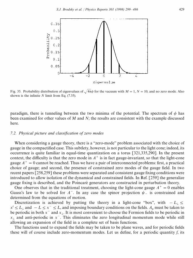
Fig. 35. Probability distribution of eigenvalues of J4p/ for the vacuum with M"1, N"10, and no zero mode. Alsoshown is the infinite N limit from Eq. (7.35).

paradigm, there is tunneling between the two minima of the potential. The spectrum of / hasbeen examined for other values of M and N; the results are consistent with the example discussedhere.

7.2. Physical picture and classification of zero modes

When considering a gauge theory, there is a “zero-mode” problem associated with the choice ofgauge in the compactified case. This subtlety, however, is not particular to the light cone; indeed, itsoccurrence is quite familiar in equal-time quantization on a torus [321,335,290]. In the presentcontext, the difficulty is that the zero mode in A` is in fact gauge-invariant, so that the light-conegauge A`"0 cannot be reached. Thus we have a pair of interconnected problems: first, a practicalchoice of gauge; and second, the presence of constrained zero modes of the gauge field. In tworecent papers [258,259] these problems were separated and consistent gauge fixing conditions wereintroduced to allow isolation of the dynamical and constrained fields. In Ref. [259] the generalizegauge fixing is described, and the Poincare generators are constructed in perturbation theory.

One observes that in the traditional treatment, choosing the light-cone gauge A`"0 enablesGauss’s law to be solved for A~. In any case the spinor projection t

~is constrained and

determined from the equations of motion.Discretization is achieved by putting the theory in a light-cone “box”, with !¸

M4

xi4¸M

and !¸4x~4¸, and imposing boundary conditions on the fields. Ak must be taken tobe periodic in both x~ and x

M. It is most convenient to choose the Fermion fields to be periodic in

xM

and anti-periodic in x~. This eliminates the zero longitudinal momentum mode while stillallowing an expansion of the field in a complete set of basis functions.

The functions used to expand the fields may be taken to be plane waves, and for periodic fieldsthese will of course include zero-momentum modes. Let us define, for a periodic quantity f, its


Fig. 36. Probability distribution of eigenvalues of J4p/ for the vacuum with couplings g"1, g"0, g"!1, andg"!2, all for M"1 and N"50. The positive VEV solution to the constraint equation is used.

longitudinal zero mode

S f T0,

12¸P

L

~L

dx~ f (x~, xM) (7.36)

and the corresponding normal mode part

S f T/,f!S f T

0. (7.37)

We shall further denote the “global zero mode” — the mode independent of all the spatialcoordinates — by S f T:

S f T,1XP

L

~L

dx~PLM

~LM

d2xM

f (x~, xM) . (7.38)


Finally, the quantity which will be of most interest to us is the “proper zero mode”, defined by

f0,S f T

0!S f T . (7.39)

By integrating over the appropriate direction(s) of space, we can project the equations of motiononto the various sectors. The global zero mode sector requires some special treatment, and will notbe discussed here.

We concentrate our attention on the proper zero mode sector, in which the equations of motionbecome

!2MA`

0"gJ`

0, (7.40)

!2(`)2A`

0!2

MA~

0!2

i`Ai

0"gJ~

0, (7.41)

!2MAi

0#

i`

A`0#

ijAj

0"gJi

0. (7.42)

We first observe that Eq. (7.40), the projection of Gauss’ law, is a constraint which determines theproper zero mode of A` in terms of the current J`:

A`0"!g(1/2

M)J`

0. (7.43)

Eqs. (7.41) and (7.42) then determine the zero modes A~0

and Ai0.

Eq. (7.43) is clearly incompatible with the strict light-cone gauge A`"0, which is most naturalin light-cone analyses of gauge theories. Here we encounter a common problem in treating axialgauges on compact spaces, which has nothing to do with light-cone quantization per se. The pointis that any x~-independent part of A` is in fact gauge invariant, since under a gauge transforma-tion

A`PA`#2~

K , (7.44)

where K is a function periodic in all coordinates. Thus, it is not possible to bring an arbitrary gaugefield configuration to one satisfying A`"0 via a gauge transformation, and the light-cone gauge isincompatible with the chosen boundary conditions. The closest we can come is to set the normalmode part of A` to zero, which is equivalent to

~A`"0 . (7.45)

This condition does not, however, completely fix the gauge — we are free to make arbitraryx~-independent gauge transformations without undoing Eq. (7.45). We may therefore imposefurther conditions on Ak in the zero-mode sector of the theory.

To see what might be useful in this regard, let us consider solving Eq. (7.42). We begin by actingon Eq. (7.42) with

i. The transverse field Ai

0then drops out and we obtain an expression for the

time derivative of A`0:

`A`

0"g(1/2

M)

iJi0

. (7.46)

[This can also be obtained by taking a time derivative of Eq. (7.43), and using current conservationto re-express the right-hand side in terms of Ji]. Inserting this back into Eq. (7.42) we then find,after some rearrangement,

!2M(di

j!

ij/2

M)Aj

0"g(di

j!

ij/2

M)Jj

0. (7.47)


Now the operator (dij!

ij/2

M) is nothing more than the projector of the two-dimensional

transverse part of the vector fields Ai0and Ji

0. No trace remains of the longitudinal projection of the

field (ij/2

M)Aj

0in Eq. (7.47). This reflects precisely the residual gauge freedom with respect to

x~-independent transformations. To determine the longitudinal part, an additional condition isrequired.

More concretely, the general solution to Eq. (7.47) is

Ai0"!g(1/2

M)Ji

0#

iu(x`, x

M) , (7.48)

where u must be independent of x~ but is otherwise arbitrary. Imposing a condition on, say, iAi

0will uniquely determine u.

In Ref. [259], for example, the condition

iAi

0"0 (7.49)

was proposed as being particularly natural. This choice, taken with the other gauge conditions wehave imposed, has been called the “compactification gauge”. In this case

u"g(1/(2M)2)

iJi0

. (7.50)

Of course, other choices are also possible. For example, we might generalize Eq. (7.50) to

u"ag(1/(2M)2)

iJi0

, (7.51)

with a a real parameter. The gauge condition corresponding to this solution is

iAi

0"!g(1!a)(1/2

M)

iJi0

. (7.52)

We shall refer to this as the “generalized compactification gauge”. An arbitrary gauge fieldconfiguration Bk can be brought to one satisfying Eq. (7.52) via the gauge function

K(xM)"!(1/2

M)[g(1!a)(1/2

M)

iJi0#

iBi

0] . (7.53)

This is somewhat unusual in that K(xM) involves the sources as well as the initial field configuration,

but this is perfectly acceptable. More generally, u can be any (dimensionless) function of gaugeinvariants constructed from the fields in the theory, including the currents JB. For our purposesEq. (7.52) suffices.

We now have relations defining the proper zero modes of Ai,

Ai0"!g(1/2

M)(di

j!a

ij/2

M)Jj

0, (7.54)

as well as A`0

[Eq. (7.43)]. All that remains is to use the final constraint, Eq. (7.41), to determineA~

0. Using Eqs. (7.46) and (7.52), we find that Eq. (7.41) can be written as

2MA~

0"!gJ~

0!2ag(1/2

M)

`iJi0

. (7.55)

After using the equations of motion to express `Ji0

in terms of the dynamical fields at x`"0, thismay be straightforwardly solved for A~

0by inverting the 2

M. In what follows, however, we shall have

no need of A~0

. It does not enter the Hamiltonian, for example; as usual, it plays the role ofa multiplier to Gauss’ law, Eq. (7.42), which we are able to implement as an operator identity.

We have shown how to perform a general gauge fixing of Abelian gauge theory in DLCQ andcleanly separate the dynamical from the constrained zero-longitudinal momentum fields. The


various zero-mode fields must be retained in the theory if the equations of motion are to be realizedas the Heisenberg equations. We have further seen that taking the constrained fields properly intoaccount renders the ultraviolet behavior of the theory more benign, in that it results in theautomatic generation of a counter term for a non-covariant divergence in the fermion self-energy inlowest-order perturbation theory.

The solutions to the constraint relations for the Ai0

are all physically equivalent, being related bydifferent choices of gauge in the zero mode sector of the theory. There is a gauge which isparticularly simple, however, in that the fields may be taken to satisfy the usual canonicalanti-commutation relations. This is most easily exposed by examining the kinematical Poincaregenerators and finding the solution for which these retain their free-field forms. The uniquesolution that achieves this is u"0 in Eq. (7.48). For solutions other than this one, complicatedcommutation relations between the fields will be necessary to correctly translate them in theinitial-value surface.

It would be interesting to study the structure of the operators induced by the zero modes fromthe point of view of the light-cone power-counting analysis of Wilson [456]. As noted in theIntroduction, to the extent that DLCQ coincides with reality, effects which we would normallyassociate with the vacuum must be incorporated into the formalism through the new, non-canonical interactions arising from the zero modes. Particularly interesting is the appearance ofoperators that are non-local in the transverse directions. These are interesting because the stronginfrared effects they presumably mediate could give rise to transverse confinement in the effectiveHamiltonian for QCD. There is longitudinal confinement already at the level of the canonicalHamiltonian; that is, the effective potential between charges separated only in x~ grows linearlywith the separation. This comes about essentially from the non-locality in x~ (i.e. the small-k`

divergences) of the light-cone formalism.It is clearly of interest to develop non-perturbative methods for solving the constraints, since we

are ultimately interested in non-perturbative diagonalization of P~. Several approaches to thisproblem have recently appeared in the literature [209,210,33,382], in the context of scalar fieldtheories in 1#1 dimensions. For QED with a realistic value of the electric charge, however, itmight be that a perturbative treatment of the constraints could suffice; that is, that we could usea perturbative solution of the constraint to construct the Hamiltonian, which would then bediagonalized non-perturbatively. An approach similar in spirit has been proposed in Ref. [456],where the idea is to use a perturbative realization of the renormalization group to construct aneffective Hamiltonian for QCD, which is then solved non-perturbatively. There is some evidencethat this kind of approach might be useful. Wivoda and Hiller have recently used DLCQ to studya theory of neutral and interacting charged scalar fields in 3#1 dimensions [458]. They discoveredthat including four-fermion operators precisely analogous to the perturbative ones appearing inP~Z

significantly improved the numerical behavior of the simulation.The extension of the present work to the case of QCD is complicated by the fact that the

constraint relations for the gluonic zero modes are non-linear, as in the /4 theory. A perturbativesolution of the constraints is of course still possible, but in this case, since the effective coupling atthe relevant (hadronic) scale is large, it is clearly desirable to go beyond perturbation theory. Inaddition, because of the central role played by gauge fixing in the present work, we may expectcomplications due to the Gribov ambiguity [189], which prevents the selection of unique represen-tatives on gauge orbits in non-perturbative treatments of Yang—Mills theory. As a step in this


direction, work is in progress on the pure glue theory in 2#1 dimensions [259]. There it isexpected that some of the non-perturbative techniques used recently in 1#1 dimensions[33,382,379—381,331] can be applied.

7.3. Dynamical zero modes

Our concern in this section is with zero modes that are true dynamical independent fields. Theycan arise due to the boundary conditions in gauge theory one cannot fully implement thetraditional light-cone gauge A`"0. The development of the understanding of this problem inDLCQ can be traced in Refs. [206—209,325,326]. The field A` turns out to have a zero mode whichcannot be gauged away [258,259,261,379—381,331]. This mode is indeed dynamical, and is theobject we study in this paper. It has its analogue in instant form approaches to gauge theory. Forexample, there exists a large body of work on Abelian and non-Abelian gauge theories in 1#1dimensions quantized on a cylinder geometry [321,217]. There indeed this dynamical zero modeplays an important role. We too shall concern ourselves in the present section with non-Abeliangauge theory in 1#1 dimensions, revisiting the model introduced by ’t Hooft [424].

The specific task we undertake here is to understand the zero-mode subsector of the pure gluetheory, namely where only zero-mode external sources excite only zero-mode gluons. We shall seethat this is not an approximation but rather a consistent solution, a sub-regime within the completetheory. A similar framing of the problem lies behind the work of Luscher [314] and van Baal [434]using the instant form Hamiltonian approach to pure glue gauge theory in 3#1 dimensions. Thebeauty of this reduction in the (1#1)-dimensional theory is twofold. First, it yields a theory whichis exactly soluble. This is useful given the dearth of soluble models in field theory. Secondly, thezero-mode theory represents a paring down to the point where the front and instant forms aremanifestly identical, which is nice to know indeed. We solve the theory in this specific dynamicalregime and find a discrete spectrum of states whose wavefunctions can be completely determined.These states have the quantum numbers of the vacuum.

We consider an SU(2) non-Abelian gauge theory in 1#1 dimensions with classical sourcescoupled to the gluons. The Lagrangian density is

L"12Tr(FklFkl)#2 Tr(JkAk) (7.56)

where Fkl"lAl!lAk!g[Ak, Al]. With a finite interval in x~ from !¸ to ¸, we imposeperiodic boundary conditions on all gauge potentials Ak.

We cannot eliminate the zero mode of the gauge potential. The reason is evident: it is invariantunder periodic gauge transformations. But, of course, we can always perform a rotation in color

space. In line with other authors [14,385,146—148], we choose this so that oA`3

is the only non-zero

element, since in our representation only p3 is diagonal. In addition, we can impose the subsidiary

gauge condition oA~3"0. The reason is that there still remains freedom to perform gauge trans-

formations that depend only on light-cone time x` and the color matrix p3.The above procedure would appear to have enabled complete fixing of the gauge. This is still not

so. Gauge transformations

»"expMix~(np/2¸)p3N (7.57)


generate shifts, according to Eq. (7.53), in the zero-mode component

oA`3

PoA`3

#np/g¸ . (7.58)

All of these possibilities, labelled by the integer n, of course still satisfy ~A`"0, but as one sees

n"0 should not really be included. One can verify that the transformations » also preserve thesubsidiary condition. One notes that the transformation is x~-dependent and Z

2periodic. It is thus

a simple example of a Gribov copy [189] in 1#1 dimensions. We follow the conventionalprocedure by demanding

oA`3

Onp/g¸ , n"$1,$2,2 . (7.59)

This eliminates singularity points at the Gribov “horizons” which in turn correspond to a vanish-ing Faddeev—Popov determinant [434].

For convenience, we henceforth use the notation

oA`3

"v , x`"t , w2" oJ``

oJ~`

/g2 and oJ~3

"12B . (7.60)

We pursue a Hamiltonian formulation. The only conjugate momentum is

p, oP~3

"~ oA`3

"~v . (7.61)

The Hamiltonian density ¹`~"~ oA`3

P~3!L leads to the Hamiltonian

H"12[p2#(w2/v2)#Bv](2¸) . (7.62)

Quantization is achieved by imposing a commutation relation at equal light-cone time on thedynamical degree of freedom. Introducing the variable q"2¸v, the appropriate commutationrelation is [q(x`), p(x`)]"i. The field theoretic problem reduces to quantum mechanics of a singleparticle as in Manton’s treatment of the Schwinger model in Refs. [321]. One thus has to solve theSchrodinger equation

12A!

d2

dq2#

(2¸w)2q2

#

Bq2¸Bt"Et , (7.63)

with the eigenvalue E"E/(2¸) actually being an energy density.All eigenstates t have the quantum numbers of the naive vacuum adopted in standard front form

field theory: all of them are eigenstates of the light-cone momentum operator P` with zeroeigenvalue. The true vacuum is now that state with lowest P~ eigenvalue. In order to get an exactly

soluble system we eliminate the source 2B"oJ~3

.

The boundary condition that is to be imposed comes from the treatment of the Gribov problem.Since the wavefunction vanishes at q"0 we must demand that the wavefunctions vanish at thefirst Gribov horizon q"$2p/g. The overall constant R is then fixed by normalization. This leads


to the energy density only assuming the discrete values

E(l)m"(g2/8p2)(X(l)

m)2, m"1, 2,2, (7.64)

where X(l)m

denotes the mth zero of the lth Bessel function Jl. In general, these zeroes can only beobtained numerically. Thus

tm(q)"RJqJl(J2E(l)

mq) (7.65)

is the complete solution. The true vacuum is the state of lowest energy namely with m"1.The exact solution we obtained is genuinely non-perturbative in character. It describes vacuum-

like states since for all of these states P`"0. Consequently, they all have zero invariant massM2"P`P~. The states are labelled by the eigenvalues of the operator P~. The linear dependenceon ¸ in the result for the discrete energy levels is also consistent with what one would expect froma loop of color flux running around the cylinder.

In the source-free equal time case Hetrick [217,218] uses a wavefunction that is symmetric aboutq"0. For our problem this corresponds to

tm(q)"N cos(J2e

mq) , (7.66)

where N is fixed by normalization. At the boundary of the fundamental modular region q"2p/gand t

m"(!1)mN, thus J2e

m2p/g"mp and

e"18g2(m2!1) . (7.67)

Note that m"1 is the lowest-energy state and has as expected one node in the allowed region04g42p/g. Hetrick [217] discusses the connection to the results of Rajeev [387] but it amountsto a shift in e and a redefining of mPm/2. It has been argued by van Baal that the correct boundarycondition at q"0 is t(0)"0. This would give a sine which matches smoothly with the Besselfunction solution. This calculation offers the lesson that even in a front-form approach, the vacuummight not be just the simple Fock vacuum. Dynamical zero modes do imbue the vacuum witha rich structure.

8. Non-perturbative regularization and renormalization

The subject of renormalization is a large one and high-energy theorists have developed a stan-dard set of renormalization techniques based on perturbation theory (see, for example, Ref. [111]).However, many of these techniques are poorly suited for light-front field theory. Researchers inlight-front field theory must either borrow techniques from condensed matter physics[374,435,453] or nuclear physics or come up with entirely new approaches. Some progress in thisdirection has already been made, see, for example, Refs. [294,444—447,456]. A considerable amountof work is focusing on these questions [8,2,85,134,194,233,464]; particularly see the work ofBassetto et al. [5,23—26], Bakker et al. [309,310,399], Brisudova et al. [48—50], and Zhang et al.[461—466]. It should be noted, however, that the work of Perry and collaborators [48—50,461—466]has strange aspects beyond all the effort. Front-form QCD is a theory with many useful symmetrieslike gauge invariance, Lorentz invariance, thus boost, rotational and chiral invariance. But these


authors, particularly in Refs. [49,50,466], somehow manage to admittedly give up each and everyone of them, including rotational invariance (thus no degeneracies of multiplets). This shows howdifficult the problem is. But it is not really what one aims at.

The biggest challenge to renormalization of light-front field theory is the infrared divergencesthat arise. Recall that the Hamiltonian for a free particle is

P~"(P2M#m2)/2P`. (8.1)

Small longitudinal momentum P` is associated with large energies. Thus, light-front field theory issubject to infrared longitudinal divergences. These divergences are quite different in nature fromthe infrared divergences found in equal-time quantized field theory. In order to remove smallP` states, one must introduce non-local counter terms into the Hamiltonian. Power countingarguments allow arbitrary functions of transverse momenta to be associated with these counterterms. This is in contrast to more conventional approaches where demanding locality stronglyconstrains the number of allowed operators.

One hopes to use light-front field theory to perform bound state calculations. In this caseone represents a bound state by a finite number of particles (a Tamm—Dancoff truncation)whose momenta are restricted to some finite interval. This has a number of implications. Inparticular, momentum cutoffs and Tamm—Dancoff truncations both tend to break various sym-metries of a theory. Proper renormalization must restore these symmetries. In contrast, conven-tional calculations choose regulators (like dimensional regularization) that do not break manysymmetries.

In conventional approaches, one is often concerned simply whether the system is renormalizable,that is, whether the large cutoff limit is well defined. In bound-state calculations, one is alsointerested in how quickly the results converge as one increases the cutoffs since numericalcalculations must be performed with a finite cutoff. Thus, one is potentially interested in the effectsof irrelevant operators along with the usual marginal and relevant operators.

Conventional renormalization is inherently perturbative in nature. However, we are interested inmany phenomena that are essentially non-perturbative: bound states, confinement, and spontan-eous symmetry breaking. The bulk of renormalization studies in light-front field theory to datehave used perturbative techniques [456,182]. Non-perturbative techniques must be developed.

Generally, one expects that renormalization will produce a large number of operators in thelight-front Hamiltonian. A successful approach to renormalization must be able to produce theseoperators automatically (say, as part of a numerical algorithm). In addition, there should be onlya few free parameters which must be fixed phenomenologically. Otherwise, the predictive power ofa theory will be lost.

8.1. Tamm—Dancoff integral equations

Let us start by looking at a simple toy model that has been studied by a number of authors[435,182,374,426,427,244]. In fact, it is the famous Kondo problem truncated to one-particle states[277]. Consider the homogeneous integral equation

(p!E)/(p)#gPK

0

dp@ /(p@)"0 (8.2)


with eigenvalue E and eigenvector /(p). This is a model for Tamm—Dancoff equation of a singleparticle of momentum p with Hamiltonian H(p,p@)"pd(p!p@)#g. We will focus on the E(0bound state solution:

/(p)"constant/(p!E) , E"K/(1!e~1@g) . (8.3)

Note that the eigenvalue diverges in the limit KPR. Proper renormalization involves modifyingthe system to make E and /(p) independent of K in the limit KPR. Towards this end, we adda counterterm CK to the Hamiltonian. Invoking the high-low analysis [454], we divide the interval0(p(K into two subintervals: 0(p(¸, a “low-momentum region”, and ¸(p(K, a “high-momentum region”, where the momentum scales characterized by E, ¸, and K are assumed to bewidely separated. The idea is that the eigenvalue and eigenvector should be independent of thebehavior of the system in the high momentum region. The eigenvalue equation can be written astwo coupled equations

p3[0, ¸] , (p!E)/(p)#(g#CK)PL

0

dp@ /(p@)#(g#CK)PK

L

dp@ /(p@)"0 , (8.4)

p3[¸, K] , (p!E)/(p)#(g#CK)PK

L

dp@ /(p@)#(g#CK)PL

0

dp@ /(p@)"0 . (8.5)

Integrating Eq. (8.5) in the limit ¸, KAE,

PK

L

dp /(p)"!

(g#CK)log (K/¸)1#(g#CK)log (K/¸) P

L

0

dp@ /(p@) , (8.6)

and substituting this expression into Eq. (8.4), we obtain an eigenvalue equation with the high-momentum region integrated out

p3[0, ¸] , (p!E)/(p)#(g#CK)

1#(g#CK)log (K/¸) PL

0

dp@ /(p@)"0 . (8.7)

If we demand this expression to be independent of K,

ddK A

(g#CK)1#(g#CK)log (K/¸)B"0 , (8.8)

we obtain a differential equation for CK,

dCK/dK"(g#CK)2/K . (8.9)

Solving this equation, we are free to insert an arbitrary constant !1/Ak!log k

g#CK"Ak

1!Ak log (K/k). (8.10)

Substituting this result back into Eq. (8.7),

p3[0, ¸], (p!E)/(p)#Ak

1!Ak log (¸/k)PL

0

dp@ /(p@)"0 , (8.11)


we see that K has been removed from the equation entirely. Using Eq. (8.10) in the originaleigenvalue equation

(p!E)/(p)#Ak

1!Ak log (K/k)PK

0

dp@ /(p@)"0 (8.12)

gives the same equation as Eq. (8.11) with ¸ replaced by K. The eigenvalue is now,

E"K/(1!(K/k)e~1@Ak) , limK?=

E"!ke1@Ak . (8.13)

Although the eigenvalue is still a function of the cutoff for finite K, the eigenvalue does becomeindependent of the cutoff in the limit KPR, and the system is properly renormalized.

One can think of Ak as the renormalized coupling constant and k as the renormalization scale. Inthat case, the eigenvalue should depend on the choice of Ak for a given k but be independent ofk itself. Suppose, for Eq. (8.13), we want to change k to a new value, say k@. In order that theeigenvalue remains the same, we must also change the coupling constant from Ak to Ak{,

ke1@Ak"k@e1@Ak{. (8.14)

In the same manner, one can write down a b-function for Ak [436],

k(d/dk)Ak"A2k . (8.15)

Using these ideas one can examine the general case. Throughout, we will be working withoperators projected onto some Tamm—Dancoff subspace (finite particle number) of the full Fockspace. In addition, we will regulate the system by demanding that each component of momentumof each particle lies within some finite interval. One defines the “cutoff” K to be an operator whichprojects onto this subspace of finite particle number and finite momenta. Thus, for any operatorO,O,KOK. Consider the Hamiltonian

H"H0#»#CK , (8.16)

where, in the standard momentum space basis, H0

is the diagonal part of the Hamiltonian, » is theinteraction term, and CK is the counter term which is to be determined and is a function of thecutoff. Each term of the Hamiltonian is hermitian and compact. Schrodinger’s equation can bewritten

(H0!E)D/T#(»#CK)D/T"0 (8.17)

with energy eigenvalue E and eigenvector D/T. The goal is to choose CK such that E and D/T areindependent of K in the limit of large cutoff.

One now makes an important assumption: the physics of interest is characterized by energy scaleE and is independent of physics near the boundary of the space spanned by K. Following theapproach of the previous section, one defines two projection operators, Q and P, whereK"Q#P, QP"PQ"0, and Q and P commute with H

0. Q projects onto a “high-momentum

region” which contains energy scales one does not care about, and P projects onto a “low-momentum region” which contains energy scales characterized by E. Schrodinger’s equation (8.17)


can be rewritten as two coupled equations:

(H0!E)PD/T#P(»#CK)PD/T#P(»#CK)QD/T"0 , (8.18)

and

(H0!E)QD/T#Q(»#CK)QD/T#Q(»#CK)PD/T"0 . (8.19)

Using Eq. (8.19), one can formally solve for QD/T in terms of PD/T,

QD/T"(1/Q(E!H)Q)(»#CK)PD/T . (8.20)

The term with the denominator is understood to be defined in terms of its series expansion in ».One can substitute this result back into Eq. (8.18),

(H0!E)PD/T#P(»#CK)PD/T#P(»#CK)(1/Q(E!H)Q) (»#CK)PD/T"0 . (8.21)

In order to properly renormalize the system, we could choose CK such that Eq. (8.21) is indepen-dent of one’s choice of K for a fixed P in the limit of large cutoffs. However, we will make a strongerdemand: that Eq. (8.21) should be equal to Eq. (8.17) with the cutoff K replaced by P.

One can express CK as the solution of an operator equation, the “counter term equation”,

»K"»!»F»K . (8.22)

where »K"»#CK, and provided that we can make the approximation

»(Q/(E!H0))»+»QF». (8.23)

This is what we will call the “renormalizability condition”. A system is properly renormalized if, aswe increase the cutoffs K and P, Eq. (8.23) becomes an increasingly good approximation. In thestandard momentum space basis, this becomes a set of coupled inhomogeneous integral equations.Such equations generally have a unique solution, allowing us to renormalize systems withouthaving to resort to perturbation theory. This includes cases where the perturbative expansiondiverges or converges slowly.

There are many possible choices for F that satisfy the renormalizability condition. For instance,one might argue that we want F to resemble 1/(E!H

0) as much as possible and choose

F"1/(k!H0) , (8.24)

where the arbitrary constant k is chosen to be reasonably close to E. In this case, one might be ableto use a smaller cutoff in numerical calculations.

One might argue that physics above some energy scale k is simpler and that it is numerically toodifficult to include the complications of the physics at energy scale E in the solution of the counterterm equation. Thus, one could choose

F"!h(H0!k)/H

0, (8.25)

where the arbitrary constant k is chosen to be somewhat larger than E but smaller than the energyscale associated with the cutoff. The h-function is assumed to act on each diagonal element in thestandard momentum space basis. The difficulty with this renormalization scheme is that it involvesthree different energy scales, E, k and the cutoff which might make the numerical problem more


difficult. One can relate our approach to conventional renormalization group concepts. In renor-malization group language, »K is the bare interaction term and » is the renormalized interactionterm. In both of the renormalization schemes introduced above, we introduced an arbitrary energyscale k; this is the renormalization scale. Now, physics (the energy eigenvalues and eigenvectors)should not depend on this parameter or on the renormalization scheme itself, for that matter. Howdoes one move from one renormalization scheme to another? Consider a particular choice ofrenormalized interaction term » associated with a renormalization scheme which uses F in thecounter term equation. We can use the counter term equation to find the bare coupling »K in termsof ». Now, to find the renormalized interaction term »@ associated with a different renormalizationscheme using a different operator F@ in the counter term equation, we simply use the counter termequation with »K as given and solve for »@

»@"»K#»KF@»@ . (8.26)

Expanding this procedure order by order in » and summing the result, we can obtain an operatorequation relating the two renormalized interaction terms directly

»@"»#»(F@!F)»@ . (8.27)

The renormalizability condition ensures that this expression will be independent of the cutoff in thelimit of large cutoff.

For the two particular renormalization schemes mentioned above, Eqs. (8.24) and (8.25), we canregard the renormalized interaction term » as an implicit function of k. We can see how therenormalized interaction term changes with k in the case (8.24):

k d»/dk"!»(k/(H0!k)2)» (8.28)

and in the case of Eq. (8.25),

k d»/dk"»d(H0!k)». (8.29)

This is a generalization of the b-function. The basic idea of asymptotic and box counter termrenormalization in the 3#1 Yukawa model calculation in an earlier section can be illustrated witha simple example. Consider an eigenvalue equation of the form [426,427],

k/(k)!gPK

0

dq »(k, q)/(q)"E/(k) . (8.30)

Making a high—low analysis of this equation as above and assuming that

»LH

(k, q)"»HL

(k, q)"»HH

(k, q)"f . (8.31)

Then one finds the following renormalized equation:

k/(k)!gPK

0

dq [»(k, q)!f ]/(q)!Ak

1#Ak ln (K/k)PK

0

dq /(q)"E/(k) . (8.32)

One has renormalized the original equation in the sense that the low-energy eigenvalue E isindependent of the high-energy cutoff and we have an arbitrary parameter C which can be adjustedto fit the ground-state energy level.


One can motivate both the asymptotic counter term and one-box counter term in the Yukawacalculation as different choices in our analysis. For a fixed k we are free to choose Ak at will. Thesimple asymptotic counter term corresponds to Ak"0. However, subtracting the asymptoticbehavior of the kernel with the term g f causes the wavefunction to fall off more rapidly than itwould otherwise at large q. As a result the (Ak/(1#Ak ln K/k)):/ dq is finite, and this term can beretained as an arbitrary adjustable finite counter term.

The perturbative counter terms correspond to Ak"g f then expanding in g ln K/k. Then onefinds

k/(k)!gPK

0

dq [»(k, q)!f ]/(q)!g f=+n/0

(!g f ln K/k)nPK

0

dq /(q)"E . (8.33)

Keeping the first two terms in the expansion one gets the so-called “Box counter term”

k/(k)!gPK

0

dq »(k, q)/(q)#g2f 2ln K/kPK

0

dq /(q)"E . (8.34)

Note that the box counter term contains f 2 indicating that it involves the kernel at highmomentum twice. Ideally, one would like to carry out the non-perturbative renormalizationprogram rigorously in the sense that the cutoff independence is achieved for any value of thecoupling constant and any value of the cutoff. In practical cases, either one may not have the luxuryto go to very large cutoff or the analysis itself may get too complicated. For example, theassumption of a uniform high-energy limit was essential for summing up the series. In reality,»

HHmay differ from »

LH.

The following is a simplified two-variable problems that are more closely related to theequations and approximations used in the Yukawa calculation. The form of the asymptoticcounter term that was used can be understood by considering the following equation:

kx(1!x)

/(k, x)!gPK

0

dqP1

0

dy K(k, q)/(q, y)"E/(k, x) . (8.35)

This problem contains only x dependence associated with the free energy, and no x dependence inthe kernel. It is easily solved using the high—low analysis used above and one finds

k/(kx)!gPK

0

dqP1

0

dy(K(k, q)!f )/(q, y) (8.36)

!

Ak1#1

6Akln K/kP

K

0

dqP1

0

dy /(q, y)"E/(kx) . (8.37)

The factor of 1/6 comes from the integral :10

dx x(1!x). This result motivates our choice for GK inthe Yukawa calculation.

8.2. Wilson renormalization and confinement

QCD was a step backwards in the sense that it forced upon us a complex and mysteriousvacuum. In QCD, because the effective coupling grows at long distances, there is always copiousproduction of low-momentum gluons, which immediately invalidates any picture based on a few


constituents. Of course, this step was necessary to understand the nature of confinement and ofchiral symmetry breaking, both of which imply a nontrivial vacuum structure. But for 20 years wehave avoided the question: Why did the CQM work so well that no one saw any need fora complicated vacuum before QCD came along?

A bridge between equal-time quantized QCD and the equal-time CQM would clearly beextremely complicated, because in the equal-time formalism there is no easy non-perturbative wayto make the vacuum simple. Thus, a sensible description of constituent quarks and gluons would bein terms of quasiparticle states, i.e., complicated collective excitations above a complicated groundstate. Understanding the relation between the bare states and the collective states would involveunderstanding the full solution to the theory. Wilson and collaborators argue that on the lightfront, however, simply implementing a cutoff on small longitudinal momenta suffices to make thevacuum completely trivial. Thus, one immediately obtains a constituent-type picture, in which allpartons in a hadronic state are connected directly to the hadron. The price one pays to achieve thisconstituent framework is that the renormalization problem becomes considerably more complic-ated on the light front [178—183].

Wilson and collaborators also included a mass term for the gluons as well as the quarks (theyinclude only transverse polarization states for the gluons) in H

&3%%. They have in mind here that all

masses that occur in H&3%%

should roughly correspond to constituent rather than current masses.There are two points that should be emphasized in this regard.

First, cutoff-dependent masses for both the quarks and gluons will be needed anyway as counterterms. This occurs because all the cutoffs one has for a non-perturbative Hamiltonian calculationsviolate both equal-time chiral symmetry and gauge invariance. These symmetries, if present, wouldhave protected the quarks and gluons from acquiring this kind of mass correction. Instead, in thecalculations discussed here both the fermion and gluon self-masses are quadratically divergent ina transverse momentum cutoff K.

The second point is more physical. When setting up perturbation theory (more on this below)one should always keep the zeroth order problem as close to the observed physics as possible.Furthermore, the division of a Hamiltonian into free and interacting parts is always completelyarbitrary, though the convergence of the perturbative expansion may hinge crucially on how thisdivision is made. Non-zero constituent masses for both quarks and gluons clearly come closer tothe phenomenological reality (for hadrons) than do massless gluons and nearly massless light quarks.

Now, the presence of a non-zero gluon mass has important consequences. First, it automaticallystops the running of the coupling below a scale comparable to the mass itself. This allows one to(arbitrarily) start from a small coupling at the gluon mass scale so that perturbation theory iseverywhere valid, and only extrapolate back to the physical value of the coupling at the end. Thequark and gluon masses also provide a kinematic barrier to parton production; the minimum freeenergy that a massive parton can carry is m2/p`, so that as more partons are added to a state andthe typical p` of each parton becomes small, the added partons are forced to have high energies.Finally, the gluon mass eliminates any infrared problems of the conventional equal-time type.

In their initial work they use a simple cutoff on constituent energies, that is, requiring

(p2M#m2)/p`(K2/P` (8.38)

for each constituent in a given Fock state. Imposing Eq. (8.38) does not completely regulate thetheory, however; there are additional small-p` divergences coming from the instantaneous terms in


the Hamiltonian. They regulate these by treating them as if the instantaneously exchanged gluonsand quarks were actually constituents.

Having stopped the running of the coupling below the constituent mass scale, one arbitrarilytake it to be small at this scale, so that perturbation theory is valid at all energy scales. Now one canuse power counting to identify all relevant and marginal operators (relevant or marginal in therenormalization group sense). Because of the cutoffs one must use, these operators are notrestricted by Lorentz or gauge invariance. Because we have forced the vacuum to be trivial, theeffects of spontaneous chiral symmetry breaking must be manifested in explicit chiral symmetry-breaking effective interactions. This means the operators are not restricted by chiral invarianceeither. There are thus a large number of allowed operators. Furthermore, since transverse divergen-ces occur for any longitudinal momentum, the operators that remove transverse cutoff dependencecontain functions of dimensionless ratios of all available longitudinal momenta. That is, manycounter terms are not parameterized by single coupling constants, but rather by entire functions oflongitudinal momenta. A precisely analogous result obtains for the counter terms for light-frontinfrared divergences; these will involve entire functions of transverse momenta. The counter termfunctions can in principle be determined by requiring that Lorentz and gauge invariance will berestored in the full theory.

The cutoff Hamiltonian, with renormalization counter terms, will thus be given as a power seriesin gK:

H(K)"H(0)#gKH(1)#g2KH(2)#2 , (8.39)

where all dependence on the cutoff K occurs through the running coupling gK, and cutoff-dependent masses.

The next stage in building a bridge from the CQM to QCD is to establish a connection betweenthe ad hoc qqN potentials of the CQM and the complex many-body Hamiltonian of QCD.

In lowest order the canonical QCD Hamiltonian contains gluon emission and absorption terms,including emission and absorption of high-energy gluons. Since a gluon has energy (k2

M#k2)/k` for

momentum k, a high-energy gluon can result either if kM

is large or k` is small. But in the CQM,gluon emission is ignored and only low-energy states matter. How can one overcome this doubledisparity? The answer is that we can change the initial cutoff Hamiltonian H(K) by applyinga unitary transformation to it. We imagine constructing a transformation º that generates a neweffective Hamiltonian H

%&&:

H%&&"ºsH(K)º . (8.40)

We then choose º to cause H%&&

to look as much like a CQM as we can [35,444—446].The essential idea is to start out as though we were going to diagonalize the Hamiltonian H(K),

except that we stop short of computing actual bound states. A complete diagonalization wouldgenerate an effective Hamiltonian H

%&&in diagonal form; all its off-diagonal matrix elements would

be zero. Furthermore, in the presence of bound states the fully diagonalized Hamiltonian would actin a Hilbert space with discrete bound states as well as continuum quark—gluon states. Ina confined theory there would only be bound states. What we seek is a compromise: an effectiveHamiltonian in which some of the off-diagonal elements can be nonzero, but in return the Hilbertspace for H

%&&remains the quark—gluon continuum that is the basis for H(K). No bound states


should arise. All bound states are to occur through the diagonalization of H%&&

, rather than beingpart of the basis in which H

%&&acts.

To obtain a CQM-like effective Hamiltonian, we would ideally eliminate all off-diagonalelements that involve emission and absorption of gluons or of qqN pairs. It is the emission andabsorption processes that are absent from the CQM, so we should remove them by the unitarytransformation. However, we would allow off-diagonal terms to remain within any given Focksector, such as qqN PqqN off-diagonal terms or qqqPqqq terms. This means we allow off-diagonalpotentials to remain, and trust that bound states appear only when the potentials are diagonalized.

Actually, as discussed in Ref. [456], we cannot remove all the off-diagonal emission andabsorption terms. This is because the transformation º is sufficiently complex that we only knowhow to compute it in perturbation theory. Thus, we can reliably remove in this way only matrixelements that connect states with a large energy difference; perturbation theory breaks down if wetry to remove, for example, the coupling of low-energy quark to a low-energy quark—gluon pair.They therefore introduce a second cutoff parameter j2/P`, and design the similarity transforma-tion to remove off-diagonal matrix elements between sectors where the energy difference betweenthe initial and final states is greater than this cutoff. For example, in second order the effectiveHamiltonian has a one-gluon exchange contribution in which the intermediate gluon state has anenergy above the running cutoff. Since the gluon energy is (k2

M#k2)/k`, where k is the exchanged

gluon momentum, the cutoff requirement is

(k2M#k2)/k`'j2/P`. (8.41)

This procedure is known as the “similarity renormalization group” method. For a more detaileddiscussion and for connections to renormalization group concepts see Ref. [456].

The result of the similarity transformation is to generate an effective light-front HamiltonianH

%&&, which must be solved non-perturbatively. Guided by the assumption that a constituent

picture emerges, in which the physics is dominated by potentials in the various Fock space sectors,we can proceed as follows.

We first split H%&&

anew into an unperturbed part H0and a perturbation ». The principle guiding

this new division is that H0

should contain the most physically relevant operators, e.g., constitu-ent-scale masses and the potentials that are most important for determining the bound-statestructure. All operators that change particle number should be put into », as we anticipate thattransitions between sectors should be a small effect. This is consistent with our expectation thata constituent picture results, but this must be verified by explicit calculations. Next we solveH

0non-perturbatively in the various Fock space sectors, using techniques from many-body

physics. Finally, we use bound-state perturbation theory to compute corrections due to ».We thus introduce a second perturbation theory as part of building the bridge. The first

perturbation theory is that used in the computation of the unitary transformation º for theincomplete diagonalization. The second perturbation theory is used in the diagonalization ofH

%&&to yield bound-state properties. Perry in particular has emphasized the importance of

distinguishing these two different perturbative treatments [367]. The first is a normal field-theoretic perturbation theory based on an unperturbed free field theory. In the second perturbationtheory a different unperturbed Hamiltonian is chosen, one that includes the dominant potentialsthat establish the bound-state structure of the theory. Our working assumption is that thedominant potentials come from the lowest-order potential terms generated in the perturbation


expansion for H%&&

itself. Higher-order terms in H%&&

would be treated as perturbations relative tothese dominant potentials.

It is only in the second perturbative analysis that constituent masses are employed for the freequark and gluon masses. In the first perturbation theory, where we remove transitions tohigh-mass intermediate states, it is assumed that the expected field theoretic masses can be used, i.e.,near-zero up- and down-quark masses and a gluon mass of zero. Because of renormalizationeffects, however, there are divergent mass counter terms in second order in H(K). H

%&&also has

second-order mass terms, but they must be finite — all divergent renormalizations are accomplishedthrough the transformation º. When we split H

%&&into H

0and », we include in H

0both

constituent quark and gluon masses and the dominant potential terms necessary to give a reason-able qualitative description of hadronic bound states. Whatever is left in H

%&&after subtracting H

0is

defined to be ».In both perturbation computations the same expansion parameter is used, namely the coupling

constant g. In the second perturbation theory the running value of g measured at the hadronic massscale is used. In relativistic field theory g at the hadronic scale has a fixed value g

sof order one; but

in the computations an expansion for arbitrarily small g is used. It is important to realize thatcovariance and gauge invariance are violated when g differs from g

s; the QCD coupling at any

given scale is not a free parameter. These symmetries can only be fully restored when the couplingat the hadronic scale takes its physical value g

s.

The conventional wisdom is that any weak-coupling Hamiltonian derived from QCD will haveonly Coulomb-like potentials, and certainly will not contain confining potentials. Only a strong-coupling theory can exhibit confinement. This wisdom is wrong [456]. When H

%&&is constructed by

the unitary transformation of Eq. (8.40), with º determined by the “similarity renormalizationgroup” method, H

%&&has an explicit confining potential already in second order! We shall explain

this result below. However, first we should give the bad news. If quantum electrodynamics (QED) issolved by the same process as we propose for QCD, then the effective Hamiltonian for QED hasa confining potential too. In the electro-dynamic case, the confining potential is purely an artifactof the construction of H

%&&, an artifact which disappears when the bound states of H

%&&are

computed. Thus the key issues, discussed below, are to understand how the confining potential iscancelled in the case of electrodynamics, and then to establish what circumstances would preventa similar cancelation in QCD.

9. Chiral symmetry breaking

In the mid-70s QCD emerged from current algebra and the Parton model. In current algebra onemakes use of the partially conserved axial-current hypothesis (PCAC), which states that lighthadrons would be subjected to a fermionic symmetry called “chiral symmetry” if only the pionmass was zero. If this were the case, the symmetry would be spontaneously broken, and the pionsand kaons would be the corresponding Goldstone bosons. The real world slightly misses this stateof affairs by effects quantifiable in terms of the pion mass and decay constant. This violation can beexpressed in terms of explicit symmetry breaking due to the nonzero masses of the fundamentalfermion fields, quarks of three light flavors, and typically one assigns values of 4 MeV for theup-quark, 7 MeV for the down-quark and 130 MeV for the strange-quark [171,403]. Light-front


field theory is particularly well suited to study these symmetries [152]. This section follows closelythe review of Daniel Mustaki [341].

9.1. Current algebra

To any given transformation of the fermion field we associate a current

dLd(kt)

dth"itM ck

dth

, (9.1)

where dt is the infinitesimal variation parameterized by h. Consider first the free Dirac theory inspace—time and light-front frames. For example, the vector transformation is defined in space—timeby

tÂe~*ht , dt"!iht , (9.2)

whence the current

jk"tM ckt . (9.3)

In a light-front frame the vector transformation will be defined as

t`

Âe~*ht`

, dt`"!iht

`, dt"dt

`#dt

~, (9.4)

where dt~

is calculated in Section 2. The distinction in the case of the vector is of course academic:

dt~"!iht

~Ndt"!iht . (9.5)

Therefore, for the free Dirac theory the light-front current jI k is

jI k"jk . (9.6)

One checks easily that the vector current is conserved:

k jk"0 . (9.7)

therefore the space—time and light-front vector charges, which measure fermion number

Q,Pd3x j0(x) , QI ,Pd3xJ j`(x) , (9.8)

are equal [325].The space—time chiral transformation is defined by

tÂe~*hc5t , dt"!ihc5t , (9.9)

where c5,ic0c1c2c3. From the Hamiltonian, one sees that the space—time theory with nonzero

fermion masses is not chirally symmetric. The space—time axial-vector current associated to thetransformation is

jk5"tM ckc

5t (9.10)

and

k jk5"2imtM c

5t . (9.11)


As expected, this current is not conserved for non-zero fermion mass. The associated charge is

Q5,Pd3x j0

5"Pd3x tM c0c

5t . (9.12)

The light-front chiral transformation is

t`

Âe~*hc5t`

, dt`"!ihc

5t

`. (9.13)

This is a symmetry of the light-front theory without requiring zero bare masses. Using Mck, c5N"0,

one finds

dt~

(x)"!hc5Pdy~

e(x~!y~)4

(icM) ³

M!m)c`t

`(y) . (9.14)

This expression differs from

!ihc5t~"!hc

5Pdy~e(x~!y~)

4(ic

M) ³

M#m)c`t

`(y) , (9.15)

therefore jI k5Ojk

5(except for the plus component, due to (c`)2"0). To be precise,

jI k5"jk

5#imtM ckc

5Pdy~e(x~!y~)

2c`t

`(y) . (9.16)

A straightforward calculation shows that

k jI k5"0 , (9.17)

as expected. Finally, the light-front chiral charge is

QI5,Pd3xJ jI`

5"Pd3xJ tM c`c

5t (9.18)

From the canonical anti-commutator

Mt(x), ts(y)Nx0/y0

"d3(x!y) , (9.19)

one derives

[t, Q5]"c

5tN[Q, Q

5]"0 , (9.20)

so that fermion number, viz., the number of quarks minus the number of anti-quarks is conservedby the chiral charge. However, the latter are not conserved separately. This can be seen by using themomentum expansion of the field one finds

Q5"P

d3p2p0

+s/B1

sCDpDp0

(bs(p, s)b(p, s)#ds(p, s)d(p, s)

#

mp0

(ds(!p, s)bs(p, s)e2*p0t#b(p, s)d(!p, s)e~2*p0t)D . (9.21)


This implies that when Q5

acts on a hadronic state, it will add or absorb a continuum ofquark—antiquark pairs (the well-known pion pole) with a probability amplitude proportional tothe fermion mass and inversely proportional to the energy of the pair. Thus, Q

5is most unsuited for

classification purposes.In contrast, the light-front chiral charge conserves not only fermion number, but also the number

of quarks and anti-quarks separately. In effect, the canonical anti-commutator is

Mt`(x), ts

`(y)N

x`/y`"(K

`/J2) d3(xJ !yJ ) , (9.22)

hence the momentum expansion of the field reads

t`

(x)"Pd3pJ

(2p)3@223@4Jp`+

h/B1@2

[w(h)e~*pxb(pJ , h)#w(!h)e`*pxds(pJ , h)] (9.23)

and

Mb(pJ , h), bs(qJ , h@)N"2p`d3(pJ !qJ )dhh{

"Md(pJ , h), ds(qJ , h@)N , (9.24)

+h/B1@2

w(h)ws(h)"K`

. (9.25)

In the rest frame of a system, its total angular momentum along the z-axis is called “light-fronthelicity”; the helicity of an elementary particle is just the usual spin projection; we label theeigenvalues of helicity with the letter “h”. It is easiest to work in the so-called “chiral representa-tion” of Dirac matrices, where

c5"C

1 0 0 0

0 1 0 0

0 0 !1 0

0 0 0 !1 D , w A#12B"C

1

0

0

0 D , w A!12B"C

0

0

0

1 D (9.26)

Nws(h)c5w(h@)"2hd

hh{. (9.27)

Inserting Eq. (9.23) into Eq. (9.18), one finds

QI5"P

d3pJ2p`

+h

2h [bs(pJ , h)b(pJ , h)#ds(pJ , h)d(pJ , h)] . (9.28)

This is just a superposition of fermion and anti-fermion number operators, and thus our claim isproved. This expression also shows that QI

5annihilates the vacuum, and that it simply measures

(twice) the sum of the helicities of all the quarks and anti-quarks of a given state. Indeed, ina light-front frame, the handedness of an individual fermion is automatically determined by itshelicity. To show this, note that

c5w($1

2)"$w($1

2)N1

2(1$c

5)w($1

2)"w($1

2), 1

2(1$c

5)w(G1

2)"0 . (9.29)

Defining as usual

t`R

,12

(1#c5)t

`, t

`L,1

2(1!c

5)t

`, (9.30)


it follows from Eq. (9.23) that t`R

contains only fermions of helicity #12

and anti-fermions ofhelicity !1

2, while t

`Lcontains only fermions of helicity !1

2and anti-fermions of helicity #1

2.

Also, we see that when acted upon by the right- and left-hand charges

QIR,1

2(QI #QI

5) , QI

L,1

2(QI !QI

5) , (9.31)

a chiral fermion (or anti-fermion) state may have eigenvalues #1 (resp. !1) or zero.In a space—time frame, this identification between helicity and chirality applies only to massless

fermions.

9.2. Flavor symmetries

We proceed now to the theory of three flavors of free fermions tf, where f"u, d, s, and

t,Ctu

td

tsD and M,C

mu

0 0

0 md

0

0 0 msD . (9.32)

The vector, and axial-vector, flavor non-singlet transformations are defined, respectively, as

tÂe~*jaha@2t , tÂe~*jahac5@2t , (9.33)

where the summation index a runs from 1 to 8. The space—time Hamiltonian P0 is invariant undervector transformations if the quarks have equal masses (“SU(3) limit”), and invariant under chiraltransformations if all masses are zero (“chiral limit”).

The light-front Hamiltonian is

P~"+f

iJ24 Pd3xJ Pdy~ e(x~!y~)ts

f`(y)(m2

f!D

M)t

f`(x)

(9.34)

"

iJ24 Pd3xJ Pdy~ e(x~!y~)ts

`(y)(M2!D

M)t

`(x) .

Naturally, P~ is not invariant under the vector transformations

t`

Â e~*jaha@2t`

(9.35)

unless the quarks have equal masses. But if they do, then P~ is also invariant under the chiraltransformations

t`

Â e~*jahac5@2t`

, (9.36)

whether this common mass is zero or not.One finds that the space—time currents

jka"12tM ck jat , jka

5"1

2tM ckc

5ja t , (9.37)


have the following divergences:

k jka"itM [M, 12ja]t , k jka

5"itM c

5MM, 1

2jaNt . (9.38)

These currents have obviously the expected conservation properties.Turning to the light-front frame we find

jI ka"jka!itM CM,ja2 D ckPdy~

e(x~!y~)4

c`t`

(y) . (9.39)

So jI ka and jka may be equal for all k only if the quarks have equal masses. The vector, flavornon-singlet charges in each frame are two different octets of operators, except in the SU(3) limit.

For the light-front current associated with axial transformations, we get

jI ka5"jka

5!itM GM,

ja2 Hc5ckPdy~

e(x~!y~)4

c`t`

(y) . (9.40)

Hence, jI ka5

and jka5

are not equal (except for k"#), even in the SU(3) limit, unless all quark massesare zero. Finally, one obtains the following divergences:

k jI ka"tM CM2,ja2 D Pdy~

e(x~!y~)4

c`t`(y) ,

(9.41)

k jI ka5"!tM CM2,

ja2 D c

5Pdy~e(x~!y~)

4c`t

`(y) .

As expected, both light-front currents are conserved in the SU(3) limit, without requiring zeromasses. Also note how light-front relations often seem to involve the masses squared, while thecorresponding space—time relations are linear in the masses. The integral operator

Pdy~e(x~!y~)

2,

1x~

(9.42)

compensates for the extra power of mass.The associated light-front charges are

QI a,Pd3xJ tM c`ja2

t, QI a5,Pd3xJ tM c`c

5

ja2t . (9.43)

Using the momentum expansion of the fermion triplet, Eq. (9.23), where now

b(pJ , h),[bu(pJ , h), b

d(pJ , h), b

s(pJ , h)] and d(pJ , h),[d

u(pJ , h), d

d(pJ , h), d

s(pJ , h)] , (9.44)

one can express the charges as

QI a"Pd3pJ2p`

+hCbs(pJ , h)

ja2

b(pJ , h)!ds(pJ , h)jaT2

d(pJ , h)D , (9.45)

QI a5"P

d3pJ2p`

+h

2h Cbs(pJ , h)ja2

b(pJ , h)!ds(pJ , h)jaT2

d(pJ , h)D , (9.46)


where the superscript T denotes matrix transposition. Clearly, all 16 charges annihilate the vacuum[235,247,248,302,303,394]. As QI a and QI a

5conserve the number of quarks and anti-quarks separate-

ly, these charges are well-suited for classifying hadrons in terms of their valence constituents,whether the quark masses are equal or not [120]. Since the charges commute with P` and P

M, all

hadrons belonging to the same multiplet have the same momentum. But this common value ofmomentum is arbitrary, because in a light-front frame one can boost between any two values ofmomentum, using only kinematic operators.

One finds that these charges generate an SU(3)?SU(3) algebra:

[QI a, QI b]"ifabcQI c , [QI a, QI b5]"ifabcQI c5 , [QI a

5, QI b

5]"ifabcQI c , (9.47)

and the corresponding right- and left-hand charges generate two commuting algebras denotedSU(3)

Rand SU(3)

L[247,248,302,303,305,306,30,74,118—120,135,142,234—237,332,350,87,88,394].

Most of these papers in fact study a larger algebra of light-like charges, namely SU(6), but thesub-algebra SU(3)

R?SU(3)

Lsuffices for our purposes.

Since

[t`, QI a

5]"1

2c5jat

`, (9.48)

the quarks form an irreducible representation of this algebra. To be precise, the quarks (resp.anti-quarks) with helicity #1

2(resp. !1

2) transform as a triplet of SU(3)

Rand a singlet of SU(3)

L,

the quarks (resp. anti-quarks) with helicity !12

(resp. #12) transform as a triplet of SU(3)

Land

a singlet of SU(3)R. Then, for example, the ordinary vector SU(3) decuplet of J"3

2baryons with

h"#32

is a pure right-handed (10,1) under SU(3)R?SU(3)

L. The octet (J"1

2) and decuplet (J"3

2)

with h"#12

transform together as a (6,3). For bosonic states we expect both chiralities tocontribute with equal probability. For example, the octet of pseudo-scalar mesons arises froma superposition of irreducible representations of SU(3)

R?SU(3)

L:

DJPC"0~`T"(1/J2)D(8,1)!(1,8)T , (9.49)

while the octet of vector mesons with zero helicity corresponds to

DJPC"1~~T"(1/J2)D(8,1)#(1,8)T , (9.50)

and so on. These low-lying states have ¸z"0, where

¸z"!iPd3xJ tM c`(x1

2!x2

1)t (9.51)

is the orbital angular momentum along z.In the realistic case of unequal masses, the chiral charges are not conserved. Hence, they generate

multiplets which are not mass-degenerate — a welcome feature. The fact that the invariance of thevacuum does not enforce the “invariance of the world” (viz., of energy), in sharp contrast with theorder of things in space—time (Coleman’s theorem), is yet another remarkable property of thelight-front frame.


In contrast with the space—time picture, free light-front current quarks are also constituentquarks because

f They can be massive without preventing chiral symmetry, which we know is (approximately)obeyed by hadrons,

f They form a basis for a classification of hadrons under the light-like chiral algebra.

9.3. Quantum chromodynamics

In the quark—quark—gluon vertex gjkAk, the transverse component of the vector current is

jM(x)"2#

im4 P dy~ e(x~!y~) [tM

`(y)c`c

Mt

`(x)#tM

`(x)c`c

Mt

`(y)] , (9.52)

where the dots represent chirally symmetric terms, and where color, as well as flavor, factors andindices have been omitted for clarity. The term explicitly written out breaks chiral symmetry fornon-zero quark mass. Not surprisingly, it generates vertices in which the two quark lines haveopposite helicity.

The canonical anti commutator for the bare fermion fields still holds in the interactive theory (foreach flavor). The momentum expansion of t

`(x) remains the same except that now the

x` dependence in b and d and

Mb(pJ , h, x`), bs(qJ , h@, y`)Nx`/y`

"2p`d3(pJ !qJ )dhh{

"Md(pJ , h, x`), ds(qJ , h@, y`)Nx`/y`

(9.53)

The momentum expansions of the light-like charges remain the same (keeping in mind that thecreation and annihilation operators are now unknown functions of “time”). Hence, the charges stillannihilate the Fock vacuum, and are suitable for classification purposes.

We do not require annihilation of the physical vacuum (QCD ground state). The successes ofCQMs suggest that to understand the properties of the hadronic spectrum, it may not be necessaryto take the physical vacuum into account. This is also the point of view taken by the authors ofa recent paper on the renormalization of QCD [182]. Their approach consists in imposing an“infrared” cutoff in longitudinal momentum, and in compensating for this suppression by means ofHamiltonian counter terms. Now, only terms that annihilate the Fock vacuum are allowed in theirHamiltonian P~. Since all states in the truncated Hilbert space have strictly positive longitudinalmomentum except for the Fock vacuum (which has p`"0), the authors hope to be able to adjustthe renormalizations in order to fit the observed spectrum, without having to solve first for thephysical vacuum.

Making the standard choice of gauge: A~"0, one finds that the properties of vector and

axial-vector currents are also unaffected by the inclusion of QCD interactions, except for thereplacement of the derivative by the covariant derivative. The divergence of the renormalized,space—time, non-singlet axial current is anomaly-free [111]. As jka

5and jI ka

5become equal in the

chiral limit, the divergence of the light-front current is also anomaly-free (and goes to zero in thechiral limit). The corresponding charges, however, do not become equal in the chiral limit. This canonly be due to contributions at x~-infinity coming from the Goldstone boson fields, whichpresumably cancel the pion pole of the space—time axial charges. Equivalently, if one chooses


periodic boundary conditions, one can say that this effect comes from the longitudinal zero modesof the fundamental fields.

From soft pion physics we know that the chiral limit of SU(2)?SU(2) is well-described byPCAC. Now, using PCAC one can show that in the chiral limit Qa

5(a"1, 2, 3) is conserved, but

Qa5

is not [87,234]. In other words, the renormalized light-front charges are sensitive to spontan-eous symmetry breaking, although they do annihilate the vacuum. It is likely that this behaviorgeneralizes to SU(3)?SU(3), viz., to the other five light-like axial charges. Its origin, again, must liein zero modes.

In view of this “time”-dependence, one might wonder whether the light-front axial charges areobservables. From PCAC, we know that it is indeed the case: their matrix elements between hadronstates are directly related to off-shell pion emission [142,87]. For a hadron A decaying intoa hadron B and a pion, one finds

SBDQI a5(0)DAT"!

2i(2p)3p`A

m2A!m2

B

SB, naDATd3(pJA!pJ

B) . (9.54)

Note that in this reaction, the mass of hadron A must be larger than the mass of B due to the pionmomentum.

9.4. Physical multiplets

Naturally, we shall assume that real hadrons fall into representations of an SU(3)?SU(3)algebra. We have identified the generators of this algebra with the light-like chiral charges. But thiswas done in the artificial case of the free quark model. It remains to check whether thisidentification works in the real world.

Of course, we already know that the predictions based on isospin (a"1, 2, 3) and hyper-charge(a"8) are true. Also, the nucleon-octet ratio D/F is correctly predicted to be 3/2, and severalrelations between magnetic moments match well with experimental data.

Unfortunately, several other predictions are in disagreement with observations [104]. Forexample, G

A/G

Vfor the nucleon is expected to be equal to 5/3, while the experimental value is about

1.25. Dominant decay channels such as N*PNn, or b1Pun, are forbidden by the light-like

current algebra. The anomalous magnetic moments of nucleons, and all form factors of therho-meson would have to vanish. De Alwis and Stern [120] point out that the matrix element ofjI ka between two given hadrons would be equal to the matrix element of jI ka

5between the same two

hadrons, up to a ratio of Clebsch-Gordan coefficients. This is excluded though because vector andaxial-vector form factors have very different analytic properties as functions of momentum transfer.

In addition there is, in general, disagreement between the values of ¸z

assigned to any givenhadron. This comes about because in the classification scheme, the value of ¸

zis essentially an

afterthought, when group-theoretical considerations based on flavor and helicity have been takencare of. On the other hand, at the level of the current quarks, this value is determined by covarianceand external symmetries. Consider, for example, the ¸

zassignments in the case of the pion, and of

the rho-meson with zero helicity. As we mentioned earlier, the classification assigns to these statesa pure value of ¸

z, namely zero. However, at the fundamental level, one expects these mesons to

contain a wave-function /1

attached to ¸z"0 (anti-parallel qqN helicities), and also a wavefunction


/2

attached to ¸z"$1 (parallel helicities). Actually, the distinction between the pion and the

zero-helicity rho is only based on the different momentum dependence of /1

and /2

[305,306]. Ifthe interactions were turned off, /

2would vanish and the masses of the two mesons would be

degenerate (and equal to (mu#m

d)).

We conclude from this comparison with experimental data, that if indeed real hadrons arerepresentations of some SU(3)?SU(3) algebra, then the generators Ga and Ga

5of this classifying

algebra must be different from the current light-like charges QI a and QI a5

(except however fora"1, 2, 3, 8). Furthermore, in order to avoid the phenomenological discrepancies discussed above,one must forego kinematical invariance for these generators; that is, Ga(kI ) and Ga

5(kI ) must depend

on the momentum kI of the hadrons in a particular irreducible multiplet.Does that mean that our efforts to relate the physical properties of hadrons to the underlying

field theory turn out to be fruitless? Fortunately no, as argued by De Alwis and Stern [120]. Thefact that these two sets of generators (the QI ’s and the G’s) act in the same Hilbert space, in additionto satisfying the same commutation relations, implies that they must actually be unitary equivalent(this equivalence was originally suggested by Dashen, and by Gell-Mann [173]). There exists a setof momentum-dependent unitary operators º(kI ) such that

Ga(kI )"º(kI )QI aºs(kI ) , Ga5(kI )"º(kI )QI a

5ºs(kI ) . (9.55)

Current quarks, and the real-world hadrons built out of them, fall into representations of thisalgebra. Equivalently (e.g., when calculating electro-weak matrix elements), one may consider theoriginal current algebra, and define its representations as “constituent” quarks and “constituent”hadrons. These quarks (and antiquarks) within a hadron of momentum kI are represented bya “constituent fermion field”,

skI`(x)D

x`/0,º(kI )t

`(x)D

x`/0ºs(kI ) , (9.56)

on the basis of which the physical generators can be written in canonical form:

GI a,Pd3xJ sN c`ja2

s , GI a5,Pd3xJ sN c`c

5

ja2

s . (9.57)

it follows that the constituent annihilation/creation operators are derived from the currentoperators via

akI (pJ , h),º(kI )b(pJ , h)ºs(kI ) , ckI s(pJ , h),º(kI )ds(pJ , h)ºs(kI ) . (9.58)

Due to isospin invariance, this unitary transformation cannot mix flavors, it only mixes helicities.It can therefore be represented by three unitary 2]2 matrices ¹f(kI , pJ ) such that

akIf(pJ , h)" +

h{/B1@2

¹fhh{

(kI , pJ ) bf(pJ , h@) , ckI

f(pJ , h)" +

h{/B1@2

¹f*hh{

(kI , pJ )df(pJ , h@) , (9.59)

one for each flavor f"u, d, s. Since we need the transformation to be unaffected when kI and pJ areboosted along z or rotated around z together, the matrix ¹ must actually be a function of onlykinematical invariants. These are

m,p`

k`and i

M,p

M!mk

Mwhere +

#0/45*56%/54

m"1 , +#0/45*56%/54

iM"0 . (9.60)


Invariance under time reversal (x`Â!x`) and parity (x1Â!x1) further constrains its functionalform, so that finally [305,306]

¹f(kI , pJ )"exp[!i (iM/Di

MD) ) p

Mbf(m, i2

M)] . (9.61)

Thus, the relationship between current and constituent quarks is embodied in the three functionsbf(m, i2

M), which we must try to extract from comparison with experiment. (In first approximation it

is legitimate to take bu

and bd

equal since SU(2) is such a good symmetry.)Based on some assumptions abstracted from the free-quark model [150,304—306] has derived

a set of sum rules obeyed by mesonic wavefunctions. Implementing then the transformationdescribed above, Leutwyler finds various relations involving form factors and scaling functions ofmesons, and computes the current quark masses. For example, he obtains

Fn(Fo , Fo"3Fu , Fo((3/J2)DF(D , (9.62)

and the u// mixing angle is estimated to be about 0.07 rad. Ref. [304] also shows that the averagetransverse momentum of a quark inside a meson is substantial (Dp

MD3.4

'400 MeV), thus justifyinga posteriori the basic assumptions of the relativistic CQM (e.g., Fock space truncation andrelativistic energies). This large value also provides an explanation for the above-mentioned failuresof the SU(3)?SU(3) classification scheme [104]. On the negative side, it appears that the functionaldependence of the b

f’s cannot be easily determined with satisfactory precision.

10. The prospects and challenges

Future work on light-cone physics can be discussed in terms of developments along two distinctlines. One direction focuses on solving phenomenological problems while the other will focus onthe use of light-cone methods to understand various properties of quantum field theory. Ultimatelyboth point towards understanding the physical world.

An essential feature of relativistic quantum field theories such as QCD is that particle number isnot conserved, i.e. if we examine the wavefunction of a hadron at fixed-time t or light-cone time x`,any number of particles can be in flight. The expansion of a hadronic eigenstate of the fullHamiltonian has to be represented as a sum of amplitudes representing the fluctuations overparticle number, momentum, coordinate configurations, color partitions, and helicities. Theadvantage of the light-cone Hamiltonian formalism is that one can conceivably predict theindividual amplitudes for each of these configurations. As we have discussed in this review, thebasic procedure is to diagonalize the full light-cone Hamiltonian in the free light-cone Hamiltonianbasis. The eigenvalues are the invariant mass squared of the discrete and continuum eigenstates ofthe spectrum. The projection of the eigenstate on the free Fock basis are the light-cone wavefunc-tions and provide a rigorous relativistic many-body representation in terms of its degrees offreedom. Given the light-cone wavefunction one can compute the structure functions and distribu-tion amplitudes. More generally, the light-cone wavefunctions provide the interpolation betweenhadron scattering amplitudes and the underlying parton subprocesses.

The unique property of light-cone quantization that makes the calculations of light conewavefunctions particularly useful is that they are independent of the reference frame. Thus, when


one does a non-perturbative bound-state calculation of a light-cone wavefunction, that samewavefunction can be used in many different problems.

Light-cone methods have been quite successful in understanding recent experimental results, aswe discussed in Sections 5 and 6. We have seen that light-cone methods are very useful forunderstanding a number of properties of nucleons as well as many exclusive processes. We also sawthat these methods can be applied in conjunction with perturbative QCD calculations. Futurephenomenological application will continue to address specific experimental results that havea distinct non-perturbative character and which are therefore difficult to address by other methods.

The simple structure of the light-cone Hamiltonian can be used as a basis to infer information onthe non-perturbative and perturbative structure of QCD. For example, factorization theoriesseparating hard and soft physics in large momentum transfer exclusive and inclusive reactions[299]. Mueller et al. [67,98] have pioneered the investigation of structure functions at xP0 in thelight-cone Hamiltonian formalism. Mueller’s approach is to consider the light-cone wavefunctionsof heavy quarkonium in the large N

#limit. The resulting structure functions display energy

dependence related to the Pomeron.One can also consider the hard structure of the light-cone wavefunction. The wavefunctions of

a hadron contain fluctuations which are arbitrarily far off the energy shell. In the case of light-wavequantization, the hadron wavefunction contains partonic states of arbitrarily high invariant mass.If the light-cone wavefunction is known in the domain of low invariant mass, then one can use theprojection operators formalism to construct the wavefunction for large invariant mass by integra-tion of the hard interactions. Two types of hard fluctuations emerge: “extrinsic” componentsassociated with gluon splitting gPqqN and the qPqg bremsstrahlung process and “intrinsic”components associated with multi-parton interactions within the hadrons, ggPQQM , etc.

One can use the probability of the intrinsic contribution to compute the xP1 power-lawbehavior of structure functions, the high relative transverse momentum fall-off of the light-conewavefunctions, and the probability for high mass or high mass QQM pairs in the sea quarkdistribution of the hadrons [67]. The full analysis of the hard components of hadron wavefunctioncan be carried out systematically using an effective Hamiltonian operator approach.

If we contrast the light-cone approach with lattice calculations we see the potential power of thelight-cone method. In the lattice approach one calculates a set of numbers, for example a set ofoperator product coefficients [322], and then one uses them to calculate a physical observablewhere the expansion is valid. This should be contrasted with the calculation of a light-conewavefunction which gives predictions for all physical observables independent of the referenceframe. There is a further advantage in that the shape of the light-cone wavefunction can providea deeper understanding of the physics that underlies a particular experiment.

The focus is then on how to find reasonable approximations to light-cone wavefunctions thatmake non-perturbative calculations tractable. For many problems it is not necessary to knoweverything about the wavefunction to make physically interesting predictions. Thus, one attemptsto isolate and calculate the important aspects of the light-cone wavefunction. We saw in thediscussion of the properties of nuclei in this review, that spectacular results can be obtained thisway with a minimal input. Simply incorporating the angular momentum properties lead to verysuccessful results almost independent of the rest of the structure of the light-cone wavefunction.

Thus far there has been remarkable success in applying the light-cone method to theories inone-space and one-time dimension. Virtually, any 1#1 quantum field theory can be solved using


light-cone methods. For calculation in 3#1 dimensions the essential problem is that the numberof degrees of freedom needed to specify each Fock state even in a discrete basis quickly grows sinceeach particles’ color, helicity, transverse momenta and light-cone longitudinal momenta have to bespecified. Conceivably advanced computational algorithms for matrix diagonalization, such as theLanczos method could allow the diagonalization of sufficiently large matrix representations to givephysically meaningful results. A test of this procedure in QED is now being carried out by J. Hilleret al. [222] for the diagonalization of the physical electron in QED. The goal is to compute theelectron’s anomalous moment at large a

QEDnon-perturbatively.

Much of the current work in this area attempts to find approximate solution to problems in3#1 dimensions by starting from a (1#1)-dimensionally-reduced version of that theory. In somecalculations this reduction is very explicit while in others it is hidden.

An interesting approach has been proposed by Klebanov and coworkers [38,121,115]. Onedecomposes the Hamiltonian into two classes of terms. Those which have the matrix elements thatare at least linear in the transverse momentum (non-collinear) and those that are independent ofthe transverse momentum (collinear). In the collinear models one discards the non-linear interac-tions and calculates distribution functions which do not explicitly depend on transverse dimen-sions. These can then be directly compared with data. In this approximation QCD (3#1) reducesto a 1#1 theory in which all the partons move along k

Mi"0. However, the transverse polarization

of the dynamical gluons is retained. In effect the physical gluons are replaced by two scalar fieldsrepresenting left- and right-handed polarized quanta.

Collinear QCD has been solved in detail by Antonuccio et al. [9—11,13]. The results are hadroniceigenstates such as mesons with a full complement of qqN and g light-cone Fock states. Antonuccioand Dalley also obtain a glueball spectrum which closely resembles the gluonium states predictedby lattice gauge theory in 3#1 QCD. They have also computed the wavefunction and structurefunctions of the mesons, including the quark and gluon helicity structure functions. One interestingresult, shows that the gluon helicity is strongly correlated with the helicity of the parent hadron,a result also expected in 3#1 QCD [70]. While collinear QCD is a drastic approximation tophysical QCD, it provides a solvable basis as a first step to actually theory.

More recently, Antonuccio et al. [9—11,13] have noted that Fock states differing by 1 or 2 gluonsare coupled in the form of ladder relations which constrain the light-cone wavefunctions at the edgeof phase space. These relations in turn allow one to construct the leading behavior of the polarizedand unpolarized structure function at xP0, see in particular Ref. [12].

The transverse lattice method includes the transverse behavior approximately through a latticethat only operates in the transverse directions. In this method which was proposed by Bardeenet al. [17,18], the transverse degrees of freedom of the gauge theory are represented by latticevariables and the longitudinal degrees of freedom are treated with light-cone variables. Consider-able progress has been made in recent years on the integrated method by Burkardt [78,79], Griffin[190] and van de Sande et al. [116,437—439]; see also Gaete et al. [169]. This method is particularlypromising for analyzing confinement in QCD.

The importance of renormalization is seen in the Tamm—Dancoff solution of the Yukawa model.We present some simple examples of non-perturbative renormalization in the context of integralequations which seems to have all the ingredients one would want. However, the method has notbeen successfully transported to a (3#1)-dimensional field theory. We also discussed the Wilsonapproach which focuses on this issue as a guide to developing their light-cone method. They use


a unique unitary transformation to band-diagonalize the theory on the way to renormalization.The method, however, is perturbative at its core which calls into question its applicability as a truenon-perturbative renormalization. They essentially start from the confining potential one gets fromthe longitudinal confinement that is fundamental to lower dimensional theories and then builds thethree-dimensional structure on that. The methods has been successfully applied to solving for thelow-lying levels of positronium and their light-cone wavefunctions. Jones and Perry [255,256] havealso shown how the Lamb shift and its associated non-perturbative Bethe-logarithm arises in thelight cone Hamiltonian formulation of QED.

There are now many examples, some of which were reviewed here, that show that DLCQ asa numerical method provides excellent solutions to almost all two-dimensional theories witha minimal effort. For models in 3#1 dimensions, the method is also applicable, while much morecomplicated. To date only QED has been solved with a high degree of precision and some of thoseresults are presented in this review [279,264,429—431]. Of course, there one has high-orderperturbative results to check against. This has proven to be an important laboratory for developinglight-cone methods. Among the most interesting results of these calculations is the fact, thatrotational symmetry of the result appears in spite of the fact that the approximation must breakthat symmetry.

One can use light-cone quantization to study the structure of quantum field theory. The theoriesconsidered are often not physical, but are selected to help in the understanding of a particularnon-perturbative phenomenon. The relatively simple vacuum properties of light-front field theoriesunderly many of these “analytical” approaches. The relative simplicity of the light-cone vacuumprovides a firm starting point to attack many non perturbative issues. As we saw in this review intwo dimensions not only are the problems tractable from the outset, but in many cases, like theSchwinger model, the solution gives a unique insight and understanding. In the Schwinger modelwe saw that the Schwinger particle indeed has the simple parton structure that one hopes to seeQCD.

It has been known for some time that light-cone field theory is uniquely suited for to addressproblems in string theory. In addition, recently new developments in formal field theory associatedwith string theory, matrix models and M-theory have appeared which also seem particularly wellsuited to the light-cone approach [416]. Some issues in formal field theory which have proven to beintractable analytically, such as the density of the states at high energy, have been successfullyaddressed with numerical light-cone methods.

In the future one hopes to address a number of outstanding issues, and one of the mostinteresting is spontaneous symmetry breaking. We have already seen in this review that the lightcone provides a new paradigm for spontaneous symmetry breaking in /4 in 2 dimensions. Since thevacuum is simple in the light-cone approach the physics of spontaneous symmetry breakingmust reside in the zero-mode operators. It has been known for some time that these operatorssatisfy a constraint equation. We reviewed here the now well-known fact that the solution ofthis constraint equation can spontaneously break a symmetry. In fact, in the simple /4-modelthe numerical results for the critical coupling constant and the critical exponent are quitegood.

The light cone has a number of unique properties with respect to chiral symmetry. It has beenknown for a long time, for example, that the free theory of a fermion with a mass still has a chiralsymmetry in a light-cone theory. In Section 9 we reviewed chiral symmetry on the light cone. There


has recently been a few applications of light-cone methods to solve supersymmetry but as yet noone has addressed the issue of dynamical supersymmetry breaking.

Finally, let us highlight the intrinsic advantages of light-cone field theory:

f The light-cone wavefunctions are independent of the momentum of the bound state — onlyrelative momentum coordinates appear.

f The vacuum state is simple and in many cases trivial.f Fermions and fermion derivatives are treated exactly; there is no fermion doubling problem.f The minimum number of physical degrees of freedom are used because of the light-cone gauge.

No Gupta—Bleuler or Faddeev—Popov ghosts occur and unitarity is explicit.f The output is the full color-singlet spectrum of the theory, both bound states and continuum,

together with their respective wavefunctions.

Appendix A. General conventions

For completeness notational conventions are collected in line with the textbooks [39,242].¸orentz vectors. We write contravariant four-vectors of position xk in the instant form as

xk"(x0, x1, x2, x3)"(t, x, y, z)"(x0, xM, x3)"(x0, x) . (A.1)

The covariant four-vector xk is given by

xk"(x0, x

1, x

2, x

3)"(t, !x, !y, !z)"gklxl , (A.2)

and obtained from the contravariant vector by the metric tensor

gkl"A#1 0 0 0

0 !1 0 0

0 0 !1 0

0 0 0 !1B . (A.3)

Implicit summation over repeated Lorentz (k, l, i) or space (i, j, k) indices is understood. Scalarproducts are

x ) p"xkpk"x0p0#x1p

1#x2p

2#x3p

3"tE!x ) p , (A.4)

with four-momentum pk"(p0, p1, p2, p3)"(E, p). The metric tensor gkl raises the indices.Dirac matrices. Up to unitary transformations, the 4]4 Dirac matrices ck are defined by

ckcl#clck"2gkl . (A.5)

c0 is hermitean and ck anti-hermitean. Useful combinations are b"c0 and ak"c0ck, as well as

pkl"12i(ckcl!clck) , c

5"c5"ic0c1c2c3 . (A.6)


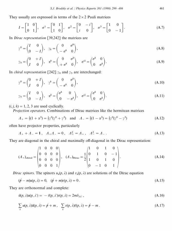
They usually are expressed in terms of the 2]2 Pauli matrices

I"C1 0

0 1D , p1"C0 1

1 0D , p2"C0 !i

i 0 D , p3"C1 0

0 !1D . (A.7)

In Dirac representation [39,242] the matrices are

c0"AI 0

0 !IB , ck"A

0 pk

!pk 0 B , (A.8)

c5"A

0 #I

I 0 B , ak"A0 pk

#pk 0 B , pij"Apk 0

0 pkB . (A.9)

In chiral representation [242] c0

and c5

are interchanged:

c0"A0 #I

I 0 B , ck"A0 pk

!pk 0 B , (A.10)

c5"A

I 0

0 !IB , ak"Apk 0

0 !pkB , pij"Apk 0

0 pkB . (A.11)

(i, j, k)"1, 2, 3 are used cyclically.Projection operators. Combinations of Dirac matrices like the hermitean matrices

K`"1

2(1#a3)"1

2c0(c0#c3) and K

~"1

2(1!a3)"1

2c0(c0!c3) (A.12)

often have projector properties, particularly

K`#K

~"1 , K

`K

~"0 , K2

`"K

`, K2

~"K

~. (A.13)

They are diagonal in the chiral and maximally off-diagonal in the Dirac representation:

(K`)#)*3!-

"A1 0 0 0

0 0 0 0

0 0 0 0

0 0 0 1B , (K`)D*3!#

"

12 A

1 0 1 0

0 1 0 !1

1 0 1 0

0 !1 0 1 B . (A.14)

Dirac spinors. The spinors ua(p, j) and va(p, j) are solutions of the Dirac equation

(p. !m)u(p, j)"0, (p. #m)v(p, j)"0 . (A.15)

They are orthonormal and complete:

uN (p, j)u(p, j@)"!vN (p, j@)v(p, j)"2mdjj{ , (A.16)

+j

u(p, j)uN (p, j)"p. #m , +j

v(p, j)vN (p, j)"p. !m . (A.17)


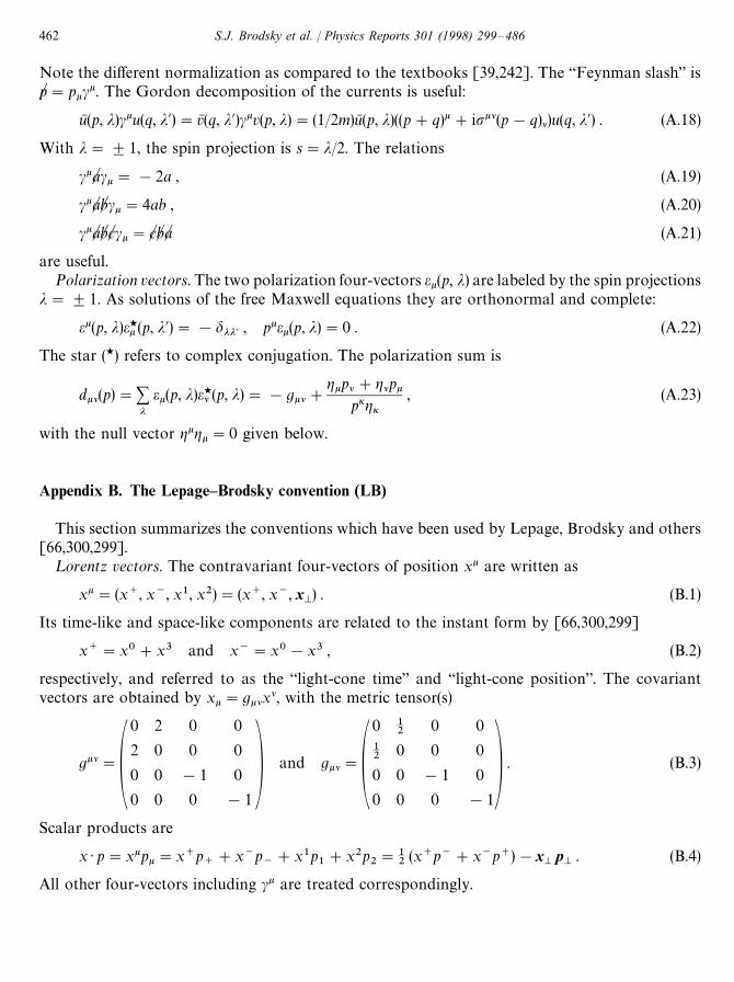
Note the different normalization as compared to the textbooks [39,242]. The “Feynman slash” isp. "pkck. The Gordon decomposition of the currents is useful:

uN (p, j)cku(q, j@)"vN (q, j@)ckv(p, j)"(1/2m)uN (p, j)((p#q)k#ipkl(p!q)l)u(q, j@) . (A.18)

With j"$1, the spin projection is s"j/2. The relations

cka. ck"!2a , (A.19)

cka. b. ck"4ab , (A.20)

cka. b. c. ck"c. b. a. (A.21)

are useful.Polarization vectors. The two polarization four-vectors ek(p, j) are labeled by the spin projections

j"$1. As solutions of the free Maxwell equations they are orthonormal and complete:

ek(p, j)ew

k (p, j@)"!djj{ , pkek(p, j)"0 . (A.22)

The star (w) refers to complex conjugation. The polarization sum is

dkl(p)"+j

ek(p, j)ew

l (p, j)"!gkl#gkpl#glpk

pigi, (A.23)

with the null vector gkgk"0 given below.

Appendix B. The Lepage–Brodsky convention (LB)

This section summarizes the conventions which have been used by Lepage, Brodsky and others[66,300,299].

¸orentz vectors. The contravariant four-vectors of position xk are written as

xk"(x`, x~, x1, x2)"(x`, x~, xM) . (B.1)

Its time-like and space-like components are related to the instant form by [66,300,299]

x`"x0#x3 and x~"x0!x3 , (B.2)

respectively, and referred to as the “light-cone time” and “light-cone position”. The covariantvectors are obtained by xk"gklxl, with the metric tensor(s)

gkl"A0 2 0 0

2 0 0 0

0 0 !1 0

0 0 0 !1 B and gkl"A0 1

20 0

12

0 0 0

0 0 !1 0

0 0 0 !1B . (B.3)

Scalar products are

x ) p"xkpk"x`p`#x~p

~#x1p

1#x2p

2"1

2(x`p~#x~p`)!x

MpM

. (B.4)

All other four-vectors including ck are treated correspondingly.


Dirac matrices. The Dirac representation of the c-matrices is used, particularly

c`c`"c~c~"0 . (B.5)

Alternating products are, for example,

c`c~c`"4c` and c~c`c~"4c~ . (B.6)

Projection operators. The projection matrices become

K`"1

2c0c`"1

4c~c` and K

~"1

2c0c~"1

4c`c~ . (B.7)

Dirac spinors. Lepage and Brodsky [66,300,299] use a particularly simple spinor representation

u(p, j)"1

Jp`(p`#bm#a

MpM)]G

s(C) for j"#1 ,

s(B) for j"!1 ,(B.8)

v(p, j)"1

Jp`(p`!bm#a

MpM)]G

s(B) for j"#1 ,

s(C) for j"!1 .(B.9)

The two s-spinors are

s(C)" 1J2 A1

0

1

0 B and s(B)" 1J2 A0

1

0

!1B . (B.10)

Polarization vectors: The null vector is

gk"(0, 2, 0) . (B.11)

In Bj+rken—Drell convention [39], one works with circular polarization, with spin projectionsj"$1"CB. The transversal polarization vectors are e

M(C)"!1/J2(1, i) and e

M(B)"

1/J2(1, !i), or collectively

eM(j)"(!1/J2) (je

x#ie

y) , (B.12)

with exand e

yas unit vectors in p

x- and p

y-direction, respectively. With e`(p, j)"0, induced by the

light-cone gauge, the polarization vector is

ek(p, j)"A0,2e

M(j)p

Mp`

, eM(j)B , (B.13)

which satisfies pkek(p, j).

Appendix C. The Kogut—Soper convention (KS)

¸orentz vectors. Kogut and Soper [274,406,41,275] have used

x`"(1/J2) (x0#x3) and x~"(1/J2) (x0!x3) , (C.1)


respectively, referred to as the “light-cone time” and “light-cone position”. The covariant vectorsare obtained by xk"gklxl, with the metric tensor

gkl"gkl"A0 1 0 0

1 0 0 0

0 0 !1 0

0 0 0 !1B . (C.2)

Scalar products are

x ) p"xkpk"x`p`#x~p

~#x1p

1#x2p

2#"x`p~#x~p`!x

MpM

. (C.3)

All other four-vectors including ck are treated correspondingly.Dirac matrices. The chiral representation of the c-matrices is used, particularly

c`c`"c~c~"0 . (C.4)

Alternating products are, for example,

c`c~c`"2c` and c~c`c~"2c~ . (C.5)

Projection operators. The projection matrices become

K`"(1/J2)c0c`"1

2c~c` and K

~"(1/J2) c0c~"1

2c`c~ . (C.6)

In the chiral representation the projection matrices have a particularly simple structure, seeEq. (A.14).

Dirac spinors. Kogut and Soper [274] use as Dirac spinors

u(k,C)"1

21@4Jk` AJ2k`

kx#ik

ym

0 B , u(k,B)"1

21@4Jk` A0

m

!kx#ik

yJ2k` B ,

(C.7)

v(k,C)"1

21@4Jk` A0

!m

!kx#ik

yJ2k` B , v(k,B)"

1

21@4Jk` AJ2k`

kx#ik

y!m

0 B .

Polarization vectors. The null vector is

gk"(0, 1, 0) . (C.8)

The polarization vectors of Kogut and Soper [274] correspond to linear polarization j"1 andj"2:

ek(p, j"1)"(0, px/p`, 1, 0) ,

ek(p, j"2)"(0, py/p`, 0, 1) . (C.9)


The following are useful relations:

cacbdab(p)"!2 ,

caclcbdab(p)"(2/p`) (c`pl#g`lp. ) ,

cackclcbdab(p)"!4gkl#2(pa/p`)Mgkaclc`!galckc`#ga`ckcl

!g`lckca#g`kclcaN . (C.10)

The remainder is the same as in Appendix A.

Appendix D. Comparing BD- with LB-spinors

The Dirac spinors ua(p, j) and va(p, j) (with j"$1) are the four linearly independent solutionsof the free Dirac equations (p. !m) u(p, j)"0 and (p. #m) v(p, j)"0. Instead of u(p, j) and v(p, j), itis sometimes convenient [39] to use spinors wr(p) defined by

w1a (p)"ua(p, C), w2a (p)"ua(p, B), w3a (p)"va(p, C), w4a (p)"va(p, B) . (D.1)

With p0"E"Jm2#p2 holds quite in general

u(p, j)"(1/JN) (E#a ) p#bm)sr for r"1, 2 , (D.2)

v(p, j)"(1/JN) (E#a ) p!bm)sr for r"3, 4 . (D.3)

Bj+rken—Drell (BD) [39] choose sra"dar. With N"2m(E#m), the four spinors are then explicitly

wra(p)"1

JN AE#m 0 p

zpx!ip

y0 E#m p

x#ip

y!p

zpz

px!ip

yE#m 0

px#ip

y!p

z0 E#m B . (D.4)

Alternatively (A), one can choose

s1a"s(C) , s2a"s(B) , s3a"s(C) , s4a"s(B) , (D.5)

with given in Eq. (B.10). With N"2m(E#pz), the spinors become explicitly

wra(p)"1

J2N AE#p

z#m !p

x#ip

yE#p

z!m !p

x#ip

ypx#ip

yE#p

z#m p

x#ip

yE#p

z!m

E#pz!m p

x!ip

yE#p

z#m p

x!ip

ypx#ip

y!E!p

z#m p

x#ip

y!E!p

z!m B . (D.6)

One verifies that both spinor conventions (BD) and (A) satisfy orthogonality and completeness

4+a/1

wN rawr{a"c0rr{

,4+r/1

c0rrwrawN rb"dab , (D.7)


respectively, with wN "wsc0. But the two do not have the same form for a particle at rest, p"0,namely

wra(m)BD

"A1 0 0 0

0 1 0 0

0 0 1 0

0 0 0 1B and wra(m)A"A

1 0 0 0

0 1 0 0

0 0 1 0

0 0 0 !1B , (D.8)

respectively, but they have the same spin projection:

p12u(m, j)"ju(m, j) and p12v(m, j)"jv(m, j) . (D.9)

Actually, Lepage and Brodsky [299] have not used Eq. (4.5), but rather

s1a"s(C) , s2a"s(B) , s3a"s(B) , s4a"s(C) . (D.10)

by which reason Eq. (4.9) becomes

p12u(0, j)"ju(0, j) and p12v(0, j)"!jv(0, j) . (D.11)

In the LC formulation the p/2 operator is a helicity operator which has a different spin for fermionsand anti-fermions.

Appendix E. The Dirac—Bergmann method

The dynamics of a classical, non-relativistic system with N degrees of freedom can be derivedfrom the blockian. Obtained from an action principle, this Lagrangian is a function of the velocityphase space variables:

¸"¸(qn, qR

n) , n"1,2, N , (E.1)

where the q’s and qR ’s are the generalized coordinates and velocities respectively. For simplicity weconsider only Lagrangians without explicit time dependence. The momenta conjugate to thegeneralized coordinates are defined by

pn"¸/qR

n. (E.2)

Now it may turn out that not all the momenta may be expressed as independent functions of thevelocities. If this is the case, the Legendre transformation that takes us from the Lagrangian to theHamiltonian is not defined uniquely over the whole phase space (q, p). There then exist a number ofconstraints connecting the q’s and p’s:

/m(q, p)"0 , m"1,2, M . (E.3)

These constraints restrict the motion to a subspace of the full 2N-dimensional phase space definedby the (p, q).


Eventually, we would like to formulate the dynamics in terms of Poisson brackets defined for anytwo dynamical quantities A(q, p) and B(q, p):

MA, BN"Aq

n

Bp

n

!

Ap

n

Bq

n

. (E.4)

The Poisson bracket (PB) formulation is the stage from which we launch into quantum mechanics.Since the PB is defined over the whole phase space only for independent variables (q, p), we are facedwith the problem of extending the PB definition (among other things) onto a constrained phasespace.

The constraints are a consequence of the form of the Lagrangian alone. Following Anderson andBergmann [15], we will call the /

.primary constraints. Now to develop the theory, consider the

quantity pnqRn!¸. If we make variations in the quantities q, qR and p we obtain

d(pnqRn!¸)"dp

nqRn!pR

ndq

n(E.5)

using Eq. (E.2) and the Lagrange equation pRn"¸/q

n. Since the right-hand side of Eq. (E.5) is

independent of dqRnwe will call p

nqRn!¸ the Hamiltonian H. Notice that this Hamiltonian is not

unique. We can add to H any linear combination of the primary constraints and the resulting newHamiltonian is just as good as the original one.

How do the primary constraints affect the equations of motion? Since not all the q’s and p’s areindependent, the variations in Eq. (E.5) cannot be made independently. Rather, for Eq. (E.5) tohold, the variations must preserve the conditions Eq. (E.3). The result is [413]

qRn"(H/p

n)#u

m/

m/p

n(E.6)

and

pRn"!(H/q

n)!u

m/

m/q

n(E.7)

where the um

are unknown coefficients. The N qR ’s are fixed by the N q’s, the N!M independent p’sand the M u’s. Dirac takes the variables q, p and u as the Hamiltonian variables.

Recalling the definition of the Poisson bracket Eq. (E.4) we can write, for any function g of the q’sand p’s

gR "gq

n

qRn#

gp

n

pRn"Mg, HN#u

mMg, /

mN (E.8)

using Eqs. (E.6) and (E.7). As mentioned already, the Poisson bracket has meaning only for twodynamical functions defined uniquely over the whole phase space. Since the /

mrestrict the

independence of some of the p’s, we must not use the condition /m"0 within the PB. The PB

should be evaluated based on the functional form of the primary constraints. After all PB’s havebeen calculated, then we may impose /

m"0. From now on, such restricted relations will be

denoted with a squiggly equal sign:

/m+0 . (E.9)

This is called a weak equality. The equation of motion for g is now

gR +Mg, HTN (E.10)


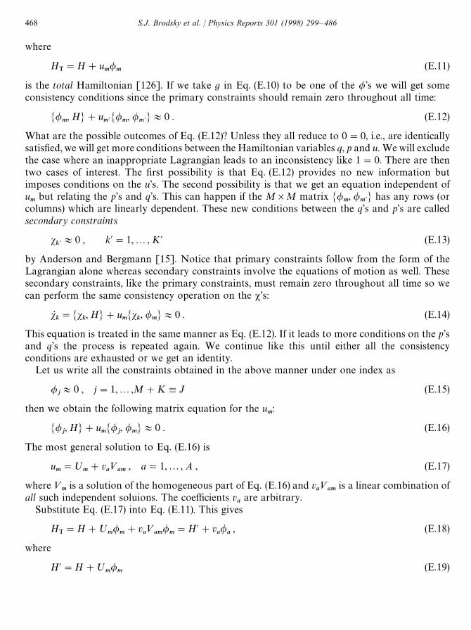
where

HT"H#u

m/m

(E.11)

is the total Hamiltonian [126]. If we take g in Eq. (E.10) to be one of the /’s we will get someconsistency conditions since the primary constraints should remain zero throughout all time:

M/m, HN#u

m{M/

m, /

m{N+0 . (E.12)

What are the possible outcomes of Eq. (E.12)? Unless they all reduce to 0"0, i.e., are identicallysatisfied, we will get more conditions between the Hamiltonian variables q, p and u. We will excludethe case where an inappropriate Lagrangian leads to an inconsistency like 1"0. There are thentwo cases of interest. The first possibility is that Eq. (E.12) provides no new information butimposes conditions on the u’s. The second possibility is that we get an equation independent ofum

but relating the p’s and q’s. This can happen if the M]M matrix M/m, /

m{N has any rows (or

columns) which are linearly dependent. These new conditions between the q’s and p’s are calledsecondary constraints

sk{+0 , k@"1,2, K@ (E.13)

by Anderson and Bergmann [15]. Notice that primary constraints follow from the form of theLagrangian alone whereas secondary constraints involve the equations of motion as well. Thesesecondary constraints, like the primary constraints, must remain zero throughout all time so wecan perform the same consistency operation on the v’s:

sRk"Ms

k, HN#u

mMs

k, /

mN+0 . (E.14)

This equation is treated in the same manner as Eq. (E.12). If it leads to more conditions on the p’sand q’s the process is repeated again. We continue like this until either all the consistencyconditions are exhausted or we get an identity.

Let us write all the constraints obtained in the above manner under one index as

/j+0 , j"1,2,M#K,J (E.15)

then we obtain the following matrix equation for the um:

M/j, HN#u

mM/

j, /

mN+0 . (E.16)

The most general solution to Eq. (E.16) is

um"º

m#v

a»

am, a"1,2, A , (E.17)

where »m

is a solution of the homogeneous part of Eq. (E.16) and va»

amis a linear combination of

all such independent soluions. The coefficients va

are arbitrary.Substitute Eq. (E.17) into Eq. (E.11). This gives

HT"H#º

m/

m#v

a»

am/

m"H@#v

a/

a, (E.18)

where

H@"H#ºm/m

(E.19)


and

/a"»

am/

m. (E.20)

Note that the u’s must satisfy consistency requirements whereas the v’s are totally arbitraryfunctions of time. Later, we will have more to say about the appearance of these arbitrary featuresin our theory.

To further classify the quantities in our theory, consider the following definitions given by Dirac[124]. Any dynamical variable, F(q, p), is called first class if

MF, /jN+0 , j"1,2, J , (E.21)

i.e., F has zero PB with all the /’s. If MF, /jN is not weakly zero F is called second class. Since the /’s

are the only independent quantities which are weakly zero, we can write the following strongequations when F is first class:

MF, /jN"c

jj{/j{

. (E.22)

Any quantity which is weakly zero is strongly equal to some linear combination of the /’s. GivenEqs. (E.21) and (E.22) it is easy to show that H@ and /

a(see Eqs. (E.19) and (E.20)) are first class

quantities. Since /ais a linear combination of primary constraints Eq. (E.20), it too is a primary

constraint. Thus, the total Hamiltonian Eq. (E.18), which is expressed as the sum of a first classHamiltonian plus a linear combination of primary first class constraints, is a first class quantity.

Notice that the number of arbitrary functions of the time appearing in our theory is equivalent tothe number of independent primary first class constraints. This can be seen by looking at Eq. (E.17)where all the inependent first class primary constraints are included in the sum. This same numberwill also appear in the general equation of motion because of Eq. (E.18). Let us make a smalldigression on the role of these arbitrary functions of time.

The physical state of any system is determined by the q’s and p’s only and not by the v’s.However, if we start out at t"t

0with fixed initial values (q

0, p

0) we arrive at different values of

(q, p) at later times depending on our choice of v. The physical state does not uniquely determinea set of q’s and p’s but a given set of q’s and p’s must determine the physical state. We thus have thesituation where there may be several sets of the dynamical variables which correspond to the samephysical state.

To understand this better consider two functions Ava

and Av@aof the dynamical variables which

evolve from some A0

with different multipliers. Compare the two functions after a short timeinterval *t by considering a Taylor expansion to first order in *t:

Ava(t)"A

0#AQ

va*t"A

0#MA

0, H

TN*t"A

0#*t[MA

0, H@N#v

aMA

0, /

aN] . (E.23)

Thus,

Ava!A

v@a"*t(v

a!v@

a)MA

0, /

aN (E.24)

or

*A"eaMA

0, /

aN (E.25)

where

ea"*t(v

a!v@

a) (E.26)


is a small, arbitrary quantity. This relationship between Ava

and Av@a

tells us that the two functions arerelated by an infinitesimal canonical transformation (ICT) [186] whose generator is a first class primaryconstraint /

a. This ICT leads to changes in the q’s and p’s which do no affect the physical state.

Furthermore, it can also be shown [126] that by considering successive ICTs that the generatorsneed not be primary but can be secondary as well. To be completely general then, we should allowfor such variations which do not change the physical state in our equations of motion. This can beaccomplished by redefining H

Tto include the first class secondary constraints with arbitrary

coefficients. Since the distinction between first class primary and first class secondary is notsignificant [413] in what follows we will not make any explicit changes.

For future considerations, let us call those transformations which do not change the physicalstate gauge transformations. The ability to perform gauge transformations is a sign that themathematical framework of our theory has some arbitrary features. Suppose we can add conditionsto our theory that eliminate our ability to make gauge transformations. These conditions wouldenter as secondary constraints since they do not follow from the form of the Lagrangian. Therefore,upon imposing these conditions, all constraints become second class. If there were any more firstclass constraints we would have generators for gauge transformations which, by assumption, canno longer be made. This is the end of the digression although we will see examples of gaugetransformations later.

In general, of the J constraints, some are first class and some are second class. A linearcombination of constraints is again a constraint so we can replace the /

jwith independent linear

combinations of them. In doing so, we will try to make as many of the constraints first class aspossible. Those constraints which cannot be brought into the first class through appropriate linearcombinations are labeled by m

s, s"1,2, S. Now form the PBs of all the m’s with each other and

arrange them into a matrix:

*,A0 Mm

1, m

2N 2 Mm

1, m

sN

Mm2, m

1N 0 2 Mm

2, m

sN

F F } F

Mms, m

1N Mm

s, m

2N 2 0 B . (E.27)

Dirac has proven that the determinant of D is non-zero (not even weakly zero). Therefore, theinverse of D exists:

(D~1)ss{

Mms{, m

ssAN"d

ssA. (E.28)

Define the Dirac bracket (DB) (Dirac called them “new Poisson brackets”) between any twodynamical quantities A and B to be

MA, BN*"MA, BN!MA, msN(D~1)

ss{Mm

s{, BN . (E.29)

The DB satisfies all the same algebraic properties (anti-symmetry, linearity, product law, Jacobiidentity) as the ordinary PB. Also, the equations of motion can be written in terms of the DB sincefor any g(p, q),

Mg, HTN*"Mg, H

TN!Mg, m

sN(D~1)

ss{Mm

s{, H

TN+Mg, H

TN . (E.30)

The last step follows because HT

is first class.


Perhaps the most important feature of the DB is the way it handles second class constraints.Consider the DB of a dynamical quantity with one of the (remaining) m’s:

Mg, msAN*"Mg, m

sAN!Mg, m

sN(D~1)

ss{Mm

s{, m

sAN"Mg, m

sAN!Mg, m

sNd

ssA"0 . (E.31)

The definition Eq. (E.28) was used in the second step above. Thus, the m’s may be set strongly equalto zero before working out the Dirac bracket. Of course, we must still be careful that we do not setm strongly to zero within a Poisson bracket. If we now replace all PBs by DBs (which is legitimatesince the dynamics can be written in terms of DBs via Eq. (E.30)) any second class constraints inH

Twill appear in the DB in Eq. (E.30). Eq. (E.31) then tells us that those constraints can be set to

zero. Thus, all we are left with in our Hamiltonian are first class constraints:

HIT"H#v

iU

i, i"1,2, I , (E.32)

where the sum is over the remaining constraints which are first class. It must be emphasized thatthis is possible only because we have reformulated the theory in terms of the Dirac brackets. Ofcourse, this reformulation in terms of the DB does not uniquely determine the dynamics for us sincewe still have arbitrary functions of the time accompanying the first class constraints. If theLagrangian is such it exhibits no first class constraints then the dynamics are completely defined.

Before doing an example from classical field theory, we should note some features of a fieldtheory that differentiate it from point mechanics. In the classical theory with a finite number ofdegrees of freedom we had constraints which were functions of the phase space variables. Goingover to field theory these constraints become functionals which in general may depend upon thespatial derivatives of the fields and conjugate momenta as well as the fields and momentathemselves:

/m"/

m[u(x), p(x),

iu,

ip] . (E.33)

The square brackets indicate a functional relationship and i,/xi. A consequence of this is that

the constraints are differential equations in general. Furthermore, the constraint itself is no longerthe only independent weakly vanishing quantity. Spatial derivatives of /

mand integrals of

constraints over spatial variables are weakly zero also.Since there are actually an infinite number of constraints for each m (one at each space-time point

x) we write

HT"H#Pdx u

m(x)/

m(x) . (E.34)

Consistency requires that the primary constraints be conserved in time:

0+M/m(x), H

TN"M/

m, HN#Pdy u

n(y)M/

m(x), /

n(y)N . (E.35)

The field theoretical Poisson bracket for any two phase space functionals is given by

MA, BNx0/y0

(x, y)"PdzAdA

dui(z)

dBdn

i(z)

!

dAdn

i(z)

dBdu

i(z)B (E.36)

with the subscript x0"y0 reminding us that the bracket is defined for equal times only. Generally,there may be a number of fields present hence the discrete label i. The derivatives appearing in the


PB above are functional derivatives. If F[ f (x)] is a functional its derivative with respect toa function f (y) is defined to be

dF[ f (x)]/df (y)"lime?0

(1/e) [F[ f (x)#ed(x!y)]!F[ f (x)]] . (E.37)

Assuming Eq. (E.36) has a non-zero determinant we can define an inverse:

Pdy Plm

(x, y)P~1mn

(y, z)"Pdy P~1lm

(x, y)Pmn

(y, z)"d-/d(x!z) , (E.38)

where

Plm

(x, y),M/l(x), /

m(y)N

x0/y0. (E.39)

Unlike the discrete case, the inverse of the PB matrix above is not unique in general. Thisintroduces an arbitrariness which was not present in theories with a finite number of degrees offreedom. The arbitrariness makes itself manifest in the form of differential (rather than algebraic)equations for the multipliers. We must then supply boundary conditions to fix the multipliers[413].

The Maxwell theory for the free electro-magnetic field is defined by the action

S"Pd4x L(x) , (E.40)

whereL is the Lagrangian density, Eq. (B.8). The action is invariant under local gauge transforma-tions. The ability to perform such gauge transformations indicates the presence of first classconstraints. To find them, we first obtain the momenta conjugate to the fields Ak: nk"!F0k asdefined in Eq. (B.12). This gives us a primary constraint, namely n0(x)"0. Using Eq. (B.26), we canwrite the canonical Hamiltonian density as

Plm

(x, y),M/l(x), /

m(y)N

x0/y0, (E.41)

where the velocity fields AQi

have been expressed in terms of the momenta ni. After a partial

integration on the second term, the Hamiltonian becomes

H"Pd3x (12pipi!A

0ini#1

4F

ikF

ik)

(E.42)

NHT"H#Pd3x v

1(x)n0(x) .

Again, for consistency, the primary constraints must be constant in time so that

0+Mn0, HTN"!Gn0, Pd3x A

0ipiH"

ipi. (E.43)

Thus, ipi+0 is a secondary constraint. We must then check to see if Eq. (E.43) leads to further

constraints by also requiring that ipiis conserved in time:

0+Mini, H

TN . (E.44)


The PB above vanishes identically however so there are no more constraints which follow fromconsistency requirements. So we have our two first class constraints:

/1"n0+0 (E.45)

and

s,/2"

ipi+0 . (E.46)

In light of the above statements the first class secondary constraints should be included in HT

aswell (Some authors call the Hamiltonian with first class secondary constraints included theextended Hamiltonian):

HT"H#Pd3x(v

1/

1#v

2/2) . (E.47)

Notice that the fundamental PB’s among the Ak and nk,MAk(x), nl(y)N

x0/y0"dlkd(x!y) (E.48)

are incompatible with the constraint n0+0 so we will modify them using the Dirac-Bergmannprocedure. The first step towards this end is to impose certain conditions to break the local gaugeinvariance. Since there are two first class constraints, we need two gauge conditions imposed as secondclass constraints. The traditional way to implement this is by imposing the radiation gauge conditions:

X1,A

0+0 and X

2,

iAi+0 . (E.49)

It can be shown [413] that the radiation gauge conditions completely break the gauge invariancethereby bringing all constraints into the second class.

The next step is to form the matrix of second class constraints with matrix elementsDij"MX

i, /

jNx0/y0

and i, j"1, 2:

D"A0 0 1 0

0 0 0 !+ 2

!1 0 0 0

0 + 2 0 0 B d(x!y) . (E.50)

To get the Dirac bracket we need the inverse of D. Recalling the definition, Eq. (E.38), we have

Pdy Dij(x, y)(D~1)

jk(y, z)"d

ikd(x!z) . (E.51)

With the help of + 2(1/Dx!yD)"!4pd(x!y) we can easily perform Eq. (2.11) element by elementto obtain

*~1"A0 0 !d(x!y) 0

0 0 0 !

14pDx!yD

d(x!y) 0 0 0

01

4pDx!yD0 0 B (E.52)


Thus, the Dirac bracket in the radiation gauge is (all brackets are at equal times)

MA(x), B(y)N*"MA(x), B(y)N!PPdu d�MA(x), ti(u)N(D~1)

ij(u, �)Mt

j(v), B(y)N , (E.53)

where t1"X

1, t

2"X

2, t

3"/

1and t

4"/

2. The fundamental Dirac brackets are

MAk(x), pl(y)N*"(dlk#d0kgl0)d(x!y)!kl (1/4pDx!yD)(E.54)

MAk(x), Al(y)N*"0"Mpk(x), pl(y)N* .

From the first of the above equations we obtain,

MAi(x), p

j(y)N*"d

ijd(x!y)!

ij(1/4pDx!yD) . (E.55)

The right-hand side of the above expression is often called the “transverse delta function” in thecontext of canonical quantization of the electro-magnetic field in the radiation gauge. In nearlyall treatments of that subject, however, the transverse delta function is introduced “by hand”so to speak. This is done after realizing that the standard commutation relation[A

i(x), n

j(y)]"id

ijd(x!y) is in contradiction with Gauss’ law. In the Dirac—Bergmann approach

the familiar equal-time commutator relation is obtained without any hand-waving arguments.The choice of the radiation gauge in the above example most naturally reflects the splitting of

A and p into transverse and longitudinal parts. In fact, the gauge condition iA

i"0 implies that the

longitudinal part of A is zero. This directly reflects the observation that no longitudinally polarizedphotons exist in nature.

Given this observation, we should somehow be able to associate the true degrees of freedom withthe transverse parts of A and p. Sundermeyer [413] shows that this is indeed the case and that, forthe true degrees of freedom, the DB and PB coincide.

We have up till now concerned ourselves with constrained dynamics at the classical level.Although all the previous developments have occurred quite naturally in the classical context, itwas the problem of quantization which originally motivated Dirac and others to develop thepreviously described techniques. Also, more advanced techniques incorporating constraints intothe path integral formulation of quantum theory have been developed.

The general problem of quantizing theories with constraints is very formidable especially whenconsidering general gauge theories. We will not attempt to address such problems. Rather, we willwork in the non-relativistic framework of the Schrodinger equation where quantum states aredescribed by a wave function.

As a first case, let us consider a classical theory where all the constraints are first class. TheHamiltonian is written then as the sum of the canonical Hamiltonian H"p

iqRi!¸ plus a linear

combination of the first class constraints:

H@"H#vj/j. (E.56)

Take the p’s and q’s to satisfy

Mqi, p

jNN(i/+) [qL

i, pL

j] (E.57)


where the hatted variables denote quantum operators and [qLi, pL

j]"qL

ipLj!pL

jqLiis the commutator.

The Schrodinger equation reads

i+ dt/dt"H@t , (E.58)

where t is the wavefunction on which the dynamical variables operate. For each constraint/jimpose supplementary conditions on the wavefunction

/Kjt"0 . (E.59)

Consistency of the Eq. (E.59) with one another demands that

[/Kj, /K

j{]t"0 . (E.60)

Recall the situation in the classical theory where anything that was weakly zero could be writtenstrongly as a linear combination of the /’s:

M/j, /

j{N"cjA

jj{/jA. (E.61)

Now if we want Eq. (E.60) to be a consequence of Eq. (E.59), an analogous relation to Eq. (E.61)must hold in the quantum theory, namely,

[/Kj, /K

j{]"cL jA

jj{/K jA . (E.62)

The problem is that the coefficients cL in the quantum theory are in general functions of theoperators pL and qL and do not necessarily commute with the /K ’s. In order for consistency then, wemust have the coefficients in the quantum theory all appearing to the left of the /K ’s.

The same conclusion follows if we consider the consistency of Eq. (E.59) with the Schrodingerequation. If we cannot arrange to have the coefficients to the left of the constraints in the quantumtheory then as Dirac says “we are out of luck” [126].

Consider now the case where there are second class constraints, ms. The problems encountered

when there are second class constraints are similar in nature to the first class case but appear evenworse. This statement follows simply from the definition of second class. If we try to imposea condition on t similarly to Eq. (E.59) but with a second class constraint we must get a contradic-tion since already Mm

s, /

jNO0 for all j at the classical level.

Of course if we imposed mKs"0 as an operator identity then there is no contradiction. In the

classical theory, the analogous constraint condition is the strong equality m"0. We have seenthat strong equalities for second class constraints emerge in the classical theory via the Dirac—Bergmann method. Thus it seems quite suggestive to postulate

MA, BN*N(i/+) [AK , BK ] (E.63)

as the rule for quantizing the theory while imposing mKs"0 as an operator identity. Any remaining

weak equations are all first class and must then be treated as in the first case using supplementaryconditions on the wave function. Hence, the operator ordering ambiguity still exists in general.

We have seen that there is no definite way to guarantee a well defined quantum theory given thecorresponding classical theory. It is possible, since the Dirac bracket depends on the gaugeconstraints imposed by hand, that we can choose such constraints in such a way as to avoid any


problems. For a general system however, such attempts would at best be difficult to implement. Wehave seen that there is a consistent formalism for determining (at least as much one can) thedynamics of a generalized Hamiltonian system. The machinery is as follows:

f Obtain the canonical momenta from the Lagrangian.f Identify the primary constraints and construct the total Hamiltonian.f Require the primary constraints to be conserved in time.f Require any additional constraints obtained by step 3 to also be conserved in time.f Separate all constraints into first class or second class.f Invert the matrix of second class constraints.f Form the Dirac bracket and write the equations of motion in terms of them.f Quantize by taking the DB over to the quantum commutator.

Of course, there are limitations throughout this program; especially in steps six and eight. If thereare any remaining first class constraints it is a sign that we still have some gauge freedom left in ourtheory. Given the importance of gauge field theory in today’s physics it is certainly worth one’swhile to understand the full implications of constrained dynamics. The material presented here ismeant to serve as a primer for further study.

References

[1] J. Abad, J.G. Esteve, A.F. Pacheco, Phys. Rev. D 32 (1985) 2729.[2] O. Abe, K. Tanaka, K.G. Wilson, Phys. Rev. D 48 (1993) 4856—4867.[3] O. Abe, G.J. Aubrecht, K. Tanaka, Phys. Rev. D 56 (1997) 2242—2249.[4] N.A. Aboud, J.R. Hiller, Phys. Rev. D 41 (1990) 937—945.[5] C. Acerbi, A. Bassetto, Phys. Rev. D 49 (1994) 1067—1076.[6] S. Adler, Nucl. Phys. B 415 (1994) 195.[7] A. Ali, V.M. Braun, H. Simma, Z. Physik C 63 (1994) 437—454.[8] E.A. Ammons, Phys. Rev. D 50 (1994) 980—990.[9] F. Antonuccio, S. Dalley, Phys. Lett. B 348 (1995) 55.

[10] F. Antonuccio, S. Dalley, Nucl. Phys. B 461 (1996) 275.[11] F. Antonuccio, S. Dalley, Phys. Lett. B 376 (1996) 154.[12] F. Antonuccio, S.J. Brodsky, S. Dalley, Phys. Lett. B 412 (1997) 104.[13] F. Antonuccio, S. Pinsky, Phys. Lett. B 397 (1997) 42—50.[14] A.M. Annenkova, E.V. Prokhatilov, V.A. Franke, Phys. Atom. Nucl. 56 (1993) 813—825.[15] J.L. Anderson, P.G. Bergman, Phys. Rev. 83 (1951) 1018.[16] K. Bardakci, M.B. Halpern, Phys. Rev. 176 (1968) 1786.[17] W.A. Bardeen, R.B. Pearson, Phys. Rev. D 13 (1976) 547.[18] W.A. Bardeen, R.B. Pearson, E. Rabinovici, Phys. Rev. D 21 (1980) 1037.[19] V. Bargmann, Proc. Natl. Acad. Sci. (USA) 34 (1948) 211.[21] D. Bartoletta et al., Phys. Rev. Lett. 62 (1989) 2436.[22] A. Bassetto, G. Nardelli, R. Soldati, Yang-Mills Theories in Algebraic Noncovariant Gauges, World Scientific,

Singapore, 1991.[23] A. Bassetto, Phys. Rev. D 47 (1993) 727—729.[24] A. Bassetto, M. Ryskin, Phys. Lett. B 316 (1993) 542—545.[25] A. Bassetto, I.A. Korchemskaya, G.P. Korchemsky, G. Nardelli, Nucl. Phys. B 408 (1993) 62—90.[26] A. Bassetto, Nucl. Phys. Proc. Suppl. C 51 (1996) 281—288.


[27] A. Bassetto, L. Griguolo, G. Nardelli, Phys. Rev. D 54 (1996) 2845—2852.[28] A. Bassetto, G. Nardelli, Int. J. Mod. Phys. A 12 (1997) 1075—1090.[29] R. Bayer, H.C. Pauli, Phys. Rev. D 53 (1996) 939.[30] J.S. Bell, Acta Phys. Austriaca (Suppl.) 13 (1974) 395.[31] E. Belz, ANL preprint, 1994.[32] C.M. Bender, L.R. Mead, S.S. Pinsky, Phys. Rev. Lett. 56 (1986) 2445.[33] C.M. Bender, S.S. Pinsky, B. Van de Sande, Phys. Rev. D 48 (1993) 816.[34] H. Bergknoff, Nucl. Phys. B 122 (1977) 215.[35] C. Bloch, Nucl. Phys. 6 (1958) 329.[36] G. Bertsch, S.J. Brodsky, A.S. Goldhaber, J.F. Gunion, Phys. Rev. Lett. 47 (1981) 297.[37] H.A. Bethe, F. de Hoffman, Mesons and Fields, Vol. II, Row, Peterson and Company, Evanston, Ill, 1955.[38] G. Bhanot, K. Demeterfi, I.R. Klebanov, Phys. Rev. D 48 (1993) 4980.[39] J.D. Bj+rken, S.D. Drell, Relativistic Quantum Mechanics, McGraw-Hill, New York, 1964; J.D.Bj+rken, S.D.

Drell, Relativistic Quantum Fields, McGraw-Hill, New York, 1965.[40] J.D. Bj+rken, E.A. Paschos, Phys. Rev. 185 (1969) 1975.[41] J.D. Bj+rken, J.B. Kogut, D.E. Soper, Phys. Rev. D 3 (1971) 1382.[42] B. Blaettel, G. Baym, L.L. Frankfurt, H. Heiselberg, M. Strikman, Phys. Rev. D 47 (1993) 2761.[43] R. Blankenbecler, S.J. Brodsky, J.F. Gunion, R. Savit, Phys. Rev. D 8 (1973) 4117.[44] G.T. Bodwin, D.R. Yennie, M.A. Gregorio, Rev. Mod. Phys. 56 (1985) 723.[45] A. Borderies, P. Grange, E. Werner, Phys. Lett. B 319 (1993) 490—496.[46] A. Borderies, P. Grange, E. Werner, Phys. Lett. B 345 (1995) 458—468.[47] J. Botts, Nucl. Phys. B 353 (1991) 20.[48] M. Brisudova, R.J. Perry, Phys. Rev. D 54 (1996) 1831—1843.[49] M. Brisudova, R.J. Perry, Phys. Rev. D 54 (1996) 6453—6458.[50] M. Brisudova, R.J. Perry, K.G. Wilson, Phys. Rev. Lett. 78 (1997) 1227—1230.[51] S.J. Brodsky, J.R. Primack, Annals Phys. 52 (1960) 315.[52] S.J. Brodsky, J.R. Primack, Phys. Rev. 174 (1968) 2071.[53] S.J. Brodsky, R. Roskies, R. Suaya, Phys. Rev. D 8 (1973) 4574.[54] S.J. Brodsky, G.R. Farrar, Phys. Rev. D 11 (1975) 1309.[55] S.J. Brodsky, B.T. Chertok, Phys. Rev. D 14 (1976) 3003.[56] S.J. Brodsky, S.D. Drell, Phys. Rev. D 22 (1980) 2236.[57] S.J. Brodsky, G.P. Lepage, S.A.A. Zaidi, Phys. Rev. D 23 (1981) 1152.[58] S.J. Brodsky, J.R. Hiller, Phys. Rev. C 28 (1983) 475.[59] S.J. Brodsky, C.-R. Ji, G.P. Lepage, Phys. Rev. Lett. 51 (1983) 83.[60] S.J. Brodsky, A.H. Mueller, Phys. Lett. B 206 (1988) 685.[61] S.J. Brodsky, G.F. de Teramond, Phys. Rev. Lett. 60 (1988) 1924.[62] S.J. Brodsky, G.P. Lepage, in: A.H. Mueller (Ed.), Perturbative Quantum Chromodynamics, World Scientific,

Singapore, 1989.[63] S.J. Brodsky, I.A. Schmidt, Phys. Lett. B 234 (1990) 144.[64] S.J. Brodsky, G.F. de Teramond, I.A. Schmidt, Phys. Rev. Lett. 64 (1990) 1011.[65] S.J. Brodsky, I.A. Schmidt, Phys. Rev. D 43 (1991) 179.[66] S.J. Brodsky, H.C. Pauli, in: H. Mitter, H. Gausterer (Eds.), Recent Aspect of Quantum Fields, Lecture Notes in

Physics, vol. 396, Springer, Berlin, 1991.[67] S.J. Brodsky, P. Hoyer, A.H. Mueller, W.-K. Tang, Nucl. Phys. B 369 (1992) 519.[68] S.J. Brodsky, G. McCartor, H.C. Pauli, S.S. Pinsky, Particle World 3 (1993) 109.[69] S.J. Brodsky, W.-K. Tang, C.B. Thorn, Phys. Lett. B 318 (1993) 203.[70] S.J. Brodsky, M. Burkardt, I. Schmidt, Nucl. Phys. B 441 (1994) 197.[71] S.J. Brodsky, F. Schlumpf, Phys. Lett. B 329 (1994) 111.[72] S.J. Brodsky, F. Schlumpf, Prog. Part. Nucl. Phys. 34 (1995) 69—86.[73] R.W. Brown, J.W. Jun, S.M. Shvartsman, C.C. Taylor, Phys. Rev. D 48 (1993) 5873—5882.[74] F. Buccella, E. Celeghin, H. Kleinert, C.A. Savoy, E. Sorace, Nuovo Cimento A 69 (1970) 133.


[75] M. Burkardt, Phys. A 504 (1989) 762.[76] M. Burkardt, A. Langnau, Phys. Rev. D 44 (1991) 1187.[77] M. Burkardt, A. Langnau, Phys. Rev. D 44 (1991) 3857.[78] M. Burkardt, Phys. Rev. D 47 (1993) 4628.[79] M. Burkardt, Phys. Rev. D 49 (1994) 5446.[80] M. Burkardt, Adv. Nucl. Phys. 23 (1996) 1—74.[81] M. Burkardt, Light front hamiltonians and confinement, hep-ph/9512318.[82] M. Burkardt, H. El-Khozondar, Phys. Rev. D 55 (1997) 6514—6521.[83] M. Burkardt, Phys. Rev. D 54 (1996) 2913—2920.[84] M. Burkardt, B. Klindworth, Phys. Rev. D 55 (1997) 1001—1012.[85] M. Burkardt, Phys. Rev. D 57 (1998) 1136.[86] F. Cardarelli, I.L. Grach, I.M. Narodetskii, G. Salme, S. Simula, Phys. Lett. B 349 (1995) 393—399.[87] R. Carlitz, D. Heckathorn, J. Kaur, W.-K. Tung, Phys. Rev. D 11 (1975) 1234.[88] R. Carlitz, W.-K. Tung, Phys. Rev. D 13 (1976) 3446.[89] C.E. Carlson, J.L. Poor, Phys. Rev. D 38 (1988) 2758.[90] A. Carroll, Lecture at the Workshop on Exclusive Processes at High Momentum Transfer, Elba, Italy, 1993.[91] A. Casher, Phys. Rev. D 14 (1976) 452.[92] S. Chang, S. Ma, Phys. Rev. 180 (1969) 1506.[93] S.J. Chang, Phys. Rev. D 13 (1976) 2778.[94] S.J. Chang, T.M. Yan, Phys. Rev. D 7 (1973) 1147.[95] S.J. Chang, R.G. Root, T.M. Yan, Phys. Rev. D 7 (1973) 1133.[96] S.J. Chang, R.G. Root, T.M. Yan, Phys. Rev. D 7 (1973) 1133.[97] L. Chao, Mod. Phys. Lett. A 8 (1993) 3165—3172.[98] Z. Chen, A.H. Mueller, Nucl. Phys. B 451 (1995) 579.[99] H.Y. Cheng, C.Y. Cheung, C.W. Hwang, Phys. Rev. D 55 (1997) 1559—1577.

[100] V.L. Chernyak, A.R. Zhitnitskii, Phys. Rep. 112 (1984) 173.[101] C.Y. Cheung, W.M. Zhang, G.-L. Lin, Phys. Rev. D 52 (1995) 2915—2925.[102] P.L. Chung, W.N. Polyzou, F. Coester, B.D. Keister, Phys. Rev. C 37 (1988) 2000.[103] P.L. Chung, F. Coester, Phys. Rev. D 44 (1991) 229.[104] F.E. Close, An Introduction to Quarks and Partons, Academic Press, New York, 1979.[105] F. Coester, W.N. Polyzou, Phys. Rev. D 26 (1982) 1349.[106] F. Coester, Prog. Nuc. Part. Phys. 29 (1992) 1.[107] F. Coester, W. Polyzou, Found. Phys. 24 (1994) 387—400.[108] S. Coleman, Comm. Math. Phys. 31 (1973) 259.[109] S. Coleman, R. Jackiw, L. Susskind, Ann. Phys. (NY) 93 (1975) 267.[110] S. Coleman, Ann. Phys. (NY) 101 (1976) 239.[111] J. Collins, Renormalization, Cambridge University Press, New York, 1984.[112] M.E. Convery, C.C. Taylor, J.W. Jun, Phys. Rev. D 51 (1995) 4445—4450.[113] D.P. Crewther, C.J. Hamer, Nucl. Phys. B 170 (1980) 353.[114] R.H. Dalitz, F.J. Dyson, Phys. Rev. 99 (1955) 301.[115] S. Dalley, I.R. Klebanov, Phys. Rev. D 47 (1993) 2517.[116] S. Dalley, B. van de Sande, Nucl. Phys B Proc. Suppl. 53 (1997) 827—830.[117] S.M. Dancoff, Phys. Rev. 78 (1950) 382.[118] R. Dashen, M. Gell-Mann, Phys. Rev. Lett. 17 (1966) 340.[119] S.P. De Alwis, Nucl. Phys. B 55 (1973) 427.[120] S.P. De Alwis, J. Stern, Nucl. Phys. B 77 (1974) 509.[121] K. Demeterfi, I.R. Klebanov, G. Bhanot, Nucl. Phys. B 418 (1994) 15.[122] N.B. Demchuk, P.Yu. Kulikov, I.M. Narodetskii, P.J. O’Donnell, Phys. Atom. Nucl. 60 (1997) 1292—1304.[123] P.A.M. Dirac, Rev. Mod. Phys. 21 (1949) 392.[124] P.A.M. Dirac, Can. Jour. Math. 2 (1950) 129.[125] P.A.M. Dirac, The Principles of Quantum Mechanics, 4th ed., Oxford Univ. Press, Oxford, 1958.


[126] P.A.M. Dirac, Lectures on Quantum Mechanics, Belfer Graduate School of Science, Yeshiva University, 1964.[127] P.A.M. Dirac, in: D.W. Duke, J.F. Owens (Eds.), Perturbative Quantum Chromodynamics, Am. Inst. Phys., New

York, 1981.[128] P.J. O’Donnell, Q.P. Xu, H.K.K. Tung, Phys. Rev. D 52 (1995) 3966—3977.[129] S.D. Drell, A.C. Hearn, Phys. Rev. Lett. 16 (1966) 908.[130] S.D. Drell, D. Levy, T.M. Yan, Phys. Rev. 187 (1969) 2159.[131] S.D. Drell, D. Levy, T.M. Yan, Phys. Rev. D 1 (1970) 1035.[132] S.D. Drell, D. Levy, T.M. Yan, Phys. Rev. D 1 (1970) 1617.[133] S.D. Drell, T.M. Yan, Phys. Rev. Lett. 24 (1970) 181.[134] A.Yu. Dubin, A.B. Kaidalov, Yu.A. Simonov, Phys. Lett. B 343 (1995) 310—314.[135] E. Eichten, F. Feinberg, J.F. Willemsen, Phys. Rev. D 8 (1973) 1204.[136] M.B. Einhorn, Phys. Rev. D 14 (1976) 3451.[137] T. Eller, H.C. Pauli, S.J. Brodsky, Phys. Rev. D 35 (1987) 1493.[138] T. Eller, H.C. Pauli, Z. Physik 42 C (1989) 59.[139] S. Elser, Hadron Structure ’94, Kosice, Slowakia, 1994; Diplomarbeit, U. Heidelberg, 1994.[140] S. Elser, A.C. Kalloniatis, Phys. Lett. B 375 (1996) 285—291.[141] G. Fang et al., Presented at the INT -Fermilab Workshop on Perspectives of High Energy Strong Interaction

Physics at Hadron Facilities, 1993.[142] F.L. Feinberg, Phys. Rev. D 7 (1973) 540.[143] T.J. Fields, K.S. Gupta, J.P. Vary, Mod. Phys. Lett. A 11 (1996) 2233—2240.[144] R.P. Feynman, Phys. Rev. Lett. 23 (1969) 1415.[145] R.P. Feynman, Photon—Hadron Interactions, Benjamin, Reading, MA, 1972.[146] V.A. Franke, Yu.A. Novozhilov, E.V. Prokhvatilov, Lett. Math. Phys. 5 (1981) 239.[147] V.A. Franke, Yu.A. Novozhilov, E.V. Prokhvatilov, Lett. Math. Phys. 5 (1981) 437.[148] V.A. Franke, Yu.A. Novozhilov, E.V. Prokhvatilov, in: Dynamical Systems and Microphysics, Academic Press,

New York, 1982, pp. 389—400.[149] L. Frankfurt, T.S.H. Lee, G.A. Miller, M. Strikman, Phys. Rev. C 55 (1997) 909.[150] H. Fritzsch, M. Gell-Mann, Proc. 16th. Int. Conf. on HEP, Batavia, IL, 1972.[151] H. Fritzsch, Mod. Phys. Lett. A 5 (1990) 625.[152] H. Fritzsch, Constituent Quarks, Chiral Symmetry, the Nucleon Spin, talk given at the Leipzig Workshop on

Quantum Field Theory Aspects of High Energy Physics CERN, September 1993, preprintTH. 7079/93.[153] S. Fubini, G. Furlan, Physics 1 (1965) 229.[154] S. Fubini, A.J. Hanson, R. Jackiw, Phys. Rev. D 7 (1973) 1732.[155] M.G. Fuda, Phys. Rev. C 36 (1987) 702—709.[156] M.G. Fuda, Phys. Rev. D 42 (1990) 2898—2910.[157] M.G. Fuda, Phys. Rev. D 44 (1991) 1880—1890.[158] M.G. Fuda, Nucl. Phys. A 543 (1992) 111c—126c.[159] M.G. Fuda, Ann. Phys. 231 (1994) 1—40.[160] M.G. Fuda, Phys. Rev. C 52 (1995) 1260—1269.[161] M.G. Fuda, Phys. Rev. D 54 (1996) 5135—5147.[162] T. Fujita, A. Ogura, Prog. Theor. Phys. 89 (1993) 23—36.[163] T. Fujita, C. Itoi, A. Ogura, M. Taki, J. Phys. G 20 (1994) 1143—1157.[164] T. Fujita, Y. Sekiguchi, Prog. Theor. Phys. 93 (1995) 151—160.[165] M. Fujita, Sh.M. Shvartsman, Role of zero modes in quantization of QCD in light-cone coordinates, CWRU-TH-

95-11, hep-th/9506046, June 1995, 21pp.[166] T. Fujita, M. Hiramoto, H. Takahashi, Bound states of (1#1)-dimensional field theories, hep-th/9609224.[167] T. Fujita, K. Yamamoto, Y. Sekiguchi, Ann. Phys. 255 (1997) 204—227.[168] M. Funke, V. Kaulfass, H. Kummel, Phys. Rev. D 35 (1987) 621.[169] P. Gaete, J. Gamboa, I. Schmidt, Phys. Rev. D 49 (1994) 5621—5624.[170] M. Gari, N.G. Stephanis, Phys. Lett. B 175 (1986) 462.[171] A. Gasser, H. Leutwyler, Nucl. Phys. B 94 (1975) 269.


[172] M. Gell-Mann, Phys. Lett. 8 (1964) 214.[173] M. Gell-Mann, Lectures given at the 1972 Schladming Winter School, Acta Phys. Austriaca 9 (Suppl.) 733 (1972).[174] S.B. Gerasimov, Yad. Fiz. 2 (1965) 598 [Sov. J. Nucl. Phys. 2 (1966) 430].[175] S.N. Ghosh, Phys. Rev. D 46 (1992) 5497—5503.[176] S. G"azek, Acta Phys. Pol. B 15 (1984) 889.[178] S. G"azek, R.J. Perry, Phys. Rev. D 45 (1992) 3734.[179] S. G"azek, R.J. Perry, Phys. Rev. D 45 (1992) 3740.[180] S. G"azek, K.G. Wilson, Phys. Rev. D 47 (1993) 4657.[181] S. G"azek, K.G. Wilson, Phys. Rev. D 48 (1993) 5863.[182] S. G"azek, A. Harindranath, S. Pinsky, J. Shigemitsu, K. Wilson, Phys. Rev. D 47 (1993) 1599.[183] S. G"azek, K.G. Wilson, Phys. Rev. D 49 (1994) 4214.[184] S. G"azek, K.G. Wilson, Phys. Rev. D 49 (1994) 6720.[185] S. Glazek (Ed.), Theory of Hadrons and Light-front QCD, World Scientific, Singapore, 1995.[186] H. Goldstein, Classical Mechanics, Addison-Wesley, Reading, MA, 1950.[187] I.L. Grach, I.M. Narodetskii, S. Simula, Phys. Lett. B 385 (1996) 317—323.[188] P. Grange, A. Neveu, H.C. Pauli, S. Pinsky, E. Werner, (Eds.), New Non-perturbative Methods and Quantization

on the Light Cone, “Les Houches Series”, Vol. 8, Springer, Berlin, 1997; Proc. Workshop at Centre de Physiquedes Houches, France, 24 February—7 March 1997.

[189] V.N. Gribov, Nucl. Phys. B 139 (1978) 1.[190] P.A. Griffin, Nucl. Phys. B 372 (1992) 270.[191] P.A. Griffin, Phys. Rev. D 46 (1992) 3538—3543.[192] D. Gromes, H.J. Rothe, B. Stech, Nucl. Phys. B 75 (1974) 313.[193] D.J. Gross, I.R. Klebanov, A.V. Matytsin, A.V. Smilga, Nucl. Phys. B 461 (1996) 109—130.[194] E. Gubankova, F. Wegner, Exact renormalization group analysis in Hamiltonian theory: I. QED Hamiltonian on

the light front, hep-th/9702162.[195] C.J. Hamer, Nucl. Phys. B 121 (1977) 159.[196] C.J. Hamer, Nucl. Phys. B 132 (1978) 542.[197] C.J. Hamer, Nucl. Phys. B 195 (1982) 503.[198] K. Harada, A. Okazaki, M. Taniguchi, M. Yahiro, Phys. Rev. D 49 (1994) 4226—4245.[199] K. Harada, A. Okazaki, M. Taniguchi, Phys. Rev. D 52 (1995) 2429—2438.[200] K. Harada, A. Okazaki, Phys. Rev. D 55 (1997) 6198—6208.[201] K. Harada, A. Okazaki, M. Taniguchi, Phys. Rev. D 54 (1996) 7656—7663.[202] K. Harada, A. Okazaki, M. Taniguchi, Phys. Rev. D 55 (1997) 4910—4919.[203] A. Harindranath, J.P. Vary, Phys. Rev. D 36 (1987) 1141.[204] A. Harindranath, J.P. Vary, Phys. Rev. D 37 (1988) 1064—1069.[205] A. Harindranath, R.J. Perry, J. Shigemitsu, Ohio State preprint, 1991.[206] T. Heinzl, S. Krusche, E. Werner, B. Zellermann, Phys. Lett. B 272 (1991) 54.[207] T. Heinzl, S. Krusche, E. Werner, Phys. Lett. B 256 (1991) 55.[208] T. Heinzl, S. Krusche, E. Werner, Nucl. Phys. A 532 (1991) 4290.[209] T. Heinzl, S. Krusche, S. Simburger, E. Werner, Z. Phys. C 56 (1992) 415.[210] T. Heinzl, S. Krusche, E. Werner, Phys. Lett. B 275 (1992) 410.[211] T. Heinzl, E. Werner, Z. Phys. C 62 (1994) 521—532.[212] T. Heinzl, Nucl. Phys. Proc. Suppl. B 39C (1995) 217—219.[213] T. Heinzl, Hamiltonian formulations of Yang-Mills quantum theory, the Gribov problem, hep-th/9604018.[214] T. Heinzl, Phys. Lett. B 388 (1996) 129—136.[215] T. Heinzl, Nucl. Phys. Proc. Suppl. A 54 (1997) 194—197.[216] S. Heppelmann, Nucl. Phys. B Proc. Suppl. 12 (1990) 159 and references therein.[217] J.E. Hetrick, Nucl. Phys. B 30 (1993) 228—231.[218] J.E. Hetrick, Int. J. Mod. Phys. A 9 (1994) 3153.[219] M. Heyssler, A.C. Kalloniatis, Phys. Lett. B 354 (1995) 453.[220] J.R. Hiller, Phys. Rev. D 43 (1991) 2418.


[221] J.R. Hiller, Phys. Rev. D 44 (1991) 2504.[222] J.R. Hiller, S.J. Brodsky, Y. Okamoto (in progress).[223] J. Hiller, S.S. Pinsky, B. van de Sande, Phys. Rev. D 51 (1995) 726.[224] L.C.L. Hollenberg, K. Higashijima, R.C. Warner, B.H.J. McKellar, Prog. Theor. Phys. 87 (1991) 3411.[225] L.C.L. Hollenberg, N.S. Witte, Phys. Rev. D 50 (1994) 3382.[226] K. Hornbostel, S.J. Brodsky, H.C. Pauli, Phys. Rev. D 38 (1988) 2363.[227] K. Hornbostel, S.J. Brodsky, H.C. Pauli, Phys. Rev. D 41 (1990) 3814.[228] K. Hornbostel, Constructing Hadrons on the Light Cone, Workshop on From Fundamental Fields to Nuclear

Phenomena, Boulder, CO, 20—22 September 1990; Cornell preprint CLNS 90/1038, 1990.[229] K. Hornbostel, Cornell Preprint CLNS 91/1078, August 1991.[230] K. Hornbostel, Phys. Rev. D 45 (1992) 3781.[231] S. Hosono, S. Tsujimaru, Int. J. Mod. Phys. A 8 (1993) 4627—4648.[232] S.Z. Huang, W. Lin, Ann. Phys. 226 (1993) 248—270.[233] T. Hyer, Phys. Rev. D 49 (1994) 2074—2080.[234] M. Ida, Progr. Theor. Phys. 51 (1974) 1521.[235] M. Ida, Progr. Theor. Phys. 54 (1975) 1199.[236] M. Ida, Progr. Theor. Phys. 54 (1975) 1519.[237] M. Ida, Progr. Theor. Phys. 54 (1975) 1775.[238] N. Isgur, C.H. Llewellyn Smith, Phys. Rev. B 217 (1989) 2758.[239] K. Itakura, Phys. Rev. D 54 (1996) 2853—2862.[240] K. Itakura, Dynamical symmetry breaking in light front Gross-Neveu model, UT-KOMABA-96-15, August 1996,

12pp. hep-th/9608062.[241] K. Itakura, S. Maedan, Prog. Theor. Phys. 97 (1997) 635—652.[242] C. Itzykson, J.B. Zuber, Quantum Field Theory, McGraw-Hill, New York, 1985.[244] J. Jackiw, in: A. Ali, P. Hoodbhoy (Eds.), M.A.B. Beg Memorial Volume, World Scientific, Singapore, 1991.[245] R. Jackiw, N.S. Manton, Ann. Phys. (NY) 127 (1980) 257.[246] W. Jaus, Phys. Rev. D 41 (1990) 3394.[247] J. Jersak, J. Stern, Nucl. Phys. B 7 (1968) 413.[248] J. Jersak, J. Stern, Nuovo Cimento 59 (1969) 315.[249] C.R. Ji, S.J. Brodsky, Phys. Rev. D 34 (1986) 1460; D 33 (1986) 1951, 1406, 2653.[250] X.D. Ji, Comments Nucl. Part. Phys. 21 (1993) 123—136.[251] C.R. Ji, Phys. Lett. B 322 (1994) 389—396.[252] C.R. Ji, G.H. Kim, D.P. Min, Phys. Rev. D 51 (1995) 879—889.[253] C.R. Ji, S.J. Rey, Phys. Rev. D 53 (1996) 5815—5820.[254] C.R. Ji, A. Pang, A. Szczepaniak, Phys. Rev. D 52 (1995) 4038—4041.[255] B.D. Jones, R.J. Perry, Phys. Rev. D 55 (1997) 7715—7730.[256] B.D. Jones, R.J. Perry, S.D. Glazek, Phys. Rev. D 55 (1997) 6561—6583.[257] J.W. Jun, C.K. Jue, Phys. Rev. D 50 (1994) 2939—2941.[258] A.C. Kalloniatis, H.C. Pauli, Z. Phys. C 60 (1993) 255.[259] A.C. Kalloniatis, H.C. Pauli, Z. Phys. C 63 (1994) 161.[260] A.C. Kalloniatis, D.G. Robertson, Phys. Rev. D 50 (1994) 5262.[261] A.C. Kalloniatis, H.C. Pauli, S.S. Pinsky, Phys. Rev. D 50 (1994) 6633.[262] A.C. Kalloniatis, Phys. Rev. D 54 (1996) 2876.[263] A.C. Kalloniatis, D.G. Robertson, Phys. Lett. B 381 (1996) 209—215.[264] M. KaluRza, H.C. Pauli, Phys. Rev. D 45 (1992) 2968.[265] M. KaluRza, H.-J. Pirner, Phys. Rev. D 47 (1993) 1620.[266] G. Karl, Phys. Rev. D 45 (1992) 247.[267] V.A. Karmanov, Nucl. Phys. B 166 (1980) 378.[268] V.A. Karmanov, Nucl. Phys. A 362 (1981) 331.[269] B.D. Keister, Phys. Rev. C 43 (1991) 2783—2790.[270] B.D. Keister, Phys. Rev. D 49 (1994) 1500—1505.


[271] Y. Kim, S. Tsujimaru, K. Yamawaki, Phys. Rev. Lett. 74 (1995) 4771—4774;Erratum-ibid. 75 (1995) 2632.

[272] D. KlabuRcar, H.C. Pauli, Z. Phys. C 47 (1990) 141.[273] J.R. Klauder, H. Leutwyler, L. Streit, Nuovo Cimento 59 (1969) 315.[274] J.B. Kogut, D.E. Soper, Phys. Rev. D 1 (1970) 2901.[275] J.B. Kogut, L. Susskind, Phys. Rep. C 8 (1973) 75.[276] S. Kojima, N. Sakai, T. Sakai, Prog. Theor. Phys. 95 (1996) 621—636.[277] J. Kondo, Solid State Physics 23 (1969) 183.[278] V.G. Koures, Phys. Lett. B 348 (1995) 170—177.[279] M. Krautgartner, H.C. Pauli, F. Wolz, Phys. Rev. D 45 (1992) 3755.[280] A.D. Krisch, Nucl. Phys. B (Proc. Suppl.) B 25 (1992) 285.[281] H.R. Krishnamurthy, J.W. Wilkins, K.G. Wilson, Phys. Rev. B 21 (1980) 1003.[282] H. Kroger, R. Girard, G. Dufour, Phys. Rev. D 35 (1987) 3944.[283] H. Kroger, H.C. Pauli, Phys. Lett. B 319 (1993) 163—170.[284] A.S. Kronfeld, B. Nizic, Phys. Rev. D 44 (1991) 3445.[285] S. Krusche, Phys. Lett. B 298 (1993) 127—131.[286] W. Kwong, P.B. Mackenzie, R. Rosenfeld, J.L. Rosner, Phys. Rev. D 37 (1988) 3210.[289] P.V. Landshoff, Phys. Rev. D 10 (1974) 10241.[290] E. Langmann, G.W. Semenoff, Phys. Lett. B 296 (1992) 117.[291] A. Langnau, S.J. Brodsky, J. Comput. Phys. 109 (1993) 84—92.[292] A. Langnau, M. Burkardt, Phys. Rev. D 47 (1993) 3452—3464.[293] T.D. Lee, Phys. Rev. 95 (1954) 1329.[294] P. Lenz, F.J. Wegner, cond-mat/9604087; Nucl. Phys. B 482 (1996) 693.[295] F. Lenz, in: D. Vautherin, F. Lenz, J.W. Negele (Eds.), Nonperturbative Quantum Field Theory, Plenum Press,

New York, 1990.[296] F. Lenz, M. Thies, S. Levit, K. Yazaki, Ann. Phys. 208 (1991) 1.[297] G.P. Lepage, S.J. Brodsky, Phys. Lett. B 87 (1979) 359.[298] G.P. Lepage, S.J. Brodsky, Phys. Rev. Lett. 43 (1979) 545, 1625 (E).[299] G.P. Lepage, S.J. Brodsky, Phys. Rev. D 22 (1980) 2157.[300] G.P. Lepage, S.J. Brodsky, T. Huang, P.B. Mackenzie, in: A.Z. Capri, A.N. Kamal (Eds.), Particles and Fields 2,

Plenum Press, New York, 1983.[301] G.P. Lepage, B.A. Thacker, CLNS-87, 1987.[302] H. Leutwyler, Acta Phys. Austriaca 5 (Suppl.) (1968) 320.[303] H. Leutwyler, in: Springer Tracts in Modern Physics, Vol. 50, Springer, New York, 1969, p. 29.[304] H. Leutwyler, Phys. Lett. B 48 (1974) 45.[305] H. Leutwyler, Phys. Lett. B 48 (1974) 431.[306] H. Leutwyler, Nucl. Phys. B 76 (1974) 413.[307] H. Leutwyler, J. Stern, Ann. Phys. 112 (1978) 94.[308] H. Li, G. Sterman, Nucl. Phys. B 381 (1992) 129.[309] N.E. Ligterink, B.L.G. Bakker, Phys. Rev. D 52 (1995) 5917—5925.[310] N.E. Ligterink, B.L.G. Bakker, Phys. Rev. D 52 (1995) 5954—5979.[311] J. Lowenstein, A. Swieca, Ann. Phys. (NY) 68 (1971) 172.[312] W. Lucha, F.F. Schoberl, D. Gromes, Phys. Rep. 200 (1991) 127.[313] M. Luke, A.V. Manohar, M.J. Savage, Phys. Lett. B 288 (1992) 355.[314] M. Luscher, Nucl. Phys. B 219 (1983) 233.[315] Y. Ma, J.R. Hiller, J. Comp. Phys. 82 (1989) 229.[316] B.Q. Ma, J. Phys. G 17 (1991) L53.[317] B.Q. Ma, Qi-Ren Zhang, Z. Phys. C 58 (1993) 479.[318] B.Q. Ma, Z. Physik A 345 (1993) 321—325.[319] B.Q. Ma, The proton spin structure in a light cone quark spectator diquark model, hep-ph/9703425.[320] N. Makins et al., NE-18 Collaboration, MIT preprint, 1994.


[321] N.S. Manton, Ann. Phys. (NY) 159 (1985) 220.[322] G. Martinelli, C.T. Sachrajda, Phys. Lett. B 217 (1989) 319.[323] J.C. Maxwell, Treatise on Electricity and Magnetism, 3rd ed., 2 Vols., reprint by Dover, New York,

1954.[324] T. Maskawa, K. Yamawaki, Prog. Theor. Phys. 56 (1976) 270.[325] G. McCartor, Z. Phys. C 41 (1988) 271.[326] G. McCartor, Z. Phys. C 52 (1991) 611.[327] G. McCartor, D.G. Robertson, Z. Phys. C 53 (1992) 679.[328] G. McCartor, D.G. Robertson, Z. Physik C 62 (1994) 349—356.[329] G. McCartor, Z. Physik C 64 (1994) 349—354.[330] G. McCartor, D.G. Robertson, Z. Physik C 68 (1995) 345—351.[331] G. McCartor, D.G. Robertson, S. Pinsky, Vacuum structure of 2D gauge theories on the light front, hep-

th/96112083.[332] H.J. Melosh, Phys. Rev. D 9 (1974) 1095.[333] A. Messiah, Quantum Mechanics, 2 Vols., North-Holland, Amsterdam, 1962.[334] G.A. Miller, Phys. Rev. C 56 (1997) 8—11.[335] J.A. Minahan, A.P. Polychronakos, Phys. Lett. B 326 (1994) 288.[336] A. Misra, Phys. Rev. D 53 (1996) 5874—5885.[337] P.M. Morse, H. Feshbach, Methods of Theoretical Physics, 2 Vols., McGraw-Hill, New York, 1953.[338] Y. Mo, R.J. Perry, J. Comp. Phys. 108 (1993) 159.[339] D. Mustaki, S. Pinsky, J. Shigemitsu, K. Wilson, Phys. Rev. D 43 (1991) 3411.[340] D. Mustaki, S. Pinsky, Phys. Rev. D 45 (1992) 3775.[341] D. Mustaki, Bowling Green State Univ. preprint, 1994.[342] T. Muta, Foundations of Quantum Chromodynamic: Lecture Notes in Physics, vol. 5, World Scientific,

Singapore, 1987.[343] O. Nachtmann, Elementarteilchenphysik, Vieweg, Braunschweig, 1986.[344] T. Nakatsu, K. Takasaki, S. Tsujimaru, Nucl. Phys. B 443 (1995) 155—200.[345] J.M. Namyslowski, Prog. Part. Nuc. Phys. 74 (1984) 1.[346] E. Noether, Kgl. Ges. d. Wiss. Nachrichten, Math.-phys. Klasse, Gottingen, 1918.[347] Y. Nakawaki, Prog. Theor. Phys. 70 (1983) 1105.[348] H.W.L. Naus, H.J. Pirner, T.J.Fields, J.P. Vary, QCD near the light cone, hep-th/9704135[349] A. Ogura, T. Tomachi, T. Fujita, Ann. Phys. 237 (1995) 12—45.[350] H. Osborn, Nucl. Phys. B 80 (1974) 90.[351] Particle Data Group, Phys. Rev. D 45 (1992) 1.[352] H.C. Pauli, Nucl. Phys. A 396 (1981) 413.[353] H.C. Pauli, Z. Phys. A 319 (1984) 303.[354] H.C. Pauli, S.J. Brodsky, Phys. Rev. D 32 (1985) 1993.[355] H.C. Pauli, S.J. Brodsky, Phys. Rev. D 32 (1985) 2001.[356] H.C. Pauli, Nucl. Phys. A 560 (1993) 501.[357] H.C. Pauli, in: B. Geyer, E.M. Ilgenfritz (Eds.), Quantum Field Theoretical Aspects of High Energy Physics,

Naturwissenschaftlich Theoretisches Zentrum der Universitat, Leipzig, 1993.[358] H.C. Pauli, A.C. Kalloniatis, S.S. Pinsky, Phys. Rev. D 52 (1995) 1176.[359] H.C. Pauli, J. Merkel, Phys. Rev. D 55 (1997) 2486—2496.[360] H.C. Pauli, R. Bayer, Phys. Rev. D 53 (1996) 939.[361] H.C. Pauli, Solving gauge field theory by discretized light-cone quantization, Heidelberg Preprint MPIH-V25-

1996, hep-th/9608035.[362] H.C. Pauli, in: B.N. Kursunoglu, S. Mintz, A. Perlmutter (Eds.), Neutrino Mass, Monopole Condensation, Dark

matter, Gravitational waves, Light-Cone Quantization, Plenum Press, New York, 1996, pp. 183—204.[363] R.J. Perry, A. Harindranath, K.G. Wilson, Phys. Rev. Lett. 65 (1990) 2959.[364] R.J. Perry, A. Harindranath, Phys. Rev. D 43 (1991) 4051.[365] R.J. Perry, Phys. Lett. B 300 (1993) 8.


[366] R.J. Perry, K.G. Wilson, Nucl. Phys. B 403 (1993) 587.[367] R.J. Perry, Hamiltonian light-front field theroy and quantum chromodynamics, Hadron 94, Gramado, Brasil,

April 1994.[368] R.J. Perry, Ann. Phys. 232 (1994) 116—222.[369] V.N. Pervushin, Nucl. Phys. B 15 (1990) 197.[370] I. Pesando, Mod. Phys. Lett. A 10 (1995) 525—538.[371] I. Pesando, Mod. Phys. Lett. A 10 (1995) 2339—2352.[372] S.S. Pinsky, Proc. 4th Conf. on the Intersections between Particle and Nuclear Physics. Tucson, AZ, May 1991,

World Scientific, Singapore, 1991.[373] S.S. Pinsky, Proc. Division of Particles and Fields of the APS, Vancouver, B.C., Canada, 18—22 August 1991,

World Scientific, Singapore.[374] S.S. Pinsky, in: J. Tran Thanh Van (Ed.), Proc. 27th Recontre de Moriond, Les Arcs, Savoie, France, 22—28 March,

1992, Editions Frontieres, Dreux.[375] S.S. Pinsky, Proc. Orbis Scientiae, 25—27 January 1993, Coral Gables, FL, Nova Science.[376] S.S. Pinsky, in: S. Dubnicka, A. Dubnickova (Eds.), Proc. “Hadron Structure ’93” Banska Stiavnica Slovakia, 5—10

September 1993, Institute of Physics, Slovak Academy of Science.[377] S.S. Pinsky, in: St. Glazek (Ed.), Proc. Theory of Hadrons and Light-Front QCD Polona Zgorselisko Poland,

August 1994, World Scientific, Singapore.[378] S.S. Pinsky, Proc. Orbis Scientiae, 25—28 January 1996, Coral Gables FL, Nova Science.[379] S.S. Pinsky, R. Mohr, Proc. Conf. on Low Dimensional Field Theory, Telluride Summer Research Institute,

August 1996; Int. J. of Mod. Phys. A, to appear.[380] S.S. Pinsky, Wilson loop on a Light-cone cylinder, hep-th/9702091.[381] S. Pinsky, Phys. Rev. D 56 (1997) 5040—5049.[382] S.S. Pinsky, B. van de Sande, Phys. Rev. D 49 (1994) 2001.[383] S.S. Pinsky, A.C. Kalloniatis, Phys. Lett. B 365 (1996) 225—232.[384] S.S. Pinsky, D.G. Robertson, Phys. Lett. B 379 (1996) 169—178.[385] E.V. Prokhvatilov, V.A. Franke, Sov. J. Nucl. Phys. 49 (1989) 688.[386] J. Przeszowski, H.W.L. Naus, A.C. Kalloniatis, Phys. Rev. D 54 (1996) 5135—5147.[387] S.G. Rajeev, Phys. Lett. B 212 (1988) 203.[388] D.G. Robertson, G. McCartor, Z. Phys. C 53 (1992) 661.[389] D.G. Robertson, Phys. Rev. D 47 (1993) 2549—2553.[390] F. Rohrlich, Acta Phys. Austriaca VIII (Suppl.) (1971) 2777.[391] R.E. Rudd, Nucl. Phys. B 427 (1994) 81—110.[392] M. Sawicki, Phys. Rev. D 32 (1985) 2666.[393] M. Sawicki, Phys. Rev. D 33 (1986) 1103.[394] H. Sazdjian, J. Stern, Nucl. Phys. B 94 (1975) 163.[395] F. Schlumpf, Phys. Rev. D 47 (1993) 4114.[396] F. Schlumpf, Phys. Rev. D 48 (1993) 4478.[397] F. Schlumpf, Mod. Phys. Lett. A 8 (1993) 2135.[398] F. Schlumpf, J. Phys. G 20 (1994) 237.[399] N.C.J. Schoonderwoerd, B.L.G. Bakker, Equivalence of renormalized covariant and light front perturbation

theory, 11pp. hep-ph/9702311, February 1997.[400] S. Schweber, Relativistic Quantum Field Theory, Harper and Row, New York, 1961.[401] J. Schwinger, Phys. Rev. 125 (1962) 397.[402] J. Schwinger, Phys. Rev. 128 (1962) 2425.[403] M.A. Shifman, A.I. Vainshtein, V.I. Zakharov, Nucl. Phys. B 147 (1979) 38.[404] S. Simula, Phys. Lett. B 373 (1996) 193—199.[405] C.M. Sommerfield, Yale preprint July, 1973.[406] D.E. Soper, Ph.D Thesis, 1971; SLAC Report No. 137, 1971.[407] M.G. Sotiropoulos, G. Sterman, Nucl. Phys. B 425 (1994) 489.[408] P.P. Srivastava, Nuovo Cim. A 107 (1994) 549—558.


[409] P. Stoler, Phys. Rev. Lett. 66 (1991) 1003.[410] T. Sugihara, M. Matsuzaki, M. Yahiro, Phys. Rev. D 50 (1994) 5274—5288.[411] T. Sugihara, M. Yahiro, Phys. Rev. D 53 (1996) 7239—7249.[412] T. Sugihara, M. Yahiro, Phys. Rev. D 55 (1997) 2218—2226.[413] K. Sundermeyer, Constrained Dynamics, Springer, New York, 1982.[414] L. Susskind, G. Frye, Phys. Rev. 164 (1967) 2003.[415] L. Susskind, Phys. Rev. 165 (1968) 1535.[416] L. Susskind, Stanford preprint SU-ITP-97-11, April 1997, hep-th/9704080; hep-th/9611164.[418] A. Szczepaniak, E.M. Henley, S.J. Brodsky, Phys. Lett. B 243 (1990) 287.[419] A. Szczepaniak, L. Mankiewicz, Univ. of Florida Preprint, 1991.[420] A. Tam, C.J. Hamer, C.M. Yung, J. Phys. G 21 (1995) 1463—1482.[421] I. Tamm, J. Phys. (USSR) 9 (1945) 449.[422] A.C. Tang, S.J. Brodsky, H.C. Pauli, Phys. Rev. D 44 (1991) 1842.[423] M. Tachibana, Phys. Rev. D 52 (1995) 6008—6015.[424] G. ’t Hooft, Published in Erice Subnucl. Phys. (1975) 261.[425] M. Thies, K. Ohta, Phys. Rev. D 48 (1993) 5883—5894.[426] C.B. Thorn, Phys. Rev. D 19 (1979) 639.[427] C.B. Thorn, Phys. Rev. D 20 (1979) 1934.[428] T. Tomachi, T. Fujita, NUP-A-91-10, September 1991, 45pp.[429] U. Trittmann, H.C. Pauli, Heidelberg preprint MPI H-V4-1997, January. 1997, hep-th/9704215.[430] U. Trittmann, H.C. Pauli, Heidelberg preprint MPI H-V7-1997, April 1997, hep-th/9705021.[431] U. Trittmann, Heidelberg preprint MPI H-V17-1997, April 1997, hep-th/9705072.[432] W.K. Tung, Phys. Rev. 176 (1968) 2127.[433] W.K. Tung, Group Theory in Physics, World Scientific, Singapore, 1985.[434] P. van Baal, Nucl. Phys. B 369 (1992) 259.[435] B. van de Sande, S. Pinsky, Phys. Rev. D 46 (1992) 5479.[436] B. van de Sande, S.S. Pinsky, Phys. Rev. D 49 (1994) 2001.[437] B. van de Sande, M. Burkardt, Phys. Rev. D 53 (1996) 4628.[438] B. van de Sande, Phys. Rev. D 54 (1996) 6347.[439] B. van de Sande, S. Dalley, Orbis Scientiae: Neutrino Mass, Dark Matter, Gravitational Waves, Condensation of

Atoms, Monopoles, Light-Cone Quantization, Miami Beach, FL, 25—28 January 1996.[440] J.B. Swenson, J.R. Hiller, Phys. Rev. D 48 (1993) 1774.[441] S. Tsujimaru, K. Yamawaki, MPI H-V19-1997, April 1997, 47pp., hep-th/9704171.[442] J.P. Vary, T.J. Fields, H.J. Pirner, ISU-NP-94-14, August 1994. 5pp., hep-ph/9411263.[443] J.P. Vary, T.J. Fields, H.-J. Pirner, Phys. Rev. D 53 (1996) 7231—7238.[444] F.J. Wegner, Phys. Rev. B 5 (1972) 4529.[445] F.J. Wegner, Phys. Rev. B 6 (1972) 1891.[446] F.J. Wegner, in: C. Domb, M.S. Green (Eds.), Phase Transitions and Critical Phenomena, vol. 6, Academic Press,

London, 1976.[447] F.J. Wegner, Annalen Physik 3 (1994) 77.[448] S. Weinberg, Phys. Rev. 150 (1966) 1313.[449] H. Weyl, Z. Phys. 56 (1929) 330.[450] E. Wigner, Ann. Math. 40 (1939) 149.[451] K.G. Wilson, Phys. Rev. B 140 (1965) 445.[452] K.G. Wilson, Phys. Rev. D 2 (1970) 1438.[453] K.G. Wilson, Rev. Mod. Phys. 47 (1975) 773.[454] K.G. Wilson, in: A. Perlmutter (Ed.), New Pathways in High Energy Physics, vol. II, Plenum Press, New York,

1976, pp. 243—264.[455] K.G. Wilson, in: R. Petronzio et al. (Eds.) Proc. Int. Symp. Capri, Italy, 1989 [Nucl. Phys. B (Proc. Suppl.) 17 (1989)].[456] K.G. Wilson, T.S. Walhout, A. Harindranath, W.M. Zhang, R.J. Perry, S.D. G"azek, Phys. Rev. D 49 (1994)

6720—6766.


[457] R.S. Wittman, in: M.B. Johnson, L.S. Kisslinger (Eds.), Nuclear and Particle Physics on the Light Cone, WorldScientific, Singapore, 1989.

[458] J.J. Wivoda, J.R. Hiller, Phys. Rev. D 47 (1993) 4647.[459] P.M. Wort, Carleton University preprint, February 1992.[460] C.M. Yung, C.J. Hamer, Phys. Rev. D 44 (1991) 2598.[461] W.M. Zhang, A. Harindranath, Phys. Rev. D 48 (1993) 4868—4880.[462] W.M. Zhang, A. Harindranath, Phys. Rev. D 48 (1993) 4881.[463] W.M. Zhang, A. Harindranath, Phys. Rev. D 48 (1993) 4903.[464] W.M. Zhang, Phys. Lett. B 333 (1994) 158—165.[465] W.M. Zhang, G.L. Lin, C.Y. Cheung, Int. J. Mod. Phys. A 11 (1996) 3297—3306.[466] W.M. Zhang, Phys. Rev. D 56 (1997) 1528—1548.[467] D.C. Zheng, J.P. Vary, B.R. Barret, Nucl. Phys. A 560 (1993) 211.[468] A.R. Zhitnitskii, Phys. Lett. B 165 (1985) 405.[469] G. Zweig, CERN Reports Th. 401 and 412, 1964; in: A. Zichichi (Ed.), Proc. Int. School of Phys. Ettore Majorana,

Erice, Italy, 1964, Academic, New York, p. 192.


Quantum chromodynamics and other field theories on the light ...

Documents

Transcript of Quantum chromodynamics and other field theories on the light ...