Quantitative Analysis of Three-Dimensional Cone-Beam ...

Western University Western University

Scholarship@Western Scholarship@Western

Electronic Thesis and Dissertation Repository

10-25-2018 2:00 PM

Quantitative Analysis of Three-Dimensional Cone-Beam Quantitative Analysis of Three-Dimensional Cone-Beam

Computed Tomography Using Image Quality Phantoms Computed Tomography Using Image Quality Phantoms

Rudy Baronette, The University of Western Ontario

Supervisor: Holdsworth, David W., The University of Western Ontario

Co-Supervisor: Teeter, Matthew G., The University of Western Ontario

A thesis submitted in partial fulfillment of the requirements for the Master of Science degree in

Medical Biophysics

© Rudy Baronette 2018

Follow this and additional works at: https://ir.lib.uwo.ca/etd

Part of the Medical Biophysics Commons

Recommended Citation Recommended Citation Baronette, Rudy, "Quantitative Analysis of Three-Dimensional Cone-Beam Computed Tomography Using Image Quality Phantoms" (2018). Electronic Thesis and Dissertation Repository. 5797. https://ir.lib.uwo.ca/etd/5797

This Dissertation/Thesis is brought to you for free and open access by Scholarship@Western. It has been accepted for inclusion in Electronic Thesis and Dissertation Repository by an authorized administrator of Scholarship@Western. For more information, please contact [email protected].

https://ir.lib.uwo.ca/

https://ir.lib.uwo.ca/etd

https://ir.lib.uwo.ca/etd?utm_source=ir.lib.uwo.ca%2Fetd%2F5797&utm_medium=PDF&utm_campaign=PDFCoverPages

http://network.bepress.com/hgg/discipline/668?utm_source=ir.lib.uwo.ca%2Fetd%2F5797&utm_medium=PDF&utm_campaign=PDFCoverPages

https://ir.lib.uwo.ca/etd/5797?utm_source=ir.lib.uwo.ca%2Fetd%2F5797&utm_medium=PDF&utm_campaign=PDFCoverPages

mailto:[email protected]

i

Abstract

In the clinical setting, weight-bearing static 2D radiographic imaging and supine 3D

radiographic imaging modalities are used to evaluate radiographic changes such as, joint

space narrowing, subchondral sclerosis, and osteophyte formation. These respective imaging

modalities cannot distinguish between tissues with similar densities (2D imaging), and do not

accurately represent functional joint loading (supine 3D imaging). Recent advances in cone-

beam CT (CBCT) have allowed for scanner designs that can obtain weight-bearing 3D

volumetric scans. The purpose of this thesis was to analyze, design, and implement advanced

imaging techniques to quantify image quality parameters of reconstructed image volumes

generated by a commercially-available CBCT scanner, and a novel ceiling-mounted CBCT

scanner. In addition, imperfections during rotation of the novel ceiling-mounted CBCT

scanner were characterized using a 3D printed calibration object with a modification to the

single marker bead method, and prospective geometric calibration matrices.

Keywords

cone-beam CT, geometric calibration, image-based corrections, image quality, joint space

narrowing, joint loading, knee, osteoarthritis, quantitative analysis, single-plane fluoroscopy,

weight-bearing

ii

Co-Authorship Statement

The following thesis contains manuscripts intended for publication within scientific journals.

Chapter 2 is an original manuscript entitled, “Quantitative Performance Evaluation of a

Peripheral Cone-Beam Computed Tomography Scanner with Weight-bearing Capabilities.”

The manuscript is co-authored by Rudolphe J. Baronette, Xunhua Yuan, Steven I. Pollmann,

Matthew G. Teeter, and David W. Holdsworth. In my role as a MSc candidate, I participated

in designing the study, performed cone-beam CT scans and reconstruction, performed the

effective dose estimation, analyzed all data, performed the statistical analysis, and wrote the

manuscript text. Xunhua Yuan and Steven I. Pollmann advised on study design,

interpretation of the data, and provided editorial input. Matthew Teeter and David

Holdsworth, as the candidate’s supervisors, designed the study, reviewed the results, gave

editorial assistance and provided mentorship.

Chapter 3 is an or original manuscript entitled, “Three-dimensional cone-beam CT

reconstruction in a natural weight-bearing stance using ceiling-mounted x-ray fluoroscopy.”

The manuscript is co-authored by Rudolphe J. Baronette, Steven I. Pollmann, Matthew G.

Teeter, and David W. Holdsworth. In my role as a MSc candidate, I participated in designing

the study, performed cone-beam CT scans and reconstruction, performed the effective dose

estimation, characterized gantry motion, analyzed all data, performed the statistical analysis,

and wrote the manuscript text. Steven I. Pollmann advised on study design, and interpretation

of the data. Matthew Teeter and David Holdsworth, as the candidate’s supervisors, designed

the study, reviewed the results, gave editorial assistance and provided mentorship.

iii

Acknowledgments

I would like to begin by thanking my primary supervisor, Dr. David Holdsworth, for this

opportunity and his mentorship throughout my graduate education. He has helped me to

increase my understanding of x-ray imaging system, develop a thorough method for problem

solving, improve my communication of my scientific research, and has provided valuable

insight to each of my projects. I would also like to thank my co-supervisor Dr. Matthew

Teeter, specifically for helping to improve my communication, and providing opportunities

to apply clinical skills in the radiostereometric analysis lab. As a member of my advisory

committee, Dr. Trevor Birmingham has provided invaluable clinical insights for applications

and advantages of my work. The accomplishments within this thesis could not have

happened without the support of individuals within the Holdsworth group at Robarts

Research Institute. Specifically, Steve Pollmann, who created numerous programs for me and

was always willing to provide advice on whatever challenge I was facing, and Jeremy Gill

for his help in developing the orbital acquisition protocol, angular encoder, and geometric

calibration in my 2nd project. I would also like to thank Dr. Xunhua Yuan, who helped with

much of the geometric calibration work, gave me a comprehensive background in

radiostereometric analysis, and was always willing to share his scientific wisdom. Finally, I

would like to thank my family and friends for their support during this journey. This includes

my parents Gary and Kathy, my sister Savannah, my brother Oliver, my aunt Simone, and

especially my girlfriend Sarah who has supported me throughout my graduate education.

iv

List of Abbreviations

2D two-dimensional

3D three-dimensional

ADU analog-to-digital unit

AINO adaptive imaging noise optimization

BMD bone-mineral density

CBCT Cone-beam computed tomography

CT computed tomography

CTDI computed tomography dose index

FOV field-of-view

GRAIL gait real-time analysis interactive lab

HU Hounsfield unit

kVp kilovoltage peak

LAC linear attenuation coefficient

lp/mm line pairs per millimetre

mA milliamperes

mAs milliampere seconds

MBRSA model-based radiostereometric analysis

mm millimetre

MRI magnetic resonance imaging

v

MTF modulation transfer function

NSAIDs non-steroidal anti-inflammatory drugs

OA osteoarthritis

PLA polylactic acid

ROI region of interest

RSA radiostereometric analysis

RSPA roentgen single-plane photogrammetry

TKA total knee arthroplasty

µm micrometre or micron

vi

Table of Contents

Abstract ................................................................................................................................ i

Co-Authorship Statement.................................................................................................... ii

Acknowledgments.............................................................................................................. iii

List of Abbreviations ......................................................................................................... iv

Table of Contents ............................................................................................................... vi

List of Tables ..................................................................................................................... ix

List of Figures ..................................................................................................................... x

Chapter 1 ............................................................................................................................. 1

1 Introduction .................................................................................................................... 1

1.1 Knee Osteoarthritis ................................................................................................. 1

1.2 Review of Current Methods for Knee Motion Analysis ......................................... 2

1.2.1 3D Motion Capture Gait Analysis .............................................................. 2

1.2.2 Radiography ................................................................................................ 4

1.2.3 Radiostereometric Analysis ........................................................................ 4

1.2.4 Fluoroscopy................................................................................................. 7

1.2.5 Computed Tomography .............................................................................. 9

1.2.6 Cone-beam Computed Tomography ......................................................... 10

1.3 Thesis Objectives and Hypotheses ........................................................................ 12

1.4 Thesis Organization .............................................................................................. 13

1.5 References ............................................................................................................. 13

Chapter 2 ........................................................................................................................... 22

2 Quantitative Performance Evaluation of a Peripheral Cone-Beam Computed

Tomography Scanner with Weight-bearing Capabilities ............................................. 22

2.1 Introduction ........................................................................................................... 22

2.2 Methods................................................................................................................. 23

vii

2.2.1 Extremity CT Scanner............................................................................... 23

2.2.2 Image quality phantoms and data acquisition ........................................... 24

2.2.3 Spatial Resolution ..................................................................................... 26

2.2.4 Linearity .................................................................................................... 29

2.2.5 Uniformity................................................................................................. 29

2.2.6 Noise ......................................................................................................... 30

2.2.7 Geometric Accuracy ................................................................................. 32

2.2.8 Effective Dose Estimation ........................................................................ 32

2.2.9 Statistical Analysis .................................................................................... 33

2.3 Results ................................................................................................................... 33


2.3.2 Linearity .................................................................................................... 35

2.3.3 Uniformity................................................................................................. 39

2.3.4 Noise ......................................................................................................... 42



2.4 Discussion ............................................................................................................. 44

2.5 Conclusion ............................................................................................................ 48

2.6 References ............................................................................................................. 48

Chapter 3 ........................................................................................................................... 54

3 Three-dimensional cone-beam CT reconstruction in a natural weight-bearing stance

using ceiling-mounted x-ray fluoroscopy .................................................................... 54

3.1 Introduction ........................................................................................................... 54

3.2 Methods................................................................................................................. 56

3.2.1 Data Acquisition ....................................................................................... 56

3.2.2 Flat-panel detector linearity ...................................................................... 58

viii

3.2.3 Ceiling-mounted gantry motion characterization ..................................... 58


3.2.5 Image Quality Assessment ........................................................................ 62

3.3 Results ................................................................................................................... 69

3.3.1 Flat-panel detector linearity ...................................................................... 69

3.3.2 Ceiling-mounted Gantry Rotation Reproducibility .................................. 70

3.3.3 Geometric Projection Matrices Reproducibility ....................................... 73


3.3.5 Linearity .................................................................................................... 76

3.3.6 Noise ......................................................................................................... 76

3.3.7 Uniformity................................................................................................. 77


3.3.9 3D Printed Calibration Cube ..................................................................... 79

3.3.10 Cadaveric Specimen.................................................................................. 80


3.4 Discussion ............................................................................................................. 81

3.5 Conclusion ............................................................................................................ 85

3.6 References ............................................................................................................. 85

Chapter 4 ........................................................................................................................... 91

4 Conclusions and Future Directions .............................................................................. 91

4.1 Summary of Results .............................................................................................. 91

4.1. Related Future Directions ..................................................................................... 94

4.2. References ............................................................................................................. 95

Curriculum Vitae .............................................................................................................. 97

ix

List of Tables

Table 2.1: Manufacturer’s clinical imaging standards for spatial resolution, linearity,

uniformity, noise, and geometric accuracy. ............................................................................ 26

Table 2.2: CT numbers (HU) and standard deviation (HU), measured in one central and four

peripheral ROIs for the 300-image projection protocol in the small phantom. Average

difference and average measured standard deviation (±SD) were calculated. ....................... 38


peripheral ROIs for 450-image projection protocol in the small phantom. Average difference

and average measured standard deviation (±SD) were calculated. ......................................... 38


peripheral ROIs for the 300-image projection protocol in the large phantom. Average



peripheral ROIs for the 450-image projection protocol in the large phantom. Average


Table 2.6: Results of non-linear regression of standard deviations occurring in the small and

large phantoms. The equations are shown in the form, σ2total = A * E−1 + σ2

system, where R2

value for all equations = 0.99. ................................................................................................. 42

Table 3.1: Geometric projection matrices calculated using the calibration algorithm within a

day, summarizing magnitude and reproducibility of geometric imperfections. Geometric

imperfections were reported as the maximum deviation from the average value during

rotation. Geometric reproducibility was defined as the average standard deviation across

multiple acquisitions within a day. ......................................................................................... 73


peripheral ROIs for reconstructed image volumes at the central slice. Average difference and

average measured standard deviation (±SD) were calculated. ............................................... 77

x

List of Figures

Figure 1.1: Gait real-time interactive analysis lab (GRAIL) located at the Wolf Orthopaedic

Biomechanics Laboratory. ........................................................................................................ 3

Figure 1.2: Example of bi-planar setup in the radiostereometric analysis lab located at

Robarts Research Institute. ....................................................................................................... 6

Figure 1.3: Radiostereometric analysis calibration cage for a bi-planar examination. ............. 7

Figure 1.4: NRT Adora X-ray Fluoroscopy system pictured at the Wolf Orthopaedic

Biomechanics Laboratory. ........................................................................................................ 9

Figure 1.5: Planmed Verity extremity cone-beam computed tomography scanner located at

the Wolf Orthopaedic Biomechanics Laboratory. .................................................................. 12

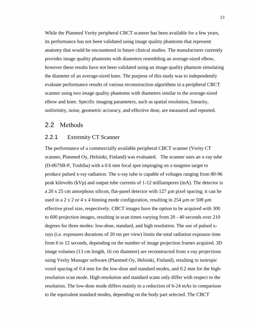
Figure 2.1: Peripheral cone-beam CT scanner pictured in conventional scan (a) mode and

weight-bearing scan (b) mode. ................................................................................................ 24

Figure 2.2: Large custom-built phantom (left) and small phantom (right) designed to evaluate

the performance of cone-beam CT scanners. .......................................................................... 25

Figure 2.3: Images of small phantom a) resolution coils, created with alternating aluminum

and Mylar sheets, b) the 5° axial slanted-edge image. In the large phantom, c) bar pattern

plate, created with alternating aluminum and Mylar sheets, and d) the axial slanted-edge

image, showing a 5° from the central axis. ............................................................................. 28

Figure 2.4: Image of linearity plates used in the small phantom (a) containing vials of air,

water, and iodine (Omnipaque) in various concentrations, measured in mg ml-1. Image of

linearity plate in large phantom (b) containing plastics within various bone mineral densities,

measured in mg hydroxyapatite cm-3. ..................................................................................... 29

Figure 2.5: Slices through an area of uniform density in the small (a) and large (b) phantoms,

show the location of the line profile used to characterize system uniformity. ROIs located

xi

within the small (c) and large (d) phantoms used to assess uniformity (red & yellow) and

noise (red only). ...................................................................................................................... 31

Figure 2.6: a) slice from small phantom with five steel beads in axial plane. b) Slices from

large phantom containing: five steel beads in the axial plane, and c) in (x-z) direction with

thirty tungsten-carbide beads spaced 15 mm in all directions. ............................................... 32

Figure 2.7: Modulation transfer function of the cone-beam CT system measured from the

slanted-edge plate (lines) and resolution coils (symbols) of the small phantom using the 6s (a)

and 9s (b) exposure acquisitions. ............................................................................................ 34


slanted-edge (line) and bar patterns (symbols) in the large phantom, using (a) 6s and (b) 9s

exposures. Additionally, modulation transfer function evaluated with the slanted-edge

located within the x-y plane in the large phantom, using (c) 6 and (d) 9s exposures. ............ 35

Figure 2.9: Plots of measured CT number versus known iodine concentrations, including

results of linear regression, within the linearity plate of small phantom using the (a) 300- and

(b) 450- image projection protocols. Plots of measured CT number versus known bone

mineral densities, including results of linear regression, within the linearity plate of large

phantom using the (c) 300- and (d) 450-image projection protocols. A beam-hardening

correction was applied to images of the large phantom using the (e) 300- and (f) 450- image

projection protocols. ............................................................................................................... 37

Figure 2.10: Radial signal profiles taken through the centre of the small phantom using the:

(a) current, (b) current with AINO, (c) beta, and (d) beta with AINO reconstruction

algorithms. All line profiles were obtained on the central reconstructed slice. ...................... 40

Figure 2.11: Radial signal profiles taken through the centre of the large phantom using the:

(a) current, (b) current with AINO, (c) beta, (d) beta with AINO, (e) beam-hardening

correction, and (f) beam-hardening correction with AINO reconstruction algorithms. All line

profiles were obtained on the central reconstructed slice. ...................................................... 41

Figure 2.12: Measured noise in the small phantom using the 300 frame (a) and 450 frame (b)

protocols, expressed as average standard deviation of the signal intensity (HU), plotted as a

xii

function of increasing exposure. Tube voltage used for the small phantom was 90 kVp, with

tube current varying from 1 to 12 mA, using 6s (a) or 9s (b) exposure time. Similarly,

measured noise in the large phantom using the 300 frame (c) and 450 frame (d) protocols,

expressed as average standard deviation of the signal intensity (HU), plotted as a function of

increasing exposure. Tube voltage used for the large phantom was 96 kVp, with tube current

varying from 1 to 12 mA, using 6s (c) or 9s (d) exposure time. ............................................. 43

Figure 3.1: Ceiling-mounted x-ray fluoroscopy system setup for an upright acquisition of an

image quality phantom. ........................................................................................................... 58

Figure 3.2: Image of the 3D-printed calibration phantom (left) with a sample x-ray projection

image (right) showing the locations of each marker bead at each vertex were used to

characterize gantry motion. ..................................................................................................... 59

Figure 3.3: Schematic diagram of the acquisition geometry depicting a point projection of an

object located in 3D (X, Y, Z) onto a 2D detector (U, V). ..................................................... 61

Figure 3.4: Reconstructed slice from the image quality phantom depicting (a) uncorrected

and (b) corrected slanted-edge image, showing a 5° from the central axis, and an (c)

uncorrected and (d) corrected bar pattern plate, created with alternating aluminum and Mylar

sheets. ...................................................................................................................................... 64

Figure 3.5: Reconstructed (a) uncorrected and (b) corrected linearity slice containing various

bone mineral densities representing materials encountered in musculoskeletal imaging,

measured in mg hydroxyapatite cm-3. ..................................................................................... 65

Figure 3.6: (a) Uncorrected and (b) corrected reconstructed slice through an area of uniform

density. (c) ROIs used to assess noise (red only) and uniformity (red & yellow). (d) The

location of line profile used to analyze variation of CT numbers across the field-of-view

(FOV). ..................................................................................................................................... 66

Figure 3.7: Reconstructed (a) uncorrected and (b) corrected slices from image quality

phantom with five steel beads in axial plane. (c) uncorrected and (d) corrected slices in X-Y

direction with thirty tungsten-carbide beads spaced 15 mm in all directions. ........................ 68

xiii

Figure 3.8: Various plots with non-linear best-fit lines illustrating the relationships between

(a) x-ray photon fluence and total copper sheet thickness, (b) signal intensity and total copper

sheet thickness, (c) signal intensity and x-ray photon fluence, and (d) bright-field corrected

signal intensity and x-ray photon fluence. .............................................................................. 70

Figure 3.9: (a) Comparison of centroid trajectory of a single high-contrast marker bead

versus the averaged U coordinates of the eight diametrically opposed vertices of the 3D

printed calibration cube, where the thick line indicates the best-fit sinusoid. (b) The resulting

residual plot from a sinusoidal fit is plotted as a function of angle, calculated by subtracting

the measured centroid location from the best-fit line. ............................................................ 71

Figure 3.10: (a) Comparison five acquisitions of centroid trajectory of the averaged U

coordinates of the eight diametrically opposed vertices of the 3D printed calibration cube,

where the thick line indicates the best-fit sinusoid. (b) The resulting residual plot. .............. 71

Figure 3.11: (a) Comparison five acquisitions of centroid trajectory of the averaged V


where the thick line indicates the best-fit sinusoid. (b) The resulting residual plot from a

sinusoidal fit are plotted as a function of angle, determined by subtracting the measured

centroid location from the best-fit line.................................................................................... 72

Figure 3.12: Average deviations in (a) τ and (b) ξ as a function of angle, acquired at intervals

over a year. .............................................................................................................................. 73

Figure 3.13: Reproducibility of prospective geometric parameters that include: (a) the

location of the piercing point (U0, V0) and source-to-detector distance (SDD), (b) extrinsic

translations (Tx, Ty, Tz), and (c) extrinsic rotations (Rx, Ry, Rz). Parameters are plotted as a

difference from their average value during gantry rotation. ................................................... 74

Figure 3.14: Evaluation of modulation transfer function of reconstructed image volumes

using bar patterns in the axial direction, as well as slanted-edge images in the axial and X-Y

planes. ..................................................................................................................................... 75

Figure 3.15: Results of linear regression from analysis of bone mineral densities analyzed in

the reconstructed linearity plate of the image quality phantom. ............................................. 76

xiv

Figure 3.16: Measured noise from resulting image reconstructions, expressed as standard

deviation within a uniform ROI, plotted as a function of increasing radiation exposure. ...... 77

Figure 3.17: Radial signal profile plotted across the central slice of a reconstructed image

volume. (120 kVp, 64 mAs) ................................................................................................... 78

Figure 3.18: Reconstructed axial slices taken from the top, middle, and bottom of uncorrected

(a-c) and corrected (d-f) image volumes, respectively. .......................................................... 79

Figure 3.19: Projection views of the frozen cadaveric knee in the axial, coronal, and sagittal

planes. The uncorrected (a-c), residual-corrected (d-f), and artefact-corrected (g-i)

reconstructed image volumes. ................................................................................................. 80

1

Chapter 1

1 Introduction

1.1 Knee Osteoarthritis

Osteoarthritis (OA) is the most common musculoskeletal disease, impacting

approximately 10-15% of adults over the age of sixty.34 Although this disease is most

common in the hip and knee, the diagnosis of knee OA – whether by symptoms and

radiographic changes, or by radiographic criteria alone – is more prevalent than hip OA.97

Symptoms of OA may include pain, stiffness, and limited joint function.21 With respect to

radiographic changes, OA is mainly characterized by joint space narrowing, subchondral

sclerosis, and osteophyte formation.72 Non-operative treatment strategies aim to reduce

pain and physical disability to limit structural deterioration in affected joints using non-

pharmaceutical methods such as weight loss and aerobic exercise, as well as

pharmaceutical methods including: non-steroidal anti-inflammatory drugs (NSAIDs),

corticosteroid injections, hyaluronic acid injections, and glucosamine.39, 89, 91 The surgical

option may be a partial- or total-knee arthroplasty (TKA), which are both intended to

reduce pain and improve knee function in patients.19

The initiation and progression of knee OA has been related to the mechanics of

ambulation.6 Changes resulting from OA are most frequently observed in the medial

compartment, compared to the lateral or patellofemoral compartments of the knee.69

Patients can functionally adapt to pathological joint changes such as a ligament injury or

articular cartilage degeneration.6 For example, it has been observed from in vivo studies

that some patients with knee OA develop new gait patterns to lower the load at the knee

and reduce the rate at which OA progresses.7, 49, 69 Consequently, these changes in gait

may increase the loads observed in other joints in the lower extremity (hip, knee, and

ankle).5, 69

Total knee arthroplasty has become the gold standard for management of severe OA of

the knee, since it has been proven as a safe and cost-effective method.36, 58, 73, 96 Knee

joint replacement is one of the most effective ways to reduce pain and improve function

2

for patients with end-stage OA.38, 56 In Canada, hip and knee arthroplasty rates have

increased substantially from 2012-2017, with the respective volumes of these procedures

growing by 17.8% (55 981 hip replacements) and 15.5% (67 169 knee replacements).37

Indications for operative treatments are demonstration of radiographic OA and

experience of persistent pain for six months after failure of non-operative treatments.98

TKA is not without risk or complications; adverse outcomes can occur, which may

include: mortality, surgical site infection, and cardiovascular complications (myocardial

infarction, congestive heart failure, arrhythmia, or pulmonary embolus).11, 68 Main risk

factors for these negative outcomes are associated with a patient’s medical history and

age.11

Despite long-term pain relief and patient satisfaction, many TKA patients continue to

have impairments and functional limitations when compared with age-matched

controls.26, 70 After unilateral TKA, patients tend to walk slower, have less peak knee

flexion during gait, and have altered sagittal knee moments compared to controls.63, 65

An increased sagittal knee moment is a biomechanical indication of increased loading in

the medial knee compartment, which is related to the severity of OA, and is the best

predictor of OA progression.4 Furthermore, the contralateral knee is more likely to suffer

OA disease progression more than the ipsilateral or contralateral hip or ankle.79 Within 10

years of the original TKA, 40% of patients will undergo a second TKA on the

contralateral knee.64, 79 Although TKA has revolutionized end-stage OA treatment, it

remains an inadequate technique for approximately 19% of patients since they are

unsatisfied with the outcomes related to pain relief and restoring function.15 Therefore,

accurate knowledge of joint motion and loading during weight-bearing activities, such as

walking, is integral for developing strategies for alleviating joint pain and restoring

functionality.

1.2 Review of Current Methods for Knee Motion Analysis

1.2.1 3D Motion Capture Gait Analysis

Gait analysis is a robust technique used to assess dynamic musculoskeletal movement

during functional activities and has numerous applications in orthopaedic investigations,

3

which include the evaluation of joint function following corrective surgery, comparison

of different treatment options and therapies, and understanding the pathology of

musculoskeletal disorders and trauma. This technique uses reflective skin-mounted

external markers attached to specific landmarks on the subject, and high-speed cameras

to track rigid body motion (Figure 1.1); however, it cannot provide quantitative

information about joint micro-motion and its accuracy is hindered by soft-tissue artefacts.

This phenomenon occurs because optical markers on the skin may not reflect the motion

of the underlying bony structures.80 Studies using gait analysis have demonstrated distinct

gait patterns between healthy and OA patients,6, 63, 69 as well as differences between the

non-operated and operated knee in the same patient.4, 26 One of the best methods to

evaluate knee OA progression may be to perform measurements under dynamic loading

in order to evaluate biomechanical function of the knee.66 Overall, this modality provides

excellent overall kinematic measurements, and with the addition of force plates, kinetic

measurements within the lower extremities.

Figure 1.1: Gait real-time interactive analysis lab (GRAIL) located at the Wolf

Orthopaedic Biomechanics Laboratory.

4

1.2.2 Radiography

Radiography is a non-invasive medical imaging modality that creates a single, static, two-

dimensional (2D) radiographic image using ionizing radiation. X-rays are emitted from

the source, attenuated by the region of interest, then the attenuated x-rays are absorbed by

the detector to form the resultant x-ray image. The attenuation properties of tissues such

as bone, air, and soft tissue have different atomic numbers, which results in a

heterogenous distribution of intensities on the image due to the attenuation of x-ray

photons.17 The amount of x-ray photon attenuation within a tissue is dependent on the

linear attenuation coefficient (LAC), which depends on the absorption and scatter

occurring per unit thickness of a tissue for a specific x-ray energy.17 In the current clinical

setting, the Kellgren-Lawrence classification system uses weight-bearing radiographic

images to grade the severity of knee OA based on osteophyte formation, joint space

narrowing, and subchondral osteosclerosis.16, 44 The success of TKA is evaluated using

weight-bearing antero-posterior and lateral radiographs, however the image quality can

be influenced by patient positioning and orientation of the x-ray detector.76 Although

radiography is effective at demonstrating the progression of OA, it has some limitations

that include: the superimposition of tissue due to a 3D object being represented as a 2D

image, and the inability to distinguish between two tissues with similar densities.74

1.2.3 Radiostereometric Analysis

Radiostereometric analysis (RSA) is the gold standard for three-dimensional (3D)

migration measurements of orthopaedic implants. RSA uses static radiographic images to

estimate relative skeletal motion between successive clinical examinations to measure

migration and wear of orthopaedic implants in the ankle,18, 29 knee,75, 83-86 hip,33, 61 wrist,59

elbow,23, 24 and shoulder joints.2, 32, 88 This technique has been applied to assess cervical99

and lumbar spine fracture healing.8 RSA utilizes simultaneous bi-planar x-rays (Figure

1.2) to obtain accurate 3D measurements of joint micro-motion using marker-based

methods or model-based RSA (MBRSA) techniques.77 The marked-based method

requires surgical implantation of at least three tantalum marker beads into each bone

comprising the joint of interest, while MBRSA matches contours of virtual shadows to

5

the shape and location of digital models to obtain measurements of joint micro-motion.40

Both techniques create a spatial model of the rigid object using stereoscopic x-ray

sources that generates two projections from simultaneous radiographic exposures,

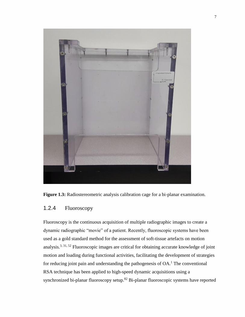
however precision is lower with MBRSA.45 The calibration cage shown in Figure 1.3 is

present during the acquisition stereoscopic radiographs to determine photogrammetric

projection parameters of the two x-ray sources. Images of the tantalum beads are

analyzed with model-based non-linear image analysis algorithms that determine the

centroid of the marker to subpixel accuracy.14 Marker-based RSA is extremely dependent

upon the ability to identify the same marker bead in both radiographs.48 Reported

accuracy for marker-based RSA at 95% significance level ranges between 0.05 and 0.5

mm for translations and between 0.15° and 1.15° for rotations.47 In a separate study,

MBRSA pose-estimation algorithms were optimized to improve accuracy of the method

which proved to be comparable to conventional marker-based RSA.46 Although this

technique has many advantages, it is limited by a small field-of-view (FOV) resulting

from the intersection between the two x-ray beams and it can only evaluate implanted

markers with static images in a single joint.

6

Figure 1.2: Example of bi-planar setup in the radiostereometric analysis lab located at

Robarts Research Institute.

7

Figure 1.3: Radiostereometric analysis calibration cage for a bi-planar examination.

1.2.4 Fluoroscopy

Fluoroscopy is the continuous acquisition of multiple radiographic images to create a

dynamic radiographic “movie” of a patient. Recently, fluoroscopic systems have been

used as a gold standard method for the assessment of soft-tissue artefacts on motion

analysis.3, 31, 52 Fluoroscopic images are critical for obtaining accurate knowledge of joint

motion and loading during functional activities, facilitating the development of strategies

for reducing joint pain and understanding the pathogenesis of OA.1 The conventional

RSA technique has been applied to high-speed dynamic acquisitions using a

synchronized bi-planar fluoroscopy setup.82 Bi-planar fluoroscopic systems have reported

8

measurement errors of 0.094 mm for translations and 0.083° for rotations.41 A major

constraint of implementation into routine clinical practice is caused by the need for

highly specialized imaging equipment that may not be readily available in a hospital

environment. Additionally, this technique has a small FOV that is restricted to the regions

where the two x-ray beams intersect, therefore only one joint with implanted markers can

be examined at a time. Single-plane x-ray fluoroscopy setups are more practical for

clinical implementation since this approach requires less radiation, is less

computationally intensive, utilizes equipment currently available in most hospitals, and

allows for natural dynamic motion in a large FOV to evaluate dynamic 3D motions of the

lower extremity.10, 22, 60, 92 Calibration of geometrical information pertaining to intrinsic

and extrinsic camera parameters is required to determine the spatial position and

orientation of the object. The position and orientation of the calibration object also

defines the coordinate system where joint motion is reconstructed. Although in-plane

translations (Tx and Ty) and rotation (Rz) can be accurately predicted from a single 2D

view, precise measurement for out-of-plane rotations (Rx and Ry) and translation (Tz) are

very difficult.30, 67, 92 Single-plane fluoroscopic setups using fluoroscopic shape matching

have reported mean errors between 0.03-0.70 mm for translations and 0.03-0.12° for

rotations.78

Roentgen single-plane photogrammetric analysis (RSPA) was developed to aide in the

analysis of real-time musculoskeletal movement using a single radiation source with an

RSA approach.30, 43, 94 This technique requires a priori knowledge of the 3D geometry of

the markers from conventional marker-based RSA in order to calculate joint motion. In

knee movement simulations, the maximum difference between the original and simulated

movement for rotations and translations were 0.27° and 0.9 mm.94 An example of a

single-plane fluoroscopy system for RSPA is shown in Figure 1.4.

Although single-plane fluoroscopic systems provide excellent evaluations of dynamic

joint motion, it is significantly limited by the requirement to have a 3D model of the

anatomy of interest in order to accurately characterize 3D joint motion. This highlights

the need for rapid, low-dose peripheral computed tomography systems that provide

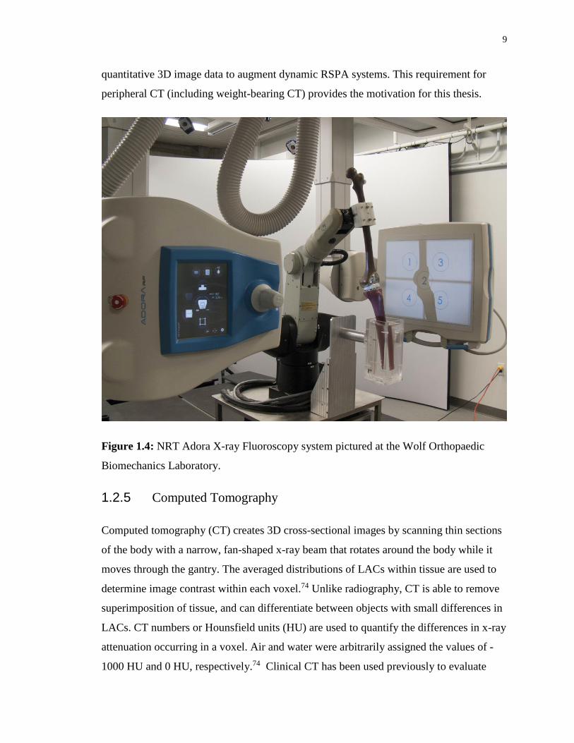
9

quantitative 3D image data to augment dynamic RSPA systems. This requirement for

peripheral CT (including weight-bearing CT) provides the motivation for this thesis.

Figure 1.4: NRT Adora X-ray Fluoroscopy system pictured at the Wolf Orthopaedic

Biomechanics Laboratory.

1.2.5 Computed Tomography

Computed tomography (CT) creates 3D cross-sectional images by scanning thin sections

of the body with a narrow, fan-shaped x-ray beam that rotates around the body while it

moves through the gantry. The averaged distributions of LACs within tissue are used to

determine image contrast within each voxel.74 Unlike radiography, CT is able to remove

superimposition of tissue, and can differentiate between objects with small differences in

LACs. CT numbers or Hounsfield units (HU) are used to quantify the differences in x-ray

attenuation occurring in a voxel. Air and water were arbitrarily assigned the values of -

1000 HU and 0 HU, respectively.74 Clinical CT has been used previously to evaluate

10

knee-joint alignment, and patellar subluxation.42, 93 Recent studies with clinical CT

scanners have simulated weight-bearing conditions by applying an axial load to a

patient’s legs during an image acquisition while in a supine position.12, 28, 71 Although CT

provides high quality cross-sectional images with excellent contrast resolution, it is

typically unable to acquire images in a natural weight-bearing stance, due to fundamental

scanner design limitations.

1.2.6 Cone-beam Computed Tomography

Cone-beam computed tomography (CBCT) is based on the same principles as a

conventional CT scanner, but designed for higher resolution imaging.9 CBCT uses a

rotating flat-panel detector with a cone-shaped x-ray beam that does not require patient

translation to acquire volumetric images. There are two possible scanner design

configurations: 1) rotating object and 2) rotating gantry. The rotating gantry configuration

is the most common configuration for commercial dedicated extremity CBCT scanners.

This design mounts the tube and detector on a gantry that rotates around a central axis.9

Numerous 2D fluoroscopic projections are acquired over various angles around the area

of interest to construct volumetric images. The differences in x-ray attenuation are

determined by the object’s electron density and physical density in each projection

image. The reconstructed images are comprised of a 3D matrix of voxels with each voxel

containing a CT number, which is proportional to the mean linear attenuation coefficient

of the material within that voxel.9 Similar to conventional CT, the grey-level of each

voxel in a CBCT image is measured with HU, which are directly scaled to the x-ray

absorption characteristics of air and water (-1000 HU and 0 HU, respectively).9

Recent advances in CBCT have created scanner designs that utilize a motorized gantry to

allow for weight-bearing imaging of the lower extremity in either a single or double leg

stance.20, 57, 62, 95 These CBCT scanner designs allow for an increased distance from the

torso, which lowers radiation dose because less scattered radiation can interact with

radiosensitive organs within the torso.87 Previous studies have demonstrated that

extremity CBCT images produce an equal or smaller effective dose, while maintaining

image quality comparable to conventional CT.13, 50, 51 The overall image quality in CBCT

11

is determined by the geometry and characteristics of the x-ray source and detector. The

ideal detector has a large area with a consistent, linear, uniform response to all x-ray

energies, and no geometric distortion.9 The image quality can be optimized by various

scan parameters including: scan time, field of view, spatial resolution, temporal

resolution, contrast resolution, and image dose.9 Image quality is typically evaluated

using the spatial, contrast, and temporal resolution.74 Spatial resolution is defined as the

ability to differentiate between two small objects that are very close together.74 Contrast

resolution determines the ability to differentiate between objects with similar LACs.74

Temporal resolution refers to the acquisition rate of the projections images that are used

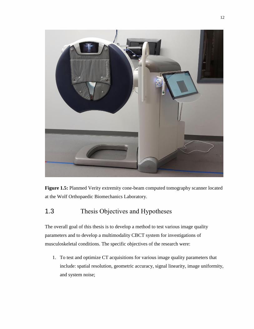
in image reconstruction.74 An example of a commercially available CBCT scanner is

shown in Figure 1.5.

In both CT and CBCT, imprecision of geometric calibration information may lead to loss

of spatial resolution, double contours, or star artefacts.54, 81, 90 Most volumetric

reconstruction algorithms assume the gantry rotation occurs in a perfect circular

trajectory,27 however there may be imperfections in the trajectory of the gantry’s rotation.

These imperfections may be either parallel to the axis of rotation or tangential to the

circle of rotation and perpendicular to the line joining the x-ray source and detector.25

Image-based geometric calibration can be incorporated into the reconstruction algorithm

either concurrently or prospectively to characterize imperfections in gantry motion during

rotation.25 Geometric calibration of an imaging system determines various parameters,

which can be divided into five intrinsic and six extrinsic geometric calibration

parameters.55 The intrinsic parameters describe the inherent properties of the x-ray

system geometry that remain constant throughout operation; this includes pixel size,

source-to-image distance, and detector offset.53 The extrinsic parameters indicate the 3D

rotational and translational matrices of the entire imaging system relative to the

calibration object.53 A minimum of six points of correspondence are required to calculate

these eleven geometric calibration parameters.35 CBCT is ideally suited for extremity

musculoskeletal health applications since it can obtain true weight-bearing, 3D

volumetric scans with optimal image quality at a low-dose when compared to

conventional CT.

12

Figure 1.5: Planmed Verity extremity cone-beam computed tomography scanner located

at the Wolf Orthopaedic Biomechanics Laboratory.

1.3 Thesis Objectives and Hypotheses

The overall goal of this thesis is to develop a method to test various image quality

parameters and to develop a multimodality CBCT system for investigations of

musculoskeletal conditions. The specific objectives of the research were:

1. To test and optimize CT acquisitions for various image quality parameters that

include: spatial resolution, geometric accuracy, signal linearity, image uniformity,

and system noise;

13

2. To develop a method for producing accurate CBCT reconstructions from a

ceiling-mounted single-plane x-ray fluoroscopy system using a custom 3D printed

calibration object for geometric calibration and in-house software for image

reconstruction.

1.4 Thesis Organization

Chapter two describes the methodology for the primary goal of testing and optimizing CT

acquisitions for basic imaging parameters that were quantified using phantoms

mimicking diameters of the upper and lower extremity. Chapter three describes the

acquisition of CBCT image volumes using a ceiling-mounted single-plane x-ray

fluoroscopy system. Finally, the thesis is concluded in Chapter four with a summary of

the major results of these projects and a discussion of potential areas for future work.

1.5 References

1. Ackland, D. C., Keynejad, F., & Pandy, M. G. (2011). Future trends in the use of

X-ray fluoroscopy for the measurement and modelling of joint motion. Proc Inst

Mech Eng H, 225(12), 1136-1148.

2. Akbari-Shandiz, M., Mozingo, J. D., Holmes, D. R., & Zhao, K. D. (2017).

Three-Dimensional Glenohumeral Joint Kinematic Analyses from Asynchronous

Biplane Fluoroscopy Using an Interpolation Technique. In A. Wittek, G. Joldes,

P. M. F. Nielsen, B. J. Doyle, & K. Miller (Eds.), Computational Biomechanics

for Medicine (pp. 101-110). Cham: Springer International Publishing.

3. Akbarshahi, M., Schache, A. G., Fernandez, J. W., Baker, R., Banks, S., & Pandy,

M. G. (2010). Non-invasive assessment of soft-tissue artifact and its effect on

knee joint kinematics during functional activity. Journal of biomechanics, 43(7),

1292-1301.

4. Alnahdi, A. H., Zeni, J. A., & Snyder-Mackler, L. (2011). Gait after unilateral

total knee arthroplasty: frontal plane analysis. Journal of orthopaedic research :

official publication of the Orthopaedic Research Society, 29(5), 647-652.

5. Andriacchi, T. P., & Mundermann, A. (2006). The role of ambulatory mechanics

in the initiation and progression of knee osteoarthritis. Current opinion in

rheumatology, 18(5), 514-518.

14

6. Andriacchi, T. P., Mundermann, A., Smith, R. L., Alexander, E. J., Dyrby, C. O.,

& Koo, S. (2004). A framework for the in vivo pathomechanics of osteoarthritis at

the knee. Annals of Biomedical Engineering, 32(3), 447-457.

7. Astephen, J. L., Deluzio, K. J., Caldwell, G. E., Dunbar, M. J., & Hubley-Kozey,

C. L. (2008). Gait and neuromuscular pattern changes are associated with

differences in knee osteoarthritis severity levels. Journal of biomechanics, 41(4),

868-876.

8. Axelsson, P., & Karlsson, B. S. (2005). Standardized provocation of lumbar spine

mobility: three methods compared by radiostereometric analysis. Spine, 30(7),

792-797.

9. Badea, C. T., Drangova, M., Holdsworth, D. W., & Johnson, G. A. (2008). In

vivo small-animal imaging using micro-CT and digital subtraction angiography.

Phys Med Biol, 53(19), R319-350.

10. Banks, S. A., & Hodge, W. A. (1996). Accurate measurement of three-

dimensional knee replacement kinematics using single-plane fluoroscopy. IEEE

Trans Biomed Eng, 43(6), 638-649.

11. Basilico, F. C., Sweeney, G., Losina, E., Gaydos, J., Skoniecki, D., Wright, E. A.,

& Katz, J. N. (2008). Risk factors for cardiovascular complications following

total joint replacement surgery. Arthritis Rheum, 58(7), 1915-1920.

12. Biedert, R. M., & Gruhl, C. (1997). Axial computed tomography of the

patellofemoral joint with and without quadriceps contraction. Archives of

Orthopaedic and Trauma Surgery, 116(1-2), 77-82.

13. Biswas, D., Bible, J. E., Bohan, M., Simpson, A. K., Whang, P. G., & Grauer, J.

N. (2009). Radiation exposure from musculoskeletal computerized tomographic

scans. J Bone Joint Surg Am, 91(8), 1882-1889.

14. Börlin, N. (2000). Model-based measurements in digital radiographs: Univ.

15. Bourne, R. B., Chesworth, B. M., Davis, A. M., Mahomed, N. N., & Charron, K.

D. (2010). Patient satisfaction after total knee arthroplasty: who is satisfied and

who is not? Clin Orthop Relat Res, 468(1), 57-63.

16. Brandt, K. D., Fife, R. S., Braunstein, E. M., & Katz, B. (2010). Radiographic

grading of the severity of knee osteoarthritis: Relation of the kellgren and

lawrence grade to a grade based on joint space narrowing, and correlation with

arthroscopic evidence of articular cartilage degeneration. Arthritis & Rheumatism,

34(11), 1381-1386.

17. Bushberg, J. T., & Boone, J. M. (2002). The essential physics of medical imaging:

Lippincott Williams & Wilkins.

15

18. Carlsson, A., Markusson, P., & Sundberg, M. (2005). Radiostereometric analysis

of the double-coated STAR total ankle prosthesis: a 3-5 year follow-up of 5 cases

with rheumatoid arthritis and 5 cases with osteoarthrosis. Acta orthopaedica,

76(4), 573-579.

19. Carr, A. J., Robertsson, O., Graves, S., Price, A. J., Arden, N. K., Judge, A., &

Beard, D. J. (2012). Knee replacement. Lancet, 379(9823), 1331-1340.

20. Carrino, J. A., Al Muhit, A., Zbijewski, W., Thawait, G. K., Stayman, J. W.,

Packard, N., . . . Siewerdsen, J. H. (2014). Dedicated cone-beam CT system for

extremity imaging. Radiology, 270(3), 816-824.

21. Das, S. K., & Farooqi, A. (2008). Osteoarthritis. Best Pract Res Clin Rheumatol,

22(4), 657-675.

22. Dennis, D. A., Mahfouz, M. R., Komistek, R. D., & Hoff, W. (2005). In vivo

determination of normal and anterior cruciate ligament-deficient knee kinematics.

Journal of biomechanics, 38(2), 241-253.

23. Ericson, A., Arndt, A., Stark, A., Noz, M. E., Maguire, G. Q., Jr., Zeleznik, M. P.,

& Olivecrona, H. (2007). Fusion of radiostereometric analysis data into computed

tomography space: application to the elbow joint. Journal of biomechanics, 40(2),

296-304.

24. Ericson, A., Olivecrona, H., Stark, A., Noz, M. E., Maguire, G. Q., Zeleznik, M.

P., & Arndt, A. (2010). Computed tomography analysis of radiostereometric data

to determine flexion axes after total joint replacement: application to the elbow

joint. Journal of biomechanics, 43(10), 1947-1952.

25. Fahrig, R., & Holdsworth, D. W. (2000). Three-dimensional computed

tomographic reconstruction using a C-arm mounted XRII: image-based correction

of gantry motion nonidealities. Med Phys, 27(1), 30-38.

26. Farquhar, S., & Snyder-Mackler, L. (2010). The Chitranjan Ranawat Award: The

nonoperated knee predicts function 3 years after unilateral total knee arthroplasty.

Clin Orthop Relat Res, 468(1), 37-44.

27. Feldkamp, L. A., Davis, L. C., & Kress, J. W. (1984). Practical Cone-Beam

Algorithm. J Opt Soc Am A, 1(6), 612-619.

28. Ferri, M., Scharfenberger, A. V., Goplen, G., Daniels, T. R., & Pearce, D. (2008).

Weightbearing CT scan of severe flexible pes planus deformities. Foot Ankle Int,

29(2), 199-204.

29. Fong, J. W., Veljkovic, A., Dunbar, M. J., Wilson, D. A., Hennigar, A. W., &

Glazebrook, M. A. (2011). Validation and precision of model-based

radiostereometric analysis (MBRSA) for total ankle arthroplasty. Foot Ankle Int,

32(12), 1155-1163.

16

30. Garling, E. H., Kaptein, B. L., Geleijns, K., Nelissen, R. G., & Valstar, E. R.

(2005). Marker Configuration Model-Based Roentgen Fluoroscopic Analysis.

Journal of biomechanics, 38(4), 893-901.

31. Garling, E. H., Kaptein, B. L., Mertens, B., Barendregt, W., Veeger, H. E.,

Nelissen, R. G., & Valstar, E. R. (2007). Soft-tissue artefact assessment during

step-up using fluoroscopy and skin-mounted markers. Journal of biomechanics,

40 Suppl 1, S18-24.

32. Gobezie, R., Lavery, K. P., Bragdon, C., Higgins, L. D., Malchau, H., & Warner,

J. J. P. (2006). Radiostereometric analysis of the anatomical total shoulder

arthroplasty and reverse total shoulder replacement: an analysis of component

stability and polyethylene wear. The Orthopaedic Journal at Harvard Medical

School, 110-112.

33. Goyal, P., Howard, J. L., Yuan, X., Teeter, M. G., & Lanting, B. A. (2017). Effect

of Acetabular Position on Polyethylene Liner Wear Measured Using

Simultaneous Biplanar Acquisition. The Journal of arthroplasty, 32(5), 1670-

1674.

34. Haq, I., Murphy, E., & Dacre, J. (2003). Osteoarthritis. Postgrad Med J, 79(933),

377-383.

35. Hartley, R., & Zisserman, A. (2004). Multiple view geometry in computer vision.

Cambridge: Cambridge University Press.

36. Hayes, D. A., Miller, L. E., & Block, J. E. (2012). Knee Osteoarthritis Treatment

with the KineSpring Knee Implant System: A Report of Two Cases. Case Rep

Orthop, 2012, 297326.

37. Hip and Knee Replacements in Canada, 2016–2017: Canadian Joint Replacement

Registry Annual Report. 51.

38. Hip and Knee Replacements in Canada: Canadian Joint Replacement Registry

2015 Annual Report. 63.

39. Hunter, D. J. (2011). Osteoarthritis. Best Pract Res Clin Rheumatol, 25(6), 801-

814.

40. Hurschler, C., Seehaus, F., Emmerich, J., Kaptein, B. L., & Windhagen, H.

(2009). Comparison of the model-based and marker-based roentgen

stereophotogrammetry methods in a typical clinical setting. The Journal of

arthroplasty, 24(4), 594-606.

41. Iaquinto, J. M., Tsai, R., Haynor, D. R., Fassbind, M. J., Sangeorzan, B. J., &

Ledoux, W. R. (2014). Marker-based validation of a biplane fluoroscopy system

for quantifying foot kinematics. Medical engineering & physics, 36(3), 391-396.

17

42. Inoue, M., Shino, K., Hirose, H., Horibe, S., & Ono, K. (1988). Subluxation of the

patella. Computed tomography analysis of patellofemoral congruence. J Bone

Joint Surg Am, 70(9), 1331-1337.

43. Ioppolo, J., Borlin, N., Bragdon, C., Li, M., Price, R., Wood, D., . . . Nivbrant, B.

(2007). Validation of a low-dose hybrid RSA and fluoroscopy technique:

Determination of accuracy, bias and precision. Journal of biomechanics, 40(3),

686-692.

44. Kan, H., Arai, Y., Kobayashi, M., Nakagawa, S., Inoue, H., Hino, M., . . . Kubo,

T. (2017). Fixed-flexion view X-ray of the knee superior in detection and follow-

up of knee osteoarthritis. Medicine (Baltimore), 96(49), e9126.

45. Kaptein, B. L., Valstar, E. R., Spoor, C. W., Stoel, B. C., & Rozing, P. M. (2006).

Model-based RSA of a femoral hip stem using surface and geometrical shape

models. Clin Orthop Relat Res, 448, 92-97.

46. Kaptein, B. L., Valstar, E. R., Stoel, B. C., Rozing, P. M., & Reiber, J. H. (2004).

Evaluation of three pose estimation algorithms for model-based roentgen

stereophotogrammetric analysis. Proc Inst Mech Eng H, 218(4), 231-238.

47. Karrholm, J. (1989). Roentgen stereophotogrammetry. Review of orthopedic

applications. Acta Orthop Scand, 60(4), 491-503.

48. Karrholm, J., Herberts, P., Hultmark, P., Malchau, H., Nivbrant, B., & Thanner, J.

(1997). Radiostereometry of hip prostheses. Review of methodology and clinical

results. Clin Orthop Relat Res(344), 94-110.

49. Kaufman, K. R., Hughes, C., Morrey, B. F., Morrey, M., & An, K. N. (2001).

Gait characteristics of patients with knee osteoarthritis. Journal of biomechanics,

34(7), 907-915.

50. Koivisto, J., Kiljunen, T., Kadesjo, N., Shi, X. Q., & Wolff, J. (2015). Effective

radiation dose of a MSCT, two CBCT and one conventional radiography device

in the ankle region. J Foot Ankle Res, 8(1), 8.

51. Koivisto, J., Kiljunen, T., Wolff, J., & Kortesniemi, M. (2013). Assessment of

effective radiation dose of an extremity CBCT, MSCT and conventional X ray for

knee area using MOSFET dosemeters. Radiat Prot Dosimetry, 157(4), 515-524.

52. Kuo, M. Y., Tsai, T. Y., Lin, C. C., Lu, T. W., Hsu, H. C., & Shen, W. C. (2011).

Influence of soft tissue artifacts on the calculated kinematics and kinetics of total

knee replacements during sit-to-stand. Gait Posture, 33(3), 379-384.

53. Kyriakopoulos, K. J., Yiannakos, P., Kallipolites, V., & Domales, K. (1999). A

geometric calibration methodology for single-head cone-beam X-ray systems. J

Intell Robot Syst, 24(2), 151-174.

18

54. Kyriakou, Y., Lapp, R. M., Hillebrand, L., Ertel, D., & Kalender, W. A. (2008).

Simultaneous misalignment correction for approximate circular cone-beam

computed tomography. Phys Med Biol, 53(22), 6267-6289.

55. Li, X., Da, Z., & Liu, B. (2010). A generic geometric calibration method for

tomographic imaging systems with flat-panel detectors--a detailed

implementation guide. Med Phys, 37(7), 3844-3854.

56. Loughead, J. M., Malhan, K., Mitchell, S. Y., Pinder, I. M., McCaskie, A. W.,

Deehan, D. J., & Lingard, E. A. (2008). Outcome following knee arthroplasty

beyond 15 years. Knee, 15(2), 85-90.

57. Ludlow, J. B., & Ivanovic, M. (2014). Weightbearing CBCT, MDCT, and 2D

imaging dosimetry of the foot and ankle. International Journal of Diagnostic

Imaging, 1(2), 1.

58. Lutzner, J., Kasten, P., Gunther, K. P., & Kirschner, S. (2009). Surgical options

for patients with osteoarthritis of the knee. Nat Rev Rheumatol, 5(6), 309-316.

59. Madanat, R., Moritz, N., & Aro, H. T. (2007). Three-dimensional computer

simulation of radiostereometric analysis (RSA) in distal radius fractures. Journal

of biomechanics, 40(8), 1855-1861.

60. Mahfouz, M. R., Hoff, W. A., Komistek, R. D., & Dennis, D. A. (2003). A robust

method for registration of three-dimensional knee implant models to two-

dimensional fluoroscopy images. IEEE Trans Med Imaging, 22(12), 1561-1574.

61. Malchau, H., Karrholm, J., Wang, Y. X., & Herberts, P. (1995). Accuracy of

migration analysis in hip arthroplasty. Digitized and conventional radiography,

compared to radiostereometry in 51 patients. Acta Orthop Scand, 66(5), 418-424.

62. Marzo, J., Kluczynski, M., Notino, A., & Bisson, L. (2016). Comparison of a

Novel Weightbearing Cone Beam Computed Tomography Scanner Versus a

Conventional Computed Tomography Scanner for Measuring Patellar Instability.

Orthop J Sports Med, 4(12), 2325967116673560.

63. McClelland, J. A., Webster, K. E., & Feller, J. A. (2007). Gait analysis of patients

following total knee replacement: a systematic review. Knee, 14(4), 253-263.

64. McMahon, M., & Block, J. A. (2003). The risk of contralateral total knee

arthroplasty after knee replacement for osteoarthritis. J Rheumatol, 30(8), 1822-

1824.

65. Milner, C. E. (2009). Is gait normal after total knee arthroplasty? Systematic

review of the literature. J Orthop Sci, 14(1), 114-120.

66. Miyazaki, T., Wada, M., Kawahara, H., Sato, M., Baba, H., & Shimada, S.

(2002). Dynamic load at baseline can predict radiographic disease progression in

19

medial compartment knee osteoarthritis. Annals of the Rheumatic Diseases, 61(7),

617-622.

67. Muhit, A. A., Pickering, M. R., Scarvell, J. M., Ward, T., & Smith, P. N. (2013).

Image-assisted non-invasive and dynamic biomechanical analysis of human

joints. Phys Med Biol, 58(13), 4679-4702.

68. Mulcahy, H., & Chew, F. S. (2014). Current concepts in knee replacement:

complications. AJR Am J Roentgenol, 202(1), W76-86.

69. Mundermann, A., Dyrby, C. O., & Andriacchi, T. P. (2005). Secondary gait

changes in patients with medial compartment knee osteoarthritis: increased load at

the ankle, knee, and hip during walking. Arthritis Rheum, 52(9), 2835-2844.

70. Noble, P. C., Gordon, M. J., Weiss, J. M., Reddix, R. N., Conditt, M. A., &

Mathis, K. B. (2005). Does Total Knee Replacement Restore Normal Knee

Function? Clinical Orthopaedics and Related Research, &NA;(431), 157-165.

71. Oswald, M. H., Jakob, R. P., Schneider, E., & Hoogewoud, H. M. (1993).

Radiological analysis of normal axial alignment of femur and tibia in view of total

knee arthroplasty. The Journal of arthroplasty, 8(4), 419-426.

72. Peat, G., McCarney, R., & Croft, P. (2001). Knee pain and osteoarthritis in older

adults: a review of community burden and current use of primary health care.

Annals of the Rheumatic Diseases, 60(2), 91-97.

73. Rankin, E. A., Alarcon, G. S., Chang, R. W., Cooney, L. M., Costley, L. S.,

Delitto, A., . . . Marciel, C. (2004). NIH consensus statement on total knee

replacement December 8-10, 2003. Journal of Bone and Joint Surgery-American

Volume, 86a(6), 1328-1335.

74. Romans, L. E. (2010). Computed Tomography for Technologists: A

Comprehensive Text: Lippincott Williams & Wilkins.

75. Saari, T., Carlsson, L., Karlsson, J., & Karrholm, J. (2005). Knee kinematics in

medial arthrosis. Dynamic radiostereometry during active extension and weight-

bearing. Journal of biomechanics, 38(2), 285-292.

76. Sarmah, S. S., Patel, S., Hossain, F. S., & Haddad, F. S. (2012). The radiological

assessment of total and unicompartmental knee replacements. J Bone Joint Surg

Br, 94(10), 1321-1329.

77. Selvik, G. (1990). Roentgen stereophotogrammetric analysis. Acta Radiol, 31(2),

113-126.

78. Seslija, P., Teeter, M. G., Yuan, X., Naudie, D. D., Bourne, R. B., Macdonald, S.

J., . . . Holdsworth, D. W. (2012). Measurement of joint kinematics using a

20

conventional clinical single-perspective flat-panel radiography system. Med Phys,

39(10), 6090-6103.

79. Shakoor, N., Block, J. A., Shott, S., & Case, J. P. (2002). Nonrandom evolution of

end-stage osteoarthritis of the lower limbs. Arthritis Rheum, 46(12), 3185-3189.

80. Stagni, R., Fantozzi, S., Cappello, A., & Leardini, A. (2005). Quantification of

soft tissue artefact in motion analysis by combining 3D fluoroscopy and

stereophotogrammetry: a study on two subjects. Clinical biomechanics, 20(3),

320-329.

81. Strobel, N. K., Heigl, B., Brunner, T. M., Schuetz, O., Mitschke, M. M., Wiesent,

K., & Mertelmeier, T. (2003, 2003/06/09/). Improving 3D image quality of x-ray

C-arm imaging systems by using properly designed pose determination systems

for calibrating the projection geometry. Paper presented at the Medical Imaging

2003.

82. Tashman, S., & Anderst, W. (2003). In-vivo measurement of dynamic joint

motion using high speed biplane radiography and CT: Application to canine ACL

deficiency. J Biomech Eng-T Asme, 125(2), 238-245.

83. Teeter, M. G. (2012). Assessment of Wear in Total Knee Arthroplasty Using

Advanced Radiographic Techniques. 202.

84. Teeter, M. G., Leitch, K. M., Pape, D., Yuan, X., Birmingham, T. B., & Giffin, J.

R. (2015). Radiostereometric analysis of early anatomical changes following

medial opening wedge high tibial osteotomy. Knee, 22(1), 41-46.

85. Teeter, M. G., Perry, K. I., Yuan, X., Howard, J. L., & Lanting, B. A. (2017).

Contact Kinematic Differences Between Gap Balanced vs Measured Resection

Techniques for Single Radius Posterior-Stabilized Total Knee Arthroplasty. The

Journal of arthroplasty, 32(6), 1834-1838.

86. Teeter, M. G., Perry, K. I., Yuan, X., Howard, J. L., & Lanting, B. A. (2018).

Contact Kinematics Correlates to Tibial Component Migration Following Single

Radius Posterior Stabilized Knee Replacement. The Journal of arthroplasty,

33(3), 740-745.

87. Tuominen, E. K., Kankare, J., Koskinen, S. K., & Mattila, K. T. (2013). Weight-

bearing CT imaging of the lower extremity. AJR Am J Roentgenol, 200(1), 146-

148.

88. Van de Kleut, M. L., Yuan, X., Athwal, G. S., & Teeter, M. G. (2018). Validation

of radiostereometric analysis in six degrees of freedom for use with reverse total

shoulder arthroplasty. Journal of biomechanics, 68, 126-131.

21

89. Van Manen, M. D., Nace, J., & Mont, M. A. (2012). Management of primary

knee osteoarthritis and indications for total knee arthroplasty for general

practitioners. J Am Osteopath Assoc, 112(11), 709-715.

90. von Smekal, L., Kachelriess, M., Stepina, E., & Kalender, W. A. (2004).

Geometric misalignment and calibration in cone-beam tomography. Med Phys,

31(12), 3242-3266.

91. Walker-Bone, K., Javaid, K., Arden, N., & Cooper, C. (2000). Regular review:

medical management of osteoarthritis. BMJ, 321(7266), 936-940.

92. Yamazaki, T., Watanabe, T., Nakajima, Y., Sugamoto, K., Tomita, T.,

Yoshikawa, H., & Tamura, S. (2004). Improvement of depth position in 2-D/3-D

registration of knee implants using single-plane fluoroscopy. Ieee Transactions on

Medical Imaging, 23(5), 602-612.

93. Yoshino, N., Takai, S., Ohtsuki, Y., & Hirasawa, Y. (2001). Computed

tomography measurement of the surgical and clinical transepicondylar axis of the

distal femur in osteoarthritic knees. The Journal of arthroplasty, 16(4), 493-497.

94. Yuan, X., Ryd, L., Tanner, K. E., & Lidgren, L. (2002). Roentgen single-plane

photogrammetric analysis (RSPA.) A new approach to the study of

musculoskeletal movement. J Bone Joint Surg Br, 84(6), 908-914.

95. Zbijewski, W., De Jean, P., Prakash, P., Ding, Y., Stayman, J. W., Packard, N., . .

. Siewerdsen, J. H. (2011). A dedicated cone-beam CT system for musculoskeletal

extremities imaging: design, optimization, and initial performance

characterization. Med Phys, 38(8), 4700-4713.

96. Zeni, J. A., Jr., Axe, M. J., & Snyder-Mackler, L. (2010). Clinical predictors of

elective total joint replacement in persons with end-stage knee osteoarthritis.

BMC musculoskeletal disorders, 11(1), 86.

97. Zhang, W., Moskowitz, R. W., Nuki, G., Abramson, S., Altman, R. D., Arden, N.,

. . . Tugwell, P. (2007). OARSI recommendations for the management of hip and

knee osteoarthritis, part I: critical appraisal of existing treatment guidelines and

systematic review of current research evidence. Osteoarthritis and cartilage,

15(9), 981-1000.

98. Zhang, W., Moskowitz, R. W., Nuki, G., Abramson, S., Altman, R. D., Arden, N.,

. . . Tugwell, P. (2008). OARSI recommendations for the management of hip and

knee osteoarthritis, Part II: OARSI evidence-based, expert consensus guidelines.

Osteoarthritis and cartilage, 16(2), 137-162.

99. Zoëga, B., Kärrholm, J., & Lind, B. (1998). Plate fixation adds stability to two-

level anterior fusion in the cervical spine: a randomized study using

radiostereometry. European Spine Journal, 7(4), 302-307.

22

Chapter 2

2 Quantitative Performance Evaluation of a Peripheral Cone-

Beam Computed Tomography Scanner with Weight-bearing

Capabilities

2.1 Introduction

Weight-bearing radiographs provide functional information about joint biomechanics of

the foot, ankle, and knee.27-29, 48, 56 Due to their two-dimensional nature, the appearance of

the joint is heavily dependent on positioning and the angle of joint flexion.25 In cases

where patients have severe deformities, two-dimensional images may not be conclusive

and additional 3D views are required for a more sophisticated evaluation of osseous

structures.12 Routine volumetric imaging, such as computed tomography (CT) or

magnetic resonance imaging (MRI), does not allow for weight-bearing imaging to be

performed in a clinical healthcare setting. Recent studies, using these conventional

modalities, have simulated weight-bearing conditions by applying an axial load to a

subject’s leg while in a supine position.20, 43, 52 However, these studies do not represent

the physiological stresses of the joints in a normal weight-bearing stance, and the setup is

impractical for routine clinical exams.

Recent advances in cone-beam computed tomography (CBCT) have resulted in scanners

that utilize a motorized gantry, with a wide range of movements that includes horizontal

tilting and lowering the gantry to the floor. These movements allow for weight-bearing

images while a subject is in a single-leg stance inside the CBCT gantry, in addition to

supine scans. Although there are numerous studies using peripheral CBCT scanners to

compare image quality to conventional CT6, 26,42, 49 and quantify effective dose,33-35 there

are no studies to verify the basic imaging parameters required for accurate and precise

measurements involving evaluations of weight-bearing joint alignment,27-29, 39 fracture

detection,23, 40 arthrography,36, 37, 47 and arthritic disease progression in the upper and

lower extremities.3, 38, 39

23

While the Planmed Verity peripheral CBCT scanner has been available for a few years,

its performance has not been validated using image quality phantoms that represent

anatomy that would be encountered in future clinical studies. The manufacturer currently

provides image quality phantoms with diameters resembling an average-sized elbow,

however these results have not been validated using an image quality phantom simulating

the diameter of an average-sized knee. The purpose of this study was to independently

evaluate performance results of various reconstruction algorithms in a peripheral CBCT

scanner using two image quality phantoms with diameters similar to the average-sized

elbow and knee. Specific imaging parameters, such as spatial resolution, linearity,

uniformity, noise, geometric accuracy, and effective dose, are measured and reported.

2.2 Methods

2.2.1 Extremity CT Scanner

The performance of a commercially available peripheral CBCT scanner (Verity CT

scanner, Planmed Oy, Helsinki, Finland) was evaluated. The scanner uses an x-ray tube

(D-067SB-P, Toshiba) with a 0.6 mm focal spot impinging on a tungsten target to

produce pulsed x-ray radiation. The x-ray tube is capable of voltages ranging from 80-96

peak kilovolts (kVp) and output tube currents of 1-12 milliamperes (mA). The detector is

a 20 x 25 cm amorphous silicon, flat-panel detector with 127 µm pixel spacing; it can be

used in a 2 x 2 or 4 x 4 binning mode configuration, resulting in 254 µm or 508 µm

effective pixel size, respectively. CBCT images have the option to be acquired with 300

to 600 projection images, resulting in scan times varying from 20 - 40 seconds over 210

degrees for three modes: low-dose, standard, and high resolution. The use of pulsed x-

rays (i.e. exposures durations of 20 ms per view) limits the total radiation exposure time

from 6 to 12 seconds, depending on the number of image projection frames acquired. 3D

image volumes (13 cm length, 16 cm diameter) are reconstructed from x-ray projections

using Verity Manager software (Planmed Oy, Helsinki, Finland), resulting in isotropic

voxel spacing of 0.4 mm for the low-dose and standard modes, and 0.2 mm for the high-

resolution scan mode. High-resolution and standard scans only differ with respect to the

resolution. The low-dose mode differs mainly in a reduction of 6-24 mAs in comparison

to the equivalent standard modes, depending on the body part selected. The CBCT

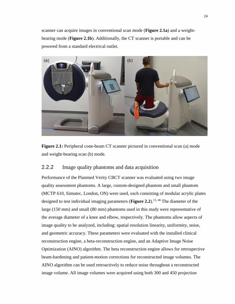
24

scanner can acquire images in conventional scan mode (Figure 2.1a) and a weight-

bearing mode (Figure 2.1b). Additionally, the CT scanner is portable and can be

powered from a standard electrical outlet.

Figure 2.1: Peripheral cone-beam CT scanner pictured in conventional scan (a) mode

and weight-bearing scan (b) mode.

2.2.2 Image quality phantoms and data acquisition

Performance of the Planmed Verity CBCT scanner was evaluated using two image

quality assessment phantoms. A large, custom-designed phantom and small phantom

(MCTP 610, Simutec, London, ON) were used, each consisting of modular acrylic plates

designed to test individual imaging parameters (Figure 2.2).15, 46 The diameter of the

large (150 mm) and small (80 mm) phantoms used in this study were representative of

the average diameter of a knee and elbow, respectively. The phantoms allow aspects of

image quality to be analyzed, including: spatial resolution linearity, uniformity, noise,

and geometric accuracy. These parameters were evaluated with the installed clinical

reconstruction engine, a beta-reconstruction engine, and an Adaptive Image Noise

Optimization (AINO) algorithm. The beta reconstruction engine allows for retrospective

beam-hardening and patient-motion corrections for reconstructed image volumes. The

AINO algorithm can be used retroactively to reduce noise throughout a reconstructed

image volume. All image volumes were acquired using both 300 and 450 projection

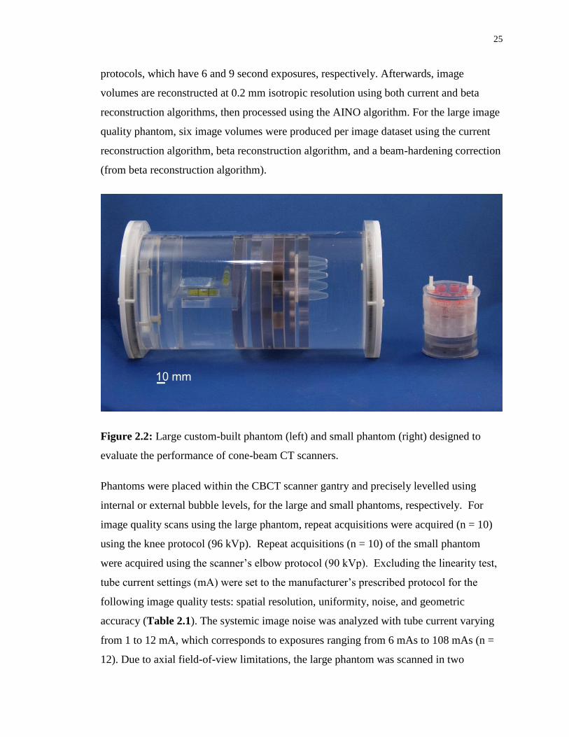
25

protocols, which have 6 and 9 second exposures, respectively. Afterwards, image

volumes are reconstructed at 0.2 mm isotropic resolution using both current and beta

reconstruction algorithms, then processed using the AINO algorithm. For the large image

quality phantom, six image volumes were produced per image dataset using the current

reconstruction algorithm, beta reconstruction algorithm, and a beam-hardening correction

(from beta reconstruction algorithm).

Figure 2.2: Large custom-built phantom (left) and small phantom (right) designed to

evaluate the performance of cone-beam CT scanners.

Phantoms were placed within the CBCT scanner gantry and precisely levelled using

internal or external bubble levels, for the large and small phantoms, respectively. For

image quality scans using the large phantom, repeat acquisitions were acquired (n = 10)

using the knee protocol (96 kVp). Repeat acquisitions (n = 10) of the small phantom

were acquired using the scanner’s elbow protocol (90 kVp). Excluding the linearity test,

tube current settings (mA) were set to the manufacturer’s prescribed protocol for the

following image quality tests: spatial resolution, uniformity, noise, and geometric

accuracy (Table 2.1). The systemic image noise was analyzed with tube current varying

from 1 to 12 mA, which corresponds to exposures ranging from 6 mAs to 108 mAs (n =

12). Due to axial field-of-view limitations, the large phantom was scanned in two

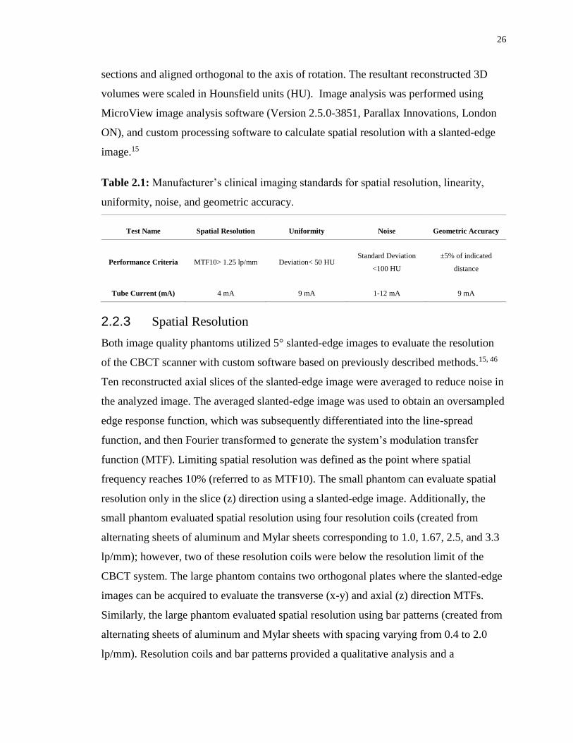
26

sections and aligned orthogonal to the axis of rotation. The resultant reconstructed 3D

volumes were scaled in Hounsfield units (HU). Image analysis was performed using

MicroView image analysis software (Version 2.5.0-3851, Parallax Innovations, London

ON), and custom processing software to calculate spatial resolution with a slanted-edge

image.15

Table 2.1: Manufacturer’s clinical imaging standards for spatial resolution, linearity,

uniformity, noise, and geometric accuracy.

Test Name Spatial Resolution Uniformity Noise Geometric Accuracy

Performance Criteria MTF10> 1.25 lp/mm Deviation< 50 HU Standard Deviation

<100 HU

±5% of indicated

distance

Tube Current (mA) 4 mA 9 mA 1-12 mA 9 mA

2.2.3 Spatial Resolution

Both image quality phantoms utilized 5° slanted-edge images to evaluate the resolution

of the CBCT scanner with custom software based on previously described methods.15, 46

Ten reconstructed axial slices of the slanted-edge image were averaged to reduce noise in

the analyzed image. The averaged slanted-edge image was used to obtain an oversampled

edge response function, which was subsequently differentiated into the line-spread

function, and then Fourier transformed to generate the system’s modulation transfer

function (MTF). Limiting spatial resolution was defined as the point where spatial

frequency reaches 10% (referred to as MTF10). The small phantom can evaluate spatial

resolution only in the slice (z) direction using a slanted-edge image. Additionally, the

small phantom evaluated spatial resolution using four resolution coils (created from

alternating sheets of aluminum and Mylar sheets corresponding to 1.0, 1.67, 2.5, and 3.3

lp/mm); however, two of these resolution coils were below the resolution limit of the

CBCT system. The large phantom contains two orthogonal plates where the slanted-edge

images can be acquired to evaluate the transverse (x-y) and axial (z) direction MTFs.

Similarly, the large phantom evaluated spatial resolution using bar patterns (created from

alternating sheets of aluminum and Mylar sheets with spacing varying from 0.4 to 2.0

lp/mm). Resolution coils and bar patterns provided a qualitative analysis and a

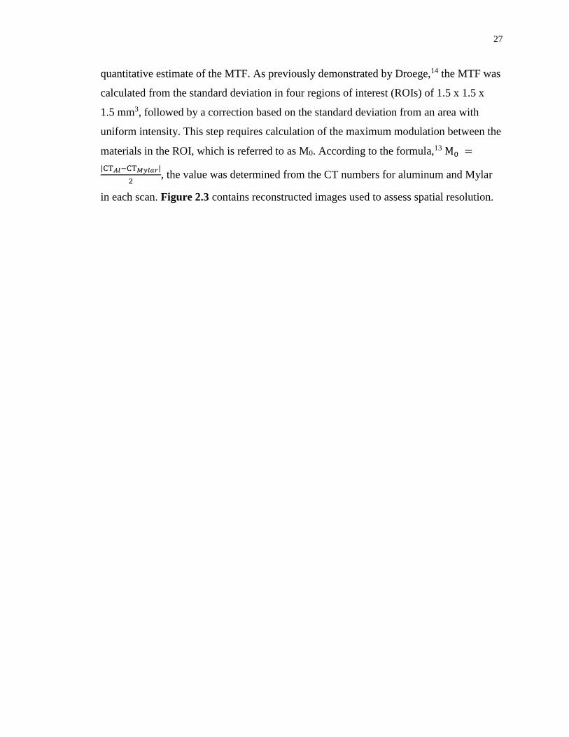
27

quantitative estimate of the MTF. As previously demonstrated by Droege,14 the MTF was

calculated from the standard deviation in four regions of interest (ROIs) of 1.5 x 1.5 x

1.5 mm3, followed by a correction based on the standard deviation from an area with

uniform intensity. This step requires calculation of the maximum modulation between the

materials in the ROI, which is referred to as M0. According to the formula,13 M0 =

|CT𝐴𝑙−CT𝑀𝑦𝑙𝑎𝑟|

2, the value was determined from the CT numbers for aluminum and Mylar

in each scan. Figure 2.3 contains reconstructed images used to assess spatial resolution.

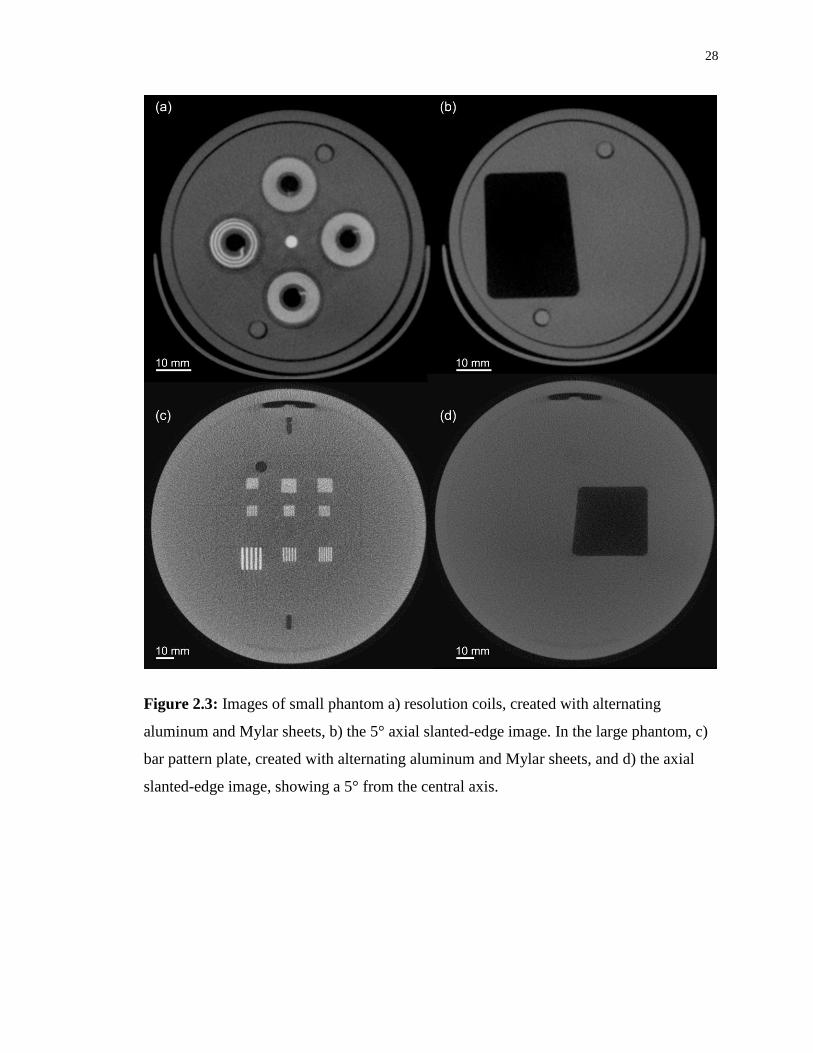
28

Figure 2.3: Images of small phantom a) resolution coils, created with alternating

aluminum and Mylar sheets, b) the 5° axial slanted-edge image. In the large phantom, c)

bar pattern plate, created with alternating aluminum and Mylar sheets, and d) the axial

slanted-edge image, showing a 5° from the central axis.

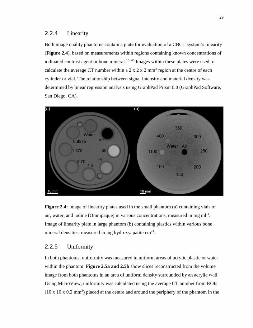
29

2.2.4 Linearity

Both image quality phantoms contain a plate for evaluation of a CBCT system’s linearity

(Figure 2.4), based on measurements within regions containing known concentrations of

iodinated contrast agent or bone mineral.15, 46 Images within these plates were used to

calculate the average CT number within a 2 x 2 x 2 mm3 region at the centre of each

cylinder or vial. The relationship between signal intensity and material density was

determined by linear regression analysis using GraphPad Prism 6.0 (GraphPad Software,

San Diego, CA).

Figure 2.4: Image of linearity plates used in the small phantom (a) containing vials of

air, water, and iodine (Omnipaque) in various concentrations, measured in mg ml-1.

Image of linearity plate in large phantom (b) containing plastics within various bone

mineral densities, measured in mg hydroxyapatite cm-3.

2.2.5 Uniformity

In both phantoms, uniformity was measured in uniform areas of acrylic plastic or water

within the phantom. Figure 2.5a and 2.5b show slices reconstructed from the volume

image from both phantoms in an area of uniform density surrounded by an acrylic wall.

Using MicroView, uniformity was calculated using the average CT number from ROIs

(10 x 10 x 0.2 mm3) placed at the centre and around the periphery of the phantom in the

30

image. The average CT number in peripheral ROIs was subtracted from central ROIs to

quantify the system’s uniformity. A line profile was also plotted across the central slice to

analyze variation of CT numbers across the field-of-view (FOV).

2.2.6 Noise

Image noise was reported as the standard deviation at the centre of the image inside a

uniform ROI (10 x 10 x 0.2 mm3). Large (96 kVp) and small (90 kVp) phantoms were

analyzed over 15 mm with ROIs spaced 1 mm between each measurement (n = 15),

shown as the red ROI in Figures 2.5c and 2.5d. The relationship between image noise

and exposure was determined by obtaining images of each phantom, as described in

Section B. The total measured noise (σtotal) can be considered as a quadrature summation

of photon noise (σphoton) and system noise (σsystem).19, 30 Consequently, the average noise

measured as a function of photon flux can be fitted with non-linear regression to the

equation, σ2𝑡𝑜𝑡𝑎𝑙 = 𝐴 × 𝐸−1 + σ2

𝑠𝑦𝑠𝑡𝑒𝑚, where σtotal is measured noise in HU, E is

exposure in mAs, and A and σ2system are constant terms. The constant term A is a scaling

factor between variance and photon flux, which is unique to each CT scanner. Non-linear

fitting was performed using the Levenberg-Marquardt algorithm (GraphPad Prism 6.0).

31

Figure 2.5: Slices through an area of uniform density in the small (a) and large (b)

phantoms, show the location of the line profile used to characterize system uniformity.

ROIs located within the small (c) and large (d) phantoms used to assess uniformity (red

& yellow) and noise (red only).

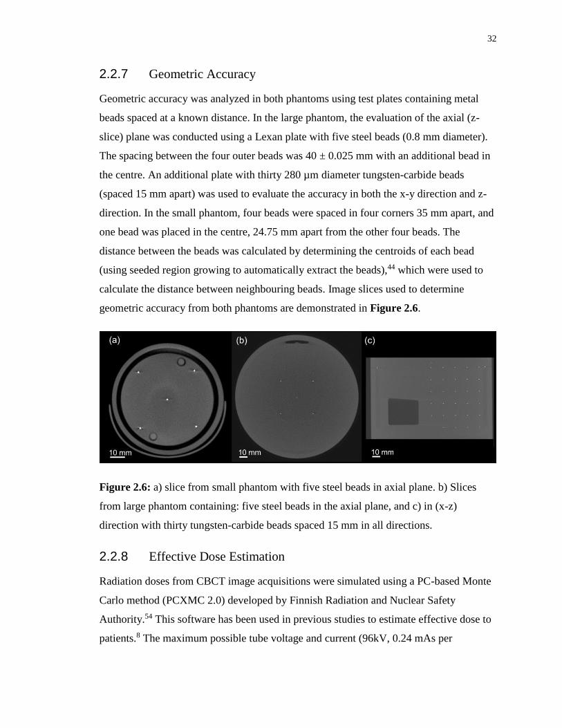
32

2.2.7 Geometric Accuracy

Geometric accuracy was analyzed in both phantoms using test plates containing metal

beads spaced at a known distance. In the large phantom, the evaluation of the axial (z-

slice) plane was conducted using a Lexan plate with five steel beads (0.8 mm diameter).

The spacing between the four outer beads was 40 ± 0.025 mm with an additional bead in

the centre. An additional plate with thirty 280 µm diameter tungsten-carbide beads

(spaced 15 mm apart) was used to evaluate the accuracy in both the x-y direction and z-

direction. In the small phantom, four beads were spaced in four corners 35 mm apart, and

one bead was placed in the centre, 24.75 mm apart from the other four beads. The

distance between the beads was calculated by determining the centroids of each bead

(using seeded region growing to automatically extract the beads),44 which were used to

calculate the distance between neighbouring beads. Image slices used to determine

geometric accuracy from both phantoms are demonstrated in Figure 2.6.

Figure 2.6: a) slice from small phantom with five steel beads in axial plane. b) Slices

from large phantom containing: five steel beads in the axial plane, and c) in (x-z)

direction with thirty tungsten-carbide beads spaced 15 mm in all directions.

2.2.8 Effective Dose Estimation

Radiation doses from CBCT image acquisitions were simulated using a PC-based Monte

Carlo method (PCXMC 2.0) developed by Finnish Radiation and Nuclear Safety

Authority.54 This software has been used in previous studies to estimate effective dose to

patients.8 The maximum possible tube voltage and current (96kV, 0.24 mAs per

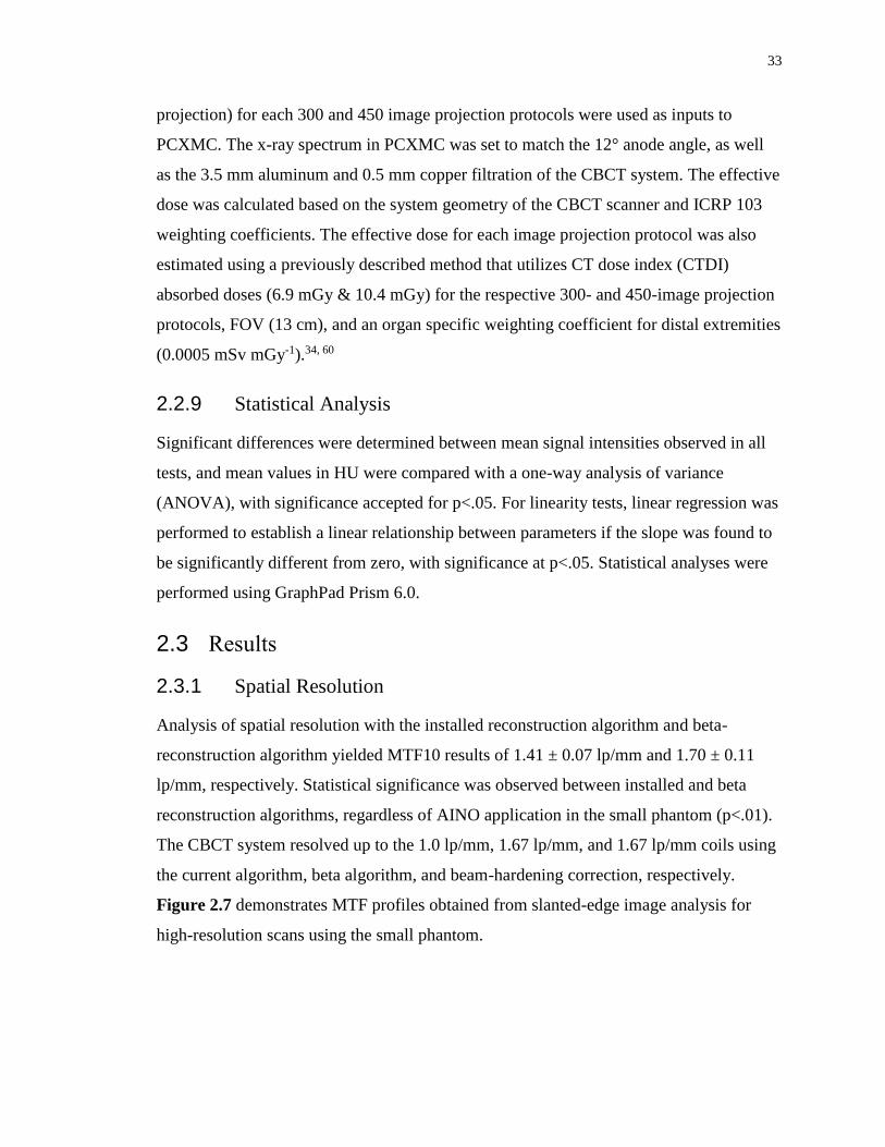
33

projection) for each 300 and 450 image projection protocols were used as inputs to

PCXMC. The x-ray spectrum in PCXMC was set to match the 12° anode angle, as well

as the 3.5 mm aluminum and 0.5 mm copper filtration of the CBCT system. The effective

dose was calculated based on the system geometry of the CBCT scanner and ICRP 103

weighting coefficients. The effective dose for each image projection protocol was also

estimated using a previously described method that utilizes CT dose index (CTDI)

absorbed doses (6.9 mGy & 10.4 mGy) for the respective 300- and 450-image projection

protocols, FOV (13 cm), and an organ specific weighting coefficient for distal extremities

(0.0005 mSv mGy-1).34, 60

2.2.9 Statistical Analysis

Significant differences were determined between mean signal intensities observed in all

tests, and mean values in HU were compared with a one-way analysis of variance

(ANOVA), with significance accepted for p<.05. For linearity tests, linear regression was

performed to establish a linear relationship between parameters if the slope was found to

be significantly different from zero, with significance at p<.05. Statistical analyses were

performed using GraphPad Prism 6.0.

2.3 Results


Analysis of spatial resolution with the installed reconstruction algorithm and beta-

reconstruction algorithm yielded MTF10 results of 1.41 ± 0.07 lp/mm and 1.70 ± 0.11

lp/mm, respectively. Statistical significance was observed between installed and beta

reconstruction algorithms, regardless of AINO application in the small phantom (p<.01).

The CBCT system resolved up to the 1.0 lp/mm, 1.67 lp/mm, and 1.67 lp/mm coils using

the current algorithm, beta algorithm, and beam-hardening correction, respectively.

Figure 2.7 demonstrates MTF profiles obtained from slanted-edge image analysis for

high-resolution scans using the small phantom.

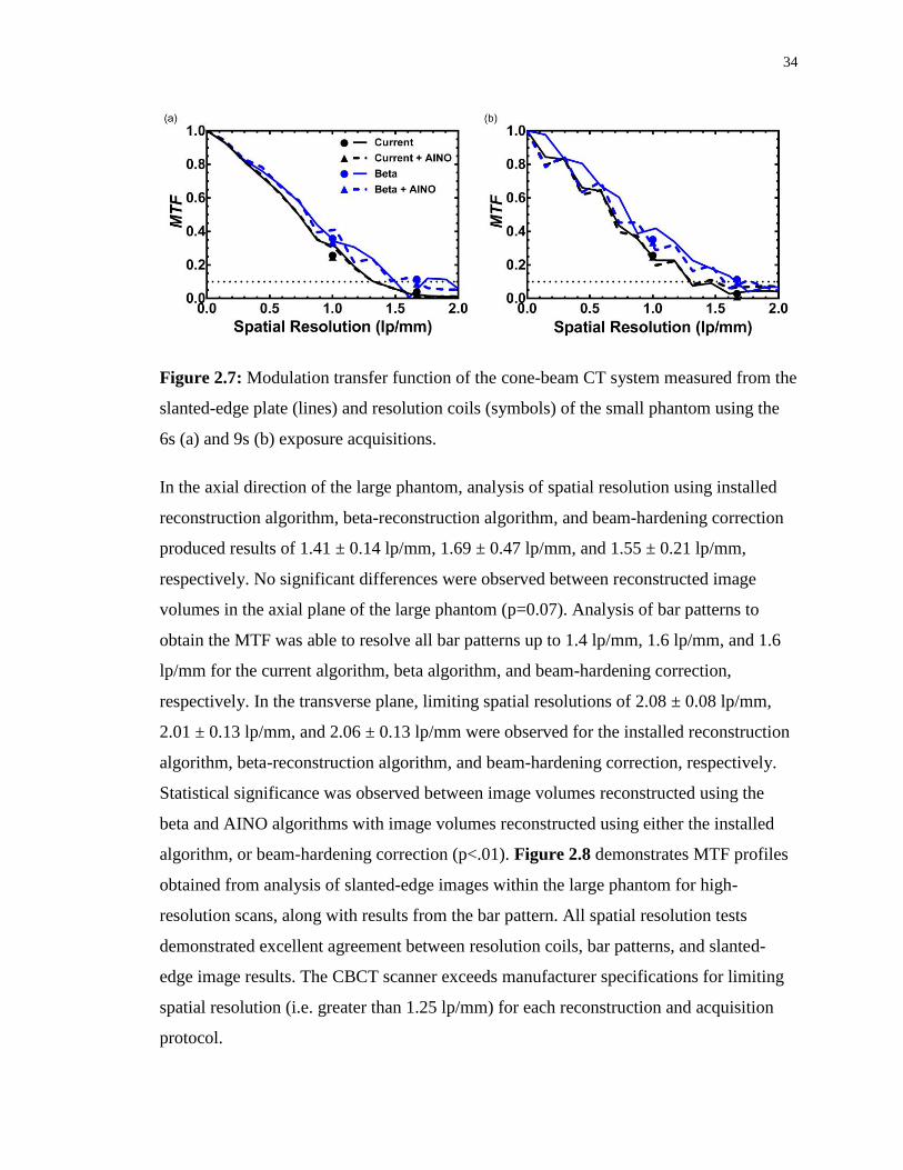
34


slanted-edge plate (lines) and resolution coils (symbols) of the small phantom using the

6s (a) and 9s (b) exposure acquisitions.

In the axial direction of the large phantom, analysis of spatial resolution using installed

reconstruction algorithm, beta-reconstruction algorithm, and beam-hardening correction

produced results of 1.41 ± 0.14 lp/mm, 1.69 ± 0.47 lp/mm, and 1.55 ± 0.21 lp/mm,

respectively. No significant differences were observed between reconstructed image

volumes in the axial plane of the large phantom (p=0.07). Analysis of bar patterns to

obtain the MTF was able to resolve all bar patterns up to 1.4 lp/mm, 1.6 lp/mm, and 1.6

lp/mm for the current algorithm, beta algorithm, and beam-hardening correction,

respectively. In the transverse plane, limiting spatial resolutions of 2.08 ± 0.08 lp/mm,

2.01 ± 0.13 lp/mm, and 2.06 ± 0.13 lp/mm were observed for the installed reconstruction

algorithm, beta-reconstruction algorithm, and beam-hardening correction, respectively.

Statistical significance was observed between image volumes reconstructed using the

beta and AINO algorithms with image volumes reconstructed using either the installed

algorithm, or beam-hardening correction (p<.01). Figure 2.8 demonstrates MTF profiles

obtained from analysis of slanted-edge images within the large phantom for high-

resolution scans, along with results from the bar pattern. All spatial resolution tests

demonstrated excellent agreement between resolution coils, bar patterns, and slanted-

edge image results. The CBCT scanner exceeds manufacturer specifications for limiting

spatial resolution (i.e. greater than 1.25 lp/mm) for each reconstruction and acquisition

protocol.

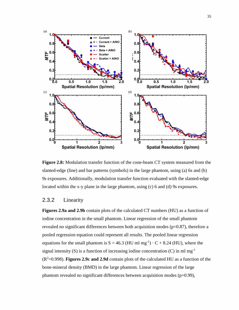
35


slanted-edge (line) and bar patterns (symbols) in the large phantom, using (a) 6s and (b)

9s exposures. Additionally, modulation transfer function evaluated with the slanted-edge

located within the x-y plane in the large phantom, using (c) 6 and (d) 9s exposures.

2.3.2 Linearity

Figures 2.9a and 2.9b contain plots of the calculated CT numbers (HU) as a function of

iodine concentration in the small phantom. Linear regression of the small phantom

revealed no significant differences between both acquisition modes (p=0.87), therefore a

pooled regression equation could represent all results. The pooled linear regression

equations for the small phantom is S = 46.3 (HU ml mg-1) · C + 8.24 (HU), where the

signal intensity (S) is a function of increasing iodine concentration (C) in ml mg-1

(R2=0.998). Figures 2.9c and 2.9d contain plots of the calculated HU as a function of the

bone-mineral density (BMD) in the large phantom. Linear regression of the large

phantom revealed no significant differences between acquisition modes (p=0.99),

36

therefore a pooled regression equation (Intensity = BMD · 1.26 HU / mg cm-3 + 74.86

HU) could determine the expected CT number from the regression line (R2=0.998).

Figures 2.9e and 2.9f show the impact of the beam-hardening correction on the system’s

linearity in the large phantom. Linear regression of the beam-hardening corrected image

revealed no significant differences between length of scan (p=0.85), therefore the pooled

regression equation (Intensity = BMD · 1.11 HU / mg cm-3 + 53.42 HU) could calculate

the expected CT number from the regression line (R2=0.992). The system demonstrates a

high degree of linearity (p < .01) with all algorithms tested in response to signal

intensities that will be encountered in clinical musculoskeletal imaging.

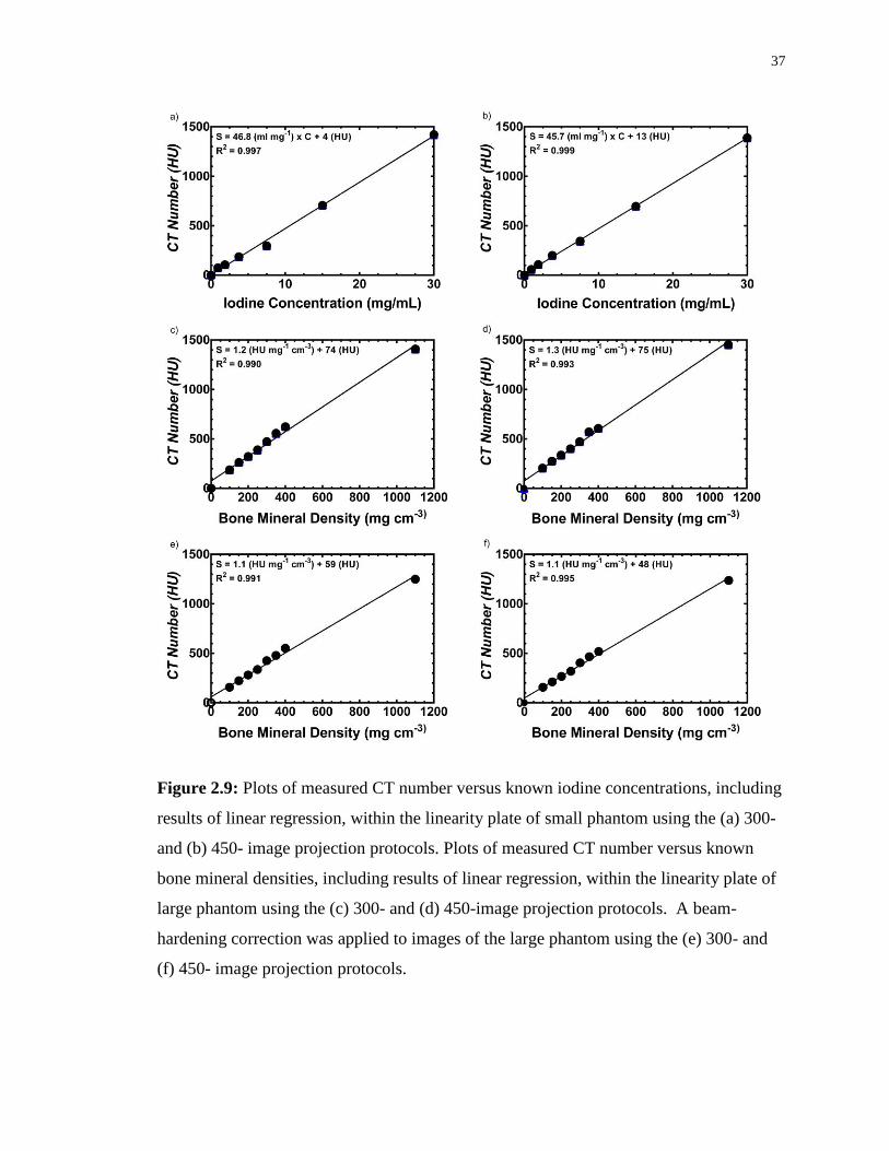
37

Figure 2.9: Plots of measured CT number versus known iodine concentrations, including

results of linear regression, within the linearity plate of small phantom using the (a) 300-

and (b) 450- image projection protocols. Plots of measured CT number versus known

bone mineral densities, including results of linear regression, within the linearity plate of

large phantom using the (c) 300- and (d) 450-image projection protocols. A beam-

hardening correction was applied to images of the large phantom using the (e) 300- and

(f) 450- image projection protocols.

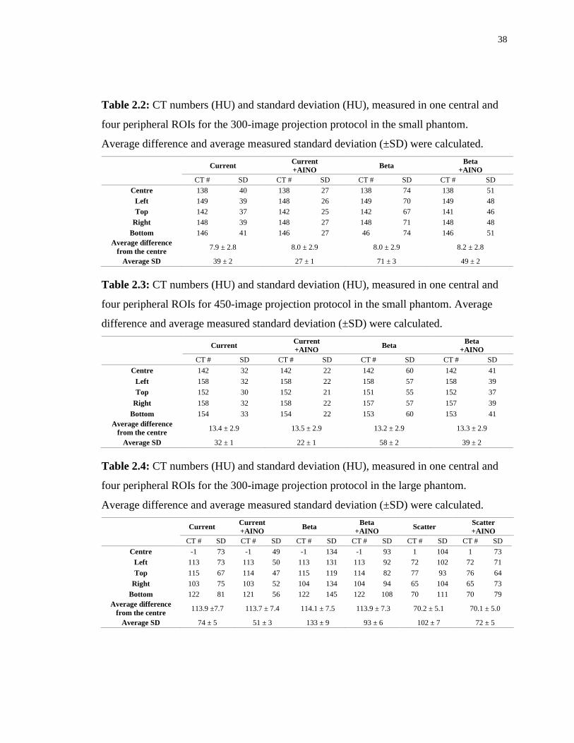
38

Table 2.2: CT numbers (HU) and standard deviation (HU), measured in one central and

four peripheral ROIs for the 300-image projection protocol in the small phantom.

Average difference and average measured standard deviation (±SD) were calculated.

Current

Current

+AINO Beta

Beta

+AINO

CT # SD CT # SD CT # SD CT # SD

Centre 138 40 138 27 138 74 138 51

Left 149 39 148 26 149 70 149 48

Top 142 37 142 25 142 67 141 46

Right 148 39 148 27 148 71 148 48

Bottom 146 41 146 27 46 74 146 51

Average difference

from the centre 7.9 ± 2.8 8.0 ± 2.9 8.0 ± 2.9 8.2 ± 2.8

Average SD 39 ± 2 27 ± 1 71 ± 3 49 ± 2


four peripheral ROIs for 450-image projection protocol in the small phantom. Average

difference and average measured standard deviation (±SD) were calculated.

Current

Current

+AINO Beta

Beta

+AINO

CT # SD CT # SD CT # SD CT # SD

Centre 142 32 142 22 142 60 142 41

Left 158 32 158 22 158 57 158 39

Top 152 30 152 21 151 55 152 37

Right 158 32 158 22 157 57 157 39

Bottom 154 33 154 22 153 60 153 41

Average difference

from the centre 13.4 ± 2.9 13.5 ± 2.9 13.2 ± 2.9 13.3 ± 2.9

Average SD 32 ± 1 22 ± 1 58 ± 2 39 ± 2


four peripheral ROIs for the 300-image projection protocol in the large phantom.


Current

Current

+AINO Beta

Beta

+AINO Scatter

Scatter

+AINO

CT # SD CT # SD CT # SD CT # SD CT # SD CT # SD

Centre -1 73 -1 49 -1 134 -1 93 1 104 1 73

Left 113 73 113 50 113 131 113 92 72 102 72 71

Top 115 67 114 47 115 119 114 82 77 93 76 64

Right 103 75 103 52 104 134 104 94 65 104 65 73

Bottom 122 81 121 56 122 145 122 108 70 111 70 79

Average difference

from the centre 113.9 ±7.7 113.7 ± 7.4 114.1 ± 7.5 113.9 ± 7.3 70.2 ± 5.1 70.1 ± 5.0

Average SD 74 ± 5 51 ± 3 133 ± 9 93 ± 6 102 ± 7 72 ± 5

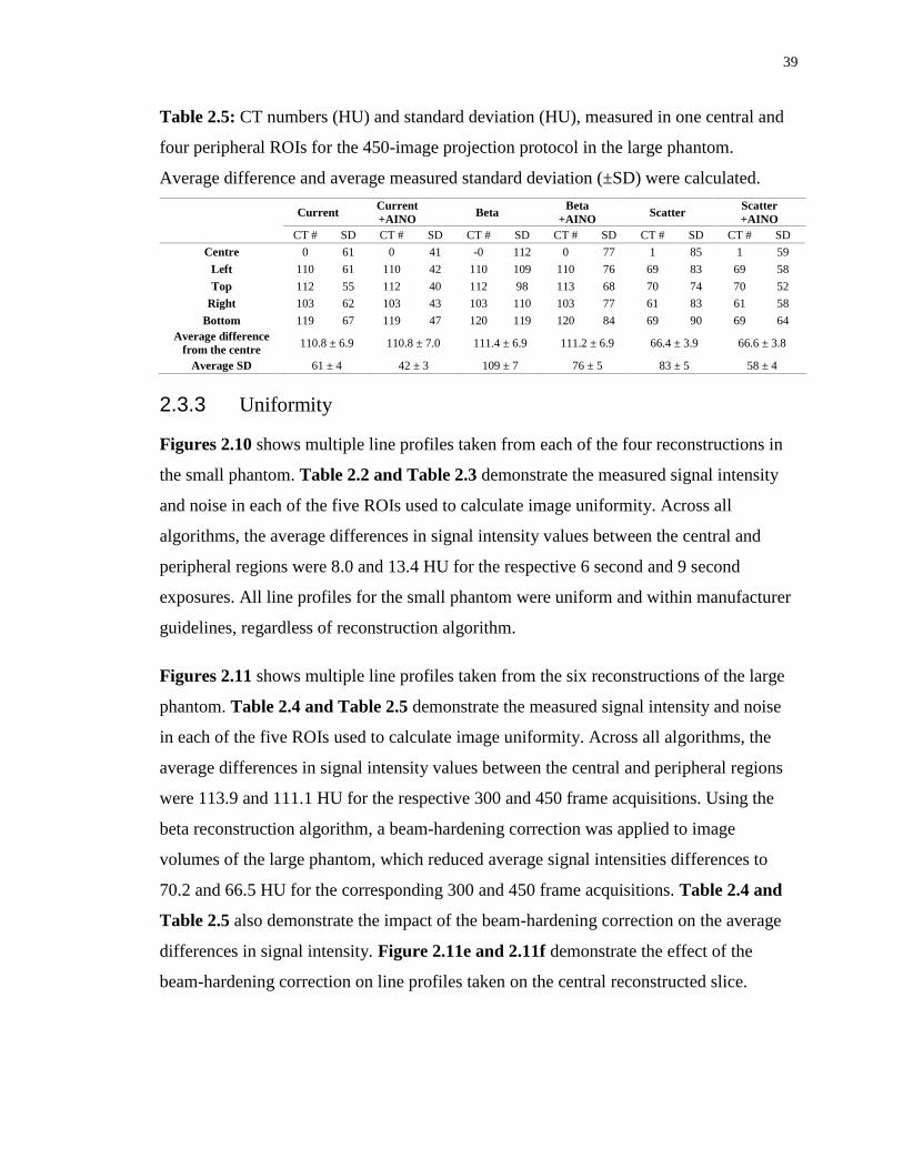
39


four peripheral ROIs for the 450-image projection protocol in the large phantom.


Current

Current

+AINO Beta

Beta

+AINO Scatter

Scatter

+AINO

CT # SD CT # SD CT # SD CT # SD CT # SD CT # SD

Centre 0 61 0 41 -0 112 0 77 1 85 1 59

Left 110 61 110 42 110 109 110 76 69 83 69 58

Top 112 55 112 40 112 98 113 68 70 74 70 52

Right 103 62 103 43 103 110 103 77 61 83 61 58

Bottom 119 67 119 47 120 119 120 84 69 90 69 64

Average difference

from the centre 110.8 ± 6.9 110.8 ± 7.0 111.4 ± 6.9 111.2 ± 6.9 66.4 ± 3.9 66.6 ± 3.8

Average SD 61 ± 4 42 ± 3 109 ± 7 76 ± 5 83 ± 5 58 ± 4

2.3.3 Uniformity

Figures 2.10 shows multiple line profiles taken from each of the four reconstructions in

the small phantom. Table 2.2 and Table 2.3 demonstrate the measured signal intensity

and noise in each of the five ROIs used to calculate image uniformity. Across all

algorithms, the average differences in signal intensity values between the central and

peripheral regions were 8.0 and 13.4 HU for the respective 6 second and 9 second

exposures. All line profiles for the small phantom were uniform and within manufacturer

guidelines, regardless of reconstruction algorithm.

Figures 2.11 shows multiple line profiles taken from the six reconstructions of the large

phantom. Table 2.4 and Table 2.5 demonstrate the measured signal intensity and noise

in each of the five ROIs used to calculate image uniformity. Across all algorithms, the

average differences in signal intensity values between the central and peripheral regions

were 113.9 and 111.1 HU for the respective 300 and 450 frame acquisitions. Using the

beta reconstruction algorithm, a beam-hardening correction was applied to image

volumes of the large phantom, which reduced average signal intensities differences to

70.2 and 66.5 HU for the corresponding 300 and 450 frame acquisitions. Table 2.4 and

Table 2.5 also demonstrate the impact of the beam-hardening correction on the average

differences in signal intensity. Figure 2.11e and 2.11f demonstrate the effect of the

beam-hardening correction on line profiles taken on the central reconstructed slice.

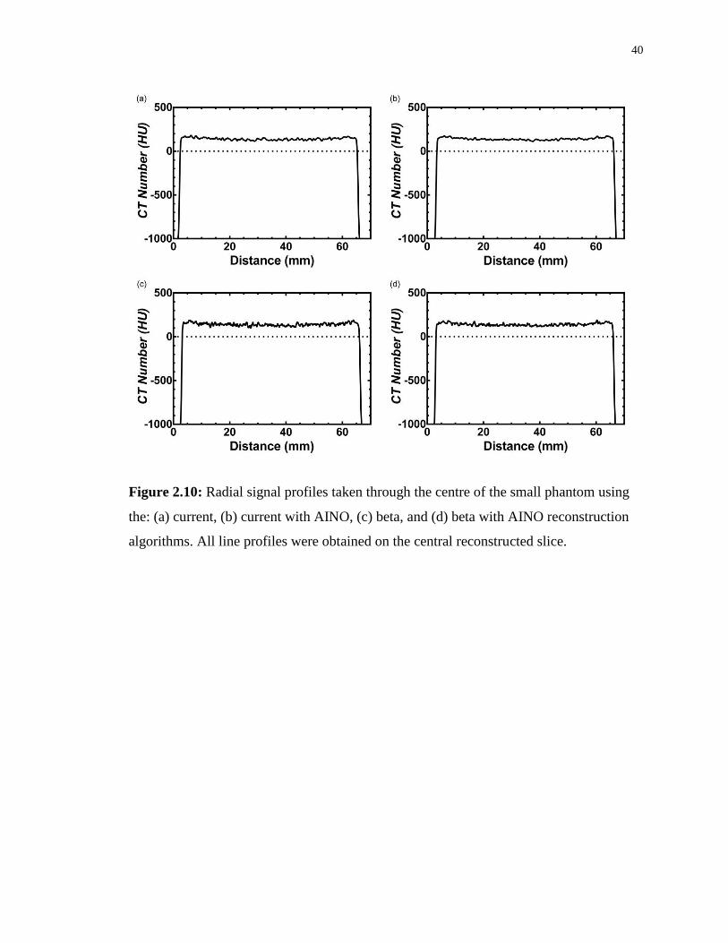
40

Figure 2.10: Radial signal profiles taken through the centre of the small phantom using

the: (a) current, (b) current with AINO, (c) beta, and (d) beta with AINO reconstruction

algorithms. All line profiles were obtained on the central reconstructed slice.

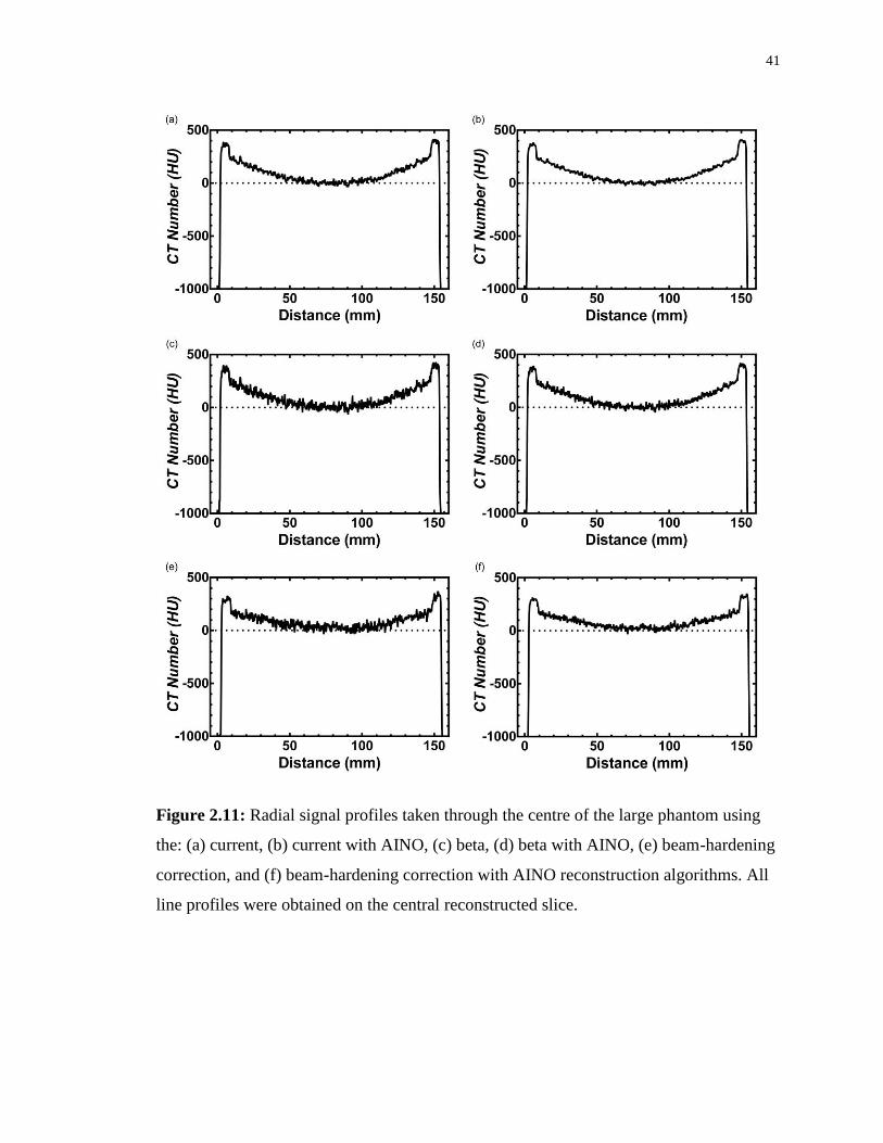
41

Figure 2.11: Radial signal profiles taken through the centre of the large phantom using

the: (a) current, (b) current with AINO, (c) beta, (d) beta with AINO, (e) beam-hardening

correction, and (f) beam-hardening correction with AINO reconstruction algorithms. All

line profiles were obtained on the central reconstructed slice.

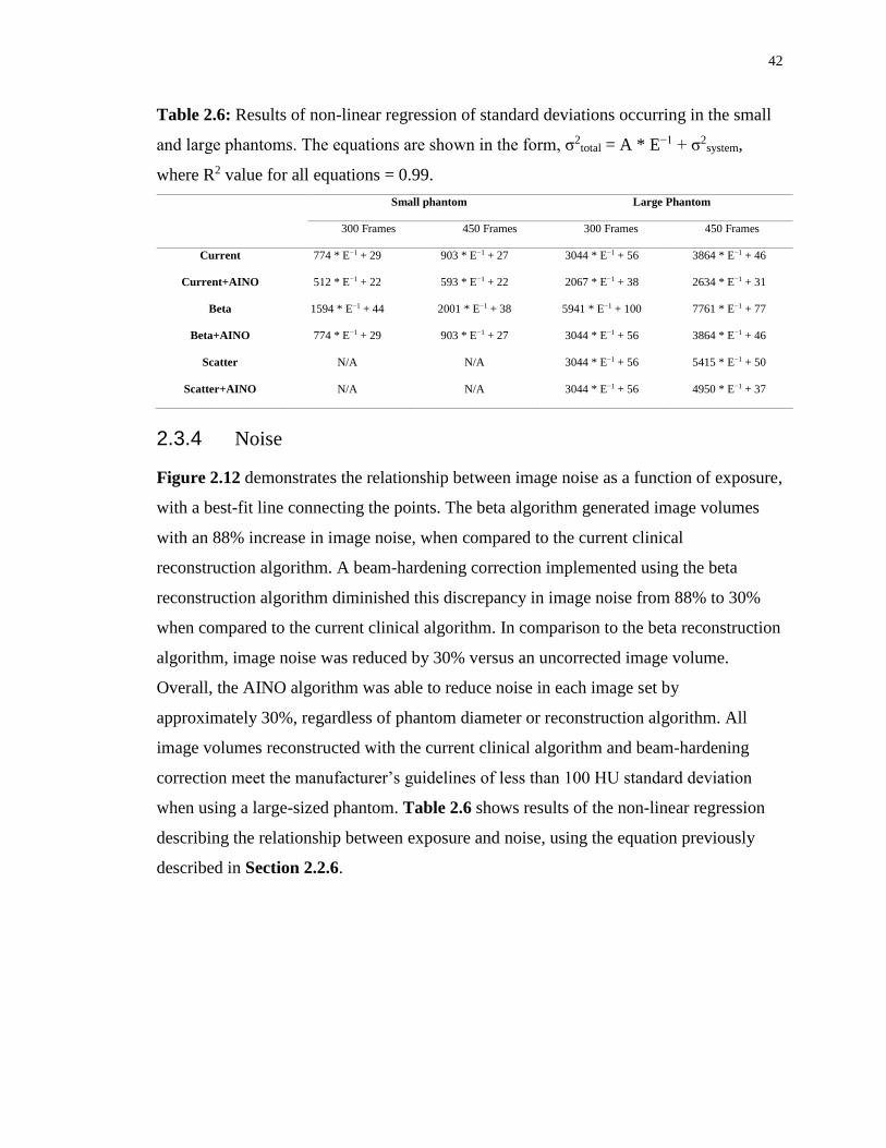
42

Table 2.6: Results of non-linear regression of standard deviations occurring in the small

and large phantoms. The equations are shown in the form, σ2total = A * E−1 + σ2

system,

where R2 value for all equations = 0.99.

Small phantom Large Phantom

300 Frames 450 Frames 300 Frames 450 Frames

Current 774 * E−1 + 29 903 * E−1 + 27 3044 * E−1 + 56 3864 * E−1 + 46

Current+AINO 512 * E−1 + 22 593 * E−1 + 22 2067 * E−1 + 38 2634 * E−1 + 31

Beta 1594 * E−1 + 44 2001 * E−1 + 38 5941 * E−1 + 100 7761 * E−1 + 77

Beta+AINO 774 * E−1 + 29 903 * E−1 + 27 3044 * E−1 + 56 3864 * E−1 + 46

Scatter N/A N/A 3044 * E−1 + 56 5415 * E−1 + 50

Scatter+AINO N/A N/A 3044 * E−1 + 56 4950 * E−1 + 37

2.3.4 Noise

Figure 2.12 demonstrates the relationship between image noise as a function of exposure,

with a best-fit line connecting the points. The beta algorithm generated image volumes

with an 88% increase in image noise, when compared to the current clinical

reconstruction algorithm. A beam-hardening correction implemented using the beta

reconstruction algorithm diminished this discrepancy in image noise from 88% to 30%

when compared to the current clinical algorithm. In comparison to the beta reconstruction

algorithm, image noise was reduced by 30% versus an uncorrected image volume.

Overall, the AINO algorithm was able to reduce noise in each image set by

approximately 30%, regardless of phantom diameter or reconstruction algorithm. All

image volumes reconstructed with the current clinical algorithm and beam-hardening

correction meet the manufacturer’s guidelines of less than 100 HU standard deviation

when using a large-sized phantom. Table 2.6 shows results of the non-linear regression

describing the relationship between exposure and noise, using the equation previously

described in Section 2.2.6.

43

Figure 2.12: Measured noise in the small phantom using the 300 frame (a) and 450 frame

(b) protocols, expressed as average standard deviation of the signal intensity (HU),

plotted as a function of increasing exposure. Tube voltage used for the small phantom

was 90 kVp, with tube current varying from 1 to 12 mA, using 6s (a) or 9s (b) exposure

time. Similarly, measured noise in the large phantom using the 300 frame (c) and 450

frame (d) protocols, expressed as average standard deviation of the signal intensity (HU),

plotted as a function of increasing exposure. Tube voltage used for the large phantom was

96 kVp, with tube current varying from 1 to 12 mA, using 6s (c) or 9s (d) exposure time.


Average distance between centroids of the four steel beads, in the small phantom, was

calculated to be 35.01 ± 0.07 mm compared to the nominal 35 mm spacing (p=0.28). In

the large phantom, the average distance between centroids of the four steel beads, spaced

40 mm apart, was calculated to be 39.98 ± 0.16 mm for the axial geometry (p=0.55). In

the transverse plane, the average distance between the centroids of the tungsten-carbide

beads was found to be 15.01 ± 0.06 mm in the (x-y) plane and 15.07 ± 0.16 mm in the z-

44

direction (slice direction), compared to the nominal 15 mm spacing. No statistical

significance was observed between all algorithms in the transverse plane (p=0.07). All

results pass the manufacturer specifications and demonstrate excellent in-plane and out-

of-plane geometric accuracy, regardless of exposure time, reconstruction algorithm, or

diameter of the image quality phantom.


Using PCXMC, the effective dose was calculated to be 14 µSv, and 21 µSv, for the

respective 300, and 450 image projection acquisitions. Alternatively, the effective dose

was calculated to be 45 µSv, and 68 µSv, for the respective 300-, and 450- image

projection acquisitions when using the CTDI absorbed dose, FOV, and an organ specific

weighting coefficient for distal extremities. The latter method was expected to produce a

higher effective dose estimate, since the organ-specific weighting coefficients were

derived from conventional CT.

2.4 Discussion

The Planmed Verity cone-beam CT scanner demonstrates excellent performance,

consistent with manufacturer guidelines, while acquiring image volumes at a low-dose.

Image quality phantoms in this study resembled the average-sized elbow and an average-

sized knee. Therefore, the system’s performance was evaluated with objects that mimic

the anatomy encountered in future clinical musculoskeletal imaging studies, in terms of

spatial resolution, noise, uniformity, linearity, geometric accuracy, and effective dose.

Overall, the scanner passed all image quality tests according to the manufacturer’s

guidelines, apart from the uniformity test using the large-sized phantom. This

demonstrates the need for additional beam-hardening correction when scanning structures

with larger diameters.

Over the range of densities analyzed, the scanner demonstrated a highly linear response,

regardless of phantom size or reconstruction algorithm used. The signal-level calibration

of the CBCT system was excellent, with water and peripheral air returning values of 0.48

and -1120 HU in the small phantom, and 0.49 and -975 HU in the large phantom. Upon

further investigation with the large phantom, air inside the linearity plate returned a value

45

of -642 HU. Previous researchers observed similar effects with earlier CT scanners; they

attributed increases or decreases in CT number to scanner-dependent beam-hardening

corrections, which are crucial to the magnitude and direction of environmental density

artefacts.24, 55 A similar decrease in signal intensity was observed in the analysis of a

uniform water phantom with CBCT imaging.51 The beam-hardening correction was

applied to large-phantom image volumes that resulted in CT numbers for water,

peripheral air, and internal air, returning intensity values of 0.46 HU, -1000 HU, and -815

HU, respectively. The observed value of -815 was approximately 20% greater than

expected; however, these results are comparable to previous studies demonstrating

inaccuracies in HU signal intensity values for internal air cavities.22 Although there was a

discrepancy between internal and peripheral air intensity values, the scanner maintains a

linear response to materials of increasing linear attenuation coefficients, regardless of

reconstruction algorithm.

Uniformity and noise measurements are dependent on the size of the object; therefore, the

use of small- and large-sized phantoms was necessary to cover possible anatomies that

may be encountered in future studies. Signal uniformity was preserved within 50 HU

with the small-sized phantom; however, image volumes of the large-sized phantom did

not sustain signal uniformity within 50 HU, which was attributed to beam-hardening and

scatter. The average difference in signal uniformity was not impacted by the AINO

algorithm for either phantom used in this study. A cupping effect was detected on the line

profile intensity plot for the large phantom, which significantly contributes to lower

homogeneity of the image.42 Similar results were observed with the analysis of a uniform

water phantom with flat-panel CBCT images.51 Typically, CBCT images have larger

occurrence and magnitude of physics-based artefacts, when compared to conventional

CT.5, 58, 59 Within the beta algorithm, a beam-hardening correction can be applied to

reduce signal intensity differences from 114 HU to 70 HU in the 6s exposure, and from

111 HU to 66 HU in the 9s exposure. Although these measurements do not meet

manufacturer requirements, the beam-hardening correction was able to improve image

uniformity by approximately 40%. The currently installed reconstruction algorithm

produced image noise measurements within manufacturer guidelines, regardless of AINO

algorithm implementation, diameter of phantom, or number of frames obtained. The beta

46

reconstruction algorithm passed manufacturer guidelines with the small-sized phantom;

however, the scanner required the AINO algorithm or a beam-hardening correction to

pass manufacturer standards with respect to the large-sized phantom. We have

demonstrated the effects of photon flux on noise at 96 kVp and 90 kVp with clinical scan

exposure settings. Figure 2.12 shows that exposures between 30-50 mAs would optimize

image quality and dose; exposures above 9 mA may not significantly improve the image

quality, in terms of noise. Conventional CT demonstrates less noise and better soft tissue

contrast when compared to CBCT.11, 37 The decrease of soft-tissue contrast resolution in

CBCT is caused in part by scattered radiation, which increases noise and decreases the

contrast-to-noise ratio.1, 2, 50 Overall, previous studies have demonstrated CBCT images

provide diagnostic information not apparent on radiographs and this information is

obtained at a lower radiation dose than conventional CT.17, 31 The AINO algorithm allows

for lower tube current during exposure, reducing image noise by approximately 30% in

all cases, allowing for lower effective doses while maintaining optimal image quality.

Spatial resolution was evaluated quantitatively and qualitatively in both phantoms

through slanted-edge images, or a bar pattern. Using slanted-edge images in the axial

plane, overall limiting spatial resolution (MTF10) with the installed and beta

reconstruction algorithms was 1.42 lp/mm and 1.68 lp/mm, respectively. This result is

consistent with bar pattern analysis, which indicated objects at 1.4 and 1.6 lp/mm could

be resolved for the respective current and beta algorithms. The calculation of the MTF

using the bar pattern is immune to noise and is not influenced by the orientation of the

image.13 In addition, analysis with bar patterns uses simpler tools to obtain the MTF,

when compared to the conventional slanted-edge image analysis. In the transverse plane,

the overall limiting spatial resolution using the current and beta reconstruction algorithms

was 2.00 lp/mm and 1.97 lp/mm, respectively. Discrepancies between axial and

transverse planes were due to excessive noise in the edge response function, which

influences the derivation of the edge response function to the line spread function when

calculating MTF.45, 53 Furthermore, spatial resolution has a directional dependency in the

transverse plane, which may impact measurements when an object is located in the

periphery, such as the slanted-edge in the transverse plane.45 Throughout the study, no

statistical significance was observed between AINO reconstructed images and the

47

original reconstruction, which suggests the AINO algorithm does not degrade spatial

resolution. Significant differences were shown between the current and beta

reconstruction algorithms, regardless of the image phantom diameter or application of

AINO algorithm (p<.01). Regardless, the spatial resolution passed manufacturer

standards using qualitative and quantitative analyses. Regarding geometric accuracy,

there were no statistically significant discrepancies, indicating excellent geometric

accuracy in all imaging planes with the peripheral CBCT scanner. Geometric accuracy is

essential for accurate patient-to-image registration using either anatomical landmarks or

fiducial markers.21 These results were comparable to studies analyzing spatial resolution

and geometric accuracy of various CBCT scanners.4, 16, 32 We have demonstrated the beta

reconstruction improves spatial resolution and uniformity, while maintaining linearity

and geometric accuracy, at the cost of increased image noise. The beam-hardening

correction was able to retrospectively enhance image uniformity and reduce image noise,

without affecting linearity, geometric accuracy, and spatial resolution.

The effective dose for the Planmed Verity was calculated to be 14 µSv, and 21 µSv for

the respective 300-, and 450-image projection acquisitions using PCXMC. These results

were comparable to measurements obtained in previous studies that reported an effective

dose of 13 µSv.34, 36 The effective dose estimation based on CTDI absorbed dose, FOV,

and organ specific weighting coefficient for distal extremities, resulted in calculations of

45 µSv, and 68 µSv for the 300 and 450 image projections, respectively. For a CBCT

system, it may not be appropriate to characterize dose with the conventional CTDI

approach, since reconstructed image volumes are reconstructed using multiple

independent 2D projections, rather than contiguous thin slices.18 Previous studies have

demonstrated effective dose calculations that use dose-length product with an organ-

specific weighting coefficient are inaccurate.7, 9 Although there is a discrepancy between

the two effective dose estimation methods, the results are comparable to approximately

two chest x-rays, where the effective dose may vary from 7 – 50 µSv per view.41 Overall,

the effective dose associated with this scanner for all imaging acquisitions was minimal

compared to 2.2 mSv, the average annual effective dose resulting from background

radiation in Canada.10 The stochastic effects of ionizing radiation arising from diagnostic

imaging has been associated with a cancer risk coefficient of 5.5 x 10-2 Sv-1, thereby a

48

scan with an effective dose of 68 µSv has a 3.74 x 10-6 % increase to the stochastic

effects of radiation.57

2.5 Conclusion

To the best of our knowledge, we have performed the first quantitative performance

evaluation with multiple reconstruction algorithms for the Planmed Verity cone-beam

extremity CT scanner, using phantoms that mimic the size of an average knee or elbow.

The system exceeds the manufacturer’s guidelines in terms of resolution, noise,

uniformity, geometric accuracy, and linearity at a smaller diameter, representative of the

upper extremity anatomy. Except for the uniformity test, the system surpassed

manufacturer specifications for resolution, noise, and geometric accuracy with the larger

phantom, which simulated the lower extremity. This result was expected since objects

with larger diameters create longer ray paths for the x-ray photons. This results in an

increased attenuation of the x-ray beam, as well as a decreased photon flux at the

detector. The peripheral CBCT imaging system demonstrates potential for studies of

musculoskeletal treatments and their effects on joint biomechanics since it provides

volumetric upper extremity data as well as weight-bearing 3D volumetric data about the

lower extremity, while providing optimal image quality at a low dose.

2.6 References

1. Akbarzadeh, A., Ay, M. R., Ghadiri, H., Sarkar, S., & Zaidi, H. (2010).

Measurement of scattered radiation in a volumetric 64-slice CT scanner using

three experimental techniques. Phys Med Biol, 55(8), 2269-2280.

2. Alsufyani, N. A., Noga, M. L., Finlay, W. H., & Major, P. W. (2013). Topical

contrast agents to improve soft-tissue contrast in the upper airway using cone

beam CT: a pilot study. Dentomaxillofac Radiol, 42(7), 20130022.

3. Aurell, Y., Andersson, M., & Forslind, K. (2018). Cone-beam computed

tomography, a new low-dose three-dimensional imaging technique for assessment

of bone erosions in rheumatoid arthritis: reliability assessment and comparison

with conventional radiography - a BARFOT study. Scand J Rheumatol, 47(3),

173-177.

4. Ballrick, J. W., Palomo, J. M., Ruch, E., Amberman, B. D., & Hans, M. G.

(2008). Image distortion and spatial resolution of a commercially available cone-

49

beam computed tomography machine. Am J Orthod Dentofacial Orthop, 134(4),

573-582.

5. Barrett, J. F., & Keat, N. (2004). Artifacts in CT: recognition and avoidance.

Radiographics, 24(6), 1679-1691.

6. Biswas, D., Bible, J. E., Bohan, M., Simpson, A. K., Whang, P. G., & Grauer, J.

N. (2009). Radiation exposure from musculoskeletal computerized tomographic

scans. J Bone Joint Surg Am, 91(8), 1882-1889.

7. Brady, S. L., Mirro, A. E., Moore, B. M., & Kaufman, R. A. (2015). How to

Appropriately Calculate Effective Dose for CT Using Either Size-Specific Dose

Estimates or Dose-Length Product. AJR Am J Roentgenol, 204(5), 953-958.

8. Choi, J. H., Maier, A., Keil, A., Pal, S., McWalter, E. J., Beaupre, G. S., . . .

Fahrig, R. (2014). Fiducial marker-based correction for involuntary motion in

weight-bearing C-arm CT scanning of knees. II. Experiment. Med Phys, 41(6),

061902.

9. Christner, J. A., Kofler, J. M., & McCollough, C. H. (2010). Estimating effective

dose for CT using dose-length product compared with using organ doses:

consequences of adopting International Commission on Radiological Protection

publication 103 or dual-energy scanning. AJR Am J Roentgenol, 194(4), 881-889.

10. Commission, C. N. S. (2014). Natural Background Radiation in Canada.

11. De Cock, J., Mermuys, K., Goubau, J., Van Petegem, S., Houthoofd, B., &

Casselman, J. W. (2012). Cone-beam computed tomography: a new low dose,

high resolution imaging technique of the wrist, presentation of three cases with

technique. Skeletal Radiol, 41(1), 93-96.

12. Dirschl, D. R., & Dawson, P. A. (2004). Injury severity assessment in tibial

plateau fractures. Clin Orthop Relat Res, 423(423), 85-92.

13. Droege, R. T., & Morin, R. L. (1982). A practical method to measure the MTF of

CT scanners. Med Phys, 9(5), 758-760.

14. Droege, R. T., & Rzeszotarski, M. S. (1985). An MTF method immune to

aliasing. Med Phys, 12(6), 721-725.

15. Du, L. Y., Umoh, J., Nikolov, H. N., Pollmann, S. I., Lee, T. Y., & Holdsworth,

D. W. (2007). A quality assurance phantom for the performance evaluation of

volumetric micro-CT systems. Phys Med Biol, 52(23), 7087-7108.

16. Eggers, G., Klein, J., Welzel, T., & Muhling, J. (2008). Geometric accuracy of

digital volume tomography and conventional computed tomography. Br J Oral

Maxillofac Surg, 46(8), 639-644.

50

17. Faccioli, N., Foti, G., Barillari, M., Atzei, A., & Mucelli, R. P. (2010). Finger

fractures imaging: accuracy of cone-beam computed tomography and multislice

computed tomography. Skeletal Radiol, 39(11), 1087-1095.

18. Fahrig, R., Dixon, R., Payne, T., Morin, R. L., Ganguly, A., & Strobel, N. (2006).

Dose and image quality for a cone-beam C-arm CT system. Med Phys, 33(12),

4541-4550.

19. Faulkner, K., & Moores, B. M. (1984). Noise and contrast detection in computed

tomography images. Phys Med Biol, 29(4), 329-339.



29(2), 199-204.

21. Fitzpatrick, J. M., West, J. B., & Maurer, C. R., Jr. (1998). Predicting error in

rigid-body point-based registration. IEEE Trans Med Imaging, 17(5), 694-702.

22. Ford, N. L., Martin, E. L., Lewis, J. F., Veldhuizen, R. A., Drangova, M., &

Holdsworth, D. W. (2007). In vivo characterization of lung morphology and

function in anesthetized free-breathing mice using micro-computed tomography. J

Appl Physiol (1985), 102(5), 2046-2055.

23. Geijer, M., Borjesson, A. M., & Gothlin, J. H. (2011). Clinical utility of

tomosynthesis in suspected scaphoid fracture. A pilot study. Skeletal Radiol,

40(7), 863-867.

24. Goodsitt, M. M., Chan, H. P., Way, T. W., Larson, S. C., Christodoulou, E. G., &

Kim, J. (2006). Accuracy of the CT numbers of simulated lung nodules imaged

with multi-detector CT scanners. Med Phys, 33(8), 3006-3017.

25. Guermazi, A., Roemer, F. W., Felson, D. T., & Brandt, K. D. (2013). Motion for

debate: osteoarthritis clinical trials have not identified efficacious therapies

because traditional imaging outcome measures are inadequate. Arthritis Rheum,

65(11), 2748-2758.

26. Gupta, R., Cheung, A. C., Bartling, S. H., Lisauskas, J., Grasruck, M., Leidecker,

C., . . . Brady, T. J. (2008). Flat-panel volume CT: fundamental principles,

technology, and applications. Radiographics, 28(7), 2009-2022.

27. Hirschmann, A., Buck, F. M., Fucentese, S. F., & Pfirrmann, C. W. (2015).

Upright CT of the knee: the effect of weight-bearing on joint alignment. Eur

Radiol, 25(11), 3398-3404.

28. Hirschmann, A., Buck, F. M., Herschel, R., Pfirrmann, C. W. A., & Fucentese, S.

F. (2017). Upright weight-bearing CT of the knee during flexion: changes of the

patellofemoral and tibiofemoral articulations between 0 degrees and 120 degrees.

Knee Surg Sports Traumatol Arthrosc, 25(3), 853-862.

51

29. Hirschmann, A., Pfirrmann, C. W., Klammer, G., Espinosa, N., & Buck, F. M.

(2014). Upright cone CT of the hindfoot: comparison of the non-weight-bearing

with the upright weight-bearing position. Eur Radiol, 24(3), 553-558.

30. Holdsworth, D. W., Drangova, M., & Fenster, A. (1993). A high-resolution XRII-

based quantitative volume CT scanner. Med Phys, 20(2 Pt 1), 449-462.

31. Huang, A. J., Chang, C. Y., Thomas, B. J., MacMahon, P. J., & Palmer, W. E.

(2015). Using cone-beam CT as a low-dose 3D imaging technique for the

extremities: initial experience in 50 subjects. Skeletal Radiol, 44(6), 797-809.

32. Kobayashi, K., Shimoda, S., Nakagawa, Y., & Yamamoto, A. (2004). Accuracy

in measurement of distance using limited cone-beam computerized tomography.

Int J Oral Max Impl, 19(2), 228-231.







35. Koivisto, J., Wolff, J., Jarnstedt, J., Dastidar, P., & Kortesniemi, M. (2014).

Assessment of the effective dose in supine, prone, and oblique positions in the

maxillofacial region using a novel combined extremity and maxillofacial cone

beam computed tomography scanner. Oral Surg Oral Med Oral Pathol Oral

Radiol, 118(3), 355-362.

36. Kokkonen, H. T., Suomalainen, J. S., Joukainen, A., Kroger, H., Sirola, J.,

Jurvelin, J. S., . . . Toyras, J. (2014). In vivo diagnostics of human knee cartilage

lesions using delayed CBCT arthrography. Journal of orthopaedic research :


37. Koskinen, S. K., Haapamaki, V. V., Salo, J., Lindfors, N. C., Kortesniemi, M.,

Seppala, L., & Mattila, K. T. (2013). CT arthrography of the wrist using a novel,

mobile, dedicated extremity cone-beam CT (CBCT). Skeletal Radiol, 42(5), 649-

657.

38. Makarova, D. V., & Kushnyr, K. V. (2015). A Standardized Protocol for Cone-

Beam Computed Tomography of the Hand and Wrist in Rheumatoid Arthritis.

Sovremennye Tehnologii V Medicine, 7(4), 135-139.





52

40. Mermuys, K., Vanslambrouck, K., Goubau, J., Steyaert, L., & Casselman, J. W.

(2008). Use of digital tomosynthesis: case report of a suspected scaphoid fracture

and technique. Skeletal Radiol, 37(6), 569-572.

41. Mettler, F. A., Jr., Huda, W., Yoshizumi, T. T., & Mahesh, M. (2008). Effective

doses in radiology and diagnostic nuclear medicine: a catalog. Radiology, 248(1),

254-263.

42. Neubauer, J., Voigt, J. M., Lang, H., Scheuer, C., Goerke, S. M., Langer, M., . . .

Kotter, E. (2014). Comparing the image quality of a mobile flat-panel computed

tomography and a multidetector computed tomography: a phantom study. Invest

Radiol, 49(7), 491-497.

43. Nicholson, J. A., Sutherland, A. G., & Smith, F. W. (2011). Single bundle anterior

cruciate reconstruction does not restore normal knee kinematics at six months: an

upright MRI study. J Bone Joint Surg Br, 93(10), 1334-1340.

44. Otsu, N. (1979). A Threshold Selection Method from Gray-Level Histograms. 5.

45. Ozaki, Y., Watanabe, H., Nomura, Y., Honda, E., Sumi, Y., & Kurabayashi, T.

(2013). Location dependency of the spatial resolution of cone beam computed

tomography for dental use. Oral Surg Oral Med Oral Pathol Oral Radiol, 116(5),

648-655.

46. Petrov, I. E., Nikolov, H. N., Holdsworth, D. W., & Drangova, M. (2011,

2011/03/03/). Image performance evaluation of a 3D surgical imaging platform.

Paper presented at the SPIE Medical Imaging.

47. Ramdhian-Wihlm, R., Le Minor, J. M., Schmittbuhl, M., Jeantroux, J., Mahon, P.

M., Veillon, F., . . . Bierry, G. (2012). Cone-beam computed tomography

arthrography: an innovative modality for the evaluation of wrist ligament and

cartilage injuries. Skeletal Radiol, 41(8), 963-969.

48. Richter, M., Seidl, B., Zech, S., & Hahn, S. (2014). PedCAT for 3D-imaging in

standing position allows for more accurate bone position (angle) measurement

than radiographs or CT. Foot Ankle Surg, 20(3), 201-207.

49. Schulze, D., Heiland, M., Thurmann, H., & Adam, G. (2004). Radiation exposure

during midfacial imaging using 4- and 16-slice computed tomography, cone beam

computed tomography systems and conventional radiography. Dentomaxillofac

Radiol, 33(2), 83-86.

50. Schulze, R., Heil, U., Gross, D., Bruellmann, D. D., Dranischnikow, E.,

Schwanecke, U., & Schoemer, E. (2011). Artefacts in CBCT: a review.

Dentomaxillofac Radiol, 40(5), 265-273.

53

51. Siewerdsen, J. H., & Jaffray, D. A. (2001). Cone-beam computed tomography

with a flat-panel imager: magnitude and effects of x-ray scatter. Med Phys, 28(2),

220-231.

52. Stehling, C., Souza, R. B., Hellio Le Graverand, M. P., Wyman, B. T., Li, X.,

Majumdar, S., & Link, T. M. (2012). Loading of the knee during 3.0T MRI is

associated with significantly increased medial meniscus extrusion in mild and

moderate osteoarthritis. Eur J Radiol, 81(8), 1839-1845.

53. Takenaga, T., Katsuragawa, S., Goto, M., Hatemura, M., Uchiyama, Y., &

Shiraishi, J. (2015). Modulation transfer function measurement of CT images by

use of a circular edge method with a logistic curve-fitting technique. Radiol Phys

Technol, 8(1), 53-59.

54. Tapiovaara, M., & Siiskonen, T. (2008). A PC-based Monte Carlo program for

calculating patient doses in medical x-ray examinations (2nd Ed.). 31.

55. Tarver, R. D., Holden, R. W., & Ellis, J. H. (1983). Experimental lung nodule

model: CT numbers, nodule size, and actual calcium content. J Comput Assist

Tomogr, 7(3), 402-406.



148.

57. Valentin, J. (2007). The 2007 Recommendations of the International Commission

on Radiological Protection. ICRP publication 103. Ann ICRP, 37(2-4), 1-332.

58. Yu, L., Vrieze, T. J., Bruesewitz, M. R., Kofler, J. M., DeLone, D. R., Pallanch, J.

F., . . . McCollough, C. H. (2010). Dose and image quality evaluation of a

dedicated cone-beam CT system for high-contrast neurologic applications. AJR

Am J Roentgenol, 194(2), W193-201.

59. Zain-Alabdeen, E. H., & Alsadhan, R. I. (2012). A comparative study of accuracy

of detection of surface osseous changes in the temporomandibular joint using

multidetector CT and cone beam CT. Dentomaxillofac Radiol, 41(3), 185-191.





54

Chapter 3

3 Three-dimensional cone-beam CT reconstruction in a natural

weight-bearing stance using ceiling-mounted x-ray

fluoroscopy

3.1 Introduction

Weight-bearing three-dimensional (3D) images (or cross-sectional slices) for

investigation of various musculoskeletal diseases have become a recent focus in the

medical imaging community. Previous research has demonstrated significant differences

between non-weight-bearing and weight-bearing conditions.9, 38 In the current clinical

setting, weight-bearing radiographs are used to evaluate joint biomechanics of the knee,

ankle, and foot.2, 23 Although radiographs are used extensively in clinical practice, they

are two-dimensional (2D) representations of a three-dimensional (3D) object, which

limits their accuracy when detecting complex fractures, patellofemoral abnormalities, or

post-operative measurements of total knee arthroplasty (TKA) component positioning.8,

20, 50 Recent studies have used clinical computed tomography (CT) or magnetic resonance

imaging (MRI) scanners to simulate weight-bearing conditions, but do not allow for

standing weight-bearing imaging in a clinical setting, or may overestimate patellofemoral

anomalies for surgical realignment surgery.15, 32, 44 Furthermore, these studies do not

represent the physiological stresses of the joints in a normal weight-bearing situation, and

the setup is impractical for routine clinical exams.

Recent advances in cone-beam computed tomography (CBCT) technology have

developed dedicated flat-panel cone-beam CT scanners for musculoskeletal imaging that

enable weight-bearing imaging of a single-leg in an upright position.3, 31, 32, 53 Despite the

commercial availability of dedicated diagnostic CBCT scanners (such as the Planmed

Verity, described in Chapter 2), many hospitals have difficulty accommodating additional

medical imaging equipment due to cost, space, and workflow constraints. A cone-beam

computed tomography (CBCT) system created from an existing ceiling-mounted x-ray

fluoroscopy system with a digital flat-panel detector has excellent potential to be used for

evaluations of static 3D joint positions and orientations of both lower extremities under

55

natural weight-bearing conditions. A ceiling-mounted CBCT system with adjustable

trajectories during image acquisition has the potential to provide excellent initial

evaluation of bony anatomical relationships and 3D visualization of bone and joint

morphology within the hip, knee, ankle, foot, and spine. The ceiling-mounted system can

rotate parallel to the floor, enabling multiple weight-bearing positions for bilateral

evaluations of joints in the lower extremity, while producing higher resolution images –

at a lower patient dose – when compared to conventional CT.25, 26, 34, 42 The lower

radiation dose is a result of the CBCT scanner design, which allows for an increased

distance of the x-ray source from the torso, since less scattered radiation can interact with

radiosensitive organs within the torso.48

Gantry rotation for ceiling-mounted systems are subject to geometric imperfections,

where the motion of the x-ray source and detector may deviate significantly from a

perfect circular trajectory. The geometric imperfections include gravity-induced

mechanical flex, bearing irregularities, or vibration that may impact the motion in the

centre of rotation during radiographic image acquisition.7, 13 Failure to adequately correct

for imperfections will result in mis-registration, loss of detail, and image artefacts.22

Previous authors have utilized image-based calibration objects to characterize gantry

motion, either concurrently or prospectively.4, 13, 52 In these studies, image data was

analyzed to generate a full 3D transformation matrix, which includes intrinsic, rotation,

and translation matrices. Image-based corrections were established using previously

described methods that applied angle-dependent shift corrections that resolve

imperfections in two directions.13 For the image-based correction, there are three

underlying assumptions to be made: (1) deviations from a perfect trajectory are small, (2)

long-term reproducibility of gantry motion during rotation is acceptable, and (3)

imperfections during gantry rotation are either parallel to the axis of rotation, or

tangential to the circle of rotation and perpendicular to the line joining the x-ray source

and the detector.13 The latter described motion (3) will only produce insignificant

changes to magnification; therefore, it will be ignored, as have other investigators in the

past.6, 13 These assumptions allow perspective geometric calibration to generate a set of

angle-dependent image shifts, which can be applied either prior to image reconstruction,

or during backprojection using cone-beam backprojection reconstruction algorithms.13

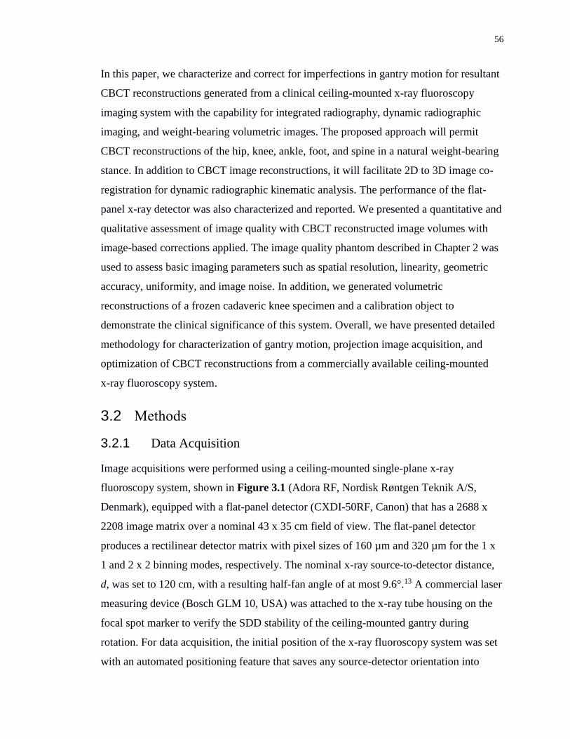
56

In this paper, we characterize and correct for imperfections in gantry motion for resultant

CBCT reconstructions generated from a clinical ceiling-mounted x-ray fluoroscopy

imaging system with the capability for integrated radiography, dynamic radiographic

imaging, and weight-bearing volumetric images. The proposed approach will permit

CBCT reconstructions of the hip, knee, ankle, foot, and spine in a natural weight-bearing

stance. In addition to CBCT image reconstructions, it will facilitate 2D to 3D image co-

registration for dynamic radiographic kinematic analysis. The performance of the flat-

panel x-ray detector was also characterized and reported. We presented a quantitative and

qualitative assessment of image quality with CBCT reconstructed image volumes with

image-based corrections applied. The image quality phantom described in Chapter 2 was

used to assess basic imaging parameters such as spatial resolution, linearity, geometric

accuracy, uniformity, and image noise. In addition, we generated volumetric

reconstructions of a frozen cadaveric knee specimen and a calibration object to

demonstrate the clinical significance of this system. Overall, we have presented detailed

methodology for characterization of gantry motion, projection image acquisition, and

optimization of CBCT reconstructions from a commercially available ceiling-mounted

x-ray fluoroscopy system.

3.2 Methods

3.2.1 Data Acquisition

Image acquisitions were performed using a ceiling-mounted single-plane x-ray

fluoroscopy system, shown in Figure 3.1 (Adora RF, Nordisk Røntgen Teknik A/S,

Denmark), equipped with a flat-panel detector (CXDI-50RF, Canon) that has a 2688 x

2208 image matrix over a nominal 43 x 35 cm field of view. The flat-panel detector

produces a rectilinear detector matrix with pixel sizes of 160 µm and 320 µm for the 1 x

1 and 2 x 2 binning modes, respectively. The nominal x-ray source-to-detector distance,

d, was set to 120 cm, with a resulting half-fan angle of at most 9.6°.13 A commercial laser

measuring device (Bosch GLM 10, USA) was attached to the x-ray tube housing on the

focal spot marker to verify the SDD stability of the ceiling-mounted gantry during

rotation. For data acquisition, the initial position of the x-ray fluoroscopy system was set

with an automated positioning feature that saves any source-detector orientation into

file:///D:/Western/Manuscripts/ThesisChapters/Edit_MGT/ORBIS_01+mgt.docx%23_ENREF_5

57

memory. Reproducibility of the automated positioning feature was determined with

geometric projection matrices to have a 400 µm standard deviation. Therefore, image-

based geometric calibrations were acquired prior to image projection data acquisitions.

Images were acquired using the cine-radiographic mode at 15 frames/s during gantry

rotation, with speeds up to 14° per second. Consequently, images can be obtained in ~1º

intervals around the object over the full angular range of 540°. During rotation of the

ceiling-mounted gantry, a total of 576 projections can be acquired in approximately 40s.

Each x-ray exposure triggers a custom-designed x-ray detector that encodes the angular

position of the gantry based on values from a potentiometer located in the gantry’s

rotation motor. All images were corrected for pixel-to-pixel sensitivity variation before

reconstruction, through the application of a bright-field image. Projection images of the

image quality phantom were acquired at approximately 0.681° per projection using 120

kVp tube voltage, 100-200 mA tube current, and 1 ms exposure time, resulting in 0.1-0.2

mAs per exposure (31 mAs- 62 mAs, n = 300). The frozen cadaveric specimen,

containing fifty-four, 0.8mm diameter zirconium dioxide beads (n = 54) implanted into

the cruciate and collateral ligaments, was scanned in an upright position at approximately

0.933° per projection using 85 kVp tube voltage, 250 mA tube current, and 1 ms

exposure time, resulting in 0.25 mAs per exposure (100 mAs, n = 400). All projection

images were acquired using the 2 x 2 binning mode, resulting in a 1344 x 1104 matrix

with 320 µm pixel size.

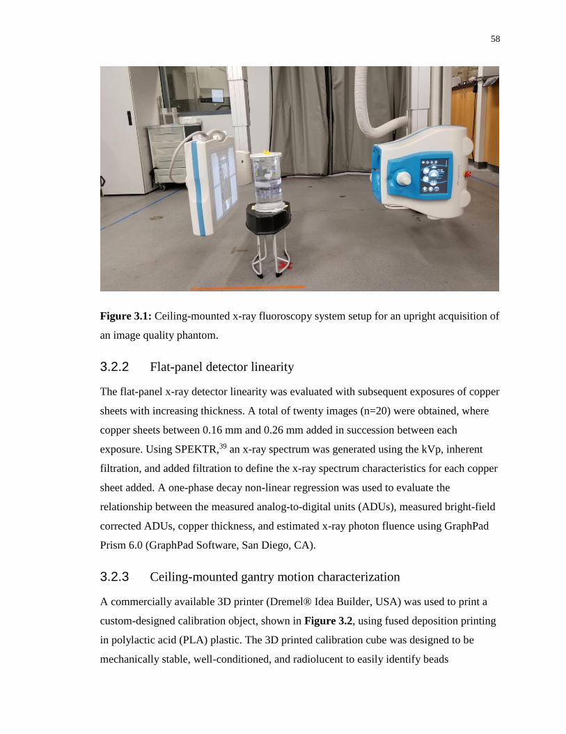
58

Figure 3.1: Ceiling-mounted x-ray fluoroscopy system setup for an upright acquisition of

an image quality phantom.

3.2.2 Flat-panel detector linearity

The flat-panel x-ray detector linearity was evaluated with subsequent exposures of copper

sheets with increasing thickness. A total of twenty images (n=20) were obtained, where

copper sheets between 0.16 mm and 0.26 mm added in succession between each

exposure. Using SPEKTR,39 an x-ray spectrum was generated using the kVp, inherent

filtration, and added filtration to define the x-ray spectrum characteristics for each copper

sheet added. A one-phase decay non-linear regression was used to evaluate the

relationship between the measured analog-to-digital units (ADUs), measured bright-field

corrected ADUs, copper thickness, and estimated x-ray photon fluence using GraphPad

Prism 6.0 (GraphPad Software, San Diego, CA).

3.2.3 Ceiling-mounted gantry motion characterization

A commercially available 3D printer (Dremel® Idea Builder, USA) was used to print a

custom-designed calibration object, shown in Figure 3.2, using fused deposition printing

in polylactic acid (PLA) plastic. The 3D printed calibration cube was designed to be

mechanically stable, well-conditioned, and radiolucent to easily identify beads

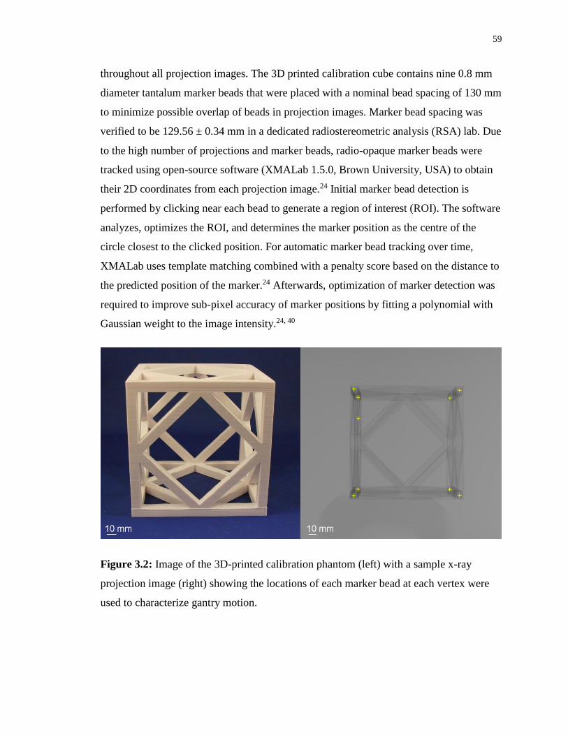
59

throughout all projection images. The 3D printed calibration cube contains nine 0.8 mm

diameter tantalum marker beads that were placed with a nominal bead spacing of 130 mm

to minimize possible overlap of beads in projection images. Marker bead spacing was

verified to be 129.56 ± 0.34 mm in a dedicated radiostereometric analysis (RSA) lab. Due

to the high number of projections and marker beads, radio-opaque marker beads were

tracked using open-source software (XMALab 1.5.0, Brown University, USA) to obtain

their 2D coordinates from each projection image.24 Initial marker bead detection is

performed by clicking near each bead to generate a region of interest (ROI). The software

analyzes, optimizes the ROI, and determines the marker position as the centre of the

circle closest to the clicked position. For automatic marker bead tracking over time,

XMALab uses template matching combined with a penalty score based on the distance to

the predicted position of the marker.24 Afterwards, optimization of marker detection was

required to improve sub-pixel accuracy of marker positions by fitting a polynomial with

Gaussian weight to the image intensity.24, 40

Figure 3.2: Image of the 3D-printed calibration phantom (left) with a sample x-ray

projection image (right) showing the locations of each marker bead at each vertex were

used to characterize gantry motion.

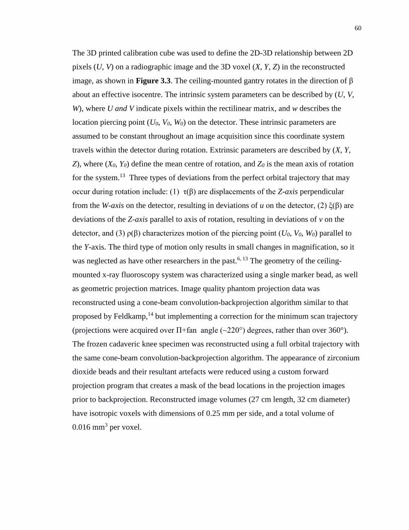
60

The 3D printed calibration cube was used to define the 2D-3D relationship between 2D

pixels (U, V) on a radiographic image and the 3D voxel (X, Y, Z) in the reconstructed

image, as shown in Figure 3.3. The ceiling-mounted gantry rotates in the direction of β

about an effective isocentre. The intrinsic system parameters can be described by (U, V,

W), where U and V indicate pixels within the rectilinear matrix, and w describes the

location piercing point (U0, V0, W0) on the detector. These intrinsic parameters are

assumed to be constant throughout an image acquisition since this coordinate system

travels within the detector during rotation. Extrinsic parameters are described by (X, Y,

Z), where (X0, Y0) define the mean centre of rotation, and Z0 is the mean axis of rotation

for the system.13 Three types of deviations from the perfect orbital trajectory that may

occur during rotation include: (1) τ(β) are displacements of the Z-axis perpendicular

from the W-axis on the detector, resulting in deviations of u on the detector, (2) ξ(β) are

deviations of the Z-axis parallel to axis of rotation, resulting in deviations of v on the

detector, and (3) ρ(β) characterizes motion of the piercing point (U0, V0, W0) parallel to

the Y-axis. The third type of motion only results in small changes in magnification, so it

was neglected as have other researchers in the past.6, 13 The geometry of the ceiling-

mounted x-ray fluoroscopy system was characterized using a single marker bead, as well

as geometric projection matrices. Image quality phantom projection data was

reconstructed using a cone-beam convolution-backprojection algorithm similar to that

proposed by Feldkamp,14 but implementing a correction for the minimum scan trajectory

(projections were acquired over Π+fan angle (~220°) degrees, rather than over 360°).

The frozen cadaveric knee specimen was reconstructed using a full orbital trajectory with

the same cone-beam convolution-backprojection algorithm. The appearance of zirconium

dioxide beads and their resultant artefacts were reduced using a custom forward

projection program that creates a mask of the bead locations in the projection images

prior to backprojection. Reconstructed image volumes (27 cm length, 32 cm diameter)

have isotropic voxels with dimensions of 0.25 mm per side, and a total volume of

0.016 mm3 per voxel.

61

Figure 3.3: Schematic diagram of the acquisition geometry depicting a point projection

of an object located in 3D (X, Y, Z) onto a 2D detector (U, V).

Reproducibility of imperfections during ceiling-mounted gantry motion, over a year, was

characterized with five projection-image acquisitions of the 3D printed calibration cube

placed near the centre of rotation to minimize motion in the x-direction and was not

moved between image acquisitions. In each projection image, the origin of the world

coordinate system can be inferred from averaged U,V coordinates of the eight

diametrically opposed vertices in the 3D printed calibration cube.7 The averaged U,V

coordinates represent a sinusoidal curve near the centre of rotation; therefore, we fit this

data as a function of image projection number to the equation: 𝑈 = 𝑎 + 𝑏 sin(𝛽 + 𝑐).13

One set of images was acquired with a single high-contrast bead placed within the 3D

printed calibration cube to determine if any discrepancies exist between the results of the

sinusoidal fit of a single marker bead versus an averaged synthetic marker. The following

assumptions were made for the prospective calibration: (1) rotation only occurs in the Z-

axis, (2) motion on the Y-axis can be neglected, and (3) intrinsic parameters are

consistent throughout a rotation. The residuals resulting from the best-fit sinusoid provide

direct estimates of deviations from the perfect circular orbit, and were used to apply

62

corrections to images before backprojection. In addition, the prospective geometric

matrices were generated using the 3D coordinates of the 9 beads and their respective 2D

coordinates to characterize gantry motion during rotation within a day.30 Extrinsic

projection matrices were computed after fixing the intrinsic parameters to the average for

that day.


Dose simulations were performed using a commercial Monte Carlo simulation program

for calculating patient dose in medical x-ray examinations (PCXMC2.0, STUK,

Finland).47 This software has been used in previous studies to estimate effective dose to

patients.5, 47 Tube voltage and current remained constant for each projection image; these

values were used as inputs to PCXMC. Therefore, the tube voltage and current inputs for

the image quality phantom and cadaveric knee specimen were 120 kVp at 0.2 mAs, and

85 kVp at 0.25 mAs, respectively. The x-ray spectrum in PCXMC was set to match the

12° anode angle, as well as the inherent and added filtration (3.05 mm Al, 2.0 mm Al).

3.2.5 Image Quality Assessment

Quality of image volumes was evaluated using a large custom-designed phantom

containing modular acrylic plates designed to test individual imaging parameters, as

described in Chapter 2.36 The diameter (154 mm) and length (305 mm) of the large

phantom was representative of the average diameter and length of a single knee within

the field-of-view (FOV). The image quality phantom was placed in an upright position

and levelled using an external bubble level. The phantom was used to analyze parameters

of image quality, including: spatial resolution, linearity, uniformity, noise, and geometric

accuracy. Image volumes were reconstructed from 320 projection images at 0.32 mm

isotropic resolution using a cone-beam convolution-backprojection algorithm. The

resulting reconstructed 3D images volumes (32 cm width, 27 cm height) were rescaled in

Hounsfield units (HU). Image analysis was performed using MicroView image analysis

software (Version 2.5.0-3943, Parallax Innovations, London ON), and custom processing

software to calculate spatial resolution with slanted-edge images.12

63

3.2.5.1 Spatial Resolution

The image quality phantom evaluated spatial resolution of reconstructed image volumes

using 5° slanted-edge images to evaluate the resolution of the image volumes with

custom software based on previously described methods.12, 36 The image quality phantom

contains two orthogonal plates with slanted-edge images to evaluate the slice (Z) (Figure

3.4b) and transverse (X-Y) (Figure 3.7d) modulation transfer functions (MTF). Ten axial

slices from the reconstructed image volume (n = 10 slices) were averaged to reduce

noise. Limiting spatial resolution was determined at the point where spatial frequency

reaches 10% (referred to as MTF10). Spatial resolution was also assessed with bar

patterns (made with alternating sheets of aluminum and Mylar sheets with spacing

varying from 0.4 to 2.0 lp/mm). The bar pattern, shown in Figure 3.4d, quantitatively

and qualitatively estimated the MTF by analyzing the standard deviation in four ROIs

(1.5 x 1.5 x 1.5 mm3), followed by a correction with the standard deviation from an area

with uniform intensity placed over the bar patterns.11 Calculation of the maximum

modulation between materials in the ROI, defined as M0 =|CT𝐴𝑙−CT𝑀𝑦𝑙𝑎𝑟|

2, where the

averaged CT numbers, from the FOV, for aluminum and Mylar were used.10

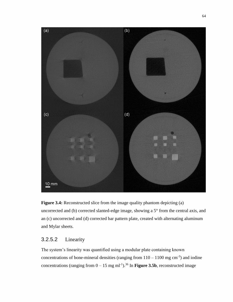
64

Figure 3.4: Reconstructed slice from the image quality phantom depicting (a)

uncorrected and (b) corrected slanted-edge image, showing a 5° from the central axis, and

an (c) uncorrected and (d) corrected bar pattern plate, created with alternating aluminum

and Mylar sheets.

3.2.5.2 Linearity

The system’s linearity was quantified using a modular plate containing known

concentrations of bone-mineral densities (ranging from 110 – 1100 mg cm-3) and iodine

concentrations (ranging from 0 – 15 mg ml-1).36 In Figure 3.5b, reconstructed image

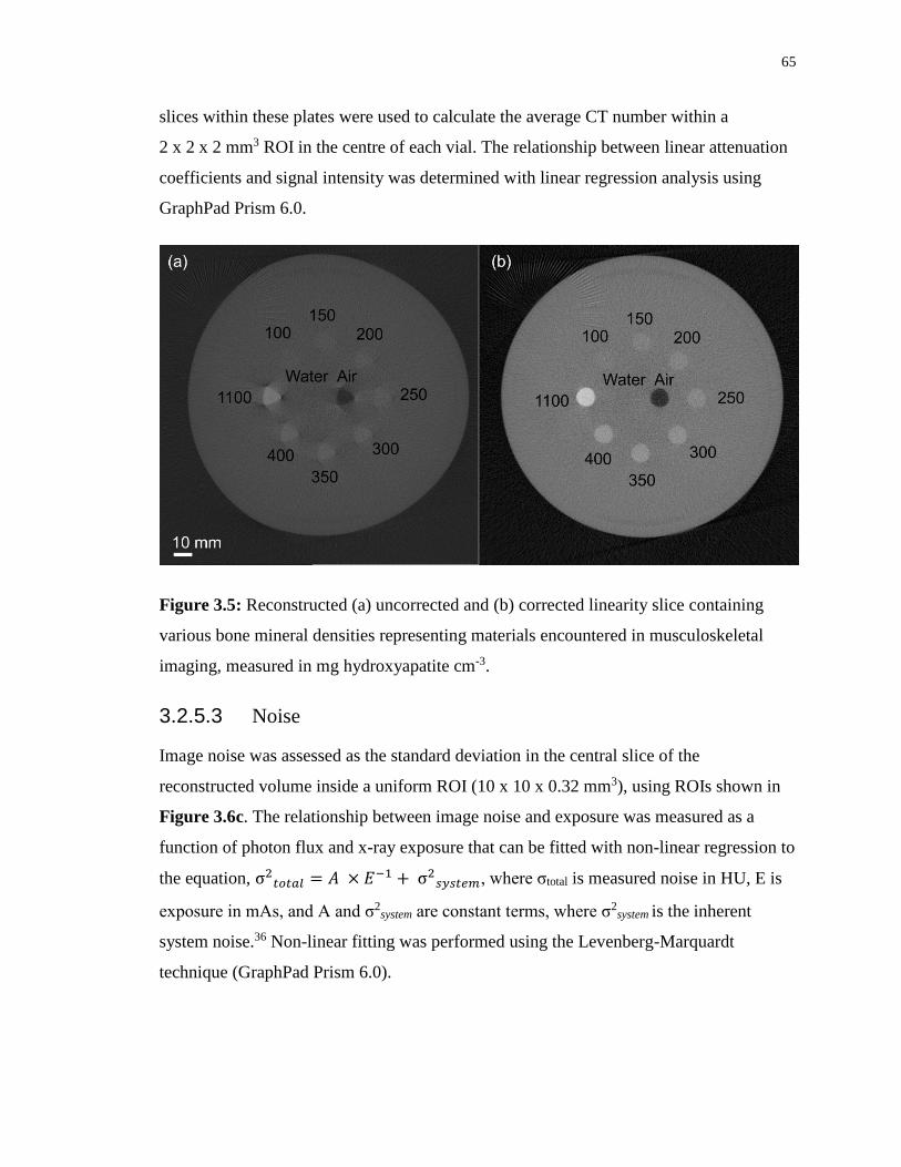
65

slices within these plates were used to calculate the average CT number within a

2 x 2 x 2 mm3 ROI in the centre of each vial. The relationship between linear attenuation

coefficients and signal intensity was determined with linear regression analysis using

GraphPad Prism 6.0.

Figure 3.5: Reconstructed (a) uncorrected and (b) corrected linearity slice containing

various bone mineral densities representing materials encountered in musculoskeletal

imaging, measured in mg hydroxyapatite cm-3.

3.2.5.3 Noise

Image noise was assessed as the standard deviation in the central slice of the

reconstructed volume inside a uniform ROI (10 x 10 x 0.32 mm3), using ROIs shown in

Figure 3.6c. The relationship between image noise and exposure was measured as a

function of photon flux and x-ray exposure that can be fitted with non-linear regression to

the equation, σ2𝑡𝑜𝑡𝑎𝑙 = 𝐴 × 𝐸−1 + σ2

𝑠𝑦𝑠𝑡𝑒𝑚, where σtotal is measured noise in HU, E is

exposure in mAs, and A and σ2system are constant terms, where σ2

system is the inherent

system noise.36 Non-linear fitting was performed using the Levenberg-Marquardt

technique (GraphPad Prism 6.0).

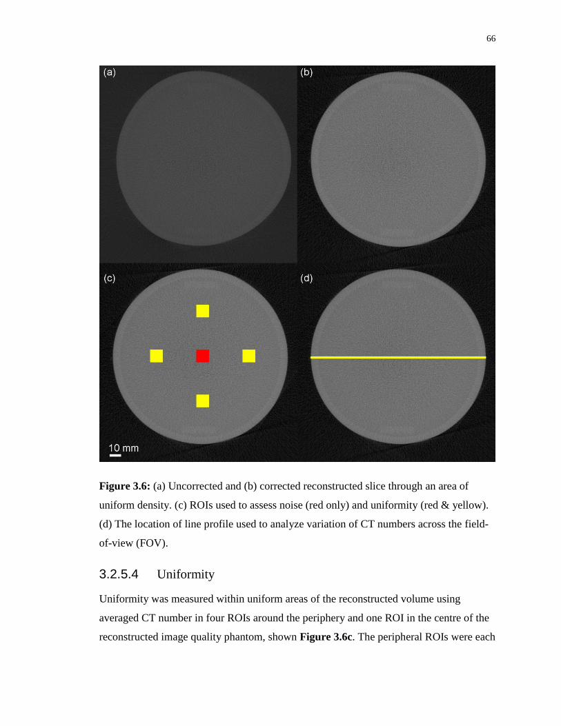
66

Figure 3.6: (a) Uncorrected and (b) corrected reconstructed slice through an area of

uniform density. (c) ROIs used to assess noise (red only) and uniformity (red & yellow).

(d) The location of line profile used to analyze variation of CT numbers across the field-

of-view (FOV).

3.2.5.4 Uniformity

Uniformity was measured within uniform areas of the reconstructed volume using

averaged CT number in four ROIs around the periphery and one ROI in the centre of the

reconstructed image quality phantom, shown Figure 3.6c. The peripheral ROIs were each

67

subtracted from the central ROI to determine the system’s uniformity. In addition, a line

profile was plotted across the central slice to qualitatively assess uniformity, shown in

Figure 3.6d.

3.2.5.5 Geometric Accuracy

Geometric accuracy was assessed using test plates containing metal beads spaced at a

known distance. The image quality phantom can assess geometric accuracy in the axial

and transverse directions. Axial geometric accuracy was assessed with four outer beads

spaced 40 ± 0.025 mm with an additional bead in the centre. In the transverse direction, a

modular plate containing thirty 280 µm diameter tungsten-carbide beads (spaced 15 mm

apart) were used to evaluate the geometric accuracy. The centroids of each bead (using

seeded region growing to automatically extract the beads),35 were used to estimate the

distance between neighbouring beads. Image slices used to determine geometric accuracy

from both phantoms are demonstrated in Figure 3.7.

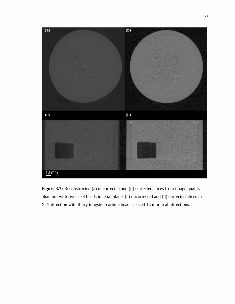
68

Figure 3.7: Reconstructed (a) uncorrected and (b) corrected slices from image quality

phantom with five steel beads in axial plane. (c) uncorrected and (d) corrected slices in

X-Y direction with thirty tungsten-carbide beads spaced 15 mm in all directions.

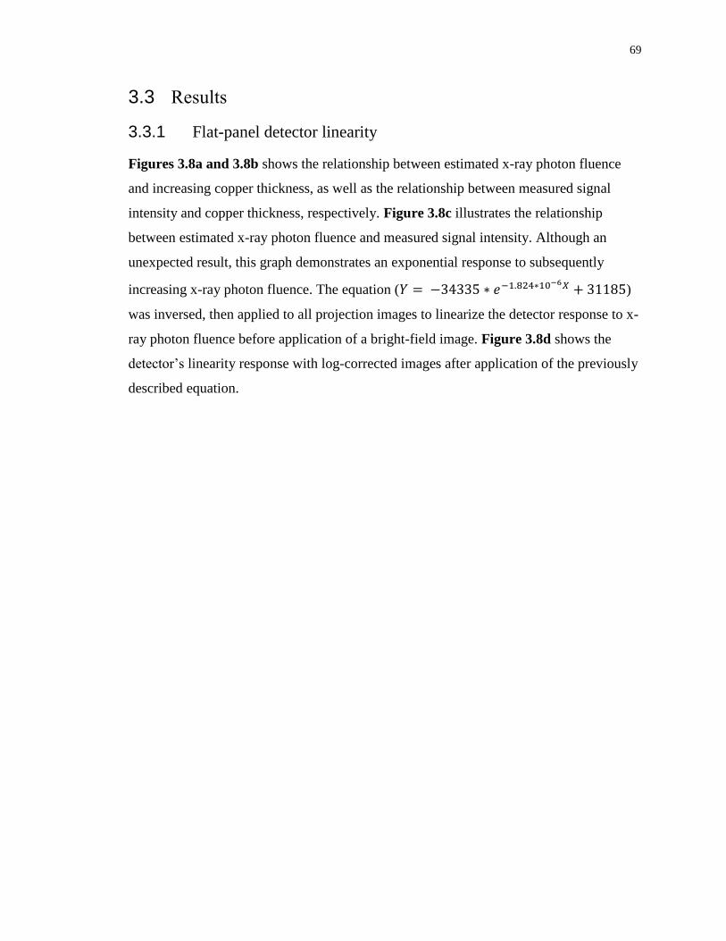
69

3.3 Results

3.3.1 Flat-panel detector linearity

Figures 3.8a and 3.8b shows the relationship between estimated x-ray photon fluence

and increasing copper thickness, as well as the relationship between measured signal

intensity and copper thickness, respectively. Figure 3.8c illustrates the relationship

between estimated x-ray photon fluence and measured signal intensity. Although an

unexpected result, this graph demonstrates an exponential response to subsequently

increasing x-ray photon fluence. The equation (𝑌 = −34335 ∗ 𝑒−1.824∗10−6𝑋 + 31185)

was inversed, then applied to all projection images to linearize the detector response to x-

ray photon fluence before application of a bright-field image. Figure 3.8d shows the

detector’s linearity response with log-corrected images after application of the previously

described equation.

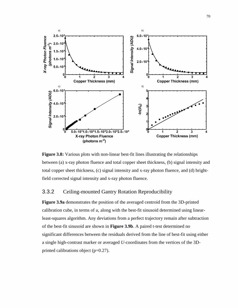
70

Figure 3.8: Various plots with non-linear best-fit lines illustrating the relationships

between (a) x-ray photon fluence and total copper sheet thickness, (b) signal intensity and

total copper sheet thickness, (c) signal intensity and x-ray photon fluence, and (d) bright-

field corrected signal intensity and x-ray photon fluence.

3.3.2 Ceiling-mounted Gantry Rotation Reproducibility

Figure 3.9a demonstrates the position of the averaged centroid from the 3D-printed

calibration cube, in terms of u, along with the best-fit sinusoid determined using linear-

least-squares algorithm. Any deviations from a perfect trajectory remain after subtraction

of the best-fit sinusoid are shown in Figure 3.9b. A paired t-test determined no

significant differences between the residuals derived from the line of best-fit using either

a single high-contrast marker or averaged U-coordinates from the vertices of the 3D-

printed calibrations object (p=0.27).

71

Figure 3.9: (a) Comparison of centroid trajectory of a single high-contrast marker bead

versus the averaged U coordinates of the eight diametrically opposed vertices of the 3D

printed calibration cube, where the thick line indicates the best-fit sinusoid. (b) The

resulting residual plot from a sinusoidal fit is plotted as a function of angle, calculated by

subtracting the measured centroid location from the best-fit line.

Figure 3.10a demonstrates the position of the averaged centroid from the 3D-printed

calibration object, in terms of u, along with the best-fit sinusoid determined using linear-

least-squares algorithm. Any deviations from a perfect trajectory remain after subtraction

of the best-fit sinusoid are shown in Figure 3.10b. Over five data acquisitions, the gantry

motion was highly reproducible, generating a standard deviation of 0.58 pixels (0.19 mm)

and a maximum deviation of 10.3 pixels (3.3 mm) from the best-fit line.

Figure 3.10: (a) Comparison five acquisitions of centroid trajectory of the averaged U


where the thick line indicates the best-fit sinusoid. (b) The resulting residual plot.

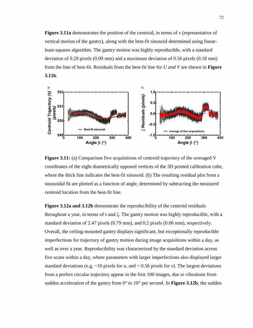
72

Figure 3.11a demonstrates the position of the centroid, in terms of v (representative of

vertical motion of the gantry), along with the best-fit sinusoid determined using linear-

least-squares algorithm. The gantry motion was highly reproducible, with a standard

deviation of 0.29 pixels (0.09 mm) and a maximum deviation of 0.56 pixels (0.18 mm)

from the line of best-fit. Residuals from the best-fit line for U and V are shown in Figure

3.11b.

Figure 3.11: (a) Comparison five acquisitions of centroid trajectory of the averaged V


where the thick line indicates the best-fit sinusoid. (b) The resulting residual plot from a

sinusoidal fit are plotted as a function of angle, determined by subtracting the measured

centroid location from the best-fit line.

Figure 3.12a and 3.12b demonstrate the reproducibility of the centroid residuals

throughout a year, in terms of τ and ξ. The gantry motion was highly reproducible, with a

standard deviation of 2.47 pixels (0.79 mm), and 0.2 pixels (0.06 mm), respectively.

Overall, the ceiling-mounted gantry displays significant, but exceptionally reproducible

imperfections for trajectory of gantry motion during image acquisitions within a day, as

well as over a year. Reproducibility was characterized by the standard deviation across

five scans within a day, where parameters with larger imperfections also displayed larger

standard deviations (e.g. ~10 pixels for u, and < 0.56 pixels for v). The largest deviations

from a perfect circular trajectory appear in the first 100 images, due to vibrations from

sudden acceleration of the gantry from 0° to 10° per second. In Figure 3.12b, the sudden

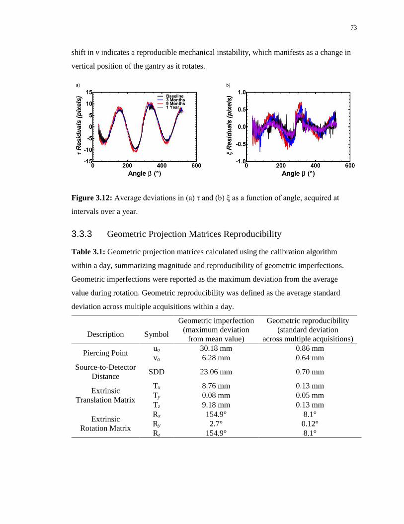
73

shift in v indicates a reproducible mechanical instability, which manifests as a change in

vertical position of the gantry as it rotates.

Figure 3.12: Average deviations in (a) τ and (b) ξ as a function of angle, acquired at

intervals over a year.

3.3.3 Geometric Projection Matrices Reproducibility

Table 3.1: Geometric projection matrices calculated using the calibration algorithm

within a day, summarizing magnitude and reproducibility of geometric imperfections.

Geometric imperfections were reported as the maximum deviation from the average

value during rotation. Geometric reproducibility was defined as the average standard

deviation across multiple acquisitions within a day.

Description

Symbol

Geometric imperfection

(maximum deviation

from mean value)

Geometric reproducibility

(standard deviation

across multiple acquisitions)

Piercing Point uo 30.18 mm 0.86 mm

vo 6.28 mm 0.64 mm

Source-to-Detector

Distance SDD 23.06 mm 0.70 mm

Extrinsic

Translation Matrix

Tx 8.76 mm 0.13 mm

Ty 0.08 mm 0.05 mm

Tz 9.18 mm 0.13 mm

Extrinsic

Rotation Matrix

Rx 154.9° 8.1°

Ry 2.7° 0.12°

Rz 154.9° 8.1°

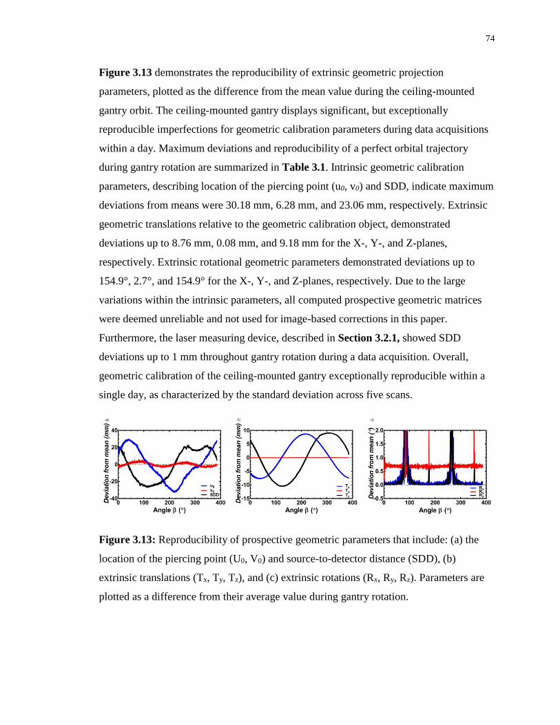
74

Figure 3.13 demonstrates the reproducibility of extrinsic geometric projection

parameters, plotted as the difference from the mean value during the ceiling-mounted

gantry orbit. The ceiling-mounted gantry displays significant, but exceptionally

reproducible imperfections for geometric calibration parameters during data acquisitions

within a day. Maximum deviations and reproducibility of a perfect orbital trajectory

during gantry rotation are summarized in Table 3.1. Intrinsic geometric calibration

parameters, describing location of the piercing point (u0, v0) and SDD, indicate maximum

deviations from means were 30.18 mm, 6.28 mm, and 23.06 mm, respectively. Extrinsic

geometric translations relative to the geometric calibration object, demonstrated

deviations up to 8.76 mm, 0.08 mm, and 9.18 mm for the X-, Y-, and Z-planes,

respectively. Extrinsic rotational geometric parameters demonstrated deviations up to

154.9°, 2.7°, and 154.9° for the X-, Y-, and Z-planes, respectively. Due to the large

variations within the intrinsic parameters, all computed prospective geometric matrices

were deemed unreliable and not used for image-based corrections in this paper.

Furthermore, the laser measuring device, described in Section 3.2.1, showed SDD

deviations up to 1 mm throughout gantry rotation during a data acquisition. Overall,

geometric calibration of the ceiling-mounted gantry exceptionally reproducible within a

single day, as characterized by the standard deviation across five scans.

Figure 3.13: Reproducibility of prospective geometric parameters that include: (a) the

location of the piercing point (U0, V0) and source-to-detector distance (SDD), (b)

extrinsic translations (Tx, Ty, Tz), and (c) extrinsic rotations (Rx, Ry, Rz). Parameters are

plotted as a difference from their average value during gantry rotation.

75


Analysis of slanted-edge images determined the limiting spatial resolution of 1.88 lp/mm

and 1.99 lp/mm in the axial and transverse planes, respectively. The system was able to

resolve bar patterns up to 2.0 lp/mm. Figure 3.14 displays MTF profiles obtained from

analysis of slanted-edge images and bar patterns.

Figure 3.14: Evaluation of modulation transfer function of reconstructed image volumes

using bar patterns in the axial direction, as well as slanted-edge images in the axial and

X-Y planes.

76

3.3.5 Linearity

Figure 3.15 contains a plot of the measured CT number (HU) as a function of bone-

mineral density. The equation, S = 1.157 (HU ml mg-1) · C + 84.2 (HU), produced by

linear regression revealed a highly linear response from the system, where the signal

intensity (S) is a function of increasing iodine concentration (C) in ml mg-1 (R2=0.9859).

Over the tested range of linear attenuation coefficients, the system demonstrates a high

degree of linearity (p < .01) in response to signal intensities that will be encountered in

clinical musculoskeletal imaging.

Figure 3.15: Results of linear regression from analysis of bone mineral densities

analyzed in the reconstructed linearity plate of the image quality phantom.

3.3.6 Noise

Figure 3.16 demonstrates the relationship between exposure and image noise in

reconstructed image volumes, plotted with a best-fit line derived from the equation

described in Section 3.2.5.3.

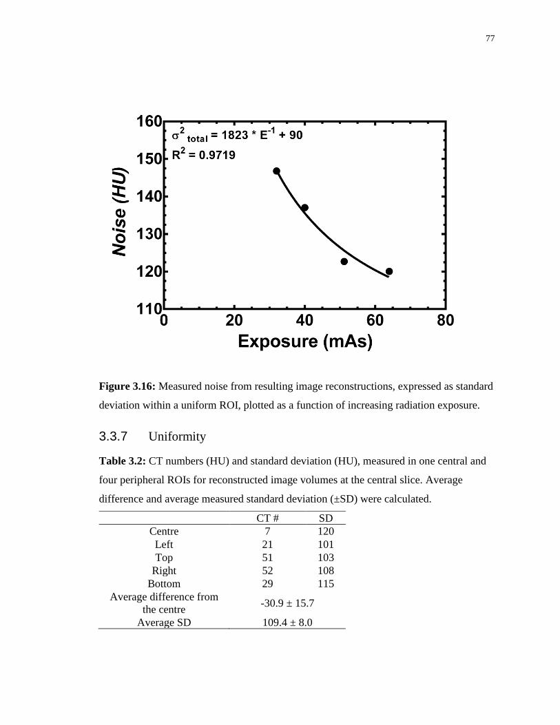
77

Figure 3.16: Measured noise from resulting image reconstructions, expressed as standard

deviation within a uniform ROI, plotted as a function of increasing radiation exposure.

3.3.7 Uniformity


four peripheral ROIs for reconstructed image volumes at the central slice. Average

difference and average measured standard deviation (±SD) were calculated.

CT # SD

Centre 7 120

Left 21 101

Top 51 103

Right 52 108

Bottom 29 115

Average difference from

the centre -30.9 ± 15.7

Average SD 109.4 ± 8.0

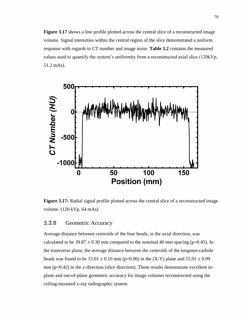
78

Figure 3.17 shows a line profile plotted across the central slice of a reconstructed image

volume. Signal intensities within the central region of the slice demonstrated a uniform

response with regards to CT number and image noise. Table 3.2 contains the measured

values used to quantify the system’s uniformity from a reconstructed axial slice (120kVp,

51.2 mAs).

Figure 3.17: Radial signal profile plotted across the central slice of a reconstructed image

volume. (120 kVp, 64 mAs)


Average distance between centroids of the four beads, in the axial direction, was

calculated to be 39.87 ± 0.30 mm compared to the nominal 40 mm spacing (p=0.45). In

the transverse plane, the average distance between the centroids of the tungsten-carbide

beads was found to be 15.01 ± 0.10 mm (p=0.06) in the (X-Y) plane and 15.01 ± 0.09

mm (p=0.42) in the z-direction (slice direction). These results demonstrate excellent in-

plane and out-of-plane geometric accuracy for image volumes reconstructed using the

ceiling-mounted x-ray radiographic system.

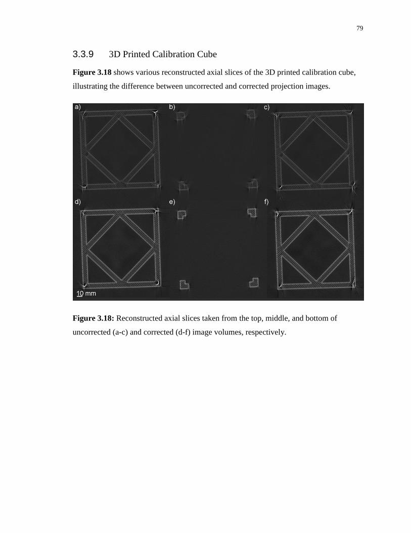
79

3.3.9 3D Printed Calibration Cube

Figure 3.18 shows various reconstructed axial slices of the 3D printed calibration cube,

illustrating the difference between uncorrected and corrected projection images.

Figure 3.18: Reconstructed axial slices taken from the top, middle, and bottom of

uncorrected (a-c) and corrected (d-f) image volumes, respectively.

80

3.3.10 Cadaveric Specimen

Figure 3.19 shows various reconstructed views in the axial, coronal, and sagittal planes,

where the differences between uncorrected, residual-corrected, and artefact-corrected

reconstructed image volumes are demonstrated.

Figure 3.19: Projection views of the frozen cadaveric knee in the axial, coronal, and

sagittal planes. The uncorrected (a-c), residual-corrected (d-f), and artefact-corrected (g-i)

reconstructed image volumes.

81


Based on ICRP 103 weighting coefficients, the effective dose was calculated to be 20 –

40 µSv for a single weight-bearing ceiling-mounted CBCT scan of both lower extremities

using 300 - 576 projection images for volumetric reconstructions (120 kVp, 0.2 mAs per

projection). The effective dose for the frozen cadaveric specimen was 14 µSv for single

leg while in an upright position using 400 images used in the reconstruction (85 kVp,

0.25 mAs per projection).

3.4 Discussion

We have demonstrated the quantitative and qualitative imaging performance of CBCT

reconstructions of the lower extremities resulting from the ceiling-mounted x-ray

fluoroscopy imaging system with the capability for integrated weight-bearing

radiography and dynamic kinematic imaging. The imaging system can produce accurate

weight-bearing CBCT reconstructions with corrections for highly reproducible

mechanical imperfections in gantry motion throughout a day. The imperfections in gantry

motion were exceptionally reproducible, which allowed for prospective image-based

calibration to correct images prior to backprojection.13 Although perturbations in gantry

motion were highly reproducible within two months, the auto-positioning feature slightly

varies the initial position of the source and detector between automatic positions scans;

therefore, geometric calibration is required prior to CBCT data acquisition with the

ceiling-mounted x-ray fluoroscopy system. The ceiling-mounted x-ray fluoroscopy

imaging system can acquire image volumes with a larger FOV (32 cm x 27 cm vs. 16 cm

x 13 cm) when compared to current commercially available weight-bearing CBCT

scanners. Flexible, yet highly reproducible, trajectories allow for the capability to obtain

3D volumetric images of the hip, knee, ankle, foot, and spine while in a normal weight-

bearing stance. In addition to CBCT image volumes, this system can acquire dynamic 2D

radiographic images, facilitating 2D to 3D co-registration.

Image quality of reconstructed image volumes are dependent on the accuracy of data

from each angular position around the centre of rotation, which must be substantially

better than the expected spatial resolution of the final volumetric image.13 Although the

82

ceiling-mounted x-ray fluoroscopy system displays geometric imperfections (maximum

side-to-side deviation of 10.3 pixels or 3.3 mm), we have proven these are remarkably

reproducible, allowing accurate image-based corrections on a calibration acquired prior

to image projection acquisition. Currently, there are two existing approaches for the

characterization of gantry motion during CBCT projection image acquisitions, which are

either: (1) assume an effective centre of rotation for an equatorial orbit using a single

marker bead located near the centre of rotation, or (2) prospective geometric projection

matrices to correct for geometric imperfections determined from a minimum of six

marker beads, on a view-by-view basis. Respectively, these approaches can be classified

as either (1) first-order corrections that account for in-plane variations from the ideal

orbital trajectory, or (2) second-order corrections that resolve out-of-plane deviations that

may occur.7 In our study, we implemented a simplified approach (1) that uses the

averaged U, V centroid from the eight vertices in the 3D printed calibration cube to

determine in-plane image-based corrections for imperfections in gantry motion, based on

a sinusoidal fit of the isocentre.7, 13 The techniques allows for simple first-order

approximations for displacements from sinusoidal fit, in τ(β) and ξ(β) (U and V), to be

applied as image-based corrections. During initialization of gantry motion, the largest

imperfections were observed due to sudden acceleration from the starting position.

Standard deviation of 2.47 pixels (0.79 mm) and 0.20 pixels (0.06 mm) for the respective

U and V coordinates for various image acquisitions within a year confirms the

exceptional reproducibility of the gantry rotation, which was comparable to previous

studies.13 A limitation of our study is the 38s acquisition time required to complete one

projection image acquisition with the ceiling-mounted x-ray fluoroscopy system.

Previous researchers have developed numerous motion compensation techniques that

account and correct for involuntary motion during projection image acquisition.1, 5, 43

These studies successfully implemented a motion compensation corrections across a

range of motion amplitudes, from sub-mm to centimetre drifts.43 Overall, imperfections

of the ceiling-mounted gantry rotation were remarkably reproducible over a year,

allowing for the use of calibrations previously acquired for image-based corrections.

The second approach, computation of prospective geometric projection matrices, utilizes

a minimum of six marker beads to define prospective intrinsic and extrinsic geometric

83

matrices to describe the relationship between 2D pixels (U, V) on a radiographic image

and the 3D voxel (X, Y, Z) in the reconstructed image.5, 13, 30, 41, 45 Intrinsic parameters

include pixel size (ΔU, ΔV), source-to-detector distance (SDD), and location of the

piercing point on the detector (U0, V0); whereas the extrinsic parameters describe

rotations and translations of the ceiling-mounted gantry relative to the origin of the

geometric calibration object. In our study, this approach yielded unrealistic values for

intrinsic geometric parameters that fluctuated simultaneously throughout each image

acquisition, as other researchers have observed in the past.51 Consistent with our

approach, intrinsic geometric matrices were averaged and fixed to remain constant, then

used to generate the extrinsic projection matrices. The extrinsic translation and rotation

matrices were highly reproducible throughout a day, yet vary over time due to small

variations in the initial orientation of the source and detector, caused by the auto-

positioning feature. The extrinsic rotations in the X- and Z-planes exhibited significant

deviations from the average value at two points approximately 180° apart, which indicate

that the 3D printed calibration cube may not be well-conditioned for those calibration

positions. Other researchers have recommended approximately five times the number of

samples to achieve higher accuracy of geometric calibration.18 According to Li et al.,30 a

minimum of 5.5 (6) point correspondences are required to solve for the prospective

calibration matrices, and point correspondence data may be inaccurate due to digitization

and image noise. Implementation of prospective geometric calibration is computationally

intensive, and does not allow use of standard cone-beam backprojection algorithms.13

With our approach, we have successfully demonstrated various image quality parameters

within a reconstructed image volume, in terms of linearity, spatial resolution, uniformity,

noise, and geometric accuracy. Additionally, we have successfully reconstructed a single

frozen cadaveric knee specimen in an upright position. Previous work has performed a

quantitative analysis CBCT reconstructed image volumes from an O-arm using the same

image quality phantom.36 Reconstructed image volumes exhibited a highly linear

response over the ranges of densities analyzed, representing the linear attenuation

coefficients of cortical bone, cartilage, muscle, and other soft tissues that will be

encountered in future studies. The spatial resolution of reconstructed image volumes from

the ceiling-mounted gantry surpassed the O-arm in both axial and transverse planes;36

84

however, spatial resolution differed slightly between axial and transverse plane

measurements. This may have been caused by excessive noise in the edge-response

function, which influences the derivation of the edge response function to the line spread

function when calculating MTF.46 High spatial resolution is important for the detection of

subtle fractures that do not present on radiographs, and for the visualization of the

trabecular architecture of subchondral bone.37 Geometric accuracy within reconstructed

image volumes was excellent, indicating reliable and accurate measurements for

application to patient-to-image registrations.16 In clinical practice, extremity CBCT

scanners have been successfully used in evaluations of joint arthrography, bone healing,

fracture detection, and joint alignment.19, 21, 27, 29 Uniformity and noise measurements are

dependent on the diameter of the object within the FOV. In our study, reconstructed

images volumes displayed a cupping effect on the line profile across the central slice,

indicating the occurrence of beam-hardening. The detector used in this study produces

images with a 12 bit depth (i.e. 4096 grey levels), but displays non-linear (but

correctable) response over all exposures used in the study due to limited dynamic range.

In order to reduce noise without increasing radiation dose, enhancement of detector

quantum efficiency is essential.28

The effective dose was estimated using a commercial Monte Carlo simulation program

for calculating patient dose in medical x-ray examinations. The effective dose was

estimated to be 20 µSv per CBCT acquisition reconstructed using 300 projection images

(120 kVp, 60 mAs). For the frozen cadaveric specimen, the effective dose was estimated

to be 14 µSv while in an upright position reconstructed with 400 projection images (85

kVp, 80mAs) using a full orbital trajectory. The resulting effective dose is comparable to

current commercially available weight-bearing CBCT scanners,25, 26, 31 and is equivalent

to approximately two chest x-rays per projection image acquisition.33 The stochastic

effects of ionizing radiation arising from diagnostic imaging has been associated with a

cancer risk coefficient of 5.5 x 10-2 Sv-1, thereby a scan from this ceiling-mounted x-ray

fluoroscopy system carries a 1.1 x 10-6 % increase to the stochastic effects of radiation

over a lifetime.49 The effective dose associated with CBCT acquisitions from a ceiling-

mounted x-ray fluoroscopy system is minimal compared to 2.2 mSv, comprising of less

than 1% of the average annual total effective dose from background radiation for

85

Canadian residents.17 This ceiling-mounted x-ray fluoroscopy system demonstrates

potential for weight-bearing imaging of the lower extremity in biomechanically relevant

positions to assess the effects of various musculoskeletal treatments, while generating a

lower dose when compared to conventional CT.

3.5 Conclusion

We have demonstrated for the first time that a ceiling-mounted single-plane x-ray

fluoroscopy system can generate accurate CBCT reconstructions using image-based

corrections for highly reproducible imperfections in gantry motion. Implementation of a

simple image-shift correction protocol allows the implementation of standard cone-beam

reconstruction algorithms to produce accurate 3D reconstructions. Deviations from the

perfect orbital trajectory were highly reproducible within a day and over a year,

characterized from a sinusoidal fit of a synthetic point at the centre of the projection

image, as well as extrinsic geometric projection matrices. An image-quality phantom

assessed image quality parameters of reconstructed image volumes in terms of spatial

resolution, linearity, geometric accuracy, image noise, and uniformity. The successful

reconstruction of an upright cadaveric knee specimen demonstrates the significant

clinical potential of this system. The ceiling-mounted x-ray fluoroscopy system allows

for a larger FOV compared to currently available CBCT scanners. Future studies will

include: image acquisition with an offset detector to increase the FOV, 2D to 3D co-

registration for kinematic analysis of the knee during gait, and simultaneous weight-

bearing acquisitions of both lower extremities.

3.6 References

1. Berger, M., Muller, K., Aichert, A., Unberath, M., Thies, J., Choi, J. H., . . .

Maier, A. (2016). Marker-free motion correction in weight-bearing cone-beam CT

of the knee joint. Med Phys, 43(3), 1235-1248.

2. Brandt, K. D., Fife, R. S., Braunstein, E. M., & Katz, B. (2010). Radiographic

grading of the severity of knee osteoarthritis: Relation of the kellgren and

lawrence grade to a grade based on joint space narrowing, and correlation with

arthroscopic evidence of articular cartilage degeneration. Arthritis & Rheumatism,

34(11), 1381-1386.

86

3. Carrino, J. A., Al Muhit, A., Zbijewski, W., Thawait, G. K., Stayman, J. W.,

Packard, N., . . . Siewerdsen, J. H. (2014). Dedicated cone-beam CT system for

extremity imaging. Radiology, 270(3), 816-824.

4. Cho, Y., Moseley, D. J., Siewerdsen, J. H., & Jaffray, D. A. (2005). Accurate

technique for complete geometric calibration of cone-beam computed tomography

systems. Med Phys, 32(4), 968-983.

5. Choi, J. H., Maier, A., Keil, A., Pal, S., McWalter, E. J., Beaupre, G. S., . . .

Fahrig, R. (2014). Fiducial marker-based correction for involuntary motion in

weight-bearing C-arm CT scanning of knees. II. Experiment. Med Phys, 41(6),

061902.

6. Concepcion, J. A., Carpinelli, J. D., Kuo-Petravic, G., & Reisman, S. (1992). CT

fan beam reconstruction with a nonstationary axis of rotation. IEEE Trans Med

Imaging, 11(1), 111-116.

7. Daly, M. J., Siewerdsen, J. H., Cho, Y. B., Jaffray, D. A., & Irish, J. C. (2008).

Geometric calibration of a mobile C-arm for intraoperative cone-beam CT. Med

Phys, 35(5), 2124-2136.

8. Dirschl, D. R., & Dawson, P. A. (2004). Injury severity assessment in tibial

plateau fractures. Clin Orthop Relat Res, 423(423), 85-92.

9. Draper, C. E., Besier, T. F., Fredericson, M., Santos, J. M., Beaupre, G. S., Delp,

S. L., & Gold, G. E. (2011). Differences in patellofemoral kinematics between

weight-bearing and non-weight-bearing conditions in patients with patellofemoral

pain. Journal of orthopaedic research : official publication of the Orthopaedic

Research Society, 29(3), 312-317.

10. Droege, R. T., & Morin, R. L. (1982). A practical method to measure the MTF of

CT scanners. Med Phys, 9(5), 758-760.

11. Droege, R. T., & Rzeszotarski, M. S. (1985). An MTF method immune to

aliasing. Med Phys, 12(6), 721-725.

12. Du, L. Y., Umoh, J., Nikolov, H. N., Pollmann, S. I., Lee, T. Y., & Holdsworth,

D. W. (2007). A quality assurance phantom for the performance evaluation of

volumetric micro-CT systems. Phys Med Biol, 52(23), 7087-7108.

13. Fahrig, R., & Holdsworth, D. W. (2000). Three-dimensional computed

tomographic reconstruction using a C-arm mounted XRII: image-based correction

of gantry motion nonidealities. Med Phys, 27(1), 30-38.

14. Feldkamp, L. A., Davis, L. C., & Kress, J. W. (1984). Practical Cone-Beam

Algorithm. J Opt Soc Am A, 1(6), 612-619.

87



29(2), 199-204.

16. Fitzpatrick, J. M., West, J. B., & Maurer, C. R., Jr. (1998). Predicting error in

rigid-body point-based registration. IEEE Trans Med Imaging, 17(5), 694-702.

17. Grasty, R. L., & LaMarre, J. R. (2004). The annual effective dose from natural

sources of ionising radiation in Canada. Radiat Prot Dosimetry, 108(3), 215-226.

18. Hartley, R., & Zisserman, A. (2004). Multiple view geometry in computer vision.

Cambridge: Cambridge University Press.

19. Hirschmann, A., Buck, F. M., Fucentese, S. F., & Pfirrmann, C. W. (2015).

Upright CT of the knee: the effect of weight-bearing on joint alignment. Eur

Radiol, 25(11), 3398-3404.

20. Hirschmann, M. T., Konala, P., Amsler, F., Iranpour, F., Friederich, N. F., &

Cobb, J. P. (2011). The position and orientation of total knee replacement

components: a comparison of conventional radiographs, transverse 2D-CT slices

and 3D-CT reconstruction. J Bone Joint Surg Br, 93(5), 629-633.

21. Huang, A. J., Chang, C. Y., Thomas, B. J., MacMahon, P. J., & Palmer, W. E.

(2015). Using cone-beam CT as a low-dose 3D imaging technique for the

extremities: initial experience in 50 subjects. Skeletal Radiol, 44(6), 797-809.

22. Jaffray, D. A., Siewerdsen, J. H., Wong, J. W., & Martinez, A. A. (2002). Flat-

panel cone-beam computed tomography for image-guided radiation therapy. Int J

Radiat Oncol Biol Phys, 53(5), 1337-1349.

23. Kan, H., Arai, Y., Kobayashi, M., Nakagawa, S., Inoue, H., Hino, M., . . . Kubo,

T. (2017). Fixed-flexion view X-ray of the knee superior in detection and follow-

up of knee osteoarthritis. Medicine (Baltimore), 96(49), e9126.

24. Knorlein, B. J., Baier, D. B., Gatesy, S. M., Laurence-Chasen, J. D., & Brainerd,

E. L. (2016). Validation of XMALab software for marker-based XROMM. J Exp

Biol, 219(Pt 23), 3701-3711.









88



28. Lee, S. C., Kim, H. K., Chun, I. K., Cho, M. H., Lee, S. Y., & Cho, M. H. (2003).

A flat-panel detector based micro-CT system: performance evaluation for small-

animal imaging. Phys Med Biol, 48(24), 4173-4185.

29. Lepojarvi, S., Niinimaki, J., Pakarinen, H., & Leskela, H. V. (2016). Rotational

Dynamics of the Normal Distal Tibiofibular Joint With Weight-Bearing

Computed Tomography. Foot Ankle Int, 37(6), 627-635.

30. Li, X., Da, Z., & Liu, B. (2010). A generic geometric calibration method for

tomographic imaging systems with flat-panel detectors--a detailed

implementation guide. Med Phys, 37(7), 3844-3854.

31. Ludlow, J. B., & Ivanovic, M. (2014). Weightbearing CBCT, MDCT, and 2D

imaging dosimetry of the foot and ankle. International Journal of Diagnostic

Imaging, 1(2), 1.





33. Mettler, F. A., Jr., Huda, W., Yoshizumi, T. T., & Mahesh, M. (2008). Effective

doses in radiology and diagnostic nuclear medicine: a catalog. Radiology, 248(1),

254-263.

34. Neubauer, J., Neubauer, C., Gerstmair, A., Krauss, T., Reising, K., Zajonc, H., . . .

Voigt, J. (2016). Comparison of the Radiation Dose from Cone Beam Computed

Tomography and Multidetector Computed Tomography in Examinations of the

Hand. Rofo, 188(5), 488-493.

35. Otsu, N. (1979). A Threshold Selection Method from Gray-Level Histograms. 5.

36. Petrov, I. E., Nikolov, H. N., Holdsworth, D. W., & Drangova, M. (2011,

2011/03/03/). Image performance evaluation of a 3D surgical imaging platform.

Paper presented at the SPIE Medical Imaging.

37. Posadzy, M., Desimpel, J., & Vanhoenacker, F. (2017). Staging of Osteochondral

Lesions of the Talus: MRI and Cone Beam CT. Journal of the Belgian Society of

Radiology, 101(S2).

38. Powers, C. M., Ward, S. R., Fredericson, M., Guillet, M., & Shellock, F. G.

(2003). Patellofemoral kinematics during weight-bearing and non-weight-bearing

knee extension in persons with lateral subluxation of the patella: a preliminary

study. J Orthop Sports Phys Ther, 33(11), 677-685.

89

39. Punnoose, J., Xu, J., Sisniega, A., Zbijewski, W., & Siewerdsen, J. H. (2016).

Technical Note: spektr 3.0-A computational tool for x-ray spectrum modeling and

analysis. Med Phys, 43(8), 4711.

40. Rogers, S. S., Waigh, T. A., Zhao, X., & Lu, J. R. (2007). Precise particle tracking

against a complicated background: polynomial fitting with Gaussian weight. Phys

Biol, 4(3), 220-227.

41. Rougee, A., Picard, C., Ponchut, C., & Trousset, Y. (1993). Geometrical

calibration of X-ray imaging chains for three-dimensional reconstruction. Comput

Med Imaging Graph, 17(4-5), 295-300.

42. Sisniega, A., Stayman, J. W., Cao, Q., Yorkston, J., Siewerdsen, J. H., &

Zbijewski, W. (2016, 2016/03/22/). Image-based motion compensation for high-

resolution extremities cone-beam CT. Paper presented at the SPIE Medical

Imaging.

43. Sisniega, A., Stayman, J. W., Yorkston, J., Siewerdsen, J. H., & Zbijewski, W.

(2017). Motion compensation in extremity cone-beam CT using a penalized

image sharpness criterion. Phys Med Biol, 62(9), 3712-3734.

44. Stehling, C., Souza, R. B., Hellio Le Graverand, M. P., Wyman, B. T., Li, X.,

Majumdar, S., & Link, T. M. (2012). Loading of the knee during 3.0T MRI is

associated with significantly increased medial meniscus extrusion in mild and

moderate osteoarthritis. Eur J Radiol, 81(8), 1839-1845.

45. Strobel, N. K., Heigl, B., Brunner, T. M., Schuetz, O., Mitschke, M. M., Wiesent,

K., & Mertelmeier, T. (2003, 2003/06/09/). Improving 3D image quality of x-ray

C-arm imaging systems by using properly designed pose determination systems

for calibrating the projection geometry. Paper presented at the Medical Imaging

2003.

46. Takenaga, T., Katsuragawa, S., Goto, M., Hatemura, M., Uchiyama, Y., &

Shiraishi, J. (2015). Modulation transfer function measurement of CT images by

use of a circular edge method with a logistic curve-fitting technique. Radiol Phys

Technol, 8(1), 53-59.

47. Tapiovaara, M., & Siiskonen, T. (2008). A PC-based Monte Carlo program for

calculating patient doses in medical x-ray examinations (2nd Ed.). 31.



148.

49. Valentin, J. (2007). The 2007 Recommendations of the International Commission

on Radiological Protection. ICRP publication 103. Ann ICRP, 37(2-4), 1-332.

90

50. Wagenaar, F. C., Koeter, S., Anderson, P. G., & Wymenga, A. B. (2007).

Conventional radiography cannot replace CT scanning in detecting tibial tubercle

lateralisation. Knee, 14(1), 51-54.

51. Wiesent, K., Barth, K., Navab, N., Durlak, P., Brunner, T., Schuetz, O., &

Seissler, W. (2000). Enhanced 3-D-reconstruction algorithm for C-arm systems

suitable for interventional procedures. IEEE Trans Med Imaging, 19(5), 391-403.

52. Xu, Y., Yang, S., Ma, J., Li, B., Wu, S., Qi, H., & Zhou, L. (2017). Simultaneous

calibration phantom commission and geometry calibration in cone beam CT. Phys

Med Biol, 62(17), N375-N390.





91

Chapter 4

4 Conclusions and Future Directions

4.1 Summary of Results

Total knee arthroplasty (TKA) has become the gold standard for treatment of end-stage

osteoarthritis (OA) and has seen substantial increases for implementation of this

technique. Although TKA is a highly successful, safe, and cost-effective method for

treating end-stage OA, many patients continue to have functional limitations.13

Approximately 20% of patients still remain unsatisfied with outcomes related to pain

relief and functionality.4 In some studies, various patients with OA developed new gait

patterns to compensate for pain, which consequently result in increased joint loads within

the contralateral hip, knee, and ankle.12 Within ten years of their initial TKA, for

approximately 40% of patients, the contralateral knee will undergo accelerated OA

disease progression, resulting in a second TKA.10, 18 This has led to the implementation of

various techniques to study joint motion and loading in the weight-bearing lower

extremities to improve patient outcomes, in terms of pain management and restoration of

functionality.2, 3 Overall, weight-bearing imaging is one of the best methods to evaluate

the biomechanical function and OA progression in the knee.11

Previous researchers have used high-speed gait analysis to categorize gait patterns

between healthy and OA patients,12 and identify differences between the operated and

non-operated knee joint within the same patient.1 However, this technique is dependent

on the positioning of external reflective markers on the skin, which may not accurately

represent motion underlying bony structures,19 and it cannot provide quantitative

measurements about joint micro-motion. Radiography is a non-invasive medical imaging

modality that creates a single, static, two-dimensional radiographic image with ionizing

radiation of bone and soft tissue within the field-of-view (FOV). In clinical settings, the

success of TKA has been evaluated with anteroposterior and lateral radiographs, although

reproducibility of these images can be limited by patient positioning and orientation of

the detector.16 Despite the ability to effectively track late-stage disease progression of

OA, radiography is a two-dimensional representation of a three-dimensional structure

92

that cannot accurately distinguish between soft tissue with similar linear attenuation

coefficients.15 Radiostereometric analysis (RSA) utilizes simultaneous bi-planar x-ray

exposures to obtain three-dimensional measurements of migration in orthopaedic

implants.17 Although this technique yields accurate measurements, it can only evaluate

implanted markers of a single joint in a static image and is limited by a small FOV due to

the required intersection of the x-ray sources. Fluoroscopy is another radiographic

imaging modality that can obtain multiple images to create a dynamic radiographic video

of a patient. This modality enables dynamic single-planar or bi-planar RSA of the lower

extremity and has become the gold standard for assessments of soft-tissue artefacts from

motion capture gait analysis.6, 7, 20 Despite the fact that fluoroscopy can provide three-

dimensional measurements of the lower extremities, similar to previously described

radiographic imaging modalities, it is still a two-dimensional representation of a three-

dimensional object. Computed tomography, unlike previously described radiographic

imaging modalities, removes the superimposition of tissues, and distinguishes between

two materials with similar densities. Clinical CT scans are unable to obtain functional

weight-bearing images due to scanner design limitations. Recent studies have applied an

axial load to a patient’s leg to simulate weight-bearing in the lower extremity while in a

supine position.5 Cone-beam computed tomography (CBCT) is based on the same

principles as a clinical CT scanner, but allow for a variety of scanner designs that could

potentially overcome the limitations of radiography, fluoroscopy, and conventional

computed tomography.

In Chapter 2, titled “Quantitative Performance Evaluation of a Peripheral Cone Beam CT

Scanner with Weight-bearing Capabilities”, we described a technique to quantify image

quality parameters of image volumes reconstructed from various algorithms. The

hypothesis was that a peripheral cone-beam CT scanner would generate different

measurements relating to image quality based on the diameter of the phantom, or

reconstruction algorithm implemented was shown to be correct. All image quality

measurements were acquired at a 200 µm resolution, and compared to standards set by

the manufacturer of the CBCT scanner. Various image quality tests included: spatial

resolution, linearity, image noise, uniformity, geometric accuracy, and effective dose.

Large- (154 mm) and small- (70 mm) diameter image quality phantoms were scanned ten

93

times at 96 kVp and 90 kVp, respectively; for image noise, tube current varied from 1 to

12 mA, totalling 12 scans, resulting in exposures ranging from 6 to 108 mAs. Effective

dose was estimated using a PC-based Monte Carlo method, as well as a CTDI-based

estimate with organ specific weighting coefficients. In this study, we demonstrated that

the system’s performance exceeds the manufacturer’s guidelines for all image quality

tests using the small-diameter phantom. As expected, the large-diameter phantom,

representing the lower extremity, exhibited increase in image noise and non-uniformity.

Overall, the peripheral CBCT imaging system shows potential for weight-bearing 3D

volumetric studies for evaluations of musculoskeletal treatments and their impact on joint

biomechanics, while providing optimal image quality at a low dose. Our analysis of

noise performance vs exposure indicates that exposure should be maintained below

approximately 40 mAs, to optimize performance and minimize dose.

In Chapter 3, titled “Three-dimensional computed tomographic reconstruction in a

natural weight-bearing stance using ceiling-mounted x-ray fluoroscopy”, a technique to

generate reconstructed image volumes with a commercially available ceiling-mounted x-

ray fluoroscopy while rotating around an object of interest was implemented. The

hypothesis that imperfections in ceiling-mounted gantry motion were highly

reproducible, and could be used for image-based corrections was shown to be valid.

Gantry motion was characterized throughout a year using a 3D printed calibration cube

with a modification of the single marker bead method, and was also used to compute

prospective geometric calibration matrices using 2D-3D point correspondence. In

addition, effective dose resulting from one image acquisition was estimated using a PC-

based Monte Carlo simulation. Image-based corrections using the modified single-marker

approach were applied before backprojection, and resultant reconstructed image volumes

were evaluated using a large-diameter image quality phantom. Within one day,

imperfections in gantry motion were remarkably reproducible, resulting in standard

deviations 0.58 pixels (0.19 mm) and 0.56 pixels (0.18 mm) for the respective U and V

coordinates. Over a year, gantry motion was remarkably reproducible resulting in 2.47

pixels (0.79 mm) and 0.20 pixels (0.06 mm) for the U and V coordinates, respectively.

These results indicate imperfections in gantry motion are exceptionally reproducible over

a year, and image-based calibrations can be applied to previously acquired datasets. In

94

this study, we demonstrated this ceiling-mounted x-ray fluoroscopy system can

accurately reconstruct image volumes at a dose equivalent to commercially available

CBCT scanners.

4.1. Related Future Directions

The validation of image quality resulting from reconstructed image volumes using an

image quality phantom to quantify various image quality parameters will enable

numerous studies to take place. These studies include comparisons of non-weight-bearing

versus weight-bearing joint alignment, in vivo visualization of the meniscus, involuntary

motion compensation corrections, and evaluations of medial tibio-femoral osteoarthritis.

Reconstructed image volumes can provide unmatched biomechanical information of joint

loading and alignment in the lower extremity.14 In clinical orthopaedics, advanced

imaging modalities, such as CBCT, have become invaluable for detection of complex

fractures that do not present on plain radiographs. Weight-bearing volumetric imaging is

ideal for surgical measurements regarding patellar instability since these images can

provide a true functional representation of the knee joint.9 Other researchers have

demonstrated CBCT arthrography can be used clinically within the knee to detect

cartilage lesions of varying severity and diagnose the degeneration of tissue surrounding

the lesions through the use of contrast-enhanced images.8

As described in Chapters 2 and 3, the quantification of various imaging quality

parameters resulting from reconstructed image volumes can be used to directly compare

reconstructed image volumes from various cone-beam CT scanners. These studies ensure

reconstructed image volumes are reliable and accurate portrayals of a joint in the lower

extremity while in a weight-bearing position. Therefore, the reconstructed image volumes

could be used as computational bone models for finite element modelling or 2D-3D

registration in dynamic single-plane flat-plane fluoroscopy to assess joint loading and

kinematics. Overall, this thesis developed a novel ceiling-mounted CBCT system with

the capability to acquire 3D image volumes of both knees in a weight-bearing position,

and quantified various image quality parameters within reconstructed image volumes

from a commercially available peripheral CBCT scanner, and our novel ceiling-mounted

CBCT system. The novel ceiling-mounted CBCT system provides a unique combination

95

of 2D dynamic single-planar fluoroscopy, and 3D volumetric weight-bearing imaging.

This approach is more broadly applicable to sites that have medical imaging space

constraints, and it will facilitate 2D to 3D co-registration with 3D CBCT image volumes

and 2D dynamic single-plane images produced by one ceiling-mounted fluoroscopic

x-ray system.

4.2. References

1. Alnahdi, A. H., Zeni, J. A., & Snyder-Mackler, L. (2011). Gait after unilateral

total knee arthroplasty: frontal plane analysis. Journal of orthopaedic research :


2. Andriacchi, T. P., & Mundermann, A. (2006). The role of ambulatory mechanics

in the initiation and progression of knee osteoarthritis. Current opinion in

rheumatology, 18(5), 514-518.

3. Banks, S. A., & Hodge, W. A. (1996). Accurate measurement of three-

dimensional knee replacement kinematics using single-plane fluoroscopy. IEEE

Trans Biomed Eng, 43(6), 638-649.

4. Bourne, R. B., Chesworth, B. M., Davis, A. M., Mahomed, N. N., & Charron, K.

D. (2010). Patient satisfaction after total knee arthroplasty: who is satisfied and

who is not? Clin Orthop Relat Res, 468(1), 57-63.



29(2), 199-204.

6. Garling, E. H., Kaptein, B. L., Mertens, B., Barendregt, W., Veeger, H. E.,

Nelissen, R. G., & Valstar, E. R. (2007). Soft-tissue artefact assessment during

step-up using fluoroscopy and skin-mounted markers. Journal of biomechanics,

40 Suppl 1, S18-24.

7. Iaquinto, J. M., Tsai, R., Haynor, D. R., Fassbind, M. J., Sangeorzan, B. J., &

Ledoux, W. R. (2014). Marker-based validation of a biplane fluoroscopy system

for quantifying foot kinematics. Medical engineering & physics, 36(3), 391-396.







96



10. McMahon, M., & Block, J. A. (2003). The risk of contralateral total knee

arthroplasty after knee replacement for osteoarthritis. J Rheumatol, 30(8), 1822-

1824.

11. Miyazaki, T., Wada, M., Kawahara, H., Sato, M., Baba, H., & Shimada, S.

(2002). Dynamic load at baseline can predict radiographic disease progression in

medial compartment knee osteoarthritis. Annals of the Rheumatic Diseases, 61(7),

617-622.

12. Mundermann, A., Dyrby, C. O., & Andriacchi, T. P. (2005). Secondary gait

changes in patients with medial compartment knee osteoarthritis: increased load at

the ankle, knee, and hip during walking. Arthritis Rheum, 52(9), 2835-2844.

13. Noble, P. C., Gordon, M. J., Weiss, J. M., Reddix, R. N., Conditt, M. A., &

Mathis, K. B. (2005). Does Total Knee Replacement Restore Normal Knee

Function? Clinical Orthopaedics and Related Research, &NA;(431), 157-165.

14. Richter, M., Seidl, B., Zech, S., & Hahn, S. (2014). PedCAT for 3D-imaging in

standing position allows for more accurate bone position (angle) measurement

than radiographs or CT. Foot Ankle Surg, 20(3), 201-207.

15. Romans, L. E. (2010). Computed Tomography for Technologists: A

Comprehensive Text: Lippincott Williams & Wilkins.

16. Sarmah, S. S., Patel, S., Hossain, F. S., & Haddad, F. S. (2012). The radiological

assessment of total and unicompartmental knee replacements. J Bone Joint Surg

Br, 94(10), 1321-1329.

17. Selvik, G. (1990). Roentgen stereophotogrammetric analysis. Acta Radiol, 31(2),

113-126.

18. Shakoor, N., Block, J. A., Shott, S., & Case, J. P. (2002). Nonrandom evolution of

end-stage osteoarthritis of the lower limbs. Arthritis Rheum, 46(12), 3185-3189.

19. Stagni, R., Fantozzi, S., & Cappello, A. (2006). Propagation of anatomical

landmark misplacement to knee kinematics: performance of single and double

calibration. Gait Posture, 24(2), 137-141.

20. Yuan, X., Ryd, L., Tanner, K. E., & Lidgren, L. (2002). Roentgen single-plane

photogrammetric analysis (RSPA.) A new approach to the study of

musculoskeletal movement. J Bone Joint Surg Br, 84(6), 908-914.

97

Curriculum Vitae

Rudolphe J. Baronette

Education

2015-2018 M.Sc. Medical Biophysics

Western University

2010-2015 B.Sc. Medical Radiation Sciences

McMaster University

B.Sc. Life Sciences

McMaster University

Advanced College Diploma, Medical Radiation Sciences

Mohawk College

Scholarships and Awards

2016 Cum Laude Abstract Award

Imaging Network of Ontario

2015 Collaborative Training Program in Musculoskeletal Health

Research Transdisciplinary Bone & Joint Award

Bone & Joint Institute, Western University

2010-2014 McMaster All-Canadian Academic Scholar

McMaster University

Abstracts and Presentations

1. Baronette RJ, Yuan X, Pollmann SI, Teeter MG, Holdsworth DW. Performance

evaluation of a peripheral cone-beam CT scanner with weight-bearing

capabilities. Poster presentation at the 2018 Canadian Bone & Joint Conference,

London, ON.

2. Baronette RJ, Yuan X, Pollmann SI, Teeter MG, Holdsworth DW. Performance

evaluation of a peripheral cone-beam CT scanner with weight-bearing

capabilities. Poster presentation at the 2018 Imaging Network of Ontario

Conference, Toronto, ON.

3. Baronette RJ, Yuan X, Teeter MG, Holdsworth DW. Calibrating single-plane

fluoroscopy using a 3D printed calibration object. Poster presentation at the 2017

Imaging Network of Ontario Conference, London, ON.

98

4. Baronette RJ, Yuan X, Teeter MG, Holdsworth DW. Calibrating single-plane

fluoroscopy using a 3D printed calibration object. Poster presentation at the 2017

London Health Research Day, London, ON.

5. Baronette RJ, Yuan X, Teeter MG, Holdsworth DW. Performance evaluation of

a peripheral cone-beam CT scanner with weight-bearing capabilities. Poster

presentation at the 2016 Canadian Bone & Joint Conference, London, ON.



presentation at the 2016 Imaging Network of Ontario Conference, Toronto, ON.



presentation at the 2016 London Health Research Day, London, ON.

Athletic Achievements

• 1st all-time, 4 x 400m relay, McMaster University.

• 2nd all-time, 300m dash, McMaster University.

• 7th overall, 4 x 200m relay, 2013 Canadian Interuniversity Sport Track & Field

Championships, Edmonton, AB.

• 8th overall, 300m dash, 2013 Canadian Interuniversity Sport Track & Field

Championships, Edmonton, AB.

• Silver medal, 4 x 200m relay, 2013 Ontario University Athletics Track & Field

Championships, Toronto, ON.

• Bronze medal, 4 x 200m and 4 x 400m relay, 2011 Ontario University Athletics

Track & Field Championships, Toronto, ON.

Quantitative Analysis of Three-Dimensional Cone-Beam ...

Documents

Transcript of Quantitative Analysis of Three-Dimensional Cone-Beam ...