California State University Long Beach

Fluid Mechanics

CE 336

Pumps and Centrifugal Equipment

Experiment 6

Prepared by Marc Brunet 008743265

Presented to Professor Mohamed El-Tawansy

Conducted on Tuesday, November 20th, 2012

Submitted on Tuesday, December 4th, 2012

1

NOTE: Dr. El-Tawansy, although this experiment was designatedas a group report, I am providing my own individual report in

Table of Contents

PurposeAbstractBackground and theoryThe equipment usedExperimental procedureRaw dataSample calculationExperimental resultsDiscussionConclusionBibliography

2

Group 4 Tuesday

Purpose of the experiment

A quantitative energetic analysis of a hydraulic pump was at the heart of this study and was its main purpose.

After having successfully initialized a hydraulic circuit with the input of a kinetic centrifugal mixed flow impeller pump, its systemand performance curves were tabulated and then analyzed.

The study was comprehensive and included the frictional forces that opposed the impeller pump.

The major losses were calculated with the knowledge of the experimental Darcy-Weisbach friction coefficient.

The minor losses were calculated with the knowledge of the water’s speed through the pipesand the individual minor restrictive obstructioncoefficients for the components that were inlinein the hydraulic circuit.

3

Abstract of the experiment

Fundamentally, a hydraulic jump is a tangibleexample of the conservation of energy principle.

The jump’s occurrence is the resultant of a collision between flows of fluids that possess asignificantly different amount of kinetic energy. The faster moving flow is suddenly

4

slowed down and a fraction of its kinetic energyis converted to potential energy.

In a limiting case, a maximal amount of lift is transferred to a flow which is slowed to a halt from a high velocity. Below, figure 1 depicts a hydraulic jump.

The theory behind the computations

5

Water freefalls and isaccelerated to

Slowerdownstream flowis impacted andthen slows down

A fraction of the fastmoving water’s kineticenergy is converted to

Figure 1: The Burdekin dam in

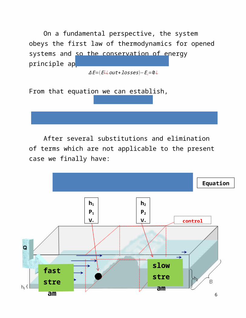
On a fundamental perspective, the system obeys the first law of thermodynamics for openedsystems and so the conservation of energy principle applies.

ΔE=(E¿¿out+losses)−E¿=0 ¿

From that equation we can establish, Eout+losses=E¿

Workout+Pot.Eout+KineticEout+losses=Pot.E¿+KineticE¿+Work¿

After several substitutions and elimination of terms which are not applicable to the presentcase we finally have:

h1+P1γ

+V1

2

2g=h2+

P2

γ+V2

2

2g+headlosses

6

Equation

h1

P1

V1

h2

P2

V2

faststream

slowstream

control

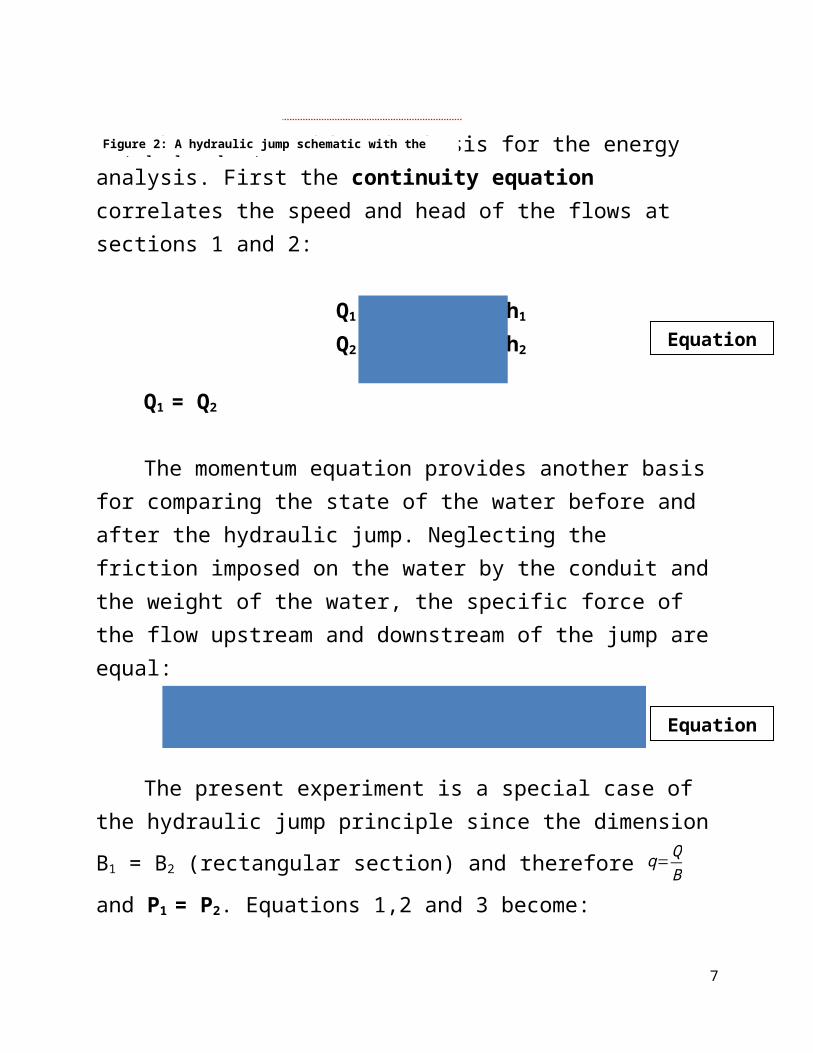
Figure 2 provides the basis for the energy analysis. First the continuity equation correlates the speed and head of the flows at sections 1 and 2:

Q1 = B1 * V1 * h1

Q2 = B2 * V2 * h2 Q1 = Q2

The momentum equation provides another basis for comparing the state of the water before and after the hydraulic jump. Neglecting the friction imposed on the water by the conduit andthe weight of the water, the specific force of the flow upstream and downstream of the jump areequal:

Q2g∗B∗h1

+(h¿¿1¿¿2∗B1)=Q2

g∗B∗h2+(h¿¿2¿¿2∗B2)¿¿¿¿

The present experiment is a special case of the hydraulic jump principle since the dimensionB1 = B2 (rectangular section) and therefore q=

QB

and P1 = P2. Equations 1,2 and 3 become:

7

Figure 2: A hydraulic jump schematic with the control volume elements

Equation

Equation

headlosses=q2

2g ( 1y1

2−1y22 )+(y1−y2)

q=y1v1=y2v2

y12

2+q2gy1

=y2

2

2+q2gy2

After several substitutions and combining equations 1a, 2a and 3a, the following relations are established; they will be used extensively in the following analysis.

y2y1

=12 (√1+8NF1

2−1)

y1y2

=12 (√1+8NF2

2−1)

headloss=(y2−y1 )3

4y1y2

q=(y1+y2 )√(gy1y2)

2

Froude¿1=NF1=qy1

√(gy1)

8

Equation

Equation

Equation

Froude¿2=NF2=qy2

√(gy2)

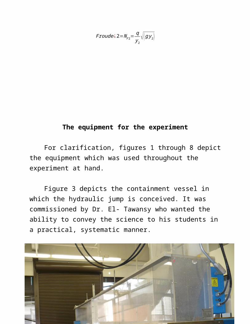
The equipment for the experiment

For clarification, figures 1 through 8 depictthe equipment which was used throughout the experiment at hand.

Figure 3 depicts the containment vessel in which the hydraulic jump is conceived. It was commissioned by Dr. El- Tawansy who wanted the ability to convey the science to his students ina practical, systematic manner.

9

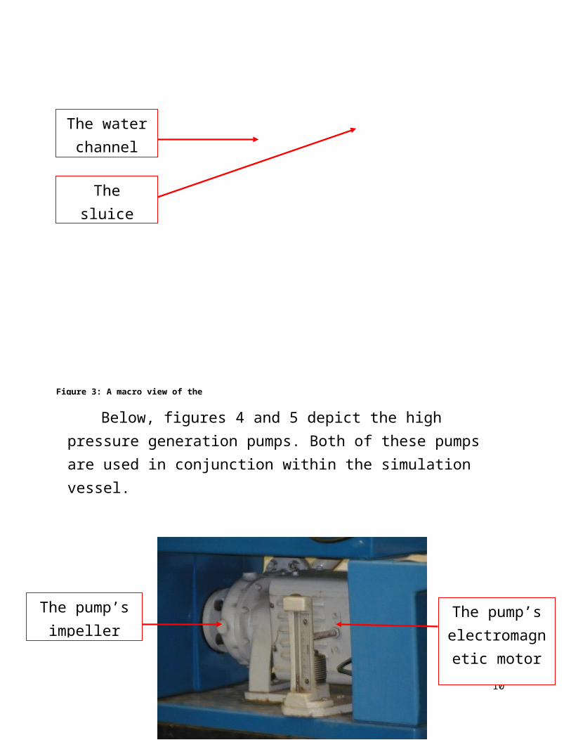
Below, figures 4 and 5 depict the high pressure generation pumps. Both of these pumps are used in conjunction within the simulation vessel.

10

Thesluice

The waterchannel

Figure 3: A macro view of the

The pump’simpeller

The pump’selectromagnetic motor

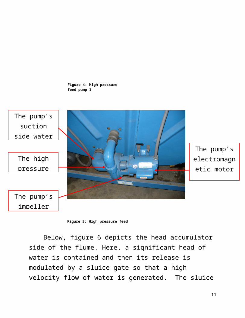
Below, figure 6 depicts the head accumulator side of the flume. Here, a significant head of water is contained and then its release is modulated by a sluice gate so that a high velocity flow of water is generated. The sluice

11

The highpressure

The pump’ssuction

side water

The pump’simpeller

The pump’selectromagnetic motor

Figure 4: High pressure feed pump 1

Figure 5: High pressure feed pump 2

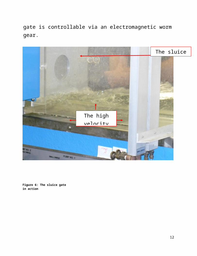
gate is controllable via an electromagnetic wormgear.

12

The sluicegate

The highvelocity

Figure 6: The sluice gatein action

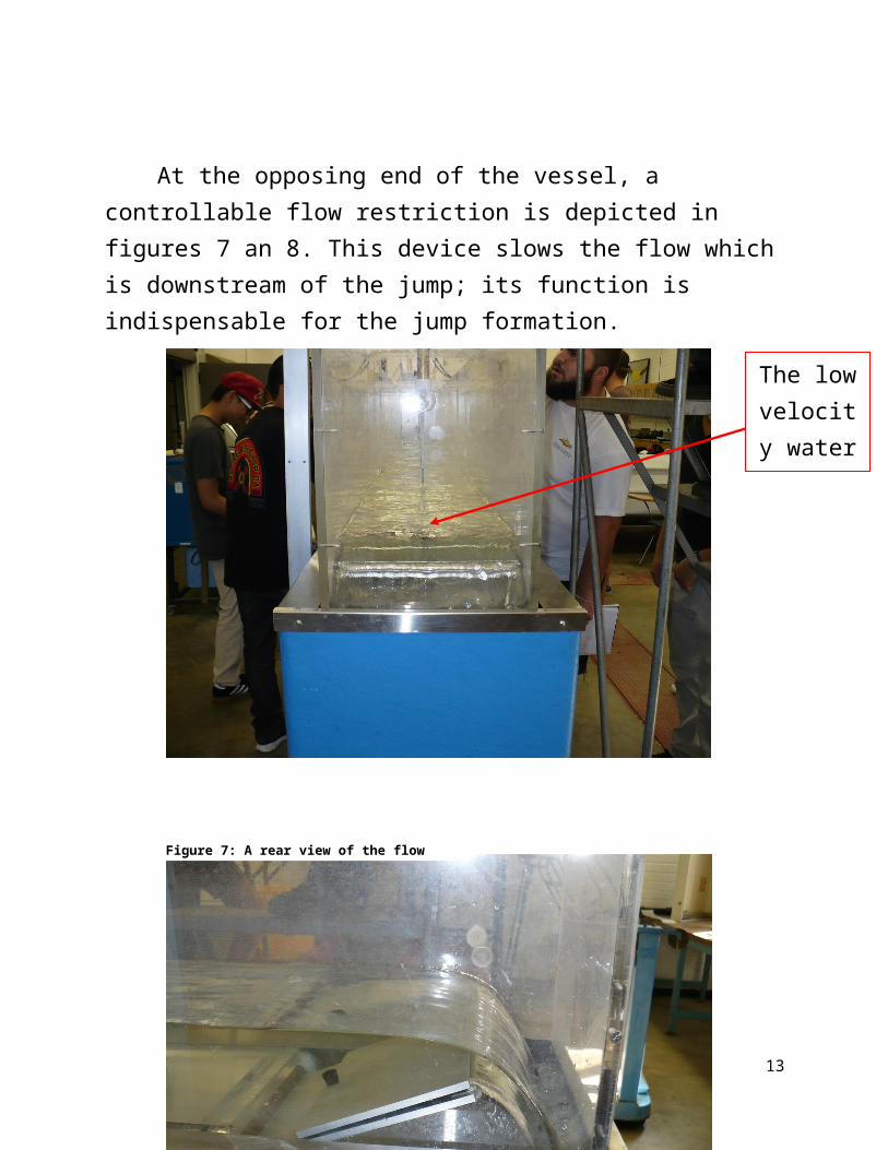
At the opposing end of the vessel, a controllable flow restriction is depicted in figures 7 an 8. This device slows the flow whichis downstream of the jump; its function is indispensable for the jump formation.

13

Figure 7: A rear view of the flow restrictor in action

The lowvelocity waterflow

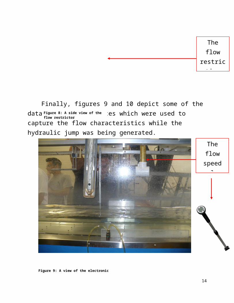
Finally, figures 9 and 10 depict some of the data acquisition devices which were used to capture the flow characteristics while the hydraulic jump was being generated.

14

Figure 8: A side view of the flow restrictor

Theflow

restriction

Theflowspeed

analyze

Figure 9: A view of the electronic water speed sensor

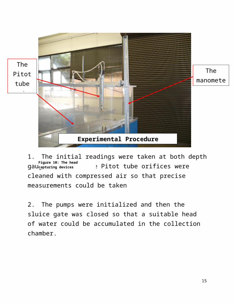
1. The initial readings were taken at both depthgauges and then the Pitot tube orifices were cleaned with compressed air so that precise measurements could be taken

2. The pumps were initialized and then the sluice gate was closed so that a suitable head of water could be accumulated in the collection chamber.

15

ThePitottubesystem

Themanomete

Figure 10: The head capturing devices

Experimental Procedure

3. When an adequate head of water had been accumulated in the collection chamber, the sluice gate was opened.

4. The flow restrictor’s angle was adjusted until a good hydraulic jump could be induced in the vessel’s main channel.

5. The depth of the flow (upstream and downstream from the jump) was recorded with the depth gauges.

6. The main manometer (pump side) was read and the data was recorded so that a flow quantity could be determined.

7. The static and dynamic pressures were recorded upstream from the jump with the Pitot tube as was the speed downstream from the jump using the electronic speed sensor.

16

8. The run was over. The head in the collection chamber was lowered by changing the sluice gate opening and steps 3-7 were

Run 1 2 3 4 5 6 7 8∆h Pump #1Manometer

(ft)0.96 0.93 0.94 0.91 0.93 0.96 0.95 0.96

QM Pump #1from chart**(lit/min)

340 320 330 300 320 340 335 345

QM Pump #1converted(ft3/sec)

0.200

0.188

0.194

0.177

0.188

0.200

0.197 0.200

∆h Pump #2Manometer

(ft)1.36 1.31 1.27 1.25 1.32 1.32 1.27 1.33

QM Pump #2from chart**(lit/min)

430 410 400 390 410 410 400 420

QM Pump #2converted(ft3/sec)

0.253

0.241

0.235

0.230

0.241

0.241

0.235 0.247

QM Total PumpOutput

(ft3/sec)

0.453

0.429

0.429

0.407

0.429

0.441

0.432 0.447

∆h1 UpstreamPitot

(inches)

6.800

8.500

8.400

8.400

8.200

7.900

7.700 7.500

V2 DowstreamJump

Digital Probe(ft/sec)

0.850

0.920

1.020

1.020

1.050

1.020

1.080 1.050

17

**Note: The pump QM values are based on the flume data chart. They were obtained using the ∆hactual that were acquired on the manometers. The chart converted these values to volumetric flow in liters per minute – these were then convertedto ft3 per second.

The actual volumetric flow rate was obtained on the conversion chart which is located on the flume body.

Since ∆h2 PUMP 1 = 0.94 ft, the chart provides an equivalency of 330 liters per minute. This value converted to the English system means thatQM PUMP 1 = 0.194 ft3/second.

Since ∆h2 PUMP 2 = 1.27 ft, the chart provides an equivalency of 400 liters per minute. This

value converted to the English system means thatQM PUMP 2 = 0.235 ft3/second.

18

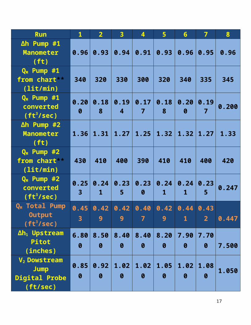
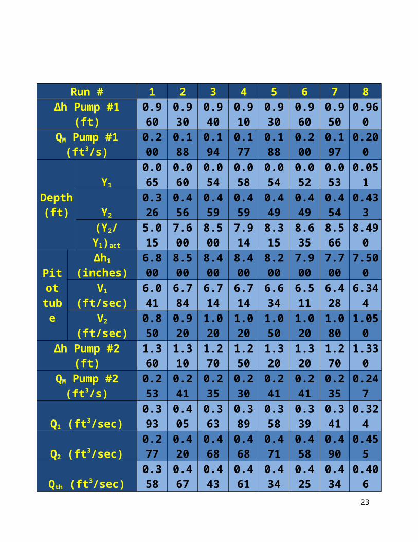
Raw Data TableBelow, table 1 depicts the actual state of the

working water for the experiment. SI values have been converted to US standards.

Sample Calculations

* Note: Below, the calculations to all the data that is in the

Table 1: The experimental data that was acquired

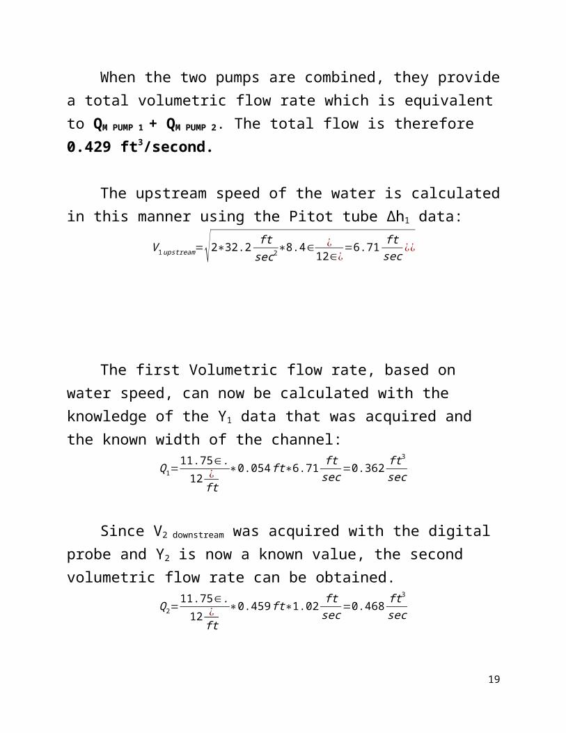
When the two pumps are combined, they providea total volumetric flow rate which is equivalentto QM PUMP 1 + QM PUMP 2. The total flow is therefore 0.429 ft3/second.

The upstream speed of the water is calculatedin this manner using the Pitot tube ∆h1 data:

V1upstream=√2∗32.2 ftsec2

∗8.4∈ ¿12∈¿

=6.71 ftsec ¿¿

The first Volumetric flow rate, based on water speed, can now be calculated with the knowledge of the Y1 data that was acquired and the known width of the channel:

Q1=11.75∈.12 ¿

ft∗0.054ft∗6.71 ft

sec=0.362 ft3sec

Since V2 downstream was acquired with the digital probe and Y2 is now a known value, the second volumetric flow rate can be obtained.

Q2=11.75∈.12 ¿

ft∗0.459ft∗1.02 ft

sec=0.468 ft3sec

19

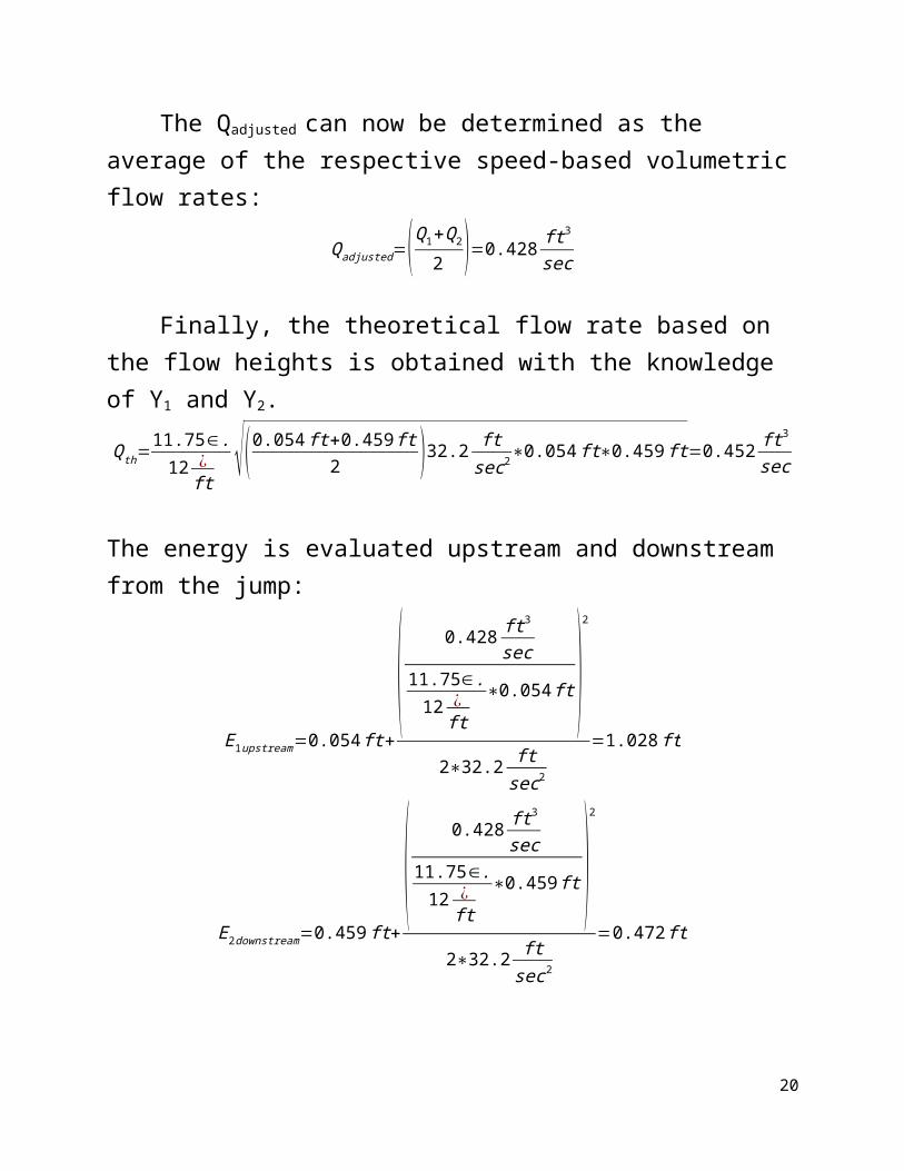
The Qadjusted can now be determined as the average of the respective speed-based volumetricflow rates:

Qadjusted=(Q1+Q2

2 )=0.428 ft3sec

Finally, the theoretical flow rate based on the flow heights is obtained with the knowledge of Y1 and Y2.

Qth=11.75∈.12 ¿

ft √(0.054ft+0.459ft2 )32.2 ft

sec2∗0.054ft∗0.459ft=0.452 ft3

sec

The energy is evaluated upstream and downstream from the jump:

E1upstream=0.054ft+

( 0.428 ft3

sec11.75∈.12 ¿

ft∗0.054ft )

2

2∗32.2 ftsec2

=1.028ft

E2downstream=0.459ft+( 0.428 ft3

sec11.75∈.12 ¿

ft∗0.459ft )

2

2∗32.2 ftsec2

=0.472ft

20

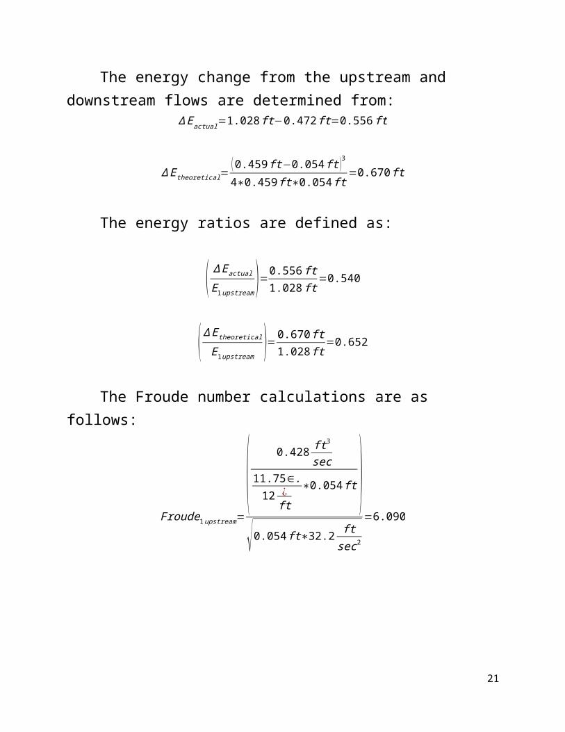
The energy change from the upstream and downstream flows are determined from:

∆Eactual=1.028ft−0.472ft=0.556ft

∆Etheoretical=(0.459ft−0.054ft)3

4∗0.459ft∗0.054ft=0.670ft

The energy ratios are defined as:

( ∆Eactual

E1upstream )=0.556ft1.028ft

=0.540

(∆Etheoretical

E1upstream )=0.670ft1.028ft

=0.652

The Froude number calculations are as follows:

Froude1upstream=( 0.428 ft3

sec11.75∈.12 ¿

ft∗0.054ft )

√0.054ft∗32.2 ftsec2

=6.090

21

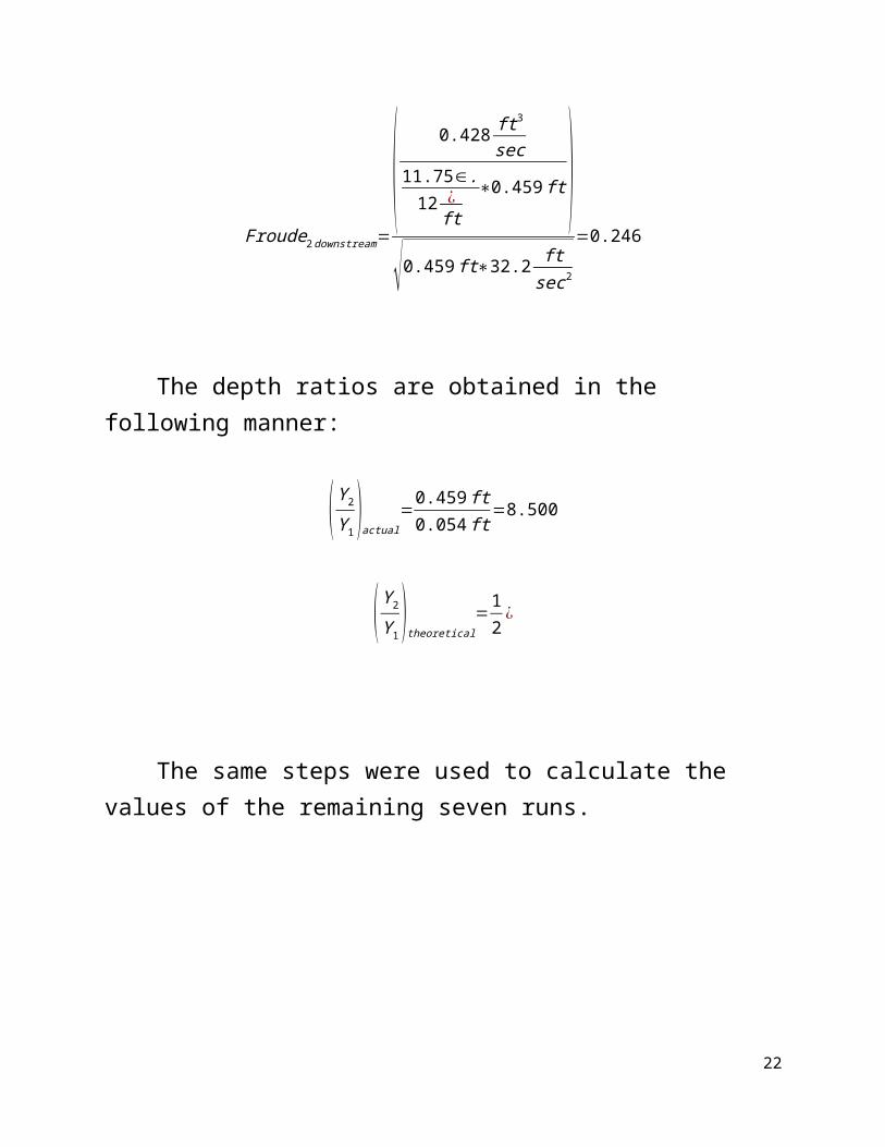
Froude2downstream=( 0.428 ft3

sec11.75∈.12 ¿

ft∗0.459ft )

√0.459ft∗32.2 ftsec2

=0.246

The depth ratios are obtained in the following manner:

(Y2

Y1)actual=0.459ft

0.054ft=8.500

(Y2

Y1)theoretical=1

2¿

The same steps were used to calculate the values of the remaining seven runs.

22

Run # 1 2 3 4 5 6 7 8∆h Pump #1

(ft)0.960

0.930

0.940

0.910

0.930

0.960

0.950

0.960

QM Pump #1(ft3/s)

0.200

0.188

0.194

0.177

0.188

0.200

0.197

0.200

Depth(ft)

Y1

0.065

0.060

0.054

0.058

0.054

0.052

0.053

0.051

Y2

0.326

0.456

0.459

0.459

0.449

0.449

0.454

0.433

(Y2/Y1)act

5.015

7.600

8.500

7.914

8.315

8.635

8.566

8.490

Pitottube

∆h1

(inches)6.800

8.500

8.400

8.400

8.200

7.900

7.700

7.500

V1

(ft/sec)6.041

6.784

6.714

6.714

6.634

6.511

6.428

6.344

V2

(ft/sec)0.850

0.920

1.020

1.020

1.050

1.020

1.080

1.050

∆h Pump #2(ft)

1.360

1.310

1.270

1.250

1.320

1.320

1.270

1.330

QM Pump #2(ft3/s)

0.253

0.241

0.235

0.230

0.241

0.241

0.235

0.247

Q1 (ft3/sec)0.393

0.405

0.363

0.389

0.358

0.339

0.341

0.324

Q2 (ft3/sec)0.277

0.420

0.468

0.468

0.471

0.458

0.490

0.455

Qth (ft3/sec)0.358

0.467

0.443

0.461

0.434

0.425

0.434

0.40623

Qadj (ft3/sec)0.342

0.431

0.425

0.440

0.421

0.407

0.422

0.395

(Y2/ Y1)theo

4.784

6.973

8.127

7.524

8.058

8.254

8.310

8.239

EnergyHead E1 (ft)

0.496

0.859

1.014

0.950

0.999

1.004

1.036

0.982

E2 (ft)0.343

0.470

0.472

0.473

0.463

0.462

0.467

0.446

EnergyChange ∆Ea (ft)

0.153

0.390

0.542

0.476

0.536

0.542

0.568

0.536

∆ET (ft)0.210

0.567

0.670

0.606

0.635

0.670

0.670

0.631

EnergyRatios ∆Ea / E1

0.308

0.453

0.534

0.502

0.537

0.540

0.549

0.546

∆ET / E1

0.423

0.660

0.661

0.638

0.636

0.667

0.647

0.643

FroudeNumber Fr1

3.719

5.272

6.090

5.663

6.041

6.180

6.220

6.169

Fr2

0.331

0.252

0.246

0.254

0.252

0.244

0.248

0.249

Specific

Force(ft2)

F1 upstream

0.190

0.212

0.210

0.210

0.207

0.204

0.201

0.198

F2

downstream

0.080

0.133

0.137

0.137

0.133

0.132

0.137

0.126

24

Complete Data Table

Below, table 2 provides all the results that wererequired to populate the table on page 41 of the labmanual.

Table 2: The experiment’s data

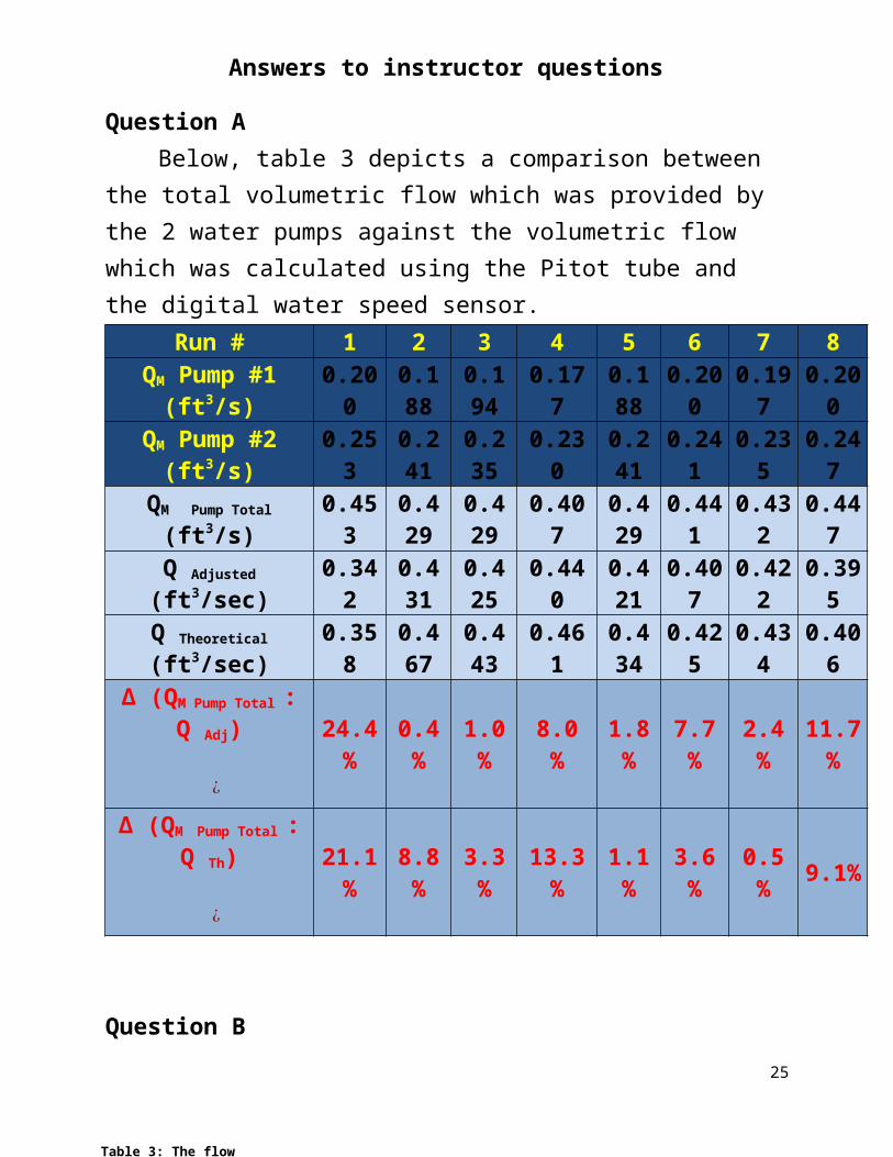
Question ABelow, table 3 depicts a comparison between

the total volumetric flow which was provided by the 2 water pumps against the volumetric flow which was calculated using the Pitot tube and the digital water speed sensor.

Run # 1 2 3 4 5 6 7 8QM Pump #1(ft3/s)

0.200

0.188

0.194

0.177

0.188

0.200

0.197

0.200

QM Pump #2(ft3/s)

0.253

0.241

0.235

0.230

0.241

0.241

0.235

0.247

QM Pump Total

(ft3/s)0.453

0.429

0.429

0.407

0.429

0.441

0.432

0.447

Q Adjusted

(ft3/sec)0.342

0.431

0.425

0.440

0.421

0.407

0.422

0.395

Q Theoretical

(ft3/sec)0.358

0.467

0.443

0.461

0.434

0.425

0.434

0.406

∆ (QM Pump Total :Q Adj)

¿

24.4%

0.4%

1.0%

8.0%

1.8%

7.7%

2.4%

11.7%

∆ (QM Pump Total :Q Th)

¿

21.1%

8.8%

3.3%

13.3%

1.1%

3.6%

0.5% 9.1%

Question B25

Answers to instructor questions

Table 3: The flow

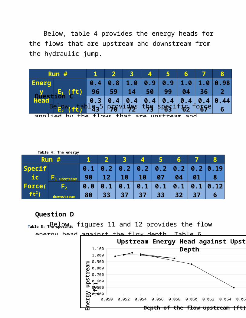
Below, table 4 provides the energy heads for the flows that are upstream and downstream from the hydraulic jump.

Run # 1 2 3 4 5 6 7 8Energy

HeadE1 (ft)

0.496

0.859

1.014

0.950

0.999

1.004

1.036

0.982

E2 (ft)0.343

0.470

0.472

0.473

0.463

0.462

0.467

0.446

Run # 1 2 3 4 5 6 7 8Specific

Force(ft2)

F1 upstream

0.190

0.212

0.210

0.210

0.207

0.204

0.201

0.198

F2

downstream

0.080

0.133

0.137

0.137

0.133

0.132

0.137

0.126

26

Question CBelow, table 5 provides the specific force

applied by the flows that are upstream and

Question DBelow, figures 11 and 12 provides the flow

energy head against the flow depth. Table 6

Table 4: The energyheads

Table 5: The specific force data

0.050 0.052 0.054 0.056 0.058 0.060 0.062 0.064 0.066 0.0680.4000.5000.6000.7000.8000.9001.0001.100

Upstream Energy Head against Upstream Depth

Depth of the flow upstream (ft) Ener

gy u

pstr

eam

(ft)

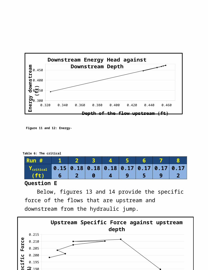
Run # 1 2 3 4 5 6 7 8Ycritical

(ft)0.156

0.182

0.180

0.184

0.179

0.175

0.179

0.172

Question EBelow, figures 13 and 14 provide the specific

force of the flows that are upstream and downstream from the hydraulic jump.

27

Figure 11 and 12: Energy- depth analysis

Table 6: The critical depth data

0.320 0.340 0.360 0.380 0.400 0.420 0.440 0.4600.300

0.350

0.400

0.450

Downstream Energy Head against Downstream Depth

Depth of the flow upstream (ft) Ener

gy d

owns

trea

m (f

t)

0.050 0.052 0.054 0.056 0.058 0.060 0.062 0.064 0.066 0.0680.175

0.180

0.185

0.190

0.195

0.200

0.205

0.210

0.215

Upstream Specific Force against upstream depth

Depth of the flow upstream (ft) Upst

ream

Spe

cifi

c Fo

rce

(ft2

)

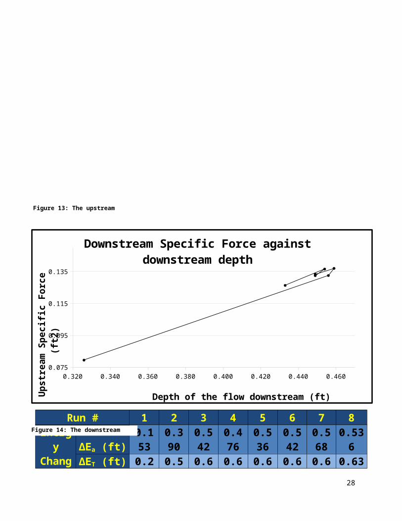
Run # 1 2 3 4 5 6 7 8Energy

Chang∆Ea (ft)

0.153

0.390

0.542

0.476

0.536

0.542

0.568

0.536

∆ET (ft) 0.2 0.5 0.6 0.6 0.6 0.6 0.6 0.6328

Figure 13: The upstream specific force

Figure 14: The downstream specific force

0.050 0.052 0.054 0.056 0.058 0.060 0.062 0.064 0.066 0.0680.175

0.180

0.185

0.190

0.195

0.200

0.205

0.210

0.215

Upstream Specific Force against upstream depth

Depth of the flow upstream (ft) Upst

ream

Spe

cifi

c Fo

rce

(ft2

)

0.320 0.340 0.360 0.380 0.400 0.420 0.440 0.4600.075

0.095

0.115

0.135

Downstream Specific Force against downstream depth

Depth of the flow downstream (ft) Upstream Specific Force

(ft2)

10 67 70 06 35 70 70 1

Run # 1 2 3 4 5 6 7 8Energy

Ratios

∆Ea / E1

0.308

0.453

0.534

0.502

0.537

0.540

0.549

0.546

∆ET / E1

0.423

0.660

0.661

0.638

0.636

0.667

0.647

0.643

DepthRatios

(Y2/Y1)act

5.015

7.600

8.500

7.914

8.315

8.635

8.566

8.490

(Y2/Y1)theo

4.784

6.973

8.127

7.524

8.058

8.254

8.310

8.239

29

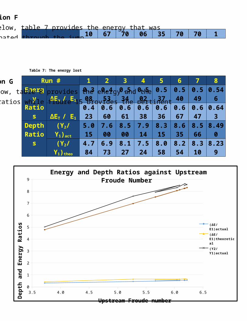
Question FBelow, table 7 provides the energy that was

dissipated through the jump.

Question GBelow, table 8 provides the energy and the

depth ratios while figure 15 provides the pertinent

Table 7: The energy lost in the jump

Table 8: The pertinent

3.5 4.0 4.5 5.0 5.5 6.0 6.50

1

2

3

4

5

6

7

8

9Energy and Depth Ratios against Upstream

Froude Number

(ΔE/E1)actual(ΔE/E1)theoretical(Y2/Y1)actual

Upstream Froude numberDept

h an

d En

ergy

Rat

ios

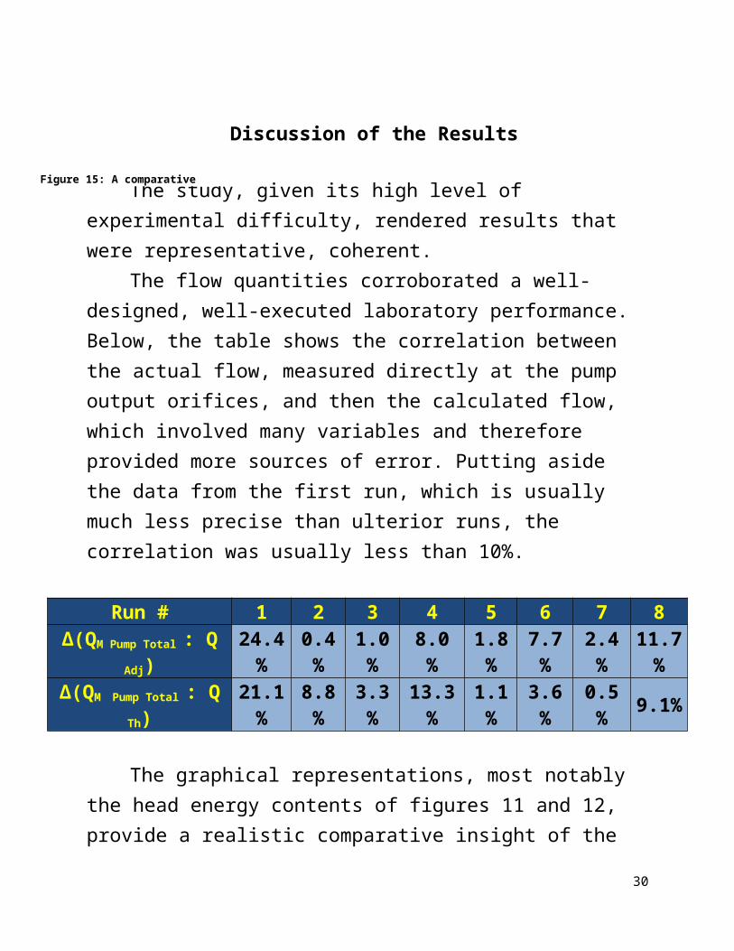
The study, given its high level of experimental difficulty, rendered results that were representative, coherent.

The flow quantities corroborated a well-designed, well-executed laboratory performance. Below, the table shows the correlation between the actual flow, measured directly at the pump output orifices, and then the calculated flow, which involved many variables and therefore provided more sources of error. Putting aside the data from the first run, which is usually much less precise than ulterior runs, the correlation was usually less than 10%.

Run # 1 2 3 4 5 6 7 8∆(QM Pump Total : Q

Adj)24.4%

0.4%

1.0%

8.0%

1.8%

7.7%

2.4%

11.7%

∆(QM Pump Total : QTh)

21.1%

8.8%

3.3%

13.3%

1.1%

3.6%

0.5% 9.1%

The graphical representations, most notably the head energy contents of figures 11 and 12, provide a realistic comparative insight of the

30

Discussion of the Results

Figure 15: A comparative ratio analysis

chaotic behavior of the high velocity, low depthupstream flow of water and the relatively calm, steady behavior of the low velocity, high depth downstream flow. The upstream head varies significantly as a result of its impact on the high depth flow.

The specific force depictions of figures 13 and 14 reinforce the chaotic behavior of the upstream flow while displaying a constant, nearly steady-state characteristics of the downstream flow.

A high degree of correlation between the theoretical data and the actual data is notable in figure 15. The energetic ratios diverged less than 20% while the depth ratios differed byless than 10%.

Inducing a hydraulic jump was shown to be a difficult task that involved several potential pitfalls. However, given Dr. El-Tawansy’s substantial experimental abilities as a laboratory scientist in conjunction with his

31

Conclusion

remarkable dexterity, it was possible to observethe phenomena with a high level of detail.

The notable difference in speed between the upstream and downstream flows, mostly constant at a 6:1 ratio, were indicative of the collisionwhich served to convert kinetic energy into potential energy. The conservation of energy principle was clearly demonstrated conceptually,with the significant elevation in water height at the velocity decrease interface, and then later analytically when the numerical analysis was performed.

There were some inhibiting experimental factors which disserved the final analysis. Notably, the depth measurements were strenuous. More precisely, the upstream flow’s height was difficult to capture given its relative compactness. It would have been interesting to see if a digital speed tester could have been used, in addition to the conventional method, and then compared in its relative efficacy.

It would be of notable interest to attempt the depth measurements, with the conventional tools, outside the vessel. A suggestion would be

32

to draw, with a permanent marker, several lines on the channel’s glass surface and then proceed with a conventional measurement.

Bibliography

1. Chu, Hsiao-ling. CE336 Fluid Mechanics Laboratory. California State University Long Beach. 1993.

2. Street, Robert, Gary Watters, and John Vernard. Elementary Fluid Mechanics. New York:John Wiley & Sons, Inc., 1996.

33