Protection contre les courts-circuits des réseaux à courant ...
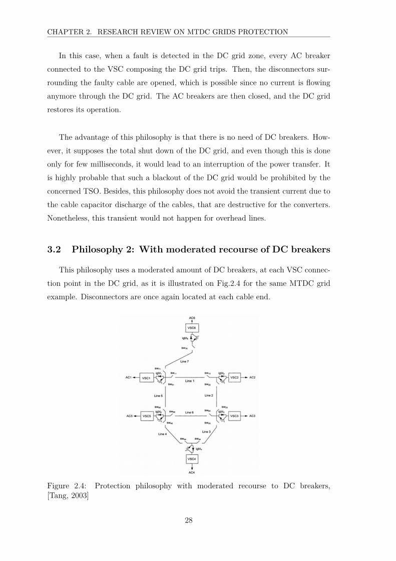
317
HAL Id: tel-00933263 https://tel.archives-ouvertes.fr/tel-00933263v2 Submitted on 24 Feb 2014 HAL is a multi-disciplinary open access archive for the deposit and dissemination of sci- entific research documents, whether they are pub- lished or not. The documents may come from teaching and research institutions in France or abroad, or from public or private research centers. L’archive ouverte pluridisciplinaire HAL, est destinée au dépôt et à la diffusion de documents scientifiques de niveau recherche, publiés ou non, émanant des établissements d’enseignement et de recherche français ou étrangers, des laboratoires publics ou privés. Protection contre les courts-circuits des réseaux à courant continu de forte puissance Justine Descloux To cite this version: Justine Descloux. Protection contre les courts-circuits des réseaux à courant continu de forte puissance. Autre. Université de Grenoble, 2013. Français. NNT: 2013GRENT044. tel-00933263v2
-
Upload
khangminh22 -
Category
Documents
-
view
2 -
download
0
Transcript of Protection contre les courts-circuits des réseaux à courant ...
HAL Id: tel-00933263https://tel.archives-ouvertes.fr/tel-00933263v2
Submitted on 24 Feb 2014
HAL is a multi-disciplinary open accessarchive for the deposit and dissemination of sci-entific research documents, whether they are pub-lished or not. The documents may come fromteaching and research institutions in France orabroad, or from public or private research centers.
L’archive ouverte pluridisciplinaire HAL, estdestinée au dépôt et à la diffusion de documentsscientifiques de niveau recherche, publiés ou non,émanant des établissements d’enseignement et derecherche français ou étrangers, des laboratoirespublics ou privés.
Protection contre les courts-circuits des réseaux àcourant continu de forte puissance
Justine Descloux
To cite this version:Justine Descloux. Protection contre les courts-circuits des réseaux à courant continu de forte puissance.Autre. Université de Grenoble, 2013. Français. NNT : 2013GRENT044. tel-00933263v2
THÈSEPour obtenir le grade de
DOCTEUR DE L’UNIVERSITÉ DE GRENOBLESpécialité : Génie Électrique
Arrêté ministériel : 7 août 2006
Présentée par
Justine DESCLOUX
Thèse dirigée par Bertrand RAISONet codirigée par Jean-Baptiste CURIS
préparée au sein du Laboratoire de Génie Électrique de Grenoble (G2Elab)
dans l’École Doctorale Électronique, Électrotechnique, Automatique et
Traitement du Signal
Protection contre les courts-circuits desréseaux à courant continu de forte puissance
THÈSE SOUTENUE PUBLIQUEMENT LE 20 septembre 2013,
DEVANT LE JURY COMPOSÉ DE :
M. Jean-Claude MAUNProfesseur, École Polytechnique de Bruxelles Rapporteur
M. Mario PAOLONEProfesseur, École Polytechnique Fédérale de Lausanne Rapporteur
Mme. Anne-Marie DENISIngénieur, RTE Examinateur
M. Stephen FINNEYProfesseur, University of Strathclyde Examinateur
M. Wolfgang GRIESHABERDocteur, Alstom Grid Examinateur
M. Xavier GUILLAUDProfesseur, École Centrale de Lille Examinateur
M. Jean-Baptiste CURISIngénieur, RTE Encadrant
M. Bertrand RAISONProfesseur, Université de Grenoble Directeur

Remerciements
Mes premiers remerciements vont à toi Bertrand, qui a dirigé cette thèse en
apportant toute l’originalité dont tu disposes dans le monde bien carré du contrôle
commande des réseaux électriques. En plus de ton investissement incontestable dans
ces travaux et de ton encadrement au jour le jour, ce malgré tes responsabilités ad-
ministratives, je te remercie aussi pour l’immense réconfort que tu m’as apporté
lors des phases où la pertinence des résultats de simulations n’était pas évidente à
appréhender seule. Merci de t’être adapté à mes déplacements de fin de rédaction
jusqu’à effectuer les dernières corrections de ce manuscrit par mail et directement
dans les .tex. J’ai été ravie de travailler avec toi pendant ces trois années, mais aussi
de discuter météo montagne, skitour, cuisine (à caractère digeste ou non) ou autre
sujet hors cadre avec toi en partageant un café, et de découvrir tes lectures on ne
peut plus inattendues lors des déplacements en train. Mille mercis !
Merci Jean-Baptiste d’avoir suivi assidûment ces travaux et apporté l’expérience
des réseaux réels. Merci de t’être déplacé à Grenoble pour chaque réunion, et d’avoir
maintenu un regard critique même après ton changement de poste. Merci aussi pour
tes messages de soutien chaleureux dans les dernières lignes droites, qui m’ont aidés
à garder le cap.
Je remercie Xavier Guillaud d’avoir accepté de présider le jury de cette thèse,
ainsi que les rapporteurs, Jean-Claude Maun et Mario Paolone, pour la rapidité avec
laquelle ils ont lu mon manuscrit et l’intérêt qu’ils ont porté à mon travail.
Merci également aux autres membres du jury qui ont accepté de juger ce travail:
Anne-Marie Denis, Stephen Finney et Wolfgang Grieshaber, pour leurs apports,
leurs commentaires sur le manuscrit et les questions qu’ils ont posées lors de la sou-
iii

REMERCIEMENTS
tenance.
J’associe à ces remerciements l’ensemble du personnel du G2Elab: direction,
personnels administratifs, techniques, enseignants et chercheurs avec qui j’ai eu
l’occasion de discuter ou simplement pour leurs bonjours souriants qui participent à
l’aura de bonne humeur générale du labo. Merci particulièrement aux membres de
l’équipe Syrel pour leurs éclaircissements sur des questions techniques ou pratiques,
à Camille pour les travaux communs sur les limiteurs de courant supraconducteurs,
ainsi qu’à Delphine, Daniel et Lauric pour avoir partagé les encadrements de TP.
Je remercie également toutes les personnes de RTE qui ont suivi ces travaux
dans le cadre du projet Twenties, et surtout Anne-Marie Denis, Olivier Despouys,
Samuel Nguefeu et Jean-Pierre Taisne pour les échanges que nous avons eu et leur
expertise sur le domaine du transport d’électricité en courant continu.
Je remercie Pierre Rault pour les échanges sur notre sujet commun, et pour le
support EMTP-rv ! Sans toi je me serais arrachée les cheveux bien de nombreuses
fois à cause des changements de version du logiciel. Je te souhaite tout le courage
qu’il faut pour les dernières lignes de ton manuscrit et ta soutenance.
Merci à toutes les personnes du L2EP de m’avoir accueillie dans leur laboratoire
de Lille pour réaliser les tests sur le démonstrateur Twenties, et en particulier à
Fred, Hicham et Sid qui ont travaillé très dur sur cette maquette.
Je remercie Jean Mahseredjian et Sébastien Dennetière pour leur aide et les
réponses qu’ils ont apportées à mes questions de modélisation des câbles.
Aussi, j’aimerais remercier mes amis et ma famille, toutes les personnes auxquelles
je pense évidemment quand je me remémore ces trois ans.
Un immense merci à Jean-Louis, avec qui j’ai partagé le même bureau, les week
ends et les soirées, les déprimes et les rigolades. Merci pour tout ton réconfort et ton
écoute quand il fallait. Merci d’avoir fabriqué le petit vélo blanc qui m’accompagnait
sur tous mes trajets de dernière année (oui, sauf quand il pleut ou qu’il neige ou
iv

REMERCIEMENTS
qu’il fait froid), merci de regarder aux mêmes endroits quand on est assis à côté,
merci d’être mon ami même si j’habite à Paris !
Merci à Rémi de m’avoir transformée en skieuse de poudreuse, de m’avoir ap-
pris à mettre des crampons et à utiliser un piolet, de m’avoir forcée à courir autour
de chaque massif sous des trombes d’eau et de monter 2000m de dev avec 30 kg
sur le dos, et de savoir expliquer n’importe quel principe d’électrotechnique (voire
astrophysique) sauf comment fonctionnent les protections. Merci à Titouan pour
les ateliers peinture collectifs et fartage de ski, merci à Archie de s’intéresser à la
mode et de ne pas se laisser aller sous la dictature des GrenobleX en GoreTex, merci
à Raph d’être exactement le contraire pour créer le débat, merci à Teu pour les
soirées à l’ouest ou autres échanges sans fin dans les maisons lilloises. Merci Imane
de m’avoir prêté ton lit quand mon appartement était rempli de cafards, merci Tim
et Anto pour les sorties grosse popo et au hazard. Merci Isa, Néné, Aurélien, les
deux Xaviers et tous les autres jojos parisiens de m’avoir fait croire pendant trois
ans que vous étiez d’accord avec moi sur le fait que, une thèse, c’est un vrai travail,
et de m’avoir malgré tout prévenue que je serai fatiguée les premiers mois à Paris.
Merci à Luce d’avoir cusiné une semaine pour faire le meilleur pot de thèse, et merci
aussi à Anna, Célia et Zazou pour toute leur aide.
Merci Gaspard pour ta manière unique de construire des phrases exclusivement
composées d’acronymes ou de mots anglais, peu importe le sujet, mais surtout merci
d’oublier de temps en temps la rationalité et de me faire partager toutes tes qualités
dont je ne ferai pas la liste ici.
À ma soeur Caro, merci de lutter contre la déformation professionnelle et de ne
pas te focaliser uniquement sur le gaz en me posant des questions sur le transport
d’électricité, et merci de m’avoir donné un peu de ton expérience sur les entreprises
de la branche IEG. Merci à mon frère/beau-frère Bertrand de pousser l’esthétisme
jusque dans les power point (qui sont, je le sais, passés de mode). Merci à vous
deux d’être aussi mes amis, et de m’avoir logée nourrie et blanchie chez vous, dans
des petits appartements ou des grandes maisons, avant chacune de mes réunions à
Paris et toutes les autres fois. À ma soeur Élo, merci de m’avoir permis de rédiger
les dernières lignes de ce manuscrit sur une île paradisiaque et d’avoir fait tomber
v

REMERCIEMENTS
le stress de la dernière ligne droite en me prêtant ton paddle sur l’îlot Tenia !
Merci à toi maman pour toutes tes petites attentions poétiques qui réchauffent,
pour tous ces albums-photos-historiques que tu crées à chaque évènement afin de
se souvenir des bons moments. Merci à toi papa pour tes conseils et ton avis tou-
jours bien tranché, merci d’adapter ton organisation sans faille quand je suis là alors
que tu détestes l’incertitude, de t’attendrir malgré ton (mon) caractère sanguin, par
amour et confiance masquée, que tu ne dévoiles qu’aux moments opportuns. Merci
à vous deux pour cette proximité qui n’a pas besoin de mots pour s’installer.
Merci enfin à tous ceux qui sont venus le 20 septembre 2013 à Grenoble écouter
cette soutenance et célébrer la fin de ces trois ans avec moi.
vi

REMERCIEMENTS
vii

Contents
Remerciements . . . . . . . . . . . . . . . . . . . . . . . . . . . . . . . . . iii
Contents . . . . . . . . . . . . . . . . . . . . . . . . . . . . . . . . . . . . . ix
List of Figures . . . . . . . . . . . . . . . . . . . . . . . . . . . . . . . . . . xv
List of Tables . . . . . . . . . . . . . . . . . . . . . . . . . . . . . . . . . . xxi
General introduction 1
1 Relevance of HVDC applications and thesis objectives 9
1 Development of HVDC links . . . . . . . . . . . . . . . . . . . . . . . 9
2 General operation of HVDC links . . . . . . . . . . . . . . . . . . . . 11
2.1 Possible HVDC link structures . . . . . . . . . . . . . . . . . . 12
2.2 HVDC links currently under operation in Europe and planed
installations . . . . . . . . . . . . . . . . . . . . . . . . . . . . 14
3 New conversion technologies . . . . . . . . . . . . . . . . . . . . . . . 15
2 Research review on MTDC grids protection 23
1 HVDC link behiavior under fault conditions . . . . . . . . . . . . . . 23
1.1 Fault phenomenon . . . . . . . . . . . . . . . . . . . . . . . . 23
1.2 Protection system components . . . . . . . . . . . . . . . . . . 24
2 Overall behavior of a HVDC link under fault conditions . . . . . . . . 25
2.1 Traveling wave propagation . . . . . . . . . . . . . . . . . . . 26
2.2 MTDC grid protection difficulties . . . . . . . . . . . . . . . . 27
3 Possible protection strategies . . . . . . . . . . . . . . . . . . . . . . . 27
3.1 Philosophy 1: Without recourse of DC breakers . . . . . . . . 27
3.2 Philosophy 2: With moderated recourse of DC breakers . . . . 28
3.3 Philosophy 3: With full use of DC breakers . . . . . . . . . . . 29
4 Current breaking technology . . . . . . . . . . . . . . . . . . . . . . . 30
4.1 Electrical arc phenomenon . . . . . . . . . . . . . . . . . . . . 30
ix
CONTENTS
4.2 Research state on DC breaker . . . . . . . . . . . . . . . . . . 31
4.2.1 Mechanical breakers . . . . . . . . . . . . . . . . . . 31
4.2.2 Power-electronic breakers . . . . . . . . . . . . . . . 33
4.3 Hybrid breakers . . . . . . . . . . . . . . . . . . . . . . . . . . 34
5 Review of protection principles found in anterior works . . . . . . . . 36
5.1 Use of DC breakers . . . . . . . . . . . . . . . . . . . . . . . . 36
5.2 Review of protection principles found in anterior works . . . . 37
5.2.1 Overcurrent and undervoltage protections . . . . . . 37
5.2.2 Differential current protection . . . . . . . . . . . . . 37
5.2.3 Current and voltage derivatives . . . . . . . . . . . . 38
5.2.4 Distance protection using traveling wave propaga-
tion theory . . . . . . . . . . . . . . . . . . . . . . . 38
6 Thesis objectives . . . . . . . . . . . . . . . . . . . . . . . . . . . . . 40
3 MTDC network components and grid test modeling 45
1 Conducting cables . . . . . . . . . . . . . . . . . . . . . . . . . . . . . 46
1.1 Cable composition . . . . . . . . . . . . . . . . . . . . . . . . 46
1.2 Line theory reminder . . . . . . . . . . . . . . . . . . . . . . . 48
1.3 Frequency domain models . . . . . . . . . . . . . . . . . . . . 51
1.4 Time-domain models . . . . . . . . . . . . . . . . . . . . . . . 53
1.4.1 Localized-parameters models . . . . . . . . . . . . . 53
1.4.2 Distributed-parameters models . . . . . . . . . . . . 54
1.4.3 Cable structure modeling . . . . . . . . . . . . . . . 57
1.4.4 Cable parameters choice . . . . . . . . . . . . . . . . 58
1.4.5 Cable model behavior . . . . . . . . . . . . . . . . . 60
2 AC side and substations . . . . . . . . . . . . . . . . . . . . . . . . . 66
2.1 AC/DC conversion . . . . . . . . . . . . . . . . . . . . . . . . 66
2.1.1 EMTP-rv VSC components model . . . . . . . . . . 66
2.1.2 VSC control strategy . . . . . . . . . . . . . . . . . . 67
2.2 AC producers and AC grid . . . . . . . . . . . . . . . . . . . . 69
3 Faults and protection relative components . . . . . . . . . . . . . . . 70
3.1 Fault . . . . . . . . . . . . . . . . . . . . . . . . . . . . . . . . 70
3.2 Sensors . . . . . . . . . . . . . . . . . . . . . . . . . . . . . . . 70
3.2.1 Current sensor . . . . . . . . . . . . . . . . . . . . . 71
x

CONTENTS
3.2.2 Voltage sensor . . . . . . . . . . . . . . . . . . . . . 72
3.3 DC Circuit Breaker . . . . . . . . . . . . . . . . . . . . . . . . 73
4 Studied grid structures . . . . . . . . . . . . . . . . . . . . . . . . . . 74
4.1 HVDC link . . . . . . . . . . . . . . . . . . . . . . . . . . . . 74
4.1.1 HVDC link characteristics . . . . . . . . . . . . . . . 74
4.1.2 Protection elements and notations . . . . . . . . . . 74
4.2 Twenties grid test . . . . . . . . . . . . . . . . . . . . . . . 75
4.2.1 Twenties grid test model characteristics . . . . . . 75
4.2.2 Additional protection elements . . . . . . . . . . . . 76
4 Signals behavior under fault conditions 81
1 Fault-related parameters . . . . . . . . . . . . . . . . . . . . . . . . . 83
1.1 Fault type . . . . . . . . . . . . . . . . . . . . . . . . . . . . . 83
1.2 Fault location . . . . . . . . . . . . . . . . . . . . . . . . . . . 85
1.3 Fault impedance . . . . . . . . . . . . . . . . . . . . . . . . . 87
2 Source-related parameters . . . . . . . . . . . . . . . . . . . . . . . . 88
2.1 Short-circuit power of AC sources . . . . . . . . . . . . . . . . 88
2.2 AC and DC filter . . . . . . . . . . . . . . . . . . . . . . . . . 89
2.2.1 DC capacitor . . . . . . . . . . . . . . . . . . . . . . 89
2.2.2 Smoothing reactor . . . . . . . . . . . . . . . . . . . 90
2.3 VSC control strategy . . . . . . . . . . . . . . . . . . . . . . . 91
3 Grid-related parameters . . . . . . . . . . . . . . . . . . . . . . . . . 91
3.1 Link length . . . . . . . . . . . . . . . . . . . . . . . . . . . . 91
3.2 Grid topology: number of feeders connected to a busbar . . . 92
3.3 Feeder junction . . . . . . . . . . . . . . . . . . . . . . . . . . 94
5 Protection strategy 101
1 Protection plan specification . . . . . . . . . . . . . . . . . . . . . . . 102
2 DC grid constraints . . . . . . . . . . . . . . . . . . . . . . . . . . . . 103
2.1 Grid components perturbation withstand capability . . . . . . 103
2.2 Sensitivity constraint . . . . . . . . . . . . . . . . . . . . . . . 106
2.3 Selectivity constraint . . . . . . . . . . . . . . . . . . . . . . . 107
2.4 Protection chain operation time . . . . . . . . . . . . . . . . . 108
3 Main protection . . . . . . . . . . . . . . . . . . . . . . . . . . . . . . 108
3.1 Preliminary signals analysis . . . . . . . . . . . . . . . . . . . 109
xi
CONTENTS
3.1.1 Polarity selectivity . . . . . . . . . . . . . . . . . . . 109
3.1.2 Link selectivity . . . . . . . . . . . . . . . . . . . . . 110
3.2 Possible trails . . . . . . . . . . . . . . . . . . . . . . . . . . . 112
3.3 Busbar-level communication . . . . . . . . . . . . . . . . . . . 113
3.3.1 Cable protection . . . . . . . . . . . . . . . . . . . . 113
3.3.2 Busbar protection . . . . . . . . . . . . . . . . . . . 114
3.4 Cable-level communication . . . . . . . . . . . . . . . . . . . . 115
3.4.1 Cable differential protection . . . . . . . . . . . . . . 115
3.4.2 Directional criterion protection . . . . . . . . . . . . 119
3.5 Communicant principles comparison . . . . . . . . . . . . . . 124
3.6 Non-communicative protection principle . . . . . . . . . . . . 125
3.6.1 Voltage differential protection . . . . . . . . . . . . . 125
3.6.2 Other possible trail . . . . . . . . . . . . . . . . . . . 127
3.7 Conclusion on the main protection . . . . . . . . . . . . . . . 128
4 Backup protection . . . . . . . . . . . . . . . . . . . . . . . . . . . . 128
4.1 Purpose of the backup protection . . . . . . . . . . . . . . . . 128
4.2 Multi-criterion protection . . . . . . . . . . . . . . . . . . . . 129
5 Safety of connection manoeuvres of links . . . . . . . . . . . . . . . . 134
5.1 Power transfer variation . . . . . . . . . . . . . . . . . . . . . 134
5.2 Disconnection of a link . . . . . . . . . . . . . . . . . . . . . . 134
5.3 Connection of a link . . . . . . . . . . . . . . . . . . . . . . . 134
6 Proposed protection system . . . . . . . . . . . . . . . . . . . . . . . 137
6 Protection plan validation 143
1 Complete protection plan implementation in EMTP-rv . . . . . . . . 144
1.1 Data processing . . . . . . . . . . . . . . . . . . . . . . . . . . 144
1.2 Thresholds setting determination process . . . . . . . . . . . . 145
1.2.1 Differential current . . . . . . . . . . . . . . . . . . . 145
1.2.2 Busbar differential . . . . . . . . . . . . . . . . . . . 148
1.2.3 Backup . . . . . . . . . . . . . . . . . . . . . . . . . 148
1.2.4 Safe connection verification . . . . . . . . . . . . . . 151
2 EMTP-rv results . . . . . . . . . . . . . . . . . . . . . . . . . . . . . 154
2.1 Differential current protection . . . . . . . . . . . . . . . . . . 154
2.1.1 Fault resistance influence . . . . . . . . . . . . . . . 156
xii
CONTENTS
2.1.2 Fault location influence . . . . . . . . . . . . . . . . 158
2.1.3 Worst case scenarios . . . . . . . . . . . . . . . . . . 160
2.1.4 Frequency sampling requirements . . . . . . . . . . . 162
2.1.5 Impact of synchronization error . . . . . . . . . . . . 164
2.2 Backup protection . . . . . . . . . . . . . . . . . . . . . . . . 165
2.2.1 Validity domain of the backup protection . . . . . . 168
2.3 Busbar protection . . . . . . . . . . . . . . . . . . . . . . . . . 169
2.4 Conclusion on the theoretical performances of the protection
system . . . . . . . . . . . . . . . . . . . . . . . . . . . . . . . 170
3 Real Time HIL demonstrator . . . . . . . . . . . . . . . . . . . . . . 172
3.1 Overall mock-up design and description . . . . . . . . . . . . . 173
3.1.1 Real-time simulator . . . . . . . . . . . . . . . . . . 174
3.1.2 Digital-analog interconnection . . . . . . . . . . . . . 176
3.1.3 Physical devices . . . . . . . . . . . . . . . . . . . . 177
3.2 Protection system components . . . . . . . . . . . . . . . . . . 180
3.2.1 Protection-related physical devices . . . . . . . . . . 181
3.2.2 Physical devices positioning . . . . . . . . . . . . . . 183
3.2.3 Protection relays implementation . . . . . . . . . . . 183
3.3 Demonstrator control . . . . . . . . . . . . . . . . . . . . . . . 187
3.4 Real Time HIL tests results . . . . . . . . . . . . . . . . . . . 187
3.4.1 Tests description . . . . . . . . . . . . . . . . . . . . 188
3.4.2 Test series 1 results . . . . . . . . . . . . . . . . . . . 188
3.4.3 Mock-up reconfiguration . . . . . . . . . . . . . . . . 198
3.4.4 Test series 2 results . . . . . . . . . . . . . . . . . . . 200
3.4.5 EMTP-rv study validation . . . . . . . . . . . . . . . 204
3.5 Real Time HIL demonstrator benefits . . . . . . . . . . . . . . 211
4 Current relaxation during breaker tripping action . . . . . . . . . . . 211
4.1 Incorporation of superconducting fault current limiters . . . . 212
4.1.1 SCFCL introduction . . . . . . . . . . . . . . . . . . 212
4.1.2 Simulation results . . . . . . . . . . . . . . . . . . . 214
4.2 Incorporation of feeder inductors . . . . . . . . . . . . . . . . 217
4.2.1 Inductors value choice . . . . . . . . . . . . . . . . . 218
4.2.2 Impact on the grid constraint and protections . . . . 221
4.2.3 Voltage differential protection . . . . . . . . . . . . . 222
xiii

CONTENTS
5 Conclusion on the protection system . . . . . . . . . . . . . . . . . . 226
General conclusion 231
Appendix A Protection principles 239
1 Difficulty to find non-communicant selective principles . . . . . . . . 239
2 Backup protection: other trails . . . . . . . . . . . . . . . . . . . . . 241
2.1 Frequency domain analysis protection . . . . . . . . . . . . . . 242
2.2 Complex signal-processing methods . . . . . . . . . . . . . . . 244
2.2.1 Traveling wave based protection using reflections . . 244
2.2.2 Wavelet-based protection . . . . . . . . . . . . . . . 247
Appendix B Protection plan validation 253
1 Worst case faults clearance by the backup protection . . . . . . . . . 253
2 Complete list of conducted tests on the mock-up . . . . . . . . . . . . 255
2.1 Test conducted on March, 25th 2013 . . . . . . . . . . . . . . 255
2.1.1 First test series - 3 nodes grid . . . . . . . . . . . . . 255
2.1.2 Second test series . . . . . . . . . . . . . . . . . . . . 257
2.2 Test conducted on May, 29th 2013 - Preparation of the backup
mode . . . . . . . . . . . . . . . . . . . . . . . . . . . . . . . . 257
2.2.1 Test 20 . . . . . . . . . . . . . . . . . . . . . . . . . 257
2.2.2 Test 21 . . . . . . . . . . . . . . . . . . . . . . . . . 257
2.2.3 Test 22 . . . . . . . . . . . . . . . . . . . . . . . . . 258
2.2.4 Test 23 . . . . . . . . . . . . . . . . . . . . . . . . . 258
Bibliography 263
Résumé étendu 275
xiv

List of Figures
1 Meshed grid example . . . . . . . . . . . . . . . . . . . . . . . . . . . 2
2 Twenties project features . . . . . . . . . . . . . . . . . . . . . . . . 3
1.1 Transmission capacity of HVAC and HVDC links . . . . . . . . . . . 10
1.2 HVDC link scheme . . . . . . . . . . . . . . . . . . . . . . . . . . . . 11
1.3 +U monopolar link scheme with ground return . . . . . . . . . . . . 12
1.4 ±U bipolar link scheme with grounded middle point . . . . . . . . . . 12
1.5 ±U bipolar link scheme with monopolar operation possibility . . . . . 12
1.6 ±U bipolar HVDC link with neutral conductor . . . . . . . . . . . . 13
1.7 +U1,−U2 HVDC link . . . . . . . . . . . . . . . . . . . . . . . . . . . 13
1.8 Back-to-back HVDC link scheme . . . . . . . . . . . . . . . . . . . . 14
1.9 Development of offshore wind farms in North Sea . . . . . . . . . . . 15
1.10 2-level converter . . . . . . . . . . . . . . . . . . . . . . . . . . . . . . 16
1.11 3-level converter . . . . . . . . . . . . . . . . . . . . . . . . . . . . . . 17
1.12 Half-bridge sub-module scheme . . . . . . . . . . . . . . . . . . . . . 17
1.13 MMC converter scheme . . . . . . . . . . . . . . . . . . . . . . . . . . 18
2.1 DC current and voltage behavior under fault conditions . . . . . . . . 25
2.2 Bewley Lattice diagram . . . . . . . . . . . . . . . . . . . . . . . . . 26
2.3 Protection philosophy without recourse to DC breakers . . . . . . . . 27
2.4 Protection philosophy with moderated recourse to DC breakers . . . . 28
2.5 Protection philosophy with full recourse to DC breakers . . . . . . . . 29
2.6 Passive commutation principle . . . . . . . . . . . . . . . . . . . . . . 32
2.7 Active commutation principle . . . . . . . . . . . . . . . . . . . . . . 32
2.8 Semi-conductor based breaker . . . . . . . . . . . . . . . . . . . . . . 34
2.9 Conventional hybrid method . . . . . . . . . . . . . . . . . . . . . . . 34
2.10 Hybrid method with forced commutation . . . . . . . . . . . . . . . . 35
xv
LIST OF FIGURES
2.11 Differential current . . . . . . . . . . . . . . . . . . . . . . . . . . . . 37
2.12 Examples of samples . . . . . . . . . . . . . . . . . . . . . . . . . . . 39
3.1 Cable layers arrangement example . . . . . . . . . . . . . . . . . . . . 46
3.2 Line portion . . . . . . . . . . . . . . . . . . . . . . . . . . . . . . . . 48
3.3 Π line model with 3 sections . . . . . . . . . . . . . . . . . . . . . . . 54
3.4 Cable structures . . . . . . . . . . . . . . . . . . . . . . . . . . . . . . 58
3.5 Layout of the cables . . . . . . . . . . . . . . . . . . . . . . . . . . . 59
3.6 Frequency scan response of the different structure models . . . . . . . 61
3.7 Frequency scan response of the cable models . . . . . . . . . . . . . . 61
3.8 HVDC link simulation . . . . . . . . . . . . . . . . . . . . . . . . . . 62
3.9 Steady state simulation results . . . . . . . . . . . . . . . . . . . . . . 63
3.10 HVDC link simulation . . . . . . . . . . . . . . . . . . . . . . . . . . 63
3.11 Pole-to-screen fault on the positive pole . . . . . . . . . . . . . . . . . 63
3.12 Fault simulation results . . . . . . . . . . . . . . . . . . . . . . . . . . 64
3.13 Coupling effect simulation results . . . . . . . . . . . . . . . . . . . . 65
3.14 VSC structure model . . . . . . . . . . . . . . . . . . . . . . . . . . . 67
3.15 Substation topology . . . . . . . . . . . . . . . . . . . . . . . . . . . . 68
3.16 AC side model . . . . . . . . . . . . . . . . . . . . . . . . . . . . . . . 69
3.17 Current sensor influence on the measured signal . . . . . . . . . . . . 72
3.18 Voltage sensor influence on the measured signal . . . . . . . . . . . . 73
3.19 DC Circuit Breaker model . . . . . . . . . . . . . . . . . . . . . . . . 73
3.20 HVDC link test model . . . . . . . . . . . . . . . . . . . . . . . . . . 74
3.21 Protection elements arrangement . . . . . . . . . . . . . . . . . . . . 75
3.22 Twenties grid test model . . . . . . . . . . . . . . . . . . . . . . . . 76
4.1 HVDC link test case . . . . . . . . . . . . . . . . . . . . . . . . . . . 82
4.2 Behavior of the grid in fault conditions . . . . . . . . . . . . . . . . . 83
4.3 Fault types . . . . . . . . . . . . . . . . . . . . . . . . . . . . . . . . 83
4.4 Fault types . . . . . . . . . . . . . . . . . . . . . . . . . . . . . . . . 84
4.5 Fault location parameter on the HVDC link test model . . . . . . . . 85
4.6 Signals measured at left cable end for several fault locations . . . . . 86
4.7 Zoom on the reflections for the case Cpos−2 . . . . . . . . . . . . . . . 87
4.8 Signals measured at left cable end for several fault impedances . . . . 88
4.9 DC filter and parameters . . . . . . . . . . . . . . . . . . . . . . . . . 89
xvi
LIST OF FIGURES
4.10 Signals measured at left cable end for several DC capacitor values . . 90
4.11 Signals measured at left cable end for several DC inductor values . . 91
4.12 Current measurements for several link lengths . . . . . . . . . . . . . 92
4.13 Grid topologies simulated to study the influence of the number of
feeders connected to a busbar . . . . . . . . . . . . . . . . . . . . . . 93
4.14 Current measurements . . . . . . . . . . . . . . . . . . . . . . . . . . 93
4.15 Current measurements . . . . . . . . . . . . . . . . . . . . . . . . . . 94
4.16 Feeder inductors location . . . . . . . . . . . . . . . . . . . . . . . . . 94
4.17 Simulation of a fault on the Twenties grid structure . . . . . . . . . 95
4.18 Current I21 . . . . . . . . . . . . . . . . . . . . . . . . . . . . . . . . 95
5.1 HVDC link simulation under default fault conditions . . . . . . . . . 103
5.2 Current flowing through the diodes of station 1 . . . . . . . . . . . . 104
5.3 Diode constraint for several fault locations on HVDC link test case . 104
5.4 Current measurements at DC cables end for fault case Cpos−3 . . . . . 105
5.5 Time-line of the fault clearing process . . . . . . . . . . . . . . . . . . 108
5.6 Current measurement at PR13+ and PR13− for Cint . . . . . . . . . . 110
5.7 Measurements at PR13+ for an internal and an external fault . . . . . 110
5.8 Current and voltage derivatives at PR13+ for Cint and Cext . . . . . . 111
5.9 Communication strategies . . . . . . . . . . . . . . . . . . . . . . . . 113
5.10 Busbar fault illustration . . . . . . . . . . . . . . . . . . . . . . . . . 114
5.11 Data propagation delay on the differential current . . . . . . . . . . . 116
5.12 Transient behavior of the cable differential current . . . . . . . . . . . 117
5.13 Transient behavior of the current derivatives at each end of a cable . 120
5.14 Current sign data exchange between two relays of a faulty link . . . . 121
5.15 Current sign data exchange between two relays of a healthy link . . . 122
5.16 Feeder inductors arrangement . . . . . . . . . . . . . . . . . . . . . . 125
5.17 Voltage measurement at the inductor terminals . . . . . . . . . . . . 126
5.18 Current sign data exchange between two relays of a faulty link . . . . 126
5.19 Backup action in case of breaker failure . . . . . . . . . . . . . . . . . 129
5.20 Backup does not trip because C3 is not verified . . . . . . . . . . . . 132
5.21 Backup fault clearing process principle . . . . . . . . . . . . . . . . . 132
5.22 Protection relay of the VSC side of the busbar . . . . . . . . . . . . . 133
5.23 Inverse time principle to speed up the backup clearing process . . . . 134
xvii

LIST OF FIGURES
5.24 Progressive connection device . . . . . . . . . . . . . . . . . . . . . . 135
5.25 Progressive connection implementation . . . . . . . . . . . . . . . . . 136
5.26 Protection system implementation for a station relay PRij . . . . . . 138
5.27 Protection system implementation for a feeder relay PRi . . . . . . . 139
6.1 Twenties grid test used for the validation of the protection system . 143
6.2 Power flowing through the stations . . . . . . . . . . . . . . . . . . . 146
6.3 Differential current during a power flow variation . . . . . . . . . . . 147
6.4 Voltage measurements during the connexion of cables either healthy
or faulty, with different fault resistances . . . . . . . . . . . . . . . . 151
6.5 Connection process of Link1 . . . . . . . . . . . . . . . . . . . . . . . 152
6.6 Voltage measurements for a connection of a faulty link . . . . . . . . 153
6.7 Differential current of each link during the connection-disconnection
process of Link1 . . . . . . . . . . . . . . . . . . . . . . . . . . . . . . 153
6.8 Fault clearance illustration . . . . . . . . . . . . . . . . . . . . . . . . 155
6.9 Fault clearance illustration . . . . . . . . . . . . . . . . . . . . . . . . 156
6.10 Detection time as a function of the fault resistance . . . . . . . . . . 157
6.11 Current to break as a function of the fault resistance . . . . . . . . . 158
6.12 Fault location influence . . . . . . . . . . . . . . . . . . . . . . . . . . 159
6.13 Detection time and diode constraint for faults occurring at cable ends 162
6.14 Differential current for several synchronization errors . . . . . . . . . 164
6.15 Criteria related to backup operation . . . . . . . . . . . . . . . . . . . 166
6.16 Current measurements for the fault clearing process . . . . . . . . . . 166
6.17 Current measurements for the fault clearing process . . . . . . . . . . 167
6.18 Busbar fault clearing process . . . . . . . . . . . . . . . . . . . . . . . 170
6.19 Mock-up overview . . . . . . . . . . . . . . . . . . . . . . . . . . . . . 172
6.20 Mock-up configuration . . . . . . . . . . . . . . . . . . . . . . . . . . 173
6.21 Notations used for the mock-up . . . . . . . . . . . . . . . . . . . . . 174
6.22 Kundur AC power grid model . . . . . . . . . . . . . . . . . . . . . . 175
6.23 PHIL concept . . . . . . . . . . . . . . . . . . . . . . . . . . . . . . . 177
6.24 Physical VSC and control . . . . . . . . . . . . . . . . . . . . . . . . 178
6.25 Nexans cable structure . . . . . . . . . . . . . . . . . . . . . . . . . . 179
6.26 Nexans cable on their drums . . . . . . . . . . . . . . . . . . . . . . . 180
6.27 Protection relay organization . . . . . . . . . . . . . . . . . . . . . . . 181
xviii
LIST OF FIGURES
6.28 DC breaker device . . . . . . . . . . . . . . . . . . . . . . . . . . . . 181
6.29 Fault generator device . . . . . . . . . . . . . . . . . . . . . . . . . . 183
6.30 Protection relays implementation . . . . . . . . . . . . . . . . . . . . 185
6.31 Protection interactions . . . . . . . . . . . . . . . . . . . . . . . . . . 187
6.32 SCADA system to control the mock-up . . . . . . . . . . . . . . . . . 187
6.33 Current signal filtering effects . . . . . . . . . . . . . . . . . . . . . . 190
6.34 Test T1 results, calculated differential current and current sensor mea-
surements . . . . . . . . . . . . . . . . . . . . . . . . . . . . . . . . . 191
6.35 Test T1: Protection operation times related to PR45 and PR54 . . . . 192
6.36 Zoom on the detection time for test T1 . . . . . . . . . . . . . . . . . 192
6.37 Test T1 results, voltage sensor measurements . . . . . . . . . . . . . . 194
6.38 Test T2 results, calculated differential current and current sensor mea-
surements . . . . . . . . . . . . . . . . . . . . . . . . . . . . . . . . . 194
6.39 Test T3: Protection operation times related to the backup at PR54 . 196
6.40 Test T3: Current measurements and breaker state . . . . . . . . . . . 196
6.41 Tests T1 and T3: Current I54 and breaker CB54 state . . . . . . . . . 198
6.42 Mock-up reconfiguration . . . . . . . . . . . . . . . . . . . . . . . . . 199
6.43 Test T4 and T5 results: Differential current of the 2 protected cables 201
6.44 Test T4: Protection operation times . . . . . . . . . . . . . . . . . . . 201
6.45 Test T6: Protection operation times . . . . . . . . . . . . . . . . . . . 203
6.46 Test T6: Current measurements . . . . . . . . . . . . . . . . . . . . . 203
6.47 Test T6: Voltages measurements . . . . . . . . . . . . . . . . . . . . . 204
6.48 WideBand model of the cables on their drums . . . . . . . . . . . . . 206
6.49 Differential current calculated by PR54 . . . . . . . . . . . . . . . . . 208
6.50 Current measurements I45 and zoom at the first front arrival time . . 209
6.51 Current measurement: PR54 . . . . . . . . . . . . . . . . . . . . . . . 209
6.52 Current measurements I24 and zoom . . . . . . . . . . . . . . . . . . 210
6.53 Current measurement: PR42 . . . . . . . . . . . . . . . . . . . . . . . 210
6.54 Layers . . . . . . . . . . . . . . . . . . . . . . . . . . . . . . . . . . . 212
6.55 Scheme of the SCFCL . . . . . . . . . . . . . . . . . . . . . . . . . . 213
6.56 Scheme of the SCFCL . . . . . . . . . . . . . . . . . . . . . . . . . . 214
6.57 Currents measured at each end of the faulty cable . . . . . . . . . . . 215
6.58 Time constraints . . . . . . . . . . . . . . . . . . . . . . . . . . . . . 216
6.59 Oscillation responsible for the jump between 2200 and 2400m . . . . 216
xix
LIST OF FIGURES
6.60 Inductors located at cable ends . . . . . . . . . . . . . . . . . . . . . 218
6.61 Influence of the inductors on the current to break . . . . . . . . . . . 220
6.62 Influence of the inductors on the current to break . . . . . . . . . . . 221
A.1 Busbar-level measurements . . . . . . . . . . . . . . . . . . . . . . . . 240
A.2 Busbar-level other measurements . . . . . . . . . . . . . . . . . . . . 241
A.3 EMTP-rv tests . . . . . . . . . . . . . . . . . . . . . . . . . . . . . . 242
A.4 Frequency domain based protection principle for a HVDC link . . . . 243
A.5 Frequency domain based protection principle for a multi-terminal DC
grid . . . . . . . . . . . . . . . . . . . . . . . . . . . . . . . . . . . . 243
A.6 Illustration of the protection principle based on a current step injec-
tion for a healthy link . . . . . . . . . . . . . . . . . . . . . . . . . . 245
A.7 Illustration of the protection principle based on a current step injec-
tion for a faulty link . . . . . . . . . . . . . . . . . . . . . . . . . . . 246
A.8 EMTP-rv tests . . . . . . . . . . . . . . . . . . . . . . . . . . . . . . 247
A.9 Dyadic wavelet decomposition . . . . . . . . . . . . . . . . . . . . . . 249
A.10 Current decomposition illustration . . . . . . . . . . . . . . . . . . . 250
B.1 Mock-up configuration . . . . . . . . . . . . . . . . . . . . . . . . . . 255
B.2 3 nodes grid configuration . . . . . . . . . . . . . . . . . . . . . . . . 256
6.3 Exemple de réseau maillé: http://www.greenunivers.com . . . . . . . 276
6.4 Twenties, source: http://www.twenties-project.eu . . . . . . . . . . 277
6.5 Capacité de transmission des liaisons HVAC et HVDC . . . . . . . . 278
6.6 Schéma de liaison HVDC . . . . . . . . . . . . . . . . . . . . . . . . . 279
6.7 Convertisseur à deux niveaux . . . . . . . . . . . . . . . . . . . . . . 280
6.8 Schéma de convertisseur multi-niveaux . . . . . . . . . . . . . . . . . 281
6.9 Sous-modeule demi pont . . . . . . . . . . . . . . . . . . . . . . . . . 281
6.10 Protection différentielle de câble . . . . . . . . . . . . . . . . . . . . . 285
6.11 Protection différentielle de barre . . . . . . . . . . . . . . . . . . . . . 285
6.12 Protection différentielle de tension . . . . . . . . . . . . . . . . . . . . 286
6.13 Protection de secours défaillance disjoncteur . . . . . . . . . . . . . . 286
xx
List of Tables
1.1 IFA2000 main features . . . . . . . . . . . . . . . . . . . . . . . . . . 14
1.2 LCC and VSC comparison . . . . . . . . . . . . . . . . . . . . . . . . 16
1.3 INELFE main features . . . . . . . . . . . . . . . . . . . . . . . . . . 19
3.1 EMTP-rv cable models . . . . . . . . . . . . . . . . . . . . . . . . . . 57
3.2 Cable geometrical properties . . . . . . . . . . . . . . . . . . . . . . . 59
3.3 Cable components dielectric properties . . . . . . . . . . . . . . . . . 59
3.4 Arrival time of the travelling wave . . . . . . . . . . . . . . . . . . . . 65
3.5 AC and DC filter parameters . . . . . . . . . . . . . . . . . . . . . . 68
3.6 Parameters . . . . . . . . . . . . . . . . . . . . . . . . . . . . . . . . 70
3.7 Current sensor parameters . . . . . . . . . . . . . . . . . . . . . . . . 72
3.8 Voltage sensor parameters . . . . . . . . . . . . . . . . . . . . . . . . 73
4.1 Parameters influencing the signals behavior . . . . . . . . . . . . . . . 82
4.2 Default parameters of the fault . . . . . . . . . . . . . . . . . . . . . 82
4.3 Cases parameters for position influence study . . . . . . . . . . . . . 85
4.4 Characteristic times, pole-to-ground fault, several locations . . . . . . 87
4.5 Cases parameters for resistance influence study . . . . . . . . . . . . 88
4.6 Cases parameters for DC capacitor influence study . . . . . . . . . . 89
4.7 Cases parameters for smoothing reactor influence study . . . . . . . . 90
4.8 Cases parameters for link length influence study . . . . . . . . . . . . 92
4.9 Parameters influencing the signals behavior . . . . . . . . . . . . . . . 96
5.1 Parameters influence on the time constraint tendency . . . . . . . . . 106
5.2 Internal and external fault cases . . . . . . . . . . . . . . . . . . . . . 109
5.3 Propagation delay of the data through the optical fiber . . . . . . . . 116
5.4 Differential current behavior under fault conditions . . . . . . . . . . 117
xxi
LIST OF TABLES
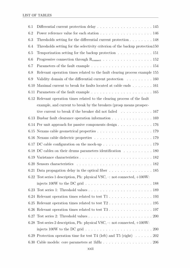
6.1 Differential current protection delay . . . . . . . . . . . . . . . . . . . 145
6.2 Power reference value for each station . . . . . . . . . . . . . . . . . . 146
6.3 Thresholds setting for the differential current protection . . . . . . . . 148
6.4 Thresholds setting for the selectivity criterion of the backup protection150
6.5 Temporization setting for the backup protection . . . . . . . . . . . . 151
6.6 Progressive connection through Rconnect . . . . . . . . . . . . . . . . . 152
6.7 Parameters of the fault example . . . . . . . . . . . . . . . . . . . . . 154
6.8 Relevant operation times related to the fault clearing process example 155
6.9 Validity domain of the differential current protection . . . . . . . . . 160
6.10 Maximal current to break for faults located at cable ends . . . . . . . 161
6.11 Parameters of the fault example . . . . . . . . . . . . . . . . . . . . . 165
6.12 Relevant operation times related to the clearing process of the fault
example, and current to break by the breakers (prosp means prospec-
tive current to break if the breaker did not failed . . . . . . . . . . . 167
6.13 Busbar fault clearance operation information . . . . . . . . . . . . . . 169
6.14 Per unit approach for passive components design . . . . . . . . . . . . 176
6.15 Nexans cable geometrical properties . . . . . . . . . . . . . . . . . . . 179
6.16 Nexans cable dielectric properties . . . . . . . . . . . . . . . . . . . . 179
6.17 DC cable configuration on the mock-up . . . . . . . . . . . . . . . . . 179
6.18 DC cables on their drums parameters identification . . . . . . . . . . 180
6.19 Varistance characteristics . . . . . . . . . . . . . . . . . . . . . . . . . 182
6.20 Sensors characteristics . . . . . . . . . . . . . . . . . . . . . . . . . . 182
6.21 Data propagation delay in the optical fiber . . . . . . . . . . . . . . . 185
6.22 Test series 1 description, Ph: physical VSC, –: not connected, +100W:
injects 100W to the DC grid . . . . . . . . . . . . . . . . . . . . . . . 188
6.23 Test series 1: Threshold values . . . . . . . . . . . . . . . . . . . . . . 189
6.24 Relevant operation times related to test T1 . . . . . . . . . . . . . . . 193
6.25 Relevant operation times related to test T2 . . . . . . . . . . . . . . . 195
6.26 Relevant operation times related to test T3 . . . . . . . . . . . . . . . 197
6.27 Test series 2: Threshold values . . . . . . . . . . . . . . . . . . . . . . 200
6.28 Test series 2 description, Ph: physical VSC, –: not connected, +100W:
injects 100W to the DC grid . . . . . . . . . . . . . . . . . . . . . . . 200
6.29 Protection operation time for test T4 (left) and T5 (right) . . . . . . 202
6.30 Cable models: core parameters at 1kHz . . . . . . . . . . . . . . . . . 206
xxii

LIST OF TABLES
6.31 Inductance matrix L′[mH/km], C: core, S: screen . . . . . . . . . . . 207
6.32 SCFCLs design . . . . . . . . . . . . . . . . . . . . . . . . . . . . . . 213
6.33 Thresholds setting for the voltage differential protection . . . . . . . . 223
6.34 Thresholds setting for the voltage differential protection . . . . . . . . 224
6.35 Differential current and voltage differential principles for a fault ex-
ample occurring near PR13 . . . . . . . . . . . . . . . . . . . . . . . . 225
6.36 Differential current and voltage differential principles for a fault ex-
ample occurring near PR54 . . . . . . . . . . . . . . . . . . . . . . . . 225
A.1 Internal and external fault cases . . . . . . . . . . . . . . . . . . . . . 239
B.1 Relevant operation times related to the clearing process of the fault
example, and current to break by the breakers (prosp means prospec-
tive current to break if the breaker did not fail . . . . . . . . . . . . . 253
B.2 Relevant operation times related to the clearing process of the fault
example, and current to break by the breakers (prosp means prospec-
tive current to break if the breaker did not fail . . . . . . . . . . . . . 254
B.3 First test series, tripping OK means that the fault is cleared with the
main cable differential protection . . . . . . . . . . . . . . . . . . . . 256
B.4 First test series, tripping OK means that the fault is cleared with the
main cable differential protection . . . . . . . . . . . . . . . . . . . . 256
B.5 First test series, tripping OK means that the fault is cleared with the
main cable differential protection . . . . . . . . . . . . . . . . . . . . 257
xxiii


General introduction

General introduction
The development and investigation of new transmission solution is emphasized
by the required global energy transition due to consumption increase and sustain-
able development concerns, currently subjected to numerous debates.
In this context, the European Union launched a climate and energy package,
adopted by the European Parliament on December 2008. The package focuses on
greenhouse gases emissions cuts, renewable and energy efficiency, and supports the
so called three 20 target, which is actually composed of four objectives:
• To reduce emissions of greenhouse gases by 20% by 2020.
• To increase energy efficiency to save 20% of European Union energy consump-
tion by 2020.
• To reach 20% of renewable energy in the total energy consumption in the EU
by 2020.
• To reach 10% of biofuels in the total consumption of vehicles by 2020.
In the frame of the energy transition, the expected reduction of electrical con-
sumption, the increase of decentralized renewable resources and the storage capacity
development hope let imagine lower needs in electricity transmission. Beside, the
transmission grid is often associated to centralized production due to nuclear power
plants. In [Maillard, 2013], the Chairman of the RTE Management Board reviews
this idea. Among his arguments, the remoteness of the renewable plants from the
consumption centers, the impossibility to locally absorb large power production and
the limits in storage facilities are highlighted. The German example is reminded
since the country is currently experiencing a physical and economical waste due to
the lack of sufficient transmission grid, which sometimes lead to restrain the renew-
able production. His conclusion is that no matter the choices that are kept for the
1

GENERAL INTRODUCTION
future, the transmission grid adjustment is a real challenge and must be carried out,
otherwise, no possible energy transition is foreseeable.
As a part of those challenges, RTE participates to the reinforcement of a pan-
European grid, and to the creation of a Supergrid over long term. Numerous Eu-
ropean project emerged in that sense, and many Supergrid concept were born. As
the Desertec1 concept considers long transmission lines to link Europe to photo-
voltaics farms producing bulk power in Africa, other grids meshing the North Sea
(see Fig.1) were investigated.
Figure 1: Meshed grid example, http://www.greenunivers.com
Supergrids appears as a complementary and required solution to the market
mechanisms that already exist to support the integration of renewable resources.
By reinforcing interconnections between all European countries, and by reinforcing
the mutualization of the electricity produced by the most efficient infrastructures,
the Supergrids might reduce the total cost of energy for each participating countries,
and improve the European energy independence.
In this context, the European Commission launched in 2010 the project called
1www.desertec.org
2
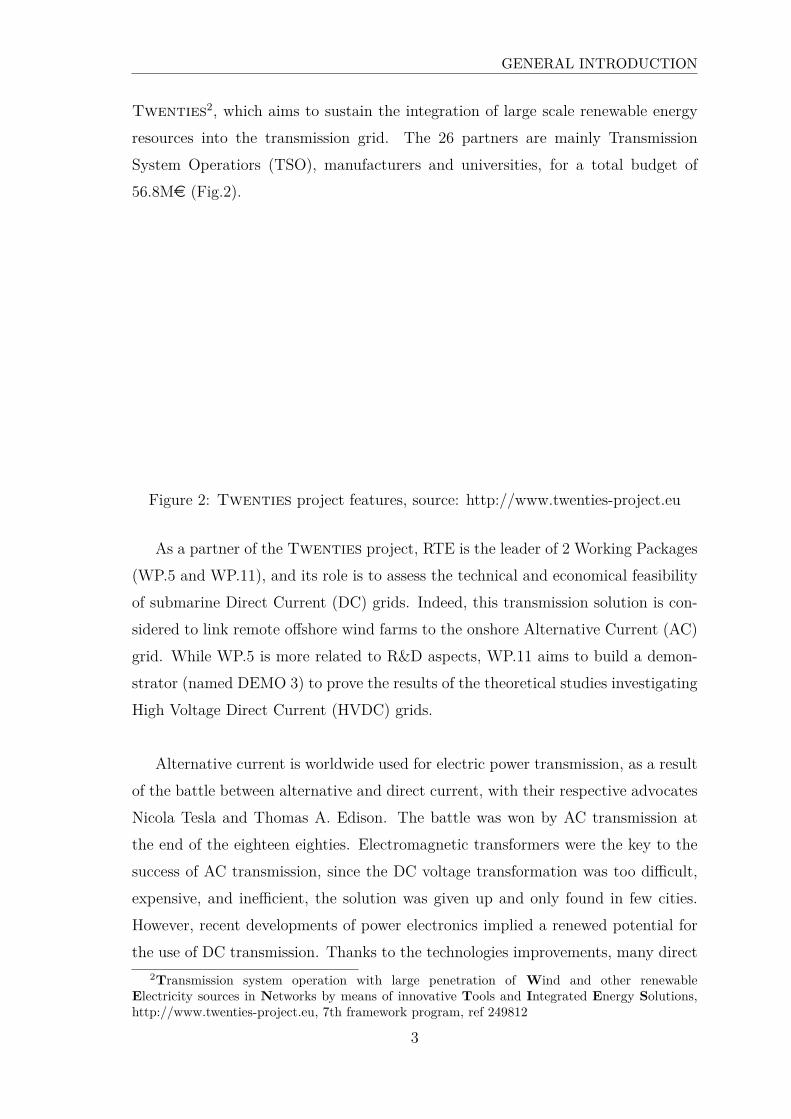
GENERAL INTRODUCTION
Twenties2, which aims to sustain the integration of large scale renewable energy
resources into the transmission grid. The 26 partners are mainly Transmission
System Operatiors (TSO), manufacturers and universities, for a total budget of
56.8Me (Fig.2).
Figure 2: Twenties project features, source: http://www.twenties-project.eu
As a partner of the Twenties project, RTE is the leader of 2 Working Packages
(WP.5 and WP.11), and its role is to assess the technical and economical feasibility
of submarine Direct Current (DC) grids. Indeed, this transmission solution is con-
sidered to link remote offshore wind farms to the onshore Alternative Current (AC)
grid. While WP.5 is more related to R&D aspects, WP.11 aims to build a demon-
strator (named DEMO 3) to prove the results of the theoretical studies investigating
High Voltage Direct Current (HVDC) grids.
Alternative current is worldwide used for electric power transmission, as a result
of the battle between alternative and direct current, with their respective advocates
Nicola Tesla and Thomas A. Edison. The battle was won by AC transmission at
the end of the eighteen eighties. Electromagnetic transformers were the key to the
success of AC transmission, since the DC voltage transformation was too difficult,
expensive, and inefficient, the solution was given up and only found in few cities.
However, recent developments of power electronics implied a renewed potential for
the use of DC transmission. Thanks to the technologies improvements, many direct2Transmission system operation with large penetration of Wind and other renewable
Electricity sources in Networks by means of innovative Tools and Integrated Energy Solutions,http://www.twenties-project.eu, 7th framework program, ref 249812
3

GENERAL INTRODUCTION
current interconnection were built in several countries, where AC transmission was
less effective. This is the case for long transmission line aiming to transmit bulk
power, which is why the Direct Current solution was considered in the Twenties
project. RTE investigated two main problematics, namely:
• the control of converter stations composing the considered DC grid,
• the protection of the DC grid.
Research work were thus supervised by RTE and lead to two Ph.D projects. The
first one on control were conducted by Pierre Rault at the Laboratory of Electrical
Engineering and Power Electronics of Lille (L2EP), and the second one on protec-
tions was conducted in Grenoble Electrical Engineering laboratory (G2Elab), and
is presented in this manuscript.
This thesis, untitled "Protection plan for a Multi-Terminal and High Voltage
Direct Current grid" aims thus to investigate possible protection systems for DC
grid applications against short-circuit faults due to insulation breakdown or exter-
nal constraints, in order to propose a complete protection plan, including a main
protection and one or several backup principles in case one component fails.
In Chapter 1, the relevance of DC application is explained and the technologies
composing such infrastructures are discussed. Chapter 2 goes into details in the
topic by developing the fault phenomenon and reviewing the possible protection
strategies that were found in the literature. Then, Chapter 3 presents the models
that were used to investigate the DC grid behavior under fault conditions. The
parameters influence on the signals resulting of a fault are subjected to a parametric
study addressed in Chapter 4. In Chapter 5, the constraints related to DC grid
protection are expressed and a complete protection plan proposal is given. Finally,
the related protection system is validated and its limits are discussed in Chapter
6. The validation was performed using simulations and a low-scale physical demon-
strator (Twenties DEMO 3), implemented in the L2EP. This thesis will end with
a conclusion providing the major points addressed by this work and a proposition of
further works to ensure the development of Multi-Terminal Direct Current (MTDC)
grid protection plans.
4

GENERAL INTRODUCTION
5

CHAPTER 1
Relevance of HVDC applications and
thesis objectives

Chapter 1
Relevance of HVDC applications
and thesis objectives
This chapter presents the relevance of HVDC links and the reason of their large
development. Projects related to the interconnection between France and its neigh-
bor countries are mentioned. Finally, the AC - DC conversion technologies are
detailed.
1 Development of HVDC links
Alternative Current is widely used for the transmission of electrical power. Nev-
ertheless, High Voltage Direct Current grids turn out to be more attractive and
less costly for certain applications. It allows, for example, to interconnect two non-
synchronous systems or with different frequencies, but above all, HVDC links char-
acteristics became a very popular solution when they aim to transmit bulk power
over long distances. Indeed, from a certain amount of power to transmit, there is
a critical length beyond which AC transmission is not viable anymore. This is due
to the fact that the intrinsic losses and undervoltages need to be compensated for.
Even though it is possible to use voltage standing up station for overhead lines,
the capacitive effect inherent to AC transmission based on underground or undersea
cables is too large, leading the DC solution to be less expansive and more efficient
[Valenza and Cipollini, 1995]. The cost of AC - DC converters is compensated by
the gain of active power that can be transmitted. Fig.1.1 justifies the DC choice,
by illustrating the transmitting power capacity for several link cases, as a function
9

CHAPTER 1. RELEVANCE OF HVDC APPLICATIONS AND THESISOBJECTIVES
of the link length and for several voltage levels.Tr
ansm
issi
on c
apac
ity in
%
Distance in km
Figure 1.1: Transmission capacity of HVAC and HVDC links, [Asplund, 2004]
Consequently, HVDC links are under a wide development phase, especially for
application related to offshore grids, either for countries interconnection or for off-
shore wind farms connection. Nonetheless, those links require very complex power
electronics systems to ensure the AC - DC conversion at each connection point
with AC grid or source, which are extremely costly. HVDC links based on Voltage
Source Converters (VSC) are the most interesting, particularly because those con-
verters permit the control of the active and reactive power independently, and also
to reverse the power flow very quickly [Guo and Zhao, 2009]. By this way, the VSC
can be controlled in the four quadrants and so to feed or to absorb active and re-
active power. This converter type offers the possibility to connect several converter
stations in order to create a true DC grid, that can have several structures (meshed,
looped, ...). Those so called Multi-Terminal High Voltage DC grids (MT-HVDC or
MTDC) are not developed yet, and the technical barriers are still under investiga-
tion in several institutions.
While the research on the control of the VSC is still ongoing in several insti-
tutions (KU Leuven - Belgium, École Centrale de Lille - France, ...), this thesis
focuses on the protection of MTDC grid in case of a fault event, resulting of insu-
lation breakdown or external constraints. Even though the detection of a fault in
10
2. GENERAL OPERATION OF HVDC LINKS
the DC zone can be performed by several existing methods, the identification of the
faulty element is still unknown.
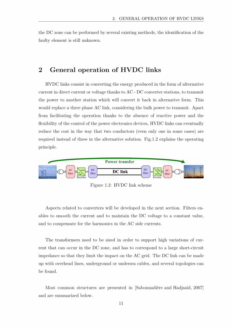
2 General operation of HVDC links
HVDC links consist in converting the energy produced in the form of alternative
current in direct current or voltage thanks to AC - DC converter stations, to transmit
the power to another station which will convert it back in alternative form. This
would replace a three phase AC link, considering the bulk power to transmit. Apart
from facilitating the operation thanks to the absence of reactive power and the
flexibility of the control of the power electronics devices, HVDC links can eventually
reduce the cost in the way that two conductors (even only one in some cases) are
required instead of three in the alternative solution. Fig.1.2 explains the operating
principle.
DC link
Power transfer
AC filter
DC filter
Rectifier
DC filter
AC filter
Inverter
Figure 1.2: HVDC link scheme
Aspects related to converters will be developed in the next section. Filters en-
ables to smooth the current and to maintain the DC voltage to a constant value,
and to compensate for the harmonics in the AC side currents.
The transformers need to be sized in order to support high variations of cur-
rent that can occur in the DC zone, and has to correspond to a large short-circuit
impedance so that they limit the impact on the AC grid. The DC link can be made
up with overhead lines, underground or undersea cables, and several topologies can
be found.
Most common structures are presented in [Sabonnadière and Hadjsaïd, 2007]
and are summarized below.
11

CHAPTER 1. RELEVANCE OF HVDC APPLICATIONS AND THESISOBJECTIVES
2.1 Possible HVDC link structures
a) +U Link with ground or sea return
The advantage of this technology is that it uses only one monopolar link, which
is less costly. The current return path is the ground or the sea.
Figure 1.3: +U monopolar link scheme with ground return
b) ±U link with grounded middle point
When the return current cannot be done by ground or sea, which is usually
the case, especially for submarine links due to the magnetic field that can create
perturbations prohibited by navigating instrumentation of boats, the return is made
in a cable of opposite polarity.
Figure 1.4: ±U bipolar link scheme with grounded middle point
c) ±U bipolar link with monopolar operation possibility
For this kind of structure, electrodes are remote to the station in order to con-
stitute a preferred return current path by ground, in case a monopolar operation is
required. This would be the case for example when there is a problem in one cable.
Figure 1.5: ±U bipolar link scheme with monopolar operation possibility
12
2. GENERAL OPERATION OF HVDC LINKS
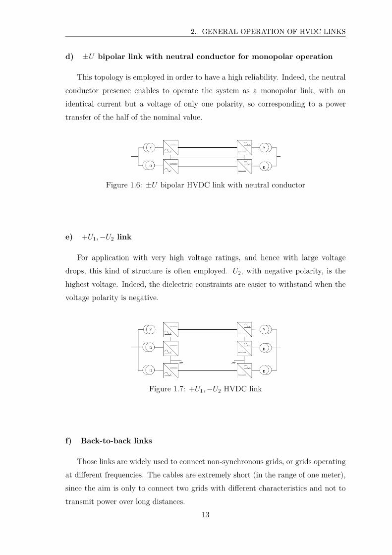
d) ±U bipolar link with neutral conductor for monopolar operation
This topology is employed in order to have a high reliability. Indeed, the neutral
conductor presence enables to operate the system as a monopolar link, with an
identical current but a voltage of only one polarity, so corresponding to a power
transfer of the half of the nominal value.
Figure 1.6: ±U bipolar HVDC link with neutral conductor
e) +U1,−U2 link
For application with very high voltage ratings, and hence with large voltage
drops, this kind of structure is often employed. U2, with negative polarity, is the
highest voltage. Indeed, the dielectric constraints are easier to withstand when the
voltage polarity is negative.
Figure 1.7: +U1,−U2 HVDC link
f) Back-to-back links
Those links are widely used to connect non-synchronous grids, or grids operating
at different frequencies. The cables are extremely short (in the range of one meter),
since the aim is only to connect two grids with different characteristics and not to
transmit power over long distances.
13
CHAPTER 1. RELEVANCE OF HVDC APPLICATIONS AND THESISOBJECTIVES
Figure 1.8: Back-to-back HVDC link scheme
2.2 HVDC links currently under operation in Europe and
planed installations
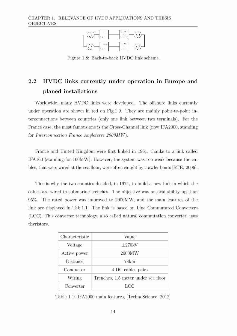
Worldwide, many HVDC links were developed. The offshore links currently
under operation are shown in red on Fig.1.9. They are mainly point-to-point in-
terconnections between countries (only one link between two terminals). For the
France case, the most famous one is the Cross-Channel link (now IFA2000, standing
for Interconnection France Angleterre 2000MW ).
France and United Kingdom were first linked in 1961, thanks to a link called
IFA160 (standing for 160MW). However, the system was too weak because the ca-
bles, that were wired at the sea floor, were often caught by trawler boats [RTE, 2006].
This is why the two counties decided, in 1974, to build a new link in which the
cables are wired in submarine trenches. The objective was an availability up than
95%. The rated power was improved to 2000MW, and the main features of the
link are displayed in Tab.1.1. The link is based on Line Commutated Converters
(LCC). This converter technology, also called natural commutation converter, uses
thyristors.
Characteristic Value
Voltage ±270kV
Active power 2000MW
Distance 78km
Conductor 4 DC cables pairs
Wiring Trenches, 1.5 meter under sea floor
Converter LCC
Table 1.1: IFA2000 main features, [TechnoScience, 2012]
14

3. NEW CONVERSION TECHNOLOGIES
Other HVDC links were developed and others are currently planed, as shown on
Fig.1.9 for the North Sea area.
Figure 1.9: Development of offshore wind farms in North Sea, source:http://www.greenunivers.com
Among the planned projects, some of them are linking multiple terminals (more
than two), and are no longer point-to-point links but Multi-Terminal grids. Those
grids cannot be based on LCC technology. Indeed, for LCC technologies, the power
flow reverse is done by inverting the voltage polarity. It is thus impossible to build
MTDC grids because they would operate at a constant voltage polarity, which leads
to the development of a new converter type, namely Voltage Source Converter. This
solution is detailed in the next section.
3 New conversion technologies
Voltage Source Converters uses transistors instead of thyristors. The Insulated
Gate Bipolar Transistors (IGBT) which compose the VSC can be controlled to be
blocked or conducting. A large number of IGBT are connected in series in each arm.
They are controlled to change their state simultaneously, with an accuracy close to
the microsecond [Nee and Angquist, 2010a]. The output voltage is built thanks to
15
CHAPTER 1. RELEVANCE OF HVDC APPLICATIONS AND THESISOBJECTIVES
the Pulse Width Modulation (PWM) technique.
The main advantage of VSC is that as mentioned earlier, they enables a simul-
taneous control of the active and reactive power exchanged between the converter
and the grid connected to it.
Besides, the power flow direction change does not require the voltage polarity
reversal, which is the case for LCC converters. VSC are hence appropriate for Multi-
Terminal DC grids since the voltage polarity can now be maintained constant. The
main differences between LCC and VSC are given in Tab.1.2.
LCC VSC
Thyristors Transistors
Unidirectional current Constant voltage polarity
Consume reactive power Produce or consume reactive power
Low frequency harmonics generation
(requires large filters)
High frequency harmonics generation
(easily filtered)
Table 1.2: LCC and VSC comparison, [Vissouvanadin Soubaretty, 2011]
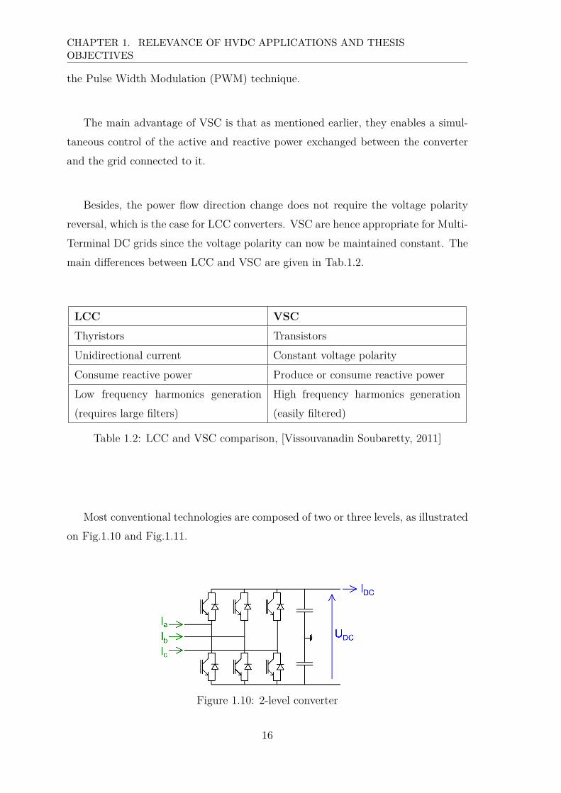
Most conventional technologies are composed of two or three levels, as illustrated
on Fig.1.10 and Fig.1.11.
Figure 1.10: 2-level converter
16
3. NEW CONVERSION TECHNOLOGIES
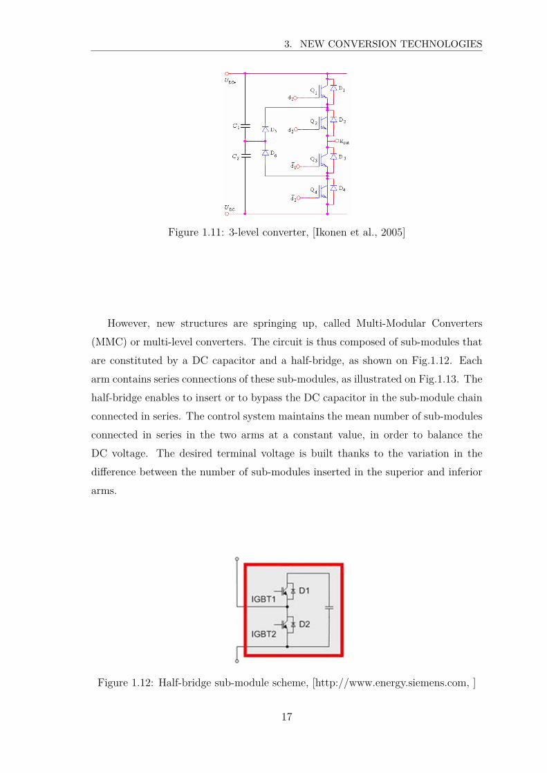
Figure 1.11: 3-level converter, [Ikonen et al., 2005]
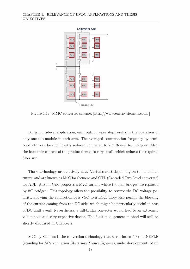
However, new structures are springing up, called Multi-Modular Converters
(MMC) or multi-level converters. The circuit is thus composed of sub-modules that
are constituted by a DC capacitor and a half-bridge, as shown on Fig.1.12. Each
arm contains series connections of these sub-modules, as illustrated on Fig.1.13. The
half-bridge enables to insert or to bypass the DC capacitor in the sub-module chain
connected in series. The control system maintains the mean number of sub-modules
connected in series in the two arms at a constant value, in order to balance the
DC voltage. The desired terminal voltage is built thanks to the variation in the
difference between the number of sub-modules inserted in the superior and inferior
arms.
Figure 1.12: Half-bridge sub-module scheme, [http://www.energy.siemens.com, ]
17
CHAPTER 1. RELEVANCE OF HVDC APPLICATIONS AND THESISOBJECTIVES
Figure 1.13: MMC converter scheme, [http://www.energy.siemens.com, ]
For a multi-level application, each output wave step results in the operation of
only one sub-module in each arm. The averaged commutation frequency by semi-
conductor can be significantly reduced compared to 2 or 3-level technologies. Also,
the harmonic content of the produced wave is very small, which reduces the required
filter size.
Those technology are relatively new. Variants exist depending on the manufac-
turers, and are known as M2C for Siemens and CTL (Cascaded Two Level converter)
for ABB. Alstom Grid proposes a M2C variant where the half-bridges are replaced
by full-bridges. This topology offers the possibility to reverse the DC voltage po-
larity, allowing the connection of a VSC to a LCC. They also permit the blocking
of the current coming from the DC side, which might be particularly useful in case
of DC fault event. Nevertheless, a full-bridge converter would lead to an extremely
voluminous and very expensive device. The fault management method will still be
shortly discussed in Chapter 2.
M2C by Siemens is the conversion technology that were chosen for the INEFLE
(standing for INterconnexion ÉLectrique France Espagne), under development. Main
18

3. NEW CONVERSION TECHNOLOGIES
features of the INELFE link are described in Tab.1.3.
Characteristic Value
Voltage ±320kV
Active power 2x1000MW
Distance 64km
Conductor Underground cables
Converter Siemens M2C
Commissioning date 2014
Table 1.3: INELFE main features, source: http://www.inelfe.eu
As any electrical system, those links are subjected to faults, that can be due
to several phenomena, and must be protected in order to ensure the material and
people safety. This will be developed in Chapter 2.
19

CHAPTER 2
Research view on MTDC grid
protection

Chapter 2
Research review on MTDC grids
protection
In this chapter, the behavior of the HVDC grid under fault condition is inves-
tigated. The most important features of the protection system are given, and the
possible protection philosophies are detailed. The chosen one uses DC breakers,
so their technologies are presented. Finally, the protection principles found in the
literature are summarized, and the thesis objectives are clarified.
1 HVDC link behiavior under fault conditions
1.1 Fault phenomenon
In HVDC links, the faults that can happen are mostly line-to-ground or line-
to-line. They are mainly caused by the degradation of the insulation material. For
overhead lines, the insulation material is the air, and the degradation might be
caused by pollution or lightning strike, arcing with vegetation, and are usually fugi-
tive (non-permanent). At the opposite, cable faults are permanent faults since they
are most often due to external mechanical constraint, or, if the insulation is deterio-
rated, this results also in a permanent fault since the material (XLPE, impregnated
paper) is damaged for ever.
Internal converter faults can also occur, but are not considered in this thesis.
Also, since underground or undersea cable are considered, only permanent faults
will be assumed.
23
CHAPTER 2. RESEARCH REVIEW ON MTDC GRIDS PROTECTION
1.2 Protection system components
The protection system aims to detect the presence of an eventual fault, to iden-
tify the faulty device and then to control the breakers, whose tripping leads to the
insulation of the faulty component from the rest of the grid.
A protection system is thus the arrangement of three main components:
• the sensors, that are measuring the electrical variables required for the fault
detection and faulty component identification,
• the computation interfaces, including the algorithms that process the data
measured by the sensors, in order to compare them to some predefined criteria,
• the breakers, that enable the opening of the circuit and hence the insulation
of the faulty material.
In real applications, the protection system usually consists of the association of
several elements for the protection of a considered system. By this way, in the case
of the failure of the main protection system, one or several backup principles enable
the fault detection and clearance. Several protective zones are considered, each one
protected by a protection system. They must cover the whole grid. Therefore, the
transmission cables, the converters, the busbars, the filters, and all the other ele-
ments are protected by several systems. On this thesis, the considered protective
zone is limited to the cables and the busbar. Also, AC protections will not be treated,
and it is assumed that they are able to clear faults that happen in the AC grid sides.
The protection system has to be able to detect and to clear faults with variable
types. The magnitude of the currents to break can largely differ. Furthermore, the
protections must not limit the normal operation of the grid. Therefore, they need
to remain stable during perturbations due to healthy variation in the grid structure
or power flow.
One of the main difficulties resides in the identification of the faulty component.
Indeed, the overcurrent generated by a short-circuit will propagate all along the grid,
24
2. OVERALL BEHAVIOR OF A HVDC LINK UNDER FAULT CONDITIONS
implying a perturbation everywhere. The strategy has thus to be defined such that
it enables the fault localization, in order to insulate only a minor part of the grid,
and not to shut down the whole zone. This is even more important in meshed or
looped grids since the contribution to the fault comes from each sources connected
to it, and all the cables composing the grid.
2 Overall behavior of a HVDC link under fault
conditions
HVDC grid protection presents particular difficulties compared to traditional
AC system because of the non-existence of current zero-crossing and the low line
impedance, that does not limit the fault current. As a consequence, the DC current
will rise much faster and interrupting the fault current is significantly more difficult
in meshed DC than it is in AC networks.
The shape of a current measured during a fault even can be sketched as illustrated
on Fig.2.1.
Time
Cur
rent
First wave front
Transient
Steady-stateNormal operation
Time
Vol
tage
First wave front
Transient
Steady-state
Normal operation
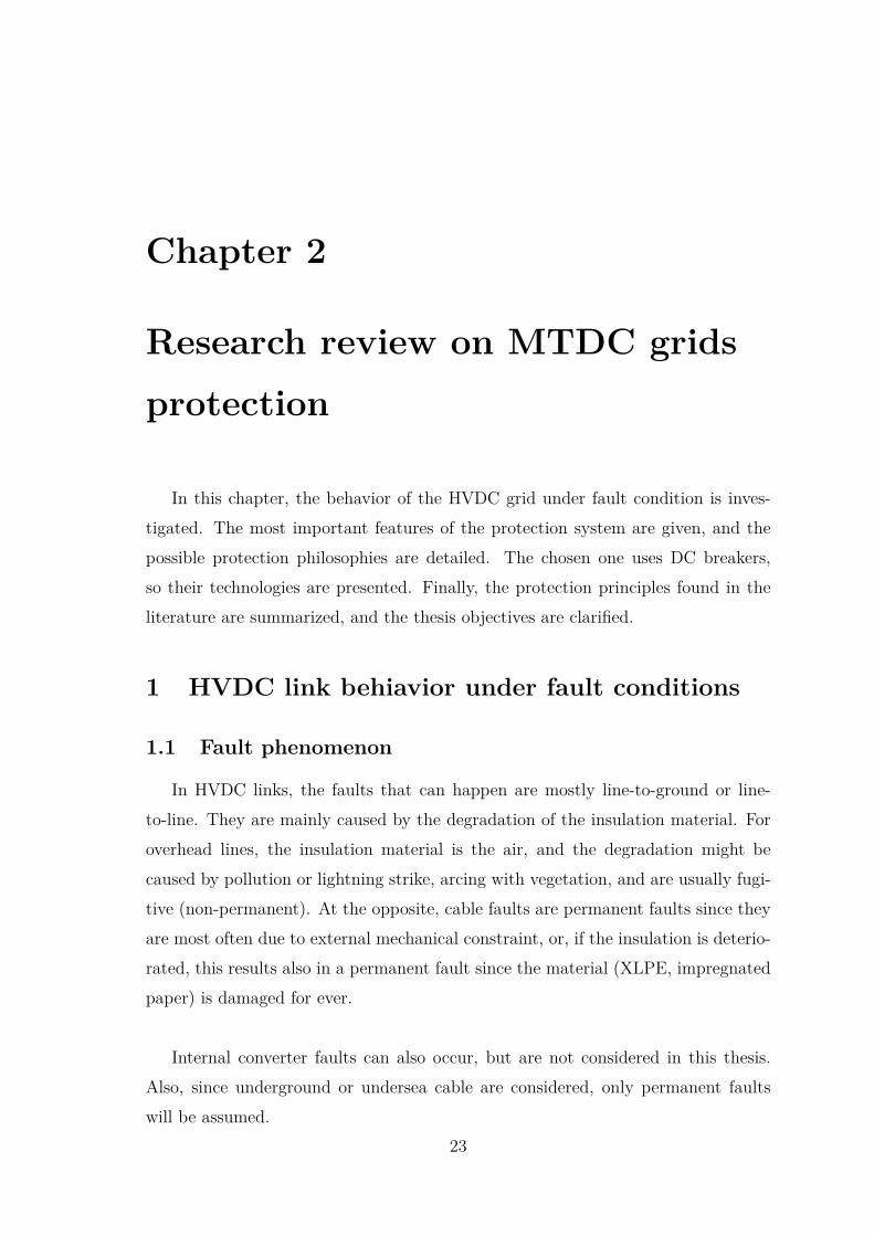
Figure 2.1: DC current and voltage behavior under fault conditions
Three main steps can be defined in those shapes:
25
CHAPTER 2. RESEARCH REVIEW ON MTDC GRIDS PROTECTION
• the first wave front,
• the transient phase,
• and the steady-state.
The first current wave front is due to the cables capacitor discharge, and can
reach very large value (in the range of 50 kiloAmps). The transient that follows
corresponds to the propagation of the perturbation generated by the fault in the
whole grid. Finally, the signals stabilize in a steady-state, which corresponds to the
AC side contributions. The MTDC grid components, and especially the converters,
cannot withstand those large current values, which restricts the protection system
to operate in a very small time (in the range of 5ms). This notion will be detailed
in Chapter 5, but this time range needs to be kept in mind. Indeed, this implies
that the protections cannot wait for the steady-state, since this one occurs several
tens of milliseconds after the fault. Furthermore, note that today, the fastest AC
mechanical breakers open in 40ms, and re-close in about 100 - 120ms. This later fact
adds another constraint related to the DC current breaking speed of the breakers.
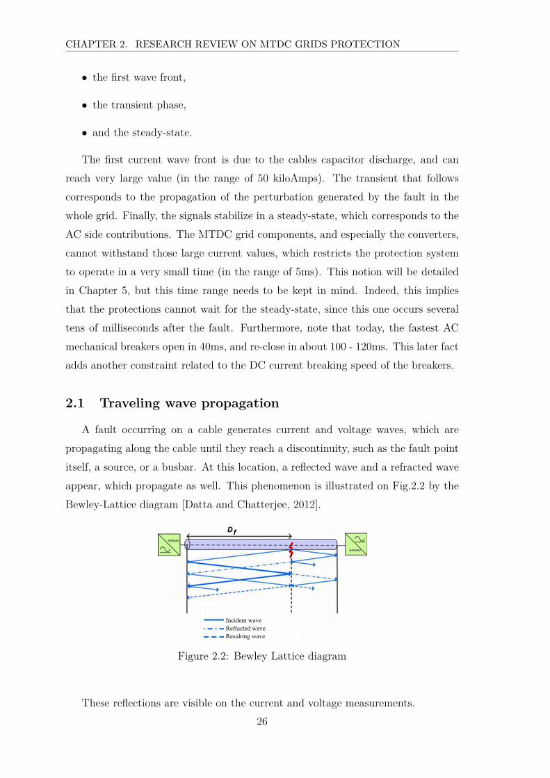
2.1 Traveling wave propagation
A fault occurring on a cable generates current and voltage waves, which are
propagating along the cable until they reach a discontinuity, such as the fault point
itself, a source, or a busbar. At this location, a reflected wave and a refracted wave
appear, which propagate as well. This phenomenon is illustrated on Fig.2.2 by the
Bewley-Lattice diagram [Datta and Chatterjee, 2012].
Incident waveRefracted waveResulting wave
Figure 2.2: Bewley Lattice diagram
These reflections are visible on the current and voltage measurements.
26
3. POSSIBLE PROTECTION STRATEGIES
2.2 MTDC grid protection difficulties
The fact that the low cable reactance does not limit the fault current leads to
another difficulty for MTDC grids. Indeed, there is only a very small difference
between the measurements of two different points, one located on the faulty area
and the other one in a healthy part. This get the identification of the faulty device
even harder. This phenomenon is developed in Chapter 5.
The protection strategy will be discussed in this current chapter.
3 Possible protection strategies
Several philosophies [Tang, 2003] can be possible for the DC grid protection
system, and are summarized in this section.
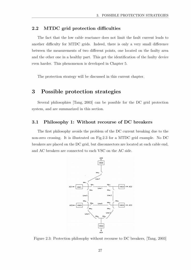
3.1 Philosophy 1: Without recourse of DC breakers
The first philosophy avoids the problem of the DC current breaking due to the
non-zero crossing. It is illustrated on Fig.2.3 for a MTDC grid example. No DC
breakers are placed on the DC grid, but disconnectors are located at each cable end,
and AC breakers are connected to each VSC on the AC side.
Figure 2.3: Protection philosophy without recourse to DC breakers, [Tang, 2003]
27
CHAPTER 2. RESEARCH REVIEW ON MTDC GRIDS PROTECTION
In this case, when a fault is detected in the DC grid zone, every AC breaker
connected to the VSC composing the DC grid trips. Then, the disconnectors sur-
rounding the faulty cable are opened, which is possible since no current is flowing
anymore through the DC grid. The AC breakers are then closed, and the DC grid
restores its operation.
The advantage of this philosophy is that there is no need of DC breakers. How-
ever, it supposes the total shut down of the DC grid, and even though this is done
only for few milliseconds, it would lead to an interruption of the power transfer. It
is highly probable that such a blackout of the DC grid would be prohibited by the
concerned TSO. Besides, this philosophy does not avoid the transient current due to
the cable capacitor discharge of the cables, that are destructive for the converters.
Nonetheless, this transient would not happen for overhead lines.
3.2 Philosophy 2: With moderated recourse of DC breakers
This philosophy uses a moderated amount of DC breakers, at each VSC connec-
tion point in the DC grid, as it is illustrated on Fig.2.4 for the same MTDC grid
example. Disconnectors are once again located at each cable end.
Figure 2.4: Protection philosophy with moderated recourse to DC breakers,[Tang, 2003]
28
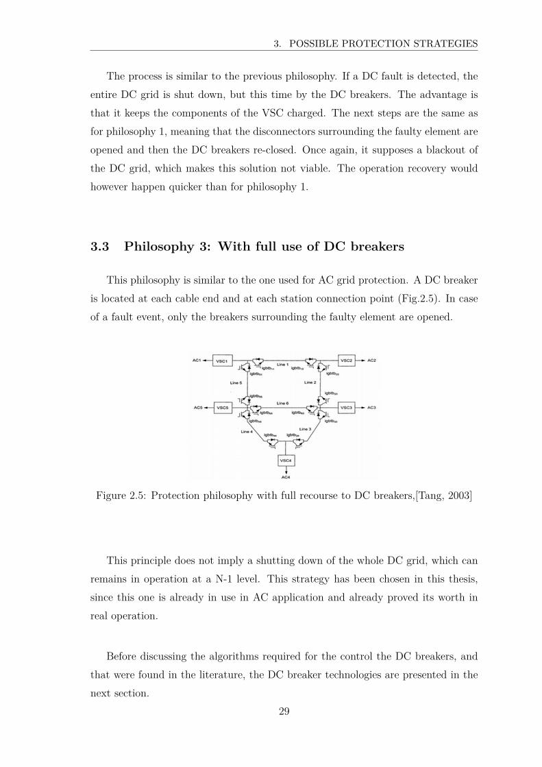
3. POSSIBLE PROTECTION STRATEGIES
The process is similar to the previous philosophy. If a DC fault is detected, the
entire DC grid is shut down, but this time by the DC breakers. The advantage is
that it keeps the components of the VSC charged. The next steps are the same as
for philosophy 1, meaning that the disconnectors surrounding the faulty element are
opened and then the DC breakers re-closed. Once again, it supposes a blackout of
the DC grid, which makes this solution not viable. The operation recovery would
however happen quicker than for philosophy 1.
3.3 Philosophy 3: With full use of DC breakers
This philosophy is similar to the one used for AC grid protection. A DC breaker
is located at each cable end and at each station connection point (Fig.2.5). In case
of a fault event, only the breakers surrounding the faulty element are opened.
Figure 2.5: Protection philosophy with full recourse to DC breakers,[Tang, 2003]
This principle does not imply a shutting down of the whole DC grid, which can
remains in operation at a N-1 level. This strategy has been chosen in this thesis,
since this one is already in use in AC application and already proved its worth in
real operation.
Before discussing the algorithms required for the control the DC breakers, and
that were found in the literature, the DC breaker technologies are presented in the
next section.
29
CHAPTER 2. RESEARCH REVIEW ON MTDC GRIDS PROTECTION
4 Current breaking technology
Special attention needs to be paid on the breakers, since they are the compo-
nents that are responsible for the fault clearance once the tripping order is sent. In
fault conditions, the contact separation where flows a short-circuit current cannot
be performed instantaneously. Indeed, the area located between the two ends that
aimed to be separated, but initially connected one to another, becomes ionized and
hence is conducting [Vacquié, 1986]. This results in an arc, which implies the dis-
sipation of the energy in a certain time, and avoids severe overvoltages that would
happen in the case of an instantaneous dissipation, not withstandable for the grid.
Nevertheless, it is easier to interrupt a lower power arc. This is why in AC grids the
tripping is done when the current is at a zero-crossing instant, which occurs each
half-period.
A technological lock is hence inherent to the DC case, since their is no zero-
crossing in the current shape, at least naturally. This results in a high quantity
of energy to dissipate, which corresponds to the electromagnetic energy stored in
the proper inductance of the circuit, equivalent to 12LI2 [Pelenc, 2002]. Available
breakers used for AC applications are thus non-adapted to break DC currents.
During current breaking process, once the contact is separated, the voltage at
the initial contact terminals is re-established, and increases in a transient way. The
rising speed of this Transient Recovery Voltage (TRV) can take very high val-
ues. If the electrical field did not recover its dielectric rigidity, this high voltage
can lead to another arcing phenomenon, which would lead to a breaking failure
[Schoenemann et al., 2004].
4.1 Electrical arc phenomenon
Electrical arcs can occur for many reasons. For example, in transmission lines, an
arc is created when the voltage overpasses the breakdown voltage. The breakdown
voltage depends on the distance between the electrodes and the dielectric rigidity of
the field. The temperature, the pressure and the hydrometry are influencing factors
[Andrea et al., 2010b]. If the source does not limit the current, this one is irre-
versible. Arcs can also appear in breakers when two conductors initially conducting
30

4. CURRENT BREAKING TECHNOLOGY
a current are separated. The arc is extinguished when the current is reduced to zero
and when the field recovers its dielectric rigidity [Vacquié, 1986].
4.2 Research state on DC breaker
Breakers are manufactured such that the arc time constant (noted Θ, which is
defined in [Andrea et al., 2010b]) is as low as possible. By this way, mechanical
breakers using gases such as SF6 or vacuum were developed in order to improve
their breaking capability.
Several kinds of breakers were developed for DC application purposes. Some of
the methods consist in combining the mechanical breakers used in AC systems with
other elements able to break large DC currents. Other methods are based on power
electronics. This section summarizes those techniques.
4.2.1 Mechanical breakers
Mechanical breakers used in AC applications are not sized to break large DC
currents, because of the huge energy that need to be dissipated. To enable such a
breaking process, they can be combined with other elements that would create an
artificial current zero-crossing.
Two methods exist to force the DC current to cross zero at the breaker level.
The first one consist of the addition of a branch in parallel of the breaker. The
created commutation can thus be either passive or active. The second way is to use
a pyrotechnic method.
a) Passive commutation process
In this case, the current zero-crossing is obtained thanks to the superposition of
two currents: the fault current, that needs to be extinguished, and the current com-
ing from another branch, added to that purpose. This second branch is composed
of an inductor L and a capacitor C in series, as illustrated on Fig.2.6.
31
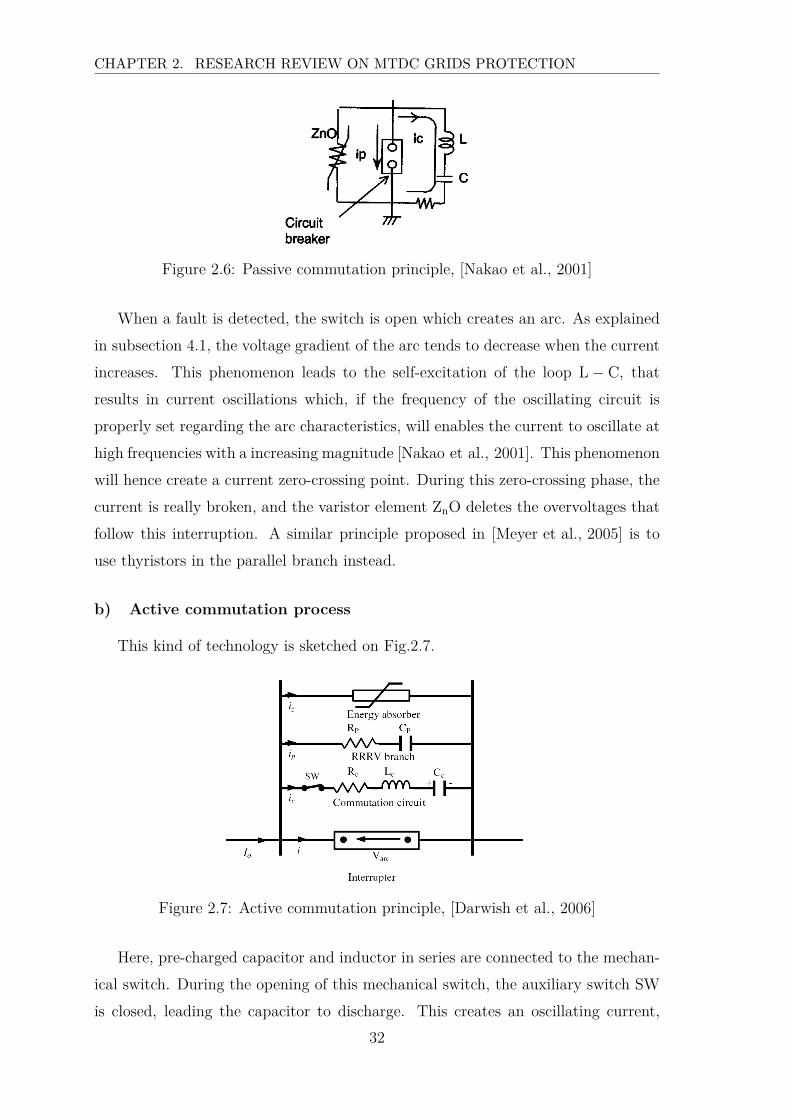
CHAPTER 2. RESEARCH REVIEW ON MTDC GRIDS PROTECTION
Figure 2.6: Passive commutation principle, [Nakao et al., 2001]
When a fault is detected, the switch is open which creates an arc. As explained
in subsection 4.1, the voltage gradient of the arc tends to decrease when the current
increases. This phenomenon leads to the self-excitation of the loop L − C, that
results in current oscillations which, if the frequency of the oscillating circuit is
properly set regarding the arc characteristics, will enables the current to oscillate at
high frequencies with a increasing magnitude [Nakao et al., 2001]. This phenomenon
will hence create a current zero-crossing point. During this zero-crossing phase, the
current is really broken, and the varistor element ZnO deletes the overvoltages that
follow this interruption. A similar principle proposed in [Meyer et al., 2005] is to
use thyristors in the parallel branch instead.
b) Active commutation process
This kind of technology is sketched on Fig.2.7.
Figure 2.7: Active commutation principle, [Darwish et al., 2006]
Here, pre-charged capacitor and inductor in series are connected to the mechan-
ical switch. During the opening of this mechanical switch, the auxiliary switch SW
is closed, leading the capacitor to discharge. This creates an oscillating current,
32
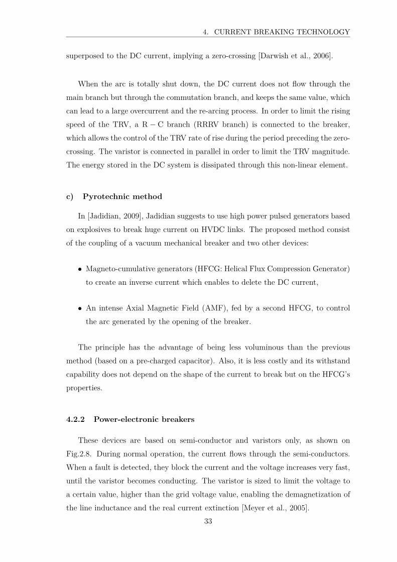
4. CURRENT BREAKING TECHNOLOGY
superposed to the DC current, implying a zero-crossing [Darwish et al., 2006].
When the arc is totally shut down, the DC current does not flow through the
main branch but through the commutation branch, and keeps the same value, which
can lead to a large overcurrent and the re-arcing process. In order to limit the rising
speed of the TRV, a R − C branch (RRRV branch) is connected to the breaker,
which allows the control of the TRV rate of rise during the period preceding the zero-
crossing. The varistor is connected in parallel in order to limit the TRV magnitude.
The energy stored in the DC system is dissipated through this non-linear element.
c) Pyrotechnic method
In [Jadidian, 2009], Jadidian suggests to use high power pulsed generators based
on explosives to break huge current on HVDC links. The proposed method consist
of the coupling of a vacuum mechanical breaker and two other devices:
• Magneto-cumulative generators (HFCG: Helical Flux Compression Generator)
to create an inverse current which enables to delete the DC current,
• An intense Axial Magnetic Field (AMF), fed by a second HFCG, to control
the arc generated by the opening of the breaker.
The principle has the advantage of being less voluminous than the previous
method (based on a pre-charged capacitor). Also, it is less costly and its withstand
capability does not depend on the shape of the current to break but on the HFCG’s
properties.
4.2.2 Power-electronic breakers
These devices are based on semi-conductor and varistors only, as shown on
Fig.2.8. During normal operation, the current flows through the semi-conductors.
When a fault is detected, they block the current and the voltage increases very fast,
until the varistor becomes conducting. The varistor is sized to limit the voltage to
a certain value, higher than the grid voltage value, enabling the demagnetization of
the line inductance and the real current extinction [Meyer et al., 2005].
33
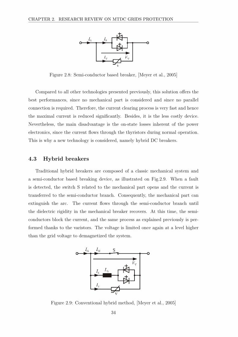
CHAPTER 2. RESEARCH REVIEW ON MTDC GRIDS PROTECTION
Figure 2.8: Semi-conductor based breaker, [Meyer et al., 2005]
Compared to all other technologies presented previously, this solution offers the
best performances, since no mechanical part is considered and since no parallel
connection is required. Therefore, the current clearing process is very fast and hence
the maximal current is reduced significantly. Besides, it is the less costly device.
Nevertheless, the main disadvantage is the on-state losses inherent of the power
electronics, since the current flows through the thyristors during normal operation.
This is why a new technology is considered, namely hybrid DC breakers.
4.3 Hybrid breakers
Traditional hybrid breakers are composed of a classic mechanical system and
a semi-conductor based breaking device, as illustrated on Fig.2.9. When a fault
is detected, the switch S related to the mechanical part opens and the current is
transferred to the semi-conductor branch. Consequently, the mechanical part can
extinguish the arc. The current flows through the semi-conductor branch until
the dielectric rigidity in the mechanical breaker recovers. At this time, the semi-
conductors block the current, and the same process as explained previously is per-
formed thanks to the varistors. The voltage is limited once again at a level higher
than the grid voltage to demagnetized the system.
Figure 2.9: Conventional hybrid method, [Meyer et al., 2005]
34
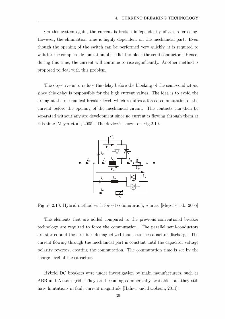
4. CURRENT BREAKING TECHNOLOGY
On this system again, the current is broken independently of a zero-crossing.
However, the elimination time is highly dependent on the mechanical part. Even
though the opening of the switch can be performed very quickly, it is required to
wait for the complete de-ionization of the field to block the semi-conductors. Hence,
during this time, the current will continue to rise significantly. Another method is
proposed to deal with this problem.
The objective is to reduce the delay before the blocking of the semi-conductors,
since this delay is responsible for the high current values. The idea is to avoid the
arcing at the mechanical breaker level, which requires a forced commutation of the
current before the opening of the mechanical circuit. The contacts can then be
separated without any arc development since no current is flowing through them at
this time [Meyer et al., 2005]. The device is shown on Fig.2.10.
Figure 2.10: Hybrid method with forced commutation, source: [Meyer et al., 2005]
The elements that are added compared to the previous conventional breaker
technology are required to force the commutation. The parallel semi-conductors
are started and the circuit is demagnetized thanks to the capacitor discharge. The
current flowing through the mechanical part is constant until the capacitor voltage
polarity reverses, creating the commutation. The commutation time is set by the
charge level of the capacitor.
Hybrid DC breakers were under investigation by main manufacturers, such as
ABB and Alstom grid. They are becoming commercially available, but they still
have limitations in fault current magnitude [Hafner and Jacobson, 2011].
35
CHAPTER 2. RESEARCH REVIEW ON MTDC GRIDS PROTECTION
The research is still ongoing, and as a partner of the Twenties project, Alstom
grid made a prototype of their breakthrough. They have recourse to a clever shrewd-
ness in the process, which cannot be communicated yet since this new technology is
under patent process. The press release delivered on May, 25th 20131 told that the
prototype was able to break currents exceeding 3kA current in less than 2.5ms.
The DC breakers can also be helped by the converters. Indeed, a full-bridge
multi-level converter retains full control during faults. It can thus limit the current to
break, by adapting the control methods for such events or adding new devices such as
DC - DC converters [Jovcic et al., 2013]. Once again, those full-bridge technologies
suffer from excessive number of switches, and thus are not considered in this thesis.
5 Review of protection principles found in ante-
rior works
This part aims to present the protection algorithms that were investigated in the
literature.
5.1 Use of DC breakers
This method is the closest to the one used for AC systems, and is based on the
principle explained in section 1.2, which is reminded below:
• the sensors, that are measuring the electrical variables required for the fault
detection and faulty component identification,
• the computation interfaces includes protection algorithms that process the
data measured by the sensor, detect the fault and identify the DC breaker
that needs to trip,
• the breakers are controlled and the chosen ones clear the fault.
The protection algorithms that were found in the literature are commented in
the next part.1The press release can be found on the Twenties website at: http://www.twenties-
project.eu/node/21
36
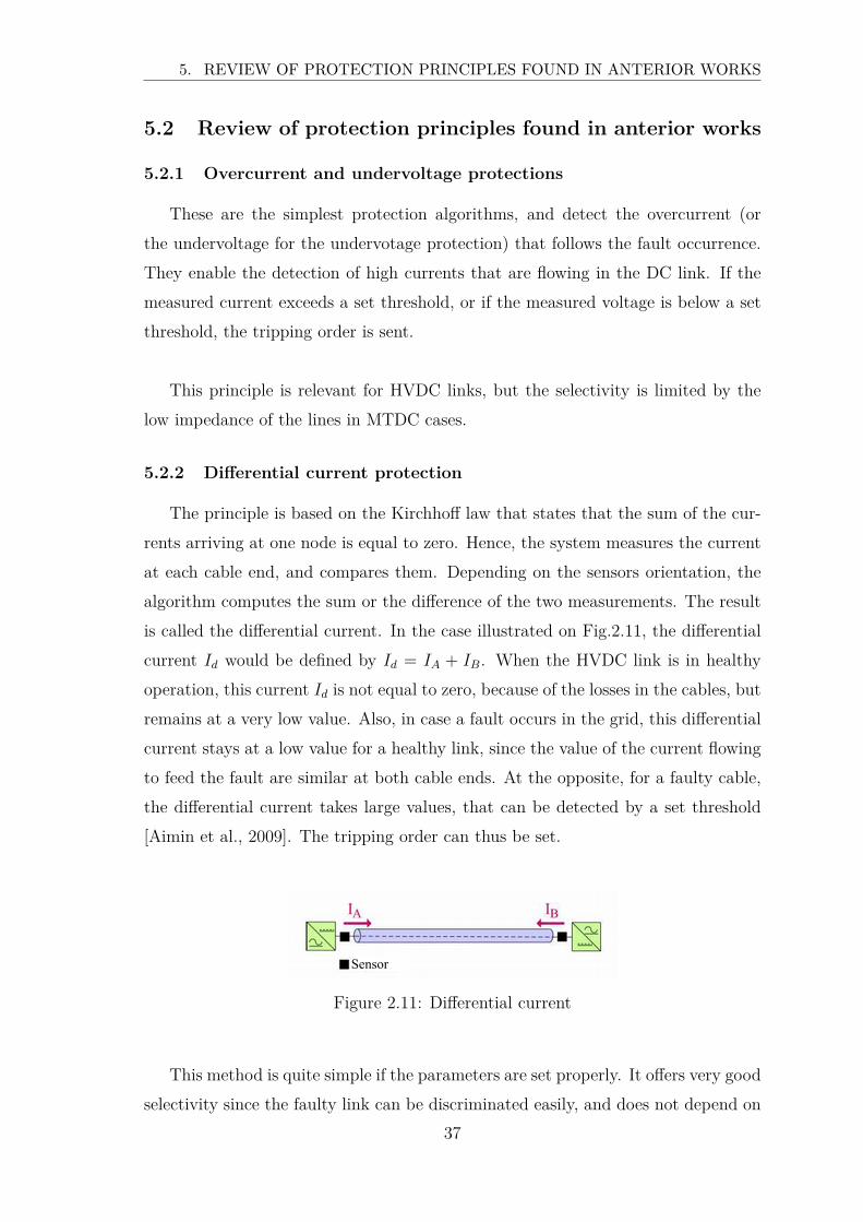
5. REVIEW OF PROTECTION PRINCIPLES FOUND IN ANTERIOR WORKS
5.2 Review of protection principles found in anterior works
5.2.1 Overcurrent and undervoltage protections
These are the simplest protection algorithms, and detect the overcurrent (or
the undervoltage for the undervotage protection) that follows the fault occurrence.
They enable the detection of high currents that are flowing in the DC link. If the
measured current exceeds a set threshold, or if the measured voltage is below a set
threshold, the tripping order is sent.
This principle is relevant for HVDC links, but the selectivity is limited by the
low impedance of the lines in MTDC cases.
5.2.2 Differential current protection
The principle is based on the Kirchhoff law that states that the sum of the cur-
rents arriving at one node is equal to zero. Hence, the system measures the current
at each cable end, and compares them. Depending on the sensors orientation, the
algorithm computes the sum or the difference of the two measurements. The result
is called the differential current. In the case illustrated on Fig.2.11, the differential
current Id would be defined by Id = IA + IB. When the HVDC link is in healthy
operation, this current Id is not equal to zero, because of the losses in the cables, but
remains at a very low value. Also, in case a fault occurs in the grid, this differential
current stays at a low value for a healthy link, since the value of the current flowing
to feed the fault are similar at both cable ends. At the opposite, for a faulty cable,
the differential current takes large values, that can be detected by a set threshold
[Aimin et al., 2009]. The tripping order can thus be set.
Sensor
Figure 2.11: Differential current
This method is quite simple if the parameters are set properly. It offers very good
selectivity since the faulty link can be discriminated easily, and does not depend on
37
CHAPTER 2. RESEARCH REVIEW ON MTDC GRIDS PROTECTION
the line impedance. However, the inconvenient is that the previous statements
are valid only in steady-state, which happens too late compared to the required
protection speed.
5.2.3 Current and voltage derivatives
The principle is the same than the overcurrent or undervoltage principle, but
uses the derivative of the measurements instead. More recent schemes adopt prin-
ciples that are based on traveling wave theory.
For those principles, the currents (or voltages) are measured, and their deriva-
tives dIdt
(or dVdt
) are computed, and using a threshold, the detection is done and the
tripping orders are sent. A pondered sum of dIdt
and dVdt
can also be used in order to
have a more reliable system.
This method has the advantage of using the first incident wave, which allows a
quick detection [Naidoo and Ijumba, 2005]. However, as well as the overcurrent and
the undervoltage protection principles, the selectivity is limited by the low cable
impedance.
5.2.4 Distance protection using traveling wave propagation theory
According to traveling wave propagation theory, when a fault occurs, progressive
current and voltage waves imply fast variations over the whole cable length. The
waves generated by the fault contain enough information to detect and eliminate it
[K. and N., 2005].
For AC applications, the magnitude of the generated waves depends on the volt-
age phase at the fault occurrence time. High difficulties reside in the detection of a
fault that happens at a voltage zero-crossing point. Nevertheless, this problem does
not exist for DC applications [Shang et al., 2001].
The waves are propagating at a speed that depends on the cable geometry and
on the relative permittivity of the field where it is wired. For long overhead lines,
this speed is in the range of the speed of light, but for cables, this speed is about 3
times lower [Thomas et al., 2009].
38
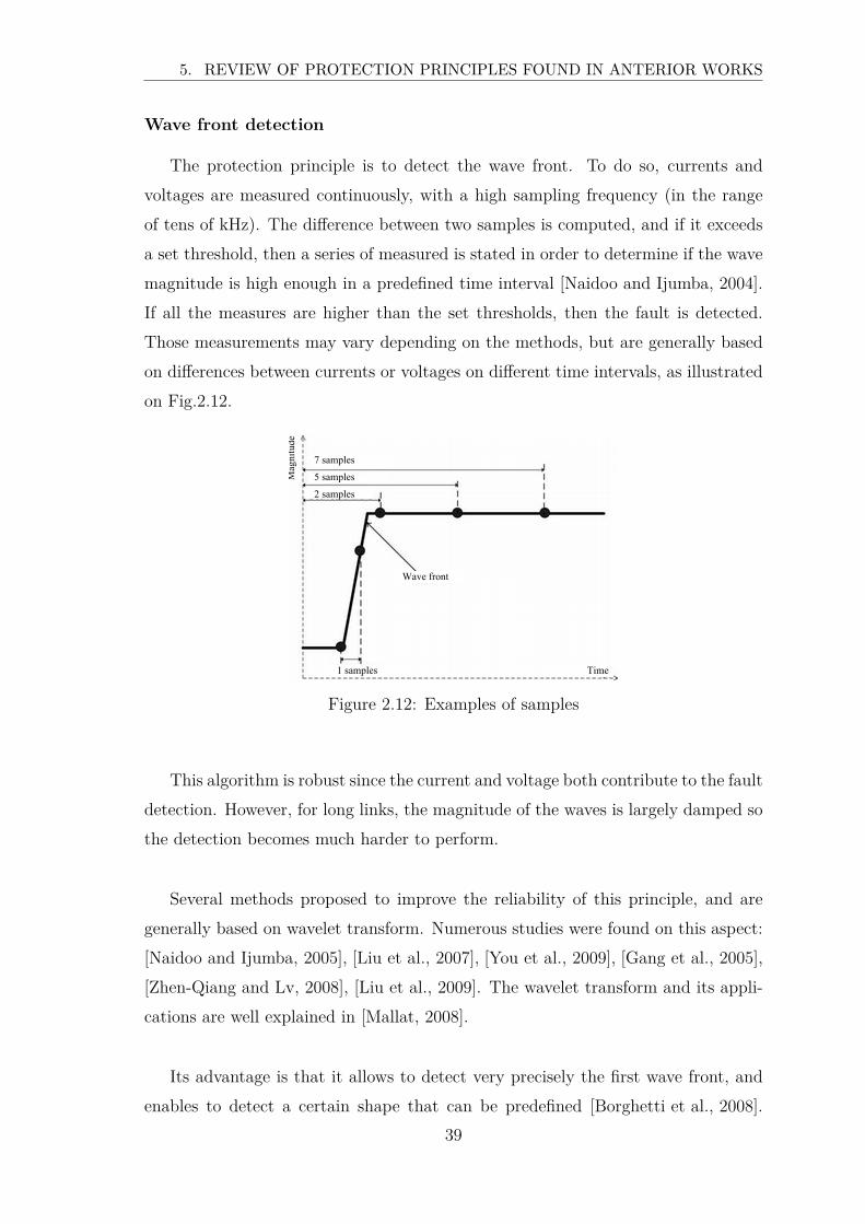
5. REVIEW OF PROTECTION PRINCIPLES FOUND IN ANTERIOR WORKS
Wave front detection
The protection principle is to detect the wave front. To do so, currents and
voltages are measured continuously, with a high sampling frequency (in the range
of tens of kHz). The difference between two samples is computed, and if it exceeds
a set threshold, then a series of measured is stated in order to determine if the wave
magnitude is high enough in a predefined time interval [Naidoo and Ijumba, 2004].
If all the measures are higher than the set thresholds, then the fault is detected.
Those measurements may vary depending on the methods, but are generally based
on differences between currents or voltages on different time intervals, as illustrated
on Fig.2.12.
Mag
nitu
de
7 samples
5 samples
2 samples
1 samples
Wave front
Time
Figure 2.12: Examples of samples
This algorithm is robust since the current and voltage both contribute to the fault
detection. However, for long links, the magnitude of the waves is largely damped so
the detection becomes much harder to perform.
Several methods proposed to improve the reliability of this principle, and are
generally based on wavelet transform. Numerous studies were found on this aspect:
[Naidoo and Ijumba, 2005], [Liu et al., 2007], [You et al., 2009], [Gang et al., 2005],
[Zhen-Qiang and Lv, 2008], [Liu et al., 2009]. The wavelet transform and its appli-
cations are well explained in [Mallat, 2008].
Its advantage is that it allows to detect very precisely the first wave front, and
enables to detect a certain shape that can be predefined [Borghetti et al., 2008].
39
CHAPTER 2. RESEARCH REVIEW ON MTDC GRIDS PROTECTION
However, the wavelet transforms are very complex signal processing methods, so
the methods require a large computation time which is prohibited for DC protection
purposes. Furthermore, it assumes a very accurate knowledge of the grid structure
and parameters, which makes the real application of those principles questionable.
Nevertheless, the idea was investigated for a backup protection application, and is
summarized in Appendix A2.
6 Thesis objectives
The thesis objective is to implement and test a complete protection system for
MTDC grids. As the DC breakers, able to clear high DC currents, are investigated
by Alstom grid as a partner of the Twenties European project, this present work
focuses only on the protection algorithms, and not on the breaking technology. To
ensure the selectivity using the philosophy chosen in section 1, a protection relay
needs to be installed at each end of cable, on each pole, and on both sides of the
busbars composing the DC grid. Each protection relay is associated with a DC
circuit breaker, sensors and a relay.
To assess the possible algorithms, the precise behavior of the MTDC grid in fault
conditions has to be investigated first, in order to deal with very accurate signals.
To do so, a DC grid model needs to be implemented, since no MTDC grid exists so
no real records can be used. The aim of Chapter 3 is to present the models that
were used.
Then, based on the chosen philosophy of the protection plan, and on the prin-
ciples found in the literature, a protection system proposal will be addressed in
Chapter 5.
40

6. THESIS OBJECTIVES
41

CHAPTER 3
MTDC network components and grid
test modeling


Chapter 3
MTDC network components and
grid test modeling
To study the protection of DC grids, the transients following a fault occurrence
have to be investigated. As no real application records of such transients were avail-
able, simulation studies were considered, and the development of a real mock-up
has been conducted (the mock-up configuration and its results will be described in
Chapter 6).
Several software can perform this task, such as PSCAD, Matlab - SimPow-
erSystem. Those softwares provide a lot of features, as well as the powerful tool
EMTP-rv. This later one can perform either time-domain and frequency-domain
simulations, and is often used worldwide by TSO for transient studies. The sim-
ulation software was chosen in order to simulate fault transients as accurately as
possible. For such transients, cables behavior are a key components. Thus, EMTP-
rv was chosen by RTE as its library provides the most complex cable models.
This chapter presents the models that were used for each components of the grid,
namely the conducting cables, the AC grid and the substations, the fault and the
protection relays components, excluding the protection algorithms, since they will
be investigated in Chapter 5.
Topology (mentioned in Chapter 1) ±U link with grounded middle point is
considered, and were chosen by RTE for both L2EP and G2Elab researches on the
45
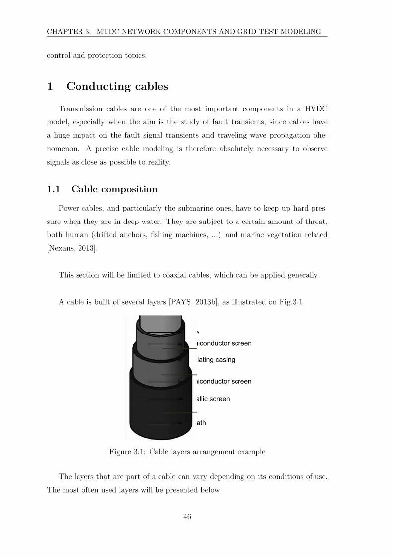
CHAPTER 3. MTDC NETWORK COMPONENTS AND GRID TEST MODELING
control and protection topics.
1 Conducting cables
Transmission cables are one of the most important components in a HVDC
model, especially when the aim is the study of fault transients, since cables have
a huge impact on the fault signal transients and traveling wave propagation phe-
nomenon. A precise cable modeling is therefore absolutely necessary to observe
signals as close as possible to reality.
1.1 Cable composition
Power cables, and particularly the submarine ones, have to keep up hard pres-
sure when they are in deep water. They are subject to a certain amount of threat,
both human (drifted anchors, fishing machines, ...) and marine vegetation related
[Nexans, 2013].
This section will be limited to coaxial cables, which can be applied generally.
A cable is built of several layers [PAYS, 2013b], as illustrated on Fig.3.1.
Figure 3.1: Cable layers arrangement example
The layers that are part of a cable can vary depending on its conditions of use.
The most often used layers will be presented below.
46

1. CONDUCTING CABLES
The conducting core can be made up of copper, aluminum or aluminum alloy.
It can be solid or cabled rounded. In submarine links applications, the cable is
subjected to major stresses (in particular due to the water mass) whose core can
support up to 60 % of the overall stresses applied to the cable [PAYS, 2013a]. Its
maximal elongation under traction as well as its mechanical withstand capability at
the junction-level are important factors to consider.
The electrical properties of the material that composes the insulating casing goes
with the cable use. Impregnated and pre-impregnated papers are favored for sub-
marine HVDC links [PAYS, 2013a]. Indeed, impregnated paper insulation sustains
voltage polarity reversal. However, the VSC conversion technology does not require
the voltage polarity reversal to inverse the power flow. Thus, polyethylene can be
used instead [Nee and Angquist, 2010b].
Then, screens composed by conducting materials are placed on the core and on
the external part of the insulating casing in order to ensure the internal magnetic
field repartition of the cable, to block external electrostatic fields and to discharge
capacitive currents. Furthermore, the grounding mode of the screen can lead to dif-
ferent phenomena and hence have an effect on the core dimensioning and operation
conditions.
The sheath is the easiest protection. It is traditionally made up of lead for very
high voltage cables. A polyethylene sheath could also be added as a protection
against corrosion in case of a sea current return. It guarantees the waterproof prop-
erty and serves as a shock absorber.
Finally, the role of the armor is to support stresses that are transmitted to the
cable during its wiring, and to ensure the external mechanical protection. It is in
most cases constituted by galvanized steel threads, and can have several structures
(single threads layer or double, crossed or not).
Cables are thus characterized by their geometry and by the material properties
they are made up of (permeability, permittivity, ...).
47
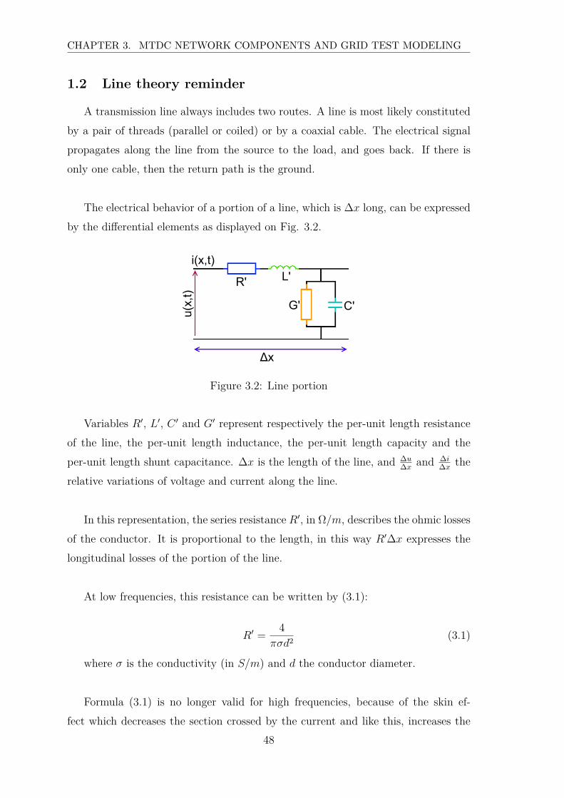
CHAPTER 3. MTDC NETWORK COMPONENTS AND GRID TEST MODELING
1.2 Line theory reminder
A transmission line always includes two routes. A line is most likely constituted
by a pair of threads (parallel or coiled) or by a coaxial cable. The electrical signal
propagates along the line from the source to the load, and goes back. If there is
only one cable, then the return path is the ground.
The electrical behavior of a portion of a line, which is ∆x long, can be expressed
by the differential elements as displayed on Fig. 3.2.
Δx
u(x,t)
i(x,t)
R' L'
G' C'
Figure 3.2: Line portion
Variables R′, L′, C ′ and G′ represent respectively the per-unit length resistance
of the line, the per-unit length inductance, the per-unit length capacity and the
per-unit length shunt capacitance. ∆x is the length of the line, and ∆u∆x
and ∆i∆x
the
relative variations of voltage and current along the line.
In this representation, the series resistance R′, in Ω/m, describes the ohmic losses
of the conductor. It is proportional to the length, in this way R′∆x expresses the
longitudinal losses of the portion of the line.
At low frequencies, this resistance can be written by (3.1):
R′ =4
πσd2(3.1)
where σ is the conductivity (in S/m) and d the conductor diameter.
Formula (3.1) is no longer valid for high frequencies, because of the skin ef-
fect which decreases the section crossed by the current and like this, increases the
48
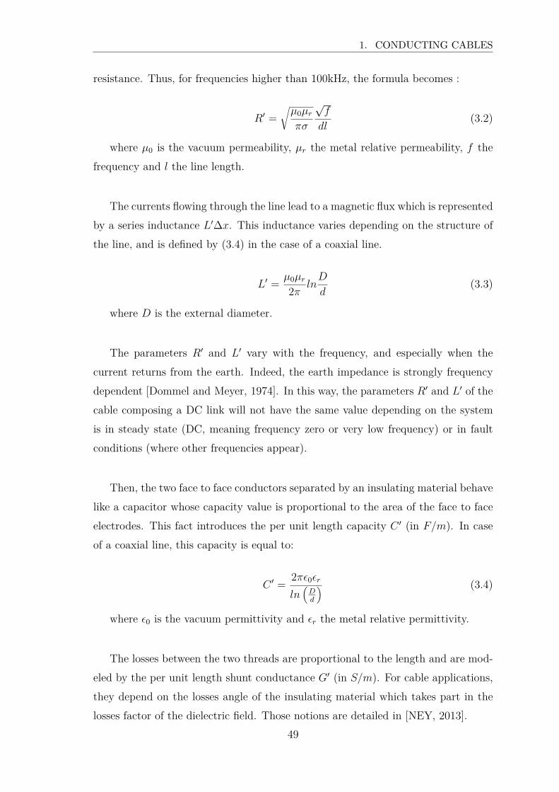
1. CONDUCTING CABLES
resistance. Thus, for frequencies higher than 100kHz, the formula becomes :
R′ =√
µ0µr
πσ
√f
dl(3.2)
where µ0 is the vacuum permeability, µr the metal relative permeability, f the
frequency and l the line length.
The currents flowing through the line lead to a magnetic flux which is represented
by a series inductance L′∆x. This inductance varies depending on the structure of
the line, and is defined by (3.4) in the case of a coaxial line.
L′ =µ0µr
2πlnD
d(3.3)
where D is the external diameter.
The parameters R′ and L′ vary with the frequency, and especially when the
current returns from the earth. Indeed, the earth impedance is strongly frequency
dependent [Dommel and Meyer, 1974]. In this way, the parameters R′ and L′ of the
cable composing a DC link will not have the same value depending on the system
is in steady state (DC, meaning frequency zero or very low frequency) or in fault
conditions (where other frequencies appear).
Then, the two face to face conductors separated by an insulating material behave
like a capacitor whose capacity value is proportional to the area of the face to face
electrodes. This fact introduces the per unit length capacity C ′ (in F/m). In case
of a coaxial line, this capacity is equal to:
C ′ =2πǫ0ǫr
ln(
Dd
) (3.4)
where ǫ0 is the vacuum permittivity and ǫr the metal relative permittivity.
The losses between the two threads are proportional to the length and are mod-
eled by the per unit length shunt conductance G′ (in S/m). For cable applications,
they depend on the losses angle of the insulating material which takes part in the
losses factor of the dielectric field. Those notions are detailed in [NEY, 2013].
49

CHAPTER 3. MTDC NETWORK COMPONENTS AND GRID TEST MODELING
Now, the behavior of a line can be expressed by the simultaneous equations
(3.5,3.6):
v(x) − v(x+ ∆x) = (R′ + jL′ω) i∆x (3.5)
i(x) − i(x+ ∆x) = (G′ + jC ′ω) v∆x (3.6)
where v and i are respectively the voltage and the current, j is the complex
number such that j2 = −1, and ω = 2πf .
The well-known Telegrapher’s equation 3.7 is obtained by derivation of the sys-
tem (3.5,3.6).
d2v
dx2= (R′ + jL′ω) (G′ + jC ′ω) v (3.7)
The solution of (3.7) is given by (3.8) assuming (3.9) and the characteristic
impedance ZC given by (3.10).
v(x, t) = V.ejωte−γx + V.ej(ωt+Φ)eγx (3.8)
γ2 = (α+ jβ)2 = (R′ + jL′ω) (G′ + jC ′ω) (3.9)
ZC =R′ + jL′ω
G′ + jC ′ω(3.10)
where Φ represents a phase difference.
The solution (3.8) can now be decomposed in two parts, that match with the
incident wave Vi and the reflected wave Vr :
Vi = V.e−γx (3.11)
Vr = V.ej(Φ+γx) (3.12)
The existence of the term eγx = eαxejβx allows to deduce some characteristics of
50
1. CONDUCTING CABLES
the line:
• The pulsation ω describes the time-related frequency, and the propagation
constant β characterizes the spacial-related frequency.
• The signal is mitigated due to power losses. The attenuation by unit length
is given by the α coefficient (in m−1). For a given distance, the attenuation
increases with the frequency.
Several assumptions can be made in order to simplify the line representation. For
example, a lossless line (R′ = G′ = 0), or a line where the parameters are no longer
distributed along the whole length but localized in a given point could be consid-
ered to downsize the complexity of the model and to reduce the computation time.
Several methods are used to model those transmission lines, and will be explained
in the following subsections. Nevertheless, even though these simplifications enable
an easier representation, they do not transcribe all the phenomena that really exist.
Indeed, the more simplified the model is, the more inaccurate the results will be.
Numerous line and cable models exist, and can be dispatched into two wide
groups depending on the resolution techniques used in the simulation software
[Marti, 1988]: the time-relative models and the frequency-relative ones.
1.3 Frequency domain models
When the cable is modeled in the frequency domain, the time domain solution
is obtained thanks to inverse transformation algorithms such as the Fast Fourier
Transform (FFT). Therefore, the frequency dependence phenomenon of the line or
cable parameters is taken into account. Nevertheless, abrupt changes in the system
configuration (such as faults occurrence and breaker switching) as well as the mod-
eling of non linear elements become very complex when frequency-based methods of
analysis are used. Consequently, time domain modeling are preferred.
However, accurate computation of electromagnetic transients for underground
cables (as well as for overhead lines) requires the frequency domain characterization
of two matrix functions, namely the propagation and the characteristic admittance,
generally noted H and respectively YC. This frequency domain characterization can
51

CHAPTER 3. MTDC NETWORK COMPONENTS AND GRID TEST MODELING
be then used to create a time domain model with better accuracy.
As explained in [Kocar et al., 2010], the general description of a line can be given
by equations (3.13), (3.14) and (3.15) in the frequency domain.
Ik = YCVk − H (YCVm + Im) (3.13)
where k and m are the line terminals.
The bold vectors Ik and Vk represent the currents and voltages. The size n of the
vectors corresponds to the number of conductors.
The n-by-n propagation matrix H and n-by-n characteristic admittance matrix
YC are given by (3.14) and (3.15):
H = e(−√
YSZS l) (3.14)
YC =√
YSZ−1S (3.15)
where l is the length of the line, YS is the shunt admittance per-unit length, and ZS
the series impedance matrix per-unit length. These two matrices can be found from
the geometry and electrical parameters of the line or cable. This task is performed
thanks to the Cable Data block of EMTP-rv library.
The exact representation of a line in the frequency domain is given by the EMTP-
rv model Exact Π, defined by equation (3.13). This is not a time domain model,
and it can only be used for a steady state solution exciting a unique frequency or to
compute a frequency scan [Marti, 1993]. This model is interesting since it enables
the comparison of other models with theoretically exact values, but only in the fre-
quency domain.
The time domain solution of (3.13) is obtained thanks to the convolution (3.16):
ik = yc ∗ vk − h ∗ um (3.16)
52
1. CONDUCTING CABLES
where um is given by:
um = yc ∗ vm + im (3.17)
The propagation function constitutes a high order wide-band system with inher-
ent time delays, and the frequency dependency problems are even more complex for
underground cables [Kocar et al., 2008]. In order to solve (3.16), assumptions are
made depending on the models. Those assumptions are described for each model,
in the following subsections.
Besides, for a multi-phase cable or line, the matrix H contains several prop-
agation modes with different velocities. The H matrix can be decomposed into
decoupled propagation modes, thanks to a transformation. Thus, the solution of H
is easier to get the in the mode domain. Then, the inverse transformation is done to
obtain H in phase domain. The transformation matrix between modes and phases,
named Q, is also subjected to assumptions depending on the models.
The assumptions made on these functions will be explained for each model.
1.4 Time-domain models
Several types of line and cable models draw attention: localized parameters
models and distributed parameters models, frequency-dependent or not. Those
different models already exist in EMTP-rv libraries and will be developed below.
1.4.1 Localized-parameters models
a) Π Line
The model is represented by an association of coupled Π circuits, as shown on
Fig.3.3. The G parameter is most often neglected. The parameters are localised in
a certain number of points along the line or the cable, depending on the number of
Π sections used. The parameters R′, L′, and C ′ are evaluated at a given frequency,
and the propagation phenomenon is not taken into account.
53
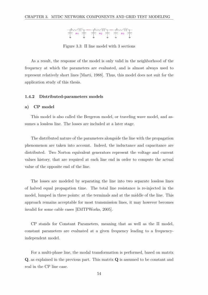
CHAPTER 3. MTDC NETWORK COMPONENTS AND GRID TEST MODELING
Figure 3.3: Π line model with 3 sections
As a result, the response of the model is only valid in the neighborhood of the
frequency at which the parameters are evaluated, and is almost always used to
represent relatively short lines [Marti, 1988]. Thus, this model does not suit for the
application study of this thesis.
1.4.2 Distributed-parameters models
a) CP model
This model is also called the Bergeron model, or traveling wave model, and as-
sumes a lossless line. The losses are included at a later stage.
The distributed nature of the parameters alongside the line with the propagation
phenomenon are taken into account. Indeed, the inductance and capacitance are
distributed. Two Norton equivalent generators represent the voltage and current
values history, that are required at each line end in order to compute the actual
value of the opposite end of the line.
The losses are modeled by separating the line into two separate lossless lines
of halved equal propagation time. The total line resistance is re-injected in the
model, lumped in three points: at the terminals and at the middle of the line. This
approach remains acceptable for most transmission lines, it may however becomes
invalid for some cable cases [EMTPWorks, 2005].
CP stands for Constant Parameters, meaning that as well as the Π model,
constant parameters are evaluated at a given frequency leading to a frequency-
independent model.
For a multi-phase line, the modal transformation is performed, based on matrix
Q, as explained in the previous part. This matrix Q is assumed to be constant and
real in the CP line case.
54

1. CONDUCTING CABLES
Simulation results of a CP model are faster and more precise than the Π cir-
cuit case. Nonetheless, the model generally shows very low damping effects at high
frequencies, and the validity of the results is limited to a short frequency range.
Therefore, a CP line evaluated at a given frequency could give valid responses for
the representation of a system in normal operation, but can no longer transcribe the
fast transients generated by a short-circuit for example.
In order to improve the validity of cable models on a large frequency range,
frequency dependent models were investigated in order to take the frequency depen-
dency problem into account. The three frequency dependent models that can be
found in EMTP-rv library are described below.
b) FD model
The FD model is the first one to take the frequency dependency of the parame-
ters into account.
For multi-phase cases, the modal transformation matrix Q is, alike the CP model,
assumed to be constant and real. However, the model represents the frequency de-
pendency of the resistance R and the inductance L by approximating with rational
transfer functions the characteristic impedance and the propagation function for
each mode [Marti, 1982].
The model is valid for a relatively large frequency range (from direct current
conditions up to 1MHz [Marti, 1982]) for overhead lines. Nevertheless, problems
exist for underground cables since the Q elements are strongly frequency dependent.
Hence, the model is no longer valid for such applications.
c) FDQ model
This model is also well known as the LMarti model [Marti, 1993], and as well
as the FD model, the characteristic admittance and the propagation function are
decomposed into modes and they are approximating with rational functions for each
mode.
55

CHAPTER 3. MTDC NETWORK COMPONENTS AND GRID TEST MODELING
The FDQ model overcomes the limitations of the FD line thanks to a frequency
dependent matrix Q, also approximated using rational functions. It enables an
accurate representation of both low and high frequencies phenomena in the same
simulation, even for underground or undersea cables where frequency dependency
problems are more complex than in overhead lines.
d) FDQ model limitations
In the FDQ model, rational transfer functions approximation over a range of
frequencies are used. They are preferred since they enable an efficient computation
of convolution integrals in time domain with a recursive scheme.
The estimation of the rational transfer functions in the frequency domain is based
on identification techniques, and can be performed thanks to least-square techniques.
Nevertheless, these techniques often introduce errors, especially for the propagation
matrix H and Q when underground cables are considered. These techniques often
result in poor fits and ill-conditioned equations [Kocar et al., 2008].
As FDQ has several problems and fails very often, new methods were introduced,
resulting in the so-called WideBand cable model. This model will replace the FDQ
model, which will be removed in further EMTP-rv versions1.
e) WideBand model
The line or cable WideBand (WB) is the most sophisticated EMTP-rv model
available, and is detailed in [Morched et al., 1999].
The characteristic admittance matrix YC is fitted directly in the phase domain.
The propagation matrix H is first fitted in the modal domain, and the results are
then used for fitting H in the phase domain. The identification of the propagation
function as a rational transfer function is done using a weighted vector fitting tech-
nique, detailed in [Kocar et al., 2008], and which avoid a lot of errors and numerical
1Information originated from EMTP-rv developers
56
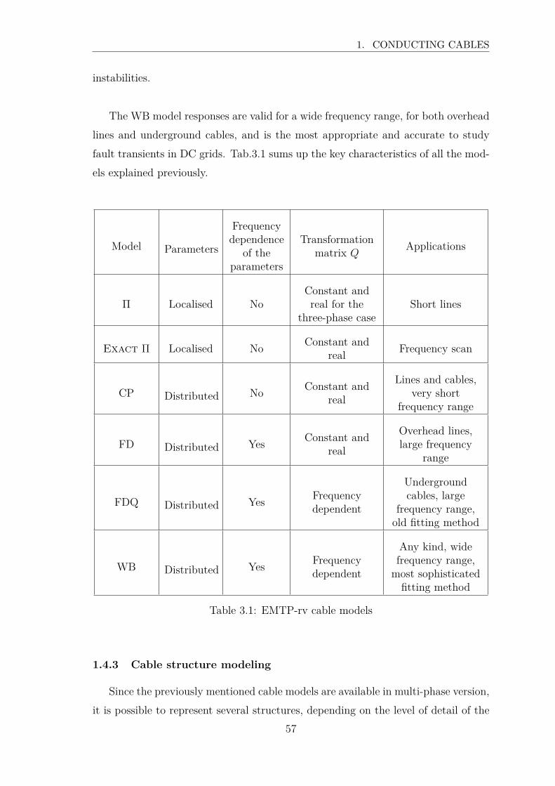
1. CONDUCTING CABLES
instabilities.
The WB model responses are valid for a wide frequency range, for both overhead
lines and underground cables, and is the most appropriate and accurate to study
fault transients in DC grids. Tab.3.1 sums up the key characteristics of all the mod-
els explained previously.
Model Parameters
Frequencydependence
of theparameters
Transformationmatrix Q
Applications
Π Localised NoConstant andreal for the
three-phase caseShort lines
Exact Π Localised NoConstant and
realFrequency scan
CP Distributed NoConstant and
real
Lines and cables,very short
frequency range
FD Distributed YesConstant and
real
Overhead lines,large frequency
range
FDQ Distributed YesFrequencydependent
Undergroundcables, large
frequency range,old fitting method
WB Distributed YesFrequencydependent
Any kind, widefrequency range,
most sophisticatedfitting method
Table 3.1: EMTP-rv cable models
1.4.3 Cable structure modeling
Since the previously mentioned cable models are available in multi-phase version,
it is possible to represent several structures, depending on the level of detail of the
57
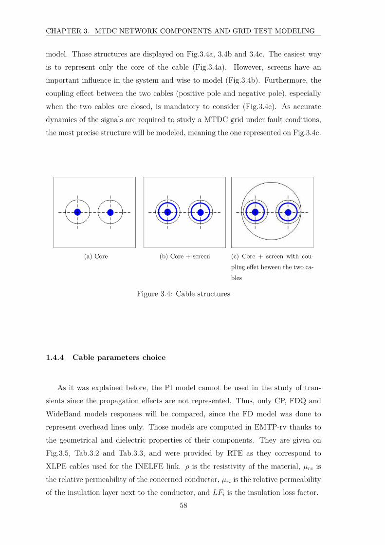
CHAPTER 3. MTDC NETWORK COMPONENTS AND GRID TEST MODELING
model. Those structures are displayed on Fig.3.4a, 3.4b and 3.4c. The easiest way
is to represent only the core of the cable (Fig.3.4a). However, screens have an
important influence in the system and wise to model (Fig.3.4b). Furthermore, the
coupling effect between the two cables (positive pole and negative pole), especially
when the two cables are closed, is mandatory to consider (Fig.3.4c). As accurate
dynamics of the signals are required to study a MTDC grid under fault conditions,
the most precise structure will be modeled, meaning the one represented on Fig.3.4c.
(a) Core (b) Core + screen (c) Core + screen with cou-
pling effet beween the two ca-
bles
Figure 3.4: Cable structures
1.4.4 Cable parameters choice
As it was explained before, the PI model cannot be used in the study of tran-
sients since the propagation effects are not represented. Thus, only CP, FDQ and
WideBand models responses will be compared, since the FD model was done to
represent overhead lines only. Those models are computed in EMTP-rv thanks to
the geometrical and dielectric properties of their components. They are given on
Fig.3.5, Tab.3.2 and Tab.3.3, and were provided by RTE as they correspond to
XLPE cables used for the INELFE link. ρ is the resistivity of the material, µrc is
the relative permeability of the concerned conductor, µri is the relative permeability
of the insulation layer next to the conductor, and LFi is the insulation loss factor.
58
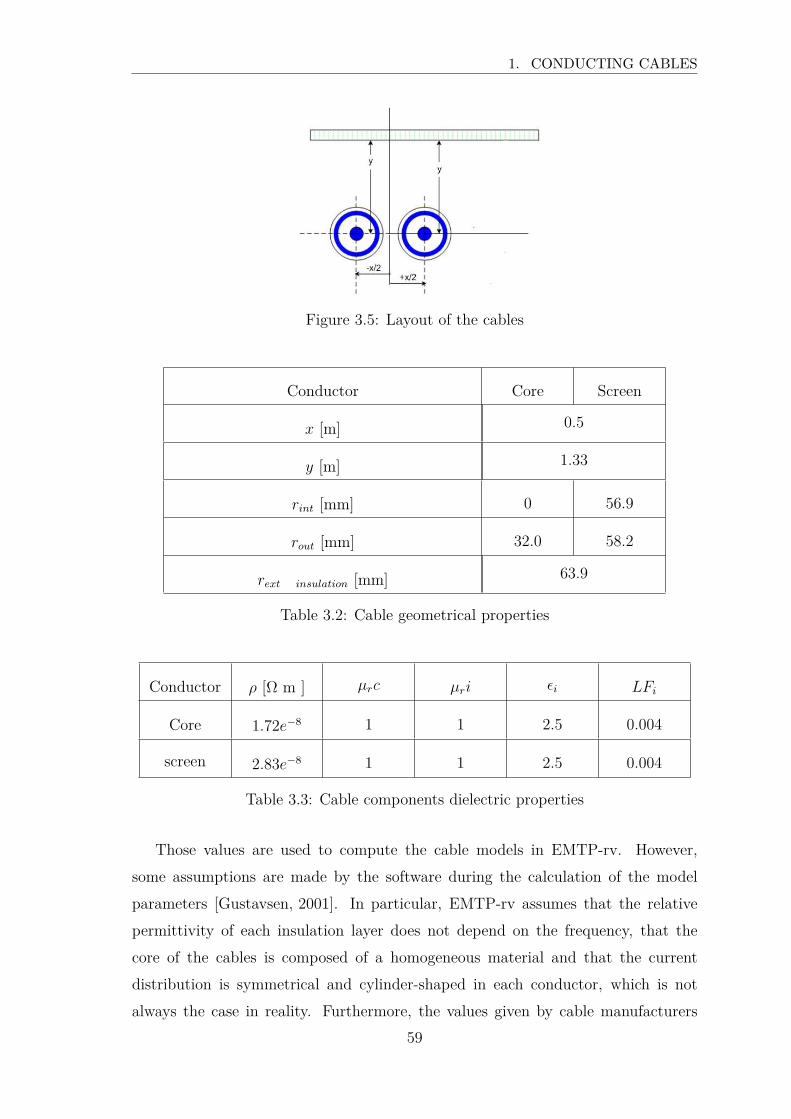
1. CONDUCTING CABLES
Figure 3.5: Layout of the cables
Conductor Core Screen
x [m] 0.5
y [m] 1.33
rint [mm] 0 56.9
rout [mm] 32.0 58.2
rext insulation [mm] 63.9
Table 3.2: Cable geometrical properties
Conductor ρ [Ω m ] µrc µri ǫi LFi
Core 1.72e−8 1 1 2.5 0.004
screen 2.83e−8 1 1 2.5 0.004
Table 3.3: Cable components dielectric properties
Those values are used to compute the cable models in EMTP-rv. However,
some assumptions are made by the software during the calculation of the model
parameters [Gustavsen, 2001]. In particular, EMTP-rv assumes that the relative
permittivity of each insulation layer does not depend on the frequency, that the
core of the cables is composed of a homogeneous material and that the current
distribution is symmetrical and cylinder-shaped in each conductor, which is not
always the case in reality. Furthermore, the values given by cable manufacturers
59
CHAPTER 3. MTDC NETWORK COMPONENTS AND GRID TEST MODELING
can be imprecise. Those errors, even very low, can have an impact on the responses
of the models, and particularly on the damping effects and on the propagation
speed. It is thus suitable to do some conversions explained in [Gustavsen, 2001] to
take those effects into account. However, a cable specimen would be required to do
so, but was not available in the lab.
1.4.5 Cable model behavior
As mentioned in the previous paragraph, CP, FDQ and WideBand models will be
compared. The Exact Π model can only be used for a frequency domain simulation,
and gives the exact representation. Thus, the closer to the Exact Π the frequency
response of a model is, the more precise it is.
a) Frequency domain analysis
Five models will be compared in this part, thanks to a frequency scan done by
EMTP-rv :
• a CP model evaluated for the frequency 1kHz (default frequency in EMTP-rv)
• a CP model evaluated for the frequency 50Hz
• a FDQ model
• a WideBand model
• an Exact Π model
Their length is 100km. The frequency scan is done from 1Hz to 10kHz, with a
frequency step of 1Hz. An other one is done from 10µHz to 1Hz with a frequency
step of 10µHz, to look precisely at the DC response. The corresponding curves are
given on Fig.3.6a and Fig.3.6b.
Looking at the magnitude as a function of the frequency, the CP models show a
very low attenuation at high frequencies, whereas the FDQ and WideBand models
attenuation is much more clear, which matches the Exact Π model response. At
low frequencies, the CP model responses are higher and the FDQ, WideBand and
Exact Π ones are really close.
The frequency domain analysis show that FDQ and WideBand models, even
using simplifying assumptions, are really accurate since they give the same response
60
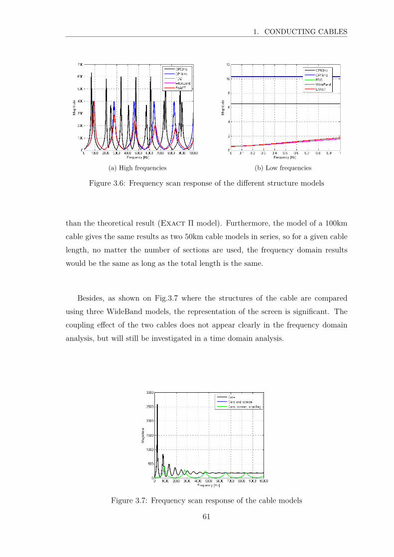
1. CONDUCTING CABLES
(a) High frequencies (b) Low frequencies
Figure 3.6: Frequency scan response of the different structure models
than the theoretical result (Exact Π model). Furthermore, the model of a 100km
cable gives the same results as two 50km cable models in series, so for a given cable
length, no matter the number of sections are used, the frequency domain results
would be the same as long as the total length is the same.
Besides, as shown on Fig.3.7 where the structures of the cable are compared
using three WideBand models, the representation of the screen is significant. The
coupling effect of the two cables does not appear clearly in the frequency domain
analysis, but will still be investigated in a time domain analysis.
Figure 3.7: Frequency scan response of the cable models
61
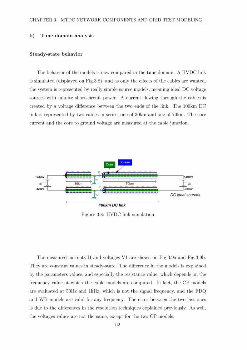
CHAPTER 3. MTDC NETWORK COMPONENTS AND GRID TEST MODELING
b) Time domain analysis
Steady-state behavior
The behavior of the models is now compared in the time domain. A HVDC link
is simulated (displayed on Fig.3.8), and as only the effects of the cables are wanted,
the system is represented by really simple source models, meaning ideal DC voltage
sources with infinite short-circuit power. A current flowing through the cables is
created by a voltage difference between the two ends of the link. The 100km DC
link is represented by two cables in series, one of 30km and one of 70km. The core
current and the core to ground voltage are measured at the cable junction.
Figure 3.8: HVDC link simulation
The measured currents I1 and voltages V1 are shown on Fig.3.9a and Fig.3.9b.
They are constant values in steady-state. The difference in the models is explained
by the parameters values, and especially the resistance value, which depends on the
frequency value at which the cable models are computed. In fact, the CP models
are evaluated at 50Hz and 1kHz, which is not the signal frequency, and the FDQ
and WB models are valid for any frequency. The error between the two last ones
is due to the differences in the resolution techniques explained previously. As well,
the voltages values are not the same, except for the two CP models.
62
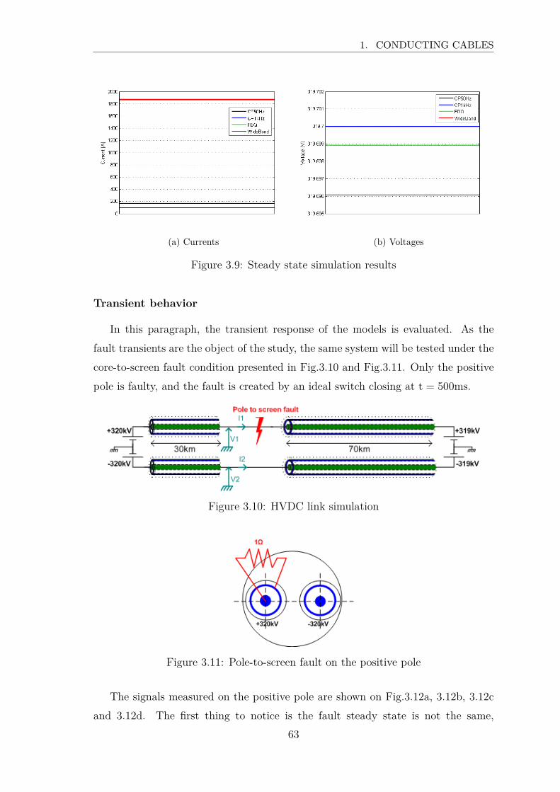
1. CONDUCTING CABLES
(a) Currents (b) Voltages
Figure 3.9: Steady state simulation results
Transient behavior
In this paragraph, the transient response of the models is evaluated. As the
fault transients are the object of the study, the same system will be tested under the
core-to-screen fault condition presented in Fig.3.10 and Fig.3.11. Only the positive
pole is faulty, and the fault is created by an ideal switch closing at t = 500ms.
Figure 3.10: HVDC link simulation
Figure 3.11: Pole-to-screen fault on the positive pole
The signals measured on the positive pole are shown on Fig.3.12a, 3.12b, 3.12c
and 3.12d. The first thing to notice is the fault steady state is not the same,
63
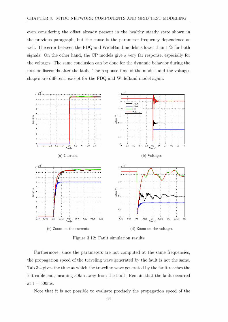
CHAPTER 3. MTDC NETWORK COMPONENTS AND GRID TEST MODELING
even considering the offset already present in the healthy steady state shown in
the previous paragraph, but the cause is the parameter frequency dependence as
well. The error between the FDQ and WideBand models is lower than 1 % for both
signals. On the other hand, the CP models give a very far response, especially for
the voltages. The same conclusion can be done for the dynamic behavior during the
first milliseconds after the fault. The response time of the models and the voltages
shapes are different, except for the FDQ and WideBand model again.
(a) Currents (b) Voltages
(c) Zoom on the currents (d) Zoom on the voltages
Figure 3.12: Fault simulation results
Furthermore, since the parameters are not computed at the same frequencies,
the propagation speed of the traveling wave generated by the fault is not the same.
Tab.3.4 gives the time at which the traveling wave generated by the fault reaches the
left cable end, meaning 30km away from the fault. Remain that the fault occurred
at t = 500ms.
Note that it is not possible to evaluate precisely the propagation speed of the
64
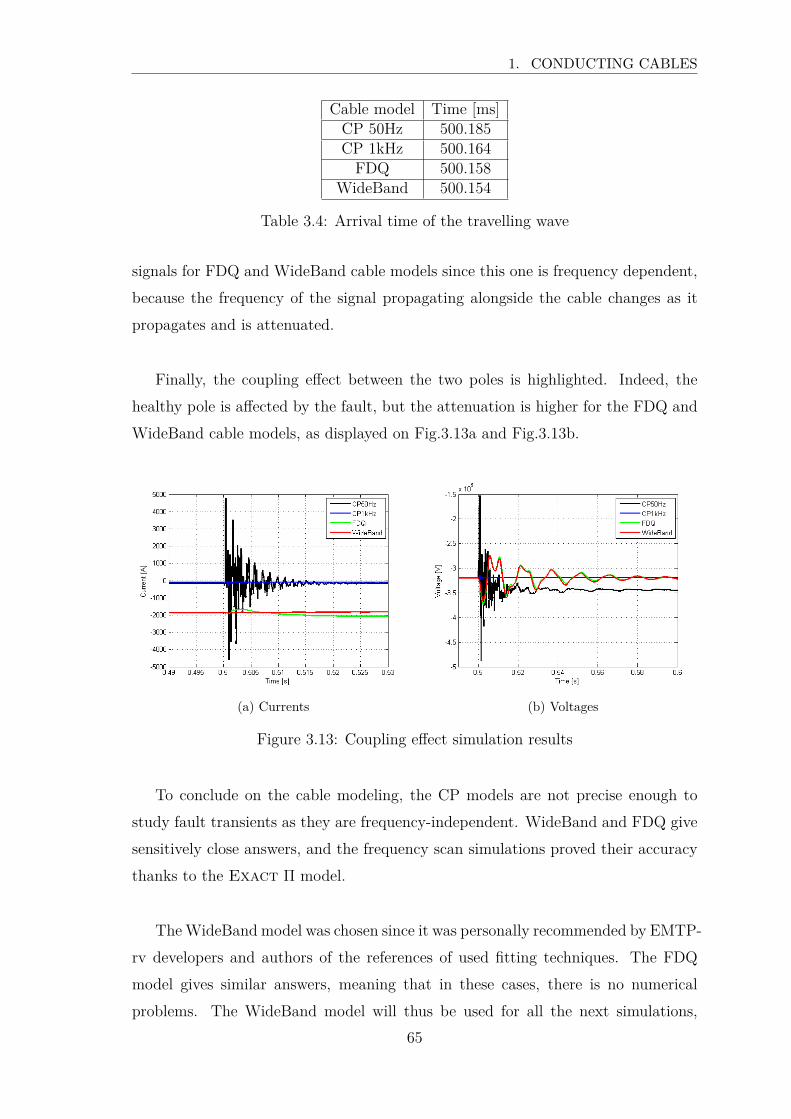
1. CONDUCTING CABLES
Cable model Time [ms]CP 50Hz 500.185CP 1kHz 500.164
FDQ 500.158WideBand 500.154
Table 3.4: Arrival time of the travelling wave
signals for FDQ and WideBand cable models since this one is frequency dependent,
because the frequency of the signal propagating alongside the cable changes as it
propagates and is attenuated.
Finally, the coupling effect between the two poles is highlighted. Indeed, the
healthy pole is affected by the fault, but the attenuation is higher for the FDQ and
WideBand cable models, as displayed on Fig.3.13a and Fig.3.13b.
(a) Currents (b) Voltages
Figure 3.13: Coupling effect simulation results
To conclude on the cable modeling, the CP models are not precise enough to
study fault transients as they are frequency-independent. WideBand and FDQ give
sensitively close answers, and the frequency scan simulations proved their accuracy
thanks to the Exact Π model.
The WideBand model was chosen since it was personally recommended by EMTP-
rv developers and authors of the references of used fitting techniques. The FDQ
model gives similar answers, meaning that in these cases, there is no numerical
problems. The WideBand model will thus be used for all the next simulations,
65
CHAPTER 3. MTDC NETWORK COMPONENTS AND GRID TEST MODELING
except other mention.
2 AC side and substations
2.1 AC/DC conversion
As mentioned in Chapter 1, the AC/DC conversion can be done thanks to two
kinds of power electronics elements: LCC or VSC. Since the voltage polarity remains
constant irrespectively to the power flow transfer direction when VSC are used, it is
easier to implement multi-terminal HVDC systems. Thus, only VSC will be treated
in this section. The study focuses on two-level VSC, but the MTDC system behavior
based on MMC will be discussed in the conclusion of the thesis. Indeed, MMC mod-
eling is currently the topic of a whole Ph.D work done by Hani Saad and conducted
at the École Polytechnique de Montreal. The EMTP-rv averaged and detailed mod-
els of MMC are available [Saad et al., 2013], [Peralta et al., 2012], but the detailed
models are for now too slow to compute, and thus were not appropriate for fault
transient studies at this time. This is why 2-level VSC were consider for this thesis.
As the model of the two-level VSC and its control was done in the framework of
another Ph.D thesis2, this part only gives the headlines of this work.
2.1.1 EMTP-rv VSC components model
The converter itself is represented by a detailed model, meaning that each IGBT
shown in Fig.3.14 is modeled. The hundreds IGBT normally disposed in series in
each arm are simplified and represented by only one per arm. Those IGBT are con-
trolled by an intersective Pulse Width Modulation (PWM) whose carrying frequency
typically range between 1 − 2kHz depending on the converter topology, system fre-
quency and specific objectives of the considered application [Bahrman et al., 2003].
The EMTP-rv model uses a triangle PWM pattern with a carrying frequency of
1350Hz.
The VSC is associated with a DC filter, composed of capacitors CDC and series
inductors LDC, commonly called smoothing reactors.
2Pierre Rault L2EP and RTE - CNER
66

2. AC SIDE AND SUBSTATIONS
Figure 3.14: VSC structure model
2.1.2 VSC control strategy
A simplified line diagram of the substation and its associated controllers are
presented in Fig.3.15. The role of the low level is to convert voltage references
into transistor switching orders, so it depends on the converter unit topology. It is
achieved by the PWM. The AC current control is done by a decoupled controller in
the dq frame. Controllers are standard PI controllers and are tuned for a desired
dynamic performance. For further information, refer to [Nguefeu et al., 2011] and
[Andersen and al., 2005].
The converter goes with AC and DC filters. The DC filter is composed of
the two capacities represented on Fig.3.14 to maintain the voltage level, and a
smoothing reactor (one on each pole) to attenuate the current oscillations. The
value of the smoothing reactor and the capacities has an impact on the fault tran-
sient since it modifies the dI/dt, and will be investigated in Chapter 4. The de-
fault values taken for the next simulations are depicted in Tab.3.5 and come from
[Nguefeu et al., 2011]. The AC filter is shown on Fig.3.15.
AC and DC filters parameters are given in Tab.3.5.
67
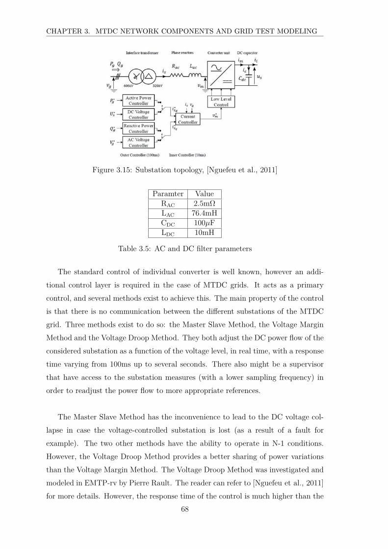
CHAPTER 3. MTDC NETWORK COMPONENTS AND GRID TEST MODELING
Figure 3.15: Substation topology, [Nguefeu et al., 2011]
Paramter ValueRAC 2.5mΩLAC 76.4mHCDC 100µFLDC 10mH
Table 3.5: AC and DC filter parameters
The standard control of individual converter is well known, however an addi-
tional control layer is required in the case of MTDC grids. It acts as a primary
control, and several methods exist to achieve this. The main property of the control
is that there is no communication between the different substations of the MTDC
grid. Three methods exist to do so: the Master Slave Method, the Voltage Margin
Method and the Voltage Droop Method. They both adjust the DC power flow of the
considered substation as a function of the voltage level, in real time, with a response
time varying from 100ms up to several seconds. There also might be a supervisor
that have access to the substation measures (with a lower sampling frequency) in
order to readjust the power flow to more appropriate references.
The Master Slave Method has the inconvenience to lead to the DC voltage col-
lapse in case the voltage-controlled substation is lost (as a result of a fault for
example). The two other methods have the ability to operate in N-1 conditions.
However, the Voltage Droop Method provides a better sharing of power variations
than the Voltage Margin Method. The Voltage Droop Method was investigated and
modeled in EMTP-rv by Pierre Rault. The reader can refer to [Nguefeu et al., 2011]
for more details. However, the response time of the control is much higher than the
68
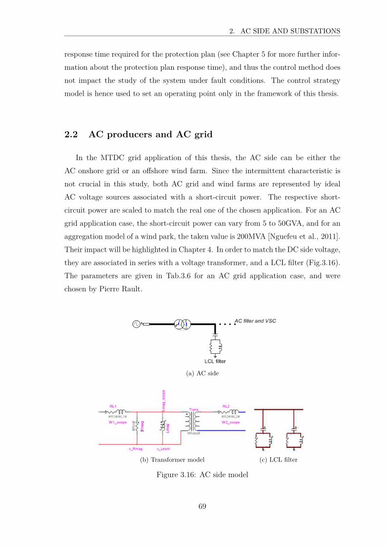
2. AC SIDE AND SUBSTATIONS
response time required for the protection plan (see Chapter 5 for more further infor-
mation about the protection plan response time), and thus the control method does
not impact the study of the system under fault conditions. The control strategy
model is hence used to set an operating point only in the framework of this thesis.
2.2 AC producers and AC grid
In the MTDC grid application of this thesis, the AC side can be either the
AC onshore grid or an offshore wind farm. Since the intermittent characteristic is
not crucial in this study, both AC grid and wind farms are represented by ideal
AC voltage sources associated with a short-circuit power. The respective short-
circuit power are scaled to match the real one of the chosen application. For an AC
grid application case, the short-circuit power can vary from 5 to 50GVA, and for an
aggregation model of a wind park, the taken value is 200MVA [Nguefeu et al., 2011].
Their impact will be highlighted in Chapter 4. In order to match the DC side voltage,
they are associated in series with a voltage transformer, and a LCL filter (Fig.3.16).
The parameters are given in Tab.3.6 for an AC grid application case, and were
chosen by Pierre Rault.
(a) AC side
(b) Transformer model (c) LCL filter
Figure 3.16: AC side model
69

CHAPTER 3. MTDC NETWORK COMPONENTS AND GRID TEST MODELING
Paramter ValueVAC 400kVSsc 50GVA
LCL cutting frequency 500HzTransformer nominal power 1000MVA
Winding 1 voltage 400kVWinding 2 voltage 320kV
Winding R 0.005puWinding X 0.15pu
Table 3.6: Parameters [Nguefeu et al., 2011]
3 Faults and protection relative components
By joining all the elements already detailed in this part, the grid can be modeled
and simulated in healthy conditions. The last components to inspect are related to
the simulation of fault conditions. The protection strategy and algorithms are not
treated in this part, but their inputs (meaning current and voltage measurements)
and their eventual action (opening of circuit breakers) are dealt with. Note that the
current and voltage sensors used by the VSC’s control system cannot be used for
protection purpose, since the dynamic requirements are not the same.
3.1 Fault
The first element to model is the fault itself. As mentioned in Chapter 2, only
permanent faults will be studied in this thesis. Thus, no self-extinguishing faults are
considered and no arcing effects are modeled, even though they exist in the liter-
ature (such as Cassie [Andrea et al., 2010a], Mayr [Andrea et al., 2010b], Habedank
[Darwish and Elkalashy, 2005] or Kizilcay [Idarraga Ospina et al., 2008]). This solves
a huge work which would evaluate the large amount of arc model parameters. The
fault can be easily represented by a constant resistance in series with an ideal switch.
The location of the ideal switch depends on the nature of the fault: pole-to-ground
(PG) or pole-to-pole (PP).
3.2 Sensors
Sensors are keys components in this study, since they give all the inputs that are
used by the protection algorithms. A difference has to be performed between the
70

3. FAULTS AND PROTECTION RELATIVE COMPONENTS
real values of the currents and voltages in the grid, even if that grid is a model, and
the values given by sensors and which can be used by other components. If ideal
sensors with no signal degradation existed, the real values and the measured values
would be the same. However, no such sensors can be manufactured and the signals
deterioration has to be modeled since it might have an impact on the protection
algorithms decision. Furthermore, the real values of the signals are required to
verify the withstand capability of the other components. These values are obtained
by the EMTP-rv ideal sensors library. The measured values correspond to the real
values in the grid, and are then processed to take the degradation effects of the real
sensors into account.
3.2.1 Current sensor
Many current measurement ways can be used. The concerned application de-
termines the choice of the technology. In this study, the sensor has to be chosen to
measure DC currents obviously at their nominal values, but especially to measure
large overcurrents up to several kiloAmps when a fault occurs. Since the protections
have to act very quickly, so the response of the sensor has to match the requested
time constraints.
a) Technology
While a large number of technologies exist and theoretically fulfil the require-
ments of the application, only the ones based on the magnetic field detection are
matured technologies or are not only at the university-research stage. Indeed, even if
magneto-optic sensors based on the Faraday effect seem to have remarkable charac-
teristics ([Petersen, 1995], [Rahmatian and Ortega, 2006], [Takahashi et al., 2010])
particularly in terms of band width, the Hall effect technologies appear to be more
relevant, and namely the Hall effect with flux compensation shows the best per-
formances in terms of band width, measuring range, response time and accuracy
[Eric Favre, 2004]. The measurement principles are detailed in [Correvon, 2005].
b) Model
The goal was not to model the elements of a Hall effect sensor, but to modify the
values of the current measured by the ideal EMTP-rv sensor to approach the values
that would be produced by an Hall effect sensor. The corresponding representation
71
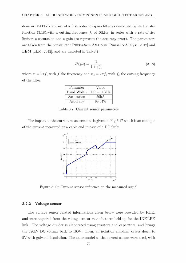
CHAPTER 3. MTDC NETWORK COMPONENTS AND GRID TEST MODELING
done in EMTP-rv consist of a first order low-pass filter as described by its transfer
function (3.18),with a cutting frequency fc of 50kHz, in series with a rate-of-rise
limiter, a saturation and a gain (to represent the accuracy error). The parameters
are taken from the constructor Puissance Analyse [PuissanceAnalyse, 2012] and
LEM [LEM, 2012], and are depicted in Tab.3.7.
H(jω) =1
1 + j ωωc
(3.18)
where w = 2πf , with f the frequency and wc = 2πfc with fc the cutting frequency
of the filter.
Paramter ValueBand Width DC − 50kHzSaturation 50kAAccuracy 99.04%
Table 3.7: Current sensor parameters
The impact on the current measurements is given on Fig.3.17 which is an example
of the current measured at a cable end in case of a DC fault.
Figure 3.17: Current sensor influence on the measured signal
3.2.2 Voltage sensor
The voltage sensor related informations given below were provided by RTE,
and were acquired from the voltage sensor manufacturer held up for the INELFE
link. The voltage divider is elaborated using resistors and capacitors, and brings
the 320kV DC voltage back to 100V. Then, an isolation amplifier drives down to
5V with galvanic insulation. The same model as the current sensor were used, with
72
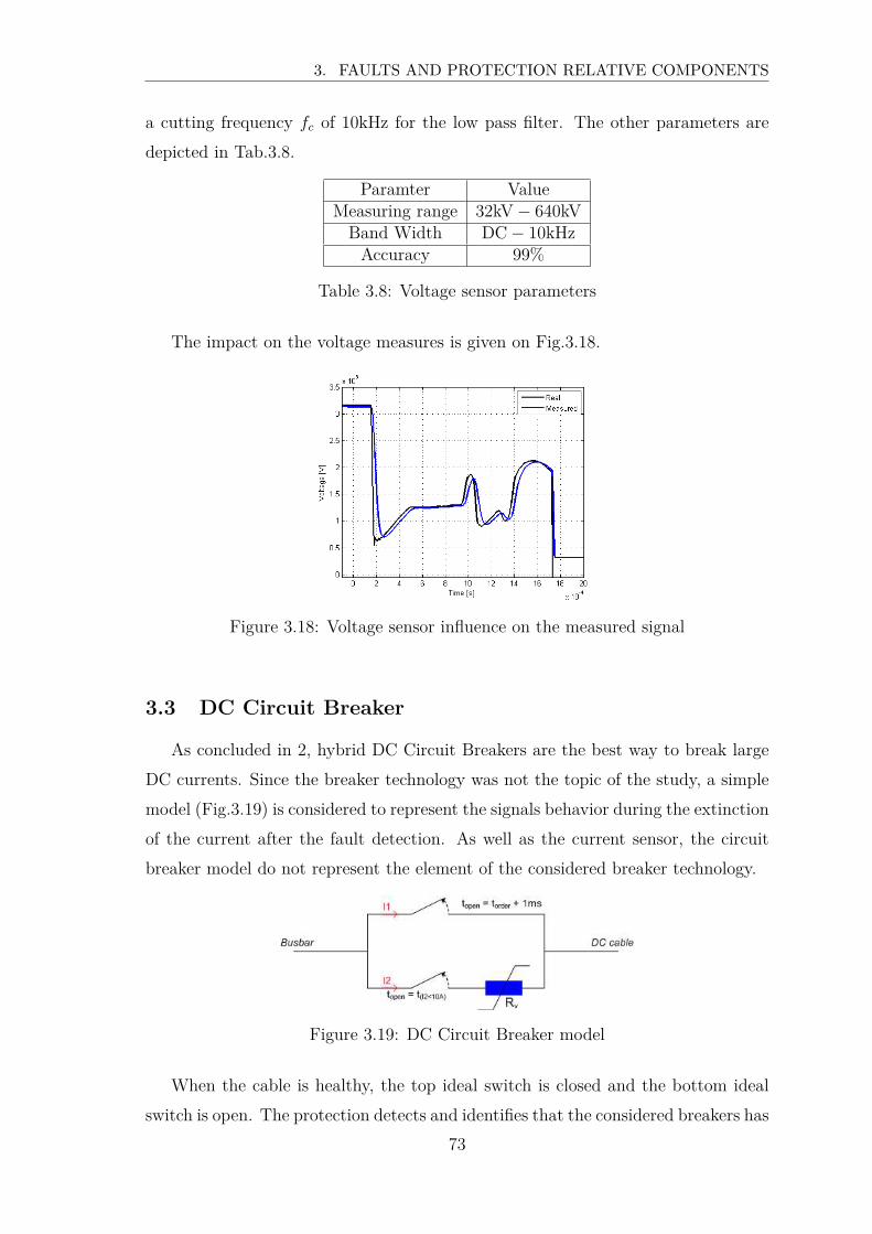
3. FAULTS AND PROTECTION RELATIVE COMPONENTS
a cutting frequency fc of 10kHz for the low pass filter. The other parameters are
depicted in Tab.3.8.
Paramter ValueMeasuring range 32kV − 640kV
Band Width DC − 10kHzAccuracy 99%
Table 3.8: Voltage sensor parameters
The impact on the voltage measures is given on Fig.3.18.
Figure 3.18: Voltage sensor influence on the measured signal
3.3 DC Circuit Breaker
As concluded in 2, hybrid DC Circuit Breakers are the best way to break large
DC currents. Since the breaker technology was not the topic of the study, a simple
model (Fig.3.19) is considered to represent the signals behavior during the extinction
of the current after the fault detection. As well as the current sensor, the circuit
breaker model do not represent the element of the considered breaker technology.
Figure 3.19: DC Circuit Breaker model
When the cable is healthy, the top ideal switch is closed and the bottom ideal
switch is open. The protection detects and identifies that the considered breakers has
73
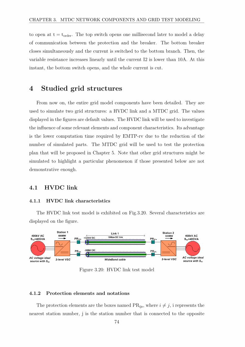
CHAPTER 3. MTDC NETWORK COMPONENTS AND GRID TEST MODELING
to open at t = torder. The top switch opens one millisecond later to model a delay
of communication between the protection and the breaker. The bottom breaker
closes simultaneously and the current is switched to the bottom branch. Then, the
variable resistance increases linearly until the current I2 is lower than 10A. At this
instant, the bottom switch opens, and the whole current is cut.
4 Studied grid structures
From now on, the entire grid model components have been detailed. They are
used to simulate two grid structures: a HVDC link and a MTDC grid. The values
displayed in the figures are default values. The HVDC link will be used to investigate
the influence of some relevant elements and component characteristics. Its advantage
is the lower computation time required by EMTP-rv due to the reduction of the
number of simulated parts. The MTDC grid will be used to test the protection
plan that will be proposed in Chapter 5. Note that other grid structures might be
simulated to highlight a particular phenomenon if those presented below are not
demonstrative enough.
4.1 HVDC link
4.1.1 HVDC link characteristics
The HVDC link test model is exhibited on Fig.3.20. Several characteristics are
displayed on the figure.
Figure 3.20: HVDC link test model
4.1.2 Protection elements and notations
The protection elements are the boxes named PRijs, where i 6= j, i represents the
nearest station number, j is the station number that is connected to the opposite
74
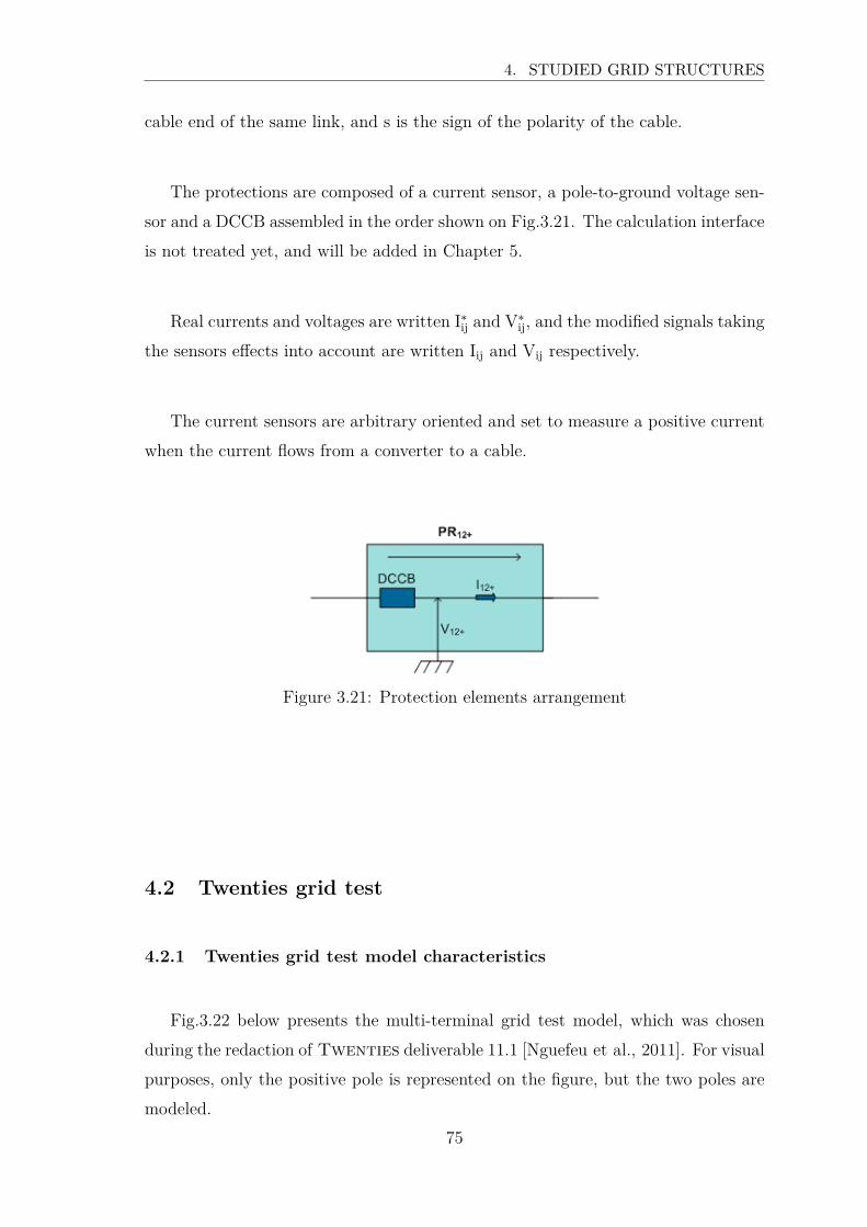
4. STUDIED GRID STRUCTURES
cable end of the same link, and s is the sign of the polarity of the cable.
The protections are composed of a current sensor, a pole-to-ground voltage sen-
sor and a DCCB assembled in the order shown on Fig.3.21. The calculation interface
is not treated yet, and will be added in Chapter 5.
Real currents and voltages are written I∗ij and V∗
ij, and the modified signals taking
the sensors effects into account are written Iij and Vij respectively.
The current sensors are arbitrary oriented and set to measure a positive current
when the current flows from a converter to a cable.
Figure 3.21: Protection elements arrangement
4.2 Twenties grid test
4.2.1 Twenties grid test model characteristics
Fig.3.22 below presents the multi-terminal grid test model, which was chosen
during the redaction of Twenties deliverable 11.1 [Nguefeu et al., 2011]. For visual
purposes, only the positive pole is represented on the figure, but the two poles are
modeled.
75
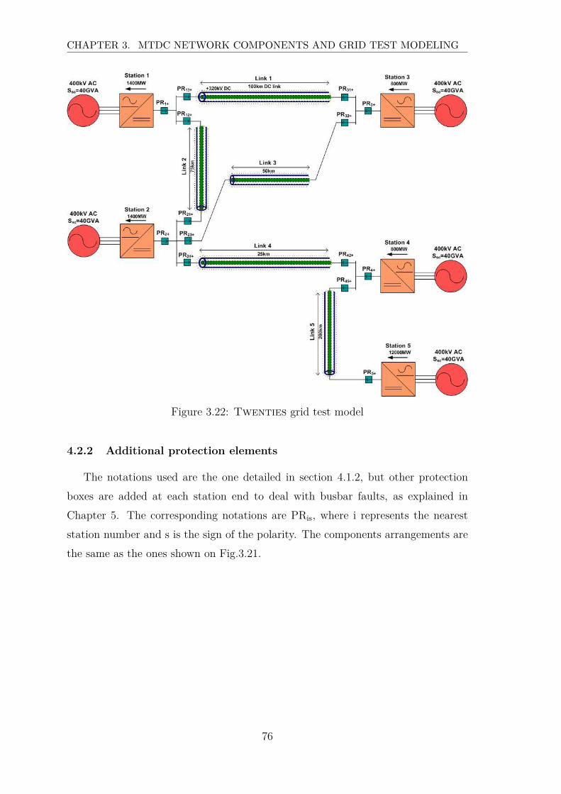
CHAPTER 3. MTDC NETWORK COMPONENTS AND GRID TEST MODELING
Figure 3.22: Twenties grid test model
4.2.2 Additional protection elements
The notations used are the one detailed in section 4.1.2, but other protection
boxes are added at each station end to deal with busbar faults, as explained in
Chapter 5. The corresponding notations are PRis, where i represents the nearest
station number and s is the sign of the polarity. The components arrangements are
the same as the ones shown on Fig.3.21.
76

4. STUDIED GRID STRUCTURES
77

CHAPTER 4
Signals behavior under fault
conditions

Chapter 4
Signals behavior under fault
conditions
Now, the model of each element of the grid has been detailed. Accurate sim-
ulation of DC fault can therefore be made. This chapter constitutes a parametric
study to highlight the components of the grid that have an influence on the signals
that will be used by the protection system, which will be developed in Chapter 5.
As mentioned in Chapter 2, the protection system needs to operate in a very short
time (in the range of 5ms), that is why the results that follow will be focused on
this small duration transients.
The impact of three kinds of parameters will be discussed: sources-related, grid-
related and fault-related parameters. The effect of most of them on the currents
and voltages will be argued thanks to the simulation of the HVDC test case model,
others will be examined through the Twenties grid test model, and some other
structures will be defined to highlight their influence. The parameters that will vary
are listed in Tab.4.1. The simulation sampling frequency were set to 1MHz.
The default parameters of the grid were given in Chapter 3, and some of them are
reminded on Fig.4.1. The default parameters for the fault are mentioned in Tab.4.2.
In each section of this chapter, the influence of one parameter will be presented
by varying only this one parameter, and keeping the others at their default value.
Thus, only the value of the parameter that changes will be provided.
81
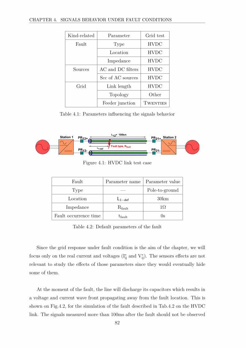
CHAPTER 4. SIGNALS BEHAVIOR UNDER FAULT CONDITIONS
Kind-related Parameter Grid test
Fault Type HVDC
Location HVDC
Impedance HVDC
Sources AC and DC filters HVDC
Scc of AC sources HVDC
Grid Link length HVDC
Topology Other
Feeder junction Twenties
Table 4.1: Parameters influencing the signals behavior
L12= 100km
L1-def
PR12+
PR12-
PR21+
PR21-
Station 1 Station 2
Fault type, Rfault
Figure 4.1: HVDC link test case
Fault Parameter name Parameter value
Type — Pole-to-ground
Location L1−def 30km
Impedance Rfault 1Ω
Fault occurrence time tfault 0s
Table 4.2: Default parameters of the fault
Since the grid response under fault condition is the aim of the chapter, we will
focus only on the real current and voltages (I∗ij and V∗
ij). The sensors effects are not
relevant to study the effects of those parameters since they would eventually hide
some of them.
At the moment of the fault, the line will discharge its capacitors which results in
a voltage and current wave front propagating away from the fault location. This is
shown on Fig.4.2, for the simulation of the fault described in Tab.4.2 on the HVDC
link. The signals measured more than 100ms after the fault should not be observed
82
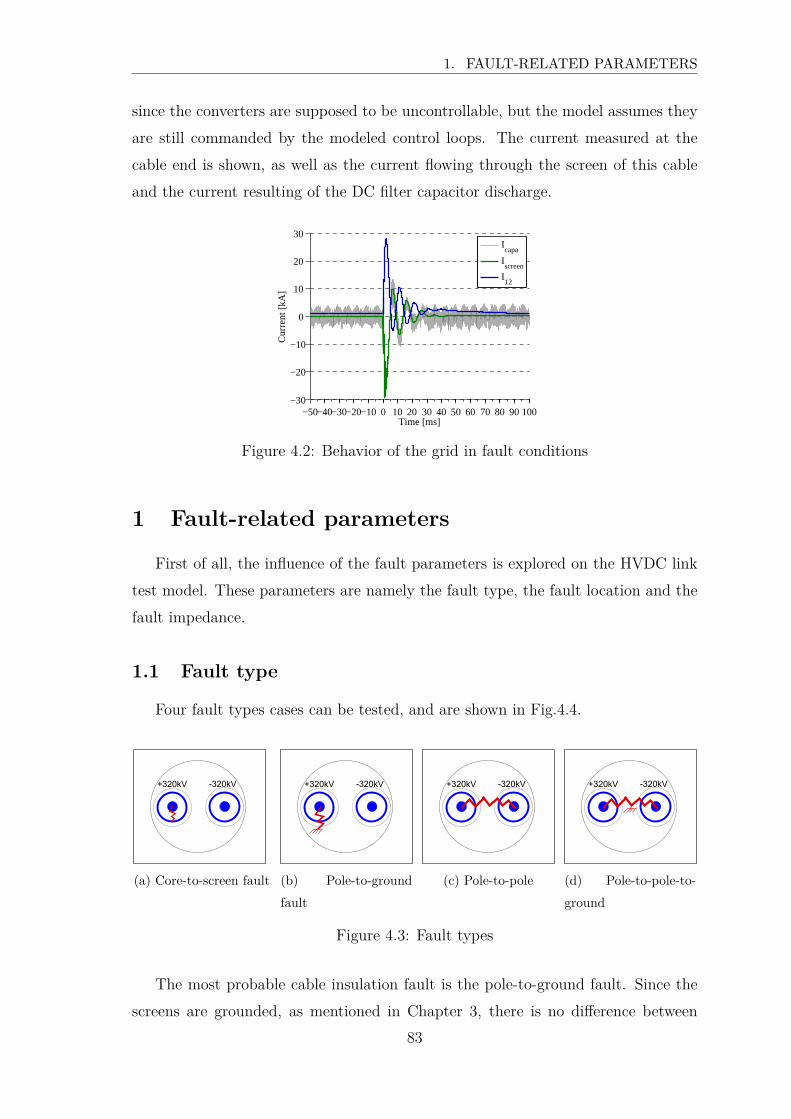
1. FAULT-RELATED PARAMETERS
since the converters are supposed to be uncontrollable, but the model assumes they
are still commanded by the modeled control loops. The current measured at the
cable end is shown, as well as the current flowing through the screen of this cable
and the current resulting of the DC filter capacitor discharge.
−50−40−30−20−10 0 10 20 30 40 50 60 70 80 90 100−30
−20
−10
0
10
20
30
Time [ms]
Cur
rent
[kA
]
Icapa
Iscreen
I12
Figure 4.2: Behavior of the grid in fault conditions
1 Fault-related parameters
First of all, the influence of the fault parameters is explored on the HVDC link
test model. These parameters are namely the fault type, the fault location and the
fault impedance.
1.1 Fault type
Four fault types cases can be tested, and are shown in Fig.4.4.
+320kV -320kV
(a) Core-to-screen fault
+320kV -320kV
(b) Pole-to-ground
fault
+320kV -320kV
(c) Pole-to-pole
+320kV -320kV
(d) Pole-to-pole-to-
ground
Figure 4.3: Fault types
The most probable cable insulation fault is the pole-to-ground fault. Since the
screens are grounded, as mentioned in Chapter 3, there is no difference between
83

CHAPTER 4. SIGNALS BEHAVIOR UNDER FAULT CONDITIONS
a pole-to-screen fault and a pole-to-ground fault. Also, it is not probable that a
fault links the core and the ground of a cable, without passing through the screen.
Therefore, two types of faults are considered in the rest of this thesis, namely pole-
to-ground fault and pole-to-pole faults, that both include the grounding effect. They
correspond respectively to tested case Ctype−pg and Ctype−pp. Pole-to-pole faults are
very unlikely along a cable, but can still happen and thus need to be investigated.
However, pole-to-pole fault can occur at the substation connection point. The re-
sulting currents and voltages few milliseconds after the fault instant are shown on
Fig.4.4.
type-pp
type-pg
Cu
rren
t[.
10
kA
]
Time [ms]0 50 100 150 200 250 300
-1
-0.5
0
0.5
1
1.5
2
2.5
3
(a) Currents I+12
type-pp
type-pg
Cu
rren
t[.
10
kA
]
Time [ms]0 50 100 150 200 250 300
-3
-2.5
-2
-1.5
-1
-0.5
0
0.5
(b) Currents I−
12
type-pp
type-pg
Volt
age
[.1
00
kV
]
Time [ms]0 50 100 150 200 250 300
-2
-1
0
1
2
3
4
(c) Voltages V+12
type-pp
type-pg
Volt
age
[.1
00
kV
]
Time [ms]0 50 100 150 200 250 300
-7
-6
-5
-4
-3
-2
-1
0
1
2
(d) Voltages V−
12
Figure 4.4: Fault types
Two differences can be noticed on those figures: one related to the steady-state
after the fault, and one related to the transient phase of the signals.
The steady-state signals after the fault occurrence are not meaningful since the
84

1. FAULT-RELATED PARAMETERS
converters IGBT are not controllable in real applications considering the loss of
voltage at the converter terminals, which is not the case in our simulations.
However, some observations can be made. The voltages V+12 are close to zero
for both cases (Fig.4.4c), since the positive pole is faulty for the two fault types.
This is also the case for the voltage V−12 concerning the pole-to-pole fault. However,
in pole-to-ground conditions, the voltage of the healthy link decreases to twice the
nominal voltage value (Fig.4.4d), making the pole-to-pole voltage keeping the nom-
inal value. Since the controllability of the VSC is kept after the fault in our models,
that implies that the current related to the case Ctype−pg is reduced to zero after a
few milliseconds after the fault.
The transient behavior of the fault depends on the cable length and sources
characteristics and will be investigated later in this chapter. However, the difference
between a pole-to-ground fault and a pole-to-pole is obviously due to the fact that
the solicited passive components are not the same.
1.2 Fault location
Five locations are tested through the simulation of a pole-to-ground fault. The
lengths are defined in Fig.4.5 and the values are provided in Tab.4.3.
L12= 100km
L1-def
PR12+
PR12-
PR21+
PR21-
Station 1 Station 2
Ldef-2
Pole to ground fault
Figure 4.5: Fault location parameter on the HVDC link test model
Case name L1−def Ldef−2
Cpos−1 0 100
Cpos−2 30 70
Cpos−3 50 50
Cpos−4 70 30
Cpos−5 100 0
Table 4.3: Cases parameters for position influence study
85
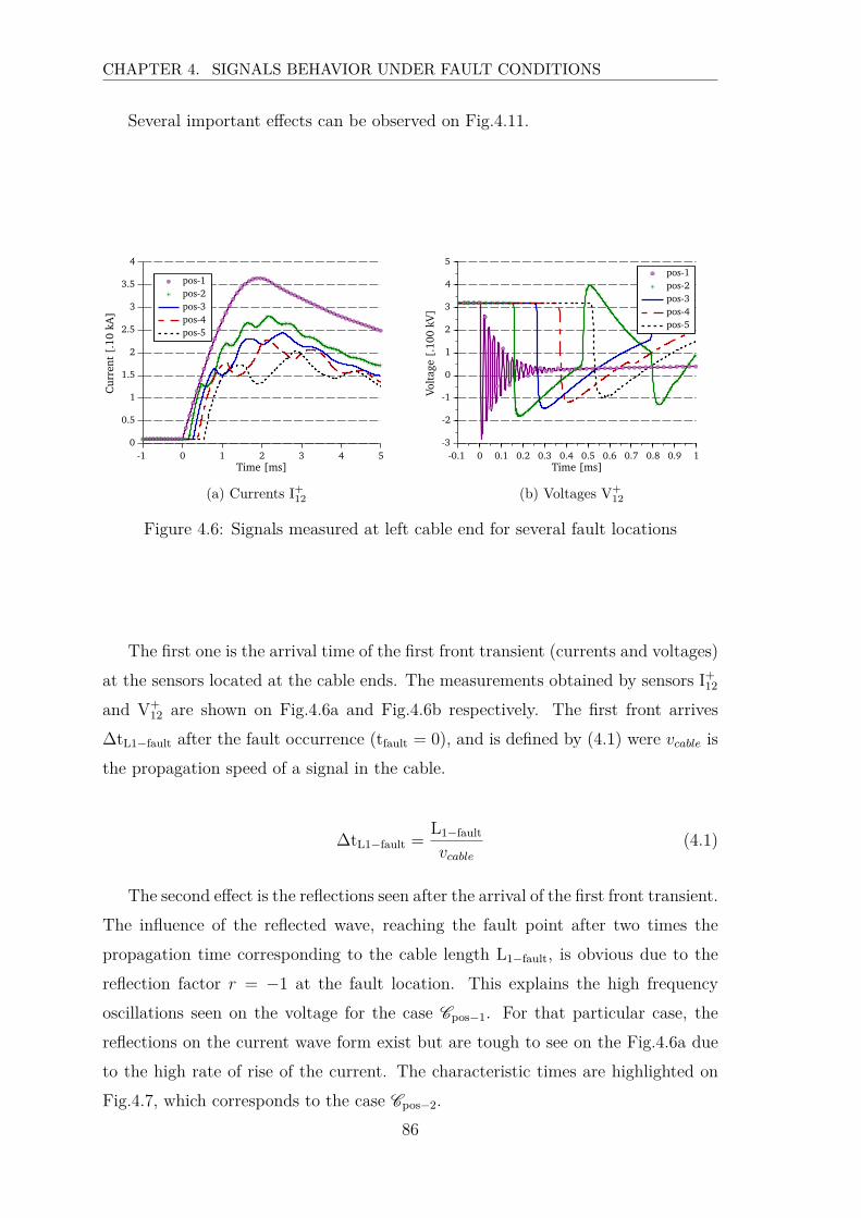
CHAPTER 4. SIGNALS BEHAVIOR UNDER FAULT CONDITIONS
Several important effects can be observed on Fig.4.11.
pos-5
pos-4
pos-3
pos-2
pos-1
Cu
rren
t[.
10
kA
]
Time [ms]-1 0 1 2 3 4 5
0
0.5
1
1.5
2
2.5
3
3.5
4
(a) Currents I+12
pos-5
pos-4
pos-3
pos-2
pos-1
Volt
age
[.1
00
kV
]
Time [ms]-0.1 0 0.1 0.2 0.3 0.4 0.5 0.6 0.7 0.8 0.9 1
-3
-2
-1
0
1
2
3
4
5
(b) Voltages V+12
Figure 4.6: Signals measured at left cable end for several fault locations
The first one is the arrival time of the first front transient (currents and voltages)
at the sensors located at the cable ends. The measurements obtained by sensors I+12
and V+12 are shown on Fig.4.6a and Fig.4.6b respectively. The first front arrives
∆tL1−fault after the fault occurrence (tfault = 0), and is defined by (4.1) were vcable is
the propagation speed of a signal in the cable.
∆tL1−fault =L1−fault
vcable
(4.1)
The second effect is the reflections seen after the arrival of the first front transient.
The influence of the reflected wave, reaching the fault point after two times the
propagation time corresponding to the cable length L1−fault, is obvious due to the
reflection factor r = −1 at the fault location. This explains the high frequency
oscillations seen on the voltage for the case Cpos−1. For that particular case, the
reflections on the current wave form exist but are tough to see on the Fig.4.6a due
to the high rate of rise of the current. The characteristic times are highlighted on
Fig.4.7, which corresponds to the case Cpos−2.
86
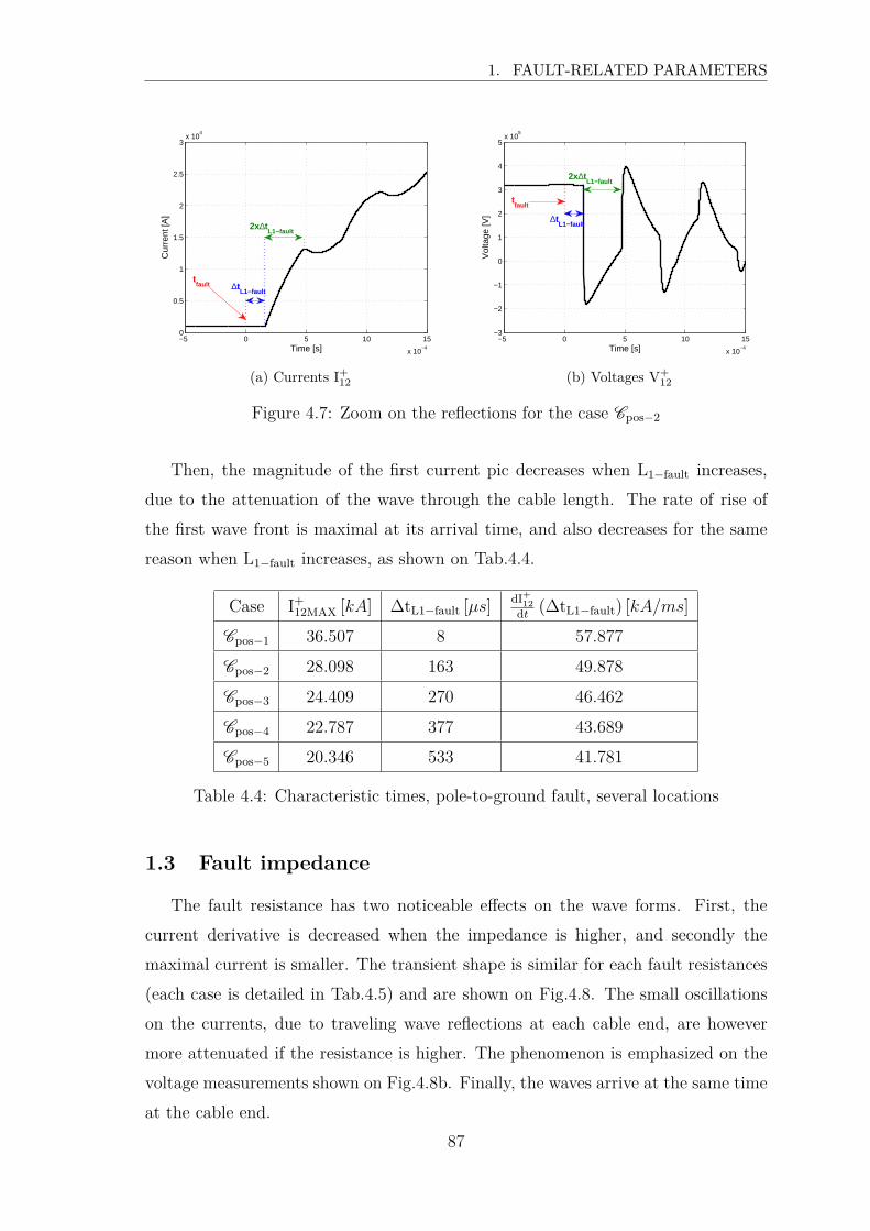
1. FAULT-RELATED PARAMETERS
−5 0 5 10 15
x 10−4
0
0.5
1
1.5
2
2.5
3x 10
4
Time [s]
Cur
rent
[A]
∆tL1−fault
tfault
2x∆tL1−fault
(a) Currents I+12
−5 0 5 10 15
x 10−4
−3
−2
−1
0
1
2
3
4
5x 10
5
Time [s]
Vol
tage
[V] ∆t
L1−fault
tfault
2x∆tL1−fault
(b) Voltages V+12
Figure 4.7: Zoom on the reflections for the case Cpos−2
Then, the magnitude of the first current pic decreases when L1−fault increases,
due to the attenuation of the wave through the cable length. The rate of rise of
the first wave front is maximal at its arrival time, and also decreases for the same
reason when L1−fault increases, as shown on Tab.4.4.
Case I+12MAX [kA] ∆tL1−fault [µs] dI+
12
dt(∆tL1−fault) [kA/ms]
Cpos−1 36.507 8 57.877
Cpos−2 28.098 163 49.878
Cpos−3 24.409 270 46.462
Cpos−4 22.787 377 43.689
Cpos−5 20.346 533 41.781
Table 4.4: Characteristic times, pole-to-ground fault, several locations
1.3 Fault impedance
The fault resistance has two noticeable effects on the wave forms. First, the
current derivative is decreased when the impedance is higher, and secondly the
maximal current is smaller. The transient shape is similar for each fault resistances
(each case is detailed in Tab.4.5) and are shown on Fig.4.8. The small oscillations
on the currents, due to traveling wave reflections at each cable end, are however
more attenuated if the resistance is higher. The phenomenon is emphasized on the
voltage measurements shown on Fig.4.8b. Finally, the waves arrive at the same time
at the cable end.
87
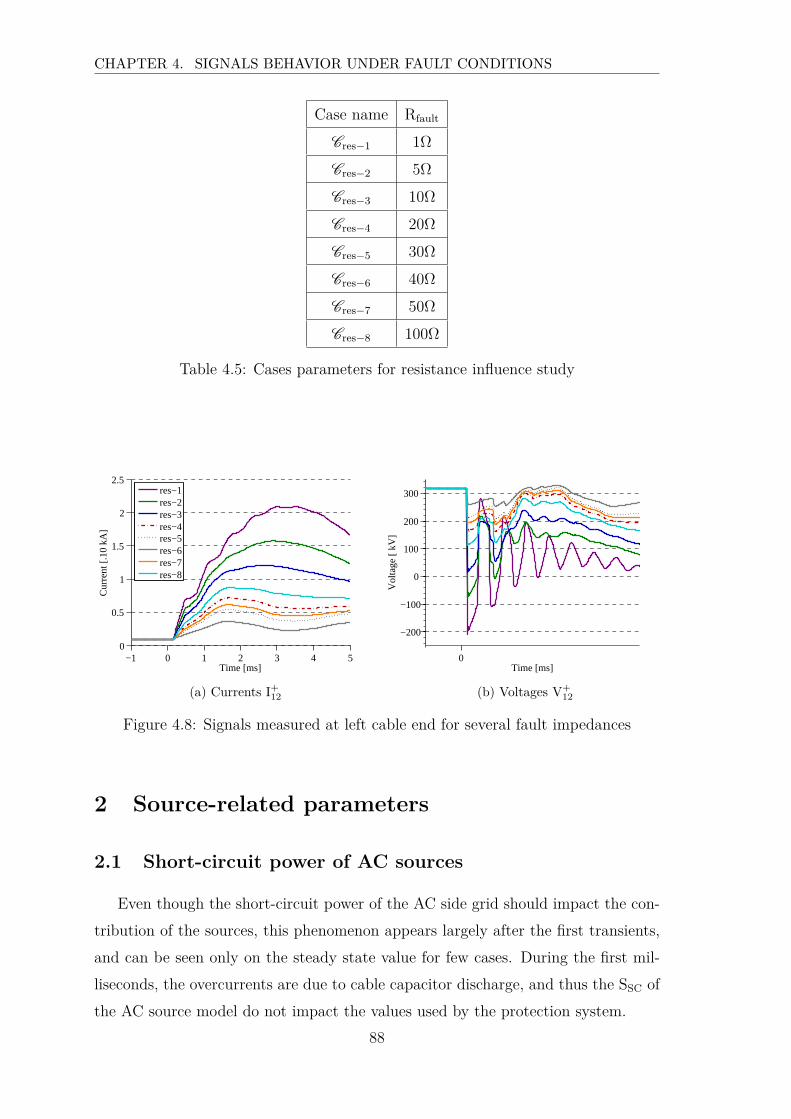
CHAPTER 4. SIGNALS BEHAVIOR UNDER FAULT CONDITIONS
Case name Rfault
Cres−1 1Ω
Cres−2 5Ω
Cres−3 10Ω
Cres−4 20Ω
Cres−5 30Ω
Cres−6 40Ω
Cres−7 50Ω
Cres−8 100Ω
Table 4.5: Cases parameters for resistance influence study
−1 0 1 2 3 4 50
0.5
1
1.5
2
2.5
Time [ms]
Cur
rent
[.10
kA
]
res−1res−2res−3res−4res−5res−6res−7res−8
(a) Currents I+12
0
−200
−100
0
100
200
300
Time [ms]
Vol
tage
[ kV
]
(b) Voltages V+12
Figure 4.8: Signals measured at left cable end for several fault impedances
2 Source-related parameters
2.1 Short-circuit power of AC sources
Even though the short-circuit power of the AC side grid should impact the con-
tribution of the sources, this phenomenon appears largely after the first transients,
and can be seen only on the steady state value for few cases. During the first mil-
liseconds, the overcurrents are due to cable capacitor discharge, and thus the SSC of
the AC source model do not impact the values used by the protection system.
88
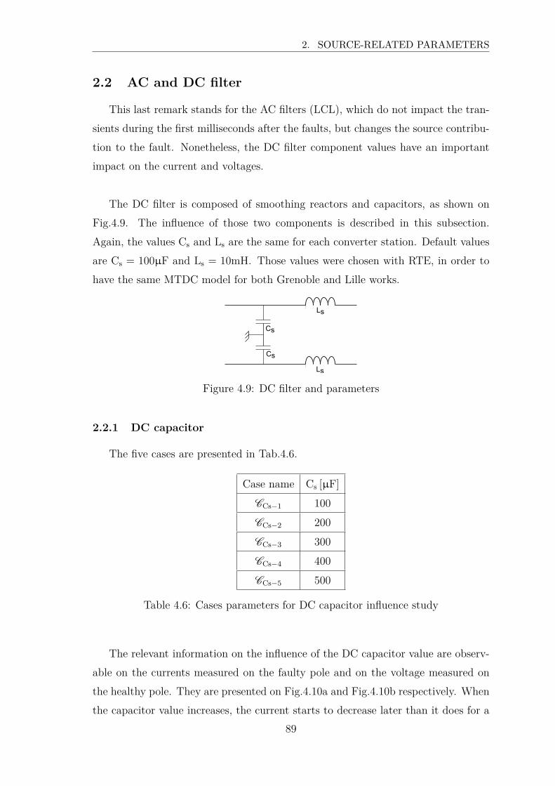
2. SOURCE-RELATED PARAMETERS
2.2 AC and DC filter
This last remark stands for the AC filters (LCL), which do not impact the tran-
sients during the first milliseconds after the faults, but changes the source contribu-
tion to the fault. Nonetheless, the DC filter component values have an important
impact on the current and voltages.
The DC filter is composed of smoothing reactors and capacitors, as shown on
Fig.4.9. The influence of those two components is described in this subsection.
Again, the values Cs and Ls are the same for each converter station. Default values
are Cs = 100µF and Ls = 10mH. Those values were chosen with RTE, in order to
have the same MTDC model for both Grenoble and Lille works.
Ls
Ls
Cs
Cs
Figure 4.9: DC filter and parameters
2.2.1 DC capacitor
The five cases are presented in Tab.4.6.
Case name Cs [µF]
CCs−1 100
CCs−2 200
CCs−3 300
CCs−4 400
CCs−5 500
Table 4.6: Cases parameters for DC capacitor influence study
The relevant information on the influence of the DC capacitor value are observ-
able on the currents measured on the faulty pole and on the voltage measured on
the healthy pole. They are presented on Fig.4.10a and Fig.4.10b respectively. When
the capacitor value increases, the current starts to decrease later than it does for a
89
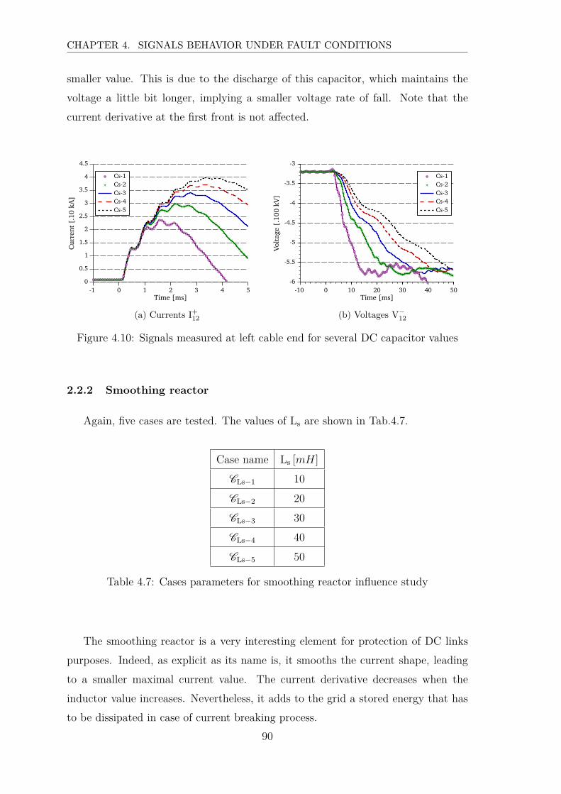
CHAPTER 4. SIGNALS BEHAVIOR UNDER FAULT CONDITIONS
smaller value. This is due to the discharge of this capacitor, which maintains the
voltage a little bit longer, implying a smaller voltage rate of fall. Note that the
current derivative at the first front is not affected.
Cs-5
Cs-4
Cs-3
Cs-2
Cs-1
Cu
rren
t[.
10
kA
]
Time [ms]-1 0 1 2 3 4 5
0
0.5
1
1.5
2
2.5
3
3.5
4
4.5
(a) Currents I+12
Cs-5
Cs-4
Cs-3
Cs-2
Cs-1
Volt
age
[.1
00
kV
]
Time [ms]-10 0 10 20 30 40 50
-6
-5.5
-5
-4.5
-4
-3.5
-3
(b) Voltages V−
12
Figure 4.10: Signals measured at left cable end for several DC capacitor values
2.2.2 Smoothing reactor
Again, five cases are tested. The values of Ls are shown in Tab.4.7.
Case name Ls [mH]
CLs−1 10
CLs−2 20
CLs−3 30
CLs−4 40
CLs−5 50
Table 4.7: Cases parameters for smoothing reactor influence study
The smoothing reactor is a very interesting element for protection of DC links
purposes. Indeed, as explicit as its name is, it smooths the current shape, leading
to a smaller maximal current value. The current derivative decreases when the
inductor value increases. Nevertheless, it adds to the grid a stored energy that has
to be dissipated in case of current breaking process.
90

3. GRID-RELATED PARAMETERS
−1 0 1 2 3 4 50
0.5
1
1.5
2
2.5
Time [ms]
Cur
rent
[.10
kA
]
Ls−1Ls−2Ls−3Ls−4Ls−5
(a) Currents I+12
0
−200
−100
0
100
200
300
400
Time [ms]
Vol
tage
[ kV
]
res−1res−2res−3res−4res−5
(b) Voltages V+12
Figure 4.11: Signals measured at left cable end for several DC inductor values
2.3 VSC control strategy
The VSC outer control strategy does not impact the transients since its response
time to an event is in the range of 100ms. Several simulations were done using a
master slave control, or droop control, and no variations were noticed on the fault
signals.
Besides, a master slave control cannot be considered in real application since
the loss of the voltage controlled station would lead to a whole DC grid black out.
Those aspects are detailed in [Rault, 2013].
3 Grid-related parameters
3.1 Link length
First of all, the link length influence is assessed thanks to the simulation of the
HVDC link for two different link lengths. The fault is always at 30% of the total
length away station 1. Cases parameters are given in Tab.4.8.
91

CHAPTER 4. SIGNALS BEHAVIOR UNDER FAULT CONDITIONS
Case name Link length L1−fault
Clength−1 100 30
Clength−2 200 60
Table 4.8: Cases parameters for link length influence study
The resulting currents are shown on Fig.4.14b for the left hand side cable end,
and on Fig.4.15a for the right hand side end. The wave front arrival time is higher
for the 200km long cable since the fault is further for each ends. Also, the current
is reduced at the two ends for the same reason, because of the attenuation through
the cable length. The transient shape is modified because the reflections do not
correspond to the same length, once again.
−1 0 1 2 3 4 50
0.5
1
1.5
2
2.5
3
Time [ms]
Cur
rent
[.10
kA
]
length−1length−2
(a) I+12
−1 0 1 2 3 4 5−0.5
0
0.5
1
1.5
2
Time [ms]
Cur
rent
[.10
kA
]
length−1length−2
(b) I+21
Figure 4.12: Current measurements for several link lengths
3.2 Grid topology: number of feeders connected to a busbar
Only one feeder was considered from the beginning of the parametric study.
The previous tendencies remain valid for any topology, but the number of feeders
connected to a busbar has an impact on the signals. This is investigated thanks to
the use of two new grid topologies, which are shown on Fig.4.13.
92
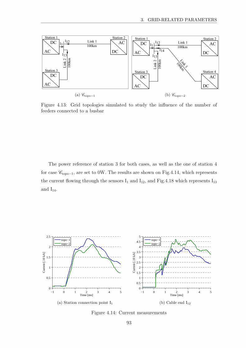
3. GRID-RELATED PARAMETERS
AC
DC AC
DC100kmLink 1
Station 1
AC
DCStation 3
Station 2
Link
2
I12
I13
I1
100k
m
(a) Ctopo−1
AC
DC AC
DC100kmLink 1
Station 1
AC
DCStation 3
AC
DC
Station 2
Station 4
Link
2 Link 3
I12
I13
I1
100k
m 100km
I14
(b) Ctopo−2
Figure 4.13: Grid topologies simulated to study the influence of the number offeeders connected to a busbar
The power reference of station 3 for both cases, as well as the one of station 4
for case Ctopo−1, are set to 0W. The results are shown on Fig.4.14, which represents
the current flowing through the sensors I1 and I12, and Fig.4.18 which represents I13
and I14.
−1 0 1 2 3 4 50
0.5
1
1.5
2
2.5
Time [ms]
Cur
rent
[.10
kA
]
topo−1topo−2
(a) Station connection point I1
−1 0 1 2 3 4 50
0.5
1
1.5
2
2.5
3
3.5
4
4.5
5
Time [ms]
Cur
rent
[.10
kA
]
topo−1topo−2
(b) Cable end I12
Figure 4.14: Current measurements
93
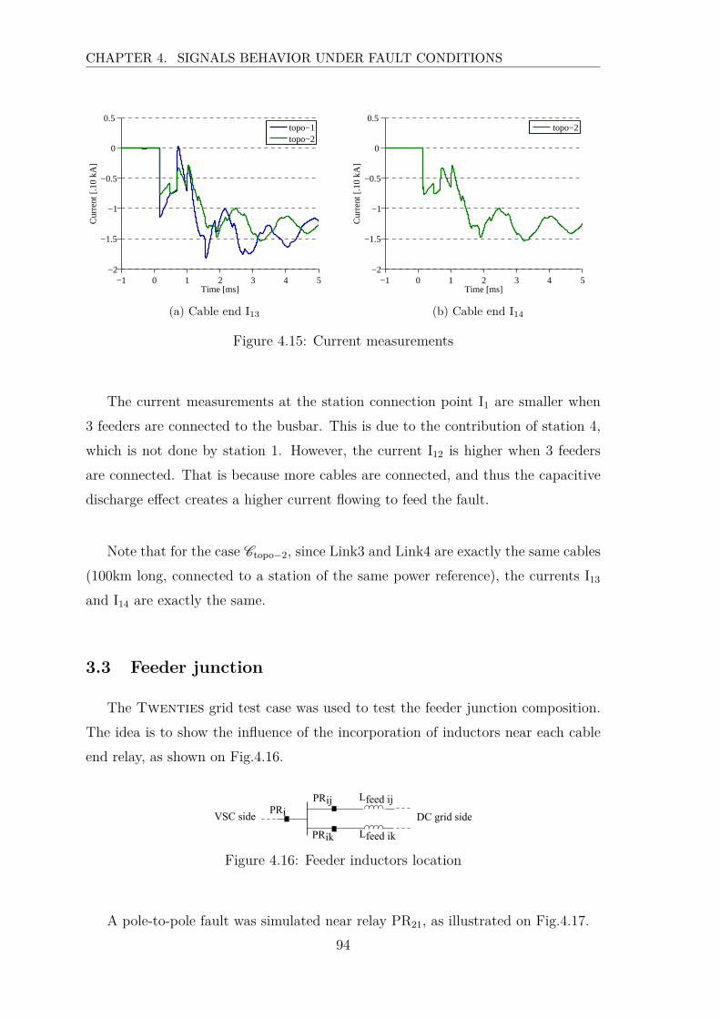
CHAPTER 4. SIGNALS BEHAVIOR UNDER FAULT CONDITIONS
−1 0 1 2 3 4 5−2
−1.5
−1
−0.5
0
0.5
Time [ms]
Cur
rent
[.10
kA
]
topo−1topo−2
(a) Cable end I13
−1 0 1 2 3 4 5−2
−1.5
−1
−0.5
0
0.5
Time [ms]
Cur
rent
[.10
kA
]
topo−2
(b) Cable end I14
Figure 4.15: Current measurements
The current measurements at the station connection point I1 are smaller when
3 feeders are connected to the busbar. This is due to the contribution of station 4,
which is not done by station 1. However, the current I12 is higher when 3 feeders
are connected. That is because more cables are connected, and thus the capacitive
discharge effect creates a higher current flowing to feed the fault.
Note that for the case Ctopo−2, since Link3 and Link4 are exactly the same cables
(100km long, connected to a station of the same power reference), the currents I13
and I14 are exactly the same.
3.3 Feeder junction
The Twenties grid test case was used to test the feeder junction composition.
The idea is to show the influence of the incorporation of inductors near each cable
end relay, as shown on Fig.4.16.
PRij
PRik
PRiVSC side DC grid side
Lfeed ij
Lfeed ik
Figure 4.16: Feeder inductors location
A pole-to-pole fault was simulated near relay PR21, as illustrated on Fig.4.17.
94

3. GRID-RELATED PARAMETERS
AC
DC AC
DC100kmLink 1
Station 1
AC
DCStation 2
25kmLink 4 AC
DC
AC
DC
Station 3
Station 4
Station 5
75km
200k
m
Link
2
Link
5
Link 3
50km
PR42
PR4
PR45
PR5
PR24
PR13
PR12
PR31
PR32
PR23
PR21
PR1
PR2
PR3
Figure 4.17: Simulation of a fault on the Twenties grid structure
The conclusions that were made about the smoothing reactor (cases CLs−i, i =
1..5) on the HVDC link are valid for the inductors Lfeed, meaning that the current
is smoothed (Fig.4.18). Moreover, this inductance has the advantage of reducing
the current (due to cable capacitor discharge) arriving to the converter (like the
DC filter smoothing reactor), but also to decrease the current created by the cable
discharge, arriving to the relays.
−1 0 1 2 3 4 50
1
2
3
4
5
6
Time [ms]
Cur
rent
[.10
kA
]
Lfeed−1Lfeed−2Lfeed−3Lfeed−4Lfeed−5Lfeed−6Lfeed−7Lfeed−8
Figure 4.18: Current I21
The parameters influence on the first current transients following the fault even
are recapitulated in Tab.4.9.
95
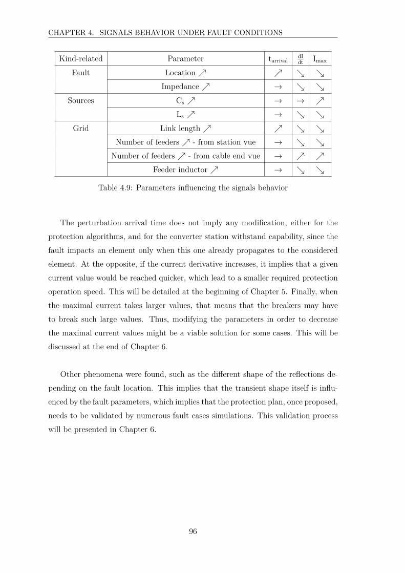
CHAPTER 4. SIGNALS BEHAVIOR UNDER FAULT CONDITIONS
Kind-related Parameter tarrivaldIdt
Imax
Fault Location ր ր ց ցImpedance ր → ց ց
Sources Cs ր → → րLs ր → ց ց
Grid Link length ր ր ց ցNumber of feeders ր - from station vue → ց ց
Number of feeders ր - from cable end vue → ր րFeeder inductor ր → ց ց
Table 4.9: Parameters influencing the signals behavior
The perturbation arrival time does not imply any modification, either for the
protection algorithms, and for the converter station withstand capability, since the
fault impacts an element only when this one already propagates to the considered
element. At the opposite, if the current derivative increases, it implies that a given
current value would be reached quicker, which lead to a smaller required protection
operation speed. This will be detailed at the beginning of Chapter 5. Finally, when
the maximal current takes larger values, that means that the breakers may have
to break such large values. Thus, modifying the parameters in order to decrease
the maximal current values might be a viable solution for some cases. This will be
discussed at the end of Chapter 6.
Other phenomena were found, such as the different shape of the reflections de-
pending on the fault location. This implies that the transient shape itself is influ-
enced by the fault parameters, which implies that the protection plan, once proposed,
needs to be validated by numerous fault cases simulations. This validation process
will be presented in Chapter 6.
96

3. GRID-RELATED PARAMETERS
97


CHAPTER 5
Protection strategy

Chapter 5
Protection strategy
This part deals with the protection algorithms that are relevant for a MTDC
grid, including main protection and backup algorithms in case of failure or non trip-
ping of the protective relay.
This protection system is specifically designed for a MTDC grid and based on
operational experience gained from protection practice of AC grids, meaning that
the selectivity is ensured thanks to the use of DC circuit breakers located at each
cable end and at each station connection point.
This work was conducted considering each converter of the grid as a two-level
VSC. The generalization of the proposed protection plan for other conversion tech-
nologies will be discussed in the conclusion of this thesis.
First of all, the specification and the constraints related to the protection oper-
ation of a DC grid will be presented. Then, the protection plan will be developed.
A busbar protection will be described, and two algorithms will be chosen for the
cable protection, one with a communication assumption, and another one without
any data exchange with other relays. Then, a backup principle in case of a breaker
failure will be detailed, and the global protection system is summed-up at the end
of the chapter.
101

CHAPTER 5. PROTECTION STRATEGY
1 Protection plan specification
A protection system is used to protect an electrical circuit and its users against
damage. This thesis focuses on the protection against short-circuit faults, due to
insulation breakdown. This phenomenon translates into a low or high impedance
fault, and between pole and ground (PG) or pole and pole (PP). The protection plan
has to handle all the possibilities, and must have the following properties defined in
[Ghandhari et al., 2011]:
• Sensitivity: The protection system has to detect any fault occurring in the
DC part of the grid, meaning either low impedance faults and high impedance
faults. Following the example of the AC protection strategy, it is not neces-
sarily the same algorithm which is used depending on the fault impedance.
• Selectivity: The protection system should only operate after a fault (not
during normal operation), and only if the fault is in its own coverage domain.
Several coverage domains can be defined depending on the level of the protec-
tion (main, backup).
• Speed: The protection system should be fast enough to interrupt faults before
they may damage equipment or can no longer be interrupted by the breakers.
• Reliability: A good protection system is reliable and has a backup system in
case the primary protection system or a breaker fails.
• Robustness: The protection system should have the ability to detect faults
in normal mode as in degraded mode, and to discriminate faults from any
other operation occurring (set-point changes, operations, ...).
• Seamless: After the fault clearance, the remaining part of the system should
continue operating in a secure state. This means that the system itself can
accept the transients generated by the fault and its clearing process, and that
the protection system will remain stable during the transient implied by the
clearing process.
The speed, the sensitivity and the selectivity constraints will be detailed in sec-
tion 2.1, 2.2 and 2.3 respectively. The reliability is the subject of section 4 which
defines the backup protection principle. The robustness to any operation point of
102
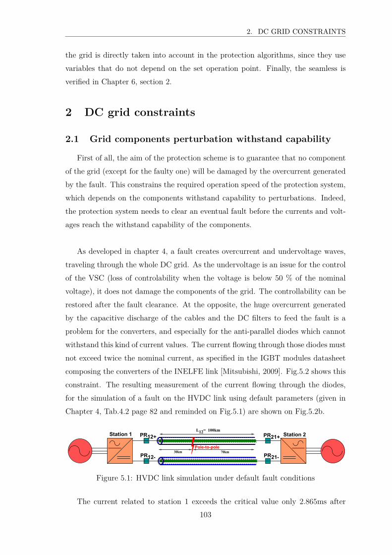
2. DC GRID CONSTRAINTS
the grid is directly taken into account in the protection algorithms, since they use
variables that do not depend on the set operation point. Finally, the seamless is
verified in Chapter 6, section 2.
2 DC grid constraints
2.1 Grid components perturbation withstand capability
First of all, the aim of the protection scheme is to guarantee that no component
of the grid (except for the faulty one) will be damaged by the overcurrent generated
by the fault. This constrains the required operation speed of the protection system,
which depends on the components withstand capability to perturbations. Indeed,
the protection system needs to clear an eventual fault before the currents and volt-
ages reach the withstand capability of the components.
As developed in chapter 4, a fault creates overcurrent and undervoltage waves,
traveling through the whole DC grid. As the undervoltage is an issue for the control
of the VSC (loss of controlability when the voltage is below 50 % of the nominal
voltage), it does not damage the components of the grid. The controllability can be
restored after the fault clearance. At the opposite, the huge overcurrent generated
by the capacitive discharge of the cables and the DC filters to feed the fault is a
problem for the converters, and especially for the anti-parallel diodes which cannot
withstand this kind of current values. The current flowing through those diodes must
not exceed twice the nominal current, as specified in the IGBT modules datasheet
composing the converters of the INELFE link [Mitsubishi, 2009]. Fig.5.2 shows this
constraint. The resulting measurement of the current flowing through the diodes,
for the simulation of a fault on the HVDC link using default parameters (given in
Chapter 4, Tab.4.2 page 82 and reminded on Fig.5.1) are shown on Fig.5.2b.
L12= 100km
30km 70km
PR12+
PR12-
PR21+
PR21-
Station 1 Station 2
Pole-to-pole
Figure 5.1: HVDC link simulation under default fault conditions
The current related to station 1 exceeds the critical value only 2.865ms after
103
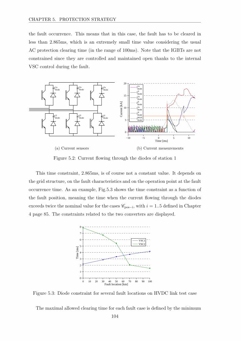
CHAPTER 5. PROTECTION STRATEGY
the fault occurrence. This means that in this case, the fault has to be cleared in
less than 2.865ms, which is an extremely small time value considering the usual
AC protection clearing time (in the range of 100ms). Note that the IGBTs are not
constrained since they are controlled and maintained open thanks to the internal
VSC control during the fault.
I2udiode I3udiodeI1udiode
I1ldiode I3ldiodeI2ldiode
(a) Current sensors
−10 −5 0 5 10
0
5
10
15
20
Time [ms]
Cur
rent
[kA
]
Idiode1u
Idiode1l
Idiode2u
Idiode2l
Idiode3u
Idiode3l
IdiodeMAX
(b) Current measurements
Figure 5.2: Current flowing through the diodes of station 1
This time constraint, 2.865ms, is of course not a constant value. It depends on
the grid structure, on the fault characteristics and on the operation point at the fault
occurrence time. As an example, Fig.5.3 shows the time constraint as a function of
the fault position, meaning the time when the current flowing through the diodes
exceeds twice the nominal value for the cases Cpos−i, with i = 1..5 defined in Chapter
4 page 85. The constraints related to the two converters are displayed.
0 10 20 30 40 50 60 70 80 90 1000
1
2
3
4
5
6
7
8
Fault location [km]
Tim
e [m
s]
VSC1VSC2
Figure 5.3: Diode constraint for several fault locations on HVDC link test case
The maximal allowed clearing time for each fault case is defined by the minimum
104
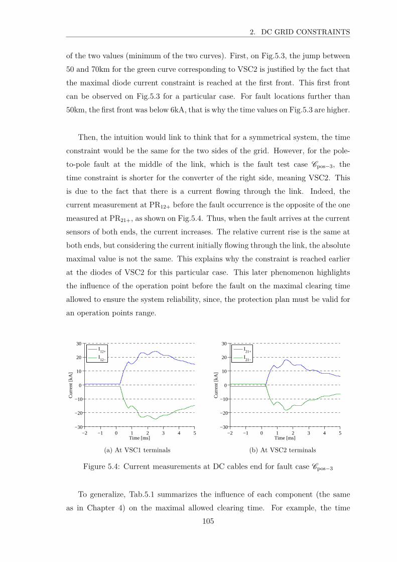
2. DC GRID CONSTRAINTS
of the two values (minimum of the two curves). First, on Fig.5.3, the jump between
50 and 70km for the green curve corresponding to VSC2 is justified by the fact that
the maximal diode current constraint is reached at the first front. This first front
can be observed on Fig.5.3 for a particular case. For fault locations further than
50km, the first front was below 6kA, that is why the time values on Fig.5.3 are higher.
Then, the intuition would link to think that for a symmetrical system, the time
constraint would be the same for the two sides of the grid. However, for the pole-
to-pole fault at the middle of the link, which is the fault test case Cpos−3, the
time constraint is shorter for the converter of the right side, meaning VSC2. This
is due to the fact that there is a current flowing through the link. Indeed, the
current measurement at PR12+ before the fault occurrence is the opposite of the one
measured at PR21+, as shown on Fig.5.4. Thus, when the fault arrives at the current
sensors of both ends, the current increases. The relative current rise is the same at
both ends, but considering the current initially flowing through the link, the absolute
maximal value is not the same. This explains why the constraint is reached earlier
at the diodes of VSC2 for this particular case. This later phenomenon highlights
the influence of the operation point before the fault on the maximal clearing time
allowed to ensure the system reliability, since, the protection plan must be valid for
an operation points range.
−2 −1 0 1 2 3 4 5−30
−20
−10
0
10
20
30
Time [ms]
Cur
rent
[kA
]
I12+
I12−
(a) At VSC1 terminals
−2 −1 0 1 2 3 4 5−30
−20
−10
0
10
20
30
Time [ms]
Cur
rent
[kA
]
I21+
I21−
(b) At VSC2 terminals
Figure 5.4: Current measurements at DC cables end for fault case Cpos−3
To generalize, Tab.5.1 summarizes the influence of each component (the same
as in Chapter 4) on the maximal allowed clearing time. For example, the time
105

CHAPTER 5. PROTECTION STRATEGY
constraint tends to increase (ր) when the parameter Ls increases. This means that
there is more time to clear the fault if the DC filter inductance is higher. The fault
location cannot be included in this table, since distance from a fault to a converter
station increases, it means that this same fault becomes closer to another converter
station.
Parameter Tendency Time constraint tendency
Fault type PG → PP ցRfault ր րSsc ր −→Cs ր ցLs ր ր
Lfeed ր րNfeed ր ր
Table 5.1: Parameters influence on the time constraint tendency
Considering this short time constraint, which is in the range of 5ms, the cables
withstand capability to overcurrents does not limit the maximal clearing time. In-
deed, XLPE cables can usually withstand short-circuit currents up to 60kA for half
a second [Nexans, 2013], which is a lot higher than the diodes current withstand
capability. The only thing to consider for the cables is the overloading case, namely
when a fault in a meshed part of the grid is cleared and thus the power initially
flowing in the faulty cable is re-dispatched to other links. The non-overload cable
verification is not the responsibility of the protection plan but the dispatching center.
In this chapter, the current breaking capability of the breakers is not considered
as a constraint. The protection system will be built in order to send a tripping
order to the breakers as quickly as possible, and especially before the VSC diodes
constraint is reached. Then, the required current breaking capability considering
the proposed protection system will be assessed and discussed in Chapter 6.
2.2 Sensitivity constraint
A set protection principle is able to detect faults up to a certain impedance value.
For a given protection principle, this maximal impedance value depends obviously
106
2. DC GRID CONSTRAINTS
on the grid structure and the set thresholds associated to the protection principle.
The proposed protection plan performances, in terms of maximal fault resistance
detection, will be detailed in Chapter 6. However, the goal of this current chapter
is to develop a protection system sensitive enough to cover faults with impedance
included in the range 0 − 200Ω. This value was defined considering the TSO’s
experience feedback which points out that faults with a resistance higher than 200Ω
are extremely rare in underground cables. However, the higher the maximal fault
impedance detected by the protection plan is, the higher are its performances.
2.3 Selectivity constraint
Besides the diode current withstand capability constraint, the fault needs to
be cleared before the internal protection of the VSC disconnect the station from
the DC grid. Indeed, the substations are equipped with internal protective devices
to ensure their safety. However, the protection plan must act before the internal
VSC protection in order to guarantee the selectivity. These VSC internal protection
principles were provided by RTE for the Siemens converters used in the INELFE
HVDC link, but since they are confidential, they are not displayed in this thesis.
However, both criteria are combined with a temporization delay, which is included
in a range starting from 5ms up to 100ms, depending on the criterion. Hence,
those internal protective principle would act after the main protection that will be
proposed in this chapter.
Otherwise, the protection plan algorithms have to be selective (at least for the
main protection algorithm), meaning that only the breakers located at the terminals
of the fault element have to trip, and no unwanted trippings are allowed. This means
also that the protection must not trip during an event resulting from a normal oper-
ation of the grid, such as a power transfer variation or a connection/disconnection of
a cable. The robustness to power reference variation will be dealt with considering
each protection principle on a case by case basis, when choosing the thresholds. The
verification of the healthy state of a cable during the connection of a link process
will be treated in section 5.
Moreover, the AC grid protection should not respond to a DC fault, if this later
one is cleared by the DC protection systems. This last requirement is assumed to be
checked given the large difference in the response time of both protection system.
107
CHAPTER 5. PROTECTION STRATEGY
2.4 Protection chain operation time
Based on these assumptions, the clearing process of a fault has to be performed
in a very short time (in the range of 5ms), including the time to detect the fault,
to discriminate between the faulty and healthy parts of the grid and the current
breaking process time of the DC circuit breakers. This is illustrated on the time-line
displayed on Fig.5.5.
tfault
tclearing
Propagation of the fault to the sensors
Fault detection
Selectivity rules application
Current breaking process by DCCB Time
Δtpropa tdetectΔ tselectΔ tbreakerΔ
Figure 5.5: Time-line of the fault clearing process
Considering this time constraint, and the fact that the fault steady-state is
reached much later, the conclusion is that the fault has to be cleared during the
transient phase of the signals. This contributes to the fact that no AC grid protec-
tion principle can be duplicated without adapting it, and that traveling wave based
protection principles have to be developed.
This chapter will investigate only the detection and the selectivity rules applica-
tions, since the propagation of the fault to the sensors is the response of the grid, so
there is no element that can act on this, and since the DC breaker is not the scope
of this Ph.D work, but under prototype process by Alstom Grid, in the framework
of the Twenties project.
3 Main protection
In this part, the plausible principles for a main protection are investigated. They
must fulfill the constraints explained in the previous part. In the rest of the chapter,
the Twenties grid model (see Chapter 3 page 76 for grid structure) will be used
for simulation examples, except other mention.
108
3. MAIN PROTECTION
3.1 Preliminary signals analysis
As mentioned in Chapter 3 section 4.1.2, one protection relay is composed of
a current sensor, a pole-to-ground voltage sensor and a DC breaker. The only
information the relay has comes from those elements. The first intuition is to use
overcurrent and undervoltage protection principles. Two fault types are used here,
and are defined in Tab.5.2.
Case name Type Link Location Rfault
Cint Pole-to-ground Link1, positive pole 30km away Station1 10Ω
Cext Pole-to-ground Link3, positive pole Near Station3 1Ω
Table 5.2: Internal and external fault cases
Note that the current and voltages displayed here take into account the sensor
effects.
3.1.1 Polarity selectivity
As mentioned in Chapter 1, a pole-to-ground fault may require the tripping
of both healthy and faulty poles, which is the case considering the Twenties grid
implementation used in this thesis. However, the polarity selectivity does not present
any problem since the difference between the faulty pole and the healthy pole can
be done using a simple overcurrent principle, as shown on Fig.5.6 for the fault case
Cint. The very low fluctuations on the healthy pole current are due to the coupling
effect between the two poles.
109
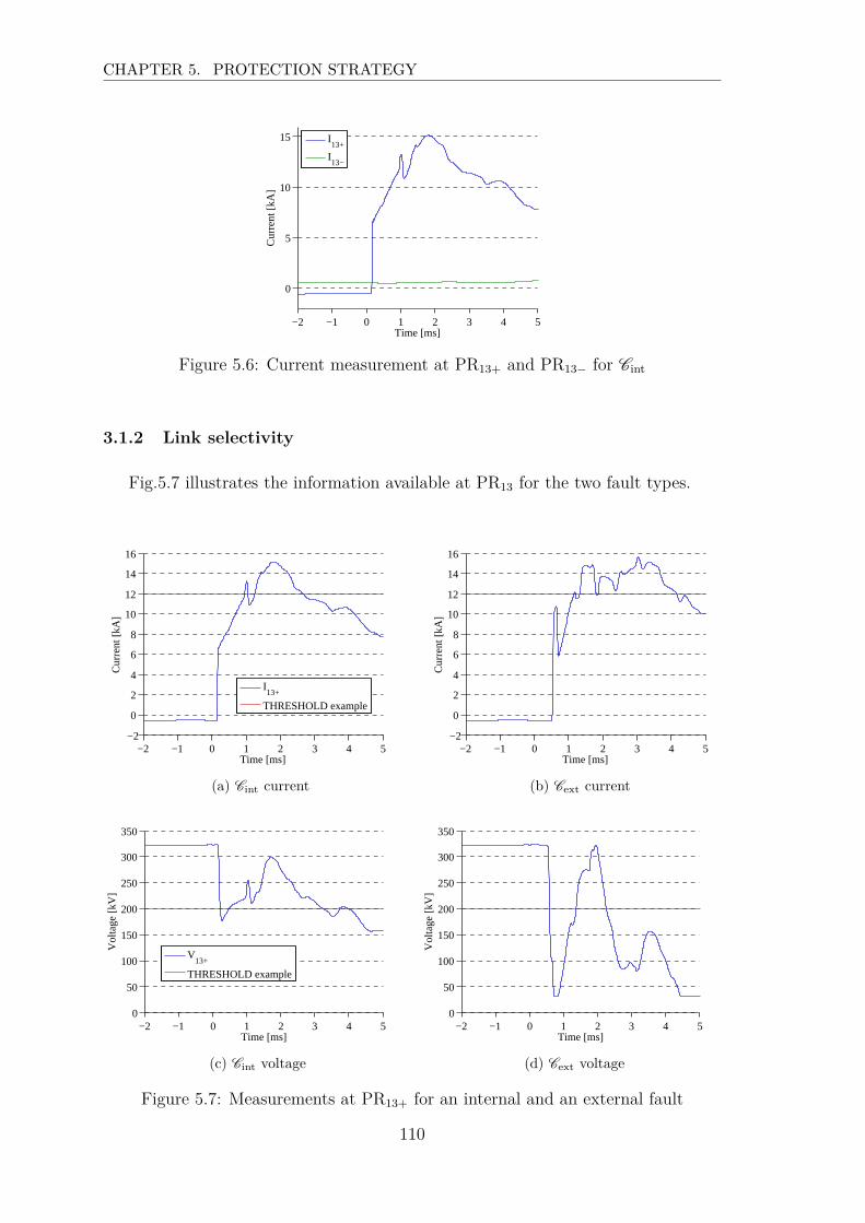
CHAPTER 5. PROTECTION STRATEGY
−2 −1 0 1 2 3 4 5
0
5
10
15
Time [ms]
Cur
rent
[kA
]
I13+
I13−
Figure 5.6: Current measurement at PR13+ and PR13− for Cint
3.1.2 Link selectivity
Fig.5.7 illustrates the information available at PR13 for the two fault types.
−2 −1 0 1 2 3 4 5−2
0
2
4
6
8
10
12
14
16
Time [ms]
Cur
rent
[kA
]
I13+
THRESHOLD example
(a) Cint current
−2 −1 0 1 2 3 4 5−2
0
2
4
6
8
10
12
14
16
Time [ms]
Cur
rent
[kA
]
(b) Cext current
−2 −1 0 1 2 3 4 50
50
100
150
200
250
300
350
Time [ms]
Vol
tage
[kV
]
V13+
THRESHOLD example
(c) Cint voltage
−2 −1 0 1 2 3 4 50
50
100
150
200
250
300
350
Time [ms]
Vol
tage
[kV
]
(d) Cext voltage
Figure 5.7: Measurements at PR13+ for an internal and an external fault
110
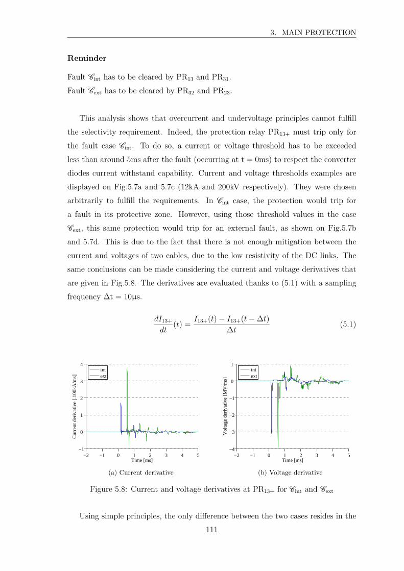
3. MAIN PROTECTION
Reminder
Fault Cint has to be cleared by PR13 and PR31.
Fault Cext has to be cleared by PR32 and PR23.
This analysis shows that overcurrent and undervoltage principles cannot fulfill
the selectivity requirement. Indeed, the protection relay PR13+ must trip only for
the fault case Cint. To do so, a current or voltage threshold has to be exceeded
less than around 5ms after the fault (occurring at t = 0ms) to respect the converter
diodes current withstand capability. Current and voltage thresholds examples are
displayed on Fig.5.7a and 5.7c (12kA and 200kV respectively). They were chosen
arbitrarily to fulfill the requirements. In Cint case, the protection would trip for
a fault in its protective zone. However, using those threshold values in the case
Cext, this same protection would trip for an external fault, as shown on Fig.5.7b
and 5.7d. This is due to the fact that there is not enough mitigation between the
current and voltages of two cables, due to the low resistivity of the DC links. The
same conclusions can be made considering the current and voltage derivatives that
are given in Fig.5.8. The derivatives are evaluated thanks to (5.1) with a sampling
frequency ∆t = 10µs.
dI13+
dt(t) =
I13+(t) − I13+(t− ∆t)∆t
(5.1)
−2 −1 0 1 2 3 4 5−1
0
1
2
3
4
Time [ms]
Cur
rent
der
ivat
ive
[.100
kA/m
s]
intext
(a) Current derivative
−2 −1 0 1 2 3 4 5−4
−3
−2
−1
0
1
Time [ms]
Vol
tage
der
ivat
ive
[MV
/ms]
intext
(b) Voltage derivative
Figure 5.8: Current and voltage derivatives at PR13+ for Cint and Cext
Using simple principles, the only difference between the two cases resides in the
111
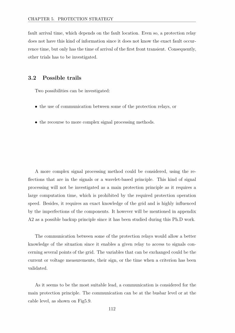
CHAPTER 5. PROTECTION STRATEGY
fault arrival time, which depends on the fault location. Even so, a protection relay
does not have this kind of information since it does not know the exact fault occur-
rence time, but only has the time of arrival of the first front transient. Consequently,
other trials has to be investigated.
3.2 Possible trails
Two possibilities can be investigated:
• the use of communication between some of the protection relays, or
• the recourse to more complex signal processing methods.
A more complex signal processing method could be considered, using the re-
flections that are in the signals or a wavelet-based principle. This kind of signal
processing will not be investigated as a main protection principle as it requires a
large computation time, which is prohibited by the required protection operation
speed. Besides, it requires an exact knowledge of the grid and is highly influenced
by the imperfections of the components. It however will be mentioned in appendix
A2 as a possible backup principle since it has been studied during this Ph.D work.
The communication between some of the protection relays would allow a better
knowledge of the situation since it enables a given relay to access to signals con-
cerning several points of the grid. The variables that can be exchanged could be the
current or voltage measurements, their sign, or the time when a criterion has been
validated.
As it seems to be the most suitable lead, a communication is considered for the
main protection principle. The communication can be at the busbar level or at the
cable level, as shown on Fig5.9.
112
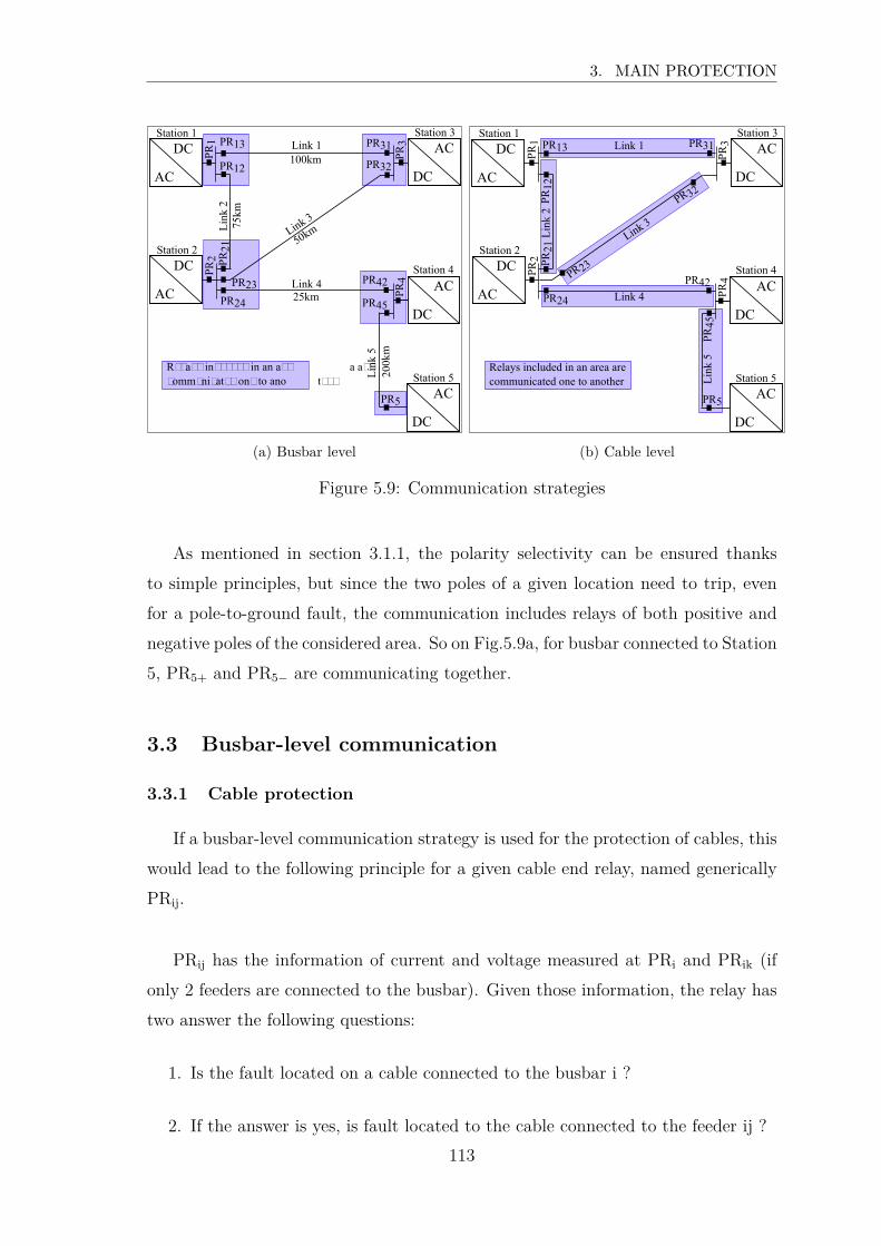
3. MAIN PROTECTION
AC
DC AC
DC100kmLink 1
Station 1
AC
DCStation 2
25kmLink 4 AC
DC
AC
DC
Station 3
Station 4
Station 5
75km
200k
m
Link
2
Link
5
Link 3
50km
PR42
PR4
PR45
PR5
PR24
PR13
PR12
PR31
PR32
PR23
PR21
PR1
PR2
PR3
Relays included in an are a are communicated one to ano ther
(a) Busbar level
AC
DC AC
DC
Link 1Station 1
AC
DCStation 2
Link 4AC
DC
AC
DC
Station 3
Station 4
Station 5
Link
2
Link
5
Link 3
PR42
PR4
PR45
PR5
PR24
PR13
PR12
PR31
PR32
PR23PR21
PR1
PR2
PR3
Relays included in an area are communicated one to another
(b) Cable level
Figure 5.9: Communication strategies
As mentioned in section 3.1.1, the polarity selectivity can be ensured thanks
to simple principles, but since the two poles of a given location need to trip, even
for a pole-to-ground fault, the communication includes relays of both positive and
negative poles of the considered area. So on Fig.5.9a, for busbar connected to Station
5, PR5+ and PR5− are communicating together.
3.3 Busbar-level communication
3.3.1 Cable protection
If a busbar-level communication strategy is used for the protection of cables, this
would lead to the following principle for a given cable end relay, named generically
PRij.
PRij has the information of current and voltage measured at PRi and PRik (if
only 2 feeders are connected to the busbar). Given those information, the relay has
two answer the following questions:
1. Is the fault located on a cable connected to the busbar i ?
2. If the answer is yes, is fault located to the cable connected to the feeder ij ?
113
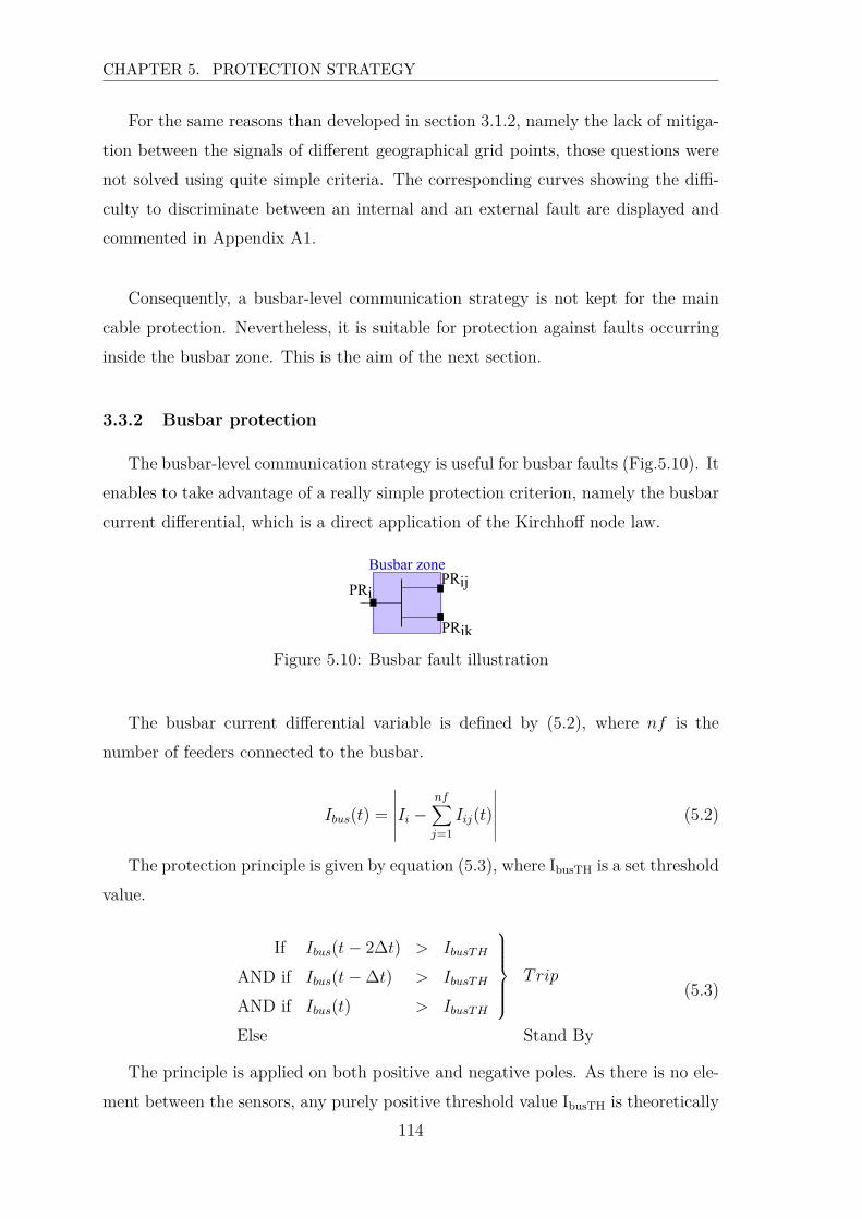
CHAPTER 5. PROTECTION STRATEGY
For the same reasons than developed in section 3.1.2, namely the lack of mitiga-
tion between the signals of different geographical grid points, those questions were
not solved using quite simple criteria. The corresponding curves showing the diffi-
culty to discriminate between an internal and an external fault are displayed and
commented in Appendix A1.
Consequently, a busbar-level communication strategy is not kept for the main
cable protection. Nevertheless, it is suitable for protection against faults occurring
inside the busbar zone. This is the aim of the next section.
3.3.2 Busbar protection
The busbar-level communication strategy is useful for busbar faults (Fig.5.10). It
enables to take advantage of a really simple protection criterion, namely the busbar
current differential, which is a direct application of the Kirchhoff node law.
PRij
PRik
PRi
Busbar zone
Figure 5.10: Busbar fault illustration
The busbar current differential variable is defined by (5.2), where nf is the
number of feeders connected to the busbar.
Ibus(t) =
∣
∣
∣
∣
∣
∣
Ii −nf∑
j=1
Iij(t)
∣
∣
∣
∣
∣
∣
(5.2)
The protection principle is given by equation (5.3), where IbusTH is a set threshold
value.
If Ibus(t− 2∆t) > IbusT H
AND if Ibus(t− ∆t) > IbusT H
AND if Ibus(t) > IbusT H
Trip
Else Stand By
(5.3)
The principle is applied on both positive and negative poles. As there is no ele-
ment between the sensors, any purely positive threshold value IbusTH is theoretically
114
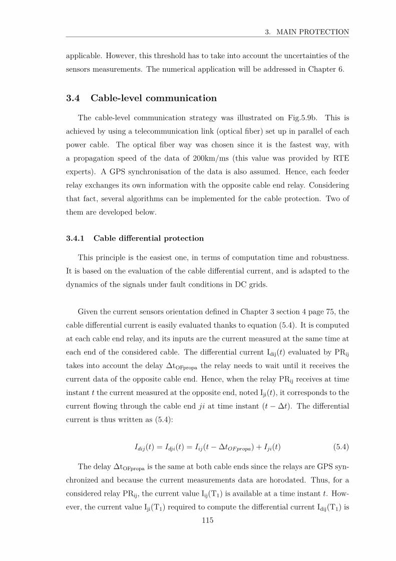
3. MAIN PROTECTION
applicable. However, this threshold has to take into account the uncertainties of the
sensors measurements. The numerical application will be addressed in Chapter 6.
3.4 Cable-level communication
The cable-level communication strategy was illustrated on Fig.5.9b. This is
achieved by using a telecommunication link (optical fiber) set up in parallel of each
power cable. The optical fiber way was chosen since it is the fastest way, with
a propagation speed of the data of 200km/ms (this value was provided by RTE
experts). A GPS synchronisation of the data is also assumed. Hence, each feeder
relay exchanges its own information with the opposite cable end relay. Considering
that fact, several algorithms can be implemented for the cable protection. Two of
them are developed below.
3.4.1 Cable differential protection
This principle is the easiest one, in terms of computation time and robustness.
It is based on the evaluation of the cable differential current, and is adapted to the
dynamics of the signals under fault conditions in DC grids.
Given the current sensors orientation defined in Chapter 3 section 4 page 75, the
cable differential current is easily evaluated thanks to equation (5.4). It is computed
at each cable end relay, and its inputs are the current measured at the same time at
each end of the considered cable. The differential current Idij(t) evaluated by PRij
takes into account the delay ∆tOFpropa the relay needs to wait until it receives the
current data of the opposite cable end. Hence, when the relay PRij receives at time
instant t the current measured at the opposite end, noted Iji(t), it corresponds to the
current flowing through the cable end ji at time instant (t − ∆t). The differential
current is thus written as (5.4):
Idij(t) = Idji(t) = Iij(t− ∆tOF propa) + Iji(t) (5.4)
The delay ∆tOFpropa is the same at both cable ends since the relays are GPS syn-
chronized and because the current measurements data are horodated. Thus, for a
considered relay PRij, the current value Iij(T1) is available at a time instant t. How-
ever, the current value Iji(T1) required to compute the differential current Idij(T1) is
115
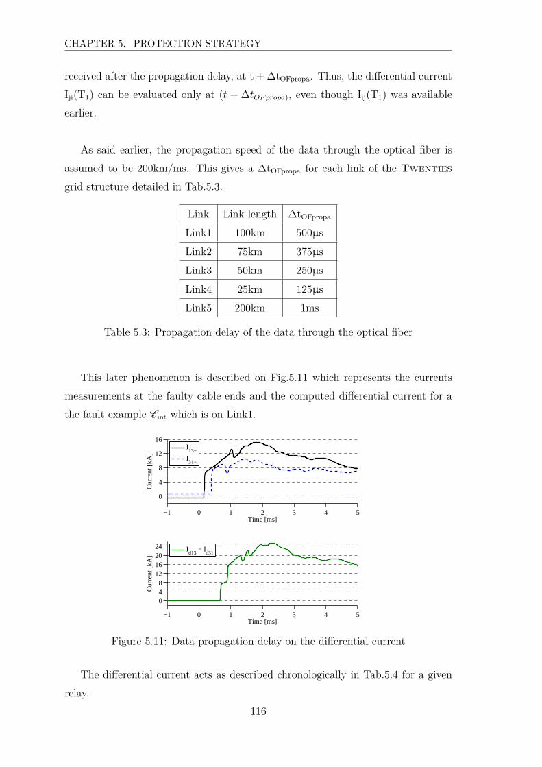
CHAPTER 5. PROTECTION STRATEGY
received after the propagation delay, at t + ∆tOFpropa. Thus, the differential current
Iji(T1) can be evaluated only at (t + ∆tOF propa), even though Iij(T1) was available
earlier.
As said earlier, the propagation speed of the data through the optical fiber is
assumed to be 200km/ms. This gives a ∆tOFpropa for each link of the Twenties
grid structure detailed in Tab.5.3.
Link Link length ∆tOFpropa
Link1 100km 500µs
Link2 75km 375µs
Link3 50km 250µs
Link4 25km 125µs
Link5 200km 1ms
Table 5.3: Propagation delay of the data through the optical fiber
This later phenomenon is described on Fig.5.11 which represents the currents
measurements at the faulty cable ends and the computed differential current for a
the fault example Cint which is on Link1.
−1 0 1 2 3 4 5
0
4
8
12
16
Time [ms]
Cur
rent
[kA
]
I13+
I31+
−1 0 1 2 3 4 5
048
12162024
Time [ms]
Cur
rent
[kA
]
Id13
= Id31
Figure 5.11: Data propagation delay on the differential current
The differential current acts as described chronologically in Tab.5.4 for a given
relay.
116
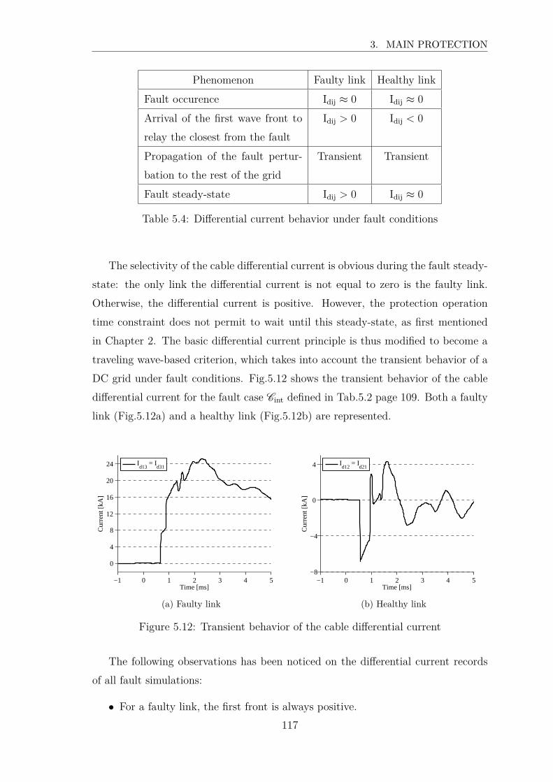
3. MAIN PROTECTION
Phenomenon Faulty link Healthy link
Fault occurence Idij ≈ 0 Idij ≈ 0
Arrival of the first wave front to
relay the closest from the fault
Idij > 0 Idij < 0
Propagation of the fault pertur-
bation to the rest of the grid
Transient Transient
Fault steady-state Idij > 0 Idij ≈ 0
Table 5.4: Differential current behavior under fault conditions
The selectivity of the cable differential current is obvious during the fault steady-
state: the only link the differential current is not equal to zero is the faulty link.
Otherwise, the differential current is positive. However, the protection operation
time constraint does not permit to wait until this steady-state, as first mentioned
in Chapter 2. The basic differential current principle is thus modified to become a
traveling wave-based criterion, which takes into account the transient behavior of a
DC grid under fault conditions. Fig.5.12 shows the transient behavior of the cable
differential current for the fault case Cint defined in Tab.5.2 page 109. Both a faulty
link (Fig.5.12a) and a healthy link (Fig.5.12b) are represented.
−1 0 1 2 3 4 5
0
4
8
12
16
20
24
Time [ms]
Cur
rent
[kA
]
Id13
= Id31
(a) Faulty link
−1 0 1 2 3 4 5−8
−4
0
4
Time [ms]
Cur
rent
[kA
]
Id12
= Id21
(b) Healthy link
Figure 5.12: Transient behavior of the cable differential current
The following observations has been noticed on the differential current records
of all fault simulations:
• For a faulty link, the first front is always positive.
117
CHAPTER 5. PROTECTION STRATEGY
• For a healthy link, the first front is always negative.
This is due to the fact that for a given link, the traveling wave generated by the
fault arrives by the exterior of the link, which discharges (cable capacitive effect),
creating a current flowing from the link to the fault. During the short time the
traveling wave reached the relay of one end but not the other one, and given the
sensor orientation, this is traduced by a negative differential current.
A selective threshold enables the fault detection for the faulty link. If small
enough, the threshold is exceeded at the front transient arrival. However, a set
threshold could eventually be exceeded in the case of a healthy link, because of
the oscillations during the transient part. Indeed, the threshold has to be set small
enough to detect quickly faults with resistance up to 100Ω, so if a blank fault occurs,
this threshold is smaller than the oscillation magnitude of the differential current.
To avoid unwanted trippings of healthy link protections, a negative threshold is
added to detect the first negative front. This negative front defines the fact that the
fault is exterior to the link. The over-passing of this threshold will imply the blocking
of the tripping order, for a duration time corresponding to the fault clearing process
time. Therefore, the selectivity is ensured. The cable differential current protection
algorithm is thus defined by equation (5.5), where IdTH+ and IdTH− are the positive
and negative set thresholds, and ∆tblock is the blocking time corresponding to the
fault clearing time process.
To improve the robustness of the algorithm, a validation of the threshold over-
passing of 3 consecutive samples, for both positive and negative threshold, is added.
IF − −− Idij(t− 2∆t) > IdT H+
and if Idij(t− ∆t) > IdT H+
and if Idij(t) > IdT H+
Trip
ELSE IF Idij(t− 2∆t) < IdT H−
and if Idij(t− ∆t) < IdT H−
and if Idij(t) < IdT H−
Block for ∆tblock
ELSE − − − − − − − − − − − − − − Stand By
(5.5)
This algorithm can be implemented in each protection relay, on both positive
118
3. MAIN PROTECTION
and negative pole. The only difference between the positive and the negative pole
algorithm resides in the thresholds sign that are inverted due to the polarity rever-
sal. However, in the present case, if a pole is faulty, the protection of both positive
and negative pole of the cable ends trip thanks to the communication as mentioned
in section 3.2. For pole-to-pole faults, the differential current of both poles exceed
the threshold.
The positive and negative thresholds do not necessarily have the same value.
Theoretically, any positive threshold taking into account the sensors uncertainties
enables the detection. The negative threshold need to be small enough to be over-
passed to ensure the selectivity. The smallest the threshold are, the fastest is the
protection clearing process. Thus, they were chosen to detect faults up to 200Ω
anywhere in the grid. The numerical applications and validation will be developed
in Chapter 6.
In order to be sure that the protection will record the negative front for healthy
links, the sampling frequency needs to be at least three times smaller than the propa-
gation time of the fault through the smallest cable. Indeed, if the sampling frequency
is higher, the first front will be hidden between two samples, and unwanted trippings
may occur. To ensure that the negative front will be validated by 3 samples, for
the Twenties grid test case, the time step must be less or equal to 43µs (since the
propagation of the fault in Link4 of 25km is 129µs). This corresponds to a sampling
frequency of 23kHz.
This protection principle requires two different optical fiber links wired in parallel
of each power cable to ensure the communication of the current measurement data
in both ways.
3.4.2 Directional criterion protection
This principle is also based on the first current wave front. This directional
principle takes advantage of the sign of the first current wave front. The physics
beyond this criterion is the same than the one beyond the differential current cri-
terion, namely the fact that the first current wave front is positive (considering the
sensors orientation defined in this thesis) at each end of faulty link, and only for the
119

CHAPTER 5. PROTECTION STRATEGY
faulty link. The current wave starts with a negative front at one end for any healthy
link, due to the propagation phenomenon of a signal through the cables.
The sign of the first wave front can be detected by several principles. In this
thesis, the association of the current derivative with a positive or negative thresh-
old is used as defined in equations (5.6), where dITH+ and dITH− are positive and
negative thresholds. The sign values are then exchanged between the relays of the
two cable ends.
Sij(t) =
1 ifdIij
dt(t) > dITH+
−1 ifdIij
dt(t) < dITH-
0 otherwise
(5.6)
However, it is extremely necessary to be careful with the propagation phe-
nomenon of the fault, and to only consider the first front, not the other ones following
the fault arrival. The current derivative is shown on Fig.5.13 for a healthy link and
a faulty link, that corresponds to the same fault condition and the same relays as
the ones presented on Fig.5.12 for the differential current illustration.
−1 0 1 2 3 4 5−1
−0.5
0
0.5
1
1.5
2
Time [ms]
Cur
rent
der
ivat
ive
[.100
kA
/ms]
I13+
I31+
(a) Faulty link
−1 0 1 2 3 4 5−2
−1.5
−1
−0.5
0
0.5
1
1.5
2
Time [ms]
Cur
rent
der
ivat
ive
[.100
kA
/ms]
I12+
I21+
(b) Healthy link
Figure 5.13: Transient behavior of the current derivatives at each end of a cable
As well as the differential current, the selectivity is based on the blocking of the
tripping order in case a negative front is detected at one cable end. If not, the other
peaks following the first front, related to the reflections of the fault along the cable
ends, may exceed the set threshold, and imply unwanted trippings.
120

3. MAIN PROTECTION
The implementation is however more complex than the differential criterion. In-
deed, the first one uses only one variable to discriminate between a faulty and a
healthy link. Even though this variable (the differential current) is evaluated thanks
to several measurements coming from different geographical locations, the choice is
done on one signal. At the opposite, the directional criterion requires that the relay
verifies two criteria, that may be (in most cases) checked and received at different
times. This is explained below on Fig.5.14 for a faulty link and on Fig.5.15 for a
healthy link, for the same fault example that was shown on Fig.5.13. The value
∆tOFpropa is the same than in the previous section, given in Tab.5.3 page 116, and
Sij is the sign of the first current wave front.
On the Fig.5.14 example, if the values S13(t) and S31(t) were continuously ex-
changed between the relays, PR13 would receive the information of the positive front,
given by S31 = 1, at a time were S13 has already descended to zero. This would result
in a non-tripping action of the relays, leading the non-clearance of the fault.
0 0.5 1 1.5−1.5
−1−0.5
00.5
11.5
2
Time [ms]
dI/d
t [.1
00 k
A/m
s]
I13+
dITH+
dITH−
Send S13
Receive S31∆t
OFpropa
0 0.5 1 1.5−1
−0.50
0.51
1.52
2.5
Time [ms]
Cur
rent
der
ivat
ive
[.100
kA
/ms]
I31+Send S
31Receive S
13
∆tOFpropa
Figure 5.14: Current sign data exchange between two relays of a faulty link
121
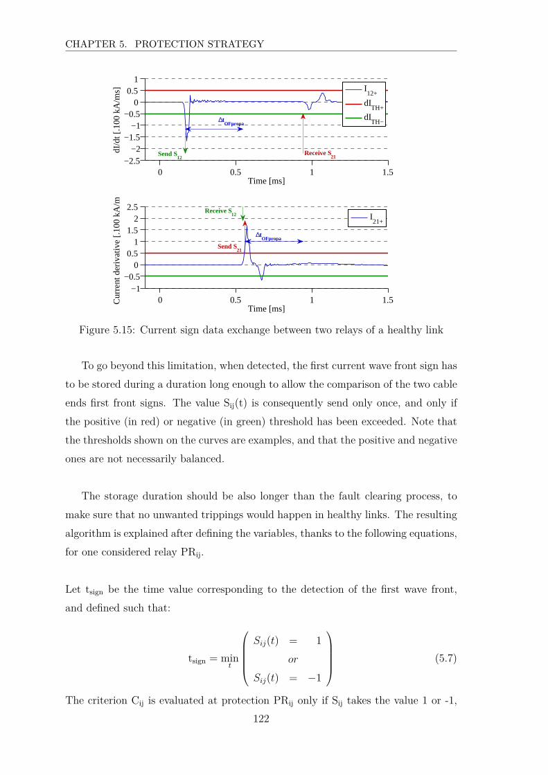
CHAPTER 5. PROTECTION STRATEGY
0 0.5 1 1.5−2.5
−2−1.5
−1−0.5
00.5
1
Time [ms]
dI/d
t [.1
00 k
A/m
s]
I12+
dITH+
dITH−
Send S12
Receive S21
∆tOFpropa
0 0.5 1 1.5−1
−0.50
0.51
1.52
2.5
Time [ms]
Cur
rent
der
ivat
ive
[.100
kA
/ms]
I21+
Send S21
Receive S12
∆tOFpropa
Figure 5.15: Current sign data exchange between two relays of a healthy link
To go beyond this limitation, when detected, the first current wave front sign has
to be stored during a duration long enough to allow the comparison of the two cable
ends first front signs. The value Sij(t) is consequently send only once, and only if
the positive (in red) or negative (in green) threshold has been exceeded. Note that
the thresholds shown on the curves are examples, and that the positive and negative
ones are not necessarily balanced.
The storage duration should be also longer than the fault clearing process, to
make sure that no unwanted trippings would happen in healthy links. The resulting
algorithm is explained after defining the variables, thanks to the following equations,
for one considered relay PRij.
Let tsign be the time value corresponding to the detection of the first wave front,
and defined such that:
tsign = mint
Sij(t) = 1
or
Sij(t) = −1
(5.7)
The criterion Cij is evaluated at protection PRij only if Sij takes the value 1 or -1,
122
3. MAIN PROTECTION
and can then be defined such that:
∀t ∈ [tsign; tsign + ∆tstop] , Cij(t) =
1 if Sij(tsign) = 1
−1 if Sij(tsign) = −1(5.8)
where ∆tstop is set to correspond to the fault clearing process duration, taken the
data propagation delay through the optical fiber into consideration.
The directional cable protection algorithm becomes:
IF − − Cij = 1
and if Cji = 1
Trip
ELSE − − − − − − Stand By
(5.9)
Several cases are included in the ELSE. First, if Cij = 1 and Cji = −1, or vice-
versa, then the link is healthy but a fault is present in the grid. In the differential
current protection, the relay was blocked for a duration corresponding to the fault
clearing process time. Here, this temporization delay is included in the value of
the sign, as defined in equation (5.6). The resulting blocking time is thus equal to
the delay ∆tstop. Then, there is a low probability to have Cij = −1 and Cji = −1.
This would correspond to the case of a long healthy cable, were the traveling wave
generated by the fault arrives to the considered healthy link by both ways, leading
the cable to discharge in both directions. Furthermore, the case where Cij = −1 and
Cji = 0 corresponds to a healthy link, remote from the fault location. The current
wave front is attenuated along the healthy cable so the threshold is reached for only
one end (the closest to the fault). Finally, the case where Cij = 1 and Cji = 0 cannot
happen if the thresholds are set properly (meaning dITH+ > |dITH−|).
Thresholds choice, for both positive and negative ones, have to be set small
enough to be exceeded for the maximal fault resistance to detect, but as well as
the differential current, it does not need to be higher than a certain value since the
selectivity is ensured thanks to the blocking of the protection in case of a negative
threshold exceeding.
123
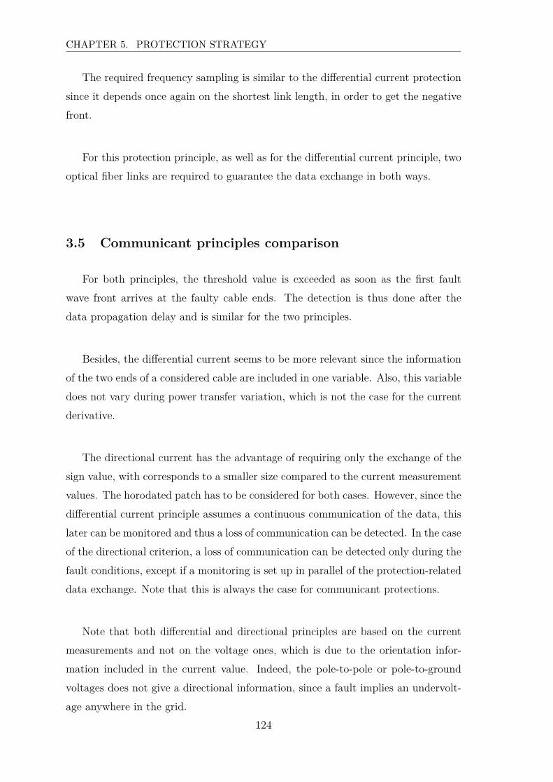
CHAPTER 5. PROTECTION STRATEGY
The required frequency sampling is similar to the differential current protection
since it depends once again on the shortest link length, in order to get the negative
front.
For this protection principle, as well as for the differential current principle, two
optical fiber links are required to guarantee the data exchange in both ways.
3.5 Communicant principles comparison
For both principles, the threshold value is exceeded as soon as the first fault
wave front arrives at the faulty cable ends. The detection is thus done after the
data propagation delay and is similar for the two principles.
Besides, the differential current seems to be more relevant since the information
of the two ends of a considered cable are included in one variable. Also, this variable
does not vary during power transfer variation, which is not the case for the current
derivative.
The directional current has the advantage of requiring only the exchange of the
sign value, with corresponds to a smaller size compared to the current measurement
values. The horodated patch has to be considered for both cases. However, since the
differential current principle assumes a continuous communication of the data, this
later can be monitored and thus a loss of communication can be detected. In the case
of the directional criterion, a loss of communication can be detected only during the
fault conditions, except if a monitoring is set up in parallel of the protection-related
data exchange. Note that this is always the case for communicant protections.
Note that both differential and directional principles are based on the current
measurements and not on the voltage ones, which is due to the orientation infor-
mation included in the current value. Indeed, the pole-to-pole or pole-to-ground
voltages does not give a directional information, since a fault implies an undervolt-
age anywhere in the grid.
124
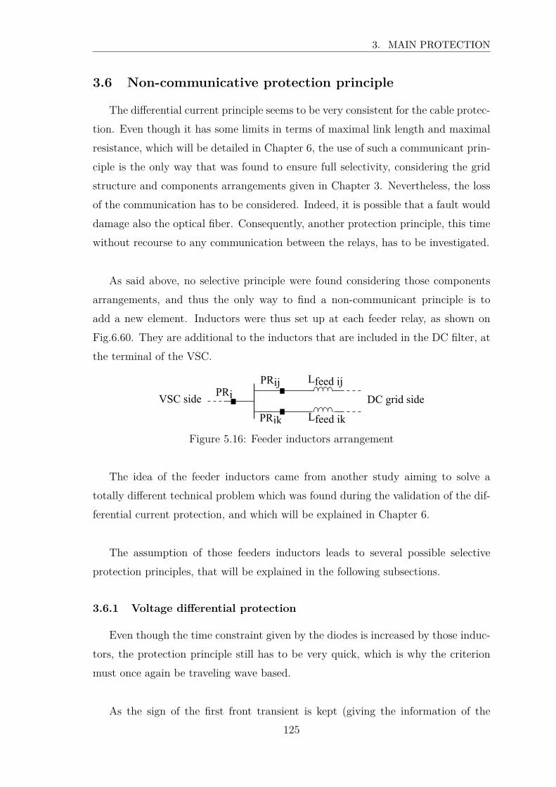
3. MAIN PROTECTION
3.6 Non-communicative protection principle
The differential current principle seems to be very consistent for the cable protec-
tion. Even though it has some limits in terms of maximal link length and maximal
resistance, which will be detailed in Chapter 6, the use of such a communicant prin-
ciple is the only way that was found to ensure full selectivity, considering the grid
structure and components arrangements given in Chapter 3. Nevertheless, the loss
of the communication has to be considered. Indeed, it is possible that a fault would
damage also the optical fiber. Consequently, another protection principle, this time
without recourse to any communication between the relays, has to be investigated.
As said above, no selective principle were found considering those components
arrangements, and thus the only way to find a non-communicant principle is to
add a new element. Inductors were thus set up at each feeder relay, as shown on
Fig.6.60. They are additional to the inductors that are included in the DC filter, at
the terminal of the VSC.
PRij
PRik
PRiVSC side DC grid side
Lfeed ij
Lfeed ik
Figure 5.16: Feeder inductors arrangement
The idea of the feeder inductors came from another study aiming to solve a
totally different technical problem which was found during the validation of the dif-
ferential current protection, and which will be explained in Chapter 6.
The assumption of those feeders inductors leads to several possible selective
protection principles, that will be explained in the following subsections.
3.6.1 Voltage differential protection
Even though the time constraint given by the diodes is increased by those induc-
tors, the protection principle still has to be very quick, which is why the criterion
must once again be traveling wave based.
As the sign of the first front transient is kept (giving the information of the
125
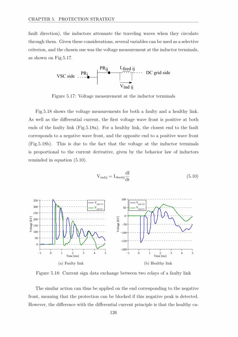
CHAPTER 5. PROTECTION STRATEGY
fault direction), the inductors attenuate the traveling waves when they circulate
through them. Given these considerations, several variables can be used as a selective
criterion, and the chosen one was the voltage measurement at the inductor terminals,
as shown on Fig.5.17.
PRijPRiVSC side
DC grid sideLfeed ij
Vind ij
Figure 5.17: Voltage measurement at the inductor terminals
Fig.5.18 shows the voltage measurements for both a faulty and a healthy link.
As well as the differential current, the first voltage wave front is positive at both
ends of the faulty link (Fig.5.18a). For a healthy link, the closest end to the fault
corresponds to a negative wave front, and the opposite end to a positive wave front
(Fig.5.18b). This is due to the fact that the voltage at the inductor terminals
is proportional to the current derivative, given by the behavior law of inductors
reminded in equation (5.10).
Vindij = Lfeedij
dIdt
(5.10)
−1 0 1 2 3 4 5
0
50
100
150
200
250
300
350
Time [ms]
Vol
tage
[kV
]
Vind 13+
Vind 31+
(a) Faulty link
−1 0 1 2 3 4 5−200
−150
−100
−50
0
50
100
Time [ms]
Vol
tage
[kV
]
Vind 12+
Vind 21+
(b) Healthy link
Figure 5.18: Current sign data exchange between two relays of a faulty link
The similar action can thus be applied on the end corresponding to the negative
front, meaning that the protection can be blocked if this negative peak is detected.
However, the difference with the differential current principle is that the healthy ca-
126

3. MAIN PROTECTION
ble end corresponding to the positive first wave front does not have the information
that its opposite end has seen a negative one, since no communication is assumed.
However, this healthy cable end corresponds to the most remote end from the fault,
and thus meaning that the traveling wave went through at least two inductors be-
fore arriving to this cable end. The relay related to this healthy cable end can
thus discriminate between a internal fault thanks to the attenuation and properly
set threshold, meaning a positive threshold small enough to detect high resistance
internal faults but high enough to discriminate with small resistance external faults.
Thus, the new principle, which was named voltage differential principle, is based
on the two phenomena:
• the attenuation given by the inductors, and
• the sign of the first front transient, giving the direction of the fault.
The resulting algorithm is developed in equation (5.11).
IF Vindij(t) > dVindTH+ ; Trip
ELSE IF Vindij(t) < dVindTH- ; Block for ∆tblock
ELSE ; Stand By
(5.11)
where dVindTH+ and dVindTH− are thresholds, and ∆tblock a delay corresponding to
the fault clearing process time, alike for the differential current principle.
Note that the relevance and the selectivity of this algorithm is extremely depen-
dent on the inductors value. This phenomenon will be quantified in Chapter 6.
This protection principle is seen as a main protection because of its full selectivity
and its rapidity, but it can act as a backup in case the communication is lost.
3.6.2 Other possible trail
The presence of inductors at the feeders protection relays also enables to use
overcurrent or undervoltage principles, due to the filtering effect that attenuates the
signals related to healthy links. However, those principles do not add any advantages
127
CHAPTER 5. PROTECTION STRATEGY
compared to the voltage differential principle, and thus are not developed in this
thesis.
3.7 Conclusion on the main protection
Three possible principles were found for the main cable protection:
• the differential current protection,
• the directional protection,
• the voltage differential protection.
The directional protection do not add any advantages regarding the differential
current. Thus, only the two other principles are kept for the protection plan. The
busbar protection is performed thanks to the busbar differential current principle.
4 Backup protection
4.1 Purpose of the backup protection
Any transmission grid requires a backup protection system in case of the fail-
ure of any component of the main system. The main concern is a breaker failure.
The lost of the optical fiber was already solved thanks to the voltage differential
principle. Additionally, the monitoring of the communication can be done at the
dispatching center level.
If a breaker failure happens during a fault clearing process, all the relays con-
nected to the same busbar need to trip to avoid the fault feeding by the rest of the
grid. This is shown on Fig5.19, in case of the breaker located on the right hand side
of the faulty cable failed. Thus, when the backup protection triggers, the tripping
order is sent to all DC breakers of the busbar, so the short-circuit current cannot
flow through the other lines of the grid.
128
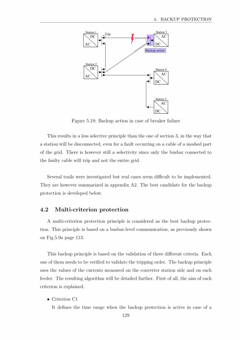
4. BACKUP PROTECTION
AC
DC AC
DC
Station 1
AC
DCStation 2
AC
DC
AC
DC
Station 3
Station 4
Station 5
Trip
Backup action
Figure 5.19: Backup action in case of breaker failure
This results in a less selective principle than the one of section 3, in the way that
a station will be disconnected, even for a fault occurring on a cable of a meshed part
of the grid. There is however still a selectivity since only the busbar connected to
the faulty cable will trip and not the entire grid.
Several trails were investigated but real cases seem difficult to be implemented.
They are however summarized in appendix A2. The best candidate for the backup
protection is developed below.
4.2 Multi-criterion protection
A multi-criterion protection principle is considered as the best backup protec-
tion. This principle is based on a busbar-level communication, as previously shown
on Fig.5.9a page 113.
This backup principle is based on the validation of three different criteria. Each
one of them needs to be verified to validate the tripping order. The backup principle
uses the values of the currents measured on the converter station side and on each
feeder. The resulting algorithm will be detailed further. First of all, the aim of each
criterion is explained.
• Criterion C1
It defines the time range when the backup protection is active in case of a
129
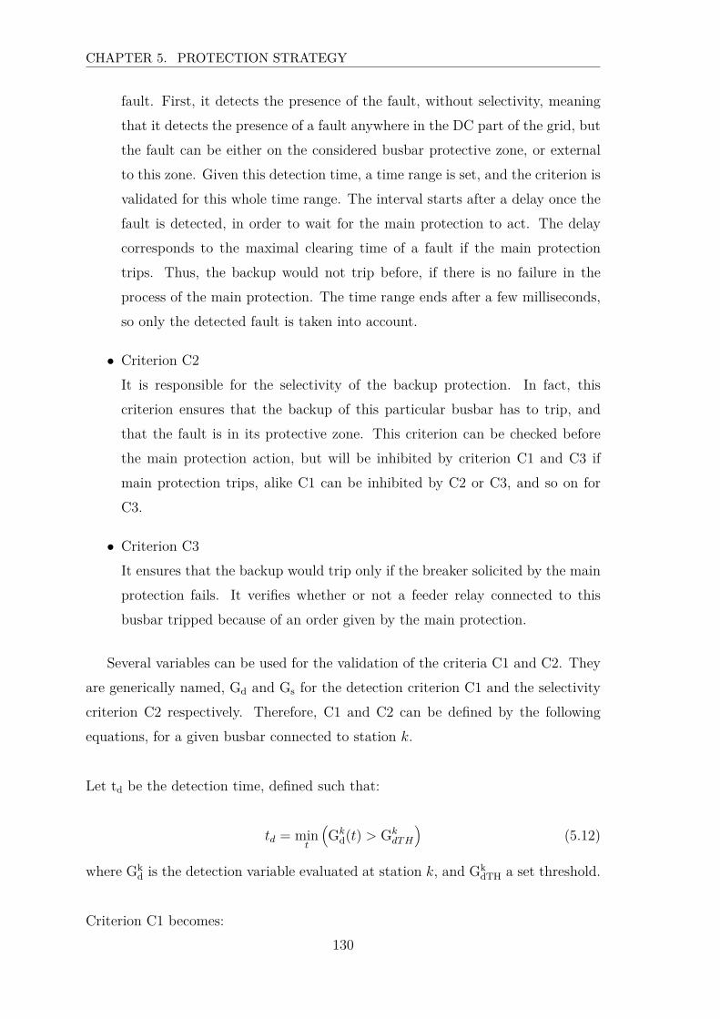
CHAPTER 5. PROTECTION STRATEGY
fault. First, it detects the presence of the fault, without selectivity, meaning
that it detects the presence of a fault anywhere in the DC part of the grid, but
the fault can be either on the considered busbar protective zone, or external
to this zone. Given this detection time, a time range is set, and the criterion is
validated for this whole time range. The interval starts after a delay once the
fault is detected, in order to wait for the main protection to act. The delay
corresponds to the maximal clearing time of a fault if the main protection
trips. Thus, the backup would not trip before, if there is no failure in the
process of the main protection. The time range ends after a few milliseconds,
so only the detected fault is taken into account.
• Criterion C2
It is responsible for the selectivity of the backup protection. In fact, this
criterion ensures that the backup of this particular busbar has to trip, and
that the fault is in its protective zone. This criterion can be checked before
the main protection action, but will be inhibited by criterion C1 and C3 if
main protection trips, alike C1 can be inhibited by C2 or C3, and so on for
C3.
• Criterion C3
It ensures that the backup would trip only if the breaker solicited by the main
protection fails. It verifies whether or not a feeder relay connected to this
busbar tripped because of an order given by the main protection.
Several variables can be used for the validation of the criteria C1 and C2. They
are generically named, Gd and Gs for the detection criterion C1 and the selectivity
criterion C2 respectively. Therefore, C1 and C2 can be defined by the following
equations, for a given busbar connected to station k.
Let td be the detection time, defined such that:
td = mint
(
Gkd(t) > Gk
dT H
)
(5.12)
where Gkd is the detection variable evaluated at station k, and Gk
dTH a set threshold.
Criterion C1 becomes:
130
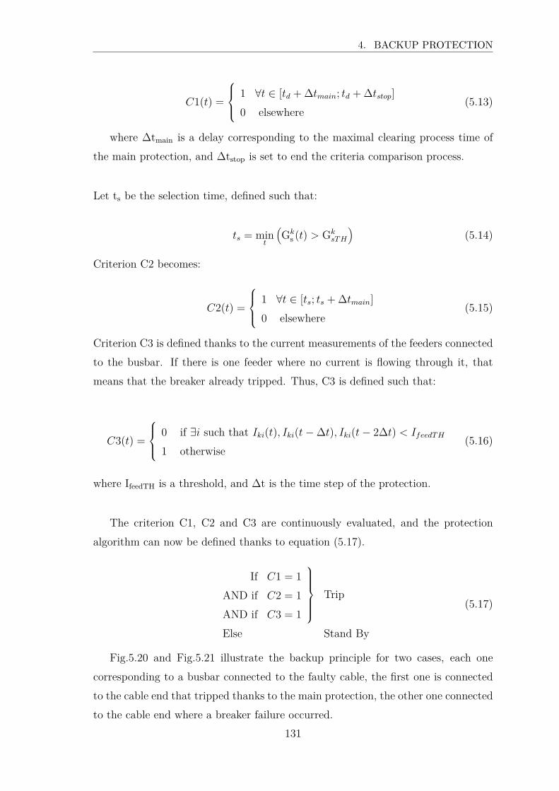
4. BACKUP PROTECTION
C1(t) =
1 ∀t ∈ [td + ∆tmain; td + ∆tstop]
0 elsewhere(5.13)
where ∆tmain is a delay corresponding to the maximal clearing process time of
the main protection, and ∆tstop is set to end the criteria comparison process.
Let ts be the selection time, defined such that:
ts = mint
(
Gks (t) > Gk
sT H
)
(5.14)
Criterion C2 becomes:
C2(t) =
1 ∀t ∈ [ts; ts + ∆tmain]
0 elsewhere(5.15)
Criterion C3 is defined thanks to the current measurements of the feeders connected
to the busbar. If there is one feeder where no current is flowing through it, that
means that the breaker already tripped. Thus, C3 is defined such that:
C3(t) =
0 if ∃i such that Iki(t), Iki(t− ∆t), Iki(t− 2∆t) < IfeedT H
1 otherwise(5.16)
where IfeedTH is a threshold, and ∆t is the time step of the protection.
The criterion C1, C2 and C3 are continuously evaluated, and the protection
algorithm can now be defined thanks to equation (5.17).
If C1 = 1
AND if C2 = 1
AND if C3 = 1
Trip
Else Stand By
(5.17)
Fig.5.20 and Fig.5.21 illustrate the backup principle for two cases, each one
corresponding to a busbar connected to the faulty cable, the first one is connected
to the cable end that tripped thanks to the main protection, the other one connected
to the cable end where a breaker failure occurred.
131
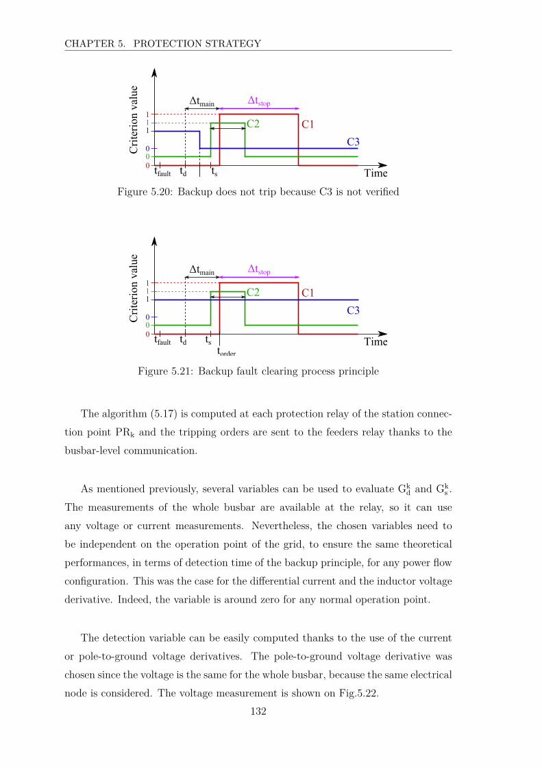
CHAPTER 5. PROTECTION STRATEGY
Timetfault td ts
Δtmain Δtstop
C1C2C
riter
ion
valu
e
0
1
0
1
0C3
1
tFigure 5.20: Backup does not trip because C3 is not verified
Timetfault td ts
Δtmain Δtstop
C1C2
Crit
erio
n va
lue
0
1
0
1
0C3
1
torder
Figure 5.21: Backup fault clearing process principle
The algorithm (5.17) is computed at each protection relay of the station connec-
tion point PRk and the tripping orders are sent to the feeders relay thanks to the
busbar-level communication.
As mentioned previously, several variables can be used to evaluate Gkd and Gk
s .
The measurements of the whole busbar are available at the relay, so it can use
any voltage or current measurements. Nevertheless, the chosen variables need to
be independent on the operation point of the grid, to ensure the same theoretical
performances, in terms of detection time of the backup principle, for any power flow
configuration. This was the case for the differential current and the inductor voltage
derivative. Indeed, the variable is around zero for any normal operation point.
The detection variable can be easily computed thanks to the use of the current
or pole-to-ground voltage derivatives. The pole-to-ground voltage derivative was
chosen since the voltage is the same for the whole busbar, because the same electrical
node is considered. The voltage measurement is shown on Fig.5.22.
132
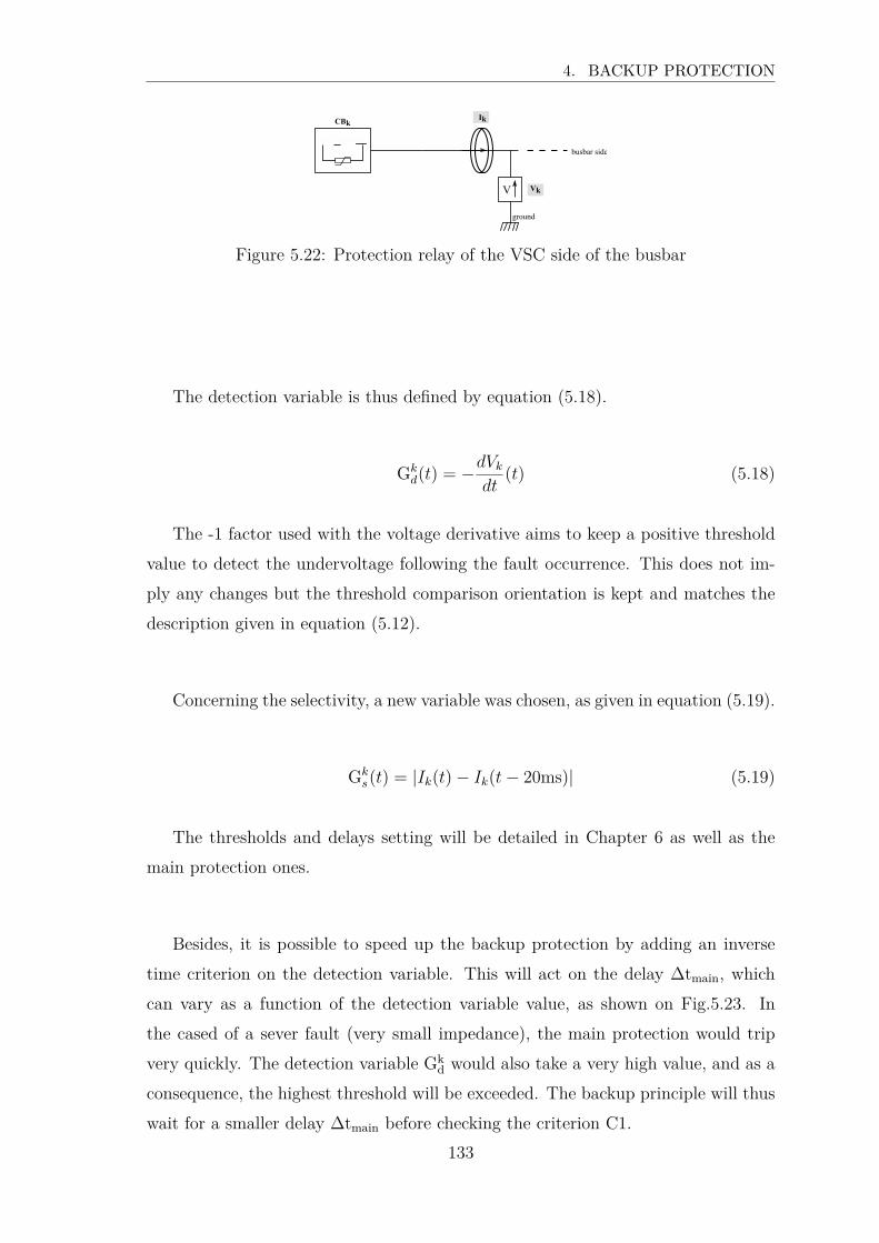
4. BACKUP PROTECTION
busbar side
CBk
V Vk
ground
Ik
Figure 5.22: Protection relay of the VSC side of the busbar
The detection variable is thus defined by equation (5.18).
Gkd(t) = −dVk
dt(t) (5.18)
The -1 factor used with the voltage derivative aims to keep a positive threshold
value to detect the undervoltage following the fault occurrence. This does not im-
ply any changes but the threshold comparison orientation is kept and matches the
description given in equation (5.12).
Concerning the selectivity, a new variable was chosen, as given in equation (5.19).
Gks(t) = |Ik(t) − Ik(t− 20ms)| (5.19)
The thresholds and delays setting will be detailed in Chapter 6 as well as the
main protection ones.
Besides, it is possible to speed up the backup protection by adding an inverse
time criterion on the detection variable. This will act on the delay ∆tmain, which
can vary as a function of the detection variable value, as shown on Fig.5.23. In
the cased of a sever fault (very small impedance), the main protection would trip
very quickly. The detection variable Gkd would also take a very high value, and as a
consequence, the highest threshold will be exceeded. The backup principle will thus
wait for a smaller delay ∆tmain before checking the criterion C1.
133
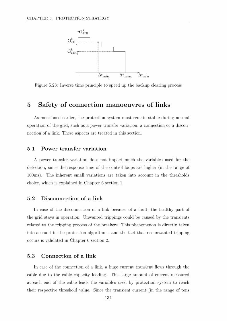
CHAPTER 5. PROTECTION STRATEGY
GdTHk
Δtmain
GdTHjk
Δtmainj
kGdTH0
Δtmain0
Figure 5.23: Inverse time principle to speed up the backup clearing process
5 Safety of connection manoeuvres of links
As mentioned earlier, the protection system must remain stable during normal
operation of the grid, such as a power transfer variation, a connection or a discon-
nection of a link. These aspects are treated in this section.
5.1 Power transfer variation
A power transfer variation does not impact much the variables used for the
detection, since the response time of the control loops are higher (in the range of
100ms). The inherent small variations are taken into account in the thresholds
choice, which is explained in Chapter 6 section 1.
5.2 Disconnection of a link
In case of the disconnection of a link because of a fault, the healthy part of
the grid stays in operation. Unwanted trippings could be caused by the transients
related to the tripping process of the breakers. This phenomenon is directly taken
into account in the protection algorithms, and the fact that no unwanted tripping
occurs is validated in Chapter 6 section 2.
5.3 Connection of a link
In case of the connection of a link, a huge current transient flows through the
cable due to the cable capacity loading. This large amount of current measured
at each end of the cable leads the variables used by protection system to reach
their respective threshold value. Since the transient current (in the range of tens
134
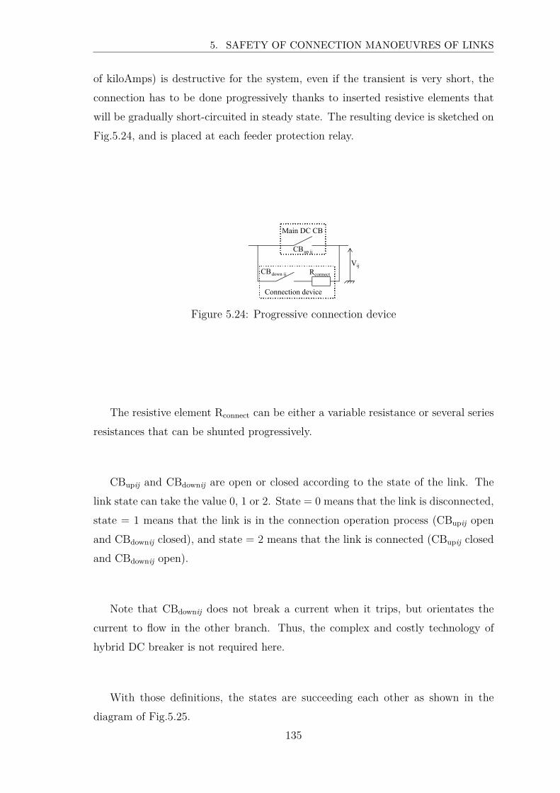
5. SAFETY OF CONNECTION MANOEUVRES OF LINKS
of kiloAmps) is destructive for the system, even if the transient is very short, the
connection has to be done progressively thanks to inserted resistive elements that
will be gradually short-circuited in steady state. The resulting device is sketched on
Fig.5.24, and is placed at each feeder protection relay.
Main DC CB
Connection device
CBdown ij Rconnect
CBup ij
Vij
Figure 5.24: Progressive connection device
The resistive element Rconnect can be either a variable resistance or several series
resistances that can be shunted progressively.
CBupij and CBdownij are open or closed according to the state of the link. The
link state can take the value 0, 1 or 2. State = 0 means that the link is disconnected,
state = 1 means that the link is in the connection operation process (CBupij open
and CBdownij closed), and state = 2 means that the link is connected (CBupij closed
and CBdownij open).
Note that CBdownij does not break a current when it trips, but orientates the
current to flow in the other branch. Thus, the complex and costly technology of
hybrid DC breaker is not required here.
With those definitions, the states are succeeding each other as shown in the
diagram of Fig.5.25.
135
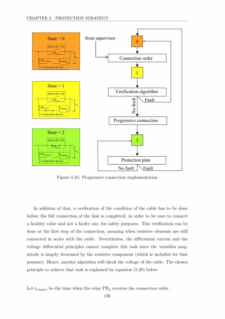
CHAPTER 5. PROTECTION STRATEGY
2
1
0
Connection order
from supervisor
Verification algorithm
Progressive connection
Protection plan
Fault
No
faul
t
FaultNo fault
Main DC CB
Connection device
CBdown ij Rconnect
CBup ij
Vij
State = 0
Main DC CB
Connection device
CBdown ij Rconnect
CBup ij
Vij
State = 1
Main DC CB
Connection device
CBdown ij Rconnect
CBup ij
Vij
State = 2
Figure 5.25: Progressive connection implementation
In addition of that, a verification of the condition of the cable has to be done
before the full connection of the link is completed, in order to be sure to connect
a healthy cable and not a faulty one, for safety purposes. This verification can be
done at the first step of the connection, meaning when resistive elements are still
connected in series with the cable. Nevertheless, the differential current and the
voltage differential principles cannot complete this task since the variables mag-
nitude is largely decreased by the resistive component (which is included for that
purpose). Hence, another algorithm will check the voltage of the cable. The chosen
principle to achieve that task is explained by equation (5.20) below.
Let tconnect be the time when the relay PRij receives the connection order.
136

6. PROPOSED PROTECTION SYSTEM
IF ∃t ∈ [tconnect; tconnect + ∆tverif] such thatVij > VconnectTH
then decrease Rconnect and State = 2
ELSE State = 0
(5.20)
where ∆tverif is a delay corresponding to the loading process of the cables, and
VconnectTH is a threshold.
Simulation examples will be shown in Chapter 6.
6 Proposed protection system
The protection system implementation is summarized in this section. Two cases
are treated: a relay connected to a station (Fig.5.26) and a relay connected to a
feeder (Fig.5.27).
As mentioned earlier, the voltage differential algorithm was found in a later
stage of the work, thanks to the incorporation of the feeders inductors. Thus, the
protection plan was validated (in Chapter 6 section 2) at first stage considering
the optical fiber communication link and no feeder inductors. Then, the feeders
inductors were incorporated for another purpose, as it will be developed in Chapter
6 section 4. Hence, the validation process of the voltage differential protection will
be done at the end of Chapter 6. It is still included in the protection system as a
backup against the loss of the optical fiber, as shown on Fig.5.27.
137
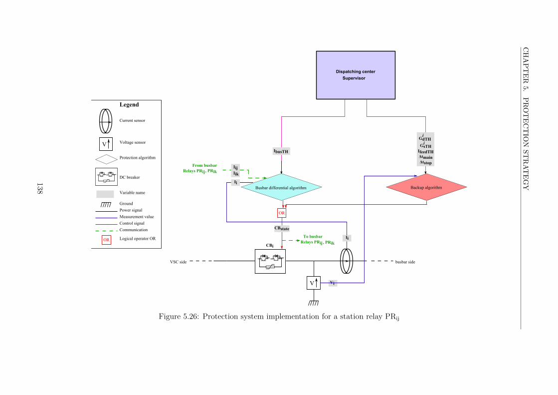
CH
AP
TE
R5.
PR
OT
EC
TIO
NST
RA
TE
GY
VSC side busbar side
Backup algorithmBusbar differential algorithm
Dispatching centerSupervisor
CBi
Ii
Iik
Ii
OR
VijCBstate
IbusTH
To busbarRelays PRij
i
i
GsTHIfeedTHΔtmainΔtstop
GdTH
, PRik
IijFrom busbarRelays PRij , PRik
V Vi
V
Legend
Current sensor
Voltage sensor
Protection algorithm
DC breaker
Variable name
Power signalMeasurement valueControl signalCommunication
Ground
OR Logical operator OR
Figure 5.26: Protection system implementation for a station relay PRij
138
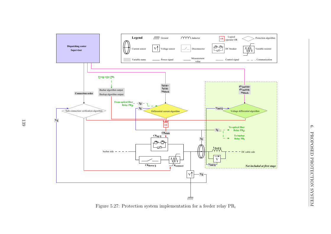
6.P
RO
PO
SED
PR
OT
EC
TIO
NSY
STE
M
busbar side DC cable side
V
V
Voltage differential algorithmDifferential current algorithm
Dispatching centerSupervisor
Safe connection verification algorithm
CBup ij
CBdown ij Rconnect
Lfeed ij
Iij
Iji
Iij
From optical fiberRelay PRji
OR
Vij
VijVind ij
VijCBstate
Vij
From relay PRi
Busbar algorithm output
Backup algorithm outputConnection order
IdTH+IdTH-
Δtblock
dVindTH+dVindTH-
Δtblock
IijTo optical fiber
Relay PRji
To busbarRelay PRi
VijVind ij
V
Protection algorithmLegend
Current sensor Voltage sensor DC breaker
Variable name Power signal Measurementvalue
Control signal Communication
Ground ORLogical
operator ORInductor
Disconnector Variable resistor
Not included at first stage
Figure 5.27: Protection system implementation for a feeder relay PRi
139

CHAPTER 6
Protection plan validation

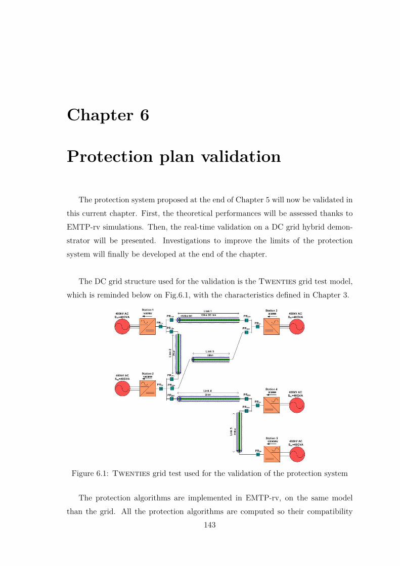
Chapter 6
Protection plan validation
The protection system proposed at the end of Chapter 5 will now be validated in
this current chapter. First, the theoretical performances will be assessed thanks to
EMTP-rv simulations. Then, the real-time validation on a DC grid hybrid demon-
strator will be presented. Investigations to improve the limits of the protection
system will finally be developed at the end of the chapter.
The DC grid structure used for the validation is the Twenties grid test model,
which is reminded below on Fig.6.1, with the characteristics defined in Chapter 3.
Figure 6.1: Twenties grid test used for the validation of the protection system
The protection algorithms are implemented in EMTP-rv, on the same model
than the grid. All the protection algorithms are computed so their compatibility
143

CHAPTER 6. PROTECTION PLAN VALIDATION
can be tested.
1 Complete protection plan implementation in EMTP-
rv
The inputs of the protection algorithms are the current and voltage computed
by EMTP-rv, considering the sensors models developed in Chapter 3. Indeed, the
protection system do not have access to the real current and voltages, and the inputs
can only be the measurement outputs of the sensors. The signals that are shown
for illustration in this chapter are the real current, and not the one issued by the
sensors model, since the constraint in the grid depends on those real current.
As mentioned in Chapter 5, the busbar protection, the differential current protec-
tion and the backup protection will be treated in section 2. The voltage differential
protection will be discussed when the feeder inductors will be considered, in section
4.
1.1 Data processing
The frequency sampling of the protection relays is set to 100kHz, meaning a time
step of 10µs.
The delay resulting of the propagation delay of the data through the optical fiber
link was given in Chapter 5 section 3.4.1 in Tab.5.3 for each link. Another delay
was added to take into account the data conversion (analog - digital conversion and
digital - analog), and was set to one time step for (10µs) each conversion. This gives
the new delays in Tab.6.1, and these global delays are notated ∆tOF.
144
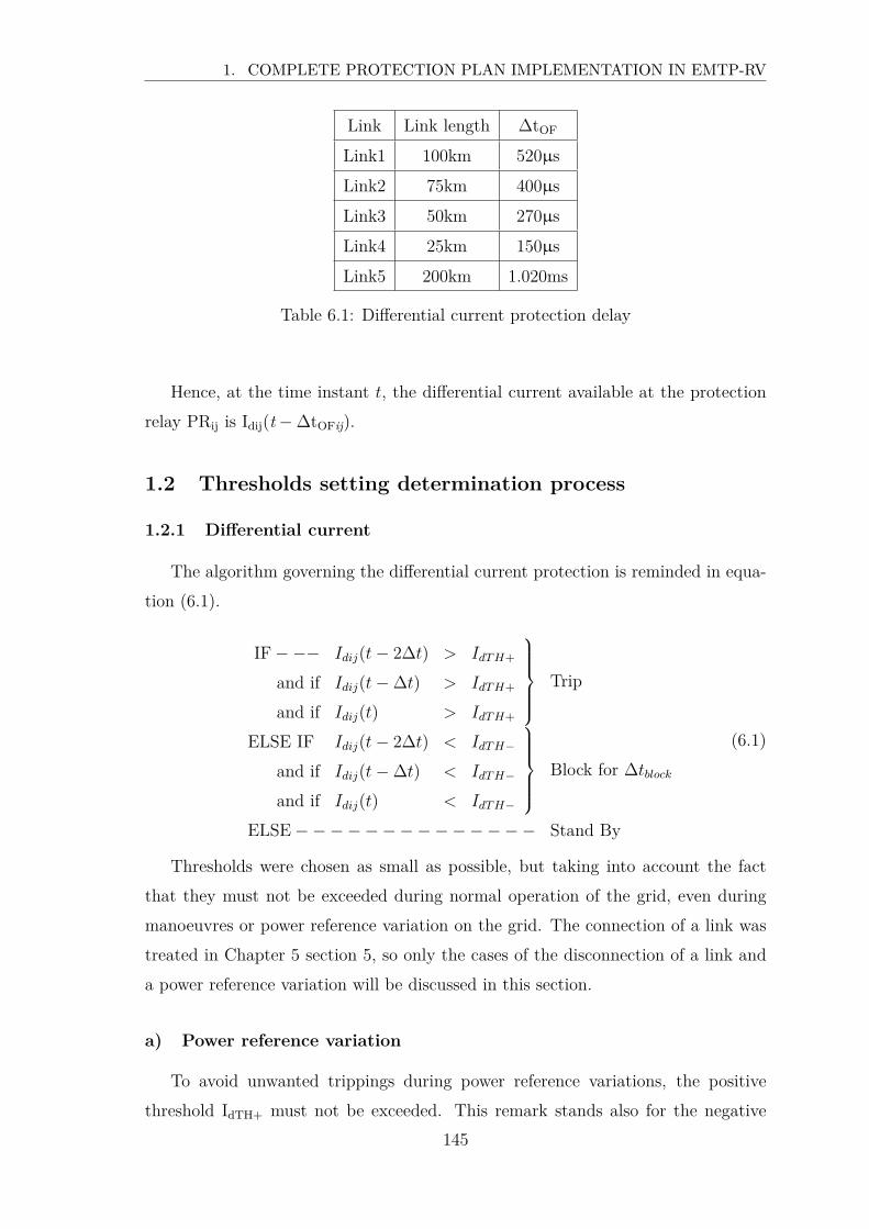
1. COMPLETE PROTECTION PLAN IMPLEMENTATION IN EMTP-RV
Link Link length ∆tOF
Link1 100km 520µs
Link2 75km 400µs
Link3 50km 270µs
Link4 25km 150µs
Link5 200km 1.020ms
Table 6.1: Differential current protection delay
Hence, at the time instant t, the differential current available at the protection
relay PRij is Idij(t − ∆tOFij).
1.2 Thresholds setting determination process
1.2.1 Differential current
The algorithm governing the differential current protection is reminded in equa-
tion (6.1).
IF − −− Idij(t− 2∆t) > IdT H+
and if Idij(t− ∆t) > IdT H+
and if Idij(t) > IdT H+
Trip
ELSE IF Idij(t− 2∆t) < IdT H−
and if Idij(t− ∆t) < IdT H−
and if Idij(t) < IdT H−
Block for ∆tblock
ELSE − − − − − − − − − − − − − − Stand By
(6.1)
Thresholds were chosen as small as possible, but taking into account the fact
that they must not be exceeded during normal operation of the grid, even during
manoeuvres or power reference variation on the grid. The connection of a link was
treated in Chapter 5 section 5, so only the cases of the disconnection of a link and
a power reference variation will be discussed in this section.
a) Power reference variation
To avoid unwanted trippings during power reference variations, the positive
threshold IdTH+ must not be exceeded. This remark stands also for the negative
145
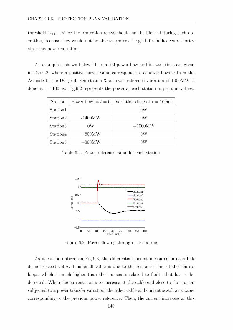
CHAPTER 6. PROTECTION PLAN VALIDATION
threshold IdTH−, since the protection relays should not be blocked during such op-
eration, because they would not be able to protect the grid if a fault occurs shortly
after this power variation.
An example is shown below. The initial power flow and its variations are given
in Tab.6.2, where a positive power value corresponds to a power flowing from the
AC side to the DC grid. On station 3, a power reference variation of 1000MW is
done at t = 100ms. Fig.6.2 represents the power at each station in per-unit values.
Station Power flow at t = 0 Variation done at t = 100ms
Station1 0W
Station2 -1400MW 0W
Station3 0W +1000MW
Station4 +800MW 0W
Station5 +800MW 0W
Table 6.2: Power reference value for each station
0 50 100 150 200 250 300 350 400−1.5
−1
−0.5
0
0.5
1
1.5
Time [ms]
Pow
er [p
u]
Station1Station2Station3Station4Station5
Figure 6.2: Power flowing through the stations
As it can be noticed on Fig.6.3, the differential current measured in each link
do not exceed 250A. This small value is due to the response time of the control
loops, which is much higher than the transients related to faults that has to be
detected. When the current starts to increase at the cable end close to the station
subjected to a power transfer variation, the other cable end current is still at a value
corresponding to the previous power reference. Then, the current increases at this
146

1. COMPLETE PROTECTION PLAN IMPLEMENTATION IN EMTP-RV
later cable end after the propagation time related to the cable length. Since the
control loops have a quite high response time (largely higher than the propagation
time of a signal through the cable), the current difference between the two ends is
sensitively small. Hence, the thresholds take into account the oscillations present in
the signal, due to AC/DC conversion, and the transient that can appear in power
variations.
0 100 200 300 400−100
0
100
200
Time [ms]
Diff
eren
tial c
urre
nt [A
]
0 100 200 300 400−100
0
100
200
Time [ms]
Diff
eren
tial c
urre
nt [A
]
0 100 200 300 400−100
0
100
200
Time [ms]
Diff
eren
tial c
urre
nt [A
]
0 100 200 300 400−100
0
100
200
Time [ms]
Diff
eren
tial c
urre
nt [A
]
0 100 200 300 400−100
0
100
200
Time [ms]
Diff
eren
tial c
urre
nt [A
]
Link1 Link2
Link3 Link4
Link5
Figure 6.3: Differential current during a power flow variation
b) Disconnection of a link
When a fault occurs and is cleared by the breakers of the faulty cable ends, the
differential current protection needs to remain stable. The transients following the
tripping may imply unwanted trippings, which is also why the negative threshold
147

CHAPTER 6. PROTECTION PLAN VALIDATION
IdTH− and the blocking time ∆tblock were introduced. They are set in order to avoid
such unwanted tripping events.
The thresholds for the differential current protection are chosen to match the
constraints emphasized in this subsection, and are given in Tab.6.3.
Threshold name Value
IdTH+ 500A
IdTH− -500A
∆tblock 30ms
Table 6.3: Thresholds setting for the differential current protection
Note that the threshold values could be different for any protection relay, but
since the selectivity was guaranteed with those values, they were used for each relay.
This is validated in section 2.1 where this principle was implemented and tested.
1.2.2 Busbar differential
The busbar differential current threshold can theoretically be any positive value,
and the closest to zero it is, the fastest thee protection operates and the highest
the maximal fault resistance that can be detected is. A margin needs however to
be taken into account, and to avoid unwanted trippings due to other fault clearing
process, a threshold value of IbusTH = 500A were thus set for each station. The
results related to the busbar protection are shown in section 2.3.
1.2.3 Backup
The backup thresholds were set in order to be selective in case of a breaker failure.
Three thresholds have to be set, and correspond to the values, GkdTH Gk
sTH and
IfeedTH that were mentioned in Chapter 5. The value of GkdTH is responsible of the
detection, without any selectivity purpose. It was chosen to be the same value for
each station relay (k = 1..5), and is equal to 200kV/ms, which is reached even
reached for faults with resistance of resΩ. Also, the threshold IfeedTH is used to
verify if there is still a current flowing through the cable. It is thus set to 10A. Note
148
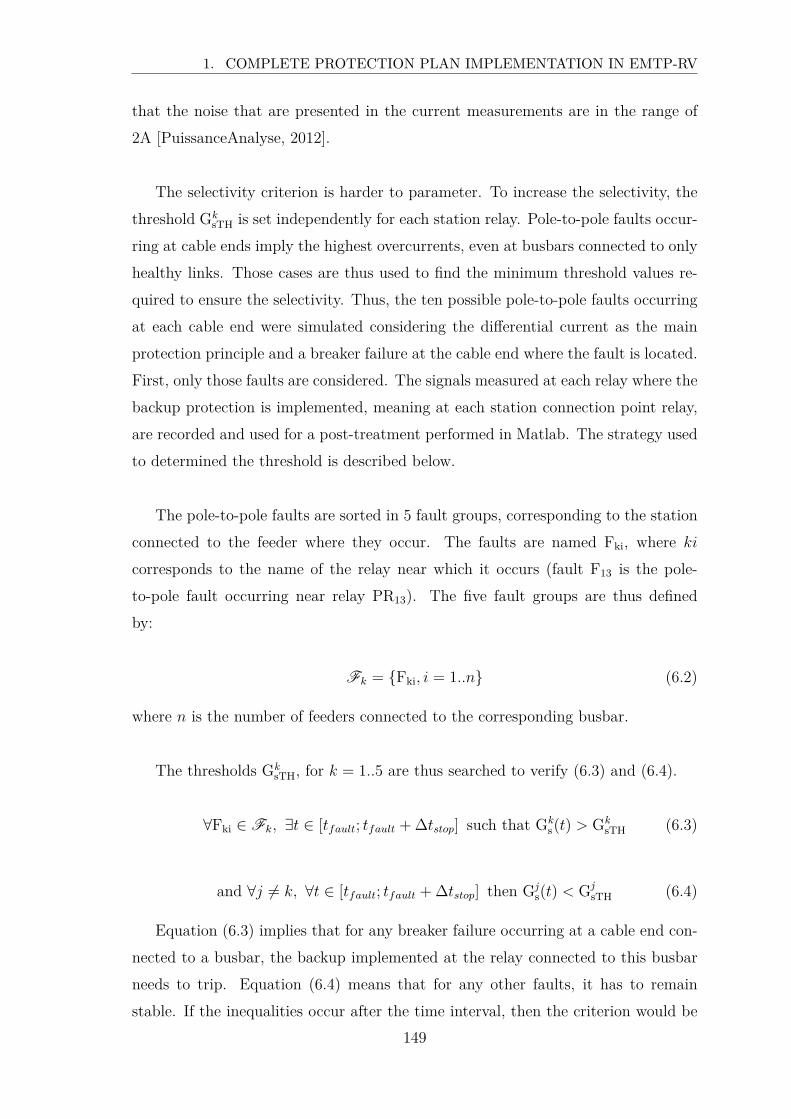
1. COMPLETE PROTECTION PLAN IMPLEMENTATION IN EMTP-RV
that the noise that are presented in the current measurements are in the range of
2A [PuissanceAnalyse, 2012].
The selectivity criterion is harder to parameter. To increase the selectivity, the
threshold GksTH is set independently for each station relay. Pole-to-pole faults occur-
ring at cable ends imply the highest overcurrents, even at busbars connected to only
healthy links. Those cases are thus used to find the minimum threshold values re-
quired to ensure the selectivity. Thus, the ten possible pole-to-pole faults occurring
at each cable end were simulated considering the differential current as the main
protection principle and a breaker failure at the cable end where the fault is located.
First, only those faults are considered. The signals measured at each relay where the
backup protection is implemented, meaning at each station connection point relay,
are recorded and used for a post-treatment performed in Matlab. The strategy used
to determined the threshold is described below.
The pole-to-pole faults are sorted in 5 fault groups, corresponding to the station
connected to the feeder where they occur. The faults are named Fki, where ki
corresponds to the name of the relay near which it occurs (fault F13 is the pole-
to-pole fault occurring near relay PR13). The five fault groups are thus defined
by:
Fk = Fki, i = 1..n (6.2)
where n is the number of feeders connected to the corresponding busbar.
The thresholds GksTH, for k = 1..5 are thus searched to verify (6.3) and (6.4).
∀Fki ∈ Fk, ∃t ∈ [tfault; tfault + ∆tstop] such that Gks(t) > Gk
sTH (6.3)
and ∀j 6= k, ∀t ∈ [tfault; tfault + ∆tstop] then Gjs(t) < Gj
sTH (6.4)
Equation (6.3) implies that for any breaker failure occurring at a cable end con-
nected to a busbar, the backup implemented at the relay connected to this busbar
needs to trip. Equation (6.4) means that for any other faults, it has to remain
stable. If the inequalities occur after the time interval, then the criterion would be
149
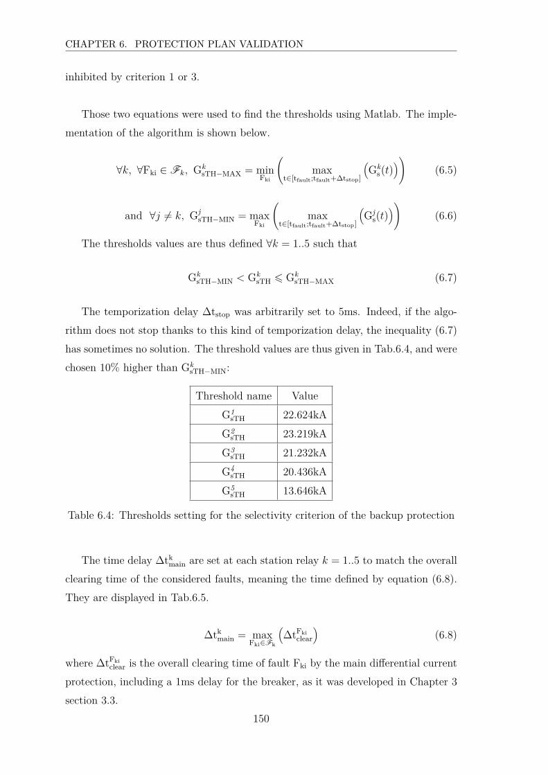
CHAPTER 6. PROTECTION PLAN VALIDATION
inhibited by criterion 1 or 3.
Those two equations were used to find the thresholds using Matlab. The imple-
mentation of the algorithm is shown below.
∀k, ∀Fki ∈ Fk, GksTH−MAX = min
Fki
(
maxt∈[tfault;tfault+∆tstop]
(
Gks(t)
)
)
(6.5)
and ∀j 6= k, GjsTH−MIN = max
Fki
(
maxt∈[tfault;tfault+∆tstop]
(
Gjs(t)
)
)
(6.6)
The thresholds values are thus defined ∀k = 1..5 such that
GksTH−MIN < Gk
sTH 6 GksTH−MAX (6.7)
The temporization delay ∆tstop was arbitrarily set to 5ms. Indeed, if the algo-
rithm does not stop thanks to this kind of temporization delay, the inequality (6.7)
has sometimes no solution. The threshold values are thus given in Tab.6.4, and were
chosen 10% higher than GksTH−MIN:
Threshold name Value
G1sTH 22.624kA
G2sTH 23.219kA
G3sTH 21.232kA
G4sTH 20.436kA
G5sTH 13.646kA
Table 6.4: Thresholds setting for the selectivity criterion of the backup protection
The time delay ∆tkmain are set at each station relay k = 1..5 to match the overall
clearing time of the considered faults, meaning the time defined by equation (6.8).
They are displayed in Tab.6.5.
∆tkmain = max
Fki∈Fk
(
∆tFki
clear
)
(6.8)
where ∆tFki
clear is the overall clearing time of fault Fki by the main differential current
protection, including a 1ms delay for the breaker, as it was developed in Chapter 3
section 3.3.
150
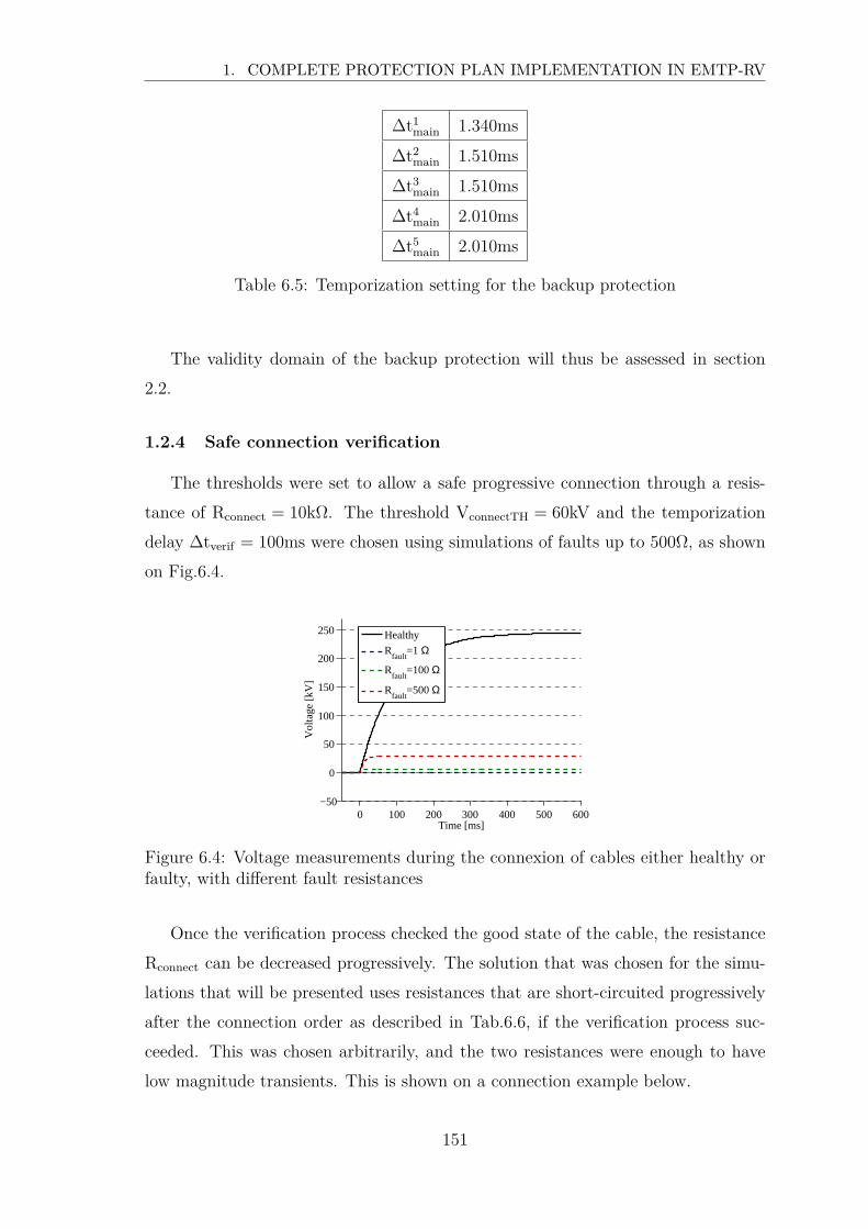
1. COMPLETE PROTECTION PLAN IMPLEMENTATION IN EMTP-RV
∆t1main 1.340ms
∆t2main 1.510ms
∆t3main 1.510ms
∆t4main 2.010ms
∆t5main 2.010ms
Table 6.5: Temporization setting for the backup protection
The validity domain of the backup protection will thus be assessed in section
2.2.
1.2.4 Safe connection verification
The thresholds were set to allow a safe progressive connection through a resis-
tance of Rconnect = 10kΩ. The threshold VconnectTH = 60kV and the temporization
delay ∆tverif = 100ms were chosen using simulations of faults up to 500Ω, as shown
on Fig.6.4.
0 100 200 300 400 500 600−50
0
50
100
150
200
250
Time [ms]
Vol
tage
[kV
]
Healthy
Rfault
=1 Ω
Rfault
=100 Ω
Rfault
=500 Ω
Figure 6.4: Voltage measurements during the connexion of cables either healthy orfaulty, with different fault resistances
Once the verification process checked the good state of the cable, the resistance
Rconnect can be decreased progressively. The solution that was chosen for the simu-
lations that will be presented uses resistances that are short-circuited progressively
after the connection order as described in Tab.6.6, if the verification process suc-
ceeded. This was chosen arbitrarily, and the two resistances were enough to have
low magnitude transients. This is shown on a connection example below.
151
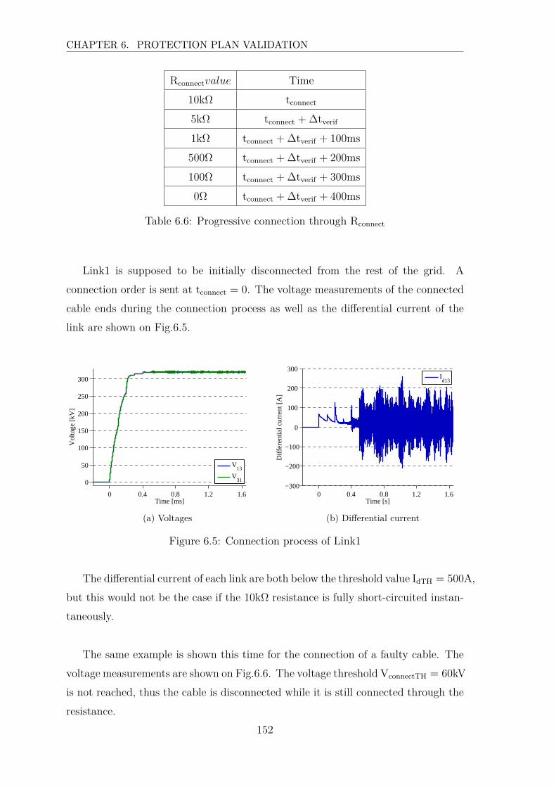
CHAPTER 6. PROTECTION PLAN VALIDATION
Rconnectvalue Time
10kΩ tconnect
5kΩ tconnect + ∆tverif
1kΩ tconnect + ∆tverif + 100ms
500Ω tconnect + ∆tverif + 200ms
100Ω tconnect + ∆tverif + 300ms
0Ω tconnect + ∆tverif + 400ms
Table 6.6: Progressive connection through Rconnect
Link1 is supposed to be initially disconnected from the rest of the grid. A
connection order is sent at tconnect = 0. The voltage measurements of the connected
cable ends during the connection process as well as the differential current of the
link are shown on Fig.6.5.
0 0.4 0.8 1.2 1.6
0
50
100
150
200
250
300
Time [ms]
Vol
tage
[kV
]
V13
V31
(a) Voltages
0 0.4 0.8 1.2 1.6−300
−200
−100
0
100
200
300
Time [s]
Diff
eren
tial c
urre
nt [A
]
Id13
(b) Differential current
Figure 6.5: Connection process of Link1
The differential current of each link are both below the threshold value IdTH = 500A,
but this would not be the case if the 10kΩ resistance is fully short-circuited instan-
taneously.
The same example is shown this time for the connection of a faulty cable. The
voltage measurements are shown on Fig.6.6. The voltage threshold VconnectTH = 60kV
is not reached, thus the cable is disconnected while it is still connected through the
resistance.
152
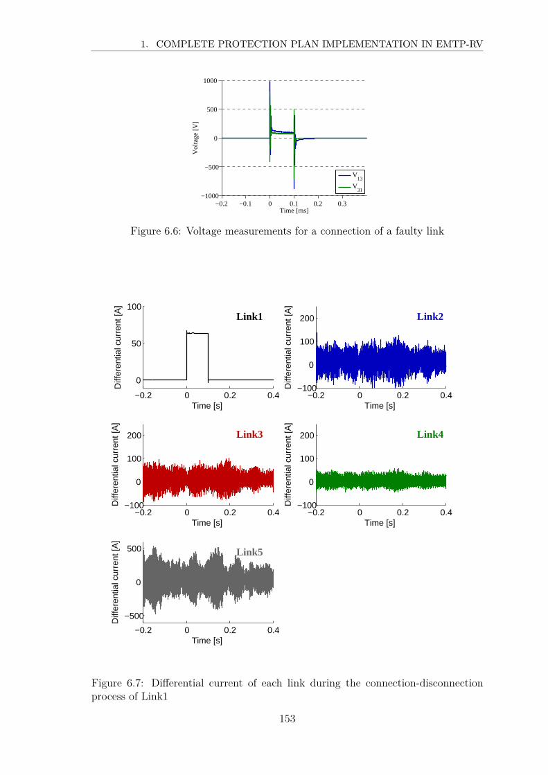
1. COMPLETE PROTECTION PLAN IMPLEMENTATION IN EMTP-RV
−0.2 −0.1 0 0.1 0.2 0.3−1000
−500
0
500
1000
Time [ms]
Vol
tage
[V]
V13
V31
Figure 6.6: Voltage measurements for a connection of a faulty link
−0.2 0 0.2 0.4
0
50
100
Time [s]
Diff
eren
tial c
urre
nt [A
]
−0.2 0 0.2 0.4−100
0
100
200
Time [s]
Diff
eren
tial c
urre
nt [A
]
−0.2 0 0.2 0.4−100
0
100
200
Time [s]
Diff
eren
tial c
urre
nt [A
]
−0.2 0 0.2 0.4−100
0
100
200
Time [s]
Diff
eren
tial c
urre
nt [A
]
−0.2 0 0.2 0.4
−500
0
500
Time [s]
Diff
eren
tial c
urre
nt [A
]
Link1 Link2
Link3 Link4
Link5
Figure 6.7: Differential current of each link during the connection-disconnectionprocess of Link1
153

CHAPTER 6. PROTECTION PLAN VALIDATION
The differential currents of the healthy links are shown on Fig.6.7 for a duration
including the whole connection - disconnection process. They remain below the
threshold, so there is no unwanted trippings of healthy links, and the grid stays in
a N-1 operation state.
This connection process is more likely related to the grid operation and no other
results on this process will be provided in this thesis, since this the priority were
given to the protections.
2 EMTP-rv results
In this section, the protection principle theoretical performances are assessed
thanks to the simulation of the protection system implemented as detailed in the
previous section. The differential current, the backup and the busbar protection will
be treated.
2.1 Differential current protection
First of all, the fault clearing process responding to the main differential current
algorithm is detailed through an example. A pole-to-ground fault is simulated on
Link1, with the parameters defined in Tab.6.7.
Parameter Value
Type Pole-to-ground
Location Link1
Position 30km away Station 1
Impedance 1Ω
Table 6.7: Parameters of the fault example
Fig.6.8 shows the fault clearing process. On Fig.6.9a the current measured at
the faulty cable ends is presented. The fault is cleared 1.660ms after the fault
occurrence, and the current to break are 32.263kA and 18.926kA for PR13 and PR31
respectively. The difference is due to the fault location, which is closer to PR13 than
to PR31.
154
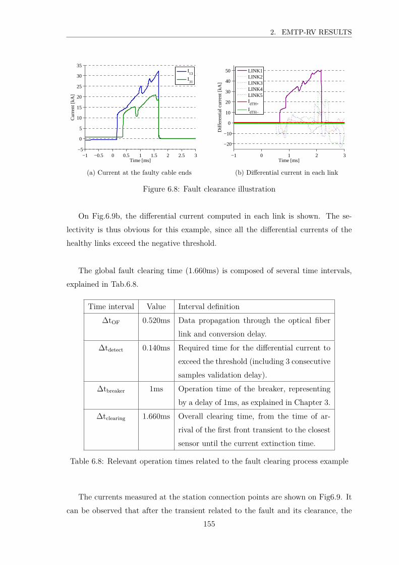
2. EMTP-RV RESULTS
−1 −0.5 0 0.5 1 1.5 2 2.5 3−5
0
5
10
15
20
25
30
35
Time [ms]
Cur
rent
[kA
]
I13
I31
(a) Current at the faulty cable ends
−1 0 1 2 3
−20
−10
0
10
20
30
40
50
Time [ms]
Diff
eren
tial c
urre
nt [k
A]
LINK1LINK2LINK3LINK4LINK5IdTH+
IdTH−
(b) Differential current in each link
Figure 6.8: Fault clearance illustration
On Fig.6.9b, the differential current computed in each link is shown. The se-
lectivity is thus obvious for this example, since all the differential currents of the
healthy links exceed the negative threshold.
The global fault clearing time (1.660ms) is composed of several time intervals,
explained in Tab.6.8.
Time interval Value Interval definition
∆tOF 0.520ms Data propagation through the optical fiber
link and conversion delay.
∆tdetect 0.140ms Required time for the differential current to
exceed the threshold (including 3 consecutive
samples validation delay).
∆tbreaker 1ms Operation time of the breaker, representing
by a delay of 1ms, as explained in Chapter 3.
∆tclearing 1.660ms Overall clearing time, from the time of ar-
rival of the first front transient to the closest
sensor until the current extinction time.
Table 6.8: Relevant operation times related to the fault clearing process example
The currents measured at the station connection points are shown on Fig6.9. It
can be observed that after the transient related to the fault and its clearance, the
155

CHAPTER 6. PROTECTION PLAN VALIDATION
currents recover to their initial values. The current initially flowing through the
faulty cable is now flowing through Link2 and Link3, meaning through the cables
connected to the busbars where the faulty link were connected. Hence, the power
reference is kept.
−40 −20 0 20 40 60 80 100−20
−10
0
10
20
30
Time [ms]
Cur
rent
[kA
]
I1
I2
I3
I4
I5
(a) Current at station connection point
−40 −20 0 20 40 60 80 100−15
−10
−5
0
5
10
15
20
Time [ms]
Cur
rent
[kA
]
I12
I32
(b) Current measured at the end of the healthy
links
Figure 6.9: Fault clearance illustration
Several parameters can affect the tripping time and the currents to break. They
are investigated in the following next subsections.
2.1.1 Fault resistance influence
The fault resistance impact on the protection system performances were assessed
thanks to the simulation of 30 cases. This number of cases was chosen arbitrarily.
The fault is always located on link 1 and 30km away station 1, and only the fault
resistance changes compared to the fault detailed previously. Thus, fault resistances
Rfault = i × 1, i × 10 and i × 100, with i the integer i = 1..10, were simulated. The
results are shown below.
a) Influence on the required operation speed of the protection
As it was detailed in Chapter 4 and reminded at the beginning of Chapter 5,
a high fault resistance damped the signals, and thus decreases the current flowing
through the diodes of the converters. This results in a higher acceptable clearing
time for a considered fault.
156
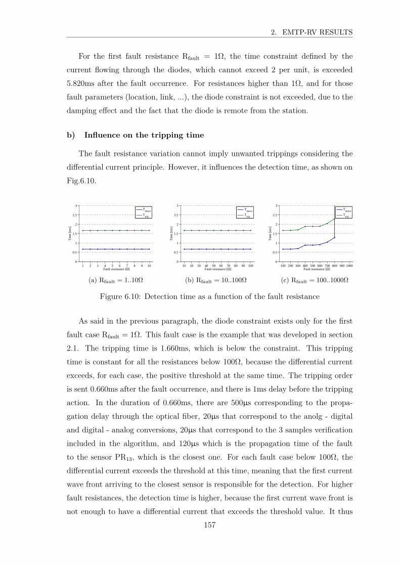
2. EMTP-RV RESULTS
For the first fault resistance Rfault = 1Ω, the time constraint defined by the
current flowing through the diodes, which cannot exceed 2 per unit, is exceeded
5.820ms after the fault occurrence. For resistances higher than 1Ω, and for those
fault parameters (location, link, ...), the diode constraint is not exceeded, due to the
damping effect and the fact that the diode is remote from the station.
b) Influence on the tripping time
The fault resistance variation cannot imply unwanted trippings considering the
differential current principle. However, it influences the detection time, as shown on
Fig.6.10.
1 2 3 4 5 6 7 8 9 100
0.5
1
1.5
2
2.5
3
Fault resistance [Ω]
Tim
e [m
s]
Tdetect
Ttrip
(a) Rfault = 1..10Ω
10 20 30 40 50 60 70 80 90 1000
0.5
1
1.5
2
2.5
3
Fault resistance [Ω]
Tim
e [m
s]
Tdetect
Ttrip
(b) Rfault = 10..100Ω
100 200 300 400 500 600 700 800 900 10000
0.5
1
1.5
2
2.5
3
Fault resistance [Ω]T
ime
[ms]
Tdetect
Ttrip
(c) Rfault = 100..1000Ω
Figure 6.10: Detection time as a function of the fault resistance
As said in the previous paragraph, the diode constraint exists only for the first
fault case Rfault = 1Ω. This fault case is the example that was developed in section
2.1. The tripping time is 1.660ms, which is below the constraint. This tripping
time is constant for all the resistances below 100Ω, because the differential current
exceeds, for each case, the positive threshold at the same time. The tripping order
is sent 0.660ms after the fault occurrence, and there is 1ms delay before the tripping
action. In the duration of 0.660ms, there are 500µs corresponding to the propa-
gation delay through the optical fiber, 20µs that correspond to the anolg - digital
and digital - analog conversions, 20µs that correspond to the 3 samples verification
included in the algorithm, and 120µs which is the propagation time of the fault
to the sensor PR13, which is the closest one. For each fault case below 100Ω, the
differential current exceeds the threshold at this time, meaning that the first current
wave front arriving to the closest sensor is responsible for the detection. For higher
fault resistances, the detection time is higher, because the first current wave front is
not enough to have a differential current that exceeds the threshold value. It thus
157
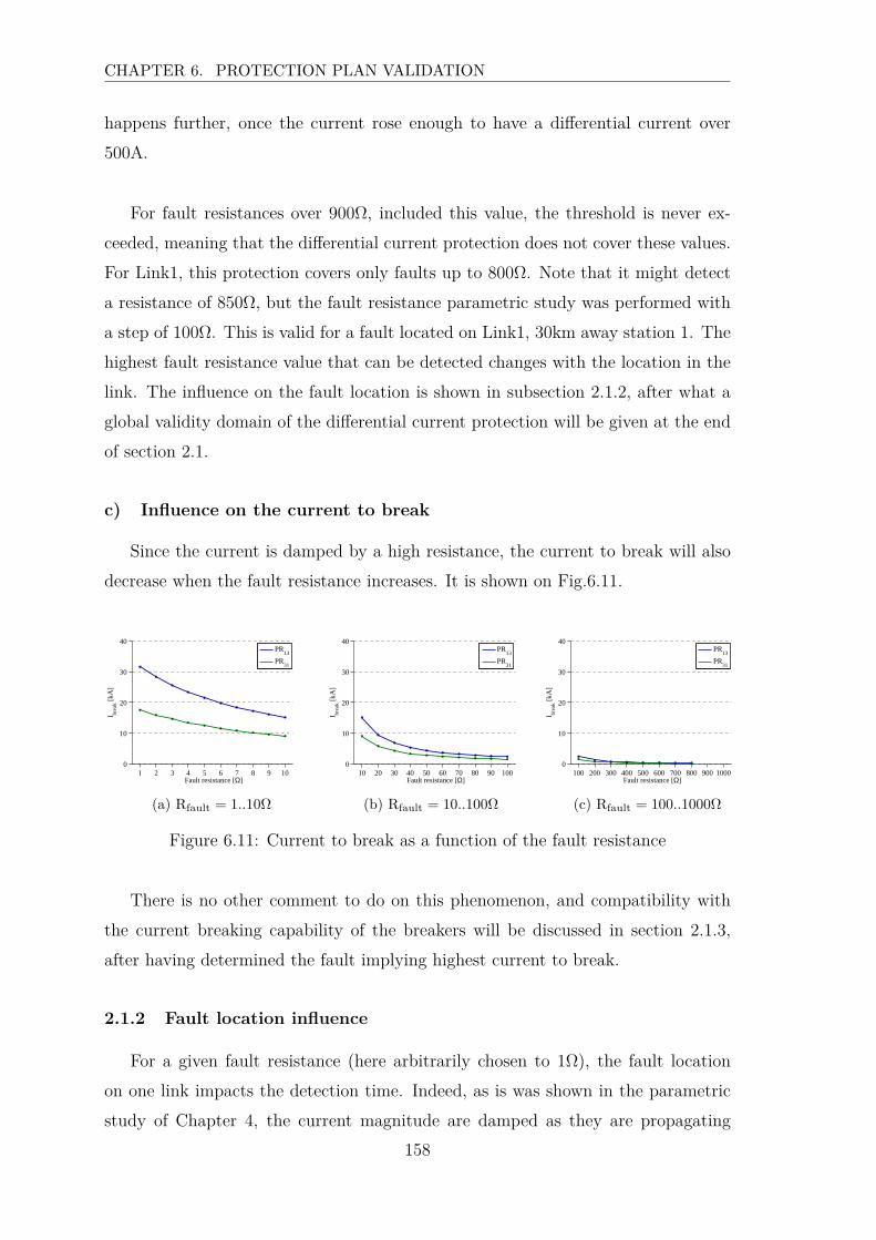
CHAPTER 6. PROTECTION PLAN VALIDATION
happens further, once the current rose enough to have a differential current over
500A.
For fault resistances over 900Ω, included this value, the threshold is never ex-
ceeded, meaning that the differential current protection does not cover these values.
For Link1, this protection covers only faults up to 800Ω. Note that it might detect
a resistance of 850Ω, but the fault resistance parametric study was performed with
a step of 100Ω. This is valid for a fault located on Link1, 30km away station 1. The
highest fault resistance value that can be detected changes with the location in the
link. The influence on the fault location is shown in subsection 2.1.2, after what a
global validity domain of the differential current protection will be given at the end
of section 2.1.
c) Influence on the current to break
Since the current is damped by a high resistance, the current to break will also
decrease when the fault resistance increases. It is shown on Fig.6.11.
1 2 3 4 5 6 7 8 9 100
10
20
30
40
Fault resistance [Ω]
I brea
k [kA
]
PR13
PR31
(a) Rfault = 1..10Ω
10 20 30 40 50 60 70 80 90 1000
10
20
30
40
Fault resistance [Ω]
I brea
k [kA
]
PR13
PR31
(b) Rfault = 10..100Ω
100 200 300 400 500 600 700 800 900 10000
10
20
30
40
Fault resistance [Ω]
I brea
k [kA
]
PR13
PR31
(c) Rfault = 100..1000Ω
Figure 6.11: Current to break as a function of the fault resistance
There is no other comment to do on this phenomenon, and compatibility with
the current breaking capability of the breakers will be discussed in section 2.1.3,
after having determined the fault implying highest current to break.
2.1.2 Fault location influence
For a given fault resistance (here arbitrarily chosen to 1Ω), the fault location
on one link impacts the detection time. Indeed, as is was shown in the parametric
study of Chapter 4, the current magnitude are damped as they are propagating
158
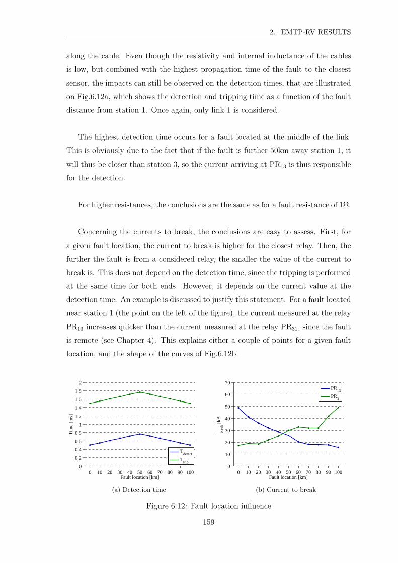
2. EMTP-RV RESULTS
along the cable. Even though the resistivity and internal inductance of the cables
is low, but combined with the highest propagation time of the fault to the closest
sensor, the impacts can still be observed on the detection times, that are illustrated
on Fig.6.12a, which shows the detection and tripping time as a function of the fault
distance from station 1. Once again, only link 1 is considered.
The highest detection time occurs for a fault located at the middle of the link.
This is obviously due to the fact that if the fault is further 50km away station 1, it
will thus be closer than station 3, so the current arriving at PR13 is thus responsible
for the detection.
For higher resistances, the conclusions are the same as for a fault resistance of 1Ω.
Concerning the currents to break, the conclusions are easy to assess. First, for
a given fault location, the current to break is higher for the closest relay. Then, the
further the fault is from a considered relay, the smaller the value of the current to
break is. This does not depend on the detection time, since the tripping is performed
at the same time for both ends. However, it depends on the current value at the
detection time. An example is discussed to justify this statement. For a fault located
near station 1 (the point on the left of the figure), the current measured at the relay
PR13 increases quicker than the current measured at the relay PR31, since the fault
is remote (see Chapter 4). This explains either a couple of points for a given fault
location, and the shape of the curves of Fig.6.12b.
0 10 20 30 40 50 60 70 80 90 1000
0.2
0.4
0.6
0.8
1
1.2
1.4
1.6
1.8
2
Fault location [km]
Tim
e [m
s]
Tdetect
Ttrip
(a) Detection time
0 10 20 30 40 50 60 70 80 90 1000
10
20
30
40
50
60
70
Fault location [km]
I brea
k [kA
]
PR13
PR31
(b) Current to break
Figure 6.12: Fault location influence
159
CHAPTER 6. PROTECTION PLAN VALIDATION
Both the resistance and the location of the fault impact the detection time. Since
the conclusions on the fault location are the same for another fault resistance, this
implies that for some resistance values, the fault might be detected if it occurs near
a relay, but will not be detected if it is located at the middle of the link. Thus, the
validity domain of the differential current protection (Tab.6.9) will be provided for
each link for the worst case in terms of detection, it means for faults occurring at
the middle of the links. Therefore, it is possible that higher fault resistances can be
detected if they happen somewhere else than at the middle of a cable. Once again,
the constraint defined by the current flowing through the diodes of the converters is
not exceeded for such high fault resistances.
Link
Maximal fault resistance
detected at the middle of
the link
Tripping time
LINK1 800Ω 3.300ms
LINK2 900Ω 2.930ms
LINK3 900Ω 2.810ms
LINK4 900Ω 1.350ms
LINK5 800Ω 2.900ms
Table 6.9: Validity domain of the differential current protection
2.1.3 Worst case scenarios
a) Worst case from the detection point of view
The differential current protection validity domain were assessed in the previous
paragraph from the detection point of view, meaning in terms of tripping time.
The worst case corresponds thus to faults occurring at the middle of Link1, with a
resistance of 800Ω, for a maximal tripping time occurring 3.300ms after the fault
occurrence.
b) Worst case in terms of current to break
The worst case in terms of current to break is now investigated. Given the
conclusions of sections 2.1.1 and 2.1.2, the worst case would occur for a fault located
160
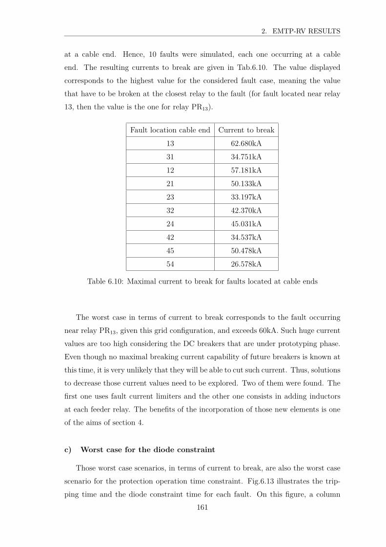
2. EMTP-RV RESULTS
at a cable end. Hence, 10 faults were simulated, each one occurring at a cable
end. The resulting currents to break are given in Tab.6.10. The value displayed
corresponds to the highest value for the considered fault case, meaning the value
that have to be broken at the closest relay to the fault (for fault located near relay
13, then the value is the one for relay PR13).
Fault location cable end Current to break
13 62.680kA
31 34.751kA
12 57.181kA
21 50.133kA
23 33.197kA
32 42.370kA
24 45.031kA
42 34.537kA
45 50.478kA
54 26.578kA
Table 6.10: Maximal current to break for faults located at cable ends
The worst case in terms of current to break corresponds to the fault occurring
near relay PR13, given this grid configuration, and exceeds 60kA. Such huge current
values are too high considering the DC breakers that are under prototyping phase.
Even though no maximal breaking current capability of future breakers is known at
this time, it is very unlikely that they will be able to cut such current. Thus, solutions
to decrease those current values need to be explored. Two of them were found. The
first one uses fault current limiters and the other one consists in adding inductors
at each feeder relay. The benefits of the incorporation of those new elements is one
of the aims of section 4.
c) Worst case for the diode constraint
Those worst case scenarios, in terms of current to break, are also the worst case
scenario for the protection operation time constraint. Fig.6.13 illustrates the trip-
ping time and the diode constraint time for each fault. On this figure, a column
161
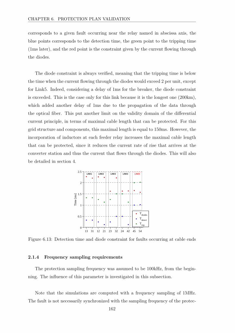
CHAPTER 6. PROTECTION PLAN VALIDATION
corresponds to a given fault occurring near the relay named in abscissa axis, the
blue points corresponds to the detection time, the green point to the tripping time
(1ms later), and the red point is the constraint given by the current flowing through
the diodes.
The diode constraint is always verified, meaning that the tripping time is below
the time when the current flowing through the diodes would exceed 2 per unit, except
for Link5. Indeed, considering a delay of 1ms for the breaker, the diode constraint
is exceeded. This is the case only for this link because it is the longest one (200km),
which added another delay of 1ms due to the propagation of the data through
the optical fiber. This put another limit on the validity domain of the differential
current principle, in terms of maximal cable length that can be protected. For this
grid structure and components, this maximal length is equal to 150ms. However, the
incorporation of inductors at each feeder relay increases the maximal cable length
that can be protected, since it reduces the current rate of rise that arrives at the
converter station and thus the current that flows through the diodes. This will also
be detailed in section 4.
13 31 12 21 23 32 24 42 45 540
0.5
1
1.5
2
2.5
Fault location [Near relay number]
Tim
e [m
s]
Tdiodes
Tdetect
Ttrip
LINK1 LINK2 LINK3 LINK4 LINK5
Figure 6.13: Detection time and diode constraint for faults occurring at cable ends
2.1.4 Frequency sampling requirements
The protection sampling frequency was assumed to be 100kHz, from the begin-
ning. The influence of this parameter is investigated in this subsection.
Note that the simulations are computed with a frequency sampling of 1MHz.
The fault is not necessarily synchronized with the sampling frequency of the protec-
162

2. EMTP-RV RESULTS
tion system.
For a faulty link, the augmentation of the frequency sampling would not impact
the detection phenomenon, but only the time of the detection. Indeed, the differ-
ence between two samples would still be positive, but the validation process using
3 consecutive samples would thus be longer. Also, the exact first time when the
differential current exceeds the threshold becomes the knowledge of the protection
at the first sample consecutive to the phenomenon. For example, with a sampling
frequency of 100kHz, where samples are recorded at t = 10µs, t = 20µs, t = 30µs,
... if the prospective differential current exceeds the threshold at t = 12µs, the
protection would know it only at t = 20µs, because the differential current is not
computed at t = 12µs. Waiting then for 3 consecutive samples validation (samples
at t = 20µs, t = 30µs, t = 40µs), the tripping order is sent after a total of t = 28µs
once the differential current exceeded the threshold. If the sampling frequency is
10kHz (samples recorded at t = 100µs, t = 200µs, t = 300µs, ...), then the tripping
order would this time be sent after t = 282µs. But still, the detection occurs.
At the opposite, the frequency sampling impacts the protection process. This
was mentioned in Chapter 5. The algorithm is looking for a negative front in that
case. The negative front duration corresponds to the propagation time of the wave
through the cable. If no samples exist during this front, then the blocking of the
protection does not occur, which can lead to unwanted trippings. Furthermore, since
the protection uses once again 3 consecutive samples as a validation of the blocking
process, 3 samples need to be present in this negative front. The required frequency
sampling of the protection system is thus defined by the minimal cable length, in
our case 25km. Thus, since the propagation time of a perturbation through the
25km cable is equal to 129µs, the frequency sampling has to be up than 23kHz.
However, using a frequency sampling of 23kHz and given the conclusion expressed
concerning the faulty link case, this would result in a delay in the trippings leading to
diode constraint exceeding for some cases. It is thus highly dangerous to decrease the
frequency sampling, and 100kHz, meaning a time step of 10µs, should be conserved.
163
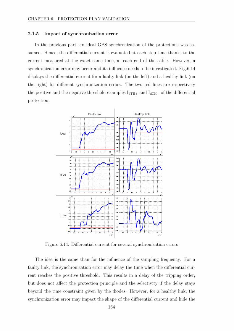
CHAPTER 6. PROTECTION PLAN VALIDATION
2.1.5 Impact of synchronization error
In the previous part, an ideal GPS synchronization of the protections was as-
sumed. Hence, the differential current is evaluated at each step time thanks to the
current measured at the exact same time, at each end of the cable. However, a
synchronization error may occur and its influence needs to be investigated. Fig.6.14
displays the differential current for a faulty link (on the left) and a healthy link (on
the right) for different synchronization errors. The two red lines are respectively
the positive and the negative threshold examples IdTH+ and IdTH− of the differential
protection.
Figure 6.14: Differential current for several synchronization errors
The idea is the same than for the influence of the sampling frequency. For a
faulty link, the synchronization error may delay the time when the differential cur-
rent reaches the positive threshold. This results in a delay of the tripping order,
but does not affect the protection principle and the selectivity if the delay stays
beyond the time constraint given by the diodes. However, for a healthy link, the
synchronization error may impact the shape of the differential current and hide the
164
2. EMTP-RV RESULTS
negative front transient that is used by the protection algorithm to block the pro-
tection during ∆tblock. This would result in an unwanted tripping of the protection.
Nevertheless, there is a maximum synchronization error that guaranties no un-
wanted tripping of the healthy links. In fact, the negative front transient would be
hidden if the propagation time of the wave is equal or lower than the synchronization
error. Thus, the maximum error allowed depends on the length of the link and is
the value of the propagation time of the wave generated by the fault through the
cable. For example, this value is equal to 515µs for a 100km long cable. Since the
already installed GPS synchronization devices ensure a synchronization error lower
than 5µs [Siemens, 2008], no unwanted tripping would occur on a link longer than
1km, which covers most of the cases of DC links in a transmission grid. For shorter
links, other communication principles would require further investigations in order
to avoid unwanted trippings.
2.2 Backup protection
Alike the differential current protection, the backup protection principle is illus-
trated through an fault example. This fault example parameters are provided in
Tab.6.11.
Parameter Value
Type Pole-to-pole
Location Link1
Position neat relay PR13
Impedance 1Ω
Fault occurrence time t = 0
Table 6.11: Parameters of the fault example
The differential current protection detects this fault at t = 440µs. The DC
breaker of relay PR31 thus trips at t = 1.440ms, and a breaker failure is simulated
at the relay PR13. The three criterion C1,C2 and C3 related to the backup principle
of relay PR1 and relay PR3, meaning the stations connected to the faulty cable, are
shown on Fig.6.15. On Fig.6.15a, it can be seen that the three criterion are both
165
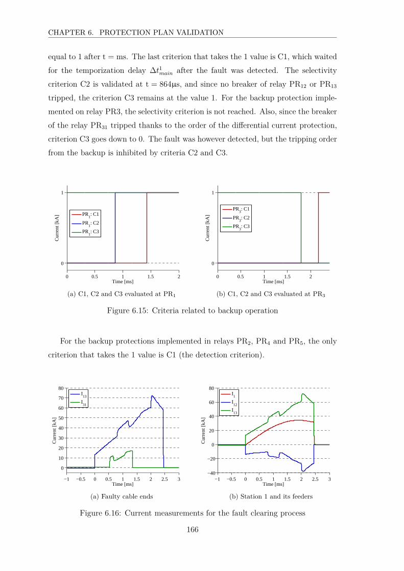
CHAPTER 6. PROTECTION PLAN VALIDATION
equal to 1 after t = ms. The last criterion that takes the 1 value is C1, which waited
for the temporization delay ∆t1main after the fault was detected. The selectivity
criterion C2 is validated at t = 864µs, and since no breaker of relay PR12 or PR13
tripped, the criterion C3 remains at the value 1. For the backup protection imple-
mented on relay PR3, the selectivity criterion is not reached. Also, since the breaker
of the relay PR31 tripped thanks to the order of the differential current protection,
criterion C3 goes down to 0. The fault was however detected, but the tripping order
from the backup is inhibited by criteria C2 and C3.
0 0.5 1 1.5 2
0
1
Time [ms]
Cur
rent
[kA
]
PR1: C1
PR1: C2
PR1: C3
(a) C1, C2 and C3 evaluated at PR1
0 0.5 1 1.5 2
0
1
Time [ms]
Cur
rent
[kA
]
PR3: C1
PR3: C2
PR3: C3
(b) C1, C2 and C3 evaluated at PR3
Figure 6.15: Criteria related to backup operation
For the backup protections implemented in relays PR2, PR4 and PR5, the only
criterion that takes the 1 value is C1 (the detection criterion).
−1 −0.5 0 0.5 1 1.5 2 2.5 3
0
10
20
30
40
50
60
70
80
Time [ms]
Cur
rent
[kA
]
I13
I31
(a) Faulty cable ends
−1 −0.5 0 0.5 1 1.5 2 2.5 3−40
−20
0
20
40
60
80
Time [ms]
Cur
rent
[kA
]
I1
I12
I13
(b) Station 1 and its feeders
Figure 6.16: Current measurements for the fault clearing process
166
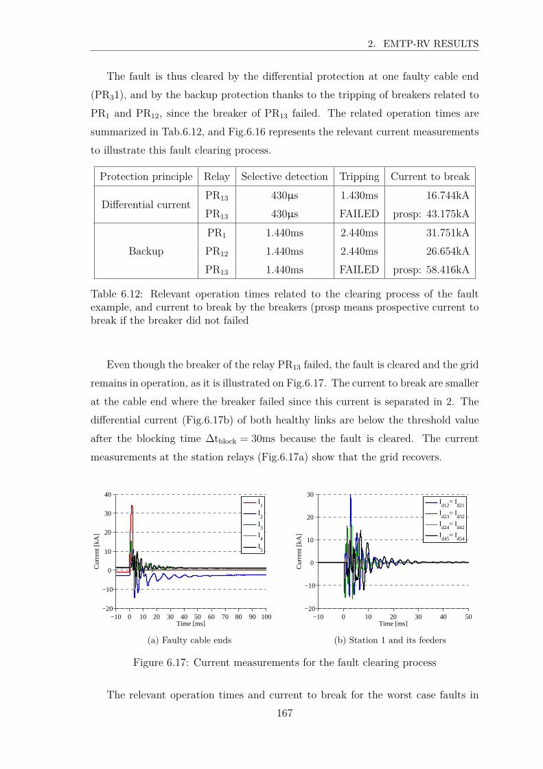
2. EMTP-RV RESULTS
The fault is thus cleared by the differential protection at one faulty cable end
(PR31), and by the backup protection thanks to the tripping of breakers related to
PR1 and PR12, since the breaker of PR13 failed. The related operation times are
summarized in Tab.6.12, and Fig.6.16 represents the relevant current measurements
to illustrate this fault clearing process.
Protection principle Relay Selective detection Tripping Current to break
Differential currentPR13 430µs 1.430ms 16.744kA
PR13 430µs FAILED prosp: 43.175kA
Backup
PR1 1.440ms 2.440ms 31.751kA
PR12 1.440ms 2.440ms 26.654kA
PR13 1.440ms FAILED prosp: 58.416kA
Table 6.12: Relevant operation times related to the clearing process of the faultexample, and current to break by the breakers (prosp means prospective current tobreak if the breaker did not failed
Even though the breaker of the relay PR13 failed, the fault is cleared and the grid
remains in operation, as it is illustrated on Fig.6.17. The current to break are smaller
at the cable end where the breaker failed since this current is separated in 2. The
differential current (Fig.6.17b) of both healthy links are below the threshold value
after the blocking time ∆tblock = 30ms because the fault is cleared. The current
measurements at the station relays (Fig.6.17a) show that the grid recovers.
−10 0 10 20 30 40 50 60 70 80 90 100−20
−10
0
10
20
30
40
Time [ms]
Cur
rent
[kA
]
I1
I2
I3
I4
I5
(a) Faulty cable ends
−10 0 10 20 30 40 50−20
−10
0
10
20
30
Time [ms]
Cur
rent
[kA
]
Id12
= Id21
Id23
= Id32
Id24
= Id42
Id45
= Id54
(b) Station 1 and its feeders
Figure 6.17: Current measurements for the fault clearing process
The relevant operation times and current to break for the worst case faults in
167
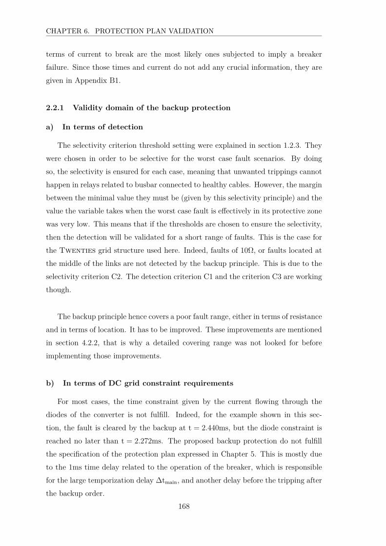
CHAPTER 6. PROTECTION PLAN VALIDATION
terms of current to break are the most likely ones subjected to imply a breaker
failure. Since those times and current do not add any crucial information, they are
given in Appendix B1.
2.2.1 Validity domain of the backup protection
a) In terms of detection
The selectivity criterion threshold setting were explained in section 1.2.3. They
were chosen in order to be selective for the worst case fault scenarios. By doing
so, the selectivity is ensured for each case, meaning that unwanted trippings cannot
happen in relays related to busbar connected to healthy cables. However, the margin
between the minimal value they must be (given by this selectivity principle) and the
value the variable takes when the worst case fault is effectively in its protective zone
was very low. This means that if the thresholds are chosen to ensure the selectivity,
then the detection will be validated for a short range of faults. This is the case for
the Twenties grid structure used here. Indeed, faults of 10Ω, or faults located at
the middle of the links are not detected by the backup principle. This is due to the
selectivity criterion C2. The detection criterion C1 and the criterion C3 are working
though.
The backup principle hence covers a poor fault range, either in terms of resistance
and in terms of location. It has to be improved. These improvements are mentioned
in section 4.2.2, that is why a detailed covering range was not looked for before
implementing those improvements.
b) In terms of DC grid constraint requirements
For most cases, the time constraint given by the current flowing through the
diodes of the converter is not fulfill. Indeed, for the example shown in this sec-
tion, the fault is cleared by the backup at t = 2.440ms, but the diode constraint is
reached no later than t = 2.272ms. The proposed backup protection do not fulfill
the specification of the protection plan expressed in Chapter 5. This is mostly due
to the 1ms time delay related to the operation of the breaker, which is responsible
for the large temporization delay ∆tmain, and another delay before the tripping after
the backup order.
168
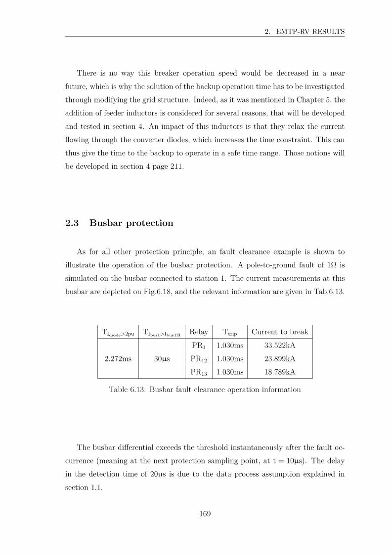
2. EMTP-RV RESULTS
There is no way this breaker operation speed would be decreased in a near
future, which is why the solution of the backup operation time has to be investigated
through modifying the grid structure. Indeed, as it was mentioned in Chapter 5, the
addition of feeder inductors is considered for several reasons, that will be developed
and tested in section 4. An impact of this inductors is that they relax the current
flowing through the converter diodes, which increases the time constraint. This can
thus give the time to the backup to operate in a safe time range. Those notions will
be developed in section 4 page 211.
2.3 Busbar protection
As for all other protection principle, an fault clearance example is shown to
illustrate the operation of the busbar protection. A pole-to-ground fault of 1Ω is
simulated on the busbar connected to station 1. The current measurements at this
busbar are depicted on Fig.6.18, and the relevant information are given in Tab.6.13.
TIdiode>2pu TIbus1>IbusTHRelay Ttrip Current to break
2.272ms 30µs
PR1 1.030ms 33.522kA
PR12 1.030ms 23.899kA
PR13 1.030ms 18.789kA
Table 6.13: Busbar fault clearance operation information
The busbar differential exceeds the threshold instantaneously after the fault oc-
currence (meaning at the next protection sampling point, at t = 10µs). The delay
in the detection time of 20µs is due to the data process assumption explained in
section 1.1.
169
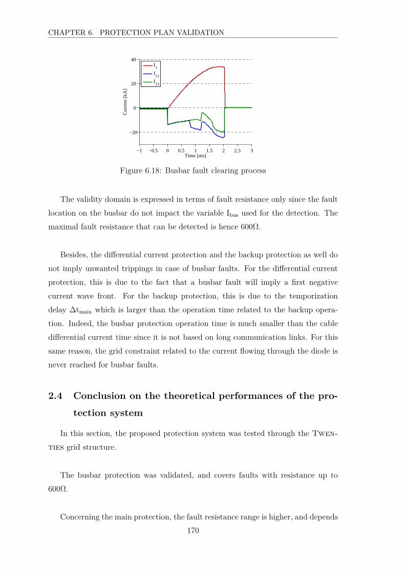
CHAPTER 6. PROTECTION PLAN VALIDATION
−1 −0.5 0 0.5 1 1.5 2 2.5 3
−20
0
20
40
Time [ms]
Cur
rent
[kA
]
I1
I12
I13
Figure 6.18: Busbar fault clearing process
The validity domain is expressed in terms of fault resistance only since the fault
location on the busbar do not impact the variable Ibus used for the detection. The
maximal fault resistance that can be detected is hence 600Ω.
Besides, the differential current protection and the backup protection as well do
not imply unwanted trippings in case of busbar faults. For the differential current
protection, this is due to the fact that a busbar fault will imply a first negative
current wave front. For the backup protection, this is due to the temporization
delay ∆tmain which is larger than the operation time related to the backup opera-
tion. Indeed, the busbar protection operation time is much smaller than the cable
differential current time since it is not based on long communication links. For this
same reason, the grid constraint related to the current flowing through the diode is
never reached for busbar faults.
2.4 Conclusion on the theoretical performances of the pro-
tection system
In this section, the proposed protection system was tested through the Twen-
ties grid structure.
The busbar protection was validated, and covers faults with resistance up to
600Ω.
Concerning the main protection, the fault resistance range is higher, and depends
170

2. EMTP-RV RESULTS
on the cable length. Note that for those two principles, the fault resistance covering
range is largely acceptable since the experience feedback of TSO’s points out that
faults with a resistance higher than 200Ω are extremely rare in underground cables.
While the time constraint related to the current flowing through the diodes is
never reached for faults occurring on busbars, it is exceeded for some faults in Link5.
This is due to the 1ms delay related to the data communication through the optical
fiber. The simulations points out that using this grid structure, a maximal allowed
cable length of 150km is required to ensure the protection plan specification.
The main concern highlighted by those simulations is the dramatically huge cur-
rents to be broken by the DC breakers. Indeed, the DC breakers are still under
prototyping process, and they do not have this kind of huge current breaking capa-
bility. Some solutions hence need to be found to decrease these large values, and
the best one that was found was to add inductors at each feeder relay. This will be
the topic of section 4
These modifications in the grid structure will also improve the backup protec-
tion, which has a poor validity domain. The improvements will be either on its fault
detection range and on the compatibility with the DC grid constraint.
Before going through those grid modification, the validation of the whole pro-
tection chain on a real-time mock-up will be presented in the next section. This
demonstrator is the Twenties DEMO 3 demonstrator, mentioned in the introduc-
tion of this manuscript.
171
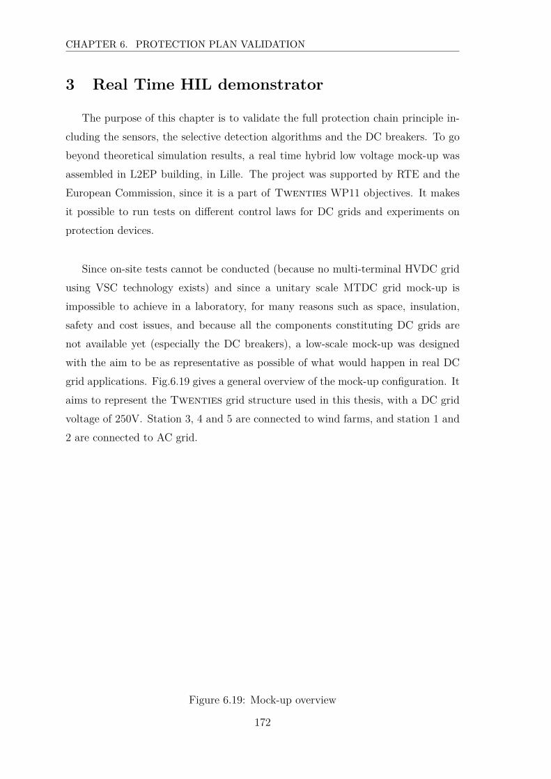
CHAPTER 6. PROTECTION PLAN VALIDATION
3 Real Time HIL demonstrator
The purpose of this chapter is to validate the full protection chain principle in-
cluding the sensors, the selective detection algorithms and the DC breakers. To go
beyond theoretical simulation results, a real time hybrid low voltage mock-up was
assembled in L2EP building, in Lille. The project was supported by RTE and the
European Commission, since it is a part of Twenties WP11 objectives. It makes
it possible to run tests on different control laws for DC grids and experiments on
protection devices.
Since on-site tests cannot be conducted (because no multi-terminal HVDC grid
using VSC technology exists) and since a unitary scale MTDC grid mock-up is
impossible to achieve in a laboratory, for many reasons such as space, insulation,
safety and cost issues, and because all the components constituting DC grids are
not available yet (especially the DC breakers), a low-scale mock-up was designed
with the aim to be as representative as possible of what would happen in real DC
grid applications. Fig.6.19 gives a general overview of the mock-up configuration. It
aims to represent the Twenties grid structure used in this thesis, with a DC grid
voltage of 250V. Station 3, 4 and 5 are connected to wind farms, and station 1 and
2 are connected to AC grid.
Figure 6.19: Mock-up overview
172

3. REAL TIME HIL DEMONSTRATOR
3.1 Overall mock-up design and description
The organization of the mock up is explained on Fig.6.20. Two main parts can
be highlighted:
• Devices that are actually physical
• Devices that are real-time simulated (in the blue form)
Figure 6.20: Mock-up configuration
The interface between the real-time simulator and the physical devices is achieved
thanks to high bandwidth amplifiers.
Two out of the five VSC are actual converters, and are connected to the AC
grid or offshore wind farms thanks to a power amplifier configured as a three-phase
amplifier.The three other VSC are real-time simulated.
The control of the mock-up (converter engagement, control type, power reference,
fault creation) is done thanks to a SCADA system.
173
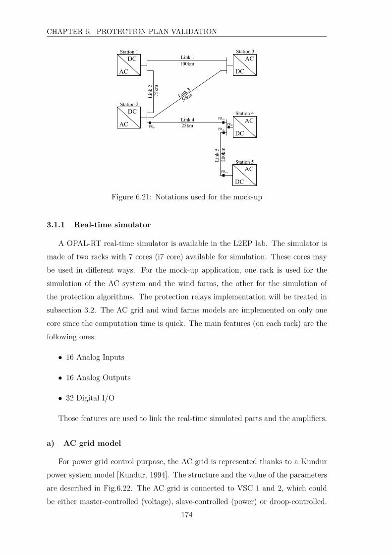
CHAPTER 6. PROTECTION PLAN VALIDATION
AC
DC AC
DC100kmLink 1
Station 1
AC
DCStation 2
25kmLink 4 AC
DC
AC
DC
Station 3
Station 4
Station 575
km
200k
m
Link
2
Link
5
Link 3
50km
PR42
PR41
PR45PR24
PR54
Figure 6.21: Notations used for the mock-up
3.1.1 Real-time simulator
A OPAL-RT real-time simulator is available in the L2EP lab. The simulator is
made of two racks with 7 cores (i7 core) available for simulation. These cores may
be used in different ways. For the mock-up application, one rack is used for the
simulation of the AC system and the wind farms, the other for the simulation of
the protection algorithms. The protection relays implementation will be treated in
subsection 3.2. The AC grid and wind farms models are implemented on only one
core since the computation time is quick. The main features (on each rack) are the
following ones:
• 16 Analog Inputs
• 16 Analog Outputs
• 32 Digital I/O
Those features are used to link the real-time simulated parts and the amplifiers.
a) AC grid model
For power grid control purpose, the AC grid is represented thanks to a Kundur
power system model [Kundur, 1994]. The structure and the value of the parameters
are described in Fig.6.22. The AC grid is connected to VSC 1 and 2, which could
be either master-controlled (voltage), slave-controlled (power) or droop-controlled.
174
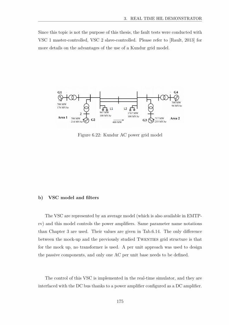
3. REAL TIME HIL DEMONSTRATOR
Since this topic is not the purpose of this thesis, the fault tests were conducted with
VSC 1 master-controlled, VSC 2 slave-controlled. Please refer to [Rault, 2013] for
more details on the advantages of the use of a Kundur grid model.
Area 1 Area 2700 MW214 MVAr
G2
G1
G3
G4
700 MW94 MVAr
967 MW100 MVAr
1767 MW100 MVAr
400 MW
700 MW176 MVAr
717 MW255 MVAr
Figure 6.22: Kundur AC power grid model
b) VSC model and filters
The VSC are represented by an average model (which is also available in EMTP-
rv) and this model controls the power amplifiers. Same parameter name notations
than Chapter 3 are used. Their values are given in Tab.6.14. The only difference
between the mock-up and the previously studied Twenties grid structure is that
for the mock up, no transformer is used. A per unit approach was used to design
the passive components, and only one AC per unit base needs to be defined.
The control of this VSC is implemented in the real-time simulator, and they are
interfaced with the DC bus thanks to a power amplifier configured as a DC amplifier.
175
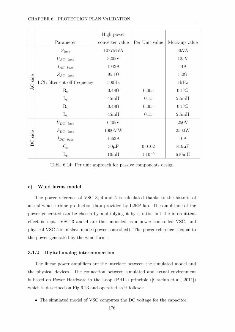
CHAPTER 6. PROTECTION PLAN VALIDATION
High power
Parameter converter value Per Unit value Mock-up value
AC
side
Sbase 1077MVA 3kVA
UAC−base 320kV 125V
IAC−base 1943A 14A
ZAC−base 95.1Ω 5.2Ω
LCL filter cut-off frequency 500Hz 1kHz
Rs 0.48Ω 0.005 0.17Ω
Ls 45mH 0.15 2.5mH
Rt 0.48Ω 0.005 0.17Ω
Lt 45mH 0.15 2.5mH
DC
side
UDC−base 640kV 250V
PDC−base 1000MW 2500W
IDC−base 1563A 10A
Cs 50µF 0.0102 819µF
Ls 10mH 1.10−5 610mH
Table 6.14: Per unit approach for passive components design
c) Wind farms model
The power reference of VSC 3, 4 and 5 is calculated thanks to the historic of
actual wind turbine production data provided by L2EP lab. The amplitude of the
power generated can be chosen by multiplying it by a ratio, but the intermittent
effect is kept. VSC 3 and 4 are thus modeled as a power controlled VSC, and
physical VSC 5 is in slave mode (power-controlled). The power reference is equal to
the power generated by the wind farms.
3.1.2 Digital-analog interconnection
The linear power amplifiers are the interface between the simulated model and
the physical devices. The connection between simulated and actual environment
is based on Power Hardware in the Loop (PHIL) principle ([Craciun et al., 2011])
which is described on Fig.6.23 and operated as it follows:
• The simulated model of VSC computes the DC voltage for the capacitor.
176
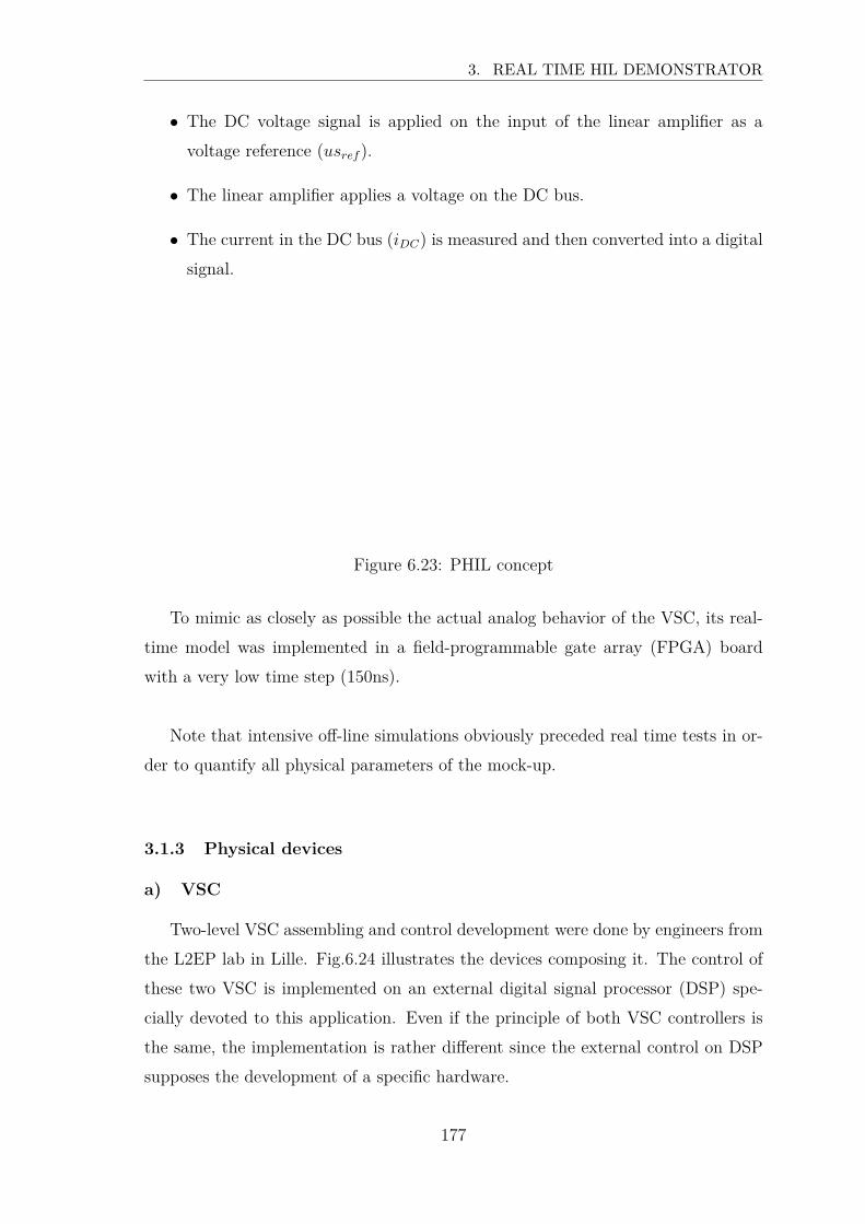
3. REAL TIME HIL DEMONSTRATOR
• The DC voltage signal is applied on the input of the linear amplifier as a
voltage reference (usref ).
• The linear amplifier applies a voltage on the DC bus.
• The current in the DC bus (iDC) is measured and then converted into a digital
signal.
Figure 6.23: PHIL concept
To mimic as closely as possible the actual analog behavior of the VSC, its real-
time model was implemented in a field-programmable gate array (FPGA) board
with a very low time step (150ns).
Note that intensive off-line simulations obviously preceded real time tests in or-
der to quantify all physical parameters of the mock-up.
3.1.3 Physical devices
a) VSC
Two-level VSC assembling and control development were done by engineers from
the L2EP lab in Lille. Fig.6.24 illustrates the devices composing it. The control of
these two VSC is implemented on an external digital signal processor (DSP) spe-
cially devoted to this application. Even if the principle of both VSC controllers is
the same, the implementation is rather different since the external control on DSP
supposes the development of a specific hardware.
177
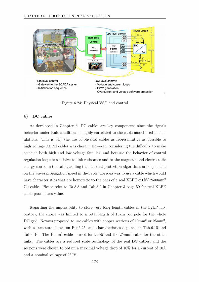
CHAPTER 6. PROTECTION PLAN VALIDATION
Low level control: - Voltage and current loops - PWM generation - Overcurrent and voltage software protection
High level control: - Gateway to the SCADA system - Initialization sequence
Figure 6.24: Physical VSC and control
b) DC cables
As developed in Chapter 3, DC cables are key components since the signals
behavior under fault conditions is highly correlated to the cable model used in sim-
ulations. This is why the use of physical cables as representative as possible to
high voltage XLPE cables was chosen. However, considering the difficulty to make
coincide both high and low voltage families, and because the behavior of control
regulation loops is sensitive to link resistance and to the magnetic and electrostatic
energy stored in the cable, adding the fact that protection algorithms are dependent
on the waves propagation speed in the cable, the idea was to use a cable which would
have characteristics that are homotetic to the ones of a real XLPE 320kV 2500mm2
Cu cable. Please refer to Ta.3.3 and Tab.3.2 in Chapter 3 page 59 for real XLPE
cable parameters value.
Regarding the impossibility to store very long length cables in the L2EP lab-
oratory, the choice was limited to a total length of 15km per pole for the whole
DC grid. Nexans proposed to use cables with copper sections of 10mm2 or 25mm2,
with a structure shown on Fig.6.25, and characteristics depicted in Tab.6.15 and
Tab.6.16. The 10mm2 cable is used for Link5 and the 25mm2 cable for the other
links. The cables are a reduced scale technology of the real DC cables, and the
sections were chosen to obtain a maximal voltage drop of 10% for a current of 10A
and a nominal voltage of 250V.
178

3. REAL TIME HIL DEMONSTRATOR
Insulation XLPE
Core
Screen
Outer sheath
Figure 6.25: Nexans cable structure
10mm2 Nexans cable
Conductor Core Screen
rint [mm] 0 2.55
rout [mm] 1.85 2.72
rext insulation [mm] 4.3
25mm2 Nexans cable
Conductor Core Screen
rint [mm] 0 3.05
rout [mm] 3.95 4.10
rext insulation [mm] 5.8
Table 6.15: Nexans cable geometrical properties
Cable section ρc ǫiL’[mH/m] C’[µF/m]
10mm2 1.72e−8 2.3 4.8e−1 3.22e−4
25mm2 1.72e−8 2.3 3.79e−2 4.15e−4
Table 6.16: Nexans cable dielectric properties
Assuming that, the DC cable configuration in the mock-up is given on Tab.6.17.
Link Number of drums per pole Drum length [m] Total cable length [km]
Link1 10 227 2.270
Link2 8 227 1.816
Link3 5 227 1.135
Link4 2 227 0.454
Link5 9 161 1.449
Table 6.17: DC cable configuration on the mock-up
This kind of cable has the same propagation speed than the real high power
DC cables. However as the total length is smaller, the propagation time has to
179

CHAPTER 6. PROTECTION PLAN VALIDATION
be increased. The idea was to keep cable on their cable drums to increase their
linear inductance and thus the propagation time (tpropa =√
LC). As illustrated on
Fig.6.26, the cables were installed on their cable drums, and they were connected to
each other with shielded junction box.
Figure 6.26: Nexans cable on their drums
In this configuration, the linear inductance and capacitance for each cable was
measured and new propagation speeds were calculated. Tab.6.18 summarizes the
characteristics. Note that the parameters identification were done at a frequency of
1kHz.
Cable number R′[Ω/km] L′[mH/km] C′[µF/km] Mock-up cable tpropa[µs]
Link1 0.6806 38.106 0.409 285
Link2 0.6806 38.106 0.409 228
Link3 0.6806 38.106 0.409 142
Link4 0.6806 38.106 0.409 57
Link5 1.6977 40.511 0.320 570
Table 6.18: DC cables on their drums parameters identification
3.2 Protection system components
Each protection relay is composed of a voltage and a current sensors, a DC
breaker and is organized as shown on Fig.6.27.
Protections implementation will be described in subsection 3.2.3, but the breaker
state of one feeder or one station connection point is the same for both positive
180

3. REAL TIME HIL DEMONSTRATOR
DC breaker Currentsensor
+125V
VSC side DC cable side
DC breaker Currentsensor
-125V
Voltagesensor
Breaker state
Figure 6.27: Protection relay organization
and negative poles, because they are controlled by the same protection algorithm.
Indeed, only pole-to-pole fault will be generated so there is no need to implement the
selectivity regarding the faulty pole. The breaker control will be detailed further.
3.2.1 Protection-related physical devices
a) DC breaker
DC breaker devices, that are associated to protection relays and to the fault
generator device, are composed of IGBT and diodes in order to create a 4 quad-
rants switch (Fig.6.28). They are associated with surge arresters (placed at each
IGBT terminals) so the overvoltages created during the current breaking process
are limited. The surge arrester is a varistor with characteristics given in Tab.6.19.
Figure 6.28: DC breaker device
181
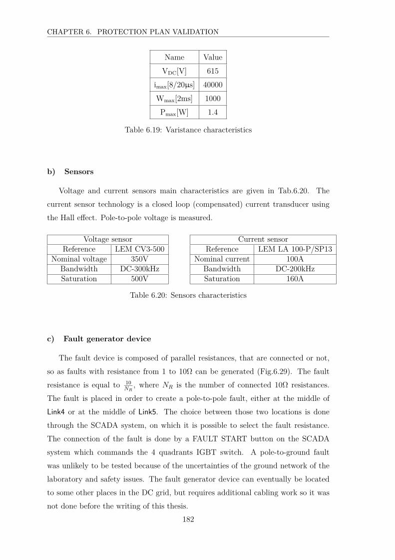
CHAPTER 6. PROTECTION PLAN VALIDATION
Name Value
VDC[V] 615
imax[8/20µs] 40000
Wmax[2ms] 1000
Pmax[W] 1.4
Table 6.19: Varistance characteristics
b) Sensors
Voltage and current sensors main characteristics are given in Tab.6.20. The
current sensor technology is a closed loop (compensated) current transducer using
the Hall effect. Pole-to-pole voltage is measured.
Voltage sensorReference LEM CV3-500
Nominal voltage 350VBandwidth DC-300kHzSaturation 500V
Current sensorReference LEM LA 100-P/SP13
Nominal current 100ABandwidth DC-200kHzSaturation 160A
Table 6.20: Sensors characteristics
c) Fault generator device
The fault device is composed of parallel resistances, that are connected or not,
so as faults with resistance from 1 to 10Ω can be generated (Fig.6.29). The fault
resistance is equal to 10NR
, where NR is the number of connected 10Ω resistances.
The fault is placed in order to create a pole-to-pole fault, either at the middle of
Link4 or at the middle of Link5. The choice between those two locations is done
through the SCADA system, on which it is possible to select the fault resistance.
The connection of the fault is done by a FAULT START button on the SCADA
system which commands the 4 quadrants IGBT switch. A pole-to-ground fault
was unlikely to be tested because of the uncertainties of the ground network of the
laboratory and safety issues. The fault generator device can eventually be located
to some other places in the DC grid, but requires additional cabling work so it was
not done before the writing of this thesis.
182

3. REAL TIME HIL DEMONSTRATOR
Pole -
Pole +
10Ω 10Ω
MODBUSTCP/IP
SCADA
PLC
10Ω 10Ω 10Ω 10Ω 10Ω 10Ω 10Ω 10Ω
Figure 6.29: Fault generator device
3.2.2 Physical devices positioning
Due to cost issues, only 10 breakers could be bought and their location on the
mock-up is displayed on Fig.6.20 page 173, where only the positive pole is repre-
sented, but the two poles are equally equipped. Each breaker is associated with a
current and a voltage sensor, as illustrated on Fig.6.27 page 181. The voltage sensor
however is not used for protection purposes.
This implementation was used for the first test series, and was then modified in
order to conduct other tests that will be explained in subsection 3.4.
3.2.3 Protection relays implementation
a) Tested protection principles
The protection algorithms related to the following principles are implemented
on the mock-up.
• Cable differential protection
• Busbar protection
• Backup
Indeed, the protection using the voltage measurement between the feeders induc-
tance terminals cannot be implemented since those inductances were not placed on
183

CHAPTER 6. PROTECTION PLAN VALIDATION
the mock-up. This is due to the fact that this protection algorithm was investigated
only after the mock-up development.
A protection relay is associated with each breaker located on the positive pole,
and controls the breakers of both positive and negative pole. As mentioned in 3.1.1,
the protection principles are real-time simulated in a totally independent simulator,
with a frequency sampling of 100kHz. The inputs are the current measurements
provided by the sensors, and the outputs are the breaker states.
Giving this configuration, the cable differential protection are implemented in
each relay they can be, meaning only at PR24, PR42, PR45 and PR54. Note that
PR54 and PR5 that have been defined in the previous parts of this chapter are here
the same protection, since no component is placed between them. This protection
is named PR5 for the mock-up study. Busbar protection is implemented at PR4.
Only the busbars connected to station 4 and station 5 are equipped with backup
protection, since station 2 is not equipped with enough breaker and sensors. How-
ever, since station 4 is not composed of a physical converter, the current shape I4
under fault conditions does not correspond to what it would be in real applications.
Indeed, I4 remains constant, and makes it impossible to apply the backup protection
principle at this node. Protection algorithms related to each relay are implemented,
as shown on Fig.6.30, which represents the model which is real-time simulated.
184

3. REAL TIME HIL DEMONSTRATOR
PR24
PR42
PR45
PR54
PRs4
Cable differential
Busbar differential
Backup
Cable differential
Cable differential
Cable differential
I24
I42
I45
I54
Is4
CB24
CB42
CB45
CB54
CBs4
CAN CNA
AN
ALO
G IN
PU
TS: C
UR
RE
NT
ME
AS
UR
EM
EN
TS
AN
ALO
G O
UTP
UTS
: BR
EA
KE
R S
TATE
S
Figure 6.30: Protection relays implementation
b) Other information related to the algorithms
For the cable differential protection, the optical fiber link is modeled using a delay
corresponding to the propagation time of the data (200km/ms). The considered
length is the one of the grid that was aimed to be represented by the mock-up, and
not the real cable length, meaning 25, 50, 75, 100 and 200km. The numerical values
for those delays are the same than the one used in the EMTP-rv study in section 1,
and are reminded in Tab.6.21. The time delays are approximated to the upper value
in order to fit the sampling frequency of the simulation. The different protection
algorithms are not reminded here, as they are described in Chapter 5.
Link number Length [km] Propagation time [µs] Simulation delay [µs]
Link1 100 500 500
Link2 75 375 380
Link3 50 250 250
Link4 25 125 130
Link5 200 1000 1000
Table 6.21: Data propagation delay in the optical fiber
185
CHAPTER 6. PROTECTION PLAN VALIDATION
The backup is implemented using the same variable for the detection and the
selectivity criterion. These variables, used by the backup protection algorithm as
explained in 1, are named Gid and Gi
s, where i corresponds to the station number
connected to the concerned busbar. It is evaluated thanks to equation (6.9).
Gid = Gi
s = |Ii (t) − Ii (t − 20ms)| (6.9)
c) Threshold scaling
The mock-up purpose was to represent the behavior of a DC grid as close as
possible to what it would be in real application. Even though, it cannot pretend to
behave exactly the same way with a scaling factor, for several reasons such as the
fact that some of the converters are not physical, or because the cables drummed.
As a scaling process cannot be done to define the threshold applied on the protec-
tion algorithms, they were adjusted thanks to EMTP-rv simulations of the mock-up.
The model uses CP cable models, and will be described further in 3.4.5.
The effects to be observed on the mock-up are the transient behavior in the
signals and the protection relays functioning (selective detection, no unwanted trip-
pings). This is to highlight the fact that the threshold values (as long as they allow
a selective detection) are not very important here, since they will only affect the
operation time related to ∆tdetect, which was defined in 2. Indeed, the effect of the
reduction or increase of the threshold values is known, and can be assessed thanks
to the results with a given threshold value. The numerical values will be given at
the beginning each paragraph related to a test series, since they are set for the whole
series and do not change.
d) Signal processing chain
The real-time simulated protection plan and its interactions with the mock-up
are illustrated on Fig.6.31. For clarity of illustration purposes, only the main cable
differential protection is represented on the scheme.
186
3. REAL TIME HIL DEMONSTRATOR
Figure 6.31: Protection interactions
3.3 Demonstrator control
The mock-up is controlled thanks to a SCADA system (Fig.6.32). It enables to
control manually the connection of the VSC, the power references, and the creation
of a fault. The protection plan can also be controlled by the console related to the
simulator. It is possible to activate, disactivate a protection relay, or to simulate a
breaker failure by forcing the breaker state to a 0 constant value.
Figure 6.32: SCADA system to control the mock-up
3.4 Real Time HIL tests results
The tests regarding DC faults and protections plan validation are presented in
this subsection. Other tests related to substation control had been conducted, such
187

CHAPTER 6. PROTECTION PLAN VALIDATION
as power dispatch identification, drop control dynamics observation, on so on. About
this topic, please refer to [Rault, 2013] and deliverable twenties 11.3 for details about
configurations and conclusions.
3.4.1 Tests description
As said earlier in this chapter, the cable differential protection and the backup
protection have been tested through several tests that will be presented further. One
test series was done on the Twenties grid DEMO3 implementation presented ear-
lier in the current section, and a second test series has been conducted for another
configuration of the mock-up. A complete list of the tests that have been conducted
on the mock-up can be found in appendix B2. Only the relevant cases will be ad-
dressed in this subsection.
3.4.2 Test series 1 results
Three of the tests that were conducted on the Twenties configuration are high-
lighted here. They are described in Tab.B.3. The notations used are the same as in
Fig.6.21.
Test Faulty link Rfault VSC 2 VSC 5 Operation point Comments
T1 Link5 5Ω – Ph VSC5 +100W —
T2 Link4 10Ω Ph Ph VSC5 +300W —
T3 Link5 5Ω – Ph VSC5 +100W Cable differen-
tial protection
disconnected at
PR54
Table 6.22: Test series 1 description, Ph: physical VSC, –: not connected, +100W:injects 100W to the DC grid
The threshold values set for this test series is given in Tab.6.23.
188
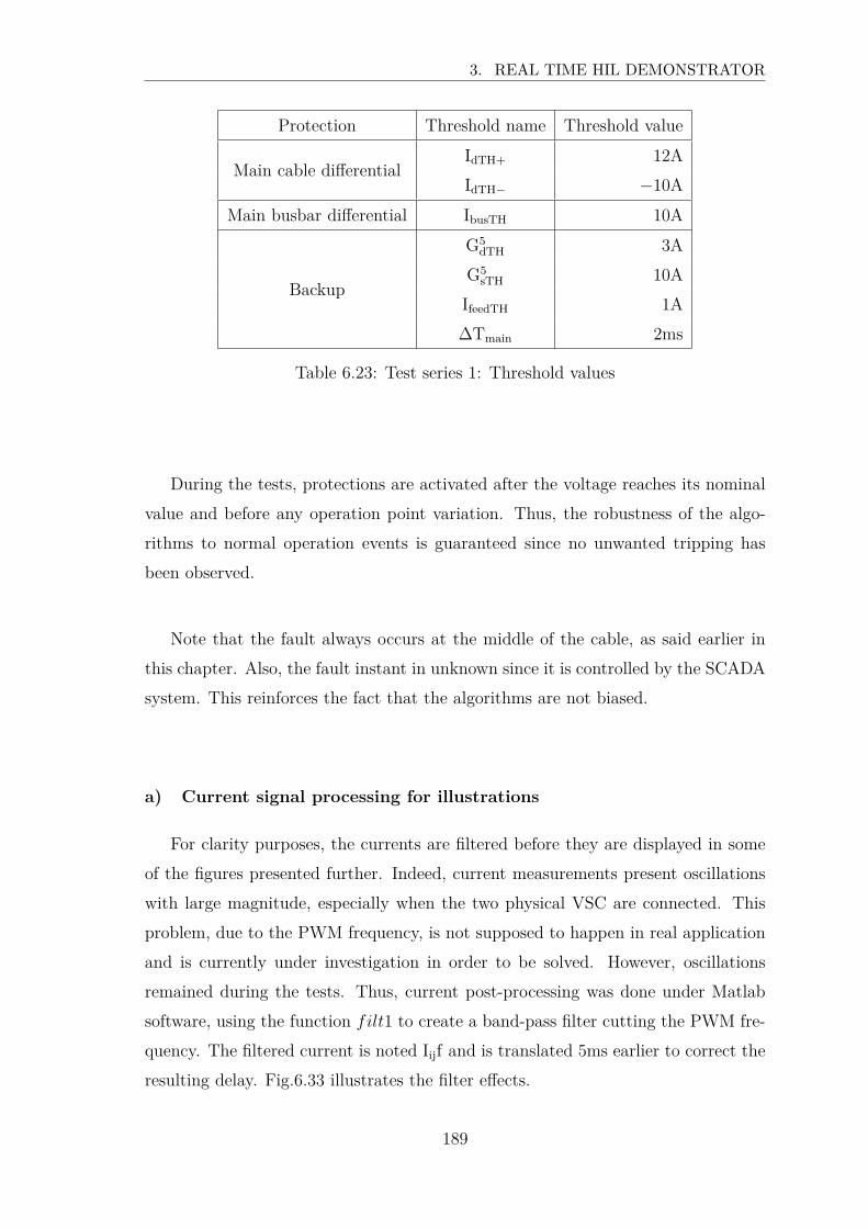
3. REAL TIME HIL DEMONSTRATOR
Protection Threshold name Threshold value
Main cable differentialIdTH+ 12A
IdTH− −10A
Main busbar differential IbusTH 10A
Backup
G5dTH 3A
G5sTH 10A
IfeedTH 1A
∆Tmain 2ms
Table 6.23: Test series 1: Threshold values
During the tests, protections are activated after the voltage reaches its nominal
value and before any operation point variation. Thus, the robustness of the algo-
rithms to normal operation events is guaranteed since no unwanted tripping has
been observed.
Note that the fault always occurs at the middle of the cable, as said earlier in
this chapter. Also, the fault instant in unknown since it is controlled by the SCADA
system. This reinforces the fact that the algorithms are not biased.
a) Current signal processing for illustrations
For clarity purposes, the currents are filtered before they are displayed in some
of the figures presented further. Indeed, current measurements present oscillations
with large magnitude, especially when the two physical VSC are connected. This
problem, due to the PWM frequency, is not supposed to happen in real application
and is currently under investigation in order to be solved. However, oscillations
remained during the tests. Thus, current post-processing was done under Matlab
software, using the function filt1 to create a band-pass filter cutting the PWM fre-
quency. The filtered current is noted Iijf and is translated 5ms earlier to correct the
resulting delay. Fig.6.33 illustrates the filter effects.
189
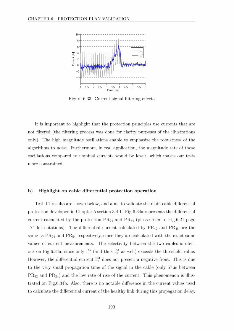
CHAPTER 6. PROTECTION PLAN VALIDATION
1 1.5 2 2.5 3 3.5 4 4.5 5 5.5 6
−4
−2
0
2
4
6
8
10
Time [ms]
Cur
rent
[A]
I24
I24
f
Figure 6.33: Current signal filtering effects
It is important to highlight that the protection principles use currents that are
not filtered (the filtering process was done for clarity purposes of the illustrations
only). The high magnitude oscillations enable to emphasize the robustness of the
algorithms to noise. Furthermore, in real application, the magnitude rate of those
oscillations compared to nominal currents would be lower, which makes our tests
more constrained.
b) Highlight on cable differential protection operation
Test T1 results are shown below, and aims to validate the main cable differential
protection developed in Chapter 5 section 3.4.1. Fig.6.34a represents the differential
current calculated by the protection PR24 and PR54 (please refer to Fig.6.21 page
174 for notations). The differential current calculated by PR42 and PR45 are the
same as PR24 and PR54 respectively, since they are calculated with the exact same
values of current measurements. The selectivity between the two cables is obvi-
ous on Fig.6.34a, since only I45d (and thus I54
d as well) exceeds the threshold value.
However, the differential current I24d does not present a negative front. This is due
to the very small propagation time of the signal in the cable (only 57µs between
PR42 and PR24) and the low rate of rise of the current. This phenomenon is illus-
trated on Fig.6.34b. Also, there is no notable difference in the current values used
to calculate the differential current of the healthy link during this propagation delay.
190
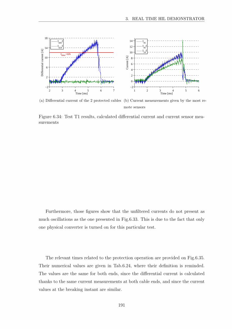
3. REAL TIME HIL DEMONSTRATOR
2 3 4 5 6 7−2
2
6
10
14
18
Time [ms]
Diff
eren
tial c
urre
nt [A
]
Id45
f
Id24
f
IdTH+
=12A
(a) Differential current of the 2 protected cables
1 2 3 4 5 6−2
0
2
4
6
8
10
12
14
Time [ms]
Cur
rent
[A]
I45
I45
f
I24
f
(b) Current measurements given by the most re-
mote sensors
Figure 6.34: Test T1 results, calculated differential current and current sensor mea-surements
Furthermore, those figures show that the unfiltered currents do not present as
much oscillations as the one presented in Fig.6.33. This is due to the fact that only
one physical converter is turned on for this particular test.
The relevant times related to the protection operation are provided on Fig.6.35.
Their numerical values are given in Tab.6.24, where their definition is reminded.
The values are the same for both ends, since the differential current is calculated
thanks to the same current measurements at both cable ends, and since the current
values at the breaking instant are similar.
191
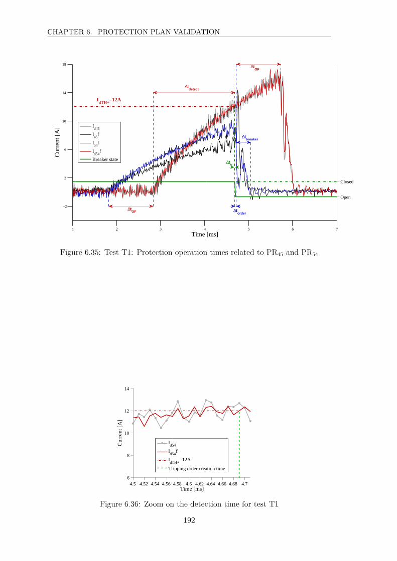
CHAPTER 6. PROTECTION PLAN VALIDATION
1 2 3 4 5 6 7
−2
2
6
10
14
18
Time [ms]
Cur
rent
[A]
1
Open
Closed
Id45
I45
f
I54
f
Id54
f
Breaker state
∆tOF
∆torder
∆tbreaker
IdTH+
=12A
∆tV
∆tOF
∆tdetect
Figure 6.35: Test T1: Protection operation times related to PR45 and PR54
4.5 4.52 4.54 4.56 4.58 4.6 4.62 4.64 4.66 4.68 4.76
8
10
12
14
Time [ms]
Cur
rent
[A]
Id54
Id54
f
IdTH+
=12A
Tripping order creation time
Figure 6.36: Zoom on the detection time for test T1
192
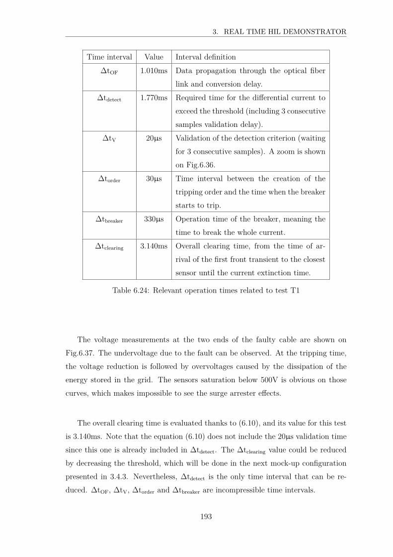
3. REAL TIME HIL DEMONSTRATOR
Time interval Value Interval definition
∆tOF 1.010ms Data propagation through the optical fiber
link and conversion delay.
∆tdetect 1.770ms Required time for the differential current to
exceed the threshold (including 3 consecutive
samples validation delay).
∆tV 20µs Validation of the detection criterion (waiting
for 3 consecutive samples). A zoom is shown
on Fig.6.36.
∆torder 30µs Time interval between the creation of the
tripping order and the time when the breaker
starts to trip.
∆tbreaker 330µs Operation time of the breaker, meaning the
time to break the whole current.
∆tclearing 3.140ms Overall clearing time, from the time of ar-
rival of the first front transient to the closest
sensor until the current extinction time.
Table 6.24: Relevant operation times related to test T1
The voltage measurements at the two ends of the faulty cable are shown on
Fig.6.37. The undervoltage due to the fault can be observed. At the tripping time,
the voltage reduction is followed by overvoltages caused by the dissipation of the
energy stored in the grid. The sensors saturation below 500V is obvious on those
curves, which makes impossible to see the surge arrester effects.
The overall clearing time is evaluated thanks to (6.10), and its value for this test
is 3.140ms. Note that the equation (6.10) does not include the 20µs validation time
since this one is already included in ∆tdetect. The ∆tclearing value could be reduced
by decreasing the threshold, which will be done in the next mock-up configuration
presented in 3.4.3. Nevertheless, ∆tdetect is the only time interval that can be re-
duced. ∆tOF, ∆tV, ∆torder and ∆tbreaker are incompressible time intervals.
193
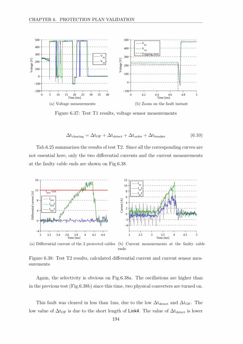
CHAPTER 6. PROTECTION PLAN VALIDATION
0 5 10 15 20 25 30 35 40−200
−100
0
100
200
300
400
500
Time [ms]
Vol
tage
[V]
V45
V54
(a) Voltage measurements
4 4.2 4.4 4.6 4.8 5−100
0
100
200
300
400
500
Time [ms]
Vol
tage
[V]
V45
V54
Tripping time
(b) Zoom on the fault instant
Figure 6.37: Test T1 results, voltage sensor measurements
∆tclearing = ∆tOF + ∆tdetect + ∆torder + ∆tbreaker (6.10)
Tab.6.25 summarizes the results of test T2. Since all the corresponding curves are
not essential here, only the two differential currents and the current measurements
at the faulty cable ends are shown on Fig.6.38.
3 3.2 3.4 3.6 3.8 4 4.2 4.4−4
0
4
8
12
16
Time [ms]
Diff
eren
tial c
urre
nt [A
]
Id24
Id24
f
Id45
f
IdTH+
=12A
(a) Differential current of the 2 protected cables
2 2.5 3 3.5 4 4.5 5
−4
−2
0
2
4
6
8
10
12
Time [ms]
Cur
rent
[A]
I24
I24
f
I42
f
(b) Current measurements at the faulty cableends
Figure 6.38: Test T2 results, calculated differential current and current sensor mea-surements
Again, the selectivity is obvious on Fig.6.38a. The oscillations are higher than
in the previous test (Fig.6.38b) since this time, two physical converters are turned on.
This fault was cleared in less than 1ms, due to the low ∆tdetect and ∆tOF. The
low value of ∆tOF is due to the short length of Link4. The value of ∆tdetect is lower
194
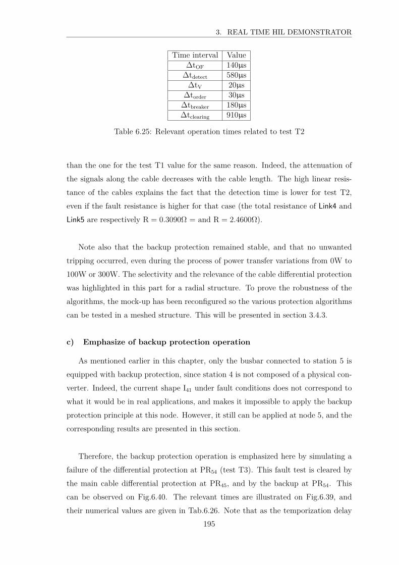
3. REAL TIME HIL DEMONSTRATOR
Time interval Value∆tOF 140µs
∆tdetect 580µs∆tV 20µs
∆torder 30µs∆tbreaker 180µs∆tclearing 910µs
Table 6.25: Relevant operation times related to test T2
than the one for the test T1 value for the same reason. Indeed, the attenuation of
the signals along the cable decreases with the cable length. The high linear resis-
tance of the cables explains the fact that the detection time is lower for test T2,
even if the fault resistance is higher for that case (the total resistance of Link4 and
Link5 are respectively R = 0.3090Ω = and R = 2.4600Ω).
Note also that the backup protection remained stable, and that no unwanted
tripping occurred, even during the process of power transfer variations from 0W to
100W or 300W. The selectivity and the relevance of the cable differential protection
was highlighted in this part for a radial structure. To prove the robustness of the
algorithms, the mock-up has been reconfigured so the various protection algorithms
can be tested in a meshed structure. This will be presented in section 3.4.3.
c) Emphasize of backup protection operation
As mentioned earlier in this chapter, only the busbar connected to station 5 is
equipped with backup protection, since station 4 is not composed of a physical con-
verter. Indeed, the current shape I41 under fault conditions does not correspond to
what it would be in real applications, and makes it impossible to apply the backup
protection principle at this node. However, it still can be applied at node 5, and the
corresponding results are presented in this section.
Therefore, the backup protection operation is emphasized here by simulating a
failure of the differential protection at PR54 (test T3). This fault test is cleared by
the main cable differential protection at PR45, and by the backup at PR54. This
can be observed on Fig.6.40. The relevant times are illustrated on Fig.6.39, and
their numerical values are given in Tab.6.26. Note that as the temporization delay
195
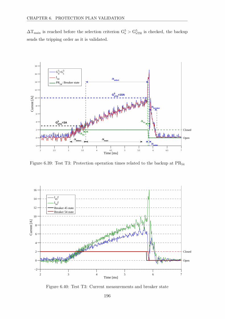
CHAPTER 6. PROTECTION PLAN VALIDATION
∆Tmain is reached before the selection criterion G5s > G5
sTH is checked, the backup
sends the tripping order as it is validated.
2 2.5 3 3.5 4 4.5 5 5.5 6 6.5 7
−2
0
2
4
6
8
10
12
14
16
18
Time [ms]
Cur
rent
[A]
Open
Closed
Gd5=G
s5
I54
PR54
: Breaker state
∆torder
∆tbreaker
GdTH5 =3A
GsTH5 =10A
∆tVs
∆tdetect
∆tmain
∆tselect
∆tVd
Figure 6.39: Test T3: Protection operation times related to the backup at PR54
2 3 4 5 6 7
−2
0
2
4
6
8
10
12
14
16
Time [ms]
Cur
rent
[A]
Open
Closed
I45
f
I54
f
Breaker 45 stateBreaker 54 state
Figure 6.40: Test T3: Current measurements and breaker state
196
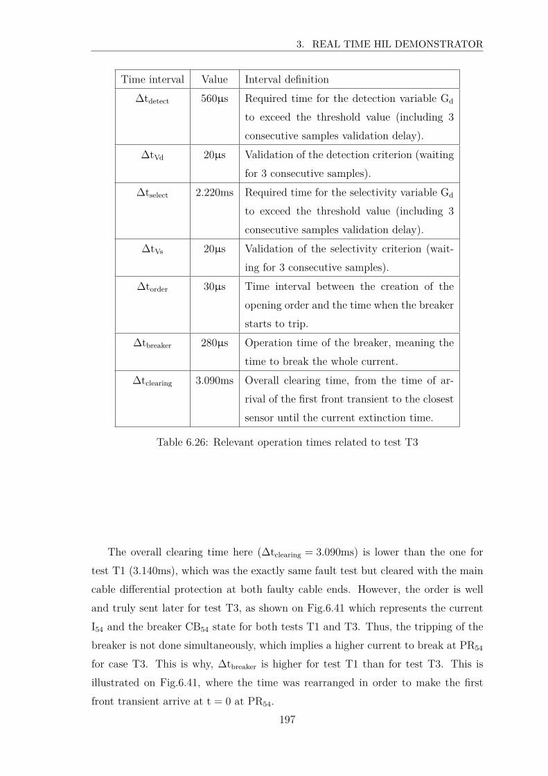
3. REAL TIME HIL DEMONSTRATOR
Time interval Value Interval definition
∆tdetect 560µs Required time for the detection variable Gd
to exceed the threshold value (including 3
consecutive samples validation delay).
∆tVd 20µs Validation of the detection criterion (waiting
for 3 consecutive samples).
∆tselect 2.220ms Required time for the selectivity variable Gd
to exceed the threshold value (including 3
consecutive samples validation delay).
∆tVs 20µs Validation of the selectivity criterion (wait-
ing for 3 consecutive samples).
∆torder 30µs Time interval between the creation of the
opening order and the time when the breaker
starts to trip.
∆tbreaker 280µs Operation time of the breaker, meaning the
time to break the whole current.
∆tclearing 3.090ms Overall clearing time, from the time of ar-
rival of the first front transient to the closest
sensor until the current extinction time.
Table 6.26: Relevant operation times related to test T3
The overall clearing time here (∆tclearing = 3.090ms) is lower than the one for
test T1 (3.140ms), which was the exactly same fault test but cleared with the main
cable differential protection at both faulty cable ends. However, the order is well
and truly sent later for test T3, as shown on Fig.6.41 which represents the current
I54 and the breaker CB54 state for both tests T1 and T3. Thus, the tripping of the
breaker is not done simultaneously, which implies a higher current to break at PR54
for case T3. This is why, ∆tbreaker is higher for test T1 than for test T3. This is
illustrated on Fig.6.41, where the time was rearranged in order to make the first
front transient arrive at t = 0 at PR54.
197
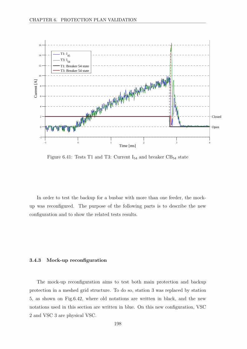
CHAPTER 6. PROTECTION PLAN VALIDATION
−1 0 1 2 3 4
−2
0
2
4
6
8
10
12
14
16
Time [ms]
Cur
rent
[A]
0 1
Open
Closed
T1: I45
T3: I54
T1: Breaker 54 stateT3: Breaker 54 state
Figure 6.41: Tests T1 and T3: Current I54 and breaker CB54 state
In order to test the backup for a busbar with more than one feeder, the mock-
up was reconfigured. The purpose of the following parts is to describe the new
configuration and to show the related tests results.
3.4.3 Mock-up reconfiguration
The mock-up reconfiguration aims to test both main protection and backup
protection in a meshed grid structure. To do so, station 3 was replaced by station
5, as shown on Fig.6.42, where old notations are written in black, and the new
notations used in this section are written in blue. On this new configuration, VSC
2 and VSC 3 are physical VSC.
198
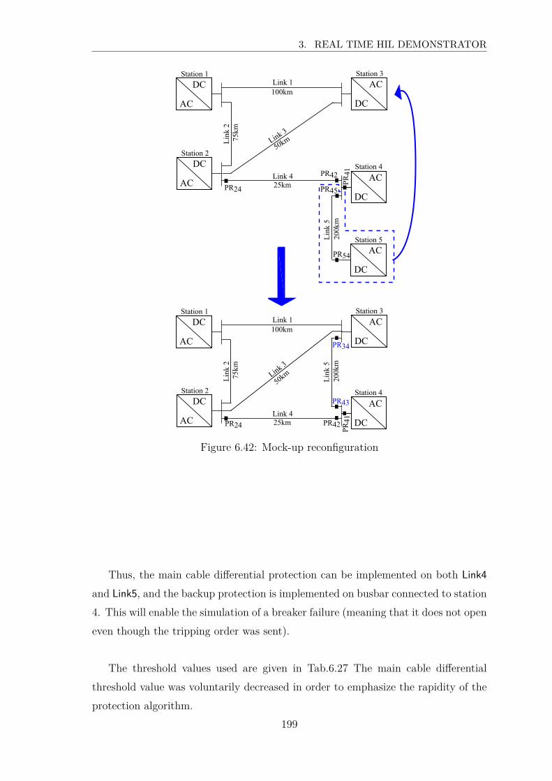
3. REAL TIME HIL DEMONSTRATOR
AC
DC AC
DC100kmLink 1
Station 1
AC
DCStation 2
25kmLink 4 AC
DC
AC
DC
Station 3
Station 4
Station 575
km
200k
m
Link
2
Link
5
Link 3
50km
PR42
PR41
PR45
PR54
AC
DC AC
DC100kmLink 1
Station 1
AC
DCStation 2
25kmLink 4
AC
DC
Station 3
Station 4
75km
200k
m
Link
2
Link
5
Link 3
50km
PR42
PR41
PR34
PR24
PR43
PR24
Figure 6.42: Mock-up reconfiguration
Thus, the main cable differential protection can be implemented on both Link4
and Link5, and the backup protection is implemented on busbar connected to station
4. This will enable the simulation of a breaker failure (meaning that it does not open
even though the tripping order was sent).
The threshold values used are given in Tab.6.27 The main cable differential
threshold value was voluntarily decreased in order to emphasize the rapidity of the
protection algorithm.
199
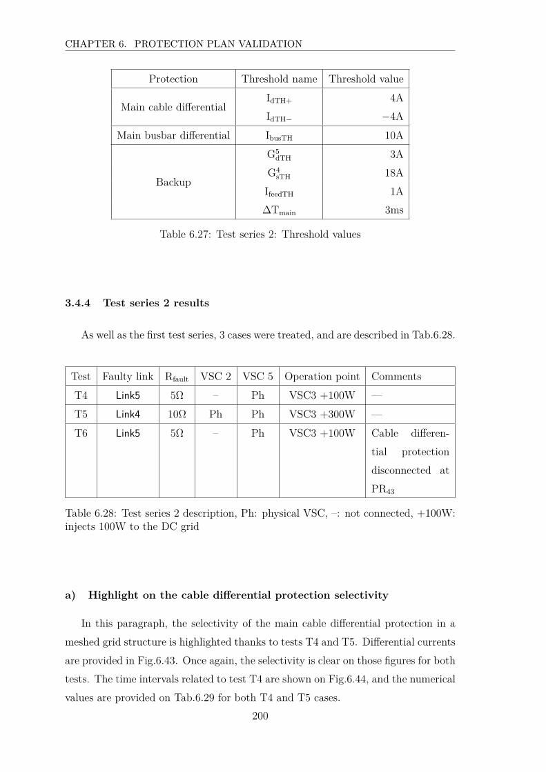
CHAPTER 6. PROTECTION PLAN VALIDATION
Protection Threshold name Threshold value
Main cable differentialIdTH+ 4A
IdTH− −4A
Main busbar differential IbusTH 10A
Backup
G5dTH 3A
G4sTH 18A
IfeedTH 1A
∆Tmain 3ms
Table 6.27: Test series 2: Threshold values
3.4.4 Test series 2 results
As well as the first test series, 3 cases were treated, and are described in Tab.6.28.
Test Faulty link Rfault VSC 2 VSC 5 Operation point Comments
T4 Link5 5Ω – Ph VSC3 +100W —
T5 Link4 10Ω Ph Ph VSC3 +300W —
T6 Link5 5Ω – Ph VSC3 +100W Cable differen-
tial protection
disconnected at
PR43
Table 6.28: Test series 2 description, Ph: physical VSC, –: not connected, +100W:injects 100W to the DC grid
a) Highlight on the cable differential protection selectivity
In this paragraph, the selectivity of the main cable differential protection in a
meshed grid structure is highlighted thanks to tests T4 and T5. Differential currents
are provided in Fig.6.43. Once again, the selectivity is clear on those figures for both
tests. The time intervals related to test T4 are shown on Fig.6.44, and the numerical
values are provided on Tab.6.29 for both T4 and T5 cases.
200
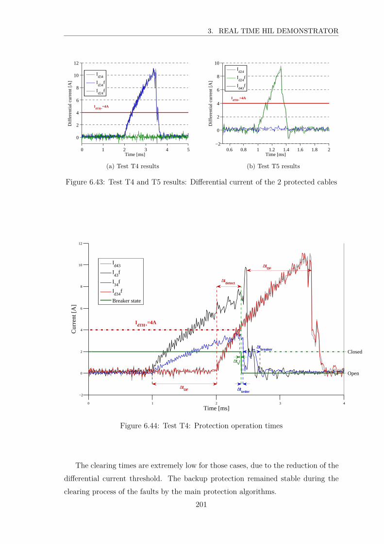
3. REAL TIME HIL DEMONSTRATOR
0 1 2 3 4 5
0
2
4
6
8
10
12
Time [ms]
Diff
eren
tial c
urre
nt [A
]
Id34
Id34
f
Id24
f
IdTH+
=4A
(a) Test T4 results
0.6 0.8 1 1.2 1.4 1.6 1.8 2−2
0
2
4
6
8
10
Time [ms]
Diff
eren
tial c
urre
nt [A
]
Id24
Id24
f
Id43
f
IdTH+
=4A
(b) Test T5 results
Figure 6.43: Test T4 and T5 results: Differential current of the 2 protected cables
0 1 2 3 4
−2
0
2
4
6
8
10
12
Time [ms]
Cur
rent
[A]
0 1
Open
Closed
Id43
I43
f
I34
f
Id34
f
Breaker state
∆tOF
∆torder
∆tbreaker
IdTH+
=4A
∆tV
∆tOF
∆tdetect
Figure 6.44: Test T4: Protection operation times
The clearing times are extremely low for those cases, due to the reduction of the
differential current threshold. The backup protection remained stable during the
clearing process of the faults by the main protection algorithms.
201
CHAPTER 6. PROTECTION PLAN VALIDATION
Time interval Value∆tOF 1.010ms
∆tdetect 380µs∆tV 20µs
∆torder 30µs∆tbreaker 270µs∆tclearing 1.690ms
Time interval Value∆tOF 140µs
∆tdetect 160µs∆tV 20µs
∆torder 30µs∆tbreaker 110µs∆tclearing 440µs
Table 6.29: Protection operation time for test T4 (left) and T5 (right)
b) Highlight on the backup protection
Test T6 simulates the failure of breaker at PR43 location, meaning that it does
not trip. This case is different compared to test T3 since 2 feeders are connected
to busbar 4. Fig.6.45 shows the backup operation times related to this test, and
Fig.6.46 shows the current measurements at each end of the faulty cable. The
breaker of PR34 trips around 1.5ms after the fault due to the main cable differential
protection. The effect can be noticed on the current measured at the opposite end
I43 on Fig.6.46, where an overcurrent can be seen at this particular time. Indeed,
the current shape presents a discontinuity at this time due to the tripping of only
one end, which implies an augmentation of the current of the opposite end.
The backup variable G4s exceed the selectivity threshold G4
sT Haround 5ms later,
and since the current of both feeders is not close to zero, the tripping order is sent
to breakers of PR4 and PR42, as expected. Once again, the selectivity threshold is
exceeded later after the time out ∆Tmain.
An overcurrent can be observed in I34 during the current breaking process of the
opposite cable end. This can be explained by Fig.6.47 which represents the volt-
ages of the two faulty cable ends. Indeed, when breakers of PR4 and PR42 trip, an
overvoltage occurs and thus the surge arresters located at the breakers terminals of
PR34 become conducting, and makes a current flowing to the fault, which becomes
temporarily alimented, until the energy is dissipated.
202

3. REAL TIME HIL DEMONSTRATOR
0 1 2 3 4 5 6 7 8
0
4
8
12
16
20
Time [ms]
Cur
rent
[A]
0 1
Open
Closed
Gd4 = G
s4
I43
PR43
: Breaker state ∆torder
∆tbreaker
GdTH4 =3A
GsTH4 =18A
∆tVs
∆tdetect
∆tdetect
∆tselect
∆tVd
Figure 6.45: Test T6: Protection operation times
0 1 2 3 4 5 6 7 8
−2
2
6
10
14
18
22
Time [ms]
Cur
rent
[A]
0 1
Open
Closed
I43
f
I34
f
PR34
: Breaker state
PR4 and PR
42:Breaker state
Figure 6.46: Test T6: Current measurements
203
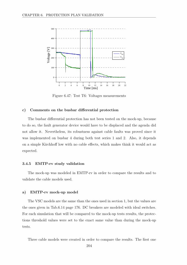
CHAPTER 6. PROTECTION PLAN VALIDATION
0 2 4 6 8 10 12 14 16 18 20 22
0
100
200
300
400
500
Time [ms]
Vol
tage
[V]
V43
V34
Figure 6.47: Test T6: Voltages measurements
c) Comments on the busbar differential protection
The busbar differential protection has not been tested on the mock-up, because
to do so, the fault generator device would have to be displaced and the agenda did
not allow it. Nevertheless, its robustness against cable faults was proved since it
was implemented on busbar 4 during both test series 1 and 2. Also, it depends
on a simple Kirchhoff low with no cable effects, which makes think it would act as
expected.
3.4.5 EMTP-rv study validation
The mock-up was modeled in EMTP-rv in order to compare the results and to
validate the cable models used.
a) EMTP-rv mock-up model
The VSC models are the same than the ones used in section 1, but the values are
the ones given in Tab.6.14 page 176. DC breakers are modeled with ideal switches.
For each simulation that will be compared to the mock-up tests results, the protec-
tions threshold values were set to the exact same value than during the mock-up
tests.
Three cable models were created in order to compare the results. The first one
204

3. REAL TIME HIL DEMONSTRATOR
is a CP model using parameters that were identified at 1kHz. The second one uses
geometrical and dielectric parameters of the cables to create a WideBand model
(those parameters were provided in subsection 3.1.3 b)). This model claims to be
the most accurate one, but since the cables are on their drums, the coupling ef-
fect is minimized so another model was created. This later one aims to represent
the drum effect by representing the winding constituted by the cable. A Wide-
Band cable model was therefore created, composed of N cable sections (Fig.6.48a),
but with a length decreased N times and connected on to another, as shown on
Fig.6.48b. However, a complete drum model cannot be done because EMTP-rv ca-
ble data generation block is limited to a certain number of conductors. Thus, several
assumptions were made:
• The number of windings composing one drum is reduced to 5.
• The windings are configured as shown on Fig.6.48c.
• The length of the winding is constant.
Thus, the length of one winding Lw has been evaluated by Lw = Ld/5, where Ld
is the length of the cable winded around one drum (227m for the 25mm2 section
and 161m for the 10mm2 section).
The geometrical parameters and dielectric properties are the same as the ones
used in the previous model.
Therefore, 5 cables were created (5 cores and 5 screens), representing 5 winding
(N = 5) configured as shown on Fig.6.48c. Thus, 2 types of drum were modeled:
one for the 10mm2 cable and one for 25mm2, and are connected in series to match
the number of drums constituting the links, as mentioned in Tab.6.17.
205

CHAPTER 6. PROTECTION PLAN VALIDATION
(a) Drum
Lw
(b) Cables
C1S1
C2 S2
C4S4
S5C5
C3S3
(c) Configuration
Figure 6.48: WideBand model of the cables on their drums
The core parameters of those 3 cable models are given Tab.6.30 for a frequency of
1kHz. The values corresponding to the CP model are the ones that have been identi-
fied, and the ones related to the two other models were calculated by EMTP-rv. For
each one of those 3 models, the positive pole and the negative pole are represented
separately. The two cable types (sections 10mm2 and 25mm2) are presented.
Model CP WideBand WideBand on the drum
Structure Core Core and screen 5 cables, core and screen
25m
m2 R′[Ω/km] 0.6806e−0 1.6275e−0 1.62751e−0
L′[H/km] 3.8106e−2 2.2742e−3 2.2742e−3
C′[F/km] 4.0969e−7 4.9485e−7 4.9485e−7
10m
m2 R′[Ω/km] 1.6977 2.6070 2.6072
L′[H/km] 4.0511e−2 2.3760e−3 2.3760e−3
C′[F/km] 3.2022e−7 3.9873e−7 3.9873e−7
Table 6.30: Cable models: core parameters at 1kHz
The parameters are the same for the two WideBand models. Indeed, the cable
206
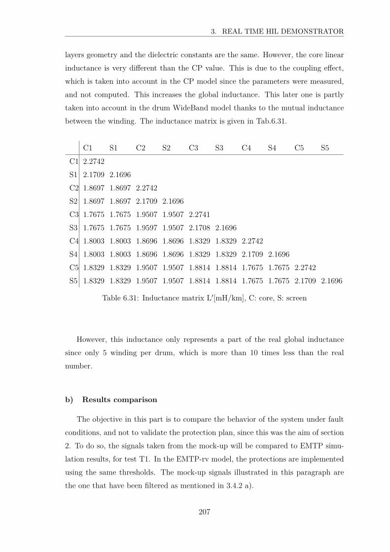
3. REAL TIME HIL DEMONSTRATOR
layers geometry and the dielectric constants are the same. However, the core linear
inductance is very different than the CP value. This is due to the coupling effect,
which is taken into account in the CP model since the parameters were measured,
and not computed. This increases the global inductance. This later one is partly
taken into account in the drum WideBand model thanks to the mutual inductance
between the winding. The inductance matrix is given in Tab.6.31.
C1 S1 C2 S2 C3 S3 C4 S4 C5 S5
C1 2.2742
S1 2.1709 2.1696
C2 1.8697 1.8697 2.2742
S2 1.8697 1.8697 2.1709 2.1696
C3 1.7675 1.7675 1.9507 1.9507 2.2741
S3 1.7675 1.7675 1.9597 1.9507 2.1708 2.1696
C4 1.8003 1.8003 1.8696 1.8696 1.8329 1.8329 2.2742
S4 1.8003 1.8003 1.8696 1.8696 1.8329 1.8329 2.1709 2.1696
C5 1.8329 1.8329 1.9507 1.9507 1.8814 1.8814 1.7675 1.7675 2.2742
S5 1.8329 1.8329 1.9507 1.9507 1.8814 1.8814 1.7675 1.7675 2.1709 2.1696
Table 6.31: Inductance matrix L′[mH/km], C: core, S: screen
However, this inductance only represents a part of the real global inductance
since only 5 winding per drum, which is more than 10 times less than the real
number.
b) Results comparison
The objective in this part is to compare the behavior of the system under fault
conditions, and not to validate the protection plan, since this was the aim of section
2. To do so, the signals taken from the mock-up will be compared to EMTP simu-
lation results, for test T1. In the EMTP-rv model, the protections are implemented
using the same thresholds. The mock-up signals illustrated in this paragraph are
the one that have been filtered as mentioned in 3.4.2 a).
207
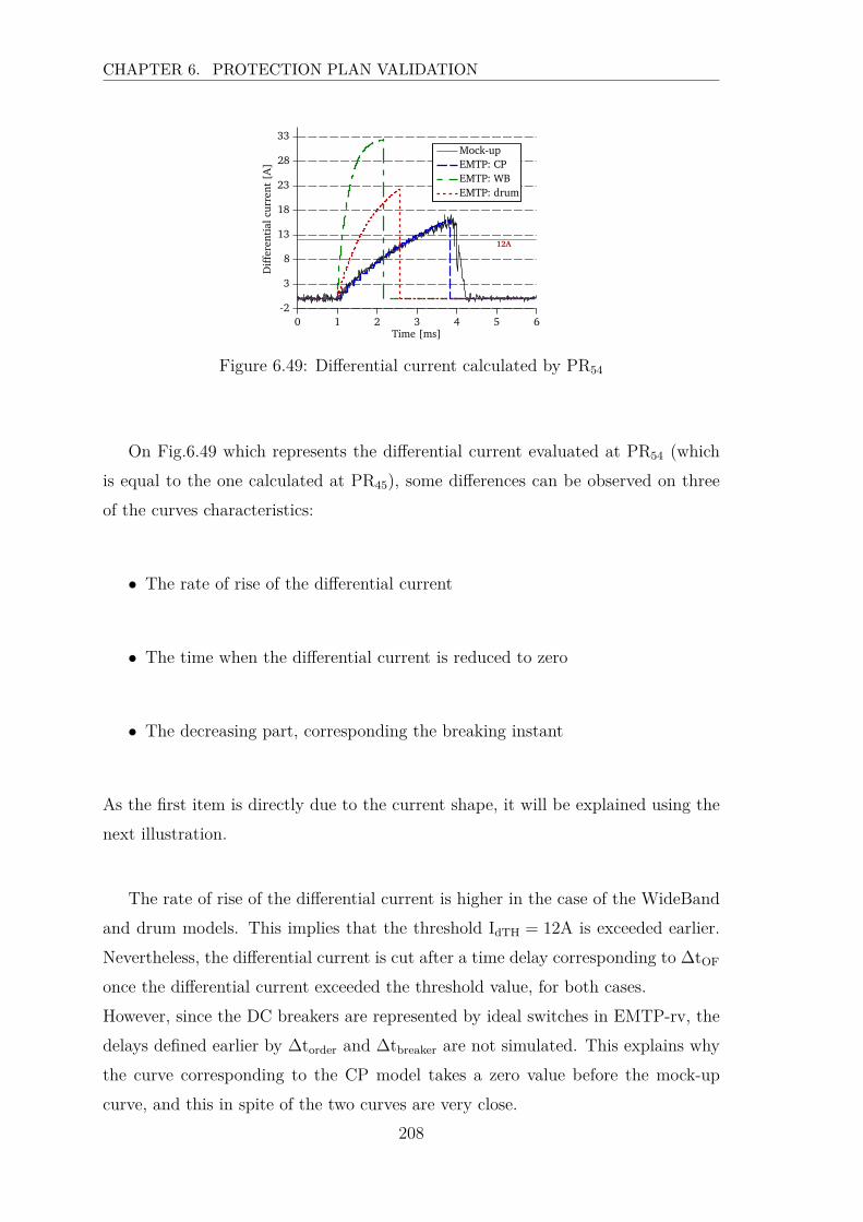
CHAPTER 6. PROTECTION PLAN VALIDATION
EMTP: drum
EMTP: WB
EMTP: CP
Mock-up
Dif
fere
nti
al
curr
en
t[A
]
Time [ms]
12A
0 1 2 3 4 5 6
-2
3
8
13
18
23
28
33
Figure 6.49: Differential current calculated by PR54
On Fig.6.49 which represents the differential current evaluated at PR54 (which
is equal to the one calculated at PR45), some differences can be observed on three
of the curves characteristics:
• The rate of rise of the differential current
• The time when the differential current is reduced to zero
• The decreasing part, corresponding the breaking instant
As the first item is directly due to the current shape, it will be explained using the
next illustration.
The rate of rise of the differential current is higher in the case of the WideBand
and drum models. This implies that the threshold IdTH = 12A is exceeded earlier.
Nevertheless, the differential current is cut after a time delay corresponding to ∆tOF
once the differential current exceeded the threshold value, for both cases.
However, since the DC breakers are represented by ideal switches in EMTP-rv, the
delays defined earlier by ∆torder and ∆tbreaker are not simulated. This explains why
the curve corresponding to the CP model takes a zero value before the mock-up
curve, and this in spite of the two curves are very close.
208
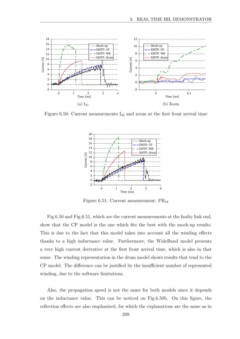
3. REAL TIME HIL DEMONSTRATOR
EMTP: drum
EMTP: WB
EMTP: CP
Mock-upC
urr
en
t[A
]
Time [ms]0 1 2 3 4
-2
0
2
4
6
8
10
12
14
16
18
(a) I45
EMTP: drum
EMTP: WB
EMTP: CP
Mock-up
Cu
rren
t[A
]
Time [ms]0 0.1
-2
0
2
4
6
8
10
12
(b) Zoom
Figure 6.50: Current measurements I45 and zoom at the first front arrival time
EMTP: drum
EMTP: WB
EMTP: CP
Mock-up
Cu
rren
t[A
]
Time [ms]0 1 2 3 4
-2
0
2
4
6
8
10
12
14
16
18
20
Figure 6.51: Current measurement: PR54
Fig.6.50 and Fig.6.51, which are the current measurements at the faulty link end,
show that the CP model is the one which fits the best with the mock-up results.
This is due to the fact that this model takes into account all the winding effects
thanks to a high inductance value. Furthermore, the WideBand model presents
a very high current derivative at the first front arrival time, which is also in that
sense. The winding representation in the drum model shows results that tend to the
CP model. The difference can be justified by the insufficient number of represented
winding, due to the software limitations.
Also, the propagation speed is not the same for both models since it depends
on the inductance value. This can be noticed on Fig.6.50b. On this figure, the
reflection effects are also emphasized, for which the explanations are the same as in
209
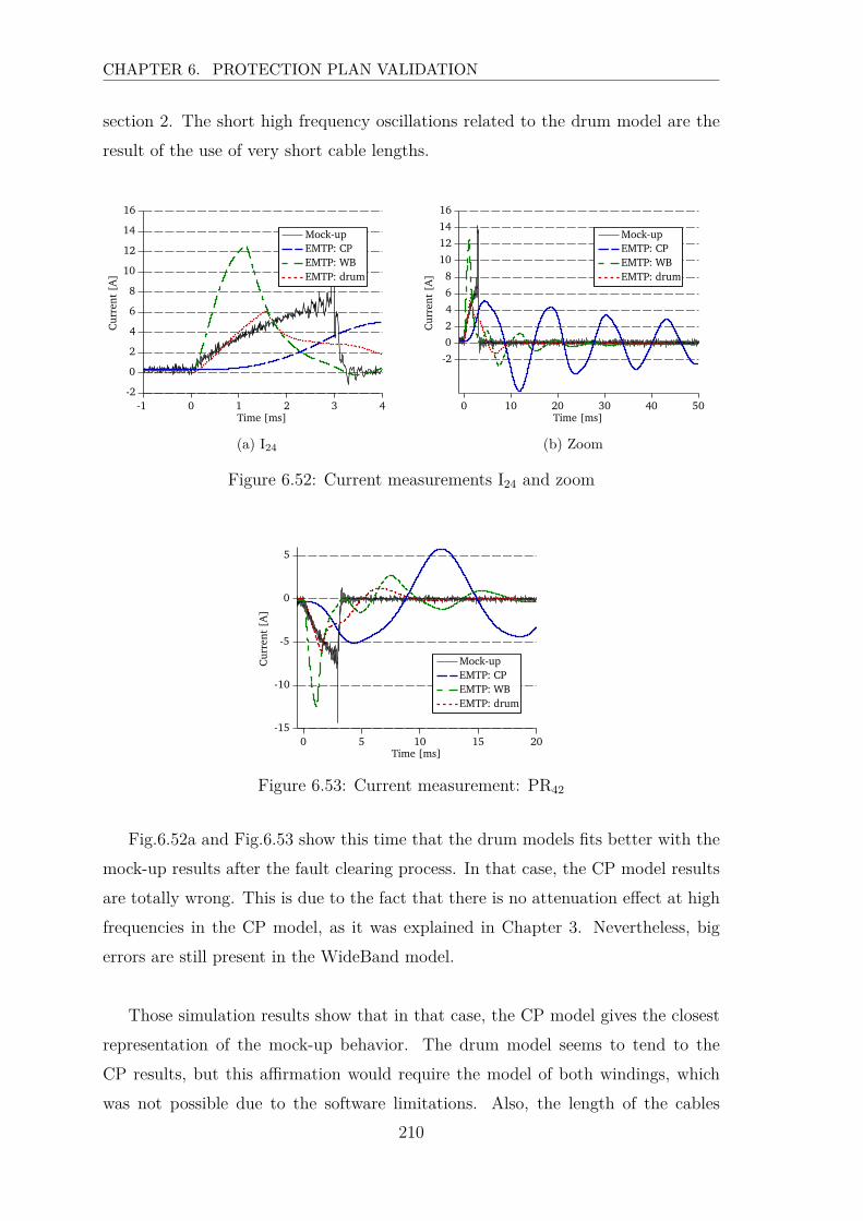
CHAPTER 6. PROTECTION PLAN VALIDATION
section 2. The short high frequency oscillations related to the drum model are the
result of the use of very short cable lengths.
EMTP: drum
EMTP: WB
EMTP: CP
Mock-up
Cu
rren
t[A
]
Time [ms]-1 0 1 2 3 4
-2
0
2
4
6
8
10
12
14
16
(a) I24
EMTP: drum
EMTP: WB
EMTP: CP
Mock-up
Cu
rren
t[A
]Time [ms]
0 10 20 30 40 50
-2
0
2
4
6
8
10
12
14
16
(b) Zoom
Figure 6.52: Current measurements I24 and zoom
EMTP: drum
EMTP: WB
EMTP: CP
Mock-upCu
rren
t[A
]
Time [ms]0 5 10 15 20
-15
-10
-5
0
5
Figure 6.53: Current measurement: PR42
Fig.6.52a and Fig.6.53 show this time that the drum models fits better with the
mock-up results after the fault clearing process. In that case, the CP model results
are totally wrong. This is due to the fact that there is no attenuation effect at high
frequencies in the CP model, as it was explained in Chapter 3. Nevertheless, big
errors are still present in the WideBand model.
Those simulation results show that in that case, the CP model gives the closest
representation of the mock-up behavior. The drum model seems to tend to the
CP results, but this affirmation would require the model of both windings, which
was not possible due to the software limitations. Also, the length of the cables
210
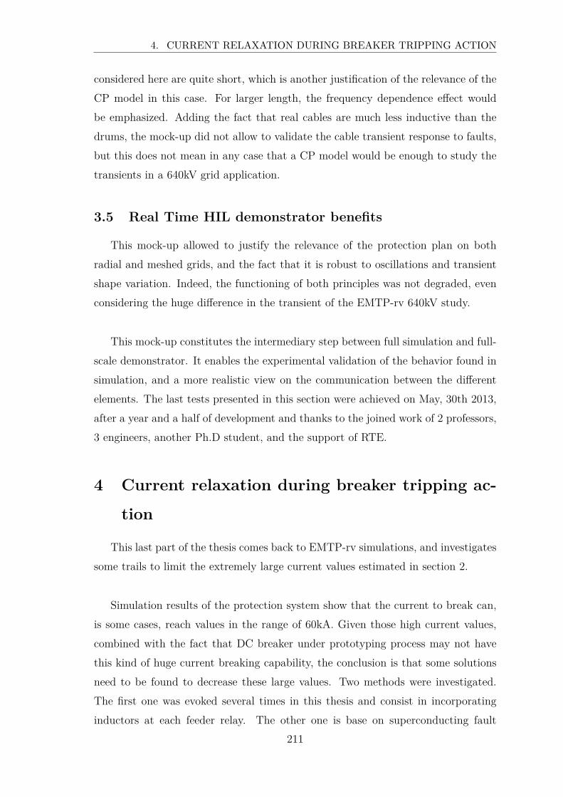
4. CURRENT RELAXATION DURING BREAKER TRIPPING ACTION
considered here are quite short, which is another justification of the relevance of the
CP model in this case. For larger length, the frequency dependence effect would
be emphasized. Adding the fact that real cables are much less inductive than the
drums, the mock-up did not allow to validate the cable transient response to faults,
but this does not mean in any case that a CP model would be enough to study the
transients in a 640kV grid application.
3.5 Real Time HIL demonstrator benefits
This mock-up allowed to justify the relevance of the protection plan on both
radial and meshed grids, and the fact that it is robust to oscillations and transient
shape variation. Indeed, the functioning of both principles was not degraded, even
considering the huge difference in the transient of the EMTP-rv 640kV study.
This mock-up constitutes the intermediary step between full simulation and full-
scale demonstrator. It enables the experimental validation of the behavior found in
simulation, and a more realistic view on the communication between the different
elements. The last tests presented in this section were achieved on May, 30th 2013,
after a year and a half of development and thanks to the joined work of 2 professors,
3 engineers, another Ph.D student, and the support of RTE.
4 Current relaxation during breaker tripping ac-
tion
This last part of the thesis comes back to EMTP-rv simulations, and investigates
some trails to limit the extremely large current values estimated in section 2.
Simulation results of the protection system show that the current to break can,
is some cases, reach values in the range of 60kA. Given those high current values,
combined with the fact that DC breaker under prototyping process may not have
this kind of huge current breaking capability, the conclusion is that some solutions
need to be found to decrease these large values. Two methods were investigated.
The first one was evoked several times in this thesis and consist in incorporating
inductors at each feeder relay. The other one is base on superconducting fault
211
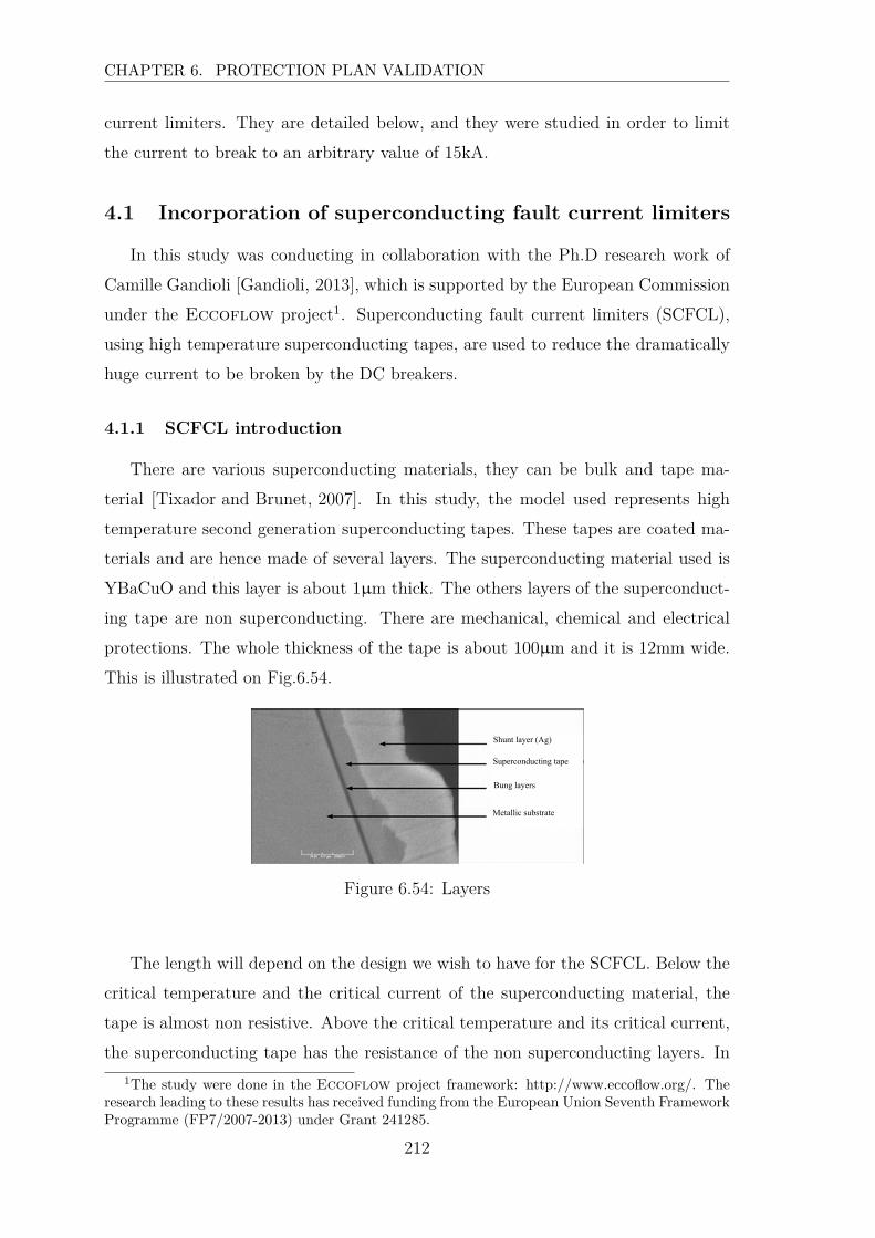
CHAPTER 6. PROTECTION PLAN VALIDATION
current limiters. They are detailed below, and they were studied in order to limit
the current to break to an arbitrary value of 15kA.
4.1 Incorporation of superconducting fault current limiters
In this study was conducting in collaboration with the Ph.D research work of
Camille Gandioli [Gandioli, 2013], which is supported by the European Commission
under the Eccoflow project1. Superconducting fault current limiters (SCFCL),
using high temperature superconducting tapes, are used to reduce the dramatically
huge current to be broken by the DC breakers.
4.1.1 SCFCL introduction
There are various superconducting materials, they can be bulk and tape ma-
terial [Tixador and Brunet, 2007]. In this study, the model used represents high
temperature second generation superconducting tapes. These tapes are coated ma-
terials and are hence made of several layers. The superconducting material used is
YBaCuO and this layer is about 1µm thick. The others layers of the superconduct-
ing tape are non superconducting. There are mechanical, chemical and electrical
protections. The whole thickness of the tape is about 100µm and it is 12mm wide.
This is illustrated on Fig.6.54.
Shunt layer (Ag)
Superconducting tape
Bung layers
Metallic substrate
Figure 6.54: Layers
The length will depend on the design we wish to have for the SCFCL. Below the
critical temperature and the critical current of the superconducting material, the
tape is almost non resistive. Above the critical temperature and its critical current,
the superconducting tape has the resistance of the non superconducting layers. In
1The study were done in the Eccoflow project framework: http://www.eccoflow.org/. Theresearch leading to these results has received funding from the European Union Seventh FrameworkProgramme (FP7/2007-2013) under Grant 241285.
212
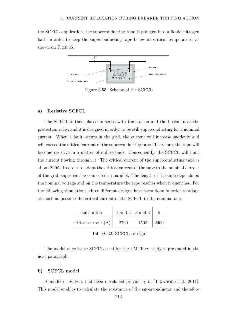
4. CURRENT RELAXATION DURING BREAKER TRIPPING ACTION
the SCFCL application, the superconducting tape is plunged into a liquid nitrogen
bath in order to keep the superconducting tape below its critical temperature, as
shown on Fig.6.55.
Figure 6.55: Scheme of the SCFCL
a) Resistive SCFCL
The SCFCL is then placed in series with the station and the busbar near the
protection relay, and it is designed in order to be still superconducting for a nominal
current. When a fault occurs in the grid, the current will increase suddenly and
will exceed the critical current of the superconducting tape. Therefore, the tape will
become resistive in a matter of milliseconds. Consequently, the SCFCL will limit
the current flowing through it. The critical current of the superconducting tape is
about 300A. In order to adapt the critical current of the tape to the nominal current
of the grid, tapes can be connected in parallel. The length of the tape depends on
the nominal voltage and on the temperature the tape reaches when it quenches. For
the following simulations, three different designs have been done in order to adapt
as much as possible the critical current of the SCFCL to the nominal one.
substation 1 and 2 3 and 4 5
critical current (A) 2700 1500 2400
Table 6.32: SCFCLs design
The model of resistive SCFCL used for the EMTP-rv study is presented in the
next paragraph.
b) SCFCL model
A model of SCFCL had been developed previously in [Tixador et al., 2011].
This model enables to calculate the resistance of the superconductor and therefore
213
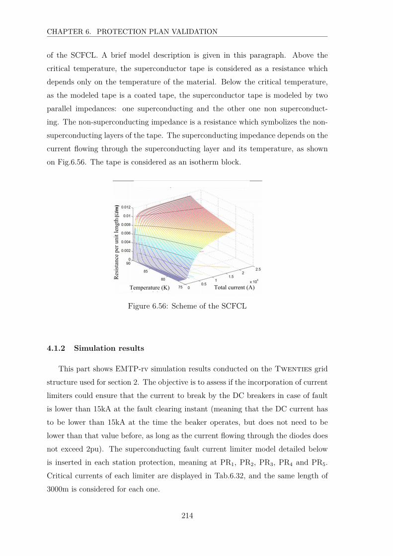
CHAPTER 6. PROTECTION PLAN VALIDATION
of the SCFCL. A brief model description is given in this paragraph. Above the
critical temperature, the superconductor tape is considered as a resistance which
depends only on the temperature of the material. Below the critical temperature,
as the modeled tape is a coated tape, the superconductor tape is modeled by two
parallel impedances: one superconducting and the other one non superconduct-
ing. The non-superconducting impedance is a resistance which symbolizes the non-
superconducting layers of the tape. The superconducting impedance depends on the
current flowing through the superconducting layer and its temperature, as shown
on Fig.6.56. The tape is considered as an isotherm block.
Res
ista
nce
per u
nit l
engt
h
Temperature (K) Total current (A)
Figure 6.56: Scheme of the SCFCL
4.1.2 Simulation results
This part shows EMTP-rv simulation results conducted on the Twenties grid
structure used for section 2. The objective is to assess if the incorporation of current
limiters could ensure that the current to break by the DC breakers in case of fault
is lower than 15kA at the fault clearing instant (meaning that the DC current has
to be lower than 15kA at the time the beaker operates, but does not need to be
lower than that value before, as long as the current flowing through the diodes does
not exceed 2pu). The superconducting fault current limiter model detailed below
is inserted in each station protection, meaning at PR1, PR2, PR3, PR4 and PR5.
Critical currents of each limiter are displayed in Tab.6.32, and the same length of
3000m is considered for each one.
214
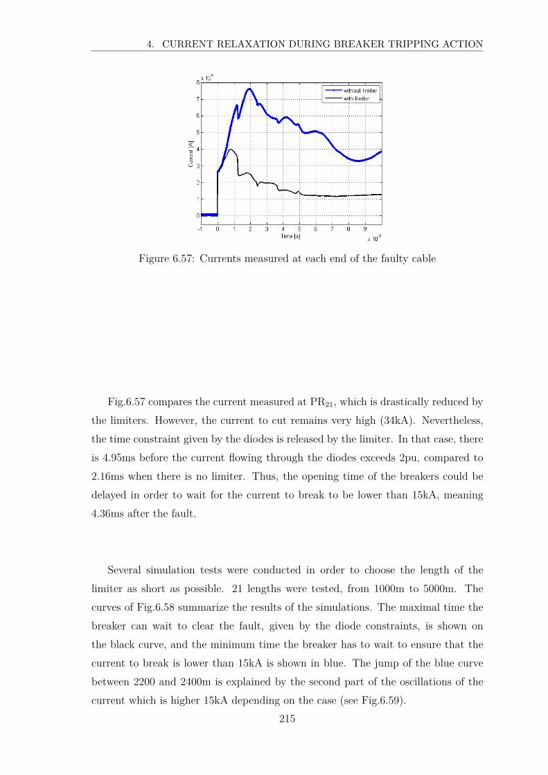
4. CURRENT RELAXATION DURING BREAKER TRIPPING ACTION
Figure 6.57: Currents measured at each end of the faulty cable
Fig.6.57 compares the current measured at PR21, which is drastically reduced by
the limiters. However, the current to cut remains very high (34kA). Nevertheless,
the time constraint given by the diodes is released by the limiter. In that case, there
is 4.95ms before the current flowing through the diodes exceeds 2pu, compared to
2.16ms when there is no limiter. Thus, the opening time of the breakers could be
delayed in order to wait for the current to break to be lower than 15kA, meaning
4.36ms after the fault.
Several simulation tests were conducted in order to choose the length of the
limiter as short as possible. 21 lengths were tested, from 1000m to 5000m. The
curves of Fig.6.58 summarize the results of the simulations. The maximal time the
breaker can wait to clear the fault, given by the diode constraints, is shown on
the black curve, and the minimum time the breaker has to wait to ensure that the
current to break is lower than 15kA is shown in blue. The jump of the blue curve
between 2200 and 2400m is explained by the second part of the oscillations of the
current which is higher 15kA depending on the case (see Fig.6.59).
215
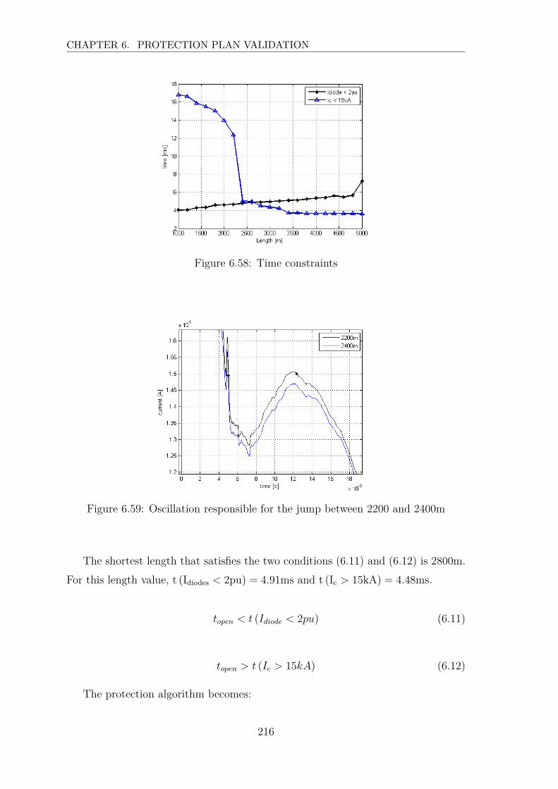
CHAPTER 6. PROTECTION PLAN VALIDATION
Figure 6.58: Time constraints
Figure 6.59: Oscillation responsible for the jump between 2200 and 2400m
The shortest length that satisfies the two conditions (6.11) and (6.12) is 2800m.
For this length value, t (Idiodes < 2pu) = 4.91ms and t (Ic > 15kA) = 4.48ms.
topen < t (Idiode < 2pu) (6.11)
topen > t (Ic > 15kA) (6.12)
The protection algorithm becomes:
216
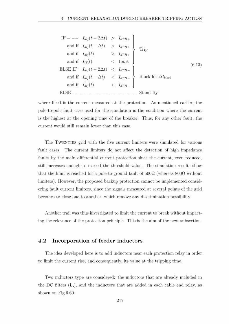
4. CURRENT RELAXATION DURING BREAKER TRIPPING ACTION
IF − −− Idij(t− 2∆t) > IdT H+
and if Idij(t− ∆t) > IdT H+
and if Idij(t) > IdT H+
and if Iij(t) < 15kA
Trip
ELSE IF Idij(t− 2∆t) < IdT H−
and if Idij(t− ∆t) < IdT H−
and if Idij(t) < IdT H−
Block for ∆tblock
ELSE − − − − − − − − − − − − − − Stand By
(6.13)
where Ifeed is the current measured at the protection. As mentioned earlier, the
pole-to-pole fault case used for the simulation is the condition where the current
is the highest at the opening time of the breaker. Thus, for any other fault, the
current would still remain lower than this case.
The Twenties grid with the five current limiters were simulated for various
fault cases. The current limiters do not affect the detection of high impedance
faults by the main differential current protection since the current, even reduced,
still increases enough to exceed the threshold value. The simulation results show
that the limit is reached for a pole-to-ground fault of 500Ω (whereas 800Ω without
limiters). However, the proposed backup protection cannot be implemented consid-
ering fault current limiters, since the signals measured at several points of the grid
becomes to close one to another, which remove any discrimination possibility.
Another trail was thus investigated to limit the current to break without impact-
ing the relevance of the protection principle. This is the aim of the next subsection.
4.2 Incorporation of feeder inductors
The idea developed here is to add inductors near each protection relay in order
to limit the current rise, and consequently, its value at the tripping time.
Two inductors type are considered: the inductors that are already included in
the DC filters (Ls), and the inductors that are added in each cable end relay, as
shown on Fig.6.60.
217

CHAPTER 6. PROTECTION PLAN VALIDATION
PRij
PRik
PRiVSC side DC grid side
Lfeed ij
Lfeed ik
Figure 6.60: Inductors located at cable ends
There is thus 10 inductors Ls included in the DC filters of the 5 stations (positive
and negative pole), and 20 feeder inductors (10 cable ends times 2 poles). The
objective is to find the 30 inductors values that ensure a current to break lower than
15kA for any fault case.
4.2.1 Inductors value choice
The objective is to ensure that the current to break does not exceed 15kA, for
any fault that can happen on the grid. Therefore, the worst case fault scenarios
can be taken into account to perform the study. The worst case fault is defined by
the fault leading to the highest current to break. It is a pole-to-pole fault occurring
near a relay, and the location of this one was known thanks to the simulations of
those 10 possible faults. The worst case fault scenario is thus the pole-to-pole fault
occurring near the relay PR13, with a current to break equal to 62.680kA. The worst
case scenario for the busbar differential protection is also considered, and is a fault
occurring on the busbar connected to station 5, with a current to break of 28.533kA.
The ideal method would be to set the inductor value one by one, in order to
minimize it. Nevertheless, the modification of one inductor value has both a local
influence and a global influence on the grid. Indeed, the modification of a single
inductor value lead to a modification in the signal measured near this inductor, but
also in the signals measured remotely in the grid. An exhaustive study would thus
be the only solution to ensure an optimal inductor values set. Nevertheless, the
required simulation number becomes too high when the number of inductor values
that need to be chosen is consequent. In the Twenties grid case, if the inductor
values are chosen among 8 values for example, then 815 ≈ 3.1013 simulations need
to be performed to test all the cases, and this for each fault case.
Thus, the influence of the variation of the inductor values were first investigated,
assuming that the DC filter inductors Ls both take the same values, and that the
218

4. CURRENT RELAXATION DURING BREAKER TRIPPING ACTION
feeder inductors Lfeed of the two ends of a cable have the same value. There is thus
only 6 inductor value to choose, one for Ls and five for Lfeed. A study were done
to choose those six inductors between a set of two values: 32mH and 48mH. Thus,
only 26 = 64 simulations were required for each fault case. The conclusion on the
variation influence are the following ones:
• The solution Ls = 32mH and Lfeed = 32mH for each feeder enables to limit the
current to break below 15kA.
• If one inductor is increased, then it can imply a current to break higher than
15kA somewhere else in the grid.
Thus, a parametric study assuming that the feeder inductor take the same value
everywhere in the grid were chosen. The two worst case faults were used to deter-
mine the smallest inductor values.
The inductor are chosen in a set of 8 values: 10mH, 15mH, 20mH, 25mH, 30mH,
35mH, 40mH and 45mH, which were chosen arbitrarily. There is thus 64 possible
cases, that were simulated for both the cable and the busbar faults.
a) Cable fault occurring near relay PR13
For this fault case, among the 64 possibilities, 28 inductor values set enables to
limit the current to break below 15kA. Two solutions can be kept:
• Solution 1: minimizes the source inductors, then minimizes the feeder induc-
tors: Ls = 10mH and Lfeed = 40mH
• Solution 2: minimizes the feeder inductors, then minimizes the source induc-
tors: Ls = 25mH and Lfeed = 30mH
The curves presented in Fig.6.61 illustrate the influence of each inductor.
219
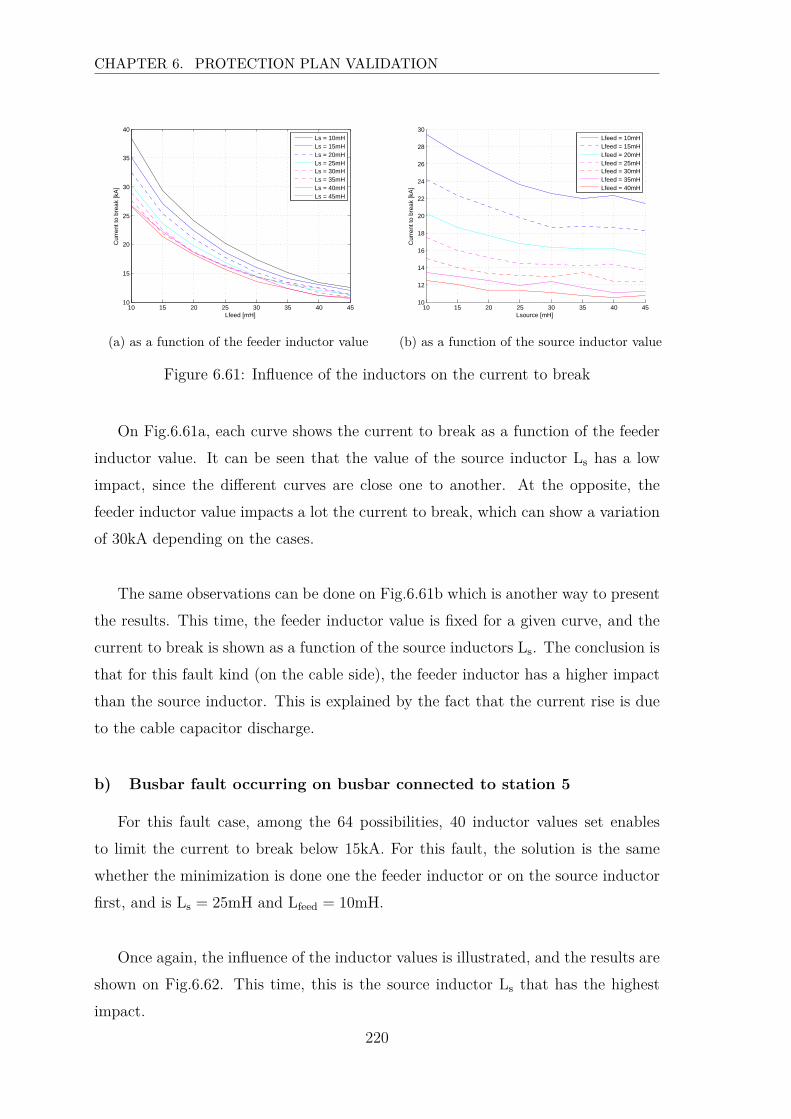
CHAPTER 6. PROTECTION PLAN VALIDATION
10 15 20 25 30 35 40 4510
15
20
25
30
35
40
Lfeed [mH]
Cur
rent
to b
reak
[kA
]
Ls = 10mHLs = 15mHLs = 20mHLs = 25mHLs = 30mHLs = 35mHLs = 40mHLs = 45mH
(a) as a function of the feeder inductor value
10 15 20 25 30 35 40 4510
12
14
16
18
20
22
24
26
28
30
Lsource [mH]
Cur
rent
to b
reak
[kA
]
Lfeed = 10mHLfeed = 15mHLfeed = 20mHLfeed = 25mHLfeed = 30mHLfeed = 35mHLfeed = 40mH
(b) as a function of the source inductor value
Figure 6.61: Influence of the inductors on the current to break
On Fig.6.61a, each curve shows the current to break as a function of the feeder
inductor value. It can be seen that the value of the source inductor Ls has a low
impact, since the different curves are close one to another. At the opposite, the
feeder inductor value impacts a lot the current to break, which can show a variation
of 30kA depending on the cases.
The same observations can be done on Fig.6.61b which is another way to present
the results. This time, the feeder inductor value is fixed for a given curve, and the
current to break is shown as a function of the source inductors Ls. The conclusion is
that for this fault kind (on the cable side), the feeder inductor has a higher impact
than the source inductor. This is explained by the fact that the current rise is due
to the cable capacitor discharge.
b) Busbar fault occurring on busbar connected to station 5
For this fault case, among the 64 possibilities, 40 inductor values set enables
to limit the current to break below 15kA. For this fault, the solution is the same
whether the minimization is done one the feeder inductor or on the source inductor
first, and is Ls = 25mH and Lfeed = 10mH.
Once again, the influence of the inductor values is illustrated, and the results are
shown on Fig.6.62. This time, this is the source inductor Ls that has the highest
impact.
220
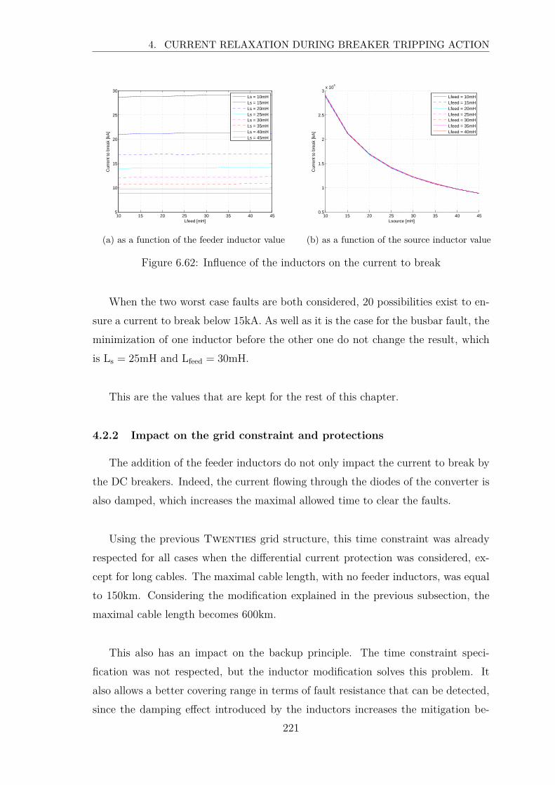
4. CURRENT RELAXATION DURING BREAKER TRIPPING ACTION
10 15 20 25 30 35 40 455
10
15
20
25
30
Lfeed [mH]
Cur
rent
to b
reak
[kA
]
Ls = 10mHLs = 15mHLs = 20mHLs = 25mHLs = 30mHLs = 35mHLs = 40mHLs = 45mH
(a) as a function of the feeder inductor value
10 15 20 25 30 35 40 450.5
1
1.5
2
2.5
3x 10
4
Lsource [mH]
Cur
rent
to b
reak
[kA
]
Lfeed = 10mHLfeed = 15mHLfeed = 20mHLfeed = 25mHLfeed = 30mHLfeed = 35mHLfeed = 40mH
(b) as a function of the source inductor value
Figure 6.62: Influence of the inductors on the current to break
When the two worst case faults are both considered, 20 possibilities exist to en-
sure a current to break below 15kA. As well as it is the case for the busbar fault, the
minimization of one inductor before the other one do not change the result, which
is Ls = 25mH and Lfeed = 30mH.
This are the values that are kept for the rest of this chapter.
4.2.2 Impact on the grid constraint and protections
The addition of the feeder inductors do not only impact the current to break by
the DC breakers. Indeed, the current flowing through the diodes of the converter is
also damped, which increases the maximal allowed time to clear the faults.
Using the previous Twenties grid structure, this time constraint was already
respected for all cases when the differential current protection was considered, ex-
cept for long cables. The maximal cable length, with no feeder inductors, was equal
to 150km. Considering the modification explained in the previous subsection, the
maximal cable length becomes 600km.
This also has an impact on the backup principle. The time constraint speci-
fication was not respected, but the inductor modification solves this problem. It
also allows a better covering range in terms of fault resistance that can be detected,
since the damping effect introduced by the inductors increases the mitigation be-
221
CHAPTER 6. PROTECTION PLAN VALIDATION
tween the signals, and thus enables a better discrimination between internal and
external fault. Due to agenda limitation, the results on the backup considering this
new grid structure could be shown in the thesis.
4.2.3 Voltage differential protection
As explained in Chapter 5 section 3.6, the incorporation of feeder inductors en-
ables to use another protection principle, which does not require any communication
along the cables. The algorithm is based on the voltage measurement at the inductor
terminals, and is reminded in (6.14).
IF Vindij(t) > dVindTH+ ; Trip
ELSE IF Vindij(t) < dVindTH- ; Block for ∆tblock
ELSE ; Stand By
(6.14)
The theoretical performances were tested through EMTP-rv simulations, and
are resumed in this subsection.
a) Threshold settings
The pole-to-pole faults occurring at each cable end are used to find the thresholds
values guaranteeing the full selectivity of the criterion.
A negative threshold value of dVindTH− = −40kV, set at each feeder protection
relay, enables to discriminate the faults occurring close to the relay but external to
their protective zone.
The positive threshold values were chosen to ensure the selectivity of the princi-
ple, similarly than it was performed for the backup protection, as explained below.
Let the fault groups F intki and F ext
ki being the groups of faults defined for each
protection relay PRki by (6.15) and (6.16) respectively.
Fintki = Fki; Fik (6.15)
Fextki = Fij, i 6= k and j 6= k (6.16)
Let Fext−negki the fault group now defined by (6.17), which represents the faults
222
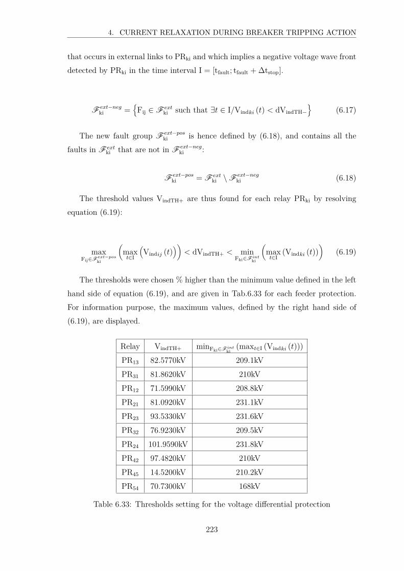
4. CURRENT RELAXATION DURING BREAKER TRIPPING ACTION
that occurs in external links to PRki and which implies a negative voltage wave front
detected by PRki in the time interval I = [tfault; tfault + ∆tstop].
Fext−negki =
Fij ∈ Fextki such that ∃t ∈ I/Vindki (t) < dVindTH−
(6.17)
The new fault group Fext−poski is hence defined by (6.18), and contains all the
faults in F extki that are not in F
ext−negki :
Fext−poski = F
extki \ F
ext−negki (6.18)
The threshold values VindTH+ are thus found for each relay PRki by resolving
equation (6.19):
maxFij∈F
ext−pos
ki
(
maxt∈I
(
Vindij (t))
)
< dVindTH+ < minFki∈F int
ki
(
maxt∈I
(Vindki (t)))
(6.19)
The thresholds were chosen % higher than the minimum value defined in the left
hand side of equation (6.19), and are given in Tab.6.33 for each feeder protection.
For information purpose, the maximum values, defined by the right hand side of
(6.19), are displayed.
Relay VindTH+ minFki∈F intki
(maxt∈I (Vindki (t)))
PR13 82.5770kV 209.1kV
PR31 81.8620kV 210kV
PR12 71.5990kV 208.8kV
PR21 81.0920kV 231.1kV
PR23 93.5330kV 231.6kV
PR32 76.9230kV 209.5kV
PR24 101.9590kV 231.8kV
PR42 97.4820kV 210kV
PR45 14.5200kV 210.2kV
PR54 70.7300kV 168kV
Table 6.33: Thresholds setting for the voltage differential protection
223

CHAPTER 6. PROTECTION PLAN VALIDATION
b) Voltage differential protection validation
The fault clearing process of the worst case faults in terms of current to break
are summarized in Tab.6.34. The tripping times and the current to break that are
displayed correspond to the maximal values between the two ends of the faulty cable.
Relay near the fault ttrip Current to break
PR13 1.550ms 9.322kA
PR31 1.550ms 10.257kA
PR12 1.400ms 7.801kA
PR21 1.410ms 6.115kA
PR23 1.270ms 8.581kA
PR32 1.270ms 8.340kA
PR24 1.140ms 9.691kA
PR42 1.140ms 10.531kA
PR45 2.080ms 9.725kA
PR54 2.060ms 11.987kA
Table 6.34: Thresholds setting for the voltage differential protection
Note that since there is no communication between the relays, the trippings are
not synchronized at the two cable ends. This could eventually lead to higher cur-
rents to break at the cable end which trips last. However, the time difference is
small and considering those high feeder inductor values, the current remains below
15kA.
The pole-to-pole fault example occurring near PR13 is used to compare the dif-
ferential current protection and the voltage differential principle, and the results are
provided in Tab.6.35.
224

4. CURRENT RELAXATION DURING BREAKER TRIPPING ACTION
Relayttrip Current to break
Current Voltage Current Voltage
PR13 1.590ms 1.010ms 8.957kA 8.799kA
PR31 1.590ms 1.550ms 9.473kA 9.322kA
Table 6.35: Differential current and voltage differential principles for a fault exampleoccurring near PR13
The shortest detection time occurs for the cable end close to the fault, with the
voltage differential principle. This is due to the fact that there is no delay due to
communication. The highest detection time is though also for the voltage differential
principle, at the other cable end. Indeed, there is a mitigation in the signal while it
propagates through the cable, which damps the waves, which leads to a delay of the
detection. This is not the case for the differential current. Indeed, the differential
current is the same at both cable ends, and once the perturbation is seen at one
end. For this fault case, the communication link enables a quicker detection of the
fault.
The same comparison is done for a fault occurring on the longest cable, near
PR54. The results are given in Tab.6.36.
Relayttrip Current to break
Current Voltage Current Voltage
PR45 2.120ms 2.060ms 5.252kA 12.208kA
PR54 2.120ms 1.010ms 12.445kA 7.408kA
Table 6.36: Differential current and voltage differential principles for a fault exampleoccurring near PR54
In this case, the tripping time related to the differential current is sensitively
higher than the one for the voltage differential criterion. This is due to the longer
communication delay. Indeed, for short links smaller than 200km, the differential
current is quicker than the voltage differential protection. However, for longer links,
the voltage differential protection becomes faster.
225
CHAPTER 6. PROTECTION PLAN VALIDATION
Beside, the impact of the non-synchronization of the trippings of the two cable
ends is highlighted on this example. This explains the fact that the current to break
at PR45 is higher if the voltage differential principle is considered, since the tripping
is done around 1ms before at the other cable end.
The two principle can thus be both implemented in the protection system. The
voltage differential can thus be a backup in case of the communication loss for links
smaller than 200km. For links higher than this value, it becomes the main cable
protection.
Note that the validity domain of the voltage differential protection depends
strongly on the feeder inductors value. Indeed, for smaller inductor values, the
mitigation of the signals is reduced, and thus the maximal fault resistance that can
be detected is also reduced. The inductor value choice can thus be chosen in order
to ensure the detection of a given fault resistance. For the presented inductor values,
the maximal fault resistance detected is Rfault = 50Ω. For higher fault resistances,
the differential current protection is responsible for the fault clearance.
5 Conclusion on the protection system
The theoretical performances of the protection system were assessed thanks to
EMTP-rv study. The thresholds settings and the validity domain of the different
protection principles strongly depends on the grid structure. Indeed, the thresholds
might be subjected to change if the grid configuration changes. Other calculations
would be required but can be performed similarly than explained in section 1, and
new threshold values would be sent by the supervisor to the relays.
The proposed protection system thus includes inductors located near each feeder
relay, and this way enables the recourse to a non-communicant protection principle.
This later one can hence support the protection system in case of the loss of the
optical fiber link. The differential current protection is however crucial in the system
since it is the only one that can detect high impedance faults.
Even though the inductor values seems to be high (25mH and 30mH), they are
226

5. CONCLUSION ON THE PROTECTION SYSTEM
not prohibited. Indeed, the stability of the control loops under those conditions were
validated in the L2EP. Furthermore, smoothing reactors up to 100mH are already
considered for industrialized HVDC project by ABB.
Nevertheless, even though the addition of feeder inductors limits the current to
break below a certain value, it also increases the energy store in the system and thus
that needs to be dissipated. This means that other investigations are required on
the current limitation during breaker tripping action.
227

General conclusion

General conclusion
In electricity transmission, the inherent qualities of alternative grids fade in front
of the difficulty imposed by the reactive power transportation, when overhead lines
or, particularly, underground or submarine cables reach critical lengths. In the
frame of the thought aiming to operate at best renewable energy resources, coming
from wind or hydro power stations, the creation of a high voltage direct current
grid is assumed to dispatch those energies to the consumption centers. As men-
tioned in Chapter 1, from a certain amount of power to transmit, there is a critical
length beyond which AC transmission is not viable anymore, and where DC links be-
comes both more efficient and less costly. The new conversion technologies, namely
the voltage source converters, now enables the connection of several terminals and
therefore the creation of a true grid, which can either have a looped, meshed, or
radial structure. The advantages of such grid structure in relation to point-to-point
links are obvious in terms of reliability of the transmission grid. Nevertheless, some
technological locks remains, and the protection against faults of those grids is cur-
rently largely debated. This Ph.D thesis aims to propose a complete protection
plan against insulation faults in cable or busbar, including a main protection and
two backups in case of failure of a component, for a submarine DC grid. The target
application would be a grid linking offshore wind farms and countries through the
North Sea.
Even though several protection philosophies, detailed in Chapter 2, can be fol-
lowed, the one used for the protection of AC grids was chosen since this one already
proved its worth in operation. A given grid structure composed of five nodes and five
links was chosen. This structure was subjected to EMTP-rv model and simulations
to study the constraints related to the protection operation, and to investigate the
grid behavior under fault conditions. A parametric study was presented in Chapter
231
GENERAL CONCLUSION
4 to show this grid behavior. The protection system must respond to several spec-
ifications, that were detailed at the beginning of Chapter 5. The very restrictive
constraint, in terms of operation time range of the protection system, is given by
the current flowing through the diodes of the converters, and requires a maximal
operation time of the protection in the range of few milliseconds. This implies that
the selective detection has to be performed during the transient phase of the sig-
nals. In order to represent the transients phenomena following a fault occurrence,
a very detailed model of the grid was created and was presented in Chapter 3. The
main characteristics of undergrounds or submarine cables is that they present power
damping in the signals due to their low resistivity. As it is explained in Chapter 5,
selective criteria are thus harder to find, which forces the recourse to communicant
protection principles. The differential current was found to be the most relevant
solution. Even though it is already used in AC applications, it was modified to
become a traveling wave based criterion adapted to fault transients related to DC
grids. The EMTP-rv validation of the protection principles, presented at the begin-
ning of Chapter 6, highlighted the dramatically huge current that would need to be
broken by the DC breakers. Those DC breakers, still under prototyping phase as
mentioned in Chapter 2, might not be able to cut those kind of large currents, in the
range of several tens of kiloAmps. This is the reason why a solution to limit these
currents was investigated. The best trail is to incorporate inductors at the cable
ends. This results in a lower rate of rise of the current, and if the inductor values
can be set in order to ensure that the current to break would be below a given value.
This grid structure modification enables the discovery of a non-communicant prin-
ciple, which cannot be implemented without the presence of those new inductors.
This later principle, named voltage differential protection, can thus be combined
with the differential current protection and act either as a backup in case of the
loss of the communication link, or acts as a main protection since its operation is
quicker for very long links. Besides, the addition of the inductors at the cable ends
releases the constraint related to the current flowing through the diodes, and hence
enables a larger validity domain of the differential current protection, in terms of
maximal cable length that can be covered. A backup protection in case a breaker
fails was also proposed. Once again, the presence of the inductors improves the
validity domain of the protection principle.
232
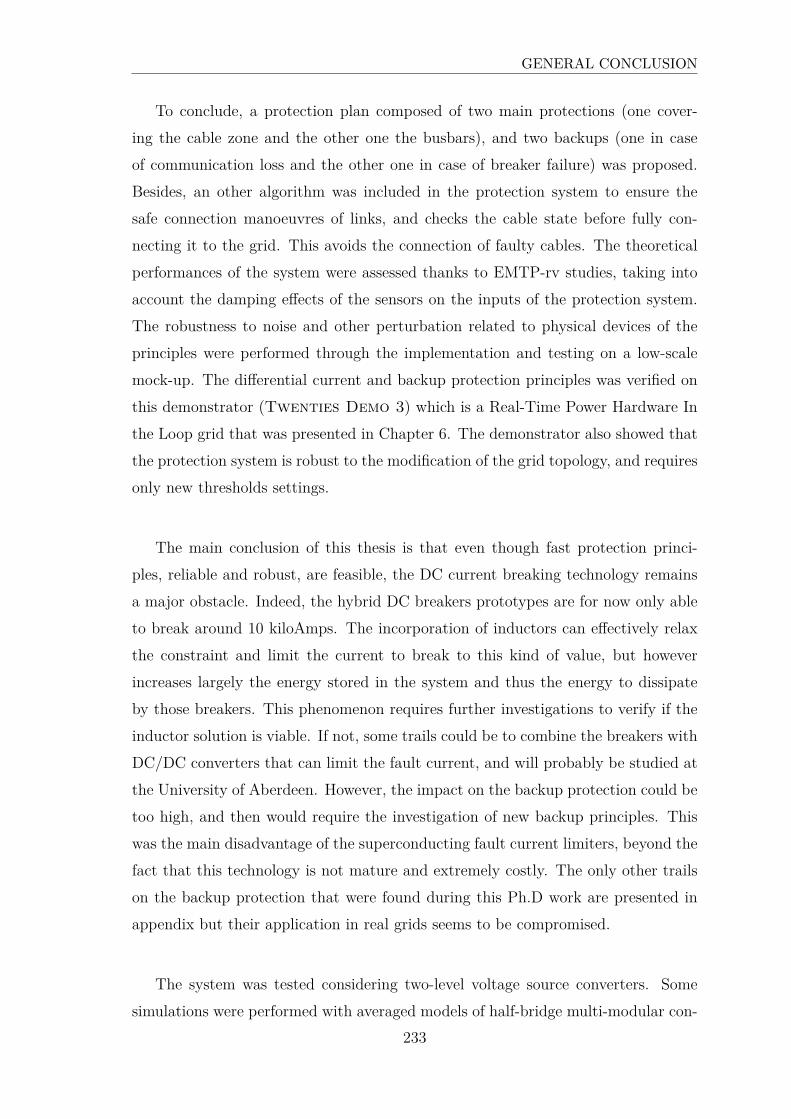
GENERAL CONCLUSION
To conclude, a protection plan composed of two main protections (one cover-
ing the cable zone and the other one the busbars), and two backups (one in case
of communication loss and the other one in case of breaker failure) was proposed.
Besides, an other algorithm was included in the protection system to ensure the
safe connection manoeuvres of links, and checks the cable state before fully con-
necting it to the grid. This avoids the connection of faulty cables. The theoretical
performances of the system were assessed thanks to EMTP-rv studies, taking into
account the damping effects of the sensors on the inputs of the protection system.
The robustness to noise and other perturbation related to physical devices of the
principles were performed through the implementation and testing on a low-scale
mock-up. The differential current and backup protection principles was verified on
this demonstrator (Twenties Demo 3) which is a Real-Time Power Hardware In
the Loop grid that was presented in Chapter 6. The demonstrator also showed that
the protection system is robust to the modification of the grid topology, and requires
only new thresholds settings.
The main conclusion of this thesis is that even though fast protection princi-
ples, reliable and robust, are feasible, the DC current breaking technology remains
a major obstacle. Indeed, the hybrid DC breakers prototypes are for now only able
to break around 10 kiloAmps. The incorporation of inductors can effectively relax
the constraint and limit the current to break to this kind of value, but however
increases largely the energy stored in the system and thus the energy to dissipate
by those breakers. This phenomenon requires further investigations to verify if the
inductor solution is viable. If not, some trails could be to combine the breakers with
DC/DC converters that can limit the fault current, and will probably be studied at
the University of Aberdeen. However, the impact on the backup protection could be
too high, and then would require the investigation of new backup principles. This
was the main disadvantage of the superconducting fault current limiters, beyond the
fact that this technology is not mature and extremely costly. The only other trails
on the backup protection that were found during this Ph.D work are presented in
appendix but their application in real grids seems to be compromised.
The system was tested considering two-level voltage source converters. Some
simulations were performed with averaged models of half-bridge multi-modular con-
233
GENERAL CONCLUSION
verters, but the short transient study would require the use of detailed models.
Considering the large number of components, the simulations are too long and were
thus prohibited. Nevertheless, there is no reason that the differential current and the
voltage differential criteria would become less relevant with those converter technolo-
gies, since the traveling wave principle remains. This is not the case for the backup
protection, once again.
Full bridge converter types were not investigated since they suppose a totally
different protection strategy, due to their ability to delete the fault current them-
selves.
The main question remains in the validity of the cable model. Indeed, the global
work on the current to break evaluation is strongly dependent on the cable model
response. The WideBand model was chosen since it is the most complex and most
representative model, but no comparison with real DC cable tests were found in the
literature. The mock-up could not validate the model since the physical cables were
kept on their drums. Such physical tests and comparisons would be a huge step in
the validation of the DC grid behavior of EMTP-rv models. Note however that the
FDQ model response where sensitively close to the WideBand one. Adding to that,
a full DC breaker model would enable the validation of the protection system.
In this thesis, the protection of DC grids was investigated based on a DC grid
point of view only. The global transmission grid is composed at 99% of AC lines.
Therefore, the impact of the DC system has to be investigated from the AC grid
point of view, and that not only in terms of protection, but also considering the
overall operation of such DC grids, considering the bulk power they are supposed
to transmit.
234

GENERAL CONCLUSION
235


Appendices


Appendix A
Protection principles
1 Difficulty to find non-communicant selective prin-
ciples
As mentioned in Chapter 5, the selectivity (insulate only the faulty cable) cannot
be achieved if only a busbar level communication is considered.
Fig.A.1 shows the current measurements for busbar 1 and 3 for the two fault cases
Cint and Cext, defined in Chapter 5 and reminded in Tab.A.1. The idea here was
to find a criterion based on a busbar-level communication that enables a selective
detection.
Case name Type Link Location Rfault
Cint Pole-to-ground Link1, positive pole 30km away Station1 10Ω
Cext Pole-to-ground Link3, positive pole Near Station3 1Ω
Table A.1: Internal and external fault cases
Reminder
Fault Cint has to be cleared by PR13 and PR31.
Fault Cext has to be cleared by PR32 and PR23.
On Fig.A.1a, it can be noticed that the protection that has to trip (PR13) can
be discriminated from the other ones, since this is the only current that is positive
239
APPENDIX A. PROTECTION PRINCIPLES
and higher than the current of the station connection point protection PR1. This is
also the case for PR31 on Fig.A.1c and PR32 on Fig.A.1d. This criterion was thus
tested.
−2 −1 0 1 2 3 4 5
−8
−4
0
4
8
12
16
Time [ms]
Cur
rent
[kA
]
I1+
I12+
I13+
(a) Cint, Busbar 1
−2 −1 0 1 2 3 4 5
−8
−4
0
4
8
12
16
Time [ms]
Cur
rent
[kA
]
I1+
I12+
I13+
(b) Cext, Busbar 1
−2 −1 0 1 2 3 4 5
−6
−4
−2
0
2
4
6
8
10
Time [ms]
Cur
rent
[kA
]
I3+
I31+
I32+
(c) Cint, Busbar 3
−2 −1 0 1 2 3 4 5−20
−10
0
10
20
30
40
Time [ms]
Cur
rent
[kA
]
I3+
I31+
I32+
(d) Cext, Busbar 3
Figure A.1: Busbar-level measurements
However, on Fig.A.1b, there is also a positive current higher than the other ones
(I13+), but for this fault, PR13 must not trip since the fault is on another link. This
phenomenon is also highlighted on Fig.A.2 for the measurements of busbar 2 and
4 for the fault Cint. On Fig.A.2a, there would be an unwanted tripping from PR21,
and another one by PR42 on Fig.A.2b.
240

2. BACKUP PROTECTION: OTHER TRAILS
−2 −1 0 1 2 3 4 5
−8
−4
0
4
8
Time [ms]
Cur
rent
[kA
]
I2+
I21+
I23+
I24+
(a) Cint, Busbar 2
−2 −1 0 1 2 3 4 5−8
−4
0
4
8
Time [ms]
Cur
rent
[kA
]
I4+
I42+
I45+
(b) Cint, Busbar 4
Figure A.2: Busbar-level other measurements
This is example was given to show that some simple criteria might be found but
can result in unwanted trippings for some cases.
2 Backup protection: other trails
Other trails were investigated for the backup protection. They are all based
on complex signal processing techniques and thus require large computation times.
This is why they were investigated only considering high fault resistances, which
avoid the time constraint given by the current flowing through the diodes.
At the time those principles were imagined, another grid structure was under
used for EMTP-rv simulation. The examples will thus be illustrated using the grid
shown on Fig.A.3.
241
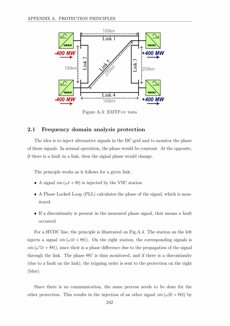
APPENDIX A. PROTECTION PRINCIPLES
+400 MW
+400 MW
-400 MW
-400 MW 100km
270km 250km150km
100km
Link 1
Link
2
Link
3
Link 4Link
5Figure A.3: EMTP-rv tests
2.1 Frequency domain analysis protection
The idea is to inject alternative signals in the DC grid and to monitor the phase
of those signals. In normal operation, the phase would be constant. At the opposite,
if there is a fault in a link, then the signal phase would change.
The principle works as it follows for a given link:
• A signal sin (ωt+ Θ) is injected by the VSC station
• A Phase Locked Loop (PLL) calculates the phase of the signal, which is mon-
itored
• If a discontinuity is present in the measured phase signal, that means a fault
occurred
For a HVDC line, the principle is illustrated on Fig.A.4. The station on the left
injects a signal sin (ω1t+ Θ1). On the right station, the corresponding signals is
sin (ω′1t+ Θ1), since their is a phase difference due to the propagation of the signal
through the link. The phase Θ1′ is thus monitored, and if there is a discontinuity
(due to a fault on the link), the tripping order is sent to the protection on the right
(blue).
Since there is no communication, the same process needs to be done for the
other protection. This results in the injection of an other signal sin (ω2t+ Θ2) by
242
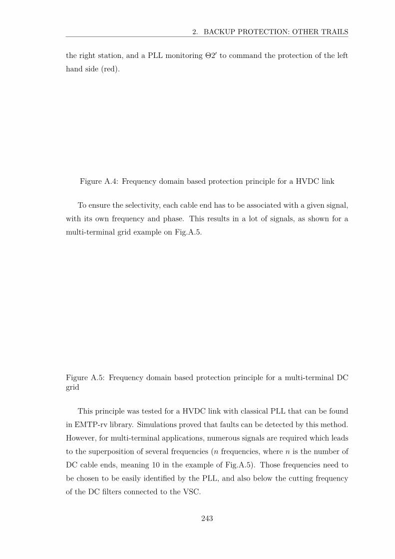
2. BACKUP PROTECTION: OTHER TRAILS
the right station, and a PLL monitoring Θ2′ to command the protection of the left
hand side (red).
Figure A.4: Frequency domain based protection principle for a HVDC link
To ensure the selectivity, each cable end has to be associated with a given signal,
with its own frequency and phase. This results in a lot of signals, as shown for a
multi-terminal grid example on Fig.A.5.
PLL
PLL PLL
PLL
Figure A.5: Frequency domain based protection principle for a multi-terminal DCgrid
This principle was tested for a HVDC link with classical PLL that can be found
in EMTP-rv library. Simulations proved that faults can be detected by this method.
However, for multi-terminal applications, numerous signals are required which leads
to the superposition of several frequencies (n frequencies, where n is the number of
DC cable ends, meaning 10 in the example of Fig.A.5). Those frequencies need to
be chosen to be easily identified by the PLL, and also below the cutting frequency
of the DC filters connected to the VSC.
243
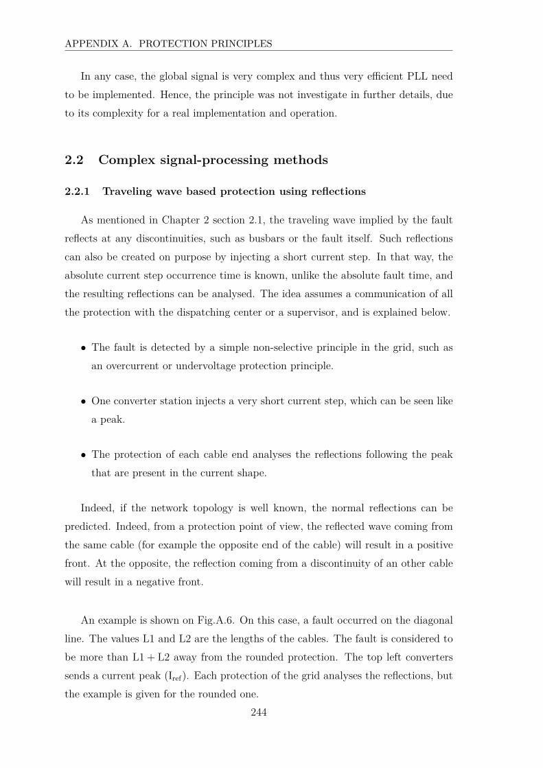
APPENDIX A. PROTECTION PRINCIPLES
In any case, the global signal is very complex and thus very efficient PLL need
to be implemented. Hence, the principle was not investigate in further details, due
to its complexity for a real implementation and operation.
2.2 Complex signal-processing methods
2.2.1 Traveling wave based protection using reflections
As mentioned in Chapter 2 section 2.1, the traveling wave implied by the fault
reflects at any discontinuities, such as busbars or the fault itself. Such reflections
can also be created on purpose by injecting a short current step. In that way, the
absolute current step occurrence time is known, unlike the absolute fault time, and
the resulting reflections can be analysed. The idea assumes a communication of all
the protection with the dispatching center or a supervisor, and is explained below.
• The fault is detected by a simple non-selective principle in the grid, such as
an overcurrent or undervoltage protection principle.
• One converter station injects a very short current step, which can be seen like
a peak.
• The protection of each cable end analyses the reflections following the peak
that are present in the current shape.
Indeed, if the network topology is well known, the normal reflections can be
predicted. Indeed, from a protection point of view, the reflected wave coming from
the same cable (for example the opposite end of the cable) will result in a positive
front. At the opposite, the reflection coming from a discontinuity of an other cable
will result in a negative front.
An example is shown on Fig.A.6. On this case, a fault occurred on the diagonal
line. The values L1 and L2 are the lengths of the cables. The fault is considered to
be more than L1 + L2 away from the rounded protection. The top left converters
sends a current peak (Iref). Each protection of the grid analyses the reflections, but
the example is given for the rounded one.
244

2. BACKUP PROTECTION: OTHER TRAILS
Figure A.6: Illustration of the protection principle based on a current step injectionfor a healthy link
In any cases (different lengths), the normal reflections can be predicted. Thus,
if another reflection is seen, it corresponds to the fault. Furthermore, if this non-
predicted reflection results in a positive front (Fig.A.7), then the fault is on the cable
where the considered protection is connected, and the tripping order can be sent.
245

APPENDIX A. PROTECTION PRINCIPLES
Figure A.7: Illustration of the protection principle based on a current step injectionfor a faulty link
The protection can thus follow the rules below:
1. Detection of the fault somewhere in the grid
2. Non response of the main protection algorithms
3. The converter stations send successively current peaks until the faulty link is
identified.
A converter station send a current peak once the previous one is mitigated enough
to ensure that the reflection analysis will not be altered by the previous reflections.
This principle was tested using EMTP-rv simulations on the MTDC grid of
Fig.A.3. The current measurements for the faulty link are shown on Fig.A.8 for two
fault cases with resistance of 100Ω and 200Ω.
246
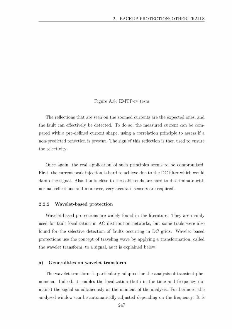
2. BACKUP PROTECTION: OTHER TRAILS
Figure A.8: EMTP-rv tests
The reflections that are seen on the zoomed currents are the expected ones, and
the fault can effectively be detected. To do so, the measured current can be com-
pared with a pre-defined current shape, using a correlation principle to assess if a
non-predicted reflection is present. The sign of this reflection is then used to ensure
the selectivity.
Once again, the real application of such principles seems to be compromised.
First, the current peak injection is hard to achieve due to the DC filter which would
damp the signal. Also, faults close to the cable ends are hard to discriminate with
normal reflections and moreover, very accurate sensors are required.
2.2.2 Wavelet-based protection
Wavelet-based protections are widely found in the literature. They are mainly
used for fault localization in AC distribution networks, but some trails were also
found for the selective detection of faults occurring in DC grids. Wavelet based
protections use the concept of traveling wave by applying a transformation, called
the wavelet transform, to a signal, as it is explained below.
a) Generalities on wavelet transform
The wavelet transform is particularly adapted for the analysis of transient phe-
nomena. Indeed, it enables the localization (both in the time and frequency do-
mains) the signal simultaneously at the moment of the analysis. Furthermore, the
analysed window can be automatically adjusted depending on the frequency. It is
247

APPENDIX A. PROTECTION PRINCIPLES
possible to decompose the signal into several frequency ranges, which is suitable
with the propagation of the waves whose characteristics vary with the frequency.
This is why those aspects seem to be interesting for fault detection. The detail of
wavelet transform is not detailed here but the reader can refer to [Mallat, 2008] for
further information. In order to understand the global principle, a short description
is presented.
Wavelet transform decomposes a signal based on a wavelet family, thanks to a
scalar product. The resulting numbers are traditionally called wavelet coefficients.
This wavelet family is composed of translations and dilatations of a mother wavelet
ψ. The components of the family are defined by (A.1):
ψu,s(t) =1√sψ(
t− u
s
)
(A.1)
where u and s are reals which represent the translation parameter and the scaling
factor of the decomposition respectively.
Hence, the continuous wavelet transform of a signal f is defined by (A.2):
Wf (u, s) = 〈f, ψu,s〉 =∫ +∞
−∞f(t)
1√sψ(
t− u
s
)
dt (A.2)
Several kinds of wavelet transform can be applied, and the principle has already
been widely used for AC distribution grids. The discrete wavelet transform is the
most appropriate since the signal to be transform is sampled, and the dyadic trans-
form is usually employed [Evrenosoglu and Abur, 2005]. It consists in sampling the
scaling factor s and the translation parameter u in powers of 2. Thus, they can be
written s = 2j and u = k.2j. This method is equivalent to treat the wavelet trans-
form like a filter bank. For each decomposition level, two coefficients are evaluated:
an approximation coefficient (A), that corresponds to low frequencies components,
and a detail coefficient (D), which corresponds to high frequencies components. Each
level corresponds to a time and frequency range. The global idea is represented on
Fig.A.9.
248
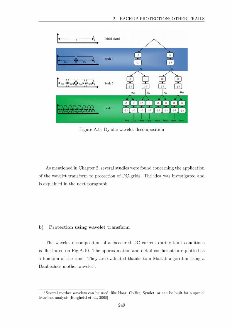
2. BACKUP PROTECTION: OTHER TRAILS
Initial signal
Scale 2
Scale 1
Scale 3
Figure A.9: Dyadic wavelet decomposition
As mentioned in Chapter 2, several studies were found concerning the application
of the wavelet transform to protection of DC grids. The idea was investigated and
is explained in the next paragraph.
b) Protection using wavelet transform
The wavelet decomposition of a measured DC current during fault conditions
is illustrated on Fig.A.10. The approximation and detail coefficients are plotted as
a function of the time. They are evaluated thanks to a Matlab algorithm using a
Daubechies mother wavelet1.
1Several mother wavelets can be used, like Haar, Coiflet, Symlet, or can be built for a specialtransient analysis [Borghetti et al., 2008]
249
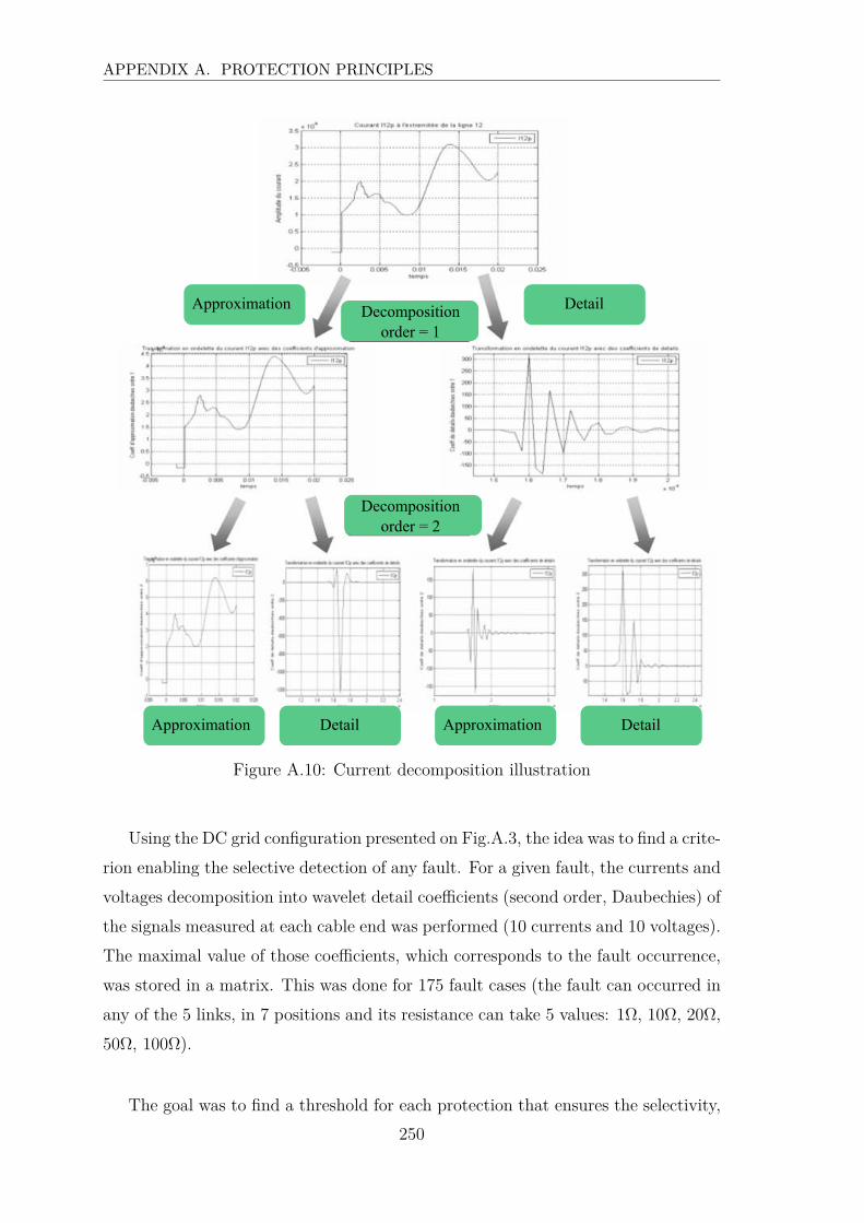
APPENDIX A. PROTECTION PRINCIPLES
Approximation DetailDecomposition order = 1
Decomposition order = 2
Approximation Approximation DetailDetail
Figure A.10: Current decomposition illustration
Using the DC grid configuration presented on Fig.A.3, the idea was to find a crite-
rion enabling the selective detection of any fault. For a given fault, the currents and
voltages decomposition into wavelet detail coefficients (second order, Daubechies) of
the signals measured at each cable end was performed (10 currents and 10 voltages).
The maximal value of those coefficients, which corresponds to the fault occurrence,
was stored in a matrix. This was done for 175 fault cases (the fault can occurred in
any of the 5 links, in 7 positions and its resistance can take 5 values: 1Ω, 10Ω, 20Ω,
50Ω, 100Ω).
The goal was to find a threshold for each protection that ensures the selectivity,
250

2. BACKUP PROTECTION: OTHER TRAILS
meaning that for a given protection, the threshold is exceeded for any fault occurring
on the cable it is connected to, and this threshold is not exceeded for any other faults,
external to the link. A criterion based on such threshold and assuming a cable-level
communication was found, but is similar to the directional criterion developed in
Chapter 5 section 3.4.2. In this case, the recourse to complex signal processing
methods such as the wavelet transform would be useless, so a criterion assuming no
communication was investigated. However, no solution were found considering all
those faults. Indeed, the selectivity might be ensured for faults with resistance of 1Ω,
but the higher fault resistance cases then are not detected. Even though, a multi-
criterion principle was considered, but does not provide any advantages compared
to the backup protection proposal of Chapter 5 section 4.
251

APPENDIX A. PROTECTION PRINCIPLES
252
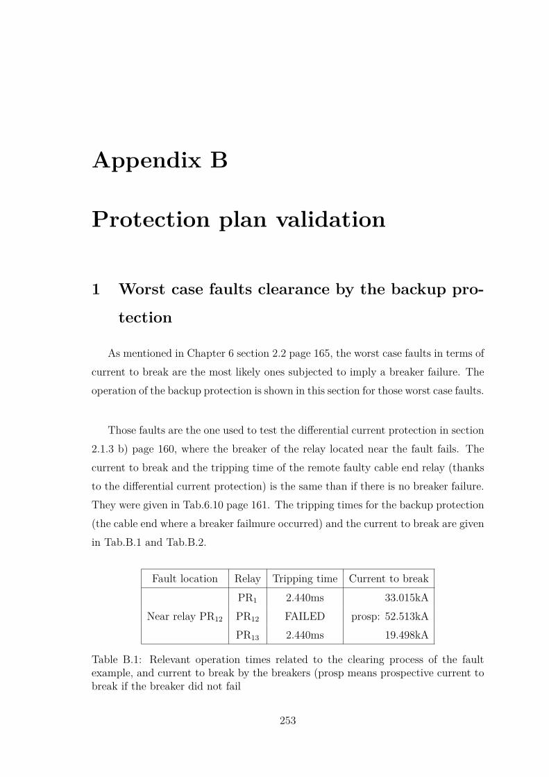
Appendix B
Protection plan validation
1 Worst case faults clearance by the backup pro-
tection
As mentioned in Chapter 6 section 2.2 page 165, the worst case faults in terms of
current to break are the most likely ones subjected to imply a breaker failure. The
operation of the backup protection is shown in this section for those worst case faults.
Those faults are the one used to test the differential current protection in section
2.1.3 b) page 160, where the breaker of the relay located near the fault fails. The
current to break and the tripping time of the remote faulty cable end relay (thanks
to the differential current protection) is the same than if there is no breaker failure.
They were given in Tab.6.10 page 161. The tripping times for the backup protection
(the cable end where a breaker failmure occurred) and the current to break are given
in Tab.B.1 and Tab.B.2.
Fault location Relay Tripping time Current to break
Near relay PR12
PR1 2.440ms 33.015kA
PR12 FAILED prosp: 52.513kA
PR13 2.440ms 19.498kA
Table B.1: Relevant operation times related to the clearing process of the faultexample, and current to break by the breakers (prosp means prospective current tobreak if the breaker did not fail
253
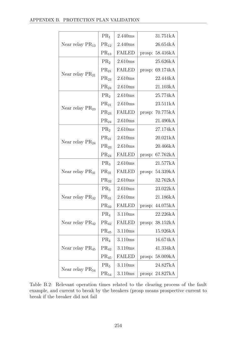
APPENDIX B. PROTECTION PLAN VALIDATION
Near relay PR13
PR1 2.440ms 31.751kA
PR12 2.440ms 26.654kA
PR13 FAILED prosp: 58.416kA
Near relay PR21
PR2 2.610ms 25.626kA
PR21 FAILED prosp: 69.174kA
PR23 2.610ms 22.444kA
PR24 2.610ms 21.103kA
Near relay PR23
PR2 2.610ms 25.774kA
PR21 2.610ms 23.511kA
PR23 FAILED prosp: 70.775kA
PR24 2.610ms 21.490kA
Near relay PR24
PR2 2.610ms 27.174kA
PR21 2.610ms 20.021kA
PR23 2.610ms 20.466kA
PR24 FAILED prosp: 67.762kA
Near relay PR31
PR3 2.610ms 21.577kA
PR31 FAILED prosp: 54.339kA
PR32 2.610ms 32.762kA
Near relay PR32
PR3 2.610ms 23.022kA
PR31 2.610ms 21.186kA
PR32 FAILED prosp: 44.075kA
Near relay PR42
PR4 3.110ms 22.226kA
PR42 FAILED prosp: 38.152kA
PR45 3.110ms 15.926kA
Near relay PR45
PR4 3.110ms 16.674kA
PR42 3.110ms 41.334kA
PR45 FAILED prosp: 58.009kA
Near relay PR54
PR5 3.110ms 24.827kA
PR54 3.110ms prosp: 24.827kA
Table B.2: Relevant operation times related to the clearing process of the faultexample, and current to break by the breakers (prosp means prospective current tobreak if the breaker did not fail
254
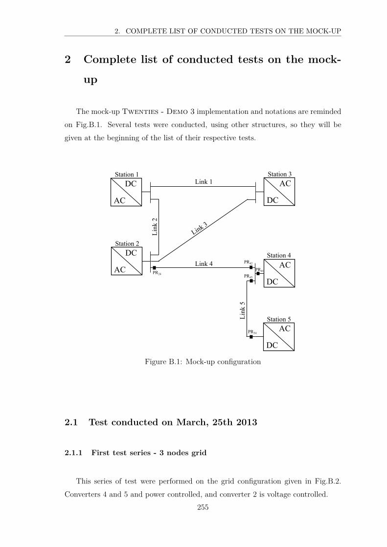
2. COMPLETE LIST OF CONDUCTED TESTS ON THE MOCK-UP
2 Complete list of conducted tests on the mock-
up
The mock-up Twenties - Demo 3 implementation and notations are reminded
on Fig.B.1. Several tests were conducted, using other structures, so they will be
given at the beginning of the list of their respective tests.
AC
DC AC
DC
Link 1Station 1
AC
DCStation 2
Link 4 AC
DC
AC
DC
Station 3
Station 4
Station 5
Link
2
Link
5Link 3
PR42
PR41
PR45PR24
PR54
Figure B.1: Mock-up configuration
2.1 Test conducted on March, 25th 2013
2.1.1 First test series - 3 nodes grid
This series of test were performed on the grid configuration given in Fig.B.2.
Converters 4 and 5 and power controlled, and converter 2 is voltage controlled.
255

APPENDIX B. PROTECTION PLAN VALIDATION
Figure B.2: 3 nodes grid configuration
Only the main cable differential protection was implemented, and the threshold
value IdTH+ was set to 12A. The fault can be either on link 4 (horizontal) or on link
5 (vertical).
Test Fault position Rfault Operation point Tripping
T1 Link5 10Ω no power transfer OK
T2 Link5 10Ω station 5 injects 300W OK
T3 Link5 5Ω no power transfer OK
T4 Link5 5Ω station 5 injects 300W OK
T5 Link4 10Ω no power transfer OK
Table B.3: First test series, tripping OK means that the fault is cleared with themain cable differential protection
Between tests T5 and T6, the master and slave controlled converters were ex-
changed.
Test Fault position Rfault Operation point Tripping
T6 Link4 10Ω no power transfer OK
T7 Link4 10Ω station 5 injects 300W OK
T8 Link4 5Ω no power transfer OK
Table B.4: First test series, tripping OK means that the fault is cleared with themain cable differential protection
256

2. COMPLETE LIST OF CONDUCTED TESTS ON THE MOCK-UP
2.1.2 Second test series
This test series was conducted on the 5 nodes grid structure given on Fig.B.1.
Converters 3, 4 and 5 are power controlled, and converters 1 and 2 are drooped
controlled. Only converters 2 and 5 are physical.
Test Fault position Rfault Operation point Tripping
T10 Link4 10Ω station 5 injects 300W OK
T11 Link5 10Ω stations 3, 4 and 5 inject
respectively 600W, 390W
and 220W
OK
T12 Link5 5Ω stations 3, 4 and 5 inject
respectively 600W, 390W
and 220W
OK
Table B.5: First test series, tripping OK means that the fault is cleared with themain cable differential protection
2.2 Test conducted on May, 29th 2013 - Preparation of the
backup mode
2.2.1 Test 20
No physical converter is connected, all the stations are the amplifiers. A load is
placed near station 5 to create a power transfer.
Cable differential protection threshold is set to 6A.
The fault on link 5, with a resistance of 5Ω is cleared by the differential protection
at PR54, but the breaker of PR45 is set to trip 10ms after.
2.2.2 Test 21
The node near station 2 is disconnected to the source. Converter of station 5 is
physical, and no power transfer is created.
257

APPENDIX B. PROTECTION PLAN VALIDATION
The threshold IdTH+ is set to 12A, and the 5Ω fault on link 5 is cleared 3.140ms
after its occurrence.
2.2.3 Test 22
The same configuration than test 21 is used and the same fault is done. The
differential protection is disconnected at PR54, so the backup can be tested.
The fault is cleared by the cable differential protection at PR45, and by the
backup at PR54.
2.2.4 Test 23
The same configuration than the two previous tests is used, and station 5 injects
300W. A fault of 10Ω is done on link 4, and is cleared by the differential protection
at both cable ends.
258

2. COMPLETE LIST OF CONDUCTED TESTS ON THE MOCK-UP
259


Bibliography


Bibliography
[Aimin et al., 2009] Aimin, L., Zexiang, C., Qizhen, S., Xiaohua, L., Dayong, R.,
and Zeming, Y. (2009). Study on the dynamic performance characteristics of
hvdc control and protections for the hvdc line fault. In Power and Energy Society
General Meeting, PES.
[Andersen and al., 2005] Andersen, B. and al. (2005). Vsc transmission. Technical
report, CIGRE.
[Andrea et al., 2010a] Andrea, J., Schweitzer, P., and Tisserand, E. (2010a). A
new dc and ac arc fault electrical model. In Electrical Contacts (HOLM), 2010
Proceedings of the 56th IEEE Holm Conference on, pages 1–6.
[Andrea et al., 2010b] Andrea, J., Schweitzer, P., Tisserand, E., Roth, P., and We-
ber, S. (2010b). Repeatable and calibrated arc fault generator. In Industrial
Electronics (ISIE), 2010 IEEE International Symposium on, pages 1022–1026.
[Asplund, 2004] Asplund, G. (2004). Sustainable energy systems with hvdc trans-
mission. In IEEE Power Engineering Society General Meeting.
[Bahrman et al., 2003] Bahrman, M., Johansson, J., and Nilsson, B. (2003). Voltage
source converter transmission technologies: the right fit for the application. In
Power Engineering Society General Meeting, 2003, IEEE, volume 3, pages –1847
Vol. 3.
[Borghetti et al., 2008] Borghetti, A., Bosetti, M., Di Silvestro, M., Nucci, C. A.,
and Paolone, M. (2008). Continuous-wavelet transform for fault location in dis-
tribution power networks: Definition of mother wavelets inferred from fault orig-
inated transients. Power systems, IEEE Transactions on, 23(2):380–388.
[Correvon, 2005] Correvon, M. (2005). Mesure de courant, transducers, hes so
course on système électroniques.
263
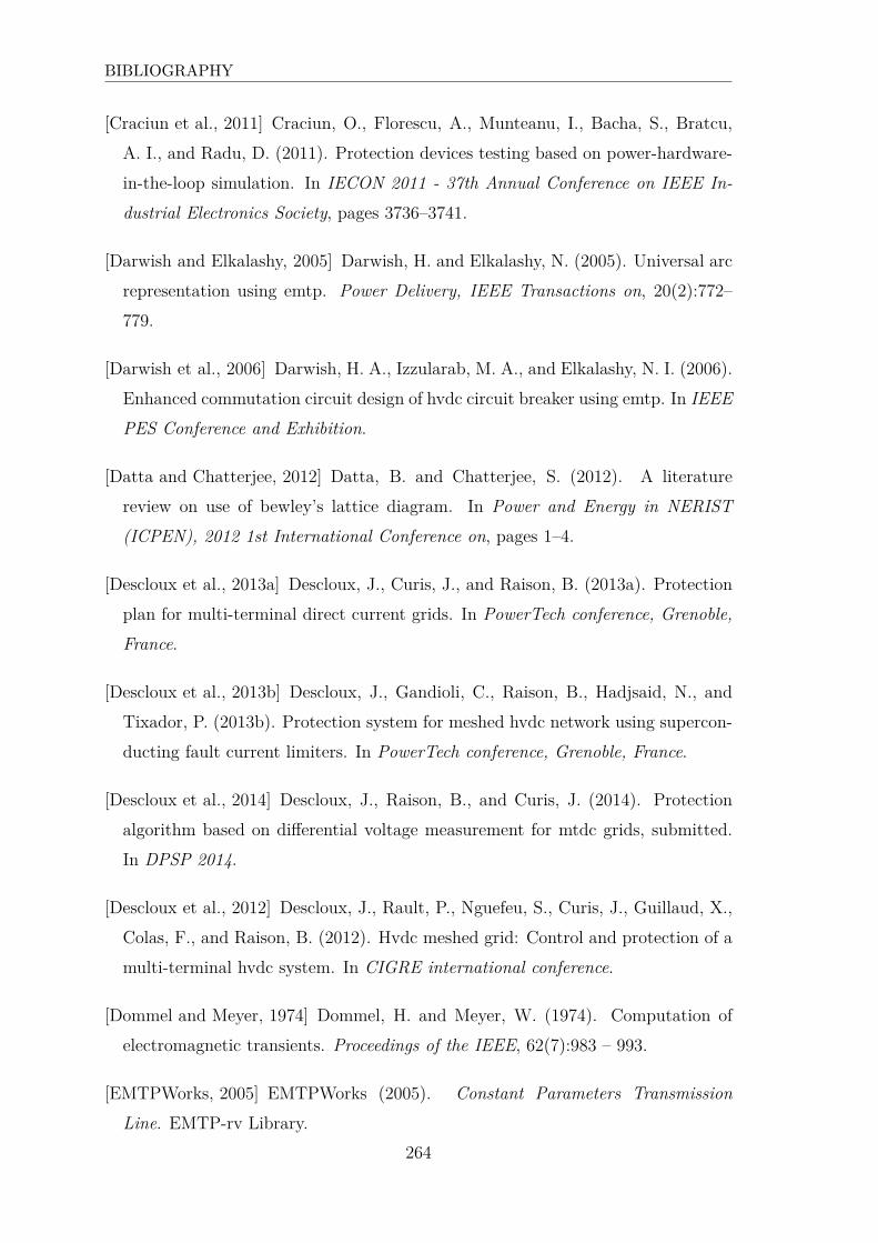
BIBLIOGRAPHY
[Craciun et al., 2011] Craciun, O., Florescu, A., Munteanu, I., Bacha, S., Bratcu,
A. I., and Radu, D. (2011). Protection devices testing based on power-hardware-
in-the-loop simulation. In IECON 2011 - 37th Annual Conference on IEEE In-
dustrial Electronics Society, pages 3736–3741.
[Darwish and Elkalashy, 2005] Darwish, H. and Elkalashy, N. (2005). Universal arc
representation using emtp. Power Delivery, IEEE Transactions on, 20(2):772–
779.
[Darwish et al., 2006] Darwish, H. A., Izzularab, M. A., and Elkalashy, N. I. (2006).
Enhanced commutation circuit design of hvdc circuit breaker using emtp. In IEEE
PES Conference and Exhibition.
[Datta and Chatterjee, 2012] Datta, B. and Chatterjee, S. (2012). A literature
review on use of bewley’s lattice diagram. In Power and Energy in NERIST
(ICPEN), 2012 1st International Conference on, pages 1–4.
[Descloux et al., 2013a] Descloux, J., Curis, J., and Raison, B. (2013a). Protection
plan for multi-terminal direct current grids. In PowerTech conference, Grenoble,
France.
[Descloux et al., 2013b] Descloux, J., Gandioli, C., Raison, B., Hadjsaid, N., and
Tixador, P. (2013b). Protection system for meshed hvdc network using supercon-
ducting fault current limiters. In PowerTech conference, Grenoble, France.
[Descloux et al., 2014] Descloux, J., Raison, B., and Curis, J. (2014). Protection
algorithm based on differential voltage measurement for mtdc grids, submitted.
In DPSP 2014.
[Descloux et al., 2012] Descloux, J., Rault, P., Nguefeu, S., Curis, J., Guillaud, X.,
Colas, F., and Raison, B. (2012). Hvdc meshed grid: Control and protection of a
multi-terminal hvdc system. In CIGRE international conference.
[Dommel and Meyer, 1974] Dommel, H. and Meyer, W. (1974). Computation of
electromagnetic transients. Proceedings of the IEEE, 62(7):983 – 993.
[EMTPWorks, 2005] EMTPWorks (2005). Constant Parameters Transmission
Line. EMTP-rv Library.
264
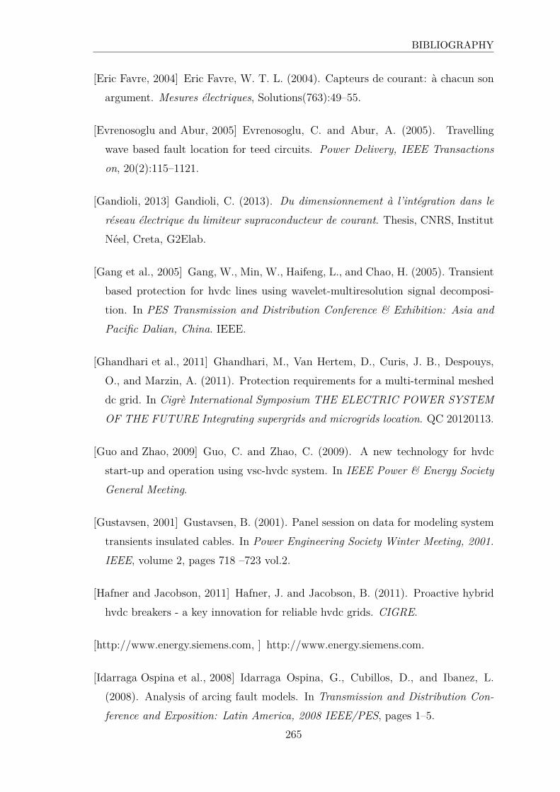
BIBLIOGRAPHY
[Eric Favre, 2004] Eric Favre, W. T. L. (2004). Capteurs de courant: à chacun son
argument. Mesures électriques, Solutions(763):49–55.
[Evrenosoglu and Abur, 2005] Evrenosoglu, C. and Abur, A. (2005). Travelling
wave based fault location for teed circuits. Power Delivery, IEEE Transactions
on, 20(2):115–1121.
[Gandioli, 2013] Gandioli, C. (2013). Du dimensionnement à l’intégration dans le
réseau électrique du limiteur supraconducteur de courant. Thesis, CNRS, Institut
Néel, Creta, G2Elab.
[Gang et al., 2005] Gang, W., Min, W., Haifeng, L., and Chao, H. (2005). Transient
based protection for hvdc lines using wavelet-multiresolution signal decomposi-
tion. In PES Transmission and Distribution Conference & Exhibition: Asia and
Pacific Dalian, China. IEEE.
[Ghandhari et al., 2011] Ghandhari, M., Van Hertem, D., Curis, J. B., Despouys,
O., and Marzin, A. (2011). Protection requirements for a multi-terminal meshed
dc grid. In Cigrè International Symposium THE ELECTRIC POWER SYSTEM
OF THE FUTURE Integrating supergrids and microgrids location. QC 20120113.
[Guo and Zhao, 2009] Guo, C. and Zhao, C. (2009). A new technology for hvdc
start-up and operation using vsc-hvdc system. In IEEE Power & Energy Society
General Meeting.
[Gustavsen, 2001] Gustavsen, B. (2001). Panel session on data for modeling system
transients insulated cables. In Power Engineering Society Winter Meeting, 2001.
IEEE, volume 2, pages 718 –723 vol.2.
[Hafner and Jacobson, 2011] Hafner, J. and Jacobson, B. (2011). Proactive hybrid
hvdc breakers - a key innovation for reliable hvdc grids. CIGRE.
[http://www.energy.siemens.com, ] http://www.energy.siemens.com.
[Idarraga Ospina et al., 2008] Idarraga Ospina, G., Cubillos, D., and Ibanez, L.
(2008). Analysis of arcing fault models. In Transmission and Distribution Con-
ference and Exposition: Latin America, 2008 IEEE/PES, pages 1–5.
265
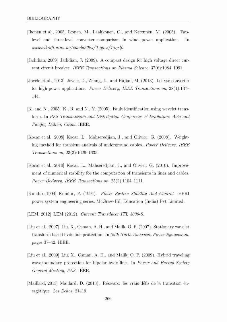
BIBLIOGRAPHY
[Ikonen et al., 2005] Ikonen, M., Laakkonen, O., and Kettunen, M. (2005). Two-
level and three-level converter comparison in wind power application. In
www.elkraft.ntnu.no/smola2005/Topics/15.pdf.
[Jadidian, 2009] Jadidian, J. (2009). A compact design for high voltage direct cur-
rent circuit breaker. IEEE Transactions on Plasma Science, 37(6):1084–1091.
[Jovcic et al., 2013] Jovcic, D., Zhang, L., and Hajian, M. (2013). Lcl vsc converter
for high-power applications. Power Delivery, IEEE Transactions on, 28(1):137–
144.
[K. and N., 2005] K., R. and N., Y. (2005). Fault identification using wavelet trans-
form. In PES Transmission and Distribution Conference & Exhibition: Asia and
Pacific, Dalien, China. IEEE.
[Kocar et al., 2008] Kocar, L., Mahseredjian, J., and Olivier, G. (2008). Weight-
ing method for transient analysis of underground cables. Power Delivery, IEEE
Transactions on, 23(3):1629–1635.
[Kocar et al., 2010] Kocar, L., Mahseredjian, J., and Olivier, G. (2010). Improve-
ment of numerical stability for the computation of transients in lines and cables.
Power Delivery, IEEE Transactions on, 25(2):1104–1111.
[Kundur, 1994] Kundur, P. (1994). Power System Stability And Control. EPRI
power system engineering series. McGraw-Hill Education (India) Pvt Limited.
[LEM, 2012] LEM (2012). Current Transducer ITL 4000-S.
[Liu et al., 2007] Liu, X., Osman, A. H., and Malik, O. P. (2007). Stationary wavelet
transform based hvdc line protection. In 39th North American Power Symposium,
pages 37–42. IEEE.
[Liu et al., 2009] Liu, X., Osman, A. H., and Malik, O. P. (2009). Hybrid traveling
wave/boundary protection for bipolar hvdc line. In Power and Energy Society
General Meeting, PES. IEEE.
[Maillard, 2013] Maillard, D. (2013). Réseaux: les vrais défis de la transition én-
ergétique. Les Echos, 21419.
266
BIBLIOGRAPHY
[Mallat, 2008] Mallat, S. (2008). A Wavelet Tour of Signal Processing, Third Edi-
tion: The Sparse Way. Academic Press, 3rd edition.
[Marti, 1982] Marti, J. (1982). Accuarte modelling of frequency-dependent trans-
mission lines in electromagnetic transient simulations. Power Apparatus and Sys-
tems, IEEE Transactions on, PAS-101(1):147 –157.
[Marti, 1988] Marti, L. (1988). Simulation of transients in underground cables
with frequency-dependent modal transformation matrices. Power Delivery, IEEE
Transactions on, 3(3):1099 –1110.
[Marti, 1993] Marti, L. (1993). Simulation of electromagnetic transients in under-
ground cables using the emtp. In Advances in Power System Control, Operation
and Management, 1993. APSCOM-93., 2nd International Conference on, pages
147 –152 vol.1.
[Meyer et al., 2005] Meyer, C., Kowal, M., and Doncker, R. W. D. (2005). Circuit
breaker concepts for future high-power dc-applications. IEEE IAS, nan:p. 860–
866.
[Mitsubishi, 2009] Mitsubishi (2009). Mitsubishi hvigbt modules cm1500hc-66r.
Technical report, Mitsubishi.
[Morched et al., 1999] Morched, A., Gustavsen, B., and Tartibi, M. (1999). A uni-
versal model for accurate calculation of electromagnetic transients on overhead
lines and underground cables. Power Delivery, IEEE Transactions on, 14(3):1032
–1038.
[Naidoo and Ijumba, 2004] Naidoo, D. and Ijumba, N. M. (2004). Hvdc line protec-
tion for the proposed future hvdc systems. In International Conference on Power
System Technology, POWERCON, Singapore, pages 1327–1332. IEEE.
[Naidoo and Ijumba, 2005] Naidoo, D. and Ijumba, N. M. (2005). A protection sys-
tem for long hvdc transmission lines. In Inaugural PES Conference and Exposition
in Africa, Durban, South Africa. IEEE.
[Nakao et al., 2001] Nakao, H., Nakagoshi, Y., Hatano, M., Koshizuka, T., Nishi-
waki, S., Kobayashi, A., Murao, T., and Yanabu, S. (2001). D.c. current inter-
267
BIBLIOGRAPHY
ruption in hvdc sf6 gas mrtb by means of self-excited oscillation superimposition.
IEEE Transactions on Power Delivery, 16(4):687–693.
[Nee and Angquist, 2010a] Nee, H.-P. and Angquist, L. (2010a). Perspectives on
power electronics and grid solutions for offshore wind farms. Technical Report
10:96, Elforsk.
[Nee and Angquist, 2010b] Nee, H.-P. and Angquist, L. (2010b). Perspectives on
power electronics and grid solutions for offshore wind farms. Technical Report
10:96, Elforsk.
[Nexans, 2013] Nexans (2013). Câbles sous-marins, www.nexans.fr. Consulted on
February, 2013.
[NEY, 2013] NEY, M. (2013). Bases de l’électromagnétisme. Tech-
niques de l’ingénieur Électromagnétisme. Propagation, base documentaire :
TIB277DUO.(ref. article : e1020). fre.
[Nguefeu et al., 2011] Nguefeu, S., Rault, P., Grieshaber, W., and Hassan, F.
(2011). Twenties delivrable 11.1, demo 3 requirement specifications: detailed
specifications for a dc network and detailed specifications for alstom grid’s dc
breaker. Technical report, RTE, ALSTOM Grid.
[PAYS, 2013a] PAYS, M. (2013a). Câbles de transport d’énergie applications. Tech-
niques de l’ingénieur Réseaux électriques mixtes - Ingénierie des réseaux, base
documentaire : TIB267DUO.(ref. article : d4521). fre.
[PAYS, 2013b] PAYS, M. (2013b). Câbles de transport d’énergie technologies. car-
actéristiques. Techniques de l’ingénieur Réseaux électriques mixtes - Ingénierie
des réseaux, base documentaire : TIB267DUO.(ref. article : d4520). fre.
[Pelenc, 2002] Pelenc, Y. (2002). Interruption des circuits alimentés en courant
continu. Techniques de l’ingénieur, D4 700:1–16.
[Peralta et al., 2012] Peralta, J., Saad, H., Dennetiere, S., Mahseredjian, J., and
Nguefeu, S. (2012). Detailed and averaged models for a 401-level mmc–hvdc
system. Power Delivery, IEEE Transactions on, 27(3):1501–1508.
268

BIBLIOGRAPHY
[Petersen, 1995] Petersen, A. (1995). Portable optical ac- and proposed dc-current
sensor for high voltage applications. Power Delivery, IEEE Transactions on,
10(2):595 –599.
[PuissanceAnalyse, 2012] PuissanceAnalyse (2012). HVDC : système de mesure
forts courants http://www.puissance-analyse.com/capteurs-de-courant/hvdc-
systeme-de-mesure-forts-courants.html, consulted on March 2013.
[Rahmatian and Ortega, 2006] Rahmatian, F. and Ortega, A. (2006). Applications
of optical current and voltage sensors in high-voltage systems. In Transmis-
sion Distribution Conference and Exposition: Latin America, 2006. TDC ’06.
IEEE/PES, pages 1 –4.
[Rault, 2013] Rault, P. (2013). Control and stability of VSC-based MTDC grids.
Thesis, L2EP, Ecole Centrale Lille.
[RTE, 2006] RTE (2006). L’interconnexion électrique France – Angleterre
(IFA2000), un maillon stratégique au coeur de l’Europe de l’Électricité.
[Saad et al., 2013] Saad, H., Peralta, J., Dennetiere, S., Mahseredjian, J., Jatske-
vich, J., Martinez, J., Davoudi, A., Saeedifard, M., Sood, V., Wang, X., Cano,
J., and Mehrizi-Sani, A. (2013). Dynamic averaged and simplified models for
mmc-based hvdc transmission systems. Power Delivery, IEEE Transactions on,
28(3):1723–1730.
[Sabonnadière and Hadjsaïd, 2007] Sabonnadière, J.-C. and Hadjsaïd, N. (2007).
Lignes et réseaux électriques 1. Hermes Science Publications.
[Schoenemann et al., 2004] Schoenemann, T., Kiefer, J., Leung, S. Y., Oerzen, B.,
Inkinen, T., and Huguenot, P. (2004). Commutation process in gas circuit break-
ers: close-operation and commutation failure during an open-operation. In Electri-
cal Contacts, 2004. Proceedings of the 50th IEEE Holm Conference on Electrical
Contacts and the 22nd International Conference on Electrical Contacts, pages
53–57.
[Shang et al., 2001] Shang, L., Herold, G., Jaeger, J., Krebs, R., and Kumar, A.
(2001). High-speed fault identification and protection for hvdc line using wavelet
technique. In Porto Power Tech Conference, Porto, Portugal, volume 3.
269
BIBLIOGRAPHY
[Siemens, 2008] Siemens (2008). Guide de mise en service et de maintenance,
equipement de protection siemens 7sd52, 7sd52-service-v2-7. Technical report,
Siemens.
[Takahashi et al., 2010] Takahashi, M., Sasaki, K., Hirata, Y., Murao, T., Takeda,
H., Nakamura, Y., Ohtsuka, T., Sakai, T., and Nosaka, N. (2010). Field test of dc
optical current transformer for hvdc link. In Power and Energy Society General
Meeting, 2010 IEEE, pages 1 –6.
[Tang, 2003] Tang, L. (2003). Control and protection of Multi-Terminal DC trans-
mission systems based on Voltage Source Converters. Thesis, McGill University,
Department of Electrical and Computer Engineering, Montreal, Quebec, Canada.
[TechnoScience, 2012] TechnoScience (2012). Techno-science website. Consulted on
February, 2013.
[Thomas et al., 2009] Thomas, D., Sumner, M., Coggins, D., Wang, X., Wang, J.,
and Geertsma, L. R. (2009). Fault location for dc marine power systems. In
Electric Ship Technologies Symposium, ESTS, pages 456–460. IEEE.
[Tixador and Brunet, 2007] Tixador, P. and Brunet, Y. (2007). Supraconducteurs,
bases théoriques. Techniques de l’ingénieur, D2 701.
[Tixador et al., 2011] Tixador, P., Nguyen Nhat, T., Okada Vieira, H.,
and Ponceau, R. (2011). Impact of conductor inhomogeneity on fcl transient
performance. IEEE transactions on applied superconductivity, 21.
[Vacquié, 1986] Vacquié, S. (1986). Arc électrique. Techniques de l’ingénieur, D
324:1–16.
[Valenza and Cipollini, 1995] Valenza, D. and Cipollini, G. (1995). Hvdc submarine
power cables systems state of the art and future developments. In Energy Manage-
ment and Power Delivery, 1995. Proceedings of EMPD ’95., 1995 International
Conference, IEEE.
[Vissouvanadin Soubaretty, 2011] Vissouvanadin Soubaretty, B. (2011). Matéri-
aux de câble à isolation synthétique pour des applications au transport d’énergie
HVDC. Thesis, Univerité de Toulouse.
270

BIBLIOGRAPHY
[You et al., 2009] You, M., Zhang, B.-H., Cao, R.-F., Xu, J.-D., Zhang, S., Bo, Z.-
Q., and Klimek, A. (2009). Study of non-unit transient-based protection for hvdc
transmission lines. In Power and Energy Engineering Conference, APPEC Asia
Pacific.
[Zhen-Qiang and Lv, 2008] Zhen-Qiang and Lv, Y.-P. (2008). A novel scheme of
hvdc transmission line voltage traveling wave protection based on wavelet trans-
form. In International Conference on High Voltage Engineering and Application,
Chongqing, China. IEEE.
271


Resume etendu

Résumé étendu
La recherche et le développement de nouvelles solutions de transmission d’électricité
sont soutenus par la nécessité de transition énergétique globale, de par les préoccu-
pations relatives à l’augmentation de la consommation et au développement durable,
actuellement sujets de larges débats.
Dans ce contexte, l’Union Européenne a lancé un paquet nommé climat et én-
ergie, adopté par le Parlement Européen en décembre 2008. Ce paquet se concentre
notamment sur la réduction des émissions de gaz à effet de serre, la pénétration
des énergies renouvelables, l’efficacité énergétique, et soutient le célèbre objectif des
3x20, à savoir :
• 20% de réduction des émissions de gaz à effet de serre d’ici 2020,
• L’augmentation de l’efficacité énergétique de manière à économiser 20% de la
consommation énergétique européenne d’ici 2020,
• L’atteinte d’un taux de pénétration de 20% d’énergie renouvelable dans la
consommation énergétique totale de l’union européenne d’ici 2020.
Dans le cadre de la transition énergétique, les attentes en termes de réduction
de consommation et d’augmentation de productions décentralisées peuvent laisser
sous-entendre une baisse des besoins en transport d’électricité. Par ailleurs, le réseau
de transport est souvent associé à la production centralisée due à la forte proportion
de production nucléaire dans le mix énergétique français. Dans [Maillard, 2013],
le président du directoire de RTE revisite cette idée. Entre autres, l’éloignement
géographique des ressources solaires ou éoliennes par rapport aux lieux de consom-
mation, l’impossibilité d’absorber localement de fortes puissances produites et les
limites en termes de capacité de stockage sont soulignés. L’exemple allemand est
rappelé puisque le pays fait actuellement l’expérience d’un gâchis économique dû
275

RÉSUMÉ ÉTENDU
aux lacunes du réseau de transport, ce qui entraine parfois l’obligation de restrein-
dre la production d’origine renouvelable. Ses conclusions montrent que l’adaptation
du réseau de transport est un réel challenge à relever, sans quoi la transition énergé-
tique n’est pas possible, et ce indépendamment des choix retenus pour le futur.
Dans ce cadre, RTE participe au renforcement d’un réseau pan-européen, et à
long terme à la création d’un supergrid. Des projets européens émergent dans ce
sens, et plusieurs concepts de supergrid voient le jour. Alors que le projet Desertec
considère la liaison de l’Europe à des parcs photovoltaïques de grande ampleur en
Afrique, d’autres réseaux maillant la mer du Nord sont investigués.
Figure 6.3: Exemple de réseau maillé: http://www.greenunivers.com
Ces supergrids apparaissent comme des solutions complémentaires et nécessaires
à l’intégration des énergies d’origine renouvelable dans les mécanismes de marché
qui existent déjà. Grâce au renforcement des interconnexions entre tous les pays
européens, et à la mutualisation de l’électricité produite par les infrastructures les
plus efficaces, ces supergrids permettraient éventuellement une réduction du coût
total de l’énergie pour chaque pays participant, et l’amélioration de l’indépendance
énergétique de l’Europe.
Dans ce contexte, la Commission Européenne a démarré en 2010 le projet nommé
Twenties, qui vise à soutenir l’intégration de production d’électricité d’origine renou-
velable à large échelle dans le réseau de transport. Les 26 partenaires sont majori-
276
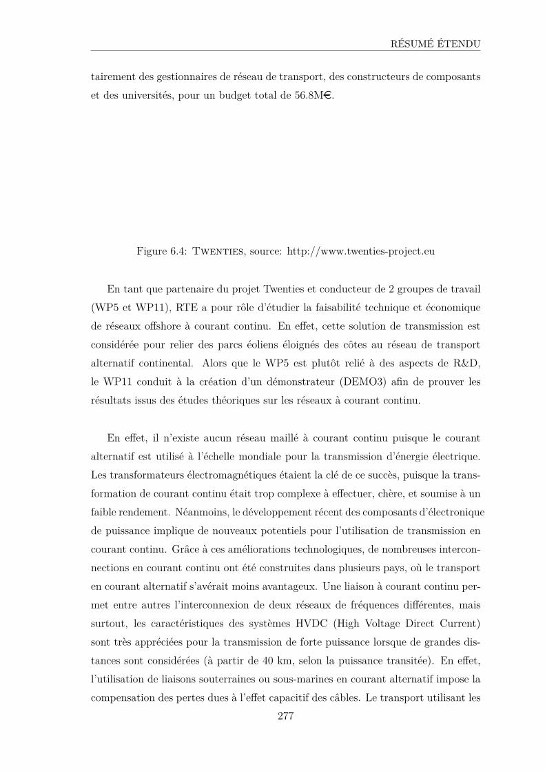
RÉSUMÉ ÉTENDU
tairement des gestionnaires de réseau de transport, des constructeurs de composants
et des universités, pour un budget total de 56.8Me.
Figure 6.4: Twenties, source: http://www.twenties-project.eu
En tant que partenaire du projet Twenties et conducteur de 2 groupes de travail
(WP5 et WP11), RTE a pour rôle d’étudier la faisabilité technique et économique
de réseaux offshore à courant continu. En effet, cette solution de transmission est
considérée pour relier des parcs éoliens éloignés des côtes au réseau de transport
alternatif continental. Alors que le WP5 est plutôt relié à des aspects de R&D,
le WP11 conduit à la création d’un démonstrateur (DEMO3) afin de prouver les
résultats issus des études théoriques sur les réseaux à courant continu.
En effet, il n’existe aucun réseau maillé à courant continu puisque le courant
alternatif est utilisé à l’échelle mondiale pour la transmission d’énergie électrique.
Les transformateurs électromagnétiques étaient la clé de ce succès, puisque la trans-
formation de courant continu était trop complexe à effectuer, chère, et soumise à un
faible rendement. Néanmoins, le développement récent des composants d’électronique
de puissance implique de nouveaux potentiels pour l’utilisation de transmission en
courant continu. Grâce à ces améliorations technologiques, de nombreuses intercon-
nections en courant continu ont été construites dans plusieurs pays, où le transport
en courant alternatif s’avérait moins avantageux. Une liaison à courant continu per-
met entre autres l’interconnexion de deux réseaux de fréquences différentes, mais
surtout, les caractéristiques des systèmes HVDC (High Voltage Direct Current)
sont très appréciées pour la transmission de forte puissance lorsque de grandes dis-
tances sont considérées (à partir de 40 km, selon la puissance transitée). En effet,
l’utilisation de liaisons souterraines ou sous-marines en courant alternatif impose la
compensation des pertes dues à l’effet capacitif des câbles. Le transport utilisant les
277
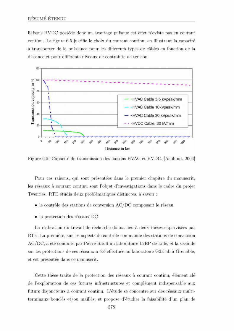
RÉSUMÉ ÉTENDU
liaisons HVDC possède donc un avantage puisque cet effet n’existe pas en courant
continu. La figure 6.5 justifie le choix du courant continu, en illustrant la capacité
à transporter de la puissance pour les différents types de câbles en fonction de la
distance et pour différents niveaux de contrainte de tension.
Tran
smis
sion
cap
acity
in %
Distance in km
Figure 6.5: Capacité de transmission des liaisons HVAC et HVDC, [Asplund, 2004]
Pour ces raisons, qui sont présentées dans le premier chapitre du manuscrit,
les réseaux à courant continu sont l’objet d’investigations dans le cadre du projet
Twenties. RTE étudia deux problématiques distinctes, à savoir :
• le contrôle des stations de conversion AC/DC composant le réseau,
• la protection des réseaux DC.
La réalisation du travail de recherche donna lieu à deux thèses supervisées par
RTE. La première, sur les aspects de contrôle-commande des stations de conversion
AC/DC, a été conduite par Pierre Rault au laboratoire L2EP de Lille, et la seconde
sur les protections de ces réseaux a été effectuée au laboratoire G2Elab à Grenoble,
et est présentée dans ce manuscrit.
Cette thèse traite de la protection des réseaux à courant continu, élément clé
de l’exploitation de ces futures infrastructures et complément indispensable aux
futurs disjoncteurs à courant continu. L’étude se concentre sur des réseaux multi-
terminaux bouclés et/ou maillés, et propose d’étudier la faisabilité d’un plan de
278

RÉSUMÉ ÉTENDU
protection comportant plusieurs principes, composés d’algorithmes principal et de
secours en cas de défaillance de celui-ci ou d’un disjoncteur.
Le chapitre 1 détaille la pertinence du recours au courant continu, et discute les
différentes technologies utilisées. Les liaisons HVDC consistent à convertir l’énergie
produite sous forme de courant alternatif en courant ou tension continue grâce à
des stations de conversion, puis de transformer cette énergie en courant alternatif
triphasé. Outre l’avantage de faciliter l’exploitation grâce à l’absence de puissance
réactive, les liaisons HVDC présentent une souplesse dans les réglages des dispositifs
d’électronique de puissance. Le schéma 6.6 présente le principe de fonctionnement.
DC link
Power transfer
AC filter
DC filter
Rectifier
DC filter
AC filter
Inverter
Figure 6.6: Schéma de liaison HVDC
Les filtres assurent le lissage du courant et le maintien d’une tension constante
côté continu, ainsi que la compensation des harmoniques du courant côté alternatif.
Les transformateurs, quant à eux, sont dimensionnés de manière à supporter les
fortes variations de courant susceptibles de se produire dans la partie continue, et
doivent posséder une forte impédance de court-circuit afin d’en limiter l’impact sur
le réseau. La liaison DC peut être constituée de lignes aériennes ou de câbles souter-
rains ou sous-marins, et différentes topologies peuvent être appliquées.
Que ce soit au niveau d’une source de production ou pour le raccord de la liai-
son HVDC à un réseau alternatif, la conversion AC/DC ou DC/AC est nécessaire.
Les deux types de convertisseurs les plus connus sont les LCCs (Line-Commutated
Converters), qui utilisent des thyristors, et les VSCs (Voltage Source Converters),
qui sont constitués de transistors. Les VSC sont les convertisseurs les plus récents et
les transistors (IGBT) peuvent être passants ou bloqués sur commande. Un grand
nombre d’IGBTs sont connectés en série dans chaque bras. Ils sont commandés
pour changer d’état simultanément, avec une précision de l’ordre de la fraction de
µs. Le principal avantage du VSC repose sur la possibilité du contrôle simultané des
puissances active et réactive échangées entre le convertisseur et le réseau qui y est
279
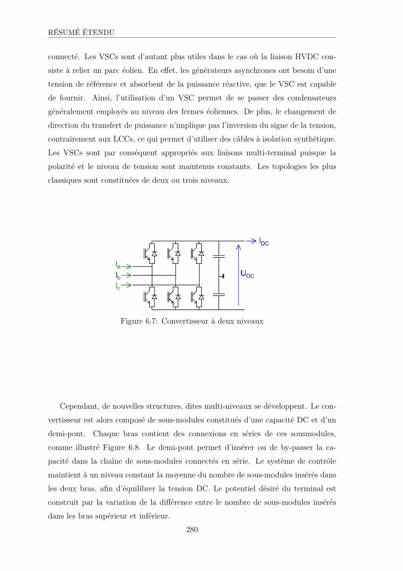
RÉSUMÉ ÉTENDU
connecté. Les VSCs sont d’autant plus utiles dans le cas où la liaison HVDC con-
siste à relier un parc éolien. En effet, les générateurs asynchrones ont besoin d’une
tension de référence et absorbent de la puissance réactive, que le VSC est capable
de fournir. Ainsi, l’utilisation d’un VSC permet de se passer des condensateurs
généralement employés au niveau des fermes éoliennes. De plus, le changement de
direction du transfert de puissance n’implique pas l’inversion du signe de la tension,
contrairement aux LCCs, ce qui permet d’utiliser des câbles à isolation synthétique.
Les VSCs sont par conséquent appropriés aux liaisons multi-terminal puisque la
polarité et le niveau de tension sont maintenus constants. Les topologies les plus
classiques sont constituées de deux ou trois niveaux.
Figure 6.7: Convertisseur à deux niveaux
Cependant, de nouvelles structures, dites multi-niveaux se développent. Le con-
vertisseur est alors composé de sous-modules constitués d’une capacité DC et d’un
demi-pont. Chaque bras contient des connexions en séries de ces sousmodules,
comme illustré Figure 6.8. Le demi-pont permet d’insérer ou de by-passer la ca-
pacité dans la chaîne de sous-modules connectés en série. Le système de contrôle
maintient à un niveau constant la moyenne du nombre de sous-modules insérés dans
les deux bras, afin d’équilibrer la tension DC. Le potentiel désiré du terminal est
construit par la variation de la différence entre le nombre de sous-modules insérés
dans les bras supérieur et inférieur.
280

RÉSUMÉ ÉTENDU
Figure 6.8: Schéma de convertisseur multi-niveaux,[http://www.energy.siemens.com, ]
Figure 6.9: Sous-modeule demi pont, [http://www.energy.siemens.com, ]
Dans le cas d’une structure multi-niveaux, chaque échelon de l’onde de sortie
résulte de l’opération d’un seul sous-module dans chaque bras. La moyenne de la
fréquence de commutation par semi-conducteur peut être réduite de manière signi-
ficative par rapport à une topologie 2 niveaux. Le contenu harmonique de l’onde
produite est très faible, réduisant ainsi la taille des filtres nécessaires. Ces technolo-
gies sont très récentes et commencent juste à se développer. Des variantes existent
chez les principaux fabricants, et sont connues sous le nom de M2C (Modular Multi-
level Converter) pour Siemens et CTL (Cascaded Two Level converter) pour ABB.
Alstom Grid propose lui aussi une variante du M2C en remplaçant les demi-ponts des
sous-modules par des ponts complets. Cette topologie offre la possibilité d’inverser
le signe de la tension côté DC, permettant ainsi la connexion d’un VSC à un LCC.
281
RÉSUMÉ ÉTENDU
Elle permet aussi de bloquer la circulation de courant provenant du côté DC, ce
qui est particulièrement utile lors d’un défaut intervenant dans la partie DC. Cela
permettrait notamment l’économie de disjoncteurs DC. Néanmoins, le nombre de
composants d’électronique de puissance de cette dernière technologie est prohibitif.
Le chapitre 2 se concentre sur le phénomène de défaut et en révisant les philoso-
phies de protection possibles qui ont été trouvées dans la littérature. La stratégie
retenue dans le cadre de cette thèse repose sur celle déjà utilisée dans le cas de la
protection des réseaux de transport AC et qui a déjà fait ses preuves en exploita-
tion, c’est-à-dire que la sélectivité est obtenue grâce au recours à des disjoncteurs à
courant continu disposés à chaque extrémité de câble et à chaque point de raccorde-
ment des stations de conversion. La technologie de coupure d’un courant DC est
discutée dans ce même chapitre mais la disponibilité de ces disjoncteurs est une hy-
pothèse forte dans cette étude, puisqu’actuellement ce type de dispositif ultra rapide
est en phase de prototypage. Le partenaire industriel en charge de l’évaluation de
la faisabilité de ces objets est Alstom Grid dans le cadre de Twenties. Cette thèse
se concentre sur la détection sélective des défauts, point clé pour commander les
disjoncteurs.
Etant donné l’impossibilité de test on-site vue l’inexistence de ce type de réseau,
le recours à la modélisation est nécessaire et la représentation des éléments consti-
tuant le système électrique à courant continu est une étape clé de cette étude, qui a
été réalisée sous le logiciel de simulation de transitoires électromagnétiques EMTP-
rv. Chaque élément est détaillé dans le chapitre trois du manuscrit, dont les deux
principaux sont les câbles conducteurs et les convertisseurs AC/DC. Les câbles sont
représentés par un modèle tenant compte de la dépendance fréquentielle des carac-
téristiques. Les convertisseurs sont quant à eux représentés par un modèle détaillé,
et le modèle de contrôle commande de ceux-ci a été réalisé au sein du laboratoire
L2EP par Pierre Rault.
Le chapitre 4 utilise le modèle de réseau complet sous EMTP-rv pour étudier
le comportement d’un réseau DC en conditions de défaut, et montrer l’influence de
chaque paramètre sur les grandeurs représentatives d’un défaut d’isolement, grâce à
une étude paramétrique.
282

RÉSUMÉ ÉTENDU
L’objectif est d’être capable d’éliminer, et ce de manière sélective, un défaut
d’isolement intervenant au niveau des câbles ou jeux de barre DC. Les relais de pro-
tection doivent donc inclure des algorithmes de détection sélectifs, afin de contrôler
les disjoncteurs à courant continu localisés à chaque bout de câble.
Le chapitre 5 est le cœur des travaux puisqu’après des indications sur les élé-
ments régissant les contraintes de rapidité du système de protection, les algorithmes
envisageables sont développés, pour finalement fournir une proposition de plan de
protection complet.
La problématique majeure repose sur la rapidité d’action du système de protec-
tion. Cette contrainte temporelle est nécessaire pour assurer la tenue du matériel et
l’opérabilité des convertisseurs AC/DC. Effectivement, un défaut se traduit d’une
part par une circulation de courant destructrice pour les diodes qui composent les
convertisseurs, et une chute de tension impliquant l’impossibilité de commander les
IGBTs.
La faible résistivité des câbles DC ne permet pas de limiter l’apport des capacités
phase/terre de ces mêmes câbles au courant de défaut. Les amplitudes limites sont
ainsi atteintes en un temps de l’ordre de 5ms.
La contrainte de rapidité s’applique aussi aux organes de coupure, et est bien
connue des constructeurs qui l’ont prise en compte dans leurs technologies de dis-
joncteur à courant continu haute tension. La problématique de la forte amplitude
des courants à couper demeure, celle-ci pouvant se résoudre par l’ajout d’éléments
capables de limiter le courant ou sa montée (limiteur supraconducteur, inductance,
...). Ces éléments permettent par ailleurs de relaxer la contrainte temporelle qui
est intrinsèquement liée aux amplitudes. Néanmoins, la compatibilité de leur di-
mensionnement en vue d’un développement du réseau DC (nouveau raccordement
notamment) reste à prouver.
En conclusion à ces éléments, la méthode qui a été choisie consiste à détecter
de manière sélective le défaut dès l’arrivée du premier front aux capteurs les plus
283
RÉSUMÉ ÉTENDU
proches, et d’envisager les éléments limitant le courant pour soutenir le fonction-
nement des disjoncteurs, voire leur donner une marge supplémentaire (en terme
d’amplitude de courant à couper), ce qui augmenterait la fiabilité du système de
protection DC global.
Par conséquent, les algorithmes doivent travailler dans le domaine de la cen-
taine de kiloHertz, engageant un besoin de captation des grandeurs haute tension
cohérent avec cette valeur. Le système de protection qui a été défini est composé de
4 algorithmes résumés ci-dessous.
Une fréquence de 100kHz a été supposée pour la réalisation des calculs par les
relais de protection. Etant donné la simplicité des opérations effectuées (sommes,
comparaison à un seuil), le résultat du calcul est supposé connu au pas de temps
suivant, soit 10µs plus tard. Un retard a été ajouté afin de tenir compte des temps
de transmission entre relais, soit 20µs intra-poste, auxquels on ajoute un retard de
1ms par 200km pour une transmission inter-poste.
Protection différentielle de câble
Le courant différentiel est mesuré à chaque relais localisé en bout de câble, l’ordre
d’ouverture est envoyé après dépassement d’un seuil, avec une validation effectuée
sur 3 échantillons consécutifs, ce qui ajoute un délai de 30µs. Si un premier front de
courant négatif est observé (i.e. présence de défaut mais externe au câble considéré),
la protection se bloque pendant la durée du transitoire suivant le défaut et son élimi-
nation. Le temps de détection dépend de la longueur du câble (délai de transmission
par fibre optique directe inter-poste 200km/ms). Pour une liaison de 100km, ordre
envoyé environ 600µs (y compris temps de traitement) après l’apparition du défaut.
Il faut ajouter à cela le temps d’action du disjoncteur, inconnu pour le moment.
284
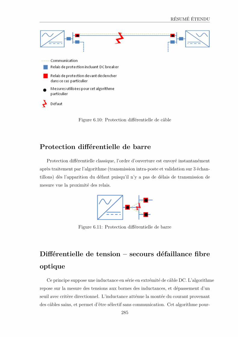
RÉSUMÉ ÉTENDU
Figure 6.10: Protection différentielle de câble
Protection différentielle de barre
Protection différentielle classique, l’ordre d’ouverture est envoyé instantanément
après traitement par l’algorithme (transmission intra-poste et validation sur 3 échan-
tillons) dès l’apparition du défaut puisqu’il n’y a pas de délais de transmission de
mesure vue la proximité des relais.
Figure 6.11: Protection différentielle de barre
Différentielle de tension – secours défaillance fibre
optique
Ce principe suppose une inductance en série en extrémité de câble DC. L’algorithme
repose sur la mesure des tensions aux bornes des inductances, et dépassement d’un
seuil avec critère directionnel. L’inductance atténue la montée du courant provenant
des câbles sains, et permet d’être sélectif sans communication. Cet algorithme pour-
285
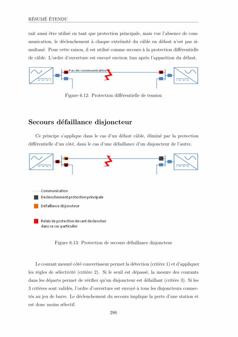
RÉSUMÉ ÉTENDU
rait aussi être utilisé en tant que protection principale, mais vue l’absence de com-
munication, le déclenchement à chaque extrémité du câble en défaut n’est pas si-
multané. Pour cette raison, il est utilisé comme secours à la protection différentielle
de câble. L’ordre d’ouverture est envoyé environ 1ms après l’apparition du défaut.
Figure 6.12: Protection différentielle de tension
Secours défaillance disjoncteur
Ce principe s’applique dans le cas d’un défaut câble, éliminé par la protection
différentielle d’un côté, dans le cas d’une défaillance d’un disjoncteur de l’autre.
Figure 6.13: Protection de secours défaillance disjoncteur
Le courant mesuré côté convertisseur permet la détection (critère 1) et d’appliquer
les règles de sélectivité (critère 2). Si le seuil est dépassé, la mesure des courants
dans les départs permet de vérifier qu’un disjoncteur est défaillant (critère 3). Si les
3 critères sont validés, l’ordre d’ouverture est envoyé à tous les disjoncteurs connec-
tés au jeu de barre. Le déclenchement du secours implique la perte d’une station et
est donc moins sélectif.
286
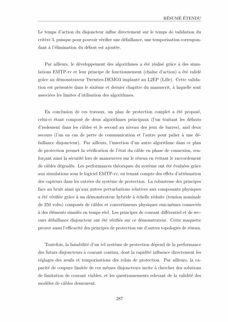
RÉSUMÉ ÉTENDU
Le temps d’action du disjoncteur influe directement sur le temps de validation du
critère 3, puisque pour pouvoir vérifier une défaillance, une temporisation correspon-
dant à l’élimination du défaut est ajoutée.
Par ailleurs, le développement des algorithmes a été réalisé grâce à des simu-
lations EMTP-rv et leur principe de fonctionnement (chaîne d’action) a été validé
grâce au démonstrateur Twenties-DEMO3 implanté au L2EP (Lille). Cette valida-
tion est présentée dans le sixième et dernier chapitre du manuscrit, à laquelle sont
associées les limites d’utilisation des algorithmes.
En conclusion de ces travaux, un plan de protection complet a été proposé,
celui-ci étant composé de deux algorithmes principaux (l’un traitant les défauts
d’isolement dans les câbles et le second au niveau des jeux de barres), and deux
secours (l’un en cas de perte de communication et l’autre pour palier à une dé-
faillance disjoncteur). Par ailleurs, l’insertion d’un autre algorithme dans ce plan
de protection permet la vérification de l’état du câble en phase de connexion, ren-
forçant ainsi la sécurité lors de manœuvres sur le réseau en évitant le raccordement
de câbles dégradés. Les performances théoriques du système ont été évaluées grâce
aux simulations sous le logiciel EMTP-rv, en tenant compte des effets d’atténuation
des capteurs dans les entrées du système de protection. La robustesse des principes
face au bruit ainsi qu’aux autres perturbations relatives aux composants physiques
a été vérifiée grâce à un démonstrateur hybride à échelle réduite (tension nominale
de 250 volts) composés de câbles et convertisseurs physiques eux-mêmes connectés
à des éléments simulés en temps réel. Les principes de courant différentiel et de sec-
ours défaillance disjoncteur ont été vérifiés sur ce démonstrateur. Cette maquette
prouve aussi l’efficacité des principes de protection sur d’autres topologies de réseau.
Toutefois, la faisabilité d’un tel système de protection dépend de la performance
des futurs disjoncteurs à courant continu, dont la rapidité influence directement les
réglages des seuils et temporisations des relais de protection. Par ailleurs, la ca-
pacité de coupure limitée de ces mêmes disjoncteurs incite à chercher des solutions
de limitation de courant viables, et les questionnements relevant de la validité des
modèles de câbles demeurent.
287
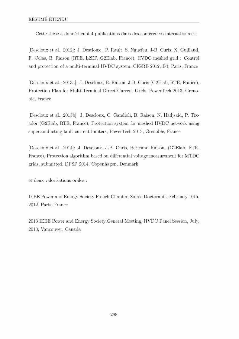
RÉSUMÉ ÉTENDU
Cette thèse a donné lieu à 4 publications dans des conférences internationales:
[Descloux et al., 2012]: J. Descloux , P. Rault, S. Nguefeu, J-B. Curis, X. Guillaud,
F. Colas, B. Raison (RTE, L2EP, G2Elab, France), HVDC meshed grid : Control
and protection of a multi-terminal HVDC system, CIGRE 2012, B4, Paris, France
[Descloux et al., 2013a]: J. Descloux, B. Raison, J-B. Curis (G2Elab, RTE, France),
Protection Plan for Multi-Terminal Direct Current Grids, PowerTech 2013, Greno-
ble, France
[Descloux et al., 2013b]: J. Descloux, C. Gandioli, B. Raison, N. Hadjsaid, P. Tix-
ador (G2Elab, RTE, France), Protection system for meshed HVDC network using
superconducting fault current limiters, PowerTech 2013, Grenoble, France
[Descloux et al., 2014]: J. Descloux, J-B. Curis, Bertrand Raison, (G2Elab, RTE,
France), Protection algorithm based on differential voltage measurement for MTDC
grids, submitted, DPSP 2014, Copenhagen, Denmark
et deux valorisations orales :
IEEE Power and Energy Society French Chapter, Soirée Doctorants, February 10th,
2012, Paris, France
2013 IEEE Power and Energy Society General Meeting, HVDC Panel Session, July,
2013, Vancouver, Canada
288

Protection contre les courts-circuits des réseauxélectriques à courant continu de forte puissance
Résumé Dans le domaine du transport de l’électricité, les qualités intrinsèques des réseauxalternatifs s’estompent devant la difficulté imposée par le transport de la puissance réac-tive lorsque les lignes aériennes ou, plus particulièrement, les câbles souterrains ou sous-marins atteignent des longueurs critiques. Dans le cadre des réflexions visant à exploiterau mieux les énergies renouvelables d’origine éolienne off-shore ou hydrolienne, l’hypothèsede la création d’un réseau électrique à haute tension continue pour acheminer ces énergiesjusqu’aux centres de consommation est considérée. Ce travail de thèse, encadrée par RTEet le laboratoire de Génie Electrique de Grenoble (G2Elab), est en lien avec le projetTWENTIES, financé dans le cadre du programme FP7 de la Commission Européenne,qui a pour vocation d’analyser les obstacles à l’intégration de volumes croissants d’énergierenouvelable dans le système électrique européen, et de proposer des solutions pour leverces verrous technologiques. Les travaux traitent de la protection des réseaux à courantcontinu, élément clé de l’exploitation de ces futures infrastructures et complément indis-pensable aux futurs disjoncteurs à courant continu. L’étude se concentre sur des réseauxmulti-terminaux bouclés et/ou maillés, et propose d’étudier la faisabilité d’un plan deprotection comportant plusieurs principes, composés d’algorithmes principal et de secoursen cas de défaillance de celui-ci ou d’un disjoncteur.
Mots clés Réseau de transport d’électricité, courant continu, câble, plan de protection,
système de protection, court-circuit.
Protection plan for a Multi-Terminal and High VoltageDirect Current grid
Abstract In electricity transmission, the inherent qualities of alternative grids fade infront of the difficulty imposed by the reactive power transportation, when overhead linesor, particularly underground or submarine cables reach critical lengths. In the frame ofthe thought aiming to operate at best renewable energy resources, coming from wind orhydro power stations, the creation of a high voltage direct current grid is assumed todispatch those energies to the consumption centers. Indeed, from a certain amount ofpower to transmit, there is a critical length beyond which AC transmission is not viableanymore, and where DC links becomes both more efficient and less costly. The new con-version technologies, namely the voltage source converters, now enables the connectionof several terminals and therefore, the creation of a true grid, which can either have alooped, meshed, or radial structure. The advantages of such grid structure in relation topoint-to-point links are obvious in terms of reliability of the transmission grid. Never-theless, some technological locks remain, and the protection against faults of those gridsis currently largely debates. This Ph.D work, advised by RTE and Grenoble ElectricalEngineering laboratory (G2Elab) is linked with the TWENTIES project, which aims toanalyse the potential obstacles to the integration of renewable resources in the Europeanelectrical system, and to propose solutions to lift those technological barriers.This Ph.Dthesis aims to propose a complete protection plan against insulation faults in cable orbusbar, including a main protection and two backups in case of failure of a component,for a submarine DC grid. The target application would be a grid linking offshore windfarms and countries through the North Sea.
Keywords Transmission power grid, direct current, cable, protection plan, protection
system, short-circuit.